CPSC-608 Database SystemsFall

2010

Instructor: Jianer ChenOffice: HRBB 315CPhone: 845-4259

Email: chen@cse.tamu.edu

1

Notes #9

LQP Optimization with Size

2

LQP Optimization with Size

Two techniques:

3

LQP Optimization with Size

Two techniques:

• Estimating sizes of immediate relations

For natural join:

T(R(X, y) S(y, Z)) = T(R)•T(S)/max{V(R, y), V(S, y)}

4

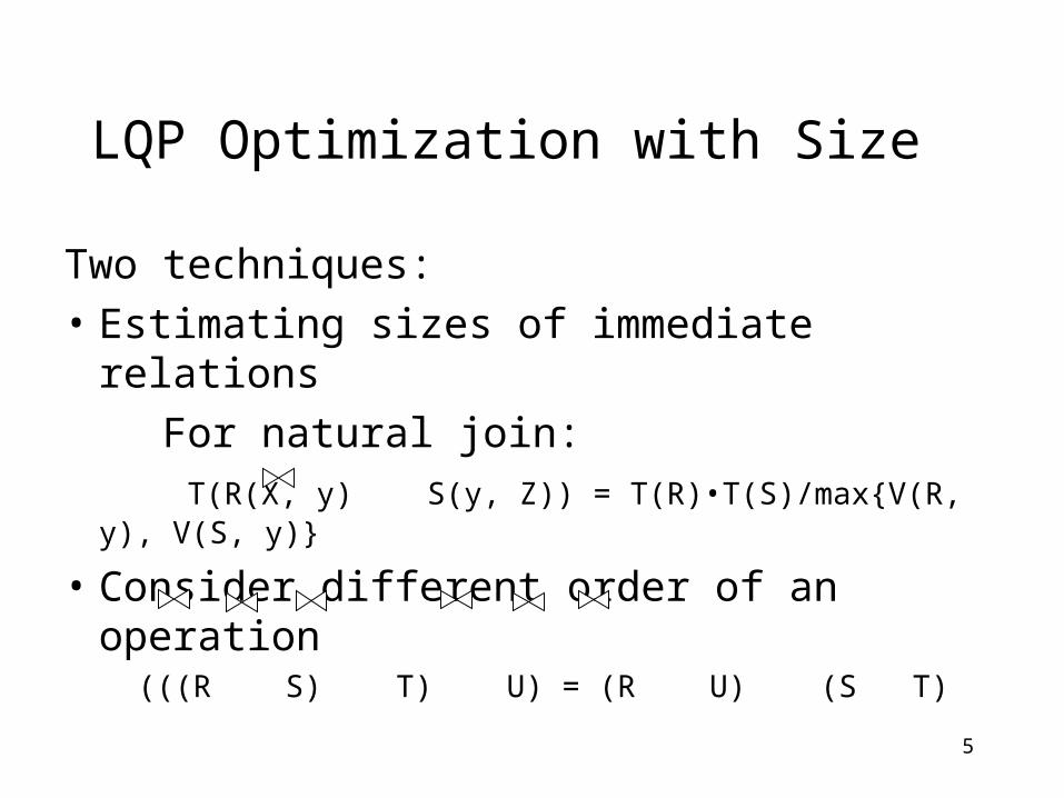
LQP Optimization with Size

Two techniques:

• Estimating sizes of immediate relations

For natural join:

T(R(X, y) S(y, Z)) = T(R)•T(S)/max{V(R, y), V(S, y)}

• Consider different order of an operation (((R S) T) U) = (R U) (S T)

5

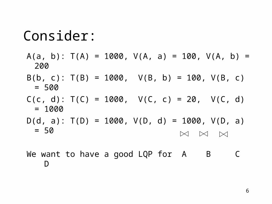
Consider:

A(a, b): T(A) = 1000, V(A, a) = 100, V(A, b) = 200

B(b, c): T(B) = 1000, V(B, b) = 100, V(B, c) = 500

C(c, d): T(C) = 1000, V(C, c) = 20, V(C, d) = 1000

D(d, a): T(D) = 1000, V(D, d) = 1000, V(D, a) = 50

We want to have a good LQP for A B C D

6

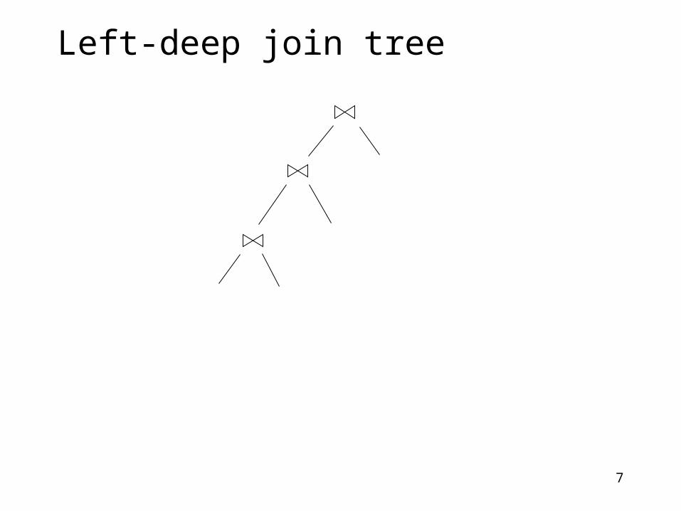
Left-deep join tree

7

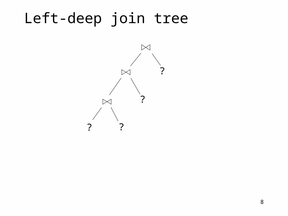
Left-deep join tree

8

? ?

?

?

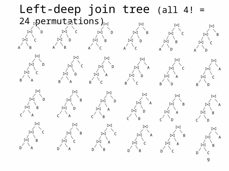
Left-deep join tree (all 4! = 24 permutations)

9

A B

C

D

B A

C

D

A B

D

C

B A

D

C

C A

B

D

C A

D

B

B C

A

D

C B

A

D

D A

B

C

D A

C

B

D B

A

C

D B

C

A

D C

A

B

D C

B

A

C B

D

A

C D

A

B

C D

B

A

B C

D

A

B D

A

C

B D

C

A

A C

B

D

A C

D

B

A D

B

C

A D

C

B

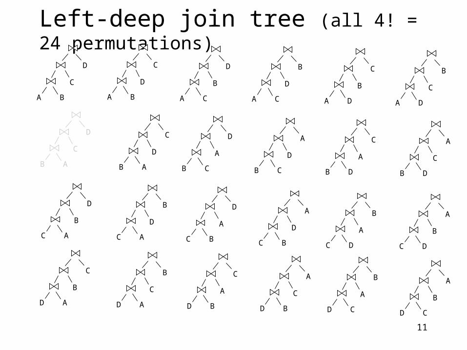
Left-deep join tree (all 4! = 24 permutations)

10

A B

C

D

B A

C

D

A B

D

C

B A

D

C

C A

B

D

C A

D

B

B C

A

D

C B

A

D

D A

B

C

D A

C

B

D B

A

C

D B

C

A

D C

A

B

D C

B

A

C B

D

A

C D

A

B

C D

B

A

B C

D

A

B D

A

C

B D

C

A

A C

B

D

A C

D

B

A D

B

C

A D

C

B

Left-deep join tree (all 4! = 24 permutations)

11

A B

C

D

B A

C

D

A B

D

C

B A

D

C

C A

B

D

C A

D

B

B C

A

D

C B

A

D

D A

B

C

D A

C

B

D B

A

C

D B

C

A

D C

A

B

D C

B

A

C B

D

A

C D

A

B

C D

B

A

B C

D

A

B D

A

C

B D

C

A

A C

B

D

A C

D

B

A D

B

C

A D

C

B

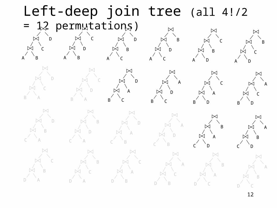
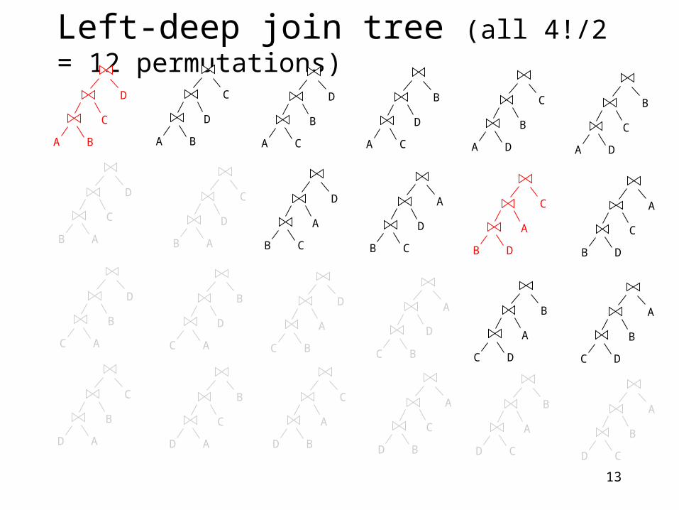
Left-deep join tree (all 4!/2 = 12 permutations)

12

A B

C

D

B A

C

D

A B

D

C

B A

D

C

C A

B

D

C A

D

B

B C

A

D

C B

A

D

D A

B

C

D A

C

B

D B

A

C

D B

C

A

D C

A

B

D C

B

A

C B

D

A

C D

A

B

C D

B

A

B C

D

A

B D

A

C

B D

C

A

A C

B

D

A C

D

B

A D

B

C

A D

C

B

Left-deep join tree (all 4!/2 = 12 permutations)

13

A B

C

D

B A

C

D

A B

D

C

B A

D

C

C A

B

D

C A

D

B

B C

A

D

C B

A

D

D A

B

C

D A

C

B

D B

A

C

D B

C

A

D C

A

B

D C

B

A

C B

D

A

C D

A

B

C D

B

A

B C

D

A

B D

A

C

B D

C

A

A C

B

D

A C

D

B

A D

B

C

A D

C

B

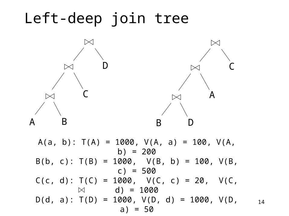
Left-deep join tree

14

A B

C

D

B D

A

C

A(a, b): T(A) = 1000, V(A, a) = 100, V(A, b) = 200B(b, c): T(B) = 1000, V(B, b) = 100, V(B, c) = 500C(c, d): T(C) = 1000, V(C, c) = 20, V(C, d) = 1000D(d, a): T(D) = 1000, V(D, d) = 1000, V(D, a) = 50

T(R(X, y) S(y, Z)) = T(R)•T(S)/max{V(R, y), V(S, y)}

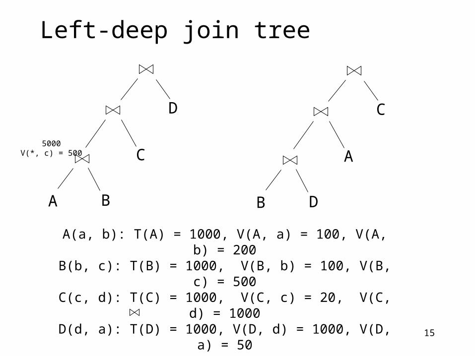
Left-deep join tree

15

A B

C

D

B D

A

C

A(a, b): T(A) = 1000, V(A, a) = 100, V(A, b) = 200B(b, c): T(B) = 1000, V(B, b) = 100, V(B, c) = 500C(c, d): T(C) = 1000, V(C, c) = 20, V(C, d) = 1000D(d, a): T(D) = 1000, V(D, d) = 1000, V(D, a) = 50

T(R(X, y) S(y, Z)) = T(R)•T(S)/max{V(R, y), V(S, y)} 5000

V(*, c) = 500

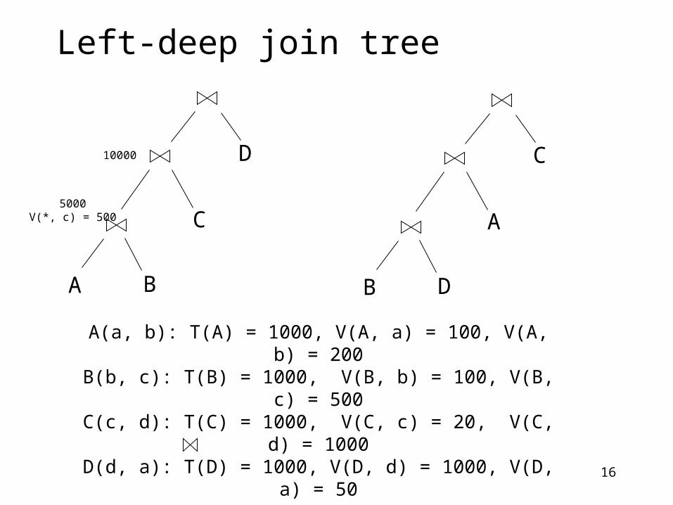
Left-deep join tree

16

A B

C

D

B D

A

C

A(a, b): T(A) = 1000, V(A, a) = 100, V(A, b) = 200B(b, c): T(B) = 1000, V(B, b) = 100, V(B, c) = 500C(c, d): T(C) = 1000, V(C, c) = 20, V(C, d) = 1000D(d, a): T(D) = 1000, V(D, d) = 1000, V(D, a) = 50

T(R(X, y) S(y, Z)) = T(R)•T(S)/max{V(R, y), V(S, y)} 5000

V(*, c) = 500

10000

Left-deep join tree

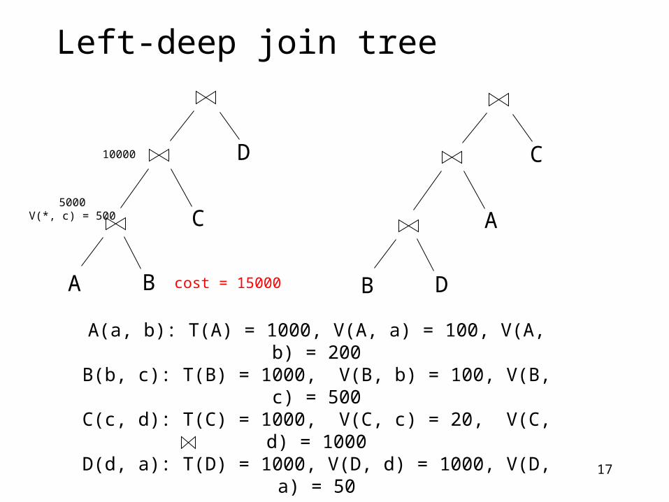
17

A B

C

D

B D

A

C

A(a, b): T(A) = 1000, V(A, a) = 100, V(A, b) = 200B(b, c): T(B) = 1000, V(B, b) = 100, V(B, c) = 500C(c, d): T(C) = 1000, V(C, c) = 20, V(C, d) = 1000D(d, a): T(D) = 1000, V(D, d) = 1000, V(D, a) = 50

T(R(X, y) S(y, Z)) = T(R)•T(S)/max{V(R, y), V(S, y)} 5000

V(*, c) = 500

10000

cost = 15000

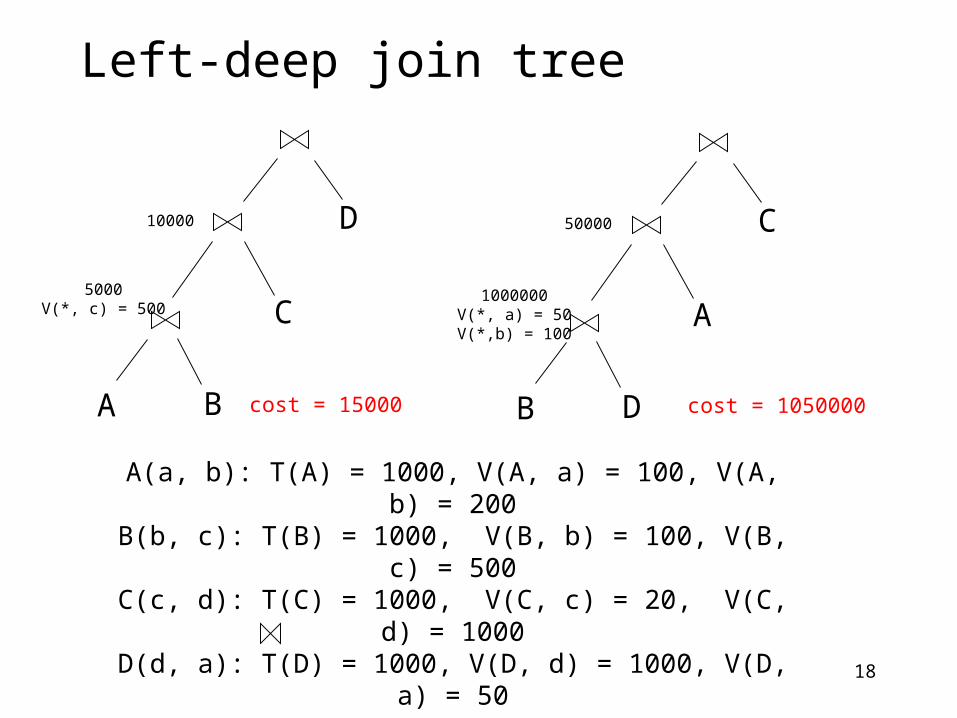
Left-deep join tree

18

A B

C

D

B D

A

C

A(a, b): T(A) = 1000, V(A, a) = 100, V(A, b) = 200B(b, c): T(B) = 1000, V(B, b) = 100, V(B, c) = 500C(c, d): T(C) = 1000, V(C, c) = 20, V(C, d) = 1000D(d, a): T(D) = 1000, V(D, d) = 1000, V(D, a) = 50

T(R(X, y) S(y, Z)) = T(R)•T(S)/max{V(R, y), V(S, y)} 5000

V(*, c) = 500

10000

1000000V(*, a) = 50V(*,b) = 100

50000

cost = 15000 cost = 1050000

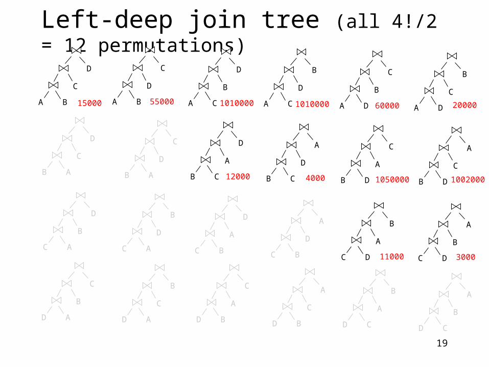
Left-deep join tree (all 4!/2 = 12 permutations)

19

A B

C

D

B A

C

D

A B

D

C

B A

D

C

C A

B

D

C A

D

B

B C

A

D

C B

A

D

D A

B

C

D A

C

B

D B

A

C

D B

C

A

D C

A

B

D C

B

A

C B

D

A

C D

A

B

C D

B

A

B C

D

A

B D

A

C

B D

C

A

A C

B

D

A C

D

B

A D

B

C

A D

C

B

60000

1050000

55000 1010000 101000015000 20000

100200012000 4000

11000 3000

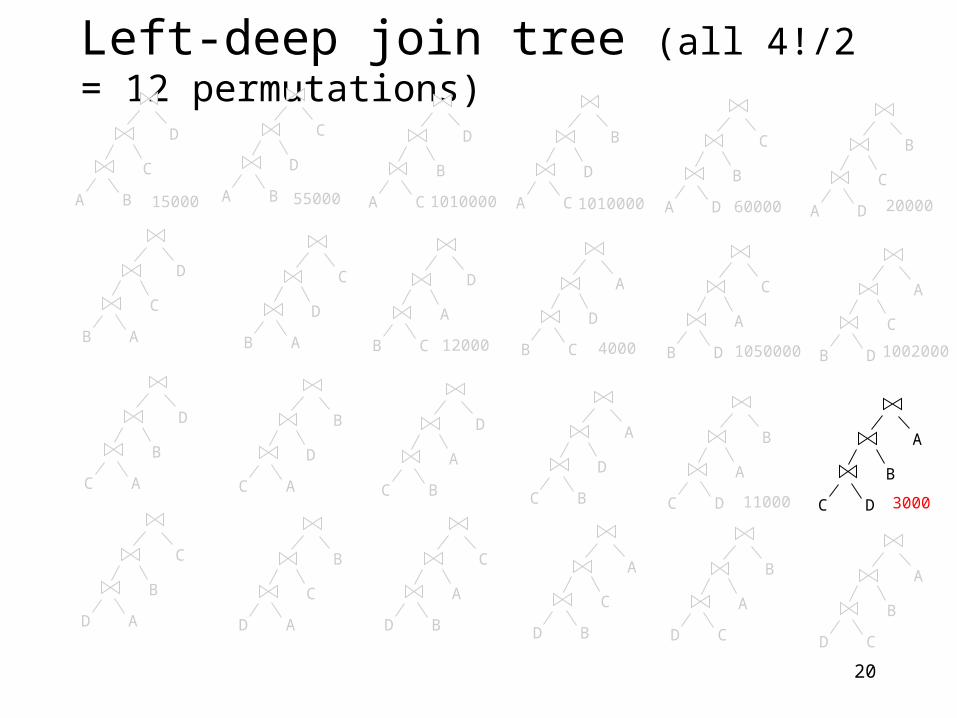
Left-deep join tree (all 4!/2 = 12 permutations)

20

A B

C

D

B A

C

D

A B

D

C

B A

D

C

C A

B

D

C A

D

B

B C

A

D

C B

A

D

D A

B

C

D A

C

B

D B

A

C

D B

C

A

D C

A

B

D C

B

A

C B

D

A

C D

A

B

C D

B

A

B C

D

A

B D

A

C

B D

C

A

A C

B

D

A C

D

B

A D

B

C

A D

C

B

60000

1050000

55000 1010000 101000015000 20000

100200012000 4000

11000 3000

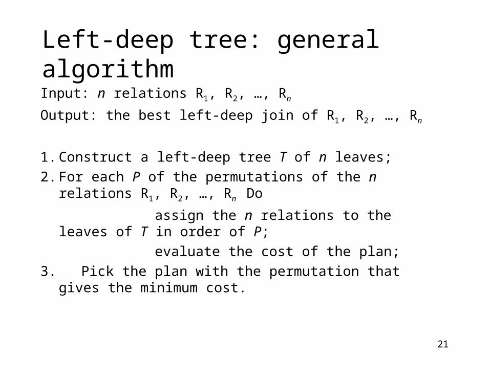
Left-deep tree: general algorithm

Input: n relations R1, R2, …, Rn

Output: the best left-deep join of R1, R2, …, Rn

1. Construct a left-deep tree T of n leaves;

2. For each P of the permutations of the n relations R1, R2, …, Rn Do

assign the n relations to the leaves of T in order of P;

evaluate the cost of the plan;

3. Pick the plan with the permutation that gives the minimum cost.

21

Dynamic ProgrammingConsider all tree structures.

22

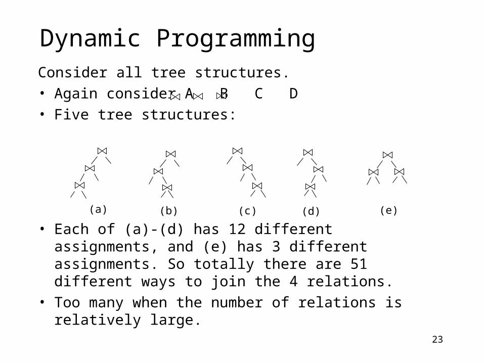
Dynamic ProgrammingConsider all tree structures.

• Again consider A B C D

• Five tree structures:

• Each of (a)-(d) has 12 different assignments, and (e) has 3 different assignments. So totally there are 51 different ways to join the 4 relations.

• Too many when the number of relations is relatively large.

23

(a) (e)(d)(c)(b)

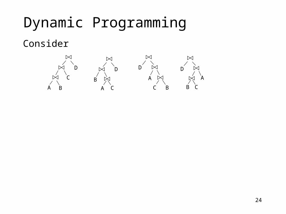
Dynamic ProgrammingConsider

24

D DDD

AA

AA BB

B

B CCC

C

Dynamic ProgrammingConsider

25

D DDD

AA

AA BB

B

B CCC

C

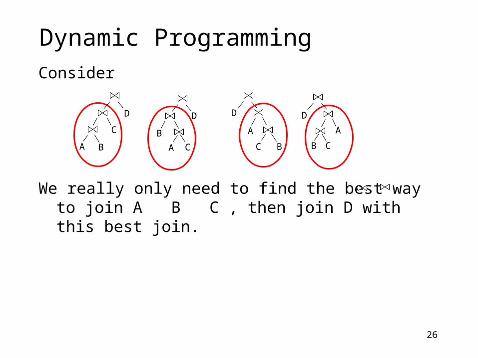
Dynamic ProgrammingConsider

We really only need to find the best way to join A B C , then join D with this best join.

26

D DDD

AA

AA BB

B

B CCC

C

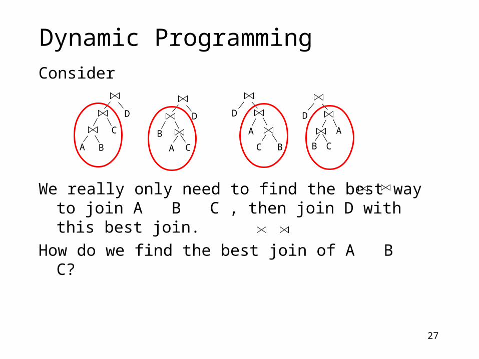
Dynamic ProgrammingConsider

We really only need to find the best way to join A B C , then join D with this best join.

How do we find the best join of A B C?

27

D DDD

AA

AA BB

B

B CCC

C

Dynamic ProgrammingConsider

We really only need to find the best way to join A B C , then join D with this best join.

How do we find the best join of A B C?

We consider all possible ways:

(A B) C, (A C) B, (B C) A.

28

D DDD

AA

AA BB

B

B CCC

C

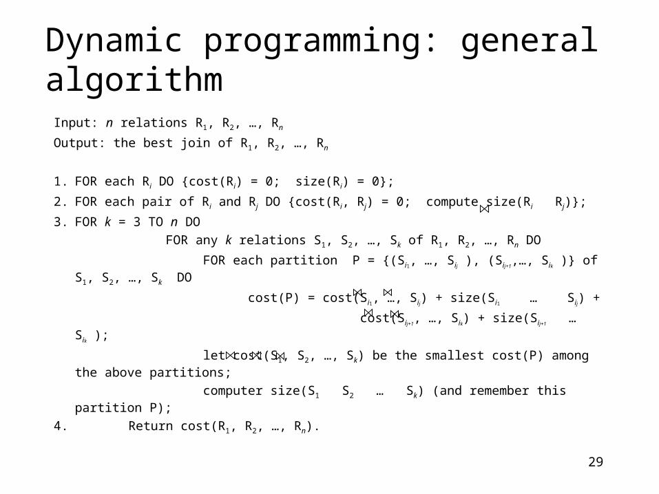
Dynamic programming: general algorithm

Input: n relations R1, R2, …, Rn

Output: the best join of R1, R2, …, Rn

1. FOR each Ri DO {cost(Ri) = 0; size(Ri) = 0};

2. FOR each pair of Ri and Rj DO {cost(Ri, Rj) = 0; compute size(Ri Rj)};

3. FOR k = 3 TO n DO

FOR any k relations S1, S2, …, Sk of R1, R2, …, Rn DO

FOR each partition P = {(Si1, …, Sij ), (Sij+1,…, Sik )} of S1, S2, …, Sk DO

cost(P) = cost(Si1, …, Sij) + size(Si1 … Sij) +

cost(Sij+1, …, Sik) + size(Sij+1

… Sik );

let cost(S1, S2, …, Sk) be the smallest cost(P) among the above partitions;

computer size(S1 S2 … Sk) (and remember this partition P);

4. Return cost(R1, R2, …, Rn).

29

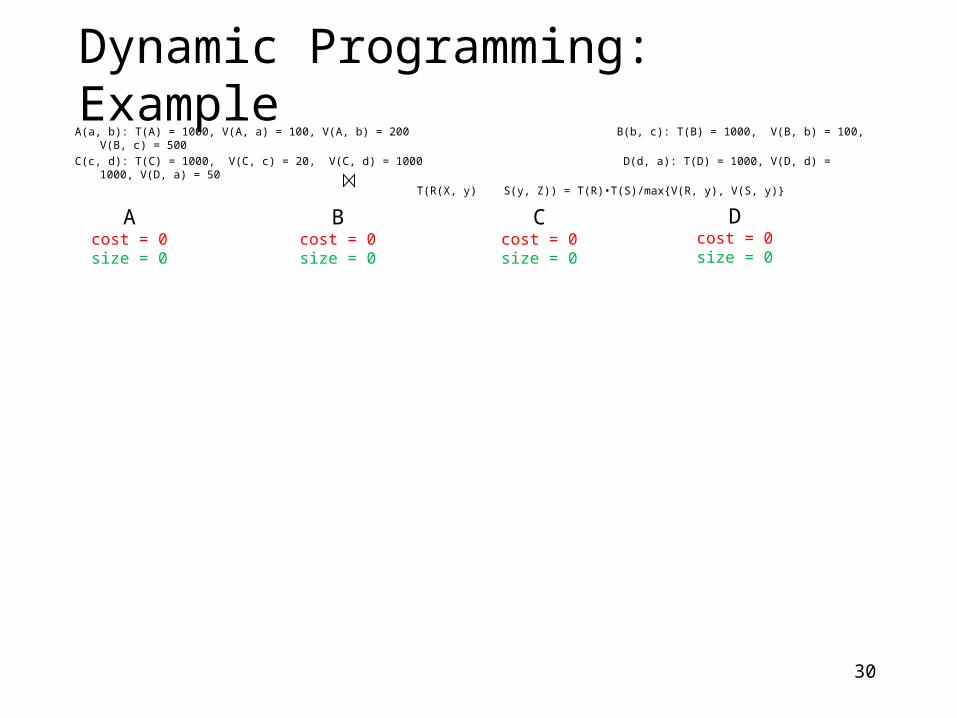
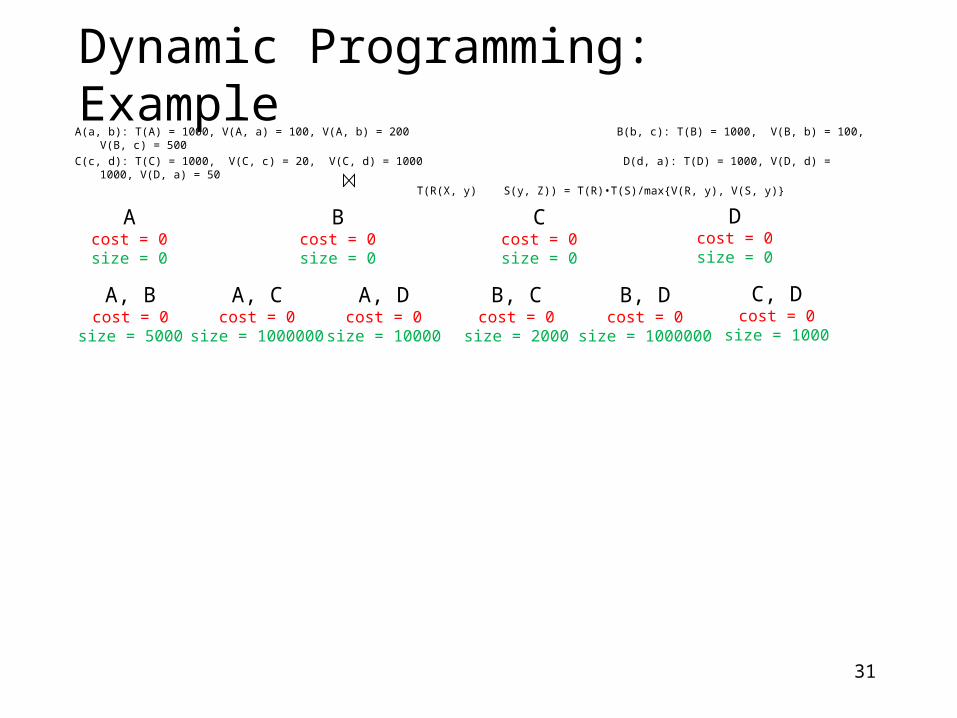
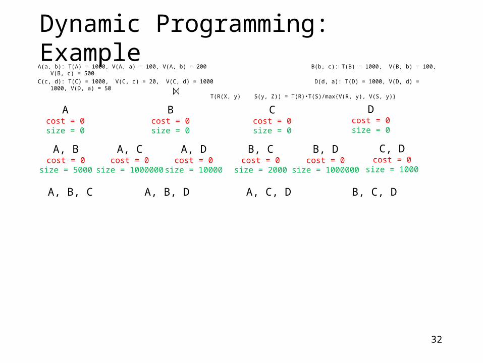
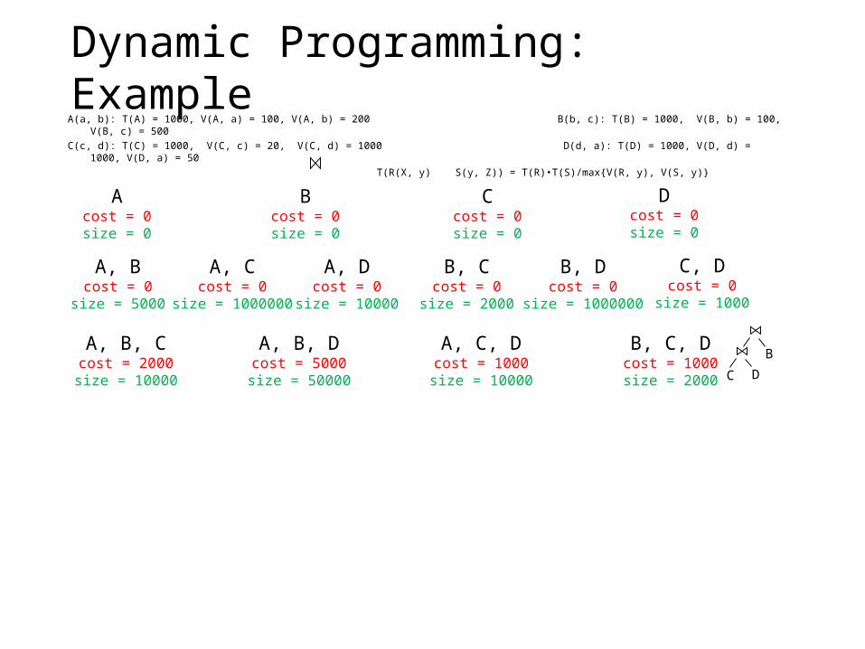
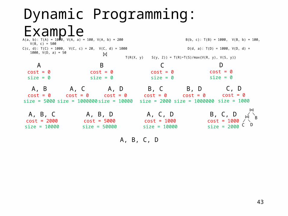
Dynamic Programming: ExampleA(a, b): T(A) = 1000, V(A, a) = 100, V(A, b) = 200 B(b, c): T(B) = 1000, V(B, b) = 100, V(B, c) = 500

C(c, d): T(C) = 1000, V(C, c) = 20, V(C, d) = 1000 D(d, a): T(D) = 1000, V(D, d) = 1000, V(D, a) = 50

T(R(X, y) S(y, Z)) = T(R)•T(S)/max{V(R, y), V(S, y)}

30

Acost = 0size = 0

Dcost = 0size = 0

Ccost = 0size = 0

Bcost = 0size = 0

Dynamic Programming: ExampleA(a, b): T(A) = 1000, V(A, a) = 100, V(A, b) = 200 B(b, c): T(B) = 1000, V(B, b) = 100, V(B, c) = 500

C(c, d): T(C) = 1000, V(C, c) = 20, V(C, d) = 1000 D(d, a): T(D) = 1000, V(D, d) = 1000, V(D, a) = 50

T(R(X, y) S(y, Z)) = T(R)•T(S)/max{V(R, y), V(S, y)}

31

Acost = 0size = 0

Dcost = 0size = 0

Ccost = 0size = 0

Bcost = 0size = 0

A, Bcost = 0

size = 5000

C, Dcost = 0

size = 1000

B, Dcost = 0

size = 1000000

B, Ccost = 0

size = 2000

A, Dcost = 0

size = 10000

A, Ccost = 0

size = 1000000

Dynamic Programming: ExampleA(a, b): T(A) = 1000, V(A, a) = 100, V(A, b) = 200 B(b, c): T(B) = 1000, V(B, b) = 100, V(B, c) = 500

C(c, d): T(C) = 1000, V(C, c) = 20, V(C, d) = 1000 D(d, a): T(D) = 1000, V(D, d) = 1000, V(D, a) = 50

T(R(X, y) S(y, Z)) = T(R)•T(S)/max{V(R, y), V(S, y)}

32

Acost = 0size = 0

Dcost = 0size = 0

Ccost = 0size = 0

Bcost = 0size = 0

A, Bcost = 0

size = 5000

C, Dcost = 0

size = 1000

B, Dcost = 0

size = 1000000

B, Ccost = 0

size = 2000

A, Dcost = 0

size = 10000

A, Ccost = 0

size = 1000000

A, B, C B, C, DA, C, DA, B, D

Dynamic Programming: ExampleA(a, b): T(A) = 1000, V(A, a) = 100, V(A, b) = 200 B(b, c): T(B) = 1000, V(B, b) = 100, V(B, c) = 500

C(c, d): T(C) = 1000, V(C, c) = 20, V(C, d) = 1000 D(d, a): T(D) = 1000, V(D, d) = 1000, V(D, a) = 50

T(R(X, y) S(y, Z)) = T(R)•T(S)/max{V(R, y), V(S, y)}

33

Acost = 0size = 0

Dcost = 0size = 0

Ccost = 0size = 0

Bcost = 0size = 0

A, Bcost = 0

size = 5000

C, Dcost = 0

size = 1000

B, Dcost = 0

size = 1000000

B, Ccost = 0

size = 2000

A, Dcost = 0

size = 10000

A, Ccost = 0

size = 1000000

A, B, C B, C, DA, C, DA, B, D

Dynamic Programming: ExampleA(a, b): T(A) = 1000, V(A, a) = 100, V(A, b) = 200 B(b, c): T(B) = 1000, V(B, b) = 100, V(B, c) = 500

C(c, d): T(C) = 1000, V(C, c) = 20, V(C, d) = 1000 D(d, a): T(D) = 1000, V(D, d) = 1000, V(D, a) = 50

T(R(X, y) S(y, Z)) = T(R)•T(S)/max{V(R, y), V(S, y)}

34

Acost = 0size = 0

Dcost = 0size = 0

Ccost = 0size = 0

Bcost = 0size = 0

A, Bcost = 0

size = 5000

C, Dcost = 0

size = 1000

B, Dcost = 0

size = 1000000

B, Ccost = 0

size = 2000

A, Dcost = 0

size = 10000

A, Ccost = 0

size = 1000000

A, B, C B, C, DA, C, DA, B, D

CB B

D B

C

C

D D

Dynamic Programming: ExampleA(a, b): T(A) = 1000, V(A, a) = 100, V(A, b) = 200 B(b, c): T(B) = 1000, V(B, b) = 100, V(B, c) = 500

C(c, d): T(C) = 1000, V(C, c) = 20, V(C, d) = 1000 D(d, a): T(D) = 1000, V(D, d) = 1000, V(D, a) = 50

T(R(X, y) S(y, Z)) = T(R)•T(S)/max{V(R, y), V(S, y)}

35

Acost = 0size = 0

Dcost = 0size = 0

Ccost = 0size = 0

Bcost = 0size = 0

A, Bcost = 0

size = 5000

C, Dcost = 0

size = 1000

B, Dcost = 0

size = 1000000

B, Ccost = 0

size = 2000

A, Dcost = 0

size = 10000

A, Ccost = 0

size = 1000000

A, B, C B, C, DA, C, DA, B, D

CB B

D B

C

C

D D

Dynamic Programming: ExampleA(a, b): T(A) = 1000, V(A, a) = 100, V(A, b) = 200 B(b, c): T(B) = 1000, V(B, b) = 100, V(B, c) = 500

C(c, d): T(C) = 1000, V(C, c) = 20, V(C, d) = 1000 D(d, a): T(D) = 1000, V(D, d) = 1000, V(D, a) = 50

T(R(X, y) S(y, Z)) = T(R)•T(S)/max{V(R, y), V(S, y)}

36

Acost = 0size = 0

Dcost = 0size = 0

Ccost = 0size = 0

Bcost = 0size = 0

A, Bcost = 0

size = 5000

C, Dcost = 0

size = 1000

B, Dcost = 0

size = 1000000

B, Ccost = 0

size = 2000

A, Dcost = 0

size = 10000

A, Ccost = 0

size = 1000000

A, B, C B, C, DA, C, DA, B, D

CB B

D B

C

C

D D

Dynamic Programming: ExampleA(a, b): T(A) = 1000, V(A, a) = 100, V(A, b) = 200 B(b, c): T(B) = 1000, V(B, b) = 100, V(B, c) = 500

C(c, d): T(C) = 1000, V(C, c) = 20, V(C, d) = 1000 D(d, a): T(D) = 1000, V(D, d) = 1000, V(D, a) = 50

T(R(X, y) S(y, Z)) = T(R)•T(S)/max{V(R, y), V(S, y)}

37

Acost = 0size = 0

Dcost = 0size = 0

Ccost = 0size = 0

Bcost = 0size = 0

A, Bcost = 0

size = 5000

C, Dcost = 0

size = 1000

B, Dcost = 0

size = 1000000

B, Ccost = 0

size = 2000

A, Dcost = 0

size = 10000

A, Ccost = 0

size = 1000000

A, B, C B, C, DA, C, DA, B, D

CB B

D B

C

C

D D

2000

Dynamic Programming: ExampleA(a, b): T(A) = 1000, V(A, a) = 100, V(A, b) = 200 B(b, c): T(B) = 1000, V(B, b) = 100, V(B, c) = 500

C(c, d): T(C) = 1000, V(C, c) = 20, V(C, d) = 1000 D(d, a): T(D) = 1000, V(D, d) = 1000, V(D, a) = 50

T(R(X, y) S(y, Z)) = T(R)•T(S)/max{V(R, y), V(S, y)}

38

Acost = 0size = 0

Dcost = 0size = 0

Ccost = 0size = 0

Bcost = 0size = 0

A, Bcost = 0

size = 5000

C, Dcost = 0

size = 1000

B, Dcost = 0

size = 1000000

B, Ccost = 0

size = 2000

A, Dcost = 0

size = 10000

A, Ccost = 0

size = 1000000

A, B, C B, C, DA, C, DA, B, D

CB B

D B

C

C

D D

2000

2000

Dynamic Programming: ExampleA(a, b): T(A) = 1000, V(A, a) = 100, V(A, b) = 200 B(b, c): T(B) = 1000, V(B, b) = 100, V(B, c) = 500

C(c, d): T(C) = 1000, V(C, c) = 20, V(C, d) = 1000 D(d, a): T(D) = 1000, V(D, d) = 1000, V(D, a) = 50

T(R(X, y) S(y, Z)) = T(R)•T(S)/max{V(R, y), V(S, y)}

39

Acost = 0size = 0

Dcost = 0size = 0

Ccost = 0size = 0

Bcost = 0size = 0

A, Bcost = 0

size = 5000

C, Dcost = 0

size = 1000

B, Dcost = 0

size = 1000000

B, Ccost = 0

size = 2000

A, Dcost = 0

size = 10000

A, Ccost = 0

size = 1000000

A, B, C B, C, DA, C, DA, B, D

CB B

D B

C

C

D D

2000 10001000000

10000002000 1000

Dynamic Programming: ExampleA(a, b): T(A) = 1000, V(A, a) = 100, V(A, b) = 200 B(b, c): T(B) = 1000, V(B, b) = 100, V(B, c) = 500

C(c, d): T(C) = 1000, V(C, c) = 20, V(C, d) = 1000 D(d, a): T(D) = 1000, V(D, d) = 1000, V(D, a) = 50

T(R(X, y) S(y, Z)) = T(R)•T(S)/max{V(R, y), V(S, y)}

40

Acost = 0size = 0

Dcost = 0size = 0

Ccost = 0size = 0

Bcost = 0size = 0

A, Bcost = 0

size = 5000

C, Dcost = 0

size = 1000

B, Dcost = 0

size = 1000000

B, Ccost = 0

size = 2000

A, Dcost = 0

size = 10000

A, Ccost = 0

size = 1000000

A, B, C B, C, DA, C, DA, B, D

CB B

D B

C

C

D D

2000 10001000000

10000002000 1000

Dynamic Programming: ExampleA(a, b): T(A) = 1000, V(A, a) = 100, V(A, b) = 200 B(b, c): T(B) = 1000, V(B, b) = 100, V(B, c) = 500

C(c, d): T(C) = 1000, V(C, c) = 20, V(C, d) = 1000 D(d, a): T(D) = 1000, V(D, d) = 1000, V(D, a) = 50

T(R(X, y) S(y, Z)) = T(R)•T(S)/max{V(R, y), V(S, y)}

41

Acost = 0size = 0

Dcost = 0size = 0

Ccost = 0size = 0

Bcost = 0size = 0

A, Bcost = 0

size = 5000

C, Dcost = 0

size = 1000

B, Dcost = 0

size = 1000000

B, Ccost = 0

size = 2000

A, Dcost = 0

size = 10000

A, Ccost = 0

size = 1000000

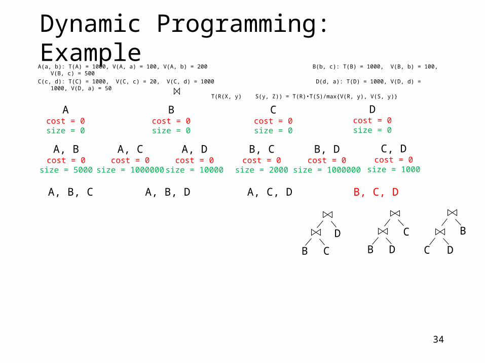
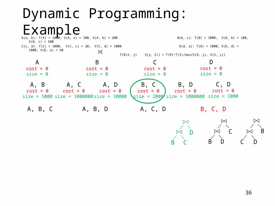
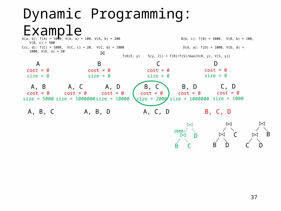
A, B, C B, C, Dcost = 1000size = 2000

A, C, DA, B, D

BC D

Dynamic Programming: ExampleA(a, b): T(A) = 1000, V(A, a) = 100, V(A, b) = 200 B(b, c): T(B) = 1000, V(B, b) = 100, V(B, c) = 500

C(c, d): T(C) = 1000, V(C, c) = 20, V(C, d) = 1000 D(d, a): T(D) = 1000, V(D, d) = 1000, V(D, a) = 50

T(R(X, y) S(y, Z)) = T(R)•T(S)/max{V(R, y), V(S, y)}

Acost = 0size = 0

Dcost = 0size = 0

Ccost = 0size = 0

Bcost = 0size = 0

A, Bcost = 0

size = 5000

C, Dcost = 0

size = 1000

B, Dcost = 0

size = 1000000

B, Ccost = 0

size = 2000

A, Dcost = 0

size = 10000

A, Ccost = 0

size = 1000000

A, B, Ccost = 2000size = 10000

B, C, Dcost = 1000size = 2000

A, C, Dcost = 1000size = 10000

A, B, Dcost = 5000size = 50000

BC D

Dynamic Programming: ExampleA(a, b): T(A) = 1000, V(A, a) = 100, V(A, b) = 200 B(b, c): T(B) = 1000, V(B, b) = 100, V(B, c) = 500

C(c, d): T(C) = 1000, V(C, c) = 20, V(C, d) = 1000 D(d, a): T(D) = 1000, V(D, d) = 1000, V(D, a) = 50

T(R(X, y) S(y, Z)) = T(R)•T(S)/max{V(R, y), V(S, y)}

43

Acost = 0size = 0

Dcost = 0size = 0

Ccost = 0size = 0

Bcost = 0size = 0

A, Bcost = 0

size = 5000

C, Dcost = 0

size = 1000

B, Dcost = 0

size = 1000000

B, Ccost = 0

size = 2000

A, Dcost = 0

size = 10000

A, Ccost = 0

size = 1000000

A, B, Ccost = 2000size = 10000

B, C, Dcost = 1000size = 2000

A, C, Dcost = 1000size = 10000

A, B, Dcost = 5000size = 50000

A, B, C, D

BC D

Dynamic Programming: ExampleA(a, b): T(A) = 1000, V(A, a) = 100, V(A, b) = 200 B(b, c): T(B) = 1000, V(B, b) = 100, V(B, c) = 500

C(c, d): T(C) = 1000, V(C, c) = 20, V(C, d) = 1000 D(d, a): T(D) = 1000, V(D, d) = 1000, V(D, a) = 50

T(R(X, y) S(y, Z)) = T(R)•T(S)/max{V(R, y), V(S, y)}

44

Acost = 0size = 0

Dcost = 0size = 0

Ccost = 0size = 0

Bcost = 0size = 0

A, Bcost = 0

size = 5000

C, Dcost = 0

size = 1000

B, Dcost = 0

size = 1000000

B, Ccost = 0

size = 2000

A, Dcost = 0

size = 10000

A, Ccost = 0

size = 1000000

A, B, Ccost = 2000size = 10000

B, C, Dcost = 1000size = 2000

A, C, Dcost = 1000size = 10000

A, B, Dcost = 5000size = 50000

A, B, C, D

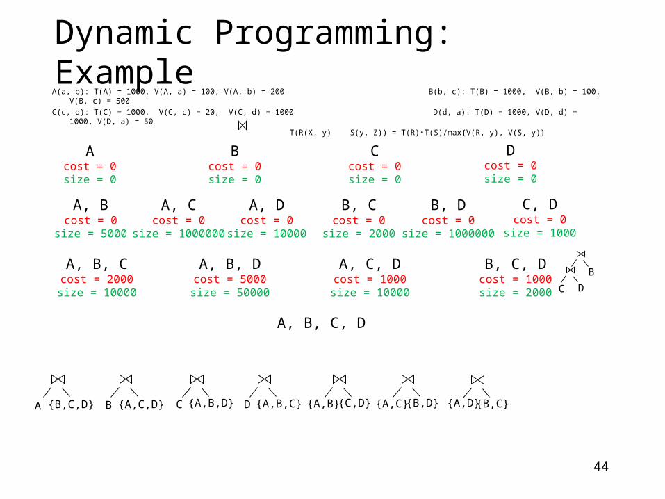
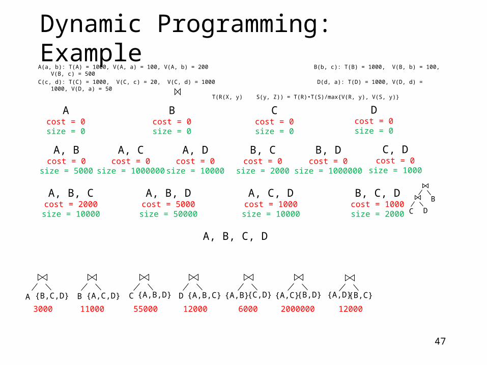
A

{B,C,D} DCB {A,C,D} {A,B,D} {A,B,C}

{A,B} {C,D} {A,C} {B,D} {A,D}{B,C}

BC D

Dynamic Programming: ExampleA(a, b): T(A) = 1000, V(A, a) = 100, V(A, b) = 200 B(b, c): T(B) = 1000, V(B, b) = 100, V(B, c) = 500

C(c, d): T(C) = 1000, V(C, c) = 20, V(C, d) = 1000 D(d, a): T(D) = 1000, V(D, d) = 1000, V(D, a) = 50

T(R(X, y) S(y, Z)) = T(R)•T(S)/max{V(R, y), V(S, y)}

45

Acost = 0size = 0

Dcost = 0size = 0

Ccost = 0size = 0

Bcost = 0size = 0

A, Bcost = 0

size = 5000

C, Dcost = 0

size = 1000

B, Dcost = 0

size = 1000000

B, Ccost = 0

size = 2000

A, Dcost = 0

size = 10000

A, Ccost = 0

size = 1000000

A, B, Ccost = 2000size = 10000

B, C, Dcost = 1000size = 2000

A, C, Dcost = 1000size = 10000

A, B, Dcost = 5000size = 50000

A, B, C, D

A

{B,C,D} DCB {A,C,D} {A,B,D} {A,B,C}

{A,B} {C,D} {A,C} {B,D} {A,D}{B,C}

3000

BC D

Dynamic Programming: ExampleA(a, b): T(A) = 1000, V(A, a) = 100, V(A, b) = 200 B(b, c): T(B) = 1000, V(B, b) = 100, V(B, c) = 500

C(c, d): T(C) = 1000, V(C, c) = 20, V(C, d) = 1000 D(d, a): T(D) = 1000, V(D, d) = 1000, V(D, a) = 50

T(R(X, y) S(y, Z)) = T(R)•T(S)/max{V(R, y), V(S, y)}

46

Acost = 0size = 0

Dcost = 0size = 0

Ccost = 0size = 0

Bcost = 0size = 0

A, Bcost = 0

size = 5000

C, Dcost = 0

size = 1000

B, Dcost = 0

size = 1000000

B, Ccost = 0

size = 2000

A, Dcost = 0

size = 10000

A, Ccost = 0

size = 1000000

A, B, Ccost = 2000size = 10000

B, C, Dcost = 1000size = 2000

A, C, Dcost = 1000size = 10000

A, B, Dcost = 5000size = 50000

A, B, C, D

A

{B,C,D} DCB {A,C,D} {A,B,D} {A,B,C}

{A,B} {C,D} {A,C} {B,D} {A,D}{B,C}

3000 6000

BC D

Dynamic Programming: ExampleA(a, b): T(A) = 1000, V(A, a) = 100, V(A, b) = 200 B(b, c): T(B) = 1000, V(B, b) = 100, V(B, c) = 500

C(c, d): T(C) = 1000, V(C, c) = 20, V(C, d) = 1000 D(d, a): T(D) = 1000, V(D, d) = 1000, V(D, a) = 50

T(R(X, y) S(y, Z)) = T(R)•T(S)/max{V(R, y), V(S, y)}

47

Acost = 0size = 0

Dcost = 0size = 0

Ccost = 0size = 0

Bcost = 0size = 0

A, Bcost = 0

size = 5000

C, Dcost = 0

size = 1000

B, Dcost = 0

size = 1000000

B, Ccost = 0

size = 2000

A, Dcost = 0

size = 10000

A, Ccost = 0

size = 1000000

A, B, Ccost = 2000size = 10000

B, C, Dcost = 1000size = 2000

A, C, Dcost = 1000size = 10000

A, B, Dcost = 5000size = 50000

A, B, C, D

A

{B,C,D} DCB {A,C,D} {A,B,D} {A,B,C}

{A,B} {C,D} {A,C} {B,D} {A,D}{B,C}

3000 11000 55000 12000 6000 2000000 12000

BC D

Dynamic Programming: ExampleA(a, b): T(A) = 1000, V(A, a) = 100, V(A, b) = 200 B(b, c): T(B) = 1000, V(B, b) = 100, V(B, c) = 500

C(c, d): T(C) = 1000, V(C, c) = 20, V(C, d) = 1000 D(d, a): T(D) = 1000, V(D, d) = 1000, V(D, a) = 50

T(R(X, y) S(y, Z)) = T(R)•T(S)/max{V(R, y), V(S, y)}

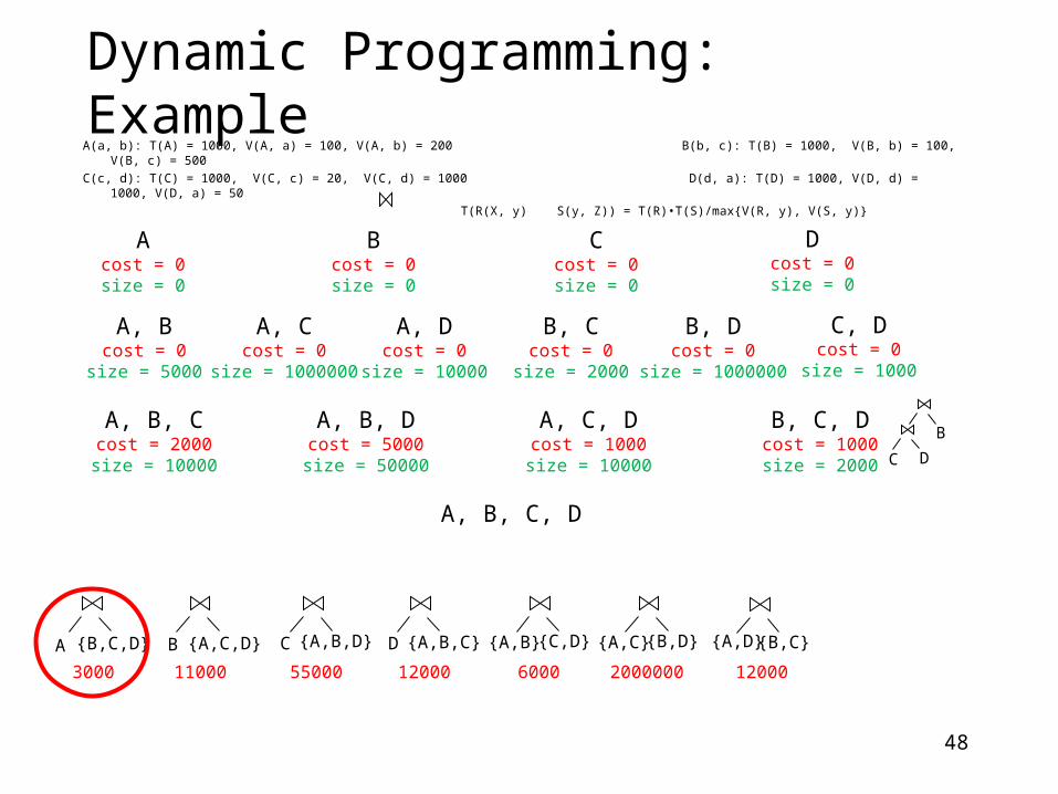
48

Acost = 0size = 0

Dcost = 0size = 0

Ccost = 0size = 0

Bcost = 0size = 0

A, Bcost = 0

size = 5000

C, Dcost = 0

size = 1000

B, Dcost = 0

size = 1000000

B, Ccost = 0

size = 2000

A, Dcost = 0

size = 10000

A, Ccost = 0

size = 1000000

A, B, Ccost = 2000size = 10000

B, C, Dcost = 1000size = 2000

A, C, Dcost = 1000size = 10000

A, B, Dcost = 5000size = 50000

A, B, C, D

A

{B,C,D} DCB {A,C,D} {A,B,D} {A,B,C}

{A,B} {C,D} {A,C} {B,D} {A,D}{B,C}

3000 11000 55000 12000 6000 2000000 12000

BC D

Dynamic Programming: ExampleA(a, b): T(A) = 1000, V(A, a) = 100, V(A, b) = 200 B(b, c): T(B) = 1000, V(B, b) = 100, V(B, c) = 500

C(c, d): T(C) = 1000, V(C, c) = 20, V(C, d) = 1000 D(d, a): T(D) = 1000, V(D, d) = 1000, V(D, a) = 50

T(R(X, y) S(y, Z)) = T(R)•T(S)/max{V(R, y), V(S, y)}

49

Acost = 0size = 0

Dcost = 0size = 0

Ccost = 0size = 0

Bcost = 0size = 0

A, Bcost = 0

size = 5000

C, Dcost = 0

size = 1000

B, Dcost = 0

size = 1000000

B, Ccost = 0

size = 2000

A, Dcost = 0

size = 10000

A, Ccost = 0

size = 1000000

A, B, Ccost = 2000size = 10000

B, C, Dcost = 1000size = 2000

A, C, Dcost = 1000size = 10000

A, B, Dcost = 5000size = 50000

A, B, C, D

A

{B,C,D} DCB {A,C,D} {A,B,D} {A,B,C}

{A,B} {C,D} {A,C} {B,D} {A,D}{B,C}

3000 11000 55000 12000 6000 2000000 12000

A

BC D

Dynamic Programming: ExampleA(a, b): T(A) = 1000, V(A, a) = 100, V(A, b) = 200 B(b, c): T(B) = 1000, V(B, b) = 100, V(B, c) = 500

C(c, d): T(C) = 1000, V(C, c) = 20, V(C, d) = 1000 D(d, a): T(D) = 1000, V(D, d) = 1000, V(D, a) = 50

T(R(X, y) S(y, Z)) = T(R)•T(S)/max{V(R, y), V(S, y)}

50

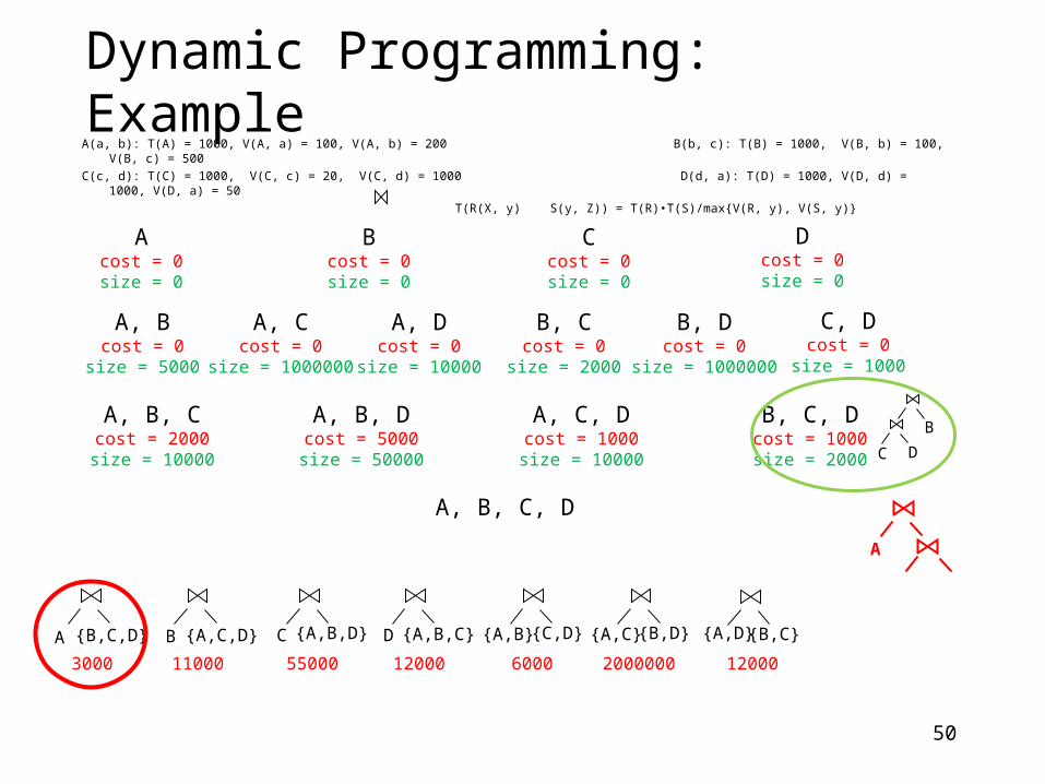
Acost = 0size = 0

Dcost = 0size = 0

Ccost = 0size = 0

Bcost = 0size = 0

A, Bcost = 0

size = 5000

C, Dcost = 0

size = 1000

B, Dcost = 0

size = 1000000

B, Ccost = 0

size = 2000

A, Dcost = 0

size = 10000

A, Ccost = 0

size = 1000000

A, B, Ccost = 2000size = 10000

B, C, Dcost = 1000size = 2000

A, C, Dcost = 1000size = 10000

A, B, Dcost = 5000size = 50000

A, B, C, D

A

{B,C,D} DCB {A,C,D} {A,B,D} {A,B,C}

{A,B} {C,D} {A,C} {B,D} {A,D}{B,C}

3000 11000 55000 12000 6000 2000000 12000

A

BC D

Dynamic Programming: ExampleA(a, b): T(A) = 1000, V(A, a) = 100, V(A, b) = 200 B(b, c): T(B) = 1000, V(B, b) = 100, V(B, c) = 500

C(c, d): T(C) = 1000, V(C, c) = 20, V(C, d) = 1000 D(d, a): T(D) = 1000, V(D, d) = 1000, V(D, a) = 50

T(R(X, y) S(y, Z)) = T(R)•T(S)/max{V(R, y), V(S, y)}

51

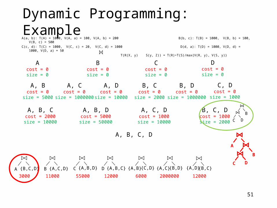
Acost = 0size = 0

Dcost = 0size = 0

Ccost = 0size = 0

Bcost = 0size = 0

A, Bcost = 0

size = 5000

C, Dcost = 0

size = 1000

B, Dcost = 0

size = 1000000

B, Ccost = 0

size = 2000

A, Dcost = 0

size = 10000

A, Ccost = 0

size = 1000000

A, B, Ccost = 2000size = 10000

B, C, Dcost = 1000size = 2000

A, C, Dcost = 1000size = 10000

A, B, Dcost = 5000size = 50000

A, B, C, D

A

{B,C,D} DCB {A,C,D} {A,B,D} {A,B,C}

{A,B} {C,D} {A,C} {B,D} {A,D}{B,C}

3000 11000 55000 12000 6000 2000000 12000

A

B

C D

BC D

Dynamic Programming: ExampleA(a, b): T(A) = 1000, V(A, a) = 100, V(A, b) = 200 B(b, c): T(B) = 1000, V(B, b) = 100, V(B, c) = 500

C(c, d): T(C) = 1000, V(C, c) = 20, V(C, d) = 1000 D(d, a): T(D) = 1000, V(D, d) = 1000, V(D, a) = 50

T(R(X, y) S(y, Z)) = T(R)•T(S)/max{V(R, y), V(S, y)}

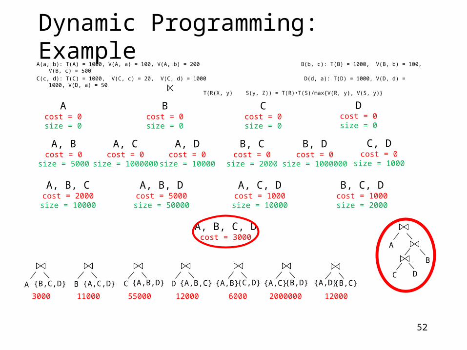
52

Acost = 0size = 0

Dcost = 0size = 0

Ccost = 0size = 0

Bcost = 0size = 0

A, Bcost = 0

size = 5000

C, Dcost = 0

size = 1000

B, Dcost = 0

size = 1000000

B, Ccost = 0

size = 2000

A, Dcost = 0

size = 10000

A, Ccost = 0

size = 1000000

A, B, Ccost = 2000size = 10000

B, C, Dcost = 1000size = 2000

A, C, Dcost = 1000size = 10000

A, B, Dcost = 5000size = 50000

A, B, C, Dcost = 3000

A

{B,C,D} DCB {A,C,D} {A,B,D} {A,B,C}

{A,B} {C,D} {A,C} {B,D} {A,D}{B,C}

3000 11000 55000 12000 6000 2000000 12000

A

B

C D

LQP Optimization with Size: Summary• Estimating sizes of immediate relations• Consider different order of an operation

left-deep tree

dynamic programming

53

Construction of Physical Query Plan

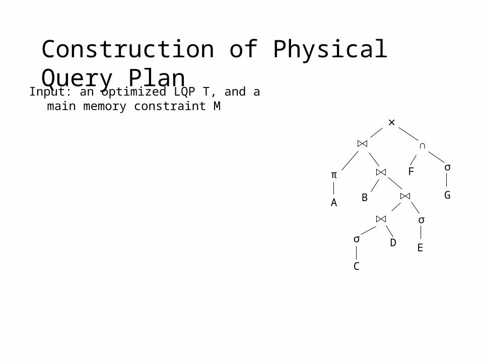
Construction of Physical Query PlanInput: an optimized LQP T, and a main memory

constraint M

×

∩

π

σ

σ

σ

G

F

ED

C

BA

Construction of Physical Query PlanInput: an optimized LQP T, and a main memory

constraint M

1. Replacing each leaf R of T by “scan(R)”;

×

∩

π

σ

σ

σ

scan(G)

scan(F)

scan(E)scan(D)

scan(C)

scan(B)scan(A)

Construction of Physical Query PlanInput: an optimized LQP T, and a main memory

constraint M

1. Replacing each leaf R of T by “scan(R)”;

2. Combining the “scan’s” with other operations;

×

∩

π

σ

σ

σ

scan(G)

scan(F)

scan(E)scan(D)

scan(C)

scan(B)scan(A)

index-scan

index-scan

Construction of Physical Query PlanInput: an optimized LQP T, and a main memory

constraint M

1. Replacing each leaf R of T by “scan(R)”;

2. Combining the “scan’s” with other operations;

3. Replacing each internal node v of T by a proper algorithm;

×

∩

π

σ

σ

σ

scan(G)

scan(F)

scan(E)scan(D)

scan(C)

scan(B)scan(A)

index-scan

index-scan

J2P

J2P

J1P

J1P

CJ

I1P

Construction of Physical Query PlanInput: an optimized LQP T, and a main memory

constraint M

1. Replacing each leaf R of T by “scan(R)”;

2. Combining the “scan’s” with other operations;

3. Replacing each internal node v of T by a proper algorithm;

4. For each edge e in T, decide if e should be “materialized”;

×

∩

π

σ

σ

σ

scan(G)

scan(F)

scan(E)scan(D)

scan(C)

scan(B)scan(A)

index-scan

index-scan

J2P

J2P

J1P

J1P

CJ

I1P

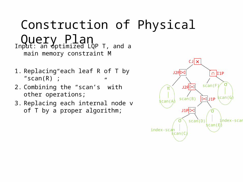
Construction of Physical Query PlanInput: an optimized LQP T, and a main memory

constraint M

1. Replacing each leaf R of T by “scan(R)”;

2. Combining the “scan’s” with other operations;

3. Replacing each internal node v of T by a proper algorithm;

4. For each edge e in T, decide if e should be “materialized”;

×

∩

π

σ

σ

σ

scan(G)

scan(F)

scan(E)scan(D)

scan(C)

scan(B)scan(A)

index-scan

index-scan

J2P

J2P

J1P

J1P

CJ

I1P

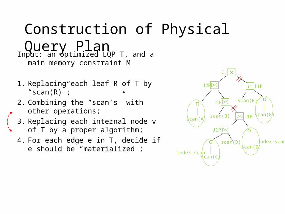
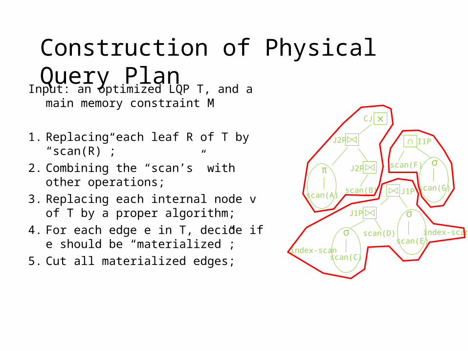
Construction of Physical Query PlanInput: an optimized LQP T, and a main memory

constraint M

1. Replacing each leaf R of T by “scan(R)”;

2. Combining the “scan’s” with other operations;

3. Replacing each internal node v of T by a proper algorithm;

4. For each edge e in T, decide if e should be “materialized”;

5. Cut all materialized edges;

×

∩

π

σ

σ

σ

scan(G)

scan(F)

scan(E)scan(D)

scan(C)

scan(B)scan(A)

index-scan

index-scan

J2P

J2P

J1P

J1P

CJ

I1P

Construction of Physical Query PlanInput: an optimized LQP T, and a main memory

constraint M

1. Replacing each leaf R of T by “scan(R)”;

2. Combining the “scan’s” with other operations;

3. Replacing each internal node v of T by a proper algorithm;

4. For each edge e in T, decide if e should be “materialized”;

5. Cut all materialized edges;

6. Each subtree is a call to the subroutine at the root of the subtree. The order of the calls follows the bottom-up order in the structure.

×

∩

π

σ

σ

σ

scan(G)

scan(F)

scan(E)scan(D)

scan(C)

scan(B)scan(A)

index-scan

index-scan

J2P

J2P

J1P

J1P

CJ

I1P

1

2

3

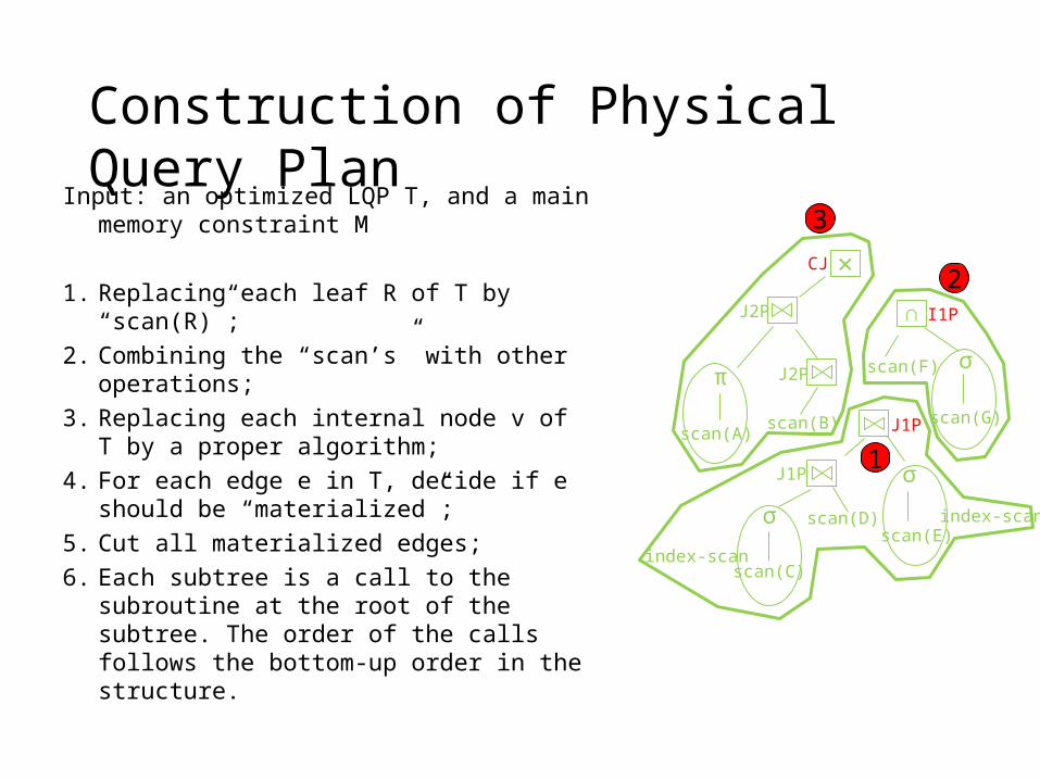
Construction of Physical Query PlanInput: an optimized LQP T, and a main memory

constraint M

1. Replacing each leaf R of T by “scan(R)”;

2. Combining the “scan’s” with other operations;

3. Replacing each internal node v of T by a proper algorithm;

4. For each edge e in T, decide if e should be “materialized”;

5. Cut all materialized edges;

6. Each subtree is a call to the subroutine at the root of the subtree. The order of the calls follows the bottom-up order in the structure.

×

∩

π

σ

σ

σ

scan(G)

scan(F)

scan(E)scan(D)

scan(C)

scan(B)scan(A)

index-scan

index-scan

J2P

J2P

J1P

J1P

CJ

I1P

1

2

3

This produces an executable code for the input DB program

Physical Query Plan: Summary

• Replacing internal nodes of a LQP by proper algorithms;

• Deciding if a subroutine call should be pipelined or materialized;

• Many optimization techniques are involved here;

• In practice, heuristic optimization techniques are used to construct good physical query plans;

• The resulting physical query plan is an executable code.

secondarystorage(disks)

in tables(relations)

databaseadministrator

DDLlanguage

database programmer

DML (query)language

DBMS

file manager

buffermanager

mainmemorybuffers

index/file manager

DML complier

DDL complier

query execution

engine

transaction manager

concurrency control

lock table

logging &recovery

graduate database

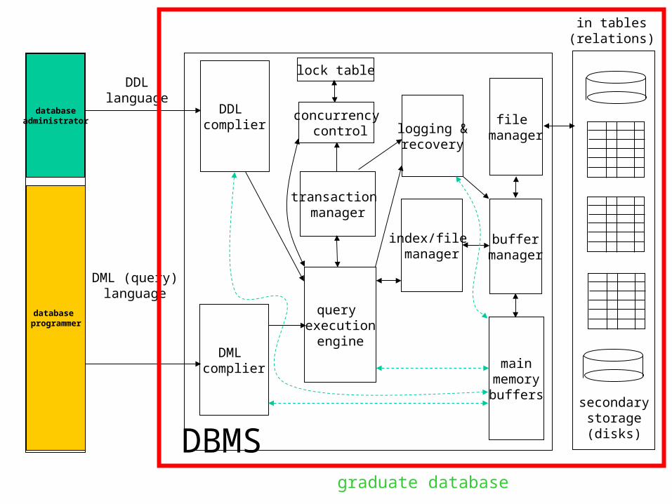
secondarystorage(disks)

in tables(relations)

databaseadministrator

DDLlanguage

database programmer

DML (query)language

DBMS

file manager

buffermanager

mainmemorybuffers

index/file manager

DML complier

DDL complier

query execution

engine

transaction manager

concurrency control

lock table

logging &recovery

graduate database
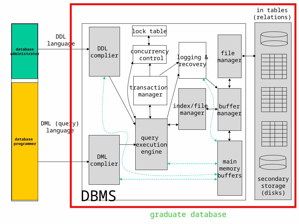