CPSC 425: Computer Vision

Instructor: Fred Tungftung@cs.ubc.ca

Department of Computer ScienceUniversity of British Columbia

Lecture Notes 2015/2016 Term 2

1 / 105

Menu February 9, 2016

Topics:Review for midterm

Reading: (after midterm)Paper: “Distinctive Image Features from Scale-Invariant Keypoints”Forsyth & Ponce (2nd ed.) 5.4

Reminders:Midterm exam, in class, Thursday, February 11TA office hours between now and midterm exam:— Kai: today, 4:00–5:30pm, ICCS X150 Table 4— Moumita: tomorrow, 3:00–4:30pm, ICCS X150 Table 4Reading week February 15-19Assignment 4 due Thursday, February 25www: http://www.cs.ubc.ca/~ftung/cpsc425/piazza: https://piazza.com/ubc.ca/winterterm22015/cpsc425/

2 / 105

Today’s Fun Example

Demo of chromatic adaptation

3 / 105

Lecture 10: Re-cap

Approaches to texture exploit pyramid (i.e. scaled) and orientedrepresentations

Human colour perception— colour matching experiments— additive and subtractive matching— principle of trichromacy

RGB and CIE XYZ are linear colour spaces

Uniform colour space: differences in coordinates are a good guideto differences in perceived colour

HSV colour space: more intuitive description of colour for humaninterpretation

(Human) colour constancy: perception of intrinsic surface colourunder different colours of lighting

4 / 105

Paths to Understanding

Five distinct “paths” to a deeper understanding of CPSC 425 coursematerial:

1 mathematics (i.e., theory)

2 “visualize” computation(s)

3 experiment— on simple (test) cases— on real images

4 read code

5 write code

5 / 105

Midterm Review: Readings

Lecture 1–10 slides

Assigned readings from Forsyth & Ponce (2nd ed.)— Paper “Texture Synthesis by Non-parametric Sampling”

Assignments 2–3

iClicker questions

Lecture exercises

Practice problems (with solutions)

6 / 105

Midterm Details

60 minutes

Closed book, no calculators

Format similar to posted practice problems— Part A: Multiple-part true/false— Part B: Short answer

No coding questions

7 / 105

Camera Obscura (Latin for ‘dark chamber’)

Reinerus Gemma-Frisius observed an eclipse of the sun at Louvain onJanuary 24, 1544. He used this illustration in his book, “De RadioAstronomica et Geometrica,” 1545. It is thought to be the firstpublished illustration of a camera obscura.

Credit: John H., Hammond, “The Camera Obscura, A Chronicle”

8 / 105

Pinhole Camera (Simplified)

x’

x

zf’

imageplane

pinhole object

9 / 105

Pinhole Camera (Simplified) (cont’d)

x’

x

zf’

imageplane

pinhole object

f’

x’

imageplane

10 / 105

Perspective Projection

Forsyth & Ponce (1st ed.) Figure 1.4

3D object point, P[x , y , z], projects to 2D image point P ′[x ′, y ′] where

x ′ = f ′xz

y ′ = f ′yz

11 / 105

Summary of Projection Equations3D world point, P[x , y , z], projects to 2D image point P ′[x ′, y ′] where

Perspectivex ′ = f ′

xz

y ′ = f ′yz

Weak Perspectivex ′ = m x

y ′ = m ym =

f ′

z0

Orthographicx ′ = x

y ′ = y

12 / 105

Sample Question: Image Formation

True of false: A pinhole camera uses an orthographic projection.

13 / 105

Why Not a Pinhole Camera?

Credit: E. Hecht. “Optics,” Addison-Wesley, 1987

14 / 105

Why Not a Pinhole Camera (cont’d)?

If pinhole is too big then many directions are averaged, blurringthe image

If pinhole is too small then diffraction becomes a factor, alsoblurring the image

Generally, pinhole cameras are dark, because only a very smallset of rays from a particular scene point hits the image plane

Equivalently, pinhole cameras are slow, because only a very smallamount of light from a particular scene point hits the image planeper unit time

15 / 105

Pinhole Model (Simplified) with Lens

x’

x

z

imageplane

objectlens

z’

16 / 105

Vignetting

Image credit: Cambridge in Colour

17 / 105

Chromatic Aberration

Image credit: Trevor Darrell

18 / 105

Lens Distortion

Image credit: Fig. 2.13 in Szeliski

19 / 105

Sample Question: Cameras and Lenses

True of false: Snell’s Law describes how much light is reflected andhow much passes through the boundary between two materials.

20 / 105

Linear Filters (cont’d)

I ′(X ,Y ) =k∑

j=−k

k∑i=−k

F (i , j) I (X + i ,Y + j)

For each X and Y , superimpose the filter, F (X ,Y ), on the imagecentered at (X ,Y )

Compute the new pixel value, I′(X ,Y ), as the sum of m ×m values,where each value is the product of the original pixel value in I(X ,Y )and the corresponding value in the filter

21 / 105

22 / 105

Linear Filters: Boundary Effects

3 standard ways to deal with boundaries

1 Ignore these locations— Make the computation undefined for the top and bottom k rowsand the leftmost and rightmost k columns

2 Pad the image with zeros— Return zero whenever a value of I is required at some positionoutside the defined limits of X and Y

3 Assume periodicity— The top row wraps around to the bottom row; the leftmostcolumn wraps around to the rightmost column

23 / 105

Linear Filters

The correlation of F (X ,Y ) and I(X ,Y ) is

I′(X ,Y ) =k∑

j=−k

k∑i=−k

F (i , j) I (X + i ,Y + j)

Visual interpretation: Superimpose the filter F on the image I at(X,Y), perform an element-wise multiply, and sum up the values

Convolution is like correlation except filter “flipped”— When F (−i ,−j) = F (i , j) the two are equivalent

24 / 105

Linear Systems: Characterization Theorem

Any linear, shift invariant operation can be expressed as a convolution

25 / 105

26 / 105

Example 1 (cont’d): Smoothing with a Gaussian

Idea: Weigh contributions of neighbouring pixels by nearness

2D Gaussian (continuous case):

Gσ(x , y) =1

2πσ2 exp−

x2 + y2

2σ2

Forsyth & Ponce (2nd ed.)Figure 4.2

27 / 105

Gaussian: Area Under the Curve

σ σσσ σσσσ

68%

99.99%

99.7%

95%

28 / 105

Efficient Implementation: Separability

A 2D function of x and y is separable if it can be written as theproduct of two functions, one a function only of x and the other afunction only of y

Both the 2D box filter and the 2D Gaussian filter are separable

Both can be implemented as two 1D convolutions:— First, convolve each row with a 1D filter— Then, convolve each column with a 1D filter— Aside: or vice versa

The 2D Gaussian is the only (non trivial) 2D function that is bothseparable and rotationally invariant.

29 / 105

Linear Filters: Additional Properties

Let ⊗ denote convolution. Let I(X ,Y ) be a digital image. Let F and Gbe digital filters

Convolution is associative. That is,

G ⊗ (F ⊗ I(X ,Y )) = (G ⊗ F )⊗ I(X ,Y )

Convolution is symmetric. That is,

(F ⊗G)⊗ I(X ,Y ) = (G ⊗ F )⊗ I(X ,Y )

Convolving I(X ,Y ) with filter F and then convolving the result with filterG can be achieved in a single step, namely convolving I(X ,Y ) withfilter G ⊗ F = G ⊗ F

30 / 105

Bilateral Filter

An edge-preserving non-linear filter

Like a Gaussian filter, the filter weights depend on spatial distancefrom the center pixel— Idea: Pixels nearby (in space) should have greater influencethan pixels far away

Unlike a Gaussian filter, the filter weights also depend on rangedistance from the center pixel— Idea: Pixels with similar brightness value should have greaterinfluence than pixels with dissimilar brightness value

31 / 105

Bilateral Filter

Application: Denoising

Figure credit: Alexander Wong

32 / 105

Sample Question: Filters

What does the following 3× 3 linear, shift invariant filter compute whenapplied to an image? −1 −1 −1

0 0 01 1 1

33 / 105

Continuous Case

x

yi(x,y)

Denote the image as a function, i(x , y), where x and y are spatialvariables

34 / 105

Discrete Case

Idea: Superimpose (regular) grid on continuous image

i(x,y)

x

y

Sample the underlying continuous image according to the tessellationimposed by the grid

35 / 105

Discrete Case (cont’d)

���������������

���������������

i(x,y)

x

y

pixel

Each grid cell is called a picture element (or pixel)

Denote the discrete image as

I(X ,Y )

We can store the pixels in a matrix or array

36 / 105

SamplingIt’s clear that some information may be lost when we work on adiscrete pixel grid.

Figure credit: Forsyth & Ponce (2nd ed.) Figure 4.737 / 105

Sampling Theory

Exact reconstruction requires constraint on the rate at whichi(x , y) can change between samples— “rate of change” means derivative— the formal concept is bandlimited signal— “bandlimit” and “constraint on derivative” are linked

An image is bandlimited if it has some maximum spatial frequency

A fundamental result (Sampling Theorem) is:For bandlimited signals, if you sample regularly at orabove twice the maximum frequency (called the Nyquistrate), then you can reconstruct the original signal exactly

38 / 105

Sampling Theory (cont’d)

Sometimes undersampling is unavoidable, and there is a trade-offbetween “things missing” and “artifacts.”

Medical imaging: usually try to maximize information content,tolerate some artifactsComputer graphics: usually try to minimize artifacts, tolerate someinformation missing

39 / 105

Template Matching

Figure credit: Kristen Grauman

40 / 105

Template Matching

We can think of convolution/correlation as comparing a template (thefilter) with each local image patch.

Consider the filter and image patch as vectors.

Applying a filter at an image location can be interpreted ascomputing the dot product (recall: element-wise multiply and sum)between the filter and the local image patch.

But... The dot product may be large simply because the image regionis bright. We need to normalize the result in some way.

41 / 105

Template Matching

Let a and b be vectors. Let θ be the angle between them

We knowcos θ =

a · b|a| |b|

=a · b√

(a · a) (b · b)

where · is dot product and | | is vector magnitude

Correlation is a dot product

Correlation measures similarity between the filter and each local imageregion

Normalized correlation varies between −1 and 1

Normalized correlation attains the value 1 when the filter and imageregion are identical (up to a scale factor)

42 / 105

Template Matching

Figure credit: Kristen Grauman

43 / 105

Example 1 (cont’d): Normalized Correlation

Template (left), image (middle), normalized correlation (right)

Note peak value at the true position of the hand

Credit: W. Freeman et al., “Computer Vision for Interactive ComputerGraphics,” IEEE Computer Graphics and Applications, 1998

44 / 105

Sample Question: Template Matching

True or false: Normalized correlation is robust to a constant scaling inthe image brightness.

45 / 105

Scaled Representations

Goals:

to find template matches at all scales— template size constant, image scale varies— e.g., finding hands or faces when we don’t know what size theywill be in the image

efficient search for image–to–image correspondences— look first at coarse scales, refine at finer scales— much less cost (but may miss best match)

to examine all levels of detail— find edges with different amounts of blur— find textures with different spatial frequencies

(i.e., different levels of detail)

46 / 105

Shrinking an Image

256 × 256 128 × 128 64 × 64 32 × 32 16 × 16

nosmoothing

Gaussianσ = 1

Gaussianσ = 2

Forsyth & Ponce (2nd ed.) Figures 4.12–4.14 (top rows)

47 / 105

Image Pyramid

An image pyramid is a collection of representations of an image

Typically, each layer of the pyramid is half the width and half the heightof the previous layer

In a Gaussian pyramid, each layer is smoothed by a Gaussian filterand resampled to get the next layer

48 / 105

Example 1: A Gaussian Pyramid

Forsyth & Ponce (2nd ed.) Figure 4.17

49 / 105

From Template Matching to Local Feature Detection

Slide credit: Li Fei-Fei, Rob Fergus, and Antonio Torralba

50 / 105

Estimating Derivatives

Recall, for a 2D (continuous) function, f (x , y)

∂f∂x

= limε→0

f (x + ε, y) − f (x , y)

ε

Differentiation is linear and shift invariant, and therefore can beimplemented as a convolution

A (discrete) approximation is

∂f∂x

≈ F (X + 1,Y ) − F (X ,Y )

∆x

51 / 105

Estimating Derivatives

A similar definition (and approximation) holds for∂f∂y

.

Image noise tends to result in pixels not looking exactly like theirneighbours, so simple “finite differences” are sensitive to noise.

The usual way to deal with this problem is to smooth the image prior toderivative estimation.

52 / 105

What Causes an Edge?What causes an edge?

• Depth discontinuity• Surface orientation

discontinuity• Reflectance

discontinuity (i.e., change in surface material properties)

• Illumination discontinuity (e.g., shadow)

Slide credit: Christopher Rasmussen

53 / 105

Smoothing and Differentiation

Edge: a location with high gradient (derivative)

Need smoothing to reduce noise prior to taking derivative

Need two derivatives, in x and y direction

We can use derivative of Gaussian filters— because differentiation is convolution, and— convolution is associative

Let ⊗ denote convolution

D ⊗ (G ⊗ I(X ,Y )) ≡ (D ⊗G)⊗ I(X ,Y )

54 / 105

Gradient Magnitude

Let I(X ,Y ) be a (digital) image

Let Ix (X ,Y ) and Iy (X ,Y ) be estimates of the partial derivatives in thex and y directions, respectively.

Call these estimates Ix and Iy (for short)

The vector [Ix , Iy ] is the gradient

The scalar√

Ix 2 + Iy 2 is the gradient magnitude

55 / 105

Two Generic Approaches to Edge Detection

x

y

r

r

r

r

i(r)

d i(r) dr

d2i(r) dr2

Two generic approaches to edge point detection:— (significant) local extrema of a first derivative operator— zero crossings of a second derivative operator

56 / 105

Marr/Hildreth Laplacian of Gaussian (cont’d)

Steps:

1 Gaussian for smoothing

2 Laplacian (52) for differentiation where

52f (x , y) ≡ ∂2f (x , y)

∂x2 +∂2f (x , y)

∂y2

3 locate zero-crossings in the Laplacian of the Gaussian (52G)where

52G(x , y) =−1

2πσ4

[2 − x2 + y2

σ2

]exp− x2 + y2

2σ2

57 / 105

Marr/Hildreth Laplacian of Gaussian (cont’d)Here’s a 1D plot of the Laplacian of the Gaussian (52G). . .

t

g(t)

. . . with its characteristic “Mexican hat” shape

58 / 105

Canny Edge Detection (cont’d)

Steps:

1 Apply directional derivatives of Gaussian

2 Non-maximum suppression— thin multi-pixel wide “ridges” down to single pixel width

3 Linking and thresholding— Low, high edge-strength thresholds— Accept all edges over low threshold that are connected

to edge over high threshold

59 / 105

Edge Hysteresis

One way to deal with broken edge chains is to use hysteresis

Hysteresis: A lag or momentum factor

Idea: Maintain two thresholds khigh and klow— Use khigh to find strong edges to start edge chain— Use klow to find weak edges which continue edge chain

Typical ratio of thresholds is (roughly)

khigh

klow= 2

60 / 105

61 / 105

How do humans perceive boundaries?

Figure credit: Szeliski Fig. 4.31. Original: Martin et al. 2004

Each image shows multiple (4-8) human-marked boundaries. Pixelsare darker where more humans marked a boundary.

62 / 105

Sample Question: Edges

Why is non-maximum suppression applied in the Canny edgedetector?

63 / 105

What is a corner?

Credit: John Shakespeare, Sydney Morning Herald

We can think of a corner as any locally distinct 2D image feature that(hopefully) corresponds to a distinct position on an 3D object ofinterest in the scene.

64 / 105

Why are corners “distinct"?

A corner can be localized reliably.

Thought experiment:Place a small window over a patch of constant image value. If youslide the window in any direction, the image in the window will notchange.Place a small window over an edge. If you slide the window in thedirection of the edge, the image in the window will not change→ Cannot estimate location along an edgePlace a small window over a corner. If you slide the window in anydirection, the image in the window changes.

65 / 105

Autocorrelation

Figure credit: Szeliski Fig. 4.5

66 / 105

Corner Detection

Edge detectors perform poorly at corners

Observations:

The gradient is ill defined exactly at a corner

Near a corner, the gradient has two (or more) distinct values

67 / 105

Harris Corner DetectorThe Harris corner detector

=

∑∑∑∑

2

2

yyx

yxx

IIIIII

C

Form the second-moment matrix:Sum over a small region around the hypothetical corner

Gradient with respect to x, times gradient with respect to y

Matrix is symmetric Slide credit: David Jacobs

68 / 105

Harris Corner Detector

Filter image with Gaussian

Compute magnitude of the x and y gradients at each pixel

Construct C in a window around each pixel— Harris uses a Gaussian window

Solve for product of the λs

If λs both are big (product reaches local maximum abovethreshold) then we have a corner— Harris also checks that ratio of λs is not too high

69 / 105

70 / 105

71 / 105

Example 1: Harris Corners

Originally developed as features for motion tracking

Greatly reduces amount of computation (compared to trackingevery pixel)

Translation and rotation invariant (but not scale invariant)

72 / 105

Harris Corner Detector

Not scale invariant:

Slide credit: Trevor Darrell

73 / 105

Sample Question: Corners

The Harris corner detector is stable under some image transformations(features are considered stable if the same locations on an object are

typically selected in the transformed image).True or false: The Harris corner detector is stable under image blur.

74 / 105

Texture

We will look at two main questions:

1 How do we represent texture?→ Texture analysis

2 How do we generate new examples of a texture?→ Texture synthesis

75 / 105

Texture Synthesis

Why might we want to synthesize texture?

1 To fill holes in images (inpainting)— Art directors might want to remove telephone wires. Restorersmight want to remove scratches or marks.— We need to find something to put in place of the pixels thatwere removed— We synthesize regions of texture that fit in and look convincing

2 To produce large quantities of texture for computer graphics— Good textures make object models look more realistic

76 / 105

Texture Synthesis

Figure credit: Szeliski Fig. 10.49

77 / 105

Texture Synthesis

Photo Credit: Associated Press78 / 105

Efros and Leung: Synthesizing One PixelSynthesizing One PixelSynthesizing One Pixel

Infinite sample image

Generated image– Assuming Markov property, what is conditional probability

distribution of p, given the neighbourhood window?– Instead of constructing a model, let’s directly search the

input image for all such neighbourhoods to produce a histogram for p

– To synthesize p, just pick one match at random

SAMPLE

p

What is conditional probability distribution of p, given theneighbourhood window?Directly search the input image for all such neighbourhoods toproduce a histogram for pTo synthesize p, pick one match at random

Credit: http://graphics.cs.cmu.edu/people/efros/research/NPS/efros-iccv99.ppt

79 / 105

Efros and Leung: Really Synthesizing One PixelReally Synthesizing One PixelReally Synthesizing One Pixel

finite sample image

Generated image

p

– However, since our sample image is finite, an exact neighbourhood match might not be present

– So we find the best match using SSD error (weighted by a Gaussian to emphasize local structure), and take all samples within some distance from that match

SAMPLE

Since the sample image is finite, an exact neighbourhood matchmight not be presentFind the best match using SSD error, weighted by a Gaussian toemphasize local structure, and take all samples within somedistance from that match

Credit: http://graphics.cs.cmu.edu/people/efros/research/NPS/efros-iccv99.ppt

80 / 105

Efros and Leung: Synthesizing Many Pixels

For multiple pixels, "grow" the texture in layers— In the case of hole-filling, start from the edges of the hole

For an interactive demo, seehttp://jltmtz.github.io/efros-and-leung-js/(written by Julieta Martinez, a previous CPSC 425 TA)

81 / 105

Efros and Leung: Randomness ParameterRandomness ParameterRandomness Parameter

Credit: http://graphics.cs.cmu.edu/people/efros/research/NPS/efros-iccv99.ppt

82 / 105

“Big Data" Meets Inpainting

Figure credit: Hays and Efros 2007

83 / 105

“Big Data" Meets Inpainting

Algorithm sketch (Hays and Efros 2007):1 Create a short list of a few hundred “best matching" images based

on global image statistics2 Find patches in the short list that match the context surrounding

the image region we want to fill3 Blend the match into the original image

Purely data-driven, requires no manual labelling of images

84 / 105

The Goal of Texture Analysis

25

The Goal of Texture Analysis

True (infinite) texture

ANALYSIS

generated image

input image

“Same” or “different”

Compare textures and decide if they’re made of the same “stuff”.Compare textures and decide if they’re made of the same “stuff”

Credit: Bill Freeman

85 / 105

Texture Segmentation

Question: Is texture a property of a point or a property of a region?

Answer: We need a region to have a texture.

There is a “chicken–and–egg” problem. Texture segmentation can bedone by detecting boundaries between regions of the same (or similar)texture. Texture boundaries can be detected using standard edgedetection techniques applied to the texture measures determined ateach point

We compromise! Typically one uses a local window to estimate textureproperties and assigns those texture properties as point properties ofthe window’s center row and column

86 / 105

Texture Representation

Observation: Textures are made up of generic sub-elements, repeatedover a region with similar statistical properties

Idea: Find the sub-elements with filters, then represent each point inthe image with a summary of the pattern of sub-elements in the localregion

Question: What filters should we use?

Answer: Human vision suggests spots and oriented edge filters at avariety of different orientations and scales

Question: How do we “summarize”?

Answer: Compute the mean or maximum of each filter response overthe region— Other statistics can also be useful

87 / 105

Texture Representation

Observation: Textures are made up of generic sub-elements, repeatedover a region with similar statistical properties

Idea: Find the sub-elements with filters, then represent each point inthe image with a summary of the pattern of sub-elements in the localregion

Question: What filters should we use?

Answer: Human vision suggests spots and oriented edge filters at avariety of different orientations and scales

Question: How do we “summarize”?

Answer: Compute the mean or maximum of each filter response overthe region— Other statistics can also be useful

88 / 105

Texture Representation

Observation: Textures are made up of generic sub-elements, repeatedover a region with similar statistical properties

Idea: Find the sub-elements with filters, then represent each point inthe image with a summary of the pattern of sub-elements in the localregion

Question: What filters should we use?

Answer: Human vision suggests spots and oriented edge filters at avariety of different orientations and scales

Question: How do we “summarize”?

Answer: Compute the mean or maximum of each filter response overthe region— Other statistics can also be useful

89 / 105

Texture Representation

Figure credit: Leung and Malik 2001

90 / 105

Spots and Bars (Fine Scale)

Forsyth & Ponce (1st ed.) Figures 9.3–9.4

91 / 105

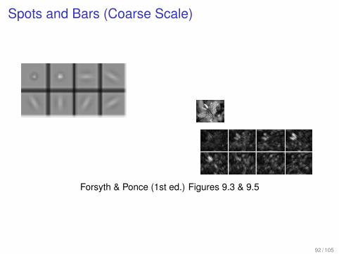
Spots and Bars (Coarse Scale)

Forsyth & Ponce (1st ed.) Figures 9.3 & 9.5

92 / 105

Laplacian Pyramid

Building a Laplacian pyramid:— Create a Gaussian pyramid— Take the difference between one Gaussian pyramid

level and the next (before subsampling)

Properties— Also known as the difference-of-Gaussian (DOG)

function, a close approximation to the Laplacian— It is a band pass filter – each level represents a different

band of spatial frequencies

Reconstructing the original image:— Reconstruct the Gaussian pyramid starting at top

93 / 105

Oriented Pyramids (cont’d)

Forsyth & Ponce (1st ed.) Figure 9.13

Reprinted from “Shiftable MultiScale Transforms,” by Simoncelli et al., IEEETransactions on Information Theory, 1992, c©1992, IEEE

94 / 105

Final Texture Representation

Steps:

1 Form a Laplacian and oriented pyramid (or equivalent set ofresponses to filters at different scales and orientations)

2 Square the output (makes values positive)

3 Average responses over a neighborhood by blurring with aGaussian

4 Take statistics of responses— Mean of each filter output— Possibly standard deviation of each filter

95 / 105

Sample Question: Texture

How does the top-most image in a Laplacian pyramid differ from theothers?

96 / 105

Colour Matching Experiments: I

Forsyth & Ponce (2nd ed.) Figure 3.2

Show a split field to subjects. One side shows the light whose colourone wants to match. The other a weighted mixture of three primaries(fixed lights)

97 / 105

Colour Matching Experiments: II

Many colours can be represented as a positive weighted sum ofA, B, C

WriteM = a A + b B + c C

where the = sign should be read as “matches”

This is additive matching

Defines a colour description system— two people who agree on A, B, C need only supply

(a,b, c)

98 / 105

Colour Matching Experiments: II (cont’d)

Some colours can’t be matched this way

Instead, we must write

M + a A = b B + c C

where, again, the = sign should be read as “matches”

This is subtractive matching

Interpret this as (−a,b, c)

Problem for designing displays:

Choose phosphors R, G, B so that positive linear combinations matcha large set of colours

99 / 105

Linear Colour Spaces

A choice of primaries yields a linear colour space— the coordinates of a colour are given by the weights of the

primaries used to match it

Choice of primaries is equivalent to choice of colour space

RGB: Primaries are monochromatic energies, say 645.2 nm,526.3 nm, 444.4 nm

CIE XYZ: Primaries are imaginary, but have other convenientproperties. Colour coordinates are (X ,Y ,Z ), where X is theamount of the X primary, etc.

100 / 105

Uniform Colour Spaces

McAdam ellipses demonstrate that differences in x , y are a poorguide to differences in perceived colour

A uniform colour space is one in which differences in coordinatesare a good guide to differences in perceived colour— example: CIE LAB

101 / 105

HSV Colour Space

More natural description of colour for human interpretation

Hue: attribute that describes a pure colour— e.g. ’red’, ’blue’

Saturation: measure of the degree to which a pure colour is diluted bywhite light

— pure spectrum colours are fully saturatedValue: intensity or brightness

Hue + saturation also referred to as chromaticity.

102 / 105

Colour Constancy

Image colour depends on both light colour and surface colour

Colour constancy: determine hue and saturation under differentcolours of lighting

It is surprisingly difficult to predict what colours a human willperceive in a complex scene— depends on context, other scene information

Humans can usually perceive— the colour a surface would have under white light— the colour of the reflected light (separate surface colour from

measured colour)

103 / 105

Summary Table

Summary of what we’ve seen so far:

Representation Result is. . . Approach Technique

intensity dense (2D)templatematching

(normalized)correlation,SSD

edgerelativelysparse (1D)

derivatives 52G, Canny

corner sparse (0D)locally distinctfeatures

Harris

104 / 105

Questions?

105 / 105