CPS216: Advanced Database Systems

Notes 03:Query Processing (Overview, contd.)

Shivnath Babu

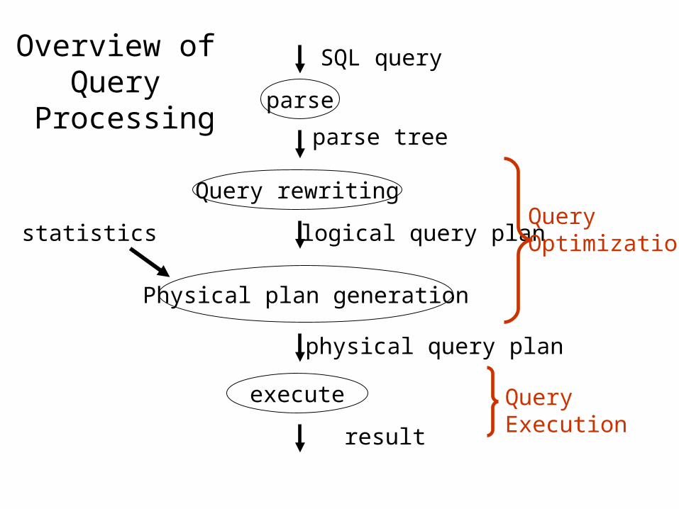
parse

Query rewriting

Physical plan generation

execute

result

SQL query

parse tree

logical query planstatistics

physical query plan

QueryOptimization

Query Execution

Overview of Query

Processing

parse

Query rewriting

Physical plan generation

execute

result

SQL query

parse tree

logical query planstatistics

physical query plan

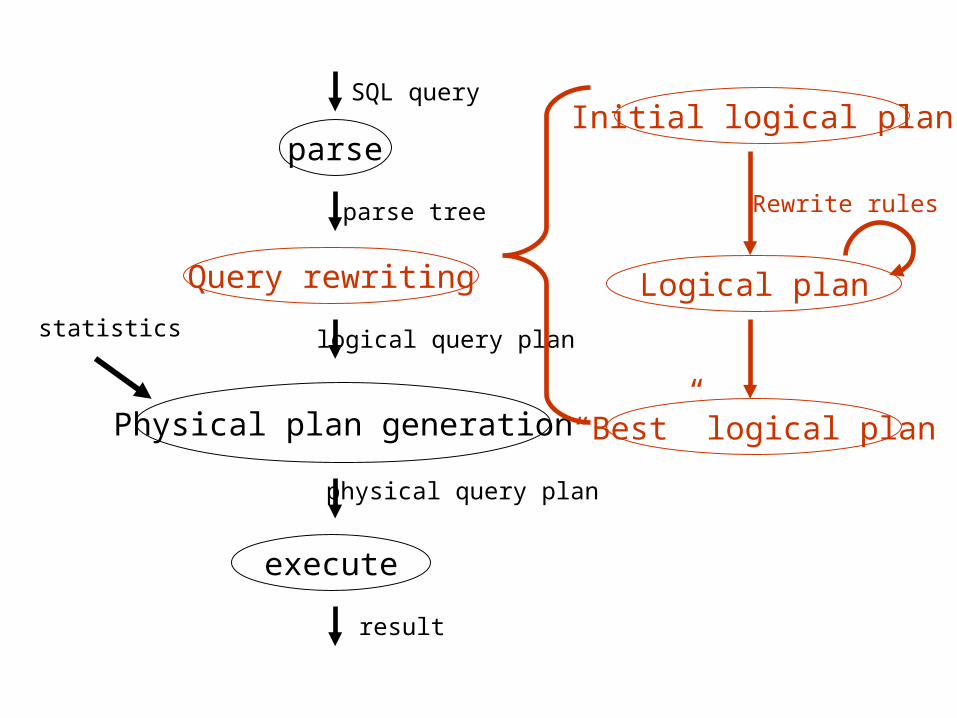
Initial logical plan

“Best” logical plan

Logical plan

Rewrite rules

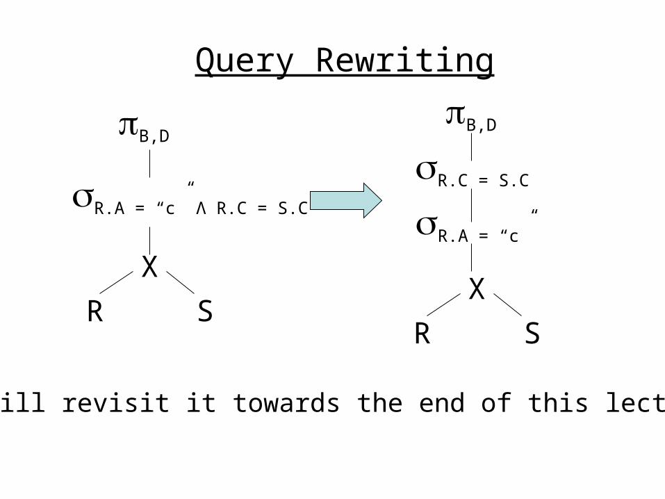
Query Rewriting

B,D

R.A = “c” Λ R.C = S.C

X

R S

B,D

R.A = “c”

X

R S

R.C = S.C

We will revisit it towards the end of this lecture

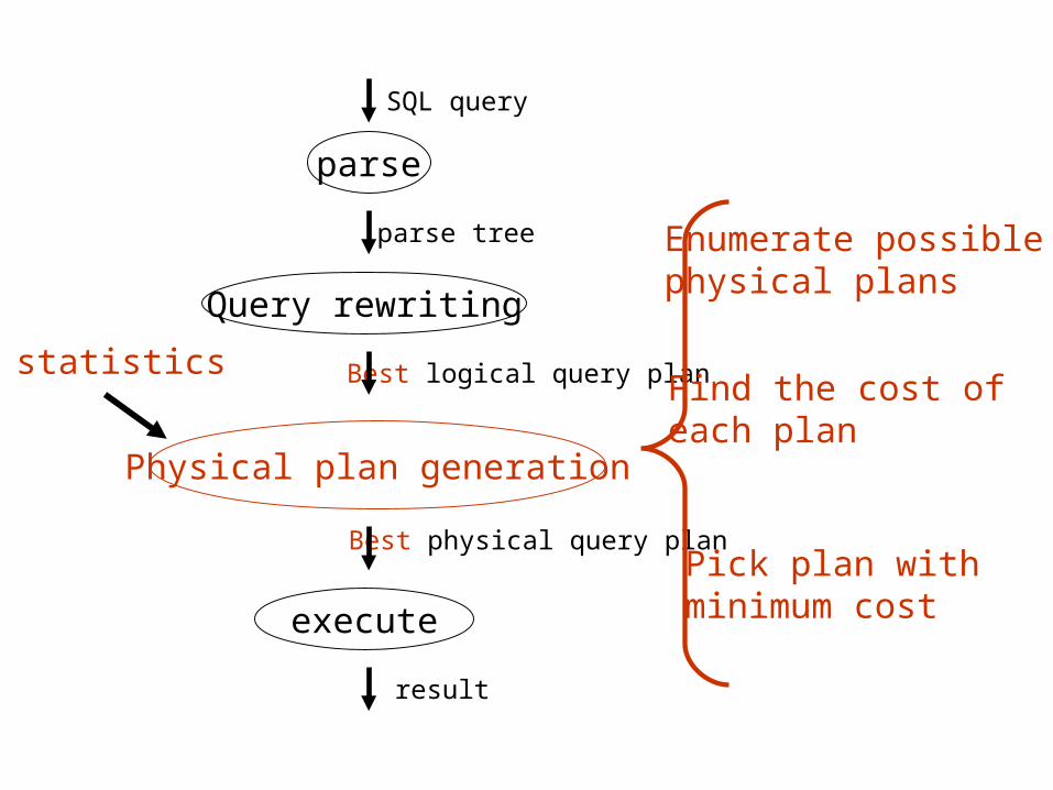
parse

Query rewriting

Physical plan generation

execute

result

SQL query

parse tree

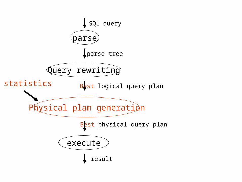
Best logical query planstatistics

Best physical query plan

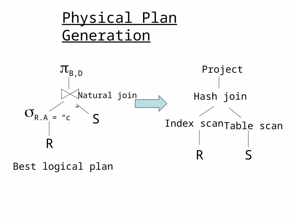
Physical Plan Generation

B,D

R.A = “c”

R

S

Natural join

Best logical planR S

Index scan Table scan

Hash join

Project

parse

Query rewriting

Physical plan generation

execute

result

SQL query

parse tree

Best logical query planstatistics

Best physical query plan

Enumerate possible physical plans

Find the cost of each plan

Pick plan with minimum cost

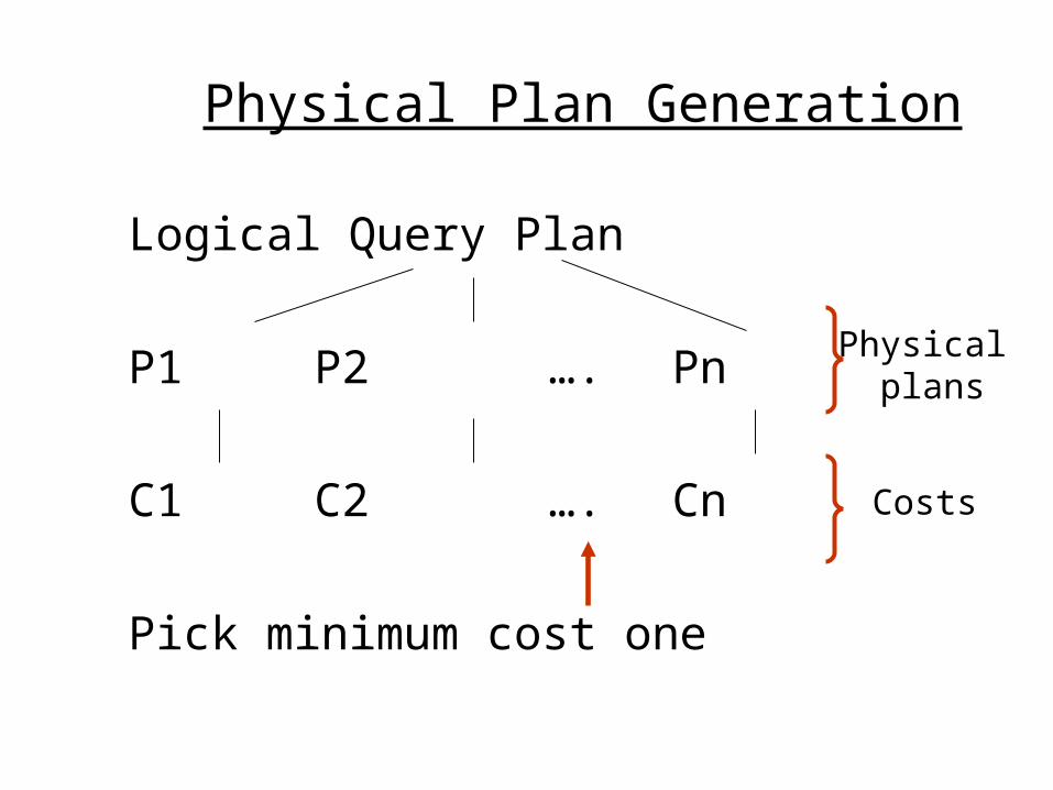
Physical Plan Generation

Logical Query Plan

P1 P2 …. Pn

C1 C2 …. Cn

Pick minimum cost one

Physical plans

Costs

Plans for Query Execution• Roadmap

– Path of a SQL query– Operator trees– Physical Vs Logical plans– Plumbing: Materialization Vs pipelining

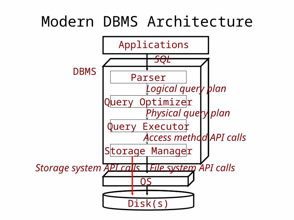
Modern DBMS Architecture

Disk(s)

Applications

OS

Parser

Query Optimizer

Query Executor

Storage Manager

Logical query plan

Physical query plan

Access method API calls

SQL

File system API callsStorage system API calls

DBMS

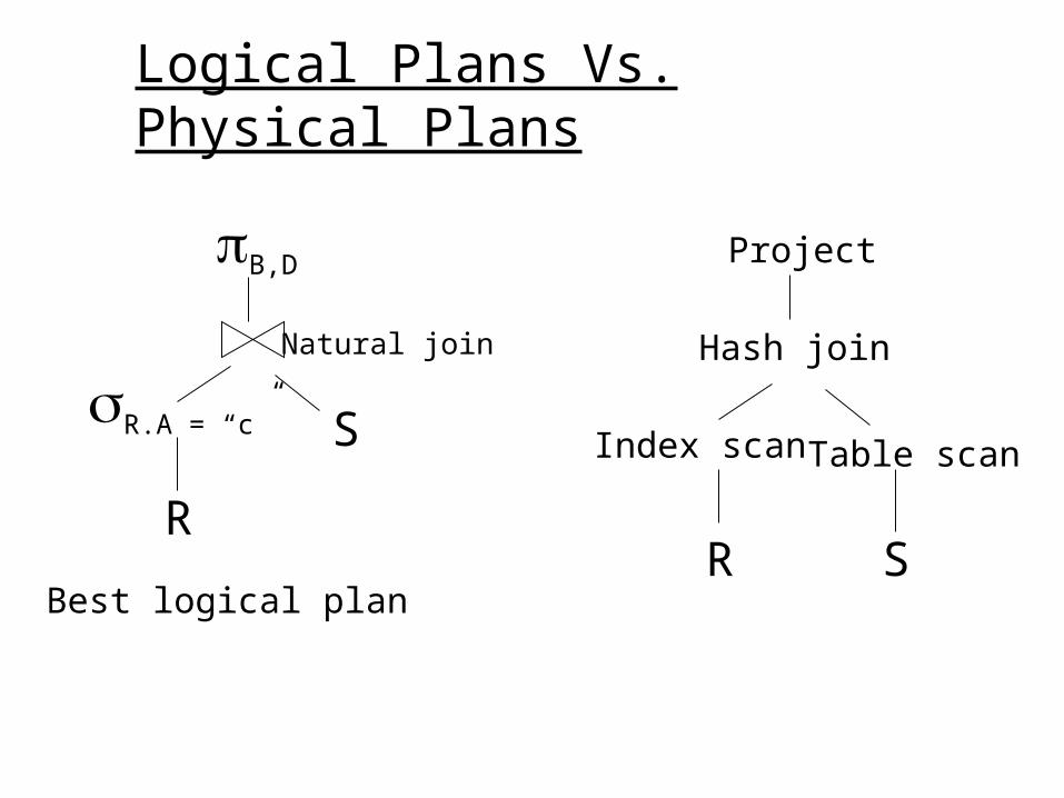
Logical Plans Vs. Physical Plans

B,D

R.A = “c”

R

S

Natural join

Best logical planR S

Index scan Table scan

Hash join

Project

B,D

R.A = “c”

R

S

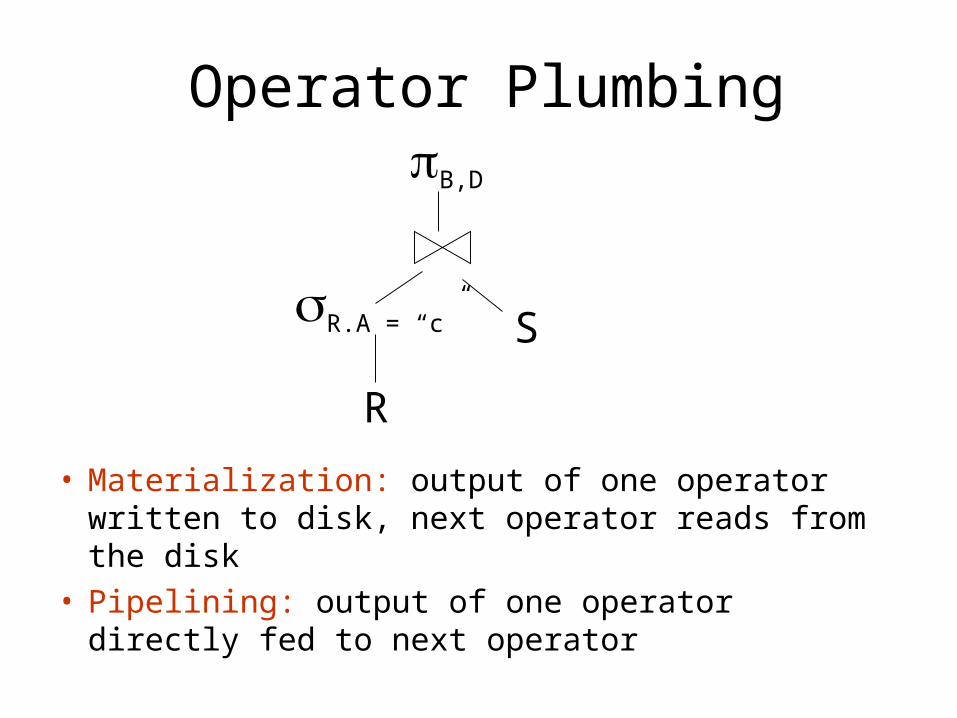
Operator Plumbing

• Materialization: output of one operator written to disk, next operator reads from the disk

• Pipelining: output of one operator directly fed to next operator

B,D

R.A = “c”

R

S

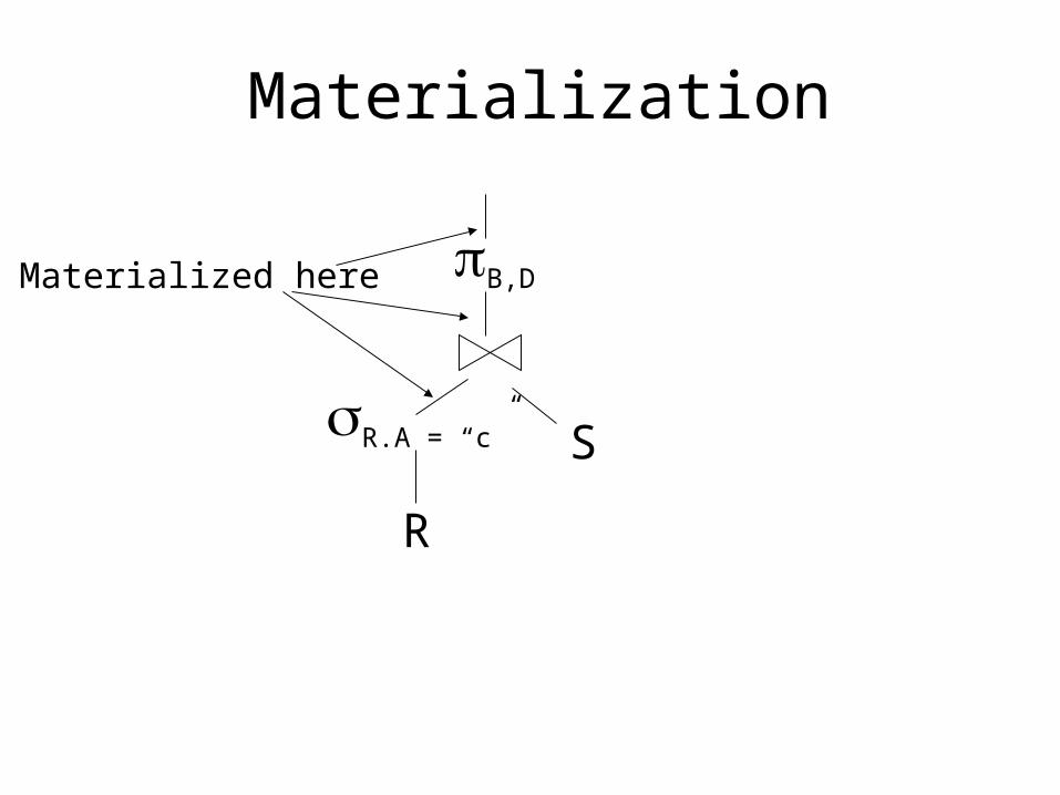
Materialization

Materialized here

B,D

R.A = “c”

R

S

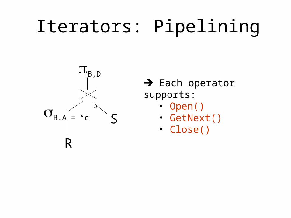
Iterators: Pipelining

Each operator supports:• Open()• GetNext()• Close()

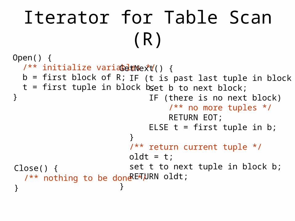
Iterator for Table Scan (R)

Open() { /** initialize variables */ b = first block of R; t = first tuple in block b;}

GetNext() { IF (t is past last tuple in block b) { set b to next block; IF (there is no next block) /** no more tuples */ RETURN EOT; ELSE t = first tuple in b; } /** return current tuple */ oldt = t; set t to next tuple in block b; RETURN oldt;}

Close() { /** nothing to be done */}

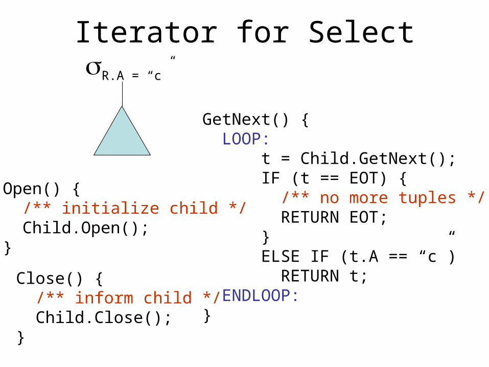
Iterator for Select

Open() { /** initialize child */ Child.Open();}

GetNext() { LOOP: t = Child.GetNext(); IF (t == EOT) { /** no more tuples */ RETURN EOT; } ELSE IF (t.A == “c”) RETURN t; ENDLOOP:}

Close() { /** inform child */ Child.Close();}

R.A = “c”

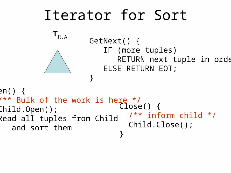
Iterator for Sort

Open() { /** Bulk of the work is here */ Child.Open(); Read all tuples from Child and sort them}

GetNext() { IF (more tuples) RETURN next tuple in order; ELSE RETURN EOT;}

Close() { /** inform child */ Child.Close();}

R.A

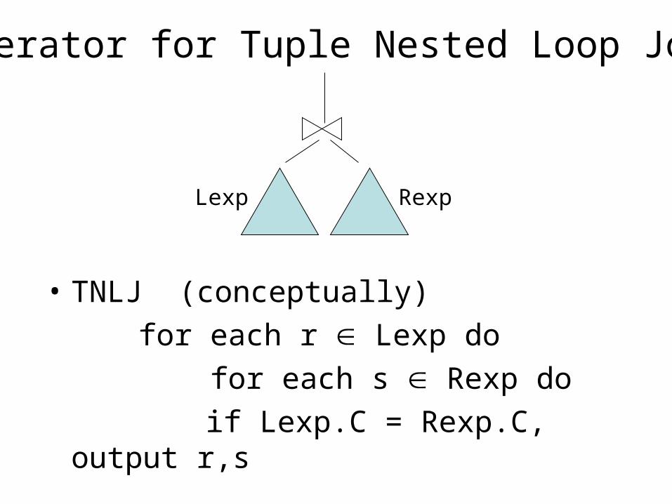
• TNLJ (conceptually)

for each r Lexp do

for each s Rexp do

if Lexp.C = Rexp.C, output r,s

Iterator for Tuple Nested Loop Join

Lexp Rexp

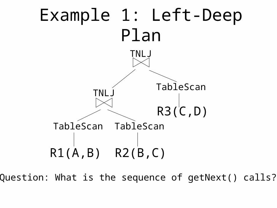
Example 1: Left-Deep Plan

R1(A,B)

TableScan

R2(B,C)

TableScan

R3(C,D)

TableScan

TNLJ

TNLJ

Question: What is the sequence of getNext() calls?

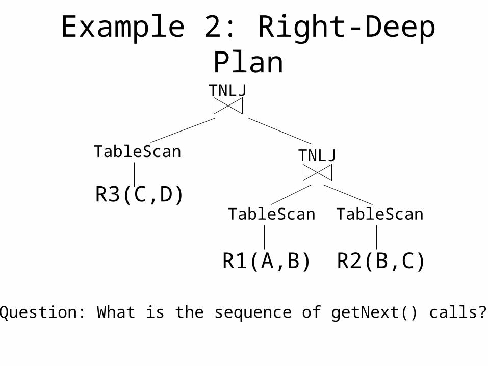
Example 2: Right-Deep Plan

R3(C,D)

TableScan

TNLJ

R1(A,B)

TableScan

R2(B,C)

TableScan

TNLJ

Question: What is the sequence of getNext() calls?

Example

Worked on blackboard

Cost Measure for a Physical Plan

• There are many cost measures– Time to completion– Number of I/Os (we will see a lot of this)– Number of getNext() calls

• Tradeoff: Simplicity of estimation Vs. Accurate estimation of performance as seen by user

Textbook outline

Chapter 15

15.1 Physical operators- Scan, Sort (Ch. 11.4), Indexes (Ch. 13)

15.2-15.6 Implementing operators +

estimating their cost

15.8 Buffer Management

15.9 Parallel Processing

Chapter 16

16.1 Parsing

16.2 Algebraic laws

16.3 Parse tree logical query plan

16.4 Estimating result sizes

16.5-16.7 Cost based optimization

Textbook outline (contd.)

Chapter 5 Relational Algebra

Chapter 6 SQL

Background Material

parse

Query rewriting

Physical plan generation

execute

result

SQL query

parse tree

logical query planstatistics

physical query plan

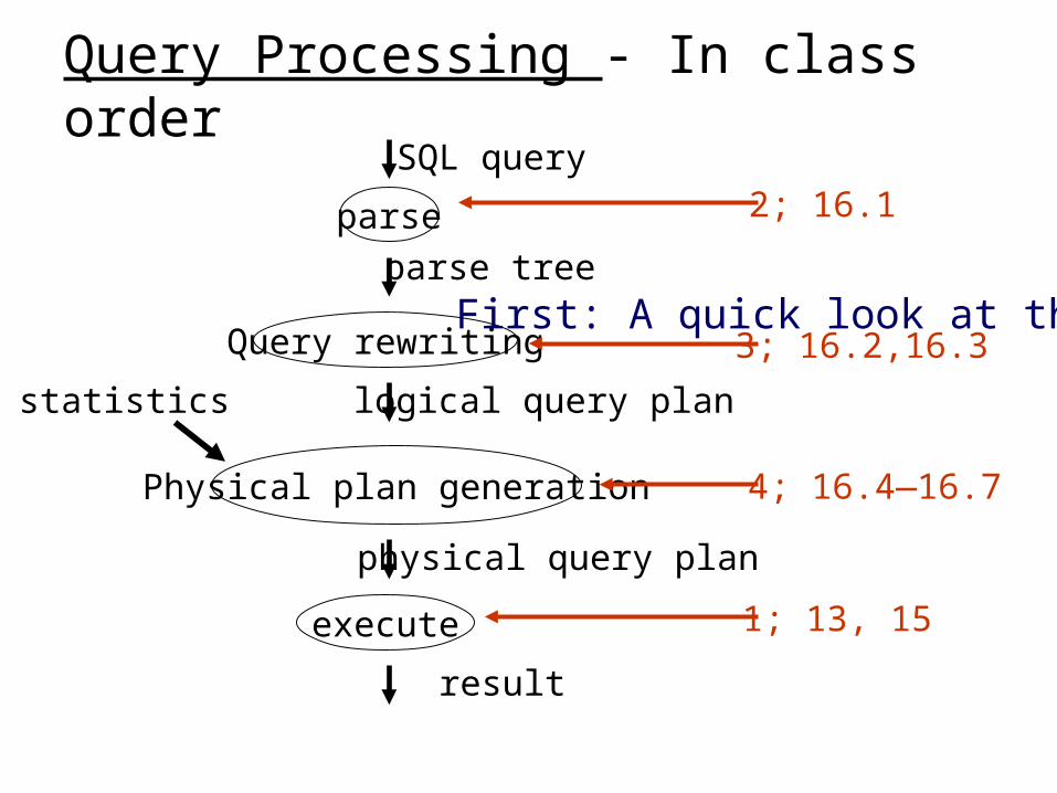
Query Processing - In class order

2; 16.1

3; 16.2,16.3

1; 13, 15

4; 16.4—16.7

First: A quick look at this

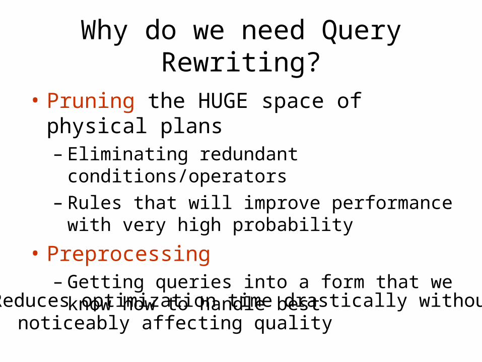
Why do we need Query Rewriting?

• Pruning the HUGE space of physical plans– Eliminating redundant conditions/operators– Rules that will improve performance with very

high probability

• Preprocessing– Getting queries into a form that we know how

to handle best

Reduces optimization time drastically without noticeably affecting quality

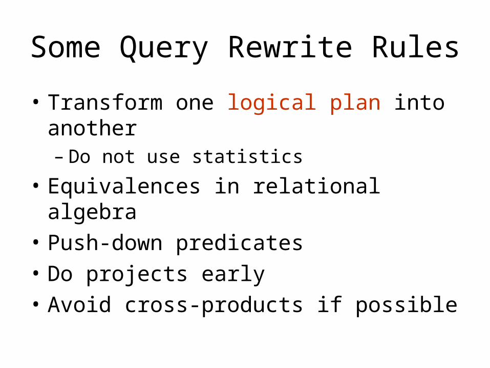
Some Query Rewrite Rules

• Transform one logical plan into another– Do not use statistics

• Equivalences in relational algebra

• Push-down predicates

• Do projects early

• Avoid cross-products if possible

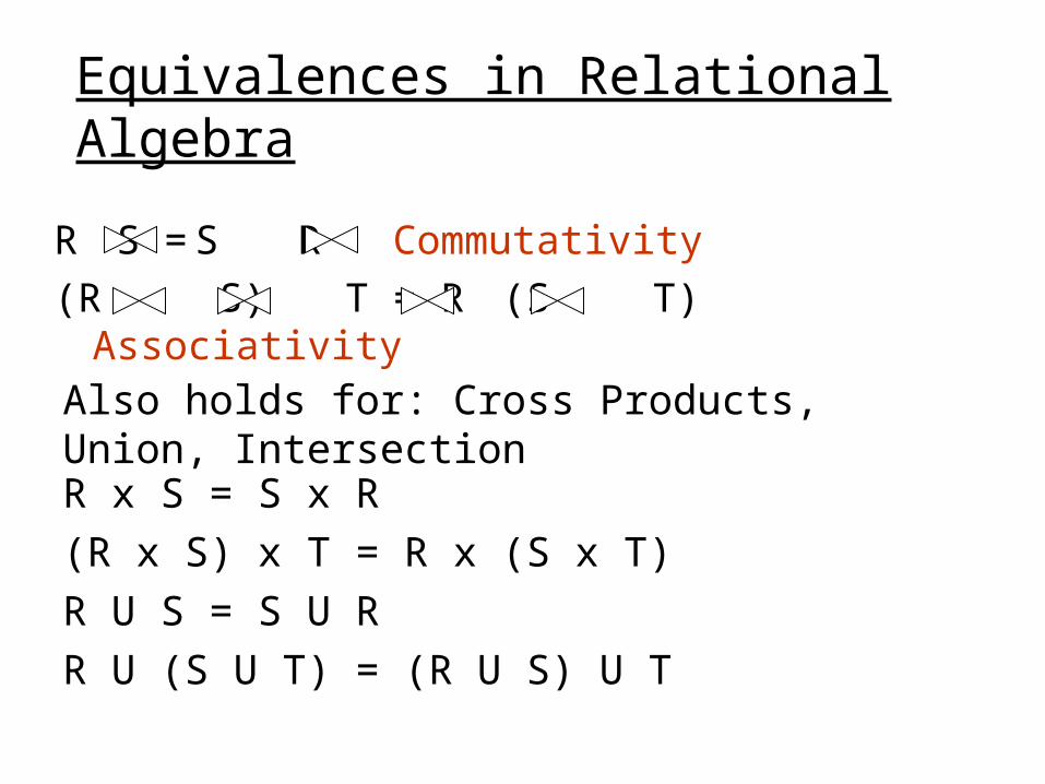
Equivalences in Relational Algebra

R S = S R Commutativity

(R S) T = R (S T) Associativity

Also holds for: Cross Products, Union, Intersection

R x S = S x R

(R x S) x T = R x (S x T)

R U S = S U R

R U (S U T) = (R U S) U T

Apply Rewrite Rule (1)

B,D [ R.C=S.C [R.A=“c”(R X S)]]

B,D

R.A = “c” Λ R.C = S.C

X

R S

B,D

R.A = “c”

X

R S

R.C = S.C

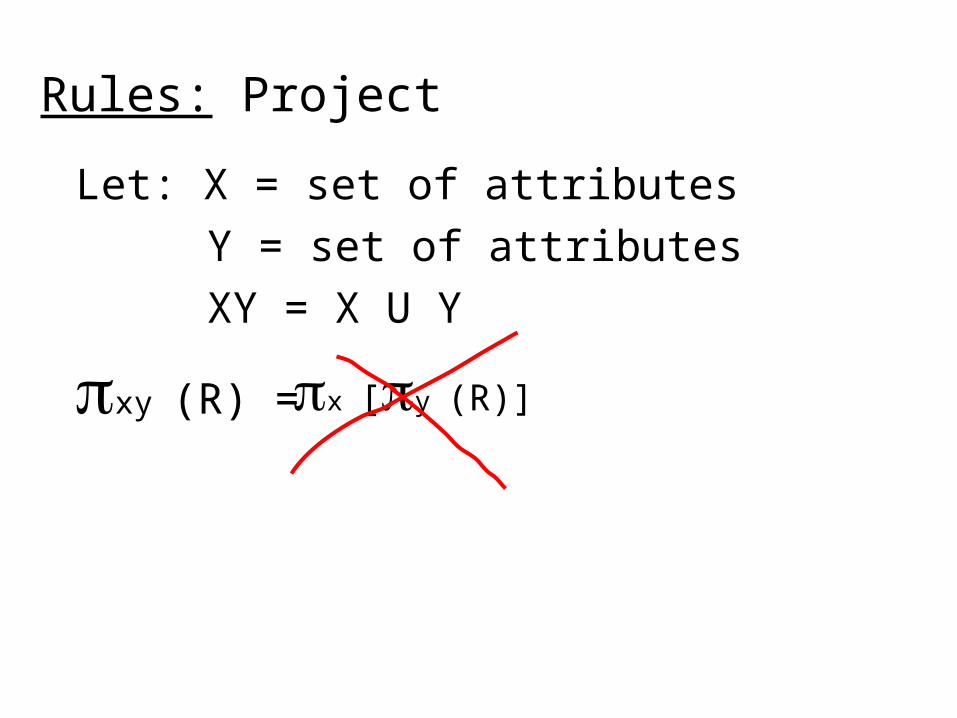
Rules: Project

Let: X = set of attributes

Y = set of attributes

XY = X U Y

xy (R) = x [y (R)]

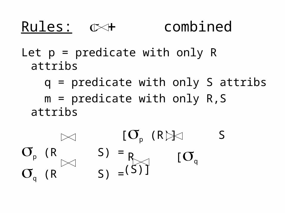
Let p = predicate with only R attribs

q = predicate with only S attribs

m = predicate with only R,S attribs

p (R S) =

q (R S) =

Rules: combined

[p (R)] S

R [q (S)]

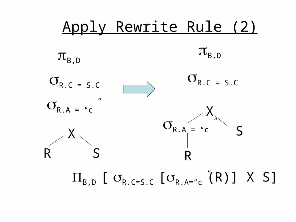
Apply Rewrite Rule (2)

B,D [ R.C=S.C [R.A=“c”(R)] X S]

B,D

R.A = “c”

X

R

S

R.C = S.C

B,D

R.A = “c”

X

R S

R.C = S.C

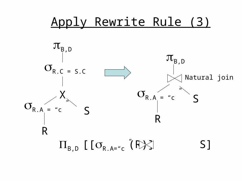
Apply Rewrite Rule (3)

B,D [[R.A=“c”(R)] S]

B,D

R.A = “c”

R

S

B,D

R.A = “c”

X

R

S

R.C = S.CNatural join

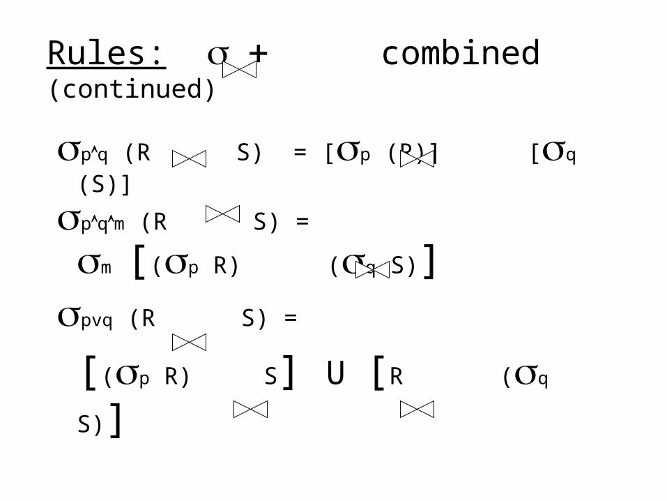
Rules: combined (continued)

pq (R S) = [p (R)] [q (S)]

pqm (R S) =

m [(p R) (q S)]pvq (R S) =

[(p R) S] U [R (q S)]

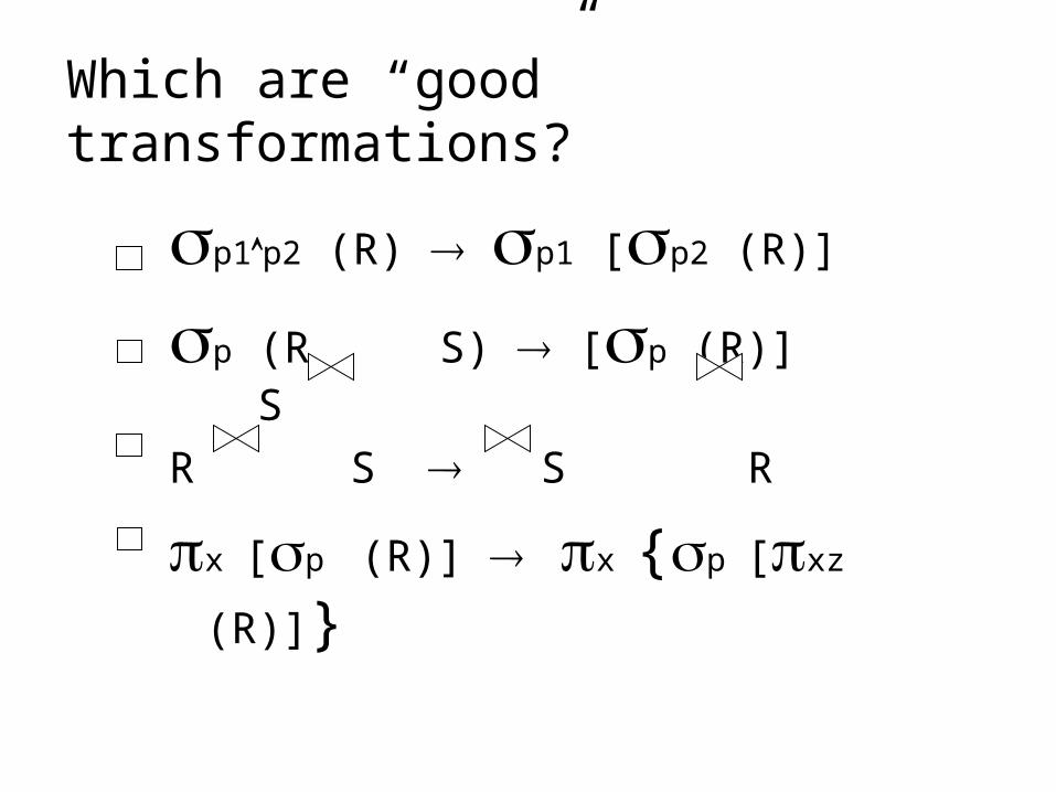
p1p2 (R) p1 [p2 (R)]

p (R S) [p (R)] S

R S S R

x [p (R)] x {p [xz (R)]}

Which are “good” transformations?

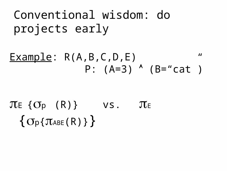
Conventional wisdom: do projects early

Example: R(A,B,C,D,E) P: (A=3) (B=“cat”)

E {p (R)} vs. E {p{ABE(R)}}

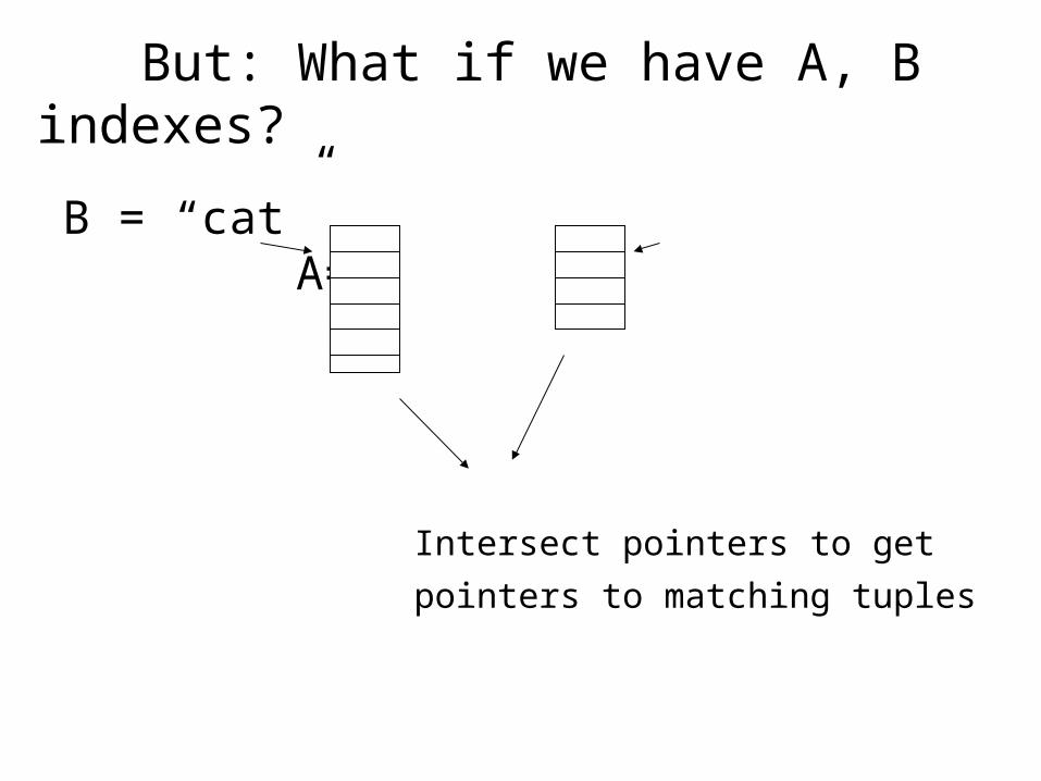
But: What if we have A, B indexes?

B = “cat” A=3

Intersect pointers to get

pointers to matching tuples

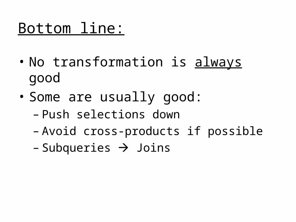
Bottom line:

• No transformation is always good

• Some are usually good: – Push selections down– Avoid cross-products if possible– Subqueries Joins

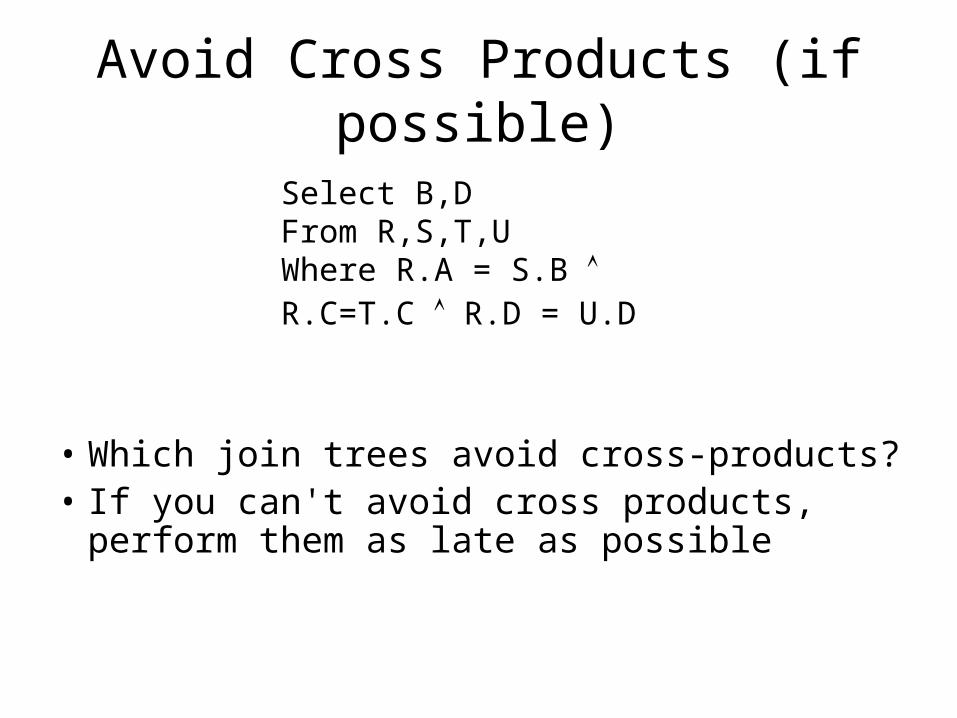
Avoid Cross Products (if possible)

• Which join trees avoid cross-products?• If you can't avoid cross products, perform

them as late as possible

Select B,DFrom R,S,T,UWhere R.A = S.B R.C=T.C R.D = U.D

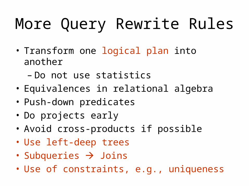
More Query Rewrite Rules

• Transform one logical plan into another– Do not use statistics

• Equivalences in relational algebra• Push-down predicates• Do projects early• Avoid cross-products if possible• Use left-deep trees• Subqueries Joins • Use of constraints, e.g., uniqueness