C:/Program Files/TeXnicCenter/Documenti …luigi/courses/metmodoc/m06.pli.en.pdf · area and using...

Methods and Models for Combinatorial Optimization

Solution Methods for Integer Linear Programming

L. De Giovanni M. Di Summa G. Zambelli

Contents

1 Preliminary definitions 2

2 Branch-and-Bound for integer linear programming 22.1 Branch-and-Bound: general principles . . . . . . . . . . . . . . . . . . . . . 11

3 Alternative formulations 173.1 Good formulations . . . . . . . . . . . . . . . . . . . . . . . . . . . . . . . 183.2 Ideal formulation . . . . . . . . . . . . . . . . . . . . . . . . . . . . . . . . 22

4 The cutting plane method 284.1 Gomory cuts . . . . . . . . . . . . . . . . . . . . . . . . . . . . . . . . . . . 29

1


1 Preliminary definitions

An integer linear programming problem is a problem of the form

zI = max cTxAx ≤ bx ≥ 0xi ∈ Z, i ∈ I,

(1)

where A ∈ Rm×n, b ∈ Rm, c ∈ Rn, and I ⊆ {1, . . . , n} is the index set of the integervariables. Variables xi with i /∈ I are the continuous variables. If the problem has bothinteger and continuous variables, then it is a mixed integer linear programming problem,while if all variables are integer it is a pure integer linear programming problem.

The setX = {x ∈ Rn |Ax ≤ b, x ≥ 0, xi ∈ Z for every i ∈ I}

is the feasible region of the problem.

zL = max cTxAx ≤ bx ≥ 0

(2)

is called the linear relaxation (or continuous relaxation) of (1).

Note the following easy fact:zI ≤ zL. (3)

This is because if xI is the optimal solution of (1) and xL is the optimal solution of (2),then xI satisfies the constraints of (2), and thus zI = cTxI ≤ cTxL = zL.

In the following we illustrate the basics of two methods that are widely used by inte-ger linear programming solvers: the Branch-and-Bound method and the cutting planemethod.

2 Branch-and-Bound for integer linear programming

The most common method for the solution of integer linear programming problems iscalled Branch-and-Bound. This method exploits the following simple observation:

Given a partition of the feasible region X into subsets X1, . . . , Xp, define z(k)I =

max{cTx | x ∈ Xk} for k = 1, . . . , p. Then

zI = maxk=1,...,p

z(k)I .

L. De Giovanni M. Di Summa G. Zambelli - Methods and Models for Combinatorial

Optimization

2


The Branch-and-Bound method proceeds by partitioning X into smaller subsets andsolving the problem max cTx on every subset. This is done recursively, by further dividingthe feasible regions of the subproblems in subsets. If this recursion were carried outcompletely, in the end we would enumerate all integer solutions of the problem. In thiscase, at least two issues would arise: first, if the problem has infinitely many feasiblesolutions the complete enumeration is not possible; second, even assuming that the feasibleregion contains a finite number of points, this number might be extremely large and thusthe enumeration would require an unpractical amount of time.

The Branch-and-Bound algorithm aims at exploring only the “promising” areas of thefeasible region, by storing upper and lower bounds for the optimal value within a certainarea and using these bounds to decide that certain subproblems do not need to be solved.

In the following we illustrate the method with an example. The general principles, whichare valid for a wider class of combinatorial optimization problems, will be examined later.

Example Consider the following problem (P0):

z0I = max 5x1 +174x2

x1 + x2 ≤ 510x1 + 6x2 ≤ 45

x1, x2 ≥ 0x1, x2 ∈ Z

(P0)

The feasible region of (P0) (blue points) and the feasible region of its linear relaxation(light blue quadrilateral) are represented in the next picture. (The arrow indicates thedirection of optimization.)

After solving the linear relaxation of (P0), we obtain the optimal solution x1 = 3.75,x2 = 1.25 (red point), whose objective value is z0L = 24.06.


Optimization

3


We have thus obtained an upper bound for the optimal value z0I of (P0), namely z0I ≤ 24.06.Now, since x1 must take an integer value in (P0), the optimal solution has to satisfy eitherthe condition x1 ≤ 3 or x1 ≥ 4. It follows that the optimal solution of (P0) will be thebetter of the optimal solutions of the subproblems (P1) and (P2) defined as follows:

z1I = max 5x1 +174x2

x1 + x2 ≤ 510x1 + 6x2 ≤ 45

x1 ≤ 3x1, x2 ≥ 0x1, x2 ∈ Z

(P1)

z2I = max 5x1 +174x2

x1 + x2 ≤ 510x1 + 6x2 ≤ 45

x1 ≥ 4x1, x2 ≥ 0x1, x2 ∈ Z

(P2)

This operation is called a branching on variable x1. Note that the solution (3.75, 1.25)does not belong to the linear relaxation of (P1) or (P2). We can represent the subproblemsand the corresponding bounds by means of a tree, called the Branch-and-Bound tree.

The leaves of the tree are the active problems (in our case, problems (P1) and (P2)).

Consider problem (P1), which is represented below.

The optimal solution of the linear relaxation of (P1) is x1 = 3, x2 = 2, with objectivevalue z1L = 23.5. Since this solution is integer, (3, 2) is also the optimal integer solutionof (P1). For this reason, there is no need to branch on node (P1), which can be pruned.We say that (P1) is pruned by optimality. Also note that the optimal solution of (P0) willnecessarily have objective value z0I ≥ z1I = 23.5. Therefore LB = 23.5 is a lower bound


Optimization

4


for the optimal value, and (3, 2) is called the incumbent solution, i.e., the best integersolution found so far.

The Branch-and-Bound tree is now the following.

The only non-pruned leaf is (P2), which therefore is the only active problem, and isrepresented below.

The optimal solution of the linear relaxation of (P2) is x1 = 4, x2 = 0.83, with objectivevalue z2L = 23.54. Then z2I ≤ 23.54 and therefore 23.54 is an upper-bound for the optimalvalue of (P2). Note that LB = 23.5 < 23.54, thus (P1) might have a better solution thanthe incumbent solution. Since the value of x2 is 0.83, which is not an integer, we branchon x2, obtaining the subproblems (P3) and (P4) shown below.

z2I = max 5x1 +174x2

x1 + x2 ≤ 510x1 + 6x2 ≤ 45

x1 ≥ 4x2 ≤ 0

x1, x2 ≥ 0x1, x2 ∈ Z

(P3)

z2I = max 5x1 +174x2

x1 + x2 ≤ 510x1 + 6x2 ≤ 45

x1 ≥ 4x2 ≥ 1

x1, x2 ≥ 0x1, x2 ∈ Z

(P4)


Optimization

5


The Branch-and-Bound tree is now the following.

The active nodes are (P3) and (P4). If we solve the linear relaxation of (P3) (see thepicture below),

we find the optimal solution x1 = 4.5, x2 = 0, with objective value z3L = 22.5. Then thevalue of the optimal integer solution of (P3) must satisfy z3I ≤ 22.5, but since we havealready found an integer solution with value 23.5 (which is a lower bound), we do notneed to further explore the feasible region of (P3), as we are sure that it cannot containany integer solution with value larger than 22.5 (and 23.5 > 22.5). We can then prunenode (P3) by bound.

The current Branch-and-Bound tree, shown below, now contains a single active prob-lem: (P4).


Optimization

6


By solving the linear relaxation of (P4), we determine that there is no feasible solution inthe linear relaxation, and therefore (P4) contains no integer solution.

Node (P4) can then be pruned by infeasibility. The Branch-and-Bound tree, shown below,does not have any active node and therefore the incumbent solution is the best integersolution of the problem; in other words, (3, 2) is an optimal solution of (P0).

Infeasibleproblem


Optimization

7


Branch-and-Bound for (mixed) integer linear programming We now describeformally the Branch-and-Bound method. We want to solve problem (P0):

zI = max cTxAx ≤ bx ≥ 0xi ∈ Z, i ∈ I.

where I is, as usual, the index set of the integer variables.

The algorithm will store a lower bound LB for the optimal value zI as well as the in-cumbent solution, i.e., the best integer solution x∗ for (P0) found so far (thus x∗

i ∈ Z forevery i ∈ I, and cTx∗ = LB). A Branch-and-Bound tree T will be constructed, whosenon-pruned leaves will be the active nodes. We denote by ℓ the maximum index of a node(Pi) in the Branch-and-Bound tree.

Branch-and-Bound method

Initialization: T := {(P0)}, ℓ := 0, LB := −∞, x∗ not defined.

1. If there is an active node in T , select an active node (Pk); otherwise return theoptimal solution x∗ and STOP.

2. Solve the linear relaxation of (Pk), thus determining either an optimal solution

x(k) of value z(k)L , or the infeasibility of the problem.

(a) If the linear relaxation of (Pk) is infeasible, prune (Pk) in T (pruning byinfeasibility);

(b) If z(k)L ≤ LB, then (Pk) cannot have better solutions than the incumbent

solution x∗; then prune (Pk) in T (pruning by bound);

(c) If x(k)i ∈ Z for every i ∈ I, then x(k) is an optimal solution of (Pk) (and

feasible for (P0)), therefore

• If cTx(k) > LB (always true if (b) does not hold), set x∗ := x(k) andLB := cTx(k);

• Prune (Pk) in T (pruning by optimality);

3. If none of cases (a), (b), (c) holds, then select an index h ∈ I such that x(k)h /∈ Z,

branch on variable xh, and construct the following two children of (Pk) in T :

(Pℓ+1) := (Pℓ) ∩ {xh ≤ ⌊x(k)h ⌋} , (Pℓ+2) := (Pℓ) ∩ {xh ≥ ⌈x

(k)h ⌉}

Make (Pℓ+1) and (Pℓ+2) active and (Pk) non-active. Set ℓ := ℓ+ 2 and go to 1.


Optimization

8


In the above algorithm and in the following, given a number a we denote by ⌊a⌋ e ⌈a⌉the rounding-down and rounding-up of a to the closest integer, respectively.

There are many fundamental details to take care of in order to make a Branch-and-Boundmethod efficient. Here we examine only the following aspects.

Solution of the linear relaxation of every node The linear relaxation of any nodecorresponds to the linear relaxation of the parent node plus a single constraint. If therelaxation of the parent node has been solved with the simplex method, we know anoptimal basic solution of the relaxation of the parent node. By using a variant of thesimplex method called “dual simplex method”, one can efficiently obtain an optimalsolution for the same problem with a new constraint added. This feature allows for afast exploration of the nodes of the Branch-and-Bound tree in (mixed) integer linearprogramming problems.

Selection of an active node Step 1 of the algorithm requires to select a node fromthe list of active nodes. The number of nodes that will be opened overall depends on howthis list is handled; in particular, this depends on the criteria used to select an activenode. In fact, there are two conflicting targets to keep in mind when choosing an activenode:

- finding a (good) feasible integer solution as soon as possible. This brings at leasttwo advantages: an integer solution provides a lower bound for the optimal value ofthe problem, and having a good lower bound increases the chances of pruning somenodes by bound. Furthermore, in the event that one needs to stop the algorithmbefore its natural termination, we have at least found a (good) feasible solution forthe problem, though maybe not the optimal one;

- exploring a small number of nodes.

The above targets suggest the following strategies:

Depth-First-Search This corresponds to a LIFO (Last In First Out) strategy onthe list of active nodes. With this strategy, new constraints are added one afterthe other at every branching and therefore it is likely to find an integer solutionsoon. Another advantage is that a small number of nodes are active and thus asmall amount of memory is needed. The main drawback is that it is possible that“non-promising nodes” are explored, i.e., nodes that do not contain (good) integersolutions.

Best-Node In order to avoid visiting nodes not containing good integer solutions,one can select an active node such that its upper bound zkL is as large as possible,i.e., zkL = maxt z

tL, where the maximum is taken over the index set of active nodes.

A drawback of this strategy is that many nodes have to be kept active and thereforea large amount of memory is needed.


Optimization

9


In practice, a hybrid approach consists in starting with the Depth-First-Search strat-egy in order to find an integer solution as soon as possible (so that pruning by boundbecomes possible), and then using the Best-Node strategy. Furthermore, integer linearprogramming solvers usually make use of heuristics to find an integer solution quicklybefore starting the Branch-and-Bound method.

Evaluation of feasible solutions In order to prune nodes by bound, good qualityfeasible solutions are needed. For this reason, when designing a Branch-and-Bound algo-rithm we have to decide how and when feasible solutions should be computed. There areseveral options, among which we mention the following:

- waiting for the enumeration to generate a node whose linear relaxation has an integeroptimal solution;

- implementing a heuristic algorithm that finds a good integer solution before startingthe exploration;

- exploiting (several times during the algorithm, with frequency depending on thespecific problem) the information obtained during the exploration of the tree toconstruct better and better feasible solutions (e.g., by rounding the solution of thelinear relaxation in a suitable way, so that a feasible integer solution is obtained).

In any case, the trade-off between the quality of the incumbent solution and the compu-tational effort needed to obtain it has to be taken into account.

Stopping criteria The Branch-and-Bound method naturally stops when there are noactive nodes left. In this case, the incumbent solution is an optimal integer solution.However, one can stop the algorithm when a given time limit or memory limit has beenreached, but in this case the incumbent solution (if any has been found) is not guaranteedto be optimal. Nonetheless, it is possible to estimate the quality of this solution. Indeed,at any time during the construction of the Branch-and-Bound tree we know a lower boundLB (given by the value of the incumbent solution), but also an upper bound UB, given by

the maximum of all values z(k)L of the active nodes: this value is an optimistic estimation

of the integer optimal value zI (meaning that zI ≤ UB). If the algorithm is stoppedbefore its natural termination, the difference between the value of the incumbent solutionLB and the bound UB is an estimation of the quality of the incumbent solution. Forthis reason, a possible stopping criterion might be to terminate the algorithm when thedifference between these two bounds is smaller than a given value (fixed in advance).

Choice of the branching variable There are several options for the choice of thebranching variable, but a common one is to select the variable with the most fractionalvalue, i.e., the variable whose fractional part is the closest to 0.5. In other words, if wedefine fi = x

(k)i − ⌊x

(k)i ⌋, we choose h ∈ I such that

h = argmini∈I{min{fi, 1− fi}}.


Optimization

10


2.1 Branch-and-Bound: general principles

The Branch-and-Bound method for mixed integer linear programming described aboveis an application of a more general scheme, valid for every combinatorial optimizationproblem.

A combinatorial optimization problem is defined as follows:

min /max f(x)s.t. x ∈ X

where X is a FINITE set of points and f(x) is a generic objective function. Examples ofcombinatorial optimization problems are the following:

• shortest path problem:X = {all possible paths from s to t}, f(x): cost of path x ∈ X;

• graph coloring:X = {all feasible combinations of color assignments to the nodes of the graph}, f(x):number of colors used in the combination x ∈ X;

• linear programming:X = {all feasible basic solutions}, f(x) = cTx.

A general method for finding an optimal solution among all the solutions in X is basedon an enumeration scheme that exploit the finiteness of the space of feasible solutions.This scheme can be seen as a universal algorithm for combinatorial optimization:

1. generate all possible solutions x;

2. for every such x, verify whether x ∈ X;

3. if so, calculate f(x);

4. choose a feasible x achieving the best possible value f(x).

The above scheme is extremely simple, but has two clear disadvantages. First, calculatingf(x) is not always an easy task (for instance, there are problems in which for each x asimulation is needed to evaluate f(x)); second, the cardinality of X might be extremely

large. This leads us to two questions:

1. how to generate the space of (feasible) solutions;

2. how to efficiently explore this space.

The branch-and-bound algorithm takes into account these issues when implementing theenumeration scheme seen above.


Optimization

11


How to generate solutions: the branching operation We make the followingobservation:

Given a combinatorial optimization problem z = max /min{f(x) : x ∈ X}and given a subdivision of the feasible region X into sets X1, . . . , Xp such that⋃p

i=1 Xi = X, let z(k) = max /min{f(x) : x ∈ Xk} for k = 1, . . . , p. Then thevalue of the optimal solution is z = max /mink=1,...,p z

(k).

We can then apply the principle of divide et impera: we split X into smaller subsetsand we solve the problem on each subset. This is done recursively by in turn dividingthe feasible region of the subproblems into smaller subsets. If this recursion were carriedout completely, we would eventually enumerate all feasible solutions. The successivesubdivisions ofX can be represented by means of a tree, called the tree of feasible solutions(see Figure 1).

Figure 1: How to generate solutions: the branching operation.

Let P0 be a given combinatorial optimization problem, with solution set E0 = X. E0 isthe root of the tree and, more generally, Ei is the solution set associated with node i. Thebranching operation of a node Ei generates some child nodes. This subdivision must besuch that

Ei =⋃

j child of i

Ej

i.e., every solution of the parent node must be in (at least) one of its children. In otherwords, during the construction of the tree no solution can be lost (otherwise the aboveobservation would not hold). A desirable, but not necessary, condition is the disjointnessof the child nodes (in this case the subdivision would be a partition of the parent node):

Ej ∩ Ek = ∅, ∀ j, k children of i.

The subdivisions would terminate when every node contains only one solution. Therefore,if Ef is a leaf node, one has |Ef | = 1.


Optimization

12


The construction of child nodes to subdivide a parent node is called BRANCH-ING : a set of level h is subdivided into t sets of level h+ 1.

Example 1 Consider a combinatorial optimization problem with n binary variables xi ∈ {0, 1},i = 1, . . . , n.

In this case, given a problem Pi and the corresponding set of feasible solutions Ei, we can easilyobtain two subproblems and two subsets of Ei by fixing one of the binary variables to 0 for onesubproblem and to 1 for the other subproblem. With this binary branching rule (in which everynode is subdivided into two child nodes), we obtain a tree as in Figure 2.

Level 0

Level 1

Level 2

Level n

Figure 2: Binary branching.

At every level, one of the variables is fixed to 0 or 1. Then a node of level h contains all the

feasible solutions with variables x1, . . . , xh fixed at some precise value, and therefore all nodes

are disjoint. The leaves are at level n, where all variables have been fixed: every leaf represents

one of the possible binary strings of length n, i.e., one specific solution of the problem. Note

that the number of leaves is 2n and the number of levels is n+1 (including the root, whose level

is 0).

How to efficiently explore: the bounding operation In general, the number ofleaves yielded by the branching operations is exponentially large. For this reason, thecomplete construction of the tree of feasible solutions (which corresponds to enumeratingall feasible solutions) cannot be carried out in practice. We then need a method thatallows us to explore only “good” areas of the feasible region, ensuring that the optimalsolution does not lie in one of the other areas. To do so, for every node we consider aBOUND, i.e., an optimistic estimation of the value that the objective value can take in


Optimization

13


the region represented by that node. For instance, given a minimization problem withbinary variables, suppose that we know a feasible solution of value 10. With the initialfeasible region we associate node E0 and then develop the first level of the branching treeby fixing variable x1 to 0 and 1, thus obtaining two child nodes E1 and E2 (see Figure 3).

Figure 3: Use of bounds.

Let z(1) be the optimal value of the objective function in E1 and z(2) be the optimal valueof the objective function in E2. As already observed, the optimal value of the objectivefunction for the initial problem is

z = min{z(1), z(2)}.

Suppose that, without enumerating all possible solutions, we have somehow establishedthat every solution such that x1 = 0 has objective value at least 9. This means that theobjective function value over E1 is at least 9. Then 9 is an optimistic estimation of theobjective function in E1, i.e., z

(1) ≥ 9. Similarly, suppose that we have a lower boundof 11 for E2: no solution satisfying x1 = 1 (solutions in E1) has objective value smallerthan 11: in other words, z(2) ≥ 11. Our first observation says that z = min{z(1), z(2)}.Furthermore, by using the information of the known feasible solution, we have z ≤ 10;since z(2) ≥ 11 ≥ 10, it is not possible to find a solution with objective value larger than10 in E2. Therefore

E2 does not contain the optimal solution and thus we do not need to developand explore the subtree rooted at E2.

A similar argument does not hold for node E1: one of the solutions in this node mighthave objective value smaller than 10 and therefore this node might contain an optimalsolution.

In general, if a feasible solution x of value f(x) = f is known, the availability of a boundassociated with the nodes of the branching tree allows us to “prune” (i.e., not develop)subtrees that are guaranteed to contain no optimal solution, i.e., the subtrees rooted atnodes whose bound is not better than f .

Note that, even though the leaf nodes of the subtree rooted at E2 have not been con-structed, we know that none of them contains a solution of value better than 11, and since


Optimization

14


we have a feasible solution of value 10, this information is sufficient to exclude them aspossible optimal solutions: we have implicitly explored the subtree. Therefore, the bound-ing operation allows us to perform an implicit enumeration of all the feasible solutions ofa combinatorial optimization problem.

The Branch-and-Bound method: general scheme From the above observations,it is possible to define the Branch-and-Bound method for the solution of combinatorialoptimization problems. This is an algorithm that enumerates explicitly or implicitly allthe feasible solutions, based on the following operations:

• branching operation: construction of the tree of feasible solutions;

• availability of a feasible solution of value f ;

• bounding operation: optimistic estimation of the objective function for the solutionsrepresented by each node (bound), in order to avoid the complete development of allsubtrees (implicit enumeration of the solutions represented by nodes whose boundis not better than f).

The Branch-and-Bound method can be summarized as follows. Given a combinatorialoptimization problem z = min /max{f(x) : x ∈ X}, define:

• P0: the initial optimization problem;

• L: the list of open nodes: every node is represented as a pair (Pi, Bi), where Pi isthe subproblem and Bi is the corresponding bound;

• z: the value of the best feasible solution found so far;

• x: the best feasible solution found so far (incumbent solution).


Optimization

15


Branch-and-Bound method

0. Initialization: Compute an optimistic estimation B0 of the objective functionand set L = {(P0, B0)}, x = ∅, z = +∞(min)[−∞(max)].

1. Stopping criterion: If L = ∅, then STOP: x is an optimal solution.

If time limit exceeded, or number of nodes exceeded,or number of open nodes |L| exceeded, etc.STOP: x is a feasible solution (not necessarily optimal).

2. Node selection: Select (Pi, Bi) ∈ L for the branching operation.

3. Branching : Subdivide Pi into t subproblems Pij, j = 1, . . . , tsuch that

⋃

j Pij = Pi.

4. Bounding : Compute an optimistic estimation Bij (corresponding to a—perhaps not feasible— solution xR

ij) for each subproblem Pij.

5. Pruning : If Pij is not feasible, go to 1.

If Bij is not better than z, go to 1.

If xRij is feasible and better than z, set z ← Bij , x← xR

ij;delete from L all nodes k with Lk not better than z; go to 1.

Otherwise, add (Pij, Bij) to L and go to 1.

The above is a generic solution scheme for combinatorial optimization problems. Toimplement a Branch-and-Bound algorithm for a specific problem, as we did for mixedinteger linear programming problems, the following elements should be determined:

(1) Branching rules: how to construct the tree of feasible solutions.

(2) Bound computation: how to estimate node bounds.

(3) Pruning rule: how to close (i.e., prune) nodes.

(4) Exploration rules: defining priorities in the exploration of the open nodes.

(5) How to compute the value of one or more feasible solutions (these solutions will becompared with bounds in order to close nodes).

(6) Stopping criteria: conditions for the termination of the algorithm.

The strategy for each of the above points depends on the specific problem.


Optimization

16


3 Alternative formulations

Consider an integer linear programming problem:

zI = max cTxAx ≤ bx ≥ 0xi ∈ Z, i ∈ I

(4)

where A ∈ Qm×n, b ∈ Qm, c ∈ Qn and I ⊆ {1, . . . , n} is the index set of the integervariables.1 Let

X = {x ∈ Rn |Ax ≤ b, x ≥ 0, xi ∈ Z for every i ∈ I}

be the feasible region of the problem, and let

zL = max cTxAx ≤ bx ≥ 0

(5)

be the linear relaxation of (4).

Notice that the linear relaxation is not unique. Given a matrix A′ ∈ Rm′×n and a vectorb′ ∈ Rm′

, we say thatA′x ≤ b′

x ≥ 0

is a formulation for X if

X = {x ∈ Rn |A′x ≤ b′, x ≥ 0, xi ∈ Z for every i ∈ I}.

In this case, the linear programming problem

z′L = max cTxA′x ≤ b′

x ≥ 0(6)

is a linear relaxation of (4), as well. It is clear that X can have infinitely many possibleformulations, and therefore there are infinitely many possible linear relaxations for (4).

1From now on all coefficients will be rational, as this condition is essential to ensure some of theproperties illustrated in this section, which do not always hold if the coefficients are irrational. (Afterall, we are interested in implementing algorithms, and therefore the rationality assumption does not poseany practical restriction.


Optimization

17


3.1 Good formulations

Given two formulations for X,Ax ≤ b, x ≥ 0

andA′x ≤ b, x ≥ 0,

we say that the first formulation is better than the second one if

{x ∈ Rn |Ax ≤ b, x ≥ 0} ⊆ {x ∈ Rn |A′x ≤ b′, x ≥ 0}.

This notion is justified by the fact that, if Ax ≤ b, x ≥ 0 is a better formulation thanA′x ≤ b′, x ≥ 0, then

zI ≤ zL ≤ z′L,

and therefore the linear relaxation given by Ax ≤ b, x ≥ 0 yields a tighter bound onthe optimal value of the integer problem than the bound given by the linear relaxationA′x ≤ b′, x ≥ 0.

Recall that having good bounds is essential for visiting only a small number of nodes ofthe Branch-and-Bound tree.

Example 2 Facility location.

There are n possible locations where facilities can be opened to provide some service to mcustomers. If facility i, i = 1, . . . , n, is opened, a fixed cost fi must be paid. The cost forserving customer j with facility i is cij for i = 1, . . . , n and j = 1, . . . ,m. Every customermust be served from exactly one facility (but the same facility can serve more customers).The problem is to decide which facilities should be opened and to assign each customerto a facility at the minimum total cost.

We have the following decision variables:

yi =

{

1 if facility i is opened,0 otherwise,

i = 1, . . . , n.

xij =

{

1 if facility i serves customer j,0 otherwise

i = 1, . . . , n, j = 1, . . . ,m.

The total cost isn

∑

i=1

fiyi +n

∑

i=1

m∑

j=1

cijxij

which is the objective function to minimize.


Optimization

18


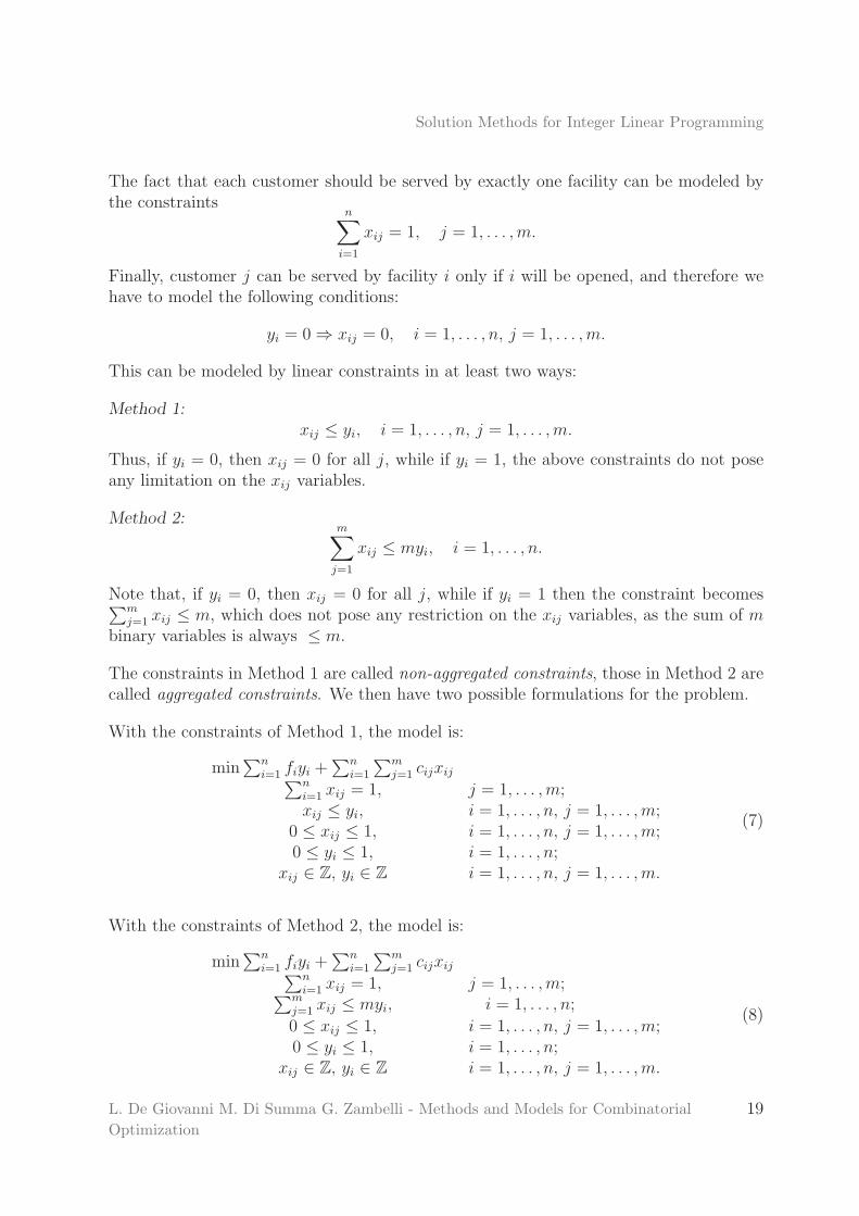
The fact that each customer should be served by exactly one facility can be modeled bythe constraints

n∑

i=1

xij = 1, j = 1, . . . ,m.

Finally, customer j can be served by facility i only if i will be opened, and therefore wehave to model the following conditions:

yi = 0⇒ xij = 0, i = 1, . . . , n, j = 1, . . . ,m.

This can be modeled by linear constraints in at least two ways:

Method 1:

xij ≤ yi, i = 1, . . . , n, j = 1, . . . ,m.

Thus, if yi = 0, then xij = 0 for all j, while if yi = 1, the above constraints do not poseany limitation on the xij variables.

Method 2:m∑

j=1

xij ≤ myi, i = 1, . . . , n.

Note that, if yi = 0, then xij = 0 for all j, while if yi = 1 then the constraint becomes∑m

j=1 xij ≤ m, which does not pose any restriction on the xij variables, as the sum of mbinary variables is always ≤ m.

The constraints in Method 1 are called non-aggregated constraints, those in Method 2 arecalled aggregated constraints. We then have two possible formulations for the problem.

With the constraints of Method 1, the model is:

min∑n

i=1 fiyi +∑n

i=1

∑m

j=1 cijxij∑n

i=1 xij = 1, j = 1, . . . ,m;xij ≤ yi, i = 1, . . . , n, j = 1, . . . ,m;

0 ≤ xij ≤ 1, i = 1, . . . , n, j = 1, . . . ,m;0 ≤ yi ≤ 1, i = 1, . . . , n;

xij ∈ Z, yi ∈ Z i = 1, . . . , n, j = 1, . . . ,m.

(7)

With the constraints of Method 2, the model is:

min∑n

i=1 fiyi +∑n

i=1

∑m

j=1 cijxij∑n

i=1 xij = 1, j = 1, . . . ,m;∑m

j=1 xij ≤ myi, i = 1, . . . , n;

0 ≤ xij ≤ 1, i = 1, . . . , n, j = 1, . . . ,m;0 ≤ yi ≤ 1, i = 1, . . . , n;

xij ∈ Z, yi ∈ Z i = 1, . . . , n, j = 1, . . . ,m.

(8)


Optimization

19


The first formulation has more constraints than the second one (there are mn non-aggregated constraints and only n aggregated constraints). We now verify that the firstformulation is better than the second one. To see this, let P1 be the set of points (x, y)that satisfy

∑n

i=1 xij = 1, j = 1, . . . ,m;xij ≤ yi, i = 1, . . . , n, j = 1, . . . ,m;

0 ≤ xij ≤ 1, i = 1, . . . , n, j = 1, . . . ,m;0 ≤ yi ≤ 1, i = 1, . . . , n;

and let P2 be the set of points (x, y) that satisfy

∑n

i=1 xij = 1, j = 1, . . . ,m;∑m

j=1 xij ≤ myi, i = 1, . . . , n;

0 ≤ xij ≤ 1, i = 1, . . . , n, j = 1, . . . ,m;0 ≤ yi ≤ 1, i = 1, . . . , n.

We show that P1 ( P2.

First of all we verify that P1 ⊆ P2. To do so, we show that if (x, y) ∈ P1 then (x, y) ∈ P2.If (x, y) ∈ P1, then xij ≤ yi for all i = 1, . . . , n, j = 1, . . . ,m. Then for every fixed i ∈{1, . . . , n}, the sum of the m inequalities xij ≤ yi for j = 1, . . . ,m gives

∑m

j=1 xij ≤ myi,and therefore (x, y) ∈ P2.

Finally, in order to show that P1 6= P2, it is sufficient to find a point in P2 \ P1. Taken = 2, m = 4, and consider the point given by

x11 = 1, x12 = 1, x13 = 0, x14 = 0;

x21 = 0, x22 = 0, x23 = 1, x24 = 1;

y1 =1

2, y2 =

1

2.

This point satisfy the aggregated constraints but violates the non-aggregated constraints,because 1 = x11 6≤ y1 =

12. �

Example 3 Multi-period production.A company is planning the production over a time horizon of n periods. For each periodt = 1, . . . , n, the company knows an estimation of the demand dt. If production takesplace in period t, then the company pays a fixed cost ft (this cost is independent of theamount produced) and a cost ct for each unit produced. Moreover, part of the amountproduced can be stored in stock at the cost of ht for each unit of product stored fromperiod t to period t+ 1, for t = 1, . . . , n− 1.

The company wants to decide how much to produce in each period and how much to storein stock at the end of each period, so as to satisfy the demand and minimize the totalcost.


Optimization

20


For every period t = 1, . . . , n, let xt be a variable indicating the amount produced inperiod t. Let yt be a binary variable taking value 1 if production takes place in period t,0 otherwise. Finally, let st be the amount stored in stock at the end of period t. For easeof notation, we define s0 = 0.

The total cost isn

∑

t=1

ctxt +n

∑

t=1

ftyt +n−1∑

t=1

htst,

which is the objective function to minimize.

In every period t, the available amount of product is st−1 + xt, of which dt unit are usedto satisfy the demand in period t and the rest is stored in stock. Then

st−1 + xt = dt + st, t = 1, . . . , n.

Of course,st ≥ 0, t = 1, . . . , n− 1; xt ≥ 0, t = 1, . . . , n.

Finally, we have to ensure that if production takes place in period t then yt = 1. Thiscan be enforced as follows:

xt ≤Myy t = 1, . . . , n,

where M is an upper bound on the maximum value that xt can take. For instance, onecan take M =

∑n

t=1 dt. We also have to impose

0 ≤ yt ≤ 1 t = 1, . . . , n

yt ∈ Z t = 1, . . . , n.

The optimal solution of the continuous relaxation of this formulation can have fractionalcomponents. As an example, assume that the storage cost are very high compared to theother costs. Then in the optimal solution we have st = 0 for every t = 1, . . . , n−1. In thissituation, the demand is satisfied at the minimum cost if xt = dt for every t = 1, . . . , n.Now, with integrality restriction we would have yt = 1 for every t = 1, . . . , n. However,in the continuous relaxation we will have yt = dt/M < 1.

It is possible to write a better formulation by using additional variables. For every periodi = 1, . . . , n and every period j = i, . . . , n, let wij be the amount produced in period iused to satisfy (part of) the demand in period j.

Then the total amount sold in period t is given by∑t

i=1 wit, and therefore we have toimpose

t∑

i=1

wit ≥ dt t = 1, . . . , n.


Optimization

21


It is also clear that

xt =n

∑

j=t

wtj t = 1, . . . , n

and

st =t

∑

i=1

n∑

j=t+1

wij t = 1, . . . , n− 1.

Finally,wij ≤ djyi, i = 1, . . . , n, j = i, . . . , n

and yt ∈ {0, 1} for t = 1, . . . , n, to force yt to take value 1 whenever xt > 0.

Let P1 be the set of points (x, y, s) that satisfy

st−1 + xt = dt + st t = 1, . . . , n;xt ≤Myy t = 1, . . . , n;xt ≥ 0 t = 1, . . . , n;st ≥ 0 t = 1, . . . , n− 1;

0 ≤ yt ≤ 1 t = 1, . . . , n

and let P2 be the set of points (x, y, s) for which there exists some w such that (x, y, s, w)satisfies

∑t

i=1 wit ≥ dt t = 1, . . . , n;xt =

∑n

j=t wtj t = 1, . . . , n;

st =∑t

i=1

∑n

j=t+1wij t = 1, . . . , n− 1;

wij ≤ djyi, i = 1, . . . , n, j = i, . . . , n;wij ≥ 0 i = 1, . . . , n, j = i, . . . , n;

0 ≤ yt ≤ 1 t = 1, . . . , n.

One can verify that every point in P2 satisfies also the constraints of P1, thus P2 ⊆ P1.On the other hand, the point st = 0 (t = 1, . . . , n− 1), xt = dt (t = 1, . . . , n), yt = dt/M(t = 1, . . . , n) is in P1 but not in P2. To see this, note that the only w satisfying xt =∑n

j=t wtj (t = 1, . . . , n) is given by wtt = dt for t = 1, . . . , n and wij = 0 for 1 ≤ i < j ≤ n.However, this point violates the constraint wtt ≤ dtyt. This shows that P2 ( P1. �

3.2 Ideal formulation

We define as the ideal formulation for X the formulation for X whose continuous relax-ation is as small as possible (with respect to set inclusion). In the following we formalizethis notion.

Definition 1 A set P ⊆ Rn is a polyhedron if there exists a system of linear inequalitiesCx ≤ d, x ≥ 0 (where C ∈ Rm×n and d ∈ Rm) such that P = {x |Cx ≤ d, x ≥ 0}.


Optimization

22


We can then say that a polyhedron P is a formulation for the set X if

X = {x ∈ P | xi ∈ Z ∀i ∈ I}.

Given tow polyhedra P and P ′, both being a formulation for X, we say that P is a betterformulation than P ′ if P ⊂ P ′.

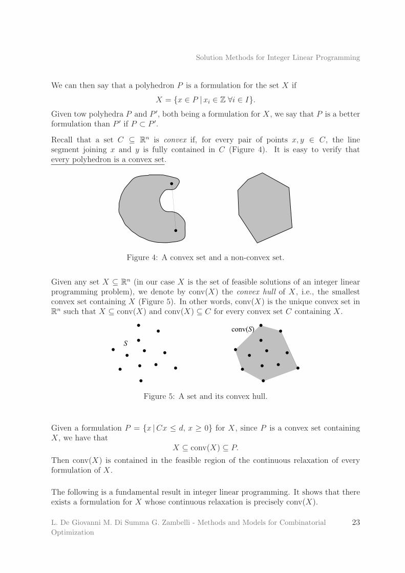
Recall that a set C ⊆ Rn is convex if, for every pair of points x, y ∈ C, the linesegment joining x and y is fully contained in C (Figure 4). It is easy to verify thatevery polyhedron is a convex set.

Figure 4: A convex set and a non-convex set.

Given any set X ⊆ Rn (in our case X is the set of feasible solutions of an integer linearprogramming problem), we denote by conv(X) the convex hull of X, i.e., the smallestconvex set containing X (Figure 5). In other words, conv(X) is the unique convex set inRn such that X ⊆ conv(X) and conv(X) ⊆ C for every convex set C containing X.

Figure 5: A set and its convex hull.

Given a formulation P = {x |Cx ≤ d, x ≥ 0} for X, since P is a convex set containingX, we have that

X ⊆ conv(X) ⊆ P.

Then conv(X) is contained in the feasible region of the continuous relaxation of everyformulation of X.

The following is a fundamental result in integer linear programming. It shows that thereexists a formulation for X whose continuous relaxation is precisely conv(X).


Optimization

23


Theorem 1 (Fundamental Theorem of Integer Linear Programming) Given A ∈ Qm×n

and b ∈ Qm, let X = {x ∈ Rn |Ax ≤ b, x ≥ 0, xi ∈ Z for every i ∈ I}. Then conv(X) isa polyhedron.In other words, there exist a matrix A ∈ Qm×n and a vector b ∈ Qm such that

conv(X) = {x ∈ Rn | Ax ≤ b, x ≥ 0}.

Given A ∈ Qm×n and b ∈ Qm such that conv(X) = {x ∈ Rn | Ax ≤ b, x ≥ 0},we say that Ax ≤ b, x ≥ 0 is the ideal formulation for X. The previoustheorem says that such a formulation always exists.

Figure 6: A formulation for a set of integer points and the ideal formulation.

We now consider again our integer linear programming problem:

zI = max cTxx ∈ X

(9)

where X = {x ∈ Rn |Ax ≤ b, x ≥ 0, xi ∈ Z for every i ∈ I}, for some given matrixA ∈ Qm×n and vector b ∈ Qm.

Let Ax ≤ b the ideal formulation for X, and consider the following linear programmingproblem:

z = max cTx

Ax ≤ bx ≥ 0.

(10)

We need to extend the notion of basic solution to a system of the above type, which isnot in standard form. By adding slack variables, we obtain

z = max cTx

Ax+ Is = bx ≥ 0, s ≥ 0.

(11)


Optimization

24


From the theory of linear programming, we know that there exists an optimal solution(x∗, s∗) for (11) that is a basic solution of the system. By construction, s∗ = b− Ax∗. If(x∗, s∗) is a basic solution of Ax+ Is = b, x, s ≥ 0, then we say that x∗ is a basic solutionfor the system Ax ≤ b, x ≥ 0. Therefore there exists an optimal solution of (10) that isa basic solution of the system Ax ≤ b, x ≥ 0.

Theorem 2 Let X = {x ∈ Rn |Ax ≤ b, x ≥ 0, xi ∈ Z for every i ∈ I}. The systemAx ≤ b, x ≥ 0 is the ideal formulation of X if and only if all its basic solutions areelements of X. In particular, zI = z for every cost vector c ∈ Rn.

The above theorem implies that solving (10) is equivalent to solving (9). This is because,given a basic optimal solution x∗ for (10) (thus z = cTx∗), by the theorem x∗ ∈ X, andtherefore x∗ is feasible for the integer linear programming problem (9), implying thatz = cTx∗ ≤ zI ; but (10) is a continuous relaxation of (9), thus the inequality zI ≤ z alsoholds; then z = zI , and thus x∗ is optimal also for (9).

Therefore, in principle, solving an integer linear programming problem is equivalent tosolving a linear programming problem (with no integer variables) in which the constraintsdefine the ideal formulation. However, there are two major problems which make integerlinear programming harder than linear programming:

• the ideal formulation, in general, is not known, and it can be very difficult to findit;

• even in the cases in which the ideal formulation is known, it is often described bya huge number of constraints, and therefore problem (10) cannot be solved directlywith standard linear programming algorithms (such as the simplex method).

Example 4 Maximum weight matching.Let G = (V,E) be an undirected graph. A matching in G is a set of edges M ⊆ E suchthat no two edges in M share a common vertex. In other words, M ⊆ E is a matching ifevery node of G is the endpoint of at most one edge in M .

The maximum weight matching problem is the following: given an undirected graphG = (V,E) and weights on its edges we, e ∈ E, find a matching M in G whose edges havemaximum total weight

∑

e∈M we.

This can be formulated as an integer linear programming problem. For every edge e ∈ E,let xe be a binary variable such that

xe =

{

1 if e is in the matching,0 otherwise,

e ∈ E.

Let M = {e ∈ | xe = 1}. The weight of M is given by

∑

e∈E

wexe.


Optimization

25


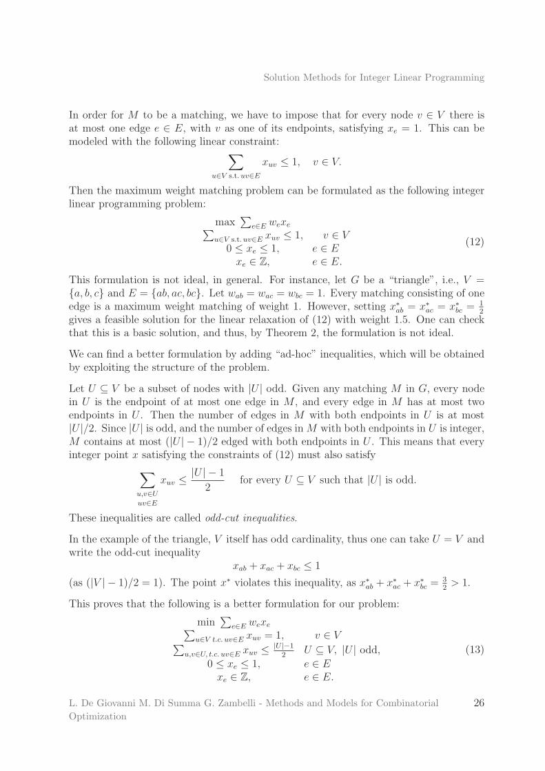
In order for M to be a matching, we have to impose that for every node v ∈ V there isat most one edge e ∈ E, with v as one of its endpoints, satisfying xe = 1. This can bemodeled with the following linear constraint:

∑

u∈V s.t. uv∈E

xuv ≤ 1, v ∈ V.

Then the maximum weight matching problem can be formulated as the following integerlinear programming problem:

max∑

e∈E wexe∑

u∈V s.t. uv∈E xuv ≤ 1, v ∈ V0 ≤ xe ≤ 1, e ∈ Exe ∈ Z, e ∈ E.

(12)

This formulation is not ideal, in general. For instance, let G be a “triangle”, i.e., V ={a, b, c} and E = {ab, ac, bc}. Let wab = wac = wbc = 1. Every matching consisting of oneedge is a maximum weight matching of weight 1. However, setting x∗

ab = x∗ac = x∗

bc =12

gives a feasible solution for the linear relaxation of (12) with weight 1.5. One can checkthat this is a basic solution, and thus, by Theorem 2, the formulation is not ideal.

We can find a better formulation by adding “ad-hoc” inequalities, which will be obtainedby exploiting the structure of the problem.

Let U ⊆ V be a subset of nodes with |U | odd. Given any matching M in G, every nodein U is the endpoint of at most one edge in M , and every edge in M has at most twoendpoints in U . Then the number of edges in M with both endpoints in U is at most|U |/2. Since |U | is odd, and the number of edges in M with both endpoints in U is integer,M contains at most (|U | − 1)/2 edged with both endpoints in U . This means that everyinteger point x satisfying the constraints of (12) must also satisfy

∑

u,v∈U

uv∈E

xuv ≤|U | − 1

2for every U ⊆ V such that |U | is odd.

These inequalities are called odd-cut inequalities.

In the example of the triangle, V itself has odd cardinality, thus one can take U = V andwrite the odd-cut inequality

xab + xac + xbc ≤ 1

(as (|V | − 1)/2 = 1). The point x∗ violates this inequality, as x∗ab + x∗

ac + x∗bc =

32> 1.

This proves that the following is a better formulation for our problem:

min∑

e∈E wexe∑

u∈V t.c. uv∈E xuv = 1, v ∈ V∑

u,v∈U, t.c. uv∈E xuv ≤|U |−1

2U ⊆ V, |U | odd,

0 ≤ xe ≤ 1, e ∈ Exe ∈ Z, e ∈ E.

(13)


Optimization

26


Indeed, it is possible to show that (13) is the ideal formulation for the maximum weightmatching problem, and therefore it would be sufficient to solve its continuous relaxationto find the optimum of the integer problem. However, the number of constraints is expo-nential (there are 2|V |−1 subsets of V with odd cardinality) and it is therefore practicallyimpossible to solve the relaxation. (Even for a graph with just 40 nodes, there are morethan 500 billion odd-cut inequalities). A better strategy is to solve a sequence of linearrelaxations, starting from problem (12) and at every iteration adding one or more odd-cut inequalities that exclude the current optimal solution, until an optimal solution of theinteger problem is found. This idea is discussed in the next section (in a more generalframework).


Optimization

27


4 The cutting plane method

The idea behind the cutting plane method is to solve a sequence of linear relaxations thatapproximate better and better the convex hull of the feasible region around the optimalsolution.

More formally, suppose that we want to solve the integer linear programming problem(PI)

max cTxx ∈ X

(PI)

where X = {x ∈ Rn |Ax ≤ b, x ≥ 0, xi ∈ Z for every i ∈ I}, for some given matrixA ∈ Qm×n and vector b ∈ Qm.

We say that a linear inequality αTx ≤ β, where α ∈ Rn and β ∈ R, is valid for X ifαTx ≤ β is satisfied by every x ∈ X. Note that if A′x ≤ b′, x ≥ 0, is a formulation forX, then also the system obtained by adding a valid inequality αTx ≤ β to the systemA′x ≤ b′ is a formulation for X.

Given a point x∗ /∈ conv(X), we say that a valid inequality for X αTx ≤ β cuts off (orseparates) x∗ if αx∗ > β. Such an inequality is also called a cut or cutting plane. IfA′x ≤ b′, x ≥ 0 is a formulation for X, x∗ is a point satisfying A′x∗ ≤ b′, x∗ ≥ 0, andαTx ≤ β is a cutting plane separating x∗, then also the system A′x ≤ b′, αTx ≤ β, x ≥ 0is a formulation for X.

Cutting plane method

Start with the linear relaxation max{cTx |Ax ≤ b, x ≥ 0}.

1. Solve the current linear relaxation, and let x∗ be a basic optimal solution;

2. If x∗ ∈ X, then x∗ is optimal for (PI); STOP.

3. Otherwise, find an inequality αTx ≤ β that is valid for X and cuts off x∗;

4. Add the inequality αTx ≤ β to the current linear relaxation and go to 1.

It is clear that the above method is a general framework for tackling integer linear pro-gramming problems, but in order to implement it one needs an automatic technique tofind valid inequalities that cut off the current solution. Below, we give a possible techniqueto do this.


Optimization

28


4.1 Gomory cuts

Gomory cutting plane method can be applied only to pure integer linear programmingproblems (although there are extensions to the mixed integer case). Thus we consider theproblem

zI = min cTxAx = bx ≥ 0x ∈ Zn

(14)

where A ∈ Qm×n and b ∈ Qm. Define X = {x |Ax = b, x ≥ 0, x ∈ Zn}.

Solve the continuous relaxation with the simplex method, thus obtaining the problem intableau form with respect to an optimal basis B (below, N is the set of indices of thenon-basic variables):

min z−z +

∑

j∈N cjxj = −zBxβ[i] +

∑

j∈N aijxj = bi, i = 1, . . . ,m

x ≥ 0.

Since B is an optimal basis, the reduced costs are non-negative: cj ≥ 0 for every j ∈ N .The optimal basic solution x∗ is given by

x∗β[i] = bi, i = 1, . . . ,m;

x∗j = 0, j ∈ N ;

therefore x∗ ∈ Zn if and only if bi ∈ Z for all i = 1, . . . ,m.

If this is not the case, let h ∈ {1, . . . ,m} be an index such that bh /∈ Z.

Every vector x satisfying Ax = b, x ≥ 0, also satisfies

xβ[h] +∑

j∈N

⌊ahj⌋xj ≤ bh

becausebh = xβ[h] +

∑

j∈N

ahjxj ≥ xβ[h] +∑

j∈N

⌊ahj⌋xj,

where the inequalities follows from the fact that xj ≥ 0 and ahj ≥ ⌊ahj⌋ for every j.

Now, since all variables are constrained to take an integer value, every feasible solutionsatisfies

xβ[h] +∑

j∈N

⌊ahj⌋xj ≤ ⌊bh⌋ (15)

because xβ[h] +∑

j∈N⌊ahj⌋xj is an integer number.


Optimization

29


Inequality (15) is a Gomory cut. The above discussion shows that the Gomory cut (15)is a valid inequality for X. Moreover, we now verify that it cuts off the current optimalsolution x∗:

x∗β[h] +

∑

j∈N

⌊ahj⌋x∗j = x∗

β[h] = bh > ⌊bh⌋,

where the inequality bh > ⌊bh⌋ holds because bh is not integer.

It is convenient to rewrite the Gomory cut (15) in an equivalent form. By adding a slackvariable s, (15) becomes

xβ[h] +∑

j∈N

⌊ahj⌋xj + s = ⌊bh⌋, s ≥ 0.

Since all coefficients in the above equations are integer, if x has integer entries then s isan integer as well. We can then require s to be an integer variable.

If from the above equation we subtract the tableau equation

xβ[h] +∑

j∈F

ahjxj = bh,

we obtain∑

j∈N

(⌊ahj⌋ − ahj)xj + s = ⌊bh⌋ − bh.

This form of the cut is known as Gomory fractional cut (or Gomory cut in fractionalform).

If we add this constraint to the previous optimal tableau, we obtain

min z−z +

∑

j∈N cjxj = −zBxβ[i] +

∑

j∈N aijxj = bi, i = 1, . . . ,m∑

j∈N(⌊ahj⌋ − ahj)xj +s = ⌊bh⌋ − bhx, s ≥ 0.

This problem is already in tableau form with respect to the basic variables xβ[1], . . . , xβ[m], s(i.e., the same basis as before, plus variable s); moreover, this basis is feasible for the dual,as all reduced costs are non-negative (they coincide with the previous reduced costs).

Also note that bi ≥ 0 for i = 1, . . . ,m, while the right-hand side of the constraint in whichs appears is ⌊bh⌋ − bh < 0. We can then solve this new linear relaxation with the dualsimplex method; s will leave the basis at the first iteration.

Example 5 Solve the following problem with Gomory cutting plane method.


Optimization

30


min z = −11x1 − 4.2x2

−x1 + x2 ≤ 28x1 + 2x2 ≤ 17

x1, x2 ≥ 0 integer.

(16)

The feasible region of the linear relaxation is shown in the picture:

We add slack variables x3 and x4 to put the system in standard form:

−z − 11x1 − 4.2x2 = 0−x1 + x2 + x3 = 28x1 + 2x2 + x4 = 17

x1, x2, x3, x4 ≥ 0 integer.

Note that we can impose that x3 and x4 are integer because since all coefficients areinteger, whenever x1 and x2 are integer also x3 and x4 are integer. Thus we have a pureinteger programming problem and we can apply Gomory cutting plane method.If we solve the linear relaxation, we obtain the following tableau:

−z +1.16x3 +1.52x4 = 28.16x2 +0.8x3 +0.1x4 = 3.3

x1 −0.2x3 +0.1x4 = 1.3

The corresponding basic solution is x3 = x4 = 0, x1 = 1.3, x2 = 3.3 (the upper vertex ofthe quadrilateral in the above picture), with objective function value z = −28.16. Sincethe values of x1 and x2 are not integer, this is not a feasible solution of (16). We canderive, e.g., a Gomory cut from the equation x2 + 0.8x3 + 0.1x4 = 3.3, thus obtaining

x2 ≤ 3.


Optimization

31


If this constraint is added to the original linear relaxation, we obtain a better formulation:

min z = 11x1 + 4.2x2

−x1 + x2 ≤ 28x1 + 2x2 ≤ 17

x2 ≤ 3x1, x2 ≥ 0

whose feasible region is the following:

cut 1

In order to solve this new problem, we first write the cut in fractional form with a slackvariable x5:

−0.8x3 − 0.1x4 + x5 = −0.3.

We then add the constraint to the previous tableau:

−z +1.16x3 +1.52x4 = 28.16x2 +0.8x3 +0.1x4 = 3.3

x1 −0.2x3 +0.1x4 = 1.3−0.8x3 −0.1x4 +x5 = −0.3

If the dual simplex method is applied, x5 leaves the basis and x3 enters, as min{

1.160.8

, 1.520.1

}

=1.160.8

. After this single iteration, we obtain the following optimal tableau:

−z +1.375x4 +1.45x5 = 27.725x2 +x5 = 3

x1 +0.125x4 −0.25x5 = 1.375x3 +0.125x4 −1.25x5 = 0.375

The corresponding basic solution is x1 = 1.375, x2 = 3 x3 = 0.375 (upper-right vertex inthe previous picture), with objective value z = 27.725.


Optimization

32


From the equation x3 + 0.125x4 − 1.25x5 = 0.375 of the tableau, we obtain the Gomorycut

x3 − 2x5 ≤ 0.

Since x3 = 2 + x1 − x2 and x5 = 3 − x2, in the original space of variables (x1, x2) theabove inequality can be rewritten as

x1 + x2 ≤ 4.

If this constraint is added to the original problem, we obtain the new linear relaxation

min z = 11x1 + 4.2x2

−x1 + x2 ≤ 28x1 + 2x2 ≤ 17

x2 ≤ 3x1 + x2 ≤ 4x1, x2 ≥ 0

shown in the picture.

cut 1

cut 2

Written in fractional form, the cut is

−0.125x4 − 0.75x5 + x6 = −0.375.

If we add this constraint to the tableau, we obtain

−z +1.375x4 +1.45x5 = 27.725x2 +x5 = 3

x1 +0.125x4 −0.25x5 = 1.375x3 +0.125x4 −1.25x5 = 0.375−0.125x4 −0.75x5 +x6 = −0.375


Optimization

33


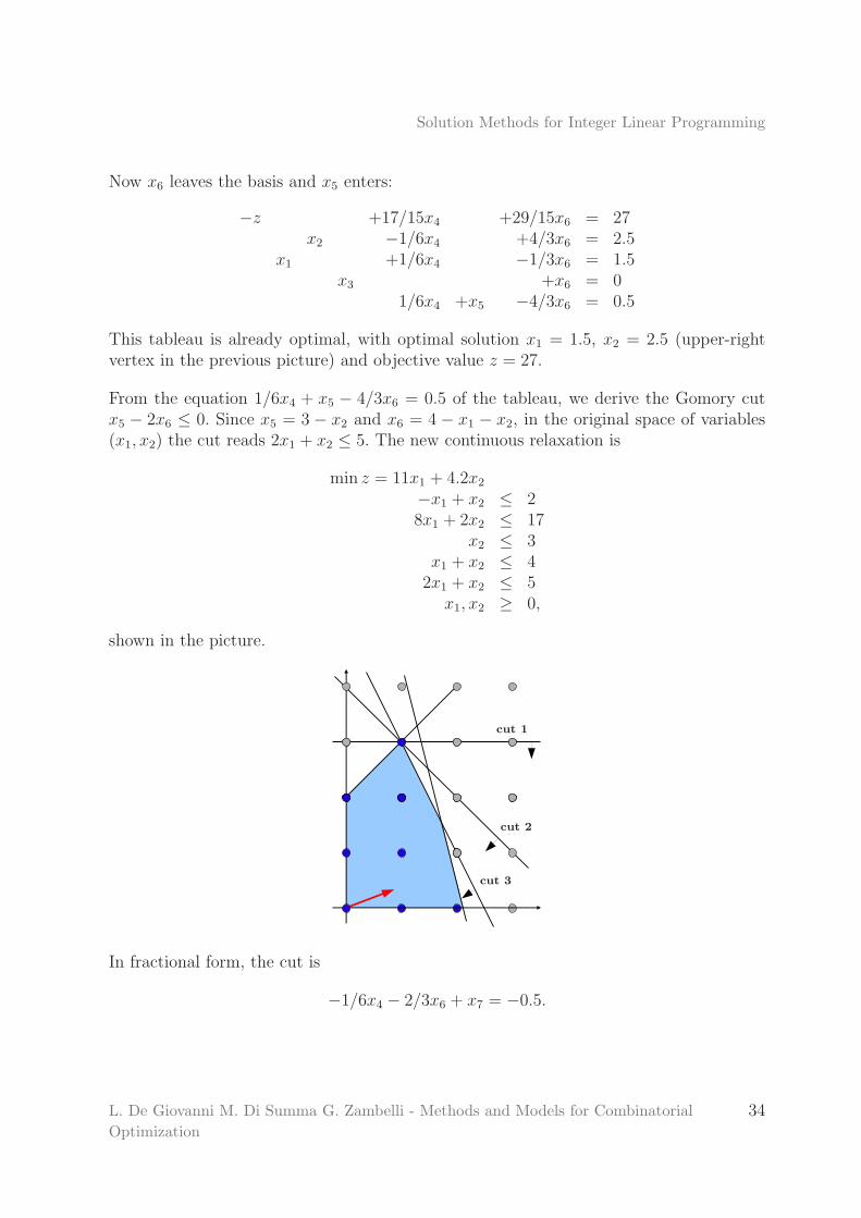
Now x6 leaves the basis and x5 enters:

−z +17/15x4 +29/15x6 = 27x2 −1/6x4 +4/3x6 = 2.5

x1 +1/6x4 −1/3x6 = 1.5x3 +x6 = 0

1/6x4 +x5 −4/3x6 = 0.5

This tableau is already optimal, with optimal solution x1 = 1.5, x2 = 2.5 (upper-rightvertex in the previous picture) and objective value z = 27.

From the equation 1/6x4 + x5 − 4/3x6 = 0.5 of the tableau, we derive the Gomory cutx5 − 2x6 ≤ 0. Since x5 = 3 − x2 and x6 = 4 − x1 − x2, in the original space of variables(x1, x2) the cut reads 2x1 + x2 ≤ 5. The new continuous relaxation is

min z = 11x1 + 4.2x2

−x1 + x2 ≤ 28x1 + 2x2 ≤ 17

x2 ≤ 3x1 + x2 ≤ 42x1 + x2 ≤ 5

x1, x2 ≥ 0,

shown in the picture.

cut 1

cut 2

cut 3

In fractional form, the cut is

−1/6x4 − 2/3x6 + x7 = −0.5.


Optimization

34


We add this constraint to the tableau:

−z +17/15x4 +29/15x6 = 27x2 −1/6x4 +4/3x6 = 2.5

x1 +1/6x4 −1/3x6 = 1.5x3 +x6 = 0

1/6x4 +x5 −4/3x6 = 0.5−1/6x4 −2/3x6 +x7 = −0.5

In this case, two iterations of the dual simplex method are needed to obtain an optimaltableau: first x7 leaves the basis and x6 enters, then x3 leaves and x4 enters the basis. Weobtain:

−z +13/15x3 +76/15x7 = 23, 6x2 +2/3x3 +1/3x7 = 3

x1 −1/3x3 +1/3x7 = 14/3x3 +x4 −10/3x7 = 3−2/3x3 +x5 −1/3x7 = 0−1/3x4 x6 −2/3x7 = 0

The corresponding optimal solution is x1 = 1, x2 = 3, with objective value z = 23.6.Since this solution has integer components, this is an optimal solution for the initialinteger linear programming problem.


Optimization

35

C:/Program Files/TeXnicCenter/Documenti …luigi/courses/metmodoc/m06.pli.en.pdf · area and using...

Documents

Transcript of C:/Program Files/TeXnicCenter/Documenti …luigi/courses/metmodoc/m06.pli.en.pdf · area and using...