Course: WB3250 Signaalanalyse (2007-2008)Exercise session 1 - RECAP - CONTINUOUS-TIME SIGNALS

PART 1: recap complex numbers, Euler formula and integrals

Recap - complex numbers, Euler formula

Consider a complex number x = a + jb with a, b ∈ R and j =√−1.

Modulus |x| of x: |x| =√

a2 + b2

Argument ∠x of x: ∠x = tan−1(

ba

)

The modulus and argument of x allow one to rewrite x in polar form:

x = a + jb = |x| ej∠x

where ejy ∆= cos(y)+jsin(y) (Euler formula). Thus, we have that x = |x| (cos(∠x) + jsin(∠x))

and that Re(x) = a = |x|cos(∠x), Im(x) = b = |x|sin(∠x). The different concepts are illus-trated in the complex plane in Figure 1.

Re

Im

. x|x|

a

b

x

. x

Figure 1: Complex plane

Finally, the conjugate x of x = a + jb = |x|ej∠x is defined as:

x = a − jb = |x| e−j∠x

The conjugate is also represented in Figure 1.

1

Exercises

a. Consider the complex number x = 1 + 2j. Compute |x|, ∠x and x.

b. Given two complex numbers x and y, prove that |xy| = |x| |y| and that ∠(xy) =∠x + ∠y

c. Given two complex numbers x and y, prove that |xy| = |x|

|y|and that ∠(x

y) = ∠x − ∠y

d. Given x = 1 + 2j and y = 2 + j. Compute xy and xy.

e. Show that x = 3 ejπ is also equal to -3.

f. Show that ej2π and ej10π are both equal to 1.

g. Given x = 3 ejπ and y = 2 ej π

2 . Compute xy and xy.

h. Show that xx is equal to |x|2.

i. Show that cos(φ) = 12

(

ejφ + e−jφ)

for φ ∈ R. Give a similar expression for sin(φ).

Recap - integral

In order to compute∫ t=t2

t=t1f(t)dt of a function f(t) of the variable t, we need to compute the

primitive Pf (t) of f(t). The primitive Pf (t) is the function such that:

d Pf(t)

dt= f(t)

Having determined the primitive, the integral can then be computed as follows:

∫ t=t2

t=t1

f(t)dt = [Pf(t)]t=t2t=t1

= Pf (t = t2) − Pf (t = t1)

Exercises

a. Compute∫ 2π

0cos(t)dt.

b Compute∫ 2π

0ejntdt with n an integer. Distinguish the case where n = 0 and where

n 6= 0.

c. Compute∫ ∞

0ae−btdt with a, b ∈ R and b > 0.

PART 2: continuous-time signals

A continuous-time signal x(t) is a physical variable as a function of the time t. The signalx(t) is valued in R for each t ∈ R.

2

Exercise 1. Consider the signals x(t), y(t) and z(t) given in the figure below. Note thatx(t) = 0 and y(t) are zero everywhere expect between t = 0 and t = 1 and that z(t) is zeroeverywhere except between t = 0 and t = 2. Express z(t) as a linear combination of shiftedversions of x(t) and y(t).

0 1

1 1 1

2

0 1 0 1 2

x(t) y(t) z(t)

t t t

Exercise 2. cfr. book pp. 37, exercise 1.1.i.

Exercise 3. cfr. book pp. 39, exercise 1.4, sub-questions (a) and (b)

The references to the book pertains to the third edition. At the end of the session, there is a

conversion table for the second edition.

3

SOLUTIONS.

Solution of the exercises on complex numbers.

a. |x| =√

1 + 4 =√

5 and ∠x = tan−1 21

= 1.1 rad. x = 1 − 2j.

b. Let us write x and y in polar form:

x = |x| ej∠x y = |y| ej∠y

We can then write that:

xy = |x| ej∠x |y| ej∠y = |x||y| ej(∠x+∠y)

and we see that |xy| = |x||y| and that ∠(xy) = ∠x + ∠y.

c. Let us also write x and y in polar form:

x = |x| ej∠x y = |y| ej∠y

We can then write that:

x

y=

|x| ej∠x

|y| ej∠y=

|x||y| ej(∠x−∠y)

and we see that |xy| = |x|

|y|and that ∠(x

y) = ∠x − ∠y

d. xy = (1 + 2j)(2 + j) = 2 + 4j + j + 2j2 = 2 + 5j − 2 where we made use of the fact thatj2 = −1. Thus, xy = 5j. Now, let us compute x/y

x

y=

xy

yy=

(1 + 2j)(2 − j)

(2 + j)(2 − j)=

2 − j + 4j + 2

4 − 2j + 2j + 1=

4 + 3j

5=

4

5+

3

5j

e. x = 3 ejπ can be written as x = 3 (cos(π) + jsin(π)) and thus x = 3(−1 + 0j) = −3.

f. ej2π can be written as

ej2π = 1 ej2π = 1 (cos(2π) + jsin(2π))

which is equal to 1. The same can be said for ej10π. Indeed, ej10π can be written as1 (cos(10π) + jsin(10π)) which is also equal to 1. In fact, ej2nπ = 1 for all integer n.

g. The product and ration of x and y can e.g. be deduced as follows:

xy = (3 ejπ)(2 ej π

2 ) = 6 ej(π+ π

2) = 6 ej 3π

2 (= −6j)

3 ejπ

2 ej π

2

=3

2ej(π−π

2) =

3

2ej π

2 (=3

2j)

4

h. xx = (|x| ej∠x)(|x| e−j∠x) = |x|2ej0 = |x|2.

i. 12

(

ejφ + e−jφ)

= 12(cos(φ) + j sin(φ) + cos(−φ) + j sin(−φ)) = 1

2(2cos(φ)) = cos(φ). In

order to find an expression for sin(φ), we use a similar reasoning. Since sin(−φ) = −sin(φ),we will consider:

ejφ − e−jφ

which is equal to 2j sin(φ). Consequently:

sin(φ) =1

2j

(

ejφ − e−jφ)

=−j

2

(

ejφ − e−jφ)

Solution of the exercises on integrals.

a. Here f(t) = cos(t) and thus Pf(t) = sin(t). Consequently, the integral is equal to∫ 2π

0cos(t)dt = sin(2π)− sin(0) = 0− 0 = 0. This is in fact logic since we integrate a cosine

over one of its period.

b. Here f(t) = ejnt. Let us first consider the case n 6= 0. Using Euler formula, we canrewrite it as: f(t) = ejnt = cos(nt) + jsin(nt) whose primite is given by:

Pf(t) =sin(nt)

n+ j

−cos(nt)

n

Consequently,

∫ 2π

0

ejntdt =

(

sin(2πn)

n+ j

−cos(2πn)

n

)

−(

sin(0)

n+ j

−cos(0)

n

)

= (0− j

n)− (0− j

n) = 0

where we have used the fact that n is an integer. Consider now the case n = 0. Thenf(t) = 1 whose primitive if Pf(t) = t. Consequently, when n = 0, the integral is equal to2π − 0 = 2π.

c. Here f(t) = ae−bt. The primitive is thus: Pf(t) = −ab

e−bt. Consequently:

∫ ∞

0

ae−btdt =

[−a

be−bt

]∞

0

= 0 − −a

b=

a

b

Indeed, since b > 0, limt→∞ e−bt = 0.

Solution of the exercises on continuous-time signals.

Exercise 1. z(t) = y(t) + 2x(t − 1) − y(t− 1)

Exercise 2. Denote the triangular pulse of length τ by vτ (t) (i.e. vτ (t)∆= (1− 2|t|/τ)pτ (t)).

The signal x(t) in subplot (a) of Figure P1.1 is equal to p4(t) + p2(t). The signal x(t) insubplot (b) is equal to 4

3v8(t) − 1

3v2(t). The signal in subplot (c) is equal to 2 p4(t) + v4(t).

5

The one in subplot (d) is p2(t)−v2(t). The signal x(t) in subplot (e) is a periodic signal withperiod 2. The first period (i.e. from t = 0 till t = 2) is given by p1(t− 1

2). Consequently, we

have:

x(t) =∞

∑

k=−∞

p1(t −1

2+ 2k)

Exercise 3. The signal x(t) in sub-question (a) is given by:

x(t) = 1 for − 1 ≤ t < 1x(t) = −1 for 1 ≤ t < 3x(t) = 0 elsewhere

The signal in sub-question (b) is:

x(t) = −t for 0 ≤ t < 1x(t) = 1 for 1 ≤ t < 2x(t) = 0 elsewhere

Conversion table.

THIRD edition SECOND editionp. 37 exercise 1.1.i p. 47 exercise 1.1.a

p. 39 p. 49

6

Course: WB3250 Signaalanalyse (2007-2008)Exercise session 2:CONTINUOUS-TIME FOURIER SERIES AND TRANSFORM

The references to the book pertains to the third edition. At the end of the session, there is a

conversion table for the second edition.

PART 1: Fourier series of (continuous-time) periodic signals

A continuous-time signal x(t) is a physical variable as a function of the time t. The signalx(t) is valued in R for each t ∈ R.

A signal x(t) is even if x(t) = x(−t) and it is odd if x(t) = −x(−t).

A continuous-time signal x(t) is periodic if and only if we can find T ∈ R such thatx(t) = x(t + T ) for all t. The smallest T having this propriety is called the fundamen-tal period of x(t). The fundamental frequency ω0 of x(t) is defined as ω0 = 2π

Twith T the

fundamental period. See pp. 5-6 of the book for more details.

Each periodic signal x(t) can be decomposed in a series of harmonics k ω0 of its fundamentalfrequency ω0 i.e.

x(t) =

∞∑

k=−∞

ck ejkω0t with ck =1

T

∫ T

2

−T

2

x(t) e−jkω0t dt

with T the fundamental period of x(t). This decomposition is called the Fourier series ofx(t) and the coefficients ck are called the Fourier coefficients of x(t). This is fact the com-plex exponential form of the Fourier series. The Fourier series can also be expressed in atrigonometrical form (see p. 101 of the book for more details).

The power P of a periodic signal x(t) is defined by:

P∆=

1

T

∫ T

2

−T

2

x2(t)dt

with T the fundamental period of x(t). The power can also be computed using the Fouriercoefficients (Parseval’s Theorem):

P =

+∞∑

k=−∞

|ck|2

Exercise 1 (examination problem January 2006). The continuous-time signal x(t) isgenerated according to

x(t) =

3∑

k=1

bkcos(kω0t)

1

with ω0 = π/5 rad/sec, and

bk =

2kπ

for k = 1, 30 voor k = 2

a. Is x(t) a periodic signal, and if so, what is its fundamental period?

b. Is x(t) an even or odd function? Motivate your answer.

c. Determine the Fourier series of x(t) in the complex exponential form. For this purpose,use the formula cos(φ) = 1

2

(

ejφ + e−jφ)

.

d. Determine the power of the signal x(t).

Exercise 2 (examination January 2007). In Figure 1, the infinite-time signal x(t) isdepicted over the interval [−10, 10]. This continuous-time signal x(t) is periodic and isgenerated as

x(t) = a0 +

3∑

k=1

ak sin(kω0t)

with ω0 = 2π10

rad/s, a0 = 1, a1 = 2, a2 = 0 and a3 = 12.

−10 −8 −6 −4 −2 0 2 4 6 8 10−4

−3

−2

−1

0

1

2

3

4

t [sec]

x(t)

Figure 1: signal x(t) of exercise 2

a. Is x(t) an odd signal, an even signal or neither of the two? Motivate your answer.

b. Determine the fundamental period of x(t) and its fundamental frequency.

c. Determine the Fourier series of x(t) in the complex exponential form.

d. Determine the power of the signal x(t).

2

Exercise 3. Let x(t) = sin(0.4πt), y(t) = cos(1.4πt + π4) and z(t) = x(t) + y(t).

a. Is z(t) a periodic signal? If yes, what is its fundamental period Tz?

b. Prove using the formula cos(φ) = 12

(

ejφ + e−jφ)

that z(t) can be written as follows:

z(t) = a−2e−jω2t + a−1e

−jω1t + a1ejω1t + a2e

jω2t

with a1 = 0.5e−j π

2 , a−1 = 0.5ej π

2 , a2 = 0.5ej π

4 , a−2 = 0.5e−j π

4 , ω1 = 0.4π and ω2 = 1.4π.

c. Prove that the expression in item [b.] is equivalent to the Fourier series of z(t).

d. Compute the power Pz of the periodic signal z(t) using Parseval’s theorem. Verifythat we obtain the same value for the power Pz if we use, instead, the definition of thepower of a signal:

Pz∆=

1

T

∫ T

2

−T

2

z2(t)dt

Note for this purpose that cos(A)cos(B) = 12(cos(A − B) + cos(A + B)).

Exercise 4 (examination November 2006). Consider the infinite-time signal x(t) de-picted in Figure 2 in the interval [−40, 40]. The continuous-time signal x(t) is a periodicsignal with a fundamental period of 40 seconds.

−40 −30 −20 −10 0 10 20 30 40−2

−1.5

−1

−0.5

0

0.5

1

1.5

2

t [sec]

x(t)

Figure 2: signal x(t) of exercise 4

a. Is the signal x(t) an even signal or an odd signal? Motivate your answer.

b. What is the fundamental frequency ω0 of the signal x(t)?

3

The complex exponential form of the Fourier series of the periodic signal x(t) is given by:

x(t) =

∞∑

k=−∞

ck ejkω0t

where the fundamental frequency ω0 has been determined in item [b.] and where the Fouriercoefficients ck are given by:

ck =

0 when k = 0

2kπ

sin(

k π2

)

when k 6= 0

c. Explain based on Figure 2 why c0 = 0

d. Based on the complex exponential form of the Fourier series given above, determinethe parameters ak (k = 0... +∞), bk (k = 1... + ∞) in the trigonometrical form of theFourier series of x(t):

x(t) = a0 ++∞∑

k=1

(ak cos(kω0t) + bk sin(kω0t))

e. Determine the power of x(t)

Exercise 5. Consider the periodic signal x(t) represented in the figure below.

a. Compute the Fourier series of x(t). Hint: determine separately c0 and ck for k 6= 0.

b. Check the value of c0 based on the figure representing x(t).

c. Compute the power of the periodic signal x(t) using Parseval’s theorem. Verify thatwe obtain the same value for the power if we use, instead, the definition of the power

of a signal: P∆= 1

T

∫T

2

−T

2

x2(t)dt. Remember for this purpose that, if x ≤ π,

∞∑

k=1

1

k2sin2(k x) = 0.5 x (π − x)

4

d. How does the Fourier series change if the signal x(t) is right-shifted by 0.5 T ?

Exercise 6. Consider the periodic signal x(t) given in the figure below.

Compute the Fourier series of x(t) by making use of the results obtained in Exercise 5.

Exercise 7 (examination June 2007). Consider the continuous-time signal x(t) =e−tcos(10t)u(t) with u(t) the unit step function. Does there exist a Fourier series for thesignal x(t)? Motivate your answer.

PART 2: Continuous-time Fourier transform

The Fourier transform F(x(t)) = X(ω) of a continuous-time signal x(t) describes the fre-quency content of the signal x(t). X(ω) is a complex function of the frequency ω. It isdefined as:

X(ω)∆=

∫ ∞

−∞

x(t) e−jωt dt

The Fourier transform of a given signal x(t) can be computed

• either by applying the definition (thus by evaluating the integral above)

• or by using standard Fourier transform pairs in combination with properties of theFourier transforms. A very simple example: if we know that the Fourier transform ofx1(t) is given by X1(ω) and that the Fourier transform of x2(t) is given by X2(ω), thenthe Fourier transform X(ω) of x(t) = x1(t) + x2(t) can be deduced by the linearityproperty of the Fourier transform i.e. X(ω) = X1(ω)+X2(ω). Table 3.2 on page 144 ofthe book summarizes the Fourier transforms of some common signals. The propertiesof the Fourier transform are presented in Section 3.6 of the book and are summarizedin Table 3.1 on page 141.

5

Exercise 1. Consider the signal h(t) defined as follows:

h(t) = 1 if 0 ≤ t < 1h(t) = 0 elsewhere

a. The rectangular pulse pτ (t) of length τ is defined as:

pτ (t) = 1 if −τ2

≤ t < τ2

pτ (t) = 0 elsewhere.

Give an expression of h(t) using pτ (t).

b. Knowing that the Fourier transform of pτ (t) is given by 2ω

sin(ωτ2

) (see page 119 of thebook), compute the Fourier transform H(ω) using what has been found in item [a.]and the hint below.

c. Which linear operation have we to perform on h(t) to obtain that the Fourier transformof the resulting signal is real for all ω (i.e. Im(X(ω)) = 0 for all ω)?

d. What is the Fourier transform G(ω) of g(t)∆= h(t) − h(−t) ? Use a property of the

Fourier transform (see the hint below).

Hints for items [b.] and [c.]: consider a signal x(t) whose Fourier transform is denotedby X(ω). Then, the Fourier transforms of x(t − c) (c ∈ R) and of x(−t) are given by:

F(x(t − c)) = X(ω) e−jωc expression (3.41) in the book

F(x(−t)) = X(−ω) expression (3.45) in the book

Exercise 2. Let a, ω0, φ be given constants. Compute the Fourier transform X(ω) of:

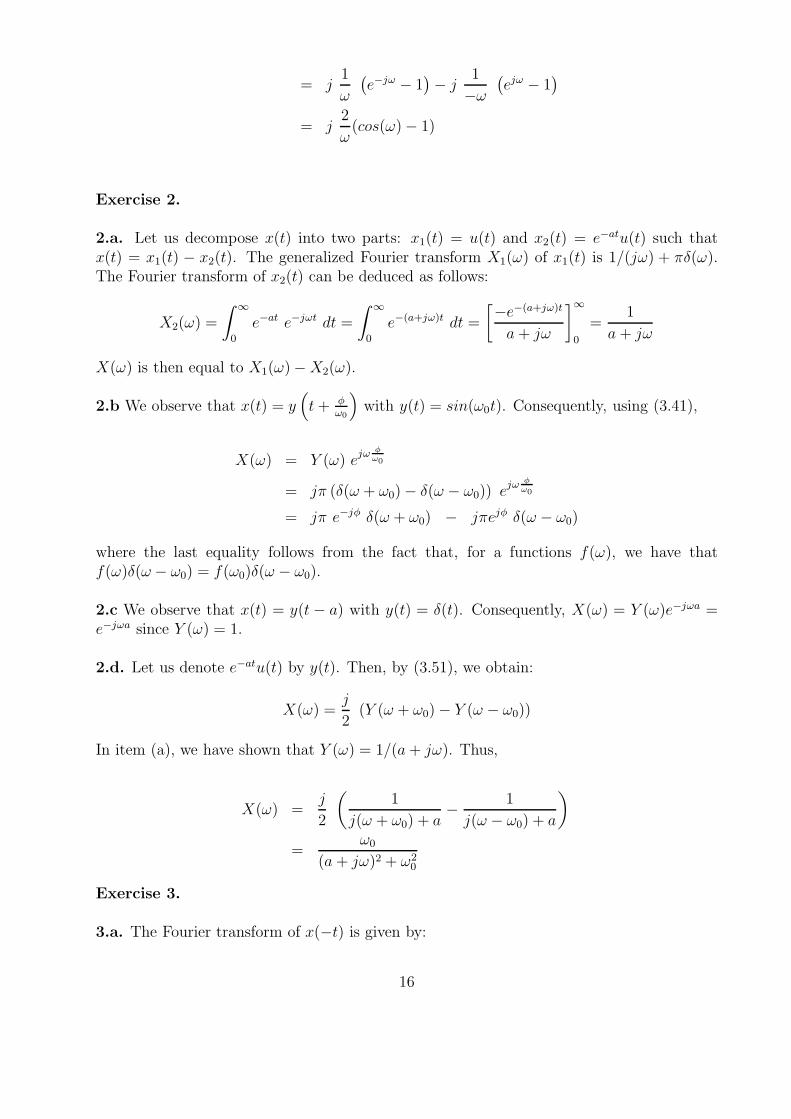
a. x(t) = (1 − e−at) u(t) with u(t) the unit step function (see page 2 of the book).

b. x(t) = sin(ω0 t + φ).

c. x(t) = δ(t − a) with δ(t) the unit impulse.

d. x(t) = e−at sin(ω0t) u(t).

Hint: recall that, in Table 3.2 of the book, we see that

6

F(u(t)) = 1/(jω) + πδ(ω)

F(sin(ω0t)) = jπ (δ(ω + ω0) − δ(ω − ω0))

F(δ(t)) = 1

Recall furthermore for item [d.] that, if x(t) = y(t)sin(ω0t), then the Fourier transformX(ω) of x(t) is given by: X(ω) = (j/2) (Y (ω + ω0) − Y (ω − ω0)) with Y (ω) the Fouriertransform of y(t). This is property (3.51) of the book.

Exercise 3.

a. Prove that the Fourier transform of x(−t) is given by X(−ω). Prove subsequently thatX(ω) = X(−ω) for real-valued x(t). Finally, show that Im(X(ω)) = 0 ∀ω for evensignals and Re(X(ω)) = 0 ∀ω for odd signals.

b. Prove the property (3.50) of the book

c. Prove the property (3.52) of the book

Exercise 4. Consider the signal x(t) depicted below:

The Fourier series of the signal x(t) is:

x(t) =

∞∑

k=−∞

akejkω0t

with a0 = V τT

, ak = Vkπ

sin(kπτT

) and ω0 = 2π/T . See exercise 5 of PART 1 of this session.

a. Compute the Fourier transform X(ω) of x(t) from its Fourier series. Recall for thispurpose that the Fourier transform of ejωot is given by 2πδ(ω − ω0). This is property(3.74) in the book.

7

b. Compute the Fourier transform G(ω) of g(t) = x(t) pT (t) with pT (t) the rectangularpulse of length T (see item [a.] of exercise 1). The signal g(t) corresponds to one ofthe periods of x(t).

8

SOLUTIONS.

SOLUTIONS: PART 1

Exercise 1.

1.a. The signal x(t) is made up of the sum of two cosines (since b2 = 0). Since these twocosine functions are integer multiples of ω0, we can directly conclude that x(t) is periodicand that the fundamental frequency is ω0. The fundamental period is then 2π/ω0 = 10 sec.

We can also make the full reasoning. For this purpose, we also start by the fact that x(t)is made up of the sum of two cosines. The fundamental period of the first cosine is T1 = 2π

ω0

.

The fundamental period of the second cosine is T2 = 2π3ω0

. The signal x(t) is then periodic ifand only if (cfr. pp. 5-6 of the book) T1/T2 can be written as a ratio q/r of two integers.Here, x(t) is indeed periodic since

T1

T2=

3

1.

Since 3 and 1 are two coprime integers, the fundamental period T of x(t) is T = T1 = 3T2..Consequently, T = 2π

ω0

= 10 s since ω0 = π/5. The result can be verified as follows:

x(t + 10) = b1 cos(π

5(t + 10))

︸ ︷︷ ︸

=cos(π

5t)

+b3 cos(3π

5(t + 10))

︸ ︷︷ ︸

=cos( 3π

5t)

= x(t)

The above equation shows that x(t) is periodic of period T = 10s and T is the fundamentalperiod because is the smallest number for which the above equation holds.

1.b. x(t) is an even function. Because cos(t) = cos(−t) for all t, it follows that x(t) = x(−t).

1.c. The signal x(t) is given by:

x(t) = b1cos(ω0t) + b3cos(3ω0t)

with b1 = 2/π and b3 = 2/(3π). It is asked to determine the Fourier series of x(t) in itscomplex exponential form i.e. to rewrite x(t) as a summation of complex exponentials atharmonics of its fundamental frequency ω0:

x(t) =

∞∑

k=−∞

ck ejkω0t

To determine the Fourier coefficients in this expansion, use can be made of the definition

ck = 1T

∫T

2

−T

2

x(t) e−jkω0t dt. However, here, the use of the definition is not at all neces-

sary since x(t) is already given in the form of a summation of cosines at harmonics of the

9

fundamental frequency ω0 of x(t)1. Consequently, in order to determine the Fourier co-efficients, we will just rewrite the cosines into complex exponentials using Euler formula:cos(φ) = 1

2

(

ejφ + e−jφ)

. This delivers:

x(t) = b1cos(ω0t) + b3cos(3ω0t) =b1

2

(

ejω0t + e−jω0t)

+b3

2

(

ej3ω0t + e−j3ω0t)

=b3

2e−j3ω0t +

b1

2e−jω0t +

b1

2ejω0t +

b3

2ej3ω0t

The latter expression is the Fourier series of x(t) (exponential form). It is indeed in the form

x(t) =∞

∑

k=−∞

ck ejkω0t with the following values for the Fourier coefficients ck:

c1 = c−1 =b1

2=

1

π

c3 = c−3 =b3

2=

1

3π

ck = 0 for all other values of k

1.d. Using Parseval’s theorem, The power of x(t) is given by

3∑

k=−3

|ck|2 = 2(1

π2+

1

9π2) =

20

9π2.

Exercise 2.

2.a. Due to the constant term a0, the signal is neither even nor odd since

x(−t) = a0 +3

∑

k=1

ak sin(kω0(−t)) = a0 −3

∑

k=1

ak sin(kω0t)

is neither equal to x(t) nor to −x(t).

2.b. Since x(t) is made up of harmonics of ω0. The fundamental frequency is thus equal toω0 = 2π

10rad/s. The fundamental period is thus given by: T = 2π

ω0

= 10 seconds. That x(t)has indeed a period of 10 seconds can also be checked in Figure 1.

2.c. The signal x(t) can be rewritten as:

1i.e. x(t) is already given in the trigonometrical form of the Fourier series.

10

x(t) = a0 +

3∑

k=1

aksin(kω0t)

= a0 +

3∑

k=1

ak

2j

(

ejkω0t − e−jkω0t)

since sin(φ) = 12j

(

ejφ − e−jφ)

The Fourier series of a signal of fundamental frequency ω0 is defined as

x(t) =

∞∑

k=−∞

ckejkω0t

with ck the Fourier coefficients. Comparing the two expressions, we can see that the Fouriercoefficients ck are given by c−3 = −a3

2j= j

4, c3 = a3

2j= −j

4, c−2 = c2 = 0, c−1 = −a1

2j= j,

c1 = a1

2j= −j, c0 = a0 = 1 and ck = 0 for all other k.

2.d. Using Parseval’s theorem, we have that the power P is:

P =

∞∑

k=−∞

|ck|2 = (1

4)2 + 0 + 1 + 1 + 1 + 0 + (

1

4)2 = 3.125

Exercise 3.

3.a. The fundamental period Tx of x(t) is the smallest number for which x(t + Tx) = x(t).

This number is given by Tx =(

ωx

2π

)−1=

(

0.4π2π

)−1= 5. The period of y(t) is equal to 10/7.

The signal z(t) = x(t) + y(t) is then periodic if and only if (cfr. pp. 9 of the book) Tx/Ty

can be written as a ratio q/r of two integers. Here, z(t) is indeed periodic since

Tx

Ty

=35

10=

7

2.

Since 7 and 2 are two coprime integers, the fundamental period of z(t) is Tz = 2Tx = 7Ty =10s. The result can be verified as follows:

z(t + Tz) = x(t + 2Tx)︸ ︷︷ ︸

=x(t)

+ y(t + 7Ty)︸ ︷︷ ︸

=y(t)

= z(t)

The above equation shows that z(t) is periodic of period Tz and Tz is the fundamental periodbecause is the smallest number for which the above equation holds.

3.b. The signal z(t) is equal to cos(ω1t − 0.5π) + cos(ω2t + 0.25π). Consequently, z(t) canbe rewritten as:

z(t) = 0.5(

ej(ω1t−0.5π) + e−j(ω1t−0.5π) + ej(ω2t+0.25π) + e−j(ω2t+0.25π))

11

which delivers the result.

3.c. The Fourier series of a periodic signal consists of rewriting this signal as:

z(t) =

∞∑

k=−∞

ckejkω0t

where ω0 = 2πT

denotes the fundamental frequency of the signal and T its fundamental pe-riod. In item [a.], we have shown that z(t) has a fundamental period equal to T = 10.Consequently, ω0 is here equal to 2π/T = 0.2π. Note that ω1 = 2ω0 and ω2 = 7ω0.

Using the expression of z(t) proposed in item [b.] and the relations between ω1, ω2 andω0, the coefficients ck of the Fourier series of z(t) =

∑∞k=−∞ cke

jkω0t can be read by inspec-tion: c2 = a1, c−2 = a−1, c7 = a2, c−7 = a−2 and ck = 0 for any other values of k.

3.d. Parseval’s theorem states that Pz =∑∞

k=−∞ |ck|2. Consequently, Pz = 1. We obtainthe same result via the definition. To show that, first note that

z2(t) = cos

2(ω1t − 0.5π) + cos2(ω2t + 0.25π) + 2 cos(ω1t − 0.5π) cos(ω2t + 0.25π)

= 0.5 + 0.5 cos(2ω1t − π) + 0.5 + 0.5 cos(2ω2t + 0.5π) + cos((ω2 − ω1)t + 0.75π) + cos((ω1 + ω2)t − 0.25π)

Consequently,

1

T

∫ T

2

−T

2

z2(t)dt =1

T(0.5 + 0.5)T = 1

since 2ω1, 2ω2, ω2 − ω1 and ω1 + ω2 are all harmonics of ω0 = 2π/T .

Exercise 4.

4.a. The signal x(t) is an even signal since the signal is symmetric with respect to the y-axisi.e. x(t) = x(−t).

4.b. The fundamental frequency ω0 can be derived from the fundamental period T asω0 = 2π

T= 2π

40= π

20rad/s.

4.c. That c0 = 0 is logical since the average over time of the signal is equal to 0. The pe-riodic signal x(t) indeed oscillates around 0 with the same area above and under the zero-line.

4.d. First we observe that ck = c−k. Thus the complex Fourier series can be rewritten as:

x(t) =

=0︷︸︸︷

c0 +

+∞∑

k=1

ck

(

e−jkω0t + ejkω0t)

=

+∞∑

k=1

ck (2 cos(kω0t))

12

Consequently, the coefficients bk = 0 ∀k and the coefficients ak = 2ck for k > 1 and a0 = 0.

4.e. The power is

1

T

∫ T

2

−T

2

x2(t)dt =1

40

∫ 20

−20

dt = 1

Exercise 5.

5.a. In order to determine the Fourier series of x(t), we need to compute its Fourier coeffi-cients ck. For this purpose, observe first that the fundamental period of x(t) is T and thusthat its fundamental frequency is ω0 = 2π/T .

First, let us compute the Fourier coefficient c0:

c0 =1

T

∫ T

2

−T

2

x(t)dt =1

T

∫ τ

2

− τ

2

V dt =V τ

T

Let us now compute the Fourier coefficient ck for an arbitrary k 6= 0:

ck =1

T

∫ T

2

−T

2

x(t)e−jkω0t dt

=V

T

∫ τ

2

− τ

2

e−jkω0t dt

=−V

(jkω0)T

(

e−jkω0τ

2 − ejkω0τ

2

)

Using now the fact that ω0 = 2πT

and that, for each φ ∈ R, ejφ − e−jφ = 2j sin(φ) (seeitem [i.] of the exercise on complex numbers in session 1), we obtain that, for k 6= 0,

ck =V

k πsin

(

k π τ

T

)

The Fourier series expansion of x(t) is then simply:

x(t) =

∞∑

k=−∞

ckejkω0t

5.b. We have shown that c0 = V τ/T . This value can also be deduced from the figurerepresenting x(t) since c0 is, by definition, the mean of the periodic signal (over one of itsperiod). Here, this mean can be determined by dividing the area of the pulse (i.e. V τ) bythe length T of one period.

13

5.c. Using the definition of the power, we easily obtain P = (V 2τ)/T . This power can alsobe computed using Parseval’s theorem.

P =

∞∑

k=−∞

|ck|2 = c20 +

∞∑

k=1

c2k + c2

−k

=V 2τ 2

T 2+

∞∑

k=1

2V 2

k2π2sin2

(

kπτ

T

)

=V 2τ 2

T 2+

V 2τ

πT

(

π − πτ

T

)

=V 2τ

T

5.d. Since x(t) =∑∞

k=−∞ ckejkω0t,

x(t − 0.5 T ) =

∞∑

k=−∞

ckejkω0(t−0.5 T )

=∞

∑

k=−∞

ckejkω0t

with ck = cke−jkπ = ck cos(−kπ) = ck cos(kπ) = (−1)k. Consequently, x(t − 0.5 T ) has a

Fourier series with coefficients ck and the same fundamental pulsation ω0 as x(t).

Exercise 6. Denote by x5(t) the signal considered in Exercise 5 with τ = 0.5 T . Conse-quently,

x5(t) =

∞∑

k=−∞

akejkω0t

with ω0 = 2πT

, a0 = V/2 and, for k 6= 0,

ak =V

k πsin

(

k π

2

)

The signal x(t) considered in this exercise can be written as x(t) = 2 x5(t − T4) − V . Let

us first compute the Fourier series of 2 x5(t − T4) =

∑∞k=−∞ cke

jkω0t for which the Fouriercoefficients are thus denoted ck. Using the Fourier series of x5(t) given above, we first obtain:

2 x5(t −T

4) = 2

∞∑

k=−∞

akejkω0(t−

T

4)

Consequently, we see that:

c0 = V

14

ck = 2 ak e−jkω0T

4 = 2 ak e−jk π

2

=2V

kπsin(kπ/2) e−jk π

2

=2V

kπ

1

2j

(

ejk π

2 − e−jk π

2

)

e−jk π

2

= −jV

kπ(1 − cos(kπ))

=

−j 2Vkπ

for odd k0 for even k

Now using that x(t) = 2 x5(t− T4)−V , we obtain the following for the Fourier series of x(t):

x(t) =

∞∑

k=−∞

ckejkω0t − V

=∞

∑

k=−∞

ckejkω0t

The Fourier coefficients ck of x(t) are equal to ck for all k 6= 0 while the coefficient c0 is equalto 0. We see that x(t) has no dc-component as would be expected by taking a look at thefigure representing x(t) that clearly shows that x(t) is a zero-mean signal. Note also that,as a consequence of the fact that x(t) is an odd signal, all Fourier coefficients ck of x(t) areimaginary.

Exercise 4. No, since x(t) is not periodic. The Fourier series of a signal only exists if thesignal is periodic.

SOLUTIONS: PART II

Exercise 1.

1.a. By choosing τ = 1, we see that h(t) = p1(t − 0.5).

1.b. By posing τ = 1 in the expression of the Fourier transform of pτ (t), we obtain that theFourier transform of p1(t) is 2

ωsin(ω

2). Consequently, using property (3.41) in the book,

H(ω) =2

ωsin(

ω

2) e−j ω

2 = j1

ω

(

e−jω − 1)

1.c Left-shifting h(t) by 0.5 delivers p1(t) which has a real Fourier transform.

1.d The Fourier transform of h(−t) is, by (3.45), equal to H(−ω). Consequently,

G(ω) = H(ω) − H(−ω)

15

= j1

ω

(

e−jω − 1)

− j1

−ω

(

ejω − 1)

= j2

ω(cos(ω) − 1)

Exercise 2.

2.a. Let us decompose x(t) into two parts: x1(t) = u(t) and x2(t) = e−atu(t) such thatx(t) = x1(t) − x2(t). The generalized Fourier transform X1(ω) of x1(t) is 1/(jω) + πδ(ω).The Fourier transform of x2(t) can be deduced as follows:

X2(ω) =

∫ ∞

0

e−at e−jωt dt =

∫ ∞

0

e−(a+jω)t dt =

[−e−(a+jω)t

a + jω

]∞

0

=1

a + jω

X(ω) is then equal to X1(ω) − X2(ω).

2.b We observe that x(t) = y(

t + φ

ω0

)

with y(t) = sin(ω0t). Consequently, using (3.41),

X(ω) = Y (ω) ejω φ

ω0

= jπ (δ(ω + ω0) − δ(ω − ω0)) ejω

φ

ω0

= jπ e−jφ δ(ω + ω0) − jπejφ δ(ω − ω0)

where the last equality follows from the fact that, for a functions f(ω), we have thatf(ω)δ(ω − ω0) = f(ω0)δ(ω − ω0).

2.c We observe that x(t) = y(t − a) with y(t) = δ(t). Consequently, X(ω) = Y (ω)e−jωa =e−jωa since Y (ω) = 1.

2.d. Let us denote e−atu(t) by y(t). Then, by (3.51), we obtain:

X(ω) =j

2(Y (ω + ω0) − Y (ω − ω0))

In item (a), we have shown that Y (ω) = 1/(a + jω). Thus,

X(ω) =j

2

(

1

j(ω + ω0) + a− 1

j(ω − ω0) + a

)

=ω0

(a + jω)2 + ω20

Exercise 3.

3.a. The Fourier transform of x(−t) is given by:

16

F(x(−t)) =

∫ ∞

−∞

x(−t) e−jωt dt

By posing λ = −t, we obtain the result

F(x(−t)) = −∫ −∞

∞

x(λ) ejωλ dλ =

∫ ∞

−∞

x(λ) ejωλ dλ =

∫ ∞

−∞

x(λ) e−j (−ω)λ dλ∆= X(−ω)

The conjugate X(ω) of X(ω) is equal to∫ ∞

−∞x(t) ejωt dt

∆= X(−ω) since x(t) = x(t) for

real-valued signals.

Consequently, for even signals (i.e. such that x(t) = x(−t)), we have X(ω) = X(−ω) =X(ω). This implies that Im(X(ω)) = 0 ∀ω. For odd signals (i.e. such that x(t) = −x(−t)),we have X(ω) = −X(−ω) = −X(ω). This implies that Re(X(ω)) = 0 ∀ω.

3.b.

F(x(t) ejω0t)∆=

∫ ∞

−∞

x(t) ejω0t e−jωt dt =

∫ ∞

−∞

x(t) e−j(ω−ω0)t dt∆= X(ω − ω0)

3.c. First note that x(t) cos(ω0t) = 12x(t) (ejω0t + e−jω0t). The result then follows from two

applications of the property proven in item (b).

Exercise 4.

4.a. Using property (3.74), we see that the Fourier transform X(ω) of the periodic signalx(t) is given by:

X(ω) = 2π∞

∑

k=−∞

ak δ(ω − kω0)

4.b. The signal g(t) can be rewritten as g(t) = V pτ (t). Using the fact that the Fouriertransform P (ω) of pτ (t) is (2/ω)sin( τω

2), the Fourier transform G(ω) of g(t) is:

G(ω) = V P (ω)

=2V

ωsin(

τω

2)

Conversion table.

17

THIRD edition SECOND editionp. 2 p. 6

p. 5-6 p. 8-10p. 101 p. 156p. 119 p. 173

Table 3.1, p. 141 Table 4.1, p. 189Table 3.2, p. 144 Table 4.2, p. 192

Section 3.6 Section 4.4(3.41) (4.46)(3.45) (4.50)(3.50) (4.55)(3.51) (4.56)(3.52) (4.57)(3.74) (4.79)

18

Course: WB3250 Signaalanalyse (2007-2008)Exercise session 3: FOURIER TRANSFORM AND FILTERING (A)

Most of the mechanical systems can be accurately modeled by a set of differential equationsrelating the output y(t) and the input u(t) of the system. In order to simulate the model,the differential equations have to be solved. This is often complicated. The theory of theFourier transform allows to get insights in the behaviour of the modeled system withouthaving to solve the differential equations.

An important tool for this purpose is the frequency response H(ω) of the system. Todetermine H(ω), we apply property (3.53) of the Fourier transform to the differential equa-tion(s). This delivers an expression of the Fourier transform Y (ω) of the output y(t) as alinear function of the Fourier transform X(ω) of the input x(t). Then, H(ω) is just:

H(ω) =Y (ω)

X(ω)

For example, suppose that a system is described by the differential equation dy(t)dt

+ k y(t) =x(t) (k ∈ R). This equation can be rewritten using (3.53) as jωY (ω)+kY (ω) = X(ω). Y (ω)is thus equal to the following function of X(ω): Y (ω) = (1/(jω + k))X(ω). The frequencyresponse H(ω) of the system is thus: 1/(jω + k).

The frequency response H(ω) is a very important quantity when we are interested to knowthe behaviour of a system. And this for two main reasons.

• The frequency response H(ω) allows to determine the (steady-state) response y(t) ofthe system when the input x(t) is given by x(t) = Acos(ω0t + θ) (−∞ ≤ t ≤ +∞).The response is then

y(t) = A|H(ω0)|cos(ω0t + θ + ∠H(ω0)) expression (5.11) of the book

The amplitude of x(t) is multiplied by the modulus of H(ω) evaluated at the frequencyof x(t) i.e. ω = ω0. The phase of x(t) is shifted with the argument of H(ω) at ω = ω0.See Section 5.1 for more details. The result also holds for sine functions.

• More generally, the relation Y (ω) = H(ω)X(ω) can also be used to compute theresponse y(t) for any given x(t). For this purpose, determine the Fourier transformX(ω) of x(t). With X(ω), determine Y (ω) by multiplying H(ω) and X(ω): Y (ω) =H(ω)X(ω). The output signal y(t) can then be determined by applying the inverseFourier transform on Y (ω) (see (3.38)). This methodology is equivalent to solvingdifferential equations via the Laplace transform. Indeed, the Laplace variable s is herejust replaced by jω.

Another important quantity is the inverse Fourier transform h(t) of H(ω) i.e. h(t) =F−1(H(ω)). The signal h(t) is called the impulse response of the system. From the impulse

1

response, it can be determined whether the system is stable and/or causal. The system isindeed stable if and only if h(t) tends to 0 when t tends to +∞. The system is causal if andonly if h(t) = 0 for all t < 0. These properties come from the fact that the output y(t) of asystem to an input x(t) can also be expressed as the convolution of h(t) with x(t):

y(t) = h(t) ∗ x(t)∆=

∫ ∞

−∞

h(λ) x(t − λ) dλ

Remark. (Inverse) Fourier transforms can be computed via their respective definition (3.30)and (3.38). Instead, they can be deduced via standard Fourier transform pairs (see Table3.2 on the page 144) in combination with properties of the Fourier transforms (see Table 3.1on page 141).

The references to the book pertains to the third edition. At the end of the session, there is a

conversion table for the second edition.

,

−60

−50

−40

−30

−20

−10

0

10

20

30

40

Ma

gn

itud

e (

dB

)

10−2

10−1

100

101

−180

−135

−90

−45

0

Ph

ase

(d

eg

)

Bode Diagram

Frequency (rad/sec)

Figure 1: Upper plot: |H(ω)|. Bottom plot: ∠H(ω)

Exercise 1 - Examination 27 January 2006. Consider the mass-spring-damper systemgiven by:

10d2y(t)

dt2+ 0.1

dy(t)

dt+ y(t) = x(t)

where y(t) is the position and x(t) the force.

a. Determine the frequency response H(ω) of the mass-spring-damper as well as its mod-ulus |H(ω)| and argument ∠H(ω)

2

,

0 5 10 15 20 25 30 35 40−40

−20

0

20

40

x

t

0 5 10 15 20 25 30 35 40−40

−20

0

20

40

y

t

Figure 2: Upper plot: x(t). Bottom plot: y(t)

By evaluating |H(ω)| and ∠H(ω) at all frequencies in the interval [0.01 10], we haveobtained the graph (Bode plot) presented in Figure 1. Suppose now that the force x(t) isperiodic and given by:

x(t) = sin(0.3161 t) + 20sin(10 t)

The force x(t) is represented in the upper part of Figure 2 in the interval [0 40]. This systemhas been simulated with that periodic signal x(t) and the corresponding output signal y(t)is represented in the bottom part of Figure 2.

b. Explain the shape of y(t).

,

y(t)G

v(t)

u(t)0 + +

-C

Figure 3: Closed-loop

Exercise 2. Consider the closed-loop system depicted in Figure 3 where y(t) is the controlledoutput, u(t) the command signal (and thus not the unit step function), v(t) the disturbance,C the controller and G the plant. The frequency responses of the controller and of the plantare given by:

C(ω) = 1jω

and G(ω) = 100.1 jω+1

3

a. Determine the frequency response S(ω) such that Y (ω) = S(ω)V (ω) with V (ω), Y (ω)the Fourier transforms of v(t) and y(t), respectively.

The modulus and argument of the frequency response S(ω) found in item [a.] are repre-sented in the Bode plot of Figure 4.

,

−70

−60

−50

−40

−30

−20

−10

0

10

Ma

gn

itud

e (

dB

)

10−2

10−1

100

101

102

103

0

45

90

Ph

ase

(d

eg

)

Figure 4: Upper plot: |S(ω)|. Bottom plot: ∠S(ω)

Suppose now that the disturbance v(t) is the periodic signal given below and representedfor t = 0...200 in the upper part of Figure 5.

v(t) = sin(0.05 t) + 0.1 sin(100 t)

The system has been simulated with that periodic v(t) and the corresponding output signaly(t) is represented in the bottom part of Figure 5.

b. Explain the shape of y(t)?

Exercise 3. Consider the simplified rolling mill depicted in Figure 6. This rolling mill ismade up of two rolls rotating at a speed ω0 of 2 rad/s (i.e. the rotation time is 3.1 s.).At the output of the mill, the thickness of the steel plate has to be equal to 1 mm. Inorder to obtain this constant output thickness, a feedback loop such as in Figure 7 is used.In this feedback loop, the controlled variable y(t) is the output thickness while the controlvariable u(t) is the position of the rolls. The controller C has as objective to keep the outputthickness constant and thus to compensate any disturbance v(t). In a rolling mill, the maindisturbance v(t) consists of the effect of the eccentricity of the rolls on the output thickness.The eccentricity is a generic term embedding any imperfection of the rolls e.g. the fact thatthe rolls are not perfectly round.

4

,

0 20 40 60 80 100 120 140 160 180 200−1.5

−1

−0.5

0

0.5

1

1.5

v

t

0 20 40 60 80 100 120 140 160 180 200−1.5

−1

−0.5

0

0.5

1

1.5

y

t

Figure 5: Upper plot: v(t). Bottom plot: y(t)

,ω0

ω0 u(t). y(t)

Figure 6: Rolling mill

,

y(t)G

v(t)

u(t)

reference for y(t) =1 mm + +

-C

Figure 7: Closed loop

5

A classical model for the eccentricity v(t) is:

v(t) = 0.01 (sin(ω0t) + 0.8sin(2ω0t) + 0.1sin(3ω0t)) [mm]

a. Why is v(t) modeled as a periodic signal with fundamental frequency ω0 (i.e. the rollspeed)

If we denote by G(ω) and C(ω) the frequency responses of the plant and of the controller,the Fourier transform Yv(ω) of the part of the output which is due to the disturbance isgiven by:

Yv(ω) = (1 + C(ω)G(ω))−1

︸ ︷︷ ︸

=S(ω)

V (ω)

where V (ω) is the Fourier transform of v(t). S(ω) is called the sensitivity function in controltheory.

b. In Figure 8, three candidate frequency responses S(ω) are proposed. Which sensitivityfunction is the best able to compensate the eccentricity v(t)? Explain why?

,

10−3

10−2

10−1

100

101

102

10−2

10−1

100

101

ω

Mod

ulus

of S

1(ω)

10−3

10−2

10−1

100

101

102

10−2

10−1

100

101

ω

Mod

ulus

of S

2(ω)

10−3

10−2

10−1

100

101

102

10−2

10−1

100

101

ω

Mod

ulus

of S

3(ω)

Figure 8: Candidates for S(ω)

Exercise 4. cfr. book pp. 263, exercise 5.1, sub-questions (a), (b).

Exercise 5 (examination problem August 2006). A radio device receives a continuous-time signal x(t) given by:

x(t) = x1(t)cos(2ωBt) + x2(t)cos(4ωBt)

6

ω ω

X2(ω)X1(ω)

ωΒωΒ−ωΒ −ωΒ0 0

1 1

Figure 9: X1(ω) and X2(ω)

The frequency ωB is given. The signals x1(t) and x2(t) are speech signals coming from twodifferent radio channels. Both signals x1(t) and x2(t) are band-limited with a bandwidthequal to ωB (the same ωB as above!). Thus, the Fourier transforms X1(ω) and X2(ω) ofx1(t) and x2(t) are such that X1(ω) = X2(ω) = 0 for all |ω| > ωB. We will furthermoresuppose that:

• both X1(ω) and X2(ω) are entirely real i.e. their imaginary parts are equal to zero forall ω

• X1(ω = 0) = X2(ω = 0) = 1

• X1(ω) and X2(ω) have the shapes given in Figure 9.

a. Give an expression of the Fourier transform X(ω) of x(t) as a function of X1(ω), X2(ω)and ωB and represent X(ω) in a graph. For this purpose, use the property of multi-plication by a cosine of the Fourier Transform in Table 3.1 on page 141 of the book.

We would like to reconstruct the information signal x1(t) from the received signal x(t) usinga two-step procedure:

Step 1: we generate a signal y(t) by multiplying x(t) by cos(2ωBt):

y(t) = x(t)cos(2ωBt)

Step 2: we generate a signal z(t) by filtering y(t) obtained in Step 1 with a filter whosefrequency response H(ω) is given by:

H(ω) =

2 if − ωB < ω < ωB

0 elsewhere

b. Give an expression of the Fourier transform Y (ω) of y(t) as a function of X1(ω), X2(ω)and ωB and represent Y (ω) in a graph. For this purpose, develop y(t) using thetrigonometric formula: cos(A)cos(B) = 1

2(cos(A − B) + cos(A + B)).

7

c. Show that z(t) = x1(t).

d. Suppose that ωB = 25000rad/s. Could we have used the same two-step procedure toreconstruct x1(t) if the signal x(t) was perturbed by the electricity network at 50 Hz,i.e. if the signal received by the radio was given by:

xbis(t) = x1(t)cos(2ωBt) + x2(t)cos(4ωBt) + cos(100πt)

Note that the procedure presented above is similar to the methodology used in your radioat home when you listen to AM-channels (AM= amplitude modulation). At the end of thesolution of this exercise, more technical explanations are given.

Exercise 6 (examination problem August 2006). Consider the continuous-timeFourier Transform

H(ω) =e−jω

jω + 2

a. Compute the continuous-time signal h(t) which has H(ω) as Fourier Transform. Useproperty (3.41) of the Fourier transform.

Suppose that the signal h(t) found in item [a.] is the impulse response of a filter.

b. Is this filter stable?

c. What is the frequency response of this filter?

d. Given x(t) = δ(t−2). Compute the signal y(t) which is obtained by filtering the signalx(t) with this filter.

e. Same question as in item [d.] but now for x(t) = e−tu(t). Use the hint below.

Hint (partial fraction decomposition): We can decompose the frequency functionajω+b

(jω+c)(jω+d)(a, b, c, d ∈ R) as follows:

ajω + b

(jω + c)(jω + d)=

α

jω + c− β

jω + dwith α =

b − ac

d − cand β =

b − ad

d − c

Indeed, the right-hand side term can be rewritten as follows:

αjω + αd − βjω − βc

(jω + c)(jω + d)=

(α − β)jω + αd − βc

(jω + c)(jω + d)

The latter expression is equal to ajω+b

(jω+c)(jω+d). Consequently,

ajω + b = (α − β)jω + αd − βc =⇒

a = α − βb = αd − βc

Solving this system of two equations for α and β delivers α =b − ac

d − cand β =

b − ad

d − c.

Exercise 7. Consider the following filter H(ω) = (jω)/(b + jω) with b > 0.

8

a. What is the impulse response h(t) of that filter? Use property (3.53) of the Fourier

transform and the fact that the du(t)dt

= δ(t) with u(t) the unit step function and δ(t)the unit impulse.

b. What is the signal y(t) that is obtained by filtering the input x(t) = e−atu(t) witha > 0 by H(ω) ?

9

Solutions.

Exercise 1.

1.a. We use (3.53) to rewrite the differential equation as follows:

10 (jω)2Y (ω) + 0.1 (jω)Y (ω) + Y (ω) = X(ω)

with X(ω) and Y (ω), the Fourier transforms of x(t) and y(t), respectively. The frequencyresponse H(ω) of the system is thus given by:

H(ω) =Y (ω)

X(ω)=

0.1

(jω)2 + 0.01 (jω) + 0.1

=0.1

(0.1 − ω2) + 0.01ω j

The modulus and argument of H(ω) can thus be computed for each ω:

|H(ω)| =0.1

√

(0.1 − ω2)2 + (0.01ω)2

∠H(ω) = − tan−1

(

0.01ω

(0.1 − ω2)

)

1.b. The force x(t) is made up of two frequencies from which one is the resonance fre-quency 0.3161 that can be seen in Figure 1. At this frequency, we read from the Bodeplot that H(0.3161) = |H(0.3161)|ej∠H(0.3161) ≈ 31 e−j π

2 (Indeed 30dB = 1030

20 ≈ 31).These values can of course also be deduced by filling in ω = 0.3161 in the expressions ofthe modulus and argument found in item [a.]. At the second frequencies ω = 10 within

x(t), we have H(ω = 10) ≈ 11000

e−jπ (Indeed −60dB = 10−60

20 = 0.001). Consequently,y(t) = 31sin(0.3161t− π

2)+0.02sin(10 t−π). In this expression, the sinus at ω = 10 is invis-

ible in the figure of y(t) due to its very small amplitude with respect to the one at ω = 0.3161.

Exercise 2.

2.a. If we denote by V (ω), U(ω) and Y (ω) the Fourier transforms of v(t), u(t) and y(t),respectively, we see in Figure 3 that Y (ω) = V (ω)+G(ω)U(ω) = V (ω)+G(ω)(−C(ω))Y (ω)and thus that (1+C(ω)G(ω))Y (ω) = V (ω). Consequently, the ratio between Y (ω) and V (ω)is given by the following frequency response called the sensitivity function of the closed-loopsystem:

S(ω) =1

1 + C(ω)G(ω)=

jω (0.1 jω + 1)

0.1 (jω)2 + jω + 10

=jω (0.1 jω + 1)

(10 − 0.1ω2) + jω

10

2.b. From the expression of |S(ω)|, we note that |S(ω = 0)| = 0. We observe the samephenomenon in the Bode plot of S(ω): we indeed see that |S(ω)| is going to 0 with a slopeof 20 dB by decade when ω → 0. The modulus of |S(ω)| is equal to 0.005 (i.e. -45 dB)at the frequency ω = 0.05. The argument of S(ω) at ω = 0.05 is ≈ π

2. At ω = 100, the

modulus of the frequency response S(ω) is ≈ 1 and its argument is ≈ 0. Consequently,y(t) ≈ 0.1sin(100 t) + 0.005sin(0.05t + π

2). The second sine function has an amplitude 20

times smaller than the first one and is thus invisible in the figure representing y(t).

Remark. The frequency response S(ω) is a typical sensitivity function in feedback controlwhere the goal is to attenuate disturbances having a frequency content smaller than thechosen bandwidth of the closed-loop system. The bandwidth ωB is here equal to ω = 0.8and we have observed that the disturbance at frequency 0.05 << ωB is (almost) completelyrejected while the disturbance at ω = 100 >> ωB remains unchanged.

Exercise 3.

3.a. The disturbance due to the imperfections of the rolls is periodic since the same distur-bance comes back at each rotation of the roll. Consequently, the fundamental frequency ofv(t) should be equal to the roll speed ω0 = 2rad/s.

3.b. The modulus of S1(ω) is equal to 1 for ω = ω0, ω = 2ω0 and ω = 3ω0. Consequently,the first controller keeps the effect of the eccentricity unchanged. The modulus of S2(ω) isvery small at ω = ω0, but is equal to 1 for ω = 2ω0 and ω = 3ω0. Consequently, the secondcontroller almost completely removes the first harmonics of v(t), but keeps unchanged thetwo other harmonics. The modulus of S3(ω) is very small at ω = ω0, ω = 2ω0 and ω = 3ω0.Consequently, the third controller almost completely removes all harmonics of v(t) and thusthe whole signal v(t). The third controller is thus the best controller to remove the eccen-tricity.

Exercise 4. The output y(t) to the filter for the sub-question (a) is y(t) = 3cos(3t) −5sin(6t−30). The output y(t) corresponding to sub-question (b) is y(t) =

∑3k=1(1/k)cos(2kt).

Exercise 5.

5.a. Using the property (3.52) of the book, we obtain that

X(ω) =1

2(X1(ω − 2ωB) + X1(ω + 2ωB) + X2(ω − 4ωB) + X2(ω + 4ωB))

This delivers the graph of X(ω) given in Figure 10 (the symbol w stands for ω).

5.b. Using the proposed trigonometric formula, we obtain successively:

y(t) = x(t)cos(2ωBt)

= x1(t)cos2(2ωBt) + x2(t)cos(4ωBt)cos(2ωBt)

11

4wB-4wB 2wB-2wB 3wBwB 5wB

1

0.5

w

X(w)

Figure 10: X(ω)

=1

2(x1(t) + x1(t)cos(4ωBt) + x2(t)cos(2ωBt) + x2(t)cos(6ωBt))

The Fourier Transform Y (ω) is thus given by

Y (ω) =1

2X1(ω)+

1

4(X1(ω − 4ωB) + X1(ω + 4ωB) + X2(ω − 2ωB) + X2(ω + 2ωB) + X2(ω − 6ωB) + X2(ω + 6ωB))

and can thus be represented as in Figure 11.

4wB-4wB 2wB-2wB 3wBwB 5wB

0.25

0.5

w6wB 7wB-6wB

1Y(w)

Figure 11: Y (ω)

5.c. Filtering y(t) by the proposed filter, we obtain a signal z(t) whose Fourier TransformZ(ω) is given by Z(ω) = H(ω)Y (ω). Taking a look at the representation of Y (ω), we seethat Z(ω) is then precisely equal to X1(ω) and thus z(t) = x1(t).

5.d. The same procedure can be applied without problem to retrieve x1(t) from xbis(t). In-deed, ybis(t) = y(t)+ cos(100πt)cos(2ωBt) = y(t)+ 1

2(cos(2ωB − 100π) + cos(2ωB + 100π)) .

The frequencies 2ωB − 100π and 2ωB + 100π being both larger than ωB, these two cosineswill be removed when filtering y(t) by H(ω).

12

Remark: amplitude modulation. This exercise is about the amplitude modulation (AM)technique in radio transmission. Each AM radio channel is characterized by a frequency (TheDutch Radio 1 for example by 547 kHz). Suppose that a particular radio characterized bya frequency ω1 wish to transmit a speech signal x1(t). Note that a speech signal is band-limited with a bandwidth of ωB = ±25000 rad/s. What is important to realize is that theradio channel does not directly transmit x1(t) in the air: it transmits a signal x1(t)cos(ω1t)where ω1 is the frequency characterizing the radio channel. We see that, in this signal, thecosine at frequency ω1 (i.e. the so-called carrier) has an amplitude which varies in the timeand which is equal to the speech signal. This explains the term amplitude modulation. Eachradio channel does that at its own characteristic frequency. Consequently, our radio devicereceives a signal which is very similar to the signal x(t) in this exercise where ω1 = 2ωB

and ω2 = 4ωb represents the characteristic frequencies of two different radio channels. Whenthe signal x(t) is received, the procedure presented in the exercise is followed in order toretrieve the speech signal of one of the radio stations. Now, why do we need to multiply thespeech signal by a carrier at a characteristic frequency in the first place? In fact, if x1(t) andx2(t) would be send as such in the air, the received signal would be x(t) = x1(t) + x2(t) andit would be impossible to separate those two signals by filtering since they lie in the samefrequency region. The fact that each radio channel modulates their speech signal by carriersat different frequencies makes it possible that the received signal contains non-distorted ver-sion of the frequency information of the speech signals of all radio stations. This frequencycontent is just located in another frequency range. This is evidenced in Figure 10 where wesee that the frequency information of the speech signals of the two different radio channels(the triangle and the half circle) are received without any distortion: they are just shiftedtoward an higher frequency range i.e. around the characteristic frequency of each of theradio channel1. Since the frequency information of both x1(t) and x2(t) is unharmed, it ispossible to retrieve one of these speech signals by following the procedure presented in thisexercise.

Exercise 6.

6.a. The Fourier Transform H(ω) can be written as H(ω) = Z(ω)e−jω with Z(ω) =1/(jω + 2). The inverse Fourier Transform of Z(ω) is z(t) = e−2tu(t) with u(t) the unitstep function. Since H(ω) = Z(ω)e−jω, h(t) is then h(t) = z(t − 1) (shift in time property(3.41)). Consequently, h(t) = e−2(t−1)u(t − 1).

6.b. Since the impulse response h(t) decays to 0 when t → ∞, the filter is stable.

6.c. The frequency response is by definition the Fourier Transform of the impulse response.The frequency response of the filter is thus H(ω).

6.d. The response of a linear filter to x(t) = δ(t) is by definition the impulse response h(t)of the filter. Indeed, since F(δ(t)) = 1, the Fourier transform of the response is H(ω) whoseinverse Fourier transform is the impulse response h(t). Consequently, when x(t) = δ(t − 2),

1For this to be possible, it is thus important that the difference between the characteristic frequencies oftwo channels is larger than 2ωB.

13

the output y(t) = h(t − 2) = e−2t+6u(t − 3).

6.e. The Fourier Transform Y (ω) of y(t) is given by:

Y (ω) =e−jω

jω + 2X(ω) =

e−jω

(jω + 2)(jω + 1)

with X(ω) the Fourier transform of x(t). The Fourier transform Y (ω) can now be separatedas follows:

Y (ω) = e−jω

(

1

jω + 1− 1

jω + 2

)

︸ ︷︷ ︸

∆=V (ω)

Using the shift-in-time property of Fourier Transform, we see that y(t) = v(t−1) where v(t) isthe inverse Fourier Transform of V (ω). The signal v(t) is here equal to v(t) = (e−t−e−2t)u(t).Thus, y(t) = (e−t+1 − e−2t+2)u(t − 1).

Exercise 7.

7.a. The impulse response of a system (or a filter) is the inverse Fourier transform of itsfrequency response. To compute the inverse Fourier transform of H(ω), we notice that

H(ω) = (jω)1

jω + b︸ ︷︷ ︸

Z(ω)

where Z(ω) is the Fourier transform of z(t) = e−btu(t). Using now the property (3.53) ofthe book, we conclude that the impulse response h(t) (i.e. the inverse Fourier transform ofH(ω)) is the derivative of z(t) with respect to time:

h(t) =dz(t)

dt= −be−btu(t) + e−bt du(t)

dt= −be−btu(t) + e−btδ(t)

︸ ︷︷ ︸

=δ(t)

7.b The Fourier transform Y (ω) of y(t) is

Y (ω) =jω

(b + jω)(a + jω)=

(

−ab−a

a + jω+

bb−a

b + jω

)

=⇒ y(t) =1

b − a

(

be−bt − ae−at)

u(t)

Conversion table.

14

THIRD edition SECOND editionp. 263 p. 238

Table 3.1, p. 141 Table 4.1, p. 189Table 3.2, p. 144 Table 4.2, p. 192

Section 3.6 Section 4.4Section 5.1 Section 5.1

(3.30) (4.36)(3.38) (4.43)(3.41) (4.46)(3.52) (4.57)(3.53) (4.58)(5.11) (5.15)

15

Course: WB3250 Signaalanalyse (2007-2008)Exercise session 3: FOURIER TRANSFORM AND FILTERING (B)

Ideal vs. Non-ideal filters.

Exercise 8. Consider the following signal:

x(t) = xphys(t) +1

4cos(38t) +

1

4cos(42t)

The signal x(t) is represented in Figure 1. This signal is the measurement of a physicalvariable xphys(t) which is in this situation taken equal to:

xphys(t) =1

2cos(2t)

As can be seen, the measurement is perturbed by two sinusoids one at ω = 38 rad/s andone at ω = 42 rad/s. We wish to filter away these two perturbing sinusoids.

0 0.2 0.4 0.6 0.8 1 1.2 1.4 1.6 1.8 2−1

−0.8

−0.6

−0.4

−0.2

0

0.2

0.4

0.6

0.8

1

time [s]

x(t)

Figure 1: Signal x(t) of Exercise 8

a. Does the following ideal filter achieve this objective:

Hideal(ω) =

1 for −6 < ω < 60 elsewhere

b. Why is this filter generally not implementable in practice?

Since the ideal filter is not implementable in practice, we will consider implementable alter-natives for the filter Hideal(ω). A simple alternative is to choose the filter as a Butterworthfilter. Such a filter can be generated by the function butter of Matlab. A Butterworth filteris a low-pass filter with a certain cut-off frequency ωcut (in this exercise, as for Hideal(ω), thecut-off frequency will be chosen to 6 rad/s). Besides its cut-off frequency, another degree offreedom of a Butterworth filter is its order N (i.e. its complexity). For ωcut = 6, the filtersof order N = 1, 2 and 3 are:

1

−120

−100

−80

−60

−40

−20

0

Magn

itude

(dB)

100

101

102

−270

−225

−180

−135

−90

−45

0

Phas

e (de

g)

N=1, 2, 3

N=1, 2, 3

Figure 2: Bode plot of the Butterworth filters of order N = 1, N = 2 and N = 3 (cut-offfrequency ωcut = 6 rad/s)

H1(ω) =1

jω

6+ 1

H2(ω) =1

136

(jω)2 + 8.48536

jω + 1

H3(ω) =1

1216

(jω)3 + 12216

(jω)2 + 72216

jω + 1

The frequency response of these three filters are represented in a Bode plot in Figure 2.

We have filtered x(t) with each of these three filters. Let us denote by yi(t) (i = 1, 2, 3), theoutput obtained by filtering x(t) by Hi(ω) (i = 1, 2, 3). The three outputs are representedtogether with the desired output 0.5cos(2t) in Table 1.

c. Based on the expression of H1(ω), show that the Butterworth filter is indeed imple-mentable in practice.

d. Explain the shape of the outputs in Table 1. Use for this purpose Figure 2.

2

0 1 2 3 4 5 6

−0.5

−0.4

−0.3

−0.2

−0.1

0

0.1

0.2

0.3

0.4

0.5

time [s]

0.5

cos

(2 t)

0 1 2 3 4 5 6

−0.5

−0.4

−0.3

−0.2

−0.1

0

0.1

0.2

0.3

0.4

0.5

time [s]

y(t)

0 1 2 3 4 5 6

−0.5

−0.4

−0.3

−0.2

−0.1

0

0.1

0.2

0.3

0.4

0.5

time [s]

y(t)

0 1 2 3 4 5 6

−0.5

−0.4

−0.3

−0.2

−0.1

0

0.1

0.2

0.3

0.4

0.5

time [s]

y(t)

Table 1: Top left: desired output 0.5cos(2πt); Top right: y1(t); Bottom left: y2(t); Bottomright: y3(t)

Exercise 9. Consider the infinite-time signal x(t) depicted in Figure 3 in the interval[−40, 40]. The continuous-time signal x(t) is a periodic signal with a fundamental fre-quency ω0 = π

20rad/s. We have shown in Exercise 4 of PART 1 of Session 2 that x(t) can

be written as:

x(t) =+∞∑

k=1

ak cos(kω0t)

with

ak =

0 when k = 0

4kπ

sin(

k π2

)

when k 6= 0

a. Determine a value for A and a value for ωcut in the expression of the ideal filter H(ω):

H(ω) =

A if − ωcut ≤ ω ≤ ωcut

0 elsewhere

3

−40 −30 −20 −10 0 10 20 30 40−2

−1.5

−1

−0.5

0

0.5

1

1.5

2

t [sec]

x(t)

Figure 3: signal x(t) of Exercise 9.

in such a way that, if the signal x(t) is filtered by this filter H(ω), the output signalydes(t) is equal to ydes(t) = 4

πcos( π

20t) − 4

3πcos(3π

20t). This output signal is represented

in the left part of Table 2.

Since the ideal filter designed in item [a.] is not implementable in practice, we decide toperform the filtering operation with a Butterworth filter1 with a cut-off frequency equal to4ω0 rad/s. The order of the filter has been chosen to N = 1 and the resulting output isrepresented in dashed line in the right part of Table 2.

b. Justify the choice of the cut-off frequency based on what has been found in item [a.]

c. Explain why the obtained output when N = 1 is more similar to the input x(t) thanto the desired output ydes(t).

In order to obtain an output closer to ydes(t), we have increased the order of the But-terworth filter to N = 10. This filter yields the output represented in solid line in the rightpart of Table 2.

d. Explain why the obtained output when N = 10 is now much more similar to the desiredoutput ydes(t).

1See Exercise 8 for more details on Butterworth filter.

4

−40 −30 −20 −10 0 10 20 30 40−1.5

−1

−0.5

0

0.5

1

1.5

y des(t

)

time [s]−40 −30 −20 −10 0 10 20 30 40

−1.5

−1

−0.5

0

0.5

1

1.5

time [s]

y butte

r(t)

Table 2: Left: desired output ydes(t); Right: ybutter(t) when N = 1 (black dashed) and whenN = 10 (blue solid)

SOLUTIONS

Exercise 8.

8.a. Since the frequencies ω = 38 rad/s and ω = 42 rad/s are larger than 6 rad/s and sincethe frequency ω = 2 rad/s is smaller than 6 rad/s, the output of the ideal filter will indeedbe 1

2cos(2t).

8.b. First, note that the filtering operation is always done in the time domain. Now, itis shown in the book that the impulse response h(t) of the ideal filter is nonzero for t < 0(see page 241). The filter is therefore non-causal and thus that, to compute the value of theoutput at time t = 10 s using e.g. the convolution integral h(t) ∗ x(t), we not only needthe values of the signal x(t) for t ≤ 10, but also all the values for t > 10. Since x(t) is themeasurement of a physical variable, the values of x(t) at time t > 10 are not available attime t = 10. Consequently, the ideal filter is not implementable in practice.

8.c. The impulse response h1(t) of the filter H1 is the inverse Fourier transform of H1(ω).Using Table 3.1, we see that h1(t) = 6e−6tu(t) which is equal to 0 for t < 0. The filter isthus causal and can thus be implemented in practice.

Remark. If, as usual, the measurement x(t) is under the form of a voltage, the filteringoperation H1(ω) can be easily done using the analog circuit represented in Figure 4 providedthat RC = 1

6. Indeed, the frequency response of this circuit is 1/(1 + jRCω).

8.d. Recall first that for i = 1, 2, 3:

yi(t) =1

2|Hi(2)|cos(2t+∠Hi(2))+

1

4|Hi(38)|cos(38t+∠Hi(38))+

1

4|Hi(42)|cos(42t+∠Hi(42))

We observe that the output y1(t) of the Butterworth filter with N = 1 contains still

5

x(t) y(t)

R

C

Figure 4: Analog circuit equivalent to H1(ω)

significant contribution at ω = 38 rad/s and at ω = 42 rad/s. Indeed, even though as re-quired the modulus of H1(ω = 2) is approximately 1, the modulus of H1(ω) at ω = 38 rad/sand at ω = 42 rad/s are not sufficiently small to make the contribution of these harmonicsnegligeable.

As opposed to this situation, when N is chosen equal to 3, the perturbations at ω = 38rad/s and at ω = 42 rad/s have disappeared from the output y3(t). The modulus of H3(ω)at ω = 38 rad/s and at ω = 42 rad/s are indeed much smaller than it was the case for H1(ω).We have also that |H3(ω = 2)| ≈ 1, but ∠H3(2) ≈ −40 deg = −0.7 rad/s. Consequently,the filtering away of the perturbations has to be paid by a phase shift:

y3(t) = cos(2t − 0.7)

By inspecting Figure 2, we observe the following phenomena:

• the higher N , the closer the modulus of HN(ω) is to the modulus of Hideal(ω)

• the higher N , the larger the phase shift in the bandwidth of the filter (i.e. for thefrequencies ω such that −ωcut < ω < ωcut)

The case of N = 2 perfectly illustrates this rule: the phase-shift is smaller than for N = 3,but larger than for N = 1, but the influence of the perturbations is larger than for N = 3,but smaller than for N = 1.

The choice of N should thus always be subject of a trade-off between phase shifts andfiltering of the perturbations.

Exercise 9.

9.a. Rewriting the first terms of the Fourier series of x(t), we obtain:

x(t) =4

πcos(ω0t) + 0 − 4

3πcos(3ω0t) + 0 +

4

5πcos(5ω0t) + ...

6

with ω0 = π20

rad/s. Consequently, in order to get ydes(t) = 4πcos(ω0t) − 4

3πcos(3ω0t) as the

output signal of the filter H(ω), we have to choose A = 1 and a possible choice for ωcut is4π20

rad/s. Since a4 = 0, the value of ωB can in fact be chosen in the following interval:

3π

20≤ ωcut <

5π

20

9.b. The cut-off frequency of the Butterworth filter can be chosen equal to the cut-off fre-quency of the ideal filter. Consequently ωcut = 4ω0 = 4π

20is a reasonable choice.

9.c. The obtained output when N = 1 is more similar to the input x(t) than to the desiredoutput ydes(t) because the Butterworth filter of order 1 does not allow to reduce the har-monics above 4ω0 sufficiently to significantly change the shape of x(t) (see Figure 2).

9.d. Unlike when N = 1, the Butterworth filter of order 10 allows to reject almost completelythe harmonics above 4ω0. Therefore, the obtained output when N = 10 is more similar tothe desired output ydes(t). However, a Butterworth filter of order 10 introduces a (large)phase shift of the harmonics in the bandwidth i.e. ω0 and 3ω0 and this phase shift is differentfor the harmonic in ω0 and for the harmonic in 3ω0. This explains the difference of shapebetween ydes(t) and ybutter(t).

7

Course: WB3250 Signaalanalyse (2007-2008)Exercise session 3: FOURIER TRANSFORM AND FILTERING (C)

Exercise 10. Tracking with flexible transmission.

x(t) y(t)

Figure 1: Flexible transmission system

Problem description. Consider the flexible transmission system represented in Figure 1 con-sisting of three horizontal pulleys connected by two elastic belts1. The first pulley is drivenby a DC motor. The system input x(t) is the angular position of the first pulley and theoutput y(t) is the angular position of the third pulley. The modulus |H(ω)| of the frequencyresponse of this flexible transmission system is represented in Figure 2. In this Figure, weobserve, as expected, two flexible modes.

10−2

10−1

100

101

10−2

10−1

100

101

102

ω

|H(ω)

|

Figure 2: |H(ω)|1Reference: Ion Landau et al. European Journal of Control 1:77-96, 1995.

1

Our objective is to determine the input signal x(t) that has to be applied to the systemto force the output y(t) to follow the periodical pattern that is represented in Figure 3. Thisperiodical pattern has a fundamental period of 60 s and is very close to a block signal ofamplitude 45 degrees. However, the transition between −45 and 45 is here not instantaneousas in a block signal but is done in 2.25 s.

The signal yr(t) can be expressed as the following Fourier series expansion (trigonomet-rical form):

yr(t) =

∞∑

k=1

bksin(kω0t)

with ω0 = π30

rad/s. The Fourier coefficients bk are only nonzero for odd k. The absolutevalue of these Fourier coefficients are represented at the top of Table 1. In this table, thecoefficients are represented on the left side from k = 0 till k = 120 while, on the right side,we zoom on the coefficients from k = 40 till k = 120.

0 10 20 30 40 50 60 70 80 90 100−60

−40

−20

0

20

40

60

time [s]

y r(t) [d

eg]

Figure 3: Desired output yr(t)

Open-loop approach. As a first attempt to force y(t) = yr(t), we decide to apply an inputx(t) equal to yr(t). This could seem logical since, if we turn the first pulley with 45 degrees,the third pulley will (eventually) also turn with 45 degrees.

We have done the experiment and the achieved output y(t) is represented in Figure 4where we observe that y(t) has a quite similar shape as yr(t), but we also observe thatundesirable and possibly damaging oscillations occur. In Figure 5, we zoom on one of theseoscillations.

a. Give a rough estimate of the frequency ωoscillation of these oscillations.

b. Does H(ω = ωoscillation) correspond to something in particular?

c. Explain now why the shape of the output y(t) in Figure 4. For this purpose, use canbe made of the middle of Table 1 where we represent |bk||H(kω0)|.

2

0 10 20 30 40 50 60 70 80 90 100 110−60

−40

−20

0

20

40

60

time [s]

y(t) [d

eg]

Figure 4: Achieved output y(t) when x(t) = yr(t)

2.5 3 3.5 4 4.5 5 5.5 6 6.5 7 7.5−60

−40

−20

0

20

40

60

time [s]

y(t) [d

eg]

Figure 5: Zoom of y(t)

Closed-loop approach. A possible way to remove these oscillations would be to replace thebelts by new belts with more stiffness. Suppose that this is not possible here and that,instead, we have decided to design the input x(t) using a feedback controller2 C whichwill compute x(t) based on the difference yr(t) − y(t) between the desired output yr(t) and(a measurement of) the actual output y(t). This closed-loop configuration is depicted inFigure 6. The flexible transmission system in closed loop can be seen as a system with aninput yr(t) and an output y(t). The frequency response of this system is defined as follows:

T (ω) =Y (ω)

Yr(ω)

with Yr(ω) and Y (ω), the Fourier transforms of yr(t) and y(t), respectively.

2This controller has been designed using the H∞ framework. Reference: Ferreres-Fromion, Proc. Euro-pean Control Conference, 1997.

3

x(t) y(t)

-+

controller yr(t)

Figure 6: Flexible transmission system in closed-loop configuration

10−2

10−1

100

101

10−3

10−2

10−1

100

101

ω

|T(ω)|

Figure 7: |T (ω)|

d. Determine the expression of T (ω) as a function of H(ω) and C(ω) i.e. the frequencyresponses of the flexible transmission system and of the controller, respectively.

The modulus |T (ω)| of T (ω) is represented in Figure 7.

We have run an experiment in the closed-loop configuration and we obtain an outputy(t) as depicted in Figure 8. In Figure 9, we give a detail of y(t) and we compare y(t) withthe desired yr(t).

e. Is the output y(t) obtained in the closed-loop configuration a better image of yr(t)than it was the case in the open-loop configuration (see Figure 4).

f. Explain the observation made in item [e.]. For this purpose, use can be made of thebottom of Table 1 where we represent |bk||T (kω0)|.

4

0 10 20 30 40 50 60 70 80 90 100 110−60

−40

−20

0

20

40

60

time [s]

y(t) [d

eg]

Figure 8: Output y(t) obtained in the closed-loop configuration

28 29 30 31 32 33 34 35−60

−40

−20

0

20

40

60

time [s]

y(t) [d

eg]

Figure 9: Detail of the output y(t) obtained in the closed-loop configuration (red solid)compared to the same detail of yr(t) (blue dotted)

Suppose now that the measurement of the output y(t) is achieved using an electrical sensorand that the electrical network induces a measurement error v(t) = sin(100πt):

ymeasured(t) 6= y(t)

= y(t) + sin(100πt)

This means that the signal entering into the controller is not yr(t)−y(t), but yr(t)−y(t)−v(t).

h. Knowing that T (ω = 100π) ≈ 0.0001, can you deduce whether this measurement errorwill induce a (significant) change in the shape of the actual output y(t) of the system?

5

SOLUTIONS

Exercise 10.

10.a. In Figure 4, we see that the oscillation is a damped sinusoid (a sinusoid multipliedby e−αt for some α > 0). Now, by looking at Figure 5, we observe that this sinusoid has aperiod of approximatively 0.8 s. This leads to a frequency of:

ωoscillation ≈ 2π

0.8=

5

2π ≈ 8 rad/s

10.b. By inspection of Figure 2, we see that this frequency ωoscillation corresponds to thefrequency of the first resonance peak of H(ω).

10.c. Let us first determine the output y(t). For this purpose, let us note that, sincex(t) = yr(t), we have that

x(t) =∞

∑

k=1

bksin(k ω0t)

Consequently, using formula (5.11), we obtain that:

y(t) =

∞∑

k=1

|H(kω0)| bk sin(k ω0t + ∠H(kω0))

Consequently, we see that bk|H(kω0)| represents the amplitude of the harmonic at kω0 inthe output. We can therefore explain the shape of y(t) as follows:

• The occurrence of oscillations at ω = 8 rad/s in y(t) can be explained as follows. Firstnote that the harmonics of x(t) at frequencies around ω = 8 (i.e. around k = 75)have negligeable amplitudes (see the top of Table 1). However, due to the fact thatH(ω) >> 1 at those frequencies (|H(ω = 8)| ≈ 15 (see Figure 2)), the harmonics ofy(t) at those frequencies are no longer negligeable and induces the damped sinusoidaloscillation at a frequency ω = 83. This is confirmed by comparing the top and themiddle part of Table 1 where we see that |bk||H(kω0)| >> |bk| around k = 75. Notealso that the second resonance peak is too small to induce any significant oscillation.

• That y(t) and x(t) have a quite similar shape can also be explained. Note for thispurpose that bk is significant up to k = 19 i.e that the main components of x(t) aresinusoids at frequencies smaller than 19ω0 ≈ 2 rad/s (see the top of Table 1). Note alsothat |H(ω)| ≈ 1 for ω < 2 and that consequently, bk|H(kω0)| ≈ bk for k ≤ 19. Thisis confirmed by comparing the top and the middle part of Table 1 which are similarup to k = 19. Since the harmonics up to k = 19 are the most significant harmonics of

3In fact, the damping is due to the summation of different harmonics with different phases and withfrequencies around ω = 8.

6

x(t) and that the extra harmonics of y(t) around ω = 8 are limited in amplitude sincethe resonance peak is limited (the stiffness of the elastic belts is large), the shapes ofy(t) and x(t) = yr(t) are quite similar.

10.d. In Figure 6, we see that:

X(ω) = C(ω) (Yr(ω) − Y (ω))

with X(ω), Yr(ω) and Y (ω), the Fourier transforms of x(t), yr(t) and y(t), respectively. Now,we have also that Y (ω) = H(ω)X(ω). This yields:

Y (ω) = H(ω)X(ω) = H(ω)C(ω) (Yr(ω) − Y (ω))

=⇒ (1 + H(ω)C(ω))Y (ω) = H(ω)C(ω)Yr(ω)

=⇒ T (ω) =Y (ω)

Yr(ω)=

H(ω)C(ω)

1 + H(ω)C(ω)

T is the so-called complementary sensitivity function.

10.e. Yes, the output y(t) obtained in closed loop is a better image of yr(t) than the outputobtained in open loop. The undesirable oscillations have disappeared. In fact, as can beseen in Figure 9, the only remaining discrepancy is a very short delay of approximately onesecond and smoothed edges when the signal reaches ±45degrees.

10.f. Following a similar reasoning as in item [c.], we first deduce an expression for theoutput y(t) in closed loop:

y(t) =∞

∑

k=1

|T (kω0)| bk sin(k ω0t + ∠T (kω0))

Consequently, we see that bk|T (kω0)| represents the amplitude of the harmonic at kω0 in theoutput. We can therefore explain the shape of y(t) as follows:

• The fact that the oscillations have disappeared can be explained by the fact that,unlike H(ω), T (ω) does not present any resonance peak with important amplitude.

• Similarly as in the open-loop case, we have also to note for this purpose that bk issignificant up to k = 19 i.e that the main components of yr(t) are sinusoids at frequen-cies smaller than 19ω0 ≈ 2 rad/s (see the top of Table 1). Note also that |T (ω)| ≈ 1for ω < 2 and that consequently, bk|T (kω0)| ≈ bk for k ≤ 19. This is confirmed thetop and the bottom part of Table 1 which are similar up to k = 19. Consequently,the significant harmonics of y(t) and yr(t) are approximately equal which explains thealmost perfect match between y(t) and yr(t). In fact, since |T (ω)| < 1 for all ω > 2and since |T (ω)| → 0 when ω → ∞, y(t) only misses the harmonics of yr(t) at thehighest frequencies. This yields the smoothed edges and the small delay4.

4Note that this is unavoidable since a bounded control action can never achieve T (ω) = 1 ∀ω.

7

10.h. The measurement error can be seen as a second input to the system. Consequently,

Y (ω) = T1(ω)Yr(ω) + T2(ω)V (ω)

where V (ω) is the Fourier transform of v(t) and T1(ω), T2(ω) are two frequency responsesthat have to be determined. Following a similar reasoning as in item [d.], we can deduceT1(ω) and T2(ω) as follows. First note that:

X(ω) = C(ω) (Yr(ω) − Y (ω) − V (ω))

The last equation combined with Y (ω) = H(ω)X(ω) yields:

Y (ω) = H(ω)X(ω) = H(ω)C(ω) (Yr(ω) − Y (ω) − V (ω))

=⇒ (1 + H(ω)C(ω))Y (ω) = H(ω)C(ω) (Yr(ω) − V (ω))

=⇒ Y (ω) =H(ω)C(ω)

1 + H(ω)C(ω)Yr(ω) − H(ω)C(ω)

1 + H(ω)C(ω)V (ω)

Consequently, T1(ω) = −T2(ω) = T (ω). If we denote by y1(t) the output obtained whenthere is no measurement error i.e. the output depicted in Figure 8, the actual output y(t)of the system5 when there is a measurement error is given by:

y(t) = y1(t) + |T (100π)|︸ ︷︷ ︸

=0.0001

sin(100πt + ∠T (100π))

Since the perturbation induced by v(t) on the actual output is a sinusoid of amplitude 0.0001degree and is therefore negligeable, we have that y(t) ≈ y1(t).

5NOT the measured output ymeasured(t)

8

0 20 40 60 80 100 1200

10

20

30

40

50

60

|bk|

k40 50 60 70 80 90 100 110 120

0

0.1

0.2

0.3

0.4

0.5

0.6

0.7

0.8

0.9

|bk|

k

0 20 40 60 80 100 1200

10

20

30

40

50

60

|bk| |

H(k

ω0)|

k40 50 60 70 80 90 100 110 120

0

0.1

0.2

0.3

0.4

0.5

0.6

0.7

0.8

0.9

|bk| |

H(k

ω0)|

k

0 20 40 60 80 100 1200

10

20

30

40

50

60

|bk| |

T(k

ω0)|

k40 50 60 70 80 90 100 110 120

0

0.1

0.2

0.3

0.4

0.5

0.6

0.7

0.8

0.9

|bk| |

T(k

ω0)|

k

Table 1: Top Left: |bk| in the interval [0 120]; Top Right: |bk| in the interval [40 120];Middle Left: |bk||H(kω0)| in the interval [0 120]; Middle Right: |bk||H(kω0)| in the interval[40 120]; Bottom Left: |bk||T (kω0)| in the interval [0 120]; Bottom Right: |bk||T (kω0)| inthe interval [40 120];

9

Course: WB3250 Signaalanalyse (2007-2008)Exercise session 4:DISCRETE-TIME SIGNALS AND FOURIER TRANSFORM - SAMPLING

PART 1: DISCRETE-TIME SIGNALS AND FOURIER TRANSFORM

A discrete-time signal x[n] is defined only for integer values of n. A discrete-time cane.g. be generated by sampling a continuous-time signal x(t) with a sampling period Ts i.e.x[n] = x(t = nTs) (see Part 2).

A discrete-time signal x[n] is periodic if and only if we can find an integer r such thatx[n + r] = x[n] for all integers n. The smallest integer r having this propriety is called thefundamental period of x[n]. See p. 16 of the book for more details.

The discrete-time Fourier transform DTFT F(x[n]) = X(Ω) of a discrete-time signal x[n]describes the frequency content of the signal x[n]. X(ω) is a complex function of thefrequency Ω. It is defined as (see expression (4.2) in the book):

X(Ω)∆=

∞∑

n=−∞

x[n] e−jΩn

The DTFT is always periodic with period 2π i.e. X(Ω+2π) = X(Ω). The DTFT of a givensignal x[n] can be computed

• either by applying the definition (thus by evaluating the summation above). In somecases, an important formula for doing this is the following one:

q2∑

k=q1

rk =rq1 − rq2+1

1 − rexpression (4.5) in the book

which can be applied when r is a real or complex number1 and when q1 < q2

• or by using standard DTFT pairs in combination with properties of the DTFT. Ta-ble 4.1 on page 177 of the book summarizes the DTFTs of some common signals. Theproperties of the DTFT are summarized in Table 4.2 on page 178.

The references to the book pertains to the third edition. At the end of the session, there is a

conversion table for the second edition.

Exercise 1. Determine the value of the discrete-time signal x[n] = u[n]−2u[n−1]+u[n−4]for each integer n (u[n] is the discrete-time unit-step function (see p. 14 of the book)).

1When q2 = +∞, the formula only holds when |r| < 1

1

Exercise 2. Let us consider the continuous-time signal x(t) = cos(t). This signal is sampledwith a sampling period Ts = 0.1. Is the obtained discrete-time signal x[n] periodic ? Whathappens if we change the sampling period to Ts = 0.1π

3= 0.10472...?

Exercise 3. Consider the following discrete-time signal x[n]:

x[n] =

1 for n = 0 and n = 2−1 for n = 10 elsewhere

a. Compute the DTFT X(Ω) of the finite-time signal x[n].

b. Show that X(Ω) is periodic with period 2π.

Exercise 4. Let a, b, Ω0 be given constants (|a| < 1 and b is an integer). Compute the(generalized if necessary) DTFT X(Ω) of the following discrete-time signals:

a. x[n] = an u[n] with u[n] the discrete-time unit step function (see page 14 of the book)

b. x[n] = a|n| with |.| the absolute value operator. Use the fact that x[n] = a−n whenn < 0.

c. x[n] = δ[n − b] with δ[n] the unit-pulse function (see page 15). Use a property of theDTFT.

d. x[n] = an sin(Ω0n) u[n]. Use a property of the DTFT

PART 2: SAMPLING

Computers cannot deal with continuous-time signals. To analyze the property of a signal orfor other use involving computers, signals have to be sampled. Consequently, a discrete-timesignal x[n] can be the sampled version of a continuous-time signal x(t):

x[n]∆= x(t = nTs)

where Ts is the sampling period. The sampling frequency ωs is then defined as ωs = 2πTs

.

When x[n]∆= x(t = nTs), there exists a simple relation between the continuous-time Fourier

transform X(ω) of the original continuous-time signal x(t) and the DTFT X(Ω) of thesampled signal x[n]. This relation is illustrated in the figure below:

2

X(ω)

ω

Ts Xs(ω)

ωs-ωs 2ωs-2ωs ω

2π Ω4π-2π-4π

ωs/2

π

Ts X(Ω)

−π

−ωs/2

In this figure, we see that, starting from the continuous-time X(ω), we construct Xs(ω) bysumming up shifted versions of X(ω):

Xs(ω) =1

Ts

∞∑

k=−∞

X(ω − kωs) (1)

=1

Ts

(... + X(ω − 2ωs) + X(ω − ωs) + X(ω) + X(ω + ωs) + X(ω + 2ωs) + ...)(2)

Note that the factor 1Ts

in the equations above is just a scaling factor and is therefore notreally important. The DTFT X(Ω) is then directly obtained from Xs(ω) by replacing thefrequency ω by the normalized frequency Ω = ωTs:

X(Ω) = Xs(ω =Ω

Ts

) (3)

or equivalently:

Xs(ω) = X(Ω = ωTs) (4)

The frequency normalization is such that Ω = π corresponds to ω = πTs

= ωs

2and such that

Ω = 2π corresponds to ω = ωs.

Observations. The important thing to note here is that Xs(ω) and X(Ω) contain the sameinformation: we indeed see in (3) that X(Ω) is just Xs(ω) expressed with the normalizedfrequency Ω. 2 The period of X(Ω) being 2π, Xs(ω) is therefore a periodic function withperiod ωs.

The important question now is: have we lost information by sampling? ANSWER: no in-formation is lost if and only if TsXs(ω) = X(ω) for all ω ∈ [−ωs

2ωs

2]. In other words, no

information is lost if the main interval [−ωs

2ωs

2] of Xs(ω) (or the main interval [−π π] of

X(Ω)) presents a non-distorted image of X(ω).

2If Ts = 1, we even have that ω = Ω and that Xs(ω) is equivalent to X(Ω).

3

A necessary and sufficient condition for this is that the sampling frequency ωs is chosenlarger than twice the highest frequency present in the Fourier transform X(ω) of the originalcontinuous-time signal x(t) (Shannon’s theorem). In other words, if X(ω) = 0 for |ω| > B(B given), then ωs should be chosen such that ωs > 2B. In the figure on page 3, we see thatthe condition of Shannon’s theorem is respected (X(ω) = 0 for all |ω| > ωs

2). This in turn

explains that X(Ω) is a non-distorted version of X(ω) in its main interval [−π π].

When ωs has been chosen according to Shannon’s theorem, no information is lost throughsampling and, if we would like so, the continuous-time signal x(t) can be reconstructed fromits sampled version x[n] using the following relation:

x(t) =1

π

+∞∑

n=−∞

x[n]sin(

ωs

2(t − nTs)

)

t − nTs

(5)

Note that this relation is non causal. Indeed, to compute the continuous-time signal at timet, you need x[n] from n = −∞ to n = ∞. This is in fact logical since the reconstruction canbe interpreted as filtering the “fictive” (continuous-time) signal corresponding to Xs(ω) withan ideal low-pass filter with cut-off frequency3 ωcut = ωs

2and we have seen in exercise 8 of

session 3 that ideal filtering is an non-causal operation. Moreover, it is also to be noted thatthis non-causal operation has to be performed for all t ∈ R to reconstruct the original signal.Consequently, even though we will consider this relation for this exercise session, this rela-tion is an ideal reconstruction mechanism which is rarely used in practice. Instead, simplermethods such as the Zero Order Hold (ZOH) mechanism is used to generate continuous-timesignals from discrete-time signals. The ZOH mechanism will be discussed in Session 5.

Let us now see what happens when Shannon’s theorem is not respected. Shannon’s theoremis not respected if a signal x(t) is sampled with a sampling frequency ωs while its Fouriertransform X(ω) is nonzero for |ω| > ωs

2. In this case, there is overlapping between the

different terms in the summation on the right-hand side of (2). Consequently, X(Ω) is nolonger a perfect image of X(ω) in its main interval [−π π]. This phenomenon is calledaliasing. When aliasing occurs, it is completely impossible to reconstruct x(t) from thesampled signal even if we use (5). In other words, if Shannon’s theorem is not satisfied,

x(t) 6= 1

π

+∞∑

n=−∞

x[n]sin(

ωs

2(t − nTs)

)

t − nTs

In exercises 5 and 6, we will study the theory above in detail to gain understanding.

Exercise 5. Consider the continuous-time signal x(t) = cos10t. This signal is sampled witha sampling frequency ωs = 30 rad/s (i.e. Ts = π

15s). This delivers the discrete-time signal

x[n].

a. Determine the continuous-time Fourier transform of x(t).

3In fact, ωcut can be chosen between B and ωs/2.

4

0 1 2 3 4 5

−1

−0.8

−0.6

−0.4

−0.2

0

0.2

0.4

0.6

0.8

1

time [s]

Figure 1: Exercise 5: x(t) = cos(10t) (red dashed) and x[n] = x(t = πn15

) for n = 0...29 (bluecircle)

0 1 2 3 4 5

−1

−0.8

−0.6

−0.4

−0.2

0

0.2

0.4

0.6

0.8

1

time [s]

Figure 2: Exercise 6: x(t) = cos(10t) (red dashed) and x[n] = x(t = 4πn15

) for n = 0...8 (bluecircle)

5

b. Give an expression for x[n].

c. Is Shannon’s theorem respected?

d. Give an expression for the DTFT X(Ω) of x[n] using the properties of the DTFT (seeTable 4.1). At which normalized frequencies Ω has X(Ω) delta-impulses in its maininterval [−π π]? To which actual frequencies in rad/s do these normalized frequenciescorrespond?

e. Is X(Ω) in its main interval a non-distorted image of X(ω)?

f. Determine the DTFT X(Ω) of x[n] starting from the Fourier transform X(ω) of x(t)i.e. by using the relations (1)-(2) and (3). Verify that we obtain the same result as initem [e.]

g. Give an expression for the continuous-time signal xrec(t) that is obtained by applyingthe ideal reconstruction mechanism (presented in the summary of the theory) on thediscrete-time signal x[n].

Exercise 6. Answer the same questions as in Exercise 5 when ωs is chosen equal to ωs = 152

rad/s (i.e. Ts = 4π15

s).

Moreover, we add this extra question:

h. The signals x[n] of Exercises 5 and 6 are compared with x(t) in Figures 1 and 2,respectively. Do these figures confirm what has been deduced in both exercises, inparticular with respect to Shannon’s theorem?

Exercise 7. A continuous-time signal x(t) is made-up of two parts x1(t) and x2(t):

x(t) = x1(t) +

=x2(t)︷ ︸︸ ︷

Acos(100πt)

The signal x1(t) is the signal of interest and is band-limited with a bandwidth ωB = 30π rad/si.e. X1(ω) = 0 for |ω| > ωB. The signal x2(t) is an undesirable disturbance at 50 Hz whichis due to the electricity network and which has to be filtered away.

For further use in a computer, the signal has to be sampled at a sampling frequencyωs = 80π rad/s (i.e. Ts = 1

40s). In this exercise, we will analyze what is this best method

to filter away x2(t) and to obtain a sampled signal which is a faithful image of x1(t). Forthis purpose, we will need an anti-aliasing filter (see later).

a. Is the sampling frequency ωs sufficiently high to ensure that the DTFT X1(Ω) of thesampled signal x1[n] = x1(nTs) is, in its main interval [−π π], a non-distorted imageof the continuous-time Fourier transform X1(ω) of x1(t)

6

b. Suppose that, before the sampling device, the signal x(t) is filtered by a filter whosefrequency response F (ω) is given by:

F (ω) =

1 for −40π ≤ ω ≤ 40π0 elsewhere

Such a filter is generally called an anti-aliasing filter. Denote by z(t) the signal obtainedby filtering x(t) by this filter. This signal z(t) is the signal entering the sampling devicewhich delivers z[n]. Show that the DTFT Z(Ω) of z[n] is equal to X1(Ω), the DTFTof x1[n] found in item [a.].

c. Why is it important to place the filter F (ω) before the sampling device and not after?

Exercise 8 (Examination November 2006). Some periodic vibrations due to air tur-bulence are very hazardous for the wings of an aircraft. It is therefore important to detectthem when they are occurring in order to compensate them. Suppose these hazardous vi-brations are vibrations at ω0 and 2ω0 for ω0 = 20π rad/s. An engineer at AIRBUS hasdeveloped a digital device to detect those vibrations by spectral analysis. To explain howthis device works, we first denote the continuous-time vibration (displacement) of the wingat a particular spot by x(t). The detection device works in three steps:

• Step 1: The vibration x(t) is measured as illustrated in the figure below:

Filter F(ω) Samplingx(t) z(t) z[n]

In this picture, the filter F (ω) is a so-called anti-aliasing filter and is given by:

F (ω) =

1 for −50π ≤ ω ≤ 50π0 elsewhere

and the sampling occurs with a sampling frequency equal to ωs = 100π rad/s.

• Step 2: the DTFT Z(Ω) of z[n] is computed and represented in the main interval[−π , π].

• Step 3: It is then verified whether the main interval of Z(Ω) exhibits delta-impulsesat the normalized frequencies Ω = ±0.4π and/or at Ω = ±0.8π. If such delta-impulsesare detected, an alarm goes off.

a. Show that the proposed device is able to detect hazardous vibrations x(t) = cos(ω0t)and x(t) = cos(2ω0t).

b. How does the detection device respond to a vibration x(t) = cos(120πt) (non-hazardousvibration)? Explain your answer.

7

c. How would the detection device respond to a vibration x(t) = cos(120πt) (non-hazardous vibration) if the filter F (ω) would be absent? Explain your answer.

−30 −20 −10 0 10 20 300

0.5

1

1.5

ω

Figure 3: |X(ω)| (solid) and |Ts Xs(ω)| when Ts = 0.2π (dashed) and when Ts = 0.1π(dotted)

Exercise 9. Consider the continuous-time signal x(t) = e−tu(t). This signal is sampledwith a period Ts. This delivers the signal x[n] = x(t = nTs).

a. Determine the continuous-time Fourier transform of x(t).

b. Determine the DTFT X(Ω) of x[n]. Deduce also Xs(ω) from X(Ω) based on formula (4)in the theory summary.

c. The modulus of X(ω) and of Ts Xs(ω) (for Ts = 0.2π and for Ts = 0.1π) are representedin Figure 3. Explain why, in both cases, Xs(ω) is a distorted image of X(ω).

d. Suppose now that, before the sampling of x(t), x(t) is filtered by an (anti-aliasing)filter:

F (ω) =

1 for −10 ≤ ω ≤ 100 elsewhere

This filtering operation delivers the signal y(t) whose Fourier transform is denotedY (ω). Draw the modulus of Y (ω) using the information in Figure 3.

e. The signal y(t) is subsequently sampled with sampling period Ts = 0.1π s. Draw themodulus of Ys(ω) = Y (Ω = ωTs) using what has been found in item [d.].

f. Let us define:

yrec(t) =1

π

+∞∑

n=−∞

y[n]sin(

ωs

2(t − nTs)

)

t − nTs

(6)

xrec(t) =1

π

+∞∑

n=−∞

x[n]sin(

ωs

2(t − nTs)

)

t − nTs

(7)

8

where y[n] and x[n] have been defined above and Ts = 0.1π s, ωs = 20 rad/s. Show,via a Fourier transform analysis, that the signal yrec(t) reconstructed with y[n] is abetter image of x(t) than the signal xrec(t) reconstructed with x[n]. In other words,show that the presence of the anti-aliasing filter is beneficial.

Exercise 10. CD recording. Consider the continuous-time signal x(t) corresponding toa piece of music lasting 600 s. The signal x(t) is not band-limited. However, it is importantto note that all frequencies above 120000 rad/s can not heard by a human being. We wouldlike to record this piece of music onto a CD. For this purpose, the signal has to sampled andeach element x[n] of the sampled signal will then be engraved onto the CD.

a. Show that the number of samples that has to be engraved increases with increasingvalues of the sampling frequency ωs

We would like to keep the number of samples that has to be engraved as small as possi-ble while guaranteeing that the engraved information contains all the hearable frequencyinformation of x(t).

b. Determine a device made up of a sampling block and an anti-aliasing filter whichgenerates a sampled signal having the property described above. Exercise 9 is a goodsource of inspiration for this.

9

Solutions

Exercise 1. The signal x[n] is equal to u[n] + y[n] + z[n] where y[n]∆= −2u[n − 1] and

z[n] = u[n − 4]. The discrete-time unit-step function u[n] is given by:

u[n] =

0 for n < 01 for n ≥ 0

The signal y[n] is made up with u[n − 1] which is u[n] right-shifted of one sample. Conse-quently, y[n] = −2u[n − 1] is given by:

y[n] =

0 for n < 1−2 for n ≥ 1

Using a similar reasoning, we find that:

z[n] =

0 for n < 41 for n ≥ 4

Consequently, x[n] = u[n] + y[n] + z[n] is given by:

x[n] = 1 for n = 0x[n] = −1 for n = 1, 2 and 3x[n] = 0 for any other n

Exercise 2. The signal x[n] = x(0.1 n) = cos(0.1n) is not periodic since we cannot find anyinteger rx such that 0.1rx = 2πq for some integer q (see page 16). For the second value ofTs, we can prove using the same procedure that the discrete-time signal x[n] = cos(0.1π

3n)

is periodic of (fundamental) period rx = 60. This result can be checked as follows:

x[n + 60] = cos(0.1π

3n + 2π) = x[n]

Exercise 3.

3.a. The DTFT X(Ω) =∑∞

n=−∞ x[n]e−jΩn of x[n] is here:

X(Ω) = 1 − e−jΩ + e−2jΩ

= e−jΩ(

ejΩ − 1 + e−jΩ)

= e−jΩ (2cos(Ω) − 1)

3.b. The DTFT is periodic of period 2π. Indeed,

X(Ω + 2π) = e−j(Ω+2π) (2cos(Ω + 2π) − 1) = e−jΩ (2cos(Ω) − 1)∆= X(Ω)

10

Exercise 4.

4.a. Based on the definition of the DTFT, we obtain successively:

X(Ω) =∞∑

n=−∞

x[n]e−jΩn =∞∑

n=0

ane−jΩn

=∞∑

n=0

(ae−jΩ)n

=1

1 − ae−jΩ

where, for the last equivalence, we have used formula (4.5).

4.b. Using the definition, we obtain:

X(Ω) =

∞∑

n=0

ane−jΩn +

−1∑

n=−∞

a−ne−jΩn

Posing k = −n in the second summation, the expression can be rewritten as follows:

X(Ω) =

∞∑

n=0

(ae−jΩ)n +

∞∑

k=1

(aejΩ)k

=1

1 − ae−jΩ+

aejΩ

1 − aejΩ

=1 − a2

1 + a2 − 2acos(Ω)

4.c. x[n] = z[n − b] with z[n] = δ[n]. Consequently, X(Ω) = e−jΩbZ(Ω) (shift in timeproperty). Since Z(Ω) = 1, we obtain X(Ω) = e−jΩb.

4.d. First, observe that x[n] = z[n]sin(Ω0n) with z[n] = anu[n]. In item [a.], we have proventhat Z(Ω) = 1/(1− ae−jΩ) and, using the property of multiplication by a sine, we find thatthe DTFT of z[n]sin(Ω0n) is 0.5 j (Z(Ω + Ω0) − Z(Ω − Ω0)). Consequently,

X(Ω) =j

2

(

1

1 − ae−j(Ω+Ω0)− 1

1 − ae−j(Ω−Ω0)

)

Exercise 5.

11

5.a. Using Table 3.2 of the book, we see that the continuous-time Fourier transform ofx(t) is given by X(ω) = π (δ(ω − 10) + δ(ω + 10)). X(ω) is represented in the above plot ofFigure 4.

5.b. Since Ts = π15

, the sampled signal x[n] is given by

x[n] = x(t = nTs) = cos(10nπ

15) = cos(

2π

3n)

5.c. Shannon’s theorem is here respected since the highest non-zero frequency in X(ω) is10 rad/s and we have chosen ωs > 20 rad/s.

5.d. The DTFT of x[n] is given by (see Table 4.1)

X(Ω) = π

∞∑

k=−∞

δ(Ω +2π

3− 2πk) + δ(Ω − 2π

3− 2πk)

The DTFT X(Ω) is made up of summation of delta-impulses and is periodic of period 2πsuch as every DTFT. In the main interval [−π π] for Ω, there are only two delta-impulses(when k = 0) and they are located at Ω = ±2π

3. Using the relation ω = Ω

Ts

, we obtain that

these two frequencies correspond to ω =± 2π

3π

15

= ±10 rad/s.

5.e. The DTFT X(Ω) in its main interval presents two delta-impulses at frequencies corre-sponding to ±10 rad/s. The continuous-time Fourier transform of x(t) presents two delta-impulses at ±10 rad/s. We see thus that X(Ω) is a non-distorted image of X(ω).

5.f. We will first answer item [f.] in a graphical way. For this purpose, Xs(ω) can be deducedas shown in Figure 4. We will here just deduce the main interval [−15 15] of Xs(ω) sincewe know that Xs(ω) is periodic. We start with X(ω) (above plot). Then, to X(ω), we addX(ω−ωs) (ωs = 30). This delivers the middle plot. We continue by adding X(ω +ωs). Thisdelivers the bottom plot. Wee see that the addition of both X(ω−ωs) and X(ω+ωs) do notchange anything in the main interval. This will be also the case for the terms X(ω−kωs) for|k| > 1 since X(ω−kωs) presents delta-impulses at the frequencies ω = kωs±10 = 30k±10.These frequencies are not located in the interval [−15 15] for |k| > 0. Consequently, weconclude that the main interval [−15 15] of Xs(ω) presents two delta-impulses at ω = ±10.Now that we have determined Xs(ω) in its main interval, it is straightforward to determineX(Ω) in its main interval by recalling that Ω = ωTs: the main interval of X(Ω) presentsdelta-impulses at Ω = ±10Ts = ±10π

15= ±2π

3which is what we had found in item [d.]. Note

that what is represented in the interval [−15 15] in Figure 4 is in fact TsXs(ω) (see (1)).

We can also answer item [f.] in a mathematical way. Starting fromX(ω) = π (δ(ω − 10) + δ(ω + 10)), we use (1) to determine Xs(ω):

12

,

ω

X(ω)

0

(π)(π)

10−10

ω

X(ω-ωs)+X(ω)+X(ω+ωs)

(π)(π)

10−10

(π) (π) (π)(π)

20−20−40 40ωs−ωs

ω

X(ω-ωs)+X(ω)

(π)(π)

10−10

(π) (π)

20 40ωs

Main interval [-15 15]

Figure 4: Above: X(ω) for x(t) = cos(10t). Middle: X(ω − ωs) + X(ω). Bottom: X(ω −ωs) + X(ω) + X(ω + ωs) with ωs = 30 rad/s

Xs(ω) =π

Ts

(

∞∑

k=−∞

δ(ω − 10 − kωs) + δ(ω + 10 − kωs)

)

=π

Ts

(

∞∑

k=−∞

δ(ω − 10 − 30k) + δ(ω + 10 − 30k)

)

since ωs = 30 rad/s

Using now formula (3) and recalling that Ts = π15

, we obtain:

X(Ω) = Xs(ω =Ω

Ts

) =ππ15

(

∞∑

k=−∞

δ(15Ω

π− 10 − 30k) + δ(

15Ω

π+ 10 − 30k)

)

=ππ15

(

∞∑

k=−∞

δ

(

Ω − 2π3− 2πk

π15

)

+ δ

(

Ω + 2π3− 2πk

π15

)

)

Now using the following property of the Dirac impulse:

δ

(

Ω

α

)

= α δ(Ω),

we obtain that

13

X(Ω) = π

(

∞∑

k=−∞

δ(Ω − 2π

3− 2πk) + δ(Ω +

2π

3− 2πk)

)

Consequently, as expected, we obtain the same X(Ω) as in item [d.].

5.g. As mentioned in the summary of theory, the reconstruction formula is equivalentto filtering the signal corresponding to Xs(ω) by an ideal low-pass filter whose frequencyresponse H(ω) is given by:

H(ω) =

Ts for −ωs

2≤ ω ≤ ωs

2

0 elsewhere=

Ts for −15 ≤ ω ≤ 150 elsewhere

where the factor Ts in the expression of the filter is just there to compensate the factor 1Ts

in the definition of Xs(ω) (see (1)).

Consequently, the Fourier transform Xrec(ω) of xrec(t) is given by:

Xrec(ω) = π (δ(ω − 10) + δ(ω + 10))

which is equal to X(ω). Thus xrec(t) = x(t). This is logical since Shannon’s theorem wasrespected.

Exercise 6.

6.a. X(ω) is the same as in [5.a.].

6.b. The sampled signal x[n] is here given by:

x[n] = x(nTs) = cos(10n4π

15) = cos(

8π

3n) = cos(

2π

3n + 2πn) = cos(

2π

3n)

6.c. Shannon’s theorem is here not respected since ωs < 20.

6.d. The sampled signal is here the same as in exercise 5. Consequently, the DTFT of x[n]is also the same as in item [5.d.] and has, in its main interval [−π π], two delta impulsesat Ω = ±2π

3. However, since Ts is different, these two frequencies do not correspond to 10

rad/s but to ω =± 2π

3

4π

15

= ±52

rad/s.

6.e. The DTFT X(Ω) in its main interval presents two delta-impulses at frequencies corre-sponding to ±5

2rad/s. The continuous-time Fourier transform of x(t) presents two delta-

impulses at ±10 rad/s. We see thus that, in its main interval, X(Ω) is NOT a faithful imageof X(ω). This is logical since Shannon’s theorem is here not respected.

6.f. The easiest way here is to deduce graphically the main interval of Xs(ω) and subse-quently the main interval of X(Ω) . This is done in Figure 5. Note that the main interval of

14

Xs(ω) is here [−154

154]. We here also start with X(ω) (above plot). We see that X(ω) has

no contribution in the main interval. We now add X(ω − ωs) = X(ω − 7.5) to X(ω). Thisdelivers the middle plot. We continue by adding X(ω + ωs). This delivers the bottom plot.We see that both X(ω−ωs) and X(ω+ωs) have contribution in the main interval. These twoterms are in fact the only terms in the summation (2) which have contribution in the maininterval. Indeed, X(ω − kωs) has delta-impulses at the frequencies ω = kωs ± 10 = 15k

2± 10

which are not located in the main interval for |k| > 1. Consequently, we conclude thatthe main interval [−15

4154] presents two delta-impulses at ω = ±5

2. Now that we have de-

termined Xs(ω) in its main interval, it is straightforward to determine X(Ω) in its maininterval by recalling that Ω = ωTs: the main interval of X(Ω) presents delta-impulses atΩ = ±5

2Ts = ±20π

30= ±2π

3which is what we had found in item [d]. Note that what is

represented in the interval [−154

154] in Figure 5 is in fact TsXs(ω) (see (1)).

,

ω

X(ω)

0

(π)(π)

10−10

ω

X(ω-ωs)+X(ω)

(π)(π)

10−10

(π) (π)

17.5−2.5

ω

X(ω-ωs)+X(ω)+X(ω+ωs)

(π)(π)

10−10

(π)(π) (π) (π)

17.5−17.5 −2.5 2.5

Main interval [-15/4 15/4]

Figure 5: Above: X(ω) for x(t) = cos(10t). Middle: X(ω − ωs) + X(ω). Bottom: X(ω −ωs) + X(ω) + X(ω + ωs) with ωs = 7.5 rad/s

6.g. As mentioned in the summary of theory, the reconstruction formula is equivalentto filtering the signal corresponding to Xs(ω) by an ideal low-pass filter whose frequencyresponse H(ω) is given by:

H(ω) =

Ts for −ωs

2≤ ω ≤ ωs

2

0 elsewhere=

Ts for −154≤ ω ≤ 15

4

0 elsewhere

Consequently, the Fourier transform Xrec(ω) of xrec(t) is given by:

Xrec(ω) = π

(

δ(ω − 5

2) + δ(ω +

5

2)

)

15

which is equal to the continuous-time Fourier transform of cos(52t). Thus xrec(t) = cos(5

2t)

and is thus completely different from x(t) = cos(10t). This is logical since Shannon’s theoremwas here not respected and information is lost through sampling (here the lost informationis the actual frequency of the signal x(t)).

6.h. To sum up what we have seen in Exercises 5 and 6, we can say that the signalx[n] = x(t = nTs) is a good image of x(t) in Exercise 5 since Shannon’s theorem is re-spected while the aliasing in Exercise 6 makes of x[n] a cosine corresponding to a muchlower frequency4 (i.e. ω = 2.5 rad/s) than the frequency of x(t) (i.e. ω = 10 rad/s).This is confirmed by what we observe in Figures 1 and 2. In Figure 2, we indeed see thatx[n] = x(t = nTs) corresponding to Exercise 6 is a periodic signal with a slower oscillation(i.e. a smaller frequency) than x(t) while, in Figure 1, x[n] and x(t) have the same frequency.

Exercise 7.

7.a. We observe that the sampling frequency ωs = 80π rad/s fulfills Shannon’s theorem forthe signal of interest x1(t). Indeed ωB < ωs

2. Consequently, the sampled signal x1[n] will

have a DTFT X1(Ω) which, in its main interval [−π π], will be a non-distorted image of thecontinuous-time Fourier transform X1(ω) of x1(t).

7.b. The continuous-time Fourier transform X(ω) of x(t) is:

X(ω) = X1(ω) + A π ( δ(ω + 100π) + δ(ω − 100π))

with X1(ω) = 0 for all |ω| > 30π. X(ω) is represented below for a triangular X1(ω) (leftplot: X1(ω); right plot X(ω)):

ω

X1(ω)

ωΒ−ωΒ 0

ω

X(ω)

ωΒ−ωΒ 0

(Απ) (Απ)

100π−100π

The Fourier transform Z(ω) of z(t) is given by F (ω)X(ω) and is thus equal to X1(ω). Thisyields to z(t) = x1(t). The sampled signal z[n] is thus equal to x1[n] and Z(Ω) = X1(Ω) forall Ω.

7.c. If we directly sample x(t), we obtain x[n] = x1[n] + x2[n]. As observed in item [a.],the signal x1[n] has a DTFT X1(Ω) which, in the main interval, is a non-distorted image ofX1(ω). Consequently, in this interval [−π π], X1(Ω) is non-zero only between −ΩB and ΩB

with ΩB = TsωB = 3π4

.

Note now that ωs is not high enough for Shannon’s theorem to hold for x2(t). Aliasingwill occur. The signal x2[n] is given by:

4By frequency, we mean here the actual frequency in rad/s, NOT the normalized frequency Ω.

16

x2[n] = Acos(100πnTs) = Acos(100πn1

40) = Acos(0.5πn + 2πn) = Acos(0.5πn)

which has a DTFT X2(Ω) given by:

X2(Ω) = A π

(

∞∑

k=−∞

δ(Ω + 0.5π − 2πk) + δ(Ω − 0.5π − 2πk)

)

In the main interval for Ω, X2(Ω) presents two delta-impulses at Ω = ±0.5π. Consequently,the DTFT X(Ω) = X1(Ω)+X2(Ω) of x[n] can be represented as follows in the interval [−π π]if we assume a triangular X1(Ω) (left plot: X1(Ω); right plot X(Ω)):

Ω

X1(Ω)

ΩΒ−ΩΒ 0

Ω

X(Ω)

ΩΒ−ΩΒ 0

(Απ)(Απ)

π/2π/2

Because of the aliasing, the perturbation x2(t) lying outside the bandwidth of x1(t) beforesampling is thus transformed into a perturbation at a frequency within the bandwidth ofx1[n]. The DTFT X2(Ω) of the sampled perturbation lying within the bandwidth of thesignal of interest, it is no longer possible to remove it without harming the signal of interest.

Exercise 8.

8.a. Let us begin with the case x(t) = cos(ω0t) = cos(20πt). Since ω0 is smaller than 50π,the signal z(t) obtained after filtering with F (ω) is equal to x(t). The signal z[n] is thereforegiven by z[n] = cos(ω0nTs) = cos(0.4πn). Consequently, we see that the DTFT of z[n] isgiven by:

X(Ω) = π∞∑

k=−∞

δ(Ω + 0.4π − 2πk) + δ(Ω − 0.4π − 2πk)

which, in its main interval, only presents two delta-impulses one at Ω = 0.4π and oneat Ω = −0.4π. These delta-impulses will launch the alarm. The same can be said forx(t) = cos(2ω0t). Indeed, 2ω0 is also smaller than 50π and the signal z(t) obtained af-ter filtering with F (ω) is thus also equal to x(t). The signal z[n] is here given by z[n] =cos(2ω0nTs) = cos(0.8πn). Consequently, we see that the DTFT of z[n] will present, in itsmain interval, delta-impulses at Ω = ±0.8π which will launch the alarm.

8.b. The signal x(t) will be filtered away by F (ω). Thus, z(t) = 0 ∀t and z[n] = 0 ∀n. Noalarm is launched since Z(Ω) = 0 and does not present any delta-impulses.

8.c. If there is no filter z(t) = x(t). Therefore, we have:

17

z[n] = x[n] = cos(120πnTs) = cos(12

5πn) = cos(

2

5πn + 2πn) = cos(0.4πn)

As shown in item [a.], the DTFT of such a signal z[n] will present delta-impulses at Ω =±0.4π which will launch the alarm while the vibration is not dangerous. The anti-aliasingfilter is thus absolutely necessary.

Exercise 9.

9.a. The Fourier transform X(ω) of x(t) is given by (see Table 3.2):

X(ω) =1

1 + jω

Note that x(t) is not band-limited since there exists no ωB such that X(ω) = 0 for |ω| > ωB.

9.b. Given Ts, the sampled signal has the following expression x[n] = e−nTsu[n] = bnu[n]with b = e−Ts. The DTFT X(Ω) of x[n] is given by:

X(Ω) =1

1 − be−jΩ

Using then relation (4), we see that Xs(ω) = X(Ω = Tsω) and thus that:

Xs(ω) =1

1 − be−jωTs

As always, this function is periodic with period ωs = 2πTs

. This is what we observe in Figure 3.The dashed curve has a period of 10 rad/s and the dotted curve a period of 20 rad/s.

9.c. In item [a.], we already observed that X(ω) is nonzero at each ω. Consequently, thesampling frequency can never be chosen in such a way that Shannon’s theorem holds. Con-sequently, whatever the value of ωs (and thus Ts), aliasing will occur. Consequently, Xs(ω)cannot be a perfect image of X(ω). We nevertheless see that the aliasing effects decreasewhen Ts decreases. It is logic since X(ω) is smaller and smaller for increasing |ω| and thusthe overlapping due to the shifted terms X(ω − kωs) is smaller for increasing values of ωs.

9.d. The Fourier transform Y (ω) of y(t) (output of the filter) is:

X(ω) for −10 ≤ ω ≤ 100 elsewhere

Y (ω) is thus a truncated version of X(ω) and its modulus can thus be represented as inFigure 6.

18

9.e. Due to the fact that Y (ω) = 0 for |ω| > 10, sampling y(t) at a sampling frequencyof 20 rad/s will not cause aliasing (i.e. Shannon’s theorem is respected). Consequently, inits main interval [−10 10], Ys(ω) will be a faithful image of Y (ω) i.e. Ts Ys(ω) = Y (ω) andthus |Ts Ys(ω)| = |Y (ω)|. Since Ys(ω) is periodic with period ωs = 20 rad/s, we can thusrepresent |Ts Ys(ω)| as in Figure 7.

9.f. As mentioned in the summary of theory, the reconstruction formula (6) is equivalentto filtering the signal corresponding to Ys(ω) by an ideal low-pass filter whose frequencyresponse H(ω) is given by:

H(ω) =

Ts for −10 ≤ ω ≤ 100 elsewhere

Consequently, we obtain that the Fourier Transform Yrec(ω) of yrec(t) is precisely equal toY (ω) and thus that yrec(t) = y(t).

The signal y(t) is only a filtered version of x(t). Thus, we do not have that yrec(t) =x(t). However, the application of an anti-aliasing filter is beneficial. Indeed, we have thatYrec(ω) = X(ω) for all ω ∈ [−10 10] which is not the case when the anti-aliasing filter isabsent. Indeed, if there is no anti-aliasing filter, the reconstructed signal is given by (7)and, following a similar reasoning as above, we see that the Fourier transform Xrec(ω) ofxrec(t) will be equal to H(ω)Xs(ω) with the Xs(ω) represented in Figure 3. In Figure 8, wecompare the modulus of Xrec(ω) and Yrec(ω). Since Yrec(ω) = Y (ω) is equal to X(ω) forthe frequencies in [−10 10], we see in this last figure that Yrec(ω) is a better image of X(ω)than Xrec(ω) and, consequently, the signal yrec(t) reconstructed with y[n] is a better imageof x(t) than the signal xrec(t) reconstructed with x[n].

−30 −20 −10 0 10 20 300

0.5

1

1.5

ω

Figure 6: |Y (ω)|

Exercise 10.

10.a. The length of x(t) is 600 seconds. Consequently, the signal x[n] = x(t = nTs) willcontain 600

Ts

= 300ωs

πsamples. We see thus that the number of samples increases with ωs.

10.b. We will engrave the sample of the signal z[n] generated with the following device:

19

−30 −20 −10 0 10 20 300

0.5

1

1.5

ω

Figure 7: |Ts Ys(ω)|

−30 −20 −10 0 10 20 300

0.5

1

1.5

ω

Figure 8: |Yrec(ω)| (solid) |Xrec(ω)| (dotted)

Filter F(ω) Samplingx(t) z(t) z[n]

The anti-aliasing filter F (ω) is given by

F (ω) =

1 for −120000 ≤ ω ≤ 1200000 elsewhere

and the sampling is done at a sampling frequency ωs = 240000 rad/s.

Why is this the best way. First of all, note that, by Shannon’s theorem, the samplingfrequency ωs should be al least two times larger than the highest hearable frequency in orderto keep this hearable information intact into the sampled signal. Thus:

ωs ≥ 240000

On the other hand, the smaller ωs, the smaller the number of samples in z[n]. Since we wishto have the smallest number of samples, we thus choose ωs = 240000 rad/s.

The anti-aliasing filter removes from the signal x(t) all frequency component higher thanthe hearable frequencies. Consequently, if you listen to z(t) and x(t), you do not hear any

20

difference. However, removing these frequencies are completely necessary in order to guar-antee that the sampling of z(t) occurs without aliasing i.e. to avoid that high frequencycomponents are mirrored into the low frequency components and modify these componentssuch as has been the case in Figure 3.

Note that, in the actual CD technology, ωs is not chosen equal to 240000, but to 260000rad/s.

Conversion table.

THIRD edition SECOND editionp. 14 p. 19p. 15 p. 20p. 16 p. 21p. 244 p. 233p. 465 p. 486

Table 3.2, p. 144 Table 4.2, p. 192Table 4.1, p. 177 Table 7.1, p. 308Table 4.2, p. 178 Table 7.2, p. 309

(4.2) (7.2)(4.5) (7.5)

Figure 5.17, p. 244 Figure 5.24, p. 234

21

Course: WB3250 Signaalanalyse (2007-2008)Exercise session 5:SPECTRAL ANALYSIS and FILTERING WITH DISCRETE-TIME SYSTEMS (A)

Spectral analysis

Preliminary. Consider the discrete-time signal wN [n] depicted in the top-left part of Ta-ble 1:

wN [n] =

1 for 0 ≤ n ≤ N − 10 elsewhere

a. Show that the DTFT WN (Ω) of wN [n] is given by:

WN(Ω) =1 − e−jΩN

1 − e−jΩ

b. Show that, in its main interval, the DTFT WN(Ω) is equal to 0 for all Ω = 2πkN

with kan integer 6= 0.

The modulus of WN(Ω) is represented in its main interval in Table 1 for N = 20, N = 50and N = 200. In this figure, we observe the following:

• |WN(Ω)| is made up of a central lobe of amplitude N and of width 4πN

. It presents alsosmaller secondary lobes of width 2π

N.

• All these lobes (and in particular the central one) become narrower for increasing valuesof N .1

• The amplitudes of the secondary lobes decrease for increasing value of |Ω|

• When we compare this decrease for different values of N , this decrease is faster forlarger N .

Exercise 1. (inspired by J.W. Wingerden et al., Wind Energy, Wiley, 2008).

Description. The blades of wind turbines (see the left part of Table 2) are subject to strongvibrations which induce sinusoidal strains in the blade. To enhance the life expectancy ofthe turbine, it is very important to compensate these vibrations using a feedback controller.In order to be able to design such a controller, it is absolutely necessary to know at whichfrequencies these vibrations occur. To obtain this information, the blade is experimentedin a wind tunnel under realistic circumstances and the strain x(t) in the blade is measured.Suppose that this strain x(t) is given by:

x(t) = A1 sin(ω1t) + A2 sin(ω2t) + A3 sin(ω3πt)

1This behaviour observed in Table 1 follows from the fact that the width of the lobes are inverselyproportional to N . See the first item.

1

0 5 10 15 20 25 300

0.2

0.4

0.6

0.8

1

1.2

1.4

1.6

1.8

2

n

w[n

]

−3 −2 −1 0 1 2 30

5

10

15

20

25

Ω

|W(Ω

)|

N

2π/N

4π/N

−3 −2 −1 0 1 2 30

10

20

30

40

50

60

Ω

W(Ω

)

−3 −2 −1 0 1 2 30

20

40

60

80

100

120

140

160

180

200

Ω

W(Ω

)

Table 1: Top Left: wN [n] for N = 20; Top Right: Modulus of WN(Ω) for N = 20; BottomLeft: Modulus of WN(Ω) for N = 50; Bottom Right: Modulus of WN(Ω) for N = 200

with A1 = A2 = 1, A3 = 12, ω1 = 4π, ω2 = 6π and ω3 = 30π rad/s. This expression is of

course unknown in practice. The only thing we know a-priori is that all important vibrationshave a frequency smaller than 40π rad/s. In the sequel, we will show how we can deducethe values of the vibration frequencies from the measurement of x(t).

Measurement setup. The strain x(t) is measured as illustrated in the right part of Table 2.In this picture, the anti-aliasing filter F (ω) is given by:

F (ω) =

1 for −40π ≤ ω ≤ 40π0 elsewhere

and the sampling occurs with a sampling frequency equal to ωs = 80π rad/s.

a. Are the sampling frequency and the anti-aliasing filter well chosen?

2

bladeblade

Filter F(ω) Samplingx(t) z(t) z[n]

Table 2: Left: Wind turbine; Right: Measurement device

(π/2)(π)

(π)

−πΩ

|Ζ(Ω)|

(π) (π)

πΩ1Ω2 Ω3

(π/2)

Figure 1: Main interval of |Z(Ω)|

Spectral Analysis. The measured signal z[n] is represented for n = 0...399 and for n = 0...39in the left parts of Tables 3 and 4, respectively. Based on this time-domain representation,it is very complicated (say, impossible) to deduce the frequencies of the vibrations and theirnumber. We will see that it is much more easier to do so by computing and subsequentlyinspecting the DTFT of the measured signal. This technique is called spectral analysis.

b. Show that the main interval of the modulus |Z(Ω)| of the DTFT of z[n] is as given inFigure 1 with

Ω1 =π

10= 0.31 Ω2 =

3π

20= 0.47 Ω3 =

3π

4= 2.35,

and show that we can deduce the vibration frequencies present in x(t) by inspectingthis DTFT.

3

In order to compute the DTFT Z(Ω) as represented in Figure 1, we need to measurex(t) during an infinite time. Indeed, the DTFT of a sine is only made up of delta-impulsesif this signal is considered from t = −∞ to t = +∞. This is of course not possible inpractice. Suppose that we have measured x(t) for 10 seconds. Since Ts = 1

40s, we have

therefore collected 400 samples of z[n]. These 400 samples are represented in the left partof Table 3. Mathematically, the 400 measured samples can be related to the infinite signalz[n] as follows:

z400[n] =

z[n] for 0 ≤ n ≤ 3990 elsewhere

= z[n] wN=400[n]

with ωN [n] as defined in the preliminary. Using the Matlab function fft, we compute theDTFT Z400(Ω) of these 400 samples i.e. the DTFT of z400[n]. The modulus of Z400(Ω) isrepresented for the interval [0 π] in the right part of Table 3.

c. Explain the shape of |Z400(Ω)|. Use for this purpose the preliminary exercise andrecall that the DTFT of x[n]sin(Ω0n) is j

2(X(Ω + Ω0) − X(Ω − Ω0)) where X(Ω) is

the DTFT of X(Ω).

d. Can we deduce the vibration frequencies present in x(t) by inspecting |Z400(Ω)|?

e. Can we estimate the amplitude Ai (i = 1..3) of the vibrations by inspecting |Z400(Ω)|?

Suppose now that we have only measured x(t) during one second i.e. that we have onlycollected 40 samples of z[n]:

z40[n] =

z[n] for 0 ≤ n ≤ 390 elsewhere

= z[n] wN=40[n]

The measured signal z40[n] and the modulus |Z40(Ω)| of its DTFT Z40(Ω) are representedin Table 4. Compared to the case N = 400, we observe that it is in this case much morecomplicated to deduce information about x(t) by inspecting |Z40(Ω)|.

f. Explain this phenomenon.

The situation described until now is not really realistic. Indeed, the measurement is neverdone without measurement noise. Suppose that z[n] is in fact given by:

z[n] = z(t = nTs) + v[n]

where the measurement noise v[n] is a so-called white noise (see session 6) of power equalto 1. For the moment, the only thing we have to know about this noise is that its amplitudeat each n is commonly smaller than 2 and that the DTFT of v[n] wN [n] is at each Ω of the

4

order of√

N times the power of the white noise.

N = 400 samples of the noisy z[n] have been collected. The measured signal is representedin the left part of Table 5. We see that the signal is completely corrupted by the noise.It is thus now really completely impossible to determine the vibration frequencies from thetime-domain representation. However, as can be seen in the right part of Table 5, the DTFTof this noisy measurement presents a very similar shape as the one represented in Table 3and, consequently, the vibration frequencies can still be easily determined.

g. Explain this phenomenon.

0 50 100 150 200 250 300 350 400−3

−2

−1

0

1

2

3

n

z mea

s[n]

0 0.5 1 1.5 2 2.5 30

50

100

150

200

Ω

Table 3: Left: z400[n]; Right: |Z400(Ω)| in the interval [0 π]

0 5 10 15 20 25 30 35 40−3

−2

−1

0

1

2

3

n

z mea

s[n]

0 0.5 1 1.5 2 2.5 30

5

10

15

20

25

Ω

Table 4: Left: z40[n]; Right: |Z40(Ω)| in the interval [0 π]

5

0 50 100 150 200 250 300 350 400−5

−4

−3

−2

−1

0

1

2

3

4

5

n

z mea

s[n]

0 0.5 1 1.5 2 2.5 30

50

100

150

200

Ω

Table 5: Left: noisy measurement; Right: Modulus of the DTFT of the noisy measurement

Solutions

Preliminary.

a. The DTFT WN(Ω) of wN [n] is defined by:

WN(Ω) =

∞∑

n=−∞

wN [n]e−jΩn =

N−1∑

n=0

e−jΩn

Using now the property (4.5) of the book leads to the result.

b. Let us evaluate WN(Ω) at Ω = 2πkN

for an arbitrary k 6= 0:

WN (Ω =2πk

N) =

1 −=1

︷ ︸︸ ︷

e−j2πk

1 − e−j 2πk

N

= 0

Exercise 1.

1.a. We know that the important vibrations have a frequency smaller than 40π rad/s. Con-sequently, we have to choose ωs at least two times larger than 40 π. This is the case here.The anti-aliasing filter removes from x(t) all frequencies that could be mirrored by aliasinginto the frequency range of interest i.e. [0 40π].

1.b. We see that x(t) contains three frequencies smaller than 40π. Consequently, the signalz(t) is equal to x(t). Since Ts = 1

40s, the signal z[n] is given:

6

z[n] = sin(π

10︸︷︷︸

Ω1

n) + sin(3π

20︸︷︷︸

Ω2

n) +1

2sin(

3π

4︸︷︷︸

Ω3

n)

The DTFT Z(Ω) is thus given by (Table 4.1 of the book):

Z(Ω) = j∞

∑

k=−∞

π δ(Ω + Ω1 − 2πk) − π δ(Ω − Ω1 − 2πk) + π δ(Ω + Ω2 − 2πk)...

... − π δ(Ω − Ω2 − 2πk) +π

2δ(Ω + Ω3 − 2πk) − π

2δ(Ω − Ω3 − 2πk)

Consequently, we can see that, in its main interval [−π π], the modulus of Z(Ω) presentsdelta-impulses at Ω’s equal to ±Ω1, ±Ω2 and ±Ω3. This is precisely what we observe inFigure 1.

By inspecting |Z(Ω)|, we can deduce that z[n] and z(t) contain three frequencies. We cantherefore also conclude that x(t) contains three frequencies in the frequency range of interest[0 40π] i.e. the frequency range where the important vibrations occur. At which frequenciesdo these vibrations occur? They occur at the frequencies where we observe a peak i.e. Ω1,Ω2 and Ω3. These are normalized frequencies. Based on these normalized frequencies we cannow deduce the actual frequencies of the signal x(t) by using the relation ω = Ω

Ts

:

ω1 =Ω1

Ts

=40π

10= 4π

ω2 =Ω2

Ts

=120π

20= 6π

ω3 =Ω3

Ts

=120π

4= 30π

1.c. Using the expression of z[n] given in item [b] and the property of multiplication by asine in Table 4.2 of the book, we see that the DTFT Z400(Ω) of z[n] wN [n] is equal to:

Z400(Ω) =j

2( WN=400(Ω + Ω1) − WN=400(Ω − Ω1)) + ....

... +j

2( WN=400(Ω + Ω2) − WN=400(Ω − Ω2)) +

j

4( WN=400(Ω + Ω3) − WN=400(Ω − Ω3))

In the interval [0 π], the behaviour is mainly determined by the summation of three shiftedversions of WN=400(Ω):

−j

2WN=400(Ω − Ω1) −

j

2WN=400(Ω − Ω2) −

j

4WN=400(Ω − Ω3)

7

Since N is here very large, we can conclude, based on what has been observed in the pre-liminary exercise, that the secondary lobes of WN=400(Ω) are small and that their influencein the above summation will therefore be negligeable. In other words, the secondary lobesof e.g. WN=400(Ω − Ω3) do not change the shape of the function WN=400(Ω − Ω1) andWN=400(Ω − Ω2). Since Ω1 and Ω2 are quite close, the influence of the secondary lobes ofWN=400(Ω − Ω1) on the function WN=400(Ω − Ω2) (and conversely) is relatively larger, butnot really significative. Consequently, in the interval [0 π], the modulus of |Z400(Ω)| is ap-proximately three repetitions of the shape of |WN=400(Ω)|, but centered at three differentfrequencies: Ω = Ω1, Ω = Ω2 and Ω = Ω3 and scaled by a factor 1

2or a factor 1

4(the “−j”

disappears when taking the modulus).

This scaling factor explains the amplitude of the peaks at Ω = Ωi (i = 1..3) that weobserve in Table 3. The first peak is equal to N

2= 200 since the maximal amplitude of

|WN=400(Ω − Ω1)| is N = 400. The same can be said for the second peak. The third peakhas an amplitude of N

4= 100. A (rough) expression of the peak amplitude (when N is large

enough; see later) is NAi

2where Ai is the amplitude of the sine at the frequency Ωi.

1.d. In item [c.], we have used the expression of x(t) to explain the shape of |Z400(Ω)|. Now,in practice, we have to go the other way around. We look at |Z400(Ω)| to deduce the propertiesof x(t). For example, the frequencies present in x(t). For this purpose, we proceed as follows.

By inspecting |Z400(Ω)|, we can e.g. “read” the frequencies where the three peaks appear:

Ω = 0.31

Ω = 0.47

Ω = 2.35

Based on these three normalized frequencies, we can now deduce the actual frequencies ofthe signal x(t) by using the relation ω = Ω

Ts

:

ω =0.31

Ts

= 12.4 ≈ ω1

ω =0.47

Ts

= 18.8 ≈ ω2

ω =2.35

Ts

= 94 ≈ ω3

X.e. By reading the amplitude of the three peaks, we can also deduce the amplitude of thevibrations at the three frequencies. For this purpose, we can use the relation deduced initem [c.]. The amplitude of the first two peaks is 200 which corresponds to an amplitude of1 for the corresponding sine function in x(t). The amplitude of the third peak is 100 which

8

corresponds to an amplitude of 0.5 for the corresponding sine function in x(t).

1.f. The DTFT Z40(Ω) is here given by (see item [c.])

Z40(Ω) =j

2( WN=40(Ω + Ω1) − WN=40(Ω − Ω1)) + ....

... +j

2( WN=40(Ω + Ω2) − WN=40(Ω − Ω2)) +

j

4( WN=40(Ω + Ω3) − WN=40(Ω − Ω3))

Since N is here much smaller than in item [c.], we can conclude, based on what has beenobserved in the preliminary exercise, that the secondary lobes of WN=40(Ω) are much largerthan the ones for the case N = 400. These secondary lobes therefore play a much moreimportant role in the summation above. Due to these important secondary lobes, it is muchmore difficult to determine from |Z40(Ω)| the number of sine functions in x(t). Indeed, from|Z40(Ω)|, we could conclude that x(t) contains four sine functions while it actually only con-tains three of them.

1.g. That the modulus of the DTFT Z400,noisy(Ω) of the noisy measurement presents a verysimilar shape as |Z400(Ω)| can be explained by the fact the DTFT of the noise part is of am-plitude ≈

√N = 20 which is much smaller than the amplitudes of the peaks. Consequently,

the disturbance induced by the noise on the DTFT is not significative.

Remark. In order to reduce the influence of the noise even more, spectral analysis isgenerally performed by representing the so-called periodogram instead of the modulus of theDTFT. The periodogram is defined as:

1

N|ZN,noisy(Ω)|2

which in this case delivers 1400

|Z400,noisy(Ω)|2. The periodogram is represented in Figure 2.In the case of the periodogram, the modulus of the DTFT of the noise is of amplitude ≈ 1

and the amplitude of the peaksNA2

i

4.

Conversion table.

THIRD edition SECOND editionTable 4.1, p. 177 Table 7.1, p. 308Table 4.2, p. 178 Table 7.2, p. 309

(4.5) (7.5)

9

0 0.5 1 1.5 2 2.5 30

20

40

60

80

100

Ω

Figure 2: 1400

|Z400,noisy(Ω)|2 in the interval [0 π]

10

Course: WB2310 Systeem- en Regeltechniek 3 (2006-2007)Exercise session 5:SPECTRAL ANALYSIS and FILTERING WITH DISCRETE-TIME SYSTEMS (B)

Computers nowadays play a major role in many engineering fields. This is also true for thefield of signal analysis and signal processing. From this point of view, discrete-time signalsare very important since they are the only ones that can be treated by a computer. Asseen in the Exercise 1 of this session, in order to perform the spectral analysis of a physical(continuous-time) signal x(t), we must first sample it and then use the computer to achievethe analysis. Computers1 can also be very useful to transform an initial signal x[n] (theinput) into another signal y[n] with desired properties (the output):

• Such a transformation can e.g. be the removal of high-frequency components via alow-pass filter. For this purpose, computers are not compulsory, the filtering operationcan also be done in continuous time. However, it is so that filtering is much easierto implement in a computer environment (i.e. via lines of code) than via an analogcircuit. Moreover, it is much more easier to design (almost) ideal filters in discretetime than it is the case in continuous time.

• Another possible application is digital control. Due to their simple implementation, themajority of the control laws are indeed nowadays programmed into computers. Suchdigital controllers compute the control input u[n] that has to be applied to a real-lifesystem based on a sampled version y[n] = y(t = nTs) of the actual output y(t) of thissystem. Note that the discrete-time u[n] cannot be directly applied to the system. Ithas first to be transformed into a continuous system via a digital-analog conversion(see the third part of this session for more details)

The transformation of a discrete-time signal x[n] into a new signal y[n] can be described bythe theory of discrete-time systems. A discrete-time system is a system which has a discrete-time input signal x[n] and a discrete-time output signal y[n]. While continuous-time systemsare described by a set of differential equations, discrete-time systems are described by a setof difference equations relating the input signal x[n] and the output signal y[n]. An exampleof difference equations is as follows:

y[n] = −0.5y[n − 1] + x[n − 1] (1)

The output of the discrete-time system for a given input x[n] can be computed by solving thedifference equations for each n. Even though this is effectively how the output is computedby a computer, this method is certainly not the only one to determine y[n] from x[n] and,furthermore, the difference equation representation does not say much on the properties ofthe system. It is e.g. very difficult to see whether the system in question is a low-pass filteror something else. The theory of the Discrete-Time Fourier Transform (DTFT) allows usto gain insights in the behaviour of the discrete-time system without having to solve the

1We here use the notion of “computer” in a very broad sense. This notion includes any digital devicessuch as MP3, CD player, GSM,..

1

difference equation and provides alternative methods to compute the output y[n].

An important tool for this purpose is the frequency response H(Ω) of the discrete-timesystem. To determine H(Ω), we apply the shift in time property of the DTFT (see Table 4.2p. 178) to the difference equation(s). This delivers an expression of the DTFT Y (Ω) of theoutput y[n] as a linear function of the DTFT X(Ω) of the input x[n]. Then, H(Ω) is just:

H(Ω) =Y (Ω)

X(Ω)expression (5.60) of the book

For example, suppose that a discrete-time system is described by the difference equa-tion (1). This equation can be rewritten using the shift in time property as Y (Ω) =−0.5 e−jΩ Y (Ω) + e−jΩ X(Ω). Y (Ω) is thus equal to the following function of X(Ω):Y (Ω) = (e−jΩ/(1 + 0.5e−jΩ))X(Ω). The frequency response H(Ω) of the system is thus:

e−jΩ

1+0.5e−jΩ .

Such as Y (Ω) and X(Ω), the frequency response H(Ω) of a discrete-time system is also pe-riodic with period 2π. Consequently, all the information is located in its main interval [−π π].

The frequency response H(Ω) is a very important function. There are mainly three reasonsfor this.

• The frequency response H(Ω) allows to determine the (steady-state) response y[n] ofthe system when the input x[n] is given by x[n] = Acos(Ω0n + θ) (−∞ ≤ n ≤ +∞).The response is then

y[n] = A|H(Ω0)|cos(Ω0n + θ + ∠H(Ω0)) expression (5.65) of the book

The amplitude of x[n] is multiplied by the modulus of H(Ω) evaluated at the frequencyof x[n] i.e. Ω = Ω0. The phase of x[n] is shifted with the argument of H(Ω) at Ω = Ω0.See p. 250 for more details. The result also holds for sine functions.

• More generally, because of the relation Y (Ω) = H(Ω)X(Ω), we get insights in thebehaviour of the system by looking at the frequency response H(Ω). For example, inits main interval, a low-pass filter should have a frequency response H(Ω) equal to 1for frequency up to the cut-off frequency and a frequency response which is very smallfor all the other frequencies.

• In the first item, we have seen that the frequency response gives a direct way to computethe output y[n] of the system when the input x[n] is a (co)sine function. For someother input signals, the frequency response H(Ω) provides a method to compute theoutput y[n] which can be easier than the use of the difference equations. This methodis based on the relation Y (Ω) = H(Ω)X(Ω) and is as follows: determine the Fouriertransform X(Ω) of x[n]. With X(Ω), determine Y (Ω) by multiplying H(Ω) and X(Ω):Y (Ω) = H(Ω)X(Ω). The output signal y[n] can then be determined by finding theinverse Fourier transform of Y (Ω) (see (4.27) and the remark below).

2

Remark. (Inverse) DTFTs can be computed via their respective definition (4.2) and (4.27).Instead, they can be deduced via standard Fourier transform pairs (see Table 4.1 on thepage 177) in combination with properties of the Fourier transforms (see Table 4.2 on page178).

Another important quantity is the inverse DTFT h[n] of H(Ω) i.e. h[n] = F−1(H(Ω)). Thesignal h[n] is called the pulse response of the discrete-time system since h[n] is the outputsignal of the discrete-time system described by H(Ω) when the input signal x[n] is the unitpulse function δ[n] (see page 15). From the pulse response h[n], it can be determined whetherthe system is stable and/or causal. The system is indeed stable if and only if h[n] tends to0 when n tends to +∞. The system is causal if and only if h[n] = 0 for all n < 0. Theseproperties come from the fact that the output y[n] of a system to an input x[n] can also beexpressed as the convolution of h[n] with x[n]:

y[n] = h[n] ∗ x[n]∆=

+∞∑

i=−∞

h[i] x[n − i] expression (5.58) of the book

Z-transform - Transfer function. Besides its frequency response H(Ω), a discrete-timesystem can be represented by a transfer function H(z). The transfer function H(z) is

defined as the ratio of the Z-transform Y (z)∆=∑+∞

n=−∞ y[n]z−n of the output signal and the

Z-transform of the input signal X(z)∆=∑+∞

n=−∞ x[n]z−n (see Chapter 7)

H(z) =Y (z)

X(z)=

+∞∑

n=−∞

y[n]z−n

+∞∑

n=−∞

x[n]z−n

There is a simple relation between H(Ω) and H(z):

H(Ω) = H(z = ejΩ)

Thus for example, the transfer function H(z) corresponding to H(Ω) = e−jΩ

1+0.5e−jΩ is:

H(z) =z−1

1 + 0.5z−1=

1

z + 0.5

It is possible to deduce the transfer function H(z) from a difference equation such as (1)without deducing first the frequency response H(Ω). For this purpose, we use the shiftin time property of the Z-transform which states that the Z-transform of y[n − c] (withc an integer) is equal to z−cY (z) with Y (z) the Z-transform of y[n]. Using this prop-erty, equation (1) leads to Y (z) = −0.5z−1Y (z) + z−1X(z). Consequently, we obtain thatH(z) = Y (z)/X(z) = z−1

1+0.5z−1 .

Based on H(z), we can also verify whether the discrete-time stable is stable: a system isstable if and only if all the poles of H(z) are located in the unity circle i.e. if and only if

3

the modulus of these poles are all strictly smaller than one. For the H(z) given above, wesee that z + 0.5 = 0 for z = −0.5 whose modulus is smaller than one. Thus the systemcorresponding to H(z) is stable. The equivalent of H(z) for continuous-time systems is thetransfer function H(s) in the Laplace domain.

The references to the book pertains to the third edition. At the end of the session, there is a

conversion table for the second edition.

Problem 2 (examination January 2006). Following the diagram as sketched in Figure 1,a continuous-time signal x(t) is sampled with a sampling period Ts = 0.04 s. This delivers adiscrete-time signal x[n]. Before further use in the computer, the signal x[n] is filtered witha digital filter whose frequency response H(Ω) is represented in a Bode plot in Figure 2. Theoutput of this filter is denoted y[n].

Tsx(t) x[n] y[n]Filter

Figure 1: Filtering of sampled signal.

0 0.4

0.6

0.8

1.0

|H|

Ω

0 −600

−400

−200

0

Ang

le(H

), d

egre

es

Ω

0.5π −π π

π π

−0.5π

0.5π −0.5π

Figure 2: Frequency response of discrete-time filter.

a. Suppose that x(t) = 2sin(ω0t) with ω0 = 10π rad/sec. Determine the sampled signalx[n].

4

b. Determine y[n] for the signal x[n] found in item [a.].

Problem 3. Consider two discrete-time systems described by the following difference equa-tions:

y[n] = −ay[n − 1] + x[n − 1] (2)

y[n] = bx[n − 1] + 2x[n − 2] (3)

with a ∈ R and b ∈ R

a. Determine y[n] for 0 ≤ n ≤ 3 for these two systems when x[n] is given by the unitpulse δ[n] (see page 15) i.e.

x[n] =

1 for n = 00 elsewhere

Suppose y[n] = 0 for n < 0.

b. Determine the frequency response H(Ω) of these two discrete-time systems.

c. Determine the transfer function H(z) corresponding to these two discrete-time systems.

d. Give the condition(s) that a and b have to fulfill to ensure that both discrete-timesystems are stable.

e. Suppose a and b fulfill the condition(s) found in item [d.]. Determine the pulse responseof the two systems using what has been found in [b.]. Compare these pulse responseswith what has been found in item [a.].

Problem 4 (examination August 2006). Consider the discrete-time system whosepulse response h[n] is given by:

h[n] =

2 for 1 ≤ n ≤ 40 elsewhere

a. Is this system causal? Is this system stable? Motivate your answer.

b. Determine the frequency response H(Ω) of the considered system.

c. Compute, for all values of n, the output y[n] of this system when the input x[n] isequal to sin(π

2n)

d. Same question as in item [c.] when

x[n] =

1 for n = 0 and n = 10 elsewhere

Use here the convolution expression (5.58).

5

e. What is the energy of the signal y[n] found in item [d.]? Hint. The energy of a signaly[n] is defined as

∑+∞n=−∞ y2[n].

Problem 5 (examination November 2005). Assume that the signal h[n] can be writtenas the sum of the signals a[n] and b[n]:

h[n] = a[n] + b[n].

The signals a[n] and b[n] are given by:

a[n] = 3 δ[n − 1] with δ[n] the unit pulse (see page 15)

b[n] = −3 cn−1 u[n − 1] with u[n] the discrete-time unit step function (see page 14)

with |c| < 1 a known constant.

a. Determine the DTFT of h[n].

Assume that h[n] is the pulse response of a discrete-time system.

b. Determine the transfer function H(z) of this system.

c. If we denote the input and output signals of this system by x[n] and y[n], what is thedifference equation relating y[n] and x[n]?

d. Assume that the input to this system x[n] = dn u[n], with d a known constant (|d| < 1).Determine the output y[n] of this system. Use for this purpose the hint below.

Hint (partial fraction decomposition): We can decompose the frequency function1+γe−jΩ

(1+αe−jΩ)(1+βe−jΩ)(α, β, γ ∈ R) as follows:

1 + γe−jΩ

(1 + αe−jΩ)(1 + βe−jΩ)=

δ

1 + αe−jΩ− ǫ

1 + βe−jΩwith δ =

α − γ

α − βand ǫ =

β − γ

α − β

To show this relation, use the same procedure as in the hint of Exercise 6 of Session 3.

Problem 6. Consider the discrete-time system described by the following transfer function:

H(z) =3z

z2 − z + 0.5

a. Is this system stable. Motivate your answer.

b. If we denote the input and output signals of this system by x[n] and y[n], what is thenthe difference equation relating y[n] and x[n]?

Problem 7 (examination February 2008). A continuous-time signal x1(t) is given by

x1(t) = xB(t)cos(10πt)

where the signal xB(t) is band-limited with a bandwidth equal to 30π rad/s i.e. the Fouriertransform XB(ω) of xB(t) is such that XB(ω) = 0 for |ω| > 30πrad/s.

6

a. Show that the signal x1(t) is also band-limited and that X1(ω) = 0 for all |ω| > 40πrad/s.

b. Suppose that the signal x1(t) is sampled and that this sampling delivers the discrete-time signal x1[n] = x1(t = nTs) with Ts the sampling period. What is the maximumsampling period Ts to ensure that the DTFT X1(Ω) of the sampled signal x1[n] is, in itsmain interval [−π π], a non-distorted image of the continuous-time Fourier transformX1(ω) of x1(t).

Now suppose that the continuous-time signal x1(t) (which is the signal of interest) issubject to an additive disturbance x2(t) due to the electricity network and that we actuallymeasure the signal x(t):

x(t) = x1(t) +

=x2(t)︷ ︸︸ ︷

cos(100πt)

In order to be able to filter away the disturbance, the signal x(t) is measured via the mea-surement device described in the figure below:

Sampling Filter F(Ω)x(t) x[n] z[n]

In this figure, we see that the signal x(t) is first sampled with a given sampling period Ts.This delivers the sampled signal x[n] = x(nTs). Subsequently, the sampled signal is filteredby an ideal discrete-time filter F (Ω). The frequency response of this filter in its maininterval [−π π] is given by

F (Ω) =

1 for −Ω0 ≤ Ω ≤ Ω0

0 elsewhere

for some Ω0. As already mentioned, the objective of the measurement device is to ensurethat the DTFT Z(Ω) of the discrete-time signal z[n] is, in its main interval [−π π], a non-distorted image of the continuous-time Fourier transform X1(ω) of x1(t).

c. Can we achieve this objective if Ts = 140

s? If yes, determine a possible value for Ω0 inthe expression of F (Ω) to achieve this objective.

d. Same question as in item [c.], but for Ts = 180

s

e. Same question as in item [c.], but for Ts = 1120

s

7

Solutions.

Problem 2.

2.a. The signal x[n] is given as follows:

x[n] = x(nTs) = 2 sin(ω0nTs) = 2 sin(10πn(0.04)) = 2 sin(2π

5n)

2.b. The output y[n] can be directly deduced from expression (5.65) in the book. For thispurpose, we need to determine the modulus and the argument of H(Ω) evaluated at thefrequency of x[n] i.e. Ω0 = 2π

5= 0.4π rad/s. From the bode plot of H(Ω) in Figure 2, we

read that |H(0.4π)| ≈ 0.62 and ∠H(0.4π) ≈ −460 degrees Thus ∠H(0.4π) ≈ −100 degreeswhich is also equivalent to -1.74 rad. Consequently, we obtain:

y[n] = 2 (0.62) sin(2π

5n − 1.74) = 1.24 sin(

2π

5n − 1.74)

Problem 3.

3.a. Using the first difference equation, we obtain:

y[n = 0] = −ay[−1] + x[−1] = 0 + 0 = 0

y[n = 1] = −ay[0] + x[0] = 0 + 1 = 1

y[n − 2] = −ay[1] + x[1] = −a + 0 = −a

y[n − 3] = −ay[2] + x[2] = −a(−a) + 0 = a2

Using the second difference equation, we obtain:

y[n = 0] = bx[−1] + 2x[−2] = 0 + 0 = 0

y[n = 1] = bx[0] + 2x[−1] = b + 0 = b

y[n − 2] = bx[1] + 2x[0] = 0 + 2 = 2

y[n − 3] = bx[2] + 2x[1] = 0 + 0 = 0

3.b. Using the shift in time property of the DTFT on the first difference equation, we obtain:

Y (Ω) = −a e−jΩ Y (Ω) + e−jΩ X(Ω) =⇒ H(Ω) =Y (Ω)

X(Ω)=

e−jΩ

1 + ae−jΩ

Doing the same for the second difference equation, we obtain:

Y (Ω) = be−jΩX(Ω) + 2e−j2ΩX(Ω) =⇒ H(Ω) =Y (Ω)

X(Ω)= be−jΩ + 2e−j2Ω

8

3.c. Using the relation between H(z) and H(Ω), we obtain that the transfer function of thefirst system is H(z) = z−1

1+az−1 . Noting that e−j2Ω = (e−jΩ)2, we obtain the transfer functionof the second system: H(z) = bz−1 + 2z−2.

Equivalently, the transfer functions of the system can directly be deduced from the dif-ference equations. Indeed, using the shift in time property of the Z-transform on the firstdifference equation, we obtain:

Y (z) = −a z−1 Y (Ω) + z−1 X(Ω) =⇒ H(z) =Y (z)

X(z)=

z−1

1 + az−1

Doing the same for the second difference equation, we obtain:

Y (z) = bz−1X(z) + 2z−2X(z) =⇒ H(z) =Y (z)

X(z)= bz−1 + 2z−2

3.d. For the first system, H(z) can be rewritten as:

H(z) =z−1

1 + az−1=

1

z + a

The transfer function H(z) has thus one pole in z = −a. Consequently, the condition forstability is that the modulus of a is strictly smaller than 1: |a| < 1 (the modulus of a realnumber is equivalent to its absolute value). The transfer function H(z) of the second systemcan be rewritten as:

H(z) =bz + 2

z2

This transfer function has two poles in z = 0 and is thus stable for all values of b.

3.e. The pulse response is by definition the inverse DTFT of the frequency responseH(Ω). The frequency response H(Ω) of the first system can be written as e−jΩZ(Ω)with Z(Ω) = 1/(1 + ae−jΩ). Consequently, using the shift in time property, we havethat h[n] = z[n − 1] with z[n] the inverse DTFT of Z(Ω). Using Table 4.1, we see thatz[n] = (−a)nu[n] since |a| < 1. Consequently, the pulse response of the first system ish[n] = (−a)(n−1)u[n − 1].

Consequently, we have for 0 ≤ n ≤ 3 that

h[0] = (−a)−1u[−1] =−1

a0 = 0

h[1] = (−a)0u[0] = 1

h[2] = (−a)1u[1] = −a

h[3] = (−a)2u[2] = a2

9

This is precisely what we found in item [a.]. This is perfectly logical since the pulse responseh[n] is by definition the output response y[n] of a filter H(Ω) when x[n] = δ[n].

The pulse response of the second system can be deduced as follows. The frequencyresponse H(Ω) being the DTFT of h[n], we can write that:

H(Ω) =

+∞∑

n=−∞

h[n]e−jΩn

Now, H(Ω) = be−jΩ + 2e−j2Ω. Consequently, we see by inspection that h[n] is given by:

h[n] =

b for n = 12 for n = 20 elsewhere

which is exactly what we found in item [a.].

Problem 4.

4.a. The discrete-time system is causal since h[n] = 0 ∀n < 0 and it is stable since h[n] = 0for all n larger than 4.

4.b. The frequency response of the considered system is by definition the DTFT of the pulseresponse h[n] of the system:

H(Ω) = 24∑

n=1

e−jΩn = 2e−jΩ − e−j5Ω

1 − e−jΩ

where we made use of formula (4.5) in the book.

4.c. First notice that:

H(Ω =π

2) =

e−j π

2 − e−j 5π

2

1 − e−j π

2

=−j + j

1 + j= 0

Using formula (5.65) in the book, we then conclude that y[n] = 0.

4.d. The output y[n] is given by (see formula (5.58) in the book)

y[n] =∞∑

i=−∞

h[i] x[n − i] =4∑

i=1

h[i] x[n − i]

We know that y[n] = 0 for n < 0 since the system is causal. Let us apply the formula forn ≥ 0:

y[n = 0] =4∑

i=1

h[i] x[−i] = h[1]x[−1]+h[2]x[−2]+h[3]x[−3]+h[4]x[−4] = 0 +0 +0 +0 = 0

10

y[n = 1] =4∑

i=1

h[i] x[1−i] = h[1]x[0]+h[2]x[−1]+h[3]x[−2]+h[4]x[−3] = 2∗1+0+0+0 = 2

y[n = 2] =

4∑

i=1

h[i] x[2−i] = h[1]x[1]+h[2]x[0]+h[3]x[−1]+h[4]x[−2] = 2∗1+2∗1+0+0 = 4

y[n = 3] =

4∑

i=1

h[i] x[3−i] = h[1]x[2]+h[2]x[1]+h[3]x[0]+h[4]x[−1] = 0+2∗1+2∗1+0 = 4

y[n = 4] =4∑

i=1

h[i] x[4− i] = h[1]x[3]+h[2]x[2]+h[3]x[1]+h[4]x[0] = 0+0+2∗1+2∗1 = 4

y[n = 5] =

4∑

i=1

h[i] x[5 − i] = h[1]x[4] + h[2]x[3] + h[3]x[2] + h[4]x[1] = 0 + 0 + 0 + 2 ∗ 1 = 2

y[n = 6] =

4∑

i=1

h[i] x[6 − i] = h[1]x[5] + h[2]x[4] + h[3]x[3] + h[4]x[2] = 0 + 0 + 0 + 0 = 0

and y[n] remains equal to 0 for all larger values of n. To sum up:

y[n] =

2 for n = 1 and n = 54 for 2 ≤ n ≤ 40 elsewhere

4.e. The energy of y[n] can be computed as:

∞∑

n=−∞

y2[n] = 0 + (2)2 + (4)2 + (4)2 + (4)2 + (2)2 + 0 = 56

Exercise 5

5.a. Using the linearity property of the DTFT we can write that H(Ω) = A(Ω)+B(Ω) withA(Ω) and B(Ω) the DTFTs of a[n] and b[n] respectively. Using table 4.1, we have that:

A(Ω) = 3 e−jΩ

If we define v[n] = cnu[n], then we observe that b[n] = −3v[n − 1]. Consequently, B(Ω) =−3e−jΩV (Ω) with V (Ω) the DTFT of v[n]. Since v[n] = cnu[n], V (Ω) is thus 1/(1− ce−jΩ).Consequently:

11

B(Ω) =−3 e−jΩ

1 − c e−jΩ

We have thus:

H(Ω) = 3e−jΩ − 3e−jΩ

1 − ce−jΩ

=3e−jΩ(1 − ce−jΩ) − 3e−jΩ

1 − ce−jΩ

=−3 c e−2jΩ

1 − c e−jΩ

5.b. The transfer function H(z) can be constructed by replacing each term ejΩ in H(Ω)by z:

H(z) =−3 c z−2

1 − c z−1

5.c. We can deduce the difference equation both via the frequency response H(Ω) or thetransfer function H(z). Here, we do it using the frequency response. We know that Y (Ω) =H(Ω)X(Ω) with Y (Ω) and X(Ω) the DTFT of y[n] and x[n]. Consequently, we have:

(1 − c e−jΩ) Y (Ω) = −3 c e−2jΩ X(Ω)

=⇒

Y (Ω) − c e−jΩ Y (Ω) = −3 c e−2jΩ X(Ω)

Applying the inverse DTFT on the last equation, we obtain the difference equation of thesystem:

y[n] − c y[n − 1] = −3 c x[n − 2].

5.d. We can answer to this question both using the frequency response H(Ω) or thetransfer function H(z). Here, we do it using the frequency response. We know thatY (Ω) = H(Ω)X(Ω) with Y (Ω) and X(Ω) the DTFT of y[n] and x[n]. Consequently,

Y (Ω) =−3 c e−2jΩ

1 − c e−jΩ

X(Ω)︷ ︸︸ ︷

1

1 − de−jΩ

= −3 c e−2jΩ

(

1

(1 − c e−jΩ)(1 − de−jΩ)

)

= −3 c e−2jΩ

(

cc−d

1 − c e−jΩ−

dc−d

1 − d e−jΩ

)

︸ ︷︷ ︸

V (Ω)

12

where for the last step partial fraction decomposition was used. If we denote v[n] the inverseDTFT of V (Ω) as defined above, the output signal y[n] is equal to −3 c v[n − 2] (see Table4.2). Now, using Table 4.1., we have that:

v[n] =c

c − dcn u[n] − d

c − ddn u[n] =

1

c − d

(

c(n+1) − d(n+1))

u[n]

=⇒ y[n] = −3 c v[n − 2] =−3 c

c − d

(

c(n−1) − d(n−1))

u[n − 2]

Exercise 6.

6.a. The transfer function H(z) can be rewritten as:

H(z) =3z

z2 − z + 0.5=

3z

(z − 1+j

2)(z − 1−j

2)

H(z) has thus two poles: one in z = 1+j

2and one in z = 1−j

2. Both poles has a modulus

equal to√

22

which is smaller than one. Consequently, H(z) is stable.

6.b. The transfer function can be rewritten as:

H(z) =3z

z2 − z + 0.5=

3z−1

1 − z−1 + 0.5z−2

We know that Y (z) = H(z)X(z) with Y (z) and X(z) the Z-transforms of y[n] and x[n].This leads to

(1 − z−1 + 0.5z−2) Y (z) = 3z−1X(z)

Y (z) − z−1Y (z) + 0.5z−2Y (z) = 3z−1X(z)

Using the shift in time property of the Z-transform, the inverse Z-transform of this equationis:

y[n] − y[n − 1] + 0.5y[n − 2] = 3x[n − 1]

which is the difference equation of the system.

Exercise 7.

7.a. Using the property of multiplication by a cosine for the continuous-time Fourier Trans-form, we have that X1(ω) = 1

2(XB(ω − 10π) + XB(ω + 10π)). Consequently, we see that for

13

all |ω| > 40π rad/s, X1(ω) = 0 since XB(ω) = 0 for all |ω| > 30π rad/s.

7.b. Since the signal x1(t) has a bandwidth equal to 40π rad/s, Shannon theorem tellsus that the minimal sampling frequency is equal to 80π rad/s and thus that the maximalsampling period is Ts = 1

40s.

7.c. The signal x[n] is given by x1[n] + x2[n] and thus the DTFT X(Ω) of x[n] is equal toX1(Ω) + X2(Ω). Now, suppose that Ts ≤ 1

40. Under this assumption (see item [b.]), the

DTFT X1(Ω) will be a non-distorted version of X1(ω). Moreover, X1(Ω) will be equal tozero in its main interval for Ω in the range 40πTs < |Ω| ≤ π since x1(t) has a bandwidthof 40π rad/s. Now, for Ts = 1

40s, this shows that X1(Ω) is non-zero on the whole main

interval. Let us now take a look at X2(Ω). For this purpose, we first see that

x2[n] = cos(100πnTs) = cos(5

2πn) = cos(

1

2πn)

X(Ω)

0 π−π

X1(Ω)

Figure 3: X(Ω) in its main interval for sub-question 7.c.

Consequently, X2(Ω) presents delta-impulses at Ω = ±12π. Since X1(Ω) is non-zero on the

whole main interval and thus also for Ω = ±12π, X(Ω) can be represented as shown in

Figure 3 where we see that X2(Ω) “distorts” X1(Ω). Consequently, it will be impossible toretrieve a non-distorted image of X1(Ω) after filtering of X(Ω). The objective can thus notbe attained with Ts = 1

40s.

7.d. When Ts = 180

s, the DTFT X1(Ω) will be equal to zero for all Ω such that 12π < |Ω| ≤ π.

The disturbance becomes:

x2[n] = cos(5

4πn) = cos(−3

4πn) = cos(

3

4πn)

Consequently, X2(Ω) presents delta-impulses at Ω = ±34π. There is aliasing, but the mir-

rored disturbance does not fall into the bandwidth of X1(Ω). Indeed, X1(Ω = ±34π) = 0.

Consequently, X(Ω) can be represented as shown in Figure 4 and we see that it will bepossible to retrieve a non-distorted image of X1(Ω) after filtering of X(Ω) by choosing Ω0 inthe interval:

14

X(Ω)

0 π−π

X1(Ω)

Figure 4: X(Ω) in its main interval for sub-question 7.d.

π

2≤ Ω0 <

3

4π

7.e. When Ts = 1120

s, the DTFT X1(Ω) will be equal to zero for all Ω such that 13π < |Ω| ≤

π. The disturbance becomes:

x2[n] = cos(5

6πn)

Consequently, X2(Ω) presents delta-impulses at Ω = ±56π. Note that there is here not any

aliasing. Since, X1(Ω = ±56π) = 0, we can follow the same reasoning as in item [d.] and it

will be possible to retrieve a non-distorted image of X1(Ω) after filtering by choosing Ω0 inthe interval:

π

3≤ Ω0 <

5

6π

Conversion table.

THIRD edition SECOND editionp. 14 p. 19p. 15 p. 20p. 250 p. 332p. 538 p. 614

Table 4.1 Table 7.1Table 4.2 Table 7.2Chapter 7 Chapter 11

(4.2) (7.2)(4.5) (7.5)(4.27) (7.27)(5.58) (7.48)(5.60) (7.50)(5.65) (7.55)

15

Course: WB3250 Signaalanalyse (2007-2008)Exercise session 5:SPECTRAL ANALYSIS and FILTERING WITH DISCRETE-TIME SYSTEMS (C)

Digital-Analog conversion via Zero Order Hold

Digital-Analog (D/A) conversion consists of transforming a discrete-time signal x[n](sampling period Ts) into a continuous-time signal x(t) with a similar frequency content.Such a conversion is of course necessary when the control input of a real-life system has beencomputed by a digital controller. In the Exercise 8, we will give another example where suchconversion is crucial.

In session 4, we have described the ideal Digital-Analog conversion. It was done via thefollowing relation:

x(t) =1

π

+∞∑

n=−∞

x[n]sin

(

ωs

2(t − nTs)

)

t − nTs

(1)

This conversion is ideal in the sense that if x[n] was a sampled version of x(t) i.e. x[n] =x(t = nTs), this relation allows to perfectly reconstruct x(t) (provided Shannon’s theoremwas respected during the sampling). The conversion described by (1) corresponds to filteringthe “fictive” signal corresponding to Xs(ω) by the following ideal filter:

Hideal(ω) =

Ts for −ωs

2≤ ω ≤ ωs

2

0 elsewhere

where ωs = 2πTs

. Recall that Xs(ω) is the image of the DTFT X(Ω) of x[n] in the actualfrequency range:

Xs(ω) = X(Ω = ωTs)

and that Xs(ω) is thus periodic of period ωs since X(Ω) is periodic of period 2π.

In Session 4, we have also observed that the above conversion technique is not usable inpractice. Instead, simpler methods such as the Zero Order Hold (ZOH) mechanism is usedto generate continuous-time signals from discrete-time signals. The continuous-time signalxZOH(t) generated with the ZOH is equal to x[n] for nTs ≤ t < (n + 1)Ts. This conversionmethod is illustrated below for an example.

Example. Consider the signal x(t) = cos(t) + cost(2t) represented in blue solid in the rightpart of Table 1. The signal x(t) is sampled with Ts = 0.5 s. The sampled signal x[n] isrepresented in the left part of Table 1. The signal xZOH(t) generated with the Zero-OrderHold is represented in red dashed in the right part of Table 1. Unlike the ideal conversion,we do not obtain xZOH(t) = x(t). However, for smaller values of Ts, we generally get a prettynice image of x(t).

1

Like the ideal conversion, the ZOH conversion can also be understood as a filtering oper-ation on the “fictive” signal corresponding to Xs(ω). More precisely, the Fourier transformXZOH(ω) of the continuous-time signal xZOH(t) is given by:

XZOH(ω) = HZOH(ω)Xs(ω) with HZOH(ω) =1 − ejωTs

jω

We observe that HZOH(ω) of the ZOH mechanism is a function of the sampling period Ts.For the case Ts = 0.5 such as considered in the example above, the modulus of HZOH(ω) isrepresented in the left part of Table 2 where it is compared to the filter corresponding to theideal conversion. By inspecting this figure, we observe that HZOH(ω) is also a low-pass filterbut, unlike Hideal(ω), HZOH(ω) does not completely remove the high-frequency components1

of Xs(ω). Consequently, in the example of Table 1, xZOH(t) is not just cos(t) + cos(2t), butalso contains higher frequencies, as can be evidenced by its “block”-shape. Note howeverthat these high-frequency components in xZOH(t) are smaller for smaller values of Ts.

0 1 2 3 4 5 6 7 8 9 10−2.5

−2

−1.5

−1

−0.5

0

0.5

1

1.5

2

2.5

0 1 2 3 4 5 6 7 8 9 10−2.5

−2

−1.5

−1

−0.5

0

0.5

1

1.5

2

2.5

t

Table 1: Left: sampled signal x[n] (Ts = 0.5 s); Right: Signal xZOH(t) (red dashed) comparedto x(t) (blue solid).

Exercise 8. D/A conversion for compact disks. In exercise 10 of session 4, we analyzedhow a piece of music could be stored on a CD. This is done as follows. Denote by z(t)the music signal. This signal2 is band-limited with a bandwidth equal to 120 krad/s ( 1krad/s = 1 kilo rad/s = 1000 rad/s). Consequently, we have that:

Z(ω) = 0 for all |ω| < 120 krad/s (2)

In this exercise, we will suppose for simplicity that Z(ω) is entirely real and thus that|Z(ω)| = Z(ω). Furthermore, we will suppose that Z(ω) has the shape given in the right

1These high-frequency components are due to the periodicity of Xs(ω); see session 4.2As shown in session 4, the signal z(t) is in fact the music signal from which all the frequency components

that cannot be heard have been filtered.

2

5 10 15 20 25 30 35 400

0.2 Ts

0.4 Ts

0.6 Ts

0.8 Ts

Ts

ω [rad/s]0 200 400 600 800 1000 1200 1400

0

0.2

0.4

0.6

0.8

1

ω [krad/s]

Table 2: Left: Hideal(ω) (blue dashed) and |HZOH(ω)| (red solid) for the case Ts = 0.5 (i.e.ωs = 4π). Right: Fourier Transform Z(ω) of the continuous-time music signal z(t) in theinterval [0 1500] krad/s

part of Table 2. In order to be stored on the CD, the signal z(t) is sampled at a samplingfrequency ωs = 260 krad/s (Ts = 2π

260ms) and the obtained samples z[n] are stored on the

CD. The frequency information in z[n] can be expressed as a function of the normalizedfrequencies Ω (the DTFT Z(Ω)) or as a function of the actual frequencies ω. The latter

representation is denoted Zs(ω)∆= Z(Ω = ωTs). As shown in session 4, Zs(ω) is equal to

1Ts

∑∞k=−∞ Z(ω − kωs). Consequently, TsZs(ω) is also entirely real and can be represented

as in the left part of Table 3. The quantity TsZs(ω) will be denoted Zs(ω) in the sequel.

In this exercise, we will analyze how we can listen to the CD. The discrete-time signal z[n]must for this purpose somehow been transformed into a continuous-time (electrical) signalx(t) that can subsequently be amplified by the loudspeaker. The signal x(t) in question mustof course be (almost) equal to the initial music signal z(t) i.e. the one whose sampled versionis stored on the CD. Consequently, it is required that |X(ω)| ≈ |Z(ω)| for all frequency3 .We could think that it would be sufficient to require that |X(ω)| ≈ |Z(ω)| for all hearablefrequencies i.e. for |ω| < 120 krad/s. However, even though these frequency componentsare not hearable, it is nevertheless important that

X(ω) ≈ Z(ω) = 0 for all |ω| > 120 krad/s

or more precisely:

|X(ω)| < 0.005 for all |ω| > 120 krad/s

This extra constraint is due to the fact that the loudspeaker amplifier is a nonlinear operatorwhich can therefore map high frequency components into lower frequencies.

3We here restrict attention to the modulus mainly for the sake of simplicity, but also because the phasedeformation due the reconstruction operation can be neglected.

3

0 200 400 600 800 1000 1200 14000

0.2

0.4

0.6

0.8

1

ω [krad/s]

0 200 400 600 800 1000 1200 14000

0.2

0.4

0.6

0.8

1

ω [krad/s]

|Y(ω=200 krad/s)|=0.07

ω=120 krad/s

Table 3: Left: Zs(ω) = TsZs(ω) corresponding to the discrete-time signal z[n] engravedon the CD in the interval [0 1500] krad/s (blue solid) and |HZOH(ω)| (red dashed); Right:|Y (ω)| (blue solid) and modulus |F (ω)| of the second order Butterworth filter F (ω) withcut-off frequency equal to ωs

2= 130 krad/s

To sum up, x(t) is good signal to send to the loudspeaker if

1. |X(ω)| ≈ |Z(ω)| for |ω| < 120 krad/s

2. |X(ω)| < 0.005 for all |ω| > 120 krad/s.

Note that the ideal D/A converter would do the job. However, as said above, such an idealconversion is impossible in practice and we will need to use the ZOH mechanism instead.Let us denote by y(t), the continuous-time signal generated by the ZOH. The modulus|HZOH(ω)| of the filter corresponding to the ZOH mechanism (Ts = 2π

260ms) is represented

in red dashed in the left part of Table 3. In fact, in this table, we represent4 the modulus of

HZOH(ω)∆= 1

Ts

HZOH(ω). The Fourier transform Y (ω) of y(t) is given by:

Y (ω) = HZOH(ω)Zs(ω) = HZOH(ω)Zs(ω)

and its modulus |Y (ω)| is represented in blue solid in the right part of Table 3.

a. Explain why y(t) cannot be directly sent to the loudspeaker?

Since y(t) itself cannot be sent to the loudspeaker, we could try to filter y(t) using acontinuous-time low-pass filter F (ω) as shown in the left part of Table 4. As shown insession 3, we could use a Butterworth filter. The order of this filter can not be chosen toohigh due to the problems we discussed in Session 3 (see solution 9.d in session 3), but alsobecause a high order filter is very difficult to implement in practice. The order is here chosenequal to N = 2 and the cut-off frequency equal to 130 krad/s. The modulus |F (ω)| of thefrequency response of this filter is represented in red dashed in the right part of Table 3.

4We represent scaled versions of both HZOH(ω) and Zs(ω) to be able to represent them in the samefigure.

4

b. Denoting x(t), the output of F (ω). Explain why x(t) can also not be sent to theloudspeaker?

Continuous -time filter

F(ω)

ZOHTs

x(t)y(t)z[n]

0 500 1000 1500 2000 25000

0.1

0.2

0.3

0.4

0.5

0.6

0.7

0.8

0.9

1

Table 4: Left: Reconstruction set-up for item [b.]. Right: |HZOH,2(ω)|

In fact, the simple procedure presented above to generate x(t) would perfectly work if ωs

would have been chosen larger. Let us prove it. Suppose thus that the music signal z(t) issampled at a sampling frequency ωs,2 = 1040 krad/s (Ts,2 = 2π

1040ms). The obtained discrete-

time signal z2[n] = z(t = nTs,2) is then the signal which is converted into a continuous-timesignal y2(t) by using a ZOH mechanism (Ts,2 = 2π

1040ms). In the right part of Table 4, we

represent the modulus of HZOH,2(ω)∆= 1

Ts,2

HZOH,2(ω) with HZOH,2(ω), the filter correspond-

ing to this ZOH mechanism (Ts,2 = 2π1040

ms). The signal x2(t) is then generated by filteringthe signal y2(t) with the same Butterworth filter F (ω) as previously i.e. the one representedin the right part of Table 3 (red dashed).

c. Show that this signal x2(t) can be sent to the loudspeaker.

Increasing the sampling frequency has an important drawback: it increases the numberof samples that must be stored on the CD and reduces therefore the duration of the musicpieces that can be stored on the CD. We will therefore not change the sampling frequency ofz(t). It remains equal to ωs = 260 krad/s. However, we will find a way to generate the signalz2[n] (that would be obtained from z(t) with ωs,2 = 1040 krad/s) from the signal z[n] storedon the CD (and that has been obtained from z(t) with ωs). Such an operation will be realizedby a technique called oversampling followed by a discrete-time filtering operation as shown inTable 5 (digital part). Let us first begin to present the oversampling technique. Oversamplingtransforms z[n] (sampling frequency ωs) into a signal v2[n] (sampling frequency ωs,2 = 4ωs)

5

by inserting three samples equal to zero between each sample of z[n]. This delivers thediscrete-time signal v2[n]:

5The subscript “2” in the notation v2[n] is to stress out that v2[n] is a discrete-time signal correspondingto a sampling frequency ωs,2.

5

v2[n] =

z[n4] if n is a multiple of 4

0 elsewhere

The oversampling technique is illustrated in Table 6 for a given signal z[n].

F(ω)ZOHTs,2

x2(t)

z2[n]=d2[n] y2(t)

G(Ω)oversam

pling

v2[n]z[n]

digital part analog part

Table 5: Reconstruction mechanism

0 1 2 3 4 50

0.5

1

1.5

2

2.5

3

3.5

4

4.5

5

n [samples]0 1 2 3 4 5 6 7 8 9 10 11 12 13 14 15 16 17 18 19 20

0

0.5

1

1.5

2

2.5

3

3.5

4

4.5

5

n [samples]

Table 6: Left: signal z[n]; Right: oversampled signal v2[n] corresponding to z[n]

d. Determine the DTFT V2(Ω) of v2[n] as a function of the DTFT Z(Ω) of the signal z[n]stored on the CD (z[n] = z(t = nTs)) and compare these two DTFT’s in a plot.

Based on the oversampled signal v2[n], we can generate the desired signal z2[n] by filteringv2[n] with a discrete-time low-pass filter with cut-off frequency Ωcut = π

4and with an ampli-

fication gain of Ts,2

Ts

= 4. The filter G(Ω) for this filtering operation has thus the followingfrequency response in its main interval [−π π]:

G(Ω) =

4 for −π4≤ Ω ≤ π

4

0 elsewhere in the main interval

6

We choose an ideal filter for G(Ω). It is here not a large oversimplification since, unlike forcontinuous-time filter, it is very easy to design a discrete-time filter which is (almost) ideal6.

e. Denote by d2[n], the signal obtained by filtering v2[n] by the filter G(Ω). Show thatthe signal d2[n] is equal to the signal z2[n] that would be obtained by sampling themusic signal z(t) at the sampling frequency ωs,2 (z2[n] = z(t = nTs,2)).

Now, since we could generate d2[n] = z2[n] from the stored signal z[n] via oversampling+filtering,it is straightforward to generate the signal x2(t) that can be sent to the loudspeaker i.e. wehave just to follow the procedure described above item [c.]. The full reconstruction mecha-nism for the CD technology is thus as represented in Table 5.

6The main approximation here is that an actual discrete-time filter will introduce a small delay. Thissmall delay is necessary to make the filter causal (see Chapter 10 of the book for more details).

7

Solutions

Exercise 8.

8.a. In order to be a good signal to go to the loudspeaker, the signal y(t) should fulfill thetwo following conditions:

1. |Y (ω)| ≈ |Z(ω)| for |ω| < 120 krad/s

2. |Y (ω)| < 0.005 for all |ω| > 120 krad/s.

For the first condition, recall that Zs(ω) = X(ω) for |ω| < 120 krad/s. Since Y (ω) =HZOHZs(ω), the first condition is met if HZOH(ω) ≈ 1 for |ω| < 120 krad/s. Since|HZOH(ω = 120 krad/s)| = 0.8, we can hardly say that the first condition is met, butas we will now see, the biggest problem is the second condition. The second condition isindeed definitely NOT met since the high frequency components are not sufficiently reducedby HZOH(ω). Indeed, we do not have that |Y (ω)| < 0.005 for all |ω| > 120 krad/s. Forexample, in ω = 200 krad/s, |Y (ω)| = 0.07.

8.b. The second condition (i.e. |X(ω)| < 0.005 for all |ω| > 120 krad/s) is not met. Indeed,for example, since |Y (ω = 200 krad/s)|| = 0.07, the gain of the filter F (ω) at ω = 200krad/s should be smaller than 0.005

0.07= 0.071. This is not the case since |F (ω)| in ω = 200

krad/s is ≈ 0.4.

8.c. For the case of a sampling frequency ωs,2 = 1040 krad/s, the DTFT Z2(Ω) of z2[n]expressed as a function of the normalized frequency Ω can also be expressed as a function

of the actual frequency ω = ΩTs,2

. This yields Zs,2(ω)∆= Z2(Ω = ωTs,2) which is periodic with

period ωs,2. For simplicity, we introduce the notation Zs,2(ω) = Ts,2 Zs,2(ω). The functionZs,2(ω) is equal to

∑∞k=−∞ Z(ω− kωs,2) with Z(ω) the continuous-time Fourier transform of

z(t). Consequently, Zs,2(ω) is entirely real (Z(ω) being entirely real) and can be representedas in the left part of Table 7. In this left part, Zs,2(ω) is compared with |HZOH,2(ω)| which wasalso given in the right part of Table 4. Since Y2(ω) = HZOH,2(ω)Zs,2(ω) = HZOH,2(ω)Zs,2(ω),the modulus of the Fourier transform Y2(ω) of the signal y2(t) has the shape given in bluesolid in the right part of Table 7. The signal y2(t) is then filtered by F (ω); this delivers x2(t)whose Fourier transform X2(ω) is thus equal to F (ω)Y2(ω). Consequently, we have that:

X2(ω) = F (ω) HZOH,2(ω)Zs,2(ω)︸ ︷︷ ︸

=Y2(ω)

For the sake of completion, the modulus of F (ω) is also reproduced in the right part ofTable 7.

To be a good signal for the loudspeaker, the modulus of X2(ω) should be such that:

1. |X2(ω)| ≈ |Z(ω)| for |ω| < 120 krad/s

2. |X2(ω)| < 0.005 for all |ω| > 120 krad/s.

8

The first condition is met since both |HZOH,2(ω)| and |F (ω)| are approximately equal to onefor |ω| < 120 krad/s (see Table 7). The second condition is also met. Indeed, we observethat

• the highest value of |Y2(ω)| for |ω| > 120 krad/s is obtained at ω ≈ 950 krad/s and isequal to ≈ 0.015

• |Y2(ω)| = 0 between 120 krad/s and 1040 − 120 = 920 krad/s

• |Y2(ω)| ≤ 0.015 for all |ω| > 920 krad/s.

Consequently, the second condition will be met for x2(t) if |F (ω)| is smaller than 0.0050.015

= 13

for all |ω| > 920 krad/s. As can be seen in red dashed in the right part of Table 7, this isindeed the case.

0 500 1000 1500 2000 25000

0.1

0.2

0.3

0.4

0.5

0.6

0.7

0.8

0.9

1

ω [krad/s]

0 500 1000 1500 2000 25000

0.1

0.2

0.3

0.4

0.5

0.6

0.7

0.8

0.9

1

ω [krad/s]

|Y(ω=950 krad/s)|=0.015

Table 7: Left: Zs,2(ω) = Ts,2 Zs,2(ω) in the frequency range [0 2500] krad/s (blue solid) and|HZOH,2(ω)| (red dashed); Right: |Y2(ω)| (blue solid) and |F (ω)| (red dashed)

8.d. The DTFT V2(Ω) of v2[n] is defined as:

V2(Ω) =

∞∑

n=−∞

v2[n] e−jΩn

Since v2[n] is only nonzero when n is a multiple of 4, the DTFT V2(Ω) can be rewritten as:

V2(Ω) = ... + v2[−8] ej8Ω + v2[−4] ej4Ω + v2[0] + v2[4] e−j4Ω + v2[8] e−j8Ω

=

∞∑

m=−∞

v2[4m]︸ ︷︷ ︸

=z[m]

e−j4mΩ

Recalling that Z(Ω) =∑∞

m=−∞ z[m] e−jΩm, we conclude that:

9

V2(Ω) = Z(4Ω)

Based on this formula, we see that the shape of V2(Ω) can be deduced from the shape ofZ(Ω). Consequently, let us first represent the DTFT Z(Ω) of z[n] = z(t = nTs). We knowthat Z(Ω) = Zs(ω = Ω

Ts

) and Zs(ω) is represented in Table 3. Consequently, we know alsothat:

• Like Zs(ω), Z(Ω) is entirely real

• More importantly, since Zs(ω) is, in its main interval [−130 130] krad/s, nonzerofor |ω| < 120 krad/s, the DTFT Z(Ω) is, in its main interval [−π π], nonzero for|Ω| < 120Ts = 24π

26= 2.9.

• Z(Ω) is periodic of period 2π while Zs(ω) is periodic with period ωs = 260 krad/s

• Like for Zs(ω), there is a scaling factor 1Ts

between the DTFT Z(Ω) of the sampledsignal z[n] and the Fourier Transform Z(ω) of the continuous-time signal z(t). In otherwords, Z(Ω = 0) = 0.45

Ts

since Z(ω = 0) = 0.45.

We can thus represent Z(Ω) for the normalized frequency interval [0 3π] as in the left partof Table 8 (blue dashed). From the representation of Z(Ω), we can then easily deduce theshape of V2(Ω) via the formula V2(Ω) = Z(4Ω). This leads to the plot in red solid in the leftpart of Table 8.

It is very important to note that, in the case of V2(Ω), the normalized frequency Ω cor-responds to an actual frequency ω = Ω

Ts,2

since v2[n] is a discrete-time signal corresponding

to a sampling period Ts,2 !!!

8.e. The filter G(Ω) is represented in the right part of Table 8 (blue dashed) and is com-pared to V2(Ω). Consequently, the signal d2[n] has a DTFT D2(Ω) equal to G(Ω)V2(Ω). TheDTFT D2(Ω) of d2[n] is thus as represented7 in Table 9. We will now show that this DTFTD2(Ω) is equal to the DTFT Z2(Ω) of z2[n] for all Ω. Having proved this, we will have alsoproven that z2[n] = d2[n].

To show that D2(Ω) = Z2(Ω) for all Ω, we consider first Table 7 where Zs,2(ω)∆= Z2(Ω =

ωTs,2) is represented (after multiplication by Ts,2). If we replace the actual frequency ω inthis graph by the normalized frequency Ω = ωTs,2, we obtain exactly the same figure asthe one of D2(Ω). For example, in Table 7, we see that we have a shifted version of Z(ω)centered at ωs,2 = 1040 krad/s. This frequency corresponds to the normalized frequencyΩ = 1040 Ts,2 = 2π and we effectively see that D2(Ω) presents the same pattern aroundΩ = 2π = 6.28.

Remark. Via the oversampling and the subsequent filtering, we have thus been able toretrieve the values of z(t) at t = nTs,2 = nTs

4from the values of z(t) at t = nTs i.e. we

7In fact, in this table, we represent Ts,2D2(Ω).

10

1 2 3 4 5 6 7 8 9Ω

Z(Ω=0)=V2(Ω=0)=0.45/T

s

1 2 3 4 5 6 7 8 9ΩΩ=π/4 Ω=2π+π/4 Ω=2π−π/4

G(Ω=0)=Ts2/Ts

V2(Ω=0)=0.45 / T

s

Table 8: Left: Z(Ω) (blue dashed) and V2(Ω) (red solid) in the interval [0 3π]; Right: G(Ω)(blue dashed) and V2(Ω) (red solid) in the interval [0 3π]

have been able to retrieve values of z(t) in between the available samples of z[n]. This seemsmagical, but it is not. Indeed, you have to recall that we have respected Shannon’s theoremwhen sampling the signal z(t). Consequently, z[n] contains all the information present inz(t).

11

1 2 3 4 5 6 7 8 90

0.2

0.4

0.6

0.8

1

Ω

Table 9: Ts,2 D2(Ω) in the interval [0 3π]

12

Course: WB3250 Signaalanalyse (2007-2008)Exercise session 6: STOCHASTIC PROCESSES

The values y[n] taken by a stochastic process y at each time-instant n vary at each experi-ment/realization. However, each realization of y presents the same global characteristics i.e.each realization will for example oscillate around the same value and will have the same fre-quency content.... In this session, we will restrict attention to a particular type of stochasticprocesses: the (wide-sense) stationary stochastic processes. As the term stationary indicates,a wide-sense stationary (WSS) stochastic process is a stochastic process for which the meanEy[n] and the quantity E(y[n]y[n−τ ]) (for arbitrary τ) are independent of the time instantn where they are evaluated.

Given two (jointly) stationary stochastic processes y[n] and x[n], we have the followingdefinitions:

• The variance of y[n] (constant over n) is defined as E(y[n] − Ey[n])2

• cross-correlation function: Ryx[τ ] = E (y[n]x[n − τ ])

• auto-correlation function: Ry[τ ] = E (y[n]y[n − τ ])

• The power of a stochastic process is defined as Ey2[n] = Ry[0]

• The power spectral density function Φy(Ω) is defined as the DTFT of Ry[τ ] i.e.

Φy(Ω) =+∞∑

τ=−∞

Ry[τ ]e−jΩτ

When y is obtained by filtering the WSS stochastic process x with a filter whose transferfunction is given by H(z), we have that:

Φy(Ω) = |H(z = ejΩ)|2 Φx(Ω) expression (3.26) in the lecture notes

Moreover, if both y and x are zero-mean WSS processes, we have that:

• the value of y[n] at time n is not (cor)related in any way to the value of x[n − τ ] (τfixed) =⇒ Ryx[τ ] = 0

• the signals y[n] and x[n] are independent =⇒ Ryx[τ ] = 0 ∀τ

A very common stationary stochastic process is the white noise process e[n]. A white noiseis characterized by its variance σ2

e and is defined as a stochastic process for which the sampleat time-instant n is uncorrelated with the samples at other time-instants. At time-instant

1

n, e[n] is a zero-mean random variable with variance σ2e . The properties of a white noise

of variance σ2e are thus:

Ee[n] = 0

Re[τ ] =

σ2e for τ = 0

0 elsewhere

Exercise 1. Consider the discrete-time stationary stochastic process y[n] that is generatedas:

y[n] = 10 + e[n]

with e[n] a (zero-mean) white noise of variance σ2e = 4. In Figure 1, two realizations of this

stochastic process are represented for 0 ≤ n ≤ 4.

−1 0 1 2 3 4 50

5

10

15

n

y[n]

(fir

st r

ealiz

atio

n)

−1 0 1 2 3 4 50

5

10

15

n

y[n]

(se

cond

rea

lizat

ion)

Figure 1: Upper plot: first realization. Bottom plot: second realization.

a. Why are the two realizations in Figure 1 different?

b. What is the mean of y[2]? What is the mean y[n] for the other values of n?

c. What is the variance of y[2]? What is the variance y[n] for the other values of n?

d. Does Figure 1 correspond to what is found in items [b.] and [c.]? Explain why.

e. Determine the auto-correlation function Ry[τ ] of y[n] for each value of τ .

f. Determine the power of y[n]

2

Exercise 2 (examination August 2006). Consider the discrete-time stationary stochasticprocess y[n]. The process y[n] is generated as follows:

y[n] = e[n − 1] − a e[n − 2]

with a a given real scalar and e[n] a discrete-time (zero-mean) white noise with variance σ2e .

a. Determine the mean (i.e. the expected value) of y[n] for all values of n.

b. Determine the auto-correlation function Ry[τ ] of y[n] for all values of τ . Explain whyy[n] and y[n − 2] are uncorrelated i.e. why Ry[2] is equal to 0?

c. Determine the cross-correlation function Rye[τ ] between y[n] and e[n] for all valuesof τ .

d. Determine the power of e[n] and y[n].

e. Determine the power spectral density function Φy(Ω) of y[n] and the power spectraldensity function Φe(Ω) of e[n]

f. For stochastic processes, the theorem of Parseval says that the power of a stochasticprocess y is equal to:

1

2π

∫ π

−π

Φy(Ω) dΩ

Show that this theorem holds for both y and e using what has been found in items[d.] and [e.].

e[n]

v[n]

H1

H2

+ y[n]

Figure 2: Block schema for Exercise 3

Exercise 3 (Examination January 2007). Consider the discrete-time signal y[n] gener-ated by the following difference equation:

y[n] = a y[n − 1] + b e[n] + c v[n] + d v[n − 1]

with e[n] and v[n] given discrete-time signals and a, b, c, d given real constants.

3

a. Determine the transfer functions H1(z) and H2(z) of the filters H1 and H2 in Figure 2in such a way that this figure describes the difference equation generating y[n]. Hint:use the time-shift property of the Z-transform.

b. What are the conditions on a, b, c and d so that the above difference equation rep-resents a stable system? Hint: the system is stable if and only if both the transferfunctions H1(z) and H2(z) found in item [a.] are stable.

Consider the same equation but with a = 0.9, b = 1, c = d = 0 and e[n] a white noisestochastic process with variance σ2

e = 1. This delivers the following equation generating awide-sense stationary process y[n]

y[n] = 0.9 y[n − 1] + e[n]

c. Determine the power spectral density Φy(Ω) of y[n]

d. The stochastic process can be rewritten as

y[n] = β+∞∑

k=0

αk e[n − k]

for some α and β. Determine the value of α and the value of β.

e. Determine Rye[0] and Rye[−1] (for example based on the expression found in item [d.])

f. Determine the mean of y[n] (for example based on the expression found in item [d.])

g. The power spectral density spectrum Φy(Ω) found in item [c.] is represented in Figure 3in its (main) interval [−π π] and is compared with Φe(Ω). In Figure 4, a realization ofy[n] and of e[n] are represented. We observe that y[n] has a smoother behaviour (i.e.has a less erratic behaviour) than e[n]. Explain this behaviour based on the shape ofΦy(Ω).

h. What is the power of y[n] and e[n] when σ2e = 1? Can we deduce from Figure 4 that

the power of y is larger than the power of e?

Exercise 4 (examination February 2008). Consider the wide-sense stationary stochasticprocess y generated as

y[n] =3

4x[n − 2] +

1

2x[n − 4] + v[n]

where x and v are two white noise processes with variance σ2x and σ2

v , respectively. Moreover,we suppose that x and v are independent.

a. Determine the mean of y[n] for all values of n

4

−3 −2 −1 0 1 2 310

−1

100

101

102

Ω

Φy(Ω

) (s

olid

) an

d Φ

e(Ω)

(dot

ted)

Figure 3: Φy(Ω) (solid) and Φe(Ω) (dotted) for σ2e = 1

0 50 100 150 200 250 300 350 400 450 500

−6

−4

−2

0

2

4

6

n

y[n]

0 50 100 150 200 250 300 350 400 450 500

−6

−4

−2

0

2

4

6

n

e[n]

Figure 4: Upper plot: a realization of y[n]. Bottom plot: a realization of e[n]. Both whenσ2

e = 1.

5

b. Determine Ry[τ ] for τ = 0

c. Determine the power of y

d. Determine Ryx[τ ] for all values of τ

e. Explain why the random variable y[n] (i.e. the value taken by y at time instant n) isnot correlated with the random variable x[n] (i.e. the value taken by x at time instantn) or, in other words, why Ryx[0] = 0

f. Prove the following property of the power spectral density: For a stochastic processy[n] = x1[n] + x2[n], we have that

Φy(Ω) = Φx1(Ω) + Φx2

(Ω)

when x1[n] and x2[n] are two independent (wide-sense) stationary stochastic processes.

g. Determine the power spectral density function Φy(Ω) of the signal y given above. Usefor this purpose the property given in item [f.].

6

Solutions.

Exercise 1.

1.a. y[n] is made up of the summation of a constant 10 (which does not change in differentrealizations) and of a white noise process (which is different at each realization). Conse-quently, for each value of n, the value taken by y[n] = 10 + e[n] in different realizations isdifferent.

1.b. For n = 2, we obtain successively:

Ey[2] = E (10 + e[2])

= E10 + Ee[2]

= 10 + 0 = 10

since e[2] is by definition a random variable with zero mean. The latter holds for each valueof n. Consequently, for an arbitrary value of n:

Ey[n] = E (10 + e[n])

= E10 + Ee[n]

= 10 + 0 = 10

1.c. The variance var(y) of a random variable y is defined as E(y−Ey)2. The sample y[2]is a random variable and its mean is equal to 10 (see item [b.]). Consequently, the variancevar(y[2]) of y[2] is given by:

var(y[2]) = E(y[2] − 10)2

= E(10 + e[2] − 10)2

= E(e[2])2

= σ2e = 4

since e[2] is a random variable of variance σ2e = 4. The latter holds for each value of n.

Consequently, for an arbitrary value of n:

var(y[n]) = E(y[n] − 10)2

= E(10 + e[n] − 10)2

= E(e[n])2

= σ2e = 4

1.d. By looking at Figure 1, we see effectively that, for each value of n, y[n] takes valuearound 10 and that the standard deviation with respect to this mean is

√

σ2e = 2.

7

1.e. For an arbitrary τ , we obtain:

Ry[τ ] = E (y[n] y[n − τ ])

= E ((10 + e[n]) (10 + e[n − τ ]))

= E (100 + 10 e[n] + 10 e[n − τ ] + e[n] e[n − τ ])

= E(100) + E(10 e[n]) + E(10 e[n − τ ]) + E(e[n] e[n − τ ])

= 100 + 0 + 0 + E(e[n] e[n − τ ])

= 100 + Re[τ ]

where the last step follows from the definition of the auto-correlation function. Recallingnow that e[n] is a white noise, we obtain:

Ry[τ ] =

100 + σ2e for τ = 0

100 elsewhere

1.f. The power of a stochastic process is defined as Ry[0]. The power is thus equal to 100+σ2e .

Exercise 2.

2.a. The mean of y[n] can be computed as follows:

Ey[n] = E(e[n − 1] − ae[n − 2]) = Ee[n − 1] − aEe[n − 2] = 0 ∀n

since Ee[n] = 0 for all n for a white-noise e[n].

2.b. The auto-correlation function of e[n] can be computed as follows:

Ry[τ ] = Ey[n]y[n − τ ]

= E ((e[n − 1] − ae[n − 2])(e[n − 1 − τ ] − ae[n − 2 − τ ]))

= Ee[n − 1]e[n − 1 − τ ] − aEe[n − 1]e[n − 2 − τ ] − aEe[n − 2]e[n − 1 − τ ] + a2Ee[n − 2]e[n − 2 − τ ]

= (1 + a2)Re(τ) − aRe(τ + 1) − aRe(τ − 1)

Now, by remembering that Re[τ ] = Ee[n]e[n−τ ] for a white-noise e[n] is given by Re[0] = σ2e

and Re[τ ] = 0 elsewhere, we obtain:

Ry[τ ] =

(1 + a2)σ2e for τ = 0

−aσ2e for τ = ±1

0 elsewhere

We see that Ry[τ = 2] = 0. To explain why it is logical, observe that Ry[τ = 2] =Ey[n]y[n − 2] with y[n] = e[n − 1] − ae[n − 2] and y[n − 2] = e[n − 3] − ae[n − 4]. We seethat y[n] and y[n−2] are generated by different elements of a white noise sequence (e[n−1]

8

and e[n− 2] for y[n] and e[n− 3] and e[n− 4] for y[n− 2]). These different elements are bydefinition uncorrelated. This explains why y[n] and y[n− 2] are uncorrelated and thus whyRy[2] = 0.

2.c. The cross-correlation function of y[n] with e[n] can be computed as follows:

Rye[τ ] = Ey[n]e[n − τ ]

= E ((e[n − 1] − ae[n − 2])e[n − τ ])

= Ee[n − 1]e[n − τ ] − aEe[n − 2]e[n − τ ]

= Re(τ − 1) − aRe(τ − 2)

We obtain thus:

Rye[τ ] =

σ2e for τ = 1

−aσ2e for τ = 2

0 elsewhere

2.d. The power of a stochastic signal is equal to its auto-correlation function evaluated atτ = 0. Thus, the power of e[n] is Re[0] = σ2

e and the power of y[n] is Ry[0] = (1 + a2)σ2e .

2.e. The power spectral density function Φy(Ω) of y[n] is defined as the DTFT of Ry[τ ] i.e.

Φy(Ω)∆=

∞∑

τ=−∞

Ry[τ ]e−jΩτ

= (−aσ2e)e

jΩ + ((1 + a2)σ2e) + (−aσ2

e)e−jΩ

= (1 + a2)σ2e − 2aσ2

ecos(Ω)

where the last equality follows from the fact that ejΩ + e−jΩ = 2cos(Ω). As expected, thepower spectral density function Φy(Ω) is periodic with period 2π.

The power spectral density function Φe(Ω) of e[n] is defined as the DTFT of Re[τ ] i.e.

Φe(Ω)∆=

∞∑

τ=−∞

Re[τ ]e−jΩτ

= σ2e ∀Ω

where we made use of the fact that e0 = 1 and that

Re[τ ] =

σ2e for τ = 0

0 elsewhere

9

2.f. Let us first perform the integral for Φy(Ω):

1

2π

∫ π

−π

Φy(Ω) dΩ =1

2π

∫ π

−π

(

(1 + a2)σ2e − 2aσ2

ecos(Ω))

dΩ

= (1 + a2)σ2e −

2aσ2e

2π

∫ π

−π

cos(Ω) dΩ

︸ ︷︷ ︸

=0

= (1 + a2)σ2e

which is indeed what we found in item [d.] for the power of y. Now, let us proceed with theintegral of Φe(Ω):

1

2π

∫ π

−π

Φe(Ω) dΩ =1

2π

∫ π

−π

σ2e dΩ

= σ2e

which is indeed what we found in item [d.] for the power of e.

Exercise 3

3.a. Using the shift in time property of the Z-transform, we obtain that

Y (z) = az−1Y (z) + bE(z) + cV (z) + dz−1V (z)

with Y (z), E(z) and V (z), the Z-transforms of y[n], e[n] and v[n], respectively. Since we arelooking for the transfer functions such that Y (z) = H1(z)E(z) + H2(z)V (z), we obtain:

Y (z) =b

1 − az−1︸ ︷︷ ︸

=H1(z)

E(z) +c + dz−1

1 − az−1︸ ︷︷ ︸

=H2(z)

V (z)

3.b. The system is stable if and only if both H1(z) and H2(z) are stable transfer functions.These transfer functions can be rewritten as follows:

H1(z) =bz

z − aH2(z) =

cz + d

z − a

We see that the unique pole of both H1(z) and H2(z) is in z = a. Consequently, the onlycondition for stability is that |a| < 1 i.e −1 < a < 1. No extra condition on b, c, d are neededfor stability.

3.c. Using formula (3.26) in the lecture notes, we have that:

Φy(Ω) = |H1(Ω)|2Φe(Ω) = |H1(Ω)|2

since, for a white noise e, Φe(Ω) = σ2e and σ2

e = 1 in this case. Now, using what has beenfound in item [a.], we obtain:

10

Φy(Ω) =

∣

∣

∣

∣

1

1 − 0.9e−jΩ

∣

∣

∣

∣

2

=

∣

∣

∣

∣

1

1 − 0.9 (cos(Ω) − j sin(Ω))

∣

∣

∣

∣

2

=

∣

∣

∣

∣

1

1 − 0.9cos(Ω) + j 0.9 sin(Ω)

∣

∣

∣

∣

2

=1

(1 − 0.9cos(Ω))2 + (0.9 sin(Ω))2

3.d. Using the fact that y[n] is the result of the convolution of h[n] (i.e. the pulse responseof the filter H1 (see item [a.])) and e[n], we obtain that:

y[n] =+∞∑

k=−∞

h[k]e[n − k]

Now, noticing that h[n] = (0.9)nu[n] (see Table 4.1 on page 177 of the book), we obtain:

y[n] =

+∞∑

k=0

(0.9)k e[n − k]

since u[n] = 0 for n < 0. Consequently, we have α = 0.9 and β = 1.

3.e. We have:

Rye[0] = Ey[n]e[n]

= E

((

+∞∑

k=0

(0.9)ke[n − k]

)

e[n]

)

=+∞∑

k=0

(0.9)k E (e[n − k]e[n])

=(

(0.9)0 E (e[n]e[n]) + (0.9)1 E (e[n − 1]e[n]) + (0.9)2 E (e[n − 2]e[n]) + ...)

= σ2e = 1

Rye[−1] = Ey[n]e[n + 1]

= E

((

+∞∑

k=0

(0.9)ke[n − k]

)

e[n + 1]

)

=+∞∑

k=0

(0.9)k E (e[n − k]e[n + 1])

=(

(0.9)0 E (e[n]e[n + 1]) + (0.9)1 E (e[n − 1]e[n + 1]) + (0.9)2 E (e[n − 2]e[n + 1]) + ...)

= 0

11

3.f. Using the relation found in item [d.], we have that:

Ey[n] = E

(

+∞∑

k=0

(0.9)k e[n − k]

)

=

+∞∑

k=0

(0.9)k E (e[n − k])

= 0

since Ee[n] = 0 for all n when e is a white noise.

3.g. That y[n] varies more smoothly (shows more memory) than e[n] is logical since thevalue of y at time instant n is directly dependent on the value of y at time instant n − 1.Indeed, y[n] = 0.9y[n−1]+e[n]. The white noise e[n] has a more erratic behaviour since thevalue of e[n] at time instant n is independent of the value of e[n] at previous and future timeinstants. This has direct consequence on the shape of their power spectrum. Consequently,that y[n] varies more smoothly than e[n] can be explained based on the shape of Φy(Ω) ofy[n] in Figure 3. Indeed, in this figure, we see that the power of y[n] is strongly concentratedin the low frequencies (recall that Φy(Ω) is represented in a logarithmic scale) as opposed toe[n] whose power is spread over the whole frequency range (Φe(Ω) is indeed nonzero for allΩ) and we know that a signal whose power is located in the low frequencies range is a signalwhich varies more smoothly.

3.h. The power of y is by definition equal to Ry[0] which is given by:

Ry[0] = Ey[n]y[n]

= E (0.9 y[n − 1] + e[n])2

= E(

(0.9)2 y[n − 1]y[n − 1] + 1.8 y[n − 1]e[n] + e[n]e[n])

= (0.9)2 E(y[n − 1]y[n − 1]) + 1.8 E(y[n − 1]e[n]) + E(e[n]e[n])

= (0.9)2 Ry[0] + 1.8 Rye[−1] + Re[0]

= (0.9)2 Ry[0] + 0 + σ2e

where we made use of what has been found in item [e.]. It yields:

Ry[0] = (0.9)2 Ry[0] + σ2e

=⇒ (1 − (0.9)2) Ry[0] = σ2e

=⇒ Ry[0] =σ2

e

1 − (0.9)2≈ 5.26 σ2

e

12

When σ2e = 1, the power of y is thus equal to 5.26 while the power of e is by definition

equal to σ2e = 1. In Figure 4, we see that the power of y is larger since the values taken by

y[n] for different n are spread over a wider (larger) range of amplitudes.

Exercise 4.

4.a. We have for all values of n that

Ey[n] =3

4Ex[n − 2] +

1

2Ex[n − 4] + Ev[n] = 0 + 0 + 0 = 0

since x and v are white noises and thus zero-mean.

4.b. We have that:

Ry[τ = 0] = Ey[n]y[n]

= E

(

9

16x

2[n − 2] +1

4x

2[n − 4] + v2[n − 2] +

3

4x[n − 2]x[n − 4] +

3

2x[n − 2]v[n] + x[n − 4]v[n]

)

=9

16Rx[0] +

1

4Rx[0] + Rv[0] + 0 + 0 + 0

Using now the fact that e and v are both white noises, we obtain

Ry[0] =13

16σ2

x + σ2v

4.c. The power of y is by definition equal to Ry[0]. Thus: the power of y is 1316

σ2x + σ2

v .

4.d. For an arbitrary value of τ , we have that:

Ryx[τ ] = Ey[n]x[n − τ ]

= E

(

(3

4x[n − 2] +

1

2x[n − 4] + v[n])(x[n − τ ])

)

=3

4E(x[n − 2]x[n − τ ]) +

1

2E(x[n − 4]x[n − τ ]) + E(v[n]x[n − τ ])

=3

4Rx[τ − 2] +

1

2Rx[τ − 4] + Rvx[τ ]

=3

4Rx[τ − 2] +

1

2Rx[τ − 4] + 0

=

34σ2

x for τ = 212σ2

x for τ = 40 elsewhere

since x is a white noise.

13

4.e. We first observe that y[n] is a linear combination of the random variables x[n − 2],x[n − 4] and v[n]. Second, we observe that, since x is white, the random variable x[n] isnot correlated with the previous samples of x: in particular with x[n − 2], x[n − 4]. Therandom variable x[n] is also not correlated with v[n] since v and x are independent. Com-bining the previous observations implies that y[n] and x[n] are uncorrelated and thus thatRye[0] = Ey[n]e[n] = 0.

4.f. We must prove the following: for a stochastic process y[n] = x1[n]+x2[n], we have that

Φy(Ω) = Φx1(Ω) + Φx2

(Ω)

when x1[n] and x2[n] are two independent (wide-sense) stationary processes. For this pur-pose, let us recall that

Φy(Ω) =

+∞∑

τ=−∞

Ry[τ ]e−jΩτ

where Ry[τ ] = E(y[n]y[n − τ ]). Using the fact that y[n] = x1[n] + x2[n], we can rewriteRy[τ ] as follows:

Ry[τ ] = E (x1[n]x1[n − τ ] + x1[n]x2[n − τ ] + x2[n]x1[n − τ ] + x2[n]x2[n − τ ]) = Rx1[τ ]+Rx2

[τ ]

where the last equality follows from the fact that x1[n] and x2[n] are independent. Conse-quently:

Φy(Ω) =+∞∑

τ=−∞

(Rx1[τ ] + Rx2

[τ ]) e−jΩτ

=

(

+∞∑

τ=−∞

Rx1[τ ]e−jΩτ

)

+

(

+∞∑

τ=−∞

Rx2[τ ]e−jΩτ

)

= Φx1(Ω) + Φx2

(Ω)

4.g. We can decompose the signal y[n] in this exercise in the sum of two independent signals.Indeed, y[n] = x1[n] + x2[n] with

x1[n] =3

4x[n − 2] +

1

2x[n − 4]

x2[n] = v[n]

These signals x1[n] and x2[n] are indeed independent since x[n] and v[n] are independent.

Based on the above decomposition, we can conclude that:

Φy(Ω) = Φx1(Ω) + Φx2

(Ω)

14

Let us now compute Φx1(Ω) and Φx2

(Ω). The latter can be easily determined:

Φx2(Ω) = Φv(Ω) = σ2

v

since v is a white noise of variance σ2v (see e.g. exercise 2, item [e.]).

The signal x1[n] is given by x1[n] = 34x[n − 2] + 1

2x[n − 4]. The transfer function H(z)

between x and x1 is H(z) = 34z−2 + 1

2z−4. Using now formula (3.26) of the lecture notes, we

obtain:

Φx1(Ω) = |H(Ω)|2 Φx(Ω)

︸ ︷︷ ︸

=σ2x

where H(Ω) = H(z = ejΩ) is the frequency response of H(z) and |.| denotes the modulus.We have thus:

Φx1(Ω) =

(

13

16+

3

8(ej2Ω + e−j2Ω)

)

σ2x =

(

13

16+

3

4cos(2Ω)

)

σ2x

Finally, we have thus:

Φy(Ω) = Φx1(Ω) + Φx2

(Ω) =

(

13

16+

3

4cos(2Ω)

)

σ2x + σ2

v

15

Course: WB3250 Signaalanalyse (2007-2008)Exercise session 7: WSS STOCHASTIC PROCESSES (cont’d)

The values y[n] taken by a WSS stochastic process y at each time-instant n vary at eachexperiment/realization. However, each realization of y presents the same global character-istics i.e. each realization will for example oscillate around the same value and will have thesame frequency content....

The power distribution of a WSS stochastic process y over the frequency (i.e. its fre-quency content) is represented by its power spectral density function Φy(Ω). For a whitenoise y, the power spectral density function Φy(Ω) is equal to the variance of the white noise.

When y is obtained by filtering the WSS stochastic process x with a filter whose transferfunction is given by H(z), we have that:

Φy(Ω) = |H(z = ejΩ)|2 Φx(Ω) expression (3.26) in the lecture notes

For a stochastic process y[n] = x1[n] + x2[n], we have that

Φy(Ω) = Φx1(Ω) + Φx2

(Ω)

when x1[n] and x2[n] are two independent WSS stochastic processes.

For WSS stochastic processes, the theorem of Parseval says that the power1 Py of astochastic process y can be related to its power spectral density function:

Py

∆= Ey2[n] =

1

2π

∫ π

−π

Φy(Ω) dΩ =1

π

∫ π

0

Φy(Ω) dΩ (the last equality follows from Φy(Ω) = Φy(−Ω))

Exercise 1. In this exercise, we consider a continuous-time system in the following setup:

y[n]ZOHTs

Continuous system

SamplingTs

x[n] x(t) y(t)

G(z)

This system represents a chemical plant producing a certain type of crystals. The outputy(t) is the discrepancy between the required size for these crystals and the actual size of thecrystals produced by the plant. Consequently, we wish y(t) to be as close as possible to zero.

In order to verify how close/far y(t) is from zero, we measure y(t); this is done via a samplingmechanism yielding the discrete-time signal y[n] = y(t = nTs) for some given Ts. The crystal

1The power can also be computed as the auto-correlation function for τ = 0 i.e. Ry[0].

1

size (and thus y(t)) is influenced by the amount of reactants that are fed into the plant. Thisamount is here given by Q + x(t) where Q is a given constant and x(t) a variable quantitythat can be considered as the input of the system (see the above schema). As also shown inthis schema, the continuous-time input x(t) is constructed via a ZOH based on a discrete-time signal x[n]. Consequently, the considered system can also be seen as a discrete-time

system with input x[n] and output y[n]. This discrete-time system has a transfer functionG(z) which is supposed given. It is important to note that y[n] is not only influenced byx[n] but by several process disturbances too. We have thus the following situation:

y[n]G(z)

x[n]

v[n]

+

+

In order to have an idea of the importance of those disturbances, we have experimented theplant with x[n] = 0 and measured the corresponding output y[n] = v[n]. The measurementy[n] = v[n] is represented in Table 1 (left part). With a spectral analysis (see session 5), wehave also observed that v[n] can be modeled as a zero-mean WSS stochastic process whosepower spectral density function Φv(Ω) has the shape given in Table 1 (right part).

1000 2000 3000 4000 5000 6000 7000 8000 9000 10000−0.1

−0.08

−0.06

−0.04

−0.02

0

0.02

0.04

0.06

0.08

0.1

n [samples]

v[n]

10−3

10−2

10−1

100

0

0.2

0.4

0.6

0.8

1

Ω

Φv(Ω

)

Table 1: Left: 10000 samples of a realization of the disturbance v[n]; Right: Φv(Ω)

The variations y[n] = v[n] observed when keeping x[n] = 0 are much too large. Wetherefore decide to reduce the influence of v[n] on the output y[n] with a feedback controller.The closed-loop control setup is represented in Table 2 (top left). As can be seen in thisschema, the (digital) controller C(z) uses the measurement y[n] of the output to computethe optimal x[n] for the compensation of v[n]. The closed-loop control setup is representedin Table 2 (top left). The modulus of the frequency response of the three main closed-looptransfer functions are also represented in this table. These transfer functions are very impor-tant to understand the properties of the closed loop as we will show in this exercise. The firstclosed-loop transfer function is the so-called sensitivity function S(z) = (1 + C(z)G(z))−1.The second and third transfer functions are C(z)S(z) and the so-called complementary sen-

2

sitivity function C(z)G(z)S(z).

y[n]G(z)

x[n]

v[n]

+

+C(z)

+

-

0

10−3

10−2

10−1

100

10−2

10−1

100

101

Ω

|S(Ω

)|

10−3

10−2

10−1

100

10−3

10−2

10−1

100

Ω

|C(Ω

)S(Ω

)|

10−3

10−2

10−1

100

10−6

10−5

10−4

10−3

10−2

10−1

100

101

Ω

|C(Ω

) G

(Ω)

S(Ω

)|

Table 2: Top Left: closed-loop setup; Top Right: |S(ejΩ)|; Bottom Left: |C(ejΩ)S(ejΩ)|;Bottom Right: |C(ejΩ)G(ejΩ)S(ejΩ)|

Important remark. Due to the fact that the disturbance v is modeled by a (zero-mean)WSS stochastic process, the output of the plant and the control input are also WSS stochas-tic processes for which the power content can be determined via the power spectral densityfunction. In this stochastic framework, an attenuation of the disturbance will be character-ized by an output y which has a smaller power than v.

The closed-loop control setup leads to the desired result since the output y[n] has a muchsmaller power than v[n] as shown in Table 3 (left part) and this happens with a controlinput x[n] whose power is judged very reasonable (see the right part of Table 3).

a. Determine the power spectral density functions Φy(Ω) and Φx(Ω) of the output y[n]and of the control input x[n] as a function of Φv(Ω).

3

1000 2000 3000 4000 5000 6000 7000 8000 9000 10000−0.1

−0.08

−0.06

−0.04

−0.02

0

0.02

0.04

0.06

0.08

0.1

n [samples]

y[n]

1000 2000 3000 4000 5000 6000 7000 8000 9000 10000−0.1

−0.08

−0.06

−0.04

−0.02

0

0.02

0.04

0.06

0.08

0.1

n [samples]

x[n]

Table 3: Left: output y[n] in closed loop; Right: Control input x[n] in closed loop

b. Explain, based on Table 2 and on what has been found in item [a.], why the power Py

of y[n] and the power Px of x[n] are smaller than the power Pv of v[n].

Suppose now that the measurement of y(t) is subject to a quantization error (mea-surement noise). Suppose thus that the output of the sensor does not deliver preciselyy[n] = y(t = nTs), but y[n] + e[n] instead. Here, e[n] can be considered as a white noise ofvariance σ2

e = (0.005)2. This white noise e is independent of the process disturbance v. Theclosed-loop setup becomes such as in Table 4 and a realization of the measurement noisee[n] is also represented in this table. Note that e[n] is a relatively important measurementnoise since e[n] has a maximal amplitude of the order of the signal y[n] in Table 3.

We have simulated this closed-loop setup and obtained the output y[n] and the controlinput x[n] given in the bottom part of Table 4. The values taken at each instants bythese signals are different from the ones in Table 3 (the realization of v[n] being different).However, as far as the global characteristics are concerned, the results in Tables 3 and 4 aresimilar. Consequently, the influence of the measurement noise seems negligeable.

c. Determine the power spectral density functions Φy(Ω) and Φx(Ω) of the output y[n]and of the control input x[n] as a function of Φv(Ω) and Φe(Ω) = σ2

e .

d. Explain, based on what has been found in item [c.] and on the hint below, why thepower of y[n] and x[n] are similar in Tables 3 and 4. Hint:

1

2π

∫ π

−π

|C(ejΩ)S(ejΩ)|2 dΩ = 0.001

1

2π

∫ π

−π

|C(ejΩ)G(ejΩ)S(ejΩ)|2 dΩ = 0.038

4

y[n]G(z)

x[n]

v[n]

+

+C(z)

+

-

0

+

+e[n]

measured output

actual output

1000 2000 3000 4000 5000 6000 7000 8000 9000 10000−0.1

−0.08

−0.06

−0.04

−0.02

0

0.02

0.04

0.06

0.08

0.1

n [samples]

e[n]

1000 2000 3000 4000 5000 6000 7000 8000 9000 10000−0.1

−0.08

−0.06

−0.04

−0.02

0

0.02

0.04

0.06

0.08

0.1

n [samples]

y[n]

1000 2000 3000 4000 5000 6000 7000 8000 9000 10000−0.1

−0.08

−0.06

−0.04

−0.02

0

0.02

0.04

0.06

0.08

0.1

n [samples]

x[n]

Table 4: Top Left: closed-loop setup with measurement noise; Top Right: 10000 samplesof a realization of the disturbance e[n]; Bottom Left: output y[n] with measurement noise;Bottom Right: Control input x[n] with measurement noise

e. It can very harmful for the actuators to have to vary at a very fast rate. Consequently,besides a control input x[n] with small power, it is desired that this small x[n] does nothave a power distribution concentrated in high frequencies. In this example, we willsay that the high frequencies are the ones in the (normalized) frequency range [0.5 π].Show that x[n] has indeed a small power contribution in this range.

Exercise 2 (radar range determination. Radars are devices which allow to detect anobject and to determine at which distance from the radar this object is located. For thispurpose, the radar emits a white noise x with variance σ2

x. If an object is in the neighborhood,the signal x is bounced back and comes back to the radar (with some attenuation K < 1).Of course, the bounced back signal is not the only signal received by the radar: the radarreceives a lot of other signals that we will model by a WSS stochastic signal e independentof x. Let us denote by y, the signal received by the radar. This signal is thus equal to:

y[n] = K x[n − c] + e

5

where c is an unknown integer. If we could determine this unknown integer c, we wouldbe able to determine the distance between the radar and the detected object. Indeed, ifwe know the propagation speed v of x in the air, the distance is given by cTs

2vwith Ts the

sampling period. In the sequel, we will show how the delay c can be determined.

a. Determine the cross-correlation function Ryx[τ ]∆= Ey[n]x[n − τ ] between y and x for

all τ

b. Determine, based on what has been found in item [a.], a method to determine theunknown delay c

6

Solutions.

Exercise 1.

1.a. In order to determine Φy(Ω) and Φx(Ω) as a function of Φv(Ω), we will use expression(3.26) of the lecture notes. For this purpose, we first need to determine the transfer functionsrelating y (resp. x) and v. For this purpose, in order to be able to use the Z-transformtheory, we suppose that v is a deterministic signal for which the Z-transform V (z) exists(see page 36 of the lecture notes)2. Under this assumption, we can relate the Z-transformsY (z), X(z) and V (z) of the signals y[n], x[n] and v[n] as follows:

Y (z) = G(z)

=X(z)︷ ︸︸ ︷

(−C(z)Y (z)) +V (z)

=⇒ Y (z) =1

1 + C(z)G(z)V (z) = S(z)V (z)

Equivalently, we deduce:

X(z) = −C(z)Y (z) = −C(z)S(z)V (z)

Now the transfer functions have been determined, we can go back to our stochastic frameworkand use expression (3.26) of the lecture notes to deduce that:

Φy(Ω) = |S(z = ejΩ)|2 Φv(Ω)

Φx(Ω) = |C(z = ejΩ)S(z = ejΩ)|2 Φv(Ω)

1.b. As can be seen in Table 1, the process v[n] concentrates its power in the frequencyrange [0 0.01]; Φv(Ω) is indeed negligeable outside this frequency range. As a consequence,we have that:

Pv ≈ 1

π

∫ 0.01

0

Φv(Ω) dΩ

Now, recalling that Φy(Ω) = |S(z = ejΩ)|2 Φv(Ω), we can thus write that:

Py =1

π

∫ π

0

|S(ejΩ)|2Φv(Ω) dΩ

Since Φv(Ω) is negligeable outside the frequency range [0 0.01], the last expression can beapproximated almost perfectly by:

Py ≈ 1

π

∫ 0.01

0

|S(ejΩ)|2Φv(Ω) dΩ

2This is just a trick so that everything is right mathematically. However, this trick is not important inpractice. We just want to determine the transfer function between v and y.

7

Note that 1 ≤ |S(ejΩ)| < 2 for all Ω ∈ [0.05 π], but Φv(Ω) is so negligeable at those frequen-cies that this amplification does not change the previous conclusion.

Now, we observe that |S(ejΩ)| << 1 for all Ω ∈ [0 0.01]. Consequently, we conclude that:

Py ≈ 1

π

∫ 0.01

0

|S(ejΩ)|2Φv(Ω) dΩ <<1

π

∫ 0.01

0

Φv(Ω) dΩ ≈ Pv

This is the desired behaviour since the output should be a small as possible.

The same reasoning can be done for x[n]. Indeed, |C(z = ejΩ)S(z = ejΩ)| < 1 for all Ω.

1.c. To deduce the transfer functions, like in item [a.], we assume that v and e are deter-ministic and have a Z-transform. Under this assumption, we can relate the Z-transformsY (z), X(z) , V (z) and E(z) of the signals y[n], x[n], v[n] and e[n] as follows:

Y (z) = G(z) (−C(z)Y (z) − C(z)E(z)) + V (z)

=⇒ Y (z) =1

1 + C(z)G(z)V (z) − C(z)G(z)

1 + C(z)G(z)E(z) =

Yv(z)︷ ︸︸ ︷

S(z)V (z) +

Ye(z)︷ ︸︸ ︷

(−C(z)G(z)S(z)E(z))

Equivalently, we deduce:

X(z) = −C(z) (G(z)X(z) + V (z) + E(z))

=⇒ X(z) =−C(z)

1 + C(z)G(z)V (z)− C(z)

1 + C(z)G(z)E(z) =

Xv(z)︷ ︸︸ ︷

−C(z)S(z)V (z) +

Xe(z)︷ ︸︸ ︷

(−C(z)S(z)E(z))

Coming back to the stochastic framework, we see that the output y is made of two addi-tive contributions yv (obtained by filtering v by S(z)) and ye (obtained by filtering e by−C(z)G(z)S(z)). Similarly, x is made of two additive contributions xv and xe due to v ande, respectively.

Since yv is independent of ye AND xv is independent of xe (v and e being independent),we can conclude that (see the property given in item [f.] of exercise 4 in session 6):

Φy(Ω) = Φyv(Ω) + Φye

(Ω)

Φx(Ω) = Φxv(Ω) + Φxe

(Ω)

and thus, using expression (3.26) of the lecture notes,:

Φy(Ω) = |S(ejΩ)|2 Φv(Ω) + |C(ejΩ)G(ejΩ)S(ejΩ)|2σ2e

8

Φx(Ω) = |C(ejΩ)S(ejΩ)|2 Φv(Ω) + |C(ejΩ)S(ejΩ)|2 σ2e

since Φe(Ω) = σ2e .

It is important to note that yv (resp. xv) is equivalent to y (resp. x) in item [a.] since,in this item, e = 0.

1.d. Based on what has been deduced in item [c.], we can conclude that the power Py ofy[n] is given by :

Py = Pyv+

1

2π

∫ π

−π

|C(ejΩ)G(ejΩ)S(ejΩ)|2σ2e dΩ

︸ ︷︷ ︸

=Pye

Remember that Pyvis the power of the output when there is no measurement noise (i.e. like

in Table 3).

Using now the hint, we conclude that the power Py of y[n] is here thus given by:

Py = Pyv+ 0.038 σ2

e

We see thus that the power Pyeof ye is 1

0.038= 26 times smaller than the power of e itself.

Consequently, we have that Py ≈ Pyv.

Remark. This is once again the desired property since we want y as small as possible andthus we want the power of y to be as small as possible.

Using a similar reasoning, we can deduce that the power of x[n] is given by :

Px = Pxv+ 0.001 σ2

e

Here the power Pxeof xe is 1000 times smaller than the power of e itself. Consequently, we

have that Px ≈ Pxv.

1.e. As deduced in item [c.]:

Φx(Ω) = |C(ejΩ)S(ejΩ)|2 Φv(Ω) + |C(ejΩ)S(ejΩ)|2 σ2e

Let us analyze the contribution in [0.5 π] of both terms:

• the first term |C(ejΩ)S(ejΩ)|2 Φv(Ω) has really an absolutely negligeable contributionin this range since both |C(ejΩ)S(ejΩ)| and Φv(Ω) are negligeable in this frequencyrange.

9

• the second term |C(ejΩ)S(ejΩ)|2 σ2e is generated by a white noise which has thus equal

power content at each frequency. However, this white noise is here filtered by C(z)S(z)which is a transfer function attenuating the components at each frequency, but espe-cially the components at higher frequencies (see Table 2). Consequently, the contribu-tion in the range [0.5 π] of this second term will be very small.

Exercise 2.

2.a. We have that:

Ryx[τ ] = Ey[n]x[n − τ ]

= E ((Kx[n − c] + e[n]) x[n − τ ])

= E (Kx[n − c]x[n − τ ] + e[n]x[n − τ ])

= K Ex[n − c]x[n − τ ] (since e and x are independent)

=

Kσ2x for τ = c

0 elsewhere

since x is a white noise.

2.b. We know both x (the signal we have emitted) and y (the received signal). Conse-quently, a method to determine c is to compute Ryx[τ ] for each3 τ ≥ 0 and determine theparticular τ where this function is maximal (or is nonzero). This particular τ is then thedelay c.

Remark. In practice, we cannot compute exactly Ryx[τ ], but we can approximate thisfunction. Suppose that we have N samples of x and y. Then, a consistent estimate ofRyx[τ ] for 0 ≤ τ ≤ N − 1 is

Ryx[τ ] =1

N

N−1∑

n=τ

y[n] x[n − τ ]

With this approximation, Ryx[τ ] will not precisely be equal to zero for τ 6= c. However,

Ryx[c] will be larger than Ryx[τ ] for other τ (provided N is sufficiently large).

3c is indeed positive !

10