COURSE ON COMPUTATIONAL GEOTECHNICS A Geotechnical Design · PDF fileCOURSE ON COMPUTATIONAL...

COURSE ONCOMPUTATIONAL GEOTECHNICS

A Geotechnical Design Tool

Faculty of Civil EngineeringUiTM, Malaysia

Name :……………………………

COURSE CONTENTS

· Use of Plaxis – Getting Started

· Exercise 1: Elastic analysis of drained footing

· Exercise 2: Geotextile Reinforced Embankment

· Exercise 3: Excavation of Building pit in Limburg

· Exercise 4: Shield Tunnelling in Amsterdam

· Exercise 5: Finite Element on Embankment (Undrained Failure Analysis

ON THE USE OF PLAXIS(getting started)

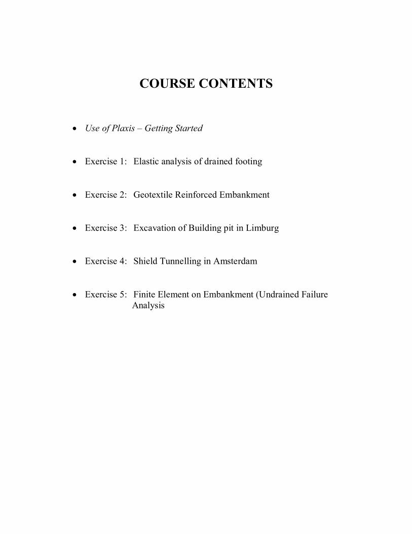
General settings – General tab sheet

1. STARTING THE PROGRAM

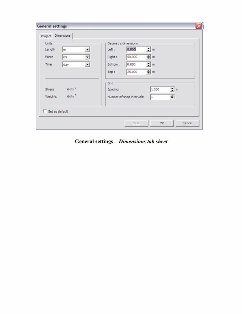
General settings – Dimensions tab sheet

Course on Computational GeotechnicsUiTM

6

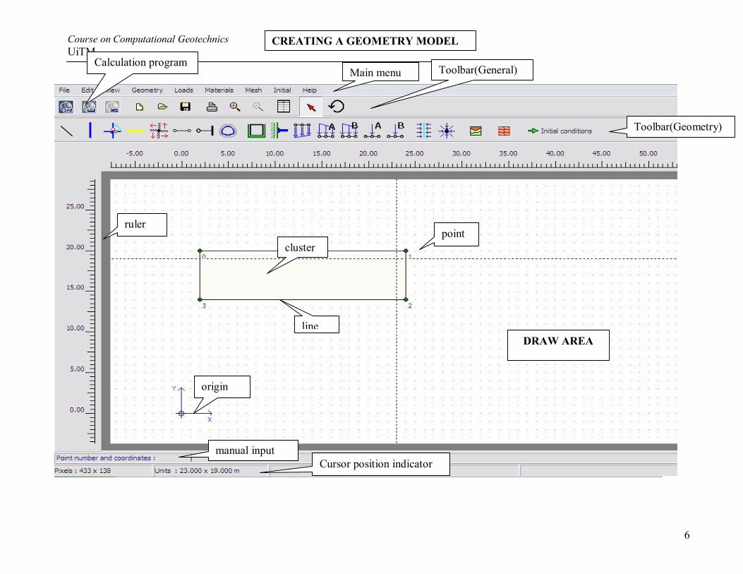
manual inputCursor position indicator

CREATING A GEOMETRY MODEL

ruler

cluster

line

point

origin

Main menu

Toolbar(Geometry)

Toolbar(General)

DRAW AREA

Calculation program


7

output program

Curve program

Coordinate tableZoom in

Geogrid Fixed-end anchor

Geometry line

Plate Hinge andRotation

Interface

Node-to-node anchor

Tunneldesigner

Standard fixities

Rotation fixity(plate)

Prescribeddisplacement

DistributedLoad system A

Distributed Loadsystem B

Point Loadsystem A

Point Loadsystem B

DrainWell

Materialsets

Generate mesh

Define initialconditions

New

Open

Save output program

output program

Zoom out

Print


8

EXERCISE 1

Elastic analysis of drained footing


9

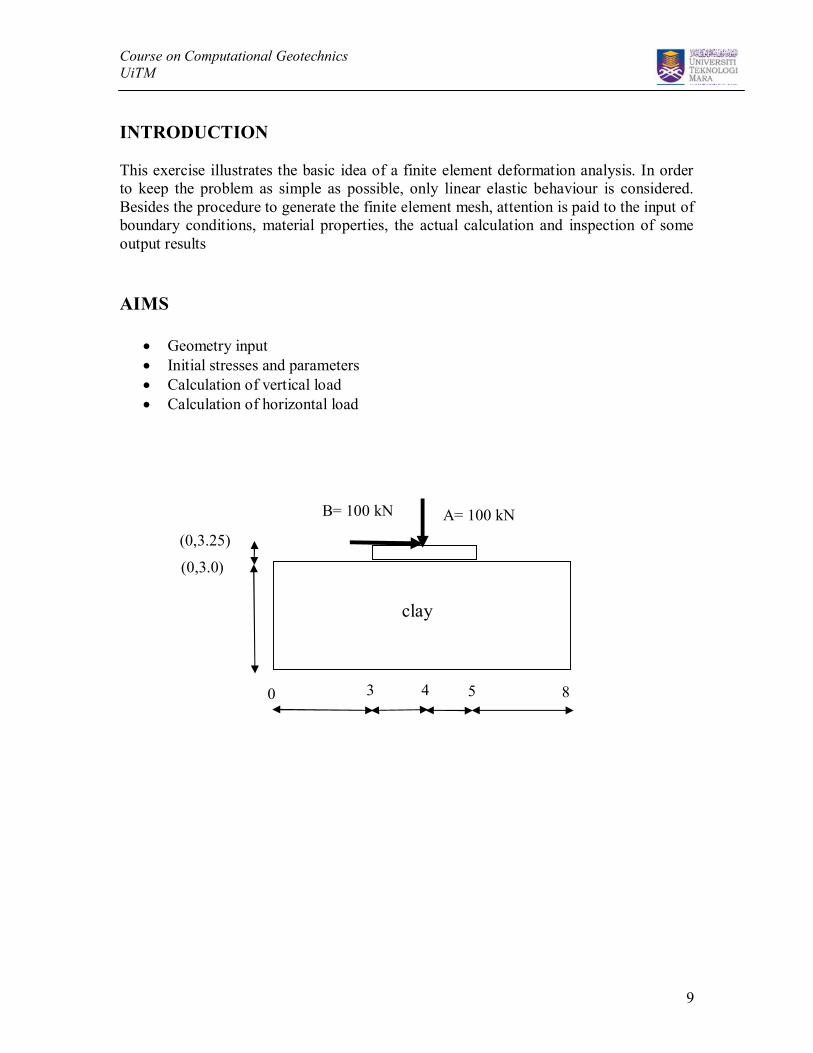
INTRODUCTION

This exercise illustrates the basic idea of a finite element deformation analysis. In orderto keep the problem as simple as possible, only linear elastic behaviour is considered.Besides the procedure to generate the finite element mesh, attention is paid to the input ofboundary conditions, material properties, the actual calculation and inspection of someoutput results

AIMS

· Geometry input· Initial stresses and parameters· Calculation of vertical load· Calculation of horizontal load

A= 100 kN B= 100 kN

clay

(0,3.25)

0

(0,3.0)

3 4 5 8


10

SCHEME OF OPERATIONS:

a) Geometry Inputi. General settings

ii. Input of geometry linesiii. Input of boundary conditionsiv. Input of material propertiesv. Mesh generation

b) Initial Conditioni. Generation of pore pressures

ii. Initial geometry configurationiii. Generation of initial stress

c) Calculationi. Construct footing (staged construction)

ii. Apply vertical forceiii. Apply horizontal force

d) Inspect Output

How to model a drained footing?

Input

Set to plane strain

Use dimension as shown

No need for large number of elements

Load system A: vertical load

Load system B: horizontal load

Material data sets


11

Input for boundary conditions:

Prescribed displacements: Standard fixitiesVertical load: Point Load system AHorizontal load: Point Load system B (direction must be changed: enter x=1.0 and y=0)

Input of material properties:

Parameter Name Clay Concrete UnitMaterial model Model Linear elastic Linear elastic -Type of materialbehaviour

Type Drained Non-porous -

Dry soil unit weight γdry 16 24 kN/m3

Wet soil unit weight γwet 18 - kN/m3

Permeability inhorizontal direction

kx 0 - m/day

Permeability invertical direction

ky 0 - m/day

Young’s modulus Eref 5000 1.35E6 kN/m2

Poissson’s ratio v 0.35 0.35 -

Initial Condition – Generation of pore pressures

· Go to ‘initial condition’ and click ok for unit weight of water = 10 kN/m3.· Draw phreatic level at coordinate (0.0, 3.0) to (8.0, 3.0).· Click on ‘Generate water pressure’

Initial Condition – Generation of Initial Stresses

· Click on ‘generate initial stress button’· Switch cluster for strip footing.· Enter Ko = 0.7 for cluster which represent clay geometry.· Click Ok


12

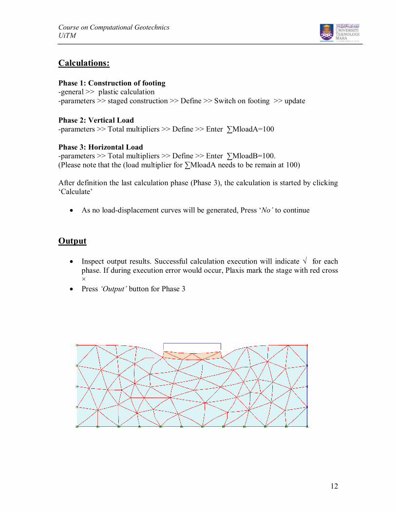
Calculations:

Phase 1: Construction of footing-general >> plastic calculation-parameters >> staged construction >> Define >> Switch on footing >> update

Phase 2: Vertical Load-parameters >> Total multipliers >> Define >> Enter ∑MloadA=100

Phase 3: Horizontal Load-parameters >> Total multipliers >> Define >> Enter ∑MloadB=100.(Please note that the (load multiplier for ∑MloadA needs to be remain at 100)

After definition the last calculation phase (Phase 3), the calculation is started by clicking‘Calculate’

· As no load-displacement curves will be generated, Press ‘No’ to continue

Output

· Inspect output results. Successful calculation execution will indicate √ for eachphase. If during execution error would occur, Plaxis mark the stage with red cross×

· Press ‘Output’ button for Phase 3


13

EXERCISE 2

Geotextile Reinforced Embankment


14

INTRODUCTION

After determination of some model parameters the construction of an embankment onsoft soil is simulated by means of a staged construction analysis. The use of undrainedbehaviour and the generation of pore pressures is reviewed in this exercise. As asuggestion of an extra exercise, the behaviour of the embankment can modelled withoutgeotextile.

AIMS

· Determination of soil stiffness parameters from CPT test results· Simulation of embankment construction in stages· Review of undrained behaviour and pore pressures· Application of geotextile elements

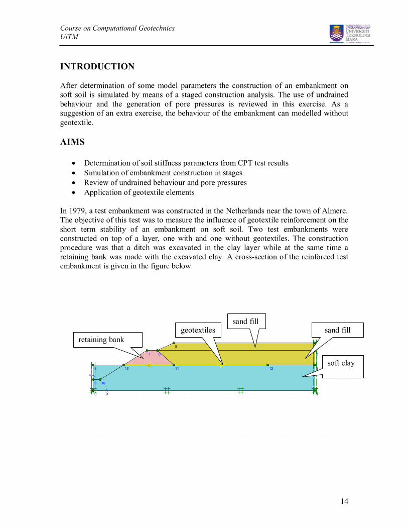
In 1979, a test embankment was constructed in the Netherlands near the town of Almere.The objective of this test was to measure the influence of geotextile reinforcement on theshort term stability of an embankment on soft soil. Two test embankments wereconstructed on top of a layer, one with and one without geotextiles. The constructionprocedure was that a ditch was excavated in the clay layer while at the same time aretaining bank was made with the excavated clay. A cross-section of the reinforced testembankment is given in the figure below.

X

Y

12

0 1

2

3

45

67

8

9 10

11 1213

retaining bankgeotextiles

sand fillsand fill

soft clay


15

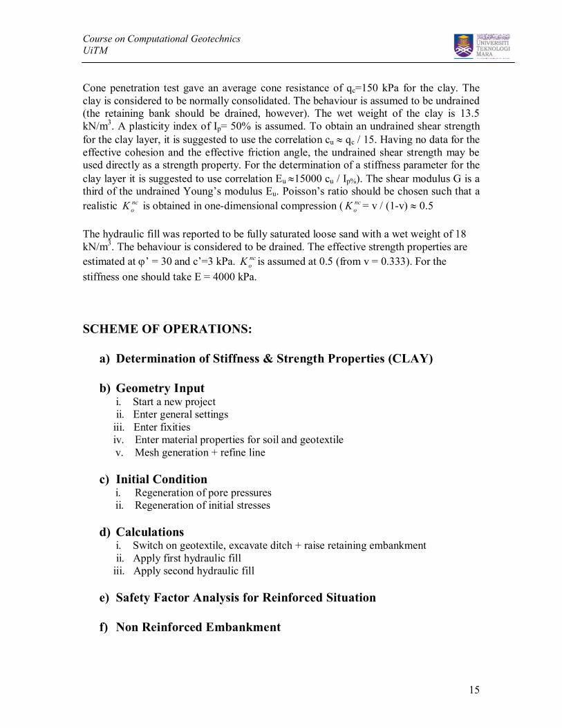
Cone penetration test gave an average cone resistance of qc=150 kPa for the clay. Theclay is considered to be normally consolidated. The behaviour is assumed to be undrained(the retaining bank should be drained, however). The wet weight of the clay is 13.5kN/m3. A plasticity index of Ip= 50% is assumed. To obtain an undrained shear strengthfor the clay layer, it is suggested to use the correlation cu » qc / 15. Having no data for theeffective cohesion and the effective friction angle, the undrained shear strength may beused directly as a strength property. For the determination of a stiffness parameter for theclay layer it is suggested to use correlation Eu »15000 cu / Ip%). The shear modulus G is athird of the undrained Young’s modulus Eu. Poisson’s ratio should be chosen such that arealistic nc

oK is obtained in one-dimensional compression ( ncoK = v / (1-v) » 0.5

The hydraulic fill was reported to be fully saturated loose sand with a wet weight of 18kN/m3. The behaviour is considered to be drained. The effective strength properties areestimated at j’ = 30 and c’=3 kPa. nc

oK is assumed at 0.5 (from v = 0.333). For thestiffness one should take E = 4000 kPa.


a) Determination of Stiffness & Strength Properties (CLAY)

b) Geometry Inputi. Start a new project

ii. Enter general settings iii. Enter fixities

iv. Enter material properties for soil and geotextilev. Mesh generation + refine line

c) Initial Conditioni. Regeneration of pore pressuresii. Regeneration of initial stresses

d) Calculationsi. Switch on geotextile, excavate ditch + raise retaining embankment

ii. Apply first hydraulic fill iii. Apply second hydraulic fill

e) Safety Factor Analysis for Reinforced Situation

f) Non Reinforced Embankment


16

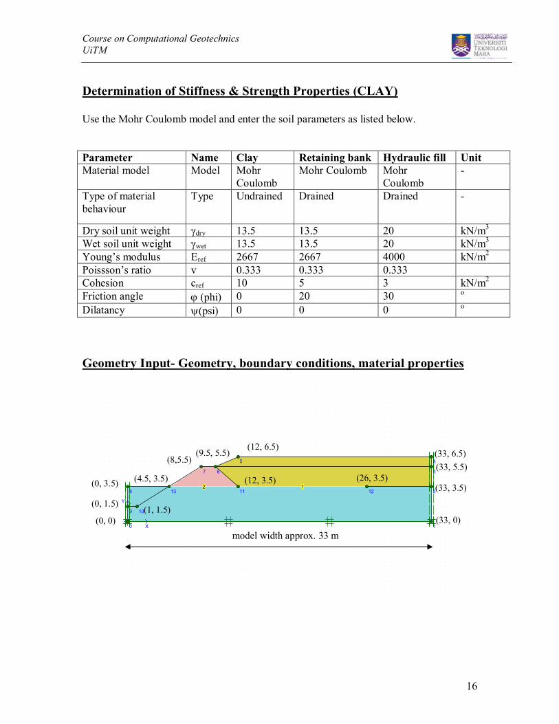
Determination of Stiffness & Strength Properties (CLAY)

Use the Mohr Coulomb model and enter the soil parameters as listed below.

Parameter Name Clay Retaining bank Hydraulic fill UnitMaterial model Model Mohr

CoulombMohr Coulomb Mohr

Coulomb-

Type of materialbehaviour

Type Undrained Drained Drained -

Dry soil unit weight γdry 13.5 13.5 20 kN/m3

Wet soil unit weight γwet 13.5 13.5 20 kN/m3

Young’s modulus Eref 2667 2667 4000 kN/m2

Poissson’s ratio v 0.333 0.333 0.333Cohesion cref 10 5 3 kN/m2

Friction angle j (phi) 0 20 30 o

Dilatancy y(psi) 0 0 0 o

Geometry Input- Geometry, boundary conditions, material properties

X

Y

12

0 1

2

3

45

67

8

9 10

11 1213(0, 3.5)

(0, 0)

(0, 1.5)(1, 1.5)

(4.5, 3.5)

(8,5.5)(9.5, 5.5)

(12, 6.5)

(12, 3.5) (26, 3.5)

(33, 6.5)(33, 5.5)

(33, 3.5)

(33, 0)

model width approx. 33 m


17

Input geometry· Enter geometry as indicated· Click ‘Geotextile’

Input boundary condition· Click Standard Fixities

Input material properties· Soil and Interfaces – Enter the material properties for the three soil data sets as

indicated in the first table of this exercise..· After entering all properties for the three soil types, drag and drop the properties

to the appropriate clusters, as indicated below:

X

Y

12

0 1

2

3

45

67

8

9 10

11 1213

Geotextile· Select geotextiles and enter 2500 kN/m as stiffness. Note that this is the stiffness

in extension. In compression no stiffness is used.

retaining bankgeotextiles sand fill

soft claysoft clay


18

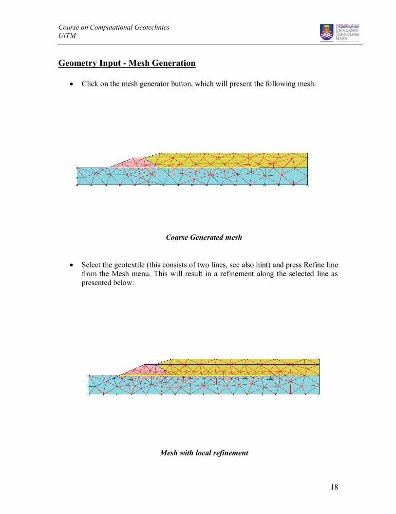
Geometry Input - Mesh Generation

· Click on the mesh generator button, which will present the following mesh:

Coarse Generated mesh

· Select the geotextile (this consists of two lines, see also hint) and press Refine linefrom the Mesh menu. This will result in a refinement along the selected line aspresented below:

Mesh with local refinement


19

Initial Condition – Generation of pore pressures

· Enter phreatic level line by two coordinates (0, 3.5) and (33, 3.5)· Generate water pressure button

Initial Condition – Generation of Initial Stresses

· Deselect all material clusters and geotextile elements that are not present at thestart of analysis.

· Switch off:-Geotextile elements-Material clusters for the hydraulic fill-Material cluster for retaining bank

· Click on Generate initial stress button and enter a Ko value for the Clay clusters of0.5. By default, Plaxis proposes Ko values that are calculated from the relation: 1-sinj. This result in a default value of 1.0 for the clay layer (j = 0). As we haveused in the undrained shear strength no input value for j is used. But as suggestedin the introduction of this exercise, we should enter Ko value calculated fromanother relation:

5.0)1(0 »

-»

vvK NC

Calculations

In the calculation list, three phases are needed. For each calculation phase, Plasticcalculation is involved. For each calculation phase the loading type Staged Constructionis selected, other settings are taken at their default values:

· Phase 1Switch on: 1) Construction geotextile

2) Construction of retaining bank3) Excavation of the ditch (left of the embankment)-switch off

· Phase 2Switch on: 1) Construction of 1st hydraulic fill

· Phase 3Switch on: 1) Construction of 2nd hydraulic fill


20

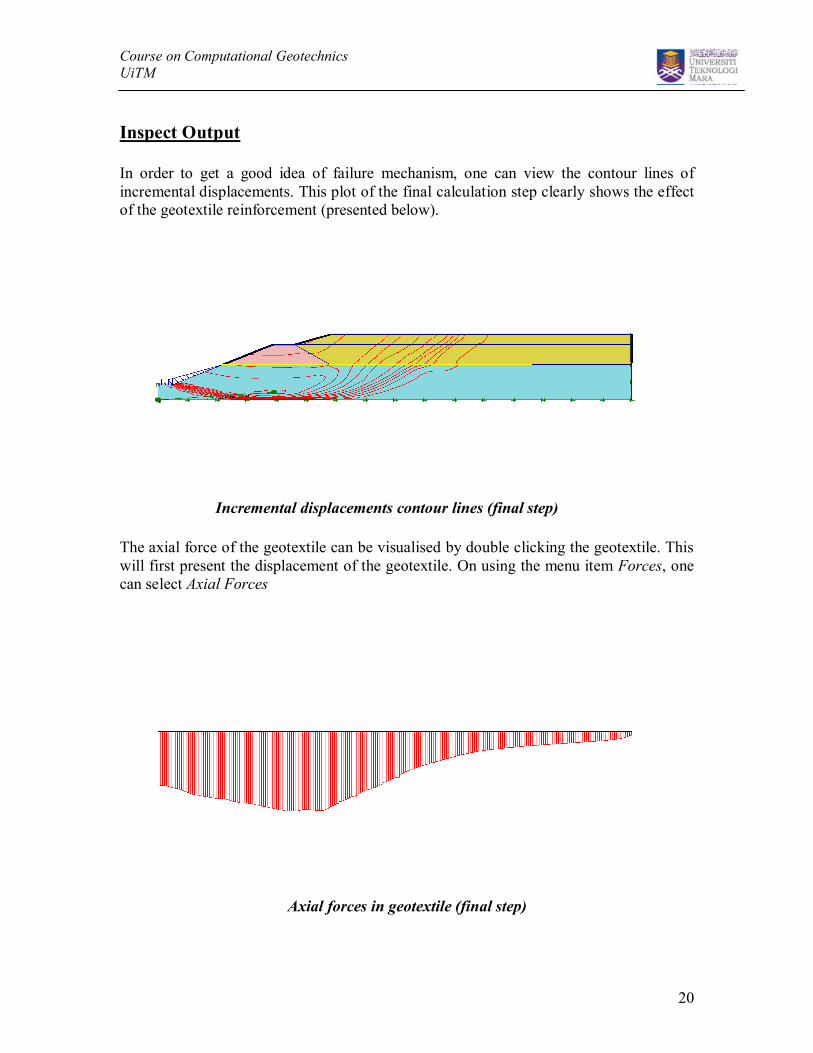
Inspect Output

In order to get a good idea of failure mechanism, one can view the contour lines ofincremental displacements. This plot of the final calculation step clearly shows the effectof the geotextile reinforcement (presented below).

Incremental displacements contour lines (final step)

The axial force of the geotextile can be visualised by double clicking the geotextile. Thiswill first present the displacement of the geotextile. On using the menu item Forces, onecan select Axial Forces

Axial forces in geotextile (final step)


21

F) SAFETY FACTOR ANALYSES


A) Safety factor analysis

Safety Factor Analysis

· Start the calculation program and select the reinforced embankment project.· In the existing calculation list, press the Next button to add the fourth calculation

phase.· This will add <Phase 4>. Please note that the previous calculation phases must be

indicated by check mark Ö.· In contrast to most other calculation, a number of steps calculation is needed for

safety factor analysis.· On the first tab sheet, select Calculation type as Phi/c reduction. On the second

tab select press the Define button and Plaxis has introduced a default value for theincremental multipliers Msf (0.1). This value may be used in most situations.

· Click on the Calculation button to start the safety factor analysis. Note that thecalculation process will skip all calculation phases that were successfully finished,and that are indicated by Ö. Phase 4 is the only calculation phase that is processed.

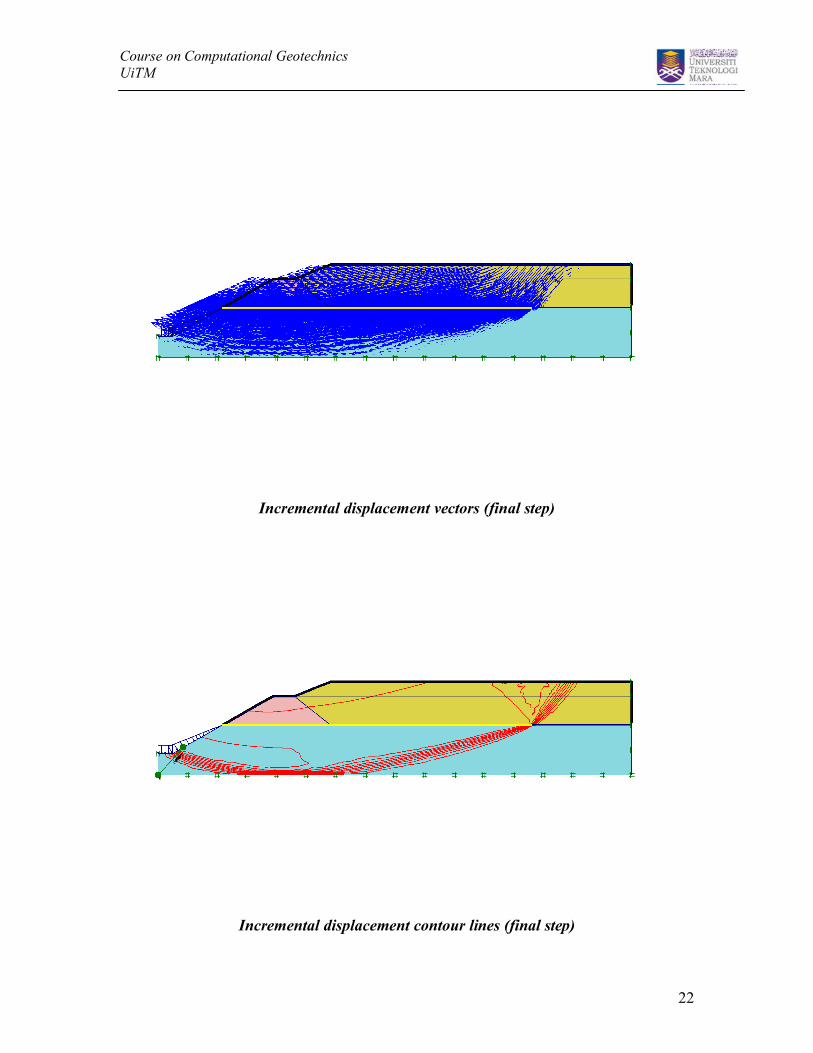
Inspect Output

Note that displacements resulting from a Phi/c reduction are non physical. Hence, thetotal displacements are not relevant. An incremental displacements plot of the last step,however, shows the failure mechanism that corresponds to the calculated value of åMsf.


22

Incremental displacement vectors (final step)

Incremental displacement contour lines (final step)


23

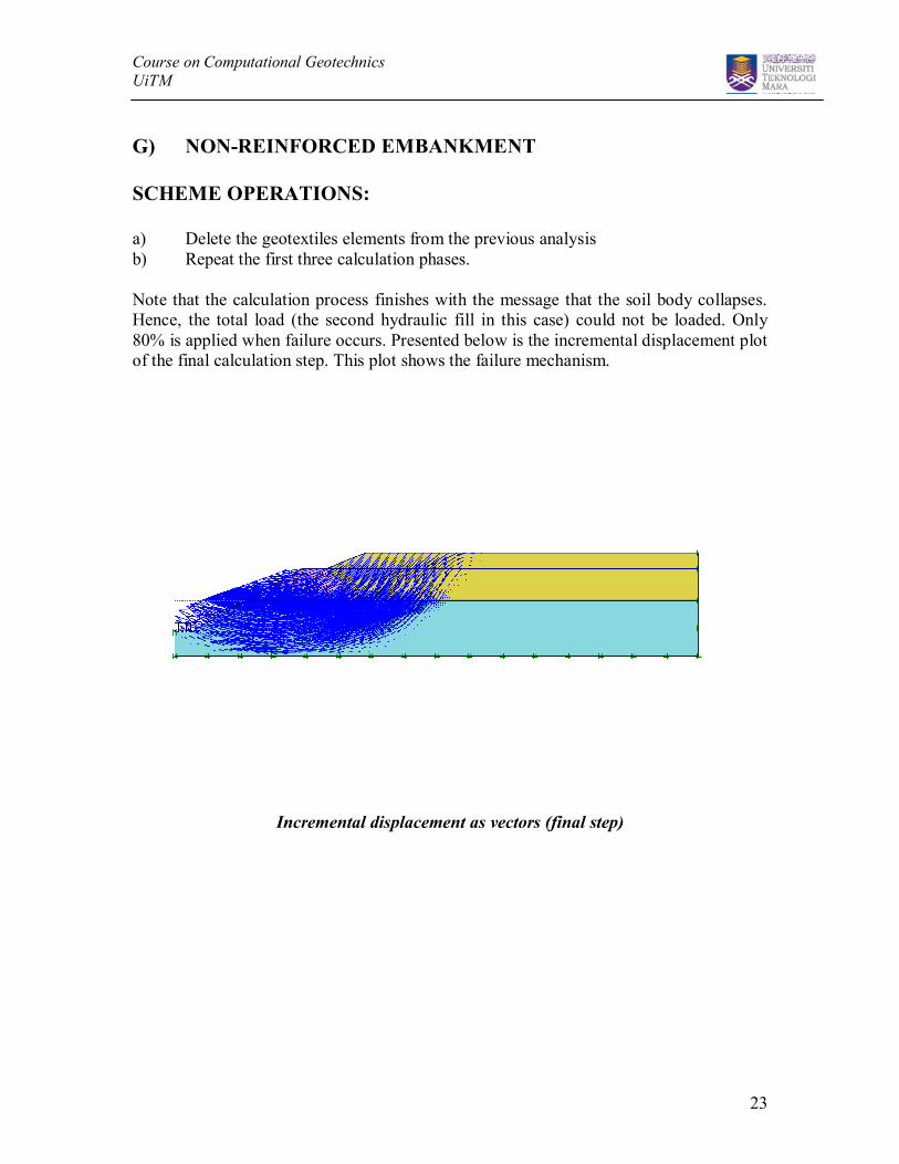
G) NON-REINFORCED EMBANKMENT

SCHEME OPERATIONS:

a) Delete the geotextiles elements from the previous analysisb) Repeat the first three calculation phases.

Note that the calculation process finishes with the message that the soil body collapses.Hence, the total load (the second hydraulic fill in this case) could not be loaded. Only80% is applied when failure occurs. Presented below is the incremental displacement plotof the final calculation step. This plot shows the failure mechanism.

Incremental displacement as vectors (final step)


24

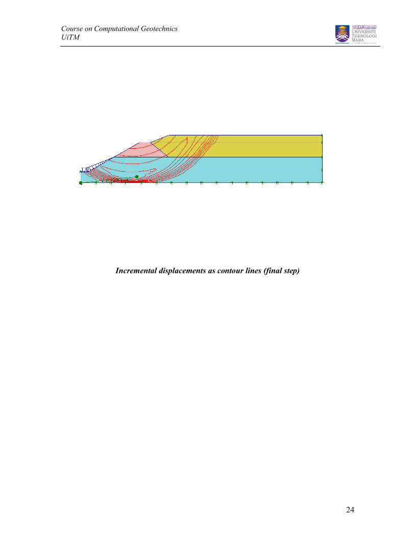
Incremental displacements as contour lines (final step)


25

EXERCISE 3

Excavation of building pit in Limburg


26

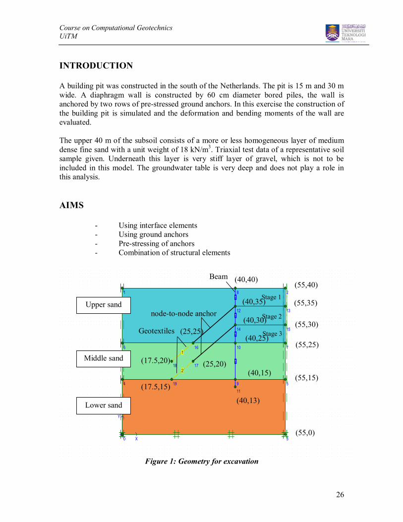
INTRODUCTION

A building pit was constructed in the south of the Netherlands. The pit is 15 m and 30 mwide. A diaphragm wall is constructed by 60 cm diameter bored piles, the wall isanchored by two rows of pre-stressed ground anchors. In this exercise the construction ofthe building pit is simulated and the deformation and bending moments of the wall areevaluated.

The upper 40 m of the subsoil consists of a more or less homogeneous layer of mediumdense fine sand with a unit weight of 18 kN/m3. Triaxial test data of a representative soilsample given. Underneath this layer is very stiff layer of gravel, which is not to beincluded in this model. The groundwater table is very deep and does not play a role inthis analysis.

AIMS

- Using interface elements- Using ground anchors- Pre-stressing of anchors- Combination of structural elements

X

Y

1

1

1

1

1

2

0

1 2

3

4 5

6 7

8

9

10

11

12 13

14 15

16

1718

19

Figure 1: Geometry for excavation

node-to-node anchor

Geotextiles

Beam(55,40)

(55,35)

(55,30)

(55,25)

(55,15)

(55,0)

(40,35)

(40,30)

(40,25)

(40,15)

(40,13)

(40,40)

(25,25)

(25,20)(17.5,20)

(17.5,15)

Stage 1

Stage 2

Stage 3

Upper sand

Middle sand

Lower sand


27

Enter fixities

Click the ‘standard fixities’ for the standard boundary condition

Input of material properties:

Parameter Name Units Upper sand Middle sand Lower sandMaterial model Model Mohr-Coulomb Mohr-Coulomb Mohr-CoulombType of materialbehaviour

Type Drained Drained Drained

Dry soil unit weight γdry kN/m3 18 18 18Wet soil unitweight

γwet kN/m3 18 18 18

Permeability inhorizontal direction

kx m/day 1.0 1.0 1.0


ky m/day 1.0 1.0 1.0

Young’s modulus Eref kN/m2 15000 25000 32000Poissson’s ratio v 0.33 0.33 0.33Cohesion cref kN/m2 1 1 1Friction angle φ o 35 35 35Dilatancy angle ψ o 5 5 5

EA(kN/m) EI(kNm2/m) w(kN/m2) LSBeam 80000000 1500000 8 -Anchor 200000 - - 1Geotextile 200000 - - -(Note: all material types are ‘elastic’)

INTERFACESRinter [-] 0.6

(sand/concrete inter)0.6(sand/concrete inter)

1.0(soil/soil interaction)


28

GEOMETRY INPUT

· Enter general settings· Enter geometry + enter beam, interfaces, anchors and geotextiles

- Chick Beam button to introduce diaphragm wall- Click Geotextile button to introduce the geotextile elements that

represent the grout body- Click interface button, which will present the cursor in the Interface

mode. As interfaces can be introduced on both sides of a geometryline, one should pay attention of the arrows o the cursor.

- Click Node-to-node anchor button and introduce the two anchors.These anchors connect the beginning of the grout-body to wall.

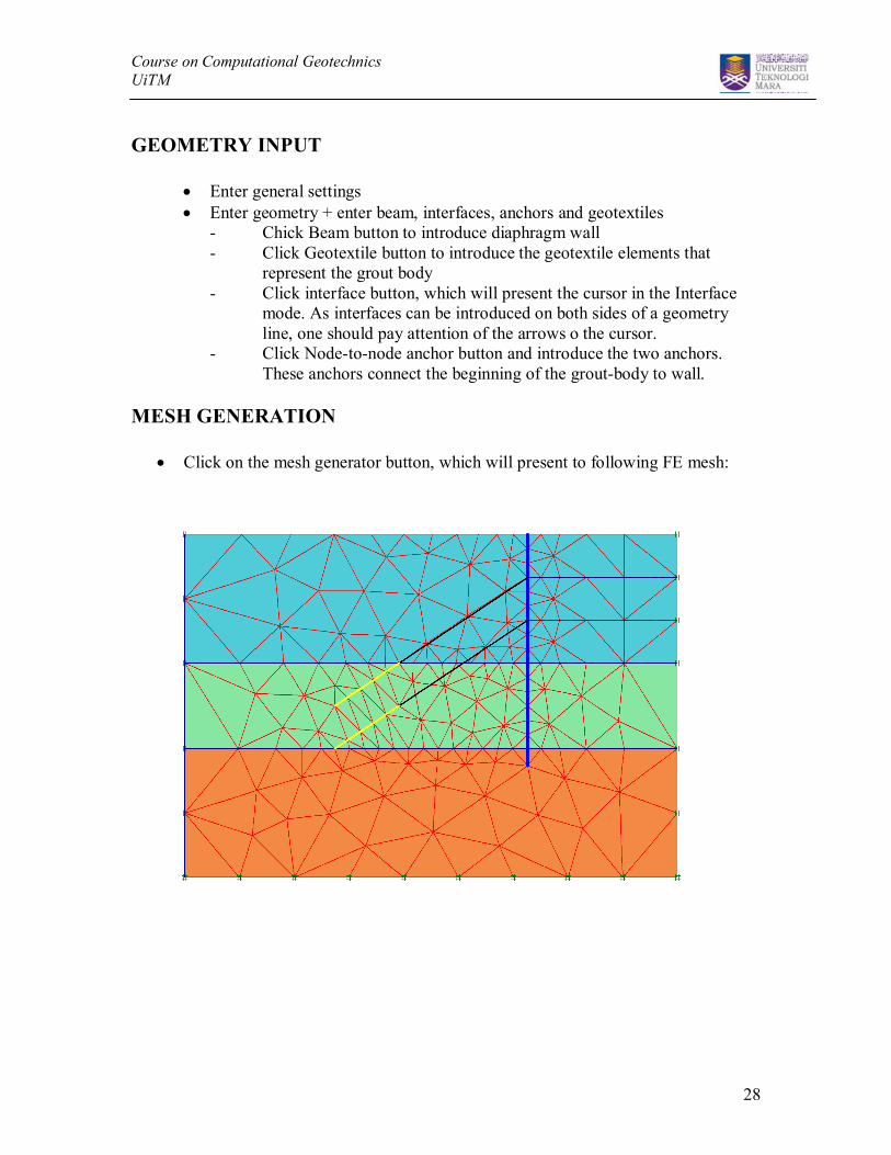
MESH GENERATION

· Click on the mesh generator button, which will present to following FE mesh:


29

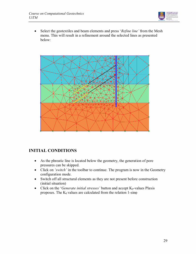
· Select the geotextiles and beam elements and press ‘Refine line’ from the Meshmenu. This will result in a refinement around the selected lines as presentedbelow:

INITIAL CONDITIONS

· As the phreatic line is located below the geometry, the generation of porepressures can be skipped.

· Click on ‘switch’ in the toolbar to continue. The program is now in the Geometryconfiguration mode.

· Switch off all structural elements as they are not present before construction(initial situation)

· Click on the ‘Generate initial stresses’ button and accept K0-values Plaxisproposes. The K0 values are calculated from the relation 1-sinφ


30

CALCULATIONS

There entire construction process consists of five phases

Phase 1: activation of diaphragm wall, ignore undrained behaviour, reset displacement to zero-parameters >> Plastic calculation >> Staged Construction >> Define >> Switch ondiaphragm wall >> update

Phase 2: Excavation Stage 1 (-5.00 m)-parameters >> plastic calculation >> Staged Construction >> Define first cluster >> update

Phase 3: Pre-stress first anchor row with 300 kN/m--parameters >> plastic calculation >> Staged Construction >>activate anchor pre-tension300 kN/m and geotextiles >> update

Phase 4: Excavation Stage 2 (-10.00 m)-parameters >> plastic calculation >> Staged Construction >> Define second cluster >> update

Phase 5: Pre-stress second anchor row with 300 kN/m-parameters >> plastic calculation >> Staged Construction >>activate anchor pre-tension 300 kN/m and geotextiles >> update

Phase 6: Excavation Stage 3 (-15.00 m)-parameters >> plastic calculation >> Staged Construction >> Define third cluster >> update


31

INSPECT OUTPUT

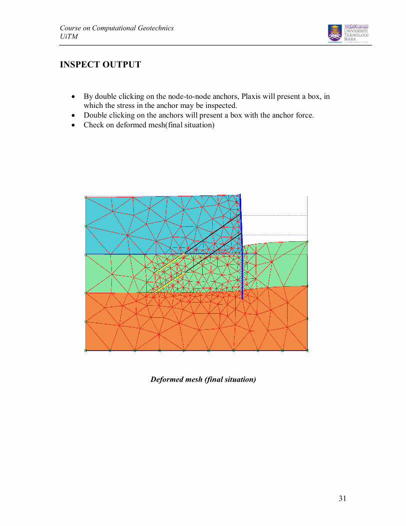
· By double clicking on the node-to-node anchors, Plaxis will present a box, inwhich the stress in the anchor may be inspected.

· Double clicking on the anchors will present a box with the anchor force.· Check on deformed mesh(final situation)

Deformed mesh (final situation)


32

EXERCISE 4

Shield Tunnelling in Amsterdam


33

INTRODUCTION

This exercise comprises the generation and excavation of a circular shield tunnel. ThePlaxis tunnel designer is used in this exercise. The excavation of the tunnel consists, inprinciple, of three stages: Excavation of the soil, removal of the water in the tunnel andsimulation of the volume loss due to tunneling. The volume loss is simulated byprescribing a contraction of the tunnel lining.

AIMS

· Generation of a finite element mesh including a circular tunnel· Calculating settlements due to tunneling.

GEOMETRY INPUT

Start a new projectGeneral setting: enter title and descriptionUse 15 nodes elementsEnter geometry dimensions

ENTER GEOMETRYEnter geometry as proposed in Figure 2


34

X

Y

1

1

1

1

0 1

2

3

4

56

7

8

9

1112

1415

18

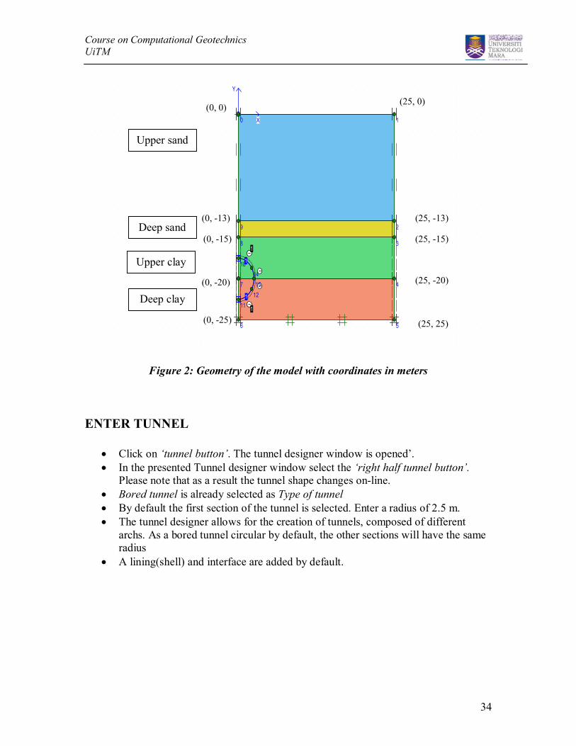
Figure 2: Geometry of the model with coordinates in meters

ENTER TUNNEL

· Click on ‘tunnel button’. The tunnel designer window is opened’.· In the presented Tunnel designer window select the ‘right half tunnel button’.

Please note that as a result the tunnel shape changes on-line.· Bored tunnel is already selected as Type of tunnel· By default the first section of the tunnel is selected. Enter a radius of 2.5 m.· The tunnel designer allows for the creation of tunnels, composed of different

archs. As a bored tunnel circular by default, the other sections will have the sameradius

· A lining(shell) and interface are added by default.

(0, 0)

(0, -13)

(0, -15)

(0, -20)

(0, -25) (25, 25)

(25, -20)

(25, -15)

(25, -13)

(25, 0)

Upper sand

Deep sand

Upper clay

Deep clay


35

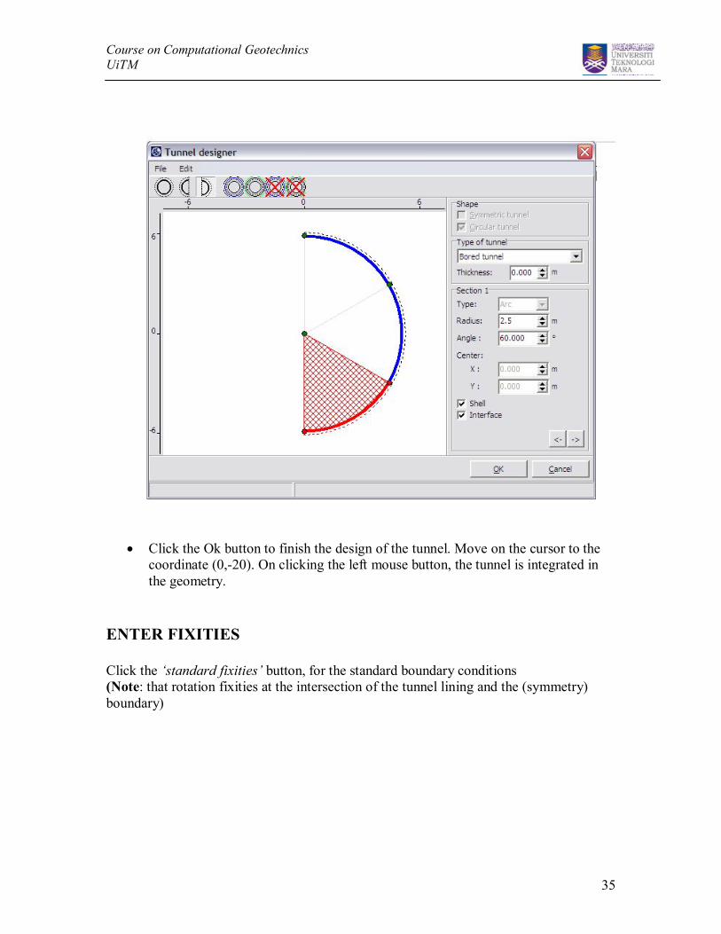
· Click the Ok button to finish the design of the tunnel. Move on the cursor to thecoordinate (0,-20). On clicking the left mouse button, the tunnel is integrated inthe geometry.

ENTER FIXITIES

Click the ‘standard fixities’ button, for the standard boundary conditions(Note: that rotation fixities at the intersection of the tunnel lining and the (symmetry)boundary)


36

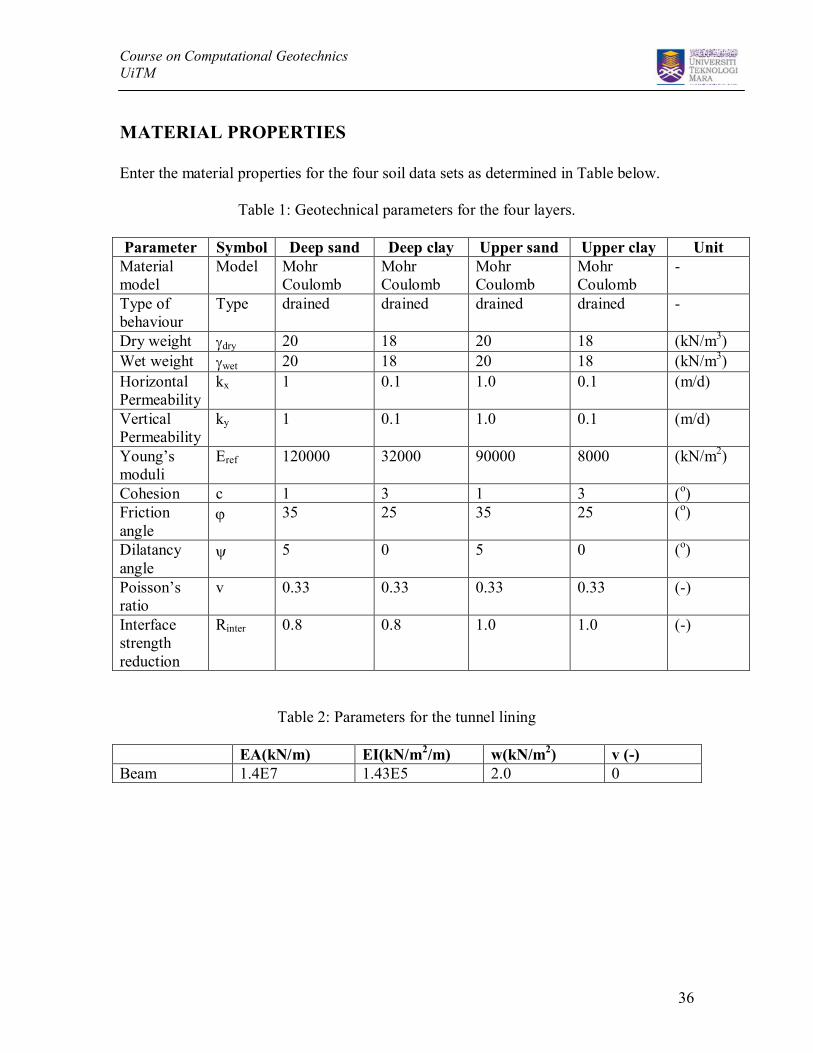
MATERIAL PROPERTIES

Enter the material properties for the four soil data sets as determined in Table below.

Table 1: Geotechnical parameters for the four layers.

Parameter Symbol Deep sand Deep clay Upper sand Upper clay UnitMaterialmodel

Model MohrCoulomb

MohrCoulomb

MohrCoulomb

MohrCoulomb

-

Type ofbehaviour

Type drained drained drained drained -

Dry weight gdry 20 18 20 18 (kN/m3)Wet weight gwet 20 18 20 18 (kN/m3)HorizontalPermeability

kx 1 0.1 1.0 0.1 (m/d)

VerticalPermeability

ky 1 0.1 1.0 0.1 (m/d)

Young’smoduli

Eref 120000 32000 90000 8000 (kN/m2)

Cohesion c 1 3 1 3 (o)Frictionangle

j 35 25 35 25 (o)

Dilatancyangle

y 5 0 5 0 (o)

Poisson’sratio

v 0.33 0.33 0.33 0.33 (-)

Interfacestrengthreduction

Rinter 0.8 0.8 1.0 1.0 (-)

Table 2: Parameters for the tunnel lining

EA(kN/m) EI(kN/m2/m) w(kN/m2) v (-)Beam 1.4E7 1.43E5 2.0 0


37

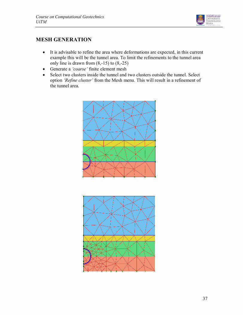
MESH GENERATION

· It is advisable to refine the area where deformations are expected, in this currentexample this will be the tunnel area. To limit the refinements to the tunnel areaonly line is drawn from (8,-15) to (8,-25)

· Generate a ‘coarse’ finite element mesh· Select two clusters inside the tunnel and two clusters outside the tunnel. Select

option ‘Refine cluster’ from the Mesh menu. This will result in a refinement ofthe tunnel area.


38

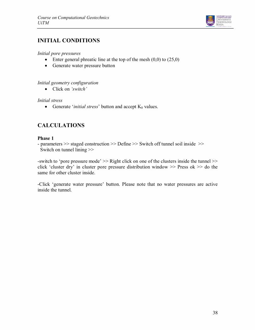
INITIAL CONDITIONS

Initial pore pressures· Enter general phreatic line at the top of the mesh (0,0) to (25,0)· Generate water pressure button

Initial geometry configuration· Click on ‘switch’

Initial stress· Generate ‘initial stress’ button and accept K0 values.

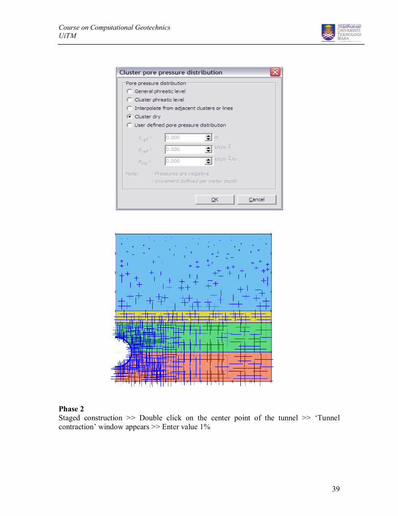
CALCULATIONS

Phase 1- parameters >> staged construction >> Define >> Switch off tunnel soil inside >> Switch on tunnel lining >>

-switch to ‘pore pressure mode’ >> Right click on one of the clusters inside the tunnel >>click ‘cluster dry’ in cluster pore pressure distribution window >> Press ok >> do thesame for other cluster inside.

-Click ‘generate water pressure’ button. Please note that no water pressures are activeinside the tunnel.


39

Phase 2Staged construction >> Double click on the center point of the tunnel >> ‘Tunnelcontraction’ window appears >> Enter value 1%


40

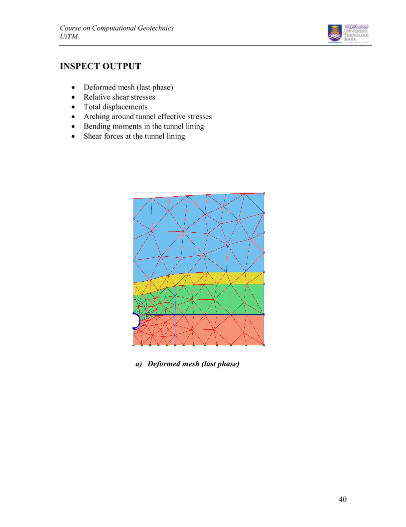
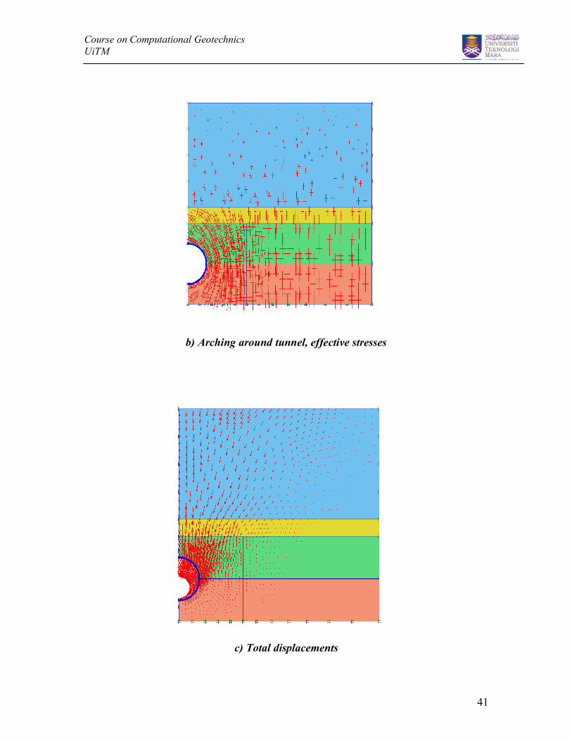
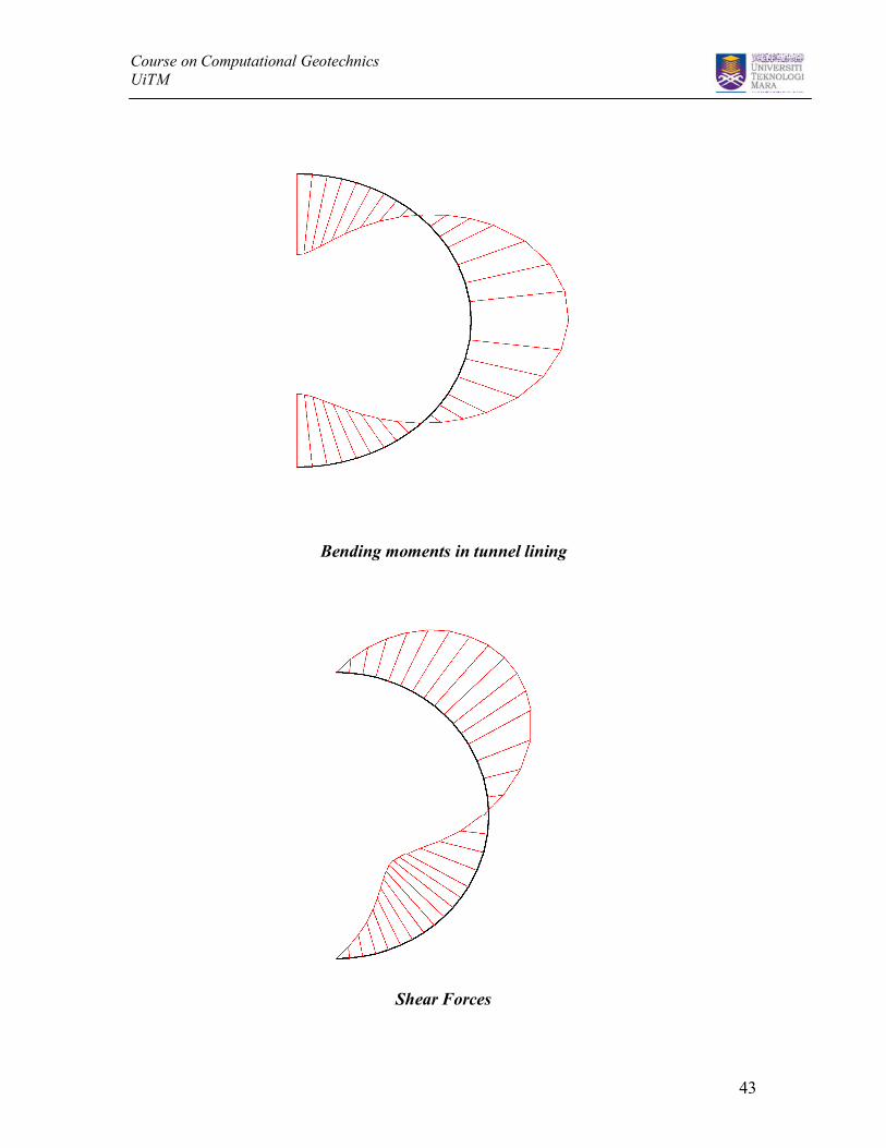
INSPECT OUTPUT

· Deformed mesh (last phase)· Relative shear stresses· Total displacements· Arching around tunnel effective stresses· Bending moments in the tunnel lining· Shear forces at the tunnel lining

a) Deformed mesh (last phase)


41

b) Arching around tunnel, effective stresses

c) Total displacements


42

e) Plastic zone around tunnel


43

Bending moments in tunnel lining

Shear Forces


44

EXERCISE 5

Finite Element on Embankment(Undrained Failure Analysis)


45

INTRODUCTION

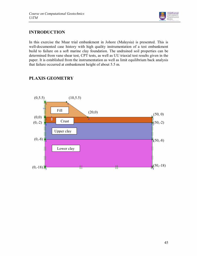
In this exercise the Muar trial embankment in Johore (Malaysia) is presented. This iswell-documented case history with high quality instrumentation of a test embankmentbuild to failure on a soft marine clay foundation. The undrained soil properties can bedetermined from vane shear test, CPT tests, as well as UU triaxial test results given in thepaper. It is established from the instrumentation as well as limit equilibrium back analysisthat failure occurred at embankment height of about 5.5 m.

PLAXIS GEOMETRY

X

Y

0 1

2

3

45

6

7

8

9 10

(0,0)

(0,5.5) (10,5.5)

(20,0)

(0,-2)

(50, 0)

(0,-18) (50,-18)

(0,-8) (50,-8)

(50,-2)

Fill

Crust

Upper clay

Lower clay


46

INPUT PROPERTIES

Parameter Name Fill Crust Upper clay Lower clayMaterial model Model MC MC MC MCType of materialbehaviour

Type Undrained Undrained Undrained Undrained

Dry soil unitweight

γdry 20 16.5 15.5 15.5

Wet soil unitweight

γwet 20 16.5 15.5 15.5

Permeability inhorizontaldirection

kx 1.00 1.296E-4 1.296E-4 9.5E-5


ky 1.00 6.912E-5 6.912E-5 5.184E-5

Young’smodulus

Eref 5200 22100 2600 3900

Poissson’s ratio v 0.30 0.30 0.30 0.30Cohesion cref 54.0 20.0 8.0 15.0Friction angle φ 0 0 0 0Dilatancy angle ψ 0 0 0 0

Identification Einc cinc grefFill 0.0 0.0 0.0Crust 2250.0 7.5 0.0Upper Clay 375.0 1.3 2.0Lower Clay 450.0 1.5 8.0

INITIAL CONDITIONS

· Initial pore pressuresPhreatic surface is set at 1m below GL

· Initial stressesSwitch off embankment and generate initial stresses based on Ko conditions.


47

CALCULATIONS

Phase 1- parameters >> staged construction >> Define >> Activate embankment cluster

Phase 2- Phi/c reduction analysis to obtain FOS for undrained condition.

Select node displacement point at the crest of embankment for curve plot of FS vs.displacement.


48

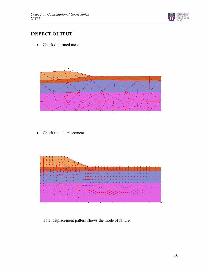
INSPECT OUTPUT

· Check deformed mesh

· Check total displacement

Total displacement pattern shows the mode of failure.


49

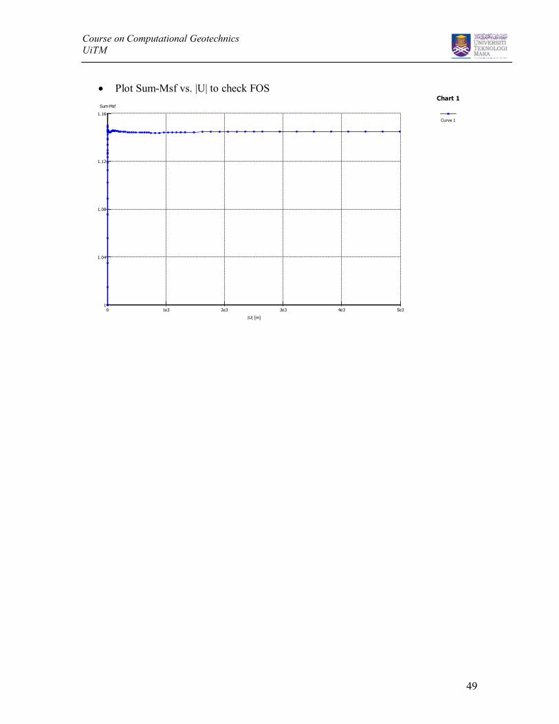
· Plot Sum-Msf vs. |U| to check FOS

0 1e3 2e3 3e3 4e3 5e31

1.04

1.08

1.12

1.16

|U| [m]

Sum-Msf

Chart 1

Curve 1

COURSE ON COMPUTATIONAL GEOTECHNICS A Geotechnical Design · PDF fileCOURSE ON COMPUTATIONAL...

Documents

Transcript of COURSE ON COMPUTATIONAL GEOTECHNICS A Geotechnical Design · PDF fileCOURSE ON COMPUTATIONAL...