5-1 12/28/2010

Module 15: Simple Harmonic Motion 15.1 Introduction: Periodic Motion There are two basic ways to measure time: by duration or periodic motion. Early clocks measured duration by calibrating the burning of incense or wax, or the flow of water or sand from a container. Our calendar consists of years determined by the motion of the sun; months determined by the motion of the moon; days by the rotation of the earth; hours by the motion of cyclic motion of gear trains; and seconds by the oscillations of springs or pendulums. In modern times a second is defined by a specific number of vibrations of radiation, corresponding to the transition between the two hyperfine levels of the ground state of the cesium 133 atom (see Section 1.3).

Sundials calibrate the motion of the sun through the sky including seasonal corrections. A clock escapement is a device that can transform continuous movement into discrete movements of a gear train. The early escapements used oscillatory motion to stop and start the turning of a weight-driven rotating drum. Soon, complicated escapements were regulated by pendulums, the theory of which was first developed by the physicist Christian Huygens in the mid 17th century. The accuracy of clocks was increased and the size reduced by the discovery of the oscillatory properties of springs by Robert Hooke. By the middle of the 18th century, the technology of timekeeping advanced to the point that William Harrison developed timekeeping devices that were accurate to one second in a century.

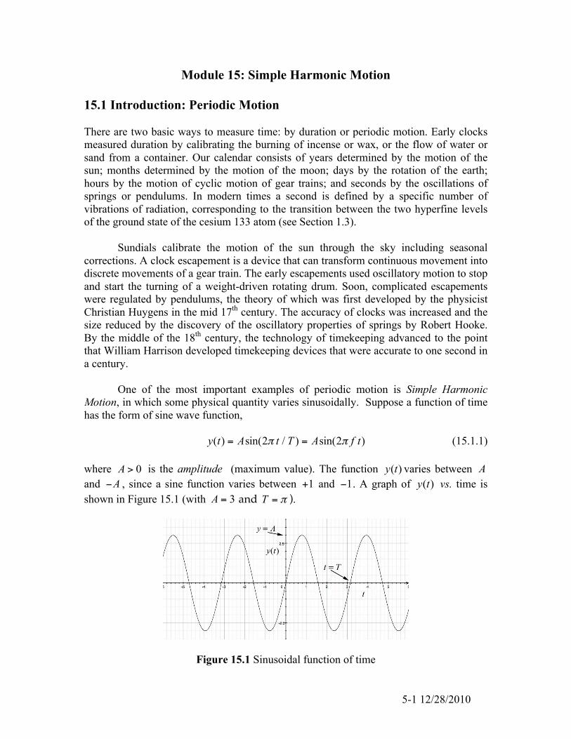
One of the most important examples of periodic motion is Simple Harmonic

Motion, in which some physical quantity varies sinusoidally. Suppose a function of time has the form of sine wave function, y(t) = Asin(2! t / T ) = Asin(2! f t) (15.1.1) where 0A > is the amplitude (maximum value). The function ( )y t varies between A and A! , since a sine function varies between 1+ and 1! . A graph of ( )y t vs. time is shown in Figure 15.1 (with A = 3 and T = ! ).

Figure 15.1 Sinusoidal function of time

5-2 12/28/2010

The sine function is periodic in time. This means that the value of the function at

time t will be exactly the same at a later time t t T! = + , where T is the period. That the sine function satisfies the periodic condition can be seen from

2 2 2( ) sin ( ) sin 2 sin ( )y t T A t T A t A t y tT T T! ! !

!" # " # " #+ = + = + = =$ % $ % $ %& ' & ' & '. (15.1.2)

The frequency, f , is defined to be 1/f T! . (15.1.3) The SI unit of frequency is inverse seconds, 1s!" #$ % , or hertz [Hz] . The angular frequency of oscillation is defined to be 2 / 2T f! " "# = (15.1.4) and is measured in radians per second. One oscillation per second, 1Hz , corresponds to an angular frequency of 12 rad s! "# . (Unfortunately, the same symbol ! is used for angular velocity in circular motion. For uniform circular motion the angular velocity is equal to the angular frequency but for non-uniform motion the angular velocity will not be constant but the angular frequency for simple harmonic motion is a constant by definition.) 15.2 Simple Harmonic Motion: Object-Spring System Our first example of a system that demonstrates simple harmonic motion is an object-spring system on a frictionless surface, shown in Figure 15.2

Figure 15.2 Object-Spring system The object is attached to one end of a spring. The other end of the spring is attached to a wall at the right in the figure. Assume that the object undergoes one-dimensional motion.

5-3 12/28/2010

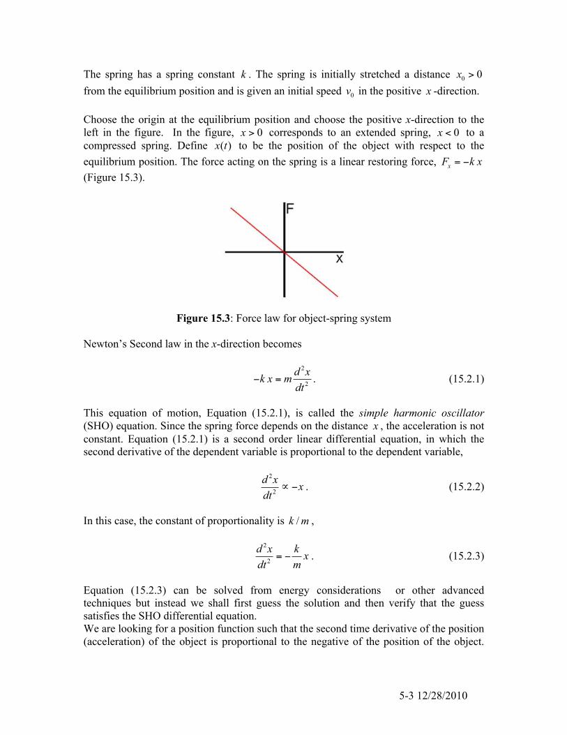
The spring has a spring constant k . The spring is initially stretched a distance 0 0x > from the equilibrium position and is given an initial speed 0v in the positive x -direction. Choose the origin at the equilibrium position and choose the positive x-direction to the left in the figure. In the figure, 0x > corresponds to an extended spring, 0x < to a compressed spring. Define ( )x t to be the position of the object with respect to the equilibrium position. The force acting on the spring is a linear restoring force, xF k x= ! (Figure 15.3).

Figure 15.3: Force law for object-spring system Newton’s Second law in the x-direction becomes

2

2

d xk x m

dt! = . (15.2.1)

This equation of motion, Equation (15.2.1), is called the simple harmonic oscillator (SHO) equation. Since the spring force depends on the distance x , the acceleration is not constant. Equation (15.2.1) is a second order linear differential equation, in which the second derivative of the dependent variable is proportional to the dependent variable,

2

2

d xx

dt! " . (15.2.2)

In this case, the constant of proportionality is /k m ,

2

2

d x kx

dt m= ! . (15.2.3)

Equation (15.2.3) can be solved from energy considerations or other advanced techniques but instead we shall first guess the solution and then verify that the guess satisfies the SHO differential equation. We are looking for a position function such that the second time derivative of the position (acceleration) of the object is proportional to the negative of the position of the object.

5-4 12/28/2010

Since the sine and cosine functions both satisfy this property, we make a preliminary guess that our position function is given by ( ) cos((2 / ) ) cos( )x t A T t A t! "= = , (15.2.4) where as in Equation (15.1.4) 2 /T! "# is the angular frequency (as of yet, undetermined). In Equation (15.2.4), the constant A is not necessarily the amplitude of the motion; A is the amplitude for the case 0 0x > , 0 0v = . We shall now find the condition the angular frequency ! must satisfy in order to insure that the function in (15.2.4) solves the simple harmonic oscillator equation (15.2.1). The first and second derivatives of the position function are given by

2

2 22

sin( )

cos( ) .

dxA t

dtd x

A t xdt

! !

! ! !

= "

= " = "

(15.2.5)

Substitute the second derivative, the second expression in (15.2.5), and the position function, Equation (15.2.4), into the SHO Equation (15.2.1), giving

2 cos( ) cos( )kA t A tm

! ! !" = " . (15.2.6)

Equation (15.2.6) is valid for all times provided that

km

! = . (15.2.7)

The period of oscillation is then

2 2 mTk

!!

"= = . (15.2.8)

One possible solution is then

x(t) = Acoskm

t!

"#

$

%&

vx (t) = 'km

Asinkm

t!

"#

$

%& .

(15.2.9)

5-5 12/28/2010

Note that at 0t = , the position of the object is 0 ( 0)x x t A! = = since cos(0) 1= and the velocity is v0 ! vx (t = 0) = 0 since sin(0) 0= . The solution in (15.2.9) describes an object that is released from rest at an initial position 0A x= but does not satisfy the initial velocity condition, vx (t = 0) = v0 ! 0 . We can try a sine function as another possible solution,

( ) sin kx t B t

m! "

= # $# $% &

. (15.2.10)

This function also satisfies the simple harmonic oscillator equation because

2

22 sind k kx B t x

dt m m!

" #= $ = $% &% &

' ( (15.2.11)

with /k m! = . The velocity associated with Equation (15.2.10) is

vx (t) =

dxdt

=km

Bcoskm

t!

"#

$

%& . (15.2.12)

The proposed solution in (15.2.10) has initial conditions 0 ( 0) 0x x t! = = and

v0 ! vx (t = 0) = ( k / m)B , thus 0 / /B v k m= . This solution describes an object that is initially at the equilibrium position but has an initial non-zero velocity component, 0 0v ! .

General Solution of Simple Harmonic Oscillator Equation Suppose 1( )x t and 2 ( )x t are both solutions of the simple harmonic oscillator equation,

2

1 12

2

2 22

( ) ( )

( ) ( )

d kx t x t

dt md kx t x t

dt m

= !

= !

(15.2.13)

5-6 12/28/2010

Then the sum 1 2( ) ( ) ( )x t x t x t= + of the two solutions is also a solution. To see this, consider

2 2 2 2

1 2 1 22 2 2 2( ) ( ( ) ( )) ( ) ( )d d d dx t x t x t x t x t

dt dt dt dt= + = + . (15.2.14)

Using the fact that 1( )x t and 2 ( )x t both solve the simple harmonic oscillator equation (15.2.13), we see that

( )

2

1 2 1 22 ( ) ( ) ( ) ( ) ( )

( ).

d k k kx t x t x t x t x t

dt m m mkx t

m

= ! + ! = ! +

= !

(15.2.15)

Thus the linear combination 1 2( ) ( ) ( )x t x t x t= + is also a solution of the SHO equation, Equation (15.2.1). Therefore the sum of the sine and cosine solutions is our general solution, x(t) = C cos(! t) + Dsin(! t) , (15.2.16) where the constant coefficients C and D depend on a given set of initial conditions 0 ( 0)x x t! = and v0 ! vx (t = 0) where 0x and 0v are constants.

For this general solution, the x-component of the velocity of the object at time t is then obtained by differentiating the position function,

vx (t) =

dxdt

= !"C sin(" t) +"Dcos(" t) . (15.2.17)

To find the constants C and D , substitute 0t = into the Equations (15.2.16) and (15.2.17). Since cos(0) 1= and sin(0) 0= , the initial position at time 0t = is x0 ! x(t = 0) = C . (15.2.18) The x-component of the velocity at time 0t = is v0 = vx (t = 0) = !"C sin(0) +"Dcos(0) ="D . (15.2.19) Thus

5-7 12/28/2010

C = x0 and D =

v0

!. (15.2.20)

The position of the object-spring system is then given by

00( ) cos sin

/k v k

x t x t tm mk m

! " ! "= +# $ # $# $ # $

% & % & (15.2.21)

and the x-component of the velocity of the object-spring system is

vx (t) = !

km

x0 sinkm

t"

#$

%

&' + v0 cos

km

t"

#$

%

&' . (15.2.22)

Although we had previously specified 0 0x > and 0 0v > , Equation (15.2.21) is a valid solution of the SHO equation (15.2.1) for any signs of 0x and 0v . Example 15.2.1: Show that

x(t) = C cos!t + C sin!t = Acos(!t + ") , where

A = (C 2 + D2 )1 2 > 0 , and ! = tan"1("D / C) . Solution: Use the identity

Acos(!t + ") = Acos(!t)cos(") # Asin(!t)sin(") . Thus

C cos(!t) + Dsin(!t) = Acos(!t)cos(") # Asin(!t)sin(") . Comparing coefficients we see that

C = Acos! .

D = !Asin" . Therefore

(C2 + D2 )1 2 = A2 (cos2! + sin2!) = A2 .

We choose the positive square root to insure that A > 0 A = (C 2 + D2 )1 2 . (15.2.23)

5-8 12/28/2010

Also

tan! =

sin!cos!

="D / AC / A

= "DC

.

Hence ! = tan"1("D / C) . (15.2.24) Thus the position as a function of time can be written as x(t) = Acos(!t + ") . (15.2.25) In Eq. (15.2.25) the quantity ! is called the phase shift. Because cos(!t + ") varies between +1 and !1, and A > 0 , A is the amplitude defined earlier. We now substitute Eq. (15.2.20) into Eq. (15.2.23) and find that the amplitude of the motion described in Equation (15.2.21), that is, the maximum maxx value of ( )x t , is A = x0

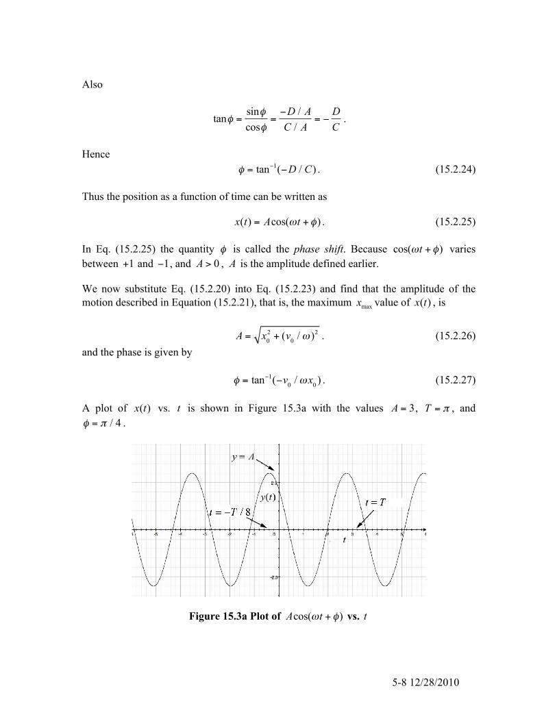
2 + (v0 /! )2 . (15.2.26) and the phase is given by ! = tan"1("v0 /#x0 ) . (15.2.27) A plot of ( )x t vs. t is shown in Figure 15.3a with the values A = 3, T = ! , and

! = " / 4 .

Figure 15.3a Plot of Acos(!t + ") vs. t

5-9 12/28/2010

Note that x(t) = Acos(!t + ") takes on its maximum value when cos(!t + ") = 1. This occurs when !t + " = 2#n where n = 0, ±1, ± 2,! ! ! . The maximum value associated with n = 0 occurs when !t + " = 0 or t = !" /# . For the case shown in Figure 15.3a when

! = " / 4 , this occurs at the instant t = !T / 8 .

Figure 15.4(i)

Figure 15.4(ii)

Figure 15.4(iii)

Let’s plot x(t) = Acos(!t + ") vs. t for ! = 0 (Figure 15.4(ii)). For ! > 0 , Figure 15.4(i) shows the plot x(t) = Acos(!t + ") vs. t . Notice that x(t) is shifted to the left compared with the case ! = 0 (compare Figures 5.4(i) with 5.4(ii)). The function

x(t) = Acos(!t + ") with ! > 0 reaches it’s a maximum value at an earlier time than the function x(t) = Acos(!t) . Hence the origin of the term phase shift. When ! < 0 , the

5-10 12/28/2010

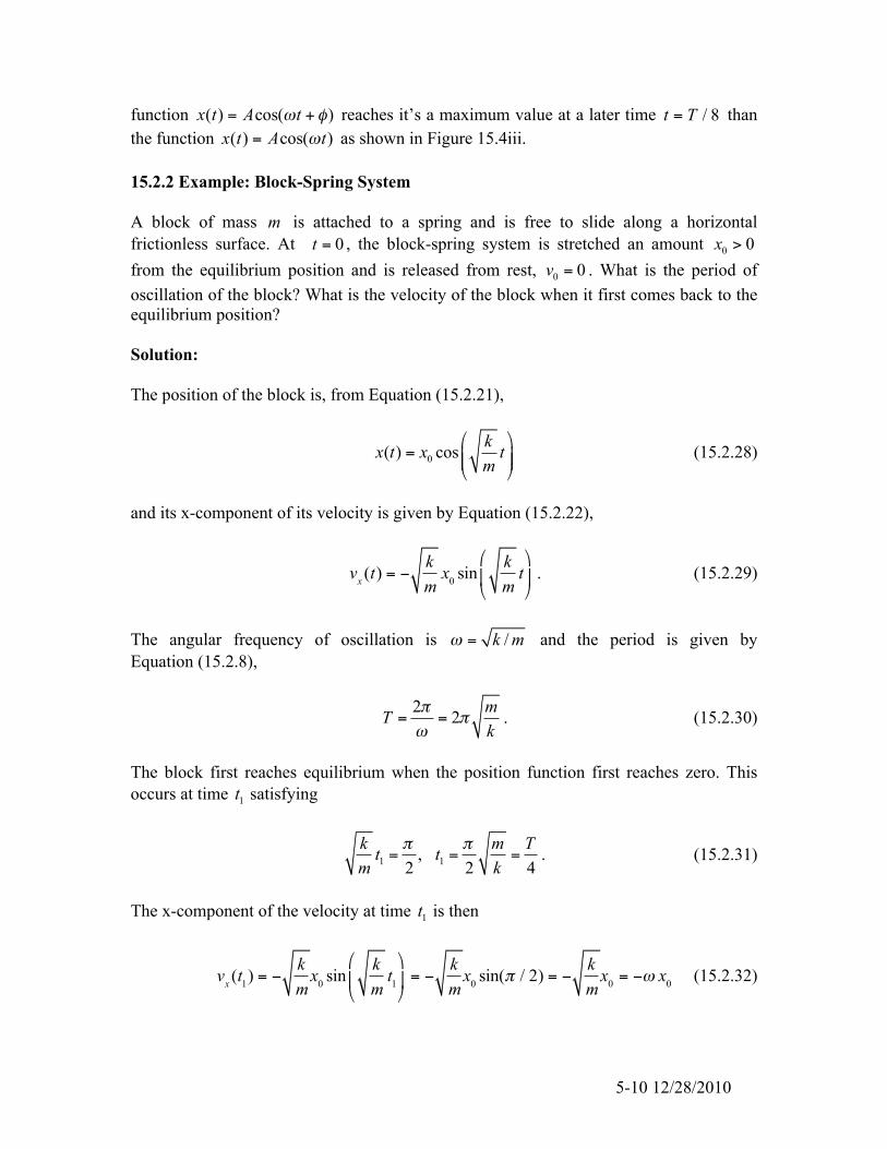
function x(t) = Acos(!t + ") reaches it’s a maximum value at a later time t = T / 8 than the function x(t) = Acos(!t) as shown in Figure 15.4iii. 15.2.2 Example: Block-Spring System A block of mass m is attached to a spring and is free to slide along a horizontal frictionless surface. At 0t = , the block-spring system is stretched an amount 0 0x > from the equilibrium position and is released from rest, 0 0v = . What is the period of oscillation of the block? What is the velocity of the block when it first comes back to the equilibrium position? Solution: The position of the block is, from Equation (15.2.21),

0( ) cosk

x t x tm

! "= # $# $

% & (15.2.28)

and its x-component of its velocity is given by Equation (15.2.22),

vx (t) = !

km

x0 sinkm

t"

#$

%

&' . (15.2.29)

The angular frequency of oscillation is /k m! = and the period is given by Equation (15.2.8),

2 2 mTk

!!

"= = . (15.2.30)

The block first reaches equilibrium when the position function first reaches zero. This occurs at time 1t satisfying

1 1,2 2 4

k m Tt tm k

! != = = . (15.2.31)

The x-component of the velocity at time 1t is then

vx (t1) = !

km

x0 sinkm

t1"

#$

%

&' = !

km

x0 sin(( / 2) = !km

x0 = !) x0 (15.2.32)

5-11 12/28/2010

Note that the block is moving in the negative x -direction at time 1t ; the block has moved from a positive initial position to the equilibrium position. 15.3 Energy and the Simple Harmonic Oscillator Let’s consider the block-spring system of Example 5.2.1 in which the block is initially stretched an amount 0 0x > from the equilibrium position and is released from rest,

0 0v = . We shall consider three states: State 1, the initial state; State 2, the state at an arbitrary time in which the position and velocity are non-zero; and State 3, the state when the object first comes back to the equilibrium position. We shall show that the position and velocity functions for the object-spring give a constant mechanical energy. Choose the equilibrium position for the zero point of the potential energy. State 1: All the energy is stored in the object-spring potential energy: 2

1 0(1/ 2)U k x= . The object is released from rest so the kinetic energy is zero, 1 0K = . The total mechanical energy is then

21 1 0

12

E U k x= = . (15.3.1)

State 2: At some time t , the position and x-component of the velocity of the object are given by

x(t) = x0 coskm

t!

"#

$

%&

vx (t) = 'km

x0 sinkm

t!

"#

$

%& .

(15.3.2)

The kinetic energy is

2 2 22 01 1 sin2 2

kK mv k x t

m! "

= = # $# $% &

. (15.3.3)

and the potential energy is

2 2 22 01 1

cos2 2

kU k x k x t

m! "

= = # $# $% &

. (15.3.4)

The total mechanical energy is the sum of the kinetic and potential energies

5-12 12/28/2010

2 22 2 2

2 2 20

20

1 12 2

1cos sin

2

1.

2

E K U mv k x

k kk x t t

m m

k x

= + = +

! "! " ! "= +# $# $ # $# $ # $# $% & % &% &

=

(15.3.5)

The total mechanical energy is equal to the initial potential energy in State 1, so the total mechanical energy is constant. This should come as no surprise; we isolated the object-spring system so that there is no external work performed on the system. State 3: Now the object is at the equilibrium position so the potential energy is zero, 3 0U = , and all the mechanical energy is in the form of kinetic energy (Figure 15.5).

23 3 eq

12

E K mv= = . (15.3.6)

Figure 15.5 State 3: at equilibrium and in motion Since the system is isolated, mechanical energy is constant, 1 2 3E E E= = . (15.3.7) Therefore the initial stored potential energy is released as kinetic energy,

2 20 eq

1 12 2k x mv= , (15.3.8)

and the x -component of velocity at the equilibrium position is given by

vx,eq = ±

km

x0 . (15.3.9)

5-13 12/28/2010

Note that the plus-minus sign indicates that when the block is at equilibrium, there are two possible motions: in the positive x -direction or the negative x -direction. If we take 0 0x > , then the block starts moving towards the origin, and

vx,eq will be negative the first

time the block moves through the equilibrium position. In hindsight, we could have used the result of the analysis of Stage 2, Equation (15.3.2), with Stages 1 and 3 as special cases, 0t = for Stage 1 and / 4 / / 2t T m k!= = from Equation (15.2.31) for Stage 3. Example 15.3.1: A simple pendulum consists of a massless string of length l and a point-like object of mass m attached to one end. Suppose the string is fixed at the other end and is initially pulled out at a small angle !0 from the vertical and released from rest.

a) Using the small angle approximation sin!0 " !0 and either energy techniques or Newton’s Second Law, show that the angle the object makes with the vertical satisfies a simple harmonic oscillator differential equation.

b) How long (period) will the pendulum take to return to its initial position?

c) What is the frequency and angular frequency of oscillation?

d) What is the speed of the object at the bottom of its swing?

e) What is the angular velocity of the object at the bottom of its swing?

f) Is the angular velocity the same as the angular frequency for the pendulum? Why

or why not?

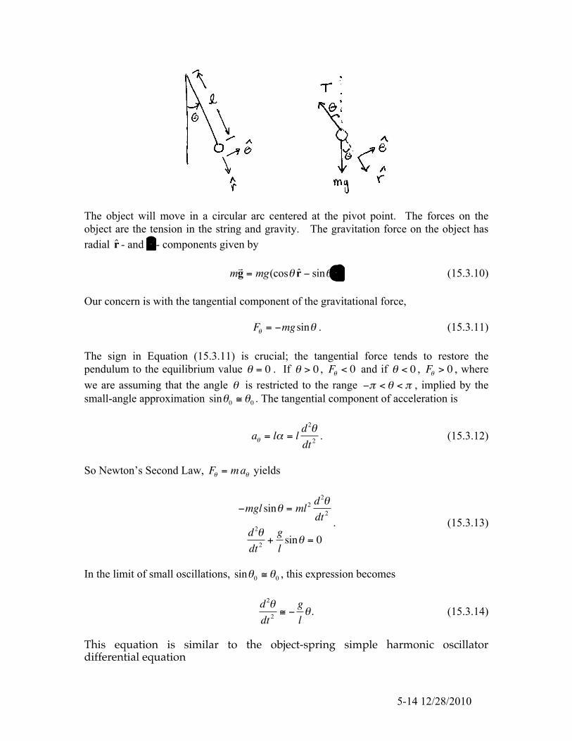
g) Why or why not does the period depend on the mass of the object? Solution: A pendulum consists of an object hanging from the end of a string or rigid rod pivoted about the pointS . The object is pulled to one side and allowed to oscillate. If the object has negligible size and the string or rod is massless, then the pendulum is called a simple pendulum. Let’s choose polar coordinates for the pendulum as shown in the figure below (left) along with the free body force diagram for the suspended object (right).

5-14 12/28/2010

The object will move in a circular arc centered at the pivot point. The forces on the object are the tension in the string and gravity. The gravitation force on the object has radial r̂ - and !̂ - components given by m

!g = mg(cos! r̂ " sin! !̂) (15.3.10) Our concern is with the tangential component of the gravitational force, F! = "mgsin! . (15.3.11) The sign in Equation (15.3.11) is crucial; the tangential force tends to restore the pendulum to the equilibrium value ! = 0 . If ! > 0 , F! < 0 and if ! < 0 , F! > 0 , where we are assuming that the angle ! is restricted to the range !" < # < " , implied by the small-angle approximation sin!0 " !0 . The tangential component of acceleration is

a! = l" = l d2!dt 2

. (15.3.12)

So Newton’s Second Law, F! = ma! yields

!mgl sin" = ml2 d

2"dt 2

d 2"dt 2

+glsin" = 0

. (15.3.13)

In the limit of small oscillations, sin!0 " !0 , this expression becomes

d 2!dt 2

" #gl!. (15.3.14)

This equation is similar to the object-spring simple harmonic oscillator differential equation

5-15 12/28/2010

d 2xdt 2

= !kmx , (15.3.15)

which describes the oscillation of a mass about the equilibrium point of a spring. The angular frequency of oscillation (denoted !0 to distinguish from the angular velocity ! = d" / dt ) is given by

!0 =km

. (15.3.16)

By comparison, the frequency of oscillation for the pendulum is approximately

!0 "gl

, (15.3.17)

with period

T =2!"0

# 2! lg

. (15.3.18)

The solutions to (15.3.14) are well-known. With the initial condition that the pendulum is released from rest at a small angle !0 , the angle the string makes with the vertical is given

!(t) = !0 cos "0 t( ) = !0 cos2#Tt$

%&'()= !0 cos

glt

$

%&'

(). (15.3.19)

The component of the angular velocity of the bob is

d!dt(t) = " g

l!0 sin

glt

#

$%&

'(. (15.3.20)

Keep in mind that the component of the angular velocity ! = d" / dt is a kinematic variable that changes with time in an oscillatory manner (sinusoidally in the limit of small oscillations). The angular frequency !0 is a parameter that describes the system. The component of the angular velocity ! , besides being time-dependent, depends on the amplitude of oscillation !0 . In the limit of small oscillations, !0 does not depend on the amplitude of oscillation. The fact that the period is independent of the mass of the object follows algebraically from the fact that the mass appears on both sides of Newton’s Second Law and hence

5-16 12/28/2010

cancels. Consider also the argument that is attributed to Galileo: If a pendulum consisting of two identical masses joined together were set to oscillate, the two halve would not exert forces on each other. So, if the pendulum were split into two pieces, the pieces would oscillate the same as if they were one piece. This argument can be extended to simple pendula of arbitrary masses. Energy Approach: We can use energy methods to find the differential equation describing the time evolution of the angle ! . When the string is at an angle ! with respect to the vertical, the gravitational potential energy (relative to a choice of zero potential energy at the bottom of the swing where ! = 0 ) is given by U = mgl 1! cos"( ) (15.3.21)

The component of the velocity of the object is given by v! = l(d! / dt) so the kinetic energy is

K =12mv!

2 =12m l d!

dt"#$

%&'

2

. (15.3.22)

The energy of the system is then

E = K +U =12m l d!

dt"#$

%&'

2

+ mgl 1( cos!( ) (15.3.23)

Since there is no non-conservative work, the energy is constant hence

0 = dE

dt=12m2l2 d!

dtd 2!dt 2

+ mgl sin! d!dt

= ml2 d!dt

d 2!dt 2

+glsin!

"

#$%

&'

. (15.3.24)

There are two solutions to this equation, the first one d! / dt = 0 is the equilibrium solution, the angular speed is zero means the suspended object is not moving. The second solution is the one we are interested in

5-17 12/28/2010

d 2!dt 2

+glsin! = 0 (15.3.25)

which is the same differential equation we found using the force method. We can find the time t1 that the object first reaches the bottom of the circular arc by setting !( t1) = 0 in Eq. (15.3.19)

0 = !0 cosglt1

"

#$%

&'. (15.3.26)

This zero occurs when the argument of the cosine satisfies

glt1 =

!2

. (15.3.27)

The component of the angular velocity at time t1 is therefore

d!dt(t1) = "

gl!0 sin

glt1

#

$%&

'(= "

gl!0 sin

)2

#$%

&'(= "

gl!0 . (15.3.28)

Note that the negative sign means that the bob is moving in the negative !̂ direction when it first reaches the bottom of the arc. The component of the velocity at time t1 is therefore

v! (t1) " v1 = ld!dt(t1) = #l

gl!0 sin

glt1

$

%&'

()= # lg!0 sin

*2

$%&

'()= # lg!0 . (15.3.29)

We can also find the component of both the velocity and angular velocity using energy methods. When we release the bob from rest, the energy is only potential energy

E =U0 = mgl 1! cos"0( ) # mgl"02

2 (15.3.30)

where we used the approximation that 20

0cos 12!

! " # . When the bob is at the bottom of

the arc, the only contribution to the energy is the kinetic energy given by

5-18 12/28/2010

K1 =12mv1

2 . (15.3.31)

Since the energy is constant, we have that U0 = K1 or

mgl!02

2=12mv1

2 . (15.3.32)

We can solve for the component of the velocity at the bottom of the arc v1 = ± gl !0 (15.3.33) noting that the two possible solutions correspond to the different directions that the bob can have when at the bottom. The component of the angular velocity is then

d!dt(t1) =

v1l= ±

gl!0 (15.3.34)

in agreement with our previous calculation. If we do not make the small angle approximation, we can still use energy techniques to find the component of the velocity at the bottom of the arc by equating the energies at the two positions

mgl 1! cos"0( ) = 12mv1

2 (15.3.35)

Hence v1 = ± 2gl 1! cos"0( ) . (15.3.36) Chapter 15 Appendix: Solution to Simple Harmonic Oscillator Equation In our analysis of the solution of the simple harmonic oscillator equation of motion, Equation (15.2.1),

2

2

d xk x m

dt! = , (15.A.1)

we assumed that the solution was a linear combination of sinusoidal functions,

5-19 12/28/2010

( ) cos( ) sin( )x t A t B t! != + , (15.A.2) where /k m! = . We shall now begin with the condition that the mechanical energy of a closed system is constant (see Section 15.3) and, after integration, determine the position of the oscillating body as a function of time. Assume that the mechanical energy of the block-spring system is given by the constant E . Choose the reference point for potential energy to be the unstretched position of the spring. Let x denote the amount the spring has been compressed ( 0x < ) or stretched ( 0x > ) from equilibrium at time t and denote the amount the spring has been compressed or stretched from equilibrium at time 0t = by 0( 0)x t x= ! . Let /v dx dt= denote the x -component of the velocity at time t and denote the x -component of the velocity at time 0t = by 0( 0)v t v= ! . The constancy of the mechanical energy is then expressed as

2 21 12 2

E K U k x mv= + = + . (15.A.3)

We can solve Equation (15.A.3) for square of the x -component of the velocity,

2 2 22 2 12

E k E kv x x

m m m E! "= # = #$ %& '

. (15.A.4)

Taking square roots, we have

22 12

dx E kx

dt m E= ! (15.A.5)

(why we take the positive square root will be explained below). Let 2 /a E m! and / 2b k E! . It’s worth noting that a has dimensions of velocity and b has dimensions of [length]!2 . Equation (15.A.5) is separable;

2

2

1

.1

dxa b x

dtdx

adtb x

= !

=!

(15.A.6)

5-20 12/28/2010

The integral on the left in the last expression in Equation (15.A.6) is well known, and the standard derivation is presented here. We make a change of variables cos! = b x with the differentials d! and dx related

by ! sin" d" = b dx . The integration variable is

! = cos"1( b x) . (15.A.7) Equation (15.A.6) then becomes

! sin" d"

1!cos2"= ba dt . (15.A.8)

This is a good point at which to check the dimensions. The term on the left in Equation (15.A.8) is dimensionless, and the product ba on the right has dimensions of inverse time, [length]!1[length " time!1] = [time!1] , so ba dt is dimensionless. Using the trigonometric identity 21 sin cos! !" = , Equation (15.A.8) reduces to d! = " ba dt . (15.A.9) Although at this point in this derivation we don’t know that ba , which has dimensions of frequency, is the angular frequency of oscillation, we’ll use some foresight and make the identification;

22k E kbaE m m

! " = = , (15.A.10)

and Equation (15.A.9) becomes d! = "# dt . (15.A.11) After integration we have ! "!0 = "# t , (15.A.12) where !0 " #$ is the constant of integration. Since ! = cos"1( b x(t)) , Equation (15.A.12) becomes

5-21 12/28/2010

cos!1( b x(t)) = !(" t + #) . (15.A.13) Take the cosine of each side of Equation (15.A.13), yielding

x(t) =

1

bcos(!(" t + #)) =

2Ek

cos(" t + #) . (15.A.14)

At 0t = ,

x0 ! x(t = 0) =

2Ek

cos" . (15.A.15)

The x-component of the velocity as a function of time is then

vx (t) =

dx(t)dt

= !"2Ek

sin(" t + #) . (15.A.16)

At 0t = ,

v0 ! vx (t = 0) = "#

2Ek

sin$ . (15.A.17)

We can determine the constant ! by dividing the expressions in Equations (15.A.17) and (15.A.15),

!

v0

"x0

= tan# (15.A.18)

Thus the constant ! can be determined by the initial conditions and the angular frequency of oscillation,

! = tan"1 "

v0

#x0

$

%&

'

() . (15.A.19)

Using the identity cos(!t + ") = cos!t cos" # sin!t sin" (15.A.20) to expand Equation (15.A.14) yields

5-22 12/28/2010

x(t) =

2Ek

cos!t cos" =2Ek

sin!t sin" , (15.A.21)

and substituting Equations (15.A.15) and (15.A.17)

00( ) cos sin

vx t x t t! !

!= + , (15.A.22)

agreeing with the solution found in Section 15.2 Note that the energy at time t is given by

2 21 1( )2 2

E t mv k x= + . (15.A.23)

Substitution of Equations (15.A.16) and (15.A.14) into Equation (15.A.23) yields

2 2 21 2 1 2( ) cos ( ) sin ( )

2 2E EE t m t k tk k

! ! " ! "= + + + . (15.A.24)

Since 2 /k m! = , Equation (15.A.24) simplifies to 2 2( ) (cos ( ) sin ( ))E t E t t E! " ! "= + + + = , (15.A.25) illustrating that the mechanical energy is constant in time. So, what about the missing ± that should have been in Equation (15.A.5)? Strictly speaking, we would need to redo the derivation for the block moving in different directions. Mathematically, this would mean replacing ! by ! "# (or ! "# ) when the block’s velocity changes direction. Changing from the positive square root to the negative and changing ! to ! "# has the collective action of reproducing Equation (15.A.22).

5-23 12/28/2010

MIT OpenCourseWare http://ocw.mit.edu 8.01SC Physics I: Classical Mechanics For information about citing these materials or our Terms of Use, visit: http://ocw.mit.edu/terms.