Coupling Thin Interrupts - IBM · 2019-12-16 · Coupling thin interrupts can also be enabled in...

Coupling Thin Interrupts and CF Performance in Shared Processor Environments

Coupling Thin Interrupts

and

Coupling Facility Performance

in Shared Processor Environments

Barbara Weiler

© Copyright IBM Corporation, 2013 of 37


PrefaceDisclaimerThe performance statements made represent IBM’s assessment of the environments described with the specific workloads and system control programs specified. Results are based on measurements and analysis. Many factors, including but not limited to the following, may result in the variances between the results provided herein and actual operating environments:

• Differences between the specified workload characteristics and your operating environment

• Differences between the specified system levels and your actual system levels

• I/O or other constraints in your environment • Incorrect assumptions in the analysis • Unknown hardware defects in processors used for measurement • Inaccurate vendor claims.

IBM does not guarantee that your results will correspond to those provided herein. This information is provided “as is”, without warranty, express or implied.

AcknowledgementsMany thanks to H. Kumar Chintapalli for creating all the configurations and collecting the vast majority of data required for this study. Thanks also to Alexandra Scolaro and Joe Fontana for helping to complete the many measurements required. Special thanks as well to David Surman, Gary King and Steve Goss as key reviewers of this paper.

RemindersNeither this document nor any part of it may be copied or reproduced in any form or by any means or translated into another language, without the prior consent of the IBM Corporation. IBM assumes no responsibility for any errors that may appear in this document. The information contained in this document is subject to change without any notice. IBM reserves the right to make any such changes without obligation to notify any person of such revision or changes. IBM makes no commitment to keep the information contained herein up to date.



TrademarksIBM, the IBM logo, and ibm.com® are trademarks or registered trademarks of International Business Machines Corporation in the United States, other countries, or both. If these and other IBM trademarked terms are marked on their first occurrence in this information with a trademark symbol (® or ™), these symbols indicate US registered or common law trademarks owned by IBM at the time this information was published. Such trademarks may also be registered or common law trademarks in other countries. A current list of IBM trademarks is available on the web at “Copyright and trademark information” at www.ibm.com/legal/us/en/copytrade.shtml.

FeedbackPlease send comments, questions or suggestions for changes to Barbara Weiler at the following email at [email protected] .

© Copyright International Business Machines Corporation 2013. All rights reserved. Note to U.S. Government Users—Documentation related to restricted rights—Use, duplication or disclosure is subject to restrictions set forth in GSA ADP Schedule contract with IBM Corp.


mailto:[email protected]

http://www.ibm.com/legal/us/en/copytrade.shtml


Introduction

The question of whether or not Coupling Facility (CF) processors could perform reasonably well in a shared processor environment is a question that has been asked since the introduction of the CF technology in the early 1990’s. Given the polling nature of Coupling Facility Control Code (CFCC), the CF firmware, it has been difficult to achieve success in this area. Along the way there have been attempts to improve the performance of coupling facilities in shared processor environments, specifically the invention of Dynamic CF Dispatching (DYNDISP).How the various sharing protocols, including the new Coupling Thin Interrupts introduced with CF Level 19 supported on zEC12 and zBC12, perform will be examined in this paper. By comparing the performance of these shared CF processor options it will be evident that the use of coupling thin interrupts in the CF provides significant improvement in CF shared processor environments. This improvement will be evident in environments that are already using shared CF processors and will expand the number of environments in which shared CF processors are viable.Coupling thin interrupts can also be enabled in z/OS. While this is a separate and distinct use of coupling thin interrupts from what will be discussed in this paper, it is beneficial in reducing the back-end polling latency which is part of asynchronous CF request activity as well as CF messaging and notification activity. This function is enabled by default with z/OS V2R1 and is defaulted on with APAR OA38781 for IOS and OA38734 for XES for z/OS V1R12 and V1R13 and is only available on zEC12, zBC12 and future platforms. It is highly recommended that this function be enabled for z/OS whether the CF processors are dedicated or shared in order to take advantage of the asynchronous service time and messaging/notification benefits it provides. This benefit will not be discussed in this paper.While the use of coupling thin interrupts in the CF provides a significant performance improvement in shared processor CF environments, using dedicated CF processors is still recommended for performance-critical production environments.



Environment

There are a number of environments in which shared processor CFs are desirable. For example, environments in which multiple CFs, each of which do not require sufficient capacity to require a dedicated processor, would benefit from shared CF processors. This is especially true with the very large processors in use today. In addition, with the larger capacity processors available, this desire might extend to configurations with larger CF requirements.The following scenarios were based on a number of environments in which customers are already sharing CF processors. The scenarios cover the sharing of test and production type environments as well as multiple production environments that share CF processors. The designation of test and production is made with respect to the amount of activity these types of environments require as well as the relative need for good, or reasonable, performance. For example, while both the production and test environments in the following experiments will do the same kind of work, the amount of work in the production environment will be significantly greater than that of an environment designated as test.The purpose of the experiments is to provide some insight as to the behavior and performance provided by coupling thin interrupts in the CF, using DYNDISP=THINinterrupts (abbreviated to THIN), and compare those results with the previously available CF sharing protocols, namely DYNDISP=OFF and DYNDISP=ON. While it is possible to use general purpose processors, CPs, as CF processors and share the CPs with z/OS and other similarly defined CFs, this is not a recommended configuration. Using CPs as CF processors creates interaction between z/OS and the CF in terms of cache reuse and other factors that may impact performance. Most customers would not use CPs as CF processors since there are financial implications that would favor the use of ICF processors. As such, this type of configuration is not considered in this paper and the CF processors in use are all ICFs. The majority of the scenarios presented were run in Simplex mode although there were a small number of configurations involving System Managed CF Structure Duplexing. None of the scenarios used User Managed Duplexing since its behavior is essentially Simplex in nature and thus adequately represented by the Simplex tests. As in any environment where resources are shared, it is critical that all participants in the sharing are evaluated. That is, the performance of any one of the sharers is dependent on what its sharing partners are doing. This may become rather complicated as a result of having many images sharing a physical



resource such as CF processors. The number of sharers in the scenarios tested was kept to a reasonable number in order to show the impacts of sharing without becoming overwhelming.The results contained in this document were obtained in a controlled environment in order to be able to make the desired comparisons. Attempts were made to ensure that the workload was stable across all the measurements. Note that due to differences in configuration, hardware or software, these results may not be achievable in other environments.

Sharing Options

There are many things to consider when evaluating performance in a shared environment. For example, all of the systems that will be sharing the processing resource must be understood in terms of their requirements and desired outcomes. It is not the purpose of this paper to describe how to set up the shared environment. Please refer to the “zEnterprise System Processor Resource/Systems Manager Planning Guide”1 for details on how to determine the weights and other system concepts related to sharing. The guide can be found via IBM Resource Link at https://www.ibm.com/servers/resourcelink/svc03100.nsf?OpenDatabase

There are now three CF processor sharing options available with the introduction of CFLEVEL 19. These options are all defined via the DYNDISP keyword in the CF. The choices are OFF, ON and THIN. Illustration 1 attempts to provide a visual representation of the different options. Assume that there are two CFs sharing a single processor and that the DYNDISP option is set the same in both CFs. Using the same option for all CFs involved in the sharing is done for the purpose of the illustration and there is no restriction that the same option be used for all CFs involved in sharing a particular processor resource. Further assume that CF2 has twice the CF request rate of CF1 and is defined with twice the weight of CF1.


https://www.ibm.com/servers/resourcelink/svc03100.nsf?OpenDatabase


Assume a single ICF with 2 CFs sharing the processor resource with CF2 having twice the request rate

DYNDISP=OFFin both CFs

CF1CF2

DYNDISP=ON in both CFs

CF1CF2

DYNDISP=THIN in both CFs

CF1CF2

Time slice end

Time slice end

Time slice end

CF goes to sleep

CF goes to sleep

Gives up processor

Gives up processor

Waking up

Waking up

Interrupt

Illustration 1: CF Sharing Options

With DYNDISP=OFF each CF will run until the end of its time slice, or the time allowed for it to be dispatched according to the PR/SM rules. This is similar to how the CF functions with dedicated processors in that it is polling for new work whenever it is not executing commands. For illustrative purposes CF2 is shown getting 2 back-to-back time slices. In actuality PR/SM will dispatch the CFs according to a dispatching priority scheme that includes whether or not the image is ready to be dispatched, whether it is in using its fair share of the CF processor, and other more complicated factors. In a sharing environment, the CF will be forced at some point to give up control of the processors it is using in order for the sharing to occur. Thus, there is a possibility that resources for processing a command, such as latches or other serializing entities, will be held over the period when others are using the processors. Since the command is “in progress” while the processor is in use by another sharer, the CF service times for commands will be elongated. And, given the dispatching priorities could be quite variable. In fact, you will notice both service times and standard deviations can be very high when sharing processors with DYNDISP=OFF.



The second option is DYNDISP=ON. With this option the CF will voluntarily sleep when it does not have work to do. This will allow the other sharers an opportunity to continue their processing. Any CF sharing with this option will adjust the amount of time it waits after it has nothing to do and the amount of time it sleeps based on the amount of requests it receives. The CF will get a timer interrupt once the sleep time has expired. It will then start looking for work and the process will start over again. Thus, as the request rate increases the behavior will approach that of having DYNDISP=OFF in that the CF will sleep less and less as the request rate rises. The action of voluntarily sleeping when there is no work to do makes this a more efficient option than DYNDISP=OFF when sharing processor resources but its efficiency is highly variable based on the algorithms used by the CF to determine when to sleep and wake. In the illustration the various lengths of dispatched time are an attempt to show some variation in the dispatch and sleeping intervals. With this case, however, the time a command may need to wait is more in line with the amount of work it might need to do such that the more work the shorter time to wait for service assuming its time slice is not up.The third, and newest, option is DYNDISP=THIN. This option is loosely based on the same principles as DYNDISP=ON. However, the difference is that the CF does not sleep for a specified period of time. Here, the CF will almost immediately give up the processor as soon as it has no work to do and become eligible for dispatching once an interrupt is received indicating that it has work to do. The benefit of this over the DYNDISP=ON option is that there is no guess work involved about when the next request will arrive, or how long to sleep, since the interrupt will alert the CF of the arrival of a command to process. Since the time the CF might not be dispatched when a request arrives is virtually eliminated by the use of the interrupt, the CF service times are improved and generally less variable. Since this option is more aggressive about giving up use of the processor when it does not have work to do, it allows for a more efficient sharing of the processor among the multiple CF images. Illustration 1 shows that for DYNDISP=THIN the interrupt may appear at varying intervals and the assumption is made that once the interrupt is received that CF is next in line for dispatching according to the PR/SM dispatching priority. The quicker release of the processor and the faster dispatch by using coupling thin interrupts makes this option much more efficient than the other sharing options.The dotted lines in Illustration 1 are intended to provide a view of the amount of time from a point where a CF request is presented, the dotted line, to the point where it is able to be executed, the next block of that particular color. The key item to note is that in each of the sharing options that is some lag between when the request is presented and when it is executed, however with the introduction of coupling thin interrupts this lag is greatly reduced and is less variable.

Logical Configuration



Figure 1 illustrates the general logical layout of the configurations used in this study. Additional details will be provided as each scenario is discussed. Each z/OS partition will send requests to a CF that has either dedicated or shared ICF processors.

Hardware and Software

The experiments were conducted on a zEnterprise EC12 (zEC12) H43. Logical configurations consisted of multiple z/OS images, each running z/OS V1.13, coupled via HCAO3 12x IFB3 connections to multiple Coupling Facilities, each running CFCC Service Level 19, on the same Central Processing Complex (CPC). Refer to Figure 1. While this violates best practices for placement of images with respect to hardware single point of failure and/or lack of failure isolation between z/OS and CF images, the use of external coupling links mimics the behavior of having multiple physical boxes while requiring minimal hardware for performance testing.

Workload


z/OS z/OS z/OS

CFCFCF

Figure 1: Logical Configuration


Each of the z/OS images is running our ACME workload. This workload is designed to send command requests to the CF in a way which mimics the major subsystem exploiters including IMS, DB2, and MQ. Each of the request types is given equal weight in the workload. That is, there is no attempt made to proportion the requests to resemble any particular customer workload. ACME uses twenty CF structures with various characteristics. The twenty structures are:

1 CQS-like LIST structure 1 VTAM-like LIST structure 1 MQ Admin-like LIST structure 5 MQ Application-like LIST structures 1 DB2-like LOCK structure 1 IMS batch-like LOCK structure 1 GRS-like LOCK structure 2 IMS-like CACHE structures 5 DB2-like CACHE structures 2 Logging-like LIST structures

In addition to these structures the necessary resource sharing structures such as XCF signaling structures, GRS lock structure, etc. are included. Although there is a single z/OS image for each CF, there are multiple connectors to each of the CF structures defined.



Results

The following results represent the experiences during very specific tests in a controlled environment. These results may be different than those experienced in other environments due to differences in workload characteristics, configuration and software levels. No guarantee, implied or explicit, is being made that these experiences will be realized in other environments.

In general the results will be presented using various production, indicated by a P in the various charts, and test, indicated by a T, CF partitions. When there are multiple CFs of the same type, P or T, there will be a number following the letter.

Synchronous service time, CF utilization, and throughput are all important indicators of how the CF is performing and relate directly to the cost associated with running the sysplex. Thus, the results of the various scenarios will be presented in terms of these values. On occasion other indicators such as standard deviation may be presented.

CF Utilization and Effective Processors

Whenever shared processors are in use the notion of effective capacity becomes more important. The Coupling Facility Usage Summary report of the “z/OS Resource Management Facility”2 (RMF) will display the number of CF processors defined as well as the effective number of CF processors used. It will also indicate the number of shared processors and the respective weight. In the same part of the report the CF will provide a utilization value. These values will change with the respective sharing options.

In addition, there is also a PR/SM view of the CFs’ use of the processors. The Partition Data Report in RMF provides this view. This view also changes with respect to the options for the sharing processors.



Coupling Facility Usage Summary Partition Data Report - Average Processor UtilizationDYNDISP CF Utilization Defined Effective Shared Weight LPAR MGMT Effective TOTAL Sum of TOTALs

CF1 OFF 16.2 1 0.1 1 10 0.00 12.50 12.5 100CF2 OFF 33.0 1 0.9 1 90 0.01 87.44 87.45

Physical 0.05 0.05CF1 ON 26.1 1 0.1 1 10 0.00 10.17 10.18 100CF2 OFF 32.9 1 0.9 1 90 0.01 89.72 89.74

Physical 0.08 0.08CF1 THIN 61.3 1 0.1 1 10 0.15 8.60 8.75 99.94CF2 OFF 33.0 1 0.9 1 90 0.10 90.06 90.17

Physical 1.02 1.02CF1 THIN 74.3 1 0.1 1 10 0.43 15.01 15.44 80.90CF2 THIN 57.1 1 0.5 1 90 1.15 57.98 59.13

Physical 6.33 6.33Table 1: Effective and Utilization Differences

Table 1 illustrates these differences. In each case shown in Table 1 there is one ICF processor being shared by the 2 CFs. CF1 is given a weight of 10 while CF2 is given a weight of 90. There is a specific amount of work that is asked of each of the CFs and the amount is the same in each case.

Comparing the cases in order from the top of the table down, note that the CF Utilization from the Coupling Facility Usage Summary portion of the table for CF 2 is consistent when DYNDISP=OFF while the same value for CF1 grows as the DYNDISP options vary. This implies that CF1 is able to accomplish more of what it is asked to do as the DYNDISP option is changed from OFF to ON and then to THIN (TI) and is at its peak when both CFs have the DYNDISP=THIN option in effect. Note that once both CFs are using DYNDISP=THIN that CF2 is now using substantially less effective processors for roughly the same amount of work. This can be determined by multiplying the CF utilization by the number of effective processors. It is important to note that this more effective use of the processors by CF2 allows CF1 to complete more work. This is evident by the increase in the CF utilization while the number of effective engines remains at .1, or 10% of the available resource per its weight.

Now, look to the right side of the table which shows the values from the Partition Data Report of RMF. With DYNDISP=OFF for both CFs the view from PR/SM is that the CF is 100% utilized. And, you can see the roughly 10% for CF1 and 90% for CF2 split with little LPAR management time. The use of 100% of the available processors is due to the polling nature of the CF. This holds true as you move down the table and introduce DYNDISP=ON for CF1 although the amount utilized by the CFs is closer to the values indicated by their weights. There is also a tiny bit more in the way of LPAR management. Continuing down the table and introducing DYNDISP=THIN for CF1 you will see that the sum of the CF totals, while close, is no longer at the 100% mark. That is due to the efficiencies noted for the use of coupling thin interrupts. Also note that the LPAR management time is higher due to its involvement in the presentation of the interrupts to the CF and the more frequent dispatching involved. This is certainly made more clear when examining the impact when both CFs have



DYNDISP=THIN in use. Here, you can see that while the LPAR management time is not relatively high that the sum of the totals is now significantly less than 100% seen with the previous sharing options. In fact, this would indicate that there is still about 20% of the resource that is not in use.

For additional information regarding the various reports please refer to the “z/OS Resource Management Facility Report Analysis” available at http://publibz.boulder.ibm.com/epubs/pdf/erbzrab0.pdf

Sharing between Production and Test CFs

The first scenario examined is one in which a production sysplex and a test sysplex are sharing the CF processors. The CF processors used in these experiments were Internal Coupling Facility processors, or ICFs. While it is possible to use CPs, general purpose processors, for a CF there are performance and cost advantages to using ICFs. All the experiments for this paper were done using ICFs.

This scenario consisted of running the ACME workload in both the production and test CFs. The definition of the production CF was that it would run with a constant workload at a request rate equivalent to what was determined to drive a single dedicated CF processor to 30% CF utilization. The test CF was defined to also run the ACME workload but here the request rate would vary from a very small rate to one where the system constraints, such as subchannel delay, would begin to be out of the recommended range. The purpose of this was to think of the production environment as a constant entity and to vary the rate on the test CF to determine the impact it might have on the production environment. The production CF was given a weight of 90 so as to ensure that it would have all the processing capacity it required. The weight of the test CF was 10. The same configuration and definition for the two CFs was used for the various sharing options.

In this environment it would be assumed that the production CF, in addition to being the more active CF, would also be more important. That is, it is desirable for the service times to the production CF to remain consistently “good” regardless of what happens in the test CF. For this experiment the CFs are sharing 1 physical ICF processor. While a minimum of 2 processors is recommended for reliability, a single processor is used here to simplify the test environment and aid in the understanding of what is happening in the CF images participating in the sharing.

Figure 2 shows the production CF Synchronous Service Times as a function of the Test Request Rate. The results are presented in this manner to visualize the impact the test CF has on the service times of the production CF. The Dedicated curve is the result of varying the request rate using the ACME workload in a


http://publibz.boulder.ibm.com/epubs/pdf/erbzrab0.pdf


configuration in which the CF had a single dedicated processor and is added for reference. This curve illustrates the “best can do” service time.

In the charts for all of the tests the production CF will be noted by the P in the legend followed by a number representing the weight given to the partition. The second designation in the legend will be OFF, ON, or TI indicating DYNDISP=OFF, DYNDISP=ON, or DYNDISP= THIN respectively. Note that both sharing images need not have the same DYNDISP setting.

Production/Test Scenario

05

1015

2025

30

0 10000 20000 30000 40000 50000

Test Request Rate

Prod

uctio

n Sy

nchr

onou

s Se

rvic

e Ti

me

Dedicated P90 OFF, T10 OFF P90 OFF, T10 ON

P90 TI, T10 TI P90 OFF, T10 TI

Figure 2: Production/Test Scenario - Production CF Synchronous Service Time

While Figure 2 only provides a view of the synchronous service time in the production CF, the legend will include the test CF setting as well since that has an impact on the production service times as shown in the chart.

Using the DYNDISP=OFF option in both the production and the test partition (P90 OFF, T10 OFF) provides the view of what happens when sharing is introduced. This approximately 2.5x growth in synchronous service time on the production CF is what inspired the creation of the original DYNDISP option. The amount of growth in the synchronous service time for the production CF is kept to a minimum since the production CF has the much more significant weight. With a more balanced weight distribution, for example a weight of 70 for the production CF and a weight of 30 for the test CF, it would be expected that the impact to the service times of the production CF would be much greater.



For this kind of scenario, sharing between production and test CFs, the recommendation prior to the introduction of coupling thin interrupts in the CF was to use DYNDISP=ON in the test CF while continuing to use DYNDISP=OFF in the production CF. This would essentially let the production CF continue to poll in order to find work, similar to how dedicated would work, while the test CF would sleep for some period of time depending on the amount of work in the system. The effect is illustrated in the P90 OFF, T10 ON curve in Figure 2. Note that as the amount of work on the test CF increases as shown by the higher Test Request Rate, the synchronous service time on the production system increases approaching times similar to those for the P90 OFF, T10 OFF case. This is because with the DYNDISP=ON option the CF will sleep less and less as the number of requests to the CF increases, approaching a behavior similar to DYNDISP=OFF.

The next DYNDISP option, DYNDISP=THIN, is illustrated by the P90 TI, P10 TI case. Here it was decided to let both of the CF partitions take advantage of the new technology. These dedicated-like service times are a significant improvement over the service times achievable with the previous sharing options. The improvement achievable with the DYNDISP=THIN option will be dependent on the CF request rate and the weight of the CF partition. This will become evident as additional scenarios are examined.

Following the current recommendation of using DYNDISP=OFF in the production CF while having the test CF uses DYNDISP=ON inspired the case where the production CF continued to use DYNDISP=OFF and the test CF used DYNDISP=THIN, or the P90 OFF, T10 TI case. This is an interesting scenario. Here, the synchronous service times for the production system as seen in Figure 2 are a few microseconds less than when both the production and test CF used the new technology. At least, that is true until the Test Request Rate reaches about 10000 requests per second. This is because the production CF is polling and not relying on an interrupt to alert it that there is work to do. However, when the test CF has a sufficient amount of work to do the production CF synchronous service times become impacted.

Note that whenever DYNDISP=ON or OFF is defined in either the production and/or test CF the curve ends in the area of 15000 requests per second on the test CF. It is at this point that the systems reach a point where either the service times begin to grow exponentially as in the P90 OFF, T10 THIN case or they begin to exhibit subchannel delays beyond the acceptable range as in the remaining cases. The current rule-of-thumb is to not exceed 10% subchannel delay. Thus, this is the point at which the measurement was stopped. The key point here is that with DYNDISP=THIN in use in both the production and test CFs, the curve continues way beyond that of the other options. This means that as a result of the new technology on both CFs there is significant additional throughput achievable before reaching the point where the subchannels become a constraint. Refer back to Table 1. The additional capacity made available due



to the efficiency gained by the use of coupling thin interrupts in the production CF allows the test CF to make use of the additional capacity. More on that later.

To complete the picture it is important to look at how the test CF is performing. Figures 3 and 4 provide that view.


0

5000

10000

15000

0 10000 20000 30000 40000 50000

Test Request Rate

Test

Syn

chro

nous

Se

rvic

e Ti

me



Figure 3: Production/Test Scenario - Test CF Synchronous Service Time - View 1

There are several things to note in this view of the test CF. First is the scale for the synchronous service times. When using DYNDISP=OFF in both the production and test CF the service times are extremely high, on the order of 15 milliseconds, when the test partition is not doing very much work and will decrease as more work is added to the system. The introduction of DYNDISP=ON in the test CF shows the advantage of this option. This change lowers the synchronous service times from the 15 millisecond range to below 5 milliseconds. While this is a substantial improvement, the service times are still unacceptable. Another thing of interest is that the dedicated curve, while it is for the production image, is included as a point of reference.

The other option combinations appear to be all flat in this view due to the scale of the y-axis. Figure 4 will provide a better view for examining the behavior of these other options.




0

50

100

150

200

0 10000 20000 30000 40000 50000

Test Request Rate

Test

Syn

chro

nous

Se

rvic

e Ti

me



Figure 4: Production/Test Scenario - Test CF Synchronous Service Time - View 2

Simply changing the scale on the y-axis provides the separation required to examine the other options. Note that when the test CF has either the DYNDISP=OFF or the DYNDISP=ON option enabled the service times never fall below around 150 microseconds. Still a significant service time given that it is more than 10 times what the service time would be with a dedicated processor. Now look at what happens when DYNDISP=THIN is introduced on the test CF. Clearly, it is a huge performance improvement over the previously described options. Note that again there is a period of time when the P90 TI, T10 TI case has a somewhat higher synchronous service time than the P90 OFF, T10 TI case. This again is due to the fact that the production CF is never giving up the processor voluntarily with the DYNDISP=OFF option.

There is one more item to note when both the production and test CFs are using the THIN option. This curve shows several places where there seems to be a jump or a step. These are the places where there was enough work presented to increase the effective capacity being used. Because the production image is using 0.5 effective processors and not its allotted 0.9, there is capacity left over for its sharing partner(s) to consume. Figure 5 shows the effective capacity used by each of the CFs with the various sharing options.




0.0

0.2

0.4

0.6

0.8

1.0

0 10000 20000 30000 40000 50000

Test Request Rate

Prod

uctio

n Ef

fect

ive

Engi

nes




0.0

0.2

0.4

0.6

0.8

1.0

0 10000 20000 30000 40000 50000

Test Request Rate

Test

Effe

ctiv

e En

gine

s

P90 OFF, T10 OFF P90 OFF, T10 ON P90 TI, T10 TI P90 OFF, T10 TI

Figure 5: Effective Capacity

It is important to examine the two charts in Figure 5 together. There are several things to note in these charts. First, it is important to note that since there is a single ICF being shared by the CFs the sum of the effective capacities of the production CF and the test CF can never be greater than 1. Obviously, in the case where there is a single dedicated engine the value is always 1.

The P90 OFF, T10 OFF case shows that the production CF is always using 0.9 effective engine while the test CF is always using 0.1 effective engines. This is expected since the CF will poll and not release the processor until it is required to do so. Thus, each is given its share of the processor resource based on its weight.



The same is true in the P90 OFF, T10 ON case. In this case, the effective engine distribution is the same as the P90 OFF, T10 OFF case since the production CF is the dominant user of the processor resource. The test CF, although it is using the DYNDISP=ON option, has such a small portion of the processor resource that any fluctuation in effective engines is not visible.

The remaining cases are more interesting. When DYNDISP=THIN in both the production CF and the test CF, P90 TI, T10 TI, there is a significant drop in the effective engines in use. This is due to the superior efficiency introduced with the use of coupling thin interrupts. Notice that now the production CF is using only 0.5 effective engines instead of the 0.9 in the previously reviewed options. Also note that the test CF is able to use up to 0.2 effective engines which is more than its share according to its weight. As in all sharing environments, unless capping is defined (Refer to the “zEnterprise Systems Processor Resource/Systems Manager Planning Guide” for more information regarding capping), if a participant is not using their share, others may use it. Of course, this extended use of resource comes at some cost in synchronous service time.

The final case to examine is the P90 OFF, T10 TI case. In this case the test CF begins using a very small amount of the effective capacity as noted on the left part of the chart in Figure 5. Note that at the same time the production CF is able to use more than its share until the point where the test CF has enough activity to limit the effective capacity available to the production CF. At that point the P90 OFF, T10 TI case looks the same as the other cases where the production CF is using the DYNDISP=OFF option. Here, the growth in synchronous service time as seen in Figures 2 through 4 is related to the amount of the effective engines in use. That is, in Figure 4 the P90 OFF, T10 TI curve seems to “hit a wall” at approximately 15000 requests per second to the test CF because it has run out of effective capacity. Note that this does not happen when the DYNDISP=THIN option is used in both the production CF and the test CF.

Additional tests were conducted where the weights were set differently however the results were very similar to those achieved in the above cases. Thus, in the interest of brevity those results are not reported in this paper.

Changing the configuration…

It is important to understand what happens when there are other factors in play. The next scenario takes the previous scenario and alters the configuration. Now, the production CF is defined with 2 shared processors and the test CF is defined with 1 shared processor thus guaranteeing that the production CF will always have at least one processor. The weights continue to be 90 for the production CF and 10 for the test CF. The production CF, as in the last scenario, will be kept at a constant request rate while the test CF will have a variable request rate. The request rate for the production CF will be the request rate which causes a



CF with 2 dedicated ICFs to be approximately 30% busy. Again, the Test Request Rate will be used along with the Synchronous Service Time to provide a view of performance.

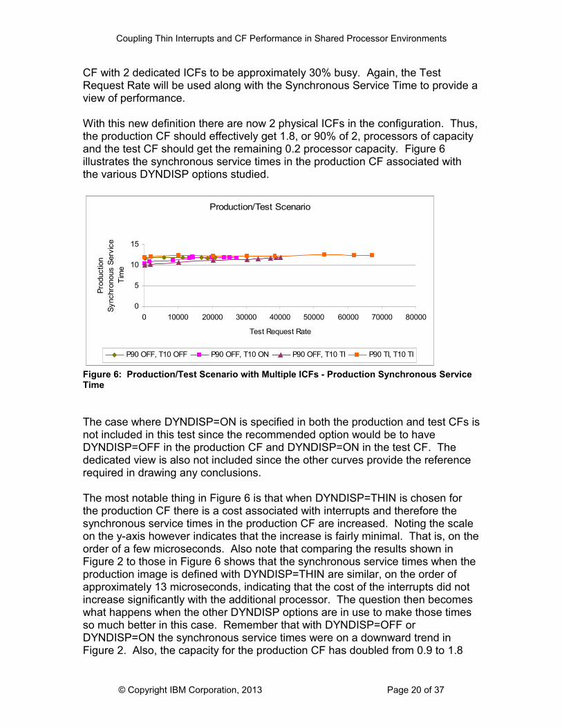
With this new definition there are now 2 physical ICFs in the configuration. Thus, the production CF should effectively get 1.8, or 90% of 2, processors of capacity and the test CF should get the remaining 0.2 processor capacity. Figure 6 illustrates the synchronous service times in the production CF associated with the various DYNDISP options studied.


0

5

10

15

0 10000 20000 30000 40000 50000 60000 70000 80000

Test Request Rate

Prod

uctio

n Sy

nchr

onou

s Se

rvic

e Ti

me

P90 OFF, T10 OFF P90 OFF, T10 ON P90 OFF, T10 TI P90 TI, T10 TI

Figure 6: Production/Test Scenario with Multiple ICFs - Production Synchronous Service Time

The case where DYNDISP=ON is specified in both the production and test CFs is not included in this test since the recommended option would be to have DYNDISP=OFF in the production CF and DYNDISP=ON in the test CF. The dedicated view is also not included since the other curves provide the reference required in drawing any conclusions.

The most notable thing in Figure 6 is that when DYNDISP=THIN is chosen for the production CF there is a cost associated with interrupts and therefore the synchronous service times in the production CF are increased. Noting the scale on the y-axis however indicates that the increase is fairly minimal. That is, on the order of a few microseconds. Also note that comparing the results shown in Figure 2 to those in Figure 6 shows that the synchronous service times when the production image is defined with DYNDISP=THIN are similar, on the order of approximately 13 microseconds, indicating that the cost of the interrupts did not increase significantly with the additional processor. The question then becomes what happens when the other DYNDISP options are in use to make those times so much better in this case. Remember that with DYNDISP=OFF or DYNDISP=ON the synchronous service times were on a downward trend in Figure 2. Also, the capacity for the production CF has doubled from 0.9 to 1.8



processors of capacity. And, since there are now two physical processors there is always one available for the production CF since its share of the physical processors is greater than 1. The production CF is using its full 1.8 processors of capacity prior to the introduction of coupling thin interrupts but only about 1.2 processors effectively when coupling thin interrupts is introduced as shown in Figure 7. Note that the P10 OFF, T10 TI case, similar to what was seen in Figure 5 for this case, is able to use the 2 effective engines until the test CF has sufficient requests to require at least 0.1 effective engines. This can be seen in Figure 10.


0.0

0.5

1.0

1.5

2.0

0 10000 20000 30000 40000 50000 60000 70000 80000

Test Request Rate

Prod

uctio

n Ef

fect

ive

Engi

nes


Figure 7: Production/Test Scenario with Multiple ICFs - Production Effective Capacity

One item to note in Figure 6 is how flat the curves are. This indicates that regardless of the increasing amount of work in the test CF, the production Synchronous Service Times are not impacted since it always has at least one processor for its work. The significantly larger proportion of the capacity given to the production CF shields it from being impacted by the much smaller, in terms of capacity, test CF.

Figures 8 and 9 illustrate what happens to the test CF in this scenario.




0

5000

10000

15000

20000

0 10000 20000 30000 40000 50000 60000 70000 80000

Test Request Rate

Test

Syn

chro

nous

Se

rvic

e Ti

me


Figure 8: Production/Test Scenario with Multiple ICFs - Test Synchronous Service Time - View 1

This view looks suspiciously like Figure 3 in which the service times for the test CF are very high initially and then trend downward. The more interesting view is shown in Figure 9.


0

20

4060

80

100

0 10000 20000 30000 40000 50000 60000 70000 80000

Test Request Rate

Test

Syn

chro

nous

Se

rvic

e Ti

me


Figure 9: Production/Test Scenario with Multiple ICFs - Test Synchronous Service Time - View 2

Remember that in this scenario the test CF is defined with a single processor while the production CF was defined with two. Figure 9 clearly shows the advantage of using DYNDISP=THIN in the test CF. It provides a significant improvement in Synchronous Service Time. And, when the DYNDISP=THIN option is employed in both the production CF and the test CF it allows for additional throughput. Figure 10 shows the effective engines used by the test CF.




0.00.2

0.40.6

0.81.0

0 10000 20000 30000 40000 50000 60000 70000 80000

Test Request Rate

Test

Effe

ctiv

e En

gine

s


Figure 10: Production/Test Scenario with Multiple ICFs - Test Effective Capacity

Note that in Figure 10 there is now some distinction between the effective engines when the test CF is employing the DYNDISP=OFF and the DYNDISP=ON options. The lower effective engines when using DYNDISP=ON in the test CF indicates a more efficient use of the processor resource. However, when employing DYNDISP=THIN in both the production CF and the test CF, P90 TI, T10 TI, the solution is even more efficient. Note that this case also allows the test CF to use more than the expected amount of processor resource since the production CF for this case uses so much less effective processor resource than it does with the other options.

Given this analysis of the Production/Test scenarios it is recommended that when sharing of CF processor resources is in effect DYNDISP=THIN be used in both the production and test CFs. While it is true that the combination of using DYNDISP=OFF in the production CF and DYNDISP=THIN in the test CF does provide a degree of Synchronous Service Time benefit in some cases, the higher efficiency that can be realized by using DYNDISP=THIN in both CFs is desirable and worth the minimal increase in any synchronous service time. Remember that the reason most customers would want to share CF processor resources is that the amount of work executed by the individual CFs is not sufficient to require the capacity of some number of dedicated processors. For production environments where the best performance is required the recommendation continues to be to use dedicated CF processors.

Sharing between Multiple Production CFs

In this scenario there is a single ICF processor being shared by two CFs. However, the CFs are of equal importance and there is an equal amount of work going on in both the CFs. Thus, the weights have been set at 50 for each of the



two CFs and the DYNDISP options are the same for both CF partitions. The activity on both of the CFs was increased at the same rate for this scenario and the ACME workload is used in all cases. Since all of the CFs are production CFs they are all contained in the same chart and are distinguished by the P1 and P2 labels in the legend as in Figure 11.

Production/Production Scenario

0500

10001500200025003000

0 50000 100000 150000 200000 250000 300000

CF Request Rate

Sync

hron

ous

Serv

ice

Tim

e

P1 (P1 OFF, P2 OFF) P2 (P1 OFF, P2 OFF) P1 (P1 ON, P2 ON)P2 (P1 ON, P2 ON) P1(P1 TI, P2 TI) P2 (P1 TI, P2 TI)Dedicated

Figure 11: Production/Production Scenario - View 1

The chart in Figure 11 shows that at very low request rates the Synchronous Service Times when using DYNDISP=OFF are extremely high. Remember that for the production and test scenarios previously examined, the weights were significantly higher for the production CF and the production Synchronous Service Times were not this high. They are significantly worse here because the weights are now equal among the sharing partners. Also, when DYNDISP=ON is used the Synchronous Services Times at low request rates are somewhat improved, but still undesirable. Figure 12 will refine the view by again altering the y-axis.




0

20

40

60

80

100

0 20000 40000 60000 80000 100000 120000

CF Request Rate

Sync

hron

ous

Serv

ice

Tim

e

P1 (P1 OFF, P2 OFF) P2 (P1 OFF, P2 OFF) P1 (P1 ON, P2 ON)P2 (P1 ON, P2 ON) P1(P1 TI, P2 TI) P2 (P1 TI, P2 TI)Dedicated

Figure 12: Production/Production Scenario - View 2

One item to note is that whether you have DYNDISP=OFF or DYNDISP=ON in the shared CFs the Synchronous Service Times seem to be fairly variable. In fact, the synchronous service times for the P1 CF with DYNDISP=OFF, P1 (P1 OFF,P2 OFF), no longer appear in the chart indicating that the service times are never below 100 microseconds although its counterpart, P2(P1 OFF,P2 OFF), certainly appears to be heading in the right direction. The variability is also presented in that the sharing partners, P1 and P2, for these sharing options are significantly different curves. It is suspected that this is due high subchannel delays. Evidence of that will be presented when discussing Figure 16. This is an example of how the lack of subchannels can add to performance variability. These cases exhibit high standard deviations as well. This is not true, however, for the case where the coupling thin interrupts are in use. In fact, in that case the P1 and P2 curves are on top of each other indicating a significantly more equal sharing of the resource. And, the significantly better service times make the subchannel use such that there are basically no delay issues.

The Synchronous Service Times for the CFs with the DYNDISP=THIN option are much more stable, similar to the dedicated service times. The difference in the time between the DYNDISP=THIN and the dedicated curves is an indication of the time required for the interrupt processing. Notice that as the amount of work increases the service times for these two curves become farther apart and at approximately 60000 requests per second the Synchronous Service Time with DYNDISP=THIN is almost twice what it is with dedicated resources. At some point this difference in the service times may no longer be acceptable for production environments where performance is imperative. Thus, there is still the recommendation to use dedicated CF processors in production environments where performance is of the utmost importance. It is also clear from this view



that when CF resources are shared DYNDISP=THIN is the best option for all the CFs participating in the sharing.

Increasing the amount of shared CF processorsGiven the significant improvement to performance shown thus far for using DYNDISP=THIN in environments sharing CF processor resources it is important to examine what happens when more CF processors are being shared. To examine this, the configuration was kept the same as in the previous scenario. That is, there are two production sysplexes sharing the CF resources and each production CF has an equal weight and an equal amount of work being driven to the CF. However, the number of CF processors and thus the work to each CF was increased. Figure 13 shows the impact this has on the Synchronous Service Times as related to the CF Utilization. Note that in each case the CF Utilization is driven to around 60% which is the recommended maximum. As expected the Synchronous Service Time increases as the CF Utilization increases. Also note that the Synchronous Service Time is fairly consistent regardless of the number of processors defined to the CF indicating that the additional processors are not adding to the interrupt overhead.


0

5

10

15

20

25

0 10 20 30 40 50 60 70

Total CF Utilization

Sync

hron

ous

Serv

ice

Tim

e

P1 TI2 P2 TI2 P1 TI4 P2 TI4 P1 TI8 P2 TI8

Figure 13: Production/Production Scenario with additional CF processors - View 1

In Figure 13 the value after the TI indicating that coupling thin interrupts is enabled in the CF indicates the number of CF logical processors defined to the partition. The number also indicates the number of physical processors in the configuration. For example, P1 TI4 indicates that this curve represents the Synchronous Service Times from the first production CF and the CF is defined with 4 CF logical processors and there are 4 physical ICFs in the configuration. Note that the Synchronous Service Times do not seem to be significantly



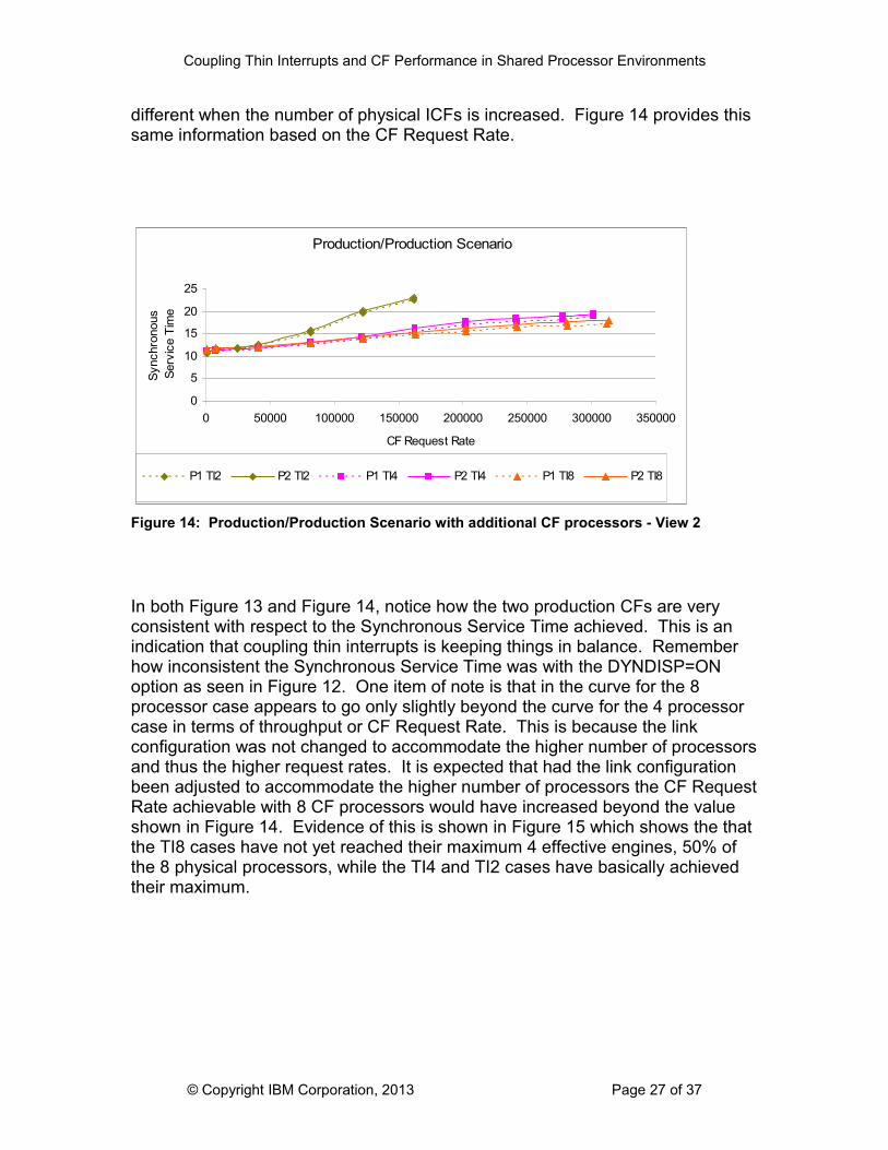
different when the number of physical ICFs is increased. Figure 14 provides this same information based on the CF Request Rate.


0

5

10

15

20

25

0 50000 100000 150000 200000 250000 300000 350000

CF Request Rate

Sync

hron

ous

Serv

ice

Tim

e


Figure 14: Production/Production Scenario with additional CF processors - View 2

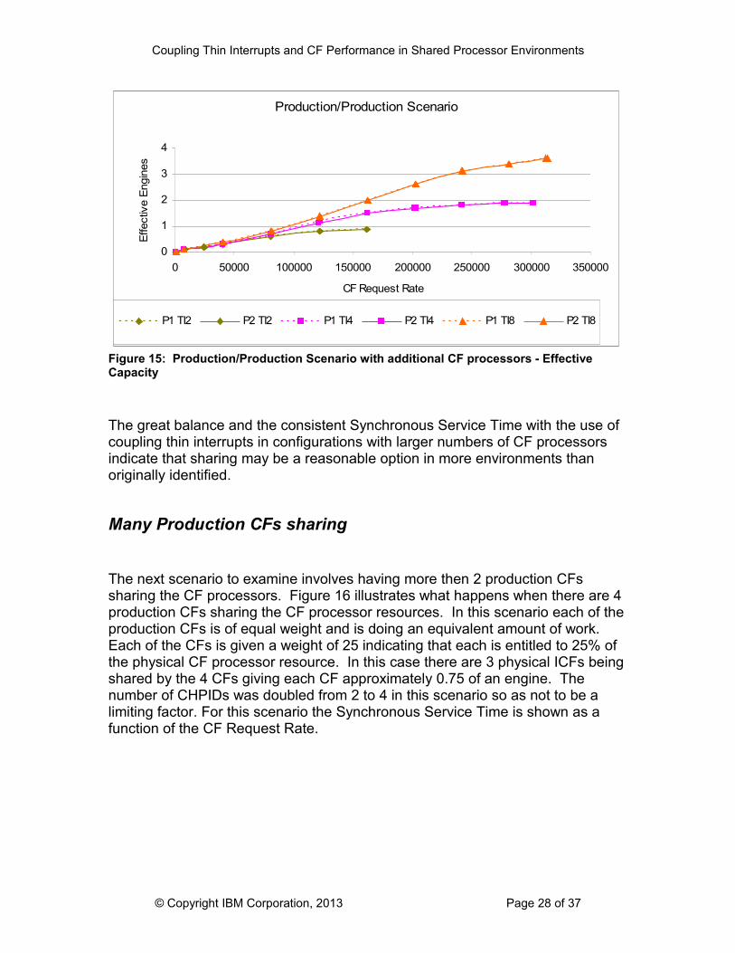
In both Figure 13 and Figure 14, notice how the two production CFs are very consistent with respect to the Synchronous Service Time achieved. This is an indication that coupling thin interrupts is keeping things in balance. Remember how inconsistent the Synchronous Service Time was with the DYNDISP=ON option as seen in Figure 12. One item of note is that in the curve for the 8 processor case appears to go only slightly beyond the curve for the 4 processor case in terms of throughput or CF Request Rate. This is because the link configuration was not changed to accommodate the higher number of processors and thus the higher request rates. It is expected that had the link configuration been adjusted to accommodate the higher number of processors the CF Request Rate achievable with 8 CF processors would have increased beyond the value shown in Figure 14. Evidence of this is shown in Figure 15 which shows the that the TI8 cases have not yet reached their maximum 4 effective engines, 50% of the 8 physical processors, while the TI4 and TI2 cases have basically achieved their maximum.




0

1

2

3

4

0 50000 100000 150000 200000 250000 300000 350000

CF Request Rate

Effe

ctiv

e En

gine

s


Figure 15: Production/Production Scenario with additional CF processors - Effective Capacity

The great balance and the consistent Synchronous Service Time with the use of coupling thin interrupts in configurations with larger numbers of CF processors indicate that sharing may be a reasonable option in more environments than originally identified.

Many Production CFs sharing

The next scenario to examine involves having more then 2 production CFs sharing the CF processors. Figure 16 illustrates what happens when there are 4 production CFs sharing the CF processor resources. In this scenario each of the production CFs is of equal weight and is doing an equivalent amount of work. Each of the CFs is given a weight of 25 indicating that each is entitled to 25% of the physical CF processor resource. In this case there are 3 physical ICFs being shared by the 4 CFs giving each CF approximately 0.75 of an engine. The number of CHPIDs was doubled from 2 to 4 in this scenario so as not to be a limiting factor. For this scenario the Synchronous Service Time is shown as a function of the CF Request Rate.




0

10

20

30

40

50

0 20000 40000 60000 80000 100000 120000 140000 160000 180000

CF Request Rate

Sync

hron

ous

Serv

ice

Tim

e

P1 ON P2 ON P3 ON P4 ON P1 TI

P2 TI P3 TI P4 TI

Figure 16: Production/Production Scenario with 4 CFs sharing the CF resource

Note that with the DYNDISP=ON option the curves for the 4 production CFs participating in sharing are much more similar than they were for the 2 production CFs shown in Figure 12. This is due to the additional CHPIDs that were added for this test.

Figure 16 indicates that with DYNDISP=THIN CF processor resources are more efficient based on the better Synchronous Service Time and additional throughput provided.

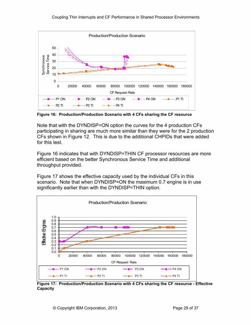
Figure 17 shows the effective capacity used by the individual CFs in this scenario. Note that when DYNDISP=ON the maximum 0.7 engine is in use significantly earlier than with the DYNDISP=THIN option.

0.00.10.20.30.40.50.60.70.80.91.0

0 20000 40000 60000 80000 100000 120000 140000 160000 180000

Effec

tive E

ngine

s

CF Request Rate


P1 ON P2 ON P3 ON P4 ON

P1 TI P2 TI P3 TI P4 TI

Figure 17: Production/Production Scenario with 4 CFs sharing the CF resource - Effective Capacity



Given the consistency with which the use of coupling thin interrupts allows the CFs to share physical resources and noting the lower number of effective processors in use in this environment as shown in Figure 17, what is the effect of using fewer physical resources?

The answer can be observed in Figure 18 where the same scenario using DYNDISP=THIN in Figure 16 is compared to the same configuration with 2 physical ICFs instead of 3. Thus, the share of each of the CFs is 0.5 processors. This case is indicated by the minus sign following the TI designation in the chart.

Production/Production ScenarioProduction View

0

10

20

30

40

50

60

0 20000 40000 60000 80000 100000 120000 140000

CF Request Rate

Syn

chro

nous

Ser

vice

Ti

me

P1 TI P2 TI P3 TI P4 TI P1 TI-

P2 TI- P3 TI- P4 TI-

Figure 18: Production/Production Scenario with fewer physical CF resources

Note that for the same request rate the Synchronous Service Time increases when the CF processor resources are reduced. For example, at a rate of 60,000 requests per second when there are 2 physical ICFs (Px TI-) the service time is approximately 50% higher than when there are 3 physical ICFs.

The impact on the Synchronous Service Time of lowering the number of physical ICFs available for sharing is evidence that even with the vast improvements provided by using coupling thin interrupts, there still needs to be careful planning when deciding to use shared CF processors. The number of physical resources being made available and the weights given to the sharing partners are key.

System Managed CF Structure Duplexing



Thus far the only scenarios examined were simplex environments. The use of System Managed CF Structure Duplexing, to be referred to simply as duplexing in this paper, has specific timing sensitivities relating to the exchange of signals between the CFs involved in the duplexing. These timing sensitivities and the timing paradigms for sharing CF processors are the justification for the following scenarios.

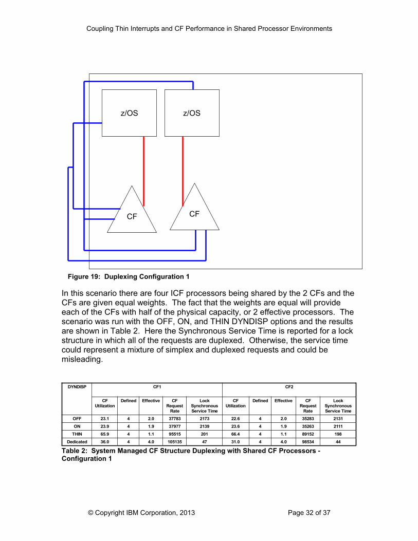
The first duplexing scenario has both of the duplexing CFs participating in processor sharing. Each CF is given the same weight so as to provide a balance between duplexing partners. Figure 19 illustrates the configuration used for this scenario. The configuration consists of 2 z/OS images, 2 CFs. The link configuration is depicted by the red and blue connections in Figure 19. The red connections indicate ICP links to represent that the z/OS image and the CF that are connected reside on the same CPC. The blue connections represent CIB links and connect each z/OS image and its “local” CF (connected by the red ICP link) to the “remote” CF. The dotted rectangle indicates that these CFs are sharing processor resources.



In this scenario there are four ICF processors being shared by the 2 CFs and the CFs are given equal weights. The fact that the weights are equal will provide each of the CFs with half of the physical capacity, or 2 effective processors. The scenario was run with the OFF, ON, and THIN DYNDISP options and the results are shown in Table 2. Here the Synchronous Service Time is reported for a lock structure in which all of the requests are duplexed. Otherwise, the service time could represent a mixture of simplex and duplexed requests and could be misleading.

DYNDISP CF1 CF2

CF Utilization

Defined Effective CF Request

Rate

Lock Synchronous Service Time

CF Utilization


Rate

Lock Synchronous Service Time

OFF 23.1 4 2.0 37783 2173 22.6 4 2.0 35283 2131

ON 23.9 4 1.9 37977 2139 23.6 4 1.9 35263 2111

THIN 65.9 4 1.1 95515 201 66.4 4 1.1 89152 198

Dedicated 36.0 4 4.0 105135 47 31.0 4 4.0 98534 44

Table 2: System Managed CF Structure Duplexing with Shared CF Processors - Configuration 1


z/OS z/OS

CFCF

Figure 19: Duplexing Configuration 1


For this scenario the same amount of work was presented to the CF. The table shows the principal data for each of the duplexing partners, CF1 and CF2. The fact that the CF Request Rate is almost 3x for the DYNDISP=THIN option indicates the superior efficiency of that option. This is no doubt due to the significant decrease in Synchronous Service Time not just for the lock structure as shown in the table but overall. A dedicated duplexed environment was also included to illustrate the best case duplexing scenario. Note, however, that for the dedicated each of the CFs is supported by 4 physical processors. That is, there is a total of 8 ICFs for the dedicated case.

The second duplexing scenario provides a bit more of a challenge for the sensitive timing required when duplexing. Figure 20 provides the configuration for this case. As in Figure 19 the red lines indicate ICP connections and the blue lines represent CIB connections and the dotted rectangle indicates which of the CFs are sharing processor resources.



The two CFs on the left are duplexing partners while the CF on the right is sharing the processor resource with one of the duplexing partners. In this scenario the CF on the right is defined as a test CF. That is, it has less importance and therefore a lower rate than the CF participating in the duplexing. The CF at the far left is defined to have dedicated processors while its duplexing partner has a weight of 90 while sharing processors with the test CF which has a weight of 10. The CF participating in the duplexing which is not sharing processor resource is defined with dedicated ICFs.

Table 3 shows the results of this scenario added to Table 2 for comparison. Note that for both of the duplexing scenarios the service times are similar for the CF that is sharing the processor resource.


z/OS z/OS z/OS

CFCFCF

Figure 20: Duplexing Configuration 2


DYNDISP CF1 CF2 CF3

CF Utilization


Rate

Lock Synch Service

Time

CF Utilization


Rate

LockSynch

Service Time

CF Utilization


Rate

Lock Synch Service

Time

OFF 23.1 4 2.0 37783 2173 22.6 4 2.0 35283 2131

ON 23.9 4 1.9 37977 2139 23.6 4 1.9 35263 2111

THIN 65.9 4 1.1 95515 201 66.4 4 1.1 89152 198

Dedicated 36.0 4 4.0 105135 47 31.0 4 4.0 98534 44

CF1DYNDISP=OFF, Dedicated, DUPLEX Production

CF2DYNDISP=THIN, SHR 90, DUPLEX Production

CF3DYNDISP=THIN, SHR 10, SIMPLEX Test

62.1 4 4.0 194855 166 77.5 4 3.6 174267 174 71 4 0.3 51792 171

Table 3: System Managed CF Structure Duplexing with Shared CF Processors - Configuration 2

It has been the recommendation not to use System Managed CF Structure Duplexing in shared engine CF environments. This was primarily due to the long and variable service times observed in these environment until the introduction of coupling thin interrupts. The two duplexing scenarios provided indicate that with the introduction of coupling thin interrupts, DYNDISP=THIN, that recommendation is perhaps not as strong if coupling thin interrupts is employed. The approximately 10x improvement in Lock Synchronous Service Time over the previously available sharing options may now make System Managed CF Structure Duplexing viable in shared CF test configurations. However, dedicated ICFs should be used in production environments where System Managed CF Structure Duplexing is employed.



Conclusions and RecommendationsThe performance answer is always, “It depends”. This is because there are usually multiple factors in play and the answer is dependent on what the toleration level is for each of these factors. In this study the conclusions and recommendations are based on the Synchronous Service Time, a key performance indicator, along with effective processor consumption and/or CF utilization. These performance indicators are evaluated based on a controlled set of factors identified in each scenario presented. The changes to DYNDISP options, CF request rate and configuration were planned to provide insight into the effect of those changes in the specific scenarios presented in order to give the reader a feel for what kinds of changes could be expected when considering or implementing the use of coupling thin interrupts (DYNDISP=THIN) in shared CF processor environments, or when implementing shared CF processor environments initially.

It is important to do careful planning when considering the use of shared CF processors given that the sensitivity of the timing in the CF is critical to the performance of the sysplex. This is especially true if System Managed CF Structure Duplexing will be implemented in this shared environment. Careful planning with respect to the number of CFs that will be sharing the processor resource and the number of physical CF processors involved in the sharing is essential. It is recommended that zPCR3 be utilized for capacity planning. zPCR can be found at:

http://www.ibm.com/support/techdocs/atsmastr.nsf/WebIndex/PRS1381

The scenarios examined show that in environments in which CF processors are shared the introduction of coupling thin interrupts provides the best sharing option. Thus, using this new technology in environments where CFs are already sharing CF resources will provide significant improvements. It will also make the sharing of CF processors more palatable in environments where it was not reasonable to do so previously. Whenever a number of CFs are sharing CF processors it is recommended for each of the CFs, regardless of production or test designations, to employ coupling thin interrupt technology by using the DYNDISP=THIN option.

There are environments where significant use of CF resources is required and where the absolute best performance is required. For these environments the recommendation continues to be to use dedicated CF processors.



References

1. IBM Corporation (2013), zEnterprise System Processor Resource/Systems Manager Planning Guide, IBM Resource Link order number SB10-7156-01, URL https://www.ibm.com/servers/resourcelink/svc03100.nsf?OpenDatabase

2. IBM Corporation (2013), z/OS Resource Management Facility, URL http://publibz.boulder.ibm.com/epubs/pdf/erbzrab0.pdf

3. IBM Corporation (2013), zPCR Processor Capacity Reference, IBM Techdocs document ID PRS1381, URL http://www.ibm.com/support/techdocs/atsmastr.nsf/WebIndex/PRS1381


http://publibz.boulder.ibm.com/epubs/pdf/erbzrab0.pdf

https://www.ibm.com/servers/resourcelink/svc03100.nsf?OpenDatabase

Coupling Thin Interrupts - IBM · 2019-12-16 · Coupling thin interrupts can also be enabled in...

Documents

Transcript of Coupling Thin Interrupts - IBM · 2019-12-16 · Coupling thin interrupts can also be enabled in...