Coupling activity-based demand generation to a truly … · Coupling activity-based demand...

Coupling activity-based demand generation to a trulyagent-based traffic simulation – activity time allocation

Michael BalmerDepartment of Computer Science

ETH ZurichCH-8092 Zurich, Switzerland

Phone: 01-632 03 64Fax: 01-632 13 74

E-mail: [email protected]

Bryan RaneyDepartment of Computer Science


Phone: 01-632 08 92Fax: 01-632 13 74


Kai NagelDepartment of Computer Science


Phone: 01-632 54 27Fax: 01-632 13 74


Transport Systems Analysis and Transport TelematicsTU Berlin, D-10623 Berlin, Germany

March 8, 2004

Abstract

There is by now agreement that activity-based demand generation for transportation simulationshould be tried. One possibility to bring activity-based demand generation into the transportationplanning process is to use it to replace the first two (or three) steps of the 4-step-process. In thiscase, the activity-based demand generation produces a standard origin-destination (OD) matrix,which is then fed into the existing assignment model. Both the OD matrix and the assignmentmodel could be time-dependent.

The advantage of this method is that it ties in with the arguably most sophisticated andbest understood part of the 4-step-process, which is the route assignment. Yet, some of theseadvantages go away when the OD matrices are time-dependent: In that situation, very few of themathematical results of static assignment carry over. In addition, coupling activity-based demandgeneration to network assignment via an OD matrix severs the connection between individualsand their performance. Any iterative feedback of the traffic system performance to the activitygeneration can only be based on aggregate measures, such as link travel times, not on individualperformance of the traveler. An obvious case where the coupling via OD-matrix goes wrong isthat it is possible for a person to leave an activity even before he/she has arrived at it.

1

In this situation, we propose, as a way toward further progress, to use a truly agent-basedrepresentation of the traffic system and the assignment process. In a truly agent-based represen-tation, each person remains individually identifiable throughout the whole simulation process.In particular, the traffic micro-simulation assumes the role of a realistic representation of thephysical system, including, say, explicit modeling of persons walking to the bus stop, or of a busbeing stuck in traffic. Also, in terms of analysis such a system offers enormous advantages: Itis, for example, possible to obtain the demographic characteristics of all drivers being stuck ina particular traffic jam. It is also possible to make each traveler react individually to exactly theconditions that this traveler has found “on the ground”, rather than to aggregated conditions.

This approach allows a completely consistent modeling of the behavioral processes relatedto transportation. In our work, we have already demonstrated that such an approach is possiblefor large scale scenarios with several millions of travelers. Our newest version of our modelingsystem is able to call arbitrary “strategy generation” modules, and feed back to them individual(or aggregated) performance. As strategy generation modules, we envisage all kinds of activity-based demand generation modules. At this point, we demonstrate, besides the use of a routingmodule, a time allocation module. This module plays the role of departure time choice modulesin OD-based models, but it makes travelers adjust all their timing, i.e. not just departure time,but also duration of activities etc., throughout the whole day. Our paper will demonstrate thatalready a simple version of a time choice module, together with a utility function to “score”different plans, leads to plausible results. The simulation will be run both on test cases andon real world scenarios. The latter will concentrate on the larger Zurich metropolitan area,with about 1 mio of travelers. One of our networks includes all streets in the Zurich area, thusallowing a very realistic evaluation of how activity plans perform “on the ground”. If possible,we will include validation and sensitivity testing in comparison with real-world traffic counts.

At this point, the main obstacle to using more sophisticated activity-based demand generationmodules in such a system is no longer the computational technology, but (1) the data conversionproblems which arise when models are ported from one geographical area to the other, and(2) the computational challenge posed by generating daily activities for several million travelers.

Keywords: traffic simulation – transportation planning – route planning – learning – multi-agentsimulation – activity-based demand generation

1 Introduction

There is by now agreement that activity-based demand generation for transportation simulationshould be tried. One possibility to bring activity-based demand generation into the transportationplanning process is to use it to replace the first two (or three) steps of the 4-step-process. In this case,the activity-based demand generation produces a standard origin-destination (OD) matrix, which isthen fed into the existing assignment model. Both the OD matrix and the assignment model couldbe time-dependent.

The advantage of this method is that it ties in with the arguably most sophisticated and best un-derstood part of the 4-step-process, which is the route assignment. Yet, some of these advantagesgo away when the OD matrices are time-dependent: In that situation, very few of the mathematicalresults of static assignment carry over. In addition, coupling activity-based demand generation tonetwork assignment via an OD matrix severs the connection between individuals and their perfor-mance. Any iterative feedback of the traffic system performance to the activity generation can onlybe based on aggregate measures, such as link travel times, not on individual performance of thetraveler. An obvious case where the coupling via OD-matrix goes wrong is that it is possible for aperson to leave an activity even before he/she has arrived at it.

2

In this situation, we propose, as a way toward further progress, to use a truly agent-based rep-resentation of the traffic system and the assignment process. In a truly agent-based representation,each person remains individually identifiable throughout the whole simulation process. In particu-lar, the traffic micro-simulation assumes the role of a realistic representation of the physical system,including, say, explicit modeling of persons walking to the bus stop, or of a bus being stuck in traffic.Also, in terms of analysis such a system offers enormous advantages: It is, for example, possible toobtain the demographic characteristics of all drivers being stuck in a particular traffic jam. It is alsopossible to make each traveler react individually to exactly the conditions that this traveler has found“on the ground”, rather than to aggregated conditions.

This multi-agent concept consists of basically two parts: (i) the simulation of the “physical”properties of the system, and (ii) the generation of the agents’ strategies. The simulation of thephysical system is the place where the agents interact with each other – car drivers produce con-gestion, traffic lights change their intervals dependent on the amount of traffic, pedestrians wait forthe next train to catch, and so on. The agents make their strategies based on what they experiencedin the physical simulation – car drivers try other routes to avoid congestion, pedestrians need toleave earlier to catch the train, traffic lights favor the main streets to maximize the throughput of anintersection, etc.

We are in the process of implementing such a multi-agent simulation for the whole Switzerland.This paper concentrates on the Zurich area, with about 260’000 agents that cross this region. Thechallenges with such an implementation are many: availability and quality of input data, computa-tional implementation and computational performance, conceptual understanding of agent learning,and validation.

In past work (Raney et al., 2003), we had reported first results which were based on typicaltransportation planning data: it used standard origin-destination matrices; it used the transporta-tion planning network from the corresponding Swiss federal planning authority; and it performedroute assignment based on these input data. The main difference to typical planning tools, such asEMME/2 (www.inro.ca) or VISUM (www.ptv.de), was that our implementation was indeed com-pletely agent-based; that is, the individuality of each traveler was fully maintained throughout theprocess. In addition, in contrast to TRANSIMS (www.transims.net), we used a so-called agentdatabase, which keeps track of several plans per agent.

This paper goes further by now also internalizing the time structure of the input data. In otherwords, it is possible for the simulation system itself to predict when agents begin and end theirmain activities. The main result is that it is possible to completely ignore the time structure ofthe time-dependent OD matrices without compromising the quality of the predictive power. Thisis similar to the approach used and results obtained with METROPOLIS (de Palma and Marchal,2002). The main difference is that our implementation uses complete daily activity chains, whilede Palma and Marchal (2002) only uses trips. We believe that our method, while computationallymore demanding, opens the door to more flexible transportation planning models in the future.

This paper will continue with an outline of the general simulation structure (Sec. 2), where wealso describe the modules we will use in more detail. Next we introduce the network and the scenario(Sec. 3). The results (Sec. 4) of the different setups of the scenario are compared with counts data(Sec. 3.3) of this region. Some computational issues are pointed out in section 5. The paper isconcluded by a section on future work (Sec. 6) and a summary (Sec. 7).

3

2 Simulation Structure

2.1 Overview

As pointed out before, our simulation is constructed around the notion of agents that make indepen-dent decisions about their actions. Each traveler of the real system is modeled as an individual agentin our simulation. The overall approach consists of three important pieces:

• Each agent independently generates a so-called plan, which encodes its intentions during acertain time period, typically a day.

• All agents’ plans are simultaneously executed in the simulation of the physical system. Thisis also called the mobility simulation.

• There is a mechanism that allows agents to learn. In our implementation, the system iteratesbetween plans generation and mobility simulation. The system remembers several plans peragent, and scores the performance of each plan. Agents normally chose the plan with thehighest score, sometimes re-evaluate plans with bad scores, and sometimes obtain new plans.Further details will be given below.

As this is an application to traffic forecasting, a plan contains the itinerary of activities the agentwants to perform during the day, plus the intervening trip legs the agent must take to travel betweenactivities. An agent’s plan details the order, type, location, duration and other time constraints ofeach activity, and the mode, route and expected departure and travel times of each leg. A typicalplan could look like this:

• stay at home till 07:38

• take the car to drive to work by the following route (encoded in a street network): 321 - 2 - 34- 65 - 21 - 34

• arrive at work at 07:58

• work for 8 hours an 24 minutes until 16:22

• take the car to drive home by the following route: 33 - 25 - 81 - 109 - 3 - 322

• arrive at home at 16:41

See Fig. 2 for a more detailed plan example. This paper concentrates on “home” and “work” as theonly activities, and “car” as the only mode.

Each of the details described in the plan, such as activity duration, is a decision that must bemade by the agent. These decisions depend on one another, but the decisions made by one agent areindependent of those made by another. We divide the task of generating a plan into sets of closelyrelated decisions, and each set is assigned to a separate module. An agent strings together calls tovarious modules in order to build up a complete plan. To support this “stringing”, the input to a givenmodule is a (possibly incomplete) plan, and the output is plan with some of the decisions updated.

Some possible modules are defined as the following:

• Activity pattern generator: Decides which activities an agent actually wants to performduring the day, and in what order it will perform them. At present this module is not used, andwe have a fixed pattern of “home-work-home” for all agents.

4

• Activity location generator: Determines where the agent will perform each activity. Atpresent this module is not used, and we have a fixed location for each agent’s “home” and“work” activity.

• Activity time generator: Determines the timing attributes the agent will utilize for each activ-ity in its plan. Activities have two possible timing attributes: “activity duration”, and “activityend time”. After starting an activity, an agent performs the activity either for the length of“duration”, or until “activity end time”, whichever is earlier. Activities cannot overlap in time.

• Router: Determines which route and which mode the agent chooses for each trip leg thatconnects activities at different locations. The study presented in this paper uses car as the onlymode.

A specialty of our approach is that arbitrary numbers and types of such modules can be “pluggedin” to the framework, as long as they generate some information that contributes to a plan. For thatreason, it is easy to, say, combine activity and mode choice into one module, or to add residentialor workplace choice. This paper will employ two modules only: “activity times generator” and“router”. Other modules will be the topic of future work.

Once the agent’s plan has been constructed via the modules, it can be fed into the mobilitysimulation module. This module executes all agents’ plans simultaneously on the network, allowingagents to interact with one another, and provides output describing what happened to the agentsduring the execution of their plans.

The above modules produce dependencies about their computed information. The outcome ofthe mobility simulation module (e.g. congestion) depends on the planning decisions made by thedecision-making modules. However, those modules can base their decisions on the output of themobility simulation (e.g. knowledge of congestion). This creates an interdependency (“chicken andegg”) problem between the decision-making modules and the mobility simulation module.

We need these modules to be consistent with one another, so we introduce feedback into themulti-agent simulation structure (Kaufman et al., 1991; Nagel, 1994/95; Bottom, 2000). This setsup an iteration cycle which runs the mobility simulation with specific plans for the agents, then usesthe time allocator and the router to update the plans; these changed plans are again fed into themobility simulation, etc, until consistency between modules is reached.

The feedback cycle is controlled by the agent database, which also keeps track of multiple plansgenerated by each agent, allowing agents to reuse those plans at will. The repetition of the iterationcycle coupled with the agent database enables the agents to learn how to improve their plans overmany iterations.

In the following sections we describe the modules in more detail.

2.2 Activity Time Allocation Module

This module is called to change the timing of an agent’s plan. At this point, a very simple approachis used which just applies a random “mutation” to the duration and end time attributes of the agent’sactivities. More precisely, for the first activity, the activity end time is the only attribute that isspecified and thus mutated, while for all other activities, the duration is what is specified and mutated.For each such attribute of each activity in an agent’s plan, this module picks a random time from theuniform distribution [−30 min, +30 min] and adds it to the attribute. Any negative duration is resetto zero; any activity end time before midnight is reset to midnight. The entire plan is returned to theagent, with only the time attributes modified.

5

Although this approach is not very sophisticated, it is sufficient in order to obtain useful results(Sec. 4.3). This is consistent with our overall assumption that, to a certain extent, simple modulescan be used in conjunction with a large number of learning iterations (e.g. Nagel et al., submitted).Since each module is implemented as a “plugin”, this module can be replaced by a more enhancedimplementation if desired.

2.3 Router

The router is implemented as a time dependent Dijkstra algorithm. It calculates link travel timesfrom the events output of the previous mobility simulation (see Sec. 2.4). The link travel times areencoded in 15 minute time bins, so they can be used as the weights of the links in the networkgraph. Apart from relatively small and essential technical details, the implementation of such analgorithm is straightforward (Jacob et al., 1999). With this and the knowledge about activity chains,it computes the fastest path from each activity to the next on in the sequence as a function in time. Itreturns the entire plan, complete with updated paths, to be used by the agents for the next mobilitysimulation.

2.4 Mobility Simulation

The mobility simulation simulates the physical world. It is implemented as a queue simulation,which means that each street (link) is represented as a FIFO (first-in first-out) queue with two re-strictions. First, each agent has to remain for a certain time on the link, corresponding to the freespeed travel time. Second, a link storage capacity is defined which limits the number of agents onthe link. If it is filled up, no more agents can enter this link.

Even though this structure is indeed very simple, it produces traffic as expected and it can rundirectly off the data typically available for transportation planning purposes. On the other hand, thereare some limitations compared to reality, i.e. number of lanes, weaving lanes, turn connectivitiesacross intersections or signal schedules cannot be included into this model.

The output that the mobility simulation produces is a list of events for each agent, such as enter-ing/leaving link, left/arrived at activity, and so on. Data for an event includes which agent experi-enced it, what happened, what time it happened, and where (link/node) the event occurred. With thisdata it is easy to produce different kinds of information and indicators like link travel time (whichi.e. will be used by the router), trip travel time, trip length, percentage of congestion, and so on.

2.5 Agent Database – Feedback

As mentioned above, the feedback mechanism is important for making the modules consistent withone another, and for enabling agents to learn how to improve their plans. In order to achieve thisimprovement, agents need to be able to try out different plans and to tell when one plan is “better”than another. The iteration cycle of the feedback mechanism allows agents to try out multiple plans.To compare plans, the agents assigns each plan a “score” based on how it performed in the mobilitysimulation.

It is very important to note that our framework always uses actual plans performance for thescore. This is in stark contrast to all other similar approaches that we are aware of – these otherapproaches always feed back some aggregated quantity such as link travel times and reconstructperformance based on those (e.g. URBANSIM www page, accessed 2003; Ettema et al., 2003).Because of unavoidable aggregation errors, such an approach can fail rather badly, in the sense that

6

the performance information derived from the aggregated information may be rather different fromthe performance that the agent in fact displayed (Raney and Nagel, 2003).

The procedure of the feedback and learning mechanism is as follows:

1. Initial conditions: Start with a plans file that specifies one complete plan per agent. The agentdatabase loads this plans file into the memory of the agents. Each agent marks its initial planas being its “selected” plan.

2. Simulate: The agent database sends the set of “selected” plans (one per agent) to the mobilitysimulation. The simulation executes the plans simultaneously and outputs events.

3. Process events: The agent database reads the events outputted by the mobility simulation andsends each one to the agent identified within it. Each agent uses its events to calculate thescore of its “selected” plan – the one it most recently sent to the mobility simulation.

4. Plan pruning: The number of plans kept in an agent’s memory for reuse can be limited to Nplans for purposes of memory conservation. If N is defined, each agent that has P > N plansdeletes its lowest-scoring P − N plans in this step. Note that when an agent that has N plansgenerates a new one (see below), it temporarily keeps N + 1 plans until the new plan has beenscored. Then in this step, it deletes the worst plan (even if it is the newest one).

5. Select plans: Each agent decides which plan to select for execution by the next mobilitysimulation. It chooses from the following selection options, according to the indicated proba-bilities:

(a) (10%) New plan, routes only: The agent sends an existing plan (chosen with equalprobability among all plans in memory) to the router. The router updates all the routesin that plan based on the link travel times calculated from the events data from the mostrecent mobility simulation, and returns the updated plan. The new plan is added to theagent’s memory and marked as “selected”.

(b) (10%) New plan, times and routes: The agent sends an existing plan (chosen withequal probability among all plans in memory) to the activity time allocation module.This module “mutates” the durations and/or end times of all activities in the plan andreturns the updated plan. The returned plan is also sent to the router for route replanning.When it comes back from the route replanner it is added to the agent’s memory andmarked as “selected”. (Note that now 20% of agents will have new routes, while only10% will have new times.)

(c) (10%) Random selection: The agent picks an existing plan, chosen with equal proba-bility among all plans in memory, without regard to their scores. This plan is marked as“selected”.

(d) (rest) Probabilistic selection: The agent picks an existing plan from memory, choosingaccording to probabilities based on the scores of the plans. The probabilities are of theform

p ∝ eβ·Sj ,

where Sj is the score of plan j, and β is an empirical constant. This is similar to a logitmodel from discrete choice theory. The chosen plan is marked as “selected”.

7

6. The cycle returns to step 2, and continues until the system has reached a relaxed state. At thispoint, there is no quantitative measure of when the system is “relaxed”; we just allow the cycleto continue until the outcome seems stable.

Note that in the above, when an agent reuses an existing plan, its previous score is not forgotten,but averaged with its new score, like so:

S := (1 − α)Sold + α · Snew , (1)

where the blending factor, α = 0.1. This allows the agent to base plan selection on more of theplans’ history than just the last iteration. Score averaging requires all plans to have an Sold, so whena new plan is generated, it is optimistically given a preliminary score equal to the score of the agent’sbest plan.

2.6 Scores for plans

In order to compare plans, it is necessary to assign a quantitative score to the performance of eachplan. In principle, arbitrary scoring schemes can be used (e.g. prospect theory (Avineri and Prashker,2003)). In this work, a simple utility-based approach is used. The approach is related to the Vickreybottleneck model (Arnott et al., 1993), but needs to be modified in order to be consistent with ourapproach based on complete daily plans (Charypar and Nagel, 2003; Raney and Nagel, 2004). Theelements of our approach are as follows:

• The total score of a plan is computed as the sum of individual contributions:

Utotal =

n∑

i=1

Uperf ,i +

n∑

i=1

Ulate,i +

n∑

i=1

Utravel ,i ,

where Utotal is the total utility for a given plan; n is the number of activities, which equalsthe number of trips; Uperf ,i is the (positive) utility earned for performing activity i; Ulate,i isthe (negative) utility earned for arriving late to activity i; and Utravel ,i is the (negative) utilityearned for traveling during trip i. In order to work in plausible real-world units, utilities aremeasured in Euro.

• A logarithmic form is used for the positive utility earned by performing an activity:

Uperf ,i(tperf ,i) = βperf · topt,i · ln

(

tperf ,i

t0,i

)

where tperf is the actual performed duration of the activity, and topt is the “typical” durationof an activity, and βperf is the marginal utility of an activity at its typical duration. βperf is thesame for all activities, since in equilibrium all activities at their typical duration need to havethe same marginal utility.

t0,i is a scaling parameter that is related both to the minimum duration and to the importanceof an activity. If the actual duration falls below t0,i, then the utility contribution of the activitybecomes negative, implying that the agent should rather completely drop that activity. A t0,i

only slightly less than topt,i means that the marginal utility of activity i rapidly increases withdecreasing tperf ,i , implying that the agent should rather cut short other activities. This paperuses

t0,i = topt,i · e−ζ/(topt,i) ,

8

where ζ is a scaling constant set to 10 hours. Note that with this specific form, Uperf ,i(topt,i) =βperf · ζ , independent of the activity type.1

• The (dis)utility of being late is uniformly assumed as:

Ulate,i = βlate · tlate,i ,

where βlate is the marginal utility (in Euro/h) for being late, and tlate,i is the number of hourslate to activity i.

• The (dis)utility of traveling is uniformly assumed as:

Utravel ,i = βtravel · ttravel ,i ,

where βtravel is the marginal utility (in Euro/h) for travel, and ttravel ,i is the number of hoursspent traveling during trip i.

At this point, our mobility simulation does not differentiate between “being an an activity loca-tion” (which potentially includes waiting) and “performing an activity”. In consequence, the simu-lation makes the agent stay at the activity location for the length of “duration”, no matter if the agentcan perform the activity or not. For example, when work starts at 8am but the agent arrives at 7amwith a duration of 8 hours, then the agent will depart from the activity location at 7am plus 8 hours= 3pm. The utility function, however, differentiates between “arrival time” and “activity start time”.The “work” activity has a particular starting time (see sec. 3.4 for the particular value), and arrivingbefore this time causes the agent to wait until then before actually starting the activity. This meansthat arriving early to an activity does not gain an agent any activity performance utility.

2.7 Verification of Implementation

We have verified that the simulation structure as described above works as we intended by runningit on a simple test scenario consisting of a circular network with 2’000 agents going back and forthbetween home and work. All agents have the same “home” location on one side of the circle andthe same “work” location on the other side. Nine routes are available between home and work, andone route is available between work and home. We ran three setups with various combinations ofdecision-making modules enabled:

1. New plan, routes only: The agents are only allowed to use the router module. They may doso with a 10% probability.

2. New plan, times only: The agents are only allowed to use the activity time allocation module.They may do so with a 10% probability.

3. New plan, times and routes: Agents may use the router module with 10% probability, orboth modules, with 10% probability. This is just as described in the step 5 of Sec. 2.5 above.

The results from these three scenarios were as expected. For more details on these verification tests,please see Raney and Nagel (2004).

1This “consequence” is actually the motivation for the specific mathematical form of the activity performance utilitycontribution. The reason for this motivation is not relevant to this paper, but is described in Charypar and Nagel (2003).

9

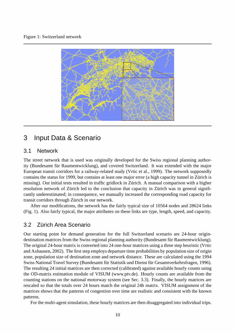
Figure 1: Switzerland network

3 Input Data & Scenario

3.1 Network

The street network that is used was originally developed for the Swiss regional planning author-ity (Bundesamt fur Raumentwicklung), and covered Switzerland. It was extended with the majorEuropean transit corridors for a railway-related study (Vrtic et al., 1999). The network supposedlycontains the status for 1999, but contains at least one major error (a high capacity tunnel in Zurich ismissing). Our initial tests resulted in traffic gridlock in Zurich. A manual comparison with a higherresolution network of Zurich led to the conclusion that capacity in Zurich was in general signifi-cantly underestimated; in consequence, we manually increased the corresponding road capacity fortransit corridors through Zurich in our network.

After our modifications, the network has the fairly typical size of 10564 nodes and 28624 links(Fig. 1). Also fairly typical, the major attributes on these links are type, length, speed, and capacity.

3.2 Zurich Area Scenario

Our starting point for demand generation for the full Switzerland scenario are 24-hour origin-destination matrices from the Swiss regional planning authority (Bundesamt fur Raumentwicklung).The original 24-hour matrix is converted into 24 one-hour matrices using a three step heuristic (Vrticand Axhausen, 2002). The first step employs departure time probabilities by population size of originzone, population size of destination zone and network distance. These are calculated using the 1994Swiss National Travel Survey (Bundesamt fur Statistik und Dienst fur Gesamtverkehrsfragen, 1996).The resulting 24 initial matrices are then corrected (calibrated) against available hourly counts usingthe OD-matrix estimation module of VISUM (www.ptv.de). Hourly counts are available from thecounting stations on the national motorway system (see Sec. 3.3). Finally, the hourly matrices arerescaled so that the totals over 24 hours match the original 24h matrix. VISUM assignment of thematrices shows that the patterns of congestion over time are realistic and consistent with the knownpatterns.

For the multi-agent simulation, these hourly matrices are then disaggregated into individual trips.

10

That is, we generate individual trips such that summing up the trips would again result in the givenOD matrix. The starting time for each trip is randomly selected between the starting and the endingtime of the validity of the OD matrix. The OD matrices assume traffic analysis zones (TAZs) whilein our simulations trips start on links. We convert traffic analysis zones to links by the followingheuristic:

• The geographic location of the zone is found via the geographical coordinate of its centroidgiven by the data base.

• A circle with radius 3 km is drawn around the centroid.

• Each link starting within this circle is now a possible starting link for the trips. One of theselinks is randomly selected and the trip start or end is assigned.

This leads to a list of approximately 5 million trips, or about 1 million trips between 6:00 AM and9:00 AM. Since the origin-destination matrices are given on an hourly basis, these trips reflect thedaily dynamics. Intra-zonal trips are not included in those matrices, as by tradition.

Since an agent should keep more than one plan during the iteration process, one million agentswould not fit into computer memory anymore. So we restrict our interests to the Zurich Area only.This is done with the following steps:

• All trips are routed using free speed travel times.

• We define the area of interest as a circle of 26 km radius around the center (“Bellevue”) ofZurich City.

• Each trip that does not cross this area is removed.

This results in 260 275 trips between 6am and 9am. All trips are now identified with an agent. The“origin” location for the morning trip is assigned to the home activity, and the “destination” locationis assigned to the work activity. The end time of the home activity is set to the departure time of theoriginal trip. The daily patterns “home-work” are then extended to the “home-work-home” pattern,where the two homes are at the same location. The duration of the “work” activity is set to 8 hours,with no fixed activity end time. At the end we get 260275 agents which have an initial day plan thatlooks like the example in Figure 2.

3.3 Counts Data

There are about 230 automatic counting stations registered at the Swiss Federal Roads Authority(Bundesamt fur Strassen). Of those, we had hourly counts data for 75 stations. Out of those, wewere able to locate 33 of them unequivocally on our network. Since we are just interested in theZurich area, only a subset can be used. Unfortunately there are only 6 useful counting stations left.Since they are bi-directional, this means that we can compare 12 links to reality.

For the future it is planned to use the counting data of Kanton Zurich (www.laerm.zh.ch). Thereare about 300 “Taxomex” counting stations registered in the whole area of the Kanton, althoughunfortunately none of these counting stations lie within the cities of Zurich and Winterthur.

11

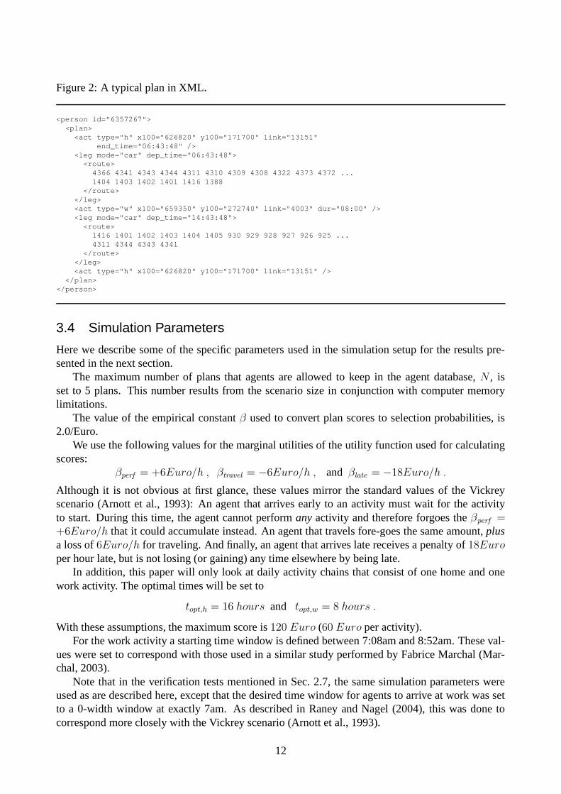
Figure 2: A typical plan in XML.

<person id="6357267"><plan><act type="h" x100="626820" y100="171700" link="13151"

end_time="06:43:48" /><leg mode="car" dep_time="06:43:48">

<route>4366 4341 4343 4344 4311 4310 4309 4308 4322 4373 4372 ...1404 1403 1402 1401 1416 1388

</route></leg><act type="w" x100="659350" y100="272740" link="4003" dur="08:00" /><leg mode="car" dep_time="14:43:48">

<route>1416 1401 1402 1403 1404 1405 930 929 928 927 926 925 ...4311 4344 4343 4341

</route></leg><act type="h" x100="626820" y100="171700" link="13151" />

</plan></person>

3.4 Simulation Parameters

Here we describe some of the specific parameters used in the simulation setup for the results pre-sented in the next section.

The maximum number of plans that agents are allowed to keep in the agent database, N , isset to 5 plans. This number results from the scenario size in conjunction with computer memorylimitations.

The value of the empirical constant β used to convert plan scores to selection probabilities, is2.0/Euro.

We use the following values for the marginal utilities of the utility function used for calculatingscores:

βperf = +6Euro/h , βtravel = −6Euro/h , and βlate = −18Euro/h .

Although it is not obvious at first glance, these values mirror the standard values of the Vickreyscenario (Arnott et al., 1993): An agent that arrives early to an activity must wait for the activityto start. During this time, the agent cannot perform any activity and therefore forgoes the βperf =+6Euro/h that it could accumulate instead. An agent that travels fore-goes the same amount, plusa loss of 6Euro/h for traveling. And finally, an agent that arrives late receives a penalty of 18Europer hour late, but is not losing (or gaining) any time elsewhere by being late.

In addition, this paper will only look at daily activity chains that consist of one home and onework activity. The optimal times will be set to

topt,h = 16 hours and topt,w = 8 hours .

With these assumptions, the maximum score is 120 Euro (60 Euro per activity).For the work activity a starting time window is defined between 7:08am and 8:52am. These val-

ues were set to correspond with those used in a similar study performed by Fabrice Marchal (Mar-chal, 2003).

Note that in the verification tests mentioned in Sec. 2.7, the same simulation parameters wereused as are described here, except that the desired time window for agents to arrive at work was setto a 0-width window at exactly 7am. As described in Raney and Nagel (2004), this was done tocorrespond more closely with the Vickrey scenario (Arnott et al., 1993).

12

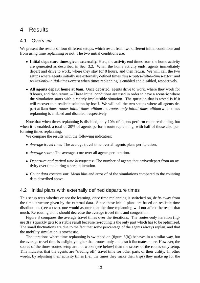
4 Results

4.1 Overview

We present the results of four different setups, which result from two different initial conditions andfrom using time replanning or not. The two initial conditions are:

• Initial departure times given externally. Here, the activity end times from the home activityare generated as described in Sec. 3.2. When the home activity ends, agents immediatelydepart and drive to work, where they stay for 8 hours, and then return. We will call the twosetups where agents initially use externally defined times times-routes-initial-times-extern androutes-only-initial-times-extern when times replanning is enabled and disabled, respectively.

• All agents depart home at 6am. Once departed, agents drive to work, where they work for8 hours, and then return. – These initial conditions are used in order to have a scenario wherethe simulation starts with a clearly implausible situation. The question that is tested is if itwill recover to a realistic solution by itself. We will call the two setups where all agents de-part at 6am times-routes-initial-times-all6am and routes-only-initial-times-all6am when timesreplanning is enabled and disabled, respectively.

Note that when times replanning is disabled, only 10% of agents perform route replanning, butwhen it is enabled, a total of 20% of agents perform route replanning, with half of those also per-forming times replanning.

We compare the results with the following indicators:

• Average travel time: The average travel time over all agents plans per iteration.

• Average score: The average score over all agents per iteration.

• Departure and arrival time histograms: The number of agents that arrive/depart from an ac-tivity over time during a certain iteration.

• Count data comparison: Mean bias and error of of the simulations compared to the countingdata described above.

4.2 Initial plans with externally defined departure times

This setup tests whether or not the learning, once time replanning is switched on, drifts away fromthe time structure given by the external data. Since these initial plans are based on realistic timedistributions (see above), one would assume that the time replanning will not affect the result thatmuch. Re-routing alone should decrease the average travel time and congestion.

Figure 3 compares the average travel times over the iterations. The routes-only iteration (fig-ure 3(a)) quickly gets to a stable result because re-routing is the only part which has to be optimized.The small fluctuations are due to the fact that some percentage of the agents always replan, and thatthe mobility simulation is stochastic.

The iterations where time replanning is switched on (figure 3(b)) behaves in a similar way, butthe average travel time is a slightly higher than routes-only and also it fluctuates more. However, thescores of the times-routes setup are not worse (see below) than the scores of the routes-only setup.This indicates that the agents are “trading off” travel time for other parts of their utility. In otherwords, by adjusting their activity times (i.e., the times they make their trips) they make up for the

13

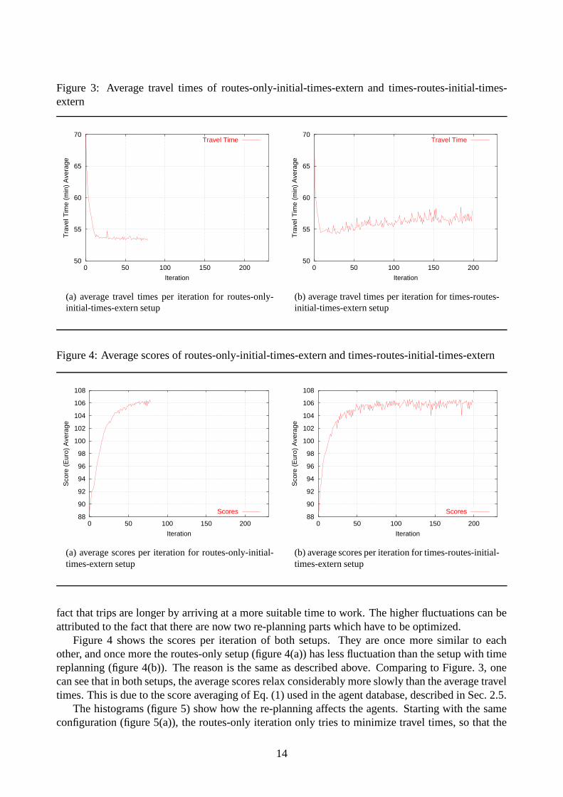
Figure 3: Average travel times of routes-only-initial-times-extern and times-routes-initial-times-extern

50

55

60

65

70

0 50 100 150 200

Tra

vel T

ime

(min

) A

vera

ge

Iteration

Travel Time

(a) average travel times per iteration for routes-only-initial-times-extern setup

50

55

60

65

70

0 50 100 150 200

Tra

vel T

ime

(min

) A

vera

ge

Iteration

Travel Time

(b) average travel times per iteration for times-routes-initial-times-extern setup

Figure 4: Average scores of routes-only-initial-times-extern and times-routes-initial-times-extern

88

90

92

94

96

98

100

102

104

106

108

0 50 100 150 200

Sco

re (

Eur

o) A

vera

ge

Iteration

Scores

(a) average scores per iteration for routes-only-initial-times-extern setup

88

90

92

94

96

98

100

102

104

106

108

0 50 100 150 200

Sco

re (

Eur

o) A

vera

ge

Iteration

Scores

(b) average scores per iteration for times-routes-initial-times-extern setup

fact that trips are longer by arriving at a more suitable time to work. The higher fluctuations can beattributed to the fact that there are now two re-planning parts which have to be optimized.

Figure 4 shows the scores per iteration of both setups. They are once more similar to eachother, and once more the routes-only setup (figure 4(a)) has less fluctuation than the setup with timereplanning (figure 4(b)). The reason is the same as described above. Comparing to Figure. 3, onecan see that in both setups, the average scores relax considerably more slowly than the average traveltimes. This is due to the score averaging of Eq. (1) used in the agent database, described in Sec. 2.5.

The histograms (figure 5) show how the re-planning affects the agents. Starting with the sameconfiguration (figure 5(a)), the routes-only iteration only tries to minimize travel times, so that the

14

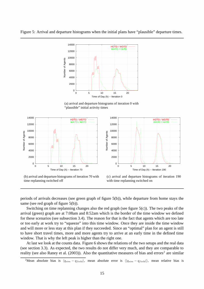
Figure 5: Arrival and departure histograms when the initial plans have “plausible” departure times.

0

2000

4000

6000

8000

10000

12000

14000

0 5 10 15 20

Num

ber

of A

gent

s

Time of Day (h) -- Iteration 0

HDTD / WDTDWATD / HATD

(a) arrival and departure histograms of iteration 0 with“plausible” initial activity times

0

2000

4000

6000

8000

10000

12000

14000

0 5 10 15 20

Num

ber

of A

gent

s



(b) arrival and departure histograms of iteration 70 withtime replanning switched off

0

2000

4000

6000

8000

10000

12000

14000

0 5 10 15 20

Num

ber

of A

gent

s



(c) arrival and departure histograms of iteration 190with time replanning switched on

periods of arrivals decreases (see green graph of figure 5(b)), while departure from home stays thesame (see red graph of figure 5(b)).

Switching on time replanning changes also the red graph (see figure 5(c)). The two peaks of thearrival (green) graph are at 7:08am and 8:52am which is the border of the time window we definedfor these scenarios (see subsection 3.4). The reason for that is the fact that agents which are too lateor too early at work try to “squeeze” into this time window. Once they are inside the time windowand will more or less stay at this plan if they succeeded. Since an “optimal” plan for an agent is stillto have short travel times, more and more agents try to arrive at an early time in the defined timewindow. That is why the left peak is higher than the right one.

At last we look at the counts data. Figure 6 shows the relations of the two setups and the real data(see section 3.3). As expected, the two results do not differ very much, and they are comparable toreality (see also Raney et al. (2003)). Also the quantitative measures of bias and errors2 are similar

2Mean absolute bias is 〈qsim − qfield〉, mean absolute error is 〈|qsim − qfield|〉, mean relative bias is

15

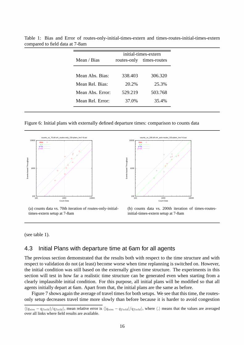
Table 1: Bias and Error of routes-only-initial-times-extern and times-routes-initial-times-externcompared to field data at 7-8am

initial-times-externMean / Bias routes-only times-routes

Mean Abs. Bias: 338.403 306.320

Mean Rel. Bias: 20.2% 25.3%

Mean Abs. Error: 529.219 503.768

Mean Rel. Error: 37.0% 35.4%

Figure 6: Initial plans with externally defined departure times: comparison to counts data

100

1000

10000

100 1000 10000

Eve

nts-

base

d T

hrou

ghpu

t

Count Data

counts_vs_70.dil-zrh_routes-only_OD-plans_hrs7-8.out

datay=x

y=2xy=x/2

(a) counts data vs. 70th iteration of routes-only-initial-times-extern setup at 7-8am

100

1000

10000

100 1000 10000

Eve

nts-

base

d T

hrou

ghpu

t

Count Data

counts_vs_200.dil-zrh_acts-routes_OD-plans_hrs7-8.out

datay=x

y=2xy=x/2

(b) counts data vs. 200th iteration of times-routes-initial-times-extern setup at 7-8am

(see table 1).

4.3 Initial Plans with departure time at 6am for all agents

The previous section demonstrated that the results both with respect to the time structure and withrespect to validation do not (at least) become worse when time replanning is switched on. However,the initial condition was still based on the externally given time structure. The experiments in thissection will test in how far a realistic time structure can be generated even when starting from aclearly implausible initial condition. For this purpose, all initial plans will be modified so that allagents initially depart at 6am. Apart from that, the initial plans are the same as before.

Figure 7 shows again the average of travel times for both setups. We see that this time, the routes-only setup decreases travel time more slowly than before because it is harder to avoid congestion

〈(qsim − qfield)/qfield〉, mean relative error is 〈|qsim − qfield|/qfield〉, where 〈.〉 means that the values are averagedover all links where field results are available.

16

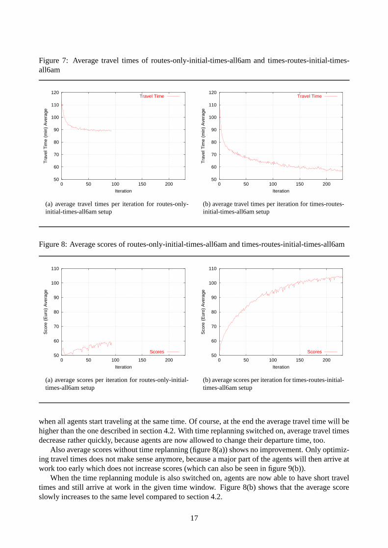
Figure 7: Average travel times of routes-only-initial-times-all6am and times-routes-initial-times-all6am

50

60

70

80

90

100

110

120

0 50 100 150 200

Tra

vel T

ime

(min

) A

vera

ge

Iteration

Travel Time

(a) average travel times per iteration for routes-only-initial-times-all6am setup

50

60

70

80

90

100

110

120

0 50 100 150 200

Tra

vel T

ime

(min

) A

vera

ge

Iteration

Travel Time

(b) average travel times per iteration for times-routes-initial-times-all6am setup

Figure 8: Average scores of routes-only-initial-times-all6am and times-routes-initial-times-all6am

50

60

70

80

90

100

110

0 50 100 150 200

Sco

re (

Eur

o) A

vera

ge

Iteration

Scores

(a) average scores per iteration for routes-only-initial-times-all6am setup

50

60

70

80

90

100

110

0 50 100 150 200

Sco

re (

Eur

o) A

vera

ge

Iteration

Scores

(b) average scores per iteration for times-routes-initial-times-all6am setup

when all agents start traveling at the same time. Of course, at the end the average travel time will behigher than the one described in section 4.2. With time replanning switched on, average travel timesdecrease rather quickly, because agents are now allowed to change their departure time, too.

Also average scores without time replanning (figure 8(a)) shows no improvement. Only optimiz-ing travel times does not make sense anymore, because a major part of the agents will then arrive atwork too early which does not increase scores (which can also be seen in figure 9(b)).

When the time replanning module is also switched on, agents are now able to have short traveltimes and still arrive at work in the given time window. Figure 8(b) shows that the average scoreslowly increases to the same level compared to section 4.2.

17

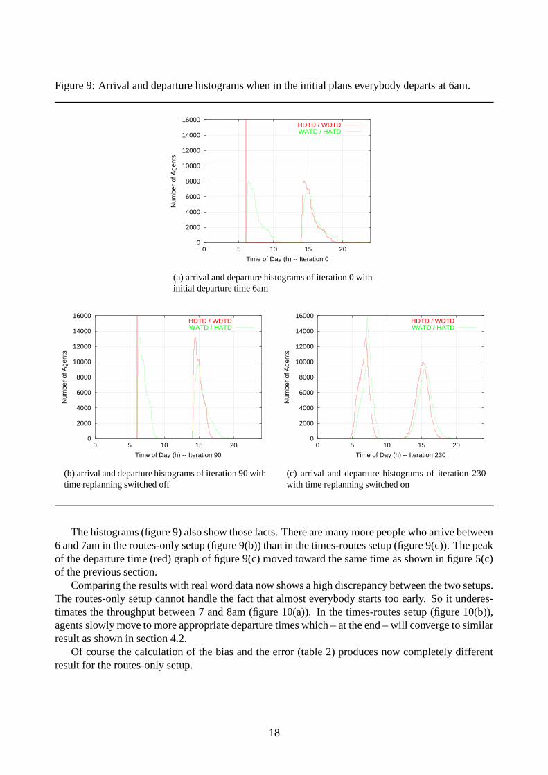
Figure 9: Arrival and departure histograms when in the initial plans everybody departs at 6am.

0

2000

4000

6000

8000

10000

12000

14000

16000

0 5 10 15 20

Num

ber

of A

gent

s



(a) arrival and departure histograms of iteration 0 withinitial departure time 6am

0

2000

4000

6000

8000

10000

12000

14000

16000

0 5 10 15 20

Num

ber

of A

gent

s



(b) arrival and departure histograms of iteration 90 withtime replanning switched off

0

2000

4000

6000

8000

10000

12000

14000

16000

0 5 10 15 20

Num

ber

of A

gent

s



(c) arrival and departure histograms of iteration 230with time replanning switched on

The histograms (figure 9) also show those facts. There are many more people who arrive between6 and 7am in the routes-only setup (figure 9(b)) than in the times-routes setup (figure 9(c)). The peakof the departure time (red) graph of figure 9(c) moved toward the same time as shown in figure 5(c)of the previous section.

Comparing the results with real word data now shows a high discrepancy between the two setups.The routes-only setup cannot handle the fact that almost everybody starts too early. So it underes-timates the throughput between 7 and 8am (figure 10(a)). In the times-routes setup (figure 10(b)),agents slowly move to more appropriate departure times which – at the end – will converge to similarresult as shown in section 4.2.

Of course the calculation of the bias and the error (table 2) produces now completely differentresult for the routes-only setup.

18

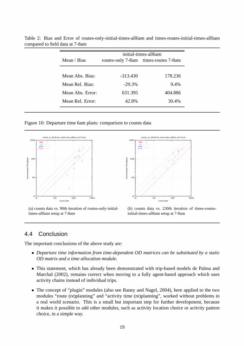
Table 2: Bias and Error of routes-only-initial-times-all6am and times-routes-initial-times-all6amcompared to field data at 7-8am

initial-times-all6amMean / Bias routes-only 7-8am times-routes 7-8am

Mean Abs. Bias: -313.430 178.236

Mean Rel. Bias: -29.3% 9.4%

Mean Abs. Error: 631.395 404.886

Mean Rel. Error: 42.8% 30.4%

Figure 10: Departure time 6am plans: comparison to counts data

10

100

1000

10000

10 100 1000 10000

Eve

nts-

base

d T

hrou

ghpu

t

Count Data

counts_vs_90.dil-zrh_routes-only_all6am_hrs7-8.out

datay=x

y=2xy=x/2

(a) counts data vs. 90th iteration of routes-only-initial-times-all6am setup at 7-8am

10

100

1000

10000

10 100 1000 10000

Eve

nts-

base

d T

hrou

ghpu

t

Count Data

counts_vs_230.dil-zrh_acts-routes_all6am_hrs7-8.out

datay=x

y=2xy=x/2

(b) counts data vs. 230th iteration of times-routes-initial-times-all6am setup at 7-8am

4.4 Conclusion

The important conclusions of the above study are:

• Departure time information from time-dependent OD matrices can be substituted by a staticOD matrix and a time allocation module.

• This statement, which has already been demonstrated with trip-based models de Palma andMarchal (2002), remains correct when moving to a fully agent-based approach which usesactivity chains instead of individual trips.

• The concept of “plugin” modules (also see Raney and Nagel, 2004), here applied to the twomodules “route (re)planning” and “activity time (re)planning”, worked without problems ina real world scenario. This is a small but important step for further development, becauseit makes it possible to add other modules, such as activity location choice or activity patternchoice, in a simple way.

19

5 Computational Issues

5.1 Mobility Simulation

Computational issues for the mobility simulation are discussed in detail elsewhere (Cetin and Nagel,2003). The main result from those investigations is that, using a Pentium cluster with 64 CPUs andMyrinet communication, the queue simulation can run more than 500 times faster than real time(excluding input and output), meaning that 24 hours of traffic of all of Switzerland can be simulatedin less than 3 minutes. For the results presented in this paper, two setups were run simultaneouslywith 12 CPU’s per setup using Ethernet communication. The average computation time is ca. 30minutes in order to simulate about 18 hours of traffic.

5.2 Performance

One iteration takes in the average about 102 minutes. The average duration of substeps of an iterationis listed below:

• about 18 sec for the departure time allocation module

• about 23 min for the router module, of which about 19 min is spent reading the events

• about 39 min for the mobility simulation module

• about 11 min for sorting events

• about 16 min for reading events and processing them into scores

• about 105 sec for writing the new plans

• the remaining time (about 12 min) are used for other I/O processes/bottlenecks, communica-tion and data preparations

With this, about 15 to 20 iterations are done per day.

5.3 Disk Usage

A complete data set generated by one iteration produces about 280 MB of data (when compressed).These will be kept for the first and the last 5 iterations and also for every 10th iteration. For each ofthe other iterations only about 40 MB are kept.

5.4 Memory Usage

Since we are simulating about 260’000 Agents which keep at most 5 different plans and each ofthem needs about 700 Bytes of memory plus some overhead, we end up by about 1 GB of Memory.The router module also needs about 200 MB of Memory, which is feasible at the moment but mightbecome problem for higher resolution networks.

20

6 Future Work

At present we only model the “primary” activities of “home” and “work”. We are working on adding“secondary” activities, such as shopping and leisure to the system. This requires the addition of twomore modules: the activity pattern generator and the activity location generator, which were men-tioned in Sec. 2. Another module we are interested in adding is a Population generation module,which would disaggregate demographic data to obtain individual households and individual house-hold members, with certain characteristics, such as a street address, car ownership, or householdincome (Beckman et al., 1996). The population would not match reality, but would result in thesame statistics. These modules should also be implemented as “plugins”. We are also investigatinginto other travel modes like public transport or pedestrian mode.

Another issue of interest is the possibility that agents could also learn during the day. They couldre-route while they are stuck in congestion, drop an activity because they are already too late, andso on. This “within day replanning” (e.g. Cascetta and Cantarella, 1991) should help to improvetheir strategies faster than only “day-by-day replanning” and the interaction with other entities (liketraffic lights, changing traffic signs and other ITS entities) can be added to the mobility simulation.Within-day learning is more realistic since some types of decisions are made on time scales muchshorter than a day (Doherty and Axhausen, 1998).

Simulation speedup can also be improved by elimination of performance bottlenecks. At themoment the agent database keeps track of all agents of the simulation. Since recalculating an agents’strategies is completely independent to other agents, it is useful to introduce parallelism into this.These “multiple agent databases” should then be controlled by a separate module which keeps trackof the feedback. This leads us to a clear separation of “agent databases” and “feedback”.

The activity time allocation module itself can be improved, too. It should recognize when agentsare too early or too late, so the adaption to a more realistic departure time should be done with feweriterations.

High resolution networks are another issue. Especially if there is more precise information avail-able about locations. The main goal will be that each agent has its home location at a street with ahouse number, probably a ramp to its garage, a private pedestrian path to the next tram station, andso on. In high resolution networks, intersection bottlenecks can be shown also at specific points in abig city. Last but not least, high resolution scenarios are indeed a computational challenge.

With high resolution networks, more precise count data is required to compare with. There issome effort to extract information of the raw data of the Kanton Zurich which gives more preciseinformation about local traffic situations.

7 Summary

The investigation described in this paper is part of a series of investigations to demonstrate the fea-sibility of multi-agent traffic simulations for transportation planning. This work should demonstratethe feasibility of this technology on a large scale, and it should be useful for research questions.

This paper presents intermediate results of this work. The intent was to test if the technology isable to generate plausible morning departure times by itself, rather than having to rely on externalinformation for this. The results show that this is possible, and that the results are no less realisticthan those obtained with an externally given departure time distribution. It is important to note thatthese results are achieved with an implementation which is both fully agent-based and fully basedon 24-hour daily activity plans. This is in contrast to previous implementations of similar scenarios.

21

The computational structure of the computational framework is such that fairly arbitrary modulescan be plugged in and used. The overall structure of this framework is that all agents keep multipleplans. In general, they select the best of those; sometimes, they re-evaluate one of the other plans;and some other times, they obtain a completely new plan. New plans can consist of new routes,which was already tested elsewhere, and of new times, which is tested in this paper. For this, avery simple random time modification module is used, which modifies times randomly in smallincrements. In conjunction with the scoring system, this is already enough to move all agents towarda departure time distribution that is realistic.

Acknowledgments

The ETH-sponsored 192-CPU Beowulf cluster “Xibalba” performed most of the computations.Marc Schmitt is doing a great job maintaining the computational system. Nurhan Cetin providedthe mobility simulation. The work also benefited from discussions with Fabrice Marchal.

References

R. Arnott, A. De Palma, and R. Lindsey. A structural model of peak-period congestion: A trafficbottleneck with elastic demand. The American Economic Review, 83(1):161, 1993.

E. Avineri and J.N. Prashker. Sensitivity to uncertainty: Need for paradigm shift. Paper 03-3744,Transportation Research Board Annual Meeting, Washington, D.C., 2003.

R. J. Beckman, K. A. Baggerly, and M. D. McKay. Creating synthetic base-line populations. Trans-portion Research Part A – Policy and Practice, 30(6):415–429, 1996.

J.A. Bottom. Consistent anticipatory route guidance. PhD thesis, Massachusetts Institute of Tech-nology, Cambridge, MA, 2000.

Bundesamt fur Statistik und Dienst fur Gesamtverkehrsfragen. Verkehrsverhal-ten in der Schweiz 1994. Mikrozensus Verkehr 1994, Bern, 1996. See alsohttp://www.statistik.admin.ch/news/archiv96/dp96036.htm.

E. Cascetta and C. Cantarella. A day-to-day and within day dynamic stochastic assignment model.Transportation Research A, 25A(5):277–291, 1991.

N. Cetin and K. Nagel. A large-scale agent-based traffic microsimulation based on queue model.In Proceedings of Swiss Transport Research Conference (STRC), Monte Verita, CH, 2003. Seewww.strc.ch.

D. Charypar and K. Nagel. Generating complete all-day activity plans with ge-netic algorithms. In Proceedings of the meeting of the International Associa-tion for Travel Behavior Research (IATBR), Lucerne, Switzerland, 2003. Seehttp://www.ivt.baum.ethz.ch/allgemein/iatbr2003.html.

A. de Palma and F. Marchal. Real case applications of the fully dynamic METROPOLIS tool-box:an advocacy for large-scale mesoscopic transportation systems. Networks and Spatial Economics,2(4):347–369, 2002.

22

S. T. Doherty and K. W. Axhausen. The developement of a unified modelling framework for thehousehold activity-travel scheduling process. In Verkehr und Mobilitat, number 66 in Stadt RegionLand. Institut fur Stadtbauwesen, Technical University, Aachen, Germany, 1998.

D. Ettema, G. Tamminga, H. Timmermans, and T. Arentze. A micro-simulation model system ofdeparture time and route choice under travel time uncertainty. In Proceedings of the meeting ofthe International Association for Travel Behavior Research (IATBR), Lucerne, Switzerland, 2003.See http://www.ivt.baum.ethz.ch/allgemein/iatbr2003.html.

R. R. Jacob, M. V. Marathe, and K. Nagel. A computational study of routing algorithms for realistictransportation networks. ACM Journal of Experimental Algorithms, 4(1999es, Article No. 6),1999.

David E. Kaufman, Karl E. Wunderlich, and Robert L. Smith. An iterative routing/assignmentmethod for anticipatory real-time route guidance. Technical Report IVHS Technical Report 91-02, University of Michigan Department of Industrial and Operations Engineering, Ann Arbor MI48109, May 1991.

F. Marchal, 2003. Personal communication.

K. Nagel. High-speed microsimulations of traffic flow. PhD thesis, University of Cologne, 1994/95.See www.inf.ethz.ch/˜nagel/papers or www.zaik.uni-koeln.de/˜paper.

K. Nagel, M. Strauss, and M. Shubik. The importance of timescales: Simple models for economicmarkets. Physica A, submitted.

B. Raney, N. Cetin, A. Vollmy, M. Vrtic, K. Axhausen, and K. Nagel. An agent-based microsim-ulation model of Swiss travel: First results. Networks and Spatial Economics, 3(1):23–41, 2003.Similar version Transportation Research Board Annual Meeting 2003 paper number 03-4267.

B. Raney and K. Nagel. Truly agent-based strategy selection for transportation simulations. Paper03-4258, Transportation Research Board Annual Meeting, Washington, D.C., 2003.

B. Raney and K. Nagel. An improved framework for large-scale multi-agent simulations of travelbehavior. In Proceedings of Swiss Transport Research Conference (STRC), Monte Verita, CH,2004. See www.strc.ch.

URBANSIM www page. URBANSIM. See www.urbansim.org, accessed 2003.

M. Vrtic and K.W. Axhausen. Experiment mit einem dynamischen umlegungsverfahren. Strassen-verkehrstechnik, 2002. Also Arbeitsberichte Verkehrs- und Raumplanung No. 138, seewww.ivt.baug.ethz.ch.

M. Vrtic, R. Koblo, and M. Vodisch. Entwicklung bimodales Personenverkehrsmodell als Grundlagefr Bahn2000, 2. Etappe, Auftrag 1. Report to the Swiss National Railway and to the Dienst furGesamtverkehrsfragen, Prognos AG, Basel, 1999. See www.ivt.baug.ethz.ch/vrp/ab115.pdf for arelated report.

23

Coupling activity-based demand generation to a truly … · Coupling activity-based demand...

Documents

Transcript of Coupling activity-based demand generation to a truly … · Coupling activity-based demand...