COUPLED SIMULATION MODELING OF FLATWOODS...

COUPLED SIMULATION MODELING OF FLATWOODS HYDROLOGY,

NUTRIENT AND VEGETATION DYNAMICS

By

LEI YANG

A DISSERTATION PRESENTED TO THE GRADUATE SCHOOL OF THE UNIVERSITY OF FLORIDA IN PARTIAL FULFILLMENT

OF THE REQUIREMENTS FOR THE DEGREE OF DOCTOR OF PHILOSOPHY

UNIVERSITY OF FLORIDA

2006

Copyright 2006

by

Lei Yang

This dissertation is dedicated to

my parents,

my high school teacher Zhiting Wang, and my friend Joseph S. Smith.

I recognize and appreciate the life-long influence they brought to me at different stages of

my life.

iv

ACKNOWLEDGMENTS

I am greatly indebted to my supervisor, Dr. Wendy D. Graham, for her constant

guidance, insight, encouragement, and continuous support as well as confidence in my

research over the past five years. Her thorough and thoughtful coaching with all aspects

of my research was unselfishly tireless, and her enthusiasm for research and quest for

excellence have left me an everlasting impression. I would like to express sincere

appreciation to Dr. Kenneth L. Campbell for his invaluable advice on addressing each of

my technical problems and concerns. Without his constant supervision and guidance

throughout the model development, the completion of this model would have been

impossible. I am grateful to Dr. James W. Jones for his insight and invaluable advice on

the methodology of the vegetation dynamic model and support in offering important crop

growth model related literature; to Dr. Mark W. Clark for introducing me to the niche

theory and the interactive relationship between wetland hydrology and vegetation

dynamics and his help in identifying pasture vegetation species for simulation; to Dr.

Gregory A. Kiker for introducing me to the Java programming language with his great

enthusiasm and his technical support regarding the ACRU2000 modeling system during

the model development. I deeply benefited from many hours of precious discussions

with each of these committee members on a multitude of perspectives regarding my

research. Without their combined supervision of each step throughout my research, this

study would not have been possible.

v

I would like to acknowledge my debt to Chris Martinez for his great cooperation as

a teammate throughout the development of hydrologic and nutrient models. I wish also

to thank Dr. Michael D. Annable for his generous comments on specific technical

problems during many brown-bag group meetings; Dr. Patrick Bohlen in MacArthur

Agro-ecology Research Center, Florida, for introducing me to the pasture sites at Buck

Island Ranch and offering useful documents; Mr. Gregory S. Hendricks for offerings of

data for Buck Island Ranch and nutrient related documents; Dr. Stuart J. Rymph from the

University of Wisconsin for providing important bahiagrass related documents; Ms.

Cheryl H. Porter for offering crop modeling documents; and Dr. William Wise and his

graduate student Min Joong Hyuk for helping with DHI software.

Also, special thanks go to a few friends including Joseph S. Smith, Tricia G. Smith,

Donna L. Miller, Paul Miller, and David R. Murphy for their friendship and support

throughout the past few years, especially during some tough times. I would like to

acknowledge all the good friends for their friendship. I am also grateful to several

labmates for their friendship and encouragement, and faculty, staff and students in the

Agricultural and Biological Engineering Department for the quality academic

environment.

Finally I particularly appreciate my parents and siblings for their unconditional

love, understanding, patience and encouragement. Without their affection, it would have

been even more difficult to complete this research.

vi

TABLE OF CONTENTS page ACKNOWLEDGMENTS ................................................................................................. iv

LIST OF TABLES...............................................................................................................x

LIST OF FIGURES ......................................................................................................... xiii

ABSTRACT.......................................................................................................................xx

CHAPTER 1 INTRODUCTION ........................................................................................................1

Study Background ........................................................................................................1 Overview of the Coupled Modeling System ................................................................8 Study Objectives...........................................................................................................9

2 LITERATURE REVIEW ...........................................................................................12

Overview of Previous Modeling Efforts.....................................................................12 ACRU2000 Modeling System....................................................................................20 Model Testing Procedures ..........................................................................................24

Model Calibration................................................................................................25 Model Validation.................................................................................................25 Sensitivity Analysis .............................................................................................26 Model Evaluation ................................................................................................28

Statistics .......................................................................................................28 Graphic representation .................................................................................31

3 HYDROLOGIC SIMULATION MODEL.................................................................34

Introduction.................................................................................................................34 Vertical Hydrologic Components ...............................................................................38

Rainfall ................................................................................................................38 Canopy Interception ............................................................................................38 Evapotranspiration...............................................................................................39 Infiltration............................................................................................................42 Soil Water Redistribution ....................................................................................42 Upward Flux........................................................................................................43 Deep Seepage ......................................................................................................44

vii

Horizontal Hydrologic Components...........................................................................44 Overland Flow.....................................................................................................45

Overland flow calculation ............................................................................46 Surface water storage apportionment ...........................................................49

Groundwater Flow...............................................................................................51 Lateral groundwater flow calculation ..........................................................54 Groundwater storage apportionment ............................................................56

Canal Flow...........................................................................................................56 Initial and Boundary Conditions.................................................................................57 Model Testing and Validation ....................................................................................58

Simulation Sequence and Model Performance Accuracy Analysis ....................58 Case 1: Overland flow along a flat rectangular plane ..................................60 Case 2: Overland and groundwater flow over an axisymmetric domain .....65

Application at Dry Lake Dairy #1, Kissimmee River Basin, Florida .................76 Site description.............................................................................................76 Results and discussion..................................................................................79

Concluding Remarks ..................................................................................................82 4 NUTRIENT SIMULATION MODEL .......................................................................87

Introduction.................................................................................................................87 Nutrient Components..................................................................................................89

Nitrogen Cycle Components ...............................................................................89 Mineralization ..............................................................................................91 Immobilization .............................................................................................92 Denitrification ..............................................................................................92 Runoff, sediment transport and percolation .................................................93 Uptake, evaporation, and fixation ................................................................94 Rainfall and fertilizer ...................................................................................95 Ammonia volatilization................................................................................95 Surface and subsurface lateral nitrate nitrogen transport .............................95 Surface and subsurface lateral ammonium nitrogen transport .....................97

Phosphorus Cycle Components ...........................................................................98 Mineralization ..............................................................................................99 Immobilization ...........................................................................................100 Runoff, sediment, percolation ....................................................................100 Uptake and evaporation..............................................................................101 Rainfall and fertilizer .................................................................................101 Surface and subsurface lateral labile phosphorus transport .......................102

Conservative Solute Transport Components .....................................................104 Initial and Boundary Conditions...............................................................................105 Model Testing and Validation ..................................................................................106

Conservative Solute Test ...................................................................................106 Scenario description ...................................................................................107 Results and discussion................................................................................107

Application at Buck Island Ranch, Lake Okeechobee Basin, Florida ..............111 Project description......................................................................................111

viii

Sensitivity analysis .....................................................................................117 Results and discussion................................................................................122

Concluding Remarks ................................................................................................133 5 VEGETATION DYNAMICS SIMULATION MODEL .........................................189

Introduction...............................................................................................................189 Methodology.............................................................................................................192

Model Structure .................................................................................................192 Plant Growth......................................................................................................193

Potential growth .........................................................................................193 Reduced growth..........................................................................................196 Dry matter partitioning...............................................................................197

Leaf Area Index.................................................................................................197 Plant Senescence ...............................................................................................198 Evapotranspiration.............................................................................................200 Nitrogen Uptake ................................................................................................201 Phosphorus Uptake............................................................................................204 Growth Reduction Factor ..................................................................................205

Water stress and logging factors ................................................................206 Nitrogen stress factor .................................................................................208 Phosphorus stress factor .............................................................................209

Hypothetical Scenario Model Testing ......................................................................209 Scenario Description .........................................................................................209 Results and Discussion ......................................................................................213

Water and nutrient responses to water retention BMP...............................213 Influence of differences in temperature sensitivities among species .........214 Species composition dynamics due to water retention BMP .....................216

Concluding Remarks ................................................................................................219 6 SUMMARY AND CONCLUSIONS.......................................................................234

Hydrologic Simulation Model ..................................................................................235 Nutrient Simulation Model .......................................................................................236 Vegetation Dynamics Simulation Model..................................................................237 Implications of the Research ....................................................................................238 Future Research Recommendations .........................................................................238

Model Pre- and Post-processing Capacity.........................................................238 Use Consistent Units for Parameters and Variables..........................................239 Documentation ..................................................................................................239 Potential Changes to Existing Objects ..............................................................239 Sub-Daily Time Step .........................................................................................240 Herbivore Movement Module ...........................................................................240 Hydrologic Model .............................................................................................240 Nutrient Model ..................................................................................................241 Vegetation Model ..............................................................................................241

ix

APPENDIX A FLOW CHART FOR THE COUPLED MODELING SYSTEM AND MODEL

PROCESSES ............................................................................................................242

B FLOW CHART OF LATERAL GROUNDWATER FLOW SIMULATION.........247

C LISTS OF NEW AND MODIFIED OBJECTS .......................................................248

D LISTS OF NEW INPUT AND OUTPUT VARIABLES.........................................262

E LISTS OF MODEL INPUT FILES..........................................................................265

F ALGORITHMS OF WATER STORAGE APPORTIONMENT.............................266

LIST OF REFERENCES.................................................................................................282

BIOGRAPHICAL SKETCH ...........................................................................................293

x

LIST OF TABLES

Table page 3-1 List of strategies for water transmission and water storage updating for

simulation sequence experiments. .........................................................................59

3-2 Statistics for the surface water depths predicted by the modified ACRU2000 model and MIKE SHE for the three experiments with the same simulation sequence.................................................................................................................62

3-3 Statistics for the surface water depths predicted by the modified ACRU2000 model and MIKE SHE for the three experiments..................................................69

3-4 Statistics for the simulated groundwater table depths by the modified ACRU2000 model, MIKE SHE, and MODFLOW for the three experiments with the same simulation sequence........................................................................75

3-5 Summary of annual water budget on Dry Lake Dairy #1 site. ..............................78

3-6 Model input parameters for the Dry Lake Dairy #1 site. .......................................85

3-7 Statistics for the simulated surface runoff and groundwater table depths by the modified ACRU2000 and FHANTM. ...................................................................85

4-1 Statistics for the solute mass predicted by the modified ACRU2000..................108

4-2 List of stocking activities for pastures S1, S4, W6 and W7. ...............................137

4-3 List of fertilization activities for pastures S1 and S4...........................................137

4-4 List of burn activities for pastures S1, S4, W6 and W7.......................................137

4-5 Percent of area occupied by different soil series and wetlands in selected summer and winter pastures.................................................................................137

4-6 Model input parameters for the winter pastures W6 and W7. .............................138

4-7 Model input parameters for the summer pastures S4 and S1...............................139

4-8 Selected hydrologic parameters for sensitivity analysis for W6..........................140

4-9 Selected nutrient parameters for sensitivity analysis for W6...............................141

xi

4-10 Selected hydrologic parameters for sensitivity analysis for S4. ..........................142

4-11 Selected nutrient parameters for sensitivity analysis for S4. ...............................143

4-12 Sensitivities of total surface runoff of the selected input parameters throughout the simulation period for the calibration site W6.................................................144

4-13 Sensitivities of maximum water table to the selected input parameters depth throughout the simulation period for the calibration site W6. .............................144

4-14 Sensitivities of total P loads to the selected input parameters throughout the simulation period for the calibration site W6. .....................................................144

4-15 Sensitivities of total N loads to the selected input parameters throughout the simulation period for the calibration site W6. .....................................................144

4-16 Sensitivities of total surface runoff to the selected input parameters throughout the simulation period for the calibration site S4. .................................................145

4-17 Sensitivities of maximum water table to the selected input parameters depth throughout the simulation period for the calibration site S4................................145

4-18 Sensitivities of total P loads to the selected input parameters throughout the simulation period for the calibration site S4. .......................................................145

4-19 Sensitivities of total N loads to the selected input parameters throughout the simulation period for the calibration site S4. .......................................................145

4-20 Annual water budget for the calibration site W6. ................................................146

4-21 Annual water budget for the verification site W7................................................146

4-22 Annual water budget for the calibration site S4...................................................146

4-23 Annual water budget for the verification site S1. ................................................146

4-24 Monthly statistics for the calibration site W6......................................................147

4-25 Annual statistics for the calibration site W6........................................................147

4-26 Monthly statistics for the verification site W7.....................................................147

4-27 Annual statistics for the verification site W7.......................................................147

4-28 Monthly statistics for the calibration site S4........................................................148

4-29 Annual statistics for the calibration site S4..........................................................148

4-30 Monthly statistics for the verification site S1 ......................................................148

xii

4-31 Annual statistics for the verification site S1 ........................................................148

5-1 Percent cover of vegetation on summer pastures S4. ..........................................222

5-2 Parameter values for the different plant species for the vegetation model. .........222

5-3 Initial composition percentage and amount for species in each land segment. ...223

5-4 Variables calculated from other models. .............................................................223

5-5 Output variables from the vegetation model........................................................223

5-6 Testing scenarios for temperature functions. .......................................................223

E-1 New input and output variables required towards the multi-directional spatial simulation beyond the existing variables in ACRU2000.....................................262

xiii

LIST OF FIGURES

Figure page 1-1 Schematic of the feedback relationships among hydrology, nutrient, and

vegetation dynamics in the coupled model system..................................................8

2-1 General structure of the lumped ACRU (v3.00) model.........................................21

2-2 Land segment configuration of the ACRU2000 model .........................................23

3-1 Schematic of an example catchment and its spatial discretization. .......................35

3-2 Hydrological processes in the modified ACRU2000 hydrologic model. ..............36

3-3 Configuration of overland flows between source land segment and adjacent land segments.................................................................................................................46

3-4 The relationship between Manning's roughness-coefficient (n) to water depth and to plant height, both of which change dynamically in the model ...................48

3-5 Structured boundary...............................................................................................49

3-6 Schematic representation of the lateral groundwater flow from the higher head hs to the lower head hd. (A) and (B) represent the situations without and with overland flow, respectively....................................................................................52

3-7 Diagram of lateral groundwater flow between two land segments. (A) and (B) represent the generalized situations without and with overland flow, respectively. ...........................................................................................................53

3-8 A rectangular plane with 20 land segments (arrow indicates water movement direction and digits assigned in each grid cell indicate the number for each land segment). ................................................................................................................60

3-9 Comparisons of the simulated surface water depth from the modified ACRU2000 model on the three experiments between two opposite simulation sequences. ..............................................................................................................63

3-10 Comparisons of the simulated surface water depths between the MIKE SHE’s overland flow model and the modified ACRU2000 hydrologic model on the three experiments with the simulation sequence from LS1 to LS20. ....................64

xiv

3-11 Schematics of two-dimensional axisymmetric domain (left) and its three-dimensional discretization (right). The digits assigned in the left diagram indicate the number for each land segment............................................................66

3-12 Comparisons of simulated water depths of the selected land segments between the modified ACRU2000 model and the MIKE SHE’s overland flow model for the three experiments. ............................................................................................68

3-13 Comparisons of the simulated water depths of the selected land segments between the modified ACRU2000 and MIKE SHE’s overland flow model for Experiment 3..........................................................................................................70

3-14 Comparisons of the groundwater table depths at the selected land segments between and the modified ACRU2000 hydrologic model and MIKE SHE’s groundwater flow model for the three experiments. ..............................................74

3-15 Location of Dry Lake Dairy #1 site. ......................................................................76

3-16 Dry Lake Dairy # 1 site map, topographic survey and location of well stations and tracer application compound. Distance scales are in feet and elevation contours are in feet above mean sea level..............................................................77

3-17 Comparisons of the continuous simulations of runoff from the modified ACRU2000 and FHANTM against the observed data. .........................................84

3-18 Comparisons of the cumulative simulated runoff from the modified ACRU2000 and FHANTM with the cumulative observed data. ...............................................84

3-19 Comparisons of the continuous simulation of groundwater table depths from the modified ACRU2000 and FHANTM against the observed data. ..........................85

3-20 Scatterplots of observed vs. simulated surface runoff depths predicted by the modified ACRU2000 and FHANTM. ...................................................................86

3-21 Scatterplots of observed vs. simulated groundwater table depths predicted by the modified ACRU2000 and FHANTM. ...................................................................86

4-1 Schematic representation of the GLEAMS nitrogen cycle....................................90

4-2 Schematic representation of the GLEAMS phosphorus cycle...............................98

4-3 Comparisons of the solute mass in the 3rd and 4th soil layers of selected land segments between the modified ACRU2000 and PMPATH...............................110

4-4 Location of MacArthur Agro-ecology Research Center......................................111

4-5 General layout of the project field . .....................................................................113

xv

4-6 Relative sensitivities of the total surface runoff of 6-year simulation period over the selected input parameters for the pasture sites W6 and S4. ...........................149

4-7 Relative sensitivities of the maximum water table depth of 6-year simulation period over the selected input parameters for the pasture sites W6 and S4.........150

4-8 Relative sensitivities of the total P load of 6-year simulation period over the selected input parameters and variables for the pasture sites W6 and S4............151

4-9 Relative sensitivities of the total N load of 6-year simulation period over the selected input parameters for the pasture sites W6 and S4..................................152

4-10 Continuous simulation of groundwater table depth from September 2000 through December 2003 for the calibration site W6............................................153

4-11 Continuous simulation of groundwater table depth from September 2000 through December 2003 for the verification site W7. .........................................153

4-12 Continuous simulation of groundwater table depth from September 2000 through December 2003 for the calibration site S4. ............................................154

4-13 Continuous simulation of groundwater table depth from September 2000 through December 2003 for the verification site S1............................................154

4-14 Continuous simulation of surface runoff from July 1998 through December 2003 for the calibration site W6...........................................................................155

4-15 Continuous simulation of surface runoff from July 1998 through December 2003 for the verification site W7. ........................................................................155

4-16 Continuous simulation of surface runoff from July 1998 through December 2003 for the calibration site S4. ...........................................................................156

4-17 Continuous simulation of surface runoff from July 1998 through December 2003 for the verification site S1...........................................................................156

4-18 Continuous simulation of P loads from July 1998 through December 2003 for the calibration site W6. ........................................................................................157

4-19 Continuous simulation of P loads from July 1998 through December 2003 for the verification site W7........................................................................................157

4-20 Continuous simulation of P loads from July 1998 through December 2003 for the calibration site S4...........................................................................................158

4-21 Continuous simulation of P loads from July 1998 through December 2003 for the verification site S1. ........................................................................................158

xvi

4-22 Continuous simulation of N loads from July 1998 through December 2003 for the calibration site W6. ........................................................................................159

4-23 Continuous simulation of N loads from July 1998 through December 2003 for the verification site W7........................................................................................159

4-24 Continuous simulation of N loads from July 1998 through December 2003 for the calibration site S4...........................................................................................160

4-25 Continuous simulation of N loads from July 1998 through December 2003 for the verification site S1. ........................................................................................160

4-26 Continuous simulation of surface runoff P concentrations from July 1998 through December 2003 for the calibration site W6............................................161

4-27 Continuous simulation of surface runoff P concentrations from July 1998 through December 2003 for the verification site W7. .........................................161

4-28 Continuous simulation of surface runoff N concentrations from July 1998 through December 2003 for the calibration site W6............................................162

4-29 Continuous simulation of surface runoff N concentrations from July 1998 through December 2003 for the verification site W7. .........................................162

4-30 Continuous simulation of surface runoff P concentrations from July 1998 through December 2003 for the calibration site S4. ............................................163

4-31 Continuous simulation of surface runoff P concentrations from July 1998 through December 2003 for the calibration site S1. ............................................163

4-32 Continuous simulation of surface runoff N concentrations from July 1998 through December 2003 for the verification site S4............................................164

4-33 Continuous simulation of surface runoff N concentrations from July 1998 through December 2003 for the verification site S1............................................164

4-34 Linear plots of monthly and annual surface runoff from 1998 to 2003 for the calibration site W6. ..............................................................................................165

4-35 Linear plots of monthly and annual surface runoff from 1998 to 2003 for the verification site W7..............................................................................................166

4-36 Linear plots of monthly and annual water table depth from 1998 to 2003 for the calibration site W6. ..............................................................................................167

4-37 Linear plots of monthly and annual water table depth from 1998 to 2003 for the verification site W7..............................................................................................168

xvii

4-38 Linear plots of monthly and annual P load from 1998 to 2003 for the calibration site W6. ................................................................................................................169

4-39 Linear plots of monthly and annual P load from 1998 to 2003 for the verification site W7..............................................................................................170

4-40 Linear plots of monthly and annual N load from 1998 to 2003 for the calibration site W6. ................................................................................................................171

4-41 Linear plots of monthly and annual N load from 1998 to 2003 for the verification site W7..............................................................................................172

4-42 Linear plots of monthly and annual surface runoff from 1998 to 2003 for the calibration site S4.................................................................................................173

4-43 Linear plots of monthly and annual surface runoff from 1998 to 2003 for the verification site S1. ..............................................................................................174

4-44 Linear plots of monthly and annual water table depth from 1998 to 2003 for the calibration site S4.................................................................................................175

4-45 Linear plots of monthly and annual water table depth from 1998 to 2003 for the verification site S1. ..............................................................................................176

4-46 Linear plots of monthly and annual P load from 1998 to 2003 for the calibration site S4...................................................................................................................177

4-47 Linear plots of monthly and annual P load from 1998 to 2003 for the verification site S1. ..............................................................................................178

4-48 Linear plots of monthly and annual N load from 1998 to 2003 for the calibration site S4...................................................................................................................179

4-49 Linear plots of monthly and annual N load from 1998 to 2003 for the verification site S1. ..............................................................................................180

4-50 Duration curves of daily surface runoff and water table depth for the calibration site W6. ................................................................................................................181

4-51 Duration curves of daily P and N loads for the calibration site W6. ...................182

4-52 Duration curves of daily surface runoff and water table depth for the verification site W7. ................................................................................................................183

4-53 Duration curves of daily P and N loads for the verification site W7...................184

4-54 Duration curves of daily surface runoff and water table depth from 1998 to 2003 for the calibration site S4. ....................................................................................185

xviii

4-55 Duration curves of daily N and P loads from 1998 to 2003 for the calibration site S4...................................................................................................................186

4-56 Duration curves of daily surface runoff and water table depth from 1998 to 2003 for the verification site S1....................................................................................187

4-57 Duration curves of daily N and P loads from 1998 to 2003 for the verification site S1...................................................................................................................188

5-1 Diagram for daily plant growth in relation to weather and water and nutrient availabilities (DM = dry matter; N = nitrogen; P = phosphorus; and SLA = specific leaf area). ................................................................................................193

5-2 Diagram of temperature function for species i. ...................................................195

5-3 An example relationship between plant biomass nitrogen concentration and growth ratio..........................................................................................................202

5-4 An example relationship between plant biomass phosphous concentration and growth ratio..........................................................................................................204

5-5 Aerial photo showing the layout of the improved summer pasture site S4 and location of associated instrumentation. S1 to S6 indicate the individual summer pasture sites and LS1 to LS12 indicate the land segments divided for the site S4. The dotted lines were made to show the boundary between land segments........210

5-6 Continuous simulation of surface runoff throughout the simulation period from 1998 to 2003. .......................................................................................................224

5-7 Continuous simulation of water table depths at land segment 9 throughout the simulation period from 1998 to 2003...................................................................224

5-8 Continuous simulation of P loads throughout the simulation period from 1998 to 2003......................................................................................................................225

5-9 Continuous simulation of N loads throughout the simulation period from 1998 to 2003. ................................................................................................................225

5-10 Continuous simulation of P concentrations throughout the simulation period from 1998 to 2003................................................................................................226

5-11 Continuous simulation of N concentrations throughout the simulation period from 1998 to 2003................................................................................................226

5-12 Comparison of predicted potential aboveground biomass for species in land segment 11 with different temperature functions. ...............................................227

xix

5-13 Comparison of temperature factors among the three selected species in land segment 11. ..........................................................................................................228

5-14 Species distribution (percent of total aboveground biomass at the end of each year) over land segments for bahia, floralta and panicum throughout the simulation period from 1998 to 2003...................................................................230

5-15 Comparisons of continuous simulation of aboveground biomass for all species in the selcted land segments 8, 11, and 12 before water retention BMP. ............231

5-16 Comparisons of continuous simulation of aboveground biomass for all species in the selcted land segments 8, 11, and 12 after water retention BMP. ...............232

5-17 Growth limiting factors for bahiagrass in land segment 8 before water retention BMP was applied. ................................................................................................233

G-1 Single land segment type neighbor receiving overland flow...............................266

G-2 Single river type neighbor receiving overland flow ............................................267

G-3 Configuration of multiple directional overland flows from source land segment to adjacent land segments. ...................................................................................269

xx

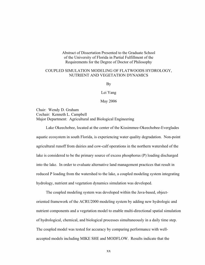
Abstract of Dissertation Presented to the Graduate School of the University of Florida in Partial Fulfillment of the Requirements for the Degree of Doctor of Philosophy

COUPLED SIMULATION MODELING OF FLATWOODS HYDROLOGY, NUTRIENT AND VEGETATION DYNAMICS

By

Lei Yang

May 2006

Chair: Wendy D. Graham Cochair: Kenneth L. Campbell Major Department: Agricultural and Biological Engineering

Lake Okeechobee, located at the center of the Kissimmee-Okeechobee-Everglades

aquatic ecosystem in south Florida, is experiencing water quality degradation. Non-point

agricultural runoff from dairies and cow-calf operations in the northern watershed of the

lake is considered to be the primary source of excess phosphorus (P) loading discharged

into the lake. In order to evaluate alternative land management practices that result in

reduced P loading from the watershed to the lake, a coupled modeling system integrating

hydrology, nutrient and vegetation dynamics simulation was developed.

The coupled modeling system was developed within the Java-based, object-

oriented framework of the ACRU2000 modeling system by adding new hydrologic and

nutrient components and a vegetation model to enable multi-directional spatial simulation

of hydrological, chemical, and biological processes simultaneously in a daily time step.

The coupled model was tested for accuracy by comparing performance with well-

accepted models including MIKE SHE and MODFLOW. Results indicate that the

xxi

coupled model is capable of simulating, with reasonable accuracy, hydrological and

solute transport processes for the hypothetical scenarios. Additionally, the model was

tested in the Kissimmee River Basin and Lake Okeechobee Basin by comparing with the

FHANTM model and against measured data. These applications demonstrated that the

coupled model is statistically close to the performance of FHANTM with respect to

hydrologic response in the Kissimmee River Basin, but much better than FHANTM with

regard to hydrologic and nutrient responses in the Lake Okeechobee Basin. From the

testing, it was concluded that the model is able to continuously simulate the surface

runoff and groundwater tables with adequate accuracy. However the model’s capacity to

simulate nutrient loading needs further testing after sufficient reliable nutrient data

becomes available. The vegetation model, coupled with the hydrologic and nutrient

models, was tested for a hypothetical scenario based on the conditions in the Lake

Okeechobee Basin. The test results show that the temporal and spatial vegetation

composition pattern can be an indicator of the ecohydrological impacts of alternative land

management practices. However, for actual application of this model, further testing is

required when more vegetation data are available.

Recommended future research includes further development of the coupled model

to enable a user-friendly pre- and post-processing graphical interface, an option for sub-

daily time steps, beef-cattle roaming simulation, and plant competition. Further testing of

the coupled model should be conducted at larger watershed scales and for the nutrient and

vegetation simulations when additional data are available.

1

CHAPTER 1 INTRODUCTION

Study Background

Lake Okeechobee is a large, multi-functional lake located at the center of the

Kissimmee-Okeechobee-Everglades aquatic ecosystem in south Florida. The lake

provides regional flood protection, water supply for agricultural, urban and natural areas,

and is a critical habitat for fish, birds and other wildlife. Water quality in the lake has

declined over recent decades due to urban development, channelization of the Kissimmee

River and agricultural operations. The 1997 Lake Okeechobee Surface Water

Improvement and Management Plan (South Florida Water Management District

[SFWMD], 1997a) found that excess phosphorus (P) loading is one of the most serious

problems the lake is facing.

The Lake Okeechobee watershed, with an area of 12,000 km2 extending from

Orlando to the Everglades, lies predominately in the southern Florida flatwoods

physiographic region characterized by flat, poorly drained, high-water table, and fine

sandy soils, which consist of Spodosols, Entisols, and Histosols (United States

Department of Agriculture [USDA], 1990). The majority of the soils in the northern

watersheds of the lake are Sposodols, with 8-20 cm thick surface horizons underlain by

spodic horizons at depth of 0.5 m to greater than 2 m (USDA, 1990). These soils, with

greater than 90% sand, are characterized by high infiltration rates and poor internal

drainage due to low permeability of the spodic horizon. When rainfall occurs, the soils

often become saturated in a short time. The water table is commonly within 1 m of the

2

ground surface during the wet season and may recede to 2 m depth during the dry season

(Knisel et al., 1985). With highly permeable surface soils there is little surface runoff

until the soil pore space is filled with water and the water table reaches the surface

(Heatwole et al., 1987); slow downward or lateral movement of water and solutes occurs

with water table recession.

The land use in the Okeechobee watershed is primarily beef cattle, dairy, and citrus.

Since 1930, ranching has intensified from native pastures to improved pastures with high

quality grasses and legumes, drainage and fertilization. During the 1950s, the dairy

industry first moved to Okeechobee County, and by the mid-1980s, there were 49

milking barns and 50,000 milk cows in the lower Kissimmee River (LKR) and Taylor

Creek/Nubbin Slough (TCNS) regions (Flaig and Reddy, 1995). The primary feed for

dairy cows, including high P containing materials, was imported into the watershed.

Animal waste management was almost non-existent until the 1970s (Flaig and Reddy,

1995). Historically, the majority of P load to the lake was derived from the LKR and the

TCNS basins with 13% contributed by the LKR basin and 22% by the TCNS basin. With

the implementation of improved management practices during recent decades, the P load

from the TCNS basin has decreased by 17% (Gunsalus et al., 1992), and the LKR basin

now provides the greatest P load to the lake. Previous studies have indicated that non-

point agricultural runoff in the northern watershed of the lake is considered to be the

primary source of excess P being discharged into Lake Okeechobee, which typically

exceeds the recommended total maximum daily loading (TMDL = 140 metric ton/year).

P in agricultural runoff mainly originates from one or more of four sources: fertilizers,

3

animal manures, mineralization of organic materials, and/or atmospheric deposition. The

first three sources can be controlled by agricultural best management practices.

In order to protect the water quality of Lake Okeechobee and reach environmental

restoration goals, a variety of best management practices (BMPs) have been implemented

in the Lake Okeechobee watershed. BMPs are on-farm activities designed to reduce

nutrient losses in drainage waters to an environmentally acceptable level, while

simultaneously maintaining an economically viable farming operation (Bottcher et al.,

1995). To reduce P loading one must either reduce P concentration or water volume.

According to Bottcher et al. (1995), there are three ways to reduce P concentrations in the

runoff water from agriculture: 1) reduce the amount of P on the farm by minimizing P

inputs to the farm and maximizing non-runoff P output from the farm; 2) reduce the

hydrologic mobility of the P that is on the farm by limiting water contact and/or reducing

the solubility or erodibility of phosphatic materials; 3) edge of field/farm pre-discharge

treatment using uptake, adsorption, deposition, or precipitation technologies, such as

wetland and/or chemical additives. There are two methods used to reduce water runoff

volume: 1) increase the evapotranspiration from the farm; 2) decrease off-farm or

groundwater irrigation water inputs to the farm by improved irrigation efficiency or by

using storage runoff as a substitute irrigation supply. From numerous studies in the

Okeechobee basin as well as generally accepted practices from other parts of the country,

Bottcher et al. (1995) summarized the BMPs appropriate for the Lake Okeechobee basin

as follows: 1) fertility BMPs including calibrated soil testing (CST), banding of fertilizer,

prevention of misplaced fertilizer, and split application; 2) animal manure BMPs

including dairy high intensity area (HIA) drainage control, collection and distribution of

4

barn manure, watering, feed and shade facilities placement, fencing animals from ditches

and streams, grazing management, selecting high P uptake crops from manure application

areas, and composting; 3) general BMPs including crop management, irrigation and

drainage management, maximum flow distance for P control, flow-way buffer strips,

limit drainage of organic and/or wetland soils, and alternative land use; 4) edge-of-

field/farm treatment including runoff retention/detention system, use of wetlands, and

chemical treatment.

Only a few of the above listed BMPs have been field tested, and even those were

tested for only a limited set of conditions (Bottcher et al., 1995). Flaig and Reddy (1995)

indicated that implementation of BMPs has not been sufficient to meet P load reduction

goals, and additional P control practices to further reduce P are needed. Recent BMPs

efforts to reduce nutrient loading from the Lake Okeechobee watershed have focused on

restoration of wetlands for their particular capacities to reduce nutrient loadings, thereby

reducing eutrophication in adjacent water bodies.

Wetlands are an important component of the Lake Okeechobee watershed.

However, many of these wetlands have disappeared or have been degraded due to

hydrologic alteration, urbanization and agricultural practices. Seasonal and year-round

isolated and connected wetlands used to occupy 25% of the watershed area (McCaffery et

al., 1976). Now many isolated wetlands are connected by shallow drainage ditches and

have been converted into pastures. Currently, wetlands represent about 15% of the land

area in the Lake Okeechobee watershed (Flaig and Havens, 1995). Wetland loss

inevitably leads to loss of biological, environmental quality and socio-functions such as

5

flood storage, groundwater recharge, sediment trapping, retention and removal of

nutrients and pollutants, and wildlife and recreational habitat (Davis and Froend, 1999).

Among all wetland functions, transport and transformation processes including

sedimentation, sediment adsorption, nutrient uptake, microbial assimilation and

transformations, and denitrification may be the most important mechanisms as they are

responsible for nutrient removal or retention. Fisher and Acreman (2004) investigated 57

wetlands from around the world and indicated that the majority of wetlands reduced

nutrient loading and there was little difference in the proportion of wetlands that reduced

nitrogen (N) to those that reduced P loading. However, they also pointed out that some

wetlands increased nutrient loading by increasing the loading of soluble N and P species,

thus potentially driving aquatic eutrophication. Busnardo et al. (1992) researched the

effect of hydroperiod on nutrient removal efficiency in replicate wetland mesocosms and

concluded that alternate draining and flooding of sediments (pulsed discharge) increased

nutrient removal efficiency compared to the continuous-flow “control”. Uusi-Kamppa et

al. (1997) indicated that in many wetlands the retention of soluble P is much less efficient

than that of particulate P. Also, waterlogged sediments are known to release P into

overlying waters (Mortimer, 1941), where it is more likely to be exported from the

watershed.

Denitrification, which occurs under anaerobic conditions to release N into the

atmosphere, is believed by many to be the major mechanism of N loss in wetlands.

Denitrification rates can be limited by carbon availability and, in this way, vegetation can

influence denitrification rates indirectly (Broadbent and Clark, 1965). Vegetation may

also influence nitrification and denitrification by influencing the oxygen concentration of

6

the wetland substrate within the rhizosphere (Armstrong, 1964) or by providing bacteria

which can fix N in root nodules. There is evidence that N removal efficiency is not

affected by the length of time the wetland has received N pollution while, in contrast, the

ability of a wetland to remove P is known to decline with time (Nichols, 1983;

Richardson, 1985).

Wetlands are not stand-alone ecosystems. They impact hydrology, water quality

and vegetation dynamics throughout the watershed. Wetlands are characterized by the

periodic excess of water inflow over outflow that provides a saturated substrate. The

effect of this characteristic is substantial water storage within wetlands and the

development of a readily identifiable wetlands flora and fauna which are adapted to

periodic anoxic conditions (Bradley and Gilvear, 2000). P loading can alter plant

communities through increased plant productivity, tissue P storage, soil P enrichment,

and shifts in plant species composition (Davis, 1991; Urban et al., 1993; Chiang et al.,

2000). Altered hydrologic regime, caused by water management infrastructure and

operations, can also affect the pattern of vegetation communities. Newman et al. (1996)

showed that P concentration and water depth are two important driving forces for cattail

invasion into the Everglades. Urban et al. (1993) also indicated that a combination of

prolonged hydroperiod and P loading stimulates cattail reproduction and encroachment

and thus results in the degradation of vegetative habitats and other ecological

characteristics in wetlands. Conversely, the physical and physiological characteristics of

vegetation influence hydrological response and nutrient cycling. The flora and fauna

impact the hydrology of many wetlands in that their incomplete decomposition leads to

the progressive development of an organic substrate that itself influences the pattern and

7

direction of water flow through wetlands and the quantity of water storage (Bradley and

Gilvear, 2000). Gurnell et al. (2000) indicated that interception, evapotranspiration, and

infiltration processes are particularly heavily influenced by the characteristics and

dynamics of the vegetation cover. Many ecologists have recognized that changing

vegetation pattern/structure causes feedback that can alter rates of hydrologic processes

and nutrient cycling, which, in turn, can cause additional changes in vegetation structure

(Lauenroth et al., 1993).

From the above discussion, it is clear that it is critical to understand the role of both

BMPs and wetland functions in nutrient removal, retention and storage in order to reduce

P loading into Lake Okeechobee. However, it is impractical to test all BMPs for their

effectiveness through field experiments. The use of computer models is therefore

beneficial because simulation results can not only predict how well a proposed BMP or

combined BMPs will reduce P loads, but can also quantitatively evaluate specific

hydrologic and biogeochemical processes associated with management activities for

BMP design and optimization.

Ecohydrologic modeling that simulates hydrological, biochemical and ecological

processes and their interrelations in soil and water bodies has captured the attention of

hydrologists and other scientists in recent years. Modeling provides a useful tool for

gaining insight into ecohydrological processes and evaluating management practices if

model predictions are accurate. Many models have been developed but they are typically

linked to the regions where they were developed and tested for a specific purpose and are

often limited to specific spatial scales. The unique flatwoods hydrology in the Lake

Okeechobee watershed requires the design of a model that can simulate integrated

8

multidimensional surface and subsurface water, nutrient, and vegetation dynamics at

multiple temporal and spatial scales.

Overview of the Coupled Modeling System

For this study, a coupled modeling system that enables the distributed simulation of

hydrology, water quality and vegetation dynamics was developed for Okeechobee

flatwoods watersheds that incorporate uplands, wetlands, and transition zones located in

between these landscapes. The proposed coupled modeling system and the feedback

relationships among its submodels are depicted in Figure 1-1. This model system

contains a hydrologic submodel as a critical component which simulates precipitation,

interception, evapotranspiration, infiltration, water movement within unsaturated soil

zones, upward flux, deep seepage, overland flow and groundwater flow. It also includes

a submodel for nutrient cycling to simulate the transport and transformation processes for

nitrogen and phosphorus. Another necessary part of the model is a vegetation submodel

that simulates plant growth dynamics under the combined influence of hydrology,

nutrient availability, and land management practices including beef-cattle stocking rates,

fire, fertilization, etc.

Roughness

Nutrient stress (N and P)

Decomposition

Uptake

Water stress/logging

Interception

Transpiration

Transport Hydrologic

Model Nutrient Model

VegetationModel

Figure 1-1. Schematic of the feedback relationships among hydrology, nutrient, and vegetation dynamics in the coupled model system.

9

The three submodels are coupled in that the interactions and feedbacks between

processes of these submodels are simulated together. As outlined in Figure 1-1, plant

communities respond to available nutrients and water, which are drivers for plant growth;

dynamics of live and standing dead vegetation alter surface water runoff through changes

in canopy structure and thus surface roughness. Hydrology in the model responds

directly to the vegetation via linkages such as Manning’s roughness coefficient and

transpiration losses. Water losses by plants vary with changes in biomass (leaf area

index) and physical canopy structure. Availability of water in surface, unsaturated and

saturated zone storage is one control on plant growth and mortality. Both surface and

subsurface water transport dissolved nutrients, and the soil water conditions affect the

biogeochemical processes, while nutrient availability and uptake kinetics can control

plant growth. Dead organic matter in different forms is a major source of nutrients.

The coupled model was developed within the Java-based, object-oriented

framework of the ACRU2000 model (Campbell et al., 2001; Clark et al., 2001; Kiker and

Clark, 2001), an agrohydrological modeling system originally created by Schulze (1989,

1995) in South Africa. The coupled model was developed by adding hydrological

components capable of multi-directional spatial simulation of overland flow and lateral

groundwater flow, nutrient components capable of multi-directional spatial simulation of

conservative solute, nitrogen and phosphorus transport, as well as a new vegetation

dynamics simulation model.

Study Objectives

The overall purpose of this study was to develop a coupled model system capable

of simulating hydrology, nutrient and vegetation dynamics simultaneously for south

10

Florida flatwoods watersheds that incorporate wetlands, uplands and transition zones.

Specific objectives of this research can be summarized as follows:

Modify the existing ACRU2000 modeling system to enable the multi-directional spatial simulation of flatwoods hydrology, nutrient and vegetation dynamics.

Test the accuracy of the modified hydrologic and nutrient models’ performance by comparing with the existing models MIKE SHE and MODFLOW.

Validate the modified hydrological model by comparing with FHANTM and against the measured data in Dry Lake Dairy #1, Kissimmee River Basin, Florida.

Calibrate, validate and evaluate the coupled hydrologic and nutrient model using the measured data from Buck Island Ranch, Lake Okeechobee Basin, Florida.

Test the coupled hydrologic, nutrient, and vegetation model using scenarios based on conditions at Buck Island Ranch, Lake Okeechobee Basin, Florida.

Investigate the interactions among wetlands hydrology and nutrient dynamics imposed by alternative land management practices and anthropogenic activities in south Florida flatwoods watersheds.

This dissertation is organized into 6 chapters. Chapter 1 briefly introduces the

background and objectives of this study, as well as giving an overview of the coupled

modeling system; Chapter 2 reviews previous modeling efforts in hydrology, nutrient

and vegetation dynamic simulation, and discusses model testing procedures including

model calibration, verification, evaluation and sensitivity analysis; Chapter 3 focuses on

the development of the multi-directional spatial simulation of the hydrologic model,

including a description of model components, algorithms, assumptions, and model testing

and validation; Chapter 4 describes the development of the multi-directional spatial

nutrient (nitrogen, phosphorus, and conservative solute) transport and transformation

model, including model components, algorithms, assumptions and modeling testing and

validation; Chapter 5 introduces the vegetation dynamics simulation model, including

11

model algorithms and testing. Finally, Chapter 6 gives a summary of the results found in

this study, conclusions, and recommendations for future work.

12

CHAPTER 2 LITERATURE REVIEW

Overview of Previous Modeling Efforts

Surface and subsurface water movement serves as a major nutrient transport

mechanism, both delivering essential nutrients to the biota and moving excess nutrients to

receiving water bodies. The importance of hydrologic transport has been long recognized

and considerable effort has been put into creating adequate models for various landscapes

(Beven and Kirkby, 1979; Beasley and Huggins, 1980). The complexity of a specific

watershed simulation model depends on the temporal and spatial resolution, and on the

extent to which important hydrological and biochemical processes are considered

(Krysanova et al., 1998). Over the past several decades many models, ranging from

lumped conceptual models to semi-distributed models to fully distributed physically-

based models, have been developed.

Early examples of lumped hydrologic models are the Stanford Watershed Model

(Crawford and Linsley, 1966), the SSARR (Streamflow Synthesis and Reservoir

Regulation) model (Rockwood et al., 1972), the Sacramento model (Burnash et al.,

1973), the tank model (Sugawara et al., 1976), HEC-1 (Hydrologic Engineering Center,

1981) and the HYMO (Williams and Hann, 1983). In these models, both differential

equations based on simplified hydraulic laws and empirical algebraic equations were

used for different processes. More recent conceptual models have incorporated soil

moisture replenishment, depletion and redistribution for the dynamic variation in areas

contributing to direct runoff (Arnold and Fohrer, 2005).

13

Progress in developing coupled hydrological/water quality models is more evident

at the field scale or in small homogeneous watersheds than at large watershed and

regional scales. Starting from the early 1970s, non-point source models have been

developed in the USA in response to the Clean Water Act. CREAMS (Chemicals,

Runoff, and Erosion from Agricultural Management Systems) (Knisel, 1980) was

developed to simulate the impact of land management on water, sediment, nutrients and

pesticides leaving the edge of a field. Subsequently, several field-scale models evolved

from the original CREAMS including GLEAMS (Groundwater Loading Effects of

Agricultural Management Systems) (Leonard et al., 1987) to simulate groundwater

pesticide loadings, EPIC (Erosion-Productivity Impact Calculator) (Williams et al., 1984)

to simulate the impact of erosion on crop productivity, and OPUS (Smith, 1992) to

estimate the effects of management practices on non-point source pollution.

Spatially-distributed models in larger watersheds represent a more complicated

problem (Krysanova et al., 1998). Semi-distributed physically-based hydrologic models

have the advantage of a simple model structure and fewer model parameters together

with a realistic representation of the watershed hydrologic process. SWAT (Soil and

Water Assessment Tool) (Arnold et al., 1993) is a continuous-time distributed simulation

watershed model to predict the effects of alternative management decisions on water,

sediment and agricultural chemical yields with reasonable accuracy in watersheds and

large river basins. SWAT was originally developed from CREAMS to a basin-scale

model SWRRB (Arnold et al., 1990), and then combined with the ROTO model (Arnold,

1990) to form the more comprehensive model SWAT. The latest version, SWAT2000,

has several significant enhancements that include: bacteria transport routines; urban

14

routines; Green and Ampt infiltration equation; improved weather generator; ability to

read in daily solar radiation, relative humidity, wind speed and potential ET; Muskingum

channel routing; and modified dormancy calculations for tropical areas (Arnold and

Fohrer, 2005). SWIM (Soil and Water Integrated Model) (Krysanova et al., 1998, 2005),

a hybrid of SWAT and MATSALU (Krysanova et al., 1989), is a continuous-time

spatially semi-distributed model, which integrates hydrological processes, vegetation

growth (agricultural crops and natural vegetation), nutrient cycling (nitrogen and

phosphorus) and sediment transport at the river basin scale. AGNPS (Agricultural Non-

Point Source pollution model) (Young et al., 1989) was developed to examine water

quality as it is affected by soil erosion from agriculture and urban areas during single

precipitation events at watershed scale. TOPMODEL (a TOPography based hydrological

MODEL) (Beven and Kirkby, 1979) is a variable contributing area conceptual model, in

which the major factors affecting runoff generation are the catchment topography and the

soil transmissivity that diminishes with depth. ANSWERS (Areal Nonpoint Source

Watershed Environment Response Simulation) (Beasley and Huggins, 1980) was

developed to evaluate the effects of BMPs on surface runoff and sediment loss from

agricultural watersheds. The current version of the model, ANSWERS-2000, is a

continuous simulation model that was developed in the mid 1990s (Bouraoui and Dillaha,

1996) with the revised nutrient submodels, improved infiltration (Green and Ampt), and

new soil moisture and plant growth components to permit long-term continuous

simulation.

Another class of models are based on differential equations for conservation of

mass, energy and momentum, and are called fully physically-based distributed models.

15

The spatial distribution of catchment parameters in such models is achieved by

representing the basin on a grid network. Examples of physically-based distributed

models include MIKE SHE (Refsgaard and Storm, 1995) and MODFLOW (McDonald

and Harbaugh, 1988). MIKE SHE is a physically-based, distributed, integrated

hydrological and water quality modeling system. It simulates the hydrological cycle

including evapotranspiration, overland flow, channel flow, soil water and ground water

movement. Related water quality modules include: 1) advection-dispersion, 2) particle

tracking, 3) sorption and degradation, 4) geochemistry, 5) biodegradation, and 6) crop

yield and nitrogen consumption. This modeling system can be used to predict pollutant

loading and transport, pesticide leaching, and outcomes of alternate BMPs on watersheds

and their underlying aquifers. MODFLOW is a three-dimensional finite difference

groundwater model of the U. S. Geological Survey, which can simulate various stresses

to the system such as wells, rivers, drains, head-dependent boundaries, recharge and

evapotranspiration. MODFLOW can simulate homogeneous/heterogeneous systems,

isotropic/anisotropic media, and steady-state/transient flow.

Model development is often linked to where the model was developed and tested.

To simulate the unique flatwoods ecohydrological issues in south Florida watersheds,

several models have been developed. These models can be approximately sorted into 3

types according to their functionalities, including (1) hydrologic models such as

DRAINMOD (Skaggs, 1980), the weighted implicit finite volume model (Lal et al.,

1998), SFWMM (South Florida Water Management Model) (SFWMD, 2005) and NSM

(Natural System Model) (SFWMD, 1998); (2) water quality models such as CREAMS-

WT (Chemicals, Runoff, and Erosion from Agricultural Management Systems-Water

16

Table) (Heatwole, 1986), EAAMOD-FIELD (Everglades Agricultural Area MODel-

Field) (Bottcher et al., 1998) and FHANTM (Field Hydrologic And Nutrient Transport

Model) (Tremwel, 1992; Fraisse and Campbell, 1996, 1997); and (3) ecohydrological

models such as ELM (Everglades Landscape Model) (Fitz et al., 2002) and

FLATWOODS (Sun et al., 1998).

Some of these models are field-scale, lumped conceptual models, incapable of

spatially distributed simulation of ecohydrologic variations. For example, DRAINMOD

(Skaggs, 1980) was designed to evaluate the effects of drainage on the water table depth

below agricultural fields in the coastal plain of North Carolina where it performed well

for the silty-clay soils, but required modifications to improve its ability to predict the

outflows from a field with sandy soils (Rogers, 1985). CREAMS-WT (Heatwole, 1986)

was modified from CREAMS (Knisel, 1980) to better represent the low phosphorus

buffering capacity of sandy soils and the hydrology of flat, sandy, high-water-table

flatwoods watersheds. FHANTM (Tremwel, 1992) is based on the DRAINMOD model

but was modified to include simulation of phosphorus movement and routing of overland

flow. The model was further modified and released as FHANTM 2.0 (Fraisse and

Campbell, 1996, 1997) for generalized use in modeling cow/calf operations. This new

version incorporates the nutrient component of GLEAMS (Leonard et al., 1987).

EAAMOD-FIELD (Bottcher et al., 1998) was developed to assess the effects of different

agricultural practices on phosphorus losses from fields in the Everglades Agricultural

Area. Zhang et al. (1995) compared CREAMS-WT and FHANTM and concluded that

there is little difference in performance of these models in estimating runoff, phosphorus

concentration and loads. Zhang et al. (1999) further compared FHANTM, FHANTM

17

2.0, and EAAMOD-FIELD and concluded EAAMOD-FIELD was the best model to use

for the regulatory program because it has the capability of simulating land use changes in

the middle of a simulation period and the most potential to be enhanced so that it can be

used in the Lake Okeechobee WOD regulatory program. Hendricks (2003) compared

FHANTM and EAAMOD, and concluded that EAAMOD predicted water table levels

more accurately than FHANTM, and EAAMOD was able to remove the depressional

storage water more quickly than FHANTM, allowing EAAMOD’s water table level to

respond more quickly when rainfall events subside.

Some of the other models, although they are physically distributed, generally are

designed for regional, long-term applications to watersheds at a scale of thousands of

square kilometers. Although scalable, performance constraints may impose practical

limits on the time and space scales. These models are not intended for local-scale

decision-making support because the details of local-scale watersheds may not be

sufficiently simulated. For instance, SFWMM (SFWMD, 2005) is a regional-scale

computer model that simulates the hydrology and the management of the water resources

system from Lake Okeechobee to Florida Bay using a mesh of 2 mile × 2 mile cells.

NSM (SFWMD, 2005) uses the same climatic inputs, time step, calibrated model

parameters and algorithm as the SFWMM, but it differs from the SFWMM in that it does

not simulate the influence of any man-made features and uses estimates of pre-subsidence

topography and historical vegetation cover. ELM (Fitz et al., 2002) is a regional-scale,

integrated ecological assessment tool designed to understand and predict the landscape

response to different water management scenarios in south Florida, USA. In simulating

changes to habitat distributions, the ELM dynamically integrates hydrology, water

18

quality, soils, periphyton, and vegetation in the Everglades region. Due to the

computational complexity in the hydrologic modules, the model generally constrains the

spatial resolution to 1.0 km2 grid cells.

Other models either require relatively small time steps to maintain stability and

accuracy, such as the weighted implicit finite-volume model (Lal et al., 1998), or are

specially designed for certain application such as FLATWOODS (Sun et al., 1998),

which was developed for the cypress wetland-pine upland landscape using a distributed,

physically based approach especially useful in the study of forest hydrology.

Vegetation models with different complexities range from simple empirical

formulae to complex physiologically-based models. These models differ as a result of

the objectives of model development, and hence the required scale and degree of detail

and comprehensiveness (Van Ittersum et al., 2003). Over the past decades, a

considerable number of vegetation models have been developed to target many different

aspects of the terrestrial carbon cycle. At the core of most of these models is a net

primary productivity submodel, although many of the mechanisms behind terrestrial

productivity are still not properly understood. As a consequence of this, as well as the

availability of data and computational capacity at the time of development, models

developed to calculate net primary productivity are quite diverse in their approaches

(Adams et al. 2003). At one end of the spectrum is the simple, empirically derived,

correlation of net primary productivity with air temperature and precipitation used, for

example, in the Miami model (Leith, 1975a). At the other end is the detailed simulation

of process-oriented, biochemistry used in the Hurley Pasture Model (Thornley and

19

Cannell, 1997), DSSAT (Jones et al., 2003) and the Wageningen crop models (Van

Ittersum et al., 2003) .

Several process-based grassland models have been reported such as ELM (Innis,

1978), PAPRAN (Seligman and Van Keulen, 1981), CENTURY (Parton et al., 1987,

1996), ERHYM-II (White, 1987), GEM (Hunt et al., 1991), CCGRASS (Verberne, 1992)

and GEMT (Chen and Cougheour, 1994). Compared with these models, the Hurley

Pasture Model (Thornley and Cannell, 1997) is more comprehensive in simulating

ecosystem processes.

A limited number of previous efforts at modeling vegetation dynamics in south

Florida flatwoods watersheds have been reported in the literature. Fitz et al. (1996)

developed a processed-oriented General Ecosystem Model (GEM) to capture the

response of macrophyte and algae communities to simulated levels of nutrients, water

and environment inputs such as light intensity, temperature and fire. The vegetation

submodel in SFWMD wetlands model (SFWMD, 1997b) was developed for sawgrass

(Cladium) and cattail (Typha) to simulate aboveground (leaves and shoots) and

belowground (roots and rhizomes) biomass and nutrient content. This model includes the

interactions between light, temperature and nutrients on plant growth and decomposition

but it does not consider the effects of hydrology, grazers or other influence on plant

growth or survival. Wu et al. (1997) developed SAWCAT using Markov Chain

probabilities to simulate vegetation dynamics in wetlands in response to levees, water

depth, and phosphorus. The transitional probability model only simulates the number,

mean size, and largest size of patches of each vegetation type, but does not simulate

biomass production.

20

Process-oriented vegetation models generally require comprehensive physiological

and phenological parameters so that application and testing of these models is difficult in

watersheds where little data are available. In this research a simple and generic

vegetation dynamics model for simulating the growth dynamics of pasture and wetland

grasses found in south Florida watersheds was developed. Details of the vegetation

model development are presented in Chapter 5.

ACRU2000 Modeling System

The ACRU (Agricultural Catchment Research Unit, v3.00) model was originally

developed in FORTRAN by Schulze (1995) in the department of Agricultural

Engineering, University of Natal, Pietermaritzburg, South Africa for simulating

catchment, forest and wetland hydrology, flood routing, and soil erosion, dam design,

irrigation modeling and crop yield modeling within South Africa. Schulze (1995) gives a

comprehensive description of ACRU (v3.00) and particular aspects of the model, such as

hydrologic sensitivity to climate change, global climate-change and agricultural

productivity are described in a range of publications (Schulze et al., 1993; Smithers and

Caldecott, 1993; New and Schulze, 1996). ACRU (v3.00) has been enhanced by many

additions in response to the need for answers to a range of water-related issues in South

Africa and elsewhere (Clark et al., 2001).

ACRU (v3.00) is described as a physical, conceptual model. It is physical in that

the hydrological processes are represented as explicitly as possible and conceptual in that

the components, relationships and processes in the system are idealized. The hydrologic

model in ACRU (v3.00) can operate either as a lumped small catchment model with

relatively homogeneous soil and land cover attributes, or as a distributed cell-type model

where complex catchments are separated into subcatchments or land segments.

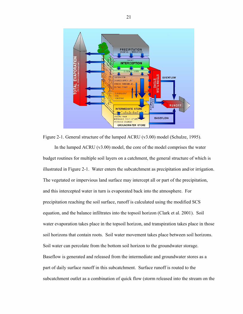
21

Figure 2-1. General structure of the lumped ACRU (v3.00) model (Schulze, 1995).

In the lumped ACRU (v3.00) model, the core of the model comprises the water

budget routines for multiple soil layers on a catchment, the general structure of which is

illustrated in Figure 2-1. Water enters the subcatchment as precipitation and/or irrigation.

The vegetated or impervious land surface may intercept all or part of the precipitation,

and this intercepted water in turn is evaporated back into the atmosphere. For

precipitation reaching the soil surface, runoff is calculated using the modified SCS

equation, and the balance infiltrates into the topsoil horizon (Clark et al. 2001). Soil

water evaporation takes place in the topsoil horizon, and transpiration takes place in those

soil horizons that contain roots. Soil water movement takes place between soil horizons.

Soil water can percolate from the bottom soil horizon to the groundwater storage.

Baseflow is generated and released from the intermediate and groundwater stores as a

part of daily surface runoff in this subcatchment. Surface runoff is routed to the

subcatchment outlet as a combination of quick flow (storm released into the stream on the

22

same day as the rainfall events) and delayed storm flow, a surrogate for post storm

interflow.

In the distributed ACRU model, a catchment is divided into a set of subcatchments

where the lumped model is applied individually throughout the entire simulation time

period, then the generated daily runoff from each subcatchment can be convoluted into a

runoff hydrograph using the triangular unit hydrograph approach for that subcatchment.

The runoff hydrograph from each subcatchment is then routed along the pre-specified

pathways to the outlet of the catchment using the Muskingum-Cunge method. No spatial

exchange of water flows is considered among subcatchments in ACRU (v3.00). This

design may be sufficient to present hydrology in watersheds where topographical

gradients dominate water movement and subcatchment hydrology is relatively

independent, but is not desirable for low-relief catchments.

To enable code expansion and functionality to meet different needs, ACRU (v3.00)

was entirely restructured into ACRU2000 (Campbell et al., 2001; Clark et al., 2001;

Kiker and Clark, 2001) within a Java-based, object-oriented framework. In ACRU2000,

the internal hydrological modeling features of ACRU (v3.00) were retained but the

underlying foundation was changed to allow new features to be developed. The

restructured version revised the surface runoff routing algorithm in ACRU (v3.00) by

executing each subcatchment every time step and then routing runoff from each

subcatchment to the outlet of watershed using the pre-specified pathway before

continuing to the next time interval. Additionally, a nutrient module, ACRU-NP

(Campbell et al., 2001), patterned after transformation and transport concepts used in the

GLEAMS model (Knisel et al. 1993), was added into ACRU2000. Campbell et al.

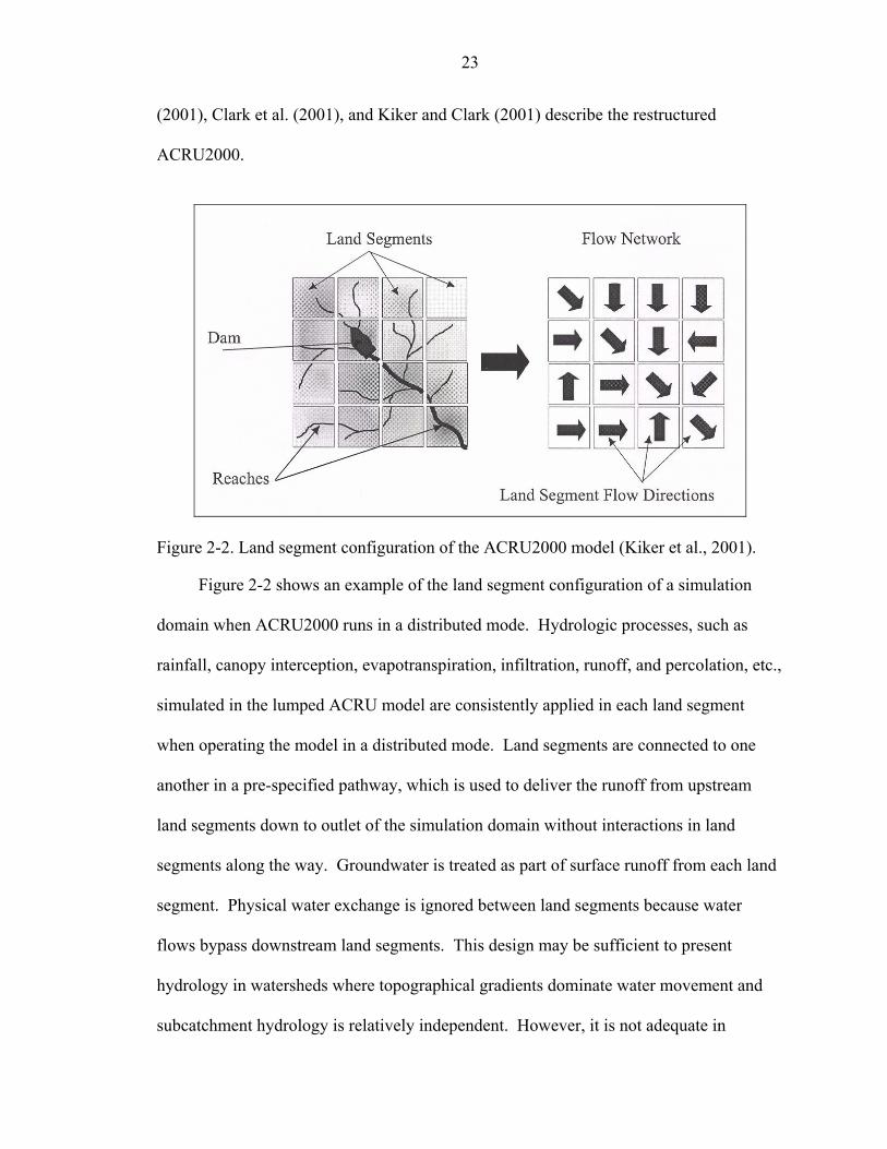
23

(2001), Clark et al. (2001), and Kiker and Clark (2001) describe the restructured

ACRU2000.

Figure 2-2. Land segment configuration of the ACRU2000 model (Kiker et al., 2001).

Figure 2-2 shows an example of the land segment configuration of a simulation

domain when ACRU2000 runs in a distributed mode. Hydrologic processes, such as

rainfall, canopy interception, evapotranspiration, infiltration, runoff, and percolation, etc.,

simulated in the lumped ACRU model are consistently applied in each land segment

when operating the model in a distributed mode. Land segments are connected to one

another in a pre-specified pathway, which is used to deliver the runoff from upstream

land segments down to outlet of the simulation domain without interactions in land

segments along the way. Groundwater is treated as part of surface runoff from each land

segment. Physical water exchange is ignored between land segments because water

flows bypass downstream land segments. This design may be sufficient to present

hydrology in watersheds where topographical gradients dominate water movement and

subcatchment hydrology is relatively independent. However, it is not adequate in

24

simulating south Florida flatwoods hydrology where water movement is primarily

dominated by hydraulic gradients and ecohydrologic variation is spatially interactive in a

significant manner. Furthermore, the nutrient model in ACRU2000, patterned after

transformation and transport concepts used in GLEAMS (Leonard et al. 1987), does not

consider the spatial transport of nutrients through lateral subsurface water movement.

In order to make the ACRU2000 model applicable in south Florida flatwoods

watersheds, modifications were needed to enable multi-directional spatial simulation of

water and nutrients. With the object-oriented design of ACRU2000, it is feasible to add

new modules while retaining the existing capacities of the model. The following

Chapters 3, 4 and 5 describe the details of modifications for hydrology and nutrient

transport simulation, and the addition of the vegetation dynamics model, respectively.

Model Testing Procedures

Model testing is a very important part in model development in that it can detect

inappropriate design in model algorithms, increase the model robustness and accuracy

through model calibration and validation, and determine the limitations and constraints of

model application through model evaluation. However, general methodologies related to

model calibration and validation have been subject to considerable discussion and dispute

during the past decades (Refsgaard, 1997).

Distributed models have the capacity to simulate spatial variations. Therefore the

number of parameters and variables are often several orders of magnitude higher than

those required for lumped models of the same area. Lumped and distributed models

should have different requirements with regard to model calibration and validation

procedures. Unfortunately, much attention has been given to specific calibration and

validation procedures for lumped models, whereas very limited attention has so far been

25

devoted to the more complicated tasks in connection with distributed models (Refsgaard,

1997). The procedure used for model calibration and validation in this study are

summarized in the following sections.

Model Calibration

Calibration is the process by which model parameters are adjusted to give the best

fit between simulated results and observed data at a particulate site. In other words,

calibration involves adjusting certain model parameters by systematically comparing

simulated results with observations while model structure remains the same. Model

calibration is built on the assumption that a well calibrated model enhances its predictive

capability by incorporating the best available data and adjusting calibration parameters to

obtain a close agreement between model output and historical data.

To calibrate a model adequately, the calibration period should include events that

significantly stress the simulation system. Calibration of distributed integrated models is

more challenging, as discussed above, due to complex model structures and large

parameter sets, and requires calibration over both time and space.

Model Validation

Validation is the process by which the calibrated model parameters are used to

predict state variables during periods when comparisons can be made to an independent

set of historical data, which were not previously used in the calibration process. The

purpose of validation is to determine if the model is sufficiently accurate for its

application as defined by objectives of the simulation study. The model is said to be

validated if its accuracy and predictive capacities in the validation period have been

proven to lie within well defined limits that may depend on intended model use.

26

Sensitivity Analysis

Sensitivity analysis (SA) is the process of varying model input parameters and

evaluating how model output changes with such variation (SFWMD, 2005). If a small

change in a parameter results in relatively large changes in the model output, the model is

said to be sensitive to that parameter. This may mean that the parameter has to be

determined very accurately. Prior to accepting the final set of calibrated model

parameters, a sensitivity analysis should be performed to determine the relative

magnitude of model response to changes in selected parameters.

The most common form of SA is independent parameter perturbation in which

parameters are varied individually by a fixed percentage around the base value (Ferreira

et al., 1995). An example of this approach is first-order analysis (Hann and Zhang,

1996), in which the first order derivatives in the Taylor series approximation of the

output variables are estimated:

i

ijiij

i

jji x

)x(y)xx(yxy

s∆

−∆+≈

∂

∂= (i = 1, 2, ⋅⋅⋅, n; j = 1, 2, ⋅⋅⋅, m) (2-1)

in which, sji is the sensitivity of output yj to the change of parameters xi; yj (j = 1, 2,⋅⋅⋅, m)

are the m predictions; xi (i = 1, 2,⋅⋅⋅, n) are the n parameters. These sensitivities sji have

units and thus are difficult to compare over parameters of interest directly. Thus one can

employ normalized or dimensionless sensitivities, Jones and Luyten (1998) used the

relative sensitivity, rsji:

j

iji

ii

jjji y

xsxxyy

rs =∂

∂= (2-2)

where xi is the calibrated value for input parameter xi, and yj is the prediction by the

calibrated model parameters. However, interactions between two or more parameters

27

(non-linear effects) may affect the model outputs, even if the output is linear in each

parameter. To check for two parameter interactions, second or high order derivatives in

the Taylor series approximation must be evaluated. In practice, the computation load to

find all possible significant derivatives may be too excessive.

Distributed integrated models are structured to enable simulation of spatial

variations in catchment characteristics and thus require more parameters, in principle,

than the lumped models. Thus it is necessary to investigate the spatial and temporal

sensitivities of input parameters. The first order method as shown in Equation (2-1) and

(2-2) was used to conduct the SA on major model outputs including surface runoff,

groundwater table depth, and P and N loads. If the output is a time series, the sensitivity

is a function of time, which may help to detect the influences of input parameters on

extreme values and trends of outputs. If the output is an individual value, an individual

sensitivity is calculated, which may help to detect the influences of input parameters on

the overall model response. The spatial sensitivities of outputs can be calculated using

the same equations when the spatial observation of output variables are available.

The significance of model sensitivity analysis is two-fold in that it provides

information on the behavior of model output to input parameters which, in turn, can be

used in model calibration; also, it gives insight in establishing priorities related to future

data collection efforts. Sensitivity analysis is distinguished from uncertainty analysis in

that it is a measure of the relative importance that each input parameter has on the range

of simulated outputs. Uncertainty analysis quantifies the confidence in particular output

variables given the probability distributions for input parameters. While sensitivity

analysis is often limited to parameter sensitivity, uncertainty may be generated by a

28

number of factors including parameter uncertainty, boundary and initial condition

uncertainty, model spatial and temporal resolution, availability and quality of data, and

model errors.

Model Evaluation

For sake of the model calibration and validation, and the comparison of models,

one needs quantitative information to measure model performance compared to observed

data or other model predictions. Statistical approaches to quantify the accuracy of model

predictions provide standardized measures of model performance although even these

methods do not provide completely clear-cut conclusions about the accuracy of model

predictions (Ramph, 2004). Given these caveats, the use of several different measures of

performance to evaluate a model may present a more complete picture of model

performance than any single measure and may allow the user to weight individual results

according to their priorities (Ramph, 2004).

Statistics

A number of statistics were used to evaluate model results in this study, including

model bias, average relative error (RE), root mean square error (RMSE), coefficient of

variation (CV), Pearson product-moment correlation coefficient (R2), and Nash-Sutcliffe

(NS) coefficient (Nash and Sutcliffe, 1970). Brief overviews of these statistical measures

are provided below.

Bias, also called the average error, determines the average deviation of the

predicted values from the measured values given N simulated-measured value pairs. As

can be seen from Equation (2-3), where Pi is the observed value, Oi is the model-

simulated value, and N is the number of observations, bias is calculated as the mean

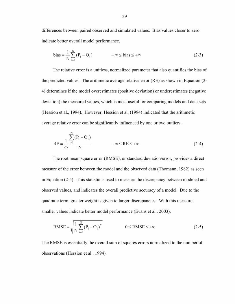
29

differences between paired observed and simulated values. Bias values closer to zero

indicate better overall model performance.

∑=

−=N

1iii )OP(

N1bias +∞≤≤∞− bias (2-3)

The relative error is a unitless, normalized parameter that also quantifies the bias of

the predicted values. The arithmetic average relative error (RE) as shown in Equation (2-

4) determines if the model overestimates (positive deviation) or underestimates (negative

deviation) the measured values, which is most useful for comparing models and data sets

(Hession et al., 1994). However, Hession et al. (1994) indicated that the arithmetic

average relative error can be significantly influenced by one or two outliers.

N

)OP(

O1RE

N

1iii∑

=

−= +∞≤≤∞− RE (2-4)

The root mean square error (RMSE), or standard deviation/error, provides a direct

measure of the error between the model and the observed data (Thomann, 1982) as seen

in Equation (2-5). This statistic is used to measure the discrepancy between modeled and

observed values, and indicates the overall predictive accuracy of a model. Due to the

quadratic term, greater weight is given to larger discrepancies. With this measure,

smaller values indicate better model performance (Evans et al., 2003).

∑=

−=N

1i

2ii )OP(

N1RMSE +∞≤≤ RMSE0 (2-5)

The RMSE is essentially the overall sum of squares errors normalized to the number of

observations (Hession et al., 1994).

30

The coefficient of variation (Young and Alward, 1983) defines a normalized error

as shown in Equation (2-6), which is the RMSE normalized to the overall mean.

∑=

−=N

1i

2ii )OP(

N1

O1CV ∞+≤∞− CV (2-6)

Using the RMSE, along with the CV, Hedden (1986) suggests that for screening

applications a model should be able to replicate observed data within an order of

magnitude, and for site-specific applications the predictions should be within a factor of

two. In the criterion of within “a factor of two” will be satisfied when the CV value is

less than one and the criterion of within “an order of magnitude” will be met when it is

less than nine.

The Pearson product-moment correlation coefficient (R2) value, also called the

goodness of fit, is a measure of the degree of linear association between two variables.

Depending on the strength of the linear relationship, the R2 can vary from 0 to 1. The

closer R2 is to 1, the better the regression explains the relationship between simulated and

observed. However, it does not explain how close the relationship is to the perfect linear

fit (R2 = 1) between observed and predicted values.

2

2i

2i

N

1iii

2

)PP()OO(

)PP)(OO(R

⎥⎥⎥⎥

⎦

⎤

⎢⎢⎢⎢

⎣

⎡

−−

−−=

∑∑

∑= 1R0 2 ≤≤ (2-7)

Like the R2 measure described above, Nash-Sutcliffe (NS) coefficient (Nash and

Sutcliffe, 1970) is another indicator of goodness-of-fit, and is one of the statistics that

have been recommended by the American Society of Civil Engineers (ASCE, 1993) for

evaluation of the performance of hydrological models. The NS can vary from 0 to 1,

31

with 1 indicating a perfect fit. Computationally, the NS could be negative but this

becomes rather meaningless as far as interpretation or results are concerned. For NS = 0,

the interpretation can be made that the model is predicting no better than using the

average of the observed data (ASCE, 1993). The statistics works best when the

coefficient of variation for the observed data set is large (ASCE, 1993).

∑

∑

=

=

−

−−= N

1i

2i

N

1i

2ii

)OO(

)PO(1NS 1NS ≤≤∞− (2-8)

Graphic representation

Graphic representation enables visualizing the relationship between predicted (Pi)

and measured (Oi) values and provides a straightforward way to compare the fit between

predicted and measured values. Scatterplots and duration curves are two commonly used

graphic representation techniques in the hydrological literature.

Scatterplot is a simple method to visualize the relationship between Pi and Oi by

fitting a regression line between Pi (Y-axis) and Oi (X-axis), relative to a line designating

a 1:1 relationship. The resulting pattern indicates the type and association/strength of the

relationship between predicted and observed values. A positive association would be

indicated by upward trend (positive slope) and a negative association would be indicated

by a downward trend (negative slope). Or, there might not be any notable association, in

which case a scatterplot would not indicate any trends whatsoever. The slope of the

regression line and its Y-intercept may provide evidence of systematic error in the model,

providing quantities that can be compared across models. A slope of 1.0 with an

intercept equal to 0.0 indicates perfect fit of the model predictions.

32

A duration curve represents the relationship between magnitude and frequency of a

variable for a particular watershed providing an estimate of the percentage of time a

given variable was equaled or exceeded over a period of time. There are different

approaches to generate duration curves for satisfying different purposes. Among these,

the flow duration curve (FDC) has widespread application in hydrologic studies such as

hydropower, water-supply and irrigation planning. In recent years, duration curves have

also been applied in other areas such as load assessment and TMDL development. For

this study, the flow and load duration curves were compared for simulated and observed

variables.

The basic procedure for generating a duration curve includes: 1) ranking the

daily/weekly/annually simulated and measured data separately from highest to lowest for

each dataset of interest; 2) calculating percent of days/weeks/years these variables were

exceeded (= rank/number of total data points); 3) plotting both simulated and measured

data vs. percent of time interval exceeded on the same plot.

Comparison of duration curves between model predictions and observed data

provides a direct evaluation of the accuracy of particular flow/load ranges. However,

there are some shortcomings of the duration curve method. For example, there is no

commonly accepted method to deal with repeated values. Therefore, using duration

curves altogether with other statistics is advisable in model evaluation.

No one of the abovementioned model evaluation approaches will be best in all

situations. Reviewing several of these measures together will provide a more complete

description of model performance (Ramph, 2004). The results should also be viewed in

the context of the intended use of the model. Users must decide for themselves what

33

level of performance is acceptable and, likewise, which approach is most appropriate to

their interests.

34

CHAPTER 3 HYDROLOGIC SIMULATION MODEL

Introduction

In the coupled modeling system, the hydrologic model plays an important role in

that it not only simulates hydrologic processes but also provides a framework for the

nutrient and vegetation models discussed in Chapters 4 and 5. Therefore, the design and

development of the hydrologic model has to take these other models into account.

An example catchment, shown in Figure 3-1A, is discretized into a network (Figure

3-1B) of multiple land segments, each of which is a unique hydrologic unit with varying

shape and size depending on land cover, topography, vegetation types and soil types.

Each land segment is bordered by either the internal boundaries, which are artificially

defined separations between two land segments, and/or the external boundaries, which

are the separation between the simulated catchment and its neighboring catchments. A

continuous unconfined groundwater system is assumed to underlie the discretized model

domain. For each land segment, it is assumed that the soil beneath is laterally

homogenous with heterogeneous vertical soil layers that are divided according to natural

soil horizons and soil properties. Additionally, soil layers in neighboring land segments

have the same number of soil layers of the same thickness, and adjacent soil layers are

laterally connected.

A fixed time step of one day is used in the coupled model. The selection of the

time step is a tradeoff between time scales required for different model processes and

general temporal scales of input data, such as rainfall and evapotranspiration.

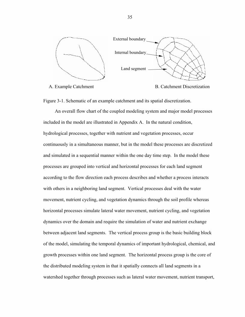
35

Figure 3-1. Schematic of an example catchment and its spatial discretization.

An overall flow chart of the coupled modeling system and major model processes

included in the model are illustrated in Appendix A. In the natural condition,

hydrological processes, together with nutrient and vegetation processes, occur

continuously in a simultaneous manner, but in the model these processes are discretized

and simulated in a sequential manner within the one day time step. In the model these

processes are grouped into vertical and horizontal processes for each land segment

according to the flow direction each process describes and whether a process interacts

with others in a neighboring land segment. Vertical processes deal with the water

movement, nutrient cycling, and vegetation dynamics through the soil profile whereas

horizontal processes simulate lateral water movement, nutrient cycling, and vegetation

dynamics over the domain and require the simulation of water and nutrient exchange

between adjacent land segments. The vertical process group is the basic building block

of the model, simulating the temporal dynamics of important hydrological, chemical, and

growth processes within one land segment. The horizontal process group is the core of

the distributed modeling system in that it spatially connects all land segments in a

watershed together through processes such as lateral water movement, nutrient transport,

A. Example Catchment B. Catchment Discretization

External boundary

Internal boundary

Land segment

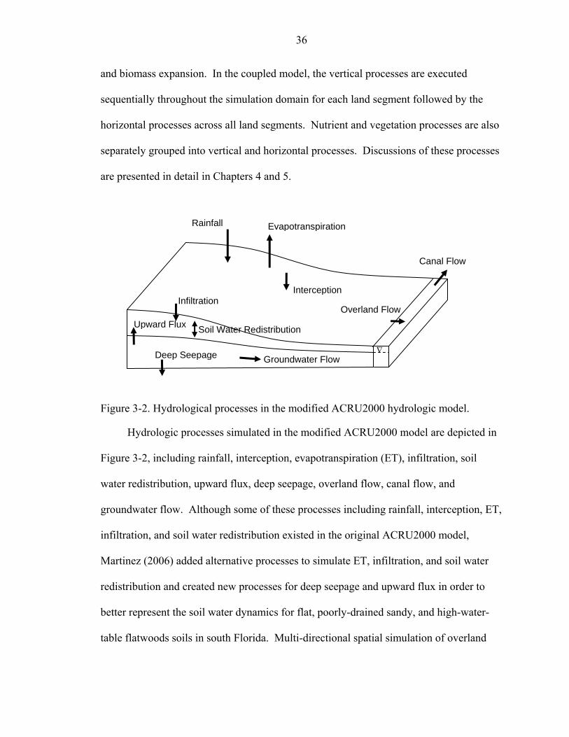
36

and biomass expansion. In the coupled model, the vertical processes are executed

sequentially throughout the simulation domain for each land segment followed by the

horizontal processes across all land segments. Nutrient and vegetation processes are also

separately grouped into vertical and horizontal processes. Discussions of these processes

are presented in detail in Chapters 4 and 5.

Figure 3-2. Hydrological processes in the modified ACRU2000 hydrologic model.

Hydrologic processes simulated in the modified ACRU2000 model are depicted in

Figure 3-2, including rainfall, interception, evapotranspiration (ET), infiltration, soil

water redistribution, upward flux, deep seepage, overland flow, canal flow, and

groundwater flow. Although some of these processes including rainfall, interception, ET,

infiltration, and soil water redistribution existed in the original ACRU2000 model,

Martinez (2006) added alternative processes to simulate ET, infiltration, and soil water

redistribution and created new processes for deep seepage and upward flux in order to

better represent the soil water dynamics for flat, poorly-drained sandy, and high-water-

table flatwoods soils in south Florida. Multi-directional spatial simulation of overland

Canal Flow

Rainfall Evapotranspiration

Overland Flow Infiltration

Groundwater Flow

Upward Flux

Deep Seepage

Soil Water Redistribution

Interception

∇

37

and lateral groundwater flow, and canal flow did not exist in the original ACRU2000

model. Developing algorithms for these processes was the primary purpose of this study.

In the following hydrologic components sections, the methodology used to simulate

each process is described, with more detail given to the new overland flow (including

canal flow) and lateral groundwater flow processes. Schulze (1995) gave a

comprehensive description of the hydrologic processes incorporated into ACRU (v3.00).

The hydrologic model was developed based on the existing hydrologic model in

ACRU2000 (Campbell et al., 2001; Clark et al., 2001; Kiker and Clark, 2001) by adding

new components and modifying existing components needed for multi-directional spatial

simulation, with an emphasis of considering lateral surface and subsurface flow exchange

throughout all soil layers between adjacent land segments. Changes were made so that

the original model features were retained for other potential applications while enabling

new functionality.

The objectives of this Chapter are

To modify the ACRU2000 hydrologic model to add new hydrologic components that enable multi-directional spatial simulation of overland flow and lateral groundwater flow;

To analyze the influence of the simulation sequence on simulation results from the modified model;

To test the ability of the modified model to accurately simulate hydrological processes by comparing with well-accepted models including MIKE SHE (DHI, 2004) and MODFLOW (McDonald and Harbaugh, 1988);

To test the reliability of the modified model in predicting major hydrologic processes by comparing with the FHANTM model simulations of a field experiment in the Kissimmee River Basin, Florida.

In the following sections, the methodology for each hydrologic component

simulated in the modified version of the hydrologic model is described, followed by the

38

description of boundary and initial conditions required for the model. Then, simulation

sequence analyses, hypothetical scenario tests and an application in Dry Lake Dairy #1,

Kissimmee River Basin, Florida are presented and discussed and conclusions are drawn.

Appendix D lists and describes the added or modified objects. Appendix E lists all newly

added variables associated with the coupled modeling system.

Vertical Hydrologic Components

Rainfall

Rainfall is the fundamental driving force behind most hydrological processes. The

success of hydrological simulation studies depends to a large extent on the precision with

which the rainfall data are observed temporally and spatially and how they are processed

in the model. Several techniques in ACRU (V3.00) are available for estimating aerial

rainfall for input files, including

• Driver station method • ACRU-300 trend surface approach • Thiessen polygon method • Inverse distance interpolation technique and • Spline interpolation technique

The design of input files in the model allows each land segment to have its own

daily time series of rainfall depth input. Therefore, the temporal and spatial distribution

of rainfall can be differentiated when such spatial rainfall data are available. But within

one land segment, or when the model is used in the lumped mode, the rainfall is assumed

to have a uniform spatial distribution.

Canopy Interception

Canopy interception is calculated as the minimum of the available rainfall and the

amount of interception storage capacity available on the intercepting vegetation leaf

canopy. The available rainfall first fills available canopy storage, then the remaining

39

rainfall is assumed to reach the land surface and is available for infiltration or/and surface

runoff. If the rainfall is less than or equal to the available canopy storage, all rainfall is

intercepted.

Evapotranspiration

The calculation of actual evapotranspiration requires three steps including reference

potential evapotranspiration (RET), potential evapotranspiration (PET), and actual

evapotranspiration (AET). The latter is further separated into soil evaporation and plant

transpiration for later use in nutrient uptake discussed in Chapter 4.

The reference evapotranspiration (RET) refers to the maximum evaporation from a

short grass surface, or the maximum evaporation from an actively growing alfalfa crop,

at least 0.3 m tall, standing erect and covering an extensive area. There are many

methods of estimating RET in ACRU (v3.00), ranging from complex physically based

equations to simple measurements and even simpler surrogates based on single variables

such as temperature:

• The daily United States Weather Bureau Class A pan evaporation. • The 1948 Penman equation • Temperature based equations in ACRU (v3.00) • The Linacre suite of equations (1977, 1984, 1991) • The Hargreaves and Samani methods (1982 & 1985) • The Blaney and Criddle (1950) equation • The Thornthwaite (1948) equation

In addition, Martinez (2006) added the Penman-Monteith grass reference potential

evapotranspiration approach (Allen et al. 1998), referred to as FAO56PM in the model.

The RET can be calculated separately and input as a time series or calculated directly by

the model with required input parameters and data.

40

For all methods, evapotranspiration is calculated in a top-down approach. First the

evaporation demand is applied to intercepted water, next to ponded water on the ground

surface, and then to the soil as evaporation and transpiration. The PET for a crop is

obtained by multiplying RET with a month-by-month crop coefficient which integrates

numerous dynamic processes relating to crop transpiration and soil evaporation.

Two existing AET calculation methods of ACRU (v3.00) have been adapted for

use, which calculate AET either as a lumped quantity or by determining soil evaporation

and transpiration separately using Ritchie’s method (Ritchie 1972). In addition, a third

simple actual evapotranspiration method was added by Martinez (2006).

When calculating evapotranspiration as a lumped quantity, the RET is multiplied

by the crop coefficient (V1CAY) to get the PET, then the layer AET within the root zone

is calculated as the minimum between the PET and the available water storage (beyond

the wilting point) for a specific soil layer. Using an approximate method (Childs and

Hanks, 1975), the layer AET is split between soil water evaporation (AEs) and plant

transpiration (AEt) for use for plant uptake of solutes and nutrients:

ts AEAETAE −= (3-1)

⎪⎩

⎪⎨

⎧

≤

>−

×=

0.2V1CAY0

0.2V1CAY)0.8

0.2V1CAY(AET0.95AEt (3-2)

When using Ritchie’s method to determine evapotranspiration, the potential soil

evaporation and plant transpiration are separated as a function of the leaf area index

(V1LAI).

ts PEPETPE −= (3-3)

41

⎪⎩

⎪⎨⎧

≥

<×−=

7.2LAIV1PET95.0

7.2LAIV1PET)21.0LAI1V7.0(PE

5.0

t (3-4)

The potential transpiration (PEt) is further adjusted by being multiplied by a crop

coefficient. The actual plant transpiration can be either equal to maximum transpiration

for a given soil layer or be less than maximum transpiration because of a deficiency of

available soil water or an excess of soil water. According to Martinez (2006), if the

FAO56PM RET is used, the potential evaporation is multiplied by a factor of 1.15 to

account for the difference in albedo between bare soil and a vegetated surface as

recommended by Allen et al. (1998). The potential soil evaporation (PEs) is further

adjusted for the percent surface cover by mulch. The soil water evaporation takes place

down to a user defined depth of the soil with recommended values ranging from 0.1 to

0.15 m (Allen et al. 1998). According to Ritchie’s method actual evaporation from the

soil surface continues at a maximum rate equal to the potential rate (stage 1) until the

accumulated soil water evaporation exceeds the stage 1 upper limit. After that, soil water

evaporation proceeds at a reduced (stage 2) rate.

The new actual evapotranspiration method that has been added to the model is a

simplification to the lumped evapotranspiration method described above. The

simplifications include neglecting water stress and the apportionment of

evapotranspiration to different layers. Potential evapotranspiration is applied to

individual soil layers in the original model according to the fraction of plant roots within

that layer. Similarly, the new method applies potential evapotranspiration from the top-

most soil layer until the wilting point is reached and then applies the remainder to the

layer below until the bottom of the root zone (the last layer containing roots) is reached.

42

Infiltration

Infiltration is a process by which water on the soil surface enters the soil.

Considering the high infiltrating capacity of flatwoods soils, the rainfall rate is assumed

to be less than the maximum infiltration rate and the water on the ground surface is

allowed to infiltrate until the soil profile becomes completely saturated. Thus in the

modified ACRU2000, saturated-excess ponding and runoff is simulated. The volume of

infiltration is taken as the minimum of the rainfall rate multiplied by grid cell area and

time step and the available void space between the water table and land surface.

Infiltrating water is moved into the top-most soil layer and is further moved into deeper

soil layers through a process discussed below. Water that infiltrates into the soil profile

will cause a rise in the water table after any depleted root zone soil moisture is

replenished.

Soil Water Redistribution

In ACRU (v3.00), unsaturated soil water redistribution downwards can take place

from the top to a subsoil horizon and from the subsoil horizon to groundwater when the

soil moisture content in the upper soil horizon is above the field capacity. Upward

redistribution, which is similar to capillary movement, takes place from the bottom soil

horizon and works up through the soil horizons. If a soil horizon is above porosity then

the excess water is moved to the soil horizon above, or in the case of the top soil horizon

the surface of the land segment, where it is added to ponded water.

Martinez (2006) created an alternative process specifically for the flatwoods soils.

This process redistributes infiltrating water based on the drained-to-equilibrium soil

moisture content of each soil layer. According to Martinez (2006), this process has to be

turned on after infiltration, net infiltration, new water table depth (if any), and new

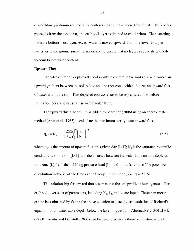
43

drained-to-equilibrium soil moisture contents (if any) have been determined. The process

proceeds from the top down, and each soil layer is drained to equilibrium. Then, starting

from the bottom-most layer, excess water is moved upwards from the lower to upper

layers, or to the ground surface if necessary, to ensure that no layer is above its drained-

to-equilibrium water content.

Upward Flux

Evapotranspiration depletes the soil moisture content in the root zone and causes an

upward gradient between the soil below and the root zone, which induces an upward flux

of water within the soil. This depleted root zone has to be replenished first before

infiltration occurs to cause a rise in the water table.

The upward flux algorithm was added by Martinez (2006) using an approximate

method (Anat et al., 1965) to calculate the maximum steady-state upward flux:

η−η

⎟⎟⎠

⎞⎜⎜⎝

⎛⎥⎦

⎤⎢⎣

⎡

+η+=

b2suf h

d1

886.11Kq (3-5)

where quf is the amount of upward flux on a given day [L/T]; Ks is the saturated hydraulic

conductivity of the soil [L/T]; d is the distance between the water table and the depleted

root zone [L]; hb is the bubbling pressure head [L]; and η is a function of the pore size

distribution index, λ, of the Brooks and Corey (1964) model, i.e., λ+=η 32 .

This relationship for upward flux assumes that the soil profile is homogenous. For

each soil layer a set of parameters, including Ks, hb, and λ, are input. These parameters

can be best obtained by fitting the above equation to a steady-state solution of Richard’s

equation for all water table depths below the layer in question. Alternatively, SOILPAR

(v2.00) (Acutis and Donatelli, 2003) can be used to estimate these parameters as well.

44

The amount of upward flux that actually occurs on a given day is the minimum of

the maximum value calculated and the amount to which the root zone was depleted (and

is now fully replenished by upward flux).

Deep Seepage

Deep seepage can occur through a restrictive layer located below the soil profile

according to Darcy’s Law. It is calculated as:

dHH

Kq dwsds

−= (3-6)

where qds is the amount of daily deep seepage through the restrictive layer [L/T]; Ks the

restrictive layer saturated hydraulic conductivity [L/T]; Hw is the height of water table

above the restrictive layer [L]; Hd is the hydraulic head below the restrictive layer [L];

and d is the thickness of the restrictive layer [L].

Horizontal Hydrologic Components

Horizontal hydrologic components including overland flow, lateral groundwater

flow and canal flow were newly added into the original ACRU2000 model. The

simulation of these components requires water exchange between adjacent land

segments. Lateral flow is simulated sequentially, with the simulation sequence

determined by the topographic elevations of land segments and the sequence of land

segment input files. More details and testing regarding the simulation sequence are

discussed in the following section.

The following assumptions were made in the simulation of multi-directional lateral

flow:

For each land segment, only outgoing overland flows are estimated except when inflows occur through external boundaries;

45

Overland flows happen only when a positive hydraulic gradient occurs between one land segment and its neighboring land segments, and the ponded water depth in this land segment exceeds its maximum depression storage;

Potential overland flows are estimated for all neighboring land segments based on hydraulic gradients. If there is insufficient storage to supply all potential outflows, actual outflows are determined through storage apportionment;

Soil within each land segment is unconfined, thus the hydraulic head is the water level elevation in this land segment above the datum;

Soils beneath land segments have the same thickness and they are split into the same number of computational soil layers;

Adjacent computational soil layers in neighboring land segments have the same thickness and are laterally connected.

Hydraulic gradients are the driving force to transfer groundwater flow laterally in saturated soils;

From each land segment only outgoing lateral groundwater flows are estimated except when lateral inflows occur through external boundaries;

Lateral groundwater flows only happen when a positive hydraulic gradient occurs between one land segment and its neighboring land segments;

Potential groundwater flows are estimated for all neighboring land segments. If there is insufficient storage to supply all potential groundwater flows, actual groundwater flows are decided through storage apportionment.

Overland Flow

Appendix B shows a flow chart of overland flow simulation for one source land

segment. The potential outgoing overland flows from the source land segment to

adjacent land segments are calculated as discussed in the following section and inflows

through the external domain boundary are input or extrapolated depending on the actual

boundary conditions. Subsequently, a storage check is conducted to guarantee there is

enough surface water storage in the source land segment to supply the potential flows. If

there is insufficient storage the available water is apportioned according to assumptions

discussed in the following section and the detailed algorithm is documented in Appendix

46

G. External boundary inflows are introduced into boundary land segments each day. The

outgoing flows are then transferred to adjacent land segments, which causes a decrease of

water storage in the source land segment and an increase of water storage in the adjacent

land segment. The whole process described in Figure 3-3 is applied to each land segment

in the simulation domain following the simulation sequence generated by the model.

Overland flow calculation

The generalized spatial relationship between one land segment and its adjacent land

segments is shown in Figure 3-3. Two types of overland flow over internal boundaries

are defined in this model:

Figure 3-3. Configuration of overland flows between source land segment and adjacent land segments. The digit (1~4) of adjacent land segment index indicates the priority to receive the overland flow from source land segment, which is determined by the water elevation of that land segment and smaller water elevations correspond to higher priorities. An adjacent land segment with a larger index has higher priority to receive the overland flow.

Unstructured boundaries, where no local obstacles exist to the flow (no singular

head losses) and a mean resistance coefficient for a given cross section of the flow can be

used. In this case, Manning’s formula is used:

Neighbor 4

Neighbor 3

Neighbor 2

∇ Qs,d,3

Qs,d,2

Qs,d,1

Qs,d,4

Neighbor 1

Source

47

i,d,s

m21

i,d,s32

i,d,si,d,si,d,si,d,s n

USRDWQ = (3-7)

where subscript s and d indicate source and destination land segments and i the specific

adjacent neighbor; Qs,d,i is the volumetric discharge from source to destination land

segments [L3/T]; Ws,d,i is the width of the cross-sectional area between source and

destination land segments [L]; Ds,d,i is the water depth of the cross-sectional area between

source and destination land segments [L], an average of water depths in both source and

destination land segments; Rs,d,i is the hydraulic radius of the flow section between source

and destination land segments and it is essentially the average surface water depths [L],

roughly equivalent to Ds,d,i for wide, shallow cross-sectional area or streams; Ss,d,i is the

water surface slope between source and destination land segments [L/L], it is estimated as

Lzz

S dsi,d,s

−= (3-4)

in which, zs and zd are the water levels of source and destination land segments,

respectively [L]; L is the distance between the centers of source and destination land

segments [L]; Um is the unit conversion for the Manning formula [L1/3/T]; ns,d,i is the

average of Manning’s roughness coefficients of source and destination land segments,

which is modified to be a function of sediment type and the interaction of the vegetation

height/density and water depth (Fitz et al. 1996). This function creates a dynamic

feedback loop between the physical process of flow and the biological process of plant

growth (Sklar et al. 2001), which is calculated as:

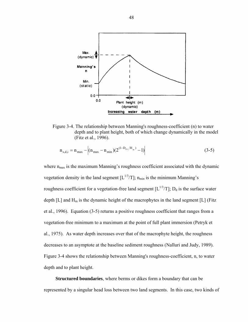
48

Figure 3-4. The relationship between Manning's roughness-coefficient (n) to water depth and to plant height, both of which change dynamically in the model (Fitz et al., 1996).

)12)(nn(nn )HD1(minmaxmaxi,d,s

mi,d −−−= − (3-5)

where nmax is the maximum Manning’s roughness coefficient associated with the dynamic

vegetation density in the land segment [L1/3/T]; nmin is the minimum Manning’s

roughness coefficient for a vegetation-free land segment [L1/3/T]; Dd is the surface water

depth [L] and Hm is the dynamic height of the macrophytes in the land segment [L] (Fitz

et al., 1996). Equation (3-5) returns a positive roughness coefficient that ranges from a

vegetation-free minimum to a maximum at the point of full plant immersion (Petryk et

al., 1975). As water depth increases over that of the macrophyte height, the roughness

decreases to an asymptote at the baseline sediment roughness (Nalluri and Judy, 1989).

Figure 3-4 shows the relationship between Manning's roughness-coefficient, n, to water

depth and to plant height.

Structured boundaries, where berms or dikes form a boundary that can be

represented by a singular head loss between two land segments. In this case, two kinds of

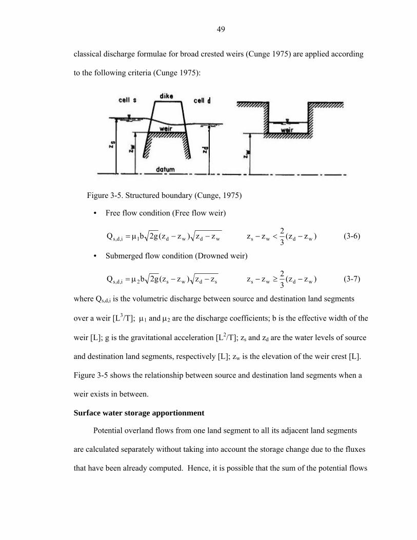
49

classical discharge formulae for broad crested weirs (Cunge 1975) are applied according

to the following criteria (Cunge 1975):

Figure 3-5. Structured boundary (Cunge, 1975)

Free flow condition (Free flow weir)

wdwd1i,d,s zz)zz(g2bQ −−µ= )zz(32zz wdws −<− (3-6)

Submerged flow condition (Drowned weir)

sdws2i,d,s zz)zz(g2bQ −−µ= )zz(32zz wdws −≥− (3-7)

where Qs,d,i is the volumetric discharge between source and destination land segments

over a weir [L3/T]; µ1 and µ2 are the discharge coefficients; b is the effective width of the

weir [L]; g is the gravitational acceleration [L2/T]; zs and zd are the water levels of source

and destination land segments, respectively [L]; zw is the elevation of the weir crest [L].

Figure 3-5 shows the relationship between source and destination land segments when a

weir exists in between.

Surface water storage apportionment

Potential overland flows from one land segment to all its adjacent land segments

are calculated separately without taking into account the storage change due to the fluxes

that have been already computed. Hence, it is possible that the sum of the potential flows

50

could exceed surface water storage in the land segment. This situation is especially likely

to occur if the time step is large. To avoid this situation, a procedure was developed to

limit the actual overland flow to its maximum available volume of storage, hereafter

simply called the available volume, which is a portion of the current volumetric water

storage on ground surface allocated to a specific neighbor based on the following

assumptions:

The storage apportionment is allocated only to those neighbors that receive the overland flows;

The current water storage in the land segment is the maximum available volumetric water storage;

The allocation of the maximum water storage in the land segment is made according to the priority of its neighbors;

The priority of the neighbors is set up according to the elevation of the water surface boundary between the land segment and its specific neighbor.

The water surface elevation of the boundary between the land segment and its neighbor is determined by the maximum of the water level or the elevation of the weir crest, whichever exists;

If a weir exists in between the land segment and its neighbor, the elevation of the weir crest has to be higher than the elevation of the land segment;

The neighbor with the lowest elevation of boundary has the highest priority for allocation of water storage from the source land segment;

A neighbor with lower priority is not allocated any water storage until the neighbor with next higher priority is filled to an equavlant water surface elevation, i.e., the two neighbours have equal water surface elevation;

The available volume for a specific neighbor can not be more than required to equilibrate the water levels of the land segment and this neighbor.

Once the available volumes are determined for all those neighbors receiving

potential overland flows from the land segment, each of them is compared with its

corresponding pre-estimated potential overland flow. If any potential overland flow

exceeds its available volume, then the actual overland flow is set equal to the available

51

volume. Otherwise, the actual overland flow is equal to its potential value. Details of the

assumptions and algorithm for surface water appointment are described in Appendix G.

Groundwater Flow

Groundwater flow here refers to lateral groundwater flow which occurs in the

saturated soils. Appendix C shows a flow chart of lateral groundwater flow simulation

for one land segment. For a source land segment, the potential outgoing lumped lateral

groundwater flows and inflows from external domain boundary are calculated, followed

by a storage check to guarantee there is sufficient groundwater storage to provide the

potential flows from the source land segment. Lumped groundwater flow available for

transfer is split into layer flows for the saturated zone in proportion to the layer

transmissivity. The layer flows are then transferred to the neighboring land segment.

The transmission of layer groundwater flow increases the void space in the soil of the

source land segment and decreases that in the neighboring land segments. At the end of

52

Figure 3-6. Schematic representation of the lateral groundwater flow from the higher

head hs to the lower head hd. (A) and (B) represent the situations without and with overland flow, respectively.

hs hd

Lateral groundwater flow

Water Table

Ground surface

∇

(A)

Impermeable strata

hs hd

Lateral groundwater flow

Water Table

Ground surface

∇Overland flow

(B)

Impermeable strata

53

Figure 3-7. Diagram of lateral groundwater flow between two land segments. (A) and (B)

represent the generalized situations without and with overland flow, respectively.

∇

Ws

∇

Qs,d,i

Qs,i,1

Qs,i,2

Qs,i,3

Qs,i,4

Qs,i,5 (A)

bdk

L

Hs zs Hd zd

(B)

bsj

Qs,i,1

Qs,i,2

Qs,i,3

Qs,i,4

Qs,i,5

∇ Ws Qs,d,i

∇

bdk

L

Hd zdHs zs

bsj

54

simulation, the water table depths are updated for all land segments. The complete

process described in Appendix C is applied to each land segment in the simulation

domain following the simulation sequence generated by the model.

Lateral groundwater flow calculation

Lateral groundwater flow is calculated first in a lumped manner between the

saturated zone of source land segment and its adjacent land segments according to

Darcy’s law. The lumped flow is then partitioned into the saturated soil layers. Figure 3-

6 shows the generalization of lateral flows between two adjacent land segments, in case

A (Figure 3-6A) the water table is below the ground surface and case B it is above the

ground surface (Figure 3-6B).

The generalization of (A) and (B) in Figure 3-6 is correspondingly illustrated in

Figure 3-7(A) and (B). First of all, using Darcy’s Law, the lumped lateral groundwater

flow from the source land segment to the destination land segment is estimated

i,d,si,d,si,d,si,d,si,d,s HWSKQ = (3-8)

Where subscript s and d indicate source and destination land segments and i the specific

neighboring land segment; Qs,d,i is the lumped lateral groundwater flow from source to

destination land segments [L3/T]; Ss,d,i is the hydraulic gradient between source and

destination land segments [L/L] and is calculated as

LZZ

S dsd,s

−= (3-9)

in which zs and zd are the groundwater heads of the source and destination land segments,

respectively [L]; and L is the distance between the centroids of the source and destination

land segments [L]; Ks,d,i is the effective horizontal saturated hydraulic conductivity [L/T],

55

an average of horizontal saturated hydraulic conductivities of the source and destination

land segments [L/T]. It is estimated as

2/)bKD1bK

D1(K

kdkdk

djsjsj

si,d,s ∑∑ += (3-10)

where subscript j and k indicate the number of soil layers below the water table of the

source and destination land segments, respectively; Ksj is the saturated horizontal

hydraulic conductivity of soil layer j of source land segment [L/T] and Kdk, that of soil

layer k of destination land segment [L/T]; bsj and bdk is the thickness of saturated soil of

layer j in source land segment and layer k in destination land segment [L]; Dsj and Ddk is

the thickness of saturated soils for source and destination and segments [L]; Ws,d,i is the

boundary width of the cross-sectional area between source and destination land segments,

perpendicular to the direction of lateral groundwater flow [L]; Hu,d,i is the average of the

thickness of saturated soil of source and destination land segments [L],

2HHH ds

i,d,s+

= (3-11)

where Hs and Hd are the thickness of saturated soils of the source and destination land

segments, respectively [L].

Next, the lateral groundwater flows from source to destination saturated soils are

distributed to individual saturated soil layers by the formula

∑=

= N

1jj,ij,i

j,ij,ii,d,sj,i,s

bK

bKQQ (j = 1,…., N) (3-12)

where Qs,i,j is the layer lateral flow from the saturated soil layer j of source land segment

to the layer j of destination land segment [L3/T]; Ki,j is the saturated horizontal hydraulic

conductivity of the layer j of source land segment [L/T]; bi,j is the thickness of saturated

56

soil of the layer j of source land segment [L]; N indicates the number of saturated soil

layers. In case the water table is located somewhere within a soil layer, the thickness of

saturated soil in this layer is the depth from the water table to the bottom of this soil

layer.

Groundwater storage apportionment

Similar to the procedure of surface water storage apportionment for overland flow,

a procedure to check if the sum of the lumped groundwater flows exceeds the available

saturated groundwater storage in the source land segment is needed. The available

groundwater storage is assumed to be the portion of volumetric water above the field

capacity. If the sum of outgoing lumped flows is greater than the available groundwater

storage, each lumped groundwater flow is adjusted using a ratio, which is the difference

between the sum of outgoing lumped flows and the available volumetric storage to the

available volumetric storage. By doing this adjustment, the actual lumped flows are

limited to the available storage. Since the groundwater flow is much slower than

overland flow this procedure is rarely invoked when the model runs at a daily time step.

Canal Flow

The interaction of canals with the simulation domain can occur both through

overland flow and lateral groundwater flow depending on the stage of canal and the water

level in the domain. When the canal stage is higher than the water level in an adjacent

land segment, back flow from the canal into the domain occurs. When the canal stage is

lower than the water level in an adjacent land segment, discharge from the domain is

released into the canal. Flow between the canal and domain is estimated using the

following equations:

57

nSWRq

2/135= Overland flow (3-13)

KWSDq = Lateral groundwater flow (3-14)

where q represents the amount of overland flow to/from the canal in Equation (3-13) and

lateral groundwater flow to/from the canal in Equation (3-14) [L3/T]; W is the width of

the land segment-canal boundary [L]; R is the water depth above the ground surface [L];

S is the water slope that is determined by the difference of water level between canal and

the adjacent land segment divided by the distance between the centroid of the canal and

the centroid of the land segment [-]; n is the Manning’s roughness coefficient, which is

assumed to be the same as the one for the adjacent land segment for this study [L1/3/T];

K is the hydraulic conductivity between the canal and the saturated soils of the adjacent

land segment, which is assumed to be the same as the saturated horizontal hydraulic

conductivity for the adjacent land segment for this study; and D is the thickness of the

saturated soil profile [L]. Currently canal flow is not an individual process in the model

but is a built-in routine inside of overland flow and lateral groundwater flow processes.

Initial and Boundary Conditions

To ensure the accuracy of the solution of the simulation model, both initial and

boundary conditions must be prescribed for the domain being simulated. Initial

conditions in the model include water table depth in the soil, ponded water depth if any,

and depressional water storage for each land segment. Boundary conditions include

boundary inflow, outflow, or fixed head conditions and the description of physical

hydraulic structures, levees, fences, and berms, etc. If physical structures exist,

geometric information and relevant empirical formula for flows through these structures

must be prescribed. Time series of atmospheric variables such as rainfall, temperature,

58

and potential ET, etc. must also be specified for the desired simulation period. Appendix

F shows the input files, required for applications in this dissertation, which contain the

initial and boundary conditions.

Model Testing and Validation

Simulation Sequence and Model Performance Accuracy Analysis

In the modified ACRU2000 hydrologic model, the simulation sequence determines

the execution order of land segments. The simulation sequence is generated according to

the spatial water flow configuration and the sequence of land segment input files

specified in the control menu file (Control.men in Appendix F). The spatial water flow

configuration is arranged according to the topographical elevation of each land segment,

which specifies the directions of outflow from each land segment and is deterministic

once the topography in a simulation domain is specified. However, the sequence of land

segment input files in Control.men is arbitrary, for instance, one can specify the sequence

from the first land segment to the last one, or its opposite, or other orders. Different

simulation sequences can produce different simulation results but the extent to which

simulated results, resulting from different simulation sequences, differ from one another

needs to be investigated. With this consideration, influence of simulation sequence on

model predictions was analyzed. Moreover, the model accuracy is the most important

indicator of whether a model is successfully developed. Simulation sequences directly

affect the accuracy of the model. Therefore it is necessary to evaluate the model

performance accuracy in terms of appropriately selected simulation sequence by

comparing the modified model with well-known models.

To investigate the influence of simulation sequence, it is important to understand

why the simulated results can be different when different simulation sequences are

59

specified. As discussed in the introduction section of this Chapter, the vertical and

horizontal hydrologic processes are executed in two separate loops in the modified

ACRU2000 model. During the vertical processes water is distributed vertically in the

soil profile, which results in variation of hydraulic heads between land segments, but

each land segment is simulated independently. Horizontal processes transfer surface and

subsurface water between neighboring land segments making them interdependent. The

simulation of horizontal processes on a particular land segment causes a change of water

levels in adjacent land segments. These influences can be propagated to downstream

land segments that are simulated later in the simulation sequence. Therefore, it is

essential to investigate the difference between different simulation sequence strategies

before a decision is made on what would be the most appropriate sequence for the model.

Table 3-1. List of strategies for water transmission and water storage updating for simulation sequence experiments.

Experiments Strategies to transfer water and update water storage*

Experiment 1 Water transferred in lateral processes is not available for transmission to downstream land segments and also does not cause head changes until the end of the day when all land segments have been simulated.

Experiment 2 Water transferred in lateral processes is available for transmission to downstream land segments but does not cause head changes until the end of the day when all land segments have been simulated.

Experiment 3 Water transferred in lateral processes is available for transmission to downstream land segments and also causes heads changes immediately.

* Water storage either on the ground surface or in the saturated soil layers.

Three experiments, corresponding to different strategies for water transmission and

storage updating, are listed in Table 3-1. These experiments were conducted based on

two hypothetical scenarios, a flat rectangular plane and an axisymmetric domain. To

further evaluate the model performance accuracy, the simulated results from the first

scenario were compared with the two-dimensional overland flow model in MIKE SHE

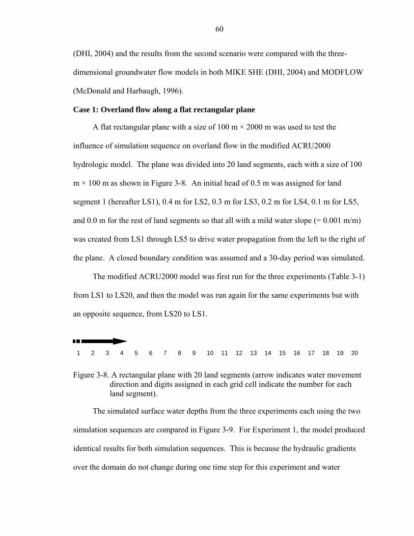
60

(DHI, 2004) and the results from the second scenario were compared with the three-

dimensional groundwater flow models in both MIKE SHE (DHI, 2004) and MODFLOW

(McDonald and Harbaugh, 1996).

Case 1: Overland flow along a flat rectangular plane

A flat rectangular plane with a size of 100 m × 2000 m was used to test the

influence of simulation sequence on overland flow in the modified ACRU2000

hydrologic model. The plane was divided into 20 land segments, each with a size of 100

m × 100 m as shown in Figure 3-8. An initial head of 0.5 m was assigned for land

segment 1 (hereafter LS1), 0.4 m for LS2, 0.3 m for LS3, 0.2 m for LS4, 0.1 m for LS5,

and 0.0 m for the rest of land segments so that all with a mild water slope (= 0.001 m/m)

was created from LS1 through LS5 to drive water propagation from the left to the right of

the plane. A closed boundary condition was assumed and a 30-day period was simulated.

The modified ACRU2000 model was first run for the three experiments (Table 3-1)

from LS1 to LS20, and then the model was run again for the same experiments but with

an opposite sequence, from LS20 to LS1.

Figure 3-8. A rectangular plane with 20 land segments (arrow indicates water movement

direction and digits assigned in each grid cell indicate the number for each land segment).

The simulated surface water depths from the three experiments each using the two

simulation sequences are compared in Figure 3-9. For Experiment 1, the model produced

identical results for both simulation sequences. This is because the hydraulic gradients

over the domain do not change during one time step for this experiment and water

1 2 3 4 5 6 7 8 9 10 11 12 13 14 15 16 17 18 19 20

61

transmission and water storage updates do not happen until the end of each time step

when all land segments have been simulated. Significant difference in surface water

depths between simulation sequences is observed in Experiment 2. Water moves faster

when the simulation order is consistent with the flow direction (from LS1 to LS20) and it

moves slower when the simulation order is against the flow direction (from LS20 to

LS1). In this experiment the water gradient remains constant during one time step,

however the water storages are updated within the time step which causes more water to

move downstream during the time step if it is available. Differences in simulated water

depths between simulation sequences also occur in Experiment 3 but they are not as

significant as those in Experiment 2. When the water slopes within the domain get

smaller (i.e. on days 20 and 30), the differences between both simulation sequences

diminish. These comparisons show that the simulation order does cause a difference in

surface water depths but the magnitude of the difference depends on the gradient and

storage update strategies.

Figure 3-10 compares the simulated surface water depths along the domain from

the three experiments with those from MIKE SHE’s overland flow model for the

simulation sequence from LS1 to LS20. On Day 2, there is a good agreement between

these two models for all three experiments. On day 10 and 20, the modified ACRU2000

hydrologic model moves water faster than MIKE SHE’s overland flow model for all

three experiments, although the models agree with each other fairly well on timing and

trends. Statistics calculated by using the predictions from MIKE SHE’s model as

observed values, and the predictions from the modified ACRU2000 model as the

simulated values quantify the differences. As shown in Table 3-2, all statistics including

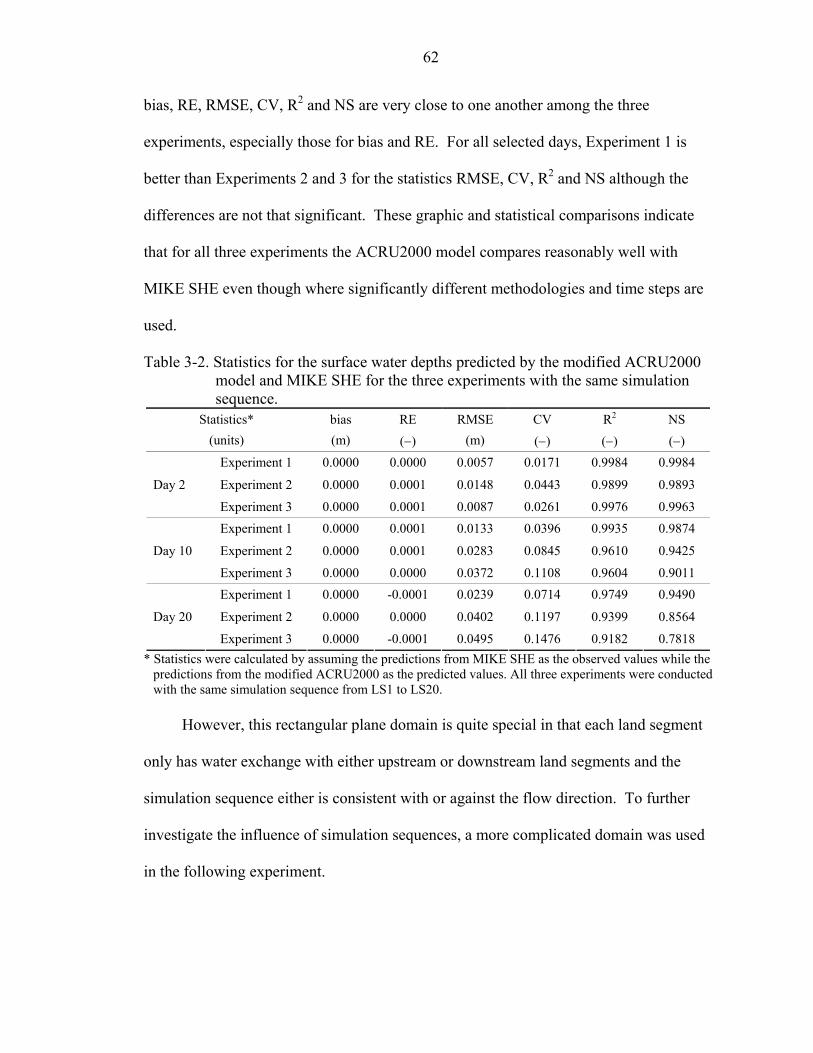
62

bias, RE, RMSE, CV, R2 and NS are very close to one another among the three

experiments, especially those for bias and RE. For all selected days, Experiment 1 is

better than Experiments 2 and 3 for the statistics RMSE, CV, R2 and NS although the

differences are not that significant. These graphic and statistical comparisons indicate

that for all three experiments the ACRU2000 model compares reasonably well with

MIKE SHE even though where significantly different methodologies and time steps are

used.

Table 3-2. Statistics for the surface water depths predicted by the modified ACRU2000 model and MIKE SHE for the three experiments with the same simulation sequence.

Statistics* bias RE RMSE CV R2 NS (units) (m) (−) (m) (−) (−) (−)

Experiment 1 0.0000 0.0000 0.0057 0.0171 0.9984 0.9984

Experiment 2 0.0000 0.0001 0.0148 0.0443 0.9899 0.9893 Day 2

Experiment 3 0.0000 0.0001 0.0087 0.0261 0.9976 0.9963 Experiment 1 0.0000 0.0001 0.0133 0.0396 0.9935 0.9874

Experiment 2 0.0000 0.0001 0.0283 0.0845 0.9610 0.9425 Day 10

Experiment 3 0.0000 0.0000 0.0372 0.1108 0.9604 0.9011 Experiment 1 0.0000 -0.0001 0.0239 0.0714 0.9749 0.9490

Experiment 2 0.0000 0.0000 0.0402 0.1197 0.9399 0.8564 Day 20

Experiment 3 0.0000 -0.0001 0.0495 0.1476 0.9182 0.7818 * Statistics were calculated by assuming the predictions from MIKE SHE as the observed values while the

predictions from the modified ACRU2000 as the predicted values. All three experiments were conducted with the same simulation sequence from LS1 to LS20.

However, this rectangular plane domain is quite special in that each land segment

only has water exchange with either upstream or downstream land segments and the

simulation sequence either is consistent with or against the flow direction. To further

investigate the influence of simulation sequences, a more complicated domain was used

in the following experiment.

63

Comparison of Surface Water Depths over Land Segments for Experiment 1

0.00

0.09

0.18

0.27

0.36

0.45

LS1 LS3 LS5 LS7 LS9 LS11 LS13 LS15 LS17 LS19

Land Segment

Wat

er D

epth

(m)

Day2 LS1-LS20Day10 LS1-LS20Day20 LS1-LS20Day30 LS1-LS20Day2 LS20-LS1Day10 LS20-LS1Day20 LS20-LS1Day30 LS20-LS1


0.00

0.09

0.18

0.27

0.36

0.45


Land Segment

Wat

er D

epth

(m)



0.00

0.09

0.18

0.27

0.36

0.45


Land Segment

Wat

er D

epth

(m)


Figure 3-9. Comparisons of the simulated surface water depth from the modified

ACRU2000 model on the three experiments between two opposite simulation sequences.

64

Comparison of Surface Water Depths over Land Segments on Day 2

0.00

0.09

0.18

0.27

0.36

0.45


Land Segment

Wat

er D

epth

(m)

MIKE SHEExperiment 1 ACRU2000Experiment 2 ACRU2000Experiment 3 ACRU2000


0.00

0.09

0.18

0.27

0.36

0.45


Land Segment

Wat

er D

epth

(m)



0.00

0.09

0.18

0.27

0.36

0.45


Land Segment

Wat

er D

epth

(m)


Figure 3-10. Comparisons of the simulated surface water depths between the MIKE

SHE’s overland flow model and the modified ACRU2000 hydrologic model on the three experiments with the simulation sequence from LS1 to LS20.

65

Case 2: Overland and groundwater flow over an axisymmetric domain

An axisymmetric domain with its 2D and 3D gridded discretization as shown in

Figure 3-11 was used to test the influence of simulation sequence on both overland and

groundwater flows in the modified ACRU2000 model. The domain, with a size of 600 m

× 600 m, is composed of 100 meter square grid cells, each of which is 2 m in depth. Four

equal-thickness computational soil layers with homogenous soil properties for each soil

layer were assumed for each land segment. The surface elevation for each land segment

was set to 10 m. Homogeneous hydrologic and physical characteristics were assumed for

each land segment including the Manning’s roughness coefficient (= 0.1 m1/3/s), soil

layer thickness (= 0.5 m), horizontal/vertical hydraulic conductivity (= 0.0000444 m/s),

specific yield (= 0.25), and storage coefficient (= 0.00005 m-1). An initial water depth of

0.5 m was assigned to the central four land segments, 0.25 m to the land segments

surrounding the central ones, and 0.0 m to the rest of land segments for the overland flow

simulation in this scenario. For the groundwater flow simulations, the previous setting

for initial water levels in each land segment was lowered by a depth of 1.5 m so that no

surface water movement would occur. A closed boundary condition was assumed. A 30-

day simulation period was used for the overland flow simulation and a 2-year simulation

period for the groundwater flow simulation.

The objectives for this case study were to investigate the difference in simulated

results for the three experiments (Table 3-1) in a more complicated domain where land

segments may interact spatially with one another in multiple directions, and compare the

simulated surface water depths with those from MIKE SHE (DHI, 2004) and

groundwater table depths with those from MIKE SHE (DHI, 2004) and MODFLOW

(McDonald and Harbaugh, 1988). A simulation sequence, which transfers water from the

66

center to boundary of the domain symmetrically following the flow direction, was

specified. An hourly time step was used for the 2D overland flow model in MIKE SHE,

a varying time step ranging from 2 to 12 hours for the 3D groundwater flow model in

MIKE SHE, and a daily time step for the groundwater flow model in MODFLOW and

the modified ACRU2000 model. The model was run separately with different initial

water level settings so that both surface overland flow and groundwater flow can be

investigated individually.

Figure 3-11. Schematics of two-dimensional axisymmetric domain (left) and its three-

dimensional discretization (right). The digits assigned in the left diagram indicate the number for each land segment.

For the overland flow simulation, the simulated surface water depths from LS19,

LS20, LS21, LS25, LS26, and LS31 were selected for analysis because of the

axisymmetric distribution of water depths over the domain. For each selected land

segment, the simulated water depths from the three experiments were compared with

those from MIKE SHE’s overland flow model as shown in Figure 3-12. Similar to the

conclusions drawn from Case 1, the comparisons from all three experiments in all

selected land segments indicate that water moves slightly faster in the modified

ACRU2000 model than in MIKE SHE. The results from Experiments 1 and 2 show

y z

x x

y

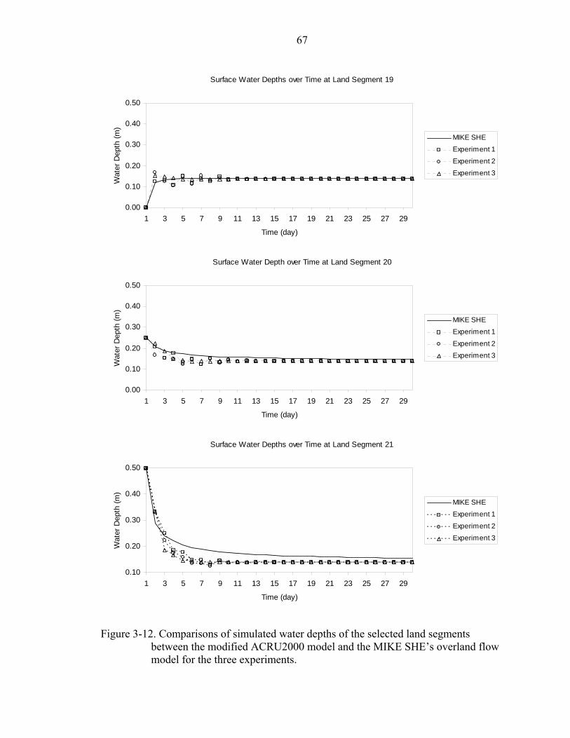
67

Surface Water Depths over Time at Land Segment 19

0.00

0.10

0.20

0.30

0.40

0.50

1 3 5 7 9 11 13 15 17 19 21 23 25 27 29

Time (day)

Wat

er D

epth

(m)

MIKE SHEExperiment 1

Experiment 2Experiment 3

Surface Water Depth over Time at Land Segment 20

0.00

0.10

0.20

0.30

0.40

0.50

1 3 5 7 9 11 13 15 17 19 21 23 25 27 29

Time (day)

Wat

er D

epth

(m)




0.10

0.20

0.30

0.40

0.50

1 3 5 7 9 11 13 15 17 19 21 23 25 27 29

Time (day)

Wat

er D

epth

(m)



Figure 3-12. Comparisons of simulated water depths of the selected land segments between the modified ACRU2000 model and the MIKE SHE’s overland flow model for the three experiments.

68


0.00

0.10

0.20

0.30

0.40

0.50

1 3 5 7 9 11 13 15 17 19 21 23 25 27 29

Time (day)

Wat

er D

epth

(m)




0.00

0.10

0.20

0.30

0.40

0.50

1 3 5 7 9 11 13 15 17 19 21 23 25 27 29

Time (day)

Wat

er D

epth

(m)




0.00

0.10

0.20

0.30

0.40

0.50

1 3 5 7 9 11 13 15 17 19 21 23 25 27 29

Time (day)

Wat

er D

epth

(m)



Figure 3-12. Continued.

69

Table 3-3. Statistics for the surface water depths predicted by the modified ACRU2000 model and MIKE SHE for the three experiments.

Statistics* bias RE RMSE CV R2 NS

(units) (m) (−) (m) (−) (−) (−) Experiment 1 -0.0015 -0.0111 0.0078 0.0589 0.9139 0.9047 Experiment 2 0.0000 0.0002 0.0121 0.0909 0.8028 0.7726 LS19

Experiment 3 0.0011 0.0082 0.0068 0.0512 0.9315 0.9278 Experiment 1 -0.0138 -0.0861 0.0175 0.1091 0.8224 0.3598 Experiment 2 -0.0164 -0.1022 0.0205 0.1281 0.7208 0.1187 LS20

Experiment 3 -0.0130 -0.0814 0.0161 0.1008 0.8827 0.4535 Experiment 1 -0.0225 -0.1207 0.0292 0.1563 0.9524 0.8059 Experiment 2 -0.0253 -0.1353 0.0322 0.1725 0.9393 0.7637 LS21

Experiment 3 -0.0265 -0.1419 0.0335 0.1794 0.9319 0.7445 Experiment 1 0.0128 0.1092 0.0214 0.1832 0.7289 0.3180 Experiment 2 0.0141 0.1205 0.0232 0.1986 0.6855 0.1983 LS25

Experiment 3 0.0141 0.1204 0.0159 0.1358 0.9322 0.6249 Experiment 1 0.0015 0.0105 0.0221 0.1546 0.4450 -0.1851 Experiment 2 0.0015 0.0102 0.0210 0.1470 0.4703 -0.0715 LS26

Experiment 3 -0.0028 -0.0193 0.0092 0.0642 0.8471 0.7955 Experiment 1 0.0256 0.2555 0.0328 0.3271 0.7377 -0.1002 Experiment 2 0.0276 0.2759 0.0355 0.3542 0.6569 -0.2900 LS31

Experiment 3 0.0290 0.2895 0.0331 0.3307 0.7684 -0.1246 * Statistics were calculated by assuming the predictions from MIKE SHE as the observed values while the

predictions from the modified ACRU2000 model as the simulated values. All three experiments were performed with the same simulation sequence.

fluctuations at early times of simulation but eventually trend to the results from

Experiment 3 in which the curve of predicted water depths appears smooth. However,

the differences among the three experiments seem to be not that significant. Both models

agree with each other fairly well on timing and trends.

Table 3-3 shows the statistics that were calculated by using the predictions from

MIKE SHE as the “observed” values. The statistics indicate that the model generally

produced better predictions in Experiment 3 than in the other two experiments with

smaller RMSE and CV values and larger R2 and NS values in four selected land segments

(LS19, LS20, LS25 and LS26) and similar predictions in LS21 and LS31 with the other

70

two Experiments. It should be noted that slightly larger values of bias and RE are

observed in Experiment 3 in some of these land segments. Overall, it was concluded that

the modified ACRU2000 model performed better in Experiment 3 for this scenario and

thus Experiment 3 is the most appropriate strategy for producing reasonable surface water

depths for this axisymmetric domain. To further visualize the comparison of simulated

results for Experiment 3, Figure 3-13 displays a time series comparison of surface water

depths for all selected land segments for these two models.

0.0

0.1

0.2

0.3

0.4

0.5

1 4 7 10 13 16 19 22 25 28

Time (day)

Sur

face

Wat

er D

epth

(m)

LS19 MIKE SHE LS20 MIKE SHE



LS19 ACRU2000 LS20 ACRU2000



Figure 3-13. Comparisons of the simulated water depths of the selected land segments

between the modified ACRU2000 and MIKE SHE’s overland flow model for Experiment 3.

71

A groundwater simulation test was made by changing initial water levels as

discussed earlier. Similar to the above overland flow simulation, the simulated

groundwater table depths also display an axisymmetric distribution pattern over the

domain. Therefore the simulated water table depths from LS19, LS20, LS21, LS25,

LS26, and LS31 were used to compare with the MIKE SHE’s predictions for all three

experiments as shown in Figure 3-14. From this figure, it is fairly difficult to tell the

difference among the simulated results from the three experiments for they all have very

similar predictions for all selected land segments. Interestingly, the ACRU results for the

three experiments are consistently located in between the predictions from MIKE SHE

and MODFLOW for all selected land segments, although these results agree with MIKE

SHE’s predictions better in LS19, LS20, LS25, LS26, and LS31 and with MODFLOW’s

predictions better in LS21. The comparisons also reveal that the ACRU2000

groundwater movement is slightly faster than MIKE SHE and a little bit slower than

MODFLOW. The difference in predicted groundwater table depths between the

modified ACRU200 model and the other two models seems larger in the central land

segments (LS20, LS21, and LS26) than it appears in the land segments along the

boundary (LS19, LS25, and LS31). This could result from the larger hydraulic gradient

variations between the central land segments and milder gradients between the boundary

land segments. In general, three models agree with one another on timing and tendency

quite well.

Table 3-4 shows the statistics that were calculated by using the predictions from

MIKE SHE and MODFLOW as the “observed” values for the three experiments for all

selected land segments. Over all selected land segments, there are no significant

72

differences among the bias, RE, RMSE, CV, and R2 values. However, some systematic

differences in the NS values are noticed between the predictions from MIKE SHE and

MODFLOW as the “observed” values: excellent NS values close to 1 for LS19, LS25,

and LS31, fairly good NS values for LS21 and LS26 and poor NS values were obtained

for LS20 when comparing to MIKE SHE’s predictions. On the other hand, the NS values

vary gradually for all selected land segment from excellent to fairly good when

comparing to MODFLOW’s predictions. Thus it is difficult to differentiate the model

performance among the three experiments and thus conclude unequivocally which

experiment provides the most appropriate strategy.

From the previous case studies for two different hypothetical scenarios, it can be

concluded that the simulation sequence affects the simulation results, but not very

significantly. Thus picking a simulation sequence that follows the flow directions

determined by the topography on the ground surface is reasonable. Moreover, among the

three alternative water transmission and water storage updating strategies, Experiment 3

appears to be the most appropriate one for reasonable simulation of overland flow but no

significant difference was observed in simulation of groundwater flow. By comparing to

results from MIKE SHE and MODFLOW, the modified ACRU2000 model has been

shown to simulate hydrology reasonably well.

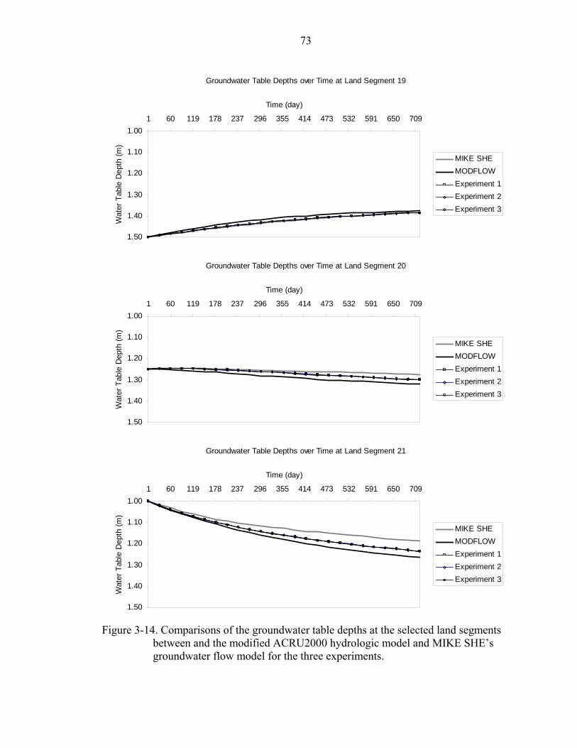
73

Groundwater Table Depths over Time at Land Segment 19

1.00

1.10

1.20

1.30

1.40

1.50

1 60 119 178 237 296 355 414 473 532 591 650 709

Time (day)

Wat

er T

able

Dep

th (m

)

MIKE SHEMODFLOWExperiment 1Experiment 2Experiment 3


1.00

1.10

1.20

1.30

1.40

1.50

1 60 119 178 237 296 355 414 473 532 591 650 709

Time (day)

Wat

er T

able

Dep

th (m

)



1.00

1.10

1.20

1.30

1.40

1.50

1 60 119 178 237 296 355 414 473 532 591 650 709

Time (day)

Wat

er T

able

Dep

th (m

)


Figure 3-14. Comparisons of the groundwater table depths at the selected land segments

between and the modified ACRU2000 hydrologic model and MIKE SHE’s groundwater flow model for the three experiments.

74


1.00

1.10

1.20

1.30

1.40

1.50

1 60 119 178 237 296 355 414 473 532 591 650 709

Time (day)W

ater

Tab

le D

epth

(m)



1.00

1.10

1.20

1.30

1.40

1.50

1 60 119 178 237 296 355 414 473 532 591 650 709

Time (day)

Wat

er T

able

Dep

th (m

)



1.00

1.10

1.20

1.30

1.40

1.50

1 60 119 178 237 296 355 414 473 532 591 650 709

Time (day)

Wat

er T

able

Dep

th (m

)


Figure 3-14. Continued.

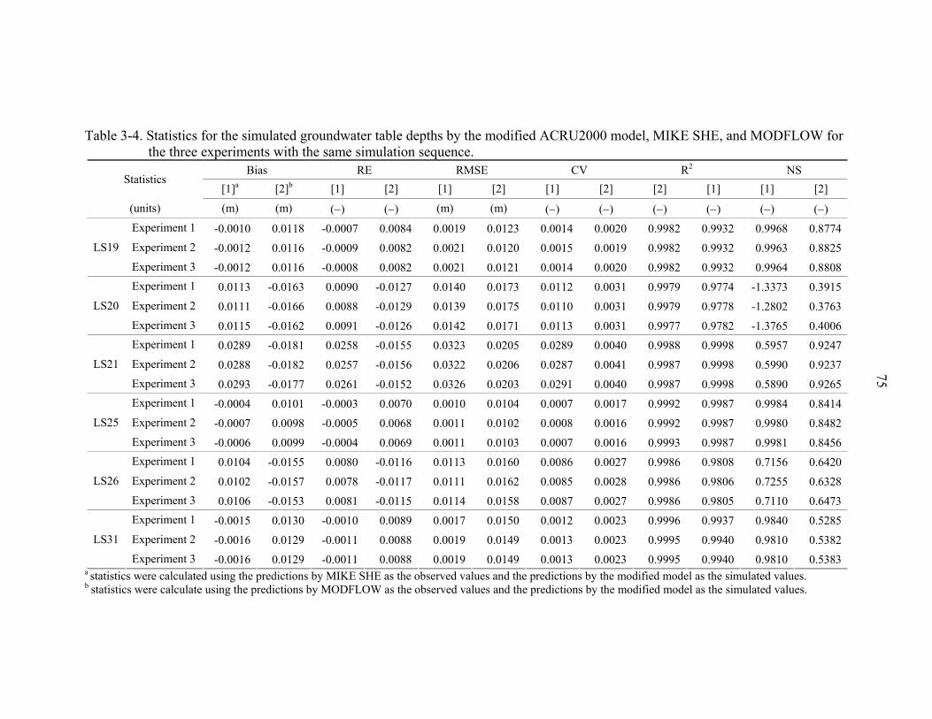
75

Table 3-4. Statistics for the simulated groundwater table depths by the modified ACRU2000 model, MIKE SHE, and MODFLOW for the three experiments with the same simulation sequence.

Bias RE RMSE CV R2 NS Statistics

[1]a [2]b [1] [2] [1] [2] [1] [2] [2] [1] [1] [2]

(units) (m) (m) (−) (−) (m) (m) (−) (−) (−) (−) (−) (−) Experiment 1 -0.0010 0.0118 -0.0007 0.0084 0.0019 0.0123 0.0014 0.0020 0.9982 0.9932 0.9968 0.8774 Experiment 2 -0.0012 0.0116 -0.0009 0.0082 0.0021 0.0120 0.0015 0.0019 0.9982 0.9932 0.9963 0.8825 LS19

Experiment 3 -0.0012 0.0116 -0.0008 0.0082 0.0021 0.0121 0.0014 0.0020 0.9982 0.9932 0.9964 0.8808 Experiment 1 0.0113 -0.0163 0.0090 -0.0127 0.0140 0.0173 0.0112 0.0031 0.9979 0.9774 -1.3373 0.3915 Experiment 2 0.0111 -0.0166 0.0088 -0.0129 0.0139 0.0175 0.0110 0.0031 0.9979 0.9778 -1.2802 0.3763 LS20

Experiment 3 0.0115 -0.0162 0.0091 -0.0126 0.0142 0.0171 0.0113 0.0031 0.9977 0.9782 -1.3765 0.4006 Experiment 1 0.0289 -0.0181 0.0258 -0.0155 0.0323 0.0205 0.0289 0.0040 0.9988 0.9998 0.5957 0.9247 Experiment 2 0.0288 -0.0182 0.0257 -0.0156 0.0322 0.0206 0.0287 0.0041 0.9987 0.9998 0.5990 0.9237 LS21

Experiment 3 0.0293 -0.0177 0.0261 -0.0152 0.0326 0.0203 0.0291 0.0040 0.9987 0.9998 0.5890 0.9265 Experiment 1 -0.0004 0.0101 -0.0003 0.0070 0.0010 0.0104 0.0007 0.0017 0.9992 0.9987 0.9984 0.8414 Experiment 2 -0.0007 0.0098 -0.0005 0.0068 0.0011 0.0102 0.0008 0.0016 0.9992 0.9987 0.9980 0.8482 LS25

Experiment 3 -0.0006 0.0099 -0.0004 0.0069 0.0011 0.0103 0.0007 0.0016 0.9993 0.9987 0.9981 0.8456 Experiment 1 0.0104 -0.0155 0.0080 -0.0116 0.0113 0.0160 0.0086 0.0027 0.9986 0.9808 0.7156 0.6420 Experiment 2 0.0102 -0.0157 0.0078 -0.0117 0.0111 0.0162 0.0085 0.0028 0.9986 0.9806 0.7255 0.6328 LS26

Experiment 3 0.0106 -0.0153 0.0081 -0.0115 0.0114 0.0158 0.0087 0.0027 0.9986 0.9805 0.7110 0.6473 Experiment 1 -0.0015 0.0130 -0.0010 0.0089 0.0017 0.0150 0.0012 0.0023 0.9996 0.9937 0.9840 0.5285 Experiment 2 -0.0016 0.0129 -0.0011 0.0088 0.0019 0.0149 0.0013 0.0023 0.9995 0.9940 0.9810 0.5382 LS31

Experiment 3 -0.0016 0.0129 -0.0011 0.0088 0.0019 0.0149 0.0013 0.0023 0.9995 0.9940 0.9810 0.5383 a statistics were calculated using the predictions by MIKE SHE as the observed values and the predictions by the modified model as the simulated values. b statistics were calculate using the predictions by MODFLOW as the observed values and the predictions by the modified model as the simulated values.

76

Application at Dry Lake Dairy #1, Kissimmee River Basin, Florida

Site description

The Dry Lake Dairy #1 is an agricultural pasture site located within the lower

Kissimmee River and Taylor Creek-Nubbin Slough Basins (Figure 3-15). The site is

located on Immokalee soil with surface depressions and little slope, thus the pasture often

becomes flooded during the rainy season. The spodic horizon for Immokalee fine sand

typically occurs at approximately 90 cm and averages 50 cm in thickness. The upper

zone of the spodic horizon is black and weakly-cemented, while the lower zone is a

mottled, dark reddish brown and is even more weakly cemented than the upper layer.

During the wet season, the water table stands near or at the surface for short periods and

recedes to below 120 cm during the dry season (Capece, 1994).

Figure 3-15. Location of Dry Lake Dairy #1 site (Capece, 1994).

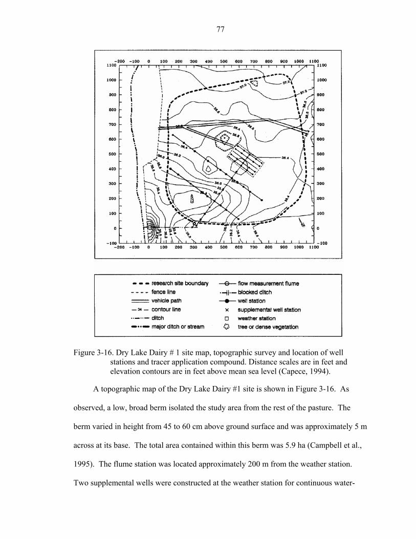
77

Figure 3-16. Dry Lake Dairy # 1 site map, topographic survey and location of well stations and tracer application compound. Distance scales are in feet and elevation contours are in feet above mean sea level (Capece, 1994).

A topographic map of the Dry Lake Dairy #1 site is shown in Figure 3-16. As

observed, a low, broad berm isolated the study area from the rest of the pasture. The

berm varied in height from 45 to 60 cm above ground surface and was approximately 5 m

across at its base. The total area contained within this berm was 5.9 ha (Campbell et al.,

1995). The flume station was located approximately 200 m from the weather station.

Two supplemental wells were constructed at the weather station for continuous water-

78

table monitoring. Water-table depth in one well near the flume also was continuously

monitored by the flume datalogger (Campbell et al., 1995). A shallow collection ditch

paralleled the perimeter berm for approximately one third of its length nearest the flume

station. This V-shaped collection ditch was grassed and was less than 30 cm deep and

approximately 3 m wide (Campbell et al., 1995). The constructed collection ditch

discharged into a trapezoidal flow measurement flume with a maximum capacity of 7.1

cfs (200 l/s). A total of 69 well stations were established on this site. Each well station

was composed of two or three wells of different depths.

Weather, runoff and groundwater quality measurements were obtained at the Dry

Lake Dairy #1 site to provide information concerning water and P movement in flat,

sandy, high-water-table soils. Summary data for annual rainfall, ET, and observed runoff

are listed in Table 3-5. These data indicate that years 1989 and 1990 were dry years

when compared to year 1991 with less rainfall and more ET. Year 1991 was relatively

wet with relatively more rainfall. A simple water budget in the last column of Table 3-5

shows year 1989 is the driest, year 1990 ranks the second, and year 1991 is the wettest

among the three years.

Table 3-5. Summary of annual water budget on Dry Lake Dairy #1 sitea. Rainfall (R) Runoff (RO) ET 100×(ET+RO-R)/RYears

(cm) (cm) (cm) (%) 1989 (April-December) 88.66 5.15 91.37 8.87

1990 117.47 25.71 100.30 7.27 1991 133.00 44.29 92.18 2.61 Total 339.13 75.14 283.85 5.86

aData from Tremwel (1992).

The purpose of this application was to validate the modified ACRU2000 model by

comparing with the lumped FHANTM model (Tremwel, 1992), which was applied in the

Dry Lake Dairy #1 site in 1992. For the modified ACRU2000 simulation, the Dry Lake

79

Dairy #1 site was divided into 4 land segments, each with identical hydrologic properties

and soil layers since no spatially distributed data were available. The discharge from the

site through the flume was estimated using the empirical formula (Tremwel, 1992)

5.05.15.2 h121409.0h508387.0h282156.3Q ++= (3-10)

in which Q is the discharge in cubic feet per second and h is the surface water depth in

feet. The measured rainfall, pre-calculated potential ET, and temperature from Tremwel

(1992) were used as the time series input and were applied uniformly for each land

segment. Some input such as soil properties (field capacity, soil porosity, wilting point,

and hydraulic conductivity) as shown in Table 3-6 were adapted from the calibrated

parameters by Tremwel (1992) for FHANTM and the rest of input were estimated. No

deep seepage process was considered in the test. No calibration was performed for the

modified ACRU2000 model.

The simulation period for this validation test was from April 1989 through

December 1991. The model was run throughout the whole simulation period and the

simulated results for surface runoff and groundwater table were compared with those

from FHANTM, for both the calibration period (April 1, 1989 to August 31, 1990) and

the verification period (September 1, 1990 to December 31, 1991). Model prediction

statistics were calculated using the results from both models to quantitatively evaluate the

model performance. Scatterplots of observed vs. simulated values were prepared to

visualize the predicted results from both models.

Results and discussion

The major output variables for this test were the surface runoff through the outlet of

the Dry Lake site and the groundwater table depth, which was taken as the field average

80

from all wells for the observations and as the mathematic average of predicted

groundwater table depths form the four land segments for the model simulation.

Continuous simulation of surface runoff is shown in Figure 3-17 for both models

against the observed data for the period from August 1989 through October 1991. Both

ACRU2000 and FHANTM successfully captured major rainfall events in the calibration

period but missed a few rainfall events during the verification period. There were some

underestimations and overestimations of event hydrograph values by both models.

Figure 3-18 illustrates the comparisons of cumulative surface runoff for the whole

simulation period. It appears that both models’ predictions agree with each other fairly

well throughout the simulation period. Furthermore they agree well with the observed

cumulative runoff during the calibration period. However, they overestimated the

observed data between the middle of January 1991 through July 1991, and

underestimated the observed data throughout the rest of the simulation period. Similar to

FHANTM, the modified ACRU2000 model performed better during the calibration

period than it did during the verification period.

Figure 3-19 compares continuous simulations of groundwater table depth from the

modified ACRU2000 model and FHANTM to the observed data for August 1989 to

December 1991. A better agreement is observed during the calibration period for both

models, while a slightly larger deviation from the observed water table depth data

observed for both models in the verification period.

Considering different weather conditions for calibration and verification periods, it

is apparent that the calibration of FHANTM was done in a relatively dry period whereas

the verification was made in a relatively wet period. The difference in weather

81

conditions for both periods could cause the calibrated parameters by FHANTM to be

suboptimal for the verification period. Since the same calibrated parameters were used in

the modified ACRU2000 model, it is not surprising that similar results were obtained.

Statistics can be used to quantitatively address the difference in both models’

performance in simulating the observed conditions. As shown in Table 3-7, six statistics

including bias, RE, RMSE, CV, R2 and NS, introduced earlier in Chapter 2, were

calculated. Statistics bias, RE, RMSE, and CV in runoff for the modified ACRU2000

model are slightly larger than those for FHANTM while R2 and NS are a little smaller

than those for FHANTM. And all statistics except NS in groundwater table are slightly

larger than those for FHANTM. The comparisons of these statistics imply that

FHANTM more accurately predicted in both runoff and water table depth than the

modified ACRU2000 model. However, considering the modified ACRU2000 model was

not calibrated specifically for the Dry Lake site, both model’s predictions are acceptable.

Furthermore, the Dry Lake Dairy #1 site is very small with an area of 5.9 ha and uniform

parameters were used over the simulation domain. Therefore, the advantages of a

distributed model like the modified ACRU2000 model may not be demonstrated by this

example. It maybe possible that better results could be achieved by the ACRU2000

model if there were sufficient data to calibrate spatially distributed parameters directly for

this model.

Scatterplots of observed versus predicted surface runoff and groundwater table

depth were prepared to further visualize the overall performance of these models. Figure

3-20 shows the linear plot for surface runoff depth. FHANTM’s predictions fall closer to

the 1:1 line than those from ACRU2000, while ACRU2000’s tend to underpredict surface

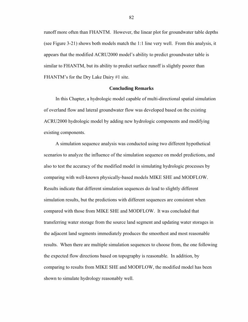
82

runoff more often than FHANTM. However, the linear plot for groundwater table depths

(see Figure 3-21) shows both models match the 1:1 line very well. From this analysis, it

appears that the modified ACRU2000 model’s ability to predict groundwater table is

similar to FHANTM, but its ability to predict surface runoff is slightly poorer than

FHANTM’s for the Dry Lake Dairy #1 site.

Concluding Remarks

In this Chapter, a hydrologic model capable of multi-directional spatial simulation

of overland flow and lateral groundwater flow was developed based on the existing

ACRU2000 hydrologic model by adding new hydrologic components and modifying

existing components.

A simulation sequence analysis was conducted using two different hypothetical

scenarios to analyze the influence of the simulation sequence on model predictions, and

also to test the accuracy of the modified model in simulating hydrologic processes by

comparing with well-known physically-based models MIKE SHE and MODFLOW.

Results indicate that different simulation sequences do lead to slightly different

simulation results, but the predictions with different sequences are consistent when

compared with those from MIKE SHE and MODFLOW. It was concluded that

transferring water storage from the source land segment and updating water storages in

the adjacent land segments immediately produces the smoothest and most reasonable

results. When there are multiple simulation sequences to choose from, the one following

the expected flow directions based on topography is reasonable. In addition, by

comparing to results from MIKE SHE and MODFLOW, the modified model has been

shown to simulate hydrology reasonably well.

83

A test was conducted to validate the modified ACRU2000 model by comparing

with the lumped FHANTM model in the Dry Lake Dairy #1 site, Kissimmee River Basin,

FL. From the comparisons and statistical analyses, it was concluded that the modified

ACRU2000 hydrologic model is capable of adequately simulating overland flow and

groundwater table at the Dry Lake Dairy #1 site, but the modified ACRU2000 model is

not better than FHANTM. However, the modified ACRU2000 model was not calibrated

but utilized input parameters calibrated by FHANTM. Thus the advantages of a

distributed model like the modified ACRU2000 may not be demonstrated by this

application. It maybe possible that better results could be achieved for the modified

ACRU2000 if there are sufficient data to calibrate spatially distributed parameters

directly from this model.

84

0

1

2

3

4

5

6

8/1/89 11/1/89 2/1/90 5/1/90 8/1/90 11/1/90 2/1/91 5/1/91 8/1/91

Time (day)

Run

off (

cm)

0

10

20

30

40

50

60

70

Rai

nfal

l (am

)

Rainfall

ACRU2000

FHANTM

Observed

Figure 3-17. Comparisons of the continuous simulations of runoff from the modified

ACRU2000 and FHANTM against the observed data.

0

10

20

30

40

50

60

70

80

8/1/89 11/1/89 2/1/90 5/1/90 8/1/90 11/1/90 2/1/91 5/1/91 8/1/91

Time (day)

Run

off (

cm)

0

10

20

30

40

50

60

70

Rai

nfal

l (cm

)

Rainfall

Cumulative ACRU2000

Cumulative FHANTM

Cumulative Observed

Figure 3-18. Comparisons of the cumulative simulated runoff from the modified

ACRU2000 and FHANTM with the cumulative observed data.

85

-200

-180

-160

-140

-120

-100

-80

-60

-40

-20

0

20

8/1/89 11/1/89 2/1/90 5/1/90 8/1/90 11/1/90 2/1/91 5/1/91 8/1/91 11/1/91

Time (day)

Wat

er T

able

Dep

th (c

m)

0

20

40

60

80

100

120

Rai

nfal

l (cm

)

RainfallACRU2000FHANTMObserved

Figure 3-19. Comparisons of the continuous simulation of groundwater table depths from

the modified ACRU2000 and FHANTM against the observed data.

Table 3-6. Model input parameters for the Dry Lake Dairy #1 site.

Parameters Unit Value Soil layer deptha m 0.10 0.10 0.10 0.10 0.15 0.15 0.15 0.15 0.50 0.50 Soil porositya m/m 0.40 0.40 0.32 0.32 0.32 0.32 0.30 0.30 0.30 0.30 Wilting pointa m/m 0.11 0.11 0.05 0.05 0.05 0.05 0.10 0.10 0.10 0.10 Field capacitya m/m 0.15 0.15 0.12 0.12 0.12 0.12 0.12 0.12 0.12 0.12 Vertical saturated hydraulic conductivityb

m/s 3.56 E-07

3.56 E-07

3.56 E-07

3.56 E-07

3.56 E-07

3.56 E-07

3.56 E-07

3.56 E-07

3.56 E-07

3.56 E-07

Lateral saturated hydraulic conductivityb

m/s 4.44 E-05

4.44 E-05

4.44 E-05

4.44 E-05

4.44 E-05

4.44 E-05

4.44 E-05

4.44 E-05

4.44 E-05

4.44 E-05

Manning’s coefficientb m1/3/s 0.1 Brooks-Corey hb cm 40.0 40.0 45.0 45.0 45.0 45.0 75.0 75.0 75.0 75.0 Brooks-Corey λb − 1.60 1.60 0.95 0.95 0.95 0.95 0.71 0.71 0.71 0.71 Brooks-Corey θ b m/m 0.11 0.11 0.05 0.05 0.05 0.05 0.10 0.10 0.10 0.10 Surface maximum depressional storageb

m 0.005

Crop coefficientb − 0.4, 0.5, 0.6, 0.6, 0.7, 0.85, 1.0, 0.85, 0.8, 0.8, 0.85, 0.6 for 12 months aCalibrated values by Tremwel (1992); bEstimated values. Table 3-7. Statistics for the simulated surface runoff and groundwater table depths by the

modified ACRU2000 and FHANTM. Statistics* bias RE RMSE CV R2 NS

ACRU2000 -0.27 -0.37 0.74 1.03 0.34 0.10 Runoff FHANTM -0.17 -0.24 0.61 0.86 0.56 0.38 ACRU2000 12.73 -0.15 23.26 -0.27 0.81 0.68 Water Table FHANTM 9.79 0.00 22.23 -0.26 0.80 0.71

*Statistics were calculated using the predictions from both calibration and verification periods. Units of bias and RMSE for runoff and water tablde depth are cm. the rest of statistics are untiless for both variables.

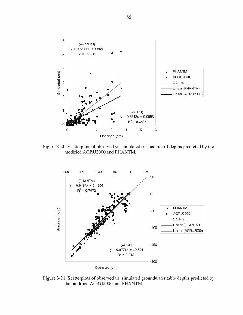
86

(FHANTM)y = 0.8371x - 0.0565

R2 = 0.5611

(ACRU)y = 0.5512x + 0.0553

R2 = 0.34250

1

2

3

4

5

6

0 1 2 3 4 5 6

Observed (cm)

Sim

ulat

ed (c

m) FHANTM

ACRU20001:1 lineLinear (FHANTM)Linear (ACRU2000)

Figure 3-20. Scatterplots of observed vs. simulated surface runoff depths predicted by the

modified ACRU2000 and FHANTM.

(FHANTM)y = 0.9494x + 5.4304

R2 = 0.7972

(ACRU)y = 0.9776x + 10.801

R2 = 0.8131

-200

-150

-100

-50

0

50-200 -150 -100 -50 0 50

Observed (cm)

Sim

ulat

ed (c

m) FHANTM

ACRU20001:1 lineLinear (FHANTM)Linear (ACRU2000)

Figure 3-21. Scatterplots of observed vs. simulated groundwater table depths predicted by

the modified ACRU2000 and FHANTM.

87

CHAPTER 4 NUTRIENT SIMULATION MODEL

Introduction

Nutrient components were not included in the original ACRU (v3.00). After the

model was entirely restructured into an object-oriented framework using the Java

programming language (ACRU2000), Campbell et al. (2001) incorporated a nutrient

module (ACRU-NP), which was patterned after transformation and transport concepts

used in GLEAMS (Leonard et al., 1987; Knisel and Davis, 1999). The goals of

Campbell’s work were to add capacities in ACRU2000 to 1) simulate nitrogen (N) and

phosphorus (P) losses in surface runoff, sediment transport, and leaching, 2) simulate N

and P cycling in the soil-water-plant-animal system, and 3) simulate N and P mass

balances in the watershed system. Since GLEAMS includes most of these capacities in

its current version it was used as a guide in development (Campbell et al., 2001). The

module includes rainfall, irrigation, fertilizers, plants, and animal wastes as potential

nutrient sources and represents management impacts on N and P transformation and

transport (Campbell et al., 2001). Nutrient simulation requires a wide range of inputs

including soil properties, irrigation parameters, crop parameters, nutrients in residues,

fertilizer application and also tillage operations. A few adjustments were made to tailor

the performance of GLEAMS when it was recoded into ACRU2000, including the

significant modification to include the capacity to simulate grazing of pastures.

However, ACRU-NP module was incapable of simulating multidirectional lateral

nutrient transport between land segments through either surface or subsurface water

88

movement. The lateral nutrient transport component in ACRU-NP was mainly designed

for transporting nutrients dissolved in runoff and adsorbed in sediments through single

outflow from one land segment. Considering the important mechanisms for delivering

nutrients into downstream water bodies through both lateral surface and subsurface water

movement in south Florida, it was necessary to modify the model to simulate lateral

nutrient transport. Additionally, the original algorithm for dealing with the soil-surface

nutrient exchange is a process of nutrient extraction and adsorption, with the ratio for

partitioning the nutrients between the water and soil phases being a function of clay

content. This method has the potential to overestimate the nutrients adsorbed onto soils

but underestimate the nutrient released into surface water, especially for south Florida

flatwood soils that contain low clay contents. To accurately simulate nutrient dynamics,

it was necessary to modify this methodology. Moreover, the testing of the nutrient

module within the framework of ACRU2000 has not been reported in the literature.

Consequently, the major purpose of this work was to modify the existing ACRU-NP

module to enable multidirectional spatial nutrient transport and test the modified model in

simulating nutrient dynamics in south Florida flatwoods soils.

The major modifications presented in this chapter include adding new components

to enable multi-directional spatial transport of N and P through surface runoff and lateral

groundwater flow, and new conservative solute transport components to strengthen the

capacities of the module to meet future needs. In addition, several existing nutrient

transformation processes including ammonification, nitrification, P mineralization,

immobilization, and denitrification were modified by Martinez (2006) and utilized in the

model presented here.

89

Similar to the hydrologic processes, the modified nutrient components are grouped

into vertical and lateral processes as shown in Appendix A. The vertical processes

consist of N and P transport and transformation processes, and conservative solute

transport, along the soil profile. These processes are executed after the vertical

hydrologic processes. The lateral processes include the lateral N, P and conservative

solute transport components, which are executed after the horizontal hydrologic

processes. Appendix A lists the individual processes and the order that these processes

are simulated in the context of the coupled modeling system. A daily time step is used in

the nutrient module.

In the following sections, the nutrient components are briefly discussed. Details

regarding the components taken from GLEAMS can be found in Knisel et al. (1993) and

Fraisse and Campbell (1997). Processes developed in this work are discussed

extensively. A conservative solute test (an extension of the hypothetical study in Chapter

3) is introduced to investigate the accuracy of the solute transport performance by

comparing with the established particle tracking model PMPATH (Chiang and

Kinzelbach, 2005). Following that, an application of the modified model to beef cattle

pastures in the Buck Island Ranch, Lake Okeechobee Basin, FL is conducted, which

includes model calibration, verification and sensitivity analysis. Conclusions regarding

the model development and performance are summarized at the end of this chapter.

Nutrient Components

Nitrogen Cycle Components

A schematic representation of the N components in GLEAMS is shown in Figure

4-1. N in the soil is divided into six classifications including nitrate-N (NO3-N),

ammonium-N (NH4-N), fresh organic N (crop residues and roots), organic N from animal

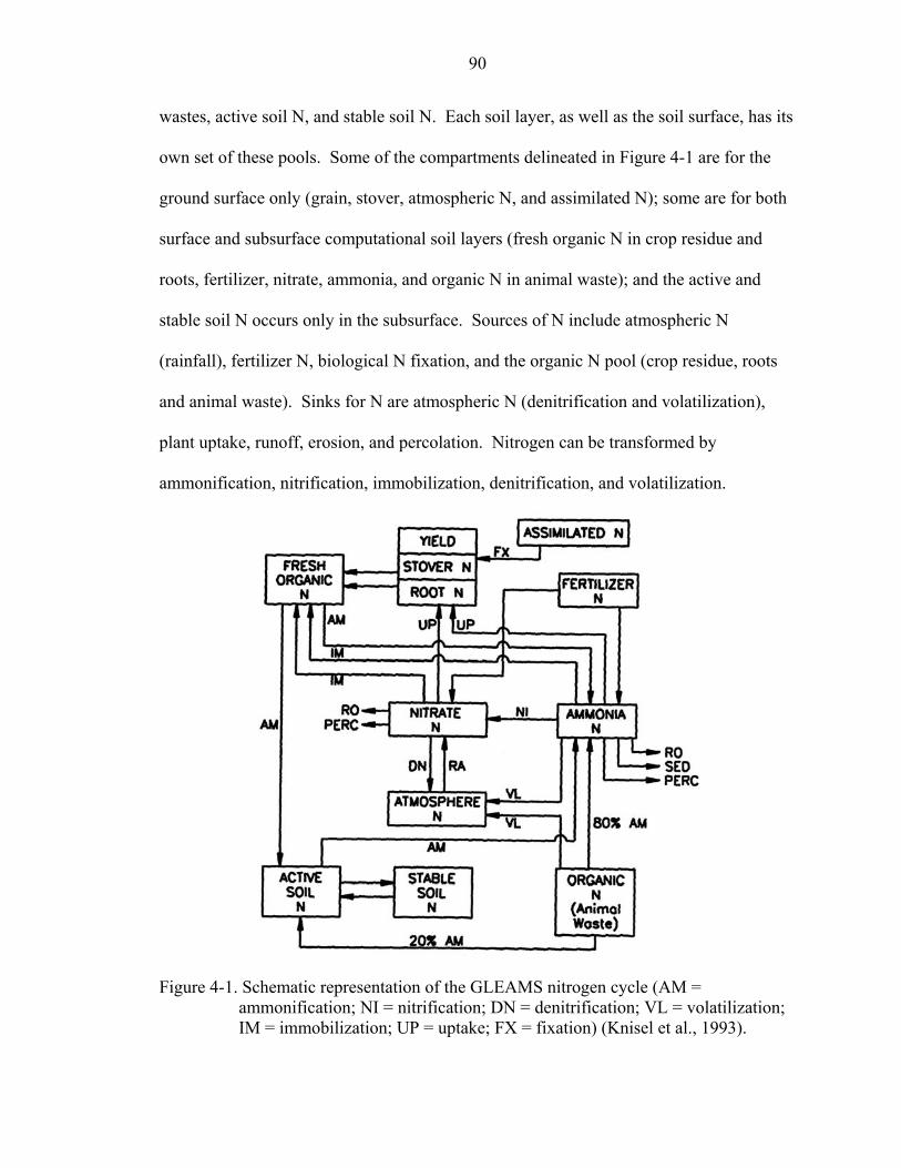
90

wastes, active soil N, and stable soil N. Each soil layer, as well as the soil surface, has its

own set of these pools. Some of the compartments delineated in Figure 4-1 are for the

ground surface only (grain, stover, atmospheric N, and assimilated N); some are for both

surface and subsurface computational soil layers (fresh organic N in crop residue and

roots, fertilizer, nitrate, ammonia, and organic N in animal waste); and the active and

stable soil N occurs only in the subsurface. Sources of N include atmospheric N

(rainfall), fertilizer N, biological N fixation, and the organic N pool (crop residue, roots

and animal waste). Sinks for N are atmospheric N (denitrification and volatilization),

plant uptake, runoff, erosion, and percolation. Nitrogen can be transformed by

ammonification, nitrification, immobilization, denitrification, and volatilization.

Figure 4-1. Schematic representation of the GLEAMS nitrogen cycle (AM =

ammonification; NI = nitrification; DN = denitrification; VL = volatilization; IM = immobilization; UP = uptake; FX = fixation) (Knisel et al., 1993).

91

Nitrogen including NO3-N and NH4-N may be transported with surface runoff and

lateral groundwater flow from one land segment to its neighboring land segments. To

calculate the amount of nitrogen mass moved with water flows, the concentrations of

nutrients in the surface water and subsurface are calculated separately. These

concentrations are then multiplied by the volume of water moving along each pathway to

obtain the mass of nutrients lost through surface runoff and lateral groundwater flow

from each land segment to its neighboring land segments, streams or water bodies.

Mineralization

N mineralization is considered a two-stage process in GLEAMS - ammonification

followed by nitrification. In the soil, organic N is divided into two pools: a stable pool

from which no mineralization occurs (C: N > 25), and an active pool available for

mineralization (C: N < 25). The active pool can be replenished from flux between it and

the stable pool (a function of relative pool sizes), from fresh organic N from

decomposing roots, and from decomposition of organic N in applied animal waste.

Ammonification of decomposing roots, other crop residues, and animal wastes in

the soil is considered a first-order process and is a function of C:N and C:P ratios of the

residue, temperature, and soil moisture content. Of the total NH4-N released by animal

waste in the soil, 20% is allocated to the active soil N pool with 80% going to an NH4-N

pool. Crop residues and animal waste on the surface use a similar function to determine

ammonification rate but liberated NH4-N stays on the surface in a soluble NH4-N pool

until moved into the soil by the next rainfall or irrigation event. As the C: N ratio of the

soil active N pool is set between 12:1 and 25:1, organic C is already partially accounted

for and ammonification of the active N pool is a function of temperature and soil water

92

content. Nitrogen flux from the active N pool can go to either the stable soil N pool or to

the free NH4-N pool.

The second stage of mineralization is nitrification, which converts N in the NH4-N

pool into NO3-N. This is considered a zero-order process (not affected by the amount of

NO3-N or NH4-N) and is modeled as a function of temperature and soil moisture.

Nitrogen from the NH4-N pool that is nitrified is transferred to the NO3-N pool.

Nitrification can also occur on the soil surface where it is a function of temperature and

soil moisture. As with the soluble NH4-N pool, the soluble nitrate pool on the soil

surface remains on the soil surface until moved into the soil by rainfall. Once in the soil,

these products join the appropriate pools in the soil.

Immobilization

Immobilization occurs when either NO3-N or NH4-N is used by soil microbes for

growth. Once incorporated into the microbe, the N is unavailable for uptake by plants

and remains so until the death and decomposition of the microbe. Thus, factors that

affect the growth rate of microbes are important in driving immobilization.

Immobilization of both soil and surface N is a function of the amount of NO3-N and NH4-

N available, C:N ratio, and C:P ratio. Immobilization is limited to 95% of total available

NO3-N and NH4-N. Immobilized N in the soil can end up either in the fresh organic N

pool or in the stable soil N pool.

Denitrification

Denitrification is generally thought to require anaerobic conditions and available

organic matter to proceed at an optimum pace. Denitrification of N from the soil NO3-N

pool to the atmosphere is driven by available organic carbon, soil moisture (an indicator

of available oxygen), and temperature. Martinez (2006) modified the denitrification

93

process using a threshold water content to determine whether denitrification will occur in

each layer. The threshold content was assumed to correspond to a saturation value of 0.8

as in the WAVE model (Vanclooster et al. 1996).

Runoff, sediment transport and percolation

Nitrogen lost from the top 1 cm active surface layer of soil is primarily a function

of the amount of water moving (percolation or runoff) and a combination of nutrient and

soil characteristics in ACRU-NP. The concentration of NH4-N in the water is dependent

on how much is adsorbed onto the soil, which is a function of the clay content of the soil.

When runoff begins, the surface active layer interacts with the runoff stream, imparting

some of the soil chemicals to the runoff. The amount of NH4-N adsorbed to the top 1 cm

of soil is also available for erosion where loss is a function of sediment loss and adsorbed

NH4-N concentration.

However, the original design was based on the assumption that no ponded water

was left on the surface on a given day. Thus it may not be true in reality. To consider the

nitrogen concentration in ponded surface water, Martinez (2006) developed a process

which uses a mixing-type model to determine the exchange of nutrients between ponded

water and the top-most soil layer. This process allows nutrients to move upward or

downward depending on the concentration gradients between ponded water and soil

water.

Loss of N to percolation is a function of concentration of NO3-N and NH4-N

available for movement (again, functions of partitioning between soil and water phases)

in each soil layer and the volume of water percolating through the soil.

94

Uptake, evaporation, and fixation

Nitrogen uptake was patterned after that in the EPIC model (Sharpley and

Williams, 1990) for estimation of nitrogen demand in ACRU2000. All crops differ in

their affinity for nitrate or ammonium, but it is assumed that nitrate and ammonium

uptake is equal to the relative mass of each species in the soil layer from which

transpiration occurs. Plant demand for N is a function of the concentration of N in the

crop, the growth ratio of the plant (current accumulated LAI as a proportion of potential

LAI at maturity) and potential yield of the crop. Potential uptake of N is a function of

available NO3-N and NH4-N and the amount of plant transpiration (calculated in the

hydrology component as a function of available water in the root zone). If supply is less

than demand, an N stress factor that represents the N deficiency in soil (further discussion

in Chapter 5), is calculated and used to lower potential growth.

In modeling N uptake by legumes N fixation occurs in this model only on days

when concentration of NO3-N + NH4-N in soils is below a crop/soil-specific threshold

value. When fixation occurs, the amount is set equal to demand. Nitrogen fixation may

also be curtailed during early crop development.

Soil water can move upward in the soil profile in ACRU2000 as discussed in

Chapter 2. NO3-N and NH4-N in the soil solution can move upward with the soil water to

successive soil layers. The rate of upward movement of NO3-N and NH4-N is a function

of the concentrations of NO3-N and NH4-N, respectively, in solution in the lower layer

and upward flux amount. Soil NH4-N is not lost to the atmosphere by volatilization in

this model.

95

Rainfall and fertilizer

Ammonium and nitrate contained in rainfall are instantaneously available nitrogen.

Their concentrations vary throughout the year but in the model it is assumed that all of

the rainfall nitrogen is in the form of nitrate and the concentration in rainfall remains the

same throughout the model simulation period (Fraisse and Campbell, 1997).

Since NO3-N and NH4-N pools are separately maintained, and nitrification and

ammonification processes are simulated separately as well, nitrate and ammonia

fertilizers are distinguished in application. Fertilizer and animal waste can be applied on

soil surface, incorporated, injected, or applied as fertigation.

Ammonia volatilization

NH4-N in the soil solution is not lost to volatilization. Volatilization losses from

surface applied animal wastes, however, are assumed to occur. The extent of the losses is

a function of the NH4-N content applied in the waste and the air temperature. Losses are

assumed to occur for a period of one week following application.

Surface and subsurface lateral nitrate nitrogen transport

To calculate the mass of nutrients carried by multi-directional spatial overland flow

and lateral groundwater flow, the concentrations of nutrients are multiplied by the

volume of water moving in each pathway to obtain the mass of nutrients lost through

surface runoff and lateral groundwater flow to neighboring land segments, streams or

water bodies. The concentrations of nitrate in surface runoff and lateral groundwater

flow are calculated:

i,d,si,d,si,d,s WM3SNOW3CNO = (4-1)

j,i,sj,i,sj,i,s WM3SNOW3CNO = (4-2)

96

where the subscript s and d indicate the source and destination land segments, and i and j

are the soil layers of source and destination land segments, respectively; CNO3Ws,d,i and

CNO3Ws,i,j are the concentrations of nitrate in surface runoff and saturated soil layers

[M/L3], respectively; SNO3s,d,i and SNO3s,i,j are the nitrate masses stored in surface runoff

and saturated soil layers [M/L2]; WMs,d,i is the water storage on the ground surface [L]

and WMs,i,j is the water storage in the saturated soil layers [L] before overland flows and

lateral groundwater flows are transferred to the neighboring land segments.

∑+= i,d,ssi,d,s QWSWM (4-3)

∑+= j,i,sj,sj,i,s QWSWM (4-4)

where WSs is the current water storage [L] and Qs,d,i is the transferred overland flow from

the source land segment to its neighboring land segments [L]; WSs,j is the current water

storage in the jth saturated soil layer of the source land segment [L]; Qs,i,j is the

transferred lateral groundwater flow from the jth layer to its counterpart soil layer within

the soil of the ith neighboring land segment [L].

Nitrate transported through surface runoff and lateral groundwater flow is

calculated:

i,d,si,d,si,d,s QW3CNO3RONO ×= (4-5)

j,i,sj,i,sj,i,s QW3CNO3RONO ×= (4-6)

where RONO3s,d,i is the nitrate mass removed from source to destination land segments or

water bodies through surface runoff [M/L2]; RONO3s,i,j is the nitrate removed from layer

j in the source land segment to layer j in the destination land segment through the lateral

groundwater flow [M/L2].

97

The conservation of nitrate mass is checked for both nitrate mass transported

through surface runoff and lateral groundwater flows. The method for checking the mass

balance can be expressed as:

⎪⎩

⎪⎨⎧

<=

≥=

ANMTNMTNMTNM

ANMTNMANMTNM (4-7)

where TNM is the nutrient mass to be transferred [M/L2] and ANM is the available mass

in storage [M/L2] on ground surface or soil layers. This approach is applied to the

following ammonium and labile P as well.

Surface and subsurface lateral ammonium nitrogen transport

The concentrations of ammonium in runoff and lateral groundwater flow are

calculated:

i,d,si,d,si,d,s WMAMONW4CNH = (4-8)

)WMSOILMSCNHKD(AMONW4CNH j,i,sj,i,sj,i,sj,i,sj,i,s +×= (4-9)

where CNH4Ws,d,i and CNH4Ws,i,j represent the concentrations of ammonium in the

surface runoff and saturated soil layers [M/L3]; AMONs,d,i and AMONs,i,j are the

ammonium in surface runoff and the saturated soil layer j [M/L2]; CNHKDs,i,j is the

ammonium partitioning coefficient for each saturated soil layer [L3/M]; SOILMSs,i,j is the

soil mass of each saturated soil layer [M/L2].

The ammonium partitioning coefficient, CNHKDs,i,j, is estimated using an

empirical relation to account for the range of clay content CLs,j [%] as

j,sj,i,s CL083.034.1CNHKD ×+= (4-10)

The soil mass in each soil layer, SOILMSs,i,j, is obtained by multiplying the bulk

density, SOILBDi,j, of the soil layer [M/L3], and DEPTHi,j, the depth of the soil layer [L]:

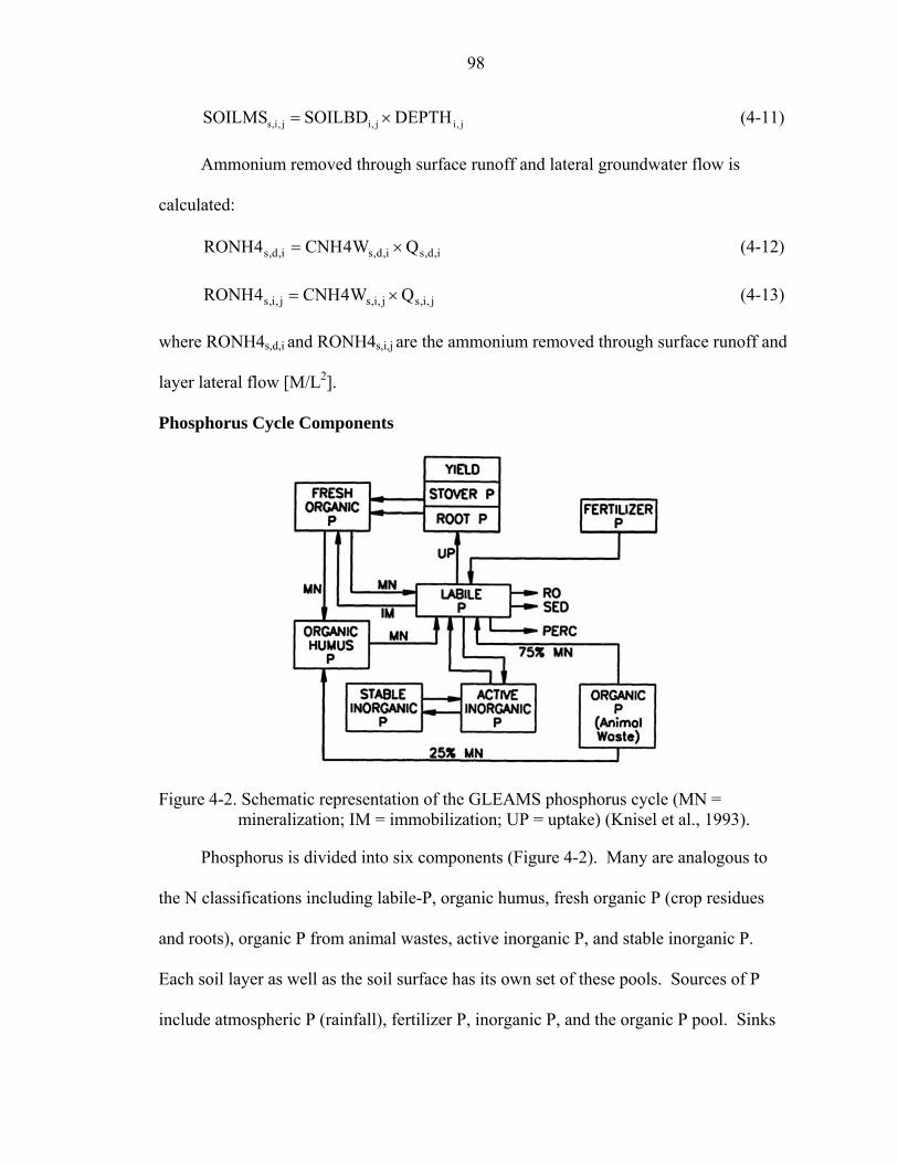
98

j,ij,ij,i,s DEPTHSOILBDSOILMS ×= (4-11)

Ammonium removed through surface runoff and lateral groundwater flow is

calculated:

i,d,si,d,si,d,s QW4CNH4RONH ×= (4-12)

j,i,sj,i,sj,i,s QW4CNH4RONH ×= (4-13)

where RONH4s,d,i and RONH4s,i,j are the ammonium removed through surface runoff and

layer lateral flow [M/L2].

Phosphorus Cycle Components

Figure 4-2. Schematic representation of the GLEAMS phosphorus cycle (MN = mineralization; IM = immobilization; UP = uptake) (Knisel et al., 1993).

Phosphorus is divided into six components (Figure 4-2). Many are analogous to

the N classifications including labile-P, organic humus, fresh organic P (crop residues

and roots), organic P from animal wastes, active inorganic P, and stable inorganic P.

Each soil layer as well as the soil surface has its own set of these pools. Sources of P

include atmospheric P (rainfall), fertilizer P, inorganic P, and the organic P pool. Sinks

99

for P are plant uptake, runoff, erosion (SED on figure), and percolation. Phosphorus can

be transformed by mineralization and immobilization.

Labile P may be transported with surface runoff and lateral groundwater flow from

one land segment to its neighboring land segments. To calculate the amount of nutrient

mass moved with water flows, the concentrations of nutrients in the water are calculated.

These concentrations are then multiplied by the volume of water moving in each pathway

to obtain the mass of nutrients lost through surface runoff and lateral groundwater flow

from this land segment to neighboring land segments, streams or water bodies.

Mineralization

P mineralization is considered a single step first-order process (Jones et al., 1984).

Mineralization of the organic humus pool supplies the labile P pool. Mineralization of

organic humus is a function of soil moisture, temperature, and P content, and uses the

same temperature and moisture factors as were used in the N component. The ratio of the

size of the active soil N pool to the stable soil N pool is also used to partition the soil

organic humus pool into the mineralizable fraction.

Mineralization of fresh organic P (roots and crop residue in the soil) supplies the

soil humus pool. The rate of mineralization is a function of residue composition, C:N

and C:P ratios, temperature and soil moisture. The same function is used to calculate P

mineralization from residue on the soil surface as well. As in the EPIC model (Sharpley

and Williams, 1990), 75% of mineralized P is added to the labile P pool and 25% to the

organic humus pool.

Mineralization of P in animal wastes is a function of temperature and soil moisture

as well as a rate constant. In accordance with Bhat et al. (1981), 75% of mineralized P is

allocated directly to the labile P pool and 25% to the organic humus pool.

100

A further similarity to the N component is the flux between the active inorganic P

pool and the stable pool. This flux is a function of the size of the active and labile P

pools as well as temperature, soil moisture and calcium carbonate concentration of the

soil (which affects sorption). It is assumed that at equilibrium, the stable pool mass will

be four times the active pool mass (Sharpley and Williams, 1990). Mineralized P from

the active pool can also be allocated to the labile P pool.

Immobilization

The same decomposition rate used in calculating immobilization of N is used in

calculating immobilization of P. The decomposition rate is a function of temperature,

soil moisture and the C:N and C:P ratios of the residue. Immobilization rate is also a

function of the concentration of labile P in the soil layer. It is assumed that residue is

40% C and that the microbes assimilate 40% of the C. As with N immobilization, P

immobilization is also limited to 95% of labile P. The same factor is used for both

nutrients so a shortage of N can limit P immobilization and vice versa. Immobilization of

surface P is calculated in the same way.

Runoff, sediment, percolation

As with N, the amount of P lost in runoff and percolation depends on the

partitioning of P between the soil and water phases. In GLEAMS, the amount of P

adsorbed to the soil is a function of the clay content of the soil. This method, however,

greatly overestimates the partitioning coefficient for the high water table flatwoods

Spodosol soils and underestimates the P concentration in soil water. An alternative

method (by Portier KM according to Fraisse and Campbell (1997)) obtained through a

study in Lake Okeechobee watershed determined the partitioning coefficient as a function

of the content of magnesium, organic carbon and/or aluminum. Martinez (2006)

101

introduced a mixing-type model to calculate P transport between the ponded water and

soil water, similar to that for N.

As with the N component, the actual amount of P lost in runoff or percolation is a

function of soluble P available and the water flux. Losses to erosion are calculated the

same as for N with corresponding losses from the animal waste, active mineral P and

stable mineral P pools as well as additional P lost from the humus pool.

Uptake and evaporation

Potential P uptake is calculated independently of demand, as a function of

transpiration and concentration of labile P in the soil water. Plant P demand is the

function of the concentration of P in the crop, the growth ratio of the plant and the

potential yield of the crop. If supply is less than demand, uptake is equal to the supply.

Otherwise, uptake is equal to the demand. Unlike the nitrogen component, growth is

assumed not to be limited by P deficiency in the original ACRU2000. However, it may

not be true in reality. A P stress factor was introduced through this work to represent the

P stress on plant growth due to P deficiency (detailed discussion in Chapter 5).

P moves upwards in the soil profile with upward soil water flux. The amount lost

to the next higher layer is a function of the concentration of labile P in the soil water in

the current soil layer and the volume of upward flux. However, it is assumed that there

are no volatilization losses of P.

Rainfall and fertilizer

The GLEAMS model includes an option to input the rainfall N concentration but it

does not allow input of rainfall P levels. This function was added to ACRU-NP by

Campbell et al. (2001) and P in rainfall and irrigation water is accounted for in the same

way as for N.

102

Both rainfall P and fertilizer P are assumed to be soluble and available to the plant

as soon as they are applied. If the fertilizer is surface applied and not incorporated, it is

stored on the surface and moved to the surface layer soluble (labile) pool on the first

occurrence of rain or irrigation following the application. All P from incorporated

fertilizers and infiltrated rainfall is added immediately to the labile P pool. Availability

of P from organic wastes is more gradual and was discussed in the mineralization and

immobilization sections.

Surface and subsurface lateral labile phosphorus transport

The concentrations of labile P in runoff and lateral flow are calculated:

i,d,si,d,si,d,s WMPLABCPLABW = (4-14)

)WMSOILMSCPKD(PLABCPLABW j,i,sj,i,sj,i,sj,i,sj,i,s +×= (4-15)

where CPLABWs,d,i and CPLABWs,i,j represent the concentrations of labile P in the

surface runoff and in the saturated soil layers, respectively [M/L3]; PLABs,d,i and PLABs,i,j

are the labile P in surface runoff [M/L2] and in the saturated soil layer j [M/L2]; CPKDs,i,j

is the labile P partitioning coefficient in the saturated soil layer [L/M].

In GLEAMS, it was assumed that P is partially adsorbed to the soil clay fraction.

However, this assumption is not adequate for sandy, high-water-table flatwoods spodosol

soils. Therefore, an algorithm was developed by Portier (personal communication,

referenced in Fraisse and Campbell (1997)) to represent the P partitioning coefficient,

CPKDs,i,j, as a function of the content of double-acid-extractable magnesium (DAMGRD

[mg/kg]), organic carbon (OCBRD [mg/kg]) and/or oxalate-extractable aluminum

(OXALRD [mg/kg]) in each soil horizon:

For the A horizon

103

2390.2j,i,s eCPKD = For 2.103DAMGRD ≥ (4-16)

2233.2j,i,s eCPKD −= For 2.103DAMGRD < when 865.1OCBRD ≥ (4-17)

4420.1j,i,s eCPKD = For 2.103DAMGRD < when 865.1OCBRD < (4-18)

For the E horizon

2410.4j,i,s eCPKD = For 45.496OXALRD ≥ (4-19)

0480.1j,i,s eCPKD = For 1.30OXALRD < (4-20)

4440.1j,i,s eCPKD = For 45.496OXALRD1.30 <≤ when 95.4DAMGRD ≥ (4-21)

7670.1j,i,s eCPKD = For 45.496OXALRD1.30 <≤ when 95.4DAMGRD <

with 25.57OXALRD < (4-22)

3500.3j,i,s eCPKD = For 45.496OXALRD1.30 <≤ when 95.4DAMGRD <

with 25.57OXALRD ≥ (4-23)

For the Bh horizon



For the Bw horizon



The soil mass for each soil layer, SOILMSs,i,j is calculated using Equation (4-11).

Labile P removed through surface runoff and lateral groundwater flow is

calculated:

104

i,d,si,d,si,d,s QCPLABWROLP ×= (4-28)

j,i,sj,i,sj,i,s QCPLABWROLP ×= (4-29)

where ROLPs,d,i and ROLPs,i,j are the labile P removed through surface runoff [M/L2] and

layer lateral flow [M/L2].

Conservative Solute Transport Components

A transport module capable of simulating conservative tracers such as bromide and

rhodamine WT (RWT) was added into the nutrient module through this work assuming

only vertical and horizontal transport processes occur (i.e. no transformation processes).

The vertical and horizontal transport processes were simulated as discussed for nitrate.

Martinez (2006) created several vertical processes to simulate the conservative

solute transport through evaporation, soil water redistribution, and exchange between

water in the top soil layer and ponded water. The evaporation solute transport process

calculates the upward movement of a conservative solute in the soil due to evaporation,

however solute is not allowed to move upward out of the soil surface layer by

evaporation. The subsurface solute transport calculates the leaching of a conservative

solute downward through the soil profile. A mixing-type model is used to determine the

exchange of solute between ponded water and soil water in the top-most soil layer, driven

by the solute concentration gradients. Surface and subsurface lateral transport processes

added through this work are described below.

The concentrations of conservative solute in the ponded water on the ground

surface and in the saturated groundwater are calculated:

i,d,si,d,si,d,s WMCONSOLCCONSOLW = (4-30)

105

j,i,sj,i,sj,i,s WMCONSOLCCONSOLW = (4-31)

where CCONSOLWs,d,i and CCONSOLWs,i,j are the concentrations of conservative solute

in the ponded water and saturated soil layers [M/L3], respectively; CONSOLs,d,i and

CONSOLs,i,j are the conservative solute mass on the ground surface and saturated soil

layers [M/L2], respectively; WMs,d,i is the water storage on the ground surface [L] and

WMs,i,j is the water storage in the saturated soil layers [L] as defined in Equations (4-3)

and (4-4), respectively.

Conservative solute removed in surface runoff is calculated:

i,d,si,d,si,d,s QCCONSOLWROCONSOL ×= (4-32)

where ROCONSOLs,d,i is the conservative solute removed in surface runoff [M/L2]; Qs,d,i

is the surface runoff generated on a given day from the current land segment to the ith

neighboring land segment [L].

Conservative solute removed in lateral groundwater flow is calculated:

j,i,sj,i,sj,i,s QCCONSOLWROCONSOL ×= (4-33)

where ROCONSOLs,i,j represents the conservative solute removed in lateral groundwater

flow from the layer j to the ith neighboring land segment [M/L2]; Qs,i,j is the lateral flow

in layer j to the ith neighboring land segment [L].

Mass balance is checked for the conservative solute in both surface runoff and

lateral groundwater flow as was described for N and P.

Initial and Boundary Conditions

Running the model requires good estimates for initial nutrient pools. This is

especially true for validation comparisons with observed data. Because of the dynamics

of the nitrate and ammonium processes, inaccurate initialization may not adversely affect

106

long-term simulation results. Initial values of different nutrient pools are very site

specific and are generally management dependent (Fraisse and Campbell, 1997). This is

especially true for systems with animal waste application and management activities such

as stocking, fertilization, and tillage operations. Model users should make every effort to

obtain good estimates of initial conditions, which may involve soil sampling and

analyses. However, soil samples commonly only determine certain nutrient variables

such as organic matter, total nitrogen, total phosphorus, nitrate, ammonium and available

phosphorus at a certain depth of soil. Stable, active mineral N and P and initial nutrient

pools in the deeper soil layers are usually unavailable. For a spatially distributed model,

the spatial distribution of initial nutrient pools is also required, which further increases

the level of effort. If initial values of the nutrient pools are not available, the model is set

up to use default values.

Agricultural activities such as stocking, fertilization, burning, etc. are treated as

time series inputs in the modified model. Nutrients from rainfall and irrigation (nitrate

and labile P only) and animal wastes must be specified as time series input and are added

to the appropriate nutrient pools.

Model Testing and Validation

Conservative Solute Test

To test the accuracy of the algorithm for the conservative solute transport

components added to ACRU2000, model results for a hypothetical scenario were

compared with those from PMPATH (Chiang and Kinzelbach, 2005), which is an

advective transport model using groundwater pore velocities from MODFLOW

(McDonald and Harbaugh, 1998).

107

Scenario description

The axisymmetric hypothetical domain with initial water levels below the ground

surface used for testing groundwater movement (Case 2) in Chapter 3 was extended for

this test. The hydrologic inputs remained the same as for the tests discussed in Chapter 3.

In order to run the model together with the added conservative solute components, an

initial solute mass has to be specified.

For the modified ACRU2000, it is assumed that 3kg of solute was initially present

in the 3rd soil layer of each of central four land segments, and that this solute mass was

uniformly distributed inside of that soil layer. However, PMPATH requires that an initial

number of particles, rather than an initial solute mass, be specified for each element

(equivalent to a soil layer in ACRU2000), with a maximum of 5000 particles per element.

Furthermore, it is difficult to set up the initial particle distribution pattern inside an

element so that it is completely uniform. After a few experiments, 4704 particles were

placed as uniformly as possible in each 3rd soil layer element for each central land

segment in PMPATH to represent the equivalent quantity of 3kg of solute. Thus, each

particle is mathematically equivalent to a mass of 3kg/4704, and it is possible to convert

the integer number of particles which appear inside a certain element into a mass of

solute in PMPATH. For comparison with the simulated results from the modified

ACRU2000, the PMPATH simulation was run using a daily time step for two years.


Considering the axisymmetric distribution of solute mass, the simulated solute

mass in the third and fourth soil layers of LS20, LS21 and LS26 from the modified

ACRU2000 model were selected to compare with the results obtained from PMPATH

(see Figure 4-3). This figure shows that there is a good agreement, particularly during

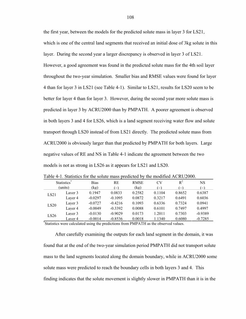
108

the first year, between the models for the predicted solute mass in layer 3 for LS21,

which is one of the central land segments that received an initial dose of 3kg solute in this

layer. During the second year a larger discrepancy is observed in layer 3 of LS21.

However, a good agreement was found in the predicted solute mass for the 4th soil layer

throughout the two-year simulation. Smaller bias and RMSE values were found for layer

4 than for layer 3 in LS21 (see Table 4-1). Similar to LS21, results for LS20 seem to be

better for layer 4 than for layer 3. However, during the second year more solute mass is

predicted in layer 3 by ACRU2000 than by PMPATH. A poorer agreement is observed

in both layers 3 and 4 for LS26, which is a land segment receiving water flow and solute

transport through LS20 instead of from LS21 directly. The predicted solute mass from

ACRU2000 is obviously larger than that predicted by PMPATH for both layers. Large

negative values of RE and NS in Table 4-1 indicate the agreement between the two

models is not as strong in LS26 as it appears for LS21 and LS20.

Table 4-1. Statistics for the solute mass predicted by the modified ACRU2000. Statistics* Bias RE RMSE CV R2 NS

(units) (kg) (−) (kg) (−) (−) (−)Layer 3 0.1947 0.0833 0.2582 0.1104 0.8652 0.6387LS21 Layer 4 -0.0297 -0.1095 0.0872 0.3217 0.6491 0.6036Layer 3 -0.0727 -0.4216 0.1093 0.6336 0.7324 0.0941LS20 Layer 4 -0.0049 -0.3392 0.0088 0.6101 0.7497 0.4997Layer 3 -0.0130 -0.9029 0.0173 1.2011 0.7303 -0.9389LS26 Layer 4 -0.0014 -0.8536 0.0018 1.1340 0.6080 -0.7285

*Statistics were calculated using the predictions from PMPATH as the observed values.

After carefully examining the outputs for each land segment in the domain, it was

found that at the end of the two-year simulation period PMPATH did not transport solute

mass to the land segments located along the domain boundary, while in ACRU2000 some

solute mass were predicted to reach the boundary cells in both layers 3 and 4. This

finding indicates that the solute movement is slightly slower in PMPATH than it is in the

109

ACRU2000 model. In ACRU2000, groundwater flow always carries a certain amount of

solute due to the assumption of uniform distribution of solute within the land segment

layer. However, in the PMPATH the particle tracking algorithm does not transport

particles from one element to the next until it travels the distance from where it is

originally located to the face between the two elements. Although the water movement

was a little faster in MODFLOW than in ACRU2000, the concentrations predicted in

each element of the PMPATH model are smaller than predicted by ACRU2000.

However, in spite of the difference in assumptions made by these models, the results

illustrated in Figure 4-3 indicate that they produce qualitatively similar results.

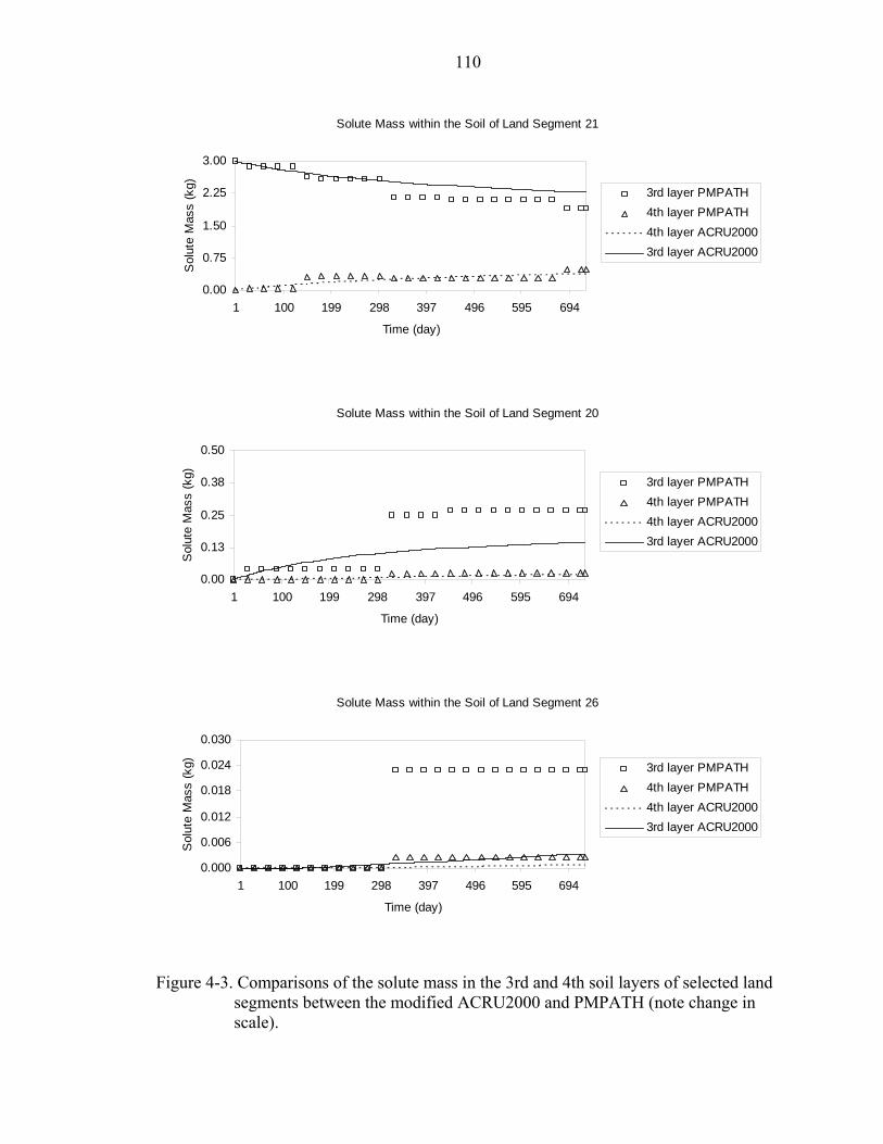
110

Solute Mass within the Soil of Land Segment 21

0.00

0.75

1.50

2.25

3.00

1 100 199 298 397 496 595 694

Time (day)

Sol

ute

Mas

s (k

g) 3rd layer PMPATH4th layer PMPATH4th layer ACRU20003rd layer ACRU2000


0.00

0.13

0.25

0.38

0.50

1 100 199 298 397 496 595 694

Time (day)

Sol

ute

Mas

s (k



0.000

0.006

0.012

0.018

0.024

0.030

1 100 199 298 397 496 595 694

Time (day)

Sol

ute

Mas

s (k


Figure 4-3. Comparisons of the solute mass in the 3rd and 4th soil layers of selected land

segments between the modified ACRU2000 and PMPATH (note change in scale).

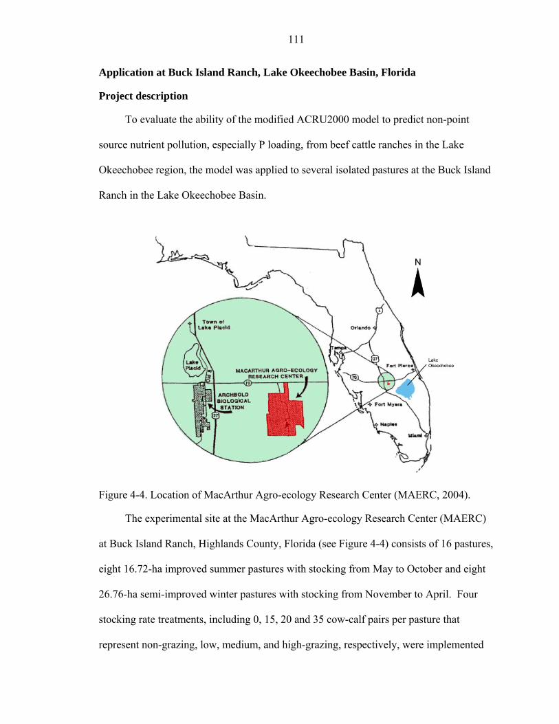
111

Application at Buck Island Ranch, Lake Okeechobee Basin, Florida

Project description

To evaluate the ability of the modified ACRU2000 model to predict non-point

source nutrient pollution, especially P loading, from beef cattle ranches in the Lake

Okeechobee region, the model was applied to several isolated pastures at the Buck Island

Ranch in the Lake Okeechobee Basin.

Figure 4-4. Location of MacArthur Agro-ecology Research Center (MAERC, 2004).

The experimental site at the MacArthur Agro-ecology Research Center (MAERC)

at Buck Island Ranch, Highlands County, Florida (see Figure 4-4) consists of 16 pastures,

eight 16.72-ha improved summer pastures with stocking from May to October and eight

26.76-ha semi-improved winter pastures with stocking from November to April. Four

stocking rate treatments, including 0, 15, 20 and 35 cow-calf pairs per pasture that

represent non-grazing, low, medium, and high-grazing, respectively, were implemented

112

for this experiment. Each of the stocking densities had two replicates in each of 16

winter and summer pastures. Figure 4-5 shows the layout of pastures and the instrument

locations. Each of the pastures was individually fenced and ditched to capture surface

runoff through a single trapezoidal flume. Nutrient concentrations, including total

phosphorus (TP), soluble-reactive phosphorus (SRP), total N (TKN), nitrate + nitrite

(NOx) and ammonium ( +4NH ) were measured from water samples collected using ISCO

automatic samples installed in each flume. Data collection started on May 19, 1998 for

the summer pastures and on May 21, 1998 for the winter pastures, and continued through

December 2003, interrupted only by occasional equipment malfunctions (MAERC,

2004). The winter pastures have two meteorological stations and the summer pastures

have one station. These meteorological stations were installed on May 21, 1998 to record

rainfall, windspeed and direction, air temperature, relative humidity, and solar radiation

using Campbell Scientific CR10X dataloggers. In addition, there were 5 tipping bucket

rain gages installed throughout the pastures to record rainfall. A main weather station is

located at the Ranch headquarters, which operated throughout the experiment, where

manual rainfall readings are taken daily and a datalogger records air temperature, relative

humidity, windspeed and direction at 3.0 m and 9.1 m, solar radiation, and soil

temperature.

For the purpose of model application, four pasture sites, including W6, W7, S1 and

S4, were selected for use. Considering the similarity in soil characteristics, and the

limited measurements of water table and nutrient loads throughout the 6-year simulation

period from each site, one site each from the summer and winter pastures was used for

calibration and the other one for verification. This allows calibration over more varied

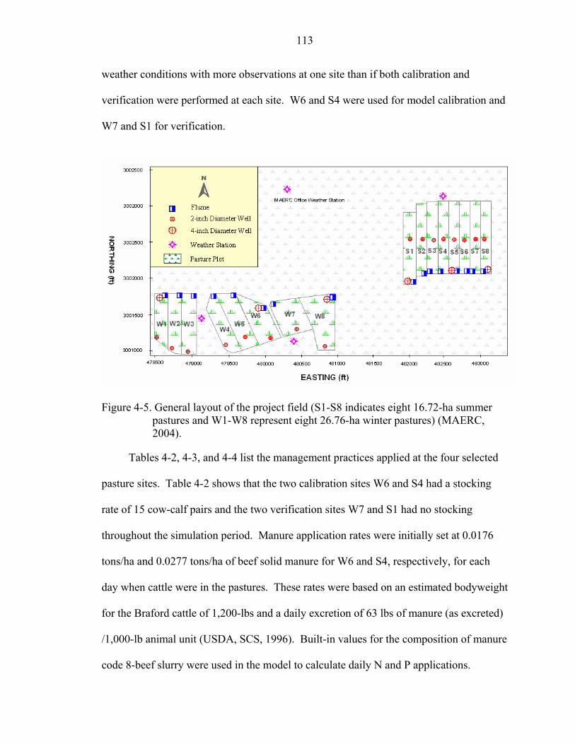
113

weather conditions with more observations at one site than if both calibration and

verification were performed at each site. W6 and S4 were used for model calibration and

W7 and S1 for verification.

Figure 4-5. General layout of the project field (S1-S8 indicates eight 16.72-ha summer

pastures and W1-W8 represent eight 26.76-ha winter pastures) (MAERC, 2004).

Tables 4-2, 4-3, and 4-4 list the management practices applied at the four selected

pasture sites. Table 4-2 shows that the two calibration sites W6 and S4 had a stocking

rate of 15 cow-calf pairs and the two verification sites W7 and S1 had no stocking

throughout the simulation period. Manure application rates were initially set at 0.0176

tons/ha and 0.0277 tons/ha of beef solid manure for W6 and S4, respectively, for each

day when cattle were in the pastures. These rates were based on an estimated bodyweight

for the Braford cattle of 1,200-lbs and a daily excretion of 63 lbs of manure (as excreted)

/1,000-lb animal unit (USDA, SCS, 1996). Built-in values for the composition of manure

code 8-beef slurry were used in the model to calculate daily N and P applications.

114

Ammonium nitrate fertilizer was applied on summer pastures S1 and S4 three times

during the simulation period for a total of 56 kg/ha nitrogen on each application (see

Table 4-3). Prescribed burns and accidental fires occurred in all four pastures at different

times (see Table 4-4). In the model, when burns or fires occur, 95% of the biomass of the

surface residue is removed.

The areas of the four selected pasture sites and the percentages of soil series within

each pasture are listed in Table 4-5. Although multiple soil series exist in each selected

pasture site, for this study it is assumed that W6 and W7 had the same soil characteristics,

and S4 and S1 also had the same soil characteristics because both winter and summer

pasture pairs have the same dominant soil types (see Table 4-5). Pineda fine sand was

assumed as the base soil series for W6 and W7 and Felda fine sand was assumed for S4

and S1. In the model, W6 and W7 were each divided into 18 land segments with surface

areas ranging from 0.6 ha to 2.6 ha. S4 and S1 were each divided into 12 land segments

with surface areas ranging from 1.6 ha to 1.8 ha. This spatial discretization was

determined based on the available topographic maps that show the contours of surface

elevation and wetlands. Using this information, an elevation value was assigned to each

land segment.

Setting up the initial input data and parameters is critical to guarantee the accuracy

of model performance. However, due to the unavailability of spatially distributed data in

these pasture sites, all initial physical and biochemical data were assumed to be the same

for each land segment in the same pasture site except a few parameters including surface

elevation, land segment area, initial water table depth, and boundary conditions (i.e.

boundary width and hydraulic structure information). Model input parameters are

115

summarized in Table 4-6 for winter pastures W6 and W7 and Table 4-7 for summer

pastures S4 and S1.

Initializing the nutrient pool parameters (see Tables 4-6 and 4-7) was difficult

because there was little nutrient information available for soils and surface residues in

any of these pastures. The literature data obtained from laboratory analyses of soil

samples do not give a breakdown of all the nutrient pools in all soil layers of interest, and

these soil analyses are typically limited to the plow layer since that may be the depth of

most concern to researchers. Therefore, the procedure for setting up initial nutrient pools

introduced in the FHANTM manual (Fraisse and Campbell, 1997) was adopted.

For each soil layer, nitrogen including all forms of nitrogen, i.e. mineralizable,

stable organic, fresh organic, humus, ammonia, etc. was required model inputs. The total

nitrogen (TN) was estimated for each computational soil layer using the data in Table 1

(Fraisse and Campbell, 1997). Nitrate-nitrogen (NO3-N) was estimated using a

concentration of 10 µg/g of soil in all soil layers. Ammonium nitrogen (NH4-N) was

estimated using a concentration of 2 µg/g of soil. Root residue from previous biomass

productivity was estimated at the beginning of the simulation as 40 kg/ha and distributed

vertically in the root zone. Stable mineral nitrogen was initialized by taking the

difference between the TN and the rest of nitrogen pools except nitrate-N.

Phosphorus pools in the soil that must be initialized include fresh organic P in crop

residue, organic humus P, labile P, and active and stable mineral P. According to Fraisse

and Campbell (1997) soil organic humus can be estimated using the following

relationships:

TN35.14724.9SORGP ×+= For the plow layer (4-9)

116

TN58.14825.11SORGP ×+= For other horizons (4-10)

where SORGP is soil organic humus [µg/g], and TN is total nitrogen [%]. The labile P

was estimated to be 8.7% of SORGP for slightly weathered soils (Fraisse and Campbell,

1997). The active mineral P pool was estimated using the following relationship derived

from Equation (12) (Fraisse and Campbell, 1997):

PSP/)PSP1(PLABPMINP −= (4-11)

where PMINP is the active mineral P [kg/ha] and PSP is the P sorption coefficient that

can be estimated according to Sharpley and Williams (1990)

73.0PH116.0BAST0054.0PSP −+= (4-12)

where BAST is base saturation [%] and PH is the soil pH for slightly weathered soils.

The stable mineral P was set as four times active mineral P (Fraisse and Campbell, 1997).

The fresh organic P is estimated as 10 kg/ha and distributed in the root zone (Fraisse and

Campbell, 1997).

Using the above discussed relationships, the initial nutrient pools were set up for

both N and P. Tables 4-6 and 4-7 list the calibrated N and P parameters based on the

initial nutrient values. Although multiple vegetation species exist in each of selected

sites, only one species, bahiagrass (Paspalum notatum Flügge) was assumed to exist for

simplicity.

Model calibration was based on personal judgment and statistical analyses for four

major output variables, i.e., groundwater table depth, runoff depth, and N and P loads.

Calibration was performed for these output variables sequentially in the order listed

above. During calibration, hydrologic parameters, including porosity, wilting point,

saturated hydraulic conductivity, restrictive layer hydraulic conductivity, Manning’s

117

roughness coefficient, surface maximum depressional storage, and crop coefficient; and

nutrient parameters, including rainfall P and N concentrations, active P, stable P, humus

P, active N, and stable N, were varied within their physically reasonable ranges until the

output variables were judged to be acceptable. It should be noted that the soil porosity

and wilting point values for both W6 and S4 (see Tables 4-6 and 4-7) are smaller than

typical values in flatwoods soils. These data were determined through the model

calibration process. Due to lack of actual soil information and other data (such as crop

coefficient), these calibrated parameters could be biased to a certain point. They can be

improved when sufficient soil data become available in the future. Upon completion of

model calibration, the resulting data sets were used for independent verification

simulations. Statistical and visualization tools introduced in Chapter 2 were used to

evaluate the model calibration and verification performance. Furthermore, the calculated

statistics were compared with those from FHANTM by Sims (2004) for winter pastures.

No comparison was made for summer pastures since no previous modeling has been

performed on any of the summer pastures.

Sensitivity analysis

Sensitivity analyses were conducted by changing a given input parameter by a

predetermined amount, with the other inputs held at their calibrated values, and running a

simulation for the period of January 1, 1998 through December 31, 2003. The sensitivity

analyses were made for the calibration sites W6 and S4. Hydrologic inputs (see Tables 4-

8 and 4-10) selected for sensitivity analysis include soil porosity, wilting point, saturated

hydraulic conductivity, restrictive layer hydraulic conductivity, Manning’s roughness

coefficient, surface maximum depressional storage, and crop coefficient, and nutrient

inputs (see Tables 4-9 and 4-11) selected for sensitivity analysis include rainfall P and N

118

concentrations, active P, stable P, organic humus P, active N, stable N, and stocking and

fertilizer rates. These choices were made as a result of the calibration process, reference

material, and intuition gained during the process of developing this model. The

sensitivity analyses were focused on two major hydrologic outputs including the total

surface runoff from the site and maximum water table depth at the measurement location,

and two major nutrient outputs including the total P and N loads from the site throughout

the simulation period. Only the selected hydrologic input parameters were tested for the

hydrologic outputs and all selected parameters were tested for the nutrient outputs.

For each input parameter, simulations were conducted for the base (calibrated)

value(s) and increments of +50%, +10%, -10%, and -50%, one at a time. If a selected

parameter could have different values by soil layer, then this parameter value was

increased or decreased by a given percentage simultaneously for all soil layers. Tables 4-

8 to 4-11 list the ranges of values for the selected hydrologic and nutrient parameters

used in the sensitivity analyses for both calibration sites W6 and S4. Tables 4-12 to 4-15

show the sensitivity analysis results for W6, and Tables 4-16 to 4-19 show the same

results for S4. As discussed in Chapter 2, the relative sensitivity is unitless, which

provides a straightforward way to compare sensitivities over the selected input

parameters that vary in their magnitudes in response to the same output variable. The

following discussions are based on the relative sensitivity analysis results.

Figure 4-6 shows the relative sensitivities of total surface runoff to the six

hydrologic input parameters for the 6-year simulation period for the calibration sites W6

and S4. The sensitivity of surface runoff to soil porosity at its increment of -50% from

the base for site W6 is not provided in Figure 4-6 because the model run was terminated

119

since the simulated water table dropped below the bottom of the soil profile. This

indicates that these soil porosity values are out of the “reasonable range”. Results show

that the two most sensitive parameters for surface runoff at W6 and S4 are crop

coefficient and soil porosity. Runoff is more sensitive to crop coefficient for W6 while it

is more sensitive to soil porosity for S4. Moreover, the third most sensitive parameter for

surface runoff is restrictive layer hydraulic conductivity for both sites. The sensitivities

of runoff to the rest of the selected hydrologic parameters are not significantly different

from one another. It should be noted that the sensitivity of surface runoff to both crop

coefficient and soil porosity are asymmetric for both sites compared with those of the rest

of the parameters. In general, surface runoff shows similar sensitivity to these hydrologic

parameters at both sites.

Figure 4-7 shows the relative sensitivities of maximum water table depth to the

same selected hydrologic parameters at both sites. Maximum depressional storage is not

shown since maximum water table depth is not sensitive to this parameter. It should be

noted that the magnitude of sensitivities of maximum water table depth is significantly

smaller than those for total surface runoff for all parameters at both sites. This is likely

due to the fact that response times for subsurface water movement are much slower than

for surface water movement. Results indicate that maximum water table depth is most

sensitive to soil porosity for W6, while it is most sensitive to crop coefficient for S4.

Note that the sensitivity of maximum water table depth to the crop coefficient is quite

asymmetric for S4. Also, it is very interesting that maximum water table depth is

significantly more sensitive to the wilting point for S4 than for W6. This is likely

because S4 has relatively smaller soil porosity values than W6 (see Tables 4-6 and 4-7),

120

which implies less water availability in the soil profile of S4 for hydrological processes

such as ET. An increase or decrease in wilting point could affect the amount of water

available for ET. The remaining parameters, saturated hydraulic conductivity and

restrictive layer hydraulic conductivity show quite similar symmetric sensitivity patterns

for both sites.

The sensitivity tests of total surface runoff and maximum water table depth to the

hydrologic input parameters demonstrate that the most sensitive hydrologic input

parameters are those that represent physical properties that directly affect the soil water

budget in a storage-limited hydrologic system, i.e., crop coefficient, soil porosity, and

restrictive layer hydraulic conductivity. Furthermore, the sensitivities of both total

surface runoff and maximum water table depth to the changes in these hydrologic

parameters do not have the same magnitudes.

Together with the hydrologic input parameters, several nutrient parameters were

selected to test the sensitivity of the total P and N load responses to the changes in these

parameters. As shown in Figure 4-8, the magnitude of sensitivities of the P load response

to the selected hydrologic parameters is similar to that for total surface runoff for both

sites. The crop coefficient and soil porosity appear to be the most sensitive parameters

for the P loads for sites W6 and S4. Furthermore, the sensitivity of the P load to

restrictive layer hydraulic conductivity is more significant than the rest of the hydrologic

parameters for both sites. Among all of the selected nutrient parameters, the rainfall P

concentration is the most sensitive nutrient parameter, followed by the active P, to the P

load response for W6. On the contrary, there is little sensitivity of the P load response to

the rainfall P concentration for S4. Instead, the stable P is the most sensitive parameter,

121

followed by the active P, to the P load response for site S4. Such a difference in

sensitivity of rainfall P concentration very likely results from the extremely different

background P values for the semi-improved pasture site W6 and the improved pasture

site S4. Generally, for both sites the P load response shows similar sensitivity patterns to

hydrologic parameters as total surface runoff.

Figure 4-9 displays the relative sensitivities of the N load response to the selected

parameters for both calibration sites. For site W6, the crop coefficient and restrictive

layer conductivity appear to be the most sensitive hydrologic parameters and the porosity

is also sensitive compared with the rest of the hydrologic parameters. Among all selected

nutrient parameters, the N load response is most sensitive to the changes in rainfall N

concentration. However, for site S4 the surface maximum depressional storage is the

most sensitive parameter of all selected parameters although the crop coefficient,

restrictive layer conductivity, and porosity are also sensitive parameters. The reason that

N load shows high sensitivity to the surface maximum depressional storage for S4 is most

likely from the combination of two aspects, reducing/increasing the surface maximum

depressional storage leads to more/less water available for surface runoff and the

nutrient-rich pasture S4 has relatively higher surface runoff N concentration. Unlike for

W6, the N load response for S4 is not very sensitive to the rainfall N concentration. As

discussed above for the P load response, this may be due to the fact that S4 is a nutrient-

rich site and almost all nutrient pools are much larger than those for W6. As a result, the

rainfall nutrient concentrations may not be major factors in changing the N load response.

In general, it is hard to draw consistent conclusions from both calibration sites for

these selected parameters because their sensitivities appear to be site-specific. This

122

implies that nonlinear relationships exist between these selected parameters and output

variables, and that there may be interactions among the input parameters.


The simulation results to be discussed include the annual water budgets conducted

for the four selected pasture sites; and the continuous simulation of major output

variables, including water table depth, surface runoff, P and N loads, and P and N

concentrations for the two pairs of calibration/verification sites: W6/W7 and S4/S1.

Daily time series plots as well as monthly and annual linear plots, and daily duration

curves of these major output variables were evaluated. Annual and monthly statistics

comparisons of the simulated versus observed results were calculated and compared with

those calculated by FHANTM (Sims, 2004).

Annual summaries for rainfall, observed and simulated runoff, simulated lateral

ground water flow, simulated ET, and simulated deep seepage are listed in Tables 4-20,

4-21, 4-22, and 4-23 for the four selected pasture sites. There was less rainfall for year

2000 than for the rest of the years during the simulation period over all selected sites.

There was relatively more rainfall for years 2002 and 2003 for the winter pasture sites

and for year 2002 for the summer pasture sites. The percentages in columns for rainfall,

ET and deep seepage indicate the percent of annual rainfall that these hydrological

components account for. These data shows that about 1-34% of annual rainfall converted

to runoff, 9-13% to deep seepage, and the remainder to evapotranspiration. These

statistics are quite close to the previous studies of pine-cypress flatwoods in the

southeastern United States according to Riekerk and Korhnak (2000).

Figure 4-10 and Figure 4-11 display the continuous simulation of groundwater

table depths for the calibration site W6 and verification site W7 from September 2000

123

through December 2003. Very good agreement on timing and trends are found between

the predicted and observed water table depths for both sites W6 and W7, with slightly

larger discrepancies during a long dry period approximately from October 2000 through

March 2001. During this dry period, the observed water table is very sensitive to small

rainfall inputs so that observed water table fluctuated more rapidly to the rainfall inputs

than the model predictions. Additionally, it is obvious that the measured water tables did

not reach the ground surface throughout the simulation period even during the heavy

rainfall inputs when surface runoff occurred. This error may come from erroneous

measuring of the ground surface elevations of wells, which may have been installed in

low spots in the field and thus the surface elevations measured at such locations may not

be an appropriate estimate of the surface elevations for the entire land segment.

The conclusions drawn from the winter pasture sites also apply to the simulation of

groundwater table depths for the summer pasture sites S4 and S1 (see Figures 4-12 and 4-

13). However, there is a better agreement between the predicted and observed water

table depths when the soils get saturated for the site S4 than for the other three sites. The

predicted water tables agree with the observed data better in the two calibration sites than

in the two verification sites.

Figures 4-14 and 4-15 show the continuous simulation of surface runoff from July

1998 to December 2003 for the calibration site W6 and verification site W7. For both

sites, the model responded fairly well to the rainfall events on both timing and trends, and

also was able to capture some of the back flows that were caused when the water

elevation in the downstream canal was higher than that in the pasture sites. Nevertheless,

the model generally did not capture the peak runoff very well. A few possible reasons

124

may explain this. First, the ditches located inside the pastures are deeper than the area’s

ground surface elevation. Thus they can collect the surface water and result in runoff at

the outlet of the pasture even when no sheet flow occurs. The current version of the

model does not consider water movement in these ditches. In the model surface runoff

occurs only when surface water is ponded on the entire land segment. Second, the

observed runoff is instantaneously measured data while the predicted runoff is the daily

average value. Using a daily time step may computationally delay the transport of runoff

to a certain extent. For example, if rainfall events last only a few hours, the resulting

overland flow could reach the downstream flume in less than a day, especially if rainfall

occurs near the flume where the runoff was measured. In the model, runoff is only

transported between land segments once a day. Therefore, the simulated overland flow

could be delayed with a resulting flattened hydrograph.

Similar conclusions can be drawn for the summer pasture sites S4 and S1 (see

Figures 4-16 and 4-17). However, the magnitude of surface runoff in the summer

pastures is generally smaller than for the winter pastures, which reduces the discrepancy

in peak runoffs to a certain extent.

Figures 4-18 and 4-19 show the continuous simulation of P loads from July 1998

through December 2003 for W6 and W7, respectively. Similar to the surface runoff

simulation, the predicted P loads agree well with the observed P loads on timing and

trend, but the model underestimates the peak P loads. Since the load is the product of the

volume of surface runoff and P concentration, the underestimation of surface peak

runoffs, as discussed earlier, directly contributes to the under-predictions of P loads.

However, Figures 4-26 and 4-27 show that underestimation of P concentrations,

125

especially for those times when peak runoff was underestimated, is likely another

contributor to the underestimation of peak P loads for winter pastures W6 and W7.

Figures 4-20 and 4-21 display the continuous simulation of P loads from July 1998

through December 2003 for the two summer pasture sites S4 and S1, respectively. The

conclusions from these figures are similar to those obtained for the winter pastures sites.

However, the magnitude of the difference in the prediction of P peak load in these

summer pastures is more significant than for the winter pastures due to the fact that the

summer pastures have high background nutrients.

Figures 4-22 and 4-23 show the continuous simulation of N load from July 1998

through December 2003 for W6 and W7, respectively. The predicted N load for sites W6

and W7 agree fairly well with the observed N loads, but the model still underestimates

the peak N loads as it did the P loads for these sites. Compared with the simuled N loads,

the observed N loads show higher peaks and more variability. Likewise, the model

underestimates, as seen in Figures 4-24 and 4-25, most of the peak observed N loads for

the two summer pasture sites S4 and S1, respectively.

Figures 4-26 through 4-33 show the continuous simulation of surface runoff P and

N concentrations for the four selected pasture sites. These figures were prepared to help

understand the P and N load prediction errors. For winter site W6, both observed P and

N concentrations have higher peaks and more variability than simulated as shown in

Figures 4-26 and 4-28. However, the magnitude of both P and N concentrations for W7

as seen in Figures 4-27 and 4-29 is smaller than that for W6, which leads to less

discrepancy. Compared with the winter pasture sites, the model performed much better

in predicting the P concentrations for S4 and S1 with a better agreement between the

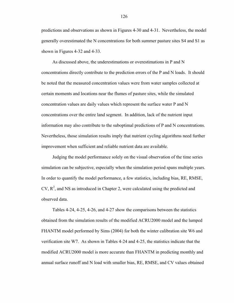
126

predictions and observations as shown in Figures 4-30 and 4-31. Nevertheless, the model

generally overestimated the N concentrations for both summer pasture sites S4 and S1 as

shown in Figures 4-32 and 4-33.

As discussed above, the underestimations or overestimations in P and N

concentrations directly contribute to the prediction errors of the P and N loads. It should

be noted that the measured concentration values were from water samples collected at

certain moments and locations near the flumes of pasture sites, while the simulated

concentration values are daily values which represent the surface water P and N

concentrations over the entire land segment. In addition, lack of the nutrient input

information may also contribute to the suboptimal predictions of P and N concentrations.

Nevertheless, those simulation results imply that nutrient cycling algorithms need further

improvement when sufficient and reliable nutrient data are available.

Judging the model performance solely on the visual observation of the time series

simulation can be subjective, especially when the simulation period spans multiple years.

In order to quantify the model performance, a few statistics, including bias, RE, RMSE,

CV, R2, and NS as introduced in Chapter 2, were calculated using the predicted and

observed data.

Tables 4-24, 4-25, 4-26, and 4-27 show the comparisons between the statistics

obtained from the simulation results of the modified ACRU2000 model and the lumped

FHANTM model performed by Sims (2004) for both the winter calibration site W6 and

verification site W7. As shown in Tables 4-24 and 4-25, the statistics indicate that the

modified ACRU2000 model is more accurate than FHANTM in predicting monthly and

annual surface runoff and N load with smaller bias, RE, RMSE, and CV values obtained

127

from the modified ACRU2000 model than from FHANTM. All statistics except RE for

the P load obtained from the modified model are also smaller than FHANTM and

indicate a better prediction in P load. Both models overestimated monthly and annual

surface runoff and N load with the positive bias and RE values. The modified model

overestimated the P load while FHANTM underestimated the P load. Both models

overestimated the N load. Smaller RMSE and CV values over all predicted output

variables from the modified ACRU2000 indicate that the modified model generally

performed better than FHANTM. For W6, the monthly CV values are generally greater

than 1.0, which indicates that the model is adequate for screening purpose for monthly

predictions (Hedden, 1996). The annual CV values are all less than one indicating the

model is accurate enough to be used for site-specific application for annual predictions.

Similar conclusions regarding the monthly and annual statistics can be applied to

surface runoff and P load (see Tables 4-26 and 4-27) for the verification site W7 as well

drawn for calibration site W6. Both models performed similarly in predicting the N load

with quite good statistics. Unlike for W6, the modified model underestimated surface

runoff, and P and N loads. FHANTM overestimated the runoff but underestimated the P

and N loads. The monthly and annual CV values for runoff indicate the model can be

used for site specific monthly and annual predictions of runoff. The CV value for the P

and N loads indicate that the model can only be used for screening application at the

monthly level, but can be used for site specific application at the annual level. Overall,

the comparison of statistics between the two models indicates that the modified

ACRU2000 performed better than FHANTM for both winter sites according to the

monthly and annual predictions.

128

No statistics for the water table depths were obtained for the FHANTM simulation.

For the modified ACRU2000 model, the monthly NS value of 0.93 and annual NS of

0.96 for the calibration site W6, and the monthly NS of 0.81 and annual NS of 0.86 for

the verification site indicate a very good overall performance in predicting water table

depths. CV values for both sites for both monthly and annual predictions indicate that the

model can be used for site-specific application in predicting the water table depth.

Comparing the statistics between the winter calibration and verification sites,

Tables 4-20 through 4-23 show that the model performed slightly better in predicting

surface runoff for the verification site with smaller bias, RE, RMSE, CV values and

higher R2 and NS value for the verification site than the calibration site. For the other

three output variables, the model performed better for the calibration site than for the

verification site with smaller bias, RE, RMSE, CV values and higher R2 and NS values

for the calibration site. Since RE, CV, R2 and NS are unitless, it is possible to compare

the statistics over the output variables. Generally, the statistics indicate that the model

performed better in predicting hydrologic variables than nutrient variables.

There are no statistics available from FHANTM for the summer pastures, thus the

evaluation of model performance in the summer pastures was made by comparing the

statistics (see Tables 4-28, 4-29, 4-30, and 4-31) with those from the winter pastures. As

seen in Tables 4-28 and 4-29, the comparisons of monthly statistics for the two

calibration sites W6 and S4 indicate the predictions of four output variables are slightly

more biased for S4 than for W6 but the general model performance for both calibration

sites are close. For both sites the model performed better in predicting the monthly P

loads than in the monthly N loads. When comparing the annual statistics for these two

129

calibration sites, the bias for all predicted variables is more apparent for S4 than for W6.

CV values for runoff, water table depth, and P load indicate that the model can be used

for site-specific monthly and annual prediction of these variables. The annual CV values

for all variables indicate the model can be used for site-specific annual prediction for all

variables. For the two verification sites, W7 and S1, the comparison of monthly statistics

(see Tables 4-26 and 4-27) indicates that the model performed better for runoff and water

table depth for W7, but it underestimated both P and N loads for W7 and overestimated

them for S1. The same conclusion can be drawn for both sites by comparing their annual

statistics for these variables.

Overall, the model performed better for the calibration sites than for the verification

sites, better for hydrologic outputs than for nutrient outputs, and better for winter pasture

sites than for summer pasture sites. According to the CV values, the model can be used

for site-specific annual prediction of both hydrologic and nutrient transport and should be

used primarily for screening application at the monthly level.

Linear plots provide a good tool to examine the agreement between the simulated

and observed data and to determine over what ranges these data agree more closely with

each other. The monthly and annual linear plots for the four major output variables from

the four selected pasture sites are provided in Figures 4-34 through 4-49. It should be

noted that the R2 values in the linear plots indicate the quality of the linear fit between

data points, but do not necessarily indicate how well the simulated values agree with the

observed values (i.e. the quality of the 1:1 line fit).

Excellent agreement between the monthly and annual surface runoff is shown in the

linear plots for the winter pasture sites W6 and W7 in Figures 4-34 and 4-35. These data

130

fall fairly close to the 1:1 line that indicates a perfect fit. The monthly and annual linear

plots of water table depths for W6 (see Figure 4-36) also indicate excellent model

performance. However, slight underestimations of water table depths in the lower range

were observed for the verification site W7 (see Figure 4-37). A fairly good agreement

between the simulated and measured P loads are shown in Figure 4-38 for site W6, while

significant underestimations of P load in the high range are shown in Figure 4-39 for site

W7. This bias is primarily caused by two extreme points and most of the other points are

scattered around the 1:1 line. These extreme points may result from the underestimations

of the peak P loads as discussed earlier. As shown in Figure 4-40, the model predicted

the monthly and annual N loads quite well for site W6 with some overestimations in the

higher ranges. However, larger underestimation of N loads throughout the entire range of

values was observed for site W7 as shown in Figure 4-41. Observed N loads for the

verification W7 were obviously higher than those for the calibration site W6. This fact

increased the difficulty of model calibration.

For the summer calibration site S4, the linear plot (see Figure 4-42) indicates a

fairly good match between the simulated and observed monthly runoff and a general

overestimation of annual runoff. A similar conclusion can be drawn from the linear plot

(see Figure 4-43) for the verification site S1, but the bias is a slightly more pronounced

than for S4. A good match is shown in the linear plot (see Figure 4-44) of monthly and

annual water table depth for the calibration site S4, but larger underestimation of monthly

and annual water table depth in the lower range were observed from the plot for S1 (see

Figure 4-45). A fairly good agreement between the simulated and observed P loads is

observed in the linear plot for site S4 (see Figure 4-46), while a slightly larger

131

underestimation in the upper range of the P loads was found for S1 (see Figure 4-47).

For the N loads, the match between the simulated and observed data for S4 are quite good

with a little underestimation at its upper range (see Figure 4-48). A larger bias in both

upper and lower ranges was observed in the linear plot of N loads for S1 (see Figure 4-

49).

Daily duration curves offer an alternative way to investigate the agreement between

daily predicted and measured values, and particularly to determine over what range of

values the simulated output variables of interest match their corresponding observations

more closely. Figure 4-50 displays the daily duration curves of surface runoff and water

table depth for the winter calibration site W6. The duration curve of surface runoff

indicates that the simulated daily runoff agrees very well with the observed runoff

throughout the simulation period. The duration curve of water table depths indicates that

the simulated water table depths are greater than the observed values at the higher and

middle range of water table depths, and less than the observed values in the lower middle

range of water table depths. The duration curves for both P and N loads for the

calibration site W6 (see Figure 4-51) are quite consistent except for high P and N loads

when the model underpredicts the response. Figure 4-52 displays the daily duration

curves of surface runoff and water table depth for the winter verification site W7. The

duration curves for surface runoff for the site W7 show a very good match. However, the

duration curve of water table depths for W7 shows significant discrepancies at the higher

range of water table depth. As for W6, the duration curve for P and N load for W7 show

that the model significantly underpredicts the observed load.

132

Figure 4-54 displays the daily duration curves of surface runoff and water table for

the summer calibration site S4. The differences between the predicted runoff and

observed runoff primarily exist at the higher and middle range of values. The model

underestimates the higher range and overestimates the middle range but generally these

differences are not very significant. Interestingly, the duration curve of the water table

depth for the site S4 indicates that the model overpredicted the observed data from the

middle to upper range and underpredicted the rest of the range, and the differences

between the simulated and observed values are generally more significant in the

overestimation range than in the underestimation range. Figure 4-55 shows the duration

curves of P and N loads for the calibration site S4. The trends and timing of the duration

curve for the P loads are similar to the previous ones for the winter pasture sites.

However, the model obviously performed better in predicting the duration curve for N

loads with those for P loads. Figure 4-56 illustrates the daily duration curves of surface

runoff and water table depth for the summer verification site S1. Compared with the

previous duration curves for surface runoff, the model performed better for S1, with a

close match between the predicted surface runoff and measured runoffs throughout the

entire range of values. The duration curve for the water table depth indicates that the

model overestimated the water table through the entire simulation period with the

predicted duration curve consistently above the observed one. Figure 4-57 shows the

duration curves of P and N loads for the verification site S1. The conclusions for the P

loads drawn from its duration curve (see Figure 4-57) are similar to the previous ones for

the other three sites. However, a better match between the prediction and observation is

observed at the lower range of P loads. Compared with the duration curve of N loads for

133

S4, the one for S1 is fairly good, with much closer agreement between the predicted and

observed N loads throughout the entire simulation period.

In general, the model performance in predicting surface runoff and water table is

better than for P and N loads for all the selected pasture sites. Furthermore, the model

did a better job in predicting output variables for the two calibration sites W6 and S4 than

for the two verification sites. This difference is particularly apparent in P and N loads,

and could be due to several factors: first, nutrient predictions inherit the errors resulting

from the hydrologic model; second, the number of nutrient observations are quite limited

during the 6-year simulation period compared with the hydrologic observations, and

therefore provide a smaller range of data for calibrating the nutrient parameters; third, the

generally higher P and N loads observed in the verification sites than in the calibration

sites increased the difficulty in model calibration; finally, insufficiency and unavailability

of input data, such as limited N and P observations throughout the 6-year simulation

period, may have led to biased simulations.

Concluding Remarks

In this chapter, a nutrient model capable of multi-directional spatial transport and

transformations of N, P and conservative solute was developed based on the existing

nutrient module ACRU-NP (Campbell et al., 2001) in the ACRU2000 modeling system.

In order to investigate the accuracy of the conservative solute transport component,

a test using the hypothetical scenario introduced in Chapter 3 together with new solute

input was conducted by comparing with the particle tracking model PMPATH (Chiang

and Kinzelbach, 2005). The testing results indicate the solute transport predicted by

ACRU2000 is in reasonable agreement with the predictions by PMPATH. Due to the

constraints of PMPATH in simulating particles instead of solute concentrations, it is

134

difficult to quantitatively judge the performance of the conservative solute transport

model in the modified ACRU2000.

To evaluate the complete performance of the nutrient model within the framework

of the previously modified hydrologic model in Chapter 3, an application to beef cattle

pastures in Buck Island Ranch, Lake Okeechobee Basin, Florida was conducted. A

complete model testing procedure including model calibration, verification, and

sensitivity analysis was conducted. The water budget for each selected site was also

determined to investigate whether the simulated major hydrologic components fall in

reasonable ranges by comparing with the literature values for similar regions. Statistics

were calculated to quantitatively evaluate the model performance for both model

calibration and verification. Two pairs of pasture sites were selected, which differ in

stocking rotation schedule, soil texture, land cover, and management activities.

Generally, the predicted monthly and annual surface runoff, water table depth, and P and

N loads are fairly promising in all these pastures. The model performance is better in

predicting runoff and water table depth than P and N loads, better for the calibration sites

than for the verification sites, and better for the winter pasture sites than for the summer

sites.

The sensitivity analyses demonstrate that crop coefficient, porosity and restrictive

layer hydraulic conductivity are the most sensitive input parameters for hydrologic

responses among all selected hydrologic inputs, and they are also sensitive parameters for

both P and N load responses. However, the sensitivities of nutrient parameters are site-

specific due to different soil texture and background nutrients. The winter pasture sites

have low background nutrients in soils, and therefore P and N loads are most sensitive to

135

rainfall P and N concentrations, respectively. On the contrary, the summer pasture sites

have high background soil nutrient concentrations and the analyses results show that P

and N loads are not sensitive to rainfall P and N concentrations, nutrient pools including

active P and stable P for P loads and active N for N loads. Surprisingly, stocking and

fertilizer rates are not sensitive parameters for either P or N responses. This seems to

imply that the residual soil nutrient mass/concentrations are responsible for runoff

nutrient outputs from these pasture sites, rather than agricultural activities such as

stocking and fertilization. However, this experiment only lasted for a period of 6 years

and the long-term impacts from stocking and fertilization may need to be investigated.

Additionally, one issue rising from the application to Buck Island is the insufficient

nutrient data that was available to calibrate the nutrient parameters. Using

instantaneously measured nutrient concentrations to calculate the nutrient loads may have

caused bias of the observed loads. Furthermore, the limited number of nutrient

observations may not adequately cover the entire range of load occurrences, which

further challenges the calibration of nutrient parameters. Moreover, a common problem

existed in the measured nutrient data for both pairs of pasture sites, i.e., for both

calibration sites with cattle stocking, the observed nutrient loads were lower than those

for their paired verification sites without cattle stocking. This makes the model

calibration even more difficult when initial nutrient pools are not well known.

Methods for partitioning nutrients between the soil and water phases so that the soil

nutrients can be transported between ponded surface water and soil water may need

further improvement with respect to flatwoods soils. In order to do this, more accurate

measured nutrient data are required. In addition, the nutrient loads carried by sediments

136

are not well considered in this multi-directional spatial simulation model since the

sediment transport in Florida flatwoods soils is not as significant as flow transport.

Nevertheless, it would enhance the model capabilities if improved sediment transport

capacities were added in the future. Finally, the method for dealing with the nutrients

released from the waste decomposition, the spatial distribution of cattle waste, and

assuming only one plant species on each land segment is oversimplified. Future work

should be done to represent these processes more accurately.

In general, it has been shown that this model is capable of simulating both

hydrology and nutrient dynamics in field-scale catchments particularly for screening

purposes. Thus, it can be used as a basis for coupling with a vegetation dynamic

simulation model to form a more complete ecohydrological modeling system.

137

Table 4-2. List of stocking activities for pastures S1, S4, W6 and W7*. Stocking Rates Timing Management Practices

S1 S4 W6 W7 October 21, 1998 Moved cattle into winter pastures 0 15 15 0 November 4, 1998 Moved cattle from winter into summer pastures 0 15 15 0 February 3, 1999 Moved cattle from summer into winter pastures 0 15 15 0 April 13, 1999 Moved cattle from winter into summer pastures 0 15 15 0 December 2-3, 1999 Moved cattle from summer into winter pastures 0 15 15 0 April 6, 2000 Moved cattle from winter into summer pastures 0 15 15 0 November 29, 2000 Moved cattle from summer into winter pastures 0 15 15 0 May 10, 2001 Moved cattle from winter into summer pastures 0 15 15 0 October 23, 2001 Moved cattle from summer into winter pastures 0 15 15 0 May 28, 2002 Moved cattle from winter into summer pastures 0 15 15 0 December 2, 2002 Moved cattle from summer into winter pastures 0 15 15 0 April 15, 2003 Moved cattle from winter into summer pastures 0 15 15 0 October 31, 2003 Moved cattle from summer into winter pastures 0 15 15 0

*Stocking information including dates, activities, and rates were obtained from the report (MAERC, 2004). Table 4-3. List of fertilization activities for pastures S1 and S4*.

Timing Management Practices Application May 1-9, 2000 Applied ammonium nitrogen fertilizer 56kg/ha April 24, 2001 Applied ammonium nitrogen fertilizer 56kg/ha March 28-29, 2003 Applied ammonium nitrogen fertilizer 56kg/ha

*Fertilization activity information was obtained from the report (MAERC, 2004). Table 4-4. List of burn activities for pastures S1, S4, W6 and W7*.

Timing Management Practices November 24-24, 1998 Prescribed burn in all winter pastures February 3, 1999 Prescribed burn in all summer pastures March 1, 2000 Accidental fire occurred in W6 April 5, 2000 Accidental fire occurred in W7 February 11-12, 2002 Prescribed burn in all winter pastures April 15-18, 2002 Prescribed burn in all summer pastures

*Burn activity information was obtained from the report (MAERC, 2004). Table 4-5. Percent of area occupied by different soil series and wetlands in selected

summer and winter pastures*.

Pasture Area Area

Mapped Soils

Felda Fine Sand

Felda Fine Sand

Bradenton Fine Sand

Gator Muck

Pineda Fine Sand

Pineda Fine Sand

Tequesta Muck

Percentage of wetlands based on area of muck soils

(unit) (ha) (ha) (%) (%) (%) (%) (%) (%) (%) (%) S1 22.0 21.6 67.0 11.3 0.7 3.1 17.9 20.9 S4 20.5 20.2 92.9 7.1 7.1 W6 32.1 32.1 38.6 59.7 1.7 1.7 W7 30.2 30.2 1.2 94.5 4.3 4.3

*Table is cited from MAERC (2004).

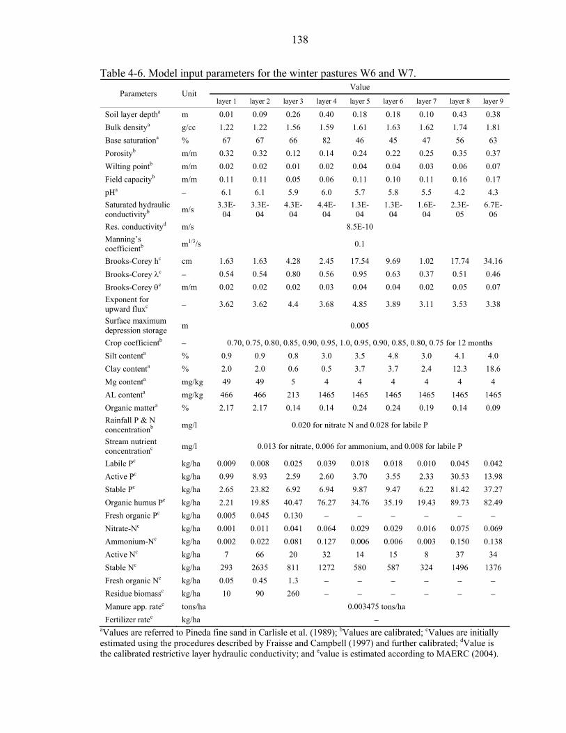
138

Table 4-6. Model input parameters for the winter pastures W6 and W7. Value

Parameters Unit layer 1 layer 2 layer 3 layer 4 layer 5 layer 6 layer 7 layer 8 layer 9

Soil layer deptha m 0.01 0.09 0.26 0.40 0.18 0.18 0.10 0.43 0.38 Bulk densitya g/cc 1.22 1.22 1.56 1.59 1.61 1.63 1.62 1.74 1.81 Base saturationa % 67 67 66 82 46 45 47 56 63 Porosityb m/m 0.32 0.32 0.12 0.14 0.24 0.22 0.25 0.35 0.37 Wilting pointb m/m 0.02 0.02 0.01 0.02 0.04 0.04 0.03 0.06 0.07 Field capacityb m/m 0.11 0.11 0.05 0.06 0.11 0.10 0.11 0.16 0.17 pHa − 6.1 6.1 5.9 6.0 5.7 5.8 5.5 4.2 4.3 Saturated hydraulic conductivityb m/s 3.3E-

04 3.3E-

04 4.3E-

04 4.4E-

04 1.3E-

04 1.3E-

04 1.6E-

04 2.3E-

05 6.7E-

06 Res. conductivityd m/s 8.5E-10 Manning’s coefficientb m1/3/s 0.1

Brooks-Corey hc cm 1.63 1.63 4.28 2.45 17.54 9.69 1.02 17.74 34.16 Brooks-Corey λc − 0.54 0.54 0.80 0.56 0.95 0.63 0.37 0.51 0.46 Brooks-Corey θc m/m 0.02 0.02 0.02 0.03 0.04 0.04 0.02 0.05 0.07 Exponent for upward fluxc − 3.62 3.62 4.4 3.68 4.85 3.89 3.11 3.53 3.38

Surface maximum depression storage m 0.005

Crop coefficientb − 0.70, 0.75, 0.80, 0.85, 0.90, 0.95, 1.0, 0.95, 0.90, 0.85, 0.80, 0.75 for 12 months Silt contenta % 0.9 0.9 0.8 3.0 3.5 4.8 3.0 4.1 4.0 Clay contenta % 2.0 2.0 0.6 0.5 3.7 3.7 2.4 12.3 18.6 Mg contenta mg/kg 49 49 5 4 4 4 4 4 4 AL contenta mg/kg 466 466 213 1465 1465 1465 1465 1465 1465 Organic mattera % 2.17 2.17 0.14 0.14 0.24 0.24 0.19 0.14 0.09 Rainfall P & N concentrationb mg/l 0.020 for nitrate N and 0.028 for labile P

Stream nutrient concentrationc mg/l 0.013 for nitrate, 0.006 for ammonium, and 0.008 for labile P

Labile Pc kg/ha 0.009 0.008 0.025 0.039 0.018 0.018 0.010 0.045 0.042 Active Pc kg/ha 0.99 8.93 2.59 2.60 3.70 3.55 2.33 30.53 13.98 Stable Pc kg/ha 2.65 23.82 6.92 6.94 9.87 9.47 6.22 81.42 37.27 Organic humus Pc kg/ha 2.21 19.85 40.47 76.27 34.76 35.19 19.43 89.73 82.49 Fresh organic Pc kg/ha 0.005 0.045 0.130 − − − − − − Nitrate-Nc kg/ha 0.001 0.011 0.041 0.064 0.029 0.029 0.016 0.075 0.069 Ammonium-Nc kg/ha 0.002 0.022 0.081 0.127 0.006 0.006 0.003 0.150 0.138 Active Nc kg/ha 7 66 20 32 14 15 8 37 34 Stable Nc kg/ha 293 2635 811 1272 580 587 324 1496 1376 Fresh organic Nc kg/ha 0.05 0.45 1.3 − − − − − − Residue biomassc kg/ha 10 90 260 − − − − − − Manure app. ratee tons/ha 0.003475 tons/ha Fertilizer ratee kg/ha −

aValues are referred to Pineda fine sand in Carlisle et al. (1989); bValues are calibrated; cValues are initially estimated using the procedures described by Fraisse and Campbell (1997) and further calibrated; dValue is the calibrated restrictive layer hydraulic conductivity; and evalue is estimated according to MAERC (2004).

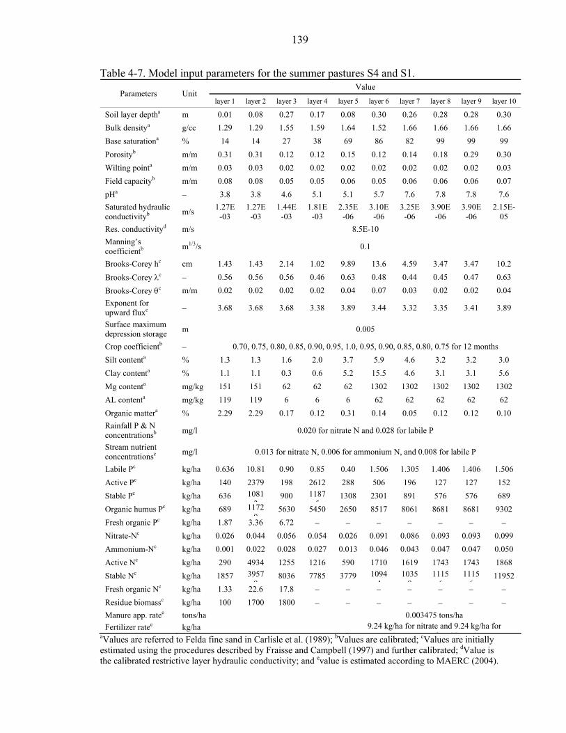
139

Table 4-7. Model input parameters for the summer pastures S4 and S1. Value

Parameters Unit layer 1 layer 2 layer 3 layer 4 layer 5 layer 6 layer 7 layer 8 layer 9 layer 10

Soil layer deptha m 0.01 0.08 0.27 0.17 0.08 0.30 0.26 0.28 0.28 0.30 Bulk densitya g/cc 1.29 1.29 1.55 1.59 1.64 1.52 1.66 1.66 1.66 1.66 Base saturationa % 14 14 27 38 69 86 82 99 99 99 Porosityb m/m 0.31 0.31 0.12 0.12 0.15 0.12 0.14 0.18 0.29 0.30 Wilting pointa m/m 0.03 0.03 0.02 0.02 0.02 0.02 0.02 0.02 0.02 0.03 Field capacityb m/m 0.08 0.08 0.05 0.05 0.06 0.05 0.06 0.06 0.06 0.07 pHa − 3.8 3.8 4.6 5.1 5.1 5.7 7.6 7.8 7.8 7.6 Saturated hydraulic conductivityb m/s 1.27E

-03 1.27E

-03 1.44E

-03 1.81E

-03 2.35E

-06 3.10E

-06 3.25E

-06 3.90E

-06 3.90E

-06 2.15E-

05 Res. conductivityd m/s 8.5E-10 Manning’s coefficientb m1/3/s 0.1

Brooks-Corey hc cm 1.43 1.43 2.14 1.02 9.89 13.6 4.59 3.47 3.47 10.2 Brooks-Corey λc − 0.56 0.56 0.56 0.46 0.63 0.48 0.44 0.45 0.47 0.63 Brooks-Corey θc m/m 0.02 0.02 0.02 0.02 0.04 0.07 0.03 0.02 0.02 0.04 Exponent for upward fluxc − 3.68 3.68 3.68 3.38 3.89 3.44 3.32 3.35 3.41 3.89

Surface maximum depression storage m 0.005

Crop coefficientb − 0.70, 0.75, 0.80, 0.85, 0.90, 0.95, 1.0, 0.95, 0.90, 0.85, 0.80, 0.75 for 12 months Silt contenta % 1.3 1.3 1.6 2.0 3.7 5.9 4.6 3.2 3.2 3.0 Clay contenta % 1.1 1.1 0.3 0.6 5.2 15.5 4.6 3.1 3.1 5.6 Mg contenta mg/kg 151 151 62 62 62 1302 1302 1302 1302 1302 AL contenta mg/kg 119 119 6 6 6 62 62 62 62 62 Organic mattera % 2.29 2.29 0.17 0.12 0.31 0.14 0.05 0.12 0.12 0.10 Rainfall P & N concentrationsb mg/l 0.020 for nitrate N and 0.028 for labile P

Stream nutrient concentrationsc mg/l 0.013 for nitrate N, 0.006 for ammonium N, and 0.008 for labile P

Labile Pc kg/ha 0.636 10.81 0.90 0.85 0.40 1.506 1.305 1.406 1.406 1.506 Active Pc kg/ha 140 2379 198 2612 288 506 196 127 127 152 Stable Pc kg/ha 636 1081

2900 1187

51308 2301 891 576 576 689

Organic humus Pc kg/ha 689 11720

5630 5450 2650 8517 8061 8681 8681 9302 Fresh organic Pc kg/ha 1.87 3.36 6.72 − − − − − − − Nitrate-Nc kg/ha 0.026 0.044 0.056 0.054 0.026 0.091 0.086 0.093 0.093 0.099 Ammonium-Nc kg/ha 0.001 0.022 0.028 0.027 0.013 0.046 0.043 0.047 0.047 0.050 Active Nc kg/ha 290 4934 1255 1216 590 1710 1619 1743 1743 1868 Stable Nc kg/ha 1857 3957

98036 7785 3779 1094

41035

91115

61115

611952

Fresh organic Nc kg/ha 1.33 22.6 17.8 − − − − − − − Residue biomassc kg/ha 100 1700 1800 − − − − − − − Manure app. ratee tons/ha 0.003475 tons/ha Fertilizer ratee kg/ha 9.24 kg/ha for nitrate and 9.24 kg/ha for

i NaValues are referred to Felda fine sand in Carlisle et al. (1989); bValues are calibrated; cValues are initially estimated using the procedures described by Fraisse and Campbell (1997) and further calibrated; dValue is the calibrated restrictive layer hydraulic conductivity; and evalue is estimated according to MAERC (2004).

140

Table 4-8. Selected hydrologic parameters for sensitivity analysis for W6. Testing Range Parameters Unit

-50% -10% Base 10% 50% Layer 1 0.160 0.288 0.320 0.352 0.480 Layer 2 0.160 0.288 0.320 0.352 0.480 Layer 3 0.060 0.108 0.120 0.132 0.180 Layer 4 0.070 0.126 0.140 0.154 0.210 Layer 5 0.120 0.216 0.240 0.264 0.360 Layer 6 0.110 0.198 0.220 0.242 0.330 Layer 7 0.125 0.225 0.250 0.275 0.375 Layer 8 0.175 0.315 0.350 0.385 0.525

Porosity

Layer 9

m/m

0.185 0.333 0.370 0.407 0.555 Layer 1 0.010 0.018 0.020 0.022 0.030 Layer 2 0.010 0.018 0.020 0.022 0.030 Layer 3 0.005 0.009 0.010 0.011 0.015 Layer 4 0.010 0.018 0.020 0.022 0.030 Layer 5 0.020 0.036 0.040 0.044 0.060 Layer 6 0.020 0.036 0.040 0.044 0.060 Layer 7 0.015 0.027 0.030 0.033 0.045 Layer 8 0.030 0.054 0.060 0.066 0.090

Wilting point

Layer 9

m/m

0.035 0.063 0.070 0.077 0.105 Layer 1 1.65 2.97 3.30 3.63 4.95 Layer 2 1.65 2.97 3.30 3.63 4.95 Layer 3 2.15 3.87 4.30 4.73 6.45 Layer 4 2.20 3.96 4.40 4.84 6.60 Layer 5 0.65 1.17 1.30 1.43 1.95 Layer 6 0.65 1.17 1.30 1.43 1.95 Layer 7 0.80 1.44 1.60 1.76 2.40 Layer 8 0.115 0.207 0.230 0.253 0.345

Saturated hydraulic conductivity

Layer 9

m/s×10-4

0.034 0.060 0.067 0.074 0.101 Restrictive layer hydraulic conductivity m/s×10-9 0.425 0.765 0.850 0.935 1.28 Manning’s roughness coefficient m1/3/s 0.05 0.09 0.10 0.11 0.15 Surface maximum depressional storage m×10-2 0.25 0.45 0.50 0.55 0.75

January 0.35 0.63 0.70 0.77 1.05 February 0.38 0.68 0.75 0.83 1.13 March 0.40 0.72 0.80 0.88 1.20 April 0.43 0.77 0.85 0.94 1.28 May 0.45 0.81 0.90 0.99 1.35 June 0.48 0.86 0.95 1.05 1.43 July 0.50 0.90 1.00 1.10 1.50 August 0.48 0.86 0.95 1.05 1.43 September 0.45 0.81 0.90 0.99 1.35 October 0.43 0.77 0.85 0.94 1.28 November 0.40 0.72 0.80 0.88 1.20

Crop coefficient

December

−

0.38 0.68 0.75 0.83 1.13

141

Table 4-9. Selected nutrient parameters for sensitivity analysis for W6. Testing Range Parameters Unit

-50% -10% Base 10% 50%Rainfall P concentration mg/l 0.014 0.025 0.028 0.031 0.042 Rainfall N concentration mg/l 0.010 0.018 0.020 0.022 0.030

Layer 1 0.50 0.89 0.99 1.09 1.49Layer 2 4.47 8.04 8.93 9.83 13.40 Layer 3 1.30 2.34 2.59 2.85 3.89 Layer 4 1.30 2.34 2.60 2.86 3.90 Layer 5 1.85 3.33 3.70 4.07 5.55 Layer 6 1.77 3.19 3.55 3.90 5.32 Layer 7 1.17 2.10 2.33 2.56 3.50 Layer 8 15.27 27.48 30.53 33.58 45.80

Active P

Layer 9

kg/ha

6.99 12.58 13.98 15.38 20.97 Layer 1 1.32 2.38 2.65 2.91 3.97Layer 2 11.91 21.44 23.82 26.21 35.74 Layer 3 3.46 6.23 6.92 7.61 10.38 Layer 4 3.47 6.25 6.94 7.64 10.41 Layer 5 4.93 8.88 9.87 10.85 14.80 Layer 6 4.73 8.52 9.47 10.41 14.20 Layer 7 3.11 5.59 6.22 6.84 9.32 Layer 8 40.71 73.28 81.42 89.56 122.13

Stable P

Layer 9

kg/ha

18.64 33.55 37.27 41.00 55.91 Layer 1 1.10 1.99 2.21 2.43 3.31Layer 2 9.93 17.87 19.85 21.84 29.78Layer 3 20.23 36.42 40.47 44.51 60.70Layer 4 38.14 68.65 76.27 83.90 114.41Layer 5 17.38 31.28 34.76 38.23 52.13Layer 6 17.59 31.67 35.19 38.71 52.78Layer 7 9.71 17.49 19.43 21.37 29.14Layer 8 44.87 80.76 89.73 98.70 134.60

Humus P

Layer 9

kg/ha

41.24 74.24 82.49 90.74 123.73Layer 1 3.66 6.59 7.32 8.05 10.98Layer 2 32.94 59.29 65.88 72.47 98.82 Layer 3 10.14 18.25 20.28 22.31 30.42 Layer 4 15.90 28.62 31.80 34.98 47.70 Layer 5 7.25 13.04 14.49 15.94 21.74 Layer 6 7.34 13.20 14.67 16.14 22.01 Layer 7 4.05 7.29 8.10 8.91 12.15 Layer 8 18.71 33.67 37.41 41.15 56.12

Active N

Layer 9

kg/ha

17.20 30.95 34.39 37.83 51.59 Layer 1 146.5 263.7 293.0 322.3 439.5Layer 2 1317.5 2371.5 2635.0 2898.5 3952.5 Layer 3 405.5 729.9 811.0 892.1 1216.5 Layer 4 636.0 1144.8 1272.0 1399.2 1908.0 Layer 5 290.0 522.0 580.0 638.0 870.0 Layer 6 293.5 528.3 587.0 645.7 880.5 Layer 7 162.0 291.6 324.0 356.4 486.0 Layer 8 748.0 1346.4 1496.0 1645.6 2244.0

Stable N

Layer 9

kg/ha

688.0 1238.4 1376.0 1513.6 2064.0 Manure application rate tons/ha 0.00174 0.00313 0.00348 0.00382 0.00521

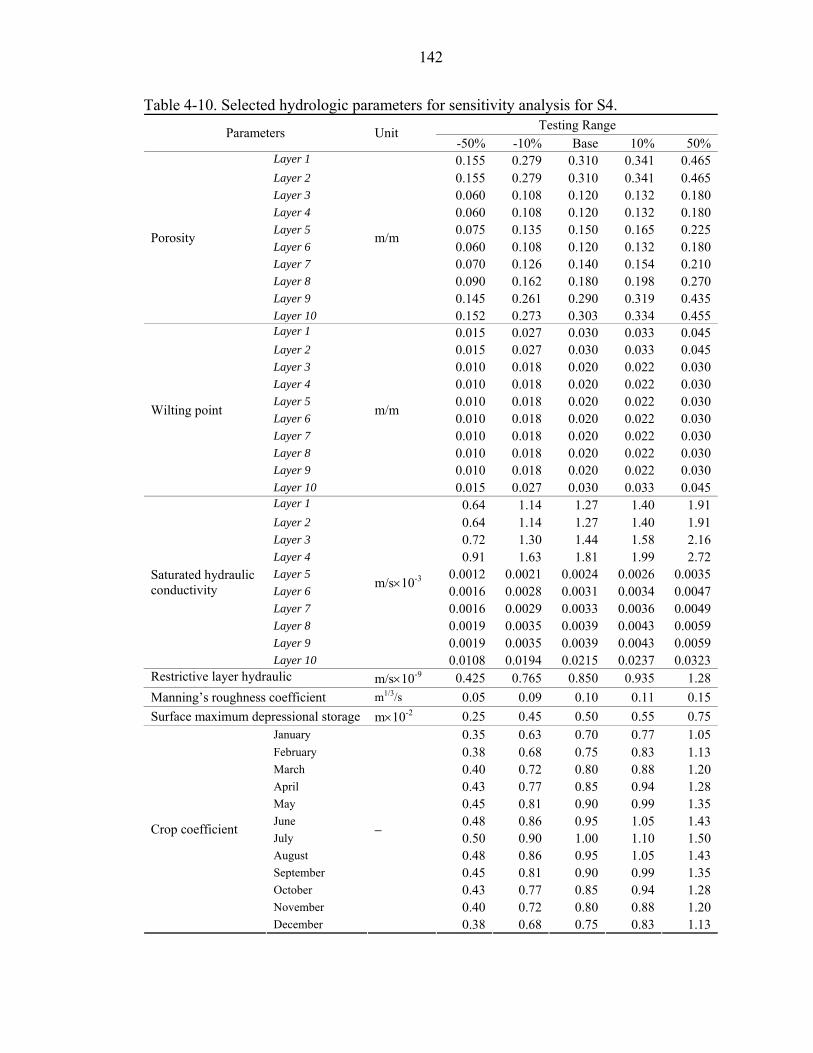
142

Table 4-10. Selected hydrologic parameters for sensitivity analysis for S4. Testing Range Parameters Unit

-50% -10% Base 10% 50% Layer 1 0.155 0.279 0.310 0.341 0.465 Layer 2 0.155 0.279 0.310 0.341 0.465 Layer 3 0.060 0.108 0.120 0.132 0.180 Layer 4 0.060 0.108 0.120 0.132 0.180 Layer 5 0.075 0.135 0.150 0.165 0.225 Layer 6 0.060 0.108 0.120 0.132 0.180 Layer 7 0.070 0.126 0.140 0.154 0.210 Layer 8 0.090 0.162 0.180 0.198 0.270 Layer 9 0.145 0.261 0.290 0.319 0.435

Porosity

Layer 10

m/m

0.152 0.273 0.303 0.334 0.455 Layer 1 0.015 0.027 0.030 0.033 0.045 Layer 2 0.015 0.027 0.030 0.033 0.045 Layer 3 0.010 0.018 0.020 0.022 0.030 Layer 4 0.010 0.018 0.020 0.022 0.030 Layer 5 0.010 0.018 0.020 0.022 0.030 Layer 6 0.010 0.018 0.020 0.022 0.030 Layer 7 0.010 0.018 0.020 0.022 0.030 Layer 8 0.010 0.018 0.020 0.022 0.030 Layer 9 0.010 0.018 0.020 0.022 0.030

Wilting point

Layer 10

m/m

0.015 0.027 0.030 0.033 0.045 Layer 1 0.64 1.14 1.27 1.40 1.91 Layer 2 0.64 1.14 1.27 1.40 1.91 Layer 3 0.72 1.30 1.44 1.58 2.16 Layer 4 0.91 1.63 1.81 1.99 2.72 Layer 5 0.0012 0.0021 0.0024 0.0026 0.0035 Layer 6 0.0016 0.0028 0.0031 0.0034 0.0047 Layer 7 0.0016 0.0029 0.0033 0.0036 0.0049 Layer 8 0.0019 0.0035 0.0039 0.0043 0.0059 Layer 9 0.0019 0.0035 0.0039 0.0043 0.0059

Saturated hydraulic conductivity

Layer 10

m/s×10-3

0.0108 0.0194 0.0215 0.0237 0.0323 Restrictive layer hydraulic

d i im/s×10-9 0.425 0.765 0.850 0.935 1.28

Manning’s roughness coefficient m1/3/s 0.05 0.09 0.10 0.11 0.15 Surface maximum depressional storage m×10-2 0.25 0.45 0.50 0.55 0.75

January 0.35 0.63 0.70 0.77 1.05 February 0.38 0.68 0.75 0.83 1.13 March 0.40 0.72 0.80 0.88 1.20 April 0.43 0.77 0.85 0.94 1.28 May 0.45 0.81 0.90 0.99 1.35 June 0.48 0.86 0.95 1.05 1.43 July 0.50 0.90 1.00 1.10 1.50 August 0.48 0.86 0.95 1.05 1.43 September 0.45 0.81 0.90 0.99 1.35 October 0.43 0.77 0.85 0.94 1.28 November 0.40 0.72 0.80 0.88 1.20

Crop coefficient

December

−

0.38 0.68 0.75 0.83 1.13

143

Table 4-11. Selected nutrient parameters for sensitivity analysis for S4. Testing Range Parameters Unit

-50% -10% Base 10% 50%Rainfall P concentration mg/l 0.014 0.025 0.028 0.031 0.042 Rainfall N concentration mg/l 0.010 0.018 0.020 0.022 0.030

Layer 1 70.0 125.9 139.9 153.9 209.9Layer 2 1189.3 2140.8 2378.6 2616.5 3568.0Layer 3 99.0 178.2 198.0 217.8 297.0Layer 4 1306.2 2351.2 2612.4 2873.6 3918.6Layer 5 143.9 259.2 287.7 316.5 431.6Layer 6 253.1 455.6 506.2 556.8 759.3Layer 7 98.0 176.3 195.9 215.5 293.9Layer 8 63.3 114.0 126.7 139.3 190.0Layer 9 63.3 114.0 126.7 139.3 190.0

Active P

Layer 10

kg/ha

75.8 136.4 151.5 166.7 227.3Layer 1 318.0 572.4 636.0 699.6 954.0Layer 2 5406.0 9730.8 10812.0 11893.2 16218.0Layer 3 450.0 810.0 900.0 990.0 1350.0Layer 4 5937.3 10687.1 11874.6 13062.0 17811.8Layer 5 654.0 1177.1 1307.9 1438.7 1961.9Layer 6 1150.0 2070.8 2300.9 2531.0 3451.3Layer 7 445.3 801.6 890.6 979.7 1335.9Layer 8 287.9 518.2 575.8 633.4 863.7Layer 9 287.9 518.2 575.8 633.4 863.7

Stable P

Layer 10

kg/ha


Humus P

Layer 10

kg/ha


Active N

Layer 10

kg/ha


Stable N

Layer 10

kg/ha

5976.0 10756.8 11952.0 13147.2 17928.0Stocking rate tons/ha 0.00174 0.00313 0.00348 0.00382 0.00521 Fertilizer rate kg/ha 4.62 8.32 9.24 10.16 13.86

144

Table 4-12. Sensitivities of total surface runoff of the selected input parameters throughout the simulation period for the calibration site W6.

Sensitivity [m3/day] Relative sensitivity [−]Parameters -50% -10% Base 10% 50% -50% -10% Base 10% 50%

Porosity −** 49087 45359 42019 32171 −** 0.82 0.00 -0.74 -0.58Wilting point 43219 44920 45359 45824 47705 -0.09 -0.10 0.00 0.10 0.10SatK* 47330 45674 45359 45085 44194 0.09 0.07 0.00 -0.06 -0.05ResK* 52953 46816 45359 43958 38734 0.33 0.32 0.00 -0.31 -0.29Crop coefficient 79106 50939 45359 40121 35749 1.49 1.23 0.00 -1.15 -0.42SurfStorage* 46497 45549 45359 45191 44491 0.05 0.04 0.00 -0.04 -0.04

*SatK= saturated hydraulic conductivity; ResK= restrictive layer hydraulic conductivity; surfStorage= surface storage. ** Not applicable. Table 4-13. Sensitivities of maximum water table to the selected input parameters depth

throughout the simulation period for the calibration site W6. Sensitivity [m] Relative sensitivity [−]Parameters

-50% -10% Base 10% 50% -50% -10% Base 10% 50% Porosity −** 1.7201 1.6903 1.6689 1.6071 −** 0.18 0.00 -0.13 -0.10Wilting point 1.7060 1.6919 1.6903 1.6903 1.6882 0.02 0.01 0.00 0.00 0.00SatK* 1.6120 1.6781 1.6903 1.7014 1.7387 -0.09 -0.07 0.00 0.07 0.06ResK* 1.6409 1.6808 1.6903 1.6994 1.7377 -0.06 -0.06 0.00 0.05 0.06Crop coefficient 1.5832 1.6785 1.6903 1.7001 1.7194 -0.13 -0.07 0.00 0.06 0.03

*SatK= saturated hydraulic conductivity; ResK= restrictive layer hydraulic conductivity; surfStorage= surface storage. ** Not applicable. Table 4-14. Sensitivities of total P loads to the selected input parameters throughout the

simulation period for the calibration site W6. Sensitivity [kg/ha] Relative sensitivity [−]Parameters

-50% -10% Base 10% 50% -50% -10% Base 10% 50% Porosity −** 3.7889 3.5117 3.2628 2.5305 −** 0.79 0.00 -0.71 -0.56Wilting point 3.3566 3.4808 3.5117 3.5469 3.6669 -0.09 -0.09 0.00 0.10 0.09SatK* 3.6739 3.5376 3.5117 3.4905 3.4109 0.09 0.07 0.00 -0.06 -0.06ResK* 4.1091 3.6283 3.5117 3.4027 2.9913 0.34 0.33 0.00 -0.31 -0.30Crop coefficient 6.1475 3.9578 3.5117 3.0957 2.7587 1.50 1.27 0.00 -1.18 -0.43SurfStorage** 3.6710 3.5498 3.5117 3.4880 3.4451 0.09 0.11 0.00 -0.07 -0.04Rainfall P 2.3878 3.2704 3.5117 3.7537 4.6369 -0.64 -0.69 0.00 0.69 0.64Active P 2.8997 3.3863 3.5117 3.6366 4.1358 -0.35 -0.36 0.00 0.36 0.36Stable P 3.5016 3.5097 3.5117 3.5138 3.5223 -0.01 -0.01 0.00 0.01 0.01

*SatK= saturated hydraulic conductivity; ResK= restrictive layer hydraulic conductivity; surfStorage= surface storage. ** Not applicable. Table 4-15. Sensitivities of total N loads to the selected input parameters throughout the

simulation period for the calibration site W6. Sensitivity [kg/ha] Relative sensitivity [−]Parameters

-50% -10% Base 10% 50% -50% -10% Base 10% 50% Porosity −** 5.6473 5.7018 5.4278 4.6585 −** -0.10 0.00 -0.48 -0.37Wilting point 5.3777 5.6044 5.7018 5.8001 5.8486 -0.11 -0.17 0.00 0.17 0.05SatK* 5.9961 5.7681 5.7018 5.6289 5.4140 0.10 0.12 0.00 -0.13 -0.10ResK* 8.1360 6.1048 5.7018 5.3173 4.0773 0.85 0.71 0.00 -0.67 -0.57Crop coefficient 10.695 6.4786 5.7018 4.8697 4.2078 1.75 1.36 0.00 -1.46 -0.52SurfStorage** 6.3471 5.7939 5.7018 5.6634 5.6235 0.23 0.16 0.00 -0.07 -0.03Rainfall N 3.4234 5.2452 5.7018 6.1564 7.9735 -0.80 -0.80 0.00 0.80 0.80Active N 5.3280 5.6473 5.7018 5.8001 6.0918 -0.13 -0.10 0.00 0.17 0.14

*SatK= saturated hydraulic conductivity; ResK= restrictive layer hydraulic conductivity; surfStorage= surface storage. ** Not applicable.

145

Table 4-16. Sensitivities of total surface runoff to the selected input parameters throughout the simulation period for the calibration site S4.

Sensitivity [m3/day] Relative sensitivity [−]Parameters -50% -10% Base 10% 50% -50% -10% Base 10% 50%

Porosity 514486 401221 377071 356119 290779 0.73 0.64 0.00 -0.56 -0.46Wilting point 353052 372690 377071 382299 382299 -0.13 -0.12 0.00 0.14 0.03SatK* 392162 379568 377071 374824 365320 0.08 0.07 0.00 -0.06 -0.06ResK* 413582 384527 377071 370110 342964 0.19 0.20 0.00 -0.18 -0.18Crop coefficient 511687 398875 377071 358874 337779 0.71 0.58 0.00 -0.48 -0.21SurfStorage* 389419 379832 377071 374772 367464 0.07 0.07 0.00 -0.06 -0.05

*SatK= saturated hydraulic conductivity; ResK= restrictive layer hydraulic conductivity; surfStorage= surface storage. Table 4-17. Sensitivities of maximum water table to the selected input parameters depth

throughout the simulation period for the calibration site S4. Sensitivity [m] Relative sensitivity [−]Parameters

-50% -10% Base 10% 50% -50% -10% Base 10% 50% Porosity 1.6549 1.5889 1.5751 1.5598 1.5343 0.10 0.09 0.00 -0.10 -0.05Wilting point 1.6732 1.5905 1.5751 1.5575 1.5575 0.12 0.10 0.00 -0.11 -0.02SatK* 1.5188 1.5662 1.5751 1.5818 1.6172 -0.07 -0.06 0.00 0.04 0.05ResK* 1.5295 1.5613 1.5751 1.5835 1.6142 -0.06 -0.09 0.00 0.05 0.05Crop coefficient 1.4023 1.5650 1.5751 1.5784 1.5844 -0.22 -0.06 0.00 0.02 0.01

*SatK= saturated hydraulic conductivity; ResK= restrictive layer hydraulic conductivity; surfStorage= surface storage. Table 4-18. Sensitivities of total P loads to the selected input parameters throughout the

simulation period for the calibration site S4. Sensitivity [kg/ha] Relative sensitivity [−]Parameters

-50% -10% Base 10% 50% -50% -10% Base 10% 50% Porosity 21.611 16.856 15.847 14.986 12.215 0.73 0.64 0.00 -0.54 -0.46Wilting point 14.717 15.674 15.847 16.054 16.054 -0.14 -0.11 0.00 0.13 0.03SatK* 16.433 15.949 15.847 15.761 15.372 0.07 0.06 0.00 -0.05 -0.06ResK* 17.325 16.153 15.847 15.571 14.457 0.19 0.19 0.00 -0.17 -0.18Crop coefficient 21.189 16.712 15.847 15.133 14.370 0.67 0.55 0.00 -0.45 -0.19SurfStorage* 16.630 16.062 15.847 15.696 15.298 0.10 0.14 0.00 -0.09 -0.07Rainfall P 15.790 15.835 15.847 15.858 15.902 -0.01 -0.01 0.00 0.01 0.01Active P 15.469 15.457 15.847 16.237 17.803 -0.05 -0.25 0.00 0.25 0.25Stable P 10.152 14.707 15.847 16.986 21.542 -0.72 -0.72 0.00 0.72 0.72

*SatK= saturated hydraulic conductivity; ResK= restrictive layer hydraulic conductivity; surfStorage= surface storage. Table 4-19. Sensitivities of total N loads to the selected input parameters throughout the

simulation period for the calibration site S4. Sensitivity [kg/ha] Relative sensitivity [−]Parameters

-50% -10% Base 10% 50% -50% -10% Base 10% 50% Porosity 9.9295 8.3176 8.0015 7.7373 7.3497 0.48 0.40 0.00 -0.33 -0.16Wilting point 7.6516 7.9431 8.0015 8.0680 8.0680 -0.09 -0.07 0.00 0.08 0.02SatK* 8.3318 8.0638 8.0015 7.9514 7.7782 0.08 0.08 0.00 -0.06 -0.06ResK* 9.8029 8.3213 8.0015 7.7053 6.6386 0.45 0.40 0.00 -0.37 -0.34Crop coefficient 14.024 8.6844 8.0015 7.4441 6.5835 1.51 0.85 0.00 -0.70 -0.35SurfStorage* 14.692 8.7898 8.0015 7.4772 6.5061 1.67 0.99 0.00 -0.66 -0.37Rainfall N 7.6872 7.9378 8.0015 8.0644 8.3241 -0.08 -0.08 0.00 0.08 0.08Active N 7.0743 7.8651 8.0015 8.1177 8.4498 -0.23 -0.17 0.00 0.15 0.11

*SatK= saturated hydraulic conductivity; ResK= restrictive layer hydraulic conductivity; surfStorage= surface storage.

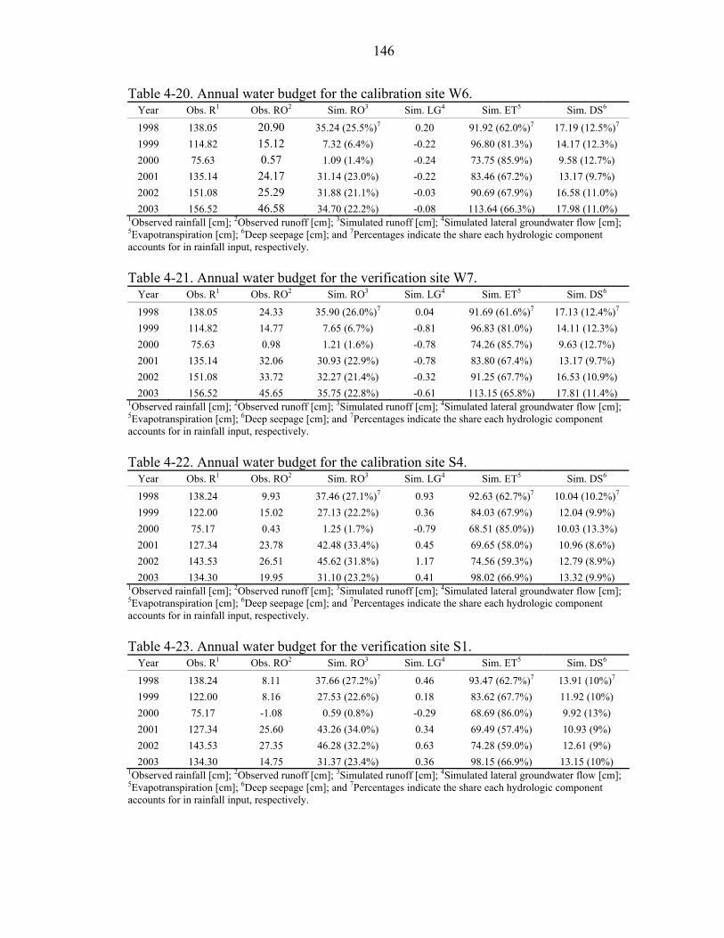
146

Table 4-20. Annual water budget for the calibration site W6. Year Obs. R1 Obs. RO2 Sim. RO3 Sim. LG4 Sim. ET5 Sim. DS6

1998 138.05 20.90 35.24 (25.5%)7 0.20 91.92 (62.0%)7 17.19 (12.5%)7 1999 114.82 15.12 7.32 (6.4%) -0.22 96.80 (81.3%) 14.17 (12.3%) 2000 75.63 0.57 1.09 (1.4%) -0.24 73.75 (85.9%) 9.58 (12.7%) 2001 135.14 24.17 31.14 (23.0%) -0.22 83.46 (67.2%) 13.17 (9.7%) 2002 151.08 25.29 31.88 (21.1%) -0.03 90.69 (67.9%) 16.58 (11.0%) 2003 156.52 46.58 34.70 (22.2%) -0.08 113.64 (66.3%) 17.98 (11.0%)

1Observed rainfall [cm]; 2Observed runoff [cm]; 3Simulated runoff [cm]; 4Simulated lateral groundwater flow [cm]; 5Evapotranspiration [cm]; 6Deep seepage [cm]; and 7Percentages indicate the share each hydrologic component accounts for in rainfall input, respectively.

Table 4-21. Annual water budget for the verification site W7.

Year Obs. R1 Obs. RO2 Sim. RO3 Sim. LG4 Sim. ET5 Sim. DS6

1998 138.05 24.33 35.90 (26.0%)7 0.04 91.69 (61.6%)7 17.13 (12.4%)7 1999 114.82 14.77 7.65 (6.7%) -0.81 96.83 (81.0%) 14.11 (12.3%) 2000 75.63 0.98 1.21 (1.6%) -0.78 74.26 (85.7%) 9.63 (12.7%) 2001 135.14 32.06 30.93 (22.9%) -0.78 83.80 (67.4%) 13.17 (9.7%) 2002 151.08 33.72 32.27 (21.4%) -0.32 91.25 (67.7%) 16.53 (10.9%) 2003 156.52 45.65 35.75 (22.8%) -0.61 113.15 (65.8%) 17.81 (11.4%)


Table 4-22. Annual water budget for the calibration site S4.


1998 138.24 9.93 37.46 (27.1%)7 0.93 92.63 (62.7%)7 10.04 (10.2%)7 1999 122.00 15.02 27.13 (22.2%) 0.36 84.03 (67.9%) 12.04 (9.9%) 2000 75.17 0.43 1.25 (1.7%) -0.79 68.51 (85.0%)) 10.03 (13.3%) 2001 127.34 23.78 42.48 (33.4%) 0.45 69.65 (58.0%) 10.96 (8.6%) 2002 143.53 26.51 45.62 (31.8%) 1.17 74.56 (59.3%) 12.79 (8.9%) 2003 134.30 19.95 31.10 (23.2%) 0.41 98.02 (66.9%) 13.32 (9.9%)


Table 4-23. Annual water budget for the verification site S1.


1998 138.24 8.11 37.66 (27.2%)7 0.46 93.47 (62.7%)7 13.91 (10%)7 1999 122.00 8.16 27.53 (22.6%) 0.18 83.62 (67.7%) 11.92 (10%) 2000 75.17 -1.08 0.59 (0.8%) -0.29 68.69 (86.0%) 9.92 (13%) 2001 127.34 25.60 43.26 (34.0%) 0.34 69.49 (57.4%) 10.93 (9%) 2002 143.53 27.35 46.28 (32.2%) 0.63 74.28 (59.0%) 12.61 (9%) 2003 134.30 14.75 31.37 (23.4%) 0.36 98.15 (66.9%) 13.15 (10%)


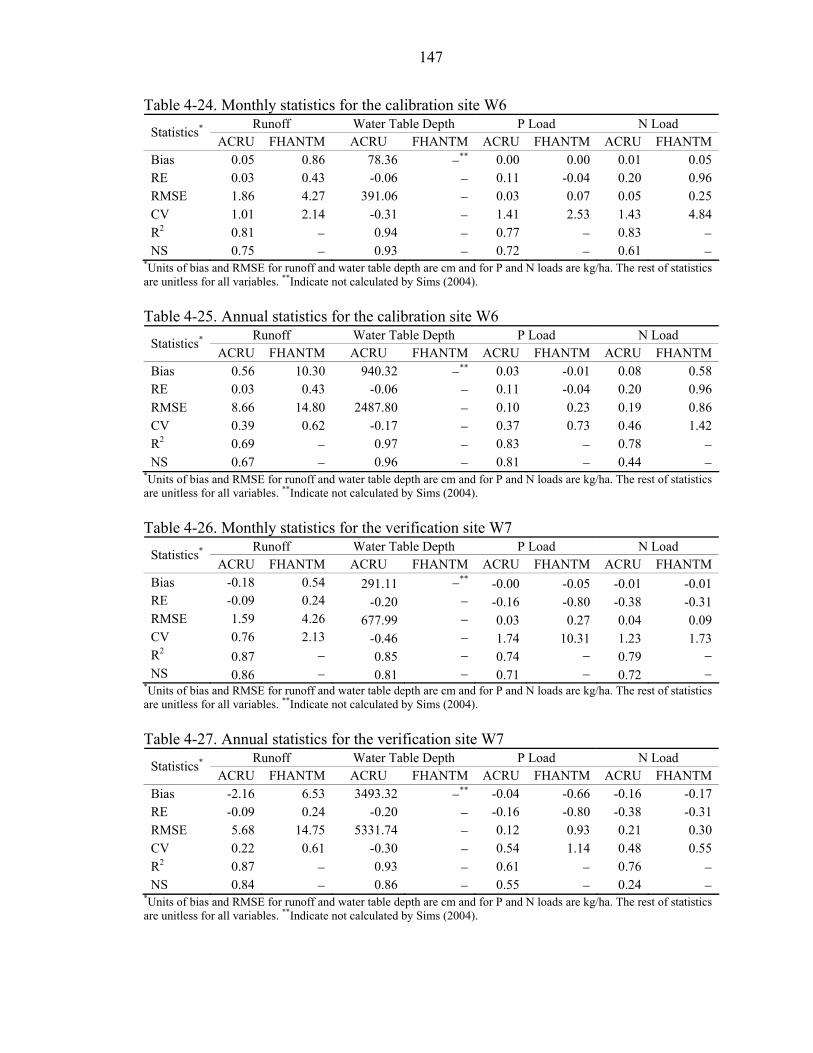
147

Table 4-24. Monthly statistics for the calibration site W6 Runoff Water Table Depth P Load N Load Statistics*

ACRU FHANTM ACRU FHANTM ACRU FHANTM ACRU FHANTM Bias 0.05 0.86 78.36 −** 0.00 0.00 0.01 0.05 RE 0.03 0.43 -0.06 − 0.11 -0.04 0.20 0.96 RMSE 1.86 4.27 391.06 − 0.03 0.07 0.05 0.25 CV 1.01 2.14 -0.31 − 1.41 2.53 1.43 4.84 R2 0.81 − 0.94 − 0.77 − 0.83 − NS 0.75 − 0.93 − 0.72 − 0.61 −

*Units of bias and RMSE for runoff and water table depth are cm and for P and N loads are kg/ha. The rest of statistics are unitless for all variables. **Indicate not calculated by Sims (2004). Table 4-25. Annual statistics for the calibration site W6

Runoff Water Table Depth P Load N Load Statistics* ACRU FHANTM ACRU FHANTM ACRU FHANTM ACRU FHANTM

Bias 0.56 10.30 940.32 −** 0.03 -0.01 0.08 0.58 RE 0.03 0.43 -0.06 − 0.11 -0.04 0.20 0.96 RMSE 8.66 14.80 2487.80 − 0.10 0.23 0.19 0.86 CV 0.39 0.62 -0.17 − 0.37 0.73 0.46 1.42 R2 0.69 − 0.97 − 0.83 − 0.78 − NS 0.67 − 0.96 − 0.81 − 0.44 −

*Units of bias and RMSE for runoff and water table depth are cm and for P and N loads are kg/ha. The rest of statistics are unitless for all variables. **Indicate not calculated by Sims (2004). Table 4-26. Monthly statistics for the verification site W7


Bias -0.18 0.54 291.11 −** -0.00 -0.05 -0.01 -0.01 RE -0.09 0.24 -0.20 − -0.16 -0.80 -0.38 -0.31 RMSE 1.59 4.26 677.99 − 0.03 0.27 0.04 0.09 CV 0.76 2.13 -0.46 − 1.74 10.31 1.23 1.73 R2 0.87 − 0.85 − 0.74 − 0.79 − NS 0.86 − 0.81 − 0.71 − 0.72 −

*Units of bias and RMSE for runoff and water table depth are cm and for P and N loads are kg/ha. The rest of statistics are unitless for all variables. **Indicate not calculated by Sims (2004). Table 4-27. Annual statistics for the verification site W7


Bias -2.16 6.53 3493.32 −** -0.04 -0.66 -0.16 -0.17 RE -0.09 0.24 -0.20 − -0.16 -0.80 -0.38 -0.31 RMSE 5.68 14.75 5331.74 − 0.12 0.93 0.21 0.30 CV 0.22 0.61 -0.30 − 0.54 1.14 0.48 0.55 R2 0.87 − 0.93 − 0.61 − 0.76 − NS 0.84 − 0.86 − 0.55 − 0.24 −

*Units of bias and RMSE for runoff and water table depth are cm and for P and N loads are kg/ha. The rest of statistics are unitless for all variables. **Indicate not calculated by Sims (2004).

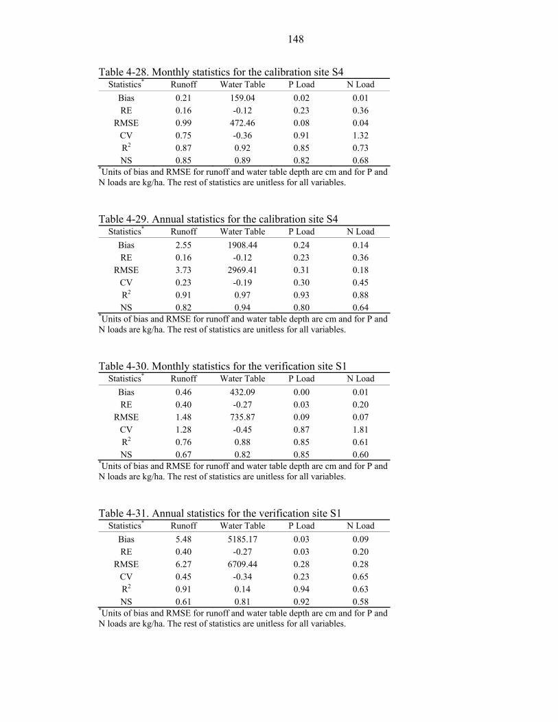
148

Table 4-28. Monthly statistics for the calibration site S4 Statistics* Runoff Water Table P Load N Load

Bias 0.21 159.04 0.02 0.01 RE 0.16 -0.12 0.23 0.36

RMSE 0.99 472.46 0.08 0.04 CV 0.75 -0.36 0.91 1.32 R2 0.87 0.92 0.85 0.73 NS 0.85 0.89 0.82 0.68

*Units of bias and RMSE for runoff and water table depth are cm and for P and N loads are kg/ha. The rest of statistics are unitless for all variables. Table 4-29. Annual statistics for the calibration site S4

Statistics* Runoff Water Table P Load N Load Bias 2.55 1908.44 0.24 0.14 RE 0.16 -0.12 0.23 0.36

RMSE 3.73 2969.41 0.31 0.18 CV 0.23 -0.19 0.30 0.45 R2 0.91 0.97 0.93 0.88 NS 0.82 0.94 0.80 0.64

*Units of bias and RMSE for runoff and water table depth are cm and for P and N loads are kg/ha. The rest of statistics are unitless for all variables. Table 4-30. Monthly statistics for the verification site S1


RMSE 1.48 735.87 0.09 0.07 CV 1.28 -0.45 0.87 1.81 R2 0.76 0.88 0.85 0.61 NS 0.67 0.82 0.85 0.60

*Units of bias and RMSE for runoff and water table depth are cm and for P and N loads are kg/ha. The rest of statistics are unitless for all variables. Table 4-31. Annual statistics for the verification site S1


RMSE 6.27 6709.44 0.28 0.28 CV 0.45 -0.34 0.23 0.65 R2 0.91 0.14 0.94 0.63 NS 0.61 0.81 0.92 0.58

*Units of bias and RMSE for runoff and water table depth are cm and for P and N loads are kg/ha. The rest of statistics are unitless for all variables.

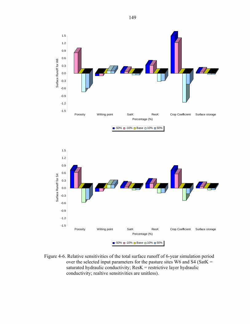
149

-1.5

-1.2

-0.9

-0.6

-0.3

0.0

0.3

0.6

0.9

1.2

1.5

Sur

face

Run

off f

or W

6

Porosity Wilting point SatK ResK Crop Coefficient Surface storagePercentage (%)

-50% -10% Base 10% 50%

-1.5

-1.2

-0.9

-0.6

-0.3

0.0

0.3

0.6

0.9

1.2

1.5

Sur

face

Run

off f

or S

4

Porosity Wilting point SatK ResK Crop Coefficient Surface storagePercentage (%)

-50% -10% Base 10% 50%

Figure 4-6. Relative sensitivities of the total surface runoff of 6-year simulation period

over the selected input parameters for the pasture sites W6 and S4 (SatK = saturated hydraulic conductivity; ResK = restrictive layer hydraulic conductivity; realtive sensitivities are unitless).

150

-0.3

-0.2

-0.1

0.0

0.1

0.2

0.3

Max

imum

Wat

er T

able

Dep

th fo

r W6

Porosity Wilting point SatK ResK Crop coefficientPercentage (%)

-50% -10% Base 10% 50%

-0.3

-0.2

-0.1

0.0

0.1

0.2

0.3

Max

imum

Wat

er T

able

Dep

th fo

r S4

Porosity Wilting point SatK ResK Crop coefficientPercentage (%)

-50% -10% Base 10% 50%

Figure 4-7. Relative sensitivities of the maximum water table depth of 6-year simulation

period over the selected input parameters for the pasture sites W6 and S4 (SatK = saturated hydraulic conductivity; ResK = restrictive layer hydraulic conductivity; relative sensitivities are unitless).

151

-1.5

-1.2

-0.9

-0.6

-0.3

0.0

0.3

0.6

0.9

1.2

1.5

P Lo

ad fo

r W

6

Porosity Wiltingpoint

SatK ResK Cropcoefficient

Surfacestorage

Rainfall P Active P Stable P

Percentage (%)

-50% -10% Base 10% 50%

-1.5

-1.2

-0.9

-0.6

-0.3

0.0

0.3

0.6

0.9

1.2

1.5

P Lo

ad fo

r S4

Porosity Wiltingpoint

SatK ResK Cropcoefficient

Surfacestorage

Rainfall P Active P Stable P

Percentage (%)

-50% -10% Base 10% 50%

Figure 4-8. Relative sensitivities of the total P load of 6-year simulation period over the

selected input parameters and variables for the pasture sites W6 and S4 (SatK = saturated hydraulic conductivity; ResK = restrictive layer hydraulic conductivity; relative sensitivities are unitless).

152

-2.0

-1.5

-1.0

-0.5

0.0

0.5

1.0

1.5

2.0

N L

oad

for W

6

Porosity Wilting point SatK ResK Cropcoefficient

Surfacestorage

Rainfall N Active N

Percentage (%)

-50% -10% Base 10% 50%

-2.0

-1.5

-1.0

-0.5

0.0

0.5

1.0

1.5

2.0

N L

oad

for S

4

Porosity Wilting point SatK ResK Cropcoefficient

Surfacestorage

Rainfall N Active N

Percentage (%)

-50% -10% Base 10% 50%

Figure 4-9. Relative sensitivities of the total N load of 6-year simulation period over the

selected input parameters for the pasture sites W6 and S4 (SatK = saturated hydraulic conductivity; ResK = restrictive layer hydraulic conductivity; relative sensitivities are unitless).

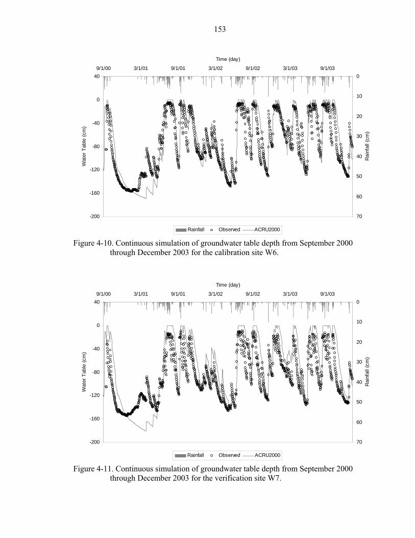
153

-200

-160

-120

-80

-40

0

409/1/00 3/1/01 9/1/01 3/1/02 9/1/02 3/1/03 9/1/03

Time (day)

Wat

er T

able

(cm

)0

10

20

30

40

50

60

70

Rai

nfal

l (cm

)

Rainfall Observed ACRU2000

Figure 4-10. Continuous simulation of groundwater table depth from September 2000 through December 2003 for the calibration site W6.

-200

-160

-120

-80

-40

0

409/1/00 3/1/01 9/1/01 3/1/02 9/1/02 3/1/03 9/1/03

Time (day)

Wat

er T

able

(cm

)

0

10

20

30

40

50

60

70

Rai

nfal

l (cm

)


Figure 4-11. Continuous simulation of groundwater table depth from September 2000 through December 2003 for the verification site W7.

154

-200

-150

-100

-50

0

509/1/00 1/1/01 5/1/01 9/1/01 1/1/02 5/1/02 9/1/02 1/1/03 5/1/03 9/1/03

Time (day)

Wat

er T

able

(cm

)

0

10

20

30

40

50

60

70

Rai

nfal

l (cm

)


Figure 4-12. Continuous simulation of groundwater table depth from September 2000 through December 2003 for the calibration site S4.

-250

-200

-150

-100

-50

0

509/1/00 3/1/01 9/1/01 3/1/02 9/1/02 3/1/03 9/1/03

Time (day)

Wat

er T

able

(cm

)

0

10

20

30

40

50

60

70

Rai

nfal

l (cm

)


Figure 4-13. Continuous simulation of groundwater table depth from September 2000 through December 2003 for the verification site S1.

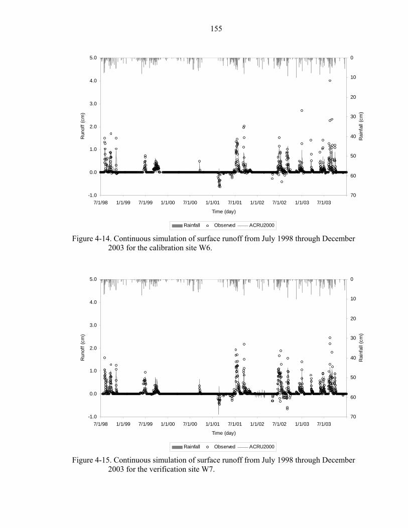
155

-1.0

0.0

1.0

2.0

3.0

4.0

5.0

7/1/98 1/1/99 7/1/99 1/1/00 7/1/00 1/1/01 7/1/01 1/1/02 7/1/02 1/1/03 7/1/03

Time (day)

Run

off (

cm)

0

10

20

30

40

50

60

70

Rai

nfal

l (cm

)


Figure 4-14. Continuous simulation of surface runoff from July 1998 through December 2003 for the calibration site W6.

-1.0

0.0

1.0

2.0

3.0

4.0

5.0

7/1/98 1/1/99 7/1/99 1/1/00 7/1/00 1/1/01 7/1/01 1/1/02 7/1/02 1/1/03 7/1/03

Time (day)

Run

off (

cm)

0

10

20

30

40

50

60

70

Rai

nfal

l (cm

)


Figure 4-15. Continuous simulation of surface runoff from July 1998 through December 2003 for the verification site W7.

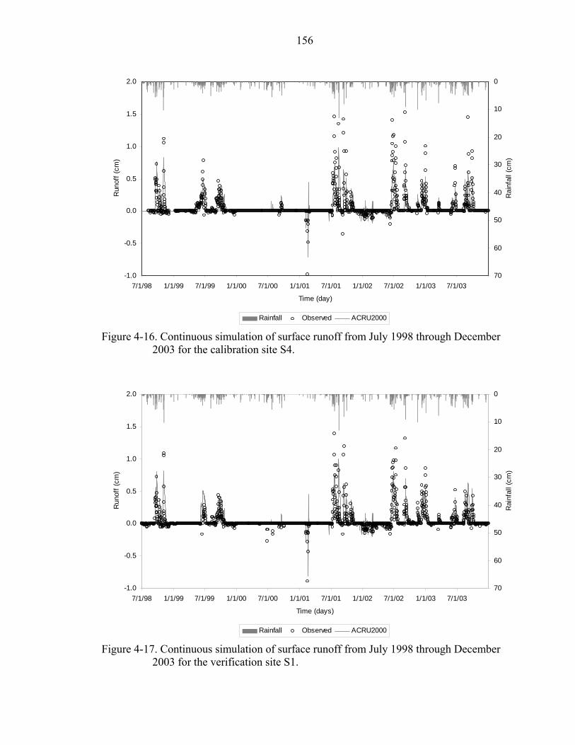
156

-1.0

-0.5

0.0

0.5

1.0

1.5

2.0

7/1/98 1/1/99 7/1/99 1/1/00 7/1/00 1/1/01 7/1/01 1/1/02 7/1/02 1/1/03 7/1/03

Time (day)

Run

off (

cm)

0

10

20

30

40

50

60

70

Rai

nfal

l (cm

)


Figure 4-16. Continuous simulation of surface runoff from July 1998 through December 2003 for the calibration site S4.

-1.0

-0.5

0.0

0.5

1.0

1.5

2.0

7/1/98 1/1/99 7/1/99 1/1/00 7/1/00 1/1/01 7/1/01 1/1/02 7/1/02 1/1/03 7/1/03

Time (days)

Run

off (

cm)

0

10

20

30

40

50

60

70

Rai

nfal

l (cm

)


Figure 4-17. Continuous simulation of surface runoff from July 1998 through December 2003 for the verification site S1.

157

-0.02

0.00

0.02

0.04

0.06

0.08

0.10

7/1/98 1/1/99 7/1/99 1/1/00 7/1/00 1/1/01 7/1/01 1/1/02 7/1/02 1/1/03 7/1/03

Time (day)

P lo

ad (k

g/ha

)

0

10

20

30

40

50

60

70

Rai

nfal

l (cm

)


Figure 4-18. Continuous simulation of P loads from July 1998 through December 2003 for the calibration site W6.

-0.02

0.00

0.02

0.04

0.06

0.08

0.10

7/1/98 1/1/99 7/1/99 1/1/00 7/1/00 1/1/01 7/1/01 1/1/02 7/1/02 1/1/03 7/1/03

Time (day)

P L

oads

(kg/

ha)

0

10

20

30

40

50

60

70

Rai

nfal

l (cm

)


Figure 4-19. Continuous simulation of P loads from July 1998 through December 2003 for the verification site W7.

158

-0.05

0.00

0.05

0.10

0.15

0.20

0.25

0.30

0.35

7/1/98 1/1/99 7/1/99 1/1/00 7/1/00 1/1/01 7/1/01 1/1/02 7/1/02 1/1/03 7/1/03

Time (day)

P L

oads

(kg/

ha)

0

10

20

30

40

50

60

70

Rai

nfal

l (cm

)


Figure 4-20. Continuous simulation of P loads from July 1998 through December 2003 for the calibration site S4.

-0.05

0.00

0.05

0.10

0.15

0.20

0.25

0.30

0.35

7/1/98 1/1/99 7/1/99 1/1/00 7/1/00 1/1/01 7/1/01 1/1/02 7/1/02 1/1/03 7/1/03

Time (day)

P L

oads

(kg/

ha)

0

10

20

30

40

50

60

70

Rai

nfal

l (cm

)


Figure 4-21. Continuous simulation of P loads from July 1998 through December 2003 for the verification site S1.

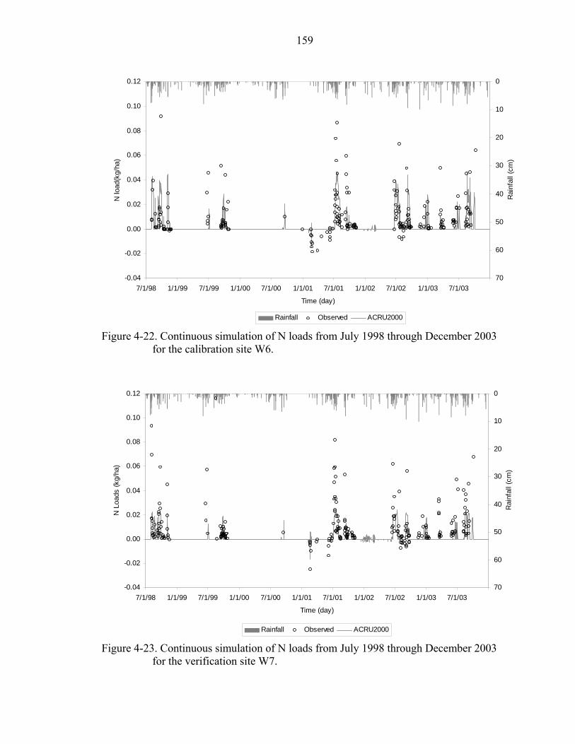
159

-0.04

-0.02

0.00

0.02

0.04

0.06

0.08

0.10

0.12

7/1/98 1/1/99 7/1/99 1/1/00 7/1/00 1/1/01 7/1/01 1/1/02 7/1/02 1/1/03 7/1/03

Time (day)

N lo

ad(k

g/ha

)

0

10

20

30

40

50

60

70

Rai

nfal

l (cm

)


Figure 4-22. Continuous simulation of N loads from July 1998 through December 2003 for the calibration site W6.

-0.04

-0.02

0.00

0.02

0.04

0.06

0.08

0.10

0.12

7/1/98 1/1/99 7/1/99 1/1/00 7/1/00 1/1/01 7/1/01 1/1/02 7/1/02 1/1/03 7/1/03

Time (day)

N L

oads

(kg/

ha)

0

10

20

30

40

50

60

70

Rai

nfal

l (cm

)


Figure 4-23. Continuous simulation of N loads from July 1998 through December 2003 for the verification site W7.

160

-0.05

0.00

0.05

0.10

0.15

0.20

7/1/98 1/1/99 7/1/99 1/1/00 7/1/00 1/1/01 7/1/01 1/1/02 7/1/02 1/1/03 7/1/03

Time (day)

N L

oads

(kg/

ha)

0

10

20

30

40

50

60

70

Rai

nfal

l (cm

)


Figure 4-24. Continuous simulation of N loads from July 1998 through December 2003 for the calibration site S4.

-0.05

0.00

0.05

0.10

0.15

0.20

7/1/98 1/1/99 7/1/99 1/1/00 7/1/00 1/1/01 7/1/01 1/1/02 7/1/02 1/1/03 7/1/03

Time (day)

N L

oads

(kg/

ha)

0

10

20

30

40

50

60

70

Rai

nfal

l (cm

)


Figure 4-25. Continuous simulation of N loads from July 1998 through December 2003 for the verification site S1.

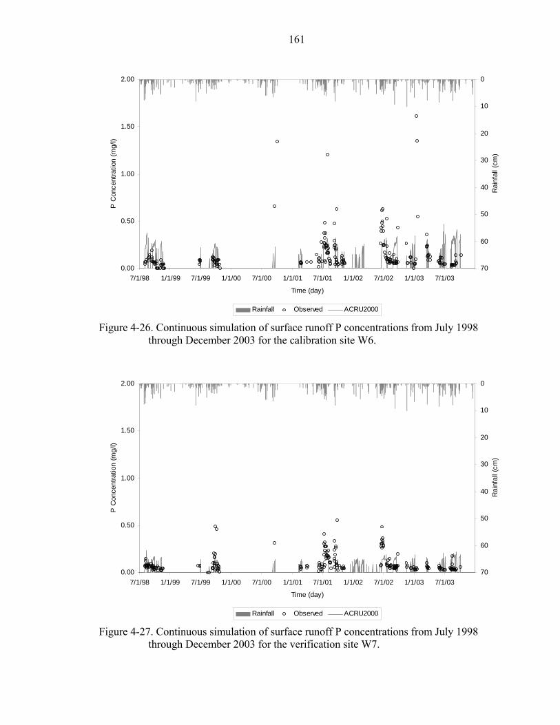
161

0.00

0.50

1.00

1.50

2.00

7/1/98 1/1/99 7/1/99 1/1/00 7/1/00 1/1/01 7/1/01 1/1/02 7/1/02 1/1/03 7/1/03

Time (day)

P C

once

ntra

tion

(mg/

l)

0

10

20

30

40

50

60

70

Rai

nfal

l (cm

)


Figure 4-26. Continuous simulation of surface runoff P concentrations from July 1998 through December 2003 for the calibration site W6.

0.00

0.50

1.00

1.50

2.00

7/1/98 1/1/99 7/1/99 1/1/00 7/1/00 1/1/01 7/1/01 1/1/02 7/1/02 1/1/03 7/1/03

Time (day)

P C

once

ntra

tion

(mg/

l)

0

10

20

30

40

50

60

70

Rai

nfal

l (cm

)


Figure 4-27. Continuous simulation of surface runoff P concentrations from July 1998 through December 2003 for the verification site W7.

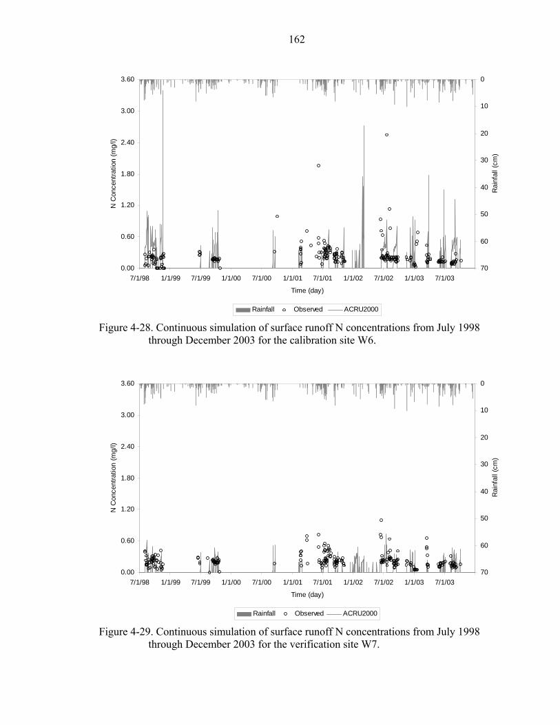
162

0.00

0.60

1.20

1.80

2.40

3.00

3.60

7/1/98 1/1/99 7/1/99 1/1/00 7/1/00 1/1/01 7/1/01 1/1/02 7/1/02 1/1/03 7/1/03

Time (day)

N C

once

ntra

tion

(mg/

l)

0

10

20

30

40

50

60

70

Rai

nfal

l (cm

)


Figure 4-28. Continuous simulation of surface runoff N concentrations from July 1998 through December 2003 for the calibration site W6.

0.00

0.60

1.20

1.80

2.40

3.00

3.60

7/1/98 1/1/99 7/1/99 1/1/00 7/1/00 1/1/01 7/1/01 1/1/02 7/1/02 1/1/03 7/1/03

Time (day)

N C

once

ntra

tion

(mg/

l)

0

10

20

30

40

50

60

70

Rai

nfal

l (cm

)


Figure 4-29. Continuous simulation of surface runoff N concentrations from July 1998 through December 2003 for the verification site W7.

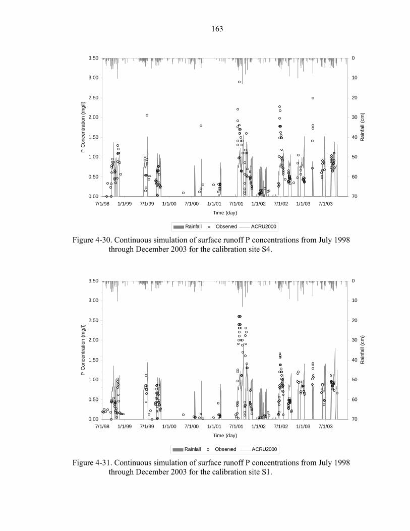
163

0.00

0.50

1.00

1.50

2.00

2.50

3.00

3.50

7/1/98 1/1/99 7/1/99 1/1/00 7/1/00 1/1/01 7/1/01 1/1/02 7/1/02 1/1/03 7/1/03

Time (day)

P C

once

ntra

tion

(mg/

l)

0

10

20

30

40

50

60

70

Rai

nfal

l (cm

)


Figure 4-30. Continuous simulation of surface runoff P concentrations from July 1998 through December 2003 for the calibration site S4.

0.00

0.50

1.00

1.50

2.00

2.50

3.00

3.50

7/1/98 1/1/99 7/1/99 1/1/00 7/1/00 1/1/01 7/1/01 1/1/02 7/1/02 1/1/03 7/1/03

Time (day)

P C

once

ntra

tion

(mg/

l)

0

10

20

30

40

50

60

70

Rai

nfal

l (cm

)


Figure 4-31. Continuous simulation of surface runoff P concentrations from July 1998 through December 2003 for the calibration site S1.

164

0.00

1.00

2.00

3.00

4.00

5.00

6.00

7.00

7/1/98 1/1/99 7/1/99 1/1/00 7/1/00 1/1/01 7/1/01 1/1/02 7/1/02 1/1/03 7/1/03

Time (day)

N C

once

ntra

tion

(mg/

l)

0

10

20

30

40

50

60

70

Rai

nfal

l (cm

)


Figure 4-32. Continuous simulation of surface runoff N concentrations from July 1998 through December 2003 for the verification site S4.

0.00

1.00

2.00

3.00

4.00

5.00

6.00

7.00

7/1/98 1/1/99 7/1/99 1/1/00 7/1/00 1/1/01 7/1/01 1/1/02 7/1/02 1/1/03 7/1/03

Time (day)

N C

once

ntra

tion

(mg/

l)

0

10

20

30

40

50

60

70

Rai

nfal

l (cm

)


Figure 4-33. Continuous simulation of surface runoff N concentrations from July 1998 through December 2003 for the verification site S1.

165

Observed vs. Simulated Monthly Runoff for W6

y = 1.028x - 0.0047R2 = 0.8104

-5

0

5

10

15

20

-5 0 5 10 15 20

Observed (cm)

Sim

ulat

ed (c

m)

Observed vs. Simulated Annual Runoff for W6

y = 0.8024x + 4.9308R2 = 0.6883

0

10

20

30

40

50

60

0 10 20 30 40 50 60

Observed (cm)

Sim

ulat

ed (c

m)

Figure 4-34. Linear plots of monthly and annual surface runoff from 1998 to 2003 for the

calibration site W6.

166

Observed vs. Simulated Monthly Runoff for W7

y = 0.9776x - 0.1326R2 = 0.8721

-5

0

5

10

15

20

25

30

-5 0 5 10 15 20 25 30

Observed (cm)

Sim

ulat

ed (c

m)

Observed vs. Simulated Annual Runoff for W7

y = 0.8711x + 1.0992R2 = 0.8658

0

10

20

30

40

50

60

0 10 20 30 40 50 60

Observed (cm)

Sim

ulat

ed (c

m)


verification site W7.

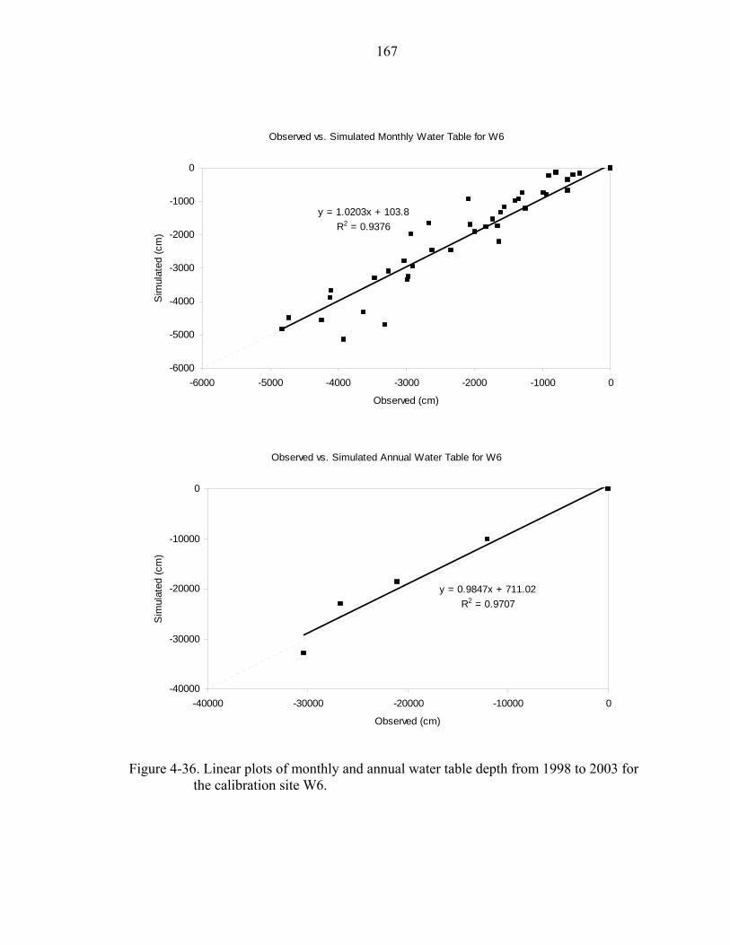
167

Observed vs. Simulated Monthly Water Table for W6

y = 1.0203x + 103.8R2 = 0.9376

-6000

-5000

-4000

-3000

-2000

-1000

0

-6000 -5000 -4000 -3000 -2000 -1000 0

Observed (cm)

Sim

ulat

ed (c

m)

Observed vs. Simulated Annual Water Table for W6

y = 0.9847x + 711.02R2 = 0.9707

-40000

-30000

-20000

-10000

0

-40000 -30000 -20000 -10000 0

Observed (cm)

Sim

ulat

ed (c

m)

Figure 4-36. Linear plots of monthly and annual water table depth from 1998 to 2003 for

the calibration site W6.

168

Observed vs. Simulated Monthly Water Table for W7

y = 0.9543x + 223.89R2 = 0.853

-6000

-5000

-4000

-3000

-2000

-1000

0

-6000 -5000 -4000 -3000 -2000 -1000 0

Observed (cm)

Sim

ulat

ed (c

m)

Observed vs. Simulated Annual Water Table for W7

y = 0.8434x + 729.4R2 = 0.9252

-40000

-30000

-20000

-10000

0

-40000 -30000 -20000 -10000 0

Observed (cm)

Sim

ulat

ed (c

m)


the verification site W7.

169

Observed vs. Simulated Monthly P Load for W6

y = 0.9572x + 0.0035R2 = 0.7656

-0.10

0.00

0.10

0.20

0.30

0.40

0.50

0.60

-0.10 0.00 0.10 0.20 0.30 0.40 0.50 0.60

Observed (kg/ha)

Sim

ulat

ed (k

g/ha

)

Observed vs. Simulated Annual P Load for W6

y = 0.8731x + 0.0654R2 = 0.8334

0.00

0.20

0.40

0.60

0.80

0.00 0.20 0.40 0.60 0.80

Observed (kg/ha)

Sim

ulat

ed (k

g/ha

)

Figure 4-38. Linear plots of monthly and annual P load from 1998 to 2003 for the


170

Observed vs. Simulated Monthly P Load for W7

y = 0.5837x + 0.0046R2 = 0.7437

-0.05

0.06

0.17

0.28

0.39

0.50

-0.05 0.06 0.17 0.28 0.39 0.50

Observed (kg/ha)

Sim

ulat

ed (k

g/ha

)

Observed vs. Simulated Annual P Load for W7

y = 0.4965x + 0.0734R2 = 0.6071

0.00

0.20

0.40

0.60

0.00 0.20 0.40 0.60

Observed (kg/ha)

Sim

ulat

ed (k

g/ha

)



171

Observed vs. Simulated Monthly N Load for W6

y = 1.2497x - 0.0017R2 = 0.8315

-0.10

0.10

0.30

0.50

0.70

0.90

-0.10 0.10 0.30 0.50 0.70 0.90

Observed (kg/ha)

Sim

ulat

ed (k

g/ha

)

Observed vs. Simulated Annual N Load for W6

y = 1.1913x + 0.0041R2 = 0.7833

0.00

0.20

0.40

0.60

0.80

1.00

1.20

0.00 0.20 0.40 0.60 0.80 1.00 1.20

Observed (kg/ha)

Sim

ulat

ed (k

g/ha

)

Figure 4-40. Linear plots of monthly and annual N load from 1998 to 2003 for the


172

Observed vs. Simulated Monthly N Load for W7

y = 0.6094x + 0.0005R2 = 0.7927

-0.05

0.08

0.21

0.34

0.47

0.60

-0.05 0.08 0.21 0.34 0.47 0.60

Observed (kg/ha)

Sim

ulat

ed (k

g/ha

)

Observed vs. Simulated Annual N Load for W7

y = 0.5677x + 0.0244R2 = 0.7613

0.00

0.20

0.40

0.60

0.80

0.00 0.20 0.40 0.60 0.80

Observed (kg/ha)

Sim

ulat

ed (k

g/ha

)



173

Observed vs. Simulated Monthly Runoff for S4

y = 0.989x + 0.2255R2 = 0.8732

-4

-2

0

2

4

6

8

10

-4 -2 0 2 4 6 8 10

Observed (cm)

Sim

ulat

ed (c

m)

Observed vs. Simulated Annual Runoff for S4

y = 0.9902x + 2.6862R2 = 0.9122

0

5

10

15

20

25

30

0 5 10 15 20 25 30

Observed (cm)

Sim

ulat

ed (c

m)


calibration site S4.

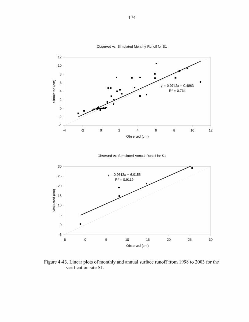
174

Observed vs. Simulated Monthly Runoff for S1

y = 0.9742x + 0.4863R2 = 0.764

-4

-2

0

2

4

6

8

10

12

-4 -2 0 2 4 6 8 10 12

Observed (cm)

Sim

ulat

ed (c

m)

Observed vs. Simulated Annual Runoff for S1

y = 0.9612x + 6.0156R2 = 0.9119

-5

0

5

10

15

20

25

30

-5 0 5 10 15 20 25 30

Observed (cm)

Sim

ulat

ed (c

m)


verification site S1.

175

Observed vs. Simulated Monthly Water Table for S4

y = 1.0191x + 183.46R2 = 0.9175

-6000

-5000

-4000

-3000

-2000

-1000

0

-6000 -5000 -4000 -3000 -2000 -1000 0

Observed (cm)

Sim

ulat

ed (c

m)

Observed vs. Simulated Annual Water Table for S4

y = 0.8975x + 281.62R2 = 0.9737

-40000

-30000

-20000

-10000

0

-40000 -35000 -30000 -25000 -20000 -15000 -10000 -5000 0

Observed (cm)

Sim

ulat

ed (c

m)


the calibration site S4.

176

Obseved vs. Simulated Monthly Water Table for S1

y = 0.8694x + 219.46R2 = 0.8798

-6000

-5000

-4000

-3000

-2000

-1000

0

-6000 -5000 -4000 -3000 -2000 -1000 0

Observed (cm)

Sim

ulat

ed (c

m)

Obseved vs. Simulated Annual Water Table for S1

y = 0.7533x + 364.25R2 = 0.9749

-40000

-30000

-20000

-10000

0

-40000 -35000 -30000 -25000 -20000 -15000 -10000 -5000 0

Observed (cm)

Sim

ulat

ed (c

m)


the verification site S1.

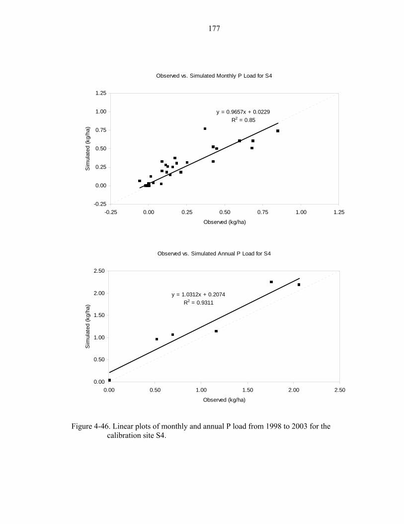
177

Observed vs. Simulated Monthly P Load for S4

y = 0.9657x + 0.0229R2 = 0.85

-0.25

0.00

0.25

0.50

0.75

1.00

1.25

-0.25 0.00 0.25 0.50 0.75 1.00 1.25

Observed (kg/ha)

Sim

ulat

ed (k

g/ha

)

Observed vs. Simulated Annual P Load for S4

y = 1.0312x + 0.2074R2 = 0.9311

0.00

0.50

1.00

1.50

2.00

2.50

0.00 0.50 1.00 1.50 2.00 2.50

Observed (kg/ha)

Sim

ulat

ed (k

g/ha

)



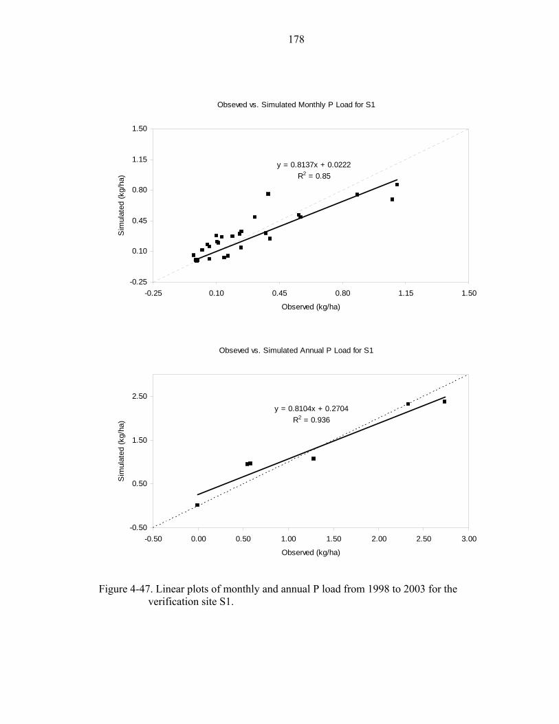
178

Obseved vs. Simulated Monthly P Load for S1

y = 0.8137x + 0.0222R2 = 0.85

-0.25

0.10

0.45

0.80

1.15

1.50

-0.25 0.10 0.45 0.80 1.15 1.50

Observed (kg/ha)

Sim

ulat

ed (k

g/ha

)

Obseved vs. Simulated Annual P Load for S1

y = 0.8104x + 0.2704R2 = 0.936

-0.50

0.50

1.50

2.50

-0.50 0.00 0.50 1.00 1.50 2.00 2.50 3.00

Observed (kg/ha)

Sim

ulat

ed (k

g/ha

)



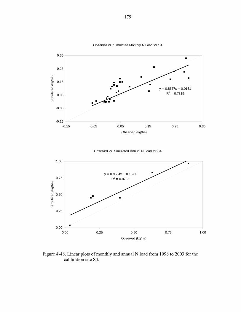
179

Observed vs. Simulated Monthly N Load for S4

y = 0.8677x + 0.0161R2 = 0.7319

-0.15

-0.05

0.05

0.15

0.25

0.35

-0.15 -0.05 0.05 0.15 0.25 0.35

Observed (kg/ha)

Sim

ulat

ed (k

g/ha

)

Observed vs. Simulated Annual N Load for S4

y = 0.9604x + 0.1571R2 = 0.8782

0.00

0.25

0.50

0.75

1.00

0.00 0.25 0.50 0.75 1.00

Observed (kg/ha)

Sim

ulat

ed (k

g/ha

)



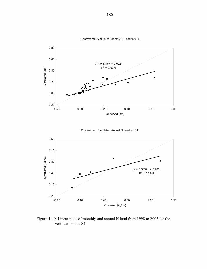
180

Obseved vs. Simulated Monthly N Load for S1

y = 0.5746x + 0.0224R2 = 0.6075

-0.20

0.00

0.20

0.40

0.60

0.80

-0.20 0.00 0.20 0.40 0.60 0.80

Observed (cm)

Sim

ulat

ed (c

m)

Obseved vs. Simulated Annual N Load for S1

y = 0.5352x + 0.286R2 = 0.6347

-0.25

0.10

0.45

0.80

1.15

1.50

-0.25 0.10 0.45 0.80 1.15 1.50

Observed (kg/ha)

Sim

ulat

ed (k

g/ha

)



181

Duration Curve of Daily Surface Runoff for W6

-1.0

0.0

1.0

2.0

3.0

4.0

0 10 20 30 40 50 60 70 80 90 100

Percent of Days Runoff Equaled or Exceeded (%)

Sur

face

Run

off (

cm)

Observed Simulated

Duration Curve of Daily Water Table Depth for W6

-175

-150

-125

-100

-75

-50

-25

0

25

0 10 20 30 40 50 60 70 80 90 100

Percent of Days Water Table Equaled or Exceeded (%)

Wat

er T

able

(cm

)

Observed Simulated

Figure 4-50. Duration curves of daily surface runoff and water table depth for the


182

Duration Curve of P Load for W6

-0.02

0.01

0.04

0.07

0.10

0 10 20 30 40 50 60 70 80 90 100

Percent of Days P Load Equaled or Exceeded (%)

P L

oad

(kg/

ha)

Observed Simulated

N Load Duration Curve for W6

-0.02

0.00

0.02

0.04

0.06

0.08

0.10

0 10 20 30 40 50 60 70 80 90 100

Percent of days Equaled or Exceeded (%)

N L

oad

(kg/

ha)

Observed Simulated

Figure 4-51. Duration curves of daily P and N loads for the calibration site W6.

183

Duration Curve of Daily Surface Runoff for W7

-1.00

0.00

1.00

2.00

3.00

0 10 20 30 40 50 60 70 80 90 100

Percent of Days Runoff Equaled or Exceeded (%)

Sur

face

Run

off (

cm)

Observed Simulated

Duration Curve of Daily Water Table Depth for W7

-200

-175

-150

-125

-100

-75

-50

-25

0

25

0 10 20 30 40 50 60 70 80 90 100

Percent of Days Water Table Equaled or Exceeded (%)

Wat

er T

able

(cm

)

Observed Simulated

Figure 4-52. Duration curves of daily surface runoff and water table depth for the


184

Duration Curve of P Load for W7

-0.02

0.00

0.02

0.04

0.06

0.08

0.10

0 10 20 30 40 50 60 70 80 90 100

Percent of Days P Load Equaled or Exceeded (%)

P L

oad

(kg/

ha)

Observed Simulated

Duration Curve of N Load for W7

-0.12

-0.08

-0.04

0.00

0.04

0.08

0.12

0 10 20 30 40 50 60 70 80 90 100

Percent of Days N Load Equaled or Exceeded (%)

N L

oad

(kg/

ha)

Observed Simulated

Figure 4-53. Duration curves of daily P and N loads for the verification site W7.

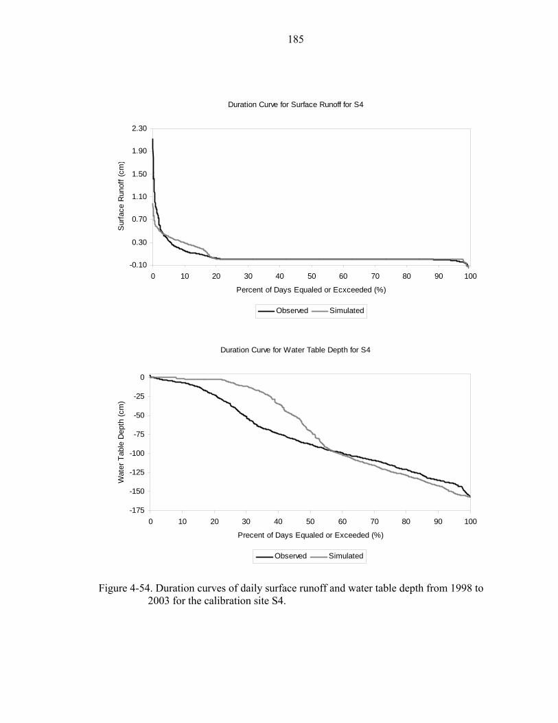
185

Duration Curve for Surface Runoff for S4

-0.10

0.30

0.70

1.10

1.50

1.90

2.30

0 10 20 30 40 50 60 70 80 90 100

Percent of Days Equaled or Ecxceeded (%)

Sur

face

Run

off (

cm)

Observed Simulated

Duration Curve for Water Table Depth for S4

-175

-150

-125

-100

-75

-50

-25

0

0 10 20 30 40 50 60 70 80 90 100

Precent of Days Equaled or Exceeded (%)

Wat

er T

able

Dep

th (c

m)

Observed Simulated

Figure 4-54. Duration curves of daily surface runoff and water table depth from 1998 to

2003 for the calibration site S4.

186

Duration Curve of P Load for S4

-0.05

0.00

0.05

0.10

0.15

0.20

0.25

0 10 20 30 40 50 60 70 80 90 100

Percent of Days Equaled or Exceeded (%)

P L

oad

(kg/

ha)

Observed Simulated

Duration Curve of N Load for S4

-0.03

0.02

0.07

0.12

0 10 20 30 40 50 60 70 80 90 100


N L

oad

(kg/

ha)

Observed Simulated

Figure 4-55. Duration curves of daily N and P loads from 1998 to 2003 for the calibration

site S4.

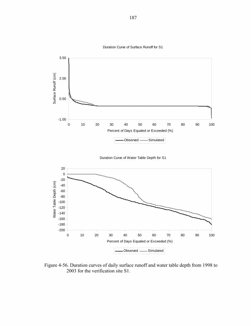
187

Duration Curve of Surface Runoff for S1

-1.00

0.50

2.00

3.50

0 10 20 30 40 50 60 70 80 90 100


Sur

face

Run

off (

cm)

Observed Simulated

Duration Curve of Water Table Depth for S1

-200-180-160-140-120-100-80-60-40-20

020

0 10 20 30 40 50 60 70 80 90 100


Wat

er T

able

Dep

th (c

m)

Observed Simulated

Figure 4-56. Duration curves of daily surface runoff and water table depth from 1998 to

2003 for the verification site S1.

188

Duration Curve of P Load for S1

-0.05

0.00

0.05

0.10

0.15

0.20

0.25

0.30

0 10 20 30 40 50 60 70 80 90 100


P L

oad

(kg/

ha)

Observed Simulated

Duration Curve of N Load for S1

-0.04

0.00

0.04

0.08

0.12

0.16

0 10 20 30 40 50 60 70 80 90 100


N L

oad

(kg/

ha)

Observed Simulated

Figure 4-57. Duration curves of daily N and P loads from 1998 to 2003 for the


189

CHAPTER 5 VEGETATION DYNAMICS SIMULATION MODEL

Introduction

A vegetation dynamics simulation model was developed to predict plant growth in

flatwoods watersheds where various landscapes such as wetlands, uplands and transition

zones coexist. Best management practices (BMPs) intended to improve water quality in

Lake Okeechobee (for example, increased water levels and reduced cattle stocking rates)

impact hydrology and nutrient cycling in these watersheds and thus affect vegetation

dynamics. Previous studies have indicated that vegetation composition patterns can

change over time and space when either hydrology or nutrient dynamics are changed.

Some species may expand spatially to encroach the habitats where other species were

previously established, while other may decline in their original habitats because of the

adverse growth environment caused by these changes. Therefore, the vegetation

composition pattern, as an integrated ecohydrologic indicator, may help to identify

changes in soil, water, and nutrient conditions in a watershed where BMPs are being

implemented if the feedback relationships between vegetation and hydrology and

nutrients are well understood. Additionally, well-calibrated numerical vegetation

simulation models can be very useful in reducing the cost of field experiments, gaining

insights into relevant processes, and predicting long-term trends. Therefore, a vegetation

dynamics simulation model was developed in this Chapter to couple with the hydrologic

and nutrient models discussed in the previous Chapters.

190

The available data to establish and calibrate a vegetation model for pasture and

wetland plants in south Florida flatwoods watersheds is very limited. Therefore a simple

model that avoids overwhelming data requirements, but is still capable of capturing the

vegetation dynamics in a logical manner is required. When sufficient data become

available in the future, the model can be further improved and calibrated.

Consequently, the objectives of this study are to develop a dynamic vegetation

model to simulate

Daily biomass productivity and leaf area index.

Plant growth dynamics limited by water and nutrient availabilities.

Evapotranspiration with consideration of multiple species.

Nutrient uptake with consideration of multiple species.

Species composition pattern over time and space as impacted by water and nutrient availability.

A vegetation model, built on a spatially heterogeneous landscape through a land

segment system in which the number, size and shape of the land segments can be defined

according to land cover, soil and vegetation types, and topography, was developed. Each

land segment is initialized with one or multiple species, which compete for light, water

and nutrients. For each time step, plant growth is simulated, driven by climate variables

including solar radiation and temperature. The growth reduction caused by suboptimal

water and nutrient availability is calculated daily and applied to reduce the potential plant

growth. Losses in plant biomass due to fire, harvest, and senescence are withdrawn from

the biomass pool and affect plant growth and competition in the next time step. Within a

land segment, homogeneity of plant distribution, plant biomass, leaf area, and soil

conditions is assumed. The population dynamics of the herbivores and their grazing

191

impacts to plant growth are not included in this study, but these impacts can be

incorporated into the model once an herbivore movement model is developed. Land

segments are dependent on each other in the sense that water and nutrient flows are

transferred between land segments, and there are feedback relationships between the

water, nutrient and vegetation models. Therefore, the vegetation development within one

land segment indirectly affects the vegetation development in another land segment.

The main processes described in this model are light interception, dry matter

production and partitioning, and leaf area development. The driving variables of the

model are climate data (radiation and temperature) and the time step is daily. The state

variables are aboveground and belowground biomass and their corresponding N and P

pools. Water stress reflecting water limitation, water logging reflecting anoxic soil water

conditions, and nitrogen (N) and phosphorus (P) stress reflecting nutrient deficiencies are

calculated on a daily basis in the model, and their combination defines a growth reduction

factor affecting the plant growth.

The following assumptions were made in the development of the vegetation model:

Light interception occurs in one canopy layer that contains all plant species of interest.

Potential plant growth is driven primarily by solar radiation and temperature, but it is reduced by the water and nutrient limitations.

Within land segments, functional groups of species are simulated instead of individual plants. Thus all plants within a species are treated as a single entity.

Total dry matter for each species is simply partitioned into aboveground and belowground biomass.

All species within land segments are assumed to have the same root lengths and have the same distribution fraction of roots in the computational soil layers.

Alive plant N and P concentrations are uniform throughout the entire plant.

192

Plant senescence starts when the sum of leaf area index (LAI) over all species is greater than the critical LAI.

When long-term inundation causes the death of plants, 25% of the aboveground and belowground biomass and the corresponding N and P are removed per day from live biomass pools to dead biomass pools.

When fire occurs, 95% of the aboveground biomass and the corresponding N and P in the aboveground biomass are removed for all species in the land segment.

Methodology

Model Structure

The model for simulating the biomass productivity of pasture and wetland grasses

in order to understand how spatial biomass distribution and composition pattern are

impacted by altered hydrology and nutrient concentrations is depicted in Figure 5-1. This

model is designed based on the previous studies by Spitters and Schapendonk (1990),

Ivens (1992), Kooman (1995), Jones and Luyten (1998), Van Oene et al. (1999), and

Jones et al. (2000).

The basic processes in this model are light interception, conversion of light into dry

matter production, and allocation of dry matter between aboveground and belowground

dry matter. The impacts from the changes in hydrology and nutrient concentrations are

expressed in growth limiting factors. Water stress or logging indicate water deficiency or

water logged soil conditions, and N and P stress factors indicate N and P deficiency.

These stress factors are combined to define a growth reduction factor that is used in the

model to reflect the adverse growth conditions causing the reduction of the potential dry

matter production. Different species have different growth niches (Whittaker and Levin,

1975) defined by the plant’s physiological and phenological characteristics, which

determine whether a species can adapt to the changing environment. The resulting plant

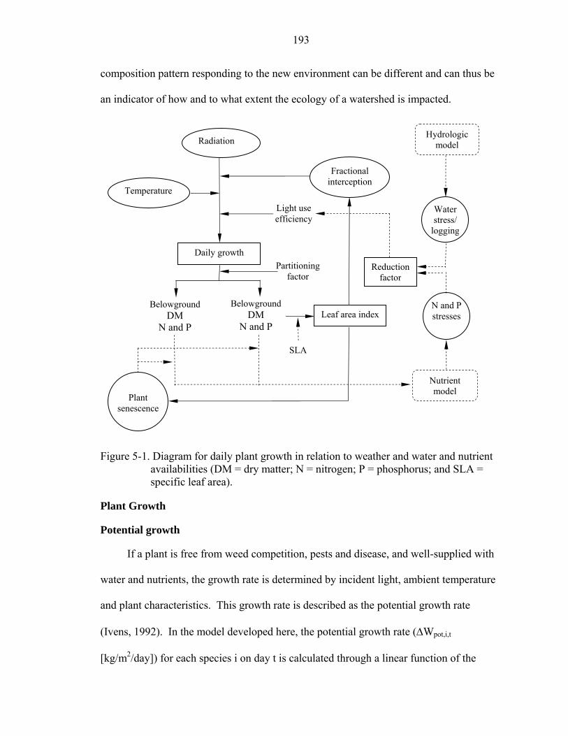
193

composition pattern responding to the new environment can be different and can thus be

an indicator of how and to what extent the ecology of a watershed is impacted.

Figure 5-1. Diagram for daily plant growth in relation to weather and water and nutrient

availabilities (DM = dry matter; N = nitrogen; P = phosphorus; and SLA = specific leaf area).

Plant Growth

Potential growth

If a plant is free from weed competition, pests and disease, and well-supplied with

water and nutrients, the growth rate is determined by incident light, ambient temperature

and plant characteristics. This growth rate is described as the potential growth rate

(Ivens, 1992). In the model developed here, the potential growth rate (∆Wpot,i,t

[kg/m2/day]) for each species i on day t is calculated through a linear function of the

Fractional interception

Radiation

Water stress/

logging

N and P stresses

Light use efficiency

Partitioning factor

SLA

Daily growth

Leaf area index

Temperature

Hydrologic model

Nutrient model

Reduction factor

Plant

senescence

Belowground DM

N and P

Belowground DM

N and P

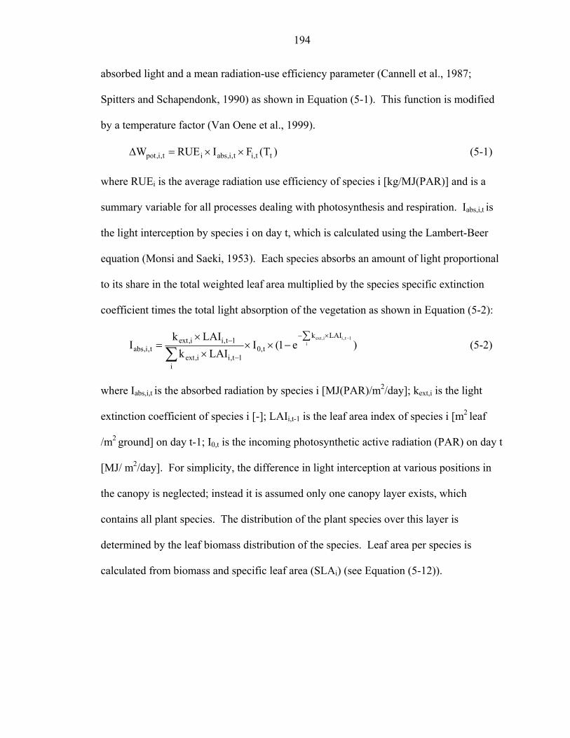
194

absorbed light and a mean radiation-use efficiency parameter (Cannell et al., 1987;

Spitters and Schapendonk, 1990) as shown in Equation (5-1). This function is modified

by a temperature factor (Van Oene et al., 1999).

)T(FIRUEW tt,it,i,absit,i,pot ××=∆ (5-1)

where RUEi is the average radiation use efficiency of species i [kg/MJ(PAR)] and is a

summary variable for all processes dealing with photosynthesis and respiration. Iabs,i,t is

the light interception by species i on day t, which is calculated using the Lambert-Beer

equation (Monsi and Saeki, 1953). Each species absorbs an amount of light proportional

to its share in the total weighted leaf area multiplied by the species specific extinction

coefficient times the total light absorption of the vegetation as shown in Equation (5-2):

)e1(ILAIk

LAIkI i

1t,ii,ext LAIk

t,0

i1t,ii,ext

1t,ii,extt,i,abs

∑−××

××

=−×−

−

−

∑ (5-2)

where Iabs,i,t is the absorbed radiation by species i [MJ(PAR)/m2/day]; kext,i is the light

extinction coefficient of species i [-]; LAIi,t-1 is the leaf area index of species i [m2 leaf

/m2 ground] on day t-1; I0,t is the incoming photosynthetic active radiation (PAR) on day t

[MJ/ m2/day]. For simplicity, the difference in light interception at various positions in

the canopy is neglected; instead it is assumed only one canopy layer exists, which

contains all plant species. The distribution of the plant species over this layer is

determined by the leaf biomass distribution of the species. Leaf area per species is

calculated from biomass and specific leaf area (SLAi) (see Equation (5-12)).

195

Figure 5-2. Diagram of temperature function for species i.

Fi,t(Tt), in Equation (5-1), is a temperature factor for assimilation for species i on

day t [-], which is written as

⎪⎪⎪

⎩

⎪⎪⎪

⎨

⎧

<<−−

≤≤

<<−−

≥≤

=

imax,ti,2opti,2optimax,timax,

i,2optti,1opt

i,1opttimin,imin,i,1optimin,t

imax,timin,t

tt,i

TTT)TT/()TT(

TTT1

TTT)TT/()TT(

TTorTT0

)T(F (5-3)

in which, Tt is the mean air temperature on day t [°C], obtained by taking the average of

daily maximum and minimum air temperatures, which are inputs to the model; Tmin,i is

the base/minimum temperature for assimilation for species i [°C]; Topt1,i is the optimum

temperature 1 for assimilation for species i [°C]; Topt2,i is the optimum temperature 2 for

assimilation for species i [°C]; Tmax,i is the maximum temperature for assimilation for

species i [°C]. An example diagram showing the relationship between the temperature

function and daily air temperature is shown in Figure 5-2. For this model, only one

temperature function is assumed for each species throughout the entire growing season.

1.0

0.0 Tmin,i Topt1,i Topt2,i Tmax,i

Fi,t(Tt) [-]

Mean air temperature [°C]

196

Reduced growth

The plant growth rate may be limited by N or P deficiency, water shortage or water

logging during different parts of the growing season:

t,it,i,pott,i,red RFWW ×∆=∆ (5-4)

t,it,it,i,pott,i CNRFWN ××∆=∆ (5-5)

t,it,it,i,pott,i CPRFWP ××∆=∆ (5-6)

where ∆Wred,i,t is the reduced dry matter production rate of species i [kg/m2/day]; ∆Ni,t

and ∆Pi,t are the N and P uptake rates corresponding to ∆Wred,i,t [kg/ha], respectively; RFi,t

is a growth reduction factor [-] of species i, which integrates the limiting factors from

water (see details in the following growth reduction factor section), N and P; and CNi,t

and CPi,t are the biomass N and P percents, respectively (see Equations (5-31) and (5-

38)) [%].

Applying the Euler’s method to Equations (5-4) to (5-6), the total dry matter

production and dry matter N and P can be calculated as

tRF)T(FIRUEWW t,itt,it,i,absi1t,i,redt,i,red ∆××××+= − (5-7)

tCNRF)T(FIRUENN t,it,itt,it,i,absi1t,it,i ∆×××××+= − (5-8)

tCPRF)T(FIRUEPP t,it,itt,it,i,absi1t,it,i ∆×××××+= − (5-9)

where Wred,i,t and Wred,i,t-1 are the dry matter production on day t and t-1, respectively

[kg/m2]; Ni,t and Ni,t-1 are the total dry matter N on day t and t-1 [kg/ha]; Pi,t and Pi,t-1 are

the total biomass P on day t and t-1 [kg/ha], respectively; and ∆t is the time step, which is

one day in this model.

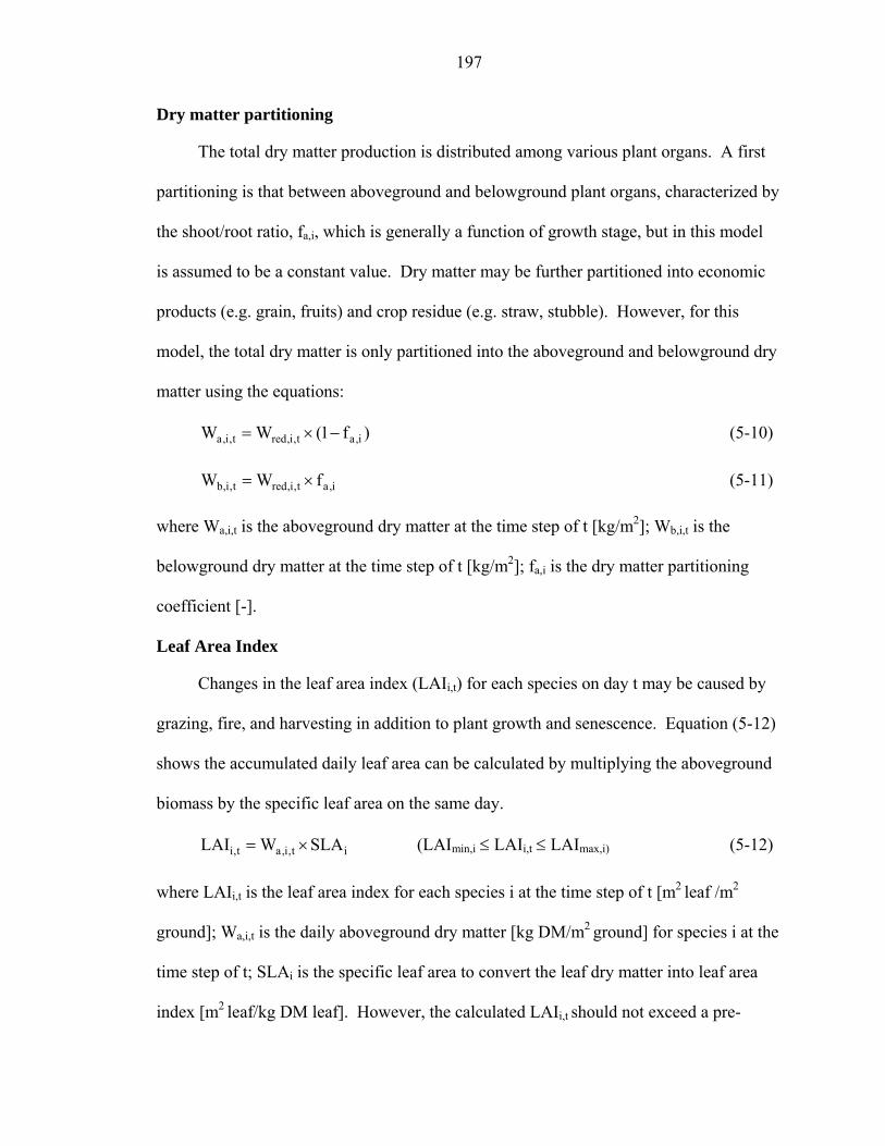
197

Dry matter partitioning

The total dry matter production is distributed among various plant organs. A first

partitioning is that between aboveground and belowground plant organs, characterized by

the shoot/root ratio, fa,i, which is generally a function of growth stage, but in this model

is assumed to be a constant value. Dry matter may be further partitioned into economic

products (e.g. grain, fruits) and crop residue (e.g. straw, stubble). However, for this

model, the total dry matter is only partitioned into the aboveground and belowground dry

matter using the equations:

)f1(WW i,at,i,redt,i,a −×= (5-10)

i,at,i,redt,i,b fWW ×= (5-11)

where Wa,i,t is the aboveground dry matter at the time step of t [kg/m2]; Wb,i,t is the

belowground dry matter at the time step of t [kg/m2]; fa,i is the dry matter partitioning

coefficient [-].

Leaf Area Index

Changes in the leaf area index (LAIi,t) for each species on day t may be caused by

grazing, fire, and harvesting in addition to plant growth and senescence. Equation (5-12)

shows the accumulated daily leaf area can be calculated by multiplying the aboveground

biomass by the specific leaf area on the same day.

it,i,at,i SLAWLAI ×= (LAImin,i ≤ LAIi,t ≤ LAImax,i) (5-12)

where LAIi,t is the leaf area index for each species i at the time step of t [m2 leaf /m2

ground]; Wa,i,t is the daily aboveground dry matter [kg DM/m2 ground] for species i at the

time step of t; SLAi is the specific leaf area to convert the leaf dry matter into leaf area

index [m2 leaf/kg DM leaf]. However, the calculated LAIi,t should not exceed a pre-

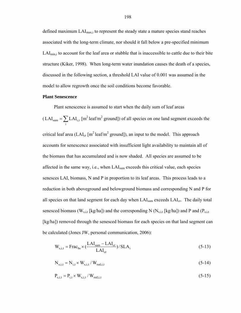
198

defined maximum LAImax,i to represent the steady state a mature species stand reaches

associated with the long-term climate, nor should it fall below a pre-specified minimum

LAImin,i to account for the leaf area or stubble that is inaccessible to cattle due to their bite

structure (Kiker, 1998). When long-term water inundation causes the death of a species,

discussed in the following section, a threshold LAI value of 0.001 was assumed in the

model to allow regrowth once the soil conditions become favorable.

Plant Senescence

Plant senescence is assumed to start when the daily sum of leaf areas

( ∑=i

t,isum LAILAI [m2 leaf/m2 ground]) of all species on one land segment exceeds the

critical leaf area (LAIcr [m2 leaf/m2 ground]), an input to the model. This approach

accounts for senescence associated with insufficient light availability to maintain all of

the biomass that has accumulated and is now shaded. All species are assumed to be

affected in the same way, i.e., when LAIsum exceeds this critical value, each species

senesces LAI, biomass, N and P in proportion to its leaf areas. This process leads to a

reduction in both aboveground and belowground biomass and corresponding N and P for

all species on that land segment for each day when LAIsum exceeds LAIcr. The daily total

senesced biomass (Ws,i,t [kg/ha]) and the corresponding N (Ns,i,t [kg/ha]) and P and (Ps,i,t

[kg/ha]) removed through the senesced biomass for each species on that land segment can

be calculated (Jones JW, personal communication, 2006):

icr

crsumbst,i,s SLA/)

LAILAILAI(FracW −

×= (5-13)

t,i,redt,i,st,it,i,s W/WNN ×= (5-14)

t,i,redt,i,st,it,i,s W/WPP ×= (5-15)

199

where Fracbs is the fraction of biomass above the critical level to senesce per day [-],

which is assumed to be a constant value in the model for all species. The senesced

biomass and biomass N and P decrease the amount of live biomass and its corresponding

N and P pools:

t,i,st,i,redt,i,red WWW −= (5-16)

t,i,st,it,i NNN −= (5-17)

t,i,st,it,i PPP −= (5-18)

Accordingly, plant residue and soil biomass are increased by the senesced biomass

and N and P:

)f1(WMM i,at,i,s1t,rt,r −×+= − (5-19)

i,at,i,s1t,st,s fWMM ×+= − (5-20)

)f1(NMM at,i,s1t,rnt,rn −×+= − (5-21)

at,i,s1t,snt,sn fNMM ×+= − (5-22)

)f1(PMM at,i,s1t,i,rpt,i,rp −×+= − (5-23)

at,i,s1t,i,spt,i,sp fPMM ×+= − (5-24)

where Mr,t and Mr,t-1 are the residue biomass on day t and t-1 [kg/ha]; Ms,t and Ms,t-1 are

the soil biomass on day t and t-1 [kg/ha]; Mrn,t and Mrn,t-1 are the residue biomass N on

day t and t-1 [kg/ha]; Msn,t and Msn,t-1 are the soil biomass N on day t and t-1 [kg/ha]; Mrp,t

and Mrp,t-1 are the residue biomass P on day t and t-1 [kg/ha]; Msn,t and Msn,t-1 are the soil

biomass P on day t and t-1 [kg/ha].

200

Evapotranspiration

Evapotranspiration (ET) described in Chapter 3 does not consider the transpiration

partitioning among multiple plant species, instead it was designed for one plant species

within a land segment. To account for the transpiration by multiple plant species with

different crop coefficients, the method for estimating ET in Chapter 3 was modified. The

ET process is important in the context of the vegetation simulation in that transpiration is

the driving force for nutrient uptake, and insufficient ET leads to reduced plant growth

due to water stress discussed in the following section.

In this process, first, a lumped potential evapotranspiration (PET) for all species in

a land segment is calculated by multiplying reference evapotranspiration (RET, input or

calculated by the model) by a crop coefficient that is weighted by the LAI of each species

within one land segment:

∑∑

−

− ×=

i1t,i

it,i1t,i

t LAI

)CAY1VLAI(CAY1WV (5-25)

where WV1CAYt is the weighted crop coefficient on day t [-], which represents all

existing plant species in the land segment. LAIi,t-1 is the leaf area of species i on day t-1

[m2 leaf/m2 ground], and V1CAYi,t is the crop coefficient of species i [-]. Using the

lumped crop coefficient, a partitioning fraction (Fract [-]), with a range of values from 0

to 0.95, can be defined as:

⎪⎩

⎪⎨

⎧

≤

>−

=2.0CAY1WV0

2.0CAY1WV8.0

)2.0CAY1WV(95.0Frac

t

tt

t (5-26)

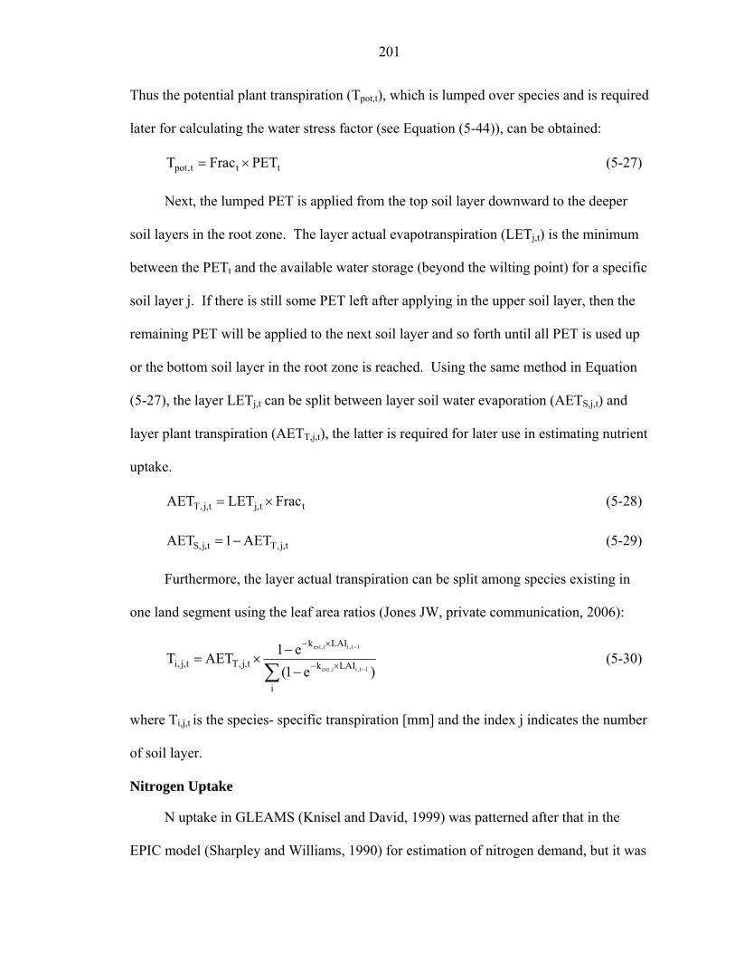
201

Thus the potential plant transpiration (Tpot,t), which is lumped over species and is required

later for calculating the water stress factor (see Equation (5-44)), can be obtained:

ttt,pot PETFracT ×= (5-27)

Next, the lumped PET is applied from the top soil layer downward to the deeper

soil layers in the root zone. The layer actual evapotranspiration (LETj,t) is the minimum

between the PETt and the available water storage (beyond the wilting point) for a specific

soil layer j. If there is still some PET left after applying in the upper soil layer, then the

remaining PET will be applied to the next soil layer and so forth until all PET is used up

or the bottom soil layer in the root zone is reached. Using the same method in Equation

(5-27), the layer LETj,t can be split between layer soil water evaporation (AETS,j,t) and

layer plant transpiration (AETT,j,t), the latter is required for later use in estimating nutrient

uptake.

tt,jt,j,T FracLETAET ×= (5-28)

t,j,Tt,j,S AET1AET −= (5-29)

Furthermore, the layer actual transpiration can be split among species existing in

one land segment using the leaf area ratios (Jones JW, private communication, 2006):

∑ −

−

×−

×−

−

−×=

i

LAIk

LAIk

t,j,Tt,j,i)e1(

e1AETT1t,ii,ext

1t,ii,ext

(5-30)

where Ti,j,t is the species- specific transpiration [mm] and the index j indicates the number

of soil layer.

Nitrogen Uptake

N uptake in GLEAMS (Knisel and David, 1999) was patterned after that in the

EPIC model (Sharpley and Williams, 1990) for estimation of nitrogen demand, but it was

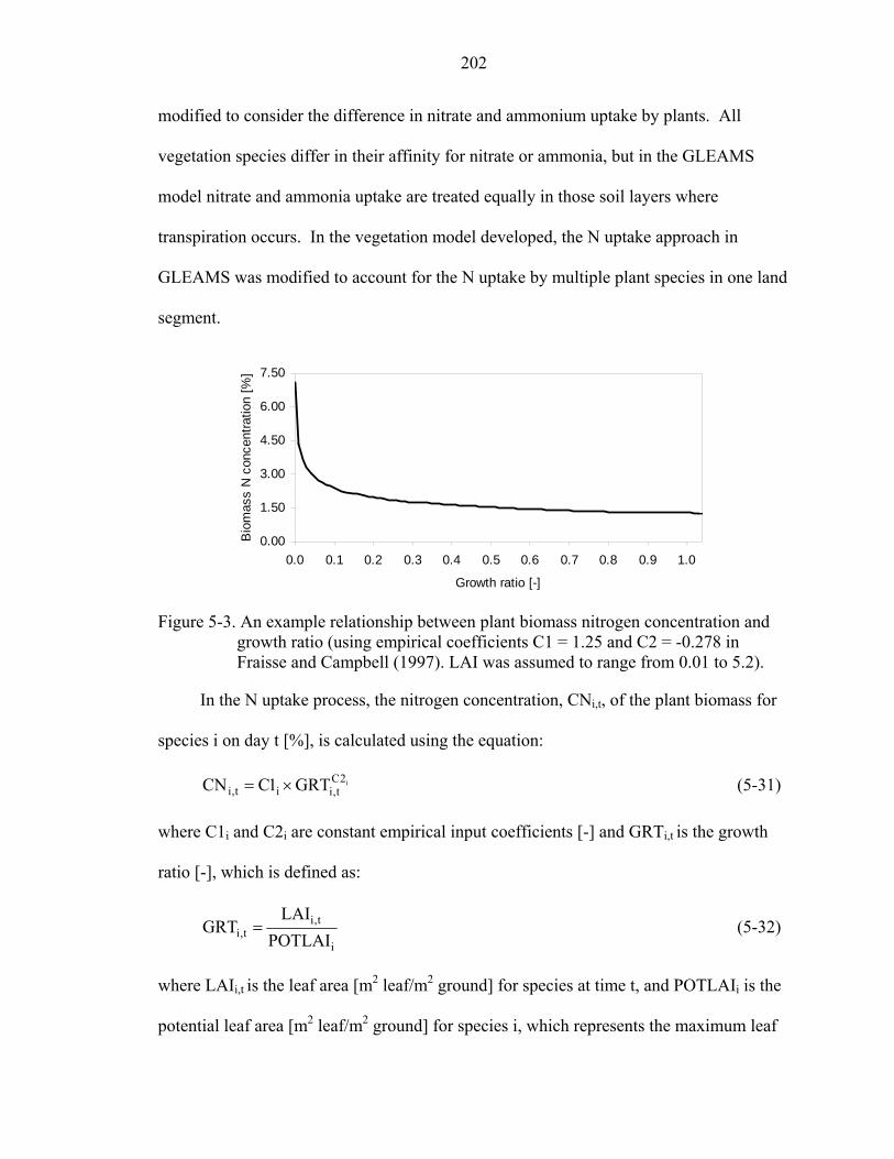
202

modified to consider the difference in nitrate and ammonium uptake by plants. All

vegetation species differ in their affinity for nitrate or ammonia, but in the GLEAMS

model nitrate and ammonia uptake are treated equally in those soil layers where

transpiration occurs. In the vegetation model developed, the N uptake approach in

GLEAMS was modified to account for the N uptake by multiple plant species in one land

segment.

0.00

1.50

3.00

4.50

6.00

7.50

0.0 0.1 0.2 0.3 0.4 0.5 0.6 0.7 0.8 0.9 1.0

Growth ratio [-]

Bio

mas

s N

con

cent

ratio

n [%

]

Figure 5-3. An example relationship between plant biomass nitrogen concentration and

growth ratio (using empirical coefficients C1 = 1.25 and C2 = -0.278 in Fraisse and Campbell (1997). LAI was assumed to range from 0.01 to 5.2).

In the N uptake process, the nitrogen concentration, CNi,t, of the plant biomass for

species i on day t [%], is calculated using the equation:

i2Ct,iit,i GRT1CCN ×= (5-31)

where C1i and C2i are constant empirical input coefficients [-] and GRTi,t is the growth

ratio [-], which is defined as:

i

t,it,i POTLAI

LAIGRT = (5-32)

where LAIi,t is the leaf area [m2 leaf/m2 ground] for species at time t, and POTLAIi is the

potential leaf area [m2 leaf/m2 ground] for species i, which represents the maximum leaf

203

area without the constraints of water and nutrient limitations over the growing season.

The relationship between the plant nitrogen concentration and growth ratio can be

illustrated through the example diagram as seen in Figure 5-3.

Using Equation (5-33) the total dry matter N, TDMNi,t, of species i at time t [kg/ha]

can be estimated:

t,i,redt,it,i WCNTDMN ×= (5-33)

where Wred,i,t is the total biomass of species i estimated in Equation (5-7). The daily N

demand, DEMNi,t [kg/ha], for species i at time step t is then calculated as the difference

between the dry matter N at two successive time steps, which represents the optimum N

required to maintain plant growth without N limitation.

1t,it,it,i TDMNTDMNDEMN −−= (5-34)

The N supply, determined by the N availability in soils, can be calculated by

multiplying the N concentration with transpiration from the respective layers. In the

model, N uptake is treated equally for both nitrate and ammonia. The amount of N taken

up by species i from each soil layer j where transpiration occurs, including nitrate uptake

(UPNHi,j,t [kg/ha]) and ammonia uptake (UPNOi,j,t [kg/ha]) can be calculated:

t,j,ij,d,st,j,i TW3CNOUPNO ×= (5-35)

t,j,ij,d,st,j,i TW4CNHUPNH ×= (5-36)

where CNO3Ws,d,j and CNH4Ws,d,j are the nitrate and ammonium concentration for the

jth soil layer, respectively, determined from Equations (4-2) and (4-9) described in

Chapter 4, and Ti,j,t is the transpiration that occurred from that soil layer for species i at

time t determined from Equation (5-25). The total uptake of N is summed for each plant

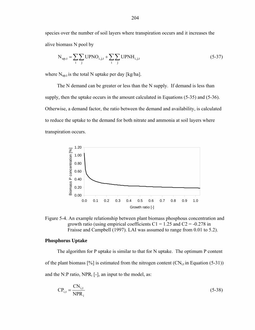
204

species over the number of soil layers where transpiration occurs and it increases the

alive biomass N pool by

∑∑∑∑ +=i j

t,j,ii j

t,j,it,up UPNHUPNON (5-37)

where Nup,t is the total N uptake per day [kg/ha].

The N demand can be greater or less than the N supply. If demand is less than

supply, then the uptake occurs in the amount calculated in Equations (5-35) and (5-36).

Otherwise, a demand factor, the ratio between the demand and availability, is calculated

to reduce the uptake to the demand for both nitrate and ammonia at soil layers where

transpiration occurs.

0.00

0.20

0.40

0.60

0.80

1.00

1.20

0.0 0.1 0.2 0.3 0.4 0.5 0.6 0.7 0.8 0.9 1.0

Growth ratio [-]

Bio

mas

s P

con

cent

ratio

n [%

]

Figure 5-4. An example relationship between plant biomass phosphous concentration and

growth ratio (using empirical coefficients C1 = 1.25 and C2 = -0.278 in Fraisse and Campbell (1997). LAI was assumed to range from 0.01 to 5.2).

Phosphorus Uptake

The algorithm for P uptake is similar to that for N uptake. The optimum P content

of the plant biomass [%] is estimated from the nitrogen content (CNi,t in Equation (5-31))

and the N:P ratio, NPRi [-], an input to the model, as:

i

t,it,i NPR

CNCP = (5-38)

205

Figure 5-4 shows an example relationship between the plant P concentration and the

growth ratio.

The total dry matter P, TDMPi,t [kg/ha] for species i at time t, is calculated using

the equation

t,i,redt,it,i WCPTDMP ×= (5-39)

and the P demand for species i at time t, DEMPi,t [kg/ha], is determined by the difference

between the dry matter P on two successive days as

1t,it,it,i TDMPTDMPDEMP −−= (5-40)

Uptake of labile P, UPLPi,t [kg/ha], is estimated for each layer where transpiration, AET,t,

occurs using

t,j,ij,d,st,j,i TCPLABWUPLP ×= (5-41)

where the concentration of labile P, CPLABWs,d,t, is determined by Equation (4-15) in

Chapter 4. The total uptake of P is the sum over all species i and all layers j where

transpiration occurs. The P taken up is converted into the plant biomass P:

∑∑=i j

t,j,it,up UPLPP (5-42)

where Pup,t is the plant biomass P [kg/ha], which will be used to calculate plant P

concentration for determining the P stress in the following section. Similar to N, a

demand factor for P that is a ratio between the demand and availability of P is calculated

to reduce the uptake of P when supply exceeds demand.

Growth Reduction Factor

The growth reduction factor, RFi,t, used in Equation (5-5) is a unitless, species-

specific growth reduction factor with a value ranging from 0 to 1, which is obtained by

206

taking the minimum value of water stress, water logging, and N and P stress factors as

shown in the following equation:

)F,F,F,Fmin(RF t,i,Pt,i,Nt,i,WLt,i,WSt,i = (5-43)

where FWS,i,t is the water stress factor for species i [-]; FWL,i,t is the water logging factor

for species i [-]; FN,i,t is the N stress factor [-]; and FP,i,t is the P stress factor [-]. The

details regarding these factors are discussed below.

Water stress and logging factors

Water is one of the limiting growth factors due to its function in transporting

nutrients and its assimilation into the plants. The basis for plant production is the uptake

of atmospheric carbon dioxide (CO2) for assimilation through the stomata in the

epidermis of leaves. As a consequence, water moves in the opposite direction through

the stomata, a process referred to as transpiration. If the water supply cannot meet the

demand for water, it consequently limits the intake of CO2 and results in the decline of

the assimilation rate. In this way, water shortages curtail plant production (Ivens et al.,

1992). On the other hand, transpiration can be hampered in soils with moisture content

above field capacity, as a result of restricted water/oxygen uptake by the roots. This

situation, referred to as water logging (Ivens et al., 1992), is common characteristic of

wetland soils.

When soil moisture is above field capacity (Fc), soil tends to be saturated and water

logging can occur. Under water logging conditions, the growth of most plants is

seriously hampered since root respiration, a prerequisite for the uptake of both water and

nutrients by the roots, is suppressed due to oxygen shortage. On the other hand, when

soil moisture is below the critical soil moisture (SWP) and before it reaches the

207

permanent wilting point (PWP), moisture extraction is hampered, which leads to drought

stress in plants. This causes a reduction in stomatal aperture and hence less water loss

and impaired CO2 assimilation (Ivens, 1992).

Both water stress and logging constrain plant growth. However, different plant

species can tolerate water stress or logging to a varying extent and thus these factors are

species-specific. Therefore, these two factors are very important in the context of

investigating the impact of water retention on ranches. The water stress factor of species

i, FWS,i,t can be expressed as a ratio between the actual transpiration and the potential

transpiration for species i:

t,pot

jt.j,i

j,i,WS T

AETF

∑= ( 1F0 t,i,WS ≤≤ ) (5-44)

where AETi,j,t is the layer actual transpiration [mm] for species i in layer j at time t; the

index j represents the number of soil layers where transpiration occurs; and Tpot,t is the

potential transpiration [mm].

When the soil moisture goes above the field capacity, the water logging factor of

species i, FWL,i,t [-], can be expressed as

3.0WWWW

7.0Ffcpo

spot,i,WL +

−

−×= ( 1F0 j,i,WL ≤≤ ) (5-45)

where Wpo is the soil porosity [-], Ws is the current soil moisture content [-] at time t, and

Wfc is the field capacity [-]. For soil layers where transpiration occurs, these soil

parameters may be different. To account for these differences, their weighted values by

the root fraction are used in Equation (5-45) to calculate the water logging factor.

208

Duration of inundation is another important factor considered in this model because

prolonged standing water may eventually kill some plants that cannot tolerate inundation

for a long period. To account for the inundation duration factor, the successive days of

inundation (it is assumed that surface ponded water has to exceed 2 cm to be considered

inundation) are recorded in the model for each species. Before the number of

accumulated days of inundation reaches the maximum length of inundation tolerance

(species specific input to the model), plants are assumed to grow at a reduced rate defined

in Equation (5-45). Once the maximum inundation tolerance is reached, it is assumed

25% of aboveground and belowground biomass dies daily while inundation continues.

During this time it is assumed that no growth for this species occurs.

Nitrogen stress factor

The N stress, FN,i,t, a factor that determines the growth reduction for species i at

time t caused by N deficiency, was modeled according to Seligman and Van Keulen

(1981), and is dependent on the actual N concentration of the shoot for species i, CNshoot,i,t

[g N/g DM], which is calculated by dividing the plant biomass Ns,i,t [kg N/ha] by the

plant biomass for species i [kg DM/ha]:

t,i,red

t,it,i,shoot W

NCN = (5-46)

where Wred,i,t is the plant biomass for species i at time t obtained in Equation (5-7); and

Ni,t is the biomass N for species i at time t, which is obtained from Equation (5-8). If

CNshoot,i,t exceeds the critical value CNcr,i [g N/g DM], plant growth is not reduced.

Below this N concentration, growth rate decreases linearly with concentration:

imin,i,cr

imin,t,i,shoott,i,N CNCN

CNCNF

−−

= ( 1F0 i,N ≤≤ ) (5-47)

209

where Nmin,i is the minimum shoot N concentration [g N/g DM] required to maintain the

plant growth input to the model by users.

Phosphorus stress factor

The P stress, FP,i,t, is a factor that determines the growth reduction for species i at

time t caused by P deficiency. Similar to the N stress factor, FP,i,t can be calculated as:

imin,i,cr

imin,t,i,shoott,i,P CPCP

CPCPF

−−

= ( 1F0 t,i,P ≤≤ ) (5-48)

where CPshoot,i,t is the shoot biomass P concentration for species i at time t, which can be

obtained by dividing the biomass P (Pi,t [kg N/ha]) by the aboveground biomass [kg

DM/ha]:

t,i,red

t,it,i,shoot W

PCP = (5-49)

If CPshoot,i,t exceeds the critical value CPcr,i [g N/g DM], plant growth is not reduced.

Below this P concentration, growth rate decreases linearly with concentration.

Hypothetical Scenario Model Testing

Scenario Description

Sufficient vegetation data are not currently available from south Florida flatwoods

watersheds to quantitatively test the vegetation model. Therefore, a hypothetical test was

designed to evaluate the algorithms of the vegetation model, coupled with the hydrologic

and nutrient models developed in Chapters 3 and 4 to determine whether the model

behaves as expected when the hydrology and nutrient concentrations are manipulated.

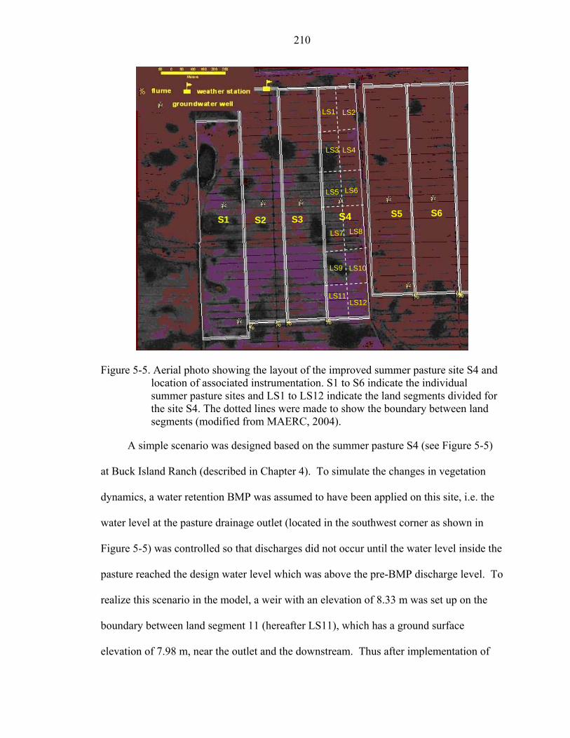
210

Figure 5-5. Aerial photo showing the layout of the improved summer pasture site S4 and

location of associated instrumentation. S1 to S6 indicate the individual summer pasture sites and LS1 to LS12 indicate the land segments divided for the site S4. The dotted lines were made to show the boundary between land segments (modified from MAERC, 2004).

A simple scenario was designed based on the summer pasture S4 (see Figure 5-5)

at Buck Island Ranch (described in Chapter 4). To simulate the changes in vegetation

dynamics, a water retention BMP was assumed to have been applied on this site, i.e. the

water level at the pasture drainage outlet (located in the southwest corner as shown in

Figure 5-5) was controlled so that discharges did not occur until the water level inside the

pasture reached the design water level which was above the pre-BMP discharge level. To

realize this scenario in the model, a weir with an elevation of 8.33 m was set up on the

boundary between land segment 11 (hereafter LS11), which has a ground surface

elevation of 7.98 m, near the outlet and the downstream. Thus after implementation of

S3 S4S2S1 S5 S6

LS3 LS4

LS1 LS2

LS5 LS6

LS7 LS8

LS9 LS10

LS11 LS12

211

the BMP discharges will occur only when the water elevation of the outlet land segment

exceeds 8.33 m. Without the application of water retention BMP, discharge would occur

when the water elevation reached 7.985 m (maximum depressional storage in depth = 0.5

cm).

Identical hydrologic and nutrient inputs, as described in Chapter 4, were used for

running the coupled model to investigate the vegetation dynamics due to the application

of the hypothetical BMP for the pasture site S4. Agricultural activities including

fertilization, burning, and stocking were not included, so that the impact due to water

retention on vegetation dynamics could be analyzed independently. By holding the water

levels higher at the outlet, the soil inundation period is prolonged in the pasture and thus

the length of anoxic soil conditions is extended as well. This type of hydrologic change

may affect nutrient cycling processes that may alter the concentrations of N and P.

Changes in both hydrologic regime and nutrient cycling may impact plant growth.

Vegetation species that do not adapt well to wet soil conditions for prolonged periods

may experience growth reduction and eventually vanish from the site while others that

adapt well to such conditions may expand their areas. Over time, the spatial composition

patterns of vegetation species may change, and these patterns may be used as an indicator

of soil and water conditions. To compare the changes in species composition pattern

over time and space, the model was run twice to obtain simulation results before and after

holding the water at a higher level (hereafter called pre-BMP and post-BMP,

respectively).

Multiple plant species exist in the pasture site S4 as seen in Table 5-1, among

which bahiagrass (Paspalum notatum Flügge) is the most dominant species accounting

212

for up to 93% of the land cover, while the remaining species account for about 7%

together. However, for this test three perennial species including bahiagrass, floralta

(Hemarthria altissima), and panicum (panicum rigidulum) were assumed to be the major

species for the pasture site S4. These vegetation species represent those adapted to soil

conditions of uplands, transition zones and wetlands, respectively.

S4 was divided into 12 land segments (see Figure 5-5), as discussed in Chapter 4.

Each land segment was assumed to have the same amount of initial total biomass

(aboveground + belowground) over all selected species, but different percentages of these

species (see Table 5-3). The hypothetical assignment of species and percentage of each

species was made up according to the locations of land segments. Land segments with

higher topographical elevations, far from wetlands were assumed to be relatively drier in

their soil conditions than those located near or in wetlands and thus to contain more

upland plant species. With the initial biomass, shoot to root ratio (fa), and specific leaf

area (SLA) (see Table 5-2), the model can initialize the aboveground and belowground

biomass and green LAI for each species in each land segment.

To run the vegetation model, inputs including the time series inputs (see Table 5-2)

such as daily solar radiation, maximum and minimum ambient temperatures and the

model parameter values must be provided. Other time series data such as grazing,

harvest, burning, and tillage must be specified as well if applicable. The required model

parameter values were obtained from the literature if they were available. However, the

data for floralta and panicum were especially difficult to find and thus they were assumed

to have the same values for some parameters as the bahiagrass. Collecting and setting up

these species-specific parameters was one of the challenges encountered during

213

development of the vegetation model. Table 5-4 lists those variables calculated through

the hydrologic and nutrient models and used in the vegetation model and Table 5-5 lists

major daily output variables from the vegetation model.

Results and Discussion

Water and nutrient responses to water retention BMP

Figures 5-6 to 5-11 show the comparison of surface runoff, water table depth, and

N and P loads and concentrations predicted by the integrated hydrology, nutrient and

vegetation dynamics simulation model before and after BMP for site S4 for a 6-year

simulation period. It is noted that after holding the water level at 8.33 m at the outlet, no

surface runoff (see Figure 5-6) and hence no N and P loads (see Figures 5-8 and 5-9) are

released downstream throughout the entire simulation period. Figure 5-7 shows that the

ponded water remains above the ground surface for much of the wet season after the

water retention BMP is implemented. A period from approximately September 2000 to

February 2001 was drier than the rest of simulation period, thus during this time the water

tables stayed fairly deep even with the water retention BMP. Several periods between the

late spring and early summer in years 1999, 2000 and 2002 were also relatively drier with

long-term water table drawdown (see Figure 5-7). After the BMP, the groundwater table

depths were much shallower than those before BMP except during the driest period

discussed above. Meanwhile, several long periods occurred during which soils became

saturated and the water table remained on the ground surface for approximately 6 months.

This occurred primarily from the middle of summer to the early spring between years

1998 and 1999, 1999 and 2000, 2001 and 2002, and 2002 and 2003. The ponded water

depth during these periods (see Figure 5-7) indicates that the soils experience prolonged

saturation and had standing water on the ground surface. Note that Figure 5-7 was made

214

using the predicted water tables for LS9 where the observation well was installed and the

observations from Figure 5-7 may not apply to the entire pasture site.

The simulated results of P and N concentrations in surface water in Figures 5-10

and 5-11, respectively indicate that both P and N concentrations were dramatically

decreased after the water retention BMP. The lower P and N concentrations likely result

from changes in biochemical processes due to prolonged anoxic soil conditions both in

soils and on surface residue. Overall, it was observed that after the water retention BMP,

the hydrologic and nutrient dynamics were significantly changed in pasture site S4. The

pasture soils become water logged for prolonged periods and nutrient concentrations

become significantly lower.

Influence of differences in temperature sensitivities among species

The sensitivity of biomass response to the temperature function was recognized

during the development of this vegetation model. To investigate the influence of

different temperature functions on the predictions of biomass, three scenarios shown in

Table 5-6 were designed. In Scenario 1, an identical temperature function was applied

for all three species; in Scenario 2, the temperature function for floralta was different

from those for other two species, bahia and panicum, which were assumed to have the

same temperature function as specified in Scenario 1. The temperature function for

floralta in Scenario 2 was modified by shifting -7 °C from the one used for the other two

species, allowing floralta to grow in a lower temperature range from 0 °C to 38 °C. In

the last scenario, the temperature functions for bahia and panicum were assumed to be the

same as those for them in Scenarios 1 and 2, but the temperature function for floralta was

further adjusted to allow this species to grow primarily during winter time, in a narrower

215

temperature range from 0 °C to 30 °C. In order to investigate the sensitivities of biomass

productivity specifically to temperature factors, all these scenario tests were performed

without simulating the growth reduction, that is, potential biomass production was

compared.

Figure 5-12 shows that the predicted aboveground biomass on LS11 varied

dramatically among the three scenarios corresponding to different temperature functions.

When the identical temperature function was used for all three species in Scenario 1, the

predicted potential biomass had similar trends and patterns throughout the simulation

period but was different in magnitude among species due to the difference in their initial

conditions. This may imply that in this scenario the three species grow in a relatively

stable situation without competition with one another. In Scenario 2, the predicted

potential biomass for floralta increased tremendously over time whereas the biomass for

bahia and panicum decreased and these species tended to disappear from this land

segment. This behavior can be explained through the temperature factors for Scenario 2

shown in Figure 5-13. Compared with bahia and panicum, floralta apparently

experienced less growth reduction during the winter time in Scenario 2. Even during the

summer time, floralta did not suffer much growth reduction. This situation allows more

time for floralta to grow in comparison to the other two species.

In Scenario 3, an opposite response from Scenario 2 occurred for predicted biomass

for all species. The temperature factors used for Scenario 3 and shown in Figure 5-13

allow both bahia and panicum to grow faster during the summer time while floralta is in

its lowest growth time. The resulting increased biomass for bahia and panicum leads to

senescence, which reduces the existing biomass for floralta in the same proportion.

216

Although floralta grows better in winter time in this scenario, the amount of biomass

produced during the winter time did not sufficiently balance the loss due to the

senescence during the summer time. Over time the production of floralta decreased and

gradually this species vanished from this land segment.

These analyses, based on hypothetical temperature functions, demonstrated that a

reasonable, species-specific temperature function is very important for reliable simulation

results. Temperature sensitivities of different species are needed in order to correctly

simulate the changes in competition of species over time and space and in response to

BMPs. Nevertheless, such data are not yet available for these species. Therefore, for the

remaining analyses in this study, the same temperature function (see Table 5-6) was

assumed for all three species for simplicity.

In addition to sensitivity to temperature, these species may differ in their responses

to photoperiod as well. Photoperiod effects were not included in the current method

because of lack of information. However, differences in photoperiod sensitivity could

also have a big impact on seasonal growth and species compositions (Jones JW, private

communication, 2006).

Species composition dynamics due to water retention BMP

Figure 5-14 shows relative plant distribution (calculated using the aboveground

biomass for each species at the end of each year of the simulation period) over land

segments throughout the entire simulation period before and after BMP implementation

in the summer pasture S4. The distribution in each land segment is expressed as the

percentage of total aboveground biomass (since the belowground biomass follows the

same patterns, it is not discussed). Simulation results from the pre-BMP scenario case

indicate that the basic composition patterns over land segments are approximately the

217

same over the entire simulation period, and no species vanished from any land segment

where it was initially assigned. Bahia accounted for the most significant percentage of

biomass over the entire pasture throughout the 6-year simulation period, followed by

panicum, and then floralta. The results before the water retention BMP indicate that pre-

BMP soil conditions were relatively favorable for the coexistence of three species.

After the water retention BMP was applied, the composition patterns of species

over the land segments throughout the simulation period changed. In the first three years,

the difference of biomass distribution among species over land segments was not

significant, and the composition patterns of species were very close to those for the pre-

BMP conditions. Although there was some rainfall variability over the first three years

(as discussed in Chapter 4) this variability was not enough to produce changes in biomass

productivity among these species. However, after year 2001, a dramatic change in the

biomass distribution pattern occurred in the land segments close to the drainage outlet,

including LS5, LS7, LS8, LS9, LS10, LS11, and LS12. Panicum grew significantly

faster in those land segments, and floralta showed a similar trend but with a smaller

magnitude. Meanwhile, the bahia biomass decreased dramatically and almost vanished

from LS12, LS11, LS10, and LS9. Additionally, floralta decreased significantly in LS11

where the drainage outlet is located. Due to the lack of a mechanism for new species to

grow in land segments where they are not originally present, there was no noticeable

change observed in LS6. The distribution pattern in 2001 remained similar in years 2002

and 2003, very likely due to the consecutive wet weather conditions. Overall, changes in

biomass distribution for the last three years under the water retention BMP scenario

demonstrate that the soil conditions became more favorable for the development of

218

panicum, the wetland species; less favorable for floralta, the transition zone species, and

least favorable for baiha, the upland species.

Figure 5-14 provides insight into the relative percentages of plant biomass

distribution, but it lacks information on the absolute biomass of each species over land

segments on a daily basis. Figures 5-15 and 5-16 show the continuous simulation of

aboveground biomass for bahia, floralta, and panicum throughout the 6-year simulation

period for the pre- and post-BMP scenarios in three selected land segments (LS8, LS11

and LS12), respectively. As seen in Figure 5-15, the aboveground biomass patterns for

all species in these selected land segments are basically similar over time for the pre-

BMP scenario, and the magnitude of biomass for each species stayed stable over the

simulation period. However, Figure 5-16 shows a significant change occurring late

during year 2001 for the post-BMP scenario as observed in Figure 5-14. Bahia biomass

was reduced significantly in LS8 around the end of year 2001, but began to grow again in

year 2002 and 2003 while panicum and floralta increased their growth in all years. In

LS11, bahia died out around the end of 2001, followed by floralta in 2001, while at the

same time panicum maintained aggressive growth through the entire simulation period.

Since LS11 is the land segment immediately connected to the outlet of pasture, after the

water retention BMP, it became the most inundated location in the pasture, which

eventually caused the die-off of bahia and floralta. The growth dynamics in LS12 was

similar to that in LS8. The difference was that bahia was not able to grow back again.

This can be explained by the difference in soil conditions in LS8 and LS12. The latter

apparently had longer saturated soil conditions than the former. Comparison of the

continuous biomass simulation results for the pre- and post-BMP scenarios further

219

support the conclusion that the application of the water retention BMP caused significant

changes in vegetation dynamics.

Figures 5-19 and 5-20 show the growth limiting factors for bahia in LS11 for the

pre- and post-BMP scenarios. Consistently, in both scenarios, water stress and water

logging were more influential factors than the N and P stress factors. This is reasonable

for a pasture site like S4 that has a high background nutrient concentration. The

comparison of water stress and logging factors for pre- and post-BMP scenarios indicates

that the frequency of water stress was decreased significantly, while that for water

logging was increased, after the water retention BMP. This result demonstrates that the

model is capable of capturing water dynamics due to the water retention BMP.

Concluding Remarks

To simulate vegetation dynamics caused by changes in hydrologic and nutrient

dynamics in south Florida flatwoods watersheds, a vegetation model was developed and

coupled with the hydrologic and nutrient models developed earlier. In this model, plant

biomass production is mainly driven by climate (solar radiation and temperature) and

affected by growth reduction factors, including water stress, water logging, and N and P

stresses. Total production is simply partitioned between aboveground and belowground

biomass and the leaf area is obtained by multiplying the aboveground biomass by the

specific leaf area. Three perennial plant species, bahia, floralta, and panicum, were

selected as representative of plants adapted to upland, transition zone and wetlands

growth conditions, respectively. An analysis of the influence of difference temperature

sensitivities among species indicate that reasonable, species-specific temperature

functions are needed to correctly simulate the plant competition over time and specie and

simulate response to BMPs.

220

A hypothetical BMP scenario based on the summer pasture site S4 at Buck Island

Ranch, Lake Okeechobee Basin, Florida was developed to take advantage of the

calibrated hydrologic and nutrient parameters computed in Chapter 4. In this scenario, it

is assumed that a water retention BMP that retained all water below an elevation of 8.33

m was implemented in pasture S4. Due to water retention, the soil in the pasture was

inundated much longer than when the water was allowed to flow freely off the pasture.

The changes in hydrology and hence in nutrient dynamics were demonstrated to have the

potential to change vegetation.

The hypothetical scenario test showed that after implementing the water retention

BMP, all surface runoff and nutrients were retained inside the pasture site and the periods

of water logging or inundation increased. With these changes in hydrology and nutrients,

wetland species like panicum survived better than bahia and floralta, while the transition

zone species floralta did better than upland species bahia. The spatial distribution

patterns of biomass were distinct over time for the pre- and post-BMP scenarios and

significant dynamics in the magnitude of biomass and the number of species were

observed through the predicted results. Consequently, it was concluded that this

vegetation model is capable of simulating vegetation dynamics caused by changes in

hydrology and nutrient cycling due to water retention BMPs.

However, the model input parameters, mostly assumed or taken from the literature,

may not be sufficient to accurately represent physiological and phenological

characteristics of the selected species. Furthermore, the model performance was

evaluated in a hypothetical scenario, not against actual field data. In order to use this

model for prediction, future efforts in collecting vegetation data and evaluating the model

221

with observed data and experimentally-derived parameters should be undertaken. In

addition, the model needs to be further developed to enable simulation of root length and

root biomass distribution to more accurately capture the nutrient uptake and

evapotranspiration differences among species, and an algorithm for simulating plant

height should be added to enable the feedback relationship between surface runoff and a

dynamic surface roughness, which is a function of vegetative cover. A start-up

mechanism for new species initiation in land segments should be added to more

accurately simulate plant competition and spatial evolution. Finally, an herbivore

movement model should be developed to simulate the impacts of cattle behavior and

grazing performance on vegetation growth.

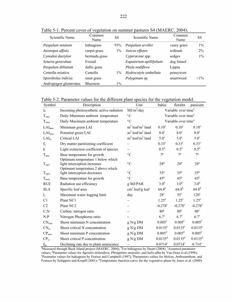
222

Table 5-1. Percent cover of vegetation on summer pastures S4 (MAERC, 2004). Scientific Name Common

Name S4 Scientific Name Common Name S4

Paspalum notatum bahiagrass 93% Paspalum urvillei vasey grass 1% Axonopus affinis carpet grass 1% Juncus effuses softrush 2% Cynodon dactylon bermuda grass Cyperaceae spp. sedges 1% Setaria geniculata Foxtail Eupatorium apillifolium dog fennel Paspalum dilitatum dallis grass Phyla nodiflora Lippia Centella asiatica Centella 1% Hydrocotyle umbellata pennywort Sporobolus indicus smut grass Polygonum sp. smartweed <1% Andropogon glomeratus Bluestem 1%

Table 5-2. Parameter values for the different plant species for the vegetation model.

Symbol Description Unit bahia floralta panicum I0 Incoming photosynthetic active radiation MJ/m2/day Variable over timea Tmin Daily Minimum ambient temperature °C Variable over timea Tmax Daily Maximum ambient temperature °C Variable over timea LAImin Minimum green LAI m2 leaf/m2 land 0.10c 0.10c 0.10c LAImax Potential green LAI m2 leaf/m2 land 8.0c 8.0c 8.0c LAIcr Critical LAI m2 leaf/m2 land 5.0c 5.0c 5.0c fa Dry matter partitioning coefficient − 0.33c 0.33c 0.33c k Light extinction coefficient of species − 0.5d 0.5d 0.5d Tmin Base temperature for growth °C 7g 7g 7g

Topt1 Optimum temperature 1 below which light interception increases °C 28g 28g 28g

Topt2 Optimum temperature 2 above which light interception decreases °C 35g 35g 35g

Tmax Base temperature for growth °C 45g 45g 45g RUE Radiation use efficiency g MJ/PAR 3.0d 3.0d 3.0d SLA Specific leaf area cm2 leaf/g leaf 64.8b 64.8b 64.8b L Maximum water logging limit day 28c 55c 120c C1 Plant NC1 − 1.25e 1.25e 1.25e C2 Plant NC2 − -0.278e -0.278e -0.278e C:N Carbon: nitrogen ratio − 80e 80e 80e N:P Nitrogen Phosphorus ratio − 6.7e 6.7e 6.7e CNmin Shoot minimum N concentration g N/g DM 0.005f 0.005f 0.005f CNcr Shoot critical N concentration g N/g DM 0.0135c 0.0135c 0.0135c CPmin Shoot minimum P concentration g N/g DM 0.005d 0.005d 0.005d CPcr Shoot critical P concentration g N/g DM 0.0135d 0.0135d 0.0135d fbs Declining rate due to plant senescence − 0.0714c 0.0714c 0.714c

aMeasured through Buck Island project (MAERC, 2004); bFor bahiagrass by Stuart (2004); cAssumed parameter values; dParameter values for Agrostis stolonifera, Phragmites australis, and Salix alba by Van Oene et al.(1998); eParameter values for bahiagrass by Fraisse and Campbell (1997); fParameters values for Holcus, Anthoxanthum, and Festuca by Schippers and Kropff (2001); gTemperature function curve for the vegetative phase by Jones et al. (2000).

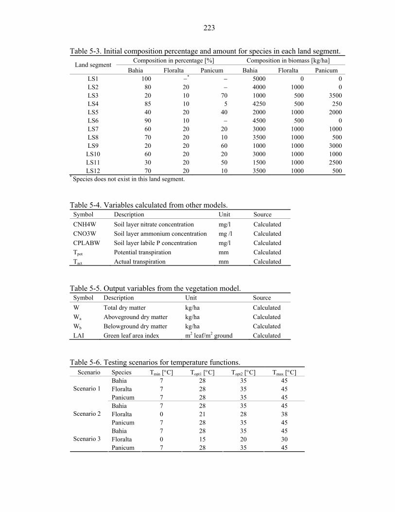
223

Table 5-3. Initial composition percentage and amount for species in each land segment. Composition in percentage [%] Composition in biomass [kg/ha]

Land segment Bahia Floralta Panicum Bahia Floralta Panicum

LS1 100 −* − 5000 0 0 LS2 80 20 − 4000 1000 0 LS3 20 10 70 1000 500 3500 LS4 85 10 5 4250 500 250 LS5 40 20 40 2000 1000 2000 LS6 90 10 − 4500 500 0 LS7 60 20 20 3000 1000 1000 LS8 70 20 10 3500 1000 500 LS9 20 20 60 1000 1000 3000

LS10 60 20 20 3000 1000 1000 LS11 30 20 50 1500 1000 2500 LS12 70 20 10 3500 1000 500

* Species does not exist in this land segment.

Table 5-4. Variables calculated from other models.

Symbol Description Unit Source CNH4W Soil layer nitrate concentration mg/l Calculated CNO3W Soil layer ammonium concentration mg /l Calculated CPLABW Soil layer labile P concentration mg/l Calculated Tpot Potential transpiration mm Calculated Tact Actual transpiration mm Calculated

Table 5-5. Output variables from the vegetation model.

Symbol Description Unit Source W Total dry matter kg/ha Calculated Wa Aboveground dry matter kg/ha Calculated Wb Belowground dry matter kg/ha Calculated LAI Green leaf area index m2 leaf/m2 ground Calculated

Table 5-6. Testing scenarios for temperature functions.

Scenario Species Tmin [°C] Topt1 [°C] Topt2 [°C] Tmax [°C] Bahia 7 28 35 45 Floralta 7 28 35 45 Scenario 1 Panicum 7 28 35 45 Bahia 7 28 35 45 Floralta 0 21 28 38 Scenario 2 Panicum 7 28 35 45 Bahia 7 28 35 45 Floralta 0 15 20 30 Scenario 3 Panicum 7 28 35 45

224

-1.00

-0.50

0.00

0.50

1.00

1.50

1/1/98 7/1/98 1/1/99 7/1/99 1/1/00 7/1/00 1/1/01 7/1/01 1/1/02 7/1/02 1/1/03 7/1/03

Time (day)

Sur

face

runo

ff (c

m)

0

10

20

30

40

50

60

70

Rai

nfal

l (cm

)

Rainfall pre-BMP post-BMP

Figure 5-6. Continuous simulation of surface runoff throughout the simulation period from 1998 to 2003.

-175

-155

-135

-115

-95

-75

-55

-35

-15

5

1/1/98 7/1/98 1/1/99 7/1/99 1/1/00 7/1/00 1/1/01 7/1/01 1/1/02 7/1/02 1/1/03 7/1/03

Time (day)

Wat

er ta

ble

dept

h (c

m)

-175

-155

-135

-115

-95

-75

-55

-35

-15

5

Rai

nfal

l (cm

)

pre-BMP WTD post-BMP PWD post-BMP WTD pre-BMP PWD

Figure 5-7. Continuous simulation of water table depths at land segment 9 throughout the simulation period from 1998 to 2003 (WTD = water table depth; PWD = ponded surface water depth).

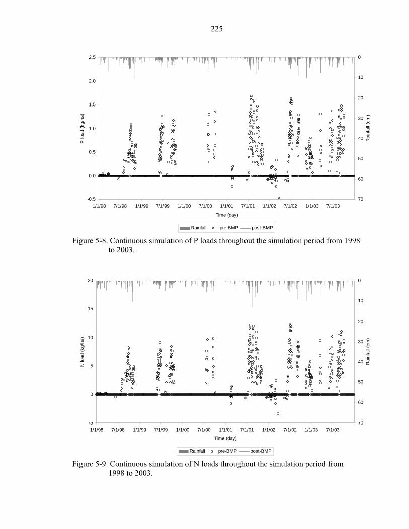
225

-0.5

0.0

0.5

1.0

1.5

2.0

2.5

1/1/98 7/1/98 1/1/99 7/1/99 1/1/00 7/1/00 1/1/01 7/1/01 1/1/02 7/1/02 1/1/03 7/1/03

Time (day)

P lo

ad (k

g/ha

)

0

10

20

30

40

50

60

70

Rai

nfal

l (cm

)


Figure 5-8. Continuous simulation of P loads throughout the simulation period from 1998 to 2003.

-5

0

5

10

15

20

1/1/98 7/1/98 1/1/99 7/1/99 1/1/00 7/1/00 1/1/01 7/1/01 1/1/02 7/1/02 1/1/03 7/1/03

Time (day)

N lo

ad (k

g/ha

)

0

10

20

30

40

50

60

70

Rai

nfal

l (cm

)


Figure 5-9. Continuous simulation of N loads throughout the simulation period from 1998 to 2003.

226

0

50

100

150

200

1/1/98 7/1/98 1/1/99 7/1/99 1/1/00 7/1/00 1/1/01 7/1/01 1/1/02 7/1/02 1/1/03 7/1/03

Time (day)

P C

once

ntra

tion

(mg/

l)

0

10

20

30

40

50

60

70

Rai

nfal

l (cm

)


Figure 5-10. Continuous simulation of P concentrations throughout the simulation period from 1998 to 2003.

0

300

600

900

1200

1500

1/1/98 7/1/98 1/1/99 7/1/99 1/1/00 7/1/00 1/1/01 7/1/01 1/1/02 7/1/02 1/1/03 7/1/03

Time (day)

N C

once

ntra

tion

(mg/

l)

0

10

20

30

40

50

60

70

Rai

nfal

l (cm

)


Figure 5-11. Continuous simulation of N concentrations throughout the simulation period from 1998 to 2003.

227

Scenario 1

0

2000

4000

6000

8000

10000

12000

1/1/98 7/1/98 1/1/99 7/1/99 1/1/00 7/1/00 1/1/01 7/1/01 1/1/02 7/1/02 1/1/03 7/1/03

Time (day)

Abo

vegr

ound

bio

mas

s (k

g/ha

)

Bahia Floralta Panicum

Scenario 2

0

2000

4000

6000

8000

10000

12000

1/1/98 7/1/98 1/1/99 7/1/99 1/1/00 7/1/00 1/1/01 7/1/01 1/1/02 7/1/02 1/1/03 7/1/03

Time (day)

Abo

vegr

ound

bio

mas

s (k

g/ha

)


Scenario 3

0

2000

4000

6000

8000

10000

12000

1/1/98 7/1/98 1/1/99 7/1/99 1/1/00 7/1/00 1/1/01 7/1/01 1/1/02 7/1/02 1/1/03 7/1/03

Time (day)

Abo

vegr

ound

bio

mas

s (k

g/ha

)


Figure 5-12. Comparison of predicted potential aboveground biomass for species in land

segment 11 with different temperature functions.

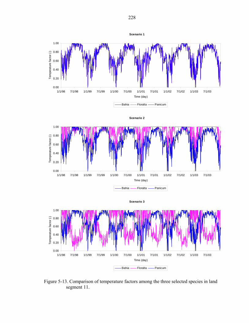
228

Scenario 3

0.00

0.20

0.40

0.60

0.80

1.00

1/1/98 7/1/98 1/1/99 7/1/99 1/1/00 7/1/00 1/1/01 7/1/01 1/1/02 7/1/02 1/1/03 7/1/03

Time (day)

Tem

pera

ture

fact

or (-

)


Scenario 2

0.00

0.20

0.40

0.60

0.80

1.00

1/1/98 7/1/98 1/1/99 7/1/99 1/1/00 7/1/00 1/1/01 7/1/01 1/1/02 7/1/02 1/1/03 7/1/03

Time (day)

Tem

pera

ture

fact

or (-

)


Scenario 1

0.00

0.20

0.40

0.60

0.80

1.00

1/1/98 7/1/98 1/1/99 7/1/99 1/1/00 7/1/00 1/1/01 7/1/01 1/1/02 7/1/02 1/1/03 7/1/03

Time (day)

Tem

pera

ture

fact

or (-

)


Figure 5-13. Comparison of temperature factors among the three selected species in land

segment 11.

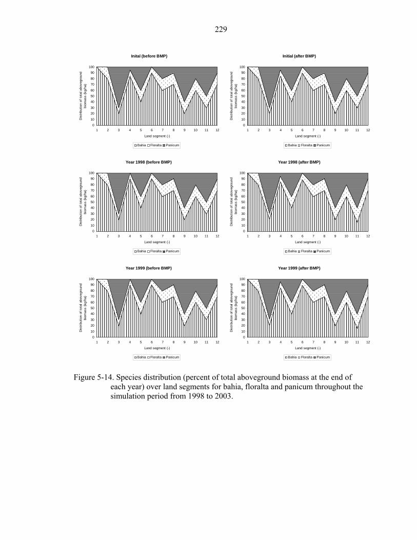
229

Inital (before BMP)

0

10

20

30

40

50

60

70

80

90

100

1 2 3 4 5 6 7 8 9 10 11 12

Land segment (-)

Dis

tribu

tion

of to

tal a

bove

grou

ndbi

omas

s (k

g/ha

)


Year 1998 (before BMP)

0

10

20

30

40

50

60

70

80

90

100

1 2 3 4 5 6 7 8 9 10 11 12

Land segment (-)

Dis

tribu

tion

of to

tal a

bove

grou

ndbi

omas

s (k

g/ha

)



0

10

20

30

40

50

60

70

80

90

100

1 2 3 4 5 6 7 8 9 10 11 12

Land segment (-)

Dis

tribu

tion

of to

tal a

bove

grou

ndbi

omas

s (k

g/ha

)


Initial (after BMP)

0

10

20

30

40

50

60

70

80

90

100

1 2 3 4 5 6 7 8 9 10 11 12

Land segment (-)

Dis

tribu

tion

of to

tal a

bove

grou

ndbi

omas

s (k

g/ha

)


Year 1998 (after BMP)

0

10

20

30

40

50

60

70

80

90

100

1 2 3 4 5 6 7 8 9 10 11 12

Land segment (-)

Dis

tribu

tion

of to

tal a

bove

grou

ndbi

omas

s (k

g/ha

)



0

10

20

30

40

50

60

70

80

90

100

1 2 3 4 5 6 7 8 9 10 11 12

Land segment (-)

Dis

tribu

tion

of to

tal a

bove

grou

ndbi

omas

s (k

g/ha

)

Bahia Floralta Panicum Figure 5-14. Species distribution (percent of total aboveground biomass at the end of

each year) over land segments for bahia, floralta and panicum throughout the simulation period from 1998 to 2003.

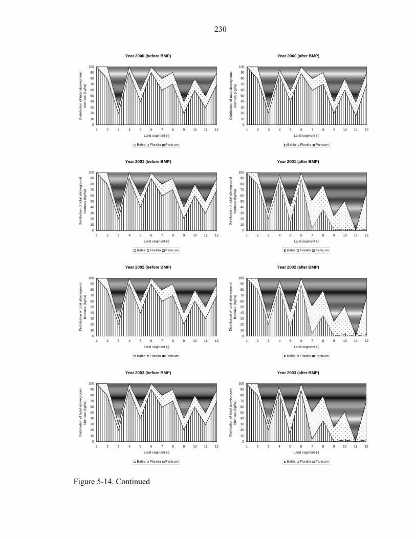
230


0

10

20

30

40

50

60

70

80

90

100

1 2 3 4 5 6 7 8 9 10 11 12

Land segment (-)

Dis

tribu

tion

of to

tal a

bove

grou

ndbi

omas

s (k

g/ha

)



0

10

20

30

40

50

60

70

80

90

100

1 2 3 4 5 6 7 8 9 10 11 12

Land segment (-)

Dis

tribu

tion

of to

tal a

bove

grou

ndbi

omas

s (k

g/ha

)



0

10

20

30

40

50

60

70

80

90

100

1 2 3 4 5 6 7 8 9 10 11 12

Land segment (-)

Dis

tribu

tion

of to

tal a

bove

grou

ndbi

omas

s (k

g/ha

)



0

10

20

30

40

50

60

70

80

90

100

1 2 3 4 5 6 7 8 9 10 11 12

Land segment (-)

Dis

tribu

tion

of to

tal a

bove

grou

ndbi

omas

s (k

g/ha

)



0

10

20

30

40

50

60

70

80

90

100

1 2 3 4 5 6 7 8 9 10 11 12

Land segment (-)

Dis

tribu

tion

of to

tal a

bove

grou

ndbi

omas

s (k

g/ha

)



0

10

20

30

40

50

60

70

80

90

100

1 2 3 4 5 6 7 8 9 10 11 12

Land segment (-)

Dis

tribu

tion

of to

tal a

bove

grou

ndbi

omas

s (k

g/ha

)



0

10

20

30

40

50

60

70

80

90

100

1 2 3 4 5 6 7 8 9 10 11 12

Land segment (-)

Dis

tribu

tion

of to

tal a

bove

grou

ndbi

omas

s (k

g/ha

)



0

10

20

30

40

50

60

70

80

90

100

1 2 3 4 5 6 7 8 9 10 11 12

Land segment (-)

Dis

tribu

tion

of to

tal a

bove

grou

ndbi

omas

s (k

g/ha

)

Bahia Floralta Panicum Figure 5-14. Continued

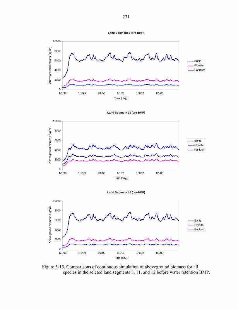
231

Land Segment 8 (pre-BMP)

0

2000

4000

6000

8000

10000

1/1/98 1/1/99 1/1/00 1/1/01 1/1/02 1/1/03

Time (day)

Abo

vegr

ound

bio

mas

s (k

g/ha

)

BahiaFloraltaPanicum


0

2000

4000

6000

8000

10000

1/1/98 1/1/99 1/1/00 1/1/01 1/1/02 1/1/03

Time (day)

Abo

vegr

ound

bio

mas

s (k

g/ha

)



0

2000

4000

6000

8000

10000

1/1/98 1/1/99 1/1/00 1/1/01 1/1/02 1/1/03

Time (day)

Abo

vegr

ound

bio

mas

s (k

g/ha

)


Figure 5-15. Comparisons of continuous simulation of aboveground biomass for all

species in the selcted land segments 8, 11, and 12 before water retention BMP.

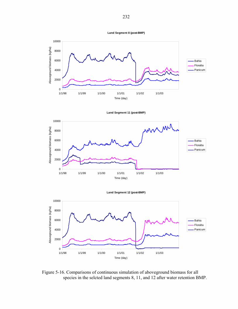
232

Land Segment 12 (post-BMP)

0

2000

4000

6000

8000

10000

1/1/98 1/1/99 1/1/00 1/1/01 1/1/02 1/1/03

Time (day)

Abo

vegr

ound

bio

mas

s (k

g/ha

)



0

2000

4000

6000

8000

10000

1/1/98 1/1/99 1/1/00 1/1/01 1/1/02 1/1/03

Time (day)

Abo

vegr

ound

bio

mas

s (k

g/ha

)



0

2000

4000

6000

8000

10000

1/1/98 1/1/99 1/1/00 1/1/01 1/1/02 1/1/03

Time (day)

Abo

vegr

ound

bio

mas

s (k

g/ha

)


Figure 5-16. Comparisons of continuous simulation of aboveground biomass for all

species in the selcted land segments 8, 11, and 12 after water retention BMP.

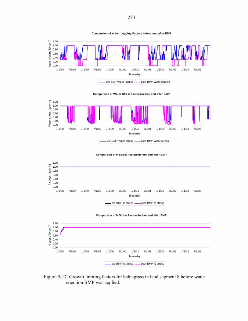
233

Comparsion of N Stress Factors before and after BMP

0.000.200.400.600.801.001.20

1/1/98 7/1/98 1/1/99 7/1/99 1/1/00 7/1/00 1/1/01 7/1/01 1/1/02 7/1/02 1/1/03 7/1/03

Time (day)

N s

tress

fact

or (-

)

pre-BMP N stress post-BMP N stress

Comparsion of P Stress Factors before and after BMP

0.000.200.400.600.801.001.20

1/1/98 7/1/98 1/1/99 7/1/99 1/1/00 7/1/00 1/1/01 7/1/01 1/1/02 7/1/02 1/1/03 7/1/03

Time (day)

P s

tress

fact

or (-

)

pre-BMP P stress post-BMP P stress

Comparsion of Water Logging Factors before and after BMP

0.000.200.400.600.801.001.20

1/1/98 7/1/98 1/1/99 7/1/99 1/1/00 7/1/00 1/1/01 7/1/01 1/1/02 7/1/02 1/1/03 7/1/03

Time (day)

Wat

er lo

ggin

g fa

ctor

(-)

pre-BMP water logging post-BMP water logging

Comparsion of Water Stress Factors before and after BMP

0.000.200.400.600.801.001.20

1/1/98 7/1/98 1/1/99 7/1/99 1/1/00 7/1/00 1/1/01 7/1/01 1/1/02 7/1/02 1/1/03 7/1/03

Time (day)

Wat

er s

tress

fact

or (-

)

pre-BMP water stress post-BMP water stress

Figure 5-17. Growth limiting factors for bahiagrass in land segment 8 before water

retention BMP was applied.

234

CHAPTER 6 SUMMARY AND CONCLUSIONS

Lake Okeechobee, located at the center of the Kissimmee-Okeechobee-Everglades

aquatic ecosystem in south Florida, is experiencing water quality degradation. Non-point

agricultural runoff from dairies and cow-calf operations in the northern watershed of the

lake is considered to be the primary source of excess phosphorus (P) loading discharged

into the lake. In order to protect the water quality of Lake Okeechobee and reach

environmental restoration goals, a variety of alternative land management practices have

been implemented in the Lake Okeechobee watersheds. To evaluate the effectiveness of

those practices, a coupled ecohydrological model integrating hydrology, nutrient and

vegetation dynamics was developed.

The coupled model was developed within the Java-based, object-oriented

framework of the existing ACRU2000 model (Campbell et al., 2001; Clark et al., 2001;

Kiker and Clark, 2001). The primary objective of this study was to develop a coupled

modeling system capable of simulating hydrology, nutrient and vegetation dynamics

simultaneously for south Florida flatwoods watersheds that incorporate wetlands, uplands

and transition zones. In this effort, a hydrologic simulation model capable of multi-

directional spatial simulation of surface and subsurface water movement was first

developed (Chapter 3). The existing nutrient components in ACRU2000 were modified

to enable multi-directional spatial transport of N, P, and conservative solute (Chapter 4).

Finally, a vegetation dynamics simulation model was developed to couple with the

235

hydrologic and nutrient models to enable the simulation of the plant growth dynamics

under the impacts of changes in water and nutrient availability (Chapter 5).

Hydrologic Simulation Model

The hydrologic model capable of multi-directional spatial simulation was

developed based on the existing hydrologic model in ACRU2000 by adding new

hydrologic components and modifying the existing components. New components

include an overland flow component capable of spatial surface water exchange between

land segments and a lateral groundwater component capable of spatial soil water

exchange between saturated soils of adjacent land segments. These components are

important in that they link different land segments together as an entity through lateral

water movement and provide the pathways capable of spatial nutrient transport.

A simulation sequence analysis was conducted to analyze the effect of simulation

sequence on model predictions, and also to compare with well-known physically based

models (MIKE SHE and MODFLOW). Results indicate that different simulation

sequences do lead to slightly different simulation results, but they are all consistent when

compared with MIKE SHE (DHI, 2004). The results also indicate that the simulation

sequence following the expected flow directions based on topography should be chosen

when there are multiple combinations of simulation sequence to choose from.

A test was conducted for the Dry Lake Dairy #1 site in the Kissimmee River Basin,

Florida to compare the capacity of the modified ACRU2000 hydrologic model in

simulating surface runoff and groundwater table to those predicted by the lumped

FHANTM model. From the comparisons and statistical analyses, it can be concluded

that the modified ACRU2000 hydrologic model is capable of adequately simulating

overland flow and lateral groundwater flow at the Dry Lake Dairy #1 site, but the

236

modified ACRU2000 model is not better than FHANTM. It is possible that ACRU2000

would perform better if it were calibrated to the observed data, particularity if sufficient

data were available to calibrate spatially distributed parameters.

Nutrient Simulation Model

The nutrient model capable of multi-directional spatial transport of N, P and

conservative solute was developed based on the existing nutrient module ACRU-NP

(Campbell et al., 2001) in the ACRU2000 modeling system by adding new lateral

transport nutrient components.

In order to investigate the accuracy of the conservative solute transport component,

the hypothetical scenario test was conducted by comparing with a particle tracking model

PMPATH (Chiang and Kinzelbach, 2005). The test results indicate that the solute

transport predicted by the modified ACRU2000 is in reasonable agreement with those by

PMPATH. Due to the constraints of PMPATH in simulating solute concentration, the

model performance in predicting conservative solute is qualitative.

To evaluate the complete performance of the coupled hydrologic and nutrient

model, an application was conducted for the beef cattle pastures at Buck Island Ranch,

Lake Okeechobee Basin, Florida. A complete model testing procedure was performed

including model calibration, verification, and sensitivity analysis using the measured data

over a 6-year period. The sensitivity analyses indicated that the hydrologic parameters

including crop coefficient, porosity, and restrictive layer hydraulic conductivity are the

most sensitive parameters to the hydrologic response. The sensitivities of nutrient

parameters tend to be more site-specific. Neither P nor N responses was found to be

sensitive to either stopcking or fertilizer rate for any site in this application. Rainfall N

and P are the two most sensitive parameters to the N and P load responses, respectively

237

for the low background nutrient winter pasture site, while and the active P and active N

are the two most senstivite parameters for the high nutrient background summer pasture

site. Statistics were calculated to evaluate the model performance for calibration and

verification. The comparison between statistics obtained using the predictions from

ACRU2000 and FHANTM indicate that the modified ACRU2000 did a much better job

in simulating hydrologic and nutrient processes. Results indicate that the coupled model

can predict hydrologic variables (surface runoff and groundwater elevations) with high

accuracy, but that it predicts nutrient loads (N and P) with relatively low accuracy.

However, it is difficult to evaluate the model performance on its nutrient simulation

capacities based on the limited nutrient observations available. Future work may be

needed to sufficiently judge the model performance, especially with regards to nutrient

simulation.

Vegetation Dynamics Simulation Model

The vegetation dynamics simulation model was developed, within the framework

of previously developed hydrologic and nutrient models, to simulate plant growth for

pasture and wetlands species. In the model, solar radiation and temperature are

considered to be the major drivers to predict plant growth while environmental impacts,

expressed in stress factors (nutrient deficiency and water availability), determine if the

plant can grow at its potential rate. Due to the lack of vegetation data available for

flatwoods soils, the testing of this model was based on a hypothetical scenario of water

retention BMP scenario at summer pasture S4 at the Buck Island Ranch. The simulated

results indicate that temperature sensitivities among species are needed to correctly

simulate the plant growth. The hypothetical scenario demonstrated that wetlands species,

represented by panicum, can tolerate prolonged water logged soil conditions much better

238

than transition zone and upland species represented by floralta and bahia, and that floralta

is more tolerant in those conditions than bahia. However, further testing is needed when

sufficient reliable vegetation data become available.

Implications of the Research

As the first working version, the multi-directional spatial, ecohydrological

simulation model marks a significant step in adapting the existing ACRU2000 model to

better represent hydrology, nutrients and vegetation dynamics for south Florida flatwoods

watersheds. Viable mechanisms have been added to enable simulation of some of the

unique aspects of flatwoods hydrology. Adaptation to other watersheds or soil conditions

at different temporal and spatial scales should be simple using adjusted parameters or by

adding relevant process components into this version. However, additional testing and

calibration are still needed to improve the robustness of the model for general use in the

future.

Future Research Recommendations

The following recommendations are made for those who may be interested in

continuing this work in the future.

Model Pre- and Post-processing Capacity

A user graphical interface (GUI) program capable of model pre- and post-

processing should be added into the modified ACRU2000. This is especially necessary

when the model runs in larger watersheds where more land segments must be defined and

parametertized. In the current version, each land segment requires its own land segment

input file that includes all required initial, boundary and parameter data. The data

required in this input file may confuse users without detailed knowledge of the model

structure. In addition, increasing the number of land segments leads to a tremendous

239

workload in preparing these land segment input files, as well as for adjusting parameters

required in model calibration and sensitivity analysis. Pre-processing capacity providing

a simple interface would make this process more efficient.

Furthermore, a post-processing program is necessary as well. The current version

of the model generates output files by land segments. When users need to compare

output variables over land segments, this must be done through spreadsheet software. It

is difficult to observe the simulation results immediately without additional tedious and

troublesome work to process the outputs. Additionally, the current output procedures do

not allow output of integer variables. This deficiency should be corrected.

Use Consistent Units for Parameters and Variables

Use of consistent units throughout the modeling system is necessary to make use of

the model easier and to minimize input errors. Unfortunately, different unit systems still

exist in the current versions of ACRU2000.

Documentation

A complete documentation regarding the modifications and additions since the

version of ACRU (v3.00) should be completed to provide the potential users an updated

manual.

Potential Changes to Existing Objects

A redesign for the control object (AAcru2000StandardProcesses) should be

considered. This object is used to determine what processes are to be added in the

execution lists (both vertical and horizontal). Currently, by switching the option variable,

a specific process can be added on or taken off from a list for each land segment.

However, this object is becoming complicated and it may be confusing for users to

customize their own process lists.

240

Another model input control object (AOldNewAcruVariableReference) is used to

establish a reference/mapping relationship between the DData object with the

CComponent object for all relationships in the model. The huge collection of hard-coded

relationships in this object has made it very cumbersome to understand. Use of an input

file, instead of hard-coded relationships in this object, could be one way to improve the

situation.

Sub-Daily Time Step

An incompatibility in the spatial and temporal resolution is a significant

impediment to a robust coupled modeling system that involves different processes having

varied temporal scales. The capacity to operate with flexible time steps is necessary,

especially when the model is applied in much smaller/larger catchments. A capacity that

would allow the model to run in a pre-specified global time step for the entire model, but

also allows specific model processes to run in their own local time steps, would make the

entire model more efficient and physically reasonable.

Herbivore Movement Module

A cattle roaming component should be added to better represent the impacts of

grazing on nutrient cycling and plant growth dynamics in this model. This is especially

important if the model will be used to investigate the effectiveness of stocking-related

BMPs.

Hydrologic Model

Hydrologic model should be tested for a wider range of conditions, including more

physical locations, larger watersheds and a wider range of runoff conditions.

241

Nutrient Model

The biased predictions of nutrient concentrations in surface runoff in this research

demonstrate that the mechanisms for simulating nutrient cycling need further

improvement. Methods for partitioning nutrients between the soil and water phases and

methods for dealing with the nutrients released from waste decomposition may require

further development.

Vegetation Model

The entire vegetation model should be further evaluated before it is used in a

predictive capacity. Components for root length and root biomass distribution dynamics

should be added so that species-specific evapotranspiration and nutrient uptake can be

more accurately simulated. An algorithm for plant height determination should also be

added to enable a feedback relationship between surface runoff and a dynamic roughness

coefficient. Moreover, a start-up mechanism for new species initiation in land segments

is especially necessary so that spatial expansion across land segments can be modeled

and plant competition can be more thoroughly considered. Finally, a herviore movement

model should be developed to simulate the impacts of cattle behavior and grazing

performance on vegetation growth.

242

APPENDIX A FLOW CHART FOR THE COUPLED MODELING SYSTEM AND MODEL

PROCESSES

Open I/O Files

Input Model Data

Last Day of Simulation Loop

Last Land Segment

Last Land Segment

End

Yes

Lateral Hydrologic Processes

Lateral Nutrient Processes

No

E

D

Yes

Vertical Hydrologic Processes

Vertical Vegetation Processes

Vertical Nutrient Processes

A

B

C

START

Yes

No

No

Yes

Note: The upper-case letters indicate expandable tree flow charts. (The process objects included are those used for the coupled multi-directional spatial simulation and do not include all existing processes in the original ACRU2000 model.)

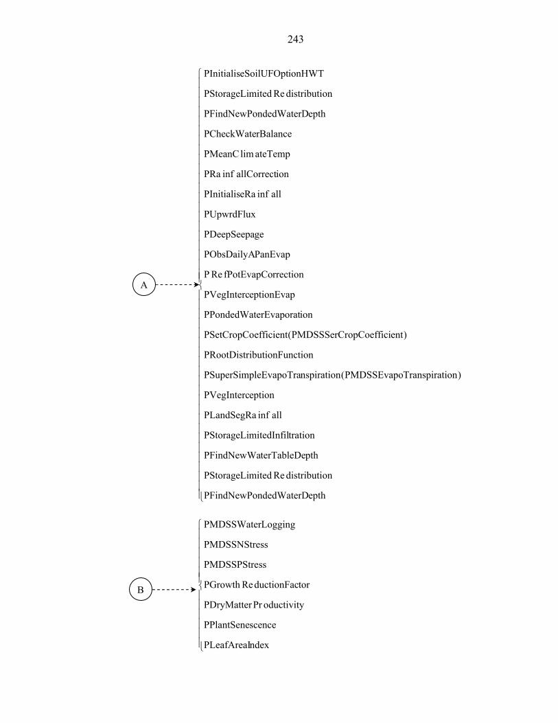
243

⎪⎪⎪⎪⎪⎪⎪⎪⎪⎪⎪⎪⎪⎪⎪⎪⎪⎪⎪⎪⎪⎪

⎩

⎪⎪⎪⎪⎪⎪⎪⎪⎪⎪⎪⎪⎪⎪⎪⎪⎪⎪⎪⎪⎪⎪

⎨

⎧

epthndedWaterDPFindNewPo

ondistributiRemitedPStorageLi

pthterTableDePFindNewWa

trationmitedInfilPStorageLi

allinfPLandSegRa

eptionPVegInterc

)ionTranspiratPMDSSEvapo(nspirationleEvapoTraPSuperSimp

ctionibutionFunPRootDistr

)entopCoefficiPMDSSSerCr(efficientPSetCropCo

ionerEvaporatPPondedWat

eptionEvapPVegInterc

rrectionfPotEvapCoReP

PanEvapPObsDailyA

gePDeepSeepa

PUpwrdFlux

allinfeRaPInitialis

ionallCorrectinfPRa

ateTemplimPMeanC

rBalancePCheckWate

epthndedWaterDPFindNewPo

ondistributiRemitedPStorageLi

ionHWTeSoilUFOptPInitialis

⎪⎪⎪⎪⎪⎪

⎩

⎪⎪⎪⎪⎪⎪

⎨

⎧

ndexPLeafAreaI

scencePPlantSene

oductivityPrPDryMatter

torductionFacRePGrowth

ssPMDSSPStre

ssPMDSSNStre

LoggingPMDSSWater

A

B

244

⎪⎪⎪⎪⎪⎪⎪⎪⎪⎪⎪⎪⎪⎪⎪⎪⎪⎪⎪⎪⎪⎪⎪⎪⎪⎪

⎩

⎪⎪⎪⎪⎪⎪⎪⎪⎪⎪⎪⎪⎪⎪⎪⎪⎪⎪⎪⎪⎪⎪⎪⎪⎪⎪

⎨

⎧

eModeloneExchangiveMixingZPConservat

rasnportubsurfaceTiveSoluteSPConservat

TransportvaporationiveSoluteEPConservat

nputsiveSoluteIPConservat

ificationPHWTDenitr

odeleExchangeMPMixingZon

ortfaceTranspPHWTSubsur

PTillage

ationPVolatiliz

PHarvest

onmobilizatiImPHWT

lizationPHWTMinera

icationPHWTNitrif

cationPHWTAmmoni

empPMeanSoilT

tonTransporPEvaporati

kePPlantUpta

nakeFixatioPNPlantUpt

ecationPAnimalDef

estionPAnimalDig

nsferutrientTraegetationNPConsumedV

TransfterssNutrientPDeadBioma

entInputsPMDSSNutri

entsalizeNutriPMDSSIniti

sessureHeadPreLayerminPDeter

cayicMatterDePMDSSOrgan

⎪⎩

⎪⎨⎧

terFlowalGroundwaPCalcLater

andFlowPCalcOverl

C

D

245

⎪⎪⎪

⎩

⎪⎪⎪

⎨

⎧

rtaceTranspouteSubsurfrvativeSolPMDSSConse

TransportuteSurfacervativeSolPMDSSConse

portrfaceTransPMDSSSubsu

tceTransporPMDSSSurfa

E

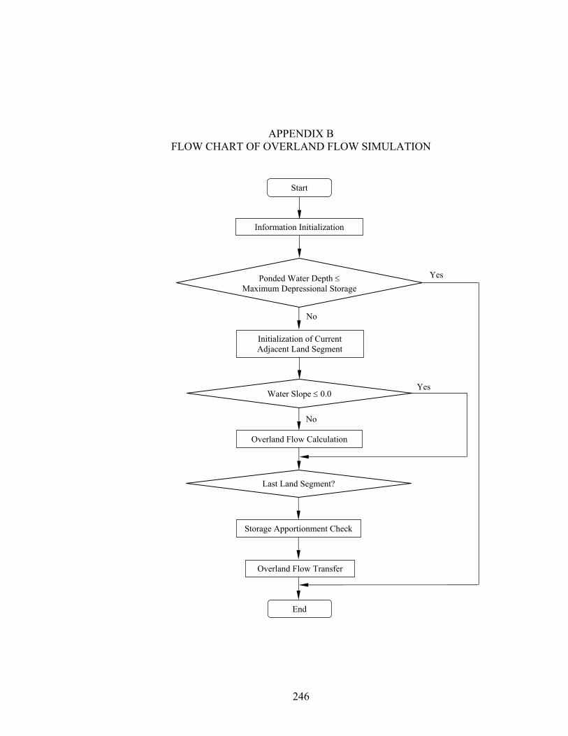
246

APPENDIX B FLOW CHART OF OVERLAND FLOW SIMULATION

Start

Initialization of Current Adjacent Land Segment

Ponded Water Depth ≤ Maximum Depressional Storage

Water Slope ≤ 0.0

End

Storage Apportionment Check

Overland Flow Transfer

Information Initialization

Overland Flow Calculation

Last Land Segment?

Yes

No

No

Yes

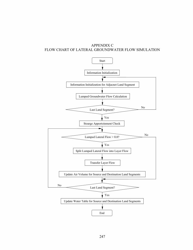
247

APPENDIX C FLOW CHART OF LATERAL GROUNDWATER FLOW SIMULATION

Start

End

Update Water Table for Source and Destination Land Segments

Information Initialization for Adjacnet Land Segment

Lumped Groundwater Flow Calculation

Information Initialization

Lumped Lateral Flow > 0.0?

Last Land Segment?

Last Land Segment?

Stoarge Apportoinment Check

Split Lumped Lateral Flow into Layer Flow

Transfer Layer Flow

Update Air Volume for Source and Destination Land Segments

No

Yes

No

No

Yes

Yes

248

APPENDIX D LISTS OF NEW AND MODIFIED OBJECTS

New objects listed below mean they did not exist but were added through this research; modified objects mean they existed in the previous model or were created by other modelers but were changed to fit the multi-directional spatial simulation model. Also, hereafter the multi-directional spatial simulation option is called MDSS for short.

New Model Objects

MAcru2000ModifiedStandard

This model object is the starting point for the model with a main method inside. It is created to decide how model input data, components, and processes are structured and in what mode the model will be executed. This object allows the model to run either with a lumped mode (MDSS= 0) or a multidirectional distributed mode (MDSS = 1).

New Process Objects

PAdjustOverlandFlow

This process object is used when the MDSS option is on (MDSS = 1). The major function of this process object is to compare calculated potential overland flow for each adjacent land segment with available amount of surface water storage in the source land segment to guarantee the conservation of mass. If potential overland flow is greater than available amount, then adjustments have to be conducted.

PAdjacentSpatialUnits

This process object is used when the MDSS option is on (MDSS = 1). The major function of this process object is to establish the relationships among adjacent land segments for one source land segment according to the boundary conditions, which is used to support the simulation of overland flow.

PCalcLateralGroundwaterFlow

This process object is invoked when the MDSS option is on (MDSS = 1). The major function of this object is to calculate the lateral groundwater flows between the saturated soils of two neighbouing land segments and transfer the lateral flows. Darcy's Law is used to estimate the lumped lateral groundwater flow when the hydraulic gradient exists between two saturated soils. Then, the lumped flow is split into the layer flows to those soil layers that contains and is below the current water table of source land segment. The layer lateral flow is transferred layer by layer.

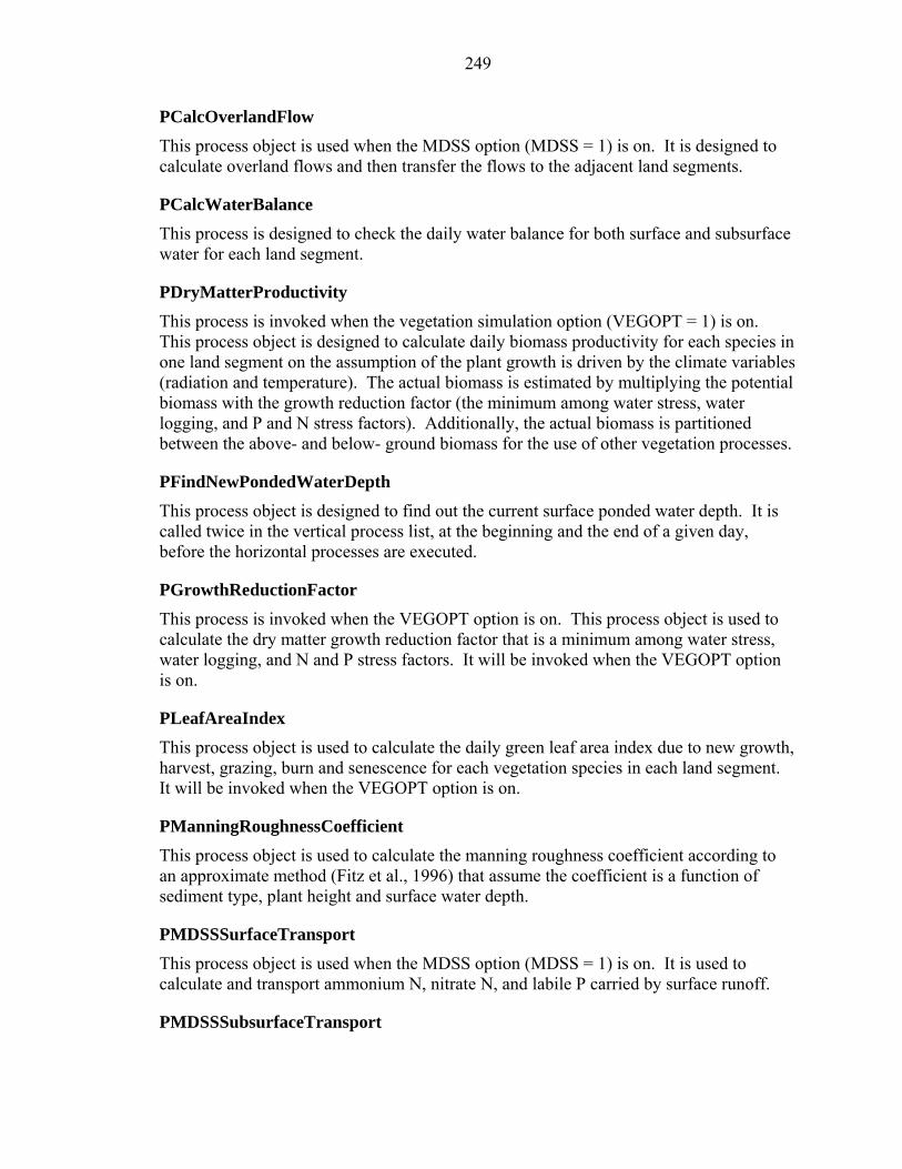
249

PCalcOverlandFlow

This process object is used when the MDSS option (MDSS = 1) is on. It is designed to calculate overland flows and then transfer the flows to the adjacent land segments.

PCalcWaterBalance

This process is designed to check the daily water balance for both surface and subsurface water for each land segment.

PDryMatterProductivity This process is invoked when the vegetation simulation option (VEGOPT = 1) is on. This process object is designed to calculate daily biomass productivity for each species in one land segment on the assumption of the plant growth is driven by the climate variables (radiation and temperature). The actual biomass is estimated by multiplying the potential biomass with the growth reduction factor (the minimum among water stress, water logging, and P and N stress factors). Additionally, the actual biomass is partitioned between the above- and belowground biomass for the use of other vegetation processes.

PFindNewPondedWaterDepth

This process object is designed to find out the current surface ponded water depth. It is called twice in the vertical process list, at the beginning and the end of a given day, before the horizontal processes are executed.

PGrowthReductionFactor This process is invoked when the VEGOPT option is on. This process object is used to calculate the dry matter growth reduction factor that is a minimum among water stress, water logging, and N and P stress factors. It will be invoked when the VEGOPT option is on.

PLeafAreaIndex This process object is used to calculate the daily green leaf area index due to new growth, harvest, grazing, burn and senescence for each vegetation species in each land segment. It will be invoked when the VEGOPT option is on.

PManningRoughnessCoefficient This process object is used to calculate the manning roughness coefficient according to an approximate method (Fitz et al., 1996) that assume the coefficient is a function of sediment type, plant height and surface water depth.

PMDSSSurfaceTransport

This process object is used when the MDSS option (MDSS = 1) is on. It is used to calculate and transport ammonium N, nitrate N, and labile P carried by surface runoff.

PMDSSSubsurfaceTransport

250

This process object is used when the MDSS option (MDSS = 1) is on. It is used to calculate and transport ammonium N, nitrate N, and labile P carried by groundwater flow.

PMDSSConservativeSoluteSurfaceTransport This process object is used when the MDSS option (MDSS = 1) is on. It is used to calculate and transport conservative solute carried by surface runoff.

PMDSSConservativeSoluteSubsurfaceTransport

This process object is used when the MDSS option (MDSS = 1) is on. It is used to calculate and transport conservative solute carried by subsurface groundwater.

PMDSSEvapoTranspiration This process is used when the VEGOPT option is selected. It is designed to calculate evapotranspiration by multiple species from one land segment by using a very simple method that is identical to that used in DRAINMOD/FHANTM. Potential ET is applied from the top down, reducing soil layers to the wilting point before moving to the next layer. The catual ET is equal to potential ET as long as there is water available.

PMDSSInitalizeNutrients

This process object is used when the MDSS option (MDSS = 1) is on. It was modified according the PInitalizeNutrient.

This process handles initialization of nutrient flux records, plant characteristics and other nutrient-related parameters as defaults when measured values are not available. If soil nutrient data are available for local conditions (soils), the model user should input those values and they will override the generalized estimates generated by the model. Also, the modified object enables to update the N fraction daily.

PMDSSNutrientInputs This process object is used when the MDSS option (MDSS = 1) is on. It was modified from PHWTNutrientInputs to make it more applicable for multi-directional spatial simulation and enable to consider the time series inputs. This process handles nutrient inputs to the watershed system through rainfall, fertilizer, and animal wastes.

This process was remodified from PHWTNutrientInputs and PNutrientInputs to make it more applicable for multi-directional spatial simluation and consider time series events, such as fertilizer, animal waste, etc. Major changes include:

(1) Runoff is included only when the model runs in a lumped mode since at this stage runoff have not been simuleted when the MDSS option is on.

(2) Modify the design in PNutrientsInputs where fertilizer and animal waste applications can not simutanluously occur. The modification enables consideration of both.

(3) Enable the application depth for fertilizer and animal waste to be different. The original related data objects were modified into time-series data objects to handle the potential events.

251

PMDSSNPlantUptakeFixation

This process object is used when the MDSS option (MDSS = 1) is on. This process calculates the N uptake by multiple plant species of ammonium and nitrate from the soil water by transpiration and/or assimilation (fixation) of nitrogen from the atmosphere by leguminous plants. Fixation is not assumed to add nitrogen to the soil until harvest and/or tillage. This process is modifed according to the existing process PNPlantUptakeFixation.

PMDSSNstress This process is invoked when the VEGOPT option is on. This process calculates the soil water N stress factor from 0.0 to 1.0 according to the method by Seligman and Van Keulen (1981).

PMDSSPPlantUptake This process object is used when the MDSS option (MDSS = 1) is on. This process calculates the uptake by multiple plant species of labile phosphorus from the soil water by transpiration.

PMDSSPStress This process is invoked when the VEGOPT option is on. This process calculates the soil water P stress factor from 0.0 to 1.0 according to according to the similar method as the N stress.

PMDSSSetCropCoefficient This process is invoked when the VEGOPT option is on. This process was modified according to PSetCropCoefficient to meet the needs when multiple plant species exist. The crop coefficient for each species needs to be set up.

PMDSSTillage This process object is used when the MDSS option (MDSS = 1) is on. This process calculates the effects of soil tillage on N and P forms and their movement. It was modified form PTillage.

PMDSSWaterLogging This process is invoked when the VEGOPT option is on. This process is designed to calculate the water logging factor (0~1) and the death indicator that indicate the plant will die caused by the long-term water logging.

POverlandFlowTransfer

This process object is used when the MDSS is on (MDSS = 1). Its major function is to transfer the actual overland flows to neighboring land segments.

PPlantSenescence

252

This process is invoked when the VEGOPT option is on. This process object is designed to calculate the reduction of live biomass both on surface and subsurface by plant sensecense. It is assumed that the decline of live biomass into dead biomass is a linear process during the period of plant senescemce. The corresponding N and P also are transferred from live biomass pools to dead biomass pools.

PSoilParameters

This process is used to estimate the soil mass, phosphorus and ammonium partitioning coefficients for each soil layer when the nutrient option (NUTRI = 1) is turned on.

PStorageApportionment This process object is used when the MDSS option is on (MDSS = 1). Its major function is to calculate the share of available water storage for each potential overland flow from source land segment.

PSortAdjacentSpatialUnits

This process object is used when the MDSS option is on (MDSS = 1). The major function of this process object is to arrange the sequence of adjacent land segments that receive potential overland flows in descending order of their boundary heights.

New Data Objects

DAboveGroundBiomassFluxRecord

Double flux record data object is to store the aboveground dry matter.

DACRUVegOption

Integer data object holds the option to determine if the model enables the vegetation dynamic simulation. VEGOPT = 1, enable simulation of vegetation dynamics; VEGOPT = 0, otherwise.

DAmmoniumPartitioningCoefficient Double data object holds the ammoinium partitioning coefficient.

DBelowGroundBiomassFluxRecord Double flux record data object is to store the belowground dry matter.

DBoundaryInflow Double data object holding the flow input from outside of simulation domain.

DBoundaryOption Integer array data object holds the boundary option including:

BOPT = 0, without weir, without downstream stage;

BOPT = 1, without weir, with downstream stage;

253

BOPT = 2, with weir, without downstream stage;

BOPT = 3, with weir, with downstream stage;

BOPT = 4, inflow boundary;

DBoundaryOutflow

Double data object holding the outflows though the domain boundary.

DBoundaryWidth

Double array data object holding the widths of boundaries for one land segment.

DCriticalLeafAreaIndex This daily data class is to store the degree days for each plant species.

DDaysofWaterlogging

Integer data object hold the number of successive days of water logged a plant suffers.

DDaysofWaterloggingLimits

Integer object holds the maximum number of days that a plant species still grow under the inundated soil conditions.

DDryMatterPartitioningCoefficient

Double data object holds the dry matter partitioning coefficient for a specific plant.

DExtinctionCoefficient

Double data object holds the extinction coefficient for a specific plant.

DGrowthReductionFactor Double data object is to store the growth reduction factor.

DHorizontalSaturatedHydraulicConductivity

Double data object holding the horizontal saturated hydraulic conductivity for soil layers.

DIncrementOfAboveGroundBiomass

Double data object is to store the daily increment of aboveground biomass.

DIncrementOfBelowGroundBiomass Double data object is to store the daily increment of belowground biomass.

DISoilHorizon Integer data object hold the integer ID of the soil horizon to indicate which soil horizon a computational soil layer belong to. It is used to choose different formula when calculate the P partitioning coefficient for sandy soils.

254

DLabilePPartitioningCoefficient

Double data object is to store the labile P partitioning coefficient.

DLayerAmmNUptake Double data object is to store the layer ammonium N uptaken by each plant species.

DLayerLabPUptake

Double data object is to store the layer labile P uptaken by each plant species.

DLayerNitNUptake

Double data object is to store the layer nitrate N uptaken by each plant species.

DLayerSoilMass Double data object is to store the layer soil mass.

DLateralGroundwaterAmmNLoad Double data object holds the ammonium N load levaing out of the simultaion domain through the lateral groundwater flow.

DLateralGroundwaterConservativeSoluteConc Double data object holds the concentration of conservative solute in lateral groundwater discharge through the watershed outlet.

DLateralGroundwaterConservativeSoluteLoad

Double data object holds the load of conservative solute in lateral groundwater discharge through the watershed outlet.

DLateralGroundwaterLabPLoad Double data object holds the labile P load levaing out of the simultaion domain through the lateral groundwater flow.

DLateralGroundwaterNitNLoad Double data object holds the nitrate N load levaing out of the simultaion domain through the lateral groundwater flow.

DLateralGroundwaterOutflow Double data object holds the total groundwater discharge through the outlet of the simulation domain.

DMaximumGrowthTemperature

Double data object holds the maximum temperature for a specific plant to enable growth.

DMaxManningRoughness

255

Double data object holds the maximum Manning’s roughness coefficient of a land segment.

DMaxSurfaceDepressionStorage Double data object holds the maximum depressional surface storage on the ground surface of a land segment.

DMDSSConservativeSoluteOption

Integer data object holds the option to determine whether or not the model simulates the multi-directional spatial transport of conservative solute (MDSSCS = 0, turn on multi-directional spatial simulation of conservative solute transport; MDSSCS = 1, turn off).

DMDSpatialSimulationOption Integer data object holds the option to determine if the model enables the multi-directional spatial simulation (MDSS = 1, turn on multi-directional spatial simulation; MDSS = 0, turn off).

DMinManningRoughness Double data object holds the minimum Manning’s roughness coefficient of a land segment.

DMinimumGrowthTemperature

Double data object holds the minimum temperature for a specific plant to enable growth.

DMinimumLeafAreaIndex Double data object holds the minimum leaf area index for a specific plant.

DNumofVegetationSpecies Integer data object holds the number of vegetation species to be simulated in one land segment.

DNeighbourWidth Double array data object holds the widths of boundaries between one land segment and its adjacent land segments or outside of the simulation domain.

DOptimum1GrowthTemperature

Double data object holds the fisrt optimum growth temperature for a specific plant.

DOptimum2GrowthTemperature Double data object holds the second optimum growth temperature for a specific plant.

DOptimumPConcentration

Double data object holds the optimum P concentration for a specific plant to grow.

256

DOutletLength

Double data object holds the distance from the center of the land segment to downstream or to the external boundary which separates the land segment and downstream.

DOverlandFlow

Double array data object holds the overland flows occurred from source land segment to adjacent land segments.

DOverlandOutflow Double data object holds the overland flow leaving the simulation domain through the watershed outlet.

DPlantDeathIndicator

Integer dat object indicates if a plant will die off the current land segment due to the water logging (= 1 to die; = 0 not to die).

DPlantNPercent

Double data object holds the plant N percent.

DPlantPPercent

Double data object holds the plant P percent.

DPlantSenescenceRate

Double data object holds the fraction of remaining biomass after plant senescence.

DPondedWaterDepth Double data object holds daily ponded water depth on the ground surface of a land segment.

DPStressFactor

Double data object holds the plant growth stress factor resulting from a shortage of phosphorus in the root zone.

DRUE Double data object holds the average light use efficiency for a specific plant.

DSenescedAboveGroundBiomass

Double data object holds the senscened aboveground biomass for a specific plant.

DSenescedBelowGroundBiomass

Double data object holds the senscened belowground biomass for a specific plant.

DShootCriticalNConc

257

Double data class is to store the critical shoot N concentration.

DShootCriticalPConc Double data class is to store the critical shoot P concentration.

DShootMinimumGrowthNConc Double data object holds the minimum shoot N concentration for maintaining plant growth.

DShootMinimumGrowthPConc Double data object holds the minimum shoot P concentration for maintaining plant growth.

DShootPConcentration

Double data class is to store the shoot P concentration.

DSpecificLeafArea

Double data object holds the specific leaf area ratio for a specific plant.

DSoilAluminumContent Double data object holds the soil aluminum content.

DSoilMagnesiumContent Double data object holds the soil aluminum content.

DStockingOption Integer data object stores the stocking option.

DStreamLabPConc Double data object holds the stream labile P concentration.

DStreamNitNConc

Double data object holds the stream nitrate N concentration.

DStreamAmmNConc Double data object holds the stream ammonium N concentration.

DTemperatureFactor Double data class is to store the temperature factor for a specific plant.

DTotalDryMatter Double data class is to store the total dry matter for a specific plant.

258

DTotalOutgoingOverlandFlow

Double data object holds the total outgoing overland flows form one land segment.

DTotalReverseOverlandFlow Double data object holds the total incoming overland flows form outside of a simulation domain.

DTotalSurfaceConservativeSoluteStorage

Double data object holds the total conservative solute mass in the surface water of a land segment.

DTotalSubSurfaceConservativeSoluteStorage

Double data object holds the total conservative solute mass within the soil water of a land segment.

DTotalSurfaceWaterStorage

Double data object holds the total water storage on the surface of a land segment.

DTotalSubSurfaceWaterStorage Double data object holds the total water storage within the soil of a land segment.

DXcoord Double data object holds the x-coordinate of the centroid of a land segment.

DYcood Double data object holds the y-coordinate of the centroid of a land segment.

DWaterStressFactor Double data class is to store the water stress factor.

DWaterLoggingFactor

Double data class is to store the water logging factor.

DWeirCoefficient Double array data object is to hold the weir coefficients.

DWeirElevation Double array data object is to hold the elevation of weir crust above the datum.

DWeirOption Integer array data object is to hold the weir options.

DWeirWidth

259

Double array data object is to hold the widths of weir crust.

New Module

ACRU_Veg To contain all plant growth related processes and collect data objects required by the vegetation dynamic simulation model.

Modified Component Objects

CComponent

To enable to create two separate vertical and horizontal process lists when the model runs with the MDSS (=1) mode, this existing component object was modified by adding instance variables and methods, including five instance variables: firstVerProcess, firstHorProcess, verProcessesList, horProcessedList, and landSegHorProcessList, and ten methods: addVerticalProcesses(PProcess), addHorizontalProcesses(PProcess), setFirstVerticalProcess(PProcess), setFirstHorizontalProcess(PProcess), getDIntegerArray(String), getFirstVerticalProcess(), getFirstHorizontalProcess(), getLandSegHorProcessesList(), runVerticalProcesses(), and runHorizontalProcesses().

Modified Control Objects

AAcru2000ModelInput

Created one instance variable horProcessesList and added two methods including addToHorizontalProcessList(String, String) and getHorizontalProcessesList() to help with creating a horizontal process list.

AAcru2000StandardModelCreator Modified the createProcessObjects() and initialiseProcess() methods to enable two separate vertical and horizontal process list to be created.

AAcru2000StandardCComponents Modified the addLandSegmentSubComponents() to enable additions of multiple plant species components.

AAcru2000StandardProcesses

Modified addLandSegmentProcesses() method to decide which processes objects will be put on the vertical and horizontal process lists when the MDSS option is on.

AOldNewAcruVariableReference Hard coded statements to establish the mapping between input and output variables and the component objects which they belong to.

AProcessCreator

260

Created one overloading method, createProcesses(), to create two separate vertical and horizontal process processes lists, and this method will be invoked only when the MDSS option is on.

Modified Data Objects

DDeepSeepageHeadBoundary

Modified the data object type from DDailyDatae to DDouble.

DDryMatterRatio Modified the data object type from DDailyData into DDouble.

DPotentialYield

Modified the data object type from DDailyData into DDouble.

DPlantID Modified the data object type from DDailyInteger into DInteger.

DPlantNC1 Modified the data object type from DDailyData into DDouble.

DPlantNC2


DPlantNitrogenPhosphorusRatio


DPlantBiomassFluxRecord Added several biomass transfer methods.

Modified Process Objects

PAnimalDigestion

Deduct the assimilated consumed biomass N and P.

PConservativeMixingZoneExchangeModel Changed startments in the codes to account for the surface runoff when the MDSS option is on. And corrected the unit conversion error.

PHWTDenitrification Added two more formula for the underestimation problems.

PHWTNutrientInputs

261

Changed statements in the codes to account for the surface runoff when the MDSS option is on.

PHWTSubsurfaceTransport Correctyed the unit conversion error.

PLabilePPartitioningCoefficient Added one overloading method to calculate the phosphorus partitioning coefficient for the specified soil layer using the empirical formula (Nair et al., 1997) for Florida flatwoods sandy soils.

PMeanSoilTemperature Changed the process object to account for the biomass produced by all plants species.

PMixingZoneExchangeModel Changed some statements in the codes to account for the surface runoff when the MDSS option is on and corrected the unit conversion error in total amount of surface water.

PNPlantUptakeFixation Added the codes to account for the mass balance check to avoide the rounding errors.

PPPlantUptake Added the codes to account for the mass balance check to avoide the rounding errors.

POrganicMatterDecay Corrected the errors in destroying the biomass for the residue layer.

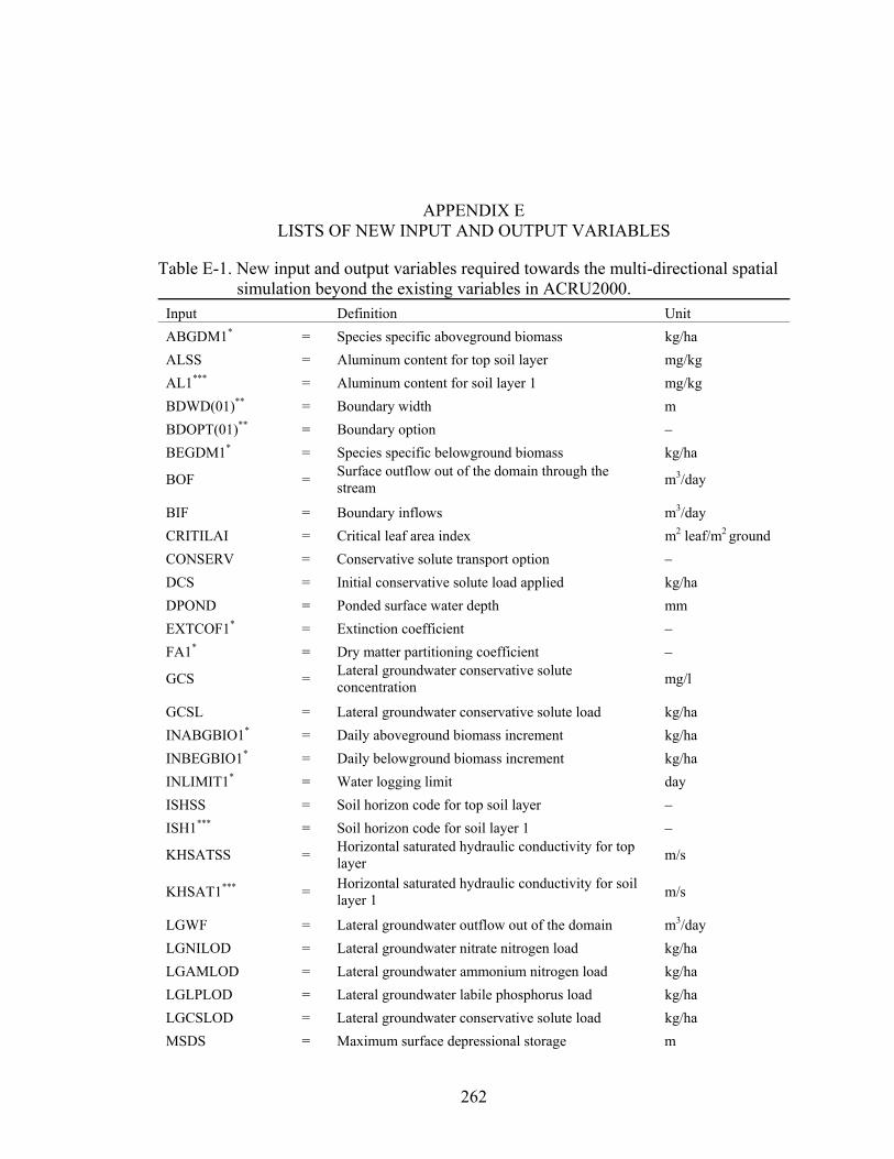
262

APPENDIX E LISTS OF NEW INPUT AND OUTPUT VARIABLES

Table E-1. New input and output variables required towards the multi-directional spatial simulation beyond the existing variables in ACRU2000.

Input Definition Unit ABGDM1* = Species specific aboveground biomass kg/ha ALSS = Aluminum content for top soil layer mg/kg AL1*** = Aluminum content for soil layer 1 mg/kg BDWD(01)** = Boundary width m BDOPT(01)** = Boundary option − BEGDM1* = Species specific belowground biomass kg/ha

BOF = Surface outflow out of the domain through the stream m3/day

BIF = Boundary inflows m3/day CRITILAI = Critical leaf area index m2 leaf/m2 ground CONSERV = Conservative solute transport option − DCS = Initial conservative solute load applied kg/ha DPOND = Ponded surface water depth mm EXTCOF1* = Extinction coefficient − FA1* = Dry matter partitioning coefficient −

GCS = Lateral groundwater conservative solute concentration mg/l

GCSL = Lateral groundwater conservative solute load kg/ha INABGBIO1* = Daily aboveground biomass increment kg/ha INBEGBIO1* = Daily belowground biomass increment kg/ha INLIMIT1* = Water logging limit day ISHSS = Soil horizon code for top soil layer − ISH1*** = Soil horizon code for soil layer 1 −

KHSATSS = Horizontal saturated hydraulic conductivity for top layer m/s

KHSAT1*** = Horizontal saturated hydraulic conductivity for soil layer 1 m/s

LGWF = Lateral groundwater outflow out of the domain m3/day LGNILOD = Lateral groundwater nitrate nitrogen load kg/ha LGAMLOD = Lateral groundwater ammonium nitrogen load kg/ha LGLPLOD = Lateral groundwater labile phosphorus load kg/ha LGCSLOD = Lateral groundwater conservative solute load kg/ha MSDS = Maximum surface depressional storage m

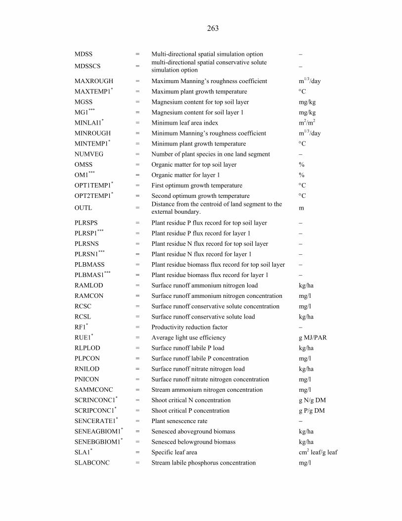
263

MDSS = Multi-directional spatial simulation option −

MDSSCS = multi-directional spatial conservative solute simulation option −

MAXROUGH = Maximum Manning’s roughness coefficient m1/3/day MAXTEMP1* = Maximum plant growth temperature °C MGSS = Magnesium content for top soil layer mg/kg MG1*** = Magnesium content for soil layer 1 mg/kg MINLAI1* = Minimum leaf area index m2/m2 MINROUGH = Minimum Manning’s roughness coefficient m1/3/day MINTEMP1* = Minimum plant growth temperature °C NUMVEG = Number of plant species in one land segment − OMSS = Organic matter for top soil layer % OM1*** = Organic matter for layer 1 % OPT1TEMP1* = First optimum growth temperature °C OPT2TEMP1* = Second optimum growth temperature °C

OUTL = Distance from the centroid of land segment to the external boundary. m

PLRSPS = Plant residue P flux record for top soil layer − PLRSP1*** = Plant residue P flux record for layer 1 − PLRSNS = Plant residue N flux record for top soil layer − PLRSN1*** = Plant residue N flux record for layer 1 − PLBMASS = Plant residue biomass flux record for top soil layer − PLBMAS1*** = Plant residue biomass flux record for layer 1 − RAMLOD = Surface runoff ammonium nitrogen load kg/ha RAMCON = Surface runoff ammonium nitrogen concentration mg/l RCSC = Surface runoff conservative solute concentration mg/l RCSL = Surface runoff conservative solute load kg/ha RF1* = Productivity reduction factor − RUE1* = Average light use efficiency g MJ/PAR RLPLOD = Surface runoff labile P load kg/ha PLPCON = Surface runoff labile P concentration mg/l RNILOD = Surface runoff nitrate nitrogen load kg/ha PNICON = Surface runoff nitrate nitrogen concentration mg/l SAMMCONC = Stream ammonium nitrogen concentration mg/l SCRINCONC1* = Shoot critical N concentration g N/g DM SCRIPCONC1* = Shoot critical P concentration g P/g DM SENCERATE1* = Plant senescence rate − SENEAGBIOM1* = Senesced aboveground biomass kg/ha SENEBGBIOM1* = Senesced belowground biomass kg/ha SLA1* = Specific leaf area cm2 leaf/g leaf SLABCONC = Stream labile phosphorus concentration mg/l

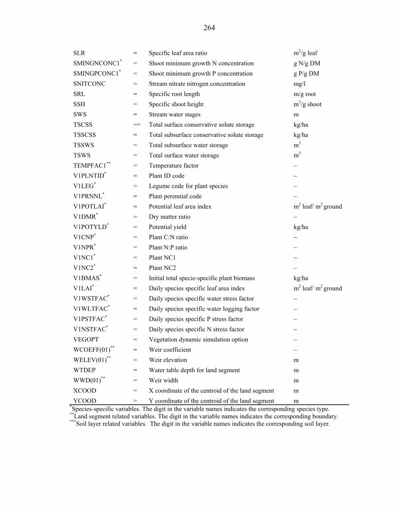
264

SLR = Specific leaf area ratio m2/g leaf SMINGNCONC1* = Shoot minimum growth N concentration g N/g DM SMINGPCONC1* = Shoot minimum growth P concentration g P/g DM SNITCONC = Stream nitrate nitrogen concentration mg/l SRL = Specific root length m/g root SSH = Specific shoot height m3/g shoot SWS = Stream water stages m TSCSS == Total surface conservative solute storage kg/ha TSSCSS = Total subsurface conservative solute storage kg/ha TSSWS = Total subsurface water storage m3 TSWS = Total surface water storage m3 TEMPFAC1** = Temperature factor − V1PLNTID* = Plant ID code − V1LEG* = Legume code for plant species − V1PRNNL* = Plant perennial code − V1POTLAI* = Potential leaf area index m2 leaf/ m2 ground V1DMR* = Dry matter ratio − V1POTYLD* = Potential yield kg/ha V1CNP* = Plant C:N ratio − V1NPR* = Plant N:P ratio − V1NC1* = Plant NC1 − V1NC2* = Plant NC2 − V1BMAS* = Initial total specie-specific plant biomass kg/ha V1LAI* = Daily species specific leaf area index m2 leaf/ m2 ground V1WSTFAC* = Daily species specific water stress factor − V1WLTFAC* = Daily species specific water logging factor − V1PSTFAC* = Daily species specific P stress factor − V1NSTFAC* = Daily species specific N stress factor − VEGOPT = Vegetation dynamic simulation option − WCOEFF(01)** = Weir coefficient − WELEV(01)** = Weir elevation m WTDEP = Water table depth for land segment m WWD(01)** = Weir width m XCOOD = X coordinate of the centroid of the land segment m YCOOD = Y coordinate of the centroid of the land segment m

*Species-specific variables. The digit in the variable names indicates the corresponding species type. **Land segment related variables. The digit in the variable names indicates the corresponding boundary. ***Soil layer related variables. The digit in the variable names indicates the corresponding soil layer.

265

APPENDIX F LISTS OF MODEL INPUT FILES

Overland Flow along a Flat Rectangular Plane cell.csv Control.men iroder LandSeg_1.men through LandSeg_20.men

Overland and Groundwater Flow over an Axisymmetric Domain

cell.csv Control.men iroder LandSeg_1.men through LandSeg_36.men

Application at Dry Lake Dairy #1, Kissimmee River Basin, Florida cell.csv Control.men iroder LandSeg_1.men through LandSeg_4.men

Buck Island Application, Lake Okeechobee Basin, Florida For winter pastures 6 and 7

cell.csv Control.men iroder LandSeg_1.men through LandSeg_18.men

For summer pastures 4 and 1 cell.csv Control.men iroder LandSeg_1.men through LandSeg_12.men

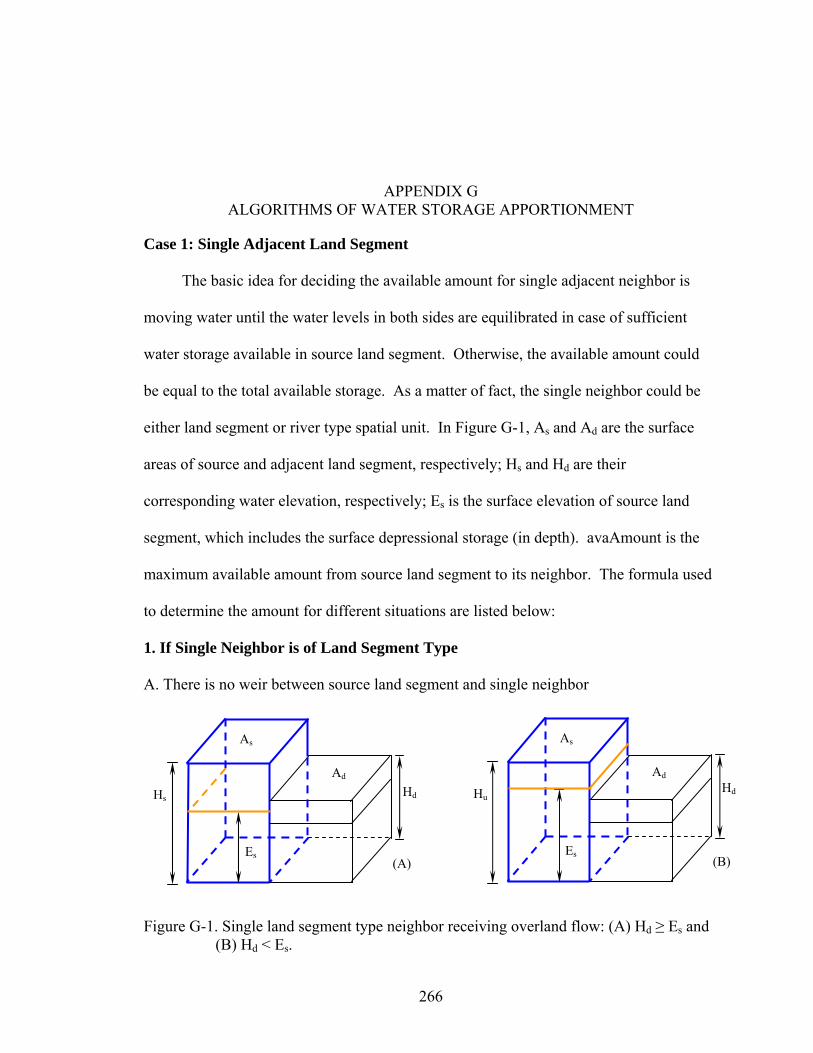
266

APPENDIX G ALGORITHMS OF WATER STORAGE APPORTIONMENT

Case 1: Single Adjacent Land Segment

The basic idea for deciding the available amount for single adjacent neighbor is

moving water until the water levels in both sides are equilibrated in case of sufficient

water storage available in source land segment. Otherwise, the available amount could

be equal to the total available storage. As a matter of fact, the single neighbor could be

either land segment or river type spatial unit. In Figure G-1, As and Ad are the surface

areas of source and adjacent land segment, respectively; Hs and Hd are their

corresponding water elevation, respectively; Es is the surface elevation of source land

segment, which includes the surface depressional storage (in depth). avaAmount is the

maximum available amount from source land segment to its neighbor. The formula used

to determine the amount for different situations are listed below:

1. If Single Neighbor is of Land Segment Type

A. There is no weir between source land segment and single neighbor

Figure G-1. Single land segment type neighbor receiving overland flow: (A) Hd ≥ Es and (B) Hd < Es.

Hd

As

Ad

Hs

Es (A)

As

Ad

Hu

Es

Hd

(B)

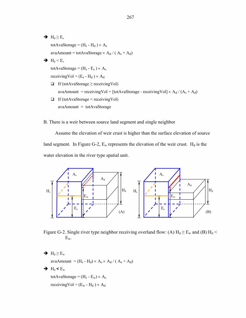
267

Hd ≥ Es

totAvaStorage = (Hs - Hd ) × As

avaAmount = totAvaStorage × Ad / ( As + Ad)

Hd < Es

totAvaStorage = (Hs - Es ) × As

receivingVol = (Es - Hd ) × Ad

If (totAvaStorage ≥ receivingVol)

avaAmount = receivingVol + [totAvaStorage - receivingVol] × Ad / (As + Ad)

If (totAvaStorage < receivingVol)

avaAmount = totAvaStorage

B. There is a weir between source land segment and single neighbor

Assume the elevation of weir crust is higher than the surface elevation of source

land segment. In Figure G-2, Ew represents the elevation of the weir crust. Hd is the

water elevation in the river type spatial unit.

Figure G-2. Single river type neighbor receiving overland flow: (A) Hd ≥ Ew and (B) Hd < Ew.

Hd ≥ Ew

avaAmount = (Hs - Hd) × As × Ad / ( As + Ad)

Hd < Ew

totAvaStorage = (Hs - Ew) × As

receivingVol = (Ew - Hd ) × Ad

Hd

As Ad

Hs

Es (A)

Ew

Hd

As

Ad

Hs

Es (B)

Ew

268

If (totAvaStorage ≥ receivingVol)

avaAmount = receivingVol + [totAvaStorage - receivingVol] × Ad / (As + Ad)

If (totAvaStorage < receivingVol)

avaAmount = totAvaStorage

2. If Single Neighbor is of River Type

A. If there is no weir in between and no downstrean water stage data available

avaAmount = (Hs - Es) × As

B. If there is a weir in between and no downstrean water stage data available

If Es ≥ Ew

avaAmount = (Hs - Es) × As

If Es ≥ Ew

avaAmount = (Hs - Ew) × As

C. If there is no weir in between and downstrean water stage data available

avaAmount = (Hs - Hwater stage) × As

D. If there is a weir in between and downstrean water stage data available

If Hwater stage ≥ Ew

avaAmount = (Hs - Hwater stage) × As

If Hwater stage < Ew

avaAmount = (Hs - Ew) × As

Case 2: Multiple Adjacent Land Segments

Figure G-2 displays the relationship between a source land segment and its 4

adjacent land segments. Assume all these neighbors receive outflows from the source

land segment and the order of water elevationss of these 4 neighbors follows: neighbour 1

> neighbour 2 > neighbour 3 > neighbour 4. Apparently, the water levels of these

neighbors are lower than that of source land segment. This diagram only displays one of

potential scenarios of the relationships between source land segment and its neighbors.

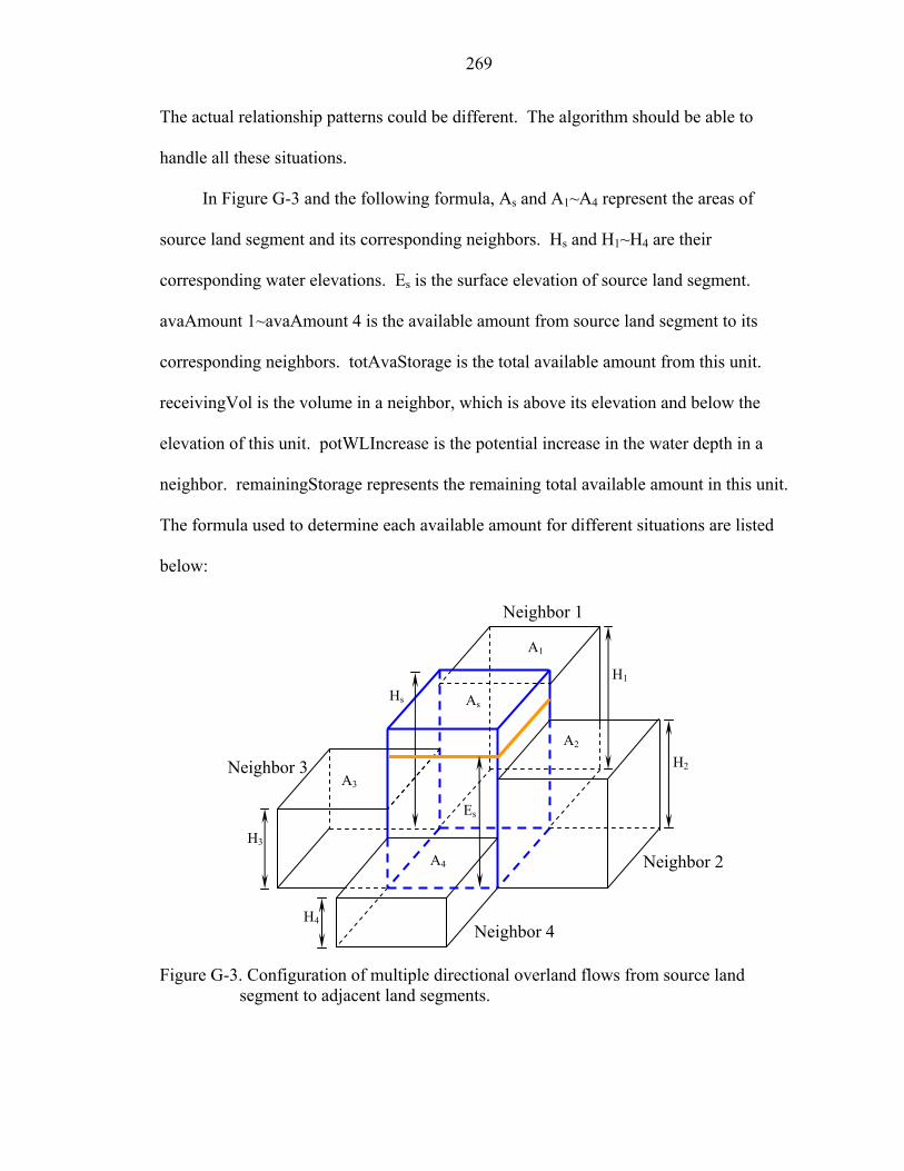
269

The actual relationship patterns could be different. The algorithm should be able to

handle all these situations.

In Figure G-3 and the following formula, As and A1~A4 represent the areas of

source land segment and its corresponding neighbors. Hs and H1~H4 are their

corresponding water elevations. Es is the surface elevation of source land segment.

avaAmount 1~avaAmount 4 is the available amount from source land segment to its

corresponding neighbors. totAvaStorage is the total available amount from this unit.

receivingVol is the volume in a neighbor, which is above its elevation and below the

elevation of this unit. potWLIncrease is the potential increase in the water depth in a

neighbor. remainingStorage represents the remaining total available amount in this unit.

The formula used to determine each available amount for different situations are listed

below:

Figure G-3. Configuration of multiple directional overland flows from source land

segment to adjacent land segments.

Neighbor 3

Neighbor 4

Neighbor 2

As

A3

A4

A2

A1

H2

H1

Hs

H3

H4

Es

Neighbor 1

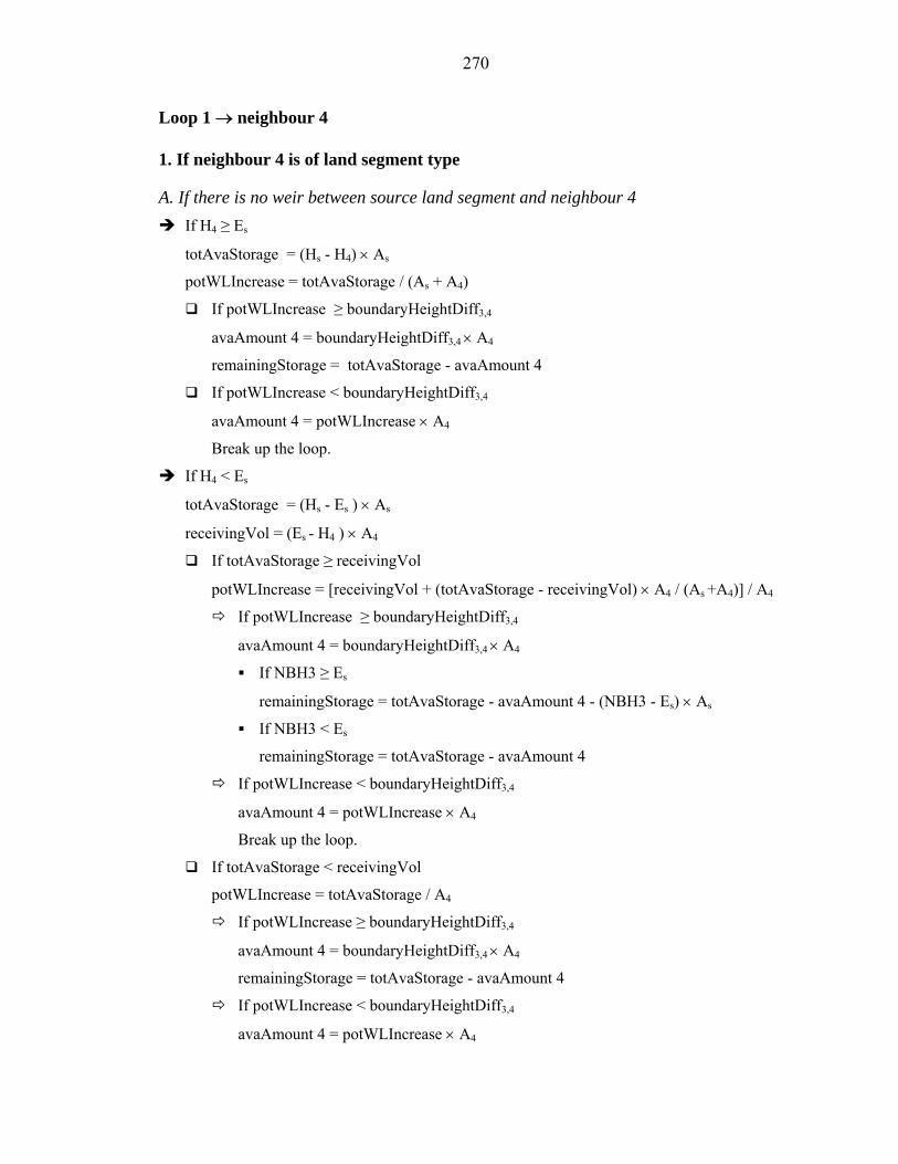
270

Loop 1 → neighbour 4

1. If neighbour 4 is of land segment type

A. If there is no weir between source land segment and neighbour 4 If H4 ≥ Es

totAvaStorage = (Hs - H4) × As

potWLIncrease = totAvaStorage / (As + A4)

If potWLIncrease ≥ boundaryHeightDiff3,4

avaAmount 4 = boundaryHeightDiff3,4 × A4

remainingStorage = totAvaStorage - avaAmount 4

If potWLIncrease < boundaryHeightDiff3,4

avaAmount 4 = potWLIncrease × A4

Break up the loop.

If H4 < Es

totAvaStorage = (Hs - Es ) × As

receivingVol = (Es - H4 ) × A4

If totAvaStorage ≥ receivingVol

potWLIncrease = [receivingVol + (totAvaStorage - receivingVol) × A4 / (As +A4)] / A4



If NBH3 ≥ Es

remainingStorage = totAvaStorage - avaAmount 4 - (NBH3 - Es) × As

If NBH3 < Es




Break up the loop.

If totAvaStorage < receivingVol

potWLIncrease = totAvaStorage / A4






271

Break up the loop.

B. If there is a weir between source land segment and neighbour 4 If H4 ≥ Ew4

totAvaStorage = (Hs - H4 ) × As

potWLIncrease = totAvaStorage / (As +A4)






Break up the loop.

If H4 < Ew4

totAvaStorage = (Hs - Ew4 ) × As

receivingVol = (Ew4 - H4) × A4

If totAvaStorage ≥ receivingVol

potWLIncrease = (totAvaStorage - receivingVol) / (As + A4)


avaAmount 4 = receivingVol + boundaryHeightDiff3,4 × A4



avaAmount 4 = receivingVol + potWLIncrease × A4

Break up the loop.

If totAvaStorage < receivingVol

avaAmount 4 = totAvaStorage

Break up the loop.

2. If neighbour 4 is of river type

A. If there is no weir in between and no downstrean water stage data available avaAmount 4 = (Hs - Es) × As

Break up the loop.

B. If there is a weir in between and no downstrean water stage data available If Es ≥ Ew4

avaAmount 4 = (Hs - Es) × As

Break up the loop

272

If Es ≥ Ew4

avaAmount 4 = (Hs – Ew4) × As

Break up the loop

C. If there is no weir in between and downstrean water stage data available avaAmount 4 = (Hs – Hwater stage) × As

D. If there is a weir in between and downstrean water stage data available If Hwater stage ≥ Ew4

avaAmount 4 = (Hs – Hwater stage) × As

Break up the loop

If Hwater stage < Ew4

avaAmount 4 = (Hs - Ew4) × As

Break up the loop


1. If neighbour 3 is of land segment type

A. If there is no weir between source land segment and neighbour 3 If H3 ≥ Es

potWLIncrease = remainingStorage / (As + A3 + A4)



avaAmount 4 = avaAmount 4 + boundaryHeightDiff2,3 × A4

remainingStorage = remainingStorage - boundaryHeightDiff2,3 × (As + A3 + A4)



avaAmount 4 = avaAmount 4 + potWLIncrease ×A4

Break up the loop.

If H3 < Es

receivingVol = (Es-H3) × (A3+A4)

If remainingStorage ≥ receivingVol

potWLIncrease = [receivingVol + (remainingStorage - receivingVol) × (A3 + A4) / (As + A3 + A4)]/(A3 + A4)



273


If NBH2 ≥ Es

remainingStorage = remainingStorage - boundaryHeightDiff2,3 × (A3 + A4) - (NBH2 - Es) × As

If NBH2 < Es

remainingStorage = remainingStorage - boundaryHeightDiff2,3 × (A3 +A4)



avaAmount 4 = avaAmount 4 + potWLIncrease × A4

Break up the loop.

If remainingStorage < receivingVol

potWLIncrease = remainingStorage / (A3 + A4)




remainingStorage = remainingStorage - boundaryHeightDiff2,3 × (A3 + A4)




Break up the loop.


potWLIncrease = remainingStorage / (As + A3 + A4)




remainingStorage = remainingStorage – boundaryHeightDiff2,3 × (As + A3 + A4)




Break up the loop.

If H3 < Ew3



274

potWLIncrease = (remainingStorage - receivingVol) / (As + A3 + A4)




remainingStorage = remainingStorage - receivingVol - boundaryHeightDiff2,3 × (A3+A4)




Break up the loop.


avaAmount 3 = remainingStorage

Break up the loop.


A. If there is no weir in between and no downstrean water stage data available avaAmount 3 = remainingStorage

Break up the loop.

B. If there is no weir in between and downstrean water stage data available maxStorage = (Hs – Hwater stage) × As

If maxStorage ≥ remainingStorage


Break up the loop

If maxStorage < remainingStorage

avaAmount 3 = maxStorage

remainingStorage = remainingStorage- avaAmount 3

C. If there is a weir in between and no downstrean water stage data available If Es ≥ Ew3


Break up the loop

If Es < Ew3


Break up the loop

275


maxStorage = (Hs – Hwater stage) × As

if maxStorage ≥ remainingStorage


if maxStorage < remainingStorage


remainingStorage = remainingStorage - avaAmount 3


maxStorage = (Hs – Ew3) × As

if maxStorage ≥ remainingStorage


if maxStorage < remainingStorage


Break up the loop


1. If neighbour 2 is of land segment type A. If there is no weir between source land segment and neighbour 2

If H2 ≥ Es

potWLIncrease = remainingStorage / (As + A2 + A3 + A4)





remainingStorage = remainingStorage - boundaryHeightDiff1,2 × (As + A2 + A3 + A4)





Break up the loop.

If H2 < Es

receivingVol = (Es - H2) × (A2 + A3 + A4)

276


potWLIncrease = [receivingVol + (remainingStorage - receivingVol) × (A2 +A3 +A4)/ (As + A2 + A3 + A4)] / (A2 + A3 + A4)





If NBH1 ≥ Es

remainingStorage = remainingStorage - boundaryHeightDiff1,2 × (A2 + A3 + A4) - (NBH1 - Es) × As

If NBH1 < Es

remainingStorage = remainingStorage - boundaryHeightDiff1,2 × (A2 + A3 + A4)





Break up the loop.


potWLIncrease = remainingStorage / (A2 + A3 + A4)





remainingStorage = remainingStorage - boundaryHeightDiff1,2 × (A2 + A3 + A4)





Break up the loop.


potWLIncrease = remainingStorage / (As + A2 + A3 + A4)



277



remainingStorage = remainingStorage - boundaryHeightDiff1,2 × (As + A2 + A3 + A4)





Break up the loop.

If H2 < Ew2


if remainingStorage ≥ receivingVol

potWLIncrease = (remainingStorage - receivingVol) / (As + A2 + A3 + A4)

if potWLIncrease ≥ boundaryHeightDiff1,2




remainingStorage = remainingStorage - receivingVol - boundaryHeightDiff1,2 × (A2 + A3 + A4)

if potWLIncrease < boundaryHeightDiff1,2




Break up the loop.



Break up the loop.



Break up the loop.

B. If there is no weir in between and downstrean water stage data available maxStorage = (Hs - Hwater stage) × As


278


Break up the loop




C. If there is a weir in between and no downstrean water stage data available If Es ≥ Ew2


Break up the loop

If Es < Ew2

avaAmount 2 = (Hs – Ew2) × As

Break up the loop


maxStorage = (Hs - Hwater stage) × As







maxStorage = (Hs - Ew2) × As



If totAvaStorage < remainingStorage


Break up the loop


1. If neighbor 1 is of land segment type

A. If there is no weir in between If H1 ≥ Es

avaAmount 1 = remainingStorage × A1 / (As + A1 + A2 + A3 + A4)

279

avaAmount 2 = avaAmount 2 + remainingStorage × A2 / (As + A1 + A2 + A3 + A4)



If H1 < Es

receivingVol = (Es - H1 ) × ( A1 + A2 + A3 + A4 )


amountToAllNeigh = receivingVol + (remainingStorage - receivingVol) × (A1 + A2 + A3 + A4) / ( As + A1 + A2 + A3 + A4)

avaAmount 1 = amountToAllNeigh × A1 / (A1 + A2 + A3 + A4)

avaAmount 2 = avaAmount 2 + amountToAllNeigh × A2 /(A1 + A2 + A3 + A4)

avaAmount 3 = avaAmount 3 + amountToAllNeigh × A3 / (A1 + A2 + A3 + A4)



avaAmount 1 = remainingStorage × A1 / (A1 + A2 + A3 + A4)

avaAmount 2 = avaAmount 2 + remainingStorage × A2 / (A1 + A2 + A3 + A4)



B. If there is a weir in between If H1 ≥ Ew1

avaAmount 1 = remainingStorage × A1 / (As + A1 + A2 + A3 + A4)




If H1 < Ew1

receivingVol = (Ew - H1) × A1


amountToAllNeigh = (remainingStorage - receivingVol) × (A1 + A2 + A3 + A4) / ( As + A1 + A2 + A3 + A4)

avaAmount 1 = receivingVol + amountToAllNeigh × A1 / (A1 + A2 + A3 + A4)






280



B. If there is a weir in between and no downstrean water stage data available If Es ≥ Ew1


If Es < Ew1


C. If there is no weir in between and downstrean water stage data available maxStorage = (Hs – Hwater stage) × As

If maxStorage >= remainingStorage





maxStorage = (Hs - Hwater stage) × As






maxStorage = (Hs – Ew1) × As





281

Nomenclature

As Area of source land segment Ad Area of destination land segment A1 Area of adjacent land segment 1 A2 Area of adjacent land segment 2 A3 Area of adjacent land segment 3 A4 Area of adjacent land segment 4 amountToAllNeigh Amount of water for all adjacent land segments avaAmount Allocated amount of storage for single adjacent land segment avaAmount 1 Accumulated amount of storage for adjacent land segment 1 avaAmount 2 Accumulated amount of storage for adjacent land segment 2 avaAmount 3 Accumulated amount of storage for adjacent land segment 3 avaAmount 4 Accumulated amount of storage for adjacent land segment 4 boundaryHeightDiff1,2 Difference of boundary heights between land segment 1 and 2 boundaryHeightDiff2,3 Difference of boundary heights between land segment 2 and 3 boundaryHeightDiff3,4 Difference of boundary heights between land segment 3 and 4 Hs Water level of source land segment Hd Water level of destination land segment H1 Water level of adjacent land segment 1 H2 Water level of adjacent land segment 2 H3 Water level of adjacent land segment 3 H4 Water level of adjacent land segment 4 Hwater stage Downstream water stage Es Elevation of source land segment Ew1 Weir elevation between source land segment and land segment 1 Ew2 Weir elevation between source land segment and land segment 2 Ew3 Weir elevation between source land segment and land segment 3 Ew4 Weir elevation between source land segment and land segment 4 maxStorage Maximum storage can be transferred NBH1 Boundary height between land segment 1 and source land segment NBH2 Boundary height between land segment 2 and source land segment NBH3 Boundary height between land segment 3 and source land segment receivingVol Portion of water volume is allocated to an adjacent land segment remainingStorage Water storage has no been allocated potWLIncrease Potential water level increase with a given amount of water input totAvaStorage Total available amount if water storage in source land segment

282

LIST OF REFERENCES

Acutis M and Donatelli M. 2003. SOILPAR 2.00: software to estimate soil hydrological parameters and functions. European Journal of Agronomy 18: 373-377.

Adams B, White A, and Lenton TM. 2003. An analysis of some diverse approaches to modeling terrestrial net primary productivity. Ecological Modelling 177: 354-391.

Allen, R.G., Pereira, L.S., Raes, D., and M. Smith. 1998. Crop evapotranspiration: Guidelines for computing crop water requirements. FAO Irrigation and Drainage Paper Number 56, Food and Agricultural Organization of the United Nations, Rome. 300 pp.

Anat A, Duke HR, and Corey AT. 1965. Steady upward flow from water tables. Hydrology Paper No. 7, Colorado State University, Fort Collins, CO.

Armstrong W. 1964. Oxygen diffusion from the roots of British bog plants. Nature 204: 801-802.

Arnold JG, Williams JR, Nicks AD, Sammons NB. 1990. SWRRB: A Basin Scale Simulation Model for Soil and Water Resources Management. Texas A&M University Press: College Station, TX.

Arnold JG, Allen PM, and Bernhardt G. 1993. A comprehensive surface–groundwater flow model. Journal of Hydrology 142:47-69.

Arnold JG and Fohrer N. 2005. SWAT2000: current capabilities and research opportunities in applied watershed modeling. Hydrological Processes 19:564-572.

American Society of Civil Engineers (ASCE) Task Committee on Definition of Criteria for Evaluation of Watershed Models of the Watershed Management Committee. 1993. Criteria for evaluation of watershed models. Journal of Irrigation and Drainage Engineering 119(3): 429–442.

Beasley DB and Huggins LF. 1980. ANSWERS (Area Non-point Source Watershed Environment Response Simulation), User’s manual. Purdue University, West Lafayette.

Beven KJ and Kirkby MJ. 1979. A physically-based variable contributing area model of basin hydrology. Hydrology Science Bulletin 24(1):43-69.

283

Bhat KKS, Flowers TH, and O’Callagham JR. 1981. Nitrogen losses and surface runoff from landspreading of manures. In: J.C. brogan (Eds.). Proceedings of a workshop in the European Economic Community Programme of Coordination of Research on Effluents from Livestock. Wexford, Ireland, May 20-22, 1980. pp. 222-246.

Bouraoui F and Dillaha TA. 1996. ANSWERS-2000: Runoff and sediment transport model. Journal of Environment Engineering, ASCE 122(6): 493-502.

Bottcher AB, Tremwel TK, and Campbell KL. 1995. Best management practices for water quality improvement in the lake Okeechobee watershed. Ecological Engineering 5: 341-356.

Bottcher D, Pickering N, and Cooper AB. 1998. EAAMOD-FIELD: A flow and phosphorus model for high water tables. In Drainage in the 21st Century: Food Production and the Environment, ed. L. C. Brown, 599-606. St. Joseph, MI.: ASAE.

Bradley C and Gilvear DJ. 2000. Saturated and unsaturated flow dynamics in a floodplain wetland. Hydrological Processes 14: 2945-2958.

Broadbent FE and Clark FE. 1965. Soil nitrogen, W.V. Bartholomew and F.E. Clark (Eds.). Agron. 10, 344.

Brooks RH and Corey AT. 1964. Hydraulic properties of porous media. Hydrology Paper No. 3, Colorado State University, Fort Collins, CO.

Burnash RJC, Ferral RL, and McGuire RA. 1973. A General Streamflow Simulation System—Conceptual Modeling for Digital Computers. Report by the Joliet Federal State River Forecasts Center, Sacramento, CA.

Busnardo MJ, Gersberg RM, Langis R, Sinicrope TL, and Zedler JB. 1992. Nitrogen and phosphorus removal by wetland mesocosms subjected to different hydroperiods. Ecological Engineering 1: 287-307.

Capece JC. 1994. Hydrology and contaminant transport on flatwoods watersheds. Ph.D. dissertation. Gainesville, FL: University of Florida.

Campbell KL, Capece JC, and Tremwel TK. 1995. Surface/subsurface hydrology and phosphorus transport in the Kissimmee River Basin, Florida, Ecological Engineering 5: 301-330.

Campbell KL, Kiker GA, and Clark DJ. 2001. Development and testing of a nitrogen and phosphorus process model for Southern African water quality issues. 2001 ASAE Annual International meeting. Paper No. 012085, St. Joseph, MI.: ASAE.

Cannell MGR, Milne R, Sheppard LJ, and Unsworth MH. 1987. Radiation interception and productivity of willow. J Appl Ecol 24: 261-78.

284

Carlisle VW, Sodek F, Coillins III ME, Hammond LC, and Harris WG. 1989. Characterization data for selected Florida soils. University of Florida, IFAS Soil Science Department - soil Characterization laboratory in cooperation with USDA SCS.

Chen DX, and Coughenour MB. 1994. GEMT ± a general model for energy and mass transfer of land surfaces and its application at the Fife sites. Agricultural and Forest Meteorology 68: 145±171.

Chiang C, Craft CB, Rogers DW, and Richardson CJ. 2000. Effects of 4 years nitrogen and phosphorus additions on Everglades plant communities. Aquatic Botany 68: 61-78.

Chiang WH and Kinzelbach W. Accessed at April 15, 2005. Processing MODFLOW for Windows (PMWIN), Version 5.3.0. Available http://www.pmwin.net/pmwin5.htm.

Childs SW and Hanks JR. 1975. Model of soil salinity effects on crop growth. Soil Science Society of American Journal 39: 617-622.

Clark DJ, Kiker GA, and Schulze RE. September 2001. Object-oriented restructuring of the ACRU agrohydrological modeling system, Tenth South African National Hydrology Symposium 26-28.

Crawford NH and Linsley RS. 1966. Digital Simulation in Hydrology: The Stanford Watershed Model IV. Technical Report no. 39, Department of Civil Engineering, Stanford University, Palo Alto, CA.

Cunge JA. 1975. Two-dimensional modeling of flood plains, Unsteady Flow in Open Channels. Volume II, Chapter 17. Water Resources Publications, P.O. Box 303, Fort Collins, Colorado 80533, USA: 705-762.

Danish Hydraulic Institute (DHI). 2004. MIKE SHE Water Movement - User Guide and Technical Reference Manual. Agern Allé 5 DK-2970 Hørsholm, Denmark.

Davis SM. 1991. Growth, decomposition, and nutrient retention of Cladium Jamaicense Crantz Typha Domingensis Pers. In the Florida Everglades. Aquatic Botany 40: 204-224.

Davis JA and Froend R. 1999. Loss and Degradation of wetlands in southern Australia: underlying causes, consequences and solutions. Wetlands Ecology and Management 7: 14-23.

Evans BM, Sheeder SA, and Lehning DW. 2003. A spatial technique for estimating streambank erosion based on watershed characteristics. Journal of Spatial Hydrology, Vol.3, No.1.

http://www.pmwin.net/pmwin5.htm.

285

Ferreira VA, Weesies GA, Yoder DC, Foster GR, and Renard KG. 1995. The site and condition specific nature of sensitivity analysis. Journal of Soil and Water Conservation 50(5): 493-497.

Fisher J and Acreman MC. 2004. Wetland nutrient removal: a review of the evidence. Hydrology and Earth System Sciences 8(4): 673-685.

Fitz HC, DeBellevue EB, Costanza R, Boumans R, Maxwell T, Wainger L, and Sklar FH. 1996. Development of a general ecosystem model for a range of scales and ecosystems, Ecological Modelling 88: 264-295.

Fitz HC, Wang N, Godin J, Sklar FH, Trimble B, and Rutchey K. 2002. Calibration Performance of ELM v2.1a: 1979-1995 Water Quality and Hydrology. Report to the RECOVER Model Refinement Team, available at http://www.sfwmd.gov/org/wrp/elm/results/cal_ver/elm2.1/ELMcalibAnalysis_draft.pdf, South Florida Water Management District, West Palm Beach, FL.

Flaig EG and Reddy KR. 1995. Fate of phosphorus in the lake Okeechobee watershed, Florida, USA: overview and recommendations. Ecological Engineering 5: 127-142.

Flaig EG and Havens KE. 1995. Historical trends in the Lake Okeechobee ecosystems. I. Land use and nutrient loadings. Arch. Hydrobiol. (Suppl.), 107: 1-24.

Fraisse CW and Campbell KL. 1996. Modified FHANTM for water quality modeling of beef cow/calf operations in south Florida. Paper No. 962057, St. Joseph, MI.: ASAE.

Fraisse CW and Campbell KL. 1997. FHANTM (Field Hydrologic And Nutrient Transport Model) Version 2.0 User's Manual. Gainesville, FL: Agricultural and Biological Engineering Dept., IFAS, University of Florida.

Gurnell AM, Hupp CR, and Gregory SV. 2000. Linking hydrology and ecology. Hydrological Processes 14: 2814-2815.

Gunsalus B, Flaig EG, and Ritter GJ. 1992. Effectiveness of agricultural best management practices implemented in the Taylor Creek/Nubbin Slough and lower Kissimmee River basins. Proc. Natl. Rural Clean Waters Program Syrup, 1992, pp. 161-172.

Hann CT and Zhang J. 1996. Impact of uncertain knowledge of model parameters on estimated runoff and phosphorus loads in the Lake Okeechobee Basin. Trans. ASAE 39(2): 511-516.

Hedden KF. 1986. Example field testing of soil fate and transport model, PRZM, Dougherty Plain, Georgia. In Vadose Zone Modeling of Organic Pollutants, eds. S. C. Hern and S. M. Melancon, 81-101, Mich.: Lewis Publishers Inc.

http://www.sfwmd.gov/org/wrp/elm/results/cal_ver/elm2.1/ELMcalibAnalysis_draft.pdf

http://www.sfwmd.gov/org/wrp/elm/results/cal_ver/elm2.1/ELMcalibAnalysis_draft.pdf

286

Hendricks GS. 2003. Performance evaluation of two hydrologic/water quality models on beef pastures at Buck Island Ranch. Master Thesis. Gainesville, FL: University of Florida.

Heatwole CD. 1986. Field and basin scale water quality models for evaluating agricultural nonpoint pollution abatement programs in a south Florida Modified CREAMS hydrology model for Coastal Plain watersheds. Trans. ASAE 30(4): 1014-1022.

Heatwole CD, Campbell KL, and Bottcher AB. 1987. Modified CREAMS hydrology model for Coastal Plain watersheds. Trans. ASAE 30(4): 1014-1022.

Hession WC, Shanholtz VO, Mostaghimi S, and Dillaha TA. 1994. Uncalibrated performance of the finite element storm hydrograph model. Trans. ASAE 37(3): 777-783.

Hunt HW, Trlica MJ, Redente EF, Moore JC, Detling JK, Kittel TGF, Walter DE, Fowler MC, Klein DA, and Elliot ET. 1991. Simulation model for the effects of climate change on temperate grassland ecosystems. Ecological Modelling 53:205-246.

Hydrologic Engineering Center. 1981. HEC-1, Flood Hydrograph Package—User’s Manual. US Army Corps of Engineers: Davis, CA.

Innis GS. 1978. Grassland simulation model. Ecological Studies 26. New York: Springer-Verlag.

Ivens WPMF. 1992. World Food Production: Biophysical Factors in Agricultural Production, Open universiteit, Heerlen, the Netherlands.

Jones CA, Cole CV, Sharpley AN, and Williams JR. 1984. A simplified soil and plant phosphorus model: I. Documentation. Soil Sci. Soc. Am. J. 48: 800-805.

Jones JW, and Luyten J. 1998. Simulation of biological processes. In Agricultural Systems Modeling and Simulation, eds. R. M. Peart and R.B. Curry. Marcel Dekker, Inc. pp 19-62.

Jones JW, Hoogenboom G, Porter CH, Boote KJ, Batchelor WD, Hunt LA, Wilkens PW, Singh U, Gijsman AJ, and Ritchie JT. 2003. The DSSAT cropping system model. Europ. J. Agronomy 18: 235-265.

Jones JW, Boote KJ, White J, Hoogenboom G, and Porter CH. 2000. Phenology sub-module for CROPGRO, in DSSAT v.4.0 Documentation and source code listing. Agricultural and Biological Engineering Department Research report No. 2000-1201. University of Florida, Gainesville, Florida.

Kiker GA. 1998. Development and comparison of savanna ecosystem models to explore the concept of carrying capacity. PhD Dissertation. Cornell University.

287

Kiker GA and Clark DJ. 2001. The development of a Java-based, object-oriented modeling system for simulation of Southern African hydrology. 2001 ASAE Annual International Meeting. ASAE Paper no. 012030. St. Joseph, MI.:ASAE.

Knisel WG (ed.). 1980. CREAMS: A field scale model for chemicals, runoff, and erosion from agricultural management systems. USDA Conservation Research Report 26: 643.

Knisel WG, Yates P, Sheridan JM, Woody TK, Allen III LH, and Asmussen LE. 1985. Hydrology and hydrogeology of Upper Taylor Creek watershed, Okeechobee County, Florida: data and analysis. ARS-25, USDA-Agricultural Research Service, Washington, D.C.

Knisel WG, Leonard RA, and Davis FM. 1993. GLEAMS version 2.10 Part I: Nutrient Component Documentation. Unpublished, USDA/ARS. Tifton, GA. 44p.

Knisel WG and Davis FM. 1999. GLEAMS (Groundwater Loading Effects of agricultural Management Systems) Version 3.0 User Manual. SEWRL-WGK/FMD-050199. Tifton, GA. 167p.

Krysanova V, Meiner A, Roosaare J, and Vasilyev A. 1989. Simulation modelling of the coastal waters pollution from agricultural watershed. Ecological Modelling 49: 7-29.

Krysanova V, Müller-Wohlfeil DI, Becker A. 1998. Development and test of a spatially distributed hydrological/water quality model for mesoscale watersheds. Ecological Modelling 106: 261–289.

Krysanova V, Hattermann F, and Wechsung F. 2005. Development of the ecohydrological model SWIM for regional impact studies and vulnerability assessment. Hydrologic Processes 19: 763-783.

Lal AMW. 1998. Weighted implicit finite-volume model for overland flow. Journal of Hydraulic Engineering. 124: 941-950.

Lauenroth WK, Urban DL, Coffin DP, Parton WJK, Shugart HH, Kirchner TB, and Smith TM. 1993, Modeling vegetation structure-ecosystem processes interactions across sites and ecosystem. Ecological Modeling 67: 49-80.

Leith H. 1975a. Modeling the primary productivity of the world. In: Leith H, Whittalcher, RH. (Eds); Primary Productivity of the Biosphere. Springer-Verlag, New York.

Leonard RA, Knisel WG, and Still DA. 1987. GLEAMS: Groundwater loading effects of agricultural management systems. Transactions of the ASAE 30 (5): 1404-1418.

Martinez C. 2006. Object-oriented hydrologic and water-quality model for high-water-table environments. Ph.D. dissertation. Gainesville, FL: University of Florida.

288

MacArthur Ecology Research Center (MAERC). Optimization of best management practices (BMPs) for beef cattle ranching in the Lake Okeechobee Basin. SFWMD contact C-13414. Final report. Prepared for the South Florida Water Management District. July 2004.

McCaffery PM, Hinkley WM, MacGill R and Cherr GD. 1976. Report of investigations in the Kissimmee-Lake Okeechobee Watershed. Fla. Depart. Environ. Reg. Tech. Series, Vol. 2, No. 2. Tallahassee. Florida.

McDonald MG and Harbaugh AW. 1988. A Modular Three-dimensional Finite-difference Ground-water Flow Model. US Geological Survey, Techniques of Water Resources Investigation Book 6, Chapter A1; 586 pp.

McDonald MG and Harbaugh AW. 1996. MODFLOW: the modular three dimensional finite-difference ground water flow model. USGS.

Monsi M and Saeki T. 1953. Uber den Lictfaktor in den Pflanzengesell -schaften und sein Bedeutung fur die Stoffproduktion. Japan J. Bot. 14: 22-52.

Mortimer C. 1941. The exchange of dissolved substances between mud and water in lakes. Journal of Ecology 30: 147-201.

Nair VD, Graetz DA, and Portier KM. 1995. Forms of phosphorus in soil profiles from dairies of south Florida. Soil Sci. Soc. Am. Journal 59: 1244-1249.

Nalluri C and Judy ND. 1989. Factors affecting roughness in coefficient in vegetated channels. In: B.C. Yen (Editors), Channel Flow and Catchment Runoff: Centennial of Manning's Formula and Kuichling's Rational Formula. University of Virginia, Charlottesville, VA, pp. 589.

Nash JE and Sutcliffe JV. 1970. River flow forecasting through conceptual models part I - a discussion of principles. Journal of Hydrology 10: 282–290.

New MG and Schulze RE. 1996. Hydrologic sensitivity to climate change in the Langriver catchment, Stellenbosch, South Africa and some implications for geomorphic processes. Zeitschrift fur Geomorephologie, Supplementband 107: 11-34.

Newman S, Grace JB, and Koebel JW. 1996. Effects of nutrients and hydroperiod on Typha, Cladium, and Eleocharis: implication for Everglades restoration. Ecological Applications 6(3): 774-783.

Nichols DS. 1983. Capacity of natural wetlands top remove nutrients from wastewater. Journal of the Water Pollution Control Federation 55: 495-505.

Parton WJ, Schimel DS, Cole CV, and Ojima DS. 1987. Analysis of factors controlling soil organic matter levels in Great Plains Grasslands. Soil Society of America Journal 51: 1173±1179.

http://water.usgs.gov/software/modflow.html

289

Parton WJ, Coughenour MB, Scurlock JMO, Ojima DS, Gilmanov TG, Scholes RJ, Schimel DS, Kirchner TB, Menaut JC, Seastedt TR, Garcia ME, Kamnalrut A, Kinyamario JI, and Hall DO. 1996. Global grassland ecosystem modelling: development and test of ecosystem models for grassland systems. In: Breymeyer AI, Hall DO, Melillo JM, Agren GI, eds. Global change: effects on coniferous forests and grasslands. (SCOPE 56). Chichester: John Wiley and Sons, 229±267.

Petryk S, Asce AM and III B, 1975. Analysis of flow through vegetation. J. Hydraul. Div., HY7: 871-883.

Refsgaard JC. 1997. Parameterization, calibration and validation of distributed hydrological models. Journal of Hydrology 198: 69-97.

Refsgaard JC and Storm B. 1995. MIKE SHE. In Computer Models of Watersheds Hydrology, Singh V (ed.). Water Resources Publication: Highlands Ranch. CO; 809-846.

Richardson CJ. 1985. Mechanisms controlling phosphorus retention capacity in freshwater wetlands. Science 228: 1424-1427.

Ritchie JT. 1972. Model for predicting evaporation from a row crop with incomplete cover. Water Resources Research 8(5): 1204-1213.

Rockwood DM, Davis ED, and Anderson JA. 1972. User Manual for COSSARR Model. US Army Engineering Division, North Pacific: Portland, OR.

Rogers JS. 1985. Water management model evaluation for shallow sandy soils. Trans. ASAE 28(3): 785-790.

Rymph SJ. 2004. Modeling growth and composition of perennial tropical forage grasses. Ph.D. dissertation. Gainesville, FL: University of Florida.

Schippers P and Kropff MJ. 2001. Competition for light and nitrogen among grassland species: a simulation analysis. Function Ecology 15: 155-164.

Schulze RE. 1989. ACRU: Background, Concepts and Theory. WRC Report No. 154/1/89. ACRU Report No.35.

Schulze RE. 1995. Hydrology and Agrohydrology: a text to accompany the ACRU 3.00 Agrohydrological modelling System. WRC Report No. TT69/95. ACRU Report No.43.

Schulze RE, Kiker GA, and Kunz RP. 1993. Global climate-change and agricultural productivity in southern Africa. Global environmental Change 3:330-349.

290

Seligman NG and Van Keulen H. 1981. PAPRAN: A simulation model of annual pasture production limited by rainfall and nitrogen. p. 192-220. In M.J. Frissel and J.A. van Veen (ed.) Simulation of nitrogen behaviour of soil-plant systems. Pudoc. Wageningen, the Netherlands.

Sharpley AN and Williams JR (Eds). 1990. EPIC-Erosion/Productivity impact calculator: 1. Model Documentation. U.S. Department of Agriculture, Agricultural Research Service, technical Bulletin No. 1768. 235p.

South Florida Water Management District (SFWMD). 1997a. Surface water improvement and management (SWIM) plan update for Lake Okeechobee. West Palm Beach, Florida.

South Florida Water Management District (SFWMD). 1997b. SFWMD wetlands model: calibration of the coupled periphyton/vegetation model to WCA-2A. HydroQual, Inc. October 21. West Palm Beach, Florida (material via private communication).

South Florida Water Management District (SFWMD). 1998. Natural system model version 4.5 documentation. Planning department. West Palm Beach, Florida. February 1998.

South Florida Water Management District (SFWMD). 2005. Documentation of the South Florida Water Management Model, version 5.5. Final Draft. West Palm Beach, Florida (material via private communication).

South Florida Water Management District (SFWMD). Accesses April 28, 2005. Hydrologic Systems Modeling. Available at: http://www.sfwmd.gov/org/pld/hsm/hsm.html.

Spitters CJT and Schapendonk AHCM. 1990. Evaluation of breeding strategies for drought tolerance in potato by means of crop growth simulation. Plant and Soil 123: 193-203.

Sims R. 2004. Performance evaluation of the field hydrologic and nutrient transport model (FHANTM 2.0) on beef pastures at Buck Island Ranch, Florida. A technical paper presented to the graduate school of the University Of Florida in partial fulfillment of the requirements for the degree of master of interdisciplinary ecology. University of Florida.

Skaggs RW. 1980. DRAINMOD reference report: methods for design and evaluation of drainage-water management systems for soils with high water tables. Soil Conservation Service, United States Department of Agriculture, Fort Worth, TX.

Sklar FH, Fitz HC, Wu Y, Zee RV, and McVoy C. 2001, The design of ecological landscape models for Everglades restoration. Ecological Economics 37: 379-401.

Smithers JC and Caldecott RE. 1993. Development and verification of hydrograph routing in a daily simulation-model. Water SA, 19, 263-267.

http://www.sfwmd.gov/org/pld/hsm/hsm.html.

291

Smith RE. 1992. Opus, An integrated simulation model for transport of nonpoint-source pollutants at the field scale, Vols. 1 & 2. US Department of Agriculture, ARS-98.

Sugawara M, Ozaki E, Wantanabe I, and Katsuyama Y. 1976. Tank model and its application to Bird Creek, Wollombi Brook, Bihin River, Sanaga River, and Nam Mune. Research Note 11, National Center for Disaster Prevention, Tokyo, Japan.

Sun G, Riekerk H, and Comerford NB. 1998. Modeling the forest hydrology of wetland-upland ecosystems in Florida, Journal of the American Water Resources Association, 34(4): 827-841.

Thornley JHM and Cannell MGR. 1997. Temperate grassland response to climate change: an analysis using the Hurley Pasture Model. Annals of Botany 80: 205-221.

Thomann RV. 1982. Verification of water quality models. Journal of Environmental Engineering. Div. ASCE 108(5): 923-939.

Tremwel TK. 1992. Field hydrologic and nutrient transport model, FHANTM. Ph.D. dissertation. Gainesville, FL: University of Florida.

Urban NH, Davis SM, and Aumen NG. 1993. Fluctuations in Sawgrass and Cattail densities in Everglades Water Conservation area 2A under varying nutrient, hydrologic and fire Regimes. Aquatic Botany 46: 204-223.

United States Department of Agriculture (USDA). 1990. State soil geographic database for Florida. U.S. Department of Agriculture, Soil Conservation Service, Gainesville, Florida.

United States Department of Agriculture (USDA), SCS. 1996. Agricultural waste management field handbook. United States Department of Agriculture. Washington, D.C.

Uusi-Kamppa J, Turtola E and Ylaranta T. 1997. The interactions of buffer zones and phosphorous runoff. In: Buffer Zones: Their process and potential in Water Protection, N.E. Haycock, T.P. Burt, K.W.T. Goulding and G. Pinay. (Eds) Quest Envronmental, Harpenden, UK.

Van Ittersum MK, Leffelaar PA, Van Keulen H, Kropff MJ, Bastiaans L, and Goudriaan J. 2003. On approaches and applications of the Wageningen crop models. European Journal of Agronomy 18:201-234.

Verberne ELJ. 1992. Simulation of the nitrogen and water balance in a system of grassland and soil. Nota 258. DLO-Institut voor Bodemvruchtbaarheid, Oosterweg 92, 9750 RA, Haren, Netherlands.

http://www.awra.org/jawra/authors/author_RiekerkHans.html

http://www.awra.org/jawra/authors/author_ComerfordNicholasB.html

http://www.awra.org/jawra/toc/toc_34_4.html

292

White JR. 1987. ERHYM-II: model description and user guide for the BASIC version. US Department of Agriculture, Agricultural Research Service, ARS-59, Washington, D. C.

Whittaker RH and Levin SA. 1975. Niche: theory and application. Stroudsburg, Pa.: Dowden, Hutchinson & Ross. New York: distributed by Halsted Press,

William JR, Jones CA, and Dyke PT. 1984. A modeling approach to determining the relationship between erosion and soil productivity. Transactions of the ASAE 27:129-144.

Williams JR and Hann RW. 1983. HYMO: Problem-oriented language for hydrologic modeling—User’s Manual. USDA: ARS-S-9.

Williams JR, Renard KG, and Dyke PT. 1983. EPIC–a new model for assessing erosion’s effect on soil productivity. Journal of Soil and Water Conservation 38(5): 381-383.

Wu Y, Sklar FH, and Rutchey K. 1997. Analysis and Simulation of Fragmentation Patterns in the Everglades. Ecological Application 7: 268-276.

Young GKK and Alward CL. 1983. Calibration and testing of nutrient and pesticide transport models. In Agricultural Management and Water Quality. F. W. Schaller and G. W. Bailey (eds.), 263-277, Ames: Iowa Sate Univ. Press.

Young RA, Onstad CA, Bosch DD, and Anderson WP. 1989. AGNPS: A nonpoint source pollution model for evaluating agricultural watersheds. Journal of Soil and Water Conservation 44(2): 168–173.

Zhang J, Haan CT, Tremwel TK, and Kiker GA. 1995. Evaluation of phosphorus loading models for south Florida. Trans. ASAE 38(3): 767-773.

Zhang J and Gornak SI. 1999. Evaluation of field-scale water quality models for the Lake Okeechobee regulatory program. Applied Engineering in Agriculture 15(5): 441- 447.

293

BIOGRAPHICAL SKETCH

Lei Yang was born in Henan province, People’s Republic of China, in a family led

by fairly open-minded parents who always encourage their kids to pursue what they

dreamed in their lives. Lei graduated from Hohai University, China, with a BS in 1991

and a MS in 1994 majoring in hydrology and water resources engineering. Upon the

completion of her MS, she was then employed as a civil engineer in the China Institute of

Water Resources and Hydropower Research for close to three years. Excelling in

research projects developing flood inundation and mitigation simulation models, in

October 1997 she was recommended to join a research student program in Kyoto

University, Japan, financed with a Japanese MOBUSHO scholarship. With the

experience gained during that period, Lei started to pursue one of her dreams that she

wanted to reach a higher professional level in the field of hydrology and water resources

through advanced study. In August 2000, she joined the Agricultural and Biological

Engineering Department at the University of Florida as a graduate research assistant and

a PhD student.

COUPLED SIMULATION MODELING OF FLATWOODS...

Documents

Transcript of COUPLED SIMULATION MODELING OF FLATWOODS...