County-level Gridded Livestock Methane Emissions for the Contiguous United States

Alexander N. Hristov, Michael Harper, Robert Meinen, Rick Day, Juliana Lopes, Troy Ott, Aranya Venkatesh, and Cynthia A. Randles

The Pennsylvania State University and ExxonMobil Research and Engineering

USEPA Emissions Inventory Conference August 14-18, 2017

Global methane inventories

Q1: Our approach indicates that significant OH-related uncertainties in the CH4budget remain, and we find that it is not possible to implicate, with a high degree of confidence, rapid global CH4 emissions changes as the primary driver of recent

trends when our inferred OH trends and these uncertainties are considered. Rigby et al., 2017 (PNAS)

1. Is this a real growth? 2. CH4 + ·OH → ·CH3 + H2O

3. If the growth is real, what is causing it?

Global methane inventoriesSchwietzke et al., 2016 (Nature)

…..Post-2006 source increases are predominantly biogenic, outside

the Arctic, and arguably more consistent with agriculture than

wetlands

Schaefer et al., 2016 (Science)

...…the recent temporal increases in microbial emissions have been

substantially larger (than from fossil fuel)

Schwietzke et al., 2016 (Nature)

How reliable are the isotope data?

Wang et al., 2016 (Science)

-15‰ to -76‰

δ13CH4; fossil-fuel

-31‰ to -93‰

δ13CH4; biogenic

Turner et al., 2017 (PNAS)

….a large overlap in isotopic signatures of fossil fuel and non-fossil

methane…..…analysis presented here demonstrates that an increase in fossil-fuel methane sources could be a major contributor to the renewed growth in

atmospheric methane since 2007

-53 to -54‰

We have to consider how these predictions agree with global livestock population trends

6.5% increase between 2006 and

2012

8.1% increase between 2006

and 2012

3.9% increase between 2006 and

2013

Trends in global fossil fuel production, 2006 - 2015

0

5

10

15

20

25

Fossil fuel sector growth

Natural gasCrude oilCoal

BP Statistical Review of World Energy, June 2016

% g

row

th si

nce

2006

(as m

illio

n to

ns o

il eq

.)

22%

10%

20%

US methane accounting controversy

Wecht et al., 2014

40 to 90% higher than USEPA’s

estimates

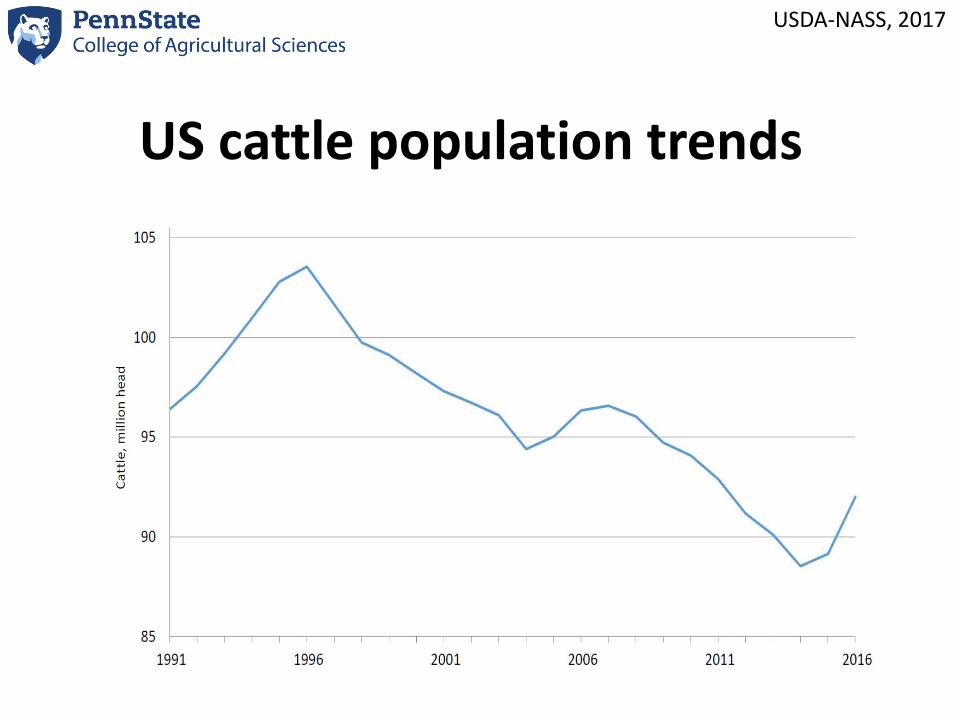
US cattle population trends

USDA-NASS, 2017

Objectives• There is a need for spatially-accurate emission

inventories for non-CO2 GHG emissions

• Using a bottom-up approach, estimate livestock (cattle, swine, and poultry) methane emissions in the contiguous United States

• Develop a spatially-explicit, gridded (0.1° x 0.1°) methane emissions inventory and maps for the livestock sector

• Compare this bottom-up analysis with other existing gridded inventories (Maasakkers et al., 2016 and EDGAR)

Inventory development process: enteric

Retrieval of cattle inventory data by state and county

Categorization by animal class

Generation of feed intake and diet composition data for each animal

category

Estimation of enteric methane emissions

Estimation of county-level enteric methane emission

Generation of emission factors based on feed intake and diet composition

for each animal category Less complex models requiring only DMI, or DMI plus NDF had predictive ability similar to

more complex models

GLOBAL NETWORK individual animal database(>5,200 individual dairy cow data)

Niu et al., in preparation

Methane emissions from enteric fermentation (Gg/yr) = Feed dry matter intake (DMI; kg/head/d) × methane

emission factor (g/kg DMI) × 365 (d/yr) × county animal population by animal category (head)

Cattle: database includes estimates for 3,063 countiesSwine and poultry: databases included 469 and 728 counties, respectively

International collaboration in database

development: THE GLOBAL NETWORK

PROJECT

Global Research Alliance on Agricultural GHG

Livestock Research Group

Research Networks, including FNN

The Feed and Nutrition Network

Europe; n = 3,015 from 82 studies

North America; n = 1,932 from 65 studies

South America; n = 108 from 3 studies

Australia & New Zealand; n = 194 from 5 studies

Dairy database (n = 5,249)

Enteric CH4 Production ModelsModel Development Model Performance

Level Model Predictor RMSPE, %1 GEI Level GEI 15.82 DMI Level DMI 15.63 DMI & NDF Level DMI, NDF 14.54 DMI & EE Level DMI, EE 15.85 Dietary Level DMI, EE, NDF 14.86 Dietary Composition Level EE, NDF 24.17 MY Level MY 20.18 ECM Level ECM 18.79 Performance ECM, MP 17.7

10 Animal Level DMI, EE, NDF, MF, BW 14.511 Animal without DMI Level EE, NDF, MP, ECM, BW 16.3- IPCC, 2006 GEI 16.1- IPCC, 1997 GEI 16.6

Conclusion: simpler models had predictive ability close to complex models

Niu et al., in preparation

Dry matter intake estimation

• Manure emission estimates were calculated using published US EPA protocols and factors

• Methane emission from manure (kg/yr) = (Animal population × VSE × Bo) × [ (WMS1 × MCF1) + ….. + (WMSn × MCFn)] × (Methane density)

• National Agricultural Statistic Services (NASS) data was utilized to provide animal populations– Cattle values were estimated for every county in the 48 contiguous states of

the United States– Swine and poultry estimates were conducted on a county basis for states with

the highest populations of each species and on a state-level for less populated states

• Uncertainty bounds for manure methane emissions were taken from USEPA: -18% (lower) and +20% (upper)

Inventory development process: manure emissions

Gridded inventory maps• County-level total enteric and total manure methane values were

allocated based upon the relative percentage of feed sources (based on USDA-NASS CropScape data) within each county

• All emission rasters were projected to geographic coordinates (latitude/longitude, WGS84 datum) and resampled to 0.1 decimal degree cells

• Gridded emissions inventories were produced for: – Cattle enteric– Cattle manure management– Total cattle emissions– Total manure emissions– Total combined emissions– The gridded inventory can be accessed at: Penn State Gridded

Livestock Methane Inventory.

Total methane emissions

Comparable total methane emissions between our analysis and USEPA or EDGAR

However, the spatial distribution of emissions differed significantly from that of EDGAR (and USEPA)

Enteric

Manure

Gridded differences in emissions between bottom-up approaches

Manure

Enteric

Current analysis vs. USEPA

Manure

Enteric

Current analysis vs. EDGAR

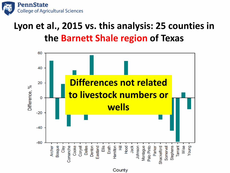
Lyon et al., 2015 vs. this analysis: 25 counties in the Barnett Shale region of Texas

Differences not related to livestock numbers or

wells

Conclusions• Atmospheric methane concentrations are increasing since 2006

– Reasons are unknown– Cannot be attributed to a specific source based on isotopic

data• For inventory purposes, DMI and methane yield are sufficient to

estimate cattle enteric methane emission factors• Manure emission factors are more complex (very diverse

manure systems!)• Good agreement in total emission estimates among bottom-up

approaches (this analysis, USEPA, EDGAR)– Large discrepancies in spatial distribution of emissions

• Conclusions from top-down inventories that use inaccurate spatial distribution emission data from gridded bottom-up inventories may be misleading

QUESTIONS?