COUNTABLE-STATE MARKOV CHAINS
38
Chapter 6 COUNTABLE-STATE MARKOV CHAINS 6.1 Introductory examples Markov chains with a countably-infinite state space (more briefly, countable-state Markov chains ) exhibit some types of behavior not possible for chains with a finite state space. With the exception of the first example to follow and the section on branching processes, we label the states by the nonnegative integers. This is convenient for modeling parameters such as customer arrivals in queueing systems, and provides a consistent notation for the general case. The following two examples give some insight into the new issues posed by countable state spaces. Example 6.1.1. Consider the familiar Bernoulli process {S n = X 1 + ··· X n ; n ≥ 1} where {X n ; n ≥ 1} is an IID binary sequence with p X (1) = p and p X (-1) = (1 - p)= q. The sequence {S n ; n ≥ 1} is a sequence of integer random variables (rv’s ) where S n = S n-1 +1 with probability p and S n = S n-1 - 1 with probability q. This sequence can be modeled by the Markov chain in Figure 6.1. -2 -1 0 1 2 n p p p p q q q q =1 - p q ... n X z X y n X z X y n X z X y n X z X y ... Figure 6.1: A Markov chain with a countable state space modeling a Bernoulli process. If p> 1/2, then as time n increases, the state X n becomes large with high probability, i.e., lim n!1 Pr {X n ≥ j } = 1 for each integer j . Similarly, for p< 1/2, the state becomes highly negative. Using the notation of Markov chains, P n 0j is the probability of being in state j at the end of the nth transition, conditional on starting in state 0. The final state j is the number of 299
Transcript of COUNTABLE-STATE MARKOV CHAINS

Chapter 6
COUNTABLE-STATE MARKOVCHAINS
6.1 Introductory examples
Markov chains with a countably-infinite state space (more briefly, countable-state Markovchains) exhibit some types of behavior not possible for chains with a finite state space.With the exception of the first example to follow and the section on branching processes,we label the states by the nonnegative integers. This is convenient for modeling parameterssuch as customer arrivals in queueing systems, and provides a consistent notation for thegeneral case.
The following two examples give some insight into the new issues posed by countable statespaces.
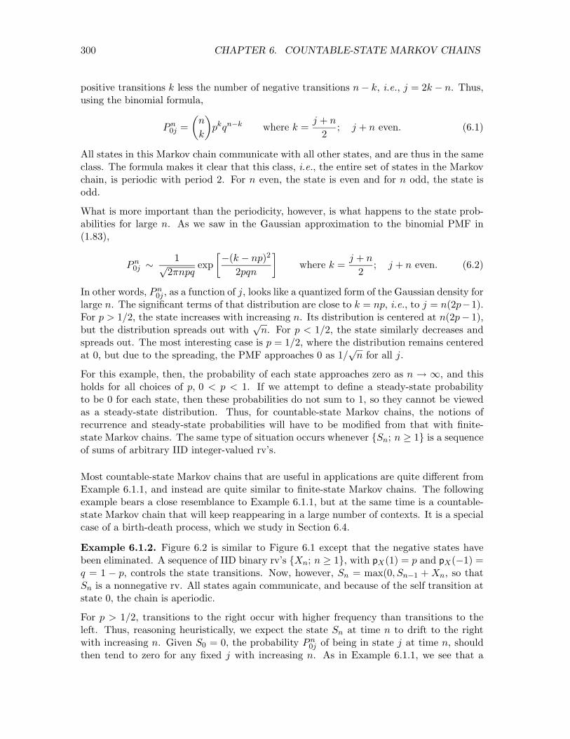
Example 6.1.1. Consider the familiar Bernoulli process {Sn = X1 + · · ·Xn; n � 1} where{Xn; n � 1} is an IID binary sequence with pX(1) = p and pX(�1) = (1 � p) = q. Thesequence {Sn; n � 1} is a sequence of integer random variables (rv’s ) where Sn = Sn�1 +1with probability p and Sn = Sn�1� 1 with probability q. This sequence can be modeled bythe Markov chain in Figure 6.1.
�2 �1 0 1 2np p p p
q q qq = 1� pq. . .n Xz
Xyn Xz
Xyn Xz
Xyn Xz
Xy. . .
Figure 6.1: A Markov chain with a countable state space modeling a Bernoulli process.If p > 1/2, then as time n increases, the state Xn becomes large with high probability,i.e., limn!1 Pr{Xn � j} = 1 for each integer j. Similarly, for p < 1/2, the statebecomes highly negative.
Using the notation of Markov chains, Pn0j is the probability of being in state j at the end
of the nth transition, conditional on starting in state 0. The final state j is the number of
299
300 CHAPTER 6. COUNTABLE-STATE MARKOV CHAINS
positive transitions k less the number of negative transitions n� k, i.e., j = 2k � n. Thus,using the binomial formula,
Pn0j =
✓n
k
◆pkqn�k where k =
j + n
2; j + n even. (6.1)
All states in this Markov chain communicate with all other states, and are thus in the sameclass. The formula makes it clear that this class, i.e., the entire set of states in the Markovchain, is periodic with period 2. For n even, the state is even and for n odd, the state isodd.
What is more important than the periodicity, however, is what happens to the state prob-abilities for large n. As we saw in the Gaussian approximation to the binomial PMF in(1.83),
Pn0j ⇠
1p2⇡npq
exp�(k � np)2
2pqn
�where k =
j + n
2; j + n even. (6.2)
In other words, Pn0j , as a function of j, looks like a quantized form of the Gaussian density for
large n. The significant terms of that distribution are close to k = np, i.e., to j = n(2p�1).For p > 1/2, the state increases with increasing n. Its distribution is centered at n(2p� 1),but the distribution spreads out with
pn. For p < 1/2, the state similarly decreases and
spreads out. The most interesting case is p = 1/2, where the distribution remains centeredat 0, but due to the spreading, the PMF approaches 0 as 1/
pn for all j.
For this example, then, the probability of each state approaches zero as n ! 1, and thisholds for all choices of p, 0 < p < 1. If we attempt to define a steady-state probabilityto be 0 for each state, then these probabilities do not sum to 1, so they cannot be viewedas a steady-state distribution. Thus, for countable-state Markov chains, the notions ofrecurrence and steady-state probabilities will have to be modified from that with finite-state Markov chains. The same type of situation occurs whenever {Sn; n � 1} is a sequenceof sums of arbitrary IID integer-valued rv’s.
Most countable-state Markov chains that are useful in applications are quite di↵erent fromExample 6.1.1, and instead are quite similar to finite-state Markov chains. The followingexample bears a close resemblance to Example 6.1.1, but at the same time is a countable-state Markov chain that will keep reappearing in a large number of contexts. It is a specialcase of a birth-death process, which we study in Section 6.4.
Example 6.1.2. Figure 6.2 is similar to Figure 6.1 except that the negative states havebeen eliminated. A sequence of IID binary rv’s {Xn; n � 1}, with pX(1) = p and pX(�1) =q = 1 � p, controls the state transitions. Now, however, Sn = max(0, Sn�1 + Xn, so thatSn is a nonnegative rv. All states again communicate, and because of the self transition atstate 0, the chain is aperiodic.
For p > 1/2, transitions to the right occur with higher frequency than transitions to theleft. Thus, reasoning heuristically, we expect the state Sn at time n to drift to the rightwith increasing n. Given S0 = 0, the probability Pn
0j of being in state j at time n, shouldthen tend to zero for any fixed j with increasing n. As in Example 6.1.1, we see that a

6.1. INTRODUCTORY EXAMPLES 301
0 1 2 3 4np p p p
q q qq = 1�pq. . .⇠: n Xz
Xyn Xz
Xyn Xz
Xyn Xz
Xy
Figure 6.2: A Markov chain with a countable state space. If p > 1/2, then as time nincreases, the state Xn becomes large with high probability, i.e., limn!1 Pr{Xn � j} =1 for each integer j.
steady state does not exist. In more poetic terms, the state wanders o↵ into the wild blueyonder.
One way to understand this chain better is to look at what happens if the chain is truncatedThe truncation of Figure 6.2 to k states (i.e., 0, 1, . . . , k�1) is analyzed in Exercise 4.9. Thesolution there defines ⇢ = p/q and shows that if ⇢ 6= 1, then ⇡i = (1 � ⇢)⇢i/(1 � ⇢k) foreach i, 0 i < k. For ⇢ = 1, ⇡i = 1/k for each i. For ⇢ < 1, the limiting behavioras k ! 1 is ⇡i = (1 � ⇢)⇢i. Thus for ⇢ < 1 ( p < 1/2), the steady state probabilitiesfor the truncated Markov chain approaches a limit which we later interpret as the steadystate probabilities for the untruncated chain. For ⇢ > 1 (p > 1/2), on the other hand,the steady-state probabilities for the truncated case are geometrically decreasing from theright, and the states with significant probability keep moving to the right as k increases.Although the probability of each fixed state j approaches 0 as k increases, the truncatedchain never resembles the untruncated chain.
Perhaps the most interesting case is that where p = 1/2. The nth order transition proba-bilities, Pn
0j can be calculated exactly for this case (see Exercise 6.3) and are very similarto those of Example 6.1.1. In particular,
Pn0j =
8<:� n(j+n)/2
�2�n for j � 0, (j + n) even� n
(j+n+1)/2
�2�n for j � 0, (j + n) odd
(6.3)
⇠r
2⇡n
exp�j2
2n
�for j � 0. (6.4)
We see that Pn0j for large n is approximated by the positive side of a quantized Gaussian
distribution. It looks like the positive side of the PMF of (6.1) except that it is no longerperiodic. For large n, Pn
0j is concentrated in a region of widthp
n around j = 0, and thePMF goes to 0 as 1/
pn for each j as n!1.
Fortunately, the strange behavior of Figure 6.2 when p � q is not typical of the Markovchains of interest for most applications. For typical countable-state Markov chains, a steadystate does exist, and the steady-state probabilities of all but a finite number of states (thenumber depending on the chain and the application) can almost be ignored for numericalcalculations.
302 CHAPTER 6. COUNTABLE-STATE MARKOV CHAINS
6.2 First passage times and recurrent states
The matrix approach used to analyze finite-state Markov chains does not generalize easilyto the countable-state case. Fortunately, a combination of first-passage-time analysis andrenewal theory are ideally suited for this purpose, especially for analyzing the long-termbehavior of countable-state Markov chains. This section develops some of the properties offirst passage times, both from a state back to itself and from one state to another. Thisis used to define recurrence and transcience and also to develop the basic properties ofrecurrent classes of states.
In Section 6.3, we use renewal theory to see that there are two kinds of recurrent states— positive recurrent and null recurrent. For example, we will see that the states of theMarkov chain in Figure 6.2 are positive recurrent for p < 1/2, null recurrent for p = 1/2, andtransient for p > 1/2. We also use renewal theory to develop the needed general theoremsabout countable-state Markov chains.
The present section will not discuss positive recurrence and null recurrence, and some of theresults will be rederived later using renewal theory. The approach here is valuable in that itis less abstract, and thus in some ways more insightful, than the renewal theory approach.
Definition 6.2.1. The first-passage-time probability, fij(n), from state i to j of a Markovchain, is the probability, conditional on X0 = i, that n is the smallest m � 1 for whichXm = j. That is, for n = 1, fij(1) = Pij. For n � 2,
fij(n) = Pr{Xn=j,Xn�1 6=j,Xn�2 6=j, . . . ,X1 6=j|X0=i} . (6.5)
The distinction between fij(n) and Pnij = Pr{Xn = j|X0 = i} is that fij(n) is the probability
that the first entry to j (after time 0) occurs at time n, whereas Pnij is the probability that
any entry to j occurs at time n, both conditional on starting in state i at time 0. Thedefinition also applies for i = j; fjj(n) is thus the probability, given X0 = j, that the firstoccurrence of state j after time 0 occurs at time n.
Since the transition probabilities are independent of time, fkj(n� 1) is also the probability,given X1 = k, that the first subsequent occurrence of state j occurs at time n. Thus wecan calculate fij(n) from the iterative relations
fij(n) =Xk 6=j
Pikfkj(n� 1); n > 1; fij(1) = Pij . (6.6)
Note that this sum excludes k = j, since Pijfjj(n�1) is the probability that state j occursfirst at epoch 1 and second at epoch n. Recall from the Chapman-Kolmogorov equationsthat Pn
ij =P
k PikPn�1kj . Thus the only di↵erence between the iterative expressions for
fij(n) and Pnij is the exclusion of k = j in the expression for fij(n).
With the iterative approach of (6.6), the first-passage-time probabilities fij(n) for a givenn must be calculated for all i before proceeding to calculate them for the next larger valueof n. This also gives us fjj(n), although fjj(n) is not used in the iteration.
6.2. FIRST PASSAGE TIMES AND RECURRENT STATES 303
Let Fij(n), for n � 1, be the probability, given X0 = i, that state j occurs at some timebetween 1 and n inclusive. Thus,
Fij(n) =nX
m=1
fij(m). (6.7)
For each i, j, Fij(n) is non-decreasing in n and (since it is a probability) is upper boundedby 1. Thus Fij(1)
�i.e., limn!1 Fij(n)
�must exist, and is the probability, given X0 = i,
that state j will ever occur. If Fij(1) = 1, then, given X0 = i, state j occurs eventuallywith probability 1. In this case, we can define a random variable (rv) Tij , conditional onX0 = i, as the first-passage time from i to j. Then fij(n) is the PMF of Tij and Fij(n) is theCDF of Tij . If Fij(1) < 1, then Tij is a defective rv, since, with some positive probability,there is no first passage to j.
The first-passage time Tjj from a state j back to itself is of particular importance. It hasthe PMF fjj(n) and the CDF Fjj(n). It is a rv (as opposed to a defective rv) if Fjj(1) = 1,i.e., if the state eventually returns to state j with probability 1, given that it starts in statej. This suggests the following definition of recurrence.
Definition 6.2.2. A state j in a countable-state Markov chain is recurrent if Fjj(1) = 1.It is transient if Fjj(1) < 1.
Thus each state j in a countable-state Markov chain is either recurrent or transient, andis recurrent if and only if an eventual return to j (conditional on X0 = j) occurs withprobability 1. Equivalently, j is recurrent if and only if Tjj , the time of first return to j,is a rv. As shown shortly, this definition is consistent with the one in Chapter 4 for thespecial case of finite-state chains. For a countably-infinite state space, however, the earlierdefinition is not adequate. An example is provided by the case p > 1/2 in Figure 6.2. Here iand j communicate for all states i and j, but it is intuitively obvious (and shown in Exercise6.2, and further explained in Section 6.4) that each state is transient.
If the initial state X0 of a Markov chain is a recurrent state j, then Tjj is the integer time ofthe first recurrence of state j. At that recurrence, the Markov chain is in the same state jas it started in, and the discrete interval from Tjj to the next occurrence of state j, say Tjj,2
has the same distribution as Tjj and is clearly independent of Tjj . Similarly, the sequence ofsuccessive recurrence intervals, Tjj , Tjj,2, Tjj,3, . . . is a sequence of IID rv’s. This sequenceof recurrence intervals1 is then the sequence of inter-renewal intervals of a renewal process,where each renewal interval has the distribution of Tjj . These inter-renewal intervals havethe PMF fjj(n) and the CDF Fjj(n).
Since results about Markov chains depend heavily on whether states are recurrent or tran-sient, we will look carefully at the probabilities Fij(n). Substituting (6.6) into (6.7) and
1Note that in Chapter 5 the inter-renewal intervals were denoted X1, X2, . . . , whereas here X0, X1, . . . isthe sequence of states in the Markov chain and Tjj , Tjj,2, . . . is the sequence of inter-renewal intervals.

304 CHAPTER 6. COUNTABLE-STATE MARKOV CHAINS
noting that fij(n) in (6.6) has a di↵erent form for n = 1 than n > 1, we obtain
Fij(n) = Pij +nX
m=2
fij(m) = Pij +nX
m=2
Xk 6=j
Pikfkj(m� 1)
= Pij +Xk 6=j
PikFkj(n� 1); n > 1; Fij(1) = Pij . (6.8)
Since Fij(n) is non-decreasing in n and upper bounded by 1, the limit Fij(1) must exist.Similarly,
Pk 6=j PikFkj(n�1) is non-decreasing in n and upper bounded by 1, so it also has
a limit, equal toP
k 6=j PikFkj(1). Thus
Fij(1) = Pij +Xk 6=j
PikFkj(1). (6.9)
For any given j, (6.9) can be viewed as a set of linear equations in the variables Fij(1)for each state i. This set of equations does not always have a unique solution to. In fact,substituting xij for Fij(1), the equations
xij = Pij +Xk 6=j
Pikxkj ; all states i (6.10)
always have a solution in which xij = 1 for all i. If state j is transient, however, thereis another solution in which xij is the true value of Fij(1) and Fjj(1) < 1. Exercise 6.1shows that if (6.10) is satisfied by a set of nonnegative numbers {xij ; 1 i J}, thenFij(1) xij for each i. In other words, Fij(1) is the minimum xij over solutions to (6.10).
An interesting feature of (6.9) arises in the case i = j,
Fjj(1) = Pjj +Xk 6=j
PjkFkj(1).
If j is recurrent, i.e., if Fjj(1) = 1, then the right side of this equation is also 1. Thus,for each k 6= j for which Pjk > 0, it is necessary that Fkj(1) = 1. In other words, if jis recurrent, then each possible transition out of j goes to a state from which an eventualreturn to j occurs with probability 1. This extends to the following lemma:
Lemma 6.2.1. Assume that state j is recurrent and that a path exists from j to i. ThenFij(1) = 1.
Proof: We just saw that if j is recurrent and Pjk > 0, then Fkj(1) = 1. Thus the lemma isproven for paths of length 1. Next consider any path of length 2, say j, k, `, where Pjk > 0and Pk` > 0. From (6.9),
Fkj(1) = Pkj +X6̀=k
Pk`F`j(1).
Since Fkj(1) = 1, the right side of the above equation is also 1. Since Pk` > 0, it followsthat F`j(1) must be 1. This argument iterates over increasing path lengths.

6.2. FIRST PASSAGE TIMES AND RECURRENT STATES 305
This lemma gives us some insight into the di↵erence between recurrence for finite-statechains and countable-state chains. For the finite-state case, j is recurrent if there is a pathback to j from each i accessible from j,. Here, not only is a return path required, but aneventual return with probability 1, (i.e., Fij(1) = 1).
The following result, Lemma 6.2.2, is similar. The two lemmas each concern a state i that isaccessible from a recurrent state j. Lemma 6.2.1 says that starting in i, an eventual returnto j must occur and Lemma 6.2.2 says that starting in j, an eventual visit to i must occur.In other words, Lemma 6.2.2 says that if j is recurrent, then any state reachable from jmust be reached eventually.
Lemma 6.2.2. Assume that state j is recurrent and that a path exists from j to i. ThenFji(1) = 1.
Proof: Let Tjj be the first-passage time from state j to j and let Tjj , Tjj,2, Tjj,3, . . . be thesequence of successive recurrence intervals. Since j is recurrent, these successive recurrenceintervals are IID rv’s (i.e., non-defective), and thus, for each n, T (n)
jj = Tjj +Tjj,2 + · · ·Tjj,n
must be a rv (see Exercise 1.13). This rv is the time of the nth recurrence of state j, andthis nth recurrence must occur eventually since T (n)
jj is a rv.
By assumption, there is a path, say j, k, `, . . . , h, i from j to i and this path is taken, startingat time 0, with probability ↵ = PjkPk` · · ·Phi > 0. If this initial path is taken, then state iis visited before the first recurrence of state j. Thus the probability that the first recurrenceof state j occurs before i is visited is at most 1�↵. In the same way, the given path from jto i can be taken starting at each recurrence of state j. It follows that the probability thatthe nth recurrence of state j occurs before the first passage to state i is at most (1� ↵)n.Since the nth recurrence of state j occurs eventually, the probability that i is never visitedis at most (1 � ↵)n. Since n is arbitrary, the probability that i is never visited is 0, soFji(1) = 1.
The above proof is a little cavalier in the sense that Fji(1) is limt!1 Fji(t) and this limithas been exchanged with others without justification. Exercise 6.5 shows how to handlethis mathematical detail.
We now get an unexpected dividend from Lemmas 6.2.1 and 6.2.2. If state j is recurrentand i is accessible from j, we now show that i is recurrent also. The reason is that, startingin state i, state j is eventually reached WP1, and then, from j, state i is eventually reached.Stating this in an equation,
Fii(t + ⌧) � Fij(t)Fji(⌧).
Going to the limits t!1, ⌧ !1,
limn!1
Fii(n) � limt!1
Fij(t) lim⌧!1
Fji(⌧) = 1.
There is a slight peculiarity here in that we have shown that i is recurrent assuming onlythat j is recurrent and that j ! i. The resolution is that, from Lemma 6.2.1, if j is recurrentand j ! i, then Fij(1) = 1, which implies that i! j.
We can summarize these results in the following theorem.
306 CHAPTER 6. COUNTABLE-STATE MARKOV CHAINS
Theorem 6.2.1. If state j of a countable-state Markov chain is recurrent, then every statei in the same class as j is recurrent, i.e., Fii(1) = 1. Also Fji(1) = 1 and Fij(1) = 1
This says that either each state in a class is recurrent or each is transient. Furthermore, fora recurrent class, the first passage time from each state to each other state is a rv.
6.3 Renewal theory applied to Markov chains
We have defined a state j to be recurrent if Fjj(1) = 1 and have seen that if j is recurrent,then the returns to state j given X0 = j form a renewal process. All of the results of renewaltheory can then be applied to the random sequence of integer times at which j is entered.Several important results from renewal theory are then stated in the following theorem.
Theorem 6.3.1. Let {Njj(t); t � 0} be the counting process for occurrences of state j upto time t in a Markov chain with X0 = j. The following conditions are then equivalent.
1. state j is recurrent.
2. limt!1Njj(t) = 1 with probability 1.
3. limt!1 E [Njj(t)] = 1.
4. limt!1P
1nt Pnjj = 1.
Proof: First assume that j is recurrent, i.e., that Fjj(1) = 1. This implies that the inter-renewal times between occurrences of j are IID rv’s, and consequently {Njj(t); t � 1} is arenewal counting process. Recall from Lemma 5.3.1 that, whether or not the expected inter-renewal time E [Tjj ] is finite, limt!1Njj(t) =1 with probability 1 and limt!1 E [Njj(t)] =1.
Next assume that state j is transient. In this case, the inter-renewal time Tjj is not a rv,so {Njj(t); t � 0} is not a renewal process. An eventual return to state j occurs only withprobability Fjj(1) < 1, and, since subsequent returns are independent, the total number ofreturns to state j is a geometric rv with mean Fjj(1)/[1�Fjj(1)]. Thus the total numberof returns is finite with probability 1 and the expected total number of returns is finite.This establishes the first three equivalences.
Finally, note that Pnjj is the probability of a transition to state j at integer time n, and
is thus equal to the expectation of a transition to j at integer time n (i.e., the number oftransitions at time t is 1 with probability Pn
jj and 0 otherwise). Since Njj(t) is the sum ofthe number of transitions to j over times 1 to t, we have
E [Njj(t)] =X
1nt
Pnjj ,
which establishes the final equivalence.
6.3. RENEWAL THEORY APPLIED TO MARKOV CHAINS 307
We have been looking at the counting process {Njj(t); t > 0}, which is the number of returnsto j by time t given X0 = j. We also want to look at the counting process {Nij(t); t > 0},which is the number of visits to state j by time t given X0 = i. If j is a recurrent state andi is in the same class, then Theorem 6.2.1 says that Tij , the first passage time from i to j,is a rv. The following sequence of recurrence times between each visit to j is a sequenceof IID rv’s with the distribution of Tjj . Thus {Nij(t); t > 0} is a delayed renewal process,which proves the following lemma.
Lemma 6.3.1. Let {Nij(t); t � 0} be the counting process for transitions into state j upto time t for a Markov chain conditional on the initial state X0 = i 6= j. Then if i and jare in the same recurrent class, {Nij(t); t � 0} is a delayed renewal process.
6.3.1 Renewal theory and positive recurrence
Recall that a state j is recurrent if the first passage time Tjj is a rv (i.e., if Fjj(1) = 1), andit then follows that {Njj(t); t > 0} is a renewal counting process. It is possible, however,for E [Tjj ] to be either finite or infinite. We have seen many positive rv’s that have infiniteexpectation, but having a first passage time that is a rv (i.e., finite with probability 1) butinfinite in expectation might seem strange at first. An example of this phenomenon is theMarkov chain of Figure 6.2 with p = 1/2, but it is tedious to verify this by direct calculationfrom Fjj(t). We will find better ways to calculate E [Tjj ] later, and can then look at severalexamples.
In studying renewal processes, we found that the expected inter-renewal interval, in thiscase E [Tjj ], is the reciprocal of the rate at which renewals occur, and that if E [Tjj ] = 1,the renewal rate is 0. Thus it is not surprising that there is a large di↵erence between thecase where E [Tjj ] =1 and that where E [Tjj ] <1. This suggests the following definition.
Definition 6.3.1. A state j in a countable-state Markov chain is positive recurrent ifFjj(1) = 1 and T jj <1. It is null recurrent if Fjj(1) = 1 and T jj =1.
Each state of a Markov chain is thus classified as one of the following three types — positiverecurrent, null recurrent, or transient. For the example of Figure 6.2, null-recurrence lieson a boundary between positive-recurrence and transience, which is often a good way toview null-recurrence.
Assume that state j is recurrent and consider the renewal process {Njj(t); t � 0}. Thefollowing theorem simply applies the limit theorems of renewal processes to this case.
Theorem 6.3.2. If j is a recurrent state in a countable-state Markov chain, then the re-newal counting process Njj(t) satisfies both
limt!1
Njj(t)/t = 1/T jj with probability 1, and (6.11)
limt!1
E [Njj(t)/t] = 1/T jj . (6.12)
Equations (6.11) and (6.12) are valid whether j is positive recurrent or null recurrent.
308 CHAPTER 6. COUNTABLE-STATE MARKOV CHAINS
Proof: The first equation, (6.11) is the strong law for renewal processes given in Theorem5.3.1. The case where T jj = 1 is treated in Exercise 5.9. The second equation is theelementary renewal theorem, Theorem 5.6.1.
Equations (6.11) and (6.12) suggest that 1/T jj has some of the properties associated witha steady-state probability for state j. For a Markov chain consisting of a single class ofstates, all positive recurrent, we will strengthen this association further in Theorem 6.3.5by showing that there is a unique steady-state distribution, {⇡j , j � 0} such that ⇡j = 1/T jj
for all j and such that ⇡j =P
i ⇡iPij for all j � 0 andP
j ⇡j = 1. The following theoremstarts this development by showing that (6.11) and (6.12) are independent of the startingstate.
Theorem 6.3.3. Let j be a recurrent state in a Markov chain and let i be any state in thesame class as j. Given X0 = i, let Nij(t) be the number of transitions into state j by timet and let T jj be the expected recurrence time of state j (either finite or infinite). Then
limt!1
Nij(t)/t = 1/T jj with probability 1 and (6.13)
limt!1
E [Nij(t)/t] = 1/T jj . (6.14)
Proof: Since i and j are recurrent and in the same class, Lemma 6.3.1 asserts that{Nij(t); t � 0} is a delayed renewal process for j 6= i. Thus (6.13) and (6.14) followfrom Theorems 5.8.1 and 5.8.2.
Theorem 6.3.4. All states in the same class of a Markov chain are of the same type —either all positive recurrent, all null recurrent, or all transient.
Proof: Let j be a recurrent state. From Theorem 6.2.1, all states in a class are recurrentor all are transient. Suppose that j is positive recurrent, so that 1/T jj > 0. Let i be inthe same class as j, and consider the renewal-reward process on {Njj(t); t � 0} for whichR(t) = 1 whenever the process is in state i (i.e., if Xn = i, then R(t) = 1 for n t < n+1).The reward is 0 otherwise. Let E [R] be the expected reward in an inter-renewal interval;this must be positive since i is accessible from j. From the strong law for renewal-rewardprocesses, Theorem 5.4.1,
limt!1
1t
Z t
0R(⌧)d⌧ =
E [R]T jj
with probability 1.
The term on the left is the time-average number of transitions into state i, given X0 = j,and this is 1/T ii from (6.13). Since E [R] > 0 and T jj < 1, we have 1/T ii > 0, so i ispositive recurrent. Thus if one state is positive recurrent, the entire class is, completing theproof.
If all of the states in a Markov chain are in a null-recurrent class, then 1/T jj = 0 for eachstate, and one might think of 1/T jj = 0 as a “steady-state” probability for j in the sensethat 0 is both the time-average rate of occurrence of j and the limiting probability of j.However, these “probabilities” do not add up to 1, so a steady-state probability distribution
6.3. RENEWAL THEORY APPLIED TO MARKOV CHAINS 309
does not exist. This appears rather paradoxical at first, but the example of Figure 6.2 withp = 1/2 will help clarify the situation. As time n increases (starting with X0 = i, say), therandom variable Xn spreads out over more and more states around i, and thus is less likelyto be in each individual state. For each j, limn!1 Pn
ij = 0. Thus,P
j
�limn!1 Pn
ij
�= 0.
On the other hand, for every n,P
j Pnij = 1. This is one of those unusual examples where
a limit and a sum cannot be interchanged.
6.3.2 Steady state
In Section 4.3.1, we defined the steady-state distribution of a finite-state Markov chain asa probability vector ⇡⇡⇡ that satisfies ⇡⇡⇡ = ⇡⇡⇡[P ]. In the same way, we define the steady-statedistribution of a countable-state Markov chain as a PMF {⇡i; i � 0} that satisfies
⇡j =X
i
⇡iPij for all j; ⇡i � 0 for all i;X
i
⇡i = 1. (6.15)
Assume that a set of numbers {⇡i; i � 0} exists satisfying (6.15) and assume that this setis chosen as the initial PMF for the Markov chain, i.e., Pr{X0 = i} = ⇡i for each i � 0.Then for each j � 0,
Pr{X1 = j} =X
i
Pr{X0 = i}Pij =X
i
⇡iPij = ⇡j .
In the same way, using induction on n,
Pr{Xn = j} =X
i
Pr{Xn�1 = i}Pij =X
i
⇡iPij = ⇡j . (6.16)
for all j and all n � 0. The fact that Pr{Xn = j} = ⇡j for all j � 0 and n � 0 motivatesthe definition of steady-state distribution above. On the other hand, Theorem 6.3.2 showedthat 1/T jj can be viewed as a ‘steady-state’ probability for state j, both in a time-averageand a limiting ensemble-average sense. In this section, we bring these notions of steadystate together and relate ⇡j to 1/T jj .
Before doing this, it will be helpful to restrict our attention to Markov chains with a singleclass of states. For finite-state chains, it was su�cient to restrict attention to a singlerecurrent class, whereas now a new term is needed, since a Markov chain with a single classmight be positive recurrent, null recurrent, or transient.
Definition 6.3.2. An irreducible class of states C is a class for which Pij = 0 for all i 2 Cand j /2 C. An irreducible Markov chain is a Markov chain for which all states are in asingle irreducible class, i.e., for which all states communicate
The following results are largely restricted to irreducible Markov chains, since the relationsbetween multiple classes are largely the same as for finite-state Markov chains. Between-class relations are largely separable from the properties of states within an irreducible class,and thus irreducible classes can be studied most e�ciently by considering irreducible Markovchains.
The following lemma will start the process of associating steady-state probabilities {⇡i; i �0} satisfying (6.15) with recurrence rates 1/T jj .

310 CHAPTER 6. COUNTABLE-STATE MARKOV CHAINS
Lemma 6.3.2. Consider an irreducible countable-state Markov chain in which a PMF{⇡i; i � 0} satisfies (6.15). Then this chain is positive recurrent.
Proof: Consider using the given PMF {⇡i; i � 0} as the initial distribution of the Markovchain, i.e., Pr{X0=j} = ⇡j for all j � 0. Then, as shown above, Pr{Xn=j} = ⇡j for alln � 0, j � 0. For any given j, let eNj(t) be the number of occurrences of state j from time1 to t given the PMF {⇡i; i � 0} for X0. Equating Pr{Xn=j} = ⇡j to the expectation ofan occurrence of j at time n, we have,
(1/t)Eh eNj(t)
i= (1/t)
X1nt
Pr{Xn=j} = ⇡j for all integers t � 1.
Conditioning this on the possible starting states i,
⇡j = (1/t)Eh eNj(t)
i= (1/t)
Xi
⇡iE [Nij(t)] for all integer t � 1. (6.17)
For any given state i, let Tij be the time (perhaps infinite) of the first occurrence of state jgiven X0 = i. Conditional on Tij = m, we have Nij(t) = 1 + T̂jj(m, t). where N̂jj(m, t) isthe number of recurrences of j from m + 1 to t. Thus, for all t > m,
E [Nij(t) | Tij=m] = 1 + E [Njj(t�m)] 1 + E [Njj(t)] . (6.18)
For t < m, the left side of (6.18) is 0 and for t = m, it is 1. Thus (6.18) is valid for all mincluding m =1. Since the upper bound does not depend on m, E [Nij(t)] 1+E [Njj(t)].Substituting this into (6.17) and summing over i, we get
⇡j (1/t)X
i⇡i�1 + E [Njj(t)]
�= (1/t) + (1/t)E [Njj(t)] . (6.19)
From this, E [Njj(t)] � t⇡j � 1. SinceP
i ⇡i = 1, there must be some j for which ⇡j isstrictly positive. For any given such j, limt!1 E [Njj(t)] =1.
This shows (using Theorem 6.3.1) that state j is recurrent. It then follows from Theorem6.3.2 that limt!1(1/t)E [Njj(t)] exists and is equal to 1/T jj for all j. Taking this limit in(6.19),
⇡j limt!1
(1/t)E [Njj(t)] = 1/T jj . (6.20)
Since ⇡j > 0, T jj <1, so that state j is positive recurrent. From Theorem 6.3.4, all statesare then positive recurrent.
With this lemma, we can prove the following theorem. The theorem is particularly valuablefor applications, since it says that if you can find steady state probabilities, then you canforget about all the nuances and subtleties of countable-state chains; the chain can betreated pretty much as a finite-state chain. More than that, the theorem provides a linkbetween steady state probabilities and expected first-passage-times.

6.3. RENEWAL THEORY APPLIED TO MARKOV CHAINS 311
Theorem 6.3.5. Assume an irreducible Markov chain with transition probabilities {Pij}.If (6.15) has a solution, then the solution {⇡i; i � 0} is unique. Furthermore the chain ispositive recurrent and
⇡j = 1/T jj > 0 for all j � 0. (6.21)
Conversely, if the chain is positive recurrent then (6.15) has a solution.
Proof: First assume that {⇡j ; j � 0} satisfies (6.15). From Lemma 6.3.2, each state j ispositive recurrent, so that T jj < 1 and 1/T jj > 0 for all j. Using (6.19), we see that⇡j 1/T jj for all j. We next develop a lower bound on ⇡j from (6.17). For each integerm > 0,
⇡j � (1/t)mX
i=1
⇡iE [Nij(t)] for all integer t � 1.
Using Theorem 6.3.3 to take the limit of this as t!1,
⇡j � limt!1
(1/t)E [Njj(t)] = 1/T jj .
Combined with ⇡j 1/T jj , this establishes (6.21).
Conversely, assume the chain is positive recurrent. We will choose ⇡j = 1/T jj and thenshow that the resulting {⇡i; i � 0} is a PMF satisfying (6.15). Each ⇡j is positive since bydefinition of positive recurrence, T jj <1. We first show that
Pj ⇡j = 1. For any given i,
consider the renewal process {Nii(t); t > 0 and for any j, let Rij(t) be the reward processassigning unit reward on each occurrence of state j. Let Rij be the aggregate reward inthe first inter-renewal interval. For j = i, note that Rii = 1 since a unit reward occurs atthe end of the interval and can not occur elsewhere. Since each step of the Markov processenters some state j and the first renewal occurs at time Tii, we have
Tii =1X
j=1
Rij .
Taking the expectation of each side,
E [Tii] = E
24 lim
`!1
X̀j=1
Rij
35 = lim
`!1
X̀j=1
E [Rij ] , (6.22)
where the interchange of limit and expectation is warranted because the terms in the limitare non-decreasing and bounded. Using Theorem 5.4.1, E [Rij ] = ⇡j/⇡i. Thus we canrewrite (6.22) as 1/⇡i =
Pj ⇡j/⇡i, which shows that
Pj ⇡j = 1.
Finally we must show that ⇡i =P
j ⇡jPji. The proof is a variation on the one just used. Welook again at the renewal process Nii(t) and define a reward function Ri(j,i)(t) that assignsone unit of reward for each transition from state j to state i. A unit reward can occur only
312 CHAPTER 6. COUNTABLE-STATE MARKOV CHAINS
at the end of the first renewal and that unit reward goes to the state j from which thetransition to i occurs. Thus, arguing as above,
1Xj=1
Ri(j,i) = 11X
j=1
E⇥Ri(j,i)
⇤= 1. (6.23)
By looking at the delayed renewal process {Nij(t); t � 0, we see that Ri(j,i)(t) is 1 whenevera renewal of state j occurs followed immediately by a transition to i. Thus the reward ratefor Ri(j,i)(t) is ⇡jPji. Applying Theorem 5.4.1, the expected reward over the first renewalof state i is ⇡jPji/⇡i. Substituting this into (6.23) then completes the proof.
In practice, it is usually easy to see whether a chain is irreducible. We shall also see by anumber of examples that the steady-state distribution can often be calculated from (6.15).Theorem 6.3.5 then says that the calculated distribution is unique and that its existenceguarantees that the chain is positive recurrent. It also shows that the expected inter-renewalinterval Tjj for each state j is given simply by 1/⇡j . Finally, Exercise 6.7 provides a simpleway to calculate T ij .
6.3.3 Blackwell’s theorem applied to Markov chains
The results so far about steady state have ignored a large part of what we would intuitivelyview as a steady state, i.e., the notion that Pn
ij should approach ⇡j as n!1, independentof i. We know from studying finite-state Markov chains that this is too much to hope forif an irreducible chain is periodic, but the discussion for countable-state chains has not yetdiscussed periodicity.
Consider applying Blackwell’s theorem to the renewal process {Njj(t); t � 0} for a positive-recurrent chain. Recall that the period of a given state j in a Markov chain (whether thechain has a countable or finite number of states) is the greatest common divisor of the setof integers n > 0 such that Pn
jj > 0. If this period is d, then {Njj(t); t � 0} is arithmeticwith span d (i.e., renewals occur only at times that are multiples of d). From Blackwell’stheorem in the arithmetic form of (5.64),
limn!1
Pndjj = d/T jj . (6.24)
As with finite-state chains, all states have the same period d for a periodic positive-recurrentchain, and, as in Theorem 4.2.3, the states can be partitioned into d classes and all tran-sitions cycle from S0 to S1 to S2 and so forth to Sd�1 and then back to S0. For the casewhere state j is aperiodic (i.e., d = 1), this says that
limn!1
Pnjj = 1/T jj . (6.25)
Finally, Blackwell’s theorem for delayed renewal processes, Theorem 5.8.3, asserts that ifthe states are aperiodic, then for all states, i and j,
limn!1
Pnij = 1/T jj . (6.26)

6.3. RENEWAL THEORY APPLIED TO MARKOV CHAINS 313
An aperiodic positive-recurrent Markov chain is defined to be an ergodic chain, and theinterpretation of this is the same as with finite- state Markov chains. In particular, forergodic chains, the steady-state probability ⇡j is, with probability 1, the time average rateof that state. It is also the time and ensemble average rate of the state, and, from (6.26),the limiting probability of the state, independent of the starting state.
The independence of starting state in the limit n!1 in (6.26) is unfortunately not uniformin i and j. For example, the state can change by at most 1 per unit time in the examplein Figure 6.2, and thus starting in a very high-numbered state i will significantly influencePn
ij until n is very large.
6.3.4 Age of a renewal process
Consider a renewal process {N(t); t > 0} in which the inter-renewal random variables{Wj ; j � 1} are arithmetic with span 1. We will use a Markov chain to model the age ofthis process (see Figure 6.3). The probability that a renewal occurs at a particular integertime depends on the past only through the integer time back to the last renewal. The stateof the Markov chain during a unit interval will be taken as the age of the renewal processat the beginning of the interval. Thus, each unit of time, the age either increases by one ora renewal occurs and the age decreases to 0 (i.e., if a renewal occurs at time t, the age attime t is 0).
0 1 2 3 4nP00 P01 P12 P23 P34
P10P20 P30 P40
HY. . .n Xz
Xyn Xz n Xz n Xz
⇠:
Figure 6.3: A Markov chain model of the age of a renewal process.
Pr{W > j} is the probability that an inter-renewal interval lasts for more than j time units.We assume that Pr{W > 0} = 1, so that each renewal interval lasts at least one time unit.The probability Pj,0 in the Markov chain is the probability that a renewal interval has du-ration j+1, given that the interval exceeds j. Thus, for example, P00 is the probability thatthe renewal interval is equal to 1. Pj,j+1 is 1� Pj,0, which is Pr{W > j + 1} /Pr{W > j}.We can then solve for the steady state probabilities in the chain: for j > 0,
⇡j = ⇡j�1Pj�1,j = ⇡j�2Pj�2,j�1Pj�1,j = ⇡0P0,1P1,2 . . . Pj�1,j .
The first equality above results from the fact that state j, for j > 0 can be entered onlyfrom state j � 1. The subsequent equalities come from substituting in the same expressionfor ⇡j�1, then ⇡j�2, and so forth.
⇡j = ⇡0Pr{W > 1}Pr{W > 2}Pr{W > 0}Pr{W > 1} . . .
Pr{W > j}Pr{W > j � 1} = ⇡0Pr{W > j} . (6.27)
We have cancelled out all the cross terms above and used the fact that Pr{W > 0} = 1.Another way to see that ⇡j = ⇡0Pr{W > j} is to observe that state 0 occurs exactly once
314 CHAPTER 6. COUNTABLE-STATE MARKOV CHAINS
in each inter-renewal interval; state j occurs exactly once in those inter-renewal intervals ofduration j or more.
Since the steady-state probabilities must sum to 1, (6.27) can be solved for ⇡0 as
⇡0 =1P1
j=0 Pr{W > j} =1
E [W ]. (6.28)
The second equality follows by expressing E [W ] as the integral of the complementary CDFof W . As a check on (6.28) (and an easier way of getting deriving it), note that this issimply Theorem 6.3.5 applied to state 0. Combining (6.28) with (6.27), the steady-stateprobabilities for j � 0 are
⇡j =Pr{W > j}
E [W ]. (6.29)
In terms of the renewal process, ⇡j is the probability that, at some large integer time,the age of the process will be j. Note that if the age of the process at an integer time isj, then the age increases toward j + 1 at the next integer time, at which point it eitherdrops to 0 or continues to rise. Thus ⇡j can be interpreted as the fraction of time that theage of the process is between j and j + 1. Recall from (5.30) (and the fact that residuallife and age are equally distributed) that the CDF of the time-average age is given byFZ(j) =
R j0 Pr{W > w} dw/E [W ]. Thus, the probability that the age is between j and
j +1 is FZ(j +1)�FZ(j). Since W is an integer random variable, this is Pr{W > j} /E [W ]in agreement with the result here.
The analysis here gives a new, and intuitively satisfying, explanation of why the age of arenewal process is so di↵erent from the inter-renewal time. The Markov chain shows theever increasing loops that give rise to large expected age when the inter-renewal time isheavy tailed (i.e., has a CDF that goes to 0 slowly with increasing time). These loops canbe associated with the isosceles triangles of Figure 5.8. The advantage here is that we canassociate the states with steady-state probabilities if the chain is positive recurrent. Evenwhen the Markov chain is null recurrent (i.e., the associated renewal process has infiniteexpected age), it seems easier to visualize the phenomenon of infinite expected age.
6.4 Birth-death Markov chains
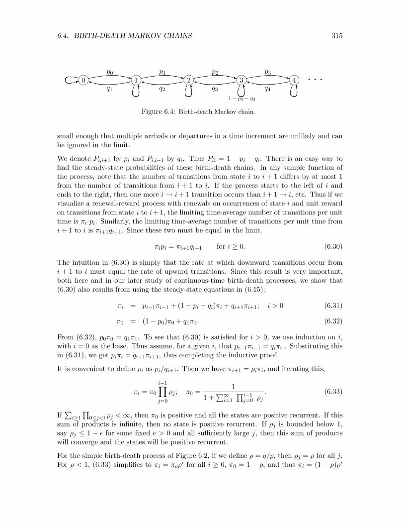
A birth-death Markov chain is a Markov chain in which the state space is the set of nonneg-ative integers; for all i � 0, the transition probabilities satisfy Pi,i+1 > 0 and Pi+1,i > 0, andfor all |i� j| > 1, Pij = 0 (see Figure 6.4). A transition from state i to i+1 is regarded as abirth and one from i+1 to i as a death. Thus the restriction on the transition probabilitiesmeans that only one birth or death can occur in one unit of time. Many applications ofbirth-death processes arise in queueing theory, where the state is the number of customers,births are customer arrivals, and deaths are customer departures. The restriction to onlyone arrival or departure at a time seems rather peculiar, but usually such a chain is a finelysampled approximation to a continuous-time process, and the time increments are then
6.4. BIRTH-DEATH MARKOV CHAINS 315
0 1 2 3 4np0 p1 p2 p3
q1 q2 q3 q4
1� p3 � q3
. . .O O O O
⇠: n XzXy
n XzXy
n XzXy
n XzXy
Figure 6.4: Birth-death Markov chain.
small enough that multiple arrivals or departures in a time increment are unlikely and canbe ignored in the limit.
We denote Pi,i+1 by pi and Pi,i�1 by qi. Thus Pii = 1 � pi � qi. There is an easy way tofind the steady-state probabilities of these birth-death chains. In any sample function ofthe process, note that the number of transitions from state i to i + 1 di↵ers by at most 1from the number of transitions from i + 1 to i. If the process starts to the left of i andends to the right, then one more i! i + 1 transition occurs than i + 1! i, etc. Thus if wevisualize a renewal-reward process with renewals on occurrences of state i and unit rewardon transitions from state i to i+1, the limiting time-average number of transitions per unittime is ⇡i pi. Similarly, the limiting time-average number of transitions per unit time fromi + 1 to i is ⇡i+1qi+1. Since these two must be equal in the limit,
⇡ipi = ⇡i+1qi+1 for i � 0. (6.30)
The intuition in (6.30) is simply that the rate at which downward transitions occur fromi + 1 to i must equal the rate of upward transitions. Since this result is very important,both here and in our later study of continuous-time birth-death processes, we show that(6.30) also results from using the steady-state equations in (6.15):
⇡i = pi�1⇡i�1 + (1� pi � qi)⇡i + qi+1⇡i+1; i > 0 (6.31)
⇡0 = (1� p0)⇡0 + q1⇡1. (6.32)
From (6.32), p0⇡0 = q1⇡1. To see that (6.30) is satisfied for i > 0, we use induction on i,with i = 0 as the base. Thus assume, for a given i, that pi�1⇡i�1 = qi⇡i . Substituting thisin (6.31), we get pi⇡i = qi+1⇡i+1, thus completing the inductive proof.
It is convenient to define ⇢i as pi/qi+1. Then we have ⇡i+1 = ⇢i⇡i, and iterating this,
⇡i = ⇡0
i�1Yj=0
⇢j ; ⇡0 =1
1 +P1
i=1
Qi�1j=0 ⇢j
. (6.33)
IfP
i�1
Q0j<i ⇢j <1, then ⇡0 is positive and all the states are positive recurrent. If this
sum of products is infinite, then no state is positive recurrent. If ⇢j is bounded below 1,say ⇢j 1 � ✏ for some fixed e > 0 and all su�ciently large j, then this sum of productswill converge and the states will be positive recurrent.
For the simple birth-death process of Figure 6.2, if we define ⇢ = q/p, then ⇢j = ⇢ for all j.For ⇢ < 1, (6.33) simplifies to ⇡i = ⇡o⇢i for all i � 0, ⇡0 = 1 � ⇢, and thus ⇡i = (1 � ⇢)⇢i

316 CHAPTER 6. COUNTABLE-STATE MARKOV CHAINS
for i � 0. Exercise 6.2 shows how to find Fij(1) for all i, j in the case where ⇢ � 1. Wehave seen that the simple birth-death chain of Figure 6.2 is transient if ⇢ > 1. This is notnecessarily so in the case where self-transitions exist, but the chain is still either transientor null recurrent. An example of this will arise in Exercise 7.3.
6.5 Reversible Markov chains
Many important Markov chains have the property that, in steady state, the sequence ofstates looked at backwards in time, i.e.,. . .Xn+1,Xn,Xn�1, . . . , has the same probabilisticstructure as the sequence of states running forward in time. This equivalence between theforward chain and backward chain leads to a number of results that are intuitively quitesurprising and that are quite di�cult to derive by other means. We shall develop and studythese results here and then redevelop them in Chapter 7 for Markov processes with discretestate spaces. This set of ideas, and its use in queueing and queueing networks, has beenan active area of queueing research over many years . It leads to many simple results forsystems that initially appear very complex. We only scratch the surface here and refer theinterested reader to [16] for a more comprehensive treatment. Before going into reversibility,we describe the backward chain for an arbitrary Markov chain.
The defining characteristic of a Markov chain {Xn; n � 0} is that for all n � 0,
Pr{Xn+1 | Xn,Xn�1, . . . ,X0} = Pr{Xn+1 | Xn} . (6.34)
For homogeneous chains, which we have been assuming throughout, Pr{Xn+1 = j | Xn = i} =Pij , independent of n. For any k > 1, we can extend (6.34) to get
Pr{Xn+k,Xn+k�1, . . . ,Xn+1 | Xn,Xn�1, . . . ,X0}
= Pr{Xn+k | Xn+k�1}Pr{Xn+k�1 | Xn+k�2} . . .Pr{Xn+1 | Xn}
= Pr{Xn+k,Xn+k�1, . . . ,Xn+1 | Xn} . (6.35)
By letting A+ be any event defined on the states Xn+1 to Xn+k and letting A� be anyevent defined on X0 to Xn�1, this can be written more succinctly as
Pr�A+ | Xn, A�
= Pr
�A+ | Xn
. (6.36)
This says that, given state Xn, any future event A+ is statistically independent of any pastevent A�. This result, namely that past and future are independent given the present state,is equivalent to (6.34) for defining a Markov chain, but it has the advantage of showing thesymmetry between past and future. This symmetry is best brought out by multiplying bothsides of (6.36) by Pr{A� | Xn}, obtaining
Pr�A+, A� | Xn
= Pr
�A+ | Xn
Pr�A� | Xn
. (6.37)
Much more broadly, any 3 ordered events, say A� ! X0 ! A+) are said to satisfy theMarkov property if Pr{A+ | X0A�} = Pr{A+ | X0}. This implies the more symmetric form

6.5. REVERSIBLE MARKOV CHAINS 317
Pr{A�A+ | X0)} = Pr{A� | X0}Pr{A+ | X0}. This symmetric form says that, conditionalon the current state, the past and future states are statistically independent. Dividing bothsides by Pr{A+ | Xn} then yields
Pr�A� | Xn, A+
= Pr
�A� | Xn
. (6.38)
By letting A� be Xn�1 and A+ be Xn+1,Xn+2, . . . ,Xn+k, this becomes
Pr{Xn�1 | Xn,Xn+1, . . . ,Xn+k} = Pr{Xn�1 | Xn} .
This is the equivalent form to (6.34) for the backward chain, and says that the backwardchain is also a Markov chain. By Bayes’ law, Pr{Xn�1 | Xn} can be evaluated as
Pr{Xn�1 | Xn} =Pr{Xn | Xn�1}Pr{Xn�1}
Pr{Xn}. (6.39)
Since the distribution of Xn can vary with n, Pr{Xn�1 | Xn} can also depend on n. Thusthe backward Markov chain is not necessarily homogeneous. This should not be surprising,since the forward chain was defined with some arbitrary distribution for the initial state attime 0. This initial distribution was not relevant for equations (6.34) to (6.36), but as soonas Pr{A� | Xn} is introduced, the initial state implicitly becomes a part of each equationand destroys the symmetry between past and future. For a chain in steady state, i.e., apositive-recurrent chain for which the distribution of each Xn is the steady state distributionsatisfying (6.15), however, Pr{Xn = j} = Pr{Xn�1 = j} = ⇡j for all j, and we have
Pr{Xn�1 = j | Xn = i} = Pji⇡j/⇡i in steady state.. (6.40)
Thus the backward chain is homogeneous if the forward chain is in steady state. For a chainwith steady-state probabilities {⇡i; i � 0}, we define the backward transition probabilitiesP ⇤ij as
⇡iP⇤ij = ⇡jPji. (6.41)
From (6.39), the backward transition probability P ⇤ij , for a Markov chain in steady state,is then equal to Pr{Xn�1 = j | Xn = i}, the probability that the previous state is j giventhat the current state is i.
Now consider a new Markov chain with transition probabilities {P ⇤ij}. Over some segmentof time for which both this new chain and the old chain are in steady state, the set of statesgenerated by the new chain is statistically indistinguishable from the backward runningsequence of states from the original chain. It is somewhat simpler, in talking about forwardand backward running chains, however, to visualize Markov chains running in steady statefrom t = �1 to t = +1. If one is uncomfortable with this, one can also visualize startingthe Markov chain at some very negative time with an initial distribution equal to thesteady-state distribution.
Definition 6.5.1. A Markov chain that has steady-state probabilities {⇡i; i � 0} is re-versible if Pij = ⇡jPji/⇡i for all i, j, i.e., if P ⇤ij = Pij for all i, j.
318 CHAPTER 6. COUNTABLE-STATE MARKOV CHAINS
Thus the chain is reversible if, in steady state, the backward running sequence of statesis statistically indistinguishable from the forward running sequence. Comparing (6.41)with the steady-state equations (6.30) that we derived for birth-death chains, we have thefollowing important theorem:
Theorem 6.5.1. Every birth-death chain with a steady-state probability distribution is re-versible.
We saw that for birth-death chains, the equation ⇡iPij = ⇡jPji (which only had to be consid-ered for |i� j| 1) provided a very simple way of calculating the steady-state probabilities.Unfortunately, it appears that we must first calculate the steady-state probabilities in orderto show that a chain is reversible. The following simple theorem gives us a convenientescape from this dilemma.
Theorem 6.5.2. Assume that an irreducible Markov chain has transition probabilities {Pij}.Suppose {⇡i} is a set of positive numbers summing to 1 and satisfying
⇡iPij = ⇡jPji; all i, j. (6.42)
then, first, {⇡i; i � 0} is the steady-state distribution for the chain, and, second, the chainis reversible.
Proof: Given a solution to (6.42) for all i and j, we can sum (6.42) over i for each j.X
i
⇡iPij = ⇡j
Xi
Pji = ⇡j . (6.43)
Thus the solution to (6.42), along with the constraints ⇡i > 0,P
i ⇡i = 1, satisfies the steady-state equations, (6.15). From Theorem 6.3.5, this is the unique steady-state distribution.Since (6.42) is satisfied, the chain is also reversible.
It is often possible, sometimes by using an educated guess, to find a solution to (6.42). Ifthis is successful, then we are assured both that the chain is reversible and that the actualsteady-state probabilities have been found.
Note that the theorem applies to periodic chains as well as to aperiodic chains. If the chainis periodic, then the steady-state probabilities have to be interpreted as average values overthe period, but Theorem 6.3.5 shows that (6.43) still has a unique solution (assuming apositive-recurrent chain). On the other hand, for a chain with period d > 1, there are dsubclasses of states and the sequence {Xn} must rotate between these classes in a fixedorder. For this same order to be followed in the backward chain, the only possibility isd = 2. Thus periodic chains with periods other than 2 cannot be reversible.
There are several simple tests that can be used to show that an irreducible chain is notreversible. First, the steady-state probabilities must satisfy ⇡i > 0 for all i, and thus, ifPij > 0 but Pji = 0 for some i, j, then (6.42) cannot be satisfied and the chain is notreversible. Second, consider any set of three states, i, j, k. If PjiPikPkj is unequal toPjkPkiPij then the chain cannot be reversible. To see this, note that (6.42) requires that
⇡i = ⇡jPji/Pij = ⇡kPki/Pik.

6.6. THE M/M/1 SAMPLE-TIME MARKOV CHAIN 319
Thus, ⇡jPjiPik = ⇡kPkiPij . Equation (6.42) also requires that ⇡jPjk = ⇡kPkj . Taking theratio of these equations, we see that PjiPikPkj = PjkPkiPij . Thus if this equation is notsatisfied, the chain cannot be reversible. In retrospect, this result is not surprising. Whatit says is that for any cycle of three states, the probability of three transitions going aroundthe cycle in one direction must be the same as the probability of going around the cycle inthe opposite (and therefore backwards) direction.
It is also true (see [22] for a proof), that a necessary and su�cient condition for a chainto be reversible is that the product of transition probabilities around any cycle of arbitrarylength must be the same as the product of transition probabilities going around the cyclein the opposite direction. This doesn’t seem to be a widely useful way to demonstratereversibility.
There is another result, generalizing Theorem 6.5.2, for finding the steady-state probabilitiesof an arbitrary Markov chain and simultaneously finding the transition probabilities of thebackward chain.
Theorem 6.5.3. Assume that an irreducible Markov chain has transition probabilities {Pij}.Suppose {⇡i} is a set of positive numbers summing to 1 and that {P ⇤ij} is a set of transitionprobabilities satisfying
⇡iPij = ⇡jP⇤ji; all i, j. (6.44)
Then {⇡i} is the steady-state distribution and {P ⇤ij} is the set of transition probabilities forthe backward chain.
Proof: Summing (6.44) over i, we get the steady-state equations for the Markov chain, sothe fact that the given {⇡i} satisfy these equations asserts that they are the steady-stateprobabilities. Equation (6.44) then asserts that {P ⇤ij} is the set of transition probabilitiesfor the backward chain.
The following two sections illustrate some important applications of reversibility.
6.6 The M/M/1 sample-time Markov chain
The M/M/1 Markov chain is a sampled-time model of the M/M/1 queueing system. Recallthat the M/M/1 queue has Poisson arrivals at some rate � and IID exponentially distributedservice times at some rate µ. We assume throughout this section that � < µ (this isrequired to make the states positive recurrent). For some given small increment of time�, we visualize observing the state of the system at the sample times n�. As indicated inFigure 6.5, the probability of an arrival in the interval from (n � 1)� to n� is modeled as��, independent of the state of the chain at time (n� 1)� and thus independent of all priorarrivals and departures. Thus the arrival process, viewed as arrivals in subsequent intervalsof duration �, is Bernoulli, thus approximating the Poisson arrivals. This is a sampled-timeapproximation to the Poisson arrival process of rate � for a continuous-time M/M/1 queue.
When the system is non-empty (i.e., the state of the chain is one or more), the probabilityof a departure in the interval (n � 1)� to n� is µ�, thus modeling the exponential servicetimes. When the system is empty, of course, departures cannot occur.

320 CHAPTER 6. COUNTABLE-STATE MARKOV CHAINS
0 1 2 3 4
1� �(µ + �)
n�� �� �� ��
µ� µ� µ� µ�
. . .O O O O
⇠: n XzXy
n XzXy
n XzXy
n XzXy
Figure 6.5: Sampled-time approximation to M/M/1 queue for time increment �.
Note that in our sampled-time model, there can be at most one arrival or departure in aninterval (n� 1)� to n�. As in the Poisson process, the probability of more than one arrival,more than one departure, or both an arrival and a departure in an increment � is of order�2 for the actual continuous-time M/M/1 system being modeled. Thus, for � very small,we expect the sampled-time model to be relatively good. At any rate, if � 1/(µ + �),the self -transitions have nonnegative probability and the model can be analyzed with nofurther approximations.
Since this chain is a birth-death chain, we can use (6.33) to determine the steady-stateprobabilities; they are
⇡i = ⇡0⇢i ; ⇢ = �/µ < 1.
Setting the sum of the ⇡i to 1, we find that ⇡0 = 1� ⇢, so
⇡i = (1� ⇢)⇢i ; all i � 0. (6.45)
Thus the steady-state probabilities exist and the chain is a birth-death chain, so fromTheorem 6.5.1, it is reversible. We now exploit the consequences of reversibility to findsome rather surprising results about the M/M/1 chain in steady state. Figure 6.6 illustratesa sample path of arrivals and departures for the chain. To avoid the confusion associatedwith the backward chain evolving backward in time, we refer to the original chain as thechain moving to the right and to the backward chain as the chain moving to the left.
There are two types of correspondence between the right-moving and the left-moving chain:
1. The left-moving chain has the same Markov chain description as the right-movingchain, and thus can be viewed as an M/M/1 chain in its own right. We still labelthe sampled-time intervals from left to right, however, so that the left-moving chainmakes transitions from Xn+1 to Xn to Xn�1 etc. Thus, for example, if Xn = i andXn�1 = i+1, the left-moving chain is viewed as having an arrival in the interval fromn� to (n � 1)�. The sequence of such downward transition moving to the left is aBernoulli process
2. Each sample function . . . xn�1, xn, xn+1 . . . of the right-moving chain corresponds tothe same sample function . . . xn+1, xn, xn�1 . . . of the left-moving chain, where Xn�1 =xn�1 is to the left of Xn = xn for both chains. With this correspondence, an arrivalto the right-moving chain in the interval (n� 1)� to n� is a departure from the left-moving chain in the interval n� to (n � 1)�, and a departure from the right-movingchain is an arrival to the left-moving chain. Using this correspondence, each event inthe left-moving chain corresponds to some event in the right-moving chain.

6.6. THE M/M/1 SAMPLE-TIME MARKOV CHAIN 321
In each of the properties of the M/M/1 chain to be derived below, a property of the left-moving chain is developed through correspondence 1 above, and then that property istranslated into a property of the right-moving chain by correspondence 2.
Property 1: Since the arrival process of the right-moving chain is Bernoulli, the arrivalprocess of the left-moving chain is also Bernoulli (by correspondence 1). Looking at asample function xn+1, xn, xn�1 of the left-moving chain (i.e., using correspondence 2), anarrival in the interval n� to (n� 1)� of the left-moving chain is a departure in the interval(n� 1)� to n� of the right-moving chain. Since the arrivals in successive increments of theleft-moving chain are independent and have probability �� in each increment �, we concludethat departures in the right-moving chain are similarly Bernoulli (see Figure 6.6).
��
��
��
��
��
��
��
��
��
��H
HH
HH
HH
H
HH
HH
HH
HHr
r r r rr
rr
� -�
HH
HH
HH
HH
HH
HH
HH
HH
HH
HH
HH
HH
HH
HH
HH
HH
rr r r r r r rr r r r
r r rr
r
��
��
��
��
��
��
��
��
��
��
��
��
��
��
��
��
��
��r r r r
r r r r r rr r r
r
Departures�
Departures
State
Arrivals
Arrivals
�
-
-
Figure 6.6: Sample function of M/M/1 chain over a busy period and correspondingarrivals and departures for right and left-moving chains. Arrivals and departures areviewed as occurring between the sample times, and an arrival in the left-moving chainbetween time n� and (n + 1)� corresponds to a departure in the right-moving chainbetween (n + 1)� and n�.
The fact that the departure process is Bernoulli with departure probability �� in eachincrement is surprising. Note that the probability of a departure in the interval (n�� �, n�]is µ� conditional on Xn�1 � 1 and is 0 conditional on Xn�1 = 0. Since Pr{Xn�1 � 1} =1 � Pr{Xn�1 = 0} = ⇢, we see that the unconditional probability of a departure in theinterval (n� � �, n�] is ⇢µ� = �� as asserted above. The fact that successive departures areindependent is much harder to derive without using reversibility (see exercise 6.15).
Property 2: In the original (right-moving) chain, arrivals in the time increments aftern� are independent of Xn. Thus, for the left-moving chain, arrivals in time increments tothe left of n� are independent of the state of the chain at n�. From the correspondencebetween sample paths, however, a left chain arrival is a right chain departure, so that forthe right-moving chain, departures in the time increments prior to n� are independent of

322 CHAPTER 6. COUNTABLE-STATE MARKOV CHAINS
Xn, which is equivalent to saying that the state Xn is independent of the prior departures.This means that if one observes the departures prior to time n�, one obtains no informationabout the state of the chain at n�. This is again a surprising result. To make it seem moreplausible, note that an unusually large number of departures in an interval from (n�m)� ton� indicates that a large number of customers were probably in the system at time (n�m)�,but it doesn’t appear to say much (and in fact it says exactly nothing) about the numberremaining at n�.
The following theorem summarizes these results.
Theorem 6.6.1 (Burke’s theorem for sampled-time). Given an M/M/1 Markov chainin steady state with � < µ,
a) the departure process is Bernoulli with departure probability �� per increment,
b) the state Xn at any time n� is independent of departures prior to n�.
The proof of Burke’s theorem above did not use the fact that the departure probability is thesame for all states except state 0. Thus these results remain valid for any birth-death chainwith Bernoulli arrivals that are independent of the current state (i.e., for which Pi,i+1 = ��for all i � 0). One important example of such a chain is the sampled time approximationto an M/M/m queue. Here there are m servers, and the probability of departure from statei in an increment � is µi� for i m and µm� for i > m. For the states to be recurrent,and thus for a steady state to exist, � must be less than µm. Subject to this restriction,properties a) and b) above are valid for sampled-time M/M/m queues.
6.7 Branching processes
Branching processes provide a simple model for studying the population of various types ofindividuals from one generation to the next. The individuals could be photons in a photo-multiplier, particles in a cloud chamber, micro-organisms, insects, or branches in a datastructure.
Let Xn be the number of individuals in generation n of some population. Each of theseXn individuals, independently of each other, produces a random number of o↵spring, andthese o↵spring collectively make up generation n + 1. More precisely, a branching processis a Markov chain in which the state Xn at time n models the number of individuals ingeneration n. Denote the individuals of generation n as {1, 2, ...,Xn} and let Yk,n be thenumber of o↵spring of individual k. The random variables Yk,n are defined to be IID overk and n, with a PMF pj = Pr{Yk,n = j}. The state at time n + 1, namely the number ofindividuals in generation n + 1, is
Xn+1 =XnXk=1
Yk,n. (6.46)

6.7. BRANCHING PROCESSES 323
Assume a given distribution (perhaps deterministic) for the initial state X0. The transitionprobability, Pij = Pr{Xn+1 = j | Xn = i}, is just the probability that Y1,n+Y2,n+· · ·+Yi,n =j. The zero state (i e., the state in which there are no individuals) is a trapping state (i.e.,P00 = 1) since no future o↵spring can arise in this case.
One of the most important issues about a branching process is the probability that thepopulation dies out eventually. Naturally, if p0 (the probability that an individual has noo↵spring) is zero, then each generation must be at least as large as the generation before,and the population cannot die out unless X0 = 0. We assume in what follows that p0 > 0and X0 > 0. Recall that Fij(n) was defined as the probability, given X0 = i, that state j isentered between times 1 and n. From (6.8), this satisfies the iterative relation
Fij(n) = Pij +Xk 6=j
PikFkj(n� 1), n > 1; Fij(1) = Pij . (6.47)
The probability that the process dies out by time n or before, given X0 = i, is thus Fi0(n).For the nth generation to die out, starting with an initial population of i individuals, thedescendants of each of those i individuals must die out. Since each individual generatesdescendants independently, we have Fi0(n) = [F10(n)]i for all i and n. Because of thisrelationship, it is su�cient to find F10(n), which can be determined from (6.47). Observethat P1k is just pk, the probability that an individual will have k o↵spring. Thus, (6.47)becomes
F10(n) = p0 +1X
k=1
pk[F10(n� 1)]k =1X
k=0
pk[F10(n� 1)]k. (6.48)
Let h(z) =P
k pkzk be the z transform of the number of an individual’s o↵spring. Then(6.48) can be written as
F10(n) = h(F10(n� 1)). (6.49)
This iteration starts with F10(1) = p0. Figure 6.7 shows a graphical construction for eval-uating F10(n). Having found F10(n) as an ordinate on the graph for a given value of n, wefind the same value as an abscissa by drawing a horizontal line over to the straight line ofslope 1; we then draw a vertical line back to the curve h(z) to find h(F10(n)) = F10(n + 1).
For the two subfigures shown, it can be seen that F10(1) is equal to the smallest root ofthe equation h(z) � z = 0. We next show that these two figures are representative of allpossibilities. Since h(z) is a z transform, we know that h(1) = 1, so that z = 1 is oneroot of h(z) � z = 0. Also, h0(1) = Y , where Y =
Pk kpk is the expected number of an
individual’s o↵spring. If Y > 1, as in Figure 6.7a, then h(z) � z is negative for z slightlysmaller than 1. Also, for z = 0, h(z)� z = h(0) = p0 > 0. Since h00(z) � 0, there is exactlyone root of h(z) � z = 0 for 0 < z < 1, and that root is equal to F10(1). By the sametype of analysis, it can be seen that if Y 1, as in Figure 6.7b, then there is no root ofh(z)� z = 0 for z < 1, and F10(1) = 1.
As we saw earlier, Fi0(1) = [F10(1)]i, so that for any initial population size, there is aprobability strictly between 0 and 1 that successive generations eventually die out for Y > 1,

324 CHAPTER 6. COUNTABLE-STATE MARKOV CHAINS
��
��
��
��
��
p0 F10(1)F10(2)
F10(3)F10(1)
1
h(z)
��
��
��
��
��
p0 F10(1)
F10(2)F10(3)
F10(1)1
h(z)
z
h(z)
(a) (b)
Figure 6.7: Graphical construction to find the probability that a population dies out.Here F10(n) is the probability that a population starting with one member at generation0 dies out by generation n or before. Thus F10(1) is the probability that the populationever dies out.
and probability 1 that successive generations eventually die out for Y 1. Since state 0 isaccessible from all i, but F0i(1) = 0, it follows from Lemma 6.2.2 that all states other thanstate 0 are transient.
We next evaluate the expected number of individuals in a given generation. Conditional onXn�1 = i, (6.46) shows that the expected value of Xn is iY . Taking the expectation overXn�1, we have
E [Xn] = Y E [Xn�1] . (6.50)
Iterating this equation, we get
E [Xn] = YnE [X0] . (6.51)
Thus, if Y > 1, the expected number of individuals in a generation increases exponentiallywith n, and Y gives the rate of growth. Physical processes do not grow exponentiallyforever, so branching processes are appropriate models of such physical processes only oversome finite range of population. Even more important, the model here assumes that thenumber of o↵spring of a single member is independent of the total population, which ishighly questionable in many areas of population growth. The advantage of an oversimplifiedmodel such as this is that it explains what would happen under these idealized conditions,thus providing insight into how the model should be changed for more realistic scenarios.
It is important to realize that, for branching processes, the mean number of individualsis not a good measure of the actual number of individuals. For Y = 1 and X0 = 1, theexpected number of individuals in each generation is 1, but the probability that Xn = 0approaches 1 with increasing n; this means that as n gets large, the nth generation containsa large number of individuals with a very small probability and contains no individuals witha very large probability. For Y > 1, we have just seen that there is a positive probabilitythat the population dies out, but the expected number is growing exponentially.
A surprising result, which is derived from the theory of martingales in Chapter 9, is thatif X0 = 1 and Y > 1, then the sequence of random variables Xn/Y
n has a limit with
6.8. ROUND-ROBIN AND PROCESSOR SHARING 325
probability 1. This limit is a random variable; it has the value 0 with probability F10(1),and has larger values with some given distribution. Intuitively, for large n, Xn is either 0or very large. If it is very large, it tends to grow in an orderly way, increasing by a multipleof Y in each subsequent generation.
6.8 Round-robin and processor sharing
Typical queueing systems have one or more servers who each serve customers in FCFS order,serving one customer completely while other customers wait. These typical systems havelarger average delay than necessary. For example, if two customers with service requirementsof 10 and 1 units respectively are waiting when a single server becomes empty, then servingthe first before the second results in departures at times 10 and 11, for an average delayof 10.5. Serving the customers in the opposite order results in departures at times 1 and11, for an average delay of 6. Supermarkets have recognized this for years and have specialexpress checkout lines for customers with small service requirements.
Giving priority to customers with small service requirements, however, has some disadvan-tages; first, customers with high service requirements can feel discriminated against, andsecond, it is not always possible to determine the service requirements of customers beforethey are served. The following alternative to priorities is popular both in the computer anddata network industries. When a processor in a computer system has many jobs to accom-plish, it often serves these jobs on a time-shared basis, spending a small increment of timeon one, then the next, and so forth. In data networks, particularly high-speed networks,messages are broken into small fixed-length packets, and then the packets from di↵erentmessages can be transmitted on an alternating basis between messages.
A round-robin service system is a system in which, if there are m customers in the system,say c1, c2, . . . , cm, then c1 is served for an incremental interval �, followed by c2 being servedfor an interval �, and so forth up to cm. After cm is served for an interval �, the serverreturns and starts serving c1 for an interval � again. Thus the customers are served in acyclic, or “round-robin” order, each getting a small increment of service on each visit fromthe server. When a customer’s service is completed, the customer leaves the system, m isreduced, and the server continues rotating through the now reduced cycle as before. Whena new customer arrives, m is increased and the new customer must be inserted into thecycle of existing customers in a way to be discussed later.
Processor sharing is the limit of round-robin service as the increment � goes to zero. Thus,with processor sharing, if m customers are in the system, all are being served simultaneously,but each is being served at 1/m times the basic server rate. For the example of two customerswith service requirement 1 and 10, each customer is initially served at rate 1/2, so onecustomer departs at time 2. At that time, the remaining customer is served at rate 1 anddeparts at time 11. For round-robin service with an increment of 1, the customer with unitservice requirement departs at either time 1 or 2, depending on the initial order of service.With other increments of service, the results are slightly di↵erent.
We first analyze round-robin service and then go to the processor-sharing limit as � ! 0.As the above example suggests, the results are somewhat cleaner in the limiting case, but
326 CHAPTER 6. COUNTABLE-STATE MARKOV CHAINS
more realistic in the round-robin case. Round robin provides a good example of the use ofbackward transition probabilities to find the steady-state distribution of a Markov chain.The techniques used here are quite similar to those used in the next chapter to analyzequeueing networks.
Assume a Bernoulli arrival process in which the probability of an arrival in an interval �is ��. Assume that the ith arriving customer has a service requirement Wi. The randomvariables Wi, i � 1, are IID and independent of the arrival epochs. Thus, in terms ofthe arrival process and the service requirements, this is the same as an M/G/1 queue (seeSection 5.5.5), but with M/G/1 queues, the server serves each customer completely beforegoing on to the next customer. We shall find that the round-robin service here avoids the“slow truck e↵ect” identified with the M/G/1 queue.
For simplicity, assume that Wi is arithmetic with span �, taking on only values that arepositive integer multiples of �. Let f(j) = Pr{Wi = j�} , j � 1 and let F (j) = Pr{Wi > j�}.Note that if a customer has already received j increments of service, then the probabilitythat that customer will depart after 1 more increment is f(j +1)/F (j). This probability ofdeparture on the next service increment after the jth is denoted by
g(j) = f(j + 1)/F (j); j � 1. (6.52)
The state s of a round-robin system can be expressed as the number, m, of customers inthe system, along with an ordered listing of how many service increments each of those mcustomers have received, i.e.,
s = (m, z1, z2, . . . , zm), (6.53)
where z1� is the amount of service already received by the customer at the front of thequeue, z2� is the service already received by the next customer in order, etc. In the specialcase of an idle queue, s = (0), which we denote as �.
Given that the state Xn at time n� is s 6= �, the state Xn+1 at time n� + � evolves asfollows:
• A new arrival enters with probability �� and is placed at the front of the queue;
• The customer at the front of the queue receives an increment � of service;
• The customer departs if service is complete.
• Otherwise, the customer goes to the back of the queue
It can be seen that the state transition depends, first, on whether a new arrival occurs (anevent of probability ��), and, second, on whether a departure occurs. If no arrival and nodeparture occurs, then the queue simply rotates. The new state is s 0 = r(s), where therotation operator r(s) is defined by r(s) = (m, z2, . . . , zm, z1 + 1). If a departure but noarrival occurs, then the customer at the front of the queue receives its last unit of serviceand departs. The new state is s 0 = �(s), where the departure operator �(s) is defined by�(s) = (m� 1, z2, . . . , zm).
6.8. ROUND-ROBIN AND PROCESSOR SHARING 327
If an arrival occurs, the new customer receives one unit of service and goes to the backof the queue if more than one unit of service is required. In this case, the new state iss 0 = a(s) where the arrival operator a(s) is defined by a(s) = (m + 1, z1, z2, . . . , zm, 1). Ifonly one unit of service is required by a new arrival, the arrival departs and s 0 = s. In thespecial case of an empty queue, s = �, the state is unchanged if either no arrival occurs oran arrival requiring one increment of service arrives. Otherwise, the new state is s = (1, 1),i.e., the one customer in the system has received one increment of service.
We next find the probability of each transition for s 6= �. The probability of no arrivalis 1 � ��. Given no arrival, and given a non-empty system, s 6= �, the probability ofa departure is g(z1) = f(z1 + 1)/F (z1), i e., the probability that one more increment ofservice allows the customer at the front of the queue to depart. Thus the probability of adeparture is (1� ��)g(z1) and the probability of a rotation is (1� ��)[1� g(z1)]. Finally,the probability of an arrival is ��, and given an arrival, the new arrival will leave the systemafter one unit of service with probability g(0) = f(1). Thus the probability of an arrivaland no departure is ��[1� f(1)] and the probability of an unchanged system is ��f(1). Tosummarize, for s 6= �,
Ps,r(s) = (1� ��)[1� g(z1)]; r(s) = (m, z2, . . . , zm, z1 + 1)
Ps,d(s) = (1� ��)g(z1); d(s) = (m� 1, z2, . . . , zm)
Ps,a(s) = ��[1� f(1)]; a(s) = (m + 1, z1, z2, . . . , zm, 1)
Ps,s = ��f(1). (6.54)
For the special case of the idle state, P�,� = (1� ��) + ��f(1) and P�,(1,1) = ��(1� f(1)).
We now find the steady-state distribution for this Markov chain by looking at the back-ward Markov chain. We will hypothesize backward transition probabilities, and then useTheorem 6.5.3 to verify that the hypothesis is correct. Consider the backward transitionscorresponding to each of the forward transitions in (6.54). A rotation in forward time causesthe elements z1, . . . , zm in the state s = (m, z1, . . . , zm) to rotate left, and the left mostelement (corresponding to the front of the queue) is incremented while rotating to the rightend. The backward transition from r(s) to s corresponds to the elements z2, . . . , zm, z1 +1rotating to the right, with the right most element being decremented while rotating to theleft end. If we view the transitions in backward time as a kind of round-robin system, wesee that the rotation is in the opposite direction from the forward time system.
In the backward time system, we view the numbers z1, . . . , zm in the state as the remainingservice required before the corresponding customers can depart. Thus, these numbers de-crease in the backward moving system. Also, since the customer rotation in the backwardmoving system is opposite to that in the forward moving system, zm is the remaining serviceof the customer at the front of the queue, and z1 is the remaining service of the customerat the back of the queue. We also view departures in forward time as arrivals in backwardtime. Thus the backward transition from d(s) = (m� 1, z2, . . . , zm) to s = (m, z1, . . . , zm)corresponds to an arrival requiring z1 + 1 units of service; the arrival goes to the front ofthe queue, receives one increment of service, and then goes to the back of the queue withz1 increments of remaining service.
328 CHAPTER 6. COUNTABLE-STATE MARKOV CHAINS
The nicest thing we could now hope for is that the arrivals in backward time are Bernoulli.This is a reasonable hypothesis to make, partly because it is plausible, and partly because itis easy to check via Theorem 6.5.3. Fortunately, we shall find that it is valid. According tothis hypothesis, the backward transition probability P ⇤r(s),s is given by 1���; that is, giventhat Xn+1 is r(s) = (m, z2, . . . , zm, z1+1), and given that there is no arrival in the backwardsystem at time (n + 1)�, then the only possible state at time n is s = (m, z1, . . . , zn). Nextconsider a backward transition from d(s) = (m � 1, z2, . . . , zn) to s = (m, z1, z2, . . . , zm).This corresponds to an arrival in the backward moving system; the arrival requires z1 + 1increments of service, one of which is provided immediately, leaving the arrival at the backof the queue with z1 required increments of service remaining. The probability of thistransition is P ⇤d(s),s = ��f(z1 + 1). Calculating the other backward transitions in the sameway, the hypothesized backward transition probabilities are given by
P ⇤r(s),s = 1� �� P ⇤d(s),s = ��f(z1 + 1)
P ⇤a(s),s = 1� �� P ⇤s,s = ��f(1). (6.55)
One should view (6.55) as an hypothesis for the backward transition probabilities. Thearguments leading up to (6.55) are simply motivation for this hypothesis. If the hypothesisis correct, we can combine (6.54) and (6.55) to express the steady-state equations of Theorem6.5.3 (for s 6= f) as
⇡sPs,r(s) = ⇡r(s)P⇤r(s),s ; (1� ��)[1� g(z1)]⇡s = (1� ��)⇡r(s) (6.56)
⇡sPs,d(s) = ⇡d(s)P⇤d(s),s ; (1� ��)g(z1)⇡s = ��f(z1 + 1)⇡d(s) (6.57)
⇡sPs,a(s) = ⇡a(s)P⇤a(s),s ; ��[1� f(1)]⇡s = (1� ��)⇡a(s) (6.58)
⇡sPs,s = ⇡sP⇤s,s ; ��f(1)⇡s = ��f(1)⇡s . (6.59)
We next show that (6.57), applied repeatedly, will allow us to solve for ⇡s (if � is smallenough for the states to be positive recurrent). Verifying that the solution also satisfies(6.56) and (6.58), will then verify the hypothesis. Since f(z1 + 1)/g(z1) is F (z1) from(6.52), we have
⇡s =��
1� ��F (z1)⇡d(s). (6.60)
For m > 1, d(s) = (m� 1, z2, . . . , zm), so we can apply (6.60) to ⇡d(s), and substitute theresult back into (6.60), yielding
⇡s =
��
1� ��
!2
F (z1)F (z2)⇡d(d(s)), (6.61)
where d(d(s)) = (m� 2, z3, . . . , zm). Applying (6.60) repeatedly to ⇡d(d(s)),⇡d(d(d(s))), andso forth, we eventually get
⇡s =
��
1� ��
!m0@ mY
j=1
F (zj)
1A⇡�. (6.62)

6.8. ROUND-ROBIN AND PROCESSOR SHARING 329
Before this can be accepted as a steady-state distribution, we must verify that it satisfies(6.56) and (6.58). The left hand side of (6.56) is (1 � ��)[1 � g(z1)]⇡s , and, from (6.52),1� g(z1) = [F (z1)� f(z1 + 1)]/F (z1) = F (z1 + 1)/(z1). Thus using (6.62), the left side of(6.56) is
(1� ��)F (z1+1)F (z1)
��
1���
!m0@ mY
j=1
F (zj)
1A⇡� = (1���)
��
1���
!m0@ mY
j=2
F (zj)
1AF (z1+1)⇡�.
This is equal to (1� ��)⇡r(s), verifying (6.56). Equation (6.58) is verified in the same way.We now have to find whether there is a solution for pf such that these probabilities sum to1. First define Pm =
Pz1, . . . , zm⇡(m, z1, . . . , zm). This is the probability of m customers
in the system. Whenever a new customer enters the system, it receives one increment ofservice immediately, so each zi � 1. Using the hypothesized solution in (6.62),
Pm =
��
1� ��
!m0@ mY
j=1
1Xi=1
F (i)
1A⇡�. (6.63)
Since F (i) = Pr{W > i�}, since W is arithmetic with span �, and since the mean of anonnegative random variable is the integral of its complementary CDF, we have
�1Xi=1
F (i) = E [W ]� � (6.64)
Pm =
�
1� ��
!m ⇣E [W ]� �
⌘m⇡�. (6.65)
Defining ⇢ = [�/(1� ��)]{E [W ]� �}, we see Pm = ⇢m⇡� . If ⇢ < 1, then ⇡� = 1� ⇢, and
Pm = (1� ⇢)⇢m; m � 0. (6.66)
The condition r < 1 is required for the states to be positive recurrent. The expectednumber of customers in the system for a round-robin queue is
Pm mPm = ⇢/(1 � ⇢), and
using Little’s theorem, Theorem 5.5.4, the expected delay is ⇢/[�(1� ⇢)]. In using Little’stheorem here, however, we are viewing the time a customer spends in the system as startingwhen the number m in the state increases; that is, if a customer arrives at time n�, it goesto the front of the queue and receives one increment of service, and then, assuming it needsmore than one increment, the number m in the state increases at time (n + 1)�. Thus theactual expected delay, including the original d when the customer is being served but notcounted in the state, is � + ⇢/[�(1� ⇢)].
The relation between ⇢ and �E [W ] is shown in Figure 6.8, and it is seen that ⇢ < 1 for�E [W ] < 1. The extreme case where �� = �E [W ] is the case for which each customerrequires exactly one unit of service. Since at most one customer can arrive per time incre-ment, the state always remains at s = �, and the delay is �, i.e., the original increment ofservice received when a customer arrives.
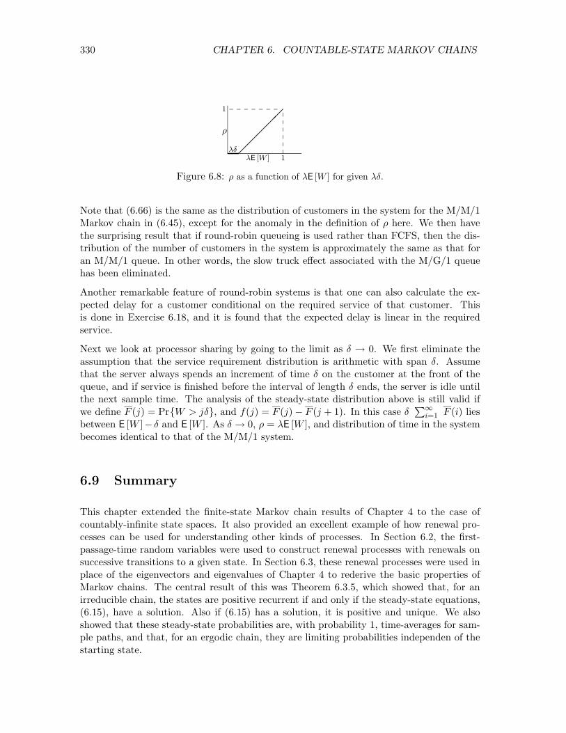
330 CHAPTER 6. COUNTABLE-STATE MARKOV CHAINS
��
��
�
��
��
�
���E [W ] 1
⇢
1
Figure 6.8: ⇢ as a function of �E [W ] for given ��.
Note that (6.66) is the same as the distribution of customers in the system for the M/M/1Markov chain in (6.45), except for the anomaly in the definition of ⇢ here. We then havethe surprising result that if round-robin queueing is used rather than FCFS, then the dis-tribution of the number of customers in the system is approximately the same as that foran M/M/1 queue. In other words, the slow truck e↵ect associated with the M/G/1 queuehas been eliminated.
Another remarkable feature of round-robin systems is that one can also calculate the ex-pected delay for a customer conditional on the required service of that customer. Thisis done in Exercise 6.18, and it is found that the expected delay is linear in the requiredservice.
Next we look at processor sharing by going to the limit as � ! 0. We first eliminate theassumption that the service requirement distribution is arithmetic with span �. Assumethat the server always spends an increment of time � on the customer at the front of thequeue, and if service is finished before the interval of length � ends, the server is idle untilthe next sample time. The analysis of the steady-state distribution above is still valid ifwe define F (j) = Pr{W > j�}, and f(j) = F (j)� F (j + 1). In this case �
P1i=1 F (i) lies
between E [W ]� � and E [W ]. As � ! 0, ⇢ = �E [W ], and distribution of time in the systembecomes identical to that of the M/M/1 system.
6.9 Summary
This chapter extended the finite-state Markov chain results of Chapter 4 to the case ofcountably-infinite state spaces. It also provided an excellent example of how renewal pro-cesses can be used for understanding other kinds of processes. In Section 6.2, the first-passage-time random variables were used to construct renewal processes with renewals onsuccessive transitions to a given state. In Section 6.3, these renewal processes were used inplace of the eigenvectors and eigenvalues of Chapter 4 to rederive the basic properties ofMarkov chains. The central result of this was Theorem 6.3.5, which showed that, for anirreducible chain, the states are positive recurrent if and only if the steady-state equations,(6.15), have a solution. Also if (6.15) has a solution, it is positive and unique. We alsoshowed that these steady-state probabilities are, with probability 1, time-averages for sam-ple paths, and that, for an ergodic chain, they are limiting probabilities independen of thestarting state.

6.9. SUMMARY 331
We found that the major complications that result from countable state spaces are, first,di↵erent kinds of transient behavior, and second, the possibility of null-recurrent states.For finite-state Markov chains, a state is transient only if it can reach some other statefrom which it can’t return. For countably infinite chains, there is also the case, as in Figure6.2 for p > 1/2, where the state just wanders away, never to return. Null recurrence is alimiting situation where the state wanders away and returns with probability 1, but withan infinite expected time. There is not much engineering significance to null recurrence; itis highly sensitive to modeling details over the entire infinite set of states. One usually usescountably infinite chains to simplify models; for example, if a bu↵er is very large and wedon’t expect it to overflow, we assume it is infinite. Finding out, then, that the chain istransient or null recurrent simply means that the modeling assumption is not very good.
We next studied birth-death Markov chains and reversibility. Birth-death chains are widelyused in queueing theory as sample time approximations for systems with Poisson arrivalsand various generalizations of exponentially distributed service times. Equation (6.33) givestheir steady-state probabilities if positive recurrent, and shows the conditions under whichthey are positive recurrent. We showed that these chains are reversible if they are positiverecurrent.
Theorems 6.5.2 and 6.5.3 provides a simple way to find the steady-state distribution of re-versible chains and also of chains where the backward chain behavior could be hypothesizedor deduced. We used reversibility to show that M/M/1 and M/M/m Markov chains satisfyBurke’s theorem for sampled-time — namely that the departure process is Bernoulli, andthat the state at any time is independent of departures before that time.
Branching processes were introduced in Section 6.7 as a model to study the growth ofvarious kinds of elements that reproduce. In general, for these models (assuming p0 > 0),there is one trapping state and all other states are transient. Figure 6.7 showed how tofind the probability that the trapping state is entered by the nth generation, and also theprobability that it is entered eventually. If the expected number of o↵spring of an elementis at most 1, then the population dies out with probability 1, and otherwise, the populationdies out with some given probability q, and grows without bound with probability 1� q.
Round-robin queueing was then used as a more complex example of how to use the backwardprocess to deduce the steady-state distribution of a rather complicated Markov chain; thisalso gave us added insight into the behavior of queueing systems and allowed us to showthat, in the processor-sharing limit, the distribution of number of customers is the same asthat in an M/M/1 queue.
For further reading on Markov chains with countably-infinite state spaces, see [9], [22], or[30]. Feller [9] is particularly complete, but Ross [22] and Wol↵ [30] are somewhat moreaccessible. Harris, [15] is the standard reference on branching processes and Kelly, [16] isthe standard reference on reversibility. The material on round-robin systems is from [32]and is generalized there.
332 CHAPTER 6. COUNTABLE-STATE MARKOV CHAINS
6.10 Exercises
Exercise 6.1. Let {Pij ; i, j � 0} be the set of transition probabilities for a countable-stateMarkov chain. For each i, j, let Fij(n) be the probability that state j occurs sometimebetween time 1 and n inclusive, given X0 = i. For some given j, assume that {xi; i � 0}is a set of nonnegative numbers satisfying xi = Pij +
Pk 6=j Pikxk for all i � 0. Show that
xi � Fij(n) for all n and i, and hence that xi � Fij(1) for all i. Hint: use induction.
Exercise 6.2. a) For the Markov chain in Figure 6.2, show that, for p � 1/2, F00(1) =2(1� p) and show that Fi0(1) = [(1� p)/p]i for i � 1. Hint: first show that this solutionsatisfies (6.10) and then show that (6.10) has no smaller solution (Exercise 6.1 shows thatFi0(1) is the smallest solution to (6.10)). Note that you have shown that the chain istransient for p > 1/2 and that it is recurrent for p = 1/2.
b) Under the same conditions as part a), show that Fij(1) equals 2(1� p) for j = i, equals[(1� p)/p]i�j for i > j, and equals 1 for i < j.
Exercise 6.3. a): Show that the nth order transition probabilities, starting in state 0, forthe Markov chain in Figure 6.2 satisfy
Pn0j = pPn�1
0,j�1 + qPn�10,j+1 j 6= 0; Pn
00 = qPn�100 + qPn�1
01 .
Hint: Use the Chapman-Kolmogorov equality, (4.7).
b) For p = 1/2, use this equation to calculate Pn0j iteratively for n = 1, 2, 3, 4. Verify (6.3)
for these values and then use induction to verify (6.3) in general. Note: this becomes anabsolute mess for p 6= 1/2, so don’t attempt this in general.
c) As a more interesting approach, which brings out the relationship of Figures 6.2 and 6.1,note that (6.3), with j + n even, is the probability that Sn = j for the chain in Figure 6.1and (6.3) with j + n odd is the probability that Sn = �j � 1 for the chain in Figure 6.1.By viewing each transition over the self loop at state 0 as a sign reversal for the chain inFigure 6.1, explain why this surprising result is true. (Again, this doesn’t work for p 6= 1/2,since the sign reversals also reverse the +1, -1 transitions.)
Exercise 6.4. Let j be a transient state in a Markov chain and let j be accessible from i.Show that i is transient also. Interpret this as a form of Murphy’s law (if something badcan happen, it will, where the bad thing is the lack of an eventual return). Note: give adirect demonstration rather than using Theorem 6.2.1.
Exercise 6.5. This exercise treats a mathematical detail from the proof of Lemma 6.2.2.Assume that j is recurrent, there is a path of probability ↵ > 0 from j to i, and n � 1 isan integer. Let Tji be the possibly defective rv giving the first-passage time from j to i.

6.10. EXERCISES 333
Verify the following equations for any integer t > 0:
Pr{Tji > t} = PrnTji > t, T (n)
jj > to
+ PrnTji > t, T (n)
jj to
PrnT (n)
jj > to
+ PrnTji > T (n)
jj
o
PrnT (n)
jj > to
+ (1� ↵)n
Pr{Tji >1} (1� ↵)n.
Exercise 6.6. (Renewal theory proof that a class is all recurrent or all transient.) Assumethat state j in a countable-state Markov chain is recurrent and i communicates with j.More specifically, assume that there is a path of length m from i to j and one of length kfrom j to i
a) Show that for any n > 0, Pm+n+kii � Pm
ij Pnjj P k
ji.
b) By summing over n, show that state i is also recurrent. Hint: Use Theorem 6.3.1.
c) Explain why this shows that all states in a class are recurrent or all are transient.
Exercise 6.7. Consider an irreducible Markov chain that is positive recurrent. Recall thetechnique used to find the expected first passage time from j to i, i.e., T ji, in Section 4.5.The state i was turned into a trapping state by turning all the transitions out of i intoa single transition Pii = 1. Here, in order to preserve the positive recurrence, we insteadmove all transitions out of state i into the single transition Pij = 1.
a) Use Figure 6.2 to illustrate that the above strategy can turn an irreducible chain into areducible chain. Also explain why states i and j are still positive recurrent and still in thesame class.
b) Let {⇡0k; k � 0} be the steady state probabilities for the positive-recurrent class in themodified Markov chain. Show that the expected first passage time T
0ji from j to i in the
modified Markov chain is (1/⇡0i)� 1.
c) Show that the expected first passage time from j to i is the same in the modified andunmodified chain.
d) Show by example that after the modification above, two states i and j that were notpositive recurrent before the modification can become positive recurrent and the abovetechnique can again be used to find the expected first passage time.
Exercise 6.8. Let {Xn; n � 0} be a branching process with X0 = 1. Let Y , �2 be themean and variance of the number of o↵spring of an individual.
a) Argue that limn!1Xn exists with probability 1 and either has the value 0 (with prob-ability F10(1)) or the value 1 (with probability 1� F10(1)).
b) Show that VAR [Xn] = �2Yn�1(Y n � 1)/(Y � 1) for Y 6= 1 and VAR [Xn] = n�2 for
Y = 1.

334 CHAPTER 6. COUNTABLE-STATE MARKOV CHAINS
Exercise 6.9. There are n states and for each pair of states i and j, a positive numberdij = dji is given. A particle moves from state to state in the following manner: Given thatthe particle is in any state i, it will next move to any j 6= i with probability Pij given by
Pij =dijP
j 6=i dij.
Assume that Pii = 0 for all i. Show that the sequence of positions is a reversible Markovchain and find the limiting probabilities.
Exercise 6.10. Consider a reversible Markov chain with transition probabilities Pij andlimiting probabilities ⇡i. Also consider the same chain truncated to the states 0, 1, . . . ,M .That is, the transition probabilities {P 0ij} of the truncated chain are
P 0ij =
(PijPm
k=0 Pik; 0 i, j M
0 ; elsewhere.
Show that the truncated chain is also reversible and has limiting probabilities given by
⇡i =⇡iPM
j=0 PijPMk=0 ⇡i
PMm=0 Pkm
.
Exercise 6.11. A Markov chain (with states {0, 1, 2, . . . , J � 1} where J is either finite orinfinite) has transition probabilities {Pij ; i, j � 0}. Assume that P0j > 0 for all j > 0 andPj0 > 0 for all j > 0. Also assume that for all i, j, k, we have PijPjkPki = PikPkjPji.
a) Assuming also that all states are positive recurrent, show that the chain is reversible andfind the steady-state probabilities {⇡i} in simplest form.
b) Find a condition on {P0j ; j � 0} and {Pj0; j � 0} that is su�cient to ensure that allstates are positive recurrent.
Exercise 6.12. a) Use the birth and death model described in figure 6.4 to find the steady-state probability mass function for the number of customers in the system (queue plus servicefacility) for the following queues:
i) M/M/1 with arrival probability ��, service completion probability µ�.
ii) M/M/m with arrival probability ��, service completion probability iµ� for i servers busy,1 i m.
iii) M/M/1 with arrival probability ��, service probability iµ� for i servers. Assume � sosmall that iµ� < 1 for all i of interest.
Assume the system is positive recurrent.
b) For each of the queues above give necessary conditions (if any) for the states in the chainto be i) transient, ii) null recurrent, iii) positive recurrent.

6.10. EXERCISES 335
c) For each of the queues find:
L = (steady-state) mean number of customers in the system.
Lq = (steady-state) mean number of customers in the queue.
W = (steady-state) mean waiting time in the system.
W q = (steady-state) mean waiting time in the queue.
Exercise 6.13. a) Given that an arrival occurs in the interval (n�, (n+1)�) for the sampled-time M/M/1 model in figure 5, find the conditional PMF of the state of the system at timen� (assume n arbitrarily large and assume positive recurrence).
b) For the same model, again in steady state but not conditioned on an arrival in (n�, (n +1)�), find the probability Q(i, j)(i � j > 0) that the system is in state i at n� and that i� jdepartures occur before the next arrival.
c) Find the expected number of customers seen in the system by the first arrival after timen�. (Note: the purpose of this exercise is to make you cautious about the meaning of “thestate seen by a random arrival”).
Exercise 6.14. Find the backward transition probabilities for the Markov chain model ofage in figure 2. Draw the graph for the backward Markov chain, and interpret it as a modelfor residual life.
Exercise 6.15. Consider the sample time approximation to the M/M/1 queue in figure6.5.
a) Give the steady-state probabilities for this chain (no explanations or calculations required–just the answer).
In parts b) to g) do not use reversibility and do not use Burke’s theorem. Let Xn be thestate of the system at time n� and let Dn be a random variable taking on the value 1 if adeparture occurs between n� and (n + 1)�, and the value 0 if no departure occurs. Assumethat the system is in steady state at time n�.
b) Find Pr{Xn = i,Dn = j} for i � 0, j = 0, 1
c) Find Pr{Dn = 1}
d) Find Pr{Xn = i | Dn = 1} for i � 0
e) Find Pr{Xn+1 = i | Dn = 1} and show that Xn+1 is statistically independent of Dn.Hint: Use part d); also show that Pr{Xn+1 = i} = Pr{Xn+1 = i | Dn = 1} for all i � 0 issu�cient to show independence.
f) Find Pr{Xn+1 = i,Dn+1 = j | Dn} and show that the pair of variables (Xn+1,Dn+1) isstatistically independent of Dn.
g) For each k > 1, find Pr{Xn+k = i,Dn+k = j | Dn+k�1,Dn+k�2, . . . ,Dn} and show thatthe pair (Xn+k,Dn+k) is statistically independent of (Dn+k�1,Dn+k�2, . . . ,Dn). Hint: use

336 CHAPTER 6. COUNTABLE-STATE MARKOV CHAINS
induction on k; as a substep, find Pr{Xn+k = i | Dn+k�1 = 1,Dn+k�2, . . . ,Dn} and showthat Xn+k is independent of Dn+k�1,Dn+k�2, . . . ,Dn.
h) What do your results mean relative to Burke’s theorem.
Exercise 6.16. Let {Xn, n � 1} denote a irreducible recurrent Markov chain having acountable state space. Now consider a new stochastic process {Yn, n � 0} that only acceptsvalues of the Markov chain that are between 0 and some integer m. For instance, if m = 3and X1 = 1, X2 = 3, X3 = 5, X4 = 6, X5 = 2, then Y1 = 1, Y2 = 3, Y3 = 2.
a) Is {Yn, n � 0} a Markov chain? Explain briefly.
b) Let pj denote the proportion of time that {Xn, n � 1} is in state j. If pj > 0 for all j,what proportion of time is {Yn, n � 0} in each of the states 0, 1, . . . ,m?
c) Suppose {Xn} is null recurrent and let pi(m), i = 0, 1, . . . ,m denote the long-run propor-tions for {Yn, n � 0}. Show that pj(m) = pi(m)E[time the X process spends in j betweenreturns to i], j 6= i.}
Exercise 6.17. Verify that (6.58) is satisfied by the hypothesized solution to p in (6.62).Also show that the equations involving the idle state f are satisfied.
Exercise 6.18. Replace the state m = (m, z1, . . . , zm) in Section 6.8 with an expandedstate m = (m, z1, w1, z2, w2, . . . , zm, wm) where m and {zi; 1 i m} are as before andw1, w2, . . . , wm are the original service requirements of the m customers.
a) Hypothesizing the same backward round-robin system as hypothesized in Section 6.8,find the backward transition probabilities and give the corresponding equations to (6.56-6.59) for the expanded state description.
b) Solve the resulting equations to show that
⇡m = ⇡ + �⇣ ��
1� ��
⌘m mYj=1
f(wj).
c) Show that the probability that there are m customers in the system, and that thosecustomers have original service requirements given by w1, . . . , wm, is
Pr{m,w1, . . . , wm} = ⇡�
��
1� ��
!m mYj=1
(wj � 1)f(wj).
d) Given that a customer has original service requirement w, find the expected time thatcustomer spends in the system.