Coulomb glass Computer simulations Jacek Matulewski, Sergei Baranovski, Peter Thomas Departament of...
81
Coulomb glass Computer simulations Jacek Matulewski, Sergei Baranovski, Peter Thomas Departament of Physics Phillips-Universitat Marburg, Germany Faculty of Physics, Astronomy and Informatics Nicolaus Copernicus University in Toruń, Poland Marburg, V 2007
-
Upload
barbara-holifield -
Category
Documents
-
view
214 -
download
0
Transcript of Coulomb glass Computer simulations Jacek Matulewski, Sergei Baranovski, Peter Thomas Departament of...

Coulomb glassComputer simulations
Jacek Matulewski, Sergei Baranovski, Peter Thomas
Departament of PhysicsPhillips-Universitat Marburg, Germany
Faculty of Physics, Astronomy and InformaticsNicolaus Copernicus University in Toruń, Poland
Marburg, V 2007

2/80
Outline
0. Example of disordered system with long-range interactions
1. Simulation procedure for computation of single particle DOS
2. The dynamics of the Coulomb gap
3. The Coulomb glass and the glass transition
4. Phononless AC conductivity in Coulomb glass

3/80
Realisation of disorder: the impurity band in semiconductor
Conduction band
Impurity band (donors)
E
Valence band
Acceptors

4/80
Realisation of disorder: the impurity band in semiconductor
Conduction band
Impurity band (donors)
E
Valence band
Acceptors

5/80
Realisation of disorder: the impurity band in semiconductor
Conduction band
Impurity band (donors)
E
Valence band
Acceptors
Occupied donor (electron) q = 0
Empty donor (hole) q = +
Occupied (electron) q =acceptor
_
_ __
+ + +

6/80
Realisation of disorder: the impurity band in semiconductor
Impurity band (donors)
Acceptors
Occupied donor (electron) q = 0
Empty donor (hole) q = +
Occupied (electron) q =acceptor
_
_ __
++ +

7/80
Realisation of disorder: the impurity band in semiconductorThe electrostatic potential at every donor site is due to Coulomb interactionwith every acceptor (-) and every other empty site (+) in the system.
N = 10K = 0.5
Occupied donor
Empty donor
Occupied acceptor
Since the sites positions are random - site potential are random too (disorder)
++
+
+
+
_
_
_
_
_

8/80
Realisation of disorder: the impurity band in semiconductor
i ji ij
ji
i
i
r
nn
rn
rH
)1)(1(
2111
21
System of randomly distributed sites with Coulomb interaction:
ij ij
j
ii r
n
rE
11Site potential: isolated sites are identical
Total energy (classical electrostatic interactions):
dimensionless units

9/80
What is the Coulomb glass?
System of randomly distributed sites with Coulomb interaction
If the system is so sparse that the distances between sites are larger than the localisation length (n < nC)
disorder => electronic wavefunctions are localisedthe chemical potential is localised in “localised” part of DOS
=> the quantum overlap may be neglected (no tunnelling)=> classical system (electrons move via incoherent hops)
Examples:compensated lightly doped semiconductorsamorphous semiconductors and alloyshopping behaviour of quasicrystalsgranular filmssilicon MOSFET’s heterostructureselectrically conducting polymers and stannic oxides nanowires
=> disorder isolator

10/80
Outline
0. Example of disordered system with long-range interactions
1. Simulation procedure for computation of single particle DOS
a) Searching for the pseudo-ground state (T = 0K). Coulomb gap
b) Monte Carlo simulations (T > 0K)
2. The dynamics of the Coulomb gap
3. The Coulomb glass and the glass transition
4. Phononless AC conductivity in Coulomb glass

11/80
Simulation procedure (T = 0K)Metropolis algorithm: the same as used to solve the salesman problemGeneral: Searching for the configuration which minimise some parameterIn our case: searching for electron arrangement which minimise total energy
N = 10K = 0.5
Occupied donor
Empty donor
Occupied acceptor
The calculating procedureisn’t a simulation of therelaxation process.(no transition rates)

12/80
Simulation procedure (T = 0K)
i ji ij
ji
i
i
r
nn
rn
rH
)1)(1(
2111
21
System of randomly distributed sites with Coulomb interaction:
ij ij
j
ii r
n
rE
11Site potential: isolated sites are identical
Total energy (classical electrostatic interactions):
Single electron transfer:
H
dimensionless units

13/80
ij
beforei
afterj rr
EEH11)()(
Total energy change during single electron transition
A (all acceptors)
Di
Dj
ir jr
ij rrr
rrE
i
beforei
11)( j
beforej r
E1)(
Site energies
+
i
afteri r
E1
)( rr
Ej
afterj
11 )(
+Total energy of the system:
j
before
rH
1)(
i
after
rH
1)(
ij
beforeafter
rrHHH
11)()(
In order to make the calculation possible we need to express the energy difference using sites energy values before the transition
rEE
rrEEH before
ibefore
jij
beforei
afterj
111 )()()()(
_

14/80
Simulation procedure (T = 0K)
i ji ij
ji
i
i
r
nn
rn
rH
)1)(1(
2111
21
ij ij
j
ii r
n
rE
11
System of randomly distributed sites with Coulomb interaction:
Single electron transfer:
Site potential: isolated sites are identical
Total energy (classical electrostatic interactions):
ij
beforei
beforej
beforei
afterj r
EEEE1)()()()(
Salesman says: transitions for which H < 0 leads to pseudo-ground state
H
hole-electron interaction

15/80
Simulation procedure (T = 0K)Metropolis algorithm for searching the pseudo-ground state of system
Step 01. Place N randomly distributed donors in the box2. Add K·N randomly distributed acceptors (all occupied)3. Distribute K·N electrons over donors
Step 1 (-sub)3. Calculate site energies of donors4. Move electron from the highest occupied site to the lowest empty one
5. Repeat points 3 and 4 until there will be no occupied empty sites below any occupied (Fermi level appears)

16/80
Step 2 (Coulomb term)6. Searching the pairs checking for occupied site i and empty j
If there is such a pair then move electron from i to j and call -sub (step 1) and go back to 6.
Effect: the pseudo-ground state (the state with the lowest energy in the pair approximation)
• Energy can be further lowered by moving two and more electrons at the same step (few percent)
01 ij
ijij rEEE
Simulation procedure (T = 0K)Metropolis algorithm for searching the pseudo-ground state of system

17/80
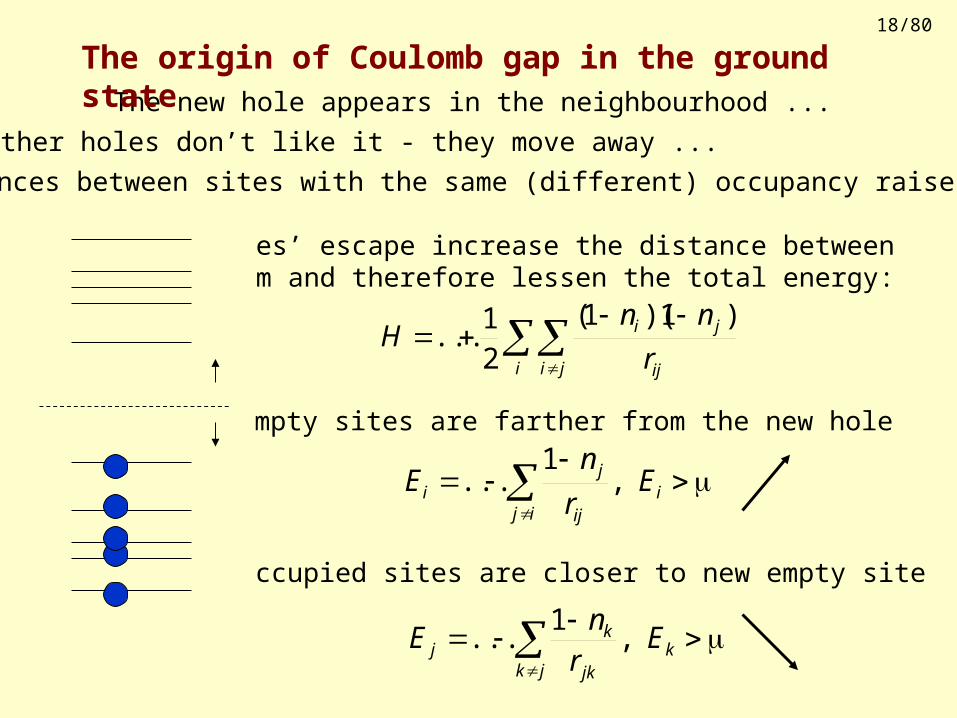
The new hole appears in the neighbourhood ...
The origin of Coulomb gap in the ground state
Other holes don’t like it - they move away ...
18/80
The new hole appears in the neighbourhood ...
The origin of Coulomb gap in the ground state
Other holes don’t like it - they move away ...
Distances between sites with the same (different) occupancy raise (lessen)
i ji ij
ji
r
nnH
)1)(1(
21
...
Holes’ escape increase the distance between them and therefore lessen the total energy:
kjk jk
kj E
rn
E ,1
...
Occupied sites are closer to new empty site
iij ij
ji E
r
nE ,
1...
Empty sites are farther from the new hole

19/80
Coulomb gap in density of states for T = 0K
Coulomb gap created due to Coulomb interaction in the system
μEi
Sin
gle-
part
icle
DO
S
Si:P
0
0.05
0.1
0.15
0.2
0.25
0.3
0.35
0.4
-4 -2 0 2 4
N=5001000 real., PBC
20/80
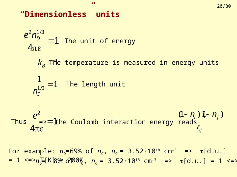
“Dimensionless” units
1Bk
14
3/12
Dne
The temperature is measured in energy units
The length unit
The unit of energy
11
3/1 Dn
14
2
e
Thus => the Coulomb interaction energy readsij
ji
r
nn )1)(1(
For example: nD=69% of nC, nC = 3.52·1018 cm-3 => [d.u.] = 1 <=> T[K] ≈ 200K
nD= 8% of nC, nC = 3.52·1018 cm-3 => [d.u.] = 1 <=> T[K] ≈ 100K

21/80
Shape of Coulomb gap for T = 0K
0
0.1
0.2
0.3
0.4
0.5
0.6
-0.2 0 0.2 0.4 0.6 0.8 1
numerical simulation result
fitting of ax2 (soft gap)
fitting of (Efros)xE
ae/0
fitting of (BSE) 47
0
0
ln
/
xE
xE
ae
Sin
gle-
part
icle
-DO
S
iEx

22/80
Shape of Coulomb gap for T = 0K S
ingl
e-pa
rtic
le-D
OS
hard gap
numerical simulation result
fitting of (Efros)xE
ae/0
fitting of (BSE) 47
0
0
ln
/
xE
xE
ae
iEx
0
0.04
0.08
0.12
0.16
0 0.1 0.2 0.3 0.4 0.5
N=5001000 real., PBC

23/80
Simulation procedure (T > 0K)Monte-Carlo simulations
Step 3 (Coulomb term)7. Searching the pairs checking for occupied site j and empty i
If there is such a pair Then move electron from i to j for sure Else move the electron from i to j with prob.
Call -sub (step 1).
Repeat step 3 thousands times (Monte Carlo)
Repeat steps 0-3 several thousand times (averaging)
Step 2 may be omitted
01 ij
ijij rEEE
kT
Eij
eTp
)(

24/80
Smearing of the Coulomb gap for T > 0K
μEi
Sin
gle-
part
icle
DO
S
T = 0.0
0.1
0.2
0.3
0.4
1
0
0.1
0.2
0.3
0.4
-4 -2 0 2 4
N=500, MC=105
1000 real., PBC

25/80
Smearing of the Coulomb gap for T > 0K
μEi
Sin
gle-
part
icle
DO
S
T = 0K
22K
44K
66K
88K
222K
0
0.1
0.2
0.3
0.4
-4 -2 0 2 4
N=500, MC=105
1000 real., PBC
nC = 3.52·1018 cm-3
= 11.4
n/nC=100%=20Å=0.3 d.u.

26/80
Smearing of the Coulomb gap for T > 0K
μEi
Sin
gle-
part
icle
DO
S
T = 0K
10K
20K
30K
40K
100K
0
0.1
0.2
0.3
0.4
-4 -2 0 2 4
N=500, MC=105
1000 real., PBC
nC = 3.52·1018 cm-3
= 11.4
n/nC=8%=20Å=0.13 d.u.

27/80
Pair distribution (T = 0K)
ij
occupiedi
emptyj r
EE1
ijr
N=400, T=0K, a=0.3, MC=103

28/80
Pair distribution (T > 0K)
ijr
ij
occupiedi
emptyj r
EE1
N=400, T=1/8 (28K for n/nC=1), =0.3, MC=103

29/80
Pair distribution (T > 0K)
ijr
ij
occupiedi
emptyj r
EE1
N=400, T=1 (222K for n/nC=1), =0.3, MC=103

30/80
Outline
0. Example of disordered system with long-range interactions
1. Simulation procedure for computation of single particle DOS
2. The dynamics of the Coulomb gap
3. The Coulomb glass and the glass transition
4. Phononless AC conductivity in Coulomb glass

31/80
The dynamics of the Coulomb gap: the time scales
Conduction band
Impurity band (donors)
Acceptors Valence band
Averaged thermal activation time (T = 7K, E=31.27 meV): 104 s
)T/exp(10 BkE
s121
00 10 the microscopic time
Lifetime of donor (inverted transfer rate up to conduction band):
Question 1: What must be the temperature to keep the electron in the imputity band?
E

32/80
The dynamics of the Coulomb gap: the time scales
Conduction band
Impurity band (donors)
)ln(2 00 tvR
ij
B
ijij r
k
Er 2exp
T
2exp 1
01
0
Miller-Abrahams transfer rate for VRH:
E Averaged thermal activation time (T = 7K, E=31.27 meV): 104 s
Question 2: How long does it takes to transfer electron from donor i to empty donor j?
ijr

33/80
The dynamics of the Coulomb gap: the time scales
Conduction band
Impurity band (donors)
)ln(2 00 tvR
E Averaged thermal activation time (T = 7K, E=31.27 meV): 104 s
Conclusion:For Si:P (n = 69% of nC) during 103s electron travel only 0.03A
ijr
< size of atom
One need to decrease the n/nC and/or wait very longThe Coulomb glass is an isolator (n/nC < 1)

34/80
The dynamics of the Coulomb gap: the gap evolution
Sin
gle-
part
icle
DO
S
0
0.1
0.2
0.3
0.4
-4 -2 0 2 4
R0 = 0.1
1.0
1.2
1.4
2.0
5.0
μEi
T = 0K

35/80
The dynamics of the Coulomb gap: the gap evolution
Sin
gle-
part
icle
DO
S
0
0.1
0.2
0.3
0.4
5 2.51 0.5
Energy:
0-0.5
-1-2
)ln(2 00 tvR

36/80
The dynamics of the Coulomb gap: the gap evolution
Sin
gle-
part
icle
DO
S
0
0.1
0.2
0.3
0.4
5 2.51 0.5
Energy:
0-0.5
-1-2
)ln(2 00 tvR
)( ln/1),0( 00 tttg R0(t0) = 1.25
Fitting: 1.26b

37/80
The dynamics of the Coulomb gap: the gap evolution
Sin
gle-
part
icle
DO
S
0
0.1
0.2
0.3
0.4
5 2.51 0.5
Energy:
0
)ln(2 00 tvR
)( ln/1),0( 00 tttg R0(t0) = 1.25
Fitting: 1.26
Yu (SCE+numeric, 1999): b = 1
Malik and Kumar (analytical., 2004): b = 2

38/80
The dynamics of the Coulomb gap: the experiment proposal
Conduction band
Impurity band (donors)
)ln(2 00 tvRrij
T = 300K
R0 = 0.1
] )/(exp[)( 0 TTT 1/4
Mott’s formula for DC conductivity(constant DOS near the Fermi level):
Random occupations of sites
T = 7K
n/nC = 8%

39/80
The dynamics of the Coulomb gap: the experiment proposal
Conduction band
Impurity band (donors)
)ln(2 00 tvRrij
R0 = 1.0
Relaxing (1st hour) ...
T = 7K
Random occupation of sites n/nC = 8%

40/80
The dynamics of the Coulomb gap: the experiment proposal
Conduction band
Impurity band (donors)
)ln(2 00 tvRrij
R0 = 1.2
Relaxing (2nd hours) ...
T = 7K
n/nC = 8%

41/80
The dynamics of the Coulomb gap: the experiment proposal
Conduction band
Impurity band (donors)
)ln(2 00 tvRrij
R0 = 1.4
Relaxing (3rd hour) ...
T = 7K
n/nC = 8%

42/80
The dynamics of the Coulomb gap: the experiment proposal
Conduction band
Impurity band (donors)
)ln(2 00 tvRrij
R0 = 5.0
] )/(exp[)( 0 TTT 1/2
SE’s formula for DC conductivity(gap in g(E ) around the Fermi level):
Pseudo-grand state reached
T = 7K
n/nC = 8%

43/80
The dynamics of the Coulomb gap: the experiment proposal
Conduction band
Impurity band (donors)
)ln(2 00 tvRrij
Pseudo-grand state reached
T = 7K
Change from 1/4-law (Mott) to 1/2-law (SE) not because of the cooling of the sample, but because it relaxed for 104 s (3h).
n/nC = 8%

44/80
The dynamics of the Coulomb gap: the gap evolution
Sin
gle-
part
icle
DO
S
0
0.1
0.2
0.3
0.4
-4 -2 0 2 4
R0 = 0.1
1.0
1.2
1.4
2.0
5.0
μEi
T = 0K

45/80
The dynamics of the Coulomb gap: the gap evolution
Sin
gle-
part
icle
DO
S
μEi
T = 0.1 d.u.
0
0.1
0.2
0.3
0.4
-4 -2 0 2 4
R0 = 0.1
1.0
1.2
1.4
2.0
5.0

46/80
The dynamics of the Coulomb gap: the gap evolution
Sin
gle-
part
icle
DO
S
μEi 0
0.1
0.2
0.3
0.4
-4 -2 0 2 4
T = 0.2 d.u. R0 = 0.1
1.0
1.2
1.4
2.0
5.0

47/80
Outline
0. Example of disordered system with long-range interactions
1. Simulation procedure for computation of single particle DOS
2. The dynamics of the Coulomb gap
3. The Coulomb glass and the glass transition
4. Phononless AC conductivity in Coulomb glass

48/80
Edwards-Anderson order parameter (EAOP)T = 0K - no transitions in the pseudo-ground state
N = 10K = 0.5
Occupied donor
Empty donor
Occupied acceptor
T = 6K - some transitions (VRH)T = 100K - a lot of transitions (NNH)
T
exp2
exp0
B
ijijijij k
Er

49/80
T = 6K - some transitions (VRH)
timeni
Edwards-Anderson order parameter (EAOP)
T = 0K - no transitions in the pseudo-ground state
timeni
T = 100K - a lot of transitions (NNH)
time
ni
time
time
time
nsrealisatiodonorsCarloMonteinq2
12 Order parameter
(per analogy to spin glass)
q = 1.0
q = 0.8
q = 0.1

50/80
Glass transition
Davies, Lee, Rice (lattice model, no actual acceptors): glass transition from random (T > 0.3K) to ordered (T = 0K) system of {ni}
a

51/80
Glass transition
Davies, Lee, Rice (lattice model, no actual acceptors): glass transition from random (T > 0.3K) to ordered (T = 0K) system of {ni}
Yu: glass transition in Coulomb glass is the phase transition of second order

52/80
Glass transition
Davies, Lee, Rice (lattice model, no actual acceptors): glass transition from random (T > 0.3K) to ordered (T = 0K) system of {ni}
Yu: glass transition in Coulomb glass is the phase transition of second order

53/80
Glass transition
Davies, Lee, Rice (lattice model, no actual acceptors): glass transition from random (T > 0.3K) to ordered (T = 0K) system of {ni}
Yu: glass transition in Coulomb glass is the phase transition of second order

54/80
Glass transition
Davies, Lee, Rice (lattice model, no actual acceptors): glass transition from random (T > 0.3K) to ordered (T = 0K) system of {ni}
Yu: glass transition in Coulomb glass is the phase transition of second order

55/80
Glass transition
Our model: random positions of sites, actual acceptors present
a
But closely locates groups are not present in the lattice model
The crowded group has higherenergy than surrounding andpreserve its occupation unchangedeven for high temperatures
a
The lattice model well describesremote donors’ interaction

56/80
Glass transition
Our model: EAOP has the same value for N=100 and N=500,glass transition has long exponential tail (nonzero values even for T > 300K)
EA
ord
er p
aram
eter
[d.u.]
our modelDavies, Lee, Rice
0.2
0.4
0.6
0.8
1
0.001 0.01 0.1 1 10 100

57/80
Glass transition
EA
ord
er p
aram
eter
our modelDavies, Lee, Rice (B = 2)
0
0.1
0.2
0.3
0.4
1 10
[d.u.] 3
Our model: EAOP has the same value for N=100 and N=500,glass transition has long exponential tail (nonzero values even for T > 300K)

58/80
Glass transition
EA
ord
er p
aram
eter
our modelDavies, Lee, Rice (B = 2)
0
0.1
0.2
0.3
0.4
100K 1000K
[K] 300K
Si:Pn/nC = 8%
Our model: EAOP has the same value for N=100 and N=500,glass transition has long exponential tail (nonzero values even for T > 300K)

59/80
Glass transition
EA
ord
er p
aram
eter
our modelDavies, Lee, Rice (B = 2)
0
0.1
0.2
0.3
0.4
197K 1965K
[K] 590K
Si:Pn/nC = 69%
Our model: EAOP has the same value for N=100 and N=500,glass transition has long exponential tail (nonzero values even for T > 300K)

60/80
- introduced to demonstrate that the Coulomb fields induce sine ordering at low temperatures- in our (random site) model it depends on N!
Modified Edwards-Anderson order parameter
nsrealisatiodonorsCarloMonteiCarloMonteim nnq
2
0
1212
normal “spin” “spin” in system with no interactions
the difference report the contribution to EA order parameter related to presence of the Coulomb interaction within the system

61/80
Goes to zero faster than the EA order parameter.
Modified Edwards-Anderson order parameter
mod
ifie
d E
A o
rder
par
amet
er our model (N = 100)
Davies, Lee, Rice (B = 2)
0
0.2
0.4
0.6
0.8
1
1.2
0.01 0.1 1 10
[d.u.]
our model (N = 500)

62/80
New order parameter related to the electron diffusion
The quest for the phase transition parameter in the Coulomb glass (Lee, Yu)Analysis of “Binder g” suggests that the glass transition is the phase transitionNeed for the parameter which rapidly goes to zero. What mechanism behind it?
N = 10K = 0.5
Occupied donor
Empty donor
Occupied acceptor
Our idea is totrace the electroninstead of the site’s occupation!

63/80
New order parameter related to the electron diffusion
The quantities which may be a base for a new order parameter:- the distance of the electron from the final site to the initial one- the total hops length- the number of hops
The value of the new order parameter may be the percentage of all electrons for which:- the distance between final and initial site is smaller than ...- the total hops length is smaller than ...- the number of hops is smaller than ...
We just measure the percentage of the electrons which stay for all simulation at the initial position.Thus the new order parameters = 1 only if the EA order parameter = 1.
The disadvantage: its value is related to the measurement time (stronger than the EA order parameter)
The advantage: its value more rapidly goes to zero => the phase transition apply to the electron diffusion in the Coulomb glass

64/80
New order parameter related to the electron diffusion
0
0.2
0.4
0.6
0.8
1
0.001 0.01 0.1 1 10 100
EA order parameterthe new order parameter
EA
and
new
ord
er p
aram
eter
s
[d.u.]
about 1%of electronsgot stacked

65/80
Glass transitions versus Coulomb gap smearing
Sin
gle-
part
icle
DO
S f
or E
= 0
0
0.1
0.2
0.3
0.01 0.1 1 10
g(0)
g(0) (Grannan and Yu; lattice model)
EA
ord
er p
aram
eter
0.0
0.5
1.0
EA order parameter
the new order parameter
[d.u.]

66/80
Glass transitions vs Coulomb gap evolution
Sin
gle-
part
icle
DO
S f
or E
= 0
0
0.1
0.2
0.3
0.01 0.1 1 10
g(0)
g(0) (Grannan and Yu; lattice model)
EA
ord
er p
aram
eter
0.0
0.5
1.0
EA order parameter
the new order parameter
electrons leavethe initial sites
almost noneelectron rests
completerandomness
gap starts to form
gap is formed

67/80
The gap transition with time limitation
EA
ord
er p
aram
eter
s
0.2
0.4
0.6
0.8
1
0.001 0.01 0.1 1 10 100
R = 0.3
R = 0.5
R = 0.75
R = 1.0No limit
[d.u.]
The gap starts to form for R > 1.2, while the order is established for R < 1.5

68/80
The gap transition with time limitation
new
ord
er p
aram
eter
s
[d.u.]
The gap starts to form for R > 1.2, while the order is established for R < 1.5
0.2
0.4
0.6
0.8
1
0.001 0.01 0.1 1 10 100
R = 0.3
R = 0.5
R = 0.75
R = 1.0No limit

69/80
0.05
0.1
0.15
0.01 0.1 1 10 100
The gap transition with time limitation
0.6
0.8
1
T = 0.1T = 0.2
0
0.5
1
EA
ord
er p
ar.
new
ord
er p
ar.
T = 0.1T = 0.2
R [d.u.]
T = 0.1T = 0.2
From random
From ground
From ground

70/80
Outline
0. Example of disordered system with long-range interactions
1. Simulation procedure for computation of single particle DOS
2. The dynamics of the Coulomb gap
3. The Coulomb glass and the glass transition
4. Phononless AC conductivity in Coulomb glass
a) Experimental results of AC conductivity measurements
b) brief introduction to Shklovskii and Efros’s model of zero-phonon AC hopping conductivity of disordered system c) results of computer simulations for T = 0K

71/80
Experimental resultsM. Lee and M.L. Stutzmann, Phys. Rev. Lett. 87, 056402 (2001)E. Helgren, N.P. Armitage and G. Gru:ner, Phys. Rev. Lett. 89, 246601 (2002)

72/80
Experimental resultsM. Lee and M.L. Stutzmann, Phys. Rev. Lett. 87, 056402 (2001)E. Helgren, N.P. Armitage and G. Gru:ner, Phys. Rev. Lett. 89, 246601 (2002)

73/80
Shklovskii and Efros’s modelPair of sites
)ˆˆˆˆ)((ˆˆ21
ˆˆˆ122112
12
21221112 aaaarI
rnn
nEnEH
Hamiltonian of a pair of sites:
2,1 1
1 j j
j
r
nE
Site energy is determined by Coulomb interaction with surrounding pairs
Overlap of site’s wavefunction
)exp()( 1212012 ararIrI
21,2112 ,,ˆ21
nnWnnH nn Notice that because of overlap I(r) “intuitive” states can be not good eigenstates
mmm WH 12ˆ
,
Anyway four states are possible a priori:
• there is no electron, so no interaction and energy is equal to 0
• there is one electron at the pair (two states)
• there are two electrons at the pair
0,0
1,1

74/80
0
0
2
1
2
1
m
m
WEI
IWE
Shklovskii and Efros’s modelPair of sites
Only pairs with one electron are interesting in context of conductivity:
mmm WH 12ˆ
1,00,1
1,00,1)ˆˆˆˆ)((ˆˆ21
ˆˆ
21
21122112
212211
mW
aaaarIrnn
nEnE
1,00,1 21 m
The isolated sites base1
2
2
2
1 Normalisation
2122
1211
m
m
WIE
WIE
2121
EEE 2212 4IEE where

75/80
Energy which pair much absorb or emit to move the electron between split-states(from to ):
Shklovskii and Efros’s modelPair of sites
2
2
1212 4
1I
rEEWWW
Source of energy: photons
20
2)(
iiQ
And finally the conductivity: Shklovskii and Efros formula for conductivity in Coulomb glasses
r
r1
)( 4
02
lnI
ar
Numerical calculation (esp. for T > 0)
Energy which must be absorbed by pairs in unit volume due to el. transition
Q = QM transition prob.(Fermi Golden Rule)
prob. of finding“proper” pair· · prob. of finding photon
with energy equals to · )(4
2 2
re

76/80
Pair distribution (T = 0K)
ij
occupiedi
emptyj r
EE1
ijr
N=400, T=0K, NMonte-Carlo=1000, a=0.27

77/80
Pairs mean spatial distance (T = 0K)
2.4
2.6
2.8
3
3.2
3.4
3.6
3.8
4
0 0.05 0.1 0.15 0.2
pair
mea
n sp
atia
l dis
tanc
e
Mott’s formula
simulations
In contradiction to the Mott’s assumption the distribution of pairs’ distances is very wide
N=1000, K=0.5, 2500 realisationsperiodic boundary conditions, AOER
02ln
Iar

78/80
Pair energy distribution (T = 0K)
0
50000
100000
150000
200000
250000
0 1 2 3 4 5 6 7 8 9 10
We work here!!!
N=500, T=0, K=0.5, aver. over 100 real.N
umbe
r of
pai
rs

79/80
Conductivity (T=0K)
1e-010
1e-009
1e-008
1e-007
1e-006
1e-005
0.001 0.01 0.1
Con
duct
ivit
y (a
rb. u
n.)
Helgren et al. (T=2.8K)n = 69%
simulations
N=500, T=0, K=0.5, aver. over 25k real.Δ(hw)=0.001 (blue), Δ(hw)=0.01 (green)
n = 69% of nC means a = 0.27 [l69%]
(in units of n-1/3)
fixed parameters for Si:P: a = 20Å, and nC = 3.52·1024 m-3 (lC = 65.7Å)
There is no crossover in numerical results!

80/80
Conductivity (T=0K)
Con
duct
ivit
y (a
rb. u
n.)N=500, T=0, K=0.5, aver. over 25k real.Δ(hw)=0.001 (blue), Δ(hw)=0.01 (green)
1e-008
1e-007
1e-006
1e-005
0.0001
0.001 0.01 0.1
simulationsHelgren 69% Si:P
crossover (?)
a = 0.36