Costly Financial Advice: Con icts of Interest or Misguided...
54
Costly Financial Advice: Conflicts of Interest or Misguided Beliefs? * Juhani T. Linnainmaa Brian T. Melzer Alessandro Previtero December 2015 Abstract Using detailed data on financial advisors and their clients, we show that conflicts of interest matter, but appear limited to a small fraction of advisors. These advisors execute trades that increase their commissions and impose costs on the mutual fund system. At the same time, most advisors invest their personal portfolios just like they advise their clients. They trade frequently, chase returns, and prefer expensive, actively managed funds over cheap index funds. Differences in advisors’ beliefs affect not only their own investment choices, but also cause substantial variation in the quality and cost of advice they give to clients. Our estimates suggest that correcting advisors’ misguided beliefs, through screening or education, may reduce the cost of advice more than policies aimed at eliminating conflicts of interest. * Juhani Linnainmaa is with the University of Chicago Booth School of Business and NBER, Brian Melzer is with the Northwestern University, and Alessandro Previtero is with the University of Texas at Austin and Western University. We thank Chuck Grace and Jonathan Reuter for valuable comments. We are grateful for feedback given by seminar participants at Boston College, Dartmouth College, University of Maryland, Georgetown University, HEC Montreal, Indiana University, University of Texas at Austin, and University of Colorado Boulder. We are especially grateful to Univeris, Fundata, and four anonymous financial firms for donating data and giving generously of their time. Alessandro Previtero received financial support from Canadian financial firms for conducting this research. Juhani Linnainmaa received financial support from the PCL Faculty Research Fund at the University of Chicago Booth School of Business. Address correspondence to Alessandro Previtero, Western University, 1255 Western Road, London, Ontario N6G 0N1, Canada (email: [email protected]).
Transcript of Costly Financial Advice: Con icts of Interest or Misguided...
Costly Financial Advice:
Conflicts of Interest or Misguided Beliefs?∗
Juhani T. Linnainmaa
Brian T. MelzerAlessandro Previtero
December 2015
Abstract
Using detailed data on financial advisors and their clients, we show that conflicts of interest
matter, but appear limited to a small fraction of advisors. These advisors execute trades that
increase their commissions and impose costs on the mutual fund system. At the same time, most
advisors invest their personal portfolios just like they advise their clients. They trade frequently,
chase returns, and prefer expensive, actively managed funds over cheap index funds. Differences
in advisors’ beliefs affect not only their own investment choices, but also cause substantial
variation in the quality and cost of advice they give to clients. Our estimates suggest that
correcting advisors’ misguided beliefs, through screening or education, may reduce the cost of
advice more than policies aimed at eliminating conflicts of interest.
∗Juhani Linnainmaa is with the University of Chicago Booth School of Business and NBER, Brian Melzer iswith the Northwestern University, and Alessandro Previtero is with the University of Texas at Austin and WesternUniversity. We thank Chuck Grace and Jonathan Reuter for valuable comments. We are grateful for feedback givenby seminar participants at Boston College, Dartmouth College, University of Maryland, Georgetown University, HECMontreal, Indiana University, University of Texas at Austin, and University of Colorado Boulder. We are especiallygrateful to Univeris, Fundata, and four anonymous financial firms for donating data and giving generously of theirtime. Alessandro Previtero received financial support from Canadian financial firms for conducting this research.Juhani Linnainmaa received financial support from the PCL Faculty Research Fund at the University of ChicagoBooth School of Business. Address correspondence to Alessandro Previtero, Western University, 1255 Western Road,London, Ontario N6G 0N1, Canada (email: [email protected]).

“Jerry, just remember—it’s not a lie if you believe it.”
–George Costanza
1 Introduction
A common criticism of the financial advisory industry is that conflicts of interest compromise the
quality, and raise the cost, of advice. Many advisors require no direct payment from clients but
instead draw compensation from commission payments on the mutual funds they sell. Within this
structure, advisors may be tempted to recommend products that maximize commissions instead
of serving the interests of their clients. A growing academic literature has assessed conflicts of
interest and shown that sales commissions raise costs and distort portfolios. Our paper contributes
to this literature in two ways. First, we measure the cost of conflicted trading on client returns
and examine how widespread conflicted trading is within a large sample of advisors. Second, we
add a new dimension to this discussion by introducing misguided beliefs as an alternative, if not
mutually exclusive, explanation for costly and low-quality advice. Under this view, advisors recom-
mend frequent trading and expensive, actively managed products not because they receive higher
commissions by doing so, but because they believe active management—even after commissions—
dominates passive management.
Our analysis uses data provided by three Canadian financial institutions. The data include
comprehensive trading and portfolio information on more than 5,000 advisors and 500,000 clients
between 1999 and 2013. Our data also include, for the vast majority of advisors, the personal
trading and account information of the advisor himself. This unique feature proves fruitful in both
portions of our analysis. The advisor’s own investment choices allow us to identify principal-agent
conflicts quite directly, since we observe the advisor’s choices as both principal and agent. The
1

advisor’s own trades also reveal his beliefs and preferences regarding investment strategies, which
allows us to test whether client trades criticized as self-serving emanate from misguided beliefs
rather than misaligned incentives.
We begin by exploring conflicts of interest, using the following methodology to measure advisor
self-interest. For each client trade, we compare the fund sold to the fund purchased, and we classify
the trade based on whether it serves the advisor’s interest, the client’s interest or both. Depending
on the particular funds purchased and sold, the advisor may receive a sales commission at the time
of purchase as well as a recurring annual commission (“trailing commission”) until the investment
is redeemed. A trade is in the advisor’s interest, under our classification, if it generates a new
up-front commission or raises the trailing commission. Clients pay up-front sales commissions (to
the advisor) on front-end load funds, deferred sales charges (to the mutual fund) on back-end load
funds sold “too early”, and recurring management expense charges (to the mutual fund) for as
long as they maintain the investment. A trade is in the client’s interest, under our classification,
if it reduces the client’s management expense charges without incurring an up-front commission or
deferred sales penalty. To avoid taking a stand on the optimality of asset allocation change, we
classify a trade as (potentially) beneficial to the client if it changes asset allocation.
We first show that conflicts of interest matter.1 Only a small fraction of trades appear to serve
solely the advisor’s interests—these are trades that benefit the advisor, hurt the client financially,
and appear to provide no other benefits to the client. These self-serving trades are concentrated
among a small number of advisors. The data suggest that it is the advisors who instigate these
trades—when a client switches advisors because his old advisor dies, retires, or leaves the industry,
1Under Canadian securities legislation, advisors do not have fiduciary duty, but they have a duty to make suitableinvestment recommendations, based on their clients’ investment goals and risk tolerance. They are not required toput the client’s interests before their own, but they are legally mandated to “deal fairly, honestly and in good faithwith their clients” (Canadian Securities Administrators 2012).
2

his propensity for executing trades that benefit the advisor interests changes to match that of the
new advisor.
Advisors who recommend self-serving trades gain substantially from doing so. Whereas the
typical advisor earns a commission between 1.5 to 2 percent of client assets under management,
self-serving advisors earn more than 3 percent of assets per year. The clients of self-serving advi-
sors, quite surprisingly, do not suffer below average investment performance. Indeed, these clients
perform better than the other advisors’ clients. The reason for this counterintuitive result is that
mutual funds, rather than clients, pay most of the fees collected by advisors. Only front-end loads
are paid directly from clients to advisors, and those charges are rare both in the industry and in our
sample. An advisor that maximizes commissions therefore collects more in fees from mutual funds,
but does not necessarily collect more from his particular clients. To the extent that self-serving
trades raise costs for investors, they do so in an indirect way. That is, mutual funds may respond
to increased commissions by charging investors higher management expenses. The picture that
emerges here is that even the most ruthless advisors do not seem to take advantage of their own
clients as much as they take advantage of the compensation scheme of the mutual fund system.
To provide further illustration of behavior that is costly to the mutual fund system and beneficial
to the financial advisor, we examine trading behavior around the expiration of deferred sales charge
(DSC) schedules. Investors pay these charges when they sell a back-end load fund “too soon” after
the purchase. When the DSC schedule expires, the advisor can earn a new sales commission or
increase the trailing commission by moving the client to a different fund. Advisors respond to this
incentive. These trades are not motivated by clients’ liquidity needs or by rebalancing or asset-
allocation considerations. Advisors almost always benefit from these trades, but so do their clients.
3

The typical transaction moves the client to a front-end load fund (with the load set to zero), which
lowers the expense ratio. Because all the fees in the system are paid by the clients’ investments,
the collective gain of the advisor and the client is paid by the rest of the system.
We next show that most advisors invest their personal portfolios just like they advise their
clients. We measure trading behavior in dimensions that previous research has suggested as being
important for performance: high turnover, preference for actively managed funds, return chasing,
disposition effect, home bias, and preference for growth over value.2 Clients and advisors both
strongly lean towards certain trading patterns. The average client and advisor, for example, pur-
chase funds with better-than-average historical returns and prefer expensive, actively managed
funds. Passive funds account for less than 1% of the average client’s portfolio, and even less of that
of the average advisor.
We find that trading behaviors are quite correlated among clients of the same advisor, and
that advisors’ own trading is strongly predictive of the common variation among their clients. We
begin by showing that common variation in trading, as measured through advisor fixed effects,
dominates the variation explained by client characteristics such as age, risk tolerance, investment
horizon and income. The strong advisor effects do not seem to be driven by client-advisor matching
on unobservable characteristics either. Clients forced to move from one advisor to another—after
the death, retirement or resignation of the advisor—change their trading patterns coincident with
2These behavioral patterns have been studied extensively. See, for example, Nofsinger and Sias (1999), Grinblattand Keloharju (2001b), Barber and Odean (2008), and Kaniel, Saar, and Titman (2008) for analyses of how investorstrade in response to past price movements; Shefrin and Statman (1985), and Odean (1998), Grinblatt and Keloharju(2001b), Feng and Seasholes (2005), Dhar and Zhu (2006), Linnainmaa (2010), and Chang, Solomon, and Westerfield(2015) for studies of the disposition effect; and Odean (1999), Barber and Odean (2000), and Grinblatt and Keloharju(2009) for analyses of trading activity; French and Poterba (1991), Coval and Moskowitz (1999), and Grinblatt andKeloharju (2001a) for studies of the home bias; French (2008) for a discussion of the underperformance of activemanagement; and Grinblatt, Keloharju, and Linnainmaa (2011), Betermier, Calvet, and Sodini (2015), and Cronqvist,Siegel, and Yu (2015) for analyses of individual investors’ preference for growth investing.
4

the switch. For example, a client that moves from an advisor recommending contrarian trades to
one recommending return-chasing trades will begin to chase returns. We trace differences in advi-
sors’ recommendations to their own beliefs and preferences. Controlling for client characteristics,
advisor’s personal behavior explains a substantial amount of variation in client behavior. An advi-
sor who encourages his clients to chase returns, for example, typically also chases returns himself.
These correlations are significant in the entire spectrum of trading patterns that we evaluate.
Differences in advisors’ beliefs do not merely add noise to client returns. They predict differences
in investment performance. During our sample, for example, return chasing improved returns and
funds with higher expense ratios underperformed cheaper (but still actively managed) funds. An
advisor’s personal portfolio is a good indicator of how he thinks money should be invested. A
comparison of clients’ performance against their advisors therefore measures how much differences
in advisors’ investment beliefs affect their clients’ returns. The average return correlation between
the advisor’s portfolio and that of his clients is 0.88.
Adjusted for risk, the average advisor’s own portfolio performs just as poorly as those of his
clients. The net alphas for the clients and advisors are between −4% and −3% per year. Advisors
benefit from their status when managing their own assets, because they earn sales and trailing
commissions also on their own purchases. Without adjusting for these rebates, the average advisor’s
personal portfolio underperforms that of his clients. Advisors’ preference for holding even more
expensive mutual funds than those they recommend to their clients explains this gap.
Advisors do not appear to engage in “window dressing,” that is, they do not make personal
trades that contradict their beliefs just to keep up the appearances. We track advisors after they
leave the industry and show that their trading behavior remains largely unchanged. They continue
5

to chase returns, invest in actively managed funds, and choose funds that are even more expensive
than those they held before.
Our results relate to studies of the financial advisory industry.3 Mullainathan, Noth, and
Schoar (2012), for example, find that advisors encourage return chasing and recommend expensive,
actively managed mutual funds even to clients who start with well-diversified, low-fee portfolios.
Our research also contributes to the literature that studies the importance of beliefs in explaining
behavior in principal-agent problems. Cheng, Raina, and Xiong (2014), for example, find that
mid-level managers in securitized finance held positive views about the state of the housing market
leading up the Great Recession, and suggest that these findings highlight “the need to expand the
incentives-based view of the crisis to incorporate a role for beliefs.”4
Our setting relates to that in Levitt and Syverson (2008), who examine how real estate agents
behave when they sell a client’s home versus when they sell their own homes. They find that real
estate agents’ own homes stay on the market for longer and sell at higher prices.
Our results are important for policy. If advisors give bad advice because they believe that active
management adds value even after fees, then policies that target conflicts of interests may prove
ineffective. How might new regulations affect the quality of advice? First, a switch to a fee-based
compensation model might not improve the quality of advice. Advisors appear to recommend
3See, for example, Bhattacharya, Hackethal, Kaesler, Loos, and Meyer (2012), Gennaioli, Shleifer, and Vishny(2015), Hackethal, Inderst, and Meyer (2012), Mullainathan, Noth, and Schoar (2012), Anagol, Cole, and Sarkar(2013), Christoffersen, Evans, and Musto (2013), Hoechle, Ruenzi, Schaub, and Schmid (2015), Chalmers and Reuter(2015), and Egan, Matvos, and Seru (2015).
4Dvorak (2015) shows that advisory firms’ own 401(k) plans are similar to the plans they design for their clients.The plans have identical categories of fund families and funds—but when they differ, the funds specific to the clients’plans are more expensive. Foerster et al. (2015) show that advisors tend to override their clients’ preferences andrecommend that they assume the same amount of risk as they do themselves. Roth and Voskort (2014) find the sameeffect in an experimental setting. When experienced professionals are asked to predict the risk preferences of others,their predictions significantly correlate with their own.
6

bad products not because they earn higher fees by doing so, but because they believe in active
management.
Second, imposing a fiduciary duty would have two effects. Other things equal, the clients of
the most conflicted advisors would be worse off; in our data, the advisors who extract the highest
commissions from mutual funds have the best-performing clients. At the same time, the fees in
the overall system might decrease. Because mutual funds cannot price discriminate, they set their
fees to be commensurate with the behavior of the average advisor. A fiduciary duty would prevent
some advisors from gaming the system and might thus lower fund fees.
Third, regulation aimed at correcting advisors’ misguided beliefs, through screening or educa-
tion, may do more to improve the quality of advice than policies aimed at eliminating conflicts
of interest. The market for financial advice is highly competitive and the barriers to entry are
low. Nevertheless, the quality of the investment advice seems low, perhaps because clients cannot
distinguish good advice from bad. A revealed-preference argument suggests that individuals who
seek financial advice are not confident in their abilities to make the right investment decisions.
Financial advisors also self-select into the industry. Those who believe that active management
adds value are more likely to become advisors than those who believe in market efficiency.
The rest of the paper is organized as follows. Section 2 describes the data and the sample.
Section 3 examines who gains from client trades, and shows how advisors execute trades that
benefit both them and their client at the expense of the mutual fund system. Section 4 describes
our measures of trading behavior and shows that advisors trade similarly to how they advice their
clients. Section 5 shows that advisors’ own portfolios correlate with those of their clients, and that
7

they earn alphas as low as those earned by their clients. Section 6 examines changes in a advisors’
behavior after they exit the industry. Section 7 concludes.
2 Data
We use the same data on financial advisors as those used in Foerster et al. (2015). These data
were provided by three Canadian financial advisory firms, known as Mutual Fund Dealers (MFDs),
who cover over 6% of the total assets of MFD advisors. Non-bank financial advisors (such as these
dealers) are the main source of financial advice in Canada—they account for $390 billion (55%)
of household assets under advice as of December 2011 (Canadian Securities Administrators 2012).
Advisors within these firms are licensed to sell mutual funds and precluded from selling individual
securities and derivatives. Advisors make recommendations and execute trades on clients’ behalf
but cannot engage in discretionary trading.
Each dealer provided a detailed history of client transactions as well as demographic information
on clients and advisors. Both clients and advisors are tagged by unique identifiers that are derived
from the social insurance numbers. We use these identifiers to link advisors to their personal
investment portfolios. Importantly, advisors’ portfolios are not visible to the public or their clients
even after the fact. Our ability to link advisors to their portfolios is incidental, and so advisors’
actions should not depend on this aspect of the data.5
Most advisors have their personal portfolios at their own firm. Out of 5,838 advisors, 4,653
appear in the data also as clients. The advisors who do not have their personal portfolios at the
firm are predominantly those who are just starting out. For example, among the 1,078 advisors
5In Section 6, we measure changes in advisor behavior after they stop advising clients. We find that advisors’behavior is largely unchanged after they leave the industry.
8

who never attract more than four clients—and typically disappear quickly—only 61% have personal
portfolios at the firm. But among the 2,534 advisors who advise at least 50 clients, 91% appear in
the data also as clients.
2.1 Advisors and their clients
Table 1 provides the key summary statistics for the clients and financial advisors. The sample
includes all individual accounts held at one of the three dealers between January 1999 and June
2012. The sample includes 5,838 advisors and 581,044 investors who are active at some point during
the 14-year sample period, and encompasses $18.9 billion of assets under advice as of June 2012.
Among clients, men and women are equally represented, and client ages range from 33 years old
at the bottom decile to 69 years old at the top decile. The average client has been with his current
advisor for three years, has one investment plan—e.g., a retirement account or general-purpose
account—and holds three mutual funds. The distribution of client assets is right-skewed: while the
median client has CND 27,000 in assets, the average account size is CND 68,100. Just over 1% of
clients report working in finance-related occupations.
Advisors are slightly different from their clients. Three-quarters of advisors are men, and
advisors’ account values—which are computed using data on the 3,483 advisors who appear in the
dealer data also as clients—are typically greater than those of their clients. The average advisor’s
account value is CND 127,100, which is nearly twice that of the average client. Retirement plans,
which receive favorable tax treatment comparable to the IRA plans in the U.S., are most prevalent
(66% of plans for clients, 54% for advisors), followed by unrestricted general-purpose plans. In some
of our analysis, we separate retirement accounts from general accounts because of the differences
in their tax treatment.
9

The second panel shows the distributions of risk tolerance, financial knowledge, salary, and
net worth for clients and advisors. Financial advisors collect this information through “Know Your
Client” forms at the start of the advisor-client relationship, and they are required to file these forms
also for themselves.6 Most advisors report either moderate-to-high or high risk tolerance, whereas
the average client is only moderately risk tolerant. Advisors also tend to report higher salaries and
net worth than those reported by their clients. Most advisors report having high financial knowledge
although, perhaps surprisingly, a handful of advisors report having “low” financial knowledge, which
corresponds to a person who has “some investing experience but does not follow financial markets
and does not understand the basic characteristics of various types of investments.”
2.2 Investment options
The clients in the data invest in 3,023 different mutual funds. In the Morningstar data, a total
of 3,764 mutual funds were available to Canadian investors at some point during the 1999–2013
sample period. Most mutual funds are offered with different load structures. The most common
types are front-end load, back-end load, low load, and no load. All options are available to clients,
but it is the advisor who decides the fund type in consultation with the client. These vehicles differ
in how costly they are to the investor, how (and when) they compensate the advisor, and how they
restrict the investor’s behavior.
The differences in the structures of these products are relevant for advisors’ and clients’ in-
centives, and we therefore briefly describe them. Every fund purchase by a client involves four
6Foerster et al. (2015) give examples of the descriptions that accompany some of the risk-tolerance and financial-knowledge categories on the Know Your Client forms.
10

parties: the client, the advisor, the mutual fund company, and the advisor’s dealer firm. Mutual
fund transactions can generate six types of payments:
1. Front-end load is a direct payment from the client to the advisor at the time of a purchase
of a front-end load fund. The minimum and maximum front-end loads are set by the mutual
fund company, but the mutual fund company does not receive any of this payment.
2. Sales commission is a payment from the mutual fund company to the advisor at the time
of a purchase of a back-end load fund. The typical sales commission is 5% of the value of the
purchase.
3. Deferred sales charge is a payment from the client to the mutual fund company at the
time the client redeems his shares in a back-end load fund. The deferred sales charge typically
starts at the same level as the sales commission, but the penalty is amortized: it is typically
5% of the value of the investment if the fund is sold in the first year, 6/7th of 5% if sold in
the second year, continuing to decrease to 1/7th of 5% if sold in year seven. The seven-year
mark for the expiration of deferred sales charge schedule is the most common, followed by
eight-year schedules. Additionally, some mutual funds free 10% of the shares each year, which
means that the client can sell a fraction of the shares each year without incurring a penalty.
The deferred sales charge is based either on the value of the initial purchase or the value of
the shares at the time of the redemption.7
7Some mutual fund families let clients “switch” from one fund to another in the same family without triggeringthe deferred sales charge. The client is typically charged a 2% switching fee for this service. When we measureperformance, we combine these switching fees with deferred sales charges. Similarly, some mutual funds, regardless oftheir type, impose restrictions on short-term trading. In the typical arrangement, a client has to pay a 2% short-termtrading fee if he sells the fund within a month of the purchase. We combine also these penalties with deferred salescharges when measuring performance.
11

4. Trailing commission is a recurring payment from the mutual fund company to the advisor.
The fund pays the trailing commission for as long as the client remains invested in the fund.
Trailing commissions of 0.25% to 1% per year are standard on all funds sold by advisors.
5. Management expense ratio is a recurring payment from the client to the mutual fund
company. These expenses are subtracted daily from the fund’s net asset value.
6. Administrative fee is a recurring payment from the client to the mutual fund company.
Some mutual funds charge this fee for shares that are placed in clients’ retirement accounts.
These payments vary across load structures, and the load structures differ in how they restrict
client behavior by imposing costs:
1. Front-end load fund. The advisor and client negotiate the front-end load, and the investor
is free to sell the mutual fund at any time without any additional cost. The trailing commission
associated with this option is typically the highest because the mutual fund company does
not pay an upfront sales commission to the advisor.
2. Back-end load fund. The client makes no payment to the advisor at the time of the
purchase, but the mutual fund company pays the advisor a sales commissions. If the client
sells the mutual fund “too soon,” he incurs a deferred sales charge. Back-end load funds
also often release 10% of the shares each year so that the client can sell these shares without
incurring a sales charge. The trailing commission associated with this option is typically low
because of the upfront sales commission.
3. Low-load fund. These investments are similar to back-end load funds, except that the sales
commission is smaller and the deferred sales charge schedule shorter.
12

4. No-load fund. The client makes no payment to the advisor at the time of the purchase,
and the mutual fund company does not pay the advisor a sales commission. The trailing
commission is often also 0%.
In every option, the client pays the mutual fund company the management expense ratio and,
if applicable, an administrative fee for funds held in retirement accounts. Advisors share their
commissions with their dealer firms. A 2010 industry study of the top ten Canadian dealers reports
that advisors received, on average, 78% of the commission payments (Fusion Consulting 2011).
Other things equal, the no-load option typically strictly dominates the other options from the
client’s viewpoint. That is, if the client could choose between these options, the no-load option
would often have the lowest management expense ratio and it would not impose any restrictions
on selling.
These features remain the same when advisors invest their own wealth. The difference is that
the payments made by the mutual fund to the advisor lower the costs of ownership. The trailing
commissions lower the advisor’s effective management expense ratio, and the sales commission acts
as a discount on new purchases. The same restrictions, however, also apply to advisors’ own trades.
For example, if the advisor sells a back-end load fund too soon, he incurs the same deferred-sales
charge as the one that would be incurred by a client. The advisor’s optimal choice of a load type
may depend on his investment horizon and the specific structure of the product. In the dealer
data, the average advisor holds 44.1% of the assets in front-end load funds, 46.4% in back-end load
funds, 4.6% in low-load funds, and 5.0% in no-load funds. For the average client, these proportions
are 28.9% (front-end load), 64.2% (back-end load), 4.5% (low load), and 2.4% (no load).
13

3 Conflicts of interest
3.1 Who benefits from trade?
Advisors can earn additional commissions by churning their clients’ portfolios. The commissions
accrue on purchases; advisors never benefit directly from having clients sell their investments.
Commission-generating trades are therefore those in which the advisor moves the client from one
investment to another. Other things equal, a move benefits the advisor if (1) he earns a new sales
commission from the fund company; (2) he charges the client a front-end load; or (3) he increases
the trailing commission. In our data, there are 6.9 million transactions in which the client moves
assets from one investment to another. (We exclude administrative transactions and transactions
where clients funds across different accounts.) The advisor obtains some direct benefit from the
move in 29.3% of the cases.
Clients can benefit or be hurt financially when they switch from one fund to another. First,
other things equal, the trade is costly if (1) the client pays a front-end load to the advisor; (2)
the management expense ratio increases; or (3) the client has to pay a deferred-sales charge. Of
the 6.9 million transactions, 31.4% are costly to the client. Second, the client is better off if (1)
the management expense ratio decreases or (2) he obtains diversification benefits. Diversification
benefits are difficult to measure without additional assumptions. We therefore adopt a conservative
standard and assume that any move into a different fund category enhances the risk-return tradeoff.
Using this standard, the client obtains some benefits from 72.0% of the moves.
These categories are not mutually exclusive. For example, both the client and the advisor
benefit when the client is moved to a similar fund with a lower management expense ratio and the
advisor receives a sales commission from the fund company for doing so. Or, in our classification,
14

neither the advisor nor the client would seem to benefit from the trade if the advisor does not
receive any additional compensation, and the client remains in the same type of a mutual fund
with a similar expense ratio.
Table 2 reports how frequently the advisor and the client gain from trades, and how often the
trades are costly to the client. We estimate the proportions separately by advisor and then average
the estimates across advisors. To facilitate comparisons, the proportions are conditional on whether
the advisor gains from the trade or not. The first block, for example, examines those trades that do
not directly benefit the advisor, and then reports the proportions for the four client benefits/costly
to the client combinations for this set of trades.
Three regularities emerge, with both statistical and economic significance. First, advisors are
more likely to benefit from the trade when the client also benefits from the trade. If the advisor
benefits from the trade, the client also benefits from the trade (and there is no immediate cost)
57% of the time. By contrast, if the advisor does not gain from the trade, the client benefits from
the trade just 39% of the time. Second, trades are more likely to cost the client when the client also
appears to obtain some benefit from doing so. On the advisor-benefits rows, for example, just 2.9%
of trades are both costly to the client and void of benefits; 26.1% are costly but also potentially
beneficial. One example of a costly but (potentially) beneficial trade is one where the client has to
pay a deferred sales charge but the management expense ratio decreases.
Third, the trades that are both costly to the client and without apparent benefits are signifi-
cantly more frequent when the advisor gains financially from the trade. When the transaction does
not increase the advisor’s compensation, the proportion of these trades is 2.9%. By contrast, when
15

the advisor financially benefits from the trade, this proportion is 5.4%.8 The trades that benefit
the advisor and that are, at the same time, costly to the client and without apparent benefits are
potentially evidence of conflicted advice. Other things equal, a higher proportion of such trades
would, by definition, make the advisor better off and the client worse off. We henceforth refer to
these trades as self-serving trades.
3.2 Self-serving trades, commissions, and alphas
In Panel A of Figure 1, we examine how self-serving trades are distributed in the cross section of
advisors, and how advisor compensation varies in the proportion of self-serving trades. Because
the unconditional proportion of self-serving trades is so low, we limit the analysis to those 2,737
advisors who move their clients from one fund to another at least 100 times.
Advisors’ commissions consist of sales commissions, trailing commissions, and front-end loads.
We compute the average annualized commission earned by the advisors on all the trades they
execute, that is, we do not compute commissions earned just on the self-serving trades. Table 3
reports the distributions of these components and the total compensation.
The ×-symbol on the left side of Panel A of Figure 1 denotes those 22% of advisors who never
recommend self-serving trades. These advisors earn an average commission of 1.5% percent per
year on the client assets under management. We rank the remaining advisors into 20 bins of equal
size based on the proportion of self-serving trades. The circles denote the average proportion of
self-serving trades within each bin. These proportions are very close to zero except for the very
right tail of the distribution. The estimate rate is below 0.5% until the top three bins. However,
8In Table 2, we estimate the proportions first for each advisor and then average across advisors. If we pool thetrades instead, these two proportions are 2.0% and 3.8%.
16

in the last bin this rate is substantially higher (3.3%). That is, a disproportionate number of the
trades identified as self-serving are concentrated among a small number of advisors. The solid line
in Panel A shows that these advisors also capture substantially higher commissions that the other
advisors. The difference in the average commission between the top category and the other advisors
is 1.6% (t-value = 9.59).9
Panel B plots the average client net alphas for the same bins. We compute the monthly return on
the aggregate portfolio held by each advisor’s clients, and then estimate the alphas by regressing the
excess return on this portfolio against the Canadian market factor, the North American size, value,
and momentum factors of Fama and French, and Canadian default and term factors, defined as the
return differences between the ten-year and 90-day Treasuries and between high-yield corporate
bonds and ten-year Treasuries.10 The two fixed income account for clients’ non-equity allocations.
We measure client returns net of fund expense ratios as well as front-end loads and deferred sales
charges. The alphas in Panel B therefore correspond to the client’s realized performance net of all
fees.
The average net alphas are significantly negative for all bins. However, similar to Panel A, the
alphas increase sharply in the right tail of the distribution. The difference in net alphas between
the top category and the other advisors is 1.2% (t-value = 3.4).
9The self-serving trades appear to be instigated by advisors. The data do not support the alternative explanationthat clients match with advisors in some dimension and then request these self-serving trades. We test this explanationby examining clients who switch from advisor a to advisor a′ when the old advisor dies, retires, or leaves the industry.We compute the change in the client-specific proportion of self-serving trades, ∆proportion of self-serving tradesi,a,a′ ,and regress this change against the difference in pre-switch rates for advisors a and a′, excluding the clients’ owntrades. In this regression, the slope coefficient on the advisor difference is 1.007 (SE = 0.058). The data thereforesuggest that the proportion of self-serving trades experienced by a client changes to match almost perfectly theaverage rate of the new advisor.
10See Foerster et al. (2015) for details.
17

The advisors who earn the highest commissions therefore also have the best-performing clients.
This pattern is possible because all commissions, except for the front-end loads, are cycled through
the mutual funds. Moreover, the front-end loads are almost always negotiated to zero. Table 3
shows that even the advisors at the 90th percentile of the distribution earn just 2 basis points
per year on assets under management on front-end loads.11 Advisors therefore do not earn their
commissions at the expense of their own clients. The estimates in Panels A and B suggest that
some advisors use the system to their advantage to increase their commissions substantially, while
sharing some of the benefits with their clients.12
To illustrate the opportunity for mutually beneficial trading, suppose that a mutual fund comes
in the front-end and back-end load versions, and that the management expense ratio is the same
for these two options. If the advisor places his client into a back-end load fund, the advisor earns
an upfront commission and an ongoing trailing commission. In the typical arrangement, the client
is locked to the investment for seven years through the deferred sales charge schedule and the fund
company pays the advisor 5% as the upfront commission and an annual trailing commission of 0.5%.
If the advisor places the client into a front-end load fund, the investor can sell the investment at
any time, the front-end load is typically negotiated to zero, but the trailing commission from the
fund company is 1% of the value of the investment.
11The Canadian Securities Administrators (2012) report notes that the financial advisory industry moved fromusing front-end loads to sales and trailing commissions in the 1990s: “In the early 1980s, advisors selling mutualfund securities were typically compensated by a front-end sales charge, then ranging between 8%–9% of the purchaseamount, paid by the investor at the time of the purchase transaction. In the late 1980s, mutual fund manufacturersintroduced the DSC option at about the same time they introduced trailing commissions. . . Over the last few years, weunderstand that Canadian advisors have increasingly been waiving the front-end sales charge altogether or charging1% or less.”
12One of the mechanisms through which the advisors at the right tail of the self-serving-trades distribution benefittheir clients is by placing them into cheaper funds. The average expense ratio for these advisors’ clients is 7 basispoints lower (t-value = −3.13) than the average of all other advisors.
18

Ignoring discounting and the future changes in the value of the investment, the advisor would
therefore earn 3.5% more in trailing commissions up to the seven-year mark by putting the client
into the front-end load fund. He would, however, forgo the 5% commission. The advisor therefore
strictly prefers the back-end load option. The client, on the other hand, at least weakly prefers
the front-end load option because it does not restrict trading. If the advisor can, however, transfer
some of the 1.5% different to the client through other trades, there is a point of indifference above
which the client also prefers the back-end load option to the front-end load option. The estimates
in Figure 1 are consistent with some advisors gaming the system to extract value from the mutual
fund system for their mutual gain.
3.3 Example of mutually beneficial trades: The expiration of the deferred sales
charge schedule
Trading around the expiration of deferred-sales charge schedules illustrates how advisors increase
their own compensation and lower their clients’ costs. After the deferred sales charge schedule
expires, the investor is no longer locked in, but he keeps paying the same management expense
ratio and the advisor still receives the same trailing commission. The advisor now has an incentive
to move the investor to a different fund. If he sells the investor another back-end load fund,
he captures another 5% commission while “locking” the investor down again. Alternatively, the
advisor can move the investor to a front-end-load fund, which typically means that the advisor
can increase his trailing commission from 0.5% per year to 1%. An opportunistic advisor has no
incentive to keep the investor in the current fund. If an investor holds a deferred-sales charge fund
19

at the expiration of the DSC schedule, he can profit by moving the investor to a different fund.
The Globe and Mail, for example, cautions its readers about this behavior:13
“Here is what to look out for. . . they watch the six-year or seven-year DSC schedule
closely. The minute a fund is no longer on a DSC schedule (meaning that the funds can
be sold without additional fee to the client), the mutual fund salesperson coincidentally
decides it is time for a change in direction. They sell the fund and put the client into a
new DSC fund, starting the clock all over again for the investor, and receiving a new 5
per cent upfront payment from the mutual fund company.”
Figure 2 plots the hazard rates of front-end load (dashed line) and back-end load funds (solid
line) up to 100 months after the purchase. In this analysis, we keep track of all first-time purchases
made during the sample period until the first sale event. The probability of selling at time t
conditional on still holding the fund at time t− 1 stays relatively constant for both types of funds.
The major differences between the two graphs are the large spikes at the seven- and eight-year
marks observed for the back-end load funds. These spikes indicate that advisors often move clients
to new funds as soon as they can do so without triggering deferred sales charges.
The spike in Figure 2 rarely harms the investor directly. This pattern only hurts the investor if
he gets locked down for another 7 years. However, almost all of the switches at the seven-year mark
are into front-end load funds; only 2.7% of these transactions put investors into another back-end
load fund. At the same time, the spike is unlikely to reflect pent up demand to trade on the part
of the clients. First, the probability that the client buys into a new fund at the seven-year mark is
0.91; for the other months, conditional on selling, this probability is 0.58. Clients at the seven-year
13“Is your adviser simply churning your funds?” Globe and Mail, May 20, 2011.
20

mark are therefore less likely to sell funds to satisfy a liquidity need. Second, conditional on buying
into another fund, the probability that the client buys a fund of the same type is 0.88; for other
months, this conditional probability is 0.28. This difference suggests that investors trading at the
seven-year mark are far less likely to do so because they want to rebalance their portfolios or to
shift their asset allocations.
Most of the time, the trade at the seven-year mark benefits both the advisor and the client.
The management expense ratio decreases in 92% of the transactions, and the trailing commission
increases in 98% of them. The average change in the expense ratio is −0.19%, and the average
change in the trailing commission is 0.49%. The standard errors, assuming that the trades are
independent from each other in the panel, are just 0.002% and 0.001%. Conditional on being
placed into a back-end load fund, these follow-up trades at the seven-year mark therefore almost
always benefit both the advisor and the client. This mutual gain is at the expense of the other
mutual fund investors.
4 Misguided beliefs
4.1 Measuring trading behavior
We define six measures of trading behavior. The first measure is turnover, which we define as
the market value of funds bought and sold divided by the beginning-of-the-month market value of
the portfolio. This measure is the same as that used in, e.g., Barber and Odean (2000). Investors
may be less active in their retirement accounts than in their general-purpose (or “open”) accounts,
and so we measure turnover separately for these account types. The second measure is active
management, which we define as the fraction of (non-money market) assets invested in actively
21

managed mutual funds. We classify as passive those funds that are either identified as index funds
in Morningstar or that call themselves index funds or target-date funds.
The third measure is return chasing. We rank all mutual funds each month based on their
returns over the prior one year period, and then measure return chasing by computing the average
percentile rank of the funds purchased by investors. This measure is the same as that used in, e.g.,
Grinblatt, Keloharju, and Linnainmaa (2012). A high measure implies that investors purchase funds
with high prior one-year returns. The fourth measure is disposition effect. We use the proportion
of gains realized-minus-proportion of losses realized (PGR-PLR) measure of Odean (1998). Every
month an investor sells shares of at least one mutual fund, we compute the proportions of gains and
losses realized using the average purchase price as the reference point. Because disposition effect
is related to taxes—an investor who realizes capital gains outside a retirement account may face
a larger tax bill if there are no offsetting capital losses—we measure disposition effect separately
within retirement accounts and open accounts. A high value of PGR-PLR implies that investors
are more likely to sell funds for which they have paper gains.
The fifth measure is home bias, which we measure by computing the fraction of the equity
holdings invested in Canadian equities. This measure is the same as that used in Foerster et al.
(2015). The last measure of trading behavior is growth tilt, which we define as the difference
between the fractions of growth funds and value funds that investors purchase.
In addition to these measures of investor behavior, we also measure the relative fees that in-
vestors pay. We rank all mutual funds each month based on their management expense ratios, and
then compute the average percentile fee of the funds held by investors. We compute these percentile
ranks separately for different types of funds. We use a 54-category classification scheme of Fun-
22
data, a company that maintains a Morningstar/CRSP-like database of mutual funds available to
Canadian investors. This classification scheme identifies fund types such as “Asia Pacific Equity”
and “U.S. Small/Mid Cap Equity.” A high value of percentile fee thus implies that investors hold
mutual funds that are more expensive than many others in their own class.
4.2 Trading behavior in client and advisor portfolios
Table 4 shows the means of our six measures of trading behavior—and the fee measure—separately
for clients and advisors. We aggregate the data to an advisor level and show the estimates for those
advisors who advice clients in the data for at least two years and whose personal portfolios are
displayed in the dealer data. We aggregate the data to the advisor level by computing the average
measure of each advisor’s clients. The first row, for example, shows that the average advisor has
an annualized turnover of 33.4% in his personal retirement account, and that the turnover of the
average client is 29.1% in these accounts. The second to the last column shows that the difference in
these turnover estimates, based on 3,276 advisor-level observations, is statistically highly significant.
The average client invests almost exclusively in actively managed mutual funds. The fraction of
assets in passive funds is just 0.9%. The average return-chasing measure is 58.7%, which indicates
that clients invest in mutual funds that have performed well over the prior one-year period. Clients
display a modest reverse disposition effect in both the retirement and open accounts, that is, they
are more likely to sells mutual funds that have decreased in value after purchase. Because this
pattern holds for both retirement and open accounts—although it is more pronounced for open
accounts—it is, at least in part, distinct from tax-loss trading.14
14This pattern is consistent with the findings of Chang, Solomon, and Westerfield (2015), who find a reversedisposition effect in mutual fund transactions.
23

Clients display pronounced home bias in both their retirement and open accounts. The home
bias measure may be higher for retirement accounts because, before 2005, Canadian tax code set a
maximum on the amount of assets that could be allocated into foreign investments for funds held
in retirement accounts. Finally, clients display a substantial preference for growth funds, with a
9.1% difference in the fractions of growth and value funds purchased.
Advisors trade similarly to their clients. Advisors have a higher turnover, they chase returns to
an even greater extent, they are more likely to sell losing mutual funds (reverse disposition effect),
they display less of a home bias, and their portfolios are not tilted as much towards growth funds.
Passive funds account for a negligible share—just 1%, below that of the average client—of the
average advisor’s portfolio. Similar to the typical client, the average advisor also invests almost
everything into actively managed funds.
Both advisors and clients invest in expensive mutual funds. The average within-fund type
percentile is 38.3% for clients, but even higher, 39.6%, for advisors. In Section 9, we show that this
pattern holds for advisors even after they exit the industry.
4.3 Explaining cross-sectional variation in client behavior
Investor trading behavior may correlate significantly with investor attributes for both rational and
behavioral reasons. For example, an investor who is hit more frequently by liquidity shocks—i.e.,
unpredictable in- and outflows of cash—may need to trade more frequently than a retiree. An
investor who believes that skill persists in the short run may be tempted to chase returns to a
greater extent than an investor who believes that skill does not exist or that it is a more stable
attribute of a mutual fund manager. Figure 3 demonstrates that behavior varies considerably in
the cross section of clients by plotting the distribution of return-chasing measures for all clients
24

who make at least 10 purchases during the sample period. Although the mean of the distribution
is positive, a non-trivial fraction of clients have estimates indicative of contrarian tendencies.
In Panel A of Table 5, we estimate the extent to which our six measures of trading behavior
vary in the cross section of clients by investor attributes. We estimate panel regressions of the form:
yiat = µt + µa + µi + θXit + εiat, (1)
where yiat is the measured behavior of client i of advisor a, µt, µa, µi are year, advisor, and investor
fixed effects, and Xi is a vector of investor attributes. The investor attributes include the variables
summarized in Table 1. We also include province fixed effects to control for geographical differences.
We estimate the panel regressions using client-year data. In the return-chasing regression, for
example, we define yiat as the average percentile rank of the funds bought in year t. We estimate
the models using OLS.
We first estimate the models both with and without advisor fixed effects to measure the extent
to which clients of the same advisor trade in the same way. Panel A of Table 5 summarizes the
importance of the advisor fixed effects and client attributes in explaining cross-sectional variation
in client behavior. In most cases, the inclusion of advisor fixed effects yields a significant boost to
the model’s explanatory power. In the return-chasing regression, for example, the client attributes
explain just 2.3% of the variation in the return-chasing estimates. With the advisor fixed effects in
the regression, the model’s explanatory power is 8.3%.
These increases in adjusted R2s are not due to endogenous matching between advisors and
clients. That is, advisors might appear to have a large impact on their clients simply because
advisors attract similar clients, and our list of investor attributes does not include all the variables
25

by which clients and advisors match. The two additional specifications in Table 5 use data on clients
who are forced to switch advisors when their old advisor dies, retires, or leaves the industry. In
these regressions, the unit of observation is an advisor-client pair. In these regressions, we include
both the advisor and investor fixed effects to control flexibly for unobserved heterogeneity. In the
two-way fixed effects regressions, F -test rejects the null hypothesis that the advisor FEs are jointly
zero at p-values that are always below 0.001.
In some cases, the inclusion of advisor fixes boosts the explanatory power of the model sig-
nificantly. In the retirement-account turnover regression, for example, investor fixed effects alone
explain 4.8% of the variation across clients; but the addition of investor fixed effects increase this
rate to 16.5%. In other cases, advisor fixed effects are relatively unimportant after controlling for
investor fixed effects. In the disposition effect estimates for the open accounts, for example, the
adjusted R2 for the two-way fixed effects regression is lower than what it is for the investor fixed
effects specification.15
Panel B of Table 5 reports estimates from regression of advisor fixed effects on advisor at-
tributes and advisor behavior. The dependent variables are the fixed effects from Panel A’s second
regressions. These estimated fixed effects are orthogonal to the investor attributes included in the
Panel A’s regression. Advisor attributes cannot therefore correlate with these fixed effects because
of client-advisor matching in these dimensions.
The key result in Panel B is that advisor’s trading behavior in his own portfolio closely tracks
the trades of the client. The (partial) correlation between the client and the advisor is statistically
15Investor fixed effects may be particularly powerful in the disposition effect specification because they can capturedifferences in investor’s portfolios. An investor who has only losing investments in his portfolio cannot exhibit adisposition effect. The significant increase in the R2 when moving from the investor-attributes specification to theinvestor fixed effects specification suggests that the fixed effects are almost entirely about something not captured byclient demographics.
26

significant in every regression, with the t-values ranging from 2.41 (disposition effect in open ac-
counts) to 20.48 (home bias in retirement accounts). The slope estimates are economically large.
In the return-chasing regression, for example, the estimated slope on the advisor’s return-chasing
measure is 0.21.
5 Investment performance
5.1 Advisor trading behavior and cross-sectional variation in client performance
Table 6 reports estimates from cross-sectional regressions that measure the in-sample correlations
between clients’ net alphas and their advisors’ trading behavior. The regressions are of the form
client αa = α+ β ∗ advisor behaviora + εa, (2)
where the alphas are measured at the advisor level. The alphas are net of funds’ expense ratios,
front-end loads, and deferred sales charges, and computed using the six-factor model that includes
the market, size, value, momentum, term, and default factors. The measures of trading behavior
are the same as those summarized in Table 4.
The slope estimates in Table 6 are scaled so that they represent the change in the annualized
net alpha given a standard-deviation shock to the measure of trading behavior. The first regression,
for example, shows that a one-standard deviation shock to turnover—that is, moving from a low-
turnover advisor to a high-turnover advisor—is associated with a 1 basis point increase (t-value =
0.20) in the annualized net alpha.
27

These estimates do not measure a causal effect of trading behavior on performance. For example,
the positive correlation between net alphas and the advisor’s home bias probably reflects the fact
that the Canadian market weathered the financial crisis better than the U.S. market. The estimates
in Table 6 show that clients performed differently during the sample period depending on how their
advisor traded.
Variation in advisors’ preference for expensive funds is the second most significant variable
in these regressions. A one-standard deviation move in the advisor distribution corresponds to a
decrease in the net alpha of 19 basis points (t-value = −3.52). Other things equal, a client who ends
up with an advisor who believes that expensive funds are a good investment will underperform his
peers.
Although some of the correlations are statistically significant, the regressions have modest ex-
planatory powers. The last regression, which explains variation in net alphas using all measures of
trading behavior, has an adjusted R2 of 2.3%.
5.2 Explaining cross-sectional variation in client performance with the advisors’
portfolios
Advisors differ significantly in how they invest their own wealth. Some of these differences may
emanate from preferences for different trading strategies. Other differences arise because advisors
personally prefer different mutual funds. Differences between advisors are economically large. The
average annualized net portfolio return for the advisors is 3.1%, and the standard deviation in these
averages across advisors is 3.5%.16
16We limit the sample to the 3,458 advisors who are in the data for at least five years.
28

These differences in advisor performance are important for clients because advisors often per-
sonally purchase the very same funds that they recommend to their clients. That is, in addition
to pursuing similar trading strategies (such as return chasing), advisors actually invest in the very
same funds as their clients.
We use a bootstrap methodology to measure this similarity in advisor-client purchase behavior.
We record every instance of an advisor purchasing a new fund, and then examine whether any of
the advisor’s clients make the same investment in the same month. The estimated probability of
the same-month client purchase is 0.931; that is, an advisor’s fund purchase almost always coincides
with at least one of his clients making the same investment. This probability might be close 1 if the
universe of mutual funds is small—advisors might recommend the same fund to their clients just by
luck. We therefore repeat this computation after matching each advisor who buys a fund against
the clients of a randomly drawn advisor who is also active in the same month. The probability that
the advisor’s purchase matches the purchase of any of these random clients is just 0.036.
An advisor’s personal portfolio is a good indicator of how he thinks money should be invested. A
comparison of clients’ performance against their advisors therefore measures how much differences in
advisors’ investment beliefs affect their clients’ returns. Table 7 reports estimates from regressions
that measure the return correlation between the advisor’s personal portfolio and the aggregate
portfolio of his clients,
client returnat − rft = α+ β ∗ advisor returnat − rft + εat. (3)
The return on the client portfolio is net of fund expense ratios but unadjusted for front-end loads
and deferred sales charges, and the return on the advisor portfolio is similarly net of fund expense
29

ratios but unadjusted for the sales and trailing commissions that advisors earn on their personal
trades.
We report estimates from panel regressions and average estimates and R2 from advisor-specific
regressions. Consistent with the similarity computations above, the performance of the client
portfolio typically tracks closely the performance of their advisor’s personal portfolio. The adjusted
R2 is 70% in the panel regressions, and the average R2 across the advisor-specific regressions is
78%. Depending on the specification, the slope coefficient ranges from 0.65 to 0.73. These estimates
imply that client performance varies significantly in the cross section of advisors based on how
advisors themselves perform. A one-standard deviation increase in advisor’s return, for example,
corresponds to a 0.65 ∗ 3.5% = 2.2% increase in client performance.
The estimates in Table 7 suggest that advisors hold similar but riskier versions of the portfolios
held by their clients. If we reverse the left and right hand side variables in column 2’s regression,
for example, the slope estimate is 1.08 (SE = 0.01). This difference between clients and advisors is
consistent with the information provided on the Know Your Client forms. Table 1 shows that the
modal response to the risk-tolerance question is “moderate” for clients but “high” for advisors.
5.3 Investment performance of advisors and clients
Table 8 reports average and median net alphas for clients and advisors. The estimates are annualized
net alphas from the six-factor model. For clients, we report net alphas both before and after
adjusting for additional expenses. These additional expenses consist of front-end loads and deferred
sales charges. For advisors, we report net alphas before and after adjusting for the sales and trailing
30

commissions that advisors receive on personal investments. In allocating these commissions, we
assume that the advisor keeps 78% of the commissions.17
In addition to the actual client and advisor portfolios, we also report the alpha for a hypothetical
portfolio that the advisors could have held instead. In this computation, we replace the advisor’s
actual portfolio with his clients’ aggregate portfolio. We assume that the advisor would have paid
the same deferred sales charges as those paid by his clients, and we credit the advisor with the sales
and trailing commissions generated by this portfolio.
The net alphas from the six-factor model are negative for the actual portfolios of the clients and
advisors. They range from −4% to −3% depending on the specification. The additional expenses
that clients pay do not contribute very much to these alphas; the average effect of these expenses
on the annualized alphas is 32 basis points. This difference is much smaller than the average
commission earned by advisors (see Table 3) and this mismatch is again the consequence of how
the mutual fund system is structured. The commissions are cycled through the mutual funds—and
therefore through management expense ratios—instead of being paid directly by clients.
The net alpha on advisors’ personal portfolio, before adjusting for the rebates, is even lower
than that earned by clients, −4% per year. This difference between the advisors and clients is
consistent with advisors’ tendency to invest in slightly more expensive funds than their clients (see
Table 4). Rebates of sales and trailing commission improve advisors’ performance, but only to the
extent they are now on par with the clients’ before-other expenses net alphas at −3.15% per year.
The estimates in Table 8 suggest that advisors have a strong preference for expensive actively
managed mutual funds. It is unlikely that advisors’ poor performance is a consequence of them
wanting to hold a portfolio similar to that held by their clients for marketing reasons. The last
17See the discussion on page 13 on the split between the dealer firm and the advisor.
31

specification in Table 8 shows that if advisors were to hold the exact same portfolio as their clients—
which would maximize the seeming alignment of interests, if that was indeed the goal—then their
alphas would have been better than what they were. The difference between the counterfactual
portfolio and advisors’ true portfolio is almost 1% per year.
6 Post-career advisors
Advisors may trade contrary to their personal beliefs for two reasons. First, even though clients
cannot observe advisors’ personal portfolios, advisors could in principle voluntarily disclose this
information to gain their clients’ trust. For example, if an advisor personally invests in expensive
actively managed funds, the client can perhaps be convinced to do the same. Although advisors
could lie about their own investments, doing so might generate legal liabilities. Second, an advisor
might suffer from cognitive dissonance if he advises his clients differently than how he invests his
own portfolio.18 In both explanations, the advisor behaves in a certain way because of the advisor-
client relationships. We can therefore test these explanations by measuring how advisors behave
after they stop advising clients. A change in advisor behavior after an exit from the industry would
therefore suggest that advisors may alter their own trading behavior because of their clients.
Table 9 presents estimates of advisor behavior before and after advisors exit the industry. The
sample consists of 982 advisors who maintain an account at the same firm even after they stop
advising clients, and who execute trades suitable for measuring each trading pattern. Because
we are comparing older advisors against their younger selves, we orthogonalize each pattern by
18These mechanisms resemble the window-dressing literature in the asset management literature. Lakonishok,Shleifer, Thaler, and Vishny (1991) and Sias and Starks (1997) show that pension fund and mutual fund managerssell underperforming stocks from their portfolios towards the end of the quarter to create an impression that theyare holding better stocks than what their past returns may suggest.
32

first estimating a pooled regression of trading behavior against log-advisor age. We collect the
intercepts plus residuals from these regressions, and compute for each advisor the active and post-
career averages.The change in behavior is therefore a pairwise t-test, comparing the behavior of the
same advisor before and after he leaves the industry.
The estimates in Table 9 suggest that active advisors’ personal investment behavior is probably
not significantly affected by the presence of their clients. Turnover decreases modestly in both
retirement and open accounts, the share of actively managed mutual funds remains at 96%, and the
return-chasing percentile rank falls from 62% to 57%. The other pairwise differences are statistically
insignificant, and the percentile fee, for example, remains close to unchanged. Advisors’ preference
for expensive mutual funds is thus not specific to the time they advise clients—they keep displaying
this tendency even after there is no need to keep up the appearances.
7 Conclusions
Many households turn to financial advisors for guidance, and the advice they get may be of low
quality. Mullainathan, Noth, and Schoar (2012) find that advisors recommend investments and
trades that are contrary to the academic view that passive investment vehicles are the optimal
choice for uninformed investors. Chalmers and Reuter (2015) estimate that the participants in the
Oregon University System’s Optional Retirement Plan would have been better off without financial
advisors. One of the concerns is that advisors do not give unbiased advise because they have no
incentives to do so. They may recommend expensive investments that are ill-suited for their clients
when such investments maximize their own compensation.
33

Our results suggest that most advisors probably give “bad” advice not because of conflicts
of interest, but because they mistakenly believe that their recommendations will outperform al-
ternatives. Our findings do not reject the conclusions drawn in studies such as those referenced
above—the advice may be of poor quality (Mullainathan, Noth, and Schoar 2012) and clients may
overpay for this advise (Chalmers and Reuter 2015). By offering insight into the underlying cause
of costly advice, our results have important policy implications. Regulations that attempt to elim-
inate conflicts of interest may prove ineffective. They merely try to force advisors to behave in
ways that contradict their beliefs about the value of active management. A switch to a fee-based
model, for example, might not fix the underlying problem. Our results suggest that advisors would
still recommend expensive, actively managed mutual funds to their clients. If advisors’ misguided
beliefs are to blame for bad advice, then the solution may involve better disclosure, or correcting
advisors’ misguided beliefs through screening or education.
The finding that advisors’ personal beliefs matter is perhaps not surprising. Advisors are not
random draws from the population. Those who believe that active management does not add value
are probably less likely to pursue a career in the financial advisory industry; and those who believe
the opposite may be drawn in. Financial advisors are financial advisors because they hold misguided
beliefs. The unfortunate consequence of this selection mechanism then is that the unsophisticated,
most-malleable investors receive financial advice from individuals who have “wrong” beliefs—they
would be better served if they were advised by those who choose not to become financial advisors.
34

REFERENCES
Anagol, S., S. Cole, and S. Sarkar (2013). Understanding the advice of commissions-motivated
agents: Evidence from the Indian life insurance market. Harvard Business School working
paper No. 12-055.
Barber, B. M. and T. Odean (2000). Trading is hazardous to your wealth: The common stock
investment performance of individual investors. Journal of Finance 55 (2), 773–806.
Barber, B. M. and T. Odean (2008). All that glitters: The effect of attention and news on the
buying behavior of individual and institutional investors. Review of Financial Studies 21 (2),
785–818.
Betermier, S., L. E. Calvet, and P. Sodini (2015). Who are the value and growth investors? HEC
Paris working paper.
Bhattacharya, U., A. Hackethal, S. Kaesler, B. Loos, and S. Meyer (2012). Is unbiased financial
advice to retail investors sufficient? Answers from a large field study. Review of Financial
Studies 25 (4), 975–1032.
Canadian Securities Administrators (2012). Mutual fund fees. Discussion paper and request for
comment 81-407.
Chalmers, J. and J. Reuter (2015). Is conflicted investment advice better than no advice? Work-
ing paper.
Chang, T. Y., D. H. Solomon, and M. M. Westerfield (2015). Looking for someone to blame:
Delegation, cognitive dissonance, and the disposition effect. Journal of Finance. Forthcoming.
Cheng, I., S. Raina, and W. Xiong (2014). Wall street and the housing bubble. American Eco-
nomic Review 104 (9), 2797–2829.
Christoffersen, S. E. K., R. Evans, and D. K. Musto (2013). What do consumers’ fund flows
maximize? Evidence from their brokers’ incentives. Journal of Finance 68 (1), 201–235.
Coval, J. D. and T. J. Moskowitz (1999). Home bias at home: Local equity preference in domestic
portfolios. Journal of Finance 54 (6), 2045–2073.
Cronqvist, H., S. Siegel, and F. Yu (2015). Value versus growth investing: Why do different
investors have different styles? Journal of Financial Economics 117 (2), 333–349.
Dhar, R. and N. Zhu (2006). Up close and personal: Investor sophistication and the disposition
effect. Management Science 52 (5), 726–740.
Dvorak, T. (2015). Do 401k plan advisors take their own advice? Journal of Pension Economics
and Finance 14 (1), 55–75.
35

Egan, M., G. Matvos, and A. Seru (2015). The market for financial adviser misconduct. University
of Chicago working paper.
Feng, L. and M. Seasholes (2005). Do investor sophistication and trading experience eliminate
behavioral biases in financial markets? Review of Finance 9 (3), 305–351.
Foerster, S., J. T. Linnainmaa, B. T. Melzer, and A. Previtero (2015). Retail financial advice:
Does one size fit all? Journal of Finance. Forthcoming.
French, K. R. (2008). Presidential address: The cost of active investing. Journal of Finance 63 (4),
1537–1573.
French, K. R. and J. Poterba (1991). Investor diversification and international equity markets.
American Economic Review 81 (2), 222–226.
Fusion Consulting (2011). State of the industry.
Gennaioli, N., A. Shleifer, and R. Vishny (2015). Money doctors. Journal of Finance 70 (1),
91–114.
Grinblatt, M. and M. Keloharju (2001a). How distance, language, and culture influence stock-
holdings and trades. Journal of Finance 56 (3), 1053–1073.
Grinblatt, M. and M. Keloharju (2001b). What makes investors trade? Journal of Finance 56 (2),
589–616.
Grinblatt, M. and M. Keloharju (2009). Sensation seeking, overconfidence, and trading activity.
Journal of Finance 64 (2), 549–578.
Grinblatt, M., M. Keloharju, and J. Linnainmaa (2011). IQ and stock market participation.
Journal of Finance 66 (6), 2121–2164.
Grinblatt, M., M. Keloharju, and J. Linnainmaa (2012). IQ, trading behavior, and performance.
Journal of Financial Economics 104 (2), 339–362.
Hackethal, A., R. Inderst, and S. Meyer (2012). Trading on advice. CEPR Discussion Paper
8091.
Hoechle, D., S. Ruenzi, N. Schaub, and M. Schmid (2015). Financial advice and bank profits.
Swiss Institute of Banking and Finance Working paper.
Kaniel, R., G. Saar, and S. Titman (2008). Individual investor trading and stock returns. Journal
of Finance 63 (1), 273–310.
Lakonishok, J., A. Shleifer, R. Thaler, and R. Vishny (1991). Window dressing by pension fund
managers. American Economic Review 81 (2), 227–231.
36

Levitt, S. D. and C. Syverson (2008). Market distortions when agents are better informed: The
value of information in real estate transactions. Review of Economics and Statistics 90 (4),
599–611.
Linnainmaa, J. (2010). Do limit orders alter inferences about investor behavior and performance?
Journal of Finance 65 (4), 1473–1506.
Mullainathan, S., M. Noth, and A. Schoar (2012). The market for financial advice: An audit
study. NBER Working Paper No. 17929.
Nofsinger, J. R. and R. W. Sias (1999). Herding and feedback trading by institutional and
individual investors. Journal of Finance 54 (6), 2263–2295.
Odean, T. (1998). Are investors reluctant to realize their losses? Journal of Finance 53 (5),
1775–1798.
Odean, T. (1999). Do investors trade too much? American Economic Review 89 (5), 1279–1298.
Roth, B. and A. Voskort (2014). Stereotypes and false consensus: How financial professionals
predict risk preferences. Journal of Economic Behavior and Organization 107 (Part B), 553–
565.
Shefrin, H. and M. Statman (1985). The disposition to sell winners too early and ride losers too
long: Theory and evidence. Journal of Finance 40 (3), 777–790.
Sias, R. W. and L. T. Starks (1997). Institutions and individuals at the turn-of-the-year. Journal
of Finance 52 (4), 1543–1562.
37

Panel A: Annualized commissions
Rank(percent of self-serving trades)
Commissions(percent)
1 2 3 4 5 6 7 8 9 10 11 12 13 14 15 16 17 18 19 200
1
2
3
4
5
Commissions (percent)Proportion of self-serving trades
Panel B: Client net alphas
Rank(percent of self-serving trades)
Net
six-factormodel
alpha(percent)
1 2 3 4 5 6 7 8 9 10 11 12 13 14 15 16 17 18 19 20!4
!3
!2
!1
0
38

Figure 1: Advisor compensation and the proportion of self-serving trades. This figureassigns advisors into bins based on the proportion of self-serving trades, and then reports averagecommissions (Panel A) and average client net alphas (Panel B) for each bin. A trade is classified asbeing self-serving if (1) the advisor earns a sales commission, increases the trailing commission, orcharges a front-end load, (2) the trade is costly to the client through an increase in the managementexpense ratio, a deferred sales charge, or a front-end load; and (3) the trade does not improveportfolio diversification. An advisor’s compensation in month t consists of sales commissions,trailing commissions, and front-end loads. We scale these amounts by the client assets undermanagement at the end of month t − 1 and then annualize the estimates. The sample consists of2,737 advisors who move their clients from one mutual fund to another at least 100 times. The×-symbol on the left denotes the 610 advisors without any self-serving trades. The other advisorsare sorted into 20 bins of equal size. The dashed lines indicate 95% confidence intervals. The redcrosses in Panel A indicate the average proportion self-serving trades within each category. Panel Breports annualized net alphas from a six-factor model that includes the Canadian market factor,the North American size, value, and momentum factors of Fama and French, and two Canadianfixed income factors for the term and default premiums. The client alphas are net of managementexpense ratios, front-end loads, and deferred sales charges.
39

Month after purchase
Conditionalsellingprobability(%
)
0 12 24 36 48 60 72 84 960
5
10
15
20
25
30
Back-end loadFront-end load
Figure 2: Conditional probability of selling around the expiration of the deferred-salescharge schedule. This figure plots the conditional probability of selling a fund in month t con-ditional on holding the fund in month t − 1. The solid line reports the estimated probability forback-end-load funds; the dashed line denotes front-end-load funds. The sample includes all po-sitions that are opened after the beginning of the sample period in 1999, and these positions aretracked until the first sell-event. The vertical line denotes the expiration of the typical deferred-salescharge schedules at the seven- and eight-year marks.
40
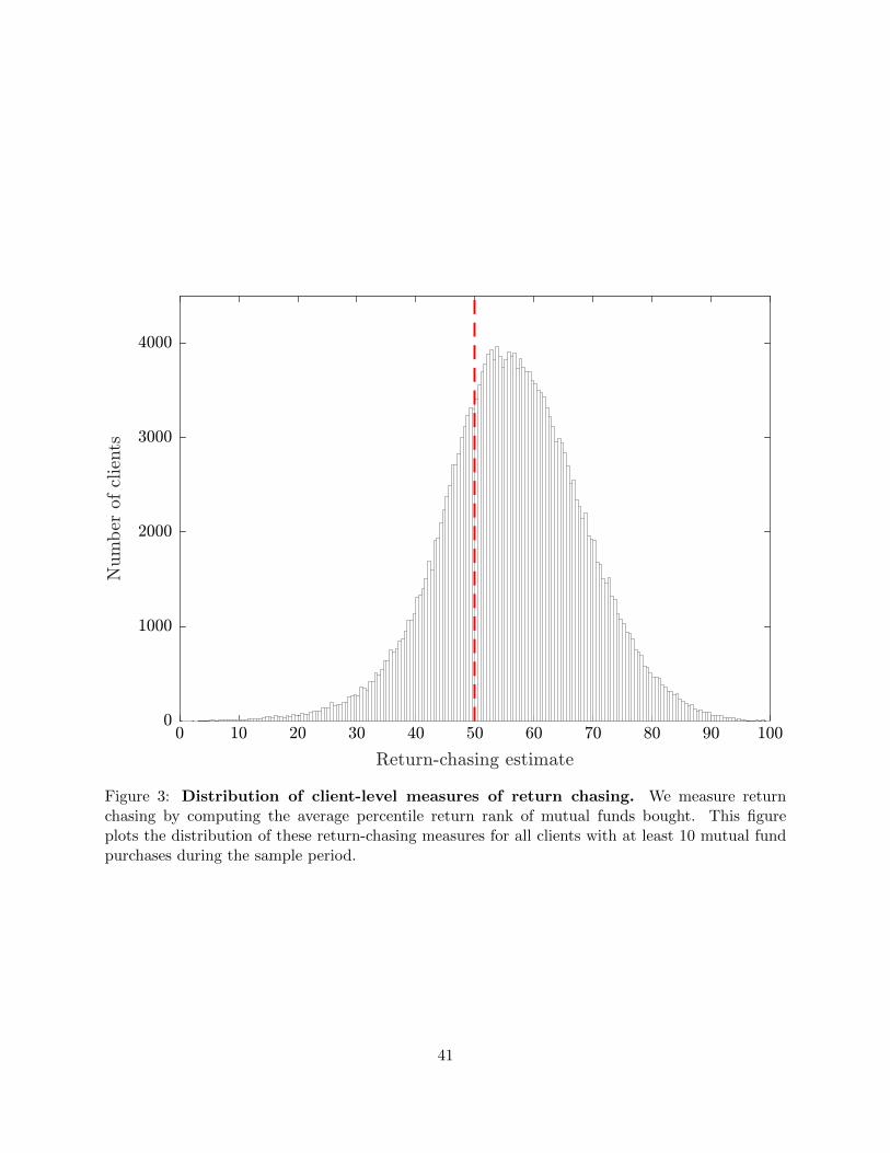
Return-chasing estimate
Num
ber
ofcl
ients
0 10 20 30 40 50 60 70 80 90 1000
1000
2000
3000
4000
Figure 3: Distribution of client-level measures of return chasing. We measure returnchasing by computing the average percentile return rank of mutual funds bought. This figureplots the distribution of these return-chasing measures for all clients with at least 10 mutual fundpurchases during the sample period.
41

Table 1: Descriptive statistics from dealer data
This table reports summary statistics for clients and financial advisors. “Account age (years)” isthe number of years an investor has been with any advisor. The account information is availablefor 3,483 advisors who appear in the dealer data also as clients. All variables are measured as ofJune 2012.
PercentilesVariable Mean 10th 25th 50th 75th 90th
Clients (N = 581,044)
Female (%) 51.4Age 51.2 33 41 51 61 69Account age (years) 3.6 1 1 3 6 7Number of plans 1.9 1 1 1 2 4Number of funds 5.2 1 2 3 7 12Account value, $K 68.1 2.1 8.1 27.3 75.6 161.2Finance professional 1.1%
Financial advisors (N = 5,838)
Female (%) 27.9Age 48.5 32 40 49 57 64Account age (years) 3.8 1 2 3.5 6 7Number of plans 3.2 1 1 3 4 6Number of funds 9.6 1 3 7 13 21Account value, $K 127.1 3.6 16.7 60.4 158.6 308.0Tenure 4.4 1 2 4 6 8Number of clients 74.3 1 3 24 100 217Number of plans/client 1.7 1 1.1 1.6 2.0 2.5Number of funds/client 4.2 1 2.0 3.7 5.6 7.5Client assets, $ thousands 5,064.0 5.2 55.4 916.9 5,493.6 14,575.3
42

Account types Clients Advisors Time horizon Clients Advisors
General 24.1% 32.5% 1–3 years 3.2% 3.7%Retirement 66.0% 54.0% 4–5 years 9.4% 7.5%Education savings 5.1% 8.1% 6–9 years 68.0% 67.6%Tax-free 4.5% 5.3% 10+ years 19.5% 21.2%Other 0.4% 0.1%
Risk tolerance Clients Advisors Salary Clients Advisors
Very low 4.2% 1.0% $30–50k 35.8% 19.9%Low 4.3% 2.7% $50–70k 35.0% 27.9%Low to Moderate 8.5% 3.1% $70–100k 16.5% 19.7%Moderate 51.5% 30.1% $100–200k 12.1% 30.3%Moderate to High 19.7% 20.7% $200–300k 0.2% 1.6%High 11.9% 42.3% Over $300k 0.3% 0.8%
Financial knowledge Clients Advisors Net worth Clients Advisors
Low 42.8% 3.4% Under $35k 4.9% 2.8%Moderate 51.4% 19.1% $35–60k 7.6% 5.0%High 5.8% 77.6% $60–100k 10.3% 8.1%
$100–200k 18.5% 12.8%Over $200k 58.8% 71.4%
43
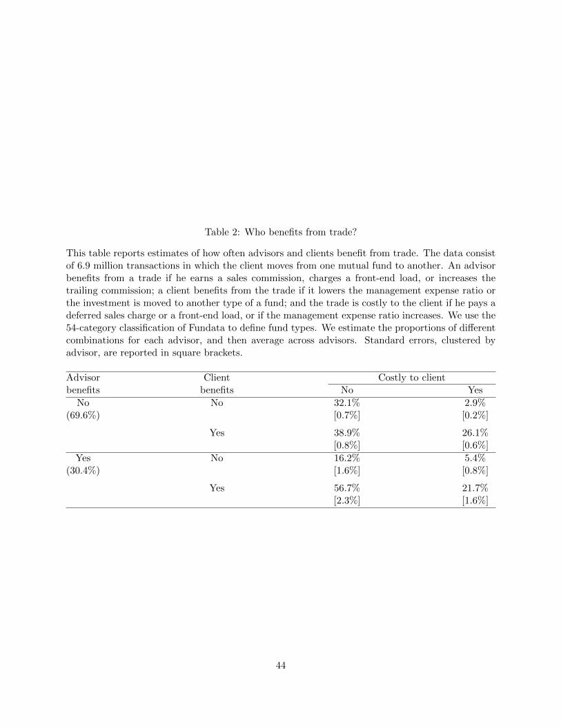
Table 2: Who benefits from trade?
This table reports estimates of how often advisors and clients benefit from trade. The data consistof 6.9 million transactions in which the client moves from one mutual fund to another. An advisorbenefits from a trade if he earns a sales commission, charges a front-end load, or increases thetrailing commission; a client benefits from the trade if it lowers the management expense ratio orthe investment is moved to another type of a fund; and the trade is costly to the client if he pays adeferred sales charge or a front-end load, or if the management expense ratio increases. We use the54-category classification of Fundata to define fund types. We estimate the proportions of differentcombinations for each advisor, and then average across advisors. Standard errors, clustered byadvisor, are reported in square brackets.
Advisor Client Costly to clientbenefits benefits No Yes
No No 32.1% 2.9%(69.6%) [0.7%] [0.2%]
Yes 38.9% 26.1%[0.8%] [0.6%]
Yes No 16.2% 5.4%(30.4%) [1.6%] [0.8%]
Yes 56.7% 21.7%[2.3%] [1.6%]
44
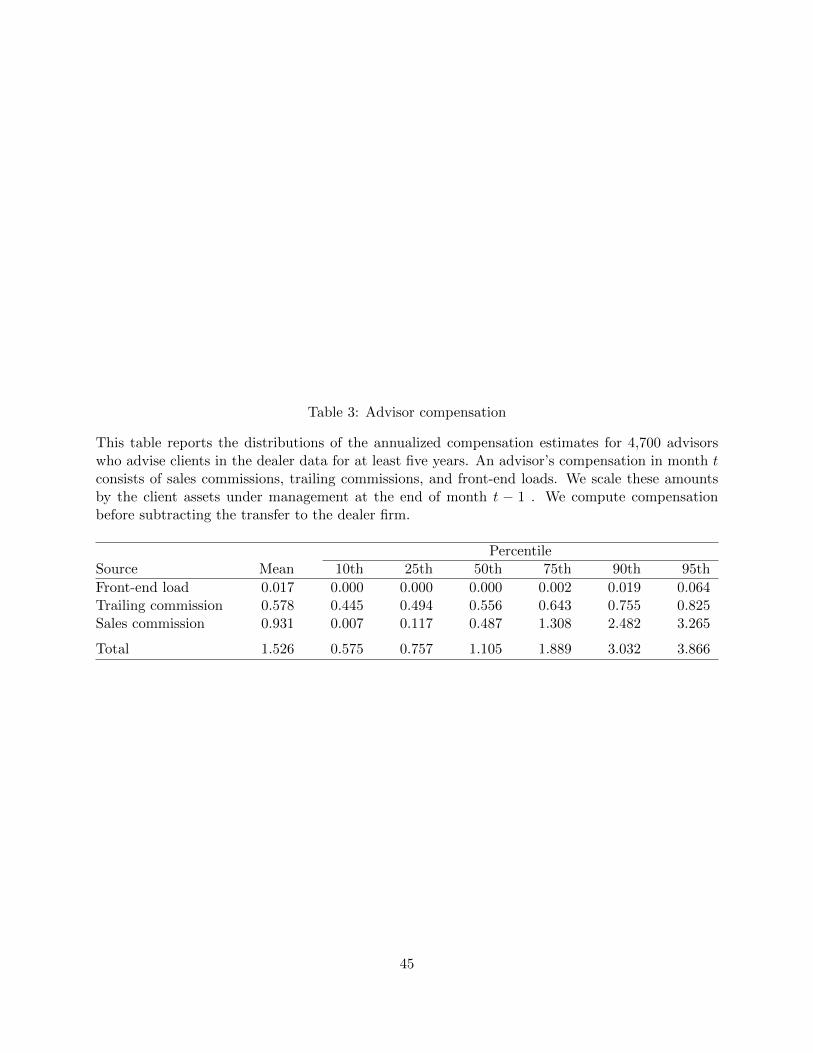
Table 3: Advisor compensation
This table reports the distributions of the annualized compensation estimates for 4,700 advisorswho advise clients in the dealer data for at least five years. An advisor’s compensation in month tconsists of sales commissions, trailing commissions, and front-end loads. We scale these amountsby the client assets under management at the end of month t − 1 . We compute compensationbefore subtracting the transfer to the dealer firm.
PercentileSource Mean 10th 25th 50th 75th 90th 95th
Front-end load 0.017 0.000 0.000 0.000 0.002 0.019 0.064Trailing commission 0.578 0.445 0.494 0.556 0.643 0.755 0.825Sales commission 0.931 0.007 0.117 0.487 1.308 2.482 3.265
Total 1.526 0.575 0.757 1.105 1.889 3.032 3.866
45

Table 4: Measures of trading behavior: Clients versus advisors
This table reports estimates of how clients and advisors trade. The measures are defined as follows:(i) Turnover is the market value of purchases and sales divided by the beginning of month marketvalue of holdings, annualized by multiplying by 12; (ii) Active management is the portfolio shareof index funds and target-date funds; (iii) Return chasing is the average percentile rank of priorone-year returns for funds bought; (iv) Disposition effect is the proportion of gains realized (PGR)minus the proportion of loses realized (PLR), computed using data on those months when theinvestor sells something; (v) Home bias is the fraction of Canadian equity mutual fund purchasesout of all equity fund purchases; and (vi) growth tilt is the fraction of growth funds bought minusthe fraction of value funds bought. We compute these measures for each client and then aggregatethe data to advisor level. The last row reports the average percentile fee rank of the funds thatclients and advisors purchase. We compute within-fund type percentile ranks using the 54-categoryclassification of Fundata. The sample includes those advisors who also appear as clients in thedealer data, and who advise clients for at least two years.
Clients Advisors Difference,Behavior Mean SE Mean SE t-value N
TurnoverRetirement accounts 29.1% 0.4% 33.4% 0.6% 7.23 3,276Open accounts 28.1% 0.5% 45.4% 1.1% 15.68 2,035
Active management 99.1% 0.1% 99.1% 0.1% 0.26 3,254Return chasing 58.7% 0.1% 60.7% 0.2% 11.98 3,170Disposition effect
Retirement accounts −2.1% 0.3% −1.0% 0.5% 2.13 2,118Open accounts −6.0% 0.8% −7.6% 1.4% −1.11 673
Home biasRetirement accounts 46.1% 0.3% 41.5% 0.4% −11.95 3,205Open accounts 40.7% 0.7% 36.3% 0.9% −6.04 1,497
Growth tilt 9.1% 0.2% 6.9% 0.3% −7.25 3,252
Percentile feewithin fund type 38.3% 0.2% 39.6% 0.4% 3.28 1,854
46
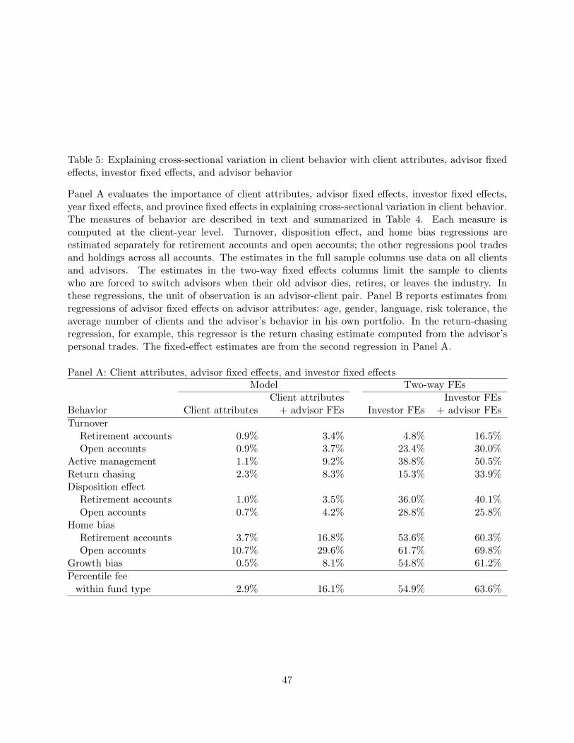
Table 5: Explaining cross-sectional variation in client behavior with client attributes, advisor fixedeffects, investor fixed effects, and advisor behavior
Panel A evaluates the importance of client attributes, advisor fixed effects, investor fixed effects,year fixed effects, and province fixed effects in explaining cross-sectional variation in client behavior.The measures of behavior are described in text and summarized in Table 4. Each measure iscomputed at the client-year level. Turnover, disposition effect, and home bias regressions areestimated separately for retirement accounts and open accounts; the other regressions pool tradesand holdings across all accounts. The estimates in the full sample columns use data on all clientsand advisors. The estimates in the two-way fixed effects columns limit the sample to clientswho are forced to switch advisors when their old advisor dies, retires, or leaves the industry. Inthese regressions, the unit of observation is an advisor-client pair. Panel B reports estimates fromregressions of advisor fixed effects on advisor attributes: age, gender, language, risk tolerance, theaverage number of clients and the advisor’s behavior in his own portfolio. In the return-chasingregression, for example, this regressor is the return chasing estimate computed from the advisor’spersonal trades. The fixed-effect estimates are from the second regression in Panel A.
Panel A: Client attributes, advisor fixed effects, and investor fixed effectsModel Two-way FEs
Client attributes Investor FEsBehavior Client attributes + advisor FEs Investor FEs + advisor FEs
TurnoverRetirement accounts 0.9% 3.4% 4.8% 16.5%Open accounts 0.9% 3.7% 23.4% 30.0%
Active management 1.1% 9.2% 38.8% 50.5%Return chasing 2.3% 8.3% 15.3% 33.9%Disposition effect
Retirement accounts 1.0% 3.5% 36.0% 40.1%Open accounts 0.7% 4.2% 28.8% 25.8%
Home biasRetirement accounts 3.7% 16.8% 53.6% 60.3%Open accounts 10.7% 29.6% 61.7% 69.8%
Growth bias 0.5% 8.1% 54.8% 61.2%
Percentile feewithin fund type 2.9% 16.1% 54.9% 63.6%
47

Panel B: Regressions of advisor fixed effects on advisor attributesIndependent Turnover Active Return Disposition effectvariable Retirement Open management chasing Retirement Open
Coefficients
Log(Age) −18.23 −14.06 −0.59 1.62 −0.42 −1.07Female 1.09 −2.16 0.07 0.48 −1.06 2.48French speaking −0.78 −0.13 0.65 −0.64 1.82 2.49log(# of clients) −0.55 −0.07 2.54 −1.82 2.23 0.81Risk tolerance
Moderate −4.63 5.22 −0.28 −0.68 −4.13 0.66Moderate to High −1.46 2.53 −0.07 0.28 −5.18 −2.03High −2.50 6.48 −0.04 0.54 −4.72 −0.72
Advisor’s behavior 0.12 0.07 0.32 0.21 0.07 0.06
t-values
Log(Age) −5.73 −4.87 −1.65 2.63 −0.29 −0.24Female 0.64 −1.26 0.36 1.31 −1.21 0.94French speaking −0.55 −0.07 2.54 −1.82 2.23 0.81log(# of clients) −2.80 −3.14 −0.04 −0.29 0.58 1.63Risk tolerance
Moderate −0.76 1.35 −0.57 −0.73 −1.83 0.11Moderate to High −0.25 0.79 −0.13 0.30 −2.29 −0.41High −0.43 2.05 −0.08 0.62 −2.20 −0.15
Advisor’s behavior 5.31 2.94 4.24 15.99 5.88 2.41
N 3,163 1,964 3,095 3,101 1,813 612Adjusted R2 6.3% 5.7% 24.0% 14.6% 3.0% 1.2%
48

(cont’d)Independent Home bias Growth Percentilevariable Retirement Open bias fee
Coefficients
Log(Age) 5.60 −0.88 0.57 2.81Female 0.16 1.75 −0.07 −0.10French speaking −1.10 0.53 0.03 1.34log(# of clients) −1.39 0.34 0.05 1.78Risk tolerance
Moderate 7.23 8.80 0.56 −0.09Moderate to High 8.44 9.26 0.28 −1.63High 8.87 13.25 0.84 −0.01
Advisor’s behavior 0.29 0.34 0.19 0.14
t-values
Log(Age) 4.04 −0.33 0.54 2.21Female 0.20 1.20 −0.12 −0.16French speaking −1.39 0.34 0.05 1.78log(# of clients) −0.73 −2.20 −0.47 −0.69Risk tolerance
Moderate 3.56 1.71 0.42 −0.06Moderate to High 4.19 1.89 0.20 −1.12High 4.61 2.80 0.66 −0.01
Advisor’s behavior 20.48 18.70 11.04 8.49
N 3,182 1,451 3,224 1,727Adjusted R2 17.0% 24.2% 7.8% 6.4%
49

Tab
le6:
Ad
vis
ortr
adin
gb
ehav
ior
and
clie
nt
net
alp
has
Th
ista
ble
rep
ort
ses
tim
ate
sfr
om
cross
-sec
tion
alre
gres
sion
sof
clie
nts
’al
ph
ason
thei
rad
vis
ors
’tr
ad
ing
beh
avio
r.T
he
mea
sure
sare
the
sam
eas
those
sum
mar
ized
inT
able
4:ac
tive
man
agem
ent,
retu
rnch
asin
g,d
isp
osi
tion
effec
t,h
ome
bia
s,gr
owth
tilt
,an
dp
erce
nti
le.
We
mea
sure
alp
has
an
db
ehav
ior
atth
ead
vis
orle
vel.
Th
eal
ph
asar
eco
mp
ute
du
sin
ga
six-f
acto
rm
od
elth
at
incl
ud
esth
eC
anad
ian
mark
etfa
ctor,
the
Nor
thA
mer
ican
size
,va
lue,
and
mom
entu
mfa
ctors
of
Fam
aan
dF
ren
ch,an
dC
an
ad
ian
def
au
ltan
dte
rmfa
ctors
.T
he
clie
nt
alp
ha
isn
etof
fun
d’s
exp
ense
rati
os,
fron
t-en
dlo
ads,
and
def
erre
dsa
les
char
ges
.T
he
slop
eco
effici
ents
are
scale
dso
that
they
rep
rese
nt
the
chan
gein
the
annu
aliz
edn
etal
ph
agi
ven
aon
e-st
and
ard
dev
iati
on
shock
toth
ead
vis
or’s
trad
ing
beh
avio
res
tim
ate.
Th
ela
stco
lum
n’s
regr
essi
onre
pla
ces
mis
sin
gva
lues
wit
hze
ros,
and
itin
clu
des
ase
tof
ind
icato
rva
riab
les
tore
pre
sent
thes
em
issi
ng
valu
es.
Exp
lan
ator
yR
egre
ssio
nva
riab
le(1
)(2
)(3
)(4
)(5
)(6
)(7
)(8
)
Coeffi
cie
nts
Tu
rnov
er0.0
10.0
3A
ctiv
em
anage
men
t−
0.1
1-0
.07
Ret
urn
chas
ing
0.10
0.0
8D
isp
osit
ion
effec
t0.
030.0
5H
ome
bia
s0.
250.2
3G
row
thti
lt0.0
60.0
5P
erce
nti
lefe
e−
0.1
9−
0.1
8
t-valu
es
Tu
rnov
er0.
200.
66
Act
ive
man
agem
ent
−2.5
5-1
.55
Ret
urn
chasi
ng
2.19
1.6
6D
isp
osi
tion
effec
t0.
811.
07
Hom
eb
ias
5.80
5.00
Gro
wth
tilt
1.3
31.2
3P
erce
nti
lefe
e−
3.5
2−
3.4
5
No.
ofad
vis
ors
2,3
50
2,43
52,
333
1,78
42,
295
2,3
58
1,555
2,4
39
Ad
just
edR
20.0
%0.
2%0.
2%0.
0%1.
4%0.0
%0.7
%2.3
%
50
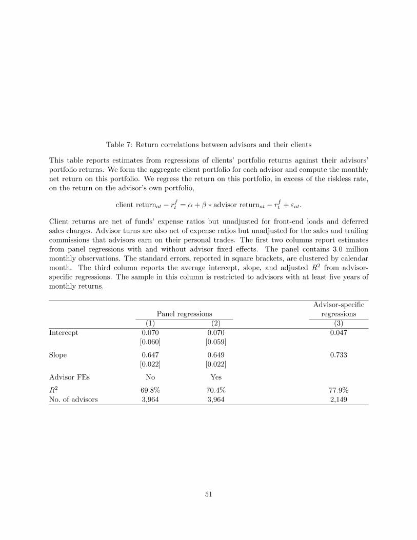
Table 7: Return correlations between advisors and their clients
This table reports estimates from regressions of clients’ portfolio returns against their advisors’portfolio returns. We form the aggregate client portfolio for each advisor and compute the monthlynet return on this portfolio. We regress the return on this portfolio, in excess of the riskless rate,on the return on the advisor’s own portfolio,
client returnat − rft = α+ β ∗ advisor returnat − rft + εat.
Client returns are net of funds’ expense ratios but unadjusted for front-end loads and deferredsales charges. Advisor turns are also net of expense ratios but unadjusted for the sales and trailingcommissions that advisors earn on their personal trades. The first two columns report estimatesfrom panel regressions with and without advisor fixed effects. The panel contains 3.0 millionmonthly observations. The standard errors, reported in square brackets, are clustered by calendarmonth. The third column reports the average intercept, slope, and adjusted R2 from advisor-specific regressions. The sample in this column is restricted to advisors with at least five years ofmonthly returns.
Advisor-specificPanel regressions regressions
(1) (2) (3)
Intercept 0.070 0.070 0.047[0.060] [0.059]
Slope 0.647 0.649 0.733[0.022] [0.022]
Advisor FEs No Yes
R2 69.8% 70.4% 77.9%No. of advisors 3,964 3,964 2,149
51

Table 8: Investment performance of clients and advisors
This table reports annualized six-factor model alphas for clients and advisors. We measure clients’alphas at the advisor level by computing the return on the aggregate portfolio held by each advisor’sclients. Net alpha is based on the return net of funds’ management expense ratios. The additionalexpenses consist of front-end loads and deferred sales charges. We subtract the average additionalexpenses from the net alpha estimate so that they do not affect covariances in the alpha estimation.Advisors’ alphas are computed using returns on their personal portfolios. The rebates consist ofsales commissions and trailing commissions that advisors earn when investing their own wealth.We assume that advisor keep 78% of the commission payments. The last line, client portfolioplus rebates, is a counterfactual alpha, constructed by assuming that the advisor holds the sameportfolio as his clients. The sample consists of 2,092 advisors who have their own portfolio andclients for at least five years. The bottom part of the table reports the Pearson and Spearman(rank) correlations between clients’ and advisors’ net alpha estimates.
Average Median SD
Clients Net alpha −3.15 −3.10 2.02Net alpha minus additional expenses −3.47 −3.38 2.06
Advisors Net alpha −4.09 −3.81 2.86Net alpha plus rebates −3.15 −2.97 2.86Client portfolio plus rebates −2.36 −2.36 2.08
Correlation between net alphas Pearson 0.16Spearman 0.28
52

Table 9: Change in advisor behavior after the end of the career
This table reports estimates how advisor behavior changes after the advisor stops advising clients.The measures are defined in Table 4. The sample consists of 982 advisors who have their personalportfolios in the data, and who execute trades suitable for measuring each trading pattern afterthey stop advising clients. We orthogonalize each measure with respect to advisor age by runninga pooled regression of behavior on (demeaned) log-age, collect the intercepts plus residuals, andthen compute for each advisor the active and post-career averages.
Active advisors Post-career Difference,Behavior Mean SE Mean SE t-value N
TurnoverRetirement accounts 31.0% 1.9% 26.1% 2.1% −1.82 770Open accounts 43.5% 3.3% 26.9% 2.7% −4.17 404
Active management 95.9% 0.4% 96.0% 0.5% 0.26 637Return chasing 61.8% 0.6% 56.7% 0.8% −5.30 597Disposition effect
Retirement accounts −4.7% 1.7% −0.5% 1.9% 1.63 316Open accounts −4.2% 4.3% −12.0% 5.0% −1.29 69
Home biasRetirement accounts 37.0% 1.3% 39.6% 1.6% 1.62 470Open accounts 46.8% 3.0% 41.4% 3.2% −1.86 150
Growth tilt 9.7% 1.0% 8.9% 1.0% −0.79 637
Percentile feewithin fund type 39.1% 1.3% 39.3% 1.6% 0.13 183
53