Cost Behavior and Stock Returns

Dashan Huang

Singapore Management University

Fuwei Jiang

Central University of Finance and Economics

Jun Tu

Singapore Management University

Guofu Zhou∗

Washington University in St. Louis

First draft: June 2014

Current version: April 2015

∗We are grateful to Jamie Alcock, Gennaro Bernile, Guojin Chen, Tarun Chordia, Sudipto Dasgupta, BingHan, Feng Li, Chen Lin, Roger Loh, Xingguo Luo, Tao Ma, Jialin Yu, Jianfeng Yu, Quan Wen, and seminarparticipants at the 2014 International Conference in Corporate Finance and Capital Market, 2014 SMU FinanceSummer Camp, 2014 Young Finance Scholars Symposium, and Central University of Finance and Economicsfor their very helpful comments. We also thank Kenneth R. French, Laura Xiaolei Liu, and Lu Zhang forkindly sharing us their data. Jun Tu acknowledges that the study was funded through a research grant (GrantNo. C207/MSS12B006) from Singapore Management University and a research grant from Sim Kee BoonInstitute for Financial Economics. Send correspondence to Guofu Zhou, Olin School of Business, WashingtonUniversity in St. Louis, St. Louis, MO 63130; e-mail: zhou@wustl.edu; phone: 314-935-6384.

Cost Behavior and Stock Returns

Abstract

In this paper, we examine the valuation implications of cost behavior, and find that firms with

high growth rate in operating costs generate substantially lower future stock returns than those

with low cost growth. A spread portfolio of long stocks with low cost growth and short stocks

with high cost growth earns an average abnormal return of 12% per year. This strategy is robust

over time, across market capitalization, and to control for alternative anomalies and risks. Cost

growth is strongly associated with deterioration in a firm’s future profitability, which investors appear

failing to incorporate into valuation. In addition, the negative cost growth-return relation is stronger

among firms with lower investor attention, higher valuation uncertainty, and higher transaction costs,

suggesting that mispricing plays an important role in explaining the cost growth effect.

JEL Classification: G12, G14

Keywords: Cost growth, Limited attention, Mispricing, Asset pricing, Anomaly

1 Introduction

Voluminous literature shows that stock prices may fail to fully incorporate public information

in earnings and its components. For examples, Ball and Brown (1968), Foster, Olsen, and Shevlin

(1984), Bernard and Thomas (1989, 1990), Kothari (2001), Livnat and Mendenhall (2006), among

others, show that stock prices react positively to earnings surprises with a positive price drift in the

post-earnings announcement periods. Cross-sectionally, Piotroski (2000), Balakrishnan, Bartov, and

Faurel (2010), Novy-Marx (2013), Fama and French (2015), Hou, Xue, and Zhang (2015) and others

show that earnings level positively predicts the average future stock returns. Moreover, studies also

find that earnings components have important impacts for stock prices above and beyond earnings. For

examples, Sloan (1996), Collins and Hribar (2000), and DeFond and Park (2001) show that accruals

negatively predict future stock returns and they attribute the accruals anomaly to earnings fixation.

Swaminathan and Weintrop (1991), Ertimur, Livnat, and Martikainen (2003), and Jegadeesh and

Livnat (2006) show that revenues (sales) surprises lead to positive contemporaneous market reaction

and post-announcement drift up to six months. At a longer horizon, however, Lakonishok, Shleifer,

and Vishny (1994) show that firms with high sales growth generate substantially lower returns in the

next five years due to investors’ over-extrapolation of past gains.

In this paper, we investigate the valuation implications of a firm’s cost behavior information

publicly available in financial statements. Costs are incurred when a firm involves business activities

to create goods and services, and they are important components of earnings. The management

and cost accountants have traditionally analyzed cost behavior for managerial decision-making and

control (Garrison and Noreen, 2002). Porter (1980) argues that a firm can achieve competitive

advantage by continuously reducing costs and cost leadership is a generic management strategy.

Despite the fact that both academics and practitioners have highlighted the strategic importance of

cost behavior, there is little research that examines explicitly its stock valuation implications. Indeed,

in their reviews on variables that explain the cross section of stock returns, Green, Hand, and Zhang

(2013, 2014), Chordia, Subrahmanyam, and Tong (2014), Lewellen (2014), McLean and Pontiff

(2015), and Harvey, Liu, and Zhu (2015) list hundreds of firm characteristics and risks, but none

of them explicitly considers pricing information in costs. In this paper, we fill this gap of the literature

by investigating whether one can forecast the cross section of future stock returns based on a simple

1

cost behavior measure, the cost growth.

We find that firms with high growth rate in operating costs generate substantially lower future

stock returns than those with low cost growth. A typical spread portfolio of long stocks with low cost

growth and short stocks with high cost growth earns an average abnormal return of 12% per year.

We compare several risk and mispricing-based interpretations for the negative cost growth effect and

find that the empirical evidence positively supports the mispricing-based one. Cross-sectionally, we

find that the negative cost growth effect is stronger among firms with lower investor attention, higher

valuation uncertainty, and higher transaction costs, confirming the mispricing explanation.

Economically, why does cost growth matter? In their profit analysis, Banker and Chen (2006)

show that cost behavior helps to forecast future earnings. Weiss (2010) shows that cost behavior

influences analysts’ earnings forecasts and hence investors’ beliefs about the value of firms. In

addition, costs are more sticky than sales in that costs decrease less with a sales activity decrease

than they increase with an equivalent sales activity increase, since managers may retain idle capacity

as product demand falls but add capacity as demand grows (e.g., Anderson, Banker, and Janakiraman,

2003). The sticky cost hence implies that increases in costs may negatively forecast a firm’s future

profitability, since future costs saving will be limited under negative sales activity shocks, resulting in

decreases in earnings. Consistent with these studies, we find that cost growth contains additional

predictive information about deterioration in a firm’s future profitability. For behavior reasons,

investors appear not paying enough attention to the negative valuation information.

This paper contributes to the recent research on how the market processes information contained

in costs beyond earnings. Lipe (1986) finds that the contemporaneous stock price reacts strongly to

five costs components. Swaminathan and Weintrop (1991) detect negative contemporaneous stock

price reaction to costs surprises using two-day cumulative announcement returns. Ertimur, Livnat,

and Martikainen (2003) further compare differential contemporaneous market reactions to sales and

costs surprises using three-day cumulative returns centered on preliminary earnings announcement

date. In contrast to these studies primarily focusing on the contemporaneous relationship between

costs and stock returns around the earnings announcement, we examine directly the predictability of

cost behavior on the cross-sectional future average stock returns over one- to five-year investment

horizons. We find that cost growth contains strong incremental forecasting power for average stock

returns beyond earnings, and, at the longer annual horizon, cost growth dominates sales growth in

2

forecasting stock returns.

Our finding of the negative cost growth effect is consistent with the behavioral asset pricing

theories of Hirshleifer and Teoh (2003), Peng and Xiong (2006), DellaVigna and Pollet (2009),

Hirshleifer, Lim, and Teoh (2009), among others, that limited investor attention and category learning

may cause underreaction to information and return predictability. In addition, Fiske and Taylor (1991)

and Libby, Bloomfield, and Nelson (2002) suggest that investors tend to value a firm only based on

a few salient variables such as earnings rather than performing a complete analysis of all relevant

variables in financial statements, even if some less salient components like cost growth contain

additional information beyond earnings.

Intuitively, there is ample anecdotal evidence that the valuation information conveyed in cost

behavior is less salient to investors.1 For examples, accountants, media, and financial analysts

concentrate most of their attention on earnings, while academic financial economists are more

concerned with dividends and cash flows and corporate managers may emphasize empire-building

policies like sales growth and market share. In addition, the increase in a firm’s costs can be driven by

increase in sales or decrease in production efficiency. Therefore, the value impact of cost growth

is relatively less salient, more uncertain and hard to digest. As a result, investors are likely to

largely ignore the negative valuation information in cost growth and fixate on other more salient

variables like sales and earnings. This interpretation is in line with behavior studies of Kahneman

and Tverskey (1973), Daniel, Hirshleifer, and Subrahmanyam (1998), Hirshleifer (2001), and many

others. In short, stocks with high prior cost growth are likely to be overvalued, leading to subsequent

underperformance in stock prices.2

Specifically, this paper focuses on a simple cost behavior measure, cost growth, the year-on-year

percentage change in a firm’s total operating costs (the sum of costs of goods sold, COGS, and selling,

general, and administrative expenses, XSGA). Using a panel of U.S. stock returns over the 1968 to

2013 period, we document that cost growth is a strong negative predictor of the cross-section of future

stock returns. Sorting by the firms’ pervious-year cost growth, we find that the average raw return

of the equal-weighted lowest cost growth decile portfolio is about 19% per year, while the average

1A recent case is Facebook whose shares fell 11% on October 29, 2014 on comments from David Wehner, chieffinancial officer, who warned analysts that Facebook’s costs would rise between 50 to 70 per cent next year, although theinformation of increasing costs on acquiring WhatsApp can be known as early as February 19, 2014.

2The q-theory of investment (e.g., Cochrane, 1991; Lyandres, Sun, and Zhang, 2008; Xing, 2008; Li and Zhang, 2010)may offer an alternative explanation for the negative cost growth effect.

3

raw return of the firms in the highest cost growth decile portfolio is as low as 5.5% per year. The

cost growth spread portfolio which goes long the lowest cost growth decile and short the highest

cost growth decile generates average returns of about 13.5% per year. The cost growth effect cannot

been explain by the standard risk measures like market beta, size and book-to-market ratio, and it

generates an average abnormal return of 12% per year based on the Fama-French three factor model.

The cost growth effect remains robust and large when we further control for alternative factors like

the momentum, liquidity, investment, and profitability factors (Carhart, 1997; Pastor and Stambaugh,

2003; Fama and French, 2015; Hou, Xue, and Zhang, 2015).

The cost growth effect is stable over time. It generates consistently positive returns in 42 out of

46 years over our sample periods 1968–2013, and it even yields a small positive return in 2008 in the

midst of the market crash. Moreover, the cost growth effect persists well beyond the first year and lasts

up to about five years after the information is publicly disclosed. In addition, the cost growth effect is

robust across different market capitalization levels: significant among the large firms and particularly

strong for the micro size firms. For example, the cost growth spread portfolios of long the lowest

cost growth quintile and short the highest growth quintile generate average returns of 10.1%, 5.9%,

and 5.3% per annum, respectively, across the micro, small, and large size groups, classified annually

using the 20th and 50th NYSE market equity percentiles, and all of them are statistically significant at

the 1% level.

We find that the cost growth effect remains strong even after controlling for other important

determinants of the cross-section of stock returns. In particular, we compare cost growth with firm

size (Banz, 1981), book-to-market (Fama and French, 1993), momentum (Jegadeesh and Titman,

1993), and monthly reversal (to capture the liquidity and microstructure effects, Jegadeesh, 1990),

industry dummies and industry adjustment (to control for any industry-specific effects, Fama and

Frnech, 1997). We find that the forecasting power of cost growth remains significant after including

these controls, and is economically comparable with well known anomalies such as size, value and

momentum.

Motivated by Richardson, Sloan, Soliman, and Tuna (2006), we decompose cost growth into sales

growth minus the change in markup (reflecting the reduction in production efficiency) and minus the

interaction between sales growth and change in markup. We examine the roles that the components

play in the negative cost growth effect. Our results show that both sales growth and reduction in

4

production efficiency (change in markup) contribute to the ability of cost growth to predict the cross

section of stock returns, either individually or jointly. However, cost growth’s predictive ability is

more powerful than its components. The decomposition analysis provides further insight into the cost

growth effect, because cost growth effectively not only captures the predictability of both sales growth

and reduction in efficiency (profitability), but also provides a partial explanation for the sales growth

and profitability anomalies documented in the literature.

In further tests, we compare the cost growth effect with a set of standard return determinants

related to growth and earnings for the cross section of stock returns in the accounting and finance

literature. We find that the negative cost growth effect remains significant in the Fama-MacBeth

regressions that control for six investment and growth-related anomalies (including the accruals from

Sloan (1996), net operating assets from Hirshleifer, Hou, Teoh, and Zhang (2004), investment-to-

asset from Lyandres, Sun, and Zhang (2008), asset growth from Cooper, Gulen, and Schill (2008),

investment growth from Xing (2008), and abnormal capital investment from Titman, Wei, and Xie

(2004)) and five earnings and profitability related anomalies (including the earnings surprises based

on quarterly earnings SUEQ, the earnings surprises based on annual earnings SUEA, gross profit

GP, return on asset ROA, and return on equity ROE from Ball and Brown (1968), Foster, Olsen,

and Shevlin (1984), Bernard and Thomas (1989, 1990), Livnat and Mendenhall (2006), Novy-Marx

(2013), Fama and French (2008, 2015), Hou, Xue, and Zhang (2015)). Our findings indicate that

cost growth contains distinct information about future stock returns that is incremental to that of other

investment, growth, earnings, and profitability related measures.

Moreover, we find that both COGS growth and XSGA growth in the calculation of cost growth

display significantly negative forecasting power for future stock returns. And the forecasting power

of cost growth is robust for various alternative definitions of operating costs such as including

depreciation and amortization expenses, excluding R&D expenses, scaling changes in costs with

alternative deflators such as lagged total asset, or calculating the total operating costs indirectly as

the difference between the sales and earnings, rather than the sum of COGS and XSGA.

We then investigate whether macroeconomic risk or mispricing is driving the negative cost growth

effect. To address this question, we regress the excess returns of cost growth deciles on the mimicking

portfolio returns of the Chen, Roll, and Ross’s (1986) five macroeconomic risk factors. The average

abnormal return of the cost growth spread portfolio is still 12% per annum based on the Chen, Roll,

5

and Ross (1986) model, and the explanatory power mainly comes from the industry production and

inflation factors. It suggests that the macroeconomic risk model seems to work similarly to the

Fama-French three-factor model, and it cannot explain away the cost growth effect. To evaluate

the mispricing-based explanation for the cost growth effect, we augment the Fama-French three-

factor model with the Hirshleifer and Jiang (2010)’s financing-based mispricing factor. We find that

the misprcing factor does a better job in explaining the cost growth effect. The average abnormal

return of the cost growth spread portfolio is reduced to be 5% per annum. The results suggest that

market misvaluation and irrational investor perceptions seem to play a more important role than

the macroeconomic risks in explaining the cost growth effect, and the market appears to fail to

incorporates the negative information about future earnings deterioration conveyed by cost growth,

leading to return predictability.

We further examine the mispricing-based explanation by conducting various regression analysis

based on proxies for limited investor attention, valuation uncertainty, and arbitrage costs. Specifically,

based on the recent psychology and asset pricing literature, firms with less attention from investors

may have more sluggish market reactions to the information embedded in cost growth; moreover, the

underreaction to cost growth should be more pronounced when the valuation uncertainty is higher

(which places a greater cognitive burden on investor attention and leaves more room for mispricing);

and, lastly, the limits to arbitrage theory suggests that the underreaction to cost growth is more likely

to be sustained in firms with higher arbitrage costs. Empirically, our Fama-MacBeth regressions show

that the negative return predictability of cost growth is substantially stronger among firms that are with

less investor attention (smaller caps, lower analyst coverage), higher valuation uncertainty (higher

idiosyncratic volatility, younger age), and higher transaction costs (lower price, higher Amihud (2002)

illiquidity measure, lower dollar volume), consistent with our hypothesis that mispricing appears to

drive the negative cost growth effect.

The mispricing-based interpretation for the negative cost growth effect is consistent with the

recent literature on the post earnings announcement drift (PEAD) effect. Bartov, Radhakrishnan,

Krinsky (2000), Hirshleifer and Teoh (2003), Peng and Xiong (2006), DellaVigna and Pollet (2009),

and Hirshleifer, Lim, and Teoh (2009), among others, suggest that limited investor attention causes

market underreaction to earnings information and induces return predictability. Liang (2003) and

Francis, LaFond, Olsson, and Schipper (2007) show that uncertainty contributes to the earnings drift,

6

and investor biases are likely to be more pronounced in cases of greater information uncertainty

(Hirshleifer, 2001; Daniel, Hirshleifer, and Subrahmanyam, 1998, 2001; Zhang, 2006). In short,

our mispricing-based interpretation is similar to the case where mispricing arises from investors’

underreaction to earnings information (e.g., Bernard and Thomas, 1989, 1990).

The rest of this paper is organized as follows. Section 2 discusses the data and the calculation of

cost growth. Section 3 shows the stock return predictability of cost growth using both portfolio tests

and Fama-MacBeth regressions. Section 4 explores the potential economic explanations for the cost

growth effect. Section 5 concludes.

2 Data

We obtain the accounting data from Compustat and monthly stock returns data from the Center

for Research in Security Prices (CRSP). We also obtain the analyst coverage data from the I/B/E/S.

We use the one-month Treasury bill rate from Ken French’s web site as the risk-free rate. We consider

all domestic common stocks trading on the New York Stock Exchange (NYSE), American Stock

Exchange (Amex), and Nasdaq stock markets with accounting and returns data available. Following

Fama and French (1993), we exclude the closed-end funds, trusts, American Depository Receipts

(ADRs), Real Estate Investment Trusts (REITs), units of beneficial interest, and financial firms that

have four-digit standard industry classification (SIC) codes between 6000 and 6999. We also exclude

firms with negative book value of equity.3 We also require firms to be listed on Compustat for two

years before including them in our sample to mitigate backfilling biases.

Our main explanatory variable, cost growth (CG) in calendar year t, is defined as the year-to-year

percentage change in a firm’s total annual operating costs (OC) from the fiscal year ending in calendar

year t −1 to the fiscal year ending in calendar year t,

CGt =OCt −OCt−1

OCt−1. (1)

3Following Fama and French (1993), we calculate the book value of equity as shareholders’ equity (SEQ), plus balancesheet deferred taxes and investment tax credits (TXDITC) if available, and minus the book value of preferred stock. Weset missing values of TXDITC equal to zero. To calculate the value of preferred stock, we set it equal to the redemptionvalue (PSTKRV) if available, the liquidating value (PSTKL) if available, or the par value (PSTK), in that order. IfSEQ is missing, we set stockholder’ equity equal to the value of common equity plus the par value of preferred stock(CEQ+PSTK) if available, or total assets minus total liabilities (AT-LT), in that order.

7

The operating costs (OC) is the sum of costs of goods sold (COGS) plus selling, general, and

administrative expenses (XSGA), following the standard textbook like Penman (2012),

OCt = COGSt +XSGAt . (2)

To include a firm’s CGt in our sample, it must have positive nonmissing operating costs in both years t

and t −1. According to the U.S. Generally Accepted Accounting Principles (GAAP) and Compustat,

COGS represents all costs that are directly related to the cost of merchandise purchased or the cost of

goods manufactured and sold to customers, such as raw materials and direct labor. XSGA includes

all operation costs incurred in the regular course of business pertaining to the securing of operating

income but not directly related to product production, such as corporate expenses, advertisement

expenses, and amortization of research and development (R&D) expenses.

In this paper, we focus on total operating costs OC since it includes all the major operating costs of

running a business beyond specific costs components like COGS or XSGA alone (Anderson, Banker,

and Janakiraman, 2003). Moreover, the accounting classification of COGS and XSGA may be subject

to managerial judgment, which may introduce bias into the cost growth estimate of specific costs

components. Our cost growth measure OC then provides broad insights into the relationship between

cost behavior and future stock returns. However, in Section 3.7 and Table 7, we show that our results

are robust to growth in COGS and growth in XSGA as well.

Our operating costs measure OC does not include depreciation and amortization expenses, since

a firm’s depreciation may depend on the accounting rules a firm chooses, which may not be related to

a firm’s business fundamentals. Following GAAP, our operating costs measure OC includes a firm’s

R&D expenses, since the valuation of these investment in intangible innovation assets is uncertain,

subjective, and open to managerial manipulation and bias. In Section 3.7, we show that adding

depreciation, removing R&D, and scaling the costs changes by alternative deflators like lagged total

assets do not change the results. In unreported tables, we obtain similar findings when we define total

operating costs indirectly as the difference between the sales and income before extraordinary items,

which may include interest expenses and taxes, rather than the sum of COGS and XSGA.

To avoid look-ahead bias and ensure that the accounting information is publicly known before we

use it, following Fama and French (1993), we allow for a minimum 6-month lag between stock returns

8

and lagged accounting-based variables. Specifically, we match a firm’s stock returns from the periods

between July of year t +1 to June of year t +2 to the annual accounting data of the fiscal year ending

in calendar year t. To ensure that we have a reasonable number of firms in our early sample, following

Cooper, Gulen, and Schill (2008), we use the sample period from 1963 to 2012 for accounting data

and the sample period from July 1968 to December 2013 (546 months) for stock returns, since some

of our tests require five-years of prior accounting data.

3 Empirical Results

We investigate the predictive power of cost growth for the cross section of stock returns using both

portfolio sorts and Fama-MacBeth regressions.

3.1 Portfolio sorts on cost growth

In this subsection, we report the performance of portfolios sorted on cost growth over the sample

period 1968:07–2013:12, and examine the ability of cost growth to predict stock returns. At the end

of June of each year t +1, we form ten decile portfolios based on lagged cost growth rates in calendar

year t, defined as the percentage changes in a firm’s total operating costs from the fiscal year ending

in calendar year t −1 to the fiscal year ending in calendar year t as in Equations (2) and (1). We hold

these portfolios for one year, from July of year t + 1 to June of year t + 2, and compute the equal-

weighted monthly returns of these cost growth decile portfolios. Decile 1 refers to firms in the lowest

cost growth decile, and decile 10 refers to firms in the highest cost growth decile. The “Low-High”

cost growth spread portfolio is computed as long the lowest cost growth decile and short the highest

cost growth decile.

Table 1 shows that the cost growth deciles’ monthly average raw returns are generally decreasing

with cost growth, from 1.57% for the lowest cost growth decile to 0.45% for the highest cost growth

decile. The average return of the cost growth spread portfolio computed as the difference between

the returns of the lowest and highest cost growth deciles is 1.12% per month, with a t-statistics of

8.13, suggesting that a trading strategy that buys the lowest cost growth decile and sells the highest

cost growth decile will earn returns of roughly 13% per year on average. Harvey, Liu, and Zhu

(2015) recently raise an important data mining concern on anomaly discovery and suggest a much

9

higher hurdle with ta t-statistic greater than 3 in testing that the average return of a spread portfolio

of a newly discovered anomaly is zero. They also argue that anomalies based on economic theories

should have a lower hurdle. Our newly discovered cost growth anomaly is linked to the standard

earnings identity and accounting valuation model, and has a large t-statistic of 8.14, appearing to be

statistically significant even under the Harvey, Liu, and Zhu’s higher hurdle condition.

We then examine whether the negative cost growth-return relationship can be explained by

standard risk factor models. We compute the alphas or abnormal returns and factor loadings by

regressing the time series of excess portfolio returns of cost growth deciles on the corresponding factor

returns of the Fama and French (1993) three-factor model. The Fama-French three factors includes

the market factor (MKT), which is the value-weighted market return of all NYSE/Amex/Nasdaq firms

minus the risk-free interest rate (the one-month Treasury bill rate), the size factor (small minus big,

SMB), which is the difference between the return on small- and big-capitalization firms, and the

value factor (high minus low, HML), which is difference between the return on high and low book-to-

market stocks. These factor returns are downloaded from Ken French’s website. The literature shows

that these factors have earned significant returns and help to explain the cross-sectional variations of

stock returns. While there is on-going debate on the extent to which these factors capture risk versus

mispricing, controlling for them provides a more conservative test of whether the cost growth effect

comes from mispricing.

Table 1 shows that the negative cost growth effect remains strong based on the risk-adjusted

abnormal returns. Specifically, the lowest cost growth decile has a monthly Fama-French three-factor

alpha of 0.30% (t = 2.02), but the highest cost growth decile has a Fama-French three-factor alpha

of −0.68% (t = −4.42). Hence, firms with low cost growth are undervalued, while firms with high

cost growth are overvalued. The Fama-French three-factor alpha of the spread portfolio between the

lowest and highest cost growth deciles is 0.98% with a t-statistic of 8.08. It indicates that the long-

short cost growth spread strategy earns an abnormal return of roughly 12% per year, and it is both

economically sizable and statistically significant at the 1% level.

In unreported tables, we find that our findings are robust with with value-weights, and we obtain

consistently high abnormal returns ranging from 0.70% to 1.01% per month for the cost growth long-

short spread portfolio, when we further control for alternative asset pricing models such as the Carhart

(1997) Fama-French and momentum four-factor model, the Pastor and Stambaugh (2003) Fama-

10

French and liquidity four-factor model, the Hou, Xue, and Zhang (2015) market, size, investment,

and profitability four-factor model, and the Fama and French (2015) market, size, value, investment,

and profitability five-factor model.4

Table 1 also presents the Fama-French three-factor loadings of these portfolios, which indicate

that all the market, size, and value factors are useful in explaining the cost growth deciles portfolios

returns. The market and size factors’ loadings exhibit a U-shape across the ten cost growth deciles,

while the loadings on value factor decrease almost monotonically from 0.37 for the lowest cost growth

decile to −0.11 for the highest cost growth decile portfolio, indicating that low cost growth firms tend

to be small value firms. Meanwhile, the cost growth spread portfolio loads negatively on market

factor (−0.14) and positively on size and value factors (0.16 and 0.48, respectively), and all of them

are statically significant.

Panel A of Figure 1 plots the average annual raw returns of cost growth spread portfolios in the

subsequent five years following portfolio formation, and Panel B plots the corresponding average

annual abnormal returns, computed as the intercepts from the time series regressions of monthly

excess portfolio returns on the Fama-French (1993) three-factor returns. At the end of June of each

year t + 1 (event-year 0), we sort firms into cost growth deciles based on cost growth rates in fiscal

year ending in calendar year t. We hold these decile portfolios for five years, from July of year t+1 to

June of year t +6, and compute the equal-weighted monthly returns for these portfolios. The average

annual returns of the portfolios formed in June of year t + 1 and held from the July of year t + 1 to

June of year t +2 are labeled as event-year 1, and from the July of year t +2 to June of year t +3 are

labeled as event-year 2, etc.

Figure 1 shows that firms in the lowest cost growth decile consistently generate larger returns

than those of firms in the highest cost growth decile over the five years post portfolio formation, in

term of both raw and abnormal returns. The average raw and abnormal returns of the cost growth

spread portfolio are positive and large. The negative cost growth effect persists for more than five

years, with virtually no reversal. The findings suggest that we seem to have detected a form of market

underreaction to negative valuation information in cost growth instead of overreaction, consistent with

4The momentum factor is the difference between the returns of firms with high and low prior (2-12) stock return. Theliquidity factor is the difference between the returns of firms with high and low historical liquidity betas with respect tothe innovations in market liquidity. The profitability factor is the difference between the returns of firms with high and lowoperating profitability. The investment factor is the difference between the returns of firms with low and high investment.

11

the case of PEAD effect where mispricing arises from investors’ underreaction to earnings information

(e.g., Bernard and Thomas, 1989, 1990). It also suggests that the market takes several years to fully

incorporate the valuation information about a firm’s fundamental embedded in cost growth.

Figure 2 plots the time-series of annual returns of the costs grow spread portfolio from 1968

to 2013. The performance of the cost growth spread portfolio is generally stable over time, and it

generates consistently positive returns in 42 years out of 46 years over our sample period. There is

no clear decreasing trend for the returns of the spread portfolio over time, in contrast to Chordia,

Subrahmanyam, and Tong (2014) and McLean and Pontiff (2015). Interestingly, we find that the cost

growth spread portfolio is negatively related to the market portfolio with a negative correlation of

−0.29, and the spread portfolio still generates a small positive return in 2008, in stark contrast to the

sharp crash of the aggregate market portfolio. These findings suggest that investing in the cost growth

strategy provides an additional benefit to the investors to hedge against the market risk.

Overall, our cost behavior measure, cost growth, defined as a firm’s year-to-year percentage

change in total operating costs, appears to be a strong negative predictor for future stock returns

in the cross-section. Cost growth contains important valuation information and the market appears to

largely ignore it. A simple cost growth strategy going long low cost growth firms and short high cost

growth firms can generate sizeable abnormal returns about 12% per year based on Fama-French three-

factor model, which is economically and statistically significant. Moreover, the cost growth effect is

consistently profitable over time, is persistent in the following five years post portfolio formation, and

cannot been explained away by standard risk measures.

3.2 Double sorts on cost growth and size

In this subsection, following Fama and French (2008), we analyze the performance of portfolios

double sorted on market capitalization and cost growth, to show that the forecasting power of cost

growth on the cross-section of stock returns is robust across firm size levels and is not driven solely

by those plentiful but tiny stocks.

Following Fama and French (2008), portfolios are formed by performing independent double

sorts by market capitalization and cost growth. Specifically, at the end of June of each year t +1, we

independently sort firms into three size groups (micro, small, and large) using the 20th and 50th NYSE

12

market equity percentiles in June of year t +1 and five cost growth quintiles based on cost growth in

fiscal year ending in calendar year t. We hold these portfolios for one year, from July of year t + 1

to June of year t + 2, and compute the equal-weighted monthly returns of these 15 (3× 5) size-cost

growth portfolios. In this subsection, we focus on five cost growth quintiles portfolios due to limited

space constraint; however, in unreported tables, we obtain even stronger results when we double sorts

firms into ten cost growth deciles rather than five quintiles.

Table 2 reports the monthly average raw returns of the double sorts on size and cost growth,

the monthly average abnormal returns, the factor loadings, and their corresponding t-statistics from

regressing the time series of excess returns of the double sorts on the Fama-French (1993) three factors

over 1968:07–2013:12 sample period. Firms below the 20% break point are denoted as “Micro”; firms

between the 20% and 50% break points are denoted as “Small”; and firms above the 50% break point

are denoted as “Large”. “Low” refers to firms in the lowest cost growth quintile (qunintile 1), and

”High” refers to firms in the highest cost growth quintile (quintile 5). The “Low-High” cost growth

spread portfolios are calculated as going long the lowest cost growth quintile and short the highest

cost growth quintile.

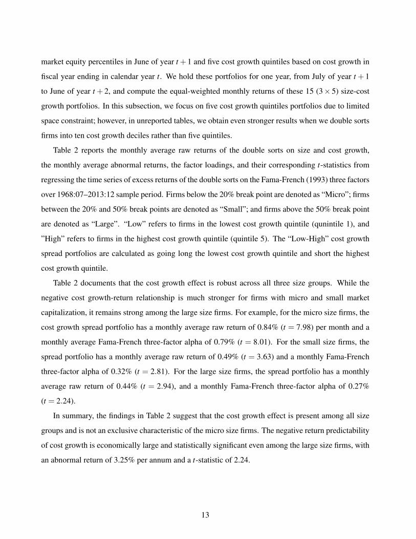
Table 2 documents that the cost growth effect is robust across all three size groups. While the

negative cost growth-return relationship is much stronger for firms with micro and small market

capitalization, it remains strong among the large size firms. For example, for the micro size firms, the

cost growth spread portfolio has a monthly average raw return of 0.84% (t = 7.98) per month and a

monthly average Fama-French three-factor alpha of 0.79% (t = 8.01). For the small size firms, the

spread portfolio has a monthly average raw return of 0.49% (t = 3.63) and a monthly Fama-French

three-factor alpha of 0.32% (t = 2.81). For the large size firms, the spread portfolio has a monthly

average raw return of 0.44% (t = 2.94), and a monthly Fama-French three-factor alpha of 0.27%

(t = 2.24).

In summary, the findings in Table 2 suggest that the cost growth effect is present among all size

groups and is not an exclusive characteristic of the micro size firms. The negative return predictability

of cost growth is economically large and statistically significant even among the large size firms, with

an abnormal return of 3.25% per annum and a t-statistic of 2.24.

13

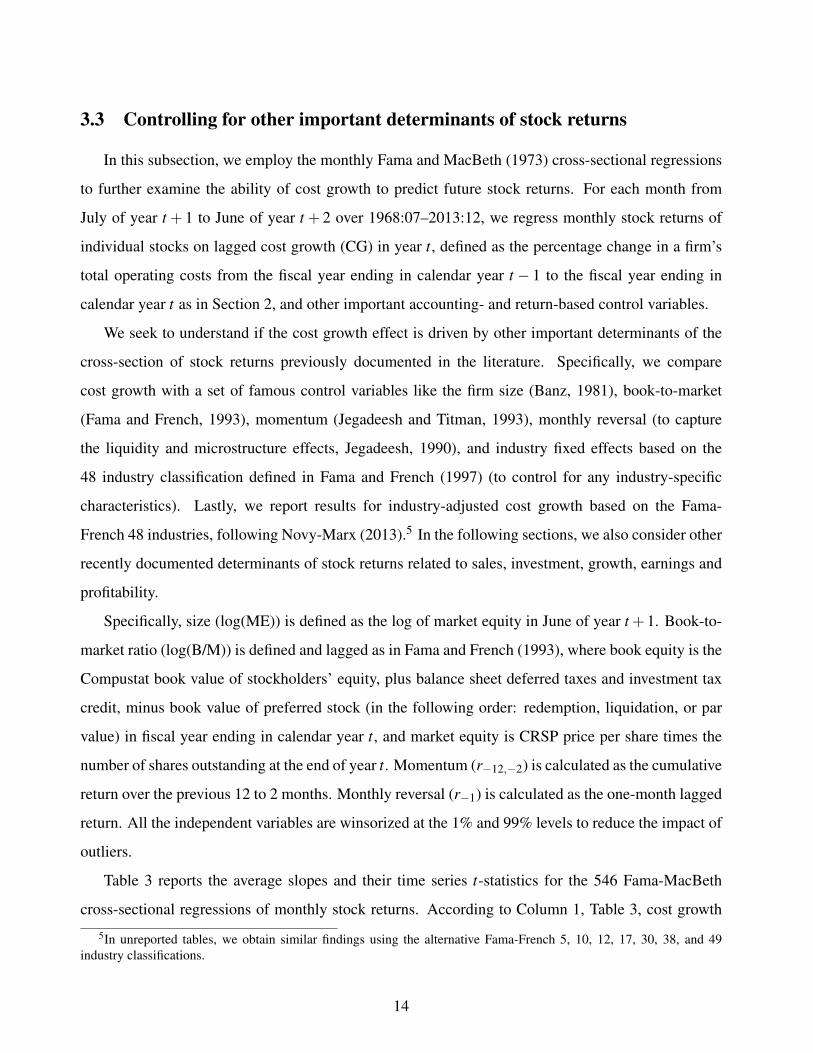
3.3 Controlling for other important determinants of stock returns

In this subsection, we employ the monthly Fama and MacBeth (1973) cross-sectional regressions

to further examine the ability of cost growth to predict future stock returns. For each month from

July of year t + 1 to June of year t + 2 over 1968:07–2013:12, we regress monthly stock returns of

individual stocks on lagged cost growth (CG) in year t, defined as the percentage change in a firm’s

total operating costs from the fiscal year ending in calendar year t − 1 to the fiscal year ending in

calendar year t as in Section 2, and other important accounting- and return-based control variables.

We seek to understand if the cost growth effect is driven by other important determinants of the

cross-section of stock returns previously documented in the literature. Specifically, we compare

cost growth with a set of famous control variables like the firm size (Banz, 1981), book-to-market

(Fama and French, 1993), momentum (Jegadeesh and Titman, 1993), monthly reversal (to capture

the liquidity and microstructure effects, Jegadeesh, 1990), and industry fixed effects based on the

48 industry classification defined in Fama and French (1997) (to control for any industry-specific

characteristics). Lastly, we report results for industry-adjusted cost growth based on the Fama-

French 48 industries, following Novy-Marx (2013).5 In the following sections, we also consider other

recently documented determinants of stock returns related to sales, investment, growth, earnings and

profitability.

Specifically, size (log(ME)) is defined as the log of market equity in June of year t +1. Book-to-

market ratio (log(B/M)) is defined and lagged as in Fama and French (1993), where book equity is the

Compustat book value of stockholders’ equity, plus balance sheet deferred taxes and investment tax

credit, minus book value of preferred stock (in the following order: redemption, liquidation, or par

value) in fiscal year ending in calendar year t, and market equity is CRSP price per share times the

number of shares outstanding at the end of year t. Momentum (r−12,−2) is calculated as the cumulative

return over the previous 12 to 2 months. Monthly reversal (r−1) is calculated as the one-month lagged

return. All the independent variables are winsorized at the 1% and 99% levels to reduce the impact of

outliers.

Table 3 reports the average slopes and their time series t-statistics for the 546 Fama-MacBeth

cross-sectional regressions of monthly stock returns. According to Column 1, Table 3, cost growth

5In unreported tables, we obtain similar findings using the alternative Fama-French 5, 10, 12, 17, 30, 38, and 49industry classifications.

14

exhibits strong negative predictability for future returns based on the Fama-MacBeth cross-sectional

regressions. The coefficient on cost growth is −0.897, which is statistically significant, with a t-

statistic of −8.24. High cost growth firms hence substantially underperform, confirming the strong

negative cost growth-return relationship documented in our earlier portfolio analysis in Table 1. In

addition, the predictive power of cost growth is at least as strong as the famous size, value, and

momentum effects. The t-statistics of cost growth are about one and a half times larger than those

associated with book-to-market, and about two and a half times larger than those associated with size

and momentum.

Columns 2 to 3 of Table 3 show that the predictive power of cost growth is not driven by

well-known determinants of the cross-section of stock returns. Cost growth has a large regression

coefficient of −0.642 and a t-statistics of −6.94, after controlling for the size (log(ME)) and book-to-

market (log(B/M)) effects. When we further control for the momentum (r−12,−2) and reversal (r−1)

effects, the regression coefficient on cost growth remains large of −0.665 (t = −8.24), signalling

strong economic and statistical significance. The regression slope coefficients on the control variables

are generally consistent with previous literature. Size and reversal are significant negative predictors

of future stock returns, while book-to-market and momentum are significant positive predictors of

future stock returns.

Columns 4 to 6 show that industry fixed effects do not subsume the predictive power of cost

growth. After controlling for the Fama-French 48 industry dummies, the t-statistics of cost growth

in fact become larger than the corresponding ones without controlling for industry dummies, while

the regression coefficients are generally unchanged. Column 7 presents the additional results of cost

growth demeaned by industry in forecasting the cross-section of stock returns. It shows that industry

adjustment helps to remove noise and the industry-adjusted cost growth can be more powerful in

forecasting, with a larger t-statistic of −9.62.

In summary, the Fama and MacBeth cross-sectional regressions results in Table 3 suggest that

the negative cost growth effect is robust after controlling for the size, book-to-market, momentum,

reversal, and industry fixed effects. The forecasting power of cost growth with industry adjustment

can be even stronger. The predictive power of cost growth is economically and statistically strong

compared to the famous size, value, and momentum effects.

15

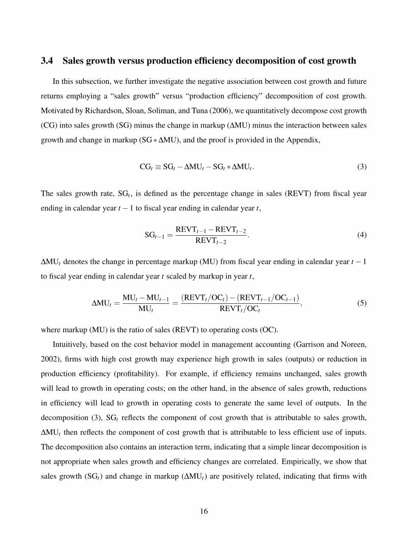
3.4 Sales growth versus production efficiency decomposition of cost growth

In this subsection, we further investigate the negative association between cost growth and future

returns employing a “sales growth” versus “production efficiency” decomposition of cost growth.

Motivated by Richardson, Sloan, Soliman, and Tuna (2006), we quantitatively decompose cost growth

(CG) into sales growth (SG) minus the change in markup (∆MU) minus the interaction between sales

growth and change in markup (SG∗∆MU), and the proof is provided in the Appendix,

CGt ≡ SGt −∆MUt −SGt ∗∆MUt . (3)

The sales growth rate, SGt , is defined as the percentage change in sales (REVT) from fiscal year

ending in calendar year t −1 to fiscal year ending in calendar year t,

SGt−1 =REVTt−1 −REVTt−2

REVTt−2. (4)

∆MUt denotes the change in percentage markup (MU) from fiscal year ending in calendar year t −1

to fiscal year ending in calendar year t scaled by markup in year t,

∆MUt =MUt −MUt−1

MUt=

(REVTt/OCt)− (REVTt−1/OCt−1)

REVTt/OCt, (5)

where markup (MU) is the ratio of sales (REVT) to operating costs (OC).

Intuitively, based on the cost behavior model in management accounting (Garrison and Noreen,

2002), firms with high cost growth may experience high growth in sales (outputs) or reduction in

production efficiency (profitability). For example, if efficiency remains unchanged, sales growth

will lead to growth in operating costs; on the other hand, in the absence of sales growth, reductions

in efficiency will lead to growth in operating costs to generate the same level of outputs. In the

decomposition (3), SGt reflects the component of cost growth that is attributable to sales growth,

∆MUt then reflects the component of cost growth that is attributable to less efficient use of inputs.

The decomposition also contains an interaction term, indicating that a simple linear decomposition is

not appropriate when sales growth and efficiency changes are correlated. Empirically, we show that

sales growth (SGt) and change in markup (∆MUt) are positively related, indicating that firms with

16

increases in sales tend to experience increases in production efficiency.6 Richardson, Sloan, Soliman,

and Tuna (2006) argue that such decomposition is an algebraic identity, which helps to mitigate the

estimation error concern (e.g., the sensitivity of cost growth to sales growth) and the misspecificatin

concern (e.g., the nonlinear interaction between sales growth and change in efficiency) for statistically

oriented regression specifications.

In this subsection, we seek to ask whether all the subcomponents of cost growth are important in

determining future stock returns or not. For example, If the cost growth effect is simply driven by

sales growth, one might expect that only the sales growth component would be negatively associated

with stock returns. In contrast, if the cost growth effect is only driven by reduction in production

efficiency, one might expect that only the change in production efficiency component would be useful

in forecasting with positive association. In addition, by decomposing cost growth to sales growth,

reduction in production efficiency and the interaction term, we are able to compare our cost growth

effect with other sales and profitability-related determinants of stock returns.

Table 4 reports the estimation results for the Fama-MacBeth regressions of monthly stock returns

on the sales growth versus production efficiency decomposition of lagged cost growth. We compare

the forecasting power of cost growth with its three components: sales growth, change in markup, and

the interaction term. We also include controls for size, book-to-market, momentum, and reversal,

similar to those presented in Table 3. Independent variables are winsorized at the 1% and 99% levels

to reduce the impact of outliers.

Columns 2 to 5 of Table 4 evaluate the forecasting power of the three components of cost growth

for the cross section of stock returns, while Column 1 reports the forecasting performance of cost

growth as a benchmark. Columns 2 shows that sales growth is a significant negative predictor of the

cross-section of stock returns, consistent with Lakonishok, Shleifer, and Vishny (1994). Columns

3 shows that change in markup, the change in production efficiency component of cost growth,

is a significant positive predictor of stock returns, consistent with Novy-Marx (2013). Column 4

shows that the predictive power of the interaction between sales growth and change in markup is

insignificant. Column 5 further shows that the slope coefficients on sales growth and change in

markup remain strong and statistically significant when including all the three components together in

6Economies of scale imply a positive correlation between sales growth and change in efficiency, because increases insales lead to lower marginal operating costs, thus higher efficiency. Sticky costs imply a positive correlation too, becausecosts saving will be limited, when sales decrease, leading to lower efficiency and earnings.

17

one regression. However, the predictive ability of cost growth reported in Column 1 is much stronger

than that of all the three components including sales growth and change in markup, in term of absolute

t-statistics.

We then examine whether cost growth contains additional predictive power beyond that in its sales

growth and change in markup components. Specifically, in Columns 6 to 8 of Table 4, we conduct

a set of pairwise Fama-MacBeth regressions, where each of the sales growth, change in markup,

and the interaction components is added into the regressions one-by-one together with cost growth.

We find that the predictive power of cost growth remains strong and significant after controlling

for all these three components, with regression coefficients of −0.661 to −0.694 and t-statistics of

−4.35 to −8.20. In contrast, neither the sales growth, change in markup, nor the interaction term are

statistically significant after controlling for cost growth in the same regressions.

In summary, our decomposition results in Table 4 suggest that both sales growth and reduction

in production efficiency (change in markup) contribute to the ability of cost growth to predict the

cross section of stock returns, either individually or jointly. However, cost growth’s predictive ability

is more powerful than its components. Most importantly, cost growth can effectively subsume all

the forecasting power in its three components including sales growth, change in markup, and the

interaction terms, and the forecasting power of all the three individual components turns insignificant

after controlling for cost growth at the annual forecasting horizon. The decomposition analysis

provides further insight into the cost growth effect, because cost growth effectively not only captures

the predictability of both sales growth and reduction in efficiency (profitability), but also provides a

partial explanation for the sales growth and profitability anomalies documented in the literature.

3.5 Comparing to investment and growth-related determinants

In this subsection, we compare the forecasting information of cost growth to other well-known

investment and growth-related determinants of the cross-section of stock returns. The decomposition

results in Table 5 shows that the sales growth of Lakonishok, Shleifer, and Vishny (1994) contributes

to the forecasting power of cost growth, indicating that our cost growth effect may be related to

the other investment and growth-related anomalies. Hence, we consider six important investment

and growth-related cross-sectional anomalies, and ask whether cost growth contains distinct and

18

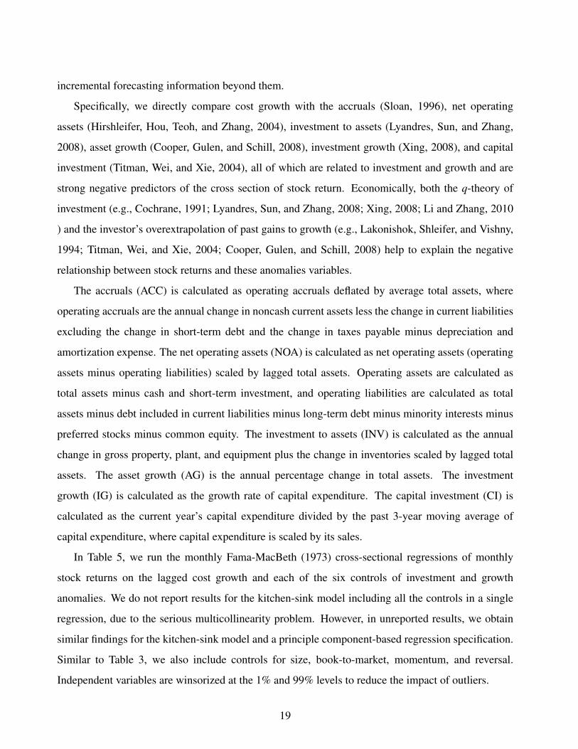
incremental forecasting information beyond them.

Specifically, we directly compare cost growth with the accruals (Sloan, 1996), net operating

assets (Hirshleifer, Hou, Teoh, and Zhang, 2004), investment to assets (Lyandres, Sun, and Zhang,

2008), asset growth (Cooper, Gulen, and Schill, 2008), investment growth (Xing, 2008), and capital

investment (Titman, Wei, and Xie, 2004), all of which are related to investment and growth and are

strong negative predictors of the cross section of stock return. Economically, both the q-theory of

investment (e.g., Cochrane, 1991; Lyandres, Sun, and Zhang, 2008; Xing, 2008; Li and Zhang, 2010

) and the investor’s overextrapolation of past gains to growth (e.g., Lakonishok, Shleifer, and Vishny,

1994; Titman, Wei, and Xie, 2004; Cooper, Gulen, and Schill, 2008) help to explain the negative

relationship between stock returns and these anomalies variables.

The accruals (ACC) is calculated as operating accruals deflated by average total assets, where

operating accruals are the annual change in noncash current assets less the change in current liabilities

excluding the change in short-term debt and the change in taxes payable minus depreciation and

amortization expense. The net operating assets (NOA) is calculated as net operating assets (operating

assets minus operating liabilities) scaled by lagged total assets. Operating assets are calculated as

total assets minus cash and short-term investment, and operating liabilities are calculated as total

assets minus debt included in current liabilities minus long-term debt minus minority interests minus

preferred stocks minus common equity. The investment to assets (INV) is calculated as the annual

change in gross property, plant, and equipment plus the change in inventories scaled by lagged total

assets. The asset growth (AG) is the annual percentage change in total assets. The investment

growth (IG) is calculated as the growth rate of capital expenditure. The capital investment (CI) is

calculated as the current year’s capital expenditure divided by the past 3-year moving average of

capital expenditure, where capital expenditure is scaled by its sales.

In Table 5, we run the monthly Fama-MacBeth (1973) cross-sectional regressions of monthly

stock returns on the lagged cost growth and each of the six controls of investment and growth

anomalies. We do not report results for the kitchen-sink model including all the controls in a single

regression, due to the serious multicollinearity problem. However, in unreported results, we obtain

similar findings for the kitchen-sink model and a principle component-based regression specification.

Similar to Table 3, we also include controls for size, book-to-market, momentum, and reversal.

Independent variables are winsorized at the 1% and 99% levels to reduce the impact of outliers.

19

Table 5 shows that the regression coefficients on cost growth in the Fama-MacBeth regression

specifications are −0.534 (t = −6.33) after controlling for accruals, −0.421 (t = −5.24) after

controlling for net operating assets, −0.427 (t = −5.00) after controlling for investment to assets,

−0.386 (t = −3.39) after controlling for asset growth, −0.502 (t = −5.82) after controlling for

investment growth, and −0.571 (t = −6.48) after controlling for abnormal capital investment,

respectively. All of the regression slopes on cost growth are economically large and statistically

significant at the 1% level. It indicates that the predictive power of cost growth is robust when

controlling for other important determinants of cross-sectional stock returns related to investment

and growth.

Moreover, consistent with the existing studies, all the six anomalies including the accruals,

net operating assets, investment to assets, asset growth, investment growth, and capital investment

are strong negative predictors of the cross-section of future stock returns, with t-statistics of slope

coefficients ranging from −5.16 to −9.28 with statistical significance. And the forecasting power of

our cost growth effect is generally comparable with these famous determinants.

In summary, our findings indicate that cost growth contains unique and incremental forecasting

information for the cross-section of stock returns, beyond that contained in other famous anomalies

variables related to investment and growth.

3.6 Comparing to earnings and profitability-related determinants

In this subsection, we further compare our cost growth effect to other earnings and profitability-

related determinants of the cross-section of stock returns. Table 5 shows that change in markup

contributes to the forecasting power of cost growth, suggesting that our cost growth effect may be

related to other profitability-related anomalies in the cross section. However, change in markup is not

a standard profitability measure in the literature, which is motivated by our decomposition formula (3).

In this subsection, we consider additional five anomalies variables related to earnings and profitability

from the standard accounting and finance literature, which are strong positive determinants of the

cross section of future stock returns. We aim to ask whether cost growth’s forecasting power is distinct

and incremental to the these previously documented earnings and profitability-related anomalies.

Specifically, we compare cost growth with the quarterly standardized unexpected earnings (SUEQ)

20

computed as the most recently announced quarterly earnings minus the quarterly earnings four

quarters ago, standardized by its standard deviation estimated over the prior eight quarters, which

is used to proxy for earnings surprises in the post earnings announcement drift (PEAD) literature as

in Ball and Brown (1968), Foster, Olsen, and Shevlin (1984), and Bernard and Thomas (1989, 1990);

the annual standardized unexpected earnings (SUEA), calculated as the annual earnings per share

before extraordinary items (EPS) in the fiscal year ending in calendar year t minus the annual EPS

one year ago in year t − 1, standardized by the stock price per share at the end of year t (Livnat

and Mendenhall, 2006); the gross profitability (GP), calculated as the as the annual gross profit

(revenue minus costs of goods sold) in year t scaled by total assets (Novy-Marx, 2013); the return

on asset (ROA), calculated as the annual income before extraordinary items (IB) in fiscal year ending

in calendar year t scaled by total assets; and the return on equity (ROE), calculated as the annual

income before extraordinary items (IB) in fiscal year ending in calendar year t scaled by book value

of equity (Novy-Marx, 2013; Fama and French, 2008, 2015; Hou, Xue, and Zhang, 2015). All of

them are earnings-based profitability measures and are positively related to subsequent stock returns

in the cross section.

In Table 6, we run the Fama-MacBeth cross-sectional regressions of monthly stock returns on

lagged cost growth and each of the five controls of earnings and profitability anomalies. We do not

report results including all the controls in a single kitchen-sink regression model due to the serious

multicollinearity problem Similar to Table 3, we also include controls for size, book-to-market,

momentum, and reversal. Independent variables are winsorized at the 1% and 99% levels to reduce

the impact of outliers. We test whether the ability of cost growth to predict returns is distinct and

incremental to the previously documented predictors related to earnings and profitability.

Table 6 shows that the regression coefficients on cost growth in the Fama-MacBeth regression

specifications are −0.604 (t = −3.82) after controlling for quarterly earnings surprises SUEQ,

−0.666 (t = −8.40) after controlling for annual earnings surprises SUEA, −0.606 (t = −7.52) after

controlling for gross profit GP, −0.675 (t =−8.65) after controlling for return of asset ROA, −0.678

(t = −8.58) after controlling for return on equity ROE, respectively. All of the regression slopes

on cost growth are economically large and statistically significant at the 1% level. It indicates that

the predictive power of cost growth is robust when controlling for other important determinants of

cross-sectional stock returns related to earnings and profitability.

21

Consistent with the literature, both the two earnings surprises measures SUEQ and SUEA are

significant and positive predictors for future stock returns. SUEQ has large t-statistic than SUEA, since

SUEQ utilizes more updated quarterly frequency accounting information, while the cost growth and

SUEA only utilizes annual frequency information. Consistent with Novy-Marx (2013), we find that

gross profit GP has significant and positive forecasting power, while the forecasting power of ROA

and ROE is insignificant. However, in unreported results, consistent with Fama and French (2015), we

find that ROA and ROE based on operating income (OIBDA) can significantly and positively predict

future stock returns.

In summary, our findings indicate that cost growth contains unique and incremental forecasting

information beyond that contained in other commonly known variables related to earnings and

profitability for the cross-section of stock returns.

3.7 Alternative measures of cost growth

In this subsection, we examine the robustness of our negative cost growth effect by performing a

set of Fama-MacBeth regressions based on various alternative definitions of cost growth.

First, our main operating costs measure OC in (2) includes all the major operating costs of running

a business such as the costs of goods sold (COGS) and selling, general, and administration expenses

(XSGA) beyond specific costs components. The OC measure hence provides broad insights into the

relationship between cost behavior and stock returns. In addition, the accounting classification of

COGS and XSGA may subject to managerial judgment, which may introduce bias into the estimate

of specific costs components like COGS and XSGA. However, in this section, we will show that the

cost growth effect is robust to growth in COGS (CGCOGS) and growth in XSGA (CGXSGA) as well.

Specifically, Columns 2 to 4 of Table 7 report the estimation results for monthly Fama-MacBeth

regressions employing lagged COGS growth and XSGA growth. Similar to those presented in Table

3, we include controls for size, book-to-market, momentum, and reversal, and winsorize independent

variables at the 1% and 99% levels to reduce the impact of outliers. COGS growth (CGCOGS) in year

t is defined as the year-to-year percentage change in annual COGS from the fiscal year ending in

calendar year t − 1 to the fiscal year ending in calendar year t, CGCOGS,t =COGSt−COGSt−1

COGSt−1; while

XSGA growth (CGXSGA) in year t is is defined as the year-to-year percentage change in annual

22

XSGA from the fiscal year ending in calendar year t − 1 to the fiscal year ending in calendar year

t, CGXSGA,t =XSGAt−XSGAt−1

XSGAt−1. COGS growth and XSGA growth have a correlation of 0.55 with

each other, and they have high correlations of 0.81 and 0.79 with our main cost growth measure CG,

respectively.

Columns 2 and 3 show that both COGS growth and XSGA growth have significant power to

predict stock returns as well. The slopes on COGS growth and XSGA growth are −0.446 (t =−7.83)

and −0.574 (t =−7.38), respectively, indicating that firms with high growth in COGS and those with

high growth in XSGA will underperform substantially in the future. Column 4 further shows that the

slope coefficients on both COGS growth and XSGA growth remain significant when including them

together in a single regression, suggesting that both variables contain strong return predictability and

contribute to the negative cost growth effect.

Second, our operating costs measure OC in (2) does not include depreciation and amortization

expenses, since a firm’s depreciation may depend on the accounting rules a firm chooses, which may

not be related to a firm’s business fundamentals. However, on the other hand, capital intensive firms

may employ more fixed assets for business operations, leading to higher depreciation and amortization

expenses, depreciation and amortization expenses hence can be viewed as parts of a firm’s operating

costs. As a robustness check, we construct an alternative measure of operating costs, OCDP, which

incorporates depreciation and amortization expenses and is defined as the sum of costs of goods sold

(COGS), selling, general, and administration expenses (XSGA), and depreciation and amortization

expenses (DP), OCDP,t = COGSt +XSGAt +DPt . We then get the corresponding alternative cost

growth measure, CGDP,t =OCDP,t−OCDP,t−1

OCDP,t−1, which is defined as the annual percentage change of OCDP

and includes the growth in depreciation and amortization expenses.

Column 5 of Table 7 reports the estimation results for monthly Fama-MacBeth regressions

employing the alternative measure of cost growth, CGDP. In unreported tables, we find that the cost

growth measure CG and CGDP are highly correlated, with correlation of more than 0.9. Consistent

with the high correlation, the estimation results in Columns 5 shows that the alternative measure CGDP

also is a strong negative predictor of the cross-section of future returns, with a regression coefficient

of −0.597 and a large t-statistic of −7.67, consistent with our earlier regression results based on our

main cost growth measure CG in Column 1 of Table 7 and Table 3.

Third, our operating costs measure OC in (2) includes a firm’s R&D expenses, following GAAP.

23

According to the reliability criterion, assets can be recognized only if they can be measured with

reasonable precision and supported by objective evidence, free of opinion and bias. So the GAAP

requires that R&D are expensed immediately in the income statement rather than booked to the

balance sheet as intangible assets, since estimates of these assets are too uncertain, subjective, and

open to managerial manipulation and bias. On the other hand, the result can be a mismatch, since

R&D expenses can be regarded as investment to intangible assets to generate future sales. As a

robustness check, we construct an alternative measure of operating costs, OCRD, which omits R&D

expenses and is defined as costs of goods sold (COGS) plus selling, general, and administration

expenses (XSGA) minus R&D expenses (XRD), OCRD,t = COGSt + XSGAt − XRDt .7 We then

get the alternative cost growth measure, CGRD,t =OCRD,t−OCRD,t−1

OCRD,t−1, which is defined as the annual

percentage change of OCRD and removes the growth in R&D expenses.

Column 6 of Table 7 reports the estimation results for monthly Fama-MacBeth regressions

employing the alternative measure of cost growth, CGRD, that omits R&D expenses. The alternative

measure CGRD also is a strong negative predictor of the cross-section of future returns, with a

regression coefficient of −0.610 and a large t-statistic of −7.88, similar with our earlier regression

results based on our main cost growth measure CG in Column 1 of Table 7 and Table 3.

Fourth, we examine the robustness of our finding by scaling the changes in operating costs by

alternative deflators. Specifically, we consider an alternative cost growth measure CGAT, in which

we deflate the year-to-year changes in operating costs by lagged total assets (AT) rather than lagged

operating costs (OC), CGAT,t =OCt−OCt−1

ATt−1. This exercise is meant to demonstrate that our finding

of negative cost growth effect is robust to different deflators, and is mainly driven by the changes

in operating costs component (OCt −OCt−1) rather than the lagged operating costs component (the

deflator, OCt−1).

Column 7 of Table 7 reports the results for monthly Fama and MacBeth (1973) cross-sectional

regression employing the alternative cost growth measure CGAT. The regression slope coefficient on

CGAT is −0.457, with a large t-statistic of −6.49, which is generally similar to the earlier findings

based on our main cost growth measure CG in Column 1 of Table 7 and Table 3. In unreported tables,

we obtain largely similar results employing alternative specifications like deflating the changes in

7In unreported results, we obtain similar findings after removing advertising expenses from our operating costsmeasure.

24

operating costs by lagged book values of equity, market values of equity, and sales. The results

indicate that our documented cost growth effect is generally driven by the changes in operating costs

component, and is robust to the choice of denominator.

Lastly, in unreported tables, we obtain similarly strong negative cost growth-return relationship,

when we define total operating costs indirectly as the difference between the sales and income before

extraordinary items, which may includes interest expenses and taxes, rather than the sum of COGS

and XSGA.

4 Economic Explanations

In this section, we seek to understand the economic forces driving our main findings of negative

cost growth-return relationship in Section 3. We examine the association between cost growth

and subsequent operating performance, and evaluate why the market fails to recognize fully the

information contained in cost growth.

4.1 Cost growth and subsequent operating performance

In this subsection, we explore the relationship between cost growth and subsequent operating

performance. The goal here is to empirically assess if the high cost growth firms, which generate lower

future returns as shown in Section 3, also experience deterioration in future operating performance.

Economically, the basic accounting identity shows that earnings are equal to sales minus costs,

indicating negative association between cost growth and operating profitability. In unreported tables,

we do find that cost growth is negatively and significantly associated with contemporaneous operating

performance, which is not surprising and consistent with the simple accounting identity of earnings.

Moreover, costs are more sticky than sales that costs decrease less with a sales activity decrease than

they increase with an equivalent sales activity increase, since managers may retain idle capacity as

product demand falls but add capacity as demand grows (e.g., Anderson, Banker, and Janakiraman,

2003). The sticky cost hence implies that increases in costs may negatively forecast a firm’s future

operating performance, since future costs saving will be limited even if future sales activity declines,

resulting in decreases in earnings (Banker and Chen, 2006).

25

Table 8 reports the estimation results for annual Fama-MacBeth (1973) cross-sectional regressions

of individual firms futture operating performance in year t + 1 on lagged cost growth and other

important control variables in year t over 1968–2013. We consider three measures of operating

performance: profit margin (PM), return on asset (ROA) and cash flow (CF), which are important

fundamental determinants of stock valuations. Profit margin (PM) is calculated as income before

extraordinary items divided by sales, return on asset (ROA) is calculated as income before extraordi-

nary items divided by total assets, and cash flow (CF) is net income plus amortization and depreciation

minus changes in working capital and capital expenditures divided by total assets in fiscal year ending

in calendar year t +1.

Our explanatory variable of interest is cost growth (CG) in fiscal year ending in calendar year t,

the percentage growth rate of operating costs as defined in Section 2. We also include controls for size

(log(ME)), book-to-market (log(B/M)), and prior year’s stock return performance (r−12,−1) in year t

as in Novy-Marx (2013). Following Hirshleifer, Hsu, and Li (2013), we include controls for lagged

operating performance in year t to accommodate persistence in operating performance and controls

for changes in operating performance in year t to accommodate the mean reversion in profitability

(e.g., Fama and French, 2006). We also include controls for industry fixed effects based on the Fama

and French (1997) 48 industry classification. Independent variables are winsorized at the 1% and 99%

levels to reduce the impact of outliers.

The estimate results in Table 8 indicate a significantly negative relation between a firm’s cost

growth and its future operating performance in the next year. Specifically, Column 1 shows that

the slope coefficient on cost growth for profit margin (PM) is −2.793, which is strongly statistically

significant, with a t-statistic of −4.48, indicating that firms with high cost growth will turn to be less

profitable in the next year than other firms. In Column 2, using the return on asset (ROA) as a measure

of operating performance, we find that high cost growth leads to significantly lower future profitability,

with a slope coefficient of −1.681 (t = −5.04). In Column 3, we obtain similarly strong negative

association between cost growth and future cash flow (CF) as a measure of operating performance,

with a slope coefficient of −2.748 (t =−8.05). Columns 4 to 6 show that adding industry fixed effects

makes no difference to these negative effects of cost growth on future profitability.

The coefficients on the control variables are generally consistent with previous literature. Size

and prior return performance are positively associated with subsequent profit margin, return on asset,

26

and cash flow with statistical significance at 1% level, while book-to-market strongly and negatively

correlate with subsequent profit margin and return on asset with statistical significance at 1% level and

marginally significantly and negatively correlate with subsequent cash flow. The significantly positive

slopes on lagged profit margin, return on asset, and cash flow and the significantly negative slopes on

change in profit margin, return on asset, and cash flow confirm both persistence and mean reversion

in operating performance documented in the literature (e.g., Fama and French, 2006).

Overall, these results in Table 8 suggest that cost growth contains negative information about

future operating performance. Firms with high cost growth appear to becoming less profitable in the

next year in terms of decreased profit margin, return on asset, and cash flows, and the market appears

to largely ignore this information.

4.2 Macroeconomic risk-based explanation

In this subsection, we explore whether macroeconomic risk can explain the negative relationship

between cost growth and future stock returns. Chen, Roll, and Ross (1986), Fama and French

(1989), and others detect significant time variation of stock returns over business cycles, and many

macroeconomic variables help to explain stock returns. Thus, it is possible that the negative cost

growth effect may be driven by systematic macroeconomic risk, and the lower returns associated with

high cost growth stocks are due to the fact that they are less risky than those low cost growth stocks.

We employ the Chen, Roll, and Ross (1986) (CRR hereafter) model to examine the macroeco-

nomic risk exposures of the cost growth portfolios. The CRR model includes five factors such as

the growth rate of industrial produciton (MP), unexpected inflation (UI), change in expected inflation

(DEI), term structure of interest rate (UTS), and default risk (UPR) factors. Since the first three

macroeconomic risk factors like MP, UI, and DEI are not tradable, we employ mimicking factors

method to track these factors, following Liu and Zhang (2008), Cooper and Priestley (2011) and Lam,

Ma, Wang, and Wei (2014). For consistency, we construct mimicking factors for all the five CRR

macroeconomic risk factors, although the UTS and UPR factors are traded assets. The basis of the

mimicking portfolios consist of 40 test portfolios: 10 size deciels, 10 book-to-market deciles, 10

momentum deciles, and 10 cost growth portfolios, all of which are based on one-way sorts. The size,

book-to-market, and momentum test portfolios have been widely used in the asset pricing literature.

27

We include cost growth portfolios because we want to understand the driving forces for the negative

cost growth premium.

Table 9 reports the the monthly average abnormal returns and factor loadings of ten cost

growth decile portfolios on the five CRR macroeconomic factors. We run the following time-series

regressions of excess returns of ten cost growth decile portfolios on the returns of the five mimicking

macroeconomic risk factors:

R j,t −R f ,t = α j +β j,MPRMP,t +β j,UIRUI,t +β j,DEIRDEI,t +β j,UTSRUTS +β j,UPRRUPR,t + ε j,t , (6)

where R j,t is the monthly return on cost growth portfolio j, and R f ,t is the risk-free rate in month

t. RMP,RUI,RDEI,RUTS, and RUPR are the five macroeconomic risk factors in CRR: the growth rate

of industrial produciton (MP), unexpected inflation (UI), change in expected inflation (DEI), term

structure of interest rate (UTS), and default risk (UPR), respectively. To explain the negative cost

growth effect, the factor loadings of high cost growth stocks on macroeconomic risk factors should be

smaller than those low cost growth stocks, and the negative spread in risk exposures should be large

enough to explain the negative spread in average returns between high and low cost growth stocks.

Table 9 shows that three of the five factors (MP, UI, and DEI) have significant explanatory power

for the cost growth spread portfolio, which is computed as the difference between the returns of the

lowest and the highest cost growth deciles. Specifically, the cost growth spread portfolio’s factor

loading on the industrial production (MP) factor is postive (βMP = 0.24) and significant (t = 3.77).

The MP factor loadings generally decrease from 0.31 (t = 2.29) for the lowest cost growth decile

to 0.08 (t = 0.48) for the highest cost growth decile, suggesting that the low cost growth portfolios

are more risky than those high cost growth portfolios in term of MP factor. The unexpected inflation

(UI) factor also helps to explain the cost growth effect, and the cost growth spread portfolio’s factor

loading on the UI factor is positive (βUI = 0.63) and significant (t = 2.96). The lowest cost growth

decile loads positively to the UI factor (βUI = 0.04), while all the other decile portfolios with higher

cost growth rates loads negatively to the UI factor. The change in expected inflation (DEI) factor too

has strong explanatory power for the cost growth effect, and the cost growth spread portfolio’s factor

loading on the DEI factor βDEI is 1.01 and significant (t = 2.05). Again, the DEI factor loadings

generally decrease from the lowest cost growth decile (4.79) to the highest cost growth decile (3.78).

28

While the term structure of interest rate (UTS) factor has statistically significant power in explaining

the cost growth spread, its economic scale is small (βUTS = 0.07 and t = 2.01). Finally, the default

premium (URP) risk factor is insignificant in explaining the cost growth spread portfolio.

However, the CRR model generates a large average monthly abnormal return of 0.99% per month

for the cost growth spread portfolio with a t-statistic of 7.01. The pricing error is economically large

and statistically significant at the 1% level. The scale of the mispricing of the CRR model is similar

to that of the Fama-French three-factor model. In the cross section, the abnormal returns generally

decrease from the lowest cost growth decile (α = 0.30% per month) to the highest cost growth decile

(α = −0.69% per month), and the pattern again is similar to that of the Fama-French three factor

model in Table 1. It indicates that the CRR macroeconomic risk model only works as well as the

Fama-French three-factor model in explaining the cost growth effect.

In summary, we find that the Chen, Roll, and Ross (1986) macroeconomic risk can not fully

explain away the negative relationship between cost growth and future stock returns. It generates a

large abnormal return of about 12% per year for the cost growth spread portfolio, similar to that of

the Fama-French three-factor model. The explanatory power of the CRR model mainly comes from

the industry production and inflation related factors.

4.3 Mispricing-based explanation

In this subsection, we explore whether a common mispricing factor helps to explain the negative

cost growth effect. Daniel, Hirshleifer, and Subrahmanyam (2001), Barberis and Shleifer (2003),

Hirshleifer and Jiang (2010), Hirshleifer, Hsu, and Li (2013), and others show that the investor

misperceptions and market misvaluation tend to comove across firms. Therefore, we may observe

certain degree of commonality in the mispricing of cost growth, if the cost growth effect reflects

market underreaction to information contained in cost growth, due to limited investor attention or

changes in investor sentiment.

We use the Hirshleifer and Jiang (2010) mispricing factor (UMO, undervalued minus overvalued)

to identify commonality in stock market misvaluation. Hirshleifer and Jiang construct the UMO factor

by going long on repurchase stocks and short on the new issue stocks. They show that the UMO

factor captures systematic mispricing in stock market, and the UMO factor loading reflects a firm’s

29

underpricing and positively predicts future returns in the cross-section. In this paper, we augment

the Fama-French three factors with the UMO factor and examine whether the common misvaluation

helps to explain the negative cost growth-return relationship.

Table 10 shows that adding the mispricing factor UMO reduces the abnormal returns of the cost

growth decile portfolios substantially. For example, the monthly average abnormal return of the cost

growth long-short spread portfolios is now 0.43% per month, which is about 55% smaller than 0.98%,

the counterpart abnormal return of the Fama-French three-factor model. In the cross section, for the

highest cost growth decile, adding the UMO factor helps to sharply reduce the monthly abnormal

return from −0.68% for the Fama-French three-factor model to −0.06 with statistical insignificance

(t = −0.37), though the abnormal returns of the low cost growth deciles are generally unchanged.

The reduction of abnormal returns is largely driven by the large negative UMO factor loadings of the

highest cost growth decile, which is −0.78 (t = −11.7), and the factor loadings gradually increase

to −0.07 (t = −0.98) for the lowest cost growth decile, producing a large UMO loading of 0.71

(t = 14.52) for the long-short cost growth spread portfolio.

In summary, the findings in Table 10 shows that the Hirshleifer and Jiang (2010) mispricing factor

UMO helps to sharply reduce the abnormal returns of the long-short cost growth spread portfolio

by more that 55% relative to the Fama-French three-model and the CRR macroeconomic risk factor

model. Firms with high cost growth have large negative exposures to the UMO factor, indicating that

high cost growth firms are subtantially overvalued relative to economic fundamentals, leading to the

subsequent poor performance. Moreover, when controlling for the UMO factor, the abnormal returns

of the cost growth spread portfolio remain economically large and statistically significant at the 1%

level, suggesting that the negative cost growth effect is incremental to the systematic mispricing as

captured by the UMO factor.

4.4 Limited attention, valuation uncertainty, and transaction costs

Given the promise of mispricing-based explanation for the negative cost growth-return relation-

ship, in this subsection, we provide further analysis for the cost growth effect based on limited investor

attention, valuation uncertainty, or transaction costs.

30

4.4.1 Limited attention

In this subsection, we test if the cost growth effect is driven by limited investor attention by running

the monthly Fama-MacBeth regressions of returns on lagged cost growth interacted with proxies

for investor attention. Bartov, Radhakrishnan, Krinsky (2000), Hirshleifer and Teoh (2003), Peng

and Xiong (2006), DellaVigna and Pollet (2009), Hirshleifer, Lim, and Teoh (2009), among others,

suggest that limited investor attention causes market underreaction to relevant earnings information

and induces mispricing. Therefore, stocks with less investor attention may experience a slower

reaction to the valuation information conveyed in cost growth, leading to greater return predictability.

We employ asset size and analyst coverage as investor attention proxies, and we argue that the

investors with limited attention would pay less attention to small firms and low analyst coverage

firms. Asset size (log(AT)) is defined as the log of total assets in fiscal year ending in calendar year

t. Analyst coverage (log(AC)) is defined as the log of average monthly number of analysts who

provide fiscal year 1 earnings estimates in year t beginning in 1976. Asset size and analyst coverage

are standardized to zero mean and unit standard deviation over full sample period for interpretation.

Hirshleifer and Teoh (2003) provide theoretical evidence that size and analyst coverage are proxies

for investor attention. Consistent with size and analyst coverage being investor attention proxies,

Hong, Lim, and Stein (2000) and Hirshleifer, Hsu, and Li (2013) show that the return predictability

of momentum and innovation efficiency decreases with size and analyst coverage.

For each month from July of year t +1 to June of year t +2, we run the monthly Fama-MacBeth

regressions of monthly stock returns of individual stocks on the interaction between lagged cost

growth and each of the investor attention proxies like asset size and analyst coverage, cost growth,

each investor attention proxy, and other lagged control variables. Cost growth (CG) is the percentage

change in annual operating costs for fiscal year ending in calendar year t as defined in Section 2.

Similar to Table 3, we also include controls for size, book-to-market, momentum, reversal, and

industry fixed effects based on the 48 industry classification defined in Fama and French (1997).

Independent variables are winsorized at the 1% and 99% levels to reduce the impact of outliers.

Panel A of Table 11 only reports the time series average slopes and corresponding t-statistics

for cost growth (CG) and the interaction between cost growth and asset size (CG∗log(AT)) and the

interaction between cost growth and analyst coverage (CG∗log(AC) from these regressions for brevity.

31

Panel A shows that the negative cost growth-return relation is stronger in magnitude among firms

with smaller size and lower analyst coverage. For example, the slope coefficient on interaction of cost

growth with asset size (CG∗log(AT)) is 0.305 (t = 3.67), and the slope coefficient on interaction of

cost growth with analyst coverage (CG∗log(AC)) is 0.262 (t = 3.06), both of which are economically

large and statistically significant at 1% level. The evidence appears to support the hypothesis that

limited investor attention leads to the negative cost growth effect.

4.4.2 Valuation uncertainty

In this subsection, we test if the cost growth effect is driven by valuation uncertainty. Hirshleifer

(2001), Daniel, Hirshleifer, and Subrahmanyam (1998, 2001), Zhang (2006), Kumar (2009), and

others show that the investors’ behavioral biases would be stronger where there is higher valuation

uncertainty. Recent empirical studies like Liang (2003) and Francis, LaFond, Olsson, and Schipper

(2007) show that uncertainty contributes to the post-earnings announcement drift. Therefore,we

expect that the negative cost growth effects would stronger among firms with higher valuation

uncertainty, since the investors might pay less attention and be more likely to apply the heuristics and

rule of thumb for highly uncertain stocks, leading to greater degree of underreaction to the information

embedded in cost growth.

We use idiosyncratic volatility (log(IVOL)) and firm age (log(1+Age)) as our proxy measures of

valuation uncertainty, following Kumar (2009) and Hirshleifer, Hsu, and Li (2013). Idiosyncratic

volatility (log(IVOL)) is the log of standard deviation of the residuals from regressing daily stock

returns on market returns over a maximus of 250 days ending on June 30 of year t + 1. Firm age

(log(1+Age)) is the log of one plus firm age defined as the number of years listed in Compustat with

non-missing price data at the end of year t. These uncertainty proxies are standardized to zero mean

and unit standard deviation over full sample period. We argue that firms with higher idiosyncratic

volatility and with younger age are regarded as having higher valuation uncertainty.

For each month from July of year t +1 to June of year t +2, we regress monthly stock returns of

individual stocks on the interaction between lagged cost growth and each of the valuation uncertainty

proxies, cost growth, each uncertainty proxy, and other lagged control variables. Panel B of Table

11 reports the time series average slopes and corresponding t-statistics for cost growth (CG), and the

interaction of cost growth with Idiosyncratic volatility (CG*log(IVOL)), and the interaction of cost

32

growth with firm age (CG*log(1+Age)) from these Fama-MacBeth cross-sectional regressions for

brevity.

According to Panel B of Table 11, the slope coefficient on interaction of cost growth with

idiosyncratic volatility (CG∗log(IVOL)) is −0.536 (t = −6.10), and the slope coefficient on

interaction of cost growth with age (CG∗log(1+Age)) is 0.205 (t = 3.04), both of which are

economically large and statistically significant. Thus, the negative cost growth-return relation is

stronger in magnitude among firms with higher valuation uncertainty such as those with higher

idiosyncratic volatility and with younger age. The evidence suggests that valuation uncertainty

appears to amplify the behavioral biases, leading to stronger cost growth effect.

4.4.3 Transaction costs

In this subsection, we test if limits to arbitrage drives the cost growth effect. If the negative cost

growth effect reflects mispricing driven by irrational investor behavior, the arbitrageurs would exploit

the profit opportunities to eliminate the mispricing. However, Shleifer and Vishny (1997) show that

mispricing can persist, when arbitrage is costly and limited due to market friction. Many recent studies

provide positive evidence on the role of transaction costs on anomalies such as accruals (Mashruwala,

Rajgopal, and Shevlin, 2006), investment (Li and Zhang, 2010), asset growth (Lam and Wei, 2011),

and earnings (Mendenhall, 2004; Ng, Rusticus, and Verdi, 2008; Chordia, Goyal, Sadka, Sadka, and

Shivakumar, 2009). We hence expect that the negative cost growth effects would stronger among

firms with higher transaction costs, where the arbitrage opportunities provided by the cost growth

effect are more difficult to exploit and thus less attractive to the investors.

We use share price (log(PRC)), Amihud (2002) illiquidity measure (log(ILLIQ)), and dollar

volume (log(DVOL)) as our proxy measures of transaction costs, following Lam, Ma, Wang, and

Wei (2014). Share price (log(PRC)) is the log of closing stock price (the average of bid and ask

prices if the closing price is not available) at the end of June of year t + 1. Stoll (2000) documents

that stock price is inversely related to bid-ask spread and brokerage commission. Amihud (2002)

illiquidity measure (log(ILLIQ)) is the log of the average of absolute daily return divided by daily

dollar trading volume over the past 12 months ending on June 30 of year t + 1. A higher illiquidity

value indicates a larger price impact per order flow, thus a larger transaction costs for the investors.

Dollar volume (log(DVOL)) is the log of the sum of daily share trading volume multiplied by the

33

daily closing price from July 1 of year t to June 30 of year t + 1. Bhushan (1994) shows that dollar

volume is inversely related to price pressure and time required to fill an order or to trade a large block

of shares. These three costs proxies are standardized to zero mean and unit standard deviation over

full sample period for interpretation. Firms with lower share price, higher Amihud (2002) illiquidity

measure, and lower dollar volume are regarded as having higher transaction costs and hence more

severe limits to arbitrage.

We run Fama-MacBeth cross-sectional regressions of monthly stock returns on the interaction

between lagged cost growth and each of the transaction costs proxies, cost growth, each transaction

costs proxy. We also include controls for size, book-to-market, momentum, reversal, and industry

fixed effects based on the 48 industry classification defined in Fama and French (1997). Panel

C of Table 11 reports the average slopes and corresponding t-statistics for cost growth (CG) and

the interaction of cost growth with share price (CG*log(PRC)), the interaction of cost growth with

Amihud (2002) illiquidity (CG*log(ILLIQ)), and the interaction of cost growth with dollar volume

(log(DVOL)) from these Fama-MacBeth regressions.

Panel C of Table 11 shows that the slope coefficient on interaction of cost growth with share

price (CG∗log(PRC)) is 0.267 (t = 3.11), the slope coefficient on interaction of cost growth with

Amihud (2002) illiquidity (CG∗log(ILLIQ)) is −0.377 (t = −3.25), and the slope coefficient on

interaction of cost growth with dollar volume (CG∗log(DVOL)) is 0.282 (t = 2.63), all of which

are economically large and statistically significant. Thus, the negative cost growth-return relation is

stronger in magnitude among firms with higher transaction costs such as those with lower share price,

higher Amihud (2002) illiquidity measure, and lower dollar volume. The evidence suggests that the

limits to arbitrage appear to help explain the negative cost growth effect.

5 Conclusion

In this paper, we show that a simple measure of cost behavior, cost growth, defined as

the percentage change in annual operating costs, contains important information about a firm’s

fundamental value, but the market appears failing to incorporate it fully and immediately. Firms

with high cost growth generate substantially lower future stock returns than those with low cost

growth. A spread portfolio strategy of long low cost growth stocks and short high cost growth stocks

34

earns an average abnormal return of 12% per year. This strategy appears to be robust over time and

across market capitalization. The cost growth effect is robust when controlling for various alternative

anomalies and risks in the literature such as size, book-to-market, momentum, liquidity, investment,

and profitability. In particular, the predictability of cost growth dominates that of sales growth in the

annual horizon, and is incremental to that of earnings surprises and levels. Therefore, we contribute

to the literature on understanding the cross section of stock returns by identifying an new accounting

variable, and contribute to the literature on finance and cost behavior by showing that cost growth is

important and it contains useful valuation information not well recognized by inattentive investors.

We provide evidence that whether mispricing or macroeconomic risk can explain the cost growth

effect: low returns associated with high cost growth. High cost growth firms have significantly lower

profit margins, returns to assets, and cash flows in the future, and the stock market appears to largely

ignore the negative valuation information conveyed in cost growth. In addition, we show that the

negative cost growth-return relation is stronger among firms with lower investor attention, higher

valuation uncertainty and higher transaction costs. These results suggest that mispricing, arising from

behavioral biases and limits to arbitrage, contributes to the negative cost growth effect.

35

References

Amihud, Y., 2002. Illiquidity and stock returns: Cross-section and time-series effects. Journal of

Financial Markets 5, 31–56.

Anderson, M.C., Banker, R.D., Janakiraman, S.N., 2003. Are selling, general, and administrative

costs “sticky”? Journal of Accounting Research 41, 47–63.

Ang, A., Hodrick, R.J., Xing, Y., Zhang, X., 2006. The cross-section of volatility and expected returns.

Journal of Finance 61, 259–299.

Balakrishnan, K., Bartov, E., Faurel, L., 2010. Post loss/profit announcement drift. Journal of

Accounting and Economics 50, 20–41.

Ball, R., Brown, P., 1968. An empirical evaluation of accounting income numbers. Journal of

Accounting Research 6, 159–178.

Banker, R.D., Chen, L., 2006. Predicting earnings using a model based on cost variability and cost

stickiness. The Accounting Review 81, 285–307.

Banz, R.W., 1981. The relationship between return and market value of common stocks. Journal of

Financial Economics 9, 3–18.

Bartov, E., Radhakrishnan, S., Krinsky, I., 2000. Investor sophistication and patterns in stock returns

after earnings announcements. The Accounting Review 75, 43–63.

Bernard, V.L., Thomas, J.K., 1989. Post-earnings announcement drift: Delayed price response or risk

premium? Journal of Accounting Research 27, 1–48.

Bernard, V.L., Thomas, J.K., 1990. Evidence that stock prices do not fully reflect the implications of

current earnings for future earnings. Journal of Accounting and Economics 13, 305–340.

Bhushan, R., 1994. An informational efficiency perspective on the post-earnings announcement drift.

Journal of Accounting and Economics 18, 45–66.

Cannon, J.N., 2014. Determinants of “sticky costs”: An analysis of costs behavior using United States

air transportatoin industry data. The Accounting Review 89, 1645–72.

Carhart, M.M., 1997. On persistence in mutual fund performance. Journal of Finance 52, 57–82.

Chen, N.F., Roll, R., Ross, S., 1986. Economic forces and the stock market. Journal of Business 59,

383–403.

36

Chordia, T., Goyal, A., Sadka, G., Sadka, R., Shivakumar, L., 2009. Liquidity and the post earnings-

announcement drift. Financial Analysts Journal 65, 18–32.

Chordia, T., Subrahmanyam, A., Tong, Q., 2014. Have capital market anomalies attenuated in the

recet era of high liquidity and trading activity? Journal of Accounting and Economics 58, 41–58.

Cochrane, J.H., 1991. Production-based asset pricing and the link between stock returns and economic

fluctuations. Journal of Finance 46, 209–237.

——, 2011. Presidential address: Discount rates. Journal of Finance 66, 1047–1108.

Collins, D., Hribar, P., 2000. Earnings-based and accruals-based anomalies: One effect or two?

Journal of Accounting and Economics 29, 101–23.

Cooper, M.J., Gulen, H., Schill, M.J., 2008. Asset growth and the cross-section of stock returns.

Journal of Finance 63, 1609–1651.

Cooper, I., Priestley, R., 2011. Real investment and risk dynamics. Journal of Financial Economics

101, 182–205.

DeFond, M.L., Park, C.W., 2001. The reversal of abnormal accruals and the market valuation of

earnings surprises. The Accounting Review 76, 375–404.

Daniel, K., Hirshleifer, D., Subrahmanyam, A., 1998. Investor psychology and security market under-

and over-reactions. Journal of Finance 53, 1839–1886.

——, 2001. Overconfidence, arbitrage, and equilibrium asset pricing. Journal of Finance 56, 921–

965.

DellaVigna, S., Pollet, J., 2009. Investor inattention and Friday earnings announcements. Journal of

Finance 64, 709–749.

Ertimur, Y., Livnat, J., Martikainen, M. 2003. Differential market reaction to revenue and expense

surprise. Review of Accounting Studies 8, 185–211.

Fama, E.F., French, K.R., 1989. Business conditions and expected returns on stocks and bonds.

Journal of Financial Economics 25, 23–49.

——, 1993. Common risk factors in returns on stocks and bonds. Journal of Financial Economics 33,

3–56.

——, 1997. Industry costs of equity. Journal of Financial Economics 43, 153–193.

37

——, 2006. Profitability, investment, and average returns. Journal of Financial Economics 82, 491–

518.

——, 2008. Dessecting anomalies. Journal of Finance 63, 1653–1678.

——, 2015. A five-factor asset pricing model. Journal of Financial Economics 116, 1–22.

Fama, E.F., MacBeth, J.D., 1973. Risk, return, and equilibrium: Empirical tests. Journal of Political

Economy 81, 607–636.

Fiske, S.T., Taylor, S.E., 1991. Social Cognition. 2nd edition. New York: McGraw-Hill.

Foster, G., Olsen, C., Shevlin, T., 1984. Earnings releases, anomalies, and the behavior of security

returns. The Accounting Review 59, 574–603.

Francis, J., Lafond, R., Olsson, P., and Schipper, K., 2007. Information uncertainty and post-earnings-

announcement-drift. Journal of Business Finance & Accounting 34, 403–433.

Garrison, R., Noreen, E., 2002. Managerial Accounting. 10th edition. New York, NY: McGraw-Hill.

Green, J., Hand, J.R.M., Zhang, X.F., 2013. The supraview of return predictive signals. Review of

Accounting Studies 18, 692–730.

——, 2014. The remarkable multidimensionality in the cross-section of expected U.S. stock returns.

Working Paper, Yale University.

Harvey, C.R., Liu, Y., Zhu, H., 2015. ...and the cross-section of expected returns. Reiview of Financial

Studies, forthcoming.

Hirshleifer, D., 2001. Investor psychology and asset pricing. Journal of Finance 56, 1533–1597.

Hirshleifer, D., Hou, K., Teoh, S.H., Zhang, Y., 2004. Do investors overvalue firms with bloated

balance sheets? Journal of Accounting and Economics 38, 297–331.

Hirshleifer, D., Hsu, P., Li, D., 2013. Innovative efficiency and stock returns. Journal of Financial

Economics 107, 632–654.

Hirshleifer, D., Jiang, D., 2010. A financing-based misvaluation factor and the cross-section of

expected returns. Review of Financial Studies 23, 3401–3436.

Hirshleifer, D., Lim, S., Teoh, S.H., 2009. Driven to distraction: Extraneous events and underreaction

to earnings news. Journal of Finance 63, 2287–2323.

——, 2011. Limited investor attention and stock market misreactions to accounting information.

38

Review of Asset Pricing Studies 1, 35–73.

Hirshleifer, D., Teoh, S.H., 2003. Limited attention, information disclosure, and financial reporting.

Journal of Accounting and Economics 36, 337–386.

Hong, H., Lim, T., Stein, J., 2000. Bad news travels slowly: Size, analyst coverage, and the

profitability of momentum strategies. Journal of Finance 55, 265–295

Hou, K., Xue, C., Zhang, L., 2015. Digesting anomalies: An investment approach. Review of

Financial Studies 28, 650–705.

Jegadeesh, N., Livnat, J., 2006. Revenue surprises and stock returns. Journal of Accounting and

Economics 41, 147–71.

Jegadeesh, N., Titman S., 1993. Returns to buying winners and selling losers: Implications for stock

market efficiency. Journal of Finance 48, 65–91.

Kahneman, D., Tversky, A., 1973. On the psychology of prediction. Psychological Review 80, 237–

251.

Kothari, S. P., 2001. Capital markets research in accounting. Journal of Accounting and Economics

31, 105–231.

Kumar, A., 2009. Hard-to-value stocks, behavioral biases, and informed tranding. Journal of

Financial and Quantitative Analysis 44, 1375–1401.

Lakonishok, J., Shleifer, A., Vishny, R., 1994. Contrarian investment, extrapolation, and risk. Journal

of Finance 49, 1541–1578.

Lam, F.Y., Ma, T., Wang, S., Wei, K.C.J., 2014. Cash holdings and stock returns: Risk and mispricing?

Working paper, HKUST.

Lam, F.Y.E.C., Wei, K.C.J., 2011. Limits-to-arbitrage, investment frictions, and the asset growth

anomaly. Journal of Financial Economics 102, 127–149.

Lewellen, J., 2014. The cross section of expected stock returns. Critical Finance Review, forthcoming.

Li, X., Livdan, D., Zhang, L., 2009. Anomalies, Review of Financial Studies 22, 4301–4334.

Li, D., Zhang, L., 2010. Does q-theory with investment frictions explain anomalies in the cross-section

of returns? Journal of Financial Economics 98, 297–314.

Liang, L., 2003. Post-earnings announcement drift and market participants’ information processing

39

biases. Review of Accounting Studies 8, 321–345.

Libby, R., Bloomfield, R., Nelson, M.W., 2002. Experimental research in financial accounting.

Accounting, Organizations and Society 27, 775–810.

Lipe, R.C., 1986. The information contained in the components of earnings. Journal of Accounting

Research 24, 37–64.

Liu, L., Zhang, L., 2009. Momentum profits, factor pricing, and macroeconomic risk. Review of

Financial Studies 21, 2417–2448.

Livnat, J., Mendenhall, R.R., 2006. Comparing the post-earnings announcement drift for surprises

calculated from analyst and time series forecasts. Journal of Accounting Research 44, 177–205.

Lyandres, E., Sun, L., Zhang, L., 2008. The new issue puzzle: Testing the investment-based

explanation. Review of Financial Studies 21, 2825–2855.

Mashruwala, C., Rajgopal, S., Shevlin, T., 2006. Why is the accrual anomaly not arbitraged away?

The role of idiosyncratic risk and transaction costs. Journal of Accounting and Economics 42, 3–33.

McLean, R.D., Pontiff, J., 2015. Does academic research destroy stock return predictability? Journal

of Finance, forthcoming.

Mendenhall, R., 2004. Arbitrage risk and post-earnings-announcement drift. Journal of Business 77,

875–894.

Ng, J., Rusticus, T.O., Verdi, R.S., 2008. Implications of transaction costs for the post-earnings

announcement drift. Journal of Accounting Research 46, 661–696.

Novy-Marx, R., 2013. The other side of value: The gross profitability premium. Journal of Financial

Economics 108, 1–28.

Pastor, L., Stambaugh, R.F., 2003. Liquidity risk and expected stock returns. Journal of Political

Economy 111, 642–685.

Peng, L., Xiong, W., 2006. Investor attention, overconfidence and category learning. Journal of

Financial Economics 80, 563–602.

Penman, S., 2012. Financial Statement Analysis and Security Valuation, 5th edition, New York:

McGraw-Hill.

Piotroski, J.D., 2000. Value investing: The use of historical financial statement information to separate

40

winners from losers. Journal of Accounting Research 38, 1–41.

Porter, M.E., 1980. Competitive Strategy, Free Press, New York.

Richardson, S.A., Sloan, R.G., Soliman, M.T., Tuna, I., 2006. The implications of accounting

distortions and growth for accruals and profitability. The Accounting Review 81, 713–743.

Shleifer, A., Vishny, R.W., 1997. The limits of arbitrage. Journal of Finance 52, 35–55.

Sloan, R., 1996. Do stock prices fully reflect information in accruals and cash flows about future

earnings? The Accounting Review 71, 289–315.

Stambaugh, R.F., Yu, J., Yuan, Y., 2012. The short of it: Investor sentiment and anomalies. Journal of

Financial Economics 104, 288–302.

Stoll, H.R., 2000. Friction. Journal of Finance 55, 1479–1514.

Swaminathan, S., Weintrop, J., 1991. The information content of earnings, revenues, and expenses.

Journal of Accounting Research 29, 418–427.

Titman, S., Wei, K.C.J., Xie, F., 2004. Capital investments and stock returns. Journal of Financial

and Quantitative Analysis 39, 677–700.

Weiss, D., 2010. Cost behavior and analysts’ earnings forecasts. The Accounting Review 85, 1441–

1471.

Xing, Y., 2008. Interpreting the value effect through the q-theory: An empirical investigation. Review

of Financial Studies 21, 1767–1795.

Zhang, X.F., 2006. Information uncertainty and stock returns. Journal of Finance 612, 105–137.

41

Appendix: Proof of growth and efficiency decomposition in (3)

The growth and efficiency decomposition of cost growth in (3) is

CGt =OCt −OCt−1

OCt−1

= SGt −∆MUt −SGt ∗∆MUt

=REVTt −REVTt−1

REVTt−1−

REVTtOCt

− REVTt−1OCt−1

REVTtOCt

− REVTt −REVTt−1

REVTt−1∗

REVTtOCt

− REVTt−1OCt−1

REVTtOCt

The RHS of the above expression can be reduce to the LHS as follows:

RHS =REVTt −REVTt−1

REVTt−1−

REVTtOCt

− REVTt−1OCt−1

REVTtOCt

− REVTt −REVTt−1

REVTt−1∗

REVTtOCt

− REVTt−1OCt−1

REVTtOCt

= (REVTt

REVTt−1−1)− (1−

REVTt−1OCt−1REVTt

OCt

)− (REVTt

REVTt−1−1)∗ (1−

REVTt−1OCt−1REVTt

OCt

)

= (REVTt

REVTt−1−1)− (1−

REVTt−1OCt−1REVTt

OCt

)− (REVTt

REVTt−1−1)+(

REVTt

REVTt−1−1)∗

REVTt−1OCt−1REVTt

OCt

= −1+REVTt−1

OCt−1REVTt

OCt

+REVTt

REVTt−1∗

REVTt−1OCt−1REVTt

OCt

−REVTt−1

OCt−1REVTt

OCt

= −1+REVTt

REVTt−1∗ REVTt−1

OCt−1∗ OCt

REVTt

= −1+OCt

OCt−1

=OCt −OCt−1

OCt−1

= LHS

42

1 2 3 4 5

0

0.04

0.08

0.12

0.16

0.20

Panel A: Mean Annual Raw Return

1 2 3 4 5−0.12

−0.08

−0.04

0

0.04

0.08

0.12

Panel B: Mean Annual Abnormal Return

Spread (1−10) Decile 1 (Low) Decile 10 (High)

Spread (1−10) Decile 1 (Low) Decile 10 (High)

Figure 1. Event-time average annual raw and abnormal returns of cost growth portfoliosThis figure plots the average annual returns of cost growth portfolios in the subsequent five years followingportfolio formation. At the end of June of each year t +1, we sort firms into cost growth deciles based on costgrowth rates in fiscal year ending in calendar year t. We hold these decile portfolios for five years, from Julyof year t + 1 to June of year t + 6, and compute the equal-weighted monthly returns for these portfolios. Thereturns of the portfolios formed in June of year t +1 and held from the July of year t +1 to June of year t +2are labeled as event-year 1, and from the July of year t + 2 to June of year t + 3 are labeled as event-year 2,etc. Decile 1 refers to firms in the lowest cost growth decile, and decile 10 refers to firms in the highest costgrowth decile. The cost growth long-short spread portfolio is computed as the difference between the returnsof decile 1 and decile 10. The top graph shows the average annual raw returns of the deciles 1 and 10 and thespread portfolio, and the bottom graph shows the corresponding average annual abnormal returns, where theabnormal returns are computed as the intercepts from regressing excess portfolio returns on the Fama-French(1993) three factors. The sample period is over 1968:07–2013:12.

43

1970 1975 1980 1985 1990 1995 2000 2005 2010

−0.4

−0.3

−0.2

−0.1

0

0.1

0.2

0.3

0.4

0.5

0.6

0.7

Cost Growth Spread Portfolio

Market Portfolio

Figure 2. Time series of annual returns of cost growth spread portfolioThis figure plots the annual returns of the costs grow spread portfolio from 1968 to 2013. At the end of Juneof each year t + 1, we sort firms into cost growth deciles based on cost growth rates in fiscal year ending incalendar year t. We hold these decile portfolios for one year, from July of year t +1 to June of year t +2, andcompute the equal-weighted monthly returns of these portfolios. The cost growth spread portfolio is computedas the difference between the returns of the lowest and the highest cost growth deciles. We also plot the annualreturns of the value-weighted CRSP market portfolio in excess of the one-month Treasury bill rate.

44

Table 1: Cost growth portfolios raw and abnormal returns and Fama-French factor loadingsThis table reports the monthly average raw returns (in percentage), monthly average abnormal returns (α , inpercentage), factor loadings, and their t-statistics (in squared brackets) of cost growth decile portfolios fromthe regressions of excess cost growth decile portfolio returns on the Fama-French (1993) three factors over1968:07–2013:12. At the end of June of each year t + 1, we form decile portfolios based on cost growth inyear t, defined as percentage changes in a firm’s total operating costs (costs of goods sold (COGS) plus selling,general, and administration expenses (SGA)) from the fiscal year ending in calendar year t −1 to the fiscal yearending in calendar year t. We hold these portfolios for one year, from July of year t + 1 to June of year t + 2,and compute the equal-weighted monthly returns of these cost growth portfolios. “Low” refers to firms in thelowest cost growth decile, and “High” refers to firms in the highest cost growth decile. The “Low-High” spreadportfolio is computed as the difference between the returns of the lowest and the highest cost growth deciles.MKT, SMB, and HML are the market, size, and value factors in Fama and French (1993).

Portfolios Return (%) α (%) βMKT βSMB βHML

Low 1.57 [4.88] 0.30 [2.02] 1.05 [30.9] 1.24 [25.4] 0.37 [7.14]

2 1.41 [5.25] 0.19 [1.91] 0.99 [44.1] 0.98 [30.3] 0.43 [12.5]

3 1.49 [5.99] 0.29 [3.66] 0.98 [53.2] 0.85 [32.2] 0.45 [16.0]

4 1.44 [6.11] 0.28 [4.21] 0.96 [62.6] 0.77 [34.5] 0.40 [17.1]

5 1.36 [5.79] 0.21 [3.17] 0.95 [61.9] 0.75 [33.7] 0.37 [15.7]

6 1.37 [5.72] 0.25 [3.89] 0.95 [63.9] 0.77 [35.9] 0.27 [12.0]

7 1.28 [5.11] 0.17 [2.42] 0.99 [62.0] 0.83 [36.1] 0.22 [9.01]

8 1.16 [4.27] 0.03 [0.36] 1.04 [54.6] 0.89 [32.6] 0.16 [5.47]

9 0.92 [3.13] -0.21 [-2.27] 1.09 [50.4] 0.99 [31.6] 0.07 [2.09]

High 0.45 [1.28] -0.68 [-4.42] 1.19 [33.3] 1.09 [21.1] -0.11 [-2.00]

Low-High 1.12 [8.14] 0.98 [8.08] -0.14 [-4.93] 0.16 [3.87] 0.48 [11.2]

45

Table 2: Double sorts on cost growth and market equityThis table reports the monthly average raw returns (in percentage), monthly average abnormal returns (α , inpercentage), factor loadings and their t-statistics (in squared brackets) of double sorts on cost growth and marketequity from regressing excess returns of double sorts on the Fama-French (1993) three factors over 1968:07–2013:12. At the end of June of each year t+1, we independently sort firms into three size groups (micro, small,and large) using the 20th and 50th NYSE market equity percentiles in June of year t + 1 and five cost growthquintiles based on cost growth rates in fiscal year ending in calendar year t as defined in Table 1. We holdthese portfolios for one year, from July of year t + 1 to June of year t + 2, and compute the equal-weightedmonthly returns of these 15 size-cost growth portfolios. “Low” refers to firms in the lowest cost growth quintilewithin each firm group, and “High” refers to firms in the highest cost growth quintile. The “Low-High” spreadportfolio is computed as the difference between the returns of the lowest and the highest cost growth quintiles.MKT, SMB, and HML are the market, size, and value factors in Fama and French (1993).

Cost growth Return (%) α (%) βMKT βSMB βHML

portfolios

Panel A: Micro size firms

Low 1.60 [5.06] 0.35 [2.35] 0.96 [27.6] 1.31 [26.2] 0.38 [7.14]

2 1.62 [6.04] 0.42 [3.85] 0.89 [35.9] 1.11 [30.7] 0.45 [11.8]

3 1.48 [5.61] 0.30 [3.00] 0.88 [37.8] 1.10 [32.7] 0.39 [11.1]

4 1.36 [4.74] 0.18 [1.55] 0.95 [35.5] 1.15 [29.8] 0.30 [7.27]

High 0.76 [2.23] -0.44 [-2.78] 1.06 [29.1] 1.29 [24.4] 0.13 [2.37]

Low-High 0.84 [7.98] 0.79 [8.01] -0.11 [-4.66] 0.02 [0.71] 0.24 [7.02]

Panel B: Small size firms

Low 1.17 [3.98] -0.15 [-1.61] 1.17 [55.7] 0.91 [30.0] 0.44 [13.7]

2 1.33 [5.28] 0.10 [1.51] 1.04 [70.1] 0.79 [36.8] 0.46 [20.2]

3 1.28 [5.14] 0.11 [1.52] 1.02 [63.7] 0.77 [33.2] 0.35 [14.5]

4 1.16 [4.32] 0.03 [0.42] 1.07 [71.0] 0.86 [39.6] 0.15 [6.68]

High 0.68 [2.01] -0.46 [-3.94] 1.23 [45.6] 0.98 [25.3] -0.12 [-3.03]

Low-High 0.49 [3.63] 0.32 [2.81] -0.06 [-2.42] -0.08 [-2.02] 0.56 [14.2]

Panel C: Large size firms

Low 1.12 [4.46] -0.05 [-0.51] 1.18 [55.9] 0.30 [9.80] 0.35 [11.0]

2 1.20 [5.39] 0.09 [1.44] 1.09 [72.9] 0.21 [9.66] 0.34 [14.8]

3 1.17 [5.33] 0.13 [2.19] 1.06 [75.0] 0.18 [8.72] 0.19 [8.79]

4 1.01 [4.14] -0.01 [-0.11] 1.12 [72.4] 0.27 [12.2] 0.02 [0.89]

High 0.68 [2.19] -0.32 [-2.77] 1.27 [48.3] 0.45 [11.8] -0.29 [-7.31]

Low-High 0.44 [2.94] 0.27 [2.24] -0.10 [-3.47] -0.15 [-3.78] 0.65 [15.3]

46

Table 3: Fama-MacBeth regressions of stock returns on cost growth and other variablesThis table reports the average slopes (in percentage) and their time series t-statistics (in parentheses) frommonthly Fama-MacBeth (1973) cross-sectional regressions of monthly stock returns from July of year t +1 toJune of year t + 2 on lagged cost growth (CG) in fiscal year ending in calendar year t as defined in Table 1and other accounting and return-based control variables. Size (log(ME)) is the log of market equity in Juneof year t + 1. The log book to market ratio (log(B/M)) is defined and lagged as in Fama and French (1993),where book equity is the Compustat book value of stockholders’ equity, plus balance sheet deferred taxes andinvestment tax credit, minus book value of preferred stock (in the following order: redemption, liquidation, orpar value) in fiscal year ending in calendar year t and market equity is CRSP price per share times the numberof shares outstanding at the end of year t. Momentum (r−12,−2) is the cumulative return over the previous 12 to2 months. Reversal (r−1) is the one-month lagged return. The industry-adjusted cost growth rates and industrydummies are based on the 48 industry classification defined in Fama and French (1997). Independent variablesare winsorized at the 1% and 99% levels, and the sample period is over 1968:07–2013:12.

(1) (2) (3) (4) (5) (6) (7)

Cost growth (CG) -0.897 -0.642 -0.665 -0.865 -0.628 -0.670

(-8.24) (-6.94) (-8.28) (-9.47) (-7.60) (-8.96)

Industry-adjusted CG -0.660

(-9.62)

log(ME) -0.114 -0.113 -0.109 -0.098 -0.111

(-2.65) (-2.96) (-2.67) (-2.67) (-2.93)

log(B/M) 0.284 0.312 0.344 0.384 0.324

(4.50) (5.56) (7.10) (8.40) (5.64)

r−12,−2 0.526 0.281 0.537

(2.93) (1.68) (2.98)

r−1 -6.347 -7.442 -6.324

(-15.4) (-18.7) (-15.3)

Industry dummy Yes Yes Yes

47

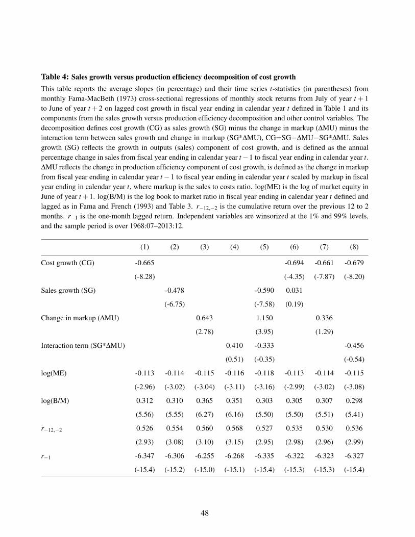
Table 4: Sales growth versus production efficiency decomposition of cost growthThis table reports the average slopes (in percentage) and their time series t-statistics (in parentheses) frommonthly Fama-MacBeth (1973) cross-sectional regressions of monthly stock returns from July of year t + 1to June of year t + 2 on lagged cost growth in fiscal year ending in calendar year t defined in Table 1 and itscomponents from the sales growth versus production efficiency decomposition and other control variables. Thedecomposition defines cost growth (CG) as sales growth (SG) minus the change in markup (∆MU) minus theinteraction term between sales growth and change in markup (SG*∆MU), CG=SG−∆MU−SG*∆MU. Salesgrowth (SG) reflects the growth in outputs (sales) component of cost growth, and is defined as the annualpercentage change in sales from fiscal year ending in calendar year t−1 to fiscal year ending in calendar year t.∆MU reflects the change in production efficiency component of cost growth, is defined as the change in markupfrom fiscal year ending in calendar year t −1 to fiscal year ending in calendar year t scaled by markup in fiscalyear ending in calendar year t, where markup is the sales to costs ratio. log(ME) is the log of market equity inJune of year t +1. log(B/M) is the log book to market ratio in fiscal year ending in calendar year t defined andlagged as in Fama and French (1993) and Table 3. r−12,−2 is the cumulative return over the previous 12 to 2months. r−1 is the one-month lagged return. Independent variables are winsorized at the 1% and 99% levels,and the sample period is over 1968:07–2013:12.

(1) (2) (3) (4) (5) (6) (7) (8)

Cost growth (CG) -0.665 -0.694 -0.661 -0.679

(-8.28) (-4.35) (-7.87) (-8.20)

Sales growth (SG) -0.478 -0.590 0.031

(-6.75) (-7.58) (0.19)

Change in markup (∆MU) 0.643 1.150 0.336

(2.78) (3.95) (1.29)

Interaction term (SG*∆MU) 0.410 -0.333 -0.456

(0.51) (-0.35) (-0.54)

log(ME) -0.113 -0.114 -0.115 -0.116 -0.118 -0.113 -0.114 -0.115

(-2.96) (-3.02) (-3.04) (-3.11) (-3.16) (-2.99) (-3.02) (-3.08)

log(B/M) 0.312 0.310 0.365 0.351 0.303 0.305 0.307 0.298

(5.56) (5.55) (6.27) (6.16) (5.50) (5.50) (5.51) (5.41)

r−12,−2 0.526 0.554 0.560 0.568 0.527 0.535 0.530 0.536

(2.93) (3.08) (3.10) (3.15) (2.95) (2.98) (2.96) (2.99)

r−1 -6.347 -6.306 -6.255 -6.268 -6.335 -6.322 -6.323 -6.327

(-15.4) (-15.2) (-15.0) (-15.1) (-15.4) (-15.3) (-15.3) (-15.4)

48

Table 5: Controlling for other investment and growth-related return determinantsThis table reports the average slopes (in percentage) and their time series t-statistics (in parentheses) frommonthly Fama-MacBeth (1973) cross-sectional regressions of monthly stock returns from July of year t +1 toJune of year t + 2 on lagged cost growth for fiscal year ending in calendar year t and other control variablesrelated to investment and growth effects. Accruals (ACC) is operating accruals (the change in noncash currentassets less the change in current liabilities excluding the change in short-term debt and the change in taxespayable minus depreciation and amortization expense) deflated by average total assets from Sloan (1996). Netoperating assets (NOA) is net operating assets (operating assets minus operating liabilities) scaled by laggedtotal assets from Hirshleifer, Hou, Teoh, and Zhang (2004). Investment to asset (INV) is calculated as thechange in gross property, plant, and equipment plus the change in inventories scaled by lagged total assetsfrom Lyandres, Sun, and Zhang (2008). Asset growth (AG) is calculated as the annual percentage change intotal assets from Cooper, Gulen, and Schill (2008). Investment growth (IG) is calculated as the growth rateof capital expenditure from Xing (2008). Capital investment (CI) is calculated as capital expenditure dividedby the average capital expenditure over the past three years from Titman, Wei, and Xie (2004), where capitalexpenditure is scaled by its sales. log(ME) is the log of market equity in June of year t +1. log(B/M) is the logbook to market ratio defined and lagged as in Fama and French (1993). r−12,−2 is is the cumulative return overthe previous 12 to 2 months. r−1 is the one-month lagged return. Independent variables are winsorized at the1% and 99% levels, and the sample period is over 1968:07–2013:12.

(1) (2) (3) (4) (5) (6)

Cost growth (CG) -0.534 -0.421 -0.427 -0.386 -0.502 -0.571(-6.33) (-5.24) (-5.00) (-3.39) (-5.82) (-6.48)

Accruals (ACC) -1.220(-5.16)

Net operating assets (NOA) -0.447(-6.19)

Investment to asset (INV) -0.601(-6.80)

Asset growth (AG) -0.552(-9.28)

Investment growth (IG) -0.084(-7.51)

Capital investment (CI) -0.144(-7.27)

log(ME) -0.122 -0.113 -0.119 -0.111 -0.121 -0.116(-3.13) (-2.95) (-3.08) (-2.91) (-3.17) (-3.05)

log(B/M) 0.317 0.325 0.313 0.280 0.290 0.262(5.79) (5.63) (5.70) (5.10) (5.19) (4.56)

r−12,−2 0.466 0.513 0.468 0.509 0.514 0.486(2.63) (2.85) (2.63) (2.84) (2.87) (2.62)

r−1 -6.395 -6.373 -6.372 -6.391 -6.311 -6.404(-15.8) (-15.5) (-15.7) (-15.5) (-15.4) (-15.6)

49

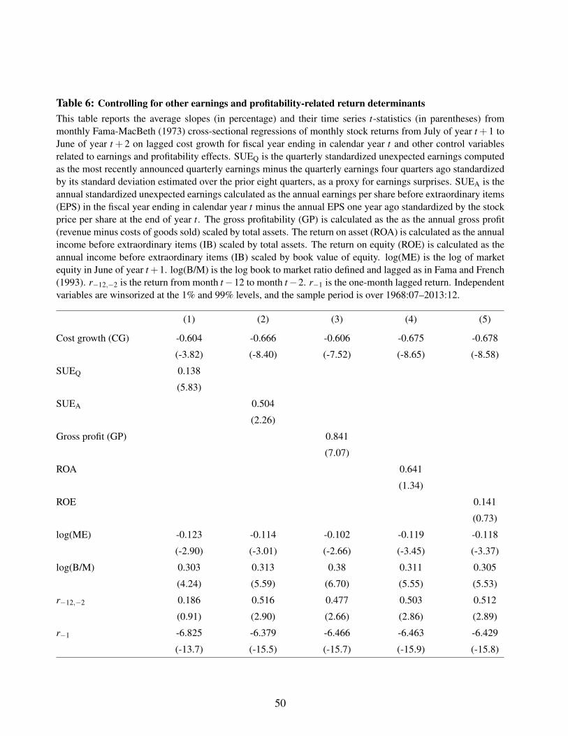
Table 6: Controlling for other earnings and profitability-related return determinantsThis table reports the average slopes (in percentage) and their time series t-statistics (in parentheses) frommonthly Fama-MacBeth (1973) cross-sectional regressions of monthly stock returns from July of year t +1 toJune of year t + 2 on lagged cost growth for fiscal year ending in calendar year t and other control variablesrelated to earnings and profitability effects. SUEQ is the quarterly standardized unexpected earnings computedas the most recently announced quarterly earnings minus the quarterly earnings four quarters ago standardizedby its standard deviation estimated over the prior eight quarters, as a proxy for earnings surprises. SUEA is theannual standardized unexpected earnings calculated as the annual earnings per share before extraordinary items(EPS) in the fiscal year ending in calendar year t minus the annual EPS one year ago standardized by the stockprice per share at the end of year t. The gross profitability (GP) is calculated as the as the annual gross profit(revenue minus costs of goods sold) scaled by total assets. The return on asset (ROA) is calculated as the annualincome before extraordinary items (IB) scaled by total assets. The return on equity (ROE) is calculated as theannual income before extraordinary items (IB) scaled by book value of equity. log(ME) is the log of marketequity in June of year t +1. log(B/M) is the log book to market ratio defined and lagged as in Fama and French(1993). r−12,−2 is the return from month t−12 to month t−2. r−1 is the one-month lagged return. Independentvariables are winsorized at the 1% and 99% levels, and the sample period is over 1968:07–2013:12.

(1) (2) (3) (4) (5)

Cost growth (CG) -0.604 -0.666 -0.606 -0.675 -0.678

(-3.82) (-8.40) (-7.52) (-8.65) (-8.58)

SUEQ 0.138

(5.83)

SUEA 0.504

(2.26)

Gross profit (GP) 0.841

(7.07)

ROA 0.641

(1.34)

ROE 0.141

(0.73)

log(ME) -0.123 -0.114 -0.102 -0.119 -0.118

(-2.90) (-3.01) (-2.66) (-3.45) (-3.37)

log(B/M) 0.303 0.313 0.38 0.311 0.305

(4.24) (5.59) (6.70) (5.55) (5.53)

r−12,−2 0.186 0.516 0.477 0.503 0.512

(0.91) (2.90) (2.66) (2.86) (2.89)

r−1 -6.825 -6.379 -6.466 -6.463 -6.429

(-13.7) (-15.5) (-15.7) (-15.9) (-15.8)

50

Table 7: Alternative measures of cost growthThis table reports the average slopes (in percentage) and their time series t-statistics (in parentheses) frommonthly Fama-MacBeth (1973) cross-sectional regressions of monthly stock returns from July of year t + 1to June of year t + 2 on various lagged alternative definitions of cost growth in fiscal year ending in calendaryear t and controls variables. CG is our main cost growth measure as defined in Table 1. CGCOGS is theannual percentage changes in costs of goods sold (COGS) from the fiscal year ending in calendar year t − 1to the fiscal year ending in calendar year t. CGXSGA is the annual percentage changes in selling, general, andadministration expenses (XSGA). CGDP is the annual percentage changes in the sum of costs of goods sold(COGS), selling, general, and administration expenses (XSGA), and depreciation and amortization expenses(DP), COGS+XSGA+DP. CGRD is the annual percentage changes in the costs of goods sold (COGS) plusselling, general, and administration expenses (XSGA) minus the R&D expenses (XRD), COGS+XSGA-XRD.CGAT is the annual change in the sume of costs of goods sold (COGS) and selling, general, and administrationexpenses (XSGA) scaled by lagged total assets (AT). log(ME) is the log of market equity in June of year t +1.log(B/M) is the log book to market ratio defined and lagged as in Fama and French (1993). r−12,−2 is the returnfrom month t −12 to month t −2. r−1 is the one-month lagged return. Independent variables are winsorized atthe 1% and 99% levels, and the sample period is over 1968:07–2013:12.

(1) (2) (3) (4) (5) (6) (7)

Cost growth (CG) -0.665

(-8.28)

CGCOGS -0.446 -0.307

(-7.83) (-5.37)

CGXSGA -0.574 -0.377

(-7.38) (-4.65)

CGDP -0.597

(-7.67)

CGRD -0.610

(-7.88)

CGAT -0.457

(-6.49)

log(ME) -0.113 -0.115 -0.112 -0.113 -0.112 -0.111 -0.116

(-2.96) (-3.04) (-2.96) (-3.00) (-2.95) (-2.93) (-3.04)

log(B/M) 0.312 0.317 0.322 0.303 0.316 0.322 0.322

(5.56) (5.60) (5.73) (5.43) (5.65) (5.70) (5.70)

r−12,−2 0.526 0.547 0.522 0.529 0.514 0.522 0.549

(2.93) (3.04) (2.92) (2.95) (2.87) (2.91) (3.05)

r−1 -6.347 -6.301 -6.354 -6.344 -6.343 -6.320 -6.339

(-15.4) (-15.2) (-15.4) (-15.4) (-15.4) (-15.3) (-15.3)

51

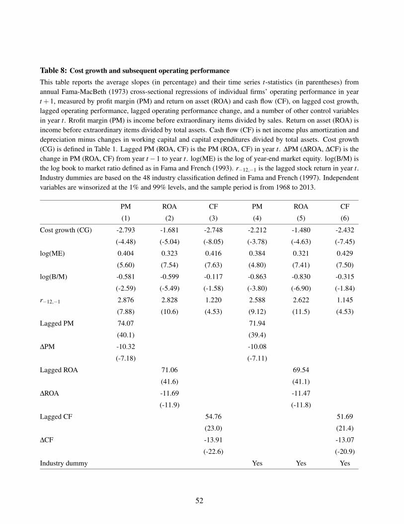
Table 8: Cost growth and subsequent operating performanceThis table reports the average slopes (in percentage) and their time series t-statistics (in parentheses) fromannual Fama-MacBeth (1973) cross-sectional regressions of individual firms’ operating performance in yeart + 1, measured by profit margin (PM) and return on asset (ROA) and cash flow (CF), on lagged cost growth,lagged operating performance, lagged operating performance change, and a number of other control variablesin year t. Rrofit margin (PM) is income before extraordinary items divided by sales. Return on asset (ROA) isincome before extraordinary items divided by total assets. Cash flow (CF) is net income plus amortization anddepreciation minus changes in working capital and capital expenditures divided by total assets. Cost growth(CG) is defined in Table 1. Lagged PM (ROA, CF) is the PM (ROA, CF) in year t. ∆PM (∆ROA, ∆CF) is thechange in PM (ROA, CF) from year t −1 to year t. log(ME) is the log of year-end market equity. log(B/M) isthe log book to market ratio defined as in Fama and French (1993). r−12,−1 is the lagged stock return in year t.Industry dummies are based on the 48 industry classification defined in Fama and French (1997). Independentvariables are winsorized at the 1% and 99% levels, and the sample period is from 1968 to 2013.

PM ROA CF PM ROA CF

(1) (2) (3) (4) (5) (6)

Cost growth (CG) -2.793 -1.681 -2.748 -2.212 -1.480 -2.432

(-4.48) (-5.04) (-8.05) (-3.78) (-4.63) (-7.45)

log(ME) 0.404 0.323 0.416 0.384 0.321 0.429

(5.60) (7.54) (7.63) (4.80) (7.41) (7.50)

log(B/M) -0.581 -0.599 -0.117 -0.863 -0.830 -0.315

(-2.59) (-5.49) (-1.58) (-3.80) (-6.90) (-1.84)

r−12,−1 2.876 2.828 1.220 2.588 2.622 1.145

(7.88) (10.6) (4.53) (9.12) (11.5) (4.53)

Lagged PM 74.07 71.94

(40.1) (39.4)

∆PM -10.32 -10.08

(-7.18) (-7.11)

Lagged ROA 71.06 69.54

(41.6) (41.1)

∆ROA -11.69 -11.47

(-11.9) (-11.8)

Lagged CF 54.76 51.69

(23.0) (21.4)

∆CF -13.91 -13.07

(-22.6) (-20.9)

Industry dummy Yes Yes Yes

52

Table 9: Cost growth portfolios abnormal returns and factor loadings on the Chen, Roll, and Ross(1986) macroeconomic factor modelThis table reports the average monthly abnormal returns or alphas (α , in percentage), factor loadings, and theirt-statistics (in squared brackets) of cost growth decile portfolios from regressing excess cost growth decileportfolio returns on the Chen, Roll, and Ross (1986) five macroeconomic factors over 1968:07–2013:12,

R j,t −R f ,t = α j +β j,MPRMP,t +β j,UIRUI,t +β j,DEIRDEI,t +β j,UTSRUTS +β j,UPRRUPR,t + ε j,t ,

where RMP, RUI, RDEI, RUTS, and RUPR are the mimicking portfolio returns that track the growth rate of industrialproduction (MP), the unexpected inflation (UI), the change in expected inflation (DEI), the term premium(UTS), and the default premium (URP), respectively. The mimicking portfolios include the ten size, book-to-market, momentum, and cost growth decile portfolios, and all of them are formed on one-way sorts. At the endof June of each year t+1, we sort firms into cost growth deciles based on cost growth rates in fiscal year endingin calendar t as defined in Table 1. We hold these portfolios for one year, from July of year t +1 to June of yeart + 2, and compute the equal-weighted monthly returns of these cost growth portfolios. “Low” refers to firmsin the lowest cost growth decile, and “High” refers to firms in the highest cost growth decile. The “Low-High”cost growth spread portfolio is computed as the difference between the returns of the lowest and the highestcost growth deciles.

α (%) βMP βUI βDEI βUTS βUPR

Low 0.30 [0.98] 0.31 [2.29] 0.04 [0.08] 4.79 [4.53] 0.66 [9.29] 1.44 [6.43]

2 0.23 [0.95] 0.21 [1.81] -0.71 [-1.88] 4.35 [4.98] 0.62 [10.5] 1.43 [7.69]

3 0.37 [1.60] 0.12 [1.11] -0.84 [-2.39] 3.82 [4.74] 0.60 [11.1] 1.40 [8.17]

4 0.39 [1.78] 0.13 [1.28] -1.15 [-3.36] 3.21 [4.09] 0.53 [10.2] 1.31 [7.87]

5 0.31 [1.43] 0.20 [1.99] -1.73 [-5.18] 3.25 [4.23] 0.54 [10.4] 1.40 [8.56]

6 0.34 [1.48] 0.13 [1.27] -1.43 [-4.14] 2.90 [3.64] 0.53 [9.97] 1.39 [8.20]

7 0.24 [0.99] 0.20 [1.86] -1.52 [-4.16] 3.25 [3.87] 0.53 [9.49] 1.41 [7.93]

8 0.12 [0.46] 0.14 [1.14] -1.30 [-3.23] 3.75 [4.05] 0.51 [8.30] 1.33 [6.76]

9 -0.11 [-0.38] 0.03 [0.23] -1.59 [-3.59] 4.25 [4.17] 0.51 [7.53] 1.37 [6.32]

High -0.69 [-1.96] 0.08 [0.48] -0.59 [-1.12] 3.78 [3.11] 0.59 [7.26] 1.43 [5.53]

Low-High 0.99 [7.01] 0.24 [3.77] 0.63 [2.96] 1.01 [2.05] 0.07 [2.01] 0.01 [0.14]

53

Table 10: Cost growth portfolios abnormal returns and factor loadings on the Fama-French andHirshleifer and Jiang (2010) mispricing factor modelThis table reports the average monthly abnormal returns or alphas (α , in percentage), factor loadings, andtheir t-statistics (in square brackets) of cost growth decile portfolios from regressing excess cost growth decileportfolio returns on the Fama-French (1993) three factors augmented with the Hirshleifer and Jiang (2010)mispricing factor (UMO) over 1972:07–2013:12. MKT, SMB, and HML are the market, size, and value factorsin Fama and French (1993). At the end of June of each year t +1, we sort firms into cost growth deciles basedon cost growth rates in fiscal year ending in calendar t as defined in Table 1. We hold these portfolios for oneyear, from July of year t + 1 to June of year t + 2, and compute the equal-weighted monthly returns of thesecost growth portfolios. “Low” refers to firms in the lowest cost growth decile, and “High” refers to firms inthe highest cost growth decile. The “Low-High” cost growth spread portfolio is computed as the differencebetween the returns of the lowest and the highest cost growth deciles.

α (%) βMKT βSMB βHML βUMO

Low 0.37 [2.22] 1.04 [26.3] 1.22 [23.2] 0.40 [5.99] -0.07 [-0.98]

2 0.18 [1.62] 1.00 [38.0] 0.95 [27.5] 0.42 [9.54] 0.03 [0.63]

3 0.33 [3.64] 0.97 [45.4] 0.83 [29.4] 0.47 [13.1] -0.03 [-0.67]

4 0.26 [3.45] 0.97 [54.2] 0.75 [31.9] 0.38 [12.7] 0.05 [1.45]

5 0.17 [2.30] 0.96 [53.9] 0.74 [31.4] 0.37 [12.4] 0.04 [1.13]

6 0.26 [3.56] 0.96 [55.0] 0.76 [33.2] 0.29 [9.93] -0.01 [-0.31]

7 0.21 [2.62] 0.98 [52.8] 0.82 [33.5] 0.23 [7.54] -0.02 [-0.67]

8 0.20 [2.15] 0.99 [45.9] 0.88 [30.8] 0.26 [7.12] -0.18 [-4.65]

9 0.09 [0.84] 1.02 [42.6] 0.97 [30.8] 0.25 [6.24] -0.34 [-8.03]

High -0.06 [-0.37] 1.01 [27.3] 1.07 [21.9] 0.29 [4.75] -0.78 [-11.7]

Low-High 0.43 [3.73] 0.03 [1.07] 0.14 [3.93] 0.10 [2.23] 0.71 [14.52]

54

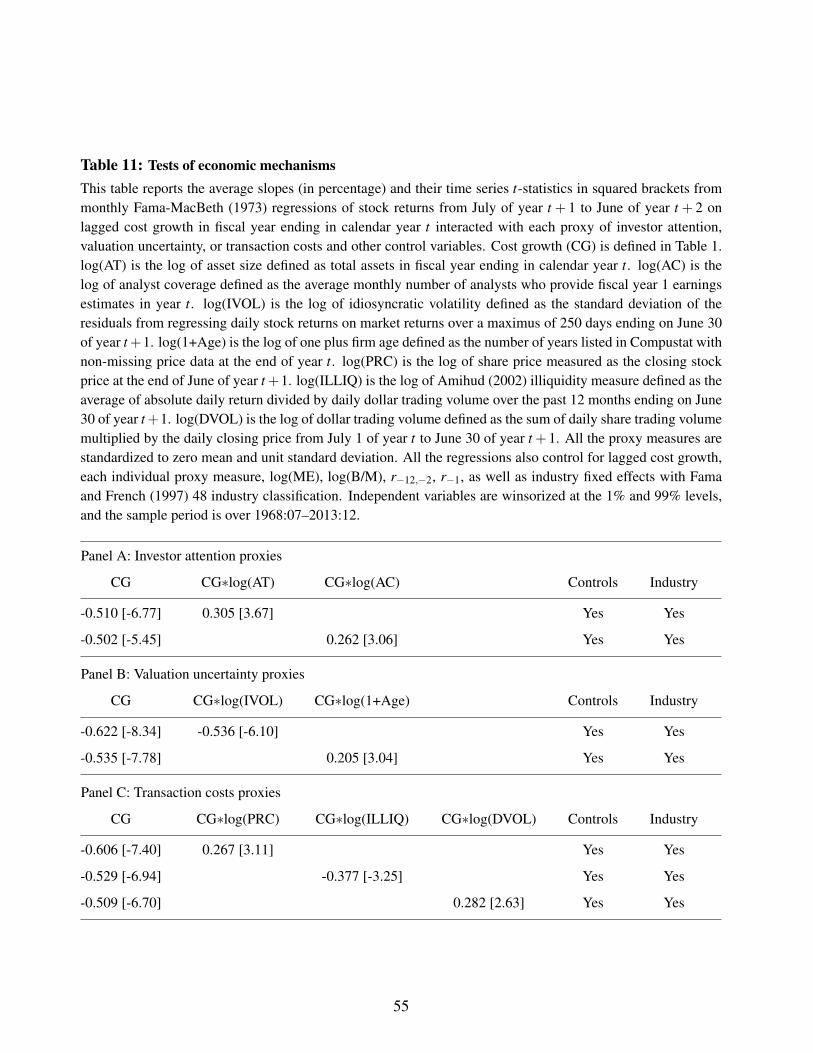
Table 11: Tests of economic mechanismsThis table reports the average slopes (in percentage) and their time series t-statistics in squared brackets frommonthly Fama-MacBeth (1973) regressions of stock returns from July of year t + 1 to June of year t + 2 onlagged cost growth in fiscal year ending in calendar year t interacted with each proxy of investor attention,valuation uncertainty, or transaction costs and other control variables. Cost growth (CG) is defined in Table 1.log(AT) is the log of asset size defined as total assets in fiscal year ending in calendar year t. log(AC) is thelog of analyst coverage defined as the average monthly number of analysts who provide fiscal year 1 earningsestimates in year t. log(IVOL) is the log of idiosyncratic volatility defined as the standard deviation of theresiduals from regressing daily stock returns on market returns over a maximus of 250 days ending on June 30of year t+1. log(1+Age) is the log of one plus firm age defined as the number of years listed in Compustat withnon-missing price data at the end of year t. log(PRC) is the log of share price measured as the closing stockprice at the end of June of year t +1. log(ILLIQ) is the log of Amihud (2002) illiquidity measure defined as theaverage of absolute daily return divided by daily dollar trading volume over the past 12 months ending on June30 of year t+1. log(DVOL) is the log of dollar trading volume defined as the sum of daily share trading volumemultiplied by the daily closing price from July 1 of year t to June 30 of year t +1. All the proxy measures arestandardized to zero mean and unit standard deviation. All the regressions also control for lagged cost growth,each individual proxy measure, log(ME), log(B/M), r−12,−2, r−1, as well as industry fixed effects with Famaand French (1997) 48 industry classification. Independent variables are winsorized at the 1% and 99% levels,and the sample period is over 1968:07–2013:12.

Panel A: Investor attention proxies

CG CG∗log(AT) CG∗log(AC) Controls Industry

-0.510 [-6.77] 0.305 [3.67] Yes Yes

-0.502 [-5.45] 0.262 [3.06] Yes Yes

Panel B: Valuation uncertainty proxies

CG CG∗log(IVOL) CG∗log(1+Age) Controls Industry

-0.622 [-8.34] -0.536 [-6.10] Yes Yes

-0.535 [-7.78] 0.205 [3.04] Yes Yes

Panel C: Transaction costs proxies

CG CG∗log(PRC) CG∗log(ILLIQ) CG∗log(DVOL) Controls Industry

-0.606 [-7.40] 0.267 [3.11] Yes Yes

-0.529 [-6.94] -0.377 [-3.25] Yes Yes

-0.509 [-6.70] 0.282 [2.63] Yes Yes

55