COST-AWARE SECURE PROTOCOL DESIGN AND ANALYSIS · COST-AWARE SECURE PROTOCOL DESIGN AND ANALYSIS By...

COST-AWARE SECURE PROTOCOL DESIGN AND ANALYSIS

By

Di Tang

A DISSERTATION

Submittedto Michigan State University

in partial fulfillment of the requirementsfor the degree of

Electrical Engineering – Doctor of Philosophy

2015

ABSTRACT

COST-AWARE SECURE PROTOCOL DESIGN AND ANALYSIS

By

Di Tang

The recent technological progresses make sensor networks feasible to be widely used in both

military and civilian applications. The nature of such networks makes energy consumption,

communication delay and security the most essential issues for wireless sensor networks.

However, these issues may be conflicting with each other. The existing works generally

try to optimize one of these key issues without providing sufficient diversity and flexibility

of various other requirements in protocol design. In this dissertation, we investigate the

relationship and design trade-offs among these conflicting issues.

To deal with the lifetime optimization and security issues, we propose a novel secure

and efficient Cost-Aware SEcure Routing (CASER) protocol to address them through two

adjustable parameters: energy balance control (EBC) and security level to enforce energy

balance and increase lifetime and determine the probabilistic distribution of random walk-

ing that provides routing security. We derive a tight numerical formula to quantitatively

estimate the routing efficiency through the number of routing hops for a given routing se-

curity level. We also prove that CASER scheme can provide provable security under the

quantitative security measurement criteria. Simulation results also show that the proposed

CASER scheme can provide an excellent balance between routing efficiency and security

while extending the network lifetime.

We then discover that the energy consumption is severely disproportional to the uniform

energy deployment for the given network topology. To solve this problem, we propose an effi-

cient non-uniform energy deployment strategy to optimize the network lifetime and increase

the message delivery ratio under the same energy resource and security requirements. Our

theoretical analysis and OPNET simulation results demonstrate that the updated CASER

protocol can provide an excellent trade-off between routing efficiency and energy consump-

tion, while significantly extending the lifetime of the sensor networks in all scenarios. For the

non-uniform energy deployment, our analysis shows that we can increase the lifetime and

the total number of messages that can be delivered by more than four times under the same

energy deployment, while achieving a high message delivery ratio and preventing routing

traceback attacks.

In WSNs, congestion introduces not only buffer overflow, but also communication delay

for forwarding messages from the source node to the sink. We propose a novel congestion-

aware routing (CAR) scheme to reduce the end-to-end communication delay while increasing

network throughput. CAR employs two routing strategies, shortest path routing strategy

and congestion-aware strategy, to achieve a trade-off between energy efficiency and com-

munication delay. The OPNET simulation results demonstrate that the proposed routing

scheme can reduce the end-to-end communication delay by 50% while increasing the network

throughput by more than two times in our settings.

People-centric urban sensing is envisioned as a novel urban sensing paradigm. Security,

communication delay and delivery ratio are essential design issues in people-centric urban

sensing networks. To address these three issues concurrently, we propose a novel delay-aware

privacy preserving (DAPP) transmission scheme based on a combination of two-phase for-

warding and secret sharing. The two-phase forwarding method detaches connection between

the application data server and the source nodes, which renders it infeasible for the appli-

cation data server to estimate source node identities. The underlying secret sharing scheme

and dynamic pseudonym ensure confidentiality of the collected data and anonymity of par-

ticipating users. DAPP provides a framework to achieve a design trade-off among security,

communication delay and delivery ratio. The security analysis demonstrates that DAPP

can preserve location privacy while defending against side information attacks. Theoretical

analysis and simulation results show that our proposed algorithms can provide a flexible and

diverse security design option for routing and data forwarding algorithm design.

Copyright byDI TANG

2015

Dedicated to my family

v

ACKNOWLEDGEMENTS

First of all, I would like to express my sincere gratitude to my advisor, Dr. Jian Ren, for his

guidance, encouragement, and support in every stage of my graduate study. His knowledge,

kindness, patience, passion, and vision affected me a lot and have provided me with lifetime

benefits.

I am also grateful to my dissertation committee members, Professor Richard Enbody,

Professor Subir Biswas, and Professor Wen Li, for their valuable comments and suggestions

on the thesis draft, as well as for the experience as a student with these three outstanding

teachers. I would also like to thank many faculty members of MSU who were the instructors

for the courses I took. The course works have greatly enriched my knowledge and provided

the background and foundations for my thesis research.

My PhD study could have never been completed without the help of my fellow graduate

students at MSU. I would like to express my special thanks to the colleagues at our lab, Yun

Li, Jian Li, Kai Zhou, Mohamed Afifi Ibrahim and Leron Lightfoot for their suggestions,

helps, and all the happy and tough time we have been through. I also want to express my

thanks to Dongliang Fang, Aimin Li, Meng Cai, Ying Liu, Jiayin Li, Qing Liu, Xiaochen

Tang, Sara Kovensky Kalt, Brain Kalt, Lei Zhang, Xiaopeng Bi, Hanqing Li, Liangliang Li,

Mingwu Gao and Qiong Huo, for their kind help during my staying at MSU, who enriched

my study and life.

Finally, I would like to express my gratitude to my family. Their endless love and support

always encourage me to deal with obstacles in every aspects of my life. In particular, I

want to express my deepest gratitude to my dear wife, Lu Zhang, for her enduring love,

encouragement, patience, and understanding.

vi

TABLE OF CONTENTS

LIST OF TABLES . . . . . . . . . . . . . . . . . . . . . . . . . . . . . . . . . . . x

LIST OF FIGURES . . . . . . . . . . . . . . . . . . . . . . . . . . . . . . . . . . . xi

LIST OF ALGORITHMS . . . . . . . . . . . . . . . . . . . . . . . . . . . . . . . . xiii

KEY TO SYMBOLS AND ABBREVIATIONS . . . . . . . . . . . . . . . . . . . . . xiv

CHAPTER 1 INTRODUCTION . . . . . . . . . . . . . . . . . . . . . . . . . . . 11.1 Source Location Privacy in Wireless Sensor Network . . . . . . . . . . . . . . 1

1.1.1 Routing Algorithm Design . . . . . . . . . . . . . . . . . . . . . . . . 21.1.2 Existing Solutions for Source Location Privacy in Wireless Sensor

Networks . . . . . . . . . . . . . . . . . . . . . . . . . . . . . . . . . 51.1.3 Summary of Major Limitations . . . . . . . . . . . . . . . . . . . . . 7

1.2 Congestion in Wireless Sensor Networks . . . . . . . . . . . . . . . . . . . . 81.2.1 Existing Solutions for Congestion Mitigation . . . . . . . . . . . . . . 91.2.2 Summary of Major Limitations . . . . . . . . . . . . . . . . . . . . . 10

1.3 Urban Sensing Networks . . . . . . . . . . . . . . . . . . . . . . . . . . . . . 111.3.1 People-Centric Urban Sensing Networks . . . . . . . . . . . . . . . . 111.3.2 Existing Solutions for Location Privacy in Urban Sensing Networks . 121.3.3 Summary of Major Limitations . . . . . . . . . . . . . . . . . . . . . 14

1.4 Proposed Research Direction . . . . . . . . . . . . . . . . . . . . . . . . . . . 151.4.1 Source Location Privacy Protection in Wireless Sensor Networks . . . 151.4.2 Congestion-Aware Routing (CAR) Algorithm in Wireless Sensor

Networks . . . . . . . . . . . . . . . . . . . . . . . . . . . . . . . . . 161.4.3 Location Privacy Protection in Urban Sensing Networks . . . . . . . 17

1.5 Overview of the Dissertation . . . . . . . . . . . . . . . . . . . . . . . . . . . 181.5.1 Design Goals . . . . . . . . . . . . . . . . . . . . . . . . . . . . . . . 181.5.2 Major Contributions . . . . . . . . . . . . . . . . . . . . . . . . . . . 191.5.3 Thesis Organization . . . . . . . . . . . . . . . . . . . . . . . . . . . 21

CHAPTER 2 COST-AWARE SECURE ROUTING: DESIGN AND ANALYSIS . . 232.1 Introduction . . . . . . . . . . . . . . . . . . . . . . . . . . . . . . . . . . . . 232.2 Models and Assumptions . . . . . . . . . . . . . . . . . . . . . . . . . . . . . 27

2.2.1 System Model . . . . . . . . . . . . . . . . . . . . . . . . . . . . . . . 272.2.2 Adversarial Model . . . . . . . . . . . . . . . . . . . . . . . . . . . . 27

2.3 The Proposed CASER Scheme . . . . . . . . . . . . . . . . . . . . . . . . . . 282.3.1 Overview of the Proposed Scheme . . . . . . . . . . . . . . . . . . . . 292.3.2 Assumptions and Energy Balance Routing . . . . . . . . . . . . . . . 29

2.3.2.1 Probability Analysis . . . . . . . . . . . . . . . . . . . . . . 302.3.2.2 Analysis on Energy Distribution . . . . . . . . . . . . . . . 31

vii

2.3.2.3 The Hop Distance Estimation . . . . . . . . . . . . . . . . . 322.3.3 Secure Routing Strategy . . . . . . . . . . . . . . . . . . . . . . . . . 342.3.4 CASER Algorithm . . . . . . . . . . . . . . . . . . . . . . . . . . . . 352.3.5 Determine Security Level Based on Cost Factor . . . . . . . . . . . . 37

2.4 Security Analysis . . . . . . . . . . . . . . . . . . . . . . . . . . . . . . . . . 392.4.1 Quantitative Security Analysis of CASER . . . . . . . . . . . . . . . 402.4.2 Dynamic Routing and Jamming Attacks . . . . . . . . . . . . . . . . 432.4.3 Energy Level and Compromised Nodes Detection . . . . . . . . . . . 45

2.5 Performance Evaluation and Simulation Results . . . . . . . . . . . . . . . . 462.5.1 Routing Efficiency and Delay . . . . . . . . . . . . . . . . . . . . . . 462.5.2 Energy Balance . . . . . . . . . . . . . . . . . . . . . . . . . . . . . . 47

2.6 Summary . . . . . . . . . . . . . . . . . . . . . . . . . . . . . . . . . . . . . 48

CHAPTER 3 COST-AWARE ENERGY DEPLOYMENT: DESIGN AND ANALYSIS 513.1 Uniform Energy Deployment . . . . . . . . . . . . . . . . . . . . . . . . . . . 51

3.1.1 Energy Consumption Analysis . . . . . . . . . . . . . . . . . . . . . . 513.1.2 Energy Balance of CASER . . . . . . . . . . . . . . . . . . . . . . . . 523.1.3 Delivery Ratio . . . . . . . . . . . . . . . . . . . . . . . . . . . . . . . 53

3.2 CASER Optimal Non-Uniform Energy Deployment . . . . . . . . . . . . . . 543.2.1 Node Energy Deployment . . . . . . . . . . . . . . . . . . . . . . . . 553.2.2 Routing in Non-Uniform Energy Deployment . . . . . . . . . . . . . . 563.2.3 Simulation Results . . . . . . . . . . . . . . . . . . . . . . . . . . . . 57

3.3 Summary . . . . . . . . . . . . . . . . . . . . . . . . . . . . . . . . . . . . . 60

CHAPTER 4 CONGESTION-AWARE ROUTING (CAR): DESIGN AND ANALYSIS 624.1 Introduction . . . . . . . . . . . . . . . . . . . . . . . . . . . . . . . . . . . . 624.2 System Model and Assumptions . . . . . . . . . . . . . . . . . . . . . . . . . 64

4.2.1 System Model . . . . . . . . . . . . . . . . . . . . . . . . . . . . . . . 644.2.2 MAC Layer Protocol . . . . . . . . . . . . . . . . . . . . . . . . . . . 65

4.3 The Proposed Routing Scheme . . . . . . . . . . . . . . . . . . . . . . . . . . 664.3.1 Overview of the Proposed Routing Scheme . . . . . . . . . . . . . . . 664.3.2 Congestion-Aware (CAR) Routing Algorithm . . . . . . . . . . . . . 68

4.4 The Analysis on Congestion through End-to-End Transmission . . . . . . . . 684.4.1 One Hop Congestion Analysis . . . . . . . . . . . . . . . . . . . . . . 694.4.2 Numerical Results . . . . . . . . . . . . . . . . . . . . . . . . . . . . 72

4.5 Performance Analysis and Simulation Results . . . . . . . . . . . . . . . . . 744.5.1 Performance Metrics . . . . . . . . . . . . . . . . . . . . . . . . . . . 74

4.5.1.1 End-to-End Packet Transmission Delay (∆) . . . . . . . . . 754.5.1.2 Network Throughput (T) . . . . . . . . . . . . . . . . . . . 75

4.5.2 Simulation Results . . . . . . . . . . . . . . . . . . . . . . . . . . . . 764.5.2.1 Simulation Setup . . . . . . . . . . . . . . . . . . . . . . . . 764.5.2.2 Source Event Location . . . . . . . . . . . . . . . . . . . . . 784.5.2.3 Sensing Range . . . . . . . . . . . . . . . . . . . . . . . . . 79

4.6 Summary . . . . . . . . . . . . . . . . . . . . . . . . . . . . . . . . . . . . . 80

viii

CHAPTER 5 DELAY-AWARE AND PRIVACY PRESERVING DATA FORWARD-ING: DESIGN AND ANALYSIS . . . . . . . . . . . . . . . . . . . . 82

5.1 Introduction . . . . . . . . . . . . . . . . . . . . . . . . . . . . . . . . . . . . 825.2 Models and Assumptions . . . . . . . . . . . . . . . . . . . . . . . . . . . . . 84

5.2.1 System Model . . . . . . . . . . . . . . . . . . . . . . . . . . . . . . . 845.2.2 Adversarial Model . . . . . . . . . . . . . . . . . . . . . . . . . . . . 845.2.3 Side Information Attack . . . . . . . . . . . . . . . . . . . . . . . . . 855.2.4 Mobility Model . . . . . . . . . . . . . . . . . . . . . . . . . . . . . . 86

5.3 The Proposed DAPP Scheme . . . . . . . . . . . . . . . . . . . . . . . . . . 865.3.1 Overview of the Proposed Privacy Scheme . . . . . . . . . . . . . . . 875.3.2 Secret Sharing . . . . . . . . . . . . . . . . . . . . . . . . . . . . . . . 885.3.3 Dynamic Pseudonyms . . . . . . . . . . . . . . . . . . . . . . . . . . 885.3.4 DAPP Scheme . . . . . . . . . . . . . . . . . . . . . . . . . . . . . . 89

5.4 Security Analysis . . . . . . . . . . . . . . . . . . . . . . . . . . . . . . . . . 915.4.1 Definitions and Security Metrics . . . . . . . . . . . . . . . . . . . . . 915.4.2 Identity Information Loss . . . . . . . . . . . . . . . . . . . . . . . . 92

5.4.2.1 Without Side Information Attack . . . . . . . . . . . . . . . 935.4.2.2 Side Information Attack . . . . . . . . . . . . . . . . . . . . 94

5.4.3 Location Information Leakage . . . . . . . . . . . . . . . . . . . . . . 965.4.3.1 The Location Information Leakage to Individual Delivery

Node . . . . . . . . . . . . . . . . . . . . . . . . . . . . . . . 975.4.3.2 The Location Information Leakage to APs . . . . . . . . . . 101

5.4.4 Joint Identity and Location Privacy Information Leakage . . . . . . . 1015.4.5 Participating Nodes Collusion . . . . . . . . . . . . . . . . . . . . . . 1025.4.6 Data Integrity . . . . . . . . . . . . . . . . . . . . . . . . . . . . . . . 103

5.5 Performance Evaluation and Simulation Results . . . . . . . . . . . . . . . . 1055.5.1 Communication Delay . . . . . . . . . . . . . . . . . . . . . . . . . . 1055.5.2 Delivery Ratio . . . . . . . . . . . . . . . . . . . . . . . . . . . . . . . 1065.5.3 Trade-off Design . . . . . . . . . . . . . . . . . . . . . . . . . . . . . 1065.5.4 Computational Complexity . . . . . . . . . . . . . . . . . . . . . . . . 1085.5.5 Numerical Simulation Results . . . . . . . . . . . . . . . . . . . . . . 109

5.6 Summary . . . . . . . . . . . . . . . . . . . . . . . . . . . . . . . . . . . . . 110

CHAPTER 6 CONCLUSIONS AND FUTURE WORK . . . . . . . . . . . . . . . 1126.1 CASER Protection Scheme . . . . . . . . . . . . . . . . . . . . . . . . . . . . 1126.2 CAR Routing Algorithm . . . . . . . . . . . . . . . . . . . . . . . . . . . . . 1136.3 DAPP Protection Scheme . . . . . . . . . . . . . . . . . . . . . . . . . . . . 1136.4 Related Future Works . . . . . . . . . . . . . . . . . . . . . . . . . . . . . . 114

BIBLIOGRAPHY . . . . . . . . . . . . . . . . . . . . . . . . . . . . . . . . . . . . 116

ix

LIST OF TABLES

Table 2.1 Routing hops for different EBC parameters (µ′ = 200, σ′ = 50√

2) . . . . 34

Table 2.2 Routing hops for various security parameters. The simulation was per-formed using OPNET. . . . . . . . . . . . . . . . . . . . . . . . . . . . . . 37

Table 2.3 Delay results for various security parameters from simulation . . . . . . . 47

Table 4.1 Parameter setting of numerical results . . . . . . . . . . . . . . . . . . . . 74

Table 4.2 Simulation parameter setting . . . . . . . . . . . . . . . . . . . . . . . . . 77

Table 4.3 Simulation scenario 1: various event locations . . . . . . . . . . . . . . . . 77

Table 4.4 Simulation scenario 2: various sensing ranges . . . . . . . . . . . . . . . . 77

Table 5.1 Notation definition . . . . . . . . . . . . . . . . . . . . . . . . . . . . . . . 87

Table 5.2 Joint privacy information leakage by collusion attacks, where n=30 . . . . 104

Table 5.3 The error rate for the reported data, where n=30 . . . . . . . . . . . . . . 106

Table 5.4 The average communication delay and joint privacy information leakagefor various k, while n = 30, λ = 100 and tα = 20 . . . . . . . . . . . . . . 108

Table 5.5 The average communication delay and joint privacy information leakagefor various (k, n), tα = 1 and λ = 10 . . . . . . . . . . . . . . . . . . . . . 111

x

LIST OF FIGURES

Figure 1.1 Nodes distribution through random routing . . . . . . . . . . . . . . . . 6

Figure 2.1 Illustration of RSIN . . . . . . . . . . . . . . . . . . . . . . . . . . . . . 25

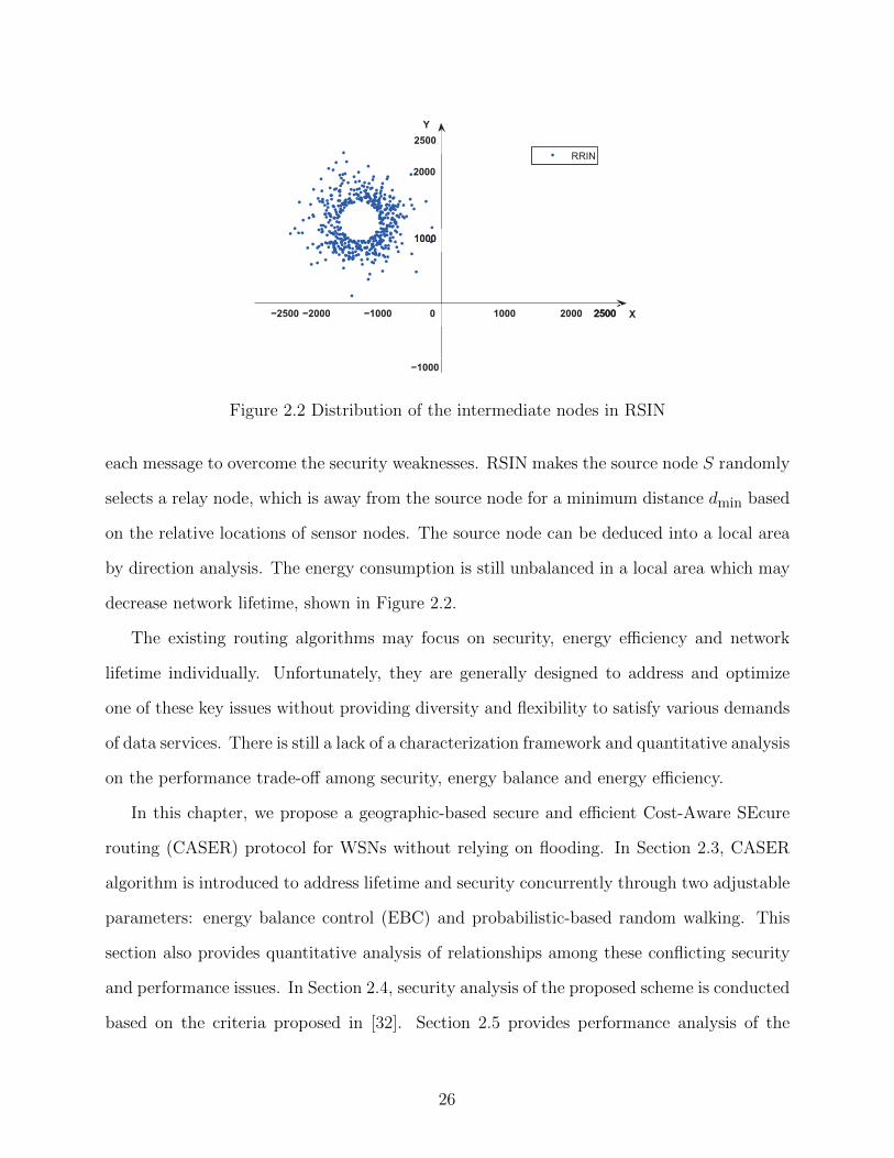
Figure 2.2 Distribution of the intermediate nodes in RSIN . . . . . . . . . . . . . . 26

Figure 2.3 Routing path and length estimation. . . . . . . . . . . . . . . . . . . . . 33

Figure 2.4 Routing source traceback analysis. . . . . . . . . . . . . . . . . . . . . . 42

Figure 2.5 Routing path distribution statistics for various energy balance controlα and security parameters β. In all simulations, the target area is1500×1500. The source node is located at (332, 259) and sink is locatedat (1250, 1250). . . . . . . . . . . . . . . . . . . . . . . . . . . . . . . . . 44

Figure 2.6 Routing path distribution statistics for energy balance control α = 0.5and security parameters β = 0.25 and RSIN in [1] with parameters:dmin = 100, ρ = 3. . . . . . . . . . . . . . . . . . . . . . . . . . . . . . . 49

Figure 2.7 Remaining energy distribution statistics after the source transmittedabout 600 messages. . . . . . . . . . . . . . . . . . . . . . . . . . . . . . 50

Figure 3.1 The remaining energy levels of the sensor nodes in the sensor domainwhen the innermost grid almost runs out of the energy, where α =0.5, β = 0.5. . . . . . . . . . . . . . . . . . . . . . . . . . . . . . . . . . . 53

Figure 3.2 Delivery ratio under different EBC α and security level β. . . . . . . . . 54

Figure 3.3 Message delivery ratio: β = 0 and varying α . . . . . . . . . . . . . . . . 58

Figure 3.4 Message delivery ratio: α = 0 and varying β . . . . . . . . . . . . . . . . 59

Figure 3.5 Message delivery ratio: dynamic changed β for various messages . . . . . 60

Figure 3.6 A snapshot of energy distribution when the remaining energy is about10% in the sensor nodes, where α = 0.5, β = 0.5. . . . . . . . . . . . . . . 61

Figure 4.1 The link layer congestion: (a) General distributed routing algorithmsthat may lead to congestion in subsequent forwarding; (b) Illustrationof the CAR routing algorithm . . . . . . . . . . . . . . . . . . . . . . . . 64

Figure 4.2 Dynamic tree formation . . . . . . . . . . . . . . . . . . . . . . . . . . . 67

xi

Figure 4.3 The end-to-end collision probability in multi hops. There are 20 con-tending nodes in the event area. . . . . . . . . . . . . . . . . . . . . . . . 73

Figure 4.4 The end-to-end transmission delay in multi hops. There are 20 contend-ing nodes in the event area. . . . . . . . . . . . . . . . . . . . . . . . . . 75

Figure 4.5 The number of retransmission through end-to-end transmission in multihops. There are 20 contending nodes in the event area. . . . . . . . . . . 76

Figure 4.6 Average end-to-end transmission delay with varying burst event locations 78

Figure 4.7 Average end-to-end transmission delay with varying event sensing ranges 80

Figure 4.8 Network throughput with varying event sensing ranges . . . . . . . . . . 81

xii

LIST OF ALGORITHMS

Algorithm 1 Node A finds the next hop routing grid based on the EBC α ∈ [0, 1] . . 30

Algorithm 2 Node A finds the next hop routing grid based on the given parameters

α, β ∈[0, 1] . . . . . . . . . . . . . . . . . . . . . . . . . . . . . . . 36

Algorithm 3 Solve equation 4f2x4−5x2+2x−1 = 0. . . . . . . . . . . . . . . . . . 39

Algorithm 4 Node A finds the next hop routing grid based on the given parameters

α, β ∈[0, 1]. . . . . . . . . . . . . . . . . . . . . . . . . . . . . . . 56

Algorithm 5 Node A derives the next hop routing node based on the MAC layer con-

gestion condition . . . . . . . . . . . . . . . . . . . . . . . . . . . . 68

Algorithm 6 Data Distribution . . . . . . . . . . . . . . . . . . . . . . . . . . . 90

Algorithm 7 Data Reconstruction and Verification . . . . . . . . . . . . . . . 91

xiii

KEY TO SYMBOLS AND ABBREVIATIONS

AP Wireless Access Point

ACK Acknowledgement

MAC Medium Access Control

CASER Cost-Aware Secure Routing

CSMA/CA Carrier Sense Multiple Access with Collision Avoidance

CAR Congestion-Aware Routing

DAPP Delay-Aware Privacy Preserving Transmission Scheme

DIFS Distributed Inter Frame Spacing

EBC Energy Balance Control

iid Independent and Identically Distributed

NSSI Normalized Source-location Space Index

QoS Quality of Service

RSIN Routing to a Single Intermediate Node

RTS/CTS Request-To-Send/Clear-To-Send Mechanism

SDI Source-location Disclosure Index

SIFS Short Inter Frame Spacing

SSI Source-Location Space Index

WSN Wireless Sensor Network

xiv

CHAPTER 1

INTRODUCTION

The recent technological advances make sensor networks technically and economically feasible

to be widely used in both military and civilian applications, such as monitoring of ambient

conditions related to the environment, precious species, critical infrastructures and traffic

conditions. Energy efficiency, network lifetime, communication delay and delivery ratio are

considered important metrics of performance measurement for wireless sensor networks, and

have been extensively studied in [2–14]. Security is another key issue of protocol design,

but yet less studied topic, partially due to the design trade-off between security and other

performance issues. To address these design issues concurrently, we employ a cost-aware

trade-off concept in designing routing algorithms for the traditional wireless sensor networks

and for the emerging people-centric urban sensing networks. The proposed schemes are

designed to provide flexible options for users to maximize the privacy protection based on

the given performance requirements.

1.1 Source Location Privacy in Wireless Sensor Network

Traditional wireless sensor networks (WSNs) consist of a large number of untethered and

unattended sensor nodes that are normally statically deployed for environment monitoring.

These sensor nodes have very limited computational processing ability and storage capacity.

They are powered by non-replenishable energy resources and equipped with a low-power

radio to send and receive messages, which make energy efficiency and lifetime two major

design metrics for WSNs protocol design.

In addition, WSNs rely on wireless communications, which is by nature a broadcast

medium. It is more vulnerable to security attacks than its wired counterpart due to lack of

a physical boundary. The low-power radio, limited processing ability and battery life make

1

security a very challenging issue. Computationally intensive cryptographic algorithms such

as public-key cryptosystem, and large scale broadcasting-based protocols, may not be feasible

for WSNs. Adversaries can even compromise some sensor nodes to obtain the cryptographic

keys and reprogram compromised sensor nodes. These threats leave WSNs vulnerable to

security attacks. Source location privacy is envisioned as one of the most essential security

issues for WSNs. The exposure of source location may divulge the information of a sensing

target, such as endangered species and critical military infrastructure. Adversaries equipped

with sensitive radio receivers can easily monitor the transmission direction of any detected

messages. They can further trace back to the source node hop by hop or deduce its location

through traffic analysis when a static routing strategy is applied.

1.1.1 Routing Algorithm Design

In WSNs, sensor readings are usually transmitted to base stations hop by hop for further

processing. Routing path is decided by a predesigned routing algorithm to ensure successful

delivery of the collected data. Routing is a very challenging design issue in WSNs due to

the inherent characteristics that distinguish WSNs from other wireless networks like ad-hoc

networks or cellular networks. The relative large number of sensor nodes makes it impossible

to build a global addressing table for each node. Due to the limited energy resources, routing

algorithm should be designed with consideration of energy efficiency. In addition, burst

events and static routing path may make the energy consumption unbalanced in a partial

area. Then sensor nodes in the area will exhaust their energy which may decrease the

network lifetime. Thus, a properly designed routing protocol should not only ensure high

message delivery ratio and guarantee low energy consumption for packet delivery, but should

also balance the energy consumption through entire sensor network, and thereby extend the

sensor network lifetime.

In existing research, many routing protocols have been proposed to address the issues of

energy efficiency, lifetime and latency. In these works, geographic routing has been widely

2

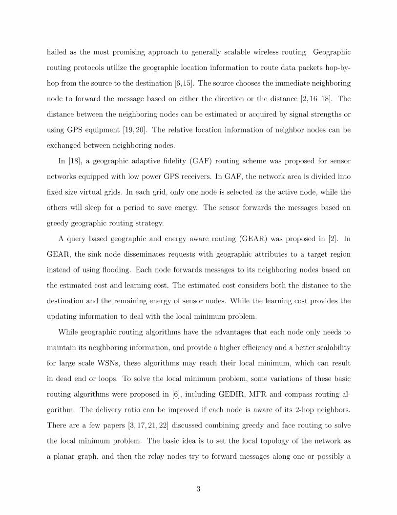
hailed as the most promising approach to generally scalable wireless routing. Geographic

routing protocols utilize the geographic location information to route data packets hop-by-

hop from the source to the destination [6,15]. The source chooses the immediate neighboring

node to forward the message based on either the direction or the distance [2, 16–18]. The

distance between the neighboring nodes can be estimated or acquired by signal strengths or

using GPS equipment [19, 20]. The relative location information of neighbor nodes can be

exchanged between neighboring nodes.

In [18], a geographic adaptive fidelity (GAF) routing scheme was proposed for sensor

networks equipped with low power GPS receivers. In GAF, the network area is divided into

fixed size virtual grids. In each grid, only one node is selected as the active node, while the

others will sleep for a period to save energy. The sensor forwards the messages based on

greedy geographic routing strategy.

A query based geographic and energy aware routing (GEAR) was proposed in [2]. In

GEAR, the sink node disseminates requests with geographic attributes to a target region

instead of using flooding. Each node forwards messages to its neighboring nodes based on

the estimated cost and learning cost. The estimated cost considers both the distance to the

destination and the remaining energy of sensor nodes. While the learning cost provides the

updating information to deal with the local minimum problem.

While geographic routing algorithms have the advantages that each node only needs to

maintain its neighboring information, and provide a higher efficiency and a better scalability

for large scale WSNs, these algorithms may reach their local minimum, which can result

in dead end or loops. To solve the local minimum problem, some variations of these basic

routing algorithms were proposed in [6], including GEDIR, MFR and compass routing al-

gorithm. The delivery ratio can be improved if each node is aware of its 2-hop neighbors.

There are a few papers [3, 17, 21, 22] discussed combining greedy and face routing to solve

the local minimum problem. The basic idea is to set the local topology of the network as

a planar graph, and then the relay nodes try to forward messages along one or possibly a

3

sequence of adjacent faces toward the destination.

Lifetime is another area that has been extensively studied in WSNs. In [23], a routing

scheme was proposed to find the sub-optimal path that can extend the lifetime of the WSNs

instead of always selecting the lowest energy path. In the proposed scheme, multiple routing

paths are set ahead by a reactive protocol such as AODV or directed diffusion. Then,

the routing scheme will choose a path based on a probabilistic method according to the

remaining energy. In [8], the authors assumed that the transmitter power level can be

adjusted according to the distance between the transmitter and the receiver. Routing is

formulated as a linear programming problem of neighboring node selection to maximize the

network lifetime. Then [24] investigated the unbalanced energy consumption for uniformly

deployed data-gathering sensor networks. In this paper, the network is divided into multiple

corona zones and each node can perform data aggregation. A localized zone-based routing

scheme was proposed to balance energy consumption among nodes within each corona. The

authors in [9] formulated the integrated design of route selection, traffic load allocation, and

sleep schedule to maximize the network lifetime. Based on the concept of opportunistic

routing, [7] developed a routing metric to address both link reliability and node residual

energy. The sensor node computes the optimal metric value in a localized area to achieve

both reliability and lifetime maximization.

Although there have been many research papers deals with the lifetime of wireless sensor

networks, only a few of them are related to energy aware geographic routing [2,4,15,25]. How

to protect source location privacy remains a problem for geographic routing protocols. When

the routing path remains unchanged for a period of time under static routing strategies, such

as geographic based routing, exposure of routing information presents significant security

threats to sensor networks. By acquisition of the location and routing information, the

adversaries may be able to trace back to the source node easily.

4

1.1.2 Existing Solutions for Source Location Privacy in Wireless Sensor Net-works

The nature of broadcast medium and limited resource makes WSNs more vulnerable to

security attacks than its wired counterpart. Location privacy is one of most important

security issues. Due to lack of a physical boundary and protection, it is possible for the

adversaries to identify the message source or even identify the source location, even if strong

data encryption is utilized. In particular, in the wireless sensor domain, anybody with an

appropriate wireless receiver can monitor and intercept the sensor network communications.

The adversaries may use expensive radio transceivers, powerful workstations and interact

with the network from a distance since they are not restricted to using sensor network

hardware. It is possible for the adversaries to perform jamming attacks and routing traceback

attacks. To solve this problem, several schemes have been proposed to provide source location

privacy through secure routing protocol design [1, 26–28].

The authors of [29] proposed to achieve source location privacy through trust mechanisms

built in WSNs and neighboring nodes categorization. However, it requires a long delay to

build the trust reputation infrastructure. Two schemes based on pseudonyms and crypto-

graphic methods were proposed in [30]. These schemes demand huge memory storage and

computational resources, which are not practical due to characteristics of WSNs and the

serious open security concerns under traceback attacks.

In [31], source location privacy is provided through broadcasting that mixes valid mes-

sages with dummy messages. The main idea is that each node needs to transmit messages

consistently. Whenever there is no valid message to transmit, the node transmits dummy

messages. The transmission of dummy messages not only consumes significant amount of

sensor energy, but also increases the network collisions and decreases the packet delivery ra-

tio. Therefore, these schemes are not quite suitable for large scale wireless sensor networks.

Dynamic routing strategies based protocols are proposed to make it infeasible for adver-

saries to locate source nodes through traffic monitoring and analysis. In this way, source

5

Nodes After R.W.

−3000

−3000

3000

1000−1000 2000−2000

−1000

−2000

1000

2000

0 X

Y

3000

Figure 1.1 Nodes distribution through random routing

location privacy can be achieved. Existing works generally employ the idea that route mes-

sages to a node/nodes away from the message source based on random walking or direct

walking. Directly application of random walking may introduce significant energy consump-

tion without achieving good security requirement. Both theoretical and practical results

demonstrate that if the message is routed randomly for h hops, then the messages will be

largely distributed within h/5 hops away from the source node. As shown in Figure 1.1, the

source node is located at (0, 0) and h = 50. The transmission range is 250 meters at most

for one hop. The statistic results show that the average hop distance between the source

and the randomly selected nodes is only 4.2 hops. To solve this, the authors employ direct

walking in phantom routing protocol [26]. Phantom routing involves two phases: a random

walking phase and a subsequent flooding/single path routing phase. Each message is routed

from the actual source to a phantom source along a designed directed walking through either

sector-based approach or hop-based approach. The direction/sector information is stored in

the header of the message. Then every forwarder on the random walking path forwards this

message to a random neighbor based on the direction/sector determined by the source node.

In this way, the phantom source can be away from the actual source. Unfortunately, once

6

the message is captured on the random walking path, the adversaries are able to get the

direction/sector information stored in the header of the message. Therefore, exposure of the

direction decreases the complexity for adversaries to trace back to the actual message source

in the magnitude of 2h. However, none of these schemes have considered energy balance and

provided quantitative source location information leakage and security analysis.

In [1,28], we developed a two-phase routing algorithm to provide both content confiden-

tiality and source location privacy. The message source randomly selects an intermediate

node in the sensor domain, then the intermediate node transmits the message to a network

mixing ring which mix the messages from different directions among the ring. The message

will be forwarded from the node in the ring domain based on probabilistic way. Then, in [32],

we firstly developed criteria to quantitatively measure source location information leakage

and security of routing-based schemes through source location disclosure index (SDI) and

source location space index (SSI).

These schemes are generally designed to protect source location privacy without providing

diversity and flexibility in protocol design. In fact, routing based schemes can preserve

source node location privacy at the cost of additional energy consumption. The dynamic

routing path selection may introduce unbalanced energy consumption in partial network,

which may decrease the network lifetime significantly. Therefore, a proper designed secure

routing algorithm should not only preserve source location privacy, but also consider energy

efficiency and network lifetime.

1.1.3 Summary of Major Limitations

To the best of our knowledge, none of these schemes have considered privacy from a cost-

aware perspective.

• The public-key encryption based algorithms are not suitable for WSNs due to the

computation complexity.

7

• Broadcasting and dummy messages based schemes introduce significant amount energy

consumption and collisions.

• Existing routing based algorithms may leak the direction information by capturing

messages.

• Security is the only metric to measure performance of existing works.

• None of existing works address the quantitative relationship between the energy effi-

ciency and security.

• Existing works fail to balance the energy consumption and extend lifetime of the net-

work.

1.2 Congestion in Wireless Sensor Networks

Wireless sensor networks are designed to collect information and transmit sensed data to one

or more sink nodes. The information of the sensed data is critical for real-time processing

and decision-making in both military and civilian applications, such as monitoring the forest

fire and target locating. For these applications, end-to-end communication delay is one of

the most significant design issues for wireless sensor networks.

In WSNs, congestion not only increases the packet end-to-end communication delay,

but also decreases the packet delivery ratio, network throughput and energy efficiency. In

traditional networks, the existing works on congestion mainly focus on traffic control in both

end-to-end and hop-by-hop communications. These algorithms are mainly applied to the

transport layer or the Medium Access Control (MAC) layer. They are designed to avoid

congestion by limiting the transmission rate or reducing traffic in the network. However,

the aforementioned strategies are unsuitable for event-driven WSNs for the following two

reasons. First, reducing the source traffic may affect the validity of decision-making. For

example, forest rangers cannot locate the real fire source since the traffic of real source node is

8

limited. Second, the traffic control strategies have a negative impact on real-time processing.

As an example, ecological observers cannot obtain the accurate number of pandas since the

traffic control algorithm postpones the transmission of critical sensor nodes to reduce the

congestion in the MAC layer. The delayed information from the partial region may affect the

correctness of real-time processing. How to reduce end-to-end communication delay remains

one of the most important design issues for congestion control algorithms.

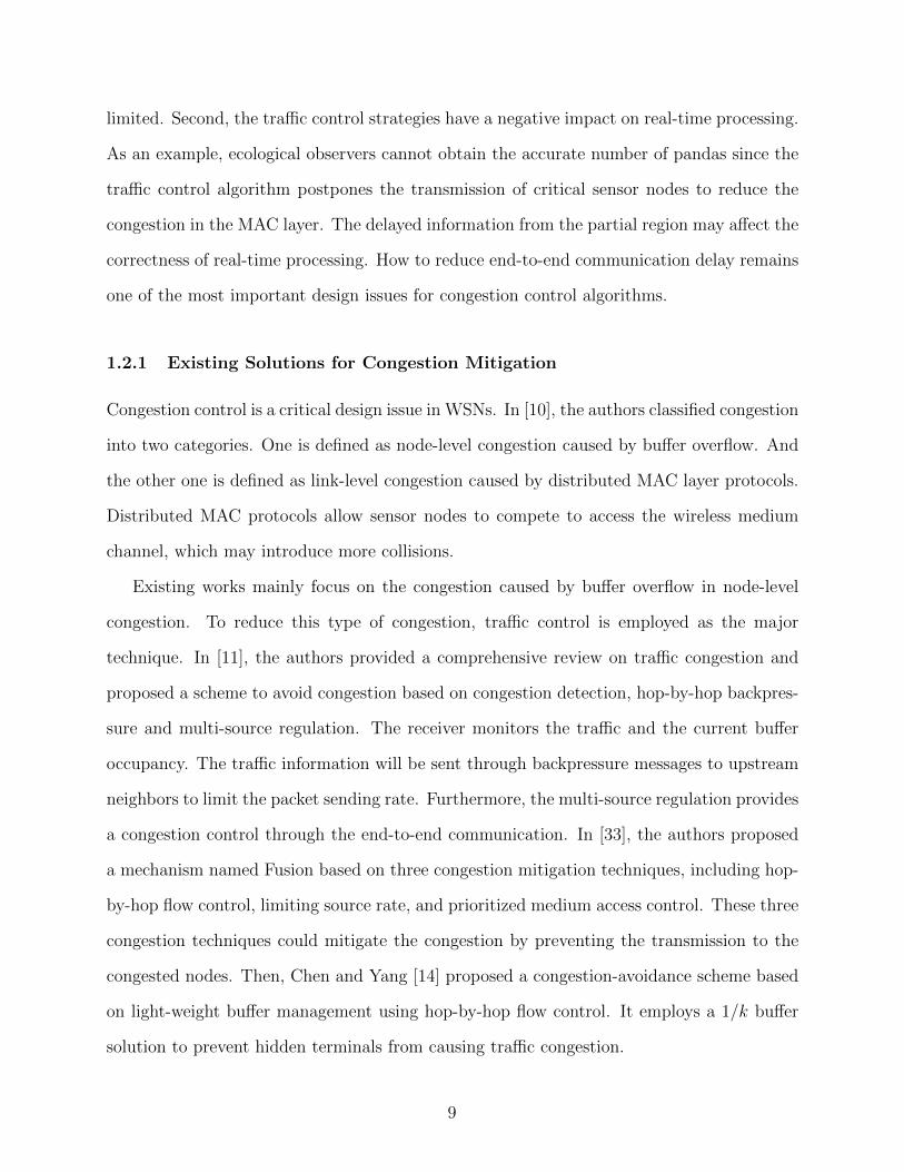
1.2.1 Existing Solutions for Congestion Mitigation

Congestion control is a critical design issue in WSNs. In [10], the authors classified congestion

into two categories. One is defined as node-level congestion caused by buffer overflow. And

the other one is defined as link-level congestion caused by distributed MAC layer protocols.

Distributed MAC protocols allow sensor nodes to compete to access the wireless medium

channel, which may introduce more collisions.

Existing works mainly focus on the congestion caused by buffer overflow in node-level

congestion. To reduce this type of congestion, traffic control is employed as the major

technique. In [11], the authors provided a comprehensive review on traffic congestion and

proposed a scheme to avoid congestion based on congestion detection, hop-by-hop backpres-

sure and multi-source regulation. The receiver monitors the traffic and the current buffer

occupancy. The traffic information will be sent through backpressure messages to upstream

neighbors to limit the packet sending rate. Furthermore, the multi-source regulation provides

a congestion control through the end-to-end communication. In [33], the authors proposed

a mechanism named Fusion based on three congestion mitigation techniques, including hop-

by-hop flow control, limiting source rate, and prioritized medium access control. These three

congestion techniques could mitigate the congestion by preventing the transmission to the

congested nodes. Then, Chen and Yang [14] proposed a congestion-avoidance scheme based

on light-weight buffer management using hop-by-hop flow control. It employs a 1/k buffer

solution to prevent hidden terminals from causing traffic congestion.

9

Several MAC layer protocols [12, 13, 34] have been proposed to reduce the link-level

congestion. In [13], the authors proposed a modified carrier sense multiple access protocol

(CSMA) to improve the network performance. The protocol aims to reduce the cost of

channel state checking, and adds a machine learning approach to predict the probability

of a successful reception. In [34], the authors proposed a power back-off scheme to resolve

collisions by limiting the transmission power. And the authors in [12] proposed an enhanced

p-persistent CSMA. They proposed a method to calculate a proper p for CSMA based on the

topology information of partial network. However, these proposed algorithms mainly focus

on modifying the existing CSMA protocols in which the requirements and assumptions are

not practical in WSNs.

Besides traffic control strategies, routing based congestion-avoidance protocols are also

effective methods to reduce the congestion in networks. The main idea of existing works

is to reroute packets to bypass congestion areas. The idea is employed in [35] to reduce

the congestion by throttling or rerouting the traffic. The authors in [36] introduced some

virtual sinks with a longer range multi-radio in WSNs. The authors assumed sensors can

communicate with a long range communication radio to bypass potential congestion areas.

[10] proposed a congestion control scheme by calculating the mean of the packet generation

rate. LACAR routing scheme in [37] was designed to probabilistically avoid congestion by

choosing lightly loaded nodes according to relative location information. In [38], a traffic-

aware dynamic routing algorithm was proposed to route the packets around the congestion

area and scatter packets to light loaded relay nodes to alleviate buffer flow. These routing

algorithms need either topology information or a long range communication radio, which is

not practical in WSNs.


• Traffic control based schemes are designed to limit transmission rate or reduce traffic

at source node, which may affect the validity of data processing results.

10

• Routing based schemes need either topology information or a long range communica-

tion radio which is not practical for WSNs.

• The messages are delivered to a centralized sink node. Lack of optional relay nodes in

a region close to sink node may aggravate congestion.

• MAC layer based schemes require limiting the transmission power or acquisition of

topology information in partial network which is not practical for WSNs.

1.3 Urban Sensing Networks

Traditional sensor networks rely on a large number of sensor nodes normally deployed stat-

ically in a target area. The recent advances in embedded system design for mobile devices

make the human-carried devices feasible for environment monitoring. People-centric urban

sensing has been envisioned as a novel urban sensing paradigm. It relies on sensors embedded

in human-carried mobile devices or vehicular electrical devices to collect and report sensing

data. Sensor nodes embedded in these mobile systems can take advantages of powerful com-

putational resources and rechargeable battery power. The new paradigm of sensor networks

also makes people not only data consumers but also data contributors. The ubiquitous elec-

trical devices carried by human and vehicles are gradually replacing the traditional static

sensor networks for many urban area applications.

1.3.1 People-Centric Urban Sensing Networks

People-centric urban sensing network, also known as participatory sensing network, dif-

fers significantly from traditional wireless sensor network. First, participatory sensor nodes

are embedded in rechargeable mobile devices, such as smart phone, iPad, laptop and auto

computer. The powerful resources equipped in these devices enhance their capabilities in

computation, sensing, data storage, reliable data communication, and energy lifetime dra-

matically. Hence, the energy efficiency is no longer as critical as in traditional wireless sensor

11

networks. Second, in urban sensing networks, sensing data collection and reporting no longer

rely on fixed infrastructure. The data can be forwarded by mobile nodes to the sink either di-

rectly or indirectly in multiple hops. Due to mobility, network topology structure constantly

changes, which make end-to-end communication delay, message delivery ratio and quality of

service (QoS) some of the most essential performance evaluation metrics in urban sensing

networks. Third, these devices are owned and operated by individuals. Instead of being only

data consumers, these devices could also collect sensing data. It makes data collection more

directly related to people’s lives and hence privacy becomes one of the major concerns of

participating users. In fact, the data collecting and reporting services put users’ privacy in

jeopardizing since both the delivery nodes and the wireless access points are able to identify

the data owner through direct communications. The uploaded sensor reading is required to

be collected with spatial-temporal information to provide accurate and high quality service

for data users. The spatial-temporal information related to collectors can be used to recover

the trajectory of them, which can seriously jeopardize participating collectors’ privacy. Side

information attack has been studied in recent research. Adversaries may obtain this kind of

information from side channels, such like video cameras, social networks and published in-

formation. It can divulge source identities in spite of usage of existing pseudonym schemes.

As a result, private location information combining with side information can be used to

recover the trajectory of participating users.

1.3.2 Existing Solutions for Location Privacy in Urban Sensing Networks

The participatory sensing concept was firstly proposed in [39]. The concept then is extended

to urban sensing and people-centric sensing. The key idea is that the network relies on

the people-carried mobile devices to collect the sensing data in urban environments. It

enables the public and professional users to collect and share the sensed data. The authors

in [40] proposed an architecture named MetroSense for urban-scale people-centric sensing

for the first time. The paper provided detailed design principles and a network model for

12

people-centric urban sensing networks. The network is composed of traditional static sensors,

mobile sensors embedded in the mobile devices, gateways and a server. The sensor nodes

deliver collected data to the server through the gateways which is considered as physical

infrastructure in the network. The paper also mentioned the trajectory privacy problem.

However, the proposed solution is based on an insufficient adversarial model.

The first implementation for privacy protection was proposed in [41]. In this paper, the

location is blurred based on tessellation and clustering against adversaries. The reported

data are eventually aggregated to improve the privacy. This idea of data aggregation is

also applied in [42, 43]. In [43], the proposed PriSense is designed based on the concept

of data slicing and mixing. It can support a wide range of statistical additive and non-

additive aggregation functions with accurate aggregation. The sensing data are divided and

distributed to cover nodes to hide the identity information of source nodes. The data are

eventually aggregated by the cover nodes and delivered to the server. However, aggregation

may also hide the accurate sensing information contained in each individual sensing data

and sacrifice the precision of service quality.

Another optional solution based on mix-zones and pseudonyms were proposed in [44–

47]. In these algorithms, mix-zones are first constructed and placed in some regions of the

network. Then, the pseudonyms are assigned to users as the communication identities when

they enter into the mix-zones. This method is designed to achieve k-anonymity to prevent

discovering user’s real identity. In [47], the authors divided the sensing area into sensitive

areas and non sensitive areas. Different pseudonyms are assigned to a user when he enters

into and departures from the mix zone. However, the mix zone relies on a trusted third

party, which may not be always true. And they cannot be placed through the entire network

to protect trajectory privacy.

Spatial cloaking [48] was proposed to enable data collectors to adjust the resolution of

location information along spatial or temporal dimensions to avoid exposure of user’s exact

location. This methodology was further studied in [49–51]. These works mainly focus on

13

the selection of anonymous locations and trade-off between quality service and anonymity.

However, the privacy protection is achieved by sacrificing the resolution of either spatial or

temporal dimensions.

Dummy location was studied in [52–54]. The fundamental idea is to report dummy loca-

tions to conceal the actual location of the reported data. Suppression based techniques [55]

was also proposed to blur the reported locations by converting the database of trajecto-

ries. [56] proposed to construct a cluster in a nearby neighborhood and then transform each

cluster into a anonymity set. In these methods, the privacy can be protected by obscuring

the exact locations, which may induce information loss for data service.

Encryption based algorithms and data exchange schemes were proposed in [57–59]. In [57],

the sensed data are encrypted and disseminated to replica sensors. The replica sensors then

store the received data and relay them upon receiving inquiries. As a consequence, the source

node identity can be concealed by the replica sensors. Nevertheless, the shared key may ei-

ther help the operator to identify the source node or enable the malicious replica nodes to

decrypt the data contents. In [58], the collected sensor readings are exchanged between par-

ticipants within wireless communication range. The data can be exchanged multiple times

to prevent adversaries from correlating the data and its identity. [60] proposed to forward

the collected data from friends to friends of the source user until the required number of

hops has been reached. In these schemes, source node may be directly identified by interme-

diate nodes through wireless communications. Additionally, malicious intermediate nodes

can also reveal and tamper with data contents through the forwarding procedure. There is

little flexibility in delivery ratio when the data are being dropped or tampered with.


• Location privacy may be achieved by yielding the accuracy of collected data.

• Privacy protection service may not be provided over the entire network.

14

• Encryption based methods may leak the identity information of the participating user

by exchanging shared keys.

• The collected data may be tampered with and dropped by the malicious intermediate

nodes.

• The assumption that there exists a trusted third party is not sufficient for adversarial

model.

• Malicious delivery nodes may collude to derive the privacy information.

• The information loss by collecting side information is not quantitatively analyzed.

1.4 Proposed Research Direction

Due to inherent characteristics, WSNs protocol design has to consider several essential design

issues concurrently, which may be conflicting with each other. In this dissertation, we analyze

the relationship among these conflicting design issues and develop algorithms to preserve

location privacy from a cost-aware perspective under various trade-off constraints. They

can provide diverse options that can be analogous to delivering of US Mail through USPS:

express mail is more expensive than regular mail; however, mails can be delivered with less

time needed. The proposed schemes also provide a secure message delivery option under the

cost-aware design-off framework.

1.4.1 Source Location Privacy Protection in Wireless Sensor Networks

In this dissertation, we propose a secure and efficient Cost-Aware SEcure Routing (CASER)

protocol that can address network lifetime and routing security concurrently in WSNs.

In CASER protocol, each sensor node needs to maintain the energy levels of its immediate

adjacent neighboring grids in addition to their relative locations. Using this information, each

sensor node can create varying filters based on the expected design trade-off between security

15

and network lifetime. Each sensor node also needs to maintain the location information of

neighbor nodes. CASER allows messages to be transmitted using two routing strategies,

random walking and deterministic routing. The two routing strategies are applied based on

the lifetime filter. The distribution of these two strategies is determined by specified security

requirements.

We then discover that the energy consumption is severely disproportional to the uniform

energy deployment for the given network topology, which greatly reduces the lifetime of

the sensor networks. To solve this problem, we propose an efficient non-uniform energy

deployment strategy to optimize the lifetime and message delivery ratio under the same

energy resource and security requirement. CASER is also updated to adapt the non-uniform

energy deployment.

In addition, we also give quantitative secure analysis on the proposed routing protocol

based on the criteria proposed in [32]. The simulations are also provided to show that

CASER can provide excellent energy balance and routing security.

CASER protocol has two major advantages: (i) It ensures balanced energy consumption

of the entire sensor network so that the lifetime of the WSNs can be maximized. (ii) CASER

protocol supports multiple routing strategies based on the routing requirements, including

fast/slow message delivery and secure message delivery to prevent routing traceback attacks

and malicious traffic jamming attacks in WSNs.

1.4.2 Congestion-Aware Routing (CAR) Algorithm in Wireless Sensor Net-works

In this dissertation, we propose a congestion-aware routing scheme to reduce the potential

congestion in the subsequent packet forwarding by monitoring the traffic in the MAC layer.

In CAR, each sensor node selects the relay node based on two different routing strategies:

the shortest path forwarding and the congestion-aware forwarding. In the shortest path

forwarding, the relay node selection follows the geographic routing strategy [61] based on

16

the geographic location. In the congestion-aware forwarding algorithm, each sensor node

selects the relay node based on the channel competing results. When traffic congestion is not

detected, the shortest path routing algorithm will be used and congestion-aware transmission

algorithm is used otherwise. The shortest path routing algorithm ensures an efficient end-to-

end message transmission from the source node to the sink node. CAR can effectively reduce

end-to-end message communication delay and improve the system throughput by reducing

traffic congestion.

1.4.3 Location Privacy Protection in Urban Sensing Networks

We propose a novel delay-aware privacy-preserving (DAPP) data reporting scheme to pre-

serve the trajectory privacy of participating users based on a combination of Shamir’s secret

sharing and two-phase routing. In this dissertation, we begin with analyzing the design

trade-off among communication delay, delivery ratio and security. We then propose a scheme

that can provide flexible message delivery options to meet various security and performance

requirements, such as communication delay and delivery ratio.

In DAPP, the data reporting includes two independent forwarding phases. In the first

phase, participating user first generates a unique pseudonym for each sensor reading. Then,

the sensor reading is decomposed into n pieces based on Sharmir’s secret sharing and these

data pieces are forwarded to randomly selected delivery nodes. In the second phase, the

selected delivery node relays its received data piece to the application data server through

a nearby wireless access point. Upon receiving k or more data pieces, the application data

server is able to reconstruct the original collected data. To ensure integrity of the recovered

data, both the original data and its hash value will be transmitted together.

Secret sharing can ensure confidentiality and integrity of the reported data. We propose

a dynamic pseudonym scheme to guarantee anonymity of the source node. DAPP can

also provide redundancy for error tolerance under additional computational overhead, which

ensures a high message delivery ratio for data transmission. This design makes both security

17

and communication delay adjustable based on selection of the (n, k) scheme.

1.5 Overview of the Dissertation

1.5.1 Design Goals

Our design goal for the secure routing algorithm in traditional wireless sensor networks can

be summarized as follows:

• To maximize the sensor network lifetime, we ensure that the energy consumption of

all sensor grids is balanced.

• To achieve a high message delivery ratio, our routing protocol should try to avoid

message dropping when an alternative routing path exists.

• The adversaries should not be able to get the source location information by analyzing

the traffic pattern.

• The adversary should not be able to get the source location information if he is only

able to monitor a certain area of the WSN and compromise a few sensor nodes.

• Only the sink node is able to identify the source location through the message received.

The recovery of the source location from the received message should be very efficient.

• The routing protocol should maximize the probability that the message is being deliv-

ered to the sink node when adversaries are only able to jam a few sensor nodes.

For the congestion-aware routing algorithm, our design goals are described as follows:

• The end-to-end communication delay caused by congestion should be effectively alle-

viated.

• The proposed scheme should rely on the existing MAC layer protocols without requiring

extra physical equipment and further modification.

18

• The energy efficiency should be addressed in the proposed scheme.

• The proposed scheme should be able to mitigate congestion caused by the traffic routed

to the centralized sink node.

We also want to achieve the following goals for the transmission scheme in urban sensing

networks:

• Adversaries should not be able to obtain real identities of participating users without

side information.

• The malicious delivery node should not be able to discover spatial-temporal information

of the reported data.

• Adversaries should not be able to recover data trajectory by collecting side information.

• The proposed scheme should provide data integrity verification for the recovered data.

• The proposed scheme should be able to provide a high delivery ratio in case some data

pieces are dropped or tampered with by malicious delivery nodes.

• The proposed scheme should provide flexibility and diversity in protocol design.

1.5.2 Major Contributions

Our contributions on routing algorithm design in WSNs can be summarized as follows:

1. We propose a secure and efficient Cost-Aware SEcure Routing (CASER) protocol for

WSNs. In this protocol, cost-aware based routing strategies can be applied to address

the message delivery requirements.

2. We devise a quantitative scheme to balance the energy consumption so that both the

sensor network lifetime and the total number of messages that can be delivered are

maximized under the same energy deployment.

19

3. We develop theoretical formulas to estimate the number of routing hops in CASER

under varying routing energy balance control and security requirements.

4. We quantitatively analyze the security of the proposed routing algorithm.

5. We provide an optimal non-uniform energy deployment strategy for the given sensor

network based on the energy consumption ratio. Our theoretical and simulation results

both show that under the same total energy deployment, we can increase the lifetime

and the number of messages that can be delivered by more than four times in the

non-uniform energy deployment scenario.

Our contributions on congestion-aware routing algorithm can be described as follows:

1. We propose a congestion aware routing algorithm to address communication delay and

energy efficiency.

2. We analyze the congestion in one-hop network and extend it to a scenario of multi-hop

network. We give the bounds for the communication delay under congestion scenarios.

3. We evaluate the performance of the proposed CAR routing algorithm on communica-

tion delay.

4. The simulation results demonstrate the proposed CAR can reduce the communication

delay very close to the ideal case.

Our contributions on forwarding scheme design in people-centric urban sensing networks

can be summarized as follows:

1. We propose a delay-aware privacy preserving (DAPP) data forwarding scheme to pro-

tect trajectory privacy of participating users in urban sensing networks.

2. We devise a secret sharing based secure message delivery option that can provide data

integrity verification of the recovered data and maximize the message delivery ratio by

introducing redundancy in reported data.

20

3. We present a dynamic pseudonym scheme to defend against side information attacks.

4. The proposed scheme is able to achieve a trade-off among security, communication

delay and delivery ratio through adjustable parameters.

5. We quantitatively analyze performance of the proposed scheme on security, communi-

cation delay and delivery ratio.

1.5.3 Thesis Organization

The dissertation is structured as follows.

Chapter 2 proposes CASER protocol for source location protection.

Section 2.1 serves as an introduction for this chapter. In Section 2.2, we present the

network model and adversarial assumptions. We propose CASER algorithm based on energy

balance routing strategy and security routing strategy in Section 2.3. In this section, we also

derive formulas to decide the energy consumption of balancing routing strategy and security

routing strategy.

In Section 2.4, we introduce a security evaluation model and present a quantitative secu-

rity analysis to demonstrate CASER can preserve the source location privacy. In addition,

the security analysis also shows that CASER can effectively defend against jamming at-

tacks and detect compromised nodes. Finally, in Section 2.5, we present the performance

evaluations and simulation results.

Chapter 3 proposes the non-uniform energy deployment through the entire network.

In Section 3.1, we investigate the energy consumption under uniform energy deployment.

Both theoretical analysis and simulation results demonstrate that the energy consumption

is severely disproportional through the entire network. The energy consumption is balanced

in a localized area. To solve this problem, in Section 3.2, we propose a non-uniform energy

deployment to extend the lifetime of the entire network, while updating the proposed CASER

to adapt the non-uniform energy deployment. The simulation results in this section show

21

the non-uniform energy deployment can significantly extend the lifetime through the entire

network under various security requirements. The overall energy consumption of networks

is well balanced, and thereby significantly extends the network lifetime.

Chapter 4 presents a congestion-aware routing algorithm to reduce the communication

delay under congestion scenarios.

Section 4.1 gives an introduction of this chapter. The system model and assumptions are

presented in Section 4.2. In Section 4.3, we describe CAR routing algorithm in detail. We

conduct the analysis for the performance of communication delay in Section 4.4. We derive

a formula to decide the communication delay in the ideal case and the worst case for the pro-

posed CAR routing algorithm. The evaluation and simulations are provided in Section 4.5,

which demonstrate CAR routing algorithm can effectively reduce the communication delay.

We conclude in Section 4.6.

Chapter 5 introduces a novel delay-aware and privacy preserving data forwarding scheme.

Section 5.1 gives an introduction to the whole chapter. Section 5.2 presents system

models and adversarial assumptions. In Section 5.3, we provide details of DAPP scheme.

In this section, a dynamic pseudonym scheme and a Shamir’s secret sharing based scheme

are proposed to ensure the data integrity and anonymity of the source node. The security

analysis is presented in Section 5.4. It quantitatively demonstrates DAPP can protect the

trajectory privacy of participating users. It also shows DAPP can effectively defend against

collusion attack and guarantee data integrity. Performance evaluation and simulation results

are provided in Section 5.5. We conclude this chapter in Section 5.6.

Chapter 6 summarizes the contributions and concludes the dissertation. An outline of

related future work is also provided.

22

CHAPTER 2

COST-AWARE SECURE ROUTING: DESIGN AND ANALYSIS

In this chapter, we propose a cost-aware secure routing protocol to achieve a trade-off be-

tween security and network lifetime through two adjustable parameters: energy balance

control (EBC) and security level. CASER can create various filters based on EBC parame-

ter to balance energy consumption and thereby increase the network lifetime. Security level

can determine the probabilistic distribution of random walking to make the routing path

dynamic and unpredictable, which can prevent adversaries from estimating direction of the

messages and defend against jamming attacks. CASER combines random walking and ge-

ographic based deterministic routing strategy to ensure secure and efficient delivery of the

collected data to the sink node. In this chapter, we develop theoretical formulas to measure

routing efficiency through estimating the number of routing hops under varying routing en-

ergy balance control parameters and security requirements. Quantitatively security analysis

and simulation results are provided to demonstrate the security properties and performance.

2.1 Introduction

In WSNs, sensor nodes are equipped with low power radios to send and receive messages

through wireless medium, which makes data uploading rely on hop by hop transmission.

Routing protocols are designed to ensure successful delivery of the collected data. Due

to the inherent characteristics of WSNs, a properly designed routing algorithm should not

only ensure a high message delivery ratio, but also guarantee low energy consumption and

maximize the network lifetime. Existing routing algorithms, such as geographic routing

algorithms, can determine a shortest routing path to increase the energy efficiency. However,

the static routing strategy may drain the energy of sensor nodes along the shortest routing

path quickly. A few of existing works have focused on providing alternative routing paths to

23

balance the energy consumption and at the same time extend the network lifetime. However,

there is still a lack of robust quantitative measurement on the trade-off between energy

consumption and energy balance.

Source location privacy is an important security issue. Location of source may expose

significant amount of information about the objects being monitored by sensor nodes. While

confidentiality of the message can be ensured through content encryption, it is much more

difficult to adequately address the source-location privacy. Privacy service in WSN is further

complicated since the sensor nodes are designed to operate unattended for long periods of

time and only consist of low-cost and low-power radio devices. Battery recharging or re-

placement may be infeasible or impossible. Hence, computationally intensive cryptographic

algorithms, such as public-key cryptosystems and large scale broadcasting-based protocols,

are not suitable for WSNs. This makes privacy preserving transmission in WSNs an ex-

tremely challenging research task.

There are three major techniques for adversaries to obtain source location information

in WSNs, which are correlation-based source identification attack, routing based traceback

attack, reducing source space attack.

Correlation-based source identification has been well studied in [28] by using a dynamic ID

assignment scheme. Both routing traceback attack and reducing source attack are carried

out through traffic pattern analysis. In existing works, there are mainly two approaches

that can protect the source-location privacy from traffic analysis attacks in WSNs, which

are broadcast-based and routing-based. For the broadcasting schemes [31, 62–65], source-

location privacy is provided through broadcasting or injection of dummy packets. In these

schemes, each node broadcasts message consistently or at a predefined probabilistic model

so that the adversary cannot distinguish the meaningful messages from dummy messages.

However, these schemes may decrease network lifetime significantly. In fact, it has been

demonstrated in [66] that the power consumption for transmission of one bit is about as

much as executing 800-1000 instructions.

24

2I

1I

3I

4I

5I6I

1S

2S

D1M

2M

3M

6M

5M

4M

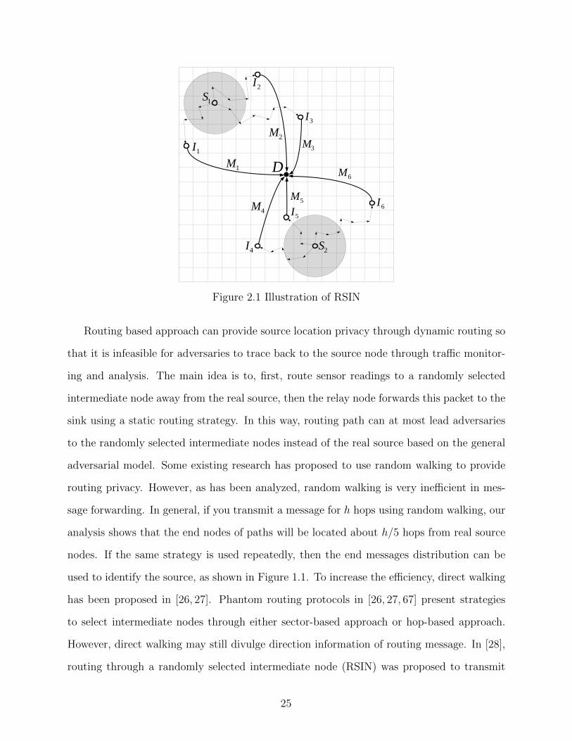
Figure 2.1 Illustration of RSIN

Routing based approach can provide source location privacy through dynamic routing so

that it is infeasible for adversaries to trace back to the source node through traffic monitor-

ing and analysis. The main idea is to, first, route sensor readings to a randomly selected

intermediate node away from the real source, then the relay node forwards this packet to the

sink using a static routing strategy. In this way, routing path can at most lead adversaries

to the randomly selected intermediate nodes instead of the real source based on the general

adversarial model. Some existing research has proposed to use random walking to provide

routing privacy. However, as has been analyzed, random walking is very inefficient in mes-

sage forwarding. In general, if you transmit a message for h hops using random walking, our

analysis shows that the end nodes of paths will be located about h/5 hops from real source

nodes. If the same strategy is used repeatedly, then the end messages distribution can be

used to identify the source, as shown in Figure 1.1. To increase the efficiency, direct walking

has been proposed in [26, 27]. Phantom routing protocols in [26, 27, 67] present strategies

to select intermediate nodes through either sector-based approach or hop-based approach.

However, direct walking may still divulge direction information of routing message. In [28],

routing through a randomly selected intermediate node (RSIN) was proposed to transmit

25

RRIN

25001000 2000�1000�2000�2500 25002500

1000

�1000

1000

2500

2000

0 X

Y

Figure 2.2 Distribution of the intermediate nodes in RSIN

each message to overcome the security weaknesses. RSIN makes the source node S randomly

selects a relay node, which is away from the source node for a minimum distance dmin based

on the relative locations of sensor nodes. The source node can be deduced into a local area

by direction analysis. The energy consumption is still unbalanced in a local area which may

decrease network lifetime, shown in Figure 2.2.

The existing routing algorithms may focus on security, energy efficiency and network

lifetime individually. Unfortunately, they are generally designed to address and optimize

one of these key issues without providing diversity and flexibility to satisfy various demands

of data services. There is still a lack of a characterization framework and quantitative analysis

on the performance trade-off among security, energy balance and energy efficiency.

In this chapter, we propose a geographic-based secure and efficient Cost-Aware SEcure

routing (CASER) protocol for WSNs without relying on flooding. In Section 2.3, CASER

algorithm is introduced to address lifetime and security concurrently through two adjustable

parameters: energy balance control (EBC) and probabilistic-based random walking. This

section also provides quantitative analysis of relationships among these conflicting security

and performance issues. In Section 2.4, security analysis of the proposed scheme is conducted

based on the criteria proposed in [32]. Section 2.5 provides performance analysis of the

26

proposed CASER.

2.2 Models and Assumptions

2.2.1 System Model

We assume that the WSNs are composed of a large number of sensor nodes and a sink node.

The sensor nodes are randomly deployed throughout the sensor domain. Each sensor node

will have a very limited and non-replenishable energy resource. The sink node is the only

destination that every sensor node will send message packets to through a multi-hop routing

strategy. The information of the sink node is made public.

For security management purpose, each sensor node may also be assigned a node ID

corresponding to the location where this message is generated. To prevent adversaries from

recovering the source location from the node ID, dynamic ID can be used. In addition,

the content of each message can also be encrypted using the shared secret key between the

node/grid and the sink node.

We also assume that each sensor node knows its relative location in the sensor domain

and has knowledge of its immediate adjacent neighboring grids and their energy levels. The

information about the relative location of the sensor domain may be broadcasted in the

network for routing information update [68,69].

The key management, including key generation, key distribution and key update, is

beyond the scope of this dissertation. However, the interested readers are referred to reference

such as [70] for more information.

2.2.2 Adversarial Model

In WSNs, the adversary may try to recover the message source node or jam the packet from

being delivered to the sink node. The adversaries would try their best to equip themselves

with advanced equipment, which means they would have some technical advantages over

27

the sensor nodes. In this dissertation, the adversaries are assumed to have the following

characteristics:

• The adversaries will have sufficient energy resources, adequate computation capability

and enough memory for data storage. On detecting an event, they could determine the

immediate sender by analyzing the strength and direction of the signal they received.

They can move to this sender’s location without too much delay. The adversaries may

also compromise some sensor nodes in the network. We assume that the adversaries

will never miss any event close to them.

• The adversaries will not interfere with the proper functioning of the network, such

as modifying packets, altering the routing path, or destroying sensor devices, since

such activities can be easily identified. However, the adversaries may carry out passive

attacks, such as eavesdropping on the communications.

• The adversaries are able to monitor the traffic in an area that is important to them

and get all of the transmitted messages. However, we assume that the adversaries

are unable to monitor the entire network. In fact, if the adversaries could monitor

the entire wireless sensor networks, then they can monitor the events directly without

relying on the sensor network.

2.3 The Proposed CASER Scheme

We now describe the proposed CASER protocol. Under the CASER protocol, routing deci-

sions can vary to emphasize different routing strategies. In this dissertation, we will focus

on two routing strategies for message forwarding: shortest path message forwarding, and

secure message forwarding through random walking to create routing path unpredictability

for source privacy and jamming prevention. As described before, we are interested in routing

schemes that can balance energy consumption.

28

2.3.1 Overview of the Proposed Scheme

In our scheme, the network is evenly divided into small grids. Each grid has a relative

location based on the grid information. The node in each grid with the highest energy level

is selected as the head node for message forwarding. In addition, each node in the grid will

maintain its own attributes, including location information, remaining energy level of its

grid, as well as the attributes of its adjacent neighboring grids. The information maintained

by each sensor node will be updated periodically. We assume that the sensor nodes in its

direct neighboring grids are all within its direct communication range. We also assume that

the whole network is fully connected through multi-hop communications.

While maximizing message source location privacy and minimizing traffic jamming for

communications between the source and the destination nodes, we can optimize the sensor

network lifetime through a balanced energy consumption throughout the sensor network.

In addition, through the maintained energy levels of its adjacent neighboring grids, it

can be used to detect and filter out the compromised nodes for active routing selection.

2.3.2 Assumptions and Energy Balance Routing

In the CASER protocol, we assume that each node maintains its relative location and the

remaining energy levels of its immediate adjacent neighboring grids. For node A, denote the

set of its immediate adjacent neighboring grids as NA and the remaining energy of grid i as

Eri, i ∈ NA. With this information, the node A can compute the average remaining energy

of the grids in NA as Ea(A) = 1|NA|

∑i∈NA Eri.

In the multi-hop routing protocol, node A selects its next hop grid only from the set NAaccording to the predetermined routing strategy. To achieve energy balance among all the

grids in the sensor network, we carefully monitor and control the energy consumption for

the nodes with relatively low energy levels by configuring A to only select the grids with

relatively higher remaining energy levels for message forwarding.

For this purpose, we introduce a parameter α ∈ [0, 1] to enforce the degree of the energy

29

balance control (EBC). We define the candidate set for the next hop node as NαA = {i ∈

NA | Eri ≥ αEa(A)} based on the EBC α. It can be easily seen that a larger α corresponds

to a better EBC. It is also clear that increasing of α may also increase the routing length.

However, it can effectively control energy consumption from the nodes with energy levels

lower than αEa(A).

We summarize the CASER routing protocol in Algorithm 1.

Algorithm 1 Node A finds the next hop routing grid based on the EBC α ∈ [0, 1]

1: Compute the average remaining energy of the adjacent neighboring grids: Ea(A) =1|NA|

∑i∈NA Eri.

2: Determine the candidate grids for the next routing hop: NαA = {i ∈ NA | Eri ≥ αEa(A)}.

3: Send the message to the grid in the NαA that is closest to the sink node based on its

relative location.

It should be pointed out that the EBC parameter α can be configured in the message

level, or in the node level based on the application scenario and the preference. When α

increases from 0 to 1, more and more sensor nodes with relatively low energy levels will

be excluded from the active routing selection. Therefore, the NαA shrinks as α increases.

In other words, as α increases, the routing flexibility may reduce. As a result, the overall

routing hops may increase. But since Ea(A) is defined as the average energy level of the

nodes in NA, this subset is dynamic and will never be empty. Therefore, the next hop grid

can always be selected from NαA .

2.3.2.1 Probability Analysis

The parameter EBC enforces the route to bypass the grids with lower remaining energy

levels to extend the lifetime of network. To analyze the effect, the network is divided into

small grids, as shown in Figure 2.3. When the source node has a message to forward to

the sink node, the source node selects a relay grid from its neighbor grids based on both

hop distance and the remaining energy level. We divide the entire sensor domain into four

30

π2 sections i (i = 1, 2, 3, 4) corresponding to F (orward), U(pper), D(own) and B(ackward).

The distance from the section Gi to the sink node is denoted as di. We also denote the

remaining energy level of section i as Ei (i = 1, 2, 3, 4). Since the initial energy distribution

each grids and the events distribution are both random variables, the remaining energy level

Ei is also a random variable and independent and identically distributed (iid). Let f(ei)

be the probability distribution function (PDF) of Ei. Based on Algorithm 1 and remaining

energy distribution, the probability that section i is not selected as a candidate direction can

be derived as follows:

P (Zi) = P

(Ei < α× Σ4

i=1Ei4

)

= P

(4 · Eiα− Σ4

i=1Ei < 0

), i = 1, · · · , 4, (2.1)

where Zi is the event that grid Gi is not selected as the candidate grid due to its relatively

low remaining energy level.

Denote Pi as the probability that grid Gi is selected as the relay grid for message for-

warding. Suppose d1 ≤ ... ≤ d4, then we have

Pi =i−1∏j=1

P (Zj) · [1− P (Zi)], i = 1, · · · , 4, (2.2)

where P (Zi) =´ 0−∞ f(zi) dzi, and f(zi) is the PDF of random variable Zi.

2.3.2.2 Analysis on Energy Distribution

Assume that each sensor node is initially deployed with equal initial energy. The energy level

decreases when the sensor node forwards message. The remaining energy level of each node

is based on the events distribution. Since the event is a random variable in the network, we

assume the remaining energy levels of the sensor nodes are iid random variables.

Since the network is randomly deployed, the number of sensor nodes in each grid is

determined by the size of the grid. So the number of sensor nodes in each grid also follows

iid. We assume that the number of sensor nodes in each grid is large enough so that the

31

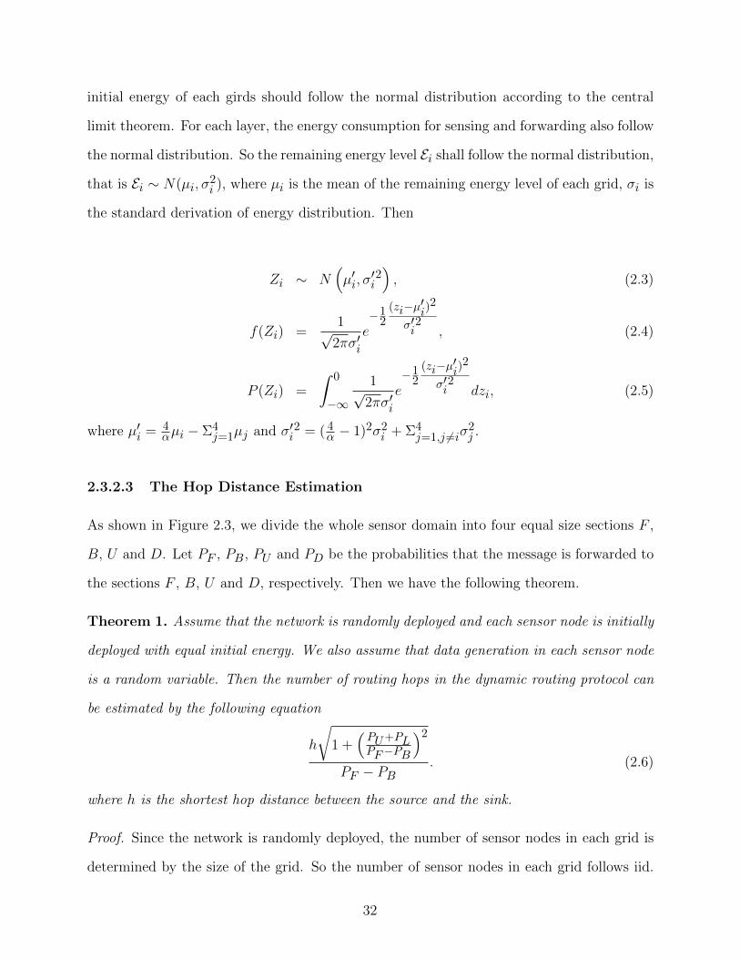
initial energy of each girds should follow the normal distribution according to the central

limit theorem. For each layer, the energy consumption for sensing and forwarding also follow

the normal distribution. So the remaining energy level Ei shall follow the normal distribution,

that is Ei ∼ N(µi, σ2i ), where µi is the mean of the remaining energy level of each grid, σi is

the standard derivation of energy distribution. Then

Zi ∼ N(µ′i, σ

′i2), (2.3)

f(Zi) =1√

2πσ′ie−1

2(zi−µ′i)

2

σ′i2 , (2.4)

P (Zi) =

ˆ 0

−∞1√

2πσ′ie−1

2(zi−µ′i)

2

σ′i2 dzi, (2.5)

where µ′i = 4αµi − Σ4

j=1µj and σ′i2 = ( 4

α − 1)2σ2i + Σ4

j=1,j 6=iσ2j .

2.3.2.3 The Hop Distance Estimation

As shown in Figure 2.3, we divide the whole sensor domain into four equal size sections F ,

B, U and D. Let PF , PB , PU and PD be the probabilities that the message is forwarded to

the sections F , B, U and D, respectively. Then we have the following theorem.

Theorem 1. Assume that the network is randomly deployed and each sensor node is initially

deployed with equal initial energy. We also assume that data generation in each sensor node

is a random variable. Then the number of routing hops in the dynamic routing protocol can

be estimated by the following equation

h

√1 +

(PU+PLPF−PB

)2

PF − PB. (2.6)

where h is the shortest hop distance between the source and the sink.

Proof. Since the network is randomly deployed, the number of sensor nodes in each grid is

determined by the size of the grid. So the number of sensor nodes in each grid follows iid.

32

B F

L

U

(a) Next hop node distribution

DS2

h

2

h2

x

2

x

(b) Routing path

Figure 2.3 Routing path and length estimation.

When the number of sensor nodes in each grid is large enough, the sum of the energy in each

grid should follow the normal distribution according to the central limit theorem. Therefore,

the energy consumption for each grid is also the iid and follows the normal distribution.

In dynamic routing algorithm, the next forwarding node is selected based on the routing

protocol. As shown in Figure 2.3, since the probability of PU and PD have similar effect,

while the PF −PB needs to move the message forward h hops, therefore we have estimation

(PF − PB) : (PU + PD) = h : x, where x is the routing hops that the message is routed in

the perpendicular direction, which can be calculated as

x =h(PU + PD)

PF − PB.

Therefore, the entire routing path length can be estimated as

h

√1 +

(PU + PDPF − PB

)2

, (2.7)

and the total number of routing hops can be estimated by

h

√1 +

(PU+PDPF−PB

)2

PF − PB.

33

According to Section 2.3.2.1, in our case G1, G2, G3 and G4 correspond the sections F ,

B, U and D, respectively. Therefore, we have PF = P1, PU = P2, PD = P3, PB = P4. Based

on Theorem 1, the total number of routing hops can be estimated according to the following

corollary.

Corollary 1. Assume that the network is randomly deployed and each sensor node is initially


is a random variable. Then for a given EBC parameter α and the hop distance h for α =

0, the number of routing hops can be estimated from the following equation:

h

√1 +

(P2+P3P1−P4

)2

P1 − P4. (2.8)

Table 2.1 Routing hops for different EBC parameters (µ′ = 200, σ′ = 50√

2)

EBC parameter Average hops Estimated

α in simulations CASER hops

0 10 10

0.1 10.26 10.05

0.2 10.38 10.09

0.3 10.63 10.18

0.4 11.02 10.34

0.5 11.15 10.64

Our simulation results conducted using OPNET network performance analysis tool demon-

strate that Corollary 1 provides a very good approximation on the actual number of routing

hops, as shown in Table 2.1.

2.3.3 Secure Routing Strategy

In the previous section, we only described the shortest path routing grid selection strategy.

However, in CASER protocol, we can support other routing strategies. In this section,

34

we propose a routing strategy that can provide routing path unpredictability and security.

The routing protocol contains two options for message forwarding: one is a deterministic

shortest path routing grid selection algorithm, and the other is a secure routing grid selection

algorithm through random walking.

In the deterministic routing approach, the next hop grid is selected from NαA based on

the relative locations of the grids. The grid that is closest to the sink node is selected for

message forwarding. In the secure routing case, the next hop grid is randomly selected from

NαA for message forwarding. The distribution of these two algorithms is controlled by a

security level called β, β ∈ [0, 1], carried in each message.

When a node needs to forward a message, the node first selects a random number γ ∈

[0, 1]. If γ > β, then the node selects the next hop grid based on the shortest routing

algorithm; otherwise, the next hop grid is selected using random walking. The security level

β is an adjustable parameter. A smaller β results in a shorter routing path and is more

energy efficient in message forwarding. On the other hand, a larger β provides more routing

diversity and security.

2.3.4 CASER Algorithm

Based on the previous description, the CASER algorithm can be described in Algorithm 2.

While providing routing path security, security routing will add extra routing overhead due

to an extended routing path.

When β increases, the probability for the next hop grid to be selected through random

walking also increases. Accordingly, the routing path becomes more random. In particular,

when β = 1, then random walking becomes the only routing strategy for the next hop grid

to be selected. The existing research [1, 28] has demonstrated that the message may never

be delivered from the source node to the destination node in this case.

When β < 1, since CASER mixes random walking with deterministic shortest path

routing, the deterministic shortest path routing guarantees that the messages are sent from

35

Algorithm 2 Node A finds the next hop routing grid based on the given parameters α, β ∈[0, 1]


∑i∈NA Eri.


3: Select a random number γ ∈ [0, 1].

4: if γ > β then5: Send the message to the grid in the Nα

A that is closest to the sink node based on itsrelative location.

6: else7: Route the message to a randomly selected grid in the set Nα

A .

8: end if

the source node to the sink node. However, the routing path becomes more dynamic and

unpredictable. In this way, it is more difficult for the adversary to capture the message

or jam the traffic. Therefore, the delivery ratio can be increased in a hostile environment.

While providing routing security, routing hop distance increases with the security level β.

Corollary 2 provides a quantitative estimation of the routing hops in this scenario.

Corollary 2. Assume that the network is randomly deployed and each sensor node is initially

deployed with equal initial energy. We also assume that data generation in each sensor node is

a random variable. Then the average number of routing hops for a message to be transmitted

from the source to the sink nodes can be estimated as follows:

h

√1 +

(β

2(1−β)

)2

1− β , (2.9)

where h is the required number of hops when the security level β = 0 (i.e., when no security

is enforced).

Proof. For a security level β, the probability that the message is routed forward using the

deterministic shortest path routing strategy is 1 − β. For probability β, the message is

forwarded using random walking. At each source, similar to Theorem 1, we can divide the

36

Table 2.2 Routing hops for various security parameters. The simulation was performed usingOPNET.

Security parameter Average hops Estimated

β in simulations CASER hops

0 10.00 10.00

0.125 11.97 11.46

0.25 14.51 13.52

0.375 17.98 16.70

0.5 23.34 22.36

entire domain into four π2 sections, correspond to F,U,D,B with probability PF = 1 −

3β4 , PU = PD = PB = β

4 . The rest part of the proof is straight according to Theorem 1.

Table 2.2 compares the average number of routing hops between simulation results and

the estimation based on Corollary 2 for various security parameters .

Remark 1. Corollary 1 and Corollary 2 are derived based on the assumption that the sensor

nodes are randomly deployed. However, in our case, the remaining energy levels for the

sensor nodes decrease exponentially when message are being transmitted based on distance

between the sensor nodes and the sink node. Therefore, the actual number of routing hops

should be slightly longer than this estimation.

2.3.5 Determine Security Level Based on Cost Factor

Based on Corollary 2, for a given routing budget, we can also find the maximum routing

security level. This result is given in the following theorem.



is a random variable. Then for a given routing cost factor f , the optimal security level can

be estimated from the following quartic equation:

4fx4 − 5x2 + 2x− 1 = 0, (2.10)

37

where x = 1− β.

Proof. According to Corollary 2, we have√1 +

(β

2(1−β)

)2

1− β = f.

Multiply both sides with 1− β, we have√1 +

(β

2(1− β)

)2

= f(1− β).

Square of both sides, we get

1 +

(β

2(1− β)

)2

= f2(1− β)2.

Equivalently, we have

4(1− β)2 + β2 = 4f2(1− β)4.

Let 1− β = x, we can derive

β2 = (1− x)2 = x2 − 2x+ 1,

reorganize the above equation, we get

4f2x4 − 5x2 + 2x− 1 = 0. (2.11)

Equation (2.11) can be solved using Ferrari’s method [71] following Algorithm 3 to recover

s = 1− β. The security level β can be recovered as: β = 1− s.

Example 1. Suppose we want to deliver a message with cost factor f = 1.5. To find the

maximum routing security level, we need to find the security parameter β. We can compute

s = 1− β as follows:

1: a← 9; c← −5; d← 2; e← −1;

38

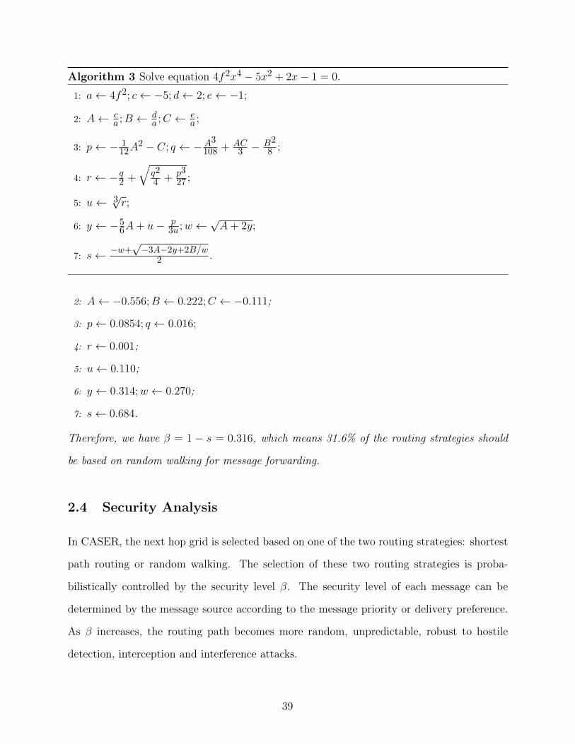
Algorithm 3 Solve equation 4f2x4 − 5x2 + 2x− 1 = 0.

1: a← 4f2; c← −5; d← 2; e← −1;

2: A← ca ;B ← d

a ;C ← ea ;

3: p← − 112A

2 − C; q ← −A3

108 + AC3 − B2

8 ;

4: r ← −q2 +

√q2

4 + p3

27 ;

5: u← 3√r;

6: y ← −56A+ u− p

3u ;w ← √A+ 2y;

7: s← −w+√−3A−2y+2B/w

2 .

2: A← −0.556;B ← 0.222;C ← −0.111;

3: p← 0.0854; q ← 0.016;

4: r ← 0.001;

5: u← 0.110;

6: y ← 0.314;w ← 0.270;

7: s← 0.684.

Therefore, we have β = 1 − s = 0.316, which means 31.6% of the routing strategies should

be based on random walking for message forwarding.

2.4 Security Analysis

In CASER, the next hop grid is selected based on one of the two routing strategies: shortest

path routing or random walking. The selection of these two routing strategies is proba-

bilistically controlled by the security level β. The security level of each message can be

determined by the message source according to the message priority or delivery preference.

As β increases, the routing path becomes more random, unpredictable, robust to hostile

detection, interception and interference attacks.

39

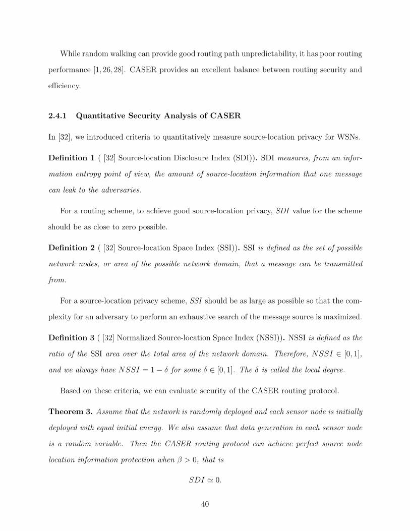
While random walking can provide good routing path unpredictability, it has poor routing

performance [1, 26, 28]. CASER provides an excellent balance between routing security and

efficiency.

2.4.1 Quantitative Security Analysis of CASER

In [32], we introduced criteria to quantitatively measure source-location privacy for WSNs.

Definition 1 ( [32] Source-location Disclosure Index (SDI)). SDI measures, from an infor-

mation entropy point of view, the amount of source-location information that one message

can leak to the adversaries.

For a routing scheme, to achieve good source-location privacy, SDI value for the scheme

should be as close to zero possible.

Definition 2 ( [32] Source-location Space Index (SSI)). SSI is defined as the set of possible

network nodes, or area of the possible network domain, that a message can be transmitted

from.

For a source-location privacy scheme, SSI should be as large as possible so that the com-

plexity for an adversary to perform an exhaustive search of the message source is maximized.

Definition 3 ( [32] Normalized Source-location Space Index (NSSI)). NSSI is defined as the

ratio of the SSI area over the total area of the network domain. Therefore, NSSI ∈ [0, 1],

and we always have NSSI = 1− δ for some δ ∈ [0, 1]. The δ is called the local degree.

Based on these criteria, we can evaluate security of the CASER routing protocol.



is a random variable. Then the CASER routing protocol can achieve perfect source node

location information protection when β > 0, that is

SDI ' 0.

40

Proof. First, in CASER, according to our assumption, a dynamic ID is used for each message,

which prevents the adversary from linking multiple messages from the same source or linking

the message to the source direction using correlation based techniques.

Second, for β > 0, due to probabilistic distribution of random walking and deterministic

routing, at each intermediate node, neither the original packet source direction, nor the hop

distance can be determined through routing traceback analysis. In fact, the adversary is

infeasible to determine the previous hop source node through routing traceback analysis.

Moreover, the probability for the adversary to receive multiple messages from the same

source node continuously is negligible for large sensor networks. Therefore, we have

SDI ' 0.



is a random variable. Then the source location that can be provided by the CASER routing

protocol is probabilistically proportional to the distribution of the random walking. That is

NSSI ' 1.

Proof. When an adversary intercepts a message m while the message is being transmitted

from node A to node B, there are two possible scenarios: (i) the message is transmitted

using random walking, or (ii) the message is transmitted using deterministic routing.

For scenario (i), suppose message m is transmitted from Si to Di, the previous source

node is located in shaded area, as shown in Figure ??, based on the routing scheme and

routing hop distance, where the angle of the shaded circular sector with horizontal lines is

π2 and symmetric to the SiDi.

Since each node routes the message forward with probability 1 − β using deterministic

routing and with probability β using random walking. It can be derived that the probability

41

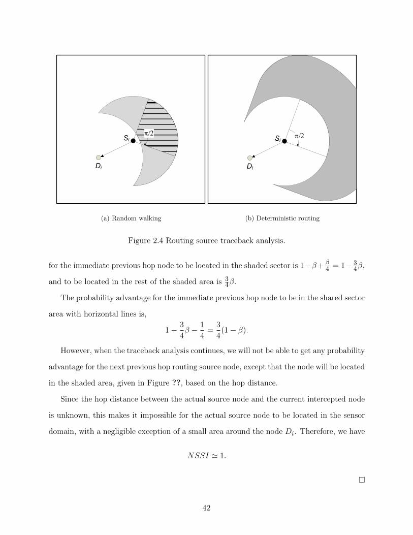
Si

Di

p/2

(a) Random walking

Si

Di

p/2

(b) Deterministic routing

Figure 2.4 Routing source traceback analysis.

for the immediate previous hop node to be located in the shaded sector is 1−β+ β4 = 1− 3

4β,

and to be located in the rest of the shaded area is 34β.

The probability advantage for the immediate previous hop node to be in the shared sector

area with horizontal lines is,

1− 3

4β − 1

4=

3

4(1− β).

However, when the traceback analysis continues, we will not be able to get any probability

advantage for the next previous hop routing source node, except that the node will be located

in the shaded area, given in Figure ??, based on the hop distance.

Since the hop distance between the actual source node and the current intercepted node

is unknown, this makes it impossible for the actual source node to be located in the sensor

domain, with a negligible exception of a small area around the node Di. Therefore, we have

NSSI ' 1.

42

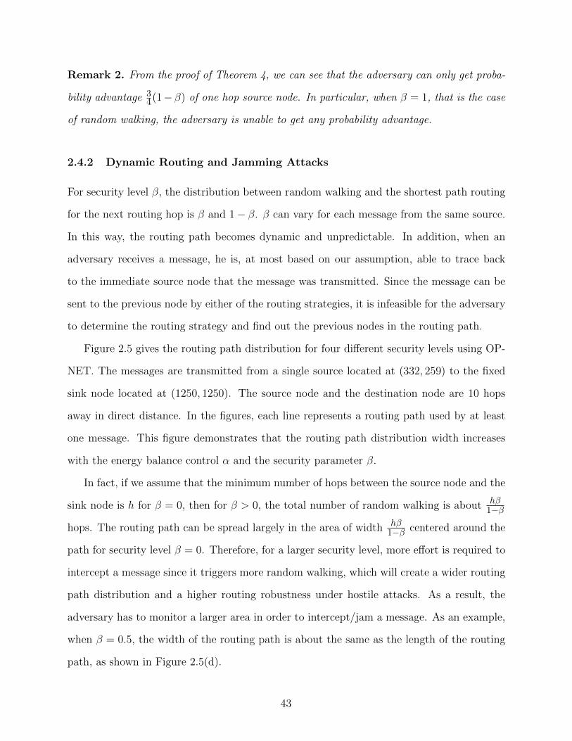
Remark 2. From the proof of Theorem 4, we can see that the adversary can only get proba-

bility advantage 34(1−β) of one hop source node. In particular, when β = 1, that is the case

of random walking, the adversary is unable to get any probability advantage.

2.4.2 Dynamic Routing and Jamming Attacks

For security level β, the distribution between random walking and the shortest path routing

for the next routing hop is β and 1− β. β can vary for each message from the same source.

In this way, the routing path becomes dynamic and unpredictable. In addition, when an

adversary receives a message, he is, at most based on our assumption, able to trace back

to the immediate source node that the message was transmitted. Since the message can be

sent to the previous node by either of the routing strategies, it is infeasible for the adversary

to determine the routing strategy and find out the previous nodes in the routing path.

Figure 2.5 gives the routing path distribution for four different security levels using OP-

NET. The messages are transmitted from a single source located at (332, 259) to the fixed

sink node located at (1250, 1250). The source node and the destination node are 10 hops

away in direct distance. In the figures, each line represents a routing path used by at least

one message. This figure demonstrates that the routing path distribution width increases

with the energy balance control α and the security parameter β.

In fact, if we assume that the minimum number of hops between the source node and the

sink node is h for β = 0, then for β > 0, the total number of random walking is about hβ1−β

hops. The routing path can be spread largely in the area of width hβ1−β centered around the

path for security level β = 0. Therefore, for a larger security level, more effort is required to

intercept a message since it triggers more random walking, which will create a wider routing

path distribution and a higher routing robustness under hostile attacks. As a result, the

adversary has to monitor a larger area in order to intercept/jam a message. As an example,

when β = 0.5, the width of the routing path is about the same as the length of the routing

path, as shown in Figure 2.5(d).

43

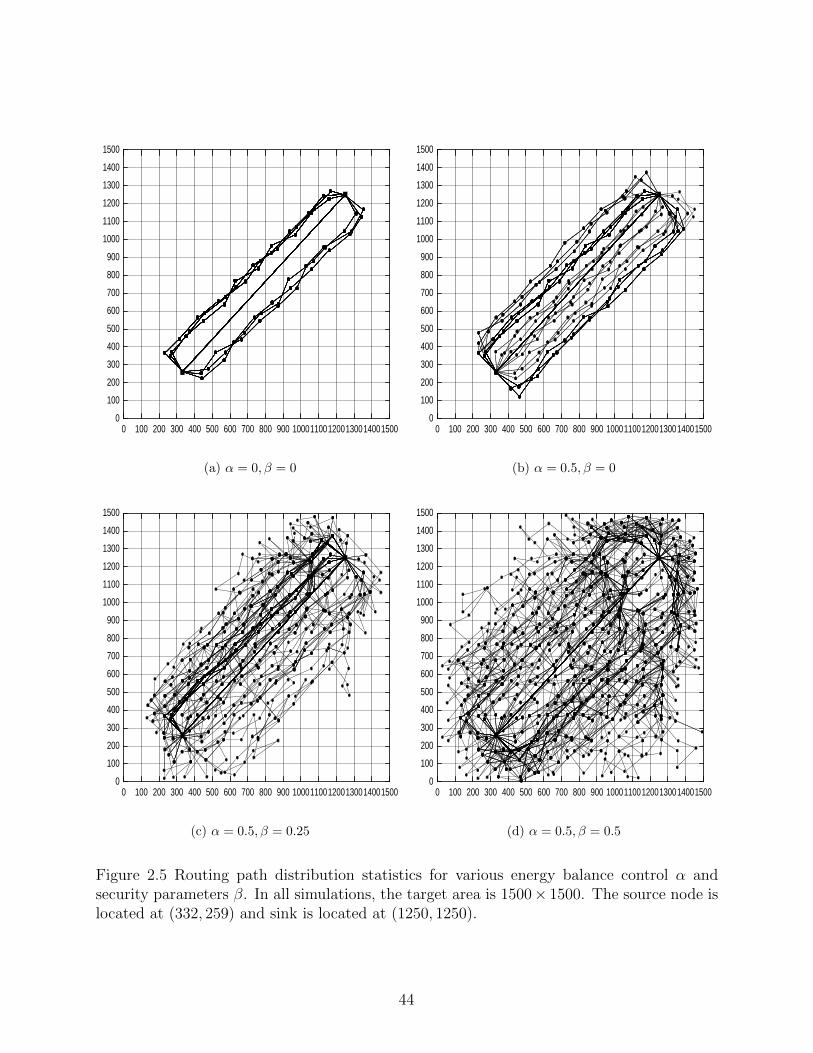
0 1 0 0 2 0 0 3 0 0 4 0 0 5 0 0 6 0 0 7 0 0 8 0 0 9 0 0 1 0 0 0 1 1 0 0 1 2 0 0 1 3 0 0 1 4 0 0 1 5 0 00

1 0 02 0 03 0 04 0 05 0 06 0 07 0 08 0 09 0 0

1 0 0 01 1 0 01 2 0 01 3 0 01 4 0 01 5 0 0

�

�

�

�

(a) α = 0, β = 0

0 1 0 0 2 0 0 3 0 0 4 0 0 5 0 0 6 0 0 7 0 0 8 0 0 9 0 0 1 0 0 0 1 1 0 0 1 2 0 0 1 3 0 0 1 4 0 0 1 5 0 00

1 0 02 0 03 0 04 0 05 0 06 0 07 0 08 0 09 0 0

1 0 0 01 1 0 01 2 0 01 3 0 01 4 0 01 5 0 0

�

�

(b) α = 0.5, β = 0

0 1 0 0 2 0 0 3 0 0 4 0 0 5 0 0 6 0 0 7 0 0 8 0 0 9 0 0 1 0 0 0 1 1 0 0 1 2 0 0 1 3 0 0 1 4 0 0 1 5 0 00

1 0 02 0 03 0 04 0 05 0 06 0 07 0 08 0 09 0 0

1 0 0 01 1 0 01 2 0 01 3 0 01 4 0 01 5 0 0

�

�

(c) α = 0.5, β = 0.25

0 1 0 0 2 0 0 3 0 0 4 0 0 5 0 0 6 0 0 7 0 0 8 0 0 9 0 0 1 0 0 0 1 1 0 0 1 2 0 0 1 3 0 0 1 4 0 0 1 5 0 00

1 0 02 0 03 0 04 0 05 0 06 0 07 0 08 0 09 0 0

1 0 0 01 1 0 01 2 0 01 3 0 01 4 0 01 5 0 0

�

�

(d) α = 0.5, β = 0.5

Figure 2.5 Routing path distribution statistics for various energy balance control α andsecurity parameters β. In all simulations, the target area is 1500× 1500. The source node islocated at (332, 259) and sink is located at (1250, 1250).

44

Jamming attacks have been extensively studied [72, 73]. The main idea is that the jam-

mers try to interfere with normal communications between the legitimate communication

parties in the link layer and/or physical layer. However, a jammer can perform attacks only

when the jammer is on the message forwarding path. As discussed in [73], dynamic routing

is an effective method to minimize the probability of jamming.

The CASER routing algorithm distributes the routing paths in a large area based on our

above analysis due to the random and independent routing selection strategy in each for-

warding node. This makes the likelihood for multiple messages to be routed to the sink node

through the same routing path very low, even for the smart jammers that have knowledge

of the routing algorithm.

2.4.3 Energy Level and Compromised Nodes Detection

Since we assume that each node has knowledge of energy levels of its adjacent neighboring

grids, each sensor node can update the energy levels based on the detected energy usage. The

actual energy is updated periodically. For WSNs with non-replenishable energy resources,

the energy level is a monotonically decreasing function. The updated energy level should

never be higher than the predicated energy level, since the predicted energy level is calculated

based on only the actually detected usage. If the updated energy level is higher than the

predicted level, the node must have been compromised and should be excluded from its list

of the adjacent neighboring grids.

We also compared the CASER algorithm with the RSIN algorithm in [1] on path dis-

tribution under the similar energy consumption. The results show that the CASER can

achieve better and more uniform path distribution, as shown in Figure 2.6. Our simulation

results show that the average number of routing hops for the two schemes are 14.51 and

15.27, respectively.

In addition, for a node with a low energy level that is caused by excessive usage due

to security attacks, according to our design, these nodes will be filtered out of the pool

45

for active routing selection. Therefore, the CASER design can minimize the possibility for

denial-of-service (DoS) attacks.

2.5 Performance Evaluation and Simulation Results

In this chapter, the simulation results illustrate the distribution of the routing path for

different security levels that makes it impossible to perform traceback attack for adversaries.

Then, we analyze the performance of the proposed CASER algorithm for routing efficiency

and energy balance. All our simulations were conducted in a targeted sensor area of size

1500× 1500 meters. The targeted area is divided into grids of 15× 15. We randomly spread

1000 sensor nodes in the this domain.

2.5.1 Routing Efficiency and Delay

For routing efficiency, we conduct simulations of the proposed CASER protocol using OP-

NET to measure the average number of routing hops for four different security levels. We

randomly deployed 1000 sensor nodes in the entire sensing domain. We also assume that

the source node and destination node are 10 hops away in direct distance. The routing hops

increase as the number of the transmitted messages increase. The routing hops also increase

with the security levels.

We performed simulations with different α and β values as shown in Tables 2.1 and

2.2. In all cases, we derived consistent results showing that the average number of routing

hops derived in this dissertation provides a very close approximation to the actual number

of routing hops. As expected, when the energy level goes down, the routing path spreads

further wider for better energy balance.

We also provided simulation results on end-to-end transmission delay in Table 2.3.

46

Table 2.3 Delay results for various security parameters from simulation

Security Parameter 0 0.125 0.25 0.375 0.5

Average Delay (Sec) 0.0148 0.0177 0.0214 0.0265 0.0344

2.5.2 Energy Balance

The CASER algorithm is designed to balance the overall sensor network energy consumption

in all grids by controlling energy spending from sensor nodes with low energy levels. In

this way, we can extend the lifetime of the sensor networks. Through the EBC α, energy

consumption from the sensor nodes with relatively lower energy levels can be regulated and

controlled. Therefore, we can effectively prevent any major sections of the sensor domain

from completely running out of energy and becoming unavailable.

In the CASER scheme, the parameter α can be adjusted to achieve the expected efficiency.

As α increases, better energy balance can be achieved. Meanwhile, the average number of

routing hops may also increase. Accordingly, the overall energy consumption may go up.

In other words, though the energy control can balance the network energy levels, it may

increase the number of routing hops and the overall energy consumption slightly. This is

especially true when the sensor nodes have very unbalanced energy levels.

In our simulations, shown in Figure 2.7, the message source is located at (332, 259) and

the message destination is located at (1250, 1250). The source node and the destination

node are 10 hops away in direct distance. There are three nodes in each grid, and each node

is deployed with energy to transmit 70 messages. We show the remaining energy levels of the

sensor nodes under two different α levels. The darker gray-scale level corresponds to a lower

remaining level. Figure ??, we set α = 0 and there is only one source node. The energy

consumption is concentrated around the shortest routing path and moves away only until

the energy runs out in that area. In Figure ??, we set α = 0.5, then the energy consumption

is spread over a large area between this node and the sink. While maximizing the availability

47

of the sensor nodes, or lifetime, this design can also guarantee a high message delivery ratio

until the energy runs out for all of the available sensor nodes in the area.

2.6 Summary

In this chapter, we present a decentralized routing algorithm CASER to balance energy con-

sumption and increase network lifetime. CASER is also designed to provide source location

privacy and defend against jamming attacks. We provide a quantitatively security analysis

and derive formulas to show the relationship among security, energy consumption balance

and energy efficiency. It also has the flexibility to support multiple routing strategies in

message forwarding to extend the lifetime while increasing routing security. Both theoretical

analysis and simulation results show that CASER can achieve a trade-off between energy

balance and security under a given energy consumption.

48

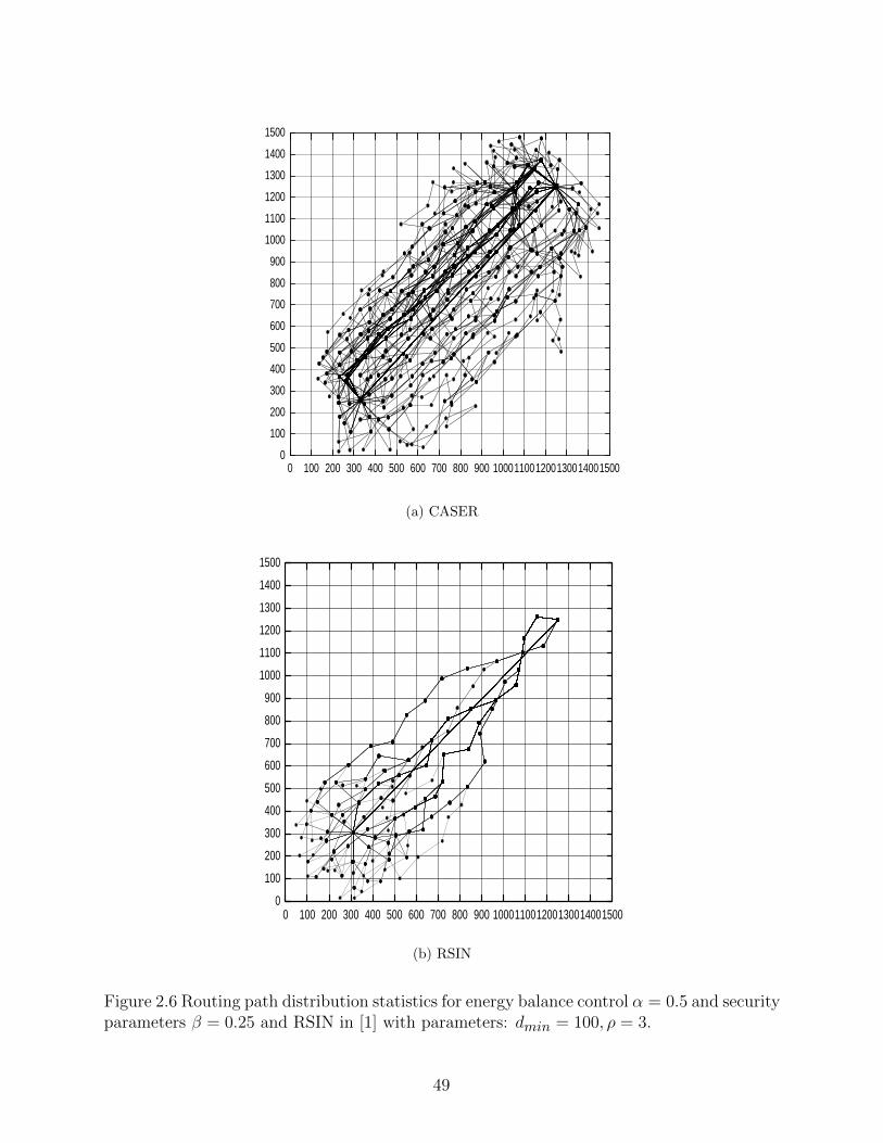
0 1 0 0 2 0 0 3 0 0 4 0 0 5 0 0 6 0 0 7 0 0 8 0 0 9 0 0 1 0 0 0 1 1 0 0 1 2 0 0 1 3 0 0 1 4 0 0 1 5 0 00

1 0 02 0 03 0 04 0 05 0 06 0 07 0 08 0 09 0 0

1 0 0 01 1 0 01 2 0 01 3 0 01 4 0 01 5 0 0

�

�

(a) CASER

0 100 200 300 400 500 600 700 800 900 1000110012001300140015000

100

200

300

400

500

600

700

800

900

1000

1100

1200

1300

1400

1500

(b) RSIN

Figure 2.6 Routing path distribution statistics for energy balance control α = 0.5 and securityparameters β = 0.25 and RSIN in [1] with parameters: dmin = 100, ρ = 3.

49

0

0.1

0.2

0.3

0.4

0.5

0.6

0.7

0.8

0.9

1

(a) α = 0

0

0.1

0.2

0.3

0.4

0.5

0.6

0.7

0.8

0.9

1

(b) α = 0.5

Figure 2.7 Remaining energy distribution statistics after the source transmitted about 600messages.

50

CHAPTER 3

COST-AWARE ENERGY DEPLOYMENT: DESIGN AND ANALYSIS

In this chapter, we propose a cost-aware energy deployment to extend the lifetime of wireless

sensor networks. We also update the proposed CASER under this energy deployment strat-

egy to preserve source location privacy. We investigate the energy consumption for CASER

scheme with uniformly distributed events. The theoretical analysis and simulations show

that CASER can balance the energy consumption in a local area, however the overall energy

consumption through the entire network is still severely imbalanced based on the distance

to the sink node under a uniform energy deployment. To solve this problem, we propose

a non-uniform energy deployment to extend the lifetime of WSN while updating CASER

under this energy deployment to preserve source location privacy.

3.1 Uniform Energy Deployment

3.1.1 Energy Consumption Analysis

In the multi-hop sensor network, the messages are generated at the source and forwarded

hop by hop through the relay nodes to the sink. The relay node closer to the sink node

consumes more energy than the outer layer sensor nodes on relaying. Assume the events are

uniformly distributed in the entire network. We could have the following theorem.

Theorem 5. Assume that all sensor nodes transmit messages to the sink node at the same

frequency, the initial energy level of each grid is equal, then the average energy consumption

for the grid with distance i to the sink node is:

n2 + n+ i− i22i

, (3.1)

where n is the distance between the sink node and the outmost grid.

51

Proof. Since all messages will be sent to the sink node, the energy consumption for the grids

with distance i to the sink node can be measured based on message forwarding for grids with

distance larger than i and message transmission for grids with distance i. The number of

grids with distance j to the sink node is 8j. The total energy consumption of the grids with

distance i to the sink can be calculated as∑nj=i 8j. The average grid energy consumption is

therefore: ∑nj=i 8j

8i=n2 + n+ i− i2

2i.

3.1.2 Energy Balance of CASER

We also conduct simulations to evaluate the energy consumption for dynamic sources in

Figure 3.1. The events are uniformly distributed through the entire network. Each sensor

node has equal probability to generate packets and acts as a source node. We assume that

the only sink node is located in the center of the target area located at (750,750), which

makes the target area symmetrical to show the energy consumption. Similar to the previous

simulation, we assume there are three nodes in each grid, and each node is deployed with

energy to transmit 70 messages. The maximum direct hop distance between the source node

and sink is 7. The simulation results shows the average energy consumption for the node is

related to the distance i to the sink.

Figure 3.1 gives the remaining energy levels close to the sink node when the sensor nodes

run out almost the entire energy, where n = 7, α = 0.5, β = 0.5. The color evenness in each

layer of the grids demonstrates the energy usage balance enforced through the EBC α.

In fact, according to equation (3.1), we can calculate the total number of messages that

can be transmitted from the outmost grid when the innermost grid runs out of energy as

210/

((n2 + n)/2) = 210/

((72 + 7)/2) = 7.5. In this case, the overall energy consumption

is only 7.5 ×∑ni=1 8j2 = 8400, when the sensor networks become unavailable. Recall that

the overall energy units deployed are 210 × ((2n + 1)2 − 1) = 47040. Therefore, the energy

52

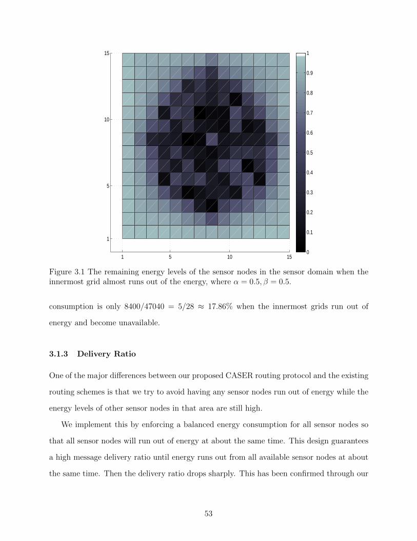
1 5 10 15

1

5

10

15

0

0.1

0.2

0.3

0.4

0.5

0.6

0.7

0.8

0.9

1

Figure 3.1 The remaining energy levels of the sensor nodes in the sensor domain when theinnermost grid almost runs out of the energy, where α = 0.5, β = 0.5.

consumption is only 8400/47040 = 5/28 ≈ 17.86% when the innermost grids run out of

energy and become unavailable.

3.1.3 Delivery Ratio

One of the major differences between our proposed CASER routing protocol and the existing

routing schemes is that we try to avoid having any sensor nodes run out of energy while the

energy levels of other sensor nodes in that area are still high.

We implement this by enforcing a balanced energy consumption for all sensor nodes so

that all sensor nodes will run out of energy at about the same time. This design guarantees

a high message delivery ratio until energy runs out from all available sensor nodes at about

the same time. Then the delivery ratio drops sharply. This has been confirmed through our

53

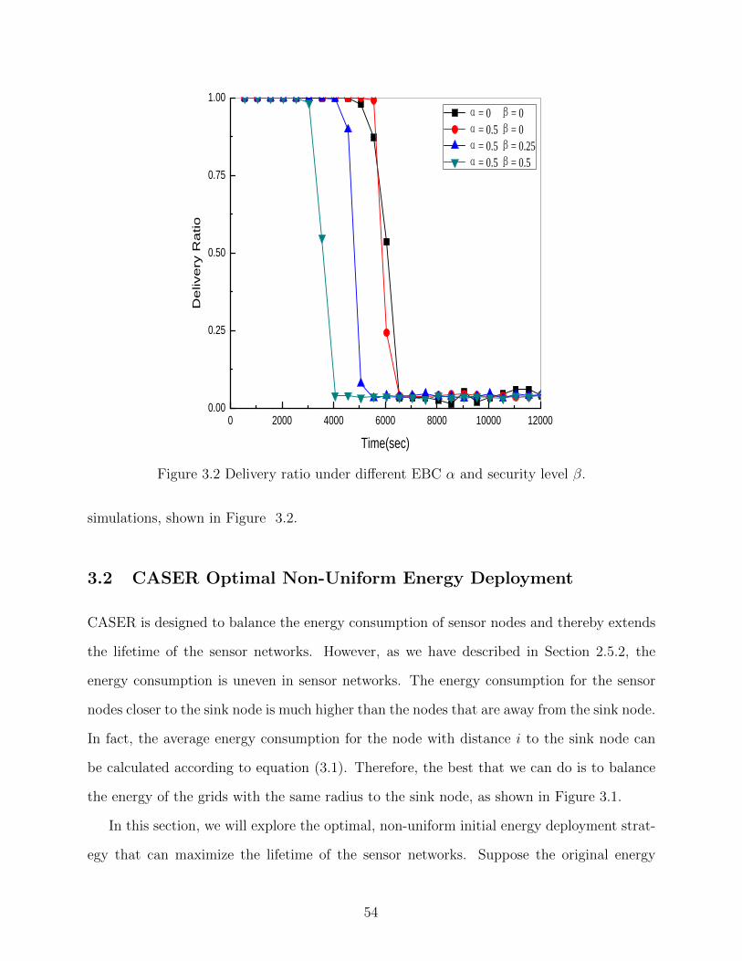
0 2000 4000 6000 8000 10000 120000.00

0.25

0.50

0.75

1.00

De

live

ry R

atio

Time(sec)

α= 0 β= 0 α= 0.5 β= 0 α= 0.5 β= 0.25 α= 0.5 β= 0.5

Figure 3.2 Delivery ratio under different EBC α and security level β.

simulations, shown in Figure 3.2.

3.2 CASER Optimal Non-Uniform Energy Deployment

CASER is designed to balance the energy consumption of sensor nodes and thereby extends

the lifetime of the sensor networks. However, as we have described in Section 2.5.2, the

energy consumption is uneven in sensor networks. The energy consumption for the sensor

nodes closer to the sink node is much higher than the nodes that are away from the sink node.

In fact, the average energy consumption for the node with distance i to the sink node can

be calculated according to equation (3.1). Therefore, the best that we can do is to balance

the energy of the grids with the same radius to the sink node, as shown in Figure 3.1.

In this section, we will explore the optimal, non-uniform initial energy deployment strat-

egy that can maximize the lifetime of the sensor networks. Suppose the original energy

54

distribution for each grid is the same, and we denote the energy level as u. We also assume

that the largest distance between the sink node and the outmost grid is n, then the total

energy unit is u((2n+ 1)2 − 1).

3.2.1 Node Energy Deployment

For the optimal energy deployment, the energy allocation of the grids should be proportional

to the energy usage. We still assume that the sink node is in the center of the sensor domain.

All sensor nodes transmit messages at the same frequency. The distance between the outmost

grid and the sink node is n according to equation (3.1), the energy allocation for the grids

with hop distance i to the sink node should be:

n2 + n+ i− i22i

v,

where v is the basic energy unit for energy deployment. Accordingly, from the outmost to

the innermost, the energy assignment should be:

v,2n− 1

n− 1v,

3(n− 1)

n− 2v, · · · , (n+ 2)(n− 1)

4v,

(n+ 1)n

2v.

The total energy units should be:

v

(8

3n3 + 4n2 +

4

3n

).

To maintain the same amount of energy, we let:

u((2n+ 1)2 − 1) = v

(8

3n3 + 4n2 +

4

3n

).

Then we have:

v =3n

(2n+ 1)(n+ 1)u. (3.2)

Example 2. We still assume that n = 7, and each grid has u = 210 energy units originally.

According to equation (3.2), we can derive that:

v =3u

2n+ 1u = 42.

55

Therefore, the non-uniform energy deployment for all of the grids from the outmost to the

innermost can be calculated as:

42, 91, 151, 231, 350, 567, 1176.

With this energy deployment, we maintained the same overall amount of energy deploy-

ment units, 47040, in the non-uniform energy deployment. However, under our assumption,

the energy consumption should be 100% before the sensor network runs out of energy and

dies. Recall that in the uniform energy deployment scenario, the sensor network dies when

only about 17.86% of the energy is consumed. Therefore, under non-uniform deployment,

the efficiency of a sensor network’s energy usage can be roughly 100/17.86 = 5.6 times com-

pare to the uniform energy deployment. The efficiency can be measured by the total number

of messages that can be delivered, or the lifetime of the sensor network under the same

transmission frequency.

3.2.2 Routing in Non-Uniform Energy Deployment

Algorithm 4 Node A finds the next hop routing grid based on the given parameters α, β ∈[0, 1]


∑i∈NA

Erin2+n+i−i2

2i

.


3: Select a random number γ ∈ [0, 1].

4: if γ > β then5: Send the message to the grid in the Nα

A that is closest to the sink node based on itsrelative location.

6: else7: Route the message to a randomly selected grid in the set Nα

A .

8: end if

56

Under the new energy deployment, we have to redefine the way we calculate the average

remaining energy of the adjacent neighboring grids since otherwise, the messages will always

be routed to the nodes that are closer to the sink node, at least initially. In this way, the

number of possible nodes for the next hop can be greatly limited and security routing may

become trivial.

For the non-uniform energy deployment case, the energy assignment is proportional to

the energy consumption. In other words, the energy assignment is constant when divided by

the energy consumption factor n2+n+i−i22i , where i = 1, 2, · · · , n. Therefore, we can define

the average remaining level as:

Ea(A) =1

|NA|∑i∈NA

Erin2+n+i−i2

2i

. (3.3)

Accordingly, we have the updated Algorithm 4.

3.2.3 Simulation Results

We conducted simulations using OPNET to compare the message delivery ratio of uniform

energy deployment (noED) and non-uniform energy deployment (ED) for different α values

when β = 0. The simulation settings are similar to Figure 3.1. However, each node is

deployed with a different energy level according to Algorithm 4. From the simulation results

in Figure 3.3, we can see that the delivery ratio increases with α. Comparing to uniform

energy deployment, the delivery ratio for non-uniform energy deployment is much higher

than the uniform energy deployment with the same α.

We also compared the total number of messages that can be delivered in the two scenarios.

Our statistics are based on the message delivery ratio that is 95% or above. In uniform

energy deployment, when α = 0, the number of messages that can be delivered is 1510.

When α = 0.25, the number of messages that can be delivered increases to 1624. The

increase is 7.55%. We found that when we further increase α, the number of messages that

57

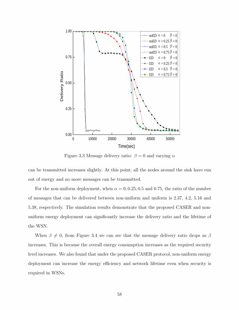
0 1 0 0 0 0 2 0 0 0 0 3 0 0 0 0 4 0 0 0 0 5 0 0 0 00 . 0 0

0 . 2 5

0 . 5 0

0 . 7 5

1 . 0 0 n o E D � = 0 � = 0 n o E D � = 0 . 2 5 � = 0 n o E D � = 0 . 5 � = 0 n o E D � = 0 . 7 5 � = 0 E D � = 0 � = 0 E D � = 0 . 2 5 � = 0 E D � = 0 . 5 � = 0 E D � = 0 . 7 5 � = 0

Deliv

ery R

atio

T i m e ( s e c )Figure 3.3 Message delivery ratio: β = 0 and varying α

can be transmitted increases slightly. At this point, all the nodes around the sink have run

out of energy and no more messages can be transmitted.

For the non-uniform deployment, when α = 0, 0.25, 0.5 and 0.75, the ratio of the number

of messages that can be delivered between non-uniform and uniform is 2.37, 4.2, 5.16 and

5.38, respectively. The simulation results demonstrate that the proposed CASER and non-

uniform energy deployment can significantly increase the delivery ratio and the lifetime of

the WSN.

When β 6= 0, from Figure 3.4 we can see that the message delivery ratio drops as β

increases. This is because the overall energy consumption increases as the required security

level increases. We also found that under the proposed CASER protocol, non-uniform energy

deployment can increase the energy efficiency and network lifetime even when security is

required in WSNs.

58

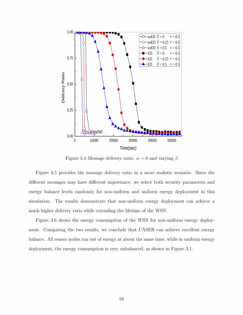
0 10000 20000 30000 40000 500000.00

0.25

0.50

0.75

1.00

De

lice

ry R

atio

Time(sec)

noED β= 0 α= 0.5 noED β= 0.25 α= 0.5 noED β= 0.5 α= 0.5 ED β= 0 α= 0.5 ED β= 0.25 α= 0.5 ED β= 0.5 α= 0.5

Figure 3.4 Message delivery ratio: α = 0 and varying β

Figure 3.5 provides the message delivery ratio in a more realistic scenario. Since the

different messages may have different importance, we select both security parameters and

energy balance levels randomly for non-uniform and uniform energy deployment in this

simulation. The results demonstrate that non-uniform energy deployment can achieve a

much higher delivery ratio while extending the lifetime of the WSN.

Figure 3.6 shows the energy consumption of the WSN for non-uniform energy deploy-

ment. Comparing the two results, we conclude that CASER can achieve excellent energy

balance. All sensor nodes run out of energy at about the same time, while in uniform energy

deployment, the energy consumption is very unbalanced, as shown in Figure 3.1.

59

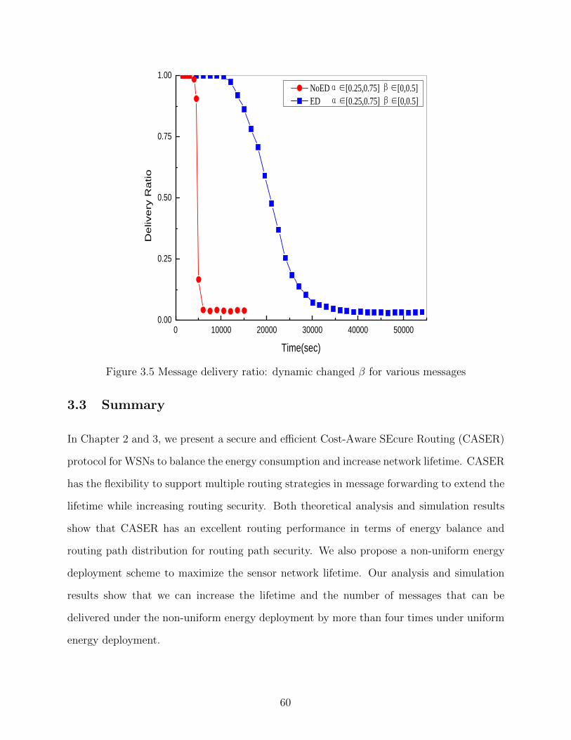
0 10000 20000 30000 40000 500000.00

0.25

0.50

0.75

1.00 NoEDα∈[0.25,0.75] β∈[0,0.5] ED α∈[0.25,0.75] β∈[0,0.5]

De

live

ry R

atio

Time(sec)

Figure 3.5 Message delivery ratio: dynamic changed β for various messages

3.3 Summary

In Chapter 2 and 3, we present a secure and efficient Cost-Aware SEcure Routing (CASER)

protocol for WSNs to balance the energy consumption and increase network lifetime. CASER

has the flexibility to support multiple routing strategies in message forwarding to extend the

lifetime while increasing routing security. Both theoretical analysis and simulation results

show that CASER has an excellent routing performance in terms of energy balance and

routing path distribution for routing path security. We also propose a non-uniform energy

deployment scheme to maximize the sensor network lifetime. Our analysis and simulation

results show that we can increase the lifetime and the number of messages that can be

delivered under the non-uniform energy deployment by more than four times under uniform

energy deployment.

60

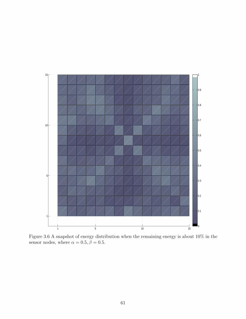
1 5 10 15

1

5

10

15

0

0.1

0.2

0.3

0.4

0.5

0.6

0.7

0.8

0.9

1

Figure 3.6 A snapshot of energy distribution when the remaining energy is about 10% in thesensor nodes, where α = 0.5, β = 0.5.

61

CHAPTER 4

CONGESTION-AWARE ROUTING (CAR): DESIGN AND ANALYSIS

WSNs are designed to collect and transmit sensed data to one or more sink nodes. The in-

formation of the sensed data is critical for real-time processing and decision-making in both

military and civilian applications, such as monitoring the forest fire and target locating. For

these applications, end-to-end transmission delay is one of the most significant design issues

for WSNs. In this chapter, we propose a congestion-aware routing scheme to reduce conges-

tion by monitoring the traffic in the MAC layer. In CAR routing scheme, each node selects

the relay node based on two different routing strategies: the shortest path forwarding and

the congestion-aware forwarding. In the shortest path forwarding, the relay node applies

geographic routing strategy [61] based relative locations, ensures an efficient message deliv-

ery through hop by hop transmission. In congestion-aware forwarding strategy, each node

selects the relay node based on the competing results of wireless medium channel, which can

effectively reduce the end-to-end message transmission delay.

4.1 Introduction

WSNs consist of a large number of untethered and unattended sensor nodes. Sensor nodes

are equipped with low-power radio devices to send and receive messages. The messages

are forwarded hop by hop from source nodes to the sink node, which may greatly create

significant traffic congestion in the area close to the sink node. Burst events may also

develop a significantly amount of traffic in a localized area. The unbalanced traffic volume

in WSNs may increase the communication delay and energy consumption in WSNs while

decreasing the network lifetime.

In traditional networks, the existing research on congestion mainly focuses on the traffic

control in both end-to-end and hop-by-hop communications. These algorithms are mainly

62

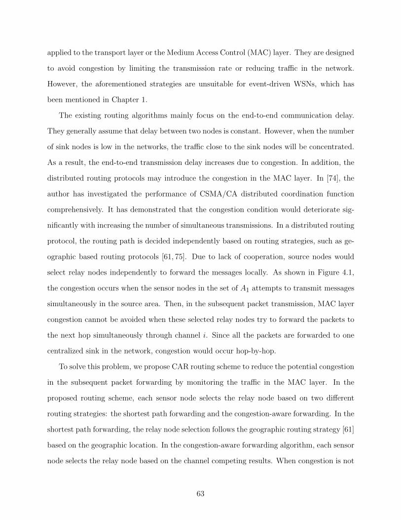
applied to the transport layer or the Medium Access Control (MAC) layer. They are designed

to avoid congestion by limiting the transmission rate or reducing traffic in the network.

However, the aforementioned strategies are unsuitable for event-driven WSNs, which has

been mentioned in Chapter 1.

The existing routing algorithms mainly focus on the end-to-end communication delay.

They generally assume that delay between two nodes is constant. However, when the number

of sink nodes is low in the networks, the traffic close to the sink nodes will be concentrated.

As a result, the end-to-end transmission delay increases due to congestion. In addition, the

distributed routing protocols may introduce the congestion in the MAC layer. In [74], the

author has investigated the performance of CSMA/CA distributed coordination function

comprehensively. It has demonstrated that the congestion condition would deteriorate sig-

nificantly with increasing the number of simultaneous transmissions. In a distributed routing

protocol, the routing path is decided independently based on routing strategies, such as ge-

ographic based routing protocols [61, 75]. Due to lack of cooperation, source nodes would

select relay nodes independently to forward the messages locally. As shown in Figure 4.1,

the congestion occurs when the sensor nodes in the set of A1 attempts to transmit messages

simultaneously in the source area. Then, in the subsequent packet transmission, MAC layer

congestion cannot be avoided when these selected relay nodes try to forward the packets to

the next hop simultaneously through channel i. Since all the packets are forwarded to one

centralized sink in the network, congestion would occur hop-by-hop.

To solve this problem, we propose CAR routing scheme to reduce the potential congestion

in the subsequent packet forwarding by monitoring the traffic in the MAC layer. In the

proposed routing scheme, each sensor node selects the relay node based on two different

routing strategies: the shortest path forwarding and the congestion-aware forwarding. In the

shortest path forwarding, the relay node selection follows the geographic routing strategy [61]

based on the geographic location. In the congestion-aware forwarding algorithm, each sensor

node selects the relay node based on the channel competing results. When congestion is not

63

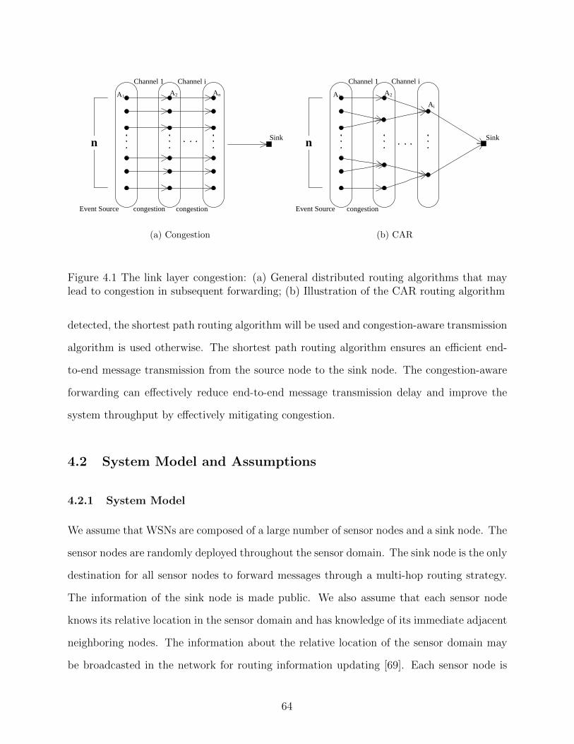
n

Channel 1

congestion

A1 A2

Sink

Channel i

congestion

An

Event Source

(a) Congestion

n

Channel 1

congestion

A1 A2

Sink

Channel i

Event Source

Ai

(b) CAR

Figure 4.1 The link layer congestion: (a) General distributed routing algorithms that maylead to congestion in subsequent forwarding; (b) Illustration of the CAR routing algorithm

detected, the shortest path routing algorithm will be used and congestion-aware transmission

algorithm is used otherwise. The shortest path routing algorithm ensures an efficient end-

to-end message transmission from the source node to the sink node. The congestion-aware

forwarding can effectively reduce end-to-end message transmission delay and improve the

system throughput by effectively mitigating congestion.

4.2 System Model and Assumptions

4.2.1 System Model

We assume that WSNs are composed of a large number of sensor nodes and a sink node. The

sensor nodes are randomly deployed throughout the sensor domain. The sink node is the only

destination for all sensor nodes to forward messages through a multi-hop routing strategy.

The information of the sink node is made public. We also assume that each sensor node

knows its relative location in the sensor domain and has knowledge of its immediate adjacent

neighboring nodes. The information about the relative location of the sensor domain may

be broadcasted in the network for routing information updating [69]. Each sensor node is

64

able to monitor the local traffic information. It can obtain information of the transmitted

packets through monitoring the physical channel within its communication range.

4.2.2 MAC Layer Protocol

Carrier sense multiple access with collision avoidance (CSMA/CA) is one of standard medium

access control protocols in WSNs. In CSMA/CA mechanism, the exponential backoff scheme

is employed as the major backoff scheme. Each node starts to monitor the physical channel

once it has a packet to transmit. Before each attempt of transmission, the tag node with

packet to transmit keeps monitoring the channel for a period of Distributed Inter Frame

Spacing (DIFS). If the channel is sensed busy, the tag node defers its transmission until

the channel is idle for DIFS. Then the station generates a random backoff interval before

transmitting. The time following an idle DIFS is divided into slots, and each slot is equal to

σ which depends on the physical layer.

In each stage of backoff, the backoff window will be uniformly chosen in the range (0, w−

1). The value of w will be initially set equal to CWmin and doubled after a failure of

transmission up to CWmax = 2mCWmin. CWmin is denoted as the minimum contention

window and m is the contending window size. The value of w will be equal to 2iCWmin

after the ith transmission attempt. The stage between the ith transmission attempt and the

(i + 1)th attempt is called as the ith stage. Once the packet is successfully transmitted by

the tag node, the value of w will be set equal to the initial value.

The backoff time counter decreases when the physical channel is detected idle. It stops

counting once the channel is busy for a successful transmission or a collision. When the

channel is sensed idle, the counter will be reactivated and decremented. Once the counter

reaches zero, the tag node transmits its packet immediately. There will be a period of Short

Inter-Frame Spacing (SIFS) before the receiver sends back an acknowledgement (ACK) to

the tag node.

The four-way handshaking technique, known as request-to-send/clear-to-send (RTS/CTS)

65

mechanism, is also utilized in the MAC layer as an access mechanism. This mechanism can

increase the system performance by solving the hidden node problem.

4.3 The Proposed Routing Scheme

We now describe the proposed routing scheme. The algorithm consists of two strategies for

routing path selection: the shortest path forwarding based on geographical information, and

the congestion-aware forwarding based on physical channel competing results.

4.3.1 Overview of the Proposed Routing Scheme

In CAR, we assume that each node maintains the relative locations of its immediate adjacent

neighboring nodes. Each node selects the relay node based on the shortest path forwarding

and congestion-aware forwarding. Firstly, the source node A composes a candidate set for

the relay node selection. The candidate set includes its all immediate adjacent neighboring

nodes that are closer to the sink node than itself. We denote this set as NA. In the shortest

path forwarding, the node A selects the node B that is closest to the sink node as the relay

node when it has packets to forward when no traffic congestion is detected. Otherwise, A

selects a relay node based on the congestion-aware forwarding scheme. If node A fails to

access the channel, it will monitor the physical channel to obtain the channel competing

results. Assume that A’s neighboring node C has successfully accessed the channel and

forwarded its packet to its relay node D. Then, if D ∈ NA, node A reselects D as its relay

node in the congestion-aware forwarding.

In the shortest path forwarding, each sensor node independently selects the relay node

according to the relative location which might increase the number of relay nodes. The

number of potential transmissions may increase with the number of relay nodes in a local

area. The number of the forwarding nodes may increase traffic congestion for the subse-

quent packet delivery [74]. The results may also introduce more transmission collision and

66

Event Sensors

Sink

Figure 4.2 Dynamic tree formation

significantly prolong the congestion delay. Our proposed CAR scheme enables the sensor

nodes to utilize the traffic condition and channel competing results to reselect relay nodes in

a congested area. In this way, we can reduce the number of concurrent transmissions in the

subsequent forwarding by decreasing the number of relay nodes. While decreasing end-to-

end transmission delay, the CAR routing strategy can also increase the network throughput

at the same time.

In addition, the proposed CAR routing scheme can reduce the energy consumption that

introduced by congestion. Instead of keeping trying to transmit the packets in a congested

area and consuming more energy, CAR can reduce the congestion by decreasing the number

of contending nodes. As a result, the number of transmission attempts for each node also

be reduced. The proposed CAR can also balance the energy consumption in congested

areas. Since the channel competing results should be uniformly distributed in the available

forwarding nodes, the forwarding nodes may take turns to be selected for message forwarding.

As shown in Figure 4.2, the black nodes might be selected as the forwarding nodes for the

current message forward. However, the gray nodes can provide more options for relay nodes

selection when burst events occur.

67

4.3.2 Congestion-Aware (CAR) Routing Algorithm

Based on the previous description, we summarize the proposed CAR routing scheme in

Algorithm 5.

Algorithm 5 Node A derives the next hop routing node based on the MAC layer congestioncondition

1: Node A determines the candidate set for the next hop node selection by choosing all itsneighboring nodes that are closer to the sink node than itself. Denoted the set as NA.

2: Selects node B in the set NA that is closest to the sink node as the next hop node basedon its relative location.

3: if the packet fails to be delivered to the next hop node, then4: Node A monitors the channel from the MAC layer to obtain the information of the

packet that can be successfully transmitted.

5: Suppose C is the node that successfully transmits the packet to its relay node D.

6: if the destination node D is in the set NA then7: Node A reselects node D as the next hop node.

8: end if

9: end if

4.4 The Analysis on Congestion through End-to-End Transmis-sion

The proposed CAR algorithm mainly focuses on solving the congestion problem caused by

the burst events. Firstly, we will give the analysis on the congestion in one hop. In the one

hop domain, the sensor nodes may keep collecting data and forward the data to the sink

node during occurrences of the burst events. Secondly, we will further analyze the end-to-

end transmission delay from the source node to the sink node through the multi-hop packet

delivery.

68

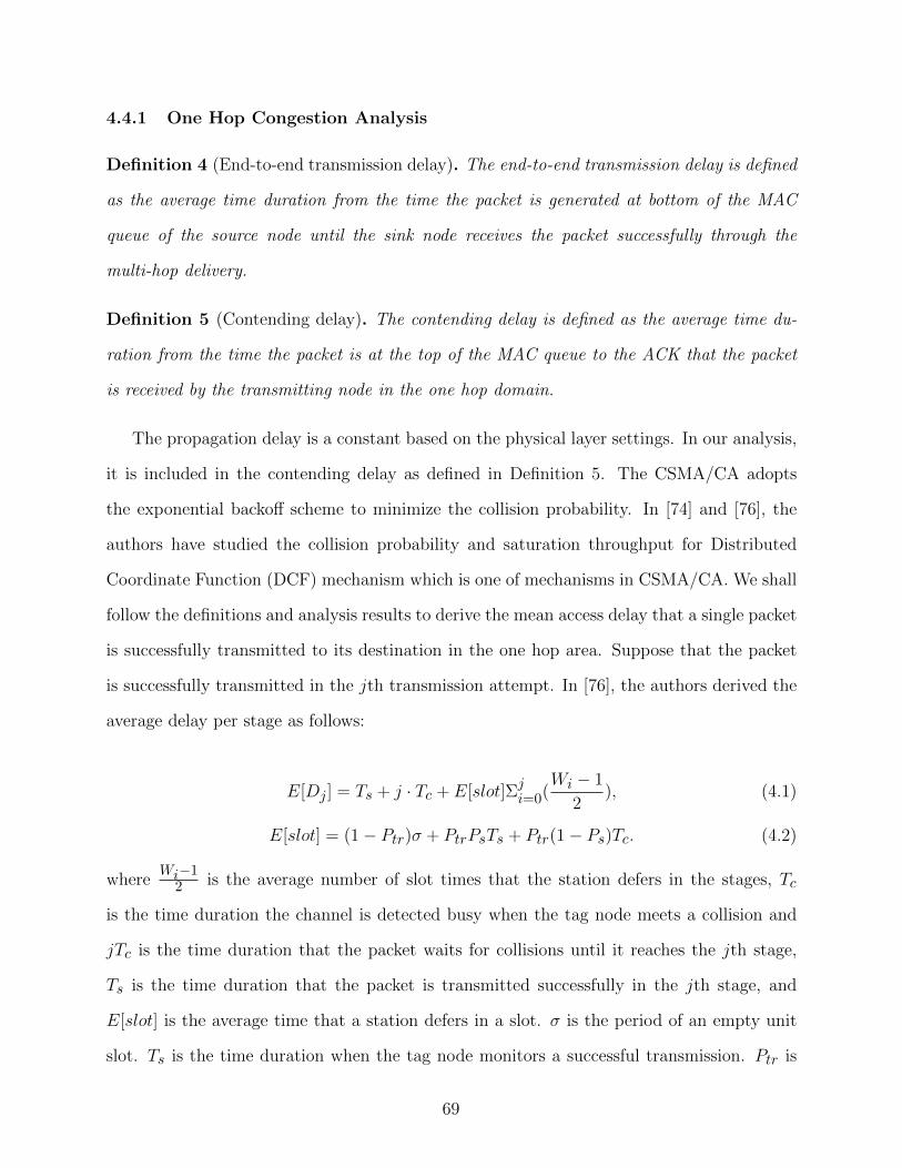
4.4.1 One Hop Congestion Analysis

Definition 4 (End-to-end transmission delay). The end-to-end transmission delay is defined

as the average time duration from the time the packet is generated at bottom of the MAC

queue of the source node until the sink node receives the packet successfully through the

multi-hop delivery.

Definition 5 (Contending delay). The contending delay is defined as the average time du-

ration from the time the packet is at the top of the MAC queue to the ACK that the packet

is received by the transmitting node in the one hop domain.

The propagation delay is a constant based on the physical layer settings. In our analysis,

it is included in the contending delay as defined in Definition 5. The CSMA/CA adopts

the exponential backoff scheme to minimize the collision probability. In [74] and [76], the

authors have studied the collision probability and saturation throughput for Distributed

Coordinate Function (DCF) mechanism which is one of mechanisms in CSMA/CA. We shall

follow the definitions and analysis results to derive the mean access delay that a single packet

is successfully transmitted to its destination in the one hop area. Suppose that the packet

is successfully transmitted in the jth transmission attempt. In [76], the authors derived the

average delay per stage as follows:

E[Dj ] = Ts + j · Tc + E[slot]Σji=0(

Wi − 1

2), (4.1)

E[slot] = (1− Ptr)σ + PtrPsTs + Ptr(1− Ps)Tc. (4.2)

whereWi−1

2 is the average number of slot times that the station defers in the stages, Tc

is the time duration the channel is detected busy when the tag node meets a collision and

jTc is the time duration that the packet waits for collisions until it reaches the jth stage,

Ts is the time duration that the packet is transmitted successfully in the jth stage, and

E[slot] is the average time that a station defers in a slot. σ is the period of an empty unit

slot. Ts is the time duration when the tag node monitors a successful transmission. Ptr is

69

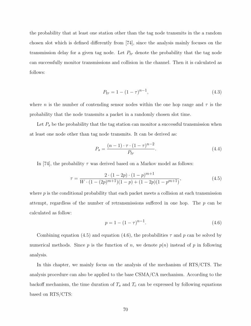
the probability that at least one station other than the tag node transmits in the a random

chosen slot which is defined differently from [74], since the analysis mainly focuses on the

transmission delay for a given tag node. Let Ptr denote the probability that the tag node

can successfully monitor transmissions and collision in the channel. Then it is calculated as

follows:

Ptr = 1− (1− τ)n−1, (4.3)

where n is the number of contending sensor nodes within the one hop range and τ is the

probability that the node transmits a packet in a randomly chosen slot time.

Let Ps be the probability that the tag station can monitor a successful transmission when

at least one node other than tag node transmits. It can be derived as:

Ps =(n− 1) · τ · (1− τ)n−2

Ptr. (4.4)

In [74], the probability τ was derived based on a Markov model as follows:

τ =2 · (1− 2p) · (1− p)m+1

W · (1− (2p)m+1)(1− p) + (1− 2p)(1− pm+1), (4.5)

where p is the conditional probability that each packet meets a collision at each transmission

attempt, regardless of the number of retransmissions suffered in one hop. The p can be

calculated as follow:

p = 1− (1− τ)n−1. (4.6)

Combining equation (4.5) and equation (4.6), the probabilities τ and p can be solved by

numerical methods. Since p is the function of n, we denote p(n) instead of p in following

analysis.

In this chapter, we mainly focus on the analysis of the mechanism of RTS/CTS. The

analysis procedure can also be applied to the base CSMA/CA mechanism. According to the

backoff mechanism, the time duration of Ts and Tc can be expressed by following equations

based on RTS/CTS:

70

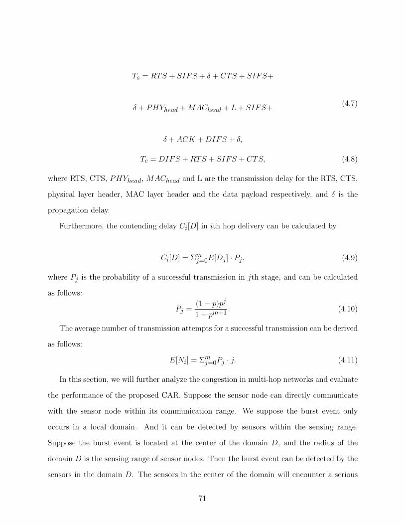
Ts = RTS + SIFS + δ + CTS + SIFS+

δ + PHYhead +MAChead + L+ SIFS+

δ + ACK +DIFS + δ,

(4.7)

Tc = DIFS +RTS + SIFS + CTS, (4.8)

where RTS, CTS, PHYhead, MAChead and L are the transmission delay for the RTS, CTS,

physical layer header, MAC layer header and the data payload respectively, and δ is the

propagation delay.

Furthermore, the contending delay Ci[D] in ith hop delivery can be calculated by

Ci[D] = Σmj=0E[Dj ] · Pj . (4.9)

where Pj is the probability of a successful transmission in jth stage, and can be calculated

as follows:

Pj =(1− p)pj1− pm+1

. (4.10)

The average number of transmission attempts for a successful transmission can be derived

as follows:

E[Ni] = Σmj=0Pj · j. (4.11)

In this section, we will further analyze the congestion in multi-hop networks and evaluate

the performance of the proposed CAR. Suppose the sensor node can directly communicate

with the sensor node within its communication range. We suppose the burst event only

occurs in a local domain. And it can be detected by sensors within the sensing range.

Suppose the burst event is located at the center of the domain D, and the radius of the

domain D is the sensing range of sensor nodes. Then the burst event can be detected by the

sensors in the domain D. The sensors in the center of the domain will encounter a serious

71

congestion. In fact, the number of sensor nodes competing for the channel access is λ ·S(D),

where λ is the density of sensor nodes and S(D) is the area of D. In the subsequent packet

delivery, the number of contending nodes may vary that is dependent on the topology and

the area of burst events. The probability that there is at least one collision in the multi-hop

delivery can be derived as:

Ph = 1− Σhi=1(1− p(ni)), (4.12)

where h denotes the hop distance from the source node to the sink node and ni is the number

of contending nodes in the ith hop.

In the ith hop transmission, the average transmission delay is calculated according to

equation (4.9). Then the end-to-end transmission delay through the delivery from the source

node to the sink node can be calculated using the following equation:

E[D] = Σhi=1Ci[D]. (4.13)

In addition, the energy of sensor nodes is largely consumed by the message transmitting

and receiving. The number of transmission attempts is one of the important issues for

energy consumption. In fact, the number of transmission attempts depends on the number of

contending nodes. Based on the aforementioned results, the average number of transmission

attempts for a successful transmission from the source node to the sink node in the multi-

layer network can be computed as follows:

N = Σhi=1Ni, (4.14)

where Ni is the average number of transmission attempts in the ith hop.

4.4.2 Numerical Results

In this section, we will give numerical results based on the theoretical analysis. Since the

number of contending nodes depends on the topology and area of events, we consider two

extreme cases for the multi-hop network: the worst case and the ideal case.

72

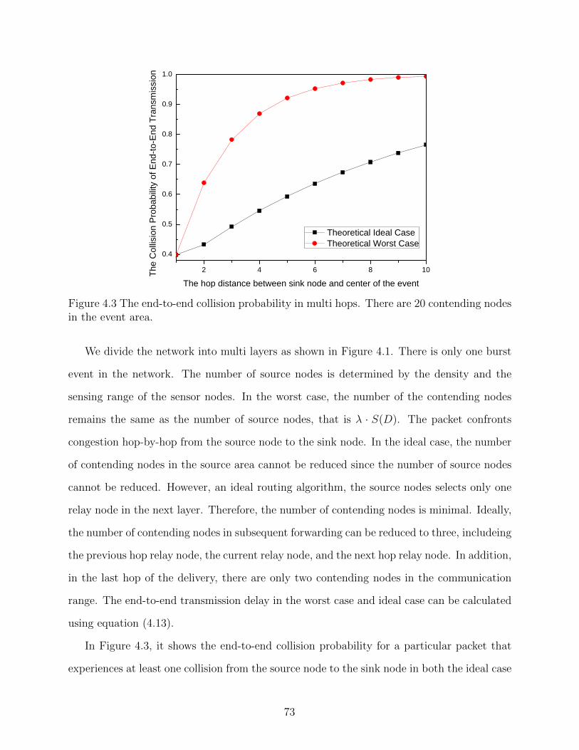
2 4 6 8 10

0.4

0.5

0.6

0.7

0.8

0.9

1.0

The

Col

lisio

n P

roba

bilit

y of

End

-to-E

nd T

rans

mis

sion

The hop distance between sink node and center of the event

Theoretical Ideal Case Theoretical Worst Case

Figure 4.3 The end-to-end collision probability in multi hops. There are 20 contending nodesin the event area.

We divide the network into multi layers as shown in Figure 4.1. There is only one burst

event in the network. The number of source nodes is determined by the density and the

sensing range of the sensor nodes. In the worst case, the number of the contending nodes

remains the same as the number of source nodes, that is λ · S(D). The packet confronts

congestion hop-by-hop from the source node to the sink node. In the ideal case, the number

of contending nodes in the source area cannot be reduced since the number of source nodes

cannot be reduced. However, an ideal routing algorithm, the source nodes selects only one

relay node in the next layer. Therefore, the number of contending nodes is minimal. Ideally,

the number of contending nodes in subsequent forwarding can be reduced to three, includeing

the previous hop relay node, the current relay node, and the next hop relay node. In addition,

in the last hop of the delivery, there are only two contending nodes in the communication

range. The end-to-end transmission delay in the worst case and ideal case can be calculated

using equation (4.13).

In Figure 4.3, it shows the end-to-end collision probability for a particular packet that

experiences at least one collision from the source node to the sink node in both the ideal case

73

and the worst case. It shows that in the ideal case, a properly designed routing algorithm

can reduce the number of contending nodes in subsequent transmission, therefore, it can

effectively decrease the end-to-end collision probability.

Then we give the numerical results of both end-to-end transmission delay and the number

of retransmission. The results are present in Figure 4.4 and Figure 4.5. The parameters in

the numerical results are listed in Table 4.1.

Table 4.1 Parameter setting of numerical results

Physical header 40 bits

MAC header 48 bits

RTS 40 bits

CTS 48 bits

Payload 250 bits

Channel bit rate 250k bits/s

Propagation delay, δ 1 µs

Slot time, σ 20 µs

SIFS 20 µs

DIFS 50 µs

Minimum CW, W 32

Number of CW size, m 5

4.5 Performance Analysis and Simulation Results

In this section, we provide theoretical evaluation and simulation results to demonstrate per-

formance of the proposed CAR routing scheme. Since congestion increases the transmission

delay and decreases packet receiving rate, we will mainly focus on the end-to-end transmis-

sion delay and the network throughput.

4.5.1 Performance Metrics

We will define two metrics to quantitatively evaluate the network performance.

74

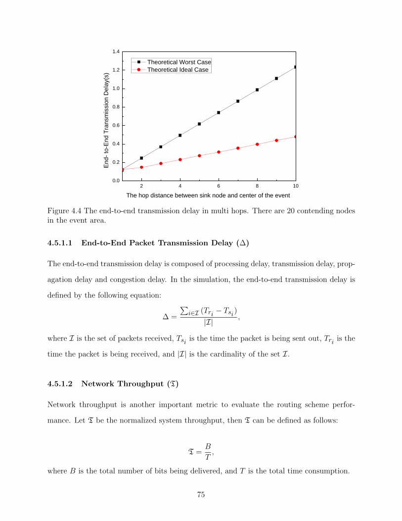
2 4 6 8 100.0

0.2

0.4

0.6

0.8

1.0

1.2

1.4

End

- to-

End

Tra

nsm

issi

on D

elay

(s)


Theoretical Worst Case Theoretical Ideal Case

Figure 4.4 The end-to-end transmission delay in multi hops. There are 20 contending nodesin the event area.

4.5.1.1 End-to-End Packet Transmission Delay (∆)

The end-to-end transmission delay is composed of processing delay, transmission delay, prop-

agation delay and congestion delay. In the simulation, the end-to-end transmission delay is

defined by the following equation:

∆ =

∑i∈I (Tri − Tsi)|I| ,

where I is the set of packets received, Tsi is the time the packet is being sent out, Tri is the

time the packet is being received, and |I| is the cardinality of the set I.

4.5.1.2 Network Throughput (T)

Network throughput is another important metric to evaluate the routing scheme perfor-

mance. Let T be the normalized system throughput, then T can be defined as follows:

T =B

T,

where B is the total number of bits being delivered, and T is the total time consumption.

75

2 4 6 8 100

3

6

9

12

15

18

The

Num

ber o

f Tra

nsm

issi

on A

ttem

pts


Theoretical Worst Case Theoretical Ideal Case

Figure 4.5 The number of retransmission through end-to-end transmission in multi hops.There are 20 contending nodes in the event area.

In the next subsection, our simulation results demonstrate that our proposed CAR rout-

ing scheme can achieve a performance close to the ideal scenario.

4.5.2 Simulation Results

We conduct simulations using OPNET in different scenarios to show the performance of

the proposed routing scheme. The results will be compared with a representative geographic

based routing protocol. We denote the proposed routing protocol as CAR and the geographic

based routing as MinRoute in the following simulation results.

4.5.2.1 Simulation Setup

The proposed CAR routing scheme is designed to reduce the link-level congestion. To show

the performance of CAR routing protocol, we conduct simulations with different event source

locations.

The sensing range is different from the communication range. Each sensor is able to

76

sense the event within the sensing range. The number of the sensor nodes that sensed the

burst events is determined by the topology and the sensing range. The actual number of

contending nodes is less than or equal to the number of source nodes due to the difference

between communication range and sensing range. The detailed simulation configurations are

summarized in Table 4.2, and two different simulation scenarios are described in Table 4.3

and Table 4.4.

Table 4.2 Simulation parameter setting

Area Size 100m× 100m

Deployment Type Random

Network Architecture Homogeneous sensor nodes

with one sink node

Number of Nodes 600

Sink Coordinate (90,90)

Communication Range 10m

Table 4.3 Simulation scenario 1: various event locations

Application Type Event-driven

Event Location (80,80); (70,70); (60,60);

(50,50); (40,40); (30,30);

(20,20)

Event Sensing Range 10m

Number of Source Nodes 18; 21; 18; 22; 16; 21; 18

Table 4.4 Simulation scenario 2: various sensing ranges

Application Type Event-driven

Event Location (20,20)

Event Sensing Range 2m; 4m; 6m; 8m; 10m

12m; 14m; 16m; 18m

20m;

Number of Source Nodes 2; 7; 16; 18; 27; 39; 49;

64 ; 76;

77

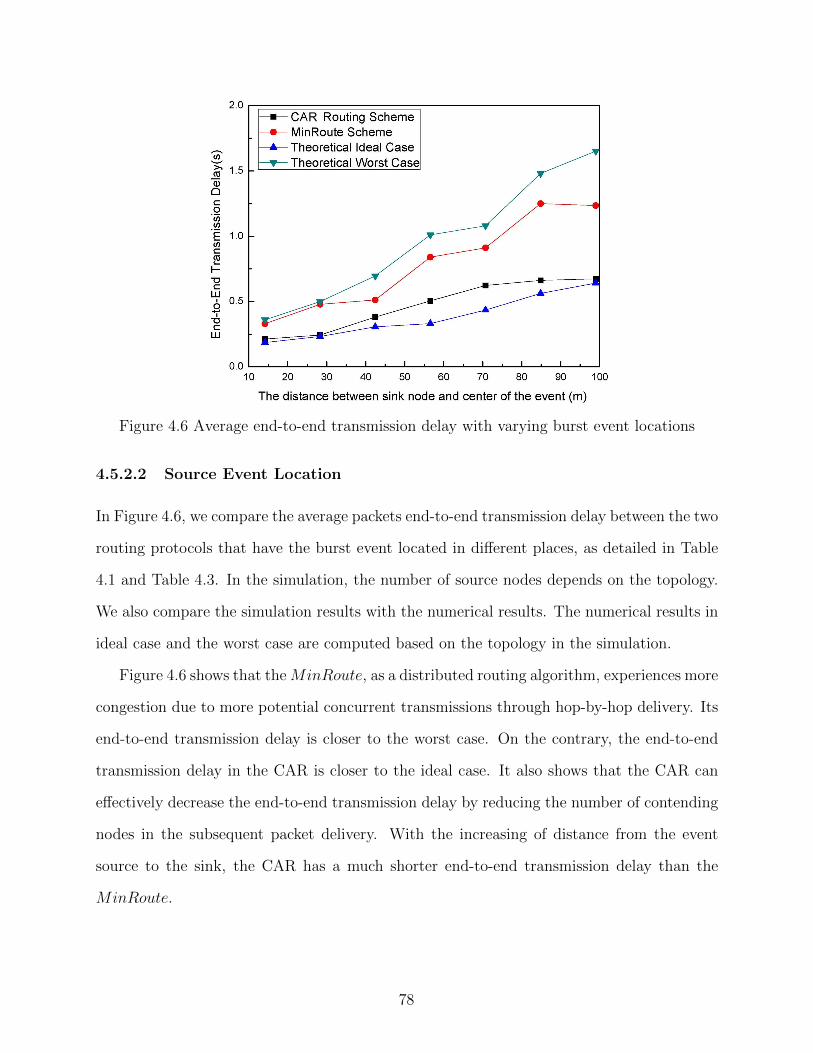
Figure 4.6 Average end-to-end transmission delay with varying burst event locations

4.5.2.2 Source Event Location

In Figure 4.6, we compare the average packets end-to-end transmission delay between the two

routing protocols that have the burst event located in different places, as detailed in Table

4.1 and Table 4.3. In the simulation, the number of source nodes depends on the topology.

We also compare the simulation results with the numerical results. The numerical results in

ideal case and the worst case are computed based on the topology in the simulation.

Figure 4.6 shows that theMinRoute, as a distributed routing algorithm, experiences more

congestion due to more potential concurrent transmissions through hop-by-hop delivery. Its

end-to-end transmission delay is closer to the worst case. On the contrary, the end-to-end

transmission delay in the CAR is closer to the ideal case. It also shows that the CAR can

effectively decrease the end-to-end transmission delay by reducing the number of contending

nodes in the subsequent packet delivery. With the increasing of distance from the event

source to the sink, the CAR has a much shorter end-to-end transmission delay than the

MinRoute.

78

4.5.2.3 Sensing Range

For a given node density, extending the event sensing range can increase the number of

source nodes. However, the number of contending nodes in event source area not only

depends on the number of source nodes but also on the communication range. The number

of contending nodes in the source area is determined by the sensing range and node density

if the sensing range is less than the communication range. If the sensing range is larger or

equal to the communication range, the number of contending nodes in the source area is

equal to λ ·S(D). However, in the multi-hop delivery, the number of contending nodes in the

subsequent forwarding can be affected by the number of source nodes since all the packets

are sent to the only sink node in the wireless sensor network. Therefore, increasing sensing

range leads to more link-level congestion for forwarding packets other than in the source

event area.

We conduct simulations for a fix event center to verify the impact of sensing range on

the performance of the CAR routing scheme. The settings of the simulations are detailed in

Table 4.4. In Figure 4.7 and Figure 4.8, the source event center is located at (80, 80) and

the sensing range increases from 2m to 20m. The number of source nodes increases with the

increment of the sensing range. It is also detailed in Table 4.4. In Figure 4.7, we compare

the end-to-end transmission delays between the CAR and the MiniRoute. We have similar

results as in Figure 4.6. CAR can effectively reduce the end-to-end transmission delay with

increasing the number of source nodes. In addition, the end-to-end transmission delay is

almost the same when there are only two source nodes that can hardly introduce congestion.

The gap of the end-to-end transmission delays between the two compared routing schemes

increases with the number of source nodes. The number of source nodes is equal to the

number of contending nodes before the sensing range reaches 10m. Furthermore, the end-to-

end transmission delay of MiniRoute increases rapidly when the event sensing range is larger

than the communication range 10m. It shows that the MiniRoute introduces much more

congestion after the turning point. Since the MiniRoute is initially designed as a distributed

79

Figure 4.7 Average end-to-end transmission delay with varying event sensing ranges

routing algorithm, the sensor node selects relay node independently. The only sink node in

the network makes the traffic more and more concentrated as the packets approach the sink

node. On the contrary, the end-to-end transmission delay in the CAR only increases linearly.

The Figure 4.7 shows that the proposed CAR has a stable performance. It can effectively

alleviate the congestion in the subsequent hop delivery. The simulation results on end-to-end

throughput is shown in Figure 4.8. It compares the results when the sensing range is larger

than the communication range.

4.6 Summary

In this chapter, we present a congestion-aware routing (CAR) scheme for WSNs to reduce

the link layer congestion. CAR routing utilizes the MAC layer traffic information to select

next hop relay node. The simulation results show that our proposed CAR routing scheme

can reduce the end-to-end packet transmission delay by more than 50% while increasing the

network throughput for more than two times in our settings.

80

Figure 4.8 Network throughput with varying event sensing ranges

81

CHAPTER 5

DELAY-AWARE AND PRIVACY PRESERVING DATA FORWARDING:DESIGN AND ANALYSIS

In this chapter, we propose a decentralized data forwarding scheme to preserve trajectory

privacy of participating users based on a combination of two-phase forwarding and secret

sharing. DAPP provides a design trade-off framework to address security, communication

delay and delivery ratio based on the selection of a (k, n) secret sharing scheme. The quan-

titative analysis and numerical results on security, communication delay and delivery ratio

will also be provided in this chapter.

5.1 Introduction

Urban sensing networks are designed to monitor urban environment. Recent technological

advances make urban sensing network feasible to rely on the sensors embedded in human-

carried mobile devices or vehicular electrical devices to collect and report data. As urban

sensing is more related to individuals, the location information collected with data may be

used to jeopardize users’ privacy. As mentioned in Chapter 1, the existing works for location

privacy protection can be divided into three categories, which are pseudonym based scheme,

compression based scheme and routing based scheme.

Pseudonym based schemes proposed in [44–47] mainly rely on a trusted third party

to dynamically assign pseudonyms to participating users to conceal their real identities.

Pseudonyms can be only used within mix-zones constructed by a trusted third party. The

assumption of the trusted third party cannot be always true. In addition, the mix-zones

cannot be placed through the entire network to preserve trajectory privacy.

Alternatively, compression based schemes in [41–43, 48–51] are designed to pre-process

the uploaded data to blur the reported location. The authors employed the techniques, such

82

as compression, aggregation, tessellation and dummy copies, to blur, suppress and even hide

the reported location contained in the collected data. The privacy protection is achieved by

sacrificing the resolution of either spatial or temporal dimensions, which may seriously cause

a loss for system QoS.

In routing based schemes [57–59], uploaded sensor readings are relayed by intermediate

nodes to the application data server hop by hop. In [58, 59], the proposed scheme is a

lack of protection for data confidentiality and vulnerable to side information attack. The

data relayed by intermediate nodes can be easily dropped and tampered with. Encryption

methods in [57] have been used to provide confidentiality of the collected data. However,

secret keys may introduce more security concerns. The secret keys may be possessed by all

sensor nodes or only shared between application data server and the source node. Hence,

either the application data server can identify the source node based key information or data

readings are made public to intermediate nodes.

Existing solutions may preserve location privacy of participating users, but without con-

sidering security from a cost-aware perspective. Few of them provide a quantitative analysis

on security and the relationship between security and its cost. In this dissertation, we pro-

pose a novel delay-aware privacy-preserving data forwarding scheme to address the two key

design issues, source location privacy and communication delay. DAPP is designed based on

a Sharmir’s secret sharing scheme and a two-phase forwarding algorithm. We also propose

a dynamic pseudonym scheme to conceal the identities of source nodes. DAPP cannot only

ensure data confidentiality and preserve location privacy, but also provide a data integrity

verification and defend against collusion attacks. The details of DAPP are presented in Sec-

tion 5.3. In Section 5.4, we conduct the quantitative analysis on security. The performance

evaluation and numerical results are provided in Section 5.5.

83

5.2 Models and Assumptions

5.2.1 System Model

Urban sensing network relies on a set of sensor nodes embedded in mobile devices or vehic-

ular systems for data sensing and reporting. These devices can get wireless Internet access

intermittently through wireless access points (APs) in the sensing area. The APs, such as

WiFi access points, may be owned and operated by the government, organizations or indi-

viduals. They are directly connected to the application data server. In this network, the

surrounding environment information is collected by the participating mobile devices and

eventually sent to the application data server.

The application data server provides environmental sensing services for data consumers

and disseminates the requested tasks to mobile devices carried by participants. Mobile de-

vices can join the system at will to participate in data sensing. They are required to report

the collected data to the application data server once they accept tasks. To provide pre-

cise services to data consumers, the data are required to be collected with spatial-temporal

information. Here we may use the term “report location” to indicate the spatial-temporal

information. The data format is {pID, (x, y), Td}, where pID is the pseudonym of the data

source, (x, y) is the coordinator where data is collected, and Td is the collecting time. This

information may divulge details about the participating user’s location. Due to the char-

acteristics of opportunistic sensing and physical infrastructure of the network, we only deal

with sensing data that is delay tolerant.

5.2.2 Adversarial Model

Our adversary model is similar to [42]. It can be summarized as follows:

• The adversary can be any parties in the network, including individual sensing nodes,

wireless access points, and even the application data servers.

84

• Adversaries are generally assumed to be honest but curious. We also assume that they

may drop or tamper with the reported data due to their own interests.

• The collected data are eventually forwarded to the application data server, which

enables it to disclose their reported location. The application data server may try to

uncover source identities of the received data and the trajectory.

• The participating user list is kept secret to delivery nodes and public, however, the

application data server can access the list due to its administrative right.

• Intermediate delivery nodes can obtain the source pseudonym of their received data.

They may collude to obtain the location privacy information or forge collected data to

fool the application data server.

5.2.3 Side Information Attack

Side information attack includes both direct side information attack and indirect side attack.

The direct side information refers to the information that an adversary can acquire based

on direct access to the communication. In our case, the direct side information may include

information {pID, (x, y), Td} of a particular event. In particular, the adversary can record

the set of identities I appear within its communication range. The nature of wireless

communications makes adversary able to extrapolate the source node located within its

communication range. If I is small enough by combining direct side information obtained,

the adversary may derive the actual ID and correlate it to the pID.

The indirect side information is defined as the information that an adversary can obtain

through indirect channels, such as media, video and web blog published on the internet,

of a particular event. In DAPP scheme, an adversary may receive data d, which contains

{pID, (x, y), Td}. To derive the actual source identity ID of pID, it may search through the

public domain to find the people who have visited location (x, y) at time Td. In this way,

the adversary may either completely identify the actual ID or limit it to a smaller subset.

85

5.2.4 Mobility Model

In urban sensing networks, sensor nodes are embedded in the mobile devices carried by

people or vehicles. In this dissertation, we apply the Manhattan street pedestrian model

described in [77]. The analysis for vehicular networks is similar based on mobility mode

presented in [78]. The Manhattan street model is proposed to emulate the movement pattern

of pedestrian on the streets. In this model, sensor nodes move on a two-way street segment.

The street segment can be modeled as a real street between two intersections. The arrivals

and departures of mobile nodes occur at the endpoints of the street segment. The velocities

of the mobile sensor nodes are independent and identically distributed (iid) random variables

with a probability density function fv(v). The direction and speed of a node remain constant

in one segment. Participating users arriving at both endpoints can be modeled as a Poisson

Process [79]. The total arrival rate is denoted as λ. At each endpoint, the mobile node

may alter its direction with a predetermined probability. The four directions at a cross road

are expressed as f(orward), l(eft), r(ight) and b(ackward), respectively. The probability for

going these directions at the intersection are Pf , Pr, Pl, Pb. This model assumes that

communications between two nodes in different street segments is not possible. As a result,

an existing connection breaks at the endpoints.

5.3 The Proposed DAPP Scheme

In this section, we present a novel delay-aware privacy-preserving (DAPP) data reporting

scheme based on a combination of Shamir’s secret sharing and two-phase routing. It can

ensure data confidentiality and also provide a data integrity verification option for the re-

ported data. We also propose a dynamic pseudonym scheme to guarantee anonymity of the

source node.

86

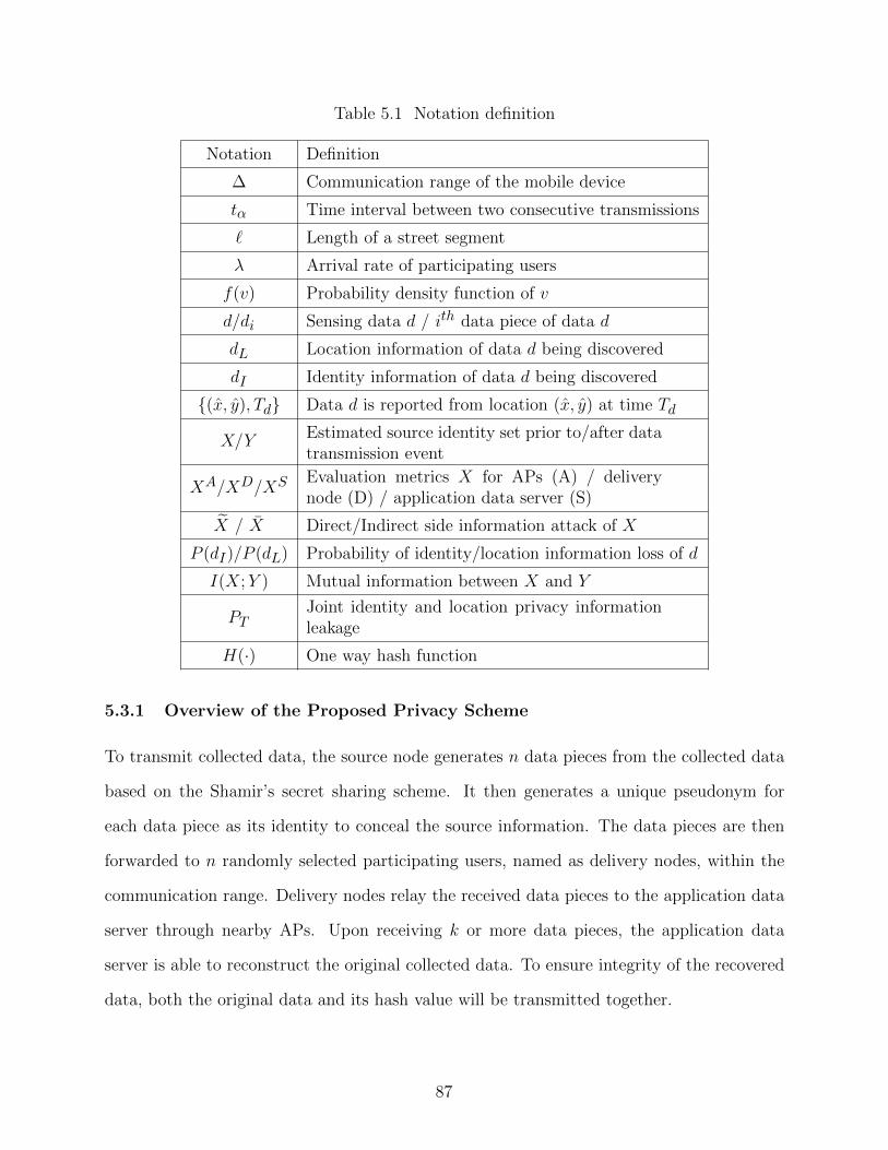
Table 5.1 Notation definition

Notation Definition

∆ Communication range of the mobile device

tα Time interval between two consecutive transmissions

` Length of a street segment

λ Arrival rate of participating users

f(v) Probability density function of v

d/di Sensing data d / ith data piece of data d

dL Location information of data d being discovered

dI Identity information of data d being discovered

{(x, y), Td} Data d is reported from location (x, y) at time Td

X/Y Estimated source identity set prior to/after datatransmission event

XA/XD/XS Evaluation metrics X for APs (A) / deliverynode (D) / application data server (S)

X / X Direct/Indirect side information attack of X

P (dI)/P (dL) Probability of identity/location information loss of d

I(X;Y ) Mutual information between X and Y

PTJoint identity and location privacy informationleakage

H(·) One way hash function

5.3.1 Overview of the Proposed Privacy Scheme

To transmit collected data, the source node generates n data pieces from the collected data

based on the Shamir’s secret sharing scheme. It then generates a unique pseudonym for

each data piece as its identity to conceal the source information. The data pieces are then

forwarded to n randomly selected participating users, named as delivery nodes, within the

communication range. Delivery nodes relay the received data pieces to the application data

server through nearby APs. Upon receiving k or more data pieces, the application data

server is able to reconstruct the original collected data. To ensure integrity of the recovered

data, both the original data and its hash value will be transmitted together.

87

5.3.2 Secret Sharing

In Shamir’s (k, n) secret sharing scheme, to share a secret S, the secret holder picks a

random k − 1 degree polynomial f(x) = a0 + a1x + a2x2 + · · · + ak−1x

k−1 over a finite

field Zq, where a0 = S and q > max(S, n) is a prime number. H generates n data pieces

Si = (i, f(i)), i = 1, · · · , n. The secret holder distributes the n data pieces to n individual

users.

The secret S can be recovered by k or more available data components using Barycentric

Lagrange Interpolation. The computational complexity to recover the secret S is only O(n).

More specifically, for k available data components, S can be recovered as follows:

1. For any k out of n secret pieces (i, f(i)), without loss of generality, we assume i =

0, · · · , k − 1. Define l(x) = (x− x0)(x− x1) · · · (x− xk−1).

2. Compute the weight

wj =1∏k

i=0,i 6=j(xj − xi). (5.1)

3. Let

lj(x) = l(x)wj

x− xjand

L(x) = l(x)k∑j=0

wjx− xj

yj . (5.2)

4. The shared secret is S = L(0).

5.3.3 Dynamic Pseudonyms

Pseudonyms have been widely used to prevent adversaries from obtaining source identities.

However, adversaries may use side information to link multiple pseudonyms or correlate

the pseudonyms to the actual identity. To solve this problem, we propose a new method

to generate dynamic pseudonyms using an ID-hash-chain. Instead of simply using hash

functions, we enable the source node to employ a secret key in the hash chain.

88

Suppose ID is the real identity of a participating user. To conceal it, the user replaces ID

with a dynamic changing pseudonym pIDi for each message transmission, where i is related

to the order of message. Each pseudonym is generated using a one way hash function H(·)

based on the previous pseudonym and the secret key. The ID-hash-chain {pID1, pID2, ...} for

the participating user ID is generated as follows:

pID1 = H(ID, K)

pID2 = H(pID1, K)

· · ·

where K is a secret key of the message source. Without knowing the secret key and the real

identity, establishing a linkage between pseudonyms, or between a pseudonym and the real

identity are both infeasible.

5.3.4 DAPP Scheme

In DAPP, to ensure security of the reporting data d, we generate n data pieces based on

Shamir’s secret sharing scheme. Each data piece is then forwarded to a randomly selected

delivery node. In this way, the original data can be concealed among n trustworthy secret

holders. The shared data d can be recovered by any k or more data pieces. Since we assume

the delivery nodes may tamper with the reporting data, the application server may receive

incorrect data pieces. Therefore, the application data server may not be able to recover the

original data. To deal with this issue, the proposed scheme is designed to be able to verify

the integrity of the recovered data.

We assume the source node H has data d to transmit. It first computes the hash value

H(d), where H(· ) is a one way hash function. d and H(d) are treated as two independent

secret data pieces. We randomly select two (k, n) secret sharing schemes to share d and H(d)

separately. The polynomial computation is operated over Zq. The procedure is described as

follows:

89

1. H chooses a prime q > max(d, n).

2. H constructs two coefficient sets, A and B. Each set contains k− 1 randomly selected

coefficients, A = {a0 = d, a1, ..., ak−1} and B = {b0 = H(d), b1, ..., bk−1} from Zq.

3. H generates two random polynomials over Zq as follows:

fa(x) =k−1∑i=0

aixi, (5.3)

fb(y) =k−1∑i=0

biyi. (5.4)

4. H computes n components fa(i), fb(i) from d and H(d), respectively, i = 1, · · · , n.

5. The ith data piece for d and H(d) is (i, fa(i), fb(i)), i = 1, · · · , n.

The proposed data distribution scheme is summarized in Algorithm 6.

Algorithm 6 Data Distribution

1: Choose a prime q > max(d, n).

2: Construct two coefficient sets A and B from Zq randomly.

3: Based on A and B, construct two polynomials fa(x) =∑k−1i=0 aix

i, and fb(y) =∑k−1i=0 biy

i over Zq to share d and H(d), respectively, as two secret values.

4: Compute n data pieces di = (i, fa(i), fb(i), q), i = 1, · · · , n.

5: Generate a pseudonym pID for d using ID-hash-chain.

6: for each i ∈ [1, n] do7: Send di to a randomly selected neighboring node Mi.

8: Insert an interval tα before sending di+1.

9: The neighboring node Mi forwards di to a wireless access point.

10: end for

DAPP includes two phases in data forwarding. In the first phase, the generated n data

pieces are distributed to n randomly selected delivery nodes before being relayed to the ap-

plication server. The data source may choose to add a time interval tα between transmissions

90

of two consecutive data pieces. A properly selected tα can effectively control the probability

for any single delivery node to receive multiple data pieces, especially in sparse networks.

Since delivery nodes may not be completely trusted, integrity of the reconstructed data has

to be verified. The reconstruction algorithm follows the Barycentric Lagrange Interpolation.

It is described in Algorithm 7.

Algorithm 7 Data Reconstruction and Verification

1: Suppose the server has received at least k out of n data pieces (i, fa(i), fb(i)) for data(d,H(d)).

2: The application data server reconstructs the original data using the Barcentric LagrangeInterpolation algorithm described in Equations (5.1) and (5.2).

3: The application data server verifies integrity of the reconstructed data by checkingwhether D = H(d) holds true.

5.4 Security Analysis

Source privacy information can be specified by two equally essential parts: spatial-temporal

information and identity information. Only when both are exposed, the complete privacy

information is disclosed.

In this section, we will provide quantitative analysis that DAPP can provide both identity

and spatial-temporal information from being disclosed to adversaries. We first introduce

several definitions and metrics.

5.4.1 Definitions and Security Metrics

Definition 6 (Identity information leakage). The identity information leakage for data d is

defined as the probability that an adversary is able to derive the source identity dI of data d.

We denote it as P (dI).

91

Definition 7 (Location information leakage). The location information leakage for data d is

defined as the probability that an adversary is able to derive the spatial-temporal information

dL of data d. The probability is denoted as P (dL).

To measure identity information loss of the received data, we introduce mutual informa-

tion.

Definition 8 (Identity information loss). Let X be the set of possible identities estimated

by adversaries prior to receiving a message, and Y be the set of estimated source identities

after receiving the message. The identity information loss for forwarding the message event

is defined as the mutual information between the X and Y . That is

I(X;Y ) = H(Y )−H(Y |X). (5.5)

Notice that source privacy information consists of both spatial-temporal information and

its correlated identity. We introduce the following metric to measure the joint information

loss.

Definition 9 (Joint information leakage). The joint identity and location privacy informa-

tion leakage PT for data d is defined as the joint probability that the adversary obtains the

spatial-temporal information and the identity of data d. That is

PT (d) = P (dL, dI)

= P (dL|dI)P (dI) (5.6)

= P (dI |dL)P (dL),

where dI and dL denote the the identity and location information of data d, respectively.

5.4.2 Identity Information Loss

The identity Information loss can be derived by the following theorem.

92

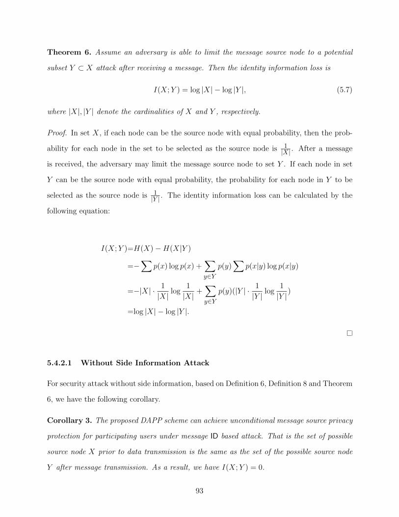
Theorem 6. Assume an adversary is able to limit the message source node to a potential

subset Y ⊂ X attack after receiving a message. Then the identity information loss is

I(X;Y ) = log |X| − log |Y |, (5.7)

where |X|, |Y | denote the cardinalities of X and Y , respectively.

Proof. In set X, if each node can be the source node with equal probability, then the prob-

ability for each node in the set to be selected as the source node is 1|X| . After a message

is received, the adversary may limit the message source node to set Y . If each node in set

Y can be the source node with equal probability, the probability for each node in Y to be

selected as the source node is 1|Y | . The identity information loss can be calculated by the

following equation:

I(X;Y )=H(X)−H(X|Y )

=−∑

p(x) log p(x) +∑y∈Y

p(y)∑

p(x|y) log p(x|y)

=−|X| · 1

|X| log1

|X| +∑y∈Y

p(y)(|Y | · 1

|Y | log1

|Y |)

=log |X| − log |Y |.

5.4.2.1 Without Side Information Attack

For security attack without side information, based on Definition 6, Definition 8 and Theorem

6, we have the following corollary.

Corollary 3. The proposed DAPP scheme can achieve unconditional message source privacy

protection for participating users under message ID based attack. That is the set of possible

source node X prior to data transmission is the same as the set of the possible source node

Y after message transmission. As a result, we have I(X;Y ) = 0.

93

Proof. DAPP introduces a two-phase message forwarding: distribution of data pieces to

randomly selected delivery nodes, and message forwarding to the application server through

the APs. Assume an adversary receives a data piece di with a unique pseudonym pID. Prior

to receiving di, the potential set for data source can be arbitrary nodes in the entire set of

population in the urban area of the delivery nodes since they are not entitled to access the

list of the participating users. For the application data server, since it has access to the

participating user list, the priori estimated set is the same as the participating users.

Through message forwarding, the adversary obtains pID instead of ID of di. The proposed

dynamic pseudonym makes it infeasible for adversaries to derive ID from pID without secret

key K. Hence, the posterior estimated identity set Y based on message forwarding event is

also equal to X. Therefore, I(X;Y ) = 0.

5.4.2.2 Side Information Attack

Side information attack is envisioned as one of the major threats to data privacy. It may

divulge part or even the entire source identity information.

Corollary 4. For DAPP, through direct side information attack, the identity information

loss to the delivery node (ID), the AP (IS) and the application data server (IA) can be

derived as follows:

ID(X;Y ) = log |X| − log |Y |, (5.8)

IS(X;Y ) = IA(X;Y ) = 0, (5.9)

where |X|, |Y | denote the cardinalities of X and Y , respectively.

Proof. Direct side information is obtained through traffic monitoring during message for-

warding. The data pieces are relayed to the application data server by randomly selected

delivery nodes. The application data server and APs may possibly collect direct side infor-

mation only about delivery nodes rather than the source node. Therefore, they are unable

94

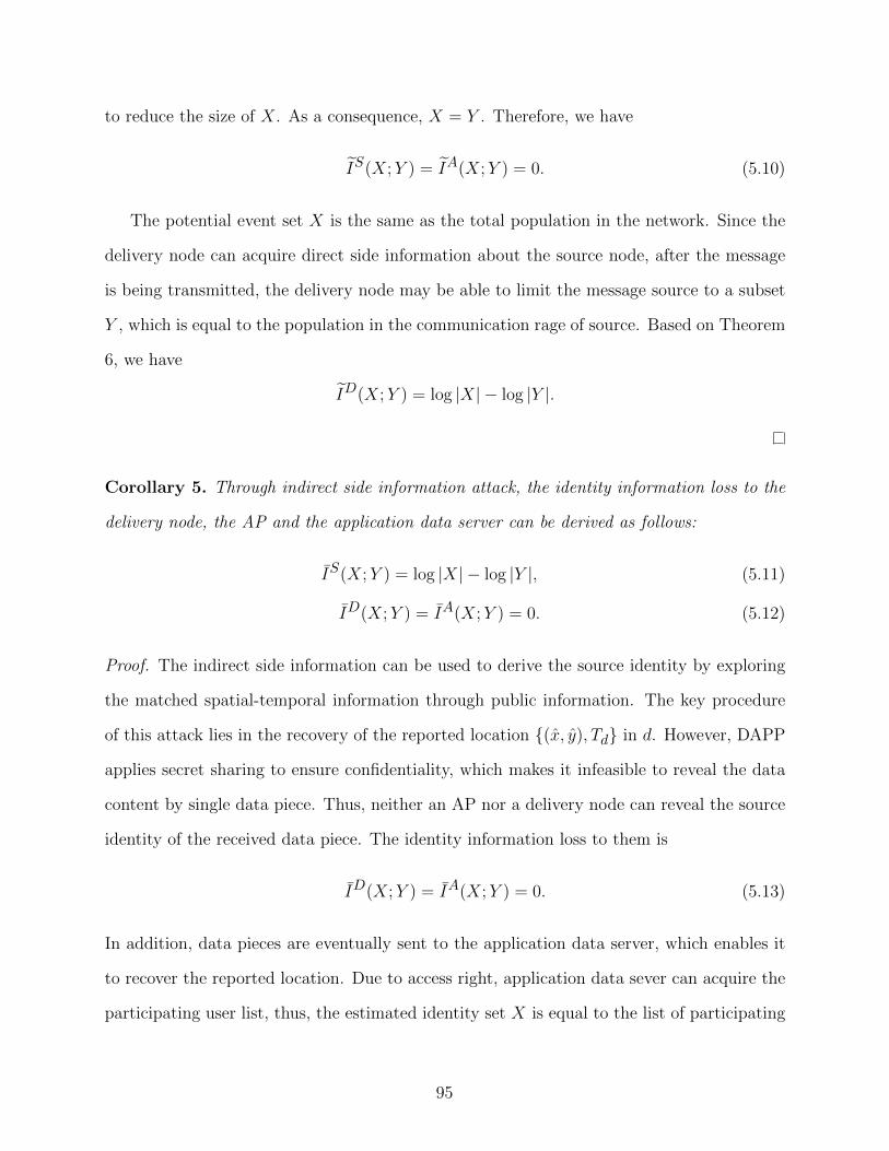
to reduce the size of X. As a consequence, X = Y . Therefore, we have

IS(X;Y ) = IA(X;Y ) = 0. (5.10)

The potential event set X is the same as the total population in the network. Since the

delivery node can acquire direct side information about the source node, after the message

is being transmitted, the delivery node may be able to limit the message source to a subset

Y , which is equal to the population in the communication rage of source. Based on Theorem

6, we have

ID(X;Y ) = log |X| − log |Y |.

Corollary 5. Through indirect side information attack, the identity information loss to the

delivery node, the AP and the application data server can be derived as follows:

IS(X;Y ) = log |X| − log |Y |, (5.11)

ID(X;Y ) = IA(X;Y ) = 0. (5.12)

Proof. The indirect side information can be used to derive the source identity by exploring

the matched spatial-temporal information through public information. The key procedure

of this attack lies in the recovery of the reported location {(x, y), Td} in d. However, DAPP

applies secret sharing to ensure confidentiality, which makes it infeasible to reveal the data

content by single data piece. Thus, neither an AP nor a delivery node can reveal the source

identity of the received data piece. The identity information loss to them is

ID(X;Y ) = IA(X;Y ) = 0. (5.13)

In addition, data pieces are eventually sent to the application data server, which enables it

to recover the reported location. Due to access right, application data sever can acquire the

participating user list, thus, the estimated identity set X is equal to the list of participating

95

users. Based on indirect side information, it can limit X into a subset Y , which is depended

on the accuracy of indirect side information.

IS(X;Y ) = log |X| − log |Y |.

5.4.3 Location Information Leakage

Spatial-temporal information is equally essential for source privacy. In the subsequent anal-

ysis, we will discuss the location information leakage of DAPP. We first prove that the data

distribution process follows Poisson process.

Theorem 7. The process of data distribution in the first forwarding phase of the proposed

DAPP scheme is a Poisson process.

Proof. In the Manhattan street model, the node arrival and departure at an endpoint of a

street segment is a Poisson process. It is straightforward to derive that the arrival process at

any points in the street segment parallelizing the endpoint is also a Poisson process. Suppose

that the participant A encounters n participants when it stays at the point (xi, yi). And it

stays at the point for a time duration δ (δ → 0). The node arrival rate at this point is λ. So

the probability that A meets n participants is

p(N(δ + t)−N(t) = n) = e−λδ · (λδ)n

n!, (5.14)

where N(t) is the number of participants that node A has encountered from time 0 to time

t.

Suppose A needs T seconds to move from (xi, yi) to (xj , yj). So the process for A to

encounter other participants for time duration T is the sum of encounter processes from

location (xi, yi) to (xj , yj). These meeting processes are mutually independent. Since the

number of the independent Poisson processes is Tδ , the sum of multiple Poisson processes is

96

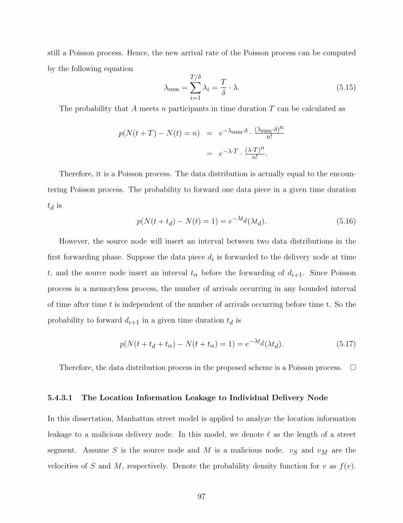
still a Poisson process. Hence, the new arrival rate of the Poisson process can be computed

by the following equation

λsum =

T/δ∑i=1

λi =T

δ· λ. (5.15)

The probability that A meets n participants in time duration T can be calculated as

p(N(t+ T )−N(t) = n) = e−λsum·δ · (λsum·δ)nn!

= e−λ·T · (λ·T )n

n! .

Therefore, it is a Poisson process. The data distribution is actually equal to the encoun-

tering Poisson process. The probability to forward one data piece in a given time duration

td is

p(N(t+ td)−N(t) = 1) = e−λtd(λtd). (5.16)

However, the source node will insert an interval between two data distributions in the

first forwarding phase. Suppose the data piece di is forwarded to the delivery node at time

t, and the source node insert an interval tα before the forwarding of di+1. Since Poisson

process is a memoryless process, the number of arrivals occurring in any bounded interval

of time after time t is independent of the number of arrivals occurring before time t. So the

probability to forward di+1 in a given time duration td is

p(N(t+ td + tα)−N(t+ tα) = 1) = e−λtd(λtd). (5.17)

Therefore, the data distribution process in the proposed scheme is a Poisson process.

5.4.3.1 The Location Information Leakage to Individual Delivery Node

In this dissertation, Manhattan street model is applied to analyze the location information

leakage to a malicious delivery node. In this model, we denote ` as the length of a street

segment. Assume S is the source node and M is a malicious node. vS and vM are the

velocities of S and M , respectively. Denote the probability density function for v as f(v).

97

Let tM be the time duration that a malicious node stays in the source node communication

range ∆. Then we have tM = 2∆z , where z = |vM −vS |. We also use P (tM > ktα) to denote

the probability that a sensor node stays in the source node communication range at least

ktα seconds. Let PM be the probability that a malicious node M is selected as the delivery

node in one data piece distribution, and c be the number of times that M has been selected

as the delivery node.

Theorem 8. Assume velocities of the malicious node and the source node are two inde-

pendent and identically distributed (i.i.d.) random variables, then the location information

leakage to the malicious delivery node can be derived as follows:

PD(dL) =

ˆ 2∆ktα

− 2∆ktα

f(z)dz

×n∑i=k

(1

4

)⌊2itαvS`

⌋(n

i

)P iM (1− PM )n−i

,(5.18)

where f(z) is the joint probability density function of z = |vM − vS |.

Proof. Since the data content can be closely related to the reporting location, leakage of

message content may inadvertently expose the source location. To deal with this potential

security issue, DAPP utilizes secret sharing to ensure data confidentiality by generating

multiple seemingly meaningless data pieces and delivers each piece through a randomly

selected delivery node. In this way, the malicious node will not be able to get the content of

the data unless it is capable of collecting up to k or more data pieces.

There are two possible scenarios for a malicious node to obtain k data pieces: (i) The

malicious node comes across the data source node at least k times to collect the data pieces

from the source node during the entire duration of the message transmission; and (ii) The

malicious node stays in the communication range of the source node at least ktα seconds.

In the first case, since velocities of the participating users are independent, the spatial

dependence degree of two arbitrary nodes is approximately 0 according to [80], which means

98

that the probability for two nodes to meet for the second time is approximate to 0 within a

limited short time duration. Thus, probability for the first case can be viewed as 0.

The success of the malicious node is determined by the likelihood of the second case.

Assume f(z) is the joint probability density function of z = |vM − vS |, then we have

P (tM ≥ ktα) = P

(2∆

z≥ ktα

)= P

(z ≤ 2∆

ktα

)=

ˆ 2∆ktα

− 2∆ktα

f(z)dz.

(5.19)

The success of case (ii) requires the malicious node to be selected as the delivery node

at least k times. In DAPP, the source node selects delivery nodes based on the principle of

randomness, thus each node in the source communication range can be selected as delivery

node with equal probability PM = 1|X| , where |X| is the total number of participants in

the communication range of S. Based on Theorem 7, the process of the participating users’

arrival and departure can be modeled as M/G/∞ based on Theory of Queues. In this model,

the source node can be denoted as the service node. tM is actually the service time for a

given participating user. Moreover, suppose λ is the arrival rate and T is the average service

time. Hence, we can have

|X| = λ · T. (5.20)

Since ` is the length of of a street segment, we have tM ≤ `max[vS,vM ]

. Without loss of

the generality, we may assume vS ≥ vM , then,

T = 2 ·ˆ ν

2∆vS`

2∆

zf(z)dz, (5.21)

where ν = Vmax − Vmin, Vmax and Vmin represent the maximum and minimum speed of the

participating users.

The location information leakage in one street segment can be described as the joint

probability of tM ≥ ktα and c ≥ k. That is

99

PD(dL)=P (tM ≥ ktα, c ≥ k)

=P (tM ≥ ktα)P (c ≥ k | tM ≥ ktα)

=P (tM ≥ ktα)n∑i=k

(n

i

)P iM (1− PM )n−i. (5.22)

In equation (5.22), all data pieces are assumed to be distributed in one street segment.

In fact, these data pieces may be distributed in several streets. S and M may change their

velocities at the endpoint of the street segment. Hence, M can stay in the communication

range of S only if they moves in the same direction. To simplify the analysis, we assume

that the probability for each direction is equal to 14 . Thus, the probability that S and M

choose same direction at an endpoint is equal to (14)2. Therefore,

PD(dL) =P (tM > ktα)

×n∑i=k

(1

4

)⌊2itαvS`

⌋(n

i


. (5.23)

Combining equation (5.19) and equation (5.23), we can get equation (5.18).

From Theorem 8, we can derive the following corollary.

Corollary 6.

limktα→∞

PD(dL) = 0. (5.24)

Proof. From equation (5.18), we have

PD(dL) =

ˆ 2∆ktα

− 2∆ktα

f(z)dz

n∑i=k

(1

4

)⌊2itαv0`

⌋(n

i


≤ˆ 2∆

ktα

− 2∆ktα

f(z)dz ·(

1

4

)⌊2ktαvS`

⌋.

(5.25)

100

Since both´ 2∆ktα

− 2∆ktα

f(z)dz and(

14

)⌊2ktαvS`

⌋are asymptotically equivalent to 0 as ktα →∞.

Therefore, we have limktα→∞ PD(dL) = 0.

5.4.3.2 The Location Information Leakage to APs

In the second forwarding phase, delivery nodes transmit the data pieces to APs, which are

assumed to be uniformly distributed in urban area. Thus, each AP has equal probability to

receive the data piece and we have the following corollary.

Corollary 7. The location information leakage to each AP can be computed by the following

equation

PA(dL) =n∑i=k

(n

i

)(1

η

)i(1− 1

η

)η−i, (5.26)

where η is the number of wireless APs in urban area. From this equation, we can see that

the location information leakage to delivery node and each AP is asymptotically equivalent

to 0 as k →∞.

5.4.4 Joint Identity and Location Privacy Information Leakage

We have discussed the identity information loss and the location information leakage sepa-

rately. The results show that the delivery node may only obtain partial identity information

that is insufficient to identify the data source. However, the reported location and the iden-

tity information may be dependent on side information attack. In order to elaborate privacy

information loss, we further investigate privacy leakage when these two pieces are considered

jointly.

Theorem 9. For the joint identity and location privacy information leakage, we have

limktα→∞

PDT = 0

limk=nn→∞

PAT = 0. (5.27)

101

Proof. Based on Definition 9, we have

PDT ≤ PD(dL),

PAT ≤ PA(dL).

The equalities in above equations may hold if the adversary can collect k or more data pieces

through side information attack. Thus, the joint identity and location privacy information

leakages to an AP and a delivery node are both dependent on the parameters (k, n; tα).

Based on Corollary 6, we have

limktα→∞

PDT ≤ limktα→∞

PD(dL) = 0.

From equation (5.26), the joint identity and location privacy information leakage to an AP

can be derived as follows

0 ≤ limk=nn→∞

PAT ≤ limk=nn→∞

PA(dL) = limk→∞

(1

η

)k= 0.

Similarly, for the application server, we have the following corollary.

Corollary 8. For the application data server, the joint identity and location privacy infor-

mation under side information attacks can be calculated by

PST =1

|Y | .

5.4.5 Participating Nodes Collusion

Participating users may conspire or share information to infer privacy information of others.

Assume there are κ (κ ≤ k1) malicious nodes in the network, where k1 is the number of

delivery nodes in urban sensing networks. The probability for an arbitrary delivery node to

102

be malicious is κk1

. Hence, the location information leakage of the reported data d is

PC(dL) =n∑i=k

(n

i

)(κ

k1

)i(1− κ

k1

)n−i. (5.28)

For each data piece di, the malicious delivery node may record a potential identity set

through traffic monitoring, I i = {ai0, · · · , ail}. As the direct side information can be shared,

the colluding users could limit the source identity to be an element in the intersection⋂ki=0 I i. The joint identity and location privacy information PCT for collusion attacks falls

as the location information leakage PC(dL) decreases. Based on equation (5.28), PC(dL)

decreases to ( κk1)k as k increases to n. Then, PCT can be asymptotically equivalent to 0 as

k = n and k →∞. Therefore, we have the following corollary.

Corollary 9.

limk=nn→∞

PCT ≤ limk=nn→∞

PC(dL) = limk→∞

(κ

k1

)k= 0.

The numerical result is presented in Table 5.2. It shows that the location privacy infor-

mation leakage can be minimized with increasing k for a given n. Furthermore, with a proper

setting on (k, n), DAPP can defend against collusion attacks even if there is a relatively high

ratio of malicious delivery nodes.

5.4.6 Data Integrity

In reality, delivery nodes may drop, tamper with and forge the received data due to their

own interests. To deal with these issues, DAPP provides a mechanism to verify the integrity

of the received data. The application data server needs k untampered data pieces to recover

the original data d and D. In case that at least one data piece in the set of k pieces has

been tampered with, we should have H(d) 6= D. Therefore, the recovered data can detect

whether the data set contains any corrupted data pieces as well as integrity of the recovered

data.

103

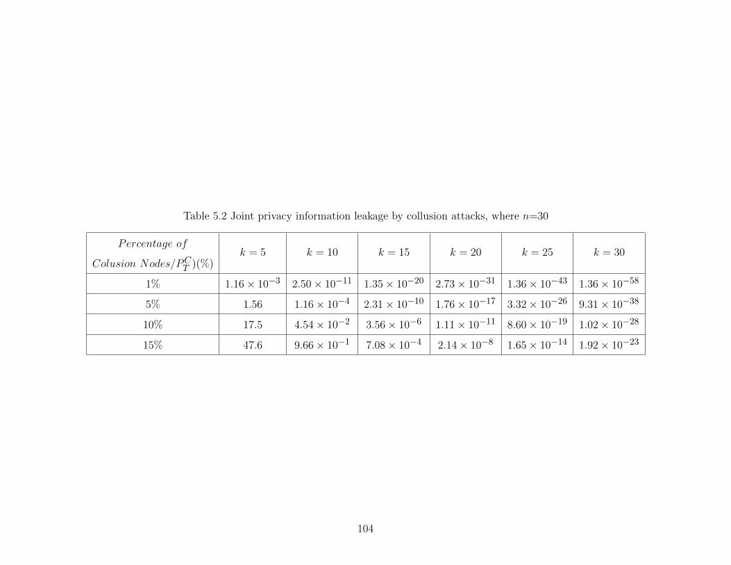
Table 5.2 Joint privacy information leakage by collusion attacks, where n=30

Percentage ofk = 5 k = 10 k = 15 k = 20 k = 25 k = 30

Colusion Nodes/PCT )(%)

1% 1.16× 10−3 2.50× 10−11 1.35× 10−20 2.73× 10−31 1.36× 10−43 1.36× 10−58

5% 1.56 1.16× 10−4 2.31× 10−10 1.76× 10−17 3.32× 10−26 9.31× 10−38

10% 17.5 4.54× 10−2 3.56× 10−6 1.11× 10−11 8.60× 10−19 1.02× 10−28

15% 47.6 9.66× 10−1 7.08× 10−4 2.14× 10−8 1.65× 10−14 1.92× 10−23

104

5.5 Performance Evaluation and Simulation Results

In urban sensing networks, QoS can be measured by communication delay and delivery ratio.

In this section, we analyze the communication delay and error rate of DAPP scheme.

5.5.1 Communication Delay

DAPP scheme includes two phases for data forwarding: data forwarding from the source

node to the delivery nodes, and from the delivery nodes to the application data server.

In the first phase, let the communication delay for the ith data piece distribution is τi,

which includes two parts. One part of the delay is introduced to encounter the ith delivery

node, denoted as γi. Theorem 7 proves that the data distribution process is a Poisson

process. Hence, γi should follow Γ distribution. The probability distribution function for γi

is given by

fγi(t) = λe−λt · (λt)(n−1)

(n− 1)!, (5.29)

where λ is the arrival rate of Poisson process. The second part is introduced by the inserted

constant interval tα. For the ith delivery node, the delay is equal to itα.

In the second phase, the delay is the time duration from the time that the delivery node

receives a data piece until it reaches the next AP. Suppose the delivery node receives one

data piece at time t and T is the average time duration that the delivery node travels from

one AP to the next AP. The time t should be uniformly distributed in the range of T . We

denote the delay in the second forwarding phase as ti for each data piece di. The total

communication delay Td can be computed as follows:

Td = min1→k{γi + ti + itα |i = 1, · · · , k}, (5.30)

where γi+ti+itα is the delay for the application data server to receive the ith data component,

and min1→k is the function to find the kth minimum value of a given set. Equation (5.30)

shows that the overall delay is determined by k when it is large. Table 5.4 gives numerical

results for various k values.

105

Table 5.3 The error rate for the reported data, where n=30

PE(%) k = 5 k = 10 k = 15 k = 20 k = 25

pe = 1% 2.64× 10−46 1.31× 10−33 1.27× 10−22 4.59× 10−13 4.83× 10−5

pe = 2% 1.70× 10−38 2.52× 10−27 7.31× 10−18 7.87× 10−10 2.51× 10−3

pe = 3% 6.20× 10−34 1.15× 10−23 4.19× 10−15 5.70× 10−8 2.33× 10−2

pe = 4% 1.05× 10−30 4.43× 10−21 3.65× 10−13 1.13× 10−6 1.06× 10−1

pe = 5% 3.35× 10−28 4.39× 10−19 1.13× 10−11 1.10× 10−5 3.28× 10−1

5.5.2 Delivery Ratio

Due to the nature of the wireless communications, the message received may contain errors.

Unreliable delivery nodes may even drop the received data pieces for their own interests. To

deal with this problem, the proposed scheme introduces redundancy to minimize the error

rate for the reporting data. The underlying secret sharing scheme ensures the reported data

can be recovered by receiving k or more valid data pieces. The extra n− k data pieces add

redundancy that can be employed for data recovery under erroneous scenarios. Let pe be

the error rate or packet loss rate of a single data piece. The overall error rate PE for the

reported data can be computed by the following equation:

PE =n∑

i=n−k+1

(n

i

)pie(1− pe)n−i. (5.31)

Based on equation (5.31), for a given n, the overall error rate PE decreases when k reduces,

and the overall error rate PE can be minimized by increasing the number of redundant

packets. Table 5.3 provides numerical results of the overall error rate for various k’s.

5.5.3 Trade-off Design

In this dissertation, DAPP is designed to achieve trade-off among several conflicting design

issues in urban sensing networks. It leverages the relationship between configurable scheme

parameters and system performance to provide flexible options for system users. Based

106

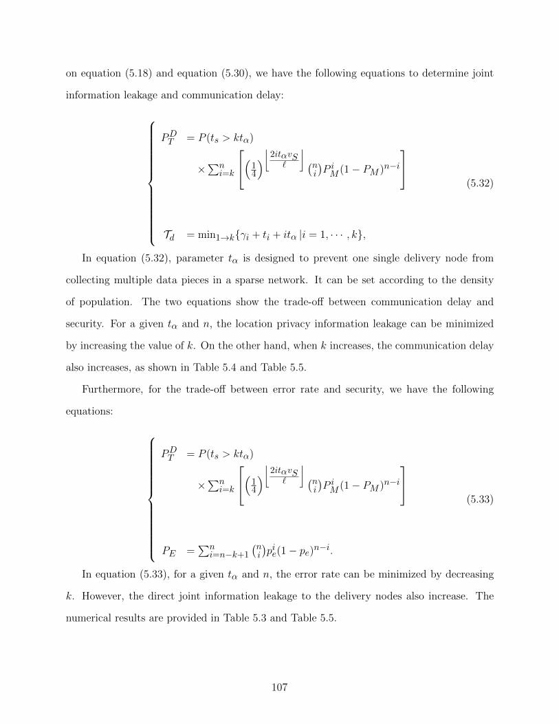
on equation (5.18) and equation (5.30), we have the following equations to determine joint

information leakage and communication delay:

PDT = P (ts > ktα)

×∑ni=k

(14

)⌊2itαvS`

⌋ (ni


Td = min1→k{γi + ti + itα |i = 1, · · · , k},

(5.32)

In equation (5.32), parameter tα is designed to prevent one single delivery node from

collecting multiple data pieces in a sparse network. It can be set according to the density

of population. The two equations show the trade-off between communication delay and

security. For a given tα and n, the location privacy information leakage can be minimized

by increasing the value of k. On the other hand, when k increases, the communication delay

also increases, as shown in Table 5.4 and Table 5.5.

Furthermore, for the trade-off between error rate and security, we have the following

equations:

PDT = P (ts > ktα)

×∑ni=k

(14

)⌊2itαvS`

⌋ (ni


PE =∑ni=n−k+1

(ni

)pie(1− pe)n−i.

(5.33)

In equation (5.33), for a given tα and n, the error rate can be minimized by decreasing

k. However, the direct joint information leakage to the delivery nodes also increase. The

numerical results are provided in Table 5.3 and Table 5.5.

107

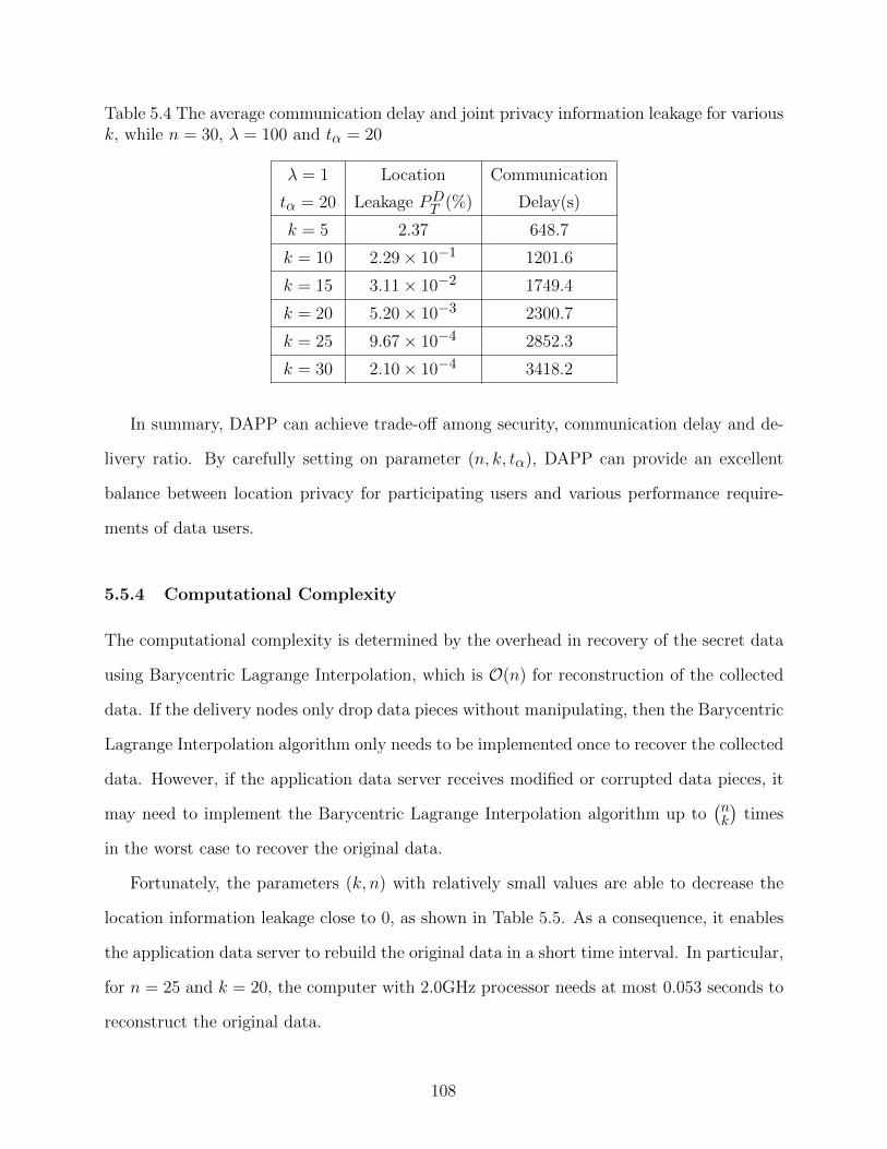
Table 5.4 The average communication delay and joint privacy information leakage for variousk, while n = 30, λ = 100 and tα = 20

λ = 1 Location Communication

tα = 20 Leakage PDT (%) Delay(s)

k = 5 2.37 648.7

k = 10 2.29× 10−1 1201.6

k = 15 3.11× 10−2 1749.4

k = 20 5.20× 10−3 2300.7

k = 25 9.67× 10−4 2852.3

k = 30 2.10× 10−4 3418.2

In summary, DAPP can achieve trade-off among security, communication delay and de-

livery ratio. By carefully setting on parameter (n, k, tα), DAPP can provide an excellent

balance between location privacy for participating users and various performance require-

ments of data users.

5.5.4 Computational Complexity

The computational complexity is determined by the overhead in recovery of the secret data

using Barycentric Lagrange Interpolation, which is O(n) for reconstruction of the collected

data. If the delivery nodes only drop data pieces without manipulating, then the Barycentric

Lagrange Interpolation algorithm only needs to be implemented once to recover the collected

data. However, if the application data server receives modified or corrupted data pieces, it

may need to implement the Barycentric Lagrange Interpolation algorithm up to(nk

)times

in the worst case to recover the original data.

Fortunately, the parameters (k, n) with relatively small values are able to decrease the

location information leakage close to 0, as shown in Table 5.5. As a consequence, it enables

the application data server to rebuild the original data in a short time interval. In particular,

for n = 25 and k = 20, the computer with 2.0GHz processor needs at most 0.053 seconds to

reconstruct the original data.

108

5.5.5 Numerical Simulation Results

In numerical simulations, we assume vi follows the uniform distribution in the range of

[Vmin, Vmax]. The results of other distributions are similar. To emulate the reality, we set up

both dense network and sparse network to show the joint information leakage to the delivery

node. In the two scenarios, we select various parameters (k, n, tα) to show the relationship

between the settings and the security performance against intermediate delivery node under

side information attack.

In the first scenario, we set the average number of people in the communication range of

the source node as λ = 10, and tα = 1. With a proper setting on (k, n), PM is small enough

to make the joint information leakage approximated to 0. The joint information leakage to

the delivery node is presented in Table 5.5.

In the second scenario, we consider a sparse network in the urban area. We set λ = 100.

Then through equation (5.20) and equation (5.21), we can derive that the average number

of people in the communication range of source node to be around 1. As a consequence,

there may be only one neighbor node around the source node to be selected as delivery

node. In such a scenario, the joint information leakage is determined by the value of P (ts ≥

ktα) ·(

14

)⌊2ktαv0L

⌋. To minimize this value, we raise tα to 20 and let k increases from 5 to

30. The joint information leakage to the delivery node is shown in Table 5.3 and Table 5.5.

The simulation results of the tables can be summarized as follows:

• Location privacy can be preserved in the proposed DAPP scheme under side informa-

tion attack.

• With proper parameter settings, the joint information leakage can be minimized to

approximately 0 for each delivery node.

• The joint information leakage, average communication delay and error rate can be

adjusted by the selection on system parameters.

109

5.6 Summary

In this chapter we propose a delay-aware privacy preserving (DAPP) data forwarding scheme

for people-centric urban sensing networks. It is developed based on Sharmir’s secret sharing,

dynamic pseudonyms and a two-phase data forwarding method. The two-phase forwarding

method detaches the connection between the source node and the application data server.

The Shamir’s secret sharing based scheme prevents delivery nodes from discovering privacy

information in the reported data. The proposed dynamic pseudonym scheme can provide

anonymity of identity against side information attacks. Both theoretical analysis and simu-

lation results demonstrate that the proposed DAPP can provide an excellent design trade-off

among security, communication delay and delivery ratio.

110

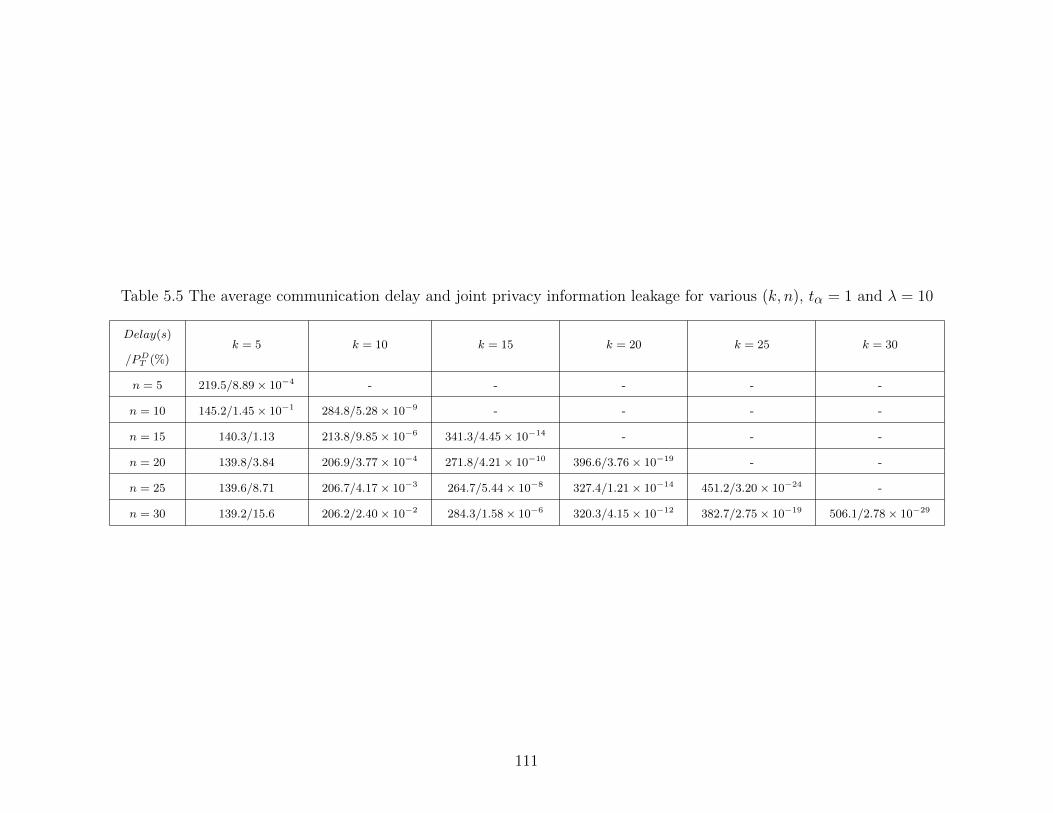
Table 5.5 The average communication delay and joint privacy information leakage for various (k, n), tα = 1 and λ = 10

Delay(s)k = 5 k = 10 k = 15 k = 20 k = 25 k = 30

/PDT (%)

n = 5 219.5/8.89× 10−4 - - - - -

n = 10 145.2/1.45× 10−1 284.8/5.28× 10−9 - - - -

n = 15 140.3/1.13 213.8/9.85× 10−6 341.3/4.45× 10−14 - - -

n = 20 139.8/3.84 206.9/3.77× 10−4 271.8/4.21× 10−10 396.6/3.76× 10−19 - -

n = 25 139.6/8.71 206.7/4.17× 10−3 264.7/5.44× 10−8 327.4/1.21× 10−14 451.2/3.20× 10−24 -

n = 30 139.2/15.6 206.2/2.40× 10−2 284.3/1.58× 10−6 320.3/4.15× 10−12 382.7/2.75× 10−19 506.1/2.78× 10−29

111

CHAPTER 6

CONCLUSIONS AND FUTURE WORK

Location privacy is an essential design and performance issue for WSNs and people-centric

networks along with other constraints such as energy efficiency, lifetime and communication

delay. In this dissertation, we intend to address location privacy and other conflicting design

constraints in a cost-aware framework for these two types of networks.

6.1 CASER Protection Scheme

For source location privacy in traditional wireless sensor networks, we present a secure and

efficient Cost-Aware SEcure Routing (CASER) protocol to balance energy consumption and

increase network lifetime. We first devise an energy balance control parameter to create an

adjustable filter to balance the energy consumption. We develop a security level parameter

to determine the probabilistic distribution of random walking. We derive formulas to decide

the energy consumption based on the energy balance control parameter and security level.

For CASER, we employ two routing strategies, shortest path routing and random walking.

The security level parameter can make routing paths dynamic and unpredictable. It can

effectively prevent adversaries from tracing back to the source location and defend against

jamming attacks. The shortest path routing strategy is used to ensure a high message

delivery ratio. Both theoretical analysis and simulation results show that CASER has an

excellent routing performance in terms of energy balance and routing path distribution for

location privacy.

We investigate the energy consumption for CASER scheme with uniformly distributed

events. The analysis and simulation results show the energy consumption is severely dispro-

portional to uniform energy deployment. The sensor nodes closer to sink node may exhaust

their residual energy for relaying messages. To solve this problem, we propose a non-uniform

112

energy deployment scheme to maximize the lifetime of WSNs. To provide equivalent security

properties, CASER scheme is updated to adapt the non-uniform energy deployment. Our

analysis and simulation results show that we can increase the lifetime and the number of

messages that can be delivered under the non-uniform energy deployment by more than four

times of uniform energy deployment under the same assumption.

CASER has the flexibility to support multiple routing strategies in message forwarding

to extend the lifetime while increasing routing security. It can achieve a trade-off between

security and network lifetime.

6.2 CAR Routing Algorithm

We introduce a congestion-aware routing (CAR) algorithm to reduce the communication

delay in WSNs. We propose to monitor traffic in the wireless medium channel and utilize

the channel competing results as a strategy to select a relay node.

We analyze communication delay in both the ideal case and the worst case. The theo-

retical analysis and simulation results demonstrate that the proposed CAR routing scheme

can reduce the end-to-end packet transmission delay by more than 50% while increasing the

network throughput for more than two times in our settings.

6.3 DAPP Protection Scheme

For location privacy in urban sensing networks, we introduce a delay-aware secure message

forwarding scheme. We first propose a Sharmir’s secret sharing based scheme to ensure

confidentiality of the collected data. The proposed scheme can also provide options for

integrity verification to prevent adversaries from dropping and tampering with the reported

data.

A dynamic pseudonym is introduced to conceal the real identity of the source node.

Through this scheme, the relationship between the source node and the pseudonyms can be

113

protected. It effectively defends against side information attacks.

We propose a two-phase forwarding scheme to detach the connection between source

nodes and application data server. In this way, the application data server is unable to

estimate the source node identity based on direct side information. Theoretical analysis

shows by using dynamic pseudonym scheme and secret-sharing, the proposed scheme can

preserve trajectory privacy.

We provide quantitatively analyze on the performance of the communication delay and

the delivery ratio under a given security level. It shows that DAPP has the flexibility

to provide a trade-off among communication delay, delivery ratio and participating user’s

privacy. The simulation results show that DAPP can minimize information leakage under

the given communication delay constraints. The built-in redundancy in DAPP can also

minimize the error rate for reporting data.

6.4 Related Future Works

The future work that directly related to this dissertation is broad and comprehensive. We

are currently working on the following two issues:

Privacy Definition and Characterization In this dissertation, we defined location pri-

vacy information leakage from probability perspective. However, there is still a lack of

quantitative measurement and characterization of privacy information in general. Our goal

is to develop a formal methodology to characterize privacy and provide a quantitative mea-

surement.

Measurement Criterion on Privacy Information Loss Publishing individual data

records without revealing sensitive information is an important yet challenging issue. Several

criteria have been proposed in existing research to measure the information loss of a privacy

protection scheme, such as k-anonymity, l-diversity and t-closeness. However, k-anonymity

114

and t-closeness cannot provide privacy if sensitive values in an equivalence class lack diver-

sity. l-diversity does not consider overall distribution for privacy information, which is also

difficult to be realized. These criteria also are not able to provide the lower bound of privacy

information loss for a published table. As a future research task, we intend to develop a

general information disclosure methodology under a given privacy leakage constraint.

115

BIBLIOGRAPHY

116

BIBLIOGRAPHY

[1] Y. Li and J. Ren, “Source-location privacy through dynamic routing in wireless sensornetworks,” in INFOCOM, 2010 Proceedings IEEE, March 2010, pp. 15–19.

[2] Y. Yu, R. Govindan, and D.Estrin, “Geographical and energy-aware routing: A recursivedata dissemination protocol for wireless sensor networks,” UCLA Computer ScienceDepartment Technical Report, Tech. Rep., May 2001.

[3] D. P. Tommaso Melodia and I. E. Akyildiz, “Optimal local topology knowledge forenergy efficient geographical routing in sensor networks,” in Twenty-third AnnualJointConference of the IEEE Computer and Communications Societies (INFOCOM), March2004, pp. 1705–1716.

[4] G. Zhao, J. Li, X. Liu, and A. Kumar, “Lifetime-aware geographic routing in wirelesssensor networks,” in Cyber-Enabled Distributed Computing and Knowledge Discovery,2009. CyberC ’09. International Conference on, Oct 2009, pp. 355–362.

[5] M. Ye, C. Li, G. Chen, and J. Wu, “Eecs: an energy efficient clustering scheme in wirelesssensor networks,” in Performance, Computing, and Communications Conference, 2005.IPCCC 2005. 24th IEEE International, April 2005, pp. 535–540.

[6] P. Bose, P. Morin, I. Stojmenovic, and J. Urrutia, “Routing with guaranteed deliveryin adhoc wireless networks,” in 3rd Int. Workshopon Discrete Algorithms and methodsfor mobile computing and communications, 1999, pp. 46–55.

[7] C.-C. Hung, K.-J. Lin, C.-C. Hsu, C.-F. Chou, and C.-J. Tu, “On enhancing network-lifetime using opportunistic routing in wireless sensor networks,” in Computer Commu-nications and Networks (ICCCN), 2010 Proceedings of 19th International Conferenceon, Aug 2010, pp. 1–6.

[8] J.-H. Chang and L. Tassiulas, “Maximum lifetime routing in wireless sensor networks,”Networking, IEEE/ACM Transactions on, vol. 12, no. 4, pp. 609–619, August 2004.

[9] F. Liu, C.-Y. Tsui, and Y. J. Zhang, “Joint routing and sleep scheduling for lifetimemaximization of wireless sensor networks,” Wireless Communications, IEEE Transac-tions on, vol. 9, no. 7, pp. 2258–2267, July 2010.

[10] C. Ee and R. Bajcsy, “Congestion control and fairness for many-to-one routing in sen-sor networks,” in ACM International Conference on Embedded Networked Sensor Sys-tems(SenSys 04), 2004.

[11] S. E. C.Y. Wan and A. Campbell, “Coda: Congestion detection and avoidance in sen-sor networks,” in ACM International Conference on Embedded Networked Sensor Sys-tems(SenSys 03), 2003, pp. 266–279.

117

[12] C. Conti and E. Gregori, “Dynamic tuning of the ieee 802.11 protocol to achieve atheoretical throughput limit,” IEEE/ACM Transactions on Networking, vol. 8, no. 6,pp. 785–799, December 2000.

[13] S. Eisenman and A. Campbell, “E-csma: Supporting enhanced CSMA performance inexperimental sensor networks using per-neighbor transmission probability thresholds,”in IEEE INFOCOM 2007, May 2007, pp. 1208–1216.

[14] S. Chen and N. Yang, “Congestion avoidance based on lightweight buffer managementin sensor networks,” IEEE Transactions on Parallel and Distributed Systems,, vol. 17,no. 9, pp. 934–946, Sept 2006.

[15] I. Stojmenovic and X. Lin, “Power-aware localized routing in wireless networks,” Par-allel and Distributed Systems, IEEE Transactions on, vol. 12, no. 11, pp. 1122–1133,Nov 2001.

[16] J. Li, J. Jannotti, D. S. J. D. Couto, D. R. Karger, and R. Morris, “A scalable loca-tion service for geographic ad hoc routing,” in the Sixth ACM Annual InternationalConference on Mobile Computing and Networking. ACM, 2000, pp. 120–130.

[17] B. Karp and H. T. Kung, “Gpsr: Greedy perimeter stateless routing for wireless net-works,” in the Sixth ACM Annual International Conference on Mobile Computing andNetworking (Mobicom), April 2000, pp. 243–254.

[18] Y. Xu, J. Heidemann, and D. Estrin, “Geography-informed energy conservation for ad-hoc routing,” in the Seventh Annual ACM/IEEE International Conference on MobileComputing and Networking, 2001, pp. 70–84.

[19] D. E. N. Bulusu, J. Heidemann, “Gps-less low cost outdoor localization for very smalldevices,” Computer science department, University of Southern California, TechnicalReport00-729, April 2000.

[20] C.-C. H. A. Savvides and M. Srivastava, “Dynamic fine-grained localization in ad-hocnetworks of sensors,” in the Seventh ACM Annual International Conference on MobileComputing and Networking (MobiCom), 2001, pp. 166–179.

[21] P. Bose, P. Morin, I. Stojmenovic, and J. Urrutia, “Routing with guaranteed deliveryin ad hoc wireless networks,” in the 3rd ACM International Workshop on DiscreteAlgorithms and Methods for Mobile Computing and Communications (DIAL M 99),Seattle, WA, August 1999, pp. 48–55.

[22] Y. Li, Y. Yang, and X. Lu, “Rules of designing routing metrics for greedy, face, andcombined greedy-face routing,” Mobile Computing, IEEE Transactions on, vol. 9, no. 4,pp. 582–595, April 2010.

[23] R. Shah and J. Rabaey, “Energy aware routing for low energy ad hoc sensor net-works,” in Wireless Communications and Networking Conference, 2002. WCNC2002.2002 IEEE, vol. 1, March 2002, pp. 350–355.

118

[24] H. Zhang and H. Shen, “Balancing energy consumption to maximize network lifetime indata-gathering sensor networks,” Parallel and Distributed Systems, IEEE Transactionson, vol. 20, no. 10, pp. 1526–1539, Oct. 2009.

[25] J. Kuruvila, A. Nayak, and I. Stojmenovic, “Hop count optimal position-based packetrouting algorithms for ad hoc wireless networks with a realistic physical layer,” SelectedAreas in Communications, IEEE Journal on, vol. 23, no. 6, pp. 1267–1275, June 2005.

[26] P. Kamat, Y. Zhang, W. Trappe, and C. Ozturk, “Enhancing source-location privacyin sensor network routing,” in Distributed Computing Systems, 2005. ICDCS 2005.Proceedings. 25th IEEE International Conference on, June 2005, pp. 599–608.

[27] C. Ozturk, Y. Zhang, W. Trappe, and M. Ott, “Source-location privacy in energy-constrained sensor network routing,” in workshop on security of ad hoc and sensornetworks - SASN. ACM, May 2004, pp. 88–93.

[28] Y. Li and J. Ren, “Preserving source-location privacy in wireless sensor networks,”in Sensor, Mesh and Ad Hoc Communications and Networks, 2009. SECON ’09. 6thAnnual IEEE Communications Society Conference on, June 2009, pp. 1–9.

[29] R. Shaikh, H. Jameel, B. d’Auriol, S. Lee, Y.-J. Song, and H. Lee, “Network levelprivacy for wireless sensor networks,” in Information Assurance and Security, 2008.ISIAS ’08. Fourth International Conference on, Sept 2008, pp. 261–266.

[30] S. Misra and G. Xue, “Efficient anonymity schemes for clustered wireless sensor net-works,” Int. J. Sen. Netw., vol. 1, pp. 50–63, Sep. 2006.

[31] M. Shao, Y. Yang, S. Zhu, and G. Cao, “Towards statistically strong source anonymityfor sensor networks,” in INFOCOM 2008. The 27th Conference on Computer Commu-nications. IEEE, April 2008, pp. 51–55.

[32] Y. Li, J. Ren, and J. Wu, “Quantitative measurement and design of source-locationprivacy schemes for wireless sensor networks,” Parallel and Distributed Systems, IEEETransactions on, vol. 23, no. 7, pp. 1302–1311, July 2012.

[33] K. J. B. Hull and H. Balakrishnan, “Mitigating congestion in wireless sensor networks,”in ACM International Conference on Embedded Networked Sensor Systems(SenSys 04),2004, pp. 134–147.

[34] E. C. J. Colbourn, M. Cui and V. R. Syrotiuk, “A carrier sense multiple access pro-tocol with power backoff (csma/pb),” Ad Hoc Networks, vol. 5, no. 8, pp. 1233–1250,November 2007.

[35] T. He, J. Stankovic, C. Lu, and T. Abdelzaher, “Speed: a stateless protocol for real-timecommunication in sensor networks,” in Proceedings of 23rd International Conference onDistributed Computing Systems, May 2003, pp. 46–55.

[36] A. C. C. Wan, S. Eisenman and J. Crowcroft, “Siphon: Over-load traffic managementusing multi-radio virtual sinks in sensor networks,” in ACM International Conferenceon Embedded Networked Sensor Systems(SenSys 05), 2005, pp. 116–129.

119

[37] M. Bhuiyan, I. Gondal, and J. Kamruzzaman, “Lacar: Location aided congestion awarerouting in wireless sensor networks,” in IEEE Wireless Communications and NetworkingConference (WCNC), April 2010, pp. 1–6.

[38] F. Ren, T. He, S. Das, and C. Lin, “Traffic-aware dynamic routing to alleviate congestionin wireless sensor networks,” IEEE Transactions on Parallel and Distributed Systems,vol. 22, no. 9, pp. 1585–1599, Sept 2011.

[39] J. Burke, D. Estrin, M. Hansen, A. Parker, N. Ramanathan, S. Reddy, and M. B.Srivastava, “Participatory sensing,” in the 1st Workshop on World-Sensor-Web, Oct2006, pp. 1–5.

[40] A. T. Campbell, S. B. Eisenman, N. D. Lane, E. Miluzzo, and R. A. Peterson, “People-centric urban sensing,” in Proceedings of the 2nd Annual International Workshop onWireless Internet, 2006, pp. 18–31.

[41] A. Kapadia, N. Triandopoulos, C. Cornelius, D. Peebles, and D. Kotz, “Anonysense:Opportunistic and privacy-preserving context collection,” Pervasive Computing, vol.5013, pp. 280–297, 2008.

[42] K. L. Huang, S. Kanhere, and W. Hu, “Towards privacy-sensitive participatory sens-ing,” in Pervasive Computing and Communications, IEEE International Conference on,March 2009, pp. 1–6.

[43] J. Shi, R. Zhang, Y. Liu, and Y. Zhang, “Prisense: Privacy-preserving data aggregationin people-centric urban sensing systems,” in Proceedings of IEEE INFOCOM 2010,March 2010, pp. 758–766.

[44] A. R. Beresford and F. Stajano, “Mix zones: User privacy in locationaware services,”in 2nd IEEE Ann. Conf. Pervasive Computing and Communications Workshops, 2004,pp. 127–131.

[45] J. Freudiger, M. H. Manshaei, J. Y. L. Boudec, and J. P. Hubaux, “On the age ofpseudonyms in mobile ad hoc networks,” in Proceeding of IEEE INFOCOM 2010, March2010, pp. 1–9.

[46] X. Liu, H. Zhao, M. Pan, H. Yue, X. Li, and Y. Fang, “Traffic-aware multiple mix zoneplacement for protecting location privacy,” in Proceeding of IEEE INFOCOM 2012,March 2012, pp. 972–980.

[47] S. Gao, J. Ma, W. Shi, G. Zhan, and C. Sun, “Trpf: A trajectory privacy-preservingframework for participatory sensing,” Information Forensics and Security, IEEE Trans-actions on, vol. 8, no. 6, pp. 874–887, June 2013.

[48] M. Gruteser and D. Grunwald, “Anonymous usage of location-based services throughspatial and temporal cloaking,” in ACM 1st Int. Conf. Mobile Systems, Applicationsand Services, 2003, pp. 31–42.

120

[49] M. Datar, N. Immorlica, P. Indyk, and V. S. Mirrokni, “Locality-sensitive hashingscheme based on p-stable distributions,” in Proceedings of the Twentieth Annual Sym-posium on Computational Geometry, 2004, pp. 253–262.

[50] T. Xu and Y. Cai, “Exploring historical location data for anonymity preservation inlocation-based service,” in Proceeding of IEEE INFOCOM 2008, March 2008, pp. 547–555.

[51] K. Vu, R. Zheng, and J. Gao, “Efficient algorithms for k-anonymous location privacy inparticipatory sensing,” in Proceeding of INFOCOM 2012, March 2012, pp. 2399–2407.

[52] S. Gao, J. Ma, W. Shi, and G. Zhan, “Towards location and trajectory privacy protectionin participatory sensing,” in Mobile Computing, Applications and Services, 2011, pp.381–386.

[53] H. Lu, C. S. Jensen, and M. L. Yiu, “Pad: Privacy-area aware, dummybased locationprivacy in mobile services,” in 7th ACM Int.Workshop on Data Engineering for Wirelessand Mobile Access, 2008, pp. 16–23.

[54] H. Kido, Y. Yanagisawa, and T. Satoh, “An anonymous communication technique usingdummies for location-based services,” in 9th Int. Symp. Privacy Enhancing Technologies(PETS¡¯10), 2005, pp. 88–97.

[55] M. Terrovitis and N. Mamoulis, “Privacy preservation in the publication of trajectories,”in Mobile Data Management, 2008. MDM ’08. 9th International Conference on, April2008, pp. 65–72.

[56] O. Abul, F. Bonchi, and M. Nanni, “Never walk alone: Uncertainty for anonymity inmoving objects databases,” in Data Engineering, 2008. ICDE 2008. IEEE 24th Inter-national Conference on, April 2008, pp. 376–385.

[57] E. De Cristofaro and R. Di Pietro, “Adversaries and countermeasures in privacy-enhanced urban sensing systems,” Systems Journal, IEEE, vol. 7, no. 2, pp. 311–322,June 2013.

[58] D. Christin, J. Guillemet, A. Reinhardt, M. Hollick, and S. Kanhere, “Privacy-preserving collaborative path hiding for participatory sensing applications,” in MobileAdhoc and Sensor Systems (MASS), IEEE 8th International Conference on, Oct 2011,pp. 341–350.

[59] ——, “Privacy-preserving collaborative path hiding for participatory sensing applica-tions,” in Mobile Adhoc and Sensor Systems (MASS), IEEE 8th International Confer-ence on, Oct 2011, pp. 341–350.

[60] L. Hu and C. Shahabi, “Privacy assurance in mobile sensing networks: Go beyondtrusted servers,” in Pervasive Computing and Communications Workshops, 8th IEEEInternational Conference on, March 2010, pp. 613–619.

121

[61] B. Karp and H. T. Kung, “Gpsr: Greedy perimeter stateless routing for wireless net-works,” in MobiCom’s 2000, Seattle, WA, 2000, pp. 243–254.

[62] L. Kang, “Protecting location privacy in large-scale wireless sensor networks,” in Com-munications, 2009. ICC ’09. IEEE International Conference on, June 2009, pp. 1–6.

[63] K. Mehta, D. Liu, and M. Wright, “Location privacy in sensor networks against a globaleavesdropper,” in IEEE International Conference on Network Protocols ICNP 2007, Oct2007, pp. 314–323.

[64] Y. Ouyang, Z. Le, D. Liu, J. Ford, and F. Makedon, “Source location privacy againstlaptop-class attacks in sensor networks,” in Proceedings of the 4th International Con-ference on Security and Privacy in Communication Netowrks, 2008, pp. 1–10.

[65] M. Shao, W. Hu, S. Zhu, G. Cao, S. Krishnamurthy, and T. L. Porta, “Cross-layerenhanced source location privacy in sensor networks,” in Proceedings of the 6th AnnualIEEE Communications Society Conference on Sensor, Mesh and Ad Hoc Communica-tions and Networks, Piscataway, NJ, USA, 2009, pp. 324–332.

[66] J. Hill, R. Szewczyk, A. Woo, S. Hollar, D. Culler, and K. Pister, “System architecturedirections for networked sensors,” SIGARCH Comput. Archit. News, vol. 28, no. 5, pp.93–104, Nov 2000.

[67] J. Yao and G. Wen, “Preserving source-location privacy in energy-constrained wirelesssensor networks,” in 28th International Conference on Distributed Computing SystemsWorkshops, ICDCS ’08, June 2008, pp. 412–416.

[68] Y. Zhang, W. Liu, Y. Fang, and D. Wu, “Secure localization and authentication inultra-wideband sensor networks,” Selected Areas in Communications, IEEE Journalon, vol. 24, no. 4, pp. 829–835, April 2006.

[69] L. Hu and D. Evans, “Localization for mobile sensor network,” in the tenth ACM AnnualInternational Conference on Mobile Computing and Networking (Mobicom), 2004, pp.45–57.

[70] H. Chan and A. Perrig, “Pike: peer intermediaries for key establishment in sensornetworks,” in INFOCOM 2005. 24th Annual Joint Conference of the IEEE Computerand Communications Societies. Proceedings IEEE, vol. 1, March 2005, pp. 524–535.

[71] WikipediA, “Quartic function,” http : //en.wikipedia.org/wiki/Quarticfunction.

[72] G. Bianchi, “Jamming sensor networks: attack and defense strategies,” IEEE Network,vol. 20, no. 3, pp. 41–47, March 2006.

[73] H.-W. L. A. Pathan and C. seon Hong, “Security in wireless sensor networks: issues andchallenges,” in the 8th International Conference on Advanced Communication Technol-ogy (ICACT), vol. 2, 2006, pp. 6–1048.

122

[74] G. Bianchi, “Performance analysis of the ieee 802.11 distributed coordination function,”IEEE Journal on Selected Areas in Communications, vol. 18, no. 3, pp. 535–547, march2000.

[75] J. Li, J. Jannotti, D. Couto, D. R. Karger, and R. Morris, “A scalable location servicefo geographic ad hoc routing,” in MobiCom’s 2000, Seattle, WA, 2000, pp. 120–130.

[76] P.Rapitis, V. Vitsas, and K. Paparrizos, “Packet delay metrics for ieee 802.11 distributedcoordination function,” Journal Mobile Networks and Applications, vol. 14, no. 6, pp.772–781, December 2009.

[77] J. Kim and S. Bohacek, “A survey-based mobility model of people for simulation ofurban mesh networks,” in Proceeding of MeshNets, 2005.

[78] B. Sun, F. Yu, K. Wu, Y. Xiao, and V. Leung, “Enhancing security using mobility-basedanomaly detection in cellular mobile networks,” Vehicular Technology, IEEE Transac-tions on, vol. 55, no. 4, pp. 1385–1396, July 2006.

[79] V. Vukadinovic, O. R. Helgason, and G. Karlsson, “An analytical model for pedestriancontent distribution in a grid of streets,” Mathematical and Computer Modelling, vol.57(11-12), pp. 2933–2944, June 2013.

[80] F. Bai, N. Sadagopan, and A. Helmy, “Important: a framework to systematically analyzethe impact of mobility on performance of routing protocols for adhoc networks,” inProceeding of IEEE INFOCOM 2003, vol. 2, March 2003, pp. 825–835.

123

COST-AWARE SECURE PROTOCOL DESIGN AND ANALYSIS · COST-AWARE SECURE PROTOCOL DESIGN AND ANALYSIS By...

Documents

Transcript of COST-AWARE SECURE PROTOCOL DESIGN AND ANALYSIS · COST-AWARE SECURE PROTOCOL DESIGN AND ANALYSIS By...