SEL-93-002

COST AND SCHEDULEESTIMATION STUDY REPORT

NOVEMBER 1993

National Aeronautics andSpace Administration

Goddard Space Flight CenterGreenbelt, Maryland 20771

SOFTWARE ENGINEERING LABORATORY SERIES

10014885W iii

Foreword

The Software Engineering Laboratory (SEL) is an organization sponsored by theNational Aeronautics and Space Administration/Goddard Space Flight Center(NASA/GSFC) and created to investigate the effectiveness of software engineeringtechnologies when applied to the development of applications software. The SEL wascreated in 1976 and has three primary organizational members:

NASA/GSFC, Software Engineering BranchUniversity of Maryland, Department of Computer ScienceComputer Sciences Corporation, Software Engineering Operation

The goals of the SEL are (1) to understand the software development process in theGSFC environment; (2) to measure the effects of various methodologies, tools, andmodels on this process; and (3) to identify and then to apply successful developmentpractices. The activities, findings, and recommendations of the SEL are recorded in theSoftware Engineering Laboratory Series, a continuing series of reports that includes thisdocument.

The major contributors to this document areSteve Condon (Computer Sciences Corporation)Myrna Regardie (Computer Sciences Corporation)Mike Stark (Goddard Space Flight Center)Sharon Waligora (Computer Sciences Corporation)

Single copies of this document can be obtained by writing toSoftware Engineering BranchCode 552Goddard Space Flight CenterGreenbelt, Maryland 20771

10014885W v

Abstract

This report describes the analysis performed and the findings of a study of the softwaredevelopment cost and schedule estimation models used by the Flight Dynamics Division (FDD),Goddard Space Flight Center. The study analyzes typical FDD projects, focusing primarily onthose developed since 1982. The study reconfirms the standard SEL effort estimation model thatis based on size adjusted for reuse; however, guidelines for the productivity and growthparameters in the baseline effort model have been updated. The study also produced a scheduleprediction model based on empirical data that varies depending on application type. Models forthe distribution of effort and schedule by life-cycle phase are also presented. Finally, this reportexplains how to use these models to plan SEL projects.

Keywords: cost estimation, planning models, reuse, schedule prediction.

10014885W vii

Contents

Executive Summary . . . . . . . . . . . . . . . . . . . . . . . . . . . . . . . . . . . . . . . . . . . . . . . . . . . . . . . . . . . . . . . . . . . . . . . . . . . . . . . . . . . . . .xi

Section 1. Introduction

1.1 Motivation for Study ... . . . . . . . . . . . . . . . . . . . . . . . . . . . . . . . . . . . . . . . . . . . . . . . . . . . . . . . . . . . . . . . . . . . . . . . . . . . 1-11.2 Document Organization .. . . . . . . . . . . . . . . . . . . . . . . . . . . . . . . . . . . . . . . . . . . . . . . . . . . . . . . . . . . . . . . . . . . . . . . . . 1-1

Section 2. Data Used in Study

Section 3. Effort Analysis

3.1 Reuse Cost Analysis, Productivity, and Total Project Effort . . . . . . . . . . . . . . . . . . . . . . . . . . . . . . . . 3-13.2 Accuracy of Models for Total Effort. . . . . . . . . . . . . . . . . . . . . . . . . . . . . . . . . . . . . . . . . . . . . . . . . . . . . . . . . . . . 3-4

3.2.1 Model Prediction Based on Final Project Statistics .. . . . . . . . . . . . . . . . . . . . . . . . . . . . 3-43.2.2 Model Predictions Based on CDR Estimates.. . . . . . . . . . . . . . . . . . . . . . . . . . . . . . . . . . . . 3-8

3.3 Distribution of Effort by Life-Cycle Phase .. . . . . . . . . . . . . . . . . . . . . . . . . . . . . . . . . . . . . . . . . . . . . . . . . . . 3-93.4 Distribution of Effort by Software Development Activity .. . . . . . . . . . . . . . . . . . . . . . . . . . . . . . . . 3-11

Section 4. Methods For Adjusting Total Effort

4.1 Overview... . . . . . . . . . . . . . . . . . . . . . . . . . . . . . . . . . . . . . . . . . . . . . . . . . . . . . . . . . . . . . . . . . . . . . . . . . . . . . . . . . . . . . . . . . 4-14.2 Scope of the Analysis .. . . . . . . . . . . . . . . . . . . . . . . . . . . . . . . . . . . . . . . . . . . . . . . . . . . . . . . . . . . . . . . . . . . . . . . . . . . . 4-24.3 Methods Used to Evaluate Success .. . . . . . . . . . . . . . . . . . . . . . . . . . . . . . . . . . . . . . . . . . . . . . . . . . . . . . . . . . . . 4-64.4 Deriving Productivity Multipliers with Optimization Procedures .. . . . . . . . . . . . . . . . . . . . . . . . . 4-6

4.4.1 Effect of Individual SEF Parameters on Productivity Estimate.. . . . . . . . . . . . . . . 4-74.4.2 Effect of Multiple SEF Parameters on Productivity Estimate.. . . . . . . . . . . . . . . 4-134.4.3 Other Productivity Analyses.. . . . . . . . . . . . . . . . . . . . . . . . . . . . . . . . . . . . . . . . . . . . . . . . . . . . . 4-18

4.5 Linear Regression Analysis of Correlations Between SEF Parameters and Effort . . . . . 4-194.5.1 Linear Regressions Without SEF Data .. . . . . . . . . . . . . . . . . . . . . . . . . . . . . . . . . . . . . . . . . 4-194.5.2 Linear Regressions With Actual and Random SEF Data .. . . . . . . . . . . . . . . . . . . . 4-20

4.6 Conclusions.. . . . . . . . . . . . . . . . . . . . . . . . . . . . . . . . . . . . . . . . . . . . . . . . . . . . . . . . . . . . . . . . . . . . . . . . . . . . . . . . . . . . . . 4-24

Section 5. Schedule Analysis

5.1 Total Schedule Duration .. . . . . . . . . . . . . . . . . . . . . . . . . . . . . . . . . . . . . . . . . . . . . . . . . . . . . . . . . . . . . . . . . . . . . . . . . 5-15.1.1 Formulating a Schedule Prediction Model.. . . . . . . . . . . . . . . . . . . . . . . . . . . . . . . . . . . . . . . 5-15.1.2 Accuracy of Schedule Prediction Based on Final Projects Statistics.. . . . . . . . . 5-75.1.3 Analysis of Schedule Growth ... . . . . . . . . . . . . . . . . . . . . . . . . . . . . . . . . . . . . . . . . . . . . . . . . . . . 5-9

5.2 Distribution of Schedule by Life-Cycle Phase.. . . . . . . . . . . . . . . . . . . . . . . . . . . . . . . . . . . . . . . . . . . . . . 5-10

Section 6. Conclusions and Recommendations

6.1 Conclusions.. . . . . . . . . . . . . . . . . . . . . . . . . . . . . . . . . . . . . . . . . . . . . . . . . . . . . . . . . . . . . . . . . . . . . . . . . . . . . . . . . . . . . . . . 6-16.2 Recommendations .. . . . . . . . . . . . . . . . . . . . . . . . . . . . . . . . . . . . . . . . . . . . . . . . . . . . . . . . . . . . . . . . . . . . . . . . . . . . . . . . 6-3

10014885W viii

Section 7. Applying the Planning Models

7.1 Creating the Initial Plan.. . . . . . . . . . . . . . . . . . . . . . . . . . . . . . . . . . . . . . . . . . . . . . . . . . . . . . . . . . . . . . . . . . . . . . . . . . 7-17.1.1 Estimating Effort . . . . . . . . . . . . . . . . . . . . . . . . . . . . . . . . . . . . . . . . . . . . . . . . . . . . . . . . . . . . . . . . . . . . . 7-17.1.2 Determining the Schedule.. . . . . . . . . . . . . . . . . . . . . . . . . . . . . . . . . . . . . . . . . . . . . . . . . . . . . . . . . . 7-27.1.3 Planning the Life-Cycle Phases .. . . . . . . . . . . . . . . . . . . . . . . . . . . . . . . . . . . . . . . . . . . . . . . . . . . 7-2

7.2 Planning for Success .. . . . . . . . . . . . . . . . . . . . . . . . . . . . . . . . . . . . . . . . . . . . . . . . . . . . . . . . . . . . . . . . . . . . . . . . . . . . . 7-37.2.1 Planning for Growth ... . . . . . . . . . . . . . . . . . . . . . . . . . . . . . . . . . . . . . . . . . . . . . . . . . . . . . . . . . . . . . . 7-37.2.2 Additional Planning Considerations .. . . . . . . . . . . . . . . . . . . . . . . . . . . . . . . . . . . . . . . . . . . . . . 7-5

7.3 Reconciling the Planning Models With the Baseline Models .. . . . . . . . . . . . . . . . . . . . . . . . . . . . . . 7-7

Appendix A. Summary of Cost and Schedule Models

Appendix B. Sample Subjective Evaluation Form

Appendix C. Effort and Schedule Detailed Distribution

Abbreviations and Acronyms

References

Standard Bibliography of SEL Literature

10014885W ix

Figures

3-1. Productivity for AGSSs and Simulators .. . . . . . . . . . . . . . . . . . . . . . . . . . . . . . . . . . . . . . . . . . . . . . . . . . . . . . . 3-63-2. Accuracy of FORTRAN Effort Estimation Model.. . . . . . . . . . . . . . . . . . . . . . . . . . . . . . . . . . . . . . . . . . . 3-73-3. Accuracy of Ada Effort Estimation Model.. . . . . . . . . . . . . . . . . . . . . . . . . . . . . . . . . . . . . . . . . . . . . . . . . . . . 3-73-4. DLOC Growth Factors: Actual DLOC Divided by CDR Estimate .. . . . . . . . . . . . . . . . . . . . . . . . 3-94-1. Effort as a Function of DLOC for 24 Older FORTRAN Projects.. . . . . . . . . . . . . . . . . . . . . . . . 4-214-2. Effort as a Function of DLOC for 15 Recent FORTRAN Projects .. . . . . . . . . . . . . . . . . . . . . . 4-214-3. Accuracy of Effort Prediction (Measured by R-Squared) for 24 Older

FORTRAN Projects .. . . . . . . . . . . . . . . . . . . . . . . . . . . . . . . . . . . . . . . . . . . . . . . . . . . . . . . . . . . . . . . . . . . . . . . . . . . . 4-224-4. Accuracy of Effort Prediction (Measured by R-Squared) for 15 Recent

FORTRAN Projects .. . . . . . . . . . . . . . . . . . . . . . . . . . . . . . . . . . . . . . . . . . . . . . . . . . . . . . . . . . . . . . . . . . . . . . . . . . . . 4-224-5. Accuracy of Effort Prediction (Measured by RMS Percent Deviation) for 24 Older FORTRAN Projects .. . . . . . . . . . . . . . . . . . . . . . . . . . . . . . . . . . . . . . . . . . . . . . . . . . . . . . . . . . . . . . . . . . . . . . . . . . . . 4-234-6. Accuracy of Effort Prediction (Measured by RMS Percent Deviation) for 15 Recent

FORTRAN Projects .. . . . . . . . . . . . . . . . . . . . . . . . . . . . . . . . . . . . . . . . . . . . . . . . . . . . . . . . . . . . . . . . . . . . . . . . . . . . 4-235-1. Coefficients of Schedule Duration Formula .. . . . . . . . . . . . . . . . . . . . . . . . . . . . . . . . . . . . . . . . . . . . . . . . . . 5-45-2. Schedule Duration Versus Technical and Management Effort . . . . . . . . . . . . . . . . . . . . . . . . . . . . . . 5-75-3. Accuracy of Schedule Duration Model for AGSSs (Based on Actual

Technical and Management Effort) . . . . . . . . . . . . . . . . . . . . . . . . . . . . . . . . . . . . . . . . . . . . . . . . . . . . . . . . . . . . . 5-85-4. Accuracy of Schedule Duration Model for Simulators (Based on Actual

Technical and Management Effort) . . . . . . . . . . . . . . . . . . . . . . . . . . . . . . . . . . . . . . . . . . . . . . . . . . . . . . . . . . . . . 5-95-5. Schedule Growth Factors (Actual Duration Divided by CDR Estimate) .. . . . . . . . . . . . . . . 5-107-1. Staffing Plan Based on Initial Size .. . . . . . . . . . . . . . . . . . . . . . . . . . . . . . . . . . . . . . . . . . . . . . . . . . . . . . . . . . . . . 7-37-2. Staffing Plan That Anticipates Growth ... . . . . . . . . . . . . . . . . . . . . . . . . . . . . . . . . . . . . . . . . . . . . . . . . . . . . . . 7-47-3. Plan Versus Actuals .. . . . . . . . . . . . . . . . . . . . . . . . . . . . . . . . . . . . . . . . . . . . . . . . . . . . . . . . . . . . . . . . . . . . . . . . . . . . . . 7-67-4. Plan for Success.. . . . . . . . . . . . . . . . . . . . . . . . . . . . . . . . . . . . . . . . . . . . . . . . . . . . . . . . . . . . . . . . . . . . . . . . . . . . . . . . . . . 7-67-5. Planning Model Versus Baseline Model (Expected Actuals). . . . . . . . . . . . . . . . . . . . . . . . . . . . . . . . 7-7

10014885W x

Tables

2-1. Projects Studied . . . . . . . . . . . . . . . . . . . . . . . . . . . . . . . . . . . . . . . . . . . . . . . . . . . . . . . . . . . . . . . . . . . . . . . . . . . . . . . . . . . 2-32-2. Detailed Line-of-Code Data . . . . . . . . . . . . . . . . . . . . . . . . . . . . . . . . . . . . . . . . . . . . . . . . . . . . . . . . . . . . . . . . . . . . . 2-52-3. Line-of-Code Summary Data .. . . . . . . . . . . . . . . . . . . . . . . . . . . . . . . . . . . . . . . . . . . . . . . . . . . . . . . . . . . . . . . . . . . 2-62-4. SLOC, DLOC, and Effort . . . . . . . . . . . . . . . . . . . . . . . . . . . . . . . . . . . . . . . . . . . . . . . . . . . . . . . . . . . . . . . . . . . . . . . . 2-72-5. Technical Staff Hours Distributed by Life-Cycle Phase .. . . . . . . . . . . . . . . . . . . . . . . . . . . . . . . . . . . . 2-82-6. Groupings of Software Development Activities.. . . . . . . . . . . . . . . . . . . . . . . . . . . . . . . . . . . . . . . . . . . . . . 2-92-7. Technical Staff Hours Distributed by Development Activity .. . . . . . . . . . . . . . . . . . . . . . . . . . . . 2-102-8. Schedule Distribution (Calendar Weeks).. . . . . . . . . . . . . . . . . . . . . . . . . . . . . . . . . . . . . . . . . . . . . . . . . . . . 2-113-1. Effort Distributed by Life-Cycle Phase.. . . . . . . . . . . . . . . . . . . . . . . . . . . . . . . . . . . . . . . . . . . . . . . . . . . . . . 3-103-2. Effort-by-Phase Models for Moderate to Low Reuse Projects .. . . . . . . . . . . . . . . . . . . . . . . . . . . 3-113-3. Preliminary Effort-by-Phase Model for High Reuse Projects .. . . . . . . . . . . . . . . . . . . . . . . . . . . . 3-113-4. Effort Distributed by Software Development Activity .. . . . . . . . . . . . . . . . . . . . . . . . . . . . . . . . . . . . 3-123-5. Effort-by-Activity Models for Moderate to Low Reuse Projects .. . . . . . . . . . . . . . . . . . . . . . . . 3-123-6. Preliminary Effort-by-Activity Models for High Reuse Projects .. . . . . . . . . . . . . . . . . . . . . . . . 3-134-1. SEF Parameters .. . . . . . . . . . . . . . . . . . . . . . . . . . . . . . . . . . . . . . . . . . . . . . . . . . . . . . . . . . . . . . . . . . . . . . . . . . . . . . . . . . . 4-44-2. Projects Used To Test Productivity Multipliers .. . . . . . . . . . . . . . . . . . . . . . . . . . . . . . . . . . . . . . . . . . . . . . 4-54-3. Projects Used To Test Correlations Between Effort and SEF Parameters .. . . . . . . . . . . . . . . . 4-54-4. Subsets of Projects Tested.. . . . . . . . . . . . . . . . . . . . . . . . . . . . . . . . . . . . . . . . . . . . . . . . . . . . . . . . . . . . . . . . . . . . . . . 4-74-5. Effect of Individual SEF Parameters on Productivity Estimate .. . . . . . . . . . . . . . . . . . . . . . . . . . . . 4-94-6. Reduction in RMS Percent Deviation Using Random SEF Values.. . . . . . . . . . . . . . . . . . . . . . 4-134-7. Subsets of SEF Parameters Tested .. . . . . . . . . . . . . . . . . . . . . . . . . . . . . . . . . . . . . . . . . . . . . . . . . . . . . . . . . . . 4-134-8. Effect of Multiple SEF Parameters on Productivity Estimate .. . . . . . . . . . . . . . . . . . . . . . . . . . . . 4-144-9. Effect of Multiple SEF Parameters on Productivity Estimate for Subset

of 23 AGSSs and Simulators.. . . . . . . . . . . . . . . . . . . . . . . . . . . . . . . . . . . . . . . . . . . . . . . . . . . . . . . . . . . . . . . . . . 4-184-10. Statistical Measures of Association Used .. . . . . . . . . . . . . . . . . . . . . . . . . . . . . . . . . . . . . . . . . . . . . . . . . . 4-194-11. Linear Regression Results for Equation 4-3 (24 Older FORTRAN Projects) . . . . . . . . . . . 4-204-12. Linear Regression Results for Equation 4-3 (15 Recent FORTRAN Projects) . . . . . . . . . 4-205-1. Project Data Used in Schedule Analysis .. . . . . . . . . . . . . . . . . . . . . . . . . . . . . . . . . . . . . . . . . . . . . . . . . . . . . . 5-25-2. Project Duration Formula Coefficients .. . . . . . . . . . . . . . . . . . . . . . . . . . . . . . . . . . . . . . . . . . . . . . . . . . . . . . . . 5-35-3. Projects Used in Formulating Schedule Equations.. . . . . . . . . . . . . . . . . . . . . . . . . . . . . . . . . . . . . . . . . . . 5-55-4. Summary of Duration Formulas .. . . . . . . . . . . . . . . . . . . . . . . . . . . . . . . . . . . . . . . . . . . . . . . . . . . . . . . . . . . . . . . . 5-65-5. Percentage of Schedule Distribution by Phase .. . . . . . . . . . . . . . . . . . . . . . . . . . . . . . . . . . . . . . . . . . . . . 5-115-6. Models for Schedule Distribution by Phase.. . . . . . . . . . . . . . . . . . . . . . . . . . . . . . . . . . . . . . . . . . . . . . . . . 5-117-1. Life-Cycle Planning Model .. . . . . . . . . . . . . . . . . . . . . . . . . . . . . . . . . . . . . . . . . . . . . . . . . . . . . . . . . . . . . . . . . . . . . 7-2

Executive Summary

IntroductionThe Software Engineering Laboratory (SEL) has been collecting and interpreting data onsoftware metrics for 16 years. Over the years it has repeatedly refined its models of the softwaredevelopment process as exhibited at the Flight Dynamics Division (FDD) of NASA's GoddardSpace Flight Center (GSFC). This Cost and Schedule Estimation Study was undertaken todetermine what changes, if any, have taken place in the software development process in recentyears and to validate or refine current FDD models. The study analyzed both FORTRAN andAda projects and focused on three main application types: Attitude Ground Support Systems(AGSSs), telemetry simulators, and dynamics simulators.

The current study sought to expand on the recent research performed for the Ada Size StudyReport (Reference 1). The SEL introduced Ada in 1985 as a potentially beneficial technologythat could improve the software development process. Most Ada systems that have beendeveloped in the FDD are systems that simulate either spacecraft telemetry (telemetrysimulators) or spacecraft dynamics (dynamics simulators).

Objective and ScopeThe Cost and Schedule Estimation Study was undertaken to

• Review the relationships and models in the SEL literature and recommend a small setof equations to be used by project managers.

• Validate these size, cost, and schedule models against recent projects. Recommendrevisions to the current estimation models.

This study sought to answer the following questions:

• Has the SEL effort estimation model changed and does it vary with language and typeof application?

• How should the number of developed lines of code (DLOC) be computed toaccurately represent total project effort?

• What are the typical productivities for FDD projects?

• Can the data in the SEL database provide any guidelines for enhancing the initialeffort estimate, which is based only on size and typical productivity estimates, byincluding additional estimation factors such as team experience and problemcomplexity?

• What impact do increased levels of reused code have on a project's cost and schedule?

• What should the schedule estimation model be?

10014885W xi

• What are the typical distributions of effort and schedule among life-cycle phases forprojects? Are the distributions different from the standard SEL distribution models?

• What is the typical distribution of effort among software development activities forprojects? Is it different from the standard SEL model?

• How do the effort and schedule models that are based on end-of-project actuals relateto the recommended SEL planning models for effort and schedule?

ApproachThe study researched many preexisting FDD models relating to effort and schedule estimationand evaluated many of these models, using data from over 30 FDD projects, including AGSSs,telemetry simulators, and dynamics simulators, that are representative of the FDD environment.The study team searched for trends in language differences as well as differences in type ofapplication. The recommended models emerged from an elimination process of consideringmany possible models using multiple combinations of project data.

ConclusionsThe study indicates that

• The standard SEL effort estimation equation, based on a size estimate adjusted forreuse, is best for predicting effort in the FDD environment. Of the three effort modelparameters—productivity, cost to reuse code, and growth factor—the productivity andreuse cost vary with language, whereas the growth factor varies with the level ofreuse. The effort model parameters do not depend on the application type (that is,AGSS, telemetry simulator, or dynamics simulator).

• DLOC (total source lines of code (SLOC) adjusted for reuse) is an accurate basis forestimating total project effort. For FORTRAN projects, DLOC should continue to becomputed with a 20-percent weight given to reused SLOC. (The 20-percent weightingis the reuse cost parameter.)

• For Ada projects, DLOC should continue to be computed with a 30-percent weightgiven to reused SLOC, but this figure may need to be reevaluated in the future. The30-percent reuse cost for Ada projects was proposed by the Ada Size Study Report. Atthat time only a small number of completed Ada projects were available for analysis,and the Ada process had been evolving from project to project. Since that time onlyone additional Ada project (POWITS) has been completed and had its final projectstatistics verified. Today, therefore, the 30-percent Ada reuse cost represents the bestmodel available for FDD Ada simulators, but as more Ada projects are completed, theAda reuse cost may need to be reevaluated.

• The significant cost savings evidenced by SAMPEX AGSS and SAMPEXTS, tworecent projects with very high reuse levels, suggest a divergence from the standard 30-percent and 20-percent reuse costs. For such high-reuse projects as these, a muchlower reuse cost may be appropriate, perhaps as low as 10 percent. SAMPEXTS,however, piloted a streamlined development process, combining some documents andcombining the preliminary design review (PDR) with the critical design review(CDR); the project's low reuse cost may result from these process changes as well asfrom the percentage of reused code. Data from more high-reuse projects are neededbefore certifying this as a trend.

10014885W xii

• The productivity experienced on recent FORTRAN AGSSs varied from 3 to 5 DLOCper technical and management hour. For planning purposes, a conservativeproductivity value of 3.5 DLOC per technical staff/technical management hour isrecommended. When support staff hours are included in the plan, an overallproductivity rate of 3.2 DLOC per hour should be used.

• The productivity on recent Ada projects showed less variability than it did on theFORTRAN projects. For planning purposes, a productivity of 5.0 DLOC per technicalstaff/technical management hour is recommended. When support staff hours areincluded in the plan, an overall productivity rate of 4.5 DLOC per hour should beused.

• The Subjective Evaluation Form (SEF) data in the SEL database provide nodemonstrable evidence that inclusion of estimates for such factors as problemcomplexity or team experience will significantly improve a manager's estimate ofproject effort. When making estimates for project effort, managers are stillencouraged to include such factors as problem complexity or team experience basedon their own personal experience, but the database of experience represented by theSEF data in the SEL database provides no guidelines.

• For projects with moderate to low code reuse (less than 70 percent), the post-CDRgrowth in DLOC due to requirement changes and TBDs is commensurate with pastSEL experience: 40 percent. For projects with high code reuse (70 percent or more),the post-CDR growth in DLOC is only about half as much (20 percent).

• An exponential model like the Constructive Cost Model (COCOMO) can be used topredict the duration of projects from total project effort; the COCOMO multiplicativefactor of 3.3 must be replaced with a factor of 5.0 for AGSSs (6.7 for simulators)when based on management and technical hours and 4.9 for AGSSs (6.5 forsimulators) when based on management, technical, and support hours.

• For projects with moderate to low code reuse, the post-CDR growth in schedule is 35percent. For projects with high reuse, the post-CDR growth in schedule is 5 percent.

• Based on the final project statistics for moderate to low-reuse projects (less than 70-percent code reuse), the distribution of the total effort and schedule among the life-cycle phases is as follows:

Phase Effort Schedule

Design: 24 ± 3% 30 ± 5%

Code: 45 ± 6% 34 ± 6%

Test: 31 ± 5% 36 ± 7%

• Based on the final project statistics for high-reuse projects (70 percent or more codereuse), the distribution of the total effort and schedule among the life-cycle phases isas shown below. The larger standard deviations for high-reuse projects demonstratethat the development process for high-reuse projects is still evolving, resulting in

10014885W xiii

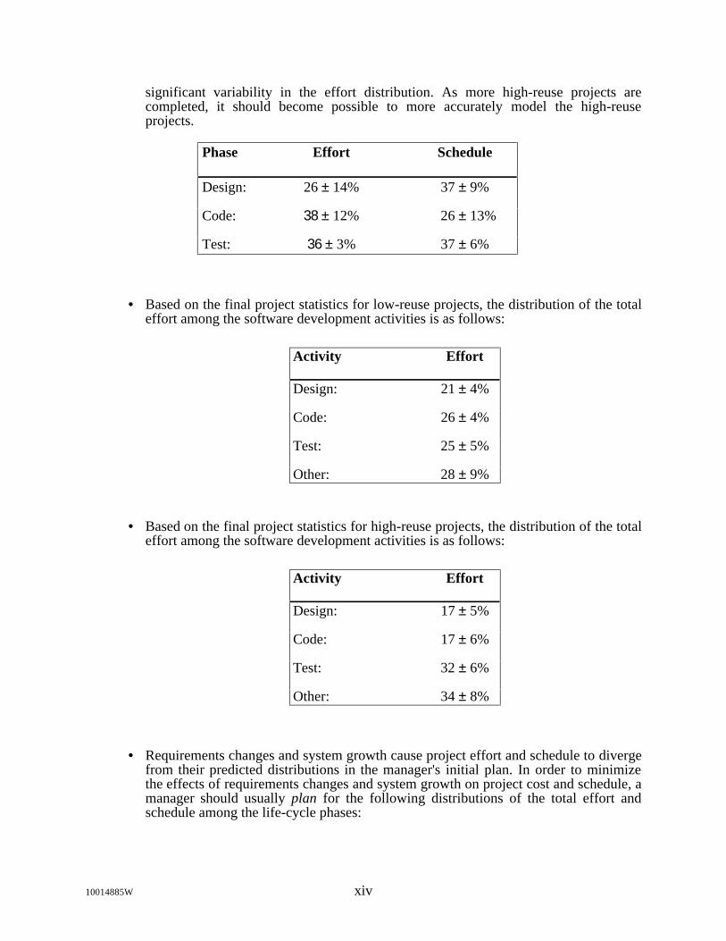
significant variability in the effort distribution. As more high-reuse projects arecompleted, it should become possible to more accurately model the high-reuseprojects.

Phase Effort Schedule

Design: 26 ± 14% 37 ± 9%

Code: 38 ± 12% 26 ± 13%

Test: 36 ± 3% 37 ± 6%

• Based on the final project statistics for low-reuse projects, the distribution of the totaleffort among the software development activities is as follows:

Activity Effort

Design: 21 ± 4%

Code: 26 ± 4%

Test: 25 ± 5%

Other: 28 ± 9%

• Based on the final project statistics for high-reuse projects, the distribution of the totaleffort among the software development activities is as follows:

Activity Effort

Design: 17 ± 5%

Code: 17 ± 6%

Test: 32 ± 6%

Other: 34 ± 8%

• Requirements changes and system growth cause project effort and schedule to divergefrom their predicted distributions in the manager's initial plan. In order to minimizethe effects of requirements changes and system growth on project cost and schedule, amanager should usually plan for the following distributions of the total effort andschedule among the life-cycle phases:

10014885W xiv

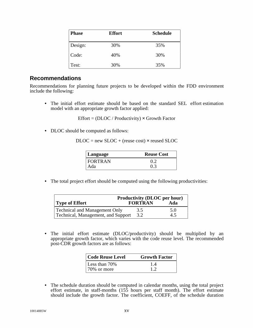
Phase Effort Schedule

Design: 30% 35%

Code: 40% 30%

Test: 30% 35%

RecommendationsRecommendations for planning future projects to be developed within the FDD environmentinclude the following:

• The initial effort estimate should be based on the standard SEL effort estimationmodel with an appropriate growth factor applied:

Effort = (DLOC / Productivity) × Growth Factor

• DLOC should be computed as follows:

DLOC = new SLOC + (reuse cost) × reused SLOC

Language Reuse CostFORTRAN 0.2Ada 0.3

• The total project effort should be computed using the following productivities:

Productivity (DLOC per hour)Type of Effort FORTRAN AdaTechnical and Management Only 3.5 5.0Technical, Management, and Support 3.2 4.5

• The initial effort estimate (DLOC/productivity) should be multiplied by anappropriate growth factor, which varies with the code reuse level. The recommendedpost-CDR growth factors are as follows:

Code Reuse Level Growth FactorLess than 70% 1.470% or more 1.2

• The schedule duration should be computed in calendar months, using the total projecteffort estimate, in staff-months (155 hours per staff month). The effort estimateshould include the growth factor. The coefficient, COEFF, of the schedule duration

10014885W xv

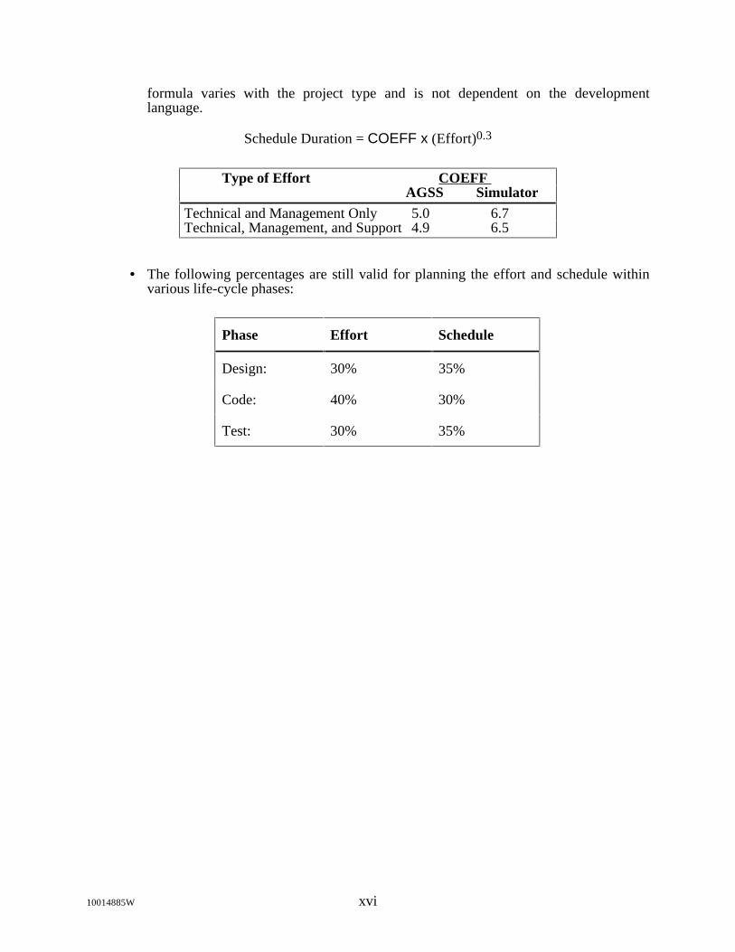
formula varies with the project type and is not dependent on the developmentlanguage.

Schedule Duration = COEFF x (Effort)0.3

Type of Effort COEFF AGSS Simulator

Technical and Management Only 5.0 6.7Technical, Management, and Support 4.9 6.5

• The following percentages are still valid for planning the effort and schedule withinvarious life-cycle phases:

Phase Effort Schedule

Design: 30% 35%

Code: 40% 30%

Test: 30% 35%

10014885W xvi

Section 1. Introduction

The Software Engineering Laboratory (SEL) is an organization sponsored by the NationalAeronautics and Space Administration/Goddard Space Flight Center (NASA/GSFC). It wascreated in 1977 to investigate the effectiveness of software engineering technologies applied tothe development of applications software. The SEL has three primary organizational members:NASA/GSFC, Software Engineering Branch; University of Maryland, Department of ComputerScience; and Computer Sciences Corporation, Software Engineering Operation.

Applications developed in the NASA Flight Dynamics Division (FDD) environment are usedprimarily to determine and predict the orbit and attitude of Earth-orbiting satellites. All of theoperational Attitude Ground Support Systems (AGSSs) developed by the FDD have been writtenin FORTRAN. Until the late 1980s the systems developed in the FDD to simulate eitherspacecraft telemetry (telemetry simulators) or spacecraft dynamics (dynamics simulators) werealso developed in FORTRAN. Beginning in 1987, however, these simulators began to bedeveloped in Ada.

1.1 Motivation for Study

The SEL has been collecting and interpreting data on software metrics for 16 years. Over theyears it has repeatedly refined its models of the software development process as exhibited at theFDD. The Cost and Schedule Estimation Study was undertaken to determine what changes, ifany, have taken place in the software development process in recent years and to validate orrefine current FDD models. The study analyzed both FORTRAN and Ada projects and focusedon three main application types: AGSSs, telemetry simulators, and dynamics simulators.

1.2 Document Organization

Section 1 describes the motivation for the study and the document's organization. Section 2discusses the data used in the study. Section 3 presents and validates models used to estimatetotal project effort. These models are followed by other models depicting the distribution ofproject effort by life-cycle phase and by software development activity. Section 4 analyzes thebenefit of adjusting initial effort or productivity estimates to take into account such factors asproblem complexity or team experience. Section 5 presents and examines the models used toestimate total project duration and life-cycle phase duration. Section 6 gives the study'sconclusions and recommendations. Section 7 describes how to apply the planning modelsproduced by this study.

Appendix A contains a matrix of costing and scheduling formulas recommended in the FDDover the last 14 years. Appendix B contains a sample of the Subjective Evaluation Form (SEF)that is completed at the end of each FDD software development project. Appendix C containsproject-by-project data on the distribution of effort and schedule by life-cycle phase and also thedistribution of effort by software development activity.

10014885W 1-1

Section 2. Data Used in Study

The Cost and Schedule Estimation Study analyzed both objective and subjective data for theprojects studied. Objective data, taken primarily from the SEL database but with occasionalreference to the software development history reports, included such data as the hours of effortexpended, the number of lines of new and reused code, and the beginning and end dates of life-cycle phases in the final project schedules. These objective data are presented in the tables in thissection and are described in the accompanying text. These data were used to support the effortmodel analysis presented in Section 3 and the schedule model analysis presented in Section 5.For some of the projects, supporting subjective data were obtained from the softwaredevelopment history reports and from discussions with developers. Additional extensivesubjective data were taken from the Subjective Evaluation Form (SEF) data in the SEL databasein order to support the analysis of subjective factors, discussed in Section 4.

Table 2-1 lists the projects studied along with their application type, language, developmentperiod, duration, and the total effort charged by technical staff and managers (but excludingsupport staff).

In the SEL, source lines of code (SLOC) are defined to include source lines, comment lines, andblank lines. Table 2-2 presents a detailed picture of SLOC for each project, classifying the totalSLOC into four categories:

• Newly written code (i.e., code for entirely new units)

• Extensively modified code (i.e., code for reused units in which 25 percent or more ofthe lines were modified)

• Slightly modified code (i.e., code for reused units in which less than 25 percent of thelines were modified)

• Verbatim code (i.e., code for units that were reused verbatim)

For estimation purposes, SLOC figures are often classified into two overall categories thatcombine newly written code and extensively modified code under the title new code and slightlymodified code and verbatim code under the title reused code. Table 2-3 presents the figures fornew code, reused code, total SLOC, and the percentage of reused code. This reuse percentage isdefined simply as the number of lines of reused code divided by the total number of SLOC. ForPAS, for example, this would be 27,139/111,868, or 24 percent.

The number for new code is combined with a weighted value for the reused code to yield thenumber of DLOC as shown in Equation 2-1. Table 2-4 presents the project totals for SLOC andDLOC side by side for comparison. This study used 20 percent for the FORTRAN reuse costand 30 percent for the Ada reuse cost. It also includes the total project effort charged by

10014885W 2-1

technical staff, technical management, and support staff (upper management, librarians,Technical Publications, and secretarial).

DLOC = (New SLOC) + (Reuse Cost) × (Reused SLOC) (2-1)

In order to effectively staff a project, a manager needs to know how much effort will be requiredin each development phase. Table 2-5 presents the effort in each of the three major life-cyclephases; system test and acceptance test are considered as one overall test phase. The effort hoursshown for each major phase, as well as the total hours for all three phases, reflect the hourscharged by technical staff and technical management, i.e., those personnel submitting PersonnelResource Forms (PRFs) to the SEL database (see Reference 2). Note that the additional efforttotal shown in Tables 2-1 and 2-4 also include hours charged during preproject and cleanupphases. In addition, Table 2-4 lists the support staff hours from preproject through cleanupphases. The numbers in Table 2-5 were used to test the accuracy of various models forpredicting effort by phase (see Section 3.3).

In addition to data on each life-cycle phase, the SEL database collects and maintains data on thenumber of hours spent by technical personnel in each of the identified software developmentactivities regardless of the life-cycle phase in which the activity occurs. These activities areslightly different in the Cleanroom software development process than in the standard softwaredevelopment process (see Reference 3). To analyze these data more easily, this study groupedthese activities into four overall categories named for the life-cycle phase in which its activitieswere felt to predominate (Table 2-6). The activity hours in each category are presented in Table 2-7. The numbers in each column reflect the hours charged by technical personnel to thatoverall activity from design phase through test phase.

Another focus of this study was the analysis of the projects' schedules. The number of weeksspent on each project in each of the four main life-cycle phases is depicted in Table 2-8. In thistable the test phase is broken out into system test and acceptance test phases just for information.Elsewhere in this study these two formerly separate test phases are treated as one combined testphase.

10014885W 2-2

Table 2-1. Projects Studied

Tech.Project Type Lang. Devel. Duration & Mgmt. 6

Period 1 (Weeks) Hours

PAS AGSS F 05/76 - 09/77 69 15760ISEEB AGSS F 10/76 - 09/77 50 15262AEM AGSS F 02/77 - 03/78 57 12588SEASAT AGSS F 04/77 - 04/78 54 14508ISEEC AGSS F 08/77 - 05/78 38 5792SMM AGSS F 04/78 - 10/79 76 14371MAGSAT AGSS F 06/78 - 08/79 62 15122FOXPRO AGSS F 02/79 - 10/79 36 2521DEA AGSS F 09/79 - 06/81 89 19475DEB AGSS F 09/79 - 05/81 83 17997DESIM TS F 09/79 - 10/80 56 4466ERBS AGSS F 05/82 - 04/84 97 49476DERBY DS F 07/82 - 11/83 72 18352GROSS DS F 12/84 - 10/87 145 15334GRODY DS A 09/85 - 10/88 160 23244COBEDS DS F 12/84 - 01/87 105 12005ASP AGSS F 01/85 - 09/86 87 17057GROAGSS AGSS F 08/85 - 03/89 188 54755GROSIM TS F 08/85 - 08/87 100 11463COBSIM TS F 01/86 - 08/87 82 6106COBEAGSS AGSS F 06/86 - 09/88 116 49931GOADA DS A 06/87 - 04/90 149 28056GOFOR DS F 06/87 - 09/89 119 12804GOESAGSS AGSS F 08/87 - 11/89 115 37806GOESIM TS A 09/87 - 07/89 99 13658UARSAGSS AGSS2 F 11/87 - 09/90 147 89514ACME AGSS2 F 01/88 - 09/90 137 7965UARS_2 AGSS2 F N/A N/A 97479UARSDSIM DS F 01/88 - 06/90 128 17976UARSTELS TS A 02/88 - 12/89 94 11526EUVEAGSS AGSS F 10/88 - 09/90 102 21658EUVE_23 AGSS F N/A N/A 21658EUVETELS TS A 10/88 - 05/90 83 4727EUVEDSIM DS A 10/88 - 09/90 1214 207754

SAMPEXTS TS A 03/90 - 03/91 48 2516SAMPEX AGSS5 F 03/90 - 11/91 85 4598SAMPEXTP AGSS5 F 03/90 - 11/91 87 6772SAMPEX_2 AGSS5 F N/A N/A 11370POWITS TS A 03/90 - 05/92 111 11695

10014885W 2-3

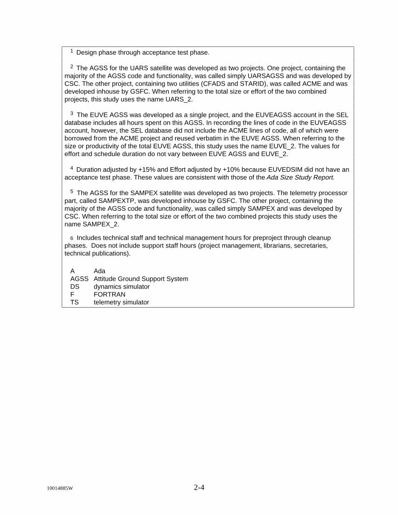
1 Design phase through acceptance test phase.

2 The AGSS for the UARS satellite was developed as two projects. One project, containing themajority of the AGSS code and functionality, was called simply UARSAGSS and was developed byCSC. The other project, containing two utilities (CFADS and STARID), was called ACME and wasdeveloped inhouse by GSFC. When referring to the total size or effort of the two combinedprojects, this study uses the name UARS_2.

3 The EUVE AGSS was developed as a single project, and the EUVEAGSS account in the SELdatabase includes all hours spent on this AGSS. In recording the lines of code in the EUVEAGSSaccount, however, the SEL database did not include the ACME lines of code, all of which wereborrowed from the ACME project and reused verbatim in the EUVE AGSS. When referring to thesize or productivity of the total EUVE AGSS, this study uses the name EUVE_2. The values foreffort and schedule duration do not vary between EUVE AGSS and EUVE_2.

4 Duration adjusted by +15% and Effort adjusted by +10% because EUVEDSIM did not have anacceptance test phase. These values are consistent with those of the Ada Size Study Report.

5 The AGSS for the SAMPEX satellite was developed as two projects. The telemetry processorpart, called SAMPEXTP, was developed inhouse by GSFC. The other project, containing themajority of the AGSS code and functionality, was called simply SAMPEX and was developed byCSC. When referring to the total size or effort of the two combined projects this study uses thename SAMPEX_2.

6 Includes technical staff and technical management hours for preproject through cleanupphases. Does not include support staff hours (project management, librarians, secretaries,technical publications).

A AdaAGSS Attitude Ground Support SystemDS dynamics simulatorF FORTRANTS telemetry simulator

10014885W 2-4

Table 2-2. Detailed Line-of-Code Data

Project Newly Extensively Slightly VerbatimName Written Modified Modified

PAS 84729 0 20041 7098ISEEB 43955 0 3506 7776AEM 45345 0 4673 893SEASAT 49316 0 4252 21825ISEEC 20075 0 6727 48618SMM 76883 0 5652 2834MAGSAT 61950 0 14297 13266FOXPRO 5354 0 1323 2449DEA 45004 0 9705 12616DEB 44644 0 8606 13016DESIM 14873 0 0 385ERBS 137739 0 5767 15635DERBY 37137 0 3901 4549GROSS 33196 3493 8574 6441GRODY 123935 1143 3037 146COBEDS 26986 0 7363 2556ASP 70951 0 0 10483GROAGSS 194169 9982 18133 14109GROSIM 31775 0 4294 2881COBSIM 45825 1342 1156 4494COBEAGSS 141084 16017 13647 7934GOADA 109807 12496 41750 7049GOFOR 22175 2867 6671 5330GOESAGSS 106834 6377 9779 5869GOESIM 59783 5784 15078 11450UARSAGSS 260382 9340 21536 11868ACME 34902 0 0 0UARS_2 295284 9340 21536 11868UARSDSIM 63861 17476 20710 4399UARSTELS 38327 6114 12163 11544EUVEAGSS 41552 13597 14844 179016EUVE_2 41552 13597 14844 213918EUVETELS 2161 371 5573 58591EUVEDSIM 20859 36248 87415 39495SAMPEXTS 0 3301 6120 52026SAMPEX 10590 1631 1282 141006SAMPEXTP 15899 1920 1777 36SAMPEX_2 26489 3551 3059 141042POWITS 12974 7980 20878 26275

10014885W 2-5

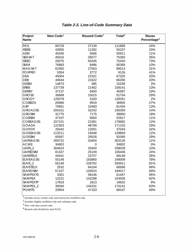
Table 2-3. Line-of-Code Summary Data

Project New Code 1 Reused Code 2 Total 3 ReuseName Percentage 4

PAS 84729 27139 111868 24%ISEEB 43955 11282 55237 20%AEM 45345 5566 50911 11%SEASAT 49316 26077 75393 35%ISEEC 20075 55345 75420 73%SMM 76883 8486 85369 10%MAGSAT 61950 27563 89513 31%FOXPRO 5354 3772 9126 41%DEA 45004 22321 67325 33%DEB 44644 21622 66266 33%DESIM 14873 385 15258 3%ERBS 137739 21402 159141 13%DERBY 37137 8450 45587 19%GROSS 36689 15015 51704 29%GRODY 125078 3183 128261 2%COBEDS 26986 9919 36905 27%ASP 70951 10483 81434 13%GROAGSS 204151 32242 236393 14%GROSIM 31775 7175 38950 18%COBSIM 47167 5650 52817 11%COBEAGSS 157101 21581 178682 12%GOADA 122303 48799 171102 29%GOFOR 25042 12001 37043 32%GOESAGSS 113211 15648 128859 12%GOESIM 65567 26528 92095 29%UARSAGSS 269722 33404 303126 11%ACME 34902 0 34902 0%UARS_2 304624 33404 338028 10%UARSDSIM 81337 25109 106446 24%UARSTELS 44441 23707 68148 35%EUVEAGSS 55149 193860 249009 78%EUVE_2 55149 228762 283911 81%EUVETELS 2532 64164 66696 96%EUVEDSIM 57107 126910 184017 69%SAMPEXTS 3301 58146 61447 95%SAMPEX 12221 142288 154509 92%SAMPEXTP 17819 1813 19632 9%SAMPEX_2 30040 144101 174141 83%POWITS 20954 47153 68107 69%

1 Includes newly written code and extensively modified code.2 Includes slightly modified code and verbatim code.3 New code plus reused code.4 Reused code divided by total SLOC.

10014885W 2-6

Table 2-4. SLOC, DLOC, and Effort

Project SLOC DLOC 1 Tech. & MGMT 2 Support 3

Name Hours Hours

PAS 111868 90157 15760 4316ISEEB 55237 46211 15262 1378AEM 50911 46458 12588 1109SEASAT 75393 54531 14508 1231ISEEC 75420 31144 5792 1079SMM 85369 78580 14371 2744MAGSAT 89513 67463 15122 1926FOXPRO 9126 6108 2521 528DEA 67325 49468 19475 2846DEB 66266 48968 17997 3267DESIM 15258 14950 4466 1194ERBS 159141 142019 49476 5620DERBY 45587 38827 18352 1870GROSS 51704 39692 15334 2207GRODY 128261 126033 23244 2560COBEDS 36905 28970 12005 1524ASP 81434 73048 17057 1875GROAGSS 236393 210599 54755 4718GROSIM 38950 33210 11463 796COBSIM 52817 48297 6106 0COBEAGSS 178682 161417 49931 4313GOADA 171102 136943 28056 2125GOFOR 37043 27442 12804 894GOESAGSS 128859 116341 37806 2876GOESIM 92095 73525 13658 1290UARSAGSS 303126 276403 89514 7854ACME 34902 34902 7965 0UARS_2 338028 311305 97479 7854UARSDSIM 106446 86359 17976 1987UARSTELS 68148 51553 11526 1034EUVEAGSS 249009 93921 21658 2538EUVE_2 283911 100901 21658 2538EUVETELS 66696 21781 4727 855EUVEDSIM 184017 95180 20775 2362SAMPEXTS 61447 20745 2516 756SAMPEX 154509 40679 4598 685SAMPEXTP 19632 18182 6772 0SAMPEX_2 174141 58861 11370 685POWITS 68107 35100 11695 308

1 Based on 20% reuse cost for FORTRAN projects and 30% reuse cost for Ada projects.

2 Includes technical staff and technical management hours for preproject through cleanup phases.

3 Includes upper management, librarians, Tech Pubs, and secretarial hours for preproject through cleanup phases.

10014885W 2-7

Table 2-5. Technical Staff Hours 1 Distributed by Life-Cycle Phase

Project Design Code Test 3-PhaseName Phase Phase Phase Total

PAS 2761 8775 3840 15376ISEEB 2871 7485 2750 13106AEM 2347 6102 3670 12119SEASAT 3516 6817 3470 13802ISEEC 1806 2433 1850 6090SMM 4533 6373 4394 15300MAGSAT 3315 5858 5955 15128FOXPRO 439 653 1210 2301DEA 3187 9682 6551 19421DEB 3565 8846 5388 17798DESIM 1427 1766 822 4015ERBS 10548 24467 13040 48055DERBY 5001 7872 4340 17213GROSS 3679 5397 6089 15165GRODY 2987 11174 4972 19133COBEDS 4008 3559 4639 12206ASP 3854 7271 5854 16979GROAGSS 11416 28132 14329 53877GROSIM 2240 4751 3942 10933COBSIM 1434 2388 1822 5644COBEAGSS 11012 18173 18410 47595GOADA 7170 10815 7901 25886GOFOR 1898 3853 6482 12233GOESAGSS 6844 19892 9808 36543GOESIM 3712 5763 3565 13039UARSAGSS 16592 42473 26612 85676ACME 2870 3723 985 7577UARS_2 19462 46196 27597 93253UARSDSIM 3100 7914 6182 17195UARSTELS 2751 4402 4014 11167EUVEAGSS 2881 9926 7732 20539EUVETELS 1107 1718 1411 4235EUVEDSIM 4258 8846 4701 17805EUVEDSIM(rev) 4258 8846 6679 19783SAMPEXTS 981 368 690 2038SAMPEX 1189 732 2578 4498SAMPEXTP 1709 3330 1600 6639SAMPEX_2 2898 4062 4178 11137POWITS 1588 5493 4597 11677

1 Includes technical staff and technical management hours for the phases listed; does not include preproject hours or cleanup phase hours; doesnot include support staff (upper management, librarians, secretaries, Tech Pubs) hours.

10014885W 2-8

Table 2-6. Groupings of Software Development Activities

Overall SOFTWARE DEVELOPMENT ACTIVITIESCategory Standard Development Process Cleanroom Process

Design Predesign PredesignCreate Design Create DesignRead/Review Design Verify/Review Design

Coding Write Code Write CodeRead/Review Code Read/Review CodeUnit Test Code

Testing Debugging PretestIntegration Test Independent TestAcceptance Test Response to SFR

Acceptance Test

Other Other Other

10014885W 2-9

Table 2-7. Technical Staff Hours Distributed by Development Activity

Project Design Coding Test Other Tech. StaffName Activity Activity Activity Activity Hours

PAS 1028 3873 2092 8383 15376ISEEB 2125 2972 1313 6696 13106AEM 2383 3144 1928 4664 12119SEASAT 1959 3687 1935 6222 13802ISEEC 1764 1730 395 2201 6090SMM 4038 4153 2188 4920 15300MAGSAT 3849 3828 2760 4691 15128FOXPRO 741 623 393 544 2301DEA 2940 3655 4826 8001 19421DEB 3557 3872 2899 7471 17798DESIM 1160 938 574 1344 4015ERBS 8798 14024 8019 17213 48055DERBY 4562 2254 2558 7839 17213GROSS 3534 4253 2615 4762 15165GRODY 4909 6467 2925 4832 19133COBEDS 2982 2538 1966 4721 12206ASP 2487 3599 4032 6861 16979GROAGSS 10829 15642 11124 16283 53877GROSIM 2408 3560 1681 3285 10933COBSIM 1269 1759 813 1802 5644COBEAGSS 11465 10545 13166 12419 47595GOADA 4967 7209 6131 7579 25886GOFOR 1427 2260 4792 3754 12233GOESAGSS 9256 11610 8976 6702 36543GOESIM 2503 2973 3081 4483 13039UARSAGSS 20561 24940 24710 15465 85676ACME 2195 1320 2370 1693 7577UARS_2 22756 26259 27080 17158 93254UARSDSIM 3117 5831 4707 3542 17195UARSTELS 2160 3067 3715 2226 11167EUVEAGSS 4419 5133 6437 4551 20539EUVETELS 644 711 1111 1771 4235EUVEDSIM 3732 5348 3807 4918 17805SAMPEXTS 341 338 546 814 2038SAMPEX 654 290 1371 2185 4498SAMPEXTP 1802 697 2620 1521 6639SAMPEX_2 2455 986 3991 3705 11138POWITS 1072 2209 4760 3636 11677

10014885W 2-10

Table 2-8. Schedule Distribution (Calendar Weeks)

Project Design Code Systest Acctest 4-Phase 1

Name Total

PAS 19 32 9 9 69ISEEB 21 21 4 4 50AEM 16 26 9 6 57SEASAT 17 24 5 8 54ISEEC 16 14 4 4 38SMM 24 24 9 19 76MAGSAT 19 24 9 10 62FOXPRO 16 10 4 6 36DEA 32 42 4 11 89DEB 32 31 10 10 83DESIM 28 20 4 4 56ERBS 42 33 12 10 97DERBY 26 23 8 15 72GROSS 23 29 18 75 145GRODY 27 67 56 10 160COBEDS 36 24 33 12 105ASP 26 27 13 21 87GROAGSS 44 75 31 38 188GROSIM 35 39 17 9 100COBSIM 23 33 15 11 82COBEAGSS 31 31 24 30 116GOADA 41 43 46 19 149GOFOR 30 33 38 18 119GOESAGSS 31 44 19 21 115GOESIM 34 29 8 28 99UARSAGSS 45 53 24 25 147ACME 42 54 15 26 137UARSDSIM 33 58 9 28 128UARSTELS 30 28 10 26 94EUVEAGSS 38 34 15 15 102EUVETELS 22 35 10 16 83EUVEDSIM2 33 43 27 18 121SAMPEXTS 23 4 8 13 48SAMPEX 39 12 19 15 85SAMPEXTP 27 33 14 13 87POWITS 29 35 9 38 111

1 System test and acceptance test phase durations are broken out separately in this table just for information. Elsewhere in this study, theseformerly separate phases are treated as one combined test phase.

2 Includes 18 weeks added to the schedule to create an artificial acceptance test phase (equal to 15% of the project duration).

10014885W 2-11

Section 3. Effort Analysis

This section derives and validates models for estimating total effort, life-cycle phase effort, andsoftware development activity effort.

Section 3.1 introduces and discusses the basic effort model for total effort. This model includesparameters for reuse cost and productivity but does not model post-CDR growth.

Section 3.2 then validates two slightly different versions of the effort model, the original modelwithout a growth factor and the same model with a growth factor added. First it validates theoriginal model using end-of-project values for both SLOC and effort. Following this it adds apost-CDR growth factor to the model, inserts the CDR SLOC estimates into the model, andvalidates the model against the actual end-of-project effort.

Section 3.3 discusses the models for the distribution of technical staff effort by life-cycle phase.

Section 3.4 presents the models for distribution of technical staff effort by software developmentactivity.

3.1 Reuse Cost Analysis, Productivity, and Total Project Effort

One of the primary concerns in planning and managing a software project is determining thetotal effort (measured in staff hours or staff months) required to complete the project. The effortdepends primarily upon the extent of the work, and the simplest and most reliable measure yetfound for describing the size of a software project in the SEL is the number of SLOC that itcontains. In the SEL, SLOC are defined to include source lines, comment lines, and blank lines.

Borrowing code written for an earlier software project and adapting it for the current projectoften requires less effort than writing entirely new code. Testing reused code also typicallyrequires less effort, because most of the software errors in the reused code have already beeneliminated. Therefore, if a software project makes significant use of reused code, the project willusually require less overall effort than if it had written all of its code from scratch.

When planning a project, FDD managers multiply the reused SLOC by a reuse cost factor, inorder to reflect the reduced cost of using old code. Adding the resulting weighted value for thereused SLOC to the number of new SLOC yields what the SEL calls the DLOC, as shown inEquation 3-1. The DLOC number is the standard measure for the size of an FDD softwareproject.

DLOC = (New SLOC) + (Reuse Cost) x (Reused SLOC) (3-1)

10014885W 3-1

The traditional reuse cost for FDD projects is 20 percent, and this remains the recommendedstandard for FORTRAN projects. The recently developed SEL model for Ada projects, however,recommends using a reuse cost of 30 percent (see Equations 3-1A and 3-1B).

FORTRAN DLOC = new SLOC + 0.2 x reused SLOC (3-1A)

Ada DLOC = new SLOC + 0.3 x reused SLOC (3-1B)

The 30-percent reuse cost for Ada projects was proposed by the Ada Size Study Report. At thetime that study was conducted, the Ada process was still evolving from project to project, andonly a small number of completed Ada projects were available for analysis. Since then only oneadditional Ada project, POWITS, has been completed and had its final project statistics verified.(The WINDPOLR final project statistics were verified too recently to be included in this report.)Today, therefore, the 30-percent Ada reuse cost still represents the best available model for FDDAda simulators. As more Ada simulators are completed, however, a clearer picture of thestandard Ada development process may become discernible. At that time the Ada reuse costshould be reevaluated.

This reevaluation is particularly advisable in light of changing development practices on high-reuse projects. These practices sometimes include combining the PDR with the CDR and alsocombining or structuring related documents in such a way as to reuse large portions ofdocuments. As the process for developing projects with high software reuse becomes moreconsistent, and as more high-reuse projects are finalized in the database, it should be possible tomodify the SEL effort model to better reflect these projects. This may include revising therecommended parameters for reuse cost and productivity.

The SEL has collected statistics on over 100 software projects during the past 2 decades. Thesestatistics include the number of new and reused SLOC in each project and the number of staffhours expended on each project. From these data SEL researchers can compute the averageproductivity, expressed in DLOC per hour, on any project. As can be seen in Equation 3-2, theproductivity calculation for a past project depends both on the effort for that project and also onthe value that is assigned as the reuse cost (embedded in the definition of DLOC).

Productivity = DLOC / Effort (3-2)

To arrive at a first-order estimate for the effort of an upcoming project, one divides the estimatedDLOC by the anticipated productivity (DLOC per hour), as shown in Equation 3-3.

Effort = DLOC / Productivity (3-3)

Figure 3-1 graphs the project productivities for 33 AGSS and simulator projects found in theSEL database. The effort used to calculate these productivities is the total technical staff andtechnical management effort; it does not include the support hours, such as project management,

10014885W 3-2

Technical Publications, secretarial, and librarian support. (Project support hours are tracked forCSC-developed projects, but are usually not tracked for GSFC in-house projects.) In theremainder of this report, all productivities are based on technical management and technicalmanagement effort only, unless specified otherwise.

Figure 3-1 contains three data points representing the overall productivities of combinedprojects. The project labeled as UARS_2 represents the total UARS AGSS, which wasdeveloped as two separate efforts, a large CSC project (identified simply as UARSAGSS in theSEL database) and a smaller GSFC inhouse project (identified as ACME). The nameSAMPEX_2 similarly denotes the total SAMPEX AGSS, which was composed of a large CSCproject (identified simply as SAMPEX) and a smaller GSFC inhouse project (identified asSAMPEXTP). The EUVE AGSS was developed as a single project, and the EUVEAGSSaccount in the SEL database includes all hours spent on this AGSS. In recording the SLOCnumber in the EUVEAGSS account, however, the SEL database did not include the ACMESLOC, all of which was borrowed from the ACME project and reused verbatim in the EUVEAGSS. The overall productivity for the EUVE AGSS is given by the EUVE_2 data point andrepresents the sum of the ACME DLOC and the EUVEAGSS DLOC, both divided by theEUVEAGSS effort.

Figure 3-1 shows significant variability in the productivities for the projects. In particular, twoprojects, SAMPEXTS and COBSIM, stand out with significantly higher productivities thansimilar projects.

The SAMPEX telemetry simulator project (SAMPEXTS) had a productivity of over 8 DLOCper hour, much higher than EUVETELS, the preceding Ada telemetry simulator. BothSAMPEXTS and EUVETELS benefited from a very high level of verbatim code reuse, but thestability of the libraries from which they borrowed was not equivalent. EUVETELS borrowedmuch of its code from UARSTELS, but the development cycles of these two projects largelyoverlapped. Thus, EUVETELS was sometimes adversely impacted by design and codingchanges made by the UARSTELS project. On the other hand, the development cycles ofSAMPEXTS and EUVETELS overlapped very little. As a result, SAMPEXTS was able toefficiently borrow code from a more stable code library. In addition SAMPEXTS piloted astreamlined development process, combining some documents and combining the PDR with theCDR. SAMPEXTS also used a lower staffing level and followed a shorter delivery schedulethan EUVETELS.

It is likely that as a result of all these advantages, the reuse cost on SAMPEXTS was actuallyless than the 30-percent standard attributed to Ada projects. Using a lower reuse cost to computethe DLOC for SAMPEXTS would result in a lower productivity value. For example, a 20-percent reuse cost would lead to a productivity of 5.9 DLOC per hour; a 10-percent reuse costwould result in a productivity of 3.6 DLOC per hour. These productivity numbers are presentedonly as suggestions. More data are needed before revising the Ada reuse cost. In all subsequentanalysis, the 30-percent reuse cost is assumed for Ada projects.

10014885W 3-3

The next Ada telemetry simulator completed, POWITS, had a lower productivity than bothEUVETELS and SAMPEXTS. POWITS also had a much lower reuse percentage thanSAMPEXTS, 69 percent versus 95 percent. In particular, the percentage of verbatim reuse wasmuch lower, 39 percent versus 85 percent. Part of the difficulty with POWITS was that thisproject was trying to model a spin-stabilized satellite by reusing the generic telemetry simulatorarchitecture that was designed for three-axis-stabilized satellites.

The COBSIM project, the other project in Figure 3-1 with a very high productivity, was the lastFORTRAN telemetry simulator developed before the switch to Ada. It was an inhouse GSFCproject. In addition to having an unusually high productivity, the software also grewsignificantly relative to both of the two preceding FORTRAN telemetry simulators and relativeto COBSIM's own CDR estimate. Measured in DLOC, COBSIM was 145 percent the size ofGROSIM and 320 percent the size of DESIM. The final COBSIM size was 330 percent of itsCDR DLOC estimate. The reasons for the significant growth and high productivity remainunresolved.

3.2 Accuracy of Models for Total Effort

This section derives recommended productivity values and then validates the accuracy ofEquation 3-3 for estimating the technical and management effort on an FDD softwaredevelopment project. Adjustments are then made to the recommended productivities to take intoaccount the addition of support staff effort. Section 3.2.1 computes the estimated effort from theend-of-project DLOC value. Section 3.2.2 computes the estimated effort from the CDR estimatefor DLOC and then applies a standard growth factor to this effort estimate.

As stated above, Equation 3-3 gives a first-order estimate for the effort of a softwaredevelopment project. Software cost estimation methods currently used in the FDD advocate theuse of additional multipliers to adjust such effort estimates or the productivities on which theyare based. The multipliers advocated reflect estimates for such contributing factors as teamexperience or problem complexity. The current study examined data from the SEFs that arecompleted at the end of each FDD project. The SEF data provide estimates for many factorssuch as problem complexity and team experience. The resulting analysis showed that the SEFdata in the SEL database provide no demonstrable evidence that inclusion of estimates for suchfactors as problem complexity or team experience will significantly improve a manager'sestimate of project effort. When making estimates for project effort, managers are stillencouraged to include such factors as problem complexity or team experience based on theirown personal experience, but the database of experience represented by the SEF data in the SELdatabase provides no guidelines. Section 4 includes a complete discussion of this topic.

3.2.1 Model Predictions Based on Final Project Statistics

In recent years, FDD AGSSs have continued to be written in FORTRAN. FDD simulators,however, are now written in Ada rather than FORTRAN. In order to determine the optimumproductivities for modeling FORTRAN and Ada FDD projects, therefore, this study hasconcentrated on the recent FORTRAN AGSSs and most of the Ada simulators, disregarding the

10014885W 3-4

earlier FORTRAN simulators. The SAMPEXTS project was excluded from the Ada productivityanalysis because it piloted a streamlined development process for which too few data areavailable at this time. The POWITS project was also deemed an outlier and was excluded. Itsproductivity was significantly lower than the other Ada projects, mainly because of the problemsencountered in modeling a spinning spacecraft.

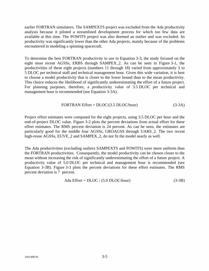
To determine the best FORTRAN productivity to use in Equation 3-3, the study focused on theeight most recent AGSSs, ERBS through SAMPEX_2. As can be seen in Figure 3-1, theproductivities of these eight projects (numbers 11 through 18) varied from approximately 3 to5 DLOC per technical staff and technical management hour. Given this wide variation, it is bestto choose a model productivity that is closer to the lower bound than to the mean productivity.This choice reduces the likelihood of significantly underestimating the effort of a future project.For planning purposes, therefore, a productivity value of 3.5 DLOC per technical andmanagement hour is recommended (see Equation 3-3A).

FORTRAN Effort = DLOC/(3.5 DLOC/hour) (3-3A)

Project effort estimates were computed for the eight projects, using 3.5 DLOC per hour and theend-of-project DLOC value. Figure 3-2 plots the percent deviations from actual effort for theseeffort estimates. The RMS percent deviation is 24 percent. As can be seen, the estimates areparticularly good for the middle four AGSSs, GROAGSS through UARS_2. The two recenthigh-reuse AGSSs, EUVE_2 and SAMPEX_2, do not fit the model nearly as well.

The Ada productivities (excluding outliers SAMPEXTS and POWITS) were more uniform thanthe FORTRAN productivities. Consequently, the model productivity can be chosen closer to themean without increasing the risk of significantly underestimating the effort of a future project. Aproductivity value of 5.0 DLOC per technical and management hour is recommended (seeEquation 3-3B). Figure 3-3 plots the percent deviations for these effort estimates. The RMSpercent deviation is 7 percent.

Ada Effort = DLOC / (5.0 DLOC/hour) (3-3B)

10014885W 3-5

05

1015

2025

3035

PRO

JEC

TS (C

hron

olog

ical

ord

er w

ithin

sub

grou

p)

0123456789

Productivity (DLOC/Hour)AG

SSs

Ada

Ada

Reg

ular

FO

RTR

AN

Tele

met

rySi

mul

ator

sD

ynam

icsSi

mul

ator

s

FOR

TRAN

FOR

TRAN

16. U

ARS_

217

. EU

VE_2

18. S

AMPE

X_2

7. M

AGSA

T8.

FO

XPR

O9.

DEB

10. D

EA11

. ER

BS12

. ASP

1. P

AS2.

ISEE

B3.

AEM

4. S

EASA

T5.

ISEE

C6.

SM

M

31. G

RO

DY

32. G

OAD

A33

. EU

VED

SIM

27. C

OBE

DS

28. G

RO

SS29

. GO

FOR

30. U

ARSD

SIM

22. G

OES

IM23

. UAR

STEL

S24

. EU

VETE

LS25

. SAM

PEXT

S26

. PO

WIT

S

19. D

ESIM

20. G

RO

SIM

21. C

OBS

IM

13. G

RO

AGSS

14. C

OBE

AGSS

15. G

OES

AGSS

DLO

C/H

R

Figu

re 3

-1. P

rodu

ctiv

ity fo

r AG

SSs

and

Sim

ulat

ors

(Bas

ed o

n Te

chni

cal &

Mgm

t Hou

rs)

Paire

d FO

RTR

ANPr

ojec

ts (C

SC

& G

SFC

In-H

ouse

)C

ombi

ned

1

2

3

4

56

7

8

9

1011

1213

1415

16

1718

19

20

21

22

2324

25

26

27

28

29

30

31

32

33

10014885W 3-6

ERBS ASP GROAGSS COBEAGSS GOESAGSS UARS_2 EUVE_2 SAMPEX_2-20%

0%

20%

40%

ER

RO

R IN

EFF

OR

T E

STI

MA

TE

ROOT-MEAN-SQUARE PERCENT ERROR = 24%

Figure 3-2. Accuracy of FORTRAN Effort Estimation Model

GOESIM UARSTELS EUVETELS GRODY GOADA EUVEDSIM-40%

-20%

0%

20%

40%

ER

RO

R IN

EFF

OR

T E

STI

MA

TE

ROOT-MEAN-SQUARE PERCENT ERROR = 7%

Figure 3-3. Accuracy of Ada Effort Estimation Model

Both GSFC in-house projects and CSC-developed projects track technical staff and technicalmanagement hours, but only CSC-developed projects track support hours (project management,librarians, Technical Publications personnel, and secretaries). In order to compare GSFC in-

10014885W 3-7

house projects with CSC-developed projects, therefore, it is necessary to have a model based ontechnical effort.

Since CSC-developed projects are planned with total cost in mind, however, it is also necessaryto have a model based on total effort, including support hours. For the 21 CSC-developedprojects from ERBS through SAMPEX the support hours add approximately 10 percent on topof the hours computed from technical effort alone. (For these 21 projects the mean value ofsupport hours divided by technical hours is 11.5 percent, with a standard deviation of 5 percent.)The appropriate model productivities are shown below.

Productivity (DLOC per hour)Type of Effort FORTRAN AdaTechnical and Management 3.5 5.0Technical, Management, and Support 3.2 4.5

3.2.2 Model Predictions Based on CDR Estimates

The effort model presented in Section 3.2.1 describes how the end-of-project DLOC value isrelated to the end-of-project effort value. During the development of a project, however, projectmanagers must rely on estimates of DLOC to predict total project effort. Requirements changes,TBDs, and in some cases the impossibility of reusing code as planned, typically cause theseDLOC estimates to grow during the life of a project. Because of this well-known tendency,project managers usually apply a growth factor to their DLOC estimates to determine the effortthat will be required for the complete project. This section proposes two values for average post-CDR growth factor, based on a project's amount of code reuse. It then validates the effortestimation model using CDR DLOC estimates along with these growth factors. Section 6presents a more complete discussion of planning models and their relationship to models that arebased on end-of-project data.

Figure 3-4 presents a project-by-project scatter plot of DLOC growth versus code reuse. Theprojects represented are the post-ERBS projects for which CDR DLOC estimates were availablein the database. The y-axis plots the DLOC growth factor, which is the end-of-project DLOCdivided by the CDR estimate. The x-axis plots the percent of code reuse attained by each project.As can be seen, the high-reuse projects (70 percent or more reuse) tended to show lower DLOCgrowth than did the low-reuse projects. Based on these data, this study recommends planning for20-percent growth in DLOC on high-reuse projects and 40-percent growth on lower reuseprojects. Equation 3-3C presents the revised effort estimation equation based on the DLOCestimated at CDR plus the DLOC due to growth.

10014885W 3-8

0% 10% 20% 30% 40% 50% 60% 70% 80% 90% 100%REUSE PERCENT

0.5

1.0

1.5

2.0

2.5

3.0

3.5

GR

OW

TH F

AC

TOR

FINAL DLOC = GROWTH FACTOR * CDR DLOC ESTIMATE

1

2

3

4

5

6

7 89 10 11

12

1314

40% GROWTH20% GROWTH

1. COBSIM 6. GOADA 11. EUVEAGSS2. UARSAGSS 7. GOESIM 12. SAMPEX3. COBEAGSS 8. GOFOR 13. SAMPEXTS4. GOESAGSS 9. UARSTELS 14. EUVETELS5. UARSDSIM 10. POWITS

Figure 3-4. DLOC Growth Factors: Actual DLOC Divided by CDR Estimate

Effort = (DLOC / Productivity) * Growth Factor (3-3C)

Code Reuse Level Growth FactorLess than 70% 1.470% or more 1.2

3.3 Distribution of Effort by Life-Cycle Phase

To staff a software project properly and to plan milestones accurately, a manager needs to knowhow much effort will be required in each of the life-cycle phases. This study examined three ofthese phases (design phase, code phase, and combined system test and acceptance test phase).

Historically, the SEL has relied on a predictive model that assumes that each project will spendthe same fixed percentage of the total project effort in a given life-cycle phase, regardless of howmuch code is reused. Table 3-1 lists the phase effort distributions for eight recent FORTRANAGSSs and eight recent Ada simulators. FORTRAN simulators were excluded, since all FDDsimulators are now written in Ada.

10014885W 3-9

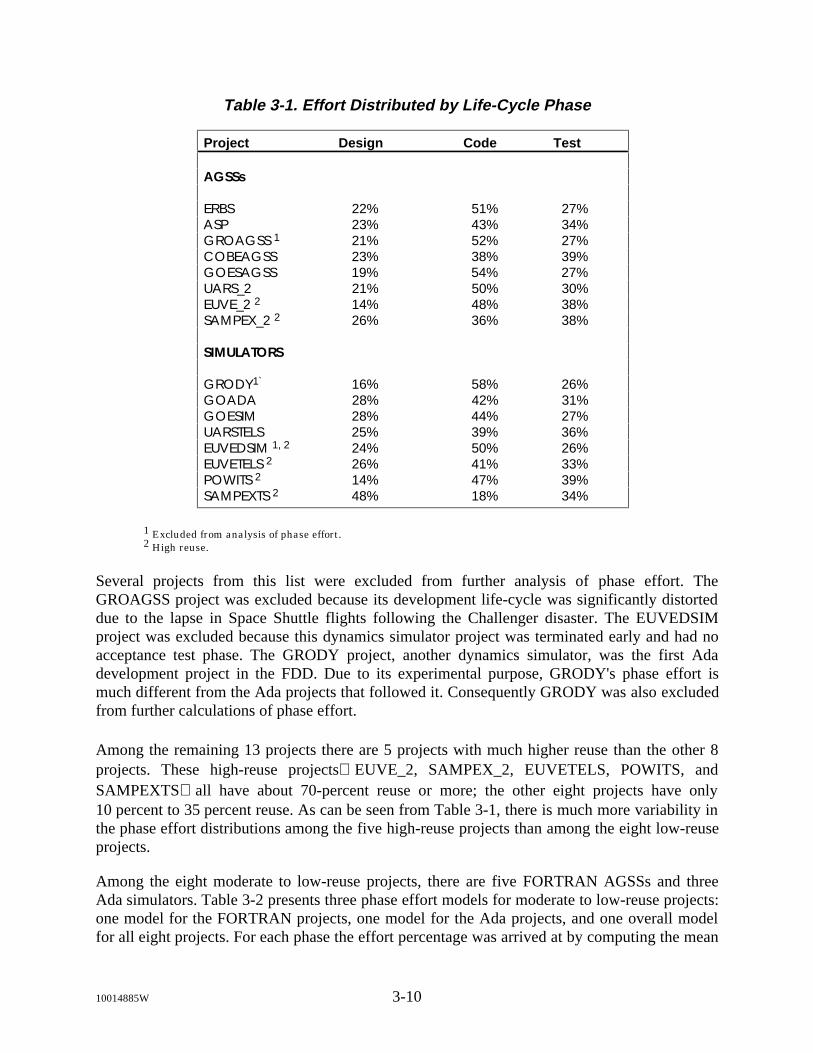
Table 3-1. Effort Distributed by Life-Cycle Phase

Project Design Code Test

AGSSs

ERBS 22% 51% 27%ASP 23% 43% 34%GROAGSS 1 21% 52% 27%COBEAGSS 23% 38% 39%GOESAGSS 19% 54% 27%UARS_2 21% 50% 30%EUVE_2 2 14% 48% 38%SAMPEX_2 2 26% 36% 38%

SIMULATORS

GRODY1` 16% 58% 26%GOADA 28% 42% 31%GOESIM 28% 44% 27%UARSTELS 25% 39% 36%EUVEDSIM 1, 2 24% 50% 26%EUVETELS 2 26% 41% 33%POWITS 2 14% 47% 39%SAMPEXTS 2 48% 18% 34%

1 Excluded from analysis of phase effort.2 High reuse.

Several projects from this list were excluded from further analysis of phase effort. TheGROAGSS project was excluded because its development life-cycle was significantly distorteddue to the lapse in Space Shuttle flights following the Challenger disaster. The EUVEDSIMproject was excluded because this dynamics simulator project was terminated early and had noacceptance test phase. The GRODY project, another dynamics simulator, was the first Adadevelopment project in the FDD. Due to its experimental purpose, GRODY's phase effort ismuch different from the Ada projects that followed it. Consequently GRODY was also excludedfrom further calculations of phase effort.

Among the remaining 13 projects there are 5 projects with much higher reuse than the other 8projects. These high-reuse projectsEUVE_2, SAMPEX_2, EUVETELS, POWITS, andSAMPEXTSall have about 70-percent reuse or more; the other eight projects have only10 percent to 35 percent reuse. As can be seen from Table 3-1, there is much more variability inthe phase effort distributions among the five high-reuse projects than among the eight low-reuseprojects.

Among the eight moderate to low-reuse projects, there are five FORTRAN AGSSs and threeAda simulators. Table 3-2 presents three phase effort models for moderate to low-reuse projects:one model for the FORTRAN projects, one model for the Ada projects, and one overall modelfor all eight projects. For each phase the effort percentage was arrived at by computing the mean

10014885W 3-10

percentages for the projects in the subset. The standard deviations are also shown. As can beseen, the AGSSs spend relatively less effort on design and more effort on coding than do theAda simulators. The moderate standard deviations for the eight-project model, however, showthat there is still a good deal of agreement between the two types of projects.

Table 3-2. Effort-by-Phase Models for Moderate to Low-Reuse Projects

5 FORTRAN AGSSs 3 Ada Simulators All 8 Projects

Phase Effort Std. Effort Std. Effort Std.Percentage Dev. Percentage Dev. Percentage Dev.

Design 21% (2%) 27% (2%) 24% (3%)Code 47% (7%) 42% (2%) 45% (6%)Test 31% (5%) 31% (4%) 31% (5%)

Table 3-3 presents a preliminary phase effort model for high-reuse projects. It is based on thefive high-reuse projects mentioned above, two FORTRAN AGSSs and three Ada simulators.The larger standard deviations for the high-reuse model reflect the greater variability in effortdistributions for high-reuse projects to date. This will be revisited when there are more data.

Table 3-3. Preliminary Effort-by-Phase Model for High-Reuse Projects

5 High-Reuse ProjectsPhase Effort Std.

Percentage Dev.

Design 26% (14%)Code 38% (12%)Test 36 (3%)

3.4 Distribution of Effort by Software Development Activity

Table 3-4 lists the effort distributions by software development activity for the same eight recentFORTRAN AGSSs and eight recent Ada simulators. The activities are grouped as shown inTable 2-5. Again the outliers GROAGSS, GRODY, and EUVEDSIM were excluded whendeveloping an effort distribution model for moderate to low-reuse and high-reuse projects.Table 3-5 presents three activity effort models for moderate to low-reuse projects: one modelbased on only FORTRAN AGSSs, one model based on only Ada simulators, and one overallmodel based on both FORTRAN AGSSs and Ada simulators. Table 3-6 presents a preliminaryactivity effort model for high-reuse projects. It is based on the same five high-reuse projects asused in the phase effort model in the preceding section, two FORTRAN AGSSs and three Adasimulators.

10014885W 3-11

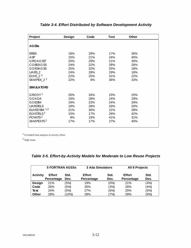
Table 3-4. Effort Distributed by Software Development Activity

Project Design Code Test Other

AGSSs

ERBS 18% 29% 17% 36%ASP 15% 21% 24% 40%GROAGSS1 20% 29% 21% 30%COBEAGSS 24% 22% 28% 26%GOESAGSS 25% 32% 25% 18%UARS_2 24% 28% 29% 18%EUVE_2 2 22% 25% 31% 22%SAMPEX_2 2 22% 9% 36% 33%

SIMULATORS

GRODY 1 26% 34% 15% 25%GOADA 19% 28% 24% 29%GOESIM 19% 23% 24% 34%UARSTELS 19% 28% 33% 20%EUVEDSIM 1,2 21% 30% 21% 28%EUVETELS 2 15% 17% 26% 42%POWITS 2 9% 19% 41% 31%SAMPEXTS 2 17% 17% 27% 40%

1 Excluded from analysis of activity effort.

2 High reuse.

Table 3-5. Effort-by-Activity Models for Moderate to Low Reuse Projects

5 FORTRAN AGSSs 3 Ada Simulators All 8 Projects

Activity Effort Std. Effort Std. Effort Std.Percentage Dev. Percentage Dev. Percentage Dev.

Design 21% (5%) 19% (0%) 21% (4%)Code 26% (5%) 26% (3%) 26% (4%)Test 24% (5%) 27% (6%) 25% (5%)Other 28% (10%) 28% (7%) 28% (9%)

10014885W 3-12

Table 3-6. Preliminary Effort-by-Activity Models for High Reuse Projects

5 High-Reuse Projects

Activity Effort Std.Percentage Dev.

Design 17% (5%)Code 17% (6%)Test 32% (6%)Other 34% (8%)

10014885W 3-13

Section 4. Methods for Adjusting Total Effort

4.1 Overview

Software cost estimation methods frequently attempt to improve project effort estimatesby factoring in the effects of project-dependent influences such as problem complexityand development team experience. Some estimation models attempt to build linearequations that include as independent variables the estimates for factors such as these.Other estimation models attempt to adjust an initial effort (or productivity) estimate byapplying several multiplicative factors, each of which is a function of a softwaredevelopment influence, such as problem complexity or team experience. In the FDD, twomodels of the latter type have been advocated over the years. The estimation modelcurrently used in the FDD advocates applying productivity multipliers to adjust theproductivity estimate shown in Equation 3-3. A previous estimation model recommendedby the FDD advocated applying similar multiplicative factors directly to the effortestimate itself. Appendix A, which presents a matrix of costing and scheduling formulasthat have been recommended in the FDD over the last 14 years, displays both these FDDmodels.

The current study sought to use empirical data in the SEL database to validate theusefulness of including such software development influences in effort estimates. Thestudy sought to determine the following:

• Does the inclusion of such factors improve the accuracy of estimates for projecteffort or productivity?

• Which factors consistently provide the greatest improvement in estimationaccuracy?

Two different approaches were followed, both using project-specific data from FDDSEFs to evaluate these effects. The first approach sought to derive a relationship betweenone or more SEF parameters and the final project productivity. By iterative optimizationmethods, the weights of the SEF parameters were adjusted until the estimatedproductivity came closest to the end-of-project productivity. Several different subsets ofprojects were evaluated, including both FORTRAN and Ada projects.

The second approach focused directly on project effort and relied on traditional linearregression methods. This approach derived linear equations for effort, in which DLOCand the SEF parameters served as the independent variables. Two subsets of projectswere evaluated, one containing 24 older FORTRAN projects and one containing 15recent FORTRAN projects.

Of the 35 SEF parameters tested, a handful seemed to improve the accuracy of the finalpredictions for either productivity or effort. Between different subsets of projects,however, there was no consistency with regard to which SEF parameters were helpful.

10014885W 4-1

As a further test, the project-specific SEF data were replaced with random numbers andthe equations for productivity and effort were rederived. The new equations (and therandom SEF data on which they were based) also resulted in improved predictions forsome SEF parameters. The number and degree of improvements resulting from randomdata were comparable to that achieved with the actual SEF data.

This study concludes that the SEF data provide no evidence of a causal relationshipbetween SEF-type parameters and either effort or productivity. This conclusion followsfrom two observations. First, the phenomenon of interest lacks continuity from oneproject subset to another and from one timeframe to another. Second, the 35 sets ofrandom integers demonstrate a degree of improvement that is comparable to thatobserved with the 35 sets of actual SEF parameter measurements.

One should not infer from the preceding statements that there is no connection betweensoftware development effort and the influences that the SEF attempts to measure. On thecontrary, it is very likely that there are some cases in which influences such as teamexperience and problem complexity will have a measurable effect on project effort. Forexample, on a small project with only one or two programmers, team experience couldbe a crucial factor in determining project effort.

The SEF data in the SEL database, however, provide no demonstrable evidence thatinclusion of estimates for factors such as problem complexity, team experience, scheduleconstraints, or requirements stability will significantly improve a manager's estimate ofproject effort. The absence of such a measurable effect may be due to the fact that thesetypical FDD projects are fairly homogeneous with regard to these influences . The effecton effort of the slight variations in these influences may be overwhelmed by otherinfluences not measured by the SEF. Alternatively, the influences of these parametersmay be invisible because the SEF does not consistently measure them. It should be notedthat it was not the purpose of this study to determine whether or not to continuecollecting SEF data, but rather to make a recommendation as to whether or not to includesuch parameters in the equation for estimating software development effort.

When making estimates for project effort, managers are still encouraged to include suchfactors as problem complexity or team experience based on their own personalexperience, but the database of experience represented by the SEF data in the SELdatabase provides no guidelines.

The remainder of this chapter is organized as follows. Section 4.2 describes the scope ofthe analysis and lists the projects studied. Section 4.3 describes the criteria used toevaluate the success of the models. Section 4.4 uses iterative optimization techniques toanalyze the usefulness of productivity multipliers. Section 4.5 uses traditional linearregression methods to analyze the usefulness of linear effort models that includesubjective factors. Section 4.6 presents conclusions.

4.2 Scope of the Analysis

In the past 14 years various models have been proposed and used in the FDD to enhancepredictions of the effort required to develop software. These models fall into two formulatypes. Although these formulas have different appearances, they are functionallyequivalent, and both are consistent with the Constructive Cost Model (COCOMO) (see

10014885W 4-2

Reference 4). Page A-3 and pages A-5 through A-7 of Appendix A give examples of thetwo formulas mentioned above, which are described more fully in the followingparagraphs.

The first formula starts with an equation for the estimated effort, expressed as a functionof software size. A multiplicative factor preceding the software size implicitly contains afirst-order estimate for the average software development productivity. Following thisfirst factor, one can then insert additional multiplicative factors that reflect the effect onproductivity of other influences. This method was advocated in An Approach to SoftwareCost Estimation (Reference 5) and Manager's Handbook for Software Development,Revision 1 (Reference 6).

The second formula is exemplified by the SEAS Basic Estimation Method (BEMS), usedin the SEAS System Development Methodology (SSDM) Standard and ProcedureNo. 1102: "Software Development Estimation" (Reference 7). The BEMS formulabegins with an explicit base development productivity. It then multiplies this averageproductivity by several optional factors, each modeling the effect of one influence onproductivity, until it arrives at the adjusted productivity estimate. Dividing the softwaresize estimate by this adjusted productivity yields the BEMS adjusted estimated effort.

For the current study, the assessments of various software development factors such asschedule constraints and requirements stability were taken from the SEF data found inthe SEL database. At the completion of each software development project in the FDD,an SEF is completed. (There are, however, no firm guidelines as to which personnel takepart in completing the SEF.) This form rates the project on 35 characteristics of thedevelopment task, the personnel, the technical management, the process, the developmentenvironment, and the final product. Each characteristic is rated on a 1-to-5 scale.Table 4-1 lists these 35 SEF parameters. A sample SEF questionnaire is included asAppendix B.

To test the validity of productivity multipliers, the study focused on 33 projects: 18AGSS projects (all written in FORTRAN), 8 telemetry simulator projects (three inFORTRAN and five in Ada), and 7 dynamics simulator projects (four in FORTRAN andthree in Ada). These 33 projects, listed in Table 4-2, include all the AGSS projects andsimulator projects whose data have been completed and verified and for which SEF datawere available.

To evaluate the utility of a linear equation composed of software developmentparameters, two project sets were used. One set consisted of 24 older FORTRANprojects. The other set consisted of 15 recent FORTRAN projects. Table 4-3 lists thesetwo sets of projects.

As mentioned previously, the UARS_2 and SAMPEX_2 projects each comprised twodevelopment projects. For the analysis in this study, the SEF values of the relatedsubprojects were weighted by the relative efforts of the subprojects and then averaged toobtain the SEF value for the project as a whole. This process resulted in noninteger SEFvalues for UARS_2 and SAMPEX_2. This step was not necessary for the EUVE AGSS,which was conducted as a single development project. The EUVE_2 data differs fromEUVEAGSS only in that EUVE_2 includes the ACME SLOC, all of which was reusedverbatim in the EUVE AGSS.

10014885W 4-3

Table 4-1. SEF Parameters

Problem Characteristics :PM01 Problem ComplexityPM02 Schedule ConstraintsPM03 Requirements StabilityPM04 Requirements Specifications QualityPM05 Documentation ExtensivenessPM06 Rigor of Review Requirements

Technical Staff Characteristics:ST07 Development Team QualityST08 Team Experience With ApplicationST09 Team Experience With EnvironmentST10 Team Stability

Technical Management Characteristics:TM11 Management PerformanceTM12 Management Experience With ApplicationTM13 Management StabilityTM14 Degree of Disciplined Project PlanningTM15 Fidelity to Project Plan

Process Characteristics:PC16 Degree Modern Programming Practices UsedPC17 Disciplined Procedures for Spec. Mods., Req't

Specs, and Interface AgreementsPC18 Used Well-Defined Req't Analysis MethodologyPC19 Used Well-Defined Design MethodologyPC20 Used Well-Defined Testing MethodologyPC21 (not applicable)PC22 Fidelity to Test PlansPC23 Used Well-Defined & Disciplined QA ProceduresPC24 Used Well-Defined & Disciplined CM Procedures

Environment Characteristics:EN25 Team Access to Development SystemEN26 Ratio of Programmers to TerminalsEN27 Constrained by Main Memory or DA StorageEN28 System Response TimeEN29 Stability of Hardware & System Support SWEN30 Effectiveness of Software Tools

Product Characteristics:PT31 Software Meets Specified RequirementsPT32 Quality of Delivered SoftwarePT33 Quality of Design in Delivered SoftwarePT34 Quality of Delivered System DocumentationPT35 Software Delivered On TimePT36 Relative Ease of Acceptance Testing

10014885W 4-4

Table 4-2. Projects Used To Test Productivity Multipliers

AGSSsPAS Telemetry SimulatorsISEEB DESIMAEM GROSIMSEASAT COBSIMISEEC GOESIMSMM UARSTELSMAGSAT EUVETELSFOXPRO POWITSDEB SAMPEXTSDEA

ERBS Dynamics SimulatorsASP COBEDSGROAGSS GROSSCOBEAGSS GOFORGOESAGSS UARSDSIMUARS_2 GRODYEUVE_2 GOADASAMPEX_2 EUVEDSIM

Table 4-3. Projects Used To Test Correlations Between Effort and SEFParameters

24 Older FORTRAN Projects

AEM FOXPRO ASPISEEB DEA DSPLBLDRPAS DEB COBSIMISEEC DESIM GROSIMSEASAT GSOC GOFORSMM DEDET UARSDSIMMAGSAT GROSS ACMEFOXPP COBEDS BBXRT

15 Recent FORTRAN Projects

AGSSs: SimulatorsERBS DESIMASP GROSIMGROAGSS COBSIMCOBEAGSS COBEDSGOESAGSS GROSSUARS_2 GOFOREUVE_2 UARSDSIMSAMPEX_2

10014885W 4-5

4.3 Methods Used to Evaluate Success

Adding SEF parameters to the estimation equation either as productivity multipliers or asadditional linear parameters alongside DLOC may result in improved estimates. Toevaluate the utility of including the SEF parameters requires determining how muchimprovement results in the accuracy of the estimate when the SEF parameters areincluded. This involves measuring the closeness of fit between the derived equation(based on one or more SEF parameters) and the final project productivities or effortsgiven by the data points. This closeness of fit could be measured in terms of the RMSpercent deviation or, in the case of linear regression results, the R-squared value. Onemust be careful in such comparisons. The R-squared values, for example, should not beused for comparison between equations with differing degrees of freedom.

In assessing the apparent improvement in fit, one should also consider what portion ofthe improvement is due to the purely mathematical effect of adding extra dimensions tothe equation. Each extra dimension adds another independent parameter to the equation.As the number of independent parameters rises, it becomes easier to make the equationmore closely fit the fixed number of data points. In the extreme case where there aremore independent parameters than the number of projects in one's dataset, it is usuallypossible to make the derived equation precisely fit the data points. Such results aremeaningless, however, because of the scarcity of data points relative to the number ofdimensions. For example, one would hesitate to estimate with a two-dimensional linearequation that was derived from only two experimental data points.

It should also be noted that estimating equations derived from end-of-project SEF datawill be less accurate when applied early in the life cycle. This is because such estimateswill be based on early assessments of the SEF parameters, which are inherently lessaccurate than the end-of-project SEF assessments used in this study.

4.4 Deriving Productivity Multipliers with Optimization Procedures

The first approach, deriving productivity multipliers with optimization procedures, beganwith a base productivity estimate and then attempted to improve it by including project-specific knowledge about one or more software development influences, until theestimated productivity came as close as possible to the final project productivity. In orderto achieve the best fit between the initial model and the given dataset of 33 projects, thebase productivity for FORTRAN was chosen to be 3.83 DLOC per hour, the meanproductivity for the 25 FORTRAN projects in the sample. Likewise, the Ada baseproductivity was chosen to be 5.13 DLOC per hour, the mean productivity for the 8 Adaprojects in the sample. (These numbers vary slightly from the moderately conservativeproductivity planning numbers recommended in Section 3.) Because all values for effortand lines of code were taken directly from the final project statistics, growth factors werenot considered.

10014885W 4-6

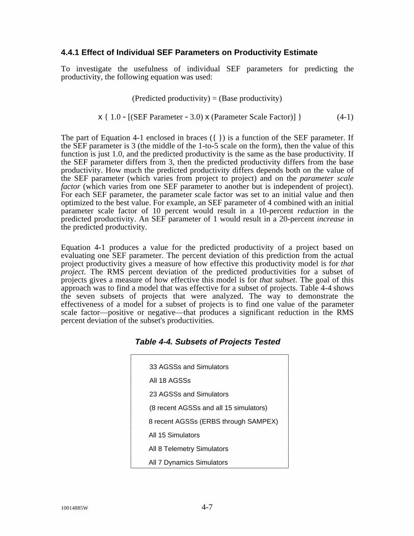
4.4.1 Effect of Individual SEF Parameters on Productivity Estimate

To investigate the usefulness of individual SEF parameters for predicting theproductivity, the following equation was used:

(Predicted productivity) = (Base productivity)

x { 1.0 - [(SEF Parameter - 3.0) x (Parameter Scale Factor)] } (4-1)

The part of Equation 4-1 enclosed in braces ({ }) is a function of the SEF parameter. Ifthe SEF parameter is 3 (the middle of the 1-to-5 scale on the form), then the value of thisfunction is just 1.0, and the predicted productivity is the same as the base productivity. Ifthe SEF parameter differs from 3, then the predicted productivity differs from the baseproductivity. How much the predicted productivity differs depends both on the value ofthe SEF parameter (which varies from project to project) and on the parameter scalefactor (which varies from one SEF parameter to another but is independent of project).For each SEF parameter, the parameter scale factor was set to an initial value and thenoptimized to the best value. For example, an SEF parameter of 4 combined with an initialparameter scale factor of 10 percent would result in a 10-percent reduction in thepredicted productivity. An SEF parameter of 1 would result in a 20-percent increase inthe predicted productivity.

Equation 4-1 produces a value for the predicted productivity of a project based onevaluating one SEF parameter. The percent deviation of this prediction from the actualproject productivity gives a measure of how effective this productivity model is for thatproject. The RMS percent deviation of the predicted productivities for a subset ofprojects gives a measure of how effective this model is for that subset. The goal of thisapproach was to find a model that was effective for a subset of projects. Table 4-4 showsthe seven subsets of projects that were analyzed. The way to demonstrate theeffectiveness of a model for a subset of projects is to find one value of the parameterscale factor—positive or negative—that produces a significant reduction in the RMSpercent deviation of the subset's productivities.

Table 4-4. Subsets of Projects Tested

33 AGSSs and Simulators

All 18 AGSSs

23 AGSSs and Simulators

(8 recent AGSSs and all 15 simulators)

8 recent AGSSs (ERBS through SAMPEX)

All 15 Simulators

All 8 Telemetry Simulators

All 7 Dynamics Simulators

10014885W 4-7

The tool used to perform these optimizations was part of the personal computer softwarepackage known as Quattro Pro, Version 4.0 (see Reference 8). This package contains atool called the Optimizer, which solves linear and nonlinear problems involving multiplevariables and multiple constraints. For the present work the Optimizer was required toadjust the value of the given parameter scale factor until an RMS percent deviationwithin the specified precision of the minimum value was achieved. The default precisionof .0005 was generally used. The Optimizer contains several switches that allow the userto specify various mathematical options, some of which are specified below. A variety ofoption settings were used at different times.

• Specify the approach used to obtain initial estimates of the basic variables in eachiteration. Linear extrapolation from a tangent vector or quadratic extrapolation arethe two choices available.

• Specify either forward or central differencing for estimates of partial derivatives.

• Specify the method for computing the search direction, either a quasi-Newtonmethod or conjugate method.

In most cases, the optimization process began with a parameter scale factor of +10percent, and the Optimizer then varied it until achieving the minimum RMS percentdeviation. In order to remove any doubt that the final result of the optimization processmight depend on the choice of the initial value, a significant number of trials wererepeated beginning with a variety of initial values. In each such case, the choice of theinitial value had no effect on the final optimized value.

Table 4-5 lists, for each subset of projects and for each SEF parameter, the parameterscale factor that yields the lowest RMS percent deviation of the predicted productivitiesversus the actual project productivities. The RMS percent deviation (expressed as adecimal number) is listed in parentheses beneath the value of each parameter scale factor.At the top of the table are listed the RMS percent deviations that result when no SEFparameter is used to adjust the mean FORTRAN and Ada productivities. These baseRMS values vary from 21 percent to 42 percent, depending on the subset of projectsconsidered. For each subset of projects, a few SEF parameters that provide the mostsignificant improvements in the RMS percent deviation are denoted by boldfaced RMSvalues. Each row of Table 4-5 represents a productivity model that is based on theinfluence of a single SEF parameter. Models displaying the simultaneous influence ofmore than one SEF parameter are described later.

Often the use of one SEF parameter improves the base RMS percent deviation by onlyone or two percentage points. Improvements of this magnitude—and sometimes larger—can easily be achieved using random values for SEF parameters and are only valid for thegiven set of SEF values and productivities; they represent no generally valid relationship.

This conclusion was verified by substituting random values for the 35 SEF parametersfor each project and then repeating the calculations that led to Table 4-5. This againresulted in 35 parameter scale factors and 35 RMS percent deviations for each of theseven subsets of projects. Since the SEF values used this time were random, none of the35 resulting rows represents the effect of PM01 or any other real SEF value on theproductivity of the subsets. The value of any one of the new 35 RMS percent deviations

10014885W 4-8

in a column is thus not important. What is important is the range and distribution of the35 RMS percent deviations and how these compare to the RMS percent deviationsresulting when no SEF data are used (the row labeled "None" in Table 4-5) and also tothe range and distribution of the RMS percent deviations resulting from real SEF data inTable 4-5.

Table 4-5. Effect of Individual SEF Parameters on Productivity Estimate(1 of 4)

Parameter Scale Factor (Root-mean-square percent deviation in predicted productivity) 1

SEF 33 All 18 23 AGSSs 8 Recent 15 8 7Parameter AGSSs & AGSSs & Simulators AGSSs Simulators Telemetry Dynamics

Simulators Simulators Simulators

None(0.339) (0.287) (0.340) (0.210) (0.392) (0.367) (0.420)

PM01 0.042 -0.077 0.140 0.066 0.173 0.094 0.250(0.335) (0.273) (0.296) (0.197) (0.329) (0.349) (0.270)

PM02 0.054 -0.023 0.116 0.027 0.128 0.100 0.149(0.329) (0.285) (0.300) (0.209) (0.334) (0.337) (0.325)

PM03 -0.057 -0.033 -0.102 -0.178 -0.087 -0.098 -0.050(0.329) (0.283) (0.316) (0.143) (0.373) (0.327) (0.417)

PM04 -0.034 -0.029 -0.040 -0.013 -0.052 -0.172 0.282(0.335) (0.283) (0.338) (0.210) (0.389) (0.305) (0.361)

PM05 0.061 0.062 0.093 0.104 0.051 0.125 -0.056(0.335) (0.279) (0.334) (0.181) (0.392) (0.363) (0.419)

PM06 0.099 0.071 0.182 0.131 0.256 0.235 0.266(0.323) (0.272) (0.312) (0.167) (0.362) (0.350) (0.375)

1Percent deviation expressed as decimal number, i.e., 0.339 means 33.9%.

10014885W 4-9

Table 4-5. Effect of Individual SEF Parameters on Productivity Estimate(2 of 4)

Parameter Scale Factor (Root-mean-square percent deviation in predicted productivity) 1

SEF 33 All 18 23 AGSSs 8 Recent 15 8 7Parameter AGSSs & AGSSs & Simulators AGSSs Simulators Telemetry Dynamics

Simulators Simulators Simulators

None(0.339) (0.287) (0.340) (0.210) (0.392) (0.367) (0.420)

ST07 0.098 0.070 0.096 0.035 0.111 0.104 0.129(0.316) (0.279) (0.313) (0.207) (0.353) (0.316) (0.390)

ST08 -0.0032 0.072 -0.073 -0.087 -0.070 -0.030 -0.168(0.339) (0.274) (0.328) (0.197) (0.380) (0.364) (0.375)

ST09 0.071 0.127 0.032 0.073 0.026 -0.049 0.109(0.326) (0.246) (0.338) (0.203) (0.390) (0.360) (0.389)

ST10 0.094 0.120 0.049 -0.0085 0.066 0.036 0.096(0.318) (0.248) (0.335) (0.210) (0.383) (0.364) (0.400)

TM11 0.078 0.0033 0.131 0.098 0.144 0.140 0.147(0.331) (0.287) (0.314) (0.191) (0.362) (0.343) (0.384)

TM12 0.097 0.029 0.131 0.086 0.168 0.101 0.256(0.326) (0.286) (0.308) (0.181) (0.354) (0.351) (0.338)

TM13 0.027 0.0057 0.046 0.022 0.053 0.013 0.110(0.337) (0.287) (0.335) (0.209) (0.386) (0.366) (0.395)

TM14 0.047 -0.017 0.131 0.047 0.280 0.225 0.348(0.334) (0.286) (0.307) (0.198) (0.315) (0.313) (0.308)

TM15 0.057 0.011 0.131 0.070 0.181 0.178 0.187(0.332) (0.287) (0.312) (0.194) (0.353) (0.312) (0.395)

1Percent deviation expressed as decimal number, i.e., 0.339 means 33.9%.

10014885W 4-10

Table 4-5. Effect of Individual SEF Parameters on Productivity Estimate (3 of 4)

Parameter Scale Factor (Root-mean-square percent deviation in predicted productivity) 1

SEF 33 All 18 23 AGSSs 8 Recent 15 8 7Parameter AGSSs & AGSSs & Simulators AGSSs Simulators Telemetry Dynamics

Simulators Simulators Simulators

None(0.339) (0.287) (0.340) (0.210) (0.392) (0.367) (0.420)

PC16 0.047 -0.055 0.106 0.0063 0.130 0.068 0.160(0.333) (0.279) (0.308) (0.210) (0.339) (0.358) (0.302)

PC17 -0.028 -0.039 0.034 0.062 0.022 -0.014 0.084(0.334) (0.268) (0.337) (0.196) (0.391) (0.366) (0.408)

PC18 -0.039 -0.059 0.039 0.045 0.036 -0.098 0.168(0.334) (0.267) (0.338) (0.206) (0.391) (0.354) (0.380)

PC19 0.090 0.059 0.124 0.089 0.140 0.083 0.214(0.322) (0.278) (0.314) (0.190) (0.362) (0.355) (0.355)

PC20 0.058 -0.018 0.107 0.056 0.127 0.058 0.166(0.330) (0.286) (0.307) (0.199) (0.347) (0.360) (0.314)

PC22 0.015 -0.086 0.101 0.049 0.125 0.122 0.127(0.338) (0.266) (0.314) (0.202) (0.355) (0.340) (0.372)

PC23 0.065 0.0 0.125 0.0084 0.212 0.189 0.266(0.332) (0.287) (0.319) (0.210) (0.345) (0.313) (0.375)

PC24 0.032 -0.047 0.092 0.045 0.114 0.109 0.120(0.337) (0.281) (0.318) (0.203) (0.362) (0.334) (0.392)

EN25 0.130 -0.151 0.162 2.021 0.161 0.107 0.212(0.310) (0.279) (0.279) (0.198) (0.310) (0.334) (0.256)

EN26 0.058 -0.140 0.167 -0.107 0.205 0.099 0.310(0.333) (0.258) (0.297) (0.201) (0.313) (0.350) (0.197)

EN27 -0.072 -0.080 -0.016 0.118 -0.063 0.180 -0.101(0.335) (0.282) (0.340) (0.198) (0.390) (0.360) (0.407)

EN28 0.015 -0.057 0.037 -0.026 0.042 -0.129 0.156(0.339) (0.284) (0.338) (0.210) (0.388) (0.335) (0.346)

EN29 -0.018 -0.062 0.033 0.031 0.034 -0.230 0.273(0.338) (0.278) (0.338) (0.208) (0.390) (0.267) (0.254)

EN30 -0.026 -0.040 0.065 0.167 0.042 -0.014 0.183(0.335) (0.268) (0.332) (0.160) (0.389) (0.366) (0.378)

1Percent deviation expressed as decimal number, i.e., 0.339 means 33.9%.

10014885W 4-11

Table 4-5. Effect of Individual SEF Parameters on Productivity Estimate(4 of 4)

Parameter Scale Factor (Root-mean-square percent deviation in predicted productivity) 1

SEF 33 All 18 23 AGSSs 8 Recent 15 8 7Parameter AGSSs & AGSSs & Simulators AGSSs Simulators Telemetry Dynamics

Simulators Simulators Simulators

None(0.339) (0.287) (0.340) (0.210) (0.392) (0.367) (0.420)

PT31 0.093 0.058 0.097 0.029 0.139 0.089 0.194(0.298) (0.269) (0.295) (0.204) (0.312) (0.334) (0.255)

PT32 0.073 0.024 0.086 0.015 0.127 0.041 0.216(0.320) (0.285) (0.311) (0.209) (0.337) (0.361) (0.232)

PT33 0.023 -0.069 0.089 -0.013 0.117 -0.046 0.306(0.338) (0.277) (0.326) (0.210) (0.367) (0.362) (0.213)

PT34 0.078 0.066 0.073 0.017 0.092 0.068 0.107(0.320) (0.271) (0.326) (0.210) (0.370) (0.357) (0.382)

PT35 0.0030 -0.053 0.084 0.118 0.070 0.041 0.140(0.339) (0.281) (0.328) (0.174) (0.384) (0.363) (0.400)

PT36 -0.036 0.0028 -0.063 0.025 -0.086 -0.121 0.036(0.336) (0.287) (0.332) (0.209) (0.376) (0.312) (0.418)

1Percent deviation expressed as decimal number, i.e., 0.339 means 33.9%.

Therefore, rather than print all 35 rows of parameter scale factors and RMS percentdeviations resulting from random SEF values, only three rows summarizing the 35 RMSpercent deviations are presented. These contain the maximum, mean, and minimumRMS percent deviations for each set of 35 RMS percent deviations and are presented inTable 4-6. The mean improvement in the RMS percent deviation was one percentagepoint each for the first four subsets (the 33 AGSSs and simulators, the 18 AGSSs, the 23AGSSs and simulators, and the 8 recent AGSSs). For the subset of 15 simulators, themean improvement was 2 percentage points, for the subset of 8 telemetry simulators, 3percentage points, and for the subset of 7 dynamics simulators, 7 percentage points.

10014885W 4-12

Table 4-6. Reduction in RMS Percent Deviation Using Random SEF Values

Root-mean-square percent deviation in predicted productivity 1

SEF 33 All 18 23 AGSSs 8 Recent 15 8 7Parameter AGSSs & AGSSs & Simulators AGSSs Simulators Telemetry Dynamics

Simulators Simulators Simulators

Base RMSvalue (no SEF used) 0.339 0.287 0.340 0.210 0.392 0.367 0.420

MaximumRMS 0.339 0.287 0.340 0.210 0.392 0.367 0.419

Mean RMS 0.331 0.275 0.329 0.196 0.372 0.338 0.350

MinimumRMS 0.293 0.233 0.287 0.138 0.300 0.257 0.123

1 Percent deviation expressed as a decimal number, i.e., 0.339 means 33.9%.

4.4.2 Effect of Multiple SEF Parameters on Productivity Estimate

Equation 4-1 can be extended to test for the simultaneous effect of multiple SEFparameters. This is done by repeating—once for each additional desired SEFparameter—the portion of the equation within the braces, as shown in Equation 4-5.Table 4-7 lists the subsets of SEF parameters whose effects on productivity were testedfor in this way. The same subsets of projects were again tested to find the change in theRMS percent deviation. The results are shown in Table 4-8.

(Predicted productivity) = (Base productivity)

x { 1.0 - [(SEF Parameter1 - 3.0) x (Parameter Scale Factor1)] }

x { 1.0 - [(SEF Parameter2 - 3.0) x (Parameter Scale Factor2)] }

x {...} x {...} x ... (4-5)

Table 4-7. Subsets of SEF Parameters Tested

Problem Characteristics: PM01 - PM06Technical Staff Characteristics: ST07 - ST10Technical Management Characteristics: TM11 - TM15Process Characteristics: PC16 - PC24Environment Characteristics: EN25 - EN30Product Characteristics: PT31 - PT36

10014885W 4-13

Table 4-8. Effect of Multiple SEF Parameters on Productivity Estimate(1 of 2)

Parameter Scale Factors Based on Actual SEF Values (RMS percent deviation based on actual SEF data) 1

[RMS percent deviation based on random SEF values]

SEF 33 All 18 23 AGSSs 8 Recent 15 8 7Parameter AGSSs & AGSSs & Simulators AGSSs Simulators Telemetry Dynamics

Simulators Simulators Simulators

None(0.339) (0.287) (0.340) (0.210) (0.392) (0.367) (0.420)

PM01 0.030 -0.121 0.069 -0.014 0.095 -0.199 0.100PM02 0.101 -0.096 0.092 0.202 0.136 0.247 0.166PM03 0.012 0.111 -0.004 -0.014 0.046 0.124 0.043PM04 -0.123 -0.095 -0.064 0.629 -0.062 -0.253 0.504PM05 -0.074 -0.180 -0.010 0.430 0.027 -8.755 0.414PM06 0.233 0.300 0.171 -0.607 0.250 0.732 -0.329

(0.262) (0.177) (0.256) (0.129)2 (0.263) (0.243)2 (0.115)2

[0.259] [0.240] [0.238] [0.116] [0.227] [0.163] [0.067]

ST07 0.064 -0.057 0.105 0.073 0.122 0.168 0.112ST08 -0.127 -0.092 -0.155 -0.143 -0.162 0.092 -0.312ST09 0.113 0.169 0.059 0.184 0.060 -0.334 0.167ST10 0.092 0.078 0.030 0.205 0.053 -0.064 -0.0078

(0.279) (0.226) (0.271) (0.261) (0.299) (0.215) (0.244)2

[0.321] [0.253] [0.307] [0.169] [0.305] [0.215] [0.219]

TM11 0.063 0.036 0.024 -0.180 -0.058 -0.037 -0.127TM12 0.131 0.162 0.080 0.064 0.051 0.030 -0.213TM13 -0.030 -0.113 -0.036 -0.028 -0.066 -0.103 -0.147TM14 -0.186 -0.274 0.067 0.421 0.304 0.192 0.541TM15 0.153 0.241 0.033 0.011 0.040 0.132 0.163

(0.310) (0.197) (0.297) (0.309)2 (0.302) (0.280)2 (0.297)2

[0.306] [0.252] [0.286] [0.139] [0.294] [0.252] [0.044]

1 Percent deviation expressed as a decimal number, i.e., 0.339 means 33.9%.2 These results are based on too few projects to have confidence in their validity.

10014885W 4-14

Table 4-8. Effect of Multiple SEF Parameters on Productivity Estimate (2 of 2)

Parameter Scale Factors Based on Actual SEF Values (RMS percent deviation based on actual SEF data) 1

[RMS percent deviation based on random SEF values]

SEF 33 All 18 23 AGSSs 8 Recent 15 8 7Parameter AGSSs & AGSSs & Simulators AGSSs Simulators Telemetry Dynamics

Simulators Simulators Simulators

None(0.339) (0.287) (0.340) (0.210) (0.392) (0.367) (0.420)

PC16 0.048 -0.188 0.081 0.154 0.163 0.144 0.147PC17 -0.050 0.126 -0.062 -0.075 -0.017 -0.290 -0.059PC18 0.017 -0.117 0.040 0.337 0.047 0.479 0.343PC19 0.059 0.175 -0.032 -5.633 -0.50 -2.781 -4.153PC20 0.055 -0.042 0.137 0.405 0.114 -0.582 0.379PC22 -0.153 -0.097 -0.164 0.298 -0.117 -3.629 0.296PC23 0.014 0.049 0.016 0.528 0.244 0.488 0.526PC24 0.084 0.028 0.093 -0.788 0.044 0.479 -0.784

(0.303) (0.176) (0.291) (0.0000)2 (0.294) (0.154)2 (0.000)2

[0.296] [0.119] [0.277] [0.0000] [0.280] [0.0000] [0.0000]

EN25 0.181 -0.119 0.141 -0.710 0.161 0.112 -0.589EN26 -0.025 -0.210 0.084 0.509 0.079 -0.120 0.505EN27 -0.017 -0.044 0.022 -0.071 -0.026 0.098 -0.063EN28 0.025 0.198 -0.064 -0.024 -0.029 0.082 -0.083EN29 -0.0068 -0.079 0.061 0.349 0.030 -0.228 0.292EN30 -0.059 0.011 -0.021 -0.074 -0.079 -0.089 0.051

(0.284) (0.230) (0.270) (0.123)2 (0.285) (0.252)2 (0.112)2

[0.292] [0.145] [0.283] [0.082] [0.260] [0.117] [0.073]

PT31 0.014 -0.089 0.063 0.100 0.0043 -0.517 0.134PT32 0.155 0.119 0.078 -0.222 0.224 0.278 -0.211PT33 -0.154 -0.282 -0.031 0.383 -0.091 -0.317 0.367PT34 0.023 0.128 -0.053 -0.126 -0.078 0.197 -0.054PT35 0.00093 0.037 0.050 0.332 0.0286 0.214 0.223PT36 -0.080 0.019 -0.084 0.325 -0.153 -0.259 0.182

(0.276) (0.202) (0.281) (0.132)2 (0.274) (0.148)2 (0.118)2

[0.288] [0.196] [0.276] [0.070] [0.266] [0.221] [0.154]

1 Percent deviation expressed as a decimal number, i.e., 0.339 means 33.9%.

2 These results are based on too few projects to have confidence in their validity.

10014885W 4-15

Although Table 4-8 seems to show greater reductions in the base RMS percent deviationsthan were shown in Table 4-5, these results must be interpreted carefully. Equation 4-4only solves for one parameter scale factor at a time. Equation 4-5 simultaneously solvesfor between four and eight parameter scale factors, depending on the subset of SEFparameters. This greater flexibility makes it easier to find a final equation that moreclosely fits the data represented by the subset of projects. But this greater flexibility canlead to statistically unreliable results when the number of datasets (that is, the number ofprojects in the project subset) is only slightly greater than the number of simultaneousSEF parameters. These unreliable RMS percent deviations are pointed out in Table 4-8.

An example to consider is the subset of six "Problem Characteristics" parameters (PM01through PM06) taken with the subset of seven dynamics simulators. Here Equation 4-5has one dependent variable (predicted productivity) and six independent variables (thesix PM factors). Thus it is a seven-dimensional equation. The dataset consists of onlyseven data points (the seven dynamics simulator projects). With experimental datacontaining experimental noise, many more data points are needed than the number ofdimensions in the equation. So although Equation 4-5 results here in an RMS percentdeviation of 11.5 percent, one cannot have confidence that the six resulting scale factorsrepresent a true picture of the effects of PM01 through PM06 on the productivity ofdynamics simulator projects.

The RMS percent deviations resulting from the actual SEF data are shown in parenthesesin Table 4-8. For comparison, the RMS percent deviation that results from using arandom set of SEF values is shown in brackets in Table 4-8. As can be readily seen, theimprovements resulting from the use of random SEF values are of the same order as theimprovements resulting from the actual SEL data SEF values. Because the parameterscale factors in Table 4-8 provide no more consistency in predicting productivity than isprovided by the models based on random SEF data, one must be very skeptical of thesemodels. One cannot say with confidence that the parameter scale factors in Table 4-8represent valid models of the influence of multiple SEF parameters on productivity.

Perhaps by more carefully selecting the SEF parameters to include in Equation 4-5 onemight develop a more successful model. This motivation guided the next stage of theinvestigation. It is useful here to consider again the models based on Equation 4-4 anddisplayed in Table 4-5. The values of the parameter scale factors in Table 4-5 show littleconsistency from one project subset to another. This could mean that the influences ofthe parameters cannot be observed by the methods of this study. It could alternativelymean that the influences have evolved over time and that they exhibit qualitativelydifferent effects in different application areas. With this second possibility in mind, thestudy sought to focus further on one broad subset of projects that would reflect the waythe FDD currently develops software.

The study chose the subset consisting of all AGSSs and simulators developed sinceDESIM, the first simulator. This is a large subset—23 projects—so one can evaluate thesimultaneous effect of several SEF parameters on this subset without undue concernabout statistically invalid results. The subset is broadly based—including both AGSSsand simulators—so a model derived from it could be widely used within the FDD. Thesubset closely represents the way the FDD develops software today because it containsall of the 8 recent AGSSs (ERBS through SAMPEX_2), and because 14 of the 15simulators cover the same period. (The first simulator, DESIM, preceded ERBS by3 years).

10014885W 4-16

Table 4-5 shows that for this subset of projects, five parameters (PM01, PM02, EN25,EN26, and PT31) when applied individually to Equation 4-4, had moderate success atreducing the RMS percent deviation. The first four of these parameters are influencesthat the project manager might have some ability to estimate during a project, so attemptswere made to model the simultaneous effect of these four parameters following theformat of Equation 4-5. SEF parameters PM03 and PM06 had only slightly less successthan the five parameters listed above at reducing the RMS percent deviation. In addition,the parameter scale factors for PM03 and PM06 (-10.2 percent and 18.2 percent,respectively) suggest a fairly strong link to productivity. These two parameters weretherefore also included in the model.

To include the effects of other SEF parameters without overwhelming the equation withtoo many parameter scale factors, additional SEF parameters that were functionallysimilar and that behaved similarly in Table 4-5 were averaged to produce additional SEFparameters. The SEF parameters TM11, TM12, TM14, and TM15 all had nearly thesame parameter scale factor (0.131) and nearly the same RMS percent deviation. Thesefour SEF parameters were averaged to produce one new parameter. The SEF parametersPC16, PC19, PC20, PC22, PC23, and PC24 all had approximately the same parameterscale factor (0.092 to 0.125) and nearly the same RMS percent deviation. These six SEFparameters were averaged to produce another new parameter.

The resulting equation followed the format of Equation 4-5 and had eight parameters (sixindividual SEF parameters plus two SEF parameter averages). When the eight parameterscale factors were optimized, the resulting equation produced an RMS percent deviationof 23.1 percent for the 23 predicted productivities. This is an improvement of 11percentage points over the prediction using no parameter scale factors to predictproductivity for this subset of projects.

Next, the real SEF data for these 23 projects were replaced with random data, theparameter scale factors were again optimized, and the RMS percent deviation for thepredicted productivities was computed. This 3-step randomization process was repeated35 times. For the 35 RMS percent deviations computed, the maximum, mean, andminimum values were 31.4 percent, 25.2 percent, and 19.2 percent, respectively. Theresults of these tests with real and random SEF data are summarized in Table 4-9.

The tests with random SEF data show that most of the reduction in the RMS percentdeviation is due to the mathematical ease of fitting the 23 final productivities in thedataset to any SEF data (even random data) when 8 parameter scale factors are availableto be assigned. The mean improvement from random data was 9 percentage points; theimprovement when applying actual SEF data was 11 percentage points, a difference ofonly 2 percentage points. As a result, one cannot claim with confidence that the modelrepresented by the eight parameter scale factors in Table 4-9 truly models softwaredevelopment productivity in the FDD.

10014885W 4-17

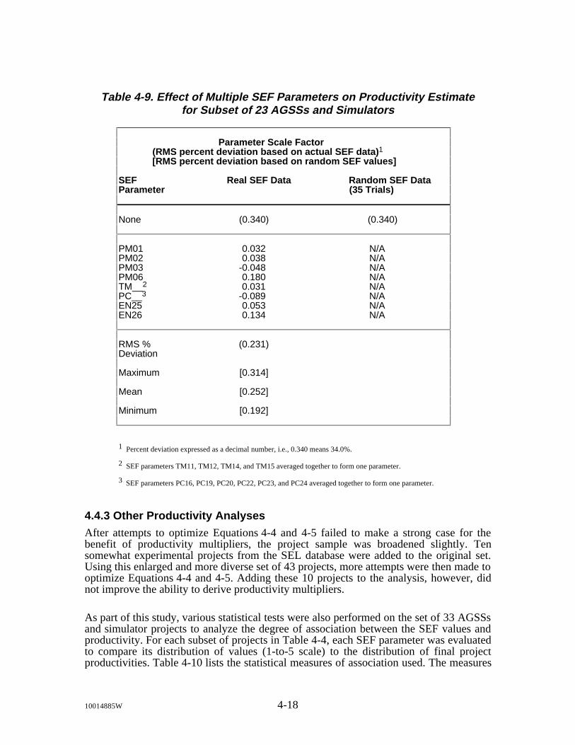
Table 4-9. Effect of Multiple SEF Parameters on Productivity Estimatefor Subset of 23 AGSSs and Simulators

Parameter Scale Factor (RMS percent deviation based on actual SEF data) 1

[RMS percent deviation based on random SEF values]

SEF Real SEF Data Random SEF DataParameter (35 Trials)

None (0.340) (0.340)

PM01 0.032 N/APM02 0.038 N/APM03 -0.048 N/APM06 0.180 N/ATM__2 0.031 N/APC__3 -0.089 N/AEN25 0.053 N/AEN26 0.134 N/A

RMS % (0.231)Deviation

Maximum [0.314]

Mean [0.252]

Minimum [0.192]

1 Percent deviation expressed as a decimal number, i.e., 0.340 means 34.0%.

2 SEF parameters TM11, TM12, TM14, and TM15 averaged together to form one parameter.

3 SEF parameters PC16, PC19, PC20, PC22, PC23, and PC24 averaged together to form one parameter.

4.4.3 Other Productivity Analyses

After attempts to optimize Equations 4-4 and 4-5 failed to make a strong case for thebenefit of productivity multipliers, the project sample was broadened slightly. Tensomewhat experimental projects from the SEL database were added to the original set.Using this enlarged and more diverse set of 43 projects, more attempts were then made tooptimize Equations 4-4 and 4-5. Adding these 10 projects to the analysis, however, didnot improve the ability to derive productivity multipliers.

As part of this study, various statistical tests were also performed on the set of 33 AGSSsand simulator projects to analyze the degree of association between the SEF values andproductivity. For each subset of projects in Table 4-4, each SEF parameter was evaluatedto compare its distribution of values (1-to-5 scale) to the distribution of final projectproductivities. Table 4-10 lists the statistical measures of association used. The measures

10014885W 4-18

were of three types: nominal measures, ordinal measures, and measures involvinginterval scales. Nominal measures provide no information about ranking or direction;they place items in bins such as "red," "blue," and "green." Ordinal measures includeinformation about ranking and direction such as "good," "better," "best." Intervalmeasures add an interval scale. This investigation of measures of association did not shedany more light on the relationship between SEF parameters and productivity within theFDD.

Table 4-10. Statistical Measures of Association Used

Nominal Measures:Pearson chi-squareGoodman and Kruskal's lambdaGoodman and Kruskal's tau

Ordinal Measures:Spearman correlation coefficientMantel-Haenszel chi-squareSomers's d

Interval Data Measures:Pearson correlation coefficient, reta coefficient

4.5 Linear Regression Analysis of Correlations Between SEF Parameters and Effort

The second approach used to validate the usefulness of including SEF-type influences ineffort estimates adopted traditional linear regression methods. This approach sought todetermine correlations between technical effort (the dependent variable) on the one handand DLOC and the SEF parameters on the other hand. The two project sets analyzed areshown in Table 4-3.

4.5.1 Linear Regressions Without SEF Data

This approach first tested the datasets without including any SEF variables, using linearregression to derive the values of a and b in Equation 4-6.

Technical_hours = a + b x DLOC (4-6)

The linear regression results for Equation 4-6 are tabulated in Table 4-11 and Table 4-12.The R-squared value was 0.623 and the RMS percent deviation was 78 percent for theolder dataset. The R-squared value was 0.951 and the RMS percent deviation was41 percent for the recent dataset. Figure 4-1 graphs the results of the linear regression forthe older dataset. Figure 4-2 graphs the results of the linear regression for the recentdataset.

10014885W 4-19

Table 4-11. Linear Regression Results for Equation 4-3(24 Older FORTRAN Projects)

a bConstants 3478.10 0.18Standard Error 3485.23 0.03

R-squared 0.623RMS percent deviation 78%Degrees of freedom 22

Table 4-12. Linear Regression Results for Equation 4-3(15 Recent FORTRAN Projects)

a bConstants -1461.74 0.30Standard Error 5836.44 0.02

R-squared 0.951RMS percent deviation 41%Degrees of freedom 13

4.5.2 Linear Regressions With Actual and Random SEF Data

Next, individual SEF parameters were included in the equation and linear regression wasused to derive the values of a, b, and c in Equation 4-7, where SEFn represents the nthSEF parameter. Again, this was done for both the older dataset and for the recent dataset.

Technical_hours = a + b x DLOC + c x SEFn (4-7)

Equation 4-7 was computed 35 times for each dataset, once for each of the 35 SEFparameters. The regressions were then repeated with 35 sets of random integers (1 to 5)substituted for the actual SEF parameter values. For the older dataset, the resultingR-squared values varied from 0.623 to 0.723 when actual SEF values were used, andfrom 0.623 to 0.691 when the random numbers were substituted. The results are graphedin Figure 4-3. For the recent dataset, the resulting R-squared values varied from 0.951 to0.968 when actual SEF values were used, and from 0.951 to 0.965 when the randomnumbers were substituted. The results are graphed in Figure 4-4.

For the older dataset, the resulting RMS percent deviations varied from 64 percent to 117percent when actual SEF values were used, and from 69 percent to 105 percent when therandom numbers were substituted. The results are graphed in Figure 4-5. For the recentdataset, the resulting RMS percent deviation values varied from 27 percent to 44 percentwhen actual SEF values were used, and from 31 percent to 50 percent when the randomnumbers were substituted. The results are graphed in Figure 4-6.

10014885W 4-20

0 10 20 30 40 50 60 70 80 90 100Developed Lines of Code (New_LOC + 0.2 x Reused_LOC)

(Thousands)

0

4

8

12

16

20

(Tho

usan

ds)

Tech

nica

l and

Man

agem

ent H

ours

a = 3478b = 0.18R-squared = 0.62RMS Pct. Dev. = 78%

Line of Regression

Figure 4-1. Effort as a Function of DLOC for 24 Older FORTRANProjects

0 50 100 150 200 250 300 350Developed Lines of Code (New_LOC + 0.2 x Reused_LOC)

(Thousands)

0

20

40

60

80

100

(Tho

usan

ds)

Tech

nica

l and

Man

agem

ent H

ours

a = -1462b = 0.3039R-squared = 0.95RMS Pct. Dev. = 41%

Line of Regression

Figure 4-2. Effort as a Function of DLOC for 15 Recent FORTRAN Projects

10014885W 4-21

No SEF Parameter Actual SEF data Random ’SEF’ data

1 4 7 10 13 16 19 22 25 28 31 34SEF Parameter Used as an Independent Variable

0.620

0.640

0.660

0.680

0.700

0.720

0.740

0.760

R-S

quar

e fo

r 24

Effo

rt P

redi

ctio

ns SEF data: actual randomMaximum R-Square: .723 .691Mean R-Square: .650 .636Minimum R-Square: .623 .623

Linear Regression Equation: Technical_hours = a + b x DLOC + c x (SEF Parameter)

Figure 4-3. Accuracy of Effort Prediction (Measured by R-Squared) for24 Older FORTRAN Projects

No SEF Parameter Actual SEF data Random ’SEF’ data

1 4 7 10 13 16 19 22 25 28 31 34SEF Parameter Used as an Independent Variable

0.948

0.952

0.956

0.960

0.964

0.968

0.972

0.976

R-S

quar

e fo

r 15

Effo

rt P

redi

ctio

ns

Linear Regression Equation: Technical_hours = a + b x DLOC + c x (SEF Parameter)

SEF data: actual randomMaximum R-Square: .968 .965Mean R-Square: .953 .954Minimum R-Square: .951 .951

Figure 4-4. Accuracy of Effort Prediction (Measured by R-Squared)for 15 Recent FORTRAN Projects

10014885W 4-22

No SEF Parameter Actual SEF data Random ’SEF’ data

1 4 7 10 13 16 19 22 25 28 31 34SEF Parameter Used as an Independent Variable

40%

50%

60%

70%

80%

90%

100%

110%

120%

130%

RM

S P

erce

nt D

evia

tion

of 2

4 E

ffort

Pre

dict

ions

Linear Regression Equation: Technical_hours = a + b x DLOC + c x (SEF Parameter)

SEF data: actual randomMaximum RMS % dev.: 117% 105%Mean RMS % dev.: 90% 90%Minimum RMS % dev.: 64% 69%

Figure 4-5. Accuracy of Effort Prediction (Measured by RMSPercent Deviation) for 24 Older FORTRAN Projects

No SEF Parameter Actual SEF data Random ’SEF’ data

1 4 7 10 13 16 19 22 25 28 31 34SEF Parameter Used as an Independent Variable

20%

25%

30%

35%

40%

45%

50%

55%

RM

S P

erce

nt D

evia

tion

of 1

5 E

ffort

Pre

dict

ions

Linear Regression Equation: Technical_hours = a + b x DLOC + c x (SEF Parameter)

SEF data: actual randomMaximum RMS % dev.: 44% 50%Mean RMS % dev.: 39% 40%Minimum RMS % dev.: 27% 31%

Figure 4-6. Accuracy of Effort Prediction (Measured by RMSPercent Deviation) for 15 Recent FORTRAN Projects

10014885W 4-23

If Figures 4-3 and 4-4 had shown fairly good agreement on which of the SEF parametersprovided the highest improvement in the R-squared values, one would feel confident thatthis approach had truly identified several SEF parameters that significantly affectedeffort. But there is very little agreement between Figures 4-3 and 4-4. For the olderdataset, the eight SEF parameters showing the most improvement in R-squared values arenumbers 3, 13, 14, 15, 31, 33, 35, and 36. For the recent dataset, the eight SEFparameters showing the most improvement in R-squared values are numbers 6, 11, 12,19, 20, 24, 27, and 31. Only one value, number 31, appears both in the group of eightfrom the older dataset and in the group of eight from the recent dataset. SEF parameternumber 13, on the other hand, shows a very significant improvement in R-squared for theolder dataset but virtually no improvement for the more recent dataset. Theimprovement observed on the older dataset may have been due merely to a chanceassociation between DLOC, SEF13, and technical effort for that dataset. This explanationgains credence from the number of random SEF values that demonstrate significantimprovements in R-squared values.

Figures 4-5 and 4-6 show which SEF parameters (and sets of random integers) resultedin the most reduction in the RMS percent deviation in the predicted technical effort forthe older dataset and for the recent dataset, respectively. Again, there is no relationshipbetween the actual SEF parameters that showed the most reduction for the older datasetand those actual SEF parameters that showed the most reduction for the recent dataset.Of the 35 sets of random numbers, several again provided significant improvement in theRMS percent deviation.

Figure 4-6 demonstrates that for the recent dataset, 5 of the 35 SEF parameters showedimprovements of 6 percentage points or more. Likewise, 4 of the 35 random number setsresulted in improvements of the RMS percent deviation of 6 percentage points or more.Furthermore, in comparing the 70 linear regressions for the recent dataset, half with realSEF data and half with random data, 2 of the 3 most dramatic improvements in the RMSpercent deviation were due to random numbers rather than to actual SEF data.

4.6 Conclusions

Each of the two approaches used in this section points to some SEF variables that seemto improve predictions of either productivity or effort. Closer scrutiny, however, revealsthat there is no evidence of a causal link between these parameters and eitherproductivity or effort. The SEF parameters that "improve" predictions vary with thesubset of projects and the timeframe of the projects; there is no continuity that wouldsuggest the discovery of a causal relationship. Moreover, the handful of such parametersthat result in improved fits between the model and the data is about what would beexpected from a set of 35 parameters that are unrelated to productivity or effort. Thiswas demonstrated in each approach by showing that random numbers substituted for theSEF values provided about the same frequency and degree of improvement as did theactual SEF values.

The SEF data in the SEL database provide no demonstrable evidence that inclusion ofestimates for such factors as problem complexity or team experience will significantlyimprove a manager's estimate of project effort. When making estimates for project effort,managers are still encouraged to include such factors as problem complexity or teamexperience based on their own personal experience, but the database of experiencerepresented by the SEF data in the SEL database provides no guidelines.

10014885W 4-24

10014885W 4-25

Section 5. Schedule Analysis

This section validates the current schedule models using over 30 projects from the FlightDynamics environment. These projects included telemetry simulators, dynamicssimulators, and AGSSs; some were developed in FORTRAN and others in Ada.

Section 5.1.1 develops and compares schedule duration models for several differentsubsets of projects. This analysis indicates that separate formulas should be used toestimate schedule duration for AGSSs and simulators. The same schedule duration modelshould be used for both Ada and FORTRAN simulators. (So far all AGSSs in the FDDhave been developed in FORTRAN.) Section 5.1.2 validates the schedule duration modelby comparing its predictions with the actual schedule durations for the completedprojects. Section 5.1.3 shows the impact of growth on schedule for typical projects andthose projects with high reuse. Section 5.2 discusses the distribution of schedule by life-cycle phase.

5.1 Total Schedule Duration

5.1.1 Formulating a Schedule Prediction Model

This section formulates schedule duration models for several subsets of projects:FORTRAN projects, Ada projects, AGSSs, telemetry simulators, and dynamicssimulators. Each model is based on the actual end-of-project effort and schedule.Table 5-1 lists the data for the projects analyzed in this section, and Table 5-2 presentsschedule data grouped by application type and development language.

The study deemed projects as schedule outliers when they differed by more than 25percent from the average of the other projects in their category; these outliers arefootnoted in Table 5-2. The Gamma Ray Observatory Dynamics Simulator (GROSS) andthe Gamma Ray Observatory AGSS (GROAGSS) were also eliminated from the nextstep of the analysis because their durations, following the Challenger disaster, wereunusually long. SAMPEXTS was excluded because it piloted a stream lined life-cycleresulting from high reuse.

The COCOMO optimal formula for computing project duration (without corrections forfactors such as complexity) is

Duration = 3.3 (staff months).3

The projects examined in this study were evaluated according to a generalized formula:

Duration = COEFF x (staff months).3

10014885W 5-1

Table 5-1. Project Data Used in Schedule Analysis

Project Type Lang. Devel. Duration Effort Period 1 (Weeks) (Hours)

PAS AGSS F 05/76 - 09/77 69 15760ISEEB AGSS F 10/76 - 09/77 50 15262AEM AGSS F 02/77 - 03/78 57 12588SEASAT AGSS F 04/77 - 04/78 54 14508SMM AGSS F 04/78 - 10/79 76 14371MAGSAT AGSS F 06/78 - 08/79 62 15122FOXPRO AGSS F 02/79 - 10/79 36 2521DEA AGSS F 09/79 - 06/81 89 19475DEB AGSS F 09/79 - 05/81 83 17997DESIM TS F 09/79 - 10/80 56 4466ERBS AGSS F 05/82 - 04/84 97 49476DERBY DS F 07/82 - 11/83 72 18352GROSS DS F 12/84 - 10/87 145 15334COBEDS DS F 12/84 - 01/87 105 12005ASP AGSS F 01/85 - 09/86 87 17057GROAGSS AGSS F 08/85 - 03/89 188 54755GROSIM TS F 08/85 - 08/87 100 11463COBSIM TS F 01/86 - 08/87 82 6106COBEAGSS AGSS F 06/86 - 09/88 116 49931GOADA DS A 06/87 - 04/90 149 28056GOFOR DS F 06/87 - 09/89 119 12804GOESAGSS AGSS F 08/87 - 11/89 115 37806GOESIM TS A 09/87 - 07/89 99 13658UARSAGSS AGSS F 11/87 - 09/90 147 89514UARSDSIM DS F 01/88 - 06/90 128 17976UARSTELS TS A 02/88 - 12/89 94 11526EUVEAGSS AGSS F 10/88 - 09/90 102 21658EUVETELS TS A 10/88 - 05/90 83 4727EUVEDSIM DS A 10/88 - 09/90 1212 207752

SAMPEXTS TS A 03/90 - 03/91 48 2516SAMPEX AGSS F 03/90 - 11/91 85 4598POWITS TS A 03/90 - 05/92 111 11695

1 Design phase through acceptance test phase.

2 Duration adjusted by +15% and Effort adjusted by +10% because EUVEDSIM did nothave an acceptance test phase. These values are consistent with those of theAda Size Study Report.

Key:A AdaAGSS Attitude Ground Support SystemDS Dynamics SimulatorF FORTRANTS Telemetry Simulator

10014885W 5-2

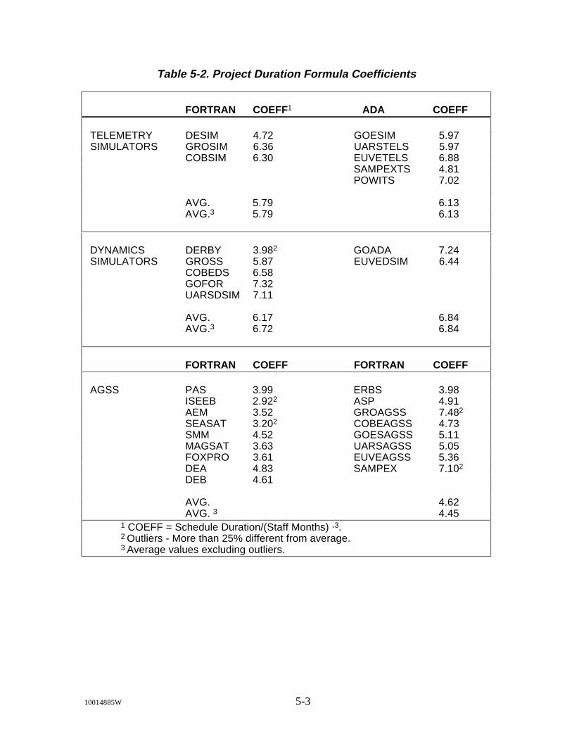
Table 5-2. Project Duration Formula Coefficients

FORTRAN COEFF1 ADA COEFF

TELEMETRY DESIM 4.72 GOESIM 5.97 SIMULATORS GROSIM 6.36 UARSTELS 5.97

COBSIM 6.30 EUVETELS 6.88SAMPEXTS 4.81POWITS 7.02

AVG. 5.79 6.13AVG.3 5.79 6.13

DYNAMICS DERBY 3.982 GOADA 7.24 SIMULATORS GROSS 5.87 EUVEDSIM 6.44

COBEDS 6.58GOFOR 7.32UARSDSIM 7.11

AVG. 6.17 6.84AVG.3 6.72 6.84

FORTRAN COEFF FORTRAN COEFF

AGSS PAS 3.99 ERBS 3.98ISEEB 2.922 ASP 4.91AEM 3.52 GROAGSS 7.482

SEASAT 3.202 COBEAGSS 4.73SMM 4.52 GOESAGSS 5.11MAGSAT 3.63 UARSAGSS 5.05FOXPRO 3.61 EUVEAGSS 5.36DEA 4.83 SAMPEX 7.102

DEB 4.61

AVG. 4.62AVG. 3 4.45

1 COEFF = Schedule Duration/(Staff Months) .3. 2 Outliers - More than 25% different from average. 3 Average values excluding outliers.

10014885W 5-3

in which the Coefficient, COEFF, is derived by substituting the actual schedule duration(calendar months) and actual effort (staff months) for each of these completed projectsand then solving for the Coefficient for each project. Figure 5-1 compares the durationformula Coefficients for all projects except GROAGSS and GROSS.

AGSS SIMULATORS

1 3 5 7 9 11 13 15 17 19 21 23 25 27 29 31 330.0

1.0

2.0

3.0

4.0

5.0

6.0

7.0

8.0

CO

EFF

ICIE

NT

VA

LUE

SIMULATORS: A - ADA F - FORTRAN

AGSS: ALL FORTRAN

F

F

FF F

A F

A

F

A

AA

A

A

1. PAS 12. DERBY 23. UARS_2 2. ISEEB 13. COBEDS 24. UARSDSIM 3. AEM 14. ASP 25. UARSTELS 4. SEASAT 15. GROSIM 26. EUVEAGSS 5. SMM 16. COBSIM 27. EUVE_2 6. MAGSAT 17. COBEAGSS 28. EUVETELS 7. FOXPRO 18. GOADA 29. EUVEDSIM 8. DEA 19. GOFOR 30. POWITS 9. DEB 20. GOESAGSS 31. SAMPEXTS10. DESIM 21. GOESIM 32. SAMPEX11. ERBS 22. UARSAGSS 33. SAMPEX_2

Figure 5-1. Coefficients of Schedule Duration Formula

Plotting these data in this way, beginning with project 13, COBEDS, and ending withproject 30, POWITS, the data reveal that the simulator projects show a pattern of largerCoefficient values than the AGSSs.

The next step of this study was to develop schedule-duration formulas in staff months(SM) by type of project. To develop the necessary formulas, the study selected project

10014885W 5-4

data beginning with COBEDS, begun in 1984, which corresponds roughly to the time atwhich the original Recommended Approach to Software Development (Reference 9) wasadopted as the standard software development process in the FDD.

An optimizing technique, based on the lowest RMS percent deviation, was used to solvefor the optimal Coefficient and exponent values for the schedule-duration formula. Theprojects (listed in Table 5-3) were grouped and analyzed by type: AGSSs, telemetrysimulators, dynamics simulators, and all simulators (telemetry and dynamics). Table 5-4presents the results of the optimizing process, first solving for the best Coefficient usingthe exponent .3 for each project type, and then solving for the best Coefficient andexponent for each project type.

Table 5-3. Projects Used in Formulating Schedule Equations

FORTRAN COEFF*

TELEMETRY GROSIM 6.36 SIMULATORS COBSIM 6.30

GOESIM 5.97UARSTELS 5.97EUVETELS 6.88POWITS 7.02

DYNAMICS COBEDS 6.58 SIMULATORS GOFOR 7.32

UARSDSIM 7.11GOADA 7.24EUVEDSIM 6.44

AGSS ASP 4.91COBEAGSS 4.73GOESAGSS 5.11UARS_2 4.92EUVEAGSS 5.36SAMPEX_2 5.42

*COEFF = Schedule Duration/(Staff Months).3

All eight cases shown in Table 5-4 have RMS percent deviation results of less than 10percent; therefore, the study recommends using only one formula for all simulators. Also,for the sake of consistency and simplicity, the exponent .3 should be used for bothAGSSs and simulators.

Figure 5-2 graphs actual project duration in weeks as a function of actual staff-months ofeffort for each project included in this step of the analysis. The figure also depicts twoseparate curves: one for simulators and one for AGSSs using a .3 exponent with the bestCoefficient.

10014885W 5-5

In conclusion, the Cost and Schedule Estimation Study recommends these formulas:

AGSS Duration = 5.0(SM).3

Simulator Duration = 6.7(SM).3

The simulator-duration formula is recommended for computing schedule duration forboth telemetry and dynamics simulator projects, whether they are written in FORTRANor Ada. The corresponding duration formulas based on support hours as well as technicaland management hours are

AGSS Duration = 4.9(SM).3

Simulator Duration = 6.5(SM).3

Table 5-4. Summary of Duration Formulas

SOLVING DURATION FORMULA FOR COEFFICIENT ONLY(EXPONENT .3 IS CONSTANT)

AGSS TELEMETRY DYNAMICS ALLSIMULATORS SIMULATORS SIMULATORS

Formula 5.0(SM).3 6.4(SM).3 6.9(SM).3 6.7(SM).3

RMS 4.9% 6.2% 6.5% 7.8%

SOLVING DURATION FORMULA FOR BOTH COEFFICIENT AND EXPONENT

AGSS TELEMETRY DYNAMICS ALLSIMULATORS SIMULATORS SIMULATORS

Formula 6.3(SM).29 6.7(SM).29 6.0(SM).33 5.3(SM).35

RMS 3.8% 6.1% 6.4% 7.4%

10014885W 5-6

TEL. SIM. DYN. SIM. AGSS

0 100 200 300 400 500 600 700EFFORT IN STAFF-MONTHS

0

50

100

150

200

250

DU

RA

TIO

N IN

WE

EK

S

6.7(SM)

6.7(SM).3

SIMULATORS

AGSS

5.0(SM) .3

Telemetry DynamicsSimulators: Simulators: AGSSs:

EUVETELS COBEDS SAMPEX_2COBSIM GOFOR ASPGROSIM UARSDSIM EUVEAGSSUARSTELS EUVEDSIM GOESAGSSPOWITS GOADA COBEAGSSGOESIM UARS_2

Figure 5-2. Schedule Duration Versus Technical and ManagementEffort

5.1.2 Accuracy of Schedule Duration Model Based on Final Projects Statistics

This section presents the accuracy of the schedule model formulated in Section 5.1. Thefirst comparison is of the AGSS actual schedules with the estimated schedules, applyingthe AGSS COEFF, 5.0, to the schedule duration model. The same type of comparison ispresented for simulators, combining telemetry and dynamics simulators, including thosedeveloped in FORTRAN and Ada. In the case of the simulators, the simulator COEFF,6.7, is substituted in the schedule model.

10014885W 5-7

Figure 5-3 shows the accuracy of applying the AGSS COEFF parameter to the schedulemodel, and Figure 5-4 shows the accuracy of applying the simulator COEFF parameterto the schedule model. SAMPEX, is an outlier and was not used in formulating theschedule model. However, SAMPEX_2 fits the model better; it is within the ± 10percent accuracy range. All of the simulator projects fit the schedule duration modelwell; they are all close to the 10 percent accuracy range.

1 2 3 4 5 6 7 8 9-50%

-40%

-30%

-20%

-10%

0%

10%

20%

30%

40%

50%

PE

RC

EN

T E

RR

OR

1. ASP 4. UARSAGGS 7. EUVE_22. COBEAGGS 5. UARS_2 8. SAMPEX3. GOESAGGS 6. EUVEAGSS 9. SAMPEX_2

Figure 5-3. Accuracy of Schedule Duration Model for AGSSs(Based on Actual Technical and Management Effort)

10014885W 5-8

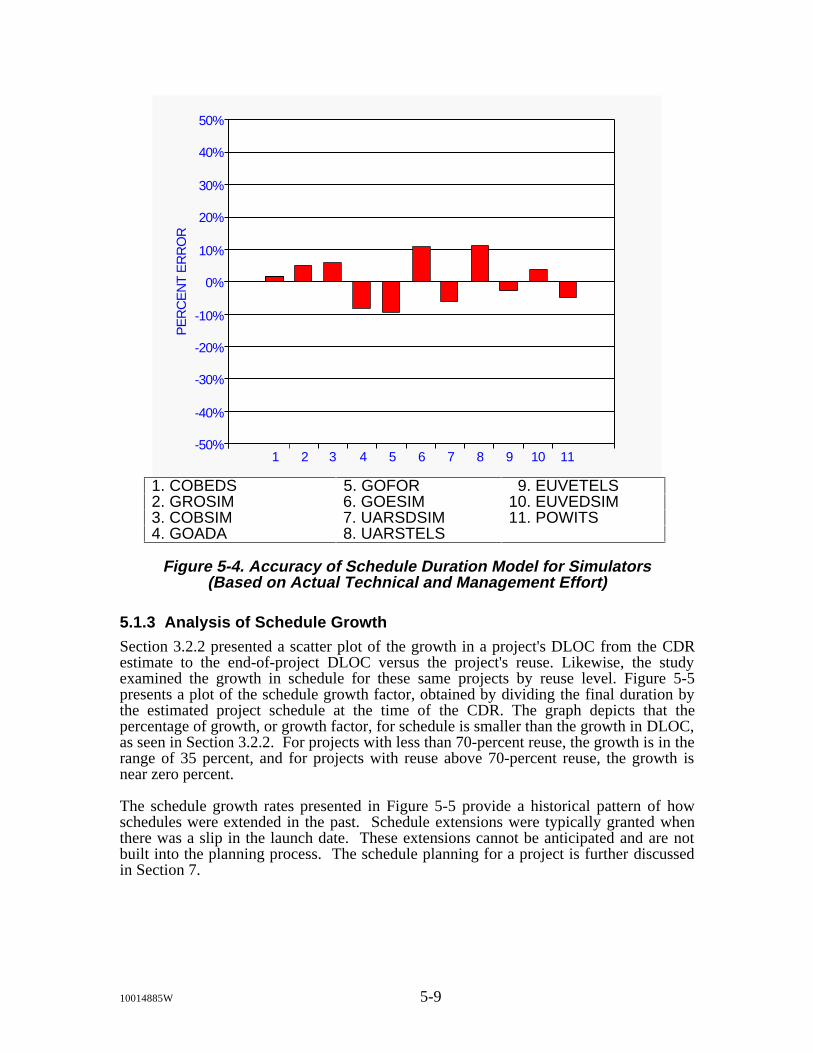
1 2 3 4 5 6 7 8 9 10 11-50%

-40%

-30%

-20%

-10%

0%

10%

20%

30%

40%

50%

PE

RC

EN

T E

RR

OR

1. COBEDS 5. GOFOR 9. EUVETELS2. GROSIM 6. GOESIM 10. EUVEDSIM3. COBSIM 7. UARSDSIM 11. POWITS4. GOADA 8. UARSTELS

Figure 5-4. Accuracy of Schedule Duration Model for Simulators(Based on Actual Technical and Management Effort)

5.1.3 Analysis of Schedule Growth

Section 3.2.2 presented a scatter plot of the growth in a project's DLOC from the CDRestimate to the end-of-project DLOC versus the project's reuse. Likewise, the studyexamined the growth in schedule for these same projects by reuse level. Figure 5-5presents a plot of the schedule growth factor, obtained by dividing the final duration bythe estimated project schedule at the time of the CDR. The graph depicts that thepercentage of growth, or growth factor, for schedule is smaller than the growth in DLOC,as seen in Section 3.2.2. For projects with less than 70-percent reuse, the growth is in therange of 35 percent, and for projects with reuse above 70-percent reuse, the growth isnear zero percent.

The schedule growth rates presented in Figure 5-5 provide a historical pattern of howschedules were extended in the past. Schedule extensions were typically granted whenthere was a slip in the launch date. These extensions cannot be anticipated and are notbuilt into the planning process. The schedule planning for a project is further discussedin Section 7.

10014885W 5-9

0% 10% 20% 30% 40% 50% 60% 70% 80% 90% 100%REUSE PERCENT

0.5

1.0

1.5

2.0

2.5

3.0

3.5

GR

OW

TH F

AC

TOR

FINAL SCHEDULE = GROWTH FACTOR * CDR SCH. ESTIMATE

1

2 34

5

6

7 89

10

11 12 13

14

35% GROWTH5% GROWTH

1. COBSIM 6. GOADA 11.EUVEAGSS2. UARSAGSS 7. GOESIM 12. SAMPEX3. COBEAGSS 8. GOFOR 13. SAMPEXTS4. GOESAGSS 9. UARSTELS 14. EUVETELS5. UARSDSIM 10. POWITS

Figure 5-5. Schedule Growth Factors (Actual Duration Divided byCDR Estimate)

5.2 Distribution of Schedule by Life-Cycle Phase

Successful software development project planning requires the manager to set meaningfulintermediate milestones. In the SEL environment, major intermediate milestones definethe end of the life-cycle phases. Thus, it is important to understand what percent of thetotal project duration is spent in the life-cycle phases on the typical project. This formsthe profile model of schedule distribution against which completed projects can becompared and assessed. Based on this profile model, a planning model for scheduledistribution is derived that, when put in place at the start of the project, will lead toproject results similar to the profile model.

Tables 5-5 and 5-6 present the analysis of current SEL project data to determine thecurrent profile model for schedule distribution among the life-cycle phases. Therelationship between the SEL planning model (from Reference 5) and this profile modelis addressed in Section 7.

The study examined percent of schedule distributed by life-cycle phase, beginningchronologically with the ERBS project. The projects are combined into groups, with anaverage and standard deviation for each group. The low–reuse model combines theAGSS, FORTRAN simulator, and Ada project and does not include the high–reuseprojects. The high–reuse model, a preliminary model is based on combining both Adaand FORTRAN projects with a reuse level of 65 percent and higher; the model shows

10014885W 5-10

high variability. The actual percentages are provided to allow the reader to model othercombinations of projects. Appendix C examines the projects in more detail, listing thosewith the most and least percentages of schedule in each phase as well as the most andleast percentages of effort by phase and percentages effort by activity.

Table 5-5. Percentage of Schedule Distribution by Phase

Project Reuse Design Code System AcceptancePercent Test Test

ERBS 13% 43.3% 34.0% 12.4% 10.3%COBEDS 27% 34.3% 22.9% 31.4% 11.4%ASP 13% 29.9% 31.0% 14.9% 24.1%GROSIM 18% 35.0% 39.0% 17.0% 9.0%COBSIM 11% 28.0% 40.2% 18.3% 13.4%COBEAGSS 12% 26.7% 26.7% 20.7% 25.9%GOADA 29% 27.5% 28.9% 30.9% 12.8%GOFOR 32% 25.2% 27.7% 31.9% 15.1%GOESAGSS 12% 27.0% 38.3% 16.5% 18.3%GOESIM 29% 34.3% 29.3% 8.1% 28.3%UARSAGSS 11% 30.6% 36.1% 16.3% 17.0%UARSDSIM 24% 25.8% 45.3% 7.0% 21.9%UARSTELS 35% 31.9% 29.8% 10.6% 27.7%EUVEAGSS 78% 37.3% 33.3% 14.7% 14.7%EUVETELS 96% 26.5% 42.2% 12.0% 19.3%POWITS 69% 26.1% 31.5% 8.1% 34.2%SAMPEXTS 95% 47.9% 8.3% 16.7% 27.1%SAMPEX 92% 45.9% 14.1% 22.4% 17.6%

Table 5-6. Models for Schedule Distribution by Phase

Model Design Code Test

5 AGSS PROJECTS 32 ± 6% 33 ± 4% 35 ± 8% 4 FORTRAN SIMULATORS 29 ± 4% 38 ± 6% 33 ± 8% 3 ADA SIMULATORS 31 ± 3% 29 ± 0% 40 ± 3% 12 LOW REUSE PROJECTS 30 ± 5% 34 ± 6% 36 ± 7% 5 HIGH REUSE PROJECTS 37 ± 9% 26 ± 13% 37 ± 6%

10014885W 5-11

Section 6. Conclusions and Recommendations

6.1 Conclusions

The study concludes the following:

• The standard SEL effort estimation equation, based on a size estimate adjustedfor reuse, is best for predicting effort in the FDD environment. Of the threeeffort model parameters—productivity, cost to reuse code, and growthfactor—the productivity and reuse costs vary with language, whereas thegrowth factor varies with the level of reuse. The effort model parameters donot depend on the application type (that is, AGSS, telemetry simulator, ordynamics simulator).

• Developed lines of code (DLOC) (total SLOC adjusted for reuse) is anaccurate basis for estimating total project effort. For FORTRAN projects,DLOC should be computed with a 20-percent weight given to reused SLOC.(The 20-percent weighting is the reuse cost parameter.) For Ada projects,DLOC should be computed with a 30-percent weight given to reused SLOC.

Note: The significant cost savings evidenced by SAMPEX AGSS andSAMPEXTS, two recent projects with very high reuse levels, suggest adivergence from the 30-percent and 20-percent reuse costs. For such high-reuse projects as these, a much lower reuse cost may be appropriate, perhaps aslow as 10 percent. SAMPEXTS piloted a streamlined development process forhigh reuse projects, combining some documents and combining the PDR withthe CDR; the project's low reuse cost may result from these process changes aswell as from the percentage of reused code. Data from more high-reuseprojects are needed before certifying this as a trend.

• The productivity experienced on recent FORTRAN AGSSs varied from 3 to5 DLOC per technical staff/technical management hour. For planningpurposes, a conservative productivity value of 3.5 DLOC per technicalstaff/technical management hour is recommended. When support staff hoursare included in the plan, an overall productivity of 3.2 DLOC per hour shouldbe used.

• The productivity on recent Ada projects showed less variability than did theFORTRAN projects. For planning purposes, a productivity of 5.0 DLOC pertechnical staff/technical management hour is recommended. When supportstaff hours are included in the plan, an overall productivity of 4.5 DLOC perhour should be used.

• The SEF data in the SEL database provide no demonstrable evidence thatinclusion of estimates for such factors as problem complexity or teamexperience will significantly improve a manager's estimate of project effort.When making estimates for project effort, managers are still encouraged toinclude such factors as problem complexity or team experience based on theirown personal experience, but the database of experience represented by theSEF data in the SEL database provides no guidelines.

10014885W 6-1

• For projects with moderate to low code reuse (less than 70 percent), the post-CDR growth in DLOC due to requirements changes and TBDs iscommensurate with past SEL experience: 40 percent. For projects with highcode reuse (70 percent or more), the post-CDR growth in DLOC is only abouthalf as much: 20 percent.

• An exponential model like COCOMO can be used to predict the duration ofprojects from total project effort; the COCOMO multiplicative factor of 3.3must be replaced with a factor of 5.0 for AGSSs (6.7 for simulators) whenbased on technical staff/technical management hours and 4.9 for AGSSs (6.5for simulators) when support hours are also included.

• For projects with moderate to low code reuse, the post-CDR growth inschedule is 35 percent. For projects with high reuse, the post-CDR growth inschedule is 5 percent.

• Based on the final project statistics for moderate to low reuse projects (lessthan 70-percent code reuse), the distribution of the total effort and scheduleamong the life-cycle phases is as follows:

Phase Effort Schedule

Design: 24 ± 3% 30 ± 5%

Code: 45 ± 6% 34 ± 6%

Test: 31 ± 5% 36 ± 7%

• Based on the final project statistics for high-reuse projects (70 percent or morecode reuse), the distribution of the total effort and schedule among the life-cycle phases is as shown below. The larger standard deviations for high-reuseprojects demonstrate that the development process for high-reuse projects isstill evolving, resulting in significant variability in the effort distribution. Asmore high-reuse projects are completed, it should become possible to moreaccurately model the high-reuse projects.

Phase Effort Schedule

Design: 26 ± 14% 37 ± 9%

Code: 38 ± 12% 26 ± 13%

Test: 36 ± 3% 37 ± 6%

10014885W 6-2

• Based on the final project statistics for low-reuse projects, the distribution ofthe total effort among the software development activities is

Activity Effort

Design: 21 ± 4%

Code: 26 ± 4%

Test: 25 ± 5%

Other: 28 ± 9%

• Based on the final project statistics for high-reuse projects, the distribution ofthe total effort among the software development activities is

Activity Effort

Design: 17 ± 5%

Code: 17 ± 6%

Test: 32 ± 6%

Other: 34 ± 8%

• Requirements changes and system growth can cause project effort andschedule to diverge from their predicted distributions in the manager's initialplan. In order to minimize the effects of requirements changes and systemgrowth on project cost and schedule, a manager should usually plan for thefollowing distributions of the total effort and schedule among the life-cyclephases. (See Section 7 for a full discussion of how to apply SEL planningmodels and relate them to baseline models for effort and schedule.)

Phase Effort Schedule

Design: 30% 35%

Code: 40% 30%

Test: 30% 35%

6.2 RecommendationsFor future projects developed within the FDD environment, the following recommenda-tions are made:

• The initial effort estimate should be based on the standard SEL effortestimation model with an appropriate growth factor applied:

Effort = DLOC × Growth Factor / Productivity

10014885W 6-3

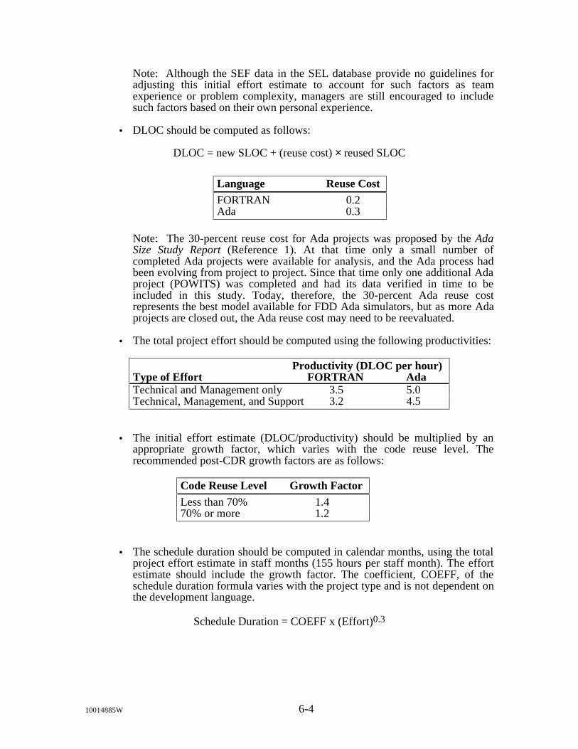
Note: Although the SEF data in the SEL database provide no guidelines foradjusting this initial effort estimate to account for such factors as teamexperience or problem complexity, managers are still encouraged to includesuch factors based on their own personal experience.

• DLOC should be computed as follows:

DLOC = new SLOC + (reuse cost) × reused SLOC

Language Reuse CostFORTRAN 0.2Ada 0.3

Note: The 30-percent reuse cost for Ada projects was proposed by the AdaSize Study Report (Reference 1). At that time only a small number ofcompleted Ada projects were available for analysis, and the Ada process hadbeen evolving from project to project. Since that time only one additional Adaproject (POWITS) was completed and had its data verified in time to beincluded in this study. Today, therefore, the 30-percent Ada reuse costrepresents the best model available for FDD Ada simulators, but as more Adaprojects are closed out, the Ada reuse cost may need to be reevaluated.

• The total project effort should be computed using the following productivities:

Productivity (DLOC per hour)Type of Effort FORTRAN AdaTechnical and Management only 3.5 5.0Technical, Management, and Support 3.2 4.5

• The initial effort estimate (DLOC/productivity) should be multiplied by anappropriate growth factor, which varies with the code reuse level. Therecommended post-CDR growth factors are as follows:

Code Reuse Level Growth FactorLess than 70% 1.470% or more 1.2

• The schedule duration should be computed in calendar months, using the totalproject effort estimate in staff months (155 hours per staff month). The effortestimate should include the growth factor. The coefficient, COEFF, of theschedule duration formula varies with the project type and is not dependent onthe development language.

Schedule Duration = COEFF x (Effort)0.3

10014885W 6-4

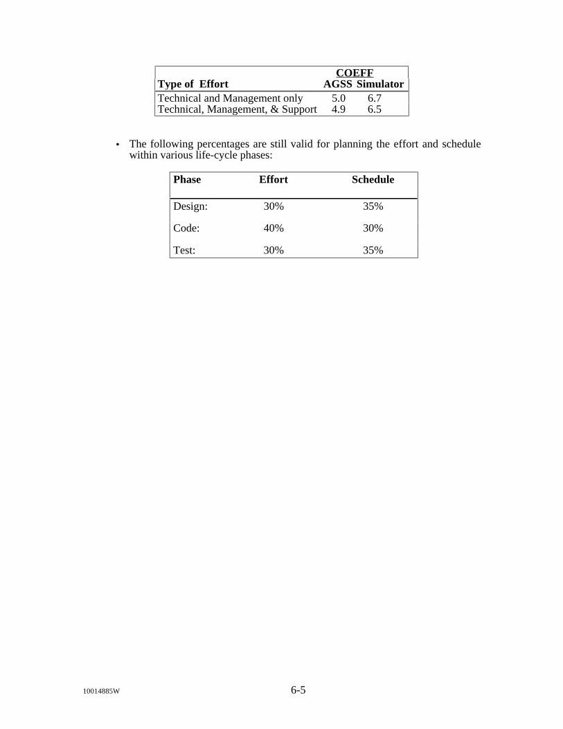
COEFFType of Effort AGSS SimulatorTechnical and Management only 5.0 6.7Technical, Management, & Support 4.9 6.5

• The following percentages are still valid for planning the effort and schedulewithin various life-cycle phases:

Phase Effort Schedule

Design: 30% 35%

Code: 40% 30%

Test: 30% 35%

10014885W 6-5

Section 7. Applying the Planning Models

This section explains how to apply the SEL planning models and relates them to theupdated baseline models for effort and schedule.

Previous sections presented updated profiles of the behavior of typical softwaredevelopment projects in the FDD. These models provide a baseline against which actualproject data (referred to as project actuals) can be monitored and compared. Theyrepresent what is expected to actually happen on a typical Flight Dynamics project.

Since the baseline models are based on project actuals, they naturally include projectchanges that result from additional information gained as projects progress throughouttheir life cycle, such as requirements clarification and modification, TBD definition, orlaunch date changes. Models such as productivity, reuse cost, and duration formulas canbe applied directly when estimating a project's overall cost and schedule but the baselinemodels for life-cycle phase distribution of effort and schedule must be adjusted whenplanning the project. Therefore, the SEL planning models for life-cycle phasedistribution differ from the baseline models.

At the start of a project, the project lead/manager has a limited amount of projectinformation on which to base the plan. Thus, the plan should be based on organizationalplanning models that anticipate predictable changes and allow some flexibility for theproject to react to unpredictable changes. The SEL planning models have been developedby applying management judgment based on many years of experience in thisenvironment.

Cost estimation and planning is a multistep process. First, the size of the job is estimatedbased on project requirements, then effort and calendar time are estimated and allocatedaccording to SEL planning models. This plan is then adjusted to handle project growthand to provide a schedule buffer.

7.1 Creating the Initial Plan

7.1.1 Estimating Effort

System size continues to be the SEL's best indicator of the amount of work to be done.Thus, effort estimates should be based on the estimated size of the system adjusted forreuse, the developed lines of code (DLOC), as was explained in Section 3.

To estimate DLOC, overall system size (SLOC) must first be determined based onrequirements and previous similar systems and the amount of code to be reused. Basedon the language, DLOC is computed as follows:

DLOC = New SLOC + reuse cost × Reused SLOC (7-1)

where reuse cost = 0.2 for FORTRAN = 0.3 for Ada

10014885W 7-1

Then, total project effort (including support hours) is estimated as follows:

Effort (hours) = DLOC/productivity (7-2)

where productivity = 3.2 DLOC/hour for FORTRAN = 4.5 DLOC/hour for Ada

This estimates the total amount of effort (technical, management, and support) thatwould be required to develop the system if (1) the size estimate is correct and (2) nothingchanges.

7.1.2 Determining the Schedule

Very often the schedule for Flight Dynamics mission projects is driven by the launchdate. This is often out of the project manager's control; however, the SEL schedule modelcan be used as a gauge to assess the level of risk resulting from the project-imposedschedule. When schedules are not predetermined, the SEL model provides a goodmethod for determining a reasonable delivery date.

The typical and minimum project durations are determined as follows:

Typical duration (m) = 4.9 × Effort(sm).3 for AGSSs = 6.5 × Effort(sm).3 for simulators (7-3)

Minimum duration (m) = .75 × Typical duration

A planned project end date that falls between the minimum and typical durations isachievable. The closer that it falls to the minimum duration, the larger the risk.

7.1.3 Planning the Life-Cycle Phases

The planning models presented in Section 3 of Reference 6 (given here in Table 7-1)should be followed to distribute time and effort to the life-cycle phases. The design phaseconsists of requirements analysis, preliminary design, and detailed design. The test phaseincludes both system test and acceptance test.

Table 7-1. Life-Cycle Planning Model

Phase Percent of Percent ofSchedule Effort

Design 35 30Code 30 40Test 35 30

10014885W 7-2

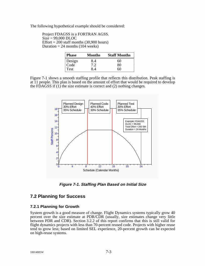
The following hypothetical example should be considered:

Project FDAGSS is a FORTRAN AGSS.Size = 99,000 DLOCEffort = 200 staff months (30,900 hours)Duration = 24 months (104 weeks)

Phase Months Staff MonthsDesign 8.4 60Code 7.2 80Test 8.4 60

Figure 7-1 shows a smooth staffing profile that reflects this distribution. Peak staffing isat 11 people. This plan is based on the amount of effort that would be required to developthe FDAGSS if (1) the size estimate is correct and (2) nothing changes.

0 4 8 12 16 20 240

2

4

6

8

10

12

14

16

18

Sta

ff P

erso

ns

Example: FDAGSSDLOC = 99,000Total Effort = 200 SMDuration = 24 Months

Schedule (Calendar Months)

Planned Design30% Effort35% Schedule

Planned Code40% Effort30% Schedule

Planned Test30% Effort35% Schedule

Figure 7-1. Staffing Plan Based on Initial Size

7.2 Planning for Success

7.2.1 Planning for Growth

System growth is a good measure of change. Flight Dynamics systems typically grow 40percent over the size estimate at PDR/CDR (usually, size estimates change very littlebetween PDR and CDR). Section 3.2.2 of this report confirms that this is still valid forflight dynamics projects with less than 70-percent reused code. Projects with higher reusetend to grow less; based on limited SEL experience, 20-percent growth can be expectedon high-reuse systems.

10014885W 7-3

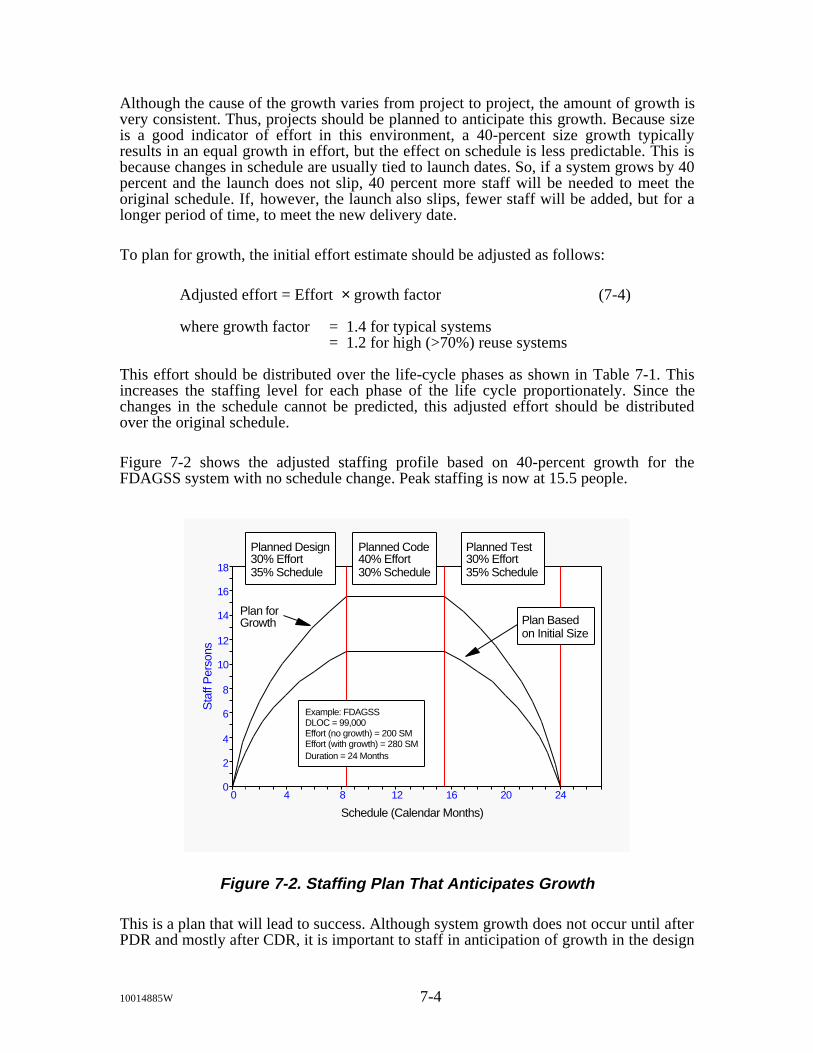
Although the cause of the growth varies from project to project, the amount of growth isvery consistent. Thus, projects should be planned to anticipate this growth. Because sizeis a good indicator of effort in this environment, a 40-percent size growth typicallyresults in an equal growth in effort, but the effect on schedule is less predictable. This isbecause changes in schedule are usually tied to launch dates. So, if a system grows by 40percent and the launch does not slip, 40 percent more staff will be needed to meet theoriginal schedule. If, however, the launch also slips, fewer staff will be added, but for alonger period of time, to meet the new delivery date.

To plan for growth, the initial effort estimate should be adjusted as follows:

Adjusted effort = Effort × growth factor (7-4)

where growth factor = 1.4 for typical systems= 1.2 for high (>70%) reuse systems

This effort should be distributed over the life-cycle phases as shown in Table 7-1. Thisincreases the staffing level for each phase of the life cycle proportionately. Since thechanges in the schedule cannot be predicted, this adjusted effort should be distributedover the original schedule.

Figure 7-2 shows the adjusted staffing profile based on 40-percent growth for theFDAGSS system with no schedule change. Peak staffing is now at 15.5 people.

0 4 8 12 16 20 240

2

4

6

8

10

12

14

16

18

Sta

ff P

erso

ns

Schedule (Calendar Months)

Plan forGrowth Plan Based

on Initial Size

Planned Design30% Effort35% Schedule

Planned Code40% Effort30% Schedule

Planned Test30% Effort35% Schedule

Example: FDAGSSDLOC = 99,000Effort (no growth) = 200 SMEffort (with growth) = 280 SMDuration = 24 Months

Figure 7-2. Staffing Plan That Anticipates Growth

This is a plan that will lead to success. Although system growth does not occur until afterPDR and mostly after CDR, it is important to staff in anticipation of growth in the design

10014885W 7-4

phases. This allows the necessary staff to be fully trained when the growth occurs,resulting in higher productivity in the later life-cycle phases. If the project waits until thegrowth occurs to staff up, the learning curve of the additional staff will increase, ratherthan relieve, the burden on the original team.

It is important to remember that plans are not set in stone; they are expected to change asthe project gets more and revised information. When the mission schedule changes, thesoftware development schedule is also likely to change.

Mission delays often result from a delay in completing the spacecraft, which in turnusually causes a delay in resolving all of the TBDs in the requirements document. Thesoftware development project schedule should also be changed correspondingly, not toprovide schedule relief, but to provide ample time to respond to mission changes.

An extension in the schedule will not require additional effort, but it does mean that lessstaff will be needed during the peak period. The staffing profile should be flattened andstretched to cover the new duration. As soon as this change is known, the projectmanager should adjust the plan and make corresponding staffing adjustments.

In reality, the mission schedule often changes about mid-way through the project. Thisresults in a stretched schedule after the completion of the design phases; i.e., the end-of-design date remains fixed, while the end-of-code and testing phase dates are usuallyadjusted in accordance with the new schedule.

Figure 7-3 shows the relationship of the likely project actuals to the original plans createdat project start for the FDAGSS. It should be noted that the actual amount of effort andtime spent in the design phases ends up being a smaller percentage of the overall projectwhen compared to the original plan. The curve for the likely actuals is based on themodels for end-of-project effort and schedule as presented in the preceding sections ofthis report: (1) the initial total effort estimate of 200 staff months (including supporthours) is multiplied by 1.4 to estimate the final total effort; (2) the total duration iscomputed from this total effort using Equation 7-3; (3) the effort distribution by phasefollows the end-of-project percentages for moderate to low-reuse projects, as shown inTable 3-2; (4) the schedule distribution by phase follows the end-of-project percentagesfor moderate to low reuse projects, as shown in Table 5-6.

7.2.2 Additional Planning Considerations

In addition to staffing projects aggressively in anticipation of growth, it is also wise to setreasonably challenging schedules. A series of little unexpected problems and the effect ofhuman nature in dealing with change typically cause a project to finish slightly later thanplanned. Thus, the wise manager will build a buffer into the schedule when planning; theSEL recommends a 10-percent buffer. This should be applied during initial planning andall subsequent changes to the schedule. Caution is advised; care should be taken not toreduce the project duration below the minimum (calculated based on effort adjusted forgrowth). Only one buffer is advised; care should be taken that only one manager appliesthis rule; otherwise, unrealistic goals will place the project at risk. Careful documentationof the planning process will guard against this problem.

10014885W 7-5

0 4 8 12 16 20 240

2

4

6

8

10

12

14

16

18

Sta

ff P

erso

ns

Schedule (Calendar Months)

Plan forGrowth

Plan Basedon Initial Size

Likely Actual

Planned Design30% Effort35% Schedule

Planned Code40% Effort30% Schedule

Planned Test30% Effort35% Schedule

Example: FDAGSSDLOC = 99,000Effort (no growth) = 200 SMEffort (with growth) = 280 SM

Figure 7-3. Plan Versus Actuals

0 4 8 12 16 20 240

2

4

6

8

10

12

14

16

18

Sta

ff P

erso

ns

Schedule (Calendar Months)

Likely Actual forOn-Schedule Delivery:40% Effort Growth,No Schedule Slip

Plan with 40% Effort Growthand 10% Schedule Buffer

Planned Design30% Effort35% Schedule

Planned Code40% Effort30% Schedule

Planned Test30% Effort35% Schedule

Figure 7-4. Plan for Success

10014885W 7-6

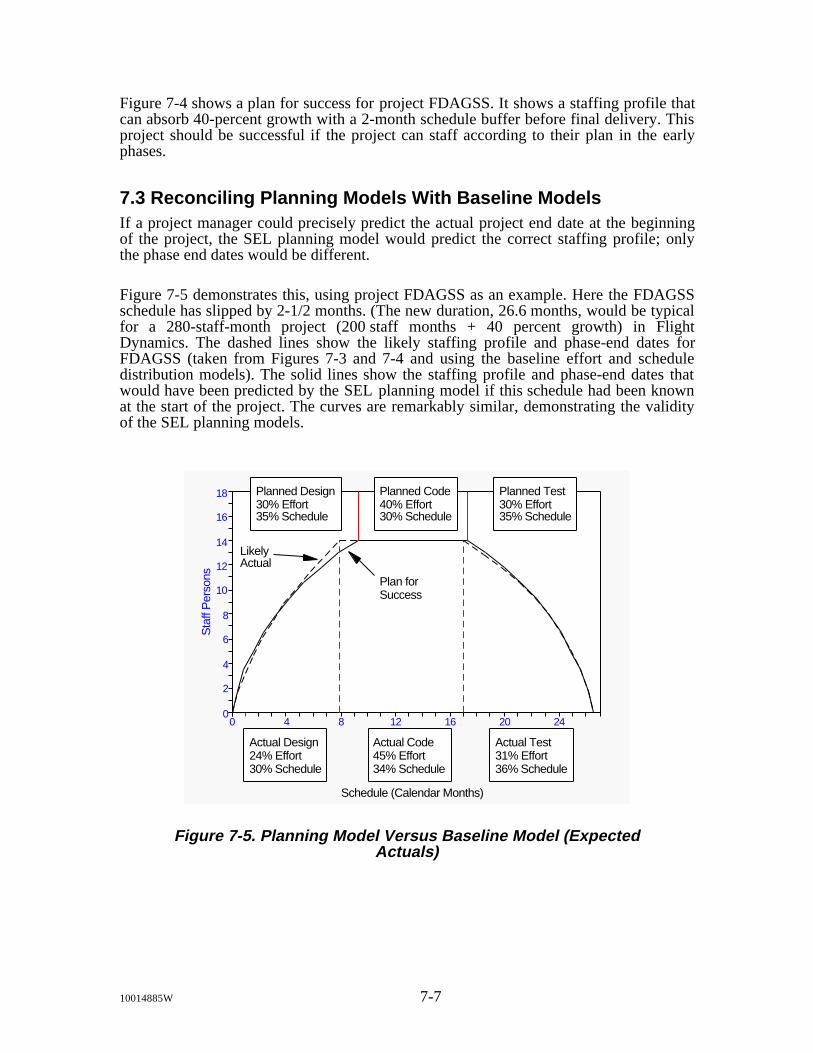
Figure 7-4 shows a plan for success for project FDAGSS. It shows a staffing profile thatcan absorb 40-percent growth with a 2-month schedule buffer before final delivery. Thisproject should be successful if the project can staff according to their plan in the earlyphases.

7.3 Reconciling Planning Models With Baseline ModelsIf a project manager could precisely predict the actual project end date at the beginningof the project, the SEL planning model would predict the correct staffing profile; onlythe phase end dates would be different.

Figure 7-5 demonstrates this, using project FDAGSS as an example. Here the FDAGSSschedule has slipped by 2-1/2 months. (The new duration, 26.6 months, would be typicalfor a 280-staff-month project (200 staff months + 40 percent growth) in FlightDynamics. The dashed lines show the likely staffing profile and phase-end dates forFDAGSS (taken from Figures 7-3 and 7-4 and using the baseline effort and scheduledistribution models). The solid lines show the staffing profile and phase-end dates thatwould have been predicted by the SEL planning model if this schedule had been knownat the start of the project. The curves are remarkably similar, demonstrating the validityof the SEL planning models.

0 4 8 12 16 20 240

2

4

6

8

10

12

14

16

18

Sta

ff P

erso

ns

Schedule (Calendar Months)

Likely Actual

Plan forSuccess

Actual Design24% Effort30% Schedule

Actual Code45% Effort34% Schedule

Actual Test31% Effort36% Schedule

Planned Design30% Effort35% Schedule

Planned Code40% Effort30% Schedule

Planned Test30% Effort35% Schedule

Figure 7-5. Planning Model Versus Baseline Model (ExpectedActuals)

10014885W 7-7

Appendix A. Summary of Cost and Schedule Models

Appendix A. Summary of Cost and Schedule Models

This appendix presents a summary of cost and schedule models that have been recommended inthe FDD over the last 14 years. The models are taken from the following seven documents:

• SEL-79-002, The Software Engineering Laboratory: Relationship Equations, KarlFreburger and Victor Basili, May 1979

• SEL-81-205, Recommended Approach to Software Development, Frank McGarry,Jerry Page, Suellen Eslinger, Victor Church, and Phillip Merwarth, April 1983

• SEL-81-205, Recommended Approach to Software Development, Revision 3, LindaLandis, Sharon Waligora, Frank McGarry, Rose Pajerski, Mike Stark, Kevin OrlinJohnson, Donna Cover, June 1992

• SEL-83-001, An Approach to Software Cost Estimation, Frank McGarry, Jerry Page,David Card, Michael Rohleder, and Victor Church, February 1984

• SEL-84-101, Manager's Handbook for Software Development, Revision 1, LindaLandis, Frank McGarry, Sharon Waligora, et al, November 1990

• Software Engineering Laboratory (SEL) Ada Size Study Report, Steve Condon andMyrna Regardie, September 1992

• SEAS System Development Methodology (SSDM) Standards and Procedures (S&P),"Standard and Procedure 1102: Software Development Estimation," ComputerSciences Corporation, January 1993

The models are presented in the accompanying matrix. Models of the same type are grouped inthe same column. Models from the same document appear in the same row. If a document doesnot contain a model of a particular type "N/A" (not applicable) appears in the field. Pagereferences to the documents appear in brackets beneath each model. Notes and a glossary for thematrix appear at the end of the appendix.

10014885W A-1

DOCUMENT

SIZE ESTIMATES

UNCERTAINTYEND OF PHASESIZE FORMULAS

The SEL: RelationshipEquations ('79)

Recommended Approach ('83)

Cost Estimation ('84)

Manager's Handbook ('90)

Recommended Approach ('92)

Ada Size Study ('92)

SSDM S&P 1102

10014885W

N/AN/AN/A

1PreprojectDELOC = New ELOC + 0.2(Reused ELOC)0.7Require. AnalysisDELOC = New ELOC + 0.2(Reused ELOC)0.5Preliminary DesignDELOC = New ELOC + 0.2(Reused ELOC)0.3Detailed DesignDELOC = New ELOC + 0.2(Reused ELOC)

0.12ImplementationDELOC = New ELOC + 0.2(Reused ELOC)0.05System Test

[p. C-4][p. C-4][p. C-5]

1Require. Definition0.75Require. AnalysisLOC = 7500 x (No. of Subsystems) 0.5Preliminary DesignLOC = 125 x (Number of Modules)0.3Detailed DesignDELOC = New ELOC + 0.2(Reused ELOC)

0.12ImplementationLOC = 1.11 x (Current SLOC)0.05System Test

[p. 4-2][p. 4-2][p. 3-6, 3-8]

0.75Require. AnalysisSLOC = 11,000 x (No. of Subsystems)0.4Preliminary DesignSLOC = 190 x (Number of Units)

0.25Detailed DesignDLOC = 200 x (New Units + (0.2 x Reused Units))0.1ImplementationSLOC = 1.26 x (Current SLOC)

0.05System Test

[p. 3-3][p. 3-3][p. 3-3]

N/AN/AN/A

N/AN/AAda DLOC = New SLOC + 0.3(Reused SLOC)FORTRAN DLOC = New SLOC + 0.2(Reused SLOC)

[p. 3-3, 4-5, 5-1,2]

N/AWeighted DSI = 1.0 x (Newly Developed DSI) + W1 x (Adapted DSI) + W2 x (Converted DSI) + W3 x (Transported DSI)where W1, W2, and W3 are supplied by user.

A-2

DOCUMENT SCHEDULE DURATION FORMULAS (2) EFFORT FORMULAS (1)

The SEL: RelationshipEquations ('79)

Recommended Approach ('83)

Cost Estimation ('84)

Manager's Handbook ('90)

Recommended Approach ('92)

Ada Size Study ('92)

SSDM S&P 1102

10014885W

Months = 5.45 x (KSLOC)exp(0.203)SMon = 0.029 x (Modules)exp(1.319)Months = 2.453 x (Modules)exp(0.275)Months = 5.104 x (SMon)exp(0.210)

[p. 32, 41][p. 15]

No equation. Instead guidelines are providedSMon = 8(F1)(F2)(F3)...(KDELOC)exp(1.05)in 2 tables on team size, phase-in,phase-out, and length of participationfor team members. Guidelines depend on schedule type and project leader experience.

[p. C-9][p. C-4]

SMon = 8.45(F1)(F2)(F3)...(KDELOC)exp(1.05)Weeks/(Staff Member) = 45 x (No. of Subsystems)Formula:End of Phase:Weeks/(Staff Member) = 0.75 x (No. of Modules)SHr = 1850 x SubsystemsRequire. AnalysisWeek/(Staff Member) = 1.0 x Developed ModuleSHr = 30 x ModulesPreliminary DesignWeeks/(Staff Member) = 1.42 x Current DurationSHr = 0.3 x DLOCDetailed DesignWeeks/(Staff Member) = 1.11 x Current DurationSHr = 1.33 x (Current SHr)Implementation

[p. 3-6]SHr = 1.05 x (Current SHr)System Test[p. 3-6, 4-4]

Weeks/(Staff Member) = 83 x (No. of Subsystems)SHr = 3000 x SubsystemsRequire. AnalysisWeeks/(Staff Member) = 1.45 x (No. of Units)SHr = 52 x UnitsPreliminary DesignWeek/(Staff Member) = 0.0087 x DLOCSHr = 0.31 x DLOCDetailed DesignWeeks/(Staff Member) = 1.54 x Current DurationSHr = 1.43 x (Current SHr)ImplementationWeeks/(Staff Member) = 1.18 x Current DurationSHr = 1.11 x (Current SHr)System Test

[p. 3-3][p. 3-3]

N/AN/A

Ada: Months = 6.5 x (Staff Months)exp(0.3)SHr = DLOC / ProductivityFORTRAN: Months = 5.0 x (Staff Months)exp(0.3)

[p. 4-3][p. 3-2]

Optimum Months = (DMC)x(RLC)exp(DMX)SHr = Weighted DSI / Adjusted ProductivityMinimum Months = 75% of Optimum MonthsAdjusted Estimated Effort = SHr / 155 (3)

RLC = [supplied by manager] (3)where Duration Model Coefficient (DMC) and DurationModel Exponent (DMX) are supplied by the user.

A-3

DOCUMENT

EFFORT AND SCHEDULE DISTRIBUTION

FORTRANADAOVERALLFORTRAN ADAOVERALLSCHEDULESCHEDULESCHEDULEEFFORTEFFORTEFFORTPHASE

The SEL: RelationshipEquations ('79)

Recommended Approach ('83)

Cost Estimation ('84)

Manager's Handbook ('90)

Recommended Approach ('92)

Ada Size Study ('92)

SSDM S&P 1102

10014885W

N/AN/AN/AN/AN/AN/AN/A

1. Compute the relative amount of effort in each of 3 types of activities: design, code, & test.2. Compute the staff hours of effort in each activity.3. Compute the staff hours of effort in each of 6 life-cycle phases.

[p. C-9,10]

N/AN/A0.05N/AN/A0.06Require. AnalysisN/AN/A0.1N/AN/A0.08Preliminary DesignN/AN/A0.15N/AN/A0.16Detailed DesignN/AN/A0.4N/AN/A0.45ImplementationN/AN/A0.2N/AN/A0.2System TestN/AN/A0.1N/AN/A0.05Acceptance Test

[p. 4-8][p. 4-8]

N/AN/A0.120.06Require. AnalysisN/AN/A0.08(4)(4)0.08Preliminary DesignN/AN/A0.150.30.320.16Detailed DesignN/AN/A0.30.340.290.4ImplementationN/AN/A0.20.160.190.2System TestN/AN/A0.150.20.20.1Acceptance Test

[p. 3-1][p. 6-4][p. 6-4][p. 3-1]

N/AN/AN/AN/AN/AN/A

0.330.29N/AN/A0.26N/ADesign0.290.33N/AN/A0.42N/AImplementation0.190.17N/AN/A0.17N/ASystem Test0.190.21N/AN/A0.15N/AAcceptance Test

[p. 4-8][p. 4-8][p. 3-12]

N/AN/AN/AN/AN/AN/A

A-4

DOCUMENT

TEAM EXPERIENCE FACTOR (F2)COMPLEXITY FACTOR (F1)

VALUEDEFINITIONVALUEDEFINITION

The SEL: RelationshipEquations ('79)

Recommended Approach ('83)

Cost Estimation ('84)

Manager's Handbook ('90)

Recommended Approach ('92)

Ada Size Study ('92)

SSDM S&P 1102

10014885W

N/AN/AN/AN/A

Effort Factor:Average Experience:Effort Factor:Project/Environment:0.5100.45Old/Old (4A)0.680.65Old/New0.860.65New/Old141New/New

1.422.51

[p. C-6][p. C-6][p. C-5][p. C-5]

0.5100.45Old/Old (4A)0.680.65Old/New0.860.65New/Old141New/New

1.422.51

[p. 4-5][p. 4-5][p. 4-5][p. 4-5]

0.5101Old/Old (4A)0.681.4Old/New0.861.4New/Old142.3New/New

1.422.61

[p. 3-4][p. 3-4][p. 3-4][p. 3-4]

N/AN/AN/AN/A

N/AN/AN/AN/A

Product. Factor:Risk:Product. Factor:Risk:1.1Lower1.1Lower1Typical1Typical

0.9Higher0.9Higher

A-5

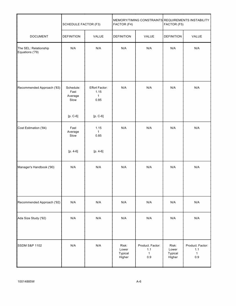
DOCUMENT

REQUIREMENTS INSTABILITYMEMORY/TIMING CONSTRAINTSFACTOR (F5)FACTOR (F4)SCHEDULE FACTOR (F3)

VALUEDEFINITIONVALUEDEFINITIONVALUEDEFINITION

The SEL: RelationshipEquations ('79)

Recommended Approach ('83)

Cost Estimation ('84)

Manager's Handbook ('90)

Recommended Approach ('92)

Ada Size Study ('92)

SSDM S&P 1102

10014885W

N/AN/AN/AN/AN/AN/A

N/AN/AN/AN/AEffort Factor:Schedule:1.15Fast

1Average0.85Slow

[p. C-6][p. C-6]

N/AN/AN/AN/A1.15Fast1Average

0.85Slow

[p. 4-6][p. 4-6]

N/AN/AN/AN/AN/AN/A

N/AN/AN/AN/AN/AN/A

N/AN/AN/AN/AN/AN/A

Product. Factor:Risk:Product. Factor:Risk:N/AN/A1.1Lower1.1Lower1Typical1Typical

0.9Higher0.9Higher

A-6

DOCUMENT

DATA VOLUMEDEVELOPMENT TOOLSENGINEERING METHODSFACTOR (F8)FACTOR (F7)FACTOR (F6)

VALUEDEFINITIONVALUEDEFINITIONVALUEDEFINITION

The SEL: RelationshipEquations ('79)

Recommended Approach ('83)

Cost Estimation ('84)

Manager's Handbook ('90)

Recommended Approach ('92)

Ada Size Study ('92)

SSDM S&P 1102

10014885W

N/AN/AN/AN/AN/AN/A

N/AN/AN/AN/AN/AN/A

N/AN/AN/AN/AN/AN/A

N/AN/AN/AN/AN/AN/A

N/AN/AN/AN/AN/AN/A

N/AN/AN/AN/AN/AN/A

Product. Factor:Risk:Product. Factor:Risk:Product. Factor:Risk:1.1Lower1.1Lower1.1Lower1Typical1Typical1Typical

0.9Higher0.9Higher0.9Higher

A-7

DOCUMENT

WORK RATE GUIDE (KDLOEC/WEEK)

SLOWAVERAGEFASTSCHEDULESCHEDULESCHEDULEPROJECT/ENVIRON.

The SEL: RelationshipEquations ('79)

Recommended Approach ('83)

Cost Estimation ('84)

Manager's Handbook ('90)

Recommended Approach ('92)

Ada Size Study ('92)

SSDM S&P 1102

10014885W

N/AN/AN/AN/A

N/AN/AN/AN/A

<0.160.24-0.16>0.24Old/Old (4A)<0.100.17-0.10>0.17Old/New<0.100.17-0.10>0.17New/Old<0.070.11-0.07>0.11New/New

[p. 4-7][p. 4-7][p. 4-7][p. 4-7]

N/AN/AN/AN/A

N/AN/AN/AN/A

N/AN/AN/AN/A

N/AN/AN/AN/A

A-8

DOCUMENT

STAFFING GUIDELINE(PCT. OF SENIOR PERSONNEL AND ANALYSTS)TEAM SIZE GUIDE

ANALYSTSSENIOR(6)PROJECT/ENVIRON.MIN. LEADER EXPERIENCE VS. MAX. TEAM SIZE

The SEL: RelationshipEquations ('79)

Recommended Approach ('83)

Cost Estimation ('84)

Manager's Handbook ('90)

Recommended Approach ('92)

Ada Size Study ('92)

SSDM S&P 1102

10014885W

N/AN/AN/AN/AN/AN/AN/A

25-33%25-33%Old/Old (4A)Years Experience:25-33%33-50%Old/New456 Applicable:33-50%33-50%New/Old234 Organization:33-50%50-67%New/New013 As Leader:

1-33-65-9Maximum Team (5):

[p. C-15][p. C-12]

25-33%25-33%Old/Old (4A)Years Experience:25-33%33-50%Old/New456 Applicable:33-50%33-50%New/Old234 Organization:33-50%50-67%New/New013 As Leader:

1-33-65-9Maximum Team (5):[p. 4-10][p. 4-9]

25-33%25-33%Old/Old (4A)Years Experience:25-33%33-50%Old/New456 Applicable:33-50%33-50%New/Old234 Organization:33-50%50-67%New/New013 As Leader:

1-32-65-9Maximum Team (5):[p. 3-5][p. 3-5]

N/AN/AN/AN/AN/AN/AN/A

N/AN/AN/AN/AN/AN/AN/A

N/AN/AN/AN/AN/AN/AN/A

A-9

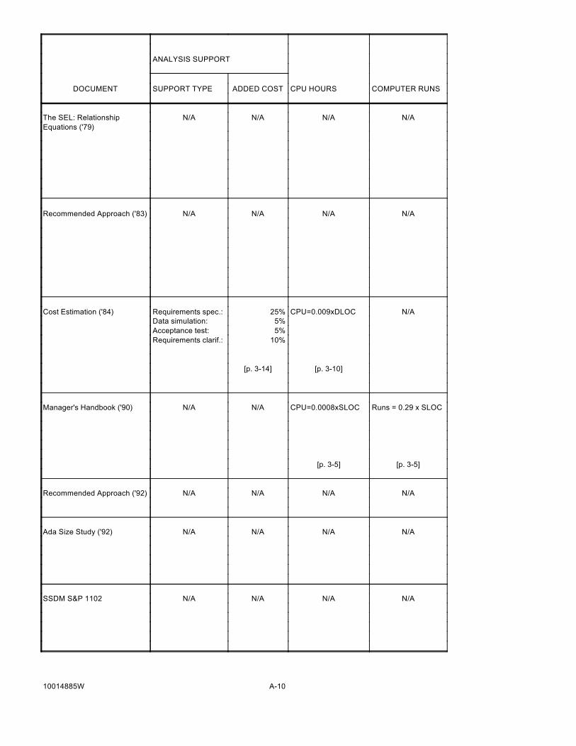
DOCUMENT

ANALYSIS SUPPORT

COMPUTER RUNSCPU HOURSADDED COSTSUPPORT TYPE

The SEL: RelationshipEquations ('79)

Recommended Approach ('83)

Cost Estimation ('84)

Manager's Handbook ('90)

Recommended Approach ('92)

Ada Size Study ('92)

SSDM S&P 1102

10014885W

N/AN/AN/AN/A

N/AN/AN/AN/A

N/ACPU=0.009xDLOC25%Requirements spec.:5%Data simulation:5%Acceptance test:

10%Requirements clarif.:

[p. 3-10][p. 3-14]

Runs = 0.29 x SLOCCPU=0.0008xSLOCN/AN/A

[p. 3-5][p. 3-5]

N/AN/AN/AN/A

N/AN/AN/AN/A

N/AN/AN/AN/A

A-10

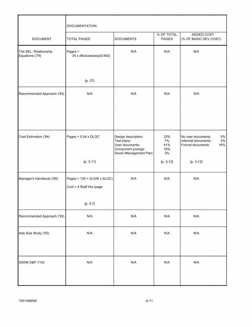
DOCUMENT

DOCUMENTATION

ADDED COST% OF TOTAL(% OF BASIC DEV.COST)PAGESDOCUMENTSTOTAL PAGES

The SEL: RelationshipEquations ('79)

Recommended Approach ('83)

Cost Estimation ('84)

Manager's Handbook ('90)

Recommended Approach ('92)

Ada Size Study ('92)

SSDM S&P 1102

10014885W

N/AN/AN/APages = 34 x (Modules)exp(0.662)

[p. 27]

N/AN/AN/AN/A

0%No user documents:33%Design description:Pages = 0.04 x DLOC5%Informal documents:7%Test plans:

16%Formal documents:41%User documents:16%Component prologs:3%Devel./Management Plan:

[p. 3-12][p. 3-12][p. 3-11]

N/AN/AN/APages = 120 + (0.026 x SLOC)

Cost = 4 Staff Hrs./page

[p. 3-7]

N/AN/AN/AN/A

N/AN/AN/AN/A

N/AN/AN/AN/A

A-11

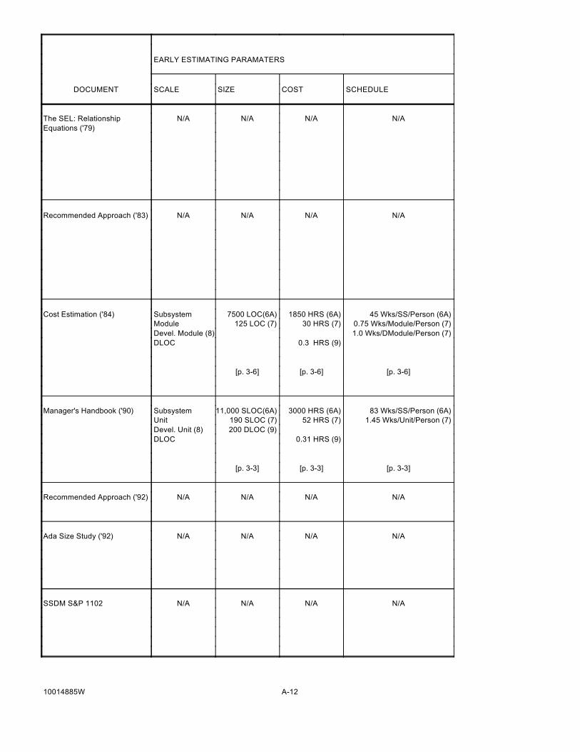
DOCUMENT

EARLY ESTIMATING PARAMATERS

SCHEDULECOSTSIZESCALE

The SEL: RelationshipEquations ('79)

Recommended Approach ('83)

Cost Estimation ('84)

Manager's Handbook ('90)

Recommended Approach ('92)

Ada Size Study ('92)

SSDM S&P 1102

10014885W

N/AN/AN/AN/A

N/AN/AN/AN/A

45 Wks/SS/Person (6A)1850 HRS (6A)7500 LOC(6A)Subsystem0.75 Wks/Module/Person (7)30 HRS (7)125 LOC (7)Module1.0 Wks/DModule/Person (7)Devel. Module (8)

0.3 HRS (9)DLOC

[p. 3-6][p. 3-6][p. 3-6]

83 Wks/SS/Person (6A)3000 HRS (6A)11,000 SLOC(6A)Subsystem1.45 Wks/Unit/Person (7)52 HRS (7)190 SLOC (7)Unit

200 DLOC (9)Devel. Unit (8)0.31 HRS (9)DLOC

[p. 3-3][p. 3-3][p. 3-3]

N/AN/AN/AN/A

N/AN/AN/AN/A

N/AN/AN/AN/A

A-12

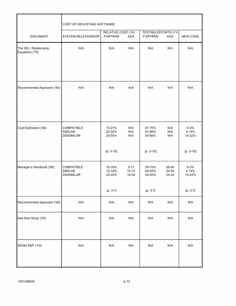
DOCUMENT

COST OF REHOSTING SOFTWARE

TESTING EFFORTS (11) RELATIVE COST (10)NEW CODEADAFORTRANADAFORTRANSYSTEM RELATIONSHIP

The SEL: RelationshipEquations ('79)

Recommended Approach ('83)

Cost Estimation ('84)

Manager's Handbook ('90)

Recommended Approach ('92)

Ada Size Study ('92)

SSDM S&P 1102

10014885W

N/AN/AN/AN/AN/AN/A

N/AN/AN/AN/AN/AN/A

0-3%N/A67-70%N/A15-21%COMPATIBLE4-14%N/A61-66%N/A22-32%SIMILAR15-32%N/A55-60%N/A33-50%DISSIMILAR

[p. 3-15][p. 3-15][p. 3-15]

0-3%36-4055-70%5-1110-16%COMPATIBLE4-14%30-3545-55%10-1515-18%SIMILAR15-32%25-3040-50%18-3020-40%DISSIMILAR

[p. 3-7][p. 3-7][p. 3-7]

N/AN/AN/AN/AN/AN/A

N/AN/AN/AN/AN/AN/A

N/AN/AN/AN/AN/AN/A

A-13

Notes:--------------------------------------------------------------------(1) Effort denoted is either total Staff Hours (SHr) or total Staff Months (SMon).(2) Duration denoted is either weeks per staff member or total calendar months.(3) Represents total estimated labor in staff months. This may vary from the Recommended Labor Commitment (RLC), used by the project manager to compute project duration.(4) Included in Detailed Design percentage(4A) The project type (e.g., orbit determination, simulator) is "OLD" when the organization has more than 2 years experience with it. The environment type (e.g., IBM 4341, VAX 8810) is "OLD" when the organization has more than 2 years experience with it.(5) Team size, not counting team leader(6) More than 5 years experience in development related activities(6A) Estimate at end of requirements analysis(7) Estimate at end of preliminary design(8) Number of developed units = N + 0.2R, Where N = number of New and Extensively Modified units R = Number of Slightly Modified and Verbatim units(9) Estimate at end of detailed design(10) Percent of original development costs(11) Percent of total rehosting cost

Glossary:--------------------------------------------------------------------Adapted Code = Reused code requiring changes to 25% or more of the lines, also known as 'Extensively Modified' CodeAdjusted Estimated Effort: estimated staff months to complete the project (SSDM S&P 1102)Compatible = Systems designed to be plug compatible (e.g., IBM S/360 and 4341).Converted Code = Reused code requiring changes to less than 25% of the lines, also known as 'Slightly Modified' CodeDELOC = Developed Executable Lines of CodeDissimilar = Systems with differences in most characteristics of architecture and organization (e.g., IBM S/360 and PDP 11/70).DLOC = Developed Lines of CodeDMC = Duration Model CoefficientDMX = Duration Model ExponentDSI = Delivered Source InstructionsE = Effort (in total staff hours, unless otherwise specified)ELOC = Executable Lines of CodeKDELOC = 1000s of Developed Executable Lines of CodeLOC = Lines of CodeNew SLOC = SLOC of New and Extensively Modified unitsReused SLOC = SLOC of Slightly Modified and Verbatim unitsRLC = Recommended Labor Commitment (in staff months), a figure used in SSDM to compute project duration. The RLC may differ from the Adjusted Estimated Effort.SHr = total Staff Hours of effortSimilar = Systems (e.g., IBM 4341 and VAX 8810) with some key architectural characteristics, such as word size.SLOC = Source Lines of Code (includes blank lines)SMon = Staff Months of effortSS = SubsystemsTransported Code = Reused code requiring no changes, also known as 'Verbatim' Code

A-14

Appendix B. Sample Subjective Evaluation Form

10014885W B-1 1

7. Assess overall quality and ability of development team.

8. How would you characterize the development team's experience and familiarity with the application area of the project?

9. Assess the development team's experience and familiarity with the development environment (hardware and support software).

How stable was the composition of the development team over the duration of the project?

SUBJECTIVE EVALUATION FORM

4. Assess the overall quality of the requirements specification documents, including their clarity, accuracy, consistency, and completeness.

5. How extensive were documentation requirements?

6. How rigorous were formal review requirements?

Name:

Project:

I. PROBLEM CHARACTERISTICS

1. Assess the intrinsic difficulty or complexity of the problem that was addressed by the software development.

2. How tight were schedule constraints on project?

3. How stable were requirements over development period?

1 2 3 4 5Easy Average Difficult

1 2 3 4 5Loose Average Tight

1 2 3 4 5 Low Average High

62

1 2 3 4 5Loose Average High

1 2 3 4 5 Low Average High

1 2 3 4 5 Low Average High

FOR LIBRARIAN'S USE ONLY

Number: ________________________________

Date: ________________________________

Entered by: ______________________________

Checked by: ______________________________

II. PERSONNEL CHARACTERISTICS: TECHNICAL STAFF

1 2 3 4 5 Low Average High

1 2 3 4 5Loose Average High

1 2 3 4 5 Low Average High

1 2 3 4 5 Low Average High

10.

Date:

IIndicate response by circling the corresponding numeric ranking.

NOVEMBER 1991

10014885W B-2 2

14. What degree of disciplined project planning was used?

15. To what degree were project plans followed?

16. To what extent did the development team use modern programming practices (PDL, top-down development, structured programming, and code reading)?

17. To what extent did the development team use well-defined or disciplined procedures to record specification modifications, requirements questions and answers, and interface agreements?

18. To what extent did the development team use a well-defined or disciplined requirements analysis methodology?

19. To what extent did the development team use a well-defined or disciplined design methodology?

20. To what extent did the development team use a well-defined or disciplined testing methodology?

11. Assess the overall performance of project management.

12. Assess project management's experience and familiarity with the application.

13. How stable was project management during the project?

SUBJECTIVE EVALUATION FORM

III. PERSONNEL CHARACTERISTICS: TECHNICAL MANAGEMENT

62

1 2 3 4 5 Low Average High

1 2 3 4 5 Low Average High

1 2 3 4 5 Low Average High

1 2 3 4 5 Low Average High

1 2 3 4 5 Low Average High

1 2 3 4 5 Low Average High

1 2 3 4 5 Low Average High

1 2 3 4 5 Low Average High

IV. PROCESS CHARACTERISTICS

1 2 3 4 5 Low Average High

1 2 3 4 5 Low Average High

IV. PROCESS CHARACTERISTICS

21. What software tools were used by the development team? Check all that apply from the list that follows and identify any other tools that were used but are not listed.

CompilerLinkerEditorGraphic display builderRequirements language processor

Structured analysis support toolPDL processorISPFSAP

CATPANVALET

Test coverage toolInterface checker (RXVP80, etc.)Language-sensitive editorSymbolic debuggerConfiguration Management Tool (CMS, etc.)Others (identify by name and function)

22. To what extent did the development team prepare and follow test plans? 1 2 3 4 5 Low Average High

10014885W B-3 3

IV. PROCESS CHARACTERISTICS (CONT'D)

V. ENVIRONMENT CHARACTERISTICS

28. Assess the system response time: were the turnaround times experienced by the team satisfactory in light of the size and nature of the jobs?

29. How stable was the hardware and system support software (including language processors) during the project?

30. Assess the effectiveness of the software tools.

31. To what degree does the delivered software provide the capabilities specified in the requirements?

32. Assess the quality of the delivered software product.

33. Assess the quality of the design that is present in the software product.

34. Assess the quality and completeness of the delivered system documentation.

35. To what degree were software products delivered on time?

36. Assess smoothness or relative ease of acceptance testing.

23. To what extent did the development team use well-defined and disciplined quality assurance procedures (reviews, inspections, and walkthroughs)?

24. To what extent did development team use well-defined or disciplined configuration management procedures?

25. How would you characterize the development team's degree of access to the development system?

26. What was the ratio of programmers to terminals?

27. To what degree was the development team constrained by the size of main memory or direct-access storage available on the development system?

SUBJECTIVE EVALUATION FORM

62

1 2 3 4 5 Low Average High

1 2 3 4 5 Low Average High

1 2 3 4 5 Low Average High

1 2 3 4 5 Low Average High

1 2 3 4 5 8:1 4:1 2:1 1:1 1:2

1 2 3 4 5 Low Average High

VI.

1 2 3 4 5 Low Average High

1 2 3 4 5 Low Average High

1 2 3 4 5 Low Average High

PRODUCT CHARACTERISTICS

1 2 3 4 5 Low Average High

1 2 3 4 5 Low Average High

1 2 3 4 5 Low Average High

1 2 3 4 5 Poor Average Very Good

1 2 3 4 5 Low Average High

Appendix C. Effort and Schedule Detailed Distribution

Appendix C. Effort and Schedule Detailed Distribution

Appendix C captures some of the detailed work performed during the Cost and ScheduleEstimation Study in the area of distributing effort and schedule by life-cycle phase anddistributing effort by activity. This portion of the analysis was an attempt to group thedistributions and search for trends by examining the projects in the highest and lowest, rangesalong with their project characteristics such as reuse percent or language type. Projects,subsequent to and including COBEDS, listed in Tables C-1 through C-3 were examined todetermine the five projects with the highest and the lowest percentages of effort or schedule for aparticular life-cycle phase. The distribution of effort by activity was also examined in a similarmanner. Tables C-4 through C-9 show the results of these analyses. There tends to be highvariability among projects as to the distribution of effort and schedule by phase as well as thedistribution of effort by activity.

Two patterns are noted here, but the study attributed no conclusions or significance to thesepatterns. The first is that projects with the lowest percentage of coding activity tend to be high-reuse projects. The second is that the projects with the highest percentages of coding activity areFORTRAN projects, but, at the same time, all are low-reuse projects.

Because of the time limitations of the study, the analysis in this area was limited; the data arearchived here to provide a basis for future analysis.

10014885W C-1

Table C-1. Effort Distribution by Phase

DESIGN % CODE % ST % AT %

PAS 18.0% 57.1% 15.4% 9.6%ISEEB 21.9% 57.1% 12.8% 8.2%AEM 19.4% 50.4% 16.7% 13.6%SEASAT 25.5% 49.4% 10.9% 14.3%SMM 29.6% 41.7% 16.7% 12.0%MAGSAT 21.9% 38.7% 19.1% 20.3%FOXPRO 19.1% 28.4% 21.7% 30.9%DEA 16.4% 49.9% 10.3% 23.5%DEB 20.0% 49.7% 15.1% 15.2%DESIM 35.5% 44.0% 10.7% 9.7%ERBS 21.9% 50.9% 16.0% 11.2%DERBY 29.1% 45.7% 11.2% 14.0%COBEDS 32.8% 29.2% 32.6% 5.4%ASP 22.7% 42.8% 18.5% 16.0%GROSIM 20.5% 43.5% 27.4% 8.6%COBSIM 25.4% 42.3% 22.4% 9.9%COBEAGSS 23.1% 38.2% 23.3% 15.4%GOADA 27.7% 41.8% 24.2% 6.3%GOFOR 15.5% 31.5% 39.9% 13.1%GOESAGSS 18.7% 54.4% 16.9% 9.9%GOESIM 28.5% 44.2% 9.4% 18.0%UARSAGSS 19.4% 49.6% 17.6% 13.4%UARSDSIM 18.0% 46.0% 8.5% 27.4%UARSTELS 24.6% 39.4% 15.2% 20.8%EUVEAGSS 14.0% 48.3% 22.2% 15.5%EUVETELS 26.1% 40.6% 13.2% 20.1%EUVEDSIM 21.5% 44.7% 23.8% 10.0%POWITS 13.6% 47.0% 11.9% 27.5%SAMPEXTS 48.1% 18.0% 18.3% 15.5%SAMPEX 26.4% 16.3% 36.8% 20.5%

10014885W C-2

Table C-2. Effort Distribution by Activity

DESIGN % CODE % TEST % OTHER %

PAS 6.7% 25.2% 13.6% 54.5%ISEEB 16.2% 22.7% 10.0% 51.1%AEM 19.7% 25.9% 15.9% 38.5%SEASAT 14.2% 26.7% 14.0% 45.1%SMM 26.4% 27.1% 14.3% 32.2%MAGSAT 25.4% 25.3% 18.2% 31.0%FOXPRO 32.2% 27.1% 17.1% 23.7%DEA 15.1% 18.8% 24.8% 41.2%DEB 20.0% 21.8% 16.3% 42.0%DESIM 28.9% 23.4% 14.3% 33.5%ERBS 18.3% 29.2% 16.7% 35.8%DERBY 26.5% 13.1% 14.9% 45.5%COBEDS 24.4% 20.8% 16.1% 38.7%ASP 14.6% 21.2% 23.7% 40.4%GROSIM 22.0% 32.6% 15.4% 30.0%COBSIM 22.5% 31.2% 14.4% 31.9%COBEAGSS 24.1% 22.2% 27.7% 26.1%GOADA 19.2% 27.8% 23.7% 29.3%GOFOR 11.7% 18.5% 39.2% 30.7%GOESAGSS 25.3% 31.8% 24.6% 18.3%GOESIM 19.2% 22.8% 23.6% 34.4%UARSAGSS 24.0% 29.1% 28.8% 18.1%UARSDSIM 18.1% 33.9% 27.4% 20.6%UARSTELS 19.3% 27.5% 33.3% 19.9%EUVEAGSS 21.5% 25.0% 31.3% 22.2%EUVETELS 15.2% 16.8% 26.2% 41.8%EUVEDSIM 21.0% 30.0% 21.4% 27.6%POWITS 9.2% 18.9% 40.8% 31.1%SAMPEXTS 16.7% 16.6% 26.8% 39.9%SAMPEX 14.5% 6.4% 30.5% 48.6%

10014885W C-3

Table C-3. Schedule Distribution by Phase

DESIGN % CODE % ST % AT %

PAS 27.5% 46.4% 13.0% 13.0%ISEEB 42.0% 42.0% 8.0% 8.0%AEM 28.1% 45.6% 15.8% 10.5%SEASAT 31.5% 44.4% 9.3% 14.8%SMM 31.6% 31.6% 11.8% 25.0%MAGSAT 30.6% 38.7% 14.5% 16.1%FOXPRO 44.4% 27.8% 11.1% 16.7%DEA 36.0% 47.2% 4.5% 12.4%DEB 38.6% 37.3% 12.0% 12.0%DESIM 50.0% 35.7% 7.1% 7.1%ERBS 43.3% 34.0% 12.4% 10.3%DERBY 36.1% 31.9% 11.1% 20.8%COBEDS 34.3% 22.9% 31.4% 11.4%ASP 29.9% 31.0% 14.9% 24.1%GROSIM 35.0% 39.0% 17.0% 9.0%COBSIM 28.0% 40.2% 18.3% 13.4%COBEAGSS 26.7% 26.7% 20.7% 25.9%GOADA 27.5% 28.9% 30.9% 12.8%GOFOR 25.2% 27.7% 31.9% 15.1%GOESAGSS 27.0% 38.3% 16.5% 18.3%GOESIM 34.3% 29.3% 8.1% 28.3%UARSAGSS 30.6% 36.1% 16.3% 17.0%UARSDSIM 25.8% 45.3% 7.0% 21.9%UARSTELS 31.9% 29.8% 10.6% 27.7%EUVEAGSS 37.3% 33.3% 14.7% 14.7%EUVETELS 26.5% 42.2% 12.0% 19.3%EUVEDSIM 27.3% 35.5% 22.3% 14.9%POWITS 26.1% 31.5% 8.1% 34.2%SAMPEXTS 47.9% 8.3% 16.7% 27.1%SAMPEX 45.9% 14.1% 22.4% 17.6%

10014885W C-4

Table C-4. Analysis of Activity Effort Distribution— Highest Percentages

FIVE PROJECTS WITH HIGHEST DESIGN PERCENTAGES

PROJECTS DESIGN % REUSE % TYPE LANG

GOESAGSS 25.3 % 12.1 % AGSS FCOBEDS 24.4 % 26.9 % DS FCOBEAGSS 24.1 % 12.1 % AGSS FUARSAGSS 24.0 % 11.0 %1 AGSS FCOBSIM 22.5 % 10.7 % TS F

FIVE PROJECTS WITH HIGHEST CODE PERCENTAGES

PROJECTS CODE % REUSE % TYPE LANG

UARSDSIM 33.9 % 23.6 % DS FGROSIM 32.6 % 17.9 % TS FGOESAGSS 31.8 % 12.1 % AGSS FCOBSIM 31.2 % 10.7 % TS FUARSAGSS 29.1 % 11.0 %1 AGSS F

FIVE PROJECTS WITH HIGHEST TEST PERCENTAGES

PROJECTS TEST % REUSE % TYPE LANG

POWITS 40.8 % 69.2 % TS AGOFOR 39.2 % 32.4 % DS FUARSTELS 33.3 % 34.8 % TS AEUVEAGSS 31.3 % 78.0 %1 AGSS FSAMPEX 30.5 % 92.1 % AGSS F

FIVE PROJECTS WITH HIGHEST OTHER PERCENTAGES

PROJECTS OTHER % REUSE % TYPE LANG

SAMPEX 48.6 % 92.1 % AGSS FEUVETELS 41.8 % 96.2 % TS AASP 40.4 % 12.9 % AGSS FSAMPEXTS 39.9 % 94.6 % TS ACOBEDS 38.7 % 26.9 % DS F

1 Reuse percent excludes ACME portion of project.

10014885W C-5

Table C-5. Analysis of Activity Effort Distribution— Lowest Percentages

FIVE PROJECTS WITH LOWEST DESIGN PERCENTAGES

PROJECTS DESIGN % REUSE % TYPE LANG

POWITS 9.2 % 69.2 % TS AGOFOR 11.7 % 32.4 % DS FSAMPEX 14.5 % 92.1 % AGSS FASP 14.6 % 12.9 % AGSS FEUVETELS 15.2 % 96.2 % TS A

FIVE PROJECTS WITH LOWEST CODE PERCENTAGES

PROJECTS CODE % REUSE % TYPE LANG

SAMPEX 6.4 % 92.1 % AGSS FSAMPEXTS 16.6 % 94.6 % TS AEUVETELS 16.8 % 96.2 % TS AGOFOR 18.5 % 32.4 % DS FPOWITS 18.9 % 69.2 % TS A

FIVE PROJECTS WITH LOWEST TEST PERCENTAGES

PROJECTS TEST % REUSE % TYPE LANG

COBSIM 14.4 % 10.7 % TS FGROSIM 15.4 % 17.9 % TS FCOBEDS 16.1 % 26.9 % DS FGOESIM 23.6 % 28.8 % TS AGOADA 23.7 % 28.5 % DS A

FIVE PROJECTS WITH LOWEST OTHER PERCENTAGES

PROJECTS OTHER % REUSE % TYPE LANG

UARSAGSS 18.1 % 11.0 %1 AGSS FGOESAGSS 18.3 % 12.1 % AGSS FUARSTELS 19.9 % 34.8 % TS AUARSDSIM 20.6 % 23.6 % DS FEUVEAGSS 22.2 % 78.0 %1 AGSS F

1 Reuse percent excludes ACME portion of project.

10014885W C-6

Table C-6. Analysis of Phase Effort Distribution—Highest Percentages

FIVE PROJECTS WITH HIGHEST DESIGN PERCENTAGES

PROJECTS DESIGN % REUSE % TYPE LANG

SAMPEXTS 48.1 % 94.6 % TS ACOBEDS 32.8 % 26.9 % DS FGOESIM 28.5 % 28.8 % TS AGOADA 27.7 % 28.5 % DS ASAMPEX 26.4 % 92.1 % AGSS F

FIVE PROJECTS WITH HIGHEST CODE PERCENTAGES

PROJECTS CODE % REUSE % TYPE LANG

GOESAGSS 54.4 % 12.1 % AGSS FUARSAGSS 49.6 % 11.0 %1 AGSS FEUVEAGSS 48.3 % 78.0 %1 AGSS FPOWITS 47.0 % 69.2 % TS AUARSDSIM 46.0 % 23.6 % DS F

FIVE PROJECTS WITH HIGHEST ST PERCENTAGES

PROJECTS ST % REUSE % TYPE LANG

GOFOR 39.9 % 32.4 % DS FSAMPEX 36.8 % 92.1 % AGSS FCOBEDS 32.6 % 26.9 % DS FGROSIM 27.4 % 17.9 % TS FGOADA 24.2 % 28.5 % DS A

FIVE PROJECTS WITH HIGHEST AT PERCENTAGES

PROJECTS AT % REUSE % TYPE LANG

POWITS 27.5 % 69.2 % TS AUARSDSIM 27.4 % 23.6 % DS FUARSTELS 20.8 % 34.8 % TS ASAMPEX 20.5 % 92.1 % AGSS FEUVETELS 20.1 % 96.2 % TS A

1 Reuse percent excludes ACME portion of project.

10014885W C-7

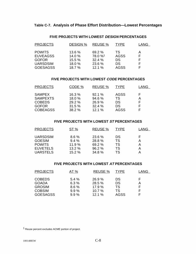
Table C-7. Analysis of Phase Effort Distribution— Lowest Percentages

FIVE PROJECTS WITH LOWEST DESIGN PERCENTAGES

PROJECTS DESIGN % REUSE % TYPE LANG

POWITS 13.6 % 69.2 % TS AEUVEAGSS 14.0 % 78.0 %1 AGSS FGOFOR 15.5 % 32.4 % DS FUARSDSIM 18.0 % 23.6 % DS FGOESAGSS 18.7 % 12.1 % AGSS F

FIVE PROJECTS WITH LOWEST CODE PERCENTAGES

PROJECTS CODE % REUSE % TYPE LANG

SAMPEX 16.3 % 92.1 % AGSS FSAMPEXTS 18.0 % 94.6 % TS ACOBEDS 29.2 % 26.9 % DS FGOFOR 31.5 % 32.4 % DS FCOBEAGSS 38.2 % 12.1 % AGSS F

FIVE PROJECTS WITH LOWEST ST PERCENTAGES

PROJECTS ST % REUSE % TYPE LANG

UARSDSIM 8.6 % 23.6 % DS FGOESIM 9.4 % 28.8 % TS APOWITS 11.9 % 69.2 % TS AEUVETELS 13.2 % 96.2 % TS AUARSTELS 15.2 % 34.8 % TS A

FIVE PROJECTS WITH LOWEST AT PERCENTAGES

PROJECTS AT % REUSE % TYPE LANG

COBEDS 5.4 % 26.9 % DS FGOADA 6.3 % 28.5 % DS AGROSIM 8.6 % 17.9 % TS FCOBSIM 9.9 % 10.7 % TS FGOESAGSS 9.9 % 12.1 % AGSS F

1 Reuse percent excludes ACME portion of project.

10014885W C-8

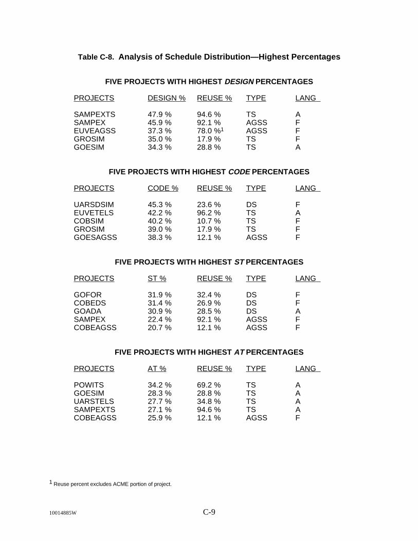
Table C-8. Analysis of Schedule Distribution—Highest Percentages

FIVE PROJECTS WITH HIGHEST DESIGN PERCENTAGES

PROJECTS DESIGN % REUSE % TYPE LANG

SAMPEXTS 47.9 % 94.6 % TS ASAMPEX 45.9 % 92.1 % AGSS FEUVEAGSS 37.3 % 78.0 %1 AGSS FGROSIM 35.0 % 17.9 % TS FGOESIM 34.3 % 28.8 % TS A

FIVE PROJECTS WITH HIGHEST CODE PERCENTAGES

PROJECTS CODE % REUSE % TYPE LANG

UARSDSIM 45.3 % 23.6 % DS FEUVETELS 42.2 % 96.2 % TS ACOBSIM 40.2 % 10.7 % TS FGROSIM 39.0 % 17.9 % TS FGOESAGSS 38.3 % 12.1 % AGSS F

FIVE PROJECTS WITH HIGHEST ST PERCENTAGES

PROJECTS ST % REUSE % TYPE LANG

GOFOR 31.9 % 32.4 % DS FCOBEDS 31.4 % 26.9 % DS FGOADA 30.9 % 28.5 % DS ASAMPEX 22.4 % 92.1 % AGSS FCOBEAGSS 20.7 % 12.1 % AGSS F

FIVE PROJECTS WITH HIGHEST AT PERCENTAGES

PROJECTS AT % REUSE % TYPE LANG

POWITS 34.2 % 69.2 % TS AGOESIM 28.3 % 28.8 % TS AUARSTELS 27.7 % 34.8 % TS ASAMPEXTS 27.1 % 94.6 % TS ACOBEAGSS 25.9 % 12.1 % AGSS F

1 Reuse percent excludes ACME portion of project.

10014885W C-9

Table C-9. Analysis of Schedule Distribution— Lowest Percentages

FIVE PROJECTS WITH LOWEST DESIGN PERCENTAGES

PROJECTS DESIGN % REUSE % TYPE LANG

GOFOR 25.2 % 32.4 % DS FUARSDSIM 25.8 % 23.6 % DS FPOWITS 26.1 % 69.2 % TS AEUVETELS 26.5 % 96.2 % TS ACOBEAGSS 26.7 % 12.1 % AGSS F

FIVE PROJECTS WITH LOWEST CODE PERCENTAGES

PROJECTS CODE % REUSE % TYPE LANG

SAMPEXTS 8.3 % 94.6 % TS ASAMPEX 14.1 % 92.1 % AGSS FCOBEDS 22.9 % 26.9 % DS FCOBEAGSS 26.7 % 12.1 % AGSS FGOFOR 27.7 % 32.4 % DS F

FIVE PROJECTS WITH LOWEST ST PERCENTAGES

PROJECTS ST % REUSE % TYPE LANG

UARSDSIM 7.0 % 23.6 % DS FGOESIM 8.1 % 28.8 % TS APOWITS 8.1 % 69.2 % TS AUARSTELS 10.6 % 34.8 % TS AEUVETELS 12.0 % 96.2 % TS A

FIVE PROJECTS WITH LOWEST AT PERCENTAGES

PROJECTS AT % REUSE % TYPE LANG

GROSIM 9.0 % 17.9 % TS FCOBEDS 11.4 % 26.9 % DS FGOADA 12.8 % 28.5 % DS ACOBSIM 13.4 % 10.7 % TS FEUVEAGSS 14.7 % 78.0 %1 AGSS F

1 Reuse percent excludes ACME portion of project.

10014885W C-10

Abbreviations and Acronyms

AEM Applications Explorer MissionAGSS Attitude Ground Support SystemASP Attached PayloadsBBXRT Broadband X-ray TelescopeCDR critical design reviewCOBE Cosmic Background ExplorerCOBEAGSS COBE Attitude Ground Support SystemCOBEDS COBE Dynamics SimulatorCOBSIM COBE Telemetry SimulatorCOCOMO Constructive Cost ModelDEA Dynamics Explorer ADEB Dynamics Explorer BDEDET DEB Definitive Attitude Determination SystemDERBY ERBS Dynamics SimulatorDESIM ERBS Telemetry SimulatorDLOC developed lines of codeDSPLBLDR GESS Display BuilderERBS Earth Radiation Budget SatelliteEUVE Extreme Ultraviolet ExplorerEUVEAGSS EUVE Attitude Ground Support SystemEUVEDSIM EUVE Dynamics SimulatorEUVETELS EUVE Telemetry SimulatorFDD Flight Dynamics DivisionFOCS FPSS Off-Null Calibrating SystemFOXPP FOCS PreprocessorFOXPRO FOCS ProcessorFPSS fine-pointing Sun sensorGESS Graphics Executive Support SystemGOADA GOES Dynamics Simulator (Ada)GOES Geostationary Operational Environmental SatelliteGOESAGSS GOES Attitude Ground Support SystemGOESIM GOES Telemetry SimulatorGOFOR GOES Dynamics Simulator (FORTRAN)GRO Gamma Ray ObservatoryGROAGSS GRO Attitude Support SystemGRODY GRO Dynamics SimulatorGROSIM GRO Telemetry SimulatorGROSS GRO Dynamics SimulatorGSFC Goddard Space Flight CenterGSOC guide star selection and occultationISEEB International Sun-Earth Explorer BISEEC International Sun-Earth Explorer CMAGSAT magnetic satellite

10014885W AB-1

PAS panoramic attitude sensorPDR preliminary design reviewPOWITS POLAR/WIND Telemetry SimulatorRMS root-mean-squareSAMPEX Solar, Anomalous, and Magnetospheric Particle ExplorerSAMPEXTP SAMPEX Telemetry ProcessorSAMPEXTS SAMPEX Telemetry SimulatorSEASAT Ocean Studies SatelliteSEF Subjective Evaluation FormSEL Software Engineering LaboratorySM staff monthsSMM Solar Maximum MissionTBD to be determinedUARS Upper Atmosphere Research SatelliteUARSAGSS UARS Attitude Ground Support SystemUARSDSIM UARS Dynamic SimulatorUARSTELS UARS Telemetry Simulator

10014885W AB-2

References

1. NASA/Goddard Space Flight Center, ADA Size Study Report, S. Condon and M. Regardie(CSC), September 1992

2. NASA/Goddard Space Flight Center, Software Engineering Laboratory (SEL), DataCollection Procedures for the Software Engineering Laboratory (SEL) Database, G. Heller,J. Valett, M. Wild, March 1992

3. NASA/Goddard Space Flight Center, Software Engineering Laboratory (SEL), SoftwareEngineering Laboratory (SEL) Cleanroom Process Model, S. Green, et al., November 1991

4. Barry W. Boehm, Software Engineering Economics, Prentice-Hall, Inc., Englewood Cliffs,New Jersey, 1981

5. NASA/Goddard Space Flight Center, An Approach to Software Cost Estimation,F. McGarry, G. Page, D. Card, et al., February 1984

6. NASA/Goddard Space Flight Center, Software Engineering Laboratory (SEL), Manager'sHandbook for Software Development, Revision 1, L. Landis, F. McGarry, S. Waligora, etal., November 1990

7. Computer Sciences Corporation (CSC), SEAS System Development Methodology (SSDM)Standards and Procedures, M. Plett, et al. (CSC), June 1990

8. Quattro Pro Version 4.0 User's Guide, Borland International, Inc., 1992

9. NASA/Goddard Space Flight Center, Software Engineering Laboratory (SEL), SoftwareEngineering Laboratory (SEL) Recommended Approach to Software Development,Revision 3, L. Landis and S. Waligora (CSC), June 1992

10014885W R-1