1

Ch 5 COST

The theory of cost is important to a manager because it provides the foundation for two important production decisions:

1) whether or not to shut down2) how much to produce

Also, this chapter supports the theory of supply.

2

“Buy low and sell high”

Increasing competitive pressures,changing technology, and customer demand have made it harder for firms to achieve high profit margins by raising their prices

– cost management, restructuring, downsizing etc.

– outsourcing and relocation of manufacturing facilities to low-wage countries

– mergers, consolidations, and then reduced headcount

3

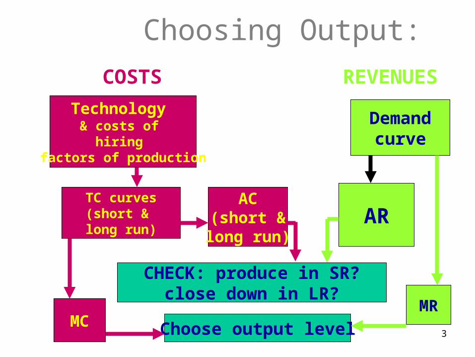
Choosing Output:

COSTS REVENUES

Technology & costs of

hiring factors of production

TC curves(short & long run)

AC(short &long run)

MC

Demandcurve

AR

MR

CHECK: produce in SR?close down in LR?

Choose output level

4

Which Costs Matter?

• Opportunity vs. accounting cost• Opportunity cost is the cost associated with

opportunities that are foregone by not putting resources in their highest valued use

• Accounting cost considers only explicit cost, the out of pocket cost for such items as wages, salaries, materials, and property rentals

• Sunk vs. incremental cost• A sunk cost is an expenditure that has been

made and cannot be recovered--they should not influence a firm’s decisions

5

Costs in the Short Run

• Total output is a function of variable inputs and fixed inputs

• Therefore, the total cost of production equals the fixed cost (the cost of the fixed inputs) plus the variable cost (the cost of the variable inputs)

• Fixed costs– costs that do not vary with output levels

• Variable costs– costs that do vary with output levels

• TC = FC + VC

6

Costs in the Short Run continued

Q

TC

Q

VC MC

Marginal Cost (MC) is the cost of expanding output by one unit. Since fixed cost have no impact on marginal cost, it can be written as:

7

Costs in the Short Run continued

• Average Total Cost (ATC) is the cost per unit of output, or average fixed cost (AFC) plus average variable cost (AVC)

• This can be written:

Q

TC

Q

TVC

Q

TFC ATC

8

The Determinants of Short-Run Cost

• The relationship between the production function and cost can be detected by looking at the relationship between either increasing returns (to a factor) and cost, or decreasing returns (i.e. when the law of diminishing returns takes effect) and cost:

9

The relationship between the production function and cost

– Increasing returns and cost

• With increasing returns, output is increasing relative to input and variable cost and total cost will fall relative to output

– Decreasing returns and cost

• With decreasing returns, output is decreasing relative to input and variable cost and total cost will rise relative to output

10

SR Cost Curves for a Firm• Unit Costs

– AFC falls continuously and – MC equals AVC and ATC at their minimum – Minimum AVC occurs at a lower output

than minimum ATC due to FC

Output

P

25

50

75

100

0 1 2 3 4 5 6 7 8 9 10 11

AFC

AVCATC

MC

11

The Firm’s Short-Run Output Decision

• Firm sets output at Q1, where SRMC=MR• subject to checking the average condition:

– if price is above SRATC1 firm produces Q1 at a profit– if price is between SRATC1 and SRAVC1 firm

produces Q1 at a loss– if price is below SRAVC1, firm produces zero output

SRAVC1

£

Output

MR

SRAVC

SRMC

Q1

SRATCSRATC1

SMC = MR

12

The firm’s long-run output decision

• The decision:– If the price is at or above LAC1, the firm

produces Q1.– If the price is below LAC1 the firm goes out

of business

AC1

£

Output(goods per week)

MR

LAC

LMC

Q1

LMC = MR

LMC always passes through the minimum point of LAC.

13

The firm’s output decisions – a summary

Marginal condition Check whether to produce

Short-run decision Long-run decision

Choose the output level at which MR = SRMC Choose the output level at which MR = LRMC

Produce this output unless price lower than SRAVC. If it is, produce zero. Produce this output unless price is lower than LRAC. If it is, produce zero.

14

Long-Run Cost Function

The long-run total cost curve describes the minimum cost of producing each output level when the firm is free to vary all input levels.

One of the first decisions to be made by the owner/manager of a firm is to decide the scale of operation (size of the firm).

15

Long-Run Average CostThe LAC is a graph that shows the different scales on which a firm can choose to operate in the long run. Long-run average cost (LRAC) is often assumed to be U-shaped:

LRAC

Ave

rag

e co

st

Output

16

Economies of ScaleHowever, economies of scale occur when long-run average costs decline as output rises:

LRAC

Ave

rag

e co

st

Output

17

Economies of Scale continued

• A cost related concept1

• When a company is experiencing economies of scale its LRAC declines as output is increasing

• Diseconomies of scale:

LRAC increasing as output increasing

1 Compare with returns to scale which is a production concept!

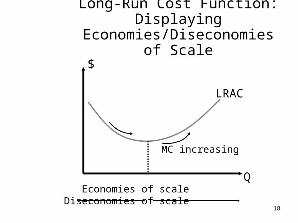
18

Long-Run Cost Function: Displaying

Economies/Diseconomies of Scale

LRAC

$

Economies of scale Diseconomies of scaleQ

MC increasing

19

Economies of scale can be classified as

a) External economies of scaleadvantages that a firm gains from the expansion and size of the industry as whole industrial clusters

b) Internal economies of scaleadvantages that a firm gains from increasing the scale of its own operation

20

Why can a firm become more efficient as the scale of

production rises?• Technical economies

• Marketing economies

• Financial economies

• Managerial economies

• Risk-bearing economies

• Administrative economies

21

Why can a firm become more inefficient as the scale of

production rises?

Diseconomies of scale:• Large enough operation may

increase input prices• Disproportionate rise in

transportation costs• Red tape• Management coordination problems• Labor specialization and repetitive

work too little stimulation, productivity suffers

22

• Primary reason for long-run scale economies (diseconomies) is the underlying pattern of returns to scale in the firm’s long-run production function

– Increasing returns to scale lead to economies of scale and decreasing returns to scale leads to diseconomies of scale

23

Using LRAC as Decision-Making Tool

• Which plant size to choose?

• Both production cost information and accurate demand forecasts are necessary

• The cost structure of the industry will determine the competitive structure of the industry

24

The long-run average cost curve LRAC: an envelope of short-run

cost curves

Output

Ave

rag

e co

st

SRATC1

Each plant sizeis designed fora given outputlevel

SRATC2

SRATC3

SRATC4

So there is a sequence of SRATCcurves, eachcorresponding toa different optimal output level.

LRAC

In the long-run, plant size itself is variable, and the long-run average cost curve LRAC is found to be the ‘envelope’ of the SRATCs

TU-91.113 Managerial Economics / Hannele Wallenius

The existence of economies of scale means that in the long run, as the

firms increases its scale of operation, the LRAC of production

falls.

SRMC

SRMC

SRMC

SRAC

SRAC

SRAC

Units of output

Cos

ts p

er u

nit (

$)

LRAC

Each individual scale of the firm will still be subject to diminishing returns and have a U-shaped SRAC curve.

26

Minimum Efficient Scale• A firm can not expect always to

achieve economies of scale when it expands: at some point it is likely that the further increase in size does not produce any reduction in the average cost per unit

– minimum efficient scale (MES)

LRAC

MES Scale of firm

$

TU-91.113 Managerial Economics / Hannele Wallenius

Increasing LRAC: Diseconomies of Scale

SRMCSRAC

SRMCSRAC

SRMCSRAC

Units of output

Cos

ts p

er u

nit (

$)

LRAC

28

Constant Returns to Scale

• Constant RTS refers to when an increase in scale of operation leads to no change in average costs per unit produced LRAC is horizontal

– when the firm doubles the use of inputs, it will double output as well as its costs

29

Production with Two (or more) Outputs--Economies

of Scope

• Economies of scope exist when the unit cost of producing two or more products/services jointly is lower than producing them separately

– producing related products, products that are complementary

• the average total cost of production decreases as a result of increasing the number of different goods produced

30

Why Advantages May Exist

For example:

1) Both products use same inputs (capital and labor)

2) The firms share management resources

3) Both products use the same labor skills and type of machinery

31

Economies of Scope continued

• Examples:– Chicken farm--poultry and eggs– Automobile company--cars and

trucks– University--teaching and research

32

An Example: PepsiCo, Inc.

33

Economies of Scope continued

• Another example is a company like Proctor & Gamble, which produces hundreds of products from soap to toothpaste. They can afford to hire expensive graphic designers and marketing experts who can use their skills across the product lines. Because the costs are spread out, this lowers the average total cost of production for each product

34

P&G acquires The Gillette

Company (29.1.2005) • Both companies have complementary

expertise in health and personal care• The companies also share

complementary technology platforms in skin care and particularly in oral care

• Same distribution channels (Wal-Mart etc.)

35

Degree of Economies of Scope

• The degree of economies of scope measures the savings in cost:

– C(Q1) is the cost of producing product Q1

– C(Q2) is the cost of producing product Q2

– C(Q1Q2) is the joint cost of producing both products

– If SC > 0 -- Economies of scope– If SC < 0 -- Diseconomies of scope

)QC(Q

)QC(Q)C(Q)C(Q SC

21,

21,21

36

Dynamic Changes in Costs--

The Learning Curve

• The learning curve measures the impact of worker’s experience on the costs of production

• It describes the relationship between a firm’s cumulative output and amount of inputs needed to produce a unit of output

• The learning curve implies:

1) The labor requirement per unit falls

2) Costs will be high at first and then will fall with learning

37

The Learning Curve

Cumulative number of machine lots produced

Hours of laborper machine lot

10 20 30 40 500

2

4

6

8

10

38

The Learning Curve

Cumulative number of machine lots produced

Hours of laborper machine lot

10 20 30 40 500

2

4

6

8

10

39

The Learning Curve

Cumulative # of machine lots produced

Hours of laborper machine lot

10 20 30 40 500

2

4

6

8

10

• The horizontal axis measures the cumulative number of hours of machine lots the firm has produced

• The vertical axis measures the number of hours of labor needed to produce each lot

40

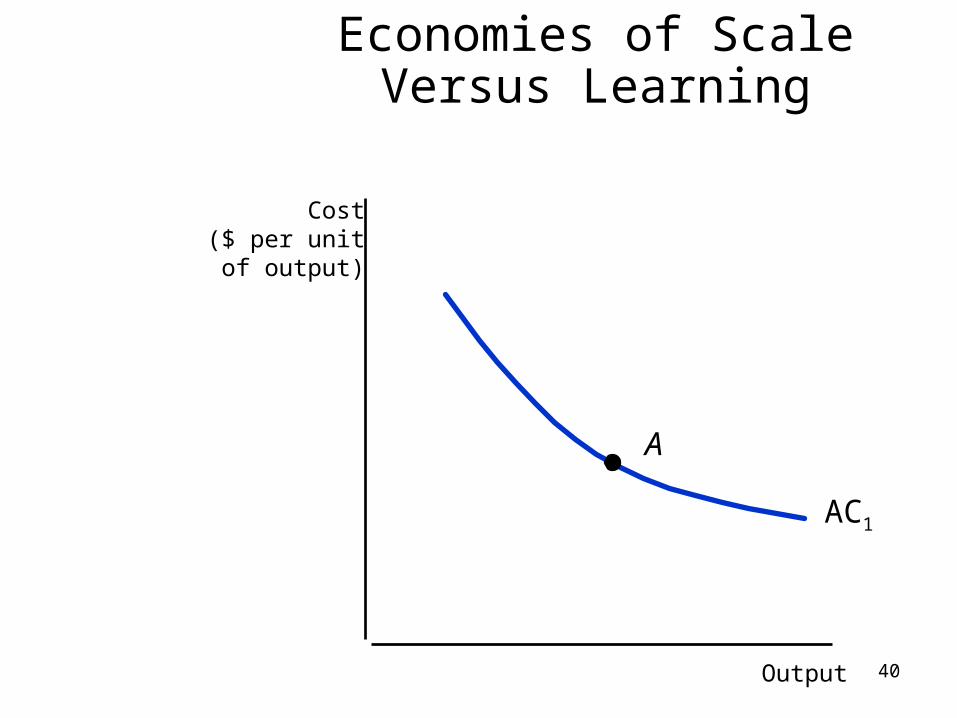
Economies of Scale Versus Learning

Output

Cost($ per unitof output)

AC1

A

41

Economies of Scale Versus Learning continued

Output

Cost($ per unitof output)

AC1

AB

Economies of Scale

42

Economies of Scale Versus Learning continued

Output

Cost($ per unitof output)

AC1

AB

Economies of Scale

AC2

Learning C