Cosinor analysis of accident risk using SPSS’s regression procedures Peter Watson 31st October...
31
Cosinor analysis of accident risk using SPSS’s regression procedures Peter Watson 31st October 1997 MRC Cognition & Brain Sciences Unit
-
Upload
herbert-oconnor -
Category
Documents
-
view
217 -
download
1
Transcript of Cosinor analysis of accident risk using SPSS’s regression procedures Peter Watson 31st October...

Cosinor analysis of accident risk using SPSS’s regression
procedures
Peter Watson
31st October 1997
MRC Cognition & Brain Sciences Unit
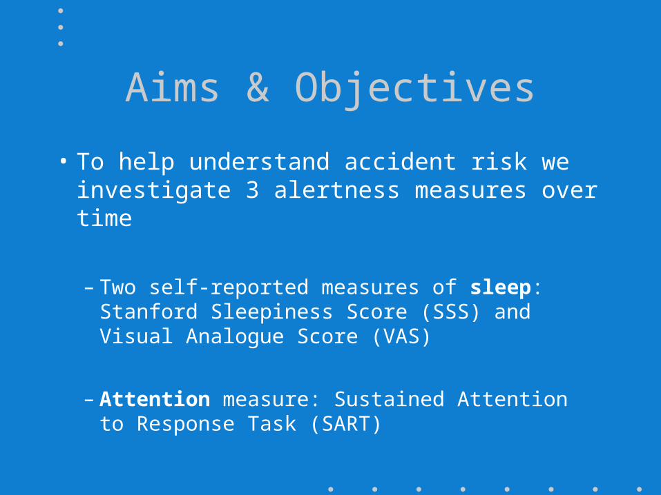
Aims & Objectives
• To help understand accident risk we investigate 3 alertness measures over time
– Two self-reported measures of sleep: Stanford Sleepiness Score (SSS) and Visual Analogue Score (VAS)
– Attention measure: Sustained Attention to Response Task (SART)

Study
• 10 healthy Peterhouse college undergrads
(5 male)
• Studied at 1am, 7am, 1pm and 7pm for four consecutive days
• How do vigilance (SART) and perceived vigilance (SSS, VAS) behave over time?

Characteristics of Sleepiness
• Most subjects “most sleepy” early in morning or late at night
• Theoretical evidence of cyclic behaviour
(ie repeated behaviour over a period of 24 hours)
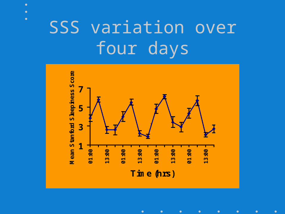
SSS variation over four days
1
3
5
70
1:0
0
13
:00
01
:00
13
:00
01
:00
13
:00
01
:00
13
:00
Time (hrs)
Mea
n S
tan
ford
Sle
epin
ess
Sco
re
1
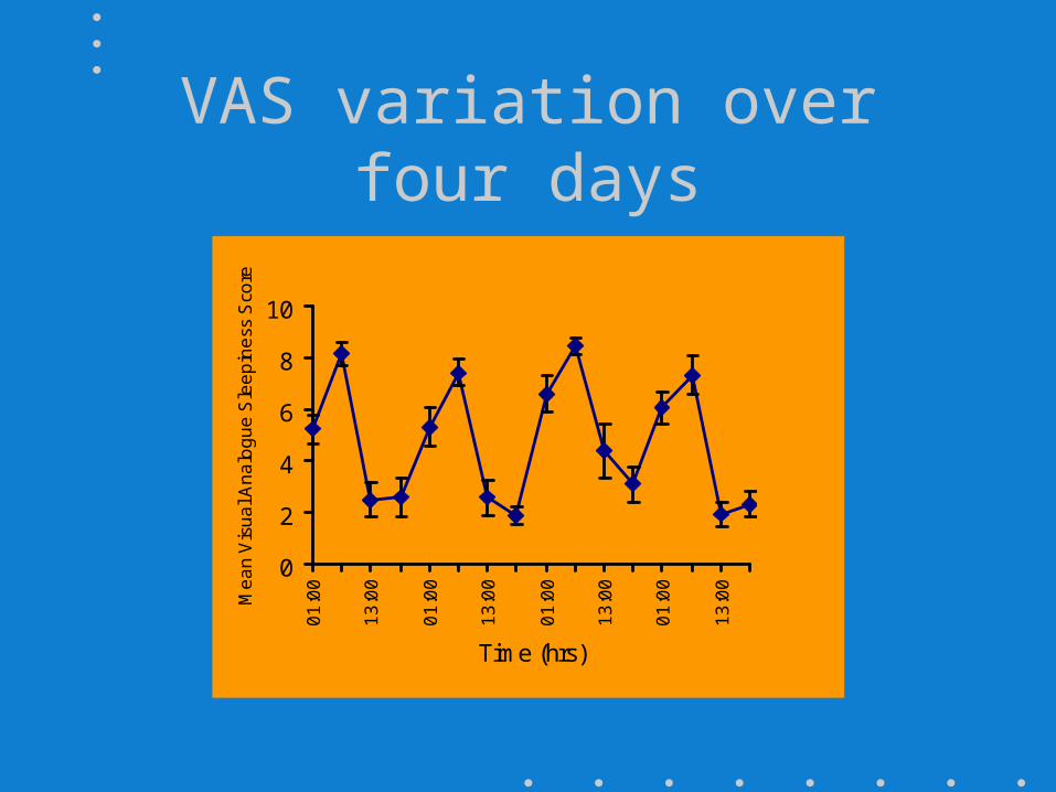
VAS variation over four days
0
2
4
6
8
100
1:0
0
13
:00
01
:00
13
:00
01
:00
13
:00
01
:00
13
:00
Time (hrs)
Me
an
Vis
ua
l An
alo
gu
e S
lee
pin
ess
Sco
re
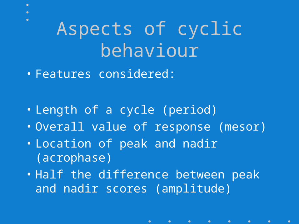
Aspects of cyclic behaviour
• Features considered:
• Length of a cycle (period)
• Overall value of response (mesor)
• Location of peak and nadir (acrophase)
• Half the difference between peak and nadir scores (amplitude)
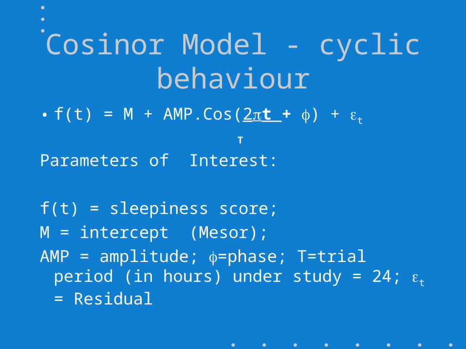
Cosinor Model - cyclic behaviour
• f(t) = M + AMP.Cos(2t + ) + t
T
Parameters of Interest:
f(t) = sleepiness score;
M = intercept (Mesor);
AMP = amplitude; =phase; T=trial period (in hours) under study = 24; t = Residual

Period, T
• May be estimated
• Previous experience (as in our example)
• Constrained so that Peak and Nadir are T/2
hours apart (12 hours in our sleep example)

Periodicity
• 24 hour Periodicity upheld via absence of Time by Day interactions
• SSS : F(9,81)=0.57, p>0.8
• VAS : F(9,81)=0.63, p>0.7

Fitting using SPSS “linear” regression
For g(t)=2t/24 and since
Cos(g(t)+) = Cos()Cos(g(t))-Sin()Sin(g(t))
it follows the linear regression:
f(t) = M + A.Cos(2t/24) + B.Sin(2t/24)
is equivalent to the above single cosine function - now fittable in SPSS “linear” regression combining Cos and Sine function
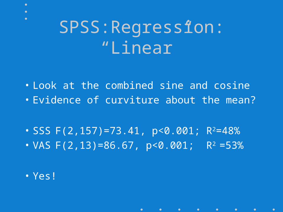
SPSS:Regression: “Linear”
• Look at the combined sine and cosine• Evidence of curviture about the mean?
• SSS F(2,157)=73.41, p<0.001; R2=48%• VAS F(2,13)=86.67, p<0.001; R2 =53%
• Yes!
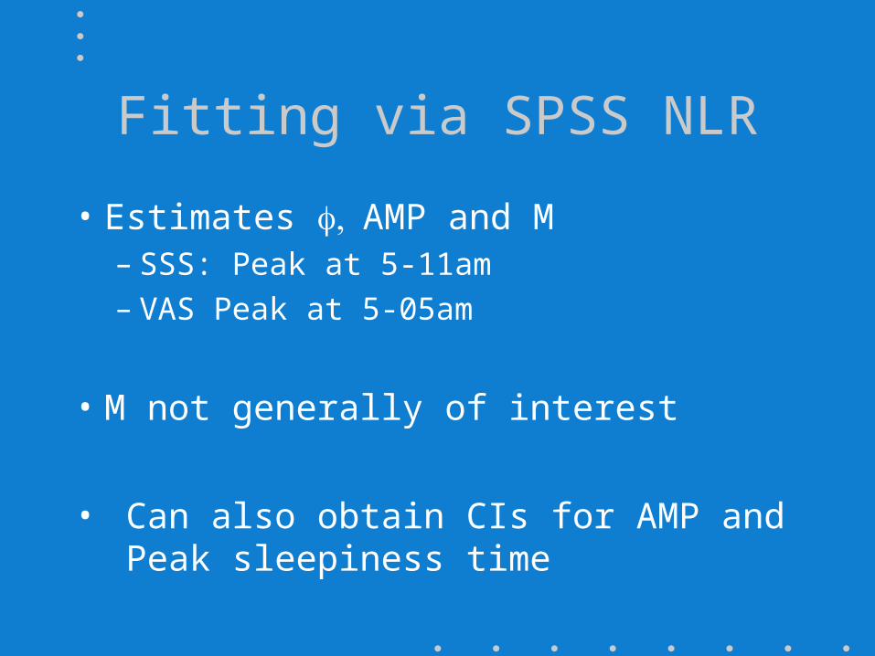
Fitting via SPSS NLR
• Estimates AMP and M– SSS: Peak at 5-11am– VAS Peak at 5-05am
• M not generally of interest
• Can also obtain CIs for AMP and Peak sleepiness time

Equivalence of NLR and “Linear” regression models
• Amplitude:
A = AMP Cos()
B = -AMP Sin()
Hence
AMP =
• Acrophase:
A = AMP Cos()
B = -AMP Sin()
Hence
ArcTan(-B/A)22 BA
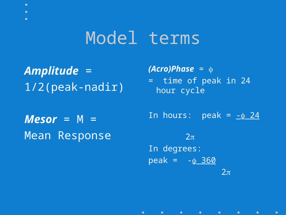
Model terms
Amplitude =
1/2(peak-nadir)
Mesor = M =
Mean Response
(Acro)Phase = = time of peak in 24 hour
cycle
In hours: peak = - 24
2
In degrees:
peak = - 360
2

Fitted Cosinor Functions (VAS in black; SSS in red)
0
1
2
3
4
5
6
7
8
9
1:00AM
7:00AM
1:00PM
7:00PM
1:00AM
Time of Day
Sle
ep
ine
ss
Sc
ore

% Amplitude
• % Amplitude = 100 x (Peak-Nadir)
overall mean
= 100 x 2 AMP
MESOR
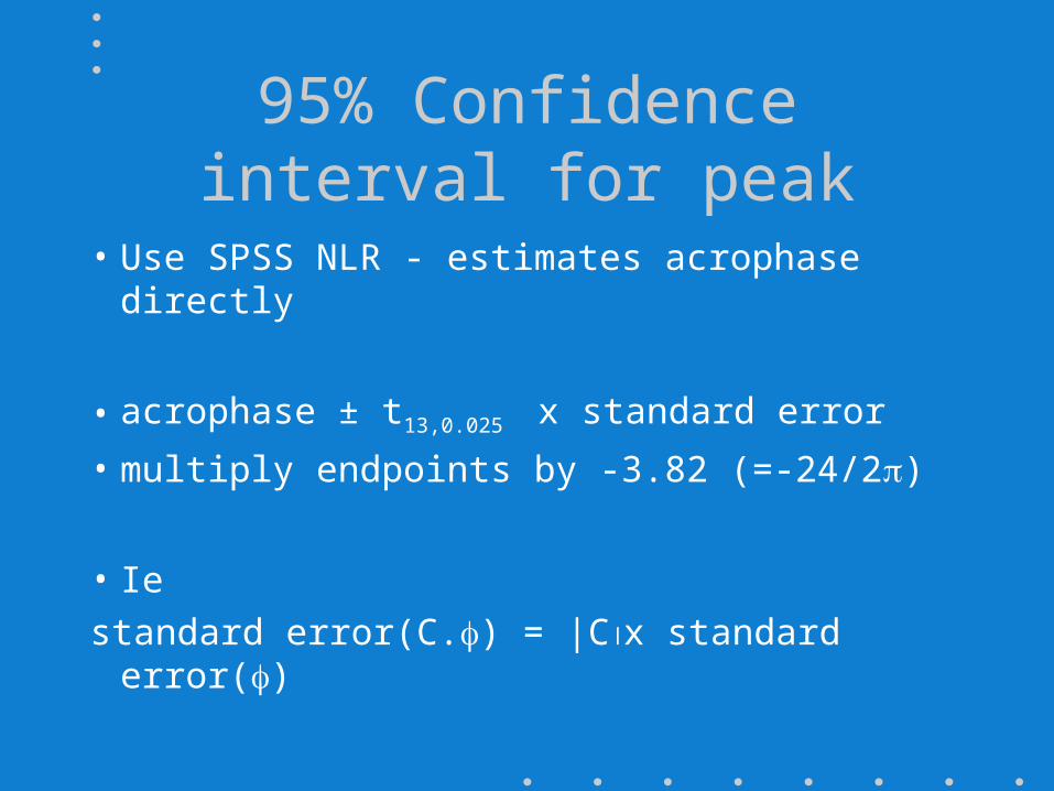
95% Confidence interval for peak
• Use SPSS NLR - estimates acrophase directly
• acrophase ± t13,0.025 x standard error
• multiply endpoints by -3.82 (=-24/2)
• Ie
standard error(C.) = |Cx standard error()

Levels of Sleepiness
• CIs for peak sleepiness and % amplitude
• Stanford Sleepiness Score:
95% CI = (4-33,5-48), amplitude=97%
Visual Analogue Score:
95% CI = (4-31,5-40), amplitude=129%
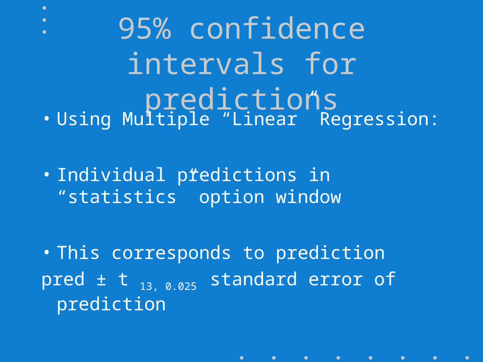
95% confidence intervals for predictions
• Using Multiple “Linear” Regression:
• Individual predictions in “statistics” option window
• This corresponds to prediction
pred ± t 13, 0.025 standard error of prediction
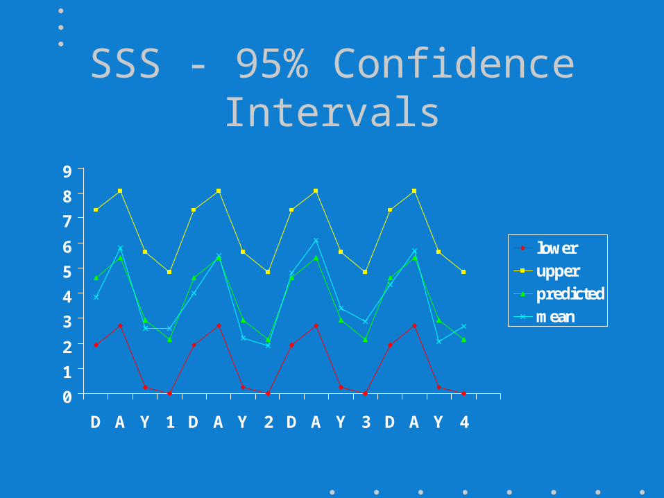
SSS - 95% Confidence Intervals
0
1
2
3
4
5
6
7
8
9
D A Y 1 D A Y 2 D A Y 3 D A Y 4
lowerupperpredictedmean

VAS 95% Confidence Intervals
0
2
4
6
8
10
12
14
D A Y 1 D A Y 2 D A Y 3 D A Y 4
MeanLowerUpperPredicted
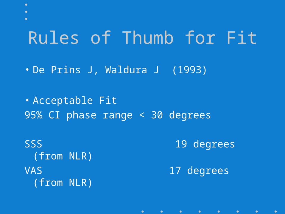
Rules of Thumb for Fit
• De Prins J, Waldura J (1993)
• Acceptable Fit
95% CI phase range < 30 degrees
SSS 19 degrees (from NLR)
VAS 17 degrees (from NLR)
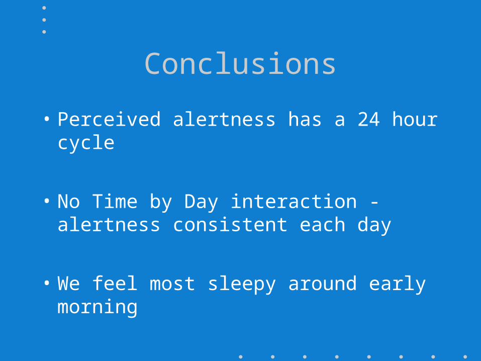
Conclusions
• Perceived alertness has a 24 hour cycle
• No Time by Day interaction - alertness consistent each day
• We feel most sleepy around early morning

Unperceived Vigilance
• Vigilance task (same 10 students as sleep indices)
• Proportion of correct responses to an attention task at 1am, 7am, 1pm and 7pm over 4 days
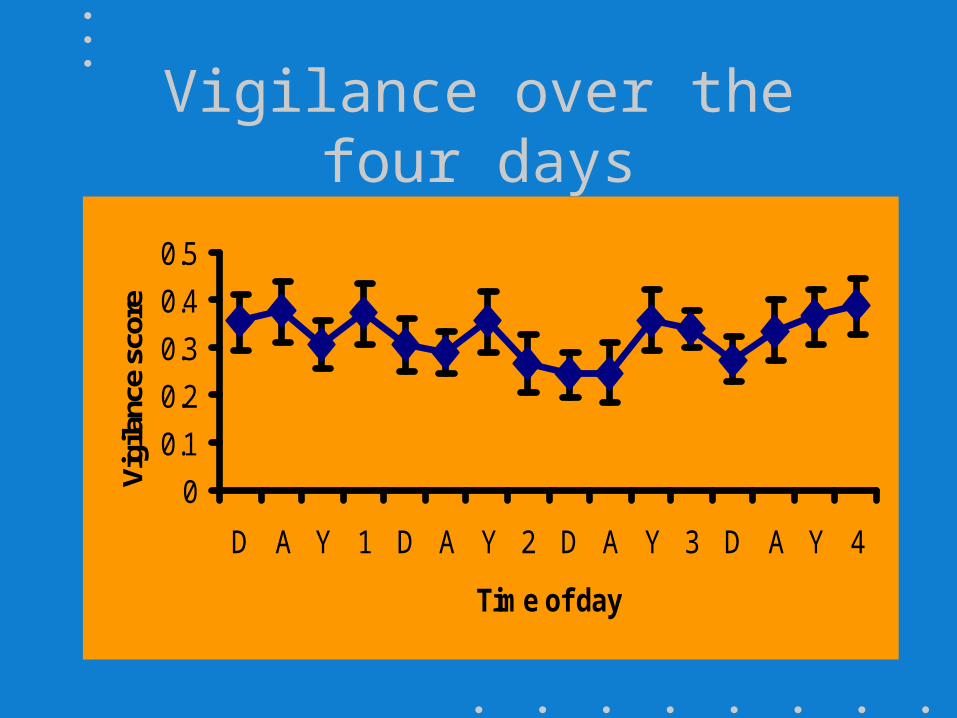
Vigilance over the four days
0
0.1
0.2
0.3
0.4
0.5
D A Y 1 D A Y 2 D A Y 3 D A Y 4
Time of day
Vigi
lanc
e sc
ore
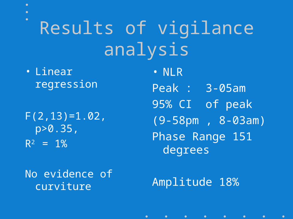
Results of vigilance analysis
• Linear regression
F(2,13)=1.02, p>0.35,
R2 = 1%
No evidence of curviture
• NLR
Peak : 3-05am
95% CI of peak
(9-58pm , 8-03am)
Phase Range 151 degrees
Amplitude 18%
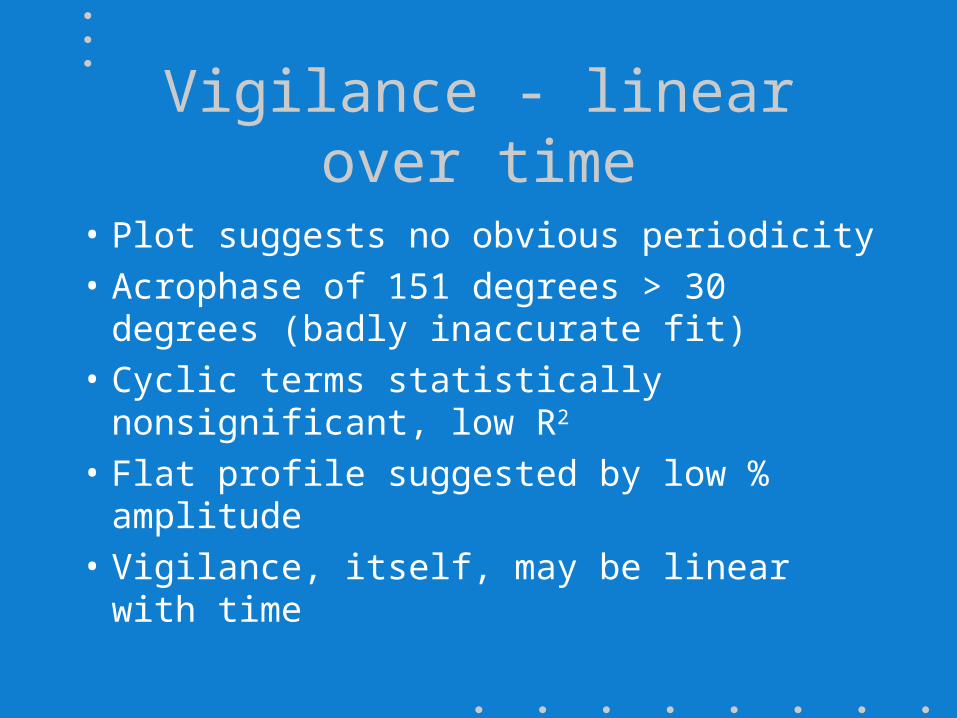
Vigilance - linear over time
• Plot suggests no obvious periodicity
• Acrophase of 151 degrees > 30 degrees (badly inaccurate fit)
• Cyclic terms statistically nonsignificant, low R2
• Flat profile suggested by low % amplitude
• Vigilance, itself, may be linear with time

Polynomial Regression
• An alternative strategy is the fitting of cubic polynomials
• Similar results to cosinor functions – two turning points for perceived sleepiness– no turning points (linear) for attention measure
Conclusions
• Cosinor analysis is a natural way of modelling cyclic behaviour
• Can be fitted in SPSS using either “linear” or nonlinear regression procedures

Thanks to helpful colleagues…..
• Avijit Datta
• Geraint Lewis
• Tom Manly
• Ian Robertson


![C-MRC it gb de Ed01 2007reducta-im.hr/katalozi/zupcasti_reduktori_rc.pdfSELEZIONE RIDUTTORE - MRC 1400 [min-1] SPEED REDUCER SELECTION - MRC GETRIEBEAUSWAHL - MRC 0.09 kW (0.12 HP)](https://static.fdocuments.us/doc/165x107/6108c986e8f90f642023ce89/c-mrc-it-gb-de-ed01-2007reducta-imhrkatalozizupcastireduktorircpdf-selezione.jpg)