AVERAGE CASE ANALYSIS OF

ALGORITHMS FOR THE MAXIMUM

SUBARRAY PROBLEM

A thesis submitted in partial fulfilment of the

requirements for the Degree

of Master of Science in Computer Science

in the University of Canterbury

by Mohammad Bashar

University of Canterbury

2007

ii

Examining Committee:

• Prof. Dr Tadao Takaoka, University of Canterbury (Supervisor) • Associate Prof. Dr Alan Sprague, University of Alabama

(External Examiner)

iii

iv

This thesis is dedicated to my Mom and Dad for their endless love and constant support.

v

vi

Abstract

Maximum Subarray Problem (MSP) is to find the consecutive array portion

that maximizes the sum of array elements in it. The goal is to locate the

most useful and informative array segment that associates two parameters

involved in data in a 2D array. It’s an efficient data mining method which

gives us an accurate pattern or trend of data with respect to some associated

parameters. Distance Matrix Multiplication (DMM) is at the core of MSP.

Also DMM and MSP have the worst-case complexity of the same order. So

if we improve the algorithm for DMM that would also trigger the

improvement of MSP. The complexity of Conventional DMM is O(n3). In

the average case, All Pairs Shortest Path (APSP) Problem can be modified

as a fast engine for DMM and can be solved in O(n2 log n) expected time.

Using this result, MSP can be solved in O(n2 log2 n) expected time. MSP

can be extended to K-MSP. To incorporate DMM into K-MSP, DMM needs

to be extended to K-DMM as well. In this research we show how DMM can

be extended to K-DMM using K-Tuple Approach to solve K-MSP in O(Kn2

log2 n log K) time complexity when K ≤ n/log n. We also present

Tournament Approach which solves K-MSP in O(n2 log2 n + Kn2) time

complexity and outperforms the K-Tuple Approach significantly.

vii

viii

Acknowledgments

The last one and half year of my academic life has been a true learning

period. This one page is not adequate to thank all those people who have

been supporting me during this time.

Firstly, I would like to thank my supervisor Professor Tadao Takaoka, who

gave me the opportunity to do this research and his continuous assistance,

guidance, support, suggestions and encouragement have been invaluable to

me. I honestly appreciate the time and effort he has given me to conduct my

research.

Secondly, I would like to express my gratitude to my lab mates and friends

who had made my university life more enjoyable and pleasant by sharing

their invaluable time. I specially thank Sung Bae, Lin Tian, Ray Hidayat,

Oliver Batchelor, Taher Amer and Tobias Bethlehem for their priceless help

and encouragement.

Finally, and most importantly, I would like to acknowledge my family’s

role in my academic endeavor. I thank my father and mother for their

unconditional love, inspiration and encouragement throughout the last few

years of my academic work.

ix

x

Table of Contents

List of Figures ...................................................................................................xv List of Tables.................................................................................................. xvii Chapter 1: Introduction ....................................................................................1

1.1 MSP Extension.........................................................................................4 1.2 A Real-life significance of K-MSP .........................................................5 1.3 Research Scope ........................................................................................5 1.4 Research Objectives.................................................................................6 1.5 Research Structure ...................................................................................6

Chapter 2: Theoretical Foundation .................................................................9 2.1 Research Assumptions.............................................................................9 2.2 Prefix Sum................................................................................................9 2.3 Maximum Subarray Problem ................................................................10

2.3.1 Exhaustive Method.......................................................................11 2.3.2 Efficient Method...........................................................................12

2.4 K-Maximum Subarray Problem ............................................................12 2.4.1 Exhaustive Method.......................................................................13 2.4.2 Efficient Method...........................................................................14

2.5 Distance Matrix Multiplication .............................................................14 2.5.1 Conventional DMM .....................................................................17 2.5.2 Fast DMM.....................................................................................17

2.6 K-Distance Matrix Multiplication .........................................................18 2.6.1 Conventional K-DMM .................................................................19 2.6.2 Fast K-DMM.................................................................................20

2.7 Lemmas ..................................................................................................20 2.7.1 Lemma 1 .......................................................................................21 2.7.2 Lemma 2 .......................................................................................21 2.7.3 Lemma 3 .......................................................................................21 2.7.4 Lemma 4 .......................................................................................22 2.7.5 Lemma 5 .......................................................................................22 2.7.6 Lemma 6 .......................................................................................23 2.7.7 Lemma 7 .......................................................................................26

Chapter 3: Related Work................................................................................29

3.1 Main Algorithm of MSP based on DMM.............................................29 3.2 The relation between MSP and DMM ..................................................31 3.3 APSP Problem Algorithms Lead to Fast DMM ...................................32

3.3.1 Dantzig’s APSP Problem Algorithm ...........................................32 3.3.2 Description of Dantzig’s APSP Problem Algorithm...................33 3.3.3 Analysis of Dantzig’s APSP Problem Algorithm .......................36

xi

3.3.4 Spira’s APSP Problem Algorithm................................................37 3.3.5 Description of Spira’s APSP Problem Algorithm.......................38 3.3.6 Analysis of Spira’s APSP Problem Algorithm............................39 3.3.7 MT’s APSP Problem Algorithm..................................................39 3.3.8 Description of MT’s APSP Problem Algorithm .........................40 3.3.9 Analysis of MT’s APSP Problem Algorithm ..............................41

3.4 Modified MT Algorithm as Fast DMM ................................................43 3.4.1 Description of Fast DMM Algorithm ..........................................44 3.4.2 Analysis of Fast DMM Algorithm...............................................46

3.5 Analysis of MSP based on Fast DMM..................................................48 3.5.1 Lemma 8 .......................................................................................48 3.5.2 Recurrence 1 .................................................................................49 3.5.3 Theorem 1 .....................................................................................50

3.6 K-MSP Algorithm..................................................................................52 Chapter 4: K-Tuple Approach........................................................................53

4.1 New Fast K-DMM Algorithm ...............................................................53 4.2 Description of New Fast K-DMM Algorithm......................................55

4.2.1 Description of Data Structure T ...................................................57 4.2.2 Description of Set W.....................................................................59

4.3 Analysis of New Fast K-DMM Algorithm ..........................................61 4.3.1 Phase 1: Dantzig’s Counterpart....................................................61 4.3.2 Phase 2: Spira’s Counterpart ........................................................69

4.4 New K-MSP Algorithm.........................................................................78 4.5 Description of New K-MSP Algorithm.................................................78

4.5.1 Base Case......................................................................................79 4.5.2 Recursive Case..............................................................................80

4.6 Analysis of New K-MSP Algorithm .....................................................84 4.6.1 Lemma 9 .......................................................................................84 4.6.2 Recurrence 2 .................................................................................85 4.6.3 Theorem 2 .....................................................................................86

Chapter 5: Tournament Approach................................................................91

5.1 Tournament Algorithm ..........................................................................91 5.2 Tournament Approach for K-MSP........................................................93

Chapter 6: Evaluation ...................................................................................101

6.1 Conventional Approach vs. K-tuple Approach...................................101 6.1.1 Dijkstra, Floyd, Dantzig, Spira and MT APSP Problem Algorithms ..................................................................................102 6.1.2 Conventional DMM vs. Fast DMM...........................................104 6.1.3 MSP with Conventional DMM vs. MSP with Fast DMM........105 6.1.4 Conventional K-DMM vs. Fast K-DMM ..................................107 6.1.5 K-MSP with Conventional K-DMM vs. K-MSP with Fast K- DMM...........................................................................................108

xii

6.2 K-Tuple Approach vs. Tournament Approach....................................110 Chapter 7: Conclusion...................................................................................113

7.1 Future Work .........................................................................................114 References .......................................................................................................115

xiii

xiv

List of Figures

Figure 1: Given input array..................................................................................2 Figure 2: Converted input array...........................................................................3 Figure 3: Prefix sum.............................................................................................9 Figure 4: K-MSP example .................................................................................12 Figure 5: Two (3, 3) matrices ............................................................................15 Figure 6: 3-layered DAG of two (3, 3) matrices ...............................................16 Figure 7: Resulting matrix C..............................................................................16 Figure 8: Resulting matrix containing the first shortest distances....................18 Figure 9: Resulting matrix containing the second shortest distances ...............19 Figure 10: Resulting matrix containing the third shortest distances.................19 Figure 11: (m, n) array .......................................................................................23 Figure 12: Solution set expansion process ........................................................34 Figure 13: Two vertices pointing to same candidate.........................................35 Figure 14: Intermediate stage of solution set expansion process......................36 Figure 15: Visualizing set S, U and U-edge ......................................................41 Figure 16: 3-layered DAG of two (n, n) matrices .............................................45 Figure 17: Intermediate stage of set W ..............................................................47 Figure 18: Visualization of array T....................................................................59 Figure 19: (a, a) array at the bottom of the recursion .......................................80 Figure 20: Four-way recursion and 6 solutions.................................................81 Figure 21: X + Y problem solving in O(K log K) time......................................83 Figure 22: Binary tournament tree.....................................................................91 Figure 23: Visualization of the intermediate recursion process........................95 Figure 24: Strip Visualization............................................................................96 Figure 25: Scope and position of a maximum subarray solution .....................97 Figure 26: (n, n) array yielding O(n2) strips and O(n2) subarrays per strip ......98 Figure 27: APSP Problem time measurement.................................................103 Figure 28: DMM time measurement ...............................................................105 Figure 29: MSP time measurement .................................................................106 Figure 30: K-DMM time measurement ...........................................................108 Figure 31: K-MSP time measurement (comparison between Conventional and K-Tuple Approach) ..................................................................110 Figure 32: K-MSP time measurement (comparison between K-Tuple and Tournament Approach)...................................................................112

xv

xvi

List of Tables

Table 1: APSP Problem time measurement ....................................................103 Table 2: DMM time measurement...................................................................104 Table 3: MSP time measurement.....................................................................105 Table 4: K-DMM time measurement ..............................................................107 Table 5: K-MSP time measurement (comparison between Conventional and K-Tuple Approach) ............................................................. 108-109 Table 6: K-MSP time measurement (comparison between K-Tuple and Tournament Approach)......................................................................111

xvii

xviii

1

Chapter 1

Introduction

Maximum Subarray Problem (MSP) is to find the most useful and informative

array portion that associates two parameters involved in data. It’s an efficient

data mining method which gives us an accurate pattern or trend of data with

respect to some associated parameters. For instance, suppose we have the

record of monthly sales of some products of a company and our task is to

analyze the sales trend with respect to some age groups and some income

levels. To formulate this into MSP, we span each sales record item over a two-

dimensional array where each row and column correlates two parameters age

and income level. The main objective of MSP is to detect a rectangular shaped

array portion that maximizes the sum of sales. By doing so we are able to track

which age groups and income levels contribute to the maximum sum of sales.

Normally all the input array elements are non-negative. When this is the case,

the straightforward solution is the whole array. To avoid this, we convert the

given input array into a modified input array containing both positive and

negative numbers. In the conversion process, we subtract the mean of the

given input array elements from each single element of the given input array

and consider the modified input array for the MSP. Analysis on this modified

input array would yield more precise evaluation of the sales trends with

respect to age groups and income levels of purchasers.

The formulation of the problem in terms of the example matrix below is as

follows:

Suppose the sales record of an arbitrary product is given in the following 2-

dimensional input array.

10 22 6 28 1 6 35 27 6 24 27 14 5 54 3 4

Sales[Row][Col]

Figure 1: Given input array

If we consider the given input array with all positive numbers the trivial

solution for the MSP is sum of the whole array which is 272 in this example.

AAggee GGrroouupp IInnccoommee LLeevveellSum = 272

2

As we explained earlier, to avoid this trivial solution we subtract the mean

value of the array elements from each individual element of the same array. In

the preceding example, the mean value of the array elements is 17 (as 272/16

= 17). In the following array we represent the modified input array after

subtracting the mean value from each individual values and we find the

maximum subarray on this modified input array.

Figure 2: Converted input array

In Figure 2, we can observe the maximum subarray is defined by the

rectangular array portion. The position of this subarray in the main array can

be tracked as (2, 2) which corresponds to the upper left corner and (4, 3) which

corresponds to the lower right corner. By tracking the maximum subarray in

Sales[Row][Col]

AAggee GGrroouupp IInnccoommee LLeevveell

-7 5 -11 11 -16 -11 18 10 -11 7 10 -3 -12 37 -14 -13

Sum = 47

3

this way, we can find the range of age groups and income levels that

contribute to the maximum sales.

The other possible application for MSP is Graphics. The brightest portion of

an image can be tracked by identifying the maximum subarray. For example, a

bitmap image consists of non-negative pixel values. So we need to convert

these non-negative pixel values into an accumulation of positive and negative

values by subtracting the mean or average from each pixel value. By applying

MSP into these modified pixel values the brightest portion in the image can be

easily traced.

1.1 Maximum Subarray Problem Extension

MSP can be extended to K-MSP where the goal is to find K maximum

subarrays. K is a positive number which is between 1 and 4

mn (m+1)(n+1)

where m and n refer to the size of the given array. We explain in details in

Chapter 2 with example how K is bounded by this number for a given array of

size (m, n).

There are two variants of K-MSP. One is disjoint and the other one is

overlapping. In the disjoint case, all maximum subarrays that have been

detected in a given array must be separated or disjoint from each other. On the

other hand, in the overlapping case, we are not enforced by such restriction.

4

All maximum subarrays that have been detected in a given array can be

overlapped with each other.

1.2 A Real-life Significance of K- Maximum Subarray Problem

A real-life example of K-MSP could be a product leaflet delivery example.

Let’s assume we own a company and we would like to deliver information of

the new products of our company on a leaflet to our potential consumers. We

also would like to target our potential customers from the area of the city

which is densely populated. After detecting the densely populated area of the

city with the help of MSP we realized that this area is not physically accessible

due to road construction work. Thus we need to identify the second most

densely populated area of the city for our new products leaflet delivery. If this

is also not accessible due to some reason we need to identify the third most

densely populated area of the city and so on. The interesting observation here

is that the first maximum subarray is available to us but practically it may not

be feasible to use all the time. And thus, K-MSP plays its role to overcome this

limitation.

1.3 Research Scope

In this research, we focus into the overlapping case of K-MSP. We also

consider 2 dimensional MSP. We assume that the size of the array is always

5

power of 2. The array size is represented by m and n. If m and n are not powers

of 2 we can extend our framework to the case where m and/or n are not power

of 2. Also all unspecified logarithms should be considered as binary.

1.4 Research Objectives

The objectives of this research are:

1. To develop efficient algorithms for K-MSP.

2. To do the average case analysis of algorithms for MSP and K-MSP.

3. To compare and evaluate existing algorithms with new algorithms for K-

MSP.

1.5 Research Structure

Chapter 2 of this research presents theoretical foundation of MSP as we define

MSP and all its relevant concepts formally. Chapter 3 provides related works

that were carried out previously by other researchers. We also rigorously

analyze the existing algorithms in this chapter. Chapter 4 reveals a K-Tuple

Approach for which we develop new algorithms for K-Distance Matrix

Multiplication and K-MSP. The description and analysis of new algorithms are

also presented in this chapter. Chapter 5 presents a Tournament Approach for

which we further develop an algorithm for K-MSP. Chapter 6 scrutinizes the

6

experiment results and comparisons between conventional approaches and

new approaches. In the end, summary and conclusion are given in Chapter 7.

7

8

Chapter 2

Theoretical Foundation

In this chapter we present a number of core concepts that are related with

MSP. As we further discuss the related work of MSP in the next chapter it will

become transparent how these concepts are related with MSP.

2.1 Research Assumptions

All numbers that appear in the given (m, n) array are random and independent

of each other.

2.2 Prefix Sum

The prefix sum of an array is an array in which each element is obtained from

the sum of those which precede it. For example, the prefix sum of:

(4, 3, 6, 7, 2) is (4, 4+3, 4+3+6, 4+3+6+7, 4+3+6+7+2) = (4, 7, 13, 20, 22)

For 2D cases, the prefix sum of

=

1 -5 98 -4 34 3 -2

1 -4 5 9 0 12 13 7 17

Figure 3: Prefix sum

9

The prefix sums s[1..m][1..n] of a 2D array a[1..m][1..n] is computed by the

following algorithm. Mathematically, s[i][j] is the sum of a[1..i][1..j].

______________________________ Algorithm 1: Prefix Sum Algorithm 1: for i := 0 to m 2: for j := 0 to n 3: s[i][j] = 0; 4: column[i][j] = 0; 5: end for; 6: end for; 7: for i := 1 to m 8: for j := 1 to n 9: column[i][j] = column[i –1][j] + a[i][j]; 10: s[i][j] = s[i][j –1] + column[i][j]; 11: end for; 12: end for; _______________________________ The complexity of the above algorithm is straightforward. It takes O(n2) time

to compute the 2D prefix sum where m = n.

2.3 Maximum Subarray Problem

We consider a 2D array a[1…m, 1…n] as input data. The MSP is to maximize

the array portion a[k...i, l…j], that is, to obtain such indices (k, l) and (i, j). We

assume the upper-left corner has co-ordinate (1, 1). In the example in Figure 2,

(k, l) corresponds to (2, 2) and (i, j) corresponds to (4, 3).

10

2.3.1 Exhaustive Method

The brute force or exhaustive algorithm to calculate maximum subarray is as

follows:

___________________________________ Algorithm 2: Exhaustive MSP Algorithm 1: max = – 999; 2: for i := 1 to m 3: for j := 1 to n 4: for k := 1 to i 5: for l := 1 to j 6: currentmax = s[i][j] – s[i][l] – s[k][j] + s[k][l]; 7: if currentmax > max) 8: max = currentmax; 9: end if; 10: end for; 11: end for; 12: end for; 13: end for; ___________________________________

We assume prefix sum is already computed by Algorithm 1 and available in

array s. Variable max is initialized to –999 which resembles a negative infinite

value by assuming all the numbers that appear in the given (m, n) array are

between 1 and 100. Thus the range for the numbers in the modified input array

becomes -100 to 100. The complexity of the above algorithm is

straightforward. Because of quadruply nested for loops the complexity

becomes O(n4) where m = n.

11

2.3.2. Efficient Method

Takaoka [1] described an elegant method for solving MSP. In Chapter 3 we

investigate this algorithm in details. This research is primarily based on

Takaoka’s MSP algorithm which solves MSP by applying divide-and-conquer

methodology.

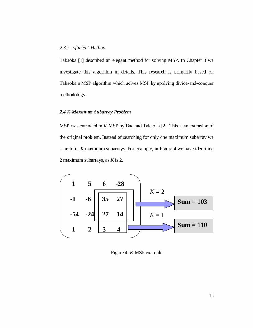
2.4 K-Maximum Subarray Problem

MSP was extended to K-MSP by Bae and Takaoka [2]. This is an extension of

the original problem. Instead of searching for only one maximum subarray we

search for K maximum subarrays. For example, in Figure 4 we have identified

2 maximum subarrays, as K is 2.

1 5 6 -28 -1 -6 35 27 -54 -24 27 14 1 2 3 4

Sum = 110 K = 1

K = 2 Sum = 103

Figure 4: K-MSP example

12

2.4.1 Exhaustive Method

The brute force or exhaustive algorithm to calculate K maximum subarrays is

as follows:

_____________________________________ Algorithm 3: Exhaustive K-MSP Algorithm 1: for r := 1 to K 2: max[r] = – 999; 3: for i := 1 to m 4: for j := 1 to n 5: for k := 1 to i 6: for l := 1 to j 7: currentmax = s[i][j] – s[i][l] – s[k][j] + s[k][l]; 8: if (currentmax > max[r] AND currentmax’s co-ordinates (i, j, k, l) 9: differ from all maximum subarrays co-ordinates (i, j, k, l) that 10: we have computed previously) 11: max[r] = currentmax; 12: end if; 13: end for; 14: end for; 15: end for; 16: end for; 17: end for; _____________________________________

In the above algorithm the first condition in the ‘if’ block checks for the

maximum sum found for a given co-ordinate (controlled by 4 ‘for’ loops). The

second condition checks the co-ordinates of current sum with all previously

computed sums so that the same solution is not repeated. Algorithm 3 differs

from Algorithm 2 in a number of ways. The outermost ‘for’ loop runs from 1

13

to K for K-MSP. Also max is a list to hold K-maximum sums. The complexity

of the above algorithm is O(Kn4) where m = n.

2.4.2 Efficient Method

Takaoka and Bae [2] modified Takaoka’s [1] MSP algorithm to deal with K-

MSP. We also modify Takaoka’s [1] MSP algorithm in Chapter 4 based on K-

Tuple Approach. In Chapter 5, we modify Takaoka’s [1] MSP algorithm once

again based on Tournament Approach.

2.5 Distance Matrix Multiplication

By translating prefix sums into distances, we can solve MSP by Distance

Matrix Multiplication (DMM) and we will show this in the next chapter. Now

we describe DMM.

The purpose of DMM is to compute the distance product C = AB for two n-

dimensional matrices A = [ai, j] and B = [bi,j] whose elements are real numbers.

ci,j = min { ai,k + bk,j } nk 1=

The meaning of ci,j is the shortest distance from vertex i in the first layer to

vertex j in the third layer in an Acyclic Directed Graph (DAG) consisting of

three layers of vertices. These vertices are labeled 1, ...,n in each layer, and the

distance from i in the first layer to j in the second layer is ai,j and that from i in

14

the second layer to j in the third layer is bi,j. The above min operation can be

replaced by max operation and thus we can define a similar product, where we

have longest distances in the 3-layered graph that we have described above.

This graph is depicted in Figure 6.

Suppose we have the following two matrices A and B.

A B

3 5 8 4 5 6 1 2 6

-2 0 8 4 7 2 2 9 -3

Figure 5: Two (3, 3) matrices

Then the 3-layered DAG would look like as follows:

15

3

2

1

3

2

1

3

2

2 2

-3 9

7

4

8

-2 0

2 6

1

6

5

4 8

3 5

1

Figure 6: 3-layered DAG of two (3, 3) matrices

Then the resulting matrix C would look like as follows:

1 3 5 2 4 3 -1 1 3

C =

Figure 7: Resulting matrix C

16

2.5.1 Conventional DMM

The algorithm for DMM which uses the exhaustive or brute-force method is

termed as Conventional DMM in this research. In the following we give the

min version of DMM algorithm where m = n.

______________________________________ Algorithm 4: Conventional DMM Algorithm 1: for i := 1 to n 2: for j := 1 to n 3: C[i][j] = 999; //infinite value 4: for k :=1 to n 5: if(A[i][k] + B[k][j] < C[i][j] ) 6: C[i][j] = A[i][k] + B[k][j]; 7: end if; 8: end for; 9: end for; 10: end for; ______________________________________

The complexity of the above algorithm is O(n3) due to triple nested for loops.

So this is obviously a naïve approach. For a big data set this approach would

not be efficient.

2.5.2 Fast DMM

Takaoka [1] proposed All Pairs Shortest Path (APSP) Problem to be used as a

fast engine for DMM. Subsequently Takaoka modified the Moffat-Takaoka’s

algorithm [3] for the all pairs shortest path problem (also known as MT

17

algorithm) and named this new algorithm as Fast DMM. This algorithm is

scrutinized in Chapter 3 which takes O(n2 log n) time.

2.6 K-Distance Matrix Multiplication

DMM can be extended to K-DMM as follows:

ci,j = min [K] { ai,k + bk,j | k=1..n }

where min[K]S is the set of K minima of S ={ ai,k + bk,j|k=1..n }. cij is now a set

of K numbers. The intuitive meaning of K-DMM of MIN-version is that cij is

the K-shortest path distances from i to j in the same graph as described before.

Let cij[k] be the k-th of cij and C[k] = [cij[k]]. In the above example k runs from

1 to 3 (as n = 3). So we have 3 different output matrices for C and these are

shown in Figure 8, 9 and 10.

1 3 5 2 4 3 -1 1 3

C[1] =

Figure 8: Resulting matrix containing the first shortest distances

18

9 12 78 12 76 9 4C[2] =

Figure 9: Resulting matrix containing the second shortest distances

10 17 11 9 15 12 8 15 9

C[3] =

Figure 10: Resulting matrix containing the third shortest distances

2.6.1 Conventional K-DMM

The exhaustive or brute-force method to find the K-DMM is termed as

Conventional K-DMM algorithm in this research. In the following we give this

algorithm where m = n.

______________________________________ Algorithm 5: Exhaustive K-DMM Algorithm 1: for i:= 1 to n 2: for j := 1 to n 3: select K minima of {ai1 + b1j,……,ain + bnj} 4: end; 5: end; ______________________________________

19

We assume binary heap is used for the priority queue and insertions of new

elements into the heap are done in bottom-up manner. Then line 1 and line 2

would contribute O(n2) complexity because of doubly nested for loops. On

line 3, before we insert and select K items from the heap we must initialize the

heap. This would cost us O(n) time for n items. Then selection of K items from

n items in the heap would cost us O(K log n) time. So the complexity of the

above algorithm becomes O(n2 (n + K log n)) which is equivalent to O(n3 + n2

K log n).

2.6.2 Fast K-DMM

Takaoka’s Fast DMM can be extended to find K-DMM in an efficient manner.

In Fast DMM, APSP Problem is used as a fast engine where we establish the

shortest path from every source to every destination. When we extend this to

K-DMM, the idea is to establish K-shortest paths from every source to every

destination. We modify Takaoka’s Fast DMM by extending it to Fast K-DMM

and we present this new algorithm in Chapter 4.

2.7 Lemmas

In this section we present a number of lemmas with their corresponding proofs

which will be used through out the research.

20

2.7.1 Lemma 1

Suppose that in a sequence of independent trials the probability of success at

each trial is p. Then the expected number of trials until the first success is 1/p.

Proof: From the properties of the geometric distribution in [4].

2.7.2 Lemma 2

Suppose that in a sequence of independent trials the probability of each of n

mutually exclusive events is 1/n. Then the expected number of trials until all n

events have occurred at least once is approximately n ln (n), where ln is natural

logarithm.

Proof: From Lemma 1 and the results given in [5].

2.7.3 Lemma 3

x−11 ≤ 1 + 2x for 0 ≤ x ≤ ½

Proof: The given condition is:

0 x ½ ≤ ≤

From the above given condition we can write the following:

21

⇒1 – 2x 0 or x ≥ 0 ≥

⇒ x (1 – 2x) 0 ≥

⇒ x – 2x2 0 ≥

⇒1 + 2x – x – 2x2 –1 0 ≥

⇒ (1 + 2x)(1 – x) 1 (proved) ≥

2.7.4 Lemma 4

0 + 1 + 2 +……. + K – 1 = 2

)1( −KK

2.7.5 Lemma 5

If an array size is (m, n) then the number of maximum subarrays is bounded by

O(m2n2) or O(n4) where m = n.

Proof: For an arbitrary array of size (m, n) we can establish the following

inequality.

K ≤ ∑∑= =

m

i

n

jij

1 1

We further simplify this inequality.

22

K = = ≤ ∑∑= =

m

i

n

jij

1 1∑∑==

n

j

m

iji

11 2m (m+1)

2n (n+1) =

4mn (m+1) (n+1) ≤ O(m2n2)

Now we consider the following example where m = n = 2.

Figure 11: (m, n) array

K = 4

mn (m+1)(n+1) = 4

22x (2 + 1)(2+1) = 9 ≤ O(m2n2 = 16)

Using the above formula we can find the possible number of K subarrays for a

given array of size (m, n).

2.7.6 Lemma 6

Part A: Now we would like to establish a formula by which we can find the

required array size of (m, n) for a given K.

Using Lemma 5, we can establish the following inequality.

23

4

mn (m+1)(n+1) K ≥

If we consider the case where m = n then the above inequality can be rewritten

as follows:

⇒4

2m (m+1)2 K ≥

⇒ m2 (m+1)2 ≥ 4K

⇒ m (m+1) ≥ 2 K

⇒ m2 + m – 2 K ≥ 0

⇒ m = 2

811 K+±−

For example, if K = 16 we would like to find the required array size of (m, n)

so that we can return 16 subarrays. We plug in K = 16 into the above equation

and round up to the nearest integer. Since m can’t be negative we only take the

positive value and we get 2.37. Then we take the ceiling of this value and get

m = 3. That is we consider m =⎥⎥⎥

⎤

⎢⎢⎢

⎡ ++−2

811 K . To have K subarrays

available we must have an array at least of size (3, 3). When an array size is (3,

24

3) there are in fact exactly 36 subarrays (using Lemma 5) available. But we

only select 16 subarrays out of 36 subarrays when K = 16.

Part B: Let b is the exact solution for the quadratic equation. That is b =

2811 K++− . Let a = ceiling (b), which means a < b + 1. We can further

rewrite this as a – 1 < b. Now using Lemma 5, we can establish the following

inequality by considering the case where m = n and setting m = a –1 and m =

b.

22

)11(4

)1(+−

− aa < 22

)1(4

+bb < K

⇒ 22

)11(4

)1(+−

− aa < K

⇒ 22

)1(4

−aa < K

⇒ )12(4

22

+− aaa < K

⇒ 4

2 234 aaa +− < K

25

⇒ 4

2 234 aaa +− + a3 < K + a3 (adding a3 on the both side)

⇒4

2 234 aaa ++ < K + a3

⇒4

)12( 22 ++ aaa < K + a3

⇒4

)1( 22 +aa < K + a3

In the above we have established the fact that when we consider array size of

(a, a) instead of exact size of (b, b) there are at most K + a3 subarrays

available.

2.7.7 Lemma 7

Endpoint independence holds for the DMM with prefix sums for a wide

variety of probability distribution on the original data array.

Proof: The basic randomness assumption in this thesis is the endpoint

independence which is mainly used for random graphs. In MSP randomness is

defined on array variables. So here we show how the endpoint independence

can be derived from the randomness assumption of the given array.

26

Let us take a 2 dimensional array given by a[1][1],….,a[n][n]. Let us assume

a[i][j] are independent random variables with prob{a[i][j] > 0} = ½. Then we

have

prob{a[1][j] +.…..+ a[i][j] > 0} = ½ ----------(I)

Also let b[j] = a[1][j] +.…..+ a[i][j] ----------(II)

Let prefix sum s[i][j] = s[i][j-1] + b[j]

Now we ignore i and thus we can write

s[j] = b[1] + b[2] +.…..+ b[j] ------------(III)

Now from (I) & (II) we have

prob{b[j] > 0} = ½ ------------(IV)

Now we consider another variable k and using (III) we can write

s[k] = b[1] + b[2] +.…..+ b[k] ------------(V)

For k < j, from (III) & (V) we have

s[j] – s[k] = b[k + 1] +.…..+ b[j]

27

As in (IV) we have shown b[j] are independent random variables with

prob{b[j] > 0} = ½ then we can write

prob{b[k + 1] +.…..+ b[j] > 0} = ½ and thus

prob{s[k] < s[j]} = ½

Hence we have any permutation of s[1], .…..,s[n] with equal probability of !

1n

,

if we sort them in increasing or decreasing order.

28

Chapter 3

Related Work

In this chapter we review and discuss previous works that were carried out by

other researchers on MSP.

3.1 Main Algorithm of MSP based on DMM

MSP was first proposed by Bentley [6]. Then it was improved by Tamaki and

Tokuyama [8]. Bentley achieved cubic time for this algorithm. Tamaki and

Tokuyama further achieved sub-cubic time for a nearly square array. These

algorithms are highly recursive and complicated. Takaoka [1] further

simplified Tamaki and Tokuyama’s algorithm by divide-and-conquer

methodology and achieved sub-cubic time for any rectangular array.

Takaoka’s [1] algorithm is as follows:

________________________________ Algorithm 6: Efficient MSP Algorithm 1: If the array becomes one element, return its value. 2: Otherwise, if m > n, rotate the array 90 degrees. 3: // Thus we assume m ≤ n. 4: Let Aleft be the solution for the left half. 5: Let Aright be the solution for the right half. 6: Let Acolumn be the solution for the column-centered problem 7: Let the solution be the maximum of those three. ________________________________

29

The above algorithm is based on prefix sum approach. The DMM of both min

and max versions are used here. Prefix sum s[i, j] for array portions of a[1..i,

1..j] for all i, j with boundary condition s[i, 0] = s[0, j] = 0 is computed and is

used throughout recursion. Takaoka divided the array into two parts by the

central vertical line and defined the three conditional solutions for the

problem. The first is the maximum subarray which can be found in the left

half, denoted as Aleft. The second is to be found on the right half, denoted as

Aright. The third is to cross the vertical center line, denoted by Acolumn. The

column-centered problem can be solved in the following way.

Acolumn = {s[i, j] – s[i, l] – s[k, j] + s[k, l]}

njnmi

nlik

≤≤+≤≤

−≤≤−≤≤

12/1

12/011

max

In the above we first fix i and k, and maximize the above by changing l and j.

Then the above problem is equivalent to maximizing the following for i =

1,…, m and k = 1,…, i –1.

Acolumn[i, k] = { – s[i, l] + s[k, l] + s[i, j] – s[k, j]} njn

nl≤≤+−≤≤

12/12/0

max

Let s*[i, j] = – s[j, i]. Then the above problem can further be converted into

30

Acolumn[i, k] = – {s[i, l] + s*[l, k] }+ {s[i, j] + s*[j, k]}….(1) 12/0min

−≤≤ nl njn ≤≤+12/max

The first part in the above is DMM of the min version and the second part is of

the max version. Let S1 and S2 be matrices whose (i, j) elements are s[i, j – 1]

and s[i, j + n/2] for i = 1..m; j = 1..n/2. For an arbitrary matrix T, let T* be that

obtained by negating and transposing T. Then the above can be computed by

the min version and taking the lower triangle, multiplying S2 and S2* by the

max version and taking the lower triangle, and finally subtracting the former

from the latter and taking the maximum from the triangle. This can be

expressed as

S2 S2* – S1 S1

* …………….(2)

max version of DMM min version of DMM

3.2 The Relation between MSP and DMM

In the previous section we have observed how MSP is further converted into

DMM. So DMM is at the core of MSP. Also DMM and MSP have the worst-

case complexity of the same order. So if we improve the algorithm of DMM

31

that also triggers the improvement of MSP. That is why an efficient fast DMM

algorithm can play a crucial role in the context of MSP.

3.3 APSP Problem Algorithms Lead to Fast DMM

The best known algorithm for DMM is O(n3 (log log n/ log n)) is by Takaoka

[9]. Takaoka [1] further proposed APSP Problem to be used as a fast engine

for DMM. Subsequently Takaoka [1] modified the Moffat-Takaoka’s

algorithm [3] for APSP Problem and achieved O(n2 log n) time complexity for

DMM. Before we describe Fast DMM in detail we take a detour here to

describe all APSP Problem algorithms that were involved into the

development of MT algorithm and thus further contribute to the development

of Fast DMM.

3.3.1 Dantzig’s APSP Problem Algorithm

Dantzig [10] developed an algorithm for Single Source Shortest Path (SSSP)

Problem, by which an all pairs solution is found by first sorting all of the edge

lists of the graph into ascending cost order, and then solving the n single

source problems. In the following, S is the solution set of vertices to which

shortest distances have been established by the algorithm. Each c in S has its

candidate edge (c, t). The algorithm is as follows:

32

__________________________________________ Algorithm 7: Dantzig’s APSP Problem Algorithm 1: for s = 1 to n do Single_Source(s); 2: procedure Single_Source(s); 3: S := {s}; d[s] := 0; 4: initialize the set of candidates to {(s, t)}, where (s, t) is the 5: shortest edge from s; 6: Dantzig_expand_S(n) //the value of limit n changes in later 7: //algorithms 8: end {Single_Source}; 9: 10: procedure Dantzig_expand_S(limit); 11: while |S| < limit do begin 12: let (c0, t0) be the candidate of least weight, where the weight 13: of (c, t) is given by d[c] + c(c, t); 14: S := S ∪ {t0}; 15: d[t0] := d[c0] + c(c0, t0); 16: if |S| = limit then break; 17: add to the set of candidates the shortest useful edge from t0; 18: for each useless candidate (v, t0) do 19: replace (v, t0) in the set of candidates by the next shortest 20: useful edge from v 21: end for; 22: end while; 23: end {Dantzig_expand_S}; 24: end for; //end of s __________________________________________

3.3.2 Description of Dantzig’s APSP Problem Algorithm

In APSP Problem we consider the problem of computing the shortest paths

from a designate vertex s, called the source, to all other vertices in the given

graph G = (V, E) where V is the set of vertices, E is the set of edges, G is a

complete directed graph of n vertices and we repeat this process for all

33

possible source vertices s∈V. APSP Problem also requires the tabulation of

the function L, where for two vertices i, j ∈ V, L(i, j) is the cost of a shortest

path from i to j.

In Dantzig’s algorithm, at first s is assigned a shortest path cost of zero and

made the only member of a set S of labeled vertices for which the shortest path

costs are known. Then, under the constraint that members c of S are “closer” to

s than nonmembers u, that is, L(s, c) ≤ L(s, u), the set S is expanded until all

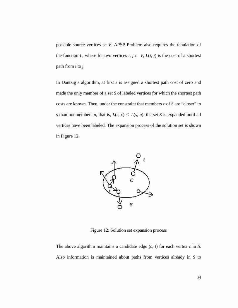
vertices have been labeled. The expansion process of the solution set is shown

in Figure 12.

Figure 12: Solution set expansion process

The above algorithm maintains a candidate edge (c, t) for each vertex c in S.

Also information is maintained about paths from vertices already in S to

34

vertices still outside S to make the expansion of S computationally easy. If a

candidate’s endpoint t is outside the current S the candidate is considered as a

useful candidate and useless otherwise. Dantzig’s algorithm requires all

candidates to be useful. To meet this requirement the candidate for a vertex c

is selected by scanning the sorted list of edges out of c in increasing cost order

until a useful edge (c, t) is found. When a useful edge (c, t) is found we are

guaranteed that t is the closest (by a single edge) vertex to c and c ∉ S. Vector

d maintains shortest path costs for vertices that are already labeled, that is

c∈S, d[c] = L(s, c). The edge cost from c to t is given by c(c, t) and the path

cost via vertex c to candidate t is given by the candidate weight d[c] + c(c, t).

Vertex t might also be the candidate of other already labeled vertices v∈S as in

Figure 13. Each time it is a candidate there will be some weight d[v] + c(v, t)

associated with its candidacy. There will be in total |S| candidates, with

endpoints scattered amongst the n – |S| unlabelled vertices∉S.

Figure 13: Two vertices pointing to same candidate

35

At each stage of the algorithm the endpoint of the least weight candidate is

added to S. If c0 is a vertex such that the candidate weight d[c0] + c(c0, t0) is

minimum over all labeled vertices c, then t0 can be included in S and given a

shortest path cost d[t0] of d[c0] + c(c0, t0). Then an onward candidate for t0 is

added to the set of candidates, the candidates for vertices that have become

useless are revised (including that of c0), and the process repeats and stops

when |S| = n. Figure 14 shows an intermediate stage of the expansion of

solution set S.

Figure 14: Intermediate stage of solution set expansion process

Initially the source s is made the only member of S, d[s] is set to zero, and the

candidate for s is the shortest edge out of s.

3.3.3 Analysis of Dantzig’s APSP Problem Algorithm

When solution set size is j, that is |S| = j, we require O(j) effort to search in an

array of candidates for the candidate with the minimum cost. After we label

the minimum cost candidate we require another O(j) effort to check the other

36

candidates to decide whether or not they remain useful. Thus total effort is

O(j2). When j = n, this is O(n2).

The other component that contributes to the running time is the effort spent

scanning edge lists looking for useful edges. As each edge of the graph will be

examined no more than once, the effort required for this is O(n2). Thus the

total time for a single source problem becomes O(n2). And the total time for

the n single source problems becomes O(n3). The time for sorting, O(n2 log n)

is absorbed within the main complexity.

3.3.4 Spira’s APSP Problem Algorithm

Spira [11] also developed an algorithm for Single Source Shortest Path (SSSP)

Problem in which an all pairs solution is found by first sorting all of the edge

lists of the graph into ascending cost order, and then solving the n single

source problems. The algorithm is as follows:

________________________________________ Algorithm 8: Spira’s APSP Problem Algorithm 1: for s = 1 to n do Single_Source(s); 2: procedure Single_Source(s); 3: S := {s}; d[s] := 0; 4: initialize the set of candidates to {(s, t)}, where (s, t) is the 5: shortest edge from s; 6: Spira_expand_S(n) 7: end {Single_Source}; 8: 9: procedure Spira_expand_S(limit);

37

10: while |S| < limit do begin 11: let (c0, t0) be the candidate of least weight; 12: if t0 is not in S then begin 13: S := S ∪ + {t0}; 14: d[t0] := d[c0] + c(c0, t0); 15: if |S| = limit then break; 16: add to the set of candidates the shortest edge from t0; 17: end if; 18: replace (c0, t0) in the set of candidates by the next shortest 19: edge from c0; 20: end while; 21: end {Spira_expand_S}; 22: end for; //end of s ________________________________________

3.3.5 Description of Spira’s APSP Problem Algorithm

Spira’s n single source problems algorithm is quite similar to that of Dantzig.

The main difference between these two algorithms is that Spira incorporated a

weak candidacy rule and relaxed the strong candidacy rule that requires all

candidates to be useful. The weak candidacy rule enforces that all candidate

edges (c, t) be such that c(c, t) ≤ c(c, u) for all unlabeled vertices u. The main

motivation behind this weak candidacy rule is that the expensive scanning of

adjacency lists could be reduced. Note that in Dantzig, t itself must be outside

S. To identify each successive minimal weight candidate in O(log n) time the

set of candidates should be implemented as a binary tournament tree. The

weakened candidacy rule implies that the minimal cost candidate will no

longer necessarily be useful. We draw the minimal candidate at the root of the

heap and replace until a useful candidate is found. Then we expand S.

38

3.3.6 Analysis of Spira’s APSP Problem Algorithm

Spira introduced the cost of an increased number of candidates that must be

examined during the labeling process by cutting the time spent scanning

adjacency lists looking for useful edges. Spira makes an important

probabilistic assumption, called endpoint independence that the minimal cost

candidate falls on each of the vertices with equal probability. Using lemma 2,

the total expected number of drawings of candidates will be O(n log n) until

we draw all candidates at least once. Each drawing would cost us O(log n)

time for the corresponding tree manipulation, thus the total effort to solve 1

single source problem is on average O(n log2 n). And the total effort to solve

the n single source problems becomes O(n2 log2 n).

3.3.7 MT’s APSP Problem Algorithm

Moffat and Takaoka [3] further developed an algorithm which is based on

Dantzig’s and Spira’s APSP Problem algorithms and famously known as MT

algorithm. They identified a critical point until which Dantzig’s APSP

Problem algorithm is used for labeling vertices. After the critical point Spira’s

APSP Problem algorithm is used for the labeling on a subset of edges.

1______________________________________ Algorithm 9: MT’s APSP Problem Algorithm 1: for s = 1 to n do Fast_Single_Source(s);

39

2: procedure Fast_Single_Source(s); 3: S := {s}; d[s] := 0; 4: initialize the set of candidates to {(s, t)}, where (s, t) is the 5: shortest edge from s; 6: Dantzig_expand_S(n – n/log n); 7: U := V – S; 8: Spira_expand_S(n), using only the U-edges 9: end {Fast_Single_Source}; 10: end for; //end of s ______________________________________

3.3.8 Description of MT’s APSP Problem Algorithm

MT algorithm is a mixture of Dantzig’s and Spira’s algorithms where these

algorithms are slightly modified. MT algorithm can be divided into two

phases. The first phase corresponds to Dantzig’s algorithm where binary heap

is used for the priority queue. This phase is used to label vertices until the

critical point is reached, that is when |S| = n – n/log n. Dantzig incorporated the

strong candidacy rule. The complexity of this algorithm consists of two

components. One is the effort required to label the minimal weight candidate

and to replace candidates that become useless. The other one is the effort

required to scan for useful edges. The second phase after the critical point

corresponds to Spira’s algorithm. This is used for labeling the last n/log n

vertices after the critical point. Spira incorporated the weak candidacy rule and

used binary tournament tree to identify minimal weight candidates more

efficiently. The weak candidacy rule does not require all candidates to be

40

useful. Moffat and Takaoka introduced the concept of set U and U-edge. U is

defined as the set of unlabeled vertices after the critical point. Also an edge is

called U-edge if it connects to a vertex in the set U. These are depicted in the

following figure.

|S| = n - n

nlog

|U| =

nn

log

U-edge

Figure 15: Visualizing set S, U and U-edge

To improve the efficiency of Spira’s algorithm, Moffat and Takaoka made an

important modification to procedure Spira_expand_S. Due to this modification

the next shortest edge is not chosen as the new candidate, instead the next

shortest U-edge is chosen as the new candidate.

3.3.9 Analysis of MT’s APSP Problem Algorithm

Suppose at some intermediate stage of the computation there are j vertices that

are labeled. That is |S| = j. So there are n – j unlabeled vertices. We assume

41

each of the n – j unlabeled vertices has the equal probability to be chosen as

next candidate. Then we can expect that 1 +jn

j−−1 candidates will need to be

taken care of as they becomes useless in each iteration of the while loop of

Dantzig_expand_S because by definition the root of the heap will become

useless always. And each of the remaining j –1 candidates will become useless

with probability p = jn −

1 . It be can shown that the useless candidates can be

replaced in O(jn

j−

+ log j ) time on average although we omit details. This

expression is O(n log n) only when j ≤ n – n/log n and this is how the critical

point was chosen. The expansion of S from 1 element to n – n/log n elements

will require O(n log n) expected time.

Now we focus on the scanning effort for useful edges. When |S| = n – n/log n

there will be n/log n U-edges scattered through each edge list. Each edge list is

a random permutation of endpoints. Because of this the least cost U-edge in

each list will lie on average in the log nth position. Also because of the strong

candidacy rule each edge list pointer will be pointing at the least cost U-edge

in the corresponding edge list. Thus the scanning effort will require O(n log n)

time on average.

42

Each heap operation in Spira_expand_S requires O(log n) time. Also the edge

scanning effort is O(log n) time. One of these two efforts will be absorbed into

another. Thus total effort required for a candidate replacement is O(log n)

time. Thus each iteration of Spira_expand_S will require O(log n) time. After

the critical point there are |U| = n/log n vertices that need to be labeled. As

each candidate is a random member of the set U the expected number of while

loop iterations required before all the members of set U gets labeled is (n/log

n) ln (n/log n) (using Lemma 2) which is bounded by O(n). Thus the total

expected time to label the set U will be O(n log n).

3.4 Modified MT Algorithm as Fast DMM

Takaoka [1] modified MT algorithm and used APSP Problem as a fast engine

for DMM. In this section we describe this algorithm in details.

_______________________________ Algorithm 10: Fast DMM Algorithm 1: Sort n rows of B and let the sorted list of indices be list [1], ..., list[n]; 2: Let V = {1……..n}; 3: for i := 1 to n do begin 4: for k := 1 to n do begin 5: cand[k] := first of list[k]; 6: d[k] := a[i, k] + b[k, cand[k]]; 7: end for; //end of k 8: Organize set V into a priority queue with keys d[1],……,d[n]; 9: Let the solution set S be empty; 10: /* Phase 1: Before the critical point */ 11: while |S| ≤ n – n/log n do begin 12: Find v with the minimum key from the queue;

43

13: Put cand[v] into S; 14: c[i, cand[v]] := d[v]; 15: Let W = {w | cand[w] = cand[v]}; 16: for w in W do 17: while cand[w] is in S do cand[w] := next of list[w]; 18: end for; //end of w 19: Reorganize the queue for W with the new keys d[w] = a[i, w] + b[w, 20: cand[w]]; 21: end while; 22: U := S; 23: /* Phase 2: After the critical point */ 24: while |S| < n do begin 25: Find v with the minimum key from the queue; 26: if cand[v] is not in S then begin 27: Put cand[v] into S; 28: c[v, cand[v]] := d[v]; 29: Let W = {w | cand[w] = cand[v]}; 30: end else W = {v}; 31: for w in W do 32: cand[w] := next of list[w]; 33: while cand[w] is in U do cand[w] := next of list[w]; 34: end for; //end of w 35: Reorganize the queue for W with the new keys d[w] = a[i, w] + b[w, 36: cand[w]]; 37: end while; 38: end for; //end of i _________________________________

3.4.1 Description of Fast DMM Algorithm

Suppose we are given two distance matrices A = [ai,j] and B = [bi,j]. The main

objective of DMM is to compute the distance product C of A and B. That is C

= AB. In this description of the algorithm, suffices are represented by brackets.

At first rows of B need to be sorted in increasing order. Then we solve the n

single source problems by MT algorithm by using the sorted lists of indices

44

list[k]. We solve the single source problem first and repeat it n times for n

different sources. The endpoint independence is assumed on the lists list[k]

using Lemma 7, that is, when we scan the list, any vertex can appear with

equal probability. We consider the 3-layered DAG in Figure 16 in further

description of this algorithm.

Figure 16: 3-layered DAG of two (n, n) matrices

From source i in the first layer, let each vertex k in the second layer have its

candidate cand[k] in the third layer, which is the first element in list[k]

initially. All the second layer vertices {k | k = 1,….,n} is organized into a

priority queue by the keys d[k] = a[i, k] + b[k, cand[k]]. The process of

deletion of v with the minimum key from the queue is repeated and cand[v] is

45

inserted into the solution set S. list[v] is scanned to get a clean candidate for v

so that cand[v] points to a vertex which is outside the current solution set S.

Then v is inserted back to the queue with the new key value. Every time the

solution set is expanded by one, we scan the lists for other w such that cand[w]

= cand[v] and construct the set W. For each w∈W we forward the

corresponding pointer to the next candidate in the list to make their candidates

cand[w] clean. The key values are changed accordingly and we reorganize the

queue according to new key values. This expansion process of the solution set

stops at the critical point where |S| = n – n/ log n. We consider U to be the

solution set at this stage and U remains unchanged from this point onwards.

After the critical point, solution set is further expanded to n in the same way to

label rest of the n/log n candidates which are outside U.

3.4.2 Analysis of Fast DMM Algorithm

Analysis of Fast DMM, not surprisingly, should be quite similar to that of MT.

First we focus on heap operations. If a binary heap is used for the priority

queue, and the reorganization of the heap is done for W in a bottom-up fashion

then the expected time for reorganization can be shown to be O(n /(n – j) + log

n), when |S| = j. This expression is bounded by O(log n) when |S| n – n/ log

n. Thus the effort requires for reorganization of the queue in phase 1 is O(n log

n) in total.

≤

46

Using Lemma 2, we can establish the fact that after the critical point the

expected number of unsuccessful trials before we get |S| = n is (n/log n) ln

(n/log n). This is bounded by O(n). The expected size of W in phase 2 is O(log

n) when S is expanded, and 1 when it is not expanded. The queue

reorganization is done differently in phase 2 by performing increase-key

separately for each w, spending O(log n) time per cand(w). From these facts,

the expected time for the queue reorganization in phase 2 can be shown to be

O(n

nlog

× log2n) = O(n log n).

|U| = n

nlog

|S| = n -

nn

log

Figure 17: Intermediate stage of set W

It can be shown that the scanning efforts to get clean candidates in phase 1 and

in phase 2 are both O(n log n) by using the same technique discussed in

section 3.3.9 for the analysis of MT algorithm. From these observations it can

be concluded that complexities before and after the critical point are balanced

to be O(n log n), resulting in the total expected time of O(n log n). Thus

expected time for the n single source problems becomes O(n2 log n). The time

for sorting is absorbed with in the main complexity.

47

3.5 Analysis of MSP (Algorithm 6) based on Fast DMM

We assume m and n are each a power of 2, and m ≤ n. By chopping the array

into squares we can consider the case where m = n. Let T(n) be the time to

analyze an array of size (n, n). Algorithm 6 splits the array first vertically and

then horizontally. We multiply (n, n/2) and (n/2, n) matrices by 4

multiplications of size (n/2, n/2) and analyze the number of comparisons. Let

M(n) be the time for multiplying two (n/2, n/2) matrices which is equal to O(n2

log n) as this is the expected time for the n single source problems by Fast

DMM. Thus we can establish the following lemma, recurrence and theorem.

3.5.1 Lemma 8

If M(n) = O(n2 log n) then M(n) satisfies the following condition:

M(n) (4 + 4/ log n)M(n/2) ≥

Proof: M(n) = n2 log n

= 4 2

2⎟⎠⎞

⎜⎝⎛ n log ⎟

⎠⎞

⎜⎝⎛

2.2 n

= 4 2

2⎟⎠⎞

⎜⎝⎛ n ⎟

⎠⎞

⎜⎝⎛ +

2log1 n

= 4 2

2⎟⎠⎞

⎜⎝⎛ n log

2n

⎟⎟⎟⎟

⎠

⎞

⎜⎜⎜⎜

⎝

⎛

+

2log

11n

48

= ⎟⎟⎟⎟

⎠

⎞

⎜⎜⎜⎜

⎝

⎛

+

2log

44n

M ⎟⎠⎞

⎜⎝⎛

2n > ⎟⎟

⎠

⎞⎜⎜⎝

⎛+

nlog44 M ⎟

⎠⎞

⎜⎝⎛

2n

Thus M(n) satisfies the condition.

3.5.2 Recurrence 1

Let T1, T2,.….., TN be the times to compute DMMs of different sizes in the

Algorithm 6. Then by ignoring some overhead time between DMMs, the

expected value E[T] of the total time T becomes

E[T] = E[T1 + T2 +.…..+ TN]

= E[T1] + E[T2] +.…..+ E[TN]

= E[E[T1 | T2, T3,.….., TN]] + E[E[T2 | T1, T3, .….., TN]] +.…..+ E[E[TN |

T1, T2,.….., TN-1]]

From the theorem of total expectation, we have E[E[X|Y]] = E[X] where X |Y is

the conditional random variable of X conditioned by Y. So we can write

E[T] = [T1] + [T2] +.…..+ [TN] 1TE

2TENTE

49

In the above, expectation operators go over the sample space of T1, T2,.….., TN.

Thus we can establish the following recurrence where total expected time is

expressed as the sum of the expected times of algorithmic components.

T(1) = 0, T(n) = 4T(n/2) + 12M(n)

M(n) = O(n2 log n)

3.5.3 Theorem 1

Suppose M(n) = O(n2 log n) and M(n) satisfies the condition M(n) (4 + 4/

log n)M(n/2). Then the above T(n) satisfies the following:

≥

T(n) ≤ 12(1 + log n)M(n)

Proof:

Basis step: Theorem 1 holds for T(1) from the algorithm.

Inductive step:

T(n) = 4T(n/2) + 12M(n)

= )(12)2

()2

log1(124 nMnMn+×+×

50

≤ )(12)(

log44

2log1

48 nMnM

n

n

+×+

+×

= )(12)()

log11(4

2loglog148 nMnM

n

n+×

+

−+×

= )(12)(

log1log

1log112 nMnM

nn

n+×

+−+

×

= )(12)(

log1log

log12 nMnM

nn

n+×

+×

= )(12)(1log

log122

nMnMn

n+×

+×

= )(12)(1log

logloglog122

nMnMn

nnn+×

+−+

×

= )(12)(1log

log)1(loglog12 nMnMn

nnn+×

+−+

×

= )(12)(1log

loglog12 nMnMn

nn +×⎟⎟⎠

⎞⎜⎜⎝

⎛+

−×

51

12 log n M(n) + 12M(n) ≤

= 12M(n) (log n + 1) = 12(1 + log n)M(n) (proved)

Thus the total complexity of Algorithm 6 based on Fast DMM becomes O(n2

log2 n). Because an extra log n effort is required on top of the Fast DMM

complexity due to the recursion in Algorithm 6.

3.6 K-MSP Algorithm

Takaoka and Bae [2] developed an algorithm for K-MSP incorporating sub-

cubic DMM algorithm. Since this sub-cubic DMM algorithm is beyond the

scope of this research we are not going to analyze this algorithm.

52

Chapter 4

K-Tuple Approach

DMM can be generalized as K-DMM as we already explained this in Chapter

2 (Sec 2.6). In this chapter we modify Takaoka’s Fast DMM based on MT

algorithm where APSP Problem is incorporated as a fast engine for DMM. In

the following algorithm, we extend the Single Source Shortest Path Problem to

the Single Source K Shortest Paths Problem and establish Fast K-DMM

algorithm by incorporating n such problems.

In the following algorithm we have the outermost loop by r. Data structure T is

used to identify edges already consumed in shortest paths for previous r. T can

be implemented as a 2D array where at every location we maintain a set of

second layer vertices of the 3-layered DAG through which a path has been

established for a given pair of source and destination.

4.1 New Fast K-DMM Algorithm

_________________________________ Algorithm 11: Fast K-DMM Algorithm 1: Sort n rows of B and let the sorted list of indices be list[1], ...,list[n] 2: Let V = {1……..n}; 3: Let the data structure T be empty; 4: for r := 1 to K do begin 5: for i := 1 to n do begin

53

6: for k := 1 to n do begin 7: cand[k] := first of list [k]; 8: while k is found in the set at T[i, cand[k]] location do begin 9: cand[k] := next of list[k]; 10: if end of list is reached then begin 11: cand[k] := n + 1; //(n + 1)th column of b holds 11: // a positive infinite value 999 12: end if; 13: end while; 14: d[k] := a[i, k] + b[k, cand[k]]; 15: end for; //end of k 16: Organize set V into a priority queue with keys d[1],……, d[n]; 17: Let the solution set S be empty; 18: /* Phase 1: Before the critical point */ 19: while |S| n – n/ log n do begin ≤20: find v with the minimum key from the queue; 21: Put cand[v] into S; 22: c[r, i, cand[v]] := d[v]; 23: Put v in the set at T[i, cand[v]] location; 24: Let W = {w | cand[w] = cand[v]}; 25: for w in W do begin 26: while cand[w] is in S OR w is found in the set at T[i, cand[w]] 27: location do begin 28: cand[w] := next of list[w]; 29: if end of list is reached then begin 30: cand[w] := n + 1; //(n + 1)th column of b holds 31: // a positive infinite value 999 32: end if; 33: end while; 34: end for; // end of w 35: Reorganize the queue for W with the new keys d[w] = a[i, w] + b[w, 36: cand[w]]; 37: end while; 38: U := S; 39: /* Phase 2: After the critical point */ 40: while |S| < n do begin 41: find v with the minimum key from the queue; 42: if cand[v] is not in S then begin 43: Put cand[v] into S; 44: c[r, i, cand[v]] := d[v]; 45: put v in the set at T[i, cand[v]] location;

54

46: Let W = {w | cand[w] = cand[v]}; 47: end else W = {v}; 48: for w in W do begin 49: cand[w] := next of list[w]; 50: while cand[w] is in U OR w is found in the set at T[i, cand[w]] 51: location do begin 52: cand[w] := next of list[w]; 53: if end of list is reached then begin 54: cand[w] := n + 1 //(n + 1)th column of b holds 55: // a positive infinite value 999 56: end if; 57: end while; 58: end for // end of w 59: Reorganize the queue for W with the new keys d[w] = a[i, w] + b[w, 60: cand[w]]; 61: end while; 62: end for; // end of i 63: end for;// end of r _________________________________

4.2 Description of New Fast K-DMM Algorithm

The new Fast K-DMM algorithm is primarily based on Fast DMM algorithm

(Algorithm 10). Some of the descriptions of Fast K-DMM algorithm should be

quite similar to that of Fast DMM algorithm. So we omit similar descriptions

here for Fast K-DMM algorithm that we’ve already discussed for Fast DMM

algorithm and only focus on the new enhancements that we have made into

Fast K-DMM algorithm.

Let A = [ai,j] and B = [bi,j] be the two distance matrices. Let C = AB be the

distance product. To represent these two distance matrices we declare two 2D

55

arrays a[1..n, 1..n] and b[1..n, 1..n + 1]. Note that each row of b has n + 1

columns. This is because we need an extra position in each row to store a

positive infinite value.

In this description we consider the 3-layered DAG in Figure 16. The variable r

in the outermost for loop runs from 1 to K which determines the number of

shortest paths for the n single source problems. As there are at most n numbers

of different paths from a source to a destination, K must be n. Also we put

999 as a positive infinite value (as we assume all the numbers that appear in

the given (m, n) array are between 1 and 100) at the (n + 1)th column of all the

rows of array b. To explain this let’s consider the following situation.

≤

Suppose for a vertex k in the second layer we have exhausted all possible

candidates in the third layer. That means all possible paths from a source to a

destination through vertex k have been established and there are no more

candidates available in the candidate list for vertex k. In this situation we

should avoid establishing any new path through vertex k for the same source

and destination. So when we reach the end of the candidate list we return a

special candidate with positive infinite key value for vertex k so that this key

value never appears at the root of the heap and thus we do not establish any

new path through vertex k for the same source and destination. So we set (n +

56

1)th position as the candidate of k which in return will access the (n + 1)th

column of the kth row where we have 999 as a positive infinite value.

We also maintain a data structure T to manage second layer vertices through

which paths have been already established. We call second layer vertex as via

vertex. In the next section we explain in details how we implement data

structure T.

4.2.1 Description of Data Structure T

To explain the data structure T we consider the 3-layered graph in Figure 6.

For example, when we finalize the distance vector for source 1(in the first

layer) and destination 2 (in the third layer) via 1 (in the second layer) we set

the value as 3 + 0 = 3. To calculate K shortest paths for a pair of source and

destination we must keep track of via vertices in the second layer through

which we establish shortest paths. To keep track of via vertices, we manipulate

data structure T as a 2D array T[1..n, 1..n + 1]. At each position of array T we

construct one empty Binary Search Tree (BST) initially. During the

finalization of a distance vector for a pair of source and destination we insert

the vertex of the second layer (through which the path has been finalized) into

the BST of the source and destination position of array T. Note that the second

dimension of T is n + 1 instead of n. It’s because we need one extra empty

position along the second dimension of T to skip ‘while’ loops on line 8, 26

57

and 50 in Algorithm 11 in the situation when reach end of the candidate list for

a second layer vertex k.

In the preceding example, at T[1, 2] position we construct a BST and insert the

value of the via vertex which is 1 in this example. In this way, when we

calculate the next shortest distance for the same pair of source and destination

we consult the BST at T[source][destination] position and verify whether the

via vertex of the second layer that we have chosen already exists or not in the

BST. If the via vertex is found in the BST that reveals a path has been already

established through this via vertex for this pair of source and destination. So

we must avoid choosing the same path for the same pair of source and

destination when we calculate the next shortest path for that pair of source and

destination.

By consulting the BST at T[source][destination] position we can take the

decision whether a particular via vertex for a pair of source and destination is

valid or not. We can visualize the array T as in Figure 18.

58

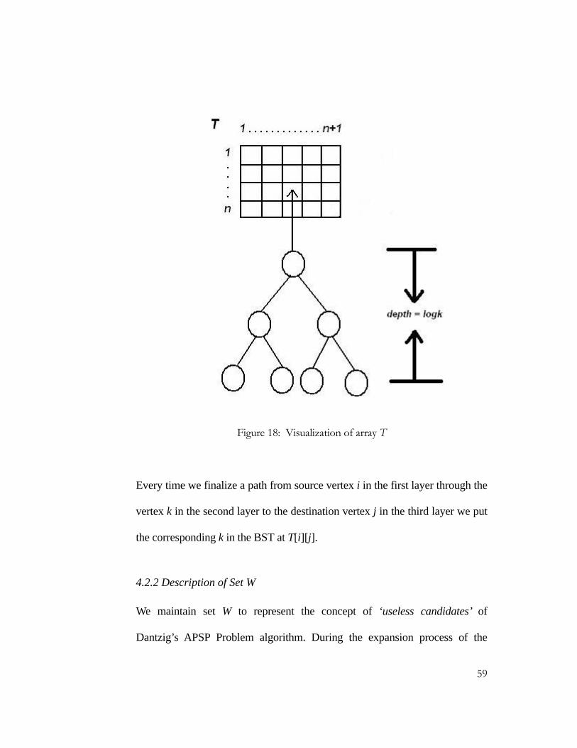
Figure 18: Visualization of array T

Every time we finalize a path from source vertex i in the first layer through the

vertex k in the second layer to the destination vertex j in the third layer we put

the corresponding k in the BST at T[i][j].

4.2.2 Description of Set W

We maintain set W to represent the concept of ‘useless candidates’ of

Dantzig’s APSP Problem algorithm. During the expansion process of the

59

solution set when a new vertex in the third layer gets added to the solution set

eventually it becomes useless candidate for vertices in the second layer. So all

the vertices in the second layer that are pointing to this recently added vertex

to the solution set must be taken care of so that they point to a clean candidate

rather than a useless candidate. We construct set W to represent the vertices in

the second layer that are pointing to useless candidates in the third layer.

When we update set W we update every member of W with new candidates

based on two conditions. The first condition is to check whether the updated

candidate for W already exists in the set S. The second condition checks for via

vertex collision in the BST. That is to check whether w already exists in the

BST at T[i][cand[w]] where i represents the current source. These two

conditions are checked inclusively. That is, if any of these two conditions is

true we update the candidate for current w with the next member of the list[w].

When we hit the end of the list by not being able to find any new candidate

that makes both conditions false, we set n + 1 position of the list[w] as new

candidate of w. As we have a positive infinite value 999 at this position this

candidate will never be chosen from the heap to avoid repetition of any of the

K shortest paths of the n single source problems.

60

4.3 Analysis of New Fast K-DMM Algorithm

The new algorithm can be divided into two parts. One is before the critical

point and the other one is after the critical point. Before the critical point we

employ Dantzig’s APSP Problem algorithm by incorporating binary heap for

the priority queue. This phase is used to label vertices to indicate they are in S

until the critical point when |S| = n – n/ log n. After the critical point Spira’s

APSP Problem algorithm is used for the labeling but on a subset of edges.

Spira’s APSP Problem algorithm also incorporates Binary heap for the priority

queue.

The endpoint independence is assumed on the lists list[k] using Lemma 7, that

is, when we scan the list, any vertex can appear with equal probability.

We also assumed a binary heap is used for the priority queue through out the

algorithm and the reorganization of the heap is done in a bottom-up manner.

4.3.1 Phase 1: Dantzig’s Counterpart

For phase 1, let us assume |S| = j. So when we finalize a distance and add a

vertex into the solution set the probability that some other vertex in the second

layer pointing to the vertex in the third layer which has been added to the

solution set isjn −

1 . And we have such n vertices in the second layer. Let P

61

represents the expected number of affected vertices in the second layer. Then

P isjn

n−

. And time to detect the vertices which must be taken care of in the

heap is bounded by O(log n) since |S|≤ n – n log n. Thus the effort for the

queue reorganization in phase 1 for the first iteration of r is:

∑−

=

nnn

j

log/

1

O(jn

n−

+ log j) ≤ O(n log n)

Proof:

We can separate the above inequality into two parts.

( O(∑−

=

nnn

j

log/

1 jnn−

) + log j ) ∑−

=

nnn

j

log/

1

≤ O(n log n)

Let A1 = O(∑−

=

nnn

j

log/

1 jnn−

) and A2 = log j ∑=j

log/

1

− nnn

Thus we need to prove:

A1 + A2 O(n log n) ≤

Let’s do part A1 and A2 separately.

Part A1:

62

A1 = O(∑−

=

nnn

j

log/

1 jnn−

) ≤ ∑−

=

1

1

n

j jnn−

(we ignore the big ‘O’ notation)

= n ∑−

=

1

1

n

j jn −1

= n (1

1−n

+ 2

1−n

+ ………+ )1(

1−− nn

)

= n (log n – γ ) (γ is Euler’s [12] Constant which is

equal to 0.577215665)

= n log n – nγ

= O(n log n – nγ )

Part A2:

A2 = log j ≤ ∑ log j ∑−

=

nnn

j

log/

1 =

n

j 1

= log 1 + log 2 + ……….+ log n

= log (1× 2 ×…….× n)

= log (n!)

63

= log (Stirling’s [13] Formula) nn ne−

= n log n – n log e

= O(n log n – n log e)

L.H.S. = A1 + A2

= O(n log n – nγ ) + O(n log n – n log e) ≤ O(n log n) (proved)

Thus the effort to reorganize the queue in phase 1 for the n single source K

shortest paths problems is ≤ O(Kn2 log n).

We now focus into the scanning efforts to get clean candidates in phase 1. Let

us assume |S| = j. The probability to get a clean candidate is n

rjn )1( −−− . Up

to critical point we can establish the following inequality:

j ≤ n – n/log n

⇒ – j – n + n/ log n ≥

⇒ n – j n – n + n/log n ≥

⇒ n – j – (r –1) n/log n – (r –1) ≥

64

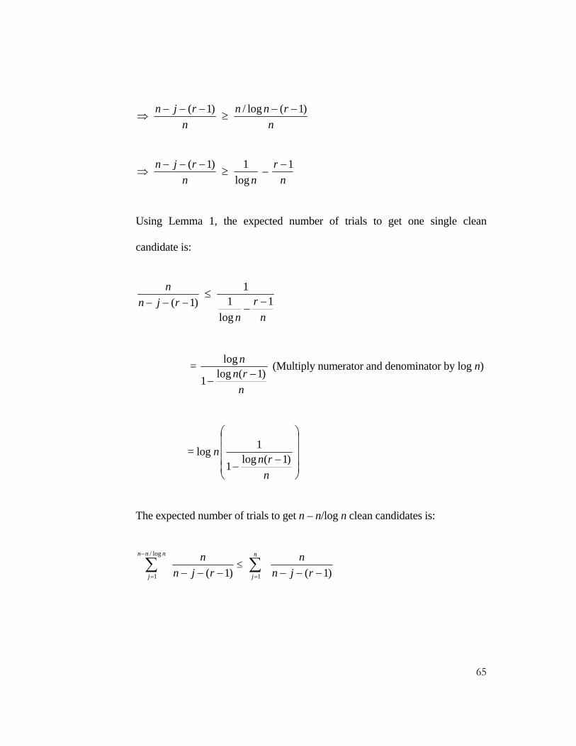
⇒ n

rjn )1( −−− ≥n

rnn )1(log/ −−

⇒ n

rjn )1( −−− ≥nlog

1 – n

r 1−

Using Lemma 1, the expected number of trials to get one single clean

candidate is:

)1( −−− rjnn ≤

nr

n1

log1

1−

−

=

nrn

n)1(log1

log−

− (Multiply numerator and denominator by log n)

= log n⎟⎟⎟⎟

⎠

⎞

⎜⎜⎜⎜

⎝

⎛

−−

nrn )1(log1

1

The expected number of trials to get n – n/log n clean candidates is:

∑−

=

nnn

j

log/

1

)1( −−− rjn

n≤ ∑

=

n

j 1 )1( −−− rjnn

65

= ∑ log n=

n

j 1 ⎟⎟⎟⎟

⎠

⎞

⎜⎜⎜⎜

⎝

⎛

−−

nrn )1(log1

1

= n log n⎟⎟⎟⎟

⎠

⎞

⎜⎜⎜⎜

⎝

⎛

−−

nrn )1(log1

1

For a BST with K vertices we need to spend O(log K) time to verify a

particular vertex’s existence in the BST. So we multiply by log K.

The expected number of trials to get n – n/log n clean candidates for 1 single

source is n log n log K≤

⎟⎟⎟⎟

⎠

⎞

⎜⎜⎜⎜

⎝

⎛

−−

nrn )1(log1

1

Thus the expected number of trials to get n – n/log n clean candidates for n

single source is ≤ n2 log n log K⎟⎟⎟⎟

⎠

⎞

⎜⎜⎜⎜

⎝

⎛

−−

nrn )1(log1

1 .

Using Lemma 2 and setting x = nrn )1(log − we can write:

66

n2 log n log K⎟⎟⎟⎟

⎠

⎞

⎜⎜⎜⎜

⎝

⎛

−−

nrn )1(log1

1≤ n2 log n log K ⎟

⎠⎞

⎜⎝⎛ −

×+nrn )1(log21

where 0 ≤nrn )1(log − ≤

21

Thus the expected number of trials to get n – n/log n clean candidates for the n

single source problems of 1 iteration of r is:

≤ Tr = n2 log n log K ⎟⎠⎞

⎜⎝⎛ −

×+nrn )1(log21

We take summation of r = 1 to K for K iterations.

∑=

K

r 1 Tr = n2 log n log K∑

=

K

r 1⎟⎠⎞

⎜⎝⎛ −

×+nrn )1(log21

= n2 log n log K + (n log2 n log K ∑=

K

r 1×2(r – 1))

Let A1 = n2 log n log K and A2 = n log2 n log K ×2(r – 1)

Thus we can write the following:

= A1 + A2 ∑=

K

r 1

67

= A1 + A2 ∑=

K

r 1∑=

K

r 1

Let’s do part A1 and A2 separately.

Part A1:

A1 = ∑ n2 log n log K ∑=

K

r 1 =

K

r 1

= Kn2 log n log K

Part A2:

∑=

K

r 1A2 = n log2 n log K ∑

=

K

r 1

×2(r – 1)

= n log2 n log K × 2 × 2

)1( −KK (using Lemma 4)

= n log2 n log K × (K2 – K)

= K2n log2 n log K – Kn log2 n log K

≤ K2n log2 n log K

We put part A1 and A2 together and get

68

∑=

K

r 1 Tr = O(Kn2 log n log K + K2n log2 n log K)

= O(Kn2 log n log K) when K ≤ n/log n

Finally we can claim the expected number of trials to get n – n/log n clean

candidates for the n single source problems of K iteration of r is ≤ O(Kn2 log n

log K) when K ≤ n/ log n.

4.3.2 Phase 2: Spira’s Counterpart

By the coupon collector’s problem in [4] we need to collect O(m log m)

coupons in average before we get m different types of coupons. After critical

point in phase 2 we need to collect n/log n vertices in the solution set. By

setting m = n/log n we need to collect (n/log n) log (n/log n) n vertices

before we get |S| = n. Each iteration in phase 2 takes O(log n) time, resulting in

O(n log n) time for 1 single source problem and O(n2 log n) time for the n

single source problems. Thus the effort for the queue reorganization in phase 2

for the n single source K shortest paths problems is

≤

≤ O(Kn2 log n)

Now we focus into the scanning efforts to get unlabelled candidates in phase 2.

Let us assume |S| = n – n/log n. Thus the probability to get an unlabelled

candidate is n

rn

n )1(log

−−.

69

Now we establish the following inequality.

log n – 1 log n ≤

⇒ log n log n + 1 ≤

⇒nlog

1 ≥1log

1+n

⇒ n

nlog

≥ 1log +n

n (Multiply both sides by n)

⇒ n

nlog

– (r – 1) ≥1log +n

n – (r – 1) (Subtract r –1 from both sides)

⇒ n

rn

n )1(log

−− ≥

n

rnn )1(

1log−−

+ (Divide both sides by n)

⇒ n

rn

n )1(log

−− ≥

nr

n1

1log1 −

−+

Using Lemma 1, the expected number of trials to get one unlabelled candidate

is:

70

n

rn

n )1(log

1

−−≤

nr

n1

1log1

1−

−+

⇒)1(

log−− r

nn

n≤

nr

n1

1log1

1−

−+

= ( ) ⎟⎟

⎠

⎞⎜⎜⎝

⎛ −−

++

+

nr

nn

n1

1log11log

1log (Multiply Numerator and

Denominator by log n +1)

=

nnr

n)1)(log1(1

1log+−

−

+

Thus the expected number of trials to get n/log n clean candidates is:

∑−=

n

nnnj log/

)1(log

−− rn

nn

≤ ∑=

n

j 1 )1(log

−− rn

nn

= ∑ =

n

j 1

nnr

n)1)(log1(1

1log+−

−

+

71

= n ×⎟⎟⎟⎟

⎠

⎞

⎜⎜⎜⎜

⎝

⎛

+−−

+

nnr

n)1)(log1(1

1log

= n (log n + 1)×⎟⎟⎟⎟

⎠

⎞

⎜⎜⎜⎜

⎝

⎛

+−−

nnr )1)(log1(1

1

For a BST with K vertices we need to spend O(log K) time to verify a

particular vertex’s existence in the BST. So we multiply the above by log K.

The expected number of trials to get n/log n clean candidates for 1 single

source is

≤ n (log n + 1) × log K×⎟⎟⎟⎟

⎠

⎞

⎜⎜⎜⎜

⎝

⎛

+−−

nnr )1)(log1(1

1

Thus the expected number of trials to get n/log n candidates for the n single

source is n2 (log n + 1) ≤ × log K×⎟⎟⎟⎟

⎠

⎞

⎜⎜⎜⎜

⎝

⎛

+−−

nnr )1)(log1(1

1

Using Lemma 2 and setting x = n

nr )1)(log1( +− we can write the following:

72

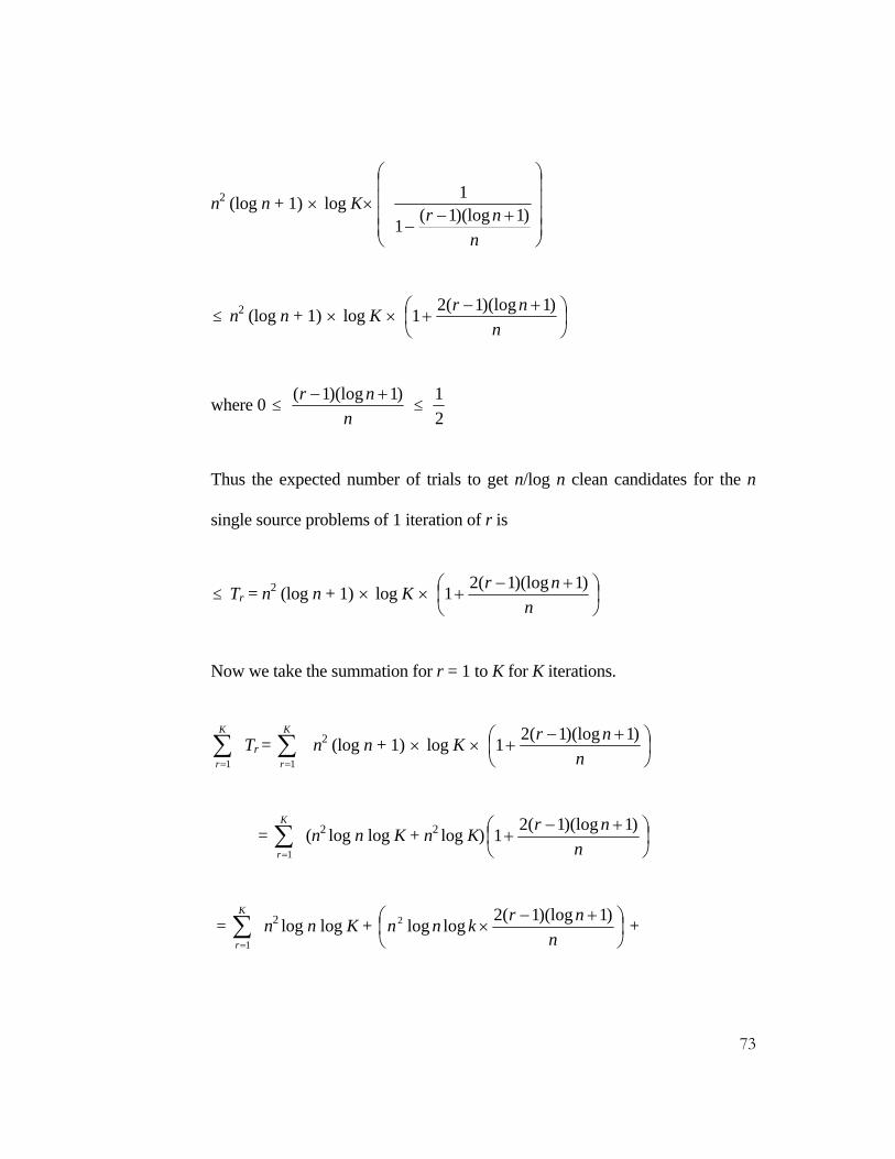
n2 (log n + 1) × log K×⎟⎟⎟⎟

⎠

⎞

⎜⎜⎜⎜

⎝

⎛

+−−

nnr )1)(log1(1

1

≤ n2 (log n + 1) × log K × ⎟⎠⎞

⎜⎝⎛ +−+

nnr )1)(log1(21

where 0 ≤n

nr )1)(log1( +− ≤ 21

Thus the expected number of trials to get n/log n clean candidates for the n

single source problems of 1 iteration of r is

≤ Tr = n2 (log n + 1) × log K × ⎟⎠⎞

⎜⎝⎛ +−+

nnr )1)(log1(21

Now we take the summation for r = 1 to K for K iterations.

∑=

K

r 1Tr = n2 (log n + 1) ∑

=

K

r 1× log K × ⎟

⎠⎞

⎜⎝⎛ +−+

nnr )1)(log1(21

= (n2 log n log K + n2 log K)∑=

K

r 1⎟⎠⎞

⎜⎝⎛ +−+

nnr )1)(log1(21

= n2 log n log K + ∑=

K

r 1⎟⎠⎞

⎜⎝⎛ +−

×n

nrknn )1)(log1(2loglog2 +

73

n2 log K + ⎟⎠⎞

⎜⎝⎛ +−

×n

nrKn )1)(log1(2log2

= n2 log n log K + (n log n log K ∑=

K

r 1× 2(r – 1) (log n + 1)) +

n2 log K + (n log K × 2(r – 1) (log n + 1))

Let A1 = n2 log n log K

A2 = n log n log K × 2(r – 1) (log n + 1)

A3 = n2 log K

A4 = n log K × 2(r – 1) (log n + 1)

Thus we can write the following:

= A1 + A2 + A3 + A4 ∑=

K

r 1

= A1 + A2 + ∑ A3 + A4 ∑=

K

r 1∑=

K

r 1 =

K

r 1∑=

K

r 1

Let’s do part A1, A2, A3 and A4 separately.

Part A1:

74

A1 = n2 log n log K ∑=

K

r 1∑=

K

r 1

= Kn2 log n log K

Part A2:

A2 = n log n log K ∑=

K

r 1∑=

K

r 1

× 2(r – 1) (log n + 1)

= n log n log K × 2 ×2

)1( −KK× (log n + 1) (using Lemma 4)

= n log n log K × (K2 – K) × (log n + 1)

= (K2n log n log K – Kn log n log K) (log n + 1)

= K2n log2 n log K – Kn log2 n log K +

K2n log n log K – Kn log n logK

K2n log2 n log K + K2n log n log K ≤

K2n log2 n log K ≤

Part A3:

75

∑=

K

r 1A3 = n2 log K ∑

=

K

r 1

= Kn2 log K

Part A4:

A4 = n log K ∑=

K

r 1∑=

K

r 1

× 2(r – 1) (log n + 1)

= n log K × 2 ×2

)1( −KK× (log n + 1) (using Lemma 4)

= n log K (K2 – K) (log n + 1)

= (K2n log K – Kn log K) (log n + 1)

= K2n log n log K – Kn log n log K + K2n log K – Kn log K

K2n log n log K + K2n log K ≤

K2n log n log K ≤

Now we put part A1, A2, A3 and A4 together and get

∑=

K

r 1 Tr = O(Kn2 log n log K + K2n log2 n log K + Kn2 log K + K2n log n log K)

76

O(Kn2 log n log K + K2n log2 n log K) ≤

O(Kn2 log n log K) when K ≤ ≤ n/log n

Finally we can claim the expected number of trials to get n/log n clean

candidates for the n single source problems of K iterations of r is O(Kn2 log

n log K) when K n/log n.

≤

≤

From these observations we can conclude the complexities before and after the

critical point are balanced to be O(n log n log K), resulting in the total

expected time of O(n log n log K). Thus the expected time for the n single

source problems becomes O(n2 log n log K). As we consider K shortest

distances from n single sources the complexity further becomes O(Kn2 log n

log K) in total when K ≤ n/log n.

The time to build the initial distance vector before the critical point is O(n log

K) as it takes O(log K) time to determine whether the vertex in the second

layer we currently consider already exists in the BST at the T[i][cand[k]

location. And as it runs n times the complexity becomes O(n log K). Thus for

the n single source K shortest paths problems the time to build the initial

distance vector is O(n2 K log K). But this complexity will be absorbed by the

greater complexity in phase 1 and phase 2. Also the complexity of

77

initialization of (n + 1)th column of array T with positive infinite values would

be absorbed by the overall complexity of the algorithm.

4.4 New K-MSP Algorithm

To incorporate Algorithm 11 into K-MSP we modify Takaoka and Bae’s [2]

K-MSP algorithm (which is based on sub-cubic DMM) and hence develop a

new algorithm for K-MSP. This new algorithm is as follows:

________________________________________________________ Algorithm 12: New K-MSP Algorithm based on K-Tuple Approach 1: If the array becomes (a, a) return solution by Algorithm 13. 2: Otherwise, if m > n, rotate the array 90 degrees. 3: Thus we assume m ≤ n. 4: Let ANW be the solution for the NW part. 5: Let ANE be the solution for the NE part. 6: Let ASW be the solution for the SW part. 7: Let ASE be the solution for the SE part. 8: Let Acolumn be the solution for the column-centered problem. 9: Let Arow be the solution for the row-centered problem. 10: Let the solution be the K-Tuple of K maxima selected from 11: {ANW ANE ASW ∪ ASE Acolumn Arow}. ∪ ∪ ∪ ∪________________________________________________________

4.5 Description of New K-MSP Algorithm

In the following we describe Algorithm 12. At first we scrutinize the base case

of the recursion. Then we describe the recursive part of the algorithm.

78

4.5.1 Base Case

In Algorithm 12, we deal with K-Tuple. To do so we find the new base

condition of the recursion. When the recursion hits an (a, a) array we select K

largest sums by an exhaustive method where a refers to the value that we have

established in Lemma 6 (Part B). We slightly modify Algorithm 2 and

represent this new exhaustive algorithm in Algorithm 13.

_______________________________________________ Algorithm 13: Modified Exhaustive Algorithm for MSP 1: for i := 1 to m 2: for j := 1 to n 3: for k := 1 to i 4: for l:= 1 to j 5: currentmax = s[i][j] – s[i][l] – s[k][j] + s[k][l]; 6: insert currentmax into the maximum subarray solution set; 7: end for; 8: end for; 9: end for; 10: end for; _______________________________________________ The above algorithm exhaustively finds all possible subarrays for a given

array. Using Lemma 6 (Part B), when we reach the bottom of the recursion

with an (a, a) array in Algorithm 12 there are at most K + a3 subarrays that can

be selected. We use Algorithm 13 to find all possible subarrays for an (a, a)

array. In this K-Tuple Approach as we need to return K items from each level

of the recursion we need to find K best subarrays out of these K + a3 subarrays.

K-minima or K-maxima of K + a3 elements can be found in CK comparisons

79

where C is a constant. To do so we incorporate the linear time selection

algorithm in [14] for selecting the Kth element from n elements. Once the Kth

element is found we can select K-minima or K-maxima by filtering n elements

by comparing them with this element. Thus in CK comparisons we can find K-

minima or K-maxima of K + a3 elements where the value of C is determined

by the selection algorithm we mentioned above.

Figure 19: (a, a) array at the bottom of the recursion

4.5.2 Recursive Case

Now we focus into the recursive part of Algorithm 12. We define 6 conditional

solutions for MSP. Let us divide the array by 4 equal parts by central

horizontal and central vertical line as in the following figure.

80

Column-centered Row-centered

Figure 20: Four-way recursion and 6 solutions

ANW = Maximum subarray to be found in the Upper-Left part

ANE = Maximum subarray to be found in the Upper-Right part

ASW = Maximum subarray to be found in the Lower-Left part

ASE = Maximum subarray to be found in the Lower-Right part

Acolumn = Maximum subarray to be stretched over the central vertical line

Arow = Maximum subarray to be stretched over the central horizontal line

Acolumn can be solved using Equation (1) as before. Also Arow can be solved in

the same way as row-centered problem is a symmetrical problem to column-

centered problem. Thus we convert MSP into DMM. Finally when we apply

Equation (2) we realize that each component of Equation (2) is now a set of K-

Tuple. We rewrite Equation (2) in the following line.

81

S2S2* – S1S1

*

Since each component of Equation (2) is a set of K-Tuple the matrix

subtraction is computed by a – b operation component-wise. Now we define

the subtraction of two sets of K-Tuples where K MAX {a} selects K largest

elements in a set a.

a – b = K MAX{ai – bj | ai ∈ a, bj ∈ b, 1 ≤ i, j ≤ K }

According to Frederickson and Johnson [15], selection of K largest elements in

Cartesian sum X + Y is solved in O(K) time where |X| = |Y| = K. In the

following we describe an O(K log K) method for X + Y problem with an

example. The same method can be used for a – b subtraction component wise.

For instance, we are given two sets X and Y as follows.

X = {2, 8, 7} Y = {3, 1, 6}

We need to first sort K items of both sets in ascending order. Using heap sort

we can sort K items in O(K log K) time. After sorting we have,

X = {2, 7, 8} Y = {1, 3, 6}

Then we select the minimum items from both sets. These are naturally first 2

items of both sets. We add these 2 items and put the resulting value with their

82

corresponding index values into Binary Heap. So 2 + 1 = 3 is inserted in the

heap with index values (1, 1). Then we find the minimum value from the heap

and extract it out of the heap. We return the minimum value that we extracted

from the heap but we save the index values for our next operation. So keep

track of (1, 1) for which 3 came for. Next, we add 1 to each index value

separately to insert new items into the heap. New index values are (1 + 1, 1) =

(2, 1) and (1, 1 + 1) = (1, 2). We add items in both index values and insert into

the heap. For index value (2, 1) we get 7 + 1 = 8 and we insert this into the

heap.

Figure 21: X + Y problem solving in O(K log K) time

For index value (1, 2) we get 2 + 3 = 5 and we insert this into the heap as well.

Then we find the minimum value from the heap and return it. This process

keeps going until we find K minima.

Finding K items from the heap would cost us again another O(K log K) time.

The complexity of X + Y problem becomes O(K log K + K log K). Finally

83

since both components are of the same order one will be absorbed with the

other. So the total complexity for X + Y problem becomes O(K log K).

4.6 Analysis of New K-MSP Algorithm

We assume m and n are each a power of 2, and m ≤ n. By chopping the array

into squares we can consider the case where m = n. Let T(n) be the time to

analyze an array of size (n, n). Algorithm 12 splits the array vertically and

horizontally. We multiply (n, n/2) and (n/2, n) matrices by 4 multiplications of

size (n/2, n/2) and analyze the number of comparisons. Let M(n) be the time

for multiplying two (n/2, n/2) matrices which is equal to O(Kn2 log n log K) as

O(Kn2 log n log K) is the expected time for the n single source K shortest paths

problems when K n/log n. Thus we can establish the following lemma,

recurrence and theorem.

≤

4.6.1 Lemma 9

If M(n) = O(Kn2 log n log K) then M(n) satisfies the following condition:

M(n) >= (4 + 4 / log n)M(n/2).

Proof: M(n) = Kn2logn log K

84

= K log K × 4 2

2⎟⎠⎞

⎜⎝⎛ n log ⎟

⎠⎞

⎜⎝⎛

2.2 n

= K log K ×4 2

2⎟⎠⎞

⎜⎝⎛ n ⎟

⎠⎞

⎜⎝⎛ +

2log1 n

= K log K × 4 2

2⎟⎠⎞

⎜⎝⎛ n log

2n

⎟⎟⎟⎟

⎠

⎞

⎜⎜⎜⎜

⎝

⎛

+

2log

11n

= ⎟⎟⎟⎟

⎠

⎞

⎜⎜⎜⎜

⎝

⎛

+

2log

44n

M ⎟⎠⎞

⎜⎝⎛

2n > ⎟⎟

⎠

⎞⎜⎜⎝

⎛+

nlog44 M ⎟

⎠⎞

⎜⎝⎛

2n

Thus M(n) satisfies the condition.

4.6.2 Recurrence 2

Let T1, T2, ….., TN be the times to compute DMMs of different sizes in the

Algorithm 12. Then by ignoring some overhead time between DMMs, the

expected value E[T] of the total time T becomes

E[T] = E[T1 + T2 +……+ TN]

= E[T1] + E[T2] + ……+ E[TN]

85

= E[E[T1 | T2, T3, …., TN]] + E[E[T2 | T1, T3,….., TN]] +…..+ E[E[TN | T1,

T2…., TN-1]]

From the theorem of total expectation, we have E[E[X|Y]] = E[X] where X |Y is

the conditional random variable of X conditioned by Y. So we can write

E[T] = [T1] + [T2] + …..+ [TN] 1TE

2TENTE

In the above, expectation operators go over the sample space of T1, T2….TN.

Thus we can establish the following recurrence where total expected time is

expressed as the sum of the expected times of algorithmic components.

T(a) = CK, T(n) = 4T(n/2) + 16C M(n)

M(n) = O(Kn2 log n log K)

4.6.3 Theorem 2

Suppose M(n) = O(Kn2 log n log K) and M(n) satisfies the condition M(n) (4

+ 4 / log n) M(n/2). Then the above T(n) satisfies the following:

≥

T(n) ≤ 16C (1 + log n) M(n) …………….(3)

Proof:

Basis step: By setting n = a into Equation (3) we get

86

L.H.S. = T(a) = CK

R.H.S. = 16C (1 + log a) M(a)

We need to show L.H.S. ≤ R.H.S.

R.H.S. = 16C (1 + log a) M(a)

= 16C (1 + log a) K(a)2 log a log K

16CK log K ≥

CK ≥

So L.H.S. ≤ R.H.S. (proved)

Thus Theorem 2 holds for T(a).

Inductive step:

T(n) = 4T(n/2) + 16C M(n)

= 4 ×16C (1 + log2n ) M(

2n ) + 16C M(n)

87

≤ 4 16C (1 + log×2n )

⎟⎟⎟⎟

⎠

⎞

⎜⎜⎜⎜

⎝

⎛

+n

nM

log44

)( + 16C M(n)

= 64C (1 + log n – log 2)

⎟⎟⎟⎟⎟

⎠

⎞

⎜⎜⎜⎜⎜

⎝

⎛

⎟⎟⎠

⎞⎜⎜⎝

⎛+

n

nM

log114

)( + 16C M(n)

= 16C (1 + log n – 1) ⎟⎟⎟⎟

⎠

⎞

⎜⎜⎜⎜

⎝

⎛

+n

nnM

log1log

)( + 16C M(n)

= 16C log n ⎟⎟⎟⎟

⎠

⎞

⎜⎜⎜⎜

⎝

⎛

+n

nnM

log1log

)( + 16C M(n)

= 16C log2 n ⎟⎟⎠

⎞⎜⎜⎝

⎛+1log)(

nnM + 16C M(n)

= 16C (log2 n + log n – log n) ⎟⎟⎠

⎞⎜⎜⎝

⎛+1log)(

nnM + 16C M(n)

= 16C (log n (log n + 1) – log n) ⎟⎟⎠

⎞⎜⎜⎝

⎛+1log)(

nnM + 16C M(n)

88

= 16C ⎟⎟⎠

⎞⎜⎜⎝

⎛+

−+1log

log)1(loglogn

nnn M(n) + 16C M(n)

= 16C ⎟⎟⎠

⎞⎜⎜⎝

⎛+

−1log

loglogn

nn M(n) + 16C M(n)

16C log n M(n) + 16C M(n) ≤

= 16C M(n) (1 + log n)

= 16C (1 + log n) M(n) (proved)

We perform K-DMM by Algorithm 12 and solve the MSP by Algorithm 13.

The complexity of K-DMM is O(Kn2 log n log K) when K n/log n and K-

Tuple matrix subtraction is O(K log K). The complexity of K-Tuple

subtraction will be absorbed by the complexity of K-DMM. As we solve the

K-MSP recursively there will be an extra log n factor. Thus the total

complexity for K-MSP becomes O(Kn2 log2 n log K) when K n/log n.

≤

≤

89

90

Chapter 5

Tournament Approach

In this chapter we develop a Tournament algorithm for K-MSP based on

Tournament Approach and achieve better time complexity over K-Tuple

Approach.

5.1 Tournament Algorithm

A classical selection problem is that of selecting K smallest or K largest

elements out of n elements. This problem can be easily explained by a typical

knock-out tournament. Suppose in a knock-out tournament there are 8 players

going to participate. The basic idea is to have a knock-out minimal round

tournament to trace the winner. We construct the following tournament tree to

Figure 22: Binary tournament tree

91

find the winner. For simplicity we identify the player by the player’s key value

and smaller the key value stronger the player is.

We organize the matches between adjacent pairs and we move the winners to

the next level of the tournament until the champion of the tournament is found.

We can observe player 1 beats player 4, 3, 2 and moves up to the root of the

tree as the winner. If we are concerned about the second best player of the

tournament we would select player 2 by conventional approach as player 2

was beaten by player 1 (winner) in the last round. This approach is currently in

practice and can be observed in today’s knock-out tournament of any game.

But the way we select the second best player is really an unjustified manner

and this was first mentioned by Dodgson [16] who is better known as Lewis

Carroll. The fact that Dodgson pointed out was all the players that were beaten

directly by the tournament winner should be considered to compete for the

second position. According to this, in the above example player 2, 3 and 4 all

have the equal right to compete for the second position. Because player 3 and

4 were directly beaten by the superior player 1 only and they were not beaten

by player 2. So there is no justification of choosing player 2 as the second best.

So another tournament is required to choose the second best among these

potential players who were directly beaten by the winner of the tournament.

92

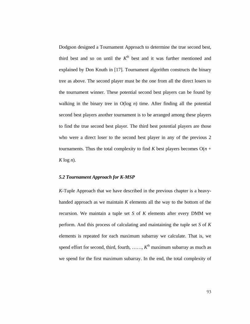
Dodgson designed a Tournament Approach to determine the true second best,

third best and so on until the Kth best and it was further mentioned and

explained by Don Knuth in [17]. Tournament algorithm constructs the binary

tree as above. The second player must be the one from all the direct losers to

the tournament winner. These potential second best players can be found by

walking in the binary tree in O(log n) time. After finding all the potential

second best players another tournament is to be arranged among these players

to find the true second best player. The third best potential players are those

who were a direct loser to the second best player in any of the previous 2

tournaments. Thus the total complexity to find K best players becomes O(n +

K log n).

5.2 Tournament Approach for K-MSP

K-Tuple Approach that we have described in the previous chapter is a heavy-

handed approach as we maintain K elements all the way to the bottom of the

recursion. We maintain a tuple set S of K elements after every DMM we

perform. And this process of calculating and maintaining the tuple set S of K

elements is repeated for each maximum subarray we calculate. That is, we

spend effort for second, third, fourth, ……, Kth maximum subarray as much as

we spend for the first maximum subarray. In the end, the total complexity of

93

K-MSP becomes a multiplication of the effort required to calculate 1

maximum subarray by the number of maximum subarrays to be searched for.

In Tournament Approach, instead of spending same effort for all K maximum

subarrays we spend some extra effort during the calculation of the first

maximum subarray and in return we spend less effort during the calculation of

all subsequent subarrays. The basic idea came from the realization of the fact

that second maximum subarray will be found based on the first maximum

subarray. Then third maximum subarray will be found based on the first and

second maximum subarrays. After finding the first maximum subarray when

we search for the second maximum subarray, if we can locate exactly from

which location of the whole array the first maximum subarray came from we

can spend less effort to find the second maximum subarray by only

considering all the candidates that were beaten by the first maximum subarray

solution.

We can visualize the recursion process of Algorithm 12 in the following

figure. At every recursion level there are 6 solutions. Out of these 6 solutions

the best one gets carried through to the upper level of recursion. The 4

solutions that are depicted as circles in the following figure are ANW, ANE, ASW

and ASE. The solutions that are depicted as rectangles are column-centered and

row-centered solutions. The final solution that is carried through to the top of

94

the tree must come from some level in the recursion and it must be either a

row-centered solution or a column-centered solution or a single element at the

bottom.

Figure 23: Visualization of the intermediate recursion process

Suppose in the above figure, we have detected the recursion level from which

the final solution returned. Also we’ve identified that it was a column-centered

solution that was carried up in the recursion. In the following figure we

95

enlarge this column-centered solution by focusing all possible strips inside the

column-centered solution.

O(n2) strips vertically

O(n2) solutions per strip

Figure 24: Strip Visualization

For simplicity we have drawn only 3 strips in the above picture for the

column-centered solution. For all values of index k and i there are O(n2) strips

from which the column-centered solution might have come up. Also within a

strip there are O(n2) possible subarrays from which the column-centered

solution might have come up. We discuss this in details later in this chapter.

We develop the following algorithm which is a modified version of Algorithm

12 for finding the first maximum subarray. We identify the solution by the

value of the sum in the maximum subarray, the indices to indicate where this

96

array is and the portion where the solution column-centered or row-centered

was calculated. The position of the solution is represented by 4 indices i, j, k, l

and scope of the solution is represented by 4 indices as well which are m1, n1,

m2 and n2.

Figure 25: Scope and position of a maximum subarray solution

_____________________________________________________________ Algorithm 14: New K-MSP Algorithm based on Tournament Approach 1: If the array becomes one element, return its value. 2: Otherwise, if m > n, rotate the array 90 degrees. 3: Thus we assume m ≤ n. 4: Let ANW be the solution for the NW part. 5: Let ANE be the solution for the NE part. 6: Let ASW be the solution for the SW part. 7: Let ASE be the solution for the SE part. 8: Let Acolumn be the solution for the column-centered problem. 9: Let Arow be the solution for the row-centered problem. 10: Let S be the maximum of those six. 11: Return S along with scope, position and recursion depth of S. _____________________________________________________________ Algorithm 10 (Fast DMM) is to be incorporated in the above algorithm for

performing DMM. During the process of finding the first maximum subarray

97

by Algorithm 14 we do some additional works as well. While we solve either

column-centered problem or row-centered we perform DMM and we compare

all the best values found among all the n2 possible strips.

After we locate the scope of the first solution the size of the scope is denoted

by n. In one single strip horizontally there are O(n2) possible subarrays and

precisely 4

2n subarrays. All O(n2) subarrays compete with each other to

become the second winner of the strip. This can be done in O(n2) time. Also

there are vertically O(n2) possible strips for a given column-centered problem.

So there are maximum O(n2) possible winners for O(n2) possible strips. In

O(n2) time we can find the overall second winner strip among all O(n2) strips.

O(n2) strips vertically

O(n2) subarrays horizontally for one single strip

Figure 26: (n, n) array yielding O(n2) strips and O(n2) subarrays per strip

Once we calculate the winner of a particular strip we keep track of the position

of the winner solution within the strip by recording the co-ordinates

information of the winner for later use. The complexity to keep track of co-

98

ordinates of the winner of a particular strip is absorbed with in the complexity

of finding the winner of that strip. In this way, the winner solution from a

winner strip is returned as column-centered problem solution.

When we complete finding the first maximum subarray we return the solution

along with solution’s scope, position and recursion depth. We now consider

the situation of finding the second maximum subarray. Using the recursion

depth information of the first maximum subarray we straightaway locate the

recursion level. Then using scope and position information of the last solution

we can exactly find where the last solution came from and thus we can detect

which 1 of the 6 solutions was responsible for the last final solution. All 6

solutions competed with each other and eventually the best one was carried up

the recursion. Let us assume column-centered solution was the winner. The

basic idea that we apply here using Tournament Approach is that all the 5

solutions that were beaten by the winner column-centered solution from that

recursion level deserve to be the second best solution from that recursion level.

Also the second best solution for the column-centered problem participates in

this race. By using the co-ordinates information of the winners of all strips that

we accumulated during the calculation of first maximum subarray we can find

the second best column-centered solution. We compare the new column-

99

centered solution with other 5 solutions and pick up the best solution and feed

up through the recursion for the second maximum subarray calculation.

Finding the second best solution for a column-centered or row-centered

problem can be done in O(n2) time. As we do this K – 1 times for K – 1

subsequent maximum subarrays the complexity for this becomes O(Kn2).

Thus the total expected time of K-MSP by Tournament Approach becomes

O(n2 log2 n + Kn2).

100

Chapter 6

Evaluation

In this chapter we present time measurements of Conventional (exhaustive)

Approach, K-Tuple Approach and Tournament Approach. All the algorithms

were implemented in programming language C. In the following sections we

focus on time measurements of a number of algorithms and we intentionally

omit implementation details of these algorithms. First we compare

Conventional Approach with K-Tuple Approach by investigating the result of

the experiments. Then we compare K-Tuple Approach with Tournament

Approach in the same way.

6.1 Conventional Approach vs. K-Tuple Approach

In the beginning, Conventional DMM (exhaustive method) was implemented.

Then we extended this to Conventional K-DMM. Also we implemented

Algorithm 6 for MSP where we incorporated Conventional DMM to solve

column-centered and row-centered problems. After this we implemented

Algorithm 12 for K-MSP where we incorporated exhaustive K-DMM

algorithm for column-centered and row-centered problems. The time

measurement was taken and recorded for further comparison with efficient

methods. In all of the above cases we fixed K = 10.

101

Then Fast version of DMM was implemented which is basically incorporation

of MT [3] APSP Problem algorithm into DMM. So MT algorithm was needed

to investigate first. Then again MT is based on Dantzig’s [10] and Spira’s [11]

APSP Problem algorithms. So Dantzig’s and Spira’s APSP Problem

algorithms were implemented before we implemented MT. Large amount of

random data were created to measure the expected time. After this, MT was

efficiently implemented. Also Dijkstra’s [25] and Floyd’s [26] APSP Problem

algorithms were implemented and compared with Dantzig, Spira and MT just

for the sake of interest. Then we extended MT to K-DMM and implemented

Algorithm 11 and the expected time was measured. Binary heap was used for

the priority queue. In the end, this Fast K-DMM was incorporated into K-MSP

algorithm which is Algorithm 12. Again the value of K was fixed to 10 in all

of the above cases.

6.1.1 Dijkstra, Floyd, Dantzig, Spira and MT APSP Problem Algorithms

Size (n)

Dijkstra (sec)

Floyd (sec)

Dantzig (sec)

Spira (sec) MT(sec)

100 0.03 0.02 0.03 0.03 0.02 200 0.26 0.16 0.17 0.15 0.12 300 0.93 0.55 0.52 0.39 0.28 400 2.07 1.24 1.15 0.66 0.50 500 4.66 2.92 2.27 1.03 0.83 600 7.46 4.45 3.63 1.94 1.33 700 12.87 7.99 5.63 2.79 1.92

102

800 18.18 11.18 8.01 3.70 2.57 900 26.03 15.93 11.15 4.05 3.07 1000 36.85 23.18 15.10 5.06 3.97

Table 1: APSP Problem time measurement

In table 1 we observe MT outplays all others when input size is 200. As input

size gets bigger we also observe MT becomes more efficient than all other

algorithms compared above. The corresponding graph is shown in Figure 27.

APSP Time Measurement

0

5

10

15

20

25

30

35

40

1 2 3 4 5 6 7 8 9 10Input(n) in Hundred

Tim

e(se

c)

DijkstraFloydDantzigSpiraMT

Figure 27: APSP Problem time measurement

103

6.1.2 Conventional DMM vs. Fast DMM

In Table 2 we observe the Fast DMM outplays the Conventional DMM when

input size is 300. A significant difference between these two can be observed

when input size is 400. As input size gets larger we also observe that Fast

DMM completely outplays Conventional DMM. The corresponding graph is

shown in Figure 28.

Size(n) Conventional DMM (sec) Fast DMM (sec)

100 0.02 0.03 200 0.15 0.16 300 0.55 0.51 400 1.45 1.12 500 3.22 2.25 600 5.02 3.62 700 8.89 5.83 800 13.26 8.23 900 19.83 11.51 1000 27.38 15.28

Table 2: DMM time measurement

104

DMM Time Measurement

0

5

10

15

20

25

30

1 2 3 4 5 6 7 8 9 10Input(n) in Hundred

Tim

e(se

c)

DMMFast DMM

Figure 28: DMM time measurement

6.1.3 MSP with Conventional DMM vs. MSP with Fast DMM

Size(n) MSP(with Conventional DMM) (sec) MSP(with Fast DMM) (sec)

100 0.14 0.76 200 1.06 1.40 300 3.19 3.35 400 8.48 8.62 500 19.35 19.45 600 29.53 27.42 700 45.08 39.14 800 76.50 62.14 900 114.92 97.20 1000 157.46 130.2

Table 3: MSP time measurement

105

In the above table, we observe MSP with Fast DMM outplays MSP with

Conventional DMM when input size is 600. When input size is 700 we

observe a significant difference between two versions of MSP. One interesting

observation is that due to recursion in the main MSP algorithm we’ve one

extra log n factor which delays MSP incorporating Fast DMM to take over

MSP incorporating Conventional DMM. We’ve seen previously Fast DMM

outplays Conventional DMM significantly when input size was 400. But after

incorporating this Fast DMM into MSP algorithm we inspect a significant

difference between two versions of MSP when input size was 700. It is due to

the overhead of recursive calls to Fast DMM from the main MSP algorithm.

The corresponding graph is shown in Figure 29.

MSP Time Measurement

020406080

100120140160180

1 2 3 4 5 6 7 8 9 10

Input(n) in Hundred

Tim

e(se

c)

MSP(DMM)MSP(Fast DMM)

Figure 29: MSP time measurement

106

6.1.4 Conventional K-DMM vs. Fast K-DMM

In the above table we observe the Fast K-DMM outplays the Conventional K-

DMM when input size is 200. A significant difference between these two can

be observed when input size is 500. As input size gets larger we also observe

that Fast K-DMM completely outplays Conventional K-DMM. The

corresponding graph is shown in Figure 30.

Size(n) Conventional K-DMM (sec) Fast K-DMM (sec)

100 0.19 0.22 200 1.50 1.26 300 5.18 3.80 400 12.42 8.20 500 24.80 16.30 600 41.80 26.90 700 68.34 40.14 800 103.10 54.70 900 147.96 72.39 1000 209.59 93.75

Table 4: K-DMM time measurement

107

K -DMM Time Measurement

0

50

100

150

200

250

1 2 3 4 5 6 7 8 9 10Input(n) in Hundred

Tim

e(se

c)

K-DMMFast K-DMM

Figure 30: K-DMM time measurement

6.1.5 K-MSP with Conventional K-DMM vs. K-MSP with Fast K-DMM

In Table 5, we observe K-MSP with Fast K-DMM outplays K-MSP with

Conventional K-DMM when input size is 700. But this difference remains

subtle until input size reaches 800. When input size is 800 we observe a

significant difference between the two versions of MSP.

Size(n) K-MSP(with

Conventional K-DMM) (sec)

K-MSP(with Fast K-DMM) (sec)

100 1.35 2.76 200 5.06 10.40 300 12.30 19.35 400 27.5 36.62 500 52.35 57.90

108

600 71.53 75.55 700 110.08 101.14 800 159.5 140.14 900 225.92 190.2 1000 305.46 245.2

Table 5: K-MSP time measurement (comparison between Conventional and K-

Tuple Approach)

Interestingly, we observe that due to recursion in the main MSP algorithm we

incur one extra log n factor which delays K-MSP incorporating Fast K-DMM

to take over K-MSP incorporating Conventional K-DMM. We’ve seen

previously Fast K-DMM outplays Conventional K-DMM significantly when

input size was 500. But after incorporating this Fast K-DMM into K-MSP

algorithm we see a significant difference between two versions of K-MSP

when input size was 800. It is due to the overhead of recursive calls to Fast K-

DMM from the main K-MSP algorithm. The corresponding graph is depicted

in Figure 31.

109

K -MSP Time Measurement

0

50

100

150

200

250

300

350

1 2 3 4 5 6 7 8 9 10

Input(n) in Hundred

Tim

e(se

c)

K-MSP(K-DMM)K-MSP(Fast K-DMM)

Figure 31: K-MSP time measurement (comparison between Conventional and

K-Tuple Approach)

6.2 K-Tuple Approach vs. Tournament Approach

Finally, Tournament Approach was implemented by incorporating Fast DMM

into the modified K-MSP algorithm that was discussed in Chapter 5. Note that

the main purpose of Tournament Approach is to avoid K-Tuple Approach. So

in this approach we don’t need to incorporate K-DMM anymore. We

incorporate Fast DMM into K-MSP as we discussed in Chapter 5.

In the following we present the time measurement of Tournament Approach

and compare it with K-Tuple Approach.

110

Size(n) K-Tuple Approach for K-MSP(sec)

Tournament Approach for K-MSP (sec)

100 2.76 1.76 200 10.40 8.40 300 19.35 16.35 400 36.62 29.62 500 57.90 49.90 600 75.55 66.42 700 101.14 91.00 800 140.14 128.14 900 190.2 175.2 1000 245.2 227.2

Table 6: K-MSP time measurement (comparison between K-Tuple and

Tournament Approach)

In the above table, we observe the difference between the performances of K-

Tuple Approach and Tournament Approach for K-MSP. Tournament

Approach right from the beginning outplays K-Tuple Approach. When input

size is 1000 we observe a significant difference between two versions of K-

MSP. The corresponding graph is depicted in Figure 32.

111

K -MSP Time Measurement

0

50

100

150

200

250

300

1 2 3 4 5 6 7 8 9 10

Input(n) in Hundred

Tim

e(se

c)

K-Tuple ApproachTournament Approach

Figure 32: K-MSP time measurement (comparison between K-Tuple and

Tournament Approach)

112

Chapter 7

Conclusion

In this research we have investigated MSP by doing the average case analysis.

The basic aim of this research was to analyze existing algorithms for both

MSP and K-MSP and develop efficient algorithms for K-MSP based on

existing framework and algorithms. And finally the goal was to compare

existing algorithms with the new algorithms based on time measurement.

We extended Fast DMM to Fast K-DMM and incorporated into MSP. To be

able to incorporate Fast K-DMM into MSP we modified existing MSP and

extended to K-MSP. With the help of advanced data structure we achieved

O(Kn2 log n log K) time complexity for K-DMM when K ≤ n/log n. When we

incorporated this K-DMM into the K-MSP an extra log n effort was required

due to the recursion. So the overall complexity for K-MSP became O(Kn2 log2

n log K) when K n/log n based on K-Tuple Approach. ≤

After this we realized K-Tuple Approach was a heavy-handed approach since

every single element becomes a set of K items. We further reviewed this

approach and came up with Tournament Approach. By Tournament Approach

we solved the K-MSP more efficiently. The basic intention was to reuse the

113

information that we gain while we solve the first maximum subarray. By doing

so, all the subsequent maximum subarrays can be detected in an efficient

manner. And we showed how the complexity of this approach further comes

down to O(n2 log2 n + Kn2).

7.1 Future Work

The main framework of MSP remains unchanged in this research. Because of

the recursion an extra log n effort is required when we use this framework. If

we could change the main framework we may be able to remove this extra log

n effort and reduce the overall complexity of both MSP and K-MSP. Another

interesting research problem would be doing average case analysis of K-MSP

for the disjoint case. Also in the Tournament Approach, with the help of

advanced data structure finding the next best sum strip-wise could be done

more efficiently and it would be really a challenging problem.

114

References

[1] Takaoka, T. 2002. Efficient Algorithms for the Maximum Subarray Problem by Distance Matrix Multiplication. Proc. CATS 2002, Melbourne, Australia, January 28-February 1, ENTCS, Vol. 61, pp. 191-200. Elsevier, Amsterdam, The Netherlands.

[2] Bae, S. E. and Takaoka, T. 2006. Improved Algorithms for the K Maximum Subarray Problem. The Computer Journal, Vol. 49, No. 3, pp 358-374.

[3] Moffat, A. and Takaoka, T. 1987. An All Pairs Shortest Path Algorithm with O(n2 log n) Expected Time. SIAM Jour. Computing, Vol. 16, pp. 1023-1031.

[4] Feller, W. 1968. An Introduction to Probability Theory and its Applications, Vol. 1, 3rd ed., New York: Wiley.

[5] Knuth, D. E. 1973. The art of Computer Programming, Vol. 1, Fundamental Algorithms, 2nd ed., Addison-Wesley, p. 74.

[6] Bentley, J. 1984. Programming Pearls: Algorithm Design Techniques. Commun. ACM, Vol. 27, No. 9, pp. 865-873.

[7] Bentley, J. 1984. Programming Pearls: Perspective on Performance. Commun. ACM, Vol. 27, No. 11, pp. 1087-1092.

[8] Tamaki, H. and Tokuyama, T. 1998. Algorithms for the Maximum Subarray Problem based on Matrix Multiplication. Proc. SODA 1998, San Francisco, CA, January 25-27, pp. 446-452. SIAM, Philadelphia, PA.

[9] Takaoka, T. 2005. An O(n3 log log n/log n) Time Algorithm for the All Pairs Shortest Path Problem. Inform Process Lett., Vol. 96, pp. 155-161.

115

[10] Dantzig, G.B. 1960. On the Shortest Route through a Network. Management Sci., Vol. 6, pp. 187-190.

[11] Spira, P.M. 1973. A New Algorithm for Finding All Shortest Paths in a Graph of Positive Arcs in Average Time O(n2 log2 n). SIAM Jour. Computing, Vol. 2, pp. 28-32.

[12] Conway, J. H. and Guy, R. K. 1996. The Euler-Mascheroni Number. The Book of Numbers, New York: Springer-Verlag, pp. 260-261.

[13] Feller, W. 1968. Stirling's Formula. An Introduction to Probability Theory and its Applications, Vol. 1, 3rd ed., New York: Wiley, pp. 50-53.

[14] Aho, A.V., Hopcroft, J.E. and Ullman, J.D. 1975. The Design and Analysis of Computer Algorithms, 2nd ed., Addison-Wesley, pp. 97-102.

[15] Frederickson, G.N. and Johnson, D.B. 1982. The Complexity of Selection and Ranking in X + Y and matrices with sorted columns. J. Comput. Syst. Sci., Vol 24, pp. 197-208.

[16] Dodgson, R. C. L. 1883. St. James’s Gazette, August 1, pp. 5-6.

[17] Knuth, D. E. 1973. The art of Computer Programming, Vol. 3, Sorting and Searching, 2nd ed., Addison-Wesley, pp. 209-218.

[18] Takaoka, T. 1992. A New Upper Bound on the Complexity of the All Pairs Shortest Path Problem. Inform Process Lett., Vol. 43, No. 4, pp. 195-199.

[19] Bae, S. E. and Takaoka, T. 2004. Algorithms for the Problem of K Maximum Sums and a VLSI Algorithm for the K Maximum Subarrays Problem. Proc. ISPAN

116

117

2004, Hong Kong, May 10–12, pp. 247–253. IEEE Computer Society Press, Los Alamitos, CA.

[20] Bae, S. E. and Takaoka, T. 2003. Parallel Approaches to the Maximum Subarray Problem. Proc. Japan-Korea Workshop on Algorithms and Computation 2003, Sendai, Japan, July 3-4, pp. 94-104. Tohoku University, Sendai, Japan.

[21] Bengtsson, F. and Chen, J. 2004. Efficient Algorithms for the K Maximum Sums. Proc. ISAAC 2004, Hong Kong, December 20-22, LNCS, 3341, pp. 137-148. Springer-Verlag, Berlin.

[22] Bae, S. E. and Takaoka, T. 2005. Improved Algorithms for the K Maximum Subarray Problem for small K. Proc. COCOON 2005, Kunming, Yunnan, China, August 16-19, pp. 621-631. Springer-Verlag, Berlin.

[23] Takaoka, T. 2004. A Faster Algorithm for the All Pairs Shortest Path Problem and its Application. Proc. COCOON 2004, Jeju Island, Korea, August 17-20, LNCS, 4106, pp. 278-289. Springer-Verlag, Berlin.

[24] Wen. Z. 1995. Fast Parallel Algorithms for the Maximum Sum Problem. Parallel Comput., Vol. 21, No. 3, pp. 461-466.

[25] Dijkstra, E.W. 1959. A Note on Two Problems in Connection with Graphs. Numer. Math., Vol. 1, pp. 269-271.

[26] Floyd, R.W. 1962. Algorithm 97: Shortest Path. Comm. ACM, Vol. 5, p. 345.