COSC 4214: Digital CommunicationsInstructor: Dr. Amir Asif

Department of Computer Science and EngineeringYork University

Handout # 3: Baseband Modulation

Topics:1. Character Coding (Formatting Textual Data)2. Pulse Code Modulation (Formatting Analog Signals).3. Nonuniform Quantization4. Baseband Transmission

Sklar: Sections 2.1 – 2.8.

2

Random Variables (1)

— Information bearing signals can take either of the three forms:

1. Textual information

2. Analog signals

3. Digital data— Before the signals are transmitted over a digital communication channel, the

information signal must be converted to digital symbols (Formatting).— The resulting digital symbols are then represented by baseband waveforms (Pulse

Modulation or Line Coding).

3

5. Probability density function of a discrete RV: is the distribution of probabilities for different values of the RV.

Example I: S = {HH, HT, TH, TT} in tossing of a coin twice with X = no. of heads

Example II: S = {NNN, NND, NDN, NDD, DNN, DND, DDN, DDD} in testing electronic components with Y = number of defective components.

6. Properties:

Random Variables (2)

Value (x) 0 1 2

P(X = x) 1/4 1/2 1/4

Value (x) 0 1 2 3

P(X = x) 1/8 3/8 3/8 1/8

y probabilit)()(.

1 toadds1)(.

positive always0)(.

xpxXPc

xpb

xpa

X

xX

X

4

6. Probability density function of a continuous RV: is represented as a continuous function of X.

Example III: Distance traveled by a car in 5 hours has an uniform distribution between 150 and 250 km.

8. Properties of pdf:

Random Variables (3)

y probabilit)()(.

1 tointegrates1)(.

positive always0)(.

b

a

X

X

X

dxxpbXaPc

dxxpb

xpa

150 250X

pX(x)

0.01

5

Random Variables (4)

Activity 1: The pdf of a discrete RV X is given by the following table.

Calculate the probability P(1 ≤ X < 3) and P(1 ≤ X ≤ 3)

Activity 2: The pdf of a continuous RV X is pX(x) = e-x u(x). Find the probability P(1 < X < 5).

Value Value ((xx)) 0 1 2 3

PP((X = xX = x)) 1/8 3/8 3/8 1/8

6

9. Distribution function: is defined as

which gives

9. Moments:

10. Mean is defined as mX = E{X}. Variance is defined as var{X} = E{X}2 – (mX)2.

Activity 3: Calculate and plot the distribution function for pdf’s specified in Activities 1 and 2. Also calculate the mean and variance in each case.

Random Variables (5)

)()( xXPxFX

RV continuousfor )()(

RV discretefor )()(

x

XX

x

xXX

dxxpxF

xpxF

RV continuousfor )(

RV discretefor )(}{

dxxpx

xpxXE

Xn

xX

nn

7

Random Processes (1)

1. The outcome of a random process is a time varying function. Examples of ransom processes are: temperature of a room; output of an amplifier; or luminance of a bulb.

2. A random process can also be thought of as a collection of RV’s for specified time instants. For example, X(tk), measured at t = tk is a RV.

8

Random Processes (2)

3. Random processes are often specified by their mean and autocorrelation.

4. Mean is defined as

5. Autocorrelation is defined as

Activity 4: Consider a random process

where A and f0 are constants, while is a uniformly distributed RV over (0, 2). Calculate the mean and autocorrelation for the aforementioned process.

process random time-continuousfor )()()(

process random time-discretefor )()()(

x

Xkk

x

xXkk

dxxptXtXE

xptXtXE

k

k

)()(),( 2121 tXtXEttRX

)2cos()( 0 tfAtX

9

Classification of Random Processes (1)

1. Wide Sense Stationary (WSS) Process: A random process is said to be WSS if its mean and autocorrelation is not affected with a shift in the time origin

2. Strict Sense Stationary (SSS) Process: A random process is said to be SSS if none of its statistics change with a shift in the time origin

3. Ergodic Process: Time averages equal the statistical averages.

Random Processes

WSS

Stationary

Ergodic

)(),(andconstant)}({ 2121 ttRttRmtxE XXX

TtTtTtxxxXXXtttxxxXXX kkkkkkpp ,,,;,,,,,,,,,;,,,,,, 212121212121

10

Classification of Random Processes (2)

Activity 5: Show that the random process in Activity 4 is a WSS process.

4. For WSS processes, the autocorrelation can be expressed as a function of single variable

5. Autocorrelation satisfies the following properties

6. Fourier transform of autocorrelation is referred to as the power spectral density (PSD)

)()(),( 2121 XXX RttRttR

nCorrelatio)()0(.4

pairs ansformFourier tr)()(.3

0at occurs Maximum)0()(.2

t.r. .function wEven )()(.1

2 tXER

fGR

RR

RR

x

xFT

x

xx

xx

Variance)(.4

pairs ansformFourier tr)()(.3

functionEven )()(.2

valuedreal Always0)(.1

dffGP

fGR

fGfG

fG

xX

xFT

x

xx

x

11

Classification of Random Processes (3)

Activity 6: Determine which of the following are valid autocorrelation function

Activity 7: Determine which of the following are valid power spectral density function

)exp()(.3

)2sin()()(.2elsewhere0

111)(.1

0

x

x

x

R

tfR

R

))10(2exp()(.3

)2(cos)()(.2

)10(10)(.1

20

2

ffS

tffS

ffS

x

x

x

12

Additive Gaussian Noise

1. Noise refers to unwanted interference that tends to obscure the information bearing signal

2. Noise can be classified into two categories:

a) Man-made Noise introduced by switching transients and simultaneous presence of neighboring signals

b) Natural Noise produced by the atmosphere, galactic sources, and heating up of electrical components. The latter is referred to as the thermal noise.

3. Thermal noise is difficult to be eliminated and often modeled by the Gaussian probability density function

which has a mean n = 0 and var(n) = 2.

2

21

21 exp)(

nN np

13

Additive White Gaussian Noise

4. Additive Gaussian Noise: refers to the following model for introduction of noise in the signal

5. Given that the noise n is a Gaussian RV and a is the dc component, which is constant, the pdf of z is given by

which has a mean n = a and var(n) = 2.

6. Additive White Gaussian Noise (AWGN): adds an additional constraint on the power spectral density

Activity 8: Calculate the variance of AWGN given its PSD is N0/2.

2

21

21 exp)(

azZ zp

process random)()(

variablerandom

tnAtz

naz

2200 )()()( N

nFTN

n fGR

14

Signal Processing with Linear Systems (1)

1. For deterministic signals, the output of the LTI system is given by

a) Convolution integral:

b) Transfer function:

where X(f) and H(f) are Fourier transforms of x(t) and h(t).

Activity 9: Determine the output of the LTI system if the input signal x(t) = e-at u(t) and the transfer function h(t) = e-bt u(t) with a ≠ b.

dthxthtxty )()()()()(

LTI Systemh(t)

Input Signal x(t)

Output Signal y(t)

)()()( 1 fHfXty

15

Signal Processing with Linear Systems (2)

2. For WSS random processes, statistics of the output of the LTI system can only be evaluated using the following formula.

Activity 10: Derive the above expressions for WSS random processes.

Activity 11: Calculate the mean and autocorrelation of the output of the LTI system if the input x(t) to the system is White Noise with PSD of N0/2 and the impulse response of the system is given by h(t) = e-bt u(t).

2|)(|)()(:PSD

)()()()(:ationAutocorrel

)(:Mean

fHfSfS

hhRR

dtth

xy

xy

xy

LTI Systemh(t)

Input Signal x(t)

Output Signal y(t)

16

Distortionless Transmission

1. For distortionless transmission, the signal can only undergo

a) Amplification or attenuation by a constant factor of K

b) Time delay of t0

In other words, there is no change in the shape of the signal

2. For distortionless transmission, the received signal must be given by

3. Based on the above model, the transfer function of the overall communication system is given by

with impulse response

)()( 0ttKxty

Communication System

h(t)Input Signal

x(t)Output Signal

y(t)

02)( ftjKefH

).()( 0ttKth

17

Ideal Filters

u

uftj

ff

ffefH

||0

||)(

:Filter Lowpass02

ffe

fffH ftj ||

||0)(

:Filter Highpass

02

u

uftj

ff

fffe

ff

fH

||0

||

||0

)(

:Filter Bandpass

02

Activity 12: Calculate the impulse response for each of the three ideal filters.

Activity 13: Calculate the PSD and autocorrelation of the output of the LPF if WGN with

PSD of N0/2 is applied at the input of the LPF.

18

Bandwidth

1. For baseband signals, absolute bandwidth is defined as the difference between the maximum and minimum frequency present in a signal.

2. Most time limited signals are not band limited so strictly speaking, their absolute bandwidth approaches infinity

t0

ttf rect)(

2

2

0

fF sinc)(

1

1

FT

19

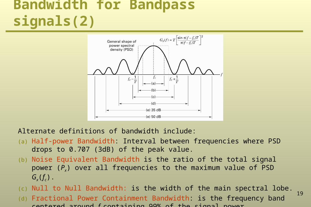
Bandwidth for Bandpass signals(2)

Alternate definitions of bandwidth include:

(a) Half-power Bandwidth: Interval between frequencies where PSD drops to 0.707 (3dB) of the peak value.

(b) Noise Equivalent Bandwidth is the ratio of the total signal power (Px) over all frequencies to the maximum value of PSD Gx(fc).

(c) Null to Null Bandwidth: is the width of the main spectral lobe.

(d) Fractional Power Containment Bandwidth: is the frequency band centered around fc

containing 99% of the signal power

20

Bandwidth for Bandpass signals(3)

Alternate definitions of bandwidth include:

(e) Bounded Power Spectral Density: the width of the band outside which the PSD has dropped to a certain specified level (35dB, 50dB) od the peak value.

(f) Absolute Bandwidth: Band outside which the PSD = 0.