Correlation and Simple Linear Regression Readings:...
21
Correlation and Simple Linear Regression Readings: DVB Ch. 7-9, 27 Scatterplot • Each pair of values is shown as a dot. • Distance along each axis represents magnitude. • Reveals nature of association between two variables. 1
Transcript of Correlation and Simple Linear Regression Readings:...

Correlation and Simple Linear Regression
Readings: DVB Ch. 7-9, 27
Scatterplot
• Each pair of values is shown as a dot.
• Distance along each axis represents magnitude.
• Reveals nature of association between two variables.
1

Example: Carbon monoxide levels were measured in the lung and the 10
subjects were asked how many cigarettes they smoked per day (Selvin, pg.
54)
cigs 12 30 40 12 2 5 20 30 75 40CO 2 11 14 16 18 18 18 22 23 26
• The plot shows a weak positive association, large CO values tend to
occur with large numbers of cigarettes.
• The dashed lines are at the average number of cigarettes and average
CO.
•
•
•
•
• • •
••
•
CO vs no. of cigarettes
number
CO
0 20 40 60
510
1520
25
• If all the values fell in the bottom left or top right quadrants, the
association would be stronger.
2

Simple Linear Regression
• Simple linear regression is used to find the best straight line fit to the
data.
• The result can be used to describe the association, and to predict
values.
• We must identify a response variable, y, and an explanatory variable,
x.
• Statistical Model
The observed value yi includes an additive deviation, εi
yi = α + βxi + εi.
• Data: (x1, y1), (x2, y2), . . . , (xn, yn)
• Assumptions: we assume that the deviations ε1, ε2, . . . , εn are
independent N(0, σ2). That is, they are independent and have normal
distributions with a common mean 0, and common variance σ2.
• Another way to write the model is
yi = µyi|xi + εi
where µyi|xi = α+ βxi is the mean of y when the predictor variable x
is equal to xi.
• To find the best line, we minimize the sum of squares of the vertical
deviations between the observed and fitted response values at each
value of the explanatory variable.
• This is called the method of least squares.
3

• Recall that the equation of a line is
y = a + bx
where a is the y − intercept and b is the slope.
• The method of least squares chooses the intercept and slope to
minimize the error sum of squares
SSE =∑
(yi − yi)2 =∑
(yi − α− βxi)2
The minimizing values are denoted as α and β.
4

Example: We would think of CO levels as a response to the number of
cigarettes smoked per day.
•
•
•
•
• • •
••
•
number of cigarettes
CO
0 20 40 60
5
10
15
20
25
• The solid line is the least squares fit
y = 13.38 + .1285x, SSE = 345.16
• The other lines are
y = 10 + .25x, SSE = 408.375
and
y = 15 + .17x, SSE = 426.604.
5

Calculations
• Nowadays a computer is typically used to carry ot the calculations.
• However, the least squares estimates of the slope and intercept can
be written as
β =SXY
SXX= r
sysx
α = y − βx.
Assessing the Fit
• We can summarize the fit using an analysis of variance table.
Source Sum of Squares Degrees of Freedom Mean SquareRegression 70.44 1 70.44Residual 345.16 8 43.15Total 415.60 9
• The Total sum of squares, SST, is the sample variance without the
division by n− 1
SST =∑
(yi − y)2.
• The Regression sum of squares, SSR, is obtained by subtraction
SSR = SST − SSE.
• The total degrees of freedom is n− 1.
• The regression degrees of freedom is 1.
• The residual degrees of freedom is the difference, n− 2.
6

The coefficient of determination
R2 =SSR
SST
is the proportion of variation in y which is explained by x.
– R2 is between 0 and 1.
– R2 = 1 implies a perfect fit
(SSE = 0), all the points are on the line.
– R2 = 0 implies no linear relationship, the best fitting line has zero
slope (SSE = SST).
– R2 = r2, i.e. the coefficient of determination is the square of
Pearson’s correlation coefficient between x and y, described
below.
• In the example R2 = 70.44/415.60 = .169 so 17% of the variation in
CO levels can be attributed to variation in numbers of cigarettes
smoked.
7

Hypothesis test for the slope
• Usually we first wish to test whether there is a significant relationship
between the variables.
• The hypotheses are H0 : β = 0 versus Ha : β 6= 0
• The test statistic is
t =β − 0
se(β).
• This has a t distribution with n− 2 degrees of freedom, if
assumptions satisfied.
• The standard error of the slope estimate, β, is
se(β) =σ√SXX
.
• where we estimate σ by
s =
√√√√√SSEn− 2
=√MSE.
and se(β) by
se(β) =s√SXX
.
8

Confidence Intervals
• We can construct a confidence interval for β, using
β ± tα/2,n−2se(β).
9

• We typically do the calculations on a computer.
• eg. minitab output for the CO/cigarette data follows
MTB > set c1
DATA> 12 30 40 12 2 5 20 30 75 40
DATA> set c2
DATA> 2 11 14 16 18 18 18 22 23 26
DATA> regress c2 1 c1
The regression equation is
C2 = 13.4 + 0.128 C1
Predictor Coef Stdev t-ratio p
Constant 13.382 3.387 3.95 0.004
C1 0.1285 0.1006 1.28 0.237 *this is the test for
association, Stdev is
s/sqrt(SXX)
s = 6.568 R-sq = 16.9% * s = sqrt(MSE) and estimates sigma
* R^2 is the coefficient of determination
and equals SSR/SST
Analysis of Variance
SOURCE DF SS MS F p
Regression 1 70.44 70.44 1.63 0.237
Error 8 345.16 43.15
Total 9 415.60
Unusual Observations *you can ignore this part
Obs. C1 C2 Fit Stdev.Fit Residual St.Resid
1 12.0 2.00 14.92 2.54 -12.92 -2.13R
9 75.0 23.00 23.02 5.29 -0.02 -0.00 X
R denotes an obs. with a large st. resid.
X denotes an obs. whose X value gives it large influence.
• In this example the test for the relationship between amount of
smoking and CO is not significant (t = 1.28, P = .237).
10

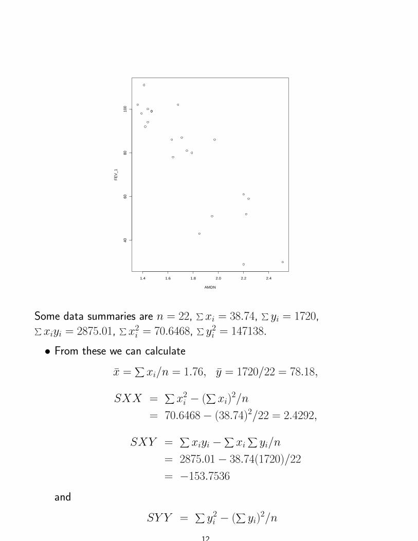
Example: (Daniel) Habib and Lutchen present a diagnositic technique
that is of interest to repiratory disorder specialists. The following are the
scores elicited by this technique, called AMDN, and the forced expiratory
volume (FEV1) scores for 22 subjects.
AMDN FEV11.36 1021.42 921.41 1111.44 941.47 991.39 981.47 991.79 801.71 871.44 1001.63 861.68 1021.75 811.95 511.64 782.22 521.85 432.24 592.51 302.20 612.20 291.97 86
A plot of the data shows a strong negative association.
11
1.4 1.6 1.8 2.0 2.2 2.4
4060
8010
0
AMDN
FE
V_1
Some data summaries are n = 22,∑xi = 38.74,
∑yi = 1720,∑
xiyi = 2875.01,∑x2i = 70.6468,
∑y2i = 147138.
• From these we can calculate
x =∑xi/n = 1.76, y = 1720/22 = 78.18,
SXX =∑x2i − (
∑xi)
2/n
= 70.6468− (38.74)2/22 = 2.4292,
SXY =∑xiyi −
∑xi
∑yi/n
= 2875.01− 38.74(1720)/22
= −153.7536
and
SY Y =∑y2i − (
∑yi)
2/n
12

= 147138− 17202/22
= 12665.27
• Pearson’s correlation coefficient (defined below) is
r =SXY√
SXX × SY Y=
−153.7536
2.4292(12665.27)= −.8766
• The least squares estimate of slope is
β =SXY
SXX=−153.7536
2.4292= −63.3.
• The intercept estimate is
α = y − βx = 78.18 + 63.3(1.76) = 189.6
• Some computer output follows from the R package
> summary(resp.out)
Call:
lm(formula = resp.y ~ resp.x)
Residuals:
Min 1Q Median 3Q Max
-29.543 -4.285 1.817 5.112 21.052
Coefficients:
Estimate Std. Error t value Pr(>|t|)
(Intercept) 189.638 13.925 13.619 1.41e-11 ***
resp.x -63.294 7.771 -8.145 8.81e-08 *** #this is the test for
association
---
Signif. codes: 0 *** 0.001 ** 0.01 * 0.05 . 0.1 1
Residual standard error: 12.11 on 20 degrees of freedom *this is s=sqrt(MSE)
Multiple R-squared: 0.7684,
F-statistic: 66.35 on 1 and 20 DF, p-value: 8.814e-08
13

> anova(resp.out)
Analysis of Variance Table *unlike MINITAB, this program doesn’t give
the SST
Response: resp.y
Df Sum Sq Mean Sq F value Pr(>F)
resp.x 1 9731.7 9731.7 66.348 8.814e-08 ***
Residuals 20 2933.5 146.7
---
Signif. codes: 0 *** 0.001 ** 0.01 * 0.05 . 0.1 1
14

Pearson Correlation Coefficient
• Denote the data (xi, yi), i, j = 1, . . . , n, then the Pearson correlation
coefficient is
r =∑
(xi − x)(yi − y)√∑(xi − x)2
∑(yi − y)2
or
r =1
n− 1
∑ (xi − x)
sx
(yi − y)
sy.
• r measures the direction and strength of the linear association
between the two variables.
• It is a dimensionless quantity.
• It has value 1 (-1) if all values on a line with positive (negative) slope.
• It has value 0 if there is no linear association (there may still be a
nonlinear association).
• Remember that association does not imply causality!!
• We shouldn’t extrapolate relationship beyond range of the data.
• This measure is sensitive to outliers.
• For calculation, use
r =SXY√
SXX × SY Ywhere
SXY =∑
(xi − x)(yi − y)
or
SXY =∑xiyi − (
∑xi
∑yi)/n
and
SXX =∑x2i − (
∑xi)
2/n.
15

• In the example, with x =number of cigarettes, y = CO, we get
∑xiyi = 5017,
∑xi = 266,
∑x2i = 11342,
∑yi = 168,
∑y2i = 3238,
so
SXY = 5017− 266(168)/10 = 548.2
SXX = 11342− 2662/10 = 4266.4,
and
SY Y = 415.6
so
r =548.2√
4266.4(415.6)= .41
16

• Some examples:
•
•
•
•
•
•
•
••
•• •
•
•
•
• ••
• •
x
y
2 3 4 5 6 7 8
78
910
11
12
13
r = -0.67
•
•
•
•
•
••
•
•
•
••
•
• •
•
••
•
•
xy
2 3 4 5 6 7 8
78
910
11
12
13
r = 0
•
•
•
•
•
•
•
••
•• •
•
•
•
• ••
• •
x
y
2 3 4 5 6 7 8
78
910
11
12
13
r = 0.42
•
•
•
•
•
•
•
••
•• •
•
•
•
• ••
• •
x
y
2 3 4 5 6 7 8
78
910
11
12
13
r = 0.86
• ••
••
•• •••
••
•
••
• ••
••
x
y
2 3 4 5 6 7 8
10
12
14
16
r = -0.1
••
••
•
•
x
y
8 10 12 14 16 18 20
24
68
10
12
14
16
r = 0.79
Notes
1. The bottom left example has strong (nonlinear) association, but small
r.
2. The bottom right shows reversal of sign due to outlier.
17

Material on this page concerns test hypotheses regarding thepopulation correlation coefficient ρ. You are not responsible forthis material, as one needs some mathematically fairlysophisticated ideas to define the population correlationcoefficient. Testing that the population correlation is 0 isequivalent to testing that the slope of a regression line equals0.
• If our data are a random sample from a population with true
correlation ρ, then r is an estimate of ρ with standard error
se(r) =
√√√√√1− r2n− 2
.
• We can test H0 : ρ = 0 vs Ha : ρ 6= 0 using
t =
√n− 2 r√1− r2
which has a t distribution with n− 2 degrees of freedom if the
population is (bivariate) normal.
• In the example,
t =√
10− 2(.41)/√
1− .412 = 1.28
which gives P = .24 (using the computer), so there is no evidence
that the population correlation is different from 0.
18

Spearman’s (Rank) Correlation Coefficient
• Rank the x’s and y’s separately.
• Calculate Pearson’s correlation coefficient on the ranks.
• In the example, the ranks are as follows (where fractions represent
mid ranks)
cigs 3.5 6.5 8.5 3.5 1 2 5 6.5 10 8.5CO 1 2 3 4 6 6 6 8 9 10
• rS = .35.
• We often get an answer similar to the Pearson correlation coefficient.
• The Spearman correlation is less sensitive to outliers than the
Pearson correlation.
• For n ≥ 10 we can test as before.
• Spearman’s measure can be used with ordinal data.
• Spearman’s correlation measures monotone (possibly nonlinear)
association.
• Ranking turns a curved monotone relationship into a linear one.
19

You are not responsible for anything following
Residual Plot - used to check assumptions
– A plot of the residuals yi − yi versus x should show random
scatter.
– Curvature indicates a more complicated model is required, such
as a quadratic y = a + bx + cx2 + ε.
– A ‘fanning out’ of residuals indicates the variance changes with
the mean or with x.
– Outliers in the x or y variable could show up.
•
•
•
•
• •
•
•
•
•
number of cigarettes
resi
dual
0 20 40 60
-10
-5
0
5
– These residuals show no problems.
20

• The confidence interval for µy|x, the mean of y when the predictor
variable equals x, is
α + βx± tα/2,n−2se(µy|x).
where
se(µy|x) = s
√√√√√1
n+
(x− x)2
Sxx
• A prediction interval for a new y at x is
α + βx± tn−2α/2 se(ynew)
where
se(ynew) = s
√√√√√1 +1
n+
(x− x)2
Sxx.
21