Correlates of fatality risk of vulnerable road users in Delhi

Accepted for publication in Accident Analysis and Prevention (2017)

Correlates of fatality risk of vulnerable road users in Delhi 1

Rahul Goel1, Parth Jain2, Geetam Tiwari3 2 1MRC Epidemiology Unit, University of Cambridge, United Kingdom 3 2Civil Engineering, Shiv Nadar University, Gautam Budh Nagar District, India 4 3Transportation Research and Injury Prevention Programme (TRIPP), Indian Institute of Technology Delhi, 5

New Delhi, India 6

Abstract 7

Pedestrians, cyclists, and users of motorised two-wheelers account for more than 85% of all the road 8

fatality victims in Delhi. The three categories are often referred to as vulnerable road users (VRUs). Using 9

Bayesian hierarchical approach with a Poisson-lognormal regression model, we present spatial analysis of 10

road fatalities of VRUs with wards as areal units. The model accounts for spatially uncorrelated as well as 11

correlated error. The explanatory variables include demographic factors, traffic characteristics, as well as 12

built environment features. We found that fatality risk has a negative association with socio-economic 13

status (literacy rate), population density, and number of roundabouts, and has a positive association with 14

percentage of population as workers, number of bus stops, number of flyovers (grade separators), and 15

vehicle kilometers travelled. The negative effect of roundabouts, though statistically insignificant, is in 16

accordance with their speed calming effects for which they have been used to replace signalised junctions 17

in various parts of the world. Fatality risk is 80% higher at the density of 50 persons per hectare (pph) than 18

at overall city-wide density of 250 pph. The presence of a flyover increases the relative risk by 15% 19

compared to no flyover. Future studies should investigate the causal mechanism through which denser 20

neighborhoods become safer. Given the risk posed by flyovers, their use as congestion mitigation measure 21

should be discontinued within urban areas. 22

1. Introduction 23

Indian cities have witnessed an exponential growth of vehicles during the previous two decades or so, 24

contributed largely by motorised two-wheelers (MTW) (Pucher et al., 2007; MoRTH, 2012). Coincident to 25

this, burden from road traffic injuries in India has also been rising, and the number of deaths have more 26

than doubled from 1991 through 2011 (Mohan et al., 2015). According to the official sources, there were 27

more than 140,000 road deaths in year 2013-14 (NCRB, 2015). When expressed as the number of road 28

deaths per 100,000 persons, fatality risk in India is 2 to 4 times higher than high-income settings such as 29

the UK, Germany, France and Canada (MoRTH, 2012). 30

A majority of the victims are men in age-group 15–59 years (Gururaj, 2008; Mohan et al., 2009; Hsiao et 31

al., 2013). Pedestrians, cyclists, and MTW riders have the largest share. The three road-user categories, 32

with no rigid barrier protecting them against traumatic forces, are often termed as vulnerable road users 33

(VRU) (Peden et al., 2004). Globally, VRUs account for around 46% of all road deaths (WHO, 2015), while 34

in India this share is much higher. 35

According to Million Death Study, a national-level mortality survey in India, VRUs accounted for 68% of all 36

road deaths during the period 2001–2003 (Hsiao et al., 2013). A study conducted in six Indian cities with 37


population ranging between 1 to 2 million reported that the proportion of VRU fatalities for years 2008 38

through 2011 varied from 84% to 93% (Mohan et al., 2016). This proportion is much lower in high–income 39

countries and is as low as 22% in the Americas (WHO, 2015). There are multiple factors contributing to 40

these differences, such as road design, provision of safe infrastructure for pedestrians and cyclists, traffic 41

management, and the enforcement of speed and alcohol limits. Apart from these, the major underlying 42

difference is how people travel in these settings. 43

According to Census 2011, close to one-third of the workers (30%) in Indian cities walk to work, 17% cycle, 44

a quarter (25%) use some form of public transport (bus, autorickshaw or train), more than one-fifth (22%) 45

use MTW and only 5% use cars (Census-India, 2016). As a result, 69% of the workers can be categorised 46

as VRUs during their commute trips. If we consider walking involved in either ends of a public transport 47

trip, the proportion of work trips involving VRU reach up to 94%. 48

When trips of all purposes are considered, data from various cities in India show that the share of non-49

motorised modes is even higher (Arora et al., 2014; RITES, 2008; Goel, 2017). As a result, a large 50

proportion of road users are exposed to high injury risk through collisions with high-powered motorised 51

vehicles such as cars, buses, and trucks. This is in complete contrast with high-income settings where a 52

large proportion of trips are carried out in cars. For instance, 86% of the work trips in the US (2009; 53

McKenzie and Rapino, 2011), 64% in the UK (2011; Gower, 2013) and 62% in the Netherlands (2007; 54

MOT, 2009) were carried out using cars. As a result, in case of a crash, the road users in these settings 55

have much higher protection. 56

Road transport in India also differs in the form of motorisation from their western counterparts. Increasing 57

motorisation is not resulting in reduction of VRUs on roads, as MTW remains a preferred mode of private 58

transport. While MTW in India account for more than two-thirds of private motorised fleet (MoRTH, 59

2012), their share in western settings such as the USA, UK, Germany and France, is only 3–10% (EEA, 2003; 60

USDOT, 2015). 61

A large number of crash-level epidemiological studies have been carried out in India to understand the 62

causal mechanism of crashes or the injury severity (Garg and Hyder, 2006). However, epidemiology of 63

crashes using ecological models is lacking. In this study, we present a spatial analysis of VRU fatalities in 64

Delhi to assess their geographic variation with respect to built environment, demographic factors, and 65

traffic characteristics. We restricted our analysis to fatal crashes as number of injury crashes reported by 66

police are highly underreported in India (Gururaja, 2006; Mohan et al., 2009; Mohan et al., 2015). Delhi 67

being the capital of India and the seat of federal government has an active police department and is a 68

dense urban area. Therefore, underreporting of traffic deaths in a setting like Delhi is highly unlikely. 69

2. Literature Review 70

Crash rates have been established to have a positive association with the speed of vehicles (Nilsson, 1981; 71

Cameron and Elvik, 2010). In addition to the probability of a crash, speed of vehicles is also a determinant 72

of severity level of injuries (OECD/ECMT, 2006; Aarts and Van Schagen, 2006). How fast vehicles travel 73

on road is a function of built environment (Ewing and Dumbaugh, 2009) and road design features (Torok, 74

2011; Flitzpatrick et al., 2001), among other factors such as speed limit (Flitzpatrick et al., 2001), or traffic 75


conditions (Torok, 2011). Given these links of crashes with speed and that of speed with built 76

environment, many studies have found association between crash rates and built environment (Ewing et 77

al., 2003). 78

There are other factors which result in higher number of crashes such as through increasing the exposure 79

to risk, increasing the chances of a crash, or increasing the severity of injury. Higher exposure to risk is a 80

function of economic and demographic factors and mode of travel. Higher crash occurrence is associated 81

with lack of law enforcement by police and lack of safe infrastructure for pedestrians and cyclists, and 82

higher severity level can result from lack of forgiving vehicle front to protect pedestrians in a collision, use 83

of seat belts by cars occupants and helmets by MTW riders and cyclists (Peden et al., 2004). 84

A large number of studies have carried out area-level crash modelling to quantify the association of road 85

traffic injuries with built environment and traffic characteristics as well as population characteristics. Such 86

models, after accounting for confounding variables, estimate the independent effects of different built 87

environment variables, such as, type of junctions, intersection density, type of roads, speed limit, road 88

widths, and road curvature. With this knowledge, built environment can be modified in ways which can 89

increase the safety of road users. The sensitivity of safety to those modifications is given by the 90

coefficients of the regression models. 91

Most of the area-level modelling studies have been carried out in settings from highly motorised 92

developed countries—US, Canada, UK, and Australia. For instance, studies from cities/states in the US 93

include San Francisco, California (LaScala et al., 2000; Wier et al., 2009), Tucson, Arizona (Guevara et al., 94

2004), Pennsylvania (Aguero-Valverde and Jovanis, 2006), Hawaii (Kim et al., 2006), Charlotte, North 95

Carolina (Pulugurtha et al., 2006), California (Chakravarty et al., 2010), San Antonio, Texas (Dumbaugh 96

et al., 2013), New York city (DiMaggio et al., 2015), Manhattan (Narayanmoorthy et al., 2013), New Jersey 97

(Demiroluk and Ozbay, 2014), and Hillsborough and Pinellas counties of Florida (Siddiqui et al., 2012; Xu 98

et al., 2017), from those in Canada include Toronto (Hadayeghi et al., 2003), Greater Vancouver region 99

(Lovegrove and Sayed, 2006) and British Columbia (MacNab, 2004), those in UK, London (Quddus, 2008), 100

England (Graham and Glaister, 2003; Noland and Quddus, 2004), and England and Wales (Jones et al., 101

2008), and in Australia, Melbourne (Amoh-Gyimah et al., 2016). Among low-and middle-income countries 102

(LMICs), the only study reported is by Wang et al. (2016) in which they modeled pedestrian crashes in 103

Shanghai city. 104

The areal unit of analyses used by various studies also varied and included counties (Aguero-Valverde and 105

Jovanis, 2006; Demiroluk and Ozbay, 2014), census tracts (LaScala et al., 2000; Chakravarty et al., 2010; 106

Narayanmoorthy et al., 2013; DiMaggio et al., 2015), census statistical area levels (Amoh-Gyimah et al., 107

2016), wards (Graham and Glaister, 2003; Noland and Quddus, 2004; Quddus, 2008), traffic analysis 108

zones (TAZ) (Hadayeghi et al., 2003; Pulugurtha et al., 2013; Siddiqui et al., 2012; Wang et al., 2016; Xu 109

et al., 2017), city blocks (Dumbaugh et al., 2013) or grids (Kim et al., 2006). 110

The modeling has been carried out using non-spatial models (Hadayeghi et al., 2003; Graham and 111

Glaister, 2003; Noland and Quddus, 2004; Kim et al., 2006; Pulugurtha et al., 2013; Lovegrove and Sayed, 112

2006; Wier et al., 2009; Chakravarty et al., 2010; Dumbaugh et al., 2013), spatial models (LaScala et al., 113

2000; Macnab, 2004; Narayanmoorthy et al., 2013; Demiroluk and Ozbay, 2014; DiMaggio et al., 2015; 114

Wang et al., 2016), as well as both (Quddus, 2008; Aguero-Valverde and Jovanis, 2006; Siddiqui et al., 115

2012; Amoh-Gyimah et al., 2016; Xu et al., 2017). Spatial models have accounted for spatial correlation 116

using traditional econometric models, such as spatial autoregressive models (Quddus, 2008; LaScala et 117


al., 2000) or spatial error models (Quddus, 2008) or using more recently developed hierarchical Bayesian 118

modelling which include specifications of error terms for uncorrelated heterogeneity as well as spatial 119

heterogeneity (Macnab, 2004; Aguero-Valverde and Jovanis, 2006; Quddus, 2008; Siddiqui et al., 2012; 120

Wang et al., 2016; Amoh-Gyimah et al., 2016; Xu et al., 2017). 121

It is noteworthy that even though a major share of global road traffic injury burden is contributed by 122

LMICs, their representation in such studies is almost absent. In Indian cities, most roads do not have 123

posted speed limits, and when they do, police rarely enforces those. As a result, speed chosen by drivers 124

is likely to be much more associated with traffic conditions, road design features and other built 125

environment factors. This underscores the importance of built environment as risk factor for crashes in 126

Indian cities. Other factors which set Indian cities apart from their high-income counterparts are lack of 127

safe infrastructure for non-motorised modes, heterogeneous mix of traffic, low level of car-based travel 128

and a high share of MTW. The contrasting contexts of on-road traffic mix, built environment, 129

demographics, and level of traffic enforcement between India and high-income countries warrant an area-130

level crash study in an Indian city. 131

3. Case study city—Delhi 132

Delhi is the capital city of India and one of the most heavily motorised large cities in India. Among the 133

cities with population more than 10 million, it has the highest ownership of cars, with more than one in 134

every 5 households owning a car (Guttikunda et al., 2014). Delhi along with its contiguous cities have 135

grown rapidly over the last two decades. The population of the region more than doubled from 10 million 136

in 1991 to 22 million in 2011, with Delhi contributing 16.7 million to the latter. Over the same period, the 137

number of registered vehicles have increased by more than 300%. Public transport (PT) is served through 138

a combination of road– and rail–based modes. These include buses, intermediate public transportation 139

such as cycle rickshaws, electric rickshaws, auto rickshaws or tuktuks, and mini buses, and rail-based 140

systems including metro rail and commuter rail (Goel and Guttikunda, 2015; Goel and Tiwari, 2015). 141

142

According to Census 2011, among all the work trips in Delhi, up to a quarter of trips are walked (26%), 143

one-tenth are cycled (11%), one-third use some form of public transport (32%), 17% use MTW and 13% 144

use cars (Census-India, 2016). A large number of grade-separated intersections have been built in Delhi 145

as a measure to reduce congestion as well as to reduce vehicular idling. Cycle lanes have been built as a 146

part of 5.8-km long bus rapid transit corridor, while almost no other road in Delhi has cycle lanes. Though 147

small isolated sections of cycle lanes have been built in various parts of the city. There is no helmet use 148

among bicycle users in Delhi. 149

4. Data 150

In this study we model road deaths corresponding to the 3-year period: 2010 to 2012. The year 2011 151

corresponds to the latest Census. The inclusion of fatalities for three years brings stability in the fatality 152

counts for disaggregated spatial units within the city. We used case-specific fatal crashes reported in First 153

Information Reports (FIRs) compiled by Delhi Traffic Police for the years 2010 through 2012. FIRs are the 154

first set of information documented by police department as reported by those involved in the crash or 155

anyone who knows about the crash or by a police official (Mohan et al., 2015). 156


The case-specific details consist of date, time, location, police station of the crash location, striking vehicle 157

type, and victim road-user type. Age and gender of crash victims were available for year 2010 only. The 158

three-year period includes a total of 5972 fatalities, which amounts to 1991 fatalities per year, and 11.9 159

fatalities per 100,000 persons, assuming 2011 census population as average of the 3-year period. In 160

comparison, New York has a fatality rate of 3 per 100,000 persons (NYDMV, 2014), Greater London, 1.6, 161

(TFL, 2014), and Amsterdam, 2 (iamsterdam, 2014). The three VRU categories, pedestrians (45.5%), 162

cyclists (5.9%), and motorised two-wheeler (MTW) riders (34.5%), contribute 86% (5138) of all the 163

fatalities. 164

The location of the crashes mentioned in the FIR data consisted of the name of the road where the crash 165

occurred along with a landmark. Using this information, geographical coordinates of the crash locations 166

were identified using Google Maps as well as Wikimapia (http://wikimapia.org/country/India/Delhi/). The 167

latter has information regarding informal landmarks known among local population and collected through 168

crowdsourcing, which are often missing in Google Maps. In addition, we referred to jurisdiction map of 169

police stations. Landmarks of some of the crash locations were reported using serial number of pillars of 170

elevated metro corridors, and were also not available on Wikimapia. For these, we visited those road 171

sections and geo-located those pillars using GPS. 172

We use wards as areal units which are administrative units in the city for the purpose of municipal 173

corporations. In 2011, Delhi was divided in to 282 wards with an average size of 4.9 km2 with more than 174

half (54%) of all the wards having an area of less than 2 km2. The average number of VRU fatalities across 175

the wards is 18 varying from a minimum of zero to maximum of 183. We used ward-specific demographic 176

and socio-economic statistics from Primary Census Abstract (PCA) reported by Census 2011. 177

From PCA, we used population, literacy rate, and percent of population who are workers. The population 178

of wards also vary from ~14,000 to ~146,000 with an average of ~58,000. Literacy rate is defined as the 179

percentage of population above 6 years who are literate. Workers have been classified based on the 180

length of employment during the past one year—main worker: 6 months or more, marginal worker: less 181

than 6 months, and non-worker: no employment. For our analysis, we only used the main worker 182

category. 183

In the absence of city-wide traffic counts, modelled vehicle kilometers travelled (VKT) were used from 184

Travel Demand Forecast Study (TDFS) commissioned by Transport Department of Delhi (RITES, 2008). The 185

study carried out traffic assignment model for 2007 which consisted of volume of vehicles in each link 186

(road segments), expressed as Passenger Car Units. TDFS also included validation of assignment model 187

with the observed traffic counts at various locations. We used model output for 2007 and estimated ward-188

specific VKT using the sum total of product of length of each link and its corresponding volume. While the 189

traffic deaths in our model refer to 2010-2012 period, we assume that 2007 traffic volume is sufficient for 190

assessing relative variation across the wards. Even if the growth in traffic volume occurred, we assume 191

that growth rate was consistent across the wards. 192

The model of road deaths presented in this study also accounts for exposure for each ward. We calculated 193

exposure as the sum of population of the ward and the total number of daily person trips destined to the 194


ward. This was then multiplied by 3 since the fatality counts correspond to a three-year period. Thus, 195

exposure accounts for population residing in the ward as well those visiting the ward during the course of 196

a day. For instance, in case of a ward with offices and other commercial land use, while the residing 197

population could be small, it will still attract a large number of people during the day. For estimating the 198

number of external trips to wards we used TDFS study. 199

From TDFS, origin-destination (OD) matrices of person trips estimated for year 2011 were available for 200

motorised modes and classified among four categories—car, MTW, intermediate public transport (IPT) 201

which includes auto rickshaws (or tuk-tuks), and public transport (PT) including bus and train. We used 202

OD matrices for year 2011 as these need to be consistent with the population which corresponds to 2011. 203

We used sum total of all modes to estimate total trips destined to each zone. The OD units in TDFS are 204

traffic analysis zones (TAZs) which were formed using wards. In cases where ward size was much bigger, 205

TAZs were formed by dividing the ward into two or more units. By overlaying the TAZ over wards in a GIS 206

platform, TAZs were mapped to their corresponding wards. Using this correspondence, ward-specific VKT 207

and exposure were calculated using zonal data. The total number of external trips to each ward are shown 208

in Table 1 as Person trips destined to ward. 209

Table 1: Descriptive statistics 210

Mean Standard Deviation Min Median Max Population 58,046 19,205 14,217 54,404 145,715 Population Density

(persons per km2)

49,359 38,216 1808 40,796 279,200 Person trips destined to ward 38,786 31,192 5287 30,450 300,213 VKT 2581 3396 20 1631 36,326 # Bus stops 12 13 0 9 67 # Flyovers 0 1 0 0 7 # Roundabouts 0 1 0 0 12 Area 4.9 10.7 0.3 1.9 80.0 # VRU fatalities 18 20 0 13 183 % Population main workers 32.3 4.0 23.7 32.3 46.1 % Population (>6 years) literate 86.6 5.5 72.0 87.5 97.1

For built environment variables we included grade separators (overpass/flyovers), roundabouts, bus 211

stops, and built-up population density. Built up area was identified using Google Earth for 2013 (Goel and 212

Guttikunda, 2015), using which ward-specific population density were estimated. The average built-up 213

population density of wards is 490 persons per hectare (pph), with 60% of the wards within 500 pph and 214

85% within 800 pph. Other built environment variables were also identified using Google Earth for year 215

2012. In case of grade-separated intersections, we used the corresponding intersection as a point location 216

to represent grade separator. Most flyovers in Delhi connect two parallel legs of a major intersection to 217

facilitate the uninterrupted movement of through moving traffic. Few flyovers span across more than one 218

intersection and are often referred to as elevated roads. For those flyovers, we denoted locations at their 219

beginnings and at their ends. Table 1 presents descriptive statistics of all the variables. 220

5. Method 221

The objective of this study is to explore the effect of built environment and demographic and 222

socioeconomic characteristics of the population on the fatality risk of VRUs. For this, we used the Bayesian 223

hierarchical modelling framework as proposed by Besag, York and Mollié (BYM) (Besag et al., 1991). The 224


model has been implemented widely such as for cancer mapping by Cramb et al. (2011) and injury 225

modelling by Quddus (2008) and Dimaggio et al. (2015). The model is described as follows: 226

𝑦𝑖 = 𝑃𝑜𝑖𝑠𝑠𝑜𝑛(𝜃𝑖)

(1) log(𝜃𝑖) = log(𝑒𝑖) + β0 + β𝑖X𝑖 + δ𝑖 + ν𝑖

(2)

where, 𝑦𝑖 are the observed VRU fatality counts in each ward 𝑖, 𝜃𝑖 are the expected count of fatalities, X𝑖 227

represents a vector of explanatory variables, or covariates for each ward, 𝑒𝑖 is the exposure, β0 is the 228

intercept, β is a vector of fixed effect parameters, δ𝑖 is the uncorrelated heterogeneity or unstructured 229

error, and ν𝑖 is the spatially correlated heterogeneity. The random error components represent the effects 230

of unmeasured/unknown risk factors. Here, δ𝑖 represents overdispersion and accounts for variation in the 231

expected fatality risk of wards after controlling for the independent variables, and ν𝑖 represents spatial 232

patterns affecting fatality risk and not accounted for by the independent variables. 233

The first level of the hierarchical modeling framework presented in the equation (1) represents ward-level 234

observed crash counts (y𝑖) generated from a Poisson distribution with an expected count of 𝜃𝑖. The 235

second level, presented in equation (2), includes the linear relationship between log of expected counts 236

and independent variables. Here, exposure (𝑒𝑖) is an offset (a covariate with coefficient value 1) and, 237

therefore, effectively acts as a denominator for left-hand side of the equation. This in turn expresses the 238

dependent variables as risk (log (λ𝑖)=log (𝜃𝑖/𝑒𝑖)). Therefore, this modelling framework accounts for 239

exposed population explicitly, rather than treating it as a covariate. Note that exposure is the sum total 240

of population and the number of external trips destined to the ward. 241

The Bayesian modelling was done using R-INLA (Rue et al., 2009) which is an R package and employs 242

Integrated Nested Laplace Approximations to estimate the posterior distributions. R-INLA has been 243

recently developed as a computationally efficient alternative to Monte Carlo Markov Chain (MCMC). 244

Unlike MCMC methods which rely on simulation methods to trace posterior distribution, INLA estimates 245

parameters using a closed-form deterministic method and is much faster. It has been applied in injury 246

modeling by Dimaggio et al. (2015). 247

R-INLA includes a latent model for uncorrelated random effects (δ𝑖), in which these effects are modelled 248

as δ𝑖~𝑁(0,1/𝜏δ), where 𝜏δ refers to the precision of the Normal distribution and is inverse of the 249

variance. log (𝜏δ) is assigned a prior of log-gamma distribution with mean and precision of 1 and 0.0005, 250

respectively. Using log (𝜏δ) instead of simply 𝜏δ provides some advantages as log (𝜏δ) is not constrained 251

to be positive. Fixed effects, including the intercept, have a Gaussian prior with fixed mean and precision 252

(𝑁(0,0.001)). 253

For spatial dependence we use the intrinsic conditional autoregressive (CAR) specification as proposed by 254

Besag et al. (1991). According to this specification, the spatial random effects ν𝑖 are distributed as: 255

ν𝑖|ν𝑗 , 𝜏ν~𝑁 (1

n𝑖 ∑ ν𝑗

𝑖~𝑗

,1

𝜏νn𝑖 ) 𝑖 ≠ 𝑗 256


where, 𝑗 refers to the indices of all wards which are neighbours of a given ward 𝑖, and n𝑖 is the total 257

number of neighbours of ward 𝑖. To determine the number of neighbours and to identify the pairs of 258

wards as neighbours, a contiguous neighbor-adjacency matrix was created using the poly2nb function in 259

the spdep R package (Bivand et al., 2011). To define neighbours, we used queen adjacency method 260

according to which two wards are neighbours if they share a common boundary or a point. 261

262

The above specification implies that spatial component of error at any ward (ν𝑖) has a normal distribution. 263

That distribution is centered around the mean of the spatial error components of all its neighbouring 264

wards and the variation around the mean is inversely proportional to the number of its neighbours. As 265

the number of neighbouring wards increase, the spread of the distribution around the mean value also 266

reduces. 267

268

Similar to log (𝜏δ),log (𝜏ν) is also assigned a prior of log-gamma distribution with mean and precision of 1 269

and 0.0005. The parameters describing the priors are often referred to as hyper-parameters, which in the 270

current specifications are 𝜏δ and 𝜏ν, for uncorrelated and spatially correlated error terms, respectively. 271

Their respective distributions are called hyperprior distributions. Fixed effects, on the other hand, have 272

no hyperparameters. Note that all the priors are defined with very large variances (inverse of variance 273

varies from 0 for intercept, to 0.0005 for hyperparameters, to 0.001 for other fixed effects), and therefore, 274

these priors are uninformative, signifying lack of our prior understanding of these effects. 275

Note that while 𝜏δ is an indicator of uncorrelated heterogeneity across all wards, 𝜏ν represents the 276

variation of the conditional autoregressive specification, therefore the two cannot be interpreted in the 277

similar manner. Using R-INLA output, we obtained the posterior distributions of spatial error components 278

of each of the ward. To estimate variance of spatial components, we simulated 1000 random values of 279

spatial components of each of the ward using their corresponding posterior distributions. For each of 280

those 1000 runs, we estimated variance of spatial error across all wards, and the mean of 1000 variance 281

values was estimated as the variance of spatial error component. 282

To compare the performance of Bayesian models, Deviance information criterion (DIC) is estimated which 283

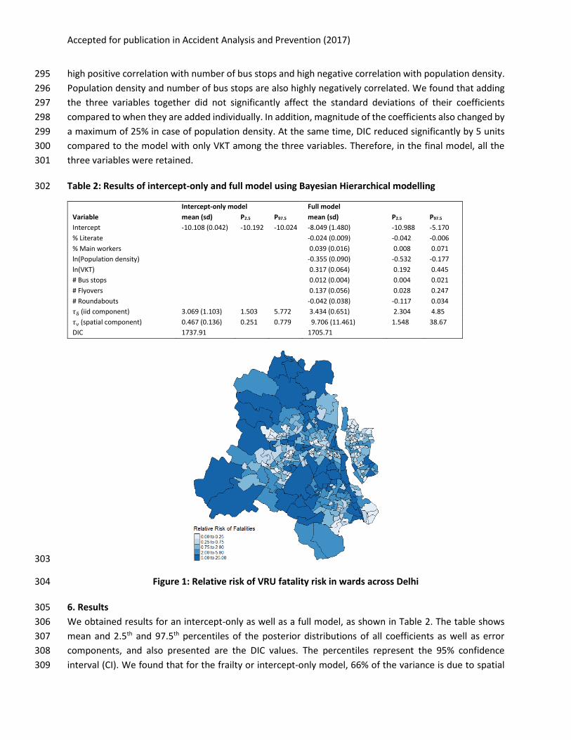
is a Bayesian version of Akaike information criterion (AIC). DIC is calculated as: 284

𝐷𝐼𝐶 = 𝐷(𝜃𝐵𝑎𝑦𝑒𝑠) + 2𝑝𝐷𝐼𝐶 285

where, the first term in right-hand side is the deviance calculated for the posterior mean of the estimated 286

parameters, and second term is the effective number of parameters in the model. Compared to maximum 287

likelihood method, in Bayesian hierarchical modeling, deviance is evaluated at mean of posterior 288

distributions rather than maximum likelihood estimate of parameters and the number of effective 289

parameters tend to be less (Gelman et al., 2014, p. 172). Similar to AIC, lower value of DIC implies higher 290

predictive accuracy. 291

5.1 Selection of variables 292

Before progressing to development of the regression model, we investigate the Pearson correlation 293

between various variables in order to avoid multicollinearity between the independent variables. VKT has 294


high positive correlation with number of bus stops and high negative correlation with population density. 295

Population density and number of bus stops are also highly negatively correlated. We found that adding 296

the three variables together did not significantly affect the standard deviations of their coefficients 297

compared to when they are added individually. In addition, magnitude of the coefficients also changed by 298

a maximum of 25% in case of population density. At the same time, DIC reduced significantly by 5 units 299

compared to the model with only VKT among the three variables. Therefore, in the final model, all the 300

three variables were retained. 301

Table 2: Results of intercept-only and full model using Bayesian Hierarchical modelling 302

Intercept-only model Full model

Variable mean (sd) P2.5 P97.5 mean (sd) P2.5 P97.5

Intercept -10.108 (0.042) -10.192 -10.024 -8.049 (1.480) -10.988 -5.170

% Literate -0.024 (0.009) -0.042 -0.006

% Main workers 0.039 (0.016) 0.008 0.071

ln(Population density) -0.355 (0.090) -0.532 -0.177

ln(VKT) 0.317 (0.064) 0.192 0.445

# Bus stops 0.012 (0.004) 0.004 0.021

# Flyovers 0.137 (0.056) 0.028 0.247

# Roundabouts -0.042 (0.038) -0.117 0.034

𝜏δ (iid component) 3.069 (1.103) 1.503 5.772 3.434 (0.651) 2.304 4.85

𝜏ν (spatial component) 0.467 (0.136) 0.251 0.779 9.706 (11.461) 1.548 38.67

DIC 1737.91 1705.71

303

Figure 1: Relative risk of VRU fatality risk in wards across Delhi 304

6. Results 305

We obtained results for an intercept-only as well as a full model, as shown in Table 2. The table shows 306

mean and 2.5th and 97.5th percentiles of the posterior distributions of all coefficients as well as error 307

components, and also presented are the DIC values. The percentiles represent the 95% confidence 308

interval (CI). We found that for the frailty or intercept-only model, 66% of the variance is due to spatial 309


component, while the rest is due to unstructured heterogeneity of ward. Full model explained 89% of the 310

variation of spatial error, however, it explained less than 20% of the variation in uncorrelated 311

heterogeneity. In the intercept-only model, exponential of intercept term,exp( β0), represents the 312

background fatality risk across the wards and exponential of sum of two error components,exp (δ𝑖 + ν𝑖), 313

represents the relative risk of each ward, and the latter is presented in Figure1. 314

On the basis of 95% CI of posterior distributions, all the coefficients are significantly different from zero, 315

except number of roundabouts. Percentage of literate population, number of roundabouts and 316

population density have a negative association with fatality risk and percentage of population as workers, 317

number of bus stops, number of flyovers, and VKT have positive association. Here, a positive association 318

indicates that with an increase in a variable, the fatality risk increases. 319

7. Discussion 320

7.1 Socio-economics and demographics 321

An increase in literacy rate, which is an indicator of socio-economic status (SES) of the ward, is associated 322

with lower risk of fatalities. This is possible because population with low SES are more likely to be VRUs 323

as they walk, cycle, use PT or ride MTW for their daily travel. In Delhi, only one-fifth of all households own 324

a car (Census-India, 2012). With low level of car ownership, whether an individual is VRU or not is highly 325

sensitive to their income level. Million Death Study (Hsiao et al., 2013) also reported pedestrian deaths 326

to be positively associated with living in poorer neighborhoods. A large number of studies have shown 327

similar results linking higher risk of fatalities, or number of road crashes in general, with lower SES 328

(Aguero-Valverde and Jovanis, 2006; Wier et al., 2009; DiMaggio et al., 2015; Xu et al., 2017). 329

The percentage of population as main workers is positively associated with the fatality risk. According to 330

Census 2011, 65% of the main workers in Delhi are in the age group 30–59, and 86% of them are males. 331

Therefore, workers represent a specific demographic group, which is predominantly male in the age group 332

30–59. This is also reflected in the age and sex distribution of injuries. For the three-year fatality data 333

(2010-2012) reported in the current study, sex of victims was reported for year 2010, according to which 334

males accounted for 91% of all fatality victims, while their share in overall population is 54% (Census-335

India, 2012). The disproportionate share of men in the age group 15-59 years was also reported by the 336

Million Death Study (Hsiao et al., 2013). This explains a positive association of main workers with fatality 337

risk. 338

It is interesting to note that even though Pearson correlation between percentage of main workers and 339

percentage of literate population is positive, the coefficients of the two variables are opposite in signs. 340

This means that SES (indicated by literacy) and demographics (indicated by workers) have their 341

independent effects which are opposite in directions. 342

343

7.2 Traffic volume and roundabouts 344

Positive effect of VKT is expected and has been consistently reported by all studies which considered it as 345

one of the covariates (Amoh-Gyimah et al., 2016; Demiroluk and Ozbay, 2014; DiMaggio et al., 2015; 346

Quddus, 2008; Xu et al., 2017; Aguero-Valverde and Jovanis, 2006; Huang et al., 2010; Wier et al., 2009). 347

According to the posterior distribution of coefficient of number of roundabouts, up to 85th percentile 348


value is a negative. One of the benefits of Bayesian method over frequentist method is that while the 349

latter reports coefficients as single values, the former reports them as distributions of values. Thus it can 350

be said that, given the data, there is more evidence in favour of a negative association of roundabouts 351

with fatality risk than a positive or no effect. 352

The negative association of roundabouts with fatality risk is also expected from international experience. 353

Roundabouts have been adopted globally as a traffic calming measure because of their effectiveness to 354

reduce road crashes. According to a meta-analysis of 28 studies in non-US locations, conversion of 355

intersections to roundabouts resulted in 50-70% reduction of the fatal crashes (Elvik, 2003). In Holland, 356

before-and-after studies of the construction of about 200 roundabouts showed a significant drop of 89% 357

of pedestrian fatalities (Schoon and Van Minnen, 1994). 358

7.3 Flyovers and bus stops 359

Apart from roundabouts, flyovers and bus stops are two other variables representing road infrastructure, 360

and we will discuss the two together because of their related features. Flyovers have a strong positive 361

association with fatality risk, with one flyover increasing the relative risk by 15% compared to no flyover. 362

Bus stops are also positively related to fatality risk. These effects are independent of the volume of traffic. 363

The coefficients of the two variables may not be isolated effects of the two infrastructure elements and 364

could also be indicating the effect of other built environment features which occur simultaneously. 365

366

Flyovers in Delhi have been built along major arterial roads (for instance the two ring roads) as well as 367

highways. Bus stops in Delhi are also located on most major roads, of which arterials and highways are 368

subsets. Most residential and commercial areas do not have enough carriageway width for movement of 369

the bus. Therefore, both bus stops and flyovers are likely to represent road types with heavy vehicular 370

movement. The roads with flyovers also have 40 to 50% higher average speed than other major roads 371

(Mohan et al., 2017). 372

A study conducted in Delhi (Khatoon et al., 2013) studied traffic characteristics before and after the 373

replacement of signalised junction with a flyover. The study reported that the average speed travelled by 374

trucks and buses as well as the variability of the speed of all vehicle types increased after the construction 375

of flyover. Another study from Delhi also found presence of flyovers as a significant factor affecting the 376

number of pedestrian crashes (Rankavat and Tiwari, 2015). Thus there is a strong evidence suggesting 377

that construction of flyovers results in high increase in the risk of injuries. 378

One of the major confounding variables which has been excluded in this analysis is the volume of trucks, 379

which may bring endogeneity in the model results. A network of national highways pass through the city 380

in multiple directions making it a natural route for long–distance trucks as well as a hub for goods 381

exchange. A large proportion of goods movement occurs in Delhi through road-based freight modes. High 382

volume of trucks is also a major source of pollution in Delhi (Goel and Guttikunda, 2015). It is possible 383

that the model may have introduced an upward bias in the effect of number of flyovers and number of 384

bus stops. However, given the magnitude of association for both bus stops and flyovers as well as high 385

statistical significance indicated by their posterior distributions, the addition of any other risk factor is 386

unlikely to change the direction of association. 387


388 Figure 2: Relative risk at different density levels compared to city-level average (250 pph) 389

7.4 Population density 390

Population density is log transformed therefore its coefficient cannot be interpreted in the similar manner 391

as other independent variables. Since the relative risk is an exponent of product of the variable and its 392

coefficient (exp(β𝑖X𝑖)), the relative risk (RR) of population density can be expressed as power functions, 393

as1: 394

𝑅𝑅 = (𝑃𝑜𝑝𝑢𝑙𝑎𝑡𝑖𝑜𝑛 𝑑𝑒𝑛𝑠𝑖𝑡𝑦)−0.355 395

In order to understand the effect of density, we expressed the relative risk with respect to the overall 396

average population density (total population/total built-up area) of 250 pph. Figure 2 indicates that 397

relative risk of fatalities is more than 1.8 times higher at density of 50 pph compared to city-level average. 398

The non-linear curve shows that at higher density levels, the effect of density flattens off and the most 399

reduction in relative risk is up to a density of 850 pph. There are various factors which could result in this 400

association of density with risk and we discuss those in the following text. 401

High density locations are more likely to have higher number of pedestrians. In the absence of dedicated 402

facilities for pedestrians and cyclists, the two slow-moving road users occupy the curb-side lane of the 403

roads. This effectively slows down the traffic and makes roads safer. With an increase in the volume of 404

pedestrian, their risk reduces, and this phenomenon is referred to as safety-in-numbers (Jacobsen, 2003; 405

Elvik and Bjørnskau, 2015). Thus the negative association of relative risk with density may likely be an 406

indicator of safety-in-numbers. 407

High density also attracts higher number of IPT, such as cycle rickshaws, auto rickshaws, and e-rickshaws. 408

These modes are demand responsive and are operated by private operators. Therefore, their volumes are 409

proportional to density or the demand. Since buses do not operate through streets in residential areas, 410

IPT is also used for last-mile connectivity of a bus or metro trip (Goel and Tiwari, 2015). In the absence of 411

1 𝑒𝛽.ln(𝑋) = 𝑋𝛽

0

0.2

0.4

0.6

0.8

1

1.2

1.4

1.6

1.8

50

15

02

50

35

04

50

55

06

50

75

08

50

95

01

05

01

15

01

25

01

35

01

45

01

55

01

65

01

75

01

85

01

95

02

05

02

15

02

25

02

35

02

45

0

Rel

ativ

e R

isk

Population density (persons per hectare)


dedicated parking bays or stops, these vehicles idle along the curb-side lane for passenger boarding and 412

alighting, leading to further congestion. On-street parking/idling effectively narrows the roads, and driver 413

tend to be more cautious while driving through those sections (Gattis, 2000). 414

In Delhi, as well as in most Indian cities, most informal neighborhoods or commercial areas have high 415

built-up density and narrow roads. Informality implies that most growth in built-up is in-situ (as opposed 416

to Greenfield development). Also, the street design is not according to municipal bye-laws which ensure 417

wide-enough streets. Formally designed high-income neighborhoods often have wider streets, but due to 418

on-street car parking by the residents, road widths are effectively reduced. 419

As a result, most through movement of motorised traffic occurs on major roads, and those driving through 420

the narrow streets tend to drive slow. In addition to slower and low volume of traffic, trucks and buses 421

are almost absent in these locations. While trucks are restricted by police, buses do not ply due to lack of 422

space. This can also be seen through a negative correlation of population density with both, number of 423

bus stops as well as VKT, which in turn are proxies of major roads. Therefore, high density should also be 424

interpreted as a proxy of residential/commercial land-use and street design, and these correlates of high 425

density act as speed calming measures. 426

The relationship of crash risk with population density has been inconsistent across the studies. While 427

Graham and Glaister (2003) and Noland and Quddus (2004) reported a negative association between 428

density and crash risk, Lovegrove and Sayed (2006), Huang et al. (2010), Dumbaugh and Li (2010), 429

Chakravarty et al. (2010), Siddiqui et al. (2012), and Narayanmoorthy et al. (2013) reported a positive 430

association between the two. Both the studies showing negative relationship were based on country-wide 431

analysis in the UK using wards as areal units, and all the studies showing positive relationship were based 432

in either US or Canada— Florida, San Antonio, California, Manhattan, and Vancouver. 433

434

The cities in the US have higher car ownership and lower population density than the UK (Guiliano and 435

Narayan, 2003). Compared to both US and UK, Delhi’s density is an order of magnitude higher and car 436

ownership a magnitude of order lower. In a setting with high car ownership, higher density may imply 437

higher number of cars against a smaller number of pedestrians. In contrast, in a setting such as Delhi, it 438

implies much higher number of pedestrians in conflict with comparatively smaller number of motorised 439

modes. Thus, density can imply different mechanisms in place in different settings. 440

441

8. Conclusion 442

Pedestrians, cyclists and MTW users constitute the largest group of fatality victims in Delhi. In Delhi as 443

well as in most Indian cities, overall traffic enforcement is weak, especially in terms of speed as well as 444

alcohol limit. In addition, the infrastructure facilities for pedestrians are poor, for cyclists almost absent, 445

and MTW use the same lanes as other motorised modes. The mixing of VRUs with vehicles of much larger 446

weight and speed results in greater injury risk. In this context, improving safety through design of built 447

environment can prove to be highly effective. Therefore, it is important to understand built environment 448

factors which affect fatality risk. In this study we assessed the risk resulting from roundabouts, bus stops, 449

flyovers and population density while controlling for traffic volumes and population characteristics. 450

451


With higher emphasis on smooth traffic flow and higher speed, a large number of flyovers have been built 452

within populated areas in Delhi as well as many Indian cities. We found that an addition of a flyover 453

increases the fatality risk in a ward by up to 15%, and this effect is independent of traffic volume. While 454

the construction of flyovers pose a challenge of lock-in, their effect on speed of vehicles can be controlled 455

by using speed enforcement by the police or using passive measures such as installment of rumble strips. 456

Given the high risk posed by addition of flyovers, their use as congestion mitigation measures within urban 457

areas should be discontinued. 458

459

In addition, cities in India need to consider the use of roundabouts as an alternative of traffic junctions to 460

minimise the number of road crashes. Many cities in India are doing exactly the reverse by replacing 461

roundabouts with traffic junctions. For traffic planners to willingly adopt roundabouts, it is important that 462

their designs are based on latest international experience which result in increased safety as well as 463

efficient traffic movement. 464

465

There is a positive association with fatality risk and social deprivation, thus indicating socio-economic 466

inequity of injury risk. Given a negative relationship of risk and population density, future studies should 467

investigate the street design and built environment features of high density locations in Delhi to 468

understand the causal mechanism behind this relationship. These factors can then be incorporated in 469

future city designs. 470

9. References 471

Aarts, L., & Van Schagen, I. (2006). Driving speed and the risk of road crashes: A review. Accident Analysis 472 & Prevention, 38(2), 215-224. 473

Aguero-Valverde, J., & Jovanis, P. P. (2006). Spatial analysis of fatal and injury crashes in Pennsylvania. 474 Accident Analysis & Prevention, 38(3), 618-625. doi: http://dx.doi.org/10.1016/j.aap.2005.12.006 475

Amoh-Gyimah, R., Saberi, M., & Sarvi, M. (2016). Macroscopic modeling of pedestrian and bicycle crashes: 476 A cross-comparison of estimation methods. Accident Analysis & Prevention, 93, 147-159. doi: 477 http://dx.doi.org/10.1016/j.aap.2016.05.001 478

Arora, A., Gadepalli, R., Sharawat, P., Vaid, A., & Keshri, A. (2014). Low-carbon Comprehensive Mobility 479 Plan: Vishakhapatnam. UNEP DTU Partnership, Technical University of Denmark. 480

Besag, J., York, J., & Mollié, A. (1991). Bayesian image restoration, with two applications in spatial 481 statistics. Annals of the Institute of Statistical Mathematics, 43(1), 1-20. doi: 10.1007/bf00116466 482

Bivand, R. S., Gómez-Rubio, V., & Rue, H. (2014). Some Spatial Statistical Extensions to R-INLA. Journal of 483 Statistical Software. 484

Cameron, M. H., & Elvik, R. (2010). Nilsson's Power Model connecting speed and road trauma: 485 Applicability by road type and alternative models for urban roads. Accident Analysis & Prevention, 486 42(6), 1908-1915. doi: http://dx.doi.org/10.1016/j.aap.2010.05.012 487

Census-India (2012). Census of India, 2011. The Government of India, New Delhi, India. 488 Census-India (2016). B-28 'Other Workers' By Distance From Residence To Place Of Work And Mode Of 489

Travel To Place Of Work – 2011(India/States/UTs/District), Census of India 2011, The Government 490 of India, New Delhi, India. Accessed online < 491 http://www.censusindia.gov.in/2011census/population_enumeration.html> 492


Chakravarthy, B., Anderson, C. L., Ludlow, J., Lotfipour, S., & Vaca, F. E. (2010). The relationship of 493 pedestrian injuries to socioeconomic characteristics in a large Southern California County. Traffic 494 injury prevention, 11(5), 508-513. 495

Cramb, S. M., Mengersen, K. L., & Baade, P. D. (2011). Developing the atlas of cancer in Queensland: 496 methodological issues. International journal of health geographics, 10(1), 1. 497

Demiroluk, S., & Ozbay, K. (2014). Spatial Analysis of County Level Crash Risk in New Jersey Using Severity-498 Based Hierarchical Bayesian Models. Paper presented at the Transportation Research Board 93rd 499 Annual Meeting. 500

DiMaggio, C. (2015). Small-Area Spatiotemporal Analysis of Pedestrian and Bicyclist Injuries in New York 501 City. Epidemiology, 26(2), 247-254. 502

Dumbaugh, E., Li, W., & Joh, K. (2013). The built environment and the incidence of pedestrian and cyclist 503 crashes. Urban Design International, 18(3), 217-228. 504

EEA (2003). Indicator fact sheet- TERM 2002 32 EU—Size and composition of the vehicle fleet. European 505 Environment Agency. 506

Elvik, R. (2003). Effects on road safety of converting intersections to roundabouts: review of evidence from 507 non-US studies. Transportation Research Record: Journal of the Transportation Research 508 Board(1847), 1-10. 509

Elvik, R. (2009). The non-linearity of risk and the promotion of environmentally sustainable 510 transport. Accident Analysis & Prevention, 41(4), 849-855. 511

Elvik, R., & Bjørnskau, T. (2017). Safety-in-numbers: a systematic review and meta-analysis of evidence. 512 Safety Science, 92, 274-282. 513

Ewing, R., & Dumbaugh, E. (2009). The built environment and traffic safety a review of empirical evidence. 514 Journal of Planning Literature, 23(4), 347-367. 515

Fitzpatrick, K., Carlson, P., Brewer, M., & Wooldridge, M. (2001). Design factors that affect driver speed 516 on suburban streets. Transportation Research Record: Journal of the Transportation Research 517 Board(1751), 18-25. 518

Garg, N., & Hyder, A. A. (2006). Review Article: Road traffic injuries in India: A review of the literature. 519 Scandinavian Journal of Public Health, 34(1), 100-109. 520

Gelman, A., Carlin, J. B., Stern, H. S., & Rubin, D. B. (2014). Bayesian data analysis (Vol. 2): Chapman & 521 Hall/CRC Boca Raton, FL, USA. 522

Giuliano, G., & Narayan, D. (2003). Another look at travel patterns and urban form: the US and Great 523 Britain. Urban studies, 40(11), 2295-2312. 524

Goel, R. (2017). Public health effects of urban transport in Delhi (Doctoral Dissertation). Transportation 525 Research and Injury Prevention Programme, Indian Institute of Technology Delhi, New Delhi. 526

Goel, R., & Guttikunda, S. K. (2015). Evolution of on-road vehicle exhaust emissions in Delhi. Atmospheric 527 Environment, 105, 78-90. 528

Goel, R., & Tiwari, G. (2016). Access–egress and other travel characteristics of metro users in Delhi and its 529 satellite cities. IATSS Research, 39(2), 164-172. 530

Goel, R., Guttikunda, S. K., Mohan, D., & Tiwari, G. (2015). Benchmarking vehicle and passenger travel 531 characteristics in Delhi for on-road emissions analysis. Travel Behaviour and Society, 2(2), 88-101. 532

Gower, L.A. (2013). 2011 Census Analysis - Method of Travel to Work in England and Wales Report. 533 Analysis and Dissemination, Office for National Statistics, UK. 534

Graham, D. J., & Glaister, S. (2003). Spatial variation in road pedestrian casualties: the role of urban scale, 535 density and land-use mix. Urban studies, 40(8), 1591-1607. 536

Grundy, C., Steinbach, R., Edwards, P., Green, J., Armstrong, B., & Wilkinson, P. (2009). Effect of 20 mph 537 traffic speed zones on road injuries in London, 1986-2006: controlled interrupted time series 538 analysis. BMJ, 339. 539


Gupta, U., Tiwari, G., Chatterjee, N., & Fazio, J. (2010). Case study of pedestrian risk behavior and survival 540 analysis. Journal of the Eastern Asia Society for Transportation Studies, 8, 2123-2139. 541

Gururaj, G. (2008). Road traffic deaths, injuries and disabilities in India: Current scenario. The national 542 medical journal of India, Volume 21. 543

Guttikunda, S. K., Goel, R., & Pant, P. (2014). Nature of air pollution, emission sources, and management 544 in the Indian cities. Atmospheric Environment, 95, 501-510. doi: 545 http://dx.doi.org/10.1016/j.atmosenv.2014.07.006 546

Hadayeghi, A., Shalaby, A., & Persaud, B. (2003). Macrolevel accident prediction models for evaluating 547 safety of urban transportation systems. Transportation Research Record: Journal of the 548 Transportation Research Board(1840), 87-95. 549

Hsiao, M., Malhotra, A., Thakur, J. S., Sheth, J. K., Nathens, A. B., Dhingra, N., . . . Collaborators, f. t. M. D. 550 S. (2013). Road traffic injury mortality and its mechanisms in India: nationally representative 551 mortality survey of 1.1 million homes. BMJ Open, 3(8). doi: 10.1136/bmjopen-2013-002621 552

Huang, H., Abdel-Aty, M., & Darwiche, A. (2010). County-level crash risk analysis in Florida: Bayesian 553 spatial modeling. Transportation Research Record: Journal of the Transportation Research 554 Board(2148), 27-37. 555

Hydén, C., & Várhelyi, A. (2000). The effects on safety, time consumption and environment of large scale 556 use of roundabouts in an urban area: a case study. Accident Analysis & Prevention, 32(1), 11-23. 557

Iamsterdam (2014). Facts & Figures: Road Safety 2012-2015. Accessed October 10, 2015 from < 558 https://www.amsterdam.nl/parkeren-verkeer/fiets/cycling-amsterdam/road-safety/> 559

Jacobsen, P. L. (2003). Safety in numbers: more walkers and bicyclists, safer walking and bicycling. Injury 560 prevention, 9(3), 205-209. 561

Jones, A. P., Haynes, R., Kennedy, V., Harvey, I. M., Jewell, T., & Lea, D. (2008). Geographical variations in 562 mortality and morbidity from road traffic accidents in England and Wales. Health & Place, 14(3), 563 519-535. doi: http://dx.doi.org/10.1016/j.healthplace.2007.10.001 564

Khatoon, M., Tiwari, G., & Chatterjee, N. (2013). Impact of grade separator on pedestrian risk taking 565 behavior. Accident Analysis & Prevention, 50, 861-870. doi: 566 http://dx.doi.org/10.1016/j.aap.2012.07.011 567

Kim, K., Brunner, I., & Yamashita, E. (2006). Influence of Land Use, Population, Employment, and Economic 568 Activity on Accidents. Transportation Research Record: Journal of the Transportation Research 569 Board, 1953, 56-64. doi: 10.3141/1953-07 570

Ladron de Guevara, F., Washington, S., & Oh, J. (2004). Forecasting crashes at the planning level: 571 simultaneous negative binomial crash model applied in Tucson, Arizona. Transportation Research 572 Record: Journal of the Transportation Research Board(1897), 191-199. 573

LaScala, E. A., Gerber, D., & Gruenewald, P. J. (2000). Demographic and environmental correlates of 574 pedestrian injury collisions: a spatial analysis. Accident Analysis & Prevention, 32(5), 651-658. doi: 575 http://dx.doi.org/10.1016/S0001-4575(99)00100-1 576

Leden, L. (2002). Pedestrian risk decrease with pedestrian flow. A case study based on data from signalized 577 intersections in Hamilton, Ontario. Accident Analysis & Prevention, 34(4), 457-464. 578

Lovegrove, G. R., & Sayed, T. (2006). Macro-level collision prediction models for evaluating neighbourhood 579 traffic safety. Canadian Journal of Civil Engineering, 33(5), 609-621. doi: 10.1139/l06-013 580

MacNab, Y. C. (2004). Bayesian spatial and ecological models for small-area accident and injury analysis. 581 Accident Analysis & Prevention, 36(6), 1019-1028. doi: 582 http://dx.doi.org/10.1016/j.aap.2002.05.001 583

McKenzie, B., & Rapino, M. (2011). Commuting in the united states: 2009: US Department of Commerce, 584 Economics and Statistics Administration, US Census Bureau Washington, DC. 585

Miller, E., & Ibrahim, A. (1998). Urban form and vehicular travel: some empirical findings. Transportation 586 Research Record: Journal of the Transportation Research Board(1617), 18-27. 587

https://www.amsterdam.nl/parkeren-verkeer/fiets/cycling-amsterdam/road-safety/


Mohan, D., Tiwari, G., & Bhalla, K. (2015). Road Safety in India- Status Report. New Delhi: Transportation 588 Research and Injury Prevention Programme, Indian Institute of Technology Delhi. 589

Mohan, D., Tiwari, G., & Mukherjee, S. (2016). Urban traffic safety assessment: A case study of six Indian 590 cities. IATSS Research, 39(2), 95-101. doi: http://dx.doi.org/10.1016/j.iatssr.2016.02.001 591

Mohan, D., Tiwari, G., Goel, R., & Lakhar, P. (2017). Evaluation of the Odd-Even Day Traffic Restriction 592 Experiments in Delhi, India. Transportation Research Record: Journal of the Transportation 593 Research Board. No. 17-04218 594

Mohan, D., Tsimhoni, O., Sivak, M., & Flannagan, M. J. (2009). Road safety in India: challenges and 595 opportunities. University of Michigan, US. 596

MoRTH (2012). Road Transport Year Book (2011-12). Transport Research Wing, Ministry of Road Transport 597 and Highways, Government of India, New Delhi 598

MOT (2009). Cycling in the Netherlands. Ministry of Transport, Public Works and Water Management, 599 Directorate-General for Passenger Transport, The Netherlands. 600

Narayanamoorthy, S., Paleti, R., & Bhat, C. R. (2013). On accommodating spatial dependence in bicycle 601 and pedestrian injury counts by severity level. Transportation Research Part B: Methodological, 55, 602 245-264. doi: http://dx.doi.org/10.1016/j.trb.2013.07.004 603

NCRB (2015). Accidental deaths & suicides in India 2014. National Crime Records Bureau, New Delhi. 604 Nilsson, G., 1981. The effects of speed limits on traffic accidents in Sweden. In:Proceedings, International 605

symposium on the effects of speed limits on traffic crashes and fuel consumption, Dublin. OECD, 606 Paris. 607

Noland, R. B., & Quddus, M. A. (2004). A spatially disaggregate analysis of road casualties in England. 608 Accident Analysis & Prevention, 36(6), 973-984. doi: http://dx.doi.org/10.1016/j.aap.2003.11.001 609

NYDMV (2014). Summary of New York City motor vehicle crashes 2014. New York State Department of 610 Motor Vehicles, New York City, US. 611

OECD/ECMT (2006). Speed management- Summary Document. Transportation Research Centre. 612 Organization for Economic Cooperation and Development and European Conference of Ministers 613 of Transport. 614

Peden, M., Scurfield, R., Sleet, D., Mohan, D., Hyder, A. A., Jarawan, E., & Mathers, C. D. (2004). World 615 report on road traffic injury prevention: World Health Organization Geneva. 616

Ponnaluri, R. V. (2012). Modeling road traffic fatalities in India: Smeed's law, time invariance and regional 617 specificity. IATSS Research, 36(1), 75-82. doi: http://dx.doi.org/10.1016/j.iatssr.2012.05.001 618

Pucher, J., Peng, Z. r., Mittal, N., Zhu, Y., & Korattyswaroopam, N. (2007). Urban transport trends and 619 policies in China and India: impacts of rapid economic growth. Transport Reviews, 27(4), 379-410. 620

Pulugurtha, S. S., Duddu, V. R., & Kotagiri, Y. (2013). Traffic analysis zone level crash estimation models 621 based on land use characteristics. Accident Analysis & Prevention, 50, 678-687. 622

Quddus, M. A. (2008). Modelling area-wide count outcomes with spatial correlation and heterogeneity: 623 An analysis of London crash data. Accident Analysis & Prevention, 40(4), 1486-1497. doi: 624 http://dx.doi.org/10.1016/j.aap.2008.03.009 625

Rankavat, S., & Tiwari, G. (2015). Association Between Built Environment and Pedestrian Fatal Crash Risk 626 in Delhi, India. Transportation Research Record: Journal of the Transportation Research 627 Board(2519), 61-66. 628

RITES (2008). Transport Demand Forecast Study and Development of an Integrated Road cum Multi-modal 629 Public Transport Network for NCT of Delhi, Household Interview Survey Report, Chapter-4, Travel 630 Characteristics, RITES Ltd. 631

RITES (2013). Total Transport System System Study on Traffic Flows and Modal Costs (Highways, Railways, 632 Airways and Coastal Shipping), A Study Report for the Planning Commission, The Government of 633 India, New Delhi, India (2013) 634

http://dx.doi.org/10.1016/j.trb.2013.07.004


Rivara, F. P. (1990). Child pedestrian injuries in the United States. Current status of the problem, potential 635 interventions, and future research needs. Am J Dis Child, 144(6), 692-696. 636

Rouphail, N. M. (1984). Midblock crosswalks: a user compliance and preference study. 637 Rue, H., Martino, S., & Lindgren, F. (2009). INLA: Functions which allow to perform a full Bayesian analysis 638

of structured (geo-) additive models using Integrated Nested Laplace Approximaxion. R Package 639 version 0.0 ed. 640

Schoon, C., & van Minnen, J. (1994). Safety of roundabouts in The Netherlands. Traffic engineering and 641 control, 35(3), 142-148. 642

Siddiqui, C., Abdel-Aty, M., & Choi, K. (2012). Macroscopic spatial analysis of pedestrian and bicycle 643 crashes. Accident Analysis & Prevention, 45, 382-391. doi: 644 http://dx.doi.org/10.1016/j.aap.2011.08.003 645

Tanaboriboon, Y., & Jing, Q. (1994). Chinese pedestrians and their walking characteristics: case study in 646 Beijing. Transportation research record, 16-16. 647

TFL (2014). Casualties in Greater London during 2013. Fact sheet, Surface Planning, Surface Transport, 648 Transport for London, London, UK. 649

Tiwari, G. (2002). Planning for bicycles and other non motorised modes: The critical element in city 650 transport system. Paper presented at the ADB International Workshop on Transport Planning, 651 Demand Management and Air Quality. 652

Tiwari, G., Bangdiwala, S., Saraswat, A., & Gaurav, S. (2007). Survival analysis: Pedestrian risk exposure at 653 signalized intersections. Transportation research part F: traffic psychology and behaviour, 10(2), 77-654 89. 655

Török, Á. (2011). Investigation of road environment effects on choice of urban and interurban driving 656 speed. International Journal for Traffic and Transport Engineering, 1(1), 1-9. 657

USCB (2011). Commuting in the United States: 2009, American Community Survey Reports. US 658 Department of Commerce, Economics and Statistics Administration, US Census Bureau, US. 659

USDOT (2015). Table 1-11: Number of U.S. Aircraft, Vehicles, Vessels, and Other Conveyances. Bureau of 660 Transportation Statistics, United States Department of Transportation. Accessed onlined 661 <https://www.rita.dot.gov/bts/sites/rita.dot.gov.bts/files/publications/national_transportation_s662 tatistics/html/table_01_11.html> 663

Wang, X., Yang, J., Lee, C., Ji, Z., & You, S. (2016). Macro-level safety analysis of pedestrian crashes in 664 Shanghai, China. Accident Analysis & Prevention, 96, 12-21. doi: 665 http://dx.doi.org/10.1016/j.aap.2016.07.028 666

WHO (2015). Global status report on road safety 2015. World Health Organization. 667 Wier, M., Weintraub, J., Humphreys, E. H., Seto, E., & Bhatia, R. (2009). An area-level model of vehicle-668

pedestrian injury collisions with implications for land use and transportation planning. Accident 669 Analysis & Prevention, 41(1), 137-145. 670

Xu, P., Huang, H., Dong, N., & Wong, S. C. (2017). Revisiting crash spatial heterogeneity: A Bayesian 671 spatially varying coefficients approach. Accident Analysis & Prevention, 98, 330-337. doi: 672 http://dx.doi.org/10.1016/j.aap.2016.10.015 673

http://dx.doi.org/10.1016/j.aap.2016.10.015

Correlates of fatality risk of vulnerable road users in Delhi

Documents

Transcript of Correlates of fatality risk of vulnerable road users in Delhi