Corrected ESI DT-COM-09-2016-003565.R1 · ... using)Evans’)method,9)either)in)toluene)or)THF) ......
30
S1 ELECTRONIC SUPPORTING INFORMATION Heteroleptic, two-coordinate [M(NHC){N(SiMe 3 ) 2 }] (M = Co, Fe) complexes: synthesis, reactivity and magnetism rationalized by an unexpected metal oxidation state Andreas A. Danopoulos,* a,b Pierre Braunstein,* b Kirill Yu. Monakhov,* c Jan van Leusen, c Paul Kögerler,* c,d Martin Clémancey, e JeanMarc Latour, e Anass Benayad, f Moniek Tromp, g Elixabete Rezabal h and Gilles Frison h a. Institute for Advanced Study (USIAS), Université de Strasbourg, 4 rue Blaise Pascal, 67081 Strasbourg Cedex, France, Email: [email protected] b. Université de Strasbourg, CNRS, CHIMIE UMR 7177, Laboratoire de Chimie de Coordination, Institut de Chimie 4 rue Blaise Pascal, 67081 Strasbourg Cedex, France, Email: [email protected] c. Institut für Anorganische Chemie, RWTH Aachen University, Landoltweg 1, 52074 Aachen, Germany, E mail: [email protected], [email protected] d. JülichAachen Research Alliance (JARAFIT) and Peter Grünberg Institute 6, Forschungszentrum Jülich, 52425 Jülich, Germany e. Laboratoire de Chimie et Biologie des Métaux, Equipe de Physicochimie des Métaux en Biologie, UMR 5249 CNRS/CEADRFBIG/, Université GrenobleAlpes,17 rue des Martyrs, Grenoble 38054, France f. CEA / DRT / LITEN / DTNM / SEN / L2N, 17 rue des Martyrs, 38054 Grenoble Cedex 9, France g. Van't Hoff Institute for Molecular Sciences, Sustainable Materials Characterisation, University of Amsterdam, Amsterdam, The Netherlands h. LCM, CNRS, Ecole Polytechnique, Université ParisSaclay, 91128 Palaiseau, France. Contents: 1. Synthesis and Characterization 2 2. Xray Crystallography 7 3. DFT Computational Studies 14 4. Studies of the Magnetic Properties 21 5. XPS Studies 25 6. EXAFS and XANES studies 27 7. References 30 Electronic Supplementary Material (ESI) for Dalton Transactions. This journal is © The Royal Society of Chemistry 2017
Transcript of Corrected ESI DT-COM-09-2016-003565.R1 · ... using)Evans’)method,9)either)in)toluene)or)THF) ......

S1
ELECTRONIC SUPPORTING INFORMATION
Heteroleptic, two-coordinate [M(NHC){N(SiMe3)2}] (M = Co, Fe)
complexes: synthesis, reactivity and magnetism rationalized by an
unexpected metal oxidation state
Andreas A. Danopoulos,*a,b Pierre Braunstein,*b Kirill Yu. Monakhov,*c Jan van Leusen,c Paul
Kögerler,*c,d Martin Clémancey,e Jean-‐Marc Latour,e Anass Benayad,f Moniek Tromp,g
Elixabete Rezabalh and Gilles Frisonh
a. Institute for Advanced Study (USIAS), Université de Strasbourg, 4 rue Blaise Pascal, 67081 Strasbourg Cedex, France, E-‐mail: [email protected]
b. Université de Strasbourg, CNRS, CHIMIE UMR 7177, Laboratoire de Chimie de Coordination, Institut de Chimie 4 rue Blaise Pascal, 67081 Strasbourg Cedex, France, E-‐mail: [email protected]
c. Institut für Anorganische Chemie, RWTH Aachen University, Landoltweg 1, 52074 Aachen, Germany, E-‐ mail: [email protected]‐aachen.de, [email protected]‐aachen.de
d. Jülich-‐Aachen Research Alliance (JARA-‐FIT) and Peter Grünberg Institute 6, Forschungszentrum Jülich, 52425 Jülich, Germany
e. Laboratoire de Chimie et Biologie des Métaux, Equipe de Physicochimie des Métaux en Biologie, UMR 5249 CNRS/CEA-‐DRF-‐BIG/, Université Grenoble-‐Alpes,17 rue des Martyrs, Grenoble 38054, France
f. CEA / DRT / LITEN / DTNM / SEN / L2N, 17 rue des Martyrs, 38054 Grenoble Cedex 9, France g. Van't Hoff Institute for Molecular Sciences, Sustainable Materials Characterisation, University of Amsterdam,
Amsterdam, The Netherlands h. LCM, CNRS, Ecole Polytechnique, Université Paris-‐Saclay, 91128 Palaiseau, France.
Contents: 1. Synthesis and Characterization 2
2. X-‐ray Crystallography 7
3. DFT Computational Studies 14
4. Studies of the Magnetic Properties 21
5. XPS Studies 25
6. EXAFS and XANES studies 27
7. References 30
Electronic Supplementary Material (ESI) for Dalton Transactions.This journal is © The Royal Society of Chemistry 2017
S2
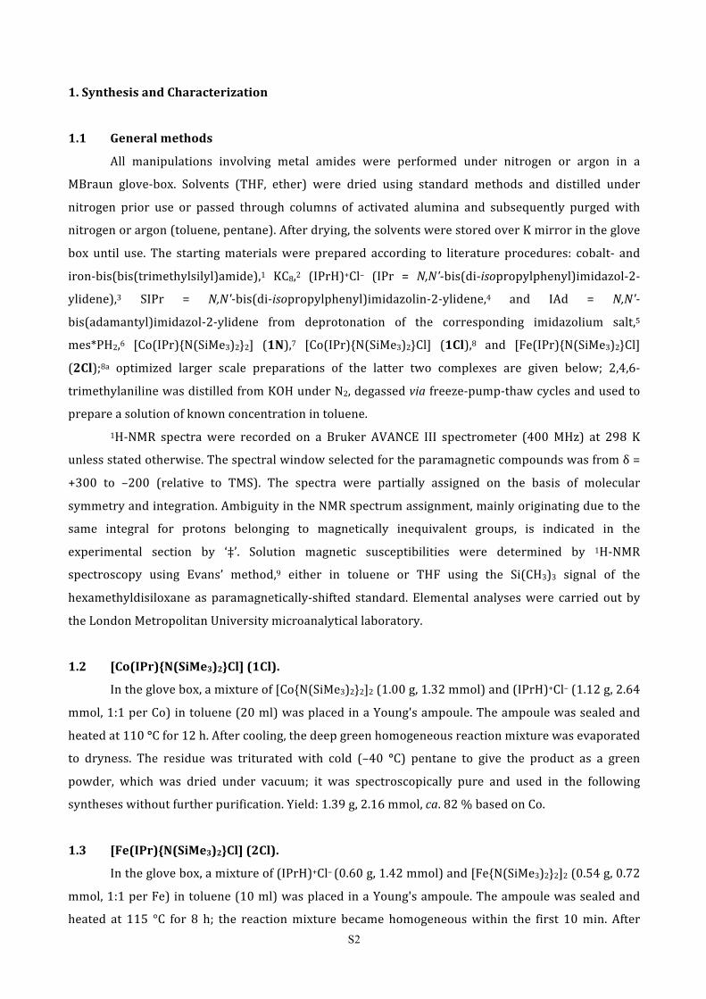
1. Synthesis and Characterization
1.1 General methods
All manipulations involving metal amides were performed under nitrogen or argon in a
MBraun glove-‐box. Solvents (THF, ether) were dried using standard methods and distilled under
nitrogen prior use or passed through columns of activated alumina and subsequently purged with
nitrogen or argon (toluene, pentane). After drying, the solvents were stored over K mirror in the glove
box until use. The starting materials were prepared according to literature procedures: cobalt-‐ and
iron-‐bis(bis(trimethylsilyl)amide),1 KC8,2 (IPrH)+Cl– (IPr = N,N'-‐bis(di-‐isopropylphenyl)imidazol-‐2-‐
ylidene),3 SIPr = N,N'-‐bis(di-‐isopropylphenyl)imidazolin-‐2-‐ylidene,4 and IAd = N,N'-‐
bis(adamantyl)imidazol-‐2-‐ylidene from deprotonation of the corresponding imidazolium salt,5
mes*PH2,6 [Co(IPr){N(SiMe3)2}2] (1N),7 [Co(IPr){N(SiMe3)2}Cl] (1Cl),8 and [Fe(IPr){N(SiMe3)2}Cl]
(2Cl);8a optimized larger scale preparations of the latter two complexes are given below; 2,4,6-‐
trimethylaniline was distilled from KOH under N2, degassed via freeze-‐pump-‐thaw cycles and used to
prepare a solution of known concentration in toluene. 1H-‐NMR spectra were recorded on a Bruker AVANCE III spectrometer (400 MHz) at 298 K
unless stated otherwise. The spectral window selected for the paramagnetic compounds was from δ =
+300 to –200 (relative to TMS). The spectra were partially assigned on the basis of molecular
symmetry and integration. Ambiguity in the NMR spectrum assignment, mainly originating due to the
same integral for protons belonging to magnetically inequivalent groups, is indicated in the
experimental section by ‘‡’. Solution magnetic susceptibilities were determined by 1H-‐NMR
spectroscopy using Evans’ method,9 either in toluene or THF using the Si(CH3)3 signal of the
hexamethyldisiloxane as paramagnetically-‐shifted standard. Elemental analyses were carried out by
the London Metropolitan University microanalytical laboratory.
1.2 [Co(IPr){N(SiMe3)2}Cl] (1Cl).
In the glove box, a mixture of [Co{N(SiMe3)2}2]2 (1.00 g, 1.32 mmol) and (IPrH)+Cl– (1.12 g, 2.64
mmol, 1:1 per Co) in toluene (20 ml) was placed in a Young's ampoule. The ampoule was sealed and
heated at 110 °C for 12 h. After cooling, the deep green homogeneous reaction mixture was evaporated
to dryness. The residue was triturated with cold (–40 °C) pentane to give the product as a green
powder, which was dried under vacuum; it was spectroscopically pure and used in the following
syntheses without further purification. Yield: 1.39 g, 2.16 mmol, ca. 82 % based on Co.
1.3 [Fe(IPr){N(SiMe3)2}Cl] (2Cl).
In the glove box, a mixture of (IPrH)+Cl– (0.60 g, 1.42 mmol) and [Fe{N(SiMe3)2}2]2 (0.54 g, 0.72
mmol, 1:1 per Fe) in toluene (10 ml) was placed in a Young's ampoule. The ampoule was sealed and
heated at 115 °C for 8 h; the reaction mixture became homogeneous within the first 10 min. After

S3
cooling, it was allowed to stand at room temperature for 12 h and then the volatiles were removed to
dryness, giving a brown oily residue, which contained small amounts of toluene. The residue was
triturated with cold pentane giving a colourless solid and a brown supernatant. The solid was collected
and dried, constituting the first crop of product. The supernatant was concentrated and cooled to –40
°C for 48 h to give a second crop of large colourless crystals. If small amounts of toluene are left after
the first evaporation of the volatiles from the reaction mixture, addition of pentane may give a
homogeneous solution which after cooling to –40 °C gives colourless crystals (in two crops). Combined
yield: 0.45 g, ca. 74%. 1H-‐NMR (C6D6): δ 59.35 (4H, DiPP aromatic‡), 20.63 (12H, CH(CH3)2), 3.95 (12H,
CH(CH3)2), –5.73 (18H, N(SiMe3)2), –15.70 (4H, CH(CH3)2‡), –19.18 (2H CH=CH, imid) ppm.
1.4 [Co(IPr){N(SiMe3)2}] (3), Method A.
A solution of [Co(IPr){N(SiMe3)2}2] (1N) (1.00 g 1.30 mmol) and Mes*PH2 (0.40 g, 1.43 mmol
1.1 equiv.) in toluene (20 ml) was stirred at 45 °C for 3 days, when it changed colour from green to
orange-‐brown. If the starting material was not completely consumed after this period (i.e. < 90 %
conversion by 1H NMR), more mes*PH2 (0.10 g, 0.13 mmol, 10%) was added and the reaction was
continued for an additional period of 24 h. After completion, the toluene was removed under reduced
pressure and the residue was extracted into ca. 20 ml pentane. The pentane solution was concentrated
to ca. 6–7 ml and cooled to –40 °C for 24 h to yield yellow-‐orange plates of 3 that were isolated and
dried under vacuum. Yield: 0.55 g, 0.90 mmol, ca. 69%. Further concentration of the supernatant and
cooling at –40 °C for 2 days gave as a second crop minor quantity of 3 contaminated with a few green
crystals of 1N, which was discarded. For C33H55CoN3Si2, calculated (%): C 65.09, H 9.10, N 6.90; found
(%): C 64.98, H 9.02, N 6.90. 1H-‐NMR (C6D6):δ, 178.10 (2H, DiPP aromatic‡), 79.10 (4H, DiPP
aromatic‡), 12.56 (12H, CH(CH3)2), 10.21 (18H, N(SiMe3)2), –39.18 (2H, CH=CH, imid‡), –48.8 (4H,
CH(CH3)2)‡), –152.19 (12H, CH(CH3)2) ppm. The 1H-‐NMR spectrum in d8-‐THF remains unchanged.
NMR spectroscopic analysis of the mother liquor after the second crop revealed the presence of 5 (31P
δ –75.0 (d)) and a minor unidentified species, δ –60.0 (d of d, JP-H = 73.0 Hz) ppm.
1.5 [Co(IPr){N(SiMe3)2}] (3), Method B.
A suspension of [Co(IPr){N(SiMe3)2Cl] (1Cl) (0.25 g, 0.39 mmol) and KC8 (0.063 g, 0.45 mmol,
1.2 equiv.) in pentane (ca. 30 ml) was stirred vigorously at room temperature for 24 h giving a yellow-‐
orange reaction mixture and black graphite. The progress of the reaction was monitored by 1H NMR
spectroscopy and, if necessary, more KC8 was added until conversion was > 95%. Finally, the graphite
and other solids were filtered off using a syringe filter and glass fibre filter paper. The solids were
washed with small amounts of pentane until the washings came out colourless (2 × 5 ml) and the
combined extracts were concentrated to dryness giving a yellow-‐orange microcrystalline powder,
which exhibited an identical 1H-‐NMR spectrum as the complex prepared by method A. Yield: 0.10 g,
0.16 mmol, ca. 41%.
S4
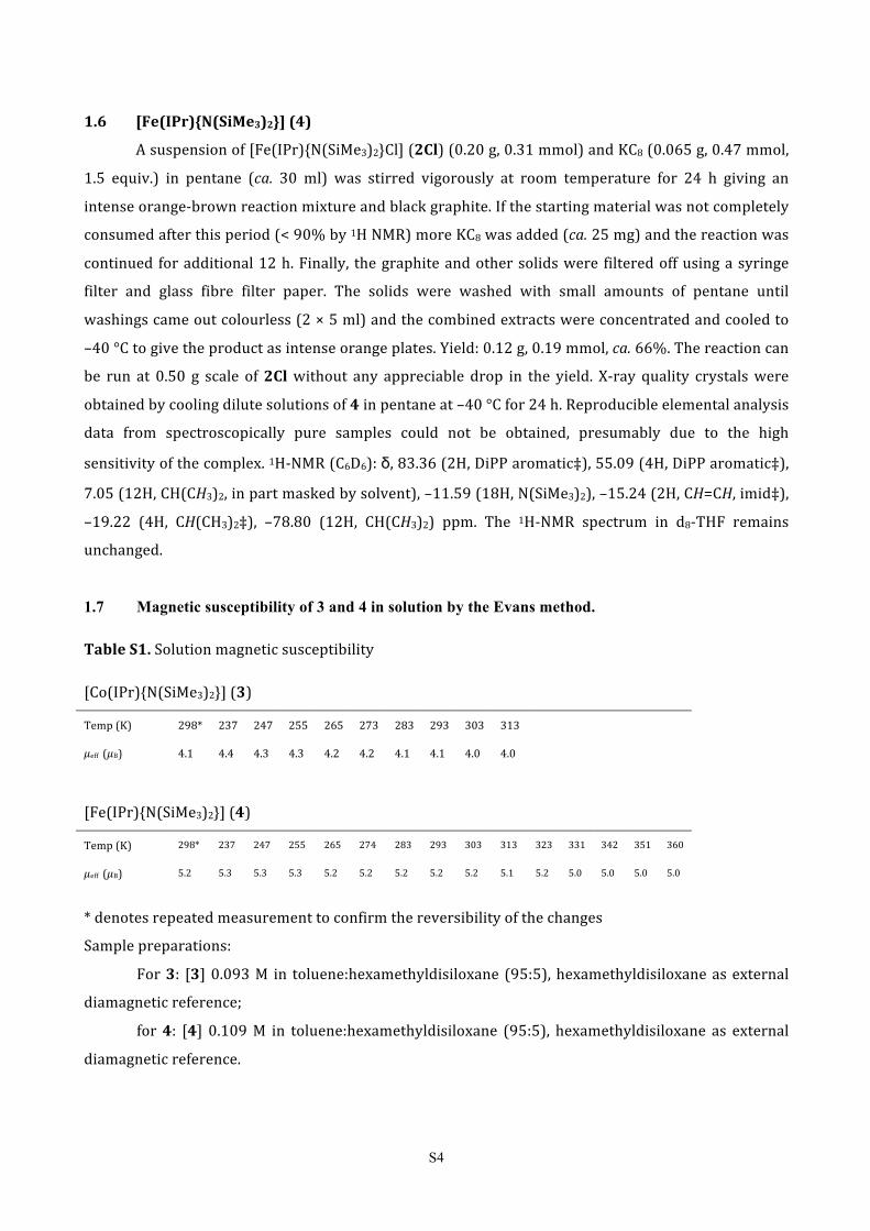
1.6 [Fe(IPr){N(SiMe3)2}] (4)
A suspension of [Fe(IPr){N(SiMe3)2}Cl] (2Cl) (0.20 g, 0.31 mmol) and KC8 (0.065 g, 0.47 mmol,
1.5 equiv.) in pentane (ca. 30 ml) was stirred vigorously at room temperature for 24 h giving an
intense orange-‐brown reaction mixture and black graphite. If the starting material was not completely
consumed after this period (< 90% by 1H NMR) more KC8 was added (ca. 25 mg) and the reaction was
continued for additional 12 h. Finally, the graphite and other solids were filtered off using a syringe
filter and glass fibre filter paper. The solids were washed with small amounts of pentane until
washings came out colourless (2 × 5 ml) and the combined extracts were concentrated and cooled to
–40 °C to give the product as intense orange plates. Yield: 0.12 g, 0.19 mmol, ca. 66%. The reaction can
be run at 0.50 g scale of 2Cl without any appreciable drop in the yield. X-‐ray quality crystals were
obtained by cooling dilute solutions of 4 in pentane at –40 °C for 24 h. Reproducible elemental analysis
data from spectroscopically pure samples could not be obtained, presumably due to the high
sensitivity of the complex. 1H-‐NMR (C6D6): δ, 83.36 (2H, DiPP aromatic‡), 55.09 (4H, DiPP aromatic‡),
7.05 (12H, CH(CH3)2, in part masked by solvent), –11.59 (18H, N(SiMe3)2), –15.24 (2H, CH=CH, imid‡),
–19.22 (4H, CH(CH3)2‡), –78.80 (12H, CH(CH3)2) ppm. The 1H-‐NMR spectrum in d8-‐THF remains
unchanged.
1.7 Magnetic susceptibility of 3 and 4 in solution by the Evans method.
Table S1. Solution magnetic susceptibility
[Co(IPr){N(SiMe3)2}] (3)
Temp (K) 298* 237 247 255 265 273 283 293 303 313
µeff (µB) 4.1 4.4 4.3 4.3 4.2 4.2 4.1 4.1 4.0 4.0
[Fe(IPr){N(SiMe3)2}] (4)
Temp (K) 298* 237 247 255 265 274 283 293 303 313 323 331 342 351 360
µeff (µB) 5.2 5.3 5.3 5.3 5.2 5.2 5.2 5.2 5.2 5.1 5.2 5.0 5.0 5.0 5.0
* denotes repeated measurement to confirm the reversibility of the changes
Sample preparations:
For 3: [3] 0.093 M in toluene:hexamethyldisiloxane (95:5), hexamethyldisiloxane as external
diamagnetic reference;
for 4: [4] 0.109 M in toluene:hexamethyldisiloxane (95:5), hexamethyldisiloxane as external
diamagnetic reference.
S5
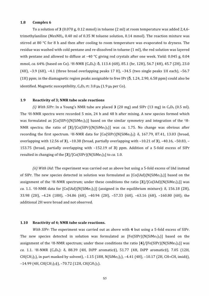
1.8 Complex 6
To a solution of 3 (0.070 g, 0.12 mmol) in toluene (2 ml) at room temperature was added 2,4,6-‐
trimethylaniline (MesNH2, 0.40 ml of 0.35 M toluene solution, 0.14 mmol). The reaction mixture was
stirred at 80 °C for 8 h and then after cooling to room temperature was evaporated to dryness. The
residue was washed with cold pentane and re-‐dissolved in toluene (1 ml), the red solution was layered
with pentane and allowed to diffuse at –40 °C giving red crystals after one week. Yield: 0.045 g, 0.04
mmol, ca. 64% (based on Co). 1H-‐NMR (C6D6): δ, 113.4 (6H), 85.1 (br, 12H), 56.7 (4H), 45.7 (2H), 23.0
(4H), –3.9 (6H), –4.1 (three broad overlapping peaks 17 H), –34.5 (two single peaks 1H each), –56.7
(1H) ppm; in the diamagnetic region peaks assignable to free IPr (δ, 1.24, 2.90, 6.58 ppm) could also be
identified. Magnetic susceptibility, C6D6 rt: 3.8 μB (1.9 μB per Co).
1.9 Reactivity of 3; NMR tube scale reactions
(i) With SIPr: In a Young's NMR tube are placed 3 (20 mg) and SIPr (13 mg) in C6D6 (0.5 ml).
The 1H-‐NMR spectra were recorded 5 min, 24 h and 48 h after mixing. A new species formed which
was formulated as [Co(SIPr){N(SiMe3)2}] based on the similar symmetry and integration of the 1H-‐
NMR spectra; the ratio of [3]/[Co(SIPr){N(SiMe3)2}] was ca. 1.75. No change was obvious after
recording the first spectrum. 1H-‐NMR data for [Co(SIPr){N(SiMe3)2]: δ, 167.79, 87.41, 13.03 (broad,
overlapping with 12.56 of 3), –10.38 (broad, partially overlapping with –10.21 of 3), –40.16, –50.83, –
153.75 (broad, partially overlapping with –152.19 of 3) ppm. Addition of a 5-‐fold excess of SIPr
resulted in changing of the [3]/[Co(SIPr)(N(SiMe3)2] to ca. 1.0.
(ii) With IAd: The experiment was carried out as above but using a 5-‐fold excess of IAd instead
of SIPr. The new species detected in solution was formulated as [Co(IAd){N(SiMe3)2}] based on the
assignment of the 1H-‐NMR spectrum; under these conditions the ratio [3]/[Co(IAd){N(SiMe3)2}] was
ca. 1.1. 1H-‐NMR data for [Co(IAd){N(SiMe3)2}] (assigned in the equilibrium mixture): δ, 156.18 (2H),
33.98 (2H), –4.24 (18H), –34.86 (6H), –40.94 (2H), –57.33 (6H), –63.16 (6H), –160.80 (6H); the
additional 2H were broad and not observed.
1.10 Reactivity of 4; NMR tube scale reactions.
With SIPr: The experiment was carried out as above with 4 but using a 5-‐fold excess of SIPr.
The new species detected in solution was formulated as [Fe(SIPr){N(SiMe3)2}] based on the
assignment of the 1H-‐NMR spectrum; under these conditions the ratio [4]/[Fe(SIPr){N(SiMe3)2}] was
ca. 1.1. 1H-‐NMR (C6D6): δ, 88.39 (4H, DiPP aromatic‡), 51.77 (4H, DiPP aromatic‡), 7.05 (12H,
CH(CH3)2), in part masked by solvent), –1.15 (18H, N(SiMe3)2), –4.41 (4H), –10.17 (2H, CH=CH, imid‡),
–14.99 (4H, CH(CH3)2‡), –70.72 (12H, CH(CH3)2).

S6
With IAd: The experiment was carried out as above but using a 5-‐fold excess of IAd. The new
species detected in solution was formulated as [Fe(IAd){N(SiMe3)2}] based on the assignment of the 1H-‐NMR spectrum; under these conditions the ratio [4]/[Fe(IAd){N(SiMe3)2}] was ca. 1.1. 1H-‐NMR
(C6D6): δ, 77.47, –7.57, –15.63, –20.25, –20.92, –31.90, –70.30.
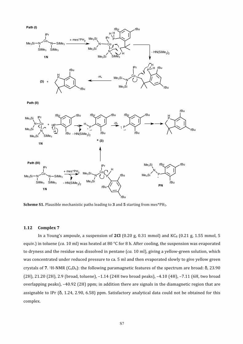
1.11 Proposed mechanisms for the reduction of [Co(IPr){N(SiMe3)2}2] (1N) by mes*PH2
The reduction mechanism is uncertain and may involve homolytic cleavage of Co-‐ligand (Co-‐C,
Co-‐P or Co-‐N) bonds and aminyl radicals [•N(SiMe3)2] analogous to the [•N(SiMe3)DiPP] radicals
postulated for the reduction of Ni(II) to Ni(I) in the interaction of IPr with [Ni{N(SiMe3)}(DiPP)]2.10
However, in the present case the major P-‐containing species that was identified after the end of the
reaction as 3,3-‐dimethyl-‐5,7-‐di-‐tert-‐butyl-‐phosphaindane 5 (Scheme S1).11 It is not certain if 5 was the
primary product from the reduction, since it may have arisen from the decomposition of the transient
phosphinidene mes*P: by intramolecular C-‐H insertion as previously described.12 The mes*P: may
have been formed after aminyl radical attack on the mes*PH2. Aminolysis of Co-‐N by mes*PH2 followed
by homolysis of the Co-‐P bond is also likely. However, formation of the transient PN radical, which has
been reported as persistent,13 has not been observed. The plausible mechanistic paths are given below
(Scheme S1). Interestingly, mes*PH2 does not appear to react further with 3 under the reaction
conditions employed. Reaction of 1N with excess of PtBu3 gave a mixture of products in which 3 is also
present.
S7
Scheme S1. Plausible mechanistic paths leading to 3 and 5 starting from mes*PH2.
1.12 Complex 7
In a Young's ampoule, a suspension of 2Cl (0.20 g, 0.31 mmol) and KC8 (0.21 g, 1.55 mmol, 5
equiv.) in toluene (ca. 10 ml) was heated at 80 °C for 8 h. After cooling, the suspension was evaporated
to dryness and the residue was dissolved in pentane (ca. 10 ml), giving a yellow-‐green solution, which
was concentrated under reduced pressure to ca. 5 ml and then evaporated slowly to give yellow green
crystals of 7. 1H-‐NMR (C6D6): the following paramagnetic features of the spectrum are broad: δ, 23.90
(2H), 21.20 (2H), 2.9 (broad, toluene), –1.14 (24H two broad peaks), –4.10 (4H), –7.11 (6H, two broad
overlapping peaks), –40.92 (2H) ppm; in addition there are signals in the diamagnetic region that are
assignable to IPr (δ, 1.24, 2.90, 6.58) ppm. Satisfactory analytical data could not be obtained for this
complex.

S8
2. X-ray crystallography
2.1 General methods
Summary of the crystal data, data collection and refinement for compounds 3, 4, 6 and 7 are
given in Table S2. The crystals were mounted on a glass fibre with grease, from Fomblin vacuum oil.
Data sets were collected on a Bruker APEX II DUO Kappa-‐CCD diffractometer equipped with an Oxford
Cryosystem liquid N2 device, using Mo-‐Kα radiation (λ = 0.71073 Å) unless otherwise stated (see
specific comments for each data set given below). The cell parameters were determined (APEX2
software)14 from reflections taken from three sets of 12 frames, each at 10 s exposure. The structures
were solved by direct methods using the program SHELXS-‐97.15 The refinement and all further
calculations were carried out using SHELXL-‐97.16 The H-‐atoms were included in calculated positions
and treated as riding atoms using SHELXL default parameters unless stated otherwise. The non-‐H
atoms were refined anisotropically, using weighted full-‐matrix least-‐squares on F2.
The following specific comments apply for the corresponding structures:
Complex 4:
The crystal was twinned. The structure was solved using the twin law:
–1 0 0
0 –1 0
1.11 0 1
and a BASF of 0.29424. The ratio for the two domains is almost 29:71%. CheckCIF lists no Alerts A or
B.
Complex 6:
The asymmetric unit contains half a molecule of the compound. The H atom of the NH group was found
(not located in calculated position). SQUEEZE instruction17 was used to eliminate the residual density
that corresponded to half a molecule of disordered pentane.
Complex 7:
The asymmetric unit contains half a molecule of the compound.

S9
Table S2. Summary of crystal data
3 4 6 7
Chemical formula C33H54CoN3Si2 C33H54FeN3Si2 C72H96Co2N6 C80H124Fe2K2N6Si4
CCDC Number 1469263 1469264 1469265 1469268
Formula Mass (g/mol) 607.90 604.82 1163.40 1472.10
Crystal system monoclinic monoclinic triclinic monoclinic
a (Å) 12.8532(6) 12.844(3) 12.1174(5) 11.0494(5)
b (Å) 13.6697(6) 13.622(3) 12.5086(5) 14.3909(7)
c (Å) 21.9596(9) 22.059(5) 13.6791(5) 28.2527(13)
α 90° 90° 102.249(1)° 90°
β 108.401(2)° 108.821(11)° 113.915(1)° 108.870(2)°
γ 90° 90° 99.529(1)° 90°
V (Å3) 3661.0(3) 3653.4(15) 1777.26(12) 4251.0(3)
Temperature (K) 173(2) 173(2) 173(2) 4251.0(3)
Space group P 21/c P 21/c P–1 P 21/c
Formula units / cell, Z 4 4 1 2
Absorption coef. µ (mm–1) 0.557 0.502 0.508 0.538
No. of reflections measured 9782 8950 10340 10281
No. of independent reflections 7012 6788 8633 6330
Rint 0.0460 0.0622 0.0257 0.0760
Final R1 values (I > 2σ(I)) 0.0429 0.1115 0.0464 0.0665
Final wR(F2) values (I > 2σ(I)) 0.0888 0.3021 0.1300 0.1527
Final R1 values (all data) 0.0755 0.1404 0.0555 0.1185
Final wR(F2) values (all data) 0.1018 0.3021 0.1359 0.1773
Goodness of fit on F2 1.043 1.342 1.140 1.033

S10
2.2 The structure of 3
Figure S1. Thermal ellipsoids of Co and its donor atoms are depicted are at 30% probability. Important bond
lengths (Å) and angles (deg.): C1-‐N2: 1.368(2), C1-‐N1: 1.368(2), C1-‐Co1: 1.9423(18), C2-‐C3: 1.343(3), C2-‐N1:
1.381(2), C4-‐C5: 1.396(3), N3-‐Si2: 1.7072(15), N3-‐Si1: 1.7119(15), N3-‐Co1: 1.8734(15), N2-‐C1-‐N1: 102.98(15),
N2-‐C1-‐Co1: 129.14(12), N1-‐C1-‐Co1: 127.88(12), N3-‐Co1-‐C1: 178.83(7), Si2-‐N3-‐Si1: 125.77(9), Si2-‐N3-‐Co1:
114.83(8), Si1-‐N3-‐Co1: 119.27(8).

S11
2.3 The structure of 4
Figure S2. Thermal ellipsoids of Fe and its donor atoms are depicted are at 30% probability. Important bond
lengths (Å) and angles (deg.): C1-‐N2: 1.366(7), C1-‐N1: 1.368(7), C1-‐Fe1: 2.015(6), C2-‐C3: 1.336(10), C2-‐N1:
1.388(8) C3-‐N2: 1.383(8), N3-‐Si2: 1.708(5), N3-‐Si1: 1.714(5), N3-‐Fe1: 1.882(5), N2-‐C1-‐N1: 103.4(5), N2-‐C1-‐Fe1:
129.3(4), N1-‐C1-‐Fe1: 127.3(4), C3-‐C2-‐N1: 107.1(6), N3-‐Fe1-‐C1: 178.2(2), Si2-‐N3-‐Si1: 126.0(3), Si2-‐N3-‐Fe1:
114.8(3), Si1-‐N3-‐Fe1: 119.1(3).

S12
2.4 The structure of 6.
Figure S3. Thermal ellipsoids of Co and its donor atoms are depicted at 30% probability. Important bond lengths
(Å) and angles (deg.): C1-‐N1: 1.3921(17), C1-‐N2: 1.3965(18), C1-‐Co1: 1.8897(14), C2-‐C3: 1.338(2), C2-‐N1:
1.392(2), C3-‐N2: 1.3971(18), N3-‐Co1: 2.0387(12), N3-‐Co1’: 2.0421(12), Co1-‐Co1: 2.5765(4), N1-‐C1-‐N2:
100.93(11), N1-‐C1-‐Co1: 128.74(10), N2-‐C1-‐Co1: 130.33(10), C3-‐C2-‐N1: 107.21(13), C2-‐C3-‐N2: 106.67(14), C1-‐
Co1-‐N3: 128.64(5), C1-‐Co1-‐N3: 129.65(6), N3-‐Co1-‐N3’: 101.70(4), C1-‐Co1-‐Co1’: 179.03(4), N3-‐Co1-‐Co1’:
50.91(3), N3’-‐Co1-‐Co1’: 50.79(3).

S13
2.5 The structure of 7
Figure S4. Thermal ellipsoids of Fe, K and its donor atoms are depicted at 30% probability. Important bond
lengths (Å) and angles (deg.): C1-‐N1: 1.368(4), C1-‐N2: 1.370(4), C1-‐Fe1: 1.988(3), C2-‐C3: 1.339(5), C2-‐N1:
1.387(4), C3-‐N2: 1.386(4), N3-‐Si2: 1.665(3), N3-‐Si1: 1.668(3), N3-‐K1: 2.742(3), N3-‐K1: 2.860(3), Si1-‐K1:
3.6115(13), Si1-‐K1 3.6306(13), Si2-‐K1: 3.6802(13), Si2 -‐K1: 3.7274(13), K1-‐N3: 2.742(3), K1-‐C36: 3.346(4), K1-‐
Si1: 3.6306(13), C33-‐Fe1: 2.110(4), C33-‐K1: 3.222(4), C32-‐Fe1: 2.131(4), C32-‐K1: 3.191(4), C31-‐Fe1: 2.132(4),
C31-‐K1: 3.255(4), C30-‐Fe1: 2.087(4), C30-‐K1: 3.341(4), C29-‐Fe1: 2.070(4), C29-‐K1: 3.336(4), C28-‐Fe1: 2.061(4),
C28-‐K1: 3.298(4), K1-‐K1’: 3.827, Fe1-‐K1: 4.520, N1-‐C1-‐N2: 102.9(2), N1-‐C1-‐Fe1: 127.9(2), N2-‐C1-‐Fe1: 128.9(2),
C3-‐C2-‐N1: 107.2(3), C2-‐C3-‐N2: 106.4(3), C1-‐Fe1-‐C28: 146.26(15), C1-‐Fe1-‐C29: 158.32(15), C28-‐Fe1-‐C29:
39.47(17), C1-‐Fe1-‐C30: 142.15(17), C28-‐Fe1-‐C30: 71.19(19), C29-‐Fe1-‐C30: 38.84(19), C1-‐Fe1-‐C33: 126.91(14),
C28-‐Fe1-‐C33: 39.11(16), C29-‐Fe1-‐C33: 70.96(16), C30-‐Fe1-‐C33: 84.28(17), C1-‐Fe1-‐C32: 118.27(14), C28-‐Fe1-‐
C32: 70.17(17), C29-‐Fe1-‐C32: 83.29(16), C30-‐Fe1-‐C32: 70.84(18), C33-‐Fe1-‐C32: 38.45(17), C1-‐Fe1-‐C31:
124.18(16), C28-‐Fe1-‐C31: 83.93(17), C29-‐Fe1-‐C31: 70.48(19), C30-‐Fe1-‐C31: 39.29(19), C33-‐Fe1-‐C31: 70.54(18),
C32-‐Fe1-‐C31: 39.00(18).
S14
3. Computational Studies
3.1 Methodology
Density functional theory (DFT) calculations were carried out with both the Gaussian09 18 and
the Orca19 packages. First, we have used the B3LYP density functional as implemented in Gaussian09,
combined with the 6-‐31G(d,p) basis set of all atoms but Co and Fe for which the LanL2DZ ECP and
related basis set has been used. Second, we have used the B3LYP density functional as implemented in
Orca, combined with the def2-‐SVP basis set of all atoms.
Single point energy calculations based on the X-‐ray structures have been achieved at both
levels for the full Co (3) and Fe (4) complexes at various electronic states. The open shell singlet state
(S=1/2-‐S=1/2) of the Co complex 3 has been initially obtained from an UDFT broken symmetry (BS)
calculation with Gaussian09, as well as with the Orca program. Other open shell states (S=3/2 -‐S=1/2
triplet for 3 and S=2-‐ S=1/2 quadruplet for 4) could be characterized using the BS formalism only with
the Orca program, starting respectively from the quintet state of 3 and the sextet state of 4.
Geometry optimizations of 3 in the triplet and closed-‐shell singlet states have been performed
with Gaussian09 without any constraint.
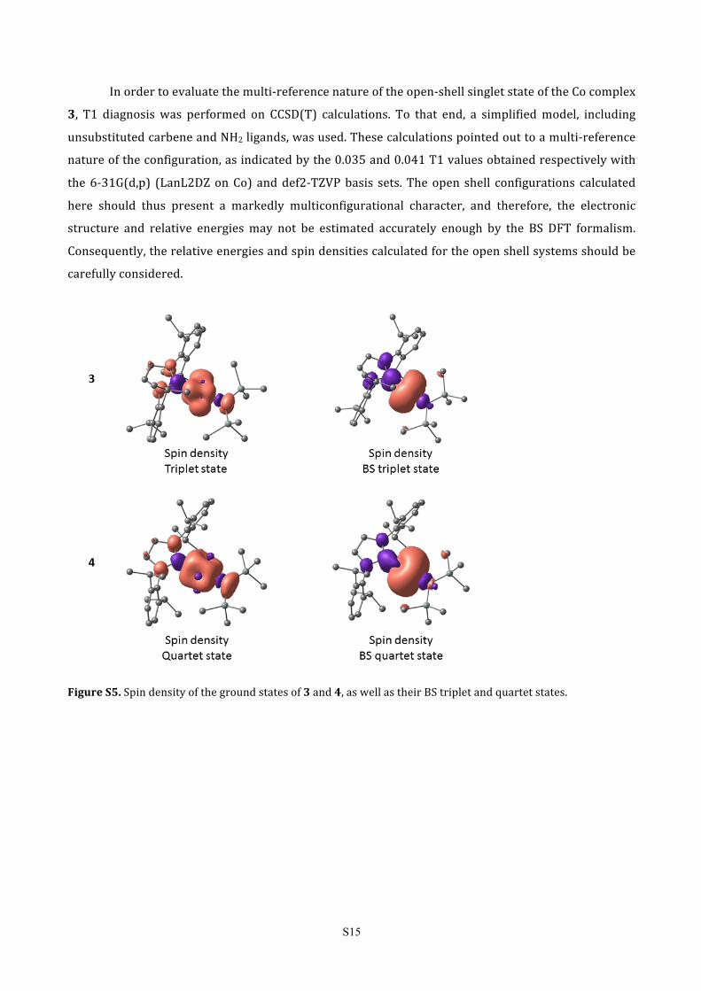
The calculations indicate triplet and quartet electronic ground states, for 3 and 4, respectively
(Table S3). The spin densities of the ground state are illustrated in Figure S5 and the α-‐spin and β-‐spin
molecular orbitals of 3 in its triplet ground state are represented in Figure S6. In 3 one single electron
is on Co and a second slightly delocalized throughout the metal and the π system of the molecule. The
delocalized π-‐interaction of a single electron induces stabilization of the linear geometry; this was
established by full geometry optimizations in the triplet and closed-‐shell singlet states at the same
level of calculation: the former led to a complex with a structure very similar to the experimental (C-‐
Co-‐N: 179.7°), whereas the latter to a bent complex (C-‐Co-‐N: 142.3°). Analogous results were obtained
for 4 (two single electrons on Fe and one π electron slightly delocalized over the molecule).
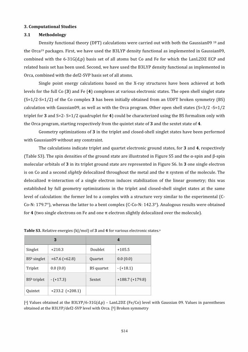
Table S3. Relative energies (kJ/mol) of 3 and 4 for various electronic states.a
3 4
Singlet +210.3 Doublet +105.5
BSb singlet +67.6 (+62.8) Quartet 0.0 (0.0)
Triplet 0.0 (0.0) BS quartet -‐ (+18.1)
BSb triplet -‐ (+17.3) Sextet +188.7 (+179.8)
Quintet +233.2 (+208.1)
[a] Values obtained at the B3LYP/6-‐31G(d,p) – LanL2DZ (Fe/Co) level with Gaussian 09. Values in parentheses obtained at the B3LYP/def2-‐SVP level with Orca. [b] Broken symmetry
S15
In order to evaluate the multi-‐reference nature of the open-‐shell singlet state of the Co complex
3, T1 diagnosis was performed on CCSD(T) calculations. To that end, a simplified model, including
unsubstituted carbene and NH2 ligands, was used. These calculations pointed out to a multi-‐reference
nature of the configuration, as indicated by the 0.035 and 0.041 T1 values obtained respectively with
the 6-‐31G(d,p) (LanL2DZ on Co) and def2-‐TZVP basis sets. The open shell configurations calculated
here should thus present a markedly multiconfigurational character, and therefore, the electronic
structure and relative energies may not be estimated accurately enough by the BS DFT formalism.
Consequently, the relative energies and spin densities calculated for the open shell systems should be
carefully considered.
Figure S5. Spin density of the ground states of 3 and 4, as well as their BS triplet and quartet states.

S16
Figure S6. α-‐spin (left) and β-‐spin (right) molecular orbitals of 3 in its triplet ground state.
S17
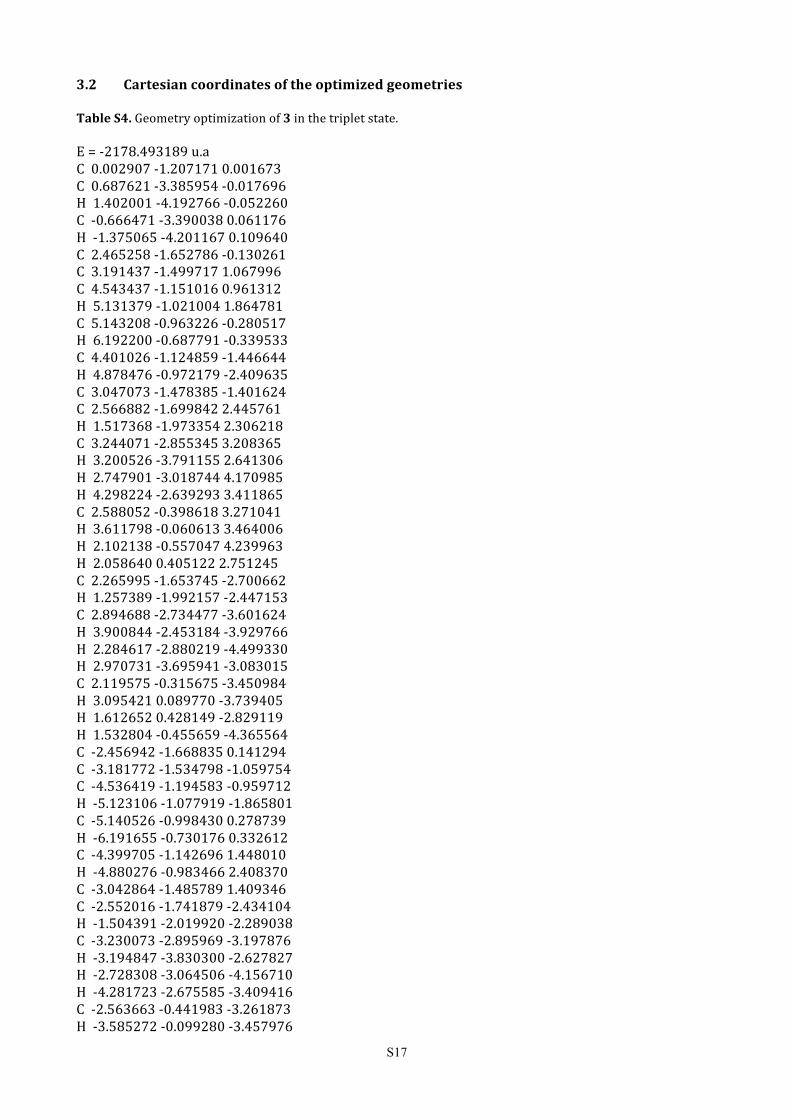
3.2 Cartesian coordinates of the optimized geometries Table S4. Geometry optimization of 3 in the triplet state. E = -‐2178.493189 u.a C 0.002907 -‐1.207171 0.001673 C 0.687621 -‐3.385954 -‐0.017696 H 1.402001 -‐4.192766 -‐0.052260 C -‐0.666471 -‐3.390038 0.061176 H -‐1.375065 -‐4.201167 0.109640 C 2.465258 -‐1.652786 -‐0.130261 C 3.191437 -‐1.499717 1.067996 C 4.543437 -‐1.151016 0.961312 H 5.131379 -‐1.021004 1.864781 C 5.143208 -‐0.963226 -‐0.280517 H 6.192200 -‐0.687791 -‐0.339533 C 4.401026 -‐1.124859 -‐1.446644 H 4.878476 -‐0.972179 -‐2.409635 C 3.047073 -‐1.478385 -‐1.401624 C 2.566882 -‐1.699842 2.445761 H 1.517368 -‐1.973354 2.306218 C 3.244071 -‐2.855345 3.208365 H 3.200526 -‐3.791155 2.641306 H 2.747901 -‐3.018744 4.170985 H 4.298224 -‐2.639293 3.411865 C 2.588052 -‐0.398618 3.271041 H 3.611798 -‐0.060613 3.464006 H 2.102138 -‐0.557047 4.239963 H 2.058640 0.405122 2.751245 C 2.265995 -‐1.653745 -‐2.700662 H 1.257389 -‐1.992157 -‐2.447153 C 2.894688 -‐2.734477 -‐3.601624 H 3.900844 -‐2.453184 -‐3.929766 H 2.284617 -‐2.880219 -‐4.499330 H 2.970731 -‐3.695941 -‐3.083015 C 2.119575 -‐0.315675 -‐3.450984 H 3.095421 0.089770 -‐3.739405 H 1.612652 0.428149 -‐2.829119 H 1.532804 -‐0.455659 -‐4.365564 C -‐2.456942 -‐1.668835 0.141294 C -‐3.181772 -‐1.534798 -‐1.059754 C -‐4.536419 -‐1.194583 -‐0.959712 H -‐5.123106 -‐1.077919 -‐1.865801 C -‐5.140526 -‐0.998430 0.278739 H -‐6.191655 -‐0.730176 0.332612 C -‐4.399705 -‐1.142696 1.448010 H -‐4.880276 -‐0.983466 2.408370 C -‐3.042864 -‐1.485789 1.409346 C -‐2.552016 -‐1.741879 -‐2.434104 H -‐1.504391 -‐2.019920 -‐2.289038 C -‐3.230073 -‐2.895969 -‐3.197876 H -‐3.194847 -‐3.830300 -‐2.627827 H -‐2.728308 -‐3.064506 -‐4.156710 H -‐4.281723 -‐2.675585 -‐3.409416 C -‐2.563663 -‐0.441983 -‐3.261873 H -‐3.585272 -‐0.099280 -‐3.457976
S18
H -‐2.075702 -‐0.604321 -‐4.229146 H -‐2.032032 0.360266 -‐2.741845 C -‐2.261152 -‐1.635443 2.711231 H -‐1.254613 -‐1.984964 2.464538 C -‐2.892911 -‐2.690539 3.639704 H -‐3.895127 -‐2.394712 3.966966 H -‐2.279159 -‐2.820112 4.537375 H -‐2.978546 -‐3.662993 3.143603 C -‐2.106667 -‐0.279876 3.428176 H -‐1.597128 0.446226 2.787598 H -‐1.519333 -‐0.399877 4.345257 H -‐3.080398 0.137179 3.707244 C 1.736369 5.057989 -‐0.820551 H 1.702620 4.798707 -‐1.885123 H 2.713406 5.516316 -‐0.623254 H 0.975731 5.825959 -‐0.644232 C 1.707019 4.056620 2.076507 H 0.914633 4.749799 2.378987 H 2.669112 4.557500 2.241482 H 1.659757 3.193209 2.750830 C 2.981240 2.391369 -‐0.138368 H 2.996144 1.477095 0.464019 H 3.921768 2.924455 0.051551 H 2.975656 2.093001 -‐1.192382 C -‐1.756553 5.059515 0.801894 H -‐1.720417 4.799992 1.866266 H -‐2.734472 5.516712 0.606419 H -‐0.996909 5.828019 0.623965 C -‐1.726597 4.055779 -‐2.096306 H -‐0.934567 4.749185 -‐2.398988 H -‐2.689135 4.555187 -‐2.262949 H -‐1.677887 3.191173 -‐2.768957 C -‐2.999911 2.390163 0.120303 H -‐3.007242 1.471114 -‐0.475243 H -‐3.942501 2.916848 -‐0.077001 H -‐2.997115 2.098634 1.176303 N 1.078630 -‐2.054292 -‐0.052018 N -‐1.066650 -‐2.060217 0.070543 N -‐0.010412 2.699714 -‐0.010278 Si 1.497784 3.508091 0.264700 Si -‐1.518749 3.510794 -‐0.283775 Co -‐0.007191 0.804126 -‐0.009157

S19
Table S5. Geometry optimization of 3 in the closed-‐shell singlet state. E = -‐2178.564149 C -‐0.596493 -‐0.790349 0.222773 C -‐2.087039 -‐2.380717 0.951145 H -‐3.055540 -‐2.826061 1.109062 C -‐0.845668 -‐2.813401 1.269821 H -‐0.515694 -‐3.708458 1.770977 C -‐3.018999 -‐0.337087 -‐0.161375 C -‐3.274598 -‐0.297269 -‐1.549443 C -‐4.322877 0.520763 -‐1.993794 H -‐4.537688 0.577947 -‐3.056559 C -‐5.101816 1.244775 -‐1.098469 H -‐5.911694 1.869467 -‐1.464422 C -‐4.853558 1.158975 0.269482 H -‐5.477841 1.717845 0.959204 C -‐3.810981 0.372699 0.771282 C -‐2.507462 -‐1.142174 -‐2.564287 H -‐1.721816 -‐1.684588 -‐2.032053 C -‐3.431727 -‐2.193118 -‐3.211953 H -‐3.898572 -‐2.834390 -‐2.457253 H -‐2.860522 -‐2.831827 -‐3.894305 H -‐4.233652 -‐1.722332 -‐3.790812 C -‐1.815325 -‐0.277788 -‐3.634402 H -‐2.538851 0.298029 -‐4.221556 H -‐1.252973 -‐0.912617 -‐4.327349 H -‐1.110897 0.426819 -‐3.177369 C -‐3.596678 0.268141 2.279919 H -‐2.606260 -‐0.164276 2.449020 C -‐4.641139 -‐0.677544 2.911267 H -‐5.654296 -‐0.281776 2.779698 H -‐4.459809 -‐0.786888 3.985918 H -‐4.617062 -‐1.675229 2.462335 C -‐3.623794 1.632122 2.992803 H -‐4.611620 2.102188 2.941974 H -‐2.893852 2.323683 2.566517 H -‐3.384198 1.499441 4.053195 C 1.484980 -‐2.047611 0.878883 C 2.224632 -‐1.382229 1.879314 C 3.599070 -‐1.639481 1.945748 H 4.199156 -‐1.142260 2.699713 C 4.211674 -‐2.526253 1.063434 H 5.279936 -‐2.710118 1.135049 C 3.457852 -‐3.178079 0.093756 H 3.945144 -‐3.871836 -‐0.584214 C 2.079370 -‐2.955852 -‐0.023887 C 1.551855 -‐0.465534 2.897432 H 0.680638 -‐0.019921 2.409540 C 1.054645 -‐1.278795 4.111663 H 0.351196 -‐2.062823 3.815121 H 0.545715 -‐0.624759 4.828397 H 1.893279 -‐1.757959 4.629596 C 2.448717 0.693988 3.359502 H 3.292836 0.348449 3.966570 H 1.869488 1.384251 3.981227 H 2.843042 1.254018 2.507566
S20
C 1.278517 -‐3.732642 -‐1.068505 H 0.283029 -‐3.284271 -‐1.133269 C 1.104827 -‐5.204685 -‐0.637856 H 2.075182 -‐5.708798 -‐0.572207 H 0.492642 -‐5.748612 -‐1.365477 H 0.621983 -‐5.290536 0.340256 C 1.896740 -‐3.665292 -‐2.477486 H 2.022314 -‐2.633660 -‐2.813978 H 1.246293 -‐4.180817 -‐3.192501 H 2.874939 -‐4.155734 -‐2.518393 C 2.514525 4.332003 1.016217 H 3.010923 3.669867 1.734271 H 2.237561 5.248256 1.552153 H 3.253934 4.610380 0.257474 C 0.155783 4.804128 -‐0.880090 H 0.803702 5.065358 -‐1.723074 H -‐0.077234 5.728882 -‐0.338028 H -‐0.780194 4.410142 -‐1.292601 C -‐0.243561 3.230228 1.694766 H -‐1.201768 2.869262 1.309439 H -‐0.421972 4.162791 2.245284 H 0.134142 2.485981 2.402454 C 3.011211 3.291999 -‐2.774039 H 2.137006 3.493723 -‐3.403014 H 3.861094 3.096932 -‐3.439476 H 3.236854 4.207117 -‐2.216099 C 4.291954 1.504290 -‐0.631501 H 4.527632 2.358620 0.011536 H 5.151824 1.339898 -‐1.292693 H 4.192093 0.620964 0.008438 C 2.498635 0.289103 -‐2.770913 H 2.352825 -‐0.613120 -‐2.170649 H 3.389148 0.144407 -‐3.396054 H 1.632416 0.399031 -‐3.431666 N -‐1.929572 -‐1.147533 0.324261 N 0.055622 -‐1.850706 0.815405 N 1.313192 2.042944 -‐0.611842 Si 0.964336 3.520036 0.263328 Si 2.707827 1.793799 -‐1.640270 Co -‐0.024391 0.802570 -‐0.622656
S21
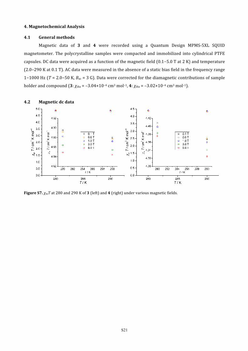
4. Magnetochemical Analysis 4.1 General methods
Magnetic data of 3 and 4 were recorded using a Quantum Design MPMS-‐5XL SQUID
magnetometer. The polycrystalline samples were compacted and immobilized into cylindrical PTFE
capsules. DC data were acquired as a function of the magnetic field (0.1−5.0 T at 2 K) and temperature
(2.0–290 K at 0.1 T). AC data were measured in the absence of a static bias field in the frequency range
1−1000 Hz (T = 2.0−50 K, Bac = 3 G). Data were corrected for the diamagnetic contributions of sample
holder and compound (3: χdia = –3.04×10⁻⁴ cm3 mol–1, 4: χdia = –3.02×10⁻⁴ cm3 mol–1).
4.2 Magnetic dc data
Figure S7. χmT at 280 and 290 K of 3 (left) and 4 (right) under various magnetic fields.

S22
Figure S8. Illustration of the best possible least–squares fits (solid lines) for the alternative electron
configuration scenarios (i), top, and (ii), bottom, for 3 (left) and 4 (right). All χmT vs. T data at 0.1 Tesla, all
magnetization curves (insets) at 2.0 K. a) SQ = 20%, b) SQ = 11%, c) (fit only to magnetization data, SQMm = 2.7%)
overall SQ = 8.4%, and d) SQ = 12%. Besides the poor SQs and curves badly reproducing the data, the estimated
ligand field parameters are physically unlikely or impossible being either very small (for a), even quasi–free ion)
values or very large values (> 60000 cm–1) with partly incorrect signs.

S23
Table S6. Least–squares fit parameters calculated by CONDON 2.020 according to the “MII+e–” model described in
the text for [M(IPr){N(SiMe3)2}].
Parameter M = Co (3) M = Fe (4)
B a) / cm–1 1115 1058
C a) / cm–1 4366 3901
ζ3d a) / cm–1 533 410
!!! b) / cm–1 27201±62 31912±20
!!! b) / cm–1 40150±223 43505±68
J c) / cm–1 –0.1±0.2 –0.5±0.1
SQ d) 7.7% 2.8%
a) Racah parameters and one-‐electron spin-‐orbit coupling constants;21 b) ligand field parameters in Wybourne notation; c) Heisenberg parameter, “–2J” convention; d) goodness of fit.
4.3 Magnetic ac data
Figure S9. In-‐phase (χm’) and out-‐of-‐phase (χm’’) magnetic molar susceptibility of 3 as a function of temperature
T at zero static bias field.

S24
Figure S10. In-‐phase (χm’) and out-‐of-‐phase (χm’’) magnetic molar susceptibility of 4 as a function of
temperature T at zero static bias field.
Figure S11. Relaxation time τ vs. T–1 of 4, black (8.5–14 K) and green lines (3.0–5.5 K): fit to Arrhenius
expression; blue dashed line: fit considering quantum tunnelling, Raman and Orbach relaxation; red line: fit
considering quantum tunnelling, Orbach and another Arrhenius-‐type relaxation.
S25
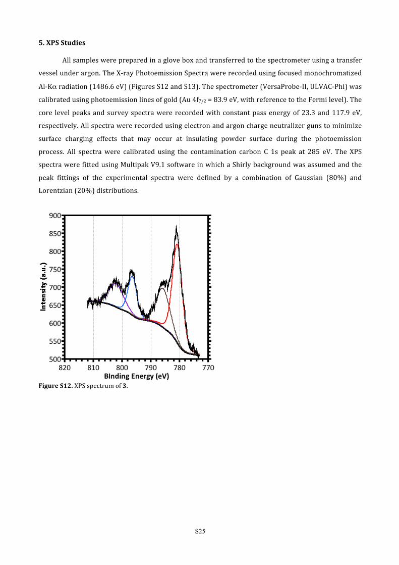
5. XPS Studies
All samples were prepared in a glove box and transferred to the spectrometer using a transfer
vessel under argon. The X-‐ray Photoemission Spectra were recorded using focused monochromatized
Al-‐Kα radiation (1486.6 eV) (Figures S12 and S13). The spectrometer (VersaProbe-‐II, ULVAC-‐Phi) was
calibrated using photoemission lines of gold (Au 4f7/2 = 83.9 eV, with reference to the Fermi level). The
core level peaks and survey spectra were recorded with constant pass energy of 23.3 and 117.9 eV,
respectively. All spectra were recorded using electron and argon charge neutralizer guns to minimize
surface charging effects that may occur at insulating powder surface during the photoemission
process. All spectra were calibrated using the contamination carbon C 1s peak at 285 eV. The XPS
spectra were fitted using Multipak V9.1 software in which a Shirly background was assumed and the
peak fittings of the experimental spectra were defined by a combination of Gaussian (80%) and
Lorentzian (20%) distributions.
Figure S12. XPS spectrum of 3.
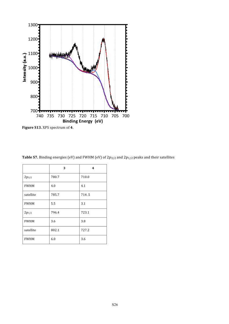
S26
Figure S13. XPS spectrum of 4. Table S7. Binding energies (eV) and FWHM (eV) of 2p3/2 and 2p1/2 peaks and their satellites
3 4
2p3/2 780.7 710.0
FWHM 4.0 4.1
satellite 785.7 714 .5
FWHM 5.5 3.1
2p1/2 796.4 723.1
FWHM 3.6 3.8
satellite 802.1 727.2
FWHM 6.0 3.6

S27
6. EXAFS and XANES Studies of 3
The Co K edge (7709 eV) XAS data was obtained at the Diamond Light Source, United Kingdom
on beam line B18. The sample of 3 was prepared in the glove box in a small capillary, sealed and
measured. The Co K-‐edge XANES data processing and EXAFS analysis were performed using IFEFFIT
version 1.2.11d with the Horae package (Athena and Artemis).22 Fitting was done in k-‐ and R-‐space
and in multiple weightings of k1, k2 and k3, simultaneously. The EXAFS could be fitted with one Co-‐N/C
contribution at 1.89(2) and one Co-‐N/C at 1.96(1) Å with low Debye Waller factors (EXAFS cannot
distinguish between N and C as they are neighbouring atoms in the periodic table and have very
similar back scatterings amplitudes), nicely corresponding to the single crystal data.
The 1st derivative of the Co K-‐edge XANES of sample 3, in comparison to some representative
Co(II) and Co(III), is given in Figure S14 (the normalised Co K edge XANES spectra are in Figure 3, in
the main paper). The first derivative can be used to accurately determine the number of pre-‐edge
features as well as the position of the pre-‐edges and main edge (the main sàp transition). For the
reference samples, one pre-‐edge is present, with the main edge being the second maximum in the 1st
derivative. For sample 3, the third maximum in the 1st derivative is the edge position, since this sample
displays two clear pre-‐edge features. It is clear that sample 3 represents an overall Co2+. The feature is
broad towards higher energy, which suggests some electron density is distributed away from the Co
centre. The XANES is known to be dependent on the ligand and geometry as well as the oxidation state
of the central metal,23 but the EXAFS in combination with XANES pre edge features supporting the
linear coordination only further support the Co2+ assignment. More support and insights in the XANES
are obtained from simulation the XANES and corresponding empty density of states (DOS) (XANES
probes the empty DOS).
Figure S14. Normalised Co K-‐edge XANES (left) and 1st derivative (right) of normalized XANES for Co references compounds as well as sample 3.
The FEFF9 code was used to perform ab initio self-‐consistent field, real-‐space, full multiple
scattering calculations.24 The calculations were performed using the Hedin-‐Lundquist exchange
correlation potential. A (final state rule) core hole is included on the absorber atom to mimic the final

S28
state of the photon absorption process. The XANES simulation including the corresponding l-‐projected
empty (DOS) as calculated simultaneously is presented in Figure S15. Whereas the 1st pre-‐edge is due
to pd hybridization, making the dipole forbidden s → d transition slightly visible, the 2nd pre-‐edge
originates from hybridization of the Co-‐p and Co-‐d with C-‐p mostly, and little mixing from Np. The high
intensity of this pre-‐edge is due to the empty character of the orbital, which is indicative of the linear
nature around the Co centre and also suggest the channel of charge redistribution being the aromatic
part of the molecule.
Figure S15. Calculated DOS (primary y-‐axis) and XANES (secondary y-‐axis) as a function of relative energy
(calculated). The vertical line at ca. –9 eV indicates the highest occupied molecular orbital. Since XANES probes
the empty density of state, the orbitals above –9 eV might be visible depending on symmetry and orbital overlap.
The main transition is Co-‐s to Co-‐p and thus the Co-‐p DOS will reflect best the features observed.

S29
6. References 1 (a) A. M. Bryan, G. J. Long, F. Grandjean and P. P. Power, Inorg. Chem. 2013, 52, 12152-‐
12160; (b) R. A. Andersen, K. Faegri, J. C. Green, A. Haaland, M. F. Lappert, W. P. Leung
and K. Rypdal, Inorg. Chem. 1988, 27, 1782-‐1786.
2 (a) J. M. Lalancette, G. Rollin and P. Dumas, Can. J. Chem. 1972, 50, 3058-‐3062; (b) D. E.
Bergbreiter and J. M. Killough, J. Am. Chem. Soc. 1978, 100, 2126-‐2134.
3 P. Tang, W. Wang and T. Ritter, J. Am. Chem. Soc. 2011, 133, 11482-‐11484.
4 A. J. Arduengo III, R. Krafczyk, R. Schmutzler, H. A. Craig, J. R. Goerlich, W. J. Marshall
and M. Unverzagt, Tetrahedron 1999, 55, 14523-‐14534.
5 A. A. Danopoulos, Unpublished results.
6 A. H. Cowley, N. C. Norman, M. Pakulski, G. Becker, M. Layh, E. Kirchner and M. Schmidt,
in Inorg. Synth., John Wiley & Sons, Inc., 1990, 27, 235-‐240.
7 B. M. Day, K. Pal, T. Pugh, J. Tuck and R. A. Layfield, Inorg. Chem. 2014, 53, 10578-‐
10584.
8 (a) A. A. Danopoulos, P. Braunstein, N. Stylianides and M. Wesolek, Organometallics
2011, 30, 6514-‐6517; (b) A. A. Danopoulos and P. Braunstein, Dalton Trans. 2013, 42,
7276-‐7280; (c) C. B. Hansen, R. F. Jordan and G. L. Hillhouse, Inorg. Chem. 2015, 54,
4603-‐4610.
9 D. F. Evans, J. Chem. Soc. 1959, 2003-‐2005.
10 M. I. Lipschutz, X. Yang, R. Chatterjee and T. D. Tilley, J. Am. Chem. Soc. 2013, 135,
15298-‐15301.
11 (a) A. H. Cowley, F. Gabbai, R. Schluter and D. Atwood, J. Am. Chem. Soc. 1992, 114,
3142-‐3144; (b) V. P. W. Böhm and M. Brookhart, Angew. Chem. Int. Ed. 2001, 40, 4694-‐
4696.
12 R. A. Aitken, W. Masamba and N. J. Wilson, Tetrahedron Lett. 1997, 38, 8417-‐8420.
13 B. Cetinkaya, A. Hudson, M. F. Lappert and H. Goldwhite, J. Chem. Soc., Chem. Commun.
1982, 609-‐610.
14 APEX2, Bruker AXS Inc., Madison USA, 2006.
15 G. M. Sheldrick, Acta Cryst. Section A 1990, 46, 467-‐473.
16 G. M. Sheldrick, University of Göttingen, Göttingen, 1999.
17 A. Spek, J. Appl. Crystallogr. 2003, 36, 7-‐13.
18 M. J. Frisch, G. W. Trucks, H. B. Schlegel, G. E. Scuseria, M. A. Robb, J. R. Cheeseman, G.
Scalmani, V. Barone, B. Mennucci, G. A. Petersson, H. Nakatsuji, M. Caricato, X. Li, H. P.
Hratchian, A. F. Izmaylov, J. Bloino, G. Zheng, J. L. Sonnenberg, M. Hada, M. Ehara, K.
S30
Toyota, R. Fukuda, J. Hasegawa, M. Ishida, T. Nakajima, Y. Honda, O. Kitao, H. Nakai, T.
Vreven, J. A. Montgomery, Jr., J. E. Peralta, F. Ogliaro, M. Bearpark, J. J. Heyd, E. Brothers,
K. N. Kudin, V. N. Staroverov, T. Keith, R. Kobayashi, J. Normand, K. Raghavachari, A.
Rendell, J. C. Burant, S. S. Iyengar, J. Tomasi, M. Cossi, N. Rega, J. M. Millam, M. Klene, J. E.
Knox, J. B. Cross, V. Bakken, C. Adamo, J. Jaramillo, R. Gomperts, R. E. Stratmann, O.
Yazyev, A. J. Austin, R. Cammi, C. Pomelli, J. W. Ochterski, R. L. Martin, K. Morokuma, V.
G. Zakrzewski, G. A. Voth, P. Salvador, J. J. Dannenberg, S. Dapprich, A. D. Daniels, Ö.
Farkas, J. B. Foresman, J. V. Ortiz, J. Cioslowski and D. J. Fox, Gaussian, Inc., Wallingford
CT, 2013, Gaussian 09 (Revision D.01).
19 (a) Orca version 3.0.3; (b) F. Neese, Wiley Interdiscip. Rev.: Comput. Mol. Sci. 2012, 2,
73-‐78.
20 (a) M. Speldrich, H. Schilder, H. Lueken and P. Kögerler, Isr. J. Chem., 2011, 51, 215-‐227;
(b) J. van Leusen, M. Speldrich, H. Schilder and P. Kögerler, Coord. Chem. Rev., 2015,
289–290, 137-‐148
21 J. S. Griffith, The Theory of Transition-Metal Ions, Cambridge University Press,
Cambridge, 1971.
22 (a) M. Newville, J. Synchrotron Radiat. 2001, 8, 322-‐324;(b) B. Ravel and M. Newville, J.
Synchrotron Radiat. 2005, 12, 537-‐541.
23 (a) M. Tromp, J. Moulin, G. Reid, J. Evans, AIP 2007, CP882, 699-‐701; (b) M. Tromp, J. A.
van Bokhoven, G. P. F. van Strijdonck, P. W. N. M. van Leeuwen, D. C. Koningsberger and
D. E. Ramaker, J. Am. Chem. Soc. 2005, 127, 777-‐789; (c) L.-‐S. Kau, D. J. Spira-‐Solomon, J.
E. Penner-‐Hahn, K. O. Hodgson and E. I. Solomon, J. Am. Chem. Soc. 1987, 109, 6433
24 (a) J. J. Rehr, J. J. Kas, M. P. Prange, A. P. Sorini, Y. Takimoto, F. Vila, C. R. Physique 2009,
10, 548-‐559; (b) J. J. Rehr, J. J. Kas, F. D. Vila, M. P. Prange, K. Jorissen, PCCP 2010, 12,
5503-‐5513.