CORPORATE NETWORKS AND PEER EFFECTS IN FIRM POLICIES:

EVIDENCE FROM INDIA ∗

Manasa Patnam†

University of Cambridge

August 2011

ABSTRACT

This paper identifies the effect of corporate network peer groups on firm policy decisions such as investment,

executive compensation and expenditure on R&D. Using panel data for all publicly listed companies in India,

I construct time-varying corporate networks based on interlocking directorates. Identification of dynamic

network peer effects, which arise due to endogenous association, is achieved by exploiting natural breaks in

network evolution that exogenously change the composition of peers. These breaks occur as a result of local

network shocks – deaths and retirements of shared directors – that are stochastic in nature and external

to the network formation process. I find significant network peer effects that are associated positively with

firms’ investment strategy and executive compensation. In addition, I use detailed stock level breakdown of

investments for each company, to show that for any two companies, the probability of investing in the same

stock at any given time is increasing in the strength of their network ties. Finally, I explore heterogeneity in

peer effects by distinguishing between network peers who belong to the same industry from those that do not

and find a greater effect of across-industry network connections.

KEYWORDS: Social Interaction Models, Corporate Finance and Governance, Development

JEL Classification: C31, O16, G34

∗I thank Paul Baker, Roger Barker, Jane Cooley, Francis DiTraglia, Eliana La Ferrara, Erica Field, RobertoGalbiati, Garance Genicot, Nicky Grant, Christian Helmers, Paul Kattuman, Manos Kitsios, Pramila Krish-nan, Vitaliy Oryschenko, Michele Pellizzari, Jaideep Prabhu, Raghavendra Rau, Mark Seasholes, Giorgio Topaand Arvind Venkataraman for helpful discussions and comments. I thank especially PVS Kumar, SandhyaRao, Gaurav Srivastava and Elangovan Venkatachalapathy for data access and management. I acknowledgesupport from the Suzy Paine Fund, Marie-Curie AMID Research Fellowship and the Luca D’Angliano Fellow-ship.†Faculty of Economics & St John’s College, University of Cambridge; mp519@cam.ac.uk

1 INTRODUCTION

Firms interact with other firms, within the same industry and across, in various ways. These

interactions can be both market and non-market based. Examples of market-based interac-

tions include formal intra-industry agreements among competing firms (cartels) or resource-

sharing alliances (strategic partnerships). Non-market based interactions occur when firms

interact with other firms informally; by entering into board interlocks or through shared

social connections between employees, among other things. In both cases, such social inter-

actions often influence firm policy decisions in accordance with their peers. Instances of such

behaviour are quite pervasive; a firm may gain information from another firm about strategic

investment opportunities or may simply mimic it’s within industry competitors’ marketing

strategy to maintain its market share. While a multitude of models, mainly theoretical, have

investigated this phenomenon, there is little empirical evidence to validate such effects.

This paper uses firm level panel data for all publicly listed companies in India, covering the

period 1998-2010, to estimate peer effects in corporate policies. Peer effects refer to the broad

class of externalities that arise when a firm’s own behaviour is responsive to the behaviour as

well as the characteristics of other firms in its chosen reference group. I examine whether peer

effects operate on firm managerial policies such as corporate market investment and executive

compensation. I construct peer groups using interactions that occur within and across indus-

try, through corporate networks based on interlocked directorates. Mizruchi (1996) defines

an interlocking to occur “...when a person affiliated with one organization sits on the board

of directors of another organization” (pg. 1). These networks are longitudinal in nature

and change over time due to entry and exit of directors. I also consider whether a firm is

influenced by its industry level peers i.e. a set of all other firms that share the same industry

classification1. Manski (1993) notes that the ‘informed specification of reference groups is a

necessary prelude to analysis of social effects’ (pg. 536). Corporate networks based on inter-

locked directorates provide a frequent and important channel for social interaction amongst

firms. There is a large literature that documents how firms choose to strategically inter-

lock with other firms, with the consequence that corporate networks are often endogenously

determined2.

A central contribution of this paper is the identification and estimation of peers effects in

endogenously formed networks. The identification of peer effects encounters well known

problems laid out in Manski (1993). Manski lists three effects that need to be distinguished

in the analysis of peer effects. The first type are endogenous effects which arise from a firm’s

1Both network and industry level peer provide different environments and mechanisms for the propagationof peer effects. Industry level peers are commonly associated to provide competitor driven peer influence inthe “keep up with the Joneses” tradition, while network peers provide a monitoring, information and learningbased explanation of peer influence.

2In Section 2, I review both the causes and consequences of board interlocks.

2

propensity to respond to the outcomes of its peers. For example, a firm is inclined to invest

more if it observes its peers investing heavily. The second are so-called contextual effects

which represent the propensity of a firm to behave in some way as a function of the exogenous

characteristics of its peer group. For instance a firm is able to spend more on investment

independently of its own profits if it receives some positive externalities from its peers’ profits3.

The third type are so-called correlated effects which describe circumstances in which firms in

the same group tend to behave similarly because they have similar individual characteristics

or face similar institutional arrangements, i.e., firms within the same industry may behave

similarly due to common industry-specific shocks. This means that there are unobservables in

a group which may have a direct effect on observed outcomes. The main empirical challenges,

therefore, consist in (1) disentangling contextual effects, from endogenous effects and (2)

distinguishing between social effects, i.e., exogenous and endogenous effects, and correlated

effects. Identification of network based peer effects is confounded by additional problems of

self-selection and endogenous network formation.

In this paper I present a novel strategy that exploits both the structure and inter-temporal

variation of the corporate network to identify network based peer effects. The structure

of the network implies that the pattern and magnitude of social interactions are non-linear

in nature which allows me to distinguish the endogenous peer effect from the exogenous

peer effect. Secondly to mitigate bias associated with non-random selection, in addition

to differencing out firm fixed effects, I use natural breaks in network evolution which arise

from local network shocks that are stochastic in nature and external to the network. In this

setting, local network shocks are in the form of deaths/retirement of directors that severs a

tie between two firms and/or exit of any peer firm. Loss of peers with high outcome values

is likely to reduce the average in the next period (net of other endogenous deletions and

additions) because they are no longer part of the peer group. Therefore, for every firm,

I use average outcomes of those peers who have been lost due to death/retirement related

director exits to instrument for its average peer outcomes in the next time period. I control

for the direct effect of director exits due to deaths/retirement on the outcome and require

only that there be no systematic differences in director exits that break interlocks and those

that do not (i.e. director exits of unconnected directors). The identification assumptions are

violated if firms choose to strategically replace the lost directors with directors of equally

well connected companies. To ensure that this is not the case, I estimate a simple difference-

in-difference regression and find no significant effect of a director death/retirement shock to

a firm in the past period on its probability of forming a new link. Finally, to purge out

correlated effects, I control for common time-varying shocks that occur both across industry

and business group by employing industry by business group by time fixed effects. As an

extension, I also estimate peer effects from a firm’s ‘global’ network of interaction wherein a

3This is especially the case with firms that have a common ownership structure wherein profits could betunnelled between firms to fund each other’s investment activities (Bertrand, Mehta, and Mullainathan 2002).

3

firm’s peer group consists of both its direct links (examined before) and its indirect links as

obtained through the corporate network.

I analyze the impact of peer interactions on the following firm policies: investment, executive

compensation and current R&D expenditure. I make a distinction between two types of

investments, corporate investments in marketable securities (henceforth corporate market

investment) and physical capital expenditure. I focus mainly on corporate market investments

for two reasons4. Firstly, there has been an increasing trend over the last decade whereby firms

have increased their holdings of liquid assets in marketable securities, either with a view to

procure strategic equity stakes or to smoothen their risk portfolio5. Secondly, there is a large

theoretical literature that focuses on social interactions in finance, particularly investments,

through models of herding and information cascades. In these models, investment decisions

may be influenced by observing the decisions of others and this leads to a convergence or

divergence of behaviour. Behavioural responses of such kind are more likely to be dynamic

in nature and involve taking decisions on expenditure items that can be easily modified.

Corporate market investments satisfy this criterion because in contrast to physical capital

expenditure, they are more liquid and managerial decisions on portfolio adjustment tend to

be more flexible. If social interactions influence investment decisions, then it has important

implications for investor welfare because it may contribute to clustered financial activity.

I also focus on executive compensation because pay-scales are closely monitored by the firm’s

board of directors. Many CEO’s themselves are directors on boards of other firms. Potentially

this could mean either that networked CEO’s are more likely to collude and influence each

other’s pay or at least have access to information on the setting of other CEO’s pay scales. The

recent phenomena of rising CEO pay, that has been popularly termed the “Lake Wobegone

Effect”6 to reflect the fact that no firm wants to admit to having a CEO who is below average,

is indicative of this aspect (Hayes and Schaefer 2009). Actions such as these, which are in

part influenced by social interactions, could lead to a distortion of performance related pay

scales.

Overall, I find evidence for positive network based peer spillovers. An increase of one standard

deviation in network peer investment leads to an increase of 0.16 standard deviations in the

growth of own firm investment. Similarly an increase of one standard deviation in network

4I also explain peer effects in capital expenditure but due to the lumpiness of physical investment, Itransform capital expenditure into a dummy variable which is equal to one if there is investment in capi-tal/infrastructure and zero if not.

5For example Brown (2009) argues that this form of investment is not merely equivalent to a simplestore of cash; rather it serves as value enhancement. He finds evidence firms may use market investmentas a risk management tool as well as to manage future financial commitments and payout policy. Allenand Phillips (2000) examine block equity ownership patterns of US corporations and note that, among otherthings, purchasing corporations could be able to effectively monitor or influence management since they arein possession of superior knowledge relative to other shareholders.

6“Where’s the stick?”, The Economist, October 2003; “Are India CEO’s Overpaid”, Business Today, July2007; “Do Indian CEO’s Overpay Themselves”, Rediff Business, October 2009.

4

peer executive compensation leads to an increase of 0.05 standard deviations in the growth of

own firm executive compensation. For investment, I also use detailed stock-wise breakdown

of investments for each company, and show that for any two companies, the probability of

investing in the same stock at any given time is increasing in the strength of their network

ties. In order to further understand the mechanisms driving the aggregate peer induced

outcome increase, I disaggregate the network into two further groups: network peers who are

in the same industry as the firm and network peers who are not. The reason for separating

peer effects using these pre-defined groups is to distinguish between the different types of

interactions that a firm can have even within its given network. I take insight from economic

theory and argue that interactions amongst industry peers are competitive in nature whereas

strategic interactions with firms not in the same industry are more benevolent in nature.

Therefore, if information is the channels through which these peers effects dissipate then it

is likely that a firm will ignore information received from its competitors and there will be

no industry network peer effects. However a finding of positive industry network peer effects

indicate that firms could potentially be mimicking the behaviour of its competitors7. I find

that for both market investment and executive compensation, industry network peer effects

are close to zero while non-industry network peer effects are positive and significant. Finally,

I find positive industry peer effects for market investment and R&D but not for executive

compensation. Comparing industry peer effects with overall network peer effects (consisting

of both network peers from same industry and network peer from different industries), I find

that for market investment network peer effects dominates whereas the opposite is true for

R&D investment.

The paper is most closely related to the small but growing body of literature that provide

evidence for corporate peer effects. In recent work, Leary and Roberts (2010) show that cor-

porate financial policies are highly interdependent. Taking the industry as the peer reference

group, they identify peer effects by using idiosyncratic shocks of peer firms as instruments

and find that a one standard deviation change in industry based peer firms’ leverage ratios

is associated with an 11% change in own firm leverage ratios. They argue that these effects

are consistent with models of learning and show that smaller, more financially constrained

firms exhibit ‘more pronounced mimicking tendencies’. Fracassi (2008) using data on board

interlocks8 in the United States provides further evidence that firms are influenced by their

social peers when making corporate policy decisions. He finds that more social connections

7I also distinguish between industry peer effects i.e. the effect of peers in a firms industry and overallnetwork peer effect (containing both industry and non-industry within network peers). The disaggregationof peer effects into industry peers and non-industry peers is different from above because the former seeksto understand how even within the network firms differentially respond between industry and non-industrypeers.

8Other work relating to corporate networks via board interlocks include Khwaja, Mian, and Qamar (2011)who estimate the value of corporate networks in Pakistan and find that membership in a highly clusteredcomponent of a network increases total external financing and better insures firms against industry andlocation shocks.

5

two companies share with each other, the more similar their level and change of investment

behaviour is over time. In the same context, Bouwman (2011) finds that governance practices

are propagated across firms through a network of shared directors. She shows that these net-

work effects lead to a convergence in governance practices because of the influence of directors

who sit on the boards of different firms. In relation to firm compensation policy, Shue (2011)

exploits random assignment of MBA students to sections within classes at Harvard Business

School and finds that executive compensation and acquisitions strategy are significantly more

similar among graduates from the same section than among graduates from different sections

within the same class.

The paper contributes to the empirical literature on firm level social interactions by providing

evidence for the presence and importance of both network and industry based peer effects in

a developing country setting. The Indian context is different from other developed country

settings such as the United States and United Kingdom which have been the focus of previous

literature, because corporate governance rules are less stringent and more informal in India

(see Estrin and Prevezer (2011)). For instance while there are clear cut regulations in the

United States that restrict intra-industry interlocks, no such rules apply in India. As such

the policy implications for a finding of positive peer effects through corporate interlocks

are more profound. Firstly, it has implications for the formulation of corporate governance

regulations depending on whether such effects are considered desirable or not. Secondly, from

a policy perspective, (only) endogenous peer effects have the capacity to generate multiplier

effects. Positive and significant network peer effects in firm market investment, wherein a

firm’s decision to invest is influenced by the aggregate investment behaviour of its peers,

have the ability to propagate asset bubbles or contribute to financial clustering. A vast

literature examining financial herding and information cascades find evidence on correlated

trading, both at the institutional & individual level9 (Seasholes 2011). The peer interactions

framework complements this literature by providing precise mediums through which such

correlated trading decisions could be influenced. For example, as discussed in the paper,

distinguishing between market-based peer effects (industry peers) from non-market based

peer effects (corporate networks, shared educational associations etc.) allows us to determine

the appropriate reference group through which these social multiplier effects emanate (if any).

Likewise, firms influencing each other on executive compensation policies have the effect of

distorting performance oriented pay-scales. CEO’s of firms are likely to be paid much above

their marginal product only to ensure that a particular standard, as determined by their

peers, is met.

The rest of the paper is organized as follows: Section 2 defines the construction of industry and

9See Allen and Babus (2009) for an excellent review of financial networks and its implications; see alsoOzsoylev (2003) for a good theoretical understanding on how social networks may lead to clustered financialdecision making.

6

network reference groups. Section 3 discusses the identification strategy which is translated

into the specification of the empirical model presented in the same Section. The data used

is described in Section 4. Section 5 discusses the results and Section 6 provided further

robustness results. Section 8 concludes.

2 CORPORATE NETWORK

Firms can potentially be influenced by two types of peer firms – those that it considers its

competitors and those with whom it shares an affiliation of sorts. As stated before, in this

paper I consider corporate network & ownership related peer groups. I also provide evidence

considering industry based peer groups. Below I provide definitions for each.

Corporate Network Affiliation: This type of affiliation comes from firm relationships

fostered through interlocked board of directorates or corporate networks. An interlocking

directorate occurs when a director of the board of one firm sits on the board of another.

This means that two firms share a direct link in the corporate network if they share a shared

director. A firm can have one or more directors who sit on the boards of other firms. Indian

corporate governance regulations mandate that a director sit on no more than fifteen firms at

a time. Corporate networks evolve over time due to link additions and deletions from shared

director entry & exits. Interlocked boards provide an important source of information about

a firm’s network. A firm can also have connections based on shared education background

of executives, past employment of employees but my data does not allow me to distinguish

such potential connections. The networks defined in this paper are based purely on firm

relationships through interlocked boards. As pointed out earlier, many authors find evidence

of similarities in corporate behaviour of firms that are linked through this type of a corporate

network. I discuss below the relevance of interlocked directorates.

Mizruchi (1996) provides a review of board interlocks where he describes the origins and

features of common board interlocks in the United States. He highlights three factors, among

other reasons, that help explain the formation of interlocks: collusion, monitoring and social

cohesion. The intent to collude between competitors as a means of restricting competition

may lead to the formation of interlocks. This is evident for instance through the findings that

most interlocks occur within a specific industry (Pennings 1980). The second reason is that

interlocking provides for a means to co-opt and monitor sources of environmental uncertainty.

Firms tend to employ board seats as devices to monitor other firms and their organizational

decision making suggesting that interlocks can act as instruments of corporate control. A

wide range of literature has found evidence suggesting that interlocks are positively associated

with firm profitability (Baysinger and Butler 1985; Burt 1983). It is unclear however, whether

this is due to the fact that firms tend to monitor each other effectively though interlocks or

that profitable firms tend to interlock more. Finally, interlocks can occur as a result of social

7

cohesion wherein individuals are invited to sit on boards of firms due to their past associations

(social, educational etc.) with other board members.

More importantly, for the purposes of this paper, there are many consequences of such board

interlocks. Mizruchi (1996) lists several and reviews evidence against each. Mainly, it is

argued that board interlocks lead to a heightened sense of corporate control whereby firms

used the board interlock to extended their control on their partner firms’ policy decisions.

Executive compensation is typical example of such a policy decision. Guedj and Barnea (2009)

use data on directors who served on the boards of S&P firms and find evidence that firms

whose directors are more central in the network, pay their CEO higher and that CEO pay

is less sensitive to firm performance. Another consequence of board interlocks is of ‘network

embeddedness’ i.e. interlocks connect multiple firms with each other and therefore provide

a standpoint from which to view how a firm’s relations with other firms affect its corporate

behaviour (Mizruchi 1996). A seminal contribution in this perspective comes from Cohen,

Frazzini, and Malloy (2008) who document connections between mutual fund managers and

corporate board members via shared education networks. They find that portfolio managers

place larger bets on connected firms and perform significantly better on these holdings relative

to their nonconnected holdings. In similar vein, Hochberg et al. (2007) find that better-

networked Venture Capital firms experience significantly better fund performance where they

measure connections through syndication relationships. Stuart and Yim (2010) exploit the

sequential timing of receiving private equity offers and provide evidence to show that that

companies which have directors with private equity deal exposure gained from interlocking

directorships are approximately 42% more likely to receive private equity. This is indicative

of gains from peer influenced information transmission in a network of interlocked boards.

Business Group Affiliation: In India, most firms are also organized into ‘business groups’

which is defined as a set of firms managed by a common group of insiders. The firms affiliated

to business groups are single entities with individual production processes however it is quite

common to find firms within such business groups sharing directors with each other. Since

the nature of social interactions amongst firms sharing a business group are akin to that

through board interlocks, I supplement the peer reference group to incorporate peers from

same business group affiliations as well. The appendix contains more details about business

groups in India.

Industry Affiliation: Finally to examine heterogeneous peer effects, I also distinguish

between the set of corporate network peers that belong to the same industry and those

that do not. An industry affiliation of a firm is based, very simply, on a shared industrial

classification. I use classifications given by the National Industrial Classification (NIC) which

is the standard classification system for economic activities in India. The NIC groups together

economic activities which are akin in terms of process type, raw material used and finished

8

goods produced. The classification does not make any distinctions according to the type of

ownership or type of economic organization, and except in some cases the c1assification does

not distinguish between large scale and small scale (GOI 2004). Basically firm affiliation into

the same industry can indicate how well as firm responds to policies of its peers who are

producing the same output as itself.

3 IDENTIFICATION OF PEER EFFECTS

The identification of peer effects is notoriously difficult as explained by Manski (1993) and

Moffitt et al. (2001)10. Manksi noted that within a linear framework without additional

information, it is impossible to infer from the observed mean distribution of a sample whether

average behaviour within a group affects the individual behaviour of members of that group.

In other words, the expected mean outcome of a peer group and its mean characteristics are

perfectly collinear due to the simultaneity induced by social interaction. The main challenges,

therefore, consist in (1) disentangling contextual effects, i.e., the influence of exogenous peer

characteristics on a household’s observed outcome, and endogenous effects, i.e., the influence

of peer outcomes on a household’s outcome, and (2) distinguishing between social effects,

i.e., exogenous and endogenous effects, and correlated effects, i.e., firms in the same network

may behave similarly because they are alike or share a common environment.

3.1 THE REFLECTION PROBLEM

This fundamental identification problem, termed reflection problem by Manski, makes it clear

that within a linear-in-means model, identification of peer effects depends on the functional

relationship in the population between the variables characterizing peer groups and those di-

rectly affecting group outcomes. In such a setting, if all individuals interact in a similar way in

groups of the same size, then it is impossible to recover the parameter on the endogenous peer

effect because it is perfectly collinear with the mean exogenous characteristics of the group.

However under special settings, wherein the social interactions are not homogenous within or

across a group, it is possible to identify both the endogenous and exogenous peer effects. Lee

(2007) was first to show formally that the spatial autoregressive model specification (SAR),

widely used in the spatial econometrics literature, can be used to disentangle endogenous

and exogenous effects. Lee notes that in a SAR model, identification of endogenous and con-

textual effects is possible if there is sufficient variation in the size of peer groups within the

sample. As stressed by Davezies et al. (2009), Lee’s identification strategy crucially requires

knowledge of peer group sizes and at least three groups of different size. Bramoulle et al.

(2009) propose an encompassing framework in which Manski’s mean regression function and

Lee’s SAR specification arise as special cases. They show that endogenous and exogenous

effects can be distinguished through a specific network structure, for example the presence

10For a summary of the literature see also Blume and Durlauf (2005).

9

of intransitive triads within a network. Intransitive triads describe a structure in which in-

dividual i interacts with individual j but not with individual k whereas j and k interact11.

In both cases it is possible to identify endogenous and exogenous effects separately because

the variation in the magnitude of social interactions, either through group size variations

or through a network structure, produces exogenous variations in reduced form coefficients

across groups that allow us to recover the endogenous effect.

In this paper, I use a rich panel of all publicly listed firms in India and estimate peer effects in

reference groups that have a non linear social interaction structure. This structure emerges

when interaction do not occur symmetrically, i.e. not everyone is related to everybody else,

even within sub-populations in the same way. A well known example of such a structure is a

social network. In a social network each person is linked to a select set of people but no to

the entire network directly. In the firms context, it means that each firm is linked to a set

of firms though shared directors and in turn their peer firms have further connections, other

than the target firm. An example of such a firm network is given below – denote a network,

in the form of an adjacency matrix12, as W –:

1 2 3

1 0 1 0

2 1 0 1

3 0 1 0

Here, Firm 1 shares a director with Firm 2 (and therefore is connected to it) but not with

Firm 3. Similarly, Firm 2 is connected with Firm 1 and also with Firm 3. The matrix W

represents the global network of all social interactions13. Within this global network we can

define a local network which is a set of all firms that any given firm is directly linked to. I use

the local network as the relevant peer group. In the above example, Firm 1’s local network

or peer group is Firm 2 whereas Firm 2’s peer group is Firm 1 and Firm 3. In this section

I use the terms local network and peer group interchangeably. In section I also consider

interactions through indirect links thereby accounting for the entire global network. The

structure of such peer groups are heterogeneous both across firms at a given time and within

firms over time due to movements of directors on the board. The across firm non-linearity

11This particular network structure produces exclusion restrictions which achieve identification in the sameway as exclusion restrictions achieve identification in a system of simultaneous equations.

12A common way to represent connectivity of network graphs is through a n× n binary symmetric matrixcalled an adjacency matrix. The adjacency matrix is non-zero for entries whose row-column indices correspondto a link between two individuals/firms and zero for those that have no links. Operations on the adjacencymatrix also yield additional information about the network such as degree, clustering etc. For more onadjacency matrices and properties of network graph see Kolaczyk (2009).

13 This type of a network/graph is also called an ‘affiliation network’/‘bipartite graph’. An affiliationnetwork refers to the set of binary relations between individuals/entities (firms) that belong to a commongroup or participate in common events (shared directors).

10

in interactions due to the asymmetric nature of the peer interaction allows us to distinguish

the endogenous effect. The structure of the network ensures that the endogenous peer effects

are identified, i.e. the parameters can be separately recovered.

Denote the set of firms as i (i = 1, ..., n), yit denotes the outcome of firm i at time t and xit

is the firm’s exogenous characteristic14 at time t. Let N denote the global network of

all interactions and η the local networks15 that are contained within N . Each firm’s peer

group, its local network η, is of size n. By assumption firm i is excluded from its peer group.

We assume that our sample of size nt is i.i.d. and from a population of networks with a fixed

and known structure. We distinguish between three types of effects: an agent’s outcome

yit is affected by (i) the mean outcome of her peer group (endogenous effects), (ii) her own

characteristics, and (iii) the mean characteristics of her peer group (contextual effects):

yit = β

∑j∈ηit yjt

nit+ γxit + δ

∑j∈ηit xjt

nit+ ςt + uit (1)

or, as is common in the peer effects literature:

yit = βy−it + γxit + δx−it + ςt + uit (2)

Hence, β captures endogenous effects and δ contextual effects. Time fixed effects are repre-

sented by ςt. We require strict exogeneity of xit with respect to uit. Note that we do not

require the residuals uit to be homoscedastic or normally distributed.

Omitting the time subscripts for clarity, denote WN as the global network peer interaction

matrix. Any i, j element within it is represented by wNij . It is row-standardized such that

wNij = 1/nij if firm i and j have a board interlock, i.e. share a director, and 0 otherwise. I

use WNi to denote the ith row vector which is used to represent a firm i’s local network16.

Its pre-multiplication with the column vector y produces a firm specific peer average denoted

by WNi yt, i.e. it is the same as y−i. Rewriting Eq. (2) we now get17:

yit = βWNit yt + γxit + δWN

it xt + ςt + uit (3)

14For ease of notation, in this section, I represent only one exogenous characteristic but the empirics takeinto account many exogenous characteristics that are described later.

15This terminology is consistent with much of the literature on statistical networks and discussed inBramoulle et al. (2009).

16WNi is the ith row of the n × n matrix WN. When post multiplied by yt whose dimension is n × 1, it

produces a 1 × 1 firm specific peer average.17The use of time dependent weights matrices is not uncommon in the social networks literature. Doreian and

Stokman (1996) refers to Eq. (3) as a ‘processual model’ and use it to detect contagion in social networks. Inthe spatial econometrics literature, recent work by Lee and Yu (2011) also develops quasi-maximum likelihoodestimation of spatial dynamic panel data models where spatial weights matrices can be time varying.

11

The reduced form of Eq. (3) is given by (Lee and Yu 2011):

yt = (I − βWNt )−1(γxt + δWN

t xt + ςt) + (I − βWNt )−1ut (4)

3.2 NON RANDOM SELECTION

The main problem with estimating network based peer effects is that the network is endoge-

nously formed. Endogenous tie formation will also typically induce a correlation between

unobserved shocks of the firm and the firms’ peers. This is especially the case when similar

group of firms share directors. To see this, decompose the error from Eq (3) in the following

parts:

uit = µi + νit + εηt (5)

µi represents all time invariant firm level unobservables, νit contains time varying firm unob-

servables and εηt contains shocks/unobservables that are common to a firm’s local network

at any given time t. In such a case a non-zero coefficient on the peer influence variable could

mean that these firms behave in a similar fashion because they share similar attitudes (and

have sorted themselves based on that) rather than the fact that network members are influ-

encing each other (Epple and Romano 2011). Firstly, I employ a first-differences specification

to eliminate any time invariant firm unobservable, µi, that may be correlated with selection

or correlated unobservables. First differencing Eq (3), we get:

4 yit = β 4WNit yt + γ 4 xit + δ4WN

it xt +4ςt +4uit (6)

I retain time fixed effects in this specification to capture common time specific trends. The

parameter β represents the contemporaneous effect of peer firms. The model, therefore, cap-

tures the effect of changes in peer firms’ contemporaneous outcomes on the change in a firms’

outcome. It is possible however that instead of responding to contemporaneous outcomes,

firms respond to the permanent component associated with their peer firms’ outcomes. For

example, Mas and Moretti (2009) use data from a supermarket chain and estimate produc-

tivity spillovers. In their model, the peer function takes the form where workers respond to

the permanent productivity of their peer workers and over time changes in the composition

of peers enables the identification of such effects. However as noted by them in the paper,

both model (permanent and contemporaneous) are ex-ante possible (Mas and Moretti 2009).

As in their paper, I am unable to distinguish between the effects of the two models, simply

because estimating fixed effects would entail employing a peer group composition or local

network fixed effect which is infeasible in the case of endogenous networks. Therefore the

estimates obtained in this paper could in part be reflecting some effect of firms’ response to

permanent rather than contemporaneous outcomes.

12

Given Eq (6), we are still confronted with the challenges of mitigating bias arising from

time varying unobservables that might influence selection into the network or time varying

unobservables, such as common productivity shocks, that are correlated with the peer effect.

I first take up the issue of network selection and return to the problem posed by correlated

effects in the next sub-section.

To tackle the selection bias, I make use of natural breaks in dynamic networks that are

independent of any selection process. The idea of using exogenous variation in networks to

isolate the endogenous component of the peer effect is similar to using class size variation

brought about due to exogenous movement of students across schools. In the network context,

it would mean having to look for local network shocks that break (or append) a tie but are

external to the network or its formation. Such shocks would bring a reduction or increase in

the network average outcome depending on the quality of the tie being broken (or appended)

and will be uncorrelated to both the propensity to form ties and aggregate network level

unobservable that affect any agents’ outcome. Identifying peer effects using variations in

the composition of groups is well established in the social interactions literature (Hanushek

et al. (2003); Hoxby (2000)). However the strategy of using naturally induced variation in

group composition to instrument for peer effects that arise from endogenously formed groups

is relatively novel. Hoxby and Weingarth (2005) use policy based reassignment of students

into schools to estimate peer effects in education. The authors use the average outcomes of

past period peers following reassignment, disallowing and excluding from this average other

endogenous movement of students, as an instrument for the endogenous peer effect. In similar

spirit but taking a different approach, Waldinger (2010) uses dismissals of scholars in the Nazi

era as a source of exogenous variation in the peer group of scientists staying in Germany to

identify peer effects in scientific publications. He uses the past period dismissal induced

reduction in peer quality to instrument for the present period peer average. Finally, Cooley

(2007) uses introduction of student accountability policies in North Carolina public schools

as an exogenous ‘utility shifter’ for identifying peer spillovers in education18. The author

uses the percentage of students held accountable in any given year to predict average peer

achievement in the classroom. The assumption is that the percentage of students in danger

of failing is independent of both group level and individual level unobservables. The common

underlying idea for the identification strategy pursued in the papers discussed above, as well

as in this paper, is the use of an exclusion restriction in the form of an exogenous shock that

is able to alter the composition of groups or/and the peer averages.

In what follows, I provide the assumptions that describe the properties of a valid exclusion

restriction such as the one described above:18The policy required that students perform above a certain level in order to be automatically promoted to

the next grade. This meant that classrooms with a high percentage of students in danger of failing were morelikely to increase their aggregate achievement because students close to failing would put in more effort (andtherefore increase achievement) so as to get promoted.

13

(A1) There exists a variable, representing a stochastic network shock, Dit−1 that changes

the response of firm i to choose the optimal outcome19 and the composition of peers,

WNit , in the next period.

(A2) The variable Dit−1 induces a shift in both the endogenous and exogenous peer aver-

ages in the next period depending on the quality of peer loss given by, WDit−1yt−1

20

(endogenous peer average shifter) or WDit−1xt−1 (exogenous peer average shifter).

(A3) Conditional on (xit, εηt), νit is independent of Dit−1.

(A4) Conditional on (xit), εηt, νit are jointly independent of WDit−1yt−1, WD

it−1xt−1.

(A1) ensures that there are no direct spillovers from the network shock Dit−1. This means

that Dit−1 affects the composition of peers and is capable of having a direct effect on the

outcome but only by changing the response of the firm in reaction to the event. Note that

the change in peer composition shifts both the exogenous and endogenous peer averages

requiring, still, a non-linear social interaction structure that allows for separability of the

exogenous and endogenous peer average shifters. In a linear-in means model this type of an

exclusion would be ineffective, since neither the exogenous/endogenous peer effects nor the

exogenous/endogenous peer shifters are individually separable. (A2) clarifies this by indexing

the network shock to be firm specific i.e. it represents a local network shock. (A3) requires

that the shock be uncorrelated with firm specific unobservables in the next time period.

Death or retirements of directors which induce a pair-wise break in links, present this sort

of a local network shock in the given context. A death or retirement of a director has two

potential effects. It can directly affect the behaviour/outcome of the firm due to a loss of an

employee and his/her productive input to firm policies. Indirectly, if the firm participates

in board interlocks and shares the director it would result in a broken link. In this case, if

the firm loses opportunities to interact (through board interlocking) with a high quality firm

it would result in a reduction in overall network average in the next period i.e. the loss of

a firm with high outcome values in period t leads to a reduction in the average in period

t+ 1. I control for the direct effect of director deaths/retirement and use this death induced

reduction to average outcomes due to broken firm linkages as an instrument. This implies

that identification requires only that there be no systematic differences in director exits that

break interlocks and those that do not (i.e. director exits of unconnected directors). The

first stage will essentially compute a differences-in-differences estimate for those firms that

experienced the shock in each time period. As an example, consider the following figure

(below): the network in time t evolves to a new structure in time t + 1. Two links have

19Note that Dit−1 does not directly enter a standard production function.20Superscript D indicates the subset of past period peers who have been lost as a result of shock Dit−1.

WDit−1yt−1 can also be written as yD−it−1 indicating the average outcomes of peers who have been lost. I

describe in detail the construction of the peer average shifters in the subsequent pages.

14

been broken and one new link has been appended. However, only one link has broken due

to a shared director death/retirement (in green) – I identify, only this type of pair-wise link

deletions.

The objective is to construct a variable that can predict the gain or loss to the next period

average, t + 1, due to deaths/retirements induced link exits. Dit is a binary variable that

indicates whether firm i experiences death or retirement of one or more directors. At given

time t, let WDit , denote the subset of past period peers who have been lost as a result of shock

Dit; its elements are defined as follows:

wDij,t =

{1 if i and j lose a shared director due to Dit, Djt = 1

0 otherwise(7)

Endogenous Effects: To instrument for the endogenous peer effect in time t I use the

average outcomes of lost peers (due to death/retirement of shared directors) in time period

t− 1, given by WDit−1yt−1. This variable measures the ‘quality’ of peer loss.

Exogenous Effects: Similarly, to instrument for the exogenous effects I use the average

exogenous characteristics of lost peers, given by WDit−1xt−1.

With these as instruments I estimate the following system using two stage least squares.

Explicitly controlling for the direct effect of the shock Dit−1 in Eq. (6), the equation of

interest is given by:

4 yit = β 4WNit yt + γ 4 xit + τ 4Dit−1 + δ4WN

it xt +4ςt +4uit (8)

The first stage equations for the endogenous and exogenous peer variables are:

4WNit yt = θf1 4WD

it−1yt−1 + ϑf1 4WDit−1xt−1 + γf1 4 xit + τ f1 4Dit−1 +4ς f1t +4uf1it (9)

4WNit xt = θf2 4WD

it−1yt−1 + ϑf2 4WDit−1xt−1 + γf2 4 xit + τ f2 4Dit−1 +4ς f2t +4uf2it

Finally, identification requires that the quality of peer loss (WDit−1(.)) be independent of both

15

νit and εηt as maintained in Assumption (A4)21. Independence with νit could be violated for

instance if firms choose to strategically replace the lost directors with directors of equally well

connected companies. This could be if firms that witnessed shared director deaths are more

likely to form new links in the next period. In section (6.1) I verify that this is not the case

and that the effect of a shared director death is insignificant in predicting the probability of

new links. Moreover, I am able to control for the direct effect of director deaths/retirement

on the firm’s outcome since not all deaths/retirements are of shared directors. I discuss the

independence of εηt and the constructed instrument in the following subsection.

3.3 CORRELATED EFFECTS

The presence of correlated unobservables within a firm’s local network could bias the peer

effects estimates. Correlated effects could arise due to a number of reasons such as common

productivity shocks (if the peer firm was in the same industry as the target firm), change

in business group policies ((if the peer firm was in the same business group as the target

firm) or other shared director related shocks. I can classify local network peers of any firms

into three types: those that belong to the same Industry (I), those that belong to the same

business group (G) and the remaining that do not belong to either the firms’ industry or

business group ( 6 I 6 G). On average 62.45% of network links are peers who belong to the

same industry or same business group. Using this property and to clarify the issue more, I

further decompose the error by dividing εηt into three parts:

εηt = εIηt + εGηt + ε 6I 6Gηt (10)

where εIηt represents the industry level common unobservables, εGηt represents the business

group level common unobservables and ε 6I 6Gηt represents the residual. To eliminate the first

two terms I use both industry by year and business group by time fixed effects. The resulting

specification is (omitting the first stage):

4yit = β4WNit yt+γ4xit+τ4Dit−1 +δ4WN

it xt+4ςt+4φIt+4τGt+4νit+4ε 6I 6Gηt (11)

where φIt and τGt represent industry by year and business group by time fixed effects that

21An easy way to see that it holds is to examine the instrument validity condition22; omitting the individualsubscript and first difference operators:

E[(WDt−1yt−1)′ut] = E[(yt−1)′(WD

t−1)′ut]

= E[(yt−1)′︸ ︷︷ ︸A

((WDt−1)ut)︸ ︷︷ ︸B

] = 0

Using the fact that that the network WN and therefore WD is symmetric, a simple reformulation of theoriginal exclusion shows that the validity condition holds because the average disturbances of lost peers intime t (vector B) are uncorrelated with the vector of own outcomes in time t − 1 (vector A). See AppendixA.1 for details.

16

will be estimated. This specification also allows us to control for both industry and business

group level fundamentals that may be driving the outcome of interest23. The remaining

correlated unobservable, ε 6I 6Gηt , are not systematically related to any firm specific pre-defined

group. Even then, the identification strategy pursued in this paper will provide consistent

estimates of the peer effects since past period peers that dropped out due to death of shared

directors are no longer in the peer group of the next period and therefore do not share the

same unobserved shocks/correlations.

4 DATA

My primary source of data is the PROWESS database provided by the Center for Monitoring

of the Indian Economy (CMIE). Prowess includes annual report information for around 29,000

companies in India from 1989 to the present year. It provides detailed balance sheets, financial

statements, industry information and group affiliation for each firm, corporate ownership

data, share prices, and other relevant data for publicly traded Indian corporations. In this

paper, I use an (un-balanced) panel of all Indian private sector firms that are publicly listed

firms – both on the Bombay Stock Exchange (BSE) and the National Stock Exchange (NSE)–

from the period 1997-2010. As in other papers (Khanna and Palepu 2000, Bertrand, Mehta,

and Mullainathan 2002), I rely on CMIE classification of firms into group and nongroup

firms, and of group firms into specific group affiliation which is based on a ”continuous

monitoring of company announcements and a qualitative understanding of the group wise

behaviour of individual companies” (CMIE 2010, pg. 4). For identifying industry affiliation,

I use information on the principal line of activity of the firm and use the National Industry

Classification (NIC) code accorded to them. This is similar to the SIC classifications of firms

in the UK and US. The PROWESS data also provides detailed information on the directors

serving on the board of each firm, along with information on the number of board meeting

attended, salary, directors’ fee etc. The listing of these directors is unique within each time

period and I undertake and exhaustive matching exercise to ensure uniqueness even across

time periods.

My second source of data comes from a Bombay Stock Exchange led initiative called Direc-

tors’ Database (www.directorsdatabase.com) and maintained by Prime Database of India.

The data contains individual as well as firm level information on all directors including the

directors educational qualifications; the directors position in the board (for example promoter

director, managing director, non-executive director, independent director, etc.); whether the

23Note that given the panel dimension of my data which contains ten time periods and about two thousandindustry and business groups, I am only able to estimate full industry by year and business group by yearfixed effects in separate specifications. However, to estimate both industry and business group by time fixedeffects, I define a time period as two year spells and interact them with both industry and business groupsindicators to estimate industry by year and business group by time fixed effects. While slightly restrictive,this is the most feasible alternative to capture industry and group time invariant shocks together.

17

director satisfies the definition of being independent according to the guidelines laid by out

by the Securities and Exchange Board of India (SEBI); the other public and private firms in

which the director is a board member. Importantly, it contains separate information about

cessations of every director in the boards of all listed firms which includes the name of each

director who ceased to be a board member, the date of such cessation and the reason for such

cessations (end of nomination, resignation, demise etc.) (Chakrabarti et. al, 2010).

Based on the above two data sources I construct time-varying networks for the all the listed

firms in my data-set. Figures (1) & (2) provide a summary of the network topology and its

evolution over time. I find, consistent with many studies (see Kossinets and Watts 2006), that

these network graphs experience a fair amount of stability over time. Figure (1) shows that

the degree and clustering coefficient witness a slight upward trend. Figure (2) summarizes

the number of director appointments & cessations for each firm along-with the corresponding

link additions and deletions. On average about 4.5 links are deleted/lost and 1 new link

is added. The last panel in this figure also shows the average number of death/retirement

related lost links (approximately 0.5 links ) in each time period. Death and retirements

related link deletions account for about 10% of all link deletions.

The outcome variables that I use for analysis are defined as follows. Market investment is

defined as the sum of all firm investments in equity shares, preference shares, debt instru-

ments (issued by the government or by non-government entities, or of short-term or long-term

nature), mutual funds and approved securities. Investments made by investment companies

that are engaged entirely, or essentially, in the business of purchase and sale of securities for

making profits from these are not included in this data field. Investments of such companies

are treated as stock in trade and not investments. For robustness I consider also investments

made by the company in only securities that are listed on securities exchanges; such securities

are called ”quoted” securities24. Executive compensation is the remuneration paid to com-

pany executives and it includes the amount of salary paid, contribution to provident fund,

value of perquisites, performance linked incentive to whole time directors and also the com-

mission paid to them. It does not include the sitting fees paid to the directors for attending

board meetings. Capital Expenditure is measured as the total expenditure incurred during

the setting up of a new plant or a new project up to the date of the commercial production.

Current R&D expenditure is measured by the total outlay of the company on research and

development during the year on its current account.

I use a fairly parsimonious specification to control for other firm exogenous characteristics.

Specifically, I include total profit before depreciation, interest, tax and amortisation; total

book value of assets (in logs); total sales of a company (in logs). All the control variables are

24Investment in mutual fund is also treated as quoted investment even if not listed on the exchanges as theirfair price is available and are easily marketable

18

lagged by one year. I also control for the number of director exits. This refers to the number

of directors who have left the company in the previous time period. Toe measure scale effects

I also include a total network size variable that measures the number of direct links i.e. the

number of other firms with whom it shares common directors.

5 RESULTS

I now report results of industry and network peer effects on firm policies. I first provide

descriptive evidence that peer groups matter. Figures (4) & (3) present nonparametric plots

of a firms’ investment expenditure against the average industry and network peer averages

of the same. In both graphs firms’ investment expenditures are increasing in their peers’

performance. Note also that this positive relation is approximately linear for both industry

and network averages. Table (1) provides summary statistics over all time periods for the

variables used in the analysis.

5.1 NETWORK PEER EFFECTS

Corporate Market Investment: Table 2 shows the results for peer effects in corporate

market investment from estimating Equation (3) using OLS and the two stage least squares

using the instrument described in Section 3.2 above. Both the outcome variable and the

endogenous peer variable are in logs. In the following results I control for the assets of each

firm but in unreported results I also asset normalize the investment variable; the results are

unchanged. Column (1) shows OLS results not accounting for potential bias in selection or

unobserved network shocks. There is a positive and statistically significant coefficient associ-

ated with the endogenous peer effects. Other control variables are also statistically significant:

a change in profits, assets and sales are all associated with a positive growth in corporate

market investment as expected. I now discuss the instrumental variable results. Column (2)

reports the first stage of the two stage least squares procedure. Recall that the instrument I

use is the average outcome of death induced deleted links in the past period, WD Mkt. Invst.

An exits of peers with high outcome values is likely to reduce the average in the next period

(net of other endogenous deletions and additions) because they no longer contribute to this

average. The first stage results confirm this; a one unit increase in the average investment

of lost peers (due to death/retirement) leads to a 6.4% reduction to the next period aver-

age investment (of existing network peers). The coefficient is statistically significant at 1%.

This result suggests that firms are unable to immediately replace dead/retired directors with

equally well connected new directors so as to restore their links. Moreover, the instrument is

highly informative as the first stage F statistic is 124.2. Therefore the endogenous peer effect

is not ‘weakly’ identified25.

25 ”Weak identification” arises when the excluded instruments are correlated with the endogenous regressors,but only weakly.

19

Column (3) & Column (4) report second stage results under different specifications. Gener-

ally, the results show a large increase in the coefficient of peer effects. Now, an increase of

one standard deviation in a firm’s network peers has almost twice the effect on the change

in writing skills it had when using OLS. An increase of one standard deviation of the en-

dogenous effects leads to an increase of 0.16 standard deviations in the growth of market

investment. All the conditioning variables, remain statistically significant throughout. Note

that the coefficient on the director exit is statistically insignificant which would imply that

exits of directors have no direct independent effect on the outcome.

Column (5) reports results that include contextual effects. For corporate market investment,

none of the contextual effects are significant. The endogenous peer effect is still statistically

significant and slightly larger in magnitude. This is not however the general pattern and

in other results I discuss the interpretation of contextual effects where they are found to

be significant. Finally, Column (6) adds scale effects separately. The average network peer

effect implicitly captures the scale effect since it normalizes the peer total by network size. I

control for the firm size by including firm sales; therefore if larger have more directors and

hence larger networks, the sales variable will potentially already capture some effect of the

network size. Even then, there might be concern that the size of the network directly enters

the model and so I calculate in each period the number of local network peers that a firm is

linked with and include this in the regression. The network size variable is endogenous due

to the above mentioned concerns of non random selection into the network and the existence

of other unobservables. Here again, I rely on the death/retirement induced local network

shocks and instrument network size in the current period with the number of firms lost due

to death/retirements of common directors in the previous period. In unreported results, I

find that the instrument is significantly negatively correlated with the endogenous network

size variable as expected. Column (6) shows that the network size variable is not signifi-

cant, after controlling for firm size, endogenous and exogenous peer effects. Table (6) further

strengthens the results by eliminating industry and business group specific shocks. I find that

both the magnitude and significance of the endogenous peer effects, as reported in Column

(1) of Table (6: A & B) remain unchanged even after accounting for industry by business

group by time fixed effects.

Executive Compensation: Table 3 shows the results for peer effects in executive com-

pensation. As before, both the outcome variable and the endogenous peer variable are in

logs. Column (1) shows OLS results not accounting for potential bias in selection or unob-

served network shocks. There is a positive and statistically significant coefficient associated

with the endogenous peer effects. Both, a change in assets and sales, are associated with

a positive growth in executive compensation. Column (2) reports the first stage of the two

stage least squares procedure. The first stage results show that a one unit increase in the

average compensation of lost peers (due to death/retirement) leads to an 8.9% reduction to

20

the next period average. The coefficient is statistically significant at 1% and the instrument

is strongly correlates with the endogenous variable (Cragg Donald F statistic in the first stage

is 178.946). Column (3) & Column (4) report second stage results under different specifica-

tions (as above). Generally, the results show a large increase in the coefficient of peer effects.

An increase of one standard deviation of the endogenous effects leads to an increase of 0.05

standard deviations in the growth of executive compensation.

Column (5) reports results that include contextual effects. It shows that the average prof-

its of peer firms negatively effects the growth of executive compensation of any given firm,

however the coefficient is quite small and close to zero. In general, the interpretation of con-

textual effects is fraught with ambiguity. Cooley (2009) provides a detailed discussion on the

specification and interpretation of contextual effects in the classroom/child learning context.

She argues that higher values of peer exogenous characteristics might reduce own outcome

values if there are positive spillovers from endogenous peer effects and we condition on this.

For instance, extending the argument in the firm setting, consider a firm whose executive

compensation levels are increasing in its peer’s compensation levels as well as own profits.

This implies that controlling for the firm’s own profits and peer firms’ compensation levels

any increase in peer profitability should decrease own compensation levels. This is because

the firm will require an increase in effort from its own executives to match up to the profits

of its peer firms (and therefore reduce compensation until effort is increased and profit is

matched), for any given own profit level and peer compensation level. Apart from peer firm

profits I find no other significant contextual effects. Finally, Column (6) includes scale effects

separately however the coefficient on network size is not significant. As before, I account for

industry and business group level unobservable in Table (6). Column (2) of Table (6: A &

B) reports these results and I find similar results to those reported above.

Capital Expenditure & R&D expenditure: Table 4 reports results for peer effects in

capital expenditure and it is quite similar to the market investment results (in the final

contextual effects specification) discussed before. Interestingly, the endogenous peer effect on

capital expenditure is positive but statistically significant only with the inclusion of contextual

effects. Table 5 reports results for peer effects in current R&D expenditure. I find no

significant network effects in current R&D expenditure in either of the specifications.

5.2 HETEROGENEITY

In order to distinguish between the different types of peers within local networks, I disaggre-

gate the overall peer effect between industry network peers and non-industry network peers.

This is important because there may be differences in how a firm responds to the behaviour

of peer firms within the network who belong to its own industry compared to those that do

not belong to the same. The disaggregation also helps establish channels though which peer

effects operate if we assume that the nature of interactions are distinct and separable between

21

the two sets of peers26. Although the precise qualitative nature of peer effects is hard to pin

down, it is possible to distinguish the different types of interactions between the groups using

some insight from economic theory. Economic theory on firms typically considers interactions

amongst industry peers to be competitive. In contrast firm strategic alliances are theorized

to be benevolent and more collaborative in nature. There is an extensive literature on such

network based firm interactions wherein firms collude and cooperate to share information and

resources (Goyal and Moraga-Gonzalez (2001); Belleflamme and Bloch (2004)). This implies

that if corporate peer effects are based on information diffusion, firms may be less willing to

trust information received from industry network peers (as compared to non-industry net-

work peers) and as a result not respond to the behaviour of this set. However if one were to

find positive and significant peer effects from industry network peers then it could potentially

imply that, keeping with the competitive spirit, firms mimic behaviours of these peers.

In Section 7.2 I distinguish between effects of industry peers which comprise all other peers

in a firms industry and distinguish it from the overall network peer effect (containing both

industry and non-industry within network peers). The present exercise is different from Sec-

tion 7.2 in that it tests for the differences in peer effects only within the overall network –

between industry network peers and non-industry network peers. In a sense this distinction

precludes any comparison between industry and overall network peer effects because network

peers also contain industry peers and vice versa. I therefore first seek to understand how even

within the network firms differentially respond between industry and non-industry peers.

Table 7 reports results that decomposes the peer effects as discussed. I present results only on

market investments and executive compensation since these are the two outcomes for which

I do find significant peer effects. The first two columns of both outcomes report the two first

stage results. Recall that the instrument is the average past period outcomes of delinked

peers due to death/retirement. In order to find separate peer effects by industry and non-

industry peers, I also decompose the instrument to separate loss to the average next period

outcome due to delinked industry peers and those due to delinked non-industry peers. Both

the instruments work well in predicting the two outcomes and are orthogonal to each other.

An exit of industry network peers with high outcome values reduces the industry network

average in the next period and has no effect on the non-industry network average in the next

period. The same applies for non-industry network peer exits. In general the joint Cragg-

Donald F-stat is high implying that both instruments are strong and informative. I now

focus on discussing peer effects from different sources. The results show that in both cases,

industry network peer effects (WNI) are statistically insignificant while non-industry network

peer effects (WNN) are positive and significant. An increase of one standard deviation

of the endogenous non-industry network peer effects leads to an increase of 0.16 standard

26There is recent and growing literature that identifies the mechanisms of peer effects by decomposing itseffect between pre-defined groups of interest. See Cohen-Cole and Zanella (2008) and Lavy and Schlosser(2007) as examples.

22

deviations in the growth of market investments and 0.05 standard deviations in the growth

of executive compensation. The coefficient on endogenous industry network peer effects

is close to zero. This indicates that the bulk of network peer effects derive from a firms

association with other non-industry firms. However a firm can have interactions with a

wide range of firms within its own industry outside of its corporate network. It is therefore

important to account and distinguish these market based interactions from the non-market

based interactions (corporate networks) discussed up till now. This is developed further in

Section 7.2.

5.3 INVESTMENT: STOCK LEVEL ANALYSIS

In order to pin down the exact nature of corporate market investment peer effects, I make

use of detailed information on each stock that a company has invested in over several years27.

The previous section established that companies are influenced by their peers in their choice

(nature and volume) of stock market investment. I refine the result now by tracking stock-wise

activity of every firm in relation with its networked and industry peers over time. Specifically

I estimate whether, for any two companies, the probability of investing in the same stock

in any given time periods is increasing in the strength of their network ties. Denote the set

of stocks of any company i at time t as Rit. I match the set of stocks for every pair in the

sample (Rit and Rjt) to see whether there is at least one stock that is common to both. Let ∅denote a null set indicating that there is no common stock between a pair of matched stocks;

the equation of interest is:

Pr(Rit ∩Rjt 6= ∅) = β1Nijt + β2Iijt + γXit,jt + εijt (12)

I estimate pair-wise or dyadic regressions where the unit of analysis is a pair of two companies

i and j28. The dependent variable is binary taking the value 1 if both i and j have invested

in the same stock in time period t. Network Strength, Nijt indicates the value of connection

between i and j and ranges from zero to one. It is equal to the inverse of path distance in

the global network between i and j – zero indicates no connection and one indicates direct

connection. All other values mean that i, j are connected but through a series of intermediate

links. I also includes a vector of pair-specific controls (differences in their profits, sales and

assets), Xit,jt. Finally I also capture whether the probability of investing in the same stock

is correlated with sharing a common industry, Iijt. I use a dyadic framework for analysis

because it allows incorporating the several thousands of stocks that exist in the entire sample,

matching effectively the stock sets of different companies. Although this framework is unable

27Detailed stock information is available for bulk of the listed companies in PROWESS only from the year2006. Data for previous years exist but only for a selected few companies. Therefore in order for the resultsto be representative of the publicly listed sample as well to make the analysis computationally feasible I useonly the years 2006-2010 for analysis

28Standard errors are adjusted using the QAP procedure to account for pair-wise dependence.

23

to distinguish whether company j is influenced by company i to invest in the same stock, it is

informative of the similarity in the patterns of stock-wise investment of both companies. I also

instrument for the potential endogeneity of the network strength variable by using director

exits due to death and retirement. This follows the same idea as all previous analysis, wherein

I use a variable that takes the value one if there are any common directors over the network

between i and j who have died or retired in the previous time period to instrument for the

strength of network tie between i and j in the current time period.

Table (8) reports results from this analysis. Column (1) reports simple OLS results. It shows

that an increase in network tie between i and j from zero to one increases the probability of

investing in the same stock by approx. 9%. Absolute differences in both profits and assets

also increase the probability of investing in the same stock. It is interesting to note that

sharing the same industry (indication of industry peers) also increases the probability of

investing in the same stock – by about 4%. Since the occurrence of investing in the same

stock is quite low29 across the whole universe of dyads, I also employ a rare events a logit

estimator to account for the underestimation in the probabilities associated with such an

event. I follow the procedure outlined in King and Zeng (2001) to estimate bias-corrected

parameter estimates and standard errors30. The results show that network strength effect is

associated with a coefficient of 1.63. this means that a change in network strength from 0

to 1 (no connection to direct connection) increases the probability of investing in the same

stock by 11%. The relative risk associated with this change (of 0 to 1) on the probability

of same stock investment is 4.56 log-odds. Column (3) incorporates pair fixed effects to

control for pair specific correlated unobservables; network strength still remains positive and

significant. Finally I report instrumental variable results. The first stage, Column (4), shows

that a global network shared director exit (due to death/retirement) in the previous period

is associated with a fall in network strength of about 0.05 units and this effect is statistically

significant31. The second stage results, both random effects and fixed effects show a positive

and significant effect of network strength, much higher in magnitude compared to the OLS

results, on the probability of investing in a similar stock.

29Investment in same stock takes the value 1 in approx 4% of dyad-year observations.30Briefly, the method incorporates three corrections into ordinal logistic regression: choice based sampling

giving greater weight to positive events, prior correction on the dependent variable based on the representationof the positive event within the population and amplification of the probability by a correction factor. Formore details on this procedure see King and Zeng (2001).

31The instrument also satisfies the criteria for a strong informative instrument; the first stage Cragg DonaldF statistic is over 100.

24

6 SENSITIVITY ANALYSIS

6.1 THREATS TO IDENTIFICATION

Identification of network effects relies solely on the occurrence of death/retirement related

local network shocks being witnessed by the firm. The validity of the instruments could be

violated for instance if firms choose to strategically replace the lost directors with directors

of equally well connected companies i.e. firms that witnessed a shared director death are

more likely to form new links in the next period. In order to test if this is the case or not,

I run a simple difference-in-difference regression comparing the network dynamics of firms

that lose connections due to death/retirement induced director exits to other firms. The

objective is to determine whether firms that experience death/retirement shock in time t− 1

are more likely to form new links in time t. Table (9) reports results on this regression. I

find no significant effect of a death shock in the past period on the probability of forming

new links and this result holds even after controlling for other firm level factors (sales, assets

etc.). The results also show that all the time fixed effects are jointly highly significant in

predicting the propensity to form new links. This suggests that there the increasing trend

over time to form new links is independent of whether a firm experiences link reduction due

to death/retirement shocks.

6.2 NETWORK MEASUREMENT: MONTE CARLO

Throughout the analysis I measure inter-firm network connections between all listed com-

panies in India. However it is true that the directors of each listed company also serve on

boards of non-listed companies. Since these non-listed companies are not part of the sam-

ple, the network omits linkages between listed and non-listed companies thereby inducing a

potential measurement error. In this section, I provide some Monte Carlo evidence to assess

the sensitivity of my results to such network related measurement error. To do so I consider

a population of two types of firms: listed and non-listed32. The objective is to compare an

estimated value of the parameter obtained from ‘sampling’ a network to the true population

parameter. Here, a sample network refers to a subset of the original population network from

drawing a sample of all listed companies.

There are three types of links in the population: links between a pair of listed companies

(‘listed links’), links between a listed company and non-listed company (‘mixed links’) and

32Note that here the population is assumed to derive from the set of all directors that serve on boards of listedcompanies. The simulations deal with sampling issues caused by partial enumeration of links from a bipartitegraph (defined in Footnote 13). Therefore I consider the list of directors to represent the entire universe ofgroups or events, and assess the measurement error induced by omitting links (and therefore firms) that sharecommon affiliation with any of these directors. This type of measurement issue is also commonly referredto as the ‘Boundary Specification’ problem in relation to bipartite graphs (Kossinets 2006). In particular, Iabstract from the possibility that there are additional ‘non-listed links’ due to non listed companies sharingcommon directors who do not serve on the boards of listed companies. This exercise is beyond the scope ofthis paper but is an interesting research agenda for the future.

25

links between a pair of non-listed companies (‘non-listed links’). To assess the bias arising

from partially enumerating links of listed companies, I use controlled network topology driven

Monte Carlo experiments similar to Paez, Scott, and Volz (2008). Details of the procedure

are outlined in the Appendix A.2. In the first experiment I control the density of listed links

(henceforth listed-density), measured as the proportion of listed links to the total number of

links in the population, and the sample size i.e. the proportion of listed companies in the

sample, in order to simulate various population networks. I then extract the sample networks

(all listed links) to estimate the peer effect parameter and compare it to the true population

parameter. Table (13) reports results from these simulations. Overall, I find that this type of

measurement error induces a downward bias i.e. the estimated parameters tend be lower than

the true population parameter. Figure (5) plots a heat-map of the root mean square errors

(henceforth RMSE). It shows that, for β = 0.2, the values of RMSE increase as the listed-

density and size fall; higher values of RMSE are indicated by (progressively) dark shades of

blue. For most the RMSE is quite low but increases sharply only at listed-density lower than

0.1. At this level and for a sample size equal to 20% of the population, the RMSE is 0.08.

The maximum RMSE, 0.40, is reached with a sample size of 10% and listed-density of 3%. In

the second experiment, I explore bias associated with a homophillic tendency to form links.

Homophily in this context arises when listed firms are more likely to form links (or share

directorates) with other listed firms. Higher homophilic tendency should decrease the extent

of measurement error because it limits the extent of mixed link omissions. Therefore even

at low listed link densities, a sufficiently high degree of homophily can reduce the extent of

bias. To examine this, I introduce an additional topological parameter, degree of homophily,

and vary it to arrive at different network configurations. The homophily parameter measures

the distribution of links that listed companies have between listed links (intra-group links)

and mixed links (inter-group links). For example a value of 0.5 indicates that 50% of all

links that listed companies have are amongst themselves. Table (14) reports results from

varying the homophily parameter at a given level of sampling size and listed-density. There

is a downward bias even in this case. Figure (6) summarizes the results; it shows that at

β = 0.2 and sample size of 20% , the bias steadily increases as the homophily parameter and

listed-density fall.

To assess the significance of these results, I construct a quasi-population network from the

observed data. I am able to do this this because the data provides information on all non-

listed companies that a director of any listed company serves on. After including these

non-listed companies, I construct an approximate population network. I find that listed

companies represent about 15% of the full list of companies. The proportion of listed links

to total links is approximately 0.7, while the degree of homophily is 0.18. Assuming that

the true population parameter lies between 0.2 and 0.3, I can expect the extent of bias to be

quite negligible; if anything, the peer effect coefficient should be slightly greater than what

26

is estimated. Moreover if we consider inference to be based on a population containing only

listed firms then the presence of links with non-listed firms enter the regression framework

as an omitted variable – average outcome of non-listed peers. My instrumental variables

strategy mitigates the effect of bias from such an omitted variable because the instrument is

uncorrelated with the omitted variable 33.

7 ALTERNATIVE PEER REFERENCE GROUPS

7.1 GLOBAL NETWORK INTERACTIONS

In this section, I account for global network interactions. Recall that a global network is the

entire graph of social interactions, both though direct connections and indirect connections.

Multiple local networks comprised solely of direct connections are all nested within the local

network. Until now I have restricted interactions to occur only though local networks. How-

ever, it is possible that a firm’s peer group consist of not only direct connections but also

indirect connections. To this extent, I construct a firm’s peer group by linking into all the

firms that it is directly or indirectly related to. Respecting the topology of the network, I give

direct connections the highest weight whilst calculating the average. To calculate weights in

the global network I use a common network statistic, the path distance. In the firm network,

we say that a path exists between firm i and j if they are connected either directly or though

a sequence of other firms. The path distance then is defined as the length of the shortest path

between them. For example, the path distance between two firms that are directly connected

is one; path distance between two firms that are connected by an intermediary firm is two.

The global network peer average is therefore just a weighted average of outcomes of all peers

where the weights are given by the inverse of the path distance.

It is useful to understand how the instrument is applicable even in this context. In the

previous section we had used average outcomes of the death induced deleted links in the

previous time period to instrument for average peer outcomes in the current period. In

this case we had only considered death induced deletion of links between two firms that are

directly connected. In the global networks we can visualize multiple such instances wherein

bilateral links are being broken due to death/retirement of shared directors. Consider three

firms i, j and k. i & j and j & k are directly connected. If j & k break a link due to

death/retirement of a shared director then, in the global interactions case, even i is affected

because the broken link results in reducing the strength of network connections for i. The

advantage of this is that the instrument is still valid and we no longer have to rely on only

bilateral link losses. The disadvantage is that the measure is prone to a lot of noise. While we

know that firm j & k have lost a link, it is not necessary the strength of connection between

33The results in Table (7) are an indication of this as it shows that decomposition of the instrument producestwo instruments that are orthogonal to each other given the superability of peer effects.

27

i & k would reduce because it is possible that in the next period i directly links with k. The

informativeness of this instrument then relies on the perturbations in connection patterns

not deviating significantly (apart from the death induced deletions) from the previous state.

Table (10) reports results on the global peer effects. While the coefficients on investment

and executive compensation peer effects remain positive and statistically significant, they are

much larger in magnitude compared to the local networks based specification. An increase

of one standard deviation of the endogenous effects leads to an increase of 0.19 (as compared

to 0.16 in the local networks case) standard deviations in the growth of market investment.

Similarly, an increase of one standard deviation of the endogenous effects leads to an increase

of 0.15 (as compared to 0.06 in the local networks case) standard deviations in the growth of

executive compensation.

7.2 INDUSTRY PEER EFFECTS

I also account for peer interactions through a shared industry affiliation and contrast it with

the network peer effect. Identification in this case is through partially overlapping groups

using peers-of-peers as an exclusion, wherein some ‘peers of peers’ do not affect an individual

directly but only through his or her own peers. I use the exogenous characteristics of an

industry peers business group to identify endogenous peer effects. The exclusion restriction

is valid since the business group’s peers (or peers-of-peers) are not directly connected to

the target firm. Appendix A.3 details the identification strategy used to estimate industry

based endogenous peer effects. Table 11 reports industry level peer effects. Note that all

specifications include time fixed effects. I report results for market investment, executive

compensation and current expenditure in R&D. I omit reporting results on other control

variables for brevity. Column (1) shows OLS results, Column (2) IV results and Column (3)

IV results with contextual effects. I do not report the first stage results, however I provide

both the Cragg-Donald first stage F statistic and the joint significance of the excluded peer

averages (instruments). I first discuss Panel A of Table 11 that reports results on corporate

market investment. I find that both the OLS and the IV coefficients are positive and statisti-

cally significant although the IV coefficient is much larger in magnitude than the OLS. I find

that a one standard deviation increase in the industry peer average investment is associated

with a 0.27 standard deviation increase in growth in own investment. The significance of the

coefficient disappears when I include contextual effects. Note that the first stage instruments

are all jointly significant and are strongly correlated with the endogenous variable Panel B

reports results on executive compensation. I find no statistically indicants industry peer ef-

fects vis-a-vis compensation. Industry Peer effects in current R&D expenditure is reported

in Panel C. In contrast to network peer effects, I find that industry R&D expenditure sig-

nificantly increases the firm’s own growth of the same. A one standard deviation increase

in the industry peer average R&D expenditure is associated with a 0.34 standard deviation

28

increase in growth in own R&D expenditure and this effect is significant at 5%. Moreover,

this effect holds even with the inclusion of contextual effects. The finding of positive indus-

try peer effects for R&D but not for executive compensation is not surprising since there is

substantial heterogeneity in performance and compensation policies amongst industry peer

whereas R&D intensity is generally concentrated within certain industries.

To distinguish between the network and industry peer effects I include both the peer averages

in a parsimonious specification. Table (12) reports results for this specification34. The results

show that network peers matter for market investment more than industry peers. In contrast,

firms respond to the behaviour of industry peers in decisions on current R&D expenditure.

The results hold even after controlling for industry by business group by time fixed effects.

8 CONCLUSION

This paper presents evidence on contemporaneous peer spillovers from firm social interac-

tions. Using firm level panel data I examine whether peer effects operate on firm policies

viz. investment, executive compensation and R&D expenditure. I find substantial evidence

for positive network based peer effects. My identification strategy exploits both the struc-

ture and the inter-temporal variation of firm networks to estimate endogenous peer effect,

distinguishing it from other exogenous and correlated peer effects as well as from issues of

non-random selection. I use information on director exits caused by deaths/retirements of

shared directors to exploit the incidence of natural breaks in the network. Using average

outcomes of those peers who have been lost due to death/retirement related director exits

to instrument for a firm’s average peer outcomes in the next time period I find that an

increase of one standard deviation in network peer investment leads to an increase of 0.16

standard deviations in the growth of own firm investment. Similarly an increase of one stan-

dard deviation in network peer executive compensation leads to an increase of 0.05 standard

deviations in the growth of own firm executive compensation. I find positive industry peer

effects for market investment and R&D but not for executive compensation. I also compare

industry peer effects with overall network peer effects and find that for market investment

network peer effects dominates whereas the opposite is true for R&D investment. Further

I show that these peer effects hold even when considering the ‘global network’ of any firm

i.e. considering both direct links and indirect links to other firms. The results found in this

paper have significance not only for the understanding of inter firm dynamics but also for

designing optimal corporate governance regulations. Directors who sit across the boards of

various companies can conduit information and influence firm strategy and policy in similar

ways without requiring the firms to collude or form an alliance by more formal, market-based

means.

34I only report results on market investment and expenditure in current R&D because I find that theinstruments set is not strongly correlated with the endogenous regressors of the other outcomes

29

As mentioned earlier, other studies that investigate peer effects in the firm context (but in

the US context) also document evidence on positive peer spillovers influencing a range of

corporate policy decisions. For instance, in the corporate network case, Fracassi (2008) finds

that an increase in the strength of social connections shared by any two firms reduces the

differences in their pattern of investment behaviour by 0.02 units i.e. it makes them their

investment patterns more similar. On the other hand, for industry peer groups, Leary and

Roberts (2010) find that one standard deviation change in industry based peer firms’ leverage

ratios is associated with an 11% change in own firm leverage ratios35.

In order to further understand the mechanisms driving the aggregate peer induced outcome

increase, I also present evidence on network peer effects disaggregated by within network

industry peers and non-industry peers. Using insight from economic theory I argue that a

firm’s link to its industry peers is more competitive in nature whereas its links to its non-

industry peers are relatively more benevolent. I find that for both market investment and

executive compensation, industry network peer effects are close to zero while non-industry

network peer effects are positive and significant. This implies that the bulk of the network

peer effects derive from a firm’s strategic alliances that are inter-industry rather than intra-

industry. Also this might suggest that information rather than mimicking is the mechanism

underlying the peer driven influence. However these results are only suggestive of the quality

and mechanisms of peer spillovers. More research, perhaps experimental, is needed to pin

down the precise channels by which peer effects operate.

It is important to emphasize that while the focus of this paper has been to provide evidence

on the existence of peer effects in different firm interaction settings, a full account of what

determines corporate policies would need to take other factors into account. For example

if firms are responding to some information received by their peers then a richer model will

be needed to account for the filtering and updating mechanism that firms employ to take

their decisions, using both their own and their peers’ information signals. This is related

to ambiguity in decision making since a firm will perceive substantial noise to be associated

with signals received from all their peers. Such a model will also be able to distinguish be-

tween models of herding versus cascading by seeking to understand whether a firm ignore

their own private signals in preference for their peers’ or not. Detailed data providing dy-

namic information on the sequence of firms’ investment in particular stocks to undertake this

exercise.

35Interestingly my results are also similar in magnitude to studies that investigate peer interactions amongststudents and households. For students in general, studies have found that a one standard deviation increasein test scores of peers increases the students own test score by around 0.1 to 0.3 standard deviations. Otherstudies on household retirement behaviour, crime, also find peer effects in a similar range. The extent ofliterature needed to be referred for this is quite large so I direct the reader to an excellent review on socialinteractions by various authors in the Handbook of Social Economics (Behabib, Bisin, and Jackson (eds.)2011)

30

References

Allen, F. and A. Babus (2009): “Networks in Finance,” The network challenge, 367.

Allen, J. and G. Phillips (2000): “Corporate equity ownership, strategic alliances,

and product market relationships,” The Journal of Finance, 55, 2791–2815.

Baysinger, B. and H. Butler (1985): “Corporate governance and the board of

directors: Performance effects of changes in board composition,” Journal of Law,

Economics, & Organization, 1, 101–124.

Behabib, J., A. Bisin, and M. Jackson (eds.) (2011): Handbook of Social Ecoomics,

Vol 1B, Elsevier.

Belleflamme, P. and F. Bloch (2004): “Market Sharing Agreements and Collusive

Networks,” International Economic Review, 45, 387–411.

Bertrand, M., P. Mehta, and S. Mullainathan (2002): “Ferreting Out Tunneling:

An Application to Indian Business Groups,” Quarterly Journal of Economics, 117,

121–148.

Blume, L. and S. Durlauf (2005): Identifying social interactions: A review, Social

Systems Research Institute, University of Wisconsin.

Bouwman, C. (2011): “Corporate Governance Propagation through Overlapping Di-

rectors,” The Review of Financial Studies.

Bramoulle, Y., H. Djebbari, and B. Fortin (2009): “Identification of peer effects

through social networks,” Journal of Econometrics, 150, 41–55.

Brown, C. (2009): “Corporate Market Investments,” mimeo.

Burt, R. (1983): Corporate profits and cooptation: Networks of market constraints and

directorate ties in the American economy, Academic Press.

CMIE (2010): “Prowess Users Manual,” Version 2.

Cohen, L., A. Frazzini, and C. Malloy (2008): “The Small World of Investing:

Board Connections and Mutual Fund Returns,” Journal of Political Economy, 116.

Cohen-Cole, E. and G. Zanella (2008): “Unpacking Social Interactions,” Economic

Inquiry, 46, 19–24.

Cooley, J. (2007): “Desegregation and the achievement gap: Do diverse peers help?”

Unpublished manuscript, University of Wisconsin-Madison.

——— (2009): “Can achievement peer effect estimates inform policy? A view from

inside the black box,” mimeo.

Davezies, L., X. D’Haultfoeuille, and D. Fougere (2009): “Identification of peer

effects using group size variation,” Econometrics Journal, 12, 397–413.

31

De Giorgi, G., M. Pellizzari, and S. Redaelli (2010): “Identification of social in-

teractions through partially overlapping peer groups,” American Economic Journal:

Applied Economics, 2, 241–275.

Doreian, P. and F. Stokman (1996): Evolution of social networks, Gordon and

Breach.

Epple, D. and R. Romano (2011): “Peer effects in education: A survey of the theory

and evidence,” Handbook of Social Economics.

Estrin, S. and M. Prevezer (2011): “The role of informal institutions in corporate

governance: Brazil, Russia, India, and China compared,” Asia Pacific journal of

management, 1–27.

Florax, R. and S. Rey (1995): “The impacts of misspecified spatial interaction in

linear regression models,” New directions in spatial econometrics, 111–135.

Fracassi, C. (2008): “Corporate finance policies and social networks,” University of

Texas–Austin Working Paper.

GOI (2004): “National Income Classification,” Government of India Report.

Gopalan, R., V. Nanda, and A. Seru (2007): “Affiliated firms and financial support:

Evidence from Indian business groups,” Journal of Financial Economics, 86, 759–

795.

Goyal, S. and J. Moraga-Gonzalez (2001): “R&d networks,” The RAND Journal

of Economics, 32, 686–707.

Guedj, I. and A. Barnea (2009): “Director Networks,” Tech. rep., Working Paper,

University of Texas at Austin and Claremont McKenna.

Hanushek, E., J. Kain, J. Markman, and S. Rivkin (2003): “Does peer ability

affect student achievement?” Journal of Applied Econometrics, 18, 527–544.

Hayes, R. and S. Schaefer (2009): “CEO pay and the Lake Wobegon effect,” Journal

of Financial Economics, 94, 280–290.

Hochberg, Y., A. Ljungqvist, and Y. Lu (2007): “Whom you know matters:

Venture capital networks and investment performance,” The Journal of Finance, 62,

251–301.

Horn, R. and C. Johnson (2005): Matrix analysis, Cambridge university press.

Hoxby, C. (2000): “Peer effects in the classroom: Learning from gender and race

variation,” .

Hoxby, C. and G. Weingarth (2005): “Taking race out of the equation: School

reassignment and the structure of peer effects,” Harvard University Working Paper.

32

Kelejian, H. and I. Prucha (1998): “A generalized spatial two-stage least squares

procedure for estimating a spatial autoregressive model with autoregressive distur-

bances,” The Journal of Real Estate Finance and Economics, 17, 99–121.

Khanna, T. and K. Palepu (2000): “Is group affiliation profitable in emerging mar-

kets? An analysis of diversified Indian business groups,” The Journal of Finance, 55,

867–891.

Khwaja, A., A. Mian, and A. Qamar (2011): “Bank Credit And Business Networks,”

Working Paper Series.

King, G. and L. Zeng (2001): “Logistic regression in rare events data,” Political

analysis, 9, 137.

Kolaczyk, E. (2009): Statistical analysis of network data: methods and models,

Springer Verlag.

Kossinets, G. (2006): “Effects of missing data in social networks,” Social Networks,

28, 247–268.

Kossinets, G. and D. Watts (2006): “Empirical analysis of an evolving social net-

work,” Science, 311, 88.

Laschever, R. (2009): “The doughboys network: Social interactions and the employ-

ment of World War I veterans,” Unpublished paper, University of Illinois at Urbana-

Champaign.

Lavy, V. and A. Schlosser (2007): “Mechanisms and impacts of gender peer effects

at school,” .

Leary, M. and M. Roberts (2010): “Do peer firms affect corporate financial policy?”

Unpublished working paper. University of Pennsylvania.

Lee, L. (2007): “Identification and estimation of econometric models with group inter-

actions, contextual factors and fixed effects,” Journal of Econometrics, 140, 333–374.

Lee, L. and J. Yu (2011): “QML estimation of spatial dynamic panel data models

with time varying spatial weights matrices,” mimeo.

Manski, C. (1993): “Identification of endogenous social effects: The reflection prob-

lem,” The Review of Economic Studies, 60, 531.

Mas, A. and E. Moretti (2009): “Peers at Work,” American Economic Review, 99,

112–145.

Mizruchi, M. (1996): “What Do Interlocks Do? an Analysis, Critique, and Assessment

of Research on Interlocking Directorates.” Annual review of sociology, 22.

Moffitt, R. et al. (2001): “Policy interventions, low-level equilibria, and social in-

teractions,” Social dynamics, 45–82.

33

Ozsoylev, H. (2003): “Knowing thy neighbor: Rational expectations and social inter-

action in financial markets,” University of Oxford, Working Paper.

Paez, A., D. Scott, and E. Volz (2008): “Weight matrices for social influence anal-

ysis: An investigation of measurement errors and their effect on model identification

and estimation quality,” Social Networks, 30, 309–317.

Pennings, J. (1980): Interlocking directorates, Jossey-Bass Inc Pub.

Seasholes, M. (2011): “Social Interactions and Investing,” Chapter 36, Behavioural

Fiance.

Shue, K. (2011): “Executive Networks and Firm Policies: Evidence from the Random

Assignment of MBA Peers,” mimeo.

Stuart, T. and S. Yim (2010): “Board interlocks and the propensity to be targeted

in private equity transactions,” Journal of Financial Economics, 97, 174–189.

Waldinger, F. (2010): “Peer Effects in Science,” CEPR Working Paper.

34

A APPENDIX

A.1 EXCLUSION RESTRICTION

Endogenous network formation biases OLS estimates though the presence of selection specific

unobservables. Recall that the elements wNij , of the endogenous network adjacency matrix

take the value one, if there is a link between firms i and j, and zero otherwise. Each binary

element wNij can be thought of as representing an underlying (latent) index function by which

firm i derives a utility from linking with firm j. This utility can be influenced by many

factors, both observable and unobservable. Let cij denote those factors that are unobservable

to the econometrician and possibly correlated with individual errors ui. This leads to biased

estimates of the endogenous peer effect, E[(WNt yt)

′ut] 6= 0, because among other things, the

elements of WNt are correlated with ut through link formation specific unobservables, cij,t.

To mitigate this concern I make use of random shocks – death/retirement of directors – to

the observed network. As before, Dit−1 is a binary variable that indicates whether firm i

experiences death or retirement of one or more directors in t− 1. Peers/links lost due to the

shock are contained in the matrix WD, whose elements wDij,t−1 take the value one if firm i

and j lose a shared director due to Dit−1, Djt−1 = 1 and zero otherwise.

To prove that the exclusion restriction holds I use the fact that the endogenous network

WN and the shock induced matrix WD are symmetric and that the errors are independent

of the shock. Symmetry implies that (WDt−1)′ = WD

t−1. Further, both WN and WD are

row-normalized which means that the row sums are equal to one. Row-normalization also

implies, following Gersgorin’s theorem, that all eigenvalues of WN are less than or equal to

one in absolute value. This ensures that |β| < 1 which in turn implies that all eigenvalues of

βWN are less than one in absolute value (Kelejian and Prucha 1998). This allows us to use

a series expansion, (I − βWN)−1 =∑∞

k=0 βk(WN)k (Horn and Johnson 2005), that gives us

the following result (omitting the first difference operators):

E[(WDt−1yt−1)′ut] = E[(yt−1)′(WD

t−1)′ut] (13)

= E[(yt−1)′ ((WDt−1)ut)]

= E[((I − βWNt−1)−1(γxt−1 + ut−1))′ ((WD

t−1)ut)]

= E[ (∞∑k=0

βk(WNt−1)kut−1)′︸ ︷︷ ︸ ((WD

t−1)ut)︸ ︷︷ ︸ ]

To show that Eq. (13) is equal to zero, it is sufficient to show that WDt−1ut = 0. The

vector, WDt−1ut represents the averages disturbances of lost peers in the next time period.

The occurrence of the combined shock, Dit−1, Djt−1 is independent of uit as maintained

35

in Assumption (A3)36. This implies that wDij,t−1 is stochastic and independent of both uit

and link formation specific unobservables, cij,t. Since ut is orthogonal to the probability

of death/retirement shock and therefore to the probability of wDij,t−1, it can be seen that

E(ut|wDij,t−1) = E(ut). Using this fact we have:

WDt−1ut =

wD11,t−1u1t + wD12,t−1u2t + . . .+ wD1n,t−1unt

wD21,t−1u1t + wD22,t−1u2t + . . .+ wD2n,t−1unt...

wDn1,t−1u1t + wDn2,t−1u2t + . . .+ wDnn,t−1unt

(14)

=

E(ut|wD1j,t−1 = 1)

E(ut|wD1j,t−1 = 1)...

E(ut|wD1j,t−1 = 1)

=

E(ut)

E(ut)...

E(ut)

= 0

To sum up, the exclusion only requires that the there be no systematic pattern in the occur-

rence of link loss.

A.2 MONTE CARLO SET UP

This section outlines the simulation procedure. I first simulate random networks with con-

trolled network topologies. Consider the following population network, WP with sub-subscripts

l and z denoting listed and non-listed firms respectively:

WP =

a1l1l · · · a1lnl b1l1z · · · b1lnz... (WL)

...... (WM)

...

anl1l · · · anlnl bnl1z · · · bnlnz

b1znl · · · bnz1l c1z1z · · · c1znz... (WM)′

...... (WZ)

...

b1znl · · · b1z1l cnz1z · · · cnznz

The matrix can be partitioned into four distinct block matrices with three different types of

links. The first type of link concerns links between listed companies, ‘listed links’ (contained

36Specifically, Assumption (A3) states that Dit−1 is independent of firm specific unobservables. Howeverconditional on Dit−1 the occurrence of a combined shock, which incorporates any other firm j, is independentof both firm specific and peer group level unobservables, given by the composite error term uit.

36

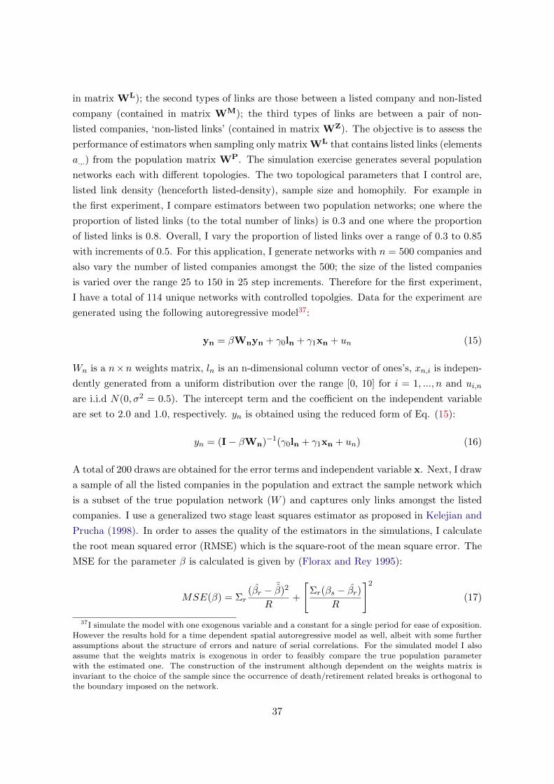
in matrix WL); the second types of links are those between a listed company and non-listed

company (contained in matrix WM); the third types of links are between a pair of non-

listed companies, ‘non-listed links’ (contained in matrix WZ). The objective is to assess the

performance of estimators when sampling only matrix WL that contains listed links (elements

a.,.) from the population matrix WP. The simulation exercise generates several population

networks each with different topologies. The two topological parameters that I control are,

listed link density (henceforth listed-density), sample size and homophily. For example in

the first experiment, I compare estimators between two population networks; one where the

proportion of listed links (to the total number of links) is 0.3 and one where the proportion

of listed links is 0.8. Overall, I vary the proportion of listed links over a range of 0.3 to 0.85

with increments of 0.5. For this application, I generate networks with n = 500 companies and

also vary the number of listed companies amongst the 500; the size of the listed companies

is varied over the range 25 to 150 in 25 step increments. Therefore for the first experiment,

I have a total of 114 unique networks with controlled topolgies. Data for the experiment are

generated using the following autoregressive model37:

yn = βWnyn + γ0ln + γ1xn + un (15)

Wn is a n×n weights matrix, ln is an n-dimensional column vector of ones’s, xn,i is indepen-

dently generated from a uniform distribution over the range [0, 10] for i = 1, ..., n and ui,n

are i.i.d N(0, σ2 = 0.5). The intercept term and the coefficient on the independent variable

are set to 2.0 and 1.0, respectively. yn is obtained using the reduced form of Eq. (15):

yn = (I− βWn)−1(γ0ln + γ1xn + un) (16)

A total of 200 draws are obtained for the error terms and independent variable x. Next, I draw

a sample of all the listed companies in the population and extract the sample network which

is a subset of the true population network (W ) and captures only links amongst the listed

companies. I use a generalized two stage least squares estimator as proposed in Kelejian and

Prucha (1998). In order to asses the quality of the estimators in the simulations, I calculate

the root mean squared error (RMSE) which is the square-root of the mean square error. The

MSE for the parameter β is calculated is given by (Florax and Rey 1995):

MSE(β) = Σr(βr − ¯

β)2

R+

[Σr(βs − βr)

R

]2

(17)

37I simulate the model with one exogenous variable and a constant for a single period for ease of exposition.However the results hold for a time dependent spatial autoregressive model as well, albeit with some furtherassumptions about the structure of errors and nature of serial correlations. For the simulated model I alsoassume that the weights matrix is exogenous in order to feasibly compare the true population parameterwith the estimated one. The construction of the instrument although dependent on the weights matrix isinvariant to the choice of the sample since the occurrence of death/retirement related breaks is orthogonal tothe boundary imposed on the network.

37

where βr is the estimate in replication r,¯β is the mean of the estimate for all replications,

βs is the true value of the parameter, and R is the number of replications in the simulation

experiment. The MSE combines both, the estimation variance as well as the bias of an

estimate into a measure of goodness of fit.

In the second experiment, I follow the same procedure outlined above but vary each simulated

network by an additional homophily parameter. This means that in addition to varying the

proportion of listed links to the total number of links, I also control the relative distribution

of listed links to mixed links in the population. I vary the degree of homophily over a range

of 0.1 to 0.70 with increments of 0.20.

A.3 IDENTIFICATION OF INDUSTRY PEER EFFECTS

To identify peer effects specific to a firms’ industry group, I construct the peer group of

each firm as the set of all other firms who share the same NIC code or belong to the same

business group. Even in this case, the resulting peer interaction structure is non-linear in

nature because each firms set of industry plus business group peers are distinct. Firm i can be

affiliated with all other firms in its industry but it is also affiliated to another set of firms that

belong to its business group who may or may not be in the same industry. To see this, denote

WI as the industry based peer interaction matrix with wIij = 1/nij if firm i shares the same

NIC code or belongs to the same business group as firm j and zero otherwise. This implies

that matrix WI has block diagonal elements of varying sizes. This brings about variation in

reduced-form coefficients across industry groups of different size that ensures identification.

The coefficient on the endogenous peer effect will be biased if firms’ own policy decision

influences their peers’ decision or if there are common time varying group specific shocks

that affect both the firm and the peer’s behaviour. In order to find a causal effect, one would

need an exclusion restriction that shifts the outcome of the firm independently of its peers.

Therefore we need a valid exclusion restriction such that it affects the average behaviors of a

firm’s peer group but not the firm’s behaviour directly.

Here the exclusion restrictions are derived from the peer interaction structure itself, specif-

ically, the overlapping nature of affiliation. I exploit the overlap between a firm’s industry

based peer group (henceforth industry group) and its ownership based peer group (henceforth

business group) to instrument for the endogenous peer effect. This identification strategy us-

ing peers-of-peers as an exclusion, wherein some ‘peers of peers’ do not affect an individual

directly but only through his or her own peers, has been recently used by many authors.

Bramoulle, Djebbari, and Fortin (2009) provide a general framework to show that endoge-

nous and exogenous effects can be distinguished through overlapping sub-groups within a

specific network structure38. In this setting, when firm i and j belong to the same industry

38Lin (2007) and Lee (2008) extend this model to a spatial autoregressive (SAR) framework where peer

38

group, the exclusion corresponds to assuming that a firm i is not directly affected by firm

j′s business group peers. I ensure that the characteristics of only those business group firms

are used that share no affiliations (industry or business) with the target firm i. Firms that

belong to j′s business group and are not associated with firm i form our excluded group, and

the instruments are generated from their exogenous characteristics. As before, to mitigate

the bias associated with selection into the industry, I employ a first differenced specification

that eliminates firm specific unobservables that are constant over time. Using the row vector,

WIi I obtain the following specification:

4 yit = αWIi 4 yt + λ4 xit + ϕWI

i 4 xt +4χt +4vit (18)

The set of excluded peers is contained in the matrix (WI)2 and their exogenous characteristics

are used as instruments for WIy. For convenience we denote the instrument set as (WEXxt)

where WEX = (WI)2 refers to the network of excluded group (EG) or ‘peers of peers’. Note

that in this case the peer reference group does not change over time so the variation in peers’

outcomes comes only from the changes in outcomes of a constant set of peers. As before, Eq.

(18) is estimated by two stage least squares. The exclusion is informative because there is

ample evidence that business groups are responsive to each other’s shocks as well as profits

(Bertrand, Mehta, and Mullainathan (2002); Gopalan, Nanda, and Seru (2007)).

effects are captured by the spatial lag term. De Giorgi, Pellizzari, and Redaelli (2010) also show that in acontext where peer groups do not overlap fully, it is possible to identify all the relevant parameters of thestandard linear-in-means model of social interactions. See also Laschever (2009).

39

Figure 1: Network Topology Summary

Note: The graph plots time series trends of the following network measures: Density - Proportion oflinks relative to total number possible; Degree - Total # links of any firm (averaged over all firms);Clustering - A measure of transitivity in link association i.e. whether two links of any firm arethemselves directly linked; AvgPath - Distance between any two firms in the network (averaged overall firms).

Figure 2: Network Dynamics

Note: The graph plots time series trends of network dynamics in a bipartite graph (following mea-sures are averaged over all firms): Appointments - Total # of new directors appointed for any firm ;Cessations - Total # of director exits for any firm; Newlink - Total # of links added due to directorappointments; Lostlink - Total # of links lost due to director exits; Death Retire - Total # of linkslost due to director exits from death or retirement.

40

Figure 3: Network Peer Investment and Firm Investment

Note: The graph is a non-parametric plot of own firm market in-vestment in relation to its network peers’ market investment.

Figure 4: Industry Peer Investment and Firm Investment

Note: The graph is a non-parametric plot of own firm market in-vestment in relation to its industry peers’ market investment.

41

Figure 5: RMSE for Network Simulations: Experiment 1, β = 0.2

Note: Each cell of the graph plots the RMSE associated with all given levels of Listed-density (Pro-portion of listed links to total number of links in the network) and Size (proportion of listed firms inthe population).

Figure 6: RMSE for Network Simulations: Experiment 2, β = 0.2, Size=20%

Note: The three dimensional surface plot maps the distribution of the RMSE over two network topology param-eters - Listed-density and Homophily (proportion of listed links relative to mixed links) for a sample size of 20%and a peer effect parameter of 0.2.

Table 1: Summary Statistics

Variable Obs Mean Std. Dev. Median 75th Percentile

Market Investments 32166 1.35 1.89 0.48 2.06Executive Compensation 32166 0.24 0.8 0.1 0.28Capital Expenditure 32166 0.08 0.27 0 0Current R&D Expnd. 32166 0.14 0.54 0 0Sales (log) 32166 3.11 2.39 3.22 4.93PBDITA 32166 107.14 953.33 2.89 20.91Assets (log) 32166 3.97 2.03 3.76 5.26Network Size 32166 6.4 10.23 3 8# Links Lost (Death) 32166 0.29 0.95 0 0

Network Averages

WN Market Investments 32166 1.5 1.5 1.23 2.44WN Executive Compensation 32166 0.26 0.31 0.18 0.39WN Capital Expenditure 32166 0.1 0.18 0 0.18WN Current R&D Expnd. 32166 0.2 0.39 0 0.28

Industry Averages

WI Market Investments 32166 1.48 1.25 1.22 1.88WI Executive Compensation 32166 0.25 0.34 0.18 0.33WI Capital Expenditure 32166 0.09 0.15 0.01 0.13WI Current R&D Expnd. 32166 0.15 0.29 0.02 0.17

Instruments

Local Network Shocks (Reduction from death induced link loss)

WD Market Investments 32166 0.24 0.94 0 0WD Executive Compensation 32166 0.04 0.17 0 0WD Capital Expenditure 32166 0.01 0.1 0 0WD Current R&D Expnd. 32166 0.02 0.21 0 0

Excluded Peer Averages

WEX Assets (log) 32166 5.03 1.39 4.98 5.83WEX Sales (log) 32166 3.92 1.47 4.21 4.88WEX PBDITA 32166 329.61 634.29 69.53 328.99

Table 2: Network Peer Effects: Corporate Market Investment

(1) (2) (3) (4) (5) (6)Mkt. Invst. WN Mkt. Invst. Mkt. Invst. Mkt. Invst. Mkt. Invst. Mkt. Invst.

WN Mkt. Invst. 0.020** 0.172* 0.149+ 0.232** 0.221*(0.005) (0.068) (0.079) (0.088) (0.094)

WD Mkt. Invst. -0.064**(0.006)

PBDITA 0.000* 0.000 0.000* 0.000* 0.000* 0.000*(0.000) (0.000) (0.000) (0.000) (0.000) (0.000)

Assets (logs) 0.105** 0.062** 0.096** 0.132** 0.101** 0.096**(0.015) (0.021) (0.016) (0.020) (0.017) (0.018)

Sales (logs) 0.040** 0.006 0.039** 0.035** 0.039** 0.040**(0.010) (0.015) (0.011) (0.012) (0.011) (0.012)

# Director Exits 0.003 -0.010+ 0.005 0.004 0.006 0.008+

(0.004) (0.005) (0.004) (0.005) (0.004) (0.005)

Growth Trajectory‡ -0.051**(0.006)

WN PBDITA -0.000 -0.000(0.000) (0.000)

WN Assets (logs) -0.054 0.050(0.101) (0.121)

WN Sales (logs) 0.064 0.084(0.108) (0.116)

Network Size -0.017(0.011)

Time Fixed Effects Yes Yes Yes Yes Yes Yes

N 19644 19644 19644 15271 19644 19644Cragg-Donald F 124.813 125.616 8.873 5.81

Notes:1. WN repesents local network peer averages.; WD represents averages of past period links that have been broken due todeath/retirement of shared directors2. PBDITA is the total Profit Before Depreciation, Interest, Tax and Amortisation; Assets in logs is total book value of assets; #Director Exits refers to the number of directors who have left the company in the previous time period; Network Size measuresthe number of direct links i.e. the number of other firms with whom it shares common directors.3. All control variables are lagged by one year.4. ‡ defined as the difference in outcome variable between period t− 1 and t− 2.5. Standard errors (in parentheses) are adjusted for autocorrelation and arbitrary heteroscedasticity at the network level.6. + indicates significance at 10%; * at 5%; ** at 1%.

Table 3: Network Peer Effects: Executive Compensation

(1) (2) (3) (4) (5) (6)Ex. Comp. WN Ex. Comp. Ex. Comp. Ex. Comp. Ex. Comp. Ex. Comp.

WN Ex. Comp. 0.053** 0.131+ 0.154+ 0.167+ 0.168+

(0.007) (0.075) (0.081) (0.101) (0.099)

WD Ex. Comp. -0.089**(0.007)

PBDITA -0.000 0.000** -0.000 0.000 0.000 0.000(0.000) (0.000) (0.000) (0.000) (0.000) (0.000)

Assets (logs) 0.069** 0.020** 0.068** 0.060** 0.069** 0.070**(0.004) (0.005) (0.005) (0.006) (0.005) (0.005)

Sales (logs) 0.005+ -0.002 0.006+ 0.012** 0.006+ 0.005+

(0.003) (0.003) (0.003) (0.004) (0.003) (0.003)

# Director Exits -0.001 -0.001 -0.001 -0.001 -0.001 -0.001(0.001) (0.001) (0.001) (0.001) (0.001) (0.001)

Growth Trajectory‡ -0.003+

(0.002)

WN PBDITA -0.000+ -0.000+

(0.000) (0.000)

WN Assets (logs) 0.016 0.001(0.026) (0.028)

WN Sales (logs) 0.003 -0.001(0.030) (0.030)

Network Size 0.003(0.003)

Time Fixed Effects Yes Yes Yes Yes Yes Yes

N 19644 19644 19644 15271 19644 19644Cragg-Donald F 178.946 179.066 8.88 5.61

Notes:1. WN repesents local network peer averages.; WD represents averages of past period links that have been broken due todeath/retirement of shared directors2. PBDITA is the total Profit Before Depreciation, Interest, Tax and Amortisation; Assets in logs is total book value of assets; #Director Exits refers to the number of directors who have left the company in the previous time period; Network Size measuresthe number of direct links i.e. the number of other firms with whom it shares common directors.3. All control variables are lagged by one year.4. ‡ defined as the difference in outcome variable between period t− 1 and t− 2.5. Standard errors (in parentheses) are adjusted for autocorrelation and arbitrary heteroscedasticity at the network level.6. + indicates significance at 10%; * at 5%; ** at 1%.

Table 4: Network Peer Effects: Capital Expenditure

(1) (2) (3) (4) (5) (6)Capex WN Capex Capex Capex Capex Capex

WN Capex 0.004 0.225 0.105 0.328+ 0.317+

(0.011) (0.151) (0.167) (0.171) (0.172)

WD Capex -0.084**(0.008)

PBDITA 0.000 -0.000 0.000 0.000 0.000 0.000(0.000) (0.000) (0.000) (0.000) (0.000) (0.000)

Assets (logs) -0.001 0.003 -0.002 -0.003 0.002 0.001(0.005) (0.003) (0.005) (0.006) (0.006) (0.006)

Sales (logs) 0.004 0.002 0.004 0.003 0.004 0.004(0.004) (0.002) (0.004) (0.004) (0.004) (0.004)

# Director Exits -0.002 -0.001 -0.002 -0.003+ -0.002 -0.002(0.001) (0.001) (0.001) (0.002) (0.002) (0.002)

Growth Trajectory‡ -0.083**(0.006)

WN PBDITA -0.000 -0.000(0.000) (0.000)

WN Assets (logs) -0.094** -0.073*(0.032) (0.036)

WN Sales (logs) 0.084* 0.089*(0.038) (0.039)

Network Size -0.004(0.004)

Time Fixed Effects Yes Yes Yes Yes Yes Yes

N 19644 19644 19644 15271 19644 19644Cragg-Donald F 117.738 117.601 9.775 6.002

Notes:1. WN repesents local network peer averages.; WD represents averages of past period links that have beenbroken due to death/retirement of shared directors2. PBDITA is the total Profit Before Depreciation, Interest, Tax and Amortisation; Assets in logs is totalbook value of assets; # Director Exits refers to the number of directors who have left the company in theprevious time period; Network Size measures the number of direct links i.e. the number of other firms withwhom it shares common directors.3. All control variables are lagged by one year.4. ‡ defined as the difference in outcome variable between period t− 1 and t− 2.5. Standard errors (in parentheses) are adjusted for autocorrelation and arbitrary heteroscedasticity at thenetwork level.6. + indicates significance at 10%; * at 5%; ** at 1%.

Table 5: Network Peer Effects: Current Expenditure in R&D

(1) (2) (3) (4) (5) (6)R&D WN R&D R&D R&D R&D R&D

WN R&D 0.007 -0.036 -0.013 0.059 0.016(0.006) (0.079) (0.080) (0.089) (0.094)

WD R&D -0.071**(0.007)

PBDITA 0.000* 0.000 0.000* 0.000* 0.000+ 0.000*(0.000) (0.000) (0.000) (0.000) (0.000) (0.000)

Assets (logs) 0.020** 0.003 0.020** 0.022** 0.023** 0.019**(0.005) (0.006) (0.005) (0.006) (0.005) (0.006)

Sales (logs) 0.003 -0.000 0.003 0.008* 0.003 0.004(0.003) (0.004) (0.003) (0.004) (0.003) (0.004)

# Director Exits 0.000 -0.000 0.000 -0.000 -0.000 0.001(0.001) (0.001) (0.001) (0.001) (0.001) (0.001)

Growth Trajectory‡ -0.084**(0.006)

WN PBDITA -0.000 -0.000(0.000) (0.000)

WN Assets (logs) 0.003 0.065*(0.027) (0.032)

WN Sales (logs) -0.027 -0.010(0.032) (0.035)

Network Size -0.011**(0.003)

Time Fixed Effects Yes Yes Yes Yes Yes Yes

N 19644 19644 19644 15271 19644 19644Cragg-Donald F 122.915 123.20 8.80 5.77

Notes:1. WN repesents local network peer averages.; WD represents averages of past period links that have beenbroken due to death/retirement of shared directors2. PBDITA is the total Profit Before Depreciation, Interest, Tax and Amortisation; Assets in logs is totalbook value of assets; # Director Exits refers to the number of directors who have left the company in theprevious time period; Network Size measures the number of direct links i.e. the number of other firms withwhom it shares common directors.3. All control variables are lagged by one year.4. ‡ defined as the difference in outcome variable between period t− 1 and t− 2.5. Standard errors (in parentheses) are adjusted for autocorrelation and arbitrary heteroscedasticity at thenetwork level.6. + indicates significance at 10%; * at 5%; ** at 1%.

Table 6: Network Peer Effects: Fixed Effects

A. Industry-Group Fixed Effects

(1) (2) (3) (4)Mkt. Invst. Ex. Comp. Capex R&D

WN Mkt. Invst. 0.164*(0.066)

WN Ex. Comp. 0.167*(0.070)

WN Capex 0.235(0.144)

WN R&D -0.022(0.074)

PBDITA 0.000 -0.000** 0.000 -0.000(0.000) (0.000) (0.000) (0.000)

Sales (log) 0.028* -0.001 -0.001 -0.003(0.011) (0.003) (0.004) (0.003)

Assets (log) 0.008 0.049** -0.012+ 0.009+

(0.017) (0.005) (0.006) (0.005)

# Director Exits 0.006 -0.001 -0.002 0.000(0.004) (0.001) (0.001) (0.001)

Time Fixed Effects Yes Yes Yes Yes

Industry-Group Fixed Effects Yes Yes Yes Yes

N 19644 19644 19644 19644Cragg-Donald F 118.865 188.356 110.894 123.75

B. Industry-Group-Time Fixed Effects

(1) (2) (3) (4)Mkt. Invst. Ex. Comp. Capex R&D

WN Mkt. Invst. 0.139*(0.068)

WN Ex. Comp. 0.190**(0.073)

WN Capex 0.241+

(0.146)

WN R&D -0.168+

(0.099)

PBDITA 0.000 -0.000** -0.000 -0.000(0.000) (0.000) (0.000) (0.000)

Sales (log) 0.021 -0.005 -0.004 -0.002(0.013) (0.004) (0.005) (0.004)

Assets (log) -0.030 0.053** -0.010 0.005(0.020) (0.006) (0.007) (0.006)

# Director Exits 0.011* -0.001 -0.001 -0.000(0.004) (0.001) (0.002) (0.001)

Industry-Group-Time Fixed Effects Yes Yes Yes Yes

N 19644 19644 19644 19644Cragg-Donald F 96.45 156.94 97.05 68.32

i) HAC robust standard errors in parentheses

Table 7: Network Peer Effects: Heterogeneous Effects

Mkt. Invst. Ex. Comp.

I: WNI I: WNN II: Mkt. Invst. I: WNI I: WNN II: Ex. Comp.

WNI Mkt. Invst. -0.048(0.158)

WNN Mkt. Invst. 0.131*(0.065)

WNI Ex. Comp. -0.117(0.195)

WNN Ex. Comp. 0.182*(0.071)

WDI Mkt. Invst. -0.092** -0.010(0.013) (0.022)

WDN Mkt. Invst. 0.004 -0.076**(0.005) (0.008)

WDI Ex. Comp. -0.350** 0.005(0.045) (0.075)

WDN Ex. Comp. 0.007 -0.115**(0.005) (0.009)

PBDITA -0.000** 0.000 0.000 -0.000** 0.000 -0.000**(0.000) (0.000) (0.000) (0.000) (0.000) (0.000)

Sales (log) 0.004 0.015 0.021 -0.001 -0.003 -0.005(0.012) (0.020) (0.013) (0.002) (0.004) (0.004)

Assets (log) -0.022 0.063* -0.031 -0.001 0.017** 0.053**(0.018) (0.030) (0.020) (0.004) (0.006) (0.006)

# Director Exits -0.016** -0.015* 0.010+ -0.001 -0.001 -0.001(0.004) (0.006) (0.005) (0.001) (0.001) (0.001)

Fixed Effects Yes Yes Yes Yes Yes Yes(Industry-Group-Time)

N 19644 19644 19644 19644 19644 19644Joint Cragg-Donald F 23.227 30.324

Notes:1. I refers to First stage of two stage least squares procedre while II refers to the second stage.2. WNI repesents local network averages of same industry peers; WNN repesents local network averages of non-industry peers;WDI represents averages of past period same industry links that have been broken due to death/retirement of shared directors;WDN represents averages of past period non-industry links that have been broken due to death/retirement of shared directors3. PBDITA is the total Profit Before Depreciation, Interest, Tax and Amortisation; Assets in logs is total book value of assets; #Director Exits refers to the number of directors who have left the company in the previous time period; Network Size measuresthe number of direct links i.e. the number of other firms with whom it shares common directors.4. All control variables are lagged by one year.5. Standard errors (in parentheses) are adjusted for autocorrelation and arbitrary heteroscedasticity at the network level.6. + indicates significance at 10%; * at 5%; ** at 1%.

Table 8: Investment in Same Stocks

(1) (2) (3) (4) (5) (6)OLS Rare Event Adj. OLS FE IV: First IV RE IV FE

Network Strength 0.091** 1.655** 0.017** 0.638** 1.187**(0.001) (0.011) (0.001) (0.245) (0.401)

Shared Director Exit† -0.005**(0.000)

Diff PBDITA‡ 0.322** 4.16** 0.132** 0.350** 0.074 -0.137**(0.0002) (0.003) (0.0006) ( (0.0001) (0.086) (0.016 )

Diff Assets (logs) 0.001** 0.053** -0.002** -0.004** 0.003** -0.001(0.000) (0.001) (0.000) (0.000) (0.0009) (0.001)

Diff Sales (logs) -0.0004** -0.011** -0.001** 0.0006** -0.0005** -0.001**(0.0000) (0.0009) (0.0009) (0.0078) (0.0000) (0.0003)

Same Industry 0.044** 0.867** -0.004** 0.049**(0.000) (0.009) (0.0685) (0.001)

Time Fixed Effects Yes Yes No No No No

Pair Fixed Effecs No No Yes No No Yes

N 11798464 11798464 11798464 5759498 5759498 5759498Cragg-Donald F 123.21 98.806

Notes:1. The units of analysis in all specifications are dyads, i.e. a pair of two companies i and j. Standard errors areadjusted using the QAP procedure to account for pair-wise dependence. The dependent variable is binary takingthe value 1 both i and j have invested in the same stock in time period t. Network Strength indicates the value ofconnection between i and j and ranges from zero to one. It is equal to the inverse of path distance in the globalnetwork between i and j – zero indicates no connection and one indicates direct connection. All other values mean thati, j are connected but through a series of intermediate links. Differences are in absolute terms due to the symmetricnature of the dyads.2. ‡ coeffcient mutiplied by 106.3. Column (2) adjusts coefficient estimates and standard errors to account for large non-events (zeroes) using theprocedure outline in King and Zeng (2001). It is a logistic regression so the coefficient estimate can be interpreted asfollows: A change in network strength from 0 to 1 (no connection to direct connection) increases the probability ofinvesting in the same stock by 11%. The relative risk associated with this change (of 0 to 1) is 4.56 log-odds.4. † is a dummy taking the value 1 if there are any common directors over the network between i and j who havedied or retired in the previous time period. For this reason The IV regressions (Columns (3) - Column (6)) discardobservations from the first year (2006) as its lag is not defined/missing.5. Time fixed effects are not included when using pair fixed effects so as to preserve some variation in the dependentvariable6. + indicates significance at 10%; * at 5%; ** at 1%.

Table 9: Sensitivity Results: Probability of New Link

(1) (2)New Link New Link

Link Loss (Death) -0.002 -0.003(0.008) (0.009)

Firm Controls No Yes

Time Fixed Effects Yes Yes

N 27084 21727Joint Significance of Time F.E 645.14 (0.00) 540.80 (0.00)

i) HAC robust standard errors in parentheses

Table 10: Network Peer Effects: Global Network

(1) (2) (3) (4)Mkt. Invst. Ex. Comp. Capex R&D

WG Mkt. Invst. 0.442*(0.191)

WG Ex. Comp. 0.632+

(0.394)

WG Capex 1.153(1.023)

WG R&D -0.341(0.503)

PBDITA 0.000 -0.000 0.000 0.000*(0.000) (0.000) (0.000) (0.000)

Assets (log) 0.090** 0.065** -0.003 0.022**(0.018) (0.006) (0.006) (0.006)

Sales (log) 0.042** 0.006+ 0.004 0.003(0.011) (0.003) (0.004) (0.003)

# Director Exits 0.008+ -0.000 -0.001 -0.000(0.005) (0.001) (0.001) (0.001)

Time Fixed Effects Yes Yes Yes Yes

N 19644 19644 19644 19644Cragg-Donald F 45.464 23.457 20.018 26.973

Notes:1. WG repesents global network peer averages2. PBDITA is the total Profit Before Depreciation, Interest, Tax and Amortisation; Assets in logsis total book value of assets; # Director Exits refers to the number of directors who have left thecompany in the previous time period; Network Size measures the number of direct links i.e. thenumber of other firms with whom it shares common directors.3. All control variables are lagged by one year.4. Standard errors (in parentheses) are adjusted for autocorrelation and arbitrary heteroscedas-ticity at the network level.5. + indicates significance at 10%; * at 5%; ** at 1%.

Table 11: Industry Peer Effects

A. Mkt. Invst.

(1) (2) (3)Mkt. Invst. Mkt. Invst. Mkt. Invst.

WI Mkt. Invst. 0.043** 0.487+ 0.456(0.010) (0.272) (0.303)

WI PBDITA -0.000(0.000)

WI Sales (log) -0.006(0.025)

WI Assets (log) 0.116**(0.044)

N 21727 17280 17280Excl. Instruments Joint Significance 40.80 (0.00) 32.80 (0.00)Cragg-Donald F 14.046 8.324

B. Executive Compensation

(1) (2) (3)Ex. Comp. Ex. Comp. Ex. Comp.

WI Ex. Comp. 0.032** 0.224 1.015(0.005) (0.317) (2.583)

WI PBDITA 0.000(0.000)

WI Sales (log) 0.020(0.071)

WI Assets (log) 0.056(0.152)

N 21727 17280 17280Excl. Instruments Joint Significance 6.58 (0.01) 0.24 (0.623)Cragg-Donald F 6.536 1.23

C. R& D

(1) (2) (3)R&D R&D R&D

WI R&D 0.049** 0.690* 0.976*(0.012) (0.302) (0.448)

WI PBDITA 0.000(0.000)

WI Sales (log) 0.002(0.014)

WI Assets (log) 0.027**(0.010)

N 21727 17280 17280Excl. Instruments Joint Significance 38.91 (0.00) 15.09 (0.00)Cragg-Donald F 14.31 5.43

i) Standard errors in parentheses

Table 12: Industry-Network Peer Effects

(1) (2) (3) (4)Mkt. Invst. Mkt. Invst. R&D R&D

WN Mkt. Invst. 0.193* 0.146+

(0.086) (0.080)

WI Mkt. Invst. 0.237 0.016(0.281) (0.257)

WN R&D -0.060 -0.016(0.114) (0.127)

WI R&D 0.690* 0.629**(0.318) (0.184)

PBDITA 0.000 0.000 0.000 0.000(0.000) (0.000) (0.000) (0.000)

Assets (log) 0.089** -0.026 0.023** 0.004(0.019) (0.022) (0.006) (0.007)

Sales (log) 0.035** 0.016 0.003 0.000(0.012) (0.014) (0.004) (0.004)

# Director exits 0.007 0.012* 0.001 0.000(0.005) (0.004) (0.002) (0.001)

Time F.E. Yes Yes

Industry-Group-Time F.E. Yes Yes

N 15630 14172 15630 14172Cragg-Donald F 10.688 14.414 10.482 13.204

Notes:1. WN repesents local network peer averages; WI repesents industry peer averages.2. PBDITA is the total Profit Before Depreciation, Interest, Tax and Amortisation; Assets in logsis total book value of assets; # Director Exits refers to the number of directors who have left thecompany in the previous time period; Network Size measures the number of direct links i.e. thenumber of other firms with whom it shares common directors.3. All control variables are lagged by one year.4. Standard errors (in parentheses) are adjusted for autocorrelation and arbitrary heteroscedas-ticity at the network level.5. + indicates significance at 10%; * at 5%; ** at 1%.

Table 13: Monte Carlo Results: Experiment 1

Size Listed-density β = 0 β = 0.1 β = 0.2 β = 0.3 β = 0.4 β = 0.5

Mean RMSE Mean RMSE Mean RMSE Mean RMSE Mean RMSE Mean RMSE

0.1 0.03 0.00 0.02 0.02 0.08 0.04 0.16 0.06 0.24 0.08 0.32 0.10 0.400.1 0.00 0.03 0.05 0.05 0.11 0.09 0.17 0.13 0.23 0.17 0.29 0.210.25 0.00 0.04 0.09 0.04 0.19 0.03 0.29 0.03 0.39 0.03 0.49 0.020.5 0.00 0.04 0.11 0.04 0.20 0.04 0.30 0.03 0.40 0.03 0.50 0.020.75 0.00 0.04 0.10 0.04 0.20 0.03 0.30 0.03 0.40 0.03 0.50 0.020.85 0.00 0.04 0.10 0.04 0.20 0.03 0.30 0.03 0.40 0.03 0.50 0.02

0.2 0.03 0.00 0.01 0.03 0.07 0.06 0.14 0.08 0.22 0.12 0.28 0.14 0.360.1 0.00 0.01 0.06 0.04 0.12 0.08 0.19 0.12 0.25 0.15 0.32 0.180.25 0.00 0.02 0.09 0.02 0.19 0.02 0.28 0.02 0.38 0.02 0.48 0.020.5 0.00 0.02 0.10 0.02 0.20 0.02 0.30 0.02 0.40 0.02 0.50 0.010.75 0.00 0.02 0.10 0.02 0.20 0.02 0.30 0.02 0.40 0.01 0.50 0.010.85 0.00 0.03 0.10 0.02 0.20 0.02 0.30 0.02 0.40 0.01 0.50 0.01

0.3 0.1 0.00 0.01 0.04 0.06 0.08 0.12 0.12 0.18 0.16 0.24 0.21 0.290.25 0.00 0.02 0.08 0.03 0.16 0.04 0.24 0.06 0.33 0.07 0.41 0.090.5 0.00 0.02 0.10 0.02 0.19 0.02 0.29 0.02 0.39 0.01 0.49 0.010.75 0.00 0.02 0.10 0.02 0.20 0.01 0.30 0.01 0.40 0.01 0.50 0.010.85 0.00 0.02 0.10 0.02 0.20 0.02 0.30 0.01 0.40 0.01 0.50 0.01

Table 14: Monte Carlo Results: Experiment 2

Size Listed-density Homophily RMSE RMSE RMSE RMSE RMSE RMSEβ = 0 β = 0.1 β = 0.2 β = 0.3 β = 0.4 β = 0.5

0.1 0.03 0.1 0.02 0.08 0.16 0.24 0.32 0.400.3 0.02 0.05 0.10 0.15 0.20 0.250.5 0.02 0.03 0.05 0.08 0.10 0.130.75 0.02 0.02 0.02 0.02 0.01 0.02

0.05 0.1 0.02 0.07 0.13 0.18 0.24 0.290.3 0.02 0.06 0.10 0.15 0.21 0.250.5 0.03 0.03 0.05 0.07 0.09 0.100.75 0.02 0.03 0.04 0.05 0.06 0.08

0.1 0.1 0.03 0.06 0.10 0.15 0.19 0.230.3 0.03 0.05 0.09 0.13 0.18 0.210.5 0.03 0.05 0.08 0.12 0.16 0.200.75 0.03 0.03 0.03 0.03 0.02 0.02

0.2 0.03 0.1 0.01 0.07 0.14 0.21 0.28 0.350.3 0.01 0.04 0.09 0.13 0.17 0.220.5 0.01 0.02 0.04 0.06 0.08 0.100.75 0.01 0.01 0.02 0.02 0.03 0.04

0.05 0.1 0.01 0.07 0.14 0.21 0.28 0.350.3 0.01 0.04 0.08 0.12 0.16 0.200.5 0.01 0.03 0.05 0.08 0.10 0.130.75 0.01 0.02 0.02 0.03 0.04 0.05

0.1 0.1 0.02 0.06 0.12 0.17 0.22 0.260.3 0.01 0.04 0.08 0.11 0.14 0.180.5 0.02 0.02 0.04 0.05 0.06 0.080.75 0.01 0.02 0.02 0.03 0.03 0.04