Copyright

by

Yu-Ren Wang

2002

APPLYING THE PDRI IN PROJECT RISK MANAGEMENT

by

YU-REN WANG, B.S., M.S.

DISSERTATION

Presented to the Faculty of the Graduate School of

The University of Texas at Austin

in Partial Fulfillment

of the Requirements

for the Degree of

DOCTOR OF PHILOSOPHY

The University of Texas at Austin

August 2002

Dedication

To my family,

especially my parents,

for their support and love.

To my friends,

for their companion and friendship,

with love and appreciation.

Acknowledgements

I am indebted to my supervising professor, Dr. G. Edward Gibson, Jr., for

his guidance and support throughout the entire research process. He provided

profound insight into the subject matter and placed confidence in me for the

conduct of this research. I would also like to thank the other members of my

dissertation committee, Dr. Richard L. Tucker, Dr. Stephen R. Thomas, Dr.

Robert B. Gilbert, and Dr. Joydeep Ghosh, for their participation and guidance in

this research effort.

I would like to acknowledge the support provided to this research by the

institutional organization, which prefers to be anonymous, and Ron Horne of

Project Consultants, and the Construction Industry Institute. This research was

funded by the institutional organization and supported by their engineering

personnel and an outside consultant. A major portion of sample projects were

provided by this institutional organization. I would also like to thank the support

from CII for providing projects for this research.

I would like to thank the staff at the UT-Austin Statistical Services, and

Dr. Robert B. Gilbert for their consultation in statistical analysis of this research.

Finally, I owe my deepest gratitude to my parents and other family members, for

their unconditional supports throughout my entire graduate study program.

v

APPLYING THE PDRI IN PROJECT RISK MANAGEMENT

Publication No._____________

Yu-Ren Wang, Ph.D.

The University of Texas at Austin, 2002

Supervisor: G. Edward Gibson, Jr.

Research conducted by the Construction Industry Institute (CII) shows

that adequate pre-project planning benefits project in the areas of cost, schedule,

and operational characteristics. Pre-project planning is the project phase

encompassing all the tasks between project initiation to detailed design. The

development of a project scope definition packages is one of the major tasks in

the pre-project planning process. Project scope definition is the process by

which projects are defined and prepared for execution. It is at this crucial stage

where risks associated with the project are analyzed and the specific project

execution approach is defined. Development of the Project Definition Rating

Index (PDRI) in 1996 provided an effective and easy-to-use tool for project scope

development for industrial projects. A complementary PDRI was developed for

building projects in 1999. Since introduction, the PDRI (both versions) have

been widely used by the construction industry and serve as an important tool for

vi

measuring project scope definition. The PDRI helps a project team to quickly

analyze the scope definition package and predict factors that may impact project

risk. However, since its introduction, little additional analyses have been

conducted looking at the PDRI.

Data from 140 capital projects representing approximately $5 billion in

total construction cost were used for this research analysis. The relationship

between good scope definition and enhanced project performance were

demonstrated. Analysis of PDRI scores identified poor definition scope

elements and quantified their potential impact to project outcomes. Risk control

procedures were examined and recommended to mediate high risk areas, such as

poorly defined scope elements. A systematic risk management approach was

proposed and explained in detail. Research limitations, conclusions and

recommendations are also discussed in this dissertation. This research effort

extends the use of PDRI as a project management tool in the process of capital

facility projects delivery.

vii

Table of Contents

List of Tables.........................................................................................................xii

List of Figures ....................................................................................................... xv

Chapter 1 Introduction ......................................................................................... 1 1.1. Background ........................................................................................... 3

1.1.1. Pre-Project Planning Research ............................................ 3 1.1.2. Construction Project Risk.................................................... 7

1.2. Research Objectives .............................................................................. 8 1.3. Organization Of The Dissertation ......................................................... 9

Chapter 2 Literature Review .............................................................................. 11 2.1. Pre-project Planning And Scope Definition........................................ 11

2.1.1. Pre-Project Planning.......................................................... 11 2.1.2. Scope Definition................................................................ 15

2.2. Project Definition Rating Index (PDRI).............................................. 17 2.3. Managing Construction Project Risk .................................................. 30

2.3.1. Identifying Construction Project Risk............................... 31 2.3.2. Quantifying Construction Project Risk ............................. 33 2.3.3. Controlling Construction Project Risk .............................. 35

2.4. Literature Review Conclusions ........................................................... 36 2.5. Summary ............................................................................................. 37

Chapter 3 Problem Statement and Research Hypotheses................................... 38 3.1. Problem Statement .............................................................................. 38 3.2. Research Hypotheses........................................................................... 39 3.3. Summary ............................................................................................. 41

Chapter 4 Research Methodology ...................................................................... 42 4.1. Literature Review And Issue Identification ........................................ 44

viii

4.2. Questionnaire Development And Finalization.................................... 45 4.3. Data Collection.................................................................................... 47 4.4. Data Analysis ...................................................................................... 51

4.4.1. Descriptive Statistics Analysis .......................................... 51 4.4.2. Regression Analysis .......................................................... 53 4.4.3. Independent Samples t-Test and Effect Size..................... 56

4.5. Analytical Model Development .......................................................... 59 4.6. Systematic Risk Management Approach ............................................ 63 4.7. Study Limitations ................................................................................ 64 4.8. Summary of Research Methodology................................................... 65

Chapter 5 Project Data Characteristics and Data Analysis ................................ 66 5.1. General Project Characteristics ........................................................... 66 5.2. Performance Characteristics................................................................ 76

5.2.1. Cost Performance .............................................................. 77 5.2.2. Schedule Performance....................................................... 79

5.3. PDRI Score Characteristics ................................................................. 82 5.4. PDRI And Project Success .................................................................. 85

5.4.1. Project Success .................................................................. 85 5.4.2. Bivariate Correlation and Linear Regression Analysis ..... 92

5.5. Findings Related To Research Hypothesis.......................................... 96 5.6. Summary ............................................................................................. 97

Chapter 6 Institutional Organization Project Analysis....................................... 99 6.1. Project Sample Characteristics.......................................................... 100

6.1.1. Construction Cost ............................................................ 100 6.1.2. Construction Schedule..................................................... 102 6.1.3. Change Orders................................................................. 106 6.1.4. Quality............................................................................. 109 6.1.5. PDRI Scores .................................................................... 111

ix

6.2. PDRI Score Evaluation ..................................................................... 112 6.2.1. PDRI Score vs. Project Performance .............................. 113 6.2.2. Unit Cost Analysis .......................................................... 117

6.3. Summary ........................................................................................... 120

Chapter 7 Risk Identification through PDRI Characteristics ........................... 122 7.1. Scope Definition Level Characteristics............................................. 122

7.1.1. Industrial Project Definition Level Characteristics ......... 123 7.1.2. Building Project Definition Level Characteristics .......... 128

7.2. Identifying Risk Through PDRI........................................................ 133 7.2.1. Risk Identification through PDRI Element Weights....... 134 7.2.2. Risk Identification through Historical Data .................... 139

7.3. Findings Related To Research Hypothesis........................................ 144 7.4. Summary ........................................................................................... 148

Chapter 8 Risk Quantification and Control through PDRI .............................. 150 8.1. Model Development Approach ......................................................... 150

8.1.1. Linear Regression Model ................................................ 151 8.1.2. Boxplots Quartile Model ................................................. 167 8.1.3. Hackney’s Accuracy Range Estimate Method................ 174

8.2. Risk Quantification Using PDRI....................................................... 185 8.2.1. Linear Regression Model ................................................ 185 8.2.2. Boxplot Quartile Analysis Model ................................... 187 8.2.3. Hackney’s Accuracy Range Estimate Model.................. 190

8.3. Risk Control Through PDRI ............................................................. 194 8.4. Risk Management Using PDRI ......................................................... 197 8.5. Limitations And Summary ................................................................ 202

Chapter 9 Conclusions and Recommendations ................................................ 204 9.1. Review of Research Objectives......................................................... 204

9.1.1. Further Validation of the PDRI....................................... 205

x

9.1.2. Identifying Project Risk and Potential Risk Impact ........ 206 9.1.3. Systematic Project Risk Management Approach

Development ................................................................... 207 9.1.4. Establish Baseline Methodology..................................... 208

9.2. Research Hypotheses......................................................................... 208 9.3. Conclusions ....................................................................................... 212 9.4. Contributions..................................................................................... 213 9.5. Recommendation for Future Research.............................................. 215

Appendix A Logic Flow Diagram for Industrial PDRI....................................... 217

Appendix B Institutional Organization Risk And Readiness Survey Questionnaires (Project Manager and User) .................................. 221

Appendix C PDRI for Industrial Projects Score Sheets ...................................... 242

Appendix D Project Performance and Success Index......................................... 247

Appendix E PDRI Element Definition Level Descriptive Statistics................... 252

Appendix F Project Cost and Completion Time ................................................. 257

Bibliography........................................................................................................ 262

Vita .................................................................................................................... 268

xi

List of Tables

Table 4.1. Sample Data Summary...............................................................51 Table 5.1. Sample Data Facility Type.........................................................67 Table 5.2. Sample Project Performance Summary versus Estimated .........82 Table 5.3. Success Index Variables and Weights (Gibson and Hamilton

1994)...........................................................................................88 Table 5.4. Industrial Project Achievement Variable Recoding, N=62........90 Table 5.5. Building Project Achievement Variable Recoding, N=78 .........91 Table 5.6. Industrial Project Regression Results.........................................93 Table 5.7. Building Project Regression Results ..........................................94 Table 6.1. Institutional Organization Project Summary............................100 Table 6.2. Unit Cost Comparison (Authorized, Actual, After 1st Year)....101 Table 6.3. Small Building Project Time Breakdown ................................105 Table 6.4. Change Orders (COs) Information for Small Building Projects

..................................................................................................107 Table 6.5. Summary of Cost, Schedule, and Change Order Performance for

the Building Projects Using a 300-point Cutoff.......................114 Table 6.6. Summary of Cost, Schedule, and Change Order Variation for the

Building Projects Using a 300-Point Cutoff ............................114 Table 6.7. Summary of Percentage of Building Projects Having At Least

One Change Order >1% of Project Cost Using a 300-Point Cutoff .......................................................................................115

Table 6.8. Summary of Cost, Schedule, and Change Order Performance for ALL Projects Using a 300-point Cutoff ...................................116

Table 6.9. Summary of Cost, Schedule, and Change Order Variation for ALL Projects Using a 300-point Cutoff ...................................116

Table 6.10. Comparison between CII Projects PDRI Score <200 and Institutional Projects PDRI Score <300 and PDRI Score >300117

Table 6.11. Unit Cost Comparison for All 42 Building Projects ................118 Table 6.12. Unit Cost Comparison for North America Building Projects ..119 Table 7.1. Worst Definition Level Averages for Industrial Projects.........124

xii

Table 7.2. Scope Elements with Most Level 5 Definitions for Industrial Projects .....................................................................................126

Table 7.3. Best Definition Level Averages for Industrial Projects ...........127 Table 7.4. Scope Elements with Most Level 1 Definitions for Industrial

Projects .....................................................................................128 Table 7.5. Worst Definition Level Averages for Building Projects ..........130 Table 7.6. Scope Elements with Most Level 5 Definitions for Building

Projects .....................................................................................131 Table 7.7. Best Definition Level Averages for Building Projects.............132 Table 7.8. Scope Elements with Most Level 1 Definitions for Building

Projects .....................................................................................133 Table 7.9. Top 15 Elements with Highest Definition Level 5 Weights ....137 Table 7.10. Summary of Mean Project Performance Using a 200-point

Cutoff .......................................................................................139 Table 7.11. Effect Size for Building PDRI Category A, example ..............140 Table 7.12. Elements with Large Effect Size Based on Schedule Performance

..................................................................................................141 Table 7.13. Elements with Large Effect Size Based on Cost Performance 143 Table 7.14. Mean Cost Performance Comparison for Cost Indicators .......146 Table 7.15. Mean Cost Performance Comparison for Schedule Indicators 147 Table 8.1. Regression Statistics: Cost Growth vs. Industrial PDRI Score 152 Table 8.2. Regression Statistics: Cost Growth vs. Building PDRI Score .154 Table 8.3. Regression Statistics: Industrial Total vs. Modified PDRI Score,

..................................................................................................159 Table 8.4. Regression Statistics: Building Total vs. Modified PDRI Score,

..................................................................................................160 Table 8.5. Regression Statistics: Schedule Growth vs. Building PDRI Score

..................................................................................................163 Table 8.6. Regression Statistics: Schedule Growth vs. Building PDRI Score

..................................................................................................164 Table 8.7. Regression Statistics: Industrial Total vs. Modified PDRI Score,

..................................................................................................166 Table 8.8. Summary Statistics for Industrial Cost Growth .......................169

xiii

Table 8.9. Summary Statistics for Building Cost Growth.........................171 Table 8.10. Summary Statistics for Industrial Schedule Growth ................172 Table 8.11. Summary Statistics for Building Schedule Growth .................174 Table 8.12. Ninety-five Percent Confidence Level Summary ....................187 Table 8.13. Summary Statistics for Industrial Cost Growth .......................188 Table 8.14. Summary Statistics for Combined Group ................................189 Table 8.15. Boxplot Cost Growth Estimate Summary................................190 Table 8.16. Performance Estimate Using the Three Models, Industrial

Projects .....................................................................................193 Table 8.17. Performance Estimate Using the Three Models, Building

Projects .....................................................................................193 Table 8.18. Ninety-five Percent Confidence Level Summary ....................195 Table 9.1. Cost Performance Indicators ....................................................211 Table 9.2. Schedule Performance Indicators.............................................212

xiv

List of Figures

Figure 2.1. Influence and Expenditure Curve for the Project Life Cycle.....12 Figure 2.2. Pre-Project Planning Process Flow Map....................................14 Figure 2.3. Sections, Categories and Elements of PDRI for Industrial

Projects .......................................................................................19 Figure 2.4. Example Description for Element A1: Reliability Philosophy ..20 Figure 2.5. Sections, Categories and Elements of PDRI for Building Projects

....................................................................................................23 Figure 2.6. Example Description for Element A1: Building Use.................24 Figure 2.7. Buildings PDRI Category A.......................................................28 Figure 4.1. Research Methodology Flow Diagram ......................................43 Figure 4.2. Annotated Sketch of the Boxplot ...............................................53 Figure 4.3. Hackney’s Checklist of Definition Rating .................................60 Figure 4.4. Definition Rating vs. Overruns ..................................................62 Figure 5.1. Industrial Project Type ...............................................................68 Figure 5.2. Building Project Type ................................................................69 Figure 5.3. Industrial Project Contract Type ................................................70 Figure 5.4. Building Project Contract Type..................................................71 Figure 5.5. Industrial Project Locations .......................................................72 Figure 5.6. Building Project Locations.........................................................72 Figure 5.7. Industrial Project Total Schedule Durations, N=62 ...................73 Figure 5.8. Building Project Total Schedule Durations, N=78.....................74 Figure 5.9. Industrial Project Total Installed Cost, N=62.............................75 Figure 5.10. Building Project Total Installed Cost, N=78..............................76 Figure 5.11. Industrial Project Cost Growth Histogram, N=62......................78 Figure 5.12. Building Project Cost Growth Histogram, N=78 .......................79 Figure 5.13. Industrial Project Schedule Growth Histogram, N=62 ..............80 Figure 5.14. Building Project Schedule Performance Histogram, N=78 .......81 Figure 5.15. Industrial Project PDRI Score Histogram, N=62 .......................84

xv

Figure 5.16. Building Project PDRI Score Histogram, N=78 ........................85 Figure 5.17. Industrial Project Success Index vs. PDRI Score.......................95 Figure 5.18. Building Project Success Index vs. PDRI Score ........................96 Figure 6.1. Average Cost Growth in Different Regions.............................102 Figure 6.2. Average Schedule Growth in Different Regions......................103 Figure 6.3. Total Project Time for Small Building Projects.......................105 Figure 6.4. Detailed Change Order Costs in Eight Category .....................108 Figure 6.5. Change Order Cost Percentage ................................................109 Figure 6.6. PM vs. User Quality Survey.....................................................110 Figure 7.1. Buildings PDRI Category A.....................................................135 Figure 8.1. Linear Regression: Cost Growth vs. Industrial PDRI Score ....152 Figure 8.2. Linear Regression: Cost Growth vs. Building PDRI Score .....153 Figure 8.3. Funnel Effect of Cost Growth, Industrial.................................155 Figure 8.4. Funnel Effect of Cost Growth, Building ..................................156 Figure 8.5. Industrial Cost Growth vs. Modified PDRI Score ...................159 Figure 8.6. Building Cost Growth vs. Modified PDRI Score.....................160 Figure 8.7. Linear Regression: Schedule Growth vs. Industrial PDRI Score

..................................................................................................162 Figure 8.8. Linear Regression: Schedule Growth vs. Building PDRI Score

..................................................................................................163 Figure 8.9. Industrial Schedule Growth vs. Modified PDRI Score ............166 Figure 8.10. Annotated Sketch of the Boxplot .............................................168 Figure 8.11. Industrial Cost Growth by PDRI Score Groups .......................169 Figure 8.12. Building Cost Growth by PDRI Score Groups ........................170 Figure 8.13. Industrial Schedule Growth by PDRI Score Groups................172 Figure 8.14. Building Schedule Growth by PDRI Score Groups .................173 Figure 8.15. Definition Rating vs. Overruns ................................................175 Figure 8.16. Scatter Plot: Cost Growth vs. Industrial PDRI Score...............176 Figure 8.17. Cost Growth Accuracy Range Estimate for Industrial Projects177 Figure 8.18. Scatter Plot: Schedule Growth vs. Industrial PDRI Score .......178

xvi

Figure 8.19. Schedule Growth Accuracy Range Estimate for Industrial Projects .....................................................................................179

Figure 8.20. Scatter Plot: Cost Growth vs. Building PDRI Score................180 Figure 8.21. Cost Growth Accuracy Range Estimate for Building Projects 182 Figure 8.22. Scatter Plot: Schedule Growth vs. Building PDRI Score.........183 Figure 8.23. Schedule Growth Accuracy Range Estimate for Building Projects

..................................................................................................184 Figure 8.24. Best Fit Line and 95 Percent Confidence Line for Industrial

Projects .....................................................................................186 Figure 8.25. Industrial Cost Growth by PDRI Groups .................................188 Figure 8.26. Scatter Plot: Schedule Growth vs. Industrial PDRI Score .......190 Figure 8.27. Cost Growth Accuracy Range Estimate for Industrial Projects192 Figure 8.28. Systematic Risk Management Process Using PDRI ................198 Figure 8.29. Example Risk Register and Action Items, November 2001.....201

xvii

Chapter 1 Introduction

Pre-project planning is “….the process of developing sufficient strategic

information with which owners can address risk and decide to commit resources

to maximize the chance for a successful project” (CII 1995). One of the key

tasks of pre-project planning is to develop a detailed scope definition for the

project. Research has shown that a complete scope definition improves project

performance in the areas of cost, schedule, quality, and operational characteristics.

Extraordinary risks are many times the result of unresolved scope issues or

unforeseen conditions (Smith and Bohn 1999). At a point of time right before

detailed design, poorly defined scope definition elements are identified during the

PDRI evaluation process within the owner’s organization. These poorly defined

scope definition elements should be treated as potential risk factors that might

cause negative impact to project outcomes.

A need exists to integrate previous research results on pre-project planning

and project risk management. This dissertation investigates the potential risk

impact caused by poorly defined scope elements and proposes a risk management

process using the Project Definition Rating Index (PDRI) in the early stage of the

project life cycle.

The Project Definition Rating Index is a project scope definition tool

developed under the guidance of Construction Industry Institute (CII). It is a

powerful and easy-to-use tool that offers a method to measure project scope

definition for completeness. Research has shown that PDRI allows a project

1

team to evaluate the completeness of scope definition prior to detailed design or

construction and helps a project team to quickly analyze the scope definition

package and predict factors that may impact project risk (Gibson and Dumont

1996). According to a national survey of top 100 U.S. large contractors, Kangari

(1995) identified ‘defective design’ as one of the most important risks ranked by

the survey participants. Poor scope definition often results in delayed design and

in some cases contributes to poor design. By identifying potential risk factors

early in a project, the project team can quickly respond to the risks and thus

reduce the possible negative impact on design and construction.

The construction industry, perhaps more than most, is plagued by high

amounts of risk (Flanagan and Norman 1993), but often this risk is not dealt with

adequately, resulting in poor performance with increased costs and time delays

(Thompson and Perry 1992). Several methods have been developed to model

construction risk (Ibbs and Crandall 1982, Ashley et al. 1988, CII 1989, Boyer

and Kangari 1989, Touran 1992, Paek et al. 1993). While most of these methods

were developed to help contractors estimate or evaluate their risk exposure, there

has been little effort to estimate or evaluate risk from the owner’s/client’s

perspectives. Mak and Picken (2000) looked into risk to the client/owner and

used risk analysis to determine construction project contingency. Their study

results showed improvement in the estimate of contingency after implementing

the risk analysis technique in estimation. Nevertheless, available literature

provides little information as to how the owner/investor should identify project

risk factors and quantify potential risk impacts during the early stage of a project.

2

This chapter will present a brief overview of the context under which the

research was conducted. Background information related to PDRI and how it

relates to the investigation are presented. Previous research is discussed as well

as the research objectives. Finally, the dissertation organization is outlined in

this chapter.

1.1. BACKGROUND

It has long been recognized by the industry practitioners the importance of

pre-project planning in the capital facility delivery process and its potential

impact on project success. Nevertheless, the pre-project planning process varies

significantly throughout industry from one organization to another. Because of

this inconsistency, the Construction Industry Institute (CII) and others chartered

several studies in the 1990’s to look at this area.

1.1.1. Pre-Project Planning Research

The research presented in this dissertation is the latest in a related series of

studies that have been performed at the University of Texas since 1991. The

following sections give a brief overview of those studies. A more in-depth

treatment is given in the next chapter.

Pre-Project Planning Research

In 1991, CII chartered a research project “to find the most effective

methods of project definition and cost estimating for appropriation approval”.

The research team was composed of two faculty members and 16 industry

practitioners (nine from owner organization and seven from contractor). This

team helped map the pre-project planning process by using IDEF0, Structured

3

Analysis and Design Techniques (Gibson et al. 1995). Pre-project planning was

defined as “the process of developing sufficient strategic information with which

owners can address risk and decide to commit resources to maximize the chance

for a successful project” (CII 1994). The research team summarized the pre-

project planning process into four major steps: organize for pre-project planning,

select project alternative(s), develop a project definition package (which is the

detailed scope definition of the project), and decide whether to proceed with the

project (Gibson et al. 1995). The research results also indicated that the pre-

project planning effort level directly affects the cost and schedule predictability of

the project (Hamilton 1994).

Front End Planning Research

CII constituted another research team in 1994 to produce effective, simple,

and easy-to-use pre-project planning tools that extend previous research efforts so

that owner and contractor companies can better achieve business, operational, and

project objectives (CII 1996). The goal of this study was to develop effective

and easy-to-use pre-project planning management tools. In order to reach this

goal, the objectives were set up to 1) quantify pre-project planning efforts, and 2)

analyze the impact of alignment. This effort produced the Project Definition

Rating Index (PDRI) for Industrial Projects as a scope definition tool.

The PDRI is a weighted matrix with 70 scope definition elements (issues

that need to be addressed in pre-project planning) grouped into 15 categories and

further grouped into three main sections. The PDRI allows a project team to

measure the completeness of a project’s scope definition and a project can score

4

up to 1000 points, with a lower score being better (Gibson and Dumont 1996).

The tool is applicable to process and manufacturing facilities such as chemical

plants, paper mills, manufacturing assembly plants, petroleum refineries and so

on. In addition to the development of the industrial PDRI, this research

investigation also analyzed the impact of alignment between business, project

management, and operations personnel of owner companies, as well as the

alignment between owners and contractors during pre-project planning. The

research results showed that achieving and maintaining alignment is a key factor

in project planning and in achieving project success (Griffith and Gibson 2001).

OFPC Project

In response to the University of Texas (UT) System Board of Regent’s

recommendation to revise the process of capital improvement projects, the UT

Office of Facility Planning and Construction (OFPC) commissioned this study to

address early project planning on University of Texas System capital projects.

The objective of this effort was to 1) describe the performance of OFPC capital

projects completed from 1990 to 1995 and use the results as a baseline for

improvement, 2) describe the extent of pre-project planning performed on these

projects, and 3) provide recommendations for improving early planning of U.T.

System capital projects (Gibson et al. 1997). The study specifically investigated

the relationship between the pre-project planning effort expended and project

performance metrics. Some of the key conclusions from the research were that

project cost estimates and schedules submitted for approval were often unrealistic

and poorly defined, and that many design and construction changes were user

5

requested because of lack of early requirements determination between planners

and project sponsors.

PDRI for Building Research

The first PDRI was developed specifically for industrial sector projects to

measure the completeness of project definition and has been widely used as a

planning tool and highly recognized by the industry. In response to requests

from the building industry for a similar tool, CII commissioned a study in 1997 to

develop a user-friendly and generic tool for measuring project scope definition for

commercial and institutional buildings and then to validate the tool through

testing on sample projects (Cho et al. 1999). A data sample of 33 projects from

10 owner organizations was collected and the relationship between PDRI scores

and project performance was analyzed using regression analysis, ANOVA, and

qualitative assessments. Analysis results revealed a significant difference

between projects with lower PDRI score (better pre-project planning efforts) and

projects with higher PDRI scores in terms of cost, schedule and change order

performance. Overall, the PDRI-Buildings effectively assists project teams in

determining the completeness of scope definition for building-type projects such

as schools, apartments, office buildings, hospitals, and so on (Gibson 1999).

Institutional Organization Project

One institutional organization (which prefers to remain anonymous)

approached researchers at UT in 2000 and expressed interest in modifying and

deploying the PDRI for their large capital program. The objective of this

research effort was to slightly modify the PDRI to reflect the needs of this

6

organization and to develop an extensible benchmarking database and path

forward for implementation. The project studied a total of 45 projects

representing $261 million in total installed cost.

A workshop was held to modify the PDRI-Buildings toward the

organization’s specific needs. A detailed project questionnaire and a user survey

were developed and sent to respective project managers and end users. From the

survey data collected from the 45 projects, it was proven for this sample that

projects with better-defined scope definition have better performance in terms of

cost, schedule, and change orders. Poor alignment (lack of user involvement)

was also commonly seen as a problem on the sample projects. The study is part

of the research effort embodied in this dissertation and will be discussed in more

depth later.

1.1.2. Construction Project Risk

Just as any other industry, construction has a sizable risk built into its

profit structure. Nevertheless, rarely do construction practitioners quantify

uncertainty and systematically assess the risk involved in a project (Al-Bahar and

Crandall 1990). Furthermore, even if risk is addressed, it is even less frequently

used to evaluate the consequences (potential impact) associated with these risks.

The risk management process contains risk identification, risk quantification and

risk control. Several analytical models have been developed to offer a

systematic approach for identifying and quantifying construction risks (Ibbs and

Crandall 1981, Ashley, Stokes, and Perng 1988, Paek and Young 1992, Kangari

1995, Smith and Bohn 1999, Mak and Picken 2000). The purpose of risk

7

modeling is to help construction practitioners identify project risks and

systematically to analyze and manage them. Through risk modeling, this

dissertation research tries to extend the usage of PDRI as a project risk

management tool at the pre-project planning.

1.2. RESEARCH OBJECTIVES

Both the PDRI for Industrial and Building Projects have been widely

accepted within the construction industry as valid tools to help with project scope

definition. The purpose of this research is to extend the usage of the PDRI

within the project management field. The four primary objectives of this

research are:

1. To further validate the PDRI through testing by measuring the

level of project scope definition and comparing to the degree of

actual project success using a more robust sample

2. To identify the specific impact of PDRI elements using statistical

analysis methods

3. To develop a systematic project risk management approach based

on the PDRI

4. To establish a baseline methodology and database for follow up

research

The first objective is a continuous effort from previous pre-project

planning research projects using the PDRI. Risk factors that might have

negative impacts on project outcomes are identified through the PDRI evaluation

process. The data collected from actual industrial/building projects and

8

statistical analysis methods are used to evaluate the effect that these risk factors

have on project cost and schedule performances. It is the primary objective of

this research to develop a systematic project risk management approach based on

PDRI. A systematic approach will be suggested to help the project team manage

project risks early in the project life cycle. The proposed systematic risk

management approach would establish a baseline methodology and database for

future PDRI and project risk management research.

1.3. ORGANIZATION OF THE DISSERTATION

This dissertation is organized into nine chapters and a set of appendices

containing supporting information and results of data collection and analysis.

Following this introductory chapter, Chapter Two provides a literature review of

research work related to pre-project planning, scope definition, Project Definition

Rating Index (PDRI), PDRI benchmarking, risk identification, risk quantification

and risk control. Chapter Three presents the research problem statement and

research hypotheses. Research methodology is presented in Chapter Four,

including development of survey questionnaire, data collection methods

employed, statistical analysis procedures used, and implementation of risk

management techniques. Chapter Five provides descriptive characteristics of

sample projects as well as results of statistical analysis. In-depth analysis for the

45 institutional projects is presented in Chapter Six due to the uniqueness of these

sample projects. Chapter Seven discusses the identification of cost and schedule

risk indicators using PDRI characteristics. In Chapter Eight, statistical analysis

models for risk quantification are developed and the analysis results from the

9

model are applied for risk control. A systematic risk management approach

using PDRI is proposed and limitations of the approach are discussed as well.

Chapter Nine discusses the research summary, achievement of research

objectives, recommendations for future research and research conclusions.

10

Chapter 2 Literature Review

An extensive literature review provides background information on

current knowledge related to the research topic. Prior to investigating the

application of PDRI in project risk management, previous research and topics

related to the PDRI and risk management were studied in detail. This literature

review is used in support development of the problem statement, research

hypotheses, and the methodologies used to test those hypotheses.

2.1. PRE-PROJECT PLANNING AND SCOPE DEFINITION

The early planning phase of capital facility projects is the main focus of

the research covered in this dissertation. Significant project decisions are made

by the project team during this early stage. How well pre-project planning is

performed will affect cost and schedule performance, operating characteristics of

the facility, as well as the overall financial success of the project (Gibson and

Hamilton 1994). The process of pre-project planning constitutes a

comprehensive framework for detailed project planning and includes scope

definition. Project scope definition, the process by which projects are selected,

defined and prepared for definition, is one key practice necessary for achieving

excellent project performance (Merrow and Yarossi 1994).

2.1.1. Pre-Project Planning

Pre-project planning is a major phase of the project life cycle. This phase

begins after a decision is made by a business unit to proceed with a project

concept and continues until the detailed design is begun. In general, industry

11

practitioners perceive that early planning efforts in the project life cycle have a

greater influence on project success than planning efforts undertaken later in the

project delivery process. Figure 2.1 identifies the conceptual relationship

between influence and expenditure in a project life cycle. The curve labeled

“influence” in Figure 2.1 reflects a company’s ability to affect the outcome of a

project during various stages of a project. The diagram illustrates that it is much

easier to influence a project’s outcome during the project planning stage when

expenditures are relatively minimal than it is to affect the outcome during project

execution or operation of the facility when expenditures are more significant (CII

1995).

PERFORM BUSINESS PLANNING

PERFORMPRE-PROJECTPLANNING

EXECUTEPROJECT

OPERATE FACILITY

I N F L U E N C E

EXPENDITURES

RAPIDLYDECREASINGINFLUENCE

LOW INFLUENCE

MAJOR INFLUENCE

EXPENDITURES INFLUENCE

High

Low Small

Large

Figure 2.1. Influence and Expenditure Curve for the Project Life Cycle

12

As previously mentioned, to further investigate early planning efforts for

capital facility projects, CII chartered a research project to determine the most

effective methods of project definition and cost estimating for appropriation

approval in 1991. The research team helped map the pre-project planning

process by using IDEF0, Structured Analysis and Design Techniques (Gibson et

al. 1995). Their development work also included a review of 62 capital projects

that were randomly selected from a nominated pool of projects from 24 owner

organizations. A detailed questionnaire was used to determine current practice

of pre-project planning and the performance outcomes on these projects. In

addition, 131 structured interviews and three case studies were conducted

(Hamilton and Gibson 1996; Griffith et al. 1999).

The CII research team defined pre-project planning as “the process of

developing sufficient strategic information with which owners can address risk

and decide to commit resources to maximize the chance for a successful project”

(CII 1994). Other aliases for pre-project planning include front-end loading,

front-end planning, feasibility analysis, programming/schematic design, and

conceptual planning. The research team looked further into the pre-project

planning process and developed a process map as shown in Figure 2.2. The pre-

project planning process can be summarized into four major steps: organization

for pre-project planning, selection of project alternative(s), development of a

project definition package (which is the detailed scope definition of the project),

and decision on whether to proceed with the project (Gibson et al. 1995).

13

Organize for Pre-Project Planning

Select Project Alternative(s)

Develop a Project

Definition Package

Decide Whether to

Proceed With Project

Prepare Pre-Project Planning Plan

Team

Formulated Idea

Validated Project Concept

Analyze Technology

Evaluate Site(s)

Prepare Conceptual Scopes and Estimates

Evaluate Alternative(s)

Selected Alternative(s)

Analyze Project Risk

Document Project Scope and Design

Define Project Execution Approach

Establish Project Control Guidelines

Authorization Package

Compile Project Definition Package

Make Decision

Project Definition Package

Decision

Select Team

Draft Charter

Figure 2.2. Pre-Project Planning Process Flow Map

This investigation showed the relationship between pre-project planning

and project success through survey research and data analysis. The data sample

represented $3.4 billion (USD) in total project costs, and the projects included

chemical, petro-chemical, power, consumer produces, petroleum refinery and

other manufacturing facilities. A regression analysis showed that a higher pre-

project planning index (i.e., more effort in pre-project planning) translates into a

more successful (predictable) project in terms of cost, schedule, attainment of

nameplate capacity, and plant utilization (Hamilton and Gibson 1996). Further

analysis showed that facilities with a high level of pre-project planning

experienced fewer scope-based change order costs on average than projects with

low pre-project planning efforts. A scope definition package which

14

encompasses the results of the pre-project planning efforts is developed for each

project. Scope definition will be discussed in the next section.

2.1.2. Scope Definition

As defined by the Project Management Institute (PMI), project scope

definition occurs early in the project life cycle when the major project

deliverables are decomposed into smaller, more manageable components in order

to provide better project control (PMI 1996). Project scope definition is the

process where projects are defined and prepared for execution and is a key

component of pre-project planning. During this process, information such as

general project requirements, necessary equipment and materials, environmental

concerns, and construction methods or procedures are identified and compiled in

the form of a project definition package. This document consists of a detailed

formulation of continuous and systematic strategies to be used during the

execution phase of the project to accomplish the project objectives. It also

includes sufficient supplemental information to permit effective and efficient

detailed engineering to proceed (Gibson et al. 1993).

Inadequate or poor scope definition, which negatively correlates to the

project performance, is recognized as one of the most serious problems on a

construction project (Smith and Tucker 1983). As stated in the Business

Roundtable’s Construction Industry Cost Effectiveness (CICE) Project Report A-

6 (Business Roundtable 1982), two of the most frequent contributing factors to

cost overrun are: poor scope definition at the estimate (budget) stage and loss of

control of project scope. Therefore, the result of a poor scope definition is that

15

final project costs can be expected to be higher because of the inevitable changes

which interrupt project rhythm, cause rework, increase project time, and lower the

productivity as well as the morale of the work force (O’Connor and Vikroy 1986).

As a result, success during the detailed design, construction, and start-up phases

of a project highly depends on the level of effort expended during the scope

definition phase as well as the integrity of project definition package (Gibson and

Dumont 1996).

For architectural practice, the total project delivery system is comprised of

programming, schematic design, design development, construction documents,

bidding, and construction (Peña et al. 1987). The architectural programming

process provides the client and designer with a clear definition of the scope of a

project and the criteria for a successful solution (Cherry 1999) and it is similar to

the scope definition phase for industrial projects mentioned earlier in this section.

Peña (1987) pointed out that good programming is the prelude to a good design.

The ability to influence the project outcome rapidly diminishes as the schematic

design and design development phases end, whereas the expenditures start to

dramatically increase as the development of construction documents is completed

and construction begins. Therefore, preparing well-developed design documents

based on complete scope definition is indispensable to project success (Cho

2000).

Several studies focusing on the project performance and success identified

the major factors that cause project failure. These studies suggest that poor

scope definition is one of the primary causes of unsuccessful projects (Merrow et

16

al. 1981, Myers and Shangraw 1986, Merrow 1988, and Broaddus 1995).

According to these studies, cost growth and inaccurate estimates, as well as

schedule slippage on most of the process plant projects are due to inadequate

scope definition. These studies further conclude that the more time and effort

invested in scope definition prior to authorization (within reason), the more

accurate the construction estimation and scheduling.

2.2. PROJECT DEFINITION RATING INDEX (PDRI)

Development of PDRI

In a study of capital costs estimating and controls, Hackney (1992)

categorized items that are most important in a project definition package and

proposed a detailed checklist for project planning. He assigned maximum

weights to each of the items in his checklist. Each weight represented the

relative ability of an item to affect the degree of uncertainty in the project

estimate. This definition checklist was intended to be used as a means for

improving areas of uncertainty and predicting project performance. Hackney’s

Definition Rating Checklist was found to be the most comprehensive and detailed

attempt for quantifying project scope definition and was used extensively for the

development of the PDRI for industrial projects.

Due to the needs for development of a tool to determine the adequacy of

scope definition and to assess pre-project planning efforts, CII constituted a

research team in 1994 to produce effective and easy-to-use pre-project planning

tools that extended previous research efforts so that owner and contractor

companies would be able to better achieve business, operational, and project

17

objectives (CII 1996). This team was made up of 15 industry practitioners (eight

owner companies and seven contractors) and the academic research team. Their

goal was to develop effective and easy-to-use pre-project planning management

tools. In order to reach this goal, two objectives were set up. First, pre-project

planning efforts were to be quantified. Second, the impact of alignment was to

be analyzed.

The development of the Project Definition Rating Index (PDRI) was a

logical extension of the pre-project planning research efforts outlined in the

previous section. Developed by the Front-End Research Team in CII, the PDRI

serves as a scope definition tool for industrial projects. The PDRI is a weighted

matrix with 70 scope definition elements (issues that need to be addressed in pre-

project planning) grouped into 15 categories and further grouped into three main

sections. A complete list of the PDRI’s element breakdown is shown in Figure

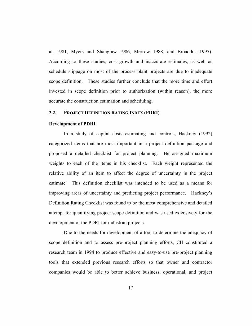
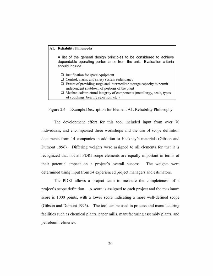
2.3. Each of the elements has a corresponding detailed description. Figure 2.4

gives an example of element description for element A1 of the industrial PDRI.

A more detailed review of the scope definition element descriptions can be found

in Project Definition Rating Index (PDRI), CII Research Report 113-11 (Gibson

and Dumont 1996).

18

SECTION I. BASIS OF PROJECT DECISION

A. Manufacturing Objective Criteria G10. Line List A1. Reliability Philosophy G11. Tie-in List A2. Maintenance Philosophy G12. Piping Specialty Item List A3. Operating Philosophy G13. Instrument Index B. Owner Philosophies H. Equipment Scope B1. Products H1. Equipment Status B2. Market Strategy H2. Equipment Location Drawings B3. Project Strategy H3. Equipment Utility Requirements B4. Affordability/Feasibility I. Civil, Structural, & Architectural B5. Capacities I1. Civil/Structural Requirements B6. Future Expansion Considerations I2. Architectural Requirements B7. Expected Project Life Cycle J. Infrastructure C. Project Requirements J1. Water Treatment Requirements C1. Technology J2. Loading/Unloading/Storage Facility Req’t C2. Processes J3. Transportation Requirements D. Site Information K. Instrument & Electrical D1. Project Objective Statement K1. Control Philosophy D2. Project Design Criteria K2. Logic Diagrams D3. Site Characteristics Available vs. Req’d K3. Electrical Area Clasifications D4. Dismantling and Demolition Req’mts K4. Substation Req’mts Power Sources Iden. D5. Lead/Discipline Scope of Work K5. Electric Single Line Diagrams D6. Project Schedule K6. Instrument & Electrical Specifications E. Building Programming E1. Process Simplification SECTION III. EXECUTION APPROACH E2. Design & Material Alts. Considered/Rej. L. Project Execution Plan E3. Design for Constructability Analysis L1. Identify Long lead/Critical Equip. & Mtls L2. Procurement Procedures and Plans SECTION II. BASIS OF DESIGN L3. Procurement Responsibility Matrix F. Site Information M. Deliverables F1. Site Location M1. CADD/Model Requirements F2. Surveys & Soil Tests M2. Deliverables Defined F3. Environmental Assessment M3. Distribution Matrix F4. Permit Requirements N. Project Control F5. Utility Sources with Supply Conditions N1. Project Control Requirements F6. Fire Protection & Safety Considerations N2. Project Accounting Requirements G. Equipment N3. Risk Analysis G1. Process Flow Sheets P. Project Execution Plan G2. Heat & Material Balances P1. Owner Approval Requirements G3. Piping & Instrumentation Diagrams P2. Engineering/Construction Plan G4. Process Safety Management P3. Shut Down/Turn Around Requirements G5. Utility Flow Diagrams P4. Pre-Commiss. Turnover Sequence Re’q G6. Specifications P5. Startup Requirements G7. Piping System Requirement List P6. Training Requirements G8. Plot Plan G9. Mechanical Equipment List

Figure 2.3. Sections, Categories and Elements of PDRI for Industrial Projects

19

A1. Reliability Philosophy

A list of the general design principles to be considered to achievedependable operating performance from the unit. Evaluation criteriashould include:

Justification for spare equipment Control, alarm, and safety system redundancy Extent of providing surge and intermediate storage capacity to permit

independent shutdown of portions of the plant Mechanical/structural integrity of components (metallurgy, seals, types

of couplings, bearing selection, etc.)

Figure 2.4. Example Description for Element A1: Reliability Philosophy

The development effort for this tool included input from over 70

individuals, and encompassed three workshops and the use of scope definition

documents from 14 companies in addition to Hackney’s materials (Gibson and

Dumont 1996). Differing weights were assigned to all elements for that it is

recognized that not all PDRI scope elements are equally important in terms of

their potential impact on a project’s overall success. The weights were

determined using input from 54 experienced project managers and estimators.

The PDRI allows a project team to measure the completeness of a

project’s scope definition. A score is assigned to each project and the maximum

score is 1000 points, with a lower score indicating a more well-defined scope

(Gibson and Dumont 1996). The tool can be used in process and manufacturing

facilities such as chemical plants, paper mills, manufacturing assembly plants, and

petroleum refineries.

20

The PDRI was validated as an effective scope definition tool using a

sample of 40 industrial projects representing approximately $3.3 billion (USD) in

authorized cost (Dumont et al., 1997). Project performance and PDRI data were

collected from the sample projects and a statistical analysis showed that PDRI

score and project success were linearly related. That is, a low PDRI score,

representing a better-defined project scope definition package, corresponds to an

increased probability for project success. Project success was judged from cost

performance, schedule performance, percentage design capacity obtained at six

months, and plant utilization attained at six months.

In addition to the development of PDRI, this research investigation also

analyzed the impact of alignment between business, project management, and

operations personnel of owner companies, as well as the alignment between

owners and contractors during pre-project planning. Alignment is defined as

“the condition where appropriate project participants are working within

acceptable tolerances to develop and meet a uniformly defined and understood set

of project objectives” (Griffith and Gibson, 2001). This effort included three

workshops, a review of sample projects, and structured interviews. Over 100

industry participants (representing 19 contractor and owner companies) were

interviewed and 20 capital projects evaluated in depth. Ten critical alignment

issues were identified to have major impact on project alignment and potential

project success. These ten critical alignment issues were further grouped into

four groups: execution processes, culture, information and tools. Both project

success and alignment information was collected for 20 industrial capital projects.

21

A linear regression analysis demonstrated that alignment effort is positively

related to project success for this sample of 20 projects. The research results

showed that achieving and maintaining alignment is a key factor in project

planning and in achieving project success (Griffith and Gibson, 2001).

With the success of the PDRI for industrial projects, many building

industry planners wanted a similar tool to address scope development of

buildings. Therefore, CII formed a team and funded a research effort to

facilitate this development effort in 1998. This team was made up of 14 industry

practitioners (11 owner companies and three contractors) and the academic

research team. The research effort included input from approximately 30

industry experts as well as extensive use of published sources for terminology and

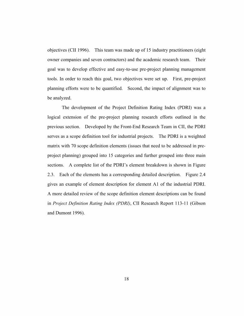
key scope element refinement. As developed, the PDRI for Building Projects

consists of 64 elements, which are grouped into 11 categories and further grouped

into three main sections. A complete list of the three sections, 11 categories, and

64 elements is given in Figure 2.5. Figure 2.6 gives an example of element

description of element A1 of the Building PDRI. The 64 elements are arranged

in a score sheet format and supported by 38 pages of detailed descriptions and

checklists (CII 1999).

22

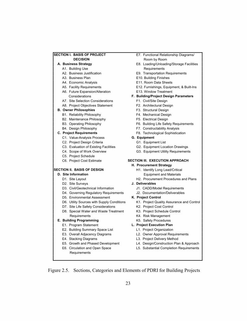
SECTION I. BASIS OF PROJECT E7. Functional Relationship Diagrams/ DECISION Room by Room A. Business Strategy E8. Loading/Unloading/Storage Facilities A1. Building Use Requirements A2. Business Justification E9. Transportation Requirements A3. Business Plan E10. Building Finishes A4. Economic Analysis E11. Room Data Sheets A5. Facility Requirements E12. Furnishings, Equipment, & Built-Ins A6. Future Expansion/Alteration E13. Window Treatment Considerations F. Building/Project Design Parameters A7. Site Selection Considerations F1. Civil/Site Design A8. Project Objectives Statement F2. Architectural Design B. Owner Philosophies F3. Structural Design B1. Reliability Philosophy F4. Mechanical Design B2. Maintenance Philosophy F5. Electrical Design B3. Operating Philosophy F6. Building Life Safety Requirements B4. Design Philosophy F7. Constructability Analysis C. Project Requirements F8. Technological Sophistication C1. Value-Analysis Process G. Equipment C2. Project Design Criteria G1. Equipment List C3. Evaluation of Existing Facilities G2. Equipment Location Drawings C4. Scope of Work Overview G3. Equipment Utility Requirements C5. Project Schedule C6. Project Cost Estimate SECTION III. EXECUTION APPROACH

H. Procurement Strategy SECTION II. BASIS OF DESIGN H1. Identify Long Lead/Critical D. Site Information Equipment and Materials D1. Site Layout H2. Procurement Procedures and Plans D2. Site Surveys J. Deliverables D3. Civil/Geotechnical Information J1. CADD/Model Requirements D4. Governing Regulatory Requirements J2. Documentation/Deliverables D5. Environmental Assessment K. Project Control D6. Utility Sources with Supply Conditions K1. Project Quality Assurance and Control D7. Site Life Safety Considerations K2. Project Cost Control D8. Special Water and Waste Treatment K3. Project Schedule Control Requirements K4. Risk Management E. Building Programming K5. Safety Procedures E1. Program Statement L. Project Execution Plan E2. Building Summary Space List L1. Project Organization E3. Overall Adjacency Diagrams L2. Owner Approval Requirements E4. Stacking Diagrams L3. Project Delivery Method E5. Growth and Phased Development L4. Design/Construction Plan & Approach E6. Circulation and Open Space L5. Substantial Completion Requirements Requirements

Figure 2.5. Sections, Categories and Elements of PDRI for Building Projects

23

A1. Building Use

Identify and list building uses or functions. These may include usessuch as:

Retail Research Storage Institutional Multimedia Food service Instructional Office Recreational Medical Light manufacturing Other

A description of other options which could also meet the facility needshould be defined. (As an example, did we consider renovatingexisting space rather than building new space?) A listing of current facilities that will be vacated due to the new project should beproduced.

Figure 2.6. Example Description for Element A1: Building Use

It was hypothesized that all elements are not equally important with

respect to their potential impact on overall project success and each element

needed to be weighted relative to the others. Higher weights were to be assigned

to those elements whose lack of definition could have the most serious negative

effect on the project performance. To develop the weights, seven “weighting”

workshops were held and 69 workshop participants consisted of 30 engineers, 31

architects, and eight other professionals directly involved in planning building

projects participated in the workshops. The element weights of the PDRI for

building projects were established using the input provided by 35 owner and

contractor organizations from the building sector (CII 1999).

During the development of the Building PDRI, a logic flow diagram was

developed by the researchers to assist with the application of the PDRI. The

24

PDRI for buildings is intended as a “point in time” tool with elements grouped by

subject matter, not in time-sequenced logic. Therefore, the logic flow diagram

was set up to identify the embedded logic that the scope elements might have and

to tie to the quantitative score of the PDRI for buildings (Furman 1999; Cho,

Furman, and Gibson 1999). As part of the early research effort for this

dissertation, a logic flow diagram was developed for the Industrial PDRI to

demonstrate the embedded logic between the scope elements. A prototype was

first sent out to 73 industry practitioners for feedback. With inputs from several

industry practitioners, a logic flow diagram was finalized for the Industrial PDRI

and is given in Appendix A.

The PDRI for building projects was validated through a total of 33

projects varying in authorized cost from $0.7 million to $200 million

(representing approximately $896 million in construction cost). PDRI scores

were calculated for each of these projects and compared to project success

criteria, such as cost and schedule performance. The results showed that

validation projects scoring below 200 outperformed those scoring above in three

important areas: cost performance, schedule performance, and the relative value

of change orders compared to budget (CII 1999).

Overall, the PDRI for building projects is a user-friendly checklist that

identifies and describes the critical element in a project scope definition package

to assist project managers in understanding the scope of work. It provides a

means for an individual or team to evaluate the status of a building project during

preproject planning with a score corresponding to the project’s overall level of

25

definition. The PDRI helps the stakeholders of a project to quickly analyze the

scope definition package and to predict factors that may impact project risk

specifically with regard to buildings (CII 1999; Cho 2000).

Scope Definition Level and PDRI Element Weights

The PDRI element weights were assigned to reflect the fact that not all of

the elements within the PDRI were equally important with respect to their

potential impact on overall project success. The data collected for determining

the PDRI element weights were based upon the subjective opinions of industrial

representatives.

The pre-assigned weights were developed through a series of workshops

to gather inputs from a broad range of construction industry experts. Higher

weights were to be assigned to those elements whose lack of definition could have

the most serious negative effect on project performance (CII 1996 and CII 1999).

The workshop participants were asked to consider each element individually and

evaluate the worst case scenario. If that element was incomplete or poorly

defined base on the description (definition level 5), the participants were

instructed to assess what percent contingency they would deem appropriate for

that element. Then the weights were normalized and converted so that the

highest score obtained from using the PFRI would be 1000 (CII 1996 and CII

1999). It should be noted that both version of the PDRI share a similar

weighting scheme and scoring methodology.

In the PDRI score sheets, the element’s state of definition was to be

evaluated using the following five-level scale:

26

1 = Complete Definition

2 = Minor Deficiencies

3 = Some Deficiencies

4 = Major Deficiencies

5 = Incomplete or Poor Definition

For each PDRI element, different weights were given to all five levels of

definition. If one element were not applicable to a particular project, a definition

level of 0 with zero weight can be applied. Please refer to Appendix B and

Appendix C for complete PDRI score sheets.

In the process of pre-project planning evaluation using PDRI, the project

team first read the description of each element, collect all data that is needed to

evaluate and then select the definition level for each element. Each element has

five pre-assigned weights for the possible five definition levels for that element.

The project team can look up the corresponding weight for the definition level

they chose for that scope element. This weight represents potential impact of the

scope element to the project performance based on the weights developed by the

industry experts input. For illustration, Section I – Category A of the PDRI for

building projects (both elements and their weights) is shown in Figure 2.7.

Hypothetical PDRI scope definition evaluations are circled in the figure as well.

Please refer to Figures 4.4 and 4.6 for PDRI element description examples.

To score an element, the project team should first read the descriptions for

each element and then collect all data needed to properly evaluate and select the

definition level for each element. After the definition level is selected, the score

27

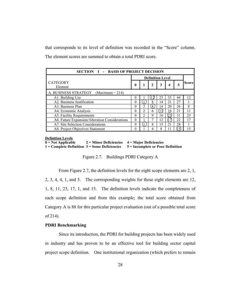
that corresponds to its level of definition was recorded in the “Score” column.

The element scores are summed to obtain a total PDRI score.

SECTION I - BASIS OF PROJECT DECISION

Definition Level CATEGORY Element 0 1 2 3 4 5 Score

A. BUSINESS STRATEGY (Maximum = 214) A1. Building Use 0 1 12 23 33 44 12 A2. Business Justification 0 1 8 14 21 27 1 A3. Business Plan 0 2 8 14 20 26 8 A4. Economic Analysis 0 2 6 11 16 21 11 A5. Facility Requirements 0 2 9 16 23 31 23 A6. Future Expansion/Alteration Considerations 0 1 7 12 17 22 17 A7. Site Selection Considerations 0 1 8 15 21 28 1 A8. Project Objectives Statement 0 1 4 8 11 15 15

Definition Levels 0 = Not Applicable 2 = Minor Deficiencies 4 = Major Deficiencies 1 = Complete Definition 3 = Some Deficiencies 5 = Incomplete or Poor Definition

Figure 2.7. Buildings PDRI Category A

From Figure 2.7, the definition levels for the eight scope elements are 2, 1,

2, 3, 4, 4, 1, and 5. The corresponding weights for these eight elements are 12,

1, 8, 11, 23, 17, 1, and 15. The definition levels indicate the completeness of

each scope definition and from this example; the total score obtained from

Category A is 88 for this particular project evaluation (out of a possible total score

of 214).

PDRI Benchmarking

Since its introduction, the PDRI for building projects has been widely used

in industry and has proven to be an effective tool for building sector capital

project scope definition. One institutional organization (which prefers to remain

28

anonymous) approached researchers at the University of Texas and expressed

interest in modifying and deploying the PDRI for their large capital program.

The objective of this research effort was to slightly modify the PDRI scope

definition to reflect the needs of this organization’s budgeting cycle and a

procedure manual, and to develop an expansible benchmarking database and path

forward for implementation.

A workshop was therefore held to modify the PDRI-Buildings toward the

organization’s specific needs. A detailed project questionnaire and a user survey

were developed and sent to the respective project managers and end users. Data

from a total of 45 building projects were collected and studied. It should be

noted that 42 of these 45 projects were essentially identical and constructed in

many locations around the world. It was proven for this sample that projects

with better-defined scope definition had better performance in terms of cost,

schedule, and change orders. Poor alignment (lack of user involvement) was

also commonly seen as a problem on the sample projects. Data collected from

these projects were analyzed and conclusions and recommendations were

provided for the organization’s future capital project development.

The average PDRI score for the 45 sample projects was 346 points. The

sample projects with a PDRI score under 300 (average 262 for this sub-sample)

outperformed projects with PDRI scores above 300 (average of 388 for this sub-

sample) in cost, schedule and change order performance. When 33 CII building

projects were added to the sample, analysis showed that projects performed by the

institutional organization still had room for improvement. Further analysis of

29

the PDRI details shows that future projects should focus on improving project

definition for PDRI Category C: (Project Requirements), Category F: (Project

Design Parameters), Category G: (Equipment) and Category H: (Procurement

Strategy) prior to the beginning development of construction documents (CDs).

The research recommended a benchmarking PDRI score of 300 or less for future

capital project development. However, they also strongly recommend that once

these goals are consistently achieved that the benchmarking scores be lowered to

200 or less. This study will be outlined in more detail later in Chapter Six.

2.3. MANAGING CONSTRUCTION PROJECT RISK

The definition for risk is elusive, and its measurement is controversial

(Lifson and Shaifer 1982). There is no consistent or uniform usage of the term

risk. Often times, risk is interpreted in association with uncertainty. In this

sense, risk implies that there is more than one possible outcome for the event,

where the uncertainty of outcomes is expressed by probability (Al-Bahar 1988).

In project management, risks are typically associated with cost, schedule, safety

and technical performance (Rao et al. 1994). For the purpose of this study, risk

is defined as the exposure to the chance of occurrences of cost or schedule growth

as a consequence of uncertainty. Risk will be studied as it relates to growth

caused by incomplete scope definition.

Risk management is a quantitative systematic approach used to manage

risks faced by project participants. It deals with both foreseeable as well as

unforeseeable risks and the choice of the appropriate technique(s) for treating

those risks. The process of risk management includes three phases: risk

30

identification, risk quantification, and risk control. The process is a continuous

cycle that consists of risk analysis, strategy implementation, and monitoring (CII

1989, Minato and Ashley 1998).

2.3.1. Identifying Construction Project Risk

Risk identification is the first process of the risk management. This

process involves the investigation of all possible potential sources of project risks

and their potential consequences. For construction projects, Al-Bahar and

Crandall (1990) defined risk identification as the process of systematically and

continuously identifying, categorizing, and assessing the significance of risks

associated with a project. Several studies have been conducted to identify and

categorize construction risk factors and allocate the ownership of risk (Ashley et

al. 1988; Al-Bahar and Crandall 1990; Kangari 1995; Smith and Bohn 1999).

From the owner’s perspective, these risk factors include fears that (1) costs will

escalate unpredictably; (2) structures will be faulty and need frequent repairs; and

(3) the project will simply be abandoned and partially paid for but incomplete and

useless (Strassman and Wells 1988).

A survey of the top 100 U.S. construction contractors classified risk

factors to allocate ownership of the risk under three categories: owner, contractor,

and shared risk (Kangari 1995). In this survey study, 23 risk factor descriptions

are identified, including permits and ordinances, site access / right of way,

defective design, changes in work, labor, equipment and material availability,

safety, quality of work, and financial failure of any party. Most of these risk

factors descriptions can be found or related to the element descriptions in the

31

PDRI. Accordingly, the scope definition elements in the PDRI can serve as a

comprehensive list of potential risk factors for capital facility project development

as addressed in pre-project planning. During the PDRI evaluation process, the

project team can obtain knowledge about the completeness of pre-project

planning efforts and also identify potential project risk factors by looking at

poorly defined scope definition elements.

Risk Analysis and Management for Projects (RAMP) is a process which

has been developed for the purpose of evaluating and controlling risk in major

projects in the United Kingdom. It proposed that any risk identified should be

entered in the “risk register”. The risks in the risk register should be classified

and if appropriate grouped to assist in their evaluation in turn to determine and

record (ICE 2000):

• Possible cause or causes of the risk

• Trigger events giving risk to risk occurring

• Possible timing and potential frequency of occurrence

• Range of possible consequences – both physical and financial

• Asset component, factor or activity associated with the risk

• Objective, ‘deliverable’ or parameter impacted

• Other related risks

• Form of relationship with other risks

• Who currently owns the risk

• The initial response to the risk

• Whether there are any risks which should be eliminated because they

duplicate or overlap with each other

32

The risk register not only identifies the potential impact but the

relationship between each risk as well. After the identification process, the

project team should determine the possible consequences resulting from the

inadequately defined project scope.

2.3.2. Quantifying Construction Project Risk

The second process, risk quantification, is needed to determine the

potential impact of the risk quantitatively. This process incorporates uncertainty

in a quantitative manner to evaluate the potential impact of risk. In this process,

an analyst integrates information from numerous sources through quantitative

and/or qualitative modeling, while preserving the uncertainty and the complex

relationships between the elements of information (Rao et al. 1994).

Several analytical models have been developed to estimate or evaluate risk

exposure for construction projects. A risk decision model was developed by

Ibbs and Crandall (1982) based on utility theory. A model using utility theory

is able to represent human decision values in the form of mathematical

formulation. By incorporating Bayesian probability analysis in this decision

model, a contractor is able to estimate the impact of their risk decision. In their

study, a theory is introduced which facilitates the analysis of complex decisions

and the selection of consistent courses of action. In addition, an illustrative

decision problem is solved, not only to explain the mechanics of the theory, but to

demonstrate that construction risk is a function of competitive economics as well

as of project-related characteristics (Ibbs and Crandall 1982). Nevertheless,

most researches studied construction risk from the contractors’ perspective.

33

Mak and Picken (2000) proposed a methodology to investigate risks to

clients, persons or organizations investing in the construction of built facilities.

It is a common practice that facility owners use a contingency allowance, a

percentage addition on top of base estimates, to provide for uncertainties

associated with construction projects. A methodology, estimating using risk

analysis (ERA), was proposed to substance the contingency by identifying

uncertainties and estimating their financial implications. The project team

identifies risks and determined risk allowances (probability times cost). Their

analysis results showed that the use of the ERA approach has improved the

overall estimating accuracy in determining contingency amounts (Mak and Picken

2000). The proposed ERA method substantiates the contingency by identifying

uncertainty and estimating their financial implications. Therefore, the risk

implications for a capital facility development project for the owners can be

expressed by project contingency amounts that account for project uncertainties.

In an effort to study estimating and contingencies, the late John Hackney

(1992) used definition rating method to appraise project definition, assign

contingency allowances, and predict estimate accuracy. The definition rating is

obtained from a checklist and it reflects the degree to which a project is “pinned

down” at a given stage of development. The contingency allowances are

established in order to compensate for the unfavorable deviations from estimated

cost that can be produced by poorly defined factors. Hackney (1992) further

indicated that the most dependable guide in establishing proper contingency

allowances is experience from past projects. With past project data, he plotted

34

percentage overruns of estimates against the definition rating at the time of

estimate and observed from the chart that there is a bias toward underestimating

the cost of partially defined projects (Hackney 1992). A similar approach will

be applied in this research to quantify the potential risk implications for partially

defined projects based on historic project data and will be outlined later.

Having identified the risk factors, and evaluated their potential impact to

the project, the next step is to manage the identified project risks as discussed in

the next section.

2.3.3. Controlling Construction Project Risk

The third phase of the risk management process is risk control. Risk

control involves measures aimed at avoiding or reducing the probability and/or

potential severity of the losses occurring. The implementation of these measures

should be monitored and be taken into account for future alternative risk

management strategies development (Al-Bahar and Crandall 1990).

Risk control includes risk avoidance, risk reduction, risk sharing, risk

transfer, insurance, risk acceptance by establishment of contingency accounts, risk

acceptance without any contingency and risk containment (CII 1989). For

example, risk avoidance is a common strategy for managing risk by avoiding risk

exposures. An owner organization is able to avoid construction risks associated

with a new technology by implementing proven technology. Although risk

avoidance eliminates the risk exposures, it also prevents the possibility of

benefiting from a new technology.

35

Risk reduction is a two-fold risk management technique. It decreases

risk exposures by (1) reducing the probability of risk, and (2) reducing the

financial consequences caused by the risk exposures. It is risk reduction that this

dissertation research focuses on as the major risk control measure.

Hackney (1992) pointed out in his study that “consideration of individual

ratings on the detailed checklist brings out those points where lack of definition

presents the greatest potential threat. These items can be given priority in further

definition of the project”. That is, these poorly defined scope elements have

potential negative impacts to the project and should be addressed later in the

project. If these poorly defined elements are properly addressed, the chance and

magnitude of the potential negative impact caused by these poorly defined

elements can be reduced. Therefore, by improving the poorly defined scope

elements (i.e. mitigating the risk) and thus lowering the PDRI score, the project

team is able to increase the probability of better project performance. The PDRI

score evaluation also serves as a good measure for monitoring the effectiveness of

risk control techniques implemented.

2.4. LITERATURE REVIEW CONCLUSIONS

The literature review revealed a strong consensus that unresolved scope

definition issues are many times associated with poor cost, schedule, safety and

technical performance. However, there is little research into which unresolved

scope elements lead to project risks early in the project life cycle from the

owner’s perspective. Mak and Picken (2000) proposed a methodology to

substantiate the contingency by identifying uncertainty and estimating their

36

financial implications. Nevertheless it is hard to determine risk allowance and

probability for each identified risk factor. Hackney (1992) used definition rating

method and graphic techniques to quantify contingency allowances.

The results of previous research revealed that decisions made early in the

project have greater influence on project outcome with less costs associated

comparing to decisions made later on in the project life cycle. As a pre-project

planning tool, the PDRI helps the project team assess project scope definition as

well as identify potential risk factors. Several published studies of risk

management give useful information for developing a systematic risk

management approach using the PDRI.

This research effort addresses application of PDRI evaluation in an

attempt to provide additional information as to what potential project problems

can occur based on actual data collected. The research will also address the

development of a systematic risk management approach using the PDRI.

2.5. SUMMARY

This chapter presented the results of the literature review covering pre-

project planning, PDRI, risk management and other related topics. The next

chapter of this dissertation presents the research problem statement and the

research hypotheses based on findings from the literature review.

37

Chapter 3 Problem Statement and Research Hypotheses

The literature review discussed in Chapter Two provides a background of

the current body of knowledge regarding pre-project planning and risk

management. The information gathered in literature review was used in

developing research objectives and in designing how to best conduct the research.

The problem statement and research hypotheses are presented in the following

section.

3.1. PROBLEM STATEMENT

It is evident from the literature review that it is important to identify and

address potential project risk factors early in the project life cycle. However,

there are few effective methods available to fulfill this need. Several problems

have been identified in the literature review. The lack of an easy-to-use tool

makes it difficult for the project teams to identify and address potential risk

factors during early project phase. Limited research results are available to

quantify the potential impact caused by unresolved scope issues. Finally, most of

currently available risk management techniques are developed for the contractors;

therefore, a systematic risk management approach geared towards addressing

risks from the owner’s perspectives is in great need. Based on the results of the

literature review, the problem statement of this dissertation research is as follows:

A need exists to identify and measure the effect that risk factors identified

in the pre-project planning process have on project cost and schedule

performance. There also exists a need to develop a systematic risk

38

management approach for the owner’s organization in the early project

planning phase.

3.2. RESEARCH HYPOTHESES

The primary purpose of this research study is to build on previous research

concerning pre-project planning, including the Project Definition Rating Index,

and risk management by developing a systematic risk management approach to

identify and address potential risk factors during the pre-project planning phase.

Major decisions regarding project scope are made during the pre-project planning

phase of the project life cycle. PDRI is a simple and easy-to-use tool for

measuring the degree of scope development on capital facility projects. This

scope definition tool is intended to help project teams identify risk factors that

may impact their project (Gibson and Dumont 1996).

Risk management contains three major processes: risk identification, risk

quantification and risk control. As previous outlined, various authors have

discussed and modeled construction project risks to address contractors’ risk

exposures in capital facility projects (Ibbs and Crandall 1982; Ashley et al. 1988;

Al-Bahar and Crandall 1990; Kangari 1995; Ashley et al. 1998; Smith and Bohn

1999). Based on the literature review, two general research hypotheses are

developed to meet the research objectives stated in Chapter One.

• H1: A PDRI score indicates the current level of scope definition and

corresponds to project performance. That is, PDRI scores correlate to

measures of project success.

39

Specifically, the first research hypothesis is that a low PDRI score would

represent a scope definition package that is well defined and, in general,

corresponds to a higher project success. Higher PDRI scores, on the other hand,

would signify that certain elements in the scope definition package lacked

adequate definition at the time of assessment, thus resulting in poorer project

performance and lower project success. Although this hypothesis was proven in

initial development efforts for both PDRI tools, it was done on an exploratory

basis with a limited sample size. This hypothesis will be tested by conducting a

regression analysis with the expanded sample project database.

• H2: The PDRI is a reliable indicator of potential project risk factors and

PDRI scores can be used to quantify risk impact on project outcomes

based on collected data from actual projects.

The first hypothesis was developed to analyze correlations between PDRI

scores and project performance. This second hypothesis was established to

examine the possibility of quantifying risk impacts with project schedule and cost

performance using statistical analysis models and PDRI scores. In addition,

developing a systematic risk management approach will be attempted to extend

the usage of the PDRI to support decision-making process in the pre-project

planning stage. The proposed risk management approach using PDRI will

40

provide a systematic approach for the project team to identify, assess and manage

project risks identified in the pre-project planning phase.

3.3. SUMMARY

This chapter outlines the problem statement and research hypotheses.

The identified problem involves the need to identify and measure the effect that

project risk factors identified during pre-project planning has on project outcome.

The research hypotheses are focused on applying PDRI in the project risk

management processes early in the project life cycle. The next chapter describes

the research methodology, including literature review, administration of the

surveys, data collection and analysis, development of statistical models, and

application of risk management processes.

41

Chapter 4 Research Methodology

The results of the literature review revealed the need for further research

into risk analysis early in the project life cycle. Data collected for this research

were collected from three main sources: previous PDRI research at the University

of Texas, the CII Benchmarking & Metrics database, and through a pre-project

planning benchmarking project for an institutional organization. The research

also compiled inputs from project professionals representing various areas in the

filed of capital facility construction, including projects from both industrial and

building sectors.

The hypotheses for this research are based on three main concepts;

antecedents to pre-project planning and scope definition, consequences of

unresolved scope issues on project outcomes, and the project risk management

process. In order to test these hypotheses, past project data were captured to

conduct statistical analysis. This analysis will be used either to support or refute

the research hypotheses depending on the results of the data analysis.

The specific methodology used for this dissertation research is presented

in this chapter. It covers the development of the questionnaire, collection and

analysis of data, and the development of risk management model as depicted in

Figure 4.1. Each phase contains several steps that are described in the following

paragraphs. Specific results of the data analysis, format of the risk management

model and recommendations for applying of the risk management model are

provided in subsequent chapters.

42

OriOri

Data Collection

LiteratureReview

IssueIdentification

QuestionnaireDevelopment

Sample ProjectSelection

Institutional Organization

Projects

CII BM&MProjects

ginal PDRIDevelopment

Projects

Access DatabaseDevelopment

DataAnalysis

Analytical ModelDevelopment

Documentation

Systematic RiskApproach

Development

Data Collection

LiteratureReview

IssueIdentification

QuestionnaireDevelopment

Sample ProjectSelection

Institutional Organization

Projects

CII BM&MProjects

ginal PDRIDevelopment

Projects

Access DatabaseDevelopment

DataAnalysis

Analytical ModelDevelopment

Documentation

Systematic RiskApproach

Development

Figure 4.1. Research Methodology Flow Diagram

43

4.1. LITERATURE REVIEW AND ISSUE IDENTIFICATION

Extensive literature review was conducted to examine existing research

that is significant to this dissertation research. This effort looked into research

topics including pre-project planning, scope definition, the Project Definition

Rating Index (PDRI), PDRI benchmarking, construction project risk, and project

risk management processes. Critical issues concerning the application of the

PDRI into project risk management were identified during literature review.

A literature review was first conducted looking at CII and other available

references to identify documented studies on early project planning and scope

definition. Numerous works were found concerning pre-project planning and

the Project Definition Rating Index and these works served as stepping stones for

this dissertation research on exploring the application of the scope definition tool

into project risk management. Existing research topics related to construction

risk and risk management processes were examined to identify the opportunities

of applying PDRI in construction project risk management. The research

proceeded with the identification of available statistical analysis methods to

develop specific risk models for the purpose of this research. Risk modeling

techniques were studied and several construction risk models were considered for

the development of PDRI risk models. During the literature review process,

issues related to early project planning and construction project risk management

were identified as outlined in Chapter 2.

The research methodologies described in the following sections were

based on the identified issues from the literature review.

44

4.2. QUESTIONNAIRE DEVELOPMENT AND FINALIZATION

Previous pre-project planning and PDRI research projects utilized survey

research as their primary technique for data collection. For detailed reasoning

behind the selection of survey research, please refer to CII (1996) and Cho et al.

(1999). Retrospective case study questionnaires developed from previous PDRI

research were adopted and refined to reflect specific needs for new data collection

efforts with the institutional organization.

Babbie (1992) described five different modes of observation in social

research: experimental research, survey research, field research, unobtrusive

research and evaluation research. Among these different observation methods,

survey research was chosen as the most appropriate method of data collection for

previous research projects on both versions of PDRI (Cho 2000).

There are three basic procedures used to conduct a survey: questionnaires,

personal interviews, and telephone interviews. Personal or telephone interviews

were regarded not feasible due to the complicated nature of the questionnaire

related to project performance and because of the time and geological constraints

(Cho, 2000). As a result, questionnaires were developed during previous PDRI

research project as a survey instrument to gather PDRI evaluation and project

performance information. The questionnaire is a self-administered survey

instrument consisting of questions to be answered by respondents. In the PDRI

survey questionnaires, specific questions were intended to obtain historical and

“after the fact” project information. The questionnaires included questions

45

regarding project basics (location, type, budget and schedule), operating

information, and evaluation using an unweighted PDRI score sheet.

Two sets of questionnaires (one for industrial projects and the other for

general building projects) were developed during the initial PDRI development

and these questionnaires were used without any changes for continuing sample

data collection efforts. However, for the institutional organization projects, a

modified PDRI survey questionnaire was employed for data collection process

and is given in Appendix B. As part of the PDRI benchmarking research effort,

a specific set of PDRI questionnaires were developed for the institutional

organization to obtain information from both construction department and

intended users within the organization. Developed by the author and research

supervisor and approved by the sponsor, the user questionnaire was developed to

gather user feedback and was sent to building users. The other questionnaire

was developed to obtain project information and was sent to project managers

who are in charge of building construction. This questionnaire was modified

from PDRI-Buildings questionnaire to reflect specific needs of the organization.

In order to obtain inputs from personnel in the institutional organization, a

workshop with nine participants was held in November 2000. During the

workshop, the descriptions of PDRI scope definition elements were modified to

accommodate the specific terminologies and capital project delivery process of

the institutional organization. The generic score sheet format and weights of the

PDRI-Buildings remained unchanged.

46

After the development of user and project manager questionnaires, these

questionnaires were sent to managers of user and construction departments for

their review. Minor questionnaire modifications were suggested and then

incorporated into the final version that was sent out to gather information from 45

projects.

The questionnaire development described earlier was geared toward the

collection of project information for the institutional organization. The CII

Benchmarking and Metrics research and PDRI development research used the

questionnaires created for the initial PDRI-Buildings and the PDRI-Industrial

research efforts.

4.3. DATA COLLECTION

After the development of survey instrument, the research proceeded with

data collection. The data collected contains both successful and unsuccessful

projects. Nevertheless, it is important to note that the sample selection for the

study is based on organizations volunteering projects for the study and not on a

random sample of a known population. Specific information concerning sources

is given below.

Three different sources were used for data collection during this phase of

the research project. Previous PDRI research, CII Benchmarking & Metrics

research, and institutional organizational PDRI Benchmarking research were the

three main resources of data. When both versions of PDRI were developed,

sample projects of actual construction were collected for PDRI validation

purpose. Initially, 23 industrial projects were surveyed to gather information

47

regarding PDRI evaluation and project performance during the PDRI validation

process (CII 1996). These projects were selected from companies represented

by participants in the Front End Planning research project (described in Chapter

Two). Following PDRI and project team alignment research efforts obtained 18

more industrial projects from CII owner and contractor member companies for a

total of 41 industrial projects. Thirty-three sample projects surveyed during the

PDRI-Buildings development effort were used for detailed analysis (CII 1999).

These projects were selected from a pool of building projects nominated by the

PDRI-Buildings research team member companies. The sample projects

represented seven different owner organizations and three contractor

organizations.

The CII Benchmarking & Metrics Program was established to provide

industry performance norms, quantify the use and value of "best practices," and to

help focus CII research and implementation efforts. A committee of industry

representatives working with the CII staff has defined critical performance and

practice use metrics and developed a strategic approach to CII's collection,

analysis, and dissemination of industry data. Questionnaires developed by the

committee were sent out to owner and contractor member companies to obtain

benchmarking and metrics data. The data are collected by trained industry

representatives, and screened by CII staff personnel prior to analysis (CII 2001).

Practice use metrics such as safety, team building, constructability, pre-project

planning, design/information technology, project change management, material

management, planning for start-up, quality management and strategic alliances

48

are evaluated through the CII Benchmarking and Metrics research program. The

PDRI was included as part of the questionnaire evaluating the pre-project

planning practice. Twenty-one projects with PDRI information were selected

from the benchmarking database for this research. These projects represented

nine contractor and 12 owner companies and they were all industrial projects.

The third PDRI data resource is PDRI-Buildings benchmarking research

efforts for the institutional organization (described in Chapter 2). With the

assistant of the consultant hired by the sponsor, modified questionnaires for the

institutional organization were sent out to project managers and building users to

collect information on PDRI evaluation, project performance and user

satisfaction. Information from a total of 45 sample building projects was

obtained for the same owner organization and these projects included both

domestic (within U.S.) and international projects. Because of confidentiality

concerns by the sponsor, certain information (building specific location and

names of individuals filling out the questionnaire) was masked by the consultant

before the information was sent to the author. The consultant not only assisted

with the data collection but also helped clarify questions acting as a “go-

between”. Specific information such as user satisfaction and owner’s

contingency was captured due to the fact that questionnaires were specifically

developed for this institutional organization. The homogeneous nature of the

sample and enhanced quality of information allowed more detailed analysis of

this sample, which will be discussed, in next chapter of this dissertation.

49

Although the data were collected by different researchers, the data

collection methods remain consistent throughout the whole data collection period

(1994 ~ 2001). That is, a questionnaire survey was used to collect the data and

all the questionnaires are filled out by survey participants and followed up by

researchers if necessary.

It also should be noted the PDRI is developed in a way that is flexible to

treat non-applicable scope elements by assigning zero weights to those elements.

Therefore, non-applicable elements will not affect the final total PDRI score.

For this research, raw scores were used to conduct the analysis instead of adjusted

score (non-applicable weights were taken out of the total maximum score of

1000). However, two industrial projects collected during the PDRI development

were not included in this research because these two projects have more than one

full category (greater than 10 elements) of “non-applicable” scope elements in

their PDRI evaluation.

In summary, information from a total of 62 industrial projects representing

a total budget cost of approximately $3.8 billion dollars was obtained for the

research. In the meantime, 78 building projects representing approximately $1.1

billion dollars in total budget cost were also collected. A detailed breakdown of

the projects is presented in Table 4.1.

50

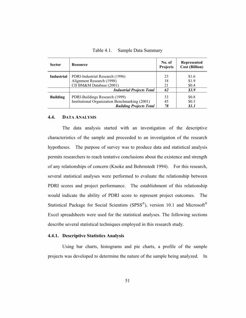
Table 4.1. Sample Data Summary

Sector Resource No. of Projects

Represented Cost (Billion)

Industrial PDRI-Industrial Research (1996) Alignment Research (1998) CII BM&M Database (2001)

23 18 21

$1.6 $1.9 $0.4

Industrial Projects Total 62 $3.9

Building PDRI-Buildings Research (1999) Institutional Organization Benchmarking (2001)

33 45

$0.8 $0.3

Building Projects Total 78 $1.1

4.4. DATA ANALYSIS

The data analysis started with an investigation of the descriptive

characteristics of the sample and proceeded to an investigation of the research

hypotheses. The purpose of survey was to produce data and statistical analysis

permits researchers to reach tentative conclusions about the existence and strength

of any relationships of concern (Knoke and Bohrnstedt 1994). For this research,

several statistical analyses were performed to evaluate the relationship between

PDRI scores and project performance. The establishment of this relationship

would indicate the ability of PDRI score to represent project outcomes. The

Statistical Package for Social Scientists (SPSS®), version 10.1 and Microsoft®

Excel spreadsheets were used for the statistical analyses. The following sections

describe several statistical techniques employed in this research study.

4.4.1. Descriptive Statistics Analysis

Using bar charts, histograms and pie charts, a profile of the sample

projects was developed to determine the nature of the sample being analyzed. In

51

addition to the two industry sectors, projects were profiled by the following

classifications:

• Type of construction (greenfield, expansion, revamp, etc.)

• Contract type (lump sum, design build, etc.)

• Project location

• Total project schedule

• Total installed cost

Scatter plots and boxplots were used to display the summary information

about the distribution of sample values. A scatter plot displays pairs of points on

typical Cartesian (perpendicular) axes, and can reveal relationships or association

between two variables in graphic. Scatter plots can provide answers to questions

such as “Are the two variables related? If so, linear or non-linear related?” and

“Does the variation of one variable depend on the other variable?”

Boxplots are an excellent tool for conveying location and variation

information in data sets, particularly for detecting and illustrating location and

variation changes between different groups of data. Figure 4.2 provides an

annotated sketch of a boxplot. The boxplot presents the median, the 25th

percentile, the 75th percentile, and values that are far removed from the rest. The

lower boundary of the box is the 25th percentile and the upper boundary is the 75th

percentile. The horizontal line inside the box depicts the median. Fifty percent

of the cases have values within the box. The length of the box corresponds to

the inter-quartile range. From the length of the box, one can determine the

spread, or variability, of the observation. From the median, one can determine

52

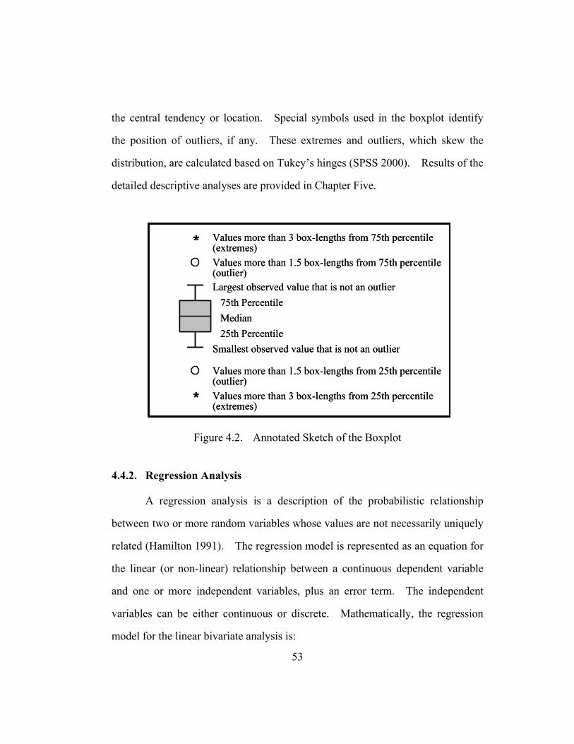
the central tendency or location. Special symbols used in the boxplot identify

the position of outliers, if any. These extremes and outliers, which skew the

distribution, are calculated based on Tukey’s hinges (SPSS 2000). Results of the

detailed descriptive analyses are provided in Chapter Five.

75th PercentileMedian25th Percentile

Smallest observed value that is not an outlier

Largest observed value that is not an outlier

Values more than 1.5 box-lengths from 75th percentile(outlier)

*

*

Values more than 3 box-lengths from 75th percentile(extremes)

Values more than 3 box-lengths from 25th percentile(extremes)

Values more than 1.5 box-lengths from 25th percentile(outlier)

75th PercentileMedian25th Percentile

Smallest observed value that is not an outlier

Largest observed value that is not an outlier

Values more than 1.5 box-lengths from 75th percentile(outlier)

*

*

Values more than 3 box-lengths from 75th percentile(extremes)

Values more than 3 box-lengths from 25th percentile(extremes)

Values more than 1.5 box-lengths from 25th percentile(outlier)

Figure 4.2. Annotated Sketch of the Boxplot

4.4.2. Regression Analysis

A regression analysis is a description of the probabilistic relationship

between two or more random variables whose values are not necessarily uniquely

related (Hamilton 1991). The regression model is represented as an equation for

the linear (or non-linear) relationship between a continuous dependent variable

and one or more independent variables, plus an error term. The independent

variables can be either continuous or discrete. Mathematically, the regression

model for the linear bivariate analysis is:

53

iii eXbbY ++= 10

where:

= dependent variable iY

= axis intercept 0b iY

= bivariate regression coefficient 1b

= independent variable iX

= error term 1e

A bivariate linear regression is a simple form of estimating the linear

relationship between a dependable variable (Y) and an independent variable (X).

The prediction equation, a regression equation without the error term, is used to

predict the value of the dependent variable from the independent variable in the

equation. As used in this study it is shown as:

ii XbbY 10 +=∧

where:

Y = the predicted value of the dependent variable ∧

i

The bivariate regression coefficient, , or the slope of the regression

line, and the intercept, , are estimated using ordinary least squares. Ordinary

least squares minimizes the error sum of squares, that is, the minimum value of

the squared difference between the observed value, , and the value predicted by

the regression equation, .

1b

0b

∧

iY

iY

54

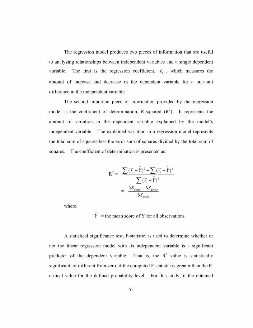
The regression model produces two pieces of information that are useful

to analyzing relationships between independent variables and a single dependent

variable. The first is the regression coefficient, , which measures the

amount of increase and decrease in the dependent variable for a one-unit

difference in the independent variable.

1b

The second important piece of information provided by the regression

model is the coefficient of determination, R-squared (R2). It represents the

amount of variation in the dependent variable explained by the model’s

independent variable. The explained variation in a regression model represents

the total sum of squares less the error sum of squares divided by the total sum of

squares. The coefficient of determination is presented as:

R2 = ∑

∑ ∑−

∧−

−

−−−

2

22

)(

)()(

YY

YYYY

i

ii

= Total

ErrorTotal

SSSSSS −

where:

−

Y = the mean score of Y for all observations

A statistical significance test, F-statistic, is used to determine whether or

not the linear regression model with its independent variable is a significant

predictor of the dependent variable. That is, the R2 value is statistically

significant, or different from zero, if the computed F-statistic is greater than the F-

critical value for the defined probability level. For this study, if the obtained

55

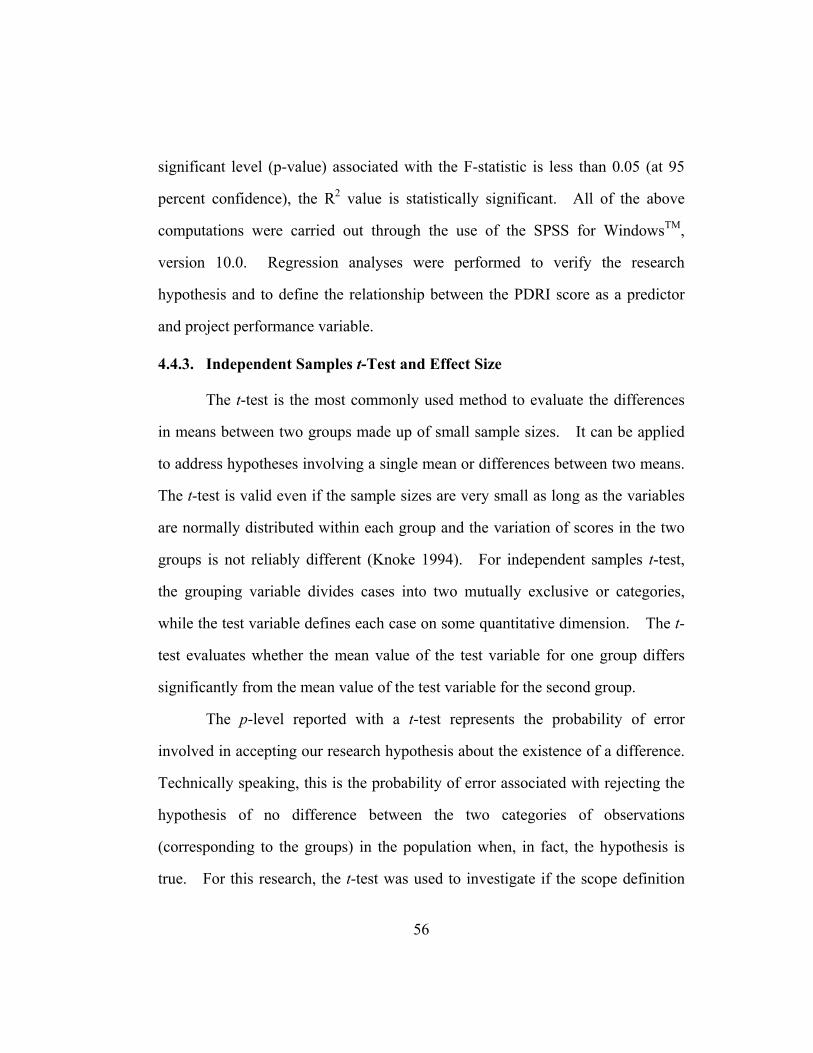
significant level (p-value) associated with the F-statistic is less than 0.05 (at 95

percent confidence), the R2 value is statistically significant. All of the above

computations were carried out through the use of the SPSS for WindowsTM,

version 10.0. Regression analyses were performed to verify the research

hypothesis and to define the relationship between the PDRI score as a predictor

and project performance variable.

4.4.3. Independent Samples t-Test and Effect Size

The t-test is the most commonly used method to evaluate the differences

in means between two groups made up of small sample sizes. It can be applied

to address hypotheses involving a single mean or differences between two means.

The t-test is valid even if the sample sizes are very small as long as the variables

are normally distributed within each group and the variation of scores in the two

groups is not reliably different (Knoke 1994). For independent samples t-test,

the grouping variable divides cases into two mutually exclusive or categories,

while the test variable defines each case on some quantitative dimension. The t-

test evaluates whether the mean value of the test variable for one group differs

significantly from the mean value of the test variable for the second group.

The p-level reported with a t-test represents the probability of error

involved in accepting our research hypothesis about the existence of a difference.

Technically speaking, this is the probability of error associated with rejecting the

hypothesis of no difference between the two categories of observations

(corresponding to the groups) in the population when, in fact, the hypothesis is

true. For this research, the t-test was used to investigate if the scope definition

56

levels are significantly different between successful and less-than-successful

projects.

However, if t-test was applied too many times, the probability of error

associated with rejecting the hypothesis purely by chance might increase. This

will be the case for this research study because the t-test was applied for all PDRI

scope elements (70 for industrial PDRI and 64 for buildings PDRI). To prevent

this, the measurement of Effect Size was employed to compare the means

between two groups.

Effect Size (ES) is a name given to a family of indices that measure the

magnitude of a treatment effect. Unlike significance tests, these indices are

independent of sample size. The results of significance tests rely heavily on two

aspects: the size of the effect and the size of the sample. One would get a

‘significant’ result either if the effect were very big (despite having only a small

sample) or if the sample were very big (even if the actual effect size were tiny). It

is important to know the statistical significance of a result, since without it there is

a danger of drawing firm conclusions from studies where the sample is too small

to justify such confidence. In the mean time, effect size quantifies the size of the

difference between two groups, and may therefore be said to be a true measure of

the significance of the difference (Coe, 2000).

Effect size can be conceptualized as a “standardized difference”. In the

simplest form, effect size is the mean difference between groups in a standard

score form (i.e., the ratio of the difference between the means to the standard

deviation). This concept is derived from a school of methodology named Meta-

57

Analysis, which was developed by Glass (1976). A meta-analysis is a

quantitative approach to reviewing research literature in a specific area and is

beyond the scope of this research. The equation for calculating Effect Size is

given as follow:

DeviationndardStaPooledGroupofMeanGroupofMeanSizeEffective 21−

=

where Pooled Standard Deviation is calculated from:

)2()1()1(

21

222

211

−+−+−

=NN

SDNSDNSDPooled

Conventional values of effect size are Small: 0.20, Medium: 0.50, and

Large: 0.80 (Welkowitz et al. 1982). Other researchers may have different

values for small, medium, and large effect size. The magnitude of effect size

depends on the subject matter. For example, in medical research d = .05 may

consider a large effect size i.e. if the drug can save even five more lives, further

research should be considered. Because there are no references to use of effect

size in construction research, conventional values of effect size will be utilized for

this research study when the scope definition levels for the sample projects were

compared. The effect size analysis can be applied to both continuous and

discrete variables (Heiman 1992). In this research, scope definition levels

(discrete variable) were used to conduct the effect size analysis.

58

4.5. ANALYTICAL MODEL DEVELOPMENT

The purpose of this phase is to develop decision support models for

project managers to use in efficiently assessing the project’s scope definition and

potential risk impact to the final project outcome. These models can be used by

owners as a project risk management tool to maintain a high probability of

success during the pre-project planning phase of the project. Furthermore, the

models can be used by both owner and contractor project management to

efficiently assess risk exposures that have the greatest impact on project success.

Three approaches were explored to establish an analytical model for the purpose

of this research: boxplots, bivariate linear regression and Hackney’s accuracy

range estimate method. The first two approaches have been discussed in

previous sections. This section is focused on the introduction of the accuracy

range estimate method proposed by Hackney (1992).

Accuracy Range Estimate Method

Hackney (1992) developed a project definition checklist and gave each

item an arbitrary maximum weight to indicate the general degree of uncertainty

produced in the overall project if that particular item is completely unknown.

Figure 4.3 gives an example of Hackney’s checklist of definition rating. The

assigned weights represent the sort of percentage overrun which might be

expected if the item in question were completely misjudged.

59

Figure 4.3. Hackney’s Checklist of Definition Rating

60

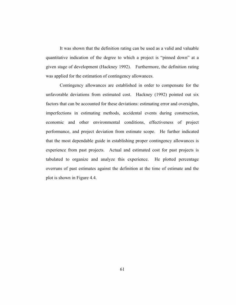
It was shown that the definition rating can be used as a valid and valuable

quantitative indication of the degree to which a project is “pinned down” at a

given stage of development (Hackney 1992). Furthermore, the definition rating

was applied for the estimation of contingency allowances.

Contingency allowances are established in order to compensate for the

unfavorable deviations from estimated cost. Hackney (1992) pointed out six

factors that can be accounted for these deviations: estimating error and oversights,

imperfections in estimating methods, accidental events during construction,

economic and other environmental conditions, effectiveness of project

performance, and project deviation from estimate scope. He further indicated

that the most dependable guide in establishing proper contingency allowances is

experience from past projects. Actual and estimated cost for past projects is

tabulated to organize and analyze this experience. He plotted percentage

overruns of past estimates against the definition at the time of estimate and the

plot is shown in Figure 4.4.

61

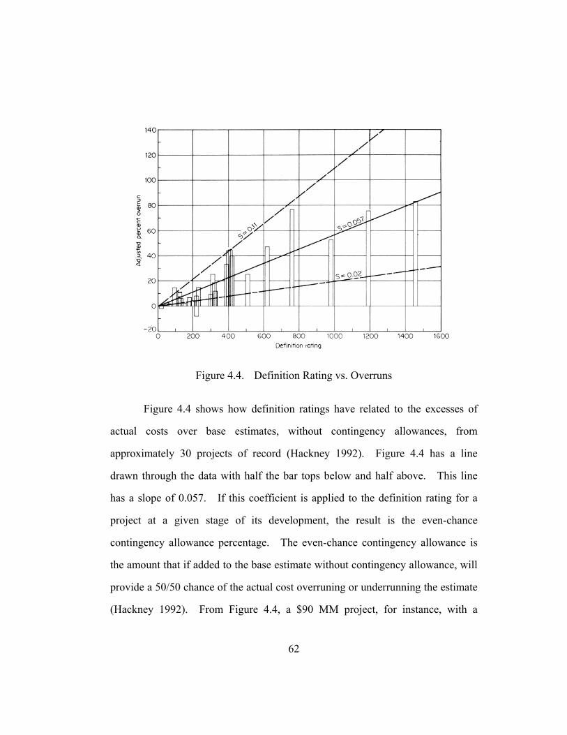
Figure 4.4. Definition Rating vs. Overruns

Figure 4.4 shows how definition ratings have related to the excesses of

actual costs over base estimates, without contingency allowances, from

approximately 30 projects of record (Hackney 1992). Figure 4.4 has a line

drawn through the data with half the bar tops below and half above. This line

has a slope of 0.057. If this coefficient is applied to the definition rating for a

project at a given stage of its development, the result is the even-chance

contingency allowance percentage. The even-chance contingency allowance is

the amount that if added to the base estimate without contingency allowance, will

provide a 50/50 chance of the actual cost overruning or underrunning the estimate

(Hackney 1992). From Figure 4.4, a $90 MM project, for instance, with a

62

definition rating of 630 will have an even-chance allowance of 35.9 (630 x 0.057)

percent and the even-chance estimate is $122 MM ($90 MM x 1.359). This

approach will be adopted for this research to establish a model to estimate the

potential risk impact.

4.6. SYSTEMATIC RISK MANAGEMENT APPROACH

Al-Bahar (1988) proposed a model, Construction Risk Management

System (CRMS), providing an effective systematic framework for quantitatively

identifying, evaluating, and responding to risk in construction projects. The

CRMS provides a formal, logical, and systematic tool that helps contractors in

identifying, analyzing, and managing risks in a construction project. Based on

his risk management system framework, this research will develop a new

prototype risk management approach by incorporating the PDRI.

In the proposed risk management technique, PDRI will be used in all three

of the risk management process: risk identification, risk quantification and risk

control. Flowcharts will be created to graphically represent the systematic risk

management that helps owners in identifying, quantifying and controlling risks in

the pre-project planning stage of a construction project.

Using results from literature review and data analysis, the research

findings are synthesized into a comprehensive risk management approach. The

proposed systematic risk management approach using PDRI can be implemented

by the project team in the pre-project planning phase of a project to increase the

probability of a successful project.

63

4.7. STUDY LIMITATIONS

It is important to note some of the potential limitations of this study in

terms of methodology and data collection. The sample selection for the study is

based on organizations volunteering projects for the study and not on a random

sample of a known population. Moreover, most of these organizations are CII

member companies and, at least anecdotally, CII companies are typically larger in

size and perform better than the average non-CII member companies. These

organizations may have selected projects with a bias toward successful projects

which tends to have lower PDRI scores and thus will influence the results. For

the building projects, the institutional organization provided both successful and

less than successful projects and made the building project sample less biased,

since this represented their entire population of projects for a particular time

period.

A second limitation relates to the nature of retrospective case studies.

The respondents are required to think back to the initial planning and designing

stage (just prior to Construction Documents development) and assess how well

each scope element was defined at that time during the “after the fact” project

data collection process. Regardless of how complete their project

documentation was, this method may still have resulted in slightly inaccurate

reporting since it is typically difficult to remember precise details. This data

collection may also have lead to some bias in self-scoring the PDRI.

64

4.8. SUMMARY OF RESEARCH METHODOLOGY

This chapter outlined the development and administration of data

collection instrument, data collection process, data analysis techniques, and

development of analytical model and systematic risk management approach.

Information from several reference resources that cover pre-project planning and

risk management were used as the foundation for this research. Raw data

obtained from previous research, CII Benchmarking and Metrics research, and

data from the institutional organization were stored in a database. Several

statistical analysis techniques were employed to conduct data analysis and to

verify the research hypotheses. Descriptive analyses of the data collected are

presented in the next chapter.

65

Chapter 5 Project Data Characteristics and Data Analysis

Data collected for the research represent 62 industrial projects and 78

building projects. These 62 industrial projects represent approximately $3.9

billion in total construction costs from 30 owner and contractor companies. This

sample included projects constructed in 11 different countries. The 78 building

projects represent approximately $1.1 billion in total construction costs and are

geographically dispersed in four regions (U.S.A., Canada, Latin America, and

Australia/Pacific). These building projects were provided by 15 different owner

and contractor companies. This chapter presents the summary of data collected

from three main sources: previous PDRI research, CII Benchmarking & Metrics

research, and institutional organizational PDRI Benchmarking research, as

described in Section 4.3 in this dissertation. Tables and figures are used to

present the sample characteristics. The various analyses performed on the data

collected from the sample projects are also presented. The results of success

index analysis, correlation analysis, and hypothesis validation are discussed.

5.1. GENERAL PROJECT CHARACTERISTICS

The 62 industrial projects had a wide range of facility types such as gas

processing, petroleum refinery, power plant, chemical plant, pulp and paper,

manufacturing facility, metal refining/processing, transmission and distribution,

pharmaceutical, and wastewater treatment. The building projects cover schools,

churches, border stations, research labs, offices, warehouses, shopping centers,

recreational facilities, fire stations, and courthouses. Table 5.1 shows the sample

66

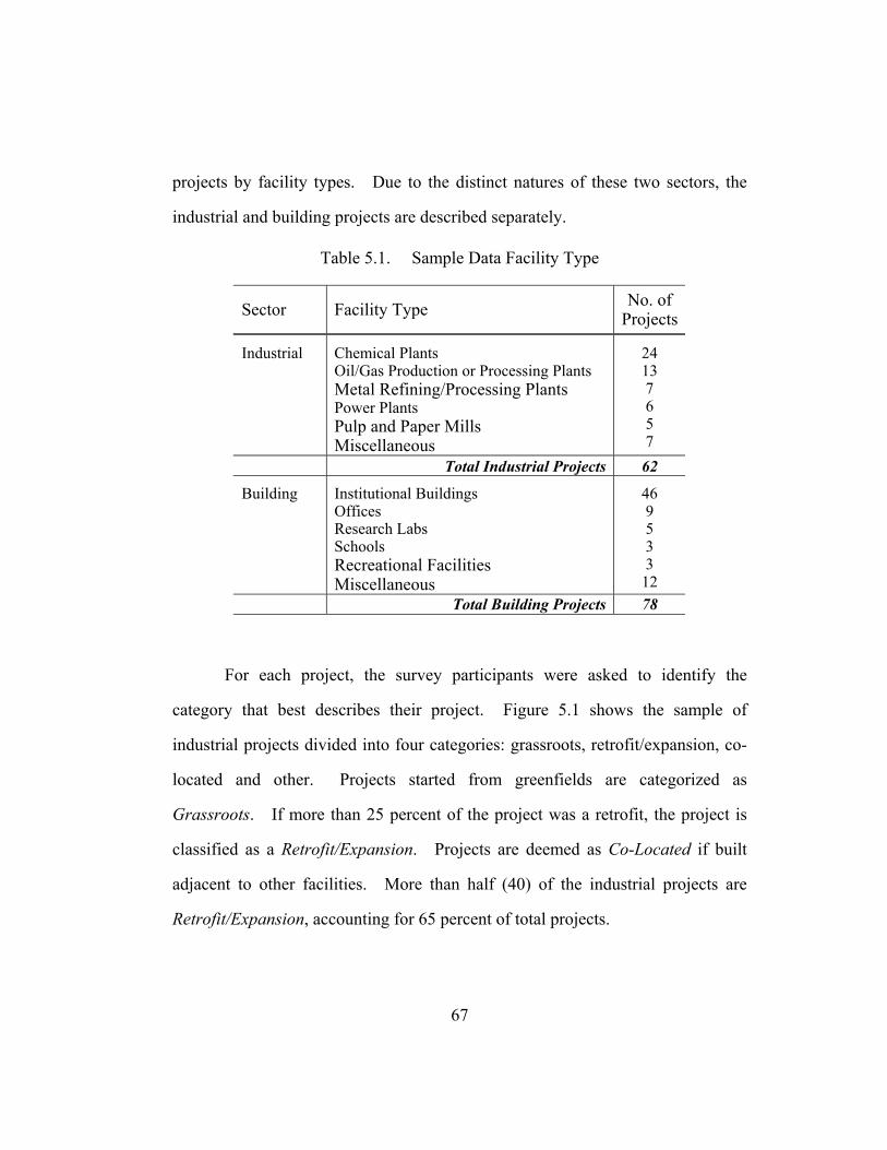
projects by facility types. Due to the distinct natures of these two sectors, the

industrial and building projects are described separately.

Table 5.1. Sample Data Facility Type

Sector Facility Type No. of Projects

Industrial Chemical Plants Oil/Gas Production or Processing Plants Metal Refining/Processing Plants Power Plants Pulp and Paper Mills Miscellaneous

24 13 7 6 5 7

Total Industrial Projects 62

Building Institutional Buildings Offices Research Labs Schools Recreational Facilities Miscellaneous

46 9 5 3 3

12 Total Building Projects 78

For each project, the survey participants were asked to identify the

category that best describes their project. Figure 5.1 shows the sample of

industrial projects divided into four categories: grassroots, retrofit/expansion, co-

located and other. Projects started from greenfields are categorized as

Grassroots. If more than 25 percent of the project was a retrofit, the project is

classified as a Retrofit/Expansion. Projects are deemed as Co-Located if built

adjacent to other facilities. More than half (40) of the industrial projects are

Retrofit/Expansion, accounting for 65 percent of total projects.

67

0 5 10 15 20 25 30 35 40 45

Other

Co-Located

Grassroot

Retrofit/Expansion

Proj

ect C

ateg

ory

Number of Projects

N = 62

Figure 5.1. Industrial Project Type

Figure 5.2 shows the sample of building projects divided into two

categories: new construction and renovation. If renovation cost was greater than

50 percent, the project is considered as a renovation project. Eighty-eight

percent (69 out of 78) of the building projects were new construction.

68

0 10 20 30 40 50 60 70 8

Renovation

New Construction

Proj

ect C

ateg

ory

Number of Projects

N = 78

0

Figure 5.2. Building Project Type

In the survey, respondents were asked to identify what kind of contract

was used for the project. These projects were categorized in three categories:

Design-Bid-Build, Design-Build, and Other. Figure 5.3 shows the number of

industrial sample projects in each contract type category along with their

percentages. It should be noted that only 28 out of the 62 surveyed industrial

projects provided sufficient project contract information. Among the 28 projects,

more than half (64 percent) were Design-Bid-Build projects.

69

Design-Bid-Build,18, 64%

Design-Build, 8,29%

Other, 2, 7% N=28

Figure 5.3. Industrial Project Contract Type

Figure 5.4 below shows the percentage of each contract type in three

different contracting categories for the 68 building projects that provided this

information. Fifty out of the surveyed 68 projects (74 percent) indicated usage

of Design-Bid-Build contracts.

70

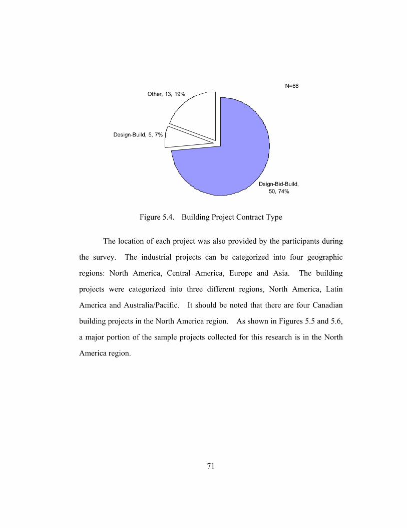
Design-Build, 5, 7%

Other, 13, 19%

Dsign-Bid-Build,50, 74%

N=68

Figure 5.4. Building Project Contract Type

The location of each project was also provided by the participants during

the survey. The industrial projects can be categorized into four geographic

regions: North America, Central America, Europe and Asia. The building

projects were categorized into three different regions, North America, Latin

America and Australia/Pacific. It should be noted that there are four Canadian

building projects in the North America region. As shown in Figures 5.5 and 5.6,

a major portion of the sample projects collected for this research is in the North

America region.

71

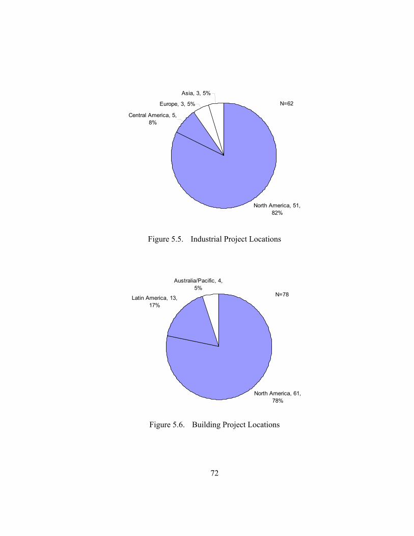
North America, 51,82%

Central America, 5,8%

Europe, 3, 5%

Asia, 3, 5%

N=62

Figure 5.5. Industrial Project Locations

North America, 61,78%

Latin America, 13,17%

Australia/Pacific, 4,5%

N=78

Figure 5.6. Building Project Locations

72

The average total project duration (design, construction and startup) for

the 62 industrial projects was 33 months with a standard deviation of 24 months.

The longest project took a total of 114 months to finish while the shortest project

took only four months to complete. Figure 5.7 shows the distribution of total

project durations for industrial projects. More than 50 percent of the industrial

sample projects have total project durations of one to three years.

0

5

10

15

20

25

<12 13 - 24 24 - 36 36 - 48 48 - 60 > 60

Months

Num

ber o

f Pro

ject

s

Average = 33.1 monsStd. Dev. = 24.3 mons

Figure 5.7. Industrial Project Total Schedule Durations, N=62

For the 78 building projects, it took an average of 21 months (design,

construction and commissioning) to finish with a standard deviation of 18 months.

The longest project duration was 98 months and the shortest project duration was

seven months. The distribution of project durations is shown in Figure 5.8.

More than 60 percent of building projects in the survey were finished within two

73

years and the sample is skewed by the projects provided by the institutional

owner.

0

5

10

15

20

25

30

35

40

<12 13 - 24 24 - 36 36 - 48 48 - 60 > 60

Months

Num

ber o

f Pro

ject

s

Average = 20.7 monsStd. Dev. = 17.9 mons

Figure 5.8. Building Project Total Schedule Durations, N=78

The total installed cost for industrial projects ranged from $0.9 million to

$635 million with a standard deviation of $118 million. The mean project cost

was approximately $65 million with half of the projects taking less than $25

million to complete. Figure 5.9 illustrates the distribution of total installed cost

for industrial projects.

74

0

2

4

6

8

10

12

14

16

18

< 10 10 - 25 25 - 50 50 - 100 100 - 200 > 200

Millions ($)

Num

ber o

f Pro

ject

s

Average = $65.2 M

Std. Dev. = $118.2 M

Figure 5.9. Industrial Project Total Installed Cost, N=62

Comparing by total installed cost, building projects are generally smaller

in size (dollar amount) than industrial projects. The mean total installed cost for

building projects was approximately $15 million with a standard deviation of $30

million. The total installed cost for building projects ranges from $0.7 million to

$200 million. More than 60 percent of the building projects in the survey took

less than $10 million to design and construct. Again, these data are skewed by

the 45 projects of the one institutional owner.

75

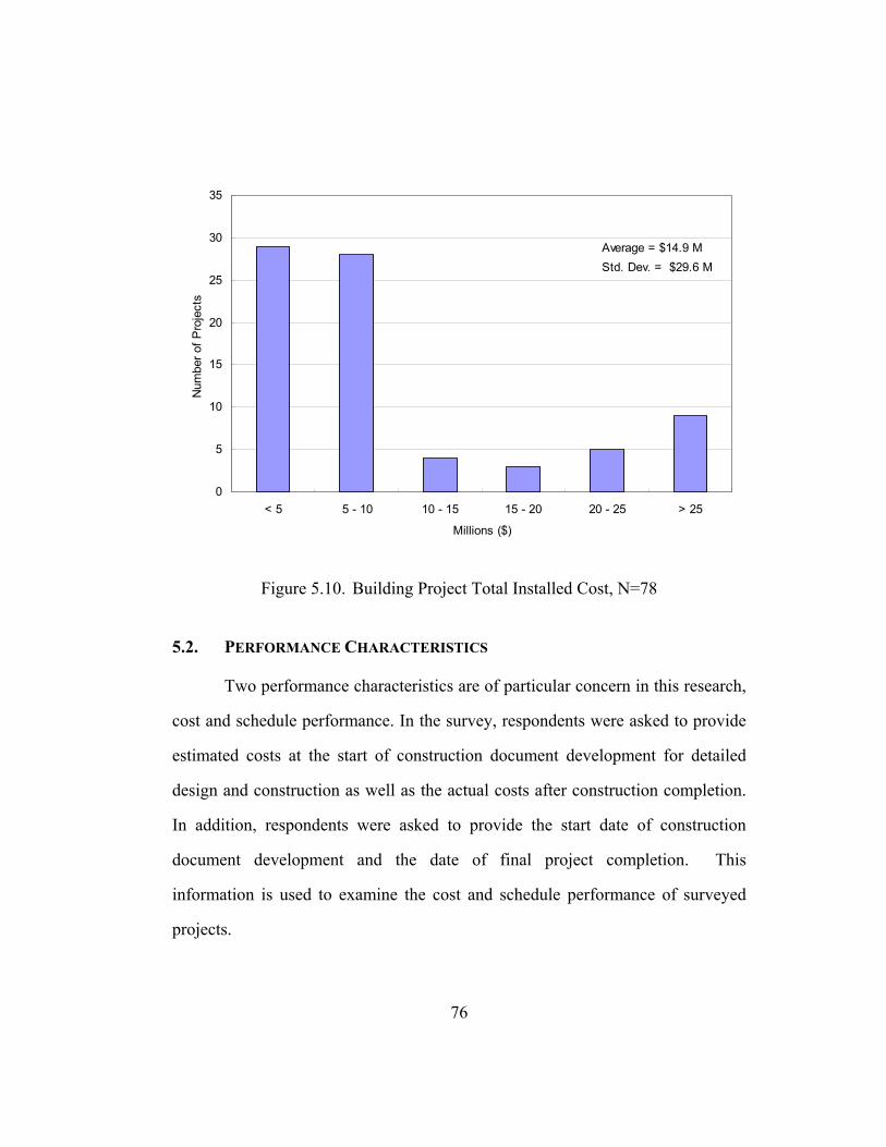
0

5

10

15

20

25

30

35

< 5 5 - 10 10 - 15 15 - 20 20 - 25 > 25

Millions ($)

Num

ber o

f Pro

ject

s

Average = $14.9 MStd. Dev. = $29.6 M

Figure 5.10. Building Project Total Installed Cost, N=78

5.2. PERFORMANCE CHARACTERISTICS

Two performance characteristics are of particular concern in this research,

cost and schedule performance. In the survey, respondents were asked to provide

estimated costs at the start of construction document development for detailed

design and construction as well as the actual costs after construction completion.

In addition, respondents were asked to provide the start date of construction

document development and the date of final project completion. This

information is used to examine the cost and schedule performance of surveyed

projects.

76

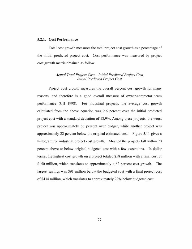
5.2.1. Cost Performance

Total cost growth measures the total project cost growth as a percentage of

the initial predicted project cost. Cost performance was measured by project

cost growth metric obtained as follow:

Actual Total Project Cost – Initial Predicted Project Cost

Initial Predicted Project Cost

Project cost growth measures the overall percent cost growth for many

reasons, and therefore is a good overall measure of owner-contractor team

performance (CII 1998). For industrial projects, the average cost growth

calculated from the above equation was 2.6 percent over the initial predicted

project cost with a standard deviation of 18.9%. Among these projects, the worst

project was approximately 86 percent over budget, while another project was

approximately 22 percent below the original estimated cost. Figure 5.11 gives a

histogram for industrial project cost growth. Most of the projects fall within 20

percent above or below original budgeted cost with a few exceptions. In dollar

terms, the highest cost growth on a project totaled $58 million with a final cost of

$150 million, which translates to approximately a 62 percent cost growth. The

largest savings was $91 million below the budgeted cost with a final project cost

of $434 million, which translates to approximately 22% below budgeted cost.

77

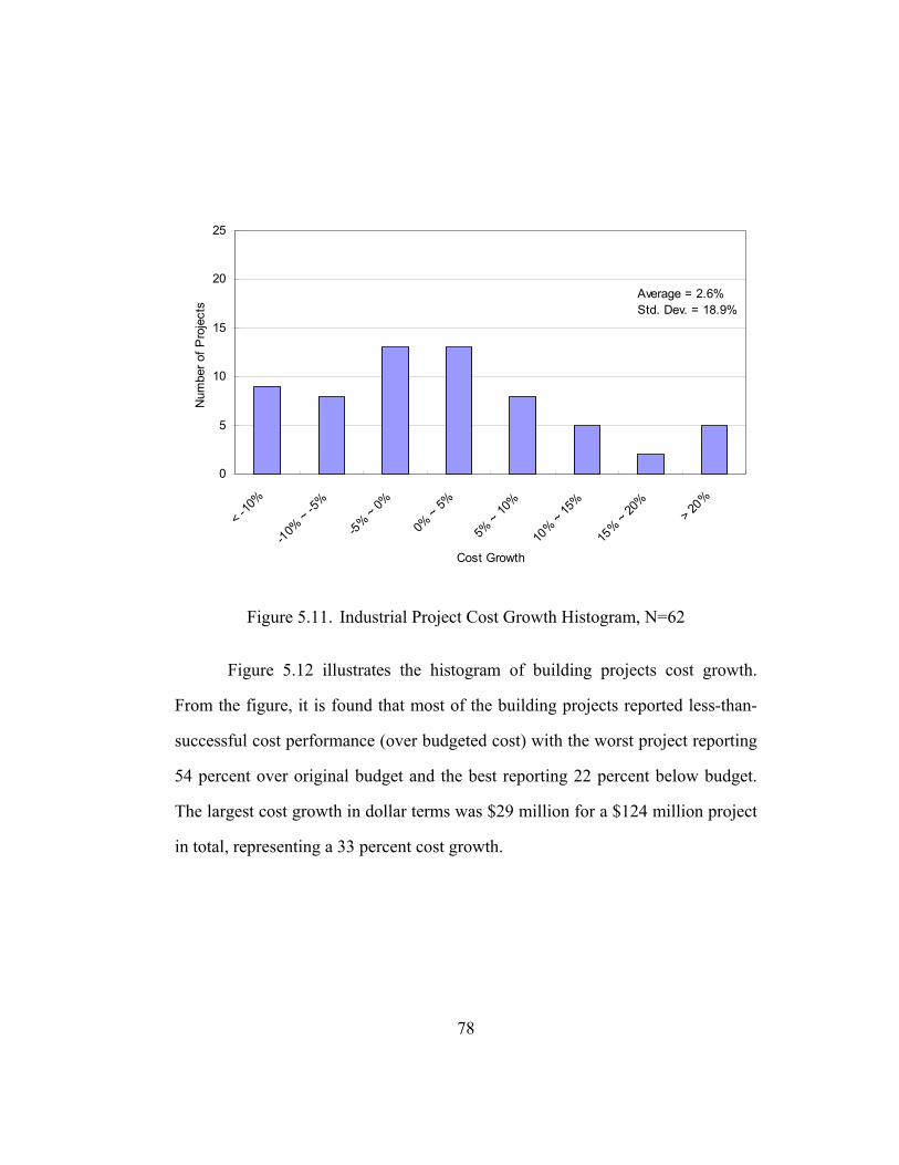
0

5

10

15

20

25

< -10%

-10% ~ -5

%

-5% ~ 0%

0% ~ 5%

5% ~ 10

%

10% ~

15%

15% ~

20%

> 20%

Cost Growth

Num

ber o

f Pro

ject

s

Average = 2.6%Std. Dev. = 18.9%

Figure 5.11. Industrial Project Cost Growth Histogram, N=62

Figure 5.12 illustrates the histogram of building projects cost growth.

From the figure, it is found that most of the building projects reported less-than-

successful cost performance (over budgeted cost) with the worst project reporting

54 percent over original budget and the best reporting 22 percent below budget.

The largest cost growth in dollar terms was $29 million for a $124 million project

in total, representing a 33 percent cost growth.

78

0

5

10

15

20

25

< -10%

-10% ~ -5

%

-5% ~ 0%

0% ~ 5%

5% ~ 10

%

10% ~

15%

15% ~

20%

> 20%

Cost Growth

Num

ber o

f Pro

ject

s

Average = 10.6%Std. Dev. = 13.3%

Figure 5.12. Building Project Cost Growth Histogram, N=78

5.2.2. Schedule Performance

The total project duration used to calculate project schedule growth was

measured from the start date of construction documents development (or

authorization for expenditure of detailed design funds for industrial projects) to

the date of substantial completion (or mechanical completion in the case of

industrial projects) in months. The following equation was used for computing

project schedule performance:

Actual Total Project Schedule – Initial Predicted Project Schedule

Initial Predicted Project Schedule

79

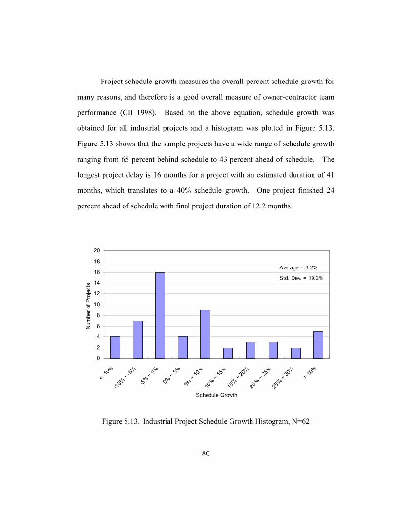
Project schedule growth measures the overall percent schedule growth for

many reasons, and therefore is a good overall measure of owner-contractor team

performance (CII 1998). Based on the above equation, schedule growth was

obtained for all industrial projects and a histogram was plotted in Figure 5.13.

Figure 5.13 shows that the sample projects have a wide range of schedule growth

ranging from 65 percent behind schedule to 43 percent ahead of schedule. The

longest project delay is 16 months for a project with an estimated duration of 41

months, which translates to a 40% schedule growth. One project finished 24

percent ahead of schedule with final project duration of 12.2 months.

0

2

4

6

8

10

12

14

16

18

20

< -10%

-10% ~ -5

%

-5% ~ 0%

0% ~ 5%

5% ~ 10

%

10% ~

15%

15% ~

20%

20% ~

25%

25% ~

30%

> 30%

Schedule Growth

Num

ber o

f Pro

ject

s

Average = 3.2%

Std. Dev. = 19.2%

Figure 5.13. Industrial Project Schedule Growth Histogram, N=62

80

Similar to the distribution of building project cost growth, most of the

building projects are behind the original estimated schedule. The 78 building

projects have an average total project duration of 20.7 months with a standard

deviation of 17.9 months. Figure 5.14 shows the histogram of building project

schedule growths. The worst project had a schedule growth of 106 percent that

doubled the original project duration to more than one year. One project

finished three months ahead of schedule, which accounted for 25 percent of the

original estimated project duration.

0

2

4

6

8

10

12

14

16

18

20

< -10%

-10% ~ -5

%

-5% ~ 0%

0% ~ 5%

5% ~ 10

%

10% ~

15%

15% ~

20%

20% ~

25%

25% ~

30%

> 30%

Schedule Growth

Num

ber o

f Pro

ject

s

Average = 16.9%

Std. Dev. = 24.6%

Figure 5.14. Building Project Schedule Performance Histogram, N=78

Table 5.2 summarizes the basic cost and schedule growth information for

both industrial and building projects. Again, performance in this table was

81

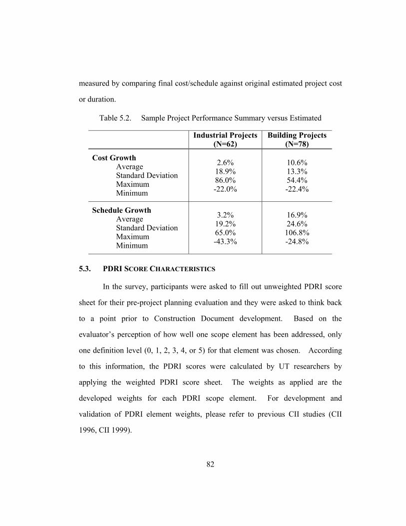
measured by comparing final cost/schedule against original estimated project cost

or duration.

Table 5.2. Sample Project Performance Summary versus Estimated

Industrial Projects (N=62)

Building Projects (N=78)

Cost Growth Average Standard Deviation Maximum Minimum

2.6% 18.9% 86.0% -22.0%

10.6% 13.3% 54.4% -22.4%

Schedule Growth Average Standard Deviation Maximum Minimum

3.2% 19.2% 65.0% -43.3%

16.9% 24.6% 106.8% -24.8%

5.3. PDRI SCORE CHARACTERISTICS

In the survey, participants were asked to fill out unweighted PDRI score

sheet for their pre-project planning evaluation and they were asked to think back

to a point prior to Construction Document development. Based on the

evaluator’s perception of how well one scope element has been addressed, only

one definition level (0, 1, 2, 3, 4, or 5) for that element was chosen. According

to this information, the PDRI scores were calculated by UT researchers by

applying the weighted PDRI score sheet. The weights as applied are the

developed weights for each PDRI scope element. For development and

validation of PDRI element weights, please refer to previous CII studies (CII

1996, CII 1999).

82

As discussed earlier in Chapter 2, elements have five pre-assigned scores,

one for each of the five possible levels of definition. The value of the score

based on a chosen definition was obtained for each element. Each of the

element scores within a category was added to produce a total score for that

category. The scores for each of the categories within a section were added to

arrive at a section score. Finally, the three section scores were added to achieve

a total PDRI score. The Industrial PDRI scoresheet is provided in Appendix C

and Building PDRI scoresheet is contained in the project manager questionnaire

in Appendix B.

The histogram of 62 PDRI scores for industrial projects is shown in Figure

5.15. The average PDRI score was 221 with a standard deviation of 104. The

distribution of PDRI scores is fairly widespread and range from 82 to 465. Note

that these scores were measured for each project at the point in time just prior to

authorization for expenditure for these industrial projects. At this point in time,

scope definition should have been completed.

83

0

2

4

6

8

10

12

14

16

18

20

<100

100 ~

150

150 ~

200

200 ~

250

250 ~

300

300 ~

350

350 ~

400

> 400

PDRI Score

Num

ber o

f Pro

ject

s

Average = 221.0

Std. Dev. = 104.1

Figure 5.15. Industrial Project PDRI Score Histogram, N=62

Similarly, the distribution of building project PDRI scores is wide spread

and the PDRI score histogram is presented in Figure 5.16. The average PDRI

score for the 78 building projects was 285 with a standard deviation of 120. The

PDRI scores range from 95 to 648. Again, these scores were calculated for each

project at the end of design development and should correspond to the end of

scope definition.

84

0

2

4

6

8

10

12

14

16

18

<100

100 ~

150

150 ~

200

200 ~

250

250 ~

300

300 ~

350

350 ~

400

> 400

PDRI Score

Num

ber o

f Pro

ject

sAverage = 285.3

Std. Dev. = 119.9

Figure 5.16. Building Project PDRI Score Histogram, N=78

5.4. PDRI AND PROJECT SUCCESS

Since one of the primary objectives of this research is to identify if

positive relationships exist between project scope definition and project success, a

measurement of project success was required. The section outlines the

measurement of project success and correlation between PDRI scores and project

success.

5.4.1. Project Success

Several studies have been conducted to measure project success (Ashley,

Jaselskis, & Lurie 1987, Morris & Hough 1987, Freeman & Beale 1992, Gibson

& Hamilton 1994, Pinto & Kharabanda 1996, and Tan 1996). The Project

85

Management Institute devoted the entire annual conference to the topic of

measuring project success in 1986 (PMI 1986). There does not seem to be a

universally accepted definition or measurement based on published literature.

Nevertheless, a mechanism for measuring the success of the sample projects was

desired for this research effort. Once the project success was measured and

quantified, a bivariate regression analysis can be performed to explore the

relationship between the PDRI score and project success.

The project success measurement method used to evaluate the sample

projects in this investigation was adopted from previous research by the

Construction Industry Institute’s Pre-Project Planning Research Team. In their

study of the relationship between pre-project planning effort and project success,

they examined the success level attained on 53 capital projects and determined

that a positive correlation existed between success and the amount of effort

expended in pre-project planning. As part of their research, they developed an

index for measuring project success based on four performance variables: Budget

Achievement, Schedule Achievement, Design Capacity, and Plant Utilization

(Gibson and Hamilton 1994).

These four variables were divided into two categories: Project Success

variables and Operating Success variables. Budget Achievement and Schedule

Achievement were categorized as Project Success variables, while Design

Capacity and Plant Utilization were categorized as Operating Success variables.

However, the Design Capacity and Plant Utilization are specific measurements

for industrial projects and are therefore not applicable to building projects. For

86

consistency, the author decided that only two Project Success variables (Budget

Achievement and Schedule Achievement) were used to measure project success

(both industrial and building projects) for this research. The definitions for

Project Success variables are as follows (Gibson and Hamilton 1994):

Budget Achievement: Adherence to the authorized budget, measured by

the percent deviation between the actual cost and the authorized cost (for

design and construction).

Schedule Achievement: Adherence to the authorized schedule for

mechanical completion, measured by the percent deviation between the

actual project duration and the authorized project duration (for design and

construction).

The Pre-Project Planning Research Team determined the relative level of

importance of each variable in the success index through interviewing 131

industry representatives. An analysis of their responses indicated that the index

variables should be weighted as shown in Table 5.3 (Gibson and Hamilton 1994).

87

Table 5.3. Success Index Variables and Weights (Gibson and Hamilton 1994)

Success Category Variable Variable Wt.

Category Wt.

Project Success Budget Achievement Schedule Achievement

0.55 0.45

0.60

Total Variable Weight 1.00 Operating Success

Design Capacity Plant Utilization

0.70 0.30

0.40

Total Variable Weight 1.00

Total Category Weight 1.00

Combining the four variables and their corresponding weights yielded an

equation for computing the Project Success Rating. The equation is shown as

follow (Gibson and Hamilton 1994):

Project Success Rating = 0.60 x [0.55 (Budget Achievement Value) +

0.45 (Schedule Achievement Value)] + 0.40 x [0.70 (Design Capacity Attainment Value) + 0.30 (Plant Utilization Attainment Value)]

As discussed earlier, only Budget Achievement and Schedule

Achievement were included in Project Success Ratings for this research. Since

only two variables were considered in the success index, for simplicity a weight

of 50 percent for each variables was used to represent the importance of these two

factors in the success index (even though this may not be indicative of relative

value for some projects). A project success index was then calculated by

averaging the two variables (budget and schedule achievement). The equation

for calculating Project Success Index is as follow:

88

Project Success Index = 0.50 (Budget Achievement Value) +

0.50 (Schedule Achievement Value)

When several categories are in the data, or the data are continuous in

nature, it can become difficult to detect patterns and discover significant

relationships. In this case, it may be necessary to combine categories or regroup

the data into fewer and larger categories (Abdul-Raheem 1994). For this

dissertation research, the large ranges of continuous variables (cost and schedule

performance) were uniformly grouped by percentiles and recoded into nominal

values ranging from one to five.

Descriptives of cost and schedule performance were examined for the

industrial and building projects in order to recode the variables. The variable

values were assigned for the projects based on the 20th percentile ranges for their

performance. For example, the cost growth for the industrial project ranged

from 40 percent below budget to 86 percent over the original budget. Each of

the 11 projects within the first 20th percentile (-40% to -10%) was assigned a

budget achievement value of five. It should be noted that bringing a project in

far under budget is not necessarily a good performance outcome. Each of the 14

projects within the second 20th percentile (-9% to -1%) was assigned a budget

achievement value of four. Projects within the third and fourth 20th percentile

were assigned values of three and two, respectively. Finally, projects within the

last 20 percentile (12% to 86%) were assigned values of one for their budget

achievement.

89

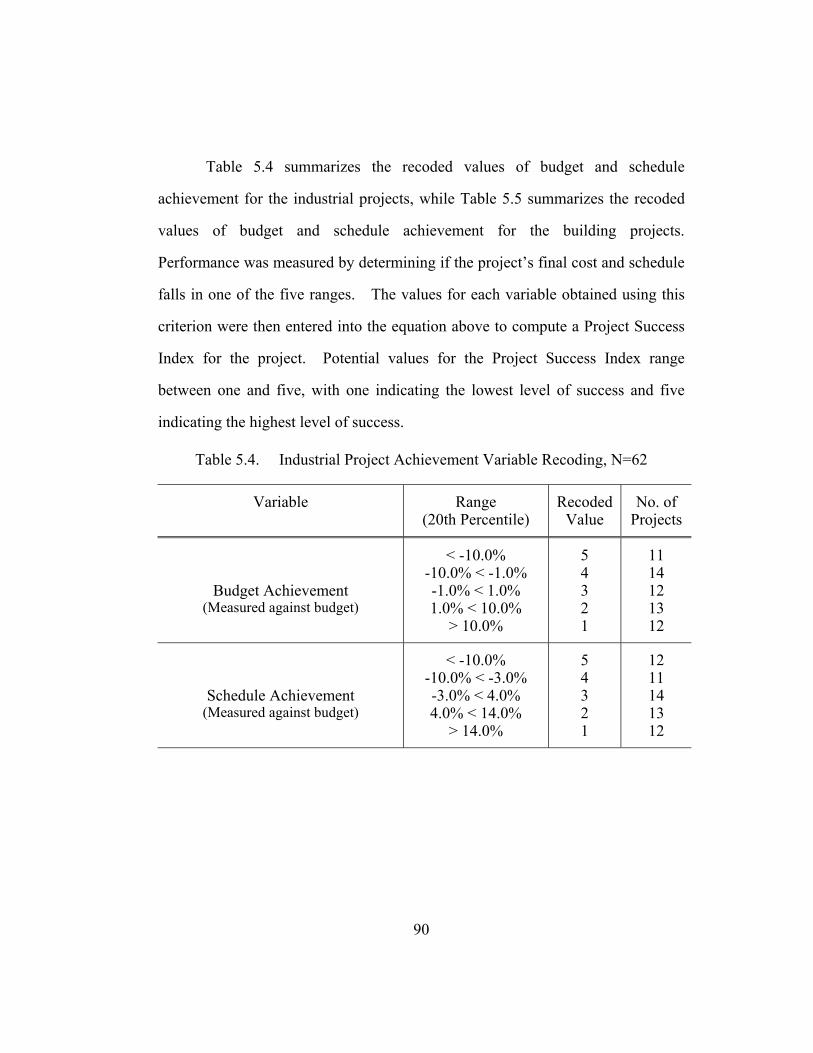
Table 5.4 summarizes the recoded values of budget and schedule

achievement for the industrial projects, while Table 5.5 summarizes the recoded

values of budget and schedule achievement for the building projects.

Performance was measured by determining if the project’s final cost and schedule

falls in one of the five ranges. The values for each variable obtained using this

criterion were then entered into the equation above to compute a Project Success

Index for the project. Potential values for the Project Success Index range

between one and five, with one indicating the lowest level of success and five

indicating the highest level of success.

Table 5.4. Industrial Project Achievement Variable Recoding, N=62

Variable Range (20th Percentile)

Recoded Value

No. of Projects

Budget Achievement (Measured against budget)

< -10.0% -10.0% < -1.0% -1.0% < 1.0% 1.0% < 10.0%

> 10.0%

5 4 3 2 1

11 14 12 13 12

Schedule Achievement (Measured against budget)

< -10.0% -10.0% < -3.0% -3.0% < 4.0% 4.0% < 14.0%

> 14.0%

5 4 3 2 1

12 11 14 13 12

90

Table 5.5. Building Project Achievement Variable Recoding, N=78

Variable Range (20th Percentile)

Recoded Value

No. of Projects

Budget Achievement (Measured against budget)

< 1.6% 1.6% < 5.6% 5.6% < 9.5% 9.5% < 16.7%

> 16.7%

5 4 3 2 1

16 15 16 15 16

Schedule Achievement (Measured against budget)

< 0.0% 0.0% < 6.3% 6.3% < 13.9% 13.9% < 31.8%

> 31.8%

5 4 3 2 1

20 11 16 15 16

Although the equation for computing a project’s success index only

includes two criteria for determining a project’s level of success, it does give a

reliable indication of project performance from a project controls perspective.

The equation is both easy to understand and simple to use. In addition, it is

relatively easy to obtain the information needed for determining the value of each

variable. The rating also provides a good basis for comparing overall

performance on various types of industrial and building projects. Note that the

rating system was established by comparing the performance within the sample

projects. Therefore, caution should be taken for the application of the rating

system to projects beyond the sample.

This success index, which is based on cost and schedule performance

variables, was used to evaluate the success of the 62 industrial and 78 building

projects. For example, an industrial project has a cost growth of 0.5 percent and

91

schedule growth of 13 percent. According to Table 5.4, the Budget

Achievement for this particular project is three and Schedule Achievement is two.

The success index, which is the average of these two, is 2.5 for this project. The

success index, PDRI, cost performance in percent deviation from authorized, and

schedule performance in percent deviation from authorized for both industrial and

building projects are detailed in Appendix D.

5.4.2. Bivariate Correlation and Linear Regression Analysis

A bivariate correlation analysis examines the relationships among pairs of

continuous variables (Knoke and Bohrnstedt 1994). The analysis assumes that

the form of the relationship between the two variables is linear and that the

dependent variable is distributed normally at every level of the independent

variable. For this analysis, the dependent variables (industrial and building

success indexes) were first tested for normality using SPSSTM. The calculated

Kolmogorov-Smirnov statistics for both the industrial and building success

indexes were significant to the level of 0.05. The null hypothesis of non-

normality was thus rejected. However, it should be noted that even when data

violate these assumptions, the methods may still be quite robust and will seldom

be wrong when making conclusions about statistically significant or insignificant

results (Knoke and Bohrnstedt 1994).

The statistical software package SPSSTM was used to conduct the bivariate

correlation tests. The independent variables tested in the bivariate analysis are

PDRI scores for both industrial and building projects. The dependent variable is

the success index. The correlation coefficients (R) between Success Index and

92

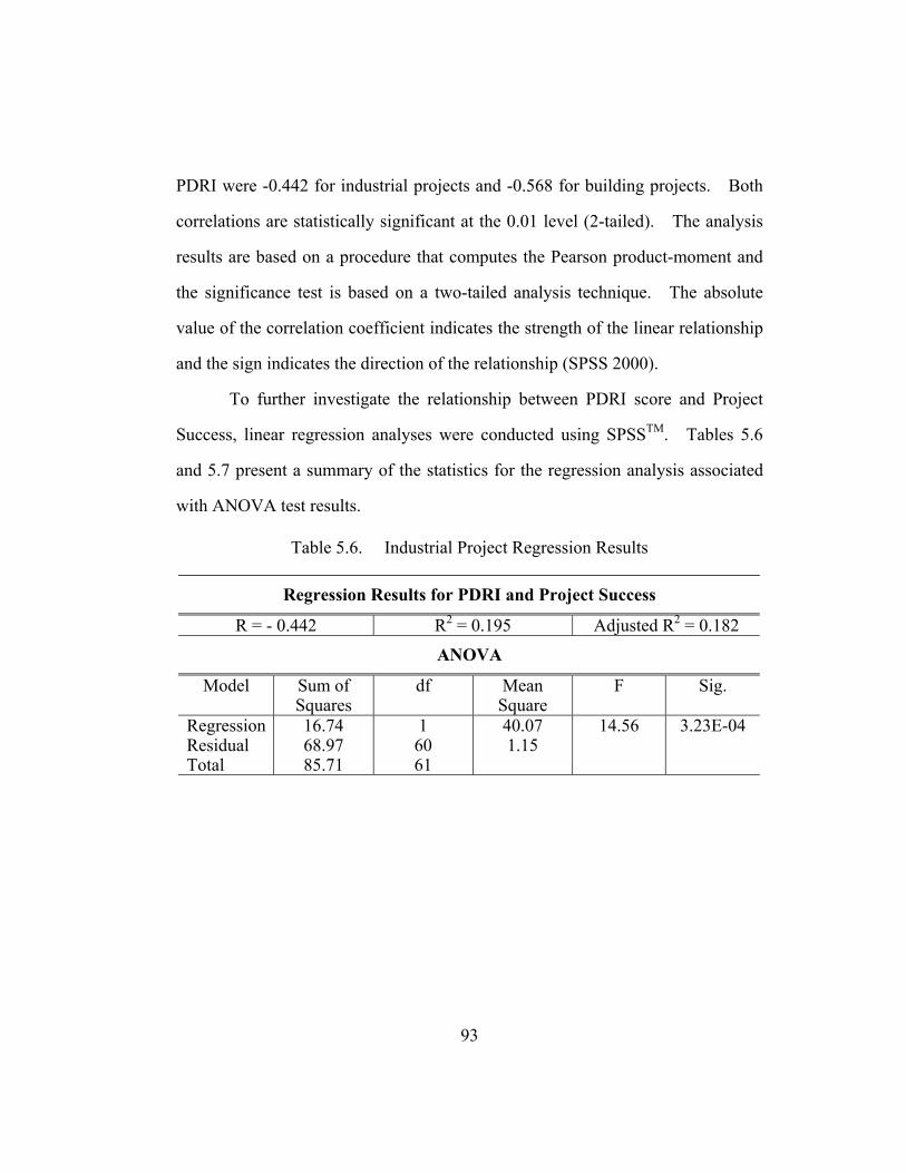
PDRI were -0.442 for industrial projects and -0.568 for building projects. Both

correlations are statistically significant at the 0.01 level (2-tailed). The analysis

results are based on a procedure that computes the Pearson product-moment and

the significance test is based on a two-tailed analysis technique. The absolute

value of the correlation coefficient indicates the strength of the linear relationship

and the sign indicates the direction of the relationship (SPSS 2000).

To further investigate the relationship between PDRI score and Project

Success, linear regression analyses were conducted using SPSSTM. Tables 5.6

and 5.7 present a summary of the statistics for the regression analysis associated

with ANOVA test results.

Table 5.6. Industrial Project Regression Results

Regression Results for PDRI and Project Success

R = - 0.442 R2 = 0.195 Adjusted R2 = 0.182

ANOVA

Model Sum of Squares

df Mean Square

F Sig.

Regression Residual Total

16.74 68.97 85.71

1 60 61

40.07 1.15

14.56 3.23E-04

93

Table 5.7. Building Project Regression Results

Regression Results for PDRI and Project Success

R = - 0.568 R2 = 0.323 Adjusted R2 = 0.314

ANOVA

Model Sum of Squares

df Mean Square

F Sig.

Regression Residual Total

34.99 73.46 108.45

1 76 77

34.99 0.97

36.20 5.83E-08

As can be seen in above tables, the correlations (R) between the project

success and PDRI score are -0.442 and -0.568, which can be described as a

moderate negative relationship between the two variables. That is, as the PDRI

score increases, the Project Success Rating decreases and vice versa. The R2

measures the amount of agreement between the predictor and criterion variables

and reflects the accuracy of future predictions. The R2 values of 0.195 for

industrial projects and 0.323 for building projects, which are significantly

different from zero, indicate that a linear relationship with the PDRI score explain

about 19.5/32.3 respectively percent of the sample variance of the project success.

Scatter plots along with best-fit lines of “Success” vs. “PDRI Score” are

shown in Figure 5.17 and 5.18 for industrial and building projects, respectively.

Least-squared linear regression analyses performed on the plots in Figure 5.17

and 5.18 verify the hypothesis that low (good) PDRI scores correlate to high

project success. The solid straight line denotes the linear trend between the two

94

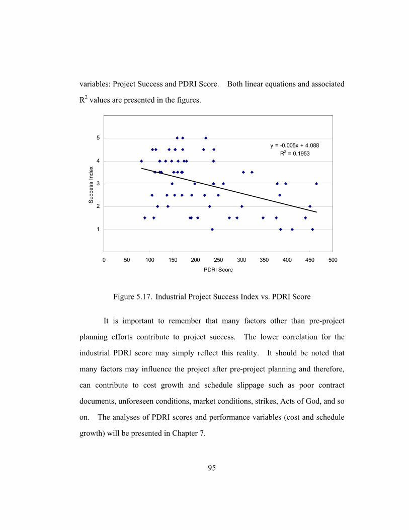
variables: Project Success and PDRI Score. Both linear equations and associated

R2 values are presented in the figures.

y = -0.005x + 4.088R2 = 0.1953

0

1

2

3

4

5

6

0 50 100 150 200 250 300 350 400 450 500

PDRI Score

Suc

cess

Inde

x

Figure 5.17. Industrial Project Success Index vs. PDRI Score

It is important to remember that many factors other than pre-project

planning efforts contribute to project success. The lower correlation for the

industrial PDRI score may simply reflect this reality. It should be noted that

many factors may influence the project after pre-project planning and therefore,

can contribute to cost growth and schedule slippage such as poor contract

documents, unforeseen conditions, market conditions, strikes, Acts of God, and so

on. The analyses of PDRI scores and performance variables (cost and schedule

growth) will be presented in Chapter 7.

95

y = -0.0056x + 4.6304R2 = 0.3226

0

1

2

3

4

5

6

0 100 200 300 400 500 600 700

PDRI Score

Suc

cess

Inde

x

Figure 5.18. Building Project Success Index vs. PDRI Score

5.5. FINDINGS RELATED TO RESEARCH HYPOTHESIS

As described in previous sections of this dissertation, a number of

different methods were used to collect and analyze data. The PDRI tool itself

was developed under the guidance of the CII and had inputs from both industry

and academia. Historical performance data were collected from 62 industrial

and 78 building projects representing approximately $5 billion in total

construction cost. This large amount of data was analyzed using various

statistical techniques to validate the PDRI as a viable vehicle that can lead to

project success.

96

The first research hypothesis was established to test where the PDRI is a

reliable indicator of project success. In order to test this hypothesis and to find

any existing correlation between these two variables (i.e. PDRI Score and Project

Success), a mechanism for measuring the project success was developed. The

results of the regression analysis using the PDRI scores and the project success

measured by success rating index demonstrated a significant correlation for both

industrial and building projects and thus supported the first research hypothesis.

The PDRI had correlations (R) of negative 0.455 and negative 0.531 for industrial

and building projects respectively. This indicates that as the PDRI score

decreases, the probability of project success (as indicated by this index) increases.

5.6. SUMMARY

The data collected from the sample capital facility projects were presented

in this chapter. Several different analysis techniques were used to evaluate the

data collected from the 62 industrial and 78 building projects. Descriptive

statistics, bivariate correlations, and linear regression analysis were all used in

analyzing the data. The cost and schedule performance collected from the

survey were used to develop a success rating index for each project. Bivariate

correlation analyses were done to identify if PDRI scores were significantly

correlated with project success as measured by the success index. For both

industrial and building projects, it was found that PDRI scores are significantly

correlated with a project success rating index.

The regression analysis also revealed correlations between the project

success and the PDRI score. The regression analysis results support the

97

hypothesis that low (good) PDRI score correlates to project success and vice

versa. In the next chapter, results from the institutional organization will be

evaluated in more detail.

98

Chapter 6 Institutional Organization Project Analysis

The 45 building projects provided by the institutional organization are

unique in nature in that these projects were almost identical building construction

projects (same functional requirements and similar footprint), they all belonged to

one owner organization, they provided more detailed project information, and

they were all completed within the past three years. The homogeneous nature of

the sample and enhanced quality of information enabled a more in-depth analysis

for this unique sample. The analysis results are presented in the following

sections. It should be noted that most of the information provided is masked due

to concerns of confidentiality by the research sponsor.

The institutional organization had a building program to construct 100

small buildings worldwide within a three-year time-frame. Management wanted

the projects to be completed before the year of 2000. A standard building plan

was developed for these building projects by the central design office and a

typical project has a total area of 10,600 square feet. Once the location of the

project is determined, a local architect was hired to adapt the standard plan to

meet the site conditions and local building code requirements. The standard plan

adaptation was accomplished through collaboration between the local architect

and the central design office. Then a local contractor is hired to carry out the

plan and construct the building. Similar execution approach was used to build

the small building projects.

99

6.1. PROJECT SAMPLE CHARACTERISTICS

The 45 surveyed building projects consisted of 40 small buildings, three

large buildings and two work-in-progress small buildings. The authorized cost

varied from $2.2 million to $26.7 million, with a total authorized cost of $236.3

million for this project sample. It should be noted that the final cost of these

project was approximately $261.4 million. These projects were built in regions

such as Latin America, Canada, Australia/Pacific, and within the U.S.

The analyses looked at four specific characteristics: project cost, schedule,

change orders, quality and PDRI scores. Table 6.1 provides an overview of

project performance characteristics between small and large buildings.

Table 6.1. Institutional Organization Project Summary

Performance Parameter (Mean) Small Buildings (n=42) Large Buildings (n=3)

Authorized Cost ($million) 4.2 19.1

Authorized Project Duration (month) 8.9 22.1

Cost Growth 16.4% 2.0%

Schedule Growth 23.0% 4.6%

Change Order Cost (% of budget cost) 15.6% 3.3%

6.1.1. Construction Cost

The authorized project costs range from $2.2 million to $26.7 million for

all 45 projects with an average project cost of $19.1 million for large building

projects, $4.8 million for two work-in-progress small buildings and $4.1 million

for the other small building projects. Given square footage of each project, the

100

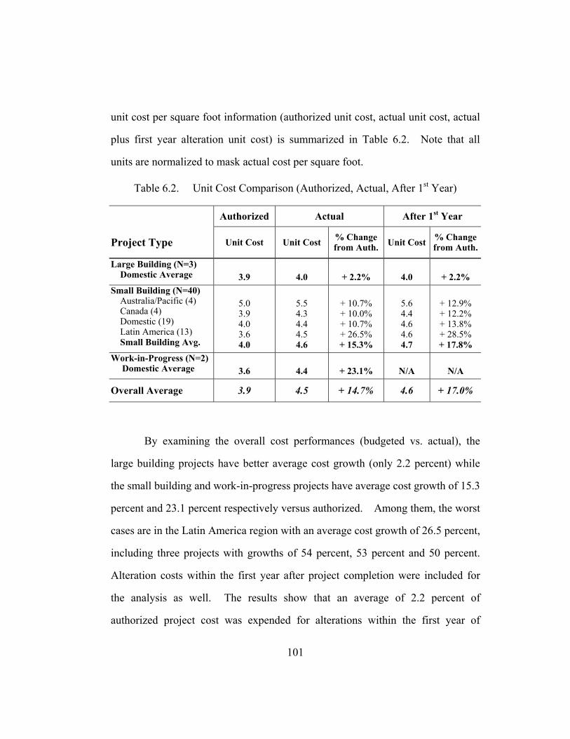
unit cost per square foot information (authorized unit cost, actual unit cost, actual

plus first year alteration unit cost) is summarized in Table 6.2. Note that all

units are normalized to mask actual cost per square foot.

Table 6.2. Unit Cost Comparison (Authorized, Actual, After 1st Year)

Authorized Actual After 1st Year

Project Type Unit Cost Unit Cost % Change from Auth. Unit Cost % Change

from Auth.

Large Building (N=3) Domestic Average

3.9

4.0

+ 2.2%

4.0

+ 2.2%

Small Building (N=40) Australia/Pacific (4) Canada (4) Domestic (19) Latin America (13) Small Building Avg.

5.0 3.9 4.0 3.6 4.0

5.5 4.3 4.4 4.5 4.6

+ 10.7% + 10.0% + 10.7% + 26.5% + 15.3%

5.6 4.4 4.6 4.6 4.7

+ 12.9% + 12.2% + 13.8% + 28.5% + 17.8%

Work-in-Progress (N=2) Domestic Average

3.6

4.4

+ 23.1%

N/A

N/A

Overall Average 3.9 4.5 + 14.7% 4.6 + 17.0%

By examining the overall cost performances (budgeted vs. actual), the

large building projects have better average cost growth (only 2.2 percent) while

the small building and work-in-progress projects have average cost growth of 15.3

percent and 23.1 percent respectively versus authorized. Among them, the worst

cases are in the Latin America region with an average cost growth of 26.5 percent,

including three projects with growths of 54 percent, 53 percent and 50 percent.

Alteration costs within the first year after project completion were included for

the analysis as well. The results show that an average of 2.2 percent of

authorized project cost was expended for alterations within the first year of

101

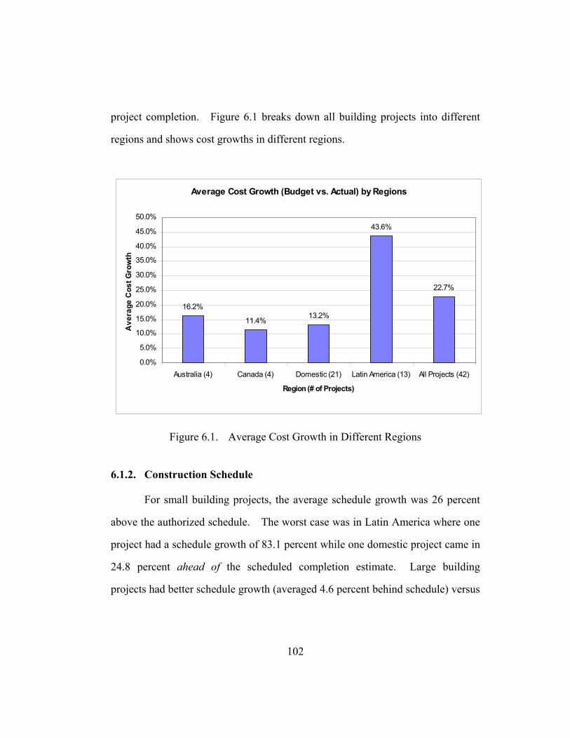
project completion. Figure 6.1 breaks down all building projects into different

regions and shows cost growths in different regions.

Average Cost Growth (Budget vs. Actual) by Regions

16.2%

11.4% 13.2%

43.6%

22.7%

0.0%

5.0%

10.0%

15.0%

20.0%

25.0%

30.0%

35.0%

40.0%

45.0%

50.0%

Australia (4) Canada (4) Domestic (21) Latin America (13) All Projects (42)

Region (# of Projects)

Ave

rage

Cos

t Gro

wth

Figure 6.1. Average Cost Growth in Different Regions

6.1.2. Construction Schedule

For small building projects, the average schedule growth was 26 percent

above the authorized schedule. The worst case was in Latin America where one

project had a schedule growth of 83.1 percent while one domestic project came in

24.8 percent ahead of the scheduled completion estimate. Large building

projects had better schedule growth (averaged 4.6 percent behind schedule) versus

102

projected when compared to small building projects. Figure 6.2 shows average

schedule growth in different regions for the sample.

Average Schedule Growth (Budget vs. Actual) by Regions

20.7%

15.2% 15.4%

46.8%

25.6%

0.0%

5.0%

10.0%

15.0%

20.0%

25.0%

30.0%

35.0%

40.0%

45.0%

50.0%

Australia (4) Canada (4) Domestic (21) Latin America(13)

All Projects (42)

Region (# of Projects)

Aver

age

Sche

dule

Gro

wth

Figure 6.2. Average Schedule Growth in Different Regions

Similar to the results of cost analysis presented previously, the Latin

America region was the worst performing region among the four (almost three

times worse on average than the others). Analysis of the questionnaire indicated

two main reasons contributing to the poor performances in the Latin America

region:

103

1. Poor site adaptation. The standard plan was translated and converted to

the local building code by a local architect. Often times, the site

adaptation prepared by the local architect was poorly done and errors and

omissions were found. Some buildings started construction while the

local architect thought that the design was 80 percent complete but as it

turned out that, according to the project manager, the design was only 50

percent to 60 percent complete. This seemed to be the main reason for

poor cost and schedule growth. This also led to the large change order

costs as identified in the next section.

2. Inability of contractor to perform. Poor contractor performance was

another contributing factor to the poor performance of Latin America

projects. In some cases, the contractor could not perform the tasks to

meet the owner’s requirement or the local material and equipment failed

to meet owner’s specifications. In some cases, American workers were

brought in to finish the job and material and equipment were imported

from America to finish the project.

Figure 6.3 shows the average total project time (from project

announcement to substantial completion) for small building projects in different

regions. The total project time ranges from 16 months for Domestic projects to

19 months for Australia/Pacific projects. The average total project time for 42

small building projects is 17 months. Table 6.3 further breaks the total project

104

time into pre-construction time (project announcement to construction start) and

construction time (construction start to substantial completion).

Total Project (Announcement to Completion)

19.5 17.4

15.6

17.816.8

0

5

10

15

20

25

Australia (4) Canada (4) Domestic (21) Latin America(13)

All Projects(42)

Region

Mon

ths

Figure 6.3. Total Project Time for Small Building Projects

Table 6.3. Small Building Project Time Breakdown

Pre-Construction Time

Construction Time

Total Time

Cost Performance

Australia/Pacific 8.3 mos. 11.2 mos. 19.5 mos. 10.7%

Canada 6.2 mos. 11.2 mos. 17.4 mos. 10.0%

Domestic 5.9 mos. 9.7 mos. 15.6 mos. 10.7%

Latin America 4.7 mos. 13.1 mos. 17.8 mos. 26.5%

105

Australia/Pacific region has the longest pre-construction time of 8.3

months and Latin America has the shortest pre-construction time of 4.7 months.

By examining the project performance and the pre-construction time, it was found

that Australia/Pacific projects (longer pre-construction time) have better cost

performance than Latin America projects (shorter pre-construction time). If

longer pre-construction time can be translated to more pre-project planning

efforts, it is recommended more time and efforts should be spent in pre-

construction process. Although Australia/Pacific projects have longer pre-

construction time, the project construction time is shorter than Latin America

projects that spent less time in pre-construction. In summary, the total time was

similar for all international projects and consistently longer than domestic

projects.

6.1.3. Change Orders

Change orders are fairly common in construction and often times have

negative impact on both schedule and cost performance of a project. On average

in this sample, change orders increased the small building project schedule by 58

days (with an average schedule duration of 266 days) translating to 21.7 percent

more than the original schedule duration. Among the small building projects, an

average of 77 change orders occurred during construction and accounted for an

average total of $0.6 MM (15.6 percent of authorized cost) in cost growth.

Although the large building projects had more change orders, 173 on average,

during construction, they accounted for a smaller percentage of total construction

cost, 3.3 percent of total cost or $0.6 MM on average. In addition, 69 percent of

106

all the projects had at least one change order that accounted for more than one

percent of the total budgeted cost. Table 6.4 further breaks down change order

costs into different regions for small building projects:

Table 6.4. Change Orders (COs) Information for Small Building Projects

Item Average Australia / Pacific Canada Domestic Latin

America Total

Average Number of COs 61 97 84 63 77

Cost Increase by COs

% to Budgeted Cost

548

10.3%

430

10.2%

432

10.3%

1,034

27.5%

651

15.6%

Days Delay by COs

% to Budgeted Schedule

58

20.7%

45

15.2%

38

14.9%

94

35.1%

58

21.7%

% of Projects that have CO Cost over 1% of Budgeted Cost

50% 25% 58% 77% 64%

Table 6.4 shows that the number of change orders is not highly related to

cost increases or schedule delays by change orders. The worst performing

region was still Latin America, which had an average change order cost increase

of 1,034 (27.5 percent of budgeted project cost), and project schedule extensions

of 94 days (35.1 percent of budged schedule).

Three out of the four regions had greater than 50 percent of projects with

at least one change order that accounted for more than one percent of the

authorized cost. These “big” change orders should be and can be avoided with

better pre-project planning. When asked for the reasons of these “big” change

orders, 12 out of 23 (52 percent) of the responses stated that these change orders

were requested from the home office. Further investigation of these changes

107

may provide project lessons learned. Figure 6.4 breaks down the change order

costs (percent of budget) into eight categories. Among them, field architect and

home office request seem to contribute to most of the change order cost.

Change Order Costs in Eight Categories (Total COs: 4.8%* of Authorized Cost)

* Only 41 Small Building Projects

3.2%

1.9%

6.5%

0.9%1.2%

0.5% 0.3% 0.3% 0.0% 1.0% 2.0% 3.0% 4.0% 5.0% 6.0% 7.0%

(1) Home Office

Request

(2) Standard

Plan (3) FieldArchitect

(4) LocalCode

(5)Unforseen

(6) Buildg.Dept

(7) General Authority

(8) Other

Cha

nge

Ord

er C

ost

Figure 6.4. Detailed Change Order Costs in Eight Category

By looking further into the causes of change orders, the change order costs can be

grouped into eight categories: Home Office Request, Standard Plan, Field

Architect, Local Code, Unforeseen, Building Department, General Authority, and

Other. Among them, Standard Plan, Field Architect, Local Code, Unforeseen

and Building Department can be broadly viewed as pre-project planning related

causes for change orders, which means that these issues can (and typically should)

be dealt with in the pre-project planning stage. Looking at the small projects

providing data, Figure 6.5 indicates that average change order costs account for

108

approximately 15 percent of estimated cost. Within this 15 percent,

approximately 11 percent of the cost is due to pre-project planning related change

order costs. These changes added approximately a total of $18.5 million to the

41 projects.

Change Order Cost Percentage for 41 Small Building Projects(Average Total Cos: 15.1% of Authorized Cost)

84.9%

3.7%

11.4% Pre-project Planning Related CO's($18.5 MM)

Non-Preproject Planning Related CO's ($6.1 MM)

Authorized Project Cost($163.1 MM)

Figure 6.5. Change Order Cost Percentage

6.1.4. Quality

The best quality measure is customer satisfaction, in this case, building

user’s satisfaction. Users were asked to rate the overall smoothness of the

project delivery on a Likert scale of 1 to 5, 1 being very difficult and 5 being very

smooth. Fifty-five percent of the user respondents indicated that the overall

109

smoothness of the project delivery was level 3, which means not so good and not

so bad. Another 29 percent of the users rated the overall smoothness at level 2,

which was less than satisfactory. Eighty-eight percent of the users therefore

rated the overall project delivery smoothness, from their perspective, equal to or

below level 3 and the total average on overall project “smoothness” was 2.7.

This shows that the users were not satisfied with the project delivery process. At

the same time, results from project manager’s survey show that project managers

gave the projects an average of 4.4, (using a Likert scale of 1 to 5 with 1 meaning

very unsuccessful and 5 meaning very successful) when asking about how the

project managers felt about the success of the project. Figure 6.6 shows the

survey question and responses from project managers and users.

User SurveyQ: Reflecting on the overall project, rate how smoothly the project has proceeded from design to turnover, with 1 being very troubled to 5 being very smooth

Smoothness Level 1 2 3 4 5Count 3 11 23 2 0

Average 2.7

PM SurveyQ: Reflecting on the overall project, rate how successful you feel the project has been using a scale of 1 to 5, with 1 being very unsuccessful to 5 being very successful

Quality Level 1 2 3 4 5Count 0 0 3 14 28

Average 4.6

Figure 6.6. PM vs. User Quality Survey

The difference between user’s and project manager’s rating on project

quality (4.4 to 2.7) indicates that those two have different sets of criteria

concerning the quality of a project. It is apparent that project managers are

110

satisfied with the outcome quality of the projects while the users have quite the

opposite experience with the process. The best solution may be to have more

user-input into the project from the early stage of the project life. The survey

also indicated that users had little involvement during construction and only 13

percent of users were involved in program definition and scope development.

Another possible quality measure is to account for alteration within the

first year of operation. Alteration costs occurring within the first year can be

deemed as a sign of poor quality of the project delivery process. The survey

results showed that 31 out of 39 (79 percent) of small building projects had

alterations within the first year (three projects did not report). The alteration

costs averaged 3.2 percent of budget per project and totaled $5.2 million. In

addition, some of the small building projects are still anticipating more alteration

costs. One major reason for this is lack of user participation in the project

delivery process. Many alterations are user requested and perhaps can be

avoided with more user input early in the process.

6.1.5. PDRI Scores

As discussed previously, the Project Definition Rating Index (PDRI) is a

weighted scope definition package checklist in score sheet format. Project

managers were asked (after the fact) to fill out the score sheet based on a point in

time just prior to development of construction documents for their projects. The

project managers evaluated the level of definition of each element and the total

scores were calculated by the researchers at The University of Texas. One

domestic large building project had the best PDRI score of 199 while the worst

111

PDRI score, 619, was from a small building project in Latin America. The

average PDRI score for all projects surveyed was 346. The average PDRI scores

for different regions are shown in Figure 6.7. Projects can be grouped into four

geographic regions: Australia/Pacific, Canada, Domestic, and Latin America as

shown in Figure 6.7.

Average PDRI Scores by Regions

315286

339

405

0

50

100

150

200

250

300

350

400

450

Australia (4) Canada (4) Domestic (21) Latin America (13)

Region (# of Projects)

Aver

age

PDRI

Sco

re

Figure 6.7. Average PDRI Scores in Different Region

6.2. PDRI SCORE EVALUATION

Overall PDRI scores were presented in previous sections and following

sections will look further into the relationship between PDRI scores and project

performance. A cutoff PDRI score will be determined to compare the

performance between the projects. In addition, performance measures will be

112

analyzed for the 45 building projects. Previous CII building projects will be

used to compare with the institutional organization projects.

6.2.1. PDRI Score vs. Project Performance

Previously PDRI research indicated that a score of 200 or below (lower

score is better) was a good indicator of a well-defined project (CII 1999).

Analysis of the institutional organization project data has revealed a significant

difference in performance between the sample projects scoring above 300 and the

projects scoring below 300 prior to development of construction documents, as

shown in Table 6.5. Several cutoff points (from 250 to 400) were evaluated to

determine if there was significant statistical difference in performance between

the two groups. It was found that a PDRI score of 300 for this sample was a

good dividing line for differing statistical significance and contained a reasonable

number of projects in both sub-samples. Variation data for the sample projects

are given in Table 6.6. Cost growth is the mean percentage change in actual cost

(contingency not included) and schedule growth is compared to that estimated

prior to development of construction documents. The reported change order

value represents the cost increase during design and construction due to change

orders.

113

Table 6.5. Summary of Cost, Schedule, and Change Order Performance for the Building Projects Using a 300-point Cutoff

PDRI Score Category < 300 > 300 Difference

Cost Growth 11% above budget 18% above budget 7%

Schedule Growth 13% behind schedule 26% behind schedule 13%

Change Orders +9% of budget +18% of budget 9% User Satisfaction 2.6

(1-5, 5: very satisfied)2.7

(1-5, 5: very satisfied) 0.1

(N=15) (N=30) Note: all difference values were statistically significant to the level of 0.05 except for user satisfaction.

Table 6.6. Summary of Cost, Schedule, and Change Order Variation for the Building Projects Using a 300-Point Cutoff

PDRI Score < 300

PDRI Score >300

Category Range Std. Dev. Range Std. Dev.

Cost Growth -1% to +37% 10% +2% to +54% 15%

Schedule Growth -25% to +45% 19% -2% to +83% 24%

Change Orders +2% to +22% 6% +2% to +55% 15%

User Satisfaction 1 to 3 0.69 1 to 5 0.84

(N=15) (N=30)

In summary, the sample projects scoring below 300 outperformed those

scoring above 300 in three important areas: cost growth, schedule growth, and the

relative value of change orders compared to budget. In addition to cost and

schedule differences, the projects scoring less than 300 had lower percentage of

114

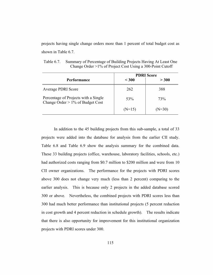
projects having single change orders more than 1 percent of total budget cost as

shown in Table 6.7.

Table 6.7. Summary of Percentage of Building Projects Having At Least One Change Order >1% of Project Cost Using a 300-Point Cutoff

PDRI Score Performance < 300 > 300

Average PDRI Score 262 388

Percentage of Projects with a Single Change Order > 1% of Budget Cost

53% 73%

(N=15) (N=30)

In addition to the 45 building projects from this sub-sample, a total of 33

projects were added into the database for analysis from the earlier CII study.

Table 6.8 and Table 6.9 show the analysis summary for the combined data.

These 33 building projects (office, warehouse, laboratory facilities, schools, etc.)

had authorized costs ranging from $0.7 million to $200 million and were from 10

CII owner organizations. The performance for the projects with PDRI scores

above 300 does not change very much (less than 2 percent) comparing to the

earlier analysis. This is because only 2 projects in the added database scored

300 or above. Nevertheless, the combined projects with PDRI scores less than

300 had much better performance than institutional projects (5 percent reduction

in cost growth and 4 percent reduction in schedule growth). The results indicate

that there is also opportunity for improvement for this institutional organization

projects with PDRI scores under 300.

115

Table 6.8. Summary of Cost, Schedule, and Change Order Performance for ALL Projects Using a 300-point Cutoff

PDRI Score Category < 300 > 300 Difference

Cost Growth 6% above budget 17% above budget 11%

Schedule Growth 9% beyond schedule 25% beyond schedule 16%

Change Orders +9% of budget +17% of budget 8% (N=46) (N=32)

Note: all difference values were statistically significant to the level of 0.05 except for user satisfaction.

Table 6.9. Summary of Cost, Schedule, and Change Order Variation for ALL Projects Using a 300-point Cutoff

PDRI Score < 300 PDRI Score >300 Category Range Std. Dev. Range Std. Dev.

Cost Growth -22% to +37% 12% +2% to +55% 14%

Schedule Growth -25% to +89% 19% -2% to +83% 23%

Change Orders +1% to +61% 10% +2% to +55% 15%

Average PDRI 207 398

(N=46) (N=32)

Table 6.10 shows a comparison of the institutional sample to the CII

database. Among the 33 CII building projects surveyed, 16 projects had PDRI

scores under 200 with average cost growth of one percent above budget, schedule

growth of two percent behind schedule and change orders of seven percent of

budget. Only one building project from the institutional organization had score

116

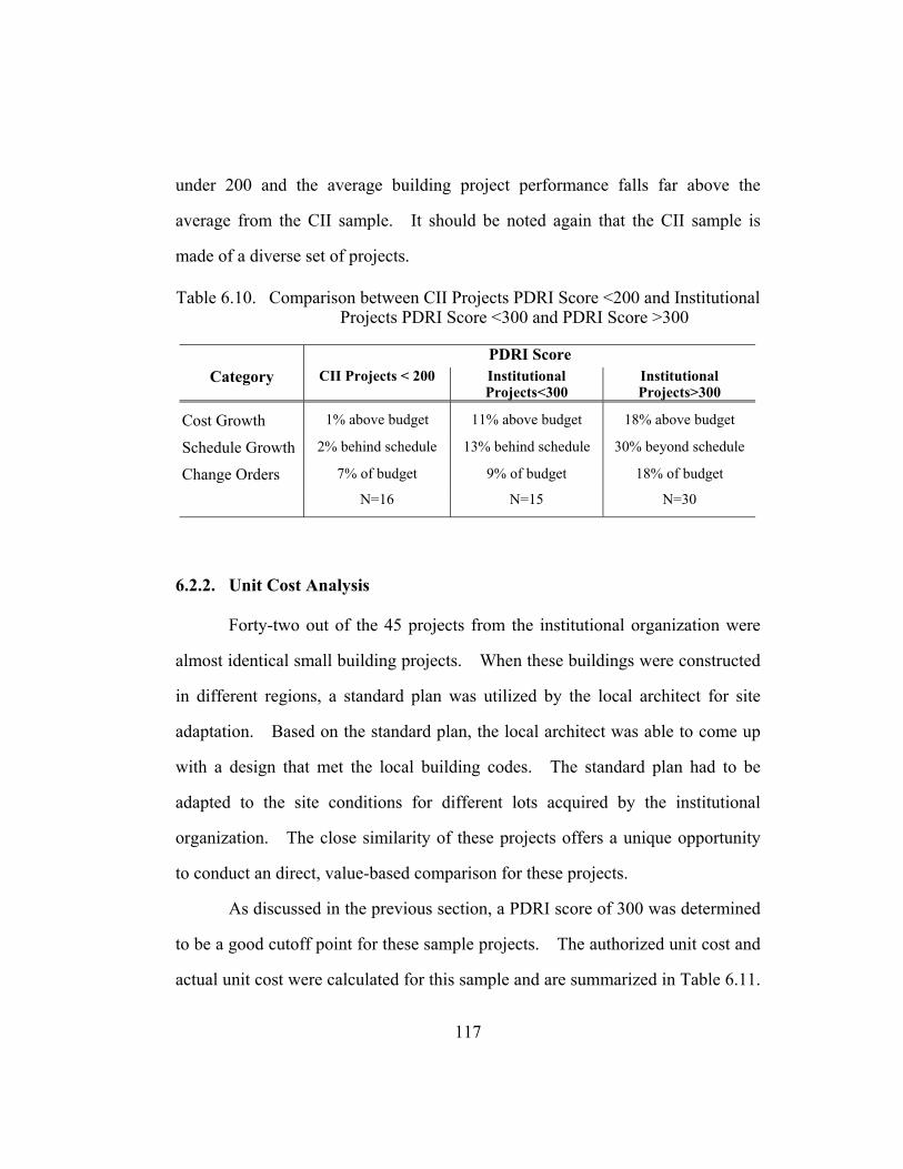
under 200 and the average building project performance falls far above the

average from the CII sample. It should be noted again that the CII sample is

made of a diverse set of projects.

Table 6.10. Comparison between CII Projects PDRI Score <200 and Institutional Projects PDRI Score <300 and PDRI Score >300

PDRI Score Category CII Projects < 200 Institutional

Projects<300 Institutional Projects>300

Cost Growth 1% above budget 11% above budget 18% above budget

Schedule Growth 2% behind schedule 13% behind schedule 30% beyond schedule

Change Orders 7% of budget 9% of budget 18% of budget

N=16 N=15 N=30

6.2.2. Unit Cost Analysis

Forty-two out of the 45 projects from the institutional organization were

almost identical small building projects. When these buildings were constructed

in different regions, a standard plan was utilized by the local architect for site

adaptation. Based on the standard plan, the local architect was able to come up

with a design that met the local building codes. The standard plan had to be

adapted to the site conditions for different lots acquired by the institutional

organization. The close similarity of these projects offers a unique opportunity

to conduct an direct, value-based comparison for these projects.

As discussed in the previous section, a PDRI score of 300 was determined

to be a good cutoff point for these sample projects. The authorized unit cost and

actual unit cost were calculated for this sample and are summarized in Table 6.11.

117

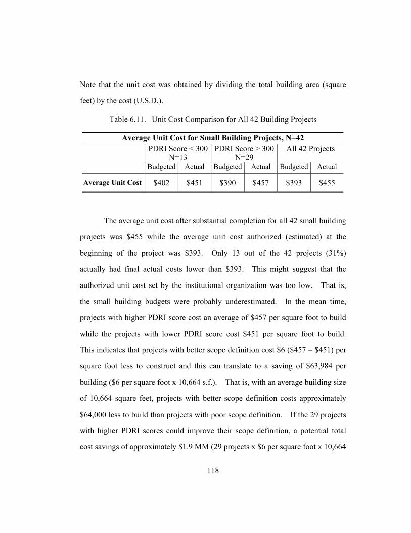
Note that the unit cost was obtained by dividing the total building area (square

feet) by the cost (U.S.D.).

Table 6.11. Unit Cost Comparison for All 42 Building Projects

Average Unit Cost for Small Building Projects, N=42 PDRI Score < 300

N=13 PDRI Score > 300

N=29 All 42 Projects

Budgeted Actual Budgeted Actual Budgeted Actual

Average Unit Cost $402 $451 $390 $457 $393 $455

The average unit cost after substantial completion for all 42 small building

projects was $455 while the average unit cost authorized (estimated) at the

beginning of the project was $393. Only 13 out of the 42 projects (31%)

actually had final actual costs lower than $393. This might suggest that the

authorized unit cost set by the institutional organization was too low. That is,

the small building budgets were probably underestimated. In the mean time,

projects with higher PDRI score cost an average of $457 per square foot to build

while the projects with lower PDRI score cost $451 per square foot to build.

This indicates that projects with better scope definition cost $6 ($457 – $451) per

square foot less to construct and this can translate to a saving of $63,984 per

building ($6 per square foot x 10,664 s.f.). That is, with an average building size

of 10,664 square feet, projects with better scope definition costs approximately

$64,000 less to build than projects with poor scope definition. If the 29 projects

with higher PDRI scores could improve their scope definition, a potential total

cost savings of approximately $1.9 MM (29 projects x $6 per square foot x 10,664

118

s.f. per building) could have been achieved. Note that this analysis does not

control for regional location and the difference between the actual average costs is

not statistically significant for two groups of projects. Therefore, caution should

be taken when interpreting the analysis results.

As mentioned earlier, these small building projects were constructed in

four different regions: Canada, U.S., Latin America, and Australia/Pacific. In

order to differentiate the effect that regions may have on the unit cost, projects in

North America (Canada and U.S.) were selected for similar unit cost analysis. A

total of 25 small building projects were selected and the unit cost analysis for

these projects was summarized in Table 6.12. Note that 22 out of the 25 projects

had a footprint of 10,700 square feet, two projects had a footprint of 6,800 square

feet and one project had a footprint of 16,000 square feet.

Table 6.12. Unit Cost Comparison for North America Building Projects

Average Unit Cost for North America Small Building Projects, N=25 PDRI Score < 300

N=11 PDRI Score > 300

N=14 All 25 Projects

Budgeted Actual Budgeted Actual Budgeted Actual

Average Unit Cost $382 $433 $408 $449 $396 $442

The average actual unit cost for the 25 North America building projects

was $442 per square foot while the budgeted unit cost was $396 per square foot.

Again, the results show signs of underestimating as can be seen from the previous

analysis. From Table 6.12, projects with better (lower) PDRI scores had an

average actual cost of $433 per square foot while projects with poor (higher)

119

PDRI scores had an average actual cost of $449. The difference of $16 ($449 –

433) per square foot can be viewed as the results of improved scope. However,

this difference is not statistically significant.

If the scope definition of a project were improved, a potential cost saving

of $16 per square foot can be achieved. That is, the actual unit cost can be

brought down from $449 per square foot to $433 per square foot. This cost

saving can be translated to a total of $169,300 ($16 per square foot x 10,584

square feet) for these projects in North America. Research conducted by CII has

indicated that approximately two percent of total project cost is spent on pre-

project planning for building projects (CII 2002). For this project sample,

approximately $93,600 ($442 per square foot x 10,584 square feet x 2%) per

project should have been spent on effective pre-project planning according to the

CII research results. In turn, the benefit/cost ratio for pre-project planning can

be estimated. By dividing the cost of pre-project planning ($93,600) from the

potential cost saving ($169,300), a benefit/cost ratio of 1.8 was obtained.

The mean actual cost per square foot for 17 international projects was

$474 and the authorized unit cost was $389. Among the 17 projects, only two

had a PDRI score of 300 or below. Therefore, the international projects were not

analyzed. Again, the data show signs of poor estimation.

6.3. SUMMARY

This chapter presented the descriptive statistics of the institutional

organization project sample and the analyses of PDRI versus project performance.

General results showed that sample projects were suffering from poor scope

120

definition and had poor cost and schedule performance. Further analysis showed

that projects with better scope definition outperformed projects with poor scope

definition. The unique sample also provided the opportunity for unit cost

comparison analysis. Two conclusions were obtained from this sample project

analyses:

1. Improved predictability of cost performance can be expected with better

scope definition

2. Improved scope definition leads to real project cost savings

It should be noted that despite the repetitious nature of this particular

building sample, no significant “learning effects” were observed when comparing

the project performance through the three-year period. That is, the performance

of projects built later in the three-year period is not significantly better than the

performance of projects built earlier. The rationale behind this might be that

only the home office had repetitive tasks when building these almost identical

building projects and home office did not improve through time. Different local

architects and contractors were hired to complete the projects and thus no learning

effects occurred.

121

Chapter 7 Risk Identification through PDRI Characteristics

The next phase of the research approach is focused on trends in pre-project

planning, especially on specific scope elements that are not well-defined in

surveyed projects. The data collected from the actual projects represented past

practices and were used for analyzing the characteristics and trends of scope

definition levels. This chapter covers the identification of poorly defined PDRI

scope elements for both industrial and building projects and the examination of

their relationship with project cost and schedule performance.

As discussed in Section 5.3, pre-assigned element weights were applied to

survey responses in order to obtain a final PDRI score. The sample project

PDRI score characteristics were described in Section 5.3 as well. In this chapter,

original survey responses using only definition levels were used for analysis. By

doing so, the trend of actual project scope definition can be analyzed without the

bias of pre-assigned weights. This chapter presents a summary of the PDRI

definition level characteristics and relationships between project performance and

element definition levels.

7.1. SCOPE DEFINITION LEVEL CHARACTERISTICS

The industrial PDRI contains 70 scope definition elements which are

grouped into 15 categories and further grouped into three sections. Similarly,

the building PDRI has 62 scope definition elements which are grouped into 11

categories and further grouped into three sections. Eight out of the 62 surveyed

industrial projects did not provide sufficient information on detailed scope

122

definition levels (i.e. they only provide rollup PDRI scores); therefore, only 54

industrial projects were analyzed for scope definition level characteristics. All

78 building projects were included in this definition level analysis. Please refer

to Chapter 2 for PDRI elements definition level/weights and illustration of scoring

PDRI. The following two sections summarize the PDRI element definition level

characteristics for industrial and building projects.

7.1.1. Industrial Project Definition Level Characteristics

Each PDRI scope definition element has five definition levels with

definition level 1 standing for complete definition, 2 for minor deficiencies, 3 for

some deficiencies, 4 for major deficiencies and 5 for incomplete or poor

definition. If the scope element is not applicable to the project, the respondent

was asked to check definition level 0, which does not affect the total PDRI score.

After receiving the survey responses, definition levels were averaged and total

number of projects was counted for each of the 70 scope elements in the industrial

PDRI or 64 elements for building projects. Appendix E summarizes the

descriptive statistics of both industrial and building PDRI scope definition levels.

First, the PDRI scope element definition levels were examined to

determine which elements were not well-defined for the 54 industrial projects.

The mean definition levels were calculated for the 70 scope elements and then

compared with each other. The 70 scope elements were sorted according to their

mean definition levels and Table 7.1 presents a list of 15 scope definition

elements with mean definition levels greater than 2.5 (which corresponds to some

123

deficiencies). This list identifies scope elements that were poorly defined by the

surveyed 54 industrial projects.

From the list, the worst-defined scope element (highest mean definition

level) is element K2: Logic Diagrams. Logic diagrams provide a method of

depicting interlock and sequencing systems for the startup, operation, alarm, and

shutdown of equipment and processes (CII 1996). Twenty-seven (50%) out of

the 54 sample projects indicated scope definition for element K2: Logic Diagrams

was either incomplete or poorly defined (definition level 5).

Table 7.1. Worst Definition Level Averages for Industrial Projects

Definition Level Average from 54 Industrial Projects Definition Level Average Larger than 2.5

K2. Logic Diagrams G13. Instrument Index P5. Start Up Requirements G11. Tie-in List G12. Piping Special Item List G10. Line List P4. Pre-Commissioning Turnover Sequence Requirements K6. Instrument & Electrical Specifications N3. Risk Analysis I1. Civil/Structural Requirements E3. Design for Constructability Analysis P6. Training Requirements G3. Piping & Instrumentation Diagrams G7. Piping System Requirements

3.1 2.9 2.8 2.8 2.8 2.8 2.7 2.6 2.6 2.6 2.6 2.5 2.5 2.5

Six out of the 13 elements in Category G, Process/Mechanical, have

definition level averages greater than 2.5. Similarly, 50% (3 out of 6) of the

elements in Category P, Project Execution Plan, are poorly-defined. The results

124

indicate that for this sample improvements were needed in scope definitions

relating to Process/Mechanical and Project Execution Plan.

Another way to identify the worst defined scope elements is to identify

scope elements with most “level 5” definitions. Definition level 5 indicates that

the scope element is either incomplete or poorly defined. Table 7.2 shows a list

of scope definition elements with most projects choosing definition level 5. Not

surprisingly, K2: Logic Diagrams, was among the scope elements that were

poorly defined by most sample projects (27 projects). Twenty projects had

scope definition level 5 for scope element N3: Risk Analysis. The average scope

definition for N3: Risk Analysis is 2.6, and this showed that these industrial

projects were not doing as well in defining the Risk Analysis for their projects.

Comparing Table 7.1 with Table 7.2, six elements have more than 10 projects

evaluating them as definition level 5 (Table 7.2) but have an average definition

level lower than 2.5 (Table 7.1). These elements were L3: Procurement

Responsibility Matrix, M3: Distribution Matrix, D1: Project Objective Statement,

E1: Process Simplification, E2: Design & Material Alterations

Considered/Rejected, and P3: Shut Down/Turn-Around Requirements. One

explanation for this would be that most of the sample projects did well in defining

these elements while only a few projects did poorly in defining these elements.

125

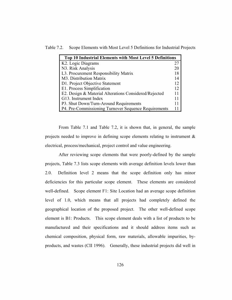
Table 7.2. Scope Elements with Most Level 5 Definitions for Industrial Projects

Top 10 Industrial Elements with Most Level 5 Definitions K2. Logic Diagrams N3. Risk Analysis L3. Procurement Responsibility Matrix M3. Distribution Matrix D1. Project Objective Statement E1. Process Simplification E2. Design & Material Alterations Considered/Rejected G13. Instrument Index P3. Shut Down/Turn-Around Requirements P4. Pre-Commissioning Turnover Sequence Requirements

27 20 18 14 12 12 11 11 11 11

From Table 7.1 and Table 7.2, it is shown that, in general, the sample

projects needed to improve in defining scope elements relating to instrument &

electrical, process/mechanical, project control and value engineering.

After reviewing scope elements that were poorly-defined by the sample

projects, Table 7.3 lists scope elements with average definition levels lower than

2.0. Definition level 2 means that the scope definition only has minor

deficiencies for this particular scope element. These elements are considered

well-defined. Scope element F1: Site Location had an average scope definition

level of 1.0, which means that all projects had completely defined the

geographical location of the proposed project. The other well-defined scope

element is B1: Products. This scope element deals with a list of products to be

manufactured and their specifications and it should address items such as

chemical composition, physical form, raw materials, allowable impurities, by-

products, and wastes (CII 1996). Generally, these industrial projects did well in

126

scope elements relating to site information, technology, business objectives, and

project scope.

Table 7.3. Best Definition Level Averages for Industrial Projects

Definition Level Average from 54 Industrial Projects Definition Level Average Lower than 2.0

G9. Mechanical Equipment List B3. Project Strategy K3. Electrical Area Classifications F4. Permit Requirements D1. Project Objective Statements E1. Process Simplification F2. Surveys & Soil Tests E2. Design & Material Alterations Considered/Rejected M1. CADD/Model Requirements K4. Substation Requirements Power Source Identification J3. Transportation Requirements B2. Market Strategy G8. Plot Plan G2. Heat & Material Balances F3. Environmental Assessment C2. Processes G1. Process Flow Sheets C1. Technology L1. Identify Long Lead/Critical Equipments & Materials B5. Capacities D6. Project Schedule D3. Site Characteristics Available and Required B1. Products F1. Site Location

1.9 1.9 1.9 1.9 1.9 1.9 1.9 1.8 1.8 1.8 1.8 1.7 1.7 1.7 1.7 1.7 1.6 1.6 1.6 1.5 1.5 1.5 1.4 1.0

Table 7.4 identifies a list of 10 scope elements with the most projects

choosing definition level 1. As mentioned earlier, scope element F1: Site

Location had all responses rating definition level 1 (except four projects indicated

not applicable for this scope element). It should be noted that 11 projects rated

127

E2: Design & Material Alterations Considered/Rejected as poorly-defined

(definition level 5) while 42 projects rated E2 as completely defined (definition

level 1). This indicated that the majority of the sample projects had a structured

approach in place to consider design and material alternatives. The low

definition level average of Scope element L1 indicated that most sample projects

did well in defining scope elements relating to procurement strategy in during

their pre-project planning process.

Table 7.4. Scope Elements with Most Level 1 Definitions for Industrial Projects

Top 10 Industrial Projects with Most Level 1 Definitions F1. Site Location D3. Site Characteristics Available & Required D6. Project Schedule E2. Design & Material Alterations Considered/Rejected D1. Project Objective Statement E1. Process Simplification M3. Distribution Matrix L3. Procurement Responsibility Matrix L1. Identify Long Lead/Critical Equipment & Materials J3. Transportation Requirement

50 47 46 43 42 42 40 36 35 34

As shown in Tables 7.3 and 7.4, scope elements relating to site

information, technology, business objectives, procurement strategy, and project

scope were better defined according to the survey results from the 54 industrial

projects.

7.1.2. Building Project Definition Level Characteristics

Similar to the PDRI for industrial projects, PDRI for building projects has

64 scope elements and each scope definition element has five definition levels

128

with definition level 1 standing for complete definition, 2 for minor deficiencies,

3 for some deficiencies, 4 for major deficiencies and 5 for incomplete or poor

definition. If this scope element is not applicable to the project, the respondent

was asked to check definition level 0, which does not affect the total PDRI score.

After receiving the survey responses, definition levels were averaged and then

sorted to examine the level of pre-project planning for the surveyed 78 building

projects. Appendix E summarizes the descriptive statistics of both industrial and

building PDRI scope definition levels.

Table 7.5 illustrates a list of poorly-defined scope definition elements with

average definition levels greater than 2.5. From the list, the most poorly-defined

scope element (highest definition level average) for the 78 surveyed building

projects is element E1: Program Statement. The Program Statement identifies

the levels of the performance of the facility in terms of space planning and

functional relationships. It should address the human, physical, and external

aspects to be considered in the design (CII 1999). Category C deals with Project

Requirements, and 4 out of the 6 elements in category C are on the list (poorly-

defined). These four elements are C1: Value-Analysis Process, C4: Scope of

Work Overview, C5: Project Schedule, and C6: Project Cost Estimate.

Surprisingly, project cost estimate and project schedule were among the

poorly-defined elements as well. Normally, these two scope elements are

assumed to be the basic requirements for project management. However, the

survey results showed that the sample project participants did not focus as much

129

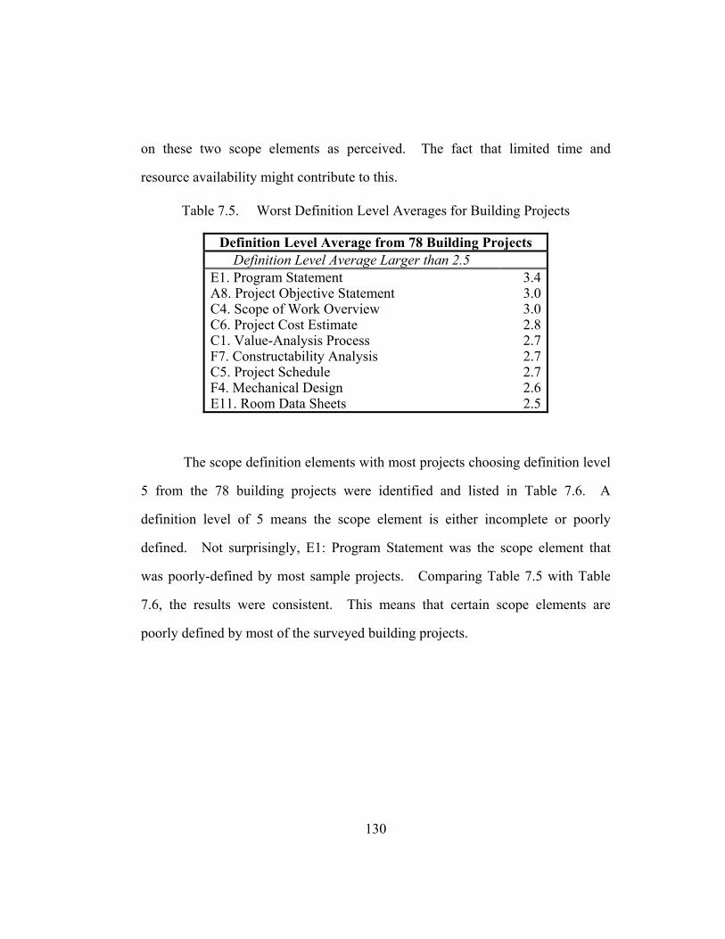
on these two scope elements as perceived. The fact that limited time and

resource availability might contribute to this.

Table 7.5. Worst Definition Level Averages for Building Projects

Definition Level Average from 78 Building Projects Definition Level Average Larger than 2.5

E1. Program Statement A8. Project Objective Statement C4. Scope of Work Overview C6. Project Cost Estimate C1. Value-Analysis Process F7. Constructability Analysis C5. Project Schedule F4. Mechanical Design E11. Room Data Sheets

3.4 3.0 3.0 2.8 2.7 2.7 2.7 2.6 2.5

The scope definition elements with most projects choosing definition level

5 from the 78 building projects were identified and listed in Table 7.6. A

definition level of 5 means the scope element is either incomplete or poorly

defined. Not surprisingly, E1: Program Statement was the scope element that

was poorly-defined by most sample projects. Comparing Table 7.5 with Table

7.6, the results were consistent. This means that certain scope elements are

poorly defined by most of the surveyed building projects.

130

Table 7.6. Scope Elements with Most Level 5 Definitions for Building Projects

Top 10 Building Projects with Most Level 5 Definitions E1. Program Statement A8. Project Objective Statement C1. Value-Analysis C4. Scope of Work Overview F4. Mechanical Design F5. Electrical Design F7. Constructability Analysis J2. Documentation/Deliverables E12. Furnishings, Equipments, and Built-ins C6. Project Cost Estimate

30 17 12 11 11 11 11 11 9 8

From Table 7.5 and Table 7.6, it is shown that, in general, the sample

projects needed to improve in defining scope elements relating to project

requirements, building programming, and building/project design parameters.

Although industrial and building sectors are two different sectors, it is

interesting to find that the survey results showed that Project Objective Statement

and Value Analysis are among the worst-defined scope elements for both building

and industrial sample projects.

After reviewing scope elements that were poorly-defined by the sample

building projects, Table 7.7 listed scope elements with average definition levels

lower than 2.0. Definition level 2 means that the scope definition only has minor

deficiencies for this particular scope element. These elements are considered

well-defined. Generally, these building projects did well for scope elements

relating to business strategy, site information, building programming, and project

execution planning. It is important to note that in general, building projects did

131

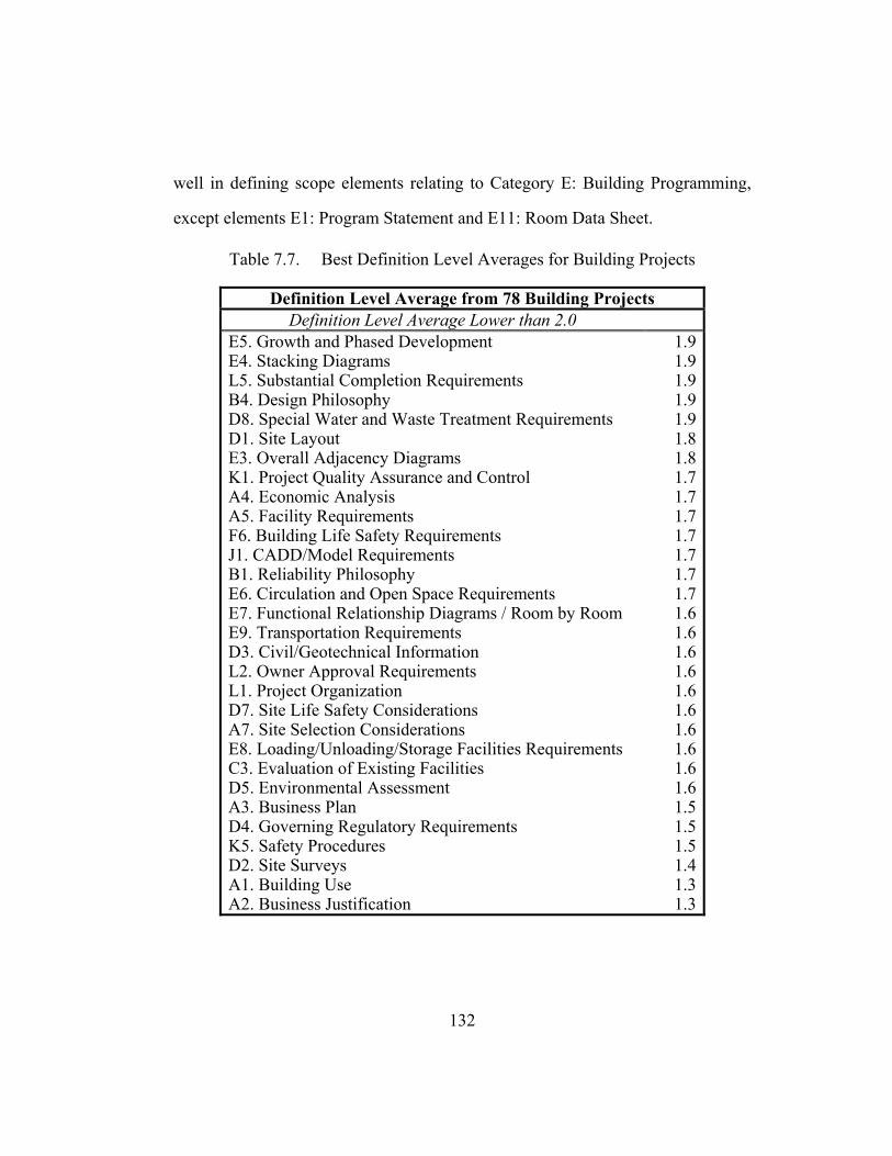
well in defining scope elements relating to Category E: Building Programming,

except elements E1: Program Statement and E11: Room Data Sheet.

Table 7.7. Best Definition Level Averages for Building Projects

Definition Level Average from 78 Building Projects Definition Level Average Lower than 2.0

E5. Growth and Phased Development E4. Stacking Diagrams L5. Substantial Completion Requirements B4. Design Philosophy D8. Special Water and Waste Treatment Requirements D1. Site Layout E3. Overall Adjacency Diagrams K1. Project Quality Assurance and Control A4. Economic Analysis A5. Facility Requirements F6. Building Life Safety Requirements J1. CADD/Model Requirements B1. Reliability Philosophy E6. Circulation and Open Space Requirements E7. Functional Relationship Diagrams / Room by Room E9. Transportation Requirements D3. Civil/Geotechnical Information L2. Owner Approval Requirements L1. Project Organization D7. Site Life Safety Considerations A7. Site Selection Considerations E8. Loading/Unloading/Storage Facilities Requirements C3. Evaluation of Existing Facilities D5. Environmental Assessment A3. Business Plan D4. Governing Regulatory Requirements K5. Safety Procedures D2. Site Surveys A1. Building Use A2. Business Justification

1.9 1.9 1.9 1.9 1.9 1.8 1.8 1.7 1.7 1.7 1.7 1.7 1.7 1.7 1.6 1.6 1.6 1.6 1.6 1.6 1.6 1.6 1.6 1.6 1.5 1.5 1.5 1.4 1.3 1.3

132

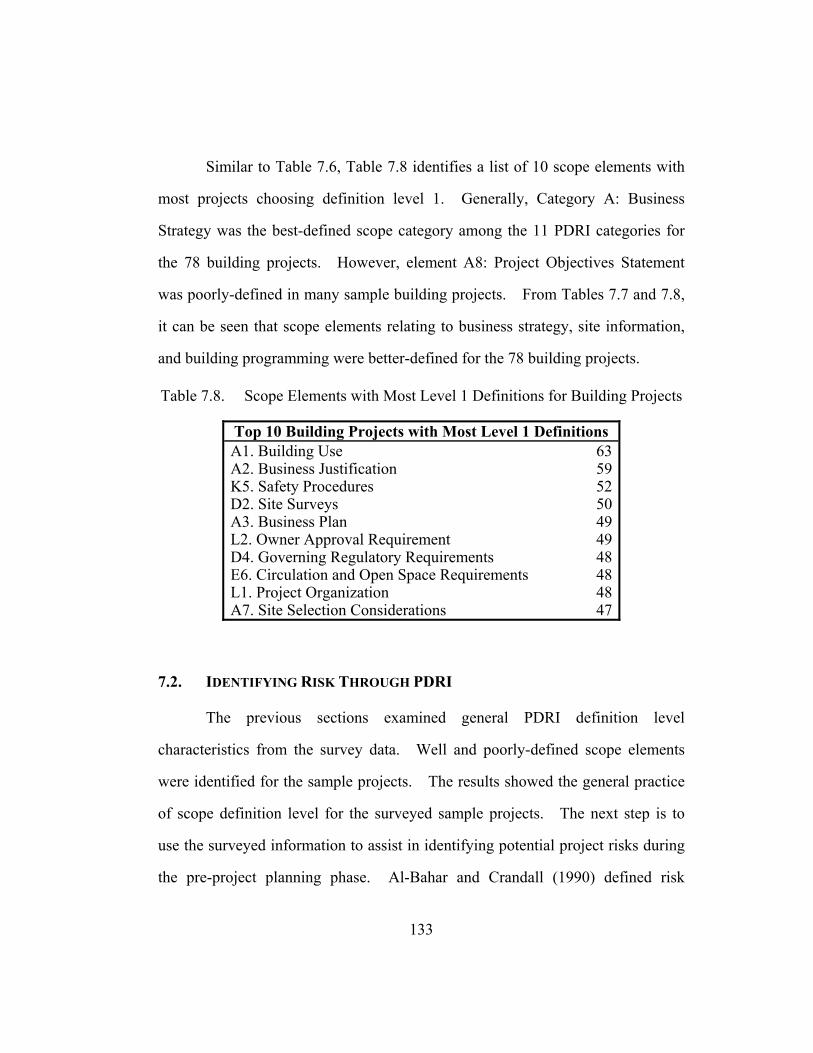
Similar to Table 7.6, Table 7.8 identifies a list of 10 scope elements with

most projects choosing definition level 1. Generally, Category A: Business

Strategy was the best-defined scope category among the 11 PDRI categories for

the 78 building projects. However, element A8: Project Objectives Statement

was poorly-defined in many sample building projects. From Tables 7.7 and 7.8,

it can be seen that scope elements relating to business strategy, site information,

and building programming were better-defined for the 78 building projects.

Table 7.8. Scope Elements with Most Level 1 Definitions for Building Projects

Top 10 Building Projects with Most Level 1 Definitions A1. Building Use A2. Business Justification K5. Safety Procedures D2. Site Surveys A3. Business Plan L2. Owner Approval Requirement D4. Governing Regulatory Requirements E6. Circulation and Open Space Requirements L1. Project Organization A7. Site Selection Considerations

63 59 52 50 49 49 48 48 48 47

7.2. IDENTIFYING RISK THROUGH PDRI

The previous sections examined general PDRI definition level

characteristics from the survey data. Well and poorly-defined scope elements

were identified for the sample projects. The results showed the general practice

of scope definition level for the surveyed sample projects. The next step is to

use the surveyed information to assist in identifying potential project risks during

the pre-project planning phase. Al-Bahar and Crandall (1990) defined risk

133

identification as the process of systematically and continuously identifying,

categorizing, and assessing the significance of risks associated with a project.

Two approaches can be used to identify potential project risk through the

application of PDRI. The first approach is using the pre-assigned scope element

weights as a reference for evaluating their potential impact on the project

outcome. The second approach is to examine the historical project data and the

project performance (actual project impacts) and identify scope elements that

distinguish between successful and less-than-successful projects (based on cost

and schedule performance). The following two sections outline the two

approaches and examples are given for both applications.

7.2.1. Risk Identification through PDRI Element Weights

One obvious way to identify project risk with the PDRI is using the pre-

assigned element weights during the pre-project planning evaluation process.

During the development of the PDRI, higher weights were to be assigned to those

elements whose lack of definition could have the most serious negative effect on

project performance (CII 1996 and CII 1999). The pre-assigned weights were

developed through a series of workshops to gather inputs from a broad range of

construction industry experts. If that element was incomplete or poorly defined

based on the description (definition level 5), the workshop participants were

instructed to assess what percent contingency they would deem appropriate for

that element. Therefore, it is logical to use the pre-assigned PDRI score as an

indicator of potential risk impact for a particular scope element.

134

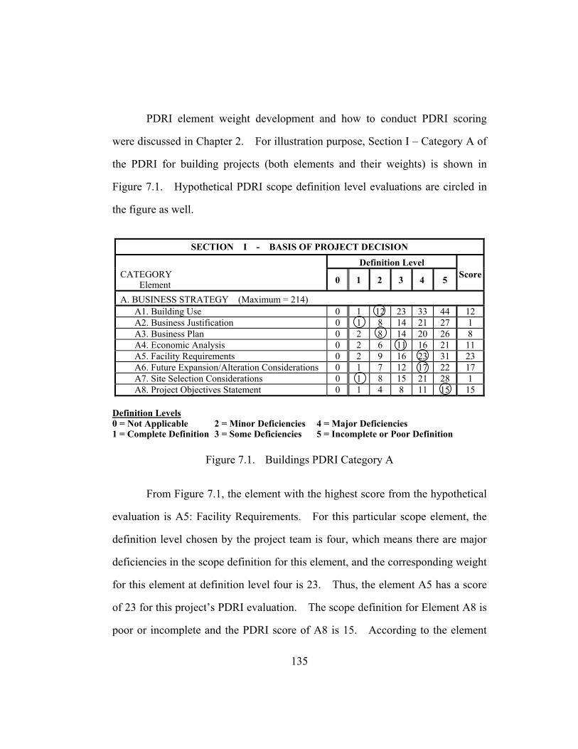
PDRI element weight development and how to conduct PDRI scoring

were discussed in Chapter 2. For illustration purpose, Section I – Category A of

the PDRI for building projects (both elements and their weights) is shown in

Figure 7.1. Hypothetical PDRI scope definition level evaluations are circled in

the figure as well.

SECTION I - BASIS OF PROJECT DECISION

Definition Level CATEGORY Element 0 1 2 3 4 5 Score

A. BUSINESS STRATEGY (Maximum = 214) A1. Building Use 0 1 12 23 33 44 12 A2. Business Justification 0 1 8 14 21 27 1 A3. Business Plan 0 2 8 14 20 26 8 A4. Economic Analysis 0 2 6 11 16 21 11 A5. Facility Requirements 0 2 9 16 23 31 23 A6. Future Expansion/Alteration Considerations 0 1 7 12 17 22 17 A7. Site Selection Considerations 0 1 8 15 21 28 1 A8. Project Objectives Statement 0 1 4 8 11 15 15

Definition Levels 0 = Not Applicable 2 = Minor Deficiencies 4 = Major Deficiencies 1 = Complete Definition 3 = Some Deficiencies 5 = Incomplete or Poor Definition

Figure 7.1. Buildings PDRI Category A

From Figure 7.1, the element with the highest score from the hypothetical

evaluation is A5: Facility Requirements. For this particular scope element, the

definition level chosen by the project team is four, which means there are major

deficiencies in the scope definition for this element, and the corresponding weight

for this element at definition level four is 23. Thus, the element A5 has a score

of 23 for this project’s PDRI evaluation. The scope definition for Element A8 is

poor or incomplete and the PDRI score of A8 is 15. According to the element

135

weights and PDRI scores, the performance impact of poorly-defined element A5,

with definition level 4 of and weight of 23, might be larger than element A8, with

definition level 5 and weight of 15.

A project team can quickly assess their potential project risk exposures by

identifying scope elements with higher PDRI scores, since higher PDRI score

indicates potential larger impact to project performance. In this hypothetical

case, the element with highest score in Category A is element A5: Facility

Requirement. Element A6: Future Expansion/Alteration Considerations has the

second highest score and element A8: Project Objective Statement has the third

highest. From the PDRI evaluation, these three elements (A5, A6, and A8)

might potentially have greater negative impact on project outcome based on their

PDRI scores. Therefore, these elements might pose greater risk comparing to

other elements with lower PDRI scores. By examining the element PDRI scores,

the project team can identify potential risk factors that might have negative impact

to project performance and then take measures to better-define the scope elements

to reduce potential risks exposures.

Table 7.9 summarizes the top 15 scope elements with highest level 5

definition weights for both industrial and building PDRI. These elements, if

poorly-defined, could result in greater impact to project outcome and therefore,

should be treated with more attention.

136

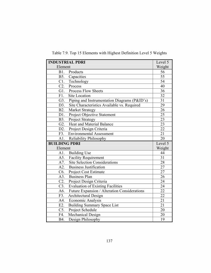
Table 7.9. Top 15 Elements with Highest Definition Level 5 Weights

INDUSTRIAL PDRI Element

Level 5 Weight

B1. Products 56 B5. Capacities 55 C1. Technology 54 C2. Process 40 G1. Process Flow Sheets 36 F1. Site Location 32 G3. Piping and Instrumentation Diagrams (P&ID’s) 31 D3. Site Characteristics Available vs. Required 29 B2. Market Strategy 26 D1. Project Objective Statement 25 B3. Project Strategy 23 G2. Heat and Material Balance 23 D2. Project Design Criteria 22 F3. Environmental Assessment 21 A1. Reliability Philosophy 20 BUILDING PDRI Element

Level 5 Weight

A1. Building Use 44 A5. Facility Requirement 31 A7. Site Selection Considerations 28 A2. Business Justification 27 C6. Project Cost Estimate 27 A3. Business Plan 26 C2. Project Design Criteria 24 C3. Evaluation of Existing Facilities 24 A6. Future Expansion / Alteration Considerations 22 F3. Architectural Design 22 A4. Economic Analysis 21 E2. Building Summary Space List 21 C5. Project Schedule 20 F4. Mechanical Design 20 B4. Design Philosophy 19

137

Although the building and industrial projects are uniquely different in

nature, there exists similar risk factors when evaluating the scope definitions.

These aspects are site considerations, project design criteria, economic analysis,

and mechanical considerations (Cho 1999).

To further investigate the potential impact of PDRI score on project performance,

projects were grouped by their PDRI scores and average cost/schedule performance was

compared. Previous PDRI research has statistically shown that projects with a PDRI

score of 200 or lower outperformed projects scoring above 200. Table 7.10 shows the

mean project performance for all the sample projects with PDRI score of 200 or below,

and those projects with a PDRI score above 200. From the results, it is evident that

projects with lower PDRI scores (better scope definition) outperform those with higher

PDRI scores (poor scope definition) for both industrial and building projects in terms of

estimate predictability.

138

Table 7.10. Summary of Mean Project Performance Using a 200-point Cutoff

PDRI Score Category < 200 > 200 Difference

Industrial Projects

Cost Growth 2.6% below budget 9.3% above budget 11.9%

Schedule Growth 0.6% ahead of schedule 8.0% behind schedule 8.6%

PDRI Score 147 317 170 (N=35) (N=27)

Building Projects

Cost Growth 2.6% below budget 12.9% above budget 15.5%

Schedule Growth 2.7% ahead of schedule 20.9% behind schedule 23.6%

PDRI Score 142 325 183 (N=17) (N=61)

7.2.2. Risk Identification through Historical Data

Another approach to identify project risk through the PDRI is to examine

the historical project data and compare the results with the current project. In

order to do so, previous projects were first divided into two groups, successful

and less-than-successful projects, based on their performance (cost and schedule).

Then, the element scope definition level means for these two groups of projects

were calculated and compared with each other. In addition to traditional

statistical significance tests (i.e., t-test), Effect Size was measured to compare the

difference between the mean definition levels for the two groups. As discussed

in Chapter 4, the equation for calculating Effect Size is as follow:

139

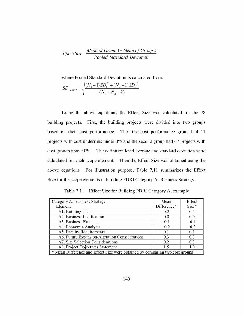
DeviationndardStaPooledGroupofMeanGroupofMeanSizeEffect 21−

=

where Pooled Standard Deviation is calculated from:

)2()1()1(

21

222

211

−+−+−

=NN

SDNSDNSDPooled

Using the above equations, the Effect Size was calculated for the 78

building projects. First, the building projects were divided into two groups

based on their cost performance. The first cost performance group had 11

projects with cost underruns under 0% and the second group had 67 projects with

cost growth above 0%. The definition level average and standard deviation were

calculated for each scope element. Then the Effect Size was obtained using the

above equations. For illustration purpose, Table 7.11 summarizes the Effect

Size for the scope elements in building PDRI Category A: Business Strategy.

Table 7.11. Effect Size for Building PDRI Category A, example

Category A: Business Strategy Element

Mean Difference*

Effect Size*

A1. Building Use 0.2 0.2 A2. Business Justification 0.0 0.0 A3. Business Plan -0.1 -0.1 A4. Economic Analysis -0.2 -0.2 A5. Facility Requirements 0.1 0.1 A6. Future Expansion/Alteration Considerations 0.3 0.3 A7. Site Selection Considerations 0.2 0.3 A8. Project Objectives Statement 1.5 1.0 * Mean Difference and Effect Size were obtained by comparing two cost groups

140

As an example, the Effect Size obtained from historic project data in Table

7.11 shows that the difference of definition level averages between the two cost

performance groups was significant (greater than 0.80) for element A8: Project

Objective Statement. This implies that, historically, projects with better cost

performance did better in defining element A8 than projects with poor cost

performance. Therefore, element A8: Project Objective Statement might serve

as a cost risk indicator based on information collected from this sample. The

project team should pay additional attention in defining this scope element in

order to reduce the potential risk exposures if the element was poorly-defined.

Similarly, scope elements with effect size greater than 0.80 were identified

for both building and industrial projects. Tables 7.12 and 7.13 summarize these

scope elements (potential risk indicators) based on their schedule and cost

performance, respectively. Note that no indicators were determined for schedule

in the building project sample.

Table 7.12. Elements with Large Effect Size Based on Schedule Performance

Building Projects (N1=20, N2=58) Element

Mean Difference*

Effect Size*

N/A Industrial Projects (N1=30, N2=24) Element

Mean Difference*

Effect Size*

A3. Operating Philosophy 0.9 0.9 G4. Process Safety Management (PSM) 1.1 1.0 G5. Utility Flow Diagrams 0.9 0.9 G7. Piping System Requirements 1.2 1.1 G13. Instrument Index 1.1 0.8 K1. Control Philosophy 0.7 0.8 K6. Instrument & Electrical Specifications 0.9 0.8 * Mean Difference and Effect Size were obtained by comparing two schedule groups

141

The results show that differences between successful and less-than-

successful building projects are not significant when the projects are divided

based on schedule performance (ahead of schedule and behind schedule). When

the industrial projects were grouped based on schedule performance, these scope

elements (A3, G4, G5, G7, G13, K1, K6) with effect size larger than 0.80 can be

regarded as performance indicators. That is, according to this sample, projects

with better schedule performance did better in defining these scope elements.

142

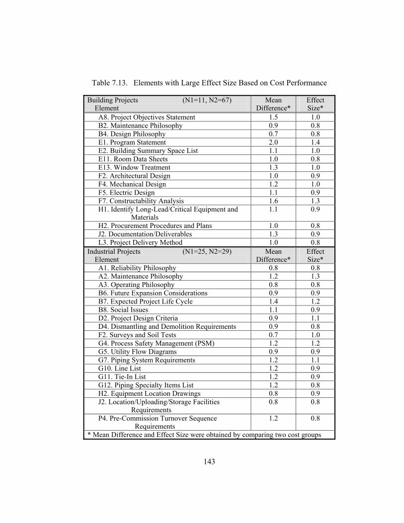
Table 7.13. Elements with Large Effect Size Based on Cost Performance

Building Projects (N1=11, N2=67) Element

Mean Difference*

Effect Size*

A8. Project Objectives Statement 1.5 1.0 B2. Maintenance Philosophy 0.9 0.8 B4. Design Philosophy 0.7 0.8 E1. Program Statement 2.0 1.4 E2. Building Summary Space List 1.1 1.0 E11. Room Data Sheets 1.0 0.8 E13. Window Treatment 1.3 1.0 F2. Architectural Design 1.0 0.9 F4. Mechanical Design 1.2 1.0 F5. Electric Design 1.1 0.9 F7. Constructability Analysis 1.6 1.3 H1. Identify Long-Lead/Critical Equipment and Materials

1.1 0.9

H2. Procurement Procedures and Plans 1.0 0.8 J2. Documentation/Deliverables 1.3 0.9 L3. Project Delivery Method 1.0 0.8 Industrial Projects (N1=25, N2=29) Element

Mean Difference*

Effect Size*

A1. Reliability Philosophy 0.8 0.8 A2. Maintenance Philosophy 1.2 1.3 A3. Operating Philosophy 0.8 0.8 B6. Future Expansion Considerations 0.9 0.9 B7. Expected Project Life Cycle 1.4 1.2 B8. Social Issues 1.1 0.9 D2. Project Design Criteria 0.9 1.1 D4. Dismantling and Demolition Requirements 0.9 0.8 F2. Surveys and Soil Tests 0.7 1.0 G4. Process Safety Management (PSM) 1.2 1.2 G5. Utility Flow Diagrams 0.9 0.9 G7. Piping System Requirements 1.2 1.1 G10. Line List 1.2 0.9 G11. Tie-In List 1.2 0.9 G12. Piping Specialty Items List 1.2 0.8 H2. Equipment Location Drawings 0.8 0.9 J2. Location/Uploading/Storage Facilities Requirements

0.8 0.8

P4. Pre-Commission Turnover Sequence Requirements

1.2 0.8

* Mean Difference and Effect Size were obtained by comparing two cost groups

143

When grouped by cost performance, scope elements with an effect size

larger than 0.80 were found for both industrial and building projects. The cost

performance indicators for building projects are scope elements A8, B2, B4, E1,

E2, E11, E13, F2, F4, F5, F7, H1, H2, J2, and L3. The cost performance

indicators for industrial projects are: A2, A3, B6, B7, B8, D2, D4, F3, G4, G5,

G7, G10, G11, G12, H2, J2, and P4.

For industrial projects, elements A3: Operating Philosophy, G4: Process

Safety Management (PSM), G5: Utility Flow Diagrams, and G7: Piping System

Requirements had large Effect Size both in cost and schedule performance

evaluations. This indicates that the definition level average differences are

significant for these four elements based on historic data and projects with

successful outcomes (both cost and schedule performance) did a better job

defining these elements than less-than-successful projects.

If the identified scope elements were not well-defined, the project is more

likely to have a less-than-successful project performance (cost/schedule growth).

Based on historical data, these elements should be viewed as potential risk

indicators and deserve more attention for future project scope development. It

should be noted that t-test results showed that the mean differences for these

elements are statistically significant to the p-level of 0.01.

7.3. FINDINGS RELATED TO RESEARCH HYPOTHESIS

One of the objectives of this research is to identify performance risk

indicators through PDRI analysis. Special attention was given to historical

project data analysis. In the previous section, PDRI elements were identified as

144

performance risk indicators by applying the Effect Size analysis. In order to

investigate the legitimacy of these scope elements, mean project performance

were calculated for each definition level. From Table 7.13, scope element A1,

Reliability Philosophy, was identified as one of the cost performance indicator for

industrial projects. Mean cost performance was taken for all projects with

definition level 1 for scope element A1. Similarly, mean cost performances

were calculated for projects with definition level 2, 3, 4 and 5 for scope element

A1. The average cost growth was negative 1.6 percent for level 1 projects and

19.1 percent for level 4 projects. The results indicate that if scope element A1,

Reliability Philosophy, were better-defined, it is more likely the industrial project

will have a better cost performance than projects having poorly-defined scope

element A1.

Following the same fashion, mean performances for selected scope

elements (from Tables 7.12 and 7.13) were calculated for illustrative purpose for

both industrial and building projects. The results are summarized in Tables 7.14

and 7.15.

145

Table 7.14. Mean Cost Performance Comparison for Cost Indicators

Scope Element Effect Size

No. of Projects

Average Cost Growth

Industrial Projects A1. Reliability Philosophy

Level 1 Level 2 Level 3 Level 4 Level 5

0.8 16 18 11 6 1

-1.6% 1.2% 7.2%

19.1% 2.3%

A2. Maintenance Philosophy Level 1 Level 2 Level 3 Level 4 Level 5

1.3 15 20 10 7 1

-5.4% 1.4%

10.9% 20.9% 2.3%

F2. Surveys and Soil Tests Level 1 Level 2 Level 3 Level 4 Level 5

1.0 20 16 11 1 0

-1.3% 6.9% 5.6%

14.6%

Building Projects A8. Project Objective Statement

Level 1 Level 2 Level 3 Level 4 Level 5

1.0 20 12 8

17 17

4.1% 3.9%

11.1% 19.1% 16.2%

E1. Program Statement Level 1 Level 2 Level 3 Level 4 Level 5

1.4 14 12 5

13 30

0.8% 9.6% 6.5%

12.4% 17.0%

F5. Electrical Design Level 1 Level 2 Level 3 Level 4 Level 5

0.9 21 29 14 2

11

3.7% 8.6%

12.6% 28.7% 23.0%

146

Table 7.15. Mean Cost Performance Comparison for Schedule Indicators

Scope Element Effect Size

No. of Projects

Average Schedule Growth

Industrial Projects A3. Operating Philosophy

Level 1 Level 2 Level 3 Level 4 Level 5

0.9 15 19 12 4 2

-2.5% 0.3% 7.1%

26.7% 15.7%

G4. Process Safety Management Level 1 Level 2 Level 3 Level 4 Level 5

1.0 16 14 12 4 3

-1.1% 0.0% 6.5% 9.2%

35.2% K1. Control Philosophy

Level 1 Level 2 Level 3 Level 4 Level 5

0.8 14 24 13 2 1

-3.4% 4.2% 8.9% 8.9% 7.7%

From Tables 7.14 and 7.15, it is apparent that projects (both industrial and

building) that did well in defining these elements outperformed those that did

poorly in defining these elements. Note that Table 7.15 only contains industrial

projects because no schedule performance indicator was identified for building

projects according to the effective size analysis.

The second research hypothesis was established to test whether the PDRI

is a reliable indicator of potential risk factors. The results of the effect size

analysis using the historical project data and average project performance

comparison demonstrates a significant relationship between certain scope

elements and project performance and thus supports the second research

hypothesis.

147

7.4. SUMMARY

This chapter examined the PDRI characteristics and related them to

construction project risk identification process. First, the PDRI survey results

were examined and element definition level averages were calculated. Poorly-

defined scope definition elements were identified for both the building and

industrial project samples. In addition, better-defined PDRI elements were

identified. The results show that the Project Objective Statement and Value

Analysis were among the most poorly-defined elements for both building and

industrial projects.

Projects were divided into two groups based on their cost and schedule

performance. The PDRI scope element definition level averages were

calculated. Within each performance group, both better-defined elements and

poorly-defined elements were identified. The results showed that projects with

less-than-successful performance did worse in defining specific scope elements

than successful projects.

Two approaches were explored to identify potential project risk through

PDRI. The first approach tries to identify potential risk factors by comparing the

pre-assigned level 5 definition weight. During the development of the PDRI,

weights were assigned to each element to represent the relative potential impacts

to project outcome based on the inputs from industry experts. In turn, the larger

the weight for the level 5 definition, the larger the potential impact the element

might have on the final project outcome. If these elements were not well-

defined, the project is more likely to have less-than-successful outcomes.

148

Furthermore, an analysis of project performance using a 200-point cutoff PDRI

score revealed that projects with lower PDRI scores (better scope definition)

outperformed projects with higher PDRI scores (poor scope definition).

The second approach identified potential risk factors based on historic

project data. The definition level averages were compared between the two

performance groups and elements with significant average definition level

differences were identified. These elements were viewed as potential performance

indicators since historically they are better-defined in successful projects.

The results of these two approaches were compared and it was found that

risk factors identified by historic data were different than those identified by

PDRI weights. The results did not contradict one another per se because for that

risk elements with high PDRI weights were recognized by industry practitioners

and therefore, were oftentimes better defined. Therefore, the results from

historical data analyses supplement the results from PDRI weights by identifying

risk factors not generally recognized by the industry practitioners.

After risk identification, the next step in a risk management process is to

quantify the potential risk impact. Chapter 8 outlines the development of risk

quantification models and describes risk control procedures based on the model

results.

149

Chapter 8 Risk Quantification and Control through PDRI

The previous chapter presented two approaches to risk identification using

the PDRI. The two approaches utilized different methods to identify the PDRI

scope elements that have the greatest potential impact on project outcomes for the

samples. This chapter outlines the development and application of three models

for the data collected (linear regression, quartile analysis, and Hackney’s method).

Modeling refers to the development of mathematical expressions that describe in

some sense the behavior of a random variable of interest (Rawlings, 1988). One

major objective of this research is to describe project cost/schedule performance

with information provided by PDRI scores. The chapter begins with a brief

overview of the proposed models used to describe the cost and schedule

performance data. By applying the proposed models, potential cost and schedule

performance impacts were determined based on obtained PDRI scores. Possible

risk control measures to reduce risk impact will be discussed and a risk

management process using PDRI will be presented and also its application will be

presented. Detailed project cost and completion time information is given in

Appendix F.

8.1. MODEL DEVELOPMENT APPROACH

As previously discussed, the PDRI can be used as an effective tool for risk

identification during the pre-project planning phase of the project life cycle.

Information collected from the survey and previous research was used to establish

models to describe the data. Three approaches were implemented to model the

150

data: linear regression, quartile analysis, and Hackney’s historic accuracy range

method. Both industrial and building project data were used for the model

development and models were developed specifically for cost and schedule

performance. Two other methods, Bayesian Statistics and Artificial Neural

Networks, were tried unsuccessfully for this sample.

8.1.1. Linear Regression Model

Regression, as one of many mathematically-based techniques available in

statistical theory used to analyze relationships between variables, is a powerful

quantitative research tool as described in Chapter 3. Regression analysis was

used as the preliminary investigations of the relationships between the PDRI

scores and cost/schedule performance. Individual project PDRI score, cost and

schedule performance are provided in Appendix D for both industrial and

building projects.

Cost Performance Regression Analysis

With cost growth as dependent variable and PDRI score as independent

variable, bivariate linear regression analysis was performed for the industrial and

building projects and the relationships shown in Figures 8.1 and 8.2 were

revealed. Again, cost growth is the actual cost of the project for design and

construction versus the cost estimate prior to project execution. It does not

include contingency for these sample projects. The least squares regression line

offers a graphical illustration of the association between cost growth and PDRI

score and the prediction equation is a useful form for summarizing that

association. Statistics shown in Tables 8.1 and 8.2 indicate a positive correlation

151

between the two variables, meaning that, as the PDRI score increases so does cost

growth. The R-Square (R2) is 0.226 for the industrial projects and 0.150 for the

building projects and both the levels of significance are 0.01.

Cost Growth vs. Industrial PDRI Score

y = 0.0009x - 0.1646R2 = 0.2257

-60%

-40%

-20%

0%

20%

40%

60%

80%

100%

0 50 100 150 200 250 300 350 400 450 500

Industrial PDRI Scores

Cos

t Gro

wth

N=62

Figure 8.1. Linear Regression: Cost Growth vs. Industrial PDRI Score

Table 8.1. Regression Statistics: Cost Growth vs. Industrial PDRI Score

Regression Results for Industrial PDRI and Cost Growth

R = 0.475 R2 = 0.226 Adjusted R2 = 0.213

ANOVA

Model Sum of Squares

df Mean Square

F Sig.

Regression Residual Total

0.491 1.685 2.175

1 60 61

0.491 0.028

17.489 9.56E-05

152

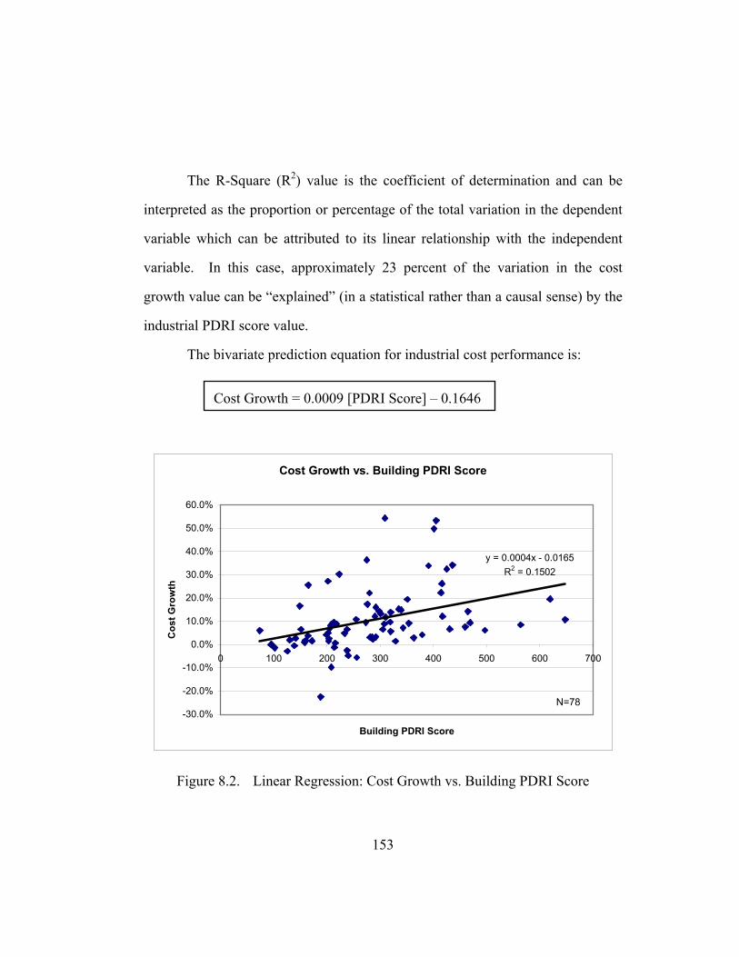
The R-Square (R2) value is the coefficient of determination and can be

interpreted as the proportion or percentage of the total variation in the dependent

variable which can be attributed to its linear relationship with the independent

variable. In this case, approximately 23 percent of the variation in the cost

growth value can be “explained” (in a statistical rather than a causal sense) by the

industrial PDRI score value.

The bivariate prediction equation for industrial cost performance is:

-30.0%

-20.0%

-10.0%

0.0%

10.0%

20.0%

30.0%

40.0%

50.0%

60.0%

Cos

t Gro

wth

Figur

Cost Growth = 0.0009 [PDRI Score] – 0.1646

Cost Growth vs. Building PDRI Score

y = 0.0004x - 0.0165R2 = 0.1502

0 100 200 300 400 500 600 700

Building PDRI Score

N=78

e 8.2. Linear Regression: Cost Growth vs. Building PDRI Score

153

Table 8.2. Regression Statistics: Cost Growth vs. Building PDRI Score

Regression Results for Building PDRI and Cost Growth

R = 0.388 R2 = 0.150 Adjusted R2 = 0.139

ANOVA

Model Sum of Squares

df Mean Square

F Sig.

Regression Residual Total

0.205 1.161 1.366

1 76 77

0.205 0.015

13.434 4.55E-04

The bivariate prediction equation for building cost performance is:

The

interpreted

variable w

variable.

growth val

building PD

The

variation is

projects wi

with highe

Cost Growth = 0.0004 [PDRI Score] – 0.0165

R-Square (R2) value is the coefficient of determination and can be

as the proportion or percentage of the total variation in the dependent

hich can be attributed to its linear relationship with the independent

In this case, approximately 15 percent of the variation in the cost

ue can be “explained” (in a statistical rather than a causal sense) by the

RI score value.

low R-Squared values obtained suggested that a major portion of the

left “unexplained”. However, the scatter plots clearly point out that

th lower PDRI scores have more predictable cost growth while projects

r PDRI scores have less predictable growth. With the assistance of

154

two straight lines drawn “free-hand” along the boundary of cost growth on the

scatter plot, Figure 8.3 further demonstrates this “funnel” effect (low PDRI

projects with less scattered cost performance and high PDRI projects with more

scattered cost performance).

Cost Growth vs. Industrial PDRI Score

-60%

-40%

-20%

0%

20%

40%

60%

80%

100%

0 50 100 150 200 250 300 350 400 450 500

PDRI Scores

Cos

t Gro

wth

Figure 8.3. Funnel Effect of Cost Growth, Industrial

Similar relationships were observed for building cost growth versus PDRI

scores as shown in Figure 8.4.

155

Cost Growth vs. Building PDRI Score

-30.0%

-20.0%

-10.0%

0.0%

10.0%

20.0%

30.0%

40.0%

50.0%

60.0%

0 100 200 300 400 500 600 700

PDRI Score

Cos

t Gro

wth

Figure 8.4. Funnel Effect of Cost Growth, Building

There are several possible reasons for the low R-Squared values obtained.

First, the scope definition completeness during pre-project planning is not the

only factor that contributes to cost growth. Many actions that occur after pre-

project planning stage of the project life-cycle have a significant affect on cost

growth and were not directly evaluated in this research. Controllable and

“uncontrollable” factors that may influence the project and can contribute to cost

growth such as poor contract documents, unforeseen conditions, market

conditions, strikes, Acts of God, and so on. Next, measurement errors might

occur during the data collection. The data were collected after-the-fact and the

156

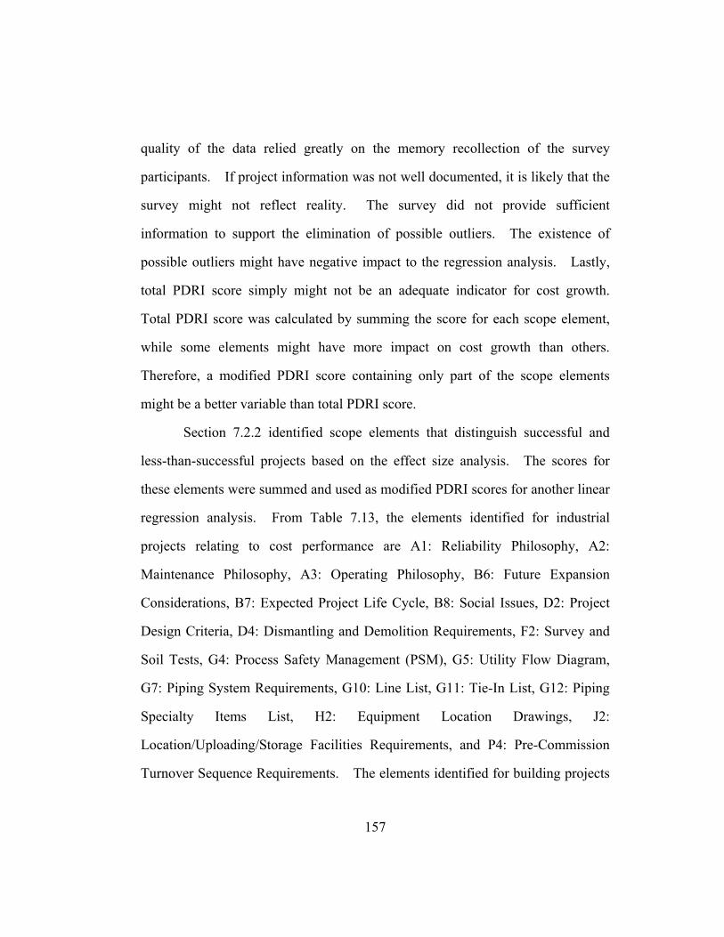
quality of the data relied greatly on the memory recollection of the survey

participants. If project information was not well documented, it is likely that the

survey might not reflect reality. The survey did not provide sufficient

information to support the elimination of possible outliers. The existence of

possible outliers might have negative impact to the regression analysis. Lastly,

total PDRI score simply might not be an adequate indicator for cost growth.

Total PDRI score was calculated by summing the score for each scope element,

while some elements might have more impact on cost growth than others.

Therefore, a modified PDRI score containing only part of the scope elements

might be a better variable than total PDRI score.

Section 7.2.2 identified scope elements that distinguish successful and

less-than-successful projects based on the effect size analysis. The scores for

these elements were summed and used as modified PDRI scores for another linear

regression analysis. From Table 7.13, the elements identified for industrial

projects relating to cost performance are A1: Reliability Philosophy, A2:

Maintenance Philosophy, A3: Operating Philosophy, B6: Future Expansion

Considerations, B7: Expected Project Life Cycle, B8: Social Issues, D2: Project

Design Criteria, D4: Dismantling and Demolition Requirements, F2: Survey and

Soil Tests, G4: Process Safety Management (PSM), G5: Utility Flow Diagram,

G7: Piping System Requirements, G10: Line List, G11: Tie-In List, G12: Piping

Specialty Items List, H2: Equipment Location Drawings, J2:

Location/Uploading/Storage Facilities Requirements, and P4: Pre-Commission

Turnover Sequence Requirements. The elements identified for building projects

157

relating to cost performance are A8: Project Objectives Statement, B2:

Maintenance Philosophy, B4: Design Philosophy, E1: Program Statement, E2:

Building Summary Space List, E11: Room Data Sheets, E13: Window Treatment,

F2: Architectural Design, F4: Mechanical Design, F5: Electric Design, F7:

Constructability Analysis, H1: Identify Long Lead/Critical Equipment and

Materials, H2: Procurement Procedures and Plans, J2: Documentation /

Deliverables, and L3: Project Delivery Method.

With cost growth as dependent variable and modified PDRI score (using

pre-assigned weights for the selected elements) as independent variable, bivariate

linear regression analysis was performed for the industrial and building projects

and these relationships are shown in Figures 8.5 and 8.6. In addition, the

regression statistics obtained were compared with results from total PDRI score

analysis. Tables 8.3 and 8.4 summarized the comparison results.

158

Industrial Cost Growth vs. Modified PDRI Score

y = 0.0039x - 0.2189R2 = 0.3921

-60%

-40%

-20%

0%

20%

40%

60%

80%

100%

0 20 40 60 80 100 120 140 160

Modified PDRI Score

Cos

t Gro

wth

N=54

Figure 8.5. Industrial Cost Growth vs. Modified PDRI Score

Table 8.3. Regression Statistics: Industrial Total vs. Modified PDRI Score,

Industrial Projects PDRI Score Regression Statistics Total Modified

R-Squared (R2) 0.226 0.392 Significant F 9.56E-05 4.17E-07 Degree of Freedom 61 61

159

Building Cost Growth vs. Modified PDRI Score

y = 0.0015x - 0.0257R2 = 0.2768

-30.0%

-20.0%

-10.0%

0.0%

10.0%

20.0%

30.0%

40.0%

50.0%

60.0%

0 20 40 60 80 100 120 140 160 180 200

Modified PDRI Score

Cos

t Gro

wth

N=78

Figure 8.6. Building Cost Growth vs. Modified PDRI Score

Table 8.4. Regression Statistics: Building Total vs. Modified PDRI Score,

Building Projects PDRI Score Regression Statistics Total Modified

R-Squared (R2) 0.150 0.277 Significant F 4.55E-04 7.56E-07 Degree of Freedom 77 77

Statistics comparisons shown in Tables 8.3 and 8.4 indicate improved R-

Squared (R2) values obtained with Modified PDRI scores. The results suggest

that, with cost growth as the dependent variable, the modified PDRI score might

160

serve as a better independent variable than total PDRI score in the bivariate linear

regression analysis for both industrial and building projects, when addressing cost

performance.

Schedule Performance Regression Analysis

A similar approach was used for schedule growth regression analysis.

With schedule growth as dependent variable and PDRI score as independent

variable, bivariate linear regression analysis was performed for the industrial and

building projects and the relationships shown in Figures 8.7 and 8.8 were

revealed. Again, schedule growth is the actual schedule of the project for design

and construction versus the schedule estimate prior to project execution. The

least squares regression line offers a graphic interpretation of the association

between schedule growth and PDRI score and the prediction equation is a useful

form for summarizing that association. Statistics shown in Tables 8.5 and 8.6

indicate a positive correlation between the two variables, meaning that, as the

PDRI score increases so does the schedule growth. The R-Square (R2) is 0.118

for the industrial projects and 0.150 for the building projects and both the levels

of significance are 0.01.

161

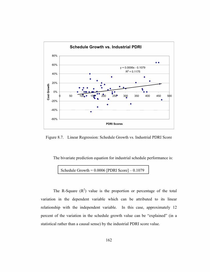
Schedule Growth vs. Industrial PDRI

y = 0.0006x - 0.1079R2 = 0.1175

-60%

-40%

-20%

0%

20%

40%

60%

80%

0 50 100 150 200 250 300 350 400 450 500

PDRI Scores

Cos

t Gro

wth

Figure 8.7. Linear Regression: Schedule Growth vs. Industrial PDRI Score

The bivariate prediction equation for industrial schedule performance is:

9

The

variation i

relationship

percent of

statistical r

Schedule Growth = 0.0006 [PDRI Score] – 0.107

R-Square (R2) value is the proportion or percentage of the total

n the dependent variable which can be attributed to its linear

with the independent variable. In this case, approximately 12

the variation in the schedule growth value can be “explained” (in a

ather than a causal sense) by the industrial PDRI score value.

162

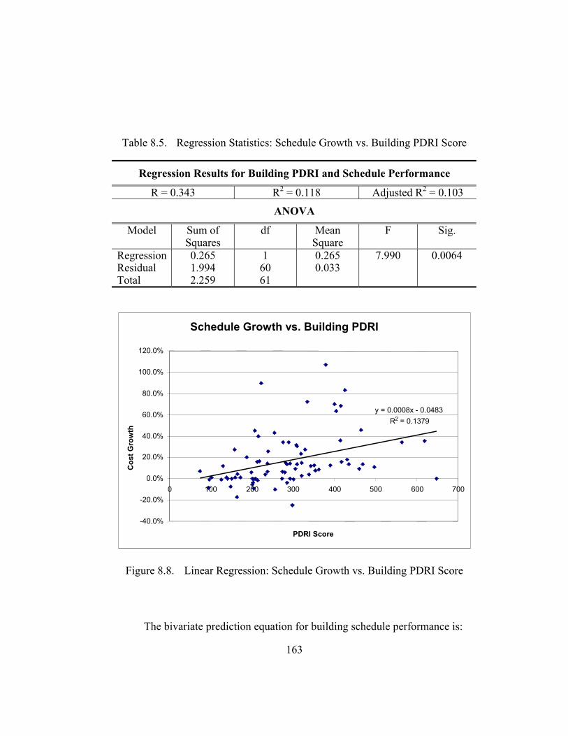
Table 8.5. Regression Statistics: Schedule Growth vs. Building PDRI Score

Regression Results for Building PDRI and Schedule Performance

R = 0.343 R2 = 0.118 Adjusted R2 = 0.103

ANOVA

Model Sum of Squares

df Mean Square

F Sig.

Regression Residual Total

0.265 1.994 2.259

1 60 61

0.265 0.033

7.990 0.0064

Schedule Growth vs. Building PDRI

y = 0.0008x - 0.0483 R2 = 0.1379

-40.0%

-20.0%

0.0%

20.0%

40.0%

60.0%

80.0%

100.0%

120.0%

0 100 200 300 400 500 600 700

PDRI Score

Cos

t Gro

wth

Figure 8.8. Linear Regression: Schedule Growth vs. Building PDRI Score

The bivariate prediction equation for building schedule performance is:

163

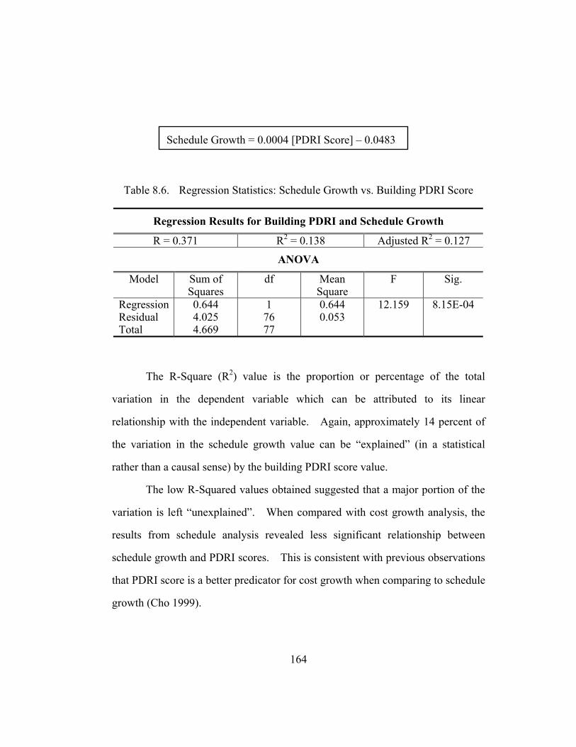
3

Table 8.

R

R

Model

RegressioResidual Total

The

variation i

relationship

the variatio

rather than

The

variation is

results fro

schedule g

that PDRI

growth (Ch

Schedule Growth = 0.0004 [PDRI Score] – 0.048

6. Regression Statistics: Schedule Growth vs. Building PDRI Score

egression Results for Building PDRI and Schedule Growth

= 0.371 R2 = 0.138 Adjusted R2 = 0.127

ANOVA

Sum of Squares

df Mean Square

F Sig.

n 0.644 4.025 4.669

1 76 77

0.644 0.053

12.159 8.15E-04

R-Square (R2) value is the proportion or percentage of the total

n the dependent variable which can be attributed to its linear

with the independent variable. Again, approximately 14 percent of

n in the schedule growth value can be “explained” (in a statistical

a causal sense) by the building PDRI score value.

low R-Squared values obtained suggested that a major portion of the

left “unexplained”. When compared with cost growth analysis, the

m schedule analysis revealed less significant relationship between

rowth and PDRI scores. This is consistent with previous observations

score is a better predicator for cost growth when comparing to schedule

o 1999).

164

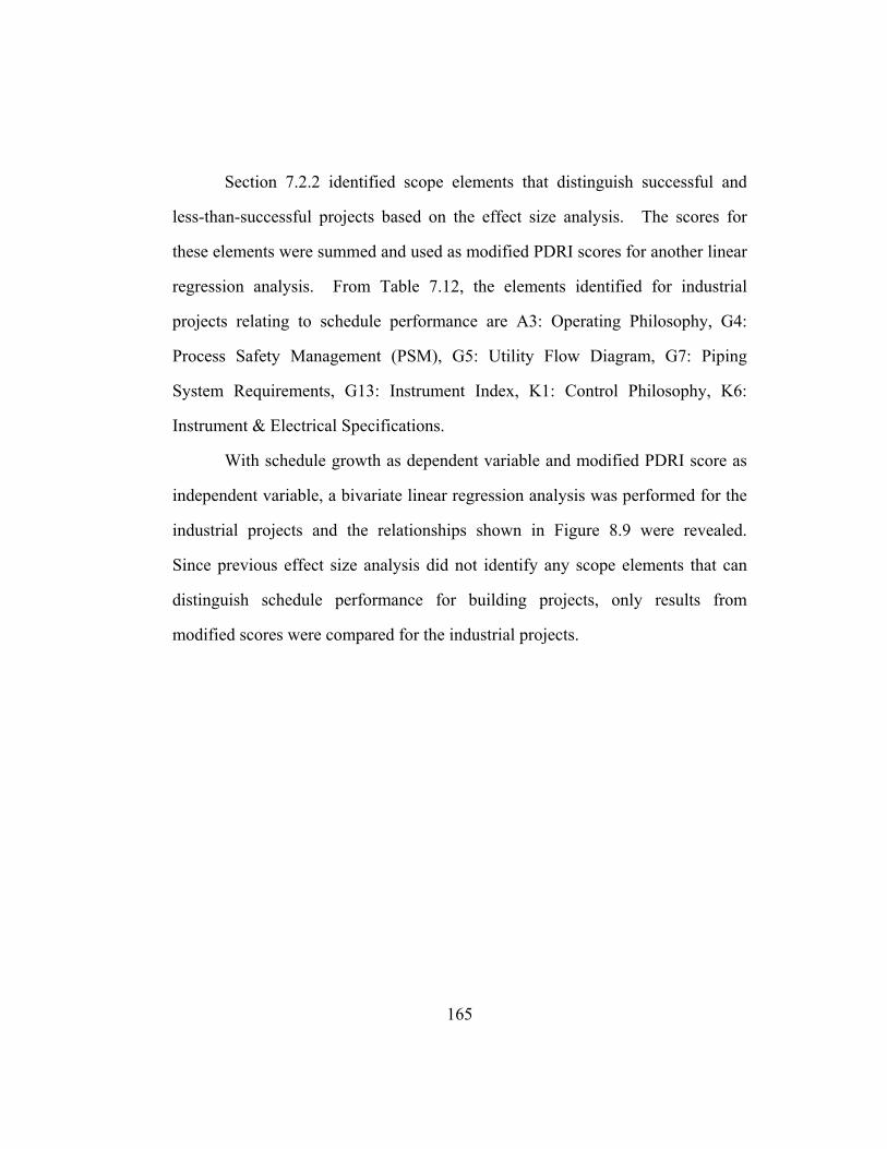
Section 7.2.2 identified scope elements that distinguish successful and

less-than-successful projects based on the effect size analysis. The scores for

these elements were summed and used as modified PDRI scores for another linear

regression analysis. From Table 7.12, the elements identified for industrial

projects relating to schedule performance are A3: Operating Philosophy, G4:

Process Safety Management (PSM), G5: Utility Flow Diagram, G7: Piping

System Requirements, G13: Instrument Index, K1: Control Philosophy, K6:

Instrument & Electrical Specifications.

With schedule growth as dependent variable and modified PDRI score as

independent variable, a bivariate linear regression analysis was performed for the

industrial projects and the relationships shown in Figure 8.9 were revealed.

Since previous effect size analysis did not identify any scope elements that can

distinguish schedule performance for building projects, only results from

modified scores were compared for the industrial projects.

165

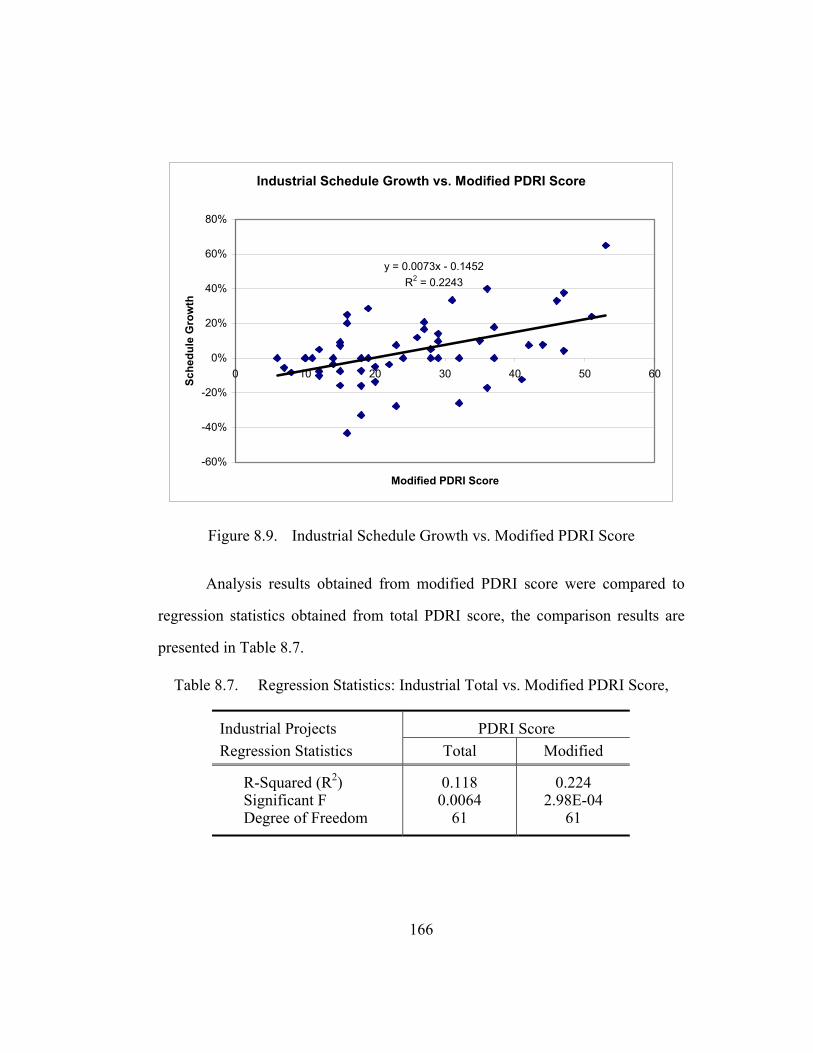
Industrial Schedule Growth vs. Modified PDRI Score

y = 0.0073x - 0.1452R2 = 0.2243

-60%

-40%

-20%

0%

20%

40%

60%

80%

0 10 20 30 40 50 6

Modified PDRI Score

Sche

dule

Gro

wth

0

Figure 8.9. Industrial Schedule Growth vs. Modified PDRI Score

Analysis results obtained from modified PDRI score were compared to

regression statistics obtained from total PDRI score, the comparison results are

presented in Table 8.7.

Table 8.7. Regression Statistics: Industrial Total vs. Modified PDRI Score,

Industrial Projects PDRI Score Regression Statistics Total Modified

R-Squared (R2) 0.118 0.224 Significant F 0.0064 2.98E-04 Degree of Freedom 61 61

166

Table 8.7 shows that modified PDRI score offered better R-Squared (R2)

value for the regression analysis. That is, the modified PDRI score when

compared with the analysis results from total PDRI score can explain a better

portion of the total variation in schedule growth.

8.1.2. Boxplots Quartile Model

Boxplots present a visual display of summary information about the

distribution of values. The boxplots, found in Figures 8.11 through 8.14, display

the median, the 25th percentile, the 75th percentile, and values that are far removed

from the rest. Fifty percent of the cases have values within the box. Figure 4.2

is reproduced below for the reference (Figure 8.10). Used in this section,

boxplots will display summary information showing how the four PDRI score

quartile-groups respond with the performance (cost/schedule growth). Both

industrial and building projects are grouped into four quartile-groups based on

their PDRI scores. All projects were first sorted by their PDRI scores. First

quartile-group contained one-quarter of the projects with the lowest PDRI scores.

The last quartile-group contained the 25 percent of projects that have highest

PDRI scores.

167

75th PercentileMedian25th Percentile

Smallest observed value that is not an outlier

Largest observed value that is not an outlier

Values more than 1.5 box-lengths from 75th percentile(outlier)

*

*

Values more than 3 box-lengths from 75th percentile(extremes)

Values more than 3 box-lengths from 25th percentile(extremes)

Values more than 1.5 box-lengths from 25th percentile(outlier)

75th PercentileMedian25th Percentile

Smallest observed value that is not an outlier

Largest observed value that is not an outlier

Values more than 1.5 box-lengths from 75th percentile(outlier)

*

*

Values more than 3 box-lengths from 75th percentile(extremes)

Values more than 3 box-lengths from 25th percentile(extremes)

Values more than 1.5 box-lengths from 25th percentile(outlier)

Figure 8.10. Annotated Sketch of the Boxplot

Cost Performance Boxplot Analysis

A boxplot of PDRI Score quartile-groups against cost growth was created

for industrial projects and presented in Figure 8.11. The associated statistics

were summarized in Table 8.8. As revealed by Figure 8.11 and Table 8.8, the

PDRI score has a definite relationship with cost growth. Projects within the

fourth quartile-group had significantly higher cost growth than those in the first

and second quartile-groups. There are also more outliers and extremes in the

fourth quartile-group. Most of the projects in the first and second quartile-

groups had final costs under their authorized budget.

168

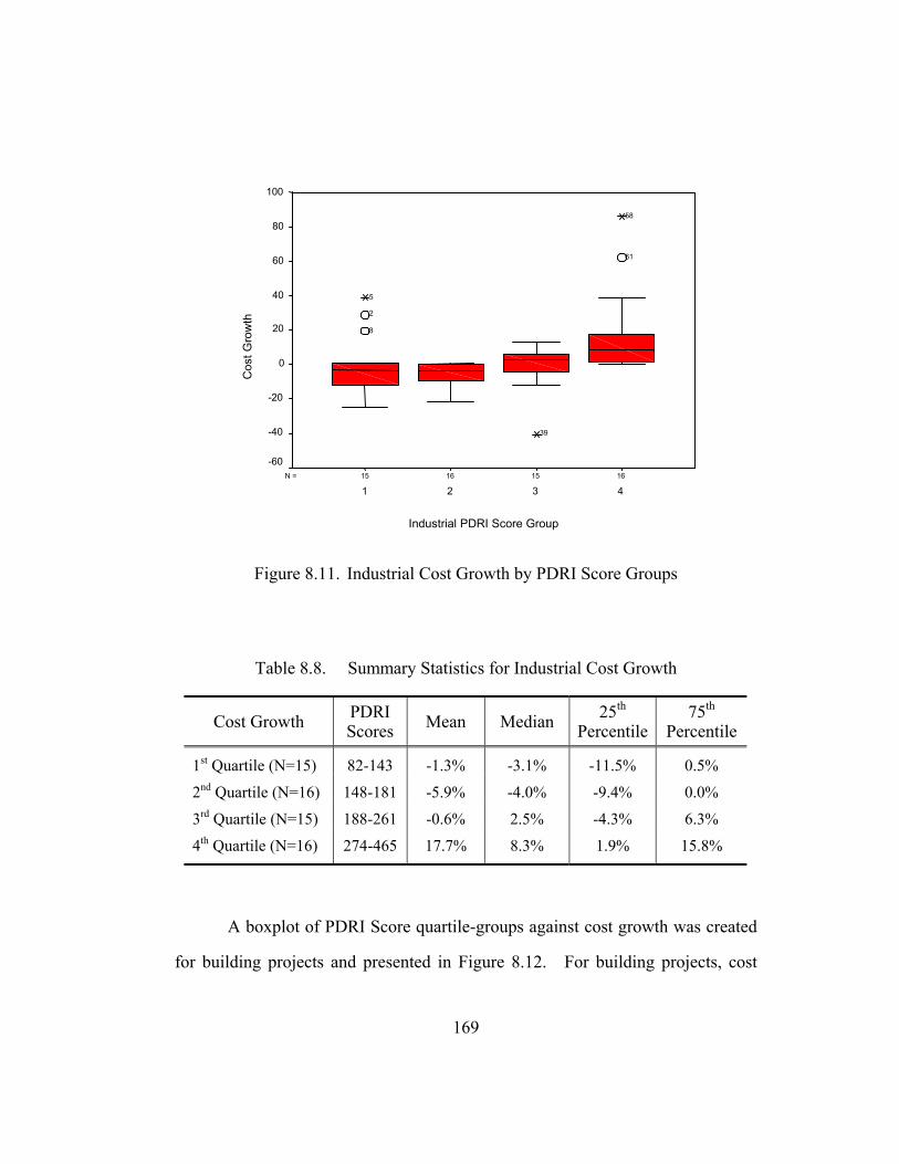
16151615N =

Industrial PDRI Score Group

4321

Cos

t Gro

wth

100

80

60

40

20

0

-20

-40

-60

61

58

39

8

2

5

Figure 8.11. Industrial Cost Growth by PDRI Score Groups

Table 8.8. Summary Statistics for Industrial Cost Growth

Cost Growth PDRI Scores Mean Median 25th

Percentile 75th

Percentile

1st Quartile (N=15) 82-143 -1.3% -3.1% -11.5% 0.5%

2nd Quartile (N=16) 148-181 -5.9% -4.0% -9.4% 0.0%

3rd Quartile (N=15) 188-261 -0.6% 2.5% -4.3% 6.3%

4th Quartile (N=16) 274-465 17.7% 8.3% 1.9% 15.8%

A boxplot of PDRI Score quartile-groups against cost growth was created

for building projects and presented in Figure 8.12. For building projects, cost

169

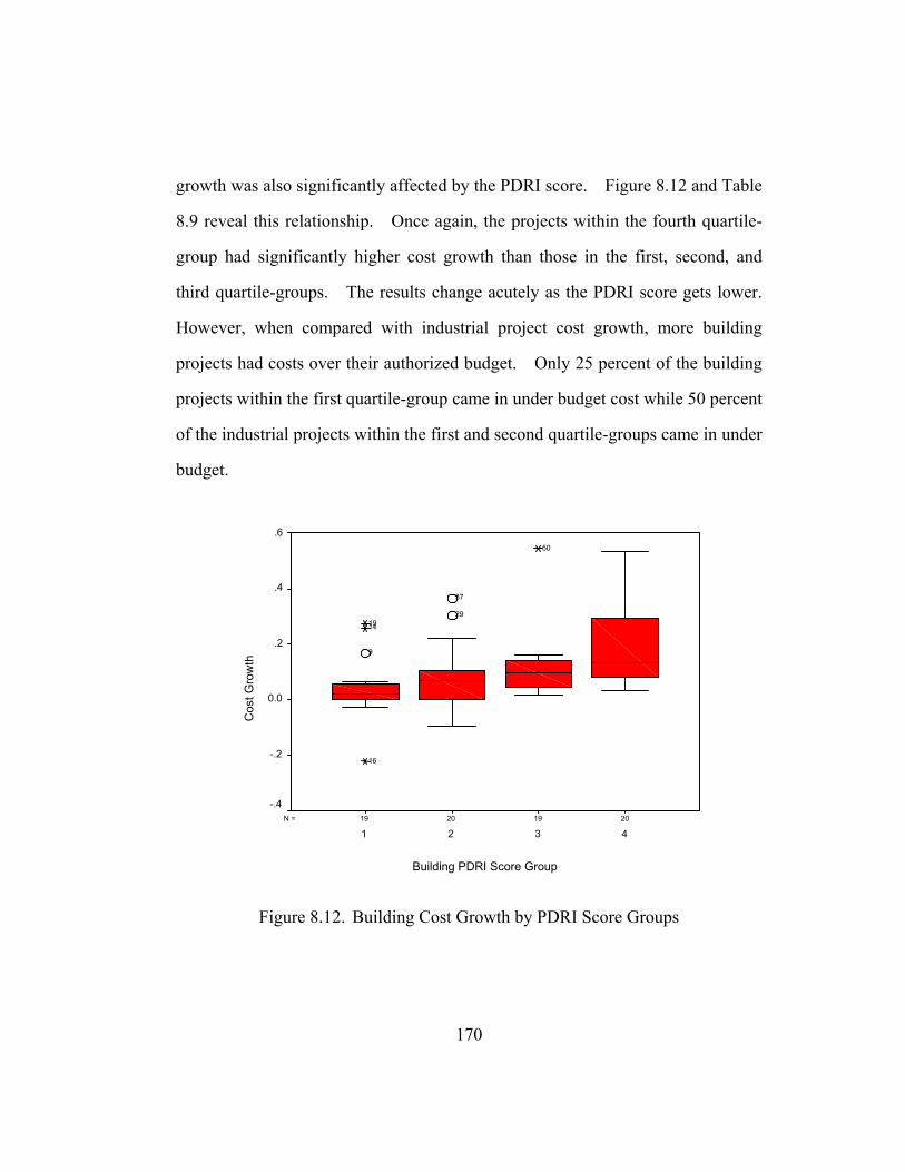
growth was also significantly affected by the PDRI score. Figure 8.12 and Table

8.9 reveal this relationship. Once again, the projects within the fourth quartile-

group had significantly higher cost growth than those in the first, second, and

third quartile-groups. The results change acutely as the PDRI score gets lower.

However, when compared with industrial project cost growth, more building

projects had costs over their authorized budget. Only 25 percent of the building

projects within the first quartile-group came in under budget cost while 50 percent

of the industrial projects within the first and second quartile-groups came in under

budget.

20192019N =

Building PDRI Score Group

4321

Cos

t Gro

wth

.6

.4

.2

0.0

-.2

-.4

50

29

37

16

9

1419

Figure 8.12. Building Cost Growth by PDRI Score Groups

170

Table 8.9. Summary Statistics for Building Cost Growth

Cost Growth PDRI Scores Mean Median 25th

Percentile 75th

Percentile

1st Quartile (N=19) 74-202 4.2% 2.1% 0.0% 5.5%

2nd Quartile (N=20) 203-280 7.6% 6.7% 0.3% 9.9%

3rd Quartile (N=19) 281-343 11.4% 9.7% 4.5% 14.0%

4th Quartile (N=20) 351-648 19.2% 13.2% 8.3% 27.8%

Schedule Performance Boxplot Analysis

A boxplot of PDRI Score quartile-groups against schedule growth was

created for industrial projects and presented in Figure 8.13. The associated

statistics were summarized in Table 8.10. Interesting results were discovered

when the distribution of values was analyzed for schedule growth. As shown in

Figure 8.13, the mean schedule growth for the second quartile-group is lower than

that obtained from the first quartile-group. Projects within the third and fourth

quartile-groups had significantly larger schedule growth variations than those in

the first and second quartile-groups.

171

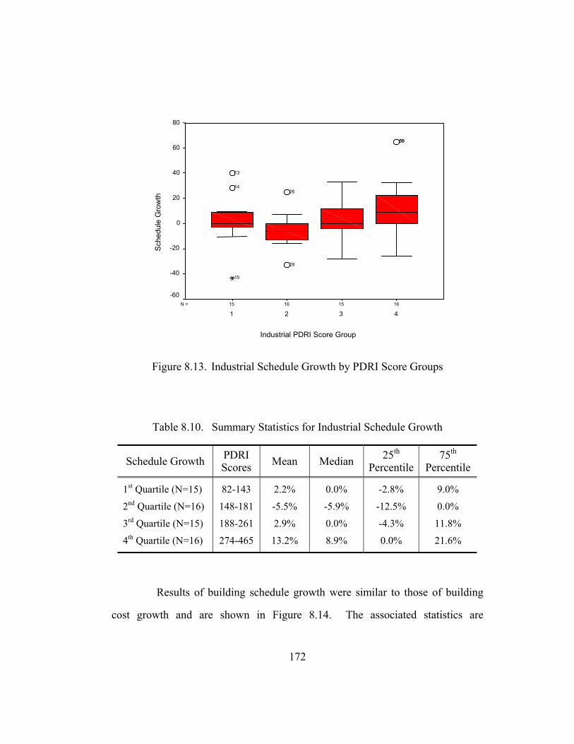
16151615N =

Industrial PDRI Score Group

4321

Sche

dule

Gro

wth

80

60

40

20

0

-20

-40

-60

59 60

28

26

15

14

13

Figure 8.13. Industrial Schedule Growth by PDRI Score Groups

Table 8.10. Summary Statistics for Industrial Schedule Growth

Schedule Growth PDRI Scores Mean Median 25th

Percentile 75th

Percentile

1st Quartile (N=15) 82-143 2.2% 0.0% -2.8% 9.0%

2nd Quartile (N=16) 148-181 -5.5% -5.9% -12.5% 0.0%

3rd Quartile (N=15) 188-261 2.9% 0.0% -4.3% 11.8%

4th Quartile (N=16) 274-465 13.2% 8.9% 0.0% 21.6%

Results of building schedule growth were similar to those of building

cost growth and are shown in Figure 8.14. The associated statistics are

172

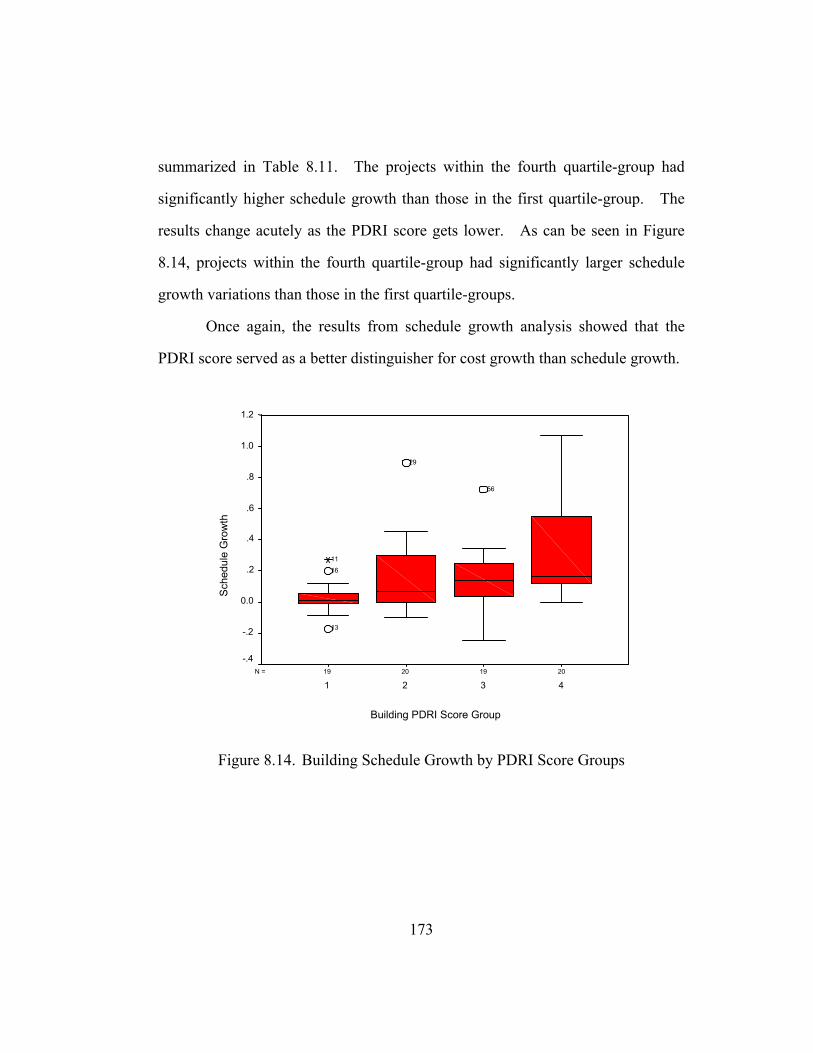
summarized in Table 8.11. The projects within the fourth quartile-group had

significantly higher schedule growth than those in the first quartile-group. The

results change acutely as the PDRI score gets lower. As can be seen in Figure

8.14, projects within the fourth quartile-group had significantly larger schedule

growth variations than those in the first quartile-groups.

Once again, the results from schedule growth analysis showed that the

PDRI score served as a better distinguisher for cost growth than schedule growth.

20192019N =

Building PDRI Score Group

4321

Sche

dule

Gro

wth

1.2

1.0

.8

.6

.4

.2

0.0

-.2

-.4

56

29

13

1611

Figure 8.14. Building Schedule Growth by PDRI Score Groups

173

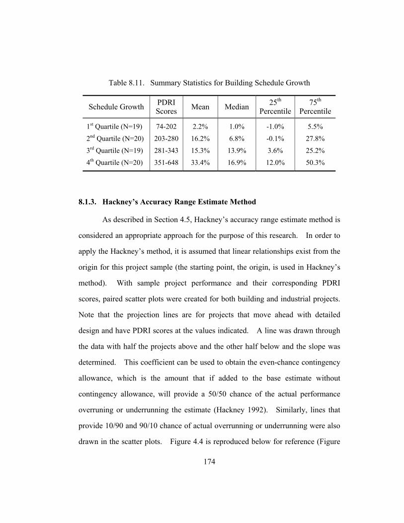
Table 8.11. Summary Statistics for Building Schedule Growth

Schedule Growth PDRI Scores Mean Median 25th

Percentile 75th

Percentile

1st Quartile (N=19) 74-202 2.2% 1.0% -1.0% 5.5%

2nd Quartile (N=20) 203-280 16.2% 6.8% -0.1% 27.8%

3rd Quartile (N=19) 281-343 15.3% 13.9% 3.6% 25.2%

4th Quartile (N=20) 351-648 33.4% 16.9% 12.0% 50.3%

8.1.3. Hackney’s Accuracy Range Estimate Method

As described in Section 4.5, Hackney’s accuracy range estimate method is

considered an appropriate approach for the purpose of this research. In order to

apply the Hackney’s method, it is assumed that linear relationships exist from the

origin for this project sample (the starting point, the origin, is used in Hackney’s

method). With sample project performance and their corresponding PDRI

scores, paired scatter plots were created for both building and industrial projects.

Note that the projection lines are for projects that move ahead with detailed

design and have PDRI scores at the values indicated. A line was drawn through

the data with half the projects above and the other half below and the slope was

determined. This coefficient can be used to obtain the even-chance contingency

allowance, which is the amount that if added to the base estimate without

contingency allowance, will provide a 50/50 chance of the actual performance

overruning or underrunning the estimate (Hackney 1992). Similarly, lines that

provide 10/90 and 90/10 chance of actual overrunning or underrunning were also

drawn in the scatter plots. Figure 4.4 is reproduced below for reference (Figure

174

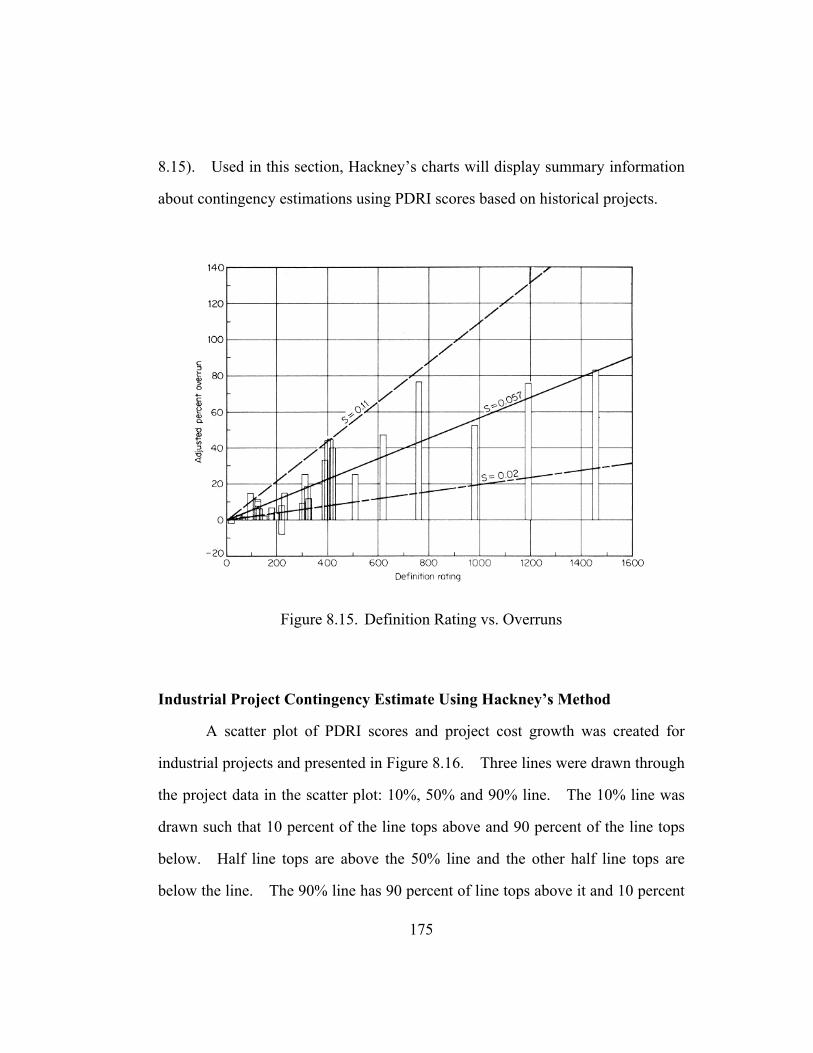
8.15). Used in this section, Hackney’s charts will display summary information

about contingency estimations using PDRI scores based on historical projects.

Figure 8.15. Definition Rating vs. Overruns

Industrial Project Contingency Estimate Using Hackney’s Method

A scatter plot of PDRI scores and project cost growth was created for

industrial projects and presented in Figure 8.16. Three lines were drawn through

the project data in the scatter plot: 10%, 50% and 90% line. The 10% line was

drawn such that 10 percent of the line tops above and 90 percent of the line tops

below. Half line tops are above the 50% line and the other half line tops are

below the line. The 90% line has 90 percent of line tops above it and 10 percent

175

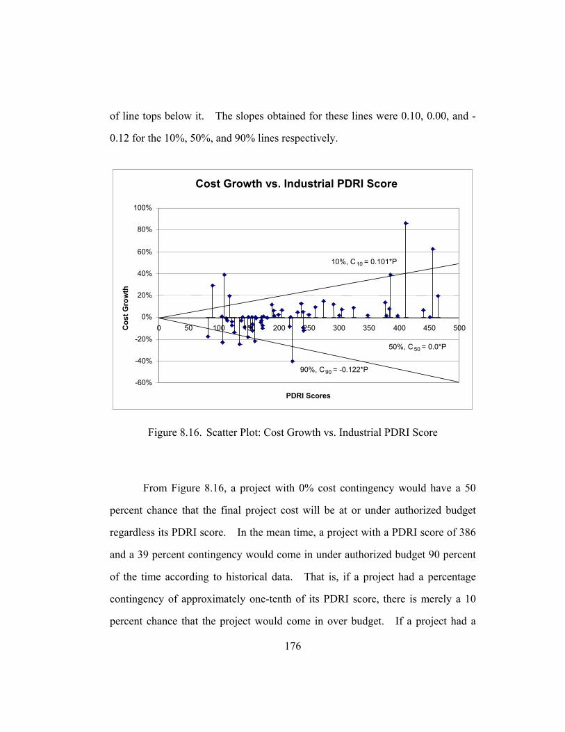
of line tops below it. The slopes obtained for these lines were 0.10, 0.00, and -

0.12 for the 10%, 50%, and 90% lines respectively.

Cost Growth vs. Industrial PDRI Score

-60%

-40%

-20%

0%

20%

40%

60%

80%

100%

0 50 100 150 200 250 300 350 400 450 500

PDRI Scores

Cos

t Gro

wth

10%, C10 = 0.101*P

50%, C 50 = 0.0*P

90%, C90 = -0.122*P

Figure 8.16. Scatter Plot: Cost Growth vs. Industrial PDRI Score

From Figure 8.16, a project with 0% cost contingency would have a 50

percent chance that the final project cost will be at or under authorized budget

regardless its PDRI score. In the mean time, a project with a PDRI score of 386

and a 39 percent contingency would come in under authorized budget 90 percent

of the time according to historical data. That is, if a project had a percentage

contingency of approximately one-tenth of its PDRI score, there is merely a 10

percent chance that the project would come in over budget. If a project had a

176

PDRI score of 200 and an estimated contingency of 10%, the chance that the final

project cost comes in under budget can be calculated from Figure 8.16. First, the

point (200, 10%) was plotted in the scatter plot and a line that passes the origin

and this point was drawn as shown in Figure 8.17.

Cost Growth vs. Industrial PDRI Score

-60%

-40%

-20%

0%

20%

40%

60%

80%

100%

0 50 100 150 200 250 300 350 400 450 500

PDRI Scores

Cos

t Gro

wth

(200, 10%) 15%, C15 = 0.050*P

Figure 8.17. Cost Growth Accuracy Range Estimate for Industrial Projects

From Figure 8.17, there are nine line tops above the drawn line and that

translates to approximately 15 percent (9/62) of total projects. Based on

historical data, if a project had a PDRI score of 200 and a cost contingency of

10%, there is an 85 percent chance that the project will come in under authorized

budget.

177

Similarly, a scatter plot of PDRI scores and project schedule growth was

created for industrial projects and presented in Figure 8.18. The slopes obtained

for these 10%, 50% and 90% lines were 0.10, 0.00, and -0.12 respectively. Like

the results from cost performance analysis, a project with 0% schedule

contingency would have a 50 percent chance that the final project schedule will

be at or under authorized project duration regardless its PDRI score. A project

with a PDRI score of 237 and a 33 percent schedule contingency (float) would

finish before the authorized schedule date 90 percent of the time according to

historical data.

Schedule Growth vs. Industrial PDRI Score

-60%

-40%

-20%

0%

20%

40%

60%

80%

0 50 100 150 200 250 300 350 400 450 500

PDRI Scores

Sche

dule

Gro

wth

10%, C10 = 0.139*P

50%, C50 = 0.000*P

90%, C90 = -0.088*P

Figure 8.18. Scatter Plot: Schedule Growth vs. Industrial PDRI Score

178

A project with a PDRI score of 200 and an estimated schedule

contingency of 10% was plotted in the scatter plot. A line that passes the origin

and this point was drawn as shown in Figure 8.19.

Schedule Growth vs. Industrial PDRI Score

-60%

-40%

-20%

0%

20%

40%

60%

80%

0 50 100 150 200 250 300 350 400 450 500

PDRI Scores

Sche

dule

Gro

wth

26%, C26 = 0.050*P(200, 10%)

Figure 8.19. Schedule Growth Accuracy Range Estimate for Industrial Projects

From Figure 8.19, there are 16 line tops above the drawn line and that

translates to approximately 26 percent (16/62) of total projects. Based on

historical data, if a project had a PDRI score of 200 and a schedule contingency of

10%, there is a 74 percent chance that the project will come in at or under the

authorized schedule.

179

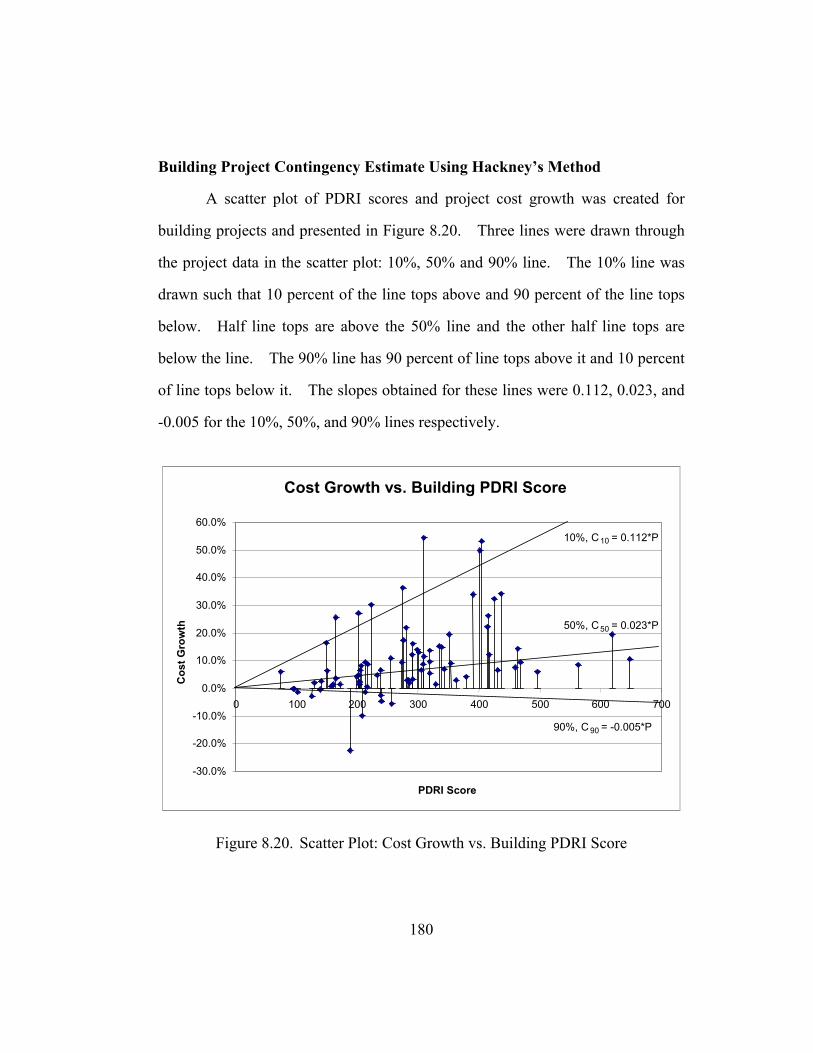
Building Project Contingency Estimate Using Hackney’s Method

A scatter plot of PDRI scores and project cost growth was created for

building projects and presented in Figure 8.20. Three lines were drawn through

the project data in the scatter plot: 10%, 50% and 90% line. The 10% line was

drawn such that 10 percent of the line tops above and 90 percent of the line tops

below. Half line tops are above the 50% line and the other half line tops are

below the line. The 90% line has 90 percent of line tops above it and 10 percent

of line tops below it. The slopes obtained for these lines were 0.112, 0.023, and

-0.005 for the 10%, 50%, and 90% lines respectively.

Cost Growth vs. Building PDRI Score

-30.0%

-20.0%

-10.0%

0.0%

10.0%

20.0%

30.0%

40.0%

50.0%

60.0%

0 100 200 300 400 500 600 700

PDRI Score

Cos

t Gro

wth

10%, C 10 = 0.112*P

90%, C 90 = -0.005*P

50%, C 50 = 0.023*P

Figure 8.20. Scatter Plot: Cost Growth vs. Building PDRI Score

180

From Figure 8.20, a project with a PDRI score of 150 and a 17 percent

cost contingency would come in under authorized budget approximately 90

percent of the time according to historical data. That is, if a project had a

percentage contingency of approximately one-ninth of its PDRI score, there is

merely a 10 percent chance that the project would come in over budget. Without

any contingency, the building projects had a 50 percent chance that the final cost

will be below authorized budget regardless of their PDRI scores. Unlike

industrial projects, a certain amount of contingency should be assigned to a

building project to attain a 50 percent chance of meeting the budget. The

amount of contingency assigned differs from project to project and is positively

related to the project’s PDRI score. To be exact, the percentage amount of

contingency equals 0.023 times the PDRI score.

A building project with a PDRI score of 200 and an estimated cost

contingency of 10% was plotted in the scatter plot. A line that passes the origin

and this point was drawn as shown in Figure 8.21.

181

Cost Growth vs. Building PDRI Score

-30.0%

-20.0%

-10.0%

0.0%

10.0%

20.0%

30.0%

40.0%

50.0%

60.0%

0 100 200 300 400 500 600 700

PDRI Score

Cos

t Gro

wth

23%, C23 = 0.050*P(200, 10%)

Figure 8.21. Cost Growth Accuracy Range Estimate for Building Projects

From Figure 8.21, there are 18 line tops above the drawn line and that

translates to approximately 23 percent (18/78) of total projects. Based on

historical data, if a project had a PDRI score of 200 and a cost contingency of

10%, there is a 77 percent chance that the project will come in under the estimated

budget.

Similarly, a scatter plot of PDRI scores and project schedule growth was

created for building projects and presented in Figure 8.22. The slopes obtained

for these 10%, 50% and 90% lines were 0.171, 0.032, and -0.018 respectively.

A project with a PDRI score of 150 and a 27 percent schedule contingency (float)

182

would finish before the authorized schedule date 90 percent of the time according

to historical data.

Schedule Growth vs. Building PDRI Score

-40.0%

-20.0%

0.0%

20.0%

40.0%

60.0%

80.0%

100.0%

120.0%

0 100 200 300 400 500 600 700

PDRI Score

Sche

dule

Gro

wth

10%, C10 = 0.171*P

90%, C 90 = -0.018*P

50%, C 50 = 0.032*P

Figure 8.22. Scatter Plot: Schedule Growth vs. Building PDRI Score

A building project with a PDRI score of 200 and an estimated schedule

contingency of 10% was plotted in the scatter plot. A line that passes the origin

and this point was drawn as shown in Figure 8.23.

183

Schedule Growth vs. Building PDRI Score

-40.0%

-20.0%

0.0%

20.0%

40.0%

60.0%

80.0%

100.0%

120.0%

0 100 200 300 400 500 600 700

PDRI Score

Sche

dule

Gro

wth

37%, C 37 = 0.05*P

(200, 10%)

Figure 8.23. Schedule Growth Accuracy Range Estimate for Building Projects

From Figure 8.23, there are 29 line tops above the drawn line and that

translates to approximately 37 percent (29/78) of total projects. Based on

historical data, if a project had a PDRI score of 200 and a schedule contingency of

10%, there is a 63 percent chance that the project will finish before the authorized

schedule date.

184

8.2. RISK QUANTIFICATION USING PDRI

As discussed in previous sections, three approaches were explored to

model the sample data. The three analysis tactics were least square linear

regression, boxplots quartile analysis, and Hackney’s accuracy range estimate.

The following sections outline the application of these models to quantify

potential risk impacts using PDRI scores. For demonstration purposes, one

example for each of the three approaches will be given to illustrate the

application.

8.2.1. Linear Regression Model

Least squares linear regression was used to describe the cost performance

data and PDRI scores for industrial projects. A scatter plot with industrial PDRI

scores and cost growth was plotted along with best fit line and 95 percent mean

confidence level lines. As revealed in Figure 8.24, with a given PDRI score, the

expected mean cost growth can be obtained.

185

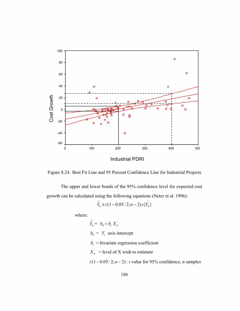
Industrial PDRI

500400 300200100 0

Cos

t Gro

wth

100

80

60

40

20

0

-20

-40

-60

Figure 8.24. Best Fit Line and 95 Percent Confidence Line for Industrial Projects

The upper and lower bonds of the 95% confidence level for expected cost

growth can be calculated using the following equations (Neter et al. 1996):

}{)2;2/05.01(∧∧

−−± hh YsntY

where:

Y = ∧

h hXbb 10 +

= axis intercept 0b iY

= bivariate regression coefficient 1b

= level of X wish to estimate hX

)2;2/05.01( −− nt : t value for 95% confidence, n samples

186

= MSE }{2∧

hYs

−−

+∑ 2

2

)()(1

XXXX

n i

h

Using above equation, the 95 percent confidence interval for expected cost

growth for PDRI scores of 200 and 400 are given in Table 8.12

Table 8.12. Ninety-five Percent Confidence Level Summary

PDRI Score ∧

hY t (.975, 60) }{∧

hYs Lower 95% Upper 95%

200 1.5% 2.0 2.5% -3.4% 6.5% 400 19.5% 2.0 4.8% 9.8% 29.2%

From Table 8.12, there is a 95 percent chance that the expected mean cost

growth for a industrial project with a PDRI score of 200 will be within the range

of -3.4% to 6.5%. The range becomes much worse (9.8% ~ 29.2%) when the

project has a PDRI score of 400. That is, the risks of project overrunning the

authorized budget increase significantly with the increase of the PDRI score. By

implementing the least square linear regression method, the project team is able to

determine the expected mean cost growth based on historical data. The same

approach can be applied to estimate schedule growth.

8.2.2. Boxplot Quartile Analysis Model

In Section 8.1.2, boxplots were created to present a visual display of

summary information about the distribution of project performance. The sample

projects were grouped by their PDRI scores and a total of four quartile-groups

187

were formed. Figure 8.11 is reproduced to represent the cost growth distribution

of the industrial projects for the four quartile-groups (Figure 8.25). Table 8.8

was recreated to represent the summary information for the boxplot (Table 8.13).

16151615N =

Industrial PDRI Score Group

4321

Cos

t Gro

wth

100

80

60

40

20

0

-20

-40 -60

61

58

39

8

2

5

Figure 8.25. Industrial Cost Growth by PDRI Groups

Table 8.13. Summary Statistics for Industrial Cost Growth

Cost Growth PDRI Scores Mean Median 25th

Percentile 75th

Percentile

1st Quartile (N=15) 82-143 -1.3% -3.1% -11.5% 0.5%

2nd Quartile (N=16) 148-181 -5.9% -4.0% -9.4% 0.0%

3rd Quartile (N=15) 188-261 -0.6% 2.5% -4.3% 6.3%

4th Quartile (N=16) 274-465 17.7% 8.3% 1.9% 15.8%

188

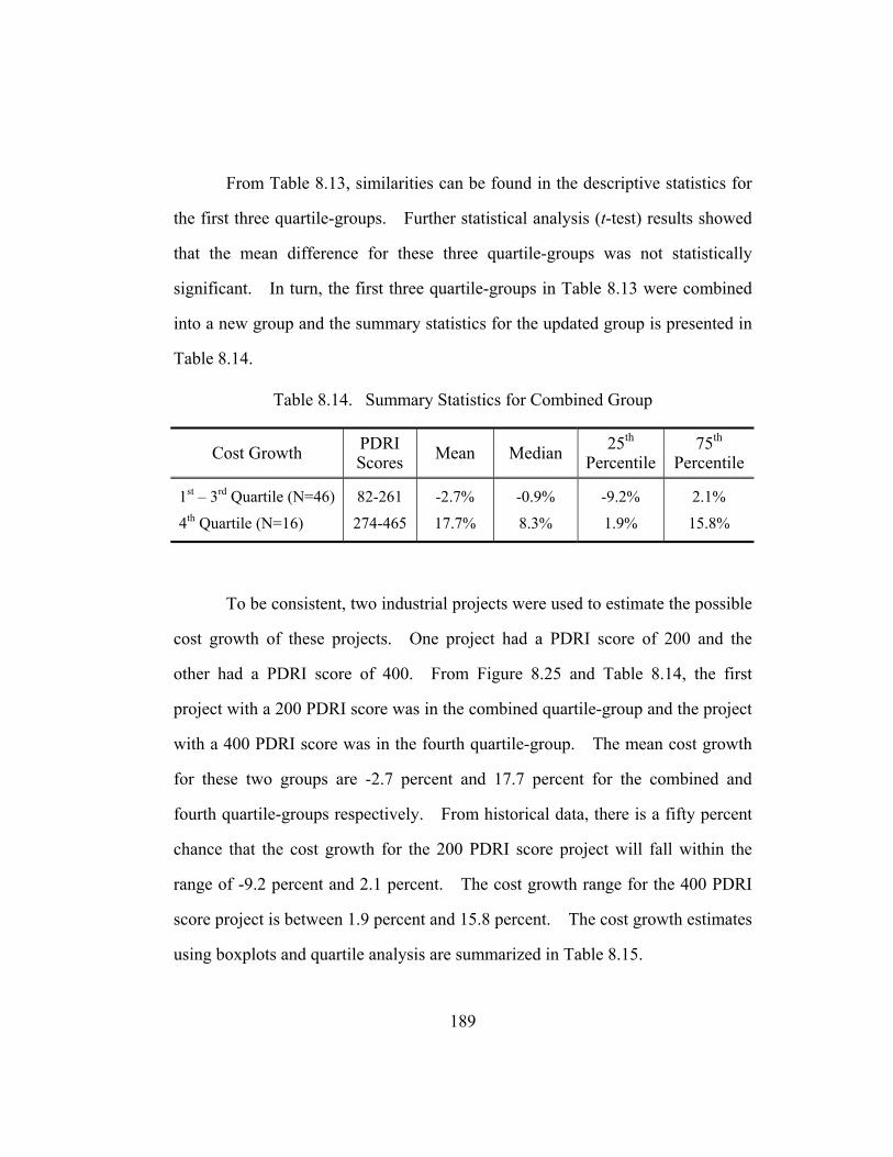
From Table 8.13, similarities can be found in the descriptive statistics for

the first three quartile-groups. Further statistical analysis (t-test) results showed

that the mean difference for these three quartile-groups was not statistically

significant. In turn, the first three quartile-groups in Table 8.13 were combined

into a new group and the summary statistics for the updated group is presented in

Table 8.14.

Table 8.14. Summary Statistics for Combined Group

Cost Growth PDRI Scores Mean Median 25th

Percentile 75th

Percentile

1st – 3rd Quartile (N=46) 82-261 -2.7% -0.9% -9.2% 2.1%

4th Quartile (N=16) 274-465 17.7% 8.3% 1.9% 15.8%

To be consistent, two industrial projects were used to estimate the possible

cost growth of these projects. One project had a PDRI score of 200 and the

other had a PDRI score of 400. From Figure 8.25 and Table 8.14, the first

project with a 200 PDRI score was in the combined quartile-group and the project

with a 400 PDRI score was in the fourth quartile-group. The mean cost growth

for these two groups are -2.7 percent and 17.7 percent for the combined and

fourth quartile-groups respectively. From historical data, there is a fifty percent

chance that the cost growth for the 200 PDRI score project will fall within the

range of -9.2 percent and 2.1 percent. The cost growth range for the 400 PDRI

score project is between 1.9 percent and 15.8 percent. The cost growth estimates

using boxplots and quartile analysis are summarized in Table 8.15.

189

Table 8.15. Boxplot Cost Growth Estimate Summary

PDRI Score Mean Cost Growth Lower 25% Upper 75%

200 -0.6% -9.2% 2.1% 400 17.7% 1.9% 15.8%

8.2.3. Hackney’s Accuracy Range Estimate Model

To estimate possible cost growth for the 200 and 400 PDRI score projects,

a scatter plot of PDRI scores and project cost growth was created for industrial

projects. Figure 8.16 was reproduced along with the 10% and 90% lines (Figure

8.26).

Cost Growth vs. Industrial PDRI Score

-60%

-40%

-20%

0%

20%

40%

60%

80%

100%

0 50 100 150 200 250 300 350 400 450 500

PDRI Scores

Cos

t Gro

wth

10%, C10 = 0.101*P

50%, C 50 = 0.0*P

90%, C90 = -0.122*P

Figure 8.26. Scatter Plot: Schedule Growth vs. Industrial PDRI Score

190

As revealed in Figure 8.26, an industrial project has a 50/50 percent

chance that the final cost will be within the authorized budget regardless of its

PDRI score. Furthermore, an industrial project with a PDRI score of 200 has a

90 percent chance that the final cost will be below the authorized if 20.2 percent

(200 x 0.101) contingency were added to the estimate. For a project with a

PDRI score of 400, the 90 percent contingency increases to 40.4 percent (400 x

0.101).

The application of Hackney’s method offers another advantage, which is

the ability to estimate the probability of cost/schedule growth given PDRI scores

and contingencies. As illustrated in Figure 8.17 of Section 8.1.3, an industrial

project with a PDRI score of 200 and a 10 percent cost contingency would have

an 85 percent chance to bring the final cost under authorized budget. Figure

8.17 was reproduced in Figure 8.27 with an added line for a project with 400

PDRI score and 10 percent contingency.

191

Cost Growth vs. Industrial PDRI Score

-60%

-40%

-20%

0%

20%

40%

60%

80%

100%

0 50 100 150 200 250 300 350 400 450 500

PDRI Scores

Cos

t Gro

wth

(200, 10%) 15%, C15 = 0.05*P

(400, 10%) 27%, C 27 = 0.025*P

Figure 8.27. Cost Growth Accuracy Range Estimate for Industrial Projects

Results from Figure 8.27 shows that an industrial project with a PDRI

score of 400 and a cost contingency of 10 percent only has a 73 percent chance

that the final cost will be below the authorized budget. Whereas a 200 PDRI

score project with the same contingency has an 85 percent chance of achieving

the budget.

As illustrated in the previous three sections, the three proposed models can

be applied to estimate the project performance given PDRI scores based on

historical data. The three methods can be applied in different situations and

should be chosen according to specific requirements. The results obtained from

the three methods are fairly consistent and it is recommended that all three

192

methods be employed. Table 8.16 demonstrates the estimation of industrial

project cost performance for PDRI scores of 200 and 400 for the three models.

Table 8.17 shows the summary estimation using similar approach for building

projects.

Table 8.16. Performance Estimate Using the Three Models, Industrial Projects

Linear Regression Model PDRI Score Expected Mean 95% Confidence Level

200 1.5% -3.4% ~ 6.5% 400 19.5% 9.8% ~ 29.2%

Boxplot Quartile Analysis Model PDRI Score Mean 50% Chance Range

200 -0.6% -4.3% ~ 6.3% 400 17.7% 1.9% ~ 15.8%

Hackney’s Accuracy Range Estimate Model PDRI Score Estimate Contingency Probability of Overrun

200 10% 15% 400 10% 27%

Table 8.17. Performance Estimate Using the Three Models, Building Projects

Linear Regression Model PDRI Score Expected Mean 95% Confidence Level

200 6.4% 3.4% ~ 9.5% 400 14.4% 8.8% ~ 20.2%

Boxplot Quartile Analysis Model PDRI Score Mean 50% Chance Range

200 4.1% 0.0% ~ 5.5% 400 19.2% 8.3% ~ 27.8%

Hackney’s Accuracy Range Estimate Model PDRI Score Estimate Contingency Probability of Overrun

200 10% 23% 400 10% 48%

193

Chapter 7 illustrated risk identification through PDRI evaluation and

statistics shows that higher PDRI scores are positively related to poor project

performance. After identifying project risks using the PDRI, implementation of

risk quantification can be done by applying any of the three proposed methods.

These models provide the project team with different perspectives during the risk

quantification process. After risk quantification, the next logical step in the risk

management process is risk control, which will be illustrated in the next section.

8.3. RISK CONTROL THROUGH PDRI

As previously discussed in the Literature Review, risk control includes

risk avoidance, risk reduction, risk sharing, risk transfer, insurance, risk

acceptance by establishment of contingency accounts, risk acceptance without any

contingency and risk containment (CII 1989). After the project team has

accomplished the PDRI evaluation, they might find that there is too much risk

involved in the project and decide not to go forth with the project to completely

avoid the potential risk. If the project is an international project, the owner

might consider forming a joint venture with a local company to share the potential

project risk. Some of the risks identified after the PDRI evaluation might be

transferred to other project participants (architect, construction management, or

contractors) through contracting strategy. In addition, the client can purchase

insurance to cover the potential loss resulted from the project uncertainties. A

common practice for the owner’s organization is to set up a certain amount of

budget in addition to the project cost estimate, often referred to as “contingency”,

194

to cover the unexpected cost. In some situations, the organization might decide

to take the risk without any risk management measures. Among these risk

control measures, risk reduction is determined most applicable for the purpose of

this study, which is to apply PDRI in the risk management process. Risk

reduction is a two-fold risk control technique and it decreases risk exposures by

reducing the probability and financial consequences caused by risk exposures.

The PDRI can be used to reduce the risk during the risk management

process. The most effective way of risk control using the PDRI is to lower PDRI

score (resolve scope deficiencies) and thus reduce the probability of cost/schedule

increase caused by poorly defined scopes. For illustration purpose, Table 8.12 is

reproduced in Table 8.18 to summarize the cost growth estimates for projects with

different scores using linear regression method. Of course, once the PDRI score

is reduced, the project estimate must be reassessed.

Table 8.18. Ninety-five Percent Confidence Level Summary

PDRI Score ∧

hY t (.975, 60) }{∧

hYs Lower 95% Upper 95%

200 1.5% 2.0 2.5% -3.4% 6.5% 400 19.5% 2.0 4.8% 9.8% 29.2%

From Table 8.18, it is evident that the expected mean cost growth is much

lower for a 200 PDRI score project than a 400 PDRI score project. If the PDRI

score for a project can be lowered from 400 to 200 by addressing poorly-defined

scope elements, the expected mean cost growth for that particular project can be

195

reduced from 19.5 percent to 1.5 percent (18 percent difference). That is, the

financial consequences caused by incomplete scope can be significantly reduced

by lowering the PDRI score. In addition, projects with a lower PDRI score have

a smaller range of expected mean cost growth (9.9 percent) than projects with

higher PDRI scores (range of 19.4 percent) when the estimates are set to 95

percent confidence levels. Therefore, lowering the PDRI score is an effective

measure to reduce the financial consequences caused by risk exposures related to

estimates.

Hackney’s accuracy range estimate model can be used to illustrate the use

of PDRI to reduce the probability of risk exposures. The results in Figure 8.27

show that two projects with the same cost contingency amount have different

probability of achieving their budgets. An industrial project with a PDRI score

of 200 and cost contingency of 10 percent has an 85 percent chance of achieving

its authorized budget (estimate and 10 percent contingency). However, there is

only a 73 percent chance that the final cost of a project with the same contingency

but higher PDRI score (400) will be below the authorized budget. Hackney’s

model shows that lowering the PDRI score by improving the poorly-defined

scope, the probability of overrunning the budget is lowered as well. That is,

PDRI is an effective tool to reduce the probability of risk exposures around cost

estimates.

From the previous two illustrations, lowering the PDRI score is an

effective risk control measure in terms of reducing the probability and financial

consequences of risk exposures. However, it should be noted that other risk

196

control techniques (i.e. risk avoidance, risk sharing, and insurance) should be

combined with risk reduction technique to minimize project risks. These

techniques are beyond the scope of this research and therefore, readers should

refer to other references for the application of these techniques in construction

projects. However, if risk issues of identified during PDRI assessments, they

can perhaps be mitigated using these methods.

8.4. RISK MANAGEMENT USING PDRI

Based on the Construction Risk Management System (CRMS) model

developed by Al-Bahar (1988), a systematic risk management system

incorporating the PDRI was proposed by the author. The format of pre-project

planning process flow diagram (CII 1995) was adopted for the development of

this systematic risk management system. The proposed risk management

process, risk identification, risk quantification and risk control, is summarized in

Figure 8.28.

From the literature review, a series of activities were identified for each of

the risk management processes: risk identification, risk quantification, and risk

control. In addition, a fourth process, risk control, was added to the proposed

risk management system in order to make the process a continuous effort. The

logical sequence to carry out these activities is presented in Figure 8.28. This

proposed systematic risk management process can begin from as early as the

conceptual stage of a project and continue until the beginning of detailed design

to achieve the project goals set by the project team.

197

RegisterRisk

MONITOR

RISK

CONTROL

RISK

QUANTIFY

RISK

IDENTIFY

RISK

ClassifyRisk

IdentifyRisk

Consequence

ConductPDRI

Evaluation

EvaluateRisk

Impact

ModelRisk

Using PDRI

DevelopModel

ImplementRisk ControlMeasures

LowerPDRIScore

ImproveScope

Definition

CollectData

ContinuousProcess

Re-evaluate

MeasureResults

RegisterRisk

MONITOR

RISK

CONTROL

RISK

QUANTIFY

RISK

IDENTIFY

RISK

ClassifyRisk

IdentifyRisk

Consequence

ConductPDRI

Evaluation

EvaluateRisk

Impact

ModelRisk

Using PDRI

DevelopModel

ImplementRisk ControlMeasures

LowerPDRIScore

ImproveScope

Definition

CollectData

ContinuousProcess

Re-evaluate

MeasureResults

Figure 8.28. Systematic Risk Management Process Using PDRI

The first series of activities in risk management process deals with risk

identification. The four major functions are: conducting PDRI evaluation,

identifying risk consequence, classifying risk, and registering risk. During the

pre-project planning process, the PDRI evaluation is carried out by the project

team, which consists of major stakeholders of the project. The PDRI score

sheets serve as a comprehensive potential project risk checklist. Poorly-defined

scope elements are identified and total PDRI score is determined. These poorly-

defined scope elements are treated as potential risk factors to the project. The

project team then attempts to identify a set of credible risk event or consequence

scenarios. The relative value of the PDRI element scores gives some indication

of risk impact. Risk classification deals with classifying risk by its nature or

potential impact and assigning the ownership of the risk. These risks are

198

grouped and documented in the risk register along with their financial

consequence, nature, and ownership.

The second series of activities in the risk management process deals with

risk quantification. There are four major functions: collecting data, developing

model, modeling risk using PDRI, and evaluating risk impact. In order to assess

the potential risk impact caused by these risk exposures, historical project

information within the company is first collected. The information collected

should at least include basic project information, project performance, and PDRI

scores. Linear regression models are developed to describe the collected data.

As discussed in earlier sections, alternative analysis models include linear

regression model, boxplot quartile model and Hackney’s accuracy range estimate

model. The models are used to estimate potential risk impact based on the

results provided by the PDRI evaluation. With the given PDRI scores and basic

project information, expected cost/schedule performance can be estimated.

Thus, potential risk impacts caused by these risk exposures are determined. For

instance, projects with a higher PDRI score (i.e., above 400) should possibly set

aside more contingency than projects with a lower PDRI score (i.e., 200 or below)

to cover the potential cost predictability problems caused by incomplete scope.

The third series of activities in the risk management process deals with

risk control. There are three major functions in this process: improving scope

definition, lowering PDRI score, and implementing risk control measures. After

potential risk impacts are estimated for the risk register, a list of action items to

improve the scope definitions are developed for risk reduction. Figure 8.29

199

illustrates an example of a partial risk register and action items identified after a

PDRI evaluation. These are the results of an evaluation of an approximately $10

million electrical/mechanical upgrade of a courthouse facilitated by the author’s

supervisor. The relative risk score shown in Figure 8.29 was obtained from the

results of PDRI evaluation. The project team evaluated each scope element in

the PDRI and the relative weight for the definition level was recorded as the

relative risk score in the risk register. The actions were subsequently assigned to

project team members. Higher priorities are given to those action items that aim

at risks with higher financial impacts. Once the poorly-defined elements are

improved, the PDRI score will be lowered and the risk of poor performance is

consequently reduced. Overall, the improved project scope benefits the project

from the aspects that unknowns are resolved and estimate is improved.

The fourth series of activities in the risk management process deals with

monitoring risk. PDRI evaluation can be applied during different stages of the

project and the obtained PDRI scores can be used as a measure to monitor risk.

Project definition should be improved as projects move into the next phase(s) and

the PDRI score is lowered as project unknowns are resolved. That is, the project

team has an objective measure with which to monitor project risk by keeping

records of the PDRI score in different project phases. Finally, the risk

management process should be a continuous efforts until the project is completed.

200

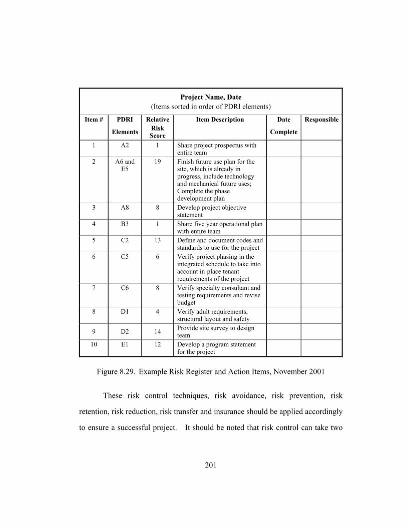
Project Name, Date (Items sorted in order of PDRI elements)

Item # PDRI Relative Item Description Date Responsible

Elements Risk Score Complete

1 A2 1 Share project prospectus with entire team

2 A6 and E5

19 Finish future use plan for the site, which is already in progress, include technology and mechanical future uses; Complete the phase development plan

3 A8 8 Develop project objective statement

4 B3 1 Share five year operational plan with entire team

5 C2 13 Define and document codes and standards to use for the project

6 C5 6 Verify project phasing in the integrated schedule to take into account in-place tenant requirements of the project

7 C6 8 Verify specialty consultant and testing requirements and revise budget

8 D1 4 Verify adult requirements, structural layout and safety

9 D2 14 Provide site survey to design team

10 E1 12 Develop a program statement for the project

Figure 8.29. Example Risk Register and Action Items, November 2001

These risk control techniques, risk avoidance, risk prevention, risk

retention, risk reduction, risk transfer and insurance should be applied accordingly

to ensure a successful project. It should be noted that risk control can take two

201

forms. The first was identified in the previous two sections. Another method is

contingency set aside to take care of unknown risks.

An objective way of measuring the results from risk control measures is to

conduct a second PDRI evaluation. The PDRI score provides an objective

measure of scope completeness and can be used to compare with each other to

obtain metrics for improvement. In addition to PDRI evaluations, the results

from other risk control measures should be tracked as well. All this information

should be well documented to monitor the progress of risk management effort.

This proposed systematic risk management process starts at the pre-project

planning stage of the project life cycle and should be continued through the

project to achieve the project goals.

8.5. LIMITATIONS AND SUMMARY

As presented in Section 4.7, there are some potential limitations of this

study. Two major limitations include non-random sample selection and nature

of retrospective case studies. In addition, the investigation of sample data

revealed the non-normality of dependent variables (cost/schedule growth) at every

level of the independent variable (PDRI score). This non-normality violated the

assumptions of linear regression and thus caution must be taken when interpreting

the results from the linear regression model. However, even when data violate

these assumptions, the method may still be quite robust and will seldom be wrong

when making conclusions about statistically significant or insignificant results

(Knoke and Bohrnstedt 1994). Stevens (1996) recommended a nominal number

of 15 data points per predictor for multivariable analysis when one or more

202

assumptions underlying regression analysis are violated. For this study, there is

only one predictor (PDRI score) and there are at least 62 (or 78) data points for

the model. Therefore, conclusions are made that the non-normality violation

does not deteriorate the ability to generalize results from the sample of interest.

This chapter outlined the development and application of three data

analysis models used in this research. Based on the historical data, the models

were developed using least squares linear regression method, boxplot quartile

analysis method, and Hackney’s accuracy range estimate method. The

application of the models involved quantifying risk impact using PDRI score.

Examples illustrating the application were given for each model. After the

quantification of risk impact, risk reduction measures incorporating PDRI

evaluation was discussed and other risk control technique were explored.

Finally, a systematic risk management system prototype using the PDRI was

introduced and discussed. A process flow chart was developed for this risk

management process as well. The risk management process is a continuous

cycle and should start at the pre-project planning stage and end with project

completion to insure the successful delivery of capital facility projects.

203

Chapter 9 Conclusions and Recommendations

This chapter completes this research study by presenting research

conclusions and recommendations. The research objectives are first reviewed

and specific conclusions relating to whether or not the research data support the

hypotheses are then discussed. Recommendations are made based on research

results and potential areas for future study are identified. The contributions of

this research are discussed at the end.

9.1. REVIEW OF RESEARCH OBJECTIVES

As identified in Chapter 1, this research effort had four primary objectives

which were:

1. To further validate the PDRI through testing by measuring the

level of project scope definition and comparing to the degree of

actual project success using a more robust sample

2. To identify the specific impact of PDRI elements using statistical

analysis methods

3. To develop a systematic project risk management approach based

on the PDRI

4. To establish a baseline methodology and database for follow up

research

The following four sections present a detailed discussion of these four

objectives.

204

9.1.1. Further Validation of the PDRI

The PDRI for industrial projects was validated as an effective scope

definition tool using a sample of 40 industrial projects representing approximately

$3.3 billion (USD) in authorized cost (Dumont et al. 1997). The PDRI for

building projects was validated through a sample of 33 building projects

representing approximately $0.9 billion (USD) in total construction cost. This

research effort continued the data collection and PDRI validation using an

expanded data set. As a result, a total of 62 industrial projects and 78 building

projects were obtained for the analysis of this research.

The previous validation method was adopted for this research. In order

to determine the effectiveness of the PDRI in predicting project success, linear

regression analyses were conducted for both industrial and building projects.

The project success was measured by success index, which was calculated using

both cost performance and schedule performance. With the PDRI score as

independent variable and project success index as dependent variable, bivariate

linear regression analyses were conducted. The results of the regression analysis

using PDRI scores and project success measured by the success index

demonstrated a significant correlation between the two variables for both

industrial and building projects. The results were consistent with previous PDRI

research results that the PDRI is an effective scope definition tool and

subsequently meet the first objective discussed in Chapter 1.

205

9.1.2. Identifying Project Risk and Potential Risk Impact

The second research objective was to identify project risk factors and their

potential impact of project performance based on data collected. Statistical

methods such as effect size analysis, linear regression analyses, and boxplot

quartile analyses were conducted. Actual project scope definition levels were

analyzed to determine if there were scope elements that distinguish between

successful and less-than-successful projects. Projects were first grouped by their

cost/schedule performance into successful and less-than-successful projects.

Then actual scope definition level averages between the two groups were

calculated and compared. Significant differences between the mean definition

levels of the two groups were determined using t-tests. If the mean definition

levels between the two performance groups were different, the magnitude of

difference was measured by effect size analysis. The results showed that

projects with better performance did better in defining certain scope elements than

others. Moreover, elements A3: Operating Philosophy, G4: Process Safety

Management (PSM), G5: Utility Flow Diagrams, and G7: Piping System

Requirements were found to be performance indicators in both cost and schedule

performance for industrial projects. The analysis results also indicated that no

element impacting both cost and schedule were found for building projects.

Only cost performance indicators were identified from this building sample.

In order to estimate the potential risk impacts caused by risk exposures as

a result of incomplete scope definition, three unique techniques were explored to

model the sample data: least squares linear regression method, boxplot quartile

206

analysis method, and Hackney’s accuracy range estimate method. The results

given in Chapter 8 showed that these models can be applied effectively to

summarize and present the data and can be used to estimate cost/schedule

performance based on given PDRI scores. These findings meet the second

stated objective of this dissertation research.

9.1.3. Systematic Project Risk Management Approach Development

Risk management process consists of three major tasks: risk identification,

risk quantification and risk control. It is shown in this research that the PDRI

can be effectively used in all of the three risk management processes. The next

logical step is to document these findings and establish a systematic risk

management approach based on these findings. By applying the CRMS model

developed by Al-Bahar (1988) and adopting the format of pre-project planning

process flow diagram (CII 1995), a systematic risk management process using

PDRI was developed and presented in Figure 8.28.

There are four major sub-processes in the proposed risk management

model: risk identification, risk quantification, risk control, and risk monitoring.

Each process consists of a series of activities that are deemed important in that

process. The PDRI is used in all four stages of the proposed risk management

model and the process may be used one or several times for each project. The

development of this unique systematic risk management system using PDRI

meets the third objective of this research.

207

9.1.4. Establish Baseline Methodology

The last research objective was to establish a baseline methodology and

database for follow-up research. The methodology established included PDRI

benchmarking, data analysis in the form of regression modeling, boxplot quartile

analysis modeling and Hackney’s accuracy range estimate modeling, and

statistical test for effect size. This methodology is unique in pre-project

planning research and provides a basis for early project risk analysis and

management for the construction industry.

Two databases were developed for follow-up research: industrial project

database and building project database. These two datasets both had data stored

in database software package AccessTM and in SPSSTM. All data are ready for

any follow-up research or benchmarking studies deemed relevant.

9.2. RESEARCH HYPOTHESES

In Chapter 3 of this dissertation, two research hypotheses were established

and discussed. The hypotheses were developed based on the results of literature

review, problem statement, findings of previous PDRI and pre-project planning

research. The hypotheses are set up to extend the usage of the PDRI from a pre-

project planning scope definition tool to a risk management tool in the early stage

of a project. These two hypotheses are discussed in detail.

H1: A PDRI score indicates the current level of scope definition and

corresponds to project performance. That is, PDRI scores correlate to

measures of project success.

208

In order to test this hypothesis and to find any existing correlation among

the two variables (PDRI score and project success), a mechanism for measuring

the project success was developed. By adopting success measures from previous

PDRI research, two variables were identified for measuring success versus the

PDRI score:

• Budget Achievement: Adherence to the estimated budget for

detailed design and construction.

• Schedule Achievement: Adherence to the estimated detailed design

and construction schedule for substantial completion

The equation derived to produce a baseline measure of success was:

Project Success Index = 0.50 (Budget Achievement Value) + 0.50 (Schedule Achievement Value)

The results of the least squares linear regression analysis using the PDRI

scores and project success measured by the success index demonstrated a

significant correlation and supported the first research hypothesis. The results

showed that as the PDRI score decreases, the probability of project success

increases. These results support the first research hypothesis.

In addition, the regression results shown in Chapter 8 indicate positive

relationships between PDRI scores and project performance (cost and schedule).

It was statistically shown that as project PDRI score decreases (for both industrial

and building projects in this sample), the project cost/schedule growth decreases.

This result also supports the first research hypothesis.

209

In Chapter 6, project unit cost and PDRI score are analyzed for the 42

institutional organization projects. By comparing the actual unit cost and

budgeted cost for the projects with their PDRI scores, it is shown that project with

lower PDRI score (better pre-project planning) cost less to construct. Taking the

real cost saving as a measure of project success, the unit cost analysis results

support the first research hypothesis by showing the real cost savings for projects

with better pre-project planning in the institutional organization sample.

However, some of the potential limitations of this analysis are

acknowledged. The primary limitation relates to generalizing the sample

characteristics to a larger population. In this study, sample project selection was

based on organizations volunteering projects and not on a random selection

process, organizations may have selected projects with a bias toward success,

which may have influenced the results. In the mean time, the sample projects

provided by the institutional organization provided a homogeneous sample and

were deemed better to generalize the sample characteristics to a larger population

within the organization.

H2: The PDRI is a reliable indicator of potential project risk factors and PDRI

scores can be used to quantify risk impact on project outcomes based on

collected data from actual projects.

The research results also support this second research hypothesis.

Sample projects were categorized into two groups based on their project

performance. The mean definition levels were compared between these two

performance groups. First, the significance of mean definition level difference

210

was tested and determined using t-tests. Then the magnitude of mean definition

level difference was determined for these identified scope elements. The

magnitude of difference was measured by effect size.

The scope elements with significant mean definition level difference were

identified as indicators of poor performance. The scope definition levels can be

related to project performance (cost/schedule growth). Tables 7.12 and 7.13 are

recreated in Tables 9.1 and 9.2 to demonstrate the cost/schedule performance

indicators identified by this research investigation.

Table 9.1. Cost Performance Indicators

Cost Performance Indicators Industrial Projects Element

Building Projects Element

A1. Reliability Philosophy A8. Project Objectives Statement A2. Maintenance Philosophy B2. Maintenance Philosophy A3. Operating Philosophy B4. Design Philosophy B6. Future Expansion Considerations E1. Program Statement B7. Expected Project Life Cycle E2. Building Summary Space List B8. Social Issues E11. Room Data Sheets D2. Project Design Criteria E13. Window Treatment D4. Dismantling and Demolition

Requirements F2. Architectural Design F4. Mechanical Design

F2. Surveys and Soil Tests F5. Electric Design G4. Process Safety Management (PSM) F7. Constructability Analysis G5. Utility Flow Diagrams H1. Identify Long-Lead/Critical G7. Piping System Requirements Equipment and Materials G10. Line List H2. Procurement Procedures and Plans G11. Tie-In List J2. Documentation/Deliverables G12. Piping Specialty Items List L3. Project Delivery Method H2. Equipment Location Drawings J2. Location/Uploading/Storage

Facilities Requirements

P4. Pre-Commission Turnover Sequence Requirements

211

Table 9.2. Schedule Performance Indicators

Schedule Performance Indicators Industrial Projects Element

Building Projects Element

A3. Operating Philosophy N/A G4. Process Safety Management (PSM) G5. Utility Flow Diagrams G7. Piping System Requirements G13. Instrument Index K1. Control Philosophy K6. Instrument & Electrical

Specifications

The PDRI scores were also used to estimate the potential risk impacts

based on historical data. Three different models were established to summarize

and describe the sample data. These models were then applied to estimate

cost/schedule performance versus estimated given a PDRI score. The results

showed that not only the probability of the risk but also the magnitude of the

financial consequences caused by the risk exposures can be estimated. These

results support this second research hypothesis.

9.3. CONCLUSIONS

A number of different methods to collect and analyze the data were

utilized in the dissertation research. Historical project performance and PDRI

data were collected from of 140 sample projects from two industry sectors

representing approximately $5 billion (USD) in total construction cost. The

large amount of data was analyzed using various statistical techniques as well as

qualitative analysis techniques. In addition, a systematic risk management

approach using the PDRI along with a risk management process flow diagram

212

were presented and discussed in detail. Three fundamental conclusions were

reached:

• The completeness of project scope definition during pre-project

planning of capital facilities has a significant and positive direct

effect on overall project success.

• There are specific scope elements identified in the PDRI that the

project team should address that can have a significant and positive

effect on project success.

• The PDRI is an effective tool for scope definition and can be applied

in risk management process during the pre-project planning.

9.4. CONTRIBUTIONS

This research investigation was exploratory in nature and contributes to

the body of knowledge by extending the knowledge of project risk management in

pre-project planning. Previous research identified the PDRI as an effective tool

for measuring project scope development and predicting project performance.

This investigation extended that research by focusing on the application of the

PDRI in different phases of risk management processes. Major contributions of

this research include:

1. This study demonstrated that completeness of scope development has a

significant and positive effect on project success. No previous research

investigation using the PDRI had as many sample projects as this study.

The homogeneous sample from the institutional organization offered a

unique sample within one single organization. The research contributes

213

to the current body of knowledge by providing in-depth analysis and

empirical evidence that scope development during pre-project planning is

important and has a positive effect on project outcomes, including

improvement of cost and schedule predictability as well and real value-

based cost savings.

2. The statistical analysis used to summarize the scope definition levels of

the sample projects is a way to measure the level of scope development

practice in the industrial and building sectors. No comparable research

was found during the literature review. This study contributes to the

current body of knowledge by showing details of industry scope

development practice for this sample.

3. The study contributes to the current body of knowledge by identifying

scope elements that have significant effect on achieving project success.

The project team can use this information to help focus their limited

resources on the issues with larger impacts on project outcomes. The

results provide specific guidance to project teams wishing to address scope

definition during pre-project planning.

4. The systematic risk management approach using the PDRI developed in

this research provides a prototype road map for risk management process

during pre-project planning. It successfully combines the usage of the

PDRI and project risk management process.

214

9.5. RECOMMENDATION FOR FUTURE RESEARCH

Through the course of this research effort, several areas have been

identified as potential areas for future study. The first is in the area of improving

the data collection process. One major limitation of this research is due to the

nature of retrospective case studies. If after-the-fact information is collected, the

quality of this information heavily relies on human recollection. As such, a

certain degree of error is expected. Using “real time” information collected from

an ongoing project should significantly enhance the reliability of the data thereby

increasing the accuracy of any conclusions that can be drawn from the analysis.

Organizations such as CII or individual organization wishing to improve their pre-

project planning process can greatly benefit from using this approach in their

benchmarking effort.

Further analysis in various areas can benefit from an improved survey

instrument and increased sample size. More detailed information concerning the

sample projects should be captured with an improved survey instrument so that

correlations between the PDRI score and other variables (i.e. project size, type of

project, contracting method) can be found to further increase the reliability of the

PDRI in predicting project performance, including estimate predictability and real

cost savings. An initial effort was performed for the institutional organization

projects. However, the effort should be continued with an increased sample size

and more detailed analysis.

This investigation utilized three different analysis methods to model the

sample data. The results obtained are satisfactory for an initial exploratory

215

study. Alternative modeling approaches to better describe the data at hand are

recommended. As an experimental effort, modeling techniques such as

Artificial Neural Network and Second Moment Bayesian Method were explored

and initial efforts showed promising results and may warrant further analysis.

216

Appendix A Logic Flow Diagram for Industrial PDRI

217

Narrative of the Logic Flow Diagram for Industrial Projects

The PDRI Logic Flow Diagram (LFD) is provided to illustrate the

interrelationship between various categories and elements of the PDRI. Note

that the LFD is not "CPM-type" logic in that certain elements are completed prior

to the point when the next elements can start. Many times elements can be

pursued concurrently. As information is gained down stream, elements already

defined have to be revisited. Also, there may be many ways to organize the

work differently than the flow shown. This LFD is provided as a guideline for

planners to use in pursuing the planning process. Your organization may want to

standardize a front-end planning process. The logic presented in these diagrams

could provide the basis for that development.

Note that Section and Category Logic Flow Diagram for the Industrial

PDRI are shown in Figures A.1 and A.2 respectively. Element Logic Flow

Diagram cannot fit on the size of this paper and can be found in the PDRI Virtual

User Group website (www.cii-pdri.org).

218

499 Points

Categories A thru E

423 Points

Categories F thru K

78 Points

Categories L thru P

Page 1 of 3

Logic Flow DiagramProject Definition Rating Index (PDRI)

for Industrial ProjectsSeptember 2000 Rev. 1

Section I:

Basis of Project Design

Section II:

Front End Definition

Section III:

Execution Approach

219

Figure A.1. Section Logic Flow Diagram

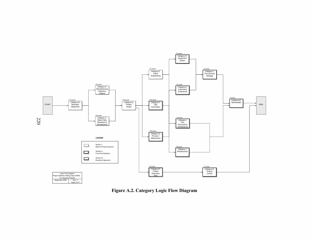
LEGEND

Section IBasis of Project Decision

Section IIFront End Definition

Section IIIExecution Approach

Project Definition Rating Index (PDRI)

September 2000 Rev. 0Page 2 of 3

Logic Flow Diagram

for Industrial Projects

STARTCategory B:

BusinessObjectives

Category A:Manufacturing

ObjectiveCriteria

Category C:Basic DataResearch &

Development

Category D:ProjectScope

Category E:Value

Engineering

Category F:Site

Information

Category G:Process /

Mechanical

Category H:Equipment

Scope

END

213 points

45 points

94 points

120 points

27 points

104 points

Category P:Project

ExecutionPlan

36 points

196 points

Category I:Civil,

Structural &Architectural

19 points

Category J:Infrastructure

25 points

Category N:ProjectControl

17 points

33 points

Category K:Instrument& Electrical

46 points

Category L:Procurement

Strategy

16 points

Category M:Deliverables

9 points

220

Figure A.2. Category Logic Flow Diagram

Appendix B Institutional Organization Risk And Readiness Survey Questionnaires (Project Manager and User)

221

BUILDING PROJECT

Risk & Readiness Assessment

(RRA) User Feedback Questionnaire

Risk & Readiness Research Team

Building Construction Department The University of Texas at Austin

Consultant

An (RRA) Project into the development of scope definition tool for temple projects

222

Date:

Name: Address: Dear ______, The Building Construction Department with the assistance of the University of Texas at Austin and an outside consultant is evaluating the project scope definition process. A research team has developed a project scope evaluation called the Risk & Readiness Assessment (RRA), and is now validating this tool with data from recently completed building projects. The enclosed questionnaire is designed to help in this effort by measuring the quality of project score definition during the pre-project planning phase. The research team will be presenting the results of this study to the Managing Director of the Building Construction Department. The RRA may be approved for use on building construction projects in the future to assist with pre-project planning.

Enclosed are survey forms that will provide the research team information for the identified projects. Please be candid in your responses.

The survey package includes a brief introduction of RRA (blue) and the RRA User Feedback Questionnaire (white). Please complete the Questionnaire and return it in the pre-addressed, stamped envelope provided. The rest of the material is for your information and does not have to be returned. If you have any questions, please feel free to contact me at (123) 456-7890 or by e-mail at abc@def.ghi Questions about the survey or the research process please feel free to contact the consultant at (123) 456-7890 or by e-mail at jkl@mno.pqr.

We would appreciate the return of the surveys by December 18, 2000.

Your participation in this effort is greatly appreciated.

Sincerely,

Director

Home Office Technical Support Services

Encl. (2) RRA Introduction RRA User Feedback Questionnaire

223

Project Risk and Readiness Assessment

Introduction Review of recently completed building projects shows that these projects suffer from poor or incomplete project scope definition. The Building Construction Department needs a user-friendly tool to assist in defining project scope, assessing risk and readiness, and maximizing the chance of project success. A research team from Building Construction Department, an outside consultant and the University of Texas at Austin has developed a tool called the “Risk & Readiness Assessment” (RRA) to serve this purpose. It is an adaptation of the Project Definition Rating Index (PDRI) into building projects. The PDRI, developed by the Construction Industry Institute (CII) is both user friendly and effective for qualifying project scope definition. By introducing RRA, the research team expects significant reduction in the number and cost of change orders, greater ability to maintain project schedules, reduction of risk during construction, improved communication, and achievement of customer satisfaction, thus ensuring the success of temple projects.

RRA Forms RRA for building projects has already been developed and your assistance will help to prove its effectiveness. To fill out the questionnaire, follow these steps: Step 1: Read the question.

Step 2: Collect all data that you need too properly evaluate and select the rating for each question.

Step 3: Select the rating that most closely matches the results of the question. This may require obtaining input form other individuals involved with this process.

Step 4: For each answer, circle the score (1-5) that corresponds to your results.

Step 5: Please make written comments as necessary.

224

SURVEY QUESTIONNAIRE BUILDING PROJECT

RISK & READINESS ASSESSMENT (RRA)

Customer Satisfaction:

Project ID Number : ___________________________________________

1. How closely did the completed temple conform to the written program? (circle only one)

1 2 3 4 5 very different -------------------------------------------------> closely matches

If the facility is very different from the program, please list the reasons for the changes:

________________________________________________________

________________________________________________________

________________________________________________________

2. How closely did the completed temple conform to the scope as defined in the work order? : (circle only one)

1 2 3 4 5 very different ------------------------------------------------> closely matches

If the facility is very different from the program, please list the reasons for the changes:

________________________________________________________

________________________________________________________

________________________________________________________

3. Have there been any alterations or retrofits already completed or anticipated during the first year of operation? ________________________________________________________

________________________________________________________

Approximate Costs: ________________________________________

225

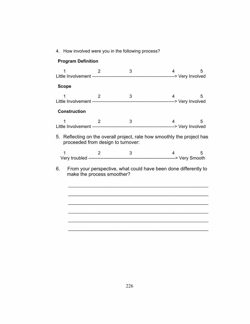
4. How involved were you in the following process?

Program Definition 1 2 3 4 5 Little Involvement -------------------------------------------------------> Very Involved

Scope 1 2 3 4 5 Little Involvement -------------------------------------------------------> Very Involved

Construction 1 2 3 4 5 Little Involvement -------------------------------------------------------> Very Involved

5. Reflecting on the overall project, rate how smoothly the project has proceeded from design to turnover:

1 2 3 4 5 Very troubled ----------------------------------------------------------> Very Smooth

6. From your perspective, what could have been done differently to make the process smoother?

________________________________________________________

________________________________________________________

________________________________________________________

________________________________________________________

________________________________________________________

________________________________________________________

226

BUILDING PROJECT

Risk & Readiness Assessment

(RRA) Project Manager Questionnaire

Risk & Readiness Research Team

Building Construction Department The University of Texas at Austin

Consultant

An (RRA) Project into the development of scope definition tool for temple projects

227

Date Name: Address: Dear: The Building Construction Department with the assistance of the University of Texas at Austin and an outside consultant is evaluating the project scope definition process. A research team has developed a project scope evaluation called the Risk & Readiness Assessment (RRA), and is now validating this tool with data from recently completed building projects. The enclosed questionnaire is designed to help in this effort by measuring the quality of project score definition during the pre-project planning phase. The research team will be presenting the results of this study to the Managing Director of the Building Construction Department. The RRA may be approved for use on building construction projects in the future to assist with pre-project planning. Enclosed are survey forms that will provide the research team information for the identified projects. Please be candid in your responses. The survey package includes a brief introduction of RRA (blue) and the RRA Questionnaire (which includes the Project Score Sheet) (white), and RRA Element Description (yellow). Please complete the Questionnaire (white) and return it in the pre-addressed, stamped envelope provided. The rest of the material is for your information and does not have to be returned. If you have any questions, please feel free to contact me at (123) 456-7890 or by e-mail at abc@def.ghi Questions about the survey or the research process please feel free to contact the consultant at (123) 456-7890 or by e-mail at jkl@mno.pqr. We would appreciate the return of the surveys by December 18, 2000. Your participation in this effort is greatly appreciated. Sincerely, Director Home Office Technical Support Services

Encl. (3) RRA Introduction – Blue RRA Questionnaire – White RRA Element Descriptions – Yellow

228

Project Risk and Readiness Assessment

Introduction Review of recently completed building projects shows that these projects suffer from poor or incomplete project scope definition. The Building Construction Department needs a user-friendly tool to assist in defining project scope, assessing risk and readiness, and maximizing the chance of project success. A research team from Building Construction Department, an outside consultant and the University of Texas at Austin has developed a tool called the “Risk & Readiness Assessment” (RRA) to serve this purpose. It is an adaptation of the Project Definition Rating Index (PDRI) into building projects. PDRI, developed by Construction Industry Institute (CII) is both user friendly and effective for qualifying project scope definition. By introducing RRA, the research team expects significant reduction in the number and cost of change orders, greater ability to maintain project schedules, reduction of risk during construction, improved communication, and achievement of customer satisfaction, thus ensuring the success of temple projects.

RRA Forms RRA for building projects has already been developed and your assistance will help to prove its effectiveness. The RRA Survey Questionnaire consists of three main sections divided into 11 categories that are further divided into individual elements. Sections, categories, and elements on the Score Sheet parallel those in the Survey Questionnaire: Steps remaining in this research effort include:

1. Benchmarking building projects 2. Analyzing the data 3. Disseminating results and conclusions 4. Refining RRA documents for application to individual

projects.

229

PROJECT MANAGER SURVEY QUESTIONNAIRE BUILDING PROJECT

RISK & READINESS ASSESSMENT (RRA)

PROJECT BACKGROUND INFORMATION

1.0. Date: 1.1 Project ID Number: 1.2. Home Office Contact:

1. Name: 2. Tel. No.: 3. E-mail:

1.3 Consultant Contact: 1. Name:

2. Tel. No.: Fax No.: 3. E-mail:

1.4 Completion Date and Return:

1. December 18, 2000 2. Return in pre-addressed envelope

230

2.0 General Project Information: 1. Project ID Number: __________________________________________

2. What is the size of the Building (e.g., number of occupants, volume/capacity, net or gross square footage, number of floors, etc.) _________________________________________________________________

_________________________________________________________________

_________________________________________________________________

_________________________________________________________________

3. From your perspective, what was the level of the project complexity?

[ ] High [ ] Average [ ] Low

4. Was there anything unique about this project? (please check all that apply)

[ ] New Standard Plan utilized [ ] First of a kind changes to Standard Plans [ ] Largest (scale) [ ] Other (e.g., special development requirements, equipment, location, execution, etc.) Please describe: _____________________________________ [ ] Not applicable

5. What was the execution contracting approach that you used on your project?

[ ] Design-Build [ ] Design-Bid-Build [ ] Other (please specify) __________________________________ 2.1. Schedule Information:

1. Please provide the following schedule information:

Planned Actual Item (mm/dd/yy) (mm/dd/yy) Project Announcement Start Date of Construction Date of Substantial Completion

2. If there were any schedule extensions or reductions during development of

231

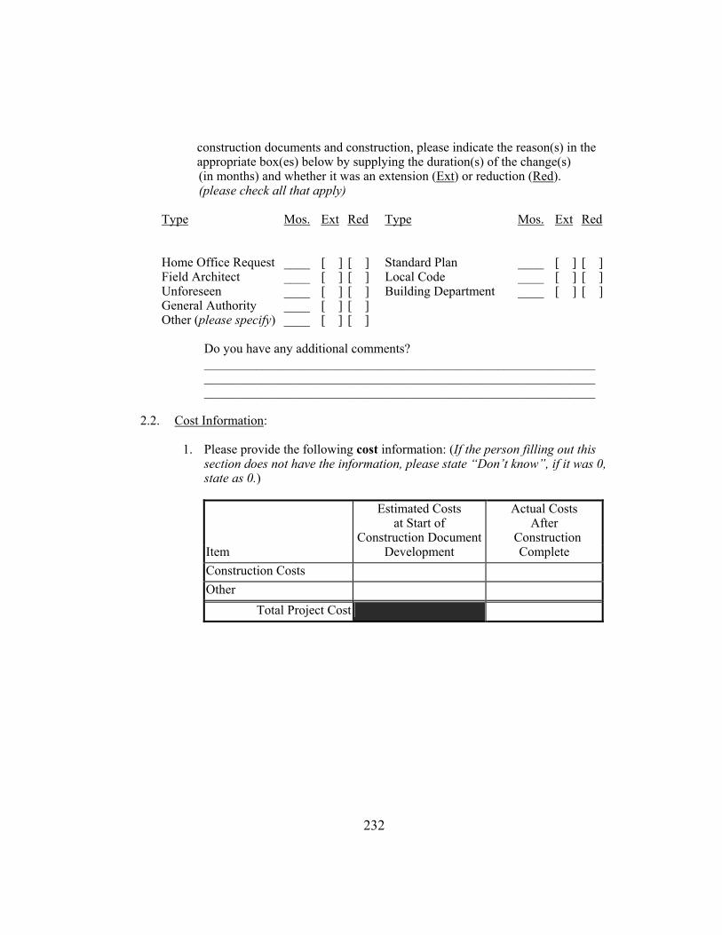
construction documents and construction, please indicate the reason(s) in the appropriate box(es) below by supplying the duration(s) of the change(s) (in months) and whether it was an extension (Ext) or reduction (Red). (please check all that apply)

Type Mos. Ext Red Type Mos. Ext Red Home Office Request ____ [ ] [ ] Standard Plan ____ [ ] [ ] Field Architect ____ [ ] [ ] Local Code ____ [ ] [ ] Unforeseen ____ [ ] [ ] Building Department ____ [ ] [ ] General Authority ____ [ ] [ ] Other (please specify) ____ [ ] [ ] Do you have any additional comments? ____________________________________________________________ ____________________________________________________________ ____________________________________________________________ 2.2. Cost Information:

1. Please provide the following cost information: (If the person filling out this section does not have the information, please state “Don’t know”, if it was 0, state as 0.)

Estimated Costs

at Start of Construction Document

Actual Costs After

Construction Item Development Complete Construction Costs Other

Total Project Cost

232

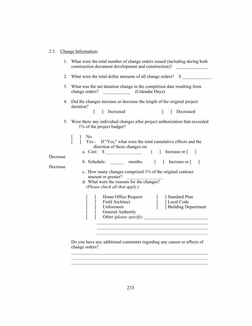
2.3. Change Information:

1. What were the total number of change orders issued (including during both construction document development and construction)? ______________

2. What were the total dollar amounts of all change orders? $ _____________ 3. What was the net duration change in the completion date resulting from

change orders? ____________ (Calendar Days) 4. Did the changes increase or decrease the length of the original project duration? [ ] Increased [ ] Decreased 5. Were there any individual changes after project authorization that exceeded 1% of the project budget? [ ] No [ ] Yes - If "Yes," what were the total cumulative effects and the

direction of these changes on: a. Cost: $ ________________ [ ] Increase or [ ] Decrease b. Schedule: ______ months. [ ] Increase or [ ] Decrease c. How many changes comprised 1% of the original contract amount or greater? ________________ d. What were the reasons for the changes? (Please check all that apply.) [ ] Home Office Request [ ] Standard Plan [ ] Field Architect [ ] Local Code [ ] Unforeseen [ ] Building Department [ ] General Authority [ ] Other (please specify) ____________________________ _________________________________________________ _________________________________________________ _________________________________________________ Do you have any additional comments regarding any causes or effects of change orders? ____________________________________________________________ ____________________________________________________________ ____________________________________________________________

233

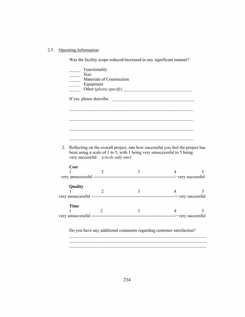
2.5. Operating Information:

Was the facility scope reduced/increased in any significant manner? _____ Functionality _____ Size _____ Materials of Construction _____ Equipment _____ Other (please specify) _______________________________ If yes, please describe _____________________________________ ________________________________________________________ ________________________________________________________ ________________________________________________________ ________________________________________________________ 2. Reflecting on the overall project, rate how successful you feel the project has

been using a scale of 1 to 5, with 1 being very unsuccessful to 5 being very successful: (circle only one) Cost 1 2 3 4 5 very unsuccessful -------------------------------------------------------> very successful Quality 1 2 3 4 5 very unsuccessful ---------------------------------------------------------> very successful Time 1 2 3 4 5 very unsuccessful ---------------------------------------------------------> very successful Do you have any additional comments regarding customer satisfaction? ______________________________________________________________ ______________________________________________________________ ______________________________________________________________

234

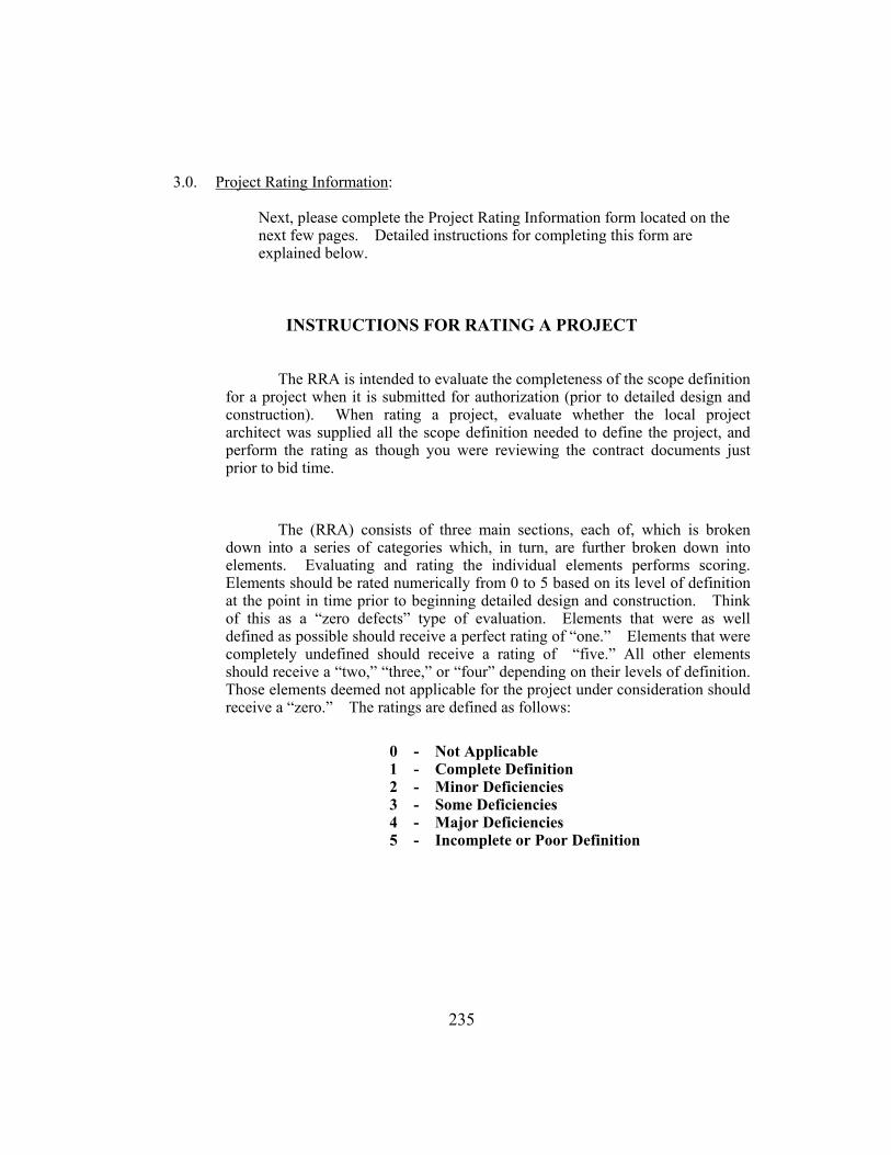
3.0. Project Rating Information: Next, please complete the Project Rating Information form located on the next few pages. Detailed instructions for completing this form are explained below.

INSTRUCTIONS FOR RATING A PROJECT

The RRA is intended to evaluate the completeness of the scope definition for a project when it is submitted for authorization (prior to detailed design and construction). When rating a project, evaluate whether the local project architect was supplied all the scope definition needed to define the project, and perform the rating as though you were reviewing the contract documents just prior to bid time.

The (RRA) consists of three main sections, each of, which is broken down into a series of categories which, in turn, are further broken down into elements. Evaluating and rating the individual elements performs scoring. Elements should be rated numerically from 0 to 5 based on its level of definition at the point in time prior to beginning detailed design and construction. Think of this as a “zero defects” type of evaluation. Elements that were as well defined as possible should receive a perfect rating of “one.” Elements that were completely undefined should receive a rating of “five.” All other elements should receive a “two,” “three,” or “four” depending on their levels of definition. Those elements deemed not applicable for the project under consideration should receive a “zero.” The ratings are defined as follows:

0 - Not Applicable 1 - Complete Definition 2 - Minor Deficiencies 3 - Some Deficiencies 4 - Major Deficiencies 5 - Incomplete or Poor Definition

235

To rate an element, first read its definition in the Description section of the 64 RRA Elements document (yellow). Some elements contain a list of items to be considered when evaluating their levels of definition. These lists may be used as checklists. Note that some of these items may not be applicable for your project. Next, refer to the Project Rating Information form and locate the element. Please choose only one definition level (0, 1, 2, 3, 4, or 5) for that element based on your perception of how well it was defined when the project was authorized. Once you have chosen the appropriate definition level for the element please check (√ ) the corresponding box. Do this for each of the 64 elements in the RRA. Be sure to rate each element.

236

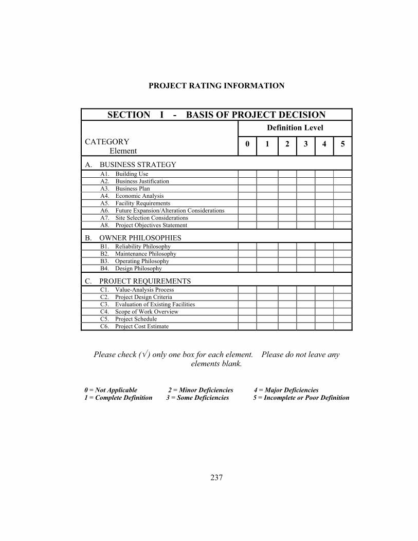
PROJECT RATING INFORMATION

SECTION I - BASIS OF PROJECT DECISION Definition Level

CATEGORY Element

0 1 2 3 4 5

A. BUSINESS STRATEGY A1. Building Use A2. Business Justification A3. Business Plan A4. Economic Analysis A5. Facility Requirements A6. Future Expansion/Alteration Considerations A7. Site Selection Considerations A8. Project Objectives Statement

B. OWNER PHILOSOPHIES B1. Reliability Philosophy B2. Maintenance Philosophy B3. Operating Philosophy B4. Design Philosophy

C. PROJECT REQUIREMENTS C1. Value-Analysis Process C2. Project Design Criteria C3. Evaluation of Existing Facilities C4. Scope of Work Overview C5. Project Schedule C6. Project Cost Estimate

Please check (√ ) only one box for each element. Please do not leave any elements blank.

0 = Not Applicable 2 = Minor Deficiencies 4 = Major Deficiencies 1 = Complete Definition 3 = Some Deficiencies 5 = Incomplete or Poor Definition

237

SECTION II - BASIS OF DESIGN

Definition Level CATEGORY Element

0 1 2 4 5

D. SITE INFORMATION D1. Site Layout D2. Site Surveys

3

D3. Civil/Geotechnical Information

D5. Environmental Assessment D6. Utility Sources with Supply Conditions D7. Site Life Safety Considerations D8. Special Water and Waste Treatment Requirements

E1. Program Statement E2. Building Summary Space List E3. Overall Adjacency Diagrams E4. Stacking Diagrams E5. Growth & Phased Development E6. Circulation and Open Space Requirements E7. Functional Relationship Diagrams/Room by Room

E8. Loading/Unloading/Storage Facilities Requirements

E9. Transportation Requirements E10. Building Finishes E11. Room Data Sheets E12. Furnishings, Equipment, & Built-Ins E13. Window Treatment F. BUILDING/PROJECT DESIGN PARAMETERS

D4. Governing Regulatory Requirements

E. BUILDING PROGRAMMING

F1. Civil/Site Design F2. Architectural Design F3. Structural Design F4. Mechanical Design F5. Electrical Design F6. Building Life Safety Requirements F7. Constructability Analysis F8. Technological Sophistication G. EQUIPMENT G1. Equipment List G2. Equipment Location Drawings G3. Equipment Utility Requirements

Please check (√ ) only one box for each element. Please do not leave any elements blank.

0 = Not Applicable 2 = Minor Deficiencies 4 = Major Deficiencies 1 = Complete Definition 3 = Some Deficiencies 5 = Incomplete or Poor Definition

238

SECTION III - EXECUTION APPROACH

Definition Level

CATEGORY Element

0 1 2 3 4 5

H. PROCUREMENT STRATEGY H1. Identify Long Lead/Critical Equip. & Materials H2. Procurement Procedures and Plans

J. DELIVERABLES J1. CADD/Model Requirements J2. Documentation/Deliverables

K. PROJECT CONTROL K1. Project Quality Assurance and Control K2. Project Cost Control K3. Project Schedule Control K4. Risk Management K5. Safety Procedures

L. PROJECT EXECUTION PLAN L1. Project Organization L2. Owner Approval Requirements L3. Project Delivery Method L4. Design/Construction Plan & Approach L5. Substantial Completion Requirements

Please check (√ ) only one box for each element. Please do not leave any

elements blank. 0 = Not Applicable 2 = Minor Deficiencies 4 = Major Deficiencies 1 = Complete Definition 3 = Some Deficiencies 5 = Incomplete or Poor Definition

239

4.0. General Information: 1. How long did it take you (or your team) to fill out both the Project Background Information and the Project Rating Information forms? Please specify in total work-hours (for example, a team of three working for four hours equals 12 total work-hours). Project Background Information: _________________ total work-hours Project Rating Information: _________________ total work-hours 2. Please have every individual involved with completing any portion of either the Project Background Information or the Project Rating Information forms complete the following information. Name: ______________________________________________________ Local Area: __________________________________________________ Position: ____________________________________________________ Department/Division: __________________________________________ Address (if different than address on page 1 of this questionnaire): _________________________________________________________ _________________________________________________________ _________________________________________________________ Phone: _______________________ Fax: ____________________ E-mail: ______________________________________________________ Which section(s) of the Project Background Information and the Project Rating Information forms did you fill out? (for example, Project Rating categories A-E and Project Background sections 2.1-2.2) _________________________________________________________ _________________________________________________________ _________________________________________________________

240

Thank you very much for your participation in this survey! Please return this form to:

Consultant P.O. Box 123 RRA PROJECT BACKGROUND AND RATING INFORMATION

241

Appendix C PDRI for Industrial Projects Score Sheets

242

INDUSTRIAL PROJECT SCORE SHEET

SECTION I - BASIS OF PROJECT DECISION Definition Level

CATEGORY Element 0 1 2 3 4 5 Score

A. MANUFACTURING OBJECTIVES CRITERIA (Maximum Score = 45) A1. Reliability Philosophy 0 1 5 9 14 20 A2. Maintenance Philosophy 0 1 3 5 7 9 A3. Operating Philosophy 0 1 4 7 12 16

CATEGORY A TOTAL B. BUSINESS OBJECTIVES (Maximum Score = 213) B1. Products 0 1 11 22 33 56 B2. Market Strategy 0 2 5 10 16 26 B3. Project Strategy 0 1 5 9 14 23 B4. Affordability/Feasibility 0 1 3 6 9 16 B5. Capacities 0 2 11 21 33 55 B6. Future Expansion Considerations 0 2 3 6 10 17 B7. Expected Project Life Cycle 0 1 2 3 5 8 B8. Social Issues 0 1 2 5 7 12

CATEGORY B TOTAL

C. BASIC DATA RESEARCH & DEVELOPMENT (Maximum Score = 94) C1. Technology 0 2 10 21 39 54 C2. Processes 0 2 8 17 28 40

CATEGORY C TOTAL D. PROJECT SCOPE (Maximum Score = 120) D1. Project Objectives Statement 0 2 25 D2. Project Design Criteria 0 3 6 11 16 22 D3. Site Characteristics Available vs. Req’d 0 2 29 D4. Dismantling and Demolition Req’mts 0 2 5 8 12 15 D5. Lead/Discipline Scope of Work 0 1 4 7 10 13 D6. Project Schedule 0 2 16

CATEGORY D TOTAL E. VALUE ENGINEERING (Maximum Score = 27) E1. Process Simplification 0 0 8 E2. Design & Material Alts. Considered/Rejected

0 0 7

E3. Design For Constructability Analysis 0 0 3 5 8 12 CATEGORY E TOTAL

Section I Maximum Score = 499 SECTION I TOTAL Definition Levels

0 = Not Applicable 2 = Minor Deficiencies 4 = Major Deficiencies 1 = Complete Definition 3 = Some Deficiencies 5 = Incomplete or Poor Definition

SECTION II - FRONT END DEFINITION

243

Definition Level CATEGORY Element

0 1 2 3 4 5 Score

F. SITE INFORMATION (Maximum Score = 104) F1. Site Location 0 2 32 F2. Surveys & Soil Tests 0 1 4 7 10 13 F3. Environmental Assessment 0 2 5 10 15 21 F4. Permit Requirements 0 1 3 5 9 12 F5. Utility Sources with Supply Conditions 0 1 4 8 12 18 F6. Fire Protection & Safety Considerations 0 1 2 4 5 8

CATEGORY F TOTAL G. PROCESS / MECHANICAL (Maximum Score = 196) G1. Process Flow Sheets 0 2 8 17 26 36 G2. Heat & Material Balances 0 1 5 10 17 23 G3. Piping & Instrumentation Diagrams (P&ID's)

0 2 8 15 23 31

G4. Process Safety Management (PSM) 0 1 2 4 6 8 G5. Utility Flow Diagrams 0 1 3 6 9 12 G6. Specifications 0 1 4 8 12 17 G7. Piping System Requirements 0 1 2 4 6 8 G8. Plot Plan 0 1 4 8 13 17 G9. Mechanical Equipment List 0 1 4 9 13 18 G10. Line List 0 1 2 4 6 8 G11. Tie-in List 0 1 6 2 3 4 G12. Piping Specialty Items List 0 1 1 2 3 4 G13. Instrument Index 0 1 2 4 5 8

CATEGORY G TOTAL H. EQUIPMENT SCOPE (Maximum Score = 33) H1. Equipment Status 0 1 4 8 12 16 H2. Equipment Location Drawings 0 1 2 5 7 10 H3. Equipment Utility Requirements 0 1 2 3 5 7

CATEGORY H TOTAL I. CIVIL, STRUCTURAL, & ARCHITECTURAL (Maximum Score = 19) I1. Civil/Structural Requirements 0 1 3 6 9 12 I2. Architectural Requirements 0 1 2 4 5 7

CATEGORY I TOTAL J. INFRASTRUCTURE (Maximum Score = 25) J1. Water Treatment Requirements 0 1 3 5 7 10 J2. Loading/Unloading/Storage Facilities Req’mts

0 1 3 5 7 10

J3. Transportation Requirements 0 1 5 CATEGORY J TOTAL

Definition Levels

0 = Not Applicable 2 = Minor Deficiencies 4 = Major Deficiencies 1 = Complete Definition 3 = Some Deficiencies 5 = Incomplete or Poor Definition

SECTION II - FRONT END DEFINITION (continued...)

244

Definition Level CATEGORY Element

0 1 2 3 4 5 Score

K. INSTRUMENT & ELECTRICAL (Maximum Score = 46) K1. Control Philosophy 0 1 3 5 7 10 K2. Logic Diagrams 0 1 4 K3. Electrical Area Classifications 0 0 2 4 7 9 K4. Substation Req’mts Power Sources Ident. 0 1 3 5 7 9 K5. Electric Single Line Diagrams 0 1 2 4 6 8 K6. Instrument & Electrical Specifications 0 1 2 3 5 6

CATEGORY K TOTAL

Section II Maximum Score = 423 SECTION II TOTAL

SECTION III - EXECUTION APPROACH Definition Level

CATEGORY Element 0 1 2 3 4 5 Score

L. PROCUREMENT STRATEGY (Maximum Score = 16) L1. Identify Long Lead/Critical Equip. & Mat’ls

0 1 2 4 6 8

L2. Procurement Procedures and Plans 0 0 1 2 4 5 L3. Procurement Responsibility Matrix 0 3

CATEGORY L TOTAL

M. DELIVERABLES (Maximum Score = 9) M1. CADD/Model Requirements 0 0 1 1 2 4 M2. Deliverables Defined 0 0 1 2 3 4 M3. Distribution Matrix 0 0 1

CATEGORY M TOTAL

N. PROJECT CONTROL (Maximum Score = 17) N1. Project Control Requirements 0 0 2 4 6 8 N2. Project Accounting Requirements 0 0 1 2 2 4 N3. Risk Analysis 0 1 5

CATEGORY N TOTAL

0

Definition Levels

0 = Not Applicable 2 = Minor Deficiencies 4 = Major Deficiencies 1 = Complete Definition 3 = Some Deficiencies 5 = Incomplete or Poor Definition

245

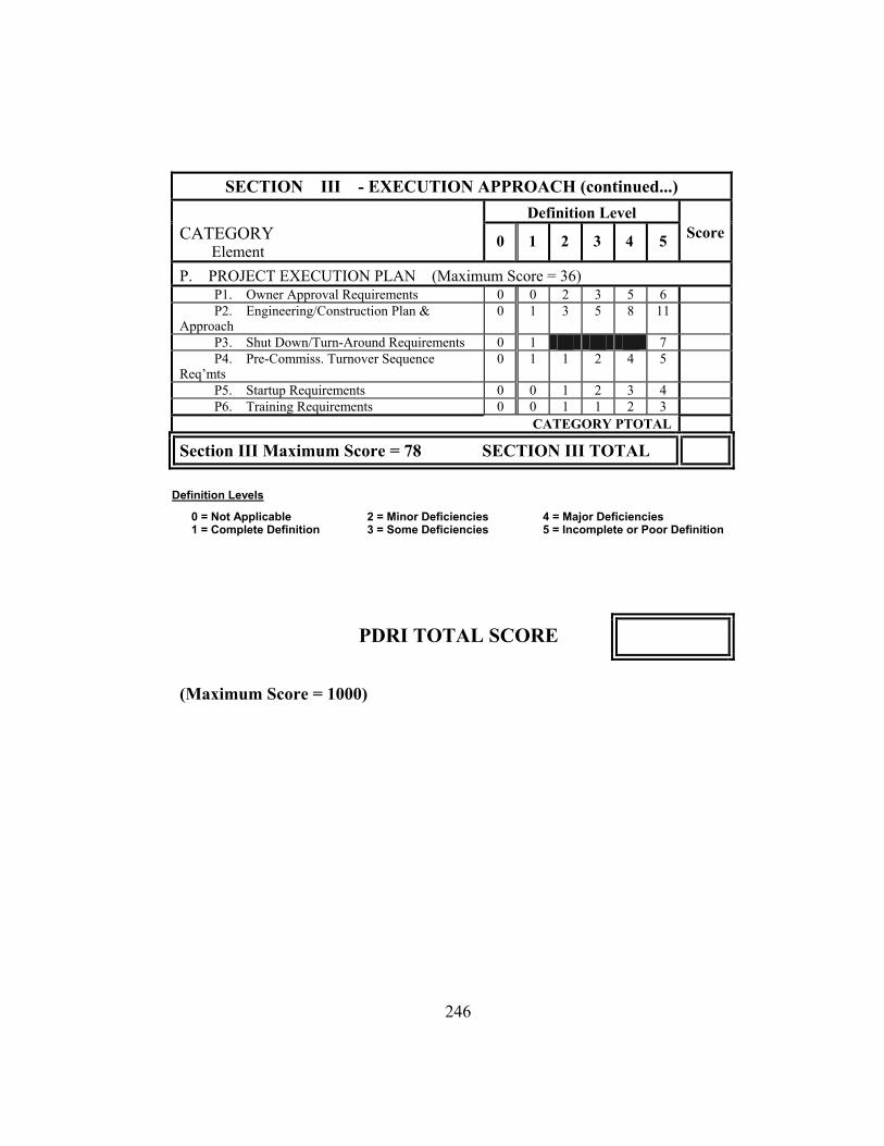
SECTION III - EXECUTION APPROACH (continued...) Definition Level

CATEGORY Element

0 1 2 3 4 5 Score

P. PROJECT EXECUTION PLAN (Maximum Score = 36) P1. Owner Approval Requirements 0 0 2 3 5 6 P2. Engineering/Construction Plan & Approach

0 1 3 5 8 11

P3. Shut Down/Turn-Around Requirements 0 1 7 P4. Pre-Commiss. Turnover Sequence Req’mts

0 1 1 2 4 5

P5. Startup Requirements 0 0 1 2 3 4 P6. Training Requirements 0 0 1 1 2 3

CATEGORY PTOTAL

Section III Maximum Score = 78 SECTION III TOTAL

Definition Levels

0 = Not Applicable 2 = Minor Deficiencies 4 = Major Deficiencies 1 = Complete Definition 3 = Some Deficiencies 5 = Incomplete or Poor Definition

PDRI TOTAL SCORE (Maximum Score = 1000)

246

Appendix D Project Performance and Success Index

247

Industrial Project Performance, Achievement, and PDRI Score

Project ID

Cost Performance

Schedule Performance

Budget Achievement

Schedule Achievement

Success Index

PDRI Score

C199 -40.4% -15.8% 5 5 5 223 C200 19.3% -17.3% 1 5 3 465 C320 1.3% 9.6% 3 2 2.5 192 C323 -3.1% 40.0% 4 1 2.5 138 C325 -0.6% -3.7% 4 4 4 181 C330 38.8% 8.9% 1 2 1.5 109 C338 5.1% -3.6% 2 4 3 240

C4711 0.0% -4.1% 3 4 3.5 172 C4721 -4.6% 1.3% 4 3 3.5 170 O133 0.5% -16.0% 3 5 4 175

7.1% -12.5% 2 5 3.5 305 O316 -0.8% 0.0% 4 3 3.5 112 O317 -9.6% 0.0% 5 3 4 240 O318 4.2% 7.5% 2 2 2 231 O319 -3.0% -10.3% 4 5 4.5 114 O324 28.9% 9.6% 1 2 1.5 90 O339 -12.4% -8.5% 5 4 4.5 156 O439 -24.8% 0.0% 5 3 4 135

-12.4% -3.2% 5 4 4.5 241 O4704 -9.9% -15.1% 5 5 5 173 O4705 -6.1% -12.1% 4 5 4.5 156 P-01 6.6% 65.0% 2 1 1.5 440 P-02 -17.4% 0.0% 5 3 4 82 P-04 -21.7% -13.8% 5 5 5 160 P-05 -7.4% -33.0% 4 5 4.5 173 P-06 0.0% 28.6% 3 1 2 140 P-09 9.5% -7.4% 2 4 3 261 P-11 0.0% 0.0% 3 3 3 149 P-12 7.8% 0.0% 2 3 2.5 384 P-16 5.9% 20.0% 2 1 1.5 191 P-18 -3.4% 25.0% 4 1 2.5 171 P-19 8.8% -26.0% 2 5 3.5 324 P-20 -9.2% 0.0% 3 4 3.5 153 P-21 -1.0% -7.7% 4 4 4 162 P-22 12.2% 10.0% 1 2 1.5 291 P-23 1.7% 7.7% 2 2 2 301 P-24 2.3% 0.0% 2 3 2.5 250 P-25 -9.1% -43.3% 4 5 4.5 143 P-26 -8.6% -27.8% 4 5 4.5 218

O314

O4703

248

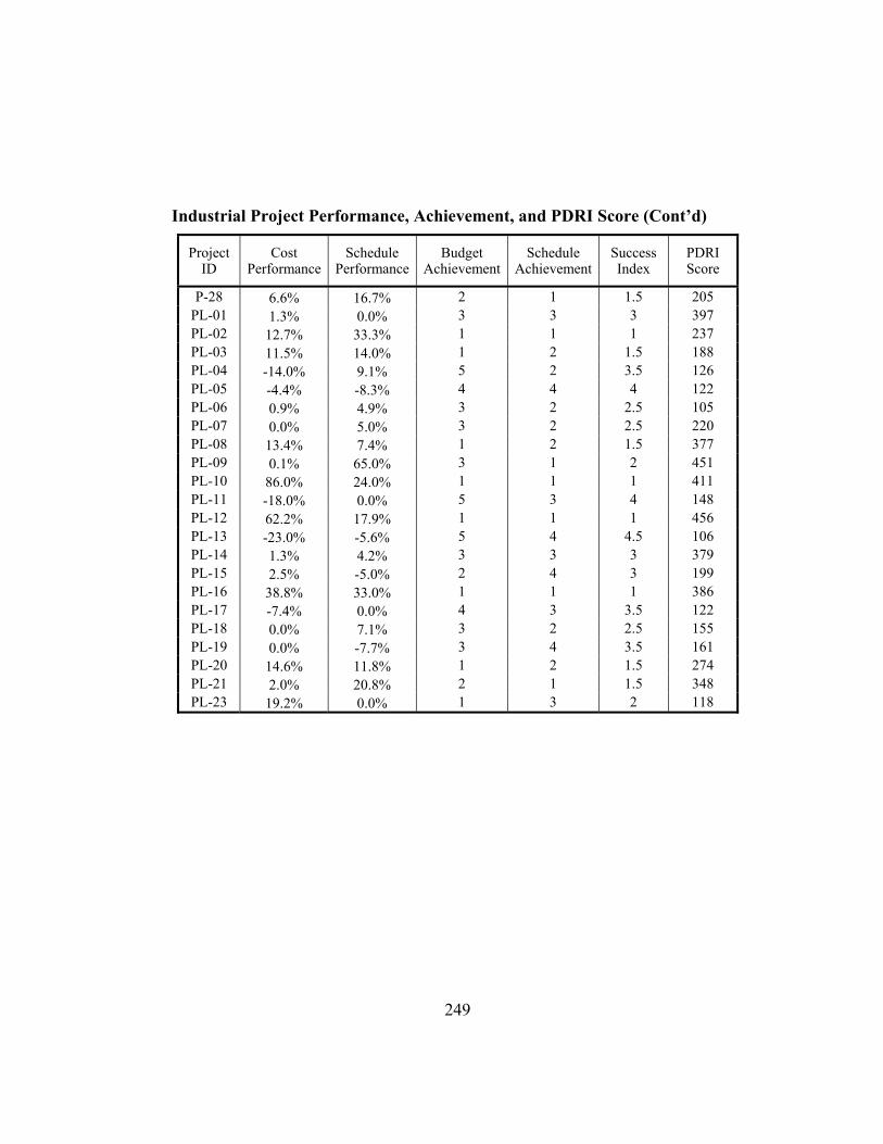
Industrial Project Performance, Achievement, and PDRI Score (Cont’d)

Project ID

Cost Performance

Schedule Performance

Budget Achievement

Schedule Achievement

Success Index

PDRI Score

P-28 6.6% 16.7% 2 1 1.5 205 PL-01 1.3% 0.0% 3 3 3 397 PL-02 12.7% 33.3% 1 1 1 237 PL-03 11.5% 14.0% 1 2 1.5 188 PL-04 -14.0% 9.1% 5 2 3.5 126 PL-05 -4.4% -8.3% 4 4 4 122 PL-06 0.9% 4.9% 3 2 2.5 105 PL-07 0.0% 5.0% 3 2 2.5 220 PL-08 13.4% 7.4% 1 2 1.5 377 PL-09 0.1% 65.0% 3 1 2 451 PL-10 86.0% 24.0% 1 1 1 411 PL-11 -18.0% 0.0% 5 3 4 148 PL-12 62.2% 17.9% 1 1 1 456 PL-13 -23.0% -5.6% 5 4 4.5 106 PL-14 1.3% 4.2% 3 3 3 379 PL-15 2.5% -5.0% 4 199 2 3 PL-16 38.8% 33.0% 1 1 1 386 PL-17 -7.4% 0.0% 4 3 3.5 122 PL-18 0.0% 7.1% 2 3 2.5 155 PL-19 0.0% -7.7% 3 4 3.5 161 PL-20 14.6% 11.8% 1 2 1.5 274 PL-21 2.0% 20.8% 2 1 1.5 348 PL-23 19.2% 0.0% 1 3 2 118

249

Building Project Performance, Achievement, and PDRI Score Project

ID Cost

Performance Schedule

PerformanceBudget

AchievementSchedule

AchievementSuccess Index

PDRI Score

CQ01 -1.3% 1.0% 5 4 4.5 102 CQ02 -0.5% 1.1% 5 4 4.5 139 CQ03 16.7% -7.4% 2 5 3.5 149 CQ04 10.7% 0.0% 2 5 3.5 648 CQ05 5.0% 0.0% 4 5 4.5 202 CQ06 -22.4% 20.0% 5 2 3.5 188 CQ07 6.6% 0.0% 3 5 4 151 CQ08 6.0% 6.9% 74 3 3 3 CQ09 1.7% 1.3% 4 4 4 160

6.8% -9.0% 3 5 CQ11 6.6% 6.9% 3 3 3 238 CQ12 25.7% 4.6% 1 4 2.5 165 LT-01 2.9% 9.0% 4 3 3.5 363 LT-02 -1.1% -1.5% 5 5 5 214 LT-04 4.2% 6.3% 4 4 4 199 ST-01 8.9% 31.8% 3 2 2.5 308 ST-02 16.1% 14.1% 2 2 2 292 ST-03 5.6% 14.7% 4 2 3 320 ST-04 1.5% 27.1% 5 2 3.5 329 ST-05 3.3% 0.0% 4 5 4.5 292 ST-06 54.4% 13.9% 1 3 2 309 ST-07 19.5% 35.5% 1 1 1 619 ST-08 13.3% -0.4% 2 5 3.5 301 ST-09 22.4% 36.0% 1 1 1 414 ST-10 14.9% 4.2% 2 4 3 339 ST-11 2.3% -3.7% 4 5 4.5 286 ST-12 6.1% 10.9% 3 3 3 497 ST-13 19.5% 12.4% 1 3 2 351 ST-14 4.2% 106.8% 4 1 2.5 379

17.4% 1 1 276 ST-16 8.5% 34.3% 3 1 2 564 ST-17 9.2% 7.7% 3 3 3 354 ST-18 6.6% 9.2% 3 3 3 305

9.4% 13.9% 3 3 469 ST-20 9.7% 23.3% 2 2 2 319 ST-21 12.1% 15.8% 2 2 2 417 ST-22 32.5% 83.1% 1 1 1 425

7.2% 12.2% 3 3 343 11.8% 30.2% 2 2 2 310

ST-25 14.3% 45.8% 2 1 1.5 465

CQ10 4 205

ST-15 34.3% 1

ST-19 3

ST-23 3 ST-24

250

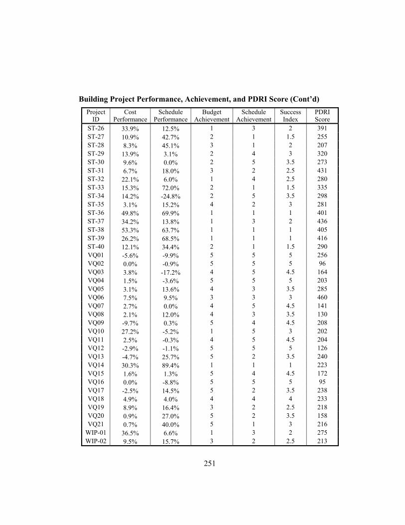
Building Project Performance, Achievement, and PDRI Score (Cont’d) Project

ID Cost

Performance Schedule

PerformanceBudget

AchievementSchedule

AchievementSuccess Index

PDRI Score

ST-26 33.9% 12.5% 1 3 2 391 ST-27 10.9% 42.7% 2 1 1.5 255 ST-28 8.3% 45.1% 3 1 2 207 ST-29 13.9% 3.1% 2 4 3 320 ST-30 9.6% 0.0% 2 5 3.5 273 ST-31 6.7% 18.0% 3 2 2.5 431 ST-32 22.1% 6.0% 1 4 2.5 280 ST-33 15.3% 72.0% 2 1 1.5 335 ST-34 14.2% -24.8% 2 5 3.5 298 ST-35 3.1% 15.2% 4 2 3 281

49.8% 69.9% 401 ST-37 34.2% 13.8% 1 3 2 436 ST-38 53.3% 63.7% 1 1 1 405 ST-39 26.2% 68.5% 1 1 1 416

12.1% 34.4% 2 1 1.5 290 5 5 5 256

VQ02 0.0% -0.9% 5 5 5 96 VQ03 3.8% -17.2% 4 5 4.5 164 VQ04 1.5% -3.6% 5 5 5 203 VQ05 3.1% 13.6% 4 3 3.5 285 VQ06 7.5% 9.5% 3 3 3 460 VQ07 2.7% 0.0% 4 5 4.5 141 VQ08 2.1% 12.0% 4 3 3.5 130 VQ09 -9.7% 0.3% 5 4 4.5 208 VQ10 27.2% -5.2% 1 5 3 202 VQ11 2.5% -0.3% 4 5 4.5 204

5 5 5 126 VQ13 -4.7% 25.7% 3.5 5 2 240 VQ14 30.3% 89.4% 1 1 1 223 VQ15 1.6% 1.3% 5 4 4.5 172 VQ16 0.0% -8.8% 5 5 5 95 VQ17 -2.5% 14.5% 5 2 3.5 238 VQ18 4.9% 4.0% 4 4 4 233 VQ19 8.9% 16.4% 3 2 2.5 218 VQ20 0.9% 27.0% 5 2 3.5 158 VQ21 0.7% 40.0% 5 1 3 216

36.5% 6.6% 1 3 2 275 WIP-02 9.5% 15.7% 3 2 2.5 213

ST-36 1 1 1

ST-40 VQ01 -5.6% -9.9%

VQ12 -2.9% -1.1%

WIP-01

251

Appendix E PDRI Element Definition Level Descriptive Statistics

252

Industrial Project Definition Level Characteristics

Scope Avg. Std. Number of Projects Dev. Level 0 Level 1 Level 2 Level 3 Level 4 Level 5

2.1 1.1 16 18 6 1 A2 2.2 1.1 20 1 1 15 10 7 A3 2.1 1.1 2 15 19 12 4 2

1.2 0.8 32 9 4 1 0 B2 1.4 1.0 1 13 21 11 7 1

1.7 1.1 22 13 B4 1.6 1.0 16 12 13 9 4 0 B5 1.3 31 1 0.7 6 12 4 0

1.7 1.1 4 1 B7 2.0 1.4 9 16 10 6 9 4 B8 1.9 1.3 11 15 11 7 7 3 C1 1.5 0.8 3 30 1 0 12 8 C2 1.6 0.8 3 27 15 8 1 0 D1 1.9 1.7 0 42 0 0 0 12 D2 2.0 0.9 0 17 24 10 2 1 D3 1.4 1.3 1 47 0 0 0 6

2.0 1.2 8 7 7 2.3 1.1 14 18 15 4 3

D6 1.4 1.3 2 46 0 0 0 6 1.9 1.7 0 0 0 0 12

E2 1.8 1.6 0 43 0 0 0 11 E3 2.6 1.2 0 13 10 20 7 4 F1 0.9 0.0 4 50 0 0 0

1.6 6 20 16 11 1 0 F3 1.5 0.8 7 23 18 4 2 0 F4 1.7 1.1 6 20 20 3 3 2 F5 2.0 29 0.9 0 15 7 2 1 F6 2.0 1.1 21 6 4 2 0 21

2 G10 2.5 0.9 5 11 9 17 4 8

2.5 1.1 7 8 G12 2.5 1.2 10 6 19 0 9 10

2.9 1.2 0 17 10 8 G2 1.6 0.9 5 3 0 6 23 17

2.5 1.3 0 9 21 14 6 4 G4 2.1 0.9 5 16 14 12 4 3 G5 2.3 0.8 3 11 17 13 8 2 G6 2.1 1.3 0 14 24 13 2 1

2.4 1.4 3 13 16 9 8

Element A1 2 11

B1 8

B3 7 7 4 1

B6 11 15 13 10

D4 12 18 2 D5 0

E1 42

0 F2 0.9

G1 1.6 0.7 25 22 4 1 0

G11 10 10 12 7

G13 8 11

G3

G7 5

253

Industrial Project Definition Level Characteristics (Cont’d)

Scope Avg. Std. Number of Projects Element Dev. Level 0 Level 1 Level 2 Level 3 Level 4 Level 5

G8 1.6 1.6 3 27 14 7 3 0 G9 1.9 1.4 0 18 24 10 2 0 H1 2.3 1.1 3 12 14 17 7 1 H2 2.3 1.0 1 13 17 17 5 1

1.1 14 2 I1 2.5 1.1 3 7 21 11 8 4 I2 2.0 1.1 10 9 18 8 7 2 J1 1.4 0.9 16 14 14 7 3 0 J2 1.9 1.1 9 12 19 8 4 2 J3 1.4 1.6 12 34 0 0 0 8 K1 2.1 0.9 0 14 24 13 2 1 K2 2.9 2.0 3 24 0 0 0 27

1.2 0 28 13 6 4 3 K4 1.8 1.1 1 28 15 4 5 1 K5 2.0 1.3 2 20 19 5 3 5 K6 2.6 1.2 1 10 15 17 6 5 L1 1.6 0.9 0 35 12 3 4 0 L2 2.1 1.1 0 18 21 9 4 2 L3 2.3 1.9 0 36 0 0 0 18 M1 1.8 1.1 0 27 20 0 4 3 M2 2.1 1.0 0 17 18 15 3 1 M3 2.0 1.8 0 40 0 0 0 14 N1 2.1 1.1 0 20 18 10 4 2 N2 2.0 0.9 0 16 22 15 0 1 N3 2.4 2.0 5 29 0 0 0 20 P1 2.1 1.1 0 18 20 11 3 2 P2 2.2 1.1 2 15 18 12 4 3 P3 1.6 1.7 9 34 0 0 0 11 P4 2.6 6 11 1.6 2 22 0 13 P5 2.8 1.5 0 14 10 11 9 10 P6 2.6 1.5 0 13 24 0 7 10

H3 2.2 2 19 12 5

K3 1.9

254

Building Project Definition Level Characteristics

Scope Avg. Std. Number of Projects Element Dev. Level 0 Level 1 Level 2 Level 3 Level 4 Level 5

A1 1.3 0.8 1 63 7 2 5 0 A2 1.2 0.6 2 59 13 4 0 0 A3 1.4 0.9 5 49 12 9 3 0 A4 1.3 0.8 20 28 18 11 1 0 A5 1.7 1.1 1 42 25 4 1 5 A6 1.2 1.0 33 16 15 11 3 0 A7 1.6 1.0 3 47 18 2 8 0 A8 2.9 1.5 3 20 12 9 17 17 B1 1.7 1.0 1 43 24 4 3 3 B2 2.2 1.2 2 24 26 12 9 5 B3 2.2 1.1 1 24 28 17 3 5 B4 1.9 0.9 0 31 33 10 2 2 C1 2.6 1.4 4 12 32 5 13 12 C2 2.0 1.1 0 30 29 9 7 3 C3 1.0 0.9 30 30 11 5 1 1 C4 3.0 1.4 0 14 19 11 23 11

2.7 1.3 0 19 22 21 6 C6 2.8 1.3 0 17 18 18 17 8 D1 1.7 1.1 6 37 21 7 4 3 D2 1.3 0.8 6 50 18 2 0 2 D3 1.5 1.1 8 44 18 2 2 4 D4 1.4 0.9 5 48 17 4 3 1 D5 1.3 0.9 11 43 14 8 1 1 D6 1.9 1.1 3 4 31 23 14 3 D7 1.5 1.0 5 43 23 2 2 3 D8 1.4 1.1 17 29 21 4 5 2 E1 3.3 1.6 4 14 12 5 13 30 E10 1.9 1.1 2 36 20 8 8 4 E11 2.2 1.0 8 20 19 12 17 2 E12 2.2 1.0 3 28 20 14 4 9 E13 2.4 1.2 0 30 12 16 16 4 E2 2.0 1.1 5 26 21 17 7 2 E3 1.3 0.9 18 31 17 9 2 1 E4 1.2 0.9 30 19 19 7 2 1 E5 1.0 1.0 39 15 13 5 5 1 E6 1.6 1.2 5 48 11 7 4 3 E7 1.5 1.2 9 37 23 6 1 2 E8 1.2 1.3 20 33 20 2 2 1 E9 1.0 1.3 30 28 12 5 2 1

C5 10

255

Building Project Definition Level Characteristics (Cont’d)

Scope Avg. Std. Number of Projects Dev. Level 3 Level 4 Level 5

F1 2.1 1.3 8 19 30 5 8 8 F2 2.3 1.2 1 22 27 13 11 4 F3 1.9 1.3 2 38 19 8 5 6 F4 2.6 1.3 0 16 28 18 5 11 F5 2.4 1.3 1 21 29 14 2 11 F6 1.7 1.0 2 40 28 3 1 4 F7 2.5 1.3 7 12 26 14 8 11 F8 1.9 1.0 2 27 35 7 4 3

2.3 1.0 2 17 26 24 6 3 G2 2.2 1.0 2 15 41 10 6 4 G3 2.2 1.1 2 20 27 20 4 5 H1 2.2 1.3 3 26 25 11 5 8 H2 2.1 1.2 5 24 25 11 7 6 J1 1.7 0.9 0 40 27 7 3 1 J2 2.1 1.4 3 32 25 2 5 11 K1 1.7 0.9 0 37 28 11 0 2 K2 2.3 1.3 0 31 16 14 13 4 K3 2.1 1.1 1 32 17 16 11 1 K4 2.0 1.2 2 34 18 13 9 2 K5 1.5 0.9 1 52 15 8 0 2 L1 1.6 1.0 2 48 17 6 2 3 L2 1.6 1.0 1 49 16 6 4 2 L3 2.2 1.2 1 26 28 11 5 7 L4 2.1 1.2 1 32 17 16 8 4 L5 1.8 1.1 1 37 24 7 7

Element Level 0 Level 1 Level 2

G1

2

256

Appendix F Project Cost and Completion Time

257

Industrial Project Cost and Completion Time

Project ID Project Cost (Millions)

Completion Time (Year)

C199 $41.6 1997 C200 $56.0 1997 C320 $1.1 1998 C323 $2.7 1998 C325 $1.3 1998 C330 $13.2 1998 C338 $3.7 1998

C4711 $16.5 1999 C4721 $40.3 1999 O133 $52.9 1997 O314 $6.6 1998

$77.7 1998 O317 $5.9 1998 O318 $14.0 1998 O319 $3.3 1998 O324 $4.9 1998 O339 $14.1 1998 O439 $22.1 1998

O4703 $12.5 1999 O4704 $38.2 1999 O4705 $26.3 1999 P-01 $92.2 1995 P-02 $434.4 1995 P-04 $125.0 1995 P-05 $635.0 1994 P-06 $18.6 1995 P-09 $21.0 1995 P-11 $83.0 1996 P-12 $120.0 1996 P-16 $68.0 1996 P-18 $75.0 1994 P-19 $22.3 1995 P-20 $24.5 1995 P-21 N/A 1994 P-22 $20.8 1996 P-23 $96.3 1996 P-24 $13.0 1995

$23.1 1994 P-26 $8.4 1995

O316

P-25

258

Industrial Project Cost and Completion Time (Cont’d)

Project ID Project Cost (Millions)

Completion Time (Year)

P-28 $8.0 1994 PL-01 $113.4 1994 PL-02 $3.4 1995 PL-03 $22.2 1992

$86.0 1994 PL-05 $8.5 1993 PL-06 $65.3 1993 PL-07 $20.4 1994 PL-08 $110.0 1994

$80.3 1995 PL-10 $565.8 1993 PL-11 $0.9 1993 PL-12 $9.7 1990 PL-13 $0.0 1992 PL-14 $152.0 1995 PL-15 $41.0 1994 PL-16 $13.9 1993 PL-17 $3.9 1994 PL-18 $2.8 1994 PL-19 $100.0 1993 PL-20 $9.4 1995 PL-21 $15.3 1995 PL-23 $7.2 1994

PL-04

PL-09

259

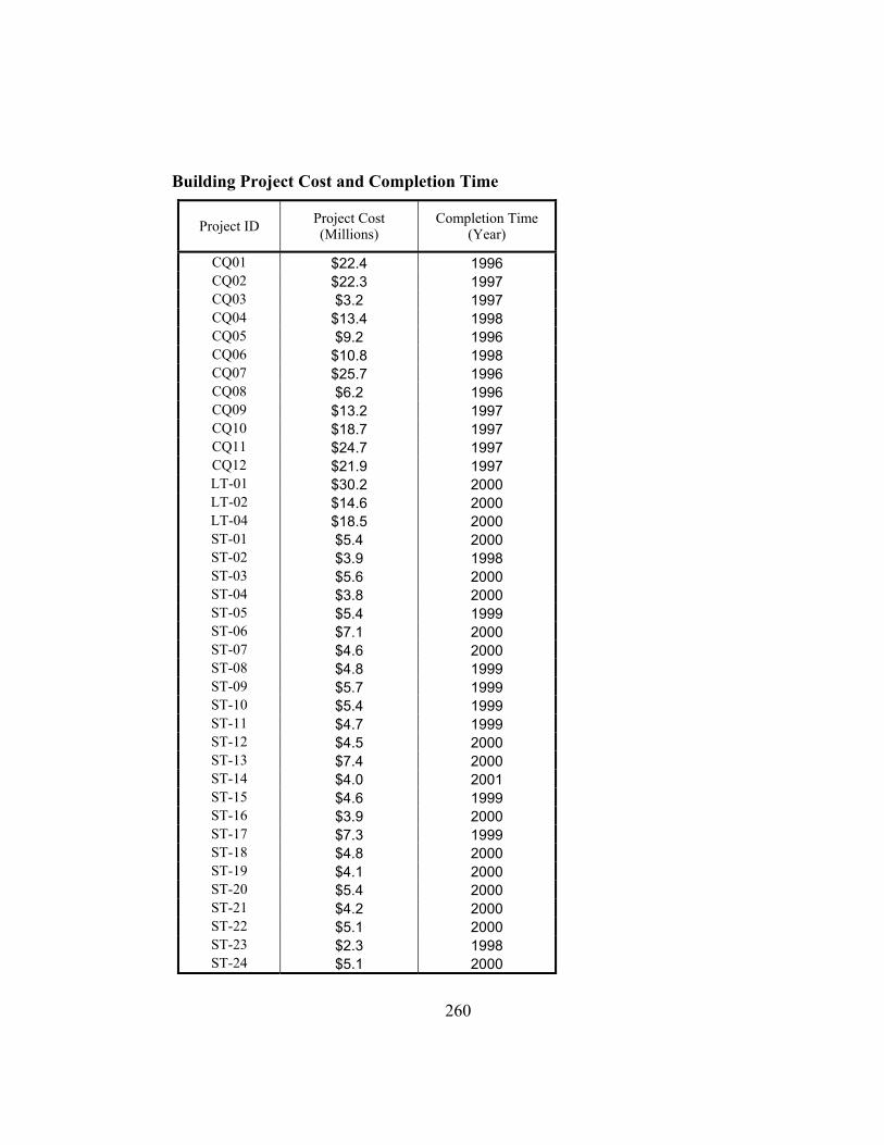
Building Project Cost and Completion Time

Project ID Project Cost (Millions)

Completion Time (Year)

CQ01 $22.4 1996 CQ02 $22.3 1997 CQ03 $3.2 1997 CQ04 $13.4 1998 CQ05 $9.2 1996 CQ06 $10.8 1998 CQ07 $25.7 1996 CQ08 $6.2 1996 CQ09 $13.2 1997 CQ10 $18.7 1997 CQ11 $24.7 1997 CQ12 $21.9 1997 LT-01 $30.2 2000 LT-02 $14.6 2000 LT-04 $18.5 2000 ST-01 $5.4 2000 ST-02 $3.9 1998 ST-03 $5.6 2000 ST-04 $3.8 2000 ST-05 $5.4 1999 ST-06 $7.1 2000 ST-07 $4.6 2000 ST-08 $4.8 1999 ST-09 $5.7 1999 ST-10 $5.4 1999 ST-11 $4.7 1999 ST-12 $4.5 2000 ST-13

$4.0 2001 ST-15 $4.6 1999

$3.9 2000 ST-17 $7.3 1999 ST-18 $4.8 2000 ST-19 $4.1 2000 ST-20 $5.4 2000 ST-21 $4.2 2000

$5.1 2000 ST-23 $2.3 1998 ST-24 $5.1 2000

$7.4 2000 ST-14

ST-16

ST-22

260

Building Project Cost and Completion Time (Cont’d)

Project ID Project Cost (Millions)

Completion Time (Year)

ST-25 $4.2 2000 ST-26 $4.8 2000 ST-27 $4.9 2000 ST-28 $4.4 2000 ST-29 $5.5 1999 ST-30 $5.1 1999 ST-31 $5.4 2000 ST-32 $5.5 1999 ST-33 $3.7 2000 ST-34 $3.2 1999 ST-35 $5.5 2000 ST-36 $5.7 2000

$5.0 2000 ST-38 $5.8 2000 ST-39 $5.0 2000 ST-40 $4.2 2000 VQ01 $9.4 1997 VQ02 $32.0 1998 VQ03 $33.9 1997 VQ04 $46.6 1999 VQ05 $125.0 1997 VQ06 $200.0 1997 VQ07 $9.8 1997

$7.8 1998 VQ09 $0.7 1998 VQ10

$42.6 1998 VQ12 $20.4 1997 VQ13 $7.9 1997 VQ14 $17.5 1998 VQ15 $4.1 1997 VQ16 $1.6 1997 VQ17 $124.4 1997 VQ18 $1.8 1999 VQ19 $1.6 1998 VQ20 $1.5 1998 VQ21 $3.6 1997

WIP-01 $5.3 2001 WIP-02 $6.5 2001

ST-37

VQ08

$1.1 1998 VQ11

261

Bibliography

Abdul-Raheem, N. (1994). “The Relationship between Perceived Leadership

Behavior of Construction Superintendents, Situational Factors, and Job Satisfaction of their Foreman”. Ph.D. thesis, University of Texas at Austin, Austin, TX

Al-Bahar, J. F. (1988). “Risk Management in Construction Project: A Systematic Analytical Approach for Contractors”. Ph.D. Thesis, University of California at Berkeley, Oakland, CA

Al-Bahar, J. F., and Crandall K. C. (1990). “Systematic Risk Management Approach for Construction Projects”. Journal of Construction Engineering and Management, Vol. 116, No. 3, pp. 533-546

Ang, A. H-S and Tang, W. H. (1975). Probability Concepts in Engineering Planning and Design, Vol.2 – Basic Principles. New York, New York: John Wiley & Sons

Birkes, D., and Dodge, Y. (1993). Alternative Methods of Regression, New York, New York: John Wileys & Sons, Inc.

Ashley, D., Jaselskis, E., and Lurie, C. B. (1987). “The Determinants of Construction Project Success”. Project Management Journal, Vol. 18, No. 2, pp. 69-79

Ashley, D. B., Stokes, S. L., and Perng, Y.-H. (1988). “Combining Multiple Expert Assessments for Construction Risk Identification”. Proc. 7th International Conference on Offshore Mechanics and Artic Engineering, Vol. VI: Computer Technology., American Society of Mechanical Engineers, New York, pp. 183-192

Babbie, E. R. (1992). The Practice of Social Research – Sixth Edition, Belmont, California: Wadsworth Pub. Co.

Boyer, L. T., and Kangari, R. (1989). “Risk Management by Expert System”. Project Management Journal, March, pp. 40-48

262

Bohrnstedt, G.W., and Knoke, D. (1988). Statistics for Social Data Analysis – Second Edition, Itasca, Illinois: F. E. Peacock Publishers. Inc.

Broaddus, J. A. (1995). Managing Inputs to Design for Project Success: Participant Handbook – CII Education Module EM-9, Austin, Texas: Construction Industry Institute, The University of Texas at Austin.

The Business Roundtable (1982). Modern Management Systems, Report A-6

Cherry, E. (1999). Programming for Design: From Theory to Practice, New York, New York: John Wiley & Sons, Inc.

Cho, C. S., Furman, J. C., and Gibson, G. E. (1999). Development of the Project Definition Rating Index (PDRI) for Building Projects – A report to the Construction Industry Institute, The University of Texas at Austin, Research Report 155-11

Cho, C. S. (2000). “Development of the Project Definition Rating Index (PDRI) for Building Projects”. Ph.D. Thesis, University of Texas at Austin, Austin, TX

Coe, R. (2000). “What’s an ‘Effective Size? A Guide for Users”. http://cem.dur.ac.uk/ebeuk/research/effectsize/ESguide.htm

The Construction Industry Institute (1989). “Management of Project Risks and Uncertainties”. Publication 6-8, University of Texas at Austin, Austin, Texas

The Construction Industry Institute (1995). “Pre-Peoject Planning Handbook”. Special Publication 39-2, Austin, TX

The Construction Industry Institute (1998). “Planning for Startup – Overview of Research”. Research Summary 121-1. Austin, TX

The Construction Industry Institute (1999). “Project Definition Rating Index (PDRI) – Building Projects”. Implementation Resource 155-2, Austin, TX

The Construction Industry Institute (2001). “Benchmarking & Metrics”. http://www.cii-benchmarking.org/aboutbmm.htm

The Construction Industry Institute (2002). “Benchmarking and Metrics Summary Report for 2001”. BMM2002-3, Austin, TX

263

Flanagan, R., and Norman, G. (1993). Risk Management and Construction, Oxford, U.K.: Blackwell Scientific

Freeman, M., and Beale, P. (1992). “Measuring Project Success”, Project Management Journal, Vol. 23, No. 1, pp. 8-16

Furman, J.C. (1999). “Logic Flow Diagrams for Planning of Building Projects”. M.S. Thesis, University of Texas at Austin, Austin, Texas.

Gibson, G. E., Kaczmarowski, J. H., and Lore, H. E. (1993). “Modeling Pre-Project Planning for the Construction of Capital Facilities – Source Document 94”, Construction Industry Institute, Austin, TX

Gibson, G. E. and Hamilton, M. R. (1994). “Analysis of Pre-Project Planning Effort and Success Variables for Capital Facility Projects”, A report to the Construction Industry Institute, Source Document 105, Austin, TX

Gibson, G. E., Kaczmarowski, J. and Lore, H. (1995). “Pre-Project Planning Process for Capital Facilities”, ASCE J. Construction Engineering and Management, Vol. 121, No. 3, pp. 312-318

Gibson, G. E. and Dumont, P.R. (1996). “Project Definition Rating Index (PDRI)”, A report to the Construction Industry Institute, Research Report 113-11, Austin, TX

Gibson, G. E., Liao, S., Broaddus, J., and Bruns, T., (1997). The university of texas system capital project performance, 1990 – 1995. OFPC Paper 97-1. Office of Facilities Planning and Construction, The University of Texas System, Austin, TX

Glass, G. V. (1976). “Primary, Secondary, and Meta-Analysis of Research”, Educational Researcher, Vol. 5, pp. 3-8

Gorsuch, R. L. (1974). Factor Analysis, Philadelphia, PA: B. Saunders Company

Griffith, A. F., Gibson, G. E., Hamilton, M. R., Tortora, A. L., and Wilson, C. T. (1999). “Project Success Index for Capital Facility Construction Projects”, ASCE J. Performance of Constructed Facilities, Vol. 13, No. 1, pp. 39-45

Hackney, J. W. (1992). Control & Management of Capital Projects – Second Edition, New York, New York: McGraw-Hill, Inc.

264

Hamilton, L. C. (1992). Regression with Graphics – A Second Course in Applied Statistics, Belmont, California: Wadsworth Inc.

Hamilton, M. R. (1994). “The Relationship between Pre-Project Planning Effort and Success for Capital Construction Projects”. Ph. D. Thesis, University of Texas at Austin, Austin, TX

Heiman, G. W. (1992). Basic Statistics for Behavioral Sciences, Boston, MA: Houghton Mifflin

Ibbs, C. W., and Crandall, K. C. (1982). “Construction Risk: Multi-attribute Approach”. Journal of Construction Engineering and Management, Vol. 108, No. 2, 1982, pp. 187-200

Jamal F. Al-Bahar, and Keith C. Crandall (1990). “Systematic Risk Management Approach for Construction Projects” Journal of Construction Engineering and Management, Vol. 116, No. 3, pp. 533-546

Kangari, R. (1995). “Risk Management Protection and Trends of U.S. Construction”. Journal of Construction Engineering and Management, Vol. 121, No. 4, pp. 422-429

Knoke, D., and Bohrnstedt, G. W. (1994). Statistics for Social Data Analysis, Itasca, Illinois: F.E. Peacock Publishers, Inc.

Laplace, P. S. (1951). A Philosophical Essay on Probabilities, unabridged and unaltered reprint of Truscott and Emory translation, New York, New York: Dover Publications, Inc., original publication date 1814.

Lee, Y. W., Bogardi, I. and Stansbury, J. (1991). “Fuzzy Decision-Making in Dredged Material Management” Journal of Environmental Engineering, ASCE, Vol. 117, No. 5, pp. 614-630

Lifson, M. W., and Shaifer, E. F., Jr. (1982). Decision and Risk Analysis for Construction Management. New York, New York: John Wiley and Sons, Inc.

Mak, S., and Picken, D. (2000). “Using Risk Analysis to Determine Construction Project Contingencies.” Journal of Construction Engineering and Management, ASCE, Vol. 126, No. 2, pp. 130-136

265

Merrow, E. W., Philips, K. E., & Myers, C. W. (1981). “Understanding Cost Growth and Performance Shortfalls in Pioneer Process Plants”, R-2569-DOE, Santa Monica, California: RAND Corporation

Merrow, E. W. (1988). “Understanding the Outcomes of Megaprojects: A Quantitative Analysis of Very Large Civilian Projects”, R-3560-PSSP, Santa Monica, California: RAND Corporation

Merrow, E. W., and Yarossi, M. E. (1994). “Managing Capital Projects: Where Have We been – Where are We Going?” Chemical Engineering, October: 108-111

Minato, T., and Ashley, D. B. (1998). “Data-Driven Analysis of ‘Corporate Risk’ Using Historical Cost-Control Data”. Journal of Construction Engineering and Management, Vol. 124, No. 1, pp. 42-47

Morris, P.W., and Hough, G.H. (1987). Anatomy of Major Projects, New York, New York: John Wiley & Son’s, Inc.

Neal, R. M. (1996). Bayesian Learning for Neural Networks, New York, New York: Springer

O’Connor, J. T., and Vickroy, C. G. (1986). “Control of Construction Project Scope – Source Document 6”, Austin, Texas: Construction Industry Institute, The University of Texas at Austin

Paek, J. H., and Lee, Y. W. (1993). “Pricing Construction Risk: Fuzzy Set Application” Journal of Construction Engineering and Management, Vol. 119, No. 4, December, pp. 743-756

Peña, W., Parshall, S., and Kelly, K. (1987). Problem Seeking – An Architectural Programming Primer, Washington, D.C.: AIA Press

Pinto, J.K. and Kharabanda, O.P. (1996). What Made Gertie Gallop?, New York, New York: Van Nostrand Reinhold

The Project Management Institute (1986). Measuring Success: 1986 Proceedings Project Management Institute. Montreal, Canada, September 20-25, Upper Darby, Pennsylvania: Project Management Institute

The Project Management Institute (2000). Project Management Body of Knowledge, Newtown Square, PA

266

Rawling, J.O. (1988). Applied Regression Analysis: A Research Tool, Belmont, California: Wadsworth, Inc.

Rao, Guru N. Grobler, Francois. and Liu, Liang Y. (1994). “Managing Uncertainty in Project Planning and Execution: Introduction and Overview.” Computing in Civil Engineering Conference Proceeding, ASCE New York, pp. 33-40

Smith, G. R. and Bohn, C. M. (1999). “Small to Medium Contractor Contingency and Assumption of Risk.” Journal of Construction Engineering and Management, ASCE, Vol. 125, No. 2, pp. 101-108

Smith, M. A. & Tucker, R. L. (1983). “An Assessment of the Potential Problems Occurring in the Engineering Phase of an Industrial Project”, A Report to Texaco, Inc., The University of Texas at Austin

SPSSTM (2000). SPSS for Windows, Base System User’s Guide, Release 10.0. Chicago, Illinois: SPSS Inc.

Steven, J. (1996). Applied Multivariate Statistics for the Social Sciences 3Edition. Mahwah, NJ: Lawrence Erlbaum Publishers

rd

Strassman, W. P., and Wells, J. (1988). The global construction industry: Strategies for entry, growth, and survival. Unwin Hyman, London

Tan, R.R. (1996). “Success Criteria and Success Factors for External Technology Transfer Projects”. Project Management Journal, Vol. 27, No. 2, pp. 45-56

Thompson, P. A., and Perry, J. G. (1992). Engineering Construction Risks: A Guide to Project Risk Analysis and Risk Management

Touran, A. (1992). “Risk Modeling and Measurement in Construction.” Civil Engineering Practice, pp. 29-45

Welkowitz, J., Ewen, R. B., and Cohen, J. (1982). Introductory Statistics for the Behavioral Sciences, San Diego, CA: Harcourt Brace Jovanovich, Publishers

Zimmermann, H. J. (1987). Fuzzy Sets, Decision Making, and Expert System, London, England: Kluwer Academic Publishers

267

Vita

Yu-Ren Wang was born in Taipie, Taiwan on June 6, 1974, the son of

Chung-Bin Wang and Hsiuo-Huei Shih. After completing his high school

education at Chien-Kuo High School, Taipei, Taiwan, in 1992, he entered

National Chiao-Tung University in Hsin-Chu, Taiwan. He received the degree

of Bachelor of Science in Civil Engineering from National Chiao-Tung University

in June, 1996. After college, he joined GAB Robins Taiwan, an international

loss adjusting company, and worked as an engineer in charge of adjusting

construction claims from July 1996 to July 1997. He then pursued his graduate

study in University of Illinois at Urbana-Champaign majoring in Construction

Management. He was awarded the degree of Master of Science in Civil

Engineering from the University of Illinois at Urbana-Champaign in August,

1998. After he completed his study in UIUC, he transferred to the University of

Texas at Austin in August 1998 to work on his doctorate in Civil Engineering.

Permanent address: 2F No. 28 Section 1, Dihwa St., Taipei, Taiwan 103

This dissertation was typed by the author.

268