Copyright by William Lloyd Bircher 2010lca.ece.utexas.edu/pubs/bircher_dissertation_20109.pdf ·...
190
Copyright by William Lloyd Bircher 2010
Transcript of Copyright by William Lloyd Bircher 2010lca.ece.utexas.edu/pubs/bircher_dissertation_20109.pdf ·...

Copyright
by
William Lloyd Bircher
2010

Dissertation Committee for William Lloyd Bircher
certifies that this is the approved version of the following dissertation:
Predictive Power Management for Multi-Core Processors
Committee:
Lizy John, Supervisor
Mattan Erez
Steve Keckler
Charles Lefurgy
Tess Moon
David Pan

Predictive Power Management for Multi-Core Processors
by
William Lloyd Bircher, B.S.E.E.; M.S.E.
Dissertation
Presented to the Faculty of the Graduate School of
The University of Texas at Austin
in Partial Fulfillment
of the Requirements
for the Degree of
Doctor of Philosophy
The University of Texas at Austin
December 2010

To Sara, Catherine and Elizabeth

v
Acknowledgements
I would like to thank Dr Lizy John for her guidance, insight and flexibility. Her
positive attitude and encouragement were instrumental in staying motivated. I appreciate
her balanced approach to work, study and life that has made my doctoral study possible.
I am grateful to my committee members, Prof. Mattan Erez, Prof. Steve Keckler,
Dr. Charles Lefurgy, Prof. Tess Moon and Prof. David Pan. Your helpful comments and
suggestions greatly improved the quality of the dissertation.
I am thankful to my fellow researchers in the Laboratory for Computer
Architecture (LCA) for our collaborations, discussions and practice talks over the years.
I enjoyed working with Dr. Madhavi Valluri and Jason Law on power modeling. This
collaboration was a great introduction to graduate research and proved to be a strong
basis for my thesis. I look forward to future collaboration with Karthik Ganesan, Jungho
Jo and the other authors who worked on the synthetic power virus paper. I would like to
thank Dimitris Kaseridis and Ciji Isen for many great discussions on research and life. I
am grateful to the other members of LCA, Ajay Joshi, Aashish Phansalkar, Juan Rubio,
Ravi Bhargava, Byeong Lee, Tao Li, Jeff Stuecheli, Jian Chen, Arun Nair, Muhammad
Farooq and Jungho Jo for attending my practice talks and providing insightful feedback.
I am thankful to Tommy Tam, Gwen Bernstrom and Dr. Charles Lefurgy at
International Business Machines for encouraging me to pursue graduate education.

vi
Thanks to Brent Kelly at Advanced Micro Devices for convincing me to join his
power and performance modeling team while completing my PhD. Working on his team
has allowed me to “amortize” the considerable efforts required for doctoral research with
gainful employment.
Finally, I would like to thank my dear wife Sara. Doctoral study requires a major
commitment from family and friends. Doctoral study while working full-time, raising a
family and remodeling a home requires an incredible commitment. I am eternally grateful
for your unwavering encouragement, support and patience without which this dissertation
would not have been possible.

vii
Predictive Power Management for Multi-Core Processors
William Lloyd Bircher, PhD.
The University of Texas at Austin, 2010
Supervisor: Lizy John
Energy consumption by computing systems is rapidly increasing due to the growth of
data centers and pervasive computing. In 2006 data center energy usage in the United
States reached 61 billion kilowatt-hours (KWh) at an annual cost of 4.5 billion USD
[Pl08]. It is projected to reach 100 billion KWh by 2011 at a cost of 7.4 billion USD.
The nature of energy usage in these systems provides an opportunity to reduce
consumption.
Specifically, the power and performance demand of computing systems vary widely in
time and across workloads. This has led to the design of dynamically adaptive or power
managed systems. At runtime, these systems can be reconfigured to provide optimal
performance and power capacity to match workload demand. This causes the system to
frequently be over or under provisioned. Similarly, the power demand of the system is
difficult to account for. The aggregate power consumption of a system is composed of
many heterogeneous systems, each with a unique power consumption characteristic.
This research addresses the problem of when to apply dynamic power management in
multi-core processors by accounting for and predicting power and performance demand

viii
at the core-level. By tracking performance events at the processor core or thread-level,
power consumption can be accounted for at each of the major components of the
computing system through empirical, power models. This also provides accounting for
individual components within a shared resource such as a power plane or top-level cache.
This view of the system exposes the fundamental performance and power phase behavior,
thus making prediction possible.
This dissertation also presents an extensive analysis of complete system power
accounting for systems and workloads ranging from servers to desktops and laptops. The
analysis leads to the development of a simple, effective prediction scheme for controlling
power adaptations. The proposed Periodic Power Phase Predictor (PPPP) identifies
patterns of activity in multi-core systems and predicts transitions between activity levels.
This predictor is shown to increase performance and reduce power consumption
compared to reactive, commercial power management schemes by achieving higher
average frequency in active phases and lower average frequency in idle phases.
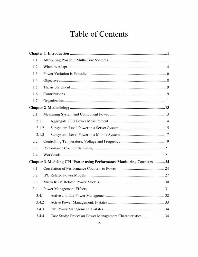
ix
Table of Contents
Chapter 1 Introduction ....................................................................................................1
1.1 Attributing Power in Multi-Core Systems ........................................................... 1
1.2 When to Adapt ..................................................................................................... 4
1.3 Power Variation is Periodic.................................................................................. 6
1.4 Objectives ............................................................................................................. 8
1.5 Thesis Statement .................................................................................................. 9
1.6 Contributions ........................................................................................................ 9
1.7 Organization ....................................................................................................... 11
Chapter 2 Methodology ..................................................................................................13
2.1 Measuring System and Component Power ........................................................ 13
2.1.1 Aggregate CPU Power Measurement ......................................................... 14
2.1.2 Subsystem-Level Power in a Server System .............................................. 15
2.1.3 Subsystem-Level Power in a Mobile System ............................................. 17
2.2 Controlling Temperature, Voltage and Frequency ............................................. 19
2.3 Performance Counter Sampling ......................................................................... 21
2.4 Workloads .......................................................................................................... 21
Chapter 3 Modeling CPU Power using Performance Monitoring Counters ............24
3.1 Correlation of Performance Counters to Power ................................................. 24
3.2 IPC Related Power Models ................................................................................ 27
3.3 Micro ROM Related Power Models................................................................... 30
3.4 Power Management Effects ............................................................................... 31
3.4.1 Active and Idle Power Management ........................................................... 32
3.4.2 Active Power Management: P-states .......................................................... 33
3.4.3 Idle Power Management: C-states .............................................................. 34
3.4.4 Case Study: Processor Power Management Characteristics ....................... 34

x
3.4.5 Power Management-Aware Model ............................................................. 37
3.5 Methodology for Power Modeling ..................................................................... 40
3.6 Summary ............................................................................................................ 43
Chapter 4 System-Level Power Analysis ......................................................................44
4.1 Average Power ................................................................................................... 44
4.1.1 Server Platform - SPEC CPU, SPECjbb and DBT-2 .................................. 44
4.1.2 SPEC CPU 2000/2006 CPU and Memory Power Comparison .................. 46
4.1.3 Desktop Platform – SYSmark 2007 ............................................................ 48
4.1.4 Desktop Platform - SPEC CPU, 3DMark and SYSmark ............................ 49
4.2 Power Consumption Variation ........................................................................... 53
4.2.1 Server Platform ........................................................................................... 53
4.2.2 Desktop Platform ........................................................................................ 59
4.3 Summary ............................................................................................................ 62
Chapter 5 Modeling System-Level Power using Trickle-Down Events .....................64
5.1 Processor Events Propagate to Rest of System .................................................. 64
5.2 Complete-System Server Power Model ............................................................. 67
5.2.1 CPU ............................................................................................................. 71
5.2.2 Memory ....................................................................................................... 73
5.2.3 Disk ............................................................................................................. 76
5.2.4 I/O ............................................................................................................... 79
5.2.5 Chipset ........................................................................................................ 80
5.2.6 Model Validation ........................................................................................ 81
5.3 Complete-System Desktop Power Model .......................................................... 84
5.3.1 System Description ..................................................................................... 84
5.3.2 Workloads ................................................................................................... 86
5.3.3 Performance Event Selection ...................................................................... 88
5.3.4 CPU ............................................................................................................. 93
5.3.5 GPU............................................................................................................. 94

xi
5.3.6 Memory ....................................................................................................... 96
5.3.7 Memory Controller ..................................................................................... 98
5.3.8 Chipset ........................................................................................................ 99
5.3.9 Disk ............................................................................................................. 99
5.3.10 Model Validation ........................................................................................ 99
5.4 Summary .......................................................................................................... 102
Chapter 6 Performance Effects of Dynamic Power Management ...........................103
6.1 Direct and Indirect Performance Impacts......................................................... 103
6.1.1 Transition Costs ........................................................................................ 103
6.1.2 Workload Phase and Policy Costs ............................................................ 104
6.1.3 Performance Effects .................................................................................. 105
6.1.4 Indirect Performance Effects .................................................................... 107
6.1.5 Direct Performance Effects ....................................................................... 109
6.2 Reactive Power Management ........................................................................... 110
6.2.1 Power and Performance Results ............................................................... 116
6.3 Summary .......................................................................................................... 118
Chapter 7 Predictive Power Management ..................................................................120
7.1 Core-Level Activity Prediction ........................................................................ 120
7.2 Commercial DVFS Algorithm ......................................................................... 125
7.3 Workload Characterization .............................................................................. 126
7.4 Periodic Power Phase Predictor – PPPP .......................................................... 130
7.5 Predicting Core Activity Level ........................................................................ 134
7.6 Predicting Power Levels................................................................................... 143
7.7 Summary .......................................................................................................... 145
Chapter 8 Related Research ........................................................................................147
8.1 Performance Counter-Driven Power Models ........................................................ 147
8.2 System-Level Power Characterization .................................................................. 149
8.3 Predictive Power Adaptation ................................................................................. 150

xii
8.4 Deadline and User-Driven Power Adaptation ....................................................... 151
Chapter 9 Conclusions and Future Work ..................................................................153
9.1 Conclusions ........................................................................................................... 153
9.2 Future Work .......................................................................................................... 156
Bibliography ...................................................................................................................158
Vita ..................................................................................................................................174

xiii
List of Tables
Table 1.1 Windows Vista Reactive DVFS ...................................................................... 5
Table 2.1 Desktop System Description ......................................................................... 14
Table 2.2 Server System Description ............................................................................ 15
Table 2.3 Subsystem Components ................................................................................ 15
Table 2.4 Laptop System Description ........................................................................... 19
Table 2.5 Workload Description ................................................................................... 22
Table 3.1. Intel Pentium 4, High and Low Correlation Performance Metrics .............. 25
Table 3.2 Percent of Fetched µops Completed/Retired – SPEC CPU 2000 ................. 26
Table 3.3 µop Linear Regression Model Comparison .................................................. 28
Table 3.5 Instruction Power Consumption .................................................................... 30
Table 3.6 µop Linear Regression Model Comparison .................................................. 31
Table 3.7 Example P-states Definition .......................................................................... 33
Table 3.8 Example C-states Definition ......................................................................... 34
Table 3.9 AMD Quad-Core Power Model .................................................................... 39
Table 4.1 Subsystem Power Standard Deviation (Watts) ............................................. 53
Table 4.2 Coefficient of Variation ............................................................................... 54
Table 4.3 Percent of Classifiable Samples .................................................................... 58
Table 4.4 Workload Phase Classification ..................................................................... 59
Table 5.1 Integer Average Model Error ........................................................................ 82
Table 5.2 Floating Point Average Model Error............................................................. 83
Table 5.3 System Comparison ...................................................................................... 85
Table 5.4 Desktop Workloads ....................................................................................... 87
Table 5.5 Average Error .............................................................................................. 101
Table 6.1 Performance Loss Due to Low Idle Core Frequency – SPEC CPU 2006 .. 111
Table 6.2 Power/Performance Study: SYSmark 2007 ................................................ 116

xiv
Table 7.1: SYSmark 2007 Components ...................................................................... 127
Table 7.2: Periodic Power Phase Predictor Field Descriptions ................................... 134
Table 7.3: SYSmark 2007 DVFS Hit Rate ................................................................. 136
Table 7.4: SYSmark 2007 Prediction Coverage ......................................................... 137
Table 7.5: Core Phase Residency by Length............................................................... 138
Table 7.6: SYSmark 2007 Power and Performance Impact of PPPP ......................... 141
Table 7.7: SYSmark 2007 P-State and C-State Residency of PPPP versus Reactive . 142
xv
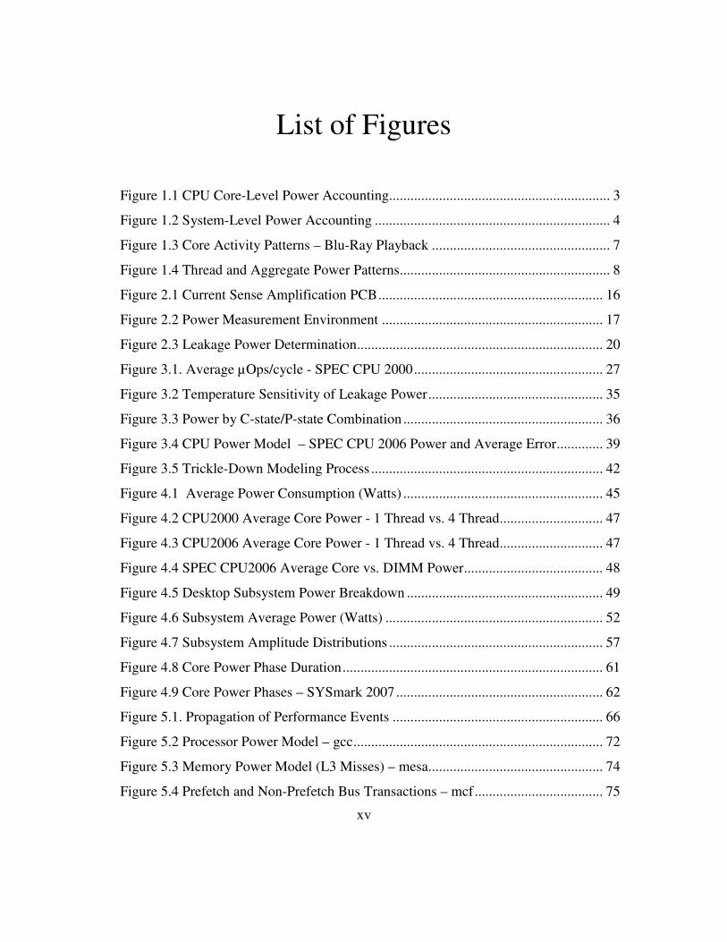
List of Figures
Figure 1.1 CPU Core-Level Power Accounting.............................................................. 3
Figure 1.2 System-Level Power Accounting .................................................................. 4
Figure 1.3 Core Activity Patterns – Blu-Ray Playback .................................................. 7
Figure 1.4 Thread and Aggregate Power Patterns........................................................... 8
Figure 2.1 Current Sense Amplification PCB ............................................................... 16
Figure 2.2 Power Measurement Environment .............................................................. 17
Figure 2.3 Leakage Power Determination..................................................................... 20
Figure 3.1. Average µOps/cycle - SPEC CPU 2000 ..................................................... 27
Figure 3.2 Temperature Sensitivity of Leakage Power ................................................. 35
Figure 3.3 Power by C-state/P-state Combination ........................................................ 36
Figure 3.4 CPU Power Model – SPEC CPU 2006 Power and Average Error ............. 39
Figure 3.5 Trickle-Down Modeling Process ................................................................. 42
Figure 4.1 Average Power Consumption (Watts) ........................................................ 45
Figure 4.2 CPU2000 Average Core Power - 1 Thread vs. 4 Thread............................. 47
Figure 4.3 CPU2006 Average Core Power - 1 Thread vs. 4 Thread............................. 47
Figure 4.4 SPEC CPU2006 Average Core vs. DIMM Power ....................................... 48
Figure 4.5 Desktop Subsystem Power Breakdown ....................................................... 49
Figure 4.6 Subsystem Average Power (Watts) ............................................................. 52
Figure 4.7 Subsystem Amplitude Distributions ............................................................ 57
Figure 4.8 Core Power Phase Duration ......................................................................... 61
Figure 4.9 Core Power Phases – SYSmark 2007 .......................................................... 62
Figure 5.1. Propagation of Performance Events ........................................................... 66
Figure 5.2 Processor Power Model – gcc ...................................................................... 72
Figure 5.3 Memory Power Model (L3 Misses) – mesa ................................................. 74
Figure 5.4 Prefetch and Non-Prefetch Bus Transactions – mcf .................................... 75

xvi
Figure 5.5 Memory Power Model (Memory Bus Transactions)- mcf .......................... 76
Figure 5.6 Disk Power Model (DMA+Interrupt) – Synthetic Disk Workload ............. 79
Figure 5.7 GPU Power Model (Non-Gated Clocks) – 3DMark06-HDR1 .................... 96
Figure 5.8 DRAM Power Model (∑DCT Access, LinkActive) – SYSmark 2007-3D . 97
Figure 5.9 Memory Controller Power (∑DCT Access, LinkActive) – HDR1 ............. 98
Figure 6.1 Direct and Indirect Performance Impact .................................................... 107
Figure 6.2 Remote and Local Probe Sensitivity .......................................................... 112
Figure 6.3 C-state vs. P-state Performance ................................................................. 113
Figure 6.4 Varying OS P-state Transition Rates ......................................................... 114
Figure 7.1: Thread and Aggregate Power Patterns ..................................................... 123
Figure 7.2: Windows Vista Reactive P-State Selection Algorithm ............................ 126
Figure 7.3: Six-Core Phenom 2 Desktop Activity Levels ........................................... 128
Figure 7.4: Utilization of Multiple Cores by SYSmark 2007 Benchmark .................. 129
Figure 7.5: Periodic Power Phase Predictor ................................................................ 132
Figure 7.6: Example of Program Phase Mapping to Predictor ................................... 133
Figure 7.7 Core-Level Phase Length Probability Distributions .................................. 140
Figure 7.8 Prediction Accuracy of Core Power for Various Predictors ...................... 144

1
Chapter 1 Introduction
Computing systems have a wide range of design objectives. Metrics such as
performance, power and cost must be carefully managed in order to meet these
objectives. While some parameters are fixed at design time, others such as performance
and power consumption may be dynamically adjusted at run-time. This allows a system
to be optimal across a wider range of workloads and usage scenarios. This dynamic
optimization, commonly known as dynamic power management, allows performance to
be exchanged for power savings. The amount of savings is constrained by the system
objectives. For example, systems with quality of service (QoS) requirements can allow
power and performance to be reduced only as long as the service demands are met.
Mobile systems powered by batteries must be optimized to deliver the highest
performance/Watt in order to maximize usage time. Compute-cluster performance
capacity must be modulated to match demand so that performance/cost is maximized.
Adaptation within these scenarios requires accurate, run-time measurement of
performance and power consumption. Run-time measurement of power and performance
allow tradeoffs to be made dynamically in response to program and usage patterns.
1.1 Attributing Power in Multi-Core Systems
Multi-core and multi-threaded systems present significant challenges to power
measurement. While performance is readily measurable at the core and program-level,

2
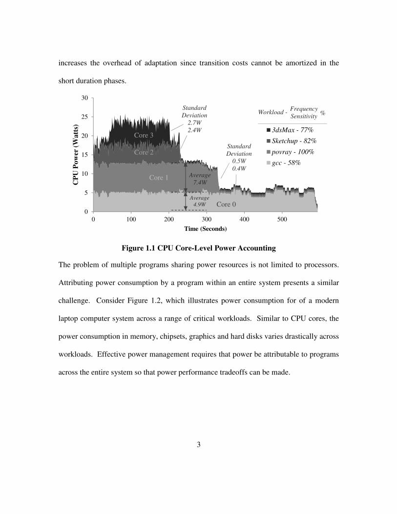
power is more difficult. Invariably power is delivered to multiple cores or system
components through a shared power plane. Power consumption by individual cores or
programs cannot be observed. Consider Figure 1.1. The power consumption of a multi-
core, multi-programmed system simultaneously executing four distinct workloads is
shown. These four workloads have power and performance characteristics that require
distinct adaptations to meet system objectives. Core 1 has the computationally efficient
ray-tracing workload, povray that scales performance nearly perfectly with core
frequency. This is important for power management since controlling adaptations such
as frequency scaling requires accounting for the potential benefit or cost of changing
frequency. In contrast cores 0, 2 and 3 are running applications that are sensitive to 58%-
80% of the change in core frequency. This difference in frequency sensitivity leads to
varying optimization points for dynamic adaptation. Similarly, the power consumption
of each workload is distinct. The highly efficient povray is able to consistently utilize
more than 2/3 of the execution pipelines. This high utilization and concentration of
floating point instructions, leads to high power consumption. At the other extreme, the
gcc compiler application is only able to utilize 1/3 of the execution pipelines using
integer instructions exclusively. In addition to differences in steady state power
consumption, these workloads have different phase behavior. While povray and gcc have
stable power consumption patterns, 3Dsmax and Sketchup (3D rendering) exhibit drastic
variations in power consumption over time. Frequent changes in power consumption
3
increases the overhead of adaptation since transition costs cannot be amortized in the
short duration phases.
Figure 1.1 CPU Core-Level Power Accounting
The problem of multiple programs sharing power resources is not limited to processors.
Attributing power consumption by a program within an entire system presents a similar
challenge. Consider Figure 1.2, which illustrates power consumption for of a modern
laptop computer system across a range of critical workloads. Similar to CPU cores, the
power consumption in memory, chipsets, graphics and hard disks varies drastically across
workloads. Effective power management requires that power be attributable to programs
across the entire system so that power performance tradeoffs can be made.
0
5
10
15
20
25
30
0 100 200 300 400 500
CP
U P
ow
er (
Wa
tts)
Time (Seconds)
3dsMax - 77%
Sketchup - 82%
povray - 100%
gcc - 58%
Average
7.4W
Average
4.9W
Standard
Deviation
2.7W
2.4W
Standard
Deviation
0.5W
0.4W
Workload -Frequency
Sensitivity%
Core 0
Core 1
Core 2
Core 3

4
Figure 1.2 System-Level Power Accounting
1.2 When to Adapt
Due to the difficulty in observing program phases in shared power plane environments,
existing power management schemes rely on reaction when performing adaptation. This
pragmatic approach leads to sub-optimal performance and power consumption. Consider
the case of the Windows Vista operating system using Dynamic Voltage and Frequency
Scaling (DVFS). To reduce power consumption during low utilization phases, the
operating system power manager reduces voltage and frequency of cores when CPU core
activity level drops below a fixed threshold. The manager periodically samples core
activity level and adjusts the DVFS operating point accordingly. This reactive approach
results in frequent over and under provisioning of performance and power, especially for
“bursty” workloads. Consider Table 1.1, which shows DVFS residency for a recent
productivity workload. This data indicates that the selection of CPU frequency is
2.9 2.7 3.3 3.3 3.3 3.2 2.9 2.9 2.6 2.9 2.8 2.6 2.8
0.5
0.9 0.9 1.4 1.4 1.4 1.4 1.3 1.3 1.4 1.3 1.7 1.4 1.6
0.8
0.9 0.94.0 3.8 3.8 3.7
1.3 1.3 1.1 1.1 1.1 1.1 1.1
0.9
2.5 2.4
2.5 2.4 2.4 2.3
2.0 2.0 1.9 2.0 1.9 2.0 1.9
0.5
3.4 3.0
3.5 3.0 3.3 2.9
1.6 1.6 1.3 1.7 1.1 1.4 1.2
0.2
14.814.1
10.2 10.6 10.2 10.5
14.3 14.211.9 11.1 11.0 10.6 10.3
0.6
0
5
10
15
20
25
30
Po
wer
(W
att
s)
CPU
Memory
Memory
ControllerGPU
Disk
Graphics
Intensive
Productivity
Compute
Intensive Compute
Intensive
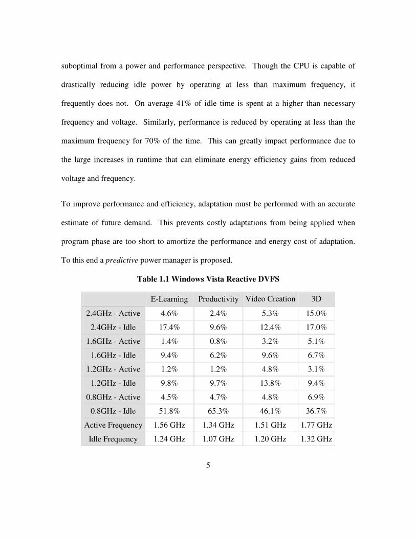
5
suboptimal from a power and performance perspective. Though the CPU is capable of
drastically reducing idle power by operating at less than maximum frequency, it
frequently does not. On average 41% of idle time is spent at a higher than necessary
frequency and voltage. Similarly, performance is reduced by operating at less than the
maximum frequency for 70% of the time. This can greatly impact performance due to
the large increases in runtime that can eliminate energy efficiency gains from reduced
voltage and frequency.
To improve performance and efficiency, adaptation must be performed with an accurate
estimate of future demand. This prevents costly adaptations from being applied when
program phase are too short to amortize the performance and energy cost of adaptation.
To this end a predictive power manager is proposed.
Table 1.1 Windows Vista Reactive DVFS
E-Learning Productivity Video Creation 3D
2.4GHz - Active 4.6% 2.4% 5.3% 15.0%
2.4GHz - Idle 17.4% 9.6% 12.4% 17.0%
1.6GHz - Active 1.4% 0.8% 3.2% 5.1%
1.6GHz - Idle 9.4% 6.2% 9.6% 6.7%
1.2GHz - Active 1.2% 1.2% 4.8% 3.1%
1.2GHz - Idle 9.8% 9.7% 13.8% 9.4%
0.8GHz - Active 4.5% 4.7% 4.8% 6.9%
0.8GHz - Idle 51.8% 65.3% 46.1% 36.7%
Active Frequency 1.56 GHz 1.34 GHz 1.51 GHz 1.77 GHz
Idle Frequency 1.24 GHz 1.07 GHz 1.20 GHz 1.32 GHz
6
1.3 Power Variation is Periodic
The major challenge in predictive power management is detecting patterns of usage that
are relevant for power adaptations. Fortunately, the most critical usage metric in modern
computing systems is architecturally visible, namely CPU active/idle state usage. CPU
active and idle states have been shown to be highly correlated to power and performance
demand in complete systems [BiJo06-1]. This allows power and performance demand in
the complete system to be tracked and predicted, using only CPU metrics.
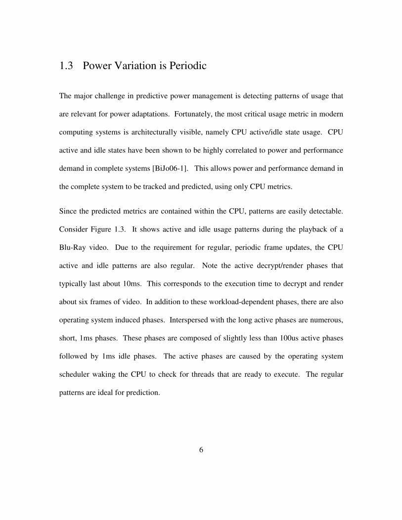
Since the predicted metrics are contained within the CPU, patterns are easily detectable.
Consider Figure 1.3. It shows active and idle usage patterns during the playback of a
Blu-Ray video. Due to the requirement for regular, periodic frame updates, the CPU
active and idle patterns are also regular. Note the active decrypt/render phases that
typically last about 10ms. This corresponds to the execution time to decrypt and render
about six frames of video. In addition to these workload-dependent phases, there are also
operating system induced phases. Interspersed with the long active phases are numerous,
short, 1ms phases. These phases are composed of slightly less than 100us active phases
followed by 1ms idle phases. The active phases are caused by the operating system
scheduler waking the CPU to check for threads that are ready to execute. The regular
patterns are ideal for prediction.

7
Figure 1.3 Core Activity Patterns – Blu-Ray Playback
Detecting patterns at the CPU-level is also advantageous since it allows component-level
patterns to be discerned from aggregate patterns. Consider Figure 1.4. The top figure
shows total CPU power consumption for a multi-core processor. The core-level power
consumption is shown in the subsequent four figures. Though the individual cores have a
regular, easily detectable pattern, the aggregate power obscures much of the periodic
behavior. This concept extends to the complete system in which individual core or thread
usage patterns induce similar patterns in shared resources such as memory or I/O devices.
Tracking and predicting CPU usage patterns provides the opportunity to more effectively
adapt power and performance to match demand of the complete system.
Co
re A
ctiv
ity
Time (ms)
Active
Idle
Active
Decrypt/Render
Idle except for scheduler
0 10 20 30 40 50 60 70

8
Figure 1.4 Thread and Aggregate Power Patterns
1.4 Objectives
The objective of this dissertation is to develop a predictive power manager using
performance counter-based power models. The specific objectives are as follows.
1. Develop performance counter-based, run-time models for complete system power
consumption.
2. Demonstrate the effectiveness of thread-level power accounting.
3. Characterize power consumption patterns of server, desktop and mobile systems.
0
50
100
150
0 20 40 60 80 100 120 140 160 180 200
Wat
ts
Seconds
Total Power = ∑CorePowerN N=0 to 3
0
50
Wat
ts
CorePower0
0
50
Wat
ts
CorePower1
0
50
Wat
ts
Core Power2
0
50
0 20 40 60 80 100 120 140 160 180 200
Wat
ts
Seconds
CorePower3
Phase
Misalignment

9
4. Design a predictive power management scheme to improve performance and
power efficiency.
1.5 Thesis Statement
Complete system power consumption of a multi-core system can be accurately estimated
by tracking core-level CPU performance events. These estimates may be used to predict
changes in power and performance of the system. Compared to commercial, reactive
power managers this predictive power manager yields higher performance and lower
power.
1.6 Contributions
This dissertation makes several contributions in the areas of modeling methodology,
power models, measurement-based workload characterization and novel power
management strategies.
a) A methodology for constructing power models based on performance events. The
methodology is shown to be effective across CPU architectures, system categories
and workloads.
b) A simple, accurate model for CPU power based on performance counters. The
model is constructed by applying linear-regression to power and performance
measurements captured on an actual system. The model demonstrates the need to
account for speculative execution when modeling power consumption.

10
c) The concept of trickle-down power events is presented. By identifying CPU
performance events that trickle-down to other subsystems, a complete-system
power model based on CPU performance counters. Power for subsystems
including memory, chipsets and disk are modeled using events directly
measureable in the CPU.
d) A characterization of complete-system power consumption for server, desktop
and mobile platforms is presented. The impacts of workloads, power
management and temperature are quantified. Statistical characterization of power
amplitude and duration is provided for numerous subsystems.
e) An analysis of the performance impacts on power management for multi-core
processors. Performance loss due to power management of shared resources is
considered. Certain workloads are found to be more sensitive to power
management. Negative interactions between operating systems are shown to
reduce performance and power efficiency.
f) A predictive power manager is proposed for controlling DVFS in a multi-core
processor. By identifying and anticipating patterns of power consumption, the
manager is able to improve performance and efficiency. It is compared to the
commercial, reactive scheme used in Windows Vista.

11
1.7 Organization
This dissertation is organized as follows:
Chapter 2 describes the methodology for measuring power and performance
events within a range of system types and subsystems ranging from CPUs to hard drives.
Techniques are provided for isolating and measuring dynamic and static power within
actual computing systems.
Chapter 3 presents an analysis of processor performance events that correlate to
power consumption. These findings direct the construction of a simple, speculation-
aware power model based on a small number of performance events. A formal
methodology for developing performance counter power models is presented.
Chapter 4 provides a broad analysis of subsystem-level power consumption across
a wide range of workloads including scientific computing, commercial transaction
processing, desktop productivity, content creation and consumption. Power is considered
in relative terms comparing across each subsystem. To inform power management
decisions, power phase behavior is considered in terms of duration and amplitude.
Chapter 5 presents an extensive number of system power models based upon
processor performance counters. The motivation behind the composition of each model
is provided. Accuracy statistics and measure versus modeled time-domain comparisons
are given.

12
Chapter 6 explores the power and performance impact of dynamic power
management. Detailed analysis of the relationship between power adaptations such as
clock gating and DVFS and performance are provided. The sub-optimal nature of a
commercial DVFS scheme is explored and explained.
Chapter 7 presents the Period Power Phase Predictor for control DVFS power
management actions. The predictor is compared to a state-of-the-art commercial DVFS
scheme in terms of performance and power consumption. Results are presented for a
desktop productivity workload that contains a high-level of power phase transitions.
Chapter 8 summarizes previous contributions in the area performance counter
power modeling and predictive power management. Chapter 9 describes conclusions
topics of future research.

13
Chapter 2 Methodology
The development of power models based on performance events requires the
measurement of power and performance on systems running a wide range of workloads.
This chapter describes the methodology for measuring power and performance events on
actual systems (not simulation) running realistic workloads. The first section describes
techniques and equipment for in-system measurement of power across a range of systems
and components. The compositions of three systems are defined: server, desktop and
laptop. The second section shows how system parameters such as temperature, voltage
and frequency can be manipulated to expose and quantify underlying properties of
systems. The third section describes how performance monitoring counters (PMC) can
be tracked in a manner that has minimal impact on the observed system. The last section
describes which workloads are preferred for power management analysis and why.
2.1 Measuring System and Component Power
To measure power consumption, a range of instrumentation methodologies are used.
Each methodology is designed to match measurement requirements while conforming to
the constraints of the measured system. The systems and measurement requirements are:
1) aggregate CPU power in a desktop system, 2) subsystem-level power in a server
system, 3) subsystem-level power in a mobile system.
14
2.1.1 Aggregate CPU Power Measurement
CPU power consumption is measured using a clamp-on current probe. The probe, an
Agilent 1146A [Ag08], reports current passing through its sensor by detecting the
magnitude and polarity of the electromagnetic field produced by the sampled current.
This type of measurement simplifies instrumentation since the observed conductors do
not have to be cut to insert current sensing resistors. The drawback of this approach is
that only wire-type conductors can be sampled. It is not possible to sample conductors
embedded in the printed circuit board. For the target system this restricts power
measurement to the input conductors of the processor voltage regulator module (VRM).
As a result, a portion of the reported power consumption is actually attributed to the
inefficiency of the VRM. These modules have an efficiency of 85%-90%. The reader
should consider the 10%-15% loss when comparing results to manufacturer reported
power consumption. The voltage provided by the current probe is sampled at 10 KHz by
a National Instruments AT-MIO-16E-2 data acquisition card[Ni08]. The LabVIEW
software tool [La10] can interpret the voltage trace or as in this case it is written to a
binary file for offline processing. The details of the system are described below in Table
2.1.
Table 2.1 Desktop System Description
System Parameters
Single Pentium 4 Xeon 2.0 GHz, 512KB L2 Cache, 2MB L3 Cache, 400 MHz FSB
4 GB PC133 SDRAM Main Memory
Two 16GB Adaptec Ultra160 10K SCSI Disks
Redhat Linux

15
2.1.2 Subsystem-Level Power in a Server System
To study component-level server power, the aggregate CPU power measurement
framework is used and extended to provide additional functionality required for
subsystem-level study. The most significant difference between the studies of CPU level
versus subsystem level is the requirement for simultaneously sampling multiple power
domains. To meet this requirement the IBM x440 server is used which provides separate,
measureable power rails for five major subsystems. It is described in Table 2.2.
Table 2.2 Server System Description
System Parameters
Four Pentium 4 Xeon 2.0 GHz, 512KB L2 Cache, 2MB L3 Cache, 400 MHz FSB
32MB DDR L4 Cache
8 GB PC133 SDRAM Main Memory
Two 32GB Adaptec Ultra160 10K SCSI Disks
Fedora Core Linux, kernel 2.6.11
By choosing this server, instrumentation is greatly simplified due to the presence of
current sensing resistors on the major subsystem power domains. Five power domains
are considered: CPU, chipset, memory, I/O, and disk. The components of each
subsystem are listed in Table 2.3.
Table 2.3 Subsystem Components
Subsystem Components
CPU Four Pentium 4 Xeons
Chipset Memory Controllers and Processor Interface Chips
Memory System Memory and L4 Cache
I/O I/O Bus Chips, SCSI, NIC
Disk Two 10K rpm 32G Disks

16
Power consumption for each subsystem (CPU, memory, etc.) can be calculated by
measuring the voltage drop across each current sensing resistor. In order to limit the loss
of power in the sense resistors and to prevent excessive drops in regulated supply voltage,
the system designer used a particularly small resistance. Even at maximum power
consumption, the corresponding voltage drop is in the tens of millivolts. In order to
improve noise immunity and sampling resolution we design a custom circuit board [Bi06]
to amplify the observed signals to levels more appropriate for the measurement
environment. The printed circuit board is shown in Figure 2.1. This board provides
amplification for eight current measurement channels. The board also provides BNC-
type connecters to allow direct connection to the data acquisition component. The entire
measurement framework is shown in Figure 2.2.
Figure 2.1 Current Sense Amplification PCB
17
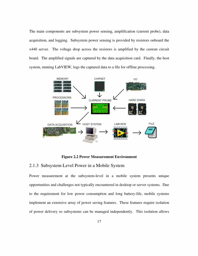
The main components are subsystem power sensing, amplification (current probe), data
acquisition, and logging. Subsystem power sensing is provided by resistors onboard the
x440 server. The voltage drop across the resistors is amplified by the custom circuit
board. The amplified signals are captured by the data acquisition card. Finally, the host
system, running LabVIEW, logs the captured data to a file for offline processing.
Figure 2.2 Power Measurement Environment
2.1.3 Subsystem-Level Power in a Mobile System
Power measurement at the subsystem-level in a mobile system presents unique
opportunities and challenges not typically encountered in desktop or server systems. Due
to the requirement for low power consumption and long battery-life, mobile systems
implement an extensive array of power saving features. These features require isolation
of power delivery so subsystems can be managed independently. This isolation allows
18
power to be measured at a finer grain than desktop/server systems that have a larger
degree of sharing across subsystems. It also leads to a wider range of power levels across
subsystems. High-power CPU subsystems may typically consume tens of Watts while
low-power chipsets may only consume a Watt or less. The measurement of different
ranges of power requires different approaches in order to maximize accuracy and
minimize perturbation. To this end a system specifically designed for power analysis is
used. The system is used by a major CPU manufacturer [Bk09] in the validation of
processors and chipsets. Depending on the expected power levels for a given subsystem
an inline current sensing resistor is implemented. High current subsystems use low value
resistors in the range of just a few milliohms. Low current subsystems use resistors in the
range of a few hundred milliohms. This approach allows the observed voltage drop due
to current flow to always be within the maximum accuracy range of the data acquisition
device. It also reduces the impact measurement has on the system. If the voltage drop
due to the sensor is too large, the effective voltage delivered to the subsystem could be
out of the subsystem’s operating range. The system characteristics and measureable
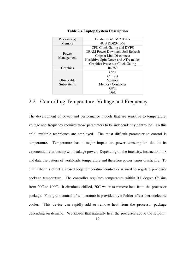
subsystems are listed below in Table 2.4.
19
Table 2.4 Laptop System Description
Processor(s) Dual-core 45nM 2.0GHz Memory 4GB DDR3-1066
Power
Management
CPU Clock Gating and DVFS DRAM Power Down and Self Refresh
Chipset Link Disconnect Harddrive Spin Down and ATA modes
Graphics Processor Clock Gating Graphics RS780
Observable
Subsystems
CPU Chipset Memory
Memory Controller GPU Disk
2.2 Controlling Temperature, Voltage and Frequency
The development of power and performance models that are sensitive to temperature,
voltage and frequency requires those parameters to be independently controlled. To this
en`d, multiple techniques are employed. The most difficult parameter to control is
temperature. Temperature has a major impact on power consumption due to its
exponential relationship with leakage power. Depending on the intensity, instruction mix
and data use pattern of workloads, temperature and therefore power varies drastically. To
eliminate this effect a closed loop temperature controller is used to regulate processor
package temperature. The controller regulates temperature within 0.1 degree Celsius
from 20C to 100C. It circulates chilled, 20C water to remove heat from the processor
package. Fine-grain control of temperature is provided by a Peltier-effect thermoelectric
cooler. This device can rapidly add or remove heat from the processor package
depending on demand. Workloads that naturally heat the processor above the setpoint,
20
cause the controller to remove the excessive heat. Workloads operating below the
setpoint cause it to add heat. The controller is able to dynamically adjust the heating or
cooling load with changes in the workload. This fine-grain control of temperature
provides two important abilities: isolation of leakage from switching power and
development of temperature sensitive leakage model.
Voltage and frequency control are provided through architectural interfaces provided in
the processor. Recent processors [Bk09] provide architectural control of processor core
frequency and voltage through model specific registers. This interface allows system-
level code to create arbitrary combinations of voltage and frequency operating points for
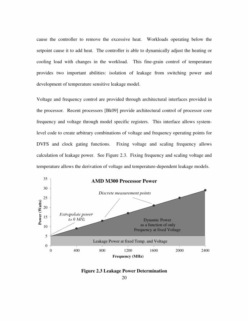
DVFS and clock gating functions. Fixing voltage and scaling frequency allows
calculation of leakage power. See Figure 2.3. Fixing frequency and scaling voltage and
temperature allows the derivation of voltage and temperature-dependent leakage models.
Figure 2.3 Leakage Power Determination
0
5
10
15
20
25
30
35
0 400 800 1200 1600 2000 2400
Po
wer
(W
att
s)
Frequency (MHz)
AMD M300 Processor Power
Extrapolate power
to 0 MHz
Leakage Power at fixed Temp. and Voltage
Dynamic Power
as a function of only
Frequency at fixed Voltage
Discrete measurement points
21
2.3 Performance Counter Sampling
To sample performance monitoring counters a small kernel that provides periodic
sampling of processor performance counters is developed. This kernel uses a device
driver to provide ring-0 access to user-mode applications. This approach is preferred
over existing user-mode performance counter libraries as it affords more precise control
of sampling and lower overhead. In all experiments, the worst-case sampling overhead
(% CPU time sampling) for performance counter access averages less than 1% for
sampling intervals as low as 16ms. In addition to the performance impact of counter
sampling, there is a power impact which must be minimized. A common problem with
periodically scheduled code, such as performance counter sampling, is excessive
scheduler activity. This activity causes CPUs to frequently exit the idle state to service
interrupts, thus increasing power consumption. The sampling kernel avoids this issue by
explicitly requesting a scheduling interval that exactly matches the required sampling
interval. As a result the scheduler only runs enough to schedule the performance counter
sampling events and background operating system activity.
2.4 Workloads
Workload selection is a critical part of dynamic power management analysis. The focus
on power accounting and prediction requires workloads with widely varying power and
performance levels. Unlike microarchitectural analysis that considers phases within an

22
instruction stream lasting only a few microseconds, dynamic power management must
also consider long duration phases ranging from hundreds to millions of microseconds.
These phases, caused by events such as thread migrations, context switches or device
interrupts provide greater opportunity (and challenge) for power management due to the
longer time for amortizing adaptation costs. To this end, this dissertation analyzes power
consumption, modeling and prediction across over sixty distinct subtests. The workloads
and their characteristics are listed in Table 2.5.
Table 2.5 Workload Description
Name
[Subtest Count]
Workload
Type
Subsystem
Target
Phase Behavior Systems
Analyzed
SPEC CPU 2000
[26]
Scientific CPU
DRAM
Instruction Server
Desktop
Laptop
SPEC CPU 2006
[29]
Scientific CPU
DRAM
Instruction Server
Desktop
Laptop
SPECjbb 2005
[1]
Transaction
Processing
CPU
DRAM
Instruction Server
DBT-2
[1]
Database I/O
Disk
Instruction
Active-Idle
Power Management
Server
SYSmark 2007
[4]
Productivity CPU
DRAM
I/O
Disk
Instruction
Active-Idle
Threadedness
Power Management
Desktop
Laptop
3DMark 2006
[6]
3D Gaming Graphics
CPU
DRAM
Instruction
Active-Idle
Power Management
Laptop
Idle
[1]
Idle CPU Active-Idle Server,
Desktop
Laptop
To develop power models for active execution (non-idle) the SPEC CPU 2000, 2006 and
SPECjbb 2005 workloads are used [Sp00] [Sp06] [Sj06]. These workloads contain
23
instruction streams that exercise a wide range of intensities in the CPU and memory
subsystems. They include integer and floating centric workloads. Within these two types
the focus varies from workloads completely bound by CPU execution speed to those
bound be memory access latency and throughput. These benchmarks provide sufficient
information to develop active power models for CPU and memory. The limitation is that
they operate in an unrealistic fully-active mode utilization only the CPU and memory
subsystems. Unlike real usage scenarios, these workloads do not frequently transition
between the active and idle states or exercise disk, graphics or I/O subsystems.
To address this limitation the DBT-2, SYSmark 2007 and 3DMark 2006 benchmarks are
included. These workloads emulate real usage scenarios by including user-input and
system interactions. DBT-2 [Os06] is intended to approximate the TPC-C transaction
processing benchmark. This workload does not require network clients, but does use
actual hard disk access through the PostgreSQL [PS06] database. SYSmark 2007 [Sm07]
is implemented using simulated user input through the application GUI (graphical user
interface). The numerous delays required for GUI interaction causes many idle phases
across the subsystems. This causes a large degree of active-idle and idle-active
transitions, thread migrations and power management events. 3DMark06 [3d06] contains
six subtests covering CPU and graphics-intensive workloads. Additionally, systems are
characterized in the idle state. This sets a baseline for power consumption and represents
common usage patterns.

24
Chapter 3 Modeling CPU Power using
Performance Monitoring Counters
Effective power management requires fine-grain accounting of power within complex,
computing systems. Since these systems contain multiple components sharing power
resources, it is difficult to attribute power to individual components. It has been shown
that performance-relevant events are strong predictors of power consumption. Due to the
widespread availability of on-chip performance monitoring facilities, it is possible to
develop accurate, run-time power models based upon performance events. This chapter
demonstrates the effectiveness of these at CPU power accounting. Models are shown
ranging from simple three-term linear to polynomial models that account for power
management and workload effects such voltage, frequency and temperature. The chapter
concludes with a formal definition of the model building methodology.
3.1 Correlation of Performance Counters to Power
While past research [LiJo03] [Be00] and intuition suggest that instructions/cycle (IPC)
alone can account for CPU power, this study considers a larger array of metrics for
building models. Correlation coefficients were calculated for all twenty-one observed
PMCs. Initially, we attempted to find correlation across multiple sample points in a
single workload trace. However, it was found that minor discrepancies in alignment of

25
the power trace to the PMC trace could cause large variations in correlation. Since there
is such a large set of workloads each workload is used as a single data point in the
correlation calculation. For each metric the average rate across each workload is
determined. For most, the metrics are converted to event/cycle form, but a few are in
other forms such as hit rates. Additional derived metrics are included such as completed
µops/cycle (retired + cancelled µops). A subset of the correlation results can be seen in
Table 3.1.
Table 3.1. Intel Pentium 4, High and Low Correlation Performance Metrics
Metric Correlation
Speculatively Issued µops/Cycle 0.89
Fetched µops/Cycle 0.84
Retired Instructions/Cycle 0.84
Completed µops/Cycle 0.83
Loads/Cycle 0.80
Retired µops/Cycle 0.79
Branches/Cycle 0.78
Stores/Cycle 0.64
Mispredicted Branches/Cycle 0.41
Level 2 Cache Misses/Cycle -0.33
Cancelled µops/Cycle 0.33
Level 2 Cache Hits/Cycle 0.31
Bus Accesses/Cycle -0.31
Trace Cache Issued µops/Cycle 0.32
Bus Utilization -0.31
Floating Point ops/µop -0.22
Prefetch Rate 0.17
Trace Cache Build µops/Cycle -0.15
Instruction TLB Hits/Cycle -0.09
Trace Cache Misses/Cycle -0.09
Instruction TLB Misses/Cycle -0.04

26
As expected IPC-related metrics show strong correlation. One of the more unexpected
findings is the weak negative correlation of floating point instruction density (ratio of all
dynamic instructions). This is in contrast to past findings [Be00] that show a strong
correlation between floating point operations per second and power. Later in section 3.3
an explanation is provided. Another unexpected result is the lack of correlation to data
prefetch rate.
This research shows that rather than considering only IPC, a more accurate model can be
constructed using a metric that encompasses power consumed due to speculation. Figure
3.1 shows the average number of µops for the SPEC 2000 benchmarks that are fetched,
completed and retired in each cycle. Table 3.2 shows the portions of fetched µops that
complete or retire, for each of the twenty-four benchmarks.
Table 3.2 Percent of Fetched µops Completed/Retired – SPEC CPU 2000
Name %Complete %Retire Name %Complete %Retire
gzip 92.7 69.8 wupwise 97.0 91.0
vpr 85.3 60.0 swim 99.9 99.7
gcc 94.2 77.7 mgrid 99.1 98.6
mcf 63.0 31.5 applu 98.7 96.6
crafty 94.6 78.4 equake 96.8 93.5
bzip2 92.0 72.1 sixtrack 99.2 97.8
vortex 98.0 95.0 mesa 92.1 75.2
gap 92.8 73.5 art 84.9 77.5
eon 91.7 81.5 facerec 95.5 90.5
parser 90.1 69.0 ammp 94.8 88.5
twolf 85.2 55.2 fma3d 97.0 94.3
lucas 99.9 95.9
apsi 97.1 93.6
Integer Avg. 88.7 69.4 Float Avg. 96.3 91.7

27
The first bar in Figure 3.1 “Fetch” shows the number of µops that are fetched from the
Trace Cache in each cycle. The second bar “Complete” shows the sum of µops that are
either retired or cancelled each cycle. Cancelled µops are due to branch misprediction.
The third bar, “Retire”, shows only µops that update the architectural state. This figure
shows that the processor fetches 21.9% more µops than are used in performing useful
work. Therefore, a more accurate power model should use the number of µops fetched
per cycle instead of the number retired. Table 3.3 provides a comparison of linear
regression power models based on these three metrics.
Figure 3.1. Average µOps/cycle - SPEC CPU 2000
3.2 IPC Related Power Models
Twenty-one processor performance metrics are examined for their correlation to power
consumption. The most correlated metrics are all similar to (retired) instructions per
cycle. Using this finding as a guide numerous linear models are constructed using
regression techniques. Power is calculated as the sum of a positive constant α0 and the
Fetch
0.89Complete
0.84
Retire
0.73
0.6
0.7
0.8
0.9
1.0
µops
/ C
ycl
e
28
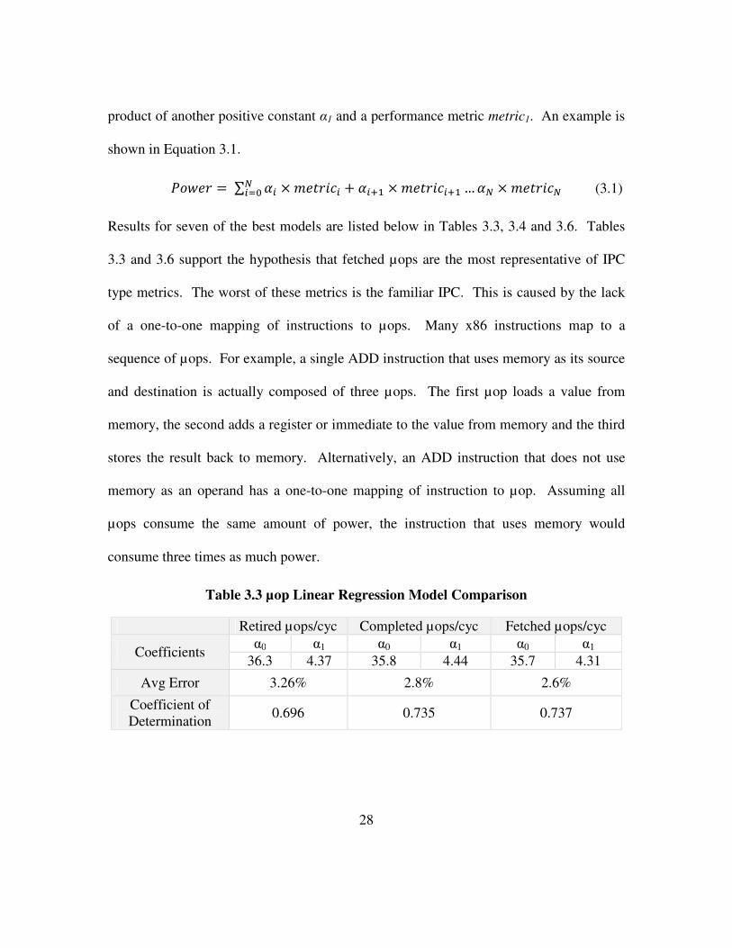
product of another positive constant α1 and a performance metric metric1. An example is
shown in Equation 3.1.
����� = ∑ ×�� ��� + �� ×�� ����� …� ×�� �������
Results for seven of the best models are listed below in Tables 3.3, 3.4 and 3.6. Tables
3.3 and 3.6 support the hypothesis that fetched µops are the most representative of IPC
type metrics. The worst of these metrics is the familiar IPC. This is caused by the lack
of a one-to-one mapping of instructions to µops. Many x86 instructions map to a
sequence of µops. For example, a single ADD instruction that uses memory as its source
and destination is actually composed of three µops. The first µop loads a value from
memory, the second adds a register or immediate to the value from memory and the third
stores the result back to memory. Alternatively, an ADD instruction that does not use
memory as an operand has a one-to-one mapping of instruction to µop. Assuming all
µops consume the same amount of power, the instruction that uses memory would
consume three times as much power.
Table 3.3 µop Linear Regression Model Comparison
Retired µops/cyc Completed µops/cyc Fetched µops/cyc
Coefficients α0 α1 α0 α1 α0 α1
36.3 4.37 35.8 4.44 35.7 4.31
Avg Error 3.26% 2.8% 2.6%
Coefficient of
Determination 0.696 0.735 0.737
(3.1)

29
Table 3.4 Instruction Linear Regression Model Comparison
Retired
instructions/cyc
Completed
instructions /cyc
Coefficients α0 α1 α0 α1
36.8 5.28 36.3 5.52
Avg Error 5.45% 4.92%
Coefficient of
Determination 0.679 0.745
Of the µop-based models fetched µops is the most representative metric for power
consumption. This suggests that µops that do not update the architected state of the
machine still consume a significant amount of power. For the case of cancelled µops,
this is not surprising since these µops did complete execution but were not retired. So,
they would have traversed nearly the entire processor pipeline consuming a similar power
level as retired µops. More surprising is the effect of fetched µops on the power model.
Fetched µops includes retired and cancelled operations. It also includes the remaining
µops that were cancelled before completing execution. Since fetched µops provides the
most accurate model, cancelled µops must be consuming a significant amount of power.
These models generate minimum and maximum power values (36W – 47W) similar to
what was found on a Pentium 3 (31W-48W) [Be00] with similar µop/cycle ranges (0 –
2.6). The stated average error values are found using the validation set described in
Table 3.1.
30
3.3 Micro ROM Related Power Models
The power models in Tables 3.3 and 3.4 perform best when applied to workloads mostly
composed of integer-type instructions (SPEC-INT). Larger errors occur for workloads
with high rates of floating point instructions (SPEC-FP). Isci et al [IsMa03] demonstrate
that FP workloads such as equake use complex microcode ROM delivered µops. While
the complex instructions execute, microcode ROM power consumption is high, but total
power consumption is reduced slightly. In order to determine if this is the case for these
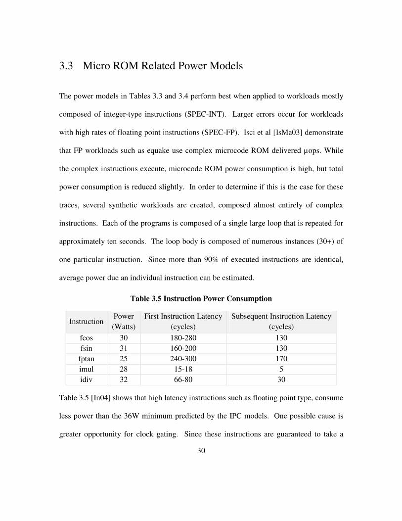
traces, several synthetic workloads are created, composed almost entirely of complex
instructions. Each of the programs is composed of a single large loop that is repeated for
approximately ten seconds. The loop body is composed of numerous instances (30+) of
one particular instruction. Since more than 90% of executed instructions are identical,
average power due an individual instruction can be estimated.
Table 3.5 Instruction Power Consumption
Instruction Power
(Watts)
First Instruction Latency
(cycles)
Subsequent Instruction Latency
(cycles)
fcos 30 180-280 130
fsin 31 160-200 130
fptan 25 240-300 170
imul 28 15-18 5
idiv 32 66-80 30
Table 3.5 [In04] shows that high latency instructions such as floating point type, consume
less power than the 36W minimum predicted by the IPC models. One possible cause is
greater opportunity for clock gating. Since these instructions are guaranteed to take a

31
long time to complete, more aggressive power saving techniques may be performed.
Further investigation will be required to validate this hypothesis. Since Table 3.5
supports the conclusion that high latency instructions consume less power, the models
can be improved by accounting for this behavior. One possible accounting method is to
note that most high latency instructions are composed of relatively long µop sequences
sourced by the microcode ROM. Microcode ROM events can be observed using the
trace cache metric, microrom µops. This metric counts the number of µops delivered
from the microcode ROM. The resultant models are given in Table 3.6. As expected
from the observations of power consumption of microcode ROM delivered instructions,
the model’s microcode ROM component is negative. This small correction allows the
power model to extend below 36W for workloads with high instances of complex
microcode ROM instructions.
Table 3.6 µop Linear Regression Model Comparison
Deliver, µROM Deliver, µROM, Build
Coefficients α0 α1 α2 α0 α1 α2 α3
36.7 4.24 -11.8 36.7 4.24 -14.6 5.74
Avg Error 2.50% 2.55%
Coefficient of
Determination 0.844 0.850
3.4 Power Management Effects
While instruction and µop-based power models accurately account for power during fully
active phases, they perform poorly in the presence of dynamic power management and
temperature variation. This section characterizes the effect that power adaptations such

32
as clock gating and dynamic voltage and frequency scaling have on power consumption.
The strong relationship between temperature and leakage power is described. These
findings are then used to develop a fully power management and temperature-aware
processor power model.
3.4.1 Active and Idle Power Management
An effective power management strategy must take advantage of program and
architecture characteristics. Designers can save energy while maintaining performance
by optimizing for the common execution characteristics. The two major power
management components are active and idle power management. Each of these
components use adaptations that are best suited to their specific program and architecture
characteristics. Active power management seeks to select an optimal operating point
based on the performance demand of the program. This entails reducing performance
capacity during performance-insensitive phases of programs. A common example would
be reducing the clock speed or issue width of a processor during memory-bound program
phases. Idle power management reduces power consumption during idle program phases.
However, the application of idle adaptations is sensitive to program phases in a slightly
different manner. Rather than identifying the optimal performance capacity given current
demand, a tradeoff is made between power savings and responsiveness. In this case the
optimization is based on the length and frequency of a program phase (idle phases) rather
than the characteristics of the phase (memory-boundedness, IPC, cache miss rate). In the
remainder of this section active power adaptations are referenced as p-states and idle

33
power adaptations as c-states. These terms represent adaption operating points as defined
in the ACPI specification. ACPI [Ac07] “…is an open industry specification co-
developed by Hewlett-Packard, Intel, Microsoft, Phoenix, and Toshiba. ACPI establishes
industry-standard interfaces enabling OS-directed configuration, power management, and
thermal management of mobile, desktop, and server platforms.”
3.4.2 Active Power Management: P-states
A p-state (performance state) defines an operating point for the processor. States are
named numerically starting from P0 to PN, with P0 representing the maximum
performance level. As the p-state number increases, the performance and power
consumption of the processor decrease. Table 3.7 shows p-state definitions for a typical
processor. The state definitions are made by the processor designer and represent a range
of performance levels that match expected performance demand of actual workloads. P-
states are simply an implementation of dynamic voltage and frequency scaling. The
resultant power reduction is obtained using these states is largely dependent on the
amount of voltage reduction attained in the lower frequency states.
Table 3.7 Example P-states Definition
P-State Frequency (MHz) VDD (Volts)
P0 FMax × 100% VMax × 100%
P1 FMax × 85% VMax × 96%
P2 FMax × 75% VMax × 90%
P3 FMax × 65% VMax × 85%
P4 FMax × 50% VMax × 80%
34
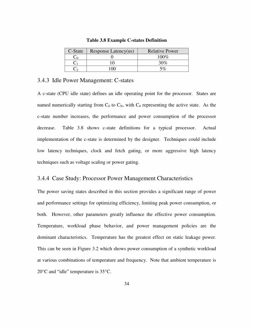
Table 3.8 Example C-states Definition
C-State Response Latency(us) Relative Power
C0 0 100%
C1 10 30%
C2 100 5%
3.4.3 Idle Power Management: C-states
A c-state (CPU idle state) defines an idle operating point for the processor. States are
named numerically starting from C0 to CN, with C0 representing the active state. As the
c-state number increases, the performance and power consumption of the processor
decrease. Table 3.8 shows c-state definitions for a typical processor. Actual
implementation of the c-state is determined by the designer. Techniques could include
low latency techniques, clock and fetch gating, or more aggressive high latency
techniques such as voltage scaling or power gating.
3.4.4 Case Study: Processor Power Management Characteristics
The power saving states described in this section provides a significant range of power
and performance settings for optimizing efficiency, limiting peak power consumption, or
both. However, other parameters greatly influence the effective power consumption.
Temperature, workload phase behavior, and power management policies are the
dominant characteristics. Temperature has the greatest effect on static leakage power.
This can be seen in Figure 3.2 which shows power consumption of a synthetic workload
at various combinations of temperature and frequency. Note that ambient temperature is
20°C and “idle” temperature is 35°C.

35
Figure 3.2 Temperature Sensitivity of Leakage Power
As expected, a linear change in frequency yields a linear change in power consumption.
However, linear changes in temperature yield exponential changes in power
consumption. Note that static power is identified by the Y-intercept in the chart. This is
a critical observation since static power consumption represents a large portion of total
power at high temperatures. Therefore, an effective power management scheme must
also scale voltage to reduce the significant leakage component. To see the effect of
voltage scaling consider Figure 3.3.
Figure 3.3 shows the cumulative effect of p-states and c-states. Combinations of five p-
states (x-axis) and four operating modes are shown. The lowest power case, C1e-Idle,
represents all cores being idle for long enough that the processor remains in the C1e state
more than 90 percent of the time. The actual amount of time spent in this state is heavily
0
10
20
30
40
50
60
35 50 65 80 95
Core
Pow
er (
Watt
s)
Die Temperature (Celsius)
Leakage
Dynamic
Dynamic power
constant for fixed
voltage and frequency
Leakage power
varies exponentially
with temperature

36
influenced by the rate of input/output (I/O) and OS interrupts. This state also provides
nearly all of the static power savings of the low-voltage p-states even when in the P0
state. Second, the C1-Idle case shows the power consumption assuming at least one core
remains active and prevents the processor from entering the C1e state. This represents an
extreme case in which the system would be virtually idle, but frequent interrupt traffic
prevents all cores from being idle. This observation is important as it suggests system
and OS design can have a significant impact on power consumption. The remaining two
cases, C0-Idle and C0-Max, show the impact of workload characteristics on power. C0-
Idle attains power savings though fine-grain clock gating.
C0-Max All Cores Active IPC ≈ 3
C0-Idle All Cores Active IPC ≈ 0
C1- Idle At Least One Active Core, Idle Core Clocks Gated
C1e-Idle “Package Idle” - All Core Clocks Gated, Memory Controller Clocks Gated
Figure 3.3 Power by C-state/P-state Combination
0
10
20
30
40
50
60
70
80
90
100
0 1 2 3 4
Pow
er (
Watt
s)
P-State
C0-Max C0-Idle C1-Idle C1e-Idle

37
The difference between C0-Idle and C0-Max is determined by the amount of power spent
in switching transistors, which would otherwise be clock-gated, combined with worst-
case switching due to data dependencies. C0-Max can be thought of as a pathological
workload in which all functional units on all cores are 100 percent utilized and the
datapath constantly switches between 0 and 1. All active phases of real workloads exist
somewhere between these two curves. High-IPC compute-bound workloads are closer to
C0-Max while low-IPC memory-bound workloads are near C0-Idle.
3.4.5 Power Management-Aware Model
The model improves on existing on-line models [Be00] [BiJo06-1] [IsMa03] by
accounting for power management and temperature effects. Like existing models it
contains a workload dependent portion that is dominated by the number of instructions
completed per second. In this case the number of fetched operations per second is used
in lieu of instructions completed. The fetched µops metric is preferred as it also accounts
for speculative execution. In addition to fetched µops, a retired floating point µops
metric is also included. This accounts for the power difference between integer and
floating point ops in the AMD processor. Unlike the Pentium 4 processor which exhibits
little difference in power consumption between integer and floating point applications,
the AMD processor exhibits much higher power consumption for high-throughput
floating point applications. A further distinction of this model is that it contains a
temperature dependent portion. Using workloads with constant utilization, processor
temperature and voltage are varied to observe the impact on static leakage power.

38
Temperature is controlled by adjusting the speed of the processor’s fan. Temperature is
observed with a 1/8 degree Celsius resolution using an on-die temperature sensor [Bk09].
This sensor can be accessed by the system under test through a built-in, on-chip register.
The resultant temperature-dependent leakage equation is shown in Table 3.9. Since
temperature is modeled over only the operating range of the processor, it can be
accounted for as a quadratic equation. Alternatively, a wider temperature range can be
accounted for using and an exponential equation in the form of a×eT×b
. The coefficients a
and b are found through regression. The term T represents the die temperature in Celsius.
For this study the quadratic form is used due to its lower computational overhead and
sufficient accuracy. Voltage is controlled using the P-State Control Register [Bk09].
This allows selection of one of five available voltage/frequency combinations. Voltage is
observed externally as a subset of the traced power data. Like the workload dependent
model, the coefficients of the static power model are tuned using regression techniques.
Note that the static power model is highly process dependent. Processors with different
semiconductor process parameters require the model to be re-tuned.
The dominant power management effects (voltage/frequency scaling, clock gating) are
further accounted for using the gateable and ungateable power models. Gateable power
is found by measuring the effect of enabling/disabling idle core clock gating. Ungateable
represents the portion of power which cannot be gated. These components are also found
experimentally. The resultant, average error in the model is 0.89%. The standard
deviation of the error for SPEC CPU2006 and SYSmark 2007 is less than 1%. Worst-

39
case error is 3.3%. Alternatively stated, 68.2% of workloads have an error of less than
1%. Per workload error is shown in Figure 3.4. The composition of the CPU model is
summarized in Table 3.9.
Table 3.9 AMD Quad-Core Power Model
Power Models Equation
Total Power ∑ (WorkloadDependentN + UngateableN + GateableN)*
��� + StaticVolt,Temp
Workload
Dependent
Power
((FetchOpsN/Sec)×CoeffF+(FloatPointOpsN/Sec) ×CoeffFP
+(DCAccessN/Sec) ×CoeffDC) ×Voltage2
Idle Power
Management
Power
(Gateable)
(%HaltedN) ×CoeffGateable×Voltage2×FrequencyN
Irreducible
Power
(Ungateable)
(%NonHaltedN) ×CoeffUngateable×Voltage2×FrequencyN
Irreducible
Power
(Static)
(Temp2×CoeffT
2+Temp
1×CoeffT
1+×CoeffT
0)VoltageN
Figure 3.4 CPU Power Model – SPEC CPU 2006 Power and Average Error
1.4%1.4%
3.0%
0.6%
0.4%
0.8%
0.4%
0.2%
2.1%
0.5%
0.3%
0.2%
0.9%
0.6%
0.5%
0.3%
0.6%
2.3%0.2%
1.0%1.6%
0.2%
0.9%0.2%
0.2%
3.3%
0.6%
0.1%
0.8%
0.0%
0.5%
1.0%
1.5%
2.0%
2.5%
3.0%
3.5%
30
31
32
33
34
35
36
37
per
lben
ch
bzi
p2
gcc
mcf
gob
mk
hm
mer
sjen
g
lib
quan
tum
h26
4re
f
om
net
pp
asta
r
xal
ancb
mk
bw
aves
gam
ess
mil
c
zeu
smp
gro
mac
s
cact
usA
DM
lesl
ie3
d
nam
d
dea
lII
sop
lex
pov
ray
calc
uli
x
Gem
sFD
TD
ton
to
lbm
wrf
sph
inx3
Wa
tts
Measured Modeled
Error %

40
3.5 Methodology for Power Modeling
With an understanding of system level events that are visible to the processor it is
possible to apply the iterative modeling process as depicted in Figure 3.5. This procedure
utilizes linear and polynomial regression techniques to build power models for individual
subsystems. The user identifies workloads which target a particular subsystem (cache,
system memory, disk) and performs regression modeling using performance events as
inputs. The model is then applied to a larger set of workloads to confirm accuracy and
the lack of outlier cases. Depending on the outcome, the process is repeated with
alternate performance events as inputs. Though an exhaustive search of performance
events can be performed, a rapid solution is found when events are selected with high
correlation to subsystem activity. Details of the modeling process in Figure 3.5 are listed
below.
1. Measure subsystem-level power using subset of workloads. Begin with simple,
easy-to-run workloads.
2. Confirm that Coefficient of Variation is greater than α for the chosen workload.
The simplest workloads often do not generate sufficient power variation for model
tuning. For example consider any of the cache-resident workloads in SPEC CPU 2000
which generate little or no activity in subsystems outside of the processor cores such as
memory. Tuning the model based on these low-variation workloads may cause the
process to include performance events that do not correlate well with power.

41
3. Based on basic domain knowledge, choose performance events, measureable by
performance counters that are most relevant to the subsystem in question. Choose
counters that are expected to “trickle-down” to other subsystems. The pool of candidate
performance counters may need to be expanded if sufficient accuracy is not achieved.
4. Using the selected performance counter events as the input variables and
subsystem power as the output variable, perform linear regression modeling. For
example, in the general linear equation y = mx + b, vary the coefficients m and b until the
sum-of-squares error is minimized. Multiple linear or polynomial regression may be
used in subsequent iterations of algorithm if sufficient accuracy is not obtained.
5. Using a subset of workloads calculate average error per sample. If less than ρ%
error cannot be achieved, choose an a new performance event. Selection of ρ is dictated
by the required model accuracy and time required for solution. Setting ρ to a low
(restrictive) value may extend time to solution. It may also prevent the process from
finding a solution.
6. Assess the representativeness of the model by manually comparing graphs of
modeled versus measured power. This avoids the case in which statistical assessment
cannot detect major errors such as those seen in Anscombe’s Quartet [An73].
7. Using complete set of workloads calculate average error per sample. If less than δ
% error cannot be achieved, choose a new performance event. Like ρ, δ is selected
according the accuracy and time-to-solution requirements.
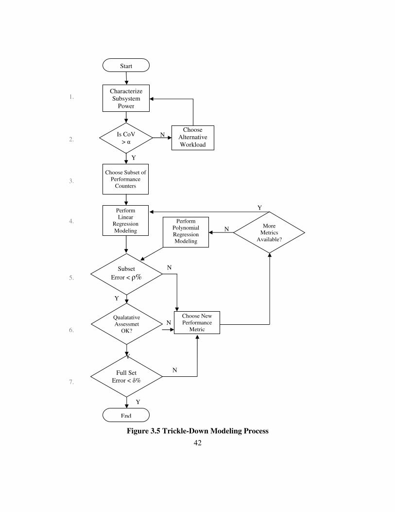
42
Figure 3.5 Trickle-Down Modeling Process
N
Y
Qualatative
Assessmet
OK?
Y
Full Set
Error < δ%
End
Start
Characterize
Subsystem
Power
Is CoV
> α
Choose
Alternative
Workload
Y
N
Choose Subset of
Performance
Counters
Perform
Linear
Regression
Modeling
Subset
Error < ρ%
Perform
Polynomial
Regression
Modeling
Choose New
Performance
Metric
N
More
Metrics
Available?
N
Y
1.
2.
3.
4.
5.
6.
7.
Y
N

43
3.6 Summary
This section describes concepts and methodologies for modeling processor power
consumption through the use of performance monitoring counters. These models achieve
average error rates of under 1% using only a handful of metrics/signals. Simple,
deterministic, processor power models such as these will increase in importance as the
need for energy efficiency increases. Techniques that maximize performance within
fixed power limits or optimize power metrics (Perf/Watt, Energy × Delay, etc.) are
becoming prevalent in processors [Po10][McPo06][ChJa09] and systems. Since these
techniques rely on accurate processor power accounting, performance counter power
models will increase in importance.

44
Chapter 4 System-Level Power Analysis
This chapter provides an extensive characterization of system-level power consumption
across platforms and workloads ranging from servers to laptops. For each system type,
workloads and subsystems specific to the system are considered. Power consumption is
considered in terms of average and variability. While average power is critical for energy
efficiency, variation including maximum and minimum power is required for effective
system and dynamic power management design.
4.1 Average Power
4.1.1 Server Platform - SPEC CPU, SPECjbb and DBT-2
For the case of SPEC CPU and SPECjbb workloads the behavior is distinct from the
DBT-2 database workload. In Figure 4.1 a comparison of average subsystem power
consumption is given for all workloads. Compared to the disk-bound DBT-2, the
memory-bound and cpu-bound applications show significantly higher CPU and memory
power consumption. While DBT-2 only increases average CPU power by 26% compared
to idle, all of these workloads increase average CPU power by more than 250%. For
memory, the top three consumers are floating point workloads. This supports the
intuitive conclusion that memory power consumption is correlated to utilization.
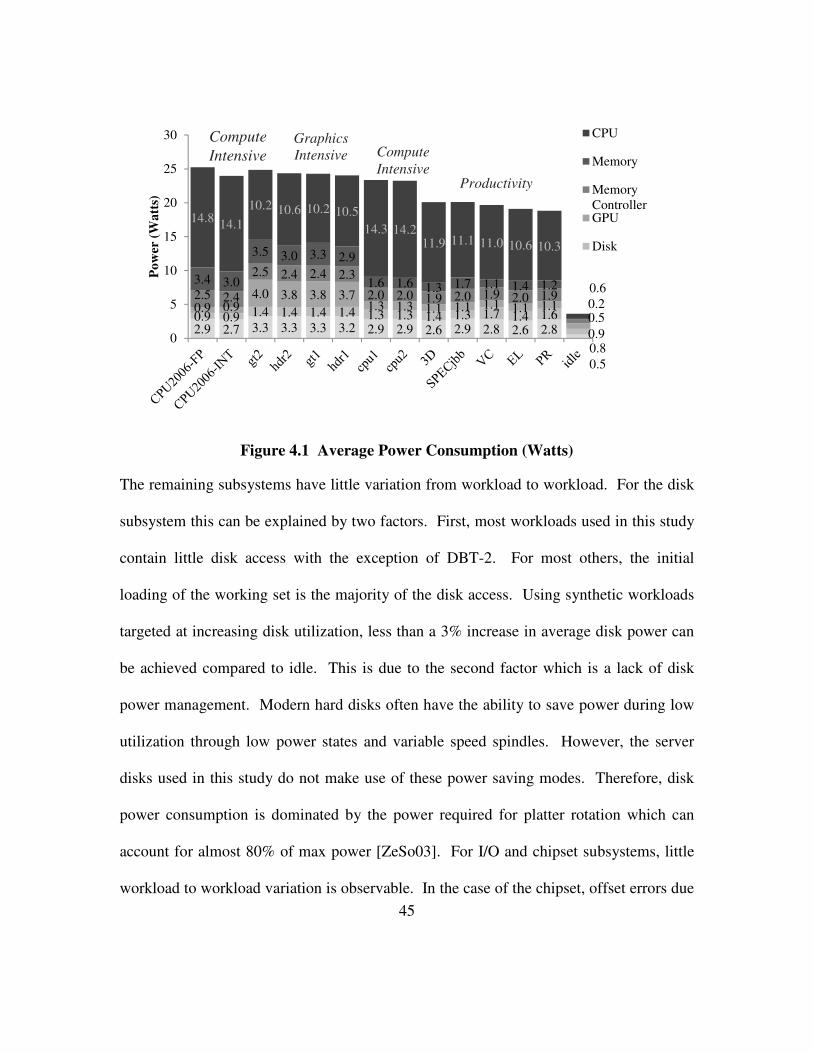
45
Figure 4.1 Average Power Consumption (Watts)
The remaining subsystems have little variation from workload to workload. For the disk
subsystem this can be explained by two factors. First, most workloads used in this study
contain little disk access with the exception of DBT-2. For most others, the initial
loading of the working set is the majority of the disk access. Using synthetic workloads
targeted at increasing disk utilization, less than a 3% increase in average disk power can
be achieved compared to idle. This is due to the second factor which is a lack of disk
power management. Modern hard disks often have the ability to save power during low
utilization through low power states and variable speed spindles. However, the server
disks used in this study do not make use of these power saving modes. Therefore, disk
power consumption is dominated by the power required for platter rotation which can
account for almost 80% of max power [ZeSo03]. For I/O and chipset subsystems, little
workload to workload variation is observable. In the case of the chipset, offset errors due
2.9 2.7 3.3 3.3 3.3 3.2 2.9 2.9 2.6 2.9 2.8 2.6 2.8
0.5
0.9 0.9 1.4 1.4 1.4 1.4 1.3 1.3 1.4 1.3 1.7 1.4 1.6
0.8
0.9 0.94.0 3.8 3.8 3.7
1.3 1.3 1.1 1.1 1.1 1.1 1.1
0.9
2.5 2.4
2.5 2.4 2.4 2.3
2.0 2.0 1.9 2.0 1.9 2.0 1.9
0.5
3.4 3.0
3.5 3.0 3.3 2.9
1.6 1.6 1.3 1.7 1.1 1.4 1.2
0.2
14.814.1
10.2 10.6 10.2 10.5
14.3 14.211.9 11.1 11.0 10.6 10.3
0.6
0
5
10
15
20
25
30
Po
wer
(W
att
s)
CPU
Memory
Memory
ControllerGPU
Disk
Graphics
Intensive
Productivity
Compute
Intensive Compute
Intensive

46
to aliasing were introduced that affected average power results. Much greater variation
can be found within each workload.
4.1.2 SPEC CPU 2000/2006 CPU and Memory Power Comparison
Compared to desktop and mobile systems servers have a different power consumption
composition across subsystems. Due to the presence of large memory subsystems,
DIMM power is a much larger component. Also, larger working sets such as those found
in SPEC CPU2006 compared to SPEC CPU2000 shift power consumption from the cores
to the DIMMs. Consider CPU2000 in Figure 4.2 and CPU2006 in Figure 4.3. Due to
comparatively small working sets, CPU2000 workloads are able to achieve higher core
power levels. The reason is that, since the working set fits completely within the on-chip
caches, the processor is able to maintain high levels of utilization. This is made more
evident by the power increases seen as the number of simultaneous threads is increased
from one to four. Since there is less performance dependence on the memory interface,
utilization and power continue to increase as threads are added. The result is different for
SPEC CPU2006. Due to the increased working set size of this benchmark, the memory
subsystem limits performance. Therefore, core power is reduced significantly for the
four-thread case. Differences for the single-thread case are much less, due to a reduced
dependency on the memory subsystem. The shift in utilization from the core to the
memory subsystem can be seen clearly in Figure 4.4. For the most compute-bound
workloads, core power is five times larger than DIMM power. However, as the

47
workloads become more memory-bound, the power levels converge to the point where
DIMM power slightly exceeds core power.
Figure 4.2 CPU2000 Average Core Power - 1 Thread vs. 4 Thread
Figure 4.3 CPU2006 Average Core Power - 1 Thread vs. 4 Thread
20 20 20 20 20 19 19 19 19 19 19 19 19 19 19 19 19 19 18 18 18 18 18 18 17 17 17
53 53 5350 49 49 49 48 48 48 48 48 47 46 46 46 46 45 45 45 45
43 42 4240 39
38
33
29
19
14
0
10
20
30
40
50
60
craf
ty
per
lbm
k
eon
gzi
p
par
ser
gap
mes
a
gal
gel
gcc
vort
ex
mg
rid
bzi
p2
sixtr
ack
vpr
Av
erag
e
apsi
wu
pw
ise
face
rec
amm
p
fma3
d
two
lf
luca
s
equak
e
applu ar
t
swim
mcf 3D
Vid
eoC
reat
ion
Ele
arn
ing
Pro
du
ctiv
ity
Wa
tts
SPEC2000-1x
SPEC2000-4x
Desktop
20 20 19 19 19 19 19 19 19 19 19 18 18 18 18 18 18 17 17 17 17 17 17 16 16 16 16 16 16 16
50 49 49 48 48 48 47 46 46 46 45 45 43 42 42 42 41 40 40 40 39 39 38 37 37 35 35 35 34 34 3329
19
14
0
10
20
30
40
50
60
gam
ess
h26
4re
f
hm
mer
calc
uli
x
nam
d
pov
ray
gro
mac
s
per
lben
ch
gob
mk
dea
lII
sjen
g
ton
to
xal
ancb
mk
cact
usa
dm
bzi
p2
Av
erag
e
asta
r
gcc
sph
inx3
wrf
bw
aves
zeu
smp
lesl
ie3
d
om
net
pp
gem
sfdtd
sop
lex
mcf
lib
quan
tum
mil
c
lbm 3D
Vid
eoC
reat
ion
Ele
arn
ing
Pro
du
ctiv
ity
Wa
tts
SPEC2006-1x
SPEC2006-4x
Desktop
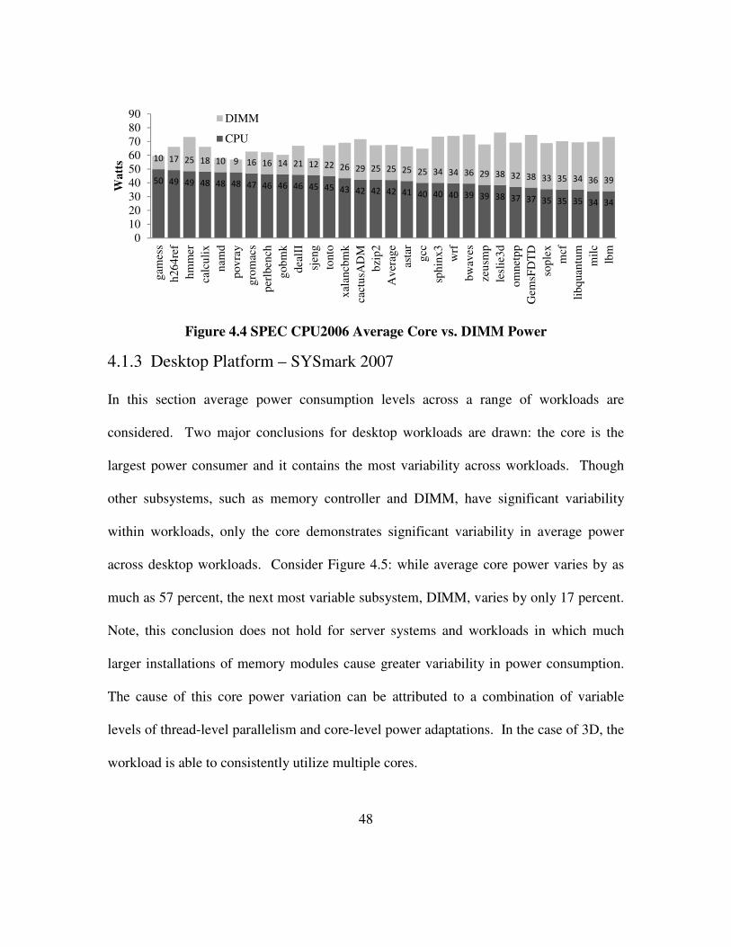
48
Figure 4.4 SPEC CPU2006 Average Core vs. DIMM Power
4.1.3 Desktop Platform – SYSmark 2007
In this section average power consumption levels across a range of workloads are
considered. Two major conclusions for desktop workloads are drawn: the core is the
largest power consumer and it contains the most variability across workloads. Though
other subsystems, such as memory controller and DIMM, have significant variability
within workloads, only the core demonstrates significant variability in average power
across desktop workloads. Consider Figure 4.5: while average core power varies by as
much as 57 percent, the next most variable subsystem, DIMM, varies by only 17 percent.
Note, this conclusion does not hold for server systems and workloads in which much
larger installations of memory modules cause greater variability in power consumption.
The cause of this core power variation can be attributed to a combination of variable
levels of thread-level parallelism and core-level power adaptations. In the case of 3D, the
workload is able to consistently utilize multiple cores.
50 49 49 48 48 48 47 46 46 46 45 45 43 42 42 42 41 40 40 40 39 39 38 37 37 35 35 35 34 34
10 17 25 18 10 9 16 16 14 21 12 22 26 29 25 25 25 25 34 34 36 29 38 32 38 33 35 34 36 39
0
10
20
30
40
50
60
70
80
90
gam
ess
h26
4re
f
hm
mer
calc
uli
x
nam
d
pov
ray
gro
mac
s
per
lben
ch
gob
mk
dea
lII
sjen
g
ton
to
xal
ancb
mk
cact
usA
DM
bzi
p2
Av
erag
e
asta
r
gcc
sph
inx3
wrf
bw
aves
zeu
smp
lesl
ie3
d
om
net
pp
Gem
sFD
TD
sop
lex
mcf
lib
quan
tum
mil
c
lbm
Wa
tts
DIMM
CPU

49
At the other extreme, the productivity workload rarely utilizes more than a single core.
Since Quad-Core AMD processor power adaptations are applied at the core level,
frequency reduction achieves significant power savings on the three idle cores. As a
result, the productivity workload consumes much less power than the 3D workload. The
remaining workloads offer intermediate levels of thread-level parallelism and therefore
have intermediate levels of power consumption. Also note that this level of power
reduction is due only to frequency scaling. With the addition of core-level voltage
scaling, the variation/power savings is expected to increase considerably.
Figure 4.5 Desktop Subsystem Power Breakdown
4.1.4 Desktop Platform - SPEC CPU, 3DMark and SYSmark
To understand subsystem-level power consumption average and standard deviation
results are presented. Figure 4.6 displays average power of each subsystem measured in
Watts. To give an indication of the variation in power consumption Table 4.1 displays
3.7 3.7 3.7 3.6
22.1 22.2 21.1 22.0
13.9 13.8 13.7 13.8
10.9 10.5 10.3 10.1
33.1
18.714.3
29.4
0
10
20
30
40
50
60
70
80
90
3D E-Learning Productivity Video
Creation
Pow
er(W
att
s) CPU
Memory
I/O
Disk
Video

50
the standard deviation of subsystem power. Two major differences are apparent
comparing desktop to server power consumption: desktop power in each subsystem is
much less while relative variability is much greater. In both cases, power management
plays a large role. Effective power management through DVFS, clock gating and link
management reduce average power during idle and low utilization phases. This leads to a
greater difference in sample-to-sample power. Additionally, semiconductor process
improvements have a major effect.
The CPU subsystem is considered first. Not surprisingly, the desktop processor has
average power that is an order of magnitude less than the server processor. This is
largely influenced by process (130nM vs. 45nM), DVFS (desktop-only) and idle power
management. While the server idle power represents at least 24% of average power,
desktop idle power is no more than 4%. These large power savings require the CPU
model to include additional metrics such as frequency, voltage and temperature. It is not
sufficient to consider metrics associated only with the instruction stream (IPC, cache
accesses).
Like CPU, the chipset also exhibits much greater power variation. Unlike the server
chipset which has nearly uniform power consumption, the desktop chipset has much
greater variation with standard deviation representing as much as 10% of average power.
The difference illustrates the impact of link (Hypertransport) power management.
Average power values are also much less due to the lack of an L3 cache in the desktop

51
processor. In both platforms the top-level cache is contained in the chipset power rail.
To reduce power consumption and cost the desktop designer lacks an L3 cache.
Yet another subsystem with order-of-magnitude power reduction is the DRAM memory.
Despite higher operating frequency (533Mhz vs 100MHz) average DRAM power is
reduced by almost a factor of 10. The reason is reduced memory voltage (2.8V vs 1.5V),
reduced capacity (8GB vs 4GB) and more aggressive memory power management. Note
that the desktop system differentiates between DRAM, “Memory” subsystem and the
Memory Controller. The server system includes both in the memory subsystem. The
desktop memory controller has a similar level of power variation as the DRAMs. This is
due to the memory controller management power savings for both subsystems. This also
allows implementation of simple trickle-down models in multiple subsystems that are
driven by the same performance metrics.
An additional subsystem, not present in the server analysis is the RS780 GPU (graphics
processing unit). This subsystem has unique bi-modal power consumption. In all cases
GPU power is either near the maximum or minimum levels. For workloads with little or
no GPU activity power ranged from 0.8W to 1.3W with little variation. The graphics-
centric workloads of 3DMark06 had much greater variation as the workload alternates
between ~1W and 4W. This gives the GPU one of the largest power variations with a
standard deviation covering over 25% of the maximum power. The bimodal power
consumption is caused by aggressive idle power management and low active power
variation.

52
Figure 4.6 Subsystem Average Power (Watts)
Lastly the desktop hard drive power is considered. Three factors affect the large average
power reduction and relative standard deviation increase: spindle speed, platter size and
link power management. Since spindle power is such a large component of drive power
consumption, reducing from 7200rpm to 5400rpm has a large impact. To conform to a
smaller form factor, disk platter diameter is reduced nearly 28% (3.5” to 2.5”). This
reduces spindle and drive head power. Less power is required to rotate a smaller mass
and move the drive head a shorter distance. Also, SATA link power management
reduces power consumption in the control electronics and links during idle phases. These
changes yield a drastic increase in variability with standard deviation representing 32% of
average power in the most intense workload (video creation).
2.9 2.7 3.3 3.3 3.3 3.2 2.9 2.9 2.6 2.9 2.8 2.6 2.8
0.5
0.9 0.9 1.4 1.4 1.4 1.4 1.3 1.3 1.4 1.3 1.7 1.4 1.6
0.8
0.9 0.94.0 3.8 3.8 3.7
1.3 1.3 1.1 1.1 1.1 1.1 1.1
0.9
2.5 2.4
2.5 2.4 2.4 2.3
2.0 2.0 1.9 2.0 1.9 2.0 1.9
0.5
3.4 3.0
3.5 3.0 3.3 2.9
1.6 1.6 1.3 1.7 1.1 1.4 1.2
0.2
14.814.1
10.2 10.6 10.2 10.5
14.3 14.211.9 11.1 11.0 10.6 10.3
0.6
0
5
10
15
20
25
30P
ow
er(W
att
s)CPU
Memory
Memory Controller
GPU
Disk
Chipset

53
Table 4.1 Subsystem Power Standard Deviation (Watts)
Workload CPU Chipset Memory Memory
Controller GPU Disk Total
idle 0.026 0.010 0.008 0.008 0.002 0.115 0.129
SPEC CPU2006 INT 2.586 0.257 1.518 0.447 0.174 0.361 2.689
SPEC CPU2006 FP 2.334 0.246 1.970 0.500 0.143 0.240 2.263
gt1 0.736 0.093 0.808 0.217 0.904 0.487 1.57
gt2 0.820 0.105 0.905 0.241 1.090 0.488 2.05
cpu1 1.989 0.262 0.706 0.168 0.356 0.469 2.02
cpu2 2.036 0.263 0.709 0.167 0.362 0.421 2.23
hdr1 0.757 0.131 1.043 0.294 1.144 0.527 1.84
hdr2 0.826 0.152 1.134 0.326 1.096 0.497 2.16
EL 0.696 0.158 0.980 0.278 0.051 0.373 1.744
VC 1.774 0.252 0.585 0.114 0.069 0.566 2.540
PR 0.683 0.250 0.811 0.155 0.086 0.438 1.506
3D 1.159 0.170 0.587 0.108 0.029 0.321 1.701
SPECjbb 1.230 0.297 1.096 0.235 0.031 0.232 2.765
4.2 Power Consumption Variation
4.2.1 Server Platform
To quantify the extent of power variation within a workload coefficient of variation
(CoV) metric is used. This metric uses standard deviation to quantify variation in a data
set, and also normalizes the variation to account for differences in average data. Since
the subsystems in this study have average power values that differ by nearly an order of
magnitude, this metric is most appropriate. Table 4.2 provides a summary of the
coefficient of variation for all workloads.
Compared to the variation in average power among workloads on a given subsystem, the
variation within a particular workload is less consistent. Subsystem-workload pairs such

54
as CPU-gcc and memory-SPECjbb have a large variety of power levels. In contrast disk-
art and chipset-mcf have as much as 300X less variation.
Table 4.2 Coefficient of Variation
CPU Chipset Memory I/O Disk
idle 8.86×10⁻³
4.61×10⁻³
1.17×10⁻³
3.86×10⁻³
1.25×10⁻³
gcc 5.16×10⁻²
1.13×10⁻²
6.90×10⁻²
4.05×10⁻³
2.44×10⁻³
mcf 3.37×10⁻²
8.53×10⁻³
3.60×10⁻²
3.81×10⁻³
1.50×10⁻³
vortex 6.99×10⁻³
4.12×10⁻³
2.06×10⁻²
3.11×10⁻³
7.82×10⁻⁴
art 2.47×10⁻³
3.66×10⁻³
5.31×10⁻³
3.12×10⁻³
2.51×10⁻⁴
lucas 1.21×10⁻²
6.34×10⁻³
5.73×10⁻³
3.09×10⁻³
3.25×10⁻⁴
mesa 6.05×10⁻³
3.49×10⁻³
8.81×10⁻³
3.86×10⁻³
3.85×10⁻⁴
mgrid 3.58×10⁻³
2.46×10⁻³
3.36×10⁻³
3.06×10⁻³
2.37×10⁻⁴
wupwise 1.56×10⁻²
6.96×10⁻³
9.45×10⁻³
3.12×10⁻³
4.95×10⁻⁴
DBT-2 1.70×10⁻¹
6.73×10⁻³
2.37×10⁻²
4.35×10⁻³
1.61×10⁻³
SPECjbb 2.34×10⁻¹
1.75×10⁻²
7.61×10⁻²
1.70×10⁻³
3.34×10⁻³
The cause for this difference can be attributed to the presence or lack of power
management in the various subsystems. The most variable subsystem, the CPU, makes
use of explicit clock gating through the instruction set. Whenever the operating system is
unable to find a schedulable process, it issues the “halt” instruction. This puts the
processor in a low power mode in which the clock signal is gated off in many parts of the
chip. This mode reduces power consumption in the processor to less than 25% of typical.
Since the memory subsystem does not make use of significant power management
modes, its variation is due only to varying levels of utilization. Since these workloads
exhibit large variations in memory utilization, this has a significant impact.
In contrast, the chipset and I/O subsystems have little variation in utilization. Since these
subsystems also do not make use of power saving modes, their total variation is low. In
55
the case of I/O, the observed workloads make little or no use of disk and network
resources. For the chipset subsystem, the causes are not as clear and require further
study. As mentioned in the previous section the lack of disk power management causes
little variation in disk power consumption. If these subsystems are to benefit from
dynamic adaptation, workloads with larger variation in utilization would be needed.
In order to justify the use of CoV for identifying workloads with distinct, adaptable
phases the probability distributions for extreme cases are considered. In order for a
subsystem-workload pair to be a strong candidate for optimization, it must have distinct
program/power phases. If a workload exhibits constant power consumption it is difficult
to identify distinct phases. Further if the difference in phases is small, it may be difficult
to distinguish a phase in the presence of sampling noise. Therefore, a strong candidate
should have multiple distinct phases. This can be observed in the power amplitude
distributions in Figure 4.7. A narrow distribution represents a constant power
consumption. A wide distribution represents many levels of power consumption.
Distinct power phases only exist in the wide distributions.
Figure 4.7 shows the average power distribution for the various subsystems. Not
surprisingly, CPUs are the dominant power users. However, unlike distributed, scientific
NAS Parallel Benchmark [FeGe05-1] and mobile, productivity workloads such as
PCMark and 3DMark [MaVa04], I/O and disk power are significant. While differences
in average subsystem power are large at 138% for disk compared to CPU, the variations
within an individual subsystem are even greater. A comparison of subsystem power

56
amplitude distributions is made in Figure 4.7. Note that the CPU distribution is truncated
at 60 Watts to prevent obscuring results from the other subsystems. A small number of
phases (6.5%) exist above 60 Watts and extending to 163 Watts.
These distributions suggest that there are significant opportunities for phase-based power
savings for CPU, I/O, and disk. These subsystems have more wider and/or multimodal
distributions. The larger variations in power consumption provide greater opportunity to
use runtime detection techniques such as [In06] [IsMa06]. In contrast, chipset and
memory have homogeneous behavior suggesting nearly constant power consumption and
less opportunity for phase detection.
The presence of power variation is not sufficient to motivate the application of power
adaptation. Due to the overhead of detection and transition, adapting for short duration
phases may not be worthwhile. Table 4.3 presents the percentage of samples that are
classifiable as phases with durations of 1 ms, 10ms, 100ms and 1000ms. A group of
power samples is considered a phase if the power level within the group remains
constant. To quantify the similarity, the coefficient of variation (CoV) is calculated for
the group. The group is considered a phase if the CoV does not exceed a specified
threshold. The boundaries of a phase are determined by samples which cause the CoV to
exceed the threshold. Results for CoV of 0.25, 0.1 and 0.05 are presented. At thresholds
of 0.25 and 0.1 excessive error exists especially in I/O subsystem phase classifications.
A probable cause of the error is the greater sample-to-sample variability of the I/O power
trace. The disk subsystem, which has higher than average error, also has a wider than
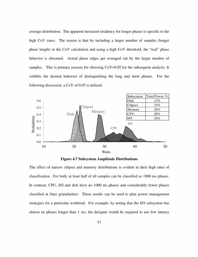
57
average distribution. The apparent increased residency for longer phases is specific to the
high CoV cases. The reason is that by including a larger number of samples (longer
phase length) in the CoV calculation and using a high CoV threshold, the “real” phase
behavior is obscured. Actual phase edges get averaged out by the larger number of
samples. This is primary reasons for choosing CoV=0.05 for the subsequent analysis. It
exhibits the desired behavior of distinguishing the long and short phases. For the
following discussion, a CoV of 0.05 is utilized.
Figure 4.7 Subsystem Amplitude Distributions
The effect of narrow chipset and memory distributions is evident in their high rates of
classification. For both, at least half of all samples can be classified as 1000 ms phases.
In contrast, CPU, I/O and disk have no 1000 ms phases and considerably fewer phases
classified at finer granularities. These results can be used to plan power management
strategies for a particular workload. For example, by noting that the I/O subsystem has
almost no phases longer than 1 ms, the designer would be required to use low latency
0.0
0.1
0.2
0.3
0.4
0.5
0.6
10 20 30 40 50
Pro
bab
ilit
y
Watts
CPU
Disk
I/O
Memory
Chipset
Subsystem Total Power %
Disk 13%
Chipset 15%
Memory 20%
CPU 28%
I/O 24%

58
adaptations. In contrast, the disk subsystem has 18.5% of samples definable as 100 ms
phases, thus providing greater opportunity to amortize adaptation costs. While chipset
and memory subsystems have a large percentage of classifiable samples, they may not be
viable candidates for adaptation. By also considering that most of the chipset and
memory samples are close to the average, standard deviations of 0.9 Watts and 1.4 Watts
respectively, there may be insufficient variation for runtime phase detection.
Table 4.3 Percent of Classifiable Samples
Duration (ms) CPU Chipset Memory I/O Disk
CoV = 0.25
1 98.5 100 100 99.5 100
10 90.8 100 100 87.6 100
100 70.0 100 100 85.3 100
1000 36.0 100 100 96.3 100
Error % 8.78 3.70 3.47 15.2 6.31
CoV = 0.10
1 91.7 100 100 81.1 100
10 66.0 100 98.6 35.7 88.6
100 43.1 100 94.4 21.0 95.6
1000 9.30 100 93.1 0.00 95.0
Error % 4.60 3.70 3.47 6.63 6.31
CoV = 0.05
1 61.6 88.3 97.7 22.4 98.4
10 25.5 78.0 91.2 1.70 32.1
100 6.00 63.2 78.6 0.00 18.5
1000 0.00 64.4 50.0 0.00 0.00
Error % 3.38 3.46 2.68 3.67 2.93
From these results, it is clear that distinct phases are detectable at granularities ranging
from seconds to milliseconds. The next step in utilizing the phases is to combine the
amplitude and duration results to direct power management strategies. An example
classification is given in Table 4.4.

59
Table 4.4 Workload Phase Classification
High Power Med Power Low Power
High Duration 5% 10% 20%
Med Duration 0% 15% 5%
Low Duration 10% 35% 0%
This classification can be used to direct selection of power saving techniques. The phase
duration selects the power management type, based on similar transition times. The
power level and frequency work in opposition to each other as a policy control. For
example, a particular phase may only occur 5% of the time. However, since it is such a
high power case it would be valuable to reduce its power. At the other extreme, a phase
may consume low power, but since it occurs frequently it would be valuable to address.
4.2.2 Desktop Platform
In this section the intra-workload phase characteristics that contribute to the variation are
considered. These results are attributable to the three dominant components of power
adaptation: hardware adaptation, workload characteristics, and OS control of adaptations.
In Figure 4.8 a distribution of the phase length of power consumption for desktop
workloads is presented. Two major conclusions are drawn: the operating system has a
significant effect on phase length and interactive workloads tend to have longer phases.
First, the two spikes at 10 ms and 100 ms show the effect of the operating system. These
can be attributed to the periodic timer tick of the scheduler and p-state transitions
requested by the operating system. In the case of Microsoft Windows Vista, the periodic
timer tick arrives every 10-16 ms [Mm05]. This affects the observed power level since

60
power consumed in the interrupt service routine is distinct from “normal” power levels.
In the case of high-IPC threads, power is reduced while servicing the interrupt, which
typically has a relatively low-IPC due to cold-start misses in the cache and branch
predictor. In the case of low-power or idle threads, power is increased since the core
must be brought out of one or more power saving states in order to service the interrupt.
This is a significant problem for power adaptations since the timer tick is not workload
dependent. Therefore, even a completely idle system must “wake up” every 10 ms to
service an interrupt, even though no useful work is being completed. Also, 10 ms phase
transitions are artificially introduced due to thread migration. Since thread scheduling is
performed on timer tick intervals, context switches, active-to-idle, and idle-to-active
transitions occur on 10 ms intervals. The 100 ms phases can be explained by the OS’s
application of p-state transitions. Experimentally, it can be shown that the minimum rate
at which the operating system will request a transition from one p-state to another is 100
ms. When p-state transitions are eliminated, the spike at the 100 ms range of Figure 4.8
is eliminated.
The second conclusion from Figure 4.8 is that interactive workloads have longer phase
durations. In the case of 3D and video creation workloads, a significant portion of time is
spent in compute-intensive loops. Within these loops, little or no user interaction occurs.
In contrast, the productivity and e-learning workloads spend a greater percentage of the
time receiving and waiting for user input. This translates into relatively long idle phases
which are evident in the lack of short duration phases in Figure 4.8.

61
1 10 100 1000
Fre
qu
en
cy
PhaseLength(ms)
3D Productivity
E-learning VideoCreation
Figure 4.8 Core Power Phase Duration
This is further supported by Figure 4.9, which group the most common phases by
combinations of amplitude and duration. Note that all phases less than 10 ms are
considered to be 10 ms. This simplifies presentation of results and is reasonable since the
OS does not apply adaptation changes any faster than 10 ms. These figures show that the
highest power phases only endure for a short time. These phases, which are present only
in 3D and – to a much lesser degree – in video creation, are only possible when multiple
cores are active. The lack of long duration high power phases is attributable to two
causes: low percent of multithreaded phases and higher IPC dependence during
multithreaded phases. The dependence on IPC for phase length increases as the number
of active cores increases. When many cores are active the power differences are caused
by changes in active power due to IPC (performance). When few cores are active, total
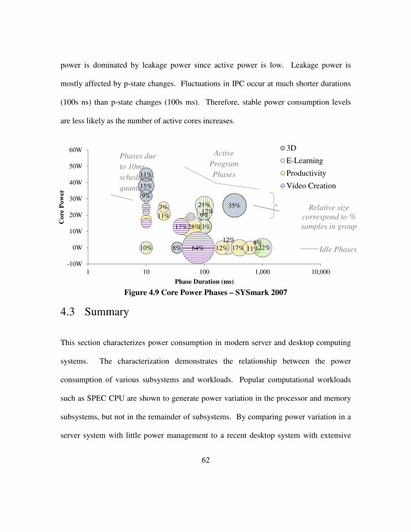
62
power is dominated by leakage power since active power is low. Leakage power is
mostly affected by p-state changes. Fluctuations in IPC occur at much shorter durations
(100s ns) than p-state changes (100s ms). Therefore, stable power consumption levels
are less likely as the number of active cores increases.
Figure 4.9 Core Power Phases – SYSmark 2007
4.3 Summary
This section characterizes power consumption in modern server and desktop computing
systems. The characterization demonstrates the relationship between the power
consumption of various subsystems and workloads. Popular computational workloads
such as SPEC CPU are shown to generate power variation in the processor and memory
subsystems, but not in the remainder of subsystems. By comparing power variation in a
server system with little power management to a recent desktop system with extensive
8%
13%
9%
35%
9%
15%
11%
8%10%
12%
22%
12%21%
11%12% 17%
28%
11%
7%
64%
17%
-10W
0W
10W
20W
30W
40W
50W
60W
1 10 100 1,000 10,000
Co
re P
ow
er
Phase Duration (ms)
3D
E-Learning
Productivity
Video Creation
Relative size
correspond to %
samples in group
Phases due
to 10ms
scheduling
quanta
Idle Phases
Active
Program
Phases

63
power management, it is shown that most variation is due to power management. This
suggests that as systems employ more aggressive power management, instantaneous
power consumption will increase its variability. Power limiting strategies will need to
account for and respond to frequent power transitions due to the increased potential for
performance loss or power overage.

64
Chapter 5 Modeling System-Level Power
using Trickle-Down Events
This chapter presents system-level power models based on performance counter events
within the processor. The first section defines the concept and intuition behind trickle-
down performance events. The second section describes the server power model. The
last section describes the laptop power model.
5.1 Processor Events Propagate to Rest of System
Trickle-down power modeling provides an accurate representation of complete-system
power consumption using a simple methodology. The approach relies on the broad
visibility of system-level events to the processor. This allows accurate, performance
counter based models to be created using only events local to the processor. These local
events can be measured using ubiquitous performance counters found in all modern
microprocessors. Local events are preferred since power models can be built using a
single interface. There is no need to create interfaces to multiple devices and subsystems
which have inconsistent or incomplete performance counter APIs (Application
Programming Interface). It is particularly common at the system level since components
are often designed by multiple vendors. Trickle-down modeling also addresses hardware
costs in systems implementing direct measurement. Rather than providing sensors and

65
power measurement hardware for multiple subsystems, measurement need only be
implemented on a single system during the design stage. The model is created based on
measurement from a small number of systems which allows power measurement
hardware to be eliminated from the final product.
While the trickle-down approach simplifies power modeling of complete systems it
requires a modest knowledge of subsystem level interaction. The effectiveness of the
model at capturing system-level power is determined by the selection of comprehensive
performance events. Some events such as top-level cache or memory accesses are
intuitive. A miss in the first level cache will necessarily generate traffic in higher level
caches and or the memory subsystem. Other events such as those found in I/O devices
are not as obvious. Consider the system diagram in Figure 5.1.
This represents the quad-socket server for which the trickle-down modeling approach is
applied. The arrows flowing outward from the processor represent events that originate
in the processor and trickle-down to other subsystems (L3 Miss, TLB Miss, MemBus
Access and Uncacheable Access). Arrows flowing inward such as DMA (Direct
Memory Access) or bus master access and I/O interrupts may not be directly generated
by the processor, but are nevertheless visible. Since DMA access is typically performed
to addresses marked as cacheable by the processor, they can be observed in the standard
cache access metrics. To distinguish DMA accesses by a particular device, events should
be qualified by address range. Each device typically uses a private range of addresses in

66
system memory for DMA access. Similarly interrupts from multiple devices can be
distinguished by interrupt number or address in the case of message signaled interrupts.
Figure 5.1. Propagation of Performance Events
With over forty detectable performance events [Sp02], the Pentium IV provides a
challenge in selecting events that are most representative of subsystem power. The
subsystem interconnections pictured in Figure 5.1 provide a starting point. By noting the
“trickle-down” effect of events in the processor, a subset of the performance events is
selected to accurately model subsystem power consumption. A simple example would be
the effect of cache misses in the processor. For a typical microprocessor the top-level
cache affects power consumption in the memory subsystem. Transactions that cannot be
satisfied (cache miss) by the top-level cause a cache line (block) sized access to the main
CPU
Chipset Memory
I/O
Disk Network
L3 Miss
TLB Miss
DMA Access
MemBus Access Uncacheable Access
I/O Interrupt
67
memory. Since the number of main memory accesses is directly proportional to the
number of cache misses, it is possible to approximate the number of accesses using only
cache misses. Since these memory accesses must go off-chip, power is consumed
proportionally in the memory controller and DRAM. In reality the relation is not so
simple, but there is still a strong causal relationship between cache misses and main
memory accesses.
5.2 Complete-System Server Power Model
Though the initial selection of performance events for modeling is dictated by an
understanding of subsystem interactions (as in the previous example), the final selection
of which event type(s) to use is determined by the average error rate and a qualitative
comparison of the measured and modeled power traces. The dominant, power-related
performance events are described below.
Cycles – Execution time in terms of CPU clock cycles. The cycles metric is combined
with most other metrics to create per cycle metrics. This corrects for slight differences in
sampling rate. Though sampling is periodic, the actual sampling rate varies slightly due
to cache effects and interrupt latency.
Halted Cycles – Cycles in which clock gating is active. When the Pentium IV processor
is idle, it saves power by gating the clock signal to portions of itself. Idle phases of
execution are “detected” by the processor through the use of the HLT (halt) instruction.

68
When the operating system process scheduler has available slack time, it halts the
processor with this instruction. The processor remains in the halted state until receiving
an interrupt. Though the interrupt can be an I/O device, it is typically the periodic OS
timer that is used for process scheduling/preemption. This has a significant effect on
power consumption by reducing processor idle power from ~36W to 9W. Because this
significant effect is not reflected in the typical performance metrics, it is accounted for
explicitly in the halted cycles counter.
Fetched µops – Micro-operations fetched. The micro-operations (µops) metric is used
rather than an instruction metric to improve accuracy. Since in the P6 architecture
instructions are composed of a varying number of µops, some instruction mixes give a
skewed representation of the amount of computation being done. Using µops normalizes
the metric to give representative counts independent of instruction mix. Also, by
considering fetched rather than retired µops, the metric is more directly related to power
consumption. Looking only at retired µops would neglect work done in execution of
incorrect branch paths and pipeline flushes.
L3 Cache Misses – Loads/stores that missed in the Level 3 cache. Most system main
memory accesses can be attributed to misses in the highest level cache, in this case L3.
Cache misses can also be caused by DMA access to cacheable main memory by I/O
devices. The miss occurs because the DMA must be checked for coherency in the
processor cache.
69
TLB Misses – Loads/stores that missed in the instruction or data Translation Lookaside
Buffer. TLB misses are distinct from cache misses in that they typically cause trickle-
down events farther away from the microprocessor. Unlike cache misses, which usually
cause a cache line to be transferred from/to memory, TLB misses often cause the transfer
of a page of data (4KB or larger). Due to the large size of pages, they are often stored on
disk. Therefore, power is consumed on the entire path from the CPU to the hard disk.
DMA Accesses – Transaction that originated in an I/O device whose destination is
system main memory. Though DMA transactions do not originate in the processor, they
are fortunately visible to the processor. As demonstrated in the L3 Miss metric
description, these accesses to the processor (by an I/O device) are required to maintain
memory coherency. Being able to observe DMA traffic is critical since it causes power
consumption in the memory subsystem. An important thing to consider in the use of the
Pentium IV’s DMA counting feature is that it cannot distinguish between DMA and
processor coherency traffic. All memory bus accesses that do not originate within a
processor are combined into a single metric (DMA/Other). For the uniprocessor case this
is not a problem. However, when using this metric in an SMP environment such as this,
care must be taken to attribute accesses to the correct source. Fortunately, the workloads
considered here have little processor-to-processor coherency traffic. This ambiguity is a
limitation of the Pentium IV performance counters and is not specific to this technique.
Processor Memory Bus Transactions – Reads or writes on processor’s external memory
bus. All transactions that enter/exit the processor must pass through this bus. Intel calls
70
this the Front Side Bus (FSB). As mentioned in the section on DMA, there is a limitation
of being able to distinguish between externally generated (other processors) and DMA
transactions.
Uncacheable Accesses – Load/Store to a range of memory defined as uncacheable.
These transactions are typically representative of activity in the I/O subsystem. Since the
I/O buses are not cached by the processor, downbound (processor to I/O) transactions and
configuration transactions are uncacheable. Since all other address space is cacheable, it
is possible to directly identify downbound transactions. Also, since configuration
accesses typically precede large upbound (I/O to processor) transactions, it is possible to
indirectly observe these.
Interrupts – Interrupts serviced by CPU. Like DMA transactions, most interrupts do not
originate within the processor. In order to identify the source of interrupts, the interrupt
controller sends a unique ID (interrupt vector number) to the processor. This is
particularly valuable since I/O interrupts are typically generated by I/O devices to
indicate the completion of large data transfers. Therefore, it is possible to attribute I/O
bus power to the appropriate device. Though, the interrupt vector information is
available in the processor, it is not available as a performance event. Therefore, the
presence of interrupt information in the processor simulated by obtaining it from the
operating system. Since the operating system maintains the actual interrupt service
routines, interrupt source accounting can be easily performed. In this case the
/proc/interrupts file available in Linux operating systems is used.

71
The form of the subsystem power models is dictated by two requirements: low
computational cost and high accuracy. Since these power models are intended to be used
for runtime power estimation, it is preferred that they have low computational overhead.
For that reason regression curve fitting is attempted using single or multiple input linear
models. If it is not possible to obtain high accuracy with a linear model, a single or
multiple input quadratic is selected.
Subsystem Power Models
The following sections describe the details of the subsystem power models. Descriptions
are given for issues encountered during the selection of appropriate input metrics. For
each subsystem a comparison of modeled and measured power under a high variation
workload is given.
5.2.1 CPU
This CPU power model improves an existing model [BiVa05] to account for halted clock
cycles. Since it is possible to measure the percent of time spent in the halt state, it is
possible to account for the greatly reduced power consumption due to clock gating. This
addition is not a new contribution, since a similar accounting was made in the model by
Isci [IsMa03]. The distinction is that this model is the first application of a performance-
based power model in an SMP environment. The ability to attribute power consumption
to a single physical processor within an SMP environment is critical for shared
computing environments. In the near future it is expected that billing of compute time in
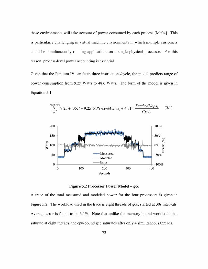
72
these environments will take account of power consumed by each process [Mc04]. This
is particularly challenging in virtual machine environments in which multiple customers
could be simultaneously running applications on a single physical processor. For this
reason, process-level power accounting is essential.
Given that the Pentium IV can fetch three instructions/cycle, the model predicts range of
power consumption from 9.25 Watts to 48.6 Watts. The form of the model is given in
Equation 5.1.
∑=
×+×−+
NumCPUs
i
ii
Cycle
sFetchedUopivePercentAct
1
31.4)25.97.35(25.9
Figure 5.2 Processor Power Model – gcc
A trace of the total measured and modeled power for the four processors is given in
Figure 5.2. The workload used in the trace is eight threads of gcc, started at 30s intervals.
Average error is found to be 3.1%. Note that unlike the memory bound workloads that
saturate at eight threads, the cpu-bound gcc saturates after only 4 simultaneous threads.
-100%
-50%
0%
50%
100%
0
50
100
150
200
0 100 200 300 400
Err
or
(%)
Wa
tts
Seconds
Measured
Modeled
Error
(5.1)

73
5.2.2 Memory
This section considers models for memory power consumption based on cache misses
and processor bus transactions.
The initial attempt at modeling memory power made use of cache misses. A model based
on only cache misses/cycle is an attractive prospect as it is a well understood metric and
is readily available in performance monitoring counters. The principle behind using
cache misses as proxy for power is that loads not serviced by the highest level cache,
must be serviced by the memory subsystem. As demonstrated in [Ja01], power
consumption in DRAM modules is highest when the module is in the active state. This
occurs when either read or write transactions are serviced by the DRAM module.
Therefore, the effect of high-power events such as DRAM read/writes can be estimated.
In this study, the number of L3 Cache load misses per cycle is used. Since the Pentium
IV utilizes a write-back cache policy, write misses do not necessarily cause an immediate
memory transaction. If the miss was due to a cold start, no memory transaction occurs.
For conflict and capacity misses, the evicted cache block will cause a memory transaction
as it updates memory.
The initial findings showed that L3 cache misses were strong predictors of memory
power consumption (Figure 5.3). The first workload considered is the integer workload
mesa from the SPEC CPU 2000 suite. Since a single instance of this workload does not
sufficiently utilize the memory subsystem, multiple instances are used to increase
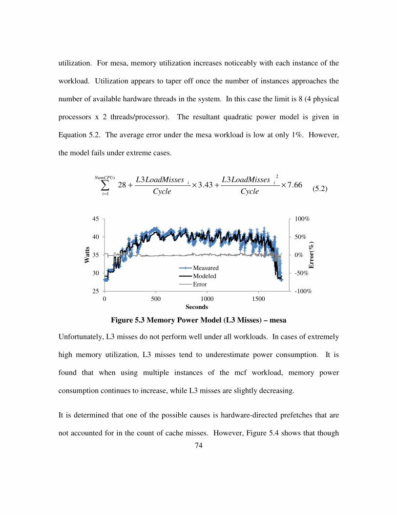
74
utilization. For mesa, memory utilization increases noticeably with each instance of the
workload. Utilization appears to taper off once the number of instances approaches the
number of available hardware threads in the system. In this case the limit is 8 (4 physical
processors x 2 threads/processor). The resultant quadratic power model is given in
Equation 5.2. The average error under the mesa workload is low at only 1%. However,
the model fails under extreme cases.
66.73
43.33
28
2
1
×+×+∑=
Cycle
LoadMissesL
Cycle
LoadMissesL iNumCPUs
i
i
Figure 5.3 Memory Power Model (L3 Misses) – mesa
Unfortunately, L3 misses do not perform well under all workloads. In cases of extremely
high memory utilization, L3 misses tend to underestimate power consumption. It is
found that when using multiple instances of the mcf workload, memory power
consumption continues to increase, while L3 misses are slightly decreasing.
It is determined that one of the possible causes is hardware-directed prefetches that are
not accounted for in the count of cache misses. However, Figure 5.4 shows that though
-100%
-50%
0%
50%
100%
25
30
35
40
45
0 500 1000 1500
Err
or(
%)
Wa
tts
Seconds
Measured
Modeled
Error
(5.2)
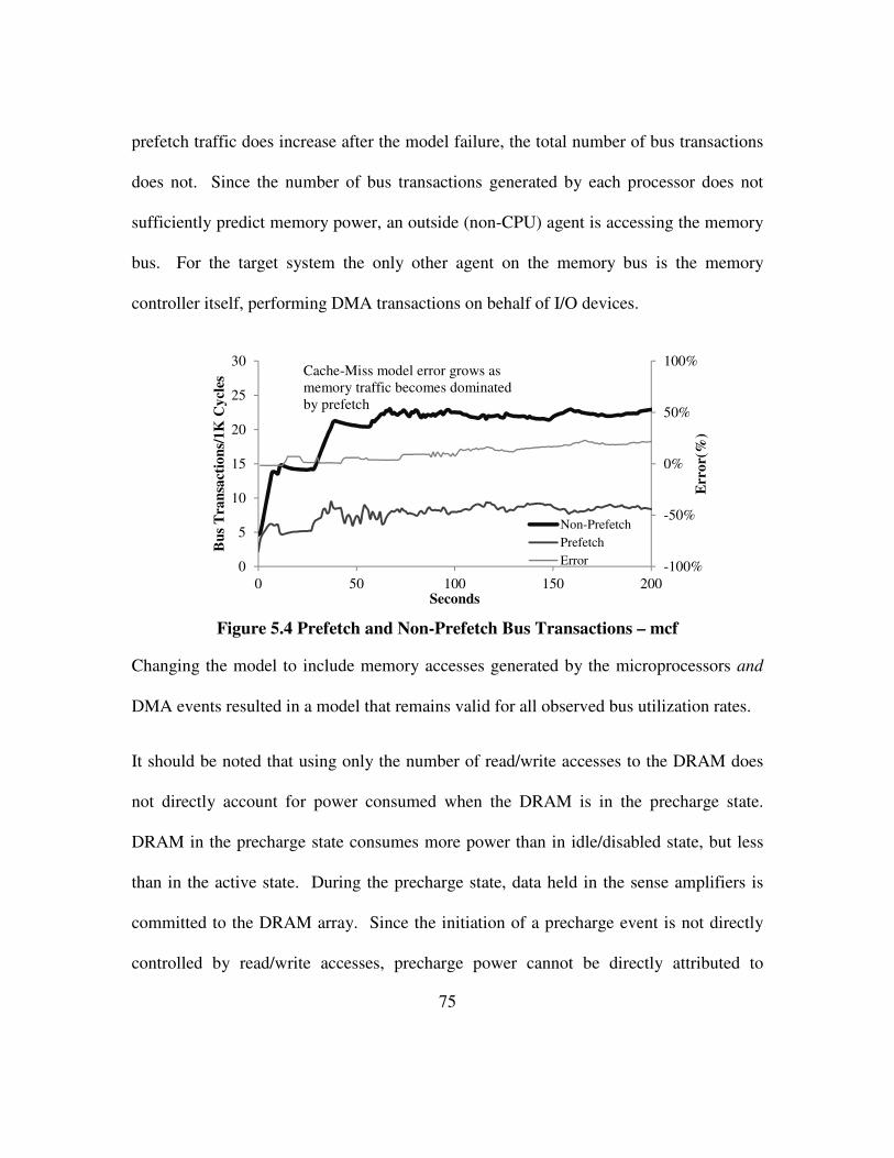
75
prefetch traffic does increase after the model failure, the total number of bus transactions
does not. Since the number of bus transactions generated by each processor does not
sufficiently predict memory power, an outside (non-CPU) agent is accessing the memory
bus. For the target system the only other agent on the memory bus is the memory
controller itself, performing DMA transactions on behalf of I/O devices.
Figure 5.4 Prefetch and Non-Prefetch Bus Transactions – mcf
Changing the model to include memory accesses generated by the microprocessors and
DMA events resulted in a model that remains valid for all observed bus utilization rates.
It should be noted that using only the number of read/write accesses to the DRAM does
not directly account for power consumed when the DRAM is in the precharge state.
DRAM in the precharge state consumes more power than in idle/disabled state, but less
than in the active state. During the precharge state, data held in the sense amplifiers is
committed to the DRAM array. Since the initiation of a precharge event is not directly
controlled by read/write accesses, precharge power cannot be directly attributed to
-100%
-50%
0%
50%
100%
0
5
10
15
20
25
30
0 50 100 150 200
Err
or(
%)
Bu
s T
ran
sact
ion
s/1
K C
ycl
es
Seconds
Non-Prefetch
Prefetch
Error
Cache-Miss model error grows as
memory traffic becomes dominated
by prefetch
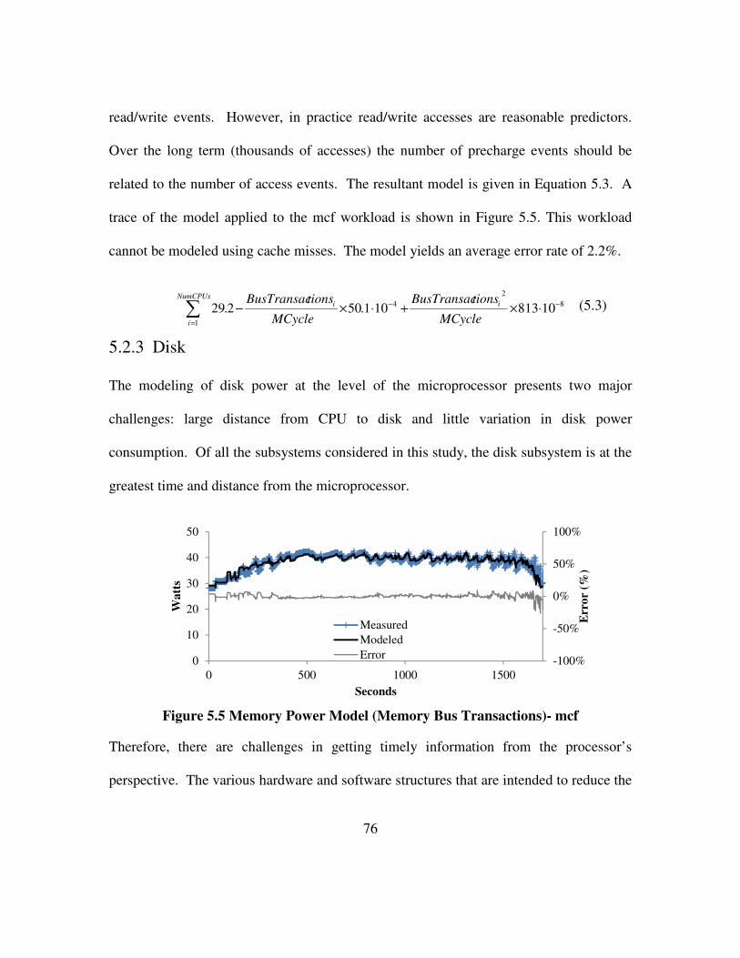
76
read/write events. However, in practice read/write accesses are reasonable predictors.
Over the long term (thousands of accesses) the number of precharge events should be
related to the number of access events. The resultant model is given in Equation 5.3. A
trace of the model applied to the mcf workload is shown in Figure 5.5. This workload
cannot be modeled using cache misses. The model yields an average error rate of 2.2%.
8
2
1
4 10813101.502.29 −
=
−
⋅×+⋅×−∑MCycle
tionsBusTransac
MCycle
tionsBusTransac iNumCPUs
i
i
5.2.3 Disk
The modeling of disk power at the level of the microprocessor presents two major
challenges: large distance from CPU to disk and little variation in disk power
consumption. Of all the subsystems considered in this study, the disk subsystem is at the
greatest time and distance from the microprocessor.
Figure 5.5 Memory Power Model (Memory Bus Transactions)- mcf
Therefore, there are challenges in getting timely information from the processor’s
perspective. The various hardware and software structures that are intended to reduce the
-100%
-50%
0%
50%
100%
0
10
20
30
40
50
0 500 1000 1500
Err
or
(%)
Wa
tts
Seconds
Measured
Modeled
Error
(5.3)

77
average access time to the distant disk by the processor make power modeling difficult.
The primary structures are: microprocessor cache, operating system disk cache, I/O
queues and I/O and disk caches. The structures offer the benefit of decoupling high-
speed processor events from the low-speed disk events. Since the power modeling
techniques rely on the close relationship between the subsystems, this is a problem.
This is evidenced in the poor performance of the first attempts. Initially, we considered
two events: DMA accesses and uncacheable accesses. Since the majority of disk
transfers are handled through DMA by the disk controller, this appeared to be a strong
predictor. The number of uncacheable accesses by the processor was also considered.
Unlike the majority of application memory, memory mapped I/O (I/O address mapped to
system address space) is not typically cached. Generally, I/O devices use memory
mapped I/O for configuration and handshaking. Therefore, it should be possible to detect
accesses to the I/O devices through uncacheable accesses. In practice neither of these
metrics fully account for fine-grain power behavior. Since such little variation exists in
the disk power consumption it is critical to accurately capture the variation that does
exist. In this case the lack of variation is due to a lack of power management features.
The addition of power management magnifies the variation present in the workload.
Accounting for and modeling the small variation in the absence of power management
suggests an accurate model can be constructed with power management.
To address this limitation the manner in which DMA transactions are performed is noted.
Coarsely stated, DMA transactions are initiated by the processor by first configuring the
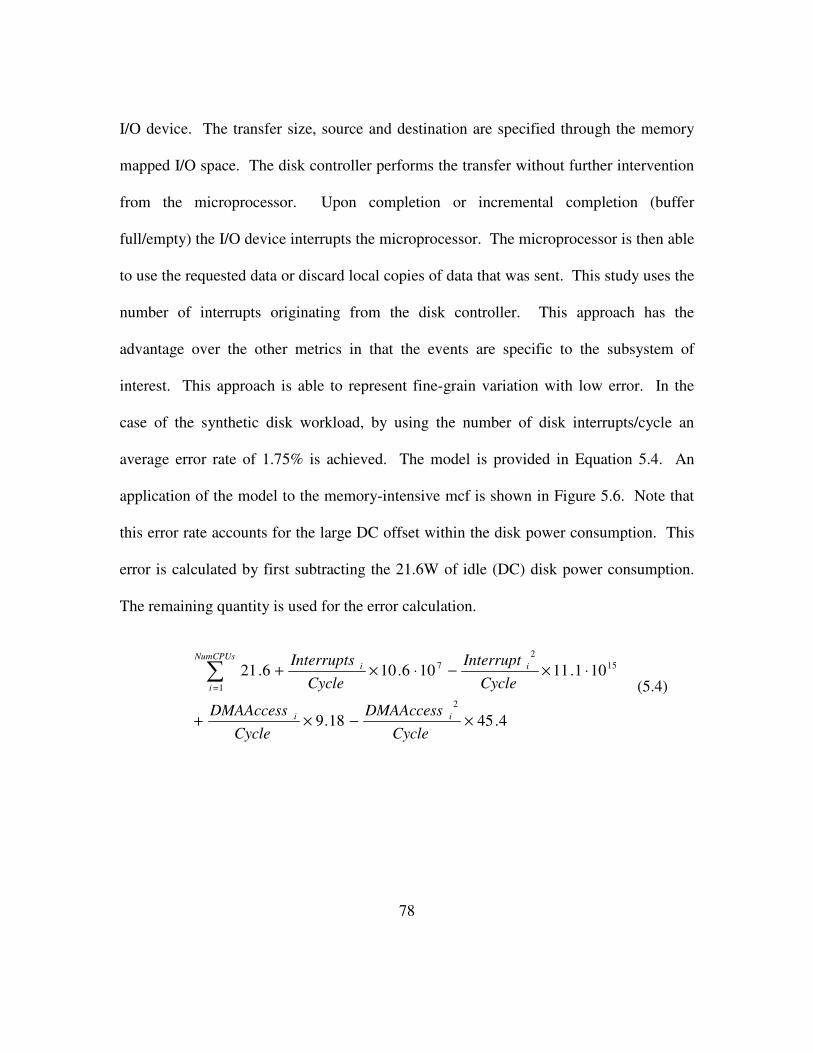
78
I/O device. The transfer size, source and destination are specified through the memory
mapped I/O space. The disk controller performs the transfer without further intervention
from the microprocessor. Upon completion or incremental completion (buffer
full/empty) the I/O device interrupts the microprocessor. The microprocessor is then able
to use the requested data or discard local copies of data that was sent. This study uses the
number of interrupts originating from the disk controller. This approach has the
advantage over the other metrics in that the events are specific to the subsystem of
interest. This approach is able to represent fine-grain variation with low error. In the
case of the synthetic disk workload, by using the number of disk interrupts/cycle an
average error rate of 1.75% is achieved. The model is provided in Equation 5.4. An
application of the model to the memory-intensive mcf is shown in Figure 5.6. Note that
this error rate accounts for the large DC offset within the disk power consumption. This
error is calculated by first subtracting the 21.6W of idle (DC) disk power consumption.
The remaining quantity is used for the error calculation.
4.4518.9
101.11106.106.21
2
1
15
2
7
×−×+
⋅×−⋅×+∑=
Cycle
DMAAccess
Cycle
DMAAccess
Cycle
Interrupt
Cycle
Interrupts
ii
NumCPUs
i
ii
(5.4)
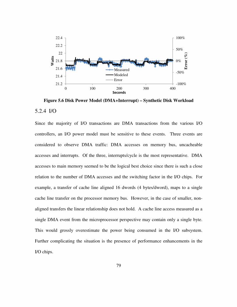
79
Figure 5.6 Disk Power Model (DMA+Interrupt) – Synthetic Disk Workload
5.2.4 I/O
Since the majority of I/O transactions are DMA transactions from the various I/O
controllers, an I/O power model must be sensitive to these events. Three events are
considered to observe DMA traffic: DMA accesses on memory bus, uncacheable
accesses and interrupts. Of the three, interrupts/cycle is the most representative. DMA
accesses to main memory seemed to be the logical best choice since there is such a close
relation to the number of DMA accesses and the switching factor in the I/O chips. For
example, a transfer of cache line aligned 16 dwords (4 bytes/dword), maps to a single
cache line transfer on the processor memory bus. However, in the case of smaller, non-
aligned transfers the linear relationship does not hold. A cache line access measured as a
single DMA event from the microprocessor perspective may contain only a single byte.
This would grossly overestimate the power being consumed in the I/O subsystem.
Further complicating the situation is the presence of performance enhancements in the
I/O chips.
-100%
-50%
0%
50%
100%
21.2
21.4
21.6
21.8
22
22.2
22.4
0 100 200 300 400
Err
or
(%)
Wa
tts
Seconds
Measured
Modeled
Error
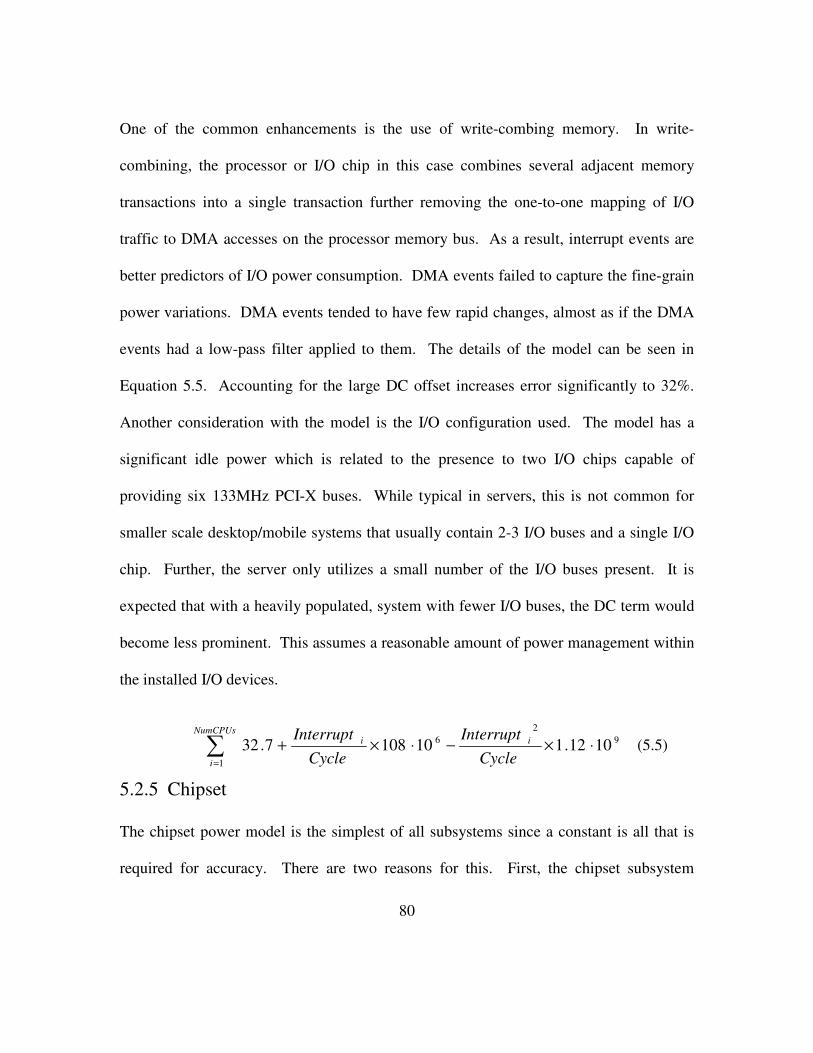
80
One of the common enhancements is the use of write-combing memory. In write-
combining, the processor or I/O chip in this case combines several adjacent memory
transactions into a single transaction further removing the one-to-one mapping of I/O
traffic to DMA accesses on the processor memory bus. As a result, interrupt events are
better predictors of I/O power consumption. DMA events failed to capture the fine-grain
power variations. DMA events tended to have few rapid changes, almost as if the DMA
events had a low-pass filter applied to them. The details of the model can be seen in
Equation 5.5. Accounting for the large DC offset increases error significantly to 32%.
Another consideration with the model is the I/O configuration used. The model has a
significant idle power which is related to the presence to two I/O chips capable of
providing six 133MHz PCI-X buses. While typical in servers, this is not common for
smaller scale desktop/mobile systems that usually contain 2-3 I/O buses and a single I/O
chip. Further, the server only utilizes a small number of the I/O buses present. It is
expected that with a heavily populated, system with fewer I/O buses, the DC term would
become less prominent. This assumes a reasonable amount of power management within
the installed I/O devices.
9
2
1
6 1012.1101087.32 ⋅×−⋅×+∑=
Cycle
Interrupt
Cycle
Interrupt iNumCPUs
i
i
5.2.5 Chipset
The chipset power model is the simplest of all subsystems since a constant is all that is
required for accuracy. There are two reasons for this. First, the chipset subsystem
(5.5)

81
exhibits little variation in power consumption. Therefore, a constant power model is an
obvious choice. Further, it is difficult to identify the effect performance events have on
power consumption compared to induced electrical noise in the sensors. The second, and
more critical reason, is a limitation in the power sampling environment. Since the chipset
subsystem uses power from more than one power domain, the total power cannot be
measured directly. Instead, it is derived by finding the average measured difference in
power between multiple domains. The average chipset power is 19.9W.
5.2.6 Model Validation
Tables 5.1 and 5.2 present summaries of average errors for the five models applied to
twelve workloads. Errors are determined by comparing modeled and measured error at
each sample. A sample corresponds to one second of program execution or
approximately 1.5 billion instructions per processor. For performance counter sampling,
the total number of events during the previous one second is used. For power
consumption, the average of all samples in the previous second (ten thousand) is used.
One second sample intervals provide a compromise between trace size and accuracy.
Reducing the sample interval to as low as 100 microseconds does increase the magnitude
of error in worst-case samples. However, the cumulative average error as shown in
Equation 5.6 is nearly identical to that obtained with one second sample intervals. The
benefit is that trace size is reduced to a practical level that allows tracing complete,
realistic workloads.
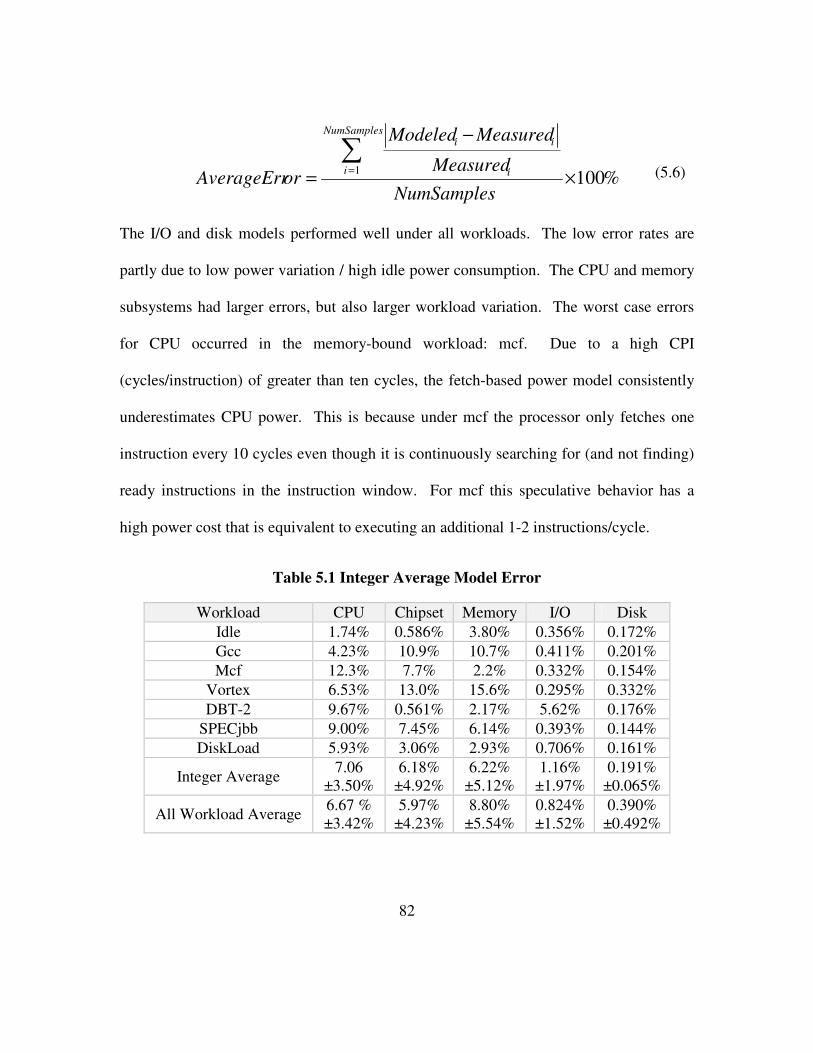
82
%1001
×
−
=
∑=
NumSamples
Measured
MeasuredModeled
orAverageErr
NumSamples
i i
ii
The I/O and disk models performed well under all workloads. The low error rates are
partly due to low power variation / high idle power consumption. The CPU and memory
subsystems had larger errors, but also larger workload variation. The worst case errors
for CPU occurred in the memory-bound workload: mcf. Due to a high CPI
(cycles/instruction) of greater than ten cycles, the fetch-based power model consistently
underestimates CPU power. This is because under mcf the processor only fetches one
instruction every 10 cycles even though it is continuously searching for (and not finding)
ready instructions in the instruction window. For mcf this speculative behavior has a
high power cost that is equivalent to executing an additional 1-2 instructions/cycle.
Table 5.1 Integer Average Model Error
Workload CPU Chipset Memory I/O Disk
Idle 1.74% 0.586% 3.80% 0.356% 0.172%
Gcc 4.23% 10.9% 10.7% 0.411% 0.201%
Mcf 12.3% 7.7% 2.2% 0.332% 0.154%
Vortex 6.53% 13.0% 15.6% 0.295% 0.332%
DBT-2 9.67% 0.561% 2.17% 5.62% 0.176%
SPECjbb 9.00% 7.45% 6.14% 0.393% 0.144%
DiskLoad 5.93% 3.06% 2.93% 0.706% 0.161%
Integer Average 7.06
±3.50%
6.18%
±4.92%
6.22%
±5.12%
1.16%
±1.97%
0.191%
±0.065%
All Workload Average 6.67 %
±3.42%
5.97%
±4.23%
8.80%
±5.54%
0.824%
±1.52%
0.390%
±0.492%
(5.6)
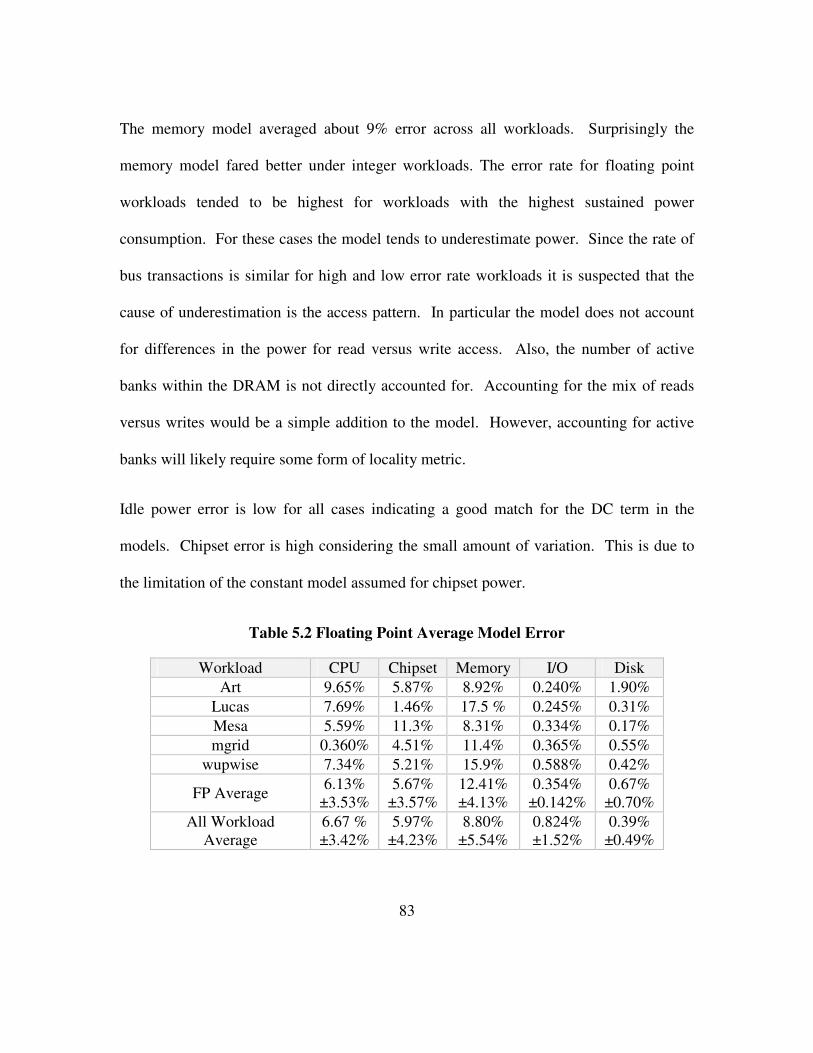
83
The memory model averaged about 9% error across all workloads. Surprisingly the
memory model fared better under integer workloads. The error rate for floating point
workloads tended to be highest for workloads with the highest sustained power
consumption. For these cases the model tends to underestimate power. Since the rate of
bus transactions is similar for high and low error rate workloads it is suspected that the
cause of underestimation is the access pattern. In particular the model does not account
for differences in the power for read versus write access. Also, the number of active
banks within the DRAM is not directly accounted for. Accounting for the mix of reads
versus writes would be a simple addition to the model. However, accounting for active
banks will likely require some form of locality metric.
Idle power error is low for all cases indicating a good match for the DC term in the
models. Chipset error is high considering the small amount of variation. This is due to
the limitation of the constant model assumed for chipset power.
Table 5.2 Floating Point Average Model Error
Workload CPU Chipset Memory I/O Disk
Art 9.65% 5.87% 8.92% 0.240% 1.90%
Lucas 7.69% 1.46% 17.5 % 0.245% 0.31%
Mesa 5.59% 11.3% 8.31% 0.334% 0.17%
mgrid 0.360% 4.51% 11.4% 0.365% 0.55%
wupwise 7.34% 5.21% 15.9% 0.588% 0.42%
FP Average 6.13%
±3.53%
5.67%
±3.57%
12.41%
±4.13%
0.354%
±0.142%
0.67%
±0.70%
All Workload
Average
6.67 %
±3.42%
5.97%
±4.23%
8.80%
±5.54%
0.824%
±1.52%
0.39%
±0.49%

84
5.3 Complete-System Desktop Power Model
In this section results for the application of the trickle-down modeling approach are
presented for a recent desktop platform. This platform differs from the previous server in
terms of process technology, system architecture, manufacturer and workload among
others. It is shown that though this platform is significantly different than the server, the
trickle-down modeling approach still accurately models power. Of particular importance
are two major differences: subsystem level power management and workload
characteristics. Power management increases the complexity and utility of the power
model as power consumption varies greatly with the application of power management.
Compare this to the server system in which power remains near a constant level due to
subsystems not reducing performance capacity, and therefore power consumption, during
periods of low utilization. Increased power variation is also attributable to desktop-
specific workloads. While server workloads tend to always operate at full speed (e.g.
SPEC CPU) desktop workloads such as SYSmark and 3DMark contain large portions of
low utilization. This exposes the impact of power management and the need to model it.
5.3.1 System Description
To validate the effectiveness of the trickle-down approach the process is applied to a
recent desktop platform. A comparison of the two systems used in this study (server and
desktop) is provided in Table 5.3. These systems differ in their power management
implementations and subsystem components. The desktop system is optimized for power

85
efficiency rather than performance. This leads to greater variation in power consumption
compared to a server since power management features reduce power greatly during low
utilization. Server systems tend to employ less aggressive power savings. Therefore,
power at low utilization is greater and overall variation is lesser. This difference is
evident in the analysis of average subsystem-level power in Tables 5.1 - 5.2 and 5.6. The
power management implementation in the desktop system also requires the use of more
extensive power models. Rather than only needing to consider CPU clock gating and
DRAM power down modes, the desktop system model must consider DVFS, chipset link
power management, disk and GPU power management. The wider range of power
consumption also leads to greater temperature sensitivity.
Table 5.3 System Comparison
Platform
Segment
Server Desktop
Manufacturer Intel AMD
Processor(s) Quad-socket 130nM
2.8GHz
Dual-core 45nM 2.0GHz
Memory 8GB DDR-200 4GB DDR3-1066
Power
Management
CPU Clock Gating
DRAM Power Down
CPU Clock Gating and DVFS
DRAM Power Down and Self
Refresh
Chipset Link Disconnect
Harddrive Spin Down and
ATA modes
GPU Clock Gating
Graphics Rage ProXL RS780
Observable
Subsystems
CPU
Chipset
Memory
I/O
Disk
CPU
Chipset
Memory
Memory Controller
GPU
Disk
86
Another major difference is the ability to measure subsystem power at a finer granularity.
The desktop platform allows direct measurement of memory controller and GPU in
addition to all the subsystems that are measureable in the server system. One exception is
the server I/O subsystem which contains numerous PCI-X busses and bridges. The
desktop system does not contain comparable I/O subsystem. Therefore, it is not included
in the study.
5.3.2 Workloads
Due to the distinctions between server and desktop systems several desktop or client-
appropriate workloads are added. In typical server or desktop benchmarks the GPU
subsystem is almost entirely idle. Therefore, to exercise the GPU subsystem the
3DMark06 benchmark is included. 3DMark06 contains six subtests covering CPU and
GPU intensive workloads. Four of the subtests target the GPU’s 3D processing engine
(gt1, gt2, hdr1, hdr2). The other two (cpu1 and cpu2) heavily utilize CPU cores but have
almost no GPU utilization. Targeting the 3D engine generates the largest power variation
since the 3D engine is by far the largest power consumer in the GPU. An interesting side
effect of the desktop GPU is intense system DRAM utilization. To reduce cost and
power consumption, desktop systems such as this use a portion of system DRAM in lieu
of locally attached, private DRAM. As a result, 3D workloads in desktop systems are
effective at generating wide power variation in the memory subsystem.
Overall subsystem level power management is exposed through the addition of the
SYSmark 2007 benchmark. This workload is implemented using simulated user input

87
through the application GUI. The numerous delays required for GUI interaction causes
many idle phases across the subsystems. This allows power management to become
active. Contrast this to the vast majority of benchmarks which, by design, operate the
CPU and other subsystems only at the 100% load level. The DBT-2 database workload is
excluded as it is not practical and relevant to run on a desktop platform. For comparison
to the server model, SPEC CPU, SPECjbb and Idle workloads are included. The
workloads on targeted subsystems are summarized below in Table 5.4.
Table 5.4 Desktop Workloads
Workload Description Subsystems Targeted
Idle Only background OS processes All (power managed)
SPEC CPU 2006
INT
perlbench, bzip2, gcc, mcf,
gobmk, hmmer, sjeng, libquantum,
h264ref, omnetpp, astar,
xalancbmk
CPU
Memory
Memory Controller
FP
bwaves, games, milc, zeusmp,
gromacs, cactusADM, leslie3d,
namd, dealII, soplex, povray,
calculix, gemsFDTD, tonto, lbm,
wrf, sphinx3
CPU
Memory
Memory Controller
3DMark06
gt1 Graphics Test 1 and 2
GPU
Memory
Memory Controller gt2
cpu1 CPU Test 1 and 2 CPU
cpu2
hdr1 High Dynamic Range Test 1 and 2
GPU
Memory
Memory Controller hdr2
SYSmark 2007
EL E-Learning CPU
Memory
Memory Controller
Chipset
Disk
VC Video Creation
PR Productivity
3D 3D
SPECjbb2005 Server-Side Java
CPU
Memory
Memory Controller

88
5.3.3 Performance Event Selection
Performance event selection is critical to the success of performance counter-driven
power models. To identify a minimum set of representative performance events, the
relationship between each event and power consumption must be understood. This
section describes the performance monitoring counter events used to construct the trickle-
down power model. The definition and insight behind selection of the counters is
provided.
Fetched µops – Micro-operations fetched. Comparable to the Pentium IV fetched micro-
operations, this metric is highly correlated to processor power. It accounts for the largest
portion of core pipeline activity including speculation. This is largely the result of fine-
grain clock gating. Clocks are gated to small portions of the pipelines when they are not
being used.
FP µops Retired – Floating point micro-operations retired. FP µops Retired accounts
for the difference in power consumption between floating point and integer instructions.
Assuming equal throughput, floating point instructions have significantly higher average
power. Ideally, the number of fetched FPU µops would be used. Unfortunately, this
metric is not available as a performance counter. This is not a major problem though
since the fetched µops metric contains all fetched µops, integer and floating point.
DC Accesses – Level 1 Data Cache Accesses. A proxy for overall cache accesses
including Level 1,2,3 data and instruction. Considering the majority of workloads, level

89
1 data cache access rate dominates cache-dependent power consumption. No other single
cache access metric correlates as well to processor core power (including caches).
%Halted/%Not-Halted – Percent time processor is in halted state. This represents
power saved due to explicit clock gating. The processor saves power using fine-grain
and coarse-grain of clock gating. Fine-grain clock gating saves power in unutilized
portions of the processor while instructions are in-flight. Coarse-grain clock gating can
save more power than fine-grain yet it requires the processor to be completely idle. The
processor applies this type of gating only when the processor is guaranteed to not have
any instructions in-flight. This condition by definition occurs following execution of the
HLT instruction. Halt residency is controlled by the operating system and interrupts
scheduling work on processors.
CPU Clock Frequency – Core clocks per second. Due to the use of DVFS, it is
necessary to track the instantaneous frequency of the processor. Though some metrics
such as µops fetched or retired implicitly track the power consumed in many components
due to clock frequency, they do not track workload-independent power consumers such
as clock grids. Using clock frequency in conjunction with %Halt it is possible to account
for power consumed in these units.
CPU Voltage – CPU Voltage Rail. Due to the application of DVFS the processor may
operate at a range of discrete voltages in order to save power. Changes in voltage have a
significant impact on power consumption due to the exponential relationship between
90
voltage and dynamic (~V2) and leakage power (~V
3). Due to a single, shared voltage
plane, the actual voltage applied is the maximum requested of all cores in a socket. The
requested voltage can be read using the P-State Status Register [Bk09].
Temperature – CPU Temperature. At the high voltages required for multi-GHz
operation, leakage power becomes a major component of power consumption. Also, at
idle when dynamic power is nearly eliminated due to clock gating leakage power can be
the dominant contributor. Since temperature has a strong relation to leakage power (T2)
it is necessary to account for this effect by measuring temperature. Temperature can be
approximated using a series of on-die thermal sensors. The output of these sensors can
be obtained using a configuration-space register [Bk09].
GPU Non-Gated Clocks – Number of GPU clocks per second. Similar to CPU power,
GPU power is greatly impacted by the amount of clock gating and DVFS. In this study
the DVFS usage is restricted to frequency changes only. Therefore, nearly all GPU
power variation can be accounted for by this single metric.
DCT Accesses – ∑ N=0-1 DCTNPageHits+DCTNPageMisses + DCTNPageConflicts. DCT
(DRAM ConTroller) Access accounts for all memory traffic flowing out of the two on-
die memory controllers, destined for system DRAM. These events include cpu-generated
and DMA traffic.
Link Active% – Percent time Hypertransport links connected. To save power in the I/O
interconnection during idle periods, the Hypertransport links are disconnected. During

91
periods of disconnect, cache snoop traffic and interrupts are blocked. This allows power
to be saved in the CPU I/O interconnect and I/O subsystem. Also, the DRAM may be
placed in self-refresh mode since DRAM access is blocked. If a cache snoop or interrupt
event occurs, the links are reconnected.
Spindle Active % – Percent time hard disk spindle is spinning. In traditional
mechanical hard drives, the spindle motor represent the largest single consumer of power
in the drive. To save energy the spindle motor can be powered down. Due to the high
latency (and energy consumption) for starting/stopping the spindle this can only be done
when the drive is expected to be idle for a long time (minutes or more). In practice,
typical workloads prevent the spindle from ever powering down. This includes all
benchmarks used in this study, except idle. Therefore, spindle activity can be sufficiently
accounted for by only distinguishing between idle and active workloads.
CPUToIOTransactions – Non-cacheable access to memory-mapped I/O devices . I/O
device activity can be approximated using a measure of how many memory transactions
generated by the CPUs are targeted at non-cacheable address space. Typically, I/O
devices contain a DMA controllers which performs access to cacheable space in system
memory. The configuration and control of these transactions is performed by the CPU
through small blocks of addresses mapped in non-cacheable space to each I/O device.
DRAMActive% – Percent time DRAM channel is active. Power savings in the DRAM
and memory controller is controlled by the memory controller. When a memory channel
92
has not issued a memory transaction for at least fixed period of time, the memory
controller sends the channel to one of the precharge power down modes [Bk09]. This
primarily saves power in the DRAM chips, but also provides a slight savings in the
memory controller.
SUBSYSTEM POWER MODELS
The impact of effective power management can be seen in the form of the power models
of this section. In all cases it is necessary to explicitly account for power management to
obtain accurate models. This causes all models to take a similar form. Previous models
[BiVa05] [BiJo06-1] are dominated by terms which were directly proportional to
workload activity factors (IPC, cache accesses). While those workload-dependent terms
are also used here, Idle Power Management and Irreducible power are also quantified.
The idle power management term estimates power saved when instructions or operations
are not actively proceeding through the subsystem. For CPUs this primarily occurs when
executing the idle loop. The CPU detects one of the idle instructions (HLT, mwait) and
takes actions such as clock or power gating. Other subsystems such as memory or I/O
links similarly detect the absence of transactions and save power through various degrees
of clock gating. Irreducible power contains the “baseline” power which is consumed at
all times. This baseline power is largely composed of leakage and ungateable
components.

93
5.3.4 CPU
To test the extensibility of performance counter power modeling across processor
architectures, the methodology is applied to an AMD Phenom quad-core processor. Like
the Intel Pentium 4 processor used in sections 3.2 and 3.3, fetched instructions is a
dominant metric for power accounting. Differences in architecture and microarchitecture
dictate that additional metrics are needed to attain high accuracy. Two areas are
prominent: floating point instruction power and architectural power management. Unlike
the Intel server processor which exhibits nearly statistically uniform power consumption
across workloads of similar fetch rate, the AMD desktop processor consumes up to 30%
more power for workloads with large proportions of floating point instructions.
To account for the difference in floating point instruction power, the desktop processor
model employs an additional metric for retired floating point instructions. A still larger
power difference is caused by the addition of architectural power management on the
desktop processor. The older, server processor only has architectural power management
in the form of clock gating when the halt instruction is issued by the operating system.
The newer, desktop processor adds architectural, DVFS. This leads to drastic reductions
in switching and leakage power. To account for these power reductions, the desktop
model includes tracking of processor frequency, voltage and temperature. The details of
the model can be found in Section 3.4.5.

94
While this model is accurate for most current generation processors, future processors
may require additional metrics to maintain comparable accuracy. Power savings
techniques such as power gating and on-die voltage regulation will require new methods
for power accounting. These techniques extend the sensitivity of leakage power
consumption to functional unit activity levels. Currently, leakage power is dictated
almost completely by architecturally visible, core-level, idle and DVFS states. Future
power gating implementations will likely be applied within subsets of a core, such as
floating point units or caches. Similarly, on-die regulation allows DVFS to be applied
independently to particular functional units. This increases the complexity of
performance counter power modeling which normally only accounts for switching power.
To accounting for these local power adaptations, models will need either detailed
knowledge of the power gating and DVFS implementations or statistical characterizations
of their application. Given the effectiveness of performance counter power models at
accounting for fine-grain switching power, it is likely that power gating and on-die
regulation can also be accounted for.
5.3.5 GPU
To estimate GPU power consumption a technique similar to that typically used for CPUs
is employed: count the number of ungated clocks. In CPUs this is done by subtracting
the number of halted clocks from all clocks [BiJo06-1]. In the case of the RS780 the
ungated clocks can be measured directly. This approach only accounts directly for power
saved due to clock gating. Power reductions due to DVFS are not explicitly represented.
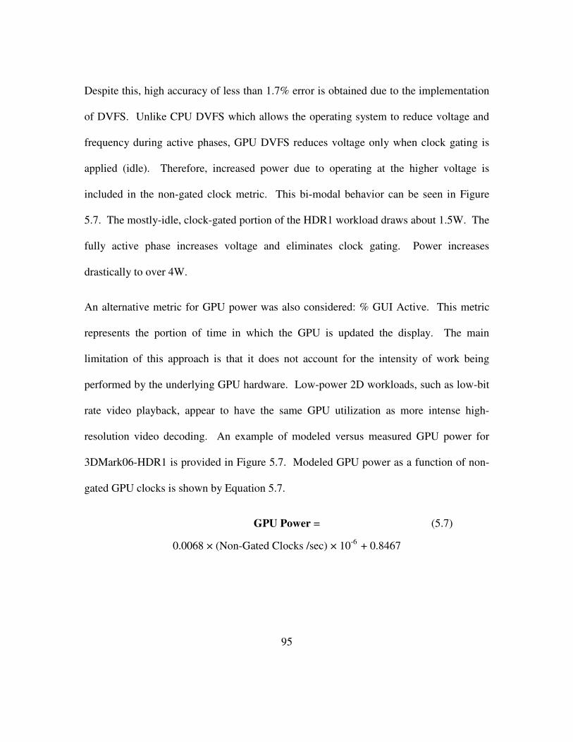
95
Despite this, high accuracy of less than 1.7% error is obtained due to the implementation
of DVFS. Unlike CPU DVFS which allows the operating system to reduce voltage and
frequency during active phases, GPU DVFS reduces voltage only when clock gating is
applied (idle). Therefore, increased power due to operating at the higher voltage is
included in the non-gated clock metric. This bi-modal behavior can be seen in Figure
5.7. The mostly-idle, clock-gated portion of the HDR1 workload draws about 1.5W. The
fully active phase increases voltage and eliminates clock gating. Power increases
drastically to over 4W.
An alternative metric for GPU power was also considered: % GUI Active. This metric
represents the portion of time in which the GPU is updated the display. The main
limitation of this approach is that it does not account for the intensity of work being
performed by the underlying GPU hardware. Low-power 2D workloads, such as low-bit
rate video playback, appear to have the same GPU utilization as more intense high-
resolution video decoding. An example of modeled versus measured GPU power for
3DMark06-HDR1 is provided in Figure 5.7. Modeled GPU power as a function of non-
gated GPU clocks is shown by Equation 5.7.
GPU Power =
0.0068 × (Non-Gated Clocks /sec) × 10-6
+ 0.8467
(5.7)
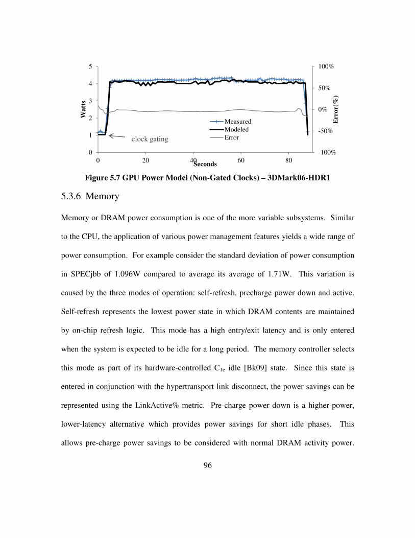
96
Figure 5.7 GPU Power Model (Non-Gated Clocks) – 3DMark06-HDR1
5.3.6 Memory
Memory or DRAM power consumption is one of the more variable subsystems. Similar
to the CPU, the application of various power management features yields a wide range of
power consumption. For example consider the standard deviation of power consumption
in SPECjbb of 1.096W compared to average its average of 1.71W. This variation is
caused by the three modes of operation: self-refresh, precharge power down and active.
Self-refresh represents the lowest power state in which DRAM contents are maintained
by on-chip refresh logic. This mode has a high entry/exit latency and is only entered
when the system is expected to be idle for a long period. The memory controller selects
this mode as part of its hardware-controlled C1e idle [Bk09] state. Since this state is
entered in conjunction with the hypertransport link disconnect, the power savings can be
represented using the LinkActive% metric. Pre-charge power down is a higher-power,
lower-latency alternative which provides power savings for short idle phases. This
allows pre-charge power savings to be considered with normal DRAM activity power.
-100%
-50%
0%
50%
100%
0
1
2
3
4
5
0 20 40 60 80
Err
or(
%)
Wa
tts
Seconds
Measured
Modeled
Errorclock gating
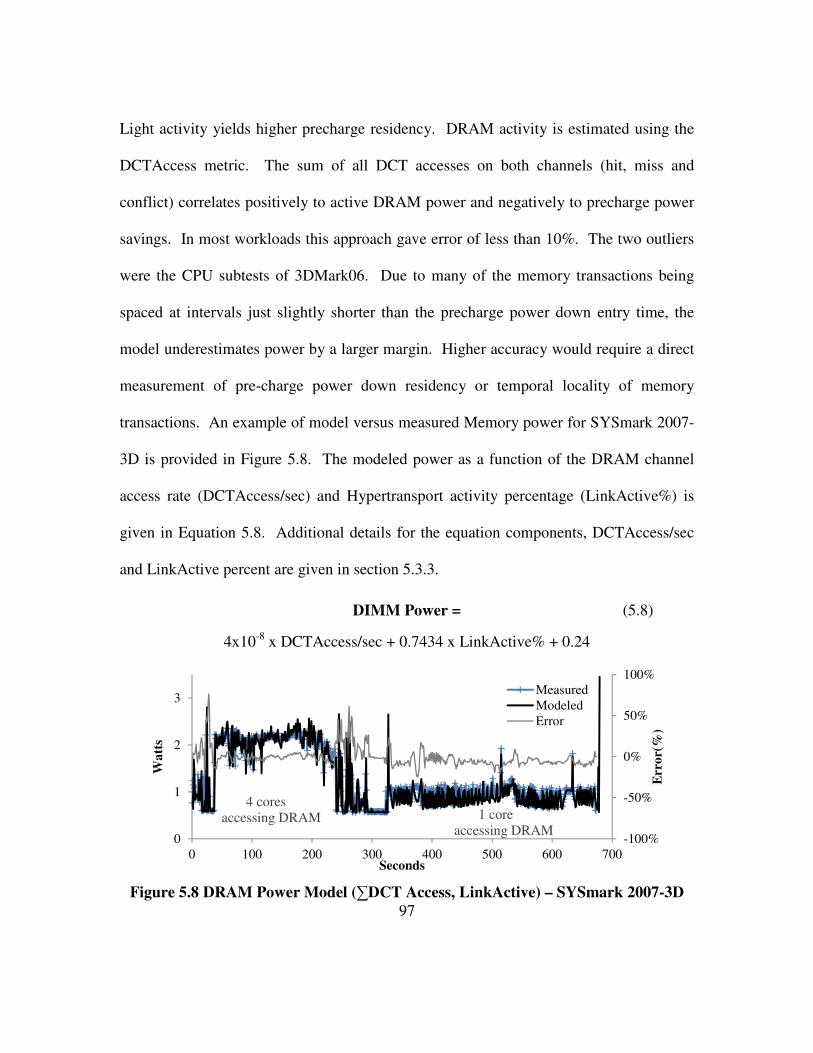
97
Light activity yields higher precharge residency. DRAM activity is estimated using the
DCTAccess metric. The sum of all DCT accesses on both channels (hit, miss and
conflict) correlates positively to active DRAM power and negatively to precharge power
savings. In most workloads this approach gave error of less than 10%. The two outliers
were the CPU subtests of 3DMark06. Due to many of the memory transactions being
spaced at intervals just slightly shorter than the precharge power down entry time, the
model underestimates power by a larger margin. Higher accuracy would require a direct
measurement of pre-charge power down residency or temporal locality of memory
transactions. An example of model versus measured Memory power for SYSmark 2007-
3D is provided in Figure 5.8. The modeled power as a function of the DRAM channel
access rate (DCTAccess/sec) and Hypertransport activity percentage (LinkActive%) is
given in Equation 5.8. Additional details for the equation components, DCTAccess/sec
and LinkActive percent are given in section 5.3.3.
DIMM Power =
4x10⁻⁸
x DCTAccess/sec + 0.7434 x LinkActive% + 0.24
Figure 5.8 DRAM Power Model (∑DCT Access, LinkActive) – SYSmark 2007-3D
-100%
-50%
0%
50%
100%
0
1
2
3
0 100 200 300 400 500 600 700
Err
or(
%)
Wa
tts
Seconds
Measured
Modeled
Error
1 core
accessing DRAM
4 cores
accessing DRAM
(5.8)
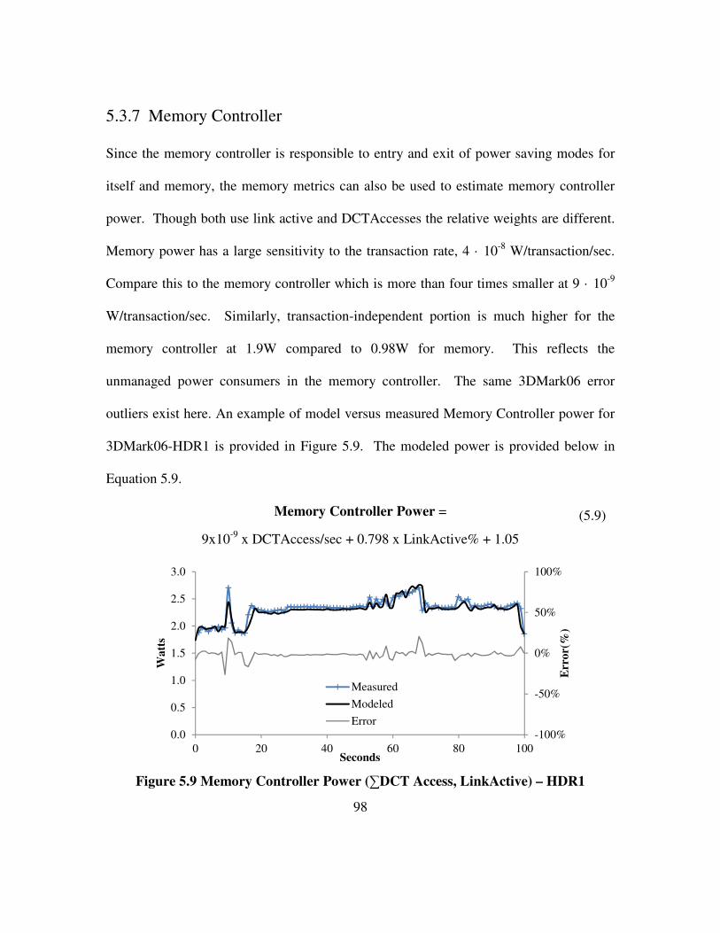
98
5.3.7 Memory Controller
Since the memory controller is responsible to entry and exit of power saving modes for
itself and memory, the memory metrics can also be used to estimate memory controller
power. Though both use link active and DCTAccesses the relative weights are different.
Memory power has a large sensitivity to the transaction rate, 4 · 10-8
W/transaction/sec.
Compare this to the memory controller which is more than four times smaller at 9 · 10-9
W/transaction/sec. Similarly, transaction-independent portion is much higher for the
memory controller at 1.9W compared to 0.98W for memory. This reflects the
unmanaged power consumers in the memory controller. The same 3DMark06 error
outliers exist here. An example of model versus measured Memory Controller power for
3DMark06-HDR1 is provided in Figure 5.9. The modeled power is provided below in
Equation 5.9.
Memory Controller Power =
9x10⁻⁹
x DCTAccess/sec + 0.798 x LinkActive% + 1.05
Figure 5.9 Memory Controller Power (∑DCT Access, LinkActive) – HDR1
-100%
-50%
0%
50%
100%
0.0
0.5
1.0
1.5
2.0
2.5
3.0
0 20 40 60 80 100
Err
or(
%)
Wa
tts
Seconds
Measured
Modeled
Error
(5.9)

99
5.3.8 Chipset
The Chipset power model represents power consumed in the Hypertransport controller.
Like the memory and memory controller subsystems, power consumption is dominated
by the link disconnect state and memory controller accesses. Overall and worst-case
were less than the others due to the workload independent contributions being relatively
the largest. The model for I/O controller power is shown in Equation 5.10.
I/O Controller Power =
-10-16
x (DCTAcc/sec)2 + 2x10
-8 x (DCTAcc/sec) + 1.24 x LinkAct% + 1.34
5.3.9 Disk
The improvements in power management for hard disks between the server-class used in
the Server study study [BiJo06-1] and the more recent desktop/mobile disk used here is
evident in the power model in Equation 5.11. Rather than the negligible power variation
previously observed (<1%), the variable portion (one standard deviation) is on average
30%. This provides more power savings, but a more difficult modeling challenge. As a
result average error is higher at 6.6%. The hard disk power model which is a function of
CPU-to-I/O transactions and spindle activity is shown in Equation 5.11.
Hard Disk Power =
3 x 10⁻⁵
x (CPUToIOTrans/sec) + 0.629 x SpindleActive + 0.498
5.3.10 Model Validation
Table 5.5 summarizes the average error results for the six subsystem power models. The
CPU subsystem had the second lowest error at 1.64% largely due to the comprehensive
(5.11)
(5.10)
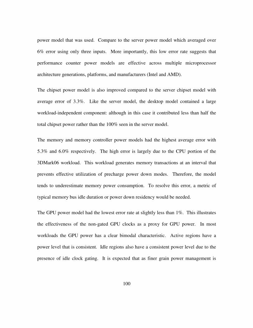
100
power model that was used. Compare to the server power model which averaged over
6% error using only three inputs. More importantly, this low error rate suggests that
performance counter power models are effective across multiple microprocessor
architecture generations, platforms, and manufacturers (Intel and AMD).
The chipset power model is also improved compared to the server chipset model with
average error of 3.3%. Like the server model, the desktop model contained a large
workload-independent component: although in this case it contributed less than half the
total chipset power rather than the 100% seen in the server model.
The memory and memory controller power models had the highest average error with
5.3% and 6.0% respectively. The high error is largely due to the CPU portion of the
3DMark06 workload. This workload generates memory transactions at an interval that
prevents effective utilization of precharge power down modes. Therefore, the model
tends to underestimate memory power consumption. To resolve this error, a metric of
typical memory bus idle duration or power down residency would be needed.
The GPU power model had the lowest error rate at slightly less than 1%. This illustrates
the effectiveness of the non-gated GPU clocks as a proxy for GPU power. In most
workloads the GPU power has a clear bimodal characteristic. Active regions have a
power level that is consistent. Idle regions also have a consistent power level due to the
presence of idle clock gating. It is expected that as finer grain power management is
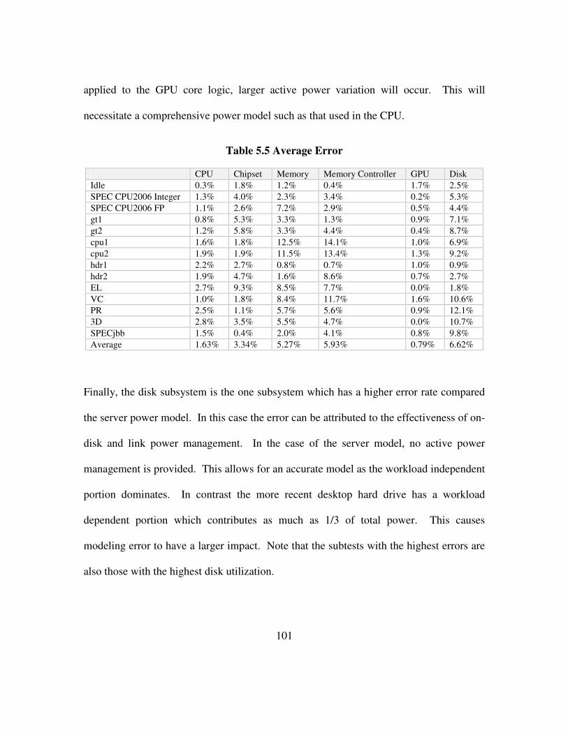
101
applied to the GPU core logic, larger active power variation will occur. This will
necessitate a comprehensive power model such as that used in the CPU.
Table 5.5 Average Error
CPU Chipset Memory Memory Controller GPU Disk
Idle 0.3% 1.8% 1.2% 0.4% 1.7% 2.5%
SPEC CPU2006 Integer 1.3% 4.0% 2.3% 3.4% 0.2% 5.3%
SPEC CPU2006 FP 1.1% 2.6% 7.2% 2.9% 0.5% 4.4%
gt1 0.8% 5.3% 3.3% 1.3% 0.9% 7.1%
gt2 1.2% 5.8% 3.3% 4.4% 0.4% 8.7%
cpu1 1.6% 1.8% 12.5% 14.1% 1.0% 6.9%
cpu2 1.9% 1.9% 11.5% 13.4% 1.3% 9.2%
hdr1 2.2% 2.7% 0.8% 0.7% 1.0% 0.9%
hdr2 1.9% 4.7% 1.6% 8.6% 0.7% 2.7%
EL 2.7% 9.3% 8.5% 7.7% 0.0% 1.8%
VC 1.0% 1.8% 8.4% 11.7% 1.6% 10.6%
PR 2.5% 1.1% 5.7% 5.6% 0.9% 12.1%
3D 2.8% 3.5% 5.5% 4.7% 0.0% 10.7%
SPECjbb 1.5% 0.4% 2.0% 4.1% 0.8% 9.8%
Average 1.63% 3.34% 5.27% 5.93% 0.79% 6.62%
Finally, the disk subsystem is the one subsystem which has a higher error rate compared
the server power model. In this case the error can be attributed to the effectiveness of on-
disk and link power management. In the case of the server model, no active power
management is provided. This allows for an accurate model as the workload independent
portion dominates. In contrast the more recent desktop hard drive has a workload
dependent portion which contributes as much as 1/3 of total power. This causes
modeling error to have a larger impact. Note that the subtests with the highest errors are
also those with the highest disk utilization.

102
5.4 Summary
In this section feasibility of predicting complete system power consumption using
processor performance events is demonstrated. The models take advantage of the trickle-
down effect of these events. These events which are visible in the processing unit, are
highly correlated to power consumption in subsystems including memory, chipset, I/O,
disk and microprocessor. Subsystems farther away from the microprocessor require
events more directly related to the subsystem, such as I/O device interrupts or clock
gating status. Memory models must take into account activity that does not originate in
the microprocessor. In this case, DMA events are shown to have a significant relation to
memory power. It is shown that complete system power can be estimated with an
average error of less than 9% for each subsystem using performance events that trickle
down from the processing unit.
The trickle-down approach is shown to be effective across system architectures,
manufacturers and time. High accuracy is achieved on systems from both major PC
designers (Intel and AMD), Server and desktop architectures, and across time with
systems from 2005 and 2010 exhibiting comparable accuracy.

103
Chapter 6 Performance Effects of
Dynamic Power Management
6.1 Direct and Indirect Performance Impacts
6.1.1 Transition Costs
Due to physical limitations, transitioning between adaptation states may impose some
cost. The cost may be in the form of lost performance or increased energy consumption.
In the case of DVFS, frequency increases require execution to halt while voltage supplies
ramp up to their new values. This delay is typically proportional to the rate of voltage
change (seconds/volt). Frequency decreases typically do not incur this penalty as most
digital circuits will operate correctly at higher than required voltages. Depending on
implementation, frequency changes may incur delays. If the change requires modifying
the frequency of clock generation circuits (phase locked loops), then execution is halted
until the circuit locks on to its new frequency. This delay may be avoided if frequency
reductions are implemented using methods which maintain a constant frequency in the
clock generator. This is the approach used in Quad-Core AMD processor c-state
implementation. Delay may also be introduced to limit current transients. If a large
number of circuits all transition to a new frequency, then excessive current draw may
result. This has a significant effect on reliability. Delays to limit transients are

104
proportional to the amount of frequency change (seconds/MHz). Other architecture-
specific adaptations may have variable costs per transition. For example, powering down
a cache requires modified contents to be flushed to the next higher level of memory. This
reduces performance and may increase power consumption due to the additional bus
traffic. When a predictive component is powered down it no longer records program
behavior. For example, if a branch predictor is powered down during a phase in which
poor predictability is expected, then branch behavior is not recorded. If the phase
actually contains predictable behavior, then performance may be lost and efficiency may
be lost. If a unit is powered on and off in excess of the actual program demand, then
power and performance may be significantly affected by the flush and warm-up cycles of
the components. In this study the focus is on fixed cost per transition effects such as
those required for voltage and frequency changes.
6.1.2 Workload Phase and Policy Costs
In the ideal case the transition costs described above do not impact performance and save
maximum power. The reality is that performance of dynamic adaption is greatly affected
by the nature of workload phases and the power manager’s policies. Adaptations provide
power savings by setting performance to the minimum level required by the workload. If
the performance demand of a workload were known in advance, then setting performance
levels would be trivial. Since they are not known, the policy manager must estimate
future demand based on the past. Existing power managers, such as those used in this
study (Windows Vista [Vi07] and SLES Linux [PaSt06]), act in a reactive mode. They

105
can be considered as predictors which always predict the next phase to be the same as the
last. This approach works well if the possible transition frequency up the adaptation is
greater than the phase transition frequency of workload. Also, the cost of each transition
must be low considering the frequency of transitions. In real systems, these requirements
cannot currently be met. Therefore, the use of power adaptations does reduce
performance to varying degrees depending on workload. The cost of mispredicting
performance demand is summarized below.
Underestimate: Setting performance capacity lower than the optimal value causes
reduced performance. Setting performance capacity lower than the optimal value may
cause increased energy consumption due to increased runtime. It is most pronounced
when the processing element has effective idle power reduction.
Overestimate: Setting performance capacity higher than the optimal value reduces
efficiency as execution time is not reduced yet power consumption is increased. This
case is common in memory-bound workloads.
Optimization Points: The optimal configuration may be different depending on which
characteristic is being optimized. For example, Energy×Delay may have a different
optimal point compared to Energy×Delay2.
6.1.3 Performance Effects
P-states and C-states impact performance in two ways: Indirect and Direct. Indirect
performance effects are due to the interaction between active and idle cores. In the case

106
of Quad-Core AMD processors, this is the dominant effect. When an active core
performs a cache probe of an idle core, latency is increased compared to probing an
active core. The performance loss can be significant for memory-bound (cache probe-
intensive) workloads. Direct performance effects are due to the current operating
frequency of an active core. The effect tends to be less compared to indirect, since
operating systems are reasonably effective at matching current operating frequency to
performance demand. These effects are illustrated in Figure 6.1.
Two extremes of workloads are presented: the compute-bound crafty and the memory-
bound equake. For each workload, two cases are presented: fixed and normal scheduling.
Fixed scheduling isolates indirect performance loss by eliminating the effect of OS
frequency scheduling and thread migration. This is accomplished by forcing the
software thread to a particular core for the duration of the experiment. In this case, the
thread runs always run at the maximum frequency. The idle cores always run at the
minimum frequency. As a result, crafty achieves 100 percent of the performance of
processor that does not use dynamic power management. In contrast, the memory-bound
equake shows significant performance loss due to the reduced performance of idle cores.
Direct performance loss is shown in the dark solid and light solid lines, which utilize OS
scheduling of frequency and threads. Because direct performance losses are caused by
suboptimal frequency in active cores, the compute-bound crafty shows a significant
performance loss. The memory-bound equake actually shows a performance

107
improvement for low idle core frequencies. This is caused by idle cores remaining at a
high frequency following a transition from active to idle.
Figure 6.1 Direct and Indirect Performance Impact
6.1.4 Indirect Performance Effects
The amount of indirect performance loss is mostly dependent on the following three
factors: Idle core frequency, OS p-state transition characteristics, and OS scheduling
characteristics. The probe latency (time to respond to probe) is largely independent of
idle core frequency above the “breakover” frequency (FreqB). Below FreqB the
performance drops rapidly at an approximately linear rate. This can be seen in Figure 6.1
as the dashed light line. The value of FreqB is primarily dependent on the inherent probe
latency of the processor and the number of active and idle cores. Increasing the active
core frequency increases the demand for probes and therefore increases FreqB. Increasing
60%
65%
70%
75%
80%
85%
90%
95%
100%
200 700 1200 1700 2200
Per
form
an
ce
Idle Core Frequency (MHz)
crafty-fixed
equake-fixed
equake
crafty
FreqB

108
the number of cores has the same effect. Therefore, multi-socket systems tend to have a
higher FreqB. Assuming at least one idle core, the performance loss increases as the ratio
of active-to-idle cores increases. For an N-core processor, the worst-case is N-1 active
cores with 1 idle core. To reduce indirect performance loss, the system should be
configured to guarantee than the minimum frequency of idle cores is greater than or equal
to FreqB. To this end the Quad-Core AMD processor uses clock ramping in response to
probes [Bk09]. When an idle core receives a probe from an active core, the idle core
frequency is ramped to the last requested p-state frequency. Therefore, probe response
performance is dictated by the minimum idle core frequency supported by the processor.
For the majority of workloads, this configuration yield less than 10 percent performance
loss due to idle core probe latency.
The other factors in indirect performance loss are due to the operating system interaction
with power management. These factors, which include OS p-state transition and
scheduling characteristics, tend to mask the indirect performance loss. Ideally, the OS
selects a high frequency p-state for active cores and a low frequency for idle cores.
However, erratic workloads (many phase transitions) tend to cause high error rates in the
selection of optimal frequency. Scheduling characteristics that favor load-balancing over
processor affinity worsen the problem. Each time the OS moves a process from one core
to another, a new phase transition has effectively been introduced. More details of OS p-
state transitions and scheduling characteristics are given in the next section on direct
performance effects.
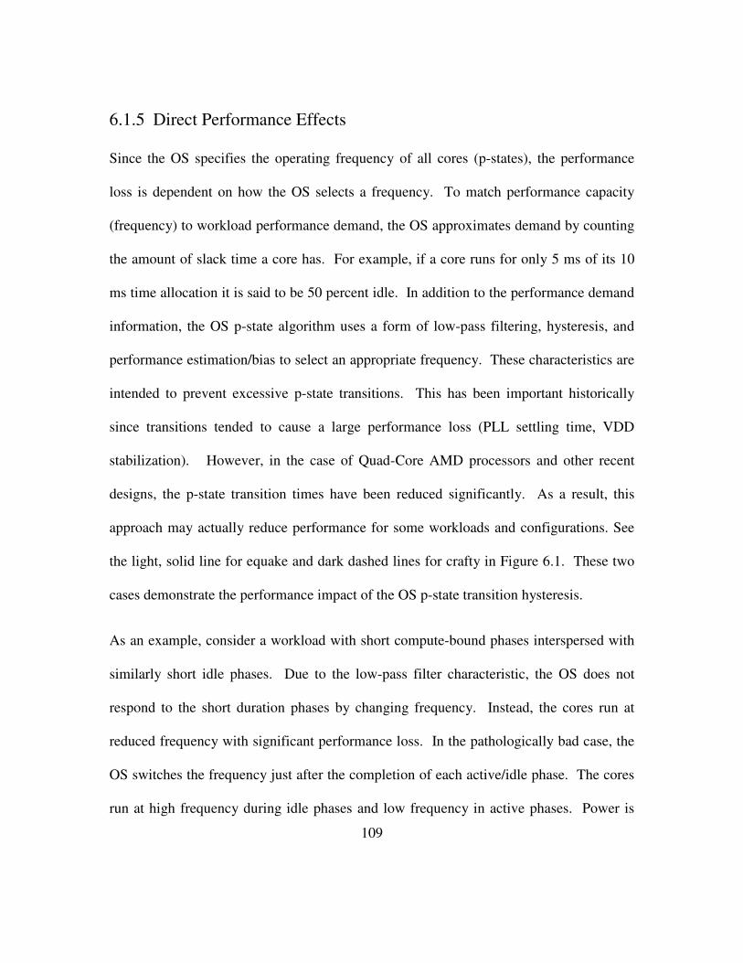
109
6.1.5 Direct Performance Effects
Since the OS specifies the operating frequency of all cores (p-states), the performance
loss is dependent on how the OS selects a frequency. To match performance capacity
(frequency) to workload performance demand, the OS approximates demand by counting
the amount of slack time a core has. For example, if a core runs for only 5 ms of its 10
ms time allocation it is said to be 50 percent idle. In addition to the performance demand
information, the OS p-state algorithm uses a form of low-pass filtering, hysteresis, and
performance estimation/bias to select an appropriate frequency. These characteristics are
intended to prevent excessive p-state transitions. This has been important historically
since transitions tended to cause a large performance loss (PLL settling time, VDD
stabilization). However, in the case of Quad-Core AMD processors and other recent
designs, the p-state transition times have been reduced significantly. As a result, this
approach may actually reduce performance for some workloads and configurations. See
the light, solid line for equake and dark dashed lines for crafty in Figure 6.1. These two
cases demonstrate the performance impact of the OS p-state transition hysteresis.
As an example, consider a workload with short compute-bound phases interspersed with
similarly short idle phases. Due to the low-pass filter characteristic, the OS does not
respond to the short duration phases by changing frequency. Instead, the cores run at
reduced frequency with significant performance loss. In the pathologically bad case, the
OS switches the frequency just after the completion of each active/idle phase. The cores
run at high frequency during idle phases and low frequency in active phases. Power is

110
increased while performance is decreased. OS scheduling characteristics exacerbate this
problem. Unless the user makes use of explicit process affinity or an affinity library,
some operating systems will attempt to balance the workloads across all cores. This
causes a process to spend less contiguous time on a particular core. At each migration
from one core to another there is a lag from when the core goes active to when the active
core has its frequency increased. The aggressiveness of the p-state setting amplifies the
performance loss/power increase due to this phenomenon. Fortunately, recent operating
systems such as Microsoft Windows Vista provide means for system designers and end
users to adjust the settings to match their workloads/hardware [Vi07].
6.2 Reactive Power Management
In this section, results are presented to show the effect that dynamic adaptations
ultimately have on performance and power consumption. All results are obtained from a
real system, instrumented for power measurement. The two major areas presented are
probe sensitivity (indirect) and operating system effects (direct).
First, the probe sensitivity of SPEC CPU2006 is considered. Table 6.1 shows
performance loss due to the use of p-states. In this experiment the minimum p-state is set
below the recommended performance breakover point for probe response. This
emphasizes the inherent sensitivity workloads have to probe response. Operating system
frequency scheduling is biased towards performance by fixing active cores at the
maximum frequency and idle cores at the minimum frequency. These results suggest that
floating point workloads tend to be most sensitive to probe latency. However, in the case

111
of SPEC CPU2000 workloads, almost no performance loss is shown. The reason, as
shown in section 4.3.1, is that smaller working set size reduces memory traffic and,
therefore, the dependence on probe latency. For these workloads only swim, equake, and
eon showed a measureable performance loss.
Table 6.1 Performance Loss Due to Low Idle Core Frequency – SPEC CPU 2006
SPEC CPU 2006 – INT
perlbench -0.8% sjeng 0.0%
bzip2 -1.0% libquantum -7.0%
gcc -3.6% h264ref -0.8%
mcf -1.8% omnetpp -3.7%
gobmk -0.3% astar -0.5%
hmmer -0.2%
SPEC CPU 2006 – FP
bwaves -5.6% soplex -6.7%
games -0.6% povray -0.5%
milc -7.9% calculix -0.6%
zeusmp -2.1% GemsFDTD -5.9%
gromacs -0.3% tonto -0.6%
cactusADM -2.6% lbm -5.6%
leslie3D -6.0% wrf -3.2%
namd -0.1% sphinx3 -5.6%
dealII -1.3%
Next, it is shown that by slightly increasing the minimum p-state frequency it is possible
to recover almost the entire performance loss. Figure 6.2 shows an experiment using a
synthetic kernel with high probe sensitivity with locally and remotely allocated memory.
The remote case simply shows that the performance penalty of accessing remote memory
can obfuscate the performance impact of minimum p-state frequency. The indirect
performance effect can be seen clearly by noting that performance increases rapidly as
the idle core frequency is increased from 800 MHz to approximately 1.1 GHz. This is a
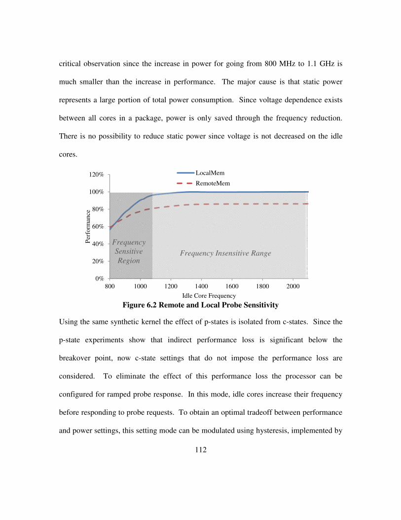
112
critical observation since the increase in power for going from 800 MHz to 1.1 GHz is
much smaller than the increase in performance. The major cause is that static power
represents a large portion of total power consumption. Since voltage dependence exists
between all cores in a package, power is only saved through the frequency reduction.
There is no possibility to reduce static power since voltage is not decreased on the idle
cores.
Figure 6.2 Remote and Local Probe Sensitivity
Using the same synthetic kernel the effect of p-states is isolated from c-states. Since the
p-state experiments show that indirect performance loss is significant below the
breakover point, now c-state settings that do not impose the performance loss are
considered. To eliminate the effect of this performance loss the processor can be
configured for ramped probe response. In this mode, idle cores increase their frequency
before responding to probe requests. To obtain an optimal tradeoff between performance
and power settings, this setting mode can be modulated using hysteresis, implemented by
0%
20%
40%
60%
80%
100%
120%
800 1000 1200 1400 1600 1800 2000
Per
form
ance
Idle Core Frequency
LocalMem
RemoteMem
Frequency Insensitive Range
Frequency
Sensitive
Region

113
adjusting a hysteresis timer. The timer specifies how long the processor remains at the
increased frequency before returning to the power saving mode. The results are shown in
Figure 6.3. The blue line represents the performance loss due to slow idle cores caused
by the application of c-states only. Like the p-state experiments, performance loss
reaches a clear breakpoint. In this case, the breakover point represents 40 percent of the
maximum architected delay. Coupling c-states with p-states, the red shows that the
breakover point is not as distinct since significant performance loss already occurs. Also,
like the p-state experiments, setting the hysteresis timer to a value of the breakover point
increases performance significantly while increasing power consumption only slightly.
Figure 6.3 C-state vs. P-state Performance
Next, the effect of operating system tuning parameters for power adaptation selection is
considered. In order to demonstrate the impact of slow p-state selection, Figure 6.4 is
presented. The effect is shown by varying a single OS parameter while running the
SYSmark E-Learning subtest. In this graph, the TimeCheck value is varied from 1 ms to
1000 ms. TimeCheck controls how often the operating system will consider a p-state
0%
20%
40%
60%
80%
100%
0% 20% 40% 60% 80% 100%
Per
form
ance
C-State Hysteresis (%Max)
C-State Only
P-State+C-State

114
change. Two major issues were found: minimum OS scheduling quanta and
increase/decrease filter.
Figure 6.4 Varying OS P-state Transition Rates
First, performance remains constant when scaling from 1 us to 10 ms (< 1 ms not
depicted). This is attributable to the OS implementation of scheduling. For Microsoft
Windows Vista, all processes are scheduled on the 10 ms timer interrupt. Setting
TimeCheck to values less than 10 ms will have no impact since p-state changes, like all
process scheduling, occur only on 10-ms boundaries. Second, even at the minimum
TimeCheck value, performance loss is at 80 percent. The reason is that other settings
become dominant below 10 ms. In order for a p-state transition to occur the workload
must overcome the in-built low-pass filter. This filter is implemented as a combination
of two thresholds: increase/decrease percent and increase/decrease time. The percent
threshold represents the utilization level that must be crossed in order to consider a p-
state change. The threshold must be exceeded for a fixed amount of time specified by
0%
20%
40%
60%
80%
100%
1 10 100 1000
Per
form
an
ce
TimeCheck (ms)
Cannot change
p-state faster
than scheduling
quanta
Performance
loss increases
as p-state lag
increases
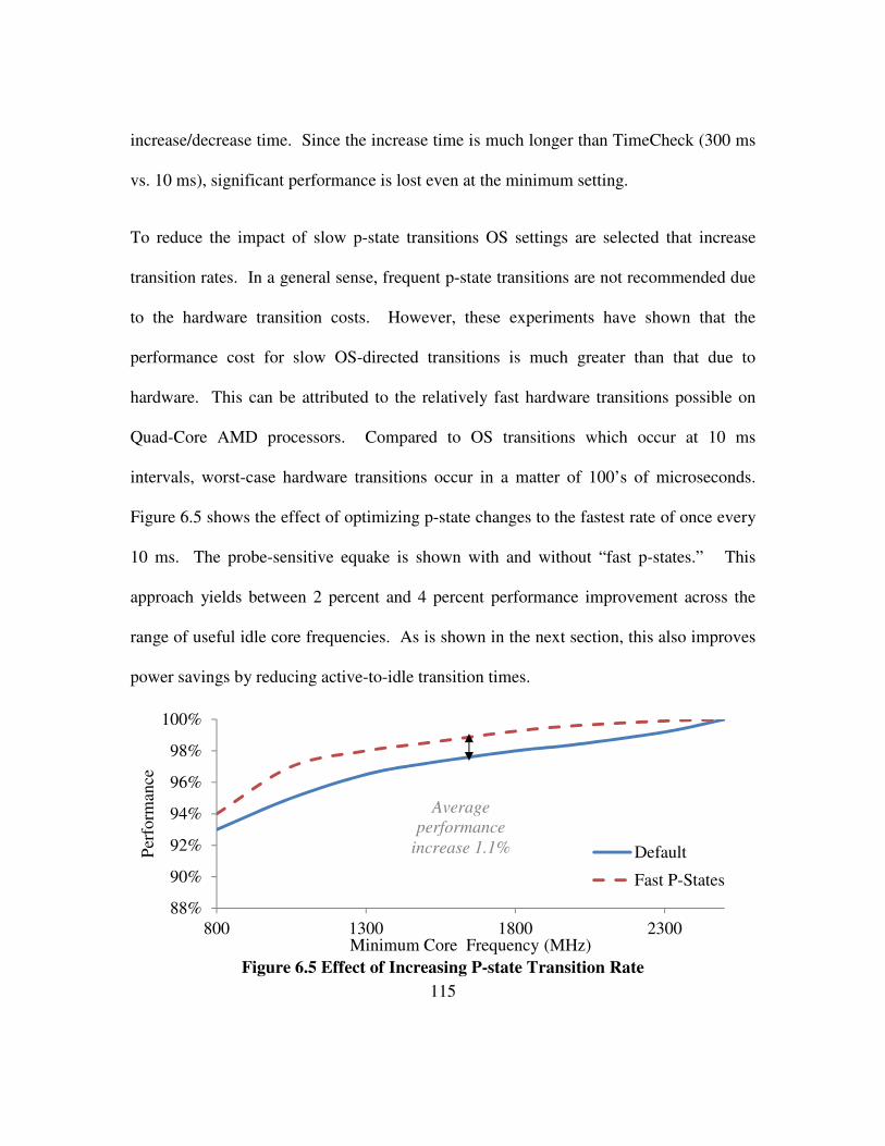
115
increase/decrease time. Since the increase time is much longer than TimeCheck (300 ms
vs. 10 ms), significant performance is lost even at the minimum setting.
To reduce the impact of slow p-state transitions OS settings are selected that increase
transition rates. In a general sense, frequent p-state transitions are not recommended due
to the hardware transition costs. However, these experiments have shown that the
performance cost for slow OS-directed transitions is much greater than that due to
hardware. This can be attributed to the relatively fast hardware transitions possible on
Quad-Core AMD processors. Compared to OS transitions which occur at 10 ms
intervals, worst-case hardware transitions occur in a matter of 100’s of microseconds.
Figure 6.5 shows the effect of optimizing p-state changes to the fastest rate of once every
10 ms. The probe-sensitive equake is shown with and without “fast p-states.” This
approach yields between 2 percent and 4 percent performance improvement across the
range of useful idle core frequencies. As is shown in the next section, this also improves
power savings by reducing active-to-idle transition times.
Figure 6.5 Effect of Increasing P-state Transition Rate
88%
90%
92%
94%
96%
98%
100%
800 1300 1800 2300
Per
form
ance
Minimum Core Frequency (MHz)
Default
Fast P-States
Average
performance
increase 1.1%
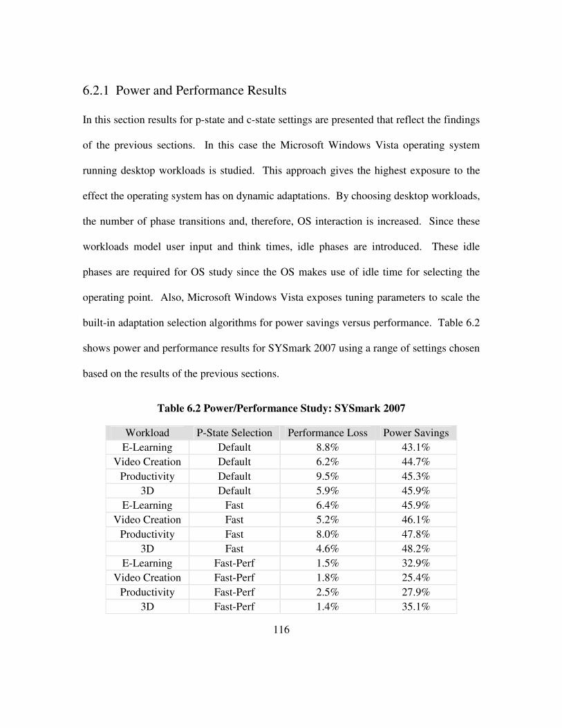
116
6.2.1 Power and Performance Results
In this section results for p-state and c-state settings are presented that reflect the findings
of the previous sections. In this case the Microsoft Windows Vista operating system
running desktop workloads is studied. This approach gives the highest exposure to the
effect the operating system has on dynamic adaptations. By choosing desktop workloads,
the number of phase transitions and, therefore, OS interaction is increased. Since these
workloads model user input and think times, idle phases are introduced. These idle
phases are required for OS study since the OS makes use of idle time for selecting the
operating point. Also, Microsoft Windows Vista exposes tuning parameters to scale the
built-in adaptation selection algorithms for power savings versus performance. Table 6.2
shows power and performance results for SYSmark 2007 using a range of settings chosen
based on the results of the previous sections.
Table 6.2 Power/Performance Study: SYSmark 2007
Workload P-State Selection Performance Loss Power Savings
E-Learning Default 8.8% 43.1%
Video Creation Default 6.2% 44.7%
Productivity Default 9.5% 45.3%
3D Default 5.9% 45.9%
E-Learning Fast 6.4% 45.9%
Video Creation Fast 5.2% 46.1%
Productivity Fast 8.0% 47.8%
3D Fast 4.6% 48.2%
E-Learning Fast-Perf 1.5% 32.9%
Video Creation Fast-Perf 1.8% 25.4%
Productivity Fast-Perf 2.5% 27.9%
3D Fast-Perf 1.4% 35.1%

117
In order to reduce p-state performance loss, the idle core frequency is set to 1250 MHz.
To prevent c-state performance loss, ramped probe mode is used with the hysteresis time
set above the breakover point. Also, C1e mode is disabled to prevent obscuring the idle
power savings of the architected p-states and c-states. The C1e state is a
microarchitectural feature that reduces power when all cores are idle. The power and
performance effects of this state can reduce the measureable effect of the p-state and c-
state decisions made by the operating system.
Two important findings are made regarding adaption settings. First, setting power
adaptations in consideration of performance bottlenecks reduces performance loss while
retaining power savings. Second, reducing OS p-state transition time increases
performance and power savings. Table 6.2 shows the resultant power and performance
for a range of OS p-state algorithm settings. It is shown that performance loss can be
limited to less than 10 percent for any individual subtest while power savings average 45
percent compared to not using power adaptations. The effect of workload characteristics
is evident in the results. E-learning and productivity show the greatest power savings due
to their low utilization levels. These workloads frequently use only a single core. At the
other extreme, 3D and video creation have less power savings and a greater dependence
on adaption levels. This indicates that more parallel workloads have less potential benefit
from p-state and c-state settings, since most cores are rarely idle. For those workloads,
idle power consumption is more critical. These results also point out the limitation of
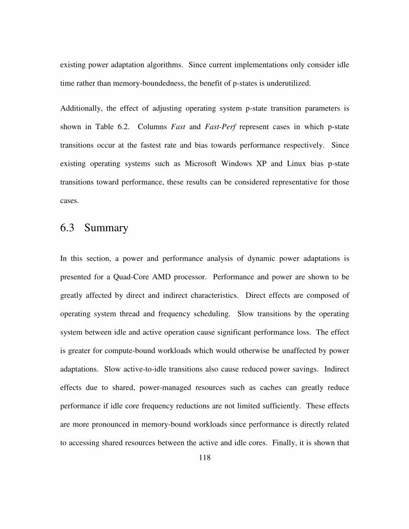
118
existing power adaptation algorithms. Since current implementations only consider idle
time rather than memory-boundedness, the benefit of p-states is underutilized.
Additionally, the effect of adjusting operating system p-state transition parameters is
shown in Table 6.2. Columns Fast and Fast-Perf represent cases in which p-state
transitions occur at the fastest rate and bias towards performance respectively. Since
existing operating systems such as Microsoft Windows XP and Linux bias p-state
transitions toward performance, these results can be considered representative for those
cases.
6.3 Summary
In this section, a power and performance analysis of dynamic power adaptations is
presented for a Quad-Core AMD processor. Performance and power are shown to be
greatly affected by direct and indirect characteristics. Direct effects are composed of
operating system thread and frequency scheduling. Slow transitions by the operating
system between idle and active operation cause significant performance loss. The effect
is greater for compute-bound workloads which would otherwise be unaffected by power
adaptations. Slow active-to-idle transitions also cause reduced power savings. Indirect
effects due to shared, power-managed resources such as caches can greatly reduce
performance if idle core frequency reductions are not limited sufficiently. These effects
are more pronounced in memory-bound workloads since performance is directly related
to accessing shared resources between the active and idle cores. Finally, it is shown that

119
performance loss and power consumption can be minimized through careful selection of
hardware adaptation and software control parameters. In the case of Microsoft Windows
Vista running desktop workloads, performance loss using a naïve operating system
configuration is less than 8 percent on average for all workloads while saving an average
of 45 percent power. Using an optimized operating system configuration, performance
loss drops to less than 2 percent with power savings of 30 percent.
While the results attained through optimizing a reactive operating system power
adaptation are promising, further improvement can be achieved through new approaches.
The existing adaptations algorithms have several limitations including poor response to
phase changes and a lack of process awareness and frequency-sensitivity. The ability to
increase the responsiveness of the reactive algorithm is limited since excessive
adaptations reduce performance and increase energy consumption. To attain higher
performance and efficiency, a predictive adaptation is required. Predictive adaptation
effectively provides the responsiveness of a maximally reactive scheme without the
overhead of excessive adaptation.
Another limitation is the lack of frequency-sensitivity awareness in current algorithms.
To make best use of dynamic processor voltage and frequency scaling, the sensitivity of a
workload to frequency should be accounted. By knowing the frequency sensitivity,
workloads which do not benefit from high frequency could achieve much lower power.
Similarly, workloads that scale well with frequency can attain higher performance by
avoiding the use of excessively low frequencies.

120
Chapter 7 Predictive Power Management
7.1 Core-Level Activity Prediction
Existing power management techniques operate by reducing performance capacity
(frequency, voltage, resource size) when performance demand is low, such as at idle or
similar low activity phases. In the case of multi-core systems, the performance and
power demand is the aggregate demand of all cores in the system. Monitoring aggregate
demand makes detection of phase changes difficult (active-to-idle, idle-to-active, etc.)
since aggregate phase behavior obscures the underlying phases generated by the
workloads on individual cores. This causes sub-optimal power management and over-
provisioning of power resources. In this study, these problems are addressed through
core-level, activity prediction.
The core-level view makes detection of phase changes more accurate, yielding more
opportunities for efficient power management. Due to the difficulty in anticipating
activity level changes, existing operating system power management strategies rely on
reaction rather than prediction. This causes sub-optimal power and performance since
changes in performance capacity by the power manager lag changes in performance
demand. To address this problem we propose the Periodic Power Phase Predictor
(PPPP). This activity level predictor decreases SYSmark 2007 client/desktop processor
power consumption by 5.4% and increases performance by 3.8% compared to the

121
reactive scheme used in Windows Vista operating system. Applying the predictor to the
prediction of processor power, accuracy is improved by 4.8% compared to a reactive
scheme.
Dynamic power management provides a significant opportunity for increasing energy
efficiency and performance of computing systems. Energy efficiency is increased by
reducing performance capacity (frequency, parallelism, speculation, etc.) when the
demand for performance is low. Efficiency or a lack thereof may impact the performance
of a system. High-density server and multi-core processor performance is limited by
power delivery and dissipation. Reducing the power consumption in one component may
allow other components to consume more power (higher voltage and frequency) and
therefore achieve higher performance. These systems would otherwise have higher
performance if they were not sharing power resources [Bl07] [McPo06] [FaWe07]
[WaCh08] [WuJu05]. Power management allows the performance of cores/systems
sharing power to increase by “borrowing” power from idle or performance-insensitive
cores/systems and reallocating it to heavily-utilized cores/systems.
The challenge in applying power management to increase efficiency and performance is
in identifying when to adapt performance capacity. The ubiquitous, architected solution
implemented in operating systems such as Windows/Linux is to react to changes in
performance demand. Though this approach is simple, it performs sub-optimally
[BiJo08] [DiSo08] for workloads with many distinct and/or short phases. Each time a
workload transitions from a phase of low performance demand to a phase of high

122
performance demand, reactive power management increases performance capacity
sometime after the phase transition. During the time between the change in demand and
capacity, performance may be less than optimal. Similarly, power consumption is sub-
optimal on transitions from high to low demand. The amount of performance loss is
proportional to the number of phase changes in the workload and the lag between demand
and capacity. For increasing performance in power-limited situations, reactions must be
fast to prevent overshooting the power limit or missing opportunities to increase
performance.
Identifying when to adapt is complicated by the presence of multiple cores sharing power
resources. Consider Figure 7.1. Core-level power consumption is shown for a system
with multiple simultaneous threads. The program threads are fixed to the cores with
thread N on core N, thread N-1 on core N-1, etc. Since power monitoring is typically
provided at the system-level [Po10], existing power control techniques use the erratic
fluctuations in the total power for predicting future behavior. This is unfortunate since in
this example, the individual threads have a periodic, easily discernable pattern, while the
pattern in the aggregate power is less discernable. If power phases can be tracked at the
core-level, accurate dynamic power management schemes can be devised.
To improve the effectiveness of power management the use of predictive, core-level
power management is proposed. Rather than reacting to changes in performance
demand, past activity patterns are used to predict future transitions. Rather than using
aggregate power information, activity and power measured at the core-level is used.
123
Figure 7.1: Thread and Aggregate Power Patterns
To analyze the effectiveness of the predictor the SYSmark 2007 benchmark is used. It
contains numerous, desktop/personal computing applications such as Word, Excel,
PowerPoint, Photoshop, Illustrator, etc. The benchmark is structured to have a high
degree of program phase transitions, including extensive use of processor idle states (c-
states) and performance states (p-states) [Ac07]. Rather than being strictly dominated by
the characteristics of the workload itself, SYSmark 2007 accounts for the impact of
periodic, operating system scheduling and I/O events. Using this observation, we
0
50
100
150
0 50 100 150 200
Wat
ts
Seconds
Total Power = ∑CorePowerN N=0 to 3
0
50
Wat
ts
CorePower0
0
50
Wat
ts
CorePower1
0
50
Wat
ts
Core Power2
0
50
0 50 100 150 200
Wat
ts
Seconds
CorePower3
Phase
Misalignment

124
construct a periodic power phase predictor. This simple periodic predictor tracks and
predicts periodic phases by their duration. By predicting future demand, aggressive
adaptations can be applied. The core-level predictive technique outperforms existing
reactive power management schemes by reducing the effective lag between workload
phase transitions and power management decisions. By predicting the individual power
contribution of each thread rather than predicting the aggregate effect, complex phases
can be predicted. The contributions of this chapter are summarized as follows.
(1) Concept of core-level power phases in multi-core systems. Core-level power phases
unveil more opportunities for power saving adaptations than are possible if only
aggregate system level information is used.
(2) A simple, periodic power phase predictor. Though prior research [DuCa03] [IsBu06]
demonstrates the effectiveness of power management using predictive schemes on
uniprocessors, this research shows its effectiveness when applied to multi-core systems
with operating system scheduling interactions. The proposed predictive power
management is compared against the reactive algorithm in the Windows Vista operating
system. Previous research focused on single-threaded SPEC CPU 2000 benchmarks,
while this study uses SYSmark 2007 which includes popular desktop/personal computing
applications such as Microsoft Word, Excel, PowerPoint, Adobe Photoshop, Illustrator,
etc. These workloads include difficult to predict power management events due to large
numbers of interspersed idle phases and frequent thread migrations.
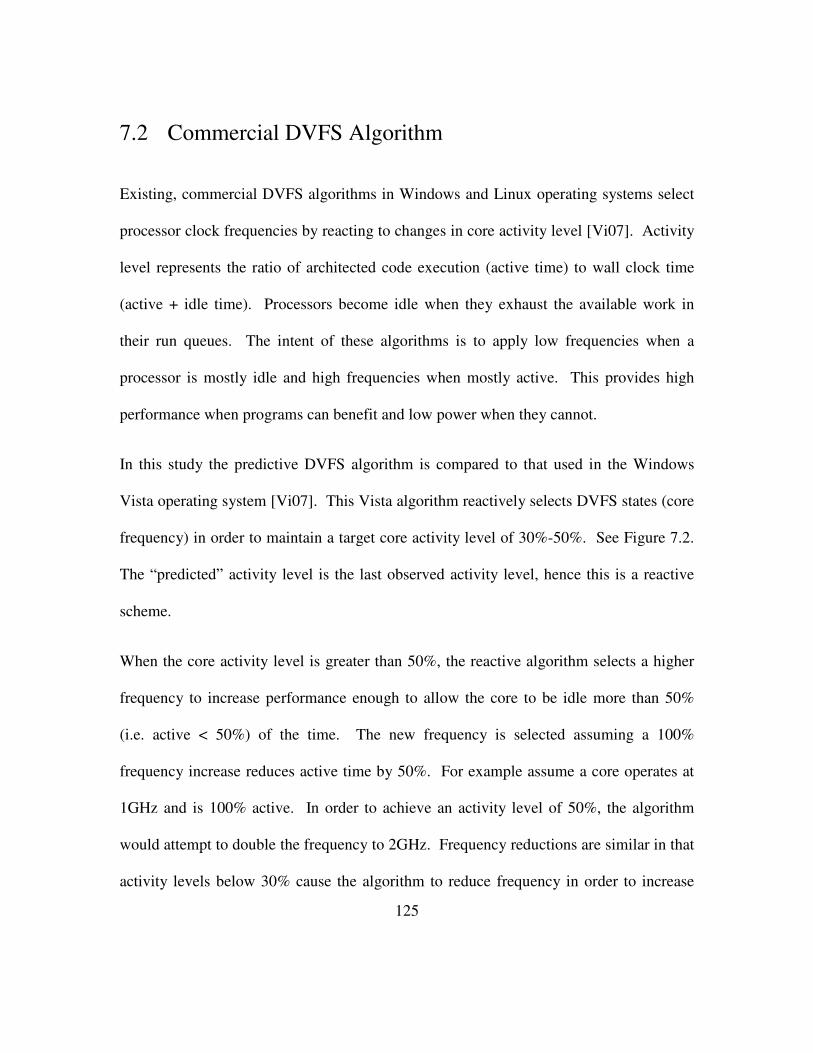
125
7.2 Commercial DVFS Algorithm
Existing, commercial DVFS algorithms in Windows and Linux operating systems select
processor clock frequencies by reacting to changes in core activity level [Vi07]. Activity
level represents the ratio of architected code execution (active time) to wall clock time
(active + idle time). Processors become idle when they exhaust the available work in
their run queues. The intent of these algorithms is to apply low frequencies when a
processor is mostly idle and high frequencies when mostly active. This provides high
performance when programs can benefit and low power when they cannot.
In this study the predictive DVFS algorithm is compared to that used in the Windows
Vista operating system [Vi07]. This Vista algorithm reactively selects DVFS states (core
frequency) in order to maintain a target core activity level of 30%-50%. See Figure 7.2.
The “predicted” activity level is the last observed activity level, hence this is a reactive
scheme.
When the core activity level is greater than 50%, the reactive algorithm selects a higher
frequency to increase performance enough to allow the core to be idle more than 50%
(i.e. active < 50%) of the time. The new frequency is selected assuming a 100%
frequency increase reduces active time by 50%. For example assume a core operates at
1GHz and is 100% active. In order to achieve an activity level of 50%, the algorithm
would attempt to double the frequency to 2GHz. Frequency reductions are similar in that
activity levels below 30% cause the algorithm to reduce frequency in order to increase

126
activity levels to 30%. Since processors have a finite number of architected DVFS states,
the algorithm selects the nearest frequency which meets the target activity level.
+� �,� -.�,�/ = 0���12345
0���12345 + 0���6785
Figure 7.2: Windows Vista Reactive P-State Selection Algorithm
7.3 Workload Characterization
To analyze the power/performance impact of the predictive power management scheme
on real-world workloads, a system running the desktop/client SYSmark 2007 benchmark
is characterized. This benchmark represents a wide range of desktop computing
applications. The benchmark components are E-Learning, Video Creation, Productivity,
and 3D. The individual subtests are listed in Table 7.1. This benchmark is particularly
important to the study of dynamic power adaptations since it provides realistic user
scenarios that include user interface and I/O delays. These delays cause a large amount
Decrease
Frequency
No Change
Increase
Frequency
0%
10%
20%
30%
40%
50%
60%
70%
80%
90%
100%
Core
Act
ivit
y L
evel
Increase Threshold = 50%
Decrease Threshold = 30%
High Performance
Demand
Region
Low Performance
Demand
Region
Hysteresis
Region

127
of idle-active transitions in the cores. Since current OSs determine dynamic adaption
levels using core activity level, the replication of these user interactions in the benchmark
is critical. For comparison, Figure 7.3 shows average active core residencies of a six-
core AMD Phenom 2 processor across a wide range of desktop workloads. The left-hand
side of the figure illustrates the problem with many popular benchmark applications. The
benchmarks spend nearly 100% of the time with all cores active. From an idle power
management perspective little can be done to improve performance and power efficiency.
The center and right-hand side workloads are more challenging for idle power
management due to the frequent occurrence of idle phases. The SYSmark subtests are the
most challenging due to their large composition of interspersed idle and active phases.
Table 7.1: SYSmark 2007 Components
E-Learning Video Creation Productivity 3D
Adobe
- Illustrator
- Photoshop
-Flash
Microsoft
- PowerPoint
Adobe
- After Effects
- Illustrator
- Photoshop
Microsoft
- Media Encoder
Sony
- Vegas
Microsoft
- Excel
- Outlook
- Word
- PowerPoint
- Project
Corel
- WinZip
Autodesk
- 3Ds Max
- SketchUp
Performance Loss for Vista Reactive Power Management [4]
8.8% 6.2% 9.5% 5.9%
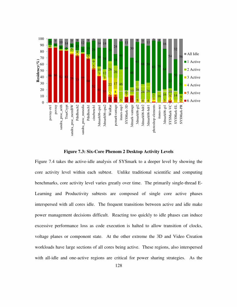
128
Figure 7.3: Six-Core Phenom 2 Desktop Activity Levels
Figure 7.4 takes the active-idle analysis of SYSmark to a deeper level by showing the
core activity level within each subtest. Unlike traditional scientific and computing
benchmarks, core activity level varies greatly over time. The primarily single-thread E-
Learning and Productivity subtests are composed of single core active phases
interspersed with all cores idle. The frequent transitions between active and idle make
power management decisions difficult. Reacting too quickly to idle phases can induce
excessive performance loss as code execution is halted to allow transition of clocks,
voltage planes or component state. At the other extreme the 3D and Video Creation
workloads have large sections of all cores being active. These regions, also interspersed
with all-idle and one-active regions are critical for power sharing strategies. As the
86 86 82 8175 73 77
68
5241
35
9 9 9 112
22
2
3 45 8
4
5
3
3
22 17
5
2
5 4 43
3
5
2
45
43
9
1012
2620
46
6 10 2824 26
7 1616
1014
9
105
6 26 13
9 19 29
30 34
34
18
44
69
46
6164 58
83 7864
23
50
31
7 10 147 5
125 3
14 1424
411
30
5 7 113 4
16
54
32
56
0
10
20
30
40
50
60
70
80
90
100
pov
ray-r
tr1
pov
ray
san
dra
_p
roc_
arit
h
Tru
eC
ryp
t
san
dra
_p
roc_
mem
BW
Pdn
Ben
ch2
san
dra
_p
roc_
mm
edia
Pdn
Ben
ch1
cin
ebench1
3dm
ark
06-c
pu1
3dm
ark
06-c
pu2
Win
Rar
pcm
ark
vanta
ge
itun
es-m
p3
SY
SM
ark
-3D
3dm
ark
-van
tag
e
3dm
ark
06-g
t2
3dm
ark
06-h
dr2
3dm
ark
06-h
dr1
pho
tosh
op
-ele
ments
itun
es-a
cc
3dm
ark
06-g
t1
SY
SM
ark
-VC
SY
SM
ark
-EL
SY
SM
ark
-PR
Res
iden
cy(%
)
All Idle
1 Active
2 Active
3 Active
4 Active
5 Active
6 Active

129
workload/operating systems adds and removes threads from cores the resultant power
level changes drastically. The power difference between cores in the active versus idle
state is much greater than differences within the active state.
Figure 7.4: Utilization of Multiple Cores by SYSmark 2007 Benchmark
The effect of these frequent transitions on power and performance is significant. Bircher
et al [BiJo08] show that the slow reaction of the Vista DVFS algorithm leads to a
performance loss of 6%-10% for SYSmark 2007. It is shown that this performance loss
is due to a large portion of the benchmark operating at DVFS state with frequencies as
0
1
2
3
4
Act
ive
Core
s
Time
E-Learning
0
1
2
3
4
Act
ive
Core
s
Time
Video Creation
0
1
2
3
4
Act
ive
Core
s
Time
Productivity
0
1
2
3
4
Act
ive
Core
s
Time
3D
Outlook Excel
Media
Encode
Photoshop
After
Effects
Sketchup
3dsMax
Photoshop
Illustrator Flash
Photoshop Flash
130
low as 1/3 of the maximum frequency. Similarly, power consumption is excessively high
due to the DVFS algorithm choosing high-power states for many of the frequent, idle
phases in the benchmark.
7.4 Periodic Power Phase Predictor – PPPP
While power management in operating systems like Windows/Linux is reactive, there
have been proposals to use predictive power management [IsBu06] [DuCa03] [DiSo08].
Isci [IsBu06] uses table-based predictors of memory operations/instruction, to direct
DVFS decisions for single-threaded workloads. Duesterwald et al. [DuCa03] examine
table-based predictor techniques to predict performance-related metrics (IPC, cache
misses/instruction and branch misprediction rates) of single-thread workloads, but not
power. Diao [DiSo08] uses machine learning to predict activity patterns. The
predictions are used to make policy decisions for entering core idle states. In contrast,
the periodic power phase predictor (PPPP) is proposed which makes use of table-based
prediction structures and the repetitive nature of power phases to predict performance
demand and/or power consumption. The predictor is shown in Figure 7.5. Like
traditional table-based predictors, the main components are: a global phase history
register (GPHR), pattern history table (PHT) and predicted level. Typically, table-based
predictors track sequences of events such as branch outcomes or IPC samples [DuCa03]
[IsBu06]. This predictor is distinct in that it tracks run-length-encoded sequences of core
active/idle phases. Activity in this case is defined as execution of architected

131
instructions. In APCI[Ac07] terminology that is popularly used for power management,
it is known as the C0 state. All other time is considered non-active or idle. Idle time is
explicitly defined as “executing” in a processor idle state via the HLT instruction or other
idle state entry method [Bk09]. This state is also known as the Cx state where x = 1 to N.
These non-C0 states are responsible for the largest power reductions due to the
application of clock and power gating. Large power changes or phases can be detected
by tracking core activity patterns. For this reason the PPPP is constructed to track core
activity patterns.
A diagram of the predictor is provided in Figure 7.5. The main feature of the predictor is
its ability to capture frequent, power-relevant events by tracking active/idle patterns.
Transitions to active or idle states and the resultant power level can be predicted by
tracking previous patterns. One of the most common events is the periodic timer tick
event used in many commercial operating systems [SiPa07]. This event occurs on a
regular interval to provide timing and responsiveness to the operating system scheduler.
When a core is otherwise idle, the timer tick produces an easily discernable pattern.

132
LengthTn LengthTn-1
Length2,
Level2
Length1,
Level1
LengthTn,
LevelTn
LengthTn-1,
LevelTn-1
LengthTn,
LevelTn
LengthTn-1,
LevelTn-1
LengthTn,
LevelTn
LengthTn-1,
LevelTn-1
Length4,
Level4
100% 4
GPHR Size = 2
GPHR Size = 2
LengthTn+2,
LevelTn+2
Tn+2
LengthTn+2,
LevelTn+2
Tn+2
LengthTn+2,
LevelTn+2
Tn+2
True True
Val
id
Pen
din
g
Lev
el
(Wat
ts,U
til%
) Detected Pattern
Tim
eSta
mp
Predicted
Phase
Most
Recent
Phase
Co
nfi
den
ce
1 2 3 4
Conf%
Conf%
Conf%
T/F
T/F
T/F
T/F
T/F
T/F
Time
GP
HT
Size
Figure 7.5: Periodic Power Phase Predictor
For Windows operating systems, the boot strap processor remains idle for periods of 16
milliseconds interrupted by active periods lasting about 100 microseconds.
The predictor tracks the duration of the idle and active phases in the length and level
fields. As a pattern of active and idle period repeats the predictor updates the quality of
the prediction using the confidence field. When a pattern is first identified, it is copied to
the GPHT and assigned a confidence level of 100%. The correctness of the prediction is
assessed by comparing the predicted time and level of the next transition (timestamp
field) to the actual transition. If a misprediction in duration or level is found, the
confidence is reduced by a tunable percentage. If multiple mispredictions occur, the

133
confidence level will drop below a confidence limit. The net effect of these parameters is
that a prediction will be invalidated after three consecutive mispredictions. The valid and
pending fields are used to determine which predictor entries can be used for predictor
matches and which have outstanding predictions respectively. Multiple predictions can
be outstanding. If conflicting prediction exist at an evaluation point, the higher
confidence prediction is used. For equal confidence predictions, the lower index
prediction is used. Additional details for each predictor field are provided in Table 7.2.
An example of the PPPP tracking and predicting core utilization level is given in Figure
7.6.
Figure 7.6: Example of Program Phase Mapping to Predictor
1ms,
20%
4ms,
80%
Pattern 1ms 4ms
Uti
liza
tio
n
Time (ms)
20%
80%
Pattern Pred.
Phase 2ms
2ms
Time (ms)
20%
80%
Uti
liza
tio
n
Pred.
Phase
Time
Stamp
Time
Stamp
4ms,
80% 1ms
2ms,
20%
2ms,
80%
2ms,
80% 2ms

134
Table 7.2: Periodic Power Phase Predictor Field Descriptions
Predictor
Field
Description
Detected
Pattern
Length,Level
Duration and level of phase pair. This is also the table index. When a
periodic phase is detected, it is used to index the prediction table.
Predicted
Phase
Length,Level
Predicted Phase at next transition. For utilization predictor this is activity
level. For power prediction this is the power level seen when this phase
previously occurred.
Timestamp
Records timestamp of when predicted phase change is to occur. This is
the most critical value produced by the predictor. It is used by the power
manager to schedule changes in power/performance capacity of the
system. This value allows for optimal selection of performance capacity
given the anticipated duration of operation at a particular performance
demand.
Confidence
“Quality” of phase as a function of past predictions and duration. The
confidence is used by the power manager to determine if a prediction will
be used or not. It is also used by the replacement algorithm to determine
if the phase will be replaced if the predictor is full. All newly detected
phases start with a confidence of 1. If the phase is subsequently
mispredicted, the confidence is reduced by a fixed ratio.
Valid Indicates if this entry has a valid phase stored with a “true” or “false.”
Pending Indicates if this phase is predicted to occur again. This value is set “true”
on the occurrence of the phase and remains true until the phase prediction
expires.
7.5 Predicting Core Activity Level
This section provides power and performance results for the core and aggregate-level
periodic power phase predictor in comparison to a commercial reactive scheme. A
comparison is made in terms of prediction accuracy, prediction coverage, power and
performance. Also, a characterization of core activity phases is given.

135
First, prediction accuracy is considered. Accuracy is defined according to the,
commercial, reactive DVFS algorithm used in the Windows Vista operating system
[Vi07]. A correct prediction is one in which the selected DVFS frequency selection keeps
the processor within the target range of 30% to 50% activity.
The accuracy of the reactive scheme is determined by analyzing traces of core DVFS and
activity levels from a real system. If the selected frequency did not cause the core to have
an activity level between 30% and 50%, the selection is considered wrong. For the
predictive schemes, the activity level trace is played back through the predictor while
allowing it to select a frequency to meet the 30%-50% target. Since core activity level
changes according to core frequency, the resultant activity level must be scaled
accordingly. The amount of scaling is determined experimentally by measuring
performance of the SYSmark workload under a range of core frequencies. Performance,
and therefore activity level, scale 70% for each 100% change in core frequency.
Using this approach results are presented for SYSmark 2007 prediction accuracy in Table
7.3. DVFS hit rate is provided for three predictors. Core-level PPPP represents the
predictor applied to each core. Aggregate PPPP represents the predictor driven by the
total activity level. All target activity levels remain the same. A single predictor, driven
by the aggregate activity level (i.e. average of all cores) is used to select the next core
frequency. Core-level reactive represents the Windows Vista DVFS algorithm.
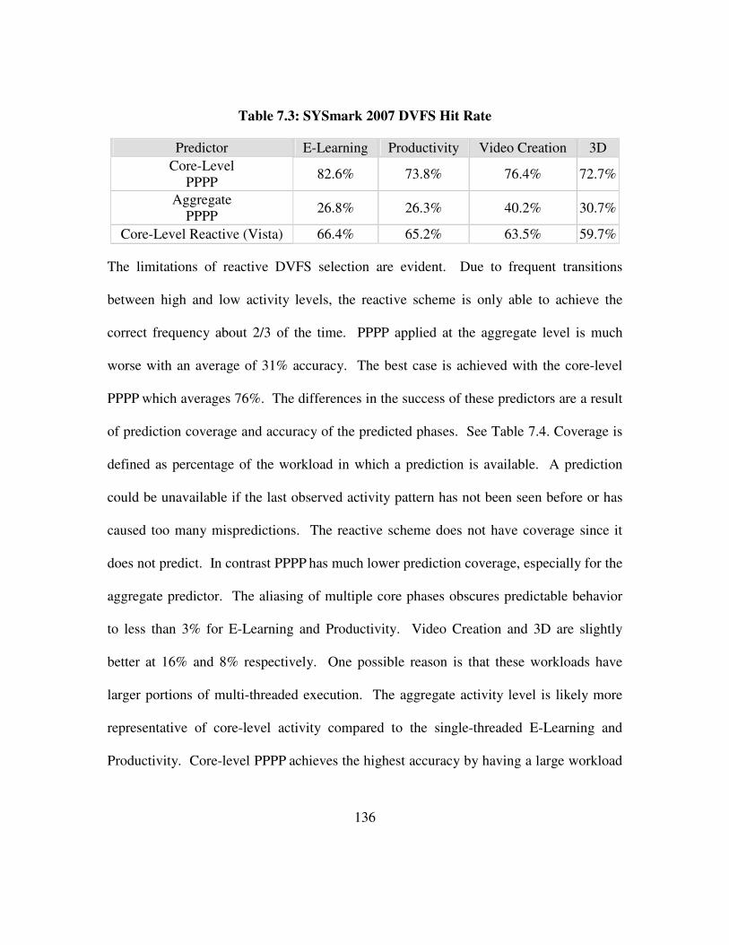
136
Table 7.3: SYSmark 2007 DVFS Hit Rate
Predictor E-Learning Productivity Video Creation 3D
Core-Level
PPPP 82.6% 73.8% 76.4% 72.7%
Aggregate
PPPP 26.8% 26.3% 40.2% 30.7%
Core-Level Reactive (Vista) 66.4% 65.2% 63.5% 59.7%
The limitations of reactive DVFS selection are evident. Due to frequent transitions
between high and low activity levels, the reactive scheme is only able to achieve the
correct frequency about 2/3 of the time. PPPP applied at the aggregate level is much
worse with an average of 31% accuracy. The best case is achieved with the core-level
PPPP which averages 76%. The differences in the success of these predictors are a result
of prediction coverage and accuracy of the predicted phases. See Table 7.4. Coverage is
defined as percentage of the workload in which a prediction is available. A prediction
could be unavailable if the last observed activity pattern has not been seen before or has
caused too many mispredictions. The reactive scheme does not have coverage since it
does not predict. In contrast PPPP has much lower prediction coverage, especially for the
aggregate predictor. The aliasing of multiple core phases obscures predictable behavior
to less than 3% for E-Learning and Productivity. Video Creation and 3D are slightly
better at 16% and 8% respectively. One possible reason is that these workloads have
larger portions of multi-threaded execution. The aggregate activity level is likely more
representative of core-level activity compared to the single-threaded E-Learning and
Productivity. Core-level PPPP achieves the highest accuracy by having a large workload
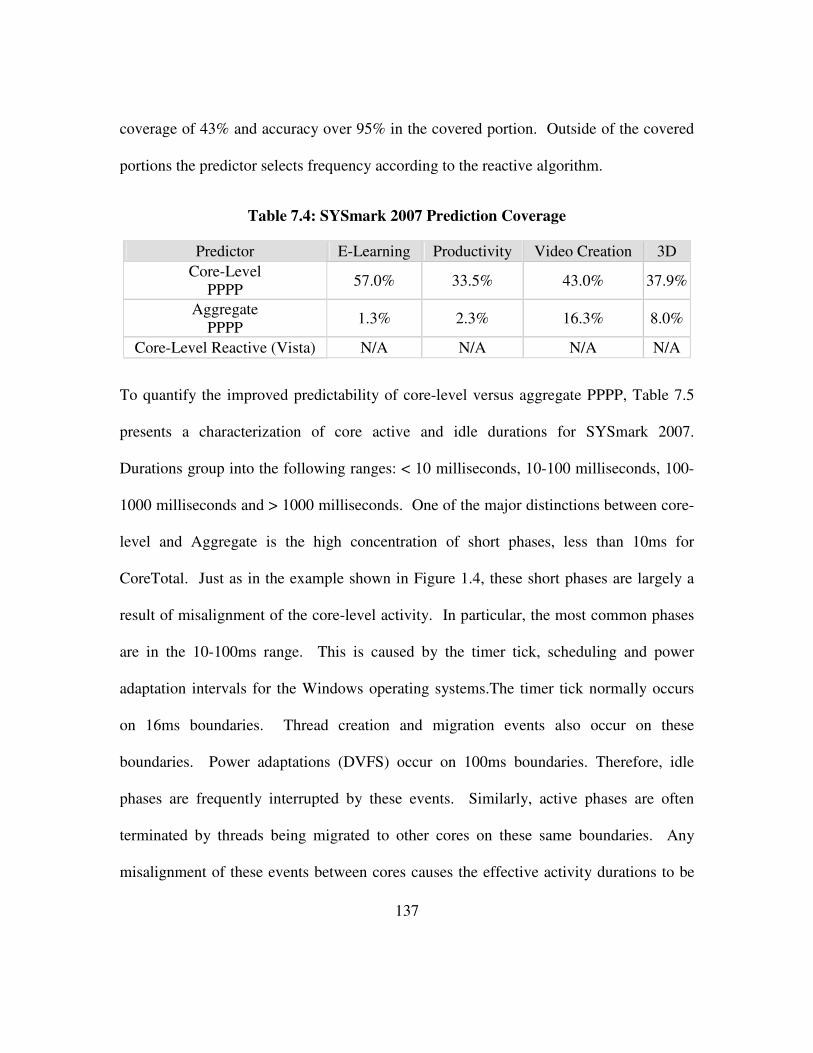
137
coverage of 43% and accuracy over 95% in the covered portion. Outside of the covered
portions the predictor selects frequency according to the reactive algorithm.
Table 7.4: SYSmark 2007 Prediction Coverage
Predictor E-Learning Productivity Video Creation 3D
Core-Level
PPPP 57.0% 33.5% 43.0% 37.9%
Aggregate
PPPP 1.3% 2.3% 16.3% 8.0%
Core-Level Reactive (Vista) N/A N/A N/A N/A
To quantify the improved predictability of core-level versus aggregate PPPP, Table 7.5
presents a characterization of core active and idle durations for SYSmark 2007.
Durations group into the following ranges: < 10 milliseconds, 10-100 milliseconds, 100-
1000 milliseconds and > 1000 milliseconds. One of the major distinctions between core-
level and Aggregate is the high concentration of short phases, less than 10ms for
CoreTotal. Just as in the example shown in Figure 1.4, these short phases are largely a
result of misalignment of the core-level activity. In particular, the most common phases
are in the 10-100ms range. This is caused by the timer tick, scheduling and power
adaptation intervals for the Windows operating systems.The timer tick normally occurs
on 16ms boundaries. Thread creation and migration events also occur on these
boundaries. Power adaptations (DVFS) occur on 100ms boundaries. Therefore, idle
phases are frequently interrupted by these events. Similarly, active phases are often
terminated by threads being migrated to other cores on these same boundaries. Any
misalignment of these events between cores causes the effective activity durations to be

138
shorter and less predictable. Further evidence of these common 10-100ms phases is
given in Figure 7.7 which shows the frequency distribution of active and idle phases
across SYSmark 2007.
Table 7.5: Core Phase Residency by Length
E-Learning Video Creation
Phase Length Core Aggregate Core Aggregate
Less Than 10 ms 11% 93% 44% 82%
10 - 100 ms 49% 7% 27% 2%
100 - 1000 ms 10% 0% 14% 9%
Greater Than 1000 ms 30% 0% 16% 7%
Productivity 3D
Phase Length Core Aggregate Core Aggregate
Less Than 10 ms 55% 97% 55% 97%
10 - 100 ms 30% 3% 30% 3%
100 - 1000 ms 5% 0% 5% 0%
Greater Than 1000 ms 11% 0% 11% 0%
Active and idle phase as considered as a group since both are relevant for prediction. Idle
phases must be predicted in order to anticipate how long a power surplus will be
available. Similarly, active phase must be predicted to anticipate durations of power
deficits. In both cases the predicted durations is needed in order to weigh the power and
performance cost of transitioning to low power states or changing the DVFS operating
point. Several local maximums are present due to the periodic nature of the interaction
between power management, OSs and system hardware. By removing or varying the
intensity of these various events and observing the change in frequency distribution, the
period length may be related to its source. Note the prevalence of phases in the 10-15ms
range that corresponds to the OS scheduling interval. Also, consider the spikes at 100ms,

139
which corresponds to the DVFS scheduling interval. Additional, longer-duration
maximums occur in the 200ms and higher range. These correspond to GUI interaction
and I/O delays occurring in the SYSmark benchmark.
Next the resultant power and performance impact of the core-level PPPP versus reactive
DVFS selection is considered. Aggregate PPPP is not considered due its poor prediction
accuracy. Table 7.6 presents power and performance results for the two schemes. Power
and performance are estimated using the measured and predicted DFVS, active and idle
states shown in Table 7.7. On average, power is reduced by 5.4% while achieving a
speedup of 3.8%. This improvement is caused by PPPP more frequently selecting high
frequencies for active phases and low frequencies for performance-insensitive idle
phases. This shift can be seen in the active residencies of all subtests. The 2.4GHz –
Active state increases by 0.6 to 2.5 percentage points. Similarly, the active time in lower
frequencies is reduced an average of 0.76 percentage points. The performance impact of
selecting a low frequency for an active phase can be large. For example, selecting
800MHz rather than 2.4GHz yields a performance loss of 47% ((1-0.8GHz/2.4GHz) x
70%). Therefore, it takes only a small change in residency to drastically impact
performance. Also, the impact on performance is larger due to active time representing
only an average of 17% total time. This magnifies the performance impact by about 6x
(1/0.17). The net effect on active frequency is an increase of 144 MHz from 1.55GHz to
1.69GHz. Note that though frequency increases by 9.3%, performance increases only
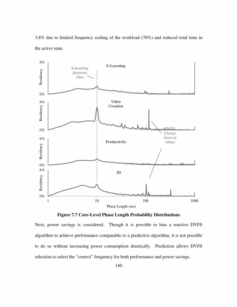
140
3.8% due to limited frequency scaling of the workload (70%) and reduced total time in
the active state.
Figure 7.7 Core-Level Phase Length Probability Distributions
Next, power savings is considered. Though it is possible to bias a reactive DVFS
algorithm to achieve performance comparable to a predictive algorithm, it is not possible
to do so without increasing power consumption drastically. Prediction allows DVFS
selection to select the “correct” frequency for both performance and power savings.
0%
6%
Res
iden
cy
E-Learning
0%
6%
Res
iden
cy
Video
Creation
0%
6%
Res
iden
cy
Productivity
0%
6%
1 10 100 1000
Res
iden
cy
Phase Length (ms)
3D
Scheduling
Quantum
16ms
DVFS
Change
Interval
100ms
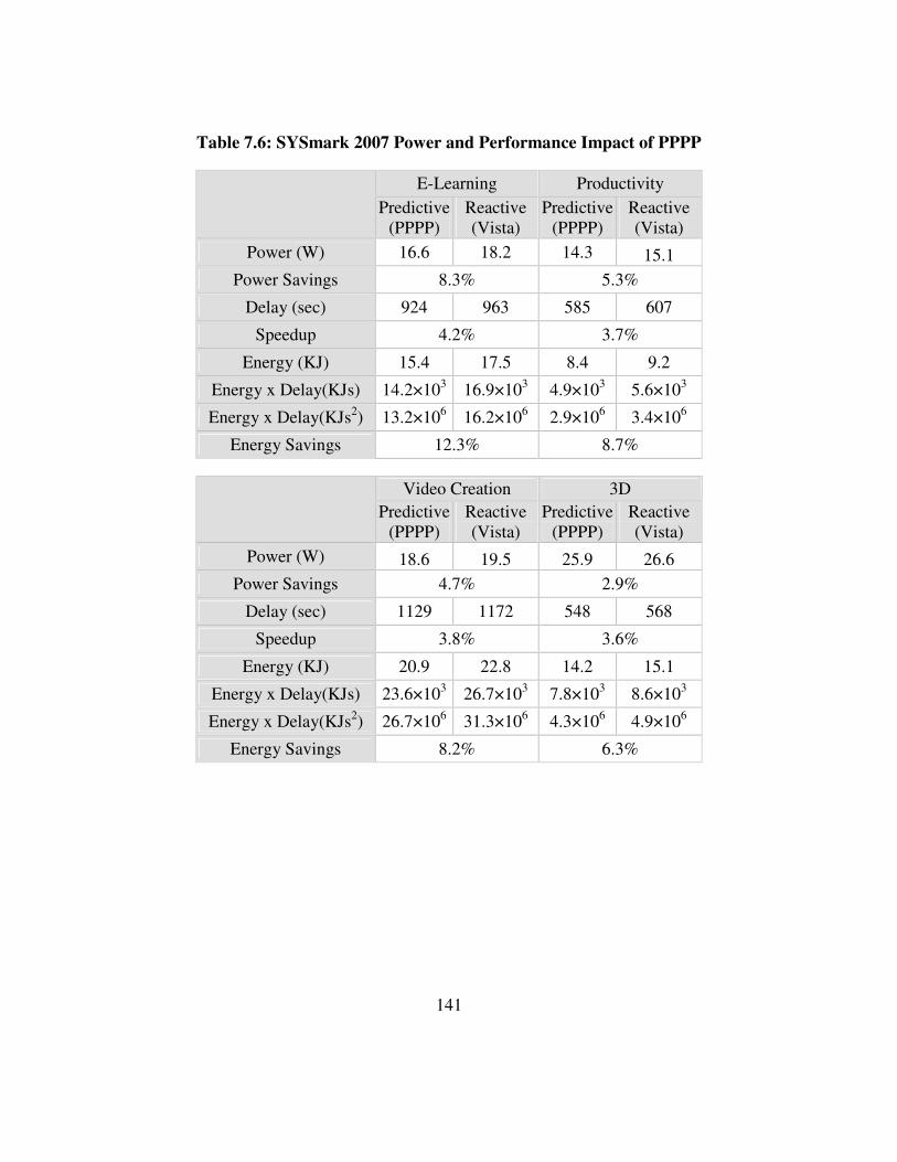
141
Table 7.6: SYSmark 2007 Power and Performance Impact of PPPP
E-Learning Productivity
Predictive
(PPPP)
Reactive
(Vista)
Predictive
(PPPP)
Reactive
(Vista)
Power (W) 16.6 18.2 14.3 15.1
Power Savings 8.3% 5.3%
Delay (sec) 924 963 585 607
Speedup 4.2% 3.7%
Energy (KJ) 15.4 17.5 8.4 9.2
Energy x Delay(KJs) 14.2×10³ 16.9×10
3 4.9×10
3 5.6×10
3
Energy x Delay(KJs2) 13.2×10
6 16.2×10
6 2.9×10
6 3.4×10
6
Energy Savings 12.3% 8.7%
Video Creation 3D
Predictive
(PPPP)
Reactive
(Vista)
Predictive
(PPPP)
Reactive
(Vista)
Power (W) 18.6 19.5 25.9 26.6
Power Savings 4.7% 2.9%
Delay (sec) 1129 1172 548 568
Speedup 3.8% 3.6%
Energy (KJ) 20.9 22.8 14.2 15.1
Energy x Delay(KJs) 23.6×10³ 26.7×10
3 7.8×10
3 8.6×10
3
Energy x Delay(KJs2) 26.7×10
6 31.3×10
6 4.3×10
6 4.9×10
6
Energy Savings 8.2% 6.3%

142
Table 7.7: SYSmark 2007 P-State and C-State Residency of PPPP versus Reactive
E-Learning Productivity
Predictive
(PPPP)
Reactive
(Vista)
Predictive
(PPPP)
Reactive
(Vista)
2.4GHz - Active 5.4% 4.6% 2.9% 2.4%
2.4GHz - Idle 7.1% 17.4% 4.4% 9.6%
1.6GHz - Active 1.2% 1.4% 0.8% 0.8%
1.6GHz - Idle 5.5% 9.4% 3.8% 6.2%
1.2GHz - Active 1.1% 1.2% 1.2% 1.2%
1.2GHz - Idle 6.9% 9.8% 6.6% 9.7%
0.8GHz - Active 3.2% 4.5% 3.8% 4.7%
0.8GHz - Idle 69.5% 51.8% 76.5% 65.3%
Active Frequency 1.72 GHz 1.56 GHz 1.47 GHz 1.34 GHz
Idle
Frequency 1.01 GHz 1.24 GHz 0.94 GHz 1.07 GHz
Video Creation 3D
Predictive
(PPPP)
Reactive
(Vista)
Predictive
(PPPP)
Reactive
(Vista)
2.4GHz - Active 6.8% 5.3% 17.5% 15.0%
2.4GHz - Idle 5.7% 12.4% 7.8% 17.0%
1.6GHz - Active 2.7% 3.2% 3.9% 5.1%
1.6GHz - Idle 5.6% 9.6% 4.6% 6.7%
1.2GHz - Active 3.8% 4.8% 2.6% 3.1%
1.2GHz - Idle 9.2% 13.8% 7.3% 9.4%
0.8GHz - Active 3.7% 4.8% 4.7% 6.9%
0.8GHz - Idle 62.3% 46.1% 51.6% 36.7%
Active Frequency 1.65 GHz 1.51 GHz 1.92 GHz 1.77 GHz
Idle
Frequency 1.01 GHz 1.20 GHz 1.07 GHz 1.32 GHz

143
In this case the predictor achieves a 3.8% performance increase while reducing power
consumption by 5.4%. The primary cause is a shift in idle frequency selections away
from the high-performance, high-leakage states. Residency in the most inefficient state,
2.4GHz – Idle, is reduced by an average of 7.8 percentage points. Residency in other idle
states above the minimum frequency also decreased, but by a smaller 3.1 percentage
points. This increases idle residency in the minimum frequency idle state of 800MHz by
an average of 15%. Average idle frequency decreases by 200MHz from 1.2GHz to
1.0GHz.
7.6 Predicting Power Levels
The second application of periodic power phase prediction is for predicting core power
consumption. Predicting power levels provides opportunities for increased performance
and efficiency. Existing power control systems such as power capping[Po10] and turbo
boost [ChJa09] apply power and performance limits statically based on user-specified or
instantaneous power consumption. Knowing power levels a priori could increase
performance by avoiding adaptations for short duration phases. For example, a core that
encounters a short, high-power phase of execution may cause the power controller to
reduce its or other processors’ frequency. If the controller could know that the phase
would be too short to cause a power or temperature violation, the reduction in
performance could be avoided.

144
To this end PPPP is applied to predict the core-level and aggregate power consumption.
Results are compared to a last value predictor also at the core and aggregate level. Core-
level power is measured using the PMC-based power model. The model allows fine-
grain, power management and temperature-aware estimation of core power.
Rather than using core activity level to predict core activity level, it is used to cross
predict power level. The predicted activity-level in the predictor is replaced by the
modeled core power level. The prediction table index remains as sequences of core
activity levels. This approach provides better pattern matching as variations in
temperature and application of DVFS tends to hide otherwise discernable patterns.
Figure 7.8 Prediction Accuracy of Core Power for Various Predictors
Figure 7.8 shows the weighted average percent accuracy of the periodic power phase
predictor compared to a last-value predictor. Weighted average is chosen since SYSmark
61.4 62.2
81.2
71.9
56.9
68.6
82.7
69.0
77.7 76.6
91.6
86.4
81.5
85.6
92.9
87.0
50
55
60
65
70
75
80
85
90
95
100
E-Learning VideoCreation Productivity 3D
Acc
ura
cy(%
)
Aggregate LastValue Aggregate PPPP
Core-Level LastValue Core-Level PPPP

145
2007 power consumption contains many idle, low-power phases. In these phases, a small
error in absolute terms yields a large percentage error. Therefore, error values are scaled
by the magnitude of measured power sample compared to the maximum observed. For
example, a 10% error on a 5W sample has half the impact of a 10% error on a 10W
sample. For all subtests, the core-level versions of the predictors outperformed the
aggregate versions. The best overall performance is 86% accuracy for the periodic core-
level predictor compared to 83% for the core-level version of the last-value predictor.
The benefit of core-level prediction of power is less pronounced than for prediction of
activity level. This is due to the smaller dynamic range of power consumption compared
to activity level. Though activity levels regularly vary from 0% to 100%, power levels
remain in a much smaller range of approximately 25% to 75%.
7.7 Summary
This section presents the concept of core-level phase prediction and its application to
dynamic power management. By observing changes in performance demand and power
consumption at the core-level, it is possible to perceive predictable phase behavior.
Prediction of phases allows power management to avoid over or under provisioning
resources in response to workload changes. Using this concept the PPPP is developed. It
is a simple, table-based prediction scheme for directing DVFS selection. It is applied to
the SYSmark2007 benchmark suite and attain significant performance and power
improvements. Compared to the reactive DVFS algorithm used by Windows Vista,
146
performance is increased by 5.4% and while power consumption is reduced by 3.8%. We
show that processor power can be predicted by PPPP with accuracy 4.8% better than a
last-value predictor.
Predictive schemes such as PPPP are the next step in improving performance and
efficiency of systems employing dynamic power management. As it was demonstrated in
the pursuit of higher single-threaded processor performance, the highest possible
performance is achieved when costly phase changes can be predicted. Prediction allows
the use of more aggressive power saving techniques since excessive performance loss can
be avoided.

147
Chapter 8 Related Research
This section summarizes related research in the areas relating to predictive processor
power management. Specifically, performance counter-driven power models, system-
level power characterization and predictive power management are covered.
8.1 Performance Counter-Driven Power Models
Contemporary research in the area of performance counter-driven power modeling has
focused primarily on the single largest consumer, the processor [LiJo03] [Be00] [IsMa03]
[CoMa05] [BrTiMa00]. System-level power modeling [HeCe06] is mostly focused on
power consumption within a single subsystem [Ja01] [ZeSo03] [KiSu06] [GuSi02].
Consistent throughout processor power modeling is the theme that power consumption is
primarily determined by the number of instructions retired per cycle. Li et al [LiJo03]
present a simple linear model for power consumption by operating system services. The
resultant models are a function of only IPC. Their modeling only considers operating
system routines and requires a separate model for each operating system routine. Most
importantly, their model is simulation-based and consequently does not correlate well
with power consumption of actual processors. In contrast, the models in this dissertation
is based on direct, in-system measurement and shows that power depends more on
fetched µop/cycle rather than IPC. Bellosa [Be00] uses synthetic workloads to
148
demonstrate a correlation between observable performance events and power
consumption. He shows that a correlation exists for: µops/sec, fµops/sec, L2
accesses/sec and memory accesses/sec. Since only synthetic workloads are characterized,
these results are not representative of realistic workloads. The most closely related work
is by Isci et al [IsMa03]. They build a comprehensive power model based on utilization
factors of the various components of the processor. Using 22 performance monitoring
counters they model average power consumption of SPEC2000 workloads within 5%.
The models in this dissertation yields similar accuracy, yet with only two PMC metrics
that aggregate power consumption across the numerous processor functional units. A
major limitation of all of these contemporary works is the lack of awareness of power
management and temperature effects. The dissertation models accurately account for
power fluctuations due to clock gating, DVFS and temperature variation.
Existing studies in system-level power modeling [Ja01] [ZeSo03] [KiSu06] have relied
on events local to the subsystem. The model in this dissertation is the first to encompass
complete system power using only events local to the processor. The most closely
related work by Heath [GuSi02], models CPU, network and disk power using operating
system counters. This model does not account for memory and chipset power. Since it
relies on comparatively high-overhead operating system routines, the run-time
performance cost is higher compared to the dissertation model that uses only fast, on-chip
performance counters.

149
8.2 System-Level Power Characterization
Existing workload power studies of computing systems consider the various levels:
microarchitecture [IsMa03] [Be00] [NaHa03], subsystem [BoEl02] [MaVa04] [FeGe05-
1], or complete system [ChAn01]. This disseration targets the subsystem level and
extends previous studies by considering a larger number of subsystems. Unlike existing
subsystem studies that analyze power on desktop or mobile uniprocessor systems, this
dissertation considers multi-core, multi-socket, desktop, mobile and server systems.
Studies at the microarchitecture level [IsMa03] [Be00] utilize performance monitoring
counters to estimate the contribution to microprocessor power consumption due to the
various functional units. These studies only consider uniprocessor power consumption
and use scientific workloads only. Since power is measured through a proxy it is not as
accurate as direct measurement. Natarajan [NaHa03] performs simulation to analyze
power consumption of scientific workloads at the functional unit level.
At the subsystem level, [BoEl02] [MaVa04] [FeGe05-1] consider power consumption in
three different hardware environments. Bohrer [BoEl02] considers CPU, hard disk, and
combined memory and I/O in a uniprocessor personal computer. The workloads
represent typical webserver functions such as http, financial, and proxy servicing. This
disseration adds multiprocessors, and considers memory and I/O separately. Mahesri and
150
Vardan [MaVa04] perform a subsystem level power study of a Pentium M laptop. They
present average power results for productivity workloads. In contrast, this dissertation
considers a server-class SMP running a commercial workload. Feng [FeGe05-1]
performs a study on a large clustered system running a scientific workload. As part of a
proposed resource management architecture, Chase [ChAn01] presents power behavior at
the system level. Lacking in all of these studies is a consideration of power phase
duration. Duration is a critical aspect since it directs power adaptions. An effective
adaptation scheme must choose adaptations that are appropriate to the expected duration
of the event. For example, since there is a performance and energy cost associated with
DVFS, changes to voltage/frequency should only be performed if the system can
amortize those costs before the next change is required.
8.3 Predictive Power Adaptation
While most existing power management schemes are reactive, there are a few related
proposals that use predictive power management [IsBu06] [DuCa03] [DiSo08]. Isci
[IsBu06] uses table-based predictors of memory operations/instruction, to direct DVFS
decisions for single-threaded workloads. Duesterwald et al. [DuCa03] examine table-
based predictor techniques to predict performance-related metrics (IPC, cache
misses/instruction and branch misprediction rates) of single-thread workloads, but not
power. Diao [DiSo08] uses machine learning to predict activity patterns. The
predictions are used to make policy decisions for entering core idle states. In contrast the

151
prediction scheme in this dissertation makes use of table-based prediction structures and
the repetitive nature of power phases to predict performance demand and/or power
consumption. Further, the validation of the predictor is performed using realistic,
representative workloads. These workloads contain complex power management events
that are not present in the simple workloads used in the contemporary research. These
events are critical to a practical power management schemed since they induce power and
performance effects larger than those seen in simple workloads.
Outside the predictive adaptation realm, there are numerous proposals for increasing
energy efficiency and staying within operating limits. To increase energy efficiency
studies have applied adaptation at the processor level [LiMa06] [LiBr05] [WuJu05]
[Vi07] [PaSt06] [KoGh05] [KoDe04] and system level [MeGo09] [RaLe03] [BoEl02].
To stay within defined operating limits studies have applied adaptation at the processor
level [HaKe07] [RaHa06] [ChJa09] [IsBu06] [McPo06] and complete system level
[LeWa07] [RaLe06] [ChDa05] [ChAn01] [Po10] [FaWe07] [WaCh08] [MiFr02].
8.4 Deadline and User-Driven Power Adaptation
In the embedded and real-time computing domains power management is performed
under a different set of requirements. Rather than focusing on reduction of average or
peak power, computation deadlines are more critical. These systems contain various
components and processes with critical deadlines for computation. For example, network
devices implement buffers to allow the network interface to queue transactions. This
152
frees the main processor to service other subsystems in an uninterrupted manner.
However, since the buffering is finite, the main processor must service and empty the
buffer with the deadline or connectivity may be lost. To reduce energy consumption,
several researchers [LuCh00] [KrLe00] [OkIs99] [PeBu00] [ShCh99] [PiSh01] [PoLa01]
propose operating the processor at the minimum voltage and frequency that satisfies the
computation deadlines as indicated by the kernel or application software. The limitation
of this approach is that the deadline must be articulated in the kernel or application
software. Other approaches infer deadlines through measurement and/or classification
[GoCh95] [PeBu98] [WeWe94] [FlRe01] [LoSm01]. Measurement-based feedback can
also be done using not-traditional metrics. Shye [ShSc08] [ShOz08] shows that user
satisfaction can be correlated to performance monitoring counters and biometric sensors.
Using these metrics, processor performance can be adjusted to the minimum level that
satisfies the user.

153
Chapter 9 Conclusions and Future Work
9.1 Conclusions
The widespread application of dynamic power management has provided the opportunity
for computing systems to attain high performance and energy efficiency across a wide
range of workloads. Practically, systems do not operate optimally due to the lack of
effective, power management, control schemes. This is largely due to a lack of run-time
power accounting and the use of reactive power management on workloads with widely
varying performance and power characteristics. The objective of this dissertation is to
improve the effectiveness of dynamic power management by addressing these
limitations. This is achieved in the following contributions:
1) Fine-Grain Accounting of Complete System Power Consumption
Using a small set of widely available performance events including IPC, cache misses
and interrupts, power models are developed by measuring power consumption on actual
systems. These linear and polynomial models are created using regression techniques
that iteratively adjust coefficients to minimize model error. This novel approach
improves upon existing research by finding that complex structures such as processors
and chipsets can be accurately represented by tracking their dominant performance
events. Unlike existing research that primarily relies on retired instruction or

154
comprehensive performance events, this approach relies on speculative events. This
approach provides higher accuracy with many fewer events to track. For a state-of-the-
art multi-core processor, these simple models achieve average error rates less than 1%.
Through an analysis of power and performance for complete systems it is discovered that
the performance events local to the processor can also predict power consumption in the
complete system. This trickle-down concept is applied to allow accurate modeling of
memory controllers, system memory, caches, chipsets, disks and I/O bridges using only
performance events in the cpu. This reduces complexity and measurement overhead by
containing all run-time measurement in low-latency on-chip performance counters.
2) Power and Performance Analysis of Computing Systems
To inform the development of power accounting and management schemes, this
dissertation presents an extensive analysis of power and performance of server, desktop
and mobile systems. It is found that the largest variation in power and performance
occurs in processors and the subsystems most closely coupled to them, such as caches
and memory controllers. The cause is largely dictated by the application of power saving
techniques such as clock gating and dynamic voltage and frequency scaling. Compared
to power variations due to instruction or transactions streams, variation due to power
management is much larger.
Additionally, this dissertation presents a new way of analyzing power consumption.
Unlike existing research that focuses on average power consumption, this study considers

155
the duration of power and performance phases. All power management schemes incur an
energy and performance penalty when the system transitions from one adaptation level to
another. To avoid costly transitions, adaption schemes must know how and when to
adapt. This new approach leads to the discovery of frequently repeating power and
performance patterns within workloads. Of these patterns, the most dominant and
predictable is the scheduling quanta of operating systems. Since active-idle and idle-
active transitions frequently occur on these boundaries, they serve as strong indicators of
phase changes.
3) Predictive Power Management
This dissertation presents the concept of core-level phase prediction and its application to
dynamic power management. By observing changes in performance demand and power
consumption at the core-level, it is possible to perceive predictable phase behavior.
Prediction of phases allows power management to avoid over or under provisioning
resources in response to workload changes. Using this concept the PPPP is developed. It
is a simple, table-based prediction scheme for directing DVFS selection. The predictor is
applied to the SYSmark2007 benchmark suite and achieves significant performance and
power improvements. Compared to the reactive DVFS algorithm used by Windows
Vista, performance is increased by 5.4% and while power consumption is reduced by
3.8%.
156
9.2 Future Work
Run-time energy accounting and predictive power management are promising tools for
improving the energy efficiency and performance of computing systems. This
dissertation has demonstrated the initial implementation of these tools at improving
processor efficiency and performance. Listed below are a few similar research areas that
are likely to yield new, valuable discoveries.
Power Managing Cloud Computing Resources
The shift away from desktop computing to cloud computing is increasing the opportunity
for predictive power management. A typical desktop system has about sixty active
processes, with less than ten of them actively consuming most computing resources. In
contrast, cloud computing servers combine hundreds of active processes from many
clients. Each of the processes has phase behavior that is independent of the others. This
combination of heterogeneous tasks makes existing reactive power management difficult
since the active-idle patterns are an aggregation of multiple independent patterns. A
significant power savings opportunity exists in accounting for and predicting the effective
usage pattern of cloud computing servers.
Functional Unit Activity Prediction
The need to increase power efficiency is pushing microarchitectural power management
beyond the core-level to individual functional units. To save power during program

157
execution, portions of pipelines or functional units can be effectively resized through
clock gating and power gating when not needed. The challenge is to apply these power
saving adaptations only when the transition cost can be amortized by long idle phases.
By defining prediction metrics for each functional unit, it is possible to detect and predict
the critical long-duration idle phases.
Process-Level Power Accounting
The entirety of this dissertation and other performance-counter power modeling research
focuses on attributing power to a particular hardware thread or core. The limitation of
this approach is that process scheduling and migration can impact the ability to discern
unique program phases. It is likely that tracking power and phase history at the process-
level will reduce aliasing thus improving predictability.
Scheduling using On-line Power and Performance Models
Another application of power accounting is for the direction of scheduling decisions. By
introducing performance models that are power-aware, optimal scheduling and power
management decisions can be made. The current state-of-the-art architectural power
adaptations provide a range of throughput and latency at the processor core-level.
Expressing those impacts as run-time power and performance models would allow major
improvements in energy efficiency and performance.

158
Bibliography
[Ac07] Advanced Configuration & Power Interface. http://www.acpi.info
(November 2007).
[Ag08] Agilent Technologies. 1146A 100 kHz /100A AC/DC Current Probe.
http://www.agilent.com, April 2008.
[An73] F. J. Anscombe. Graphs in Statistical Analysis. American Statistician,
pages 17-21, February 1973.
[Be00] F. Bellosa. The Benefits of Event-Driven Energy Accounting in Power-
Sensitive Systems. In Proceedings of the 9th Workshop on ACM SIGOPS European
Workshop: Beyond the PC: New Challenges for the Operating System (Kolding,
Denmark, September 2000), 37-42.
[Bk09] BIOS and Kernel Developer’s Guide for AMD Family 10h Processor.
http://www.amd.com. November 2009.
[BiVa05] W. L. Bircher, M. Valluri, J. Law, and L. John. Runtime identification of
microprocessor energy saving opportunities. In Proceedings of the 2005 International
Symposium on Low Power Electronics and Design (San Diego, California, August 2005),
275-280.
159
[BiJo06-1] W. L. Bircher and L. John. Complete System Power Estimation: A
Trickle-Down Approach based on Performance Events. In IEEE International
Symposium on Performance Analysis of Systems and Software (San Jose, California,
April 2007), 158-168.
[Bi06] W. L. Bircher. Measurement Based Power Phase Analysis of a
Commercial Workload. 2nd
IEEE Workshop on Unique Chips and Systems (Austin,
Texas, March 2006).
[BiJo06-3] W. L. Bircher and L. John. Power Phase Availability in a Commercial
Server Workload. In Proceedings of the 2006 International Symposium on Low Power
Electronics and Design (Tegernsee, Germany, October 2006), 350-353.
[BiJo08] W. L. Bircher and L. John. Analysis of Dynamic Power Management on
Multi-Core Processors. In Proceedings of the 22nd
Annual International Conference on
Supercomputing (Kos, Greece, June 2008), 327-338.
[BiJo10-1] W. L. Bircher and L. John. Complete System Power Estimation using
Processor Performance Events. Under Review at IEEE Transactions on Computers
(October 2010).
[BiJo10-2] W. L. Bircher and L. John. Predictive Power Management for Multi-Core
Processors. In Workshop on Energy Efficient Design (Saint-Malo, France, June 2010),
327-338.

160
[Bl07] Blade Server Technology Overview. http://www.blade.org/techover.cfm
(March 2007).
[BoEl02] P. Bohrer, E. N. Elnozahy, T. Keller, M. Kistler, C. Lefurgy, C.
McDowell, and R. Rajamony. The Case For Power Management in Web Servers. IBM
Research, Austin TX, 2002.
[BrTiMa00] D. Brooks, V. Tiwari, and M. Martonosi. Wattch: A Framework for
Architectural-Level Power Analysis and Optimizations, In Proceedings of the 27th
Annual International Symposium on Computer Architecture, (Vancouver, British
Columbia, Canada, June 2000), 83-94.
[ChJa09] J. Charles, P. Jassi, N. Ananth, A. Sadat, and A. Fedorova. Evaluation of
the Intel® Core™ i7 Turbo Boost feature. In Proceedings of the 2009 IEEE International
Symposium on Workload Characterization (Austin, Texas, October 2009), 188-197.
[ChAn01] J. Chase, D. Anderson, P. Thakar, and A. Vahdat. Managing Energy and
Server Resources in Hosting Centers. In Proceedings of the 18th ACM Symposium on
Operating System Principles (Chateau Lake Louise, Banff, Alberta, Canada, October
2001), 103-116.
[ChDa05] Y. Chen, A. Das, W. Qin, A. Sivasubramaniam, Q. Wang, and N. Gautam,
Managing Server Energy and Operational Costs in Hosting Centers. In Proceedings of

161
the 2005 ACM SIGMETRICS International Conference on Measurement and Modeling of
Computer Systems (Banff, Alberta, Canada, June 2005), 303-314.
[CoMa05] G. Contreras and M. Martonosi. Power Prediction for Intel XScale
Processors Using Performance Monitoring Unit Events. In Proceedings of the 2005
International Symposium on Low Power Electronics and Design (San Diego, California,
August 2005), 221-226.
[DhSm03] A. Dhodapkar and J. Smith. Comparing program phase detection
techniques. In Proceedings of the 36th
Annual International Symposium on
Microarchitecture (San Diego, California, December 2003), 217-228.
[DiSo08] Q. Diao and J. Song. Prediction of CPU Idle-Busy Activity Pattern. In
Proceedings of the International Symposium on High-Performance Computer
Architecture (Salt Lake City, Utah, February 2008), 27-36.
[DuCa03] E. Duesterwald, C. Cascaval, and S. Dwarkadas. Characterizing and
Predicting Program Behavior and its Variability. In Proceedings of the 12th
International
Conference on Parallel Architectures and Compilation Technique (New Orleans,
Louisiana, September 2003), 220-231.
[Po10] Dynamic Power Capping TCO and Best Practices White Paper.
http://h20195.www2.hp.com/v2/GetPDF.aspx/4AA2-3107ENW.pdf (May 2010).

162
[FaWe07] X. Fan, W. Weber, and L. Barroso. A. Power provisioning for a
warehouse-sized computer. In Proceedings of the 34th Annual International Symposium
on Computer Architecture (San Diego, California, June 2007), 13-23.
[FeGe05-1] X. Feng, R. Ge, and K. W. Cameron. Power and Energy Profiling of
Scientific Applications on Distributed Systems. In Proceedings of the 19th
IEEE
International Parallel & Distributed Processing Symposium (Denver, Colorado, April
2005), 34-50.
[GaJo10] K. Genesan, J. Jo, W. L. Bircher, D. Kaseridis, Z. Yu and L. John.
System-level Max Power (SYMPO) – A Systematic Approach for Escalating System-
Level Power Consumption using Synthetic Benchmarks. In Proceedings of the 2010
International Conference on Parallel Architectures and Compilation Techniques
(Vienna, Austria, June 2010), 19-28.
[GuSi02] S. Gurumurthi, A. Sivasubramaniam, M. J. Irwin, N. Vijaykrishnan, M.
Kandemir, T. Li, and L. K. John. Using Complete Machine Simulation for Software
Power Estimation: The SoftWatt Approach. In Proceedings of the 8th International
Symposium on High-Performance Computer Architecture (Boston, Massachusetts,
February 2002), 141-150.
[HaKe06] H. Hanson and S. W. Keckler. Power and Performance Optimization: A
Case Study with the Pentium M Processor. 7th International Austin Center for Advanced
Studies (IBM) Conference (Austin, Texas, February 2006).

163
[HaKe07] H. Hanson, S.W. Keckler, K. Rajamani, S. Ghiasi, F. Rawson, and J.
Rubio. Power, Performance, and Thermal Management for High-Performance Systems.
In Proceedings of The Third Workshop on High-Performance, Power-Aware Computing,
held in conjunction with 21st Annual International Parallel & Distributed Processing
Symposium (Long Beach, California, March 2007).
[HeCe06] T. Heath, A. P. Centeno, P. George, L. Ramos, Y. Jaluria, and R.
Bianchini. Mercury and Freon: Temperature Emulation and Management in Server
Systems. In Proceedings of the 12th
International Conference on Architectural Support
for Programming Languages and Operating Systems (San Jose, California, October
2006), 106-116.
[Am07] Inside Barcelona: AMD's Next Generation http://www.realworldtech.com
. November 2007.
[In04] Intel Corporation. IA-32 Architecture Optimization Reference Manual.
2004.
[In06] Intel Software Network. Thermal Protection And Monitoring Features: A
Software Perspective. www.intel.com/cd/ids/developer/asmona/eng/newsletter, February
2006.
164
[IsMa03] C. Isci and M. Martonosi. Runtime Power Monitoring in High-End
Processors: Methodology and Empirical Data. In 36th
International Symposium on
Microarchitecture (San Diego, California, December 2003), 93-104.
[IsMa06] C. Isci and M. Martonosi. Phase Characterization for Power: Evaluating
Control-Flow-Based and Event-Counter-Based Techniques. In Proceedings of the
Twelfth International Symposium on High-Performance Computer Architecture (Austin,
Texas, February 2006), 122-133.
[IsBu06] C. Isci, A. Buyuktosunoglu, C. Cher, P. Bose, and M. Martonosi. An
Analysis of Efficient Multi-Core Global Power Management Policies: Maximizing
Performance for a Given Power Budget. In Proceedings of the 39th Annual IEEE/ACM
International Symposium on Microarchitecture (Orlando, Florida, December 2006), 347-
358.
[IsBu06] C. Isci, G. Contreras, and M. Martonosi. Live, Runtime Phase Monitoring
and Prediction on Real Systems with Application to Dynamic Power Management. In
Proceedings of the 39th
Annual IEEE/ACM International Symposium on
Microarchitecture (Orlando, Florida, December 2006), 359-370.
[Ja01] J. Janzen. Calculating Memory System Power for DDR SDRAM. Micro
Designline, Volume 10, Issue 2, 2001.
165
[JoMa01] R. Joseph and M. Martonosi. Runtime Power Estimation in
HighPerformance Microprocessors. In Proceedings of the 2001 International Symposium
on Low Power Electronics and Design (Huntington Beach, California, 2001), 135-140.
[KiSu06] Y. Kim, S. Gurumurthi, and A. Sivasubramaniam. Understanding the
performance-temperature interactions in disk I/O of server workloads. In Proceedings of
the Twelfth International Symposium on High-Performance Computer Architecture
(Austin, Texas, February 2006), 176- 186.
[KoGh05] R. Kotla, S. Ghiasi, T. Keller, and F. Rawson. Scheduling Processor
Voltage and Frequency in Server and Cluster Systems. In Proceedings of the First
Workshop on High-Performance Power-Aware Computing in conjunction with
International Parallel and Distributed Processing Symposium (Denver, Colorado, April
2005).
[KoDe04] R. Kotla, A. Devgan, S. Ghiasi, T. Keller, and F. Rawson. Characterizing
the Impact of Different Memory-Intensity Levels. In Proceedings of the 7th Annual IEEE
Workshop on Workload Characterization (Austin, Texas, October 2004), 3-10.
[La10] National Instruments LabVIEW. http://www.ni.com/labview. 2010.
[LaSc04] J. Lau, S. Schoenmackers, and B. Calder. Structures for Phase
Classification. In Proceedings of the 2004 IEEE International Symposium on
Performance Analysis of Systems and Software (Austin, Texas, March 2004), 57-67.
166
[Pl08] Report to Congress on Server and Data Center Energy Efficiency: Public
law 109-431, Lawrence Berkeley National Laboratory, 2008.
[LeSk05] K. Lee and K. Skadron. Using Performance Counters for Runtime
Temperature Sensing in High-Performance Processors. In Proceedings of the First
Workshop on High-Performance Power-Aware Computing in conjunction with
International Parallel and Distributed Processing Symposium (Denver, Colorado, April
2005).
[LeWa10] J. Lee, E. Wang, H. Ghasemi, W. L. Bircher, Y. Cao and N. Kim.
Workload-Adaptive Process Tuning Strategy for Power-Efficient Multi-Core Processors.
In Proceedings of the 2010 International Symposium on Low Power Electronics and
Design (Austin, Texas, August 2010), 225-230.
[LeWa07] C. Lefurgy, X. Wang, and M. Ware. Server-level power control. In
Proceedings of the 4th
IEEE International Conference on Autonomic Computing
(Jacksonville, Florida, June 2007), 4.
[LiMa06] J. Li and J. Martinez. Dynamic Power-Performance Adaptation of Parallel
Computation on Chip Multiprocessors. In Proceedings of the 12th International
Symposium on High-Performance Computer Architecture (Austin, Texas, February
2006), 77-87.

167
[LiBr05] Y. Li, D. Brooks, Z. Hu, and K. Skadron. Performance, Energy, and
Thermal Considerations for SMT and CMP Architectures. In Proceedings of the 11th
International Symposium on High-Performance Computer Architecture (San Francisco,
California, February 2005), 71-82.
[LiJo03] T. Li and L. John. Run-Time Modeling and Estimation of Operating
System Power Consumption. In Proceedings of the 2003 ACM SIGMETRICS
International Conference on Measurement and Modeling of Computer Systems (San
Diego, California, June 2003), 160-171.
[Pe06] Linux Perfctr Kernel Patch Version 2.6, user.it.uu.se/~mikpe/linux/perfctr,
October 2006.
[MeGo09] D. Meisner, B. Gold, and T. Wenisch. PowerNap: Eliminating Server Idle
Power. In Proceedings of the 14th
International Conference on Architectural Support for
Programming Languages and Operating Systems (Washington, DC, March 2009), 205-
216.
[MaDo09] X. Ma, M. Dong, L. Zhong, and Z. Deng. Statistical Power Consumption
Analysis and Modeling for GPU-based Computing. In Proceedings of the ACM SOSP
Workshop on Power Aware Computing and Systems (HotPower) 2009, (Big Sky,
Montana, October 2009).
168
[MaVa04] A. Mahesri and V. Vardhan. Power Consumption Breakdown on a
Modern Laptop, In Proceedings of the 4th
International Workshop on Power-Aware
Computing Systems (Portland, Oregon, December 2004), 165-180.
[McPo06] R. McGowen, C. Poirier, C. Bostak, J. Ignowski, M. Millican, W. Parks,
and S. Naffziger. Temperature Control on a 90-nm Itanium Family Processor. IEEE
Journal of Solid State Circuits, Vol. 41, No. 1, January 2006.
[Mc04] Conversation with Gregg McKnight, IBM Distinguished Engineer, xSeries
Division. September 2004.
[MiFr02] R. J. Minerick, V. W. Freeh, and P. M. Kogge. Dynamic Power
Management Using Feedback. In Proceedings of the 3rd
Workshop on Compilers and
Operating Systems for Low Power (COLP’02) (Charlottesville, Virginia, September
2002).
[NaHa03] K. Natarajan, H. Hanson, S. Keckler, C. Moore, and D. Burger.
Microprocessor Pipeline Energy Analysis, In Proceedings of the 2003 IEEE International
Symposium on Low Power Electronics and Design (Seoul, Korea, August 2003), 282-
287.
[Ni08] National Instruments Data Acquisition Hardware.
http://www.ni.com/dataacquisition/ (April 2008).

169
[Os06] Open Source Development Lab, Database Test 2, www.osdl.org, February
2006.
[PaSt06] V. Pallipadi and A. Starikovskiy. The On Demand Governor: Past, Present
and Future. In Proceedings of the Linux Symposium (Ottawa, Canada, July 2006), 223-
238.
[PS06] PostgreSQL, www.postgresql.org, October 2006.
[Vi07] Processor Power Management in Windows Vista and Windows Server
2008. http://www.microsoft.com (November 2007).
[RaHa06] K. Rajamani, H. Hanson, J. Rubio, S. Ghiasi, and F. Rawson. Application-
Aware Power Management. In Proceedings of the 2006 IEEE International Symposium
on Workload Characterization (San Jose, California, October 2006), 39-48.
[RaLe03] K. Rajamani and C. Lefurgy. On Evaluating Request- Distribution
Schemes for Saving Energy in Server Clusters. In Proceedings of the 2003 IEEE
International Symposium on Performance Analysis of Systems and Software (Austin,
Texas, March 2003), 111-122.
[RaIb07] K. Ramani, A. Ibrahim, and D. Shimizu. PowerRed: Flexible Modeling
Framework for Power Efficiency Exploration in GPUs. In Proceedings of the First
Worskshop on General Purpose Processing on Graphics Processing Units (GPGPU)
(Boston, Massachusetts, October 2007).

170
[RaLe06] P. Ranganathan, P. Leech, D. Irwin, and J. Chase. Ensemble-Level Power
Management for Dense Blade Servers. In Proceedings of the
33rd
International
Symposium on Computer Architecture (Boston, Massachusetts, June 2006), 66-77.
[SiPa07] S. Siddah, V. Pallipadi, and A. Van de Ven. Getting Maximum Mileage
Out of Tickless. In Proceedings of the 9th
Linux Symposium (Ottawa, Canada, June 2007),
201-207.
[Sp00] SPEC CPU 2000 Version 1.3, www.spec.org/cpu2000, October 2006.
[Sp06] SPEC CPU 2006 Version 1.1, www.spec.org/cpu2006, October 2006.
[Sj06] SPECjbb 2005 Version 1.07, www.spec.org/jbb2005, October 2006.
[Sp02] B. Sprunt. Pentium 4 Performance Monitoring Features, Micro, July-
August, pp 72-82, 2002.
[Se06] Texas Instruments. INA168 High-Side Measurement Current Shunt
Monitor. ti.com, May 2006.
[Sm07] Business Applications Performance Corporation. SYSmark 2007 an
Overview of SYSmark 2007 Preview, May 2008.
[3d06] Futuremark. 3DMark06 Whitepaper v1.02, January 2006.

171
[WaCh08] X. Wang and M. Chen. Cluster Level Feedback Power Control for
Performance Optimization. In Proceedings of the 14th
International Symposium on High-
Performance Computer Architecture (Salt Lake City, Utah, February 2008), 101-110.
[Mm05] Windows Multimedia: timeEndPeriod(). http://msdn.microsoft.com/en-
us/library/ms713415(VS.85).aspx (November 2008).
[WuJu05] Q. Wu, P. Juang, M. Martonosi, L. Peh, and D. Clark. Formal control
techniques for power-performance management. IEEE Micro, 25, 5 (September/October
2005).
[ZeSo03] J. Zedlewski, S. Sobti, N. Garg, F. Zheng, A. Krishnamurthyy, and R.
Wang. Modeling Hard-Disk Power Consumption. File and Storage Technologies 2003.
[ShSc08] A. Shye, Y. Pan, B. Scholbrock, J.S. Miller, G. Memik, P.A. Dinda and
R.P. Dick. Power to the People: Leveraging Human Physiological Traits to Control
Microprocessor Frequency Learning and Leveraging the Relationship between
Architecture-Level Measurements and Individual User Satisfaction. In Proceedings of
41st IEEE/ACM International Symposium on Microarchitecture, (Lake Como, Italy,
November 2008), 188-199.
[ShOz08] A. Shye, B. Ozisikyilmaz, A. Mallik, G. Memik , P.A. Dinda , R.P. Dick
and A.N. Choudhary. Learning and Leveraging the Relationship between Architecture-
Level Measurements and Individual User Satisfaction. In Proceedings of the 35th

172
International Symposium on Computer Architecture, (Beijing, China, June 2008), 427-
438.
[LoSm01] J. Lorch and A.J. Smith. Improving dynamic voltage scaling algorithms
with PACE. In Proceedings of the 2001 ACM SIGMETRICS International Conference on
Measurement and Modeling of Computer Systems (Cambridge, Massachusetts, June
2001), 50-61.
[KrLe00] C.M. Krishna and Y-H Lee. Voltage-Clock-Scaling Adaptive Scheduling
Techniques for Low Power Hard Real-Time Systems. In Proceedings of the 6th
IEEE
RealTime Technology and Applications Symposium (Washington, District of Columbia,
May 2000), 1586 - 1593.
[OkIs99] T. Okuma, T. Ishihara, and H. Yasuura. Real-Time Task Scheduling for a
Variable Voltage Processor. In Proceedings of the 12th
International Symposium on
System Synthesis (San Jose, California, November 1999), 87-94.
[PeBu00] T. Pering, T. Burd, and R. Brodersen. Voltage Scheduling in the lpARM
Microprocessor System. In Proceedings of the International Symposium on Low Power
Electronics and Design (Vancouver, British Columbia, June 2000), 96-101.
[ShCh99] Y. Shin and K. Choit. Power Conscious Fixed Priority Scheduling for
Hard Real-Time Systems. In Proceedings of the 36th
Annual Design Automation
Conference (Atlanta, Georgia, October 1999), 134-139.
173
[PiSh01] P. Pillai and K. G. Shin. Real-time Dynamic Voltage Scaling for Low-
Power Embedded Operating Systems. In Proceedings of the 18th Symposium on
Operating System Principles (Chateau Lake Louise, Banff, October 2001),89-102.
[PoLa01] J. Pouwelse, K. Langendoen, and H. Sips. Voltage scaling on a low-power
microprocessor. In Proceedings of the 7th
International Conference on Mobile Computing
and Networking (Rome, Italy, July 2001), 251-259.
[GoCh95] K. Govil, E. Chan, and H. Wasserman. Comparing Algorithms for
Dynamic Speed-Setting of a Low-Power CPU. In Proceedings of the First International
Conference on Mobile Computing and Networking (Berkeley, California, November
1995), 13-25.
[PeBu98] T. Pering, T. Burd, and R. Brodersen. The Simulation and Evaluation of
Dynamic Voltage Scaling Algorithms. In Proceedings of International Symposium on
Low Power Electronics and Design (Monterey, California, June 1998), 76-81.
[WeWe94] M. Weiser, B. Welch, A. Demers, and S. Shenker. Scheduling for
Reduced CPU Energy. In Proceedings of the First Symposium of Operating Systems
Design and Implementation (Monterey, California, November 1994), 13-23.
[FlRe01] K. Flautner, S. Reinhardt, and T. Mudge. Automatic Performance-Setting
for Dynamic Voltage Scaling. In Proceedings of the 7th
International Conference on
Mobile Computing and Networking (Rome, Italy, July 2001), 260-271.

174
Vita
William Lloyd Bircher was born in Wichita, Kansas on December 14th
, 1973 to Mr.
William Mark Bircher and Catherine Ann Bircher. After living in Kansas for thirteen
years, he moved to Fort Worth, Texas with his family. In the Fall of 1992 he began his
undergraduate studies in the College of Engineering at the University of Texas at
Arlington. He received a Bachelor of Science in Electrical Engineering in 1997. After
graduation he joined Compaq Computer Corporation developing system firmware code.
In 2000 he joined International Business Machines also as a firmware code developer.
That same year he enrolled at the University of Texas at Austin to begin graduate studies
in computer engineering as a part-time student. In 2004 he married Sara Marie Smith. In
May 2006 he received a Master of Science degree in Electrical and Computer
Engineering. Lloyd’s graduate education was supported by International Business
Machines and Advanced Micro Devices.
Email Address: [email protected]
This manuscript was typed by William Lloyd Bircher.


![Runtime Energy Consumption Estimation for Server · PDF filepower management [AMD 2008; ... [Bircher et al. 2004; Bircher and John 2007; Lee and Skadron 2005]. Recent investigation](https://static.fdocuments.us/doc/165x107/5ab805e77f8b9ad13d8c10bb/runtime-energy-consumption-estimation-for-server-management-amd-2008-bircher.jpg)