Copyright

by

Sang-Hyun Park

2005

The Dissertation Committee for Sang-Hyun Park certifies that this is the

approved version of the following dissertation:

FUNDAMENTAL DEVELOPMENT OF

HYPOCYCLOIDAL GEAR TRANSMISSIONS

Committee:

Delbert Tesar, Supervisor

Alfred E. Traver

Ronald E. Barr

Richard H. Crawford

Eric B. Becker

Mitchell W. Pryor

FUNDAMENTAL DEVELOPMENT OF

HYPOCYCLOIDAL GEAR TRANSMISSIONS

by

Sang-Hyun Park, B.Eng.; M.S.

Dissertation

Presented to the Faculty of the Graduate School of

The University of Texas at Austin

in Partial Fulfillment

of the Requirements

for the Degree of

Doctor of Philosophy

The University of Texas at Austin

December, 2005

Dedication

I dedicate this work to my parents, Heng-Wook Park and Hyun-Young Oh, who have

always provided me with unconditional support, inspiration and encouragement.

I specially dedicate this work to my wife, Seung-Ah, who always stood by me

throughout the difficult moments of this endeavor. Without your love and support,

this research would have never been completed. I also dedicate this work to my

daughter Heewon, my innocent, playful little one, who brought to the world joy and

happiness I did not know existed.

Lastly, I dedicate this work to my grandfather, Yoon-Jong Park, who must be very

delighted with my work and proud of me in Heaven.

v

Acknowledgements

I would like to express my sincere appreciation to Dr. Delbert Tesar for the

support and guidance he provided and enthusiasm he showed for my research. I have

been impressed by his passion for the discipline of mechanical engineering as well as the

vision he has brought to the field of robotics. I would also like to express my gratitude to

Dr. Alfred Traver, Dr. Ronald Barr, Dr. Rich Crawford, Dr. Mitch Pryor, and Dr. Eric

Becker for serving on my dissertation committee and giving me an invaluable feedback.

My thanks also go out to my UTRRG colleagues. In particular, I would like to thank

Kevin Kendrick for his precious supporting work and productive discussions. I really

enjoyed working with him on various UTRRG actuator design projects. Special thanks go

out to Kyogun Chang and Josh Pholsiri whose camaraderie and wonderful conversations

enriched my graduate work at UTRRG.

This work was supported by the Office of Naval Research for the Advanced

Electric Ship R&D Consortium (Grant No. N00014-03-1-0433) and Super-Quiet

Electromechanical Submarine Actuator (Grant No. N00014-03-1-0645), and by the U.S.

Department of Energy for Nuclear Facilities Cleanup (Grant No. DE-FG04-

94EW37966).

vi

FUNDAMENTAL DEVELOPMENT OF

HYPOCYCLOIDAL GEAR TRANSMISSIONS

Publication No._____________

Sang-Hyun Park, Ph.D.

The University of Texas at Austin, 2005

Supervisor: Delbert Tesar

The objective of this research is to push the Electro-Mechanical (EM) actuator

technology forward and make it capable of meeting increasingly demanding requirements

by improving gear transmission technology which has the most significant effects on

actuator performance. The research presents in-depth parametric design and analysis of

the Hypocycloidal Gear Transmission (HGT) and its circular-arc tooth profile. This

unique combination is claimed to provide exceptional advantages including very high

torque to weight/volume ratio, quiet and smooth operation under load, almost zero lost

motion and backlash, very high efficiency, and insensitiveness to the manufacturing

errors. Careful parametric design of the highly conformal, convex-concave circular-arc

tooth profile and its tip relief can further enhance the performance of the HGT by

dramatically improving the Hertz contact property, and maximizing the contact ratio.

This high contact ratio leads to ideal load distribution and gradual pickup/release of the

vii

load (minimization of tooth-to-tooth impact). One of the key deliverables of this research

is to provide a parametric design guideline for the HGT employing the circular-arc teeth.

Several analyses were performed to establish the claimed advantages. In the tooth

meshing analysis, clearances/interferences and kinematics of the contacts were analyzed

for understanding of the contact characteristics of the HGT. Parametric decision based on

this analysis also provided an exceptionally low pressure angle for one of the prototype

HGTs. In the loaded tooth contact analysis, real contact ratio under tooth deformation and

load sharing factor were analyzed for demonstration of an effective ‘self-protecting’

feature, which made the HGT suitable for extremely heavy load applications. In the

efficiency analysis, friction power losses in the prototype HGTs were evaluated to verify

the claimed high efficiency. Finally, effects of manufacturing errors on the contact

properties were analyzed for visualization of the error-insensitiveness of the HGT. This

report successfully proves that the HGT is a promising architecture for use in EM

actuators. Sponsored by Navy and DOE, two EM actuator prototypes which employ the

HGT as a key component have been built, and set up for performance tests. The design

and analysis of these prototype HGTs have been fully documented in this report.

viii

Table of Contents

Chapter 1 Introduction ........................................................................................1 1.1 Research Objective ...................................................................................1 1.2 State-of-the-art Gear Transmissions .........................................................4

1.2.1 Epicyclic Gear Train .....................................................................5 1.2.2 Cycloidal Drive.............................................................................7 1.2.3 Harmonic Drive ............................................................................8

1.3 UTRRG Gear Transmission Development .............................................10 1.3.1 EM Actuator Development at UTRRG.......................................11 1.3.2 Preliminary Studies of Actuator Transmissions .........................14 1.3.3 Parametric Studies of Actuator Transmission.............................15 1.3.4 Development of the HGT............................................................17 1.3.5 EM Actuator Prototypes Utilizing the HGT ...............................21

1.3.5.1 ¼-Scale AWE Actuator Prototype..................................21 1.3.5.2 Rugged Manipulator Actuator Prototype........................23

1.4 Organization of Report ...........................................................................24

Chapter 2 Literature Review.............................................................................28 2.1 Introduction.............................................................................................28 2.2 Patent Review .........................................................................................29 2.3 Non-Patent Review .................................................................................49 2.4 Advantages of the HGT ..........................................................................56

Chapter 3 Parametric Design of the HGT .......................................................62 3.1 Introduction.............................................................................................62 3.2 Design Criteria ........................................................................................64

3.2.1 Reduction Ratio ..........................................................................64 3.2.2 Efficiency....................................................................................69

3.2.2.1 Sliding Power Losses......................................................70 3.2.2.2 Bearing Power Losses.....................................................71 3.2.2.3 Rolling Power Losses .....................................................75

ix

3.2.2.4 Churning Power Losses ..................................................77 3.2.2.5 Windage Power Losses ...................................................77

3.2.3 Inertia ..........................................................................................78 3.2.4 Balancing ....................................................................................82 3.2.5 Load Capacity .............................................................................84

3.2.5.1 Bending Strength ............................................................86 3.2.5.2 Contact Strength..............................................................92 3.2.5.3 Load Capacity Factors for the HGT................................97

3.2.6 Interferences..............................................................................104 3.2.7 Stiffness, Lost Motion, and Backlash .......................................105 3.2.8 Noise and Vibration ..................................................................109 3.2.9 Tolerances .................................................................................115 3.2.10 Other Design Criteria..............................................................116

3.2.10.1 Weight and Volume ....................................................116 3.2.10.2 Temperature Effects....................................................117

3.3 Parametric Study...................................................................................120 3.3.1 Critical Parameters....................................................................122 3.3.2 The Most Critical Parameters ...................................................126 3.3.3 Categorization of Design Criteria .............................................129 3.3.4 Parametric Design Based on the Most Critical Parameters ......130

3.4 Design Guide ........................................................................................140 3.4.1 Further Parametric Decision Rules ...........................................140 3.4.2 Design Procedure ......................................................................143

3.5 Representative Designs.........................................................................146 3.5.1 The ¼-Scale AWE Actuator HGT Prototype ...........................146 3.5.2 The Rugged Manipulator Actuator HGT Prototype .................149 3.5.3 Balancing System Design .........................................................151

Chapter 4 Tooth Profile for the HGT.............................................................153 4.1 Introduction...........................................................................................153 4.2 Basic Tooth Profiles..............................................................................154

4.2.1 Transverse Profile .....................................................................154

x

4.2.2 Axial Profile..............................................................................156 4.3 Circular-Arc Gears................................................................................160

4.3.1 Applications and Development.................................................160 4.3.2 Geometry and Kinematics.........................................................163 4.3.3 Interferences..............................................................................168 4.3.4 Load Capacity ...........................................................................168

4.3.4.1 Bending Strength ..........................................................169 4.3.4.2 Contact Strength............................................................170 4.3.4.3 Lubrication....................................................................172 4.3.4.4 Comparative Analysis...................................................173

4.3.5 Efficiency..................................................................................180 4.3.6 Noise and Vibration ..................................................................181 4.3.7 Stiffness (Lost Motion) .............................................................182 4.3.8 Sensitivity to Errors ..................................................................184 4.3.9 Justification of the Basic Tooth Profile Selection.....................185

4.4 Parametric Design of Circular-Arc Tooth Profile.................................189 4.4.1 Tooth Profile Synthesis.............................................................191 4.4.2 Parameterization .......................................................................196 4.4.3 Tip Relief Design......................................................................202

4.5 Generation of Circular-Arc Tooth Profile.............................................206

Chapter 5 Tooth Meshing Analysis.................................................................210 5.1 Introduction...........................................................................................210 5.2 Objectives .............................................................................................210 5.3 Tooth Meshing Analysis .......................................................................213

5.3.1 Clearance/Interference Analysis ...............................................213 5.3.1.1 Nomenclature................................................................214 5.3.1.2 Procedure – Foundation Analytics................................220 5.3.1.3 Meshing Condition with the Presence of Tip Relief.....225 5.3.1.4 Clearance/Interference Plot...........................................226

5.3.2 Backside Clearances .................................................................229 5.3.3 Effects of Center Distance Variation ........................................232

xi

5.3.4 Sliding Velocity ........................................................................232 5.3.4.1 Exact Analysis ..............................................................232 5.3.4.2 Approximate Analysis ..................................................233

5.4 Application to Prototype Designs .........................................................236 5.4.1 Clearance/Interference Analysis ...............................................237 5.4.2 Effect of Center Distance Variation..........................................249 5.4.3 Sliding Velocity Profile ............................................................250 5.4.4 Gear Meshing Simulation .........................................................251

5.5 Extremely Low Pressure Angle Design................................................252

Chapter 6 Loaded Tooth Contact Analysis....................................................255 6.1 introduction ...........................................................................................255 6.2 Analytical Model ..................................................................................256 6.3 FEA Loaded Tooth Contact Analysis ...................................................262 6.4 FEA Loaded Tooth Contact Simulation ...............................................272

6.4.1 ¼-Scale AWE Actuator HGT ...................................................272 6.4.2 The Rugged Actuator HGT.......................................................275

Chapter 7 Efficiency of the HGT ....................................................................279 7.1 Introduction...........................................................................................279 7.2 Efficiency Analyses Based on the Literature........................................280

7.2.1 Townsend (1991)’s Analysis ....................................................281 7.2.2 Pennestri and Freudenstein (1993)’s Analysis..........................284 7.2.3 Muller (1982)’ Analysis............................................................290 7.2.4 Discussion .................................................................................293

7.3 Efficiency Analysis for the HGT ..........................................................295

Chapter 8 Prototype Development..................................................................308 8.1 Introduction...........................................................................................308 8.2 Effects of Manufacturing Errors ...........................................................308

8.2.1 Effects of Center Distance Errors (CDE)..................................310 8.2.2 Effects of Tooth Spacing Errors (TSE).....................................315 8.2.3 Effects of Misalignment Errors (ME) .......................................319

xii

8.3 Fabrication of Prototypes......................................................................333 8.3.1 The ¼-Scale AWE Actuator HGT............................................333 8.3.2 The Rugged Actuator HGT.......................................................337 8.3.3 Lubricant Selection ...................................................................342 8.3.4 Test Plan....................................................................................347

8.3.4.1 Torsional Stiffness ........................................................347 8.3.4.2 Out-of-Plane Stiffness...................................................348 8.3.4.3 Accuracy/Repeatability/Angular Velocity Profile........348 8.3.4.4 Rotary Backlash/Lost Motion.......................................348 8.3.4.5 Internal Temperature Sensitivity...................................349 8.3.4.6 Torque Capacity at Various Speeds..............................349 8.3.4.7 Noise under Various Loads...........................................349 8.3.4.8 Heat Build-up under Various Loads .............................350 8.3.4.9 Friction Losses in Bearings and Gears..........................350 8.3.4.10 Acceleration/Deceleration and Rapid Reversal ..........350

Chapter 9 Conclusion.......................................................................................351 9.1 Summary and Key Results....................................................................351

9.1.1 Design of the HGT and Circular-Arc Tooth Profile .................352 9.1.1.1 Advantages of the HGT ................................................352 9.1.1.2 Design Criteria ..............................................................354 9.1.1.3 Parametric Design and Design Procedure.....................358 9.1.1.4 Basic Tooth Profile .......................................................364 9.1.1.5 Parametric Design of Circular-Arc Tooth Profile.........371 9.1.1.6 Refinement of Design Objectives .................................373 9.1.1.7 Clearance/Interference Analysis ...................................374 9.1.1.8 Extremely Low Pressure Angle Design........................380

9.1.2 Analysis of the HGT .................................................................381 9.1.2.1 Sliding Velocity Analysis .............................................381 9.1.2.2 Gear Meshing Simulation .............................................384 9.1.2.3 Loaded Tooth Contact Analysis....................................384 9.1.2.4 Efficiency Analysis Based on Literature ......................391

xiii

9.1.2.5 Exact Friction Power Loss Analysis .............................393 9.1.2.6 Effects of Manufacturing Errors ...................................398 9.1.2.7 Summary of the Key Analysis Results .........................406

9.2 Conclusion ............................................................................................409 References............................................................................................................411

Vita………………………………………...........……………………………... 428

xiv

List of Tables

Table 1-1: Requirements for the ¼-Scale AWE Actuator prototype (Pryor, Tesar, Park, et al., 2003a). .................................................................................................................................. 22

Table 1-2: Key requirements for the Rugged Actuator prototype (Park, Kendrick, Tesar, et al., 2004). .................................................................................................................................... 23

Table 2-1: Performance comparison of gear transmissions........................................................... 60 Table 3-1: Transmission ratio of the HGT prototypes. ................................................................. 68 Table 3-2: Values of z and y (Harris, 2001). ................................................................................. 73 Table 3-3: f1 for roller bearings (Harris, 2001).............................................................................. 73 Table 3-4: f0 for various bearing types and methods of lubrication (Harris, 2001). ...................... 75 Table 3-5: Factor adjustments and corresponding benefits of the HGT...................................... 103 Table 3-6: Design criteria and critical parameters....................................................................... 126 Table 3-7: The most critical design parameters and associated design criteria........................... 128 Table 3-8: System level and tooth level design parameters. ....................................................... 129 Table 3-9: Variation of K1, K2, and K12 with respect to E and negative reduction ratios. ........... 135 Table 3-10: Variation of K1, K2, and K12 with respect to 2E and negative reduction ratios. ....... 135 Table 3-11: Variation of K1, K2, and K12 with respect to E and positive reduction ratios. .......... 135 Table 3-12: Variation of K1, K2, and K12 with respect to 2E and positive reduction ratios. ........ 135 Table 3-13: Requirements for the ¼-Scale AWE Actuator Prototype (Pryor et al., 2003a). ...... 147 Table 3-14: Key requirements for the Rugged Actuator Prototype (Park et al., 2004). .............. 149 Table 3-15: Balancing design for the Rugged Actuator prototype (Park et al., 2005). ............... 152 Table 4-1: Key geometry parameters of the 3K Paradox epicyclic gear transmission (Park &

Tesar, 2000). ....................................................................................................................... 177 Table 4-2: Performance comparison between circular-arc and involute tooth profiles............... 188 Table 4-3: Parameters associated with the circular-arc tooth geometry...................................... 199 Table 5-1: Sliding velocity analysis of the Rugged Actuator HGT............................................. 233 Table 5-2: Sliding velocity comparison between the approximate and exact analyses............... 235 Table 5-3: Initial values for the tooth profile parameters of the ¼-scale AWE Actuator HGT

prototype (the reduced variables are in the shaded rows)................................................... 239 Table 5-4: Spreadsheet data of the clearance/interference in the prototype HGT....................... 247 Table 6-1: Parameters for the analytical contact model ( i = tooth pair index).......................... 257 Table 6-2: Load sharing factors from analytic model. ................................................................ 261 Table 6-3: Load sharing factors from FEA. ................................................................................ 269 Table 6-4: FEA results for the ¼-scale AWE Actuator HGT...................................................... 272 Table 7-1: Comparison of efficiencies [%] resulted from the literature analyses. ...................... 293 Table 7-2: Efficiency analysis result for the ¼-scale AWE Actuator HGT. ............................... 307 Table 7-3: Efficiency analysis result for the Rugged Actuator HGT. ......................................... 307 Table 7-4: Effects of the coefficient of friction on the HGT efficiency [%]. .............................. 307 Table 8-1: Statistical parameters of the representative TSEs. ..................................................... 315 Table 8-2: Representative Z values and corresponding possibility above/below them............... 316 Table 8-3: Three ME conditions simulated and actual ME expected.......................................... 320 Table 8-4: Required properties for gear lubricant (Lubrication of Gears, n.d.). ......................... 343 Table 8-5: ISO Viscosity grade of industrial lubricant (JIS K 2001). ......................................... 344 Table 8-6: Test data for Chevron Ultra Gear Lubricants (2003). ................................................ 345 Table 8-7: Specifications of the tested gear lubricants................................................................ 346 Table 9-1: Summary and references of discussions on the design criteria.................................. 356 Table 9-2: Factor adjustments and corresponding benefits of the HGT...................................... 357 Table 9-3: Design criteria and critical parameters....................................................................... 358

xv

Table 9-4: The most critical design parameters and associated design criteria........................... 359 Table 9-5: System level and tooth level design parameters. ....................................................... 359 Table 9-6: Performance comparison between circular-arc and involute tooth profiles............... 370 Table 9-7: Parameters associated with the circular-arc tooth geometry...................................... 372 Table 9-8: Final values for the tooth profile parameters of the ¼-scale AWE Actuator and the

Rugged Actuator HGT prototypes...................................................................................... 376 Table 9-9: Parameters for the analytical contact model ( i = tooth pair index).......................... 386 Table 9-10: Comparison of efficiencies [%] resulted from the literature analyses. .................... 392 Table 9-11: Efficiency analysis result for the ¼-scale AWE Actuator HGT. ............................. 398 Table 9-12: Efficiency analysis result for the Rugged Actuator HGT. ....................................... 398 Table 9-13: Key analysis results.................................................................................................. 407 Table 9-14: Key analysis results (continued). ............................................................................. 408

xvi

List of Figures

Figure 1-1: Electro-mechanical actuator components (Arm Automation, n.d.). ............................. 2 Figure 1-2: Function diagram of actuator transmission (Donoso & Tesar, 1998)........................... 3 Figure 1-3: Epicycloid and Hypocycloid. ....................................................................................... 5 Figure 1-4: Epicyclic drive train (Parker Bayside, 2004)................................................................ 6 Figure 1-5: Cycloidal drive (Nabtesco, 2004). ................................................................................ 7 Figure 1-6: Harmonic drive (HD Systems, 2004) ........................................................................... 9 Figure 1-7: Geometry of ‘S’ tooth profile (HD Systems, 2004).................................................... 10 Figure 1-8: Overview of actuator development at the UTRRG as of February 2005. .................. 13 Figure 1-9: ALPHA modular manipulator. ................................................................................... 14 Figure 1-10: UTRRG parametric design of 60:1 3K Paradox epicyclic gear transmission (Donoso

& Tesar, 1998). ..................................................................................................................... 15 Figure 1-11: UTRRG parametric design of 100:1 3K Paradox epicyclic gear transmission (Park &

Tesar, 2000). ......................................................................................................................... 16 Figure 1-12: Simple four-gear differential gear transmission (Shipley, 1991). ............................ 18 Figure 1-13: Expanded view of the HGT (bearings subtracted and ring gears thinned) (Park,

Kendrick, Tesar, et al., 2004)................................................................................................ 18 Figure 1-14: Standard rotary EM actuator using the HGT (proprietary) (Tesar, 2003). ............... 20 Figure 2-1: Regan (1895)’s wobble gearing (US Patent No. 546,249). ........................................ 29 Figure 2-2: Harrison (1910)’s gear transmission (US Patent No. 978,371). ................................. 30 Figure 2-3: Hatlee (1916)’s gearing and tooth profile (US Patent No. 1,192,627). ...................... 31 Figure 2-4: Wildhaber (1926)’s circular-arc tooth profile (US Patent No. 1,601,750). ................ 32 Figure 2-5: Kittredge (1939)’s patent (US Patent No. 2,168,164). ............................................... 33 Figure 2-6: Braren (1928)’s gear transmission (US Patent No. 1,694,031). ................................. 34 Figure 2-7: Heap et al. (1928)’s gear transmissions (US Patent No. 1,770,035). ......................... 34 Figure 2-8: Perry (1939)’s single stage (left) and dual stage (right) gear reducers (US Patent No.

2,170,951). ............................................................................................................................ 35 Figure 2-9: Foote (1941)’s gearing and tooth profile (US Patent No. 2,250,259). ....................... 36 Figure 2-10: Jackson (1949)’s single stage wobble gearing and kinematics study (US Patent No.

2,475,504). ............................................................................................................................ 37 Figure 2-11: Jackson (1949)’s dual stage wobble gearings (US Patent No. 2,475,504). .............. 38 Figure 2-12: Menge (1961, 1964)’s gear reducers (US Patent No. 2,972,910 and 3,144,791). .... 39 Figure 2-13: Sundt (1962)’s gearing and work on tooth profile design (US Patent No. 3,037,400).

.............................................................................................................................................. 40 Figure 2-14: Wildhaber (1969a)’s axially overlapping gear reducer (US Patent No. 3,427,901). 41 Figure 2-15: Wildhaber (1969b)’s axially overlapping gearing upgraded (US Patent No.

3,451,290). ............................................................................................................................ 42 Figure 2-16: Osterwalder (1977)’s gearings (US Patent No. 4,023,441). ..................................... 43 Figure 2-17: Davidson (1981)’s tooth profile study showing the skew angle (US Patent No.

4,270,401). ............................................................................................................................ 44 Figure 2-18: Shafter (1984)’s gearings (US Patent No. 4,452,102). ............................................. 45 Figure 2-19: Rennerfelt (1991)’s tooth design (US Patent No. 5,030,184)................................... 46 Figure 2-20: Koriakov-Savoysky et al. (1996)’s gear transmission and its tooth contact (US

Patent No. 5,505,668). .......................................................................................................... 48 Figure 2-21: Surjaatmadja and Tucker (2003)’s conceptual dual-stage gear reducer (left) and

tooth profile (right). .............................................................................................................. 56 Figure 3-1: Preliminary presentation of design challenges and considerations. ........................... 63 Figure 3-2: Velocity vector diagram of the first stage HGT. ........................................................ 65

xvii

Figure 3-3: Velocity vector diagram of the second stage HGT..................................................... 65 Figure 3-4: Assembly of balancing masses with eccentric shaft (Park et al., 2005). .................... 82 Figure 3-5: Moment diagram......................................................................................................... 83 Figure 3-6: Bending stresses in a spur gear tooth with face width, b (Juvinall & Marshek, 2000).

.............................................................................................................................................. 86 Figure 3-7: Lewis form factor for standard spur gears (Juvinall & Marshek, 2000)..................... 88 Figure 3-8: Standard gear nomenclature (Shigley & Mischke, 2001)........................................... 88 Figure 3-9: (a) Two cylinders in contact with uniform distribution of load F along cylinder length

l. (b) Elliptical distribution of contact stress across the contact zone with width 2b (Shigley & Mischke, 2001). ................................................................................................................ 93

Figure 3-10: Nomenclature of internally meshing pinion (1) and gear (2). .................................. 95 Figure 3-11: Definition of backlash and lost motion (Nabtesco, n.d.). ....................................... 106 Figure 3-12: Frequency spectrum associated with mesh frequency (Houser, 1991)................... 115 Figure 3-13: Categorization of the HGT design criteria.............................................................. 130 Figure 3-14: K1, K2, K12 vs. (-) TR for E. ..................................................................................... 136 Figure 3-15: K1, K2, K12 vs. (-) TR for 2E. ................................................................................... 136 Figure 3-16: K1, K2, K12 vs. (+) TR for E. .................................................................................... 137 Figure 3-17: K1, K2, K12 vs. (+) TR for 2E. .................................................................................. 137 Figure 3-18: HGT design procedure............................................................................................ 143 Figure 3-19: Design of the HGT for the ¼-scale AWE actuator prototype. ............................... 148 Figure 3-20: Design of the Rugged Actuator HGT subject to nominal loading.......................... 150 Figure 3-21: Design of the Rugged Actuator HGT subject to peak loading. .............................. 151 Figure 4-1: Representative involute profile for external gear (Chang & Tsai, 1992a)................ 155 Figure 4-2: Representative cycloidal profile for external gear (Chang & Tsai, 1992a). ............. 155 Figure 4-3: Representative circular-arc profile for external gear (Chang & Tsai, 1992a). ......... 156 Figure 4-4: Helical tooth parameters (only contact sides are shown with bold lines)................. 158 Figure 4-5: SymMarC & Haseg SymMarC gear cutters (Oda et al, 1993; Oda & Koide, 1996).161 Figure 4-6: Gearbox manufactured by Westland Helicopters Ltd. (Astridge et al, 1987). ......... 162 Figure 4-7: Double Circular-arc tooth profile (left) (Litvin et al, 2000), and contact condition

(right) (Litvin & Lu, 1997). ................................................................................................ 163 Figure 4-8: New circular-arc (left) and rack cutter profiles (right) (Litvin et al, 2000). ............. 163 Figure 4-9: Dyson et al. (1989)’s geometrical presentation of an externally meshing pair of

circular-arc tooth profiles. .................................................................................................. 164 Figure 4-10: Dyson et al. (1989)’s geometrical presentation of an internally meshing pair of

circular-arc tooth profiles. .................................................................................................. 165 Figure 4-11: Effect of profile curvature radii on center distance tolerance (Allan, 1965). ......... 166 Figure 4-12: (1) Micro-pitting, (2) macro-pitting, (3) scoring, and (4) tooth breakage (Dudley,

1994). .................................................................................................................................. 171 Figure 4-13: Contact condition of circular-arc gears (Lingaiah & Ramachandra, 1981)............ 174 Figure 4-14: Contact area vs. normal load for sun-planet external gear pairs............................. 178 Figure 4-15: Max. contact stress vs. normal load for sun-planet external gear pairs. ................. 178 Figure 4-16: Contact area vs. normal load for ring-planet internal gear pairs............................. 179 Figure 4-17: Max. contact stress vs. normal load for ring-planet internal gear pairs. ................. 179 Figure 4-18: Coordinates of the meshing profiles (Chang & Tsai, 1992a). ................................ 194 Figure 4-19: Coordinates of the rack profiles (Chang & Tsai, 1992a). ....................................... 194 Figure 4-20: External circular-arc tooth profile nomenclature.................................................... 198 Figure 4-21: Internal circular-arc tooth profile nomenclature. .................................................... 198 Figure 4-22: Tooth failure due to interference (ANSI/AGMA 1010-E95). ................................ 202 Figure 4-23: Interference occurring at the trailing tooth pair due to tooth deformation. ............ 203

xviii

Figure 4-24: Interference occurring at the leading tooth pair due to tooth deformation. ............ 203 Figure 4-25: Snapshot of the tooth profile generation tool. ........................................................ 206 Figure 4-26: Tooth motion simulation using the tooth profile generation tool. .......................... 208 Figure 5-1: Index ( i ) of tooth pairs for clearance/interference analysis. .................................... 215 Figure 5-2: (a) Determination of Ni , (b) Description of the centers of the tooth curvatures, (c)

Clearance/interference analysis for i = even, (d) Clearance/interference analysis for i = odd. ..................................................................................................................................... 219

Figure 5-3: Typical clearance/interference plot and indexing of tooth pairs............................... 227 Figure 5-4: Clearance/interference with tip relief and without tip relief..................................... 228 Figure 5-5: Representative clearance/interference analysis at multiple points specified on tooth

curves.................................................................................................................................. 228 Figure 5-6: Representative clearance/interference analysis at multiple points specified on tooth

curves for incremental changes of input shaft rotation....................................................... 229 Figure 5-7: Representative backside clearance/interference plot. ............................................... 231 Figure 5-8: Slider crank mechanism............................................................................................ 234 Figure 5-9: Sliding velocity comparison between the exact and approximate analyses. ............ 236 Figure 5-10: Clearance vs. pressure angle φ . ............................................................................ 240 Figure 5-11: Clearance vs. tip relief starting circle radius rR (via c )..................................... 241 Figure 5-12: Clearance vs. tooth relief radius. ............................................................................ 242 Figure 5-13: Clearance plot on backsides of teeth vs. backside clearance factor C . ................ 243 Figure 5-14: Clearances with respect to varying input angles at the contact side. ...................... 244 Figure 5-15: Clearances with respect to varying input angles at the backside. ........................... 245 Figure 5-16: Clearances with respect to 4s = and 4j = at the contact side tip reliefs. ........ 245 Figure 5-17: Clearances with respect to 4s = and 4j = at the backside tip reliefs. ............. 246 Figure 5-18: Contact side clearance/interference analysis result for the Rugged Actuator HGT.248 Figure 5-19: Backside clearance/interference analysis result for the Rugged Actuator HGT..... 248 Figure 5-20: Change of clearances with respect to the center distance variations. ..................... 249 Figure 5-21: Tooth sliding velocity profile of the ¼-scale AWE Actuator HGT........................ 250 Figure 5-22: Meshing simulation using MSC.visualNastran. ..................................................... 251 Figure 5-23: Sequence of engagement (left) and disengagement (right) of the circular-arc tooth.

............................................................................................................................................ 252 Figure 5-24: Clearances for low pressure angles (○: PA = 7°, □ : PA = 6°, ×: PA = 5°)......... 253 Figure 5-25: Clearance plot for PA = 5°. .................................................................................... 253 Figure 6-1: Parameters for tooth deformation analysis. .............................................................. 258 Figure 6-2: Load sharing factors obtained from the analytic model for different CDEs............. 261 Figure 6-3: Mesh geometry of the ¼-scale AWE Actuator HGT................................................ 264 Figure 6-4: Local mesh geometry................................................................................................ 264 Figure 6-5: 3-D mesh geometry of the ¼-scale AWE Actuator HGT internal gear.................... 265 Figure 6-6: 3-D mesh geometry of the ¼-scale AWE Actuator HGT wobble gear. ................... 265 Figure 6-7: Grouping of elements and nodes as a rigid body...................................................... 266 Figure 6-8: Load sharing factors obtained from FEA for different CDEs. ................................. 269 Figure 6-9: Comparison of analytical and FEA results for perfect condition. ............................ 270 Figure 6-10: Comparison of analytical and FEA results for CDE = 0.0004”.............................. 270 Figure 6-11: Comparison of analytical and FEA results for CDE = 0.0007”.............................. 271 Figure 6-12: Comparison of analytical and FEA results for CDE = 0.0010”.............................. 271 Figure 6-13: FEA contact simulation for 1x load (CR = 3)......................................................... 273 Figure 6-14: FEA contact simulation for 3.5x load (CR = 4)...................................................... 273

xix

Figure 6-15: FEA contact simulation for 7x load (CR = 5)......................................................... 274 Figure 6-16: Comparison of load sharing factors with increasing loads. .................................... 274 Figure 6-17: Mesh geometry of the Rugged Actuator HGT. ...................................................... 275 Figure 6-18: FEA contact simulation for nominal load (CR = 3). .............................................. 277 Figure 6-19: FEA contact simulation for peak load (CR = 5). .................................................... 277 Figure 6-20: Comparison of load sharing factors for nominal and peak loads. .......................... 278 Figure 7-1: Shipley (1991)’s representation of a four-gear differential. ..................................... 281 Figure 7-2: Index of the links in Freudenstein (1993)’s gear train.............................................. 285 Figure 7-3: Power flow analysis of the HGT. ............................................................................. 285 Figure 7-4: Miller (1982)’s representation of a gear train equivalent to the HGT. ..................... 290 Figure 7-5: Load profile for the nominal loading condition (the ¼-scale). ................................. 298 Figure 7-6: Load profile for 3.5x loading condition (the ¼-scale). ............................................. 299 Figure 7-7: Load profile for the nominal loading condition (the Rugged).................................. 300 Figure 7-8: Load profile for 5x loading condition (the Rugged)................................................. 300 Figure 7-9: Sliding velocity profile for the nominal loading condition (the ¼-scale)................. 301 Figure 7-10: Sliding velocity profile for 3.5x loading condition (the ¼-scale)........................... 302 Figure 7-11: Sliding velocity profile for the nominal loading condition (the Rugged)............... 302 Figure 7-12: Sliding velocity profile for 5x nominal loading condition (the Rugged)................ 303 Figure 7-13: Power loss profile for the nominal loading condition (the ¼-scale)....................... 304 Figure 7-14: Power loss profile for 3.5x nominal loading condition (the ¼-scale)..................... 304 Figure 7-15: Power loss profile for the nominal loading condition (the Rugged)....................... 305 Figure 7-16: Power loss profile for 5x nominal loading condition (the Rugged)........................ 305 Figure 8-1: Effects of CDE on the HGT. .................................................................................... 311 Figure 8-2: Load sharing factor for different CDEs. ................................................................... 311 Figure 8-3: Positive CDE condition (exaggerated). .................................................................... 314 Figure 8-4: Negative CDE condition (exaggerated).................................................................... 314 Figure 8-5: Effects of TSE. ......................................................................................................... 317 Figure 8-6: Comparison of load sharing factor for the perfect and TSE conditions w.r.t. the 1x

base load. ............................................................................................................................ 318 Figure 8-7: Comparison of load sharing factor for the perfect and TSE conditions w.r.t. the 3x

base load. ............................................................................................................................ 318 Figure 8-8: Comparison of load sharing factor for the perfect and TSE conditions w.r.t. the 6x

base load. ............................................................................................................................ 319 Figure 8-9: Contact pressure profile on the wobble gear without ME (1/4). .............................. 322 Figure 8-10: Contact pressure profile on the wobble gear without ME (2/4). ............................ 322 Figure 8-11: Contact pressure profile on the wobble gear without ME (3/4). ............................ 323 Figure 8-12: Contact pressure profile on the wobble gear without ME (4/4). ............................ 323 Figure 8-13: Contact pressure profile with ME of 0.05° w.r.t. axis-2 (1/4). ............................... 324 Figure 8-14: Contact pressure profile with ME of 0.05° w.r.t. axis-2 (2/4). ............................... 324 Figure 8-15: Contact pressure profile with ME of 0.05° w.r.t. axis-2 (3/4). ............................... 325 Figure 8-16: Contact pressure profile with ME of 0.05° w.r.t. axis-2 (4/4). ............................... 325 Figure 8-17: Contact pressure profile with ME of 0.1° w.r.t. axis-1 (1/4). ................................. 326 Figure 8-18: Contact pressure profile with ME of 0.1° w.r.t. axis-1 (2/4). ................................. 326 Figure 8-19: Contact pressure profile with ME of 0.1° w.r.t. axis-1 (3/4). ................................. 327 Figure 8-20: Contact pressure profile with ME of 0.1° w.r.t. axis-1 (4/4). ................................. 327 Figure 8-21: Contact pressure profile with ME of 0.05° (axis-2) and 0.1° (axis-1) (1/4). .......... 328 Figure 8-22: Contact pressure profile with ME of 0.05° (axis-2) and 0.1° (axis-1) (2/4). .......... 328 Figure 8-23: Contact pressure profile with ME of 0.05° (axis-2) and 0.1° (axis-1) (3/4). .......... 329 Figure 8-24: Contact pressure profile with ME of 0.05° (axis-2) and 0.1° (axis-1) (4/4). .......... 329

xx

Figure 8-25: Deflection of teeth under no ME. ........................................................................... 330 Figure 8-26: Deflection of teeth under ME of 0.05° w.r.t. axis-2. .............................................. 330 Figure 8-27: Deflection of teeth under ME of 0.1° w.r.t. axis-1. ................................................ 331 Figure 8-28: Deflection of teeth under ME of 0.05° w.r.t. axis-2 and 0.1° w.r.t. axis-1. ............ 331 Figure 8-29: Comparison of the max. stress and deflection for different ME conditions. .......... 332 Figure 8-30: Expanded view of the ¼-scale AWE Actuator (Park et al., 2003b). ...................... 333 Figure 8-31: Assembly of wobble gear, eccentric shaft, balancing masses, and bearings for the ¼-

scale HGT (Courtesy of Timken Co.)................................................................................. 336 Figure 8-32: Output side of the ¼-scale AWE Actuator HGT (Courtesy of Timken Co.).......... 336 Figure 8-33: Whole assembly of the ¼-scale AWE Actuator (Courtesy of Timken Co.)........... 337 Figure 8-34: The Rugged Actuator.............................................................................................. 338 Figure 8-35: Shaft assembly of the Rugged Actuator HGT. ....................................................... 339 Figure 8-36: Machined circular-arc teeth in the output internal gear. ......................................... 341 Figure 8-37: Wobble gear blank (left) and wobble gear cut by EDM (right).............................. 342 Figure 9-1: Assembly of the HGT (bearings subtracted and internal gears thinned). ................. 353 Figure 9-2: Design criteria........................................................................................................... 354 Figure 9-3: Categorization of the HGT design criteria................................................................ 360 Figure 9-4: HGT design procedure.............................................................................................. 362 Figure 9-5: Typical clearance/interference plot and indexing of tooth pairs............................... 375 Figure 9-6: Clearance/interference with tip relief and without tip relief..................................... 375 Figure 9-7: Clearances with respect to varying input angles at the contact side. ........................ 377 Figure 9-8: Clearances with respect to varying input angles at the backside. ............................. 378 Figure 9-9: Contact side clearance/interference analysis result for the Rugged HGT. ............... 379 Figure 9-10: Backside clearance/interference analysis result for the Rugged HGT.................... 379 Figure 9-11: Change of clearances with respect to the center distance variations. ..................... 380 Figure 9-12: Clearance plot for PA = 5°. .................................................................................... 381 Figure 9-13: Tooth sliding velocity profile of the ¼-scale AWE Actuator HGT........................ 382 Figure 9-14: Sliding velocity comparison between the exact and approximate analyses. .......... 383 Figure 9-15: Sequence of engagement (left) and disengagement (right) of the circular-arc tooth.

............................................................................................................................................ 384 Figure 9-16: Comparison of analytical and FEA results for perfect condition. .......................... 387 Figure 9-17: FEA contact simulations for 1x, 3.5x, and 7x loads (in the clockwise direction). . 388 Figure 9-18: Comparison of load sharing factors with increasing loads. .................................... 389 Figure 9-19: FEA contact simulations for nominal (left) and peak (right) loads. ....................... 390 Figure 9-20: Comparison of load sharing factors for nominal and peak loads. .......................... 390 Figure 9-21: Load profiles for 1x (left) and 3.5x (right) loading conditions (the ¼-scale). ........ 394 Figure 9-22: Load profiles for 1x (left) and 5x (right) loading conditions (the Rugged)............ 395 Figure 9-23: Sliding velocity profiles for 1x (left) and 3.5x (right) loads (the ¼-scale). ............ 396 Figure 9-24: Sliding velocity profiles for 1x (left) and 5x (right) loads (the Rugged)................ 396 Figure 9-25: Power loss profiles for 1x (left) and 3.5x (right) loads (the ¼-scale). .................... 396 Figure 9-26: Power loss profiles for 1x (left) and 5x (right) loads (the Rugged)........................ 397 Figure 9-27: Effects of CDE on the HGT. .................................................................................. 400 Figure 9-28: Load sharing factors obtained from FEA for different CDEs. ............................... 400 Figure 9-29: Comparisons of load sharing factors for the perfect and TSE conditions w.r.t. the 1x

(top), 3x (middle), and 6x (bottom) of the base load. ......................................................... 402 Figure 9-30: Contact pressure profile for the 3rd ME condition. ................................................. 404 Figure 9-31: Deflections of teeth under the four different ME conditions (in the clockwise

direction: perfect, 1st ME, 3rd ME, and 2nd ME conditions). ............................................... 405 Figure 9-32: Comparison of the max. stress and deflection for different ME conditions. .......... 406

1

CHAPTER 1

INTRODUCTION

1.1 RESEARCH OBJECTIVE

Electro-Mechanical (EM) actuator systems1 have found increasingly broader

applications than they did in the past. Due to their advantages including power

density, compactness, advanced control, modularity, efficiency, maintenance, as well

as environmental friendliness, EM actuators have replaced or been considered for

replacement of the conventional hydraulic or pneumatic actuation systems in many

application domains from robotics to military systems. The All-Electric-Ship (AES)

program 2 , for example, has been exploring the possibility of removing all the

hydraulics from the ship and using intelligent EM actuator systems to “drive anything

that moves on the ship (p. 9)” (Tesar, 2004a). Future Combat Systems3 (FCS) is also

proposed to be driven by Standardized Actuator Building Blocks (SABBs) which are

“fully integrated, exhibit embedded intelligence (sometimes fault tolerance), and

provide standardized quick-change interfaces” (Tesar, 2004a). EM actuators have

been replacing hydraulic actuators in space applications too. NASA’s Marshall Space

Center in Alabama designed EM actuators as part of the Second Generation Reusable

Launch Vehicle Program (Gawel, 2001). In this application, EM actuator technology

is expected not only to improve safety and reliability of the application but also 1 EM actuators referred to in this report are in-line, coaxial, rotary, self-contained actuators that use a gear transmission as a speed reducer unless otherwise mentioned. 2 This is a consortium project sponsored by Office of Naval Research. Deliverables by The University of Texas Robotics Research Group (UTRRG) are summarized in (Tesar et al, 2003a). 3 The proprietary paper proposes to establish an open architecture system for the battlefield, manned and unmanned multi-purpose mobile platforms, of all scales, from 30 lb up to 20 tons.

2

reduce the cost of maintenance. NASA’s Stennis Space Center in Mississippi also

performed a series of tests on a set of engines that included EM actuators and found

all the test objectives were met (Gawel, 2001).

As more applications emerge, requirements have become more demanding

and the exploitation boundary set by the present capability of EM actuator system

architecture calls for further expansion. The demanding requirements include higher

load-carrying capacity, lower volume/weight, lower inertia, higher efficiency, higher

precision, better shock resistance, minimum noise/vibration, etc.

Figure 1-1: Electro-mechanical actuator components (Arm Automation, n.d.).

Among the components of the EM actuator (see Figure 1-1), the most critical

component that significantly influences the actuator’s overall performance is gear

transmission. The EM actuator’s capability of meeting the aforementioned

requirements is thus determined mostly by how well the gear transmission performs.

Directly attached to the output load and connected to the input motor, the

fundamental function of the gear transmission is to efficiently transfer a high-speed,

3

low-torque input into a low-speed, high-torque output. In addition to this basic

function, the gear transmission transmits the feedback control signal from the output

load to the motor controller. Figure 1-2 shows a diagram that conceptually illustrates

how the actuator transmission functions. As an essential medium between input and

output of the EM actuator, the gear transmission’s performance parameters such as

load-carrying capacity, volume, weight, stiffness, inertia, efficiency, backlash, etc.

directly characterize the overall performance of the EM actuator.

a. Rotary power transferred from the motor to the transmission input member.b. Rotary power transferred to the transmission sub-functions.c. Velocity component of power is transferred to the velocity transmission sub-function where it is reduced.d. Torque component of power is transferred to the torque transmission sub-function where it is increased.e. Transformed power is transferred to the transmission output member (with some loss).f. Output power is transferred to the applied load.g. Feedback torque is passed back through the output member.h. Feedback torque is transferred to the torque transformation sub-function where it is reduced.i. Reduced feedback torque is passed back through the input member.j. Feedback torque is passed to the torque sensor where it is sensed and measured.k. The torque sensor converts the feedback torque into a signal which is passed to the motor controller.l. The motor controller evaluates the torque signal and commands the motor accordingly.m. Reaction torque is passed to the support structure.

InputMember

TorqueSensor

SupportStructure

OutputMember Load

MotorController

Motor

ω

τ

Transmission

ag

f

h

e

d

c

i

b

lmj

k

Power Signal

Power Signal

Figure 1-2: Function diagram of actuator transmission (Donoso & Tesar, 1998).

The overall objective of this research is to improve the EM actuator

technology and make it meet the ever demanding requirements of emerging and

4

advancing applications. To do so, the technology of the most critical (and often

troublesome) component of the EM actuator, the gear transmission technology,

should be carefully revisited and vigorously pushed forward. More explicitly, this

report will propose a promising gear transmission called Hypocycloidal Gear

Transmission (HGT) of whose design has not been pursued systematically. It is

believed that the HGT can significantly improve the EM actuator’s overall

performance index especially when it is used for high torque density (high torque

capacity to weight ratio) applications. The ultimate goal of this research is to

analytically validate and quantify this claim as well as establish a set of design

guidelines for further development of the HGT. Section 1.4 will briefly describe how

this report is organized to address this research goal.

1.2 STATE-OF-THE-ART GEAR TRANSMISSIONS

This section overviews state-of-the-art gear transmissions4. The purpose is to

review the current status of gear transmission technology, discuss their strengths and

limitations, and justify the need for an alternative technology. The state-of-the-art

gear transmissions to be discussed here are epicyclic, cycloidal, and harmonic drives.

With slight variations in arrangement and input/output configurations, these three

designs represent all the commercially available gear transmissions employing a

parallel and in-line shaft alignment.

4 This section focuses on commercially available gear transmissions that are currently used in today’s most demanding applications. It is intended to familiarize the uninitiated reader whereas Chapter 2 contains a more detailed literature review.

5

1.2.1 Epicyclic Gear Train

An epicycle is a circle which, by rolling around the outer or inner

circumference of a fixed circle, generates a curve, epicycloid or hypocycloid (Figure

1-3), respectively. This is why the planetary gear train is often called epicyclic gear

train. The Epicyclic drive train is defined by Muller (1982) as:

Mechanical system of drive members, some of which move around the circumference(s) of one or more central drive members on an arm or carrier; thus epicyclic drives may have two or three connected shafts. Drive members moving on an epicyclic have a motion compounded of a rotation about their own axes and a circular orbit or revolution about the central axis.

Figure 1-3: Epicycloid and Hypocycloid.

There are numerous configurations that can satisfy this definition. Figure 1-4

shows a representative single stage epicyclic drive train. In this particular

configuration, the input shaft pinion drives the planet gears that are engaged with the

internal stationary ring gear. The output shaft is coupled with the planet arm which

connects the multiple planet gears. Depending on which drive member is coupled

with the input/output shaft as well as how many teeth each gear member has, this

6

single stage epicyclic gear train provides for 3:1 to 12:1 reductions ratios. With dual

stages, the range of reduction ratios can be extended to 500:1 (Fox, 1991).

Figure 1-4: Epicyclic drive train (Parker Bayside, 2004).

Due to multiple planets sharing the load, epicyclic drive trains allow for high

load capacity and stiffness. However, in practice, load is not equally distributed

among the planets due to different wear rate of each planet and manufacturing errors

(Singh, 2003). Also, the abrupt change of the number of teeth in engagement

(between one and two) on each planetary gear contributes noise and vibration (due to

the shock of repeated steps in the load on the teeth). Another difficulty is their

backlash which is normally 3 arc-min or larger. The primary problem is that, because

the planet gears usually rotate at very high velocity about the centerline of the gear

train as well as their own axes, the effective inertia reflected to the motor side is very

high. This effective inertia increases with the number of planets.

7

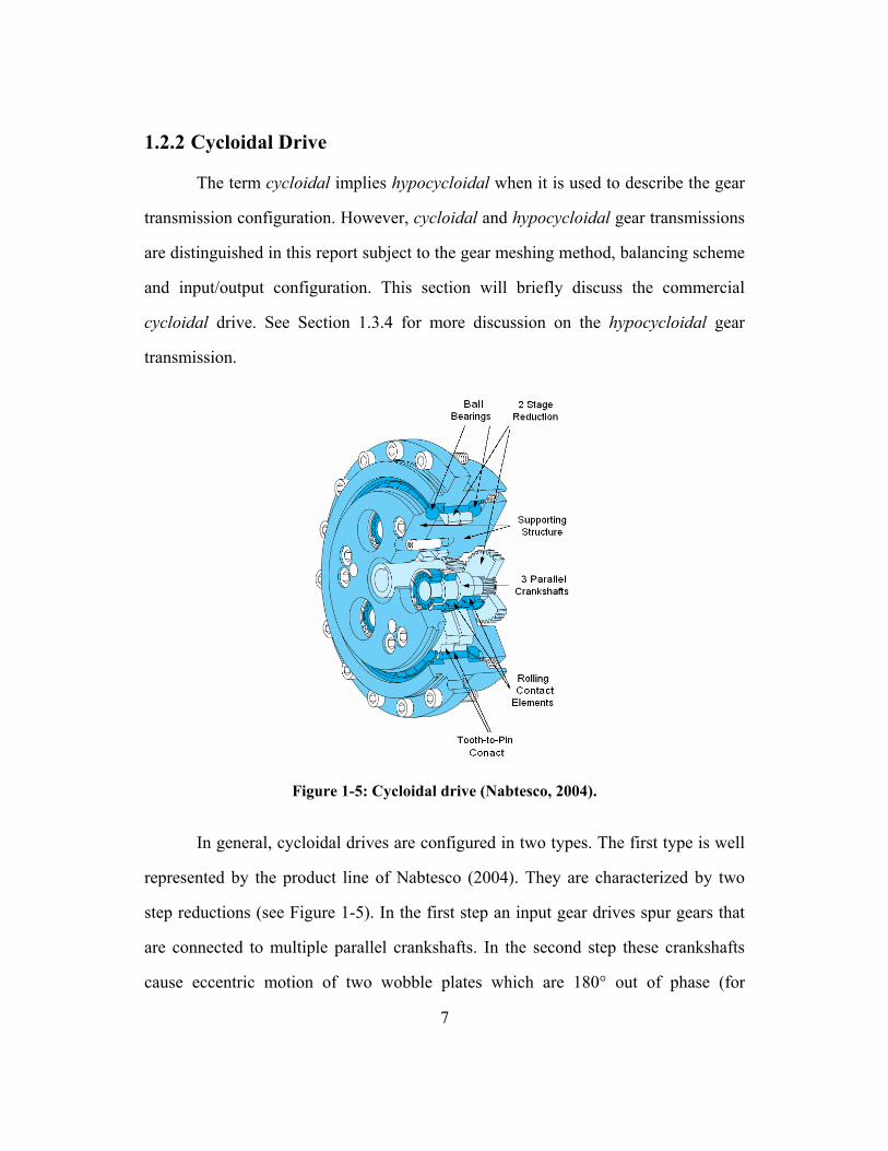
1.2.2 Cycloidal Drive

The term cycloidal implies hypocycloidal when it is used to describe the gear

transmission configuration. However, cycloidal and hypocycloidal gear transmissions

are distinguished in this report subject to the gear meshing method, balancing scheme

and input/output configuration. This section will briefly discuss the commercial

cycloidal drive. See Section 1.3.4 for more discussion on the hypocycloidal gear

transmission.

Figure 1-5: Cycloidal drive (Nabtesco, 2004).

In general, cycloidal drives are configured in two types. The first type is well

represented by the product line of Nabtesco (2004). They are characterized by two

step reductions (see Figure 1-5). In the first step an input gear drives spur gears that

are connected to multiple parallel crankshafts. In the second step these crankshafts

cause eccentric motion of two wobble plates which are 180° out of phase (for

8

balancing). This eccentric motion of the wobble plates contain cycloidal profile teeth

which engage with stationary pins located around the inside of the case. Another type

of cycloidal drive employs tooth-to-tooth engagement instead of tooth-to-pin

engagement. Corbac Cycloidal Reducers from Andantex (2004) is an example of this

type. Both types transmit torque to the output shaft through rollers by means of

rolling contacts between the two wobble plates.

Normal reduction ratio range of the cycloidal drive is around 60:1 to 190:1.

The cycloidal drive allows for relatively low effective input inertia owing to the two

step reductions. However, this adds to the complexity in design and the number of

parts, resulting in the increased sources of deformation (lost motion) and friction

power loss. While typical cycloidal drives are claimed to provide for high load-

carrying capacity, quiet operation, and shock load resistance, they suffer from

relatively heavy weight and high stiction due to many contact elements and bearings.

Especially, their backlash and torque ripple are very sensitive to machining tolerances

and dimensional variations due to temperature changes. The force path is also long

and serpentine because the input force must pass through the gear meshes in the first

stage reduction (if any), cam shaft, wobble plate, tooth-to-pin meshes, rollers, and

output shaft. This undesirable and complicated force path requires a considerable

hoop structure to keep all the forces contained (Tesar, 2003).

1.2.3 Harmonic Drive

The harmonic drive is composed of three main parts; wave generator,

flexspline, and circular spline (Figure 1-6). The wave generator is connected to the

prime mover input, and its elliptical shape causes elastic deflection of the flexspline

9

as it rotates. Through two external-internal tooth meshes that are 180º apart, the

flexspline drives the circular spline which is connected to the output load.

It is designed to provide for multiple tooth engagement (minimum of two at

no load) at any given time resulting in nearly zero backlash (less than one arc-min).

Its reduction ratio range is reasonably wide (approximately 50:1 to 200:1). For these

reasons, harmonic drives are widely used in applications requiring precision

positioning, especially in robotics and semiconductor industries. Other advantages are

simplicity in configuration, small number of parts, and good torque density.

Figure 1-6: Harmonic drive (HD Systems, 2004)

However, the small initial backlash tends to increase with wear. This wear

rate is expected to be relatively high in this particular arrangement. The low stiffness

of the component also adds to the lost motion of the system causing kinematic error,

which makes it less attractive for high-torque servo applications. Furthermore, they

have been criticized for torque ripple, low efficiency, and poor shock resistance

(Schempf & Yoerger, 1993).

In order to improve stiffness and torque capacity of the harmonic drives, a

tooth profile called ‘S’ was suggested by Kiyosawa et al. (1989) This specially

10

designed tooth profile employs larger root fillets and a series of pure convex and

concave circular arcs instead of conventional involute tooth profile. Due to

improvement in the tooth profile design, stiffness and torque capacity were almost

doubled (HD Systems, 2004). This interesting example shows how significantly tooth

profile design can influence the overall performance of the gear transmission systems.

Figure 1-7: Geometry of ‘S’ tooth profile (HD Systems, 2004).

1.3 UTRRG GEAR TRANSMISSION DEVELOPMENT

Development of gear transmission at UTRRG has been pursued in close

association with EM actuator development. For this reason, Section 1.3.1 will briefly

review the history of EM actuator development at UTRRG for better understanding

of the background of gear transmission development. Then, Section 1.3.2 and 1.3.3

will discuss past studies on gear transmissions at UTRRG. Finally, Section 1.3.4 and

1.3.5 will discuss the latest development of the HGT and its prototypes.

11

1.3.1 EM Actuator Development at UTRRG

The University of Texas Robotics Research Group (UTRRG) has developed

an extensive array of EM actuators and its component technology for more than 25

years. As shown in Figure 1-8, the UTRRG EM actuator development program

embraces conceptual/detail designs, prototypes, and actuator tests. UTRRG has

continuously conducted EM actuator design projects under the sponsorship of the

Office of Naval Research (ONR) and the Department of Energy (DOE) (Park, Bono,

Tesar, et al., 2000; Park, Hvass, Tesar, et al. 2002; Park, Pryor, Tesar, et al., 2003a;

Park, Vaculik, Tesar, et al., 2003b; Park, Krishnamoorthy, Tesar, et al., 2003c; Park,

Kendrick, Tesar, et al., 2004). More recently, two actuator prototypes, the ¼-Scale

Advanced Weapons Elevator (AWE) Actuator and the Rugged Manipulator Actuator,

have been fabricated and set up for test. Actuator testing has been another

development thread at UTRRG. Testing includes endurance & reliability tests,

nonlinear performance map generation, and condition-based maintenance (Kang &

Tesar, 2004; Yoo & Tesar, 2004; Hvass & Tesar, 2004). EM actuator component

technology has been also continuously studied. The study covers motor, gear

transmission, linear roller screw transmission, release mechanism, brake, sensor, and

precision interface technologies. A brief introduction to the component technology

can be found at the UT Robotics Research Group Web page

(http://www.robotics.utexas.edu/rrg/).

As a parallel effort to these project activities, UTRRG has established a

complete architecture of EM actuator modules (combined with standardized

interfaces) in ten distinct classes of both rotary and linear configuration. The ten

classes are standardized, high torque, high rigidity, intelligent, precision/small

12

motion, hybrid, energy saver, fault tolerant, dual input, and a 2-DOF module (Tesar

2003). Tesar states the goal of the Electro-Mechanical Actuator Architecture

(EMAA) is “to create an array of actuator modules which because of their distinctive

features (standardized interfaces, self-contained actuation and structure, fault

tolerance, intelligence, layered control, compactness and ruggedness, etc.) in total

create a complete architecture as basic building blocks for intelligent machines

(robots, manufacturing cells, mobile platforms, aircraft, ships, etc.) which can be

assembled on demand in an open architecture.”

This EMAA became the basis for creating a set of Standardized Actuator

Building Blocks (SABBs) which can be assembled on demand for numerous electro-

mechanical applications (concept of open architecture). The SABBs, in fifteen to

twenty basic sizes, hypothetically provide for an exceptional load-carrying capacity

range from 0.3 ft-lb up to 3,300,000 ft-lb which can envelop virtually all of the

present application requirements (Tesar, 2004a). Successful deployment of SABB’s

primarily depends on gear transmission performance as stated earlier, and this fact

served as motivation for the development of the HGT.

13

Figure 1-8: Overview of actuator development at the UTRRG as of February 2005.

ACTUATOR DEVELOPMENT AT UT AUSTIN

Full Scale Elevator Actuator Rudder

Trim Tab Actuator Bow Plane

Actuator

Representative Actuator Designs

Representative Test-Beds

SFW Development CBM Development

Frameless Dual Actuator Low Cost Integrated Actuator Rugged Manipulator Actuator

Precision Manipulator 1/4 Scale Elevator Actuator

Representative Actuator Prototypes

14

1.3.2 Preliminary Studies of Actuator Transmissions

Pennington and Tesar (1991) initiated a major activity at The University of

Texas for gear transmission development by providing a basic guideline for selection

of an epicyclic gear transmission. In this report they recognized that it was very

difficult to accurately model the effects of gear tooth deflections and manufacturing

errors, whereas those two factors have significant influences on the stiffness and

dynamic response of the actuator system.

McNatt and Tesar (1993) compared the specifications of various transmission

alternatives including harmonic drives and cycloidal drives, in order to select correct

architectures for the ALPHA modular manipulator applications (EM actuator

applications to shoulder, elbow and wrist, see Figure 1-9). In this report, they

discussed the fundamentals of gear transmission design, e.g., kinematics, dynamics,

stiffness, backlash, friction, weight, etc., and evaluated these performance parameters

of commercial transmissions. Based on this study, for example, the Sumitomo FA25

cycloidal drive was selected as the best available commercial drive suitable for the

ALPHA elbow application.

Figure 1-9: ALPHA modular manipulator.

15

1.3.3 Parametric Studies of Actuator Transmission

Donoso and Tesar (1998) made a successful parametric improvement in the

design of robot actuator transmissions. They proposed a parametric design

methodology to solve and optimize the selected performance parameters of the 3K

Paradox epicyclic gear transmission (for conceptual application to the ALPHA

manipulator elbow). They provided a binary matrix reformulation algorithm, which

was capable of providing a solution sequence for a relatively large parametric model.

The parametric model they built for a 60:1 ratio 3K Paradox epicyclic gear

transmission initially had 226 parameters and 139 constraints where 87 parameters

were later eliminated to make the set of model parameters determinate. Donoso and

Tesar demonstrated that their epicyclic gear transmission gained 18 times overall

benefit over the best commercial practice in terms of weight, inertia, stiffness,

backlash, and efficiency combined.

Ring 2Ring 1

Input Shaft

Sun

Planet 1

Planet 2

Planet Shaft

Planet Carrier

Ring 2Ring 1

Input Shaft

Sun

Planet 1

Planet 2

Planet Shaft

Planet Carrier

Figure 1-10: UTRRG parametric design of 60:1 3K Paradox epicyclic gear transmission (Donoso & Tesar, 1998).

16

Motivated by this progress, Park and Tesar (2000) extended the application of

the parametric design technique to 10:1, 25:1, 100:1, 250:1, and 600:1 ratio epicylic

gear transmission designs resulting in significant performance improvements over

commercial drives of corresponding reduction ratios. For example, their 100:1 ratio

epicyclic gear transmission design demonstrated a 32 times better performance index

than the standard practice in terms of weight (torque density), inertia, and stiffness

combined. They also proposed an optimal design process that allowed the designer

interventions and insights into the problem for mathematical model preparation,

reduction and reformulation. This process permitted the implementation of numerical

search schemes for quick and precise identification of optimal solutions (especially in

terms of the torque to weight ratio) for a series of simple epicyclic gear transmission

models. Figure 1-11 shows the resultant optimum 3K Paradox epicyclic gear

transmission (100:1 ratio design) (Park & Tesar, 2000).

Figure 1-11: UTRRG parametric design of 100:1 3K Paradox epicyclic gear transmission (Park & Tesar, 2000).

17

1.3.4 Development of the HGT

Development of EMAA (Electro-Mechanical Actuator Architecture) further

facilitated the evaluation of gear transmissions. A device called the Hypocycloidal

Gear Transmission (HGT) has been proposed in the EMAA development as a

principal component. In a broad sense, the HGT can be regarded as an epicyclic drive

train based on the definition by Muller (1982) (see Section 1.2.1 for the quote).

Instead of ‘arm or carrier’ the HGT employs a kinematically equivalent eccentric

shaft. Also, instead of having multiple planet gears, the HGT employs a single, dual-

stage5 planet gear (called a wobble gear hereinafter) that has a small tooth number

difference (as low as one) with a stationary internal gear and a rotating output internal

ring gear respectively.

Some literature calls this kind of architecture differential gearing. For

example, Shipley called it ‘simple four-gear differential gear transmission’ in

Dudley’s Gear Handbook (Shipley, 1991) (see Figure 1-12). However, when they

refer to differential gearing, they presume wobble gear(s) (X and Y in Figure 1-12) to

be much smaller than the internal gears (C and B in Figure 1-12) and connected by a

planet gear carrier. Due to the big difference in sizes of two mating gears, the length

of the arm is long (A in Figure 1-12) and rotational speed of the wobble gear(s) is

very high. These conditions generally lead to unfavorable inertial effects reflected to

the input side. This large effective inertia can be avoided in the HGT.

5 This report will, for convenience, call the external-internal gear pair close to the input side as the first stage, and the other external-internal gear pair close to the output side as the second stage.

18

Figure 1-12: Simple four-gear differential gear transmission (Shipley, 1991).

Figure 1-13: Expanded view of the HGT (bearings subtracted and ring gears thinned) (Park, Kendrick, Tesar, et al., 2004).

Figure 1-13 shows an expanded view of a typical HGT assembly. It is

basically composed of an eccentric shaft with balancing mass, wobble gear,

stationary internal gear (shown as fixed ring gear), and output internal gear (shown as

output ring gear). The operating principle is as follows. The eccentric shaft is

connected to the motor input and drives the wobble gear against the stationary

19

internal gear. The small eccentricity (e) of the shaft makes the wobble gear generate

the hypocycloidal motion; the wobble gear rotates not only about its own axis but also

about the axis of the gear train inside the two internal gears. This motion causes tooth

number differencing between the two internal gears and thus relative motion.

The simplicity in design and minimal number of parts make the HGT easy to

assemble and reduces the negative effects on gear contact due to the stack up of

manufacturing errors. The configuration of the HGT inherently allows for the widest

range of reduction ratio, i.e., from 50:1 to 5,000:1, and exceptional torque density

(torque to weight/volume ratio). In combination with carefully designed tooth

profiles, the HGT is designed to provide high stiffness, low power loss, nearly zero

backlash and lost motion, and smooth and quiet operation. These potential benefits,

which will be discussed further in this report, make the HGT a key performer in

EMAA actuators.

Figure 1-14 shows a representative integration of the HGT into an EM

actuator. The EM actuator shown in this figure is called the Standard Cylindrical

Rotary Actuator. Using a DC motor as a power source, the HGT as a speed

reducer/torque amplifier, and a cross roller bearing as a principal out-of-plane

moment resistant, this standardized actuator is simple in design, insensitive to

tolerances and temperature, and exceptional in torque to weight/volume ratio. This

actuator is fully upgradeable and downgradeable in size due to its simplicity in

configuration and reduced number of parts.

This standardized actuator also functions as a joint by itself without additional

need for bearings, axles, or attachments, owing to its rigidity in all six directions and

quick-change interface. Use of the standardized interface makes this actuator module

very effective for system level integration and on-demand plug-and-play. In

20

combination with a switched reluctance motor instead of the DC motor, the HGT can

be also assembled into a pancake shape actuator which is shorter in length than the

cylindrical shape actuator.

Figure 1-14: Standard rotary EM actuator using the HGT (proprietary) (Tesar, 2003).

In the EMAA there are several more proprietary concepts demonstrating

clever exploitations of the HGT. One of them is the Two-Stage HGT Actuator where

two HGT’s are stacked radially (a small HGT is enclosed by a larger HGT) in order

for the small HGT to reduce the input side inertia while the larger HGT keeps the

load inertia to a minimum. The more recent development is a design called Extreme

High Torque & Low RPM Rotary Actuator where a star compound speed reducer

delivers the motor input to the HGT. The prime reason for this configuration is to

21

minimize the inertia effective to the motor side while letting the HGT still be

responsible for an extremely high output torque.

Summarizing, in the EMAA development, the simplicity of the HGT allows

for increased design creativity and flexibility that are difficult to achieve with more

complex gear transmissions. Since the performance of the EMAA actuators is directly

determined by performance of the HGT, successful design of the HGT is the key to

the success of EMAA development.

1.3.5 EM Actuator Prototypes Utilizing the HGT

1.3.5.1 ¼-Scale AWE Actuator Prototype

Numerous applications have been identified for the EM actuator based on the

HGT. They range from industry to the battlefield including intelligent machines,

space robotics, nuclear systems, all-electric ships for the Navy, electric aircraft for

Air Force and Future Combat Systems for the Army. In particular, the concept of the

EM actuators using the HGT has been explored by Navy/ONR and Newport News

Shipbuilding for its possible applications to weapons elevators.

The weapons elevator is the most basic element in the system of weapons

handling. Thus, a significant improvement in their operation (availability, flexibility,

operational intelligence, etc.) would dramatically influence the whole weapons

handling system. The concept was to replace the conventional winch and cable driven

elevator system with an Advanced Weapons Elevator (AWE) system comprising the

EM HGT actuators that are mounted on an elevator platform, and driving climbing

gears engaged with gear racks attached to the shaft wall. The actuators are modular

and standardized, allowing easy maintenance and repair, with simple access to

22

components and replacement of parts with no need for specialized tools (Park,

Vaculik, Tesar, et al., 2003b).

To demonstrate the feasibility and capability of the EM actuator using the

HGT for this particular application, UTRRG and the Timken Company have designed

and built a quarter-scale prototype of a Weapons Elevator EM actuator which

employs the HGT as a main component. Detail design and drawings of the prototype

were provided by UTRRG to Timken who took charge of its fabrication. A separate

report for gear tooth profile design was provided by Tesar and Park (2004) to Timken

for wire-EDM gear manufacturing. As of the end of March 2005, fabrication of the

prototype was completed, and the initial spin testing was conducted. The present

report will discuss this prototype effort. Some of the pictures and testing results can

be found in Chapter 8.

Table 1-1 summarizes the primary requirements for the quarter scale actuator

model. This set of requirements was derived by UTRRG based on AWE performance

requirements supplied by Newport News Shipbuilding.

Table 1-1: Requirements for the ¼-Scale AWE Actuator prototype (Pryor, Tesar, Park, et al., 2003a).

Peak 3,300 ft-lb Output Torque

Nominal 1,290 ft-lb Output Speed 38 rpm

Operating Temperature 15 °F to 120 °F

Available Power 440 VAC, 3 Phase, 60 Hz, No limit on current

Life 5 Years Efficiency Maximized

Component Operating Stress < 35% Yield Strength Component Stall Stress < 70% Yield Strength

Component Shock Stress < 100 % Ultimate Strength

23

1.3.5.2 Rugged Manipulator Actuator Prototype

Another EM actuator prototype called the ‘Rugged Manipulator Actuator’ has

also been designed, fabricated, and set up for tests as of February 2005 (Park,

Kendrick, Tesar, et al., 2005). This DOE sponsored EM actuator prototype is

designed for use in the elbow of a robot manipulator to eliminate the human on-site

involvement in depositing (transporting, sorting, and packaging) heavy materials in a

radiation contaminated environment. Therefore, the actuator must not only be

‘rugged’ with respect to shocks and undesirable loads, but also easily maintainable,

suggesting modularity for quick change in response to failures. Since the robot will

handle heavy items it will exert large forces6 on the actuators. After careful analysis

of the task requirements, dynamic torques and duty cycle, following design

specifications were identified for the rugged elbow actuator prototype.

Table 1-2: Key requirements for the Rugged Actuator prototype (Park, Kendrick, Tesar, et al., 2004).

Peak 7,500 in-lb Output Torque

Nominal 1,500 in-lb Out-of-Plane Moment Load 10,000 in-lb

Radial Load 3,650 lb Output Speed 20 rpm

Three major upgrades have been made, in terms of gear transmission design,

for this prototype. First, the Rugged Manipulator Actuator has a slightly larger first

stage while the ¼-Scale AWE Actuator had a slightly larger second stage. This

change allowed for accommodation of the cross roller bearing in better position of the

actuator. The difference in stage sizes changes the sign of the output velocity with

6 The term forces generally refers to forces and moments in the field of robotics.

24

respect to the input velocity. More detailed discussion on this issue can be found in

Section 3.2.1. Second, the pressure angle was minimized (from 20º to 7º at the pitch

point) in the Rugged Manipulator Actuator. This amount of reduction in the pressure

angle means relief of 66 % of the normal bearing load for the same tangential load on

the gear (this tangential load still acts on the bearing). Reduction in bearing load is

very important especially in this kind of eccentricity-driven system. Third, the size of

the eccentricity was minimized. The ratio of the eccentricity to the wobble gear pitch

diameter was reduced from 4.3 % (¼-Scale) to 3.8 % (Rugged). This is an effort to

reduce the weight and inertia of the HGT. More detailed discussions with regard to

the tooth design parameters including the pressure angle and eccentricity can be

found in Chapter 4. Detailed design and analysis results for the Rugged Manipulator

Actuator prototype effort will be presented in this report. Some of the pictures and

testing results can be found in Chapter 8.

1.4 ORGANIZATION OF REPORT

Overall, this report deals with in-depth design and analysis of the

Hypocycloidal Gear Transmission (HGT). Chapter 2, 3, and 4 concentrate on the

design of the HGT while Chapter 5, 6, 7, and 8 concentrate on its analysis. However,

Chapter 5 can also be considered as an extension of the preceding design

development, while Chapter 8 puts emphasis on actual implementation of the design

and analysis in the prototypes in addition to the tolerance analysis. In the design

effort, system level (the HGT) design and tooth level (the circular-arc profile) design

have been accomplished. Before performing each design, rigorous literature review

(Chapter 2 and Section 4.3) has been done not only for a base study but also for

justification of the corresponding design. For a quick reference to the exclusive

25

advantages of the HGT, readers are referred to Section 2.4. Brief chapter-by-chapter

roadmaps are presented as follows.

Chapter 2 reviews the literature to evaluate the past development efforts,

discusses challenges, and justifies the fundamental development of the HGT. Based

on the literature review, potential advantages of the HGT have been outlined and

compared qualitatively with those of state-of-the-art gear transmissions. This

comparison argues that the HGT is the most promising architecture for EM actuator

gear transmissions.

Chapter 3 performs an in-depth parametric design of the HGT. The objective

was to address the design challenge and establish the claimed advantages. To do so,

design criteria have been identified and discussed. Then, parameters associated with

the criteria as well as their functional relationships have been established. The

ultimate goal of this chapter was to provide a parametric design guideline for the

HGT. Based on this guideline, two representative HGT prototype designs have been

presented.

Chapter 4 performs gear tooth level design which has a significant influence

on the gear transmission performance. To select and justify the basic tooth profile

which will allow the HGT to maintain its claimed advantages, the candidate tooth

profile, i.e., the circular-arc tooth profile, has been evaluated for the tooth level

design criteria identified in Chapter 3 plus manufacturing error sensitivity. For some

of the criteria, comparative analysis has also been performed. Once the basic tooth

profile was justified for the HGT, all the parameters associated with the profile along

with their functional relationships have been completely identified. Finally, an

interactive graphical tool that enables automated generation of the circular-arc tooth

profiles has been introduced.

26

Chapter 5 develops analytics for tooth meshing analysis, and solves them for

the tooth level design parameters identified in the previous discussions. Tooth

meshing analysis has been applied to the design of the circular-arc tooth profiles for

the HGT prototypes where minimization of the clearances has been rigorously

pursued as a primary objective. Sliding velocity of the tooth contacts in the HGT has

also been analyzed for use of its profile in the friction power loss analysis in Chapter

7. By taking full advantage of the tooth meshing analysis, minimization of the tooth

pressure angle has been achieved for one of the prototype designs.

Chapter 6 performs loaded tooth contact analysis for the evaluation of the

actual contact ratio under load and the associated load sharing factor of the HGT.

This chapter begins with building a mathematical contact model incorporating tooth

deformations and manufacturing errors. The clearance/interference data obtained in

Chapter 5 has been rigorously used to solve for the model. The analytic results have

been compared with FEA results. The goal of this chapter is to clearly demonstrate

the ‘self-protecting’ aspect of the HGT; as the load becomes larger, the load is not

only shared by more tooth pairs, but the load distribution over multiple tooth pairs in

contact is significantly improved making the HGT ideal for carrying extremely heavy

loads. The obtained meshing load profiles have been utilized in Chapter 7 in

combination with the velocity profiles obtained in Chapter 5 for evaluation of the

friction power losses in the HGT.

Chapter 7 discusses the efficiency of the HGT. To do so, selected analyses

from the literature has been applied for preliminary evaluations of the efficiency of

the prototype HGTs. Then, the efficiency has been more precisely determined by

analyzing the power loss in the HGT based on first principles in the sliding tooth

contacts. The sliding velocity and load distribution profiles developed in Chapter 5

27

and Chapter 6 for the prototype designs have been utilized for the representative

analyses. The purpose of this chapter was to show that most of the losses in the HGT

are in the bearings and not in the meshing gear teeth.

Chapter 8 analyzes the effects of manufacturing errors (i.e., center distance

error, tooth spacing error, misalignment error) on the HGT contact characteristics

using FEA. The objective was to demonstrate that the HGT is insensitive to

manufacturing errors. This chapter also discusses issues related to fabrication of the

prototypes including machining of the circular-arc teeth, stack-up of tolerances,

bearings, and lubricant selection.

Chapter 9 will conclude the report. This research has produced three key

deliverables. First, it supports the conclusion of exceptional advantages for the HGT

and the circular-arc tooth profile based on sound literature study, and validates these

conclusions through four distinct analyses. Second, this research presents a

comprehensive parametric study of the HGT employing circular-arc teeth, and

provides a three step design guideline. Third, this research fully addresses the design

and analysis of two prototype HGTs, and successfully delivers their designs to the

fabricators. Based on the literature study, parametric design, and analysis results, this

report fully recommends the HGT as a promising architecture for EM actuators in

this chapter.

28

CHAPTER 2

LITERATURE REVIEW

2.1 INTRODUCTION

In Chapter 1 the research objective was defined and the background of the

research was described. Chapter 2 will justify this research more strongly based on a

literature review. Through the literature review on gear transmission designs similar

to the HGT, potential development of the HGT discussed in Chapter 1 will be further

supported. Then, advantages of the HGT will be qualitatively compared with those of

the state-of-the-art transmissions that were already identified in Section 1.2. This

comparison will argue that the HGT is the most ideal candidate architecture for EM

actuator gear transmissions. The rest of the report will then be dedicated mostly to

detail design of the HGT including in-depth discussion on the tooth profile and

prototype development.

Most of the literature reviewed in this chapter are patents. This is because gear

reducer configurations similar to the HGT have been studied mostly in patents. The

earliest one was issued in 1895. Besides the patents, there are a few published papers

discussing the design of gear reducers similar to the HGT. Furthermore, most of them

deal with the single stage configuration (one pair of internal-external gears with small

tooth difference) which severely limits the reduction ratio and creates a need for an

unattractive Oldham coupling type of output mechanism. Review of selected patents

is presented in Section 2.2. Non-patent literature will be reviewed in Section 2.3.

29

Section 2.4 will summarize the advantages of the HGT based on the review, present

the comparative argument, and justify the need for further development of the HGT.

2.2 PATENT REVIEW

Regan (1895)’s patent is presumed to be the first patent using wobble gears

for speed reduction (see Figure 2-1). The difference between his design and the HGT

is that his wobble gear has external teeth on the first stage and internal teeth on the

second stage while the HGT has external teeth on both stages. The output gear of his

design thus has external gear teeth that mesh with the internal gear teeth of the

wobble gear. Unfortunately, this design not only limits torque capacity of the output

gear but also lengthens the force path. He recognized that this kind of gearing needs

counterbalancing of the eccentric wobble gear mass. The use of rolling element

bearings was in its infancy at that time which is why all bearings are small diameter

journals.

Figure 2-1: Regan (1895)’s wobble gearing (US Patent No. 546,249).

30

Harrison (1910) patented a single stage wobble gearing with external-internal

tooth meshing (see Figure 2-2). The output plate has a cup shape structure that is

assembled in between the fixed gear and the input member that has a very thin rim.

He provided a very good layout for the counterweights utilizing the space allowed by

the thin input member. This layout saves the space for the counterweights, but

sacrifices the out-of-plane stiffness of the wobble gear which can cause misalignment

between the meshing teeth. Harrison was able to take advantage of small diameter

low friction rolling element bearings. His output required the crankshaft equivalent of

the Oldham coupling at the output to accommodate the eccentric motion of the

wobble gear.

Figure 2-2: Harrison (1910)’s gear transmission (US Patent No. 978,371).

31

Hatlee (1916) presented a nice layout for a double stage wobble-fixed-output

gear arrangement in his patent (see Figure 2-3). It employs unsophisticated tooth

profiles, and he says the gear teeth can be replaced by friction surfaces. He uses

rudimentary journal bearings throughout and never mentioned the need to provide for

balancing.

Figure 2-3: Hatlee (1916)’s gearing and tooth profile (US Patent No. 1,192,627).

Wildhaber (1926) first patented the circular-arc tooth profile (circular-arc

tooth form in the normal plane). Later on, Novikov (1956) reinvented and patented a

similar idea (circular-arc tooth form in the transverse plane). The circular-arc tooth

profile is made in a helical configuration in order to maintain continuous contact in

32

the axial direction (see Figure 2-4). The basic idea is to achieve very high convex-

concave conformity between two meshing gear teeth to reduce contact stress in the

gearing. This is especially useful in the internal meshing of two gears of almost the

same size once the sensitivity of the contact pattern to the center distance error is well

known.

Figure 2-4: Wildhaber (1926)’s circular-arc tooth profile (US Patent No. 1,601,750).

Fliesberg (1935) is presumed to be the first inventor who explicitly discussed

tooth design issues for the wobble gearing system. In his patent (US Patent No.

2,049,696), he attempted to have a tooth number difference of 1 to 4 between the two

mating gears to maximize the gear ratio. He noticed that it is “impossible to use such

small differences in the number of teeth as long as in a gear with internal teeth the

profile of the teeth is conventional7 (p.2).” Thus, he ended up with shortening the

teeth compared to their peripheral width. He also wanted the pressure angle to be

between 28 and 32 degrees to avoid interferences and excessive wear. These angles

are considered very high for the structure and bearing selections he had. The overall

design revealed a long force path and a high concern for structural integrity.

7 Probably meaning involute gear teeth.

33

Kittredge (1939)’s patent provided a layout of a combination of epicyclic

gearing and a two stage wobble gearing (see Figure 2-5), which is basically similar in

form with one of the two types of the cycloidal drive today (recall Section 1.2.2).

Weaknesses of this design include the long, deformable shaft connection between the

epicyclic and wobble gearings, and the two piece design of the wobble gears (they are

attached to each other with Cardan couplings). Braren (1928) and Heap et al. (1928)

also proposed gear transmissions similar to modern cycloidal drives without the

epicyclic step reduction (see Figure 2-6 and Figure 2-7). Both of their designs

employed two wobble plates 180º out of phase ensuring balancing of the system.

Braren used tooth-to-pin meshing while Heap et al. used tooth-to-tooth engagement.

Figure 2-5: Kittredge (1939)’s patent (US Patent No. 2,168,164).

34

Figure 2-6: Braren (1928)’s gear transmission (US Patent No. 1,694,031).

Figure 2-7: Heap et al. (1928)’s gear transmissions (US Patent No. 1,770,035).

35

Perry (1939) designed a single stage wobble gear train, and showed how this

can be stacked to a double stage wobble gear train (see Figure 2-8). Each stage has an

eccentric driving a single wobble gear to drive cantilever pins in circular holes to

drive the rotating output. The design includes a counterweight, and all the bearings

used are small diameter ball bearings. Force path of the single stage wobble gear train

is relatively short but that of the double stage wobble gear train is long and

serpentine. The reduction ratio of the single stage wobble gear is limited.

Figure 2-8: Perry (1939)’s single stage (left) and dual stage (right) gear reducers (US Patent No. 2,170,951).

Foote (1941) provided a thoughtful insight into the tooth profile design in his

patent. He suggested the use of a triangular tooth form (see Figure 2-9) for the gear

train whose configuration is similar to The University of Texas HGT. He uses small

36

diameter rolling element bearings throughout to make a rather complex assembly

with considerable weight. His concentration was on minimizing the tooth number

difference (less than 3) between two internally mating gears for efficiency reasons.

His tooth form is claimed to reduce friction power loss by minimizing sliding in the

tooth meshing. He also claims that up to 1/6 of the teeth in the wobble gear are

engaged at any one time. This engagement covers an arc of 60º which is very high.

The triangular tooth form, however, inherently makes for a very high contact angle

(from 35º to 41º) and creates large forces which tend to separate the wobble gear

from its mating internal gear. His patent is one of the earliest patents which shows the

traces of tooth engagement and disengagement. The triangular tooth form is still

being used in modern cycloidal gearing such as Corbac from Andantex (2004).

Figure 2-9: Foote (1941)’s gearing and tooth profile (US Patent No. 2,250,259).

37

Jackson (1949)’s patent presented outstanding descriptions of a set of wobble

gear reducers: a single stage wobble gear (Figure 2-10), a two-stage wobble gear with

balancing mass (Figure 2-11, left), and dual-wobble gears 180º out of phase (Figure

2-11, right). All these designs use small diameter rolling element bearings. The last

configuration is similar to the present day devices such as the Nabtesco and

Sumitomo cycloidal drives. He provided a useful explanation of the kinematic layout

of the single stage wobble gear. The weakness of these designs is in the use of

multiple rolling pins for the output.

Figure 2-10: Jackson (1949)’s single stage wobble gearing and kinematics study (US Patent No. 2,475,504).

38

Figure 2-11: Jackson (1949)’s dual stage wobble gearings (US Patent No. 2,475,504).

Wildhaber (1960) extended his discussion on normal tooth profile geometry to

include a longitudinal profile by adopting a crowned surface on the external gear

while keeping the straight surface on mating internal gear (US Patent No. 2,922,294).

He did this for the design of a toothed coupling to accommodate misalignment of

shafts and reduce the sensitivity of contact to center distance errors. He discussed

how to manufacture the teeth using hobs or shaving tools, and described associated

manufacturing errors.

Menge (1961) looked at a 180º out of phase dual wobble gear reducer

producing the output without the use of rolling pins. Instead, he cleverly added one

more tooth-to-tooth meshing between the two internal gears (see Figure 2-12, left).

This design balances itself without counterweights. However, additional tooth

39

meshing not only leads to extra power losses, but also elongates the force path.

Furthermore, to make the additional meshing possible, he was forced to come up with

a structurally weak layout. Later on, Menge (1964) gave a variation to his design by

connecting the two wobble gears with stepped pins (see Figure 2-12, right). This

version is structurally better than the former one, but complexity added by the pin

connection raises a question of tolerance stack-up. He claims that the main object of

his inventions is to make the device operate silently, efficiently and free of vibration.

He also noted that multiple teeth in contact could distribute the load better as opposed

to one or two teeth as in conventional gear drives.

Figure 2-12: Menge (1961, 1964)’s gear reducers (US Patent No. 2,972,910 and 3,144,791).

Sundt (1962) said in his patent, “up to present time, differential gear reducers

of this type have been notoriously inefficient and … the noise and vibration being

quite high, and this accounts for the reason that differential gear reducers of this type

have not been widely used” (p.1). He noted that the noise/vibration and low

40

efficiency in differential type gearing are due to friction, improper conjugation of the

teeth, and excessive load on the bearings. To resolve these he attempted an analytic

derivation of the tooth form that can minimize sliding and pressure angle. The

proposed pair of tooth profiles basically resembles the combination of cycloidal tooth

and circular pin often found in the modern cycloidal gearings (see Figure 2-13). He

parametrically investigated the traces of the tooth profile and used them to determine

the curvature radii of the teeth. He also claimed that his tooth form is structurally

strong, and does not require tight manufacturing tolerances.

Figure 2-13: Sundt (1962)’s gearing and work on tooth profile design (US Patent No. 3,037,400).

Wildhaber (1969a), after 40 years of developing gear technology, proposed a

layout of his wobbling gear system. He made a single wobble gear that has two sets

41

of teeth on the same side (axial overlap) (see Figure 2-14). This configuration enabled

him to have a very thin, pancake shape gear train which produces a wide range of

reduction ratios. Also, in comparison with the side-by-side wobble gear system, this

design avoids twisting moment on the bearings (since all tooth forces act in one

plane). The most concern in this design is the alignment shift of the wobble gear teeth

due to its unavoidable thin plate design. Also, stress concentration on the corner of

the rims and shear stress of the connecting bolts should be given careful attention. In

his later design (1969b), he implemented a spherical bearing instead of roller bearing

between the output gear and the stationary shell to allow the intermeshing teeth to be

self-aligned with each other and therefore carry heavier loads (see Figure 2-15). He

claims that the teeth are designed for very little sliding and therefore high efficiency.

He also claims that the low sliding reduces the generation of noise and allows the use

of a low viscosity lubricant. A single counterweight was used to balance the single

wobble gear plate.

Figure 2-14: Wildhaber (1969a)’s axially overlapping gear reducer (US Patent No. 3,427,901).

42

Figure 2-15: Wildhaber (1969b)’s axially overlapping gearing upgraded (US Patent No. 3,451,290).

Morozumi (1970) looked at the parametric conditions for the involute tooth

forms to be used in internal gearings where two mating gears have tooth number

difference of one or two. In this patent (US Patent No. 3,546,972), he derived all the

constraints to be satisfied and laid out a series of plots identifying the design space

constrained for different pressure angles, contact ratios, and etc. The constraints dealt

with involute/trochoidal interferences, pointed tooth, undercut, negative pressure

angle, contact ratio less than unity, and trimming (usually this means tooth relief and

undercutting). Parameters included tooth numbers, pressure angle (operating,

addendum, and cutter), module 8 , addendum modification coefficients, radii of

addendum circle, center distance, and contact ratio. Basically, he shows that the use

of the involute tooth form is extremely limited for the previously mentioned gearing

8 A measure of tooth size in the metric system. In units, module ( m ) is millimeters of pitch diameter ( pD ) per tooth ( N ). Diametral pitch ( dP ) is number of teeth ( N ) per inch of pitch diameter ( pD ). Therefore, 25.4 / dm P= .

43

configuration. The size of the design space was very sensitive to the number of teeth

in the pinion, the degree of addendum modification, and the pressure angle. For

example, the pressure angle might be 56º if the tooth difference is one, 40º if it is two,

and 30º if it is three. The patent did not provide a result for the pressure angle less

than 14.5°.

Osterwalder (1977) looked at the speed reducing device whose configuration

is similar to the UTRRG HGT. The main purpose of his patent was to present two

layouts of counterweight implementations within the volume created by thinned side-

by-side wobble gear (see Figure 2-16). He says the short force path in this kind of

system is an advantage. He also claims that the system can maintain an efficiency of

up to 98 % although it is not clear whether testing or analysis was used to support this

argument. He did not provide detailed description of the tooth profile, but preferred

30° pressure angle for reduction of noise, vibration and backlash.

Figure 2-16: Osterwalder (1977)’s gearings (US Patent No. 4,023,441).

44

Davidson (1981) studied circular-arc type gear tooth geometry for internal

gear pairs aiming at the minimization of sliding between the meshing gear teeth. The

key parameter in this patent is the skew angle α which basically determines the slope

of the tooth curve at the intersection between the tooth curve and the pitch circle of

corresponding gear (see Figure 2-17). The skew angle is a function of the pitch radii

of the two mating gears, and approaches to zero as the difference between the two

pitch radii decreases (as the size of the two gears gets closer). This suggests that

internally meshing gears with a small tooth difference lead to very low pressure angle

at the pitch point. The author also gave analytic formulas for the radii of tooth

curvature that provide the maximum rolling contact. However, the origin of these

formulas was not disclosed.

Figure 2-17: Davidson (1981)’s tooth profile study showing the skew angle (US Patent No. 4,270,401).

Shafter (1984) attempted some very creative ideas in his patent (see Figure

2-18). He made a pair of an internal and a wobble gear as a module and connected it

with another module using an Oldham coupling through unique set of ball bearings

for forward, neutral, or reverse output of the gear train (depending upon which of the

modules is braked). He also provided a brief discussion on tooth profile design to

avoid tooth-to-tooth interferences. He suggested the use of short, circular-arc tooth

45

profiles with a pressure angle of 30º plus or minus 7° depending on the tooth number

difference. Preferred tooth number difference was 2 to 4 for efficiency and cost

reasons. It was claimed that the use of circular-arc tooth profiles reduced the sliding

velocities and surface stresses, and would lead to substantial cost savings as

compared to conventional gear teeth. Without mentioning the potential increase in

contact ratio due to deformation of teeth under heavy load, he estimated the angle of

contact zone in the wobble gearing.

Figure 2-18: Shafter (1984)’s gearings (US Patent No. 4,452,102).

Rennerfelt (1991)’s patent discussed drawbacks of conventional spur gear

boxes, harmonic drives, cycloidal drives, and differential gearing, and compared them

with his ‘eccentric gear’. Conventional spur gear boxes employ a plurality of

reduction stages (four or more) to achieve high gear ratios (100:1 or more). This

series of reduction stages with just one tooth pair in contact at each stage (most of the

time) adds up a high level of compliance and backlash quickly. Harmonic drives

avoid tooth interferences by using the flexspline, but require very tight manufacturing

tolerances (meaning high cost) to reduce backlash. Large frictional resistance and

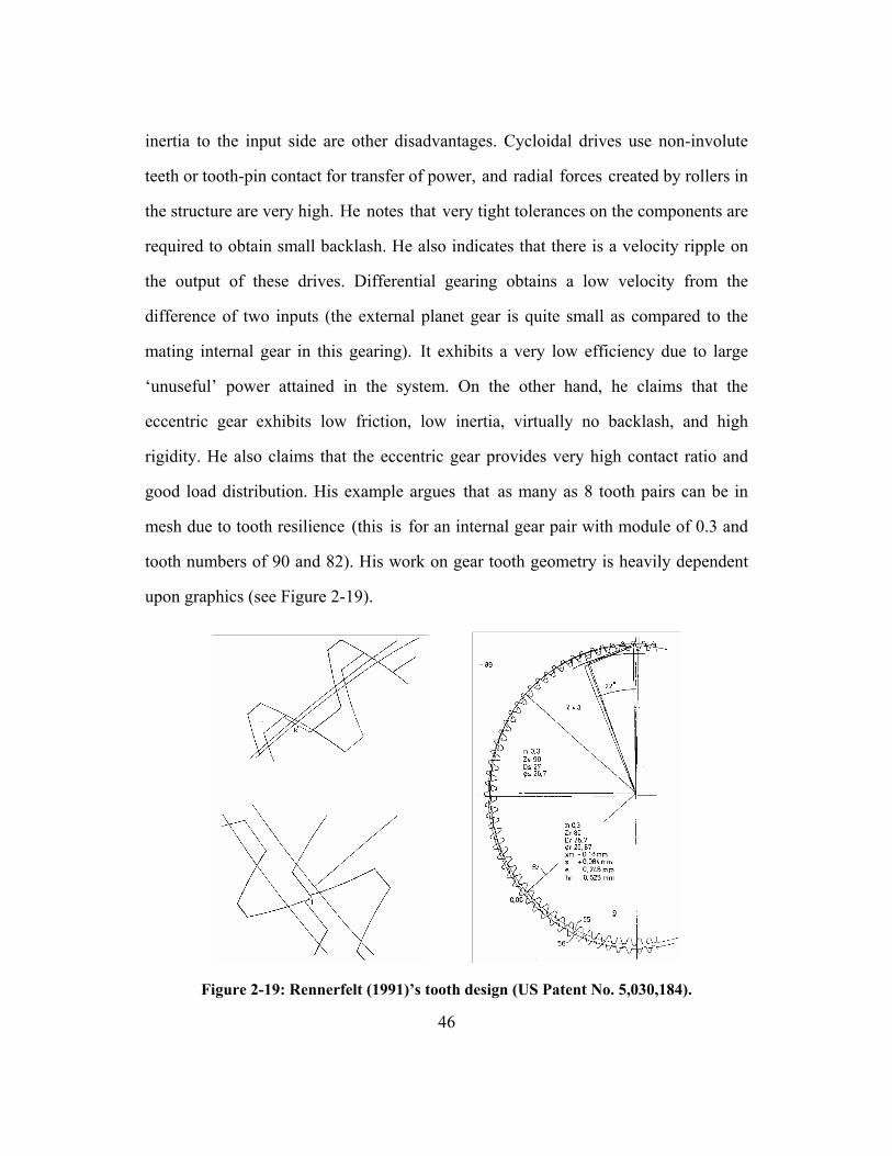
46

inertia to the input side are other disadvantages. Cycloidal drives use non-involute

teeth or tooth-pin contact for transfer of power, and radial forces created by rollers in

the structure are very high. He notes that very tight tolerances on the components are

required to obtain small backlash. He also indicates that there is a velocity ripple on

the output of these drives. Differential gearing obtains a low velocity from the

difference of two inputs (the external planet gear is quite small as compared to the

mating internal gear in this gearing). It exhibits a very low efficiency due to large

‘unuseful’ power attained in the system. On the other hand, he claims that the

eccentric gear exhibits low friction, low inertia, virtually no backlash, and high

rigidity. He also claims that the eccentric gear provides very high contact ratio and

good load distribution. His example argues that as many as 8 tooth pairs can be in

mesh due to tooth resilience (this is for an internal gear pair with module of 0.3 and

tooth numbers of 90 and 82). His work on gear tooth geometry is heavily dependent

upon graphics (see Figure 2-19).

Figure 2-19: Rennerfelt (1991)’s tooth design (US Patent No. 5,030,184).

47

Zheng et al. (1993) did an in-depth review of Morozumi (1970)’s work to

validate the use of helical gearing in his device, which is virtually identical to Regan

(1895)’s invention. They rigorously studied the boundedness of Morozumi’s

constraints for internal involute gearing. Basically what they claim is that by using

helical teeth for the wobble gear system the set of strict constraints Morozumi

identified could be relaxed. This is mainly because helical gearing has an axial

contact ratio in addition to the transverse contact ratio. They also claim that the use of

helical gears can improve the efficiency slightly. They did not discuss disadvantages

(e.g., axial forces) incurred by helical gears.

Koriakov-Savoysky et al. (1996) looked at a wobble gear configuration which

used back-to-back, 180° out-of-phase wobble gears meshing with a stationary internal

gear to drive multiple pins connected to the output (see Figure 2-20, left). The means

of meshing here is a unique gear tooth contact. The internal pair of gears with one to

six tooth number differences has two simultaneous contact zones at 10 o’clock and 2

o’clock (when the eccentricity is positioned at 12 o’clock) with respect to the plane

perpendicular to the gear axes. In this position, the wobble gear teeth contact with the

internal gear teeth on the right side of the tooth flank at 10 o’clock zone while the

wobble gear teeth contact with the internal gear teeth on the left side of the tooth

flank at 2 o’clock zone (see Figure 2-20, right). This means the contact point on a

tooth moves along the flank during the tooth’s engagement. They claim this contact

situation represents pure rolling between the meshing teeth. They also claim that due

to the dual contact zones the contact ratio is very high. For example, estimated no-

load contact ratio for the wobble-internal gear pair having tooth numbers of 80 and 81

respectively is 4.54. They also claim that the backlash in their gearing is almost

nonexistent because of the dual contacts exerting forces on the wobble gear in the

48

opposite direction of its movement. This gearing has been commercialized by Ikona

Gear Inc.

Figure 2-20: Koriakov-Savoysky et al. (1996)’s gear transmission and its tooth contact (US Patent No. 5,505,668).

However, all the advantages they claim (rolling contact, high contact ratio,

and minimum backlash) are realized only when the gear teeth are made perfect and

assumed not to deform under load, which is virtually impossible. What actually

happens in the gear mesh is that the gear rim and gear teeth deform under load, and as

a result, contact points deviate from originally intended positions. The deviation of

these contact points leads to differences in velocity along the contact tangent due to

changes in tooth curvature radii at the new contact points (as in involute gears). This

results in sliding between two teeth in mesh rather than pure rolling, and causes even

more serious power loss problem in their gearing because the contacts are supposed

to occur all over the tooth flank. The worst case is when under severe tooth

deformation one of the two contact zones disappears. This is a possible scenario

because teeth are in mesh on either of the flanks depending on the position of contact

49

zones (10 o’clock or 2 o’clock). In other words, under gear rim and gear tooth

deformations, contact ratio in their gearing may be reduced while in normal HGT

gearing it increases slightly as load increases. Another weak point of their design is

that at the 12 o’clock position where normal internal gear pairs make a pitch point

contact, there is no tooth contact. In other words, the line of action is discontinued in

the middle of the contact envelope (created by two tip circles of the internally mating

gears). This separation in the line of action can seriously affect the amount of

backlash especially when one of the contact zones is disabled. Another concern is that

under any slightly imperfect meshing condition, there could be some scuffing

problem on the external wobble gear teeth because there is no tip relief on the mating

internal gear teeth. Also, the changing pressure angle is maximized up to 35° which

is considered high in terms of bearing forces for this kind of gearing arrangement.

Altogether, this patent fails in each of its unique claims.

2.3 NON-PATENT REVIEW

Chen and Walton (1990) looked at the optimum design of KHV planetary

gears with small tooth differences. By KHV gears they mean planetary gears

composed of an internal ring gear (K), an eccentric input (H), and a planet gear with

output mechanism (V). The KHV reduction gear is basically a single stage wobble

gear, and can be made into two stages when an additional planet gear is assembled

and meshed with the same internal ring gear at 180º out-of-phase of the first planet

gear for balancing purposes. When the internal ring gear is stationary, the speed ratio,

R, between the input and the output is

2

2 1

NRN N−

=−

(3.1)

50

where 1N = tooth number of the planet gear, and 2N = tooth number of the fixed

internal ring gear. This equation shows that smaller tooth differences result in higher

speed ratios. For instance, if 1N = 99 and 2N = 100, the speed ratio of the KHV

gear is 100:1, which is high for a single stage configuration.

However, as Morozumi (1970) observed, the use of an involute tooth profile

for internal gear pairs with small tooth differences (between one and three) generally

incurs large pressure angles (30º to 54º) which lead to high tooth friction losses and

bearing loads resulting in low transmission efficiencies. Furthermore, the pressure

angle affects the size of the gear box by determining the size of the planet gear

bearing. For these reasons, Chen and Walton set their objective function as

minimization of the (operating) pressure angle in their optimum design of KHV

gears. They identified three design variables including addendum modification

factors, and eight constraints for the problem. The eight constraints dealt with contact

ratio, interference (tip and fillet), tip contact, pointed tip, undercutting, and trimming

problems in KHV gears.

With regard to the contact ratio they said, “A penalty for avoiding interference

is that the gear mesh will have a low contact ratio, although KHV transmissions have

operated successfully and over long periods with contact ratios less than unity” (p.

100). As a reason for the successful operation with low contact ratios, they said “the

actual contact ratio is always greater than the calculated value in gear pairs with small

tooth differences because tooth deformations under load cause contact sharing” (p.

102). These comments serve as an important guidance to solving a mathematical

model of this kind of gear transmission because constraints such as minimum contact

ratio of unity or conjugate contact condition can be reduced (or even relieved)

51

relative to other constraints such as interferences and undercutting (especially when

the model is too over-constrained to be solved).

Their optimization process came up with a highly constrained model with

nonlinear terms (due to the involute function), which prevented them from using a

penalty function or unidirectional search. They found that the Newton-Raphson

method can solve the problem with a certain degree of satisfaction only after

simplifying some of the constraints based on results from the past literature (Yu,

1988; Guorui et al., 1978). Those findings are basically about dominance of certain

constraints over others.

Jauregui and Sansalvador (1992) presented a methodology for the design of a

single stage wobble gear transmission. However, their design consideration was

confined to avoidance of interferences between two mating gears. The interferences

they considered as constraints were transitional interferences, orbit interferences, tip

interferences, mounting interferences, and adequate clearance. They found that the

design parameters that determine the degree of the interferences are speed ratio,

eccentricity, gear addenda, and pressure angle. Since speed ratio and eccentricity are

determined based on design requirements, gear addenda and pressure angle are the

three main parameters to be determined in the design.

Using the interference equations, they plotted the variations of the two

interferences (transitional and orbit) with respect to each of the parameters to be

determined (addendum coefficients and pressure angle). Based on the plots they

suggested a pressure angle of 35º or greater and the tooth height of 0.25 / dP to

1.7 / dP ( dP = diametral pitch; standard involute tooth height equals to 2.25 / dP ) for

tooth number difference of 6 or smaller. These parameters should still be checked

with the other constraints (tip and mounting interference, and adequate clearance) to

52

be finalized. They needed to adjust the constraints depending on which cutting tool

they wanted to use to generate the tooth profile.

Xiao-Long (1995) analyzed the load sharing characteristics of the single stage

wobble gearing with small tooth number difference. He said that large transmission

ratio, simple construction, compactness, and smooth running were advantages of this

kind of gearing, and for these reasons, it had been “widely used” (p. 313). He also

said that simultaneous multi-tooth contact in this kind of gearing especially under

load made the actual contact ratio always exceed the theoretical contact ratio, and this

phenomenon “drew an extensive attention” (p. 313). Xiao-Long referred to a Russian

paper (Yastrebov & Yanchenko, 1965) as the first literature which predicted the

possibility of multiple tooth contact in this type of gearing while in the previous

section of this report Menge (1961) was identified as the “inventor” who first

discussed the benefits of multi-tooth contact and resultant load distribution.

Xiao-Long provided foundation work for analysis of actual contact ratio and

load sharing factor in a wobble gearing with small tooth number differences (based

on the involute tooth shape). In this analysis, he successfully implemented the effects

of tooth deformation and manufacturing errors. A mathematical model he developed

described functional relationships among parameters including actual ( β ) and

theoretical (ψ ) clearance between the working profiles, normal deformation of tooth

pairs (δ ), additional rotation angle of the external gear body due to deformation (θ ),

tooth pair position error ( e ), and flexibility factor ( C ) of the tooth pair. With

geometric parameters such as the base radius of the external gear ( 1br ) and face width

of gear (b ) as well as the normal load ( P ) on the tooth, the mathematical model was

formulated as follows:

53

0 1 2 3

1

1

0 1 2 3

i

ii i

b

i ib

i ii

n i

rer

PCEb

P P P P P P

θ θ θ θ θδθ β

β ψ

δ

= = = = ⋅⋅⋅ = = ⋅⋅⋅⎧⎪⎪ = +⎪⎪⎪ = +⎨⎪⎪

=⎪⎪⎪ = + + + + ⋅⋅⋅+ + ⋅⋅⋅⎩

(3.2)

E is the modulus of elasticity, nP is the total load on the gear, and the subscript i

is the sequential number of tooth pair (for the tooth pair with a contact point in the

middle of line of action 0i = ). He obtained the flexibility factor (C ) using formula

from Hertz theory and FEM analysis for contact and bending deformation,

respectively. By means of stepwise regression on FEM computed values, he derived

empirical formulas for calculating the flexibility factor of tooth deflection due to

bending. He used a statistical approach to express the variation of the theoretical

clearance angle (ψ ) and used it for describing the actual clearance (β ).

In this analytical effort, he found out that as load increases, the number of

tooth contacts increases, and load sharing factor decreases. This means the load

achieves a better distribution as the contact ratio increases. He also found that the

contact ratio rarely exceeded five. This work was carried out for involute tooth gears,

and due to the inherent nature of the profile, it was necessary to develop

transcendental equations to solve for a set of theoretical clearances in this gearing.

Maiti and Roy (1996) analyzed the minimum tooth number difference in

internal-external involute gear pairs for two cases, one without pinion rim deflection

and the other with pinion rim deflection (as in the case of the harmonic drive). After

deriving formulas for tooth tip interference, they tabulated the minimum possible

54

tooth difference that can avoid the tip interference with respect to variation of

pressure angle, module, and center distance change. They also presented the required

amount of addendum truncation and corresponding contact ratio for each case.

Without any modification, the standard full depth involute tooth allowed for the

minimum tooth number difference of four when a pressure angle of 30º was used.

This may be the reason why some of the patents reviewed above suggested pressure

angle of 30º for the wobble gearing systems; the high pressure angle ensures the

minimum tooth difference which is desirable for a given speed ratio and efficiency.

Even if a standard stub tooth was used, no improvement resulted for the minimum

tooth number difference when 30º or higher pressure angle was used for the internal

gear pairs.

From the analysis, they found some relationships among those parameters

mentioned above. As expected, the degree of addendum truncation was extremely

sensitive to the variation of pressure angle for fixed number of tooth difference. It

became more sensitive to the module parameter as tooth number difference

decreased. Increase in the module (decrease in gear teeth number) had little effect on

the contact ratio for each of the fixed tooth number difference, but slightly increased

it. This is counterintuitive, but can be explained by necessarily larger addendum

truncations for gears with fewer teeth (for a given tooth number difference). The

excessively truncated teeth allow tighter meshing between the mating gears (leaving

less clearance) and results in slight increase in contact ratio. The analysis also showed

that involute gears with pressure angles of 22.5º or less cannot have tooth number

difference of 5 or lower even after extreme tooth modifications and center distance

modifications. The authors performed similar analyses for internal gear pairs with

deformable pinion rim (harmonic drive), and found that a tooth number difference of

55

two was easily achieved with these gears as opposed to the gears without a

deformable pinion rim which has trouble with a tooth number difference of 4 or less.

Surjaatmadja and Tucker from Halliburton (2003) proposed a dual-stage gear

reducer for downhole use in wells (see Figure 2-21, left). Its configuration is very

similar to the HGT except for relatively long tooth width. They claim their design

permits an extremely high torque capacity due to unusually high tooth contact ratios.

It also features favorable, zero-degree pressure angle at the pitch point. They

followed a unique approach to generate the tooth profiles for the mating internal-

external gears to minimize the pressure angle and maximize the length of line of

action (see Figure 2-21, right). The dedendum portion of the profile of each gear was

generated by simply making it aligned with the gear’s radius vector oriented from its

center. This ensured zero pressure angle at the pitch point. For the addendum portion

of the tooth profile they employed involute tooth curves which were drawn using

specially generated base circles. This portion of the tooth functions as a tip relief.

They did not provide the origin of the equations for determination of the sizes of

those relatively small base circles.

Unfortunately, involute curves on those two mating gears’ addenda form

convex-convex contacts, which raises the question about Hertz stress. Also, due to

the small tooth curvature radii at the contact points, the variation of operating

pressure angle is very large (i.e., zero to around 50º depending on the geometry),

which diminishes the benefit gained from the zero degree pressure angle at the pitch

circle (especially under load). Furthermore, the reduced root width of the external

gear teeth is not desirable for resisting bending fatigue stress.

56

Figure 2-21: Surjaatmadja and Tucker (2003)’s conceptual dual-stage gear reducer (left) and tooth profile (right).

2.4 ADVANTAGES OF THE HGT

Many advantages of The University of Texas HGT have been identified from

the literature review. Other than the wide range of reduction ratio in compact volume,

many advantages that are essential to the gear transmission performance are expected

to be achieved in the HGT. This section reviews these advantages and performs

comparative analysis with the state-of-the-art gear transmissions to support the

reasoning and primary objectives of this research.

First of all, the HGT configuration is exceptionally compact and simple. This

is a very attractive feature as opposed to commercial drives having to have 3 ~ 4.6

times more principal parts and 2.4 ~ 4 times more bearings than the HGT (Tesar,

2005a). This allows for ease of design, ease of assembly, good manufacturing

tolerances, cost reduction, shortest force path, and upgradeability/downgradeability of

the gear transmission. Especially, stack-up of manufacturing errors in the gear

transmission assembly is a major cause of transmission error, noise, vibration, and

lost motion. Ishida and Hidaka (1992) indicated that transmission error of the

57

cycloidal drives is affected by the errors of eccentricity of the cam, positioning error

of the disk hole, run-out error of the disk and accumulative pitch error of the internal

gear in the second reduction stage. The HGT is expected to minimize the error

stacking problem owing to simple construction and minimum number of parts.

Nabtesco and Sumitomo cycloidal drives, which are regarded as the best practice in

the current market, employ an additional reduction stage (in some of the models),

cantilever beams, multiple holes and many pins to realize the desirable performance.

Their complexity and high number of parts not only stack up local manufacturing

errors making it difficult to analyze or trouble shoot the resulting problems, but also

lead to long and serpentine force path and loss of energy.

Second, the HGT’s torque to weight ratio is expected to be superior to the

state-of-the-art drives. There are several reasons for this. First, the HGT is only

composed of internal gear pairs, which makes it geometrically easier to employ

conformal tooth profiles. Using a convex tooth profile on the external gear and a

concave tooth profile on the internal gear, the HGT can dramatically reduce Hertz

stress which is the usual cause of gear failure (pitting on the tooth surfaces). Thus, the

circular-arc type tooth profile with a very high conformity is strongly recommended

for use in the HGT (see Chapter 4 for tooth profile design). Secondly, to avoid

interferences, gear teeth are forced to have relatively short height, which favorably

enhances the bending strength of the tooth. The short teeth can discontinue the line of

action, or reduce the number of teeth in contact under load. However, with careful

customization of the line of action (making it an arc) and optimal selection of tip

relief parameters, the short teeth can still function effectively while keeping the

benefit of improved bending strength. This issue will also be discussed more in-depth

in Chapter 4. Lastly but most importantly, the HGT is expected to permit multiple

58

teeth in contact under load and distribute the load very well among the teeth in

contact. This means even under extremely high loading condition, the most loaded

tooth gets a well distributed portion of the load, and is stressed less than

commercial/standard gears. Also, the change of the load amount on each tooth during

meshing is expected to be gradual owing to the high contact ratio. In other words,

teeth in the HGT are loaded and unloaded gradually as opposed to normal gears

where teeth are loaded and unloaded abruptly due to the change of contact ratio

between one and two introducing much higher impact between the teeth in meshing.

Demonstration of this benefit is one of the major topics to be covered in this report.

The high contact ratio will bring subsequent advantages such as high stiffness

(very small lost motion), quiet/smooth operation, and almost zero backlash to the

system level of gear transmission. Variation of meshing stiffness would be more

manageable rather than abrupt changes as in normal gears whose contact ratio

switches back and forth between one and two. This is usually described as lost

motion which is quite severe in gear systems such as the harmonic gear. Little or

modest stiffness changes and aforementioned elimination of impact between the

mating gears should lead to reduction of noise and vibration in the HGT. Also, the

backlash in the HGT is expected to be almost eliminated due to extremely tight

clearances among the teeth. These consequent benefits of high contact ratio will be

also revisited and verified in this report.

Third, the HGT is expected to be very efficient in power transfer. This is

mainly due to low sliding velocity between teeth in mesh and the well-distributed

load among the teeth in contact. Power losses in gearing consists of sliding power

losses (friction power losses), rolling power losses, power losses at bearings,

lubrication churning losses, and windage losses. Among these components, friction

59

power loss is the main contributor to the overall power losses in the gear

transmission. The HGT reduces the power losses by reducing the teeth friction power

losses which are determined by the amount of sliding and normal load on the teeth in

mesh. Also, the convex-concave circular-arc tooth profile to be employed in the HGT

is presumed to be very effective in containing the lubrication while the teeth are in

mesh, and decreasing the coefficient of friction between the contacting surfaces. The

eccentric motion of the wobble gear is also assumed to move the splash type

lubrication effectively and deliver it to the necessary locations. This not only allows

effective reduction of friction losses between the tooth meshes, but also provides

adequate mean of cooling and maintenance of correct viscosity. Details on efficiency

of the HGT can be found in Chapter 7.

Fourth, effective input inertia of the HGT is inherently low due to reduced

wobble gear rotational speed and very short distance (eccentricity) between the gear

transmission axis and total unbalanced mass. Effective inertia at the motor input is an

important factor when evaluating the performance of gear transmission because it

affects the actuator’s acceleration/deceleration performance. Since rotation of the

wobble gear is relatively slower than rotation of the eccentric shaft (about 10 to 15

times depending on geometry), the effective inertia due to the wobble gear motion,

when combined with minimized eccentricity, is expected to be very low. The

question here is how to minimize the weight of the balancing mass. Since the

balancing mass is attached to the eccentric shaft which rotates at the motor speed,

adding weight to the balancing mass or extending the distance between the center of

mass of the balancing mass and the shaft axis increases the effective inertia. The

approach to this problem is to minimize the eccentricity and weight of the unbalanced

60

system, which should be manageable through parametric design of the HGT. Chapter

3 will further discuss this issue.

Table 2-1 shows a qualitative performance comparison of four gear

transmissions including the HGT. It is argued that the HGT outperforms the

commercial drives in most of the performance criteria, i.e., range of the reduction

ratio, volume/weight, load capacity, shock resistance, stiffness, efficiency,

noise/vibration, and backlash/lost motion. Harmonic drives showed strength in the

volume/weight, and effective inertia criteria, but revealed weakness in the shock

resistance and stiffness criteria. Cycloidal drives were average or above-average in all

of the performance criteria. They were good at load capacity, shock resistance,

effective inertia, and noise/vibration, but they were average at volume/weight,

stiffness, efficiency, and backlash/lost motion. Epicyclic gear trains showed good

range in the reduction ratio, load capacity, shock resistance and stiffness, but average

or below-average performance in terms of volume/weight, effective inertia,

efficiency, noise/vibration, and backlash/lost motion.

Table 2-1: Performance comparison of gear transmissions.

HGT Harmonic Cycloidal Epicyclic Reduction Ratio A C C B Volume/Weight A A C C Load Capacity A C B B

Shock Resistance A D B B Stiffness A D C B

Effective Inertia B B B D Efficiency A C C C

Noise/Vibration A C B C Backlash/Lost Motion A C C D

A = Excellent, B = Good, C = Average, and D = Below Average.

61

Since the HGT is expected to be the best performer among the state-of-the-art

gear transmissions, its basic science as well as design methods and resulting design

rules (which are not currently available) will be delivered in this research for its

further development and effective integration into EM actuators.

62

CHAPTER 3

PARAMETRIC DESIGN OF THE HGT

3.1 INTRODUCTION

Chapter 2 identified performance criteria where the HGT is considered to be

advantageous based on the literature review which supports the reasoning of this

research. These advantages included exceptionally compact and simple configuration,

superior torque to weight ratio, high efficiency, and inherently low effective inertia.

However, these advantages must be established through careful parametric decision

in the design phase. Along with these advantages, difficulties faced historically in the

design of various wobble gear systems were also discussed. The biggest challenge

was severe tooth-to-tooth interferences caused by conventional tooth profiles (even

after modification). Efficiency and inertia of this type of gearing have also been

questioned by some inventors and authors without further confirmation of their

arguments with careful analysis. Methods for effective balancing and geometric

implementation of the balancing mass into the whole wobble gear system are major

challenges as well. In addition, other criteria such as speed ratio range, tolerance to

manufacturing errors, selection of bearings and lubrication, stiffness (lost motion) and

backlash, and noise/vibration of this type of gearing need to be considered in the

design process. In summary, there are plural challenges and considerations that need

to be addressed in the design of the HGT. Figure 3-1 shows a preliminary, non-

prioritized presentation of those design challenges and considerations that have been

discussed.

63

Design of theHGT

(Design Criteria)

Interferences

Efficiency(Friction Loss, etc.)

Effective InputInertia

Load Capacity(or Torque Density)

Balancing ManufacturingTolerance

Bearings &LubricationReduction Ratio

Stiffness, LostMotion, & Backlash Noise / Vibration

Figure 3-1: Preliminary presentation of design challenges and considerations.

In the rest of this report, these design challenges and considerations will be

called design criteria. This chapter discusses each of these design criteria in more

depth and, based on that, provides a parametric design guideline for the HGT. To do

so, Section 3.2 will present functional forms of the design criteria. Some insights into

the analytics and discussion on function-parameter relationships will be provided

wherever available. Section 3.3 will then identify the most critical design parameters

by reviewing each of the functional forms, and provide guidelines to choose values

for them. After that, Section 3.4 will establish a procedure for design of the HGT.

Finally, Section 3.5 will present two representative HGT design results – for the ¼-

Scale AWE Actuator prototype and the Rugged Actuator prototype.

64

3.2 DESIGN CRITERIA

3.2.1 Reduction Ratio

The reduction ratio of a gear transmission is a performance parameter given

by the ratio of the output speed to the input speed. It also determines the ratio of

torque amplification in the gear transmission. This governing parameter is important

in terms of the motor size and backdrivability of the gear transmission. The larger the

reduction ratio, the smaller and lighter the motor required to carry the payload, which

is favorable for overall weight reduction of the EM actuator. On the other hand, the

larger the reduction ratio, the lower the backdrivability. Gear transmissions are

required not to be backdrivable in some applications, but in servo control systems

which use force or velocity feedback, backdrivability may be useful. If the gear

transmission is not backdrivable, the feedback signal from the payload to the motor

becomes nonlinear (i.e., rapid change in velocity). The reduction ratio is not the only

factor that determines the backdrivability of the gear transmission. The rate at which

the backdrivability decreases with increasing reduction ratio is dependent on the

efficiency of the transmission (Donoso & Tesar, 1998).

The reduction ratio equation of the HGT can be derived by a velocity vector

analysis as normally done for a general epicyclic gear train. Figure 3-2 and Figure 3-3

show velocity vector diagrams of the first and second stage of the HGT. Point A and

point C represent the centers of the wobble gears. Point B is the meshing point

between the first stage wobble gear and the stationary internal gear. Point D is the

meshing point between the second stage wobble gear and the output ring gear. The

symbols v , ω , and r denote the linear velocity vector, rotational speed, and gear

pitch radius of the subscripted components respectively. The subscripts, i , 1p , 2p ,

65

1r , and 2r , stand for input, first stage wobble gear, second stage wobble gear,

stationary internal gear and output internal gear respectively. The symbol e

represents the eccentricity of the HGT. The xy coordinates are located as shown in the

figures for convenient vector product calculations.

x

y

O

A

B0B =v

Av

1pr

1rr

1pω

iωe

1st StageWobble Gear

(p1)

StationaryInternal Gear

(r1)

1 0rω =

Figure 3-2: Velocity vector diagram of the first stage HGT.

x

y

O

C

DDv

Cv

2pr

2rr

2pω

iωe

2nd StageWobble Gear

(p2)

OutputInternal Gear

(r2)

2rω

Figure 3-3: Velocity vector diagram of the second stage HGT.

66

Any kinematic or geometric constraint should be set first. Because the first

stage wobble gear and second stage wobble gear are rigidly attached, the following

equation holds:

1 2p pω ω= (3.3)

The first stage internal gear is stationary, so

1 0rω = (3.4)

Also, the following geometric relations should always be satisfied:

1 1r pr e r= + (3.5)

2 2r pr e r= + (3.6)

The velocity of the point A is obtained using the relative velocity equation,

/v v vA B A B= + (3.7)

which is rewritten in terms of the given parameters as

1 1 1 1ˆ ˆ ˆˆ ˆ ˆ( )i r r p pk ej k r j k r jω ω ω− × = × + × − (3.8)

Substituting Equation (3.4) in Equation (3.8) and rearranging terms gives a speed

ratio between the input and the first stage (also second stage) wobble gear as

1

1

p

i p

er

ωω

= (3.9)

This equation says that the directions of the two rotational speeds are opposite to each

other as shown in Figure 3-2. This equation also shows that the rotational speed of the

wobble gear is very low relative to the input speed (the eccentricity can be as small as

1/10 to 1/20 the pitch radius of the wobble gear).

67

Similarly for the second stage, the velocity of the point C is obtained by

/v v vC D C D= + (3.10)

which is rewritten as

2 2 2 2ˆ ˆ ˆˆ ˆ ˆ( )i r r p pk ej k r j k r jω ω ω− × = × + × − (3.11)

Substituting Equation (3.3) and (3.9) in Equation (3.11), and rearranging terms

gives a speed ratio between the input and the second stage (output) internal gear:

22

2 1

1pr

i r p

rer r

ωω

⎛ ⎞= −⎜ ⎟⎜ ⎟

⎝ ⎠ (3.12)

Eliminating e using the geometric relations gives

2 1 1 22

1 2

p r p rr

i p r

r r r rr r

ωω

−= (3.13)

The transmission ratio, TR , is normally described as the inverse of the above ratio:

1 2

2 2 1 1 2

p ri

r p r p r

r rTR

r r r rωω

= =−

(3.14)

This reduction ratio equation can also be expressed in terms of tooth numbers.

Note that there are two diametral pitches ( 1dP and 2dP ) available:

1 1 2 21 1 2 2

1 1 2 2

, , , 2 2 2 2r p r p

d d d d

N N N Nr r r rP P P P

′ ′= = = = (3.15)

Substituting Equation (3.15) in Equation (3.14) gives

1 2

1 2

2 1 1 2

2 1 1 2

2 2

2 2 2 2

d d

d d d d

N NP PTR N N N N

P P P P

′

= ′ ′−

(3.16)

68

Therefore,

1 2

2 1 1 2

N NTRN N N N

′=

′ ′− (3.17)

where 1N = number of teeth of the first stage internal gear

1N ′ = number of teeth of the first stage wobble gear

2N = number of teeth of the second stage output ring gear

2N ′ = number of teeth of the second stage wobble gear

If a TR calculated from Equation (3.17) is positive, the direction of the input

and output rotation is opposite to each other as prescribed in Figure 3-3. If it is

negative, the direction of the input and output rotation is the same. For example, the

¼-Scale AWE Actuator HGT has an output rotational velocity opposite to the

rotational velocity of the input, while the Rugged Actuator HGT has the same

rotational direction for both input and output velocities (Table 3-1).

Table 3-1: Transmission ratio of the HGT prototypes.

Prototype ¼-Scale AWE Actuator HGT Rugged Actuator HGT

1N 45 75

1N ′ 41 70

2N 50 70

2N ′ 46 65 TR 102.5 -196

Input-Output Direction Opposite Same

One of the benefits of the HGT is its wide range of reduction ratios. By

minimizing the tooth number differences in the HGT (between two stages and/or

between two mating gears) the denominator of Equation (3.17) can be reduced to the

smallest possible number, ±1. This means that the available maximum ratio is purely

69

dependent upon the numerator which is merely a multiplication of the two tooth

numbers (the first stage wobble gear tooth number and the second stage internal gear

tooth number). For example, if the Rugged Manipulator Actuator had had a tooth

number set, 1N = 71, 1N ′ = 70, 2N = 70 and 2N ′ = 69, reduction ratio would have

been (-) 4,900 to 1, which is not achievable by any other ordinary gear transmission.

3.2.2 Efficiency

Efficiency of the gear transmission is the ratio of the output to the input

power. Efficiency becomes a central question especially when gears compose a multi-

stage drive train. This is because efficiency is highly dependent upon the

configuration of the components in the system, number of friction contacts, velocity

of the contacts, and contact forces acting on the gear teeth. Other factors include

operating temperature and adequacy of lubrication. Also, as mentioned in the

previous section, efficiency affects the backdrivability of the gear transmission; the

higher the efficiency the higher the backdrivability for the same reduction ratio.

Differential gear trains which are kinematically equivalent to the HGT have

been assumed to exhibit quite a low efficiency by several authors (Muller, 1982).

Their calculation depends on the basic efficiency9 whose application to the HGT

configuration is questionable. The HGT employs a very small eccentricity and a

planet gear (wobble gear) whose size is almost identical with the mating internal gear.

In contrast, normal differential gearing have relatively small multiple planets with

large eccentricity. This means the rotational speed of the wobble gear is very low

relative to the motor speed. Equation (3.9) showed that it could be 1/20 (or even

9 The basic efficiency of the HGT is evaluated when the eccentricity is fixed and the wobble gear drives the internal gears in mesh with respect to fixed axes.

70

lower) of the motor speed while in differential gearing it could be twice (if the

eccentricity is twice of the planet gear radius) or more of the motor speed. This is

about 40x difference in physical proportions. Chapter 7 will provide more in-depth

discussion and analysis of the efficiency of the HGT.

The efficiency of the HGT can be determined by evaluating the power losses

by first principles in the sliding tooth contacts. The power losses in the gear

transmission in general consist of sliding power losses (tooth friction losses), bearing

power losses, rolling power losses, churning power losses, and windage power losses.

The most dominant power losses in the gear transmission are the sliding power losses

and the bearing power losses. Rolling, churning, and windage power losses normally

account for small portions of the total power losses, but they may become significant

in high speed gear transmissions. Once all of these power loss components in the

HGT are evaluated, the percent efficiency (η ) of the HGT at any given time can be

obtained by

( )

100in sliding bearing churning windage

in

P P P P PP

η− + + +

= × (3.18)

Section 3.2.2.1 through Section 3.2.2.5 will discuss each of the power losses more in-

depth.

3.2.2.1 Sliding Power Losses

The sliding power losses slidingP arise from the friction forces developed as

two gear teeth contact and slide relative to each other. For the HGT with n tooth pairs

in contact, the sliding power loss at a given time is obtained by

1

ni i i

sliding s f s ni

P C C V F=

= ∑ (3.19)

71

where slidingP = sliding power loss [hp] (kW)

sC = constant (3.03×10-4 for English units; 2.00×10-3 for SI units)

fC = coefficient of friction

sV = sliding velocity [in/s] (m/s)

nF = normal force [lb] (N)

As observed in Equation (3.19), the sliding power losses can be decreased by

reducing the coefficient of friction, sliding velocity, or normal force acting on tooth

pairs in contact. The coefficient of friction is dependent on adequacy of lubrication

and/or tooth surface finish. The magnitude of sliding velocity and/or normal force on

tooth pairs, or combination of those two is significantly affected by the design of

tooth profile. For example, with the involute tooth profile, high contact ratio gears

normally exhibit more sliding power losses which work against their benefits in load

capacity. This is because usual high contact ratio gears employ a long tooth profile

which produces relatively high sliding velocities when tip contacts occur. On the

other hand, the circular-arc tooth profile in the internal gear pairs increases the

contact ratio by improving the conformity of two mating surfaces and minimizing the

clearances, and eliminates the need for elongation of tooth height and the subsequent

large velocity variation (see Chapter 5 for more detail).

3.2.2.2 Bearing Power Losses

The second component of the power losses, bearing power losses bearingP , is

given based on empirical formulae and involves factors that need to be adjusted

depending on bearing types and designs. Basically, the bearing power loss is

determined by the friction torque loss ( lossT ) and the rotational speed ( bω ) of the

bearing. For m bearings, the total bearing power loss in the HGT is expressed as:

72

1

mi i

bearing loss bi

P T ω=

= ⋅∑ (3.20)

Torque loss in bearings includes two types, load dependent torque loss ( loadT ) and

viscous torque loss ( viscousT ) (Palmgren, 1959; Harris, 2001). Therefore, total torque

loss in a bearing is obtained by summing those two torque losses:

loss load viscousT T T= + (3.21)

The load dependent torque loss ( loadT ) [in-lb] (N·mm) for ball or roller

bearings is given in a simplified form as

1load bT f F dβ= (3.22)

where 1f = complex factor depending upon bearing design and relative bearing load

Fβ = resultant force applied to the bearing [lb] (N)

bd = pitch diameter of the bearing [in] (mm)

For ball bearings, 1f is empirically obtained by

1 ( / ) ys sf z F C= (3.23)

where sF = static equivalent load [lb] (N)

sC = basic static load rating [lb] (N)

,z y = factors (tabulated below)

Values of sC are normally found in manufacturer’s catalogs along with data for the

calculation of sF . Values of z and y are shown in Table 3-2.

73

Table 3-2: Values of z and y (Harris, 2001).

Ball Bearing Type Nominal Contact Angle z y Radial deep groove 0º 0.004 ~ 0.006 0.55

Angular contact 30º ~ 40º 0.001 0.33 Thrust 90º 0.0008 0.33

Double-row, self-aligning 10º 0.0003 0.40

For roller bearings, representative values for 1f can be found in Table 3-3 which

shows a variation of 10x.

Table 3-3: f1 for roller bearings (Harris, 2001).

Roller Bearing Type f1

Radial cylindrical with cage 0.0002 ~ 0.0004 Radial cylindrical, full complement 0.00055

Tapered 0.0004 Radial needle 0.002

Thrust cylindrical 0.0015 Thrust needle 0.0015

Thrust spherical 0.00023 ~ 0.0005

In Equation (3.22), Fβ depends on the magnitude and direction of the

applied load. For radial ball bearings, Fβ is taken from the larger of

0.9 cot 0.1a rF F Fβ β= − (3.24)

or

rF Fβ = (3.25)

where aF = axial load [lb] (N)

rF = radial load [lb] (N)

β = contact angle

74

For radial roller bearings, Fβ is again taken from the larger of

0.8 cotaF Fβ β= (3.26)

or

rF Fβ = (3.27)

For thrust ball or roller bearings,

rF Fβ = (3.28)

The viscous torque losses ( viscousT ) [in-lb] (N·mm) are determined empirically.

They are given by Palmgren (1959) and Harris (2001) as follows:

7 2/3 3

0 0 07 3

0 0

10 ( ) 2000

160 10 2000b

viscousb

f n d v nT

f d v n

ν−

−

⎧ ≥⎪= ⎨× ≤⎪⎩

(3.29)

where 0f = factor dependent upon type of bearing and method of lubrication

0ν = kinematic viscosity of lubricant [cSt]

n = angular speed [rpm]

Table 3-4 presents values of 0f for various types of bearings subjected to different

types of lubrication. Equation (3.29) holds for bearings operating at moderate speeds

under non-excessive load. The equation shows that the viscous torque loss is very

sensitive to the pitch diameter of the bearing ( 3viscous bT d∝ ) while the load dependent

torque loss was proportional to the pitch diameter. Service life is in general

proportional to the size of bearing for a given load and angular velocity. Therefore,

the pitch diameter of the bearing needs to be optimized for both the service life and

the viscous power losses which are very dependent on bd .

75

Table 3-4: f0 for various bearing types and methods of lubrication (Harris, 2001).

Type of Lubrication Bearing Type

Grease Oil Mist Oil Bath Oil Jet Deep groove balla 0.7 ~ 2b 1 2 4 Self-aligned ballc 1.5 ~ 2b 0.7 ~ 1b 1.5 ~ 2b 3 ~ 4b

Thrust ball 5.5 0.8 1.5 3 Angular-contact balla 2 1.7 3.3 6.6 Cylindrical roller with

cagea 0.6 ~ 1b 1.5 ~ 2.8b 2.2 ~ 4b 2.2 ~ 4b,d

Cylindrical roller full complement 5 ~ 10b - 5 ~ 10b -

Spherical rollerc 3.5 ~ 7b 1.7 ~ 3.5b 3.5 ~ 7b 7 ~ 14b

Tapered rollera 6 3 6 8 ~ 10b,d

Needle roller 12 6 12 24 Thrust cylindrical roller 9 - 3.5 8 Thrust spherical roller - - 2.5 ~ 5b 5 ~ 10b

Thrust needle roller 14 - 5 11 a) Use 2×f0 value for paired bearings or double row bearings.

b) Lower values are for light series bearings; higher values are for heavy series bearings. c) Double row bearings only.

d) For oil bath lubrication and vertical shaft, use 2×f0.

3.2.2.3 Rolling Power Losses

Rolling power losses in the gear transmission are caused by the hydrodynamic

pressure forces acting on the gear teeth when the elastohydrodynamic (EHD) film is

formed between the teeth in mesh. These rolling power losses are developed when the

squeezed oil is pressurized further, and resists the relative motion of the mating gears.

This resistance of the gear motion leads to power dissipation in the gear transmission.

Rolling power losses are taken to be linearly proportional to the EHD film thickness.

Equation (3.30) and Equation (3.31) can be used to approximate the rolling power

losses in the gear transmission (Crook, 1963; Anderson, 1982). To be more exact,

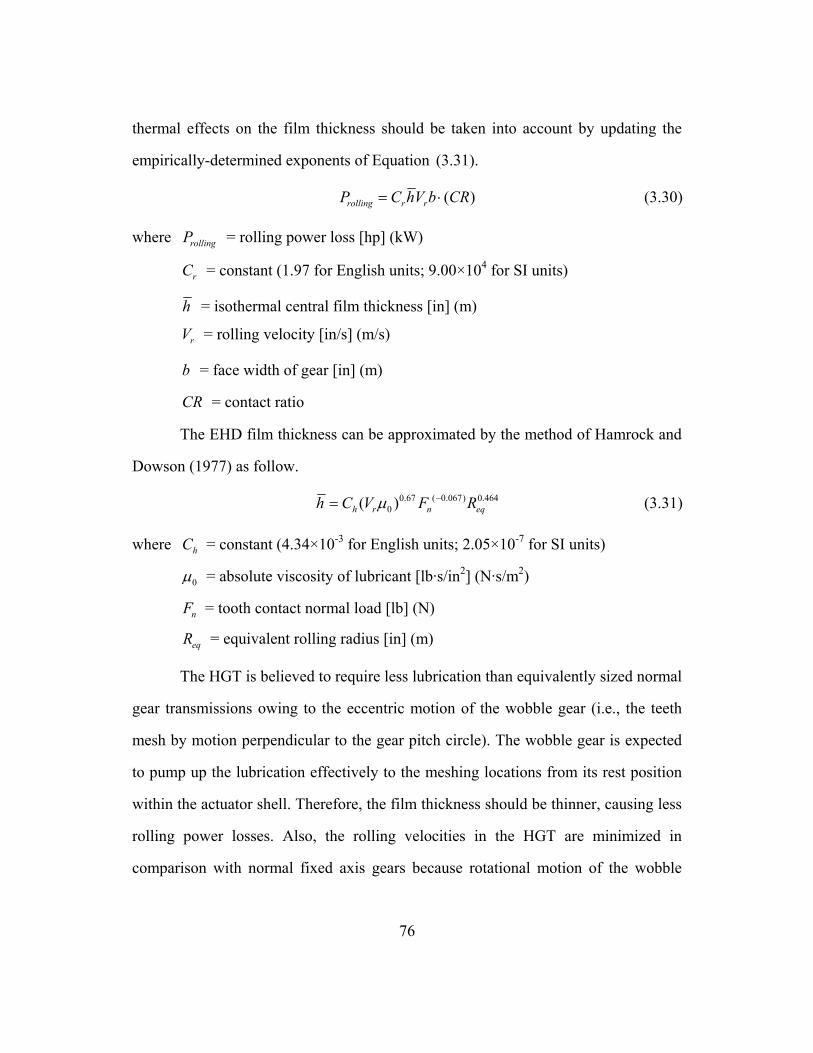
76

thermal effects on the film thickness should be taken into account by updating the

empirically-determined exponents of Equation (3.31).

( )rolling r rP C hV b CR= ⋅ (3.30)

where rollingP = rolling power loss [hp] (kW)

rC = constant (1.97 for English units; 9.00×104 for SI units)

h = isothermal central film thickness [in] (m)

rV = rolling velocity [in/s] (m/s)

b = face width of gear [in] (m)

CR = contact ratio

The EHD film thickness can be approximated by the method of Hamrock and

Dowson (1977) as follow.

0.67 ( 0.067) 0.4640( )h r n eqh C V F Rµ −= (3.31)

where hC = constant (4.34×10-3 for English units; 2.05×10-7 for SI units)

0µ = absolute viscosity of lubricant [lb·s/in2] (N·s/m2)

nF = tooth contact normal load [lb] (N)

eqR = equivalent rolling radius [in] (m)

The HGT is believed to require less lubrication than equivalently sized normal

gear transmissions owing to the eccentric motion of the wobble gear (i.e., the teeth

mesh by motion perpendicular to the gear pitch circle). The wobble gear is expected

to pump up the lubrication effectively to the meshing locations from its rest position

within the actuator shell. Therefore, the film thickness should be thinner, causing less

rolling power losses. Also, the rolling velocities in the HGT are minimized in

comparison with normal fixed axis gears because rotational motion of the wobble

77

gear within an internal gear of slightly larger diameter causes smooth tooth

engagement and disengagement (see Figure 5-23 for visualization of this motion).

3.2.2.4 Churning Power Losses

Churning power losses arise when excessive lubrication is allowed to enter

the gear mesh, gets trapped, and is then pumped out of mesh in the axial direction.

These power losses are particularly significant when gears run submerged in oil or

when the gears run at very high speed (i.e., 10,000 rpm or higher). The portion of

these losses to the total power losses in the gear transmission is very small at nominal

speed. Accurate prediction of these losses is very difficult. Nonetheless, normally

they are less important than sliding power losses or bearing power losses when

evaluating the efficiency in the design stage. As an effort to reduce the churning

losses, some gear designs have a groove in the center of the face width of the spur

gear to minimize the pumping action in the mesh (Shipley, 1991). Based on the

presumption that the speed range of gears in the HGT is very low and adequate

amount of lubrication is used, churning power losses in the HGT can be neglected.

3.2.2.5 Windage Power Losses

Windage power losses are caused by the gears having to move the air inside

the transmission. These losses are significant at very high speeds (i.e., 10,000 rpm or

higher). Calculation of windage power losses is also difficult partly due to the number

of parameters involved. Very little of the literature has attempted to provide

analytical formulae for these losses (Anderson, 1982; Shipley, 1991). Windage power

loss is basically a function of gear ratio, speeds, gear geometry, and oil viscosity.

Anderson (1982) provided the following formulae for approximation of the windage

power losses for gear and pinion.

78

2.8 4.6 0.2

, 1 0 2

2.8 4.6 0.2, 1 0 2

(1 2.3 / )( /( )) (0.028 )

(1 2.3 / ) (0.028 )windage gear w g p g w

windage pinion w p p p w

P C b R n TR R C

P C b R n R C

µ

µ

= + +

= + + (3.32)

where 1wC = constant (4.05×10-13 for English units; 2.82×10-7 for SI units)

2wC = constant (2.86×10-9 for English units; 1.90×10-2 for SI units)

b = face width of gear [in] (m)

gR = gear pitch diameter [in] (m)

pR = pinion pitch diameter [in] (m)

pn = rotational speed of the planet (wobble) gear [rpm]

The loss is also sensitive to the gear casing and blank designs. For example,

axial holes in the gear blank (web design) can be a source of windage power losses.

As observed in Equation (3.32), windage power losses are very sensitive to rotation

speed of the wobble gear and the reduction ratio. Again, since the speed range of the

wobble gear in the HGT is 10 to 20 times lower than that of the motor speed, windage

power losses in the HGT are expected to be negligible.

3.2.3 Inertia

The (mass moment of) inertia of the gear transmission reflected to the input

(motor) side is a very important performance characteristic; it directly affects the

actuator’s acceleration and deceleration performance. This is usually described as the

responsiveness of the actuator to motion commands. There are six rotating

components in the HGT to be considered for inertia calculation. They are the

eccentric shaft, balancing mass, wobble gear, output ring gear, wobble gear bearing

(between the eccentric shaft and the wobble gear), and cross-roller bearing (between

output gear and the actuator shell).

79

The effective input inertia of the HGT can be calculated by determining the

inertia of each of the rotating components and reflecting it to the input side using a

variation of the parallel axis theorem (Tesar, 1992). This parallel axis theorem uses

the g function to reflect the inertia of a rotating rigid body with respect to its own axis

to another parallel axis. For example, let the inertia of a component with respect to its own axis be compI . Then, the inertia of the component reflected to the desired axis

(input axis) *compI is given as

* 2 2/comp comp comp input comp compI I g m d= ⋅ + ⋅ (3.33)

where /comp inputg = angular velocity ratio between the component and the input

compm = mass of the component

compd = distance from the c.o.m.10 of the component to the input axis

Following this approach, all the moving inertias of the components in the

HGT can be reflected to the input, and summed to give a total reflected inertia to the

input (effective input inertia). Equation (3.34) expresses this in a mathematical form:

* * * * * *T s bm w o wb cbI I I I I I I= + + + + + (3.34)

where TI = total effective input inertia

*sI = inertia of the eccentric shaft reflected to the input

*bmI = inertia of the balancing mass reflected to the input

*wI = inertia of the wobble gear reflected to the input

*oI = inertia of the output ring gear reflected to the input

*wbI = inertia of the wobble gear bearing reflected to the input

*cbI = inertia of the cross-roller bearing reflected to the input

10 c.o.m. = center of mass.

80

Following the form of Equation (3.33), reflective inertia of the eccentric shaft

*sI , with eccentricity e , is calculated by:

* 2s s sI I m e= + (3.35)

Since e is very small ( 2 1e ), the second term of the equation approaches zero.

Reflective inertia of the balancing mass, *bmI , is calculated by:

* 2bm bm bm bmI I m d= + (3.36)

where bmd is the distance between the c.o.m. of the balancing mass and the actuator

centerline. In order to reduce this reflective inertia, either bmm (balancing mass) or

bmd should be minimized. However, reduction of one of them leads to necessary

increase of the other parameter for moment equilibrium. Thus, the solution is to

optimize (minimize) the whole term 2bm bmm d while maintaining effective balancing.

More discussion on the balancing of the HGT can be found in Section 3.2.4.

Reflective inertia of the wobble gear, *wI , is calculated by:

2

* 2 2 2 2/ 2

1 1

ww w w i w w w w

p p

IeI I g m e I m e m er r

⎛ ⎞ ⎛ ⎞= + = + = +⎜ ⎟ ⎜ ⎟⎜ ⎟ ⎜ ⎟

⎝ ⎠ ⎝ ⎠ (3.37)

where /w ig , the speed ratio between the input and the wobble gear ( /w iω ω ), is

substituted by the geometrical expression from Equation (3.9). Equation (3.37)

shows that *wI should be very low due to the small 2e .

Reflective inertia of the output ring gear, *oI , is calculated by:

2

2 1 1 2* 2/

1 2

p r p ro o o i o

p r

r r r rI I g I

r r⎛ ⎞−

= = ⎜ ⎟⎜ ⎟⎝ ⎠

(3.38)

81

where /o ig , the speed ratio between output ring gear and input ( /o iω ω ), is

substituted by the geometrical expression from Equation (3.13) Again, *oI is

negligible due to the very small 2/o ig (i.e., given /o ig = 1/100, then * /10000o oI I= ).

Reflective inertia of the wobble gear bearing, *wbI , is calculated by:

2

* 2 2 2 2/ 2

1 1

wbwb wb wb i wb wb wb wb

p p

IeI I g m e I m e m er r

⎛ ⎞ ⎛ ⎞= + = + = +⎜ ⎟ ⎜ ⎟⎜ ⎟ ⎜ ⎟

⎝ ⎠ ⎝ ⎠ (3.39)

Again, since 2e is very small, *wbI should be very small.

Reflective inertia of the cross-roller bearing, *cbI , is calculated by:

* 2/cb cb cb iI I g= (3.40)

where /cb ig is equal to the speed ratio of the HGT ( /o iω ω ). In the same manner as it

is for *oI , *

cbI is also negligible due to the very small 2/o ig . Note that only the moving

inertia of the cross roller bearing is contained in cbI .

Rewriting Equation (3.34) after some approximations stated above,

( )2

2 2

1

( )T s w wb bm s w wb bm bmp

eI I I I I m m m e m dr

⎡ ⎤⎛ ⎞⎢ ⎥≈ + + + + + + ⋅ +⎜ ⎟⎜ ⎟⎢ ⎥⎝ ⎠⎣ ⎦

(3.41)

where the exact value of each component’s inertia and mass can be obtained from a

solid model using commercial software such as SolidWorks. Equation (3.41) shows

that the mass of the eccentric shaft, wobble gear, wobble gear bearing, and balancing

need to be minimized to reduce the total effective input inertia of the HGT. The

eccentricity ( e ), and/or the distance between the c.o.m. of the balancing mass and the

actuator axis ( bmd ) also need to be minimized to reduce the total effective input

inertia of the HGT.

82

3.2.4 Balancing

The balancing mass is a required counterweight for the unbalanced mass

rotating in the HGT which rotates at the same speed as the input. As shown in Figure

3-4, balancing is accomplished with the addition of two masses to the shaft and

subtraction of material from the wobble gear blank11. The dual balancing masses are

required for moment balancing of the HGT with respect to the plane in the axial

direction (and for prevention of misalignment of the gear teeth). Mass is subtracted

from the wobble gear blank for reduction of the total unbalanced weight and

relaxation of subsequent balancing effort. Balancing of the HGT becomes convenient

(e.g., minimal occupation of the actuator volume) if the eccentricity as well as the

total weight of the unbalanced system is minimized.

Balancing Mass 1 Balancing Mass 2

Eccentric Shaft

Figure 3-4: Assembly of balancing masses with eccentric shaft (Park et al., 2005).

Balancing system parameters are determined by moment equilibrium with

respect to two planes, i.e., one containing the actuator axis, and the other in the radial

11 In some cases, these two masses can be combined into one and be housed in a volume inside the wobble gear.

83

direction of the actuator (shown as reference plane in Figure 3-5). The reference

plane is intentionally located in the middle of the axial length of the wobble gear to

provide a reference line for the equations of moment equilibrium. This way,

misalignment between the wobble gear and the mating members can be minimized.

Intersections of the two planes mentioned above are shown as dashed lines in

the moment diagram (Figure 3-5). The diagram represents the unbalanced weight of

the HGT (W0) as a concentrated mass whose center (CM0) is located12 at (d0, r0).

Along with the unbalanced weight, the diagram shows three balancing weights (W1,

W2, and W3) whose centers of masses (CM1, CM2, and CM3) are located at (d1, r1),

(d2, r2), and (d3, r3), respectively. The balancing weight (W1) corresponds to the

subtraction of the weight from the unbalanced system, if any. Thus, it is necessary to

determine the equivalent center of mass of all the subtracted weights. Other balancing

weights (W2 and W3) are actual additions of weights (counterweights).

CM0

CM1

CM2CM3

r0 = e

r1

r2r3d1

d0

d2d3

W0

W1

W2W3

Actuator Axis (CL)Ref

eren

ce P

lane

/ L

ine

Figure 3-5: Moment diagram. 12 r0 is equal to the eccentricity, e .

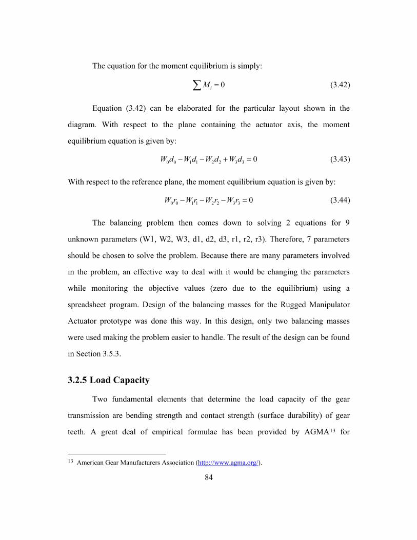
84

The equation for the moment equilibrium is simply:

0iM =∑ (3.42)

Equation (3.42) can be elaborated for the particular layout shown in the

diagram. With respect to the plane containing the actuator axis, the moment

equilibrium equation is given by:

0 0 1 1 2 2 3 3 0W d W d W d W d− − + = (3.43)

With respect to the reference plane, the moment equilibrium equation is given by:

0 0 1 1 2 2 3 3 0W r W r W r W r− − − = (3.44)

The balancing problem then comes down to solving 2 equations for 9

unknown parameters (W1, W2, W3, d1, d2, d3, r1, r2, r3). Therefore, 7 parameters

should be chosen to solve the problem. Because there are many parameters involved

in the problem, an effective way to deal with it would be changing the parameters

while monitoring the objective values (zero due to the equilibrium) using a

spreadsheet program. Design of the balancing masses for the Rugged Manipulator

Actuator prototype was done this way. In this design, only two balancing masses

were used making the problem easier to handle. The result of the design can be found

in Section 3.5.3.

3.2.5 Load Capacity

Two fundamental elements that determine the load capacity of the gear

transmission are bending strength and contact strength (surface durability) of gear

teeth. A great deal of empirical formulae has been provided by AGMA13 for

13 American Gear Manufacturers Association (http://www.agma.org/).

85

evaluation of the gear tooth bending and contact strengths of standard and modified

involute tooth profiles.

Even though the standard involute tooth profile cannot be used in the HGT

without severe modifications, approximating the tooth profile to be used in the HGT

as a modified involute will allow designers to estimate the load capacity of the HGT

in the preliminary design phase. This is a valid approach because the base analytics of

the AGMA formula are originated from Lewis bending equation and Hertz contact

theory. These two fundamentals can be universally applied for preliminary evaluation

of the gear tooth strength.

The approach is to input the major geometric parameters (e.g., tooth height,

face width, diametral pitch, etc.) of the customized tooth profile in the AGMA

formulae for evaluation of the bending and contact strengths of the HGT. AGMA

bending and contact strength formulas will be presented and discussed in Section

3.2.5.1 and 3.2.5.2. The AGMA factors appearing in the equations will be briefly

described although further discussion of them can be found in Section 3.2.5.3. Some

of the important parametric relationships that are general for any tooth profile design

will be discussed in these sections.

In order to correctly reflect the HGT’s unique properties in the strength

calculations, each of the AGMA factors should be carefully reviewed and

determined. Otherwise, the result may be often conservative. Section 3.2.5.3 will

review the AGMA factors and suggest how to customize them for proper evaluation

of the bending14 and contact strengths of the HGT. 14 Since the gear teeth of the HGT will be relatively short and the load will be exerted around mid height of the tooth, the bending moment arm should be very small. Thus, it is worth confirming if the load would cause any significant shear stresses greater than the maximum shear strength of the gear material (half of the tensile strength based on the Mohr circle). The maximum shear stress occurs at the neutral axis of the tooth thickness t with an amount of 3 /(2 )tF tb (see Figure 3-6).

86

3.2.5.1 Bending Strength

As mentioned above, the AGMA bending formula is based on the Lewis

equation. The basic Lewis equation analyzes the bending stress of spur gear teeth.

The bending stress is highest at the cross-section a (see Figure 3-6) where the tooth

profile and the constant-strength parabola are tangent. The constant-strength

parabola is a geometry (with a constant width; here, it is b ) that has uniform bending

stress at any cross-section throughout the length h with respect to the tangential load

on its tip ( tF ). This type of beam is also called a fully-stressed beam. The bending

stress of the fully-stressed beam at cross-section a is given by:

2

6 tF hbt

σ = (3.45)

Figure 3-6: Bending stresses in a spur gear tooth with face width, b (Juvinall & Marshek, 2000).

By similar triangles,

2

/ 2 1, or / 2 4h t h

t x t x= = (3.46)

Substituting Equation (3.46) into Equation (3.45) gives

87

32

tFbx

σ = (3.47)

The Lewis form factor y is defined as

23

xyp

= (3.48)

where p = circular pitch (see Figure 3-8 for nomenclature). Substituting Equation

(3.48) into Equation (3.47) gives

tFbpy

σ = (3.49)

This is the basic Lewis equation in terms of circular pitch. In terms of diametral pitch

( dP ), Equation (3.49) can be rewritten as

t dF PbY

σ = (3.50)

where

/dP p

Y yππ

==

(3.51)

Equation (3.50) shows that tooth bending stresses vary directly with load tF

and diametral pitch15 dP , and inversely with tooth width b and Lewis form factor

Y . Both Y and y are functions of tooth shape and thus vary with the number of

teeth and pressure angle of the gear. Figure 3-7 shows the values of the Lewis form

factor with respect to those two parameters for standard involute teeth.

15 Note that for the HGT, the height of the tooth is not tied directly with the diametral pitch as it normally is for involute gear teeth. This rule provides for a longer tooth to maintain a reasonable contact ratio (≈ 1.4) for most tooth meshes. Other factors can now be used to choose the basic shape of the tooth primarily with the goal of reducing bending stress by shortening the tooth height because the HGT may have a contact ratio of 3 or more.

88

Figure 3-7: Lewis form factor for standard spur gears (Juvinall & Marshek, 2000).

Figure 3-8: Standard gear nomenclature (Shigley & Mischke, 2001).

As shown in Figure 3-716, the Lewis form factor increases (bending stress

decreases) as pressure angle increases for the same number of teeth. For the same 16 The standard stub tooth (in the plot) has a working depth usually 20 % less than the standard full-depth tooth. The stub tooth is preferred for applications with low speed and intermittent operation. It

89

pressure angle, the Lewis form factor increases as tooth number increases. However,

an increase in tooth number also increases diametral pitch, which diminishes the

effect of increased Lewis form factor on the stress reduction.

There are several assumptions made for the Lewis equation (Juvinall &

Marshek, 2000): 1) the full load is applied to the tip of a single tooth, 2) the radial

component rF is negligible, 3) the load is distributed uniformly across the full face

width, 4) frictional forces are negligible, and 5) stress concentration is negligible.

To make the analysis more exact and practical, AGMA extended the Lewis

equation by including several factors as given by the following form:

d m bb t o v s

P K KF K K Kb J

σ = (3.52)

where tF = tangential load [in-lb]

oK = overload factor

vK = dynamic factor

sK = size factor

dP = diametral pitch [in-1]

b = face width [in]

mK = load distribution factor

bK = rim thickness factor

J = geometry factor

The overload factor oK reflects the degree of nonuniformity of externally

applied loads. The overload factor is also called the service factor or application

factor which has been established based on considerable field experience. The

provides greater beam strength than the full-depth tooth. For the HGT with its high contact ratio, the load point for the most heavily loaded tooth may be at the pitch circle, i.e., a stress reduction of 50 %.

90

dynamic factor vK reflects the severity of impact at tooth pairs that engage

continuously 17 . It is a function of pitch line velocity ( V ) and the level of

manufacturing precision quantified by quality-control number, VQ (AGMA 390.01).

The dynamic factor increases as pitch line velocity increases or as the quality control

number decreases as follows.

in [ft/min]

200 in [m/s]

B

Bv

A V VV

KA V V

A

⎧ +⎛ ⎞⎪⎜ ⎟⎝ ⎠⎪

= ⎨⎛ ⎞+⎪⎜ ⎟⎪⎜ ⎟⎝ ⎠⎩

(3.53)

where

2/3

50 56(1 )0.25(12 )V

A BB Q= + −

= − (3.54)

The size factor sK reflects nonuniformity of material properties due to size.

It depends upon: tooth size, diameter of the part, ratio of tooth size to the diameter of

the part, face width, area of the stress pattern, ratio of case depth to tooth size,

hardenability, and heat treatment (Shigley, 2001). The load distribution factor mK

represents the nonuniformity of distribution of load across the line of contact. This

factor also reflects misalignment of the bearings and gear. The rim thickness factor

bK adjusts the stress value when rim thickness of the gear is not sufficient enough to

resist fatigue failure. It is a function of the backup ratio, Bm , which is defined as the

ratio between rim thickness below the tooth Rt , and the whole depth of tooth th :

RB

t

tmh

= (3.55)

17 This dynamic factor should be very close to unity since little impact occurs in the HGT. More detail discussion can be found in Section 3.2.5.3.

91

In order for the rim thickness factor to be unity or less, the backup ratio Bm should

be greater than 1.2. Note that the HGT will use relatively short gear teeth which will

keep the backup ratio high.

The equation for bending endurance (allowable) strength is given by:

,t N

b allT R

S YSF K K

σ = (3.56)

where tS = bending strength for repeated loads

SF = safety factor

NY = load cycles factor

TK = temperature factor

RK = reliability factor

The load cycles factor NY is unity for 107 cycles; for shorter cycles it

increases, and for longer cycles, it decreases. The temperature factor TK is unity

with oil or gear blank temperature up to 250ºF (120ºC). The reliability factor RK 18

accounts for the effect of the statistical distribution of material fatigue failures. For

example, RK = 0.85 for reliability of 90 %, RK = 1 for 99 %, and RK = 1.5 for

99.99 %. The relationship between the reliability factor and the reliability is

nonlinear.

The bending safety factor is given by dividing the bending endurance

(allowable) strength by calculated bending stress:

, , 1 /( )b all SF t N T R

b b

S Y K KSFσ

σ σ== = (3.57)

18 Refer to the ANSI/AGMA 2001-C95 for additional information.

92

3.2.5.2 Contact Strength

Contact strength (surface durability) of gears is another critical component

that determines the load capacity of gear transmissions. Lack of this strength causes

failure on the surfaces of the gear teeth, which is generally called wear. Gear teeth are

subject to repetitive Hertzian contact stresses which lead to surface fatigue failure

called pitting. Scoring is another surface failure caused by lubrication breakdown,

and abrasion is wear of the tooth surface due to the presence of foreign material in

the gear mesh (Shigley & Mischke, 2001).

The AGMA contact strength equation is based on Hertz contact theory. This

original analysis of elastic contact stresses was published in 1881 by Heinrich Hertz

of Germany for general curved bodies in compression. A special case, contact stress

analysis between two cylindrical bodies in compression, has been applied for

evaluation of contact stresses between two gear teeth in contact. In some analyses for

crowned gear teeth in contact, Hertz theory of two spherical bodies in compression

can be applied (Lingaiah, & Ramachandra, 1981).

Figure 3-9 shows two cylinders (1 and 2) contacting each other by external

force F in the z direction. As shown in Figure 3-9 (b), the pressure profile is

elliptical, and the area of contact is a narrow rectangle of width 2b and length l .

The half-width b is given by the equation (Shigley & Mischke, 2001),

2 21 1 2 2

1 2

(1 ) / (1 ) /21/ 1/

v E v EFbl d dπ

− + −=

+ (3.58)

where v = Poisson’s ratio and E = Young’s modulus. The maximum pressure

maxP is then given by:

93

max2FP

blπ= (3.59)

Equations (3.58) and (3.59) can be applied to a cylinder and a plane surface in

compression as well; in this case, d = ∞ for the plane surface. The equations can

also be applied to the contact of a cylinder and an internal cylindrical surface (such as

convex-concave circular-arc tooth meshing); in this case, d is made negative.

Figure 3-9: (a) Two cylinders in contact with uniform distribution of load F along cylinder length l. (b) Elliptical distribution of contact stress across the contact zone with

width 2 b (Shigley & Mischke, 2001).

The stress state on the z axis in Figure 3-9 is given by the following equations

(Shigley & Mischke, 2001):

( )2 2max

2 2max 2 2

max

2 2

2 1 ( / ) ( / )

12 1 ( / ) 2( / )1 ( / )

1 ( / )

x

y

z

vp z b z b

p z b z bz b

p

z b

σ

σ

σ

= − + −

⎡ ⎤⎛ ⎞= − − + −⎢ ⎥⎜ ⎟+⎝ ⎠⎣ ⎦

= −+

(3.60)

94

The Mohr circle plot of these stress values shows that, for 0 3z b≤ ≤ , zyτ is

a maximum of about max0.3P at about 0.75z b= for a Poisson ratio of 0.30. zyτ at

this z is maxτ , and this maxτ holds for any value of z . For the same z ,

max0.3x Pσ ≈ − , max0.2y Pσ ≈ − , and max0.8z Pσ ≈ − .

In order to transform Equation (3.58) and (3.59) to a contact stress equation

in terms of the gearing notation, the following equations are used to replace some of

the parameters.

max

cos2

t

c

FF

d rl b

P

φ

σ

=

===

(3.61)

where tF = tangential force on the gear tooth

φ = pressure angle (see Figure 3-10 for nomenclature)

r = instantaneous radius of curvature on the pinion and gear tooth profiles at

the point of contact

b = face width

cσ = Hertz contact stress

Then, substituting Equation (3.58) in Equation (3.59) gives,

1 22 21 1 2 2

(1/ ) (1 )cos (1 ) / (1 ) /

tc

F r rb v E v E

σπ φ

+ +=

⎡ ⎤− + −⎣ ⎦ (3.62)

Wear occurs most prominently at the pitch line of the mating gears. The radii

of curvature of the tooth profiles at the pitch point are (see Figure 3-10)

95

11

22

sin2sin2

p

p

Dr

Dr

φ

φ

=

= (3.63)

where 1pD and 2pD are pitch diameters of the pinion and gear, respectively.

Figure 3-10: Nomenclature of internally meshing pinion (1) and gear (2).

Substituting Equation (3.63) in Equation (3.62) gives,

1 22 21 1 2 2

(1/ ) (1 )2sin cos (1 ) / (1 ) /

p ptc

D DFb v E v E

σπ φ φ

+ +=

⎡ ⎤− + −⎣ ⎦ (3.64)

Equation (3.64) becomes more practical by combining some terms into two representative parameters: elastic coefficient pC and geometry factor I (Juvinall &

Marshek, 2000). These two parameters are defined as

2 21 1 2 2

1(1 ) / (1 ) /pC

v E v Eπ=

⎡ ⎤− + −⎣ ⎦ (3.65)

sin cos2 1

RIR

φ φ=

+ (3.66)

96

where 2 1/p pR D D= . Note that for the HGT, 1R ≈ and for low values of φ ,

/ 4I φ≈ with φ given in radians.

Substituting Equation (3.65) and (3.66) in Equation (3.64) gives a

simplified equation:

1

tc p

p

FCbD I

σ = (3.67)

The AGMA includes some of the factors used in the bending stress

calculation in Equation (3.67) to reflect some practical conditions, as below.

1

tc p o v s m

p

FC K K K KbD I

σ = (3.68)

where oK = overload factor

vK = dynamic factor

sK = size factor

mK = load distribution factor

Going back to Equation (3.65) and (3.66), elastic coefficient pC is

characterized by material properties19 . On the other hand, geometry factor I is

purely, as its name implies, driven by geometry of gears, especially the tooth profile

geometry parameters. Plugging Equation (3.63) back to Equation (3.66) yields20,

1

cos 1

p

ID kφ

= (3.69)

where k is effective curvature, defined as 19 Given 1 2v v= and 1 2E E= , then 22 (1 )p

ECvπ

=−

.

20 For 0φ ⇒ , 1

1

p

ID k

≈ .

97

1 2

1 1kr r

⎛ ⎞= +⎜ ⎟⎝ ⎠

(3.70)

In convex-concave circular-arc tooth profiles, one of the radii of curvature is

negative, so the effective curvature k is reduced significantly as observed in Equation

(3.70). Making the conformity of the convex-concave tooth pair even higher (making

1 2r r≈ and 0k ⇒ ) further decreases the effective curvature, resulting in maximizing

the geometry factor, and thus minimizing Hertz contact stress (see Equation (3.69)

and (3.67)). This minimized effective curvature is the reason why circular-arc type

tooth profiles are superior in contact strength to the involute tooth profile.

The AGMA gives the following equation for contact endurance strength.

,c N H

c allT R

S Z CSF K K

σ = (3.71)

where cS = contact strength for repeated loads

SF = safety factor

NZ = load cycles factor

HC = hardness ratio factor

TK = temperature factor

RK = reliability factor

Then, the safety factor for contact strength can be obtained by:

, , 1 /( )c all SF c N H T R

c c

S Z C K KSFσ

σ σ== = (3.72)

3.2.5.3 Load Capacity Factors for the HGT

In order to properly accommodate the HGT’s unique properties in the load

capacity evaluation, the AGMA factors should be carefully adjusted for the HGT. To

98

do so, the AGMA factors of the bending/contact fatigue stress and endurance strength

equations will be reviewed here, and a guideline for how to customize these factors

for the HGT will be proposed. The first set of factors to follow is used in the bending

and contact fatigue stress equations (Equation (3.52) and (3.68)). These factors are

sensitive to the gear/gear tooth geometry (geometry factors), application (overload

factor), kinematics/dynamics (dynamic factor), and design/assembly (size, load

distribution, and rim thickness factors). While discussing each of the factors, benefit

from the HGT design will be identified. The benefits consider the special nature of

the HGT over standard AGMA gear design practice.

Geometry Factor for Bending ( J ): This factor accounts for the shape of the

mating teeth, the position at which the most damaging load is applied, load sharing

between teeth, and stress concentration due to the geometric shape. This factor should

be maximized to reduce the bending stress. The geometry factor is directly

proportional to the Lewis form factor Y (Figure 3-7) which determines tooth shape

and the loading position geometrically. Employing the short circular-arc tooth profile

for the HGT, Y (and thus J ) can be increased by about 20 %. The J factor is

inversely proportional to the stress concentration factor and load sharing ratio21.

Employing a generous root fillet radius ( 0.35 / dP> ) in the circular-arc tooth profile

should decrease the stress concentration factor, and thus increase the J factor by

about 10 %. The high contact ratio in the HGT should allow for the decrease in the

load sharing ratio, and thus an increase in the J factor by at least 30 %. Therefore,

combining all these benefits the bending stress of the HGT would be about 58 % of

the normal gear design if all the other factors are held constant.

21 Base pitch over length of the line of action.

99

Geometry Factor for Contact ( I ): This factor accounts for the radii of

curvature of the contacting tooth profiles. This factor should be maximized to reduce

the contact stress. In the convex-concave circular-arc tooth profile, one of the radii of

curvature is negative, so the effective curvature k is reduced significantly (Equation

(3.70)). Improving the conformity of the profile will further decrease the effective

curvature, and thus maximize this geometry factor. In comparison with convex-

convex tooth contact gears, the I factor of the HGT is about 20 times higher22. This

means the contact stress of the HGT should be only 22 % of the normal gear design if

all the other factors are held constant.

Overload Factor ( oK ): This factor compensates for externally applied loads of

unknown nature that are in excess of the nominal tangential loads. This factor should

be minimized to reduce the bending and contact stresses. This factor depends on the

characteristics of the applied load on the actuator, and rough estimates are provided

by the AGMA. For example, for medium shock load with uniform source of power,

the factor is assigned a value of 1.25. In the EM actuator with the HGT, however, the

torsional shock load is resisted by the high contact ratio tooth mesh in the second

stage gear pair, and the out-of-plane moment load is taken by the large cross-roller

bearing of the actuator. Therefore, the overload factor for the HGT can be

approximated to be one level lower (0.25 less) than that for the normal gear design

practice. This will allow for the HGT to have 20 % less stress value than the normal

stress values.

Dynamic Factor ( vK ): This factor accounts for the effects of pitch/profile

errors, mesh stiffness, inertia, magnitude of pitch line velocity, transmitted load, and

precision level of manufacturing. This factor should be minimized to reduce the 22 Based on the tooth geometry of the ¼-scale AWE Actuator HGT design.

100

bending and contact stresses. The high contact ratio of the HGT under loading

condition allows for minimized variation of mesh stiffness and gradual loading and

unloading (minimized impact) in the mesh. Also, the pitch line velocity of the wobble

gear in the HGT is very low relative to the planet gears in normal planetary gear

transmissions. High precision manufacturing as well as the HGT’s low sensitivity to

manufacturing errors should allow for the HGT to have this factor be very close to

unity 23 . On the other hand, the dynamic factor of a normal planetary gear

transmission of a comparable size to the ¼-scale AWE Actuator HGT24 is as high as

1.4525 for a high precision number ( 11vQ = ). The benefit here is about 30 % less

stress values for the HGT than normal design practice when all the other factors are

held constant.

Size Factor ( sK ): This factor reflects non-uniformity of material properties

due to size. AGMA suggests this factor be unity unless there is disadvantageous size

effect. This factor should be minimized to reduce the bending and contact stresses. In

general, employing a higher diametral pitch (finer teeth) gives a slight advantage

(reduction) for this factor. Increased face width generally works against this factor.

The inherent high load capacity of the circular-arc tooth profile enables the HGT to

have an optimal set of values for these two parameters, so this factor can be close to

the unity. Size factor for the HGT and for the normal gear design are considered to

be comparable (1x).

Load Distribution Factor ( mK ): This factor takes into account the non-

uniform distribution of the load across the line of contact and across the face width. 23 See the design result in Section 3.5.1. 24 Pitch diameter of the internal gear is the same as that of the HGT (6.4”) and that of the planet gear is about 1/3 of that of the HGT wobble gear (1.94”). Input speed is the same for both designs (3,950 rpm). 25 The calculation is based on Equation (3.53) and (3.54).

101

This factor should be minimized to reduce the bending and contact stresses.

Preventing misalignment of the mating gears in the HGT by accurate mountings and

by the use of precision bearings will assign 1.3 to this factor (Juvinall & Marshek,

2000). This factor is also a function of the face width. The face width of the HGT

does not normally exceed 25 % of the pitch diameter, so the factor is not affected by

this parameter in the HGT design. Crowned teeth help reduce this factor. With “less

rigid” mountings and “less accurate” gears, this factor can be as high as 1.6 (Juvinall

& Marshek, 2000). If this is the case for the normal design, the benefit would be

about 20 % less stress values for the HGT than normal design practice when all the

other factors are held constant.

Rim Thickness Factor ( bK ): This factor considers the rim thickness of the

gear as a potential source of fatigue failure. This factor should be minimized to reduce

the bending stress. As long as the rim thickness is 1.2 times of the tooth height, this

factor is assigned to unity. The bending fatigue failure hardly occurs in the rim of the

HGT with a good structural design. This factor can be considered to be comparable

for both the HGT and the normal design practice.

The next set of factors adjusts the bending and contact endurance strength

equations (Equation (3.56) and (3.71)). They are associated with life cycles (load

cycles factor), operating temperature (temperature factor), surface hardness and its

ratio between the mating gears (hardness ratio factor), and statistical reliability

(reliability factor). These factors are either operational (load cycles and temperature

factors) or material related (hardness ratio and reliability factors). Therefore, these

factors are assumed to be applied identically to both the HGT and the normal designs.

Descriptions of each factor and representative guidelines for assigning values to these

factors are provided as follows.

102

Load Cycles Factor ( NY , NZ ): This factor adjusts the endurance strengths to

reflect the desired life cycles. This factor is a function of load cycles and the Brinell

Hardness number. For 107 cycles of load, this factor is set to unity. For other cycles,

refer to the AGMA standard.

Temperature Factor ( TK ): This factor accounts for the operating temperature

in the endurance strength equations. With adequate use of lubrication, the operating

temperature of the HGT hardly exceeds 250°F. Thus, this factor can be set to unity.

Hardness Ratio Factor ( HC ): This factor accounts for the difference in surface

hardness between the material of a gear and that of the mating pinion. Since the speed

ratio between the internal gear and the wobble gear is close to unity, assuming the

Brinell hardness ratio between those two gears is less than 1.2 (which is normally the

case for the HGT), this factor is set to unity.

Reliability Factor ( RK ): This factor accounts for the statistical distribution of

material fatigue failures in the endurance strength calculations. For 99 % reliability,

RK is set to 1. For 99.99 % reliability, RK is set to 1.5. For more information on

reliability factors, consult the AGMA standard.

Table 3-5 presents normalized load capacity factors for the HGT in

comparison with those for the normal design practice (third column). Although these

factors are somewhat sensitive to design details, the table gives a general idea of how

adjustments should be made to the AGMA factors for them to be reasonably applied

to the HGT design. The fifth column converts these normalized comparison numbers,

using the proportionality (fourth column), to corresponding benefits in terms of the

load capacity. The overall benefits (last two rows) show that 3.78 times and 6.67

times of benefits in bending and contact strength are available in the HGT design

compared to the normal gear system design.

103

Table 3-5: Factor adjustments and corresponding benefits of the HGT.

Proportionality Benefit Load Capacity Factors

Nomenclature Normalized

Ratio of Factors26 Bending

Strength Contact Strength

Bending Strength

Contact Strength

J Geometry 1.72 Direct – 1.72 –

I Geometry 20.00 – Direct* – 4.47

oK Overload 0.80 Inverse Inverse* 1.25 1.12

vK Dynamic 0.70 Inverse Inverse* 1.43 1.20

sK Size 1.00 Inverse Inverse* 1.00 1.00

mK Load Distribution 0.81 Inverse Inverse* 1.23 1.11

bK Rim Thickness 1.00 Inverse – 1.00 –

NY , NZ Load Cycles 1.00 Direct Direct 1.00 1.00

TK Temperature 1.00 Inverse Inverse 1.00 1.00

HC Hardness Ratio 1.00 – Direct – 1.00

RK Reliability 1.00 Inverse Inverse 1.00 1.00

Overall Benefit for Bending Strength27 3.78 –

Overall Benefit for Contact Strength28 – 6.67

* By square root.

Bending Safety Factor: ,b allowed t Nbending

b t d o v s m b T R

S b JYSFF P K K K K K K K

σσ

⎛ ⎞⎛ ⎞= = ⎜ ⎟⎜ ⎟

⎝ ⎠⎝ ⎠

Contact Safety Factor: 1, pc allowed c N Hcontact

c p T R o v s m

bDS Z C ISFC F K K K K K K

σσ

⎛ ⎞⎛ ⎞= = ⎜ ⎟⎜ ⎟⎜ ⎟⎜ ⎟⎝ ⎠⎝ ⎠

26 Normalized ratio of the factor for the HGT to the factor for the normal design practice. 27 Actual tooth height, which affects the bending strength by specifying the highest loading position, and HGT’s inherent high contact ratio were considered by moderately improving (reducing) the load sharing factor by 30 %. Since the tooth height is directly proportional to the bending stress in the original beam stress equation (Equation ((3.45)), it should be fully considered for more accurate evaluation. 28 The high contact ratio property of the HGT can be reflected by adjusting the actual tangential load in the contact stress equation. Then, the overall benefit for contact strength can be further extended.

104

3.2.6 Interferences

There are two kinds of interference in involute internal gearing. The first type

of interference occurs when non-conjugate portions of tooth profiles make contact.

The second type of interference is tip interference which occurs when the tip of the

external gear teeth interfere with the corner of the internal gear tooth space during the

external gear’s hypocycloidal motion. Equations for these interferences can be found

in (Colbourne, 1987). Also, there can be interferences on the backside of the teeth.

These interferences can be avoided by tooth meshing analysis which is the

topic of Chapter 5. Avoidance of interferences in the HGT becomes very challenging

especially when a very small tooth number difference is preferred. By employing a

circular-arc tooth profile and controlling the design parameters (especially tooth relief

design parameters), interferences in the HGT can be avoided. See Section 4.4.3 for

more discussion on the interference and tip relief design.

Maiti and Roy (1996) showed that involute internal gears cannot have a tooth

difference of less than 5 at a pressure angle of 25° or smaller. With a pressure angle

of 30° or larger, involute gears are allowed to have a four tooth difference and with a

pressure angle of 56° or larger, they can have one tooth difference. However, these

high pressure angles increase radial and normal loads which are not desirable

especially for the configurations like the HGT where eccentric motion creates the

driving force. Increased radial and normal loads also lead to increased tooth friction

losses and bearing power losses. In order to reduce the excitation forces and power

losses in the bearings, it is necessary to eliminate axial loadings (a reason why spur

gears are preferred to helical gears) and to minimize radial loadings by lowering the

pressure angle. The goal is to reduce the pressure angle down to 5° without causing

105

any interference in the gear tooth mesh especially with heavy torque loads on the gear

transmission.

Modification of the involute profile is one possibility, but even after heavy

modifications (tip truncations, center distance adjustments, etc.), involute gears still

cannot have a tooth number difference less than 5 for a pressure angle of 22.5° or

smaller without losing all of their standard properties (Maiti & Roy, 1996). In order

to have a relatively low pressure angle, 14.5°, the modified involute gears should

have at least a 7 tooth difference to avoid interferences, which significantly reduces

the reduction ratio options and increases the size of the eccentricity. The HGT design

effort for the Rugged Actuator development (Park et al., 2005) has found that the

proposed circular-arc tooth profile allowed a 5 tooth difference at an exceptionally

low pressure angle of 7°. The design result is presented in Section 3.5.2.

3.2.7 Stiffness, Lost Motion, and Backlash

Stiffness of the EM actuator refers to two kinds of stiffness: torsional

stiffness, and stiffness to the radial (external) load on the actuator output. The latter

stiffness is dependent mostly upon the out-of-plane moment rigidity of the (cross-

roller) bearing that is located between the output and the actuator shell. On the other

hand, torsional stiffness of the EM actuator is directly coupled with the torsional

stiffness of the gear body and teeth.

Torsional stiffness of the gear transmission is an important criterion which

influences the actuator performance; depending on applications, its influence can be

significant. From the control standpoint, high torsional stiffness of the gear train

ensures high structural natural frequencies ( /n k mω = ) which translate into short

106

settling times. From the precision standpoint, high torsional stiffness reduces lost

motion, and thus improves accuracy and repeatability of the actuator.

The lost motion is defined as the angular deflection measured under a certain

amount of torque. Industrial practice is to determine the lost motion for a ± 3% of the

rated torque of the transmission (see Figure 3-11). The lost motion includes backlash

if any. Backlash of normal gear transmissions is the amount of angular motion

necessary for all the transmission’s mating parts to come into contact so that torque

(power) can be transmitted through them. In Figure 3-11, backlash is determined as

the torsion angles when the torque indicated by the hysteresis curve is zero. Torsional

stiffness is determined by /b a in this case, approximating the portion of curves to

be straight lines.

Figure 3-11: Definition of backlash and lost motion (Nabtesco, n.d.).

As the torque applied to the output of the gear transmission increases, the rate

of deflection decreases in general; gear transmissions tend to stiffen under increasing

load. This is because as load is increased, contact surfaces between mating teeth will

deform to increase the contact area, and thus increase the stiffness. Also, as load is

107

increased, more parts (i.e., tooth pairs) can come into contact due to deformations,

resulting in the increase of overall mesh stiffness of the gear transmission.

Analytic evaluation of the stiffness in the gear transmission has been

attempted in some of the literature, but is regarded as an extremely complicated

(geometrically) and unrewarding task if a high level of accuracy is pursued in the

analysis. One reason is due to numerous deflection sources in the gear transmission

including gear mesh, gear bodies, bearings and shafts. Another reason is due to

nonlinearity as explained above; as the load gets larger, not only the number of

mating components increases, but also the stiffness of each component increases.

Assuming the stiffness to be linear in discrete periods of time is one viable approach

to an inexpensive evaluation, but still requires very good interpretation of the load

distribution, contact position, contact area, and instantaneous stiffness of the system

at each incremental time which greatly affects the level of accuracy of the result.

Donoso and Tesar (1998) provided analytic formulas for evaluation of the

stiffness of two-stage 3K Paradox epicyclic gear transmissions. They analytically

evaluated tooth mesh deformation and bearing deformation assuming these two

deformations comprise about 75% of the total deformation occurring in the

transmission. In their work, they reported a formula for the meshing deformation29 as

follows.

3 31 32 16 2

3 1 2 61 3

1 2

10

mcm

m md mm

P E FN N

δ φ

−⎛ ⎞⎜ ⎟ ⎛ ⎞ ⎛ ⎞− ⎛ ⎞⎝ ⎠ ⎜ ⎟ ⎜ ⎟⎜ ⎟− −⎝ ⎠ ⎝ ⎠−⎝ ⎠

⎛ ⎞= ⋅ ⋅ ⋅ ⋅⎜ ⎟⎝ ⎠

(3.73)

29 This formula considers bending, shear, and contact deformations simultaneously. This equation is well suited for this generalized discussion on the stiffness of the gear transmission because it deals with gear level parameters (i.e., diametral pitch and tooth numbers) rather than tooth level parameters (e.g., tooth height, thickness, etc.). More discussion on tooth level stiffness can be found in Section 4.3.7.

108

where mδ = linear mesh deflection per unit face width [in/in]

, m c = constants depending on pressure angle and diametral pitch

F = mesh load [lb]

After evaluating the amount of deformation from each deformation source (tooth

meshing, bearing, and others if any), they are reflected to an angular deformation at

the center axis of the output ( oθ∆ ), and compared with the output torque ( oT ) for

calculation of the overall stiffness of the gear transmission ( 0 /o ok T θ= ∆ ).

Equation (3.73) was used for preliminary analysis of the stiffness of the HGT

after some adjustments in the design of the two prototypes (see Section 3.5). Mesh stiffness at each stage of the HGT, , 1m stageK and , 2m stageK , evaluated using the

equation are considered to be coupled as a serial spring. Thus, total stiffness of the HGT, ,m totalK , is given by

, 1 , 2,

, 1 , 2

m stage m stagem total

m stage m stage

K KK

K K⋅

=+

(3.74)

Backlash in a general gear pair is determined by measuring the leftover

clearance in the width of tooth space of one gear after the tooth thickness of the other

gear fully occupies the tooth space on the pitch circle (refer to Figure 3-8 for

nomenclature of the terms in italic). Thus, backlash B is described as the difference

between the summation of the mating gear tooth thicknesses ( Pt and Gt ) and their

circular pitch p :

( )P GB p t t= − + (3.75)

However, the operational backlash with respect to the changing relative

location of the two gears requires more complicated analytics. It can be evaluated by

analyzing the geometrical clearances on the backside (as opposed to contact side) of

109

the external tooth at a finite number of steps through the mesh cycle. See Chapter 5

for the backside clearance/interference analysis.

Operating temperature can affect the amount of backlash (i.e., operational

backlash) by changing the tooth thicknesses, diameters of the gears, and the operating

center distance between the gears (i.e., by expanding the diameter of the eccentric

shaft and the bearing race). Therefore, when evaluating the backlash, the temperature

effects on gear and gear tooth geometry need to be considered. Also, geometrical

imperfections such as tooth profile error, pitch error (spacing error), and center

distance error, definitely change the backlash. For example, with a presence of center

distance change CD∆ , variation of the backlash (Smith, 1991) is approximated by

2 tanB CD φ∆ = ∆ ⋅ (3.76)

Temperature effects on the gear geometry (tooth thickness and center distance error)

will be discussed in more depth in Section 3.2.10.2.

3.2.8 Noise and Vibration

Noise and vibration have been one of the most demanding issues in the design

and operation of the gear transmissions. This topic has a long history of research, and

numerous authors have contributed to this area of research. Houser (1991) and Smith

(2003) provided good summaries of the topic of gear noise and vibration with many

references.

From the design point of view, for normal involute gears, not much can be

done in a proactive manner for reduction of noise and vibration. The solution to the

noise and vibration problems in gear transmissions has been more effective based on

precise measurement, correct judgment, and subsequent deduction of the problem

110

than on the predictions from analytics or simulations which are often misleading. To

find out what can be done preemptively in the design stage for reduction of noise and

vibration, it is necessary to logically investigate the root cause or intermediate causes

of noise, if possible.

Houser (1991) and Smith (2003) discussed a fundamental sequence of the

noise generation as follows. Noise from a gear box is airborne noise generated by

vibrations of the supporting structure which are caused by excitations of the gear case

and the installment (foot of the gear box to the supporting structure). These

excitations are from bearing forces which are caused by responses of the bearings and

gear dynamics. Transmission error is one of the parameters that determine the

dynamic response of operating gear pairs. Other parameters that determine the

dynamic response of the operating gear pairs include inertia of balanced or

unbalanced mass, angular velocity, varying mesh stiffness, gear tooth impacts,

frictional forces, sliding velocities, air pocketing, and lubrication entrainment.

Mathematical modeling of the gear dynamics including all these parameters is a

demanding task. Lumped parameter models are often used to analyze the dynamics of

gear systems. Houser et al. (2002)’s analytic model of a simple idler gearbox is an

example of using lumped parameters.

Transmission error is defined as “the difference between the angular position

that the output shaft of a drive would occupy if the drive were perfect and the actual

position of the output” (Smith, 2003). Transmission error can be expressed in angular

units or as a linear displacement along the line of action. The respective equations for

transmission error (TE ) are

111

22 1

1

22 2 1

1

[rad]

[in] or [mm]b

NTEN

NTE RN

θ θ

θ θ

= −

⎛ ⎞= −⎜ ⎟

⎝ ⎠

(3.77)

where 1θ = angular rotation of the input gear

2θ = actual angular rotation of the output gear

2bR = base radius of the output gear

The exact method of calculating the actual position ( 2θ ) of the output gear

experiencing non-conjugate contacts is geometrically demanding. Complex analytics

for transmission error due to corner contact (outside the normal path of contact) was

provided by (Munro, Morrish, & Palmer, 1999) after rigorous definitions of the tooth

geometry.

There are plural causes of the transmission error. They include 1)

manufacturing errors leading to imperfection of gear and gear tooth geometry (e.g.

tooth profile errors, spacing errors, center distance errors, misalignment, etc.), 2)

deformation, deflection, or wear of teeth, gear bodies, case, etc., under load, 3)

thermal expansions or distortions of the gears, gear teeth, shaft, bearings, etc., 4) low

contact ratio for a specified load, and 5) dynamic unbalance of the rotating members.

Fleming (2002) also studied the effect of shaft bearing stiffness and damping on the

transmission error. From analysis of a dynamic model composed of flexible shafts,

bearings and gear meshes, he found that additional damping on the bearings (such as

squeeze film) reduced the transmission error substantially.

From a design standpoint, the HGT will be designed to have a high contact

ratio under load (up to five depending on the load), which will help enormously to

reduce the transmission error and subsequent vibration and noise. Also, the HGT will

112

provide smooth engagement and disengagement of the teeth to reduce the mesh

excitation, and subsequent vibrations and resonances of the gears. Further, careful

design of the tooth tip relief in the design stage can significantly reduce the

transmission error. Tip relief is originally intended for avoidance of interference in

the tooth design. However, if the range of the load applied on the tooth is narrowly

bounded, and the amount of tooth deformation is analyzed well due to that load, tip

relief can be designed accordingly so that continuous engagement of tooth pairs can

be secured under these tooth deformations. Although this scheme alone cannot totally

eliminate transmission error in the no load condition30, it should be very effective in

reducing the transmission error and potential vibrations when the gear transmission is

subject to a specified load.

There are often occasions when gears with low transmission error are still

unacceptably noisy (Houser and Harianto, 2003). This is because there are two other

force excitations in the gear mesh besides the transmission error excitation. They are

axial shuttling force and time-varying friction forces. The HGT employs spur gears

which eliminate the axial shuttling force. The friction forces are also expected to be

minimized in the HGT due to low pressure angle, load sharing, and entrapment of

lubrication (due to wobbling motion of the wobble gear, i.e., the teeth mesh by

entering the tooth gap perpendicular to the pitch circle).

For standard gear systems, there are general methods of reducing the gear

noise. These methods are reactive rather than proactive. They are (Houser, 1991;

Smith, 2003):

30 Houser (1991) says, “for spur gears these modifications (profile modifications) are usually an optimum for one load level, and gears operating away from this design load will have increased noise” (14.5).

113

a) Reducing the excitation at the gear teeth; normally less amplitude of input

gives less output (noise) although this is not necessarily true for some

nonlinear systems.

b) Reducing the dynamic force path and the vibration between the gear mesh

and the sound radiating panels; this can be done by shortening the force path,

inserting vibration isolators in the path, or by altering the sound radiation

properties of the external panels.

c) Reducing the housing’s acoustic efficiency; this can be done by using

sound barriers or enclosing the whole system in a soundproof box.

d) Using noise cancellation schemes or modifying the environment.

The excitation at the gear teeth mentioned in a) above is characterized by

frequency components at the gear mesh frequencies and its multiples, and by

modulation of the mesh frequency (sidebands). The two gear mesh frequencies of the

HGT (1st stage and 2nd stage) are equal to the number of meshed teeth of the ring

gears multiplied by rotational frequency of the input shaft. Thus, at the first stage of

the HGT, gear mesh frequency 1mf [Hz] is obtained by

1 1 60in

mf N ω= ⋅ (3.78)

where 1N = number of teeth in the first stage stationary ring gear

inω = motor input speed [rpm]

The second stage mesh frequency is expressed differently because not all of

the teeth in the second stage ring gear are engaged during the period of one revolution

of the input shaft. The number of teeth left unmeshed ( 2uN ) in the ring gear due to its

own rotational movement is

114

22u

NNTR

= (3.79)

where 2N = number of teeth in the second stage internal ring gear

TR = transmission ratio

Therefore, the second stage mesh frequency of the HGT, 2mf , is determined by

2 2 21( ) 1

60 60in in

m uf N N NTR

ω ω⎛ ⎞= − ⋅ = − ⋅⎜ ⎟⎝ ⎠

(3.80)

Harmonics occur at integer multiples of the mesh frequency; the second

harmonic is at 2 mf , the third harmonic at 3 mf , and so on (see Figure 3-12).

Sidebands may occur around the mesh frequency harmonics, and are commonly

spaced at the shaft input speed (Houser 1991). For a pair of spur gears each being

connected to input and output shaft respectively, equations for calculations of the

sidebands ( sbf ) are:

1 2 1 2, , 2 , 2 , ... sb m s m s m s m sf f nf f nf f nf f nf= ± ± ± ± (3.81)

where n = any integer

1sf = input shaft frequency [Hz]

2sf = output shaft frequency [Hz]

A representative frequency spectrum is shown in Figure 3-12. In this particular

example, 600Hzmf = , 1 30Hzsf = , and 2 12Hzsf = .

115

Figure 3-12: Frequency spectrum associated with mesh frequency (Houser, 1991).

3.2.9 Tolerances

Tolerances establish allowed variations in the dimensions of the mechanical

components. If the actual variation is beyond tolerance, it is regarded as an error. For

gears, the normally accepted notion is that any deviation from theoretical perfection

of the geometry, i.e., profile, pitch (spacing), or alignment (lead), is regarded as an

error. This report will follow this notion. Thus, tolerance is still a part of error, but is

defined as an ‘acceptable’ error that does not influence the fundamental performance

of the gear transmission.

The errors of interest, which could influence the performance of the HGT,

have been carefully identified. They are center distance error, tooth spacing error

(pitch error), and misalignment error. These errors are supposed to significantly

influence the contact characteristics of the gear transmission. Chapter 8 will discuss

116

the effects of these errors and attempt to demonstrate that the HGT is not so sensitive

to these errors.

Low sensitivity to manufacturing errors has a significant meaning. It means

possible magnification of the range of the ‘acceptable’ error (which was defined as

tolerance above), and consequent saving of manufacturing cost. Also, having a

preliminary knowledge of the tolerances in the design stage on critical dimensions or

constraints of the designed object can prevent ancillary effort and/or cost in the

manufacturing process.

The AGMA provides tolerance standards for involute gears in terms of quality

control number ( VQ ) with corresponding tolerance values for runout, pitch, profile,

tooth alignment, and so on. The VQ ranges from 3 (the crudest) to 15 (the most

precise). The AGMA also provides a composite tolerance which accounts for all

kinds of composite errors between two mating gears when they mesh with each other.

The measurement of composite tolerance is done by rolling the pinion, which is

intimately meshed with a gear, on a floating-center fixture and reflects all the

composite tooth-to-tooth variation, runout error, etc. to the center distance variation

of the pinion. Detail discussion on the gear tolerance standards is referred to AGMA.

Since the HGT does not employ involute gears, most of the AGMA standards on

tolerances are not directly applicable.

3.2.10 Other Design Criteria

3.2.10.1 Weight and Volume

Total weight of the HGT is the summation of the weight of each of its

components, i.e., the shaft assembly, wobble gear, two internal ring gears, and

117

bearings. The weight W of the HGT is often approximated by cylindrical volume

calculations and the associated material density ρ when sizing the whole actuator in

the preliminary design stage. If a lot of material were removed from the wobble gear

by using an optimum web structure, this weight reduction should be considered for

better estimation of the total weight. The rough approximation of the HGT weight is

given by

2( )4 o rW D L Wρπ

≈ − (3.82)

where oD = outer diameter of the HGT [in]

L = length of the HGT [in]

rW = removed weight [lb]

For maximum torque density, the weight of the HGT needs to be minimized.

The principal governing design parameters for torque density are the gear pitch

diameter and the gear face width because these parameters directly influence both of

the torque capacity (Equation (3.52) and (3.68)) and the weight of the HGT

(Equation (3.82)).

3.2.10.2 Temperature Effects

Temperature (operational) effects on a gear transmission’s performance may

be considerable. For example, they determine the efficiency of power transfer by

changing the viscosity of the lubricant in the gear transmission (Equation (3.29),

(3.30), (3.31)). This section will discuss temperature effects on the backlash and

center distance errors of the gear transmission which are of high concern in the HGT.

As mentioned in Section 3.2.7, the operating temperature can affect the

amount of backlash by changing the geometry of gear mesh. Therefore, in the

118

evaluation of backlash, temperature effects on the tooth geometry need to be

incorporated. For example, thickness of the gear tooth changes with respect to the

material’s thermal expansion coefficient α .

2

pDt T

Nπ

α⎛ ⎞

∆ = ∆ ⎜ ⎟⎝ ⎠

(3.83)

where T∆ = temperature change. The gear tooth thickness at the standard pitch

diameter is

2 2

p ds

D BtN

π= − (3.84)

where dB = designed backlash (backlash that is intentionally given). Operational

tooth thickness ( ot ) is then given by

( )12 2 2 2 2

p p pd do s

D D DTB Bt t t TN N N

π π π αα

+ ∆⎛ ⎞ ⎛ ⎞= + ∆ = − + ∆ = −⎜ ⎟ ⎜ ⎟

⎝ ⎠ ⎝ ⎠ (3.85)

Equation (3.75) can be rewritten in terms of operational backlash oB :

, ,( )o P o G oB p t t= − + (3.86)

Substituting Equation (3.85) in Equation (3.86) gives

, ,(1 )2

p P p Go d

P G

D DTB p BN N

π α ⎛ ⎞+ ∆= − + +⎜ ⎟

⎝ ⎠ (3.87)

Since circular pitch is expressed as

, ,

2 2p P p G

P G

D Dp

N Nπ π

= + (3.88)

Equation (3.87) can be rewritten as

119

, ,

2p P p G

o dP G

D DTB BN N

πα ⎛ ⎞∆= − +⎜ ⎟

⎝ ⎠ (3.89)

Using the diametral pitch expression, /d pP N D= , then

o dd

TB BP

πα∆= − (3.90)

Equation (3.90) says that operational backlash can be decreased as temperature

increases or diametral pitch decreases.

Temperature effects on center distance error can also be examined

analytically. Donoso and Tesar (1998) showed that temperature effects on the center

distance error in the internal gear pairs can be eliminated when the same material is

used throughout the gear components. This is an important observation because the

center distance error could be a concern in the HGT due to its potential cause of tooth

meshing error and interferences. The center distance between the two internally

meshing gears is

2

R PD DCD −= (3.91)

where RD = pitch diameter of the internal ring gear

PD = pitch diameter of the external planet gear

Operating center distance error (subject to temperature change) is expressed by

, ,

2o R o P

o

D DCD

−= (3.92)

where

,

,

(1 )(1 )

o R R

o P P

D D TD D T

α

α

= + ∆

= + ∆ (3.93)

120

Then, the center distance error due to the changes in diameters is expressed by

1 ( )2d o R PCD CD CD D D Tα∆ = − = − ∆ (3.94)

The position of the planet gear (wobble gear) center will change due to the

change in the distance between the center of the planet gear and the center of the shaft

(eccentricity e ). This change in operating positions of the planet center (due to

change in the eccentricity) is expressed by the following equation.

eCD e Tα∆ = ∆ (3.95)

The total change in center distance for the ring-planet gear mesh is expressed

as the difference of the two relations derived above:

( )

1 ( )21 2 02

T d e

R P

R P

CD CD CD

D D T e T

D D e T

α α

α

∆ = ∆ −∆

= − ∆ − ∆

= − − ∆ =

(3.96)

Therefore, the temperature effects on the center distance error can be neglected in the

design of the HGT. Nonetheless, temperature effects on the tooth thickness and

subsequent operating backlash should still be considered.

3.3 PARAMETRIC STUDY

Addressing the multiple design criteria simultaneously in the design phase is a

demanding task. This is not only due to the number of cost functions, design

parameters and constraints to deal with, but also due to nonlinearity in some of the

functions that threatens their convergence to a solution. The approach here is to: 1)

examine the functions developed for the design criteria and identify critical

121

parameters for each of the functions, 2) select the most critical design parameters

among the identified parameters by investigating their influence (prevalence,

nonlinearity, etc.) in the functional forms, and 3) finally, propose a guideline for

choosing values for the most critical design parameters.

The approach is based on the Pareto principle which states that a great

majority (about 80%) of problems is associated with a few (about 20%) vital causes

(parameters). This principle has been widely applied to quality improvement and

solving large-scale problems by industry, and proven to be effective and successful.

The concept can be similarly applied to engineering design; when there is a complex,

large-scale design problem possessing numerous parameters to determine (in this

case, preliminary design of the HGT with multiple design criteria and parameters), it

is more effective to sort out a few vital (critical) parameters and tackle them, rather

than attempting to deal with all the parameters at the same time to solve the problem.

Note that this parametric study is focused on the design of the HGT as a

whole while postponing the detailed design of the tooth profile to a next step (topic of

the next two chapters). Having said this, the first identified design criteria (Figure

3-1) will need to be reviewed for further categorization in terms of their degree of

relevancy to either the whole gear transmission (system level) design or detail tooth

profile (tooth level) design, or both. For example, effective input inertia and

balancing are system level design criteria while interference is a mostly tooth level

design criterion. However, most of the design criteria basically belong to both of the

design categories more or less. The degree of relevancy to either category can be

determined by reviewing each of the design criteria in its functional forms for

identification of critical parameters, and checking which level of the design those

critical parameters belong to.

122

3.3.1 Critical Parameters

The reduction ratio (TR ) of the HGT is a function of tooth numbers (or pitch

radii) of the HGT (Equation (3.14) and (3.17)). However, it could have been

expressed in terms of the eccentricity and pitch radii (or pitch diameters) as well

(Equation (3.12)). In general, employing a smaller eccentricity increases the number

of options for the reduction ratio as demonstrated in Section 3.2.1 with an example

(reduction of tooth number difference generally means reduction of the eccentricity). Thus, tooth numbers ( N ), or combination of pitch diameters ( pD ) and eccentricity

( e ) become critical parameters for this design criterion.

The efficiency of the HGT (η ) was obtained by computing the total power

losses of several forms: sliding power losses, bearing power losses, rolling power

losses, churning power losses, and windage power losses. Sliding power loss was a

function of the coefficient of friction, sliding velocity, and normal force acting on the

teeth (Equation (3.19)). Bearing power loss was a function of bearing type, bearing

force, pitch diameter of the bearing, viscosity of lubrication, and angular speed

(Equation (3.20) to (3.29)). It was noticed that, for a given angular velocity, the

viscous power loss in the bearing was proportional to the cube of the pitch diameter

(Equation (3.29)). Major parameters related to the rolling power loss were tooth

normal force, rolling velocity, face width, and absolute viscosity of the lubricant

(Equation (3.30) and (3.31)). Churning and windage power losses (Equation (3.32)

) were difficult to evaluate analytically, and became significant only for very high

speed gears. In summary, critical parameters for the efficiency criterion are normal

force on gear teeth ( nF ), rotational speed of the bearings ( bω ), bearing pitch diameter

123

( bd ), resultant bearing force ( Fβ ), sliding and rolling velocities between mating teeth

( sV , rV ), face width (b ), and viscosity of the lubricant ( 0v , 0µ ).

Forces on the gears or bearings will be represented by the tangential force tF

with pressure angle φ . Tangential force is related to the output torque ( oT ) by

2 /t o pF T D= . The two critical forces in the efficiency criterion, nF and Fβ , will be

substituted for oT , pD , and φ . For certain types of bearings and axial

configurations of the gears, Fβ can be a function of axial force as well but nF is

the dominant force component in the HGT.

The total effective input inertia of the HGT ( TI ) is a summation of each

component’s effective inertia reflected to the input (Equation (3.34)). This means it

is dependent upon the component geometry parameters (diameters, length, position of

the center of mass, etc.) and the associated g function. The most critical parameter for

the effective input inertia is eccentricity ( e ). Minimizing the eccentricity diminishes

the mass portion of the total inertia (Equation (3.41)).

A similar argument holds for the balancing of the HGT. In Equation (3.44),

0r is equal to the eccentricity e . As observed in the same equation, minimizing the

eccentricity leads to minimization of the weight of the balancing masses. Thus, the

critical parameter for balancing is the eccentricity e .

The load capacity of the HGT involves many parameters when all the AGMA

factors are considered (Equation (3.52) and (3.68)). However, the basic bending

stress equation (Equation (3.45)) reveals that it is a function of tangential force, tooth

height, face width, and thickness. All of these parameters have a linear influence on

the bending stress. The Hertz contact stress equation (Equation (3.62)) is a function

of tangential force, face width, pressure angle, curvature radii of mating teeth, and

124

material properties. Since load capacity is determined based on these two stress

factors, common parameters for both equations, tangential force ( tF ), and face width

(b ), are regarded as critical parameters. Again, the tangential force is represented by

the output torque ( oT ), and pitch diameter ( pD ), so the critical parameters become

oT , pD , and b . Depending on which stress becomes a limiting factor for load

capacity of the HGT, additional parameters can be considered critical; they are either

1) height ( h ) and thickness ( t ) of the tooth (bending stress limiting), or 2) pressure

angle (φ ) and curvature radii ( r ) of mating teeth (contact stress limiting).

Interferences in the HGT are dependent largely upon tooth profile parameters

as mentioned above. The eccentricity takes on an important role for this criterion. As

the eccentricity becomes smaller, chances of interference between two meshing gears

become higher. Thus, the eccentricity ( e ) is a critical parameter for the interference

criterion. Other parameters such as tooth height ( h ), pressure angle (φ ) and tooth

relief parameters ( rR 31, rr 32) also directly determine the presence and degree of

tooth mesh interferences. These parameters will be rigorously managed in the tooth

profile design (see Chapter 4 and Chapter 5). The stiffness ( ,m totalk ) and lost motion ( mδ ) of the HGT is a function of the

diametral pitch (tooth number over pitch diameter), pressure angle, and normal force

(Equation (3.73)). Backlash ( B ) in the HGT is dependent upon circular pitch

(inverse of the diametral pitch) and tooth thickness (Equation (3.75)). Therefore, the number of teeth ( N ), pitch diameter ( pD ), pressure angle (φ ), tangential force ( tF ),

and tooth thickness ( t ) are critical parameters for these criteria.

31 Radius of tip relief starting circle. See Chapter 4 for detail. 32 Curvature radius of tip relief. See Chapter 4 for detail.

125

Noise and vibration of the HGT was discussed in Section 3.2.8. There are

numerous sources for noise and vibration of the gear transmission, so it is difficult to

identify critical parameters for this criterion. If the mesh frequency is assumed to be a

single source of noise and vibration, input shaft speed ( inω ), number of teeth ( N ),

and transmission ratio (TR ) become critical parameters. TR is again a function of N , or combination of pD and e .

The weight (W ) of the HGT depends on gear diameter and length (including

face width of gears), and how much weight can be removed from the gear blank

without causing any structural problem (Equation (3.82)). One of the major

components of the total weight of the HGT was balancing mass. As discussed in

Section 3.2.4, reduction of the eccentricity helps reduce the balancing mass.

Therefore, the eccentricity e is a critical parameter for the weight criterion as well.

In combination with the load capacity, weight is an important parameter that

constitutes the load (torque) density of the HGT. The critical parameters for the torque density are gear pitch diameter ( pD ) and the face width (b ) because these

parameters influence both the load capacity (Equation (3.52) and (3.68)) and the

weight (Equation (3.82)).

The effect of temperature on backlash is not negligible (Equation (3.90)). The

operational backlash was affected by the temperature difference ( T∆ ) and diametral

pitch ( dP ). These parameters should be added to the backlash criteria as critical

parameters. Since N and pD were already identified as critical parameters in the

backlash criteria, only the temperature difference will be added.

Table 3-6 summarizes the parametric study by presenting critical parameters

identified for each of the design criteria.

126

Table 3-6: Design criteria and critical parameters.

Design Criteria Critical Parameters Reduction Ratio N (or pD and e )

Efficiency oT , pD , φ , bω , bd , sV , rV , b , 0v , 0µ

Effective Input Inertia e Balancing e

Load Capacity oT , pD , b , h , t , φ , r

Interferences e , h , φ , rR , rr

Stiffness, Lost Motion, & Backlash N , pD , φ , oT , t , T∆

Noise / Vibration (Mesh Frequency) inω , N (or pD and e )

Weight / Volume e , pD , b

3.3.2 The Most Critical Parameters

Before identifying the most critical parameters, there are two important things

to notice. First, the contact ratio of the HGT has not been parametrically involved in

any of the design criteria except for the rolling power loss calculation (Equation

(3.30)). However, it indirectly affects most of the design criteria. For example, the

sliding power losses depend on the number of teeth in contact (Equation (3.19)).

Also, the basic premise in the evaluation of the load capacity is that the mating gears

have a contact ratio of unity. This means, increased contact ratio will decrease the

amount of actual load on the tooth which directly affects the stress investigation (by

load sharing), and thus changes the stress number significantly. Stiffness, lost motion,

and backlash are another set of criteria where the contact ratio takes on an important

role; mesh stiffness variation, lost motion, and backlash are all reduced in high

contact ratio gearing. Noise and vibration are in general also reduced when the

contact ratio is high due to gradual loading and unloading as well as reduced

127

transmission error. For its great influence on the performance criteria, contact ratio

should be given careful attention when designing the HGT. Although it is not dealt

with in this parametric study, it will be considered as an important design objective in

the tooth profile design in Chapter 4 and Chapter 5.

Second, among the critical parameters there are some which are controllable

even after the design is complete and the gear transmission is operational. These

parameters are called operational parameters. These parameters are differentiated

from the other design parameters because they need to be included in the larger set of

actuator level operational parameters for management of actuator performance. The

management of actuator performance involves decision making and possible

operation at performance margins based on well defined performance maps33. Among

the critical parameters found in Table 3-6, oT (output torque), bω (bearing

rotational speed), T∆ (temperature difference), inω (input speed), 0v (kinematic

viscosity of lubrication), and 0µ (absolute viscosity of lubrication) are considered to

be operational parameters.

Excluding the above listed operational parameters, the design parameters that appear in the group of critical parameters are: N (tooth number), pD (pitch

diameter), e (eccentricity), φ (pressure angle), bd (bearing pitch diameter), sV

(sliding velocity), rV (rolling velocity), b (face width), h (tooth height), t (tooth

thickness), and r (curvature radii). Note that there are many other parameters

(especially tooth profile parameters, see Chapter 4) which could directly or indirectly

influence the performance of the HGT, but the above parameters have been pre-

selected as critical design parameters for the given design criteria. 33 Initial effort on defining actuator level criteria, and operational criteria and parameters for component level (prime mover, power supply, bearing, and gear transmission) has been made at the UTRRG.

128

Among these parameters, pD and e appear most frequently (six times

each) in the design criteria. They were chosen over N as critical parameters for the

reduction ratio and noise/vibration criteria. Even though when N is chosen over

pD and e for those two criteria, pD and e are still the most frequently

appearing parameters (four times each). The next most critical parameters are φ

(four times), b (three times), and N (two or three times depending on whether or

not it is chosen over pD and e for the two criteria).

In summary, evaluating the frequency of appearances of the critical

parameters in the criteria functions quickly led to selection of the most critical parameters. Pitch diameter pD and eccentricity e are classified as the first set of

the most critical design parameters to deal with in the design of the HGT. The second

set of the most critical parameters are pressure angle φ , face width b , and tooth

number N . Table 3-7 lists the first and second set of the most critical parameters

along with sets of design criteria which are impacted by the corresponding parameter.

Table 3-7: The most critical design parameters and associated design criteria.

Ranking Most Critical Design Parameter Impacted Design Criteria

Pitch Diameter pD Reduction Ratio, Efficiency, Load Capacity,

Stiffness/Lost Motion/Backlash, Noise/Vibration, Weight/Volume First

Eccentricity e Reduction Ratio, Effective Input inertia, Balancing, Interferences, Noise/Vibration, Weight/Volume

Pressure Angle φ Efficiency, Load Capacity, Stiffness/Lost Motion/Backlash, Interferences

Face Width b Efficiency, Load Capacity, Weight/Volume Second

Tooth Number N Reduction Ratio, Stiffness/Lost Motion/Backlash, Noise/Vibration

129

3.3.3 Categorization of Design Criteria

Based on which level of design (system level or tooth level) the corresponding

critical parameters fall under, the design criteria can be categorized as proposed

earlier. The design criteria can be categorized either to the whole gear transmission

level design or detail tooth profile level design, or both. The purpose is an attempt to

decouple the tooth profile design from the system level design and manage the

relevant criteria and parameters only when focusing on the tooth profile design.

However, most of the design criteria belong to both of the design categories more or

less, because they involve parameters from both categories. Table 3-8 categorizes the

critical parameters in the two groups, system level and tooth level parameters.

Table 3-8: System level and tooth level design parameters.

Parameter Category Critical Parameters System Level pD , e , N , b , bd

Tooth Level φ , h , t , r , rR , rr , sV , rV

Based on Table 3-8, design criteria can be categorized. Reduction ratio,

effective inertia, balancing, and weight criteria fall under the system level design

category. The other design criteria fall under both categories. Among them,

interference is the most relevant criteria to the tooth level design; 80 % of the critical

parameters are tooth level parameters. It is followed by load capacity (67 %) and

efficiency (50 %). Stiffness, lost motion, and backlash criteria have 33 % relevance to

the tooth profile design. Noise and vibration are considered to be relevant to both

level design criteria (50 % and 50 %). The parameters identified for this criterion in

this chapter accounted only for the gear mesh frequency which was just one of the

numerous causes of noise and vibration of the gear transmission. Figure 3-13 shows

130

the categorization result (i.e., degree of relevancy of each design criterion to the

categories). This serves as an updated presentation of Figure 3-1.

Tooth LevelDesign

ReductionRatio Effective

Input Inertia

Balancing

WeightLoad

Capacity

Efficiency Noise/Vibration

Interference

Stiffness/Lost Motion/

Backlash

System LevelDesign

Figure 3-13: Categorization of the HGT design criteria.

3.3.4 Parametric Design Based on the Most Critical Parameters

In the previous section, pitch diameter and eccentricity were selected as the

first set of the most critical parameters for the design of the HGT. This section will

discuss how these two most critical parameters can determine the basic configuration

of the HGT, and how to choose values for these two parameters in the early design

stage.

131

When designing an EM actuator, specifications given for the design of a gear

transmission usually include outer diameter, length, reduction ratio, and output

torque. The outer diameter restricts the largest pitch diameter (out of four pitch

diameters) in the HGT. Either the first stage stationary ring gear or the second stage

output ring gear can have the largest pitch diameter depending on which stage is

made larger. Let’s say the first stage is made larger to provide space for assembly of

the cross roller bearing between the (second stage) output gear and the actuator shell.

As explained in Section 3.2.1 if the first stage is made larger, the reduction ratio

becomes negative, and the rotational directions of the input and output are the same.

Continuing the discussion, here are the two design requirements given as an

example:

1 4" 100rD TR= = − (3.97)

where 1rD = pitch diameter of the first stage ring gear.

1pD = pitch diameter of the first stage wobble gear

2rD = pitch diameter of the second stage ring gear

2pD = pitch diameter of the second stage wobble gear

First, the eccentricity is chosen at a value which proves attractive for the first level of

design criteria, especially for effective input inertia, balancing, and interferences.

Sometimes it is meaningful to express it in a ratio or dimensionless form relative to

one of the pitch diameters:

1r

eED

= (3.98)

Let the eccentricity be 0.08 inches, which makes E 34 above

34 An E of 2 % has been found to be a good starting point for torque dense design of the HGT.

132

0.08 0.02 (2%)4

E = = (3.99)

Introducing pitch diameter ratio parameters, 1K , 2K , and 12K , and defining them as

11 21 2 12

1 2 2

, , pr r

p p p

DD DK K KD D D

= = = (3.100)

Note that there are geometric constraints:

1 12r pD e D= + (3.101)

2 22r pD e D= + (3.102)

Substituting Equation (3.101) in Equation (3.100) for 1K gives

1 11

1 1 1

1 12 1 (2 / ) 1 2

r r

p r r

D DKD D e e D E

= = = =− − −

(3.103)

For the given value of 0.02E = ,

11 1.0417

1 2 0.02K = ≈

− × (3.104)

Expression for 2K in terms of E can be derived from the reduction ratio equation

(Equation (3.14)):

1 2 2

1 2 2 1 1 2

1 2 22 1 1 2

1 22 1

1

111

p r r

p r p r p

p r rp r p r

pp r

D D DD D D D K D

TR D D DD D D DK DD D

= = =− −−

(3.105)

Rearranging the last term in Equation (3.105) for 2 2/r pD D gives

22 1

2 1r

p

D TRK KD TR

⎛ ⎞= = ⎜ ⎟+⎝ ⎠ (3.106)

133

or using the expression for 1K

21

1 2 1TRK

E TR⎛ ⎞⎛ ⎞= ⎜ ⎟⎜ ⎟− +⎝ ⎠⎝ ⎠

(3.107)

For the given values of 0.02E = and 100TR = − ,

21 100 1.0522

1 2 0.02 100 1K −⎛ ⎞⎛ ⎞= ≈⎜ ⎟⎜ ⎟− × − +⎝ ⎠⎝ ⎠

(3.108)

Finally, 12K can be derived by eliminating e from Equation (3.101) and (3.102):

1 1 2 2

2 2r p r pD D D D− −

= (3.109)

Since 1 1 1r pD K D= and 2 2 2r pD K D= , Equation (3.109) can be rewritten as

1 1 1 2 2 2

1 21 2

2 2( 1) ( 1)

2 2

p p p p

p p

K D D K D D

K KD D

− −=

− −=

(3.110)

Solving for 1 2/p pD D ,

1 212

2 1

11

p

p

D KKD K

−= =

− (3.111)

Using Equation (3.103) and (3.107), Equation (3.111) can be rewritten as

212

1

1 11 2 ( 1) 11 2 1

11 2 ( 1)11 2

TRK E TRE TRKK E TR

E

⎛ ⎞⎛ ⎞ −⎜ ⎟⎜ ⎟− + −− +⎝ ⎠⎝ ⎠= = =− +⎛ ⎞ −⎜ ⎟−⎝ ⎠

(3.112)

The value of 12K for the example can be obtained either by Equation (3.111) using

1K and 2K , or by Equation (3.112) using E and TR (the latter equation gives a

more precise value unless 1K and 2K use exact values).

134

122 0.02( 100 1) 1 1.2525

2 0.02( 100 1)K × − + −

= ≈× − +

(3.113)

Using 1K , 2K , and 12K , all the unknown pitch diameters can be calculated

11

1

12

12

2 2 2

4 3.840"1.0417

3.84 3.066"1.2525

1.0522 3.066" 3.226"

rp

pp

r p

DDKD

DK

D K D

= ≈ ≈

= ≈ ≈

= ≈ × ≈

(3.114)

In summary, 1K , 2K and 12K can be described by E and TR as follows.

1

2

12

11 2

11 2 12 ( 1) 1

2 ( 1)

KE

TRKE TR

E TRKE TR

=−⎛ ⎞⎛ ⎞= ⎜ ⎟⎜ ⎟− +⎝ ⎠⎝ ⎠

+ −=

+

(3.115)

Note that 1K and 2K are the ratio of the two pitch diameters at the same stage (first

and second stage respectively). Therefore, their values are very close to one given

that the eccentricity is only 2 % of the largest pitch diameter. Also note that 12K is

the ratio between the two pitch diameters of the wobble gear. Basically, this ratio

determines the overall configuration of the HGT. Depending on TR and E , this

ratio varies quite significantly compared to 1K and 2K . Table 3-9 to Table 3-12

show how much 1K , 2K , and 12K vary with respect to TR for the same E (and

2E ). Since 1K is a function of E only, it is constant for the fixed E . Figure 3-14

and Figure 3-15 plot the variations of K ’s with respect to negative TR for E and

2E respectively while Figure 3-16 and Figure 3-17 plot the variations of K ’s with

respect to positive TR for E and 2E respectively.

135

Table 3-9: Variation of K1, K2, and K12 with respect to E and negative reduction ratios.

E TR 1K 2K 12K 0.02 -10 1.0417 1.1574 3.7778 0.02 -25 1.0417 1.0851 2.0417 0.02 -50 1.0417 1.0629 1.5102 0.02 -100 1.0417 1.0522 1.2525 0.02 -200 1.0417 1.0469 1.1256

Table 3-10: Variation of K1, K2, and K12 with respect to 2E and negative reduction ratios.

2E TR 1K 2K 12K 0.04 -10 1.0870 1.2077 2.3889 0.04 -25 1.0870 1.1322 1.5208 0.04 -50 1.0870 1.1091 1.2551 0.04 -100 1.0870 1.0979 1.1263 0.04 -200 1.0870 1.0924 1.0628

Table 3-11: Variation of K1, K2, and K12 with respect to E and positive reduction ratios.

E TR 1K 2K 12K 0.02 10 1.0417 0.9470 -1.2727 0.02 25 1.0417 1.0016 0.0385 0.02 50 1.0417 1.0212 0.5098 0.02 100 1.0417 1.0314 0.7525 0.02 200 1.0417 1.0365 0.8756

Table 3-12: Variation of K1, K2, and K12 with respect to 2E and positive reduction ratios.

2E TR 1K 2K 12K 0.04 10 1.0870 0.9881 -0.1364 0.04 25 1.0870 1.0452 0.5192 0.04 50 1.0870 1.0656 0.7549 0.04 100 1.0870 1.0762 0.8762 0.04 200 1.0870 1.0815 0.9378

136

1.00

1.50

2.00

2.50

3.00

3.50

4.00

-10 -25 -50 -100 -200

TR

K1 K2 K12

Figure 3-14: K1, K2, K12 vs. (-) TR for E.

1.00

1.50

2.00

2.50

3.00

3.50

4.00

-10 -25 -50 -100 -200

TR

K1 K2 K12

Figure 3-15: K1, K2, K12 vs. (-) TR for 2E.

137

0.00

0.20

0.40

0.60

0.80

1.00

1.20

25 50 100 200 400

TR

K1 K2 K12

Figure 3-16: K1, K2, K12 vs. (+) TR for E.

0.00

0.20

0.40

0.60

0.80

1.00

1.20

25 50 100 200 400

TR

K1 K2 K12

Figure 3-17: K1, K2, K12 vs. (+) TR for 2E.

138

Table 3-9 shows that for low reduction ratios (-10 to 1 and -50 to 1) the pitch

diameter difference between the two wobble gears ( 12K ) is large. For -50 to 1, the

first stage wobble gear is 50 % larger than the second stage wobble gear. As the

reduction ratio increases, the difference becomes smaller. Table 3-10 shows that for

increased E ( 2E ), the differences ( 12K ) get smaller for the same TR in comparison

with those for E .

Table 3-11 shows that for the given E , +10 to 1 reduction ratio is not

achievable (negative value for the 12K ). The smallest integer reduction ratio that

makes 12K positive was +25 to 1, but the value of 12K was still unrealistic. For +50

to 1 reduction ratio, the first stage wobble gear is 50 % smaller than the second stage

wobble gear. If E is doubled ( 2E ), 12K becomes 0.5192 for the reduction ratio of

25 to 1 (Table 3-12) which is acceptable.

Therefore, for low positive (negative) reduction ratios, say 10:1 to 50:1 (-10:1

to -50:1), E needs to be increased for the HGT to have a good size first (second)

stage. For balance of the diameters between the two stages, it is recommend for the

HGT to be used for absolute reduction ratios of 50 to 1 or higher.

So far, the relationships between the two most critical parameters (pitch

diameters and eccentricity) have been derived. Based on given design specifications

(i.e., maximum outer diameter and reduction ratio) as well as those relationships, all

the pitch diameters in the HGT were determined. The largest pitch diameter, which is

used to subsequently determine the other pitch diameters, is normally bounded by the

weight/volume constraint (from above) and the load capacity (from below) out of the

six design criteria associated with it (see Table 3-7 for these criteria). Using the

bending stress formula presented in Equation (3.45) and the weight formula

139

presented in Equation (3.82), a representative boundedness of the pitch diameter (of

the second stage wobble gear) can be mathematically described as below.

1

2

22

12 2o a rp

a

T h W WDbt Lσ ρπ

⎛ ⎞+< < ⎜ ⎟

⎝ ⎠ (3.116)

where aσ = allowed maximum bending stress

aW = allowed maximum weight of the HGT

The eccentricity to pitch diameter ratio, / pE e D= , turned out to be a special

parameter which took a crucial role in defining the configuration of the HGT.

However, the choice of the eccentricity and resultant ratio E was still an arbitrary

decision except for the configuration control purpose. Again, Table 3-7 provided the

list of design criteria that need to be considered when choosing the eccentricity; they

were the effective input inertia, balancing, interference, noise/vibration, and

weight/volume. It is desired for all these criteria functions to be minimized, and to do

so, the eccentricity should be minimized. In this case, interference criteria becomes

the single constraint that bounds the eccentricity from below (limiting it from further

minimization). The least strict constraint for the eccentricity is for avoidance of tip

interference at the location 180° opposite to the meshing position. It is given in a

parametric form:

1 1 2 2( ) ( )2

t p p tR R R Re

− + −> (3.117)

where 1 2, t tR R = tip circle radius of wobble gear and internal gear respectively.

Avoidance of interferences needs to be addressed more rigorously in the tooth profile

design phase as suggested in the categorization diagram (Figure 3-13).

140

3.4 DESIGN GUIDE

3.4.1 Further Parametric Decision Rules

This section will continue to discuss how to determine the second set of the

most critical parameters listed in Table 3-7. The ultimate goal is to set up a design

guideline for the HGT based on some of the important steps found necessary to select

the first and second sets of the most critical parameters. The second set of the most

critical parameters have been determined to be the pressure angle (φ ), face width

(b ), and number of teeth ( N ).

First of all, pressure angle φ is a tooth level design parameter. In general, as

the pressure angle increases, the sliding and bearing power losses (Equation (3.19)

and (3.22)) increase due to the increase in the amount of normal load (on the gear

tooth ) and radial load (on the bearing) for the same tangential force. Also, as the

pressure angle increases, lost motion in the gear transmission generally increases.

Favorable aspects of the high pressure angle are that it results in higher load capacity

(the tooth is thickened near its base) and less interference. Therefore, the pressure

angle is bounded from above by efficiency or lost motion, and below by load capacity

and interference. The pressure angle should be designed according to the priority of

the criteria which varies depending on the application. This parameter needs to be

predetermined at the system level design for force analysis. It is then reviewed and

redesigned if necessary at the tooth profile design phase (mainly for interference

avoidance) and fed back to the system level design if altered.

Face width b is a system level design parameter. As the face width increases

the load capacity increases, but volume and weight also increase. In addition, the

wider the face width the higher the rolling power losses, although the portion of the

141

rolling power losses in the total power losses are normally small. Therefore, the face

width is bounded from below by the load capacity specification, and from above by

weight/volume restriction. Since this parameter is a system level design parameter, it

is determined before the tooth profile design phase.

The last parameter to be determined is the tooth number N . Note that when

the eccentricity e was determined, a new dimensionless parameter ( / )pE e D=

was introduced since it was not only meaningful but it reduced a design degree of freedom. Similarly, N can be defined in combination with pD , and replaced by a

new parameter. Conveniently, there already exists a parameter called diametral pitch

( dP ) in the gear literature, which is defined as

dp

NPD

= (3.118)

Diametral pitch appeared in the functional forms for the load capacity criterion

(Equation (3.52)), lost motion criterion (Equation (3.73)), and operational backlash

criterion (Equation (3.90)). Its prevalence in the design formulations was high

enough to be selected as one of the most critical parameters, but it has been indirectly involved in the set of the parameters being replaced by N and pD . Generally

speaking, a lower dP (coarser pitch) leads to increased load capacity, decreased lost

motion (increased stiffness), and decreased operational backlash (by increasing the

tooth thickness subject to heat expansion). This means if a lower boundary is not

provided, there is no explicit solution to the parameter dP . This is determined for the

involute gearing by undercutting constraints. For example, the minimum number of

teeth is set to 12 for the pressure angle of 25° and 18 for the pressure angle of 20°,

which determines the minimum diametral pitch for a given pitch diameter. For the

142

HGT, in addition to the undercutting constraint, the contact ratio can be a limiting

factor for dP (because it is a key feature to be maintained in the HGT). Depending

on the size of the pitch diameters and eccentricity of the two gears in an internal

mesh, the maximum contact ratio that is geometrically possible35 can be calculated,

and used in approximating an actual contact ratio. In the early design stage, the actual

contact ratio can be approximated to be about 1/8 of the total tooth number

(equivalent to 45°/360° portion of the wobble gear circumference). Thus, depending

on what kind of contact ratio is desired, the minimum number of teeth in the wobble

gear can be set, and thus the minimum diametral pitch.

The significance of dP ’s influence on the load capacity and stiffness is an

interesting question. Even though a gear pair may have a high dP (which is stated

above as undesirable for load capacity and stiffness purposes), teeth can deform more

since they are thinner, and have a higher contact ratio as the result. This high contact

ratio will then compensate for the supposedly low load capacity and low stiffness.

Also, thinner and smaller teeth are favorable in the dynamics standpoint because the

masses of each tooth subject to collision (impact) are reduced. A potential problem

here is that since teeth experience relatively large deformation periodically, fatigue

failure can occur sooner in the high diametral pitch gears. A clearer idea of the

significance of the influence of the parameter dP may be obtained from fatigue

testing or experimental formula.

35 Exact analysis of the geometrically possible maximum contact ratio for the HGT with the circular-arc tooth profile can be found in Chapter 5.

143

3.4.2 Design Procedure

The design procedure for the HGT will be structured in three steps. Figure

3-18 shows a flowchart of this three step design procedure.

1st Step

Yes

Yes

No

No

No

No

YesNeed to change , , or ?dE Pφ

Change other tooth profile parameters

Pass?

Tooth meshing simulation Pass?

Determine tooth profile parameters (Table 4-5)

Tooth Meshing Analysis

Design requirements met?

Select bearings and lubrication

Determine and set up force analysisφ

Determine (the largest pitch diameter)pD

Determine ( / )pE e D=

Yes

Design Completed

Determine and db P

Preliminary evaluation of load capacity, efficiency, stiffness, etc.

Design Requirements ( , , , , , ...)o in oT TR Dω η

No Yes

2nd Step

3rd Step

More Analyses (Loaded Tooth Contact Analysis,Efficiency, Effects of manufacturing errors, etc.)

Estimate contact ratio ( ) and load sharing factorCR

FEA estimated?CR CR≈

Determine all the other 's, inertia, and balancing designpD

Figure 3-18: HGT design procedure.

144

Determining the first set of the most critical parameters constitutes the first

step of the design process. In this first step, design requirements are gathered and

studied, and based on the key design requirements, important basic parameters are

determined for a quick configuration decision. The newly introduced parameter, E ,

plays a key role in this design step. Inertia of the system and balancing design can be

determined in this stage using the selected parameters.

The next step is to assign values for the second set of the most critical

parameters. Although the pressure angle φ was categorized as a tooth profile

parameter, it needs to be predetermined in this system level design phase for force

analysis. It will then be reviewed and redesigned if necessary in the tooth profile

design phase and fed back to the system level design if altered. The face width b

needs to be determined in this design step as well. The key factors for determining

this parameter were load capacity and the size restriction. The selection of this

parameter completes the development for the overall size and geometry of the HGT

in three dimensions.

In this design step, another new parameter, diametral pitch dP , was

introduced to replace the role of the tooth number parameter N . As E did in the

first design step, this parameter plays an important role. It determines the thickness of

gear tooth which is one of the important basic parameters necessary in the subsequent

tooth profile design phase. As noted earlier, the load capacity and stiffness of the

HGT is dependent upon this parameter especially when the contact ratio is low (one

or two) due to a low load condition.

Another decision to make at this point is to evaluate the contact ratio and the

subsequent load sharing factor. As mentioned earlier, the contact ratio is a very

important parameter in the precise evaluation of load capacity, efficiency, stiffness,

145

etc. Therefore, it must be very carefully estimated based on the number of teeth and

the arc of the contact region enveloped by two overlapping pitch diameters. At the

end of the final tooth design step, the actual contact ratio and load sharing factor will

be analyzed by means of the loaded tooth contact analysis, and compared with this

estimated contact ratio for confirmation.

An optional task in this step is the selection of bearings and lubrication. This

task can be performed after all the other design steps. Being put in this step before

checking the fulfillment of the requirements, this optional process can allow for better

estimation on the gear transmission’s efficiency.

The final step of the design procedure is in-depth tooth profile design. In this

step, tooth profile design parameters are determined. The list of these parameters can

be found in Table 4-3. They include the three tooth profile parameters previously

identified (tip circle radius, surface curvature radii, and tip relief radius) plus tip relief

starting circle radius, root circle radius, root fillet radius, and tooth width clearance.

In this step, the parameters decided in the previous steps, E , φ , and dP , are

revisited and confirmed through tooth meshing analysis (Chapter 5). If values for

these parameters need to be changed, the new values will be fed back to step two and

reiterated. Most engineering design procedures involve an iteration process, and it is

indispensable in the design of the HGT for a final determination of the critical

parameters. If the set of parameters goes through the tooth meshing analysis without

causing any problem, a tooth meshing simulation will be performed for further

confirmation of the tooth design; otherwise, the parameters will be reevaluated. This

tooth profile design step will be detailed in Chapter 4 and Chapter 5 with an example

prototype design.

146

3.5 REPRESENTATIVE DESIGNS

This section will present two representative HGT in-depth design results. One

is for the ¼-scale AWE actuator prototype, and the other is for the Rugged Actuator

prototype. The design procedure followed the design guidelines provided in the

previous sections in this chapter. More details are referred to (Park, Vaculik, Tesar, et

al., 2003b) for the ¼-scale AWE actuator, and (Park, Kendrick, Tesar, et al., 2004;

Park, Kendrick, Tesar, et al., 2005) for the Rugged actuator.

The UTRRG actuator development team also updated the ¼-scale design into

a full-scale elevator actuator design (Park, Krishnamoorthy, Tesar, et al., 2003c). with

several design improvements beyond that in the 2003 quarter scale design report.

Refer to the report for the design requirements of the full-scale AWE Actuator and

the HGT design result for this actuator.

3.5.1 The ¼-Scale AWE Actuator HGT Prototype

Section 1.3.5.1 provided background information about the ¼-scale AWE

actuator prototype development. The objective was to replace the conventional winch

and cable driven elevator system with an EM actuator system comprising of the HGT

as a major component. For demonstration of the feasibility and capability of the EM

actuator for this application, UTRRG and Timken Company have built a ¼-scale

prototype actuator. Detail design of the actuator was delivered by UTRRG to Timken

who took charge of fabrication. The design requirements are repeated in Table 3-13.

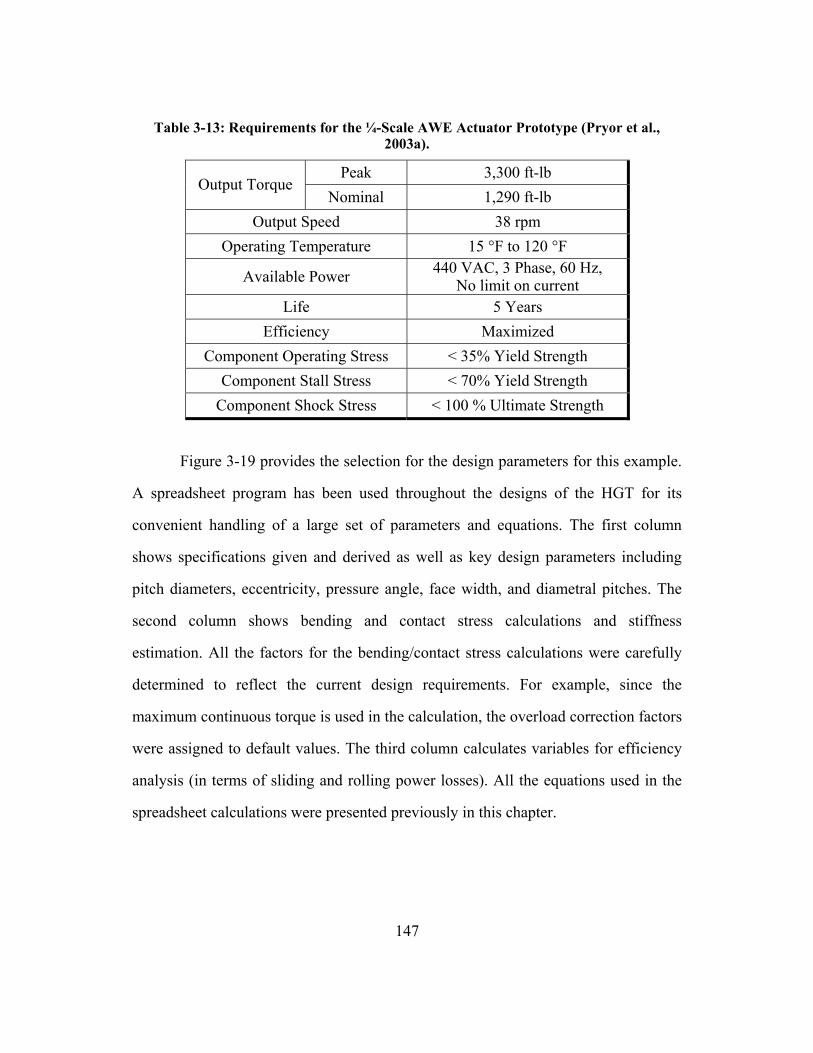
147

Table 3-13: Requirements for the ¼-Scale AWE Actuator Prototype (Pryor et al.,

2003a).

Peak 3,300 ft-lb Output Torque

Nominal 1,290 ft-lb Output Speed 38 rpm

Operating Temperature 15 °F to 120 °F

Available Power 440 VAC, 3 Phase, 60 Hz, No limit on current

Life 5 Years Efficiency Maximized

Component Operating Stress < 35% Yield Strength Component Stall Stress < 70% Yield Strength

Component Shock Stress < 100 % Ultimate Strength

Figure 3-19 provides the selection for the design parameters for this example.

A spreadsheet program has been used throughout the designs of the HGT for its

convenient handling of a large set of parameters and equations. The first column

shows specifications given and derived as well as key design parameters including

pitch diameters, eccentricity, pressure angle, face width, and diametral pitches. The

second column shows bending and contact stress calculations and stiffness

estimation. All the factors for the bending/contact stress calculations were carefully

determined to reflect the current design requirements. For example, since the

maximum continuous torque is used in the calculation, the overload correction factors

were assigned to default values. The third column calculates variables for efficiency

analysis (in terms of sliding and rolling power losses). All the equations used in the

spreadsheet calculations were presented previously in this chapter.

148

Figure 3-19: Design of the HGT for the ¼-scale AWE actuator prototype.

The reduction ratio was (-) 103.5 to 1, and the parameter E was set to 0.04

(4 %). According to these two values, all the pitch diameters were determined. The

pressure angle was assigned to a standard value, 20°. Face width was set to 1.5 inches

for each stage. Diametral pitch was set to 7.04 for both stages ensuring integer tooth

numbers. A conservative contact ratio was estimated to be 3, and 125 % of the evenly

divided load was assumed to be applied on the most loaded tooth. Based on these

parameters and the specified output torque (3,300 ft-lb), force analysis outputted the

maximum tangential forces of 5,259 lb (1st stage) and 4,649 lb (2nd stage)

respectively. Using these load values, bending and contact stresses, and

corresponding safety factors were calculated. Note that the Hertz stresses are very

149

low because of the convex-concave tooth profiles. Stiffness and efficiency were also

calculated; stiffness was calculated from the lost motion equation, and efficiency was

calculated from the sliding and rolling power loss formulae.

3.5.2 The Rugged Manipulator Actuator HGT Prototype

Section 1.3.5.2 provided background information about the Rugged Actuator

prototype development. This EM actuator prototype is designed for use in the elbow

of a robot manipulator to eliminate the human on-site involvement in depositing,

transporting, sorting, and packaging heavy materials in a radiation contaminated

environment. Since the manipulator will handle heavy items it will have to exert large

forces and resist shock loads on the actuators. The key design requirements are

repeated in Table 3-14. Two designs were delivered for the two different loading

conditions, nominal loading (1,500 in-lb) and peak loading (7,500 in-lb).

Table 3-14: Key requirements for the Rugged Actuator Prototype (Park et al., 2004).

Peak 7,500 in-lb Output Torque

Nominal 1,500 in-lb Out-of-Plane Moment Load 10,000 in-lb

Radial Load 3,650 lb Output Speed 20 rpm

Figure 3-20 and Figure 3-21 present the HGT design results for the nominal

loading and peak loading conditions respectively. The procedure is similar to that of

the ¼-scale AWE Actuator HGT. The reduction ratio was (+) 195 to 1, and the

parameter E was assigned to 0.033 (3.3 %). Based on these two values, all the pitch

diameters were determined. Pressure angle was set to 20° in this initial design, but

later on it was reduced to 7°. Face width of the HGT was set to 0.5 inches each stage,

150

but in the actual prototype it was increased to 0.75. The diametral pitch was assigned

to 15.625 for both stages. The estimated contact ratio was 3 for nominal, and 5 for the

peak loading condition. Load sharing factor was 175 % for nominal, and 125 % for

peak loading condition respectively. In summary, compared to the ¼-scale AWE

Actuator HGT, the Rugged Actuator HGT employed higher TR , lower E , lower φ ,

and higher dP .

Figure 3-20: Design of the Rugged Actuator HGT subject to nominal loading.

151

Figure 3-21: Design of the Rugged Actuator HGT subject to peak loading.

3.5.3 Balancing System Design

Table 3-15 presents a representative result of the balancing system design.

The total rotating unbalanced (eccentric) mass in the Rugged Actuator HGT was

6.534 lbm at an eccentric distance of 0.160 inches. Here, the balancing mass 1 had a

mass of 0.826 lbm at a radius of 1.204 inches from the actuator centerline and

distance of 1.217 inches from the references plane. Balancing mass 2 had a mass of

0.411 lbm, radius of 0.959 inches, and a distance of 2.011 inches. The total mass of

the rotating eccentric components and balancing mass became 7.771 lbm. The total

balancing counterweight mass is 1.237 lbm or 19 % of the unbalanced mass.

152

Table 3-15: Balancing design for the Rugged Actuator prototype (Park et al., 2005).

Eccentric Shaft Parameters Variable Value UnitsDensity of steel rho 0.284 lbm/in^3Length of eccentric shaft Le 1.766 inDiameter of eccentric shaft (ID of bearing) de 2.165 inDiameter of bearing (OD) dbo 2.835 inWidth of bearing (at OD) wb 1.378 inLength of eccentric shaft at shoulder Les 0.000 inDiameter of eccentric shaft at shoulder des 2.323 in

Widths and Other Parameters Variable Value UnitsDistance of COM of assembly from reference line dcom 3.940 inDistance between reference line and left end of eccentric shaft dref 2.987 inWidth of sun gear bearing ws 0.710 inWidth of balance mass 1 w1 0.527 inWidth of balance mass 2 w2 0.250 in

Eccentric Mass and Distance Parameters Variable Value UnitsMass of shaft (include shoulder weight) me 1.876 lbmMass of bearings (catalog) mb 1.356 lbmMass of wobble gear (reduce if drilled out) mg 3.302 lbmTotal eccentric mass m 6.534 lbmEccentric distance from the actuator centerline e 0.160 inDistance between assembly COM and mass 1 COM d1 1.217 inDistance between assembly COM and mass 2 COM d2 2.011 in

Forces of Unbalance Variable Value UnitsEccentric force (normalized by speed^2) Fe 1.045 in-lbmCentrifugal force Fc 475 lbfBalance mass 1 (motor side), total, which includes Al top lobe F1-Fal 0.651 in-lbmBalance mass 2 (output side) F2 0.394 in-lbm

Balancing Masses and Radii Parameters Variable Value UnitsInner radius of balance mass 1 and Al lobe (integral with shaft) ri1 1.375 inInner radius of balance mass 2 (subtract off ring) ri2 0.750 inOuter radius of balance mass 1and Al lobe ro1 2.325 inOuter radius of balance mass 2 ro2 2.060 inAngle of balance mass 1and Al lobe (must be less than 180°) alpha1 90 degAngle of balance mass 2(must be less than 180°) alpha2 90 degArea of mass 1 and Al lobe A1 5.521 in^2Area of mass 2 A2 5.782 in^2Center of mass 1 and Al lobe w/o holes R1 1.204 inCenter of mass 2 R2 0.959 inCenter of mass of Al lobe w/ holes (from SolidWorks) Ral 1.163 inActual mass 1 m1 0.826 lbmActual mass 2 m2 0.411 lbmActual mass Al lobe w/o holes (adjust material density) mal 0.285 lbmActual mass Al lobe w/ holes (from SolidWorks) mal 0.072 lbmActual F1 F1 0.995 in-lbmActual Fal (subtract off holes if using analytical method at right) Fal 0.343 in-lbmActual Fal (from SolidWorks) Fal 0.084 in-lbmActual F1-Fal (Analytical) F1-Fal 0.651 in-lbmActual F1-Fal (SW) F1-Fal (SW) 0.911 in-lbmF1-Fal residual R_F1-Fal 0.000 in-lbmF1-Fal residual (SolidWorks) R_F1-Fal (SW) 0.260 in-lbmRequired mass 2 m2r 0.411 lbmMass 2 residual Rm2 0.000 lbmSum(mi*ri) U 1.045 in-lbmFe-m*r Ures 0.000 in-lbmResulting center of mass Rres 0.000 inBalancing Force Ft 475 lbf

Resulting Force of Unbalance Fr 0.095 lbf

Total Mass M 7.771 lbm

153

CHAPTER 4

TOOTH PROFILE FOR THE HGT

4.1 INTRODUCTION

Chapter 3 looked at the system level design (the first two steps discussed in

Section 3.4.2) of the HGT. The parameters of interest in these design steps were

system level parameters (i.e., eccentricity to pitch diameter ratio E , face width b ,

and diametral pitch dP ) and the pressure angle φ . At the next level, the tooth level

parameters (see Table 3-8; i.e., tooth height h , thickness t , curvature radii r , tip

relief starting circle radius rR , tip relief radius rr , sliding velocity sV , rolling

velocities rV ) are crucial parameters as well for some important design criteria:

interferences, load capacity, efficiency, noise (vibration), and stiffness (lost motion)

(in the order of criticality; see Figure 3-13). In addition, tooth profile parameters also

influence the gear transmission’s performance sensitivity to the manufacturing errors.

Therefore, tooth profile selection and design is a very important step (the last step in

terms of the design procedure) for completion of the HGT design.

The goals of this chapter are: 1) to determine a basic tooth profile which will

allow the HGT to maintain its claimed advantages, and 2) to identify all the

parameters associated with the tooth profile for complete parametric design and

analysis. For preliminary selection of the basic tooth profile for the HGT, several

candidate tooth forms will be reviewed in terms of transverse and axial geometries

(Section 4.2). As a result, the circular-arc tooth profile with spur teeth will be selected

as a potential tooth form that will be the basis for the exceptional performance

154

advantages of the HGT. Section 4.3 will further support this selection. The circular-

arc tooth profile will be evaluated for the tooth level design criteria listed above plus

manufacturing error sensitivity. For some of the criteria, comparative analysis with

the involute profile will be performed for justification of the selection. Once the

circular-arc tooth profile is justified as the basic tooth profile for the HGT, parametric

design of the profile will be performed (Section 4.4). Design parameters for the

circular-arc tooth profile will be identified as well as their functional relationships.

Finally, an interactive graphical tool that enables automated generation of circular-arc

tooth profiles will be introduced (Section 4.5).

4.2 BASIC TOOTH PROFILES

4.2.1 Transverse Profile

Three profiles have been widely recognized as feasible transverse tooth

profiles. They are involute, cycloidal, and circular-arc tooth profiles. The involute

profile (Figure 4-1) is a nearly universal and standardized tooth form today for its

design simplicity, manufacturability, extensive field experience, and tolerance to

center distance error. Its generation and properties are well known, and backed by

long-determined standards. However, its medium to low load capacity, undercutting,

and interference problems have consistently encouraged gear designers to develop

alternative tooth profiles. Among numerous inventions, cycloidal and circular-arc

tooth forms have emerged as valid alternatives.

155

Figure 4-1: Representative involute profile for external gear (Chang & Tsai, 1992a).

The cycloidal profile (Figure 4-2) utilizes two generating epicycles to create

an epicycloid curve for its addendum and a hypocycloid curve for its dedendum (see

Figure 1-3 for depiction of these curves). This profile is unique in how it maintains

conjugate action36. Nonetheless, it has found limited application due to its low load

capacity, sensitivity to manufacturing errors, and large deviation of pressure angle

during operation (Dooner & Seireg, 1995). For this reason, cycloidal tooth profile

will not be considered as a candidate tooth profile for the HGT design.

Figure 4-2: Representative cycloidal profile for external gear (Chang & Tsai, 1992a).

A circular-arc profile (Figure 4-3) was first proposed in a patent by Wildhaber

(1926). A similar idea was reinvented and patented by Novikov (1956)37. Literally, it

employs circular-arcs as contact surfaces in either the plane normal to the face width

direction (Wildhaber’s idea), or the plane normal to the gear axis (Novikov’s idea). 36 Conjugate action theoretically ensures a constant speed ratio between input and output gears. 37 Circular-arc tooth profile is also referred to as the Wildhaber-Novikov (W-N) profile in some of the literature.

156

The essence of the idea is to enable two mating gear teeth to have a very low relative

curvature through the concave-convex geometry reducing surface contact stress and

sliding velocity while enhancing the entraining (rolling) velocity and lubrication

condition. These teeth also benefit from their lower bending stress due to their

relatively short height and increased thickness near the root of the tooth. All of these

characteristics are very desirable for load capacity and efficiency of the gear

transmission.

Potential drawbacks of the circular-arc tooth profile are its need for special

treatment for maintaining theoretical conjugate action and sensitivity (of the

conjugate contact) to center distance error. It is believed that these drawbacks can be

largely circumvented by careful design of tooth tip relief. Section 4.4.3 will discuss

the tip relief design in more depth.

Figure 4-3: Representative circular-arc profile for external gear (Chang & Tsai, 1992a).

4.2.2 Axial Profile

Due to its favorable performance benefits, the circular-arc tooth profile is

preferred in the HGT design as the tooth geometry on the transverse plane. This

preference over the involute profile will be further supported by the literature review

and comparative analyses in Section 4.3. As far as the axial profile is concerned, it is

157

noted that circular-arc tooth profiles discussed in the literature are mostly in helical

configuration with a few exceptions. This is because Wildhaber’s original circular-arc

gear was designed to sustain the conjugate action by axial movement of contact.

Nonetheless, the HGT prototype designs have been decided to employ spur teeth

mainly for the following reasons:

1) Reduced complexity in the design and fabrication

2) Elimination of the axial forces exerted on the bearings

3) Prevention of axial excitations which can cause noise and vibration.

As briefly mentioned in the previous section, it is believed that conjugate

action of the circular-arc profile in spur teeth can be maintained through careful

design of tooth tip relief based on tooth-to-tooth clearance and interference control

that accommodates tooth deformation under load. Note that, even with any profile

which theoretically guarantees conjugate action, it is difficult to sustain this property

(i.e., constant input-output speed ratio) because of errors from deformation, wear,

manufacturing imperfection, assembly, and temperature influences. Refer to Section

3.2.8 for a listing of numerous sources of the transmission error.

As far as noise and vibration are concerned, helical gears are usually

considered to be quieter than spur gears because of the added axial contact ratio (also

called overlap ratio) to the common transverse contact ratio. However, it is possible

that the beneficial effect of the added axial contact ratio is diminished by the axial

shuttling excitation mentioned earlier. Furthermore, in order for the helical gears to

have a sufficient axial contact ratio (i.e., > 1.5) the face width should be increased

which is constrained by the designed helix angle. The following parametric study

illustrates this design process.

158

The axial contact ratio axialCR is given by (see Figure 4-4 for nomenclature of

the parameters):

tanaxial

c

bCRPλ

= (4.1)

where b = face width

λ = helix angle

cP = circular pitch

Equation (4.1) can be rewritten with respect to the face width b as below:

tan

caxial

Pb CRλ

= (4.2)

For axialCR to be greater than 1.5, the face width b should be bounded by the

following inequality constraint:

1.5tan

cPbλ

≥ (4.3)

cP

λ

b

Figure 4-4: Helical tooth parameters (only contact sides are shown with bold lines).

For example, if cP = 0.45” (the ¼-scale AWE Actuator HGT design) and λ = 15º,

the face width b should be equal to or greater than 2.52” which is 68 % longer than

the present spur gear design’s face width, 1.5”. Increasing the helix angle would

permit a shorter face width for a fixed contact ratio and circular pitch, but it could

159

adversely affect the load capacity. Attia and El-Bahloul (1990)’s fatigue tests of

circular-arc helical gears of different helix angles38 showed that gears with higher

helix angles failed faster than low helix angle gears for the same speeds and

lubrication viscosities. Lingaiah and Ramachandra (1981) recommended that the

helix angle be 7.5 to 15.0º for optimal load capacity of the circular-arc helical gears.

They found that higher helix angles result in decreases in the contact area of the

circular-arc gears. Using an optimal helix angle, λ = 10º, with the same cP = 0.45”

and b = 1.5”, the axial contact ratio of the ¼-scale AWE Actuator HGT would have

been less than 0.6, which gives an insufficient reason for using helical gears for the

present configuration. This shows that using helical gears in the gear transmission

does not always guarantee a higher contact ratio. In order to achieve the supposed

advantage of the helical gear design (quiet operation from additional axial contact

ratio), good parametric decision on the helix angle, face width, and circular pitch

should be made based on the load capacity constraints (i.e., allowable stresses).

Regardless of the axial configuration, crowning of the tooth profile has been

found to be advantageous in localizing the contact and accommodating some meshing

errors of the gears. Allowing the tooth to have a slight curve in the face width

direction, crowning makes the bulged portion carry the full share of the load, and

effectively accounts for misalignment and distortion of two gears in mesh. An FEA

simulation of the effects of crowning on contact stress in circular-arc gears can be

found in (Chen & Tsay, 2002).

The literature study presented in the next section (Section 4.3) discusses

unique advantages of the circular-arc gears which have inspired its exploitation in the

38 The axial ratio was fixed to around 1.2 making the face widths all different, i.e., 42 mm, 29 mm, and 24 mm for helix angles of 22.3°, 33.6°, and 42.25° respectively.

160

tooth profile design for the HGT. However, due to the difference in axial

configuration pursued in between its original design (helical) and the HGT design

(spur), not all the discussions and comparative studies in the literature are directly

applicable for justifying its use in the HGT. The justification will be strictly based on

the facts that are commonly applicable for both spur and helical configurations. Note

that there exist common performance properties that both circular-arc configurations

share due to their identical forms in the transverse plane.

4.3 CIRCULAR-ARC GEARS

This section will investigate the potential benefits that the circular-arc tooth

profile will bring to the HGT design. We begin by discussing past applications and

the on-going development of circular-arc tooth profiles (Section 4.3.1), which will be

followed by a discussion on the geometry and kinematics of the profiles (Section

4.3.2). Then, in-depth discussion on circular-arc gears for each performance criterion

will be provided (Section 4.3.3 through 4.3.8). The performance criteria to be

discussed are interference, load capacity, efficiency, noise (vibration), stiffness (lost

motion), and sensitivity to errors (from the most critical criterion to the least critical

criterion for tooth level design, as suggested in the categorization diagram in Figure

3-13). Comparative analysis will be performed for some of the criteria. Finally, all the

findings and arguments made will be compiled to support the selection of the

circular-arc tooth profile over the involute profile for the HGT implementation.

4.3.1 Applications and Development

Circular-arc gears were given considerable attention in the 1960’s, but

reviewed thereafter by a limited number of researchers from Russia, UK, Germany,

161

Japan, and China. Circular-arc gears have not found widespread industrial

application. In fact, it has been totally ignored in the U.S. Allan (1965) states that the

circular-arc gears were initially considered by the Russians for application to turbo-

prop engines, helicopters, aircraft and marine drives which required very high load

capacity.

The first commercialization of circular-arc gears was done by a Japanese

company. They were called SymMarC and Haseg SymMarC (trademark of Hitachi

Ltd.). The addendum and dedendum of the cutter profiles are circular-arcs of the

same radius, and centers of both arcs are located on the pitch circle. They provide for

two points of contact at the gear mesh. In-depth analysis of these gears can be found

in (Oda et al., 1991; Oda et al., 1993; Oda & Koide, 1996).

Figure 4-5: SymMarC & Haseg SymMarC gear cutters (Oda et al, 1993; Oda & Koide, 1996).

Another commercialization was done by Associated Electrical Industries Ltd.

(Rugby, England) under trademark ‘Circarc’ (Wells, & Shotter, 1962). They tested

and compared the performance of the Circarc system with an involute gear box to

demonstrate its potential in a range of applications.

Probably the most successful real-world application of circular-arc gearing in

its history would be its utilization in the final reduction stages of the rotor drive

162

gearboxes of the Lynx and W-30 aircraft (Figure 4-6). They were manufactured by

Westland Helicopters Ltd. (Shotter, 1977). Successful exploitation of circular-arc

gears in such a critical service encouraged their further adoption in applications

where reliability and power to size/weight ratio were vital.

Figure 4-6: Gearbox manufactured by Westland Helicopters Ltd. (Astridge et al, 1987).

Double circular-arc gears employing two zones of contact at upper and lower

surfaces of the teeth have been standardized in Russia (GOST) and China (Chinese

Standard GB). This modified circular-arc profile is called double circular-arc tooth

profile (see Figure 4-7). The main advantage is further reduction of the bending

stresses while keeping the advantages of already low contact stresses. Chen and

Wang (2001) state that double circular-arc gears with precision hobbing or shaving

and tempering can replace surface-hardened and ground involute gears. Due to its

high load capacity, long service life, simplicity in manufacturing and low cost, double

circular-arc gears have found wide applications at low to medium operational speeds

such as mining, petrochemical industries, shipbuilding, etc. Proponents are currently

seeking applications in heavy-duty transmissions at higher operational speeds. In-

depth analysis of double circular-arc gears can be found in (Yakovlev, 1989; Litvin,

& Lu, 1993; Litvin, & Lu, 1997; Chen, & Wang, 2001).

163

Figure 4-7: Double Circular-arc tooth profile (left) (Litvin et al, 2000), and contact condition (right) (Litvin & Lu, 1997).

The most recent development (Litvin et al, 2000) suggests a new circular-arc

profile which can be fabricated by a parabolic rack cutter (see Figure 4-8). It claims

lower noise and vibration which makes it suitable for high-speed gear transmissions.

It is also claimed to provide higher bending and contact strength, less sensitivity to

manufacturing errors, and ease of surface treatment.

Figure 4-8: New circular-arc (left) and rack cutter profiles (right) (Litvin et al, 2000).

4.3.2 Geometry and Kinematics

The circular-arc gear pair considered in this research basically consists of two

circular-arcs in the transverse plane, the main circular-arc of the driving pinion

normally being convex and that of the mating gear tooth surface concave. There are

three kinds of circular-arc gears: all-addendum convex pinion with all-dedendum

concave gear, all-dedendum concave pinion with all-addendum convex gear, and

164

combination of these two. As mentioned earlier, modified forms such as double

circular-arc gears are also available.

Dyson et al. (1989) provided an extensive geometric and kinematics study for

the circular-arc gears. Their geometric presentation of external and internal pairs of

circular-arc gears are shown in Figure 4-9 and Figure 4-10 respectively. In their

study, they provided contours of the contact between a typical pair of circular-arc

gear teeth in mesh. They obtained expressions for the entraining (rolling) and sliding

velocities at the point of contact, and showed the directions and magnitudes of the

velocities on the contours.

Figure 4-9: Dyson et al. (1989)’s geometrical presentation of an externally meshing pair of circular-arc tooth profiles.

165

Figure 4-10: Dyson et al. (1989)’s geometrical presentation of an internally meshing pair of circular-arc tooth profiles.

The ideal contact situation would occur when the convex and concave profile

radii are made equal and full contact occurs over the length of the arcs. However, this

condition necessitates the center distance between the gear shafts to be accurate. Even

a slight change in the center distance can cause the contact to move to the tip of either

mating tooth. In Wildhaber’s original design (1926) the profile radii of the pinion and

gear teeth were equal, but later on he suggested the radius of the concave profile be

made slightly larger than that of the convex. As a rule of thumb, the radius of the

circular-arc of the pinion 1ρ is made equal to the reciprocal of the diametral pitch

dP (Chironis, 1967):

11

dPρ = (4.4)

while the circular-arc of the gear 2ρ is determined using a similar estimates:

2 11.05ρ ρ≥ (4.5)

The difference of these radii provides an accommodation for the likely center

distance errors. As the difference between the two radii increases, the gears become

166

more tolerant to the center distance errors at the expense of increased Hertz stress.

Therefore, optimization of these two conflicting cost functions is key to the

successful design of circular-arc gears (Dyson, Evans, & Snidle, 1986). The amount

of tolerance that can be accommodated in the center distance, CD∆ , is given by

Allan (1965):

22 sin cosCD ζρ γ φ∆ = (4.6)

where ζ = fractional difference in profile radii, 2 1(1 )ρ ρ ζ= −

γ = angle subtending to contact arc (see Figure 4-11)

φ = pressure angle

Figure 4-11: Effect of profile curvature radii on center distance tolerance (Allan, 1965).

An important difference between circular-arc and involute gears is their

contact characteristics. Theoretically, circular-arc gears (in helical configuration)

167

make a point contact while involute spur gears make a line contact. In reality, under

normal load on the tooth face, the contact point of circular-arc gears becomes an

ellipse, and the contact line of the involute gears results in a straight rectangular

region.

The sliding velocity between the mating involute teeth varies significantly.

For circular-arc (helical) gears, there is a dominant entraining velocity in the axial

direction, but the sliding velocity (in the direction perpendicular to the entraining

velocity component) is very small (or zero) because the motion of the contact across

the face width occurs at a constant distance (or zero distance) from the pitch point.

The magnitude of the entraining (in the face width direction) velocity rV can be

approximated by the following equation (French, 1966):

sin

pr

VV

λ= (4.7)

where pV is the pitch line velocity of the gear

λ = helix angle.

The magnitude of the sliding velocity sV can be obtained by the following equation

(Davies, 1960):

1 2( )sV CP ω ω= − (4.8)

where CP = distance between point of contact C and pitch point P

ω = angular velocity of pinion (1) and gear (2).

Depending on the design, the magnitude of sliding velocity is about 3 % to 15 % of

the entraining velocity (Shotter, 1977). For spur tooth configuration, there is no

entraining motion in the axial direction.

168

4.3.3 Interferences

The limitations of the involute profile in terms of tooth-to-tooth interferences

especially for use in the internal gears were already discussed in Section 3.2.6. For

effective avoidance of the tooth interferences, careful parametric design of the tooth

profiles should be performed (i.e., determination of tooth height, addendum and

dedendum ratio, tooth curvature radii, relief starting point, etc.; see Chapter 5 for

detail). Since the original circular-arc profile maintained conjugate action through

axial movement of the contacts, managing the tooth height was possible which made

it easier to eliminate unwanted contacts. Nonetheless, it has been realized that even

with the circular-arc tooth profiles avoidance of interference becomes challenging at

low pressure angles (Shotter, 1977; Dyson, Evans, & Snidle, 1986)39.

Using tooth meshing analysis, the circular-arc tooth design effort of the

present research has successfully minimized the pressure angle down to 7º without

causing any tooth interference (geometric overlap) in the Rugged Actuator HGT

design. Further minimization of the pressure angle (to 5º) for the same system has

been attempted. See Chapter 5 for more details on this design effort.

4.3.4 Load Capacity

Experimental results have shown that a substantial increase in load capacity

can be obtained with circular-arc gears. Allan (1965) reported three test results

showing the high load-carrying capability of circular-arc gears. The first tests carried

out by Novikov showed that circular-arc gears could carry almost four times the load

that involute gears could carry under the same geometry condition. The second test 39 Most of the studies in the literature dealt with circular-arc gear teeth in external gear pairs where errors in the center distance can dramatically affect the conjugate action of circular-arc gear teeth whose contact curvature radii are nearly equal.

169

by the Voroschilivgrad factory for 14 circular-arc gears with a helix angle of 12° at

pitch line velocity of 30 ft/s and 45 ft/s, showed their load capacity was up to 3.5

times that of involute gears with the same conditions. The other test by the

Nikolayevsk factory for highly loaded circular-arc gears with helix angles of 17° at

pitch line velocity of 180 ft/s revealed an increase of the load capacity by of a factor

of three compared to the involute gears.

The high load capacity of the circular-arc gears was continuously

demonstrated in other literature. Associated Electrical Industries Ltd. (Wells &

Shotter, 1962) reported more than five times improvement in pitting resistance with

circular-arc gears in comparison to involute gears. Shotter (1977) argued that the load

capacity of circular-arc gears appears to be about 1.5 times that of the involute for

case hardened and ground gears, and about three times for lower strength steel cut

gears. Section 4.3.4.1 through Section 4.3.4.3 will further discuss the load capacity of

the circular-arc gears in terms of bending strength, contact strength, and lubrication

respectively. Section 4.3.4.4 will demonstrate the advantages of a highly conformal

tooth profile, i.e., circular-arc profile, by comparing contact area and maximum

contact pressure of the profile with those of two conventional tooth profiles (involute

spur and involute helical).

4.3.4.1 Bending Strength

Since the basic Lewis equation (Equation (3.45)) indicates that the bending

stress proportionally decreases with the square of tooth thickness t and increases

linearly with tooth height h , pursuit of a high strength tooth form has been largely

directed towards improving the thickness to height ratio ( /t h ). The short and wide

form of the circular-arc teeth can significantly reduce the bending stress as discussed

170

earlier. Allan (1965) also indicates that it is practical for circular-arc gears to have

varying tooth width without altering the profile radius. This inherent advantage in

geometry of the circular-arc gear ensures high bending strength. Note that the

standard full-depth involute tooth profile is subject to repeated tip loading which

results in large fluctuation of load (which can cause vibration and noise) and thus

significant fatigue failure.

There exist some literature which discusses the bending strength of circular-

arc gears. Yakovlev (1989) provided an insight into the bending characteristics of the

circular-arc gears and suggested a proper range of the gear module (pitch diameter in

millimeters over tooth number) that provides for high bending strength. Tsay et al.

(1989) performed FEA to evaluate the bending stresses of circular-arc gears, and

found that the maximum principal stress was highest when the tip of the concave

tooth made contact with the root fillet of the convex tooth. The maximum principal

stress decreased as the loading position moved from the root fillet to the tip of the

convex tooth. This observation proposes an optimum contact region for the circular-

arc gear mesh. The double circular-arc gears introduced in Section 4.3.1 are designed

to reinforce the bending property of the circular-arc gears. Recall that the double

circular-arc gear employed two zones of contact, at the upper and lower surfaces (see

Figure 4-7), to significantly reduce the bending stress while keeping the inherent

advantages of its already low contact stresses.

4.3.4.2 Contact Strength

The most common pattern of gear tooth failure is initiated by Hertz contact

stresses combined with inadequate lubrication. Under a mixed lubrication condition

in which partial metal-to-metal contact between surface asperities occurs, micro-

171

pitting appears on tooth surface (see 1 of Figure 4-12). The micro-pitting develops

into macro-pitting (see 2 of Figure 4-12) which develops into uneven dynamic

loading and vibration in the gears. This macro-pitting further develops into scoring,

or tooth breakage (see 3 and 4 of Figure 4-12). The surface durability (resistance) of

gear teeth against pitting and scoring is reliably indicated by Hertz theory.

1 2

3 4

1 2

3 4

Figure 4-12: (1) Micro-pitting, (2) macro-pitting, (3) scoring, and (4) tooth breakage (Dudley, 1994).

The principle idea of the circular-arc tooth profile was to employ a highly

conformal concave-convex tooth mesh which can significantly improve the Hertz

contact condition (see Section 3.2.5.2 for the parametric argument on this). Table 3-5

showed that the geometry factor (which reflects the mesh conformity – the similarity

of the curvature at the point of contact) would allow for 4.5x higher contact strength

than standard practice in the case when circular-arc teeth are used in the HGT (the ¼-

scale AWE Actuator HGT).

Experiments and analytics in the literature have supported this theoretical

assessment. Chironis (1967) used his calculation and Russian test results to show that

172

at least three times the load capacity is possible for circular-arc gears at a helix angle

of 20° or less compared to involute gears given the same pressure angle. Ishibashi

and Yoshino (1985) experimentally proved that the contact stress of circular-arc gear

teeth is reduced with decrease of the difference in the profile curvature radii. Dyson

et al. (1986) indicated that minimizing contact stresses in the involute gears was

geometrically limited whereas it was not for the circular-arc gears which could have

virtually any combination of the profile curvature radii. Ishibashi (1987) compared

the maximum contact pressure of the circular-arc with the involute, both in a plastic-

gear and steel-pinion combination. Given the same amount of load, the circular-arc

gears maintained the maximum pressure of only about 10 % of that of the involute.

This experiment supported the typical success of using the circular-arc profile in soft

gears. Plastic circular-arc gears can bring great advantages in light-to-medium load

applications allowing for reduced weight, extreme quietness, and reduced cost.

Astridge et al. (1987) compared the contact area and the maximum contact stress of a

circular-arc gear (measured) and an involute gear (calculated). The contact area of the

circular-arc gear was 50 % larger than that of the involute gear while the maximum

contact stress of the circular-arc gear was 10 % lower than that of the involute gear.

Tsay et al. (1989) argued that the contact stress of the circular-arc gears can be

reduced by 25 % of the contact stress of traditional involute helical gears by properly

choosing the curvature radii of the circular-arc tooth pair.

4.3.4.3 Lubrication

It has been proven analytically (Hanna, 1985; Evans & Snidle, 1993; Tsay,

1995), or experimentally (Ishibashi & Yoshino, 1985; Attia & El-Bahloul, 1988; El-

Bahloul, 1989) that the lubrication condition of circular-arc gears is very favorable in

173

terms of the load capacity. Wells and Shotter (1962) used electrical resistance

measurements to give an indication of relative elastohydrodynamic (EHD) film

properties. The tests illustrated that the load capacity of circular-arc gears was up to

6.5 times greater than that of involute gears. El-Bahloul (1989) showed that the EHD

film thickness of circular-arc gears could go up to 12 times that of involute gears

depending on speed. This superior EHD film thickness of circular-arc gears is

explained as follows:

a) Circular-arc gears can retain the oil better than involute gears due to close

conformity and the low constant sliding velocity compared to the variant

(with high peak) sliding velocity between the involute teeth (El-Bahloul,

1989; Esposito & Belfiore, 2000).

b) Higher entraining velocity in circular-arc helical gears produces a strong

hydrodynamic action that forms rapid movement of the oil (Evans & Snidle,

1993; Tsay, 1995; Litvin et al, 2000).

El-Bahloul (1989) also showed that an increase of speed has more effect on

increasing the EHD film thickness for circular-arc gears than for involute helical

gears. This argument encourages high-speed application of circular-arc gears.

4.3.4.4 Comparative Analysis

For demonstration of the advantages of a highly conformal tooth profile (i.e.,

circular-arc), three gear systems with different tooth forms, i.e., involute spur,

involute helical, and circular-arc gear systems, are compared for the contact area and

the maximum contact stress. The Hertz theory is used to analyze these two contact

performance properties. Figure 4-13 shows the contact condition to be considered for

174

the circular-arc gears40. It employs a slight crowning on the contact surfaces. Thus,

there exist four principal curvatures that influence the contact properties, i.e., 1R ,

2R , 1R′ , and 2R′ . While 1R and 2R are radii of curvatures of the transverse tooth

profile (on the plane containing y and z in Figure 4-13), 1R′ and 2R′ are radii of

curvatures of the axial tooth profile (on the plane containing x and y in Figure 4-13).

Subscripts are pinion (1) and gear (2) respectively.

Figure 4-13: Contact condition of circular-arc gears (Lingaiah & Ramachandra, 1981).

1R and 2R are equal to the tooth curvature radius 1ρ and 2ρ− :

1 1

2 2

RR

ρρ

== −

(4.9)

1R′ and 2R′ are represented by Tingjian (1992) as below:

40 The circular-arc tooth pair shown in Figure 4-13 is in a helical configuration. This is the reason why the involute helical gear is included in the comparison for useful analysis.

175

21 1

1 2

22 2

2 2

sin sinsin sin

sin sinsin sin

p

p

rR

rR

ρ φ λφ λ

ρ φ λφ λ

+ ⋅′ =

⋅

+ ⋅′ =

⋅

(4.10)

where 1 2, p pr r = pitch radius of pinion (1) and gear (2), respectively

, φ λ = pressure angle and helix angle, respectively

Considering the tangent plane at the point of contact as the x-y plane, the

surfaces of the bodies near the point of contact by neglecting small quantities of

higher order are represented by the surfaces of the second degree (Timoshenko &

Goodier, 1970) as follows:

2 2

1 1 2 32 2

2 1 2 3

z A x A xy A y

z B x B xy B y

= + +

= + + (4.11)

The distance between two points on the surfaces in the small is then

2 21 2 1 1 2 2 3 3( ) ( ) ( )z z A B x A B xy A B y+ = + + + + + (4.12)

Taking such directions for x and y as to make the term containing xy disappear:

2 21 2z z Ax By+ = + (4.13)

where A and B are functions of the magnitudes of the principal curvatures of the

surface in contact (Timoshenko & Goodier, 1970). They are determined as follows:

1 1 2 2

12 2 2

1 1 2 2 1 1 2 2

1 1 1 1 12

1 1 1 1 1 1 1 1 12 cos 22

A BR R R R

B AR R R R R R R R

ψ

⎛ ⎞+ = + + +⎜ ⎟′ ′⎝ ⎠

⎡ ⎤⎛ ⎞ ⎛ ⎞ ⎛ ⎞⎛ ⎞⎢ ⎥− = − + − + − −⎜ ⎟ ⎜ ⎟ ⎜ ⎟⎜ ⎟′ ′ ′ ′⎢ ⎥⎝ ⎠ ⎝ ⎠ ⎝ ⎠⎝ ⎠⎣ ⎦

(4.14)

176

where ψ = angle between the normal planes containing 1R and 2R . For this

analysis, 0ψ = . ( )A B+ and ( )B A− are related by the auxiliary angle θ , given

by

1cos B AA B

θ − −⎛ ⎞= ⎜ ⎟+⎝ ⎠ (4.15)

Using the value of θ , the constants an and bn for the following equations

(Equation (4.16)) can be determined either from the table (p. 416) provided by

Timoshenko and Goodier (1970), or functional relationships provided by Colbourne

(1989). Here, a and b are the magnitudes of the semi-major axis and semi-minor

axis of the contact ellipse respectively (Lingaiah & Ramachandra, 1981):

13

13

1.5

1.5

na

nb

F Ca nA B

F Cb nA B

π

π

⎛ ⎞= ⎜ ⎟+⎝ ⎠

⎛ ⎞= ⎜ ⎟+⎝ ⎠

(4.16)

The associated nF (normal force) and C (material constant) are given by

2

cos cos(1 )

tn

FFCR

CE

α βν

π

=⋅ ⋅

−=

(4.17)

where ν = Poisson’s ratio and E = Young’s modulus. Then, the contact area is

calculated by

cA abπ= (4.18)

177

Since the intensity of pressure p over the surface of contact is represented by the

ordinates of a semi-ellipsoid constructed on the surface of contact (El-Bahloul, 1992),

it is calculated by

1

2 2 2

2 21ox yp pa b

⎛ ⎞= − −⎜ ⎟

⎝ ⎠ (4.19)

where the maximum contact pressure op at the center is determined by

32

no

c

FpA

= (4.20)

This procedure was applied to circular-arc (helical), involute spur, and

involute helical gears for a comparison of the contact area and maximum contact

pressure. The object system was the 100:1 ratio 3K Paradox epicyclic gear

transmission designed by Park and Tesar (2000) (see Section 1.3.3 for description).

The reason for analyzing this system instead of the HGT is: 1) it has both external

and internal gear meshes, and 2) involute profiles are not applicable for the HGT. All

the necessary parameters for specifying the tooth profiles were taken from (Park &

Tesar, 2000). Table 4-1 shows some of the key geometry parameters of the design

object.

Table 4-1: Key geometry parameters of the 3K Paradox epicyclic gear transmission (Park & Tesar, 2000).

Gear Pair Sun-Planet Ring-Planet Pitch Radius [in] 0.875 / 0.55 1.975 / 0.55

Number of Pinion Teeth 35 22 Diametral Pitch 20 20

Pressure Angle [deg] 20 20 Face Width [in] 0.27 0.27

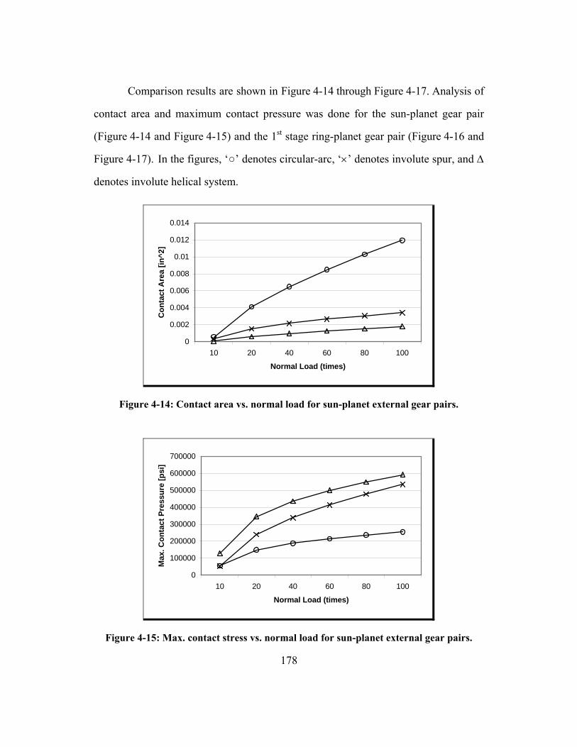
178

Comparison results are shown in Figure 4-14 through Figure 4-17. Analysis of

contact area and maximum contact pressure was done for the sun-planet gear pair

(Figure 4-14 and Figure 4-15) and the 1st stage ring-planet gear pair (Figure 4-16 and

Figure 4-17). In the figures, ‘○’ denotes circular-arc, ‘×’ denotes involute spur, and ∆

denotes involute helical system.

0

0.002

0.004

0.006

0.008

0.01

0.012

0.014

10 20 40 60 80 100

Normal Load (times)

Con

tact

Are

a [in

^2]

Figure 4-14: Contact area vs. normal load for sun-planet external gear pairs.

0

100000

200000

300000

400000

500000

600000

700000

10 20 40 60 80 100

Normal Load (times)

Max

. Con

tact

Pre

ssur

e [p

si]

Figure 4-15: Max. contact stress vs. normal load for sun-planet external gear pairs.

179

0

0.005

0.01

0.015

0.02

0.025

0.03

0.035

1 2 3 4 5 6

Normal Load (times)

Con

tact

Are

a [in

^2]

Figure 4-16: Contact area vs. normal load for ring-planet internal gear pairs.

0

100000

200000

300000

400000

500000

600000

1 2 3 4 5 6

Normal Load (times)

Max

. Con

tact

Pre

ssur

e [p

si]

Figure 4-17: Max. contact stress vs. normal load for ring-planet internal gear pairs.

For both external and internal gear pairs, contact areas of the circular-arc

system become significantly larger under increasing load than the other tooth systems

(Figure 4-14 and Figure 4-16). This condition also works favorably to increase the

mesh stiffness of the gear transmission. The maximum contact stresses of the

180

circular-arc gear system are the lowest among the three systems for both external and

internal gear pairs (Figure 4-15 and Figure 4-17). This comparative analysis

demonstrates that the tooth profile with the highest conformity, i.e., circular-arc tooth

profile, has exceptional advantages in terms of the Hertz contact characteristics over

conventional gear tooth profiles with lower conformities.

4.3.5 Efficiency

Several published papers compared the efficiency between circular-arc and

involute gears based on test results. Wells and Shotter (1962) reported that circular-

arc gears were more efficient than involute gears under same speed and load

conditions. The highest efficiency measured for their circular-arc gears was 99.4 %.

Davies (1960) recommended the circular-arc gear for its almost zero sliding velocity

at the vicinity of the pitch point. He suggested that the circular-arc gear at very low

operational speeds (with boundary lubrication condition) would be less efficient than

an involute gear, but at high speeds (with EHD lubrication condition) circular-arc

gears would be more efficient than the involute gear. His presumption was proven by

Ishibashi and Yoshino (1985). They tested four different lubricants in their efficiency

tests. Efficiency of the circular-arc gear was higher than that of the involute gear

above 100 rpm with three out of four lubricants. They concluded that efficiency of

circular-arc gears could be lower than that of the involute gear at the startup or

extremely low load, but it was generally higher for most of the speed range.

Computation of system efficiency is often approximated by evaluating the

sliding (friction) power losses in the gear system since the sliding power losses

account for a major portion of the total power losses in the gear system. The

181

expression for the sliding power loss of the circular-arc gear is in the form of

Equation (3.19), given by Dyson et al. (1986):

1(1 )loss nP CP TR Fµ ω −⎡ ⎤= ⋅ ⋅ ⋅ + ⋅⎣ ⎦ (4.21)

where µ = coefficient of friction

CP = distance between contact point and pitch point

ω = angular velocity of pinion

TR = gear ratio (negative for internal mesh)

nF = normal force of contact between pinion and gear teeth

The bracketed term in Equation (4.21) is an expression for the sliding velocity of the

circular-arc gear, which is equivalent to the expression given by Equation (4.8).

Sliding power losses of the circular-arc gear and the involute gear were

compared for the 3K Paradox planetary gear transmission which was analyzed for

contact properties in Section 4.3.4.4. Sliding power losses of the circular-arc gears

were evaluated using Equation (4.21) while those of the involute system were

evaluated using formulae provided by Anderson and Loewenthal (1982). For a

constant coefficient of friction of 0.05, the total combined sliding power loss (at the

sun-planet, 1st stage ring-planet, and 2nd stage ring-planet) of the circular-arc system

was 27 % less than that of the involute system.

4.3.6 Noise and Vibration

Attia (1989) compared the noise of three types of helical gears: involute,

circular-arc, and double circular-arc gears for an external gear mesh. Results showed

that the involute helical gears were the quietest among the three, and affected least by

the changes of the transmitted load and operation speed. The next quietest was the

182

circular-arc helical gear, followed by the double circular-arc helical gear. This is

mostly because of the relatively high transverse contact ratio in the involute helical

gears (when long teeth are used for external gear mesh), but when applied for the

HGT, this advantage for the involute profile is not available due to the impracticality

of the long teeth.

Attia also found that tooth crowning was more effective for the circular-arc

and double circular-arc gears than for the involute helical gears for noise reduction.

This encourages consideration of the crowning of the teeth for the circular-arc gears

if they were used in the HGT and suspected to be responsible for the noise.

Smith (2003) indicated that helical gears can produce axial excitation due to

the varying resultant force as the contact areas move axially along the face widths of

the gears. As discussed earlier, the axial excitation in the helical gears may diminish

the supposed benefit of their noise and vibration reduction (owing to the axial

overlap). This was one of the reasons why the HGT has been designed with spur gear

teeth (see Section 4.2.2 to review this argument).

4.3.7 Stiffness (Lost Motion)

The stiffness of a gear transmission is measured by applied torque divided by

angular deflection at the output. Tooth stiffness analysis necessitates exact analysis of

load sharing over multiple contacts as well as deflection occurring at every tooth pair

in contact (due to bending, shear, Hertzian deformations and tooth base rotation).

There is little study done on this performance criterion, especially for circular-arc

gears. Tingjian (1992) presented a formula for Hertzian deflection Hδ between two

circular-arc tooth surfaces:

183

1

2 2 2 34 ( )H nF C A Bδ ξ π⎡ ⎤= +⎣ ⎦ (4.22)

where ξ = coefficient related to ( ) /( )B A A B− + (equivalent to λ of Figure 7 in

(Tingjian, 1992))

, nF C = normal force and material constant obtained from Equation (4.17)

( )A B+ = obtained from Equation (4.14)

This equation, however, cannot represent the total deformation of the circular-arc

tooth mesh because the portion of the Hertz deformation is expected to be very small

due to the close conformity between two contact surfaces, compared to the convex-

convex tooth contact in the conventional gears. The other deformation sources, i.e.,

bending, shear, and tooth base rotation, should be evaluated to determine the total

deformation of the circular-arc tooth mesh. Note that, from the simple beam theory,

the bending deflection is proportional to the cube of the beam (tooth) height h and

thickness t ratio:

33 4

3t t

bF h F h

EI Eb tδ ⎛ ⎞= = ⎜ ⎟

⎝ ⎠ (4.23)

Therefore, reducing the tooth height to thickness ratio ( /h t ) is very desirable (by the

cube rate of the ratio) in reducing the bending deflection of the tooth. With relatively

low height to thickness ratio of the circular-arc teeth, the portion of the bending

deformation out of the total deformation should be small as well.

As shown in the comparative analysis of the contact area (Figure 4-14 and

Figure 4-16 in Section 4.3.4.4), the circular-arc gear system (with slightly crowned

teeth) showed exceptional increases in the contact area under increasing loads. This

works favorably for the mesh stiffness; as the contact area increases the stiffness of

the mesh is further increased. With multiple circular-arc tooth pairs in contact under

184

load, the HGT is believed to provide superior mesh stiffness over the conventional

gear transmissions.

4.3.8 Sensitivity to Errors

Important errors in the gear transmission that can significantly affect the tooth

contact characteristics are center distance (between two shafts) error and axial

misalignment error. These errors are caused by deflections in casing, shaft, bearings,

gear bodies, and manufacturing inaccuracy. Change in center distance leads to the

movement of the contact position on the tooth surface along with the varying

resultant load. Higher tolerance to the center distance errors can be achieved by

increasing the difference between the tooth profile curvature radii and by reduction of

the pressure angle (Equation (4.6)). Also, localization of contacts by the original

circular-arc gear reduces the sensitivity of the gear system to the misalignment errors.

Allan (1965) provided the analytic description of the center distance error in

terms of the circular-arc profile parameters, 1ρ , 2ρ , γ , and φ , as shown in

Equation (4.6) (see Figure 4-11 for nomenclature). Ou and Seireg (1986) used an

interactive graphics technique to predict the contact situation of circular-arc gears

under center distance errors, misalignment errors, and deflection conditions. Dyson et

al. (1989) provided graphical illustrations of the changes in pressure angle with

respect to the center distance change. Esposito and Belfiore (2000) analyzed the

sensitivity of pressure angle to the variation of the center distance for a series of

helical gears, and applied the results to the case of circular-arc gears. Chen and Tsay

(2001) studied the relation between the center distance change and the contact ratio

for involute tooth pinion and modified circular-arc tooth gear pair. Their results

showed the pressure angle and the contact ratio slightly increased with negative

185

center distance variation, CD−∆ (reduction of the center distance), while they

slightly decreased with positive center distance variation, CD∆ (increase of the

center distance).

The change of center distance also affects the backlash. Dyson et al. (1989)

showed that the variation of backlash with center distance was almost linear. Litvin

and Tsay (1985) proposed an analytical compensation method where they simulated

the conditions of meshing and bearing contact for misaligned circular-arc gears and

compensated them by regrinding the pinion or gear. An illustrative application of

their theory showed dramatic decrease (250 times) of the kinematical errors, along

with reduction in bending stress, contact stress and noise.

4.3.9 Justification of the Basic Tooth Profile Selection

So far, the circular-arc tooth profile has been qualitatively evaluated for each

of several tooth design criteria and compared with the involute tooth profile for

justification of its application to the HGT design. Based on the literature review,

discussions, and comparative analyses provided above as well as adjustments of the

arguments for the helical configuration to the spur configuration, performance of the

circular-arc and involute profiles can be quantified with respect to each of the criteria

for more effective justification.

To do so, the criterion will be weighted first. When categorizing the HGT

design criteria in Section 3.3.3, the criteria being associated with tooth level design at

certain levels were prioritized by the prevalence of the critical tooth level parameters.

The result (see Figure 3-13 for the diagram) can be used as the weighting factors, i.e.,

interference (80 %), load capacity (67 %), efficiency (50 %), noise/vibration (50 %),

and stiffness/lost motion (33 %). The percentage in the parentheses originally

186

represented the prevalence of the critical tooth level parameters in each criterion. At

the bottom of this list, the sensitivity to error criterion will be added with a weighting

of 33 %.

Once the weighting of the performance criteria is done, evaluation of the tooth

profiles for each criterion will be given by 1.0 (very poor), 2.0 (unattractive), 3.0

(neutral), 4.0 (good), 5.0 (excellent). Then, these evaluation values will be multiplied

by the corresponding weighing factors to provide for weighted scores. Summing up

these scores for each tooth profile will give a total score for the corresponding tooth

profile, which will then be compared with each other to determine the overall benefit

factor.

The first criterion is interference. The circular-arc helical tooth profile would

allow more control over design parameters for interference avoidance. However, with

the spur configuration for the HGT, interference avoidance could be almost equally

challenging for both profiles especially when transmission error is critical and the

desired pressure angle is low. The important thing to notice here is whether or not the

modification of the tooth profile (for interference avoidance) would diminish other

performance properties such as contact ratio which significantly affects load capacity.

Higher conformity of the circular-arc profile should better maintain a high contact

ratio once the interference is resolved. For this reason, the circular-arc is evaluated as

4.0, and the involute is evaluated as 1.0 for this criterion.

The second criterion is load capacity. The circular-arc profile is definitely

superior to the involute profile for this criterion. This was due to 1) the geometry

favorable for bending strength, 2) high conformity in the transverse plane (as well as

in the axial plane for the helical case) for favorable contact strength, and 3) an ideal

lubrication condition. Also, as shown in Table 3-5, the HGT with the circular-arc

187

gears can have 3.78 (bending) to 6.67 (contact) times benefit factor relative to

involute gears. Thus, the circular-arc is evaluated as 5.0, and the involute is evaluated

as 1.5 for this criterion.

The third criterion is efficiency. The literature showed that the involute tooth

profile is reasonably efficient, but the circular-arc tooth profile allowed for better

efficiency at high speeds. The comparative analysis showed that the sliding power

losses of the circular-arc gears were appreciably smaller compared to the involute

gears. Thus, the circular-arc is evaluated as 5.0, and the involute is evaluated as 2.0

for this criterion.

The fourth criterion is noise and vibration. For an external gear mesh, the

involute gears turned out to run quieter than the circular-arc gears owing to the long

involute teeth which enable the increase in transverse contact ratio. If the involute

profile can be used in the HGT with a generous tooth number difference between the

mating gear pairs (being free from interference problem), both the circular-arc and

involute profiles are expected to bring a comparable performance in terms of this

criterion. Nonetheless, for critical applications for the HGT, this is not the case.

Considering the relatively high transverse contact ratio and small sliding, the circular-

arc is evaluated as 4.0 while the involute is evaluated as 2.0.

The fifth criterion is stiffness and lost motion. The conformal circular-arc

tooth profile has a great advantage for this criterion because of the superior contact

areas (improving the mesh stiffness) and smaller bending deformations 41 under

41 A possible benefit from high contact and/or bending deformation (employing resilient teeth) is the probable increase in the gear transmission contact ratio. Stiffness in this case may be comparable with stiffness from stiff teeth with relatively lower contact ratio, but lost motion can be increased. The high contact ratio of the HGT is rather achieved by minimizing the clearances among the teeth than increasing the compliance of the teeth for fatigue failure reasons.

188

similar loading conditions when compared with the involute tooth profile. Thus, the

circular-arc is evaluated as 5.0, and the involute is evaluated as 1.5 for this criterion.

The last criterion is sensitivity to errors. As summarized in Section 4.3.8, the

sensitivity of the contacts in the circular-arc gears to the errors has been well studied

in the literature. The key of the studies is to reduce the transmission error by proper

design of the tip relief and to localize the contact by providing effective crowning to

the face width. The level of critical tolerance of the circular-arc tooth profile requires

further investigation, but considering the modern improvement in the manufacturing

technology, the critical tolerances of the both gear systems are expected to be higher

than the actual error level. It has also been shown that the circular-arc is not so

sensitive to the manufacturing errors in this research (see Section 8.2). Thus, the

circular-arc is evaluated as 3.0, and the involute is evaluated as 3.0 for this criterion.

Table 4-2 shows the comparison result. It reflects all the evaluations discussed

above to eventually provide the overall benefit factor (in the last row). It turned out

that the circular-arc profile could bring 2.6 times higher overall performance benefit

to the HGT than the involute profile would.

Table 4-2: Performance comparison between circular-arc and involute tooth profiles.

Evaluation Score Performance Criteria Weighting

(Total:10) Circular-Arc Involute Circular-

Arc Involute

Interference 2.60 4.0 1.0 10.40 2.60

Load Capacity 2.10 5.0 1.5 10.50 3.15

Efficiency 1.60 5.0 2.0 8.00 3.20

Noise/Vibration 1.60 4.0 2.0 6.40 3.20

Stiffness/Lost Motion 1.05 5.0 1.5 5.25 1.58

Sensitivity to Errors 1.05 3.0 3.0 3.15 3.15

Overall Benefit Factor = (43.70/16.88) = 2.59x 43.70 16.88

189

In conclusion, the fact that the HGT has only an internal gear mesh makes it

geometrically attractive for use of conformal tooth profiles. Using a circular-arc tooth

profile can dramatically reduce the Hertz stress which is often the cause of gear

failures. Again, the HGT employs two internally meshing gear pairs whose pitch

diameters are almost identical. This is an essential feature that provides for superior

torque density and very high reduction ratios while keeping the balancing effort and

effective inertia minimal. To maintain this feature, tooth number difference should be

kept low (one to five), which eliminates the possibility of using the standard involute

profile at medium-to-low pressure angles.

4.4 PARAMETRIC DESIGN OF CIRCULAR-ARC TOOTH PROFILE

Externally meshing gear pairs have less strict interference constraints than

internal gear pairs. Therefore, the conventional approach for generating conjugate

tooth profiles based on well established methods works well for external gear pairs.

This approach will be discussed in Section 4.4.1.

On the other hand, the unique configuration of the HGT featuring an

extremely narrow contact region enveloped by two internally meshing gears42 makes

it demanding to maintain theoretical conjugate contacts without causing interference.

This is why Koriakov-Savoysky et al. (1996) considered the relocation of the pitch

point43 for their wobble gear transmission’s tooth profile design. They designed the

line of contact (with Archimedean curves) in a way that the pitch point is located out

of the contact region; tooth contacts occur at the 10 o’clock and 2 o’clock regions of

42 The shape is determined by the tip circle radii and eccentricity of the two mating gears. It is represented by the shaded area of Figure 5-2 (a). 43 Recall that the pitch point is the point on the line of centers such that the distances to the gear centers are in the same ratio as the tooth numbers from the law of gearing.

190

the gear in the transverse plane but there is no actual tooth contact in the vicinity of

the pitch point region. See Section 2.2 for the review of these authors’ literature and

potential drawbacks of the design. The operation principle of the harmonic drive (i.e.,

use of a non-circular external pinion for meshing with a circular internal gear) is

another unique way of overcoming the difficulty in maintaining conjugate contacts

without interference in the internal gear pairs with small tooth number differences.

Increasing the contact ratio (with carefully managed contact position variation

along the tooth curves) in the internally meshing gear pairs can circumvent the

adverse effects of non-conjugate contacts (e.g., acceleration peaks). Recall the

statements by Chen and Walton (1990) regarding the contact ratio: “A penalty for

avoiding interference is that the gear mesh will have a low contact ratio, although

KHV transmissions (equivalent to single stage HGT) have operated successfully and

over long periods with contact ratios less than unity (p. 100). … The actual contact

ratio is always greater than the calculated value in gear pairs with small tooth

differences because tooth deformations under load cause contact sharing (p. 102).”

Through the tooth meshing analysis (Chapter 5) the contact ratio of the HGT can be

maximized. Once the clearances at the desired contact points on the tooth curves (i.e.,

at the vicinity of the intersection points between the pitch circle and the tooth

profiles) are minimized, the HGT will, by closing the tiny clearances under tooth

deformations44, not only deliver seamless, multiple engagement of teeth but also

minimize irregular changes of the velocity of the output.

For these reasons, careful parametric decisions on tooth design parameters,

especially on tip relief parameters, need to be done to ensure the desirable meshing

conditions and a high contact ratio in the HGT. To do so, all the parameters necessary 44 This concept will be demonstrated in Chapter 6.

191

to design the circular-arc tooth profile should be completely identified. Section 4.4.2

is dedicated to the identification of the tooth profile design parameters. An in-depth

discussion on tip relief will be presented in Section 4.4.3.

4.4.1 Tooth Profile Synthesis

Parametric synthesis of externally meshing, non-involute gear pairs has been

attempted by several authors mostly in a pursuit of superior load capacity relative to

that of the involute gear pairs. Lebeck and Radzimovsky (1970) mathematically

described the externally meshing spur gear action and solved it for the Hertz stress

constraint to come up with a non-involute profile which ensures high contact

strength. They found that the resultant tooth profile was a circular-arc form featuring

all-convex-addendum pinion and all-concave-dedendum gear.

Chang and Tsai (1992a, 1992b) analytically described externally meshing

spur gear tooth profiles and the corresponding rack cutter profile. They identified

three kinematic parameters, polar angle α (angle between the mesh normal vector

and the line connecting the gear centers), polar distance λ (the distance between the

contact point and the pitch point), and angular displacement 1φ (rotational angle of

the driving pinion) to characterize the tooth profile (see Figure 4-18 for

nomenclature). The polar angle α can be expressed as a polynomial function of 1φ ,

and depending on the order of the polynomial, the tooth profile is classified as

constant (0th order), linear (1st order), or quadratic (2nd order) parametric tooth profile.

Fong, Chiang, and Tsay (2002) discussed a method of synthesizing externally

meshing gear tooth profiles from the geometry of the line of action (a trace of the

contacts). They derived meshing characteristics of the profiles such as sliding

velocity, contact ratio, and undercutting from the equation of the line of action. For

192

instance, a line of action consisting of a straight line and a simple curve was found to

reduce the undercutting and increase the contact ratio. In this approach, the line of

action had to be depicted for the two external gears rotating with respect to their own

fixed axes.

Yang, Tong, and Lin (1999) discussed the following tooth profile synthesis

methods: Generating-Profile method (Dooner & Seireg, 1995; Litvin, 1989), Rack-

Profile method (Iyoi & Ishimura, 1983), Contact-Path method (Costopoulos, 1988),

and Direct-Profile-Design method (Tong & Yang, 1998). Among them, the Rack-

Profile method, Contact-Path method, and Direct-Profile-Design method are only

applicable to identical circular/non-circular pitch pairs (base conjugate planer curves).

The Generating-Profile method is applicable to non-identical pitch pairs, but it

necessitates a numerical solution to the highly nonlinear formulation.

Yeh, Yang, and Tong (2001) proposed a new method called Deviation-

Function method which is applicable to circular/non-circular and identical/non-

identical pitch pairs. The Deviation Function (DF) is defined as the distance between

contact points and the corresponding pitch point on the original pitch profile. The

‘deviated’ distance, which is equivalent to λ of the Chang and Tsai’s method

(1992a, 1992b), is described in terms of the input angular displacement. Recall that

the Chang and Tsai’s approach described ‘deviated’ angle (α ) of the contacts (rather

than distance) in a judicious functional form of the input angular displacement.

Here, the Chang and Tsai’s analytics are reviewed in more detail. They

divided the tooth and rack cutter profiles into two groups. The 1st group consists of

the pinion dedendum profile d1∑ , gear addendum profile a2∑ , and rack cutter

addendum profile ra∑ . The 2nd group consists of the pinion addendum profile 1a∑ ,

gear dedendum profile 2d∑ , and rack cutter dedendum profile rd∑ (see Figure 4-18

193

and Figure 4-19). The polar angle and polar distance are represented by α and λ in

the 1st group, and α′ and λ′ in the 2nd group, respectively.

The contact position vector 1P (or 2P ) in the 1st group as shown in Figure

4-18 is represented by

1P P nλ= + (4.24)

where the common normal vector n is defined as

cos sin1 1n i jα α= + (4.25)

Taking the derivative of Equation (4.24) and the scalar products yields the following

first order differential equation:

11

sind Rdλ αφ

= (4.26)

where 1R is the pinion pitch diameter. This equation strictly defines the relation

among the three kinematic parameters, α , λ , and 1φ . Similarly, for the 2nd group,

11

sind Rdλ αφ′

′=′

(4.27)

The feasible ranges of α and α′ should be limited as

, 02 2

π πα π α′≤ ≤ ≤ ≤ (4.28)

The α and α′ can also be represented by the pressure angle (Chang & Tsai,

1992b) since the pressure angle, φ and φ′ , can be expressed as

2

2

πφ α

πφ α

= −

′ ′= − (4.29)

194

Figure 4-18: Coordinates of the meshing profiles (Chang & Tsai, 1992a)45.

Figure 4-19: Coordinates of the rack profiles (Chang & Tsai, 1992a).

45 In this report, the pressure angle has been denoted as φ , the helix angle as λ , and so on. These symbols are temporarily changed in this section to follow the reference authors’ nomenclature.

195

The basic idea is to express the polar angles, α and α′ , in a functional form

of the input angular displacement 1φ , and use them to solve the first order differential

equations (Equation (4.26) and (4.27)) for λ and λ′ . The functional form can be

constant, linear, quadratic, or high order polynomial. For example, the involute tooth

profile can be generated by constants (since the pressure angle of the involute tooth

profile is constant):

0

0

AA

αα=′ ′=

(4.30)

where 0A and 0A′ are constant coefficients. The cycloidal and circular-arc type

tooth profiles can be generated using linear parametric functions:

0 1 1

0 1 1

A AA A

α φα φ= +′ ′ ′= +

(4.31)

where 0A , 0A′ , 1A and 1A′ are constant coefficients. Quadratic parametric functions

were used by Tsai, M., and Tsai, Y. (1998) for synthesis of a tooth profile pair that

can ensure a very high contact ratio. However, the resultant profile turned out to be

unfavorably long, slender and wavy.

Using rotation matrices (in terms of 1φ and 2φ ), the contact position vectors

are converted to the following position vectors which can describe the conjugate

tooth profiles:

1 1 11

1 1 1

cos cos( )sin sin( )

P a

RR

φ λ φ αφ λ φ α

′ ′+ −⎡ ⎤= ⎢ ⎥′ ′+ −⎣ ⎦

(4.32)

1 1 11

1 1 1

cos cos( )sin sin( )

P d

RR

φ λ α φφ λ α φ+ −⎡ ⎤

= ⎢ ⎥− + −⎣ ⎦ (4.33)

196

2 1 12

2 1 1

cos( ) cos( )sin( ) sin( )

P a

R m mR m m

φ λ α φφ λ α φ

− +⎡ ⎤= ⎢ ⎥− +⎣ ⎦

(4.34)

2 1 12

2 1 1

cos( ) cos( )sin( ) sin( )

P d

R m mR m m

φ λ α φφ λ α φ

′ ′− +⎡ ⎤= ⎢ ⎥′ ′− + +⎣ ⎦

(4.35)

where m = gear ratio ( 2 1/φ φ ). The rack cutter profiles are obtained by translating

the contact position vectors at a displacement u along the rY axis (Figure 4-19):

cos

sinPra u

λ αλ α

⎡ ⎤= ⎢ ⎥− +⎣ ⎦

(4.36)

cos

sinPrd u

λ αλ α′ ′⎡ ⎤

= ⎢ ⎥′ ′−⎣ ⎦ (4.37)

The tooth profile synthesis methods have not been successfully applied to

internal gear pairs especially with small tooth differences. The main hampering factor

is the interference (including the undercutting and pointing). Here follows some of

the restrictions of the methods that could be responsible for the difficulty (Yeh &

Yang, 2003): 1) the solution yields a zero or negative dimensions if the polar angle

constraints (i.e., Equation (4.28)) are violated, 2) the solution can yield a zero or

negative dimensions if the polar distance becomes large, and 3) the solution does not

exist if the change rate of the polar distance is high.

4.4.2 Parameterization

Our approach is to identify a complete set of parameters necessary to

analytically represent the circular-arc tooth profile. Those parameters are categorized

into: predetermined parameters, design parameters, and dependent parameters. The

predetermined parameters are literally “predetermined” in the system level design

197

(first two steps of the HGT design procedure; see Figure 3-18). Thus, the

predetermined parameters take the role of linking the system level design to the tooth

level design (third step of the design procedure) of the HGT. They are the eccentricity

ratio E , pressure angle φ , and diametral pitch dP . As discussed earlier (Section

3.3.4), the eccentricity ratio E is one of the fundamental parameters that determines

the overall configuration and most of the performance criteria of the HGT. The

pressure angle φ is also predetermined in the system level design although it is

classified as a tooth level parameter; it is required for effective system level design

and analysis, i.e., force analysis, preliminary efficiency evaluation, bearing selection,

etc. The importance of the diametral pitch dP was also discussed in Section 3.4.1.

Geometrically, dP determines the thickness of the circular-arc teeth. Tooth numbers

of the HGT ( N ) are then determined based on E and dP .

Once E , φ , dP , and N are “predetermined” in the system level design, the

solution to the tooth level design parameters follows. The tooth level design

parameters have been carefully identified in this research. They are basically three

gear circle radii, three tooth circular-arc radii, and one parameter defining the actual

tooth thickness. The three gear circle radii are: tooth root circle radius rootR , tooth tip

circle radius tR , and tooth tip relief starting circle radius rR . The three tooth

circular-arc radii are: radius of main circular-arc r , radius of tip relief circular-arc

rr , and radius of root fillet circular-arc fr . The parameter defining the actual

thickness is: backside clearance factor C . See Figure 4-20 (for external tooth profile)

and Figure 4-21 (for internal tooth profile) for nomenclature of these design

parameters.

The dependent parameters are the parameters which are to be calculated from

the predetermined and/or design parameters. Most of these parameters are position

198

vectors for the centers of the circular-arcs (i.e., main circular-arcs and tip relief

circular-arcs). The dependent parameters identified in this research are: base circle

radii bR , center positions of tooth main curvatures Pc , center positions of tip relief

curvatures Pcr , center positions of back-side tooth main curvatures ,Pc back , and center

positions of back-side tip relief curvatures ,Pcr back .

rootRpR

rRtR

bR

fr

rr

r

φ

rootRpR

rRtR

bR

fr

rr

r

φ

Figure 4-20: External circular-arc tooth profile nomenclature.

rootRpR

rR

tR

bR

fr

rr r

φ

rootRpR

rR

tR

bR

fr

rr r

φ

Figure 4-21: Internal circular-arc tooth profile nomenclature.

199

Table 4-3 presents the list of parameters identified for the circular-arc tooth

profile. In this parameterization process, there are 4 predetermined parameters, 7

design parameters, and 5 dependent parameters. The actual number of the design

parameters for the two stage HGT is 26 (6 gear/tooth parameters times 4 gears plus 1

thickness parameter times 2 stages).

Table 4-3: Parameters associated with the circular-arc tooth geometry.

Classification Parameter Nomenclature

E Eccentricity ratio ( / pe D= ) φ Pressure angle at pitch point

dP Diametral pitch ( / pN D= ) Predetermined

Parameters

N Number of teeth

rootR Tooth root circle radius

tR Tooth tip circle radius

rR Tooth tip relief starting circle radius r Radius of main circular-arc

rr Radius of tip circular-arc

fr Radius of root fillet circular-arc

Design Parameters

C Backside clearance factor at pitch circle

bR Base circle radius Pc Center position of tooth curvature Pcr Center position of tip relief curvature

,Pc back Center position of backside tooth curvature

Dependent Parameters

,Pcr back Center position of backside tip relief curvature

The functional relations among the identified parameters are developed as

follows. The subscripts 1 and 2 refer to external and internal gears, respectively. In

fact, the radii of gear circles ( rootR , rR , and tR ) are determined indirectly by newly

200

introduced factors, a , b , and c , as opposed to the radii of circular-arcs ( r , rr , and

fr ) whose values are assigned directly.

First, the root circle radii are obtained by

1 1 1 2

2 2 2 1

root p add

root p add

R R a h

R R a h

= −

= + (4.38)

where 1a and 2a are called gap factors whose range of values are confined by

1 21 ( , ) 1.5a a< < (4.39)

and ,1addh and ,2addh are addendum heights which are defined as

1 1 max1

2 2 max 2

add add

add add

h b hh b h

==

(4.40)

max1addh and max 2addh are the maximum addendum heights obtained when the tooth

tip circle and the tip relief circle meet tangentially to each other. The symbols 1b and

2b are called addendum factors whose range of values are defined by

1 20.5 ( , ) 1b b≤ ≤ (4.41)

Using ,1addh and ,2addh the tip circle radii are given as follows:

1 1 1

2 2 2

t p add

t p add

R R h

R R h

= +

= − (4.42)

The tip relief starting circle radii are determined by

1 1 1

2 2 2(2 )r p

r p

R c R

R c R

=

= − (4.43)

where 1c and 2c are called relief factors and normally given within

1 21 ( , ) 1.1c c< ≤ (4.44)

201

These factors, 1,2a , 1,2b , and 1,2c , actually determine the shape of the teeth by

determining rootR , tR , and rR , respectively. They are chosen in the tooth meshing

analysis which is the topic of Chapter 5.

The radii of the main circular-arcs are judiciously determined, while standard

values are given as

1 1

2 2

sin

sinp

p

r R

r R

φ

φ

=

= (4.45)

Regardless of the size of 1r and 2r , their center positions are located on the line

which passes through the pitch point and is tangential to the base circles. r , rr , and

fr are all determined in the tooth meshing analysis as well.

As far as tooth thickness is concerned, the tooth gap of the internal gear and

the thickness the external gear are initially made equal. The backside clearance factor

C represents the amount of tooth’s backside clearance in a percentage of the external

gear thickness. For example, C = 0.005 means 0.5 % of the thickness of the external

gear tooth will be given as the tooth’s backside clearance. In other words, the

thickness of the external gear is now 99.5 % of the original thickness which was

assigned the same as the tooth gap of the internal gear. It is evident that backlash as

well as clearances/interferences at the backside of teeth is strongly dependent on this

design parameter, C .

The tooth profile parameterization results in a set of up to 26 independent

variables (design parameters) considering two stages and four gears in the HGT. This

size of the set of variables is for the case of planar spur gears, so it will further

increase with additional axial profile parameters such as tooth crowning parameters.

202

4.4.3 Tip Relief Design

Tip relief is designed to accommodate the interferences occurring in gear

transmissions. As discussed in 3.2.6, interferences are caused by tooth deformations

(i.e., bending, contact, shear, and base rotation), manufacturing errors (i.e., center

distance error, tooth spacing error, misalignment error, etc.), and thermal influence

(usually very small). Thus, interference in the gear transmission is a highly

complicated geometrical phenomenon. It affects some of the important properties of

the gear transmissions such as transmission error, load sharing, mesh stiffness, and

even failure of teeth (see Figure 4-22 for tooth failure due to interference).

Figure 4-22: Tooth failure due to interference (ANSI/AGMA 1010-E95).

Figure 4-23 and Figure 4-24 present simplified illustrations of the interference

conditions under tooth deformation in externally meshing standard involute gear

pairs. The dashed line represents the line of action meaning the path of contacts

which is a straight line in standard involute gear pairs. In both figures the driving

gears are rotating in the clockwise direction. As shown in the figures, tooth

deformation under load can cause premature contact at the trailing tooth pair (Figure

4-23) and prolonged contact at the leading tooth pair (Figure 4-24). These

interference contacts occur outside of the supposed line of action, thus resulting in

203

non-conjugate motion between the two involute gears. These conditions explain the

tooth failure shown in Figure 4-22.

Figure 4-23: Interference occurring at the trailing tooth pair due to tooth deformation.

Figure 4-24: Interference occurring at the leading tooth pair due to tooth deformation.

The purpose of tip relief design is to compensate the deformations under load,

or geometrical errors due to manufacturing imperfection (and/or thermal condition),

to ensure the intended meshing of the mating gears. Therefore, the tip relief amount

204

and extent should reflect the necessary dimensions incurred by these factors.

Sometimes, root relief is introduced in combination with the tip relief although it is

often avoided (to prevent the weakening of tooth bending strengths) unless there is a

strong reason to do so.

Tip relief design has been practiced since the late 1930’s when the theory

behind this was proposed by Walker (1930). The topic drew attention from gear

researchers in late 1950’s and 1960’s when Harris (1958) suggested that the

Transmission Error (TE) of the gear pair be presented as a series of plots under

different levels of loads against gear rotation, which is now known as Harris Maps.

Since then, efforts have been made toward better evaluation of TE, verification of it

with experimental results, and consideration of stiffness variation in the calculation

for the involute gear pairs46. However, in a broad sense, tip relief design has been

traditionally a “black art” (Smith, 2003) or “trial and error” process (Munro, Morrish,

& Palmer, 1999).

Yildirim and Munro (1999) proposed a “systematic” approach to design tip

reliefs for externally meshing spur gears having low (one to two) and high (two to

three) contact ratios. In this literature, however, several simplifying assumptions were

made for organization of the process: i.e., linear relief, constant stiffness, no

manufacturing errors, constant transmitted load, and no contact beyond the normal

path of contact. They successfully demonstrated that depending on the amount and

extent of the tip relief and the level of loads, transmission error can be minimized. In

the literature, design load was taken to be the load specified to work favorably for

minimization of transmission errors. It was found that for low contact ratio gears,

short tip relief provides for a relatively smooth TE curve at no load while long tip 46 Refer to Munro, Morrish, & Palmer (1999) for further detail.

205

relief provides for a relatively smooth TE curve at the design load or higher load. For

high contact ratio gears, short tip relief allowed for relatively smooth TE curves at

two extreme loads, no load and design load, while long relief provided for two

relatively smooth TE curves close to each other at high loads, allowing a small

expansion of the range of the design load.

The tooth meshing analysis, which is the topic of Chapter 5 will analytically

determine the geometrical clearances in the HGT circular-arc gear meshes along the

entire tooth curve including tip relief curves at any desired moment of operation. It is

also capable of evaluating the clearances with respect to the center distance

variations. As discussed earlier, to evaluate the correct amount of necessary tip relief,

the deformation and error parameters should be carefully incorporated into the set of

clearance data.

For example, the tooth deformation of the ¼-scale AWE Actuator HGT is

approximated to be about 0.001” in the tangential direction to the pitch circle

(combined deformation of a tooth pair in mesh from the loaded tooth contact

analysis; see Chapter 6 for more detail). Tooth profile error is approximated based on

typical EDM process tolerances which are about 0.00025” for the wire-cut and

0.0005” for the sinker. With assumed 0.0005” of resultant error from misalignment,

and ± 0.00025” of tooth spacing (pitch) error, the range of the total deflection of the

contact becomes 0.00150” to 0.00225”. For zero center distance error, the current

design of the ¼-scale AWE Actuator HGT had the smallest clearance (except for one

at the pitch point) of 0.000663” at the vicinity of tip relief starting point of the leading

tooth pair. This value is 30 % to 44 % of the expected deflection. This percentage

ratio, which affects the number of teeth in contact, load sharing, and mesh stiffness of

the HGT, is a strong function of the tip relief parameters, i.e., rR and rr .

206

4.5 GENERATION OF CIRCULAR-ARC TOOTH PROFILE

UTRRG has developed a software tool for generation and visualization of the

parametrically designed circular-arc tooth profiles (Kendrick & Tesar, 2005). This

LabView based design tool assists the HGT designer through instant graphical

representation of the tooth profiles, which is accomplished through user-configurable

design parameter tables and plots for graphical feedback. In addition to the

parameter-based profile customization capabilities, the tool features two other

modules which offer gear motion simulation and interfaces to external programs such

as SolidWorks and MatLab, respectively. Figure 4-25 shows a typical screenshot

from a current session.

A

B C

A

B C

Figure 4-25: Snapshot of the tooth profile generation tool.

207

A brief description follows for the first module of the program. The user

interface is divided into three main sections as shown in Figure 4-25. Section A

handles the importing of files that serves as the basis for each particular new design.

These imported parameters include primarily the predetermined parameters described

in Section 4.4.2. The load and save function allows saving and retrieving of each

project as an additional convenience for the user. The ‘Reset Plots’ and ‘Compute’

buttons reset the axes and update the plots, respectively.

Section B (of Figure 4-25) is the core design area for the user. Displayed are

the current design parameters and associated dependent parameters. Design

parameters and dependent parameters were identified in Section 4.4.2. Four columns,

from left to right, manage these parameters for the gears in this order: 1st stage ring

gear, 1st stage wobble gear, 2nd stage ring gear, and 2nd stage wobble gear.

Section C (of Figure 4-25) provides a graphical representation of the tooth

profiles based on the current parameters. Each plot’s axes are automatically set for a

1:1 aspect ratio so that the tooth proportions appear as they will in real life. Although

the zoom tool is available for both plots, this will override the 1:1 aspect ratio and the

geometry will become disproportional (although enhanced for the chosen zoom area).

The “Reset Plot” button restores the plots to their original state.

The ‘Motion’ tab opens an additional module which can simulate a single

tooth profile as it moves through a specified range of eccentric shaft rotation (see

Figure 4-26). The visualization can assist clearance verification and will eventually

handle both approaching and recessing tooth action. In addition, the plot in Section A

includes a tracing feature which follows a user-definable point on the profile as it

traverses through the mesh. The arrow in Figure 4-26 identifies an example trace.

208

This tooth motion simulation module also incorporates a second function

which can overlay all “frames” throughout the motion into a still plot (see Section B

of Figure 4-26). The plot may assist future efforts to create a manufacturing tool, i.e.

shaper, for the internal gears. The variables defining the number of frames captured

and the angle of rotation are the same for both plots.

A BA B

Figure 4-26: Tooth motion simulation using the tooth profile generation tool.

The final module of the design tool provides interfaces to external third party

software. The first interface is for the SolidWorks 3-D modeling software through the

use of the design table. The design table is a Microsoft Excel file containing a table

of dimensions that can modify a SolidWorks file. This feature allows the designer to

209

quickly create gear models (for CAD modeling or for generating prints) by simply

replacing the design table instead of redrawing the entire gear each time. The second

option outputs an Excel file that contains an array of x-y points defining the profile of

each gear. This enables secondary analyses in programs other than LabView, such as

MatLab.

This design tool can be further extended in the future by including new

modules. On-going development includes generation of a rack cutter profile for a

given circular-arc wobble gear based on the contact point tracing and tooth motion

simulation capabilities of the program.

210

CHAPTER 5

TOOTH MESHING ANALYSIS

5.1 INTRODUCTION

The main objective of this chapter is to develop analytics for tooth meshing

analysis using the parameters identified in the previous discussions, and apply them

to the design of the circular-arc tooth profiles for the HGT prototypes. Tooth meshing

analysis is a crucial part of the HGT design process where tooth level design

parameters are determined with respect to specified objectives. Section 5.2 will be

dedicated to specify the objectives. Analytics for the evaluation of tooth-to-tooth

clearances and/or interferences will be developed in Section 5.3. Kinematic

perspective of the circular-arc tooth profile such as its associated sliding velocity

profile will be also discussed in the same section. Then, the critical clearance/

interference analysis will be applied to the design of the circular-arc tooth profile for

the HGT prototypes (the ¼-scale AWE and Rugged Actuator HGT) in Section 5.4.

Finally, Section 5.5 will take full advantage of the tooth meshing analysis to find out

the minimum pressure angle possible for the Rugged Actuator HGT prototype design.

5.2 OBJECTIVES

Since the tooth meshing analysis is still a part of the HGT design procedure,

design objectives need to be more refined and customized for this final design step.

The tooth design parameters will then be determined through the tooth meshing

analysis with respect to the refined design objectives. The design criteria which have

211

been identified to be accounted for in the tooth level design are: interference, load

capacity, efficiency, noise/vibration, stiffness/lost motion, and backlash (in the order

of criticality47; see Figure 3-13 in Section 3.3.3 for review). Representation of this set

of design criteria with objective terms such as minimize or maximize provides an

initial set of design objectives for the tooth meshing analysis as follows:

• Avoid tooth meshing interference

• Maximize load capacity

• Maximize efficiency (by minimizing the sliding power losses)

• Minimize noise/vibration

• Maximize stiffness (and minimize lost motion)

• Minimize backlash (during load reversal)

Satisfying multiple design objectives is often a difficult task mostly because

they usually conflict with each other. It is useful to identify a minimum set of design

objectives whose conflicts become more evident. To do so, some of the initial design

objectives can be represented by a single objective which is sufficient (or at least

necessary) to characterize their role.

As discussed in Section 3.3.2, the contact ratio greatly influences most of the

HGT tooth design criteria. That is, maximization of the contact ratio will increase the

load capacity (also improve the load distribution ratio) and the stiffness (also decrease

the variation of the stiffness) while decreasing the lost motion and noise/vibration of

the HGT. In addition, as discussed in Section 4.4, increasing the contact ratio (with

carefully managed contact positions along the tooth curves) can circumvent the

undesirable effects of possible non-conjugate contacts. Therefore, a new objective of

maximization of the contact ratio can substitute for the effects of the three initial 47 Depending on the requirements of a given application, this order of criticality can be altered.

212

objectives presented above (i.e., those in terms of load capacity, noise/vibration, and

stiffness/lost motion).

On the other hand, maximization of the contact ratio can increase the chance

of interference while the efficiency and backlash (during load reversal) are nearly

unaffected by the contact ratio. Thus, the objectives regarding these criteria should be

kept in play. Note that a high contact ratio generally puts more teeth in the sliding

contact condition. However, ideally distributed loads and inherently small sliding

velocities in the circular-arc HGT gears can keep the sliding power losses very low

(see Chapter 7 for further discussion on the HGT sliding power losses). Minimization

of the backlash during load reversal can be done by minimizing the backside

clearances in the circular-arc gear pair. A constraint here is to prevent the backside

collision under tooth bending/shear deformation and tooth base rotation. Also note

that minimization of the contact side clearances will ensure the maximization of the

contact ratio in the HGT. Thus, the initial set of design objectives can now be

reorganized as:

• Avoid tooth meshing interference

• Minimize the contact side clearances

• Minimize the backside clearances

• Minimize the sliding velocity

It is evident that avoiding tooth meshing interference and minimizing the

contact side clearances are two conflicting primary objectives in this new set of

design objectives. All four of these objectives will be dealt with in the tooth meshing

analysis for determination of the tooth profile design parameters. Discussions on the

tooth meshing analysis follow in the next section.

213

5.3 TOOTH MESHING ANALYSIS

The purpose of the tooth meshing analysis is to determine the tooth profile

design parameters that satisfy the four design objectives identified in the previous

section: a) avoidance of tooth meshing interference, b) minimization of the contact

side clearances, c) minimization of the backside clearances, and d) minimization of

the sliding velocity. Section 5.3.1 will discuss clearance/interference analysis which

will account for (a) and (b) of the objective list. Section 5.3.2 will discuss the

backside clearances to deal with the objective (c). Lastly, for objective (d), Section

5.3.4 will present the methods of computing the sliding velocity.

5.3.1 Clearance/Interference Analysis

The circular-arc tooth profile basically consists of three circular-arcs on each

side of a tooth; one is the tip relief (for avoidance of interference and compensation

of the tooth deformation and manufacturing tolerances), another is the main contact

surface (for conformal convex-concave contact maximizing the surface endurance),

and the other is the root fillet (for minimization of stress concentration and

maximization of the bending strength). Clearance/interference analysis is to

geometrically analyze the clearances and/or interferences between these circular-arcs

that are in contact or in potential contact. The foundation analytics to be presented in

this section is based on the main tooth contact surfaces. However, tip relief circular-

arcs can also be analyzed using the foundation analytics with substitution of some of

the associated geometric parameters.

Section 5.3.1.1 will present the nomenclature of the parameters for this

analysis. Then, in Section 5.3.1.2, the foundation analytics will be presented. These

analytics are developed for the main contact surfaces in the mating gears with no tip

214

relief. The analytics will monitor the operational clearance/interference of the

meshing tooth pairs during one cycle of the tooth mesh. One cycle takes place from

the time when tooth A (of the external gear) meshes with tooth B (of the internal

gear) to the time when the tooth A meshes with a tooth C which is right next to the

tooth B. Then, the analysis for the one mesh cycle can be applied repeatedly for

continuous meshing. The contact positions between two meshing teeth at the start of

the mesh cycle and the end of the mesh cycle should be very close to each other

within a prearranged tolerance.

The foundation analytics are then reused in Section 5.3.1.3 to analyze the

clearance/interference of the tooth pairs with the tip relief. Lastly, Section 5.3.1.4 will

show how the clearance/interference data obtained from the analysis can be

represented by clearance plots. These clearance plots are very useful in determining

the tooth profile design parameters, which is the whole purpose of the tooth meshing

analysis.

5.3.1.1 Nomenclature

Nomenclature for the clearance/interference analysis is presented in this

section. Figure 5-1 and Figure 5-2 help to understand the nomenclature. Figure 5-1

shows how the index ( i ) is determined. The tooth pair whose contact point coincides

with the pitch point is assigned 0th. Then, a tooth pair to the right (as shown in the

figure) of the 0th pair is assigned 1st, a tooth pair to the left of the 0th pair is 2nd, a

tooth pair to the right of the 1st pair is 3rd, and so on. Thus, the tooth pairs indexed

with even numbers ( i = even) are located to the left of the 0th pair, and those indexed

with odd numbers ( i = odd) are located to the right of the 0th pair.

215

Figure 5-1: Index ( i ) of tooth pairs for clearance/interference analysis.

The nomenclature includes the tooth profile design parameters identified in

Section 4.4.2 (although not all of them are shown in Figure 5-2). Figure 5-2 (a) shows

possible contact region and overall geometry, (b) describes the center position vectors

of the tooth curvatures, (c) shows the clearance/interference analysis for ( i = even),

and (d) illustrates clearance/interference analysis for ( i = odd). This figure represents

the fundamental meshing condition for the circular-arc gear teeth without tip relief. If

the tip relief is present, tR ’s are replaced with rR ’s for analysis at the main

curvatures, while r ’s are replaced with rr ’s for analysis at the tip relief curvatures.

The nomenclature for this analysis follows:

xy = coordinates fixed to wobble gear

XY = coordinates fixed to internal gear

i = tooth pair index

j = number of increments of input angle step

s = number of increments of points on the curvature to be analyzed

Ni = number of tooth pairs to be analyzed

e = eccentricity

E = eccentricity vector from 2O (origin of XY) to 1o (origin of xy)

216

1pR = pitch circle radius of wobble gear

2pR = pitch circle radius of internal gear

1N = number of teeth of wobble gear

2N = number of teeth of internal gear

α = angle between 1P and 2P w.r.t. (with respect to) XY

α′ = angle between 1P and 2P w.r.t. xy

d = reference distance

pφ = pressure angle at pitch point

θ = angular displacement of xy coordinates w.r.t. XY coordinates.

jψ = specified angular displacement of E during the one cycle of meshing

1rootR = tooth root circle radius of wobble gear

2rootR = tooth root circle radius of internal gear

1tR = tooth tip circle radius of wobble gear

1tR = tooth tip circle radius of internal gear

1rR = tooth tip relief starting circle radius of wobble gear

2rR = tooth tip relief starting circle radius of internal gear

1r = radius of main tooth curvature (circular-arc) of wobble gear

2r = radius of main tooth curvature (circular-arc) of internal gear

1rr = radius of tip curvature (circular-arc) of wobble gear

2rr = radius of tip curvature (circular-arc) of internal gear

1fr = radius of root fillet curvature (circular-arc) of wobble gear

2fr = radius of root fillet curvature (circular-arc) of internal gear

C = backside clearance factor at pitch circle

1bR = base circle radius of wobble gear

217

2bR = base circle radius of internal gear

1P = position vector of the left intersection of two tip circles w.r.t. XY

2P = position vector of the right intersection of two tip circles w.r.t. XY 1( )Pcxy i = center positions of tooth curvatures of wobble gear w.r.t. xy 1( )PcXY i = center positions of tooth curvatures of wobble gear w.r.t. XY 2( )PcXY i = center positions of tooth curvatures of internal gear w.r.t. XY

1cixP = x-component of 1( )PcXY i 1

ciyP = y-component of 1( )PcXY i 2

cixP = x-component of 2( )PcXY i 2

ciyP = y-component of 2( )PcXY i 1( )Pcrxy i = center positions of tip relief curvatures of wobble gear w.r.t. xy 1( )PcrXY i = center positions of tip relief curvatures of wobble gear w.r.t. XY 2( )PcrXY i = center positions of tip relief curvatures of internal gear w.r.t. XY

1crixP = x-component of 1( )crXY iP 1

criyP = y-component of 1( )crXY iP 2

crixP = x-component of 2( )crXY iP 2

criyP = y-component of 2( )crXY iP 1

,( )Pcxy back i = center positions of backside curvatures of wobble gear w.r.t. xy 1

,( )PcXY back i = center positions of backside curvatures of wobble gear w.r.t. XY 2

,( )PcXY back i = center positions of backside curvatures of internal gear w.r.t. XY 1

,cix backP = x-component of 1,( )cXY back iP

1,ciy backP = y-component of 1

,( )cXY back iP 2

,cix backP = x-component of 2,( )PcXY back i

2,ciy backP = y-component of 2

,( )PcXY back i 1

,( )Pcrxy back i = center positions of backside tip reliefs of wobble gear w.r.t. xy

218

1

,( )PcrXY back i = center positions of backside tip reliefs of wobble gear w.r.t. XY 2

,( )PcrXY back i = center positions of backside tip reliefs of internal gear w.r.t. XY 1

,crix backP = x-component of 1,( )PcrXY back i

1,criy backP = y-component of 1

,( )PcrXY back i 2

,crix backP = x-component of 2,( )PcrXY back i

2,criy backP = y-component of 2

,( )PcrXY back i

1 1, i i i i− −′M M = rotation matrices for vector transformations

2 1R = rotation matrix for vector transformations from coordinates xy to

coordinates XY

1q i = vectors of positions (w.r.t. XY) where the tip circle (or tip relief starting

circle) of wobble gear and the main tooth curvatures (or tip relief

curvatures) of wobble gear intersect

2q i = vectors of positions (w.r.t. XY) where the tip circle (or tip relief starting

circle) of wobble gear and the main tooth curvatures (or tip relief

curvatures) of internal gear intersect

3q i = vectors of positions (w.r.t. XY) where the tip circle (or tip relief starting

circle) of internal gear and the main tooth curvatures (or tip relief

curvatures) of wobble gear intersect

4q i = vectors of positions (w.r.t. XY) where the tip circle (or tip relief starting

circle) of internal gear and the main tooth curvatures (or tip relief

curvatures) of internal gear intersect

219

1O

2Oe

α′α ),( 22 yx PP),( 11 yx PP

yY ,

X

x

1tR

2tRWobble

Gear

InternalGear

(a)

1r

pφ

pφθ1Pcxy

x

y

Y

X

ψ

2O

1O

E

(b)

),( 11ciycix PP

),( 22ciycix PP

1tR

d

1q i2q i

X

Y

(c)

1r

2r

d

X

Y 4q i

3q i

1r2r

),( 22ciycix PP

),( 11ciycix PP

2tR

(d)

ContactRegion

2r

2Pcxy

Figure 5-2: (a) Determination of Ni , (b) Description of the centers of the tooth curvatures, (c) Clearance/interference analysis for i = even, (d) Clearance/interference

analysis for i = odd.

220

5.3.1.2 Procedure – Foundation Analytics

First, the number of teeth to be examined for clearance/interference analysis

( Ni ) should be determined. This parameter can represent the maximum contact ratio

that is geometrically feasible in the HGT design. It is computed based on the angle

(α or α′ ) subtending the contact region which is represented by the shaded area in

(a) of Figure 5-2. The angles, α and α′ , cannot exceed π . Equations for the two

circles enveloping the contact region are

2 2 2

12 2 2

2

( ) t

t

X Y e R

X Y R

+ − =

+ = (5.1)

Let the intersection point vectors with respect to the XY coordinates be

1 21 2

1 2

,P Px x

y y

P PP P⎡ ⎤ ⎡ ⎤

= =⎢ ⎥ ⎢ ⎥⎣ ⎦ ⎣ ⎦

(5.2)

Then, the angles subtending the contact region are obtained by

1 21 1

2 2

1 21 1

1 1

2cos 2cos

2cos 2cos

y y

t t

y y

t t

P PR R

P e P eR R

α

α

− −

− −

⎛ ⎞ ⎛ ⎞= =⎜ ⎟ ⎜ ⎟

⎝ ⎠ ⎝ ⎠− −⎛ ⎞ ⎛ ⎞

′ = =⎜ ⎟ ⎜ ⎟⎝ ⎠ ⎝ ⎠

(5.3)

Using these angles and the tooth numbers of the HGT, Ni is given by

2 1int int2 2Ni N Nα απ π

′⎡ ⎤ ⎡ ⎤= =⎢ ⎥ ⎢ ⎥⎣ ⎦ ⎣ ⎦ (5.4)

Once Ni is determined, the next step is to analytically describe the locations

for the movable centers of the wobble gear tooth curvatures. The centers of the Ni

curvatures of the wobble gear with respect to xy coordinates are sequentially

described using rotation matrices. Then, those center position vectors need to be

221

transformed to the XY coordinates for further analysis. The center position vector for

the wobble gear tooth curvature at 0i = with respect to the xy coordinates is given

by (see (b) of Figure 5-2):

110

1 1

cos( )

sinP p

cxyp p

r

R r

φ

φ⎡ ⎤

= ⎢ ⎥−⎢ ⎥⎣ ⎦

(5.5)

Then, center positions for the subsequent curvatures can be described in xy

coordinates using rotation matrices as follows:

1 11 1( ) ( )P M Pcxy i i i cxy i− −= (5.6)

where, for 1 Ni i≤ ≤ ,

1 11

1 1

2 2cos sin, even

2 2sin cosMi i

i iN N

ii i

N N

π π

π π−

⎡ ⎤⎛ ⎞ ⎛ ⎞−⎢ ⎥⎜ ⎟ ⎜ ⎟

⎝ ⎠ ⎝ ⎠⎢ ⎥= =⎢ ⎥⎛ ⎞ ⎛ ⎞⎢ ⎥⎜ ⎟ ⎜ ⎟⎢ ⎥⎝ ⎠ ⎝ ⎠⎣ ⎦

(5.7)

1 11

1 1

2 2cos sin, odd

2 2sin cosMi i

i iN N

ii i

N N

π π

π π−

⎡ ⎤⎛ ⎞ ⎛ ⎞⎢ ⎥⎜ ⎟ ⎜ ⎟

⎝ ⎠ ⎝ ⎠⎢ ⎥= =⎢ ⎥⎛ ⎞ ⎛ ⎞⎢ ⎥− ⎜ ⎟ ⎜ ⎟⎢ ⎥⎝ ⎠ ⎝ ⎠⎣ ⎦

(5.8)

Meanwhile, E is given by

sin

cosE x

y

E eE e

ψψ

⎡ ⎤ −⎡ ⎤= =⎢ ⎥ ⎢ ⎥

⎣ ⎦⎣ ⎦ (5.9)

where the input angular displacement ψ is bounded by the mesh cycle:

2 1

1 2

0 2 N NN N

ψ π⎛ ⎞−

≤ ≤ ⎜ ⎟⎝ ⎠

(5.10)

222

Then, 1( )Pcxy i is transformed to the XY coordinates using the translation matrix Ε

and a rotation matrix as follows:

1 12 1( ) ( )P R P ΕcXY i cxy i= + (5.11)

where

2 1

cos sinsin cos

Rθ θθ θ

−⎡ ⎤= ⎢ ⎥⎣ ⎦

(5.12)

and 1 2

1

N NN

θ ψ−= (kinematic relationship)

The center position vectors of the tooth curvatures for the internal gear are

similarly obtained by applying rotation matrices to the preceding position vectors.

The initial position vector at 0i = with respect to the XY coordinates is

220

2 2

cos( )

sinP p

cXYp p

r

R r

φ

φ⎡ ⎤

= ⎢ ⎥−⎢ ⎥⎣ ⎦

(5.13)

Then, subsequent center position vectors are obtained by

2 21 1( ) ( )P M PcXY i i i cXY i− −′= (5.14)

where, for 1 Ni i≤ ≤ ,

2 21

2 2

2 2cos sin, even

2 2sin cosMi i

i iN N

ii i

N N

π π

π π−

⎡ ⎤⎛ ⎞ ⎛ ⎞−⎢ ⎥⎜ ⎟ ⎜ ⎟

⎝ ⎠ ⎝ ⎠⎢ ⎥′ = =⎢ ⎥⎛ ⎞ ⎛ ⎞⎢ ⎥⎜ ⎟ ⎜ ⎟⎢ ⎥⎝ ⎠ ⎝ ⎠⎣ ⎦

(5.15)

223

2 21

2 2

2 2cos sin, odd

2 2sin cosMi i

i iN N

ii i

N N

π π

π π−

⎡ ⎤⎛ ⎞ ⎛ ⎞⎢ ⎥⎜ ⎟ ⎜ ⎟

⎝ ⎠ ⎝ ⎠⎢ ⎥′ = =⎢ ⎥⎛ ⎞ ⎛ ⎞⎢ ⎥− ⎜ ⎟ ⎜ ⎟⎢ ⎥⎝ ⎠ ⎝ ⎠⎣ ⎦

(5.16)

The last step is to compute clearances and/or interferences in the Ni gear

pairs. For the meshing condition without tip relief, the tooth main curvatures and tip

circles are used to solve for the geometrical distances. For i = even ( 0i ≠ ),

clearance is minimum on the circumference of the wobble gear tip circle (see (c) of

Figure 5-2). Tooth curvature equations for the wobble gear using its center positions

and curvature radii are

( ) ( )2 21 1 21cix ciyX P Y P r− + − = (5.17)

For the internal gear,

( ) ( )2 22 2 22cix ciyX P Y P r− + − = (5.18)

The equation for the tip circle of the wobble gear is given by

( ) ( )22 21x y tX E Y E R− + − = (5.19)

Solving Equation (5.17) and (5.19) simultaneously gives two solutions for every i

at every input angles jψ . For 0 ( , )α α π′< < , a solution with a smaller x value

among those two solutions is used in the set of 1q i . Similarly, solutions to Equation

(5.18) and (5.19) with smaller x’s are used in the set of 2q i . In order to determine if

the minimum distance 1 2q qi i represents clearance or interference, a reference

parameter d is introduced:

( ) ( )2 21 1 2 22 2 1ix cix iy ciyq P q P r d− + − − = (5.20)

224

From this equation,

21 2

21 2

21 2

If 0, 0 (clearance)

If 0, 0 (contact)

If 0, 0 (interference)

q q

q q

q q

i i

i i

i i

d

d

d

> >

= =

< <

(5.21)

For i = odd, clearance is minimum on the circumference of the internal gear

tip circle (see (d) of Figure 5-2). Tooth curvature equations for the internal gear using

its center positions and curvature radii are

( ) ( )2 22 2 22cix ciyX P Y P r− + − = (5.22)

For the wobble gear,

( ) ( )2 21 1 21cix ciyX P Y P r− + − = (5.23)

The equation for the tip circle of the internal gear is given by

2 2 22tX Y R+ = (5.24)

Solving Equation (5.22) and (5.24) simultaneously gives two solutions for every i

at every input angles jψ . For 0 ( , )α α π′< < , a solution with a smaller x value

among those two is used in the set of 3q i . Similarly, solutions to Equation (5.23) and

(5.24) with smaller x’s are used in the set of 4q i . In order to determine if the

minimum distance 3 4q qi i represents clearance or interference, a reference

parameter d is introduced in the following equation:

( ) ( )2 21 1 2 24 4 1ix cix iy ciyq P q P r d− + − − = (5.25)

From this equation,

225

21 2

21 2

21 2

If 0, 0 (clearance)

If 0, 0 (contact)

If 0, 0 (interference)

q q

q q

q q

i i

i i

i i

d

d

d

> >

= =

< <

(5.26)

5.3.1.3 Meshing Condition with the Presence of Tip Relief

The foundation analytics developed in the previous section is applicable to

any point on the tooth main curvatures for evaluation of the corresponding

clearance/interference by substituting the tip circle radii tR with the radii of the point

of interest. Therefore, if the tip relief is present, clearance/interference at the tip relief

starting points (and below them) can be evaluated using the same analytics by

substituting the tip circle radii tR with the tip relief starting circle radii rR (and with

smaller radii of interest for the external gear or larger radii for the internal gear).

More specifically, in Equation (5.1), tR is substituted with rR for clearance/

interference analysis of the gear mesh with the presence of tip relief. This allows for

subsequent evaluations of α , α′ , and Ni for this meshing condition. The next

procedure for obtaining the center positions of the tooth main curvatures still holds

for this meshing condition. In the final step, 1tR and 2tR in Equation (5.19) and

(5.24) should be substituted with 1rR and 2rR , respectively for the new analysis.

Clearance/interference analysis solely for the tooth tip relief curvatures can

also be done using the developed analytics. In this case, tR is kept unchanged

throughout the analysis while the tooth main curvature radii 1r and 2r are replaced

with the tip relief curvature radii 1rr and 2rr , respectively, throughout the analysis.

In the second step, 1( )PcrXY i and 2( )PcrXY i are computed instead of 1( )cXY iP and 2( )cXY iP . Based on these center position vectors new intersection vectors ( q ’s) are

226

obtained in the final step for evaluation of clearances and/or interferences at the tip

relief curvatures in contact or near-contact.

5.3.1.4 Clearance/Interference Plot

The analytics were programmed to take the tooth profile design parameters as

input parameters and output the clearance/interference information for each of the Ni

tooth pairs. The discrete values are connected with a line so that the pattern of the

data can be effectively visualized48. Figure 5-3 shows a typical clearance/interference

plot. The horizontal axis denotes the indexing of the tooth pair. The vertical axis

denotes clearance in inches. It plots a series of clearances (all of them are greater than

zero in this particular example) for tooth pairs in contact or near-contact on their

approaching and recessing sides. In this example, the rotational direction of the

eccentric shaft is counterclockwise, so the tooth pairs indexed with even numbers are

in approach and those indexed with odd numbers are in recess at the moment shown

in the figure. This representative plot shows only the minimum clearance values for a

stationary gear pair having no tip relief.

48 Note that in the clearance plots of this report, data points of the 0th tooth pair and 2nd tooth pair are not connected. This is because the analysis runs in separate routines (for approaching side and recessing side) in the clearance/interference program for counting and plotting convenience. It does not represent any physical meaning (they could have been connected).

227

12 34 56 0

Approach Recess

12 34 56 0 12 34 56 0 12 34 56 0

Approach RecessApproach Recess

Figure 5-3: Typical clearance/interference plot and indexing of tooth pairs.

Figure 5-4 illustrates how tip relief affects clearance/interference, and

potential contact ratio of the HGT. As shown in the figure, without tip relief,

interference would have occurred at the 16th tooth pair. With tip relief, the

interference was avoided (all the clearance values are positive in the potential contact

region shown in the figure).

Figure 5-5 illustrates how the minimum clearance is identified from the plural

sets of clearance/interference data evaluated at every user-defined, incremental points

( 1,2,3,...,s n= ) on the tooth surfaces. It turned out that the location where the

minimum clearance occurs was in the vicinity of the tip relief starting points of either

the wobble gear teeth (in the approaching side) or the internal gear teeth (in the

recessing side). This means determination of the design parameter rR is critical. The

bold line represents the series of minimum clearances for each indexed tooth pairs.

228

Figure 5-4: Clearance/interference with tip relief and without tip relief.

Figure 5-5: Representative clearance/interference analysis at multiple points specified on tooth curves.

229

Figure 5-6 shows a representative clearance/interference plot of an operational

gear pair. Clearance/interference was evaluated for multiple points ( 5s = in this

example) on the tooth curvatures with incremental rotations of the input shaft, jψ

( 1, 2,...,6j = ). It shows that as the eccentric shaft rotates counterclockwise, the

clearances in the approaching side (tooth pairs of even indexes) tend to decrease

while those in the recessing side (tooth pairs of odd indexes) tend to increase.

Figure 5-6: Representative clearance/interference analysis at multiple points specified on tooth curves for incremental changes of input shaft rotation.

5.3.2 Backside Clearances

The analytics developed in Section 5.3.1.2 and 5.3.1.3 can be similarly

applied to analyze the clearance/interference at the backsides of teeth. The amount of

clearances in the backsides of teeth determines the backlash during load reversal.

Backside clearance factor at the pitch circle, C , is an influential design parameter

Approach Recess

230

that determines the backside clearance/interference in the HGT. The tooth thickness

of the internal gear of the HGT at the pitch circle 2t is determined by

22

2

pDt

Nπ

= (5.27)

Then, the tooth thickness 1t of the wobble gear is determined using C as

21 2

2

(1 ) (1 )pDt t C C

Nπ

= − = − (5.28)

Let the angles taken on the pitch circles by 1t and 2t be 1τ and 2τ , respectively,

then the center positions of the backside curvatures (with respect to their

corresponding gear coordinates) are obtained by mirroring the center positions of the

corresponding contact side curvatures49 as follows:

1 11 1,

1 1

cos(2 ) sin(2 )( ) ( )

sin(2 ) cos(2 )p p

cxy back i cxy ip p

φ τ φ τφ τ φ τ

− − −⎡ ⎤= ⎢ ⎥− −⎣ ⎦

P P (5.29)

2 22 2,

2 2

cos(2 ) sin(2 )( ) ( )

sin(2 ) cos(2 )p p

cXY back i cXY ip p

φ τ φ τφ τ φ τ

− − −⎡ ⎤= ⎢ ⎥− −⎣ ⎦

P P (5.30)

The center position of the backside curvatures for the wobble gear with respect to the

xy coordinates can now be transformed to the XY coordinates using the rotation

matrix and translation matrix used in the foundation analytics:

1 1, 2 1 ,( ) ( )cXY back i cxy back i= +P R P Ε (5.31)

Once the center position vectors for the backside curvatures are obtained, the

rest of the procedure for the backside analysis is the same as that for the contact side 49 The Equation (5.29) and (5.30) are for the case when the main contact side curvature radii are assigned standard values as in Equation (4.45). For different values of the curvatures, pφ should be changed accordingly.

231

analysis. Figure 5-7 shows a representative backside clearance/interference plot.

Clearances and/or interferences were evaluated for multiple points ( 5s = in this

example) on the tooth curvatures with incremental rotations of the input shaft, jψ

( 1, 2,...,6j = ). It shows that as the eccentric shaft rotates counterclockwise, the

clearances in the approaching side (tooth pairs of even indexes) tend to decrease

while those in the recessing side (tooth pairs of odd indexes) tend to increase.

Figure 5-7: Representative backside clearance/interference plot.

When the tip relief is present in the backside clearance/interference analysis, center positions of the backside tip relief curvatures, 1

,( )PcrXY back i and 2,( )PcrXY back i are

similarly obtained as 1,( )cXY back iP and 2

,( )cXY back iP are obtained above (Equation (5.29)

through (5.31)). Then, all the arguments made in Section 5.3.1.3 (i.e., substitution of

parameters) for contact side clearance/interference analysis with the presence of tip

relief hold for the backside analysis as well.

Approach Recess

232

5.3.3 Effects of Center Distance Variation

Tolerance to the center distance variation is a main interest in the contact

analysis for the HGT. Influences of the center distance variation on loaded contact

condition will be analytically evaluated in Section 6.2 of Chapter 6. To do so,

changes in clearances and/or interference in the mating gears subject to the center

distance variation should be accurately evaluated. The center distance variation,

which is mainly due to manufacturing or assembly errors, can be incorporated in the

clearance/interference analysis for both contact side and backside by specifying the

magnitude of the vector Ε . See Section 5.4.2 for the analysis results for the ¼-scale

AWE Actuator HGT given the center distance variations.

5.3.4 Sliding Velocity

5.3.4.1 Exact Analysis

The sliding velocity of contacts in the circular-arc tooth pairs of the HGT is

obtained by (see Section 4.3.2 for the reference):

1 2( )sV CP ω ω= − (5.32)

where CP = distance between point of contact C and pitch point P

1 2ω ω− = relative angular velocity between the wobble gear (1) and the

internal gear (2)

Since the position of the pitch point and the angular velocities are known, knowledge

of the exact positions of the contact points (at each tooth pair in mesh) is key input to

this analysis. The contact positions can be obtained through the clearance/

interference analysis for the HGT; the positions where the minimum clearances occur

with respect to XY coordinates are potential contact points. Then, distances between

233

each of the contact points and the pitch point are calculated and multiplied with the

angular velocity difference of the two gears in mesh for completion of the sliding

velocity analysis.

Following this approach, sliding velocities of the Rugged Actuator HGT (1st

stage) are analyzed as an illustration. The angular velocities required for computation

are as follows for the maximum input speed of 3,000 rpm:

1

2

22.44 [rad/sec]0 (stationary)

ωω==

(5.33)

The X-Y coordinates of the contact positions from the clearance/interference

analysis, their distances from the pitch point ( CP ), and corresponding sliding

velocities ( sV ) are tabulated in Table 5-1.

Table 5-1: Sliding velocity analysis of the Rugged Actuator HGT.

i X Y CP [in] sV [in/sec] 0 ( P ) 0.0000 2.4000 0.0000 0.0000

1 0.2003 2.3892 0.2006 4.5021 2 -0.2008 2.3932 0.2009 4.5076 3 0.3996 2.3641 0.4012 9.0022 4 -0.4002 2.3662 0.4017 9.0133 5 0.5960 2.3223 0.6010 13.4870 6 -0.5964 2.3215 0.6016 13.4993

5.3.4.2 Approximate Analysis

Sliding velocities of the HGT can be conveniently approximated based on the gear geometry parameters, i.e., eccentricity e and pitch radius pR , without having

to run the clearance/interference analysis for exact contact position evaluations. The

approach is to simulate the wobble gear motion with a kinematically equivalent slider

234

crank mechanism for a relatively small rotational angle about the central portion of

the input shaft θ (Figure 5-8). To obtain PV (which will be approximated as the

sliding velocity sV ), the displacement OP is described using the geometry

parameters as below:

cos cospOP e Rα β= + (5.34)

e

A

pRβ

O

P

α

Figure 5-8: Slider crank mechanism.

Taking the derivative of Equation (5.34),

sin sinP pV e Rα α β β= − − (5.35)

where α = iω (rotational speed of the input shaft [rad/sec]). The angle β can be

expressed in terms of e , pR and α using the law of sines:

1

sin sin

sin sin

p

p

R e

eR

β α

β α−

=

⎛ ⎞= ⎜ ⎟⎜ ⎟

⎝ ⎠

(5.36)

235

The angular velocity β can be obtained by taking the derivative of the equation for

the law of sines:

cos cos

coscos

p

p

R e

eR

β β α α

α αββ

=

= (5.37)

Then, the sliding velocity sV can be approximated by rewriting Equation (5.35) as

cossin 1coss p i

p

eV V eR

αω αβ

⎛ ⎞≈ = − +⎜ ⎟⎜ ⎟

⎝ ⎠ (5.38)

Sliding velocities of the 1st stage Rugged Actuator HGT were analyzed

following this approach. Table 5-2 shows the results in the 2nd column for a side-by-

side comparison with the exact results in the 3rd column. Due to the limited mobility

of the slider and the small input angle assumption, sliding velocities are better

approximated for the tooth pairs which are close to the pitch point.

Table 5-2: Sliding velocity comparison between the approximate and exact analyses.

sV [in/sec] Tooth Pair Index Approximate Exact

0 0.0000 0.0000 1 4.5055 4.5021 2 4.5055 4.5076 3 8.9731 9.0022 4 8.9731 9.0133 5 13.3655 13.4870 6 13.3655 13.4993

Figure 5-9 plot the results from the two (exact and approximate) approaches.

Since they show excellent agreements for the contact ratio of 5 or less (which seems

236

to be a normal range of the HGT contact ratio), the approximate method will be used

for the efficiency analysis of the HGT in Chapter 7.

0

2

4

6

8

10

12

14

16

6 4 2 0 1 3 5

Tooth Pair Index

Slid

ing

Velo

city

[in/

sec]

Exact Approximate

Figure 5-9: Sliding velocity comparison between the exact and approximate analyses.

5.4 APPLICATION TO PROTOTYPE DESIGNS

The tooth meshing analysis is applied to the prototype designs for

determination of the tooth profile design parameters. Section 5.4.1 applies the

clearance/interference analysis to evaluate the clearances and/or interferences at the

contact sides and backsides of the circular-arc gear teeth, respectively. Section 5.4.2

will continue to use the clearance/interference analysis to examine the effects of

center distance variation on the meshing condition in the HGT. Section 5.4.3 will

analyze the sliding velocities of the HGT using the contact position data obtained

from the clearance/interference analysis. Finally, Section 5.4.4 will discuss

simulation of the tooth meshes of a HGT prototype which employs the final design of

the circular-arc tooth profile using commercial software.

237

5.4.1 Clearance/Interference Analysis

In this section, clearance/interference analysis is performed to determine the

tooth profile design parameters for the two HGT prototype designs. Illustrated

clearance plots are results of the application of the analysis to the ¼-scale AWE

Actuator HGT prototype design. Since the clearance/interference patterns with

respect to the design parameters are similar to both designs, actual clearance plots for

the Rugged Actuator prototype design will not be presented here for brevity.

However, when discussing the parametric decision on each design parameter for the

¼-scale AWE Actuator HGT, decisions made for the Rugged Actuator HGT will also

be discussed. The parameters will be decided through varying the design parameters,

observing clearance/interference patterns, and assigning proper values which can

support the aforesaid design objectives. There are six design parameters ( rootR , tR , rR , r , rr , and fr ) to be

determined for each gear and one design parameter (C ) to be determined for each

stage of the HGT, which makes a set of total 13 tooth profile parameters to be

determined for each stage of the HGT. Reduction of the number of parameters will

make the parametric decision process more manageable. First, tooth curvature radii

1r and 2r are assigned to the standard values as below:

1 1

2 2

sin

sinp

p

r R

r R

φ

φ

=

= (5.39)

These two curvature radii already result in a very low effective curvature. The

effective curvature is given by Equation (3.70) as

2 1

1 2 1 2 1 2 1

1 1 2 0.08sin sin sin

p p

p p p p p

R R e EkR R R R r R rφ φ φ

−= − = = = ≈ (5.40)

238

Thus, they will be fixed for the clearance/interference analysis, and changed only if

there is a very good reason to do so. Another simplifying decision is for the root fillet radii ( 1fr and 2fr ) which will be fixed throughout the analysis since they have no

effect on the clearance/interference of the HGT. These simplifying decisions on some

parameters reduce the degree of freedom of the tooth profile design by four.

Further reduction of parameters is attempted. The root circle radii ( 1rootR and

2rootR ) are functions of gap factors ( 1a and 2a ) and addenda ( 1addh and 2addh ) as

shown in Equation (4.38). The addenda ( 1addh and 2addh ) of the circular-arc tooth

profile are again functions of addendum factors ( 1b and 2b ) and the maximum

addenda ( max1addh and max 2addh ) as shown in Equation (4.40). Since the maximum

addenda ( max1addh and max 2addh ) are determined by rR and rr , if 1a , 2a , 1b and 2b

are all fixed, 1rootR and 2rootR are solely driven by rR ’s and rr ’s. Similarly, 1tR

and 2tR are also functions of 1addh and 2addh (Equation (4.42)) which are again the

functions of rR and rr (through 1b , 2b , max1addh , and max 2addh ). Therefore, having

rR and rr as primary variables and fixing the factors ( 1a , 2a , 1b and 2b ) can

further reduce the degree of freedom of the design by four.

The initial degree of freedom was 13 and now it has been reduced to 5

(13 4 4 5− − = ). The remaining design variables are 1rR , 2rR , 1rr , 2rr , and C . More

adjustments on this set of variables are available. Since the pressure angle φ has

been argued repeatedly to influence the clearance/interference significantly in the

previous discussions, it will be added to the set of design parameters (although it is

normally predetermined in the system level design steps). Also note that the 1rR and

2rR are determined through the tooth relief factors 1c and 2c (Equation (4.43)).

Therefore, if 2c and 2rr are set to be equal to 1c and 1rr (i.e., 1 2c c c= = and

1 2r r rr r r= = ), the final degree of freedom of the design parameters can come down to

239

4 ( 5 1 2 4+ − = ). The final set of design parameters are: φ (pressure angle at the

pitch point), c (tooth tip relief factor), rr (relief curvature radius), and C

(backside clearance factor).

This reduced set of design parameters will be determined through the

clearance/interference analysis as follows. The approach is to vary the four design

parameter one at a time (with the others being fixed) and examine their effects on the

clearance/interference of the HGT. Initial values for the tooth profile parameters are

shown in Table 5-3. Note that since the ¼-scale AWE Actuator was the first

prototype effort, moderate or median values (which do not pursue the objectives too

rigorously) were assigned to the design parameters. On the other hand, more

challenging values were chosen (e.g., φ = 7º) for the Rugged Actuator prototype

which was our second prototype effort.

Table 5-3: Initial values for the tooth profile parameters of the ¼-scale AWE Actuator HGT prototype (the reduced variables are in the shaded rows).

Parameter Nomenclature Initial Value

E Eccentricity ratio 0.04

dP Diametral pitch 7.0447 N Number of teeth 41 / 45 φ Pressure angle at pitch point 20º

rootR Tooth root circle radius 2.8133” / 3.2856” ( 1.15a = )

tR Tooth tip circle radius 2.9897” / 3.1098” ( 0.85b = )

rR Tooth tip relief starting circle radius 2.9391” / 3.1620” ( 1.01c = ) r Radius of main circular-arc 0.9953” / 1.0924”

rr Radius of tip circular-arc 0.1”

fr Radius of root fillet circular-arc 0.05” C Backside clearance factor 0.005

240

Figure 5-10 shows the effects of the change of the pressure angle φ (at the

pitch point) on the clearance/interference. The given pressure angles are 14.5º, 20º,

and 25º (these pressure angles are standard values for involute gears). As shown in

the figure, the clearances increase with the pressure angle. For example, with φ =

14.5°, the clearance at the 8th tooth pair is 0.0035” while that with 20º and 25º are

0.0077” and 0.0126”, respectively. The maximum clearance for φ = 14.5° at the

approaching side seemed marginally small while clearances for φ = 25° at the 0th,

1st, and 2nd pair seemed to be too large to be closed under expected tooth

deformations under load. It is evident that a very low pressure angle which makes no

interference is desirable to satisfy the design objective, i.e., minimization of the

contact side clearances. However, for the actual prototype design (the ¼-scale AWE)

the median pressure angle of 20° was selected. For the Rugged Actuator prototype, an

exceptionally low 7° pressure angle was chosen to push the technology.

Figure 5-10: Clearance vs. pressure angle φ .

241

Figure 5-11 shows clearance versus tip relief starting circle radius rR . As

discussed earlier, rR is driven by the tooth tip relief factor c which is basically the

ratio between rR and pR . Here the candidate c values are: 1.003, 1.01 and 1.02

which correspond to 1rR = 2.9187”, 2.9391” and 2.9682”, and 2rR = 3.1843”,

3.1620” and 3.1300”, respectively. The figure shows that as rR is increased (by the

increase of c ), clearances become smaller. For c = 1.003 which makes the tip relief

starting circle radius almost the same as the pitch circle radius, clearances at the

curvatures are relatively large. This is due to the early avoidance of the interference.

For c = 1.02 which delays the ‘starting’ of the tip relief more compared to the other

two cases, clearances become relatively small. Again, a large c is desirable for the

objective, but the median value was chosen for the prototype. For the Rugged

actuator HGT, a relatively small c of 1.001 was chosen to accommodate the

minimized clearances due to the very low pressure angle.

Figure 5-11: Clearance vs. tip relief starting circle radius rR (via c ).

242

Figure 5-12 shows clearance versus tooth relief curvature radius rr . It turns

out that this parameter has no significant influence on the size of the minimum

clearance which normally arises at the vicinity of the tip relief starting point while it

can still cause the tip (corner) contacts. Therefore, its effect on the clearance/

interference at the tip of the teeth needs to be observed. The figure shows that the

clearances at the tip of the teeth in the HGT increase with rr . This is because as rr

increases tR grows (or shrinks for the internal gear). The dependency of tR upon rr

can be explained as follows: tR ’s are dependent on addh ’s (Equation (4.42)), and for

fixed b ’s (as they are in this process), addh ’s are proportional to maxaddh ’s (Equation

(4.40)) whose sizes are determined by the tip relief parameters rR and rr . For the ¼-

scale AWE Actuator HGT, rr = 0.1” was chosen. For the Rugged Actuator HGT, rr

= 0.04” was chosen.

Figure 5-12: Clearance vs. tooth relief radius.

243

Figure 5-13 shows relationships between the backside clearance/interference

of the teeth and the backside clearance factor C . As discussed earlier, the backside

clearance factor is an influential parameter that determines the backlash (during load

reversal). The figure shows that as C gets larger, the backside clearances are

increased. It also shows that the change of the backside clearances becomes more

sensitive for higher C ’s; the magnitude of changes of the backside clearances from

C = 0.005 to C = 0.01 (2x increase) are almost same as that from C = 0.001 to C

= 0.005 (5x increase). Recall that C = 0.005 means 0.5 % of the thickness of the

external gear tooth will be given as the tooth’s backside clearance; the thickness of

the external gear is 99.5 % of the original thickness which was assigned the same as

the tooth gap of the internal gear. A median value of C = 0.005 is assigned for both

of the prototypes since the application priority of the prototypes has been put more on

to the objective for load-carrying capacity than on that for precision at load reversal.

Figure 5-13: Clearance plot on backsides of teeth vs. backside clearance factor C .

244

At this stage in the design, the tooth profile design parameters have been

completely determined. The final values were: φ = 20º, c = 1.01, rr = 0.1”, and

C = 0.005 (same as the initial values). Now tooth meshing is simulated with these

parameters at incremental steps ( j ) of input angles for final verification of the

minimum clearances. Figure 5-14 and Figure 5-15 show the analysis results (for

5j = ) for contact sides and backsides of the ¼-scale AWE Actuator HGT,

respectively (arrows indicate the direction of the changes with respect to the input

angles). Figure 5-16 and Figure 5-17 show the clearances at multiple points ( 4s = )

on the tooth relief curvatures with respect to the given input angle steps ( 4j = ) for

contact sides and the backsides, respectively.

Figure 5-14: Clearances with respect to varying input angles at the contact side.

245

Figure 5-15: Clearances with respect to varying input angles at the backside.

Figure 5-16: Clearances with respect to 4s = and 4j = at the contact side tip reliefs.

246

Figure 5-17: Clearances with respect to 4s = and 4j = at the backside tip reliefs.

Table 5-4 shows the resultant clearance values in inches. These are the values

plotted in Figure 5-14 and Figure 5-15. Based on these clearance values, the actual

contact ratio under tooth deformations can be estimated. One of the benefits of the

clearance/interference analysis is that it can be used to predict the meshing sequence

of tooth pairs under load. For instance, Table 5-4 shows that the clearances at the

contact side of the 1st, 2nd, 3rd, and 4th pairs are 0.000735”, 0.000663”, 0.004486”, and

0.002855” respectively. This means that meshing sequence under loading would be

2nd pair → 1st pair → 4th pair → 3rd pair (if all of these pairs are in contact, the contact

ratio would be four). This loading sequence can be verified by FEA in the tooth

contact analysis which is the topic of Chapter 6.

247

Table 5-4: Spreadsheet data of the clearance/interference in the prototype HGT.

Contact Side 8 6 4 2 0 1 3 5 7

0.007927 0.005646 0.002855 0.000663 0.000054 0.000735 0.004486 0.012465 0.0258810.007514 0.005014 0.002266 0.000352 0.000000 0.001279 0.005888 0.014999 0.0298240.007026 0.004369 0.001720 0.000134 0.000055 0.001995 0.007524 0.017829 0.0341270.006479 0.003725 0.001230 0.000019 0.000241 0.002897 0.009408 0.020970 0.0388030.005887 0.003095 0.000808 0.000015 0.000567 0.003999 0.011553 0.024437 0.043868

Backside 8 6 4 2 0 1 3 5 7

0.019554 0.008996 0.003269 0.001186 0.001229 0.002746 0.005369 0.008050 0.0096310.016661 0.007310 0.002516 0.001103 0.001428 0.003282 0.006015 0.008550 0.0097110.014067 0.005860 0.001938 0.001137 0.001722 0.003863 0.006651 0.008979 0.0096580.011759 0.004633 0.001521 0.001277 0.002100 0.004479 0.007263 0.009322 0.0094560.009721 0.003613 0.001253 0.001509 0.002552 0.005117 0.007838 0.009566 0.009091

Now for the Rugged Actuator HGT, Figure 5-18 and Figure 5-19 show the

results of the clearance/interference analysis. Figure 5-18 and Figure 5-19 plot the

minimum clearances at the contact sides and backsides of the teeth, respectively, for

the incremental angular inputs of 5j = . The values assigned for the tooth profile

design parameters were: φ = 7º, c = 1.001, rr = 0.04”, and C = 0.005. The

pressure angle was minimized to an exceptionally low value which would not be

achievable in the involute gears for the HGT configuration. The advantages of the

low pressure angle include efficient torque transfer, low load on the bearings, and

small friction forces on the tooth surface. The clearance/interference analysis detected

no interference for this set of design parameters. In addition, it results in extremely

small clearances at four tooth pairs (1st, 2nd, 4th, and 6th tooth pairs at 0ψ ) at the

vicinity of the pitch point (ranging from 55 10−× inches to 41.9 10−× inches). These

248

very small clearances will ensure a high contact ratio and smooth meshing condition

in the Rugged Actuator HGT.

Figure 5-18: Contact side clearance/interference analysis result for the Rugged Actuator HGT.

Figure 5-19: Backside clearance/interference analysis result for the Rugged Actuator HGT.

249

5.4.2 Effect of Center Distance Variation

Effects of the center distance variations ( CD∆ ) on the clearances and/or

interferences can be analyzed for both contact sides and backsides of the circular-arc

teeth in the HGT. This analysis is done by increasing or decreasing the magnitude of

the vector Ε to simulate the positive and negative CD∆ , respectively. Figure 5-20

shows the change of the clearances with respect to positive CD∆ , i.e., 0.0004”,

0.0007” and 0.0010”. The initial interferences occurring in the tooth pair meshing at

the pitch point are automatically accommodated by the free motion of the wobble

gear. The figure shows that as CD∆ increases, the clearances in the approaching

side (left side of the 0th) slightly increase while those in the recessing side (right side

of the 0th) slightly decrease. This clearance data will be utilized in the loaded tooth

contact analysis in Chapter 6 for analytical evaluation of the load sharing factor.

0

0.005

0.01

0.015

0.02

0.025

0.03

-8 -6 -4 -2 0 1 3 5 7

Tooth Pair

Cle

aran

ce [i

n]

CDE = 0.0000" CDE = 0.0004" CDE = 0.0007" CDE = 0.0010"

Figure 5-20: Change of clearances with respect to the center distance variations.

250

5.4.3 Sliding Velocity Profile

The sliding velocity profile for the Rugged Actuator HGT was presented in

Section 5.3.4 as an illustration. The sliding velocity profile for the ¼-scale AWE

Actuator HGT has been analyzed using the exact method presented in the same

section. Figure 5-21 shows the sliding velocity profile for the maximum input speed

of 3,950 rpm. Due to this higher maximum input speed and larger geometry, the

maximum sliding velocity of the ¼-scale AWE Actuator HGT is higher than that of

the Rugged Actuator HGT. Note that this sliding velocity profile also represents a

sliding velocity variation that one tooth experiences during its engagement cycle.

Therefore, the sliding velocity profile can be used in the friction power loss analysis

(topic of Chapter 7) in combination with a load sharing profile which will be obtained

in the loaded tooth contact analysis (topic of Chapter 6).

0

5

10

15

20

25

30

35

40

-4 -2 0 1 3

Tooth Pair

Slid

ing

Velo

city

[in/

sec]

Figure 5-21: Tooth sliding velocity profile of the ¼-scale AWE Actuator HGT.

251

5.4.4 Gear Meshing Simulation

Gear tooth meshing simulation was performed using MSC.visualNastran.

Figure 5-22 shows a picture captured during the simulation process for the ¼-scale

AWE Actuator HGT. Neither interference nor exceedingly large force resulted. The

output speed variation (transmission error) was very small. Figure 5-23 show the

sequence of engagement (approaching) and disengagement (recessing) of a wobble

gear tooth meshing with an internal gear tooth. The thick line denotes the internal

gear tooth. This tooth meshing simulation demonstrated that the circular-arc tooth

profile designed through the clearance/interference analysis resulted in smooth

engagement and disengagement without causing any notably high mesh acceleration

from tooth-to-tooth interference.

Figure 5-22: Meshing simulation using MSC.visualNastran.

252

Figure 5-23: Sequence of engagement (left) and disengagement (right) of the circular-arc tooth.

5.5 EXTREMELY LOW PRESSURE ANGLE DESIGN

The Rugged Actuator HGT was able to employ a low pressure angle of 7°

with the aid of the clearance/interference analysis. Now the pressure angle is

minimized further to rigorously pursue the design objectives. As discussed earlier, a

lower pressure angle also provides for more efficient torque transfer, less loading on

the bearings, and less friction power losses at the tooth contacts.

Figure 5-24 shows the variation of the clearance data with respect to the

selected very low Pressure Angles (PA). In the figure, ○, □, and × denote clearances

for PA = 7°, PA = 6°, and PA = 5°, respectively. Theoretically there exists no

interference for all of these pressure angles. The smallest clearance at the 6th tooth

pair with PA = 5° is as small as 71.1 10−× inches for this particular design. With the

current design parameters, however, PA = 5° caused interferences in the operational

condition (with incremental rotational inputs).

253

Figure 5-24: Clearances for low pressure angles (○: PA = 7°, □: PA = 6°, ×: PA = 5°).

To eliminate the interferences at PA = 5°, the tooth relief starting circle radius

rR was further decreased (increased for the internal gear) by decreasing the value of

c by 50 %. From this modification, the interferences were avoided. The clearance

plot (showing only the minimum clearances) for j = 5 is shown in Figure 5-25.

Figure 5-25: Clearance plot for PA = 5°.

254

In practice, due to the fact that the minimum clearance for PA = 5° is much

smaller than the manufacturing tolerances, this extremely low pressure angle design

is only recommended for the highest quality gears. In other words, PA = 7° can be

regarded as the ‘practically’ lowest pressure angle for the Rugged Actuator HGT.

This extremely low pressure angle design effort is an illustration of a full exploitation

of the clearance/interference analysis in the tooth meshing analysis and parametric

tooth profile design of the HGT.

255

CHAPTER 6

LOADED TOOTH CONTACT ANALYSIS

6.1 INTRODUCTION

The main objective of this chapter is to perform loaded tooth contact analysis

for evaluation of the actual contact ratio under load and the load sharing factor of the

HGT. As demonstrated in Chapter 5, the HGT has very small clearances (easily

maintained at ten thousandths of an inch; see Table 5-4) between working profiles of

the tooth pairs near the path of contact. When load is applied to the HGT, elastic

deformations will occur at the contacting tooth pairs. Then, these deformations will

cause further rotational displacement of the wobble gear, and thus close the small

clearances of the tooth pairs when the deflections are larger than the clearances. As

an increasing load is transmitted through closed contacts, another clearance at the

next tooth contact will disappear and so on. Thus, in general, minimizing the

clearances between mating tooth pairs increases the chance of having a higher contact

ratio. This is the reason why the minimization of the clearances was rigorously

pursued as a primary objective of the tooth meshing analysis in Chapter 5.

Furthermore, as the load becomes larger, the load is not only shared by more

tooth pairs, but the load distributions over the multiple tooth pairs in contact are

significantly improved. In other words, the ratio of the load carried by the most

heavily loaded tooth to the total load on the gear (the largest load sharing factor) is

significantly decreased. This is the ‘self-protecting’ aspect of the HGT which makes

it ideal for carrying extremely heavy loads.

256

Section 6.2 will present an analytical contact model for the loaded tooth

contact analysis. By solving the mathematical model, the real contact ratio and load

sharing factors can be obtained for the ¼-scale AWE Actuator HGT. The model

incorporates tooth deformation and manufacturing error parameters to simulate

practical loading conditions. Note that the effects of center distance error have been

considered separately in the clearance/interference analysis, and those associated

clearance parameters will be used in the analytical contact model. Section 6.3 will

perform FEA for the same design with respect to the same loads and the same center

distance errors to compare the results with the analytical results. Section 6.4 will

perform FEA for the increasing loaded tooth contact analysis of the HGT prototype

designs in order to demonstrate the claimed ‘self-protecting’ aspect of the HGT; i.e.,

the increasing contact ratios and improving load sharing factors with increasing loads.

The obtained meshing load profiles will be utilized in Chapter 7 in combination with

the velocity profiles obtained in Chapter 5 for evaluation of the friction power losses

in the HGT.

6.2 ANALYTICAL MODEL

In this section, an analytical contact model will be built and solved for the

actual contact ratio and load sharing factor. The illustrated results are for the given

design specifications of the ¼-scale AWE Actuator HGT. The analytical model

incorporates parameters regarding the tooth deformations (bending, transverse, and

shear) and the manufacturing errors (center distance, tooth spacing, and profile

errors). We will use data from the clearance/interference analysis to reflect the effect

of the center distance errors in the contact analysis. The analytic solution will be

257

compared with the FEA results for its validity in the next section. Table 6-1 provides

a list of parameters to be involved in the contact model.

Table 6-1: Parameters for the analytical contact model ( i = tooth pair index).

Parameter Description t

TF Total tangential load on a stage of the HGT t

iF Tangential load at the i th tooth pair

iD Total displacement of the i th tooth pair

iδ Total deflection of the i th tooth pair biδ Deflection of the i th tooth pair due to bending moment tiδ Deflection of the i th tooth pair due to transverse force siδ Deflection of the i th tooth pair due to shear force

iε Clearance at the i th tooth pair

ie∆ Total manufacturing error at the i th tooth pair

ise∆ Tooth Spacing Error (SE) at the i th tooth pair

ipe∆ Tooth Profile Error (PE) at the i th tooth pair

iK Local tangential stiffness of the i th tooth pair

In order to implement the tooth deformations in the analytical contact model,

Yoon and Rao (1996)’s approach was used to analytically describe the tooth

deformations. They divided the range of contact portion of a gear tooth into a series

of k transverse segments of rectangular cross-section and sum the deflection of each

segment (considering it as a cantilever beam) to obtain a total deflection (see Figure

6-1). The equations for the beam deflections can be derived from the strain energy

equations. Cornell (1981) derived the following equations for the gear tooth

deflections50 due to the bending moment (Equation (6.1)), transverse force (Equation

(6.2)), and shear force (Equation (6.3)): 50 The Hertz deflection is not considered here since it is expected to be very small relative to other deflections owing to the convex-concave contact of the circular-arc teeth.

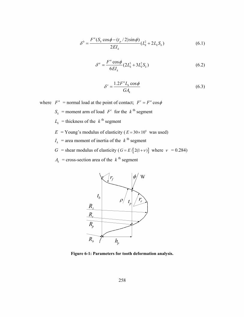
258

2( cos ( / 2)sin )( 2 )

2

nk pb

k k kk

F S tL L S

EIφ φ

δ−

= + (6.1)

3 2cos (2 3 )6

ntr

k k kk

F L L SEI

φδ = + (6.2)

1.2 cosns k

k

F LGA

φδ = (6.3)

where nF = normal load at the point of contact; cost nF F φ=

kS = moment arm of load tF for the k th segment

kL = thickness of the k th segment

E = Young’s modulus of elasticity ( 630 10E = × was used)

kI = area moment of inertia of the k th segment

G = shear modulus of elasticity ( [ ]/ 2(1 )G E ν= + where ν = 0.284)

kA = cross-section area of the k th segment

ρ

W

bt

tR

bR

pt

φfr

rr

pR

ph

rR

Figure 6-1: Parameters for tooth deformation analysis.

259

Since the height of the circular-arc tooth profile is normally short (and the

actual loading height is even shorter), two segments ( 2k = ) were considered to be

sufficient to represent the circular-arc tooth. For more accurate approximation of the

actual tooth curve, k can be increased, but then the thickness of the segment ( kL )

becomes too small (for our uniquely short teeth) to be considered as a cantilever

beam.

Using the functional descriptions of the tooth deformations presented above,

an analytical contact model has been built. Table 6-1 presented a list of parameters to

be involved in the contact model and their descriptions. Note that the clearance

parameter iε already takes into account the effects of the center distance errors.

Equation (6.4) shows the mathematical contact model. The first two independent

equations of the model describe:

1) Summation of the tangential load at each i th tooth pair ( tiF ) which is equal

to the total tangential load ( tTF ) on the mating gear pair

2) Total displacement of the i th tooth pair ( iD ) due to the clearance ( iε ),

deformations ( iδ ), and manufacturing errors ( ie∆ ) which is the same for

every tooth pairs.

0 1 2

0 1 2 3

( , , , ,...)

/

t t t t tT i

i

i i i i

i r rb t s

i i i i

i i it

i i i

F F F F FD D D D DD e

f R r CD

e se pe

K F D

ε δε φ

δ δ δ δ

⎧ = + + + ⋅⋅⋅+ + ⋅⋅⋅⎪

= = = = ⋅⋅⋅ = = ⋅⋅⋅⎪⎪ = + + ∆⎪⎪ = ∆⎨⎪ = + +⎪⎪∆ = ∆ + ∆⎪

=⎪⎩

(6.4)

260

This analytical model assumes two simplifying conditions. First, the local

tangential stiffness at each tooth pair in mesh iK is assumed to be linear; i.e., the

local load tiF is assumed to be directly proportional to the amount of the

deformation. Second, due to the very short tooth height as well as almost identical

pitch radii between the two gears, the actual loading (contact) points (where the

minimum clearances are evaluated) are very close to the circumference of the pitch

circle51. In other words, the distance between actual contact point and the point where

the pitch circle and the tooth curvature intersect is extremely small for each tooth in consideration. This fact makes it reasonable to assume a constant loading height ph

for every tooth in mesh.

This set of equations was solved simultaneously with a trial and error method,

adding equations in steps from 0i = until i n= ( n is the index of the last tooth pair

in contact which also represents the contact ratio). Each step is valid until the next

smallest clearance is equal to the total deflection of the current tooth pair(s) in mesh.

Three different Center Distance Error (CDE) values were considered in addition to

the perfect condition ( CD∆ = 0.0000”). They were: CD∆ = 0.0004”, CD∆ =

0.0007”, and CD∆ = 0.0010”. The set of the clearance data for each case obtained in

Section 5.4.2 was assigned to iε . For this representative analysis, manufacturing

errors (except for the center distance error) were not considered for a comparison

with the upcoming FEA results. Thus, ie∆ , ise∆ and ipe∆ were all set to zero.

Table 6-2 presents the final load sharing factors solved for each contact

condition. It turned out that in all four error conditions, the HGT allowed three tooth

pairs in contact (contact ratio of three) for the given load level.

51 This is a very important assumption which should be investigated using accurate plastic models in a quality photo elastic fringe analysis.

261

Table 6-2: Load sharing factors from analytic model.

Load Sharing Factor [%] CDE [in]

2i = 0i = 1i = t

TF [lb]

0.0000 19.37 66.36 14.27 12848 0.0004 17.81 62.98 19.21 12884 0.0007 15.56 62.61 21.83 12795 0.0010 13.55 61.84 24.61 12878

Figure 6-2 compares the load sharing factors on each tooth pair with respect

to the four different contact conditions. It shows that the load sharing factors decrease

somewhat at the approaching side tooth pair and the tooth pair in the middle while the

recessing side tooth pair observes a nominal increase in the load sharing factor with

increasing CDE.

0

10

20

30

40

50

60

70

2 0 1

Tooth Pair

Load

Sha

ring

Fact

or [%

]

CDE = 0.0000" CDE = 0.0004" CDE = 0.0007" CDE = 0.0010"

Figure 6-2: Load sharing factors obtained from the analytic model for different CDEs.

262

6.3 FEA LOADED TOOTH CONTACT ANALYSIS

Finite Element Analysis (FEA) was performed using ABAQUS/Standard52

for the loaded tooth contact simulation of the HGT. A complete analysis consists of

three main steps: preprocessing, simulation, and postprocessing. In the preprocessing

step, the physical model is defined and ABAQUS input file (*.inp) is created. In this

research, models were created using SolidWorks, and imported to

ABAQUS/Standard. The simulation step solves the numerical problem defined in the

preprocessing step. Computing time depends on the complexity of the problem as

well as the processing speed and memory capacity of the computer. The results of the

simulation step are visualized and evaluated in the postprocessing step. Interactive

visualization of the results can be done using a postprocessor such as

ABAQUS/CAE.

An analysis model requires the following information: material data (general,

mechanical, thermal, etc.), mesh geometry (element type, shape, order, section

property, density, and number of nodes and their coordinates), analysis steps and sub-

steps (increments), step-dependent53 loads and boundary conditions, analysis type

(static, dynamic, etc.), and output request (data of interest).

The mesh geometry greatly affects the accuracy and cost of the analysis. In

FEA, degrees of freedom (displacements, rotations, temperatures, electric potential,

acoustic pressure, etc.) are calculated at nodes of the element. The displacements at

any other point in the element are interpolated from the nodal displacements. The

52 Discussion in this section on the ABAQUS/Standard refers to the ABAQUS/Standard manual (version 6.3) published by Hibbitt, Karlsson & Sorensen (2002). 53 Some conditions are active only in a specific step (or in specific steps) defined in the analysis.

263

order of interpolation (linear or quadratic) is normally determined by the number of

nodes used in the element.

In this research, after numerous trials, 4-node continuum bilinear element

(quadrilateral, CPE4) and 8-node continuum linear brick element (hexahedron,

C3D8) were finally chosen as the most appropriate mesh element (in terms of

minimization of the mesh distortions and computation cost) for 2- and 3- dimensional

analysis, respectively. 2-dimensional analysis can significantly reduce the analysis

cost for the gear contact simulation if the out-of-plain strain or stress (in the direction

of the face width) is assumed to be zero (which is valid assumption for spur gears).

For zero out-of-plane strain analyses (normally for thick structures) Plane Strain

Elements (CPEn) are suitable while for zero out-of-plane stress analyses (normally

for thin structures) Plane Stress Elements (CPSn) are more appropriate (n is the

number of nodes). However, for the FEA such as loaded tooth contact analysis

subject to misalignment of the gears, 3-dimensional analysis must be performed.

With the reduced integration (Gauss) points and sufficient mesh densities the

selected mesh geometries resulted in minimum mesh distortions as well as high

computational efficiency. Figure 6-3 shows the mesh geometry of the ¼-scale AWE

Actuator HGT for the 2-D FEA. The global mesh seed size was assigned 0.1 for both

gears while the local mesh seed size was assigned 0.01 for the internal gear and 0.008

for the wobble gear (see Figure 6-4 for the local mesh). A slightly finer mesh was

assigned for the wobble gears because the tooth surfaces of the wobble gear were set

as slave surfaces while those of the internal gear were set as master surfaces.

264

Figure 6-3: Mesh geometry of the ¼-scale AWE Actuator HGT.

Figure 6-4: Local mesh geometry.

265

For the 3-D finite element analyses, coarser meshes were used to save

computation time. Figure 6-5 and Figure 6-6 and show the 3-D mesh geometry of the

internal gear and wobble gear, respectively.

Figure 6-5: 3-D mesh geometry of the ¼-scale AWE Actuator HGT internal gear.

Figure 6-6: 3-D mesh geometry of the ¼-scale AWE Actuator HGT wobble gear.

266

A rigid body in the FEA is a group of nodes and elements of which motion is

governed by the motion of a reference node. In other words, the degree of freedom of

the rigid body is available only at its reference node. Since the gear body can be

assumed to undergo a negligible deformation, a set of nodes and elements apart from

the tooth root were defined as a rigid body to make the analysis more effective.

Moreover, since the contact analysis has explored the effects of the tooth

deformations on the contact analysis, defining a portion of the gear body as a rigid

body (while leaving the tooth base portion under elastic deformation) is a useful

approach. For the wobble gear, a reference node for the rigid body was assigned at

the gear center (see Figure 6-7).

Figure 6-7: Grouping of elements and nodes as a rigid body.

267

ABAQUS can handle nonlinearities in the structural problems. The three

sources of the nonlinearity are: material, geometric, and boundary (contact). An

example of the material nonlinearity is the stress/strain relationship at high strain

values (after the material’s yielding point). Geometric nonlinearity occurs when the

magnitude of the displacement affects the response of the structure. One such

example is load direction changes due to large deflections or rotations. Boundary

(contact) nonlinearity applies to the HGT loaded tooth contact analyses. The response

of the structure is discontinuous and highly affected by the contact/non-contact

situation. ABAQUS solves nonlinear problems using the Newton-Raphson iteration

method. It is also capable of controlling the size of the load increments for efficient

handling of nonlinear problems.

Contact interactions were defined between the mating tooth surfaces. The

current and prospective contact nodes of the internal gear teeth were defined as

master surfaces and those of the wobble gear teeth were defined as slave surfaces.

Contact interactions here refer to properties that govern the contact behavior. In this

setup, tangential and normal behaviors are defined. Penalty friction formulation was

considered as a tangential behavior with an allowable “elastic slip” (small amount of

relative motion between the surfaces that occurs when the surfaces should be

sticking). Hard contact was considered as a normal behavior; contact constraint is

applied when the clearance between two surfaces becomes zero, and removed when

the contact pressure becomes zero or negative. Frictions between the master and slave

surfaces were modeled as small slidings which account for rotation or deformation of

the master surface by updating the load path. All the interactions between the contact

surfaces were defined in the Initial Step.

268

The ‘step’ in the ABAQUS is a period of time during which the response of

the model is computed with respect to a specified set of loads and boundary

conditions. Through a sequence of steps the response of the model evolves in the

analysis. The HGT contact model establishes an initial contact in the Initial Step.

After the Initial Step, two actual loading steps were created. The total time and the

initial time increment were set to 0.5s and 0.05s respectively for each step. Note that

ABAQUS automatically chooses the subsequent increment size. The minimum

increment size was set to 1e-006 and the maximum number of increments was set to

100. Requested outputs (field and history) in each step were stresses, strains,

displacements, reaction forces, etc.

Two boundary conditions were created in the Initial Step. The first boundary

condition is to prevent the internal gear from moving. In a real system, the first stage

ring gear is fixed to the rotary actuator shell. The second boundary condition is to

prevent the wobble gear from moving initially. While the first boundary condition

propagates through step 2 and 3, the second boundary condition is modified in the

step 2 and 3 to accommodate a rotation of the wobble gear. A vertically upward body

force was applied in step 2, and propagated through step 3. This force represents the

radial force. This force is a function of the moment and the pressure angle.

There are two methods for establishing a contact; application of a

force/moment or application of a translational/rotation displacement. Both methods

were attempted. Applying a specified moment to the reference point resulted in errors

with more than 200 warnings including convergence problems. Thus, angular

displacement was applied with respect to the reference point to simulate the moment.

The angular displacement was fine-tuned until the resultant reaction moment reached

the specified moment.

269

Table 6-3 and Figure 6-8 show the results of the FEA loaded tooth contact

simulation of the ¼-scale AWE Actuator HGT for the given specifications and

material. Contact ratio for all four conditions were three, and the load sharing factors

were found to be very close to those obtained from the analytic results (Table 6-2). It

shows the largest load sharing factor observes negligible changes for the different

CDE conditions. Visual FEA results will be presented in Section 8.2.1.

Table 6-3: Load sharing factors from FEA.

Load Sharing Factor [%] CDE [in]

2i = 0i = 1i = t

TF

0.0000 20.40 63.38 16.22 12839 0.0004 18.12 63.77 18.11 12796 0.0007 17.21 63.56 19.23 12815 0.0010 15.96 63.52 20.52 12868

0

10

20

30

40

50

60

70

2 0 1

Tooth Pair

Load

Sha

ring

Fact

or [%

]

CDE = 0.0000" CDE = 0.0004" CDE = 0.0007" CDE = 0.0010"

Figure 6-8: Load sharing factors obtained from FEA for different CDEs.

270

Figure 6-9 through Figure 6-12 compare the load sharing factors obtained

from the analytic model and the FEA nonlinear simulation for the four different

contact conditions. They showed excellent agreements.

CDE = 0.0000"

0

10

20

30

40

50

60

70

2 0 1

Tooth Pair

Load

Sha

ring

Fact

or [%

]

Analytic FEA

Figure 6-9: Comparison of analytical and FEA results for perfect condition.

CDE = 0.0004"

0

10

20

30

40

50

60

70

2 0 1

Tooth Pair

Load

Sha

ring

Fact

or [%

]

Analytic FEA

Figure 6-10: Comparison of analytical and FEA results for CDE = 0.0004”.

271

CDE = 0.0007"

0

10

20

30

40

50

60

70

2 0 1

Tooth Pair

Load

Sha

ring

Fact

or [%

]

Analytic FEA

Figure 6-11: Comparison of analytical and FEA results for CDE = 0.0007”.

CDE = 0.0010"

0

10

20

30

40

50

60

70

2 0 1

Tooth Pair

Load

Sha

ring

Fact

or [%

]

Analytic FEA

Figure 6-12: Comparison of analytical and FEA results for CDE = 0.0010”.

272

6.4 FEA LOADED TOOTH CONTACT SIMULATION

The objective of the loaded tooth contact analysis was to evaluate the actual

contact ratio under load, and load sharing factor of the HGT. It has been claimed that

under increasing loads, the HGT allows for increases in the contact ratio and

improvements of the load sharing factors making itself an excellent load carrying

system. This benefit will be verified using the FEA nonlinear contact simulations for

different (increasing) load levels. The object systems are the ¼-scale AWE Actuator

HGT and the Rugged Actuator HGT. The obtained load profiles will be utilized in

Chapter 7 for evaluations of the friction power losses in the HGT.

6.4.1 ¼-Scale AWE Actuator HGT

Three different load levels were simulated. They were measured toques at the

center of the HGT: 40,854 in-lb (1x nominal load), 144,489 in-lb (3.5x nominal load),

and 279,425 in-lb (7x nominal load). The angular displacements corresponding to

each of these load levels were: 0.0007 rad (1x load), 0.0015 rad (3.5x load), and

0.0023 rad (7x load). Table 6-4 summarizes the FEA results. Figure 6-13, Figure

6-14, and Figure 6-15 visualize the FEA results for 1x, 3.5x, and 7x load,

respectively. It is clearly shown that as the load increases, the contact ratio increases

(from 3 to 5) and the largest load sharing factor significantly decreases.

Table 6-4: FEA results for the ¼-scale AWE Actuator HGT.

Load Sharing Factor [%] Torque [in-lb] 4i = 2i = 0i = 1i = 3i =

Contact Ratio

Mises Stress [ksi]

40,854 - 20.91 62.38 16.71 - 3 85 144,489 2.67 29.66 42.14 25.53 - 4 218 279,425 12.00 27.41 33.78 24.75 2.06 5 305

273

Figure 6-13: FEA contact simulation for 1x load (CR = 3).

Figure 6-14: FEA contact simulation for 3.5x load (CR = 4).

274

Figure 6-15: FEA contact simulation for 7x load (CR = 5).

0

10

20

30

40

50

60

70

4 2 0 1 3

Tooth Pair

Load

Sha

ring

Fact

or [%

]

1.0x Load (CR=3) 3.5x Load (CR=4) 7.0x Load (CR=5)

Figure 6-16: Comparison of load sharing factors with increasing loads.

275

Figure 6-16 compares the load sharing factors for the three loading conditions.

It is clearly shown that as the load level increases, load sharing over the multiple

contacts is improved. The largest load sharing factor (of the most heavily loaded

tooth pair) was significantly reduced from 62.38 % to 33.78 %, a factor of almost 2x.

This FEA results demonstrate the effective “self-protecting” aspect of the HGT.

6.4.2 The Rugged Actuator HGT

For the Rugged Actuator FEA, the mesh geometry was more refined. Figure

6-17 shows the mesh geometry of the Rugged Actuator HGT. The global mesh seed

size was assigned 0.03 for the internal gear and 0.025 for the wobble gear. The local

mesh seed size was assigned 0.002 for the internal gear and 0.0016 for the wobble

gear. Again, slightly finer meshes were assigned for the wobble gear because the

tooth surfaces of the wobble gear were set as slave surfaces while those of the

internal gear were set as master surfaces.

Figure 6-17: Mesh geometry of the Rugged Actuator HGT.

276

The FEA contact simulations were performed for the Rugged Actuator HGT

for two different load levels. Figure 6-18 shows the contact ratio of three under a

nominal load (1,500 in-lb of torque) while Figure 6-19 shows the contact ratio of five

under a peak load (5x the nominal load, 7,500 in-lb). As the load became significant

the largest load sharing factor decreased from 41% to 26% (see Figure 6-20). This

result also demonstrates the effective ‘self-protecting’ aspect of the HGT.

Maximum contact stresses were very low (45 ksi) under the nominal loading

condition and acceptable (142 ksi) under the peak loading condition. The maximum

root stresses (to indicate tooth bending load capacity) were also much lower than

those expected in the preliminary design based on AGMA equations; 13 ksi for the

nominal and 41 ksi for the peak loading condition54 . This means that the load

capacity (in terms of bending endurance) of the Rugged Actuator HGT can now be

listed at 5 to 9 times (depending on the material strengths) of the designed load

capacity.

54 This shows the standard approach does not predict the load capacity of the circular-arc gears very well whereas the correction factor evaluation attempted in Section 3.2.5.3 deserves further refinement.

277

Figure 6-18: FEA contact simulation for nominal load (CR = 3).

Figure 6-19: FEA contact simulation for peak load (CR = 5).

278

0

5

10

15

20

25

30

35

40

45

6 4 2 0 1 3

Tooth Pair

Load

Sha

ring

Fact

or [%

]

Nominal Load (CR = 3) Peak Load (CR = 5)

Figure 6-20: Comparison of load sharing factors for nominal and peak loads.

Comparing with the result for the ¼-scale AWE Actuator HGT, the Rugged

Actuator HGT closes clearances in the approaching side quicker than it does in the

recessing side as opposed to the ¼-scale HGT case where both approaching and

recessing side clearances were closed at a similar rate. This is because of the

significant tooth geometry difference between the two designs. The main difference

was the minimized pressure angle (7°) in the Rugged Actuator HGT design. This

represents how tooth profile design can affect the contact characteristics of the HGT.

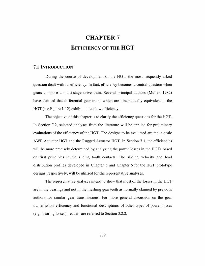
279

CHAPTER 7

EFFICIENCY OF THE HGT

7.1 INTRODUCTION

During the course of development of the HGT, the most frequently asked

question dealt with its efficiency. In fact, efficiency becomes a central question when

gears compose a multi-stage drive train. Several principal authors (Muller, 1982)

have claimed that differential gear trains which are kinematically equivalent to the

HGT (see Figure 1-12) exhibit quite a low efficiency.

The objective of this chapter is to clarify the efficiency questions for the HGT.

In Section 7.2, selected analyses from the literature will be applied for preliminary

evaluations of the efficiency of the HGT. The designs to be evaluated are the ¼-scale

AWE Actuator HGT and the Rugged Actuator HGT. In Section 7.3, the efficiencies

will be more precisely determined by analyzing the power losses in the HGTs based

on first principles in the sliding tooth contacts. The sliding velocity and load

distribution profiles developed in Chapter 5 and Chapter 6 for the HGT prototype

designs, respectively, will be utilized for the representative analyses.

The representative analyses intend to show that most of the losses in the HGT

are in the bearings and not in the meshing gear teeth as normally claimed by previous

authors for similar gear transmissions. For more general discussion on the gear

transmission efficiency and functional descriptions of other types of power losses

(e.g., bearing losses), readers are referred to Section 3.2.2.

280

7.2 EFFICIENCY ANALYSES BASED ON THE LITERATURE

Evaluation of gear transmission power losses based on experimental results

can be commonly found in the literature (Anderson & Loewenthal, 1982; Shipley,

1991). Some of the formulae from the literature were presented in Section 3.2.2, and

used in the parametric designs of the HGT prototypes for preliminary estimations of

the sliding and rolling power losses (Section 3.5).

Another branch of the study is to establish systematic relationships between

the friction losses and kinematic configuration (so called kinematic chains) of the

gear transmission (Freudenstein & Yang, 1972; Muller, 1982; Pennestri &

Freudenstein, 1993; Castillo, 2002). Based on the developed kinematic chains and

their tabulations, this type of analysis attempts to provide for unified approaches in

the evaluation of gear transmission efficiency. The motivation is that as gears are

arranged as a compound gear transmission, efficiency may decrease significantly in

some cases depending on their speeds and kinematic configurations. Assuming that

friction losses are the only losses in the gear transmission, some of the authors

attribute the cause of the efficiency drop to circulating power (also called futile

power) which is an internal power loop that is not transferred to the output. This

means that there is a continuous flow of force and velocity (tangentially) through the

gear meshes in this internal power loop.

Section 7.2.1 through Section 7.2.355 will calculate the efficiencies of the two

HGT prototype designs using the analytics from Shipley (1991), Pennestri and

Freudenstein (1993), and Muller (1982), respectively. Discussion on the analyses will

be provided in Section 7.2.4.

55 Each section will use the nomenclature of the corresponding literature.

281

7.2.1 Shipley (1991)’s Analysis

A gear train which is kinematically equivalent to the HGT is represented by

Shipley (1991) as shown in Figure 7-1. It is called four-gear differential. The

efficiency formulae in the literature are based on the tooth load and meshing velocity,

and thus power of the gear members (i.e., X-Y connected, C, and B in Figure 7-1).

Figure 7-1: Shipley (1991)’s representation of a four-gear differential.

Starting with the gears X and Y, velocity of the center of the gears is

2 2 0.2839 3950 587.17 [ft/min]12 12Av A nπ π

= × × = × × = (7.1)

where A is the arm length (eccentric) in [in] and n is the input speed in [rev/min].

Load tW at the center of the gears is

39600 /102.5 1360.9 [lb]0.2839

iA

TWA

= = = (7.2)

where iT is the input torque in [in-lb] ( /i oT T TR= ). Then, the input power aP

being transmitted is

1360.9 587.17 799075.44 [ft-lb/min]A A AP W v= × = × = (7.3)

282

Next, the meshing velocity of the fixed internal gear C is given by kinematic

relation:

6.3878587.17 6605.67 [ft/min]6.3878 5.8200

CC A

C X

dv vd d

= = × =− −

(7.4)

where d ’s are pitch diameters of the subscripted gears. The load applied to the

internal gear C is

6.3878 5.8200 1360.9 6.536.3878 6.5238 7.0976 5.8200

12519.6 [lb]

C XC A Y

C Y B X

d dW W dd d d d

−=

−−

= × ×× − ×

=

(7.5)

The equivalent power on the internal gear C is

12519.6 6605.67 82700396 [ft-lb/min]C C CP W v= × = × = (7.6)

Lastly, the meshing velocity of the rotating internal gear B is given by

kinematic relation:

6.3878 6.5298587.16 7411.29 [ft/min]( ) 5.8200(7.0976 6.5298)

C YB A

X B Y

d dv vd d d

×= = × =

− − (7.7)

Load applied to the rotating internal gear B is

7.0976 6.5298 1360.9 5.826.3878 6.5298 7.0976 5.8200

11158.7 [lb]

B YB A X

C Y B X

d dW W dd d d d

−=

−−

= × ×× − ×

=

(7.8)

The equivalent power on the rotating internal gear B is

11158.7 7411.29 8.2700396 [ft-lb/min]B B BP W v= × = × = (7.9)

283

Meanwhile, the percent power loss is defined as

2 250

coss t

Ls t

H HfpH Hφ

⎛ ⎞+= ⎜ ⎟+⎝ ⎠

(7.10)

where f = coefficient of friction

tH = specific sliding velocity at start of recess action

sH = specific sliding velocity at start of approach action

tH and sH are given by the following equations:

22

22

1 cos sin

( 1) cos sin

G ot

G

is G

m rHm r

RH mR

φ φ

φ φ

⎡ ⎤⎛ ⎞− ⎛ ⎞⎢ ⎥= − −⎜ ⎟ ⎜ ⎟⎢ ⎥⎝ ⎠⎝ ⎠ ⎣ ⎦⎡ ⎤⎛ ⎞⎢ ⎥= − − − +⎜ ⎟⎢ ⎥⎝ ⎠⎣ ⎦

(7.11)

where Gm = speed ratio of each stage

or = outside radius of the external gear (whose pitch radius is r )

iR = inside radius of the internal gear (whose pitch radius is R )

φ = pressure angle of each stage

Using Equation (7.10) and (7.11), and f = 0.0556, the percent power losses of the

1st stage and 2nd stage of the ¼-scale HGT are calculated as:

1

2

0.0071480.005731

L

L

pp

==

(7.12)

Finally, the overall efficiency of the HGT is evaluated based on the equivalent

power calculated for each of the gear members (Equation (7.3), (7.6), and (7.9)), and

the percent power losses calculated for each stage (Equation (7.12)):

56 This coefficient can be reduced to 0.01 with very high tooth surface finish and hardness.

284

1 2( ) /100

799075.44 (0.007148 82700396 0.005731 82700396) /100 799075.44

0.98667

A L C L B

A

P p P p PEP

− +=

− × + ×=

=

(7.13)

Therefore, application of Shipley’s analysis to the ¼-scale AWE Actuator HGT

design results in 98.67 % efficiency.

Being identically applied to the Rugged Actuator, the following intermediate

parameters are calculated:

1

2

12021.42344173.1

0.0069880.008071

A

C B

L

L

PP P

pp

== =

==

(7.14)

The overall efficiency of the Rugged Actuator HGT results in 97.06 %.

7.2.2 Pennestri and Freudenstein (1993)’s Analysis

Pennestri and Freudenstein (1993) proposed a systematic algorithm for the

estimation of efficiency of gear trains. The approach requires a preliminary

determination of all fundamental circuits in the labeled graph (Freudenstein, 1971).

Figure 7-2 shows Freudenstein’s gear train with indexation of the kinematic links.

285

Figure 7-2: Index of the links in Freudenstein (1993)’s gear train.

Figure 7-3 illustrates the power flow circuit in the gear train. For each gear pair and

node (represented by small circle), the input power and output power should be equal:

in outP P=∑ ∑ (7.15)

Output

1 0P =

2P′

2P′′ 3P′′

3P′

4P

Input1+

1G

2G2nd Stage

Gear Mesh

1st StageGear Mesh

Figure 7-3: Power flow analysis of the HGT.

286

In order to utilize the power flow equations to solve for the overall efficiency,

basic efficiencies iλ of gear pairs ( 1G and 2G ) needs to be determined first.

Pennestri and Freudenstein adopted the following equation from Tuplin (1957) for

approximation of the basic efficiencies:

1

1 1

22 2

1 1 115

1 1 115

N N

N N

λ

λ

⎛ ⎞= − +⎜ ⎟′⎝ ⎠

⎛ ⎞= − +⎜ ⎟′⎝ ⎠

(7.16)

where 1N = 45 (number of teeth of the 1st stage internal gear)

1N ′ = 41 (number of teeth of the 1st stage external gear)

2N = 50 (number of teeth of the 2nd stage internal gear)

2N ′ = 46 (number of teeth of the 2nd stage external gear)

For the internal gears, the negative sign is assigned to iN . The basic efficiencies 1λ

and 2λ for the ¼-scale HGT are calculated as

1

2

1 1 11 0.9995665 41 451 1 11 0.9996525 46 50

λ

λ

⎛ ⎞= − − =⎜ ⎟⎝ ⎠⎛ ⎞= − − =⎜ ⎟⎝ ⎠

(7.17)

Now considering the power flow circuit for the gear pair 1G in Figure 7-3,

the following power balance equation holds:

1 1 3 2P P Pη ′ ′+ = (7.18)

where 1 0P = and 1η is the overall efficiency of circuit 1. Table 1 of Pennestri and

Freudenstein gives the following equation for 1η :

1 11

1 1

1( 1)

rrλη

λ−

=−

(7.19)

287

where 1λ is the basic efficiency of the gear pair obtained above, and 1r is speed

ratio of the 1st stage gear pair which is given by

11

1

45 1.09756141

NrN

= = =′

(7.20)

Substituting Equation (7.17) and (7.20) in Equation (7.19) gives

1 0.995554η = (7.21)

Considering the power flow circuit for the gear pair 2G ,

2 2 3 4P P Pη ′′ ′′= + (7.22)

where 2η is the overall efficiency of circuit 2. Table 2 of Pennestri and Freudenstein

gives the following equation for 2η :

3(2 4) 4(2 3)2

3 42

34 2

1 11 n n rnn r

η ηη − −= +

− ⋅− ⋅ (7.23)

where 2r is speed ratio of the 2nd stage gear pair which is given by

22

2

50 1.08695746

NrN

= = =′

(7.24)

and 3 4/n n (ratio of absolute velocities of link 3 and 4) is obtained by the following

kinematic relation:

( )2 2 1 0i j kn r n r n− + − = (7.25)

For i = 3, j = 4 and k = 2, Equation (7.25) can be rearranged as

( )3 22 2

4 4

1n nr rn n

= − − (7.26)

288

For the known 2r and 2 4/ 103.5n n TR= = ,

3

4

7.91304nn

= (7.27)

The values of 3(2 4)η − and 4(2 3)η − in Equation (7.23) are computed using the

formulae listed in Table 1 of the literature:

23(2 4)

2 2

2 24(2 3)

2 2

1 1.086957 1 0.9960161.086957 0.999652

( 1) 0.999652(1.086957 1) 0.9956691.086957 0.999652

rrr

r

ηλ

ληλ

−

−

− −= = =

− −− −

= = =− −

(7.28)

Substituting Equation (7.24), (7.27) and (7.28) in Equation (7.23),

2 0.995614η = (7.29)

Considering the power flow balance for the input side node in Figure 7-3 (the

input power is normalized to 1),

2 21P P′ ′′+ = (7.30)

For the node between 1G and 2G ,

3 3P P′′ ′= (7.31)

Now, we have five variables ( 2P′ , 2P′′ , 3P′ , 3P′′ , and 4P ) and four equations

(Equation (7.18), (7.22), (7.30), and (7.31)). The authors provide an additional

power flow equation in their tabulated power flow ratios (Table 4), which is:

22

42

4 42 2 2

2

(1 ) 1

( 1)

nrnP

P nr rn

η

⎛ ⎞− −⎜ ⎟′′ ⎝ ⎠=

⎛ ⎞+ − − ⎜ ⎟

⎝ ⎠

(7.32)

289

Substituting the known 2r and 2 4/n n in the above equation, and letting 2 4/P P ν′′ = ,

8.31387ν = (7.33)

Collecting and organizing all the power flow balance equations,

2 1 3

2 2 3 4

2 2

3 3

2 4

00

100

P PP P PP PP P

P P

ηη

ν

′ ′− =′′ ′′− − =′ ′′− = −′ ′′− =′′− =

(7.34)

which is in a matrix form,

21

22

3

3

4

01 0 0 000 0 1 1

11 1 0 0 000 0 1 1 000 1 0 0

PPPPP

ηη

ν

′− ⎡ ⎤ ⎡ ⎤⎛ ⎞⎢ ⎥⎜ ⎟ ⎢ ⎥′′− − ⎢ ⎥⎜ ⎟ ⎢ ⎥⎢ ⎥⎜ ⎟ ′ ⎢ ⎥= −−⎢ ⎥⎜ ⎟ ⎢ ⎥′′− ⎢ ⎥⎜ ⎟ ⎢ ⎥

⎜ ⎟ ⎢ ⎥ ⎢ ⎥−⎝ ⎠ ⎣ ⎦⎣ ⎦

(7.35)

Solving the matrix,

2

2

3

3

4

6.77867.77866.80886.80880.9356

PPPPP

′ =′′=′ =′′=

=

(7.36)

Hence, the overall efficiency of the gear train ( 4P over unity) is 93.56 %.

Repeating the analysis for the Rugged Actuator HGT, the power flow values are

calculated as

290

2

2

3

3

4

12.024613.024612.056712.05670.9277

PPPPP

′ =′′=′ =′′=

=

(7.37)

Thus, the overall efficiency of the Rugged Actuator is 92.77 %.

7.2.3 Muller (1982)’ Analysis

Muller (1982) provided elaborate kinematic analysis and efficiency evaluation

guides which cover most of the possible gear transmission configurations. A

depiction of a gear transmission which is kinematically equivalent to the HGT is

presented in the literature (adopted here in Figure 7-4).

Figure 7-4: Miller (1982)’s representation of a gear train equivalent to the HGT.

Muller used the parameters called basic speed ratio and basic efficiency

rigorously in the efficiency analysis. Basic speed ratio is the ratio of the revolving

gears in mesh when the carrier of the planet gear is locked. Efficiency obtainable

from this operating condition (carrier being held) is defined as basic efficiency. The

basic speed ratio oi of the representative gear train is given in worksheet 1 (p. 335),

Equation 4 as:

291

011si

ii

= − (7.38)

where 1si is the ratio between the carrier s (as input, eccentric) and internal gear 1

(output gear). In the case of the ¼-scale AWE Actuator HGT (for 1N = 50, 1pN =

46, 2N = 45, and 2pN = 41),

1 103.5si TR= = − (7.39)

Therefore,

011 1.009662

103.5i = + = (7.40)

The basic efficiency 0η is given by Muller assuming that tooth friction loss

tζ is the only power loss:

0 01 1 1t t Lfη ζ ζ µ= − = − = − (7.41)

For the given tooth number differences, load per face width, and pitch line velocities,

1Lf and 2Lf (geometrical loss factor for the 1st and 2nd stage, respectively) can be

approximated by interpolation from Fig. 16 (p. 25):

1

2

0.0240.028

L

L

ff

≈≈

(7.42)

However, 1µ and 2µ (tooth friction loss factor) for the given specifications are out

of range of the plot shown in Fig. 18 (p. 27). Assuming the values based on the

available data in the plot,

1 2 0.1µ µ≈ ≈ (7.43)

Now the tζ for both meshes (two stages) would be

292

1 1 2 2

0.1 0.024 0.1 0.028 0.0052

t t L t Lf fζ µ µ= += × + ×=

(7.44)

Hence, the basic efficiency is given by

0 1 1 0.0052 0.99480tη ζ= − = − = (7.45)

where 0 12 21η η η= ≈ .

Worksheet 5 on p. 338 gives the following formulae for the overall efficiency

of the gear train:

00

0 121

00

0 12

1 (for 0 1)11 (for 1)

/ 1

s

i ii

i ii

ηη

η

−⎧ ≤ ≤⎪ −⎪= ⎨ −⎪ >⎪ −⎩

(7.46)

Submitting the values for 0i and 12η in Equation (7.46) (for 0 1i > ),

01

0 12

1 1.009662 1 0.6467/ 1 1.009662 / 0.99480 1si

iη

η− −

= = =− −

(7.47)

Therefore, application of Muller’s analysis to the ¼-scale AWE Actuator HGT results

in 64.67 % efficiency. Repeating the analysis for the Rugged Actuator HGT ( 1N = 70, 1pN = 65,

2N = 75, and 2pN = 70) are as follows:

1

0

0 12

1960.9948980.00225

0.99775

s

t

iiζη η

==== =

(7.48)

Submitting the values for 0i and 12η in Equation (7.46) ( 00 1i≤ ≤ ),

293

01

0 12

1 0.994898 1 0.69501 0.994898 0.99775 1s

ii

ηη− −

= = =− × −

(7.49)

Therefore, application of Muller’s analysis results in 69.5 % efficiency for the

Rugged Actuator HGT.

7.2.4 Discussion

Table 7-1 shows the efficiency evaluated from the three different literature

analyses. Shipley’s analysis expected the highest efficiency among the three. The

analysis here used the coefficient of friction ( f ) of 0.05, so the efficiency will

increase even further with a lower coefficient of friction (e.g., 99.47 % for f = 0.02

and 99.73 % for f = 0.01 for the ¼-scale HGT).

Table 7-1: Comparison of efficiencies [%] resulted from the literature analyses.

Shipley Pennestri & Freudenstein Muller

The ¼-Scale AWE Actuator HGT 98.67 93.56 64.67

The Rugged Actuator HGT 97.06 92.77 69.50

Pennestri and Freudenstein’s analysis considered internal power circulation

(see Figure 7-3) in the gear train which is probably responsible for the relatively low

ratio of the net output power to the input power. Equation (7.36) and (7.37) in

Section 7.2.2 shows that this is 6 to 7 times of the input power (for the ¼-scale HGT)

or 12 to 13 times of the input power (for the Rugged HGT) in circulation. However,

this amount of power circulation is not significant comparing to normal differential

gear trains. For example, their representative gear train has a circulating power with

the magnitude of 37 to 38 times of the input power. The gear train had a set of tooth

294

numbers, 1N = 34, 1N ′ = 16, 2N = 32, and 2N ′ = 15 (big differences in the size

between the two mating internal-external gear pairs), and the resultant efficiency was

merely 24 %. This explains why this type of gear train (differential gear trains) has

been assumed to provide low efficiency in some of the literature. In fact, the

Shipley’s representative differential gear train also exhibited a relatively low

efficiency (86 %) due to their larger size differences in the mating gear pairs (refer to

Section 12.5.7 of the literature).

As discussed in Section 3.2.2 of this report, what makes the HGT different

from the normal differential gear trains (although they are equivalent in the kinematic

configuration) is the minimal tooth number (or size) differences between the two

mating gear pairs. Since the normal differential gear train has relatively small

planet(s) with a long planet arm, the rotational speed of the planet gear(s) is very high

relative to the input speed whereas that of the wobble gear in the HGT is low.

Equation (3.9) showed that the rotational speed of the wobble gear could be 1/20 (or

even lower) of the input speed while in the differential gear train it could be twice (if

the eccentricity is twice of the planet gear radius) or more of the input speed. This is

about 40x difference in kinematic proportions.

Muller’s analysis resulted in unacceptably low efficiencies for both of the

HGT designs. The contentions are as follows. First, their efficiency calculation is

extremely sensitive to the basic efficiency whose application appropriateness for the

HGT should be clarified. Note that the basic efficiencies given in the analysis were

0.99480 and 0.99775 for the ¼-scale AWE and the Rugged, respectively. If for

example, Pennestri and Freudenstein’s basic efficiencies (0.99981 and 0.99957) were

used, the overall efficiency would have been 96.42 % and 95.66 %. In other words,

for extremely small 0.5 % and 0.2 % increases in the basic efficiency, the analysis

295

allowed 49 % and 38 % increases in the results. This extreme sensitiveness to a

certain parameter provides no physical meaning. Second, the values for the

geometrical loss factors ( 1Lf and 2Lf ) and tooth friction loss factors ( 1µ and 2µ ),

which directly influences the overall efficiency, were approximated from the

empirical data obtained for the involute teeth. Since the HGT employs the circular-

arc teeth, the data represented by Muller is inappropriate for the HGT efficiency

analysis. This fact motivated us to perform an analysis customized to our given tooth

designs using first principles of the forces, sliding velocities, and friction coefficients

to evaluate the actual friction power losses. It is discussed in the following section.

7.3 EFFICIENCY ANALYSIS FOR THE HGT

Chapter 5 and Chapter 6 analyzed the velocities and load distributions at tooth

contacts in the HGT. Tooth friction power losses are obtained based on these two

profiles. In general, tooth friction power loss is a major portion of the overall power

loss in the gear train, but it will be shown here that it is minimal in the HGT. The

basic equation of the friction power loss is

1

ni i i

L f s ni

P C V F=

= ∑ (7.50)

where LP = friction power loss

i = tooth pair index

n = number of tooth pairs in contact

fC = coefficient of friction

sV = sliding velocity at each contact

nF = normal force at each contact

296

In this analysis, the coefficient of friction will be fixed for each analysis and

varied later to see its influences on the result57. It is important to note that the discrete

velocity and the load profiles obtained in the previous chapters not only represent

velocity and load profiles among multiple tooth pairs at a specified moment, but also

represent variations of them at individual teeth during the mesh cycle (time span from

engagement to disengagement). This is a critical concept here since the power losses

need to be analyzed in time domain not in space domain. For evaluation of

continuous power losses, the discrete load profiles are curve-fitted with third order

polynomials.

Once the power loss profiles are obtained, they are integrated with respect to

the mesh cycle for conversion to energy losses. The energy loss ( LE ) is given by:

m

L LtE P

∆= ∫ (7.51)

The mesh cycle ( mt∆ ) is dependent upon the input speed ( inω [rad/sec]), circular

pitch ( cp [rad]), and contact ratio (CR ):

[sec]cm

in

pt CRω

∆ = ⋅ (7.52)

where 2 /c ip Nπ= ( iN is the number of teeth of the internal gear).

The energy losses obtained for each individual tooth for the mesh cycle are

multiplied by the number of wobble gear teeth ( wN ) to calculate the total energy loss

( TLE ) that occurs while every tooth of the wobble gear mesh once with the mating

internal gear teeth:

TL L wE E N= ⋅ (7.53)

57 For an empirical description of this parameter, refer to Anderson and Loewenthal (1982).

297

Total input energy to be compared is the energy input to run the wobble gear

until the point where every tooth in the wobble gear meshes once with the mating

internal gear teeth. Thus, this input energy is obtained by integrating the input power

inP with respect to int∆ , the time taken for the input shaft to rotate until the

aforementioned point:

in

in intE P

∆= ∫ (7.54)

where inP and int∆ can be obtained by

in in inP T ω= ⋅ (7.55)

2win

i in

NtN

πω

∆ = ⋅ (7.56)

The efficiency of the HGT is then given by

1st stage 2nd stage( ) ( )100 [%]

T Tin L L

in

E E EE

η⎡ ⎤− +⎣ ⎦= × (7.57)

This analysis procedure is applied to the ¼-scale AWE Actuator HGT and the

Rugged Actuator HGT for evaluation of their efficiencies. Two loading (output

torque) conditions are considered for each design. For the ¼-scale design, nominal

(1x) loading (40,854 in-lb of output torque) and 3.5x loading (144,489 in-lb of output

torque) cases are considered (see Figure 6-13 and Figure 6-14 for the FEA results).

For the Rugged design, nominal (1x) loading (1,560 in-lb of output torque) and 5x

loading (7,697 in-lb of output torque) cases are considered (see Figure 6-18 and

Figure 6-19 for the FEA results).

Figure 7-5 and Figure 7-6 show curve-fitted, continuous loading sequences

(series of loads applied in normal direction to the contact surfaces) in the time domain

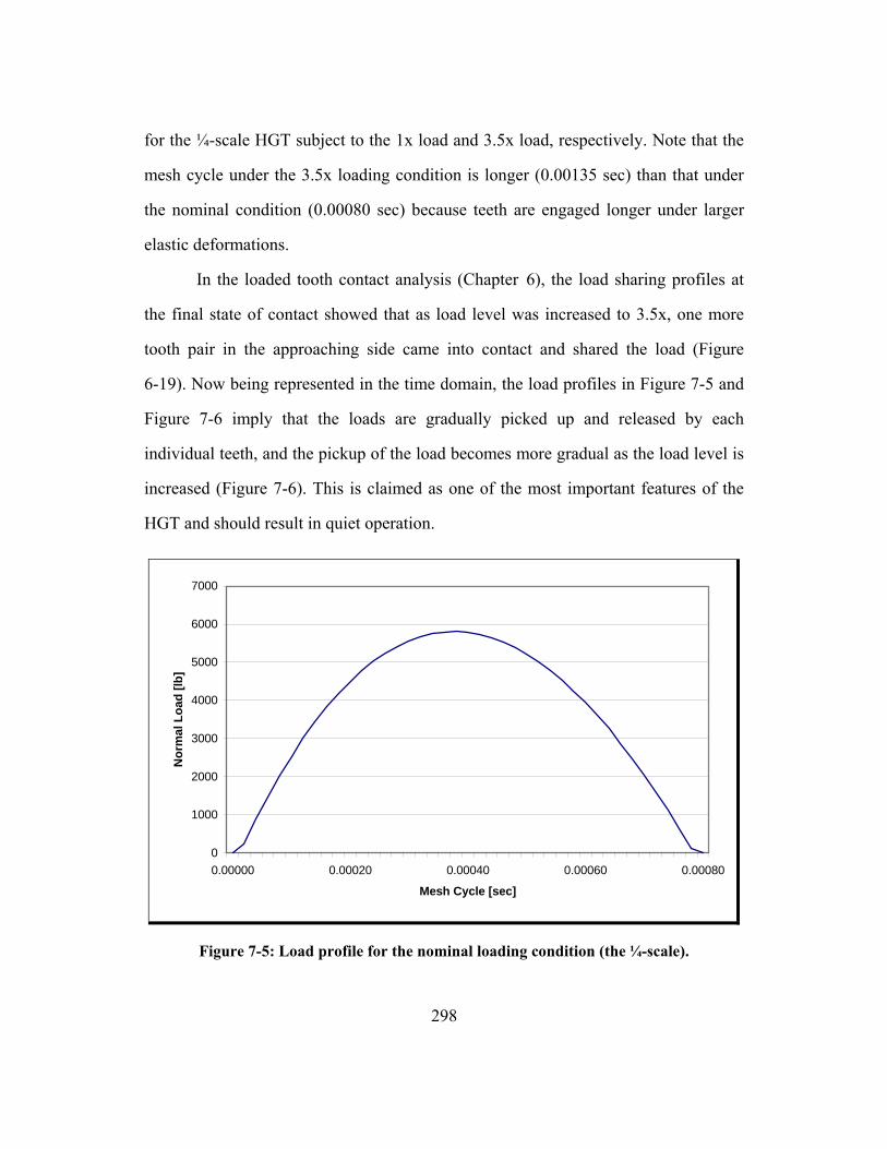
298

for the ¼-scale HGT subject to the 1x load and 3.5x load, respectively. Note that the

mesh cycle under the 3.5x loading condition is longer (0.00135 sec) than that under

the nominal condition (0.00080 sec) because teeth are engaged longer under larger

elastic deformations.

In the loaded tooth contact analysis (Chapter 6), the load sharing profiles at

the final state of contact showed that as load level was increased to 3.5x, one more

tooth pair in the approaching side came into contact and shared the load (Figure

6-19). Now being represented in the time domain, the load profiles in Figure 7-5 and

Figure 7-6 imply that the loads are gradually picked up and released by each

individual teeth, and the pickup of the load becomes more gradual as the load level is

increased (Figure 7-6). This is claimed as one of the most important features of the

HGT and should result in quiet operation.

0

1000

2000

3000

4000

5000

6000

7000

0.00000 0.00020 0.00040 0.00060 0.00080

Mesh Cycle [sec]

Nor

mal

Loa

d [lb

]

Figure 7-5: Load profile for the nominal loading condition (the ¼-scale).

299

0

2000

4000

6000

8000

10000

12000

14000

16000

18000

20000

0.00000 0.00027 0.00054 0.00081 0.00108 0.00135

Mesh Cycle [sec]

Nor

mal

Loa

d [lb

]

Figure 7-6: Load profile for 3.5x loading condition (the ¼-scale).

Figure 7-7 and Figure 7-8 show curve-fitted, continuous load profiles for the

Rugged HGT subject to the 1x load and 5x load, respectively. The mesh cycle is

0.00089 sec and 0.00133 sec for the 1x load and 5x load, respectively. Again, these

load profiles demonstrate that the load is gradually picked up and released by each

individual tooth. Due to the difference in the tooth geometry, the load profile of the

Rugged HGT is less symmetrical than that of the ¼-scale HGT for both loading

conditions. It is also shown that as load level is increased, the pickup of the load

becomes more gradual than it does under the nominal loading condition (Figure 7-8).

300

0

50

100

150

200

250

300

350

0.00000 0.00022 0.00044 0.00067 0.00089

Mesh Cycle [sec]

Nor

mal

Loa

d [lb

]

Figure 7-7: Load profile for the nominal loading condition (the Rugged).

0

200

400

600

800

1000

1200

0.00000 0.00022 0.00044 0.00067 0.00089 0.00111 0.00133

Mesh Cycle [sec]

Nor

mal

Loa

d [lb

]

Figure 7-8: Load profile for 5x loading condition (the Rugged).

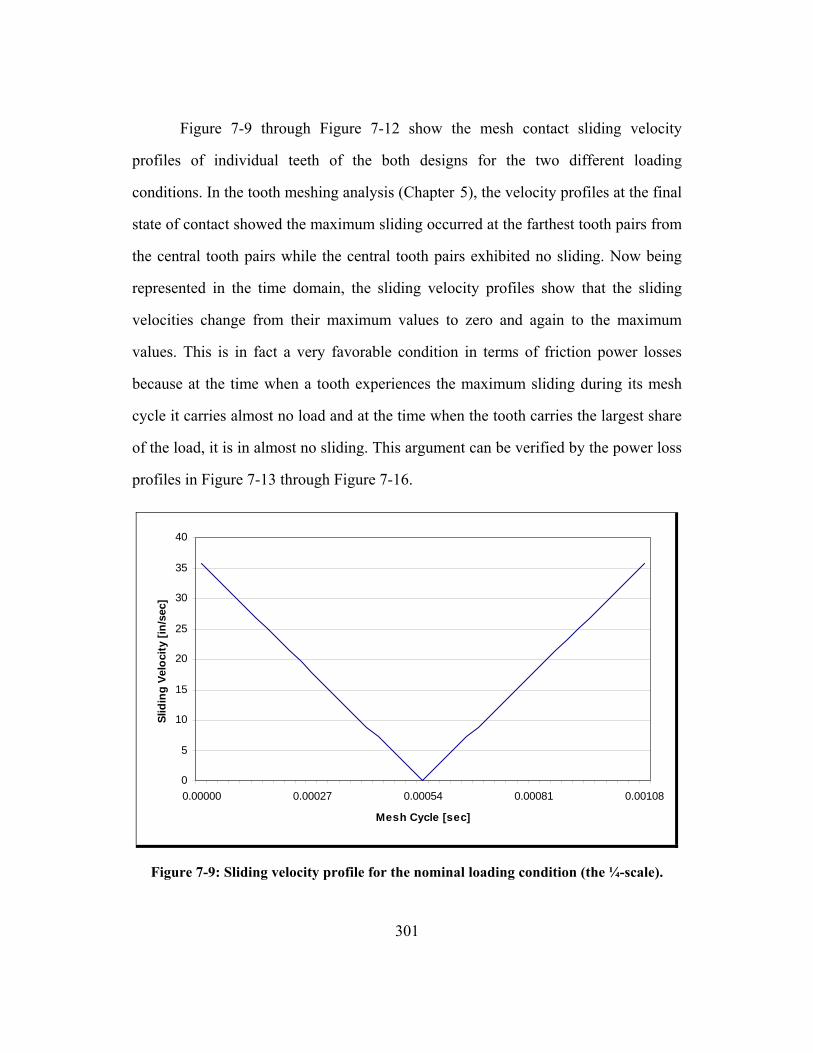
301

Figure 7-9 through Figure 7-12 show the mesh contact sliding velocity

profiles of individual teeth of the both designs for the two different loading

conditions. In the tooth meshing analysis (Chapter 5), the velocity profiles at the final

state of contact showed the maximum sliding occurred at the farthest tooth pairs from

the central tooth pairs while the central tooth pairs exhibited no sliding. Now being

represented in the time domain, the sliding velocity profiles show that the sliding

velocities change from their maximum values to zero and again to the maximum

values. This is in fact a very favorable condition in terms of friction power losses

because at the time when a tooth experiences the maximum sliding during its mesh

cycle it carries almost no load and at the time when the tooth carries the largest share

of the load, it is in almost no sliding. This argument can be verified by the power loss

profiles in Figure 7-13 through Figure 7-16.

0

5

10

15

20

25

30

35

40

0.00000 0.00027 0.00054 0.00081 0.00108

Mesh Cycle [sec]

Slid

ing

Velo

city

[in/

sec]

Figure 7-9: Sliding velocity profile for the nominal loading condition (the ¼-scale).

302

0

10

20

30

40

50

60

0.00000 0.00027 0.00054 0.00081 0.00108 0.00135

Mesh Cycle [sec]

Slid

ing

Velo

city

[in/

sec]

Figure 7-10: Sliding velocity profile for 3.5x loading condition (the ¼-scale).

0

1

2

3

4

5

6

7

8

9

10

0.00000 0.00020 0.00040 0.00060 0.00080

Mesh Cycle [sec]

Slid

ing

Velo

city

[in/

sec]

Figure 7-11: Sliding velocity profile for the nominal loading condition (the Rugged).

303

0

2

4

6

8

10

12

14

16

18

20

0.00000 0.00022 0.00044 0.00067 0.00089 0.00111 0.00133

Mesh Cycle [sec]

Slid

ing

Velo

city

[in/

sec]

Figure 7-12: Sliding velocity profile for 5x nominal loading condition (the Rugged).

Figure 7-13 through Figure 7-16 show power loss profiles; Figure 7-15 and

Figure 7-16 are for the ¼-scale HGT for the 1x and 3.5x loading conditions,

respectively. Figure 7-13 and Figure 7-14 are for the Rugged HGT for the 1x and 5x

loading conditions, respectively. These power profiles are obtained from the load and

sliding velocity profiles for the given mesh cycle, along with a constant coefficient of

friction (0.01).

304

0

100

200

300

400

500

600

700

800

900

0.00000 0.00027 0.00054 0.00081 0.00108

Mesh Cycle [sec]

Pow

er L

oss

[in-lb

/sec

]

Figure 7-13: Power loss profile for the nominal loading condition (the ¼-scale).

0

500

1000

1500

2000

2500

3000

0.00000 0.00027 0.00054 0.00081 0.00108 0.00135

Mesh Cycle [sec]

Pow

er L

oss

[in-lb

/sec

]

Figure 7-14: Power loss profile for 3.5x nominal loading condition (the ¼-scale).

305

0

2

4

6

8

10

12

14

16

0.00000 0.00020 0.00040 0.00060 0.00080

Mesh Cycle [sec]

Pow

er L

oss

[in-lb

/sec

]

Figure 7-15: Power loss profile for the nominal loading condition (the Rugged).

0

10

20

30

40

50

60

0.00000 0.00022 0.00044 0.00067 0.00089 0.00111 0.00133

Mesh Cycle [sec]

Pow

er L

oss

[in-lb

/sec

]

Figure 7-16: Power loss profile for 5x nominal loading condition (the Rugged).

306

The areas under the power loss profiles (integration of the power loss profile

with respect to the mesh cycle) represent energy losses that individual teeth will

experience during their engagement (mesh) cycles. Using Equation (7.51) through

(7.57), total energy losses TLE (for each stage), input energies inE , and overall

efficiency η of the HGT are computed.

The efficiencies of the second stage can be obtained identically as the first

stage efficiencies were obtained. However, they can be also approximated. Note that

the 2nd stages would have a slightly smaller sliding velocity profiles since the relative

angular velocities of the two mating gears are smaller (compared to the stationary and

rotating members in the 1st stage gear pairs). This slight advantage can be cancelled

or augmented with a slight difference between the amount of loads applied on each

stage. In the literature analyses (Section 7.2.1 and 7.2.3), the power losses from each

stage were found to be comparable to each other with slightly bigger losses in the

smaller stages (the 1st stage of the ¼-scale and the 2nd stage of the Rugged). Without

loss of generality, 90 % of the 1st stage power loss is assumed to be the 2nd stage

power loss for the ¼-scale HGT, and 110 % of the 1st stage power loss is assumed to

be the 2nd stage power loss for the Rugged HGT.

The combined total energy losses are now compared with the total input

energy. Table 7-2 and Table 7-3 show the analysis results for the ¼-scale AWE and

the Rugged Actuator HGT, respectively. Both systems exhibit very high efficiencies

for all loading conditions. These results of 97.5 to 98.5 % are based on a constant coefficient of friction ( fC = 0.01). Efficiency variations for different values of fC

are presented in Table 7-4. It shows that a 5x increase in fC creates a 5x increase in

mesh friction losses.

307

Table 7-2: Efficiency analysis result for the ¼-scale AWE Actuator HGT.

Input Energy [in-lb]

Energy Loss [in-lb]

Efficiency [%]

1st Stage 2nd Stage 1x Nominal Load 2297.60

19.961 17.965 98.35

1st stage 2nd Stage 3.5x Nominal Load 8141.61

78.927 71.034 98.16

Table 7-3: Efficiency analysis result for the Rugged Actuator HGT.

Input Energy [in-lb]

Energy Loss [in-lb]

Efficiency [%]

1st Stage 2nd Stage 1x Nominal Load 47.40

0.355 0.363 98.49

1st stage 2nd Stage 5x Nominal Load 236.18

2.797 3.077 97.51

Table 7-4: Effects of the coefficient of friction on the HGT efficiency [%].

The ¼-scale The Rugged Coefficient of Friction 1x Load 3.5x Load 1x Load 5x Load

0.01 98.35 98.16 98.49 97.51 0.025 95.97 95.52 96.30 94.00 0.05 92.26 91.42 92.86 88.69

308

CHAPTER 8

PROTOTYPE DEVELOPMENT

8.1 INTRODUCTION

This chapter will discuss manufacturing aspects of the HGT. Section 8.2 will

analyze the effects of manufacturing errors (i.e., center distance error, tooth spacing

error, and misalignment error) on the HGT contact characteristics using FEA. The

objective is to demonstrate that the HGT is insensitive to these manufacturing errors.

Section 8.3 will discuss issues related to the prototype development. Two EM

actuator prototypes have been built under sponsorship from ONR and DOE. They are

the ¼-scale AWE Actuator (fabricated by Timken) and the Rugged Actuator

(fabricated by UT Austin). Both EM actuators use the HGT as a primary component

whose design has been fully addressed in this report thus far. This section will discuss

issues related to fabrication of the prototype HGTs, lubricant selection, and a future

test plan. For more detailed information and discussions on the whole actuator

prototype development, readers are referred to (Park, Vaculik, Tesar, et al., 2003b)

for the ¼-scale AWE Actuator, and (Park, Kendrick, Tesar, et al., 2004; Park,

Kendrick, Tesar, et al., 2005) for the Rugged Actuator.

8.2 EFFECTS OF MANUFACTURING ERRORS

The manufacturing errors in the gear systems include gear center distance

errors, tooth spacing errors, and misalignment errors. These manufacturing errors in

general can deteriorate the desired tooth contact condition, leading to significant

309

changes in the contact ratio, transmission errors, noise and vibration, and increases in

local tooth stresses. Since effects of the manufacturing errors can be detrimental, 1)

those errors should be minimized in the manufacturing stage (which is normally

accompanied by an increase in cost), and/or 2) the effects of the errors should be

minimized (or at least known) in the design stage. Minimizing the effects of the

errors means improving the tolerance level of the gear system.

Tolerance is generally defined as geometrical variations allowed in the

manufacturing of mechanical components. If the actual manufacturing variation

exceeds the established tolerance, it is regarded as a manufacturing error. For gear

systems, however, any deviation from theoretical perfection of the geometry (in terms

of profile, pitch, lead, etc.) is normally regarded as an error. Following this notion for

the gear systems, tolerance is still a portion of an error, but can be regarded as an

‘acceptable’ error that should not affect the fundamental performance of the gears.

Therefore, improving the tolerance level of the gear system means increasing the

level of acceptable manufacturing errors, which helps to reduce the manufacturing

cost.

Preceding knowledge of the tolerance level which is critical to the

performance (critical tolerance) at the design stage can prevent ancillary effort (i.e.,

rework) and unnecessary cost in the manufacturing. Thus, analysis of the effects of

manufacturing errors on the gear system performance at the design stage is a highly

rewarding task assisting the designer to determine the level of critical tolerances.

Based on this knowledge, it is also possible to manage the effects of the errors in the

design stage.

Section 8.2.1, 8.2.2, and 8.2.3 will analyze the effects of center distance

errors, tooth spacing errors and misalignment errors, respectively, on the tooth

310

contact characteristics (e.g., contact pressure, contact ratio, load sharing factor, etc.)

of the prototype HGT. The ¼-scale AWE Actuator HGT will be considered here for

the analyses. The method of analysis is FEA where a set of representative error

values will be simulated for each error condition to observe their nonlinear effects on

the loaded tooth contact characteristics of the HGT.

8.2.1 Effects of Center Distance Errors (CDE)

The Center Distance Error (CDE) represents any manufacturing error

associated with the distance between the centers of the two gears in mesh. The CDE

moves the loading point on the tooth surfaces and affects the contact ratio, load

sharing factor, and transmission error of the HGT.

In Section 6.3, effects of the CDE on the contact ratio and load sharing factor

of the ¼-scale HGT were analyzed using FEA. For the positive CDE variations (from

0.0000” to 0.0010”), the result (Figure 6-8) showed that the highest load sharing

factor observed negligible changes for the four different CDE conditions. The range

of CDE values given in this analysis is reasonable considering the CDE of 0.0005”

for the Rugged HGT which was built in a moderate fabrication quality.

Figure 8-1 shows the snapshots of the FEA results for the CDE analysis. It

shows that the maximum Mises stress slightly increased with increasing CDE. This is

because of the reduced clearances resulting in higher deformations required at some

elements to accommodate the given displacement. The contact ratio remained the

same (CR = 3) for all the CDE conditions. The load sharing factor plot (which is

reproduced in Figure 8-2) shows that the influence of the CDE on this contact

property is negligible. The analysis here shows that the HGT contact properties are

not so sensitive to the CDE.

311

CDE = 0.0000”

Max. Stress= 82 ksi

CDE = 0.0007”

Max. Stress= 94 ksi

CDE = 0.0004”

Max. Stress= 88 ksi

CDE = 0.0010”

Max. Stress= 101 ksi

CDE = 0.0000”

Max. Stress= 82 ksi

CDE = 0.0007”

Max. Stress= 94 ksi

CDE = 0.0000”

Max. Stress= 82 ksi

CDE = 0.0007”

Max. Stress= 94 ksi

CDE = 0.0004”

Max. Stress= 88 ksi

CDE = 0.0010”

Max. Stress= 101 ksi

CDE = 0.0004”

Max. Stress= 88 ksi

CDE = 0.0010”

Max. Stress= 101 ksi

Figure 8-1: Effects of CDE on the HGT.

0

10

20

30

40

50

60

70

2 0 1

Tooth Pair

Load

Sha

ring

Fact

or [%

]

CDE = 0.0000" CDE = 0.0004"CDE = 0.0007" CDE = 0.0010"

Figure 8-2: Load sharing factor for different CDEs.

312

The CDE has a direct influence on the transmission error. Tesar (2005b)

discusses that the percent error of the output speed erroro∆ is represented by the ratio

between the CDE (ε ) and the theoretical eccentricity (e ). Assuming that the 1st stage

CDE and the 2nd stage CDEs are the same ( 1 2ε ε ε= = ), actual output speed actualoω is

described in terms of theoretical output speed theoreticaloω as follows:

erroractual theoretical theoretical

error

100

100 [%]

oo o o

o e

ω ω ω

ε

∆= ± ⋅

∆ = × (8.1)

This kinematic relation is derived as follows. Due to the CDE (ε ), the actual

angular velocity of the wobble gear varies (depending on how large ε is) with

respect to the angular position of the eccentric. It will create a sinusoidal oscillation58

which will reach a maximum when ε and e are in-line with 180° out of phase (see

Figure 8-3), and a minimum when they are overlapped with 0° (see Figure 8-4). The

point A in the figures is the theoretical center of the wobble gear while B is the

actual (deviated) center of the wobble gear due to the manufacturing error. The

figures also show that the tooth contact position C will vary in its depth by ε± for

each CDE condition. Using Equation (3.9) (the wobble-input speed relationship), the

actual maximum and minimum angular velocity of the wobble gear, actualwω , can be

described as below (where iω is the input speed):

actual

1w i

p

erεω ω±

= (8.2)

58 This oscillation is controllable (cancelable) by compensating input commands at the motor controller because the error is a fundamental harmonic whose amplitude and phase angle can be determined by direct measurement at the output.

313

Now Equation (8.2) can be rewritten in terms of theoretical angular speed of the

wobble gear theoreticalwω as follows:

actual

1 1

theoretical theoretical

w i ip p

w w

e er e r

e

εω ω ω

εω ω

= ± ⋅

= ± ⋅

(8.3)

Similarly, using Equation (3.12) (an input-output speed relation in terms of e ), the

actual maximum and minimum output speed actualoω can be described as below:

2actual

2 1

1po i

r p

rer rεω ω

⎛ ⎞⎛ ⎞±= −⎜ ⎟⎜ ⎟⎜ ⎟⎝ ⎠⎝ ⎠

(8.4)

Equation (8.4) can be rewritten in terms of the theoretical angular speed of the output

gear theoreticaloω :

2 2actual

2 1 2 1

theoretical theoretical

1 1

p po i i

r p r p

o o

r re er r e r r

e

εω ω ω

εω ω

⎛ ⎞ ⎛ ⎞⎛ ⎞ ⎛ ⎞= − ± ⋅ −⎜ ⎟ ⎜ ⎟⎜ ⎟ ⎜ ⎟⎜ ⎟ ⎜ ⎟⎝ ⎠ ⎝ ⎠⎝ ⎠ ⎝ ⎠

= ± ⋅

(8.5)

Using the percent error erroro∆ , Equation (8.1) can now be duplicated as below:

error

actual theoretical theoretical

100o

o o oω ω ω∆= ± ⋅ (8.6)

Equation (8.6) indicates that for the ¼-scale HGT, e = 0.284” and CDE =

0.0004” yield the maximum percent error of 0.14 %, which is regarded to be very

small59. For CDE = 0.0010”, the maximum percent error of the output speed would

increase to 0.35 % which is still acceptable for most heavy load applications with a

59 An ε value of 0.0001” would yield an output amplitude of 0.035 % which is quite small.

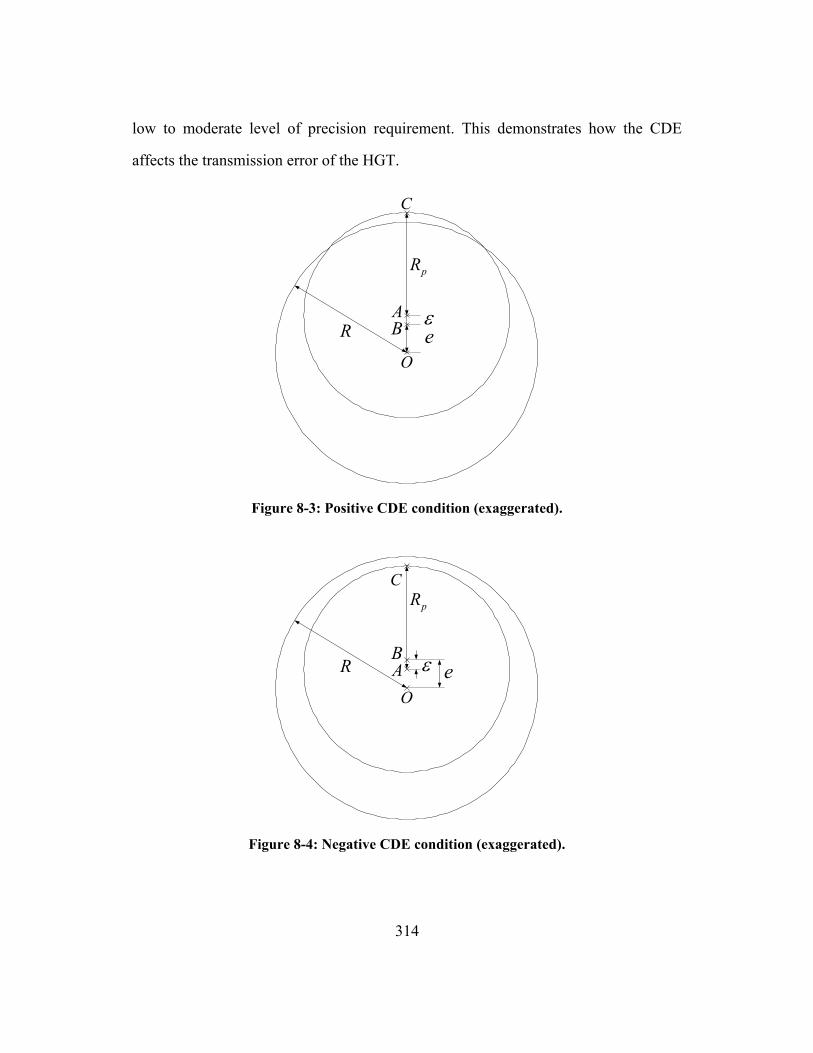
314

low to moderate level of precision requirement. This demonstrates how the CDE

affects the transmission error of the HGT.

eε

pR

R

O

AB

C

Figure 8-3: Positive CDE condition (exaggerated).

eε

pR

R

OAB

C

Figure 8-4: Negative CDE condition (exaggerated).

315

8.2.2 Effects of Tooth Spacing Errors (TSE)

Effects of Tooth Spacing Error (TSE) on the HGT contact properties were

analyzed in this research. A set of random TSE values was given to the eight spaces

of the nine tooth pairs of the ¼-scale HGT model. Table 8-1 presents the TSEs ( X )

along with the corresponding statistical parameters, i.e., standard deviation (σ ),

normal distributions (Y ) and normalized TSEs ( Z ). The arithmetic mean (µ ) of the

TSE is 0.00005. The standard deviation (σ ) is given by

( )22

( 1)n X X

n nσ

−=

−∑ ∑ (8.7)

where n is the number of data. Then, the normal distribution (Y ) is given by

2

2( )

212

X

Y eµ

σ

σ π

−−

= (8.8)

and the normalized TSE is given by

XZ µσ−

= (8.9)

Table 8-1: Statistical parameters of the representative TSEs.

Space Between TSE ( X )

Standard Deviation (σ )

Normal Distribution (Y )

Normalized TSE( Z )

8th and 6th Pair -0.0002 0.000287849 950.492 -0.869 6th and 4th Pair -0.0001 0.000287849 1209.981 -0.521 4th and 2nd Pair 0.0003 0.000287849 950.492 0.869 2nd and 0th Pair 0.0002 0.000287849 1209.981 0.521 0th and 1st Pair 0.0002 0.000287849 1209.981 0.521 1st and 3rd Pair 0.0005 0.000287849 408.361 1.563 3rd and 5th Pair -0.0002 0.000287849 950.492 -0.869 5th and 7th Pair -0.0003 0.000287849 661.766 -1.216

316

Assuming a normal distribution of the data, the standard normal ( Z ) table60

(Table 8-2) can be used to predict the possibility in [%] of having a TSE which is

bigger (for a plus Z ) or smaller (for a minus Z ) than the given TSE. For example,

the possibility of having a TSE higher than +0.000499 and lower than –0.000499 is

5.94 % and ~2.83 %, respectively. In other words, the confidence level for a random

TSE to be in the range of –0.0005 to +0.0005 is ~91.23 %.

Table 8-2: Representative Z values and corresponding possibility above/below them.

Z ±1 ±1.56 ±2 ±3 ±3.29 ±3.89 +TSE (10-3) 0.3378 0.4990 0.6256 0.9135 0.9970 1.1697 –TSE (10-3) –0.2378 –0.3990 –0.5257 –0.8135 –0.8970 –1.0697 Area from

0 to Z 0.3413 0.4406 0.4772 0.4987 0.4995 0.4999

Possibility [%] 15.87 5.94 2.28 0.13 0.05 0.01

The TSE model of the ¼-scale HGT was simulated using FEA for three

different loading conditions. The base (1x) load condition simulates an output torque

of 41,326 in-lb at the center of the HGT, which is close to the designed nominal

output torque. Two other loading conditions are ~3x of the base load (128,168 in-lb),

and ~6x of the base load (238,934 in-lb). Figure 8-5 shows the results of FEA. Figure

8-6 to Figure 8-8 present the load sharing factor plots for each loading condition.

60 This table shows representative Z values and the corresponding possibilities (frequencies of occurrence) above or below them. It is well known that the possibilities in percentile are obtained by calculating the corresponding area of the normal distribution plot (by integrating the distribution curve with respect to the corresponding range of Z ).

317

+/- 0.0005” TSE

CR = 4

CR = 4

CR = 3

Max. Stress= 278 ksi

Max. Stress= 202 ksi

Max. Stress= 101 ksi

6x Load

3x Load

1x Load

Perfect Spacing

CR = 3

CR = 5

CR = 4

Max. Stress= 86 ksi

Max. Stress= 279 ksi

Max. Stress= 205 ksi

1x Load

6x Load

3x Load

+/- 0.0005” TSE

CR = 4

CR = 4

CR = 3

Max. Stress= 278 ksi

Max. Stress= 202 ksi

Max. Stress= 101 ksi

6x Load

3x Load

1x Load

+/- 0.0005” TSE

CR = 4

CR = 4

CR = 3

Max. Stress= 278 ksi

Max. Stress= 202 ksi

Max. Stress= 101 ksi

6x Load

3x Load

1x Load

Perfect Spacing

CR = 3

CR = 5

CR = 4

Max. Stress= 86 ksi

Max. Stress= 279 ksi

Max. Stress= 205 ksi

1x Load

6x Load

3x Load

Perfect Spacing

CR = 3

CR = 5

CR = 4

Max. Stress= 86 ksi

Max. Stress= 279 ksi

Max. Stress= 205 ksi

1x Load

6x Load

3x Load

Figure 8-5: Effects of TSE.

318

0

10

20

30

40

50

60

70

4 2 0 1 2

Tooth Pair

Load

Sha

ring

Fact

or [%

]Perfect Spacing +/- 0.0005" TSE

Figure 8-6: Comparison of load sharing factor for the perfect and TSE conditions w.r.t. the 1x base load.

0

10

20

30

40

50

4 2 0 1 2

Tooth Pair

Load

Sha

ring

Fact

or [%

]

Perfect Spacing +/- 0.0005" TSE

Figure 8-7: Comparison of load sharing factor for the perfect and TSE conditions w.r.t. the 3x base load.

319

0

10

20

30

40

4 2 0 1 2

Tooth Pair

Load

Sha

ring

Fact

or [%

]Perfect Spacing +/- 0.0005" TSE

Figure 8-8: Comparison of load sharing factor for the perfect and TSE conditions w.r.t. the 6x base load.

This TSE analysis shows that there are minimal changes in the stress level,

contact ratio, and load sharing factor between the perfect and TSE conditions. It is

also notable that the differences in the load sharing factors decrease as the applied

load is increased. In other words, the effect of the TSE on the HGT can be diminished

under heavier loads. This analysis supports one of the claimed advantages of the

HGT, an ideal (self-protecting) system for heavy load applications.

8.2.3 Effects of Misalignment Errors (ME)

It is expected that under the Misalignment Error (ME) conditions, the actual

shape and area of the contacts on the tooth surfaces will vary depending on the axis

and (angular) magnitude of the ME. The purpose of this analysis is to visualize those

variations by simulating some representative ME conditions using FEA.

320

Three different ME conditions (plus perfect condition) were simulated for the

same steady-state load (5x of the nominal load). Table 8-3 summarizes the three ME

conditions and compares them with the actual misalignment errors expected in the

two prototypes. The actual ME values were derived from the out-of-plane stiffnesses

of the crossed roller bearings (17.7×107 in-lbf/rad for the ¼-scale and 4.42×107 in-

lbf/rad for the Rugged) and potential out-of-plane moments (72,300 in-lb for the ¼-

scale and 14,400 in-lb for the Rugged). Hence, this analysis considers 2.2x higher

ME in condition 1 and 4.3x higher ME in condition 2 than the actual ME expected in

the ¼-scale. In other words, the judgment from this analysis on the ME effects can be

2 to 4 times more conservative.

Table 8-3: Three ME conditions simulated and actual ME expected.

Simulated Actual (Expected)

ME 1 ME 2 ME 3 ¼-scale Rugged

ME [deg] 0.05 0.1 0.05 & 0.1 0.023 0.018

Axis of Rotation 2 1 2 & 1 1 or 2 1 or 2

Figure 8-9 through Figure 8-12 show variations of the contact pressure profile

with increasing loads for no ME (perfect) condition. As expected, the rectangular

shape contact occurs on the tooth surface and is expanded as the contact pressure

increases. The subsequent figures clearly show the sequence of the contacts and the

changes in the contact pressure and area.

Figure 8-13 through Figure 8-16 show variations of the contact pressure

profile with increasing loads for a ME of 0.05° with respect to the axis 2 (the

coordinate is shown in the figures). As expected, there is a premature contact at the

front portions of the tooth face widths where the clearances are reduced due to the

321

given misalignment. However, as load is increased, the contact area expands all the

way to the back portion of the face widths, which enables the whole length of the

tooth surfaces to take the load.

Figure 8-17 through Figure 8-20 show variations of the contact pressure

profile with increasing loads for a ME of 0.1° with respect to the axis 1. Similar

observation to the previous ME analysis applies here except for slight differences in

elevation of the contact ends at the front and back side of the tooth face width due to

the given ME (the difference is too small to be distinguishable in the figures). Note

that the stress level for this ME condition is comparable with the previous ME

condition even though a larger ME was applied.

Figure 8-21 through Figure 8-24 show variations of the contact pressure

profile for a combined ME condition, 0.05° ME with respect to the axis 2 and 0.1°

ME with respect to the axis 1. This ME condition yields a similar contact pattern to

the previous ME conditions. However, since the initial contact area is more localized,

pressure level of this ME condition is the highest among all ME conditions.

Figure 8-25 through Figure 8-28 show deflections of the teeth (of the internal

gear) for the four different ME conditions. The maximum deflections are: 0.002407”

for the perfect condition, 0.002614” for the first ME condition, 0.002624” for the

second ME condition, and 0.002647” for the combined ME condition. Again, the

deflections under the first and second ME conditions are comparable to each other

even though the magnitude of the second ME is twice of that of the first ME.

Note that crowning of the tooth profile (or relief of the edges of the tooth

profile) in the tooth face width direction will be beneficial in accommodating the

misalignment errors.

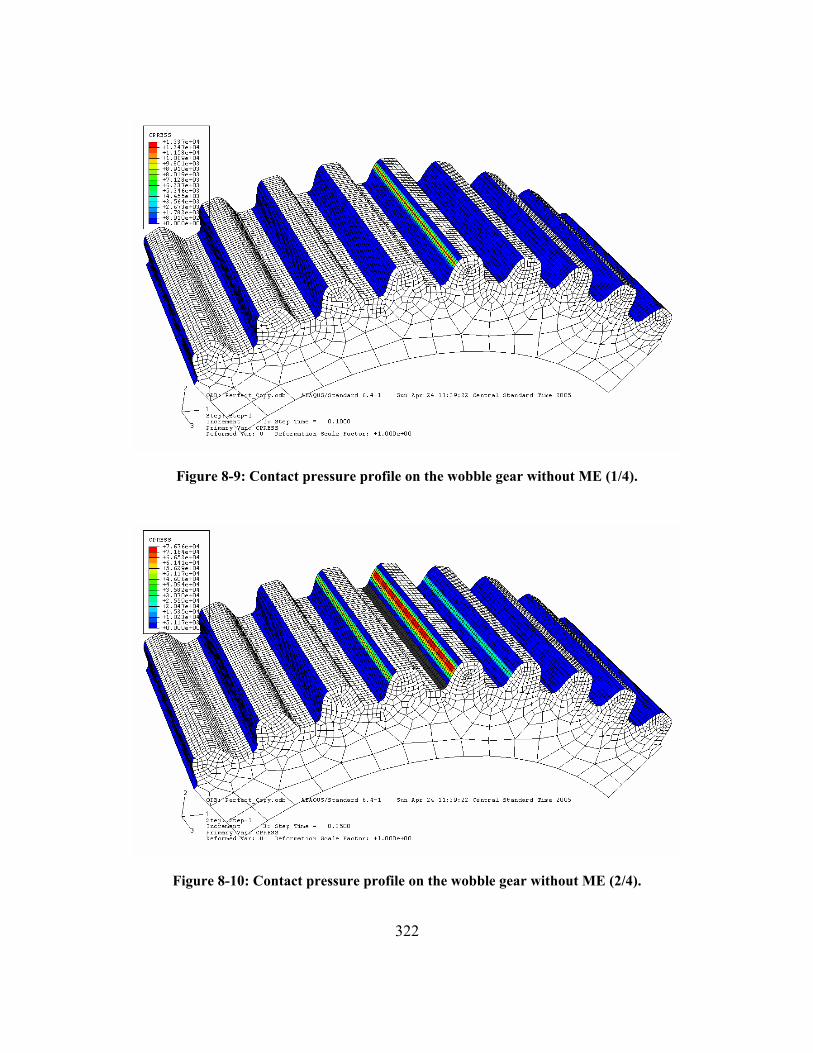
322

Figure 8-9: Contact pressure profile on the wobble gear without ME (1/4).

Figure 8-10: Contact pressure profile on the wobble gear without ME (2/4).

323

Figure 8-11: Contact pressure profile on the wobble gear without ME (3/4).

Figure 8-12: Contact pressure profile on the wobble gear without ME (4/4).

324

Figure 8-13: Contact pressure profile with ME of 0.05° w.r.t. axis-2 (1/4).

Figure 8-14: Contact pressure profile with ME of 0.05° w.r.t. axis-2 (2/4).

325

Figure 8-15: Contact pressure profile with ME of 0.05° w.r.t. axis-2 (3/4).

Figure 8-16: Contact pressure profile with ME of 0.05° w.r.t. axis-2 (4/4).

326

Figure 8-17: Contact pressure profile with ME of 0.1° w.r.t. axis-1 (1/4).

Figure 8-18: Contact pressure profile with ME of 0.1° w.r.t. axis-1 (2/4).

327

Figure 8-19: Contact pressure profile with ME of 0.1° w.r.t. axis-1 (3/4).

Figure 8-20: Contact pressure profile with ME of 0.1° w.r.t. axis-1 (4/4).

328

Figure 8-21: Contact pressure profile with ME of 0.05° (axis-2) and 0.1° (axis-1) (1/4).

Figure 8-22: Contact pressure profile with ME of 0.05° (axis-2) and 0.1° (axis-1) (2/4).

329

Figure 8-23: Contact pressure profile with ME of 0.05° (axis-2) and 0.1° (axis-1) (3/4).

Figure 8-24: Contact pressure profile with ME of 0.05° (axis-2) and 0.1° (axis-1) (4/4).

330

Figure 8-25: Deflection of teeth under no ME.

Figure 8-26: Deflection of teeth under ME of 0.05° w.r.t. axis-2.

331

Figure 8-27: Deflection of teeth under ME of 0.1° w.r.t. axis-1.

Figure 8-28: Deflection of teeth under ME of 0.05° w.r.t. axis-2 and 0.1° w.r.t. axis-1.

332

This ME analysis in terms of contact pressure and tooth deflection suggests

that: 1) combined ME (with respect to dual axes) is more detrimental than the single

ME (with respect to single axis), and 2) management of ME with respect to axis 2

should be more effective than that with respect to axis 1 because the former effect is

more significant (~2x).

Comparing with the perfect condition, the HGT observed a 17 % increase in

the maximum stress and 10 % increase in the maximum tooth deflection for the

combined ME condition whereas it observed, on average 11 % and 8.8 % increases in

these two criteria for the single ME condition. These variations are regarded to be

insignificant. Figure 8-29 compares the maximum Mises stress and maximum

deflection for the four different ME conditions. Note that, as discussed earlier, this

analysis overestimates the effects of ME because the actual misalignment errors

expected in the prototypes (based on the crossed roller bearing out-of-plane stiffness;

see Table 8-3) are 2 to 4 times lower than the simulated reference errors.

210000

220000

230000

240000

250000

260000

270000

280000

Perfect ME 1 ME 2 ME 3

Misalignment Error (ME) Conditions

Max

. Mis

es S

tres

s [p

si]

0.002250.00230.002350.00240.002450.00250.002550.00260.002650.0027

Max

. Def

lect

ion

[in]

Max. Mises Stress [psi] Max. Deflection [in]

Figure 8-29: Comparison of the max. stress and deflection for different ME conditions.

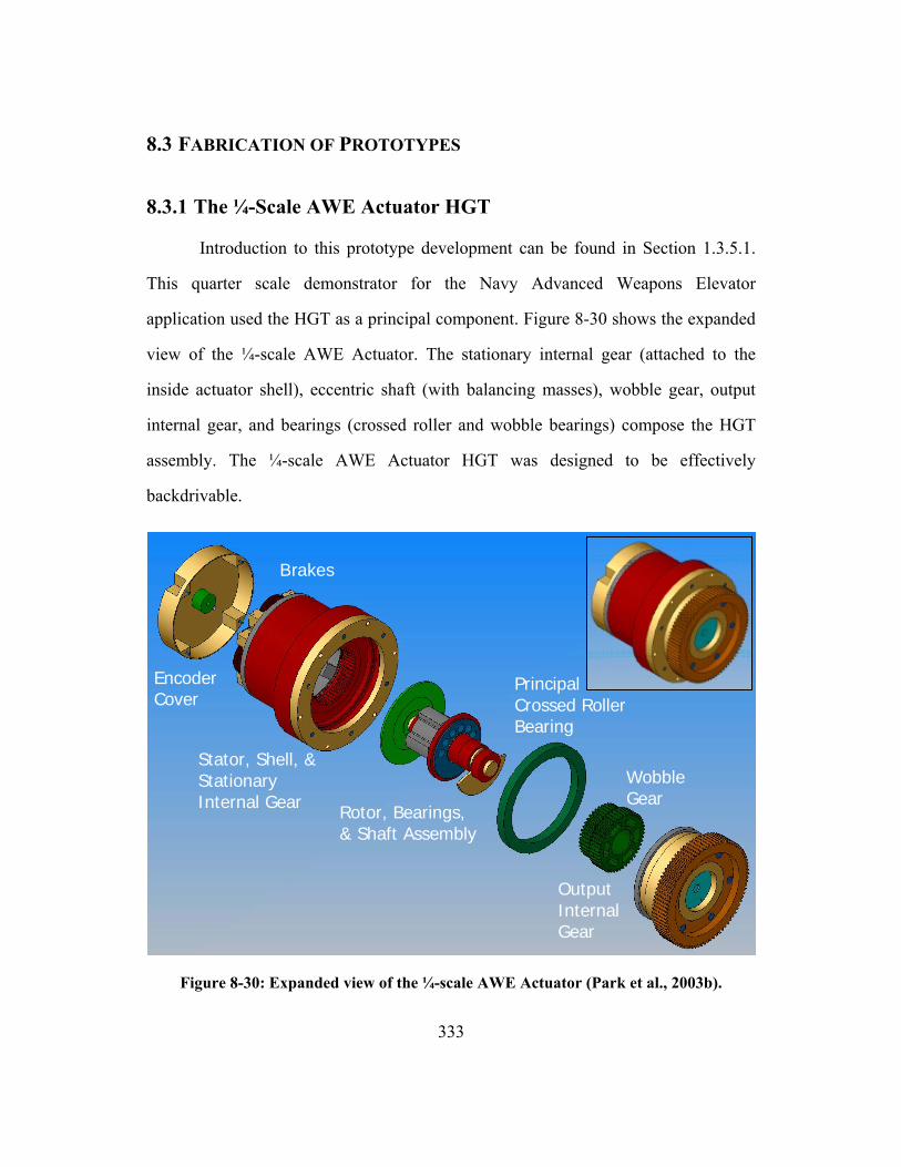
333

8.3 FABRICATION OF PROTOTYPES

8.3.1 The ¼-Scale AWE Actuator HGT

Introduction to this prototype development can be found in Section 1.3.5.1.

This quarter scale demonstrator for the Navy Advanced Weapons Elevator

application used the HGT as a principal component. Figure 8-30 shows the expanded

view of the ¼-scale AWE Actuator. The stationary internal gear (attached to the

inside actuator shell), eccentric shaft (with balancing masses), wobble gear, output

internal gear, and bearings (crossed roller and wobble bearings) compose the HGT

assembly. The ¼-scale AWE Actuator HGT was designed to be effectively

backdrivable.

Figure 8-30: Expanded view of the ¼-scale AWE Actuator (Park et al., 2003b).

Rotor, Bearings, & Shaft Assembly

Wobble Gear

Stator, Shell, & Stationary Internal Gear

Principal Crossed Roller Bearing

Output Internal Gear

Encoder Cover

Brakes

334

This initial design by UTRRG was partly modified by Timken for more

efficient manufacturability and assembly. As far as the HGT is concerned, a major

change made by Timken was to split the wobble gear into a two-piece sub assembly

as opposed to the original one-piece design proposed by UTRRG. This modification

made it more convenient to grind the gear teeth after heat treatment at the expense of

structural integrity and tolerances.

Since the gears in the HGT use circular-arc profiles that require non-standard

manufacturing methods, the processing of the gear teeth was one of the challenging

aspects of the fabrication. The gear blanks were manufactured out of AISI 8620 H

bearing grade steel. The circular-arc teeth of the all three gears were generated by

wire EDM, and then carburized and hardened to achieve a surface hardness of 58

HRC minimum. The wire EDM not only exhibits very high accuracy level61 but also

can cut very small radius contours whose diameters are as low as a few thousandths

of an inch (which is desirable for cutting root fillets of fine teeth). Timken

incorporated their proprietary engineered surface features on the gear teeth surfaces

to improve the wear resistance and reduce the coefficient of friction (Degrange,

2005).

Several challenging issues with regard to the fabrication process and potential

errors were reported. Through the heat treatment process, the 1st stage wobble gear

blank diameter was reduced more than expected allowing minimal removal of

material during the grinding process. Later on, extra grinding resulted in undersized

gear tooth thickness, and thus increased backlash. This increased backlash can affect

the contact ratio and transmission error especially at frequent load reversals. Accurate

61 The accuracy level of wire EDM for the HGT gear manufacture will be revisited in Section 8.3.2.

335

grinding of the eccentric shaft was also a challenging task because it affects the

alignment and center distance of the gear meshes.

Stack-up of tolerances has been raised as a major issue that should be

investigated and addressed further for correct control of the CDE in the HGT. In the

radial direction of the gear assembly, the run-outs and center position errors of the

components can be stacked up and cause significant CDEs. The stack-up of

tolerances identified by Timken are listed as follows:

• 1st stage fixed gear geometry run-out to shell datum

• True position of the shell center

• True position center plate bore to OD

• Center tapered bearing run-out

• Output tapered bearing run-out

• True position of shaft eccentric to tapered roller bearing centers

• True position of output gear ID to OD

• True position 2nd stage gear ID to OD

• Crossed roller bearing run-out

• Wobble gear bearing run-out

• 1st stage wobble gear tooth geometry run-out

Figure 8-31 shows the sub-assembly of the wobble gear, eccentric shaft,

balancing masses, and the wobble gear bearings. The shaft was split into a two piece

assembly by Timken. It is supported by a tapered roller bearing in the middle of the

actuator and by a roller bearing at the rotor end to accommodate thermal expansion of

the shaft and/or housing. The eccentric mass of the sub assembly was dynamically

balanced by rotating the shaft and removing material from the balancing masses.

Timken was able to achieve balancing of the sub assembly to less than 90 g·mm

336

(Degrange, 2005). Figure 8-32 shows the output side balancing mass and the 2nd stage

wobble gear. Figure 8-33 shows the whole assembly of the actuator.

Figure 8-31: Assembly of wobble gear, eccentric shaft, balancing masses, and bearings for the ¼-scale HGT (Courtesy of Timken Co.).

Figure 8-32: Output side of the ¼-scale AWE Actuator HGT (Courtesy of Timken Co.).

337

Figure 8-33: Whole assembly of the ¼-scale AWE Actuator (Courtesy of Timken Co.).

8.3.2 The Rugged Actuator HGT

Introduction to this prototype development can be found in Section 1.3.5.2.

As noted in this report, there were two major upgrades from the initial design. First,

the pressure angle has been dramatically reduced. Previously, the pressure angle was

designed to be 20º at the pitch point, but the new design employs an exceptionally

low 7° pressure angle at the pitch circle. The objective is to reduce the bearing load.

Due to this modification, the radial component of the bearing load was reduced by

66 %. Second, the size of the eccentricity has been reduced. It was 0.229” in the

previous design, but reduced to 0.16”. The purpose is to reduce unbalanced mass and

thus decrease the eccentric force. As a result, inertia of the gear train is reduced due

to less mass and smaller eccentricity. This upgrade led to reduction of the eccentric

force by 27%. Figure 8-34 shows the whole assembly of the Rugged Actuator.

338

Figure 8-34: The Rugged Actuator.

As far as the bearings are concerned, the needle roller bearings initially

specified for the wobble gear was first replaced with a combination needle

roller/angular contact ball bearing for axial retention of the wobble gear. However, it

was discovered that this combination bearing had a significant amount of clearances

(~0.003” radially and ~0.015” axially) specified by manufacture for thermal

expansion, easy assembly, and etc. At the initial spin test with increased operational

temperature, significant noise was generated from the actuator, and the clearances in

the bearing were suspected to be a source of the noise. Thus, it was replaced with a

standard needle roller bearing (SKF NA 4911) and ball bearing (SKF 61911). When

these bearings were used, the radial and axial clearances and noise levels were

significantly reduced. The principal crossed roller bearing selected was an off-the-

shelf bearing (RB15025 from THK). The out-of-plane stiffness of the crossed roller

339

bearing was 4.42×107 in-lbf/rad (5×106 Nm/rad). Note that the out-of-plane stiffness

of the ¼-scale AWE actuator from its crossed roller bearing was 17.7×107 in-lbf/rad

(2×107 Nm/rad).

The replacement of the wobble gear bearing necessitated an upgrade of the

analytically obtained balancing geometry. Since the replacement was done after the

fabrication was completed, experimental balancing of the as-built HGT had to be

done. The approach was to drill holes into the output side balance mass and insert

high density tungsten carbide slugs. The size and number of the slugs were varied to

achieve a balanced system. Figure 8-35 shows the shaft assembly of the Rugged

Actuator HGT. In this fabrication, it was possible to make both of the wobble gear

and the shaft in single pieces as opposed to the case of the ¼-scale prototype (see

Section 8.3.1).

Figure 8-35: Shaft assembly of the Rugged Actuator HGT.

340

Machining of the gear teeth was done by EDM (Electro-Discharge

Machining). This process can reproduce a part’s geometry to within ±0.0002”, which

is exceptional when compared with traditional processes. The process achieves its

high accuracy due to the low forces and deflection involved. Material is removed by

high energy metal vaporization, not by brute force of a cutting tool. Although wire

EDM is commonly used to make parts that require only profile cuts in one plane,

graphite tools can also be used to EDM parts with much more complicated geometry.

For all parts, initial lathe roughing left 0.015” of extra material on all critical surfaces

before the parts were sent out to the EDM shop for work. Once processed, the

returned parts were put back on the machine where final cuts were made based on the

actual centerline of the gear.

The fixed internal gear teeth were made in one setup using wire EDM and

therefore have the best tolerances of the four gears (~0.0002”). However, even when

using wire EDM, the part must undergo at least two setups in order for the wire to

reach all areas of the part. This is a machine restriction and the path start/stop point

was left up to EDM specialists who have this type of training and experience.

The output internal gear was made by a two step EDM process. The first

process used wire EDM to machine a graphite tool. The output was then mounted in

the machine and the graphite tool was used to ram EDM the output gear teeth. Since

the gear geometry went through two EDM processes, tolerances are likely twice the

individual process capability (~0.0004”). Figure 8-36 shows the machined output

internal gear.

341

Figure 8-36: Machined circular-arc teeth in the output internal gear.

The wobble gear was machined by a three step process. The first step made

each of the graphite tools (one for each stage) using a wire EDM process. Once these

individual tools were made, the two parts were fastened axially (with great effort to

keep concentricity) with precision pins. The second and final step used this new

composite tool to ram EDM the wobble gear blank. The final gear was then ready for

finishing cuts to put the gear on centerline. The tolerances of this part are likely equal

to or slightly worse than the output (0.0004” to 0.0005”, due to the composite nature

of the graphite tool). Figure 8-37 shows the machined wobble gear.

342

Figure 8-37: Wobble gear blank (left) and wobble gear cut by EDM (right).

8.3.3 Lubricant Selection

The purpose of lubrication in gear transmissions is to minimize tooth surface

wear, friction loss, and temperature rise. The convex-concave circular-arc tooth

profile to be employed in the HGT is claimed to be very effective in containing the

lubrication between the teeth in mesh, and decreasing the coefficient of friction

between the contact surfaces. The eccentric motion of the wobble gear should also be

very efficient in moving the splash type lubrication to the necessary locations. In

summary, lubricating the HGT will allow for minimal wear on the tooth surfaces,

effective reduction of friction losses, and adequate means of cooling.

There are three methods of lubrication – grease lubrication, splash lubrication,

and oil jet lubrication. In general, a proper lubrication method is determined based on

the tangential speed of the gear teeth (Lubrication of Gears, n.d.). For a low tangential

speed (0 to 5 m/s), grease lubrication is recommended while for a medium tangential

speed (5 to 15 m/s), splash lubrication is appropriate. For a higher speed, oil jet

343

lubrication is suitable. The tangential velocity of the wobble gear of the HGT falls

under the low speed regime. However, splash lubrication was chosen over grease

lubrication because the selected method also needs to be applied for the bearings in

proximity to the HGT. Note that the wobble gear bearings and tapered roller bearings

rotate at the speed of the eccentric shaft which can go up to 4000 rpm. Also, as noted

earlier, the wobble motion of the wobble gear can agitate the oil well enough to make

the splash lubrication be more effective (in contrast to fixed-axis rotation of normal

gears).

Table 8-4 lists the properties that gear lubricant should possess. In addition to

this list, compatibility of the lubricant with seals should also be considered. Among

these properties, correct viscosity is the most critical factor to be considered when

selecting a proper lubricant.

Table 8-4: Required properties for gear lubricant (Lubrication of Gears, n.d.).

Properties Description Correct

Viscosity Lubricant should maintain a proper viscosity to form a stable oil film at the specified temperature and speed of operation.

Anti-Scoring Property

Lubricant should have the property to prevent scoring failure of tooth surface while under high-pressure of the load.

Oxidization and Heat Stability

Good lubricant should not be oxidized easily and must perform in a moist and high-temperature environment for long duration.

Water Anti-Affinity Property

Moisture tends to condense due to temperature change, when the gears are stopped. The lubricant should have the property of isolating moisture and water from lubricant.

Antifoam Property

If the lubricant foams under agitation, it will not provide a good oil film. Hence, the antifoam property is a vital requirement.

Anticorrosion Property

Lubrication should be neutral and stable to prevent corrosion from rust that may mix into the oil.

The viscosity grade of an industrial lubricant is regulated by JIS K 2001.

Table 8-5 shows the ISO viscosity grade and equivalent AGMA lubricant grade (from

344

ANSI/AGMA 9005-D94) along with the corresponding range of kinematic viscosity

represented by the regulation. EP (Extreme Pressure) gear oils are often specified for

use in the heavy duty applications. The EP additive absorbs onto or reacts with the

surfaces to form protective coatings or surface films. The film not only prevents

interaction of the asperities on the contact surfaces but also reduces shearing of the

metal by lowering the coefficient of friction (Kubo, 1991). For this reason, an EP

gear oil will be specified for the HGT.

Table 8-5: ISO Viscosity grade of industrial lubricant (JIS K 2001).

ISO Viscosity Grade

(ISO VG)

Equivalent AGMA EP

Gear Oil Grade

Kinematic Viscosity Median Value

10-6 m2/s (cSt) (40 ºC)

Kinematic Viscosity Range

10-6 m2/s (cSt) (40 ºC)2 2.2 1.98 ~ 2.42 3 3.2 2.88 ~ 3.52 5 4.6 4.14 ~ 5.06 7 6.8 6.12 ~ 7.48 10 10 9.0 ~ 11.0 15 15 13.5 ~ 16.5 22 22 19.8 ~ 24.2 32 32 28.8 ~ 35.2 46

N/A

46 41.4 ~ 50.6 68 2 EP 68 61.2 ~ 74.8 100 3 EP 100 90.0 ~ 110 150 4 EP 150 135 ~ 165 220 5 EP 220 198 ~ 242 320 6 EP 320 288 ~ 352 460 7 EP 460 414 ~ 506 680 8 EP 680 612 ~ 748 1000 8A EP 1000 900 ~ 1100 1500 9 EP 1500 1350 ~ 1650

There are numerous off-the-shelf gear oil products with an EP additive. The

following brand name products feature a wide range of ISO grades.

• Philips 66 All Purpose Philgear® Industrial Lubricants

• Shell Omala® Fluids RL

345

• Imperial Oil Spartan EP

• Castrol Optigear® BM

• Chevron Ultra Gear Lubricants

Table 8-6 shows a set of typical test data for these EP gear oils.

Table 8-6: Test data for Chevron Ultra Gear Lubricants (2003).

Commercially available products are often classified by SAE viscosity grade,

e.g., SAE 80W-90 and SAE 85W-140. Representative brand name products that have

such grades are: Spirax HD (Shell), MP Gear Lube (76 Lubricants), Multigear EP

(Texaco), RPM Universal Gear Lubricant (Chevron), Premium Gear Oil MP (Citgo),

and Gear Oil GX (Exxon). Two locally available lubricants with two different SAE

grades were purchased and tested for the Rugged Actuator prototype. They were

Valvoline HP (SAE 80W-90) and Shell Spirax HD (SAE 85W-140). Table 8-7

compares the specification of these two EP gear oils. The specification of Valvoline

HP was very close to general ISO 220 or AGMA 5EP oil.

346

Table 8-7: Specifications of the tested gear lubricants.

Valvoline HP Shell Spirax HD SAE Grade 80W-90 85W-140

Viscosity (cSt)

40ºC 100°C

205 18.9

411 29.7

Viscosity Index 103 103 Pour Point, ºC -24 -12 Flash Point, ºC 203 200

The viscosity at the ambient temperature was very high for both oils, so it

caused a relatively high initial input torque (drag) in the range of 3~4 in-lb

(Valvoline) and 7~8 in-lb (Shell). This initial torque is also determined by the amount

of lubricant in the gear transmission volume. The amount of lubricant can be

theoretically determined by estimating the power loss for gears and bearings. For power loss LP , specific heat at constant pressure pc , and temperature rise T∆ , the

amount of lubricant flow required can be obtained by (Kubo, 1991)

L

p

Pwc T

=∆

(8.10)

A rule of thumb is that an adequate oil level for spur or helical gears having a

horizontal shaft is between 1x and 3x of the full depth of the tooth (Lubrication of

Gears, n.d.). The purpose of keeping the depth of the oil bath low is to limit the

power loss due to oil drag and churning. However, the oil for the gears in the HGT is

also used to lubricate the associated bearings, and for this reason, the oil level was

increased to about 25 % of the wobble gear diameter. The volume to be filled by oil

was calculated using the solid model of the gear transmission.

After testing the two different SAE grade oils, Valvoline HP was selected

over Shell Spirax HD. The main reason was that at usual operating temperatures, the

347

difference in viscosities between the two oils diminished while there was a relatively

big difference in viscosities at room temperature causing a high initial drag torque

and sluggishness of the operation. The film thickness formed by the oil is believed to

be adequate enough to dampen the noise and vibration. No abnormal wear patterns

were found on the tooth surfaces after the tests.

8.3.4 Test Plan

The ¼-scale AWE Actuator and Rugged Actuator will be tested by Timken

and UTRRG, respectively. The following 10 tests have been suggested by UTRRG

(Tesar, 2004d). These tests are intended to provide an initial set of data to evaluate

the overall performance and suitability of the actuator and the HGT for a wide range

of applications including Navy and DOE applications.

8.3.4.1 Torsional Stiffness

The purpose is to show that the prototype actuators are much stiffer for their

size than other state-of-the-art devices. To accomplish this test, the brake will be

engaged and current on the motor will be put on hold to ensure that the motor rotor

does not move. Then, gradual torques up to three times the rated torque will be

applied using a long torsion arm (with various gravity loads) or torsion machine

(MTS) to the output shaft (in both directions). The deformation at the end of the arm

will be measured and plotted as a function of load to determine the torsional stiffness

of the actuator. The measurement will be made in three or four distinct positions of

the actuator output.

348

8.3.4.2 Out-of-Plane Stiffness

To accomplish this, a long arm will be attached to the output plate along the

center line of the actuator. Then, up to twice the rated out-of-plane moment of the

crossed roller bearing will be applied using gravity loads or torsion machine. The

deformation at the end of the arm will be measured and plotted with respect to the

various loads to determine the out-of-plane stiffness of the actuator.

8.3.4.3 Accuracy/Repeatability/Angular Velocity Profile

To accomplish this, a precision rotary position sensor will be used on the

output of the actuator to measure the position of the output plate relative to an input

command (established by the back-plate encoder). Note that the encoder has a limited

accuracy but it should be very repeatable. Round-out will indicate how “linear” the

gear train is over several rotations of 360° (in both directions). This should be done

with various loads up to the rated load of the actuator.

8.3.4.4 Rotary Backlash/Lost Motion

To accomplish this, the actuator will be in a fixed position using the brake and

holding the motor current. Then, torques up to the rated torque will be applied using a

long torsion arm (with gravity load) or torsion machine to the output shaft in both

directions. It is important to measure carefully within the range ± 10% of the rated

torque. In this test, 5 to 10 distinct angular positions of the output shaft will be

plotted. Average of these data will represent backlash/lost motion in the HGT. Note

that the bearings are part of this effect.

349

8.3.4.5 Internal Temperature Sensitivity

The purpose is to prove that the backlash/lost motion of the HGT has less

sensitivity to the temperature effect than a similar purpose epicyclic gear train. A

limited range of tests similar to those in backlash/lost motion test (Section 8.3.4.4)

will be conducted for different temperatures, e.g., 200° F, 300° F, 400° F, and 500° F,

to examine the effects of the temperature. Note that the properties of the lubricant

have a significant influence on the result.

8.3.4.6 Torque Capacity at Various Speeds

A dynamometer will be used to load the actuator at various speeds and torque

will be measured by a torque sensor located in between the actuator and the

dynamometer. The load will be applied gradually, i.e., 0 %, 10 %, 20 %, …, 100 %

(of the rated load), to determine how well the actuator produces torque. A limited set

of tests may be performed at 125 %, 150 %, 175 %, and 200 % of the rated torque.

8.3.4.7 Noise under Various Loads

This is a related measurement that should be done in parallel with the torque

capacity tests (Section 8.3.4.6). The prototype actuators were not originally designed

for low noise but the HGT is expected to produce less noise than an equivalent

epicyclic gear train especially at heavier loads and higher temperatures. The data

from the tests should establish a data reference baseline for future work on quiet

actuators. To best test for noise the output plate should carry various levels of rotary

inertia during the tests. This inertia should be relatively large to illustrate a worst

dynamic load condition.

350

8.3.4.8 Heat Build-up under Various Loads

To accomplish this, the dynamometer is controlled to provide a constant load

of 0 %, 10 %, 25 %, 50 %, 100 %, 150 %, and 200 % of the rated load to observe

how quickly temperature builds up in the actuator to empirically determine how much

cooling would be required under various duty cycle conditions. Several tests should

be done using representative duty cycles.

8.3.4.9 Friction Losses in Bearings and Gears

Friction in the bearings and gears can be obtained at various output loads

(provided by the dynamometer) by measuring how much “holding” or “assist” torque

is required by the motor to permit back-driving the actuator. The motor torque can be

estimated by measuring the required “assist” current in the motor. The interesting

question would be the tendency of this actuator to be back-driven if the motor and

brake are locked up. It may happen that the actuator will turn a little bit under

repeated torque reversals. The loads on the dynamometer should be incremented up

to the rated torque of the actuator.

8.3.4.10 Acceleration/Deceleration and Rapid Reversal

To accomplish this, the time it takes to accelerate the actuator from zero-to-

full speed and to decelerate from full-to-zero speed at various load levels (various

voltages to the dynamometer) and with various inertia loads (various masses

concentrically attached to the output shaft) will be measured. Actuator capability of

rapid load reversal will also be determined by measuring the time it takes to reverse

to get to full speed in reverse from full speed forward. This test can damage the

actuator, so it should be the last test. After these tests, the actuator components should

be inspected for wear and deformation.

351

CHAPTER 9

CONCLUSION

9.1 SUMMARY AND KEY RESULTS

The motivation of this research was to move the EM actuator technology

forward and make it meet the ever demanding requirements of emerging and

advancing applications. To do so, the technology of the most critical (and often

failing) component of the EM actuator, the gear transmission technology, necessitated

a careful review and further development. This research proposed a promising gear

transmission architecture called the Hypocycloidal Gear Transmission (HGT) whose

design has not been pursued systematically, and a unique tooth form that can

maximize the performance of the architecture. Based on a comprehensive literature

review and comparative analysis, the advantages of the combination of the HGT and

its tooth form over the state-of-the-art technologies have been claimed. The goal of

this research was to validate these claimed advantages as well as establish a set of

design guidelines for further development of the HGT and its tooth form.

Overall, this report consists of an in-depth design and analysis. In the design

effort (Chapter 2 through Chapter 5), system level (the HGT) design and tooth level

(the circular-arc profile) design were accomplished. A rigorous literature review was

done for each design (in Chapter 2 and Section 4.3 of Chapter 4, respectively) for

identification of the advantages and justification of the work. In the analysis part

(Chapter 5 through Chapter 8), four critical analyses, i.e., tooth meshing analysis,

loaded tooth contact analysis, efficiency analysis, and manufacturing tolerance

352

analysis, were performed to support the claimed advantages of the HGT and its

circular-arc tooth profile. This section will summarize the report under the two main

concentrations of the study, design (Section 9.1.1) and analysis (Section 9.1.2), and

discuss the key results of this report.

9.1.1 Design of the HGT and Circular-Arc Tooth Profile

9.1.1.1 Advantages of the HGT

Advantages of the HGT have been identified based on comprehensive review

of the patent/non-patent literature which discussed developments of wobble gear

systems similar to the HGT. The claimed advantages are summarized as below along

with quick cross references in this report (see Section 2.4 for expanded discussion):

• Widest range of reduction ratios: up to 5,000 to 1 in an extremely compact

volume; see Section 3.2.1 for further discussion and an exemplary calculation

of the reduction ratio (4900 to 1).

• Compact and simple configuration: 4 principal parts, 1 principal bearing, and

2 or 4 ancillary bearings; allows for ease of design/assembly, minimization of

the manufacturing-error stack-up problem, reduction of cost, shortest force

path and upgradeability/downgradeability; see Figure 1-13 (repeated here in

Figure 9-1) for the configuration.

• Superior torque density: due to high contact and bending strengths of teeth,

and exceptionally high contact ratio; see Section 3.2.5 for the benefit factors,

and Section 6.4 for actual contact ratio analysis.

• Gradual loading and unloading: minimizes impact between teeth in mesh and

reduced noise/vibration; see Section 7.3 for curve-fitted load profiles.

353

• Almost zero backlash: due to extremely small contact side and backside

clearances; see Section 5.3.1 and 5.3.2 for clearance/interference analysis.

• High efficiency: due to very low friction losses and favorable lubrication

conditions; see Section 7.3 for the friction power loss analysis and Section

4.3.4.3 and 8.3.3 for discussions on the lubrication conditions in the HGT.

• Low effective input inertia: due to small eccentric mass and low speed wobble

gear; see Section 3.2.3 for discussion on the inertia and functional forms.

Figure 9-1: Assembly of the HGT (bearings subtracted and internal gears thinned).

Performance of the HGT was qualitatively compared with state-of-the-art

commercial drives, i.e., harmonic, cycloidal, and epicyclic drives in Section 2.4

(Table 2-1). In this comparative analysis, the HGT was found to be advantageous in

most of the performance criteria, i.e., range of the reduction ratio, volume/weight,

load capacity, shock resistance, stiffness, efficiency, noise/vibration, and

backlash/lost motion. Since the HGT turned out to be the most promising

architecture, its basic science and design rules deserved further investigation and

development.

354

9.1.1.2 Design Criteria

Difficulties faced historically in the design of various wobble gear systems

were also identified from the literature review. The biggest challenge was severe

tooth-to-tooth interferences caused by deformations/tolerances of conventional tooth

profiles (even after modification) especially in heavily loaded conditions. Efficiency

and inertia of this type of gearing have also been questioned by some inventors and

authors without further confirmation of their arguments with careful analysis.

Methods for effective balancing and geometric implementation of the balancing mass

into the whole wobble gear system were major challenges as well. In addition, other

criteria such as speed ratio range, tolerance to manufacturing errors, selection of

bearings and lubrication, stiffness (lost motion) and backlash, and noise/vibration of

this type of gearing should be considered in the design process (its order of criticality

varies depending on the design requirements). Figure 3-1 (repeated here in Figure

9-2) shows a preliminary, non-prioritized presentation of those multiple design

challenges and considerations (design criteria).

Design of theHGT

(Design Criteria)

Interferences

Efficiency(Friction Loss, etc.)

Effective InputInertia

Load Capacity(or Torque Density)

Balancing ManufacturingTolerance

Bearings &LubricationReduction Ratio

Stiffness, LostMotion, & Backlash Noise / Vibration

Figure 9-2: Design criteria.

355

In-depth discussions and parametric studies for each of the design criteria

were provided in Chapter 3. The ultimate goal was to provide a parametric design

guideline for the HGT based on those studies. Section 3.2 presented functional forms

of the design criteria, and some insights into the analytics such as function-parameter

relationships. Table 9-1 presents brief descriptions, importance, and representative

formula of the design criteria discussed in this section. Note that some of the design

criteria were considered in both the system level design and the tooth level design

(see Figure 3-13 which is repeated here in Figure 9-3); they were efficiency, load

capacity, interference, stiffness/lost motion/backlash, and noise/vibration. As tooth

level design criteria, these criteria were discussed in Section 4.3.3 through Section

4.3.7 as well. Thus, for effective cross-references, Table 9-1 includes the number of

these sections and some of the equations presented in these sections as well.

In order to properly accommodate the HGT’s unique properties in the load

capacity evaluation, the AGMA factors had to be carefully adjusted for the HGT.

Section 3.2.5.3 proposed a guideline for how to customize these factors for the HGT.

Table 3-5 (repeated here in Table 9-2) presented normalized load capacity factors for

the HGT in comparison with those for the normal design practice (third column).

Although these factors were somewhat sensitive to detail designs, the table gave a

general idea of how adjustments could be made to the AGMA factors for them to be

reasonably applied to the HGT design. The overall benefits (last two rows) showed

that 3.78 times and 6.67 times of benefits in bending and contact strength were

available respectively in the HGT design compared to the normal design of a

comparable gear system. Casehardening of the tooth surface could well increase these

numbers by 60 % and 20 %, respectively (Tobie, Oster, & Höhn, 2005).

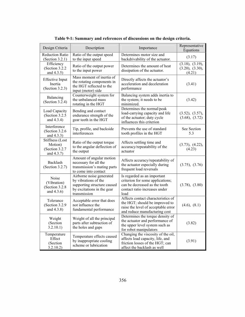
356

Table 9-1: Summary and references of discussions on the design criteria.

Design Criteria Description Importance Representative Equations

Reduction Ratio (Section 3.2.1)

Ratio of the output speed to the input speed

Determines motor size and backdrivability of the actuator. (3.17)

Efficiency (Section 3.2.2

and 4.3.5)

Ratio of the output power to the input power

Determines the amount of heat dissipation of the actuator.

(3.18), (3.19), (3.20), (3.30),

(4.21)

Effective Input Inertia

(Section 3.2.3)

Mass moment of inertia of the rotating components in the HGT reflected to the input (motor) side

Directly affects the actuator’s acceleration and deceleration performance

(3.41)

Balancing (Section 3.2.4)

Counterweight system for the unbalanced mass rotating in the HGT

Balancing system adds inertia to the system; it needs to be minimized.

(3.42)

Load Capacity (Section 3.2.5

and 4.3.4)

Bending and contact endurance strength of the gear teeth in the HGT

Determines the normal/peak load-carrying capacity and life of the actuator; duty cycle influences this criterion

(3.52), (3.57), (3.68), (3.72)

Interference (Section 3.2.6

and 4.3.3)

Tip, profile, and backside interferences

Prevents the use of standard tooth profiles in the HGT

See Section 5.3

Stiffness (Lost Motion)

(Section 3.2.7 and 4.3.7)

Ratio of the output torque to the angular deflection of the output

Affects settling time and accuracy/repeatability of the actuator

(3.73), (4.22), (4.23)

Backlash (Section 3.2.7)

Amount of angular motion necessary for all the transmission’s mating parts to come into contact

Affects accuracy/repeatability of the actuator especially during frequent load reversals

(3.75), (3.76)

Noise (Vibration)

(Section 3.2.8 and 4.3.6)

Airborne noise generated by vibrations of the supporting structure caused by excitations in the gear transmission

Is regarded as an important criterion for some applications; can be decreased as the tooth contact ratio increases under load

(3.78), (3.80)

Tolerance (Section 3.2.9

and 4.3.8)

Acceptable error that does not influence the fundamental performance

Affects contact characteristics of the HGT; should be improved to raise the level of acceptable error and reduce manufacturing cost

(4.6), (8.1)

Weight (Section 3.2.10.1)

Weight of all the principal parts after subtraction of the holes and gaps

Determines the torque density of the actuator and performance of the upper level system such as for robot manipulators

(3.82)

Temperature Effect

(Section 3.2.10.2)

Temperature effects caused by inappropriate cooling scheme or lubrication

Changing the viscosity of the oil, affects load capacity, life, and friction losses of the HGT; can affect the backlash as well

(3.91)

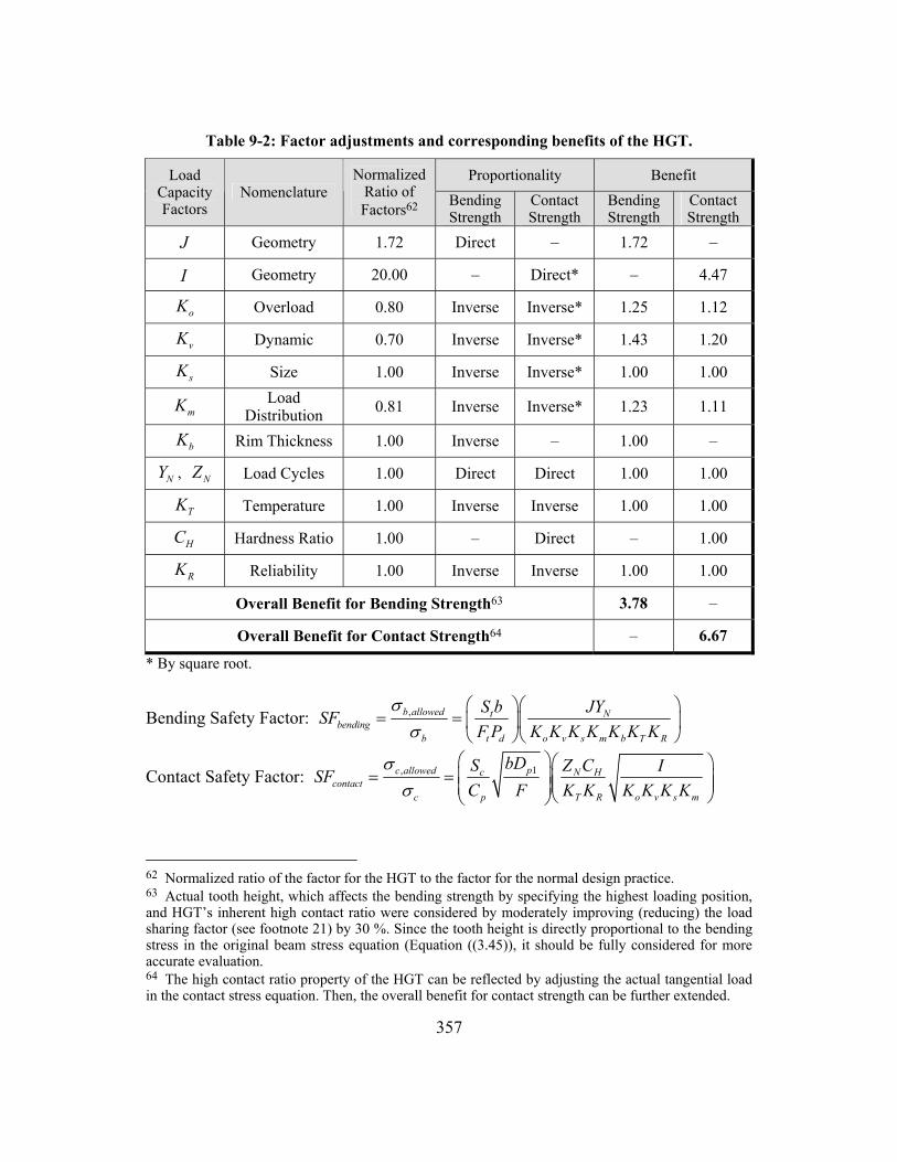
357

Table 9-2: Factor adjustments and corresponding benefits of the HGT.

Proportionality Benefit Load Capacity Factors

Nomenclature Normalized

Ratio of Factors62 Bending

Strength Contact Strength

Bending Strength

Contact Strength

J Geometry 1.72 Direct – 1.72 –

I Geometry 20.00 – Direct* – 4.47

oK Overload 0.80 Inverse Inverse* 1.25 1.12

vK Dynamic 0.70 Inverse Inverse* 1.43 1.20

sK Size 1.00 Inverse Inverse* 1.00 1.00

mK Load Distribution 0.81 Inverse Inverse* 1.23 1.11

bK Rim Thickness 1.00 Inverse – 1.00 –

NY , NZ Load Cycles 1.00 Direct Direct 1.00 1.00

TK Temperature 1.00 Inverse Inverse 1.00 1.00

HC Hardness Ratio 1.00 – Direct – 1.00

RK Reliability 1.00 Inverse Inverse 1.00 1.00

Overall Benefit for Bending Strength63 3.78 –

Overall Benefit for Contact Strength64 – 6.67

* By square root.

Bending Safety Factor: ,b allowed t Nbending

b t d o v s m b T R

S b JYSFF P K K K K K K K

σσ

⎛ ⎞⎛ ⎞= = ⎜ ⎟⎜ ⎟

⎝ ⎠⎝ ⎠

Contact Safety Factor: 1, pc allowed c N Hcontact

c p T R o v s m

bDS Z C ISFC F K K K K K K

σσ

⎛ ⎞⎛ ⎞= = ⎜ ⎟⎜ ⎟⎜ ⎟⎜ ⎟⎝ ⎠⎝ ⎠

62 Normalized ratio of the factor for the HGT to the factor for the normal design practice. 63 Actual tooth height, which affects the bending strength by specifying the highest loading position, and HGT’s inherent high contact ratio were considered by moderately improving (reducing) the load sharing factor (see footnote 21) by 30 %. Since the tooth height is directly proportional to the bending stress in the original beam stress equation (Equation ((3.45)), it should be fully considered for more accurate evaluation. 64 The high contact ratio property of the HGT can be reflected by adjusting the actual tangential load in the contact stress equation. Then, the overall benefit for contact strength can be further extended.

358

9.1.1.3 Parametric Design and Design Procedure

Parametric design of the HGT was attempted based on the concept of Pareto

principle (see Section 3.3 for further details). To do so, critical design parameters for

each of the criteria were identified in Section 3.3.1 after careful review of each of the

functional forms and representation of some of the parameters with more meaningful

parameters. Table 3-6 (repeated here in Table 9-3) presented the critical parameters

identified.

Table 9-3: Design criteria and critical parameters.

Design Criteria Critical Parameters Reduction Ratio N (or pD and e )

Efficiency oT , pD , φ , bω , bd , sV , rV , b , 0v , 0µ

Effective Input Inertia e Balancing e

Load Capacity oT , pD , b , h , t , φ , r

Interferences e , h , φ , rR , rr

Stiffness, Lost Motion, & Backlash N , pD , φ , oT , t , T∆

Noise / Vibration (Mesh Frequency) inω , N (or pD and e )

Weight / Volume e , pD , b

Section 3.3.2 then selected the most critical parameters in two groups, i.e., the

first and the second most critical parameters, among the pre-identified critical

parameters by investigating their influence (degree of prevalence) in the functional

forms. The identified most critical parameters were presented in Table 3-7 (repeated

here in Table 9-4) along with sets of design criteria which are impacted by the corresponding parameter. Pitch diameter pD and eccentricity e were classified as

359

the first set of the most critical design parameters. The second set of the most critical

parameters consisted of pressure angle φ , face width b , and tooth number N .

Table 9-4: The most critical design parameters and associated design criteria.

Ranking Most Critical Design Parameter Impacted Design Criteria

Pitch Diameter pD Reduction Ratio, Efficiency, Load Capacity,

Stiffness/Lost Motion/Backlash, Noise/Vibration, Weight/Volume First

Eccentricity e Reduction Ratio, Effective Input inertia, Balancing, Interferences, Noise/Vibration, Weight/Volume

Pressure Angle φ Efficiency, Load Capacity, Stiffness/Lost Motion/Backlash, Interferences

Face Width b Efficiency, Load Capacity, Weight/Volume Second

Tooth Number N Reduction Ratio, Stiffness/Lost Motion/Backlash, Noise/Vibration

In order to decouple the tooth profile design from the system level design, it

was attempted to categorize the design criteria to either system level or tooth level

design. However, most of the design criteria belong to both of the design categories

more or less, because they usually involve parameters from both categories. Table 3-8

(repeated here in Table 9-5) showed the critical parameters classified in the two

categories, system level and tooth level parameters.

Table 9-5: System level and tooth level design parameters.

Parameter Category Critical Parameters System Level pD , e , N , b , bd

Tooth Level φ , h , t , r , rR , rr , sV , rV

Degree of relevancy of each design criterion to each of the categories was

determined by examining the degree of prevalence of the classified parameter sets in

360

the criterion (more detail discussion can be found in Section 3.3.3). The resulting

categorization was shown in Figure 3-13 (repeated here in Figure 9-3).

Tooth LevelDesign

ReductionRatio Effective

Input Inertia

Balancing

WeightLoad

Capacity

Efficiency Noise/Vibration

Interference

Stiffness/Lost Motion/

Backlash

System LevelDesign

Figure 9-3: Categorization of the HGT design criteria.

Parametric design of the HGT then becomes the process of determining the

two most critical parameter sets instead of simultaneously managing the whole set of

design parameters. Generalizing, a whole set of design parameters of the design

object is now largely and effectively determined by directly deciding the most

governing (critical) and most influential parameters (on the performance criteria)

which must be chosen judiciously by the designer (using the degree of prevalence,

dominance, etc.) based on a careful parametric study (identification of parameters,

development of functional forms, and decision based on the function-parameter

relationships). Parametric decision processes for the first and the second set of the

most critical parameters were covered in Section 3.3.4 and 3.4.1, respectively.

361

In the first decision process, the eccentricity ratio E , a dimensionless

parameter, was identified to have multiple effects on the performance of the HGT

(especially on the reduction ratio, interference, effective input inertia and balancing).

It also determines a physical configuration of the HGT (relative size of the 1st and 2nd

stage diameters; see Figure 3-14 to Figure 3-17), not to mention reducing the degree

of freedom of the parametric design by one. It was defined as:

1r

eED

= (9.1)

An E of 2 % has been found to be a good starting point for torque dense design of

the HGT. More detail discussion on this parameter can be found in Section 3.3.4. In

the second decision process, diametral pitch ( dP ) played a similar role with E . It

was defined as

dp

NPD

= (9.2)

For the HGT, the contact ratio specifies the boundedness of this parameter (from

below). See Section 3.4.1 for more detail discussion on this parameter.

The design procedure for the HGT has been structured in three steps. A

flowchart of this three step design procedure was presented in Figure 3-18 (repeated

here in Figure 9-4). The first two steps concentrate on the system level design while

the last step concentrates on the tooth level design (determines the tooth level design

parameters). In the first step, design requirements are gathered and studied, and based

on the key design requirements, the first set of the most critical parameters are

determined for a quick configuration decision for the HGT. The dimensionless

362

parameter, E , plays a key role in this design step. Inertia of the system and balancing

design can also be determined in this stage.

1st Step

Yes

Yes

No

No

No

No

YesNeed to change , , or ?dE Pφ

Change other tooth profile parameters

Pass?

Tooth meshing simulation Pass?

Determine tooth profile parameters (Table 4-5)

Tooth Meshing Analysis

Design requirements met?

Select bearings and lubrication

Determine and set up force analysisφ

Determine (the largest pitch diameter)pD

Determine ( / )pE e D=

Yes

Design Completed

Determine and db P

Preliminary evaluation of load capacity, efficiency, stiffness, etc.

Design Requirements ( , , , , , ...)o in oT TR Dω η

No Yes

2nd Step

3rd Step

More Analyses (Loaded Tooth Contact Analysis,Efficiency, Effects of manufacturing errors, etc.)

Estimate contact ratio ( ) and load sharing factorCR

FEA estimated?CR CR≈

Determine all the other 's, inertia, and balancing designpD

Figure 9-4: HGT design procedure.

363

The next step is to assign values for the second set of the most critical

parameters. Although the pressure angle φ was categorized as a tooth profile

parameter, it needs to be predetermined in this system level design phase for force

analysis. It will then be reviewed and redesigned if necessary in the tooth profile

design phase (the third step) and fed back to the system level design if updated. The

face width b needs to be determined in this design step as well. The key factors for

determining this parameter were load capacity and the size restriction. The selection

of this parameter completes the development for the overall size and geometry of the

HGT in three dimensions. In this design step the diametral pitch dP is introduced to

replace the role of the tooth number parameter N . As E did in the first design

step, this parameter plays a crucial role in this step. It determines the thickness of

gear tooth (versus its height) which is one of the important basic parameters

necessary in the subsequent tooth profile design phase. The load capacity and

stiffness of the HGT are also dependent upon this parameter especially when the

contact ratio is low (one or two). Another decision to make at this point is to estimate

the contact ratio and the subsequent load sharing factor. The contact ratio is a very

important parameter in the precise evaluation of load capacity, efficiency, stiffness,

etc. It can be reasonably estimated based on the number of teeth in the arc of the

contact region enveloped by two overlapping pitch diameters (see (a) of Figure 5-2).

At the end of the final tooth design step, the actual contact ratio and load sharing

factor should be analyzed by means of the loaded tooth contact analysis, and

compared with this estimated contact ratio for confirmation.

The final step of the design procedure is in-depth tooth profile design. In this

step, tooth profile design parameters are determined. The list of parameters can be

found in Table 4-3 (repeated here in Table 9-7). Note that the predetermined

364

parameters in the table have been assigned values from the previous two steps. These

predetermined parameters are confirmed through tooth meshing analysis (Chapter 5)

in this design step. If values for these parameters are updated, the new values should

be fed back to step two and reiterated. Once the set of tooth profile design parameters

passes through the tooth meshing analysis without any problem such as interference

or backside collision, they are finally confirmed through meshing simulations using

commercial software or the UTRRG circular-arc tooth generation software (see

Section 4.5 for introduction of this tool).

Following this design guideline, two HGT prototype designs (the ¼-Scale

AWE Actuator and the Rugged Actuator) were pursued as representative designs of

this report. The design results were provided in Section 3.5. Note that these

representative designs were system level designs where the parameter values were

not finalized. The final step of design where all the tooth level parameters were to be

fixed was performed in Chapter 5.

9.1.1.4 Basic Tooth Profile

Chapter 4 was dedicated to: 1) determine a basic tooth profile which would

allow the HGT to maintain its claimed advantages, and 2) identify all the parameters

associated with the tooth profile for complete parametric design and analysis. For

preliminary selection of the basic tooth profile for the HGT, several candidate tooth

forms were reviewed in terms of transverse and axial geometries (Section 4.2). As a

result, the circular-arc tooth profile in spur (straight) configuration was selected as a

potential tooth form that could form the basis for the exceptional performance

advantages of the HGT. The essence of the circular-arc tooth profile was to enable

two mating gear teeth to have a very low relative curvature through the concave-

365

convex geometry reducing surface contact stress and sliding velocity while enhancing

the entraining (rolling) velocity and lubrication condition. These teeth also benefit

from their lower bending stress due to their relatively short height and increased

thickness near the tooth root. All of these characteristics are very desirable for load

capacity and efficiency of the gear transmission.

The reasons for using spur teeth in the HGT are as follows: 1) reduced

complexity in the design and fabrication, 2) elimination of the axial forces exerted on

the bearings, and 3) prevention of axial excitations which can cause noise and

vibration. One of the possible drawbacks of using a spur configuration is reduced

contact ratio due to the absence of axial overlap which is available in the helical

configuration. However, Section 4.2.2 showed that using helical gears in the gear

transmission does not always guarantee a higher contact ratio; it requires a generous

axial length (for desirable helix angles) to ensure sufficient axial overlap, which is not

attractive for compact, ‘pancake’ type actuator designs.

Another possible drawback of the spur circular-arc tooth profile is its need for

special treatment for maintaining theoretical conjugate action. However, it has been

successfully argued that conjugate action of the spur circular-arc profile can be

maintained within an acceptable tolerance through careful design of tooth tip relief

that accommodates tooth deformation under load and control over tooth-to-tooth

clearance/interference data. Note that, even with any profile which theoretically

guarantees conjugate action, it is difficult to sustain constant input-output speed ratio

because of errors from deformation, wear, manufacturing imperfection, assembly,

and temperature influences. Refer to Section 3.2.8 for further discussion on numerous

sources of the transmission error.

366

Section 4.3 supported the selection of the basic tooth profile by evaluating the

circular-arc tooth profile with respect to the tooth level design criteria plus

manufacturing error sensitivity. The first criterion considered was tooth-to-tooth

interference. Avoidance of interferences in the HGT is extremely challenging

especially when a very small tooth number difference is preferred65. Maiti and Roy

(1996) showed that involute internal gears cannot have a tooth difference of less than

5 at a pressure angle of 25° or smaller. With a pressure angle of 30° or larger,

involute gears are allowed to have a four tooth difference and with a pressure angle of

56° or larger, they can have one tooth difference. However, these high pressure

angles increase radial and normal loads which are not desirable especially for the

configurations like the HGT where eccentric motion creates the driving force.

Increased radial and normal loads also lead to increased tooth friction losses and

bearing power losses. In order to reduce the excitation forces and power losses in the

bearings, it is necessary to eliminate axial loadings (done by using spur gears) and to

minimize radial loadings by lowering the pressure angle (the target value is 5º).

According to Maiti and Roy, for the involute internal gears to have a

relatively low pressure angle, 14.5°, the modified involute gears should have at least

a 7 tooth difference to avoid interferences, which significantly reduces the reduction

ratio options and increases the size of the eccentricity. By employing a circular-arc

tooth profile and controlling the design parameters (especially tooth relief design

parameters) in the tooth meshing analysis, interferences in the HGT have been

effectively avoided. In Section 5.5, the extremely low target pressure angle (5º) was

65 A very small tooth number difference (at most 5) is preferred in the HGT design since it can reduce the effective inertia, balancing efforts/weight, and weight/volume of the HGT.

367

successfully achieved for the tooth number difference of 5 (the Rugged Actuator

HGT design).

Load capacity was another criterion where the circular-arc tooth profile

demonstrated superior advantage compared to the standard tooth profiles. As

mentioned above, the short and wide form of the circular-arc teeth can significantly

reduce bending stress. Note that the standard full-depth involute tooth profile is

subject to repeated tip loading which results in large fluctuation of load (leading to

vibration and noise) and thus significant fatigue failure. More importantly, the

circular-arc tooth profile employs a highly conformal concave-convex tooth mesh

which significantly improves the Hertz contact condition. Table 3-5 showed that the

geometry factor which reflects the mesh conformity (the similarity of the curvature at

the point of contact) would allow for 4.5x higher contact strength in the circular-arc

tooth mesh than in non-conformal standard practice. Although the involute profile

also can have a slightly conformal form when used in the internal gear mesh, it has

been indicated that minimizing contact stresses in the involute gears is geometrically

limited whereas it is not for the circular-arc gears which could have virtually any

combination of the profile curvature radii (Dyson et al., 1986).

The superior load capacity has also been proven by testing in the literature

(Wells & Shotter, 1962; El-Bahloul, 1989). They showed that up to 6.5 times of load

capacity and 12 times of EHD film thickness were available in the circular-arc gears

compared to the standard involute gears. This superior film oil thickness of circular-

arc gears was due to close conformity and low sliding velocity as opposed to the

highly variant sliding velocity between the involute teeth (El-Bahloul, 1989; Esposito

& Belfiore, 2000). El-Bahloul (1989) also showed that an increase of speed had more

368

effect on increasing the EHD film thickness for circular-arc gears than for involute

helical gears. This argument encourages high-speed application of circular-arc gears.

Comparative analyses conducted in Section 4.3.4.4 successfully proved that

the tooth profile with the highest conformity, i.e., circular-arc tooth profile, had

exceptional advantages in terms of the Hertz contact properties over involute tooth

profiles. The analyses showed that contact areas of the circular-arc tooth system

became significantly larger under increasing load than the involute tooth systems

(Figure 4-14 and Figure 4-16). The analyses also showed that the maximum contact

stresses of the circular-arc gear system were the lowest among the compared systems

(Figure 4-15 and Figure 4-17).

As far as the efficiency is concerned, literature have proven that the efficiency

of circular-arc gears is generally higher for most of the speed range except at startup

or extremely low load (see Section 4.3.5 for further discussion). A comparative

analysis performed in this research also showed that, for a constant coefficient of

friction (0.05), the total combined sliding power loss of the circular-arc tooth system

was 27 % less than that of the involute tooth system.

In terms of noise and vibration, both the circular-arc and involute profiles

have been expected to bring a comparable performance. Nonetheless, for critical

applications for the HGT, this was not the case. Considering the relatively high

transverse contact ratio and smaller sliding, the circular-arc tooth profile was

expected to be more beneficial than the involute with respect to this criterion. Attia

(1989) also found that tooth crowning was more effective for the circular-arc gears

than for the involute helical gears for noise reduction. This fact encourages

consideration of the crowning of the teeth for the circular-arc gears if they were used

in the HGT and suspected to be responsible for the noise.

369

The next criterion considered was stiffness and lost motion. The conformal

circular-arc tooth profile had a great advantage for this criterion because of the

superior contact areas which improve the mesh stiffness under the same loading

conditions. Based on the previous comparative analysis regarding the contact area,

the circular-arc tooth profile is believed to enable a very high stiffness in the gear

mesh because the mesh stiffness is increased with increases in the contact area.

Having multiple circular-arc tooth pairs in contact under load, the HGT should

provide superior mesh stiffness over the conventional gear transmissions. In addition,

the circular-arc tooth profile is regarded to be very stiff due to smaller bending

deformations. Note that, from the simple beam theory, the bending deflection is

proportional to the cube of the beam (tooth) height h and thickness t ratio:

33 4

3t t

bF h F h

EI Eb tδ ⎛ ⎞= = ⎜ ⎟

⎝ ⎠ (9.3)

Therefore, reducing the tooth height to thickness ratio ( /h t ) reduces the bending

deflection of the tooth by the cube rate of the ratio. With a relatively low height to

thickness ratio of the circular-arc teeth, the portion of the bending deformation out of

the total tooth deformation should be small66.

The last criterion considered was sensitivity to the center distance errors. As

summarized in Section 4.3.8, the sensitivity of the contacts in the circular-arc gears to

the errors has been well studied in the literature. The key of the studies was to reduce

the transmission error by proper design of the tip relief and to localize the contact by

providing effective crowning to the face width. Equation (4.6) (repeated here in

Equation (9.4)) also suggested that a higher tolerance to the center distance errors

66 This flexible choice for h and t is a major advantage over comparable cycloidal drives which have a fixed geometry to maintain their theoretical foundation of the basic gear system.

370

could be achieved by increasing the difference between the tooth profile curvature

radii and by reducing the pressure angle. The amount of tolerance that can be

accommodated in the center distance ( CD∆ ) is given by

22 sin cosCD ζρ γ φ∆ = (9.4)

where ζ = fractional difference in profile radii, 2 1(1 )ρ ρ ζ= −

γ = angle subtending to contact arc (see Figure 4-11)

φ = pressure angle

Compiling all the arguments made, the performance of the circular-arc tooth

profile and involute profile were compared in Table 4-2 (repeated here in Table 9-6)

with respect to the tooth level design criteria. The result showed that the circular-arc

profile could bring 2.7 times higher overall performance benefit to the HGT than the

involute profile would. This result fully supported the selection of the circular-arc

tooth profile as a basic tooth profile for the HGT.

Table 9-6: Performance comparison between circular-arc and involute tooth profiles.

Evaluation Score Performance Criteria Weighting

(Total:10) Circular-Arc Involute Circular-

Arc Involute

Interference 2.60 4.0 1.0 10.40 2.60

Load Capacity 2.10 5.0 1.5 10.50 3.15

Efficiency 1.60 5.0 2.0 8.00 3.20

Noise/Vibration 1.60 4.0 2.0 6.40 3.20

Stiffness/Lost Motion 1.05 5.0 1.5 5.25 1.58

Sensitivity to Errors 1.05 3.0 2.5 3.15 2.63

Overall Benefit Factor = (43.70/16.36) = 2.67x 43.70 16.36

371

9.1.1.5 Parametric Design of Circular-Arc Tooth Profile

Externally meshing gear pairs have less strict interference constraints than

internal gear pairs. Therefore, the conventional approach for generating conjugate

tooth profiles based on well established methods works well primarily for external

gear pairs. This approach was reviewed in Section 4.4.1. On the other hand, the

unique configuration of the HGT featuring an extremely narrow contact region

enveloped by two internally meshing gears makes it demanding to maintain

theoretical conjugate contacts without causing interference (see Section 4.4.1 for

further discussion). Increasing the contact ratio with carefully managed variation of

contact position along the tooth curves in the internally meshing gear pairs can

circumvent the adverse effects of non-conjugate contacts such as acceleration peaks.

Once the clearances at the desired contact points on the tooth curves are minimized,

the HGT will, by closing the tiny clearances under tooth deformations, not only

deliver seamless, multiple engagements of teeth but also minimize irregular velocity

changes at the output.

Parametric design of the circular-arc tooth profile was initiated by identifying

a complete set of parameters necessary to analytically represent the circular-arc tooth

profile. The circular-arc tooth profile basically consisted of three circular-arcs on

each side of a tooth; one was the tip relief (for avoidance of interference and

compensation of the tooth deformation and manufacturing tolerances), another was

the main contact surface (for conformal convex-concave contact maximizing the

surface endurance), and the other was the root fillet (for minimization of stress

concentration and maximization of the bending strength). A complete set of

parameters necessary to represent the circular-arc tooth profile was categorized into:

predetermined parameters, design parameters, and dependent parameters.

372

Table 9-7: Parameters associated with the circular-arc tooth geometry.

Classification Parameter Nomenclature

E Eccentricity ratio ( / pe D= ) φ Pressure angle at pitch point

dP Diametral pitch ( / pN D= ) Predetermined

Parameters

N Number of teeth

rootR Tooth root circle radius

tR Tooth tip circle radius

rR Tooth tip relief starting circle radius r Radius of main circular-arc

rr Radius of tip circular-arc

fr Radius of root fillet circular-arc

Design Parameters

C Backside clearance factor at pitch circle

bR Base circle radius Pc Center position of tooth curvature Pcr Center position of tip relief curvature

,Pc back Center position of backside tooth curvature

Dependent Parameters

,Pcr back Center position of backside tip relief curvature

The predetermined parameters are ‘predetermined’ in the system level design

(first two steps of the HGT design procedure). Thus, the predetermined parameters

take the role of linking the system level design to the tooth level design (third step of

the design procedure). They are the eccentricity ratio E , pressure angle φ , and

diametral pitch dP . Tooth numbers of the HGT ( N ) are then determined based on

E and dP . Once E , φ , dP , and N are predetermined in the system level design,

the solution to the tooth level design parameters follows. The design parameters are

basically composed of three gear circle radii, three tooth circular-arc radii, and one

parameter defining the actual tooth thickness. The dependent parameters are the

parameters which are to be calculated from the predetermined and/or design

373

parameters. Most of these parameters are position vectors for the centers of the

circular-arcs. Table 4-3 (repeated here in Table 9-7) provides the complete set of the

circular-arc tooth profile parameters. See Figure 4-20 and Figure 4-21 for the

nomenclature.

In this parameterization process, 4 predetermined parameters, 7 design

parameters, and 5 dependent parameters were identified. The actual number of the

design parameters for the two stage HGT was 26 (6 gear/tooth parameters times 4

gears plus 1 thickness parameter times 2 stages). Functional relationships of these

parameters can be found in Section 4.4.2.

9.1.1.6 Refinement of Design Objectives

These identified tooth design parameters are to be determined through the

tooth meshing analysis in Chapter 5. To do so, an initial set of design objectives was

given based on the tooth profile design criteria. They were as follows:

• Avoid tooth meshing interference

• Maximize load capacity

• Maximize efficiency (by minimizing the sliding power losses)

• Minimize noise/vibration

• Maximize stiffness (and minimize lost motion)

• Minimize backlash (especially during load reversal)

These initial set of design objectives was replaced with equivalent objectives, and

reorganized to a reduced set of design objectives as follows (detailed logical process

of this conversion of the objective form can be found in Section 5.2):

• Avoid tooth meshing interference

• Minimize the contact side clearances

374

• Minimize the backside clearances

• Minimize the sliding velocity

It was helpful to reorganize and group the design objectives because the

reduced set was more manageable, and conflicts among the objectives became more

evident. In this new set of design objectives, avoidance of tooth meshing interference

and minimization of the contact side clearances were two conflicting, primary

objectives.

9.1.1.7 Clearance/Interference Analysis

The clearance/interference analysis was used to geometrically analyze the

clearances and/or interferences between these circular-arcs that are in contact or in

potential contact. This is also a part of the parametric design process. The foundation

analytics based on the main tooth contact surfaces were presented in Section 5.3.1.2.

Tip relief circular-arcs were also analyzed using these foundation analytics with

substitution of some associated geometric parameters (see Section 5.3.1.3).

Development of analytics for the backside clearance/interference was also based on

the foundation analytics (see Section 5.3.2). Figure 5-3 (repeated here in Figure 9-5)

showed a typical clearance/interference plot. Clearance/interference plots were

rigorously used in determining the tooth profile design parameters.

Figure 5-4 (repeated here in Figure 9-6) illustrated how tip relief affected

clearance/interference and the potential contact ratio of the HGT. As shown in the

figure, without tip relief, interference would have occurred at the 16th tooth pair. With

tip relief, the interference was avoided (all the clearance values are positive in the

potential contact region shown in the figure).

375

12 34 56 0

Approach Recess

12 34 56 0 12 34 56 0 12 34 56 0

Approach RecessApproach Recess

Figure 9-5: Typical clearance/interference plot and indexing of tooth pairs.

Figure 9-6: Clearance/interference with tip relief and without tip relief.

376

The initial design parameters ( rootR , tR , rR , r , rr , fr , C ) composed a set

of 13 parameters to be determined for each stage of the HGT. Through a parameter

reduction process (see Section 5.4.1 for details) DOF of the design was reduced to

four. The final set of design parameters was: φ , c , rr , and C . This reduced set of

design parameters was determined through the clearance/interference analysis for the

¼-scale and the Rugged HGTs. The approach was to vary the four design parameter

one at a time (with the others being fixed) and examine their effects on the

clearance/interference plots. Figure 5-10 through Figure 5-13 showed this process. As

a result, Table 9-8 shows the completely determined tooth profile design parameters

for the two HGT prototypes. Since the ¼-scale AWE Actuator was the first prototype

effort, moderate or median values were assigned to the design parameters while more

challenging values were chosen (e.g., φ = 7º) for the Rugged Actuator prototype

which was our second prototype effort.

Table 9-8: Final values for the tooth profile parameters of the ¼-scale AWE Actuator and the Rugged Actuator HGT prototypes.

Parameter The ¼-Scale AWE Actuator The Rugged Actuator

E 0.04 0.033

dP 7.0447 15.625 N 41 / 45 70 / 75 φ 20º 7º

rootR 2.8133” / 3.2856” ( 1.15a = ) 2.0283” / 2.2916” ( 1.40a = )

tR 2.9897” / 3.1098” ( 0.85b = ) 2.1169” / 2.2030” ( 0.99b = )

rR 2.9391” / 3.1620” ( 1.01c = ) 2.0821” / 2.2378” ( 1.001c = ) r 0.9953” / 1.0924” 0.2535” / 0.2730”

rr 0.1” 0.04”

fr 0.05” 0.05” C 0.005 0.005

377

Tooth meshing was simulated with these parameters at incremental steps ( j )

of input angles for final verification. Figure 5-14 (repeated here in Figure 9-7) and

Figure 5-15 (repeated here Figure 9-8) showed the analysis results (for 5j = ) for

contact sides and backsides of the ¼-scale AWE Actuator HGT, respectively (arrows

indicate the direction of the changes with respect to the input angles). Additionally,

Figure 5-16 and Figure 5-17 showed the clearances at multiple points ( 4s = ) on the

tooth relief curvatures with respect to the given input angle steps ( 4j = ) for contact

sides and the backsides, respectively.

Figure 9-7: Clearances with respect to varying input angles at the contact side.

378

Figure 9-8: Clearances with respect to varying input angles at the backside.

For the Rugged Actuator HGT, Figure 5-18 (repeated here in Figure 9-9) and

Figure 5-19 (repeated here in Figure 9-10) showed the results of the clearance/

interference analysis; they plot the minimum clearances at the contact sides and

backsides of the teeth, respectively, for the incremental angular inputs of 5j = . The

pressure angle was minimized to an exceptionally low value which would have not

been achievable in the involute gears for the HGT configuration. The clearance/

interference analysis detected no interference for this set of design parameters. In

addition, it resulted in extremely small clearances at four tooth pairs at the vicinity of

the pitch point (1st, 2nd, 4th, and 6th tooth pairs at 0ψ ; ranging from 55 10−× inches to

41.9 10−× inches). These very small clearances should ensure a high contact ratio and

smooth meshing condition in the Rugged Actuator HGT.

379

Figure 9-9: Contact side clearance/interference analysis result for the Rugged HGT.

Figure 9-10: Backside clearance/interference analysis result for the Rugged HGT.

380

Effects of the center distance variations ( CD∆ ) on the clearances and/or

interferences were also analyzed. Figure 5-20 (repeated here in Figure 9-11) showed

the changes of the clearances with respect to CD∆ of 0.0004”, 0.0007” and 0.0010”.

The figure showed that as CD∆ increased, the clearances in the approaching side

(left side of the 0th) slightly increased while those in the recessing side (right side of

the 0th) slightly decreased. These clearance data have been utilized in the loaded tooth

contact analysis in Chapter 6 for analytical evaluation of the load sharing factor.

0

0.005

0.01

0.015

0.02

0.025

0.03

-8 -6 -4 -2 0 1 3 5 7

Tooth Pair

Cle

aran

ce [i

n]

CDE = 0.0000" CDE = 0.0004" CDE = 0.0007" CDE = 0.0010"

Figure 9-11: Change of clearances with respect to the center distance variations.

9.1.1.8 Extremely Low Pressure Angle Design

In Section 5.5, the pressure angle of the HGT was minimized further down to

5° using clearance/interference analysis for rigorous pursuit of the design objectives.

The clearance plot (showing only the minimum clearances) for j = 5 is shown in

Figure 5-25 (repeated here in Figure 9-12). In practice, due to the fact that the

381

minimum clearance for PA = 5° is much smaller than the manufacturing tolerances,

this extremely low pressure angle design was only recommended for the highest

quality gears. In other words, PA = 7° is regarded as the ‘practically’ lowest pressure

angle for the Rugged Actuator HGT. This extremely low pressure angle design effort

demonstrated a full exploitation of the clearance/interference analysis in the tooth

meshing analysis and parametric tooth profile design of the HGT.

Figure 9-12: Clearance plot for PA = 5°.

9.1.2 Analysis of the HGT

9.1.2.1 Sliding Velocity Analysis

Section 5.3.4 covered the sliding velocity of contacts in the circular-arc tooth

pairs of the HGT. For exact analysis (Section 5.3.4.1), the accurate positions of the

contact points (at each tooth pair in mesh) had to be known. Since the positions where

the minimum clearances occur with respect to XY coordinates are potential contact

382

points, the contact positions were obtained through the clearance/interference

analysis. The equation for the exact sliding velocities was given by

1 2( )sV CP ω ω= − (9.5)

where CP = distance between point of contact C and pitch point P

1 2ω ω− = relative angular velocity between the wobble gear (1) and the

internal gear (2)

Figure 5-21 (repeated here in Figure 9-13) showed the exact sliding velocity profile

for the ¼-scale AWE Actuator HGT (for the maximum input speed of 3,950 rpm).

The sliding velocity was at its maximum at the farthest tooth pair while it reached its

minimum (zero) at the tooth pair meshing at the pitch point.

0

5

10

15

20

25

30

35

40

-4 -2 0 1 3

Tooth Pair

Slid

ing

Velo

city

[in/

sec]

Figure 9-13: Tooth sliding velocity profile of the ¼-scale AWE Actuator HGT.

An approximate method was also presented (Section 5.3.4.2). The approach

was to simulate the wobble gear motion with a kinematically equivalent slider crank

mechanism for a relatively small rotational angle about the central portion of the

input shaft (see Figure 5-8). This approximate analysis did not require exact contact

383

position data. Instead, sliding velocities were conveniently determined using the gear geometry parameters, i.e., eccentricity e and pitch radius pR . The equation for the

approximated sliding velocity was derived as

cossin 1coss i

p

eV eR

αω αβ

⎛ ⎞= − +⎜ ⎟⎜ ⎟

⎝ ⎠ (9.6)

where iω = input angular speed [rad/sec]

α , β = angles between the cranks and perpendicular line (see Figure 5-8)

Figure 5-9 (repeated here in Figure 9-14) plotted the results from the two

approaches (for the Rugged Actuator HGT). Since they showed excellent agreements

for the contact ratio of 5 or less, the approximate method was used for the efficiency

analysis of the HGT in Chapter 7.

0

2

4

68

10

12

14

16

6 4 2 0 1 3 5

Tooth Pair Index

Slid

ing

Velo

city

[in/

sec]

Exact Approximate

Figure 9-14: Sliding velocity comparison between the exact and approximate analyses.

384

9.1.2.2 Gear Meshing Simulation

Gear tooth meshing simulation was performed using MSC.visualNastran.

Figure 5-23 (repeated here in Figure 9-15) showed the sequence of engagement

(approaching) and disengagement (recessing) of a wobble gear tooth meshing with an

internal gear tooth. This tooth meshing simulation demonstrated that the circular-arc

tooth profile designed through the clearance/interference analysis resulted in smooth

engagement and disengagement without causing any notable mesh acceleration or

large excitation due to tooth-to-tooth interference.

Figure 9-15: Sequence of engagement (left) and disengagement (right) of the circular-arc tooth.

9.1.2.3 Loaded Tooth Contact Analysis

When load is applied to the HGT, the small clearances of the tooth pairs can

be closed due to elastic deformations occurring at the contacting tooth pairs. As an

increasing load is transmitted through closed contacts, another clearance at the next

tooth contact will disappear and so on. Thus, in general, minimizing the clearances

between mating tooth pairs increases the chance of having a higher contact ratio; this

385

is the reason why the minimization of the clearances was rigorously pursued as a

primary objective of the tooth meshing analysis. The main objective of loaded tooth

contact analysis was to evaluate the actual contact ratio under load and the load

sharing factor of the HGT. The load profiles obtained from this analysis were utilized

in evaluating the friction power losses in the efficiency analysis (Chapter 7)

The fundamental premise is that as the load becomes larger, the load is not

only shared by more tooth pairs, but the load distributions over the multiple tooth

pairs in contact are significantly improved. In other words, the ratio of the load

carried by the most heavily loaded tooth to the total load on the gear (the largest load

sharing factor) is significantly decreased. This is the ‘self-protecting’ aspect of the

HGT which makes it ideal for carrying extremely heavy loads. This analysis

successfully demonstrated this hypothesis.

Loaded tooth contact analysis was first done by building an analytic contact

model and solving it. Then, the analytical results were compared with FEA for

verification. The analytical model incorporated parameters regarding the tooth

deformations (bending, transverse, and shear) and the manufacturing errors (center

distance, tooth spacing, and profile errors). In order to implement the tooth

deformations in the analytical contact model, Yoon and Rao (1996)’s approach was

used to analytically describe the tooth deformation parameters (see Section 6.2 for

further details). Data from the clearance/interference analysis were used to reflect the

effect of the center distance errors in the contact model.

Table 6-1 (repeated here in Table 9-9) presented a list of parameters to be

involved in the contact model and their descriptions. Note that the clearance

parameter iε takes into account the effects of the center distance errors.

386

Table 9-9: Parameters for the analytical contact model ( i = tooth pair index).

Parameter Description t

TF Total tangential load on a stage of the HGT t

iF Tangential load at the i th tooth pair

iD Total displacement of the i th tooth pair

iδ Total deflection of the i th tooth pair biδ Deflection of the i th tooth pair due to bending moment tiδ Deflection of the i th tooth pair due to transverse force siδ Deflection of the i th tooth pair due to shear force

iε Clearance at the i th tooth pair

ie∆ Total manufacturing error at the i th tooth pair

ise∆ Tooth Spacing Error (SE) at the i th tooth pair

ipe∆ Tooth Profile Error (PE) at the i th tooth pair

iK Local tangential stiffness of the i th tooth pair

Equation (6.4) (repeated here in Equation (9.7)) showed the mathematical

contact model. In the representative analysis, manufacturing errors (except for the

center distance error) were not considered for a comparison with the FEA results

( ie∆ , ise∆ and ipe∆ were all set to zero). Assumptions made for this analytical

contact model were discussed in Section 6.2.

0 1 2

0 1 2 3

( , , , ,...)

/

t t t t tT i

i

i i i i

i r r

b t si i i i

i i i

ti i i

F F F F FD D D D DD e

f R r CD

e se pe

K F D

ε δε φ

δ δ δ δ

⎧ = + + + ⋅⋅⋅+ + ⋅⋅⋅⎪

= = = = ⋅⋅⋅ = = ⋅⋅⋅⎪⎪ = + + ∆⎪⎪ = ∆⎨⎪ = + +⎪⎪∆ = ∆ + ∆⎪

=⎪⎩

(9.7)

387

This set of equations was solved simultaneously by means of a trial and error

approach. Three different Center Distance Error (CDE) values were considered in

addition to the perfect condition ( CD∆ = 0.0000”). They were: CD∆ = 0.0004”,

CD∆ = 0.0007”, and CD∆ = 0.0010”. Load sharing factors obtained by solving the

analytic model was plotted in Figure 6-2.

FEA nonlinear contact simulations were performed for the same load and

CDE conditions. Figure 6-9 through Figure 6-11 (only the result for perfect CDE

condition is repeated here in Figure 9-16) compared the load sharing factors obtained

from the analytic model and the FEA nonlinear simulation for the four different

contact conditions. They showed excellent agreement. For all conditions, the contact

ratio was three, and the largest load sharing factor was about 64 %.

0

10

20

30

40

50

60

70

2 0 1

Tooth Pair

Load

Sha

ring

Fact

or [%

]

Analytic FEA

Figure 9-16: Comparison of analytical and FEA results for perfect condition.

Section 6.4 presented results of the FEA loaded tooth contact simulations

performed for the ¼-scale HGT and the Rugged HGT subject to different (increasing)

load levels. Detail discussion on the setup of the FEA simulations (including mesh

388

type, mesh size, etc.) can be found in Section 6.3. Three loading conditions (1x, 3.5x,

and 7x of the nominal load) were simulated for the ¼-scale HGT. Figure 6-13 to

Figure 6-15 (repeated here in Figure 9-17) visualized the FEA results for 1x, 3.5x,

and 7x of the base load (= 40,854 in-lb), respectively. It showed that the contact ratio

increased from 3 to 5. Figure 6-16 (Figure 9-18) compared the load sharing factors

for the three loading conditions. It was clearly shown that as the load level increased,

load sharing over the multiple contacts was improved. The largest load sharing factor

(of the most heavily loaded tooth pair) was significantly reduced from 62.38 % to

33.78 %, a factor of almost 2x. This FEA results demonstrate the effective “self-

protecting” aspect of the HGT.

Figure 9-17: FEA contact simulations for 1x, 3.5x, and 7x loads (in the clockwise direction).

389

0

10

20

30

40

50

60

70

4 2 0 1 3

Tooth Pair

Load

Sha

ring

Fact

or [%

]

1.0x Load (CR=3) 3.5x Load (CR=4) 7.0x Load (CR=5)

Figure 9-18: Comparison of load sharing factors with increasing loads.

The FEA contact simulations were performed for the Rugged Actuator HGT

for two different load levels (1x and 5x of the nominal load). Figure 6-18 and Figure

6-19 (repeated here in Figure 9-19) visualized the analysis results. The contact ratio

increased from three to five as the load increased. As the load became significant the

largest load sharing factor decreased from 41% to 26% (see Figure 6-20 which is

repeated here in Figure 9-20). Again, this analysis successfully demonstrated the

effective ‘self-protecting’ aspect of the HGT.

Maximum contact stresses were very low (45 ksi) under the nominal loading

condition and acceptable (142 ksi) under the peak loading condition. The maximum

root stresses were also much lower than those expected in the preliminary design

based on AGMA equations; 13 ksi for the nominal and 41 ksi for the peak loading

condition. This means that the load capacity (in terms of bending endurance) of the

Rugged Actuator HGT can be listed at 5 to 9 times (depending on the material

strengths) of the preliminarily estimated load capacity.

390

Figure 9-19: FEA contact simulations for nominal (left) and peak (right) loads.

0

5

10

15

20

25

30

35

40

45

6 4 2 0 1 3

Tooth Pair

Load

Sha

ring

Fact

or [%

]

Nominal Load (CR = 3) Peak Load (CR = 5)

Figure 9-20: Comparison of load sharing factors for nominal and peak loads.

Also note that the nearly symmetric load distribution profile ensures a very

small amount of lost motion during load reversal. One of the most important

questions in the application of actuators for precision machine applications is the

amount of “natural” lost motion which occurs during load reversals. Systems which

have a very low “spring” stiffness deform under load and when it is reversed, the

deformation is doubled. This means that this “motion” is lost during load reversal

even though no motion command has occurred. In the case of the HGT, the load

391

distribution among the teeth is slightly non-symmetrical (skewed towards the load;

see the curve-fitted load profiles under the heavier loads in Figure 9-21 and Figure

9-22), and this shape must be inverted during load reversal causing a measurable

(both analytically and experimentally) amount of lost motion. Because of this almost

perfect load distribution, the HGT is superior in minimizing lost motion relative to

competing technologies (see Section 1.2). This means that it is the premier gear

transmission where precision operation is a high priority.

9.1.2.4 Efficiency Analysis Based on Literature

In Section 7.2, efficiencies of the ¼-scale and Rugged HGT were calculated

using selected analyses from the literature. Then, the efficiencies were more precisely

determined by analyzing the friction power losses in the HGTs based on first

principles in the sliding tooth contacts. The sliding velocity and load distribution

profiles developed in Chapter 5 and Chapter 6 for the HGT prototype designs were

utilized for the representative analyses. The analyses intended to show that most of

the losses in the HGT were in the bearings and not in the meshing gear teeth as

normally claimed by literature for similar gear transmissions.

Table 7-1 (repeated here in Table 9-10) showed the efficiencies evaluated

based on the three literature analyses. Shipley (1991)’s analysis expected the highest

efficiency among the three. The analysis used the coefficient of friction ( f ) of 0.05,

so the efficiency could increase even further with a lower coefficient of friction (e.g.,

99.47 % for f = 0.02 and 99.73 % for f = 0.01 for the ¼-scale HGT).

Pennestri and Freudenstein (1993)’s analysis considers internal power

circulation (see Figure 7-3 for the power flow diagram) in the gear train which

probably explains the relatively low ratio of the net output power to the input power.

392

However, comparing to their representative differential gear train, the presumed

circulating power is very low (6x less) in the HGT. What makes the HGT different

from the normal differential gear trains (although they were equivalent in the

kinematic configuration) is the minimal tooth number (or size) differences between

the two mating gear pairs. Since the normal differential gear train has relatively small

planet(s) with a long planet arm, the rotational speed of the planet gear(s) is very high

relative to the input speed whereas that of the wobble gear in the HGT is low.

Equation (3.9) showed that the rotational speed of the wobble gear could be 1/20 (or

even lower) of the input speed while in the differential gear train it could be twice (if

the eccentricity were twice of the planet gear radius) or more of the input speed. This

was about 40x difference in kinematic proportions.

Table 9-10: Comparison of efficiencies [%] resulted from the literature analyses.

Shipley Pennestri & Freudenstein Muller

The ¼-Scale HGT 98.67 93.56 64.67 The Rugged HGT 97.06 92.77 69.50

Muller (1982)’s analysis resulted in the lowest efficiencies for both of the

HGT designs. The contentions are as follows. First, their efficiency calculation was

extremely sensitive to the basic efficiency whose application appropriateness for the

HGT should be clarified. If Pennestri and Freudenstein’s basic efficiencies were used,

the overall efficiency would have been 96.42 % and 95.66 %. In other words, for

extremely small increases in the basic efficiency (0.5 % and 0.2 %), the analysis

allowed huge increases in the results (49 % and 38 %). This extreme sensitiveness to

a certain parameters provides no physical meaning. Second, the values for the

geometrical loss factors ( 1Lf and 2Lf ) and tooth friction loss factors ( 1µ and 2µ ),

393

which directly influences the overall efficiency, were approximated from the

empirical data obtained for the involute teeth. Since the HGT employs the circular-

arc teeth, the data represented by Muller is inappropriate for the HGT efficiency

analysis.

9.1.2.5 Exact Friction Power Loss Analysis

It is important to note that the discrete velocity and the load profiles obtained

in the previous chapters not only represent velocity and load profiles among multiple

tooth pairs at a specified moment, but also represent variations of them at individual

teeth during the mesh cycle ( mt∆ ; time span from engagement to disengagement).

This is a critical concept since the power losses need to be analyzed in the time

domain not in the space domain. For evaluation of continuous power losses, the

discrete load profiles were curve-fitted with third order polynomials. Once the power

loss profiles are obtained, they were integrated with respect to mt∆ for conversion to

energy losses ( LE ). The energy losses obtained for each individual tooth for the mesh

cycle were then multiplied by the number of wobble gear teeth ( wN ) to calculate the

total energy loss ( TLE ) that occurred while every tooth of the wobble gear meshed

once each rotation with the mating internal gear teeth.

Total input energy inE to be compared was the energy inputted to run the

wobble gear until the point where every tooth in the wobble gear meshed once with

the mating internal gear teeth. Thus, this input energy was obtained by integrating the

input power inP with respect to int∆ , the time taken for the input shaft to rotate until

the aforementioned point. The efficiency of the HGT was finally given by

1st stage 2nd stage( ) ( )100 [%]

T Tin L L

in

E E EE

η⎡ ⎤− +⎣ ⎦= × (9.8)

394

See Section 7.3 for equations for mt∆ , LE , T

LE , inE , inP , and int∆ .

Figure 7-5 and Figure 7-6 (repeated here in Figure 9-21) showed curve-fitted,

continuous loading sequences (series of loads applied in normal direction to the

contact surfaces) in the time domain for the ¼-scale HGT subject to the 1x load and

3.5x load, respectively. Note that the mesh cycle under the 3.5x loading condition

was longer (0.00135 sec) than that under the nominal condition (0.00080 sec) because

teeth were engaged longer under larger elastic deformations. Being represented in the

time domain, the load profiles in Figure 9-21 imply that the loads are gradually

picked up and released by each individual teeth, and the pickup of the load becomes

more gradual as the load level is increased.

0

1000

2000

3000

4000

5000

6000

7000

0.00000 0.00020 0.00040 0.00060 0.00080

Mesh Cycle [sec]

Nor

mal

Loa

d [lb

]

0

2000

4000

6000

8000

10000

12000

14000

16000

18000

20000

0.00000 0.00027 0.00054 0.00081 0.00108 0.00135

Mesh Cycle [sec]

Nor

mal

Loa

d [lb

]

Figure 9-21: Load profiles for 1x (left) and 3.5x (right) loading conditions (the ¼-scale).

Figure 7-7 and Figure 7-8 (repeated here in Figure 9-22) showed curve-fitted,

continuous load profiles for the Rugged HGT subject to the 1x load and 5x load,

respectively. The mesh cycle is 0.00089 sec and 0.00133 sec for the 1x load and 5x

load, respectively. Again, these load profiles demonstrate that the load is gradually

picked up and released by each individual tooth. Due to the difference in the tooth

geometry, the load profile of the Rugged HGT is less symmetrical than that of the ¼-

395

scale HGT for both loading conditions. It is also shown that as load level is increased,

the pickup of the load becomes more gradual than it does under the nominal loading

condition.

0

50

100

150

200

250

300

350

0.00000 0.00022 0.00044 0.00067 0.00089

Mesh Cycle [sec]

Nor

mal

Loa

d [lb

]

0

200

400

600

800

1000

1200

0.00000 0.00022 0.00044 0.00067 0.00089 0.00111 0.00133

Mesh Cycle [sec]

Nor

mal

Loa

d [lb

]

Figure 9-22: Load profiles for 1x (left) and 5x (right) loading conditions (the Rugged).

Figure 7-9 through Figure 7-12 (repeated here in Figure 9-23 and Figure 9-24)

showed the sliding velocity profiles of teeth of the both designs for the two different

load levels. Being represented in the time domain, the sliding velocity profiles show

that the sliding velocities change from the maximum values to zero and again to the

maximum values. This is in fact a very favorable condition in terms of friction power

losses because at the time when a tooth experiences the maximum sliding it carries

almost no load and at the time when the tooth carries the largest share of the load, it is

in almost no sliding. This argument is verified by the power loss profiles in Figure

7-13 through Figure 7-16 (repeated here in Figure 9-25 and Figure 9-26).

396

0

5

10

15

20

25

30

35

40

0.00000 0.00027 0.00054 0.00081 0.00108

Mesh Cycle [sec]

Slid

ing

Vel [

in/s

ec]

0

10

20

30

40

50

60

0.00000 0.00027 0.00054 0.00081 0.00108 0.00135

Mesh Cycle [sec]

Slid

ing

Vel [

in/s

ec]

Figure 9-23: Sliding velocity profiles for 1x (left) and 3.5x (right) loads (the ¼-scale).

0

1

2

3

4

5

6

7

8

9

10

0.00000 0.00020 0.00040 0.00060 0.00080

Mesh Cycle [sec]

Slid

ing

Vel [

in/s

ec]

0

2

4

6

8

10

12

14

16

18

20

0.00000 0.00022 0.00044 0.00067 0.00089 0.00111 0.00133

Mesh Cycle [sec]

Slid

ing

Vel [

in/s

ec]

Figure 9-24: Sliding velocity profiles for 1x (left) and 5x (right) loads (the Rugged).

0

100

200

300

400

500

600

700

800

900

0.00000 0.00027 0.00054 0.00081 0.00108

Mesh Cycle [sec]

Pow

er L

oss

[in-lb

/sec

]

0

500

1000

1500

2000

2500

3000

0.00000 0.00027 0.00054 0.00081 0.00108 0.00135

Mesh Cycle [sec]

Pow

er L

oss

[in-lb

/sec

]

Figure 9-25: Power loss profiles for 1x (left) and 3.5x (right) loads (the ¼-scale).

397

0

2

4

6

8

10

12

14

16

0.00000 0.00020 0.00040 0.00060 0.00080

Mesh Cycle [sec]

Pow

er L

oss

[in-lb

/sec

]

0

10

20

30

40

50

60

0.00000 0.00022 0.00044 0.00067 0.00089 0.00111 0.00133

Mesh Cycle [sec]

Pow

er L

oss

[in-lb

/sec

]

Figure 9-26: Power loss profiles for 1x (left) and 5x (right) loads (the Rugged).

The areas under the power loss profiles (integration of the power loss profile

with respect to the mesh cycle) represent energy losses that individual teeth

experience during their engagement (mesh) cycles. Following the approach discussed

above, total energy loss TLE in the 1st stage and total input energy inE were

obtained. The efficiency of the second stage can be obtained identically as the first

stage efficiency was obtained. However, it was approximated based on the first stage

efficiency (see Section 7.3 for further discussion). The combined (1st and 2nd stages)

total energy losses were compared with the total input energy.

Table 7-2 and Table 7-3 (repeated here in Table 9-11 and Table 9-12) show

the analysis results for the ¼-scale AWE and the Rugged Actuator HGT,

respectively. Both systems exhibited very high efficiencies for all loading conditions. These results of 97.5 to 98.5 % were based on a constant coefficient of friction ( fC

= 0.01). Efficiency variations for different values of fC were presented in Table 7-4.

It showed that a 5x increase in fC created a 5x increase in mesh friction losses.

398

Table 9-11: Efficiency analysis result for the ¼-scale AWE Actuator HGT.

Input Energy [in-lb]

Energy Loss [in-lb]

Efficiency [%]

1st Stage 2nd Stage 1x Nominal Load 2297.60

19.961 17.965 98.35

1st stage 2nd Stage 3.5x Nominal Load 8141.61

78.927 71.034 98.16

Table 9-12: Efficiency analysis result for the Rugged Actuator HGT.

Input Energy [in-lb]

Energy Loss [in-lb]

Efficiency [%]

1st Stage 2nd Stage 1x Nominal Load 47.40

0.355 0.363 98.49

1st stage 2nd Stage 5x Nominal Load 236.18

2.797 3.077 97.51

9.1.2.6 Effects of Manufacturing Errors

Chapter 8 discussed manufacturing aspects of the HGT. Section 8.2 analyzed

the effects of manufacturing errors (i.e., center distance error, tooth spacing error, and

misalignment error) on the HGT contact characteristics. The objective was to

demonstrate that the HGT is insensitive to these manufacturing errors. These

manufacturing errors in general can deteriorate the desired tooth contact condition,

leading to significant changes in the contact ratio, transmission errors, noise and

vibration, and increases in local tooth stresses. Since effects of the manufacturing

errors can be detrimental, 1) those errors should be minimized in the manufacturing

stage (which is normally accompanied by an increase in cost), and/or 2) the effects of

the errors should be minimized (or at least known) in the design stage. Minimizing

the effects of the errors means improving the tolerance level of the gear system.

399

Preceding knowledge of the tolerance level which is critical to the performance

(critical tolerance) at the design stage can prevent ancillary effort (i.e., rework) and

cost in the manufacturing. Thus, analysis of the effects of manufacturing errors on the

gear system performance at the design stage is a highly rewarding task assisting the

designer to determine the level of critical tolerances.

The method of analysis was FEA where a set of representative error values

were simulated for each error condition to observe their nonlinear effects on the

loaded tooth contact characteristics of the HGT.

The first analysis (Section 6.3) looked at the effects of Center Distance Error

(CDE) on the contact ratio and load sharing factor of the ¼-scale HGT. The range of

CDE values given in this analysis (i.e., 0.0000” to 0.0010”) was reasonable

considering the CDE of 0.0005” for the Rugged HGT which was built in a moderate

tolerance quality.

Figure 8-1 (repeated here in Figure 9-27) showed the snapshots of the FEA

results for the CDE analysis. It showed that the maximum Mises stress slightly

increased with increasing CDE. This was because of the reduced clearances resulting

in higher deformations required at some elements to accommodate the given

displacement. The contact ratio remained the same ( CR = 3) for all the CDE

conditions. The load sharing factor plot (which is reproduced here in Figure 9-28)

showed that the influence of the CDE on this contact property was negligible.

Especially, the highest load sharing factor observed almost no changes for the four

different CDE conditions. The analysis showed that the HGT contact properties were

not sensitive to the CDE.

400

CDE = 0.0000”

Max. Stress= 82 ksi

CDE = 0.0007”

Max. Stress= 94 ksi

CDE = 0.0004”

Max. Stress= 88 ksi

CDE = 0.0010”

Max. Stress= 101 ksi

CDE = 0.0000”

Max. Stress= 82 ksi

CDE = 0.0007”

Max. Stress= 94 ksi

CDE = 0.0000”

Max. Stress= 82 ksi

CDE = 0.0007”

Max. Stress= 94 ksi

CDE = 0.0004”

Max. Stress= 88 ksi

CDE = 0.0010”

Max. Stress= 101 ksi

CDE = 0.0004”

Max. Stress= 88 ksi

CDE = 0.0010”

Max. Stress= 101 ksi

Figure 9-27: Effects of CDE on the HGT.

0

10

20

30

40

50

60

70

2 0 1

Tooth Pair

Load

Sha

ring

Fact

or [%

]

CDE = 0.0000" CDE = 0.0004" CDE = 0.0007" CDE = 0.0010"

Figure 9-28: Load sharing factors obtained from FEA for different CDEs.

401

Section 8.2.1 discussed the relationship between the transmission error and

the CDE in the HGT. It has been found that the percent error of the output seed erroro∆ is represented by the ratio between the CDE ( ε ) and the theoretical

eccentricity ( e ) (Tesar, 2005b). Assuming that the 1st stage CDE and the 2nd stage

CDEs are the same ( 1 2ε ε ε= = ), actual output speed actualoω is described in terms of

theoretical output speed theoreticaloω as follows (see Section 8.2.1 for derivation of this

functional relation):

erroractual theoretical theoretical

error

100

100 [%]

oo o o

o e

ω ω ω

ε

∆= ± ⋅

∆ = × (9.9)

Equation (8.6) indicates that for the ¼-scale HGT, e = 0.284” and CDE =

0.0004” yield the maximum percent error of 0.14 %, which is regarded to be small. A

CDE value of 0.0001” would yield the maximum percent error of 0.035 % which is

very small. For CDE = 0.0010”, the maximum percent error would increase to 0.35

% which is still acceptable for most heavy load applications with a low to moderate

level of precision requirement. This demonstrated how the CDE affected the

transmission error of the HGT.

The second analysis looked at the effects of Tooth Spacing Errors (TSE). The

approach was to give a set of random TSE values to the eight spaces of the nine tooth

pairs of the ¼-scale HGT model. The confidence level for a random TSE to be in the

range of –0.0005 to +0.0005 is about 91.23 % (see Section 8.2.2 for details). The TSE

model of the ¼-scale HGT was simulated using FEA for three different loading

conditions. Figure 8-6 to Figure 8-8 (repeated here in Figure 9-29) plotted the load

sharing factors for each loading conditions.

402

010203040506070

4 2 0 1 2

Tooth Pair

Load

Sha

ring

Fact

or [%

]

Perfect Spacing +/- 0.0005" TSE

0

10

20

30

40

50

4 2 0 1 2

Tooth Pair

Load

Sha

ring

Fact

or [%

]

Perfect Spacing +/- 0.0005" TSE

0

10

20

30

40

4 2 0 1 2

Tooth Pair

Load

Sha

ring

Fact

or [%

]

Perfect Spacing +/- 0.0005" TSE

Figure 9-29: Comparisons of load sharing factors for the perfect and TSE conditions w.r.t. the 1x (top), 3x (middle), and 6x (bottom) of the base load.

403

This TSE analysis shows that there were minimal changes in the stress level,

contact ratio, and load sharing factor between the perfect and TSE conditions. It was

also notable that the differences in the load sharing factors decreased as the applied

load was increased (from 1x to 6x of the nominal load). In other words, the effect of

the TSE on the HGT could be diminished under heavier loads. This analysis

supported one of the claimed advantages of the HGT, an ideal (self-protecting)

system for heavy load applications.

The last analysis looked at the effects of Misalignment Errors (ME). Under

the ME conditions, the actual shape and area of the contacts on the tooth surfaces

would vary depending on the axis and magnitude of the ME. The purpose of this

analysis was to visualize those variations by simulating some representative ME

conditions using FEA. Three different ME conditions (plus perfect condition) were

simulated for the same steady-state load. Table 8-3 summarized the three ME

conditions and compares them with the actual misalignment errors expected in the

two prototypes. It showed that this representative analysis considered 2.2x higher ME

(0.05º) in the first condition and 4.3x higher ME (0.1º) in the second condition than

the actual ME expected (0.023°) in the ¼-scale prototype. Thus, the judgment from

this analysis on the ME effects could be 2 to 4 times more conservative.

Figure 8-9 through Figure 8-24 showed variations of the contact pressure

profile for the four different ME conditions. Results for the third ME condition are

reproduced here in Figure 9-30. This ME condition yields a similar contact pattern to

the other ME conditions. There is a premature contact at the front portions of the

tooth face widths where the clearances are reduced due to the given misalignment.

However, as load is increased, the contact area expands all the way to the back

portion of the face widths, which enables the whole length of the tooth surfaces to

404

take the load. Since the initial contact area is more localized in this last ME condition,

pressure level is the highest among all ME conditions.

Figure 9-30: Contact pressure profile for the 3rd ME condition.

Figure 8-25 through Figure 8-28 (reproduced here in Figure 9-31) showed

deflections of the teeth (of the internal gear) for the four different ME conditions. The

maximum deflections were: 0.002407” for perfect condition, 0.002614” for the first

ME condition, 0.002624” for the second ME condition, and 0.002647” for the

combined ME condition.

405

Figure 9-31: Deflections of teeth under the four different ME conditions (in the clockwise direction: perfect, 1st ME, 3rd ME, and 2nd ME conditions).

This ME analysis suggested that: 1) combined ME (with respect to dual axes)

was more detrimental than the single ME (with respect to single axis), and 2)

management of ME with respect to axis 2 should be more effective than that with

respect to axis 1 because the former effect was more significant (~2x).

Comparing with the perfect condition, the HGT observed a 17 % increase in

the maximum stress and 10 % increase in the maximum tooth deflection for the worst

combined ME condition whereas it observed, in average, 11 % and 8.8 % increases in

these two criteria for the single ME condition. These variations were regarded to be

insignificant. Figure 8-29 (repeated here in Figure 9-32) compared the maximum

Mises stress and maximum deflection for the four different ME conditions.

406

210000220000

230000240000

250000260000

270000280000

Perfect ME 1 ME 2 ME 3

Misalignment Error (ME) Conditions

Max

. Mis

es S

tres

s [p

si]

0.002250.00230.002350.00240.002450.00250.002550.00260.002650.0027

Max

. Def

lect

ion

[in]

Max. Mises Stress [psi] Max. Deflection [in]

Figure 9-32: Comparison of the max. stress and deflection for different ME conditions.

9.1.2.7 Summary of the Key Analysis Results

Table 9-13 summarizes the key results from the analysis part of the report. It

also provides cross references to various sections in the report and recommendations

for each analysis topic.

407

Table 9-13: Key analysis results.

Analysis Topic

Reference Sections Key Results Recommendations

Clearance/ Interference

Analysis

5.3.1 5.4.1

9.1.1.7

• Amount of tip relief was decided; rr = 0.1” and 0.04” for the ¼-scale and the Rugged HGT, respectively.

• Interferences of the prototype HGT designs were successfully avoided.

• Loading sequence was found; 0th → 2nd → 1st → 4th → 3rd tooth pair for the ¼-scale AWE HGT.

• CR was estimated (3 to 5).

• Optimization of the tooth design parameters should be further pursued using this analysis.

• It will be desirable to include (modularize) this analysis in the UTRRG circular-arc tooth profile generation tool.

Backside Clearance/

Interference Analysis

5.3.2 5.4.1

9.1.1.7

• Minimum backside clearance for the ¼-scale AWE HGT was 0.0011”.

• Minimum backside clearance for the Rugged HGT was 0.0005”.

• Backlash at load reversals of the prototypes can be approximated using these results.

Extremely Low Pressure Angles (PA)

5.5 9.1.1.8

• PA = 7º, 6º, and 5º were attempted for the Rugged HGT tooth design.

• PA = 5º was found to be achievable from clearance/interference analysis.

• A favorable result obtainable from using a low PA is an efficient torque transfer due to less bearing loads and less friction power losses in the HGT.

• PA = 5º is recommended for the highest quality gears due to the nearly zero clearances in the 0th, 2nd, and 4th tooth pairs.

• PA = 7º is considered as the lowest practical PA.

Sliding Velocity Analysis

5.3.4 5.4.3

9.1.2.1

• In the ¼-scale AWE HGT under the nominal load, the maximum sliding velocity was 35 in/sec at 3,950 rpm

• In the Rugged HGT under the nominal load, the maximum sliding velocity was 9 in/sec at 3,000 rpm

• Results from the exact analysis and approximate analysis were matched extremely well.

• It is recommended to use the approximate analysis when CR is less than 5.

Loaded Tooth Contact Analysis

(LTCA) using Analytical Contact Model

6.2 9.1.2.3

• To build a mathematical contact model, 12 main parameters were identified (see Table 9-9).

• The model took into account tooth deformations and manufacturing errors (CDE, TSE, and PE).

• The model was solved for four CDE conditions; the largest load sharing factor for the nominal load was 66.36 %.

• For a comparison with the FEA, the manufacturing errors were not considered in the representative analysis.

• It is recommended to further analyze the effects of the manufacturing errors using this analytical method.

LTCA using FEA

6.3 9.1.2.3

• CR = 3 for the nominal loading and all four CDE conditions.

• The largest load sharing factor for the nominal load was 63.77 %.

• The load sharing factors resulted from the analytical method and FEA showed excellent agreement for all CDE conditions.

LTCA for the ¼-scale HGT for Increasing

Loads

6.4 9.1.2.3

7.3 9.1.2.5

• As the load increased from 1x to 7x of the nominal load, CR increased from 3 to 5, while the largest load sharing factor decreased from 62.38 % to 33.78 % (self-protecting aspect)

• Load profiles have been curve-fitted using third order polynomials for representations in the time domain (Figure 9-21).

408

Table 9-14: Key analysis results (continued).

Analysis Topic Reference Sections Key Results Recommendations

LTCA for the Rugged HGT for Increasing

Loads

6.4 9.1.2.3

7.3 9.1.2.5

• As the load increased from 1x to 5x of the nominal load, CR increased from 3 to 5, while the largest load sharing factor decreased from 41 % to 26 % (self-protecting property).

• Maximum contact stresses were 45 ksi (1x load) and 142 ksi (5x load).

• Maximum root stresses were 13 ksi (1x load) and 41 ksi (5x load).

• Load profiles have been curve-fitted for their representations in the time domain (Figure 9-22).

• The load capacity of the Rugged Actuator HGT should be listed at 5 to 9 times of the preliminary designed load capacity.

Efficiency Analysis based on

Literature

7.2 9.1.2.4

• Shipley (1991)’s analysis resulted in 98.67 % and 97.06 % (using a friction coefficient of 0.05) for the ¼-scale and Rugged HGT, respectively.

• Pennestri & Freudenstein (1993)’s analysis resulted in 93.56 % and 92.77 % for the two HGTs.

• Muller (1982)’s analysis resulted in 64.67 % and 69.50 % for the two HGTs.

• Muller’s analysis was extremely sensitive to the basic efficiency; with Freudenstein’s basic efficiencies, it resulted in 96.42 % and 95.66 %.

• Muller’s approach used factors experimentally obtained for the involute gears.

Efficiency Analysis

based on First Principles in Sliding Tooth

Contacts

7.3 9.1.2.5

• For the ¼-scale HGT, the resultant efficiencies were 98.35 % and 98.16 % for 1x and 3.5x of the nominal load, respectively.

• For the Rugged HGT, the resultant efficiencies were 98.49 % and 97.51 % for 1x and 5x of the nominal load, respectively.

• These analysis results were based on a constant coefficient of friction of 0.01. For higher values, efficiencies decreased.

• It is crucial to maintain a low friction coefficient for a high efficiency.

Effects of CDEs

8.2.1 9.1.2.6

• For the 4 CDE conditions (0.0000”, 0.0004”, 0.0007” and 0.0010”), the max. Mises stress slightly increased from 82 ksi to 101 ksi.

• CR = 3 for all CDEs; the load sharing factor observed almost no change.

• Analysis shows the HGT is insensitive to the CDEs.

• For a future work, it is recommended to measure transmission errors for known CDEs.

Effects of CDEs on

Transmission Error

8.2.1 9.1.2.6

• In the ¼-scale HGT, a CDE of 0.0004” will yield the maximum percent error (transmission error) of 0.14 %. For a CDE of 0.0010”, the max. percent error will be 0.35 %.

• Again, it is recommended to measure transmission errors for known CDEs to compare the results with the analysis results.

Effects of TSEs

8.2.2 9.1.2.6

• The confidence level for a TSE to be in the range of +/-0.0005 is 91.23 %.

• For increased loads (1x to 6x of the nominal load), the differences in the load sharing factors decreased.

• This analysis shows that the effects of TSE on the HGT can be diminished under heavier loads.

Effects of MEs

8.2.3 9.1.2.6

• The first and second MEs increased the contact stress and tooth deflection by 11 % and 8.8 % (on average) compared to the perfect condition.

• The third ME increased the stress and tooth deflection by 17 % and 10 %.

• The MEs simulated in this research were up to 4.3x higher than the actually expected ME condition in the HGT prototype.

409

9.2 CONCLUSION

The goal of this research was to validate the claimed advantages of the HGT

and its circular-arc tooth form, and establish a set of design guidelines for further

development. To successfully achieve this goal, this research has produced three key

deliverables. First, it supported the conclusion of exceptional advantages for the HGT

and the circular-arc tooth profile based on sound literature study, and validated these

conclusions through four distinct analyses. Second, this research presented a

comprehensive parametric study of the HGT employing circular-arc teeth, and

provided a three step design guideline. Third, this research fully addressed the design

and analysis (including the manufacturing error sensitivity analysis) of the two

prototype HGTs, and successfully delivered their designs to the fabricators. In

conclusion, this research fully recommends exploitation of the technology in the EM

actuator systems. The HGT, with the circular-arc tooth form, is believed to push the

EM actuator technology forward and allow the EM actuators to expand its application

boundary further to the areas where use of conventional (hydraulic/pneumatic)

actuation schemes have been taken for granted.

Four topics are suggested as future work. First, since this research has been

concentrated on in-depth design and analysis of the HGT and its tooth form, it is now

valuable to cover the operational aspect of the HGT, i.e., decision making process for

its operational conditions in real time using operational criteria, operational

parameters, and performance maps (norms). Generation of performance maps for EM

actuators has been a major research focus in the UTRRG, and generation of gear

transmission performance maps has also been initiated. The operational (reference

and/or control) parameters for the gear transmission, for example, can include load,

410

speed, duty cycle, and temperature. Dependent parameters can include life, (flash)

temperature, stiffness (lost motion), backlash, efficiency, and noise.

Second, testing of the prototype HGTs will provide lessons and feedbacks to

the design and analysis of this report. For example, an initial (unloaded) spin test has

been done on the Rugged HGT by UTRRG. Running it at modest speeds (less than

1200 rpm of the motor speed) generated almost no noise although there was some

noise at higher speeds. Successful detection and correction of the causes of noise or

compensation of the noise by input signal will be attempted in the future. Overall

testing plan was presented in Section 8.3.4.

Third, more systematic tooth relief design (tip relief, root relief, and axial

relief) deserves further development since it can accommodate interferences caused

by tooth deformations and manufacturing errors in the HGT. It can also significantly

lower the sensitivity of the gear transmission performance properties (transmission

error, load sharing, mesh stiffness, and even failure) to the meshing errors. For

establishment of the relief designs, sufficient testing is a prerequisite. An example of

such testing is measurement of transmission error with respect to different load

levels.

Fourth, a software tool that supports the generation and manufacturing of the

circular-arc tooth profile can be developed. The UTRRG tool introduced in Section

4.5 assists the HGT designer to generate the circular-arc tooth profiles through GUI

user interface, instant graphical representation of the tooth profile, and a conversion

scheme to the solid model. This design tool can be further extended in the future by

including new software modules. On-going development includes generation of a

rack cutter profile for a given circular-arc wobble gear based on the contact point

tracing and tooth motion simulation capabilities of the program.

411

References

PATENTS (Chronological Order)

Regan. (1895). Power-Transmitter. U.S. Patent, # 546,249.

Harrison. (1910). Gear Reducer. U.S. Patent, # 978,371.

Hatlee. (1916). Speed Reducer. U.S. Patent, # 1,192,627.

Wildhaber. (1926). Helical Gearing. U.S. Patent, # 1,601,750.

Braren. (1928). Gear Transmission. U.S. Patent, # 1,694,031.

Heap et al. (1928). Speed Reduction Gearing. U.S. Patent, # 1,770,035.

Fliesberg. (1935). Transmission Gear. U.S. Patent, # 2,049,696.

Kittredge. (1939). Gear Reducer. U.S. Patent, # 2,168,164.

Perry. (1939). Gear Speed Reducer. U.S. Patent, # 2,170,951.

Foote. (1941). Speed Reducing Gearing. U.S. Patent, #2,250,259.

Jackson. (1949). Gear Reducers. U.S. Patent, # 2,475,504.

Novikov. (1956). U.S.S.R. Patent # 109750.

Wildhaber. (1960). Coupling. U.S. Patent, # 2,922,294.

Menge. (1961). Speed Reducer. U.S. Patent, # 2,972,910.

Sundt. (1962). Gear Reduction. U.S. Patent, # 3,037,400.

Menge. (1964). Gear Reducer. U.S. Patent, # 3,144,791.

Wildhaber. (1969a). Gearing. U.S. Patent, # 3,427,901.

Wildhaber. (1969b). Gear Drive. U.S. Patent, # 3,451,290.

Lorence. (1969). Drive Mechanism. U.S. Patent, # 3,429,393.

Morozumi. (1970). Profile Shifted Involute Gearing. U.S. Patent, # 3,546,972.

Osterwalder. (1977). Gear Reducer. U.S. Patent, # 4,023,441.

Davidson. (1981). Gear Teeth. U.S. Patent, # 4,270,401.

412

Shafter. (1984). Epicyloidal Gearing. U.S. Patent, # 4,452,102.

Rennerfelt. (1991). Eccentric Gear. U.S. Patent, # 5,030,184.

Zheng et al. (1993). High Efficiency Gear Transmission. U.S. Patent, # 5,233,412.

Koriakov-Savoysky et al. (1996). Gear System. U.S. Patent, # 5,505,668.

Colbourne et al. (2001). Gear Form Constructions. U.S. Patent, # 6,178,840.

NON-PATENTS (Alphabetical Order)

Allan, T. (1965). Some Aspects of the Design and Performance of Wildhaber-

Novikov Gearing. Proc. Inst. Mech. Engrs, Part I, v. 179, n. 30, pp. 931-954.

Andantex. (n.d.). “Correctable Backlash” Servo-Reducers. Retrived May 5, 2005,

from http://www.andantex.com/corbac.html

Anderson, N. E., & Loewenthal, S. H. (1981). Effect of Geometry and Operating

Conditions on Spur Gear System Power Loss. ASME Journal of Mechanical

Design, v. 103, pp. 151-159.

Anderson, N. E., & Loewenthal, S. H. (1982). Design of Spur Gears for Improved

Efficiency. ASME Journal of Mechanical Design, v. 104, pp. 767-774.

Arm Automation. (n.d.). Solutions. Retrieved February 28, 2005, from

http://www.armautomation.com/

Astridge, D. G., et al. (1987). Tribology of High Conformity Gears. Institution of

Mechanical Engineers, pp. 819-825.

Attia, A. Y. (1989, April). Noises of Gears: A Comparative Study. Proceedings of the

1989 Int. Power Transmission and Gearing Conference, Chicago, IL.

Attia, A. Y., & El-Bahloul, A. M. M. (1988). Lubrication Capacity of Gears of

Circular-Arc Tooth Profile. ASME Journal of Mechanical Design, v. 110, pp.

699-703.

413

Attia, A. Y., & El-Bahloul, A. M. M. (1990). Fatigue Failure of Gears of Circular-

Arc Tooth-Profile. Journal of Tribology, v. 112, pp. 453-458.

Castillo, J. M. (2002). The Analytical Expression of the Efficiency of Planetary Gear

Trains. Mechanism and Machine Theory, v. 37, pp. 197-214.

Chang, H.-L., & Tsai, Y.-C. (1992a). A Mathematical Model for Parametric Tooth

Profiles for Spur Gears. Journal of Mechanical Design, v. 114, pp. 8-15.

Chang, H.-L., & Tsai, Y.-C. (1992b). A Study of Linear Parametric Tooth Profiles

Using Pressure Angle. Journal of Chinese Society of Mechanical Engineers,

v. 13, n. 1, pp. 17-25.

Chen, C. K., & Wang, C. Y. (2001). Compensating Analysis of a Double Circular-

Arc Helical Gear by Computerized Simulation of Meshing. Institution of

Mechanical Engineers, Part C, v. 215, pp. 759-771.

Chen, E., & Walton, D. (1990). The Optimum Design of KHV Planetary Gears with

Small Tooth Differences. Int. J. Mach. Tools Manufact. v. 30, n. 1, pp. 99-

109.

Chen, Y. C., & Tsay, C. B. (2001). Contact Ratios and Transmission Errors of a

Helical Gear Set with Involute-Teeth Pinion and Modified-Circular-Arc-Teeth

Gear. JSME International Journal, Series C, v. 44, n. 3, pp. 867-874.

Chen, Y. C., & Tsay, C. B. (2002). Stress Analysis of a Helical Gear Set with

Localized Bearing Contact. Finite Elements in Analysis and Design v. 38, pp.

707-723.

Chevron Ultra Gear Lubricants. (2003). Retrieved January 4, 2005, from

http://library.cbest.chevron.com/lubes/compprd9.nsf/0/0451461a4454e29088

255f8700167723/$FILE/GL-130.pdf

Chironis, N. P. (1967). Gear Design and Application. New York, NY: McGraw-Hill.

414

Colbourne, J. R. (1987). The Geometry of Involute Gears, New York, NY: Springer-

Verlag.

Colbourne, J. R. (1989). The Contact Stress in Novikov Gears. Mechanism and

Machine Theory, v. 24, n. 3, pp. 223-229.

Cornell, R. W. (1981). Compliance and Stress Sensitivity of Spur Gear Teeth. ASME

Journal of Mechanical Design, v. 103, n. 2, pp. 447-459.

Costopoulos, T., Kanarachos, A., & Pantazis, E. (1988). Reduction of Delivery

Fluctuation and Optimum Tooth Profile of Spur Gear Rotary Pumps.

Mechanism and Machine Theory, v. 23, n. 2, pp. 141-146.

Crook, A. W. (1963). The Lubrication of Rollers; IV. Measurement of Friction and

Effective Viscosity. Philosophical Transactions of the Royal Society

(London), v. 255, n. 1056, pp. 281-312.

Davies, W. J. (1960). Novikov Gearing. Machinery, v. 96, pp. 64-73.

Degrange, D. (2005). ¼ Scale Advanced Weapons Elevator Actuator Prototype Build

Summary. Advanced Product Development, The Timken Company.

Donoso, B., & Tesar, D. (1998). Parametric Modeling and Design of Robot

Transmissions using a New Binary Matrix Solution Methodology. Ph.D.

Dissertation, The University of Texas at Austin.

Dooner, D. B. (2001, May/June). Design Formulas for Evaluating Contact Stress in

Generalized Gear Pair. Gear Technology, pp. 31-37.

Dooner, D. B., & Seireg, A. A. (1995). The Kinematic Geometry of Gearing. New

York: John Wiley & Sons, Inc.

Dudley, D. (1994). Handbook of Practical Gear Design. Lancaster, PA: Technomic

Publishing Company.

415

Dyson, A., et al. (1989). Wildhaber-Novikov Circular Arc Gears: Some Properties of

Relevance to Their Design. Proc. of the Royal Society of London, Series A, v.

425, pp. 341-363.

Dyson, A., Evans, H. P., & Snidle, R. W. (1986). Wildhaber-Novikov Circular Arc

Gears: Geometry and Kinematics. Proc. of the Royal Society of London,

Series A, v. 403, n. 1825, pp. 313-340.

El-Bahloul, A. M .M. (1989, April). Comparative Study of Lubrication Capacity of

Involute and Circular-Arc Gears. Proceedings of the 1989 International

Power Transmission and Gearing Conference, Chicago, IL.

El-Bahloul, A. M. M. (1992). Flash Temperature for Wildhaber-Novikov Circular-

Arc Gears. Wear, v. 156, pp.65-84.

Esposito, A., & Belfiore, N. P. (2000, September). Sensitivity of Wildhaber-Novikov

Gears to Center Distance Variations. ASME Design Eng. Tech. Conferences

and Computer and Information in Eng. Conferences, Baltimore, Maryland.

Evans, H. P., & Snidle, R. W. (1993). Wildhaber-Novikov Circular-Arc Gears:

Elastohydrodynamics. Journal of Tribology, v. 115, pp. 487-492.

Fleming, D. P. (2002). Effect of Bearing Dynamic Stiffness on Gear Vibration,

NASA/TM-2002-211356, NASA Glenn Research Center, Cleveland, OH.

Fong, Z.-H., Chiang, T.-W., & Tsay, C.-W. (2002). Mathematical Model for

Parametric Tooth Profile of Spur Gear Using Line of Action. Mathematical

and Computer Modeling, v. 36, pp. 603-614.

Fox, P. F. (1991). Gear Arrangements. In D. P. Townsend (Ed.), Dudley’s Gear

Handbook (2nd ed.). (pp. 3.1-3.35). New York, NY: McGraw-Hill.

French, M. J. (1966). Gear Conformity and Load Capacity. Proc. Inst. Mech. Engrs,

Part I, v. 180, , n. 43, pp. 1013-1024.

416

Freudenstein, F., & Yang, A. T. (1972). Kinematics and Statics of a Coupled Epicylic

Spur Gear Train. Mechanism and Machine Theory, v. 7, pp. 263-275.

Gawel, R. (2001). Electromechanical Actuator Reaches New Heights – Literally

[Electronic version]. Electronic Design, Retrieved March 1, 2005, from http://

www.elecdesign.com/Articles/Index.cfm?AD=1&AD=1&ArticleID=3609

Gere, J. M. (2001). Mechanics of Materials (5th ed.). Pacific Grove, CA:

Brooks/Cole.

Glover, J. H. (1965, September). Efficiency and Speed-ratio formulas for Planetary

Gear Systems. Product Engineering, pp. 72-76.

Guorui, Z., et al. (Eds.). (1978). Involute Planet Gear Reducers with Small Tooth

Differences. Mech. Ind. Press, China.

Hamrock, B. J. & Dowson, D. (1977). Isothermal Elastohydrodynamic Lubrication of

Point Contacts. III – Fully Flooded Results. ASME Journal of Lubrication

Technology, v. 99, n. 2, pp. 264-276.

Hanna, H. A. M. (1985, July). Tribological Comparative Analysis in Circ-Arc and

Involute Gears. Proc. of JSLE International Tribology Conf., Tokyo, Japan.

Harmonic Drive Technologies. (n.d.). Retrived February 28, 2005, from

http://www.harmonic-drive.com/

Harris, S. L. (1958). Dynamic Loads on the Teeth of Spur Gears. Proc. Instn. Mech.

Engrs, v. 172, pp. 87-112.

Harris, T. A. (2001). Rolling Bearing Analysis (4th ed.). New York, NY: John Wiley

& Sons.

HD Systems. (n.d.). The ‘S’ Series Tooth Form. Retrived February 28, 2005, from

http://www.hdsystemsinc.com/advantages/stooth.cfm

417

Hibbitt, Karlsson & Sorensen. (2002). ABAQUS/CAE User’s Manual (version 6.3).

Pawtucket, RI: Author.

Hibbitt, Karlsson & Sorensen. (2002). ABAQUS/Standard User’s Manual (version

6.3). Pawtucket, RI: Author.

Hibbitt, Karlsson & Sorensen. (2002). Getting Started with ABAQUS/Explicit

(version 6.3). Pawtucket, RI: Author.

Hibbitt, Karlsson & Sorensen. (2002). Getting Started with ABAQUS/Standard

(version 6.3). Pawtucket, RI: Author.

Houser, D. R. (1991). Gear Noise. In D. P. Townsend (Ed.), Dudley’s Gear

Handbook (2nd ed.). (pp. 14.1-14.32). New York, NY: McGraw-Hill.

Houser, D. R., & Harianto, J. (2003, March/April). Design Robustness and Its Effect

on Transmission Error and Other Design Parameters. Gear Technology.

Houser, D. R., Sorenson, J., et al. (2002). Comparison of Analytical Predictions with

Dynamic Noise and Vibration Measurements for a Simple Idler Gearbox.

VDI-Berichte, v. 2, n. 1665. pp. 995-1002.

Hvass, P., & Tesar, D. (2004). Condition Based Maintenance for Intelligent

Electromechanical Actuators. M.S. Thesis, The University of Texas at Austin.

Ikona Gear. (n.d.). Retrived February 28. 2005, from http://www.ikonagear.com/

Ishibashi, A. (1987). On Wear and Failure of W-N Gear Pairs with Steel Pinion and

Plastic Wheel. Institution of Mechanical Engineers, pp. 839-844.

Ishibashi, A. & Kido, S. (1969). On the Load Capacities of Novikov Gears. Bulletin

of JSME, v. 12, n. 51, pp. 547-555.

Ishibashi, A., & Yoshino, H. (1985). Design, Manufacture and Load Carrying

Capacity of Novikov Gears with 3-5 Pinion Teeth for High Gear Ratios.

Bulletin of JSME, v. 28, n. 238, pp. 701-709.

418

Ishibashi, A., & Yoshino, H. (1985). Power Transmission Efficiencies and Friction

Coefficients at Teeth of Novikov-Wildhaber and Involute Gears. Journal of

Mechanisms, Transmissions, and Automation in Design, v. 107, pp. 74-81.

Ishida, T., & Hidaka, T. (1992). Effects of Assembly and Manufacturing Errors on

Transmission Error of Planetary Gears. Proceedings of the 1992 International

Power Transmission and Gearing Conference, v. 43-1.

Iyoi, H., & Ishimura, S. (1983). X-Theory in Gear Geometry. Trans. ASME Journal

of Mechanisms, Transmissions, and Automation in Design, v. 105, pp. 286-

290.

Jauregui, J. C., & Sansalvador, R. L. (1992). Criteria for the Design of High

Efficiency Planocentric Transmissions. ASME Mechanical Design and

Synthesis, DE-v. 46, pp. 423-430.

Jauregui, J. C., & Sansalvador, R. L. (1992). Criteria for the Design of High

Efficiency Planocentric Transmissions. Mechanical Design and Synthesis,

DE-v. 46, pp. 423-430.

Johnson, K. L. (1985). Contact Mechanics. Cambridge University Press.

Juvinall, R. C., & Marshek, K. M. (2000). Fundamentals of Machine Component

Design (3rd ed.). New York: John Wiley and Sons, Inc.

Kang, S., & Tesar, D. (2004). Robust Metrology Procedures for Modular Robotic

Systems Using Indoor GPS Metrology System. Ph.D. Dissertation, The

University of Texas at Austin.

Kendrick, K., & Tesar, D. (2005). Design of an Aircraft Actuator. M.S. Thesis (In

Progress), The University of Texas at Austin.

419

Kiyosawa, Y., Sasahara, M., & Ishikawa, S. (1989, April). Performance of a Strain

Wave Gearing Using a New Tooth Profile. Proceedings of the 1989 Int.

Power Transmission and Gearing Conference, Chicago, IL, v. 2, pp. 607-612.

Kubo, A. (1991). Gear Lubrication. In D. P. Townsend (Ed.), Dudley’s Gear

Handbook (2nd ed.). (pp. 15.1-15.34). New York, NY: McGraw-Hill.

Lebeck, A. O., & Radzimovsky, E. I. (1970). The Synthesis of Tooth Profile Shapes

and Spur Gears of High Load Capacity. Journal of Engineering for Industry,

pp. 543-553.

Lewis, W. (1893). Investigation of the Strength of Gear Teeth. Proceedings of the

Engineers Club, Philadelphia, PA, pp. 16-23.

Lin, H. H., et al. (1993). Computer-Aided Design of High-Contact-Ratio Gears for

Minimum Dynamic Load and Stress. ASME Journal of Mechanical Design, v.

115, pp. 171-178.

Lingaiah, K., & Ramachandra, K. (1981). Conformity Factor In Wildhaber-Novikov

Circular-Arc Gears. Journal of Mechanical Design, v. 103, pp. 134-140.

Litvin, F. L. (1989). Theory of Gearing. NASA Publication, Washington, DC.

Litvin, F. L. (1994). Gear Geometry and Applied Theory. Englewood Cliffs, NJ: PTR

Prentice Hall.

Litvin, F. L, et al. (2000). Computerized Generation and Simulation of Meshing and

Contact of New Type of Novikov-Wildhaber Helical Gears. Technical Report

No. NASA/CR-2000-209415.

Litvin, F. L., & Lu, J. (1993). Computerized Simulation of Generation, Meshing and

Contact of Double Circular-Arc Helical Gears. Mathl. Comput. Modeling, v.

18, n. 5, pp. 31-47.

420

Litvin, F. L., & Lu, J. (1997). New Methods for Improved Double Circular-Arc

Helical Gears. NASA Report ARL-CR-339.

Litvin, F. L., & Tsay, C. (1985). Helical Gears with Circular Arc Teeth: Simulation

of Conditions of Meshing and Bearing Contact. ASME Journal of Mechanical

Design, v. 107, pp. 556-564.

Lubrication of Gears. (n.d.). In Elements of Metric Gear Technology (section 20).

Retrieved January 4, 2005, from http://www.qtcgears.com/Q410/QTC/

Q410P440.htm

Mabie, H. H., et al. (1990). Design of Nonstandard Spur Gears Cut by a Hob.

Mechanism and Machine Theory, v. 25, n. 6, pp. 635-644.

Maiti, R., & Roy, A. K. (1996). Minimum Tooth Difference in Internal-External

Involute Gear Pair. Mechanism and Machine Theory, v. 31, n. 4, pp. 475-485.

Martin, G. H. (1982). Kinematics and Dynamics of Machines (2nd ed.). New York,

NY: McGraw-Hill.

McNatt, B. S., & Tesar, D. (1993). The Design of an Advanced Actuator

Transmission for a Modular Robotic Manipulator. M.S. Thesis, The

University of Texas at Austin.

Michlin, Y., & Myunster, V. (2002). Determination of Power Losses in Gear

Transmissions with Rolling and Sliding Friction Incorporated. Mechanism

and Machine Theory, v. 37, pp. 167-174.

Miller, S. M. (2003, September). Kinematics of Meshing Surfaces Using Geometric

Algebra. Proceedings of the 2003 ASME DETC & CIE Conferences, 9th

International Power Transmission and Gearing Conference, Chicago, IL.

Muller, H. W. (1982). Epicyclic Drive Trains. Detroit, MI: Wayne State University

Press.

421

Munro, R. G., Morrish, L. & Palmer, D. (1999). Gear Transmission Error outside the

Normal Path of Contact due to Corner and Top Contact. IMech, Proceedings

of the Institution of Mechanical Engineers, Part C, v. 213, pp. 389-400.

Nabtesco. (n.d.). Retrived February 28, 2005, from http://www.nabtesco-precision.

com/

Oda, S., et al. (1988). Study on Deflection and Root Stress of WN Gear Tooth (in

Japanese). Trans. Jpn. Soc. Mech. Eng., v. 54, n. 504, p. 1882.

Oda, S., et al. (1991). The Calculation of Root Stress of WN Gear Teeth in Mesh.

Proc. of JSME Int. Conf. on Motion and Power Transmissions, pp. 886-891.

Oda, S., et al. (1993). Tooth Deflection and Bending Moment of WN Gear Tooth Due

to Concentrated Load (Haseg SymMarC Gear). JSME International Journal,

Series C, v. 36, n. 3, pp. 386-392.

Oda, S., & Koide, T. (1996). Contact Stresses of Circular Arc and Involute Helical

Gears in Mesh. Power Transmission and Gearing Conference, DE-v. 88, pp.

559-564.

Oden Gear. (n.d.). Oden Gear – How It Works. Retrived February 28. 2005, from

http://www.odencontrol.se/odengear.php

Ou, Z., & Seireg, A. (1986). Analysis and Synthesis of Circular Arc Gears by

Interactive Graphics. Journal of Mechanisms, Transmissions, and Automation

in Design, v. 108, pp. 65-71.

Palmgren, A. (1959). Ball and Roller Bearing Engineering (3rd ed.). Burbank, PA.

Park, S., Bono, M., Tesar, D., et al. (2000). Actuator Evaluation for Submarine Tab

Assisted Control. Report to NAVY, Grant # N00014-99-1-1018, Robotics

Research Group, The University of Texas at Austin.

422

Park, S., Hvass, P., Tesar, D., et al. (2002). Design of a High Torque Fault Tolerant

Submarine Actuator. Report to the ONR, Grant # N00014-01-1-0864,

Robotics Research Group, The University of Texas at Austin.

Park, S., Kendrick, K., Tesar, D., et al. (2004). Design of an Elbow Actuator for

Rugged Manipulator. White Paper, Robotics Research Group, The University

of Texas at Austin.

Park, S., Kendrick, K., Tesar, D., et al. (2005). Report on the Fabrication of the

Rugged Actuator. Robotics Research Group, The University of Texas at

Austin.

Park, S., Krishnamoorthy, G., Tesar, D., et al. (2003c). Design of a Full-Scale

Actuator for an Advanced Weapons Elevator. Report to the ONR, Grant #

N00014-03-1-0433, Robotics Research Group, The University of Texas at

Austin.

Park, S., & Tesar, D. (2000). Parametric Design of Robot Actuator Transmissions.

M.S. Thesis, The University of Texas at Austin.

Park, S., Vaculik, S., Tesar, D., et al. (2003b). Design of a ¼ Scale Actuator for an

Advanced Weapons Elevator. Report to the ONR, Grant # N00014-03-1-

0433, Robotics Research Group, The University of Texas at Austin.

Parker Bayside. (n.d.). Retrived February 28, 2005, from http://www.

baysidemotion.com/web/bmghome.nsf/?Open

Pedrero, J. I., et al. (1996). Determination of the Addendum Modification Factors for

Gears with Pre-Established Contact Ratio. Mechanism and Machine Theory,

v. 31, n. 7, pp. 937-945.

423

Pennington, C. B., & Tesar, D. (1991). The Design of Epicyclic Spur Gear

Transmissions for Robotic Actuators. M.S. Thesis, The University of Texas at

Austin.

Pennestri, E., & Freudenstein, F. (1993). The Mechanical Efficiency of Epicyclic

Gear Trains. Journal of Mechanical Design, v. 115, pp. 645-651.

Pryor, M., Tesar, D., Park, S., et al. (2003a). Design of an Weapons Elevator

Actuator and Summary of Integrated Research. 2002 Deliverables for AES

Thread 11, Robotics Research Group, The University of Texas at Austin.

Schempf, H., & Yoerger, D. R. (1993). Study of Dominant Performance

Characteristics in Robot Transmissions. Journal of Mechanical Design, v.

115, pp. 472-482.

Shigley, J. E. (1969). Kinematic Analysis of Mechanisms (2nd ed.). New York, NY:

McGraw-Hill.

Shigley, J. E., & Mischke, C. R. (2001). Mechanical Engineering Design (6th ed.).

New York, NY: McGraw-Hill.

Shin, S., & Tesar, D. (2004). Analytical Integration of Tolerances in Designing

Precision Interfaces for Modular Robotics. Ph.D. Dissertation, The University

of Texas at Austin.

Shipley, E. E. (1991). Loaded Gears in Action. In D. P. Townsend (Ed.), Dudley’s

Gear Handbook (2nd ed.). (pp. 12.1-12.71). New York, NY: McGraw-Hill.

Shotter, B. A. (1977, October). Experiences with Conformal/W-N Gearing.

Machinery and Production Engineering, pp. 322-326.

Singh, A. (2003, September). Application of a System Level Model to Study the

Planetary Load Sharing Behavior. Proceedings of the 2003 ASME DETC &

424

CIE Conferences, 9th International Power Transmission and Gearing

Conference, Chicago, IL.

Smith, J. D. (2003). Gear Noise and Vibration. Cambridge, England: Cambridge

University.

Smith, R. E. (1991). Gear Tolerances. In D. P. Townsend (Ed.), Dudley’s Gear

Handbook (2nd ed.). (pp. 7.1-7.45). New York, NY: McGraw-Hill.

State of North Carolina. (2002). Qualified Products List for Oils, Motor, Lubricants,

and Grease. North Carolina: Department of Administration. Retrieved March

25, 2005, from http://www.doa.state.nc.us/PandC/q9150-1.pdf

Surjaatmadja, J. B., & Tucker, J. C. (2003, September). High-Reduction, High-

Torque Gear Reducer Design Emphasizes Compactness. Proceedings of the

2003 ASME DETC & CIE Conferences, 9th International Power

Transmission and Gearing Conference, Chicago, IL.

Tesar, D. (2003). Electro-Mechanical Actuator Architecture. White Paper, Robotics

Research Group, The University of Texas at Austin.

Tesar, D. (2004a). Open Architecture Mechanical Systems for FCS and Anti-

Terrorism Robots. White Paper, Robotics Research Group, The University of

Texas at Austin.

Tesar, D. (2004b). Response to Review of Submitted Report Entitled: Design of a

Full-Scale Acutator for an Advanced Weapons Elevator Submitted to ATI.

Memorandum to ATI, Robotics Research Group, The University of Texas at

Austin.

Tesar, D. (2004c). Comments of HGT Efficiency. White Paper, Robotics Research

Group, The University of Texas at Austin.

425

Tesar, D. (2004d). Recommended Tests for Quarter-Scale Weapons Elevator

Actuator, The University of Texas at Austin.

Tesar, D. (2005a). Potential Value of the Actuator Technology. White Paper,

Robotics Research Group, The University of Texas at Austin.

Tesar, D. (2005b). Note on the Effect of Double Eccentric Error on the Output Speed

Variation, Internal Discussion.

Tesar, D., & Park, S. (2004). Recommended Gear Tooth Geometry and Design for

Quarter Scale Actuator Prototype. Report to the Timken Co., Robotics

Research Group, The University of Texas at Austin.

Tesar, D., & Tosunoglu, S. (1992). Robotics and Automation. Lecture Notes,

Mechanical Engineering, The University of Texas at Austin.

Textron. (n.d.). Retrived February 28, 2005, from http://www.textronpt.com/

Timoshenko, S. P., & Goodier, J. N. (1970). Theory of Elasticity, New York, NY:

McGraw-Hill.

Tingjian, Z. (1992). The Calculation of Contact Deformation for Double Circular-Arc

Gears. International Power Transmission and Gearing Conference, DE-v. 43-

1, pp. 147-151.

Tong, S. H., & Yang, D. C. H. (1998). Generation of Identical Noncircular Pitch

Curves. ASME Journal of Mechanical Design, v. 120, n. 2. pp. 337-341.

Tsai, M.-H., & Tsai, Y.-C. (1998). Design of High-Contact-Ratio Spur Gears using

Quadratic Parametric Tooth Profiles. Mechanism and Machine Theory, v. 33,

n. 5, pp. 551-564.

Tsay, C. B. (1985). Helical and Spur Gears with New Types of Tooth Surfaces. Ph.D.

Dissertation, The University of Illinois at Chicago.

426

Tsay, C. B. (1994). A Study on the Contact of the Wildhaber Novikov Gear. Journal

of CSME, v. 15, n. 2, pp. 109-117.

Tsay, C. B. (1995). Motion Velocity of the Contact Ellipse over Wildhaber-Novikov

Gears. J. of the Chinese Soc. of Mech. Engrs, v. 16, n. 2, pp. 123-131.

Tsay, C. B., et al. (1989). The Mathematical Model of Wildhaber-Novikov Gears

Applicable to Finite Element Stress Analysis. Mathl. Comput. Modeling, v.

12, n. 8, pp. 939-946.

Tuplin, W. A. (1957, April). Designing Compound Epicyclic Gear Trains for

Maximum Speed at High Velocity Ratios. Machine Design, pp. 100-104.

Velex, P., & Flamand, L. (1996). Dynamic Response of Planetary Trains to Mesh

Parametric Excitations. ASME J. of Mechanical Design, v. 118, pp. 7-14.

Walter, H. (1938, October). Gear Tooth Deflection and Profile Modification. The

Engineer, pp. 410-435.

Wells, C. F., & Shotter, B. A. (1962, March/April). The Development of ‘Circarc’

Gearing. AEI Engineering, pp. 83-88.

Xiao-Long, S. (1995). Determination of Load Sharing Factor for Planetary Gearing

with Small Tooth Number Difference. Mechanism and Machine Theory, v.

30, pp. 313-321.

Yakovlev, S. (1989). Basic Profile and the Scope of Application of Novikov Gearing.

Vestnik Mashinostroeniya, v. 69, n. 4, pp. 22-26.

Yang, D. C. H., Tong, S.-H., & Lin, J. (1999). Deviation-Function Based Pitch Curve

Modification for Conjugate Pair Design. ASME Journal of Mechanical

Design, v. 121, pp. 579-586.

Yastrebov, V. M., & Yanchenko, T. A. (1965). Izv. Vyss. Ucheb. Zaved. Mash. 8, 23.

427

Yeh, T., et al. (2001). Design of New Tooth Profiles for High-Load Capacity Gears.

Mechanism and Machine Theory, v. 36, pp. 1105-1120.

Yeh, T., Yang, D., & Tong, S. (2001). Design of New Tooth Profiles for High-Load

Capacity Gears. Mechanism and Machine Theory, v. 36, pp. 1105-1120.

Yildirim, N., & Munro, R. G. (1999). A Systematic Approach to Profile Relief

Design of Low and High Contact Ratio Spur Gears. Proc. Instn. Mech. Engrs,

Part C, v. 213, pp. 551-562.

Yildirim, N., & Munro, R. G. (1999). A New Type of Profile Relief for High Contact

Ratio Spur Gears. Proc. Instn. Mech. Engrs, Part C, v. 213, pp. 563-568.

Yoo, J., & Tesar, D. (2004). Actuator Performance Envelope through Nonlinear Test

Bed. Ph.D. Dissertation, The University of Texas at Austin.

Yoon, K. Y., & Rao, S. S. (1996). Dynamic Load Analysis of Spur Gears Using a

New Tooth Profile. Journal of Mechanical Design, v. 118, pp. 1-6.

428

Vita

Sang-Hyun Park was born in Seoul, South Korea on January 13, 1971, the son

of Heng-Wook Park and Hyun-Young Oh. After graduating from Dong-Won High

School in Suwon, South Korea in February 1990, he entered Chung-Ang University

in Seoul, South Korea in March 1990. He fulfilled his obligatory Korean military

service from January 1992 to July 1993. In February of 1996, he received the degree

of Bachelor of Engineering in Mechanical Engineering from Chung-Ang University.

During the next two years, he was employed by POSCO Engineering & Construction

Co. in Pohang, South Korea as a mechanical engineer. In August 1998, he entered the

Mechanical Engineering Department of The University of Texas at Austin for

graduate studies in Mechanical Systems and Design. In January 1999, he was offered

a Graduate Research Assistant position under Dr. Delbert Tesar in the Robotics

Research Group (RRG). In December of 2000, he received the degree of Masters of

Science in Engineering from The University of Texas at Austin. In 2001, he started

the doctoral program and was appointed a leader of the RRG Actuator Components

and Design Group. During the following years, he worked on five electro-mechanical

actuator design projects sponsored by The Office of Naval Research and The U.S.

Department of Energy.

Permanent address: 1008-202, Samsung Apt., 222, Gumi-dong, Bundang-gu,

Seongnam-si, Gyeonggi-do, South Korea

This dissertation was typed by the author.