Copyright

by

Makoto Sadahiro

2014

The Thesis Committee for Makoto Sadahiro Certifies that this is the approved version of the following thesis:

Analysis of GPU-based convolution for acoustic wave propagation modeling with finite differences:

Fortran to CUDA-C step-by-step

APPROVED BY SUPERVISING COMMITTEE:

Robert H. Tatham

Paul L. Stoffa

Mrinal Sen

Supervisor:

Co-supervisor:

Analysis of GPU-based convolution for acoustic wave propagation modeling with finite differences:

Fortran to CUDA-C step-by-step

by

Makoto Sadahiro, B.F.A.; B.A.; B.S.

Thesis

Presented to the Faculty of the Graduate School of

The University of Texas at Austin

in Partial Fulfillment

of the Requirements

for the Degree of

Master of Science in Geological Sciences

The University of Texas at Austin May 2014

iv

Acknowledgements

I like to thank my co-advisors, Dr. Paul L. Stoffa and Dr. Robert H. Tatham. The

chance of my success as a graduate student was unknown due to the lack of my

geoscience background. Regardless, they have taken me under their tutorage, and guided

me throughout my study and research. They have helped me to see the beauty of the

nature in geophysics, and given me a chance to fulfill my goal of developing software as

a geoscientist for geoscientists.

I also like to thank to Dr. Mrinal Sen for being my graduate committee, Dr. Kyle

T. Spikes for many guidance, Margo C. Grace for administrative help, Dr. Stephen P.

Grand for never kicking me out of his office with many geophysics questions, Philip A.

Guerrero for his patience and having answers to all my questions, fellow EDGER

students for many discussions and support, and essentially all faculty and staff members

of Jackson School for helping me pursue my study.

The Exploration and Development Geophysics Education and Research (EDGER)

Forum at The University of Texas at Austin supported this research. The Texas

Advanced Computing Center at The University of Texas at Austin provided the

computing resource for this investigation.

v

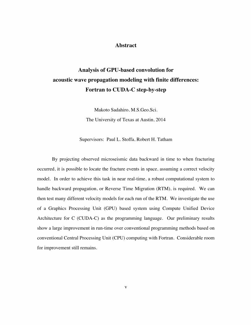
Abstract

Analysis of GPU-based convolution for acoustic wave propagation modeling with finite differences:

Fortran to CUDA-C step-by-step

Makoto Sadahiro, M.S.Geo.Sci.

The University of Texas at Austin, 2014

Supervisors: Paul L. Stoffa, Robert H. Tatham

By projecting observed microseismic data backward in time to when fracturing

occurred, it is possible to locate the fracture events in space, assuming a correct velocity

model. In order to achieve this task in near real-time, a robust computational system to

handle backward propagation, or Reverse Time Migration (RTM), is required. We can

then test many different velocity models for each run of the RTM. We investigate the use

of a Graphics Processing Unit (GPU) based system using Compute Unified Device

Architecture for C (CUDA-C) as the programming language. Our preliminary results

show a large improvement in run-time over conventional programming methods based on

conventional Central Processing Unit (CPU) computing with Fortran. Considerable room

for improvement still remains.

vi

Table of Contents

List of Figures ...................................................................................................... viii  

CHAPTER I 1  

Wave propagation modeling for microseismic monitoring ..................................... 1  1.1. INTRODUCTION ................................................................................... 1  

1.1.2. Restrictions and Assumptions ..................................................... 2  1.2. METHODS .............................................................................................. 3  1.3. MEMORY ............................................................................................... 6  1.4. CONVOLUTION .................................................................................... 9  

1.4.1. Computation methods ............................................................... 10  1.5. WAVE PROPAGATION MODELING FOR MICROSEISMIC

MONITORING .......................................................................... 12  

CHAPTER II 28  

Software Development .......................................................................................... 28  2.1. INTRODUCTION ................................................................................. 28  2.2. FORTRAN ............................................................................................ 29  2.3. C ............................................................................................................ 31  2.4. CUDA-C ................................................................................................ 31  

2.4.1. Global memory .......................................................................... 31  2.4.1.1. Memory copy (1-D vs. 2-D) .......................................... 34  2.4.1.2. Alignment (uniformity of data field by zero paddings) 34  2.4.1.3. Thread count .................................................................. 36  

2.4.2. Constant memory ...................................................................... 39  2.4.3. Review of intermediate results .................................................. 42  2.4.4. Shared memory ......................................................................... 45  

2.4.4.1. Convolution method ...................................................... 45  2.4.4.2. 1-D convolution in minor direction ............................... 48  2.4.4.3. 1-D convolution in major direction ............................... 50  

vii

2.4.4.4. Combining the best performance together .................... 52  

CHAPTER III 56  

Conclusion and recommendation for further investigation ................................... 56  

Appendix A ........................................................................................................... 60  

Appendix B ........................................................................................................... 62  

Appendix C ........................................................................................................... 66  

References ............................................................................................................. 72  

viii

List of Figures

Figure 1. SEG/EAEG velocity model. The figure shown is 2-D velocity model on

xz-plane. For 3-D velocity model, the same 2-D data is extended in the

y-direction. The model is 13500 meters wide (x-axis) and 4200 meters

deep (z-axis). ...................................................................................... 5  

Figure 2. Synthetic shot gather. An example synthetic 2-D shot gather for 4 seconds

in two way reflection time along x-axix at z=0. The source is located at

1 km deep from the surface at the 6 km on in x-direction. We monitor

the output of the synthetic shot gather so that it is consistent throughout

our investigation. ................................................................................ 5  

Figure 3. Schematic of CUDA memory model (Van Oosten, J., 2011). ................ 7  

Figure 4. Convolution operator with length 8. Each side extends 8 elements far from

the center. ......................................................................................... 11  

Figure 5a. The model is 13500 meters wide (x-axis) with 675 elements and 4200

meters deep (z-axis) with 210 elements. 1000 meters with 50 elements

are padded each sides and bottom for wave attenuation. The top is left

as a free surface. ............................................................................... 14  

Figure 5b. Three source locations on our grid. The model is 13500 meters wide (x-

axis) and 4200 meters deep (z-axis). ................................................ 15  

Figure 6a. Forward propagation from source 1 with every ~500 time steps (1

second). ............................................................................................ 17  

Figure 6b. Forward propagation from source 2 with every ~500 time steps (1

second). ............................................................................................ 18  

ix

Figure 6c. Forward propagation from source 3 with every ~500 time steps (1

second). ............................................................................................ 19  

Figure 7a. Source 1 shot gather ............................................................................ 20  

Figure 7b. Source 2 shot gather ............................................................................ 20  

Figure 7c. Source 3 shot gather ............................................................................ 21  

Figure 8a. Reverse propagation from source 1 with every ~500 time steps (1 second).

.......................................................................................................... 22  

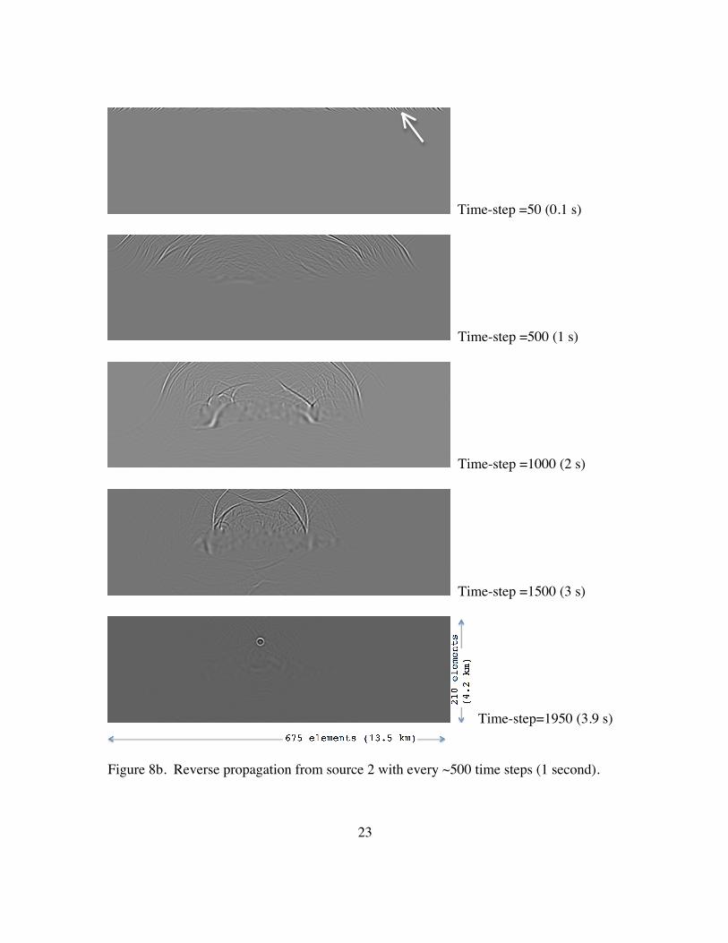
Figure 8b. Reverse propagation from source 2 with every ~500 time steps (1 second).

.......................................................................................................... 23  

Figure 8c. Reverse propagation from source 3 with every ~500 time steps (1 second).

.......................................................................................................... 24  

Figure 9a. Forward propagation from reflectivity map with every ~500 time steps (1

second). ............................................................................................ 25  

Figure 9b. Simulated ZSR section, which approximates a CMP stacked data section.

.......................................................................................................... 26  

Figure 9c. ZSR data generates the reflectivity map. ............................................ 27  

Figure 10. A 2-D representation of a 1-D array. For 3-D volume, 2-D planes extend

in the y-direction. ............................................................................. 29  

Figure 11. A 2-D representation of a 1-D array with kernels in x-direction (gray) in

x-direction. ....................................................................................... 30  

Figure 12. An example of 6x11 2-D slice (white) with zero padding (gray) for the

convolution kernel of length 3 for one side. ..................................... 35  

Figure 13. The plot of kernel time in milliseconds. As more blocks with fewer

threads each are deployed, it improves performance. ...................... 38  

Figure 14. GPU-based convolution implementation performance gains. ............ 42  

x

Figure 15. Run time measurements. Green: Total run time. Purple: Convolution

(kernel+I/O) related time. Blue: CUDA-C kernel only time. ......... 43  

Figure 16. The fraction of kernel-related run time over the total run time. This does

not show the performance gain, but shows the efficiency increase of

convolution section. ......................................................................... 44  

Figure 17. A warp of six threads runs 1-D convolutions in x-direction on z-major 2-D

data block segment in zx-plane. Dots show simultaneous access to

memory as a block for efficiency. .................................................... 46  

Figure 18. Performance gains with thread reduction and its geometry ................ 49  

Figure 19. Performance gain of convolution in major direction by thread reduction

(method 1). ....................................................................................... 51  

Figure 20. Performance gain of convolution in major direction by thread reduction

(method 2, 3, and 4). ........................................................................ 52  

Figure 21. Final performance comparison between development stages. ............ 54  

1

CHAPTER I

Wave propagation modeling for microseismic monitoring

1.1. INTRODUCTION

“GPU computing”, although it is not yet a household name, is well known by

scientists and engineers. Graphics Processing Unit (GPU) is a hardware accelerator

originally designed for personal computers in order to quickly display graphic images. A

GPU is the CPU equivalent of a graphics card, which resides on the expansion slot within

a computer system (a node). Due to its natural parallel processing capability, it has

evolved as a high-performance parallel computing platform, particularly for

computationally intense numerical problems. The real strength of a GPU is in its ability

to perform tasks in extreme parallelism with very little overhead to create parallel

processes. With large arrays of Arithmetic Logic Units (ALU), GPU computing can

offer a large performance gain because of this extreme parallelism.

Our goal in this investigation is to create a fast wave-propagation modeling

platform to process microseismic data in near real time. We start with forward acoustic

wave modeling with a synthetic seismic source to develop the software. Then we

reverse-time migrate acoustic waves for data injected at receiver locations for each time

step. In this investigation, we focus on the critical core section of our code--convolution.

We investigate the benefits and penalties of using a GPU as the compute engine.

Focusing only on convolution allows us to establish a relatively clear measure of the

performance increase.

2

1.1.2. Restrictions and Assumptions

In this investigation, we assume a planar slice of the largest 2-D dimension from a

3-D data volume that fits in a single GPU processing space. Handling data volumes

larger than this description is beyond the scope of current investigation; the greatest

disadvantage of GPU over CPU is smaller memory space. While CPUs can address

hundreds of Gigabytes of main memory space, a GPU typically has 2 Gigabytes (and

maybe 5 Gigabytes for higher-end GPU devices) of main memory. Whether sufficient

data can fit within a GPU’s device memory space or not can make large difference in

performance since it requires time-costing data reloads. As soon as the data volumes are

larger than the GPU device memory space, we pay a high price in data management

overhead for redundant memory copies for boundary conditions from the data

segmentation process. Microseismic data volume may be smaller than some marine

reflection seismic data sets, but they can still exceed the size of GPU memory space,

especially when considering the velocity data needed for the RTM. The memory

capacity of a modern GPU is improving but not yet large enough for many of our

computational problems. Thus we have to optimize our algorithm to accommodate the

memory size and the dimensions of our data.

There are many approaches we can use to benchmark the performance of our

program. We conduct this investigation by considering the best choices of algorithms for

each key part of GPU computing, which we organize as a linear workflow. We make one

change at a time introducing sequentially a new programming language, new hardware,

new memory structure, and new algorithm. We then take benchmarks at each step.

3

1.2. METHODS

In GPU code development, GPUs are referred to as a “device”, and the CPU node

that hosts the GPU ‘device’ are referred to as the “host”. In this investigation, we use a

computational system (stampede.tacc.utexas.edu) provided by the Texas Advanced

Computing Center (TACC) at The University of Texas at Austin. The system is capable

of allocating requested-nodes to perform as a dedicated single-user system, thus

performance will be consistent. Each node, a Dell PowerEdge server, is equipped with

two Intel Xeon E5-2680 (Sandy Bridge) processors running Linux (CentOS release 6.4)

with 32 Gigabytes (GB) of memory space and one NVIDIA Tesla K20m is the GPU

device (Appendix A, Hardware/OS information). The GPU device has 4.8 GB of general

purpose memory, called global memory, and 49 Kilobytes (KB) of low latency memory,

called shared memory, which memory access is shared by a maximum of 1024 process

threads (Appendix A, GPU device information). The GPU device is capable of

transferring data from/to the host system at 6 Gigabytes/sec (Appendix A, Bandwidth

test). Even though there is no clear way to compare the Xeon E5 and Tesla K20m, they

are both very close to the optimum performer of their respective computing architecture

at the time of investigation. So, in terms of a performance comparison between these two

different technologies, this is a reasonable comparison.

We use Intel Fortran to compile our Fortran code, GNU G++ to compile C code,

and NVIDIA NVCC compiler to compile CUDA-C code for GPU. We do have a choice

of using Intel C compiler, but remain with GNU GCC/G++ because NVIDIA NVCC is

based on GNU GCC/G++ compiler. For CUDA-C, we do not use any extra layer of API,

such as Thrust library for CUDA-C. This is to keep the code in as low-level language as

possible in order to facilitate understanding of events on the GPU device.

4

To benchmark the performance at each step, we use two tools: “time” utility tool,

which is a part of Unix’s command-line tools, and NVIDIA nvprof, which is a part of the

CUDA toolkit from NVIDIA. The “time” tool can read three different time

measurements, “real”, “user”, and “system” in milliseconds (ms). The “real” time

measurement is wall-clock readings from the beginning of execution to the end of

execution. The “user” is actual time our code spends when the process is active. The

“system” is the time spent in the kernel for our process. The actual run time is the sum of

measured user time and system time. We will use this measurement to compare Fortran,

C, and our initial non-optimized version of the CUDA code. Once we start focusing only

on CUDA, we use another utility tool, called “nvprof”, to measure the performance

increase within a particular CUDA routine. The nvprof is capable of measuring the

computation time spent in CUDA’s parallel sections for actual computations, memory

copies from host to device, and memory copies from the device to the host in

nanoseconds. For our investigation, most of the time measurements will be on the order

of microseconds.

For both time and nvprof, we measure at least 3 times for consistency. TACC’s

compute nodes are scheduled in a way that there is only one user for a dedicated period

of time. The bandwidth to the data file on the network file system is a shared resource,

but any anomaly from slow bandwidth will show as a part of the readings if there is any

in both time and nvprof utilities.

For test data, we use the SEG/EAEG salt model (Figure 1) for our velocity model

to compute synthetic acoustic wave forward propagation modeling (Figure 2). The

model is 13500 meters wide (x-axis) and 4200 meters deep (z-axis). Since our first

objective is to implement a robust system with forward acoustic modeling, we simply

insert a pressure source at a point near the surface to create synthetic data.

5

Figure 1. SEG/EAEG velocity model. The figure shown is 2-D velocity model on xz-plane. For 3-D velocity model, the same 2-D data is extended in the y-direction. The model is 13500 meters wide (x-axis) and 4200 meters deep (z-axis).

Figure 2. Synthetic shot gather. An example synthetic 2-D shot gather for 4 seconds in two way reflection time along x-axix at z=0. The source is located at 1 km deep from the surface at the 6 km on in x-direction. We monitor the output of the synthetic shot gather so that it is consistent throughout our investigation.

6

Unfortunately, there is an awkward word conflict in the lexicon of our

technologies. In this study, we deal with three different concepts, each with a different

meaning for the word “kernel”. In computer science, kernel refers to the core of

Operating System (OS). In convolution, kernel is the function or mask that multiplies

with the data. In GPU programming, kernel is a parallel task instruction set, which each

parallel process (thread) executes. In this report, we try to be clear which kernel we are

referring to by context or by even calling it with another name when possible.

1.3. MEMORY

GPUs come with a hierarchy of memory structure with different access latency

and size. An obvious way to gain performance is by using memory structure with low

access latency, but it comes with restrictions (mainly in size) and we have to understand

the memory access characteristics in order to optimize this process. For this project, we

are mainly concerned with four different kinds of memories that are CPU host main

memory, GPU device global memory, constant memory, and shared memory. CPU and

GPU are two distinct processing units, so they can not directly access each other’s

memory space (at least with current version of CUDA). Any data read from file into

CPU memory space has to be copied to GPU global memory space first. Data then can

be copied to lower latency memory space (see Figure 3).

7

Figure 3. Schematic of CUDA memory model (Van Oosten, J., 2011).

Following are the main CUDA memory structures and related concepts that will

dictate how we develop our optimization algorithm.

Global memory is the largest and slowest memory on the GPU device, with sizes

up to 5 GB. The memory is on board, but not on-chip. The data in global memory is

automatically cached on-chip, and then eventually replaced by new data. Repeatedly

used data elements have a good chance of taking advantage of cache memory. Because

GPU device global memory is not as large as CPU memory, GPU-based cluster

architecture is not yet as popular in the petroleum industry as conventional CPU-based

cluster systems. Global memory has the largest access latency on GPU device, but it is

8

still much faster than the CPU memory latency. As the name suggests, the scope of

global memory space is global for the GPU device. It is also the only accessible memory

space to the CPU via memory copy commands.

Shared memory is on-chip low latency memory space on the GPU device. It is

also known as user-controlled L1 cache. Majority of current GPUs have 16 KB of shared

memory available on-chip. We have to copy the context from global memory into the

shared memory in order to utilize it. Access to the shared memory is roughly 100x faster

than global memory. Thus, for variables used more than once, it easily pays to store

them in shared memory. The largest constraint is in its size. A 3-D volume data section

of 16 x 16 x 16 in dimension with 4-Byte real numbers can easily exhausts 16 KB. This

memory limit is already restrictive, but an additional constraint is the maximum number

of simultaneous processes (threads) that share the same memory. The scope of memory

is per “block”. A block is a unit of process that can hold a maximum of 1024 threads.

Thus our maximum number of threads for a shared memory space is 1024. When a

dimension of data is larger than 1024 (even for a series of 1-D convolutions), we have to

segment the array into smaller blocks. Otherwise, it may defragment the parallel process

synchronization by the boundaries that have different processing lengths. This is why our

choice of algorithm for larger datasets is a hybrid that is based on 1-D convolutions.

Local memory is a “private memory space” for each thread in a parallel section,

and they are not shared among threads. It has a latency that is the same as global

memory. Any variable allocated without a special qualifier within the CUDA kernel

code will be a local variable that is allocated in local memory. This is an additional item

we could investigate in parallel memory access schemes.

Constant memory is another low latency memory space, and it has global scope

within the device. Current GPU devices come with 64 Kilobytes of constant memory. It

9

works by manually caching the content into low latency memory space. While the other

types of memory assume simultaneous block access by threads, constant memory prefers

broadcasting single memory element to all threads. If we try to access consecutive

memory blocks via CUDA threads, the task is serialized and that degrades the memory

access efficiency. Thus, constant memory is suited to store the finite difference operator

or convolution kernel elements, since all threads access each element simultaneously.

1.4. CONVOLUTION

Convolution is the heart of our acoustic propagation modeling, and also the

critical section of our code. In order to model acoustic wave propagation in forward and

reverse time, we use the explicit Finite Differences method. The amplitude (or pressure)

of the next time step at each location is calculated using the wave equation as

approximated using a Taylor series expansion for each derivative (Equation 1 and 2,

Stoffa, P. L., Appendix B, Seismic Migration Notes). For complete mathematical

derivation of these two equations, our convolution kernel, please refer to the Appendix B,

Stoffa, P. L., Seismic Migration Notes, at the end of this report. In equation 1, P on the

left-hand side of the equation denotes the new amplitude (or pressure) of location [x, y, z]

= [i, j, k] at the next time step, n+1. We notice that the operation on the right hand side

simply convolves the amplitudes at each grid location with the finite difference operator

(See the last three lines of equation 1 for forward modeling and equation 2 for reverse-

time modeling). Higher order finite difference operators will have more terms like the

three terms within parentheses in equations 1 and 2. In our project, we consider three

options to do the convolution for 3-D seismic volumes and these are discussed in the next

section.

10

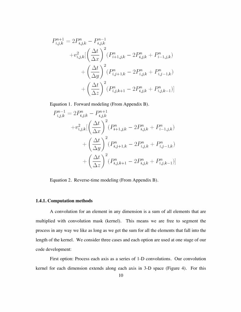
Equation 1. Forward modeling (From Appendix B).

Equation 2. Reverse-time modeling (From Appendix B).

1.4.1. Computation methods

A convolution for an element in any dimension is a sum of all elements that are

multiplied with convolution mask (kernel). This means we are free to segment the

process in any way we like as long as we get the sum for all the elements that fall into the

length of the kernel. We consider three cases and each option are used at one stage of our

code development:

First option: Process each axis as a series of 1-D convolutions. Our convolution

kernel for each dimension extends along each axis in 3-D space (Figure 4). For this

11

reason, unlike conventional 2-D or 3-D convolution kernels, which have a square or a

cube shape, our kernel has a simple shape along each axis. Instead of considering the

data as a 3-D box, we consider the data as strings that run along each axis. As we can see

in the time-step convolution equations (Equation 15, 17), the last three lines are the

derivative terms and are just summations at the current grid point.

Figure 4. Convolution operator with length 8. Each side extends 8 elements far from the center.

Second option: Convolve each element in 3-D. If all the data within the finite

difference operator radius are locally available, we can convolve in all three directions.

This represents the summation of all the second order derivatives we see in the last three

lines of the equations. Needless to say, all data within the operator radius have to fit in

within the same scope of local memory, else we are looking at a high latency from

memory access. This is a good solution if the entire data can fit within the same scope of

GPU device memory.

Third option: A combination of the first two options. We process the 3-D volume

as a series of 2-D slices, where each 2-D slice is now also considered a 1-D array. We

run 1-D convolutions in all three directions along the axis. For the first dimension, we

run 1-D convolutions on 1-D data stripes along the array major axis. Then, for other two

12

directions, we run 1-D convolutions on 2-D data blocks on two different planes that the

array major axis is the intersection of those two planes. This turns out to be a good fit to

the CUDA’s parallel memory access scheme. This method assumes all 2-D slices fit

within the GPU device memory space in order to achieve optimal performance. Even if

the GPU device memory is large enough (so the entire data can fit in the device memory),

lower latency memory space (such as shared memory) is very limited in size. We are

forced to segment the data into smaller blocks to fit into the limited space of faster

memory space. We believe this method can also work well with larger data volumes that

do not fit in GPU device memory space. This third option is our choice of algorithm as

soon as we utilize shared memory in our CUDA code.

1.5. WAVE PROPAGATION MODELING FOR MICROSEISMIC MONITORING

One of goals in this investigation is to find out the bottom-line performance

results of GPU based wave propagation modeling in order to monitor microseismic

signatures from hydraulic fracturing process. Microseismic data in general may not be as

monolithic as full-scale surface seismic survey data, but they have their own important

requirements to meet. Unlike full-scale seismic imaging that is processed prior to

drilling, microseismic imaging is conducted during the hydrofracturing process to ensure

generated fractures occur at intended locations in the subsurface. So it has to run in near

real time. Microseismic signatures are monitored by geophones on the surface above the

subject area and/or in subsurface boreholes. We use time-synced recordings from those

geophones to backtrack in time for the location of the source of seismic signature in

space. The concept is very similar to triangulation by using different latency of signals at

different locations. We do not know the travel path of each recorded seismic signature,

13

but we know the arrival time differences at each position on the recording array are

precise. Thus, we model the insertion of a seismic source into the subsurface to let the

energy propagate. Correct propagation paths with the correct propagation times will

focus to accumulate into strong signature. All incorrect paths or incorrect arrival time

will not focus and will appear as noise. We obtain the accumulation of seismic energy as

the source of the seismic signature improves with increased signal to noise as a result of

coherency processing using the wave equation.

In order to process the data in near real time, we have to be realistic in our

processes, balancing accuracy and latency. We process our model with convolution-

based application on the explicit Finite Differences method, which is robust and

sufficiently accurate for our purpose. As explained in previous section, our code supports

a long convolution kernel with linear increase of cost due to the use of 1-D convolution in

order to further increase accuracy. Since microseismic monitoring is conducted during

hydrofracturing operations, the velocity model of subsurface locations in the area of our

interest is most likely available from borehole information. And of course, if there is

more than one possible velocity model, our system allows testing different velocity

models quickly. For our study, it will be helpful if we know exactly how the source

seismic signature has traveled for particular recorded dataset. So we start with forward

modeling to create synthetic seismic data in order to accurately process it by our reverse

time modeling. For forward wave propagation modeling, we place a pressure source at

an arbitrary location in subsurface, let it propagate, and record the signature at each

geophone locations for 2000 time steps (4 seconds). Then for reverse time wave

propagation modeling, we insert the recorded data back into the geophone locations, and

let it propagate for 2000 time steps. If done correctly, the wave propagation in reverse

time modeling focuses into a single point of origin.

14

For our study, we used the SEG/EAEG velocity model. Although this model is

not typical for the geological area where microseismic data are typically recorded, it has a

complex structure and is widely used for testing seismic modeling algorithms. In order to

compute our model as a grid, we defined the physical size of each grid elements as 20

meters (0.02 Km), which translates to 50 grid elements per 1km. We also defined a time

step, or time interval, as 0.002 seconds each, to run for 2000 time steps. This translates

as 4 seconds of total run time. To summarize, we defined our subsurface area to be 4200

meters (with 210 elements) in depth (z-direction) and 13500 meters (with 675 elements)

in width (x-direction) in our computing grid for 2000 (4 seconds) time steps (Figure 5a).

Figure 5a. The model is 13500 meters wide (x-axis) with 675 elements and 4200 meters deep (z-axis) with 210 elements. 1000 meters with 50 elements are padded each sides and bottom for wave attenuation. The top is left as a free surface.

15

The dimension of the model is the same as SEG/EAEG velocity model we have

used. We then padded 50 elements (1 Km) in all three perimeters of subsurface in order

to attenuate the propagating wave at the boundaries. The ground surface is left as free

surface without paddings (Figure 5a). We recorded seismic signatures at all surface

locations at z=0. Throughout our code development, we used the same geometry to keep

a consistency.

We tested our model with three different source locations, on surface (source 1),

between surface and salt (source 2), and below salt (source 3) (Figure 5b).

Figure 5b. Three source locations on our grid. The model is 13500 meters wide (x-axis) and 4200 meters deep (z-axis).

Figure 6a, 6b, and 6c show the time lapse of forward wave propagation in

roughly every 500 time-steps (1 second) from each source locations. We let the signal to

propagate, and record the pressure at each geophone locations at each time step. This

produces a shot gather of seismic traces. As the distance and velocity between the source

and geophones change, this changes the recorded seismic traces in shot gather (Figure 7a,

7b, 7c). We also tested the model with reflectivity data. Instead of placing a single

source pressure, we place a reflectivity map at every point of data volume (Figure 9a).

16

The result of forward wave propagation is a zero source-receiver offset (ZSR) section

similar to Common Mid Point stacked data (Figure 9b).

We now insert each seismic trace from shot gathers back at each geophone

location on the surface at each time step, and let them propagate. Figure 8a, 8b, and 8c

show the reverse time wave propagation for roughly every 500 time-steps (1 second).

The result from source 1 and 2 shows clearly collapsing the wave front to a single point

of source. On the other hand, it is difficult to identify the source location with source 3.

Because of high velocity in salt formation, it is more difficult for wave front to transmit

through the salt body. As result, we are not gathering enough seismic signatures in the

seismic traces of our shot gather. Even so, the source can still be seen.

Figure 9c shows the reverse wave propagation of ZSR section. With the surface-

recorded reflectivity profile, we confirm that the source pressure placed everywhere

across the grid (not placed only at a single point) can be correctly focused back to the

original source profile as well.

17

Time-step =50 (0.1 s)

Time-step =500 (1 s)

Time-step =1000 (2 s)

Time-step =1500 (3 s)

Time-step=1950 (3.9 s)

Figure 6a. Forward propagation from source 1 with every ~500 time steps (1 second).

18

Time-step =50 (0.1 s)

Time-step =500 (1 s)

Time-step =1000 (2 s)

Time-step =1500 (3 s)

Time-step=1950 (3.9 s)

Figure 6b. Forward propagation from source 2 with every ~500 time steps (1 second).

19

Time-step =50 (0.1 s)

Time-step =500 (1 s)

Time-step =1000 (2 s)

Time-step =1500 (3 s)

Time-step=1950 (3.9 s)

Figure 6c. Forward propagation from source 3 with every ~500 time steps (1 second).

20

Figure 7a. Source 1 shot gather

Figure 7b. Source 2 shot gather

21

Figure 7c. Source 3 shot gather

22

Time-step =50 (0.1 s)

Time-step =500 (1 s)

Time-step =1000 (2 s)

Time-step =1500 (3 s)

Time-step=1950 (3.9 s)

Figure 8a. Reverse propagation from source 1 with every ~500 time steps (1 second).

23

Time-step =50 (0.1 s)

Time-step =500 (1 s)

Time-step =1000 (2 s)

Time-step =1500 (3 s)

Time-step=1950 (3.9 s)

Figure 8b. Reverse propagation from source 2 with every ~500 time steps (1 second).

24

Time-step =50 (0.1 s)

Time-step =500 (1 s)

Time-step =1000 (2 s)

Time-step =1500 (3 s)

Time-step=1950 (3.9 s)

Figure 8c. Reverse propagation from source 3 with every ~500 time steps (1 second).

25

Time-step =50 (0.1 s)

Time-step =500 (1 s)

Time-step =1000 (2 s)

Time-step =1500 (3 s)

Time-step=1950 (3.9 s)

Figure 9a. Forward propagation from reflectivity map with every ~500 time steps (1 second).

26

Figure 9b. Simulated ZSR section, which approximates a CMP stacked data section.

27

Time-step =50 (0.1 s)

Time-step =500 (1 s)

Time-step =1000 (2 s)

Time-step =1500 (3 s)

Time-step=1950 (3.9 s)

Figure 9c. ZSR data generates the reflectivity map.

28

CHAPTER II

Software Development

2.1. INTRODUCTION

The goal of this software development process is to migrate and optimize from

CPU-based Fortran code to C/C++, and then to GPU based CUDA-C code in order to

measure the performance increase at each step. We start with comparing the performance

between two languages as a necessary evil. This is because it is necessary to migrate the

convolution part of the Fortran code to C code in order to run CUDA-C code. Then we

focus performance improvement only within the CUDA convolution routine. Following

is the itemized list of steps we investigate:

Fortran

The original code

C

One-to-one translation of many of the Fortran routines

(including convolution routine to C)

CUDA-C

Global memory (automatic cache)

Explicit boundaries

Zero padding boundaries (identical process)

Constant memory (broadcasting cached global memory)

Shared memory (user-controlled L1 cache)

Convolution method (Appendix C)

29

We have a rough idea for performance gains based on the GPU memory hierarchy

so we linearized our investigation process. Thus, we expect performance gains at each

step of our investigation itemized in the list above.

2.2. FORTRAN

The original Fortran code was developed by Paul Stoffa (Institute for Geophysics,

University of Texas at Austin) in May 2013. The code runs on a single thread on a CPU.

The data were organized in z-major over x-axis and then y-axis (Figure 10). The figure

shows an array that is configured as a 2-D array (zx-plane). Long arrows indicate how a

1-D array is configured as 2-D array. Since the underlying system always accesses

memory in blocks as a minimal access unit, memory access along z-axis is more efficient

than along x-axis or y-axsis.

Figure 10. A 2-D representation of a 1-D array. For 3-D volume, 2-D planes extend in the y-direction.

Boundaries are not padded by zeros, but explicit. We process using a 1-D

convolution for each dimension using strides based on the length of the z-major axis for

z

x

30

2-D and z-x plane for 3-D. The convolution routine calculates how far each data element

is from the borders, and processes explicitly up to each border (Figure 11). The figure

shows 1-D convolution kernels in x-direction at two point locations, one with full kernel

length and another where one wing of kernel does not fit within data range, on z-major

array.

Figure 11. A 2-D representation of a 1-D array with kernels in x-direction (gray) in x-direction.

Our test case has grid points in z and x respectively and we ran for 1999 time

steps. Our initial benchmarking with Unix’s time tool measured the following run-time.

real 0m8.652s

user 0m8.541s

sys 0m0.042s

Fortran has a special place in numerical computing. Despite its age, Fortran is

still used widely in numerical computing due to its performance despite its age. With

high-end CPUs, it can perform well. Our initial test shows the Fortran version of our

code can process the data in around 8.6 seconds (user + sys = 8.54s + 0.04s).

z

x

31

2.3. C

In order to run CUDA-C language code on GPU device, we needed to rewrite

convolution related routines in the C language. The result is a hybrid code with Fortran

and C. The program entry point in Fortran calls the C routine to run the convolutions.

The process is a direct one to one translation of the algorithm. The data array is 1-D, and

C routines refer to the same data instance in the original memory location allocated by

Fortran. We built the code with no optimization, level-2 optimization, and level-3

optimization. Our C code performed significantly poorer than the Fortran code.

no optimization level-2 optimization level-3 optimization

real 2m18.714s real 0m36.669s real 0m39.474s

user 2m18.428s user 0m36.513s user 0m39.297s

sys 0m0.094s sys 0m0.028s sys 0m0.065s

One probable reason for C’s poor performance over Fortran is due to the aliasing

of memory addresses. Fortran does not need to use pointers, which means there is only

one entry point to modify values in memory. C allows multiple variable names to modify

the same memory location, so C would have to reload the array to read the most updated

values. Our test shows our code with C version of convolution routine takes nearly 36.5

seconds with level-2 optimization. The performance is about 4x worse than Fortran.

2.4. CUDA-C

2.4.1. Global memory

With CUDA-C, convolution processes for each element run in parallel on the

GPU device global memory, and there is an overhead of memory copy between CPU host

and GPU device. With this version of our code, we recorded a total run time of 4.8

32

seconds. The run-time ratio is 13.1% (4.8/36.5) from C version (~7.63x performance),

and 55.8% (4.8/8.6) from Fortran version (~1.79x performance).

real 0m5.617s

user 0m3.538s

sys 0m1.253s

Profiling result from nvprof shows our convolution routine spent an average of

320.66 microseconds for each of 1999 time steps. The profiling also shows that 50% of

execution time is within the convolution section.

Time(%) Time Calls Avg Min Max Name ======== Profiling result: 25.16 320.38ms 7996 40.07us 928ns 174.69us [CUDA memcpy HtoD] 22.95 292.20ms 1999 146.17us 145.95us 167.17us [CUDA memcpy DtoH] 1.55 19.73ms 1999 9.87us 9.38us 10.34us initializerKernel 50.34 640.99ms 1999 320.66us 306.34us 345.38us vtconvlKernelXZopY_GMEB

The profiling shows section time for CUDA related operations. This allows us to

calculate performance gain of only convolution related sections from Fortran version to

our first CUDA version. First, we calculate non-CUDA related time in CUDA version.

Total run time for CUDA version is user + sys from “time” measurement.

user + sys = 0m3.538s + 0m1.253s = 0m4.791s

Total CUDA related operation for CUDA version is sum of profiling results.

640.99ms + 320.38ms + 292.20ms + 19.73ms = 1273.3ms = 1.273s

33

Then, total non-CUDA related operation is the difference of above two.

0m4.791s - 1.273s = 3.5177 seconds

Since non-CUDA related operation is nearly identical in both versions, this is also

the time for non-convolution related routines in Fortran. So, we subtract this time

segment from total run time of Fortran version. Total run time for Fortran version is sum

of user and sys time.

user + sys = 0m8.541s + 0m0.042s = 8.583s

By subtracting non-CUDA related time of CUDA version from total run time of

Fortran version, we get the run time for the convolution routine of our Fortran code.

8.583s - 3.5177 = 5.0653s

Now finally, we take the ratio of convolution time for both versions.

CUDA convolution time / Fortran convolution time = 1.273s / 5.0653s = 0.2513

= Performance gain to 25.13% of original time, which is about 4x faster.

Next, we develop our code within CUDA-C concepts. It is difficult to compare

multiple ideas at the same time, so for this investigation, we will be focusing only on

convolution after this point. We use nvprof as the performance measurement tool from

this point on.

34

2.4.1.1. Memory copy (1-D vs. 2-D)

When we copy data from host to device, we have the choice of copying the data

with a CUDA function as one 2-D data instead of a series of 1-D data. This concept

becomes important in our next step, so we like to analyze this before moving to next step.

1-D memory copy allows us to define the source memory location, destination memory

location, data length, and stride. This is a handy feature to copy data into the middle of

an array with zero-padded boundaries. We will go over why we want this in next section.

Following is benchmark result from memory copy by these two different scenarios.

1-D memcpy ======== Profiling result: Time(%) Time Calls Avg Min Max Name 25.16 320.38ms 7996 40.07us 928ns 174.69us [CUDA memcpy HtoD] 22.95 292.20ms 1999 146.17us 145.95us 167.17us [CUDA memcpy DtoH] 1.55 19.73ms 1999 9.87us 9.38us 10.34us initializerKernel 50.34 640.99ms 1999 320.66us 306.34us 345.38us vtconvlKernelXZopY_GMEB

2-D memcpy ======== Profiling result: Time(%) Time Calls Avg Min Max Name 25.80 332.46ms 7996 41.58us 896ns 181.18us [CUDA memcpy HtoD] 22.97 296.02ms 1999 148.08us 147.97us 152.51us [CUDA memcpy DtoH] 1.53 19.67ms 1999 9.84us 9.28us 10.24us initializerKernel 49.71 640.66ms 1999 320.49us 306.05us 341.73us vtconvlKernelXZopY_GMEB

The benchmarking shows 2-D memory copy scheme has slightly degraded

performance than 1-D memory copy scheme, but it is almost negligible.

2.4.1.2. Alignment (uniformity of data field by zero paddings)

When a bundle of threads access an array in parallel, they access consecutive

elements as a block. Threads run in a unit called “warp”. Each warp consists of 32

35

threads, thus 32 consecutive memory locations in an array are accessed together at once.

Access to global memory (and shared memory as well) uses this scheme. It is thus

beneficial to run identical operation on all 32 threads in order to synchronize their

memory access timings. With our first CUDA-C version of code, we had explicit

boundary that threads perform convolution only up to the boundary of data space. This

boundary can break warp’s memory access synchronization. We can correct this problem

by padding elements for the convolution operators’ length outside boundaries with zeros.

The Figure 12 shows an example of the original 6x11 2-D slice (white) with zero padding

around (gray) it, which assumes convolution kernel of wing length 3 (two wings of 3

elements + 1 for body = total length 7). Convolution is performed in all data cells (white)

with identical operation without worried about the boundaries.

Figure 12. An example of 6x11 2-D slice (white) with zero padding (gray) for the convolution kernel of length 3 for one side.

CUDA Global memory version WITHOUT zero padding:

real 0m5.617s

user 0m3.538s

sys 0m1.253s

36

======== Profiling result: Time(%) Time Calls Avg Min Max Name 25.80 332.46ms 7996 41.58us 896ns 181.18us [CUDA memcpy HtoD] 22.97 296.02ms 1999 148.08us 147.97us 152.51us [CUDA memcpy DtoH] 1.53 19.67ms 1999 9.84us 9.28us 10.24us initializerKernel 49.71 640.66ms 1999 320.49us 306.05us 341.73us vtconvlKernelXZopY_GMEB

CUDA Global memory version WITH zero paddings:

real 0m5.668s

user 0m3.655s

sys 0m1.256s

======== Profiling result: Time(%) Time Calls Avg Min Max Name 25.82 331.51ms 7996 41.46us 896ns 180.67us [CUDA memcpy HtoD] 23.06 296.08ms 1999 148.11us 147.97us 163.58us [CUDA memcpy DtoH] 1.54 19.82ms 1999 9.91us 9.38us 10.40us initializerKernel 49.58 636.53ms 1999 318.42us 298.75us 343.04us vtconvlKernelXZopY_GMZP

We expected notable performance gain, but the benchmark shows very little

differences. The difference between those two outside GPU kernel code is whether

memory copy is performed in 1-D or 2-D and additional memory space for zero padding.

It is our understanding higher-end GPU devices are more forgiving to unsynchronized

thread processes within warps. I expect lower-end GPU devices to show more significant

difference.

2.4.1.3. Thread count

Before we proceed to the next step, we would like to step aside to investigate one

idea, thread count. Earlier, we mentioned a block is a unit for a bundle of threads. We

have used 1024 threads as default so far. How does it change if we use more blocks with

fewer threads?

37

1024 threads ======== Profiling result: Time(%) Time Calls Avg Min Max Name 25.82 331.51ms 7996 41.46us 896ns 180.67us [CUDA memcpy HtoD] 23.06 296.08ms 1999 148.11us 147.97us 163.58us [CUDA memcpy DtoH] 1.54 19.82ms 1999 9.91us 9.38us 10.40us initializerKernel 49.58 636.53ms 1999 318.42us 298.75us 343.04us vtconvlKernelXZopY_GMZP 512 threads ======== Profiling result: Time(%) Time Calls Avg Min Max Name 25.27 332.53ms 7996 41.59us 864ns 181.12us [CUDA memcpy HtoD] 27.88 366.88ms 1999 183.53us 147.87us 206.11us [CUDA memcpy DtoH] 1.32 17.35ms 1999 8.68us 8.00us 8.86us initializerKernel 45.54 599.39ms 1999 299.84us 287.58us 318.69us vtconvlKernelXZopY_GMZP 256 threads ======== Profiling result: Time(%) Time Calls Avg Min Max Name 27.11 332.81ms 7996 41.62us 896ns 181.31us [CUDA memcpy HtoD] 24.12 296.10ms 1999 148.12us 148.00us 155.78us [CUDA memcpy DtoH] 1.37 16.76ms 1999 8.39us 7.62us 8.54us initializerKernel 47.41 582.04ms 1999 291.16us 287.04us 297.60us vtconvlKernelXZopY_GMZP 128 threads ======== Profiling result: Time(%) Time Calls Avg Min Max Name 27.09 332.03ms 7996 41.52us 864ns 188.70us [CUDA memcpy HtoD] 24.14 295.82ms 1999 147.98us 147.87us 148.90us [CUDA memcpy DtoH] 1.39 17.07ms 1999 8.54us 7.90us 8.67us initializerKernel 47.38 580.64ms 1999 290.46us 287.36us 293.82us vtconvlKernelXZopY_GMZP

The average run time for each kernel invocation is roughly 318, 299, 291, and 290

microseconds for 1024, 512, 256, and 128 threads respectively. The result shows slight

improvements each time we reduce the thread count per block (Figure 13).

38

Figure 13. The plot of kernel time in milliseconds. As more blocks with fewer threads each are deployed, it improves performance.

There are probably multiple reasons for this result. But since the implementation

of our convolution kernel is very simple, one large possibility is that our code is most

likely bandwidth limited by thread count. As soon as we start using shared memory, we

have to segment our data into blocks. The scope of shared memory is by block. If we

use fewer threads, it is advantageous to be able to segment data to smaller blocks rather

than large blocks. This is another advantage of using 1-D convolution blocks over 3-D

blocks. There is more iteration with 1-D convolution, but there is less redundancy with

it. In order to keep our benchmarking consistent, we retain the thread count per block as

1024 for now until we get to the implementation of shared memory version of our code.

550  

560  

570  

580  

590  

600  

610  

620  

630  

640  

650  

1024   512   256   128  

Time  by  threads  

(milliseconds)  

39

2.4.2. Constant memory

Constant memory is a cached global memory. Thus, the access latency is good if

it is used as broadcasting memory, such as for access that all threads in the warp access to

a single element in constant memory at a time. In our case, it is suited to store our

convolution kernels. This is because all threads access each element in the convolution

kernel simultaneously.

real 0m5.366s

user 0m3.372s

sys 0m1.221s

======== Profiling result: Time(%) Time Calls Avg Min Max Name 35.25 332.41ms 7999 41.56us 896ns 180.87us [CUDA memcpy HtoD] 31.38 295.97ms 1999 148.06us 148.00us 148.45us [CUDA memcpy DtoH] 2.10 19.84ms 1999 9.93us 9.38us 10.30us initializerKernel 31.26 294.85ms 1999 147.50us 145.60us 152.99us vtconvlKernelXZopY_CMZP

The run time for convolution section is 294.85 milliseconds. Comparing to

636.53 milliseconds of non-constant memory version, this is roughly 2x speed up.

Unfortunately, this estimate is still not exactly fair. One thing we have to think

about is that constant memory is declared outside GPU code that contributed an overhead

outside GPU code in order to gain performance within GPU code. We can calculate this

overhead in the same way as we calculated for Fortran to the first CUDA-C version.

Non-GPU related time for non-constant memory version is obtained by

subtracting CUDA related time from total run time.

40

Total run time - CUDA related time = (user+sys) - (all CUDA time)

= (0m3.538s + 0m1.253s) - (640.99ms + 320.38ms + 292.20ms + 19.73ms)

= 0m4.791s - 1.273s = 3.5177 seconds

Non-GPU related time for constant memory version is obtained by again

subtracting CUDA related time from total run time.

Total run time - CUDA related time = (user+sys) - (all CUDA time)

= (0m3.372s + 0m1.221s) - (332.41ms+295.97ms+294.85ms+19.84ms)

= 0m4.593s - 0.943s = 3.65 seconds

Thus the new overhead for constant memory outside GPU code is 0.1322 seconds.

Now we compare all CUDA related time for non-constant memory version and

constant memory version along with 0.1322 seconds overhead.

Non-constant = 640.99ms + 320.38ms + 292.20ms + 19.73ms

= 1273 milliseconds

= 1.273 seconds

Constant = 332.41ms + 295.97ms + 294.85ms + 19.84ms + (0.1322 seconds

overhead)

= 943ms + 0.1322s

41

= 0.943s + 0.1322s

= 1.075 seconds

Constant / Non-constant = 1.075s / 1.273s = 0.8446.

This is speed gain to 84.46% of prior to the constant memory use (~1.19x speed

up). This does not seem to be much of a gain, but we have to remember this is a constant

overhead to allocate the convolution kernel in constant memory space. For this test, we

used small array of only 310x775x1 size volume. For a data volume of decent size, the

overhead becomes negligible very quickly. Thus we can consider this section’s result to

be a 2x speed up (Figure 14). As the data size increases, the performance approaches a

theoretical ~8x speed up. But again, what we are interested in is the bottom line

performance in different conditions, not what we can get at the best condition. We use

the number from the lesser performance, 1.19x, for calculating the performance in further

sections.

42

Figure 14. GPU-based convolution implementation performance gains.

2.4.3. Review of intermediate results

We have improved performance for total run time from 8.7 sec by Fortran to 4.6

of CUDA with zero padding boundaries and convolution kernel in constant memory,

which is 4.6 / 8.7 = 0.5287 = 52.87% of original latency, a bit shy to 2x speed

improvement (Figure 15).

0  200  400  600  800  1000  1200  1400  

Kernel-­‐related  

performance  

(milliseconds)  

CUDA_kernel  

convolution_total  (kernel  +  I/O)  

43

Figure 15. Run time measurements. Green: Total run time. Purple: Convolution (kernel+I/O) related time. Blue: CUDA-C kernel only time.

0  

5000  

10000  

15000  

20000  

25000  

30000  

35000  

40000  Run  time  (milliseconds)  

time_total  

CUDA_kernel  

convolution_total  (kernel  +  I/O)  

44

For the convolution (and memory copy) section alone, we gained performance

from 5.0653s to 1.075s. This is about 1.075s / 5.0653s = 0.2122 = 21.22% of original

latency, which is about 4.71x performance or 371% performance gain (Figure 15). We

can also observe a gain for time fraction in convolution related task over total time

(Figure 16). Even our current measured performance gain is at 4.71x, the performance

will still increase even more to theoretical 7.96x range as the size of data increases.

Figure 16. The fraction of kernel-related run time over the total run time. This does not show the performance gain, but shows the efficiency increase of convolution section.

0  0.1  0.2  0.3  0.4  0.5  0.6  0.7  0.8  0.9  1  

Time  fraction  

(Kernel-­‐related  /  total)  

45

2.4.4. Shared memory

2.4.4.1. Convolution method

Using shared memory is a way to reduce the latency to source data. It is about

100x as fast as global memory. But in order to use this low latency memory, we have to

segment our data to blocks of more manageable size. The scope of the memory is limited

within a thread block. We can still expect further notable performance gain with shared

memory due to its low access latency regardless of the overhead from process

redundancy at boundary condition that comes from memory block segmentation. There

are two important concepts for the effective use of shared memory, which are

convolution method with memory size limitation and memory access efficiency. These

two concepts unfortunately often counteract upon each other.

Shared memory on GPU devices are very limited in allocation size. Higher-end

GPUs, such as K20m, have 49 Kilobytes. Many typical mid to low-end GPUs have only

16 Kilobytes of shared memory. This is about the size of a cube with 16 elements in each

direction ((16 x 16 x 16 ) x 4-Bytes). Especially with long convolution operators, this

does not leave a lot of effective computing grid elements. With higher dimension, we

consume more data by redundant boundaries, which can quickly overwhelm actual data.

For this reason, 1-D convolution is memory efficient when we can run 1-D convolution

on striped data block segments.

Due to the nature of memory access efficiency, we prefer a warp accessing

contiguous elements of the array in z-major direction as a block for each atomic

operation. 1-D convolution in z-direction is already aligned to the warp’s block memory

access direction (array’s major direction), so we can process 1-D convolution in z-

direction with 1-D data stripe segments. 1-D convolution in x-direction and y-direction

on 1-D data stripe segments requires our z-major array to rotate to be x-major and y-

46

major arrays. A fast array rotation is possible. In fact, it is possible to operate this with

almost no overhead. But the operation requires large enough memory space to hold

multiple 1-D stripes of at least half-warp width to be efficient. With current shared

memory allocation size, we can afford to have only few 1-D stripes that fit in shred

memory space. Thus this operation can be an expensive overhead due to inefficient serial

memory access to the source global memory array. As a result, 1-D convolution in x-

direction and y-direction requires our shared memory data block to be in 2-D since

convolution runs perpendicular to the array’s major direction. The Figure 17 shows an

example warp of six threads running 1-D convolutions in x-direction. A warp of six

threads, indicated by dots, together makes a block accesses to consecutive memory

locations.

Figure 17. A warp of six threads runs 1-D convolutions in x-direction on z-major 2-D data block segment in zx-plane. Dots show simultaneous access to memory as a block for efficiency.

Our choice of algorithm is a hybrid method. We always run convolutions in 1-D,

but data block shapes vary. We run 1-D convolution in z-direction on stripe data blocks

along z-direction for entire data volume as 1-D data. For processing 3-D data, we

z

x

47

process x-direction and y-direction, as a series of 2-D data slices. We run 1-D

convolutions in x-direction on 2-D data blocks in zx-planes, and then again run 1-D

convolutions in y-direction on 2-D data blocks in zy-planes. With this scheme, we can

process all data in parallel without serializing memory access by warp. This scheme

supports long convolution operators very well, which is important for more precise

modeling.

Our method allows us to measure performance of convolution in z-direction and

x-direction separately so we analyze them separately. From a discussion in a previous

section, we know the thread count reduction increases performance due to the reduction

in memory band congestion. So far, we compared performance of convolution at each

steps with 1024 threads to keep our measurement consistent. Since the use of shared

memory is the last step for our investigation, we will measure the performance gains with

different thread count to optimize the performance. With our previous measurement with

global memory, it has shown a performance gain of roughly 10% with 256 threads over

1024 threads. Both convolution in z-direction and x-direction with shared memory has

shown a noticeable amount of performance gain when thread counts were reduced.

Especially with convolution in x-direction has shown as much as roughly 27%

performance increase with right amount of thread count and corresponding x-dimension

geometry. By following our convention, we start running convolutions with 1024

threads, and start reducing it by half at each step. For the convolution in x-direction on 2-

D plane, we also test different 2-D block geometries that fit to warp size of 32 or half-

warp size of 16. For example a convolution on 2-D plane with 1024 threads can be in

dimension of 32x32, 64x16, and 16x64. For the convolution in z-direction, we test

different 2-D block geometries, like with the convolution in x-direction. And we also test

several 1-D strip segmentation methods that treat entire data as a long strip of 1-D array.

48

The overhead of shared memory allocation is within the kernel run time. We still

use the constant memory allocated in previous section, but there is no extra overhead

above what is already measured in previous section. This simplifies our measurement.

We can now measure our performance with nvprof profiling tool alone. We measure the

performance of convolution in each direction separately, and measure the best

performance with the best of the both convolution directions to compare to the result

from our previous constant memory section.

2.4.4.2. 1-D convolution in minor direction

Since our input data is in z-major, we can not simply run 1-D convolution in x-

direction as a long strip. We run 1-D convolution in x-direction on segmented 2-D

blocks for the entire 2-D plane. We form blocks of 2-D array to cover entire 2-D data

where each block is a 2-D array of threads. For example with 1024 threads, 2x2 blocks

can cover 64x64 2-D array where each block is 32x32 threads. The kernel takes care of

data overwrap at each boundary in x-direction.

49

Figure 18. Performance gains with thread reduction and its geometry

Figure 18 shows the result of 1-D convolution in x-direction on 2-D plane. Lower

value is faster. Our test gave us an immediate insight. With high thread count, the

performance is more affected by thread count than the access geometry. With low thread

count, the performance is affected by geometry whether to retain full, or at least, a half

warp. In our test, 1-D convolution in x-direction performed the best in 16x16

configuration with 256 threads. From 144.07 milliseconds with 1024 threads, it initially

improves performance up to 111.28 milliseconds with 256 threads. Then it degrades

performance with 128 threads. This tells us the memory bandwidth was congested above

256 threads, but 128 threads were not enough to fully utilize close to100% memory

bandwidth. The optimal performance is somewhere between 256 threads and 128 threads

with this convolution kernel.

50

2.4.4.3. 1-D convolution in major direction

Since our input data is in z-major, our convolution in z-direction is already sorted

in the correct order. We run 1-D convolution in z-direction on the entire 2-D plane as

one long strip of 1-D data. This allows us to process maximum amount of data with

minimal amount of data overwrap needed for boundary conditions. The kernel takes care

of data overwrap at each boundary condition. We start with 1024 threads to segment the

entire 1-D strip to smaller strips or blocks of 1024 elements. There are several methods

for the segmentation.

Method 1. We take the entire 2-D array as a strip of 1-D array. Since the array is

already z-major, we can run simply run 1-D convolution in z-direction as a long strip.

We will segment the strip to smaller strips of N-elements where N is the number of

threads. We start segmenting the 1-D strip data with 1024 elements, and then reduce it

by half at each step to test the performance gain.

Method 2. We use the exact length of z-direction elements of our data to segment

the 1-D strip. We can keep the kernel code as simple as possible this way. We take one

z-stripe at each x locations for the iterations of 1-D convolution in z-direction. We repeat

for the element count in x-direction to convolve entire 2-D plane.

Method 3. The idea is extended from method 2. The z-dimension of our data is

326 elements. We can fit up to 3 z-stripes within 1024 threads. Thus we can test for z-

dimension x3, x2, and x1. The performance with x1 should be close to method 2, but we

expect lesser performance due to extra code segments in the kernel.

Method 4. The idea is the same as method 3. We take the series of z-stripes to

form 2-D array. The main difference from other methods above is this method invokes 2-

D kernel where the other kernel invokes 1-D kernel.

51

In reality, we should always use only method 1 since this is only method that is

not restricted to a particular data dimension. We include the result from other three tests

only to show a gain and loss when we can rig our code for a particular data dimension of

particular dataset.

Figure 19 shows the result of 1-D convolution in z-direction with method 1.

Lower time latency is better performance. In our test, 1-D convolution in z-direction

performed the best with 128 threads. From 112.3 milliseconds with 1024 threads, it

initially improves performance up to 93.514 milliseconds with 128 threads. Then it

degrades performance to 149.14 milliseconds with 64 threads. This tells us the memory

bandwidth was congested above 128 threads, but 64 threads were not enough to fully

utilize close to 100% memory bandwidth. The optimal performance is somewhere

between 128 threads and 64 threads with this convolution kernel.

Figure 19. Performance gain of convolution in major direction by thread reduction (method 1).

52

Figure 20. Performance gain of convolution in major direction by thread reduction (method 2, 3, and 4).

2.4.4.4. Combining the best performance together

We now combine the best performing methods of each z-direction and x-direction

convolutions together. We run 1-D convolution in minor direction with 256 (16x16)

threads. Then we run 1-D convolution in major direction with 128 (128x1) threads. Here

is an output profile from the final version of our code. While memory cost is the same as

previous global memory + constant memory case, the performance of convolution section

has increased to about 1.5x.

Time(%) Time Calls Avg Min Max Name 39.09 332.71ms 7999 41.59us 896ns 180.61us [CUDA memcpy HtoD] 34.78 296.06ms 1999 148.10us 147.97us 156.90us [CUDA memcpy DtoH] 13.76 117.08ms 1999 58.57us 57.79us 59.71us vtconvlKernel_minor_grid_SMZP 9.92 84.43ms 1999 42.24us 41.50us 42.50us vtconvlKernel_major_grid_SMZP 2.45 20.87ms 1999 10.44us 9.89us 10.98us initializerKernel

Since we still use constant memory for storing convolution kernel, we encounter

the overhead in the same way as previous constant memory section. For simplicity, we

use the same overhead cost to set up constant memory, which is 0.1322 seconds. Then,

53

Shared_memory_convolution_total_time =

332.71ms + 296.06ms + (117.08 + 84.43)ms + 20.87ms + (0.1322 seconds

overhead)

= 851.15ms + 0.1322s

= 0.851s + 0.1322s

= 0.9834 seconds

Shared_memory / Global+Constant = 0.9834 / 1.075 = 0.915.

It is a 9.32% gain from the global memory + constant memory version.

Similarly to the global + constant memory version, the overhead cost of setting up

constant memory becomes negligible as our dataset gets larger in dimension. Figure 21

shows the performance gain of convolution related task at each step including memory

copying costs but excluding the constant memory allocation overhead. As explained

previously, C version was only meant to be a bridge between Fortran and CUDA-C code,

so it is removed from the list as well.

54

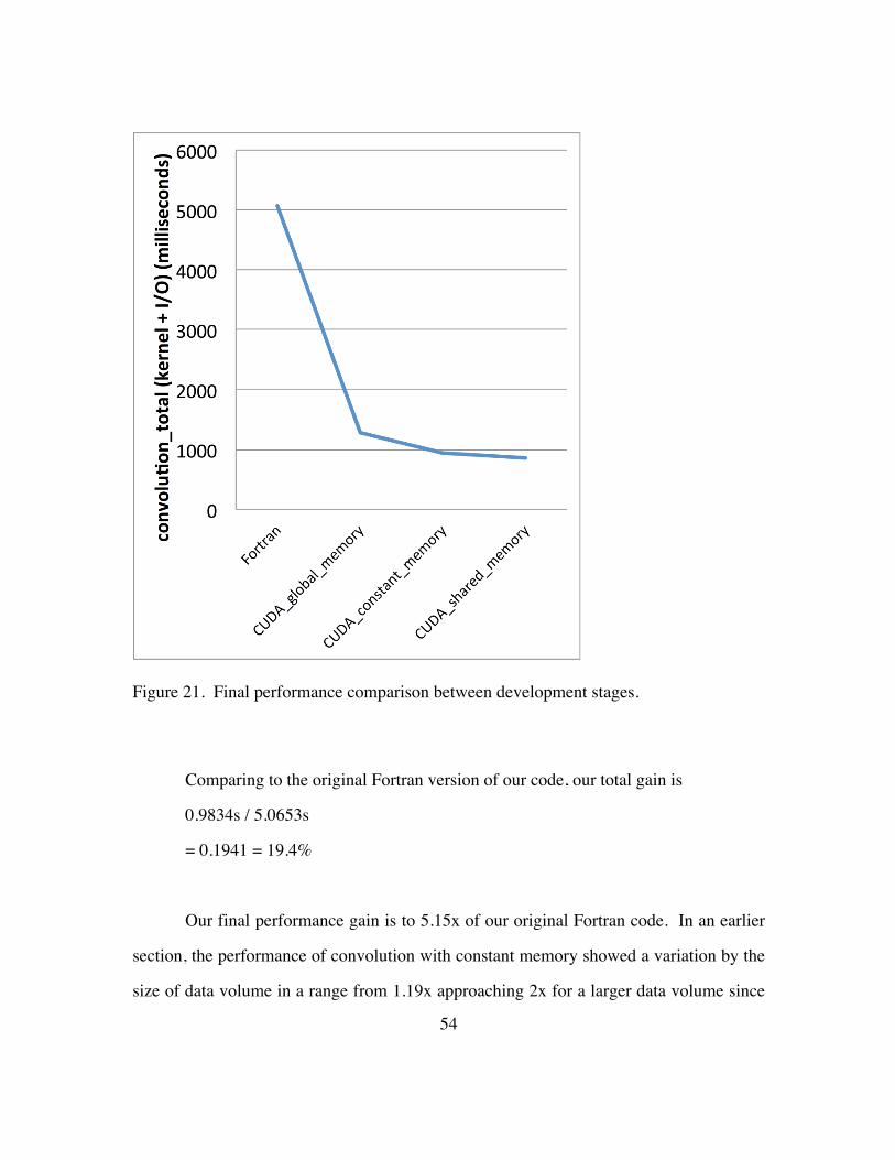
Figure 21. Final performance comparison between development stages.

Comparing to the original Fortran version of our code, our total gain is

0.9834s / 5.0653s

= 0.1941 = 19.4%

Our final performance gain is to 5.15x of our original Fortran code. In an earlier

section, the performance of convolution with constant memory showed a variation by the

size of data volume in a range from 1.19x approaching 2x for a larger data volume since

55

constant memory has a constant overhead. Our shared memory implementation is built

on top of constant memory implementation. Thus, with larger data volume size, the total

performance gain theoretically approaches a 8.7x performance gain over our original

Fortran implementation.

56

CHAPTER III

Conclusion and recommendation for further investigation

Even though we gained 1.5x in shared memory use, it did not come out to be as

high of a pay-off for the effort. In our investigation, we demonstrated our task is largely

affected by thread count. As can be seen, the performance gain comes from the reduction

of thread count; the task performed for our convolution method is memory bandwidth

intensive. We determined that the main reason for not having a larger increase in

performance is because our logical and mathematical operation is relatively simple. We

expect to see larger performance gains with logic and math intensive tasks.

Unfortunately, the operation of convolution is computationally simple, so we need to

reduce the bandwidth congestion of over-scheduled threads.

The memory transport between GPU device and CPU host takes about 64% of

convolution related time with our final version of code, and threads are racing against

each other to further reduce the operation performance within the 36% window. The

largest disadvantage of our system comes from the fact that the code migration is done

only partially from Fortran to CUDA-C. Because we focused our analysis to convolution

related operations only, we migrated only convolution related functions to CUDA-C

based code. There are functions in the Fortran code that work along with the convolution

related functions, thus the entire data volume is copied between the GPU device and CPU

host at each time step. Because of initial performance gain with CUDA-C, the data

transport has quickly become a significant fraction of the process cost. We did not

predict this change at the beginning of the investigation. This kind of pitfall is easier to

spot when you develop a code from scratch for a particular platform. The gradual change

57

in code from Fortran to CUDA-C disguised this issue until the GPU kernel was optimized

thus the problem was trickier to notice. By this we mean, this investigation was an

excellent exercise to learn how to integrate the GPU device into already existing wave

propagation platforms, but we now know the data transport issue becomes an important

issue as soon as we gain the performance the GPU makes possible. If we can keep the

data in the GPU except for the initial data copy and for the final time step, we should be

able to gain the increase of performance to 3x from our final version of the code. Our

primary conclusion is that the entire application should be coded and run in the GPU with

appropriate thread count for optimum performance to be achieved.

Our recommendation for further development of wave propagation modeling on a

GPU system is the following:

For a project where we can assume the entire data volume can fit within GPU

device memory, like our data in this investigation, the structure of the code should be

planned to avoid data transport between CPU host and GPU device. This is already a

known rule of thumb, but it is often hard to comprehend for us until we see how heavy

the penalty of not doing it can be. If it is not possible to avoid heavy data transport

between the CPU host and GPU device, we recommend using only global memory and

constant memory to keep task structure clean and simple. The gain of performance with

shared memory use is only about 10% when we consider the cost of convolution and data

transport for each time step. We think a simple and more readable structure where all the

work is done in the GPU will better pay off in future projects.

For a project with less intense numerical processes, thread count should be

optimized in order to moderately saturate memory bandwidth but not congest it. Our

study showed the convolution kernel is more data-access intensive than computation

intensive. The task for convolution is mathematically simple. We can easily congest

58

memory bandwidth. We need to either find a methods that require less memory access or

optimize the thread count while keeping in mind there are other processes that also

requires memory bandwidth with the same GPU device.

For a project where the entire data set does not fit within GPU device memory, we

recommend parallelizing with multiple GPU devices rather than trying to process all the

data with one GPU device. Using multiple GPUs allows us to set up a pipeline of

processing. Since we can separate convolution for each axis, by cleverly scheduling data

transport between CPU host and GPU device, we can most likely to hide some of

convolution process cost behind the data transport cost for further performance gain.

As stated earlier, our model has a built-in inefficiency of copying data between

CPU host and GPU device at each time step. This turned out to be a good thing in terms

of analysis. By the data movement requirement, our model reflects the case of the data

volume not fitting in one GPU device. This provides some insight for the bottom line

performance for very large datasets because of the memory movement requirements in

this investigation.

Without going outside of generalized optimization, we easily achieve a

performance gain of roughly 6x in the critical computing section (kernel + data

input/output) with a GPU-based platform with CUDA-C compared to conventional CPU-

based platform with Fortran, and considerable room for performance gain still remains

with a complete rewrite to CUDA-C based code. We look at any 3-D volume as a series

of 2-D slices, and reloading the memory for the third dimension as a necessary evil. A

realistic target for industry application is that real time seismic monitoring would be

useful if we can process beyond 1000 x 1000 elements. As a 3-D volume, we can

process a 1000 x 1000 x 160 size volume for three data arrays (one source data array, one

velocity array, and one result array) with 2 Gigabytes global memory, which is common

59

for even low-end GPU devices. With a current higher-end GPU, the size increases to

roughly 5GB, and the GPU memory size is still increasing as next generations come out.

And, of course, we can also distribute tasks to more than one GPU device as well. We

should also note the capacity of low latency memories are approaching the range where

they can also be useful.

Massively parallel computing was previously only possible on large computing

clusters. All of a sudden, we have the same power in a smaller desktop computer, or

even a laptop computer. CUDA programming is very different from conventional single

thread code development. It is complex and difficult to think through all the side effects

that are hard to foresee or observe. Yet, we believe GPU computing is certainly worth

investing our time and energy to for this and other geophysical applications.

60

Appendix A

Hardware/OS information

Stampede[.tacc.utexas.edu] Linux c557-001.stampede.tacc.utexas.edu 2.6.32-358.el6.x86_64 #1 SMP Fri Feb 22 00:31:26 UTC 2013 x86_64 x86_64 x86_64 GNU/Linux CentOS release 6.4 (Final) MemTotal: 32815524 kB model name : Intel(R) Xeon(R) CPU E5-2680 0 @ 2.70GHz model name : Intel(R) Xeon(R) CPU E5-2680 0 @ 2.70GHz model name : Intel(R) Xeon(R) CPU E5-2680 0 @ 2.70GHz model name : Intel(R) Xeon(R) CPU E5-2680 0 @ 2.70GHz model name : Intel(R) Xeon(R) CPU E5-2680 0 @ 2.70GHz model name : Intel(R) Xeon(R) CPU E5-2680 0 @ 2.70GHz model name : Intel(R) Xeon(R) CPU E5-2680 0 @ 2.70GHz model name : Intel(R) Xeon(R) CPU E5-2680 0 @ 2.70GHz model name : Intel(R) Xeon(R) CPU E5-2680 0 @ 2.70GHz model name : Intel(R) Xeon(R) CPU E5-2680 0 @ 2.70GHz model name : Intel(R) Xeon(R) CPU E5-2680 0 @ 2.70GHz model name : Intel(R) Xeon(R) CPU E5-2680 0 @ 2.70GHz model name : Intel(R) Xeon(R) CPU E5-2680 0 @ 2.70GHz model name : Intel(R) Xeon(R) CPU E5-2680 0 @ 2.70GHz model name : Intel(R) Xeon(R) CPU E5-2680 0 @ 2.70GHz model name : Intel(R) Xeon(R) CPU E5-2680 0 @ 2.70GHz

GPU device information (Tesla K20m) CUDA Device Query (Runtime API) version (CUDART static linking) Detected 1 CUDA Capable device(s) Device 0: "Tesla K20m" CUDA Driver Version / Runtime Version 5.5 / 5.0 CUDA Capability Major/Minor version number: 3.5 Total amount of global memory: 4800 MBytes (5032706048 bytes) (13) Multiprocessors x (192) CUDA Cores/MP: 2496 CUDA Cores GPU Clock rate: 706 MHz (0.71 GHz) Memory Clock rate: 2600 Mhz Memory Bus Width: 320-bit L2 Cache Size: 1310720 bytes Max Texture Dimension Size (x,y,z) 1D=(65536), 2D=(65536,65536), 3D=(4096,4096,4096) Max Layered Texture Size (dim) x layers 1D=(16384) x 2048, 2D=(16384,16384) x 2048 Total amount of constant memory: 65536 bytes Total amount of shared memory per block: 49152 bytes Total number of registers available per block: 65536 Warp size: 32 Maximum number of threads per multiprocessor: 2048 Maximum number of threads per block: 1024 Maximum sizes of each dimension of a block: 1024 x 1024 x 64 Maximum sizes of each dimension of a grid: 2147483647 x 65535 x 65535 Maximum memory pitch: 2147483647 bytes Texture alignment: 512 bytes Concurrent copy and kernel execution: Yes with 2 copy engine(s) Run time limit on kernels: No Integrated GPU sharing Host Memory: No Support host page-locked memory mapping: Yes

61

Alignment requirement for Surfaces: Yes Device has ECC support: Enabled Device supports Unified Addressing (UVA): Yes Device PCI Bus ID / PCI location ID: 3 / 0 Compute Mode: < Default (multiple host threads can use :: cudaSetDevice() with device simultaneously) > deviceQuery, CUDA Driver = CUDART, CUDA Driver Version = 5.5, CUDA Runtime Version = 5.0, NumDevs = 1, Device0 = Tesla K20m

CUDA Bandwidth Test Device 0: Tesla K20m Quick Mode Host to Device Bandwidth, 1 Device(s) PINNED Memory Transfers Transfer Size (Bytes) Bandwidth(MB/s) 33554432 6039.1 Device to Host Bandwidth, 1 Device(s) PINNED Memory Transfers Transfer Size (Bytes) Bandwidth(MB/s) 33554432 6389.1 Device to Device Bandwidth, 1 Device(s) PINNED Memory Transfers Transfer Size (Bytes) Bandwidth(MB/s) 33554432 143583.3

62

Appendix B

Stoffa, P. L., Seismic Migration Notes

63

64

65

66

Appendix C

Listing of the project code

(Final version of C/CUDA-C section only) ac_c.cpp/cu //============================================================================ // Name : ac_c.cpp/cu // Author : Makoto Sadahiro // Date : April 10th 2014 // Version : final // Copyright : Makoto Sadahiro, Paul L. Stoffa, Robert H. Tatham // Description : GPU based forward and reverse wave propagation modeling code // : with finite differences method // files : ac.f ac_util.f ac_c.cpp/cu rebuildStampede.sh // config file : ac.in // vel file : vpclip.dir //============================================================================ #include <iostream> #include <cmath> #include <algorithm> #include <stdio.h> using namespace std; extern "C" { void makefir2_(float* ox, int* length, float* dx, float* alpha, float* beta){ float dx3 = pow(*dx, 3); //dx*dx*dx; float dx3inv = 1.0 / dx3; float pi = acos(-1.0); float h_beta = *beta * 0.5; float alpha1 = *alpha * 2.0 -1.0; float alpha2 = (1.0 - *alpha) * 2.0; float central_term = 0.0; float msign = -1.0; for(int ix=1; ix<= (*length); ix++){ msign = -msign; float coef_filt = (2.0 * msign * dx3inv)/(pow((float)(ix), 2)); float arg = pi * (float)(ix) / (2.0 * ((*length) + 2)); float coef_wind = pow((alpha1 + alpha2 * cos(arg) * cos(arg)), h_beta); ox[ix + (*length)] = coef_filt * coef_wind; central_term = central_term + ox[ix + (*length)]; ox[(*length) - ix] = ox[ix + (*length)]; } ox[*length] = -2.0 * central_term; for(int ix=0; ix<(2 * (*length) + 1); ix++){ ox[ix] *= (*dx); } } // makefir2 /*******************************************************************************/

67

// initializerKernel __global__ void initializerKernel(float* d_R, int total, float num){ int i=blockIdx.x * blockDim.x + threadIdx.x; if(i<total){ d_R[i]=num; } } // initializerKernel /**********************************************/ __constant__ float d_cBz[32]; __constant__ float d_cBx[32]; __constant__ float d_cBy[32]; __global__ void vtconvlKernel_major_grid_SMZP(float* A, float* Bz, float* Bx, float* By, float* R, int nze, int nxe, int nye, int nAze, int nAxe, int nAye, int lenBze, int lenBxe, int lenBye, // one-sided length int blocksz){ unsigned int thread_id =blockIdx.x * blockDim.x + threadIdx.x; const unsigned int thread_e = 1024/8; __shared__ float d_sA[thread_e + 16]; float d_R = 0.0; int dz_nAe = nAze * nAxe; d_sA[threadIdx.x]= 0.0; if(thread_id<dz_nAe){ d_sA[lenBze+threadIdx.x] = A[thread_id]; if(((threadIdx.x)<lenBze)&&(0<(blockIdx.x))){ d_sA[threadIdx.x]=A[thread_id-lenBze]; } if(((thread_e-lenBze)<=(threadIdx.x))&&((blockIdx.x)<(blocksz-1))){ d_sA[2*lenBze+threadIdx.x]=A[thread_id+lenBze]; } __syncthreads(); if(((lenBze)<=(thread_id%nAze))&&((thread_id%nAze)<(nAze-lenBze))){ for(int ii=-lenBze; ii<=lenBze; ii++){ d_R += d_sA[lenBze+(threadIdx.x)+ii] * d_cBz[lenBze+ii]; } } R[thread_id] = d_R; } } // vtconvlKernel_major_grid_SMZP /**********************************************/ __global__ void vtconvlKernel_minor_grid_SMZP(float* A, float* Bz, float* Bx, float* By, float* R, int nxe, int nye, int nze, int n_Axe, int n_Aye, int n_Aze, // (note: xyz order rotated!!) int len_Bxe, int len_Bye, int len_Bze, // one-sided length

68

int blocksy){ int thread_id_x =blockIdx.x * blockDim.x + threadIdx.x; int thread_id_y =blockIdx.y * blockDim.y + threadIdx.y; const unsigned int thread_x = 32/2; // blockDim.x; const unsigned int thread_y = 32/2; // blockDim.y; __shared__ float d_sA[thread_y+(2*8)][thread_x]; float d_R = 0.0; if((thread_id_x<n_Axe)&&(thread_id_y<n_Aye)){ d_sA[len_Bye+threadIdx.y][threadIdx.x] = A[n_Axe * thread_id_y + thread_id_x]; if((threadIdx.y<len_Bye)&&(0<blockIdx.y)){ d_sA[threadIdx.y][threadIdx.x] = A[n_Axe * (thread_id_y - len_Bye) + thread_id_x]; } if(((thread_y-len_Bye)<=threadIdx.y)&&(blockIdx.y<(blocksy-1))){ d_sA[2*len_Bye+threadIdx.y][threadIdx.x] = A[n_Axe * (thread_id_y + len_Bye) + thread_id_x]; } __syncthreads(); if((len_Bye<=thread_id_y)&&(thread_id_y<(n_Aye-len_Bye))) for(int ii=-len_Bye; ii<=len_Bye; ii++){ d_R += d_sA[len_Bye+threadIdx.y+ii][threadIdx.x] * d_cBx[len_Bye+ii]; } R[n_Axe * thread_id_y + thread_id_x] += d_R; } } // vtconvlKernel_minor_grid_SMZP /**********************************************/ // vtconvl6g_ // This versino will process all cells with zero paddings // processing all celss on global memory, assuming volume fits in global mem // size_dVAR are the size of allocation to cover all cases void vtconvl6g_(float* a, int nze, int nxe, int nye, // elements count for each dir float* bz, float* bx, float* by, // FIR for each dir int nd_Ae, int nd_Re, // element count of actual allocation int len_bz, int len_bx, int len_by, // FIR length (one-side wing) float* r, // result is Laplace float* d_A, float* d_Bz, float* d_Bx, float* d_By, float* d_R, int size_dA, int size_dBz, int size_dBx, int size_dBy, int size_dR){ // using STATIC shared memory // keep in mind warp size is 32 // use this to reduce total thread count // unsigned int thread_per_block = 512; // unsigned int thread_per_block = 256; unsigned int thread_per_block = 1024; int nAze = nze + 2 * len_bz; int nAxe = nxe + 2 * len_bx; int nAye = nye + 2 * len_by; int nAe = nAze*nAxe; initializerKernel<<<ceil(((float)(nd_Ae))/((float)(thread_per_block))), thread_per_block>>>(d_A, nd_Ae, 0.0); // todo: check if I really need to copy all of them all the time

69

// move it to caller if appropriate cudaMemcpy2D(d_A+(len_bx * nAze)+len_bz, nAze*4, a, nze*4, nze*4, nxe, cudaMemcpyHostToDevice); cudaMemcpy(d_Bz, bz, size_dBz, cudaMemcpyHostToDevice); cudaMemcpy(d_Bx, bx, size_dBx, cudaMemcpyHostToDevice); cudaMemcpy(d_By, by, size_dBy, cudaMemcpyHostToDevice); // convolution section // Major 1-Dz convolution of 1-D stripe const unsigned int thread_per_blockDz = 1024/8; size_t blocks = ceilf(nAe/(float)(thread_per_blockDz)); vtconvlKernel_major_grid_SMZP<<<blocks, thread_per_blockDz>>>(d_A, d_Bz, d_Bx, d_By, d_R, nze, nxe, nye, nAze, nAxe, nAye, len_bz, len_bx, len_by, blocks); // Minor 1-Dx convolution of 2-D grid unsigned int thread_per_block_x = 1024/4; const unsigned int thread_per_blockxDz = 32/2; const unsigned int thread_per_blockxDx = ceilf(thread_per_block_x / (float)thread_per_blockxDz); size_t blocksx_z = ceilf(nAze/(float)thread_per_blockxDz); size_t blocksx_x = ceilf(nAxe/(float)thread_per_blockxDx); dim3 blockDim_mg(blocksx_z, blocksx_x, 1); dim3 threadDim_mg(thread_per_blockxDz, thread_per_blockxDx, 1); vtconvlKernel_minor_grid_SMZP<<<blockDim_mg, threadDim_mg>>>(d_A, d_Bz, d_Bx, d_By, d_R, nze, nxe, nye, nAze, nAxe, nAye, len_bz, len_bx, len_by, blocksx_x); cudaMemcpy2D(r, nze*4, d_R+(len_bx*(2*len_bz+nze))+len_bz, (2*len_bz+nze)*4, nze*4, nxe, cudaMemcpyDeviceToHost); } // vtconvl6g_ /*******************************************************************************/ extern struct{ int ncoef[3]; float w_alpha[3]; float w_beta[3]; } cfir_; // firlaplace3_ void firlaplace3_(float* p, float* Laplace, float* dz, float* dx, float* dy, int* fnze, int* fnxe, int* fnye, int* s_first, int* s_last){ static bool first; if(1==(*s_first)){ first=true; } else if(0==(*s_first)){

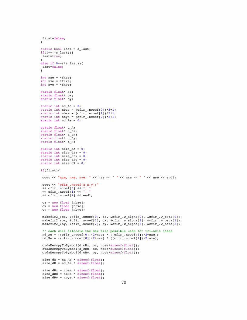
70

first=false; } static bool last = s_last; if(1==(*s_last)){ last=true; } else if(0==(*s_last)){ last=false; } int nze = *fnze; int nxe = *fnxe; int nye = *fnye; static float* oz; static float* ox; static float* oy; static int nd_Ae = 0; static int nbze = (cfir_.ncoef[0])*2+1; static int nbxe = (cfir_.ncoef[1])*2+1; static int nbye = (cfir_.ncoef[2])*2+1; static int nd_Re = 0; static float* d_A; static float* d_Bz; static float* d_Bx; static float* d_By; static float* d_R; static int size_dA = 0; static int size_dBz = 0; static int size_dBx = 0; static int size_dBy = 0; static int size_dR = 0; if(first){ cout << "nze, nxe, nye: " << nze << " " << nxe << " " << nye << endl; cout << "cfir_.ncoef[z,x,y]:" << cfir_.ncoef[0] << ", " << cfir_.ncoef[1] << ", " << cfir_.ncoef[2] << endl; oz = new float [nbze]; ox = new float [nbxe]; oy = new float [nbye]; makefir2_(oz, &cfir_.ncoef[0], dz, &cfir_.w_alpha[0], &cfir_.w_beta[0]); makefir2_(ox, &cfir_.ncoef[1], dx, &cfir_.w_alpha[1], &cfir_.w_beta[1]); makefir2_(oy, &cfir_.ncoef[2], dy, &cfir_.w_alpha[2], &cfir_.w_beta[2]); // each will allocate the max size possible used for tri-axis cases nd_Ae = ((cfir_.ncoef[0])*2+nze) * ((cfir_.ncoef[1])*2+nxe); nd_Re = ((cfir_.ncoef[0])*2+nze) * ((cfir_.ncoef[1])*2+nxe); cudaMemcpyToSymbol(d_cBz, oz, nbze*sizeof(float)); cudaMemcpyToSymbol(d_cBx, ox, nbxe*sizeof(float)); cudaMemcpyToSymbol(d_cBy, oy, nbye*sizeof(float)); size_dA = nd_Ae * sizeof(float); size_dR = nd_Re * sizeof(float); size_dBz = nbze * sizeof(float); size_dBx = nbxe * sizeof(float); size_dBy = nbye * sizeof(float);

71

cout << "fir oz: "; for(int i=0; i<nbze; i++){ cout << oz[i] << " "; } cout << endl; cout << "fir ox: "; for(int i=0; i<nbxe; i++){ cout << ox[i] << " "; } cout << endl; cout << "fir oy: "; for(int i=0; i<nbye; i++){ cout << oy[i] << " "; } cout << endl; cout << "allocating cuda device memory" << endl; cudaMalloc((void **) &d_A, size_dA); cudaMalloc((void **) &d_Bz, size_dBz); cudaMalloc((void **) &d_Bx, size_dBx); cudaMalloc((void **) &d_By, size_dBy); cudaMalloc((void **) &d_R, size_dR); } if(last){ delete[] oz; delete[] ox; delete[] oy; cudaFree(d_A); cudaFree(d_Bz); cudaFree(d_Bx); cudaFree(d_By); cudaFree(d_R); } else{ // d2/dA2 vtconvl6g_(p, nze, nxe, nye, oz, ox, oy, nd_Ae, nd_Re, cfir_.ncoef[0], cfir_.ncoef[1], cfir_.ncoef[2], Laplace, d_A, d_Bz, d_Bx, d_By, d_R, size_dA, size_dBz, size_dBx, size_dBy, size_dR); } // done with not_first & not_last } // firlaplace3 } // extern "C"

72

References

Cook, S., 2013, CUDA Programming: A Developers Guide to Parallel Computing with

GPUs: Elsevier Ippolito, G., Using C/C++ and Fortran together: http://www.yolinux.com Kirk, D. B., and W. Hwu, 2010, Programming Massively Parallel Processors: Elsevier NVIDIA, 2013, CUDA C Programming Guide, http://www.nvidia.com Stoffa, P. L., Seismic Migration Notes Van Oosten, J., 2011, CUDA Memory Model: 3D Game Engine Programming,

http://www.3dgep.com