Copyright

by

Gene Moo Lee

2015

The Dissertation Committee for Gene Moo Leecertifies that this is the approved version of the following dissertation:

Link Formation in Mobile and Economic Networks:

Model and Empirical Analysis

Committee:

Andrew B. Whinston, Supervisor

Sukjin Han

Vladimir Lifschitz

Aloysius K. Mok

Lili Qiu

Link Formation in Mobile and Economic Networks:

Model and Empirical Analysis

by

Gene Moo Lee, B.S., M.A.

DISSERTATION

Presented to the Faculty of the Graduate School of

The University of Texas at Austin

in Partial Fulfillment

of the Requirements

for the Degree of

DOCTOR OF PHILOSOPHY

THE UNIVERSITY OF TEXAS AT AUSTIN

August 2015

To Jieun, Chloe, and Irene

Acknowledgments

First of all, I’d like to thank my wonderful advisor, Andrew B. Whin-

ston. It is my greatest luck and honor to be one of his students. My Ph.D.

study was greatly supported by his advice and encouragement. Especially, his

never ending enthusiasm for research is a great inspiration to me. I dream that

some day I can be like Andy as an innovative researcher and great educator.

I’d like to also thank my dissertation committee members – Lili Qiu,

Vladimir Lifschitz, Aloysius K. Mok, Sukjin Han – for their supports.

Professionally, the research projects I conducted during my graduate

studies were possible thanks to the help of my great co-authors (alphabetically

ordered by last names): Mario Baldi, Yi-Chao Chen, Taehwan Choi, Yunsik

Choi, Wei Dong, Nick Duffield, Sukjin Han, Shu He, Ho Kim, Young Kwark,

Jae Kyu Lee, Joowon Lee, Alvin Leung, Yong Liao, Huiya Liu, Stanislav

Miskovic, Paul Pavlou, Liangfei Qiu, Lili Qiu, John S. Quarterman, Swati

Rallapalli, Zhan Shi, Donghyuk Shin, Reo Song, Tae Ho Song, Qian Tang, Jia

Wang, Andrew B. Whinston, Young Yoon, Yin Zhang, and Vincent Zhuang.

Personally, I enjoyed my daily lives with friends at the Center for Re-

search in Electronic Commerce (CREC): Meredith Bethune, Markus Blomvall,

Yanzhen Chen, Ying-Yu Chen, Yunsik Choi, Juhani Halkola, Shu He, Markus

Iivonen, Joowon Lee, Shun-Yang Lee, Liangfei Qiu, Huaxia Rui, Zhan Shi,

v

Mark Varga, Jihyun Yoo, and Vincent Zhuang. I also want to thank my Com-

puter Science friends: Jae Hyeon Bae, Apurv Bharita, Yi-Chao Chen, Tae

Won Cho, Taehwan Choi, Vacha Dave, Wei Dong, Owais Khan, Jungwoo Ha,

Eunjin (EJ) Jung, Byeongcheol (BK) Lee, Juhyun Lee, Sangmin Lee, Doo

Soon Kim, Jongwook Kim, Sangman Kim, Swati Rallapalli, Donghyuk Shin,

Han Hee Song, Joyce Whang, Young Yoon, and Sangki Yun.

Spiritually, I was greatly supported from the Great Light Presbyterian

Church of Austin. I’d like to thank Rev. David Kim and Mrs. Michelle Kim

for their leadership. I am really indebted to the members of the bible study

group “Joy” for their prayers and supports. So I thank Juhun Lee, Eunjung

Choi, Cheon-woo Han, Hyejoung Kim, Sangman Kim, Jiwoo Pak, Sooel Son,

Kayoung Lee, Eunsoo Cho, Sangki Yun, Sujin Park, Dong-ok Son, Yusun

Kang, Jin Hyuk Choi, Hae-Ok Kim, Boo Nam Shin, Ji Eun Lee, Chang-sik

Choi, Sohee Jo, Hyunjae Lee, Carroll Kim, Seokki Kwon, Jaewon Jung, as

well as the little ones.

I’d like to give my greatest thanks to my family for their supports. My

father, Dr. Sang-Won Lee, gave me the inspiration to pursue my academic

career and my mother, Mrs. Ok-hyun Kim, always supported me with en-

couragement and prayers. My father-in-law, Mr. Jong Hoon Kim, inspired

me with his energy and passions (especially I admire his 50-state road trip)

and my mother-in-law, Mrs. Heesook Park, gave our family great supports to

come to Austin to help us out. I also like to thank my mother, Mrs. Kyung-Ja

Hwang, who may be proudly watching me in the Heaven.

vi

My wife, Jieun Kim, has sacrificed a lot for me and our family. She

had to leave her families and friends in Korea to come to Austin for my study.

Her supports are priceless. So I’d like to give my greatest thank and love for

my wonderful, strong wife. There were hard times, but I am glad that we

overcome them with God’s help. During five years at Austin, God gave us

great blessings: our two lovely daughters, Chloe Daeun Lee and Irene Dahye

Lee. The love and joy I received from my little ones kept me going during

hard times. I love y’all.

Your word is a lamp for my feet, a light on my path.

– Psalm 119:105

Lastly, I’d like to thank Jesus Christ for being my Savior and Lord. There

were times when I was down but his everlasting love raised me up. Thank you

for your everlasting love for me and our family! Praise the Lord!

vii

Link Formation in Mobile and Economic Networks:

Model and Empirical Analysis

Publication No.

Gene Moo Lee, Ph.D.

The University of Texas at Austin, 2015

Supervisor: Andrew B. Whinston

In this dissertation, we study three link formation problems in mobile

and economic networks: (i) company matching for mergers and acquisitions

(M&A) network in the high-technology (high-tech) industry, (ii) mobile appli-

cation (app) matching for cross promotion network in mobile app markets, and

(iii) online friendship formation in mobile social networks. Each problem can

be modeled as link formation problem in a graph, where nodes represent inde-

pendent entities (e.g., companies, apps, users) and edges represent interactions

(e.g., transactions, promotions, friendships) among the nodes.

First, we propose a new data-analytic approach to measure firms’ dyadic

business proximity to analyze M&A network in the high-tech industry. Specif-

ically, our method analyzes the unstructured texts that describe firms’ busi-

nesses using latent Dirichlet allocation (LDA) topic modeling, and constructs

viii

a novel business proximity measure based on the output. Using CrunchBase

data including 24, 382 high-tech companies and 1, 689 M&A transactions, we

empirically validate our business proximity measure in the context of industry

intelligence and show the measure’s effectiveness in an application of M&A

network analysis. Based on the research, we build a cloud-based information

system to facilitate competitive intelligence on the high-tech industry.

Second, we analyze mobile app matching for cross promotion network

in mobile app markets. Cross promotion (CP) is a new app promotion frame-

work, in which a mobile app is promoted to the users of another app. Using

IGAWorks data covering 1, 011 CP campaigns, 325 apps, and 301, 183 users,

we evaluate the effectiveness of CP campaigns in comparison with existing

ad channels such as mobile display ads. While CP campaigns, on average,

are still suboptimal as compared with display ads, we find evidence that a

careful matching of mobile apps can significantly improve the effectiveness of

CP campaigns. Our empirical results show that app similarity, measured by

LDA from apps’ text descriptions, is a significant factor that increases the

user engagement in CP campaigns. With this observation, we propose an app

matching mechanism for the CP network to improve the ad effectiveness.

Third, we study friendship network formation in a location-based social

network. We build a structural model of social link creation that incorporates

individual characteristics and pairwise user similarities. Specifically, we de-

fine four user proximity measures from biography, geography, mobility, and

short messages (i.e., tweets). To construct proximity from unstructured text

ix

information, we build LDA topic models of user biography texts and tweets.

Using Gowalla data with 385, 306 users, three million locations, and 35 million

check-in records, we empirically estimate the structural model to find evidence

on the homophily effect in network formation.

x

Table of Contents

Acknowledgments v

Abstract viii

List of Tables xiii

List of Figures xv

Chapter 1. Introduction 1

Chapter 2. Towards A Better Measure of Business Proximity:Topic Modeling for Industry Intelligence 8

2.1 Introduction . . . . . . . . . . . . . . . . . . . . . . . . . . . . 8

2.2 CrunchBase Data . . . . . . . . . . . . . . . . . . . . . . . . . 12

2.3 Data-Analytic Method for Measuring Business Proximity . . . 17

2.4 Empirical Validation and Application . . . . . . . . . . . . . . 22

2.4.1 Validation . . . . . . . . . . . . . . . . . . . . . . . . . . 22

2.4.2 Empirical Application on M&A Networks . . . . . . . . 25

2.4.2.1 Proximity and M&A . . . . . . . . . . . . . . . 26

2.4.2.2 Statistical Model . . . . . . . . . . . . . . . . . 32

2.4.2.3 Specification . . . . . . . . . . . . . . . . . . . . 36

2.4.2.4 Results . . . . . . . . . . . . . . . . . . . . . . . 39

2.5 Platform Prototype: Information System for Industry Intelligence 47

2.5.1 Back-End System . . . . . . . . . . . . . . . . . . . . . 50

2.5.2 Front-End System . . . . . . . . . . . . . . . . . . . . . 51

2.6 Discussion and Conclusion . . . . . . . . . . . . . . . . . . . . 53

xi

Chapter 3. Matching Mobile Applications for Cross Promotion 58

3.1 Introduction . . . . . . . . . . . . . . . . . . . . . . . . . . . . 58

3.2 IGAWorks Data . . . . . . . . . . . . . . . . . . . . . . . . . . 65

3.2.1 Data Description . . . . . . . . . . . . . . . . . . . . . . 65

3.2.2 Effectiveness of Ad Channels . . . . . . . . . . . . . . . 67

3.3 Modeling Cross Promotion Network . . . . . . . . . . . . . . . 70

3.4 Mobile App Characteristics and Similarity . . . . . . . . . . . 72

3.4.1 Individual App Characteristics . . . . . . . . . . . . . . 73

3.4.2 Topic Models and App Similarity . . . . . . . . . . . . 74

3.5 Empirical Analysis . . . . . . . . . . . . . . . . . . . . . . . . 77

3.6 Matching Mechanism Design . . . . . . . . . . . . . . . . . . . 81

3.7 Conclusion and Future Directions . . . . . . . . . . . . . . . . 86

Chapter 4. Strategic Network Formation in a Location-BasedSocial Network: A Topic Modeling Approach 88

4.1 Introduction . . . . . . . . . . . . . . . . . . . . . . . . . . . . 88

4.2 Structural Model of Social Network Formation . . . . . . . . . 93

4.3 User Proximity . . . . . . . . . . . . . . . . . . . . . . . . . . 98

4.4 Gowalla Data . . . . . . . . . . . . . . . . . . . . . . . . . . . 100

4.4.1 Data Collection . . . . . . . . . . . . . . . . . . . . . . 101

4.4.2 User Sampling . . . . . . . . . . . . . . . . . . . . . . . 103

4.4.3 Topic Models and User Proximity . . . . . . . . . . . . 104

4.5 Empirical Results . . . . . . . . . . . . . . . . . . . . . . . . . 108

4.6 Conclusion and Managerial Implications . . . . . . . . . . . . . 115

Chapter 5. Conclusion 120

Bibliography 122

Vita 141

xii

List of Tables

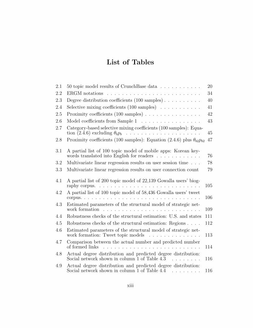
2.1 50 topic model results of CrunchBase data . . . . . . . . . . . 20

2.2 ERGM notations . . . . . . . . . . . . . . . . . . . . . . . . . 34

2.3 Degree distribution coefficients (100 samples) . . . . . . . . . . 40

2.4 Selective mixing coefficients (100 samples) . . . . . . . . . . . 41

2.5 Proximity coefficients (100 samples) . . . . . . . . . . . . . . . 42

2.6 Model coefficients from Sample 1 . . . . . . . . . . . . . . . . 43

2.7 Category-based selective mixing coefficients (100 samples): Equa-tion (2.4.6) excluding θbpb . . . . . . . . . . . . . . . . . . . . 45

2.8 Proximity coefficients (100 samples): Equation (2.4.6) plus θb2pb2 47

3.1 A partial list of 100 topic model of mobile apps: Korean key-words translated into English for readers . . . . . . . . . . . . 76

3.2 Multivariate linear regression results on user session time . . . 78

3.3 Multivariate linear regression results on user connection count 79

4.1 A partial list of 200 topic model of 22,139 Gowalla users’ biog-raphy corpus. . . . . . . . . . . . . . . . . . . . . . . . . . . . 105

4.2 A partial list of 100 topic model of 58,436 Gowalla users’ tweetcorpus. . . . . . . . . . . . . . . . . . . . . . . . . . . . . . . . 106

4.3 Estimated parameters of the structural model of strategic net-work formation . . . . . . . . . . . . . . . . . . . . . . . . . . 109

4.4 Robustness checks of the structural estimation: U.S. and states 111

4.5 Robustness checks of the structural estimation: Regions . . . . 112

4.6 Estimated parameters of the structural model of strategic net-work formation: Tweet topic models . . . . . . . . . . . . . . 113

4.7 Comparison between the actual number and predicted numberof formed links . . . . . . . . . . . . . . . . . . . . . . . . . . 114

4.8 Actual degree distribution and predicted degree distribution:Social network shown in column 1 of Table 4.3 . . . . . . . . 116

4.9 Actual degree distribution and predicted degree distribution:Social network shown in column 1 of Table 4.4 . . . . . . . . 116

xiii

4.10 Actual degree distribution and predicted degree distribution:Social network shown in column 2 of Table 4.3 . . . . . . . . 117

4.11 Actual degree distribution and predicted degree distribution:Social network shown in column 3 of Table 4.3 . . . . . . . . 117

xiv

List of Figures

1.1 Matching interactions in mobile and economic networks. . . . 3

2.1 Geo-mapping company locations and M&A transactions . . . 15

2.2 Distribution of companies over state and industry sector . . . 16

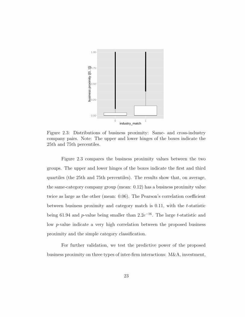
2.3 Distributions of business proximity: Same- and cross-industrycompany pairs. Note: The upper and lower hinges of the boxesindicate the 25th and 75th percentiles. . . . . . . . . . . . . . 23

2.4 Distributions of business proximity: M&A, investment, job mo-bility, and random samples. Note: The upper and lower hingesof the boxes indicate the 25th and 75th percentiles. . . . . . . 24

2.5 Distributions of proximity: M&A sample v.s. random sample.Note: In (b), we plot geographic distance rather than geo-graphic proximity. . . . . . . . . . . . . . . . . . . . . . . . . . 31

2.6 Prototype architecture and components . . . . . . . . . . . . . 49

2.7 Prototype front end: User interface screenshots . . . . . . . . 52

3.1 Screenshot of cross promotion campaigns (Source: IGAWorks) 61

3.2 Ad effectiveness comparison . . . . . . . . . . . . . . . . . . . 68

4.1 Examples of friends with similar topics in biographies and tweets107

xv

Chapter 1

Introduction

Mobile has changed the computing paradigm and the economy, affect-

ing individuals, developers, businesses, and the society at large. First, from

the individual perspective, people are adopting mobile devices as their main

Internet devices. According to eMarketer, 74% of the online population ac-

cessed the Internet from their mobile devices in 2013.1 Mobile is also a major

channel of user communication and networking. A report from Juniper Re-

search indicates that 14.7 trillion mobile messages were exchanges in 2012 and

the number will double in 2017.2 According to comScore, 68% of Facebook ac-

cesses are via mobile devices and similar phenomena are found in many other

social network services (Twitter: 86%, Instagram: 98%, Pinterest: 92%).3

From the developers’ perspective, mobile platforms such as iOS and

Android have opened up a unprecedented opportunity. The open nature of the

mobile application (app) platform allows third-party, independent developers

1 Mobile Internet user penetration worldwide from 2012 to 2017: http://www.statista.com/statistics/284202/mobile-phone-internet-user-penetration-worldwide/

2 Mobile message traffic worldwide in 2012 and 2017: http://www.statista.com/

statistics/262005/mobile-message-traffic-worldwide/3 Most social networks are now mobile first: http://www.statista.com/chart/2109/

time-spent-on-social-networks-by-platform/

1

to bring innovative ideas into the mobile app market. New app developers can

reach the global market through well-established app distribution channels.

As a result, we are experiencing a huge growth in the mobile app markets

[85, 20, 119, 74]. As of May 2015, Google Play Store and Apple App Store, two

leading app marketplaces, have 1.5 and 1.4 millions apps, respectively, while

other platforms also have substantial presence (Amazon Appstore: 360,000,

Windows Phone Store: 340,000, BlackBerry World 130,000).4 Moreover, the

number of app downloads is growing rapidly and the projected number for

2017 is 268 billion.5

Mobile economy has created a huge impact on the businesses. GSMA

reported that the total revenue of mobile ecosystem was around 2 trillion

dollars in 2013 and projected substantial revenue growth in all segments in-

cluding network infrastructure, components, apps and contents, and devices.6

In the high-tech industry, we observed that many of the high profile mergers

and acquisitions (M&A) transactions were motivated by the acquirers’ mo-

bile strategies.7 Representative cases include Facebook and WhatsApp ($19

billion), Google and Motorola ($12.5 billion), and Microsoft and Nokia ($7.2

billion).

4 Number of apps available in leading app stores as of May 2015: http://www.statista.com/statistics/276623/number-of-apps-available-in-leading-app-stores/

5Number of mobile app downloads worldwide from 2009 to 2017: http://www.statista.com/statistics/266488/forecast-of-mobile-app-downloads/

6 Mobile ecosystem total revenue forecast by segment 2013 and 2020: http://www.

statista.com/statistics/371905/mobile-ecosystem-revenue-by-segment/7WhatsApp deal dwarfs other high-profile tech acquisitions: http://www.statista.

com/chart/1927/tech-acquisitions/

2

A

B

C

D

E

F

Tech Industry

Mobile App Market

Mobile Users

● M&A● Alliance● Supply Chain● Competition● Procurement

● Cross Promotion● Bundling● Deep Linking

● Friend● Online Dating● Server-Client● Communication

Mobile and Economic Networks

Tech companies develop apps

Users use apps

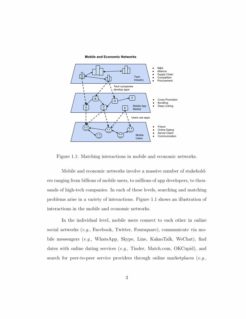
Figure 1.1: Matching interactions in mobile and economic networks.

Mobile and economic networks involve a massive number of stakehold-

ers ranging from billions of mobile users, to millions of app developers, to thou-

sands of high-tech companies. In each of these levels, searching and matching

problems arise in a variety of interactions. Figure 1.1 shows an illustration of

interactions in the mobile and economic networks.

In the individual level, mobile users connect to each other in online

social networks (e.g., Facebook, Twitter, Foursquare), communicate via mo-

bile messengers (e.g., WhatsApp, Skype, Line, KakaoTalk, WeChat), find

dates with online dating services (e.g., Tinder, Match.com, OKCupid), and

search for peer-to-peer service providers through online marketplaces (e.g.,

3

Uber, Lyft, Airbnb, TaskRabbit). In this context, users search for like-minded

people to establish online relationships or look for reliable independent service

providers to achieve their objectives.

Mobile app markets also experience active interactions in the devel-

oper community. For instance, cross promotion has emerged as a new app

promotion framework, in which new apps are exposed to potential users who

are already using other established apps. For new app developers, this is an

effective user acquisition channel because they can target the users by linking

to the right established apps. For the established developers, this is an effec-

tive way to monetize their traffic. Other emerging app interactions include

app bundling (i.e., selling multiple related apps in the app market) and deep

linking (i.e., different apps cooperate to complete complicated tasks). As the

app marketplaces are occupied with millions of apps, it is a challenge to search

and match the right apps in these interactions.

In the organizational level, mobile economy has stimulated a variety of

interactions among high-tech companies. Established tech companies seek ap-

propriate M&A and investment targets in the large pool of early-stage startups

in order to build up their mobile strategies. Firms also form strategic alliances

to secure competitive advantage in the mobile first business landscape. For

instance, Google formed Open Handset Alliance (OHA) with handset manu-

facturers (e.g., Samsung, LG, HTC) to cope with the challenge from Apple.

Another interesting case is the interaction between Samsung and Apple. Sam-

sung supplies mobile processor chips for Apple and, at the same time, the two

4

companies directly compete in the smartphone market. The common challenge

in the aforementioned interactions is how to connect with the right business

partners among massive number of possibilities.

In this dissertation, we study three link formation problems in mobile

and economic networks: (i) company matching for M&A transactions in the

high-tech industry, (ii) mobile app matching for cross promotion campaigns in

the mobile app ad market, and (iii) online friendship formation in the mobile

social networks. Each problem can be modeled as link formation problem in

a graph, where nodes represent independent entities (e.g., companies, apps,

users) and edges represent interactions (e.g., transactions, promotions, friend-

ships) among the nodes. The contribution of this dissertation is threefold.

First, based on the underlying properties of each network, we propose statisti-

cal models of link formations. Second, we introduce various dyadic proximity

measures that quantify the closeness between matching entities, including the

novel proximity constructed from latent Dirichlet allocation (LDA) topic mod-

els [18] of the entities’ text descriptions. Third, we conduct empirical analyses

on large scale datasets (e.g., CrunchBase, IGAWorks, Gowalla) to find strong

evidence that the proposed proximity measures have statistically significant

impact on the link formation procedures in mobile and economic networks.

Chapter 2 proposes a new data-analytic approach to measure firms’

dyadic business proximity. Specifically, our method analyzes the unstructured

texts that describe firms’ businesses using the natural language processing

technique of topic modeling, and constructs a novel business proximity measure

5

based on the output. When compared with existent methods, our approach

is scalable for large datasets and provides finer granularity on quantifying

firms’ positions in the spaces of product, market, and technology. We then

validate our business proximity measure in the context of industry intelligence

and show the measure’s effectiveness in an empirical application of analyzing

M&As in the U.S. high-tech industry. Based on the research, we also build

a cloud-based information system to facilitate competitive intelligence on the

high-tech industry.

Chapter 3 analyzes mobile app matching in cross promotion (CP),

which is a new app promotion framework. In a CP campaign, one mobile

app advertises another one. A network of mobile apps emerge with multiple

CP campaigns. The performance of this emerging ad framework has not been

well studied in the literature. Using data from IGAWorks that covers 1, 011

CP campaigns that ran between September 2013 and May 2014 in Korean

app markets, we evaluate CP’s effectiveness in comparison with existing ad

channels such as mobile display ads. While CP campaigns, on average, are

still suboptimal as compared with display ads, we find evidence that a care-

ful matching of mobile apps can significantly improve CP’s effectiveness. We

model the ad placement in CP campaigns as a matching problem and identify

significant factors that contribute to better app matching. The empirical re-

sults show that app similarity, measured by LDA topic models from apps’ text

descriptions, is a significant factor that increases the user engagement in CP

campaigns. With the observations, we propose an app matching mechanism

6

for CP network to optimize app matching processes.

Lastly, Chapter 4 studies friendship network formation in a location-

based social network. We build a structural model of social link creation that

incorporates individual characteristics and pairwise user similarities. Specifi-

cally, we define four user proximity measures from biography, geography, mo-

bility, and short messages (i.e., tweets). To construct proximity measures from

unstructured text information, we build LDA topic models from user biogra-

phy texts and tweets. Using Gowalla data with 385, 306 users, three million

locations, and 35 million check-in records, we empirically estimate the struc-

tural model to find evidence on the homophily effect in the social network

formation. We also conduct a counterfactual analysis to analyze the effect of

homophily on link formation.

This dissertation provides insights in understanding the emerging mo-

bile and economic networks in three different layers: users, apps, and firms.

The estimated models identified the determinants of the link formations in the

three networks. The proposed proximity measures can be used to reduce the

search space in link predictions.

7

Chapter 2

Towards A Better Measure of Business

Proximity: Topic Modeling for Industry

Intelligence

2.1 Introduction

Business proximity measures firms’ relatedness in the spaces of prod-

uct, market, and technology, which is an important concept in industry in-

telligence and also a central building block in many studies of firm strategy

and industrial organization. Not surprisingly, prior studies in different man-

agement disciplines have used or developed a handful of measures of business

proximity. One common practice has been to classify firms into industries

(or sub-industries) and to operationalize business proximity as a binary vari-

able that indicates common industry (or sub-industry) membership. Under

this definition, two firms’ businesses are either identical or completely differ-

ent. A refined extension of the common industry membership definition has

been to better utilize the hierarchical information provided by some indus-

try classification system, such as Standard Industrial Classification (SIC) or

North American Industrial Classification System (NAICS). For example, in

0A preliminary version of this chapter was published in the Proceedings of ACM Con-ference on Economics and Computation [99].

8

[113], the similarity of two firms’ businesses was determined by the number of

common consecutive digits in their industry classification codes under NAICS.

Since they used the first four digits in NAICS, the similarity quantity was one

of five possible values: 0.00, 0.25, 0.50, 0.75, or 1.00. However, this measure

is still discrete, and the level of granularity it can achieve is constrained by

the industry classification system on which it depends. There are also several

other measures that were aimed at one specific aspect of firms’ businesses,

and they typically had stronger data requirements. Stuart [107], Mowery et

al. [78], and others constructed a “technological overlap” measure using data

of firms’ patent holdings. The closeness of a pair of firms was assumed to be

proportional to the number of common antecedent patents cited. While this is

an elegant, continuous measure in the technology space, it requires complete

data on firms’ patent portfolios and does not explicitly cover the product and

market spaces. Mitsuhashi and Greve [76] applied Jaccard distance on firms’

customer geographic regions in measuring “market complementarity.” Like-

wise, this measure focuses only on the (geographic) market space and requires

all relevant firms’ customer geography data to be available.

While these measures have served the researchers’ purposes well, we

see an opportunity for a new and more general methodology in light of recent

advances in Big Data analytics. In this chapter, we propose a method that re-

quires little manual preprocessing yet provides finer granularity on quantifying

firms’ positions in the spaces of product, market, and technology. Utilizing a

machine learning technique called topic modeling [17], we analyze the publicly

9

available, unstructured texts that describe firms’ businesses. Our automatic

approach, the core of which is a Latent Dirichlet Allocation (LDA) algorithm,

represents each firm’s textual description as a probabilistic distribution over a

set of underlying topics, which we interpret as aspects of its business. Then,

our measure can be naturally constructed by quantifying the “distance” be-

tween a pair of firms’ topic distributions.

An important advantage of our method is that it imposes a much less

strong data requirement than the existent measures. This makes our approach

particularly appealing when the firms under study are small and privately held,

for which detailed information on industry classification, patent holding, and

product/customer is either highly sparse or not available at all. Motivated by

this advantage, we choose the U.S. high technology (high-tech) industry as the

empirical context to demonstrate our approach. We collect data from Crunch-

Base, an open and comprehensive source for high-tech startup activity. For the

majority of companies in our dataset, the standardized industry classification

code is unavailable, and due to various strategic reasons, most do not disclose

their customer information and key intellectual property, so the conventional

methods for measuring business proximity cannot be operationalized. Using

this dataset as an example, we detail the procedure of our data-analytic ap-

proach, and compute business proximity for each pair of companies. We then

show the validity and effectiveness of the new measure in the context of indus-

try intelligence by (1) examining the relationships between business proximity

and simple category classification, between business proximity and job mo-

10

bility, and between business proximity and investment respectively, and (2)

applying the measure in an empirical application of modeling the matching of

companies in mergers and acquisitions (M&As). In the M&A application, we

employ an innovative statistical network analysis method called Exponential

Random Graph Models (ERGMs) to accommodate the relational nature of

the data.

This research joins the rapidly growing stream of literature that lever-

ages newly developed data science techniques in examining Big Data for busi-

ness analytics (e.g., [2, 101, 24, 25, 42, 100, 117]). Our empirical analysis

shows in particular how Big Data analytics can be valuable for competitive

intelligence in the high-tech industry, where recent years have seen an “en-

trepreneurial boom” characterized by the explosion of digital startups.1 To

further illuminate the practical value of the proposed business proximity mea-

sure, we build an information system that allows analysts to use business

proximity to explore the competitive landscape of the U.S. high-tech industry.

The back end of our system handles data collection, storage, and large-scale

computation using Big Data computation platform (Condor), NoSQL database

technology (MongoDB), and various programming languages (Python, Scala).

The front end of the system is hosted on Google’s Cloud Platform and pro-

vides users an easy-to-use web interface. It is available to access at http:

//146.6.99.242/bizprox.

1See “A Cambrian Moment,” The Economist, January 18, 2014.

11

We organize the remainder of this chapter as follows. To provide a con-

text for describing the data-analytic method, we first introduce our dataset in

Section 2.2. In Section 2.3, we elaborate the procedure for constructing our

business proximity. In Section 2.4, we demonstrate the validity and effective-

ness of our measure in the context of industry intelligence. We describe the

design and implementation of the information system in Section 2.5. We lastly

discuss and conclude the chapter in Section 2.6.

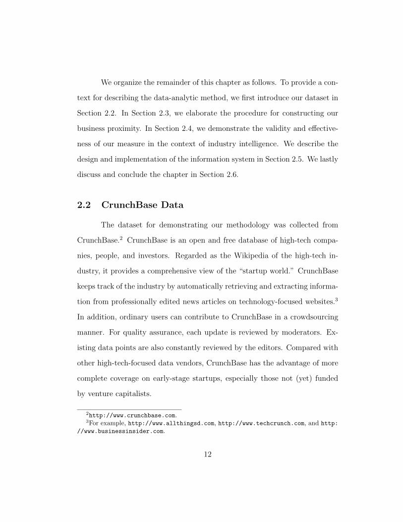
2.2 CrunchBase Data

The dataset for demonstrating our methodology was collected from

CrunchBase.2 CrunchBase is an open and free database of high-tech compa-

nies, people, and investors. Regarded as the Wikipedia of the high-tech in-

dustry, it provides a comprehensive view of the “startup world.” CrunchBase

keeps track of the industry by automatically retrieving and extracting informa-

tion from professionally edited news articles on technology-focused websites.3

In addition, ordinary users can contribute to CrunchBase in a crowdsourcing

manner. For quality assurance, each update is reviewed by moderators. Ex-

isting data points are also constantly reviewed by the editors. Compared with

other high-tech-focused data vendors, CrunchBase has the advantage of more

complete coverage on early-stage startups, especially those not (yet) funded

by venture capitalists.

2http://www.crunchbase.com.3For example, http://www.allthingsd.com, http://www.techcrunch.com, and http:

//www.businessinsider.com.

12

Data collection was carried out between April 2013 and April 2015. All

companies’ information was collected at the beginning of the period. We limit

our dataset to the U.S. based companies and exclude those for which some

basic information (e.g., founding date, business description) is missing. We

further exclude companies that had already been acquired as of April 2013.

The resulted dataset contains 24, 382 companies, the vast majority of which

are privately held, early-stage startups, unclassified under SIC or NAICS in-

dustry codes. As of April 2013, 345 of the companies (1.41%) in the dataset

were public, and the median age of the whole sample was 5.66 years old.

For each company, we also observe its headquarter location, industry sector

(CrunchBase-defined category), (co)founders, board members, key employees,

angel and venture investors that participated in each of its funding rounds, ac-

quisitions, investments, and a business description. Confirming the common

knowledge about the high-tech industry, we observe considerable geographic

clustering. Figure 2.1(a) visualizes the spatial distribution of the companies

using the headquarter-location data aggregated at the city level. The circles

are centered at the cities and their radius is proportional to the number of

companies. The major high-tech hub cities include New York City (8.08% of

the companies), San Francisco (7.92%), Los Angeles (2.17%), Chicago (2.10%),

Seattle (1.93%), Austin (1.84%), and Palo Alto (1.81%). At the state level,

as shown in Figure 2.2(a), California leads with 34.72% of the companies, fol-

lowed by New York (11.99%), Massachusetts (5.89%), and Texas (5.20%). We

also observe a highly uneven distribution of companies across the 19 industry

13

sectors (CrunchBase-defined categories). The leading sectors are “software”

(19.23%) and “web” (17.13%), and the trailing sectors are “semiconductor”

(1.00%) and “legal” (0.73%), as shown in Figure 2.2(b). In the dataset, the

people’s profiles also contain their past professional experiences. The unstruc-

tured, textual business descriptions are mostly of short to moderate length,

comprising one or more paragraphs on the key facts about the companies’

products, markets, and technologies.

For the validation of the proposed method, we use three types of inter-

firm interactions: M&A (one firm acquires another), investment (one firm

invests in another), and job mobility (an individual changes job from one firm

to another). We constantly monitored these activities from April 2013 to April

2015. Our dataset includes a total of 1, 689 M&A transactions since 2008.

Figure 2.1(b) geo-maps each of the M&A transactions using the headquarter

locations of the involved companies. A little less than two-thirds (62.59%) of

the deals is cross state. A numerically similar portion of transactions (63.56%)

is cross sector. The distribution of the number of transactions per company is

also highly skewed — the top 10 and top 20 buyers made 14.32% and 21.23%

of all the deals respectively. Among these M&A transactions, 394 (23.32%)

occurred between April 2013 and April 2015. For investments, a total of 531

transactions are recorded and the post-April-2013 number is 129 (24.29%).

Lastly, the job mobility data are computed based on position changes among

the 24, 334 people in the dataset. There are 19, 697 company pairs connected

by the job transitions in total and 9, 792 (49.71%) by post-April-2013 activities.

14

(a) Companies

(b) M&A Transactions

Figure 2.1: Geo-mapping company locations and M&A transactions

15

AKSDWVWYNDMSMTNMARHIID

MEVTALIARI

OKNELAKSDESCKYNHINWITNDCMONVCTUTMNMI

ORMDOHAZNCVACONJGAPAIL

WAFLTXMANYCA

0 2000 4000 6000 8000count

stat

e

(a) State

legalsemiconductor

securityeducation

searchcleantech

network_hostinghardware

public_relationsbiotech

enterpriseconsulting

games_videomobile

advertisingecommerce

otherweb

software

0 1000 2000 3000 4000count

indu

stry

(b) Industry Sector

Figure 2.2: Distribution of companies over state and industry sector

16

2.3 Data-Analytic Method for Measuring Business Prox-imity

Business proximity measures firms’ closeness in the spaces of product,

market, and technology. Our objective is to develop a data-driven, analytics-

based measure to improve on scalability, classification granularity, and com-

prehensiveness. The input of our method — an unstructured, textual business

description for each firm — requires no manual classification, and is also much

more likely to be available than structured information such as NAICS/SIC

code or patent portfolio, especially for high-tech startups.

Our approach builds upon a natural language processing technique

called topic modeling. Topic modeling is a statistical method to discover ab-

stract “topics” from a large collection of documents. At present, the most

common topic modeling algorithm is Latent Dirichlet Allocation [18]. LDA is

an unsupervised learning algorithm, which means it does not require manu-

ally labeling each document for training. LDA is a generative model — the

underlying assumption is that each word in each document is drawn from

the vocabulary of a topic associated with the document. Therefore given a

large collection of documents, the vocabularies of topics and the topics of the

documents can be jointly estimated.

We use the LDA model to analyze the textual descriptions of the firms.

Each description is a document, and all the descriptions together are the input

of LDA. The algorithm produces K topics (K is a parameter specified by the

researcher), each of which is represented by a set of relevant words. In addition,

17

LDA computes the topic distributions of the company descriptions. For each

description, a probability value, or weight, is assigned to each discovered topic

and the values sum up to 1. Essentially, through topic modeling, a company

i’s description is represented by a topic distribution Ti = {Ti,1, Ti,2, . . . , Ti,K},

where Ti,k is the weight on the k-th topic and∑K

k=1 Ti,k = 1.

More formally, we let the number of input descriptions (i.e., the total

number of companies) be D, where each description d ∈ {1, 2, . . . , D} is a

collection of words {wdn|n = 1, 2, . . . , Nd}. Let the total number of latent

“topics” (business aspects) expressed by the descriptions be K. Each topic

k ∈ {1, 2, . . . , K} is a probabilistic distribution over the whole vocabulary, i.e.,

the set of unique words in the description corpus. This distribution is denoted

φk, where φkw is the probability of word w in topic k. The topic proportions for

description d are θd, where θdk is the topic proportion for topic k in description

d. Assume zdn is the topic assignment of the n’th word in description d. Then,

given θd and φk, the probability of observing description d is

Nd∏n=1

(K∑k=1

P(wdn|zdn = k, φk)P(zdn = k|θd)

)=

Nd∏n=1

(K∑k=1

φkwdnθdk

), (2.3.1)

where the term inside the product operator is the probability of the n’th word

in description d being wdn. LDA takes the Bayesian approach and is a complete

generative model. It further assumes Dirichlet priors for both θ and φ, with

hyperparameters α and β respectively. Thus, the generative process of LDA

18

can be represented by the following joint distribution:

P(w, z, θ, φ|α, β) =K∏k=1

P(φk|β)D∏d=1

P(θd|α)

Nd∏n=1

P(wdn|zdn, φk)P(zdn|θd)

.

(2.3.2)

Having observed the descriptions, hence w, we compute the posterior distri-

bution

P(z, θ, φ|α, β, w) =P(w, z, θ, φ|α, β)

P(w|α, β), (2.3.3)

using Monte Carlo methods in Bayesian statistics. Finally, the estimates of θ

and φ are obtained by examining the posterior distribution.

Using LDA, each company i’s business description is represented as

a distribution over the underlying topics, Ti. We interpret the discovered

topics as the different aspects of the companies’ business. Finally, we define

the business proximity pb(i, j) between two companies i and j as the cosine

similarity4 of the two corresponding topic distributions Ti and Tj, which can

be written as follows:

pb(i, j) =Ti · Tj||Ti||||Tj||

=

∑Kk=1 Ti,kTj,k√∑K

k=1(Ti,k)2

√∑Kk=1(Tj,k)2

. (2.3.4)

The resulting proximity values range between 0 and 1, where a bigger value

indicates closer proximity between the pair of companies.

4Cosine similarity is one measure of similarity between two distributions. We can applyother similarity measures such as normalized Euclidean distance. We can also view eachtopic distribution as a set where the elements are the topics with strictly positive probability,and then use set comparison metrics such as Jaccard index and Dice’s coefficient. Our mainresults are robust to these alternative measures.

19

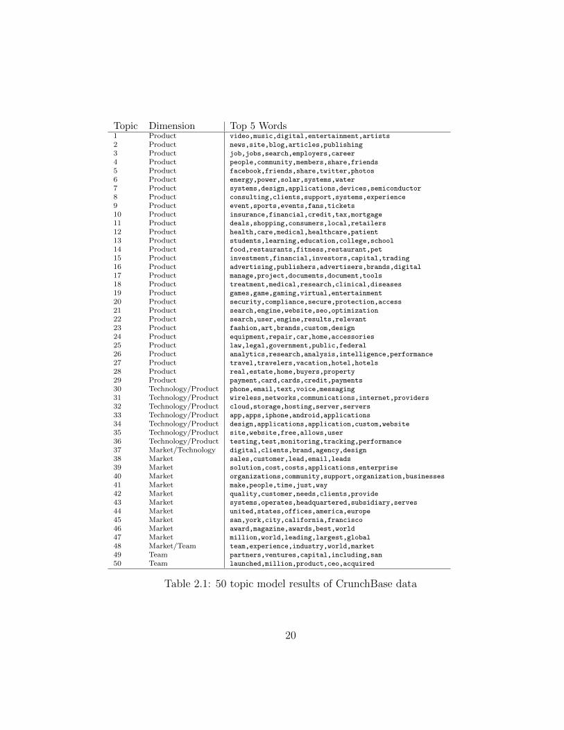
Topic Dimension Top 5 Words1 Product video,music,digital,entertainment,artists

2 Product news,site,blog,articles,publishing

3 Product job,jobs,search,employers,career

4 Product people,community,members,share,friends

5 Product facebook,friends,share,twitter,photos

6 Product energy,power,solar,systems,water

7 Product systems,design,applications,devices,semiconductor

8 Product consulting,clients,support,systems,experience

9 Product event,sports,events,fans,tickets

10 Product insurance,financial,credit,tax,mortgage

11 Product deals,shopping,consumers,local,retailers

12 Product health,care,medical,healthcare,patient

13 Product students,learning,education,college,school

14 Product food,restaurants,fitness,restaurant,pet

15 Product investment,financial,investors,capital,trading

16 Product advertising,publishers,advertisers,brands,digital

17 Product manage,project,documents,document,tools

18 Product treatment,medical,research,clinical,diseases

19 Product games,game,gaming,virtual,entertainment

20 Product security,compliance,secure,protection,access

21 Product search,engine,website,seo,optimization

22 Product search,user,engine,results,relevant

23 Product fashion,art,brands,custom,design

24 Product equipment,repair,car,home,accessories

25 Product law,legal,government,public,federal

26 Product analytics,research,analysis,intelligence,performance

27 Product travel,travelers,vacation,hotel,hotels

28 Product real,estate,home,buyers,property

29 Product payment,card,cards,credit,payments

30 Technology/Product phone,email,text,voice,messaging

31 Technology/Product wireless,networks,communications,internet,providers

32 Technology/Product cloud,storage,hosting,server,servers

33 Technology/Product app,apps,iphone,android,applications

34 Technology/Product design,applications,application,custom,website

35 Technology/Product site,website,free,allows,user

36 Technology/Product testing,test,monitoring,tracking,performance

37 Market/Technology digital,clients,brand,agency,design

38 Market sales,customer,lead,email,leads

39 Market solution,cost,costs,applications,enterprise

40 Market organizations,community,support,organization,businesses

41 Market make,people,time,just,way

42 Market quality,customer,needs,clients,provide

43 Market systems,operates,headquartered,subsidiary,serves

44 Market united,states,offices,america,europe

45 Market san,york,city,california,francisco

46 Market award,magazine,awards,best,world

47 Market million,world,leading,largest,global

48 Market/Team team,experience,industry,world,market

49 Team partners,ventures,capital,including,san

50 Team launched,million,product,ceo,acquired

Table 2.1: 50 topic model results of CrunchBase data

20

We carry out the proposed method on the CrunchBase dataset. We

run the LDA model and compute the corresponding business proximity for a

set of different K values 50, 100, 200, and 500. The main results on coefficient

signs and their statistical significance reported in the empirical validation and

application section are robust to the different choices. Due to the page limit, we

report in the main text for K = 50. To illustrate that the topic model results

comprehensively capture multiple dimensions of a firm’s business, in Table 2.1

we list 50 topics that LDA produces from our dataset. Note that each topic

is a distribution over all words in the vocabulary and that we only show the

top five keywords for brevity. We have checked all 50 topics to find that each

topic consists of words that are tightly related to each other, while cross-topic

overlaps are very small. We also observe that the topics capture the current

trends in the high-tech industry. Using the LDA results, we compute business

proximity for all company pairs in the dataset. Thanks to the huge number

of pairs (close to 300 million), we parallelize the computation algorithm for

speedy processing.

Our new data-driven approach for measuring business proximity has

overcome many of the limitations faced by the existing methods. First, the ap-

proach is scalable because the construction of the business aspects and business

proximity is automated by text mining algorithms, which is a sharp contrast to

the domain-expert-based industry classification in which manual annotation

is required as the first step. Second, the proposed method provides flexibility

to cope with dynamic industry changes. In other words, as the underlying

21

business descriptions in the industry change, the algorithm can automatically

detect the emerging topics in the industry and incorporate them into the busi-

ness proximity. Third, our approach provides finer granularity than the exist-

ing discrete similarity measures as the algorithm provides continuous similarity

measures. Forth, our approach is generally applicable to a wide range of firms

(either public or private) as long as textual business descriptions exist for the

firms. In contrast, industry classification is only sparsely available for small

companies and financial filings data are only available to public companies.

Note that only 1.41% of the high-tech companies in our dataset are public, as

discussed in Section 2.2.

2.4 Empirical Validation and Application

2.4.1 Validation

To validate the constructed business proximity measure, we first exam-

ine the relationship between the newly proposed method and the simple cate-

gory classification. While the NAICS-based proximity cannot be constructed

due to the data limitation (in fact, the CrunchBase companies are already in

a narrowly focused industry), we instead leverage the company category infor-

mation defined by CrunchBase (see Figure 2.2 for the category information).

Note that a binary indicator for same-category membership can be constructed

and serve a benchmark business proximity measure. Specifically, we compare

the business proximity measures of two groups of company pairs: (i) company

pairs in the same category and (ii) those with different categories.

22

●●●

●●

●

●

●

●

●

●

●

●

●

●

●

●

●

●

●

●

●

●

●

●

●

●

●

●

●

●●●

●

●

●

●

●●

●

●

●

●

●

●

●

●

●

●●

●

●

●

●

●●

●

●

●

●

●●

●

●

●

●

●

●

●

●

●

●

●●●

●

●

●●

●●

●

●

●●

●

●

●

●

●

●

●

●●

●

●

●

●

●

●

●●

●

●

●

●

●

●

●

●

●

●●●

●

●

●●

●

●

●

●

●

●

●

●

●

●

●

●

●

●

●

●●

●

●

●

●

●

●

●

●

●

●

●

●

●

●

●

●

●

●

●

●

●

●

●●

●

●●

●

●●

●

●●

●

●

●

●

●

●

●

●

●

●

●

●

●●

●

●

●

●

●

●

●

●

●

●

●

●

●

●

●

●

●

●

●

●

●

●

●

●

●

●

●

●

●

●

●

●

●

●

●

●

●

●

●

●

●

●

●

●

●

●

●

●

●●

●

●

●

●●

●

●

●

●

●

●●

●

●

●

●●

●

●

●

●

●

●

●

●

●

●

●

●

●

●

●

●

●

●

●

●

●

●

●

●

●

●

●

●

●

●

●

●

●

●

●

●

●

●

●

●

●

●

●

●

●

●

●

●

●

●

●

●

●

●

●

●

●

●

●

●

●

●

●

●

●

●

●

●

●

●

●

●

●

●

●

●

●

●

●

●

●

●

●

●

●

●

●

●●

●●

●

●

●

●

●

●

●

●

●

●

●

●●●●

●

●

●

●

●

●

●

●

●

●

●

●

●

●

●

●

●

●

●

●

●

●

●

●●●

●

●

●

●

●●

●

●

●

●

●

●

●

●

●

●●●

●

●●

●

●

●

●

●●

●

●

●

●

●

●

●

●

●

●

●

●

●

●

●

●

●

●

●

●

●

●

●

●

●

●

●

●

●

●

●

●

●

●

●

●

●

●

●

●

●

●

●

●

●

●

●

●

●

●

●

●

●

●

●

●●

●

●

●

●

●

●

●

●

●

●

●

●

●

●

●

●

●●

●

●

●

●

●

●

●

●

●

●

●●

●

●

●

●

●

●

●●

●

●●

●

●

●

●

●

●

●

●

●

●

●

●

●

●

●

●

●

●●

●

●

●

●

●

●

●

●

●

●

●

●

●

●

●●

●

●

●

●

●

●

●

●

●

●

●

●

●

●

●

●

●

●

●

●●

●

●

●

●

●

●

●

●

●

●

●

●

●

●

●

●

●

●

●

●

●

●

●●●

●

●

●

●

●

●

●

●

●

●

●

●

●

●

●

●

●

●

●

●

●●

●

●

●

●

●

●

●

●●●

●

●

●

●

●

●

●

●

●

●

●

●

●

●

●

●

●●

●

●

●

●

●

●

●

●

●

●

●

●

●

●

●

●

●

●

●

●

●

●

●

●

●

●

●

●

●

●

●

●

●

●

●

●●

●

●

●

●

●

●

●

●●

●

●

●

●

●

●

●

●●

●

●

●

●

●

●

●

●

●

●

●

●

●

●

●

●●●

●

●

●

●

●

●

●

●

●

●

●

●

●

●

●

●

●

●

●●

●●●

●●

●

●

●

●

●

●

●

●●

●

●

●

●

●

●

●

●

●

●

●

●

●

●

●

●

●

●

●

●

●

●

●

●

●

●●

●

●

●

●

●

●

●

●

●

●

●

●

●

●

●

●

●

●

●

●

●

●

●

●

●

●

●

●

●

●

●

●

●

●●

●

●

●

●

●

●

●

●

●

●

●

●

●

●

●

●

●

●

●

●

●

●

●

●

●

●

●

●●●

●

●●●

●

●

●

●

●

●

●

●

●

●●

●

●

●

●

●

●●

●

●

●

●●●●

●

●

●

●

●

●

●

●

●

●

●

●

●

●

●

●

●

●

●

●

●

●

●

●

●

●

●

●

●

●●

●

●

●

●

●

●

●

●

●

●

●●

●

●

●

●

●

●

●

●

●

●

●

●●

●

●

●

●●

●

●

●

●●

●

●

●

●

●

●

●

●

●●

●

●

●

●

●

●

●

●●

●

●

●

●

●

●

●

●

●

●

●

●

●

●

●

●

●

●

●

●

●

●

●

●

●

●

●

●

●

●

●

●

●

●

●

●

●●

●

●

●●

●

●

●

●

●

●

●

●

●

●

●

●

●

●

●

●

●

●

●

●●

●

●

●●

●

●

●

●

●

●

●

●

●

●

●

●

●

●

●●

●

●

●

●

●

●

●

●

●

●

●

●

●

●

●

●

●

●

●

●

●

●

●

●

●

●

●

●

●●

●

●

●

●

●

●

●

●

●

●●

●

●

●

●

●

●

●●

●

●

●

●

●

●

●

●

●

●

●

●

●

●

●

●

●

●

●

●

●

●

●●

●

●●

●

●

●

●

●

●

●

●

●

●

●

●

●

●●

●

●

●

●

●

●

●

●●●

●

●

●●

●

●

●

●

●

●

●

●

●

●

●

●

●

●

●

●●

●

●

●

●

●

●

●

●

●●

●

●

●

●

●

●

●

●

●

●

●●

●

●

●

●

●

●●

●●

●

●

●

●

●

●

●

●

●

●

●

●

●

●

●●

●

●

●

●

●

●

●

●

●

●

●

●

●

●

●

●

●

●

●

●

●

●

●

●

●

●

●

●

●

●

●

●

●

●

●

●

●

●●

●

●

●

●

●

●

●

●

●

●

●

●

●

●

●

●●

●

●

●

●

●

●

●

●

●

●

●●

●

●

●

●

●

●

●

●

●

●

●

●

●

●

●

●

●

●

●

●

●

●

●

●

●●

●

●

●

●

●

●

●

●

●

●

●

●

●

●

●

●

●

●

●

●

●

●

●

●

●

●

●

●●

●

●

●

●●

●

●

●

●●

●

●

●

●

●

●●

●

●

●

●

●●

●

●

●

●

●

●

●

●

●

●

●●●

●

●

●

●

●

●

●

●

●

●

●

●

●

●●

●

●

●

●

●

●

●

●

●

●

●

●

●

●

●

●

●

●

●

●

●

●

●

●

●

●●

●

●●

●

●

●

●

●

●

●●

●

●

●

●

●●

●

●

●

●

●

●●

●

●

●

●

●

●

●

●

●

●

●

●

●

●

●

●

●

●

●

●

●

●

●

●

●

●

●

●

●

●

●

●

●

●

●●●

●●

●

●

●

●

●

●●●

●

●

●

●

●●●

●

●

●

●

●●

●

●

●

●

●

●

●

●

●

●

●

●

●

●

●

●

●

●●

●

●

●

●

●

●

●

●

●

●

●

●

●

●

●

●

●

●

●

●

●

●

●

●

●

●

●

●●●

●

●

●

●

●

●

●

●

●

●

●

●

●

●

●

●

●

●

●

●

●

●

●●

●

●

●

●

●

●

●

●

●

●

●

●

●

●

●

●

●

●

●

●

●

●

●

●

●

●

●

●

●●

●●

●

●

●

●

●

●

●

●

●

●

●

●

●

●

●

●

●

●

●

●

●

●

●●

●

●

●

●

●

●

●

●

●

●

●

●

●

●

●

●

●●

●

●

●

●

●

●

●

●

●●

●

●

●

●

●

●

●

●

●

●

●

●

●

●

●●

●

●

●

●

●

●

●

●

●

●

●

●

●

●

●

●

●

●

●

●

●

●

●

●●

●

●

●

●●

●

●

●

●

●

●

●

●

●

●

●

●

●

●

●

●

●

●

●

●

●

●

●

●

●

●

●

●

●

●

●

●

●

●

●

●

●

●

●

●

●

●

●

●

●

●

●

●

●

●

●

●

●

●

●

●

●

●

●

●

●

●

●

●

●

●

●

●

●

●

●

●

●

●

●

●

●

●

●

●

●

●

●

●

●

●

●

●

●

●

●

●

●

●

●●

●●

●

●●●

●

●

●

●

●

●

●

●

●

●●

●

●

●

●●

●

●

●

●

●

●

●

●

●

●

●

●

●

●

●

●

●

●

●

●

●

●

●

●

●

●

●

●

●

●

●

●

●

●

●

●

●

●

●

●

●

●

●●

●

●

●

●●

●

●

●

●

●

●

●

●

●

●

●

●

●

●

●

●

●

●

●

●

●

●

●

●

●

●

●

●

●

●

●

●

●

●●

●

●

●

●

●

●

●●

●

●

●

●

●

●

●

●

●

●

●

●

●

●

●

●

●

●

●

●

●

●

●

●

●

●

●

●

●

●

●

●●

●

●

●

●●

●

●

●

●

●

●

●

●

●

●

●

●

●

●

●

●

●

●

●

●

●

●

●

●

●

●

●

●

●

●

●●●

●

●

●

●

●

●

●

●

●

●

●

●

●

●

●

●

●

●

●

●

●

●

●

●

●

●

●●

●

●●

●

●

●

●

●

●

●

●

●

●

●

●

●

●

●●

●

●

●

●

●

●

●

●

●

●

●●

●

●

●

●

●

●

●

●

●

●

●

●

●●

●●

●

●

●

●

●

●

●

●

●

●●●●

●

●●●

●

●

●

●

●

●

●

●

●

●

●

●

●

●

●

●

●●

●●

●

●

●●●

●

●●

●

●

●

●

●

●

●

●

●

●

●

●

●

●

●

●

●

●

●

●

●

●

●

●

●

●

●

●

●

●

●

●

●

●●

●

●

●

●

●

●

●

●●

●●

●

●

●●

●

●

●

●

●

●

●

●

●

●

●●●

●

●

●

●●

●

●

●

●●

●●

●

●●

●●●

●

●

●●

●

●●

●

●

●

●

●

●

●

●

●

●

●

●

●

●

●

●

●

●●●

●

●

●

●

●

●

●

●

●●

●

●

●

●

●

●

●

●

●

●

●

●

●

●

●

●

●

●

●

●

●

●

●

●

●

●

●

●

●

●

●

●

●

●

●

●

●

●

●

●

●

●

●

●

●

●

●

●

●

●

●

●

●

●●

●

●

●

●

●

●

●

●

●

●

●

●●●

●

●

●

●

●

●

●

●

●

●

●

●

●

●

●

●

●

●

●

●

●

●

●

●

●

●

●

●

●

●

●

●

●

●

●

●

●

●

●

●

●

●

●

●

●

●

●

●

●

●

●

●

●

●

●

●

●●

●

●

●

●

●●

●●

●

●

●

●

●

●

●

●

●

●

●

●

●●

●

●

●

●

●

●

●

●

●

●

●●

●

●

●

●

●

●

●

●

●

●

●

●

●

●

●●●

●

●●

●

●

●

●

●

●

●

●

●

●

●

●

●

●

●

●

●

●

●

●

●

●

●

●

●

●

●

●

●

●

●

●

●

●

●

●

●

●

●

●

●

●

●

●

●

●

●●●

●

●

●

●

●

●

●

●

●

●

●

●

●

●

●

●

●

●

●

●

●

●

●

●

●

●

●

●●

●

●●

●

●

●

●

●

●

●

●

●

●

●

●

●

●

●

●

●

●

●

●

●

●

●●

●

●

●

●

●

●

●

●

●

●

●

●●

●

●

●

●

●

●

●

●

●

●

●

●

●

●

●

●

●

●

●

●

●

●

●

●●

●

●

●

●

●

●

●

●

●

●

●

●

●

●

●

●

●

●

●

●

●

●

●

●

●

●

●●

●

●

●

●

●

●●

●

●

●

●

●

●

●

●

●

●

●

●

●●

●

●

●

●

●

●●

●

●

●

●

●

●

●

●

●

●●

●

●

●

●

●

●

●

●

●

●

●

●

●

●

●●

●

●

●

●

●

●●

●

●

●

●

●

●

●

●

●

●

●

●

●

●

●

●

●

●

●

●

●

●

●

●

●

●

●

●

●

●

●●

●

●

●

●

●

●

●

●

●

●

●

●

●

●

●

●

●

●

●

●

●

●

●

●

●

●

●

●

●

●

●

●

●

●

●

●

●

●

●

●

●●

●

●

●

●

●

●

●

●

●●●

●

●

●

●

●

●

●

●

●

●

●

●

●

●

●

●

●

●

●

●

●

●

●

●

●

●

●

●

●

●

●

●

●

●

●●

●●

●

●

●

●

●

●

●

●

●

●

●

●

●

●

●

●

●

●

●

●

●

●

●●

●

●

●●

●

●

●

●

●

●

●

●

●●●

●

●

●

●

●

●

●

●

●

●

●

●

●

●

●

●

●●

●●

●

●

●

●

●

●

●

●

●

●

●

●

●

●

●

●

●

●

●

●

●

●

●

●

●

●

●

●

●

●

●

●

●

●

●

●

●

●

●

●

●

●

●

●

●

●

●

●

●

●

●

●

●

●

●

●

●

●

●

●

●

●

●

●

●

●

●

●

●●

●

●●

●

●

●

●

●

●

●

●

●

●

●

●

●

●

●

●

●

●●

●

●

●

●

●●

●

●

●

●

●

●

●

●

●

●

●

●

●

●

●

●

●●

●

●

●

●

●

●●

●

●

●

●

●

●

●

●

●

●

●

●●●

●●

●

●

●

●

●

●

●

●

●

●

●

●

●

●

●

●

●

●

●

●

●

●

●

●

●

●●

●

●

●

●●

●

●

●

●●

●

●

●

●

●

●

●

●

●

●

●

●

●

●

●

●

●

●

●●

●

●

●

●

●

●

●

●

●

●

●

●

●

●

●

●

●

●

●

●

●●

●

●●

●

●

●

●

●

●

●

●

●

●

●

●

●

●

●

●

●

●

●

●

●

●

●

●

●●

●

●

●

●

●

●

●

●

●

●

●

●

●

●

●

●●

●

●

●

●

●

●

●

●

●●

●

●

●

●

●

●

●

●

●

●

●

●

●

●

●

●

●

●

●

●

●

●

●

●

●

●

●

●

●

●

●

●

●

●

●

●

●

●

●

●

●

●

●

●

●

●

●

●●

●

●

●

●

●

●●

●

●

●

●

●

●

●

●

●

●

●

●

●

●

●

●

●

●

●

●

●

●

●

●

●

●

●

●

●

●

●

●

●

●

●

●

●

●

●

●

●

●

●●

●

●

●

●

●●●●

●

●

●

●

●

●

●

●

●

●●

●●

●

●

●

●

●

●

●●

●●

●

●

●

●

●

●

●

●

●●

●

●

●

●●

●

●

●

●

●

●

●

●

●

●

●

●

●●

●

●

●

●

●

●

●

●

●

●

●

●

●

●

●

●

●

●

●●

●

●

●

●

●

●

●

●

●●●

●

●

●

●

●

●

●

●

●

●

●

●

●

●

●

●

●

●

●

●

●

●

●

●

●

●

●

●●

●

●

●

●

●

●

●

●

●

●

●●●

●

●

●

●

●

●

●

●

●

●

●

●●

●

●

●

●

●

●

●●

●

●

●

●

●

●

●

●

●

●

●

●●

●

●

●

●

●

●

●

●

●

●

●

●

●

●

●

●

●

●

●

●

●

●

●●●

●

●

●

●

●

●

●

●●

●

●●

●

●

●

●

●●

●

●

●

●

●

●

●

●

●

●

●

●

●

●

●

●

●

●

●

●

●

●

●

●

●

●

●

●

●●

●

●

●

●●●

●

●

●

●

●

●

●

●●

●

●●

●

●

●

●

●

●

●

●

●

●

●

●

●

●

●

●

●

●

●

●

●

●

●

●

●

●

●

●

●

●

●●

●

●

●

●

●

●

●

●

●

●

●

●

●

●●

●

●

●

●

●

●●

●

●●

●

●

●

●

●

●

●

●

●●

●

●

●

●

●

●●

●

●

●

●●●●

●

●

●

●

●

●

●

●

●

●

●

●●

●

●

●

●

●

●

●

●

●

●

●

●

●

●●

●

●

●

●

●

●

●

●

●

●

●

●●

●

●

●

●

●

●

●

●

●

●

●

●

●

●

●

●

●

●

●

●

●

●

●

●

●

●

●

●

●

●

●

●

●

●

●

●

●

●

●

●

●

●

●

●

●

●

●

●

●

●

●

●

●

●

●

●

●

●

●

●

●

●

●

●

●

●

●

●

●

●

●

●

●

●

●

●

●

●

●●

●

●

●

●

●

●

●

●

●

●

●

●

●

●

●●

●

●

●

●

●

●

●

●

●

●●

●

●●

●

●

●

●

●

●

●

●

●

●

●

●●

●

●

●

●

●

●

●

●

●

●

●

●

●

●

●

●

●

●

●

●

●

●

●●●

●●

●

●

●

●

●

●

●

●

●

●

●

●

●

●

●●

●

●

●●

●

●

●●

●

●

●

●

●

●

●

●

●

●●

●

●

●

●

●

●

●

●

●

●

●

●

●

●

●

●

●

●

●

●

●

●

●

●

●

●

●

●

●

●

●

●

●

●●

●

●

●

●

●

●

●

●

●

●

●

●

●

●

●

●

●

●

●

●

●

●

●

●

●

●

●

●

●

●●

●

●

●●

●

●

●

●

●●

●

●

●

●

●●

●

●

●

●

●

●

●

●

●

●

●

●

●

●

●

●

●

●

●

●

●

●

●

●

●

●

●

●

●

●

●

●

●

●

●

●

●

●

●

●

●

●

●

●

●

●

●

●

●

●

●

●

●

●

●

●

●

●

●

●

●

●

●

●●

●

●

●

●

●

●

●

●

●

●

●

●

●●

●

●●

●●

●●

●

●

●

●

●

●

●

●

●

●

●●

●

●

●

●

●

●

●

●

●

●

●

●

●

●

●

●

●●

●

●

●

●

●

●

●

●

●

●

●

●

●

●

●

●

●

●

●

●

●

●

●

●●

●

●

●

●

●

●

●

●

●

●

●●●

●

●

●

●

●

●

●

●

●

●

●

●

●

●

●

●

●

●

●

●

●

●

●

●

●

●

●

●

●

●

●

●●

●

●

●

●

●

●

●

●●

●

●

●

●

●

●

●●

●

●

●

●

●●

●

●●

●●

●

●

●

●

●

●

●

●●

●●

●

●

●

●

●

●

●

●

●

●

●

●

●

●

●

●

●

●

●

●

●

●

●

●

●

●

●

●

●

●

●

●

●

●

●

●

●

●

●

●

●

●

●

●

●●●

●

●

●

●

●

●

●●

●

●

●

●

●

●

●

●

●●●

●

●

●

●

●

●

●

●

●

●

●

●

●

●●

●

●

●

●●

●

●

●

●

●

●

●

●

●

●●●

●

●●

●●

●●

●

●

●

●

●

●

●

●

●

●

●

●

●

●

●

●

●

●

●

●

●

●

●

●●

●

●

●

●

●

●

●

●

●

●

●

●

●

●

●

●

●

●

●

●

●

●

●

●

●

●

●

●

●

●

●●

●

●

●

●●●

●

●●

●

●

●

●

●

●

●●

●

●

●

●

●●

●

●

●

●●

●

●

●

●

●

●

●

●

●

●

●

●

●

●

●

●

●

●

●

●

●

●

●

●

●

●

●

●●

●

●

●

●

●●

●

●

●

●

●

●

●

●

●

●

●

●

●

●

●

●

●●

●

●

●

●●●

●

●

●

●

●●

●

●

●

●

●

●

●

●

●

●

●

●

●

●

●

●

●

●

●●

●●

●●

●

●

●

●

●

●

●

●

●

●●●●

●

●

●

●

●

●

●

●

●

●

●

●

●

●

●

●

●●

●

●

●

●

●

●

●

●

●

●

●

●

●

●

●

●

●

●

●

●

●

●

●

●

●

●

●

●●

●●

●

●

●

●

●

●

●

●

●

●

●

●

●

●

●

●

●

●

●

●

●

●

●

●

●

●

●

●

●

●

●

●

●

●

●

●

●

●

●

●

●

●

●

●

●

●

●

●

●

●

●

●

●

●

●

●

●

●

●

●

●

●

●

●

●

●

●

●

●

●

●

●

●

●

●

●

●

●

●

●

●

●

●

●

●

●

●

●

●

●

●

●

●

●

●

●

●

●

●

●

●

●

●

●●

●

●

●

●

●

●

●

●

●

●

●

●

●

●

●

●

●

●

●

●

●

●

●

●

●●●●

●

●

●

●

●●

●

●

●

●

●

●

●

●

●

●

●

●●

●

●

●

●

●

●

●

●

●

●●

●

●

●

●

●

●

●●

●

●

●

●

●

●

●

●

●

●

●

●

●●

●●

●

●

●

●

●

●

●

●

●

●

●

●

●

●

●

●

●

●

●

●

●

●

●

●

●

●

●

●

●

●

●

●

●

●●

●

●

●

●

●●

●

●

●

●

●

●●

●

●

●

●

●

●

●

●

●●

●

●

●

●

●●

●

●

●

●

●

●

●

●

●

●

●

●

●

●

●

●

●

●

●

●

●

●

●

●

●

●

●

●

●●

●

●

●

●

●

●

●●

●

●

●

●●

●

●

●

●

●

●

●

●

●

●

●

●

●

●

●

●

●

●

●

●

●

●

●

●

●

●

●

●

●

●

●

●

●●

●

●●

●

●

●

●

●

●

●

●

●

●

●

●

●

●

●●●

●

●

●

●

●

●●

●

●

●

●

●

●

●

●

●

●

●

●

●

●

●

●

●

●

●

●

●

●

●

●

●

●●

●

●

●

●

●

●

●

●

●

●

●

●

●

●

●

●

●

●

●

●

●

●

●

●

●

●

●

●

●

●

●

●

●

●

●

●

●

●

●

●●

●●

●

●

●

●

●

●●

●●

●

●

●

●

●

●

●

●

●

●

●

●

●●

●

●

●

●

●

●

●

●

●

●

●

●

●

●

●

●

●

●

●●

●

●

●

●

●

●

●

●

●

●

●

●

●

●

●

●

●

●

●

●

●

●

●

●

●

●

●

●

●

●

●●

●

●

●

●

●

●

●●

●

●

●●

●

●

●

●

●●

●

●

●

●

●

●

●

●●

●

●

●●

●

●

●

●

●

●

●

●

●

●

●

●●

●

●

●●●

●●

●

●

●

●

●

●

●

●

●

●●

●

●

●

●

●

●

●●

●

●

●

●

●

●

●

●

●

●

●

●

●

●

●

●

●

●

●

●

●

●

●

●●

●

●

●

●

●

●

●

●

●

●

●

●

●

●●

●●

●

●

●

●●

●

●

●

●

●

●

●

●

●

●

●

●

●

●●

●

●

●●●

●

●●

●

●

●

●

●

●

●

●

●

●

●

●

●

●

●

●

●

●●

●

●

●

●

●

●

●

●

●

●

●

●

●

●

●

●

●

●

●●

●●

●

●

●

●

●

●

●

●

●

●

●

●

●

●

●

●

●

●

●

●

●

●

●

●

●●

●●

●

●

●

●

●

●

●

●

●●

●

●

●

●

●

●

●

●

●

●

●

●

●

●

●

●

●●

●

●●

●

●

●

●

●

●

●●

●

●

●

●

●

●

●

●

●

●

●

●

●

●

●

●

●

●

●

●

●

●

●

●

●

●●

●

●

●

●

●

●

●

●

●

●

●

●

●

●

●

●

●

●

●

●

●

●

●

●

●

●

●

●

●

●

●

●

●

●

●

●

●

●

●

●

●

●

●

●

●

●

●

●

●

●●

●

●

●

●●

●

●

●

●

●

●

●

●

●

●

●

●●

●

●

●

●

●

●

●

●

●

●

●

●

●

●

●

●

●

●●

●

●

●

●

●

●

●

●

●

●

●

●

●

●

●

●

●

●●

●

●

●

●

●

●

●

●

●

●

●

●

●

●

●

●

●

●

●

●

●

●

●

●

●

●

●

●●

●

●

●

●

●

●

●

●

●

●

●●

●

●

●

●

●

●

●

●

●

●

●

●●

●

●

●

●

●

●

●

●

●

●

●

●

●●●

●●

●

●

●

●

●

●

●

●

●

●

●

●

●

●

●

●

●

●

●●

●

●

●

●

●

●

●

●

●

●

●

●●

●

●

●

●●

●

●

●

●

●

●

●●●

●

●

●

●

●

●

●

●

●

●

●

●

●

●

●●

●

●●●

●

●

●

●

●

●

●

●

●

●

●

●

●●

●

●

●●

●●●

●

●●●●

●

●

●

●

●

●

●●

●

●

●

●

●

●

●

●

●

●

●

●

●

●

●

●

●

●

●

●

●

●

●

●

●

●

●

●

●

●

●

●

●

●

●

●

●

●

●

●

●

●

●

●

●

●

●

●

●

●

●

●

●

●●

●

●

●

●

●

●

●

●

●

●

●

●

●

●

●

●

●

●

●●

●

●

●

●

●

●

●

●

●

●●

●

●

●

●

●

●

●

●

●

●

●

●

●

●

●

●

●

●

●

●

●

●

●

●

●

●

●

●

●

●

●

●●

●

●

●

●

●●

●

●

●

●●

●●

●

●

●

●

●

●

●

●

●

●

●

●●

●

●

●

●

●

●●

●

●●

●

●

●

●

●

●

●

●

●

●●

●

●

●

●

●●

●

●

●

●

●

●

●

●

●

●

●

●●●

●

●

●

●

●

●●

●

●

●

●

●

●

●

●

●

●

●

●

●

●

●

●

●

●

●

●

●

●

●

●

●

●

●●

●

●

●

●

●

●

●

●

●

●

●

●

●

●

●

●

●

●

●

●

●

●

●

●

●

●

●●

●

●

●

●

●

●

●

●

●

●

●

●

●

●

●

●

●

●

●

●

●

●

●●

●

●

●●

●

●

●

●

●

●

●●

●

●

●

●

●

●

●

●

●

●

●

●

●

●

●

●

●

●

●

●

●

●

●

●●

●

●

●

●

●

●

●

●●

●

●

●

●

●

●

●

●

●

●

●

●

●

●

●

●

●

●

●●

●

●

●

●●

●

●

●

●

●

●

●

●

●

●

●

●●

●

●

●

●

●

●

●

●

●

●

●

●

●

●

●

●

●

●

●

●

●

●●

●

●

●

●

●

●

●

●

●

●

●

●

●

●●

●

●

●

●

●

●

●

●

●

●●

●

●

●

●

●

●

●

●

●

●

●

●

●

●

●

●

●

●

●

●●

●

●

●

●

●

●

●

●

●

●

●

●

●

●

●

●●

●●

●

●

●

●

●

●

●

●

●

●●

●

●●

●

●

●

●

●

●

●

●

●

●

●

●

●

●

●

●

●

●●

●

●

●

●

●

●

●

●

●●

●

●

●

●

●

●

●

●

●

●

●

●

●

●

●

●

●

●

●

●

●

●

●

●

●

●

●

●

●

●

●

●

●

●

●

●●

●

●

●

●

●

●

●

●

●

●

●

●

●

●

●

●

●

●

●

●

●

●

●

●

●

●●

●

●

●

●

●

●●●●

●

●

●

●

●

●

●

●

●

●

●

●

●

●

●

●

●

●

●

●

●

●

●

●

●

●●●

●

●

●

●

●

●

●

●

●

●

●●●

●

●

●●

●●

●

●

●

●

●

●

●●

●●●

●

●

●

●

●

●●

●

●

●

●

●

●

●

●●

●

●

●

●

●

●

●

●

●●

●

●●

●

●

●

●

●

●

●

●

●

●

●

●

●

●

●

●

●

●

●

●

●

●●

●

●

●

●●

●

●

●

●

●

●

●

●

●

●

●

●

●

●

●

●

●

●

●●

●

●

●

●

●

●

●

●

●

●

●

●

●

●

●

●

●

●

●

●

●●●●

●

●

●

●●

●●

●

●

●

●

●

●

●●

●●

●

●

●

●

●

●

●

●

●

●●

●

●

●

●

●

●

●

●

●

●

●

●

●●

●●

●

●

●

●

●

●

●

●

●

●

●

●

●

●

●

●●

●

●

●

●

●

●

●

●

●

●

●

●

●

●

●

●

●

●●

●

●

●

●●

●

●

●

●

●●

●

●

●

●

●

●

●

●

●

●

●

●

●

●

●

●

●

●

●

●

●

●

●

●

●●

●

●

●

●●

●

●

●●

●

●

●

●

●●

●

●

●

●

●

●●

●

●

●

●

●

●

●

●

●

●

●

●

●

●

●

●

●

●

●

●

●

●

●

●

●

●

●

●

●

●●

●

●

●

●

●

●

●

●

●●

●

●

●

●

●

●

●

●

●

●

●●

●

●

●

●

●

●

●●

●

●

●

●

●

●

●

●●

●

●●

●

●

●

●

●

●

●

●●

●

●

●●

●

●

●

●

●

●

●

●

●

●●

●

●

●●

●

●

●

●

●

●

●

●

●

●

●

●

●

●

●

●

●●

●

●

●

●

●

●

●

●

●

●

●

●

●

●

●

●●

●

●

●

●

●

●

●

●

●

●

●

●

●

●

●

●

●

●

●

●●

●

●

●

●

●

●

●

●

●

●

●

●

●

●

●

●

●

●

●

●

●

●

●

●

●●

●

●

●

●

●

●

●●

●

●

●

●

●

●

●

●

●

●

●

●

●

●

●

●

●

●

●●

●●

●

●

●

●

●

●●

●

●●●

●

●

●

●

●

●

●

●

●

●

●

●

●●

●

●

●

●

●

●

●

●

●

●

●

●

●

●

●

●

●

●

●

●

●

●

●●

●

●

●

●

●

●

●

●

●

●

●

●

●

●

●

●

●

●

●

●

●

●

●

●

●

●

●

●

●●

●

●

●

●

●

●

●

●

●

●

●

●

●

●

●

●

●

●

●

●

●

●

●

●

●

●

●

●

●

●

●

●

●

●

●

●

●

●

●

●

●

●

●

●

●

●

●

●

●

●

●

●

●

●

●

●

●

●

●

●

●

●

●

●

●

●

●

●

●

●

●

●

●

●

●

●

●

●

●

●

●

●

●

●

●

●●

●

●

●

●

●

●

●

●

●

●

●

●

●

●

●

●

●

●

●

●

●●

●

●

●

●

●

●

●

●

●

●

●

●●●

●

●

●

●

●

●

●

●

●

●

●

●

●

●

●

●

●

●

●

●

●

●

●

●●

●●

●

●

●

●

●

●

●

●

●

●

●

●

●

●

●

●

●

●

●

●

●

●

●

●

●

●

●

●

●

●

●

●

●

●

●

●

●

●

●

●

●

●●●

●

●

●

●

●

●

●

●

●

●

●

●

●

●

●

●

●

●

●

●

●

●

●

●●

●

●

●

●

●

●

●

●

●●

●

●

●

●

●

●

●

●

●

●

●

●

●

●●

●●

●

●

●

●

●

●

●

●

●

●

●

●

●

●

●●

●

●

●

●

●

●

●

●

●

●

●

●

●

●

●

●

●

●

●●

●●

●

●

●

●

●

●

●

●

●

●

●

●

●

●

●

●

●

●

●

●

●

●

●

●

●

●

●

●

●

●

●

●

●

●

●

●

●

●

●

●●

●

●

●●

●

●

●

●

●

●

●

●●

●

●

●

●

●

●

●

●

●

●

●

●

●

●

●

●

●

●

●

●

●

●

●

●

●

●

●

●

●

●

●

●

●

●●

●

●

●

●

●

●

●

●●

●

●

●

●

●

●

●

●●

●

●

●

●

●

●

●

●

●

●

●

●

●

●●

●●

●

●

●

●

●

●

●

●

●

●

●

●

●

●

●

●

●

●

●

●

●

●●●

●

●

●●●

●

●

●

●

●

●

●

●

●

●

●

●

●

●●

●

●

●●

●

●●●

●

●

●

●

●

●

●

●

●

●●●

●●

●

●

●

●

●

●

●

●

●

●

●

●

●

●

●

●

●

●

●

●

●

●

●

●

●

●

●

●●

●

●

●

●

●

●

●●

●

●

●

●

●

●

●

●

●

●

●

●

●

●

●

●

●

●

●

●

●

●

●

●

●

●●●

●

●

●

●

●●

●

●

●

●

●

●

●

●

●

●

●

●

●

●

●

●

●

●

●

●

●

●●

●

●

●

●●

●

●●●

●

●

●

●

●

●

●

●

●

●

●

●

●

●

●

●

●●

●●

●

●

●

●●

●

●

●

●

●

●

●

●

●●

●

●

●

●

●

●

●●

●

●

●

●

●

●

●

●

●

●●

●

●

●

●

●●

●

●

●

●

●

●

●

●

●

●

●

●

●

●

●

●

●

●

●

●

●

●

●

●

●

●

●

●

●

●

●

●

●

●

●

●

●

●

●

●

●

●●

●

●

●

●

●

●

●

●

●

●

●

●

●

●

●

●

●

●

●

●

●

●

●

●

●

●

●

●

●

●

●

●

●

●

●

●

●

●

●●

●

●

●

●●

●

●

●●

●

●

●

●

●

●

●

●

●

●

●

●

●

●

●

●

●

●

●

●

●

●

●

●

●

●

●

●

●

●

●

●

●

●

●

●●

●

●

●

●

●

●

●

●

●

●

●●

●

●

●

●

●

●

●

●

●

●

●

●

●

●

●

●

●

●

●●

●

●

●

●

●●

●

●●

●

●

●

●

●●

●

●

●

●

●

●

●

●

●

●

●●

●

●

●

●

●

●

●

●

●

●

●

●

●

●

●

●

●

●

●●

●

●

●

●

●

●

●

●

●

●

●

●

●

●

●

●

●

●

●

●

●●

●

●

●

●

●

●

●

●

●

●

●

●

●

●

●

●●

●

●

●

●●

●

●

●

●

●

●

●

●

●●

●

●

●

●●●

●

●

●

●

●●

●

●

●

●

●

●

●

●

●

●

●

●

●

●●

●

●

●

●

●

●

●

●

●

●

●●

●

●

●

●

●

●

●

●

●

●

●

●

●

●●

●

●

●

●

●

●

●

●

●

●

●

●

●●

●

●●

●

●

●

●

●

●

●

●

●●

●

●

●

●

●

●●

●

●

●●

●●

●

●

●

●

●

●

●

●●

●

●

●

●

●

●

●●

●

●

●

●

●●

●

●

●

●

●

●

●

●

●

●

●

●

●

●

●

●

●

●

●

●

●●

●

●

●●

●

●

●

●

●

●

●

●

●

●

●

●

●

●

●

●

●

●

●

●

●

●

●

●

●

●

●

●●

●

●

●

●

●

●

●

●

●

●

●

●

●

●

●

●

●

●

●

●

●

●

●●

●

●

●

●

●

●

●

●

●

●

●

●●

●

●●

●

●

●

●

●

●

●

●●

●

●

●

●

●

●

●

●

●

●

●

●

●

●

●

●●

●

●●

●

●

●

●

●

●●

●

●

●

●

●

●

●

●

●

●

●

●

●

●

●

●

●

●

●

●

●

●

●

●

●

●●

●●●

●

●

●

●

●●

●

●

●

●

●●●

●●

●

●

●

●

●

●

●

●

●

●

●

●

●

●

●

●

●

●

●

●

●

●●

●

●

●

●

●●

●●

●

●

●

●

●

●

●●

●

●●

●

●

●

●

●

●

●●

●

●

●

●

●

●

●

●

●

●

●

●

●

●

●

●

●

●

●

●

●

●

●

●

●

●

●

●

●

●●

●

●

●

●

●

●

●

●

●

●

●●

●

●

●

●

●

●

●

●

●

●

●

●

●

●

●

●

●

●●●●

●

●

●

●

●

●

●

●

●●

●

●

●

●

●

●

●

●

●

●

●

●

●●

●

●●

●

●

●

●

●

●

●

●●

●

●

●

●

●

●

●

●

●

●

●

●

●

●

●

●

●

●

●

●

●

●

●

●

●

●

●

●●

●

●

●

●

●

●

●

●

●

●

●

●●

●

●

●●

●

●

●

●

●

●

●

●

●

●

●●●

●

●

●

●●

●

●

●●●

●

●

●

●

●

●●

●

●

●

●

●

●

●

●

●

●

●

●

●

●

●

●

●

●

●

●

●

●

●

●

●

●

●

●

●

●

●

●

●

●

●

●

●

●

●

●

●

●

●

●●

●

●

●

●

●

●

●

●

●

●

●

●

●

●

●●

●

●

●

●

●

●

●

●

●

●

●

●

●

●

●

●

●

●

●

●

●

●

●

●

●

●

●

●

●

●

●

●

●

●

●●

●

●

●

●

●

●

●

●

●●

●

●

●

●

●●

●

●

●

●

●

●

●

●

●

●

●●

●

●

●

●

●

●

●

●

●

●

●

●

●

●

●

●

●●

●

●

●

●

●

●

●

●

●

●

●

●

●

●

●

●

●

●

●

●

●

●

●

●

●

●

●

●

●●

●

●

●

●

●

●

●

●

●

●

●

●

●

●

●

●

●

●

●

●

●

●

●

●

●

●

●

●

●●

●

●

●

●

●

●

●

●

●

●

●

●

●

●

●

●

●

●

●

●

●

●

●

●

●

●

●

●

●

●

●

●

●

●

●●

●

●

●

●

●

●

●

●

●

●

●

●

●

●

●

●

●

●

●

●

●●●

●

●

●

●

●

●

●

●

●

●

●

●

●

●

●

●

●

●

●●

●

●

●

●

●

●

●

●

●

●

●

●

●

●●

●

●

●●

●

●

●●

●

●

●

●

●

●●

●

●

●

●

●

●

●

●

●

●

●

●

●●

●

●

●

●

●

●

●

●

●

●

●

●

●

●

●

●●

●

●

●

●

●

●●

●

●

●

●

●

●

●

●

●

●

●

●

●

●

●

●

●

●

●

●

●

●

●

●

●

●

●

●

●

●

●

●

●

●

●

●

●

●

●

●

●

●

●

●

●

●

●

●●

●

●

●

●

●

●

●

●●

●

●

●

●

●

●

●

●

●

●

●

●

●

●

●

●

●

●

●

●

●

●

●

●

●

●

●

●

●

●

●

●

●

●

●

●

●

●

●

●

●

●

●

●

●

●

●

●

●

●

●

●●●

●

●

●

●

●

●

●●●

●

●

●

●

●

●

●

●●

●

●

●

●

●

●

●

●

●

●

●

●

●●

●

●

●

●

●

●

●

●

●

●

●

●

●

●

●

●

●

●

●

●

●

●

●

●

●

●

●

●

●

●

●

●

●

●●

●

●

●

●●

●

●

●

●

●

●

●

●

●

●

●

●

●

●

●

●

●

●

●

●

●

●

●

●

●

●

●

●

●

●

●

●

●

●

●

●

●

●

●

●

●

●

●

●

●

●

●

●

●

●

●●

●●

●

●

●

●

●

●

●

●

●

●

●

●

●

●

●

●

●

●

●

●

●

●

●

●

●

●

●

●

●

●●

●

●

●

●

●

●

●

●

●

●

●

●

●

●

●●

●

●

●

●●

●

●

●●

●

●

●

●

●

●

●

●●

●

●

●

●

●

●

●

●

●

●●

●

●

●●

●

●

●

●

●

●

●

●

●●

●

●

●

●

●

●●

●

●

●

●

●

●

●

●

●

●

●

●

●

●

●

●

●

●

●

●

●

●

●

●

●

●

●

●

●

●

●

●

●

●

●

●

●

●

●●

●

●

●

●

●●

●

●

●●

●

●●

●

●

●

●

●

●

●

●

●

●●

●

●

●

●

●

●

●

●

●

●

●

●

●

●

●

●

●

●

●

●

●

●

●

●

●●

●

●

●

●●

●

●

●

●

●

●

●

●

●●

●

●●

●

●

●

●

●●

●

●●

●

●

●

●

●

●●

●

●●

●

●

●

●

●

●

●●

●

●

●

●

●

●

●

●

●

●

●●●

●

●

●

●

●

●●

●●

●

●

●

●●

●

●

●

●

●●

●

●

●

●

●

●

●

●●

●

●

●

●●

●

●

●

●

●

●

●

●

●

●

●

●

●

●

●

●

●

●

●

●

●

●

●

●

●

●

●

●

●

●

●

●

●

●

●

●

●

●

●

●●

●

●

●

●

●

●●

●

●

●

●

●

●

●

●

●

●

●

●

●

●

●●

●

●

●

●

●

●

●

●

●

●

●

●

●●

●

●

●

●

●

●

●

●●

●

●●

●

●

●

●

●

●

●

●

●

●●

●

●

●

●

●

●

●

●

●

●●

●

●

●

●

●

●

●

●

●

●

●

●

●

●

●

●

●

●

●

●

●

●●

●

●

●

●

●

●

●

●●

●

●

●

●

●

●

●

●

●

●

●●

●

●

●

●

●

●

●●

●

●

●

●

●

●

●

●●

●

●●

●

●

●

●

●

●

●

●

●

●

●

●

●

●

●

●

●●●

●

●

●

●

●

●

●

●

●

●

●

●

●

●

●

●

●

●●

●

●

●

●

●

●●

●

●

●

●

●

●

●●●

●

●●

●

●

●

●

●

●

●

●

●

●

●

●

●

●

●

●

●

●

●

●●

●

●

●

●

●●

●

●

●

●

●

●

●●

●

●

●

●

●

●

●

●

●

●

●

●

●

●

●

●

●

●

●

●

●

●

●

●

●

●

●

●

●

●●

●

●

●

●

●

●

●

●

●

●

●

●

●

●

●

●

●●●

●

●

●

●

●

●●

●

●

●

●●

●

●

●●

●●

●

●

●

●

●

●

●

●

●

●

●

●

●

●

●●●●

●

●

●●

●

●

●

●

●

●

●

●

●

●

●

●

●

●

●

●

●

●

●

●

●

●

●

●●●

●

●

●

●

●

●

●

●

●●

●

●

●

●

●

●

●

●

●●

●

●

●

●

●

●

●

●

●

●

●

●

●

●

●

●

●

●

●

●●

●

●

●

●

●

●

●

●

●

●

●

●

●

●

●

●

●

●

●

●

●

●

●

●

●

●

●

●

●

●

●

●

●

●

●

●

●

●

●

●●

●

●

●

●

●

●

●

●●

●●

●

●

●

●

●

●

●●

●

●

●

●●

●

●

●

●

●

●

●

●●

●

●

●

●

●

●

●

●

●

●

●

●

●

●

●

●

●●●

●

●

●

●

●

●

●

●

●

●

●

●

●

●

●●●

●

●●

●

●

●

●

●

●

●

●

●

●

●●

●

●●

●

●

●

●

●●

●

●

●

●●

●

●

●●

●

●

●

●

●

●

●

●

●

●

●

●

●

●●

●

●

●

●

●

●

●

●

●

●

●

●

●

●

●

●

●

●

●

●

●

●

●

●

●

●

●

●

●●

●

●

●

●

●

●

●●

●

●

●

●

●

●

●

●

●

●

●

●

●

●

●

●

●

●●

●

●

●●

●

●

●

●

●

●

●

●

●

●

●

●

●

●

●

●

●

●●

●●●

●

●

●

●

●

●

●

●●

●

●

●

●

●

●

●

●●

●

●

●

●

●

●

●

●

●

●

●

●

●

●

●

●

●

●

●

●●

●

●

●●●

●

●

●

●

●

●

●

●

●

●

●

●

●

●

●

●

●

●

●●

●

●

●●

●

●

●

●

●

●

●●

●

●

●

●●

●

●

●

●●

●

●

●

●

●

●

●

●

●

●

●

●

●

●●

●

●

●

●

●

●

●

●

●

●

●

●

●

●

●

●

●

●

●

●●

●

●●

●

●

●●

●

●

●

●

●

●

●

●

●

●

●

●

●

●

●●

●

●●

●●

●

●

●●

●

●

●

●●

●●

●

●

●

●

●

●

●

●

●

●

●

●

●●

●●

●

●

●●

●

●●

●

●

●

●

●

●

●

●

●

●

●

●

●●

●

●

●

●●

●

●

●●

●

●

●

●

●

●

●

●

●

●

●

●

●

●

●●

●

●

●

●

●

●

●

●●

●

●●

●●

●

●

●

●

●

●

●

●

●

●

●

●

●

●

●

●

●

●

●●

●

●

●

●

●

●

●

●●

●

●

●

●

●

●●

●

●

●

●

●●

●

●

●

●

●

●

●

●

●

●

●

●

●

●

●

●

●

●

●

●

●

●

●●

●

●

●

●

●

●

●

●

●

●

●

●

●

●

●

●

●

●

●

●

●

●

●

●

●

●

●

●

●

●

●

●

●

●

●

●

●

●

●

●

●

●

●

●

●

●

●●

●

●

●

●

●

●

●

●●

●

●

●

●

●

●

●

●

●

●

●

●

●

●

●

●

●

●

●

●●●

●

●

●

●

●

●●●

●

●

●

●

●

●

●

●

●

●

●

●

●

●

●

●

●

●

●

●

●

●

●

●●

●

●

●

●

●

●

●●

●

●

●

●

●

●

●●

●●

●

●

●

●●

●

●

●

●

●

●

●

●

●

●●

●

●

●

●

●

●

●

●●●●

●

●

●

●

●

●

●

●

●

●

●

●

●●

●

●

●

●

●

●●

●

●

●

●●

●

●

●

●

●

●

●

●

●

●

●

●

●

●●

●

●

●

●

●

●

●

●

●

●

●●

●

●

●

●

●

●

●

●

●

●

●

●

●

●

●

●

●

●

●

●

●

●

●

●

●

●

●

●

●●

●

●

●

●●●

●

●

●

●

●

●

●

●

●

●

●

●

●

●

●

●●

●

●

●

●

●

●

●

●

●

●

●

●

●

●

●●

●

●

●

●

●

●

●

●

●

●●●

●

●

●

●

●

●

●●

●

●

●

●

●

●

●

●

●

●

●

●●

●

●●

●

●

●

●

●

●

●

●●

●

●

●

●

●●

●

●●●

●

●●●

●

●

●

●

●

●

●

●

●

●

●

●

●

●

●

●

●

●

●

●

●

●

●

●

●

●

●

●

●

●●

●

●

●

●

●

●

●

●

●

●

●

●

●

●

●

●

●

●

●

●

●

●

●●

●

●

●

●

●

●

●

●

●●

●

●

●●

●

●

●

●

●

●

●

●

●

●

●

●

●

●

●

●

●

●

●

●

●●

●

●

●

●

●

●

●

●

●

●

●

●

●

●

●

●

●

●

●

●●

●

●

●

●

●

●●●

●

●

●

●

●

●

●

●

●

●

●

●

●

●

●●

●

●

●

●

●

●

●

●

●

●

●

●

●

●

●

●

●

●

●

●

●●●

●

●

●

●

●●

●

●

●

●

●

●

●

●

●

●

●

●

●

●

●

●

●

●

●

●

●

●

●

●

●

●

●

●

●

●

●

●

●

●

●

●

●

●

●●

●

●

●

●

●

●

●

●

●

●

●

●

●

●

●

●

●

●

●

●

●

●

●

●

●

●

●●

●

●●

●

●

●

●

●

●

●

●

●

●

●

●

●

●

●

●●

●

●

●

●

●

●

●

●

●

●

●

●

●

●

●

●

●

●

●

●

●

●

●●

●

●

●●

●

●

●

●

●

●

●

●

●

●

●

●●

●

●●

●

●

●

●

●

●

●

●

●

●

●

●

●

●

●

●

●

●

●

●

●

●

●

●

●

●

●

●

●

●

●●

●

●

●

●

●

●

●

●

●

●

●

●

●

●

●

●

●

●●

●

●

●

●

●

●

●

●

●

●

●

●

●

●

●

●●●●

●●

●

●

●

●

●

●

●

●

●

●

●●

●

●

●●●

●

●

●

●

●

●

●

●

●

●

●

●

●

●

●

●

●●

●

●

●

●

●

●

●

●

●

●

●

●

●

●

●

●

●

●

●

●

●

●

●

●

●

●●

●

●

●

●

●

●

●

●

●

●

●

●

●

●

●

●

●

●

●

●

●

●●

●

●

●

●

●

●

●

●●

●

●

●

●

●

●

●

●

●

●

●

●

●

●

●

●

●●

●

●

●

●

●

●

●

●

●

●

●

●

●

●

●

●

●

●

●

●

●

●

●

●

●

●

●

●●●

●

●

●

●

●

●

●

●●

●

●

●

●

●

●

●

●●

●

●

●

●●

●

●

●

●

●

●

●

●

●

●●

●

●

●

●

●

●

●

●

●

●

●

●

●

●

●

●

●

●

●

●

●

●

●

●

●

●

●

●

●

●

●

●

●

●

●●

●

●

●

●

●

●

●

●●

●

●

●

●

●

●

●●

●

●

●

●

●

●

●

●

●

●●

●

●

●

●

●

●

●

●

●

●

●●

●

●

●

●

●

●

●

●

●

●

●

●

●

●

●

●

●

●

●

●

●

●

●

●

●

●

●

●

●

●

●

●

●●●

●

●

●

●

●

●

●●

●

●

●

●

●

●

●

●

●

●

●

●

●

●

●

●

●●

●

●

●

●

●

●

●

●

●

●

●

●

●●

●

●

●

●

●

●

●

●●●

●

●

●

●

●●

●

●

●●●

●

●

●●

●

●

●

●

●●

●

●

●

●

●

●●

●

●

●

●

●

●

●

●

●

●●

●

●

●

●●●

●

●

●

●

●

●

●

●●

●

●

●

●

●

●

●

●

●

●

●

●

●

●

●

●

●●

●

●

●

●

●

●

●

●●

●

●

●

●

●

●

●

●

●

●

●

●

●

●

●

●

●

●●

●

●

●

●

●

●

●

●

●

●●

●

●

●

●

●

●

●

●

●

●

●

●

●

●●

●

●

●●

●

●

●

●

●

●

●

●

●

●

●

●

●

●

●

●

●●

●

●

●

●

●

●●

●

●

●●●

●

●

●

●

●●

●

●

●

●

●

●

●

●

●

●

●

●

●

●

●

●

●

●

●

●

●

●●

●

●

●

●

●

●

●

●

●

●

●

●

●

●

●

●

●

●

●

●

●

●

●●

●

●

●

●

●

●

●

●

●

●

●

●

●

●

●

●

●

●

●

●

●

●

●

●

●

●

●

●

●

●

●

●

●

●

●

●

●

●

●

●

●

●

●

●

●

●

●

●

●

●

●

●

●

●

●●●●

●

●

●

●

●

●

●

●

●

●

●●

●

●

●

●●●

●

●●

●

●

●●

●

●

●

●

●

●●

●

●

●

●

●

●

●

●

●

●

●

●

●

●

●

●●

●

●

●

●

●

●

●

●

●●

●

●

●

●

●

●

●●

●

●

●●

●

●

●

●

●

●

●

●

●

●

●

●

●

●

●

●

●

●●●

●

●

●●

●

●●

●

●

●

●

●

●

●

●

●

●

●●

●

●

●

●

●

●

●

●

●

●

●

●

●

●

●

●

●

●

●

●

●●

●

●

●

●

●

●

●

●

●

●

●●

●

●

●

●

●

●

●

●

●

●

●

●

●

●

●

●

●

●

●

●

●

●●

●●

●●

●

●

●

●

●

●

●

●●

●

●

●

●

●

●

●

●

●

●

●

●

●●

●

●

●

●

●

●

●

●

●

●

●

●

●

●

●

●

●

●

●

●

●

●

●

●

●

●

●

●

●

●

●

●

●

●

●

●

●

●

●

●

●

●

●

●

●

●●

●

●

●

●

●●

●

●

●

●

●

●

●

●

●

●

●

●

●

●●

●

●

●

●

●●

●●

●

●

●

●

●

●

●

●

●

●

●

●

●

●

●

●

●

●●●

●

●

●●

●

●

●

●

●

●

●●

●

●

●

●

●●

●

●

●

●

●

●

●

●

●

●●

●

●

●

●

●

●

●

●

●

●●

●

●●

●

●

●

●

●

●

●

●

●

●

●

●

●

●

●●

●●

●

●

●

●

●

●

●

●

●

●

●

●

●

●

●

●

●

●

●

●

●

●●

●

●

●

●

●

●

●

●

●

●

●

●

●●●●●

●

●

●

●

●

●

●

●

●

●

●●

●

●

●

●

●

●

●

●

●

●

●

●

●

●

●

●

●

●

●

●

●

●

●

●

●

●

●

●

●

●

●

●

●

●

●

●

●

●

●

●

●

●

●

●

●

●●

●

●

●●

●

●

●

●

●

●

●

●

●●

●

●

●

●

●

●

●

●

●

●

●

●

●

●

●

●

●

●

●

●

●

●

●

●

●

●●

●

●●

●

●

●

●

●

●

●

●

●

●

●

●

●

●

●

●

●

●

●

●

●

●

●

●

●

●

●●●

●

●

●

●

●

●

●

●

●

●

●

●

●●

●

●

●

●●

●

●

●

●

●

●●

●

●●●

●

●

●

●

●

●

●

●

●

●

●

●

●

●●

●

●

●●

●

●●

●

●

●

●●

●

●

●●

●

●●

●

●

●

●

●

●●

●●

●

●

●

●

●●

●

●

●

●●

●

●

●

●

●

●

●●

●●

●

●

●

●

●

●

●

●

●

●

●

●

●

●

●

●

●

●

●

●

●

●

●

●

●

●

●

●

●

●

●

●●

●

●

●●

●

●

●

●

●

●

●

●

●●

●

●

●

●

●

●

●

●

●

●

●

●

●

●

●

●●

●

●

●●

●

●●

●

●

●●●●●

●

●

●

●

●

●

●●

●

●

●

●

●

●

●

●

●

●●

●

●

●

●

●

●

●

●

●

●

●

●

●

●

●

●

●

●●

●

●

●

●

●

●

●

●

●

●

●

●

●

●

●

●

●

●●

●

●

●●

●

●

●

●

●

●

●

●

●

●●

●

●

●●

●

●

●●

●

●

●

●

●

●

●

●

●

●

●

●

●

●

●

●

●

●

●

●

●

●

●

●

●

●

●

●

●

●●

●

●

●

●

●

●

●

●

●

●

●

●●

●

●

●

●

●

●●

●

●

●

●

●

●

●

●

●

●

●

●

●

●

●

●

●

●

●

●

●

●

●

●

●

●

●

●

●

●

●

●

●

●

●

●

●

●

●

●

●

●

●

●

●

●

●

●

●

●

●

●

●●

●

●

●

●●

●

●

●

●

●

●

●

●

●

●

●

●

●

●

●

●

●

●

●

●

●

●

●

●

●

●

●

●

●

●

●

●

●

●

●

●

●

●

●

●

●

●

●

●

●

●

●

●

●

●

●

●

●

●

●

●

●

●

●

●

●

●

●

●

●

●

●

●

●

●

●

●

●

●

●

●

●

●

●

●●

●

●

●

●

●

●

●

●

●

●

●

●

●

●

●

●

●

●●

●

●

●

●

●

●

●●

●

●

●

●

●

●

●

●

●

●

●

●

●

●

●

●

●

●

●

●

●

●

●

●

●

●

●

●

●

●

●

●

●

●

●

●

●

●

●

●

●

●

●

●

●

●

●

●

●

●

●

●

●

●

●

●

●

●

●

●

●●

●

●

●●

●

●

●

●

●

●

●

●

●

●

●

●

●

●

●

●

●

●●

●●

●

●

●

●

●

●

●

●

●

●

●

●

●

●

●

●

●

●

●

●

●

●

●

●

●

●●

●

●

●

●

●

●

●

●

●

●

●

●

●

●

●●

●

●

●

●●

●

●

●

●

●

●

●

●

●

●

●

●

●

●

●

●

●

●

●

●

●●

●

●

●

●

●

●

●●

●

●

●

●

●

●

●●●

●

●

●

●

●

●

●●

●

●

●

●

●

●

●

●

●

●

●

●

●

●

●

●

●

●

●

●

●

●

●

●

●●

●

●

●

●

●●

●

●

●

●

●

●

●

●

●

●

●

●

●

●

●

●

●

●

●●

●

●

●

●

●

●

●

●

●

●

●

●

●

●

●

●

●

●

●

●

●

●

●

●

●●

●

●●

●

●

●

●

●

●

●

●

●

●

●

●

●

●

●

●

●

●

●

●

●●

●

●

●

●

●

●

●

●●●

●

●

●

●

●

●

●

●

●

●

●●

●

●

●

●

●

●

●

●

●

●

●

●

●

●

●

●

●●

●●

●

●

●●

●

●

●

●

●

●

●

●

●

●

●

●

●

●

●

●

●●

●

●●

●

●

●

●

●

●

●

●

●

●

●

●

●

●

●

●

●

●

●

●

●

●

●

●

●

●

●

●

●●

●

●

●

●

●

●

●

●

●

●

●

●

●

●

●

●

●

●

●

●

●

●

●

●

●

●

●

●

●

●

●

●

●

●

●

●

●

●

●

●

●

●

●

●

●

●

●

●

●

●

●

●

●

●●

●

●

●●

●

●

●

●

●

●

●

●

●

●

●

●

●

●

●

●●

●

●

●●

●

●

●

●

●

●

●

●

●●

●

●

●

●

●

●

●

●

●

●

●

●

●

●

●

●

●

●

●

●

●

●

●

●

●

●

●

●●

●

●

●

●

●●

●

●

●

●

●

●

●

●

●

●

●

●

●

●●

●

●

●

●

●

●●

●

●

●●

●

●

●

●

●

●

●

●

●

●

●

●

●

●

●

●

●●●●

●

●

●

●

●

●

●

●●

●

●

●

●

●

●

●

●●

●

●●

●

●

●

●

●

●

●

●

●

●

●

●

●

●

●●

●

●

●

●

●

●

●

●

●

●

●

●

●

●

●

●

●

●

●

●

●

●

●

●

●

●

●

●●

●

●

●

●

●

●

●

●

●

●●

●

●

●

●

●

●

●

●

●●

●

●

●

●

●

●

●

●

●

●

●●

●

●

●

●

●

●

●

●●

●

●

●●

●

●

●

●●●

●

●

●

●●●

●

●

●

●●

●

●

●

●●

●●

●

●

●

●●

●

●

●

●

●

●

●

●

●

●

●

●●

●

●

●

●

●

●●

●

●

●

●

●

●

●

●

●

●

●

●●

●

●

●

●

●

●

●

●

●

●

●

●

●

●

●

●

●

●

●

●

●

●

●

●

●

●

●●

●

●

●

●●

●

●

●

●

●

●

●

●

●

●

●

●

●

●

●

●●

●

●

●

●

●

●

●

●

●

●●

●

●

●

●

●

●

●

●

●

●

●

●

●

●

●

●

●

●

●

●

●

●

●

●

●

●

●●

●

●

●

●

●

●

●

●

●●

●

●

●

●●

●

●●

●

●

●

●

●

●

●

●

●

●

●

●●

●

●

●

●

●

●

●

●●●●

●

●

●

●

●

●

●

●

●●

●

●

●

●

●

●

●

●

●●

●

●

●

●●

●

●

●

●

●

●

●●

●

●

●●

●

●

●

●

●

●

●

●

●

●

●

●

●

●

●

●

●

●

●

●

●

●

●

●

●

●

●

●●

●

●

●

●

●

●

●

●

●

●

●

●

●

●

●

●

●

●

●

●

●

●

●

●

●

●

●

●

●

●

●

●

●

●

●

●

●

●

●

●

●

●

●

●

●

●

●

●

●

●

●

●

●

●

●

●

●●

●

●

●

●●

●

●

●●

●

●

●

●

●

●

●

●

●

●

●

●

●

●

●

●

●

●

●

●

●

●

●

●

●

●

●

●

●

●

●

●

●

●

●

●●

●

●

●

●

●

●●

●

●

●

●

●

●

●

●

●

●

●

●

●

●

●

●

●

●

●

●

●

●

●

●

●

●

●●

●

●●

●

●

●

●

●

●

●

●

●

●

●

●

●

●

●●

●

●

●

●

●

●

●

●

●

●

●

●

●

●

●

●

●

●

●

●

●●

●

●

●

●

●

●

●

●

●

●

●

●

●

●

●

●

●

●

●

●

●

●

●

●

●

●

●

●

●

●

●

●

●

●

●

●

●

●

●

●

●

●

●

●

●

●

●

●

●

●

●

●

●●

●

●

●

●

●

●

●

●

●

●

●

●

●

●

●

●

●

●

●

●

●

●

●●●

●

●

●

●

●

●

●

●

●

●

●

●

●

●●

●

●

●

●

●

●

●

●

●

●

●

●

●

●

●

●

●

●●

●

●

●

●

●

●

●

●

●

●

●

●

●

●

●

●

●

●

●

●

●

●

●

●

●

●

●

●

●

●

●

●

●

●

●

●

●

●

●

●

●

●

●

●

●

●

●

●

●●

●

●

●

●

●

●

●

●

●●

●

●

●

●

●

●

●●

●

●

●

●

●

●

●

●

●

●

●

●

●

●●

●

●

●

●

●

●

●

●

●●

●

●

●

●

●

●

●

●●

●

●

●

●

●●

●

●

●

●

●●

●●

●

●

●

●

●

●

●

●

●●

●

●

●

●●

●

●

●

●

●

●

●

●

●

●●

●●

●●●

●

●

●

●

●

●

●

●

●

●

●

●

●●

●

●●

●

●

●

●

●

●

●

●

●

●

●

●

●

●

●

●

●

●

●

●

●

●

●

●

●●

●

●

●

●

●

●

●

●

●

●

●

●

●

●

●

●

●

●

●●

●

●

●

●

●

●

●

●

●

●

●

●

●

●

●

●

●

●

●

●

●

●

●

●

●

●

●

●

●

●

●

●

●

●

●

●

●●

●

●

●●

●

●

●

●●

●

●

●

●

●

●

●

●

●

●

●

●

●

●

●●

●

●

●

●

●

●

●

●

●

●

●

●

●

●

●

●

●

●

●●

●

●

●

●

●

●

●

●

●

●

●

●

●

●

●

●

●

●

●

●

●

●

●

●

●

●

●

●

●

●

●

●

●

●

●

●

●

●

●

●

●

●

●

●

●

●

●

●

●

●

●

●

●●●

●

●

●

●

●

●

●

●

●

●

●

●

●

●

●

●

●

●

●

●

●

●

●

●

●

●

●

●

●

●

●

●

●

●

●

●

●

●

●

●

●

●

●

●

●

●

●

●

●

●

●

●●

●

●

●

●

●

●

●

●

●

●

●

●

●●

●

●

●

●

●

●

●

●

●

●

●

●●

●

●

●

●

●

●

●

●

●

●

●●

●

●

●

●

●

●

●

●

●

●

●

●

●

●●

●

●

●

●

●●

●

●

●

●●

●

●

●

●

●

●

●

●

●●

●

●

●

●

●

●

●

●

●

●

●

●

●

●

●

●

●

●

●

●

●

●

●

●

●

●

●

●

●

●

●

●

●

●

●

●

●

●

●

●

●

●

●

●

●

●

●

●

●

●

●

●

●●

●

●

●

●

●

●

●

●

●

●

●

●

●

●●

●

●

●

●

●●

●

●

●

●

●

●

●

●

●

●

●●

●

●

●

●

●

●

●

●

●

●

●

●

●

●

●●

●

●

●

●

●●

●

●

●

●

●

●

●

●

●

●●

●

●

●

●

●●

●

●

●

●

●

●

●

●

●

●

●

●

●

●

●

●

●

●

●●

●

●

●

●

●

●

●

●

●

●

●

●

●

●

●●

●

●

●

●

●

●

●

●

●

●

●

●

●

●

●●

●

●

●

●

●

●

●

●

●

●

●

●

●

●

●

●

●

●

●

●

●

●

●

●

●

●

●●

●

●

●

●

●

●

●●

●

●

●

●

●

●

●

●●

●

●

●

●

●

●

●

●●

●

●

●

●

●

●

●

●

●

●

●

●

●

●

●

●

●

●

●

●

●

●

●

●●

●

●

●

●

●

●

●

●

●

●

●

●

●

●

●

●

●

●

●

●

●

●

●

●

●

●

●

●

●

●

●

●

●

●

●

●

●

●

●

●

●

●

●

●

●

●

●

●

●

●

●

●

●

●

●

●

●

●

●

●

●

●●

●

●

●

●

●

●

●

●

●

●

●

●

●

●

●

●

●

●

●●

●●

●

●

●

●

●

●

●

●

●

●

●

●

●

●

●

●●

●

●

●●

●

●

●

●

●

●

●

●

●

●

●

●

●

●

●

●

●

●

●

●

●

●

●

●

●

●

●

●

●

●

●

●

●

●

●

●

●

●

●

●

●

●

●

●

●●

●

●

●●

●

●

●

●

●

●

●

●

●

●●●

●

●

●

●

●

●

●

●

●

●

●

●

●

●

●

●

●

●

●

●

●

●

●

●

●

●

●●

●

●

●

●

●

●

●

●

●

●

●

●

●

●

●

●

●

●

●

●

●

●●

●

●

●

●

●

●

●

●

●

●

●

●

●

●

●

●

●

●

●

●

●

●

●

●

●

●

●

●●

●

●●

●

●

●

●

●

●

●

●

●

●

●

●

●

●

●

●

●

●

●

●

●

●●

●

●

●

●

●

●

●

●

●

●

●

●●

●

●

●

●

●

●

●

●

●

●

●

●

●

●

●

●

●

●●

●

●

●

●

●

●

●

●

●

●

●

●

●

●

●

●

●

●

●

●

●

●●

●

●

●

●

●

●

●

●

●

●

●●●

●

●

●

●

●

●

●

●

●

●

●

●●●

●

●●

●

●

●

●

●

●

●

●

●

●

●

●

●

●

●

●

●

●

●

●

●

●

●

●

●

●

●

●●

●

●

●

●

●

●●●

●●

●

●

●●

●

●

●

●

●

●

●

●

●

●

●

●

●

●

●

●

●

●

●

●

●

●

●

●

●

●

●

●

●

●

●

●

●

●

●

●

●

●

●

●

●

●

●

●

●

●

●

●

●

●●

●

●

●

●

●

●

●

●

●

●

●

●

●

●

●

●

●

●

●

●

●

●

●

●

●

●

●

●

●

●

●

●

●

●

●

●

●

●

●

●

●

●●

●

●

●

●

●

●●

●

●

●●

●

●

●

●

●

●

●

●

●

●

●

●

●

●

●

●

●

●

●

●

●

●

●

●

●

●●

●

●

●

●

●

●

●

●

●

●

●

●

●

●

●●

●

●

●

●

●

●

●

●

●

●

●

●

●

●

●

●

●

●

●

●●

●

●

●

●

●

●●●

●

●

●

●

●

●

●

●

●

●

●●

●

●

●

●

●

●

●

●

●

●

●

●

●

●

●

●

●●

●

●

●

●

●

●

●●

●●

●

●

●

●

●

●

●

●

●

●

●

●

●

●

●

●

●

●

●

●

●

●●

●

●

●

●

●

●

●

●

●

●

●

●

●

●

●

●

●

●

●

●

●

●

●

●

●

●

●

●

●

●

●

●

●

●

●

●

●

●

●●

●

●

●

●

●

●

●

●

●

●

●●●

●

●

●

●

●

●

●

●

●

●

●

●

●

●

●

●

●

●

●

●

●

●

●

●

●

●

●

●

●

●

●

●

●

●

●●

●●

●

●

●

●

●

●

●

●

●

●

●

●

●

●

●

●

●

●

●

●

●

●

●

●

●

●

●

●●

●

●

●

●

●

●

●

●

●

●

●

●●●●

●

●

●

●

●

●

●

●

●

●

●

●●

●

●

●

●

●

●

●

●

●

●

●

●

●

●

●

●●

●●

●

●

●

●

●●

●

●

●

●

●

●

●

●

●

●

●

●

●

●

●

●

●

●

●

●

●

●

●

●

●

●

●

●●

●

●

●

●

●

●

●●

●

●

●

●●

●

●

●

●●

●

●

●

●

●●

●

●

●

●●

●

●

●●

●

●●

●

●

●

●

●

●

●

●

●

●

●

●

●

●

●

●

●●

●

●

●

●

●

●

●

●

●

●

●

●

●

●

●

●

●

●

●

●

●

●

●

●

●

●

●

●

●

●

●

●

●

●

●

●●

●

●

●

●●

●

●

●

●

●●●

●

●

●

●

●

●

●

●

●

●

●●

●

●

●

●

●●

●

●

●

●

●

●

●

●

●

●

●

●

●

●

●

●

●

●

●●

●

●

●

●

●

●

●●

●

●

●●●

●

●

●

●

●

●

●

●

●

●

●

●

●

●

●

●

●●

●

●

●

●

●

●

●

●

●

●

●

●

●●

●

●

●

●

●

●

●

●

●

●

●

●

●

●

●

●

●

●

●●●●

●

●

●

●

●

●

●●

●

●

●

●

●

●

●

●●●

●

●

●

●

●

●

●

●

●

●

●

●

●

●

●

●

●

●

●

●

●

●

●

●

●

●●●

●

●●

●

●●

●

●

●

●

●

●

●

●

●

●

●

●

●

●

●

●

●

●

●

●

●

●

●

●

●

●●

●

●

●●

●

●

●

●

●

●

●

●

●

●

●

●

●

●

●

●

●

●

●

●

●

●

●

●

●

●

●

●

●

●

●

●

●

●

●

●

●

●

●

●

●●●

●

●

●

●

●

●

●

●

●

●

●●

●

●

●●

●

●

●

●●

●

●

●

●

●

●

●

●

●

●

●●

●

●

●

●

●

●

●

●

●

●

●

●

●

●●

●

●

●

●●

●

●

●

●

●

●

●

●

●

●

●

●

●

●

●

●

●

●

●

●

●

●

●

●●

●

●

●

●

●

●

●●

●

●

●

●

●

●

●

●●

●

●●

●

●

●

●

●

●

●

●

●

●

●

●

●

●

●

●●

●

●

●

●

●

●

●

●

●

●

●

●

●

●

●

●

●

●

●

●●

●

●

●

●

●

●

●

●

●

●

●●

●●

●●

●

●

●

●

●

●

●

●

●

●●

●

●

●

●

●

●

●

●

●

●

●

●

●

●●

●

●

●

●

●

●

●

●

●

●

●

●

●

●

●

●

●

●

●

●

●

●

●

●

●

●

●

●

●

●

●

●

●

●●

●

●

●

●

●

●

●

●

●

●

●

●

●

●

●●

●●

●

●

●

●●

●

●

●

●

●

●

●●

●

●

●

●

●

●

●

●

●●

●

●

●

●

●

●

●

●

●

●

●

●

●●

●

●

●

●

●

●

●

●

●

●

●

●

●

●

●

●

●

●

●

●

●

●

●

●

●

●

●

●

●

●

●

●

●

●

●

●

●

●

●●

●

●

●

●

●

●

●

●

●

●

●

●

●●

●

●

●

●●

●

●

●

●

●

●●●

●

●

●●

●●

●●

●

●

●●

●

●

●

●

●

●

●

●

●

●

●

●

●●

●

●●

●●

●

●

●

●

●

●

●

●

●

●

●

●

●

●

●

●

●

●

●

●

●

●

●

●

●

●

●

●

●

●

●

●●

●

●

●

●

●

●

●

●

●

●

●

●●

●

●

●

●●

●

●

●●

●

●●

●

●

●

●

●

●

●●

●

●

●

●

●●

●

●

●

●

●

●

●

●

●●

●

●

●

●

●

●

●

●

●

●

●

●

●

●

●

●

●

●

●

●

●

●

●

●

●

●

●●

●

●

●

●

●

●

●

●

●

●

●

●

●

●

●

●

●

●●

●

●

●

●

●

●●

●

●

●

●

●●

●

●

●●

●

●

●

●

●

●

●

●

●

●

●

●

●

●

●

●

●

●

●●

●

●

●

●

●

●

●

●

●

●

●

●

●

●

●

●

●

●

●

●

●

●

●●

●

●

●

●

●

●

●

●

●

●

●

●

●

●

●

●

●

●

●

●

●

●●●

●

●

●

●

●

●

●

●

●●

●

●

●

●

●

●

●

●

●

●

●

●

●

●

●

●

●●●

●

●

●

●

●●

●

●

●

●

●

●

●

●

●

●

●

●

●

●

●

●

●

●

●

●

●

●

●

●●

●

●

●

●

●

●

●

●

●

●

●●●

●

●

●

●

●●

●

●

●

●

●

●

●

●●

●

●

●

●

●

●

●

●

●

●

●

●

●

●

●

●

●

●

●

●

●

●

●

●

●

●

●

●

●

●

●

●

●

●

●

●

●

●

●

●

●●

●

●

●

●

●

●

●

●

●

●

●

●

●

●

●●

●

●

●

●

●

●

●

●

●

●

●

●

●

●

●

●

●

●

●

●

●

●

●

●

●

●●

●

●

●

●

●

●

●●●

●

●

●

●

●

●

●

●

●

●

●

●

●

●

●

●

●

●

●

●

●

●

●

●

●

●

●

●

●●

●

●

●

●

●

●

●

●

●

●

●

●

●

●

●

●

●●

●

●

●

●

●●

●

●

●

●

●

●

●

●

●

●

●●

●

●

●

●

●

●●

●

●

●

●

●

●

●

●

●

●

●

●

●

●

●

●

●●

●●

●

●

●

●●

●

●

●

●

●

●●

●

●

●

●

●

●

●

●

●

●

●

●

●

●

●

●

●

●

●

●

●

●●●

●

●

●

●

●

●

●

●

●

●

●

●

●

●

●

●

●

●

●

●

●

●

●

●

●

●

●

●

●

●

●

●

●

●

●

●

●

●

●●

●

●

●

●

●

●

●

●

●

●

●

●

●

●

●

●

●

●

●

●

●

●

●

●

●

●

●

●

●

●

●

●

●

●

●

●

●

●●

●●

●●

●

●

●

●

●

●

●

●●

●

●

●

●

●●

●●

●

●

●

●

●

●

●

●

●

●

●

●

●

●

●

●

●

●

●●

●

●

●

●

●

●

●●

●

●

●

●

●

●

●

●

●

●

●

●●

●

●

●

●

●

●

●

●

●

●

●

●●●

●

●

●

●●

●

●

●

●

●

●

●

●

●

●

●

●

●●

●

●

●

●

●

●

●

●

●

●

●

●

●●

●

●

●

●

●

●

●

●

●

●

●

●

●

●

●●

●

●

●

●

●

●

●

●

●

●

●

●

●

●

●

●

●

●●

●

●

●

●

●

●

●

●

●

●

●

●

●

●

●

●

●

●

●

●

●

●

●

●

●

●

●

●

●

●

●

●

●

●●

●

●

●

●

●

●

●

●

●

●

●

●

●

●

●

●

●

●

●

●●

●●●

●

●

●

●

●

●

●

●

●

●

●

●

●

●

●

●

●

●●

●

●

●

●

●

●

●

●

●

●

●

●

●

●

●

●

●●

●

●

●

●

●

●

●

●

●●

●●

●

●

●

●

●

●●●

●

●

●

●

●

●●

●

●

●

●

●●

●

●●

●

●

●

●

●●

●

●

●●

●

●

●

●

●

●

●

●

●

●

●

●

●

●

●

●●

●

●

●

●

●

●

●

●

●

●

●

●

●

●

●●

●

●

●

●

●

●

●●

●

●

●

●

●

●

●●

●

●

●

●

●

●●

●

●

●

●

●

●

●

●

●

●

●

●●

●

●

●

●

●

●

●

●

●

●

●

●

●

●●

●

●

●

●

●

●

●

●

●

●

●

●

●

●●

●

●

●

●

●

●●

●

●

●

●

●

●

●

●

●

●

●

●

●

●

●

●

●

●

●●●

●

●

●

●

●

●

●

●

●

●

●

●

●

●

●

●

●

●

●●

●

●

●

●

●

●

●

●

●

●

●

●

●

●

●●

●●

●

●

●

●

●

●

●

●

●

●

●

●

●

●

●

●

●

●

●

●

●

●

●

●

●

●

●

●

●

●

●

●

●

●

●

●

●

●

●

●

●

●

●

●

●

●

●

●

●

●

●

●

●

●●

●

●

●

●

●

●

●

●

●

●●

●

●

●

●

●

●

●

●

●

●●●

●

●

●

●

●

●

●

●●

●

●

●

●

●●

●

●

●

●

●

●

●

●

●

●●

●

●

●

●

●

●

●

●

●

●●

●●

●

●

●

●

●

●

●

●

●

●

●

●

●

●

●●

●

●

●

●

●

●

●

●

●

●

●

●

●

●

●

●

●

●

●

●

●

●

●

●

●

●

●

●

●

●

●

●

●

●

●

●

●

●●●

●

●

●

●

●

●

●

●

●

●

●

●

●

●

●

●

●

●

●

●

●

●

●

●

●

●

●●

●

●

●

●

●

●

●

●

●●

●

●

●

●

●

●

●

●

●

●

●

●

●●

●

●

●

●

●●

●

●

●●●

●

●

●

●

●

●

●

●

●

●

●

●

●●

●

●

●

●

●

●

●

●

●

●●

●

●

●

●

●●

●

●

●

●

●

●

●

●

●

●

●

●

●

●●●

●

●

●

●

●

●●

●

●

●

●

●

●

●

●

●

●

●

●

●

●

●●

●

●

●

●

●

●

●

●

●

●

●

●

●

●

●

●

●

●

●

●

●

●

●

●

●

●●

●

●●

●●

●

●

●

●

●

●

●

●

●

●

●

●

●

●

●

●

●

●●

●

●

●

●

●

●

●

●

●

●

●

●

●

●

●

●

●

●

●

●

●

●

●

●

●

●

●●

●

●

●

●

●

●

●●

●

●

●

●

●

●

●

●●

●

●

●

●

●

●

●

●

●

●

●

●

●

●

●

●

●

●

●

●

●

●●

●

●

●

●

●

●

●

●

●

●

●

●

●

●

●

●

●

●

●

●

●●

●

●

●

●

●

●

●

●

●

●

●

●

●

●

●

●

●

●

●

●

●

●

●

●●

●

●

●

●

●

●

●

●

●

●

●

●

●

●

●

●

●

●

●

●

●

●

●

●

●

●

●

●

●

●

●

●

●

●

●

●

●

●

●

●

●

●

●

●

●

●

●

●

●

●

●

●

●●

●

●

●

●

●

●

●

●

●

●

●

●

●

●

●

●

●

●

●

●

●

●

●

●

●

●

●

●

●

●

●

●

●

●

●

●

●

●

●

●

●●

●

●

●●

●

●

●●

●

●

●

●

●

●

●

●

●

●

●

●

●

●

●

●

●

●

●

●

●

●

●

●

●

●

●

●

●●

●

●

●

●

●●

●

●

●

●

●

●

●

●

●●

●

●

●

●

●

●●

●

●

●●●●

●

●

●

●

●

●

●

●

●

●

●

●

●

●

●

●

●

●

●

●

●

●

●

●

●

●

●

●

●

●

●

●

●

●

●

●

●

●

●

●●

●

●

●

●

●

●

●

●

●

●

●

●

●

●

●

●●

●

●●

●

●

●

●

●

●

●

●

●

●

●

●

●

●

●

●

●

●

●●

●

●

●

●●

●

●

●

●

●

●●

●

●

●●

●

●

●

●

●

●

●

●

●

●

●

●

●

●

●

●

●

●

●●●

●

●

●

●

●

●

●

●

●

●

●

●

●

●●

●

●

●

●

●

●

●

●

●

●

●

●

●

●

●

●

●

●

●

●

●

●

●

●

●

●

●

●

●

●

●

●

●●

●

●●

●

●●

●

●

●

●

●

●

●

●

●

●

●●

●

●

●

●

●●

●

●

●

●

●

●

●

●

●

●

●

●

●

●

●

●

●

●

●●

●

●

●

●

●

●

●

●

●

●

●

●

●

●

●

●

●●

●

●

●

●

●

●

●

●

●

●●

●

●

●

●

●

●

●

●

●

●

●

●

●

●

●

●

●

●

●

●

●●

●

●

●

●●

●

●

●

●

●

●

●

●●

●

●

●

●

●

●

●

●

●

●

●

●

●

●

●

●

●

●

●

●

●

●●

●

●

●

●

●

●

●

●

●

●

●●●

●

●

●

●

●

●

●

●

●●●

●

●

●

●

●

●

●

●

●

●

●

●

●

●

●

●

●

●

●

●

●

●

●

●

●

●

●

●

●●

●

●

●

●●

●

●

●

●

●

●

●

●●

●

●

●

●

●

●

●

●

●

●

●

●

●●

●

●

●

●●

●

●

●

●

●●

●

●

●

●

●●●

●

●

●

●

●●

●

●

●

●

●

●

●

●

●

●

●

●

●

●●●

●

●

●

●

●

●

●

●

●

●●

●

●

●●

●

●

●

●

●

●

●

●

●

●

●●

●

●

●

●

●

●

●

●

●

●

●

●

●●

●

●

●

●

●

●

●●

●

●

●●

●

●

●

●

●

●

●

●

●

●

●●

●

●

●

●

●

●

●

●

●

●

●

●

●●

●●●

●

●

●

●

●

●

●●

●

●

●

●

●

●

●

●●

●

●

●

●

●

●

●

●

●●

●●

●

●

●

●

●

●

●

●

●

●

●

●

●

●

●

●

●

●

●

●

●

●

●

●●

●

●

●

●

●

●

●

●

●

●

●

●

●

●

●

●●

●

●

●

●

●

●

●

●

●

●

●

●

●●

●

●

●

●●

●

●

●

●

●

●

●

●

●

●

●

●

●

●

●

●

●

●

●

●

●

●

●

●

●

●

●

●

●

●

●

●

●

●

●

●

●

●

●

●

●

●

●

●

●

●

●

●

●●

●

●

●

●●

●

●

●

●

●

●

●

●

●

●

●

●

●

●

●

●

●

●

●

●

●

●

●

●

●

●

●

●

●●

●

●

●●

●

●

●

●

●

●

●

●

●

●

●

●●

●

●

●

●

●

●

●

●

●

●

●

●

●

●●

●

●

●

●

●●●

●

●

●

●

●

●

●

●

●

●

●

●

●

●

●

●

●

●

●

●

●

●

●

●

●

●

●

●

●

●

●

●

●

●

●

●

●

●

●

●

●

●

●●

●●

●

●

●

●

●

●

●

●

●

●

●

●

●

●

●

●

●

●●

●

●

●

●

●

●

●

●

●

●

●

●

●

●

●

●●

●

●

●

●

●

●

●

●

●

●

●●

●

●

●

●

●

●

●●

●

●

●

●

●

●

●

●

●

●

●

●

●

●

●●

●

●●

●

●●

●

●

●

●

●

●

●

●

●

●

●

●

●

●

●

●●

●

●●

●

●

●

●

●

●

●

●

●

●

●

●

●

●

●

●

●

●

●

●

●●

●

●

●

●

●

●

●●

●

●

●

●

●

●

●

●

●

●

●

●

●

●

●

●

●

●

●

●

●

●

●

●

●

●

●

●●

●

●

●

●

●

●●

●

●

●

●

●

●

●

●

●

●

●

●

●

●

●

●

●

●

●●

●

●

●

●

●

●

●

●

●

●

●

●

●

●

●

●

●

●

●

●

●

●●

●

●

●●●

●

●

●

●

●

●

●

●

●

●

●

●

●

●

●

●

●

●

●

●

●

●

●

●

●

●

●

●●●

●

●

●

●

●

●

●

●

●

●

●

●

●●

●

●

●

●

●

●

●

●

●

●

●

●

●

●

●

●

●

●

●

●

●

●

●

●

●

●

●

●

●●

●

●

●

●

●

●●

●

●

●

●

●

●

●

●

●

●

●

●

●

●

●

●

●

●

●

●

●

●

●

●

●

●

●

●

●

●

●

●

●

●

●

●

●

●

●

●●●

●

●

●

●●

●

●

●●

●

●

●

●

●

●

●

●

●

●●●

●

●

●

●

●

●

●

●

●

●

●●

●

●

●

●

●

●

●

●

●

●

●

●

●

●

●

●

●

●●

●

●●

●

●

●

●

●

●

●

●●

●

●

●

●

●

●

●

●

●

●

●

●

●

●

●●●

●

●

●

●

●

●

●

●

●●

●●

●

●

●

●

●

●●

●

●

●

●

●

●

●

●

●

●●

●●

●●

●

●

●

●

●

●

●

●

●

●

●

●

●

●

●

●

●

●

●

●

●

●

●

●

●

●●

●

●●

●

●

●

●

●

●●

●

●

●

●

●

●●

●

●●

●

●

●

●

●

●

●

●

●

●

●

●

●

●

●

●

●●

●

●●

●

●

●

●

●

●

●

●

●

●

●

●

●

●

●

●

●

●

●

●

●

●

●●

●

●●

●

●

●

●

●

●

●

●

●●

●

●

●

●

●

●●

●

●

●

●

●

●

●

●

●

●

●

●●

●

●

●

●

●

●

●

●

●

●

●

●●●

●

●

●

●

●

●

●

●

●

●

●

●

●

●

●

●●

●

●

●

●

●

●

●

●

●

●

●

●

●

●●

●

●

●

●

●

●

●

●

●●

●

●

●

●

●●

●

●

●

●

●

●

●

●

●

●

●●

●

●

●

●

●

●

●●

●

●

●

●

●

●

●

●

●

●

●

●

●

●

●

●

●

●

●

●

●

●

●

●

●

●

●

●

●

●

●

●

●

●

●

●

●

●

●

●

●

●

●

●

●

●

●

●●

●

●

●●

●

●

●

●

●

●

●

●

●

●

●

●

●

●

●●

●

●

●

●

●●

●

●

●●

●

●

●●

●

●

●

●

●

●

●

●

●

●●

●

●

●

●

●

●

●●

●

●

●

●

●

●

●

●

●

●

●

●

●

●

●

●

●

●

●

●

●

●

●●

●

●

●

●

●

●

●

●

●

●

●

●

●

●

●

●

●

●●

●

●

●

●

●

●

●

●

●●

●

●

●

●●

●

●

●

●

●

●

●

●●

●

●●

●

●

●

●●●●

●

●

●

●

●

●

●

●

●

●

●

●

●

●

●

●

●

●●

●

●

●

●

●

●

●

●

●

●

●

●

●

●

●

●

●

●

●

●

●

●

●

●

●

●●

●

●

●

●

●

●

●

●

●

●

●

●

●

●

●

●

●

●

●

●

●

●

●

●

●

●

●

●

●

●

●

●

●

●

●

●

●

●

●

●

●

●

●

●

●

●

●

●

●

●

●

●

●

●

●

●

●

●

●●

●

●

●

●

●

●

●

●

●

●

●

●

●

●●

●

●

●

●●

●

●

●

●

●

●●

●

●

●

●

●

●

●

●

●

●

●

●

●

●

●

●●

●

●

●●

●

●

●

●

●

●

●

●

●

●

●

●

●

●

●

●

●

●

●●

●●

●

●

●

●

●

●

●

●●

●●

●●

●

●

●

●

●

●

●

●

●●

●

●

●

●

●

●●

●

●

●

●

●

●

●

●

●

●

●

●

●

●

●

●

●

●

●

●

●

●

●

●

●

●

●

●

●

●

●

●

●

●

●

●

●

●

●

●

●

●

●

●

●●

●

●

●

●

●

●

●

●●

●

●

●

●

●

●

●

●

●

●

●

●

●

●

●

●

●

●

●

●

●

●

●

●

●●

●

●

●

●

●

●

●

●

●

●

●

●

●

●

●

●●●

●

●

●

●

●

●

●

●

●

●

●●

●●

●

●

●

●

●

●

●

●

●

●

●

●

●

●

●

●

●

●

●

●

●

●

●

●●

●

●

●

●

●

●

●

●

●

●

●

●

●

●

●

●

●

●

●

●

●

●

●

●

●

●

●●

●

●

●

●●●

●

●●

●

●

●

●

●

●

●

●

●

●

●

●

●

●

●

●●

●●

●

●

●

●

●

●

●●

●●

●

●

●

●

●

●

●

●●

●

●

●

●

●

●

●

●

●●

●

●

●

●

●

●

●

●

●

●

●

●

●

●●

●

●

●

●

●

●

●

●

●

●

●

●

●

●

●

●

●

●

●

●●

●

●

●

●

●

●

●●

●

●

●

●

●

●

●

●

●

●

●

●

●

●

●

●

●

●

●

●

●

●

●

●

●

●

●

●

●

●

●

●

●

●

●

●

●

●

●

●

●

●●

●

●

●

●

●

●

●

●

●

●

●

●

●

●

●

●

●

●

●

●

●

●

●●

●

●

●

●

●●

●

●

●

●

●

●

●

●

●

●

●

●

●

●●

●

●

●

●

●

●

●

●

●

●

●

●

●

●

●

●

●●

●●

●●

●●

●

●

●

●

●

●

●

●

●

●

●●

●

●

●

●

●

●

●

●

●

●

●

●

●

●

●

●

●

●

●●

●

●

●●

●

●

●

●

●

●

●

●

●

●

●

●

●

●

●

●

●

●

●

●

●

●

●

●

●

●

●

●●

●

●

●

●●

●

●

●●

●

●

●

●

●●

●

●

●

●●●

●

●

●

●●●●

●

●

●

●

●

●

●

●

●

●

●

●

●

●

●

●

●

●

●

●

●

●

●

●

●

●

●

●

●

●

●

●

●

●

●

●

●●

●

●

●

●

●

●

●

●

●

●

●

●

●

●

●

●

●

●

●

●

●

●

●

●

●

●

●●

●

●

●

●

●

●

●

●

●

●

●

●

●

●

●

●

●●

●

●

●

●

●●

●

●

●

●●

●

●●

●●

●

●

●

●

●

●

●

●

●

●

●

●

●

●

●

●

●

●

●

●

●

●

●

●

●

●

●●

●

●

●

●●

●

●

●

●

●

●

●

●

●

●

●

●

●

●

●

●

●

●

●

●

●

●●

●

●

●

●

●

●

●

●

●

●

●

●

●

●

●

●

●

●

●

●

●

●

●

●

●

●

●

●●

●

●●

●

●

●

●

●

●

●

●

●

●

●

●

●

●

●

●

●

●

●

●

●

●

●

●

●

●

●

●

●●

●

●

●

●

●

●

●

●

●

●●

●

●

●●●

●

●

●

●

●

●

●

●

●

●

●

●

●

●

●

●

●

●

●

●

●

●

●

●

●

●

●

●

●●

●

●

●

●

●

●

●

●

●●

●

●

●

●

●

●

●

●

●

●

●

●

●

●

●●

●

●

●

●●

●

●

●

●

●●

●

●

●●

●

●

●

●

●

●

●

●

●

●

●

●

●

●

●

●

●

●

●

●

●

●

●

●

●

●

●

●

●

●

●

●

●

●

●

●

●

●

●

●

●

●

●●

●●

●

●

●

●

●

●

●

●●

●

●

●

●

●●

●●

●

●

●

●

●

●

●

●

●

●

●

●

●

●

●

●●

●

●

●

●

●

●

●

●

●

●

●

●

●

●

●

●

●

●

●

●

●

●

●

●

●

●

●

●

●

●

●

●

●

●

●●

●

●

●

●

●

●

●

●

●

●●

●

●

●

●

●

●

●

●●

●

●

●

●

●

●

●●

●

●

●●

●

●

●

●

●

●

●

●

●

●

●

●

●

●●

●

●

●

●

●

●●

●

●

●

●

●

●

●

●

●

●

●

●

●●

●

●

●

●

●

●

●

●

●

●

●

●

●

●

●

●

●

●

●

●

●

●

●

●

●

●

●

●

●

●

●

●●●

●

●●

●

●

●

●

●

●

●

●

●

●●

●

●

●

●

●

●

●

●

●

●

●

●

●

●

●●

●

●

●

●

●

●

●

●

●

●

●●●

●

●

●●

●●

●●

●

●●

●

●

●

●

●●

●

●

●●

●

●●

●●

●●

●

●●

●

●

●

●

●

●

●

●

●

●

●

●

●

●●

●

●

●

●

●

●

●

●

●

●

●

●

●

●●

●

●

●

●

●

●

●●●

●

●

●

●

●

●

●

●

●

●

●

●

●●

●

●

●

●

●

●

●

●

●

●

●

●

●

●

●

●●

●

●

●●

●

●

●

●

●

●

●

●●

●

●

●●

●

●

●

●

●

●

●

●

●

●●●

●

●

●

●

●

●

●

●

●

●

●

●

●

●

●●

●

●●

●

●

●

●

●●

●

●

●

●

●

●

●

●

●

●

●

●

●

●

●

●

●

●

●

●

●

●

●

●

●

●

●

●

●

●

●

●

●

●

●

●

●

●●

●

●

●

●●

●

●

●

●

●

●

●

●●

●

●

●

●

●

●

●

●

●

●

●

●

●

●

●

●

●

●

●

●

●

●

●

●

●

●

●

●

●

●

●

●

●

●

●

●

●

●

●

●

●

●●

●

●

●

●

●

●

●●

●●●

●

●

●

●

●

●

●

●

●

●

●

●

●

●

●●

●

●

●

●

●

●

●

●

●

●

●

●●

●

●

●

●

●

●

●

●

●

●

●

●

●●

●

●

●

●

●

●

●

●

●

●

●

●●

●

●

●

●

●

●

●

●

●

●

●

●

●●

●

●

●

●

●

●

●

●

●

●

●

●

●

●

●

●

●

●

●●

●

●

●

●

●

●

●

●●

●

●

●

●

●

●

●

●

●

●

●

●

●

●

●

●

●

●

●

●●●

●

●

●

●

●

●

●

●

●

●

●

●

●

●

●

●

●

●

●

●

●

●

●

●●

●

●

●

●

●

●

●

●

●

●

●

●

●

●

●

●

●

●

●

●

●

●●

●

●

●

●

●

●

●

●●

●

●

●

●

●

●

●

●

●

●

●

●

●

●

●

●

●

●

●

●

●

●

●

●

●●

●

●

●

●

●

●

●

●

●

●

●

●●

●

●

●

●

●

●

●

●

●

●

●

●

●

●

●

●

●

●

●

●

●

●

●

●

●

●

●

●

●

●

●

●

●

●

●

●

●

●

●

●●

●

●

●

●

●●

●

●

●

●

●

●

●●

●

●

●

●

●

●

●

●

●

●●

●

●

●

●

●

●

●

●●

●

●

●

●

●

●

●

●

●

●

●●

●

●

●

●

●

●

●

●

●

●

●

●

●

●

●

●

●

●

●

●

●

●

●

●

●

●

●

●

●

●

●

●

●

●

●

●

●

●

●

●

●

●

●

●

●

●

●

●

●

●

●

●

●

●

●

●

●

●

●

●

●●

●

●

●

●

●

●

●

●

●

●

●

●

●

●

●

●

●

●

●

●

●

●

●

●●

●

●

●

●

●

●

●

●

●

●

●

●

●

●●●

●

●

●

●

●

●

●

●

●

●

●

●

●

●

●

●

●

●

●

●

●

●

●

●

●

●

●

●

●

●

●

●

●

●

●

●●

●

●

●

●

●

●

●

●

●●

●

●

●

●

●●

●

●

●

●

●

●

●

●

●

●

●

●

●

●

●

●

●●

●

●

●

●

●

●

●

●

●

●

●

●

●

●

●

●

●

●

●

●

●

●

●●

●

●

●

●

●

●

●

●

●

●

●

●

●

●

●

●

●

●●

●

●

●

●

●

●

●●

●

●

●

●

●

●

●

●

●

●

●

●

●

●

●

●

●

●

●

●

●

●

●

●

●

●

●

●

●

●

●

●●

●●

●

●

●●

●

●

●

●

●

●

●

●

●

●

●

●

●

●

●

●

●

●●

●

●

●

●

●

●

●

●

●

●●

●

●

●

●

●

●

●

●

●

●

●

●

●

●

●

●

●

●

●

●

●●

●

●●

●●

●

●

●

●

●

●●

●

●

●

●

●

●

●

●

●

●

●

●

●

●●

●

●

●

●

●●

●●

●

●

●

●

●

●●

●

●

●

●

●●●

●

●●

●

●

●

●

●

●

●

●

●

●

●

●

●

●

●

●

●

●

●

●

●

●

●●

●

●

●

●

●

●

●●

●

●

●

●

●●

●

●

●

●

●

●

●●

●

●

●

●

●

●

●

●

●

●

●

●

●

●

●

●

●

●

●

●

●

●

●

●

●

●

●

●

●

●

●

●

●

●

●

●

●

●

●

●

●

●

●

●

●

●

●

●

●

●

●

●

●●

●

●

●

●

●

●

●

●

●

●

●●

●

●

●

●

●

●

●

●

●

●

●●

●

●

●●

●

●

●

●

●

●

●

●

●

●

●

●

●

●

●●

●

●

●

●

●●

●

●

●

●

●

●

●

●

●

●

●●

●

●

●

●

●

●

●

●

●●●

●

●

●

●

●

●

●

●

●

●

●

●

●

●

●

●

●

●

●

●

●

●

●

●

●

●

●

●

●

●

●

●●

●

●

●

●

●

●

●

●

●

●

●

●

●

●

●●

●

●

●

●

●

●

●

●

●

●

●

●

●●

●

●

●

●

●

●

●

●

●

●

●●

●

●

●

●

●

●

●

●

●

●

●

●

●

●

●

●

●

●

●

●

●

●

●

●

●

●

●

●●

●

●

●

●●

●

●

●

●

●

●

●

●

●

●

●

●

●

●

●

●

●

●

●

●

●

●

●

●

●

●

●

●

●

●

●

●●

●●

●

●

●

●

●

●

●

●

●

●

●

●

●

●

●

●

●

●

●

●

●

●

●

●

●

●

●

●

●

●

●

●

●

●●

●

●●

●

●

●

●

●

●

●

●

●

●

●

●

●

●

●

●

●

●

●

●

●●

●

●

●

●

●

●

●

●●

●

●

●

●

●

●

●

●

●

●

●

●

●

●

●

●

●●

●

●●

●

●

●

●

●

●

●

●

●

●

●●

●

●

●

●●

●

●

●

●

●

●

●

●●

●

●

●

●

●

●

●

●

●

●

●

●

●

●

●

●

●

●

●

●

●

●

●

●

●

●●

●

●

●●

●

●

●

●

●

●

●

●

●

●

●

●

●

●

●

●

●

●

●

●

●●

●

●●

●

●

●

●

●

●

●●

●

●

●

●

●

●

●

●●

●

●

●

●

●●

●

●

●

●

●

●

●

●

●

●

●●

●

●

●

●

●

●

●

●

●

●

●

●

●

●

●

●

●

●

●

●

●

●

●●

●

●

●

●

●

●

●●

●

●

●

●

●

●●

●

●

●

●●

●

●

●

●

●

●

●

●

●

●

●

●

●

●

●

●

●●

●

●

●

●

●

●

●

●

●

●

●

●

●

●

●

●

●

●

●

●

●

●

●●

●

●●

●

●

●

●

●

●

●

●

●

●

●

●

●●

●

●

●

●

●

●

●

●

●●

●

●

●●

●

●

●

●

●

●

●

●

●

●

●

●

●

●

●

●

●

●

●

●

●

●●

●

●

●

●

●

●●

●

●

●

●

●

●

●

●

●

●

●

●

●

●

●

●

●

●

●

●

●

●●

●

●

●

●

●

●

●

●

●

●

●

●

●

●●

●

●

●

●

●

●

●●

●

●

●

●

●

●

●

●

●

●

●

●

●

●

●

●

●

●

●

●

●

●●●●

●

●

●

●

●

●

●

●

●

●

●

●

●

●

●

●

●●

●

●

●

●

●

●

●

●

●

●

●

●

●

●

●

●

●

●

●

●●

●

●

●

●

●●

●

●●

●

●

●●

●

●

●

●

●

●

●●

●

●

●

●

●

●

●

●

●

●●

●

●

●

●

●

●●

●

●

●

●

●

●

●

●

●

●

●

●

●

●

●

●

●●●

●

●●

●

●

●

●

●

●

●●

●●

●

●

●

●●

●

●

●

●

●

●

●

●

●

●

●

●

●

●

●

●

●

●

●

●

●

●

●

●

●

●

●

●●

●

●

●

●

●

●

●

●●●

●

●

●

●

●

●

●●

●

●

●●

●

●

●

●

●

●

●

●

●

●

●

●

●

●

●

●

●

●

●

●

●

●

●

●

●

●

●

●

●

●

●

●

●

●

●

●

●

●

●

●

●

●

●●

●

●

●

●

●

●

●

●

●

●

●

●

●

●

●

●

●●●

●

●

●

●

●

●

●

●

●

●

●

●

●

●

●

●

●

●

●

●

●

●

●

●●●

●

●

●

●

●

●

●

●

●

●

●

●●

●

●

●

●

●

●

●

●

●

●●

●

●

●

●

●

●

●

●

●

●

●

●

●

●

●

●

●

●

●

●

●●

●

●

●

●

●

●

●

●

●

●

●

●

●

●●

●

●

●

●

●

●

●

●

●

●

●

●

●

●

●

●

●

●

●

●●

●

●

●

●

●

●●

●

●

●

●

●

●

●

●

●

●

●

●

●

●

●

●

●●

●

●

●

●

●

●

●

●

●

●

●

●●

●

●

●●

●

●

●

●

●

●

●

●

●

●

●

●●

●

●

●

●

●

●

●

●

●

●

●

●

●

●

●

●●

●

●

●

●

●

●

●

●

●

●

●

●

●

●

●

●

●

●●

●

●

●

●

●●

●

●

●

●

●

●

●

●

●

●●

●

●

●

●

●

●

●

●

●

●

●

●

●

●

●

●

●●

●

●

●

●

●●

●

●

●

●

●

●●

●

●

●●

●●

●

●

●

●

●

●

●

●

●

●

●

●

●

●

●

●

●

●

●

●

●

●

●

●

●

●

●

●

●

●

●

●

●

●

●

●

●

●●

●●●

●

●

●

●

●●

●

●

●

●

●

●

●

●

●

●

●

●

●

●

●

●

●

●

●

●

●

●

●

●

●

●

●

●

●

●●

●

●

●

●

●

●

●

●●

●

●

●

●

●

●

●

●

●

●

●

●

●

●

●

●

●

●●

●

●

●

●

●

●

●

●

●

●

●

●●

●

●

●

●

●

●●

●

●

●

●

●

●

●

●

●

●●

●

●

●

●

●

●

●

●

●

●

●

●

●

●

●

●●

●

●●

●

●

●

●

●

●

●●

●●

●●

●

●

●

●

●

●

●

●

●

●

●

●

●

●

●

●

●●

●

●

●●

●

●

●

●

●

●

●

●

●

●

●

●

●

●

●

●●

●

●

●

●

●●

●

●

●

●

●

●

●

●

●

●

●

●

●

●

●

●

●

●●

●

●

●

●

●

●

●

●

●

●●

●

●

●

●

●

●

●

●

●

●●

●

●●

●●

●

●

●

●

●

●

●

●

●

●

●

●

●

●

●

●

●

●

●

●

●

●

●

●

●

●

●

●

●

●

●●

●

●●

●

●

●

●

●●●

●

●

●

●

●

●

●

●

●

●

●●

●

●

●

●

●

●

●

●

●

●

●

●

●

●

●

●

●

●

●

●

●

●

●

●

●●

●

●

●●

●●

●

●

●

●

●

●

●

●

●

●

●

●●

●

●●

●

●

●

●

●

●

●

●

●

●

●

●

●

●

●

●

●

●

●●

●

●

●

●

●

●

●

●

●

●

●

●

●

●

●

●

●

●

●

●

●●

●

●

●●

●

●

●

●

●

●

●●

●

●

●

●

●

●

●

●

●

●

●

●

●●

●

●●

●

●

●

●●

●

●

●●

●

●

●

●

●

●

●

●

●

●

●

●

●

●

●

●

●

●

●

●

●

●

●

●

●

●

●

●

●

●

●●

●

●

●

●

●

●

●

●

●

●

●

●

●

●●

●●

●

●

●

●

●

●

●

●●

●●

●

●

●

●

●

●

●

●

●

●

●●

●

●

●

●

●

●

●

●

●

●

●

●

●

●

●

●●

●

●

●

●

●

●

●

●

●●

●

●

●

●

●

●

●

●

●

●

●

●

●●

●

●

●

●

●

●

●

●

●

●●●

●●

●

●

●

●

●

●

●

●

●

●

●

●

●

●●●

●●●

●

●

●●

●

●

●

●

●

●

●

●

●

●

●

●

●

●

●

●

●●

●

●

●

●

●●

●

●

●

●

●

●

●

●

●

●

●●

●

●●

●

●

●

●

●

●

●

●

●

●

●

●

●

●

●

●

●

●

●

●

●

●

●

●

●

●

●

●

●

●

●●

●

●

●

●

●

●

●

●

●

●

●

●

●

●

●●

●

●●

●

●

●

●

●

●●

●

●

●●

●

●

●

●

●

●

●●

●

●

●

●

●

●

●

●

●

●●

●

●●

●

●

●●

●

●

●

●●

●

●

●

●

●

●

●

●

●●

●●

●

●

●

●

●

●

●

●

●

●

●●

●

●

●

●●

●

●

●

●

●

●

●

●

●

●

●

●

●

●

●

●

●

●

●

●●

●

●

●

●

●

●

●

●

●

●

●

●●

●●

●

●

●

●

●

●

●

●

●

●

●

●

●

●

●

●

●

●

●●●

●

●

●

●

●

●

●

●

●

●

●

●

●

●

●●

●

●●

●

●

●●

●

●●

●

●

●

●

●

●●

●

●

●

●

●

●

●

●

●

●

●

●

●

●

●

●

●

●

●

●

●

●

●

●

●

●

●

●

●

●

●●

●

●

●●

●

●

●

●

●●

●

●

●

●

●

●

●●

●

●

●

●

●

●

●

●

●

●

●

●

●

●

●

●

●

●

●●

●

●

●

●

●

●

●

●

●

●

●

●

●

●

●

●

●

●

●●

●

●

●

●

●

●

●

●

●

●

●

●

●

●

●

●

●

●

●

●

●

●

●●

●

●

●

●

●●

●●

●

●

●

●

●

●

●

●

●

●

●

●

●

●

●

●

●

●

●

●

●

●

●

●

●

●

●

●

●

●

●

●

●

●

●

●

●

●

●

●

●

●

●

●

●

●

●

●

●

●

●

●

●

●

●

●

●

●

●

●

●

●

●

●

●

●

●

●

●

●

●

●

●

●

●

●

●

●●

●

●

●

●

●

●

●

●

●

●

●

●

●

●

●

●●

●

●

●

●

●

●

●

●

●

●

●

●

●

●

●

●

●

●

●

●

●●

●

●

●●

●

●

●

●

●

●

●

●

●

●

●

●

●

●

●

●

●

●

●

●●

●

●

●

●

●●

●

●

●

●

●

●

●

●

●

●

●

●

●

●

●

●

●●

●

●

●

●

●

●

●

●

●

●

●

●

●

●

●

●●

●

●

●

●

●

●

●

●

●

●

●

●

●

●

●

●

●

●●

●

●

●

●

●

●

●

●

●

●

●

●

●

●

●●

●

●

●

●

●

●●

●

●

●

●

●

●

●

●

●

●

●

●

●

●

●

●

●

●

●

●

●

●

●

●

●

●

●

●

●

●●

●

●●

●

●

●

●

●

●

●

●

●

●

●

●

●

●

●

●

●

●

●

●

●

●●

●

●●

●

●

●

●

●

●

●

●

●

●

●●

●

●

●

●

●

●

●

●

●

●

●●

●

●●

●

●

●

●

●

●

●

●

●

●

●

●

●

●

●

●

●

●

●

●

●

●

●

●

●

●

●

●

●

●

●●

●

●

●

●

●

●

●

●

●

●

●

●

●

●●

●

●

●

●

●

●

●

●

●

●

●

●

●

●

●

●

●

●

●

●

●

●

●

●

●

●

●

●

●

●

●

●

●

●

●

●

●

●

●

●

●

●

●

●

●

●

●

●

●

●

●

●

●●

●

●

●

●

●

●●●

●

●

●

●

●

●

●

●

●

●

●

●

●

●

●●

●●

●

●

●

●

●

●

●

●

●

●

●

●

●

●

●

●

●

●

●

●

●

●

●

●

●

●

●

●

●

●

●

●

●

●

●

●

●

●

●

●

●

●

●

●

●

●

●

●

●

●

●

●

●

●

●

●

●

●

●

●

●

●

●

●

●

●

●

●

●

●

●

●

●

●

●●

●

●

●

●●

●

●

●

●●

●

●

●

●

●

●

●

●

●

●

●

●

●

●

●

●

●

●●

●

●

●

●

●

●●

●

●

●

●

●

●

●

●

●

●●

●

●

●●

●

●

●

●

●

●

●

●

●

●

●

●

●

●

●

●

●

●

●

●

●

●

●

●

●

●

●

●

●

●●

●●

●

●

●

●

●

●●

●

●

●

●

●

●

●

●

●

●

●

●

●

●

●

●

●

●●

●●

●

●

●

●

●

●

●

●

●

●

●

●

●

●●

●

●

●

●

●

●

●

●

●●

●

●

●

●

●

●

●

●

●

●●

●

●

●

●

●

●

●

●

●

●

●

●

●

●

●

●

●

●

●

●

●

●

●

●

●

●

●

●

●

●

●

●

●

●

●

●

●

●

●

●

●

●

●

●

●

●

●

●

●

●●

●

●

●

●

●

●

●

●

●

●

●

●

●

●

●

●

●

●

●

●

●

●

●

●

●

●●

●

●

●

●

●

●

●

●

●

●

●

●

●

●

●

●

●

●

●●●

●

●

●

●●

●

●

●

●

●

●

●

●

●

●

●

●

●

●

●

●

●

●

●

●

●

●

●

●

●

●

●

●

●

●

●

●

●

●

●

●

●

●

●

●

●

●

●

●

●

●

●●●

●●

●

●

●

●

●

●

●

●

●

●

●

●

●●

●

●

●

●

●

●

●

●

●

●

●

●●

●

●

●

●

●

●

●

●

●

●

●

●

●

●

●

●

●

●

●

●

●

●

●

●

●

●

●

●

●

●

●

●

●

●

●

●

●

●

●

●

●

●●

●

●

●

●

●

●

●

●

●

●

●

●

●

●

●

●●

●

●

●

●

●

●

●

●

●

●

●●

●

●

●

●

●

●

●

●

●

●

●

●

●

●

●

●

●

●

●

●

●

●

●

●

●●

●

●

●

●

●

●

●

●

●●

●

●

●

●

●

●

●

●

●

●

●

●

●

●

●●

●

●

●

●

●

●

●

●

●

●

●

●●

●

●

●

●

●

●

●

●

●

●

●

●

●

●

●

●

●●

●

●●

●

●

●

●●

●

●

●●

●

●

●

●

●

●●●●●

●

●

●

●●

●

●

●

●

●

●

●

●

●

●

●

●

●

●

●

●

●●

●

●

●

●

●●●

●

●●●

●

●

●

●

●●

●●

●

●

●

●

●●

●

●

●

●

●

●

●

●

●

●

●

●

●

●

●

●

●

●

●

●

●

●

●

●

●

●

●

●

●

●

●

●

●

●

●

●

●

●●

●

●

●

●

●

●

●

●

●

●

●

●

●

●

●

●

●

●

●

●

●

●

●

●

●

●

●

●

●

●

●

●

●

●

●

●

●

●

●

●

●

●

●

●

●

●●

●

●

●

●

●

●

●

●●

●

●

●

●

●

●

●

●

●

●

●

●

●

●●

●

●

●

●

●

●

●

●

●●

●

●

●

●

●

●

●

●

●

●

●

●

●

●

●

●

●

●

●

●

●

●

●

●●

●

●

●

●

●

●

●

●

●

●

●

●

●

●

●

●

●

●

●

●

●

●

●

●

●

●

●

●

●

●

●

●●

●

●

●

●

●

●

●

●

●

●

●

●

●

●

●

●

●

●

●●

●

●

●

●

●

●

●

●

●

●

●

●

●

●

●

●

●

●

●

●

●

●

●

●

●

●

●

●

●

●

●

●

●

●

●

●

●

●

●

●

●

●

●

●●

●

●

●

●

●●

●

●

●

●

●

●

●

●

●

●●

●

●

●

●

●

●

●

●

●

●

●

●●

●

●

●

●

●

●

●

●●

●

●

●

●

●

●

●

●

●

●

●

●

●

●

●

●

●

●

●

●

●●

●

●●

●

●

●

●

●

●

●

●

●

●

●

●

●

●

●

●

●

●

●

●

●

●

●

●●●

●

●

●

●

●

●

●

●

●

●

●

●

●

●

●

●

●

●

●

●

●

●

●

●

●

●●

●

●

●

●

●

●

●

●

●●

●

●

●

●●

●

●

●

●

●

●

●

●

●

●

●

●

●

●

●

●

●●

●

●

●

●

●

●

●

●

●

●

●

●

●

●

●

●

●

●

●

●

●

●

●

●

●

●

●

●

●

●●

●

●

●

●

●

●

●

●

●

●

●

●

●

●

●

●

●

●

●

●

●

●

●

●

●

●

●

●

●

●

●

●

●

●

●

●

●

●

●

●

●

●

●

●

●

●

●●

●

●

●

●

●

●

●

●

●●

●

●

●

●

●

●

●

●

●

●

●

●

●

●

●

●

●

●

●

●

●

●

●●

●

●

●

●●

●

●

●

●

●

●

●

●

●●●

●

●

●

●

●

●

●

●

●

●

●

●

●

●

●

●

●

●

●

●

●

●

●

●

●

●

●

●

●

●

●

●

●

●

●

●

●

●

●

●

●

●

●

●●

●

●

●●

●

●

●

●

●

●

●

●

●

●

●

●

●

●

●

●

●

●

●

●

●

●

●●

●

●

●

●

●

●

●

●

●

●

●

●●

●

●

●

●

●

●

●

●

●

●

●

●

●●

●

●

●

●●

●

●

●

●●

●

●

●

●

●

●

●

●

●●

●

●

●

●

●

●

●

●

●

●

●

●

●

●

●

●

●

●

●

●

●

●

●

●

●

●

●

●

●

●

●●

●

●

●

●

●

●

●

●

●

●

●●

●

●

●

●

●

●●

●

●

●

●

●

●

●

●

●

●

●

●

●

●

●

●

●

●

●

●

●

●

●

●

●●

●

●

●

●

●

●

●

●

●

●

●

●

●

●●

●

●

●

●

●

●

●

●

●

●

●

●

●

●

●

●

●

●

●

●

●

●

●

●

●

●

●

●

●

●●

●

●●

●

●

●

●

●

●

●

●

●●

●

●

●●

●

●

●

●

●

●

●●

●

●●

●

●

●

●

●

●

●

●

●

●

●

●

●

●

●

●

●

●

●

●

●

●

●

●

●

●

●

●

●

●

●

●

●

●

●

●

●

●

●

●

●

●

●

●

●

●

●

●

●

●

●

●

●

●

●

●

●

●

●

●

●

●

●

●

●

●

●

●

●

●

●

●

●

●

●

●

●

●

●

●

●

●

●

●●

●

●

●

●

●

●

●

●

●

●

●

●

●

●

●

●

●

●●●

●

●

●

●

●

●●

●

●

●

●

●

●

●

●●

●

●

●

●

●

●

●

●

●

●

●

●

●

●

●

●

●

●

●

●

●

●

●

●●

●

●

●

●

●

●

●

●

●

●

●●

●

●

●

●

●

●

●

●

●

●

●

●●●

●

●

●

●

●

●

●

●

●

●

●

●●●●

●

●

●

●

●

●

●●

●

●

●

●

●

●

●

●

●

●●

●

●●

●

●

●

●

●

●

●

●

●

●

●

●

●

●

●

●●

●

●

●●

●

●

●

●

●

●

●

●

●

●

●

●

●

●

●

●

●

●

●

●

●

●

●

●

●

●

●

●

●

●

●

●

●

●

●

●●

●

●

●

●

●

●

●●

●

●

●●

●

●

●

●

●

●●

●

●

●

●

●

●

●

●

●

●

●●

●

●

●

●

●

●●

●

●

●

●●

●

●●

●

●

●

●

●

●

●

●

●

●

●

●

●

●

●

●

●

●

●

●

●

●

●

●

●

●

●

●

●

●

●

●

●

●

●

●

●

●

●

●

●

●●

●

●

●

●

●

●

●

●

●

●

●

●

●

●

●

●

●

●

●●

●

●

●

●

●

●

●

●

●

●

●

●

●

●

●

●

●

●

●

●

●

●

●

●

●●

●

●

●

●

●

●

●

●

●

●

●

●

●

●●●

●

●

●

●

●

●

●

●

●

●

●

●

●

●

●

●

●

●

●

●

●

●

●

●

●

●

●

●

●

●

●

●

●

●

●

●

●

●

●

●●

●

●

●

●

●

●

●●

●

●

●

●

●

●●

●

●

●

●

●

●

●

●

●

●

●●

●

●

●

●

●

●

●

●

●●

●●

●

●

●

●

●

●

●

●

●

●

●

●

●

●

●

●

●

●

●

●

●

●●

●

●

●

●

●

●

●

●●

●

●

●

●

●

●

●

●

●

●

●

●

●

●

●

●

●

●

●

●●

●

●

●

●

●

●

●

●

●

●

●

●

●

●

●

●

●

●

●

●

●

●

●

●

●

●

●

●

●

●

●

●

●

●

●

●

●

●

●

●

●

●

●

●

●

●

●

●

●●

●

●

●

●●

●

●

●

●

●

●

●

●

●

●

●

●

●

●

●

●

●

●

●●

●

●

●

●

●

●

●

●

●

●

●

●

●

●

●●

●●

●

●

●

●

●

●

●

●

●

●

●

●

●

●

●

●

●

●

●

●

●

●

●

●

●

●

●

●

●

●

●

●

●

●

●

●

●

●

●●

●

●

●

●

●●●

●

●

●

●

●

●●

●

●

●

●

●

●

●

●

●●●

●

●

●

●

●

●

●

●

●●●

●

●

●

●

●

●

●

●

●

●

●

●●

●

●

●

●

●

●

●

●

●

●

●

●

●

●●

●

●●

●

●

●

●

●●

●

●

●

●

●●

●

●

●

●

●

●

●

●

●

●

●●

●

●

●

●

●

●

●

●

●

●

●

●

●

●●

●

●

●

●

●

●

●

●

●●

●

●

●

●

●

●

●

●

●

●

●

●

●●

●

●

●

●

●

●

●

●

●●

●

●

●

●

●●

●

●

●

●

●

●

●

●

●

●

●

●

●

●

●

●

●

●

●

●

●

●

●

●

●

●●

●

●●

●

●

●

●

●

●

●

●

●●

●

●

●

●●

●

●

●●

●●●

●

●

●

●●

●

●

●

●

●

●

●

●

●

●

●

●

●

●

●

●

●

●

●

●

●●

●

●

●

●

●

●

●

●

●

●

●

●

●

●

●

●

●

●

●

●

●

●

●

●

●

●

●

●●

●

●

●●

●●

●

●

●

●

●

●

●

●

●

●

●

●

●

●

●

●

●

●

●

●

●

●

●

●

●●

●

●

●

●

●

●

●

●

●

●

●

●

●

●

●●

●

●

●

●

●

●

●

●

●●

●●

●

●

●

●

●

●

●

●

●

●

●

●

●

●

●

●

●●●

●

●

●

●

●

●

●

●

●

●

●

●

●

●

●

●

●

●

●

●

●

●

●

●

●

●

●

●

●

●

●

●

●

●

●

●

●

●

●

●

●

●

●

●

●

●●

●

●

●

●

●

●

●

●

●

●

●

●

●

●

●

●

●

●

●●

●

●

●

●

●

●●

●

●

●

●

●

●

●●

●

●

●

●

●

●

●

●

●

●

●

●

●

●

●

●

●

●

●

●

●

●

●

●

●

●

●

●●

●

●

●

●

●

●●

●

●

●

●●

●

●

●

●

●

●

●

●●

●

●

●

●

●

●

●

●

●

●

●

●

●

●

●

●

●

●

●

●●

●

●

●●

●

●

●

●

●

●

●

●●

●●

●

●

●

●●

●

●

●

●

●

●

●

●●

●

●

●●

●

●

●

●

●

●

●

●

●

●

●

●

●

●

●

●

●

●

●

●

●

●

●●

●

●

●

●

●

●●

●

●

●

●

●

●

●

●

●

●

●

●

●

●

●

●

●

●

●

●

●

●

●

●

●

●

●

●

●

●●

●

●●

●

●

●

●

●

●

●

●

●

●

●●

●

●

●

●●

●

●

●

●

●

●

●

●

●

●

●

●

●

●

●

●

●

●

●

●

●

●

●

●

●●

●

●

●

●

●

●

●

●

●

●●●

●

●

●

●

●

●

●

●

●

●

●

●

●

●

●

●

●

●

●

●●

●

●

●

●

●

●

●

●

●

●

●

●

●

●

●

●

●

●

●

●

●

●

●

●

●

●

●

●

●

●

●

●

●

●

●

●

●

●●

●

●

●

●

●

●

●

●

●

●

●

●●

●

●

●

●

●

●

●

●

●

●

●

●●

●

●

●

●

●

●

●

●

●

●

●

●

●

●

●

●

●

●

●

●

●

●

●

●

●

●

●

●

●

●

●

●

●

●●●

●

●

●

●

●

●

●

●

●

●

●

●

●

●

●

●

●

●

●

●

●

●

●

●

●

●

●

●

●

●

●

●

●

●●●

●

●

●

●

●

●

●

●

●

●

●●

●

●

●

●

●

●

●

●

●

●

●

●

●●

●

●

●

●

●

●

●

●

●

●

●

●

●

●

●

●

●

●

●

●●

●

●

●

●●

●

●

●

●

●

●

●

●

●

●

●

●●

●

●

●●

●

●

●●

●

●

●

●

●

●

●

●

●

●●

●

●

●

●●

●

●

●

●

●

●

●

●

●

●

●

●

●

●

●●

●

●●

●

●

●

●

●

●

●●

●

●

●

●

●

●

●

●

●

●

●

●

●

●

●

●

●

●

●

●

●

●

●

●

●

●●

●

●

●

●●

●

●

●

●●

●

●

●

●

●

●

●

●●

●

●

●

●

●

●

●

●

●●

●

●●

●

●

●

●

●

●

●

●●

●

●

●

●

●

●

●

●

●

●

●

●

●

●

●

●

●

●

●

●

●

●

●

●

●

●

●

●

●

●

●

●

●

●

●

●

●

●

●

●

●

●

●

●

●

●

●

●

●

●

●

●

●

●

●

●

●

●

●

●

●

●

●

●

●

●

●

●●●

●

●

●

●

●

●

●

●

●

●

●

●

●

●

●

●

●

●●

●

●

●

●

●

●

●

●

●

●

●

●

●

●

●

●

●

●

●

●

●

●

●

●

●

●

●

●

●

●

●

●

●

●●

●

●●

●

●

●

●

●

●

●

●

●●

●

●

●●

●

●

●

●

●

●

●

●

●●

●

●

●

●●

●

●

●

●●

●

●

●

●

●

●

●

●

●

●

●

●

●

●

●

●

●

●

●

●

●●

●

●

●

●

●

●●

●

●

●

●●

●

●

●

●

●

●●

●

●

●

●

●

●

●●

●

●

●

●

●

●

●

●

●

●

●

●

●

●

●

●

●

●

●

●

●

●

●●

●

●

●

●

●

●

●

●

●

●

●

●

●

●

●

●

●

●

●

●

●

●

●●

●

●●

●

●

●

●

●

●

●

●

●

●

●

●

●

●

●

●

●

●

●

●

●

●

●

●

●

●

●

●

●

●

●

●

●

●

●

●

●

●

●

●

●

●

●

●

●

●

●

●●

●

●

●

●

●●

●

●

●

●

●

●

●

●

●

●

●

●

●

●

●

●

●

●●

●●

●

●

●

●

●

●●

●

●

●

●

●●

●

●

●

●

●

●●

●

●

●

●

●●●

●

●●

●

●

●

●

●

●

●

●

●

●

●

●

●●

●●

●

●

●

●

●

●

●

●

●

●

●

●

●

●

●

●

●

●

●

●

●

●

●

●

●

●

●

●

●●

●

●

●

●

●

●

●

●

●

●

●

●

●

●

●

●

●

●

●

●

●

●

●

●

●

●●●●

●

●●

●

●

●

●

●

●

●

●

●

●

●

●●

●

●●

●

●

●

●

●

●

●

●

●

●

●

●

●

●

●

●

●

●

●

●

●

●

●

●

●

●

●●

●

●

●

●●

●

●

●●

●

●

●

●

●

●

●●

●

●

●

●

●

●

●

●

●

●

●

●

●

●

●●

●●

●

●

●

●

●●

●

●

●

●●

●

●

●

●

●

●●

●

●●

●

●

●

●

●●

●

●

●●

●

●

●

●

●

●

●

●

●

●

●●

●

●●

●

●

●●

●

●

●

●

●

●

●●

●

●

●●

●

●

●

●

●

●

●

●

●

●

●●

●

●

●

●

●

●

●

●

●

●

●

●

●

●

●●

●

●

●

●

●

●

●

●

●

●

●

●

●

●

●

●●

●

●

●

●

●

●

●

●

●

●

●

●

●

●●

●

●

●

●

●●

●

●

●

●●

●

●

●

●

●●

●

●

●

●

●

●●●

●

●

●●

●

●

●

●

●●

●

●

●

●

●●

●●

●

●

●

●

●

●

●

●

●

●

●

●

●

●

●

●

●

●

●

●

●

●

●

●●

●

●

●●

●

●

●

●●●

●

●

●

●

●

●

●

●

●

●

●

●

●

●

●

●

●

●

●

●

●

●

●

●●

●

●

●

●

●●

●

●

●

●

●

●

●

●

●

●

●

●

●

●

●

●

●

●●

●

●●

●

●

●

●

●

●

●

●

●

●

●

●

●

●

●

●

●

●●

●

●

●

●

●

●

●

●

●

●

●●

●

●

●

●

●

●

●

●

●

●

●

●●

●

●●

●

●

●

●

●

●

●

●

●

●

●

●

●

●

●●

●

●

●

●

●

●

●

●

●

●

●

●

●

●

●

●

●

●

●

●

●

●

●

●

●

●

●

●

●

●

●

●

●

●

●●

●●

●

●

●

●

●

●

●

●

●

●

●

●●

●

●

●●

●

●●

●

●

●

●

●

●

●

●

●

●

●

●

●

●

●●

●

●

●

●

●

●

●

●

●

●

●

●

●

●

●

●●

●

●

●

●●

●

●

●

●

●

●

●

●

●●

●

●

●

●

●

●

●

●

●

●

●

●●

●

●

●

●

●

●

●

●

●

●

●

●

●

●

●

●

●

●

●

●

●

●

●

●

●

●

●

●

●

●

●

●

●

●

●

●

●

●

●

●

●

●

●

●

●

●

●

●

●

●

●

●

●

●

●

●

●

●

●

●

●

●

●

●

●

●

●

●

●

●

●

●

●

●

●

●

●

●

●

●

●

●

●●

●

●

●

●

●

●

●

●

●

●

●

●

●

●

●

●

●

●●

●

●

●

●

●

●

●

●

●

●

●

●

●

●

●

●●●

●

●

●

●

●

●

●

●

●

●

●

●

●

●

●

●

●

●

●●

●

●

●

●

●●

●

●●

●

●●

●

●

●

●

●

●

●

●

●

●

●

●

●

●

●

●

●

●●

●

●

●

●

●

●

●

●

●

●

●

●

●

●

●

●●

●

●

●●

●

●●

●

●

●

●

●

●

●

●

●

●●

●

●

●

●

●

●

●

●●

●

●

●

●

●

●

●

●

●

●

●

●

●

●

●

●

●

●

●

●

●

●●

●

●

●

●●

●

●

●

●

●●●

●

●

●

●

●

●

●

●

●

●

●

●

●

●

●

●

●

●

●

●

●

●

●

●●

●

●

●

●

●

●

●

●

●

●

●

●

●

●

●

●

●

●

●

●

●

●●

●

●

●

●

●

●

●

●

●

●

●

●

●●●

●

●

●

●

●

●

●

●

●

●

●

●

●

●

●

●

●

●

●

●

●

●

●

●

●●

●

●

●

●●

●

●

●

●

●

●

●

●

●

●

●

●

●

●

●

●

●

●

●

●

●

●

●

●

●

●

●

●

●●

●

●

●

●

●

●●

●

●

●

●

●

●

●

●

●

●

●

●

●●●

●

●

●

●

●

●

●

●

●

●

●

●

●

●

●●

●

●

●

●

●

●

●

●

●

●

●

●

●

●

●

●

●

●

●

●

●●

●

●●

●

●●

●

●

●

●

●

●●

●

●

●

●

●

●

●

●

●●

●

●

●

●

●

●

●

●

●

●

●

●

●●

●

●

●

●

●

●

●

●

●

●

●

●

●

●

●

●

●

●

●

●

●

●

●

●

●

●

●

●

●

●

●

●●

●

●

●

●

●

●

●

●

●

●

●

●

●

●

●

●

●

●

●

●

●

●

●

●

●

●

●●

●

●

●

●

●

●

●

●

●

●

●

●

●

●

●

●

●

●

●

●●

●

●

●

●

●

●●

●

●

●

●

●

●

●

●

●

●

●

●

●

●

●

●

●

●

●

●

●

●

●

●

●

●

●

●

●●

●

●

●

●●

●

●

●

●

●

●

●

●

●

●

●

●

●

●

●

●

●

●

●

●

●

●

●

●

●●

●

●

●

●

●

●

●

●

●

●

●

●

●

●

●

●

●●

●

●

●

●

●

●

●

●

●

●●

●

●

●

●

●

●

●

●

●

●

●

●

●

●

●

●

●

●

●

●

●

●

●

●●

●

●

●

●

●

●

●

●

●

●

●

●

●

●

●

●

●

●

●

●

●●

●

●

●

●

●

●

●

●

●

●

●

●

●

●

●

●

●

●

●

●

●

●

●

●

●

●

●

●

●

●

●

●

●

●

●

●

●

●

●

●

●

●●

●

●

●

●

●

●

●

●

●

●●

●●

●

●

●

●

●

●

●

●

●

●

●

●

●

●

●

●

●

●

●

●

●

●

●

●

●

●

●

●

●●

●●

●

●

●●

●

●

●

●●

●

●

●

●

●

●

●

●

●

●

●

●

●

●

●

●

●

●

●

●

●

●

●

●

●

●

●●

●

●

●

●

●●

●●

●

●

●

●

●

●

●

●

●

●

●

●

●

●

●

●

●

●

●

●

●

●

●

●

●●

●●

●

●

●

●

●

●

●

●

●

●

●●

●

●

●

●

●

●

●

●

●

●

●●

●

●●

●

●

●

●

●

●

●

●

●

●

●

●

●

●●

●

●

●

●

●

●

●

●●

●

●●

●

●●

●

●

●

●

●

●

●

●●●●

●

●

●

●

●

●

●

●

●

●

●

●

●

●

●

●

●

●

●

●

●

●●

●

●

●

●

●

●

●

●

●

●

●

●

●

●

●

●

●

●●

●●

●

●

●

●

●

●

●

●

●

●

●

●

●

●

●

●●

●

●

●

●

●

●

●

●

●

●

●

●

●

●●

●●

●

●

●

●

●

●

●

●

●

●

●

●

●

●

●

●

●

●●

●

●

●

●

●

●

●

●

●

●

●

●

●

●

●

●

●

●

●

●

●

●

●

●

●

●

●●

●

●

●

●

●

●

●

●

●

●

●

●

●

●

●

●

●

●

●

●

●

●

●●

●

●

●

●

●

●

●●

●

●

●

●

●

●●

●

●

●

●

●

●●

●

●

●

●

●

●

●

●

●

●

●

●

●

●●

●

●

●

●●

●

●

●

●

●

●

●

●

●

●●

●

●

●

●

●

●

●

●

●

●

●

●●

●

●

●

●

●

●

●

●

●

●

●

●

●

●

●

●

●

●

●●

●

●

●

●

●

●

●●

●

●

●

●

●

●

●

●

●

●

●

●

●

●

●

●

●

●

●

●●

●

●

●

●

●

●

●

●

●

●

●

●

●

●

●

●

●

●

●●●

●

●●

●

●

●

●

●

●

●

●

●

●●

●

●

●●

●

●●

●

●

●

●

●

●

●

●

●

●

●

●

●

●

●

●

●

●

●

●

●

●

●

●

●

●●

●

●

●

●

●

●

●

●

●

●

●

●

●

●

●

●

●

●●

●●

●

●

●

●

●

●

●

●

●

●

●

●

●

●●

●

●

●

●

●

●●

●

●

●

●

●

●

●

●

●

●

●

●

●●

●

●

●

●

●

●

●

●●

●

●

●

●

●

●

●

●

●

●

●

●

●

●

●

●

●

●

●●

●

●

●

●

●

●

●

●

●●

●

●

●

●

●

●●

●

●

●

●

●

●

●

●

●

●

●

●

●

●

●

●

●

●

●

●

●●

●

●

●

●

●

●

●●

●

●

●

●

●

●

●

●

●

●

●

●●

●

●

●

●

●

●

●

●●

●

●

●

●

●

●

●

●●

●

●

●

●

●●

●

●

●

●

●

●

●

●

●

●

●

●

●

●

●

●

●

●

●

●

●

●

●●

●

●

●

●

●

●

●

●

●

●

●

●

●

●

●

●●●

●

●

●

●

●

●

●

●

●

●

●

●

●

●

●

●

●

●

●

●

●●●

●

●

●

●

●

●

●

●

●

●

●

●

●

●

●

●

●

●

●

●

●

●

●

●

●

●

●

●

●●

●

●

●

●

●

●

●

●

●

●

●

●

●

●

●

●

●

●

●

●●●

●

●●

●

●

●

●●●

●

●

●

●

●

●

●

●

●

●●

●

●

●

●

●

●

●

●

●

●

●

●

●

●

●

●

●

●

●

●

●

●

●●●

●

●

●

●

●

●

●

●

●

●

●●

●

●●

●

●

●

●

●

●

●

●

●

●

●

●

●

●

●

●

●

●

●

●

●

●

●●

●

●

●

●

●●

●

●

●

●

●

●

●

●

●●

●

●

●

●

●

●

●

●

●

●

●

●●

●

●

●

●

●

●●

●

●

●

●

●●

●

●

●

●

●

●

●

●

●

●

●

●

●

●●

●

●

●

●

●

●

●

●

●

●

●

●

●

●

●

●

●

●

●

●

●

●

●

●

●

●

●●

●

●

●

●

●

●

●

●

●

●

●

●

●

●

●

●

●●

●

●

●

●

●

●

●

●

●

●

●

●

●

●

●

●

●

●

●

●

●

●

●

●

●

●

●

●

●

●

●

●

●●

●

●

●

●

●

●

●

●

●

●

●

●

●

●

●

●

●

●

●

●

●

●

●

●

●

●

●

●

●

●

●

●

●

●

●

●

●

●

●

●

●

●

●

●

●

●

●

●

●

●

●

●

●●

●

●

●

●

●

●

●

●

●

●

●

●●

●

●

●

●

●

●

●

●

●

●

●

●

●

●

●

●

●

●

●●●

●

●

●

●●

●

●

●

●

●

●●

●

●

●

●

●

●

●

●

●

●

●

●

●

●

●

●

●

●

●

●

●

●

●

●

●

●

●●

●

●

●

●

●

●

●

●

●

●

●

●

●

●

●

●

●

●

●

●●

●

●

●

●

●

●

●●

●

●●

●

●

●

●

●

●●

●

●

●

●

●

●

●

●

●

●

●

●

●●●●

●

●

●

●

●

●

●●

●

●

●

●

●

●

●

●

●

●

●

●

●

●

●

●

●

●●●

●

●

●●●

●

●

●

●

●

●●

●

●

●

●

●

●

●

●

●

●

●

●

●

●

●

●

●

●

●

●

●

●

●

●

●

●

●

●

●

●

●

●

●

●

●

●

●

●

●

●

●

●

●

●

●

●

●

●

●

●

●

●

●

●

●

●

●●

●

●

●

●

●

●

●

●

●

●●

●

●

●

●

●

●

●

●

●

●

●

●

●

●●

●

●

●●●

●●

●

●

●

●

●

●

●

●

●

●

●

●

●

●

●

●

●

●

●

●

●

●●

●

●

●

●

●

●

●

●

●

●●

●●●

●

●

●●

●

●

●

●

●

●

●

●

●

●

●

●

●

●

●

●●

●

●●

●●

●

●

●

●

●●

●

●

●

●

●

●

●

●

●

●

●

●

●

●

●

●

●

●

●

●

●

●

●

●

●

●

●

●

●

●

●

●●

●●

●

●

●

●

●

●

●

●

●

●

●

●●

●

●

●

●●

●

●

●

●

●

●●

●

●

●●

●

●

●

●

●

●

●

●

●

●

●

●

●

●●

●

●

●

●

●

●

●

●

●●

●

●

●●●

●

●

●

●

●

●

●

●

●

●

●●●

●

●

●

●

●

●

●

●●●

●●

●

●

●

●

●

●

●

●

●

●

●

●

●

●

●

●

●

●

●

●

●

●

●

●

●

●

●

●

●

●

●

●

●

●●

●

●

●

●

●

●

●

●

●

●

●

●

●

●

●

●

●

●

●

●

●

●

●

●

●

●

●

●

●

●

●

●

●

●

●

●●

●

●

●

●

●●

●

●

●

●

●

●

●

●

●

●

●

●

●

●

●

●

●

●

●

●●

●

●

●

●

●

●

●●

●●

●

●

●

●

●

●

●

●

●

●

●

●

●

●

●

●

●

●

●

●

●

●

●

●

●

●

●

●

●

●

●

●

●

●

●

●

●

●

●

●

●

●

●

●

●

●

●

●

●

●

●

●

●

●

●

●

●

●

●

●

●

●●

●

●●

●

●

●

●●●

●

●

●

●

●

●

●

●

●

●

●●

●

●●

●

●

●

●

●●

●

●

●

●

●

●

●

●

●

●

●

●

●

●

●

●●

●

●

●

●

●

●

●

●

●

●

●

●

●

●

●●●

●

●

●●

●

●

●

●

●

●

●

●

●

●

●

●●

●

●

●●●

●

●

●

●

●

●

●●

●●

●

●

●

●

●

●●

●

●

●

●

●

●

●

●

●

●●

●

●

●

●

●

●

●

●●

●

●

●

●

●

●

●●

●

●

●

●

●

●

●

●

●

●

●

●

●

●

●

●

●

●

●

●●

●

●

●

●

●

●

●

●

●

●

●●

●

●

●

●

●

●

●

●

●

●

●

●

●

●

●

●

●

●

●

●

●

●

●

●

●

●

●

●

●

●

●

●

●

●

●●

●

●

●

●

●

●

●

●●

●

●

●

●

●

●

●

●

●

●

●

●

●

●

●

●

●

●

●

●

●

●

●

●

●

●

●●

●

●

●

●

●

●

●

●

●

●

●

●

●

●●

●

●

●

●

●

●

●

●

●

●

●

●

●●

●

●

●

●

●

●

●

●

●

●

●

●

●

●

●

●

●

●

●

●

●

●

●

●

●

●

●

●

●

●

●

●

●

●

●

●

●

●

●

●

●

●

●

●

●

●

●

●

●

●

●●

●

●

●

●

●

●

●

●

●

●

●

●

●

●

●

●

●

●

●

●

●

●

●

●

●

●

●

●

●

●

●

●

●

●

●

●

●

●

●

●

●●

●

●

●

●

●

●

●

●

●●

●

●

●

●

●

●

●

●

●●

●

●●

●

●

●

●

●

●

●

●

●

●

●

●

●

●

●

●

●

●

●

●

●

●●

●

●

●

●

●

●

●

●●

●

●

●

●

●●

●

●

●

●

●

●

●

●

●

●

●

●

●

●

●

●●

●

●

●

●

●

●

●

●

●

●

●

●

●

●

●

●

●

●

●

●

●

●

●

●

●

●

●

●

●

●

●

●

●●

●

●

●

●

●

●●●

●

●

●

●

●

●

●

●

●

●

●

●

●

●

●

●

●

●

●

●

●

●

●

●

●

●

●

●

●

●

●

●

●

●

●

●

●

●

●

●

●

●

●

●

●

●

●

●

●●

●

●

●

●

●

●

●

●

●

●

●

●

●

●

●

●

●

●

●

●

●

●●

●

●

●

●

●

●

●

●●

●

●

●

●

●

●

●

●

●

●

●

●

●

●

●

●

●

●

●

●

●

●●

●

●●

●

●

●

●

●

●

●

●

●

●

●●

●

●

●

●

●●

●

●

●

●

●

●

●

●

●

●

●

●

●

●

●

●

●

●

●●

●

●

●

●

●

●

●

●

●

●

●

●

●

●

●

●

●

●

●●

●●●●●

●

●

●

●

●

●

●

●

●

●

●

●

●

●

●

●

●

●

●

●

●

●

●

●●

●

●

●

●

●

●

●

●

●

●

●

●

●

●

●

●●

●

●

●

●

●

●

●

●

●

●

●

●

●

●

●

●

●

●

●

●

●●

●

●

●

●

●

●

●

●

●

●

●

●

●

●

●

●

●

●

●

●

●

●

●

●

●

●

●

●

●

●

●

●

●

●

●

●

●

●

●

●

●

●

●●

●

●

●

●

●

●

●

●

●

●

●

●

●

●

●

●

●

●●

●

●

●

●

●

●

●

●

●

●

●

●

●●

●

●

●

●

●

●

●

●

●

●

●

●

●

●

●

●

●

●

●

●

●

●

●

●

●

●

●

●●●●

●

●

●

●

●

●

●

●●

●

●

●

●

●

●

●●

●

●

●●

●

●

●●

●●

●

●

●

●

●

●

●

●

●

●

●

●

●

●

●

●

●

●

●

●

●

●●

●

●

●

●

●

●

●

●

●

●

●

●

●

●

●

●

●●

●●

●●

●

●

●

●

●

●

●

●

●

●

●

●

●

●

●

●

●

●

●

●

●

●

●●

●

●

●

●

●

●

●

●●

●

●

●●

●

●

●

●

●

●

●

●

●

●

●●

●

●●

●

●

●

●

●

●

●

●

●

●

●

●

●

●

●

●

●●●

●

●

●

●

●

●

●

●

●

●

●

●

●

●

●

●

●

●

●

●

●

●

●

●

●

●

●

●

●

●

●

●

●

●

●

●

●●

●

●

●

●

●

●

●

●

●

●

●

●

●

●

●●

●

●

●

●

●

●

●

●

●

●

●

●●

●

●

●

●

●

●

●

●

●

●

●

●

●

●

●●

●

●

●

●

●

●

●

●

●●

●

●

●

●

●

●

●

●

●

●

●

●

●

●

●

●

●

●

●

●

●

●

●

●

●

●

●

●

●

●

●●

●●

●

●

●

●

●

●

●

●

●

●

●

●

●

●

●

●

●

●

●

●

●

●

●

●

●●

●

●

●

●

●

●

●

●

●

●

●

●

●

●

●

●

●

●

●

●

●

●●

●

●

●

●

●

●

●

●

●●

●

●

●

●

●

●

●●

●

●

●

●

●

●

●

●

●●

●

●

●

●

●

●

●

●

●

●

●

●

●

●

●

●

●

●

●

●

●●

●

●

●

●

●

●

●

●

●

●

●

●

●

●

●

●

●

●

●

●

●●●●

●

●

●

●

●

●

●

●

●

●

●

●

●

●

●

●

●

●

●

●

●

●

●

●

●

●

●

●

●

●

●

●

●

●

●

●

●

●

●●

●

●

●●

●●

●

●

●

●●●

●●●

●

●

●

●

●

●

●

●

●

●●

●

●

●

●

●●

●

●●

●

●●

●

●●

●

●

●

●

●

●

●

●

●

●

●

●

●●

●

●

●

●●

●

●●

●

●

●

●

●

●

●●

●

●

●

●

●

●

●

●●

●

●

●

●

●

●

●

●

●

●

●

●

●

●

●

●

●

●

●

●

●

●

●

●

●

●

●

●●●

●

●

●

●

●

●

●

●

●

●

●

●

●

●●

●

●

●●●●

●

●

●

●

●

●

●●

●

●

●

●

●●

●

●

●

●

●

●

●

●

●

●

●

●

●

●

●

●

●

●

●

●

●

●

●

●

●

●

●

●

●●

●

●

●

●

●

●

●

●

●●

●

●

●

●

●

●

●

●

●●

●

●

●

●

●

●

●

●

●

●

●

●

●●

●

●

●●

●

●●

●

●●

●

●

●

●

●

●

●

●

●

●

●

●

●

●

●

●

●

●

●

●

●

●

●

●

●

●

●

●

●

●●

●

●

●

●

●

●

●

●

●

●

●

●

●

●

●

●

●

●

●

●

●

●

●

●

●

●

●

●

●

●

●

●

●

●

●

●

●

●

●

●

●

●

●

●

●

●

●●

●

●

●●

●

●

●

●

●

●

●

●

●

●

●

●

●

●

●

●

●

●

●

●

●●

●

●

●

●

●

●●

●●●

●●

●●

●

●

●

●

●

●●

●●

●

●●

●

●

●

●

●

●

●

●

●

●

●

●

●

●

●

●

●

●

●

●

●

●

●

●

●

●

●

●

●

●

●

●

●

●

●

●

●

●

●

●

●

●

●●

●

●

●

●

●

●

●

●

●

●●

●

●

●

●

●●

●

●

●●

●

●

●

●●

●

●

●

●

●

●

●

●

●

●

●

●

●

●

●

●

●

●

●

●

●

●

●

●●

●

●

●

●●

●

●

●

●

●

●

●

●

●●

●

●

●●

●●

●

●

●

●

●

●

●

●

●

●

●

●

●

●

●

●●

●

●

●

●

●

●

●

●

●

●

●

●●

●

●

●

●

●

●

●

●

●

●

●

●

●

●

●

●

●

●

●

●

●

●

●

●

●

●

●

●

●

●

●

●

●

●

●

●

●

●

●

●

●

●

●

●●●

●

●

●

●

●

●

●

●

●

●

●

●

●

●

●

●

●

●

●

●

●

●

●

●

●

●

●

●●

●

●

●

●

●

●

●

●

●●●

●

●

●

●

●

●

●

●

●

●

●

●●

●●

●

●

●

●

●

●

●●

●

●●●

●

●

●

●

●

●

●

●

●

●●

●

●

●

●

●●

●

●

●●

●●

●

●

●

●●●

●

●

●

●

●

●

●

●

●

●

●

●

●

●

●

●

●

●

●

●

●

●●

●

●

●

●

●

●

●

●

●

●

●

●

●

●

●

●

●

●

●

●

●

●

●

●

●

●

●

●

●●●

●

●

●

●

●

●

●

●

●

●

●

●

●

●

●

●

●

●

●

●

●

●

●

●

●

●●

●

●

●

●

●

●

●

●

●

●●

●

●

●

●

●

●

●

●●

●

●

●

●

●

●

●

●

●●

●

●

●

●

●

●

●

●

●

●

●

●

●

●

●

●

●

●

●

●

●

●

●

●

●

●

●

●

●

●

●

●

●

●

●

●

●

●

●

●

●

●

●

●●

●

●

●

●

●

●

●

●

●

●

●●

●

●

●

●

●

●

●

●

●

●

●

●

●

●

●

●●

●●

●

●

●

●

●

●

●●

●

●

●

●

●

●

●

●

●

●

●

●

●●

●

●

●●●

●

●

●

●

●

●

●

●

●

●

●

●

●

●

●

●

●

●

●

●

●

●

●●

●

●

●

●

●

●

●

●

●

●

●

●

●

●

●

●

●

●

●

●

●

●

●

●

●

●●

●

●

●

●

●

●

●

●

●

●

●

●

●

●

●

●

●

●

●

●

●

●

●

●

●

●

●

●

●

●

●

●

●

●

●

●

●

●

●

●

●

●

●●●●

●

●

●

●

●

●

●

●

●

●

●●

●

●●

●

●

●●

●

●

●

●

●

●

●

●

●

●

●

●

●

●

●

●

●

●

●

●

●

●

●

●●

●

●

●

●●

●

●

●●

●

●

●

●

●

●●

●

●

●

●●

●

●

●●

●

●●●

●

●

●

●

●

●

●

●

●

●

●

●●●

●

●

●●

●

●

●

●

●

●

●

●

●

●

●

●

●●●●

●

●

●

●

●

●

●

●●

●

●

●

●

●

●

●

●

●

●

●

●

●

●

●

●

●

●

●

●

●

●

●

●

●

●

●

●

●

●

●

●

●

●

●

●

●

●

●

●

●

●

●●●

●

●

●

●

●

●●

●

●●

●

●

●

●

●

●●

●

●

●

●

●

●

●

●

●

●

●

●

●

●

●

●

●

●

●

●

●

●

●●

●

●

●

●

●

●

●

●

●

●●

●

●

●

●

●

●●

●

●

●

●

●

●

●

●

●

●

●

●

●

●●

●

●

●

●

●

●

●

●

●

●

●

●

●

●

●

●

●

●

●

●

●

●

●

●

●

●

●

●

●

●

●

●

●

●

●

●

●

●

●

●

●

●

●

●

●

●

●

●

●

●

●

●

●

●

●

●

●

●

●

●

●●

●

●

●

●

●

●

●

●

●●

●

●

●

●

●

●

●

●

●●

●

●

●

●

●

●

●

●

●

●

●

●

●

●

●

●

●

●

●

●

●

●●

●●

●

●

●●

●

●●●●

●

●

●

●

●●

●

●

●

●

●

●

●●

●

●

●

●

●

●

●

●

●

●

●

●

●

●

●

●

●

●

●●

●

●

●

●

●

●

●●

●

●

●

●

●

●

●

●

●●

●

●

●

●

●

●

●

●

●

●

●

●

●

●

●●

●

●

●

●

●

●

●

●

●

●

●

●

●

●

●●

●

●

●

●

●

●

●

●

●

●

●

●

●

●

●

●

●

●●

●

●

●●

●

●

●

●

●

●

●

●

●

●

●

●

●

●

●

●●

●

●

●

●●

●

●

●

●

●

●

●

●

●

●

●

●

●

●

●

●

●

●

●

●

●●

●

●

●

●

●

●

●

●

●

●

●

●

●

●●

●

●

●

●

●

●

●

●

●

●●

●

●

●

●

●

●

●

●●

●

●

●

●

●

●●

●

●

●

●

●

●

●

●

●

●

●

●

●

●

●

●

●

●

●

●

●

●

●

●

●

●

●

●

●

●

●

●

●

●●

●

●

●

●

●

●

●

●

●

●

●

●

●

●

●

●

●

●

●

●

●●

●

●

●

●

●

●

●

●

●

●

●

●

●

●

●

●●

●

●

●

●

●

●

●

●

●

●

●

●

●

●

●

●

●

●

●

●

●

●

●

●

●

●

●

●

●

●

●

●

●

●

●

●

●

●

●

●

●

●

●

●

●

●

●

●

●

●

●

●

●

●

●

●

●

●

●

●●

●

●

●

●

●●●

●

●

●

●

●

●

●

●●

●

●

●

●

●●

●

●

●

●

●

●

●

●●

●

●

●

●

●

●

●

●

●

●

●

●

●

●

●

●

●

●●

●

●

●

●

●

●

●

●

●

●

●

●

●

●

●

●

●

●

●

●

●

●

●

●

●

●

●●●

●

●

●

●

●

●

●

●

●

●

●

●

●●●

●

●

●

●●

●

●

●

●

●

●

●

●

●

●

●

●

●

●

●

●

●

●

●

●

●

●

●

●

●

●

●

●

●

●

●

●●

●

●

●

●

●

●

●

●

●

●

●

●

●

●

●

●

●

●

●

●

●

●

●

●

●

●

●

●

●

●

●

●

●

●

●

●

●

●●

●

●

●

●

●

●

●

●

●

●

●

●●

●

●

●

●

●●

●●

●

●

●

●

●

●

●

●

●

●

●

●

●

●

●

●

●

●

●

●

●

●

●

●

●●

●

●

●

●

●

●

●

●

●

●

●

●

●

●

●

●

●

●

●

●

●

●

●

●

●

●

●

●

●

●●

●

●

●

●

●

●

●

●

●

●

●

●

●

●

●

●

●

●

●

●

●

●

●

●

●

●

●

●

●

●

●

●

●

●

●

●●●

●

●

●

●

●

●

●

●●●

●

●

●

●

●

●

●

●

●●

●

●

●

●

●

●●

●

●

●

●

●

●●

●

●

●

●

●

●

●

●

●

●

●

●

●

●

●

●

●

●

●

●

●

●●

●

●

●

●

●

●

●

●

●

●

●

●

●

●

●

●

●

●

●

●

●

●

●

●

●

●

●

●

●

●

●

●

●

●

●

●

●

●

●●

●

●

●

●

●

●

●

●

●

●

●

●

●

●

●

●

●

●

●

●

●

●

●

●

●

●●●

●

●

●

●

●●

●

●

●

●

●

●

●

●

●

●

●

●●

●

●

●

●

●

●

●●

●

●

●

●

●

●

●

●

●

●

●

●

●

●

●

●

●

●

●●

●

●

●

●

●

●

●

●

●

●

●

●

●

●

●

●

●

●

●

●

●

●

●

●●

●

●

●

●

●

●

●

●

●●

●

●

●

●

●

●

●

●

●

●

●

●

●

●

●

●

●

●

●

●

●

●●

●

●

●

●

●

●

●

●

●

●

●

●

●

●

●

●

●

●

●

●

●

●

●

●

●

●

●

●

●

●

●

●

●

●

●

●

●

●

●

●

●●●

●

●

●

●

●

●

●

●

●

●●●

●

●

●

●

●

●

●

●

●

●

●●

●

●●

●

●

●

●

●●

●

●

●

●

●

●

●

●

●

●

●

●

●

●

●

●

●

●

●

●

●●

●●

●

●

●

●

●

●●●●

●

●

●

●

●

●

●

●

●

●

●

●

●

●

●

●

●

●

●

●

●

●

●

●

●

●

●

●

●

●

●

●

●

●●

●

●

●

●

●

●●

●

●

●

●

●●

●

●

●●

●

●

●

●

●

●

●

●

●

●

●

●

●

●

●

●

●

●

●

●

●

●

●

●

●

●

●

●

●

●

●

●

●

●

●

●

●●●

●

●

●

●

●

●

●

●

●

●

●

●●

●

●

●

●●

●

●

●

●

●

●

●

●

●

●●●

●

●

●●

●

●

●

●

●

●

●

●

●

●

●●

●

●

●

●

●

●

●

●

●

●

●

●

●

●

●

●

●

●

●

●

●

●

●

●

●

●

●

●

●

●●

●

●

●

●

●

●

●●

●

●

●

●

●

●

●

●

●

●●

●

●

●

●

●

●

●●

●

●

●

●

●

●

●

●

●

●

●

●

●

●

●

●

●

●

●

●

●

●

●

●

●

●

●●

●

●

●

●

●

●

●

●

●

●

●

●

●

●

●

●

●●

●

●

●

●

●

●

●●

●

●

●

●

●

●

●

●

●

●

●

●

●

●

●

●

●●●

●

●

●

●

●

●

●

●

●

●

●●

●

●

●

●

●

●

●

●

●

●

●

●

●

●

●

●

●

●

●

●

●

●

●

●

●

●

●

●

●

●

●

●

●

●

●

●

●

●

●

●

●

●

●

●

●●

●

●

●

●

●

●

●

●

●

●

●

●

●

●

●

●

●

●●

●

●

●●●

●

●

●

●

●

●

●

●●

●

●

●

●

●

●

●

●●

●

●

●

●●

●

●

●

●

●

●

●

●

●

●

●

●

●

●

●

●

●

●●

●

●

●

●

●

●

●

●

●

●

●

●

●

●

●

●

●

●

●

●

●

●

●●

●

●

●

●

●

●

●

●

●

●

●

●

●

●

●

●

●

●

●

●

●

●

●

●

●

●

●

●

●

●

●

●

●

●

●

●

●

●

●

●

●

●

●

●

●●

●

●

●

●

●

●

●

●

●

●

●

●

●●

●

●

●

●●

●

●

●

●

●

●

●

●

●

●

●

●

●

●

●

●

●●

●

●

●

●●

●

●

●

●

●

●

●

●

●

●

●

●

●

●

●

●

●

●

●●●●●

●

●

●

●

●

●

●

●

●

●

●

●

●

●

●

●

●

●

●

●

●

●

●

●●

●

●

●

●

●●●

●

●

●

●

●

●●

●

●

●

●

●

●

●

●●

●

●

●

●

●

●●

●

●

●

●

●

●

●

●

●

●

●●

●

●

●

●

●

●

●

●

●

●

●

●

●

●

●

●

●

●

●

●

●

●

●

●

●

●

●

●

●

●

●

●

●●

●

●

●

●

●

●●

●

●

●

●

●

●

●

●●

●

●

●

●

●

●

●

●

●

●●

●●

●

●

●

●

●

●

●

●

●

●

●

●

●

●

●

●

●●●●

●

●

●

●

●

●

●

●

●

●

●

●

●●

●

●

●

●

●

●

●

●

●

●

●●

●

●

●

●

●

●

●

●●

●

●

●

●

●

●

●

●

●●

●

●

●

●

●

●●

●

●

●

●

●

●

●

●

●●

●

●

●

●●

●

●

●

●

●

●

●

●

●

●

●

●

●

●

●●

●

●

●

●

●●

●

●

●

●

●

●

●●

●

●

●

●

●

●

●

●

●

●

●

●

●

●

●

●

●

●

●

●

●

●

●

●

●

●

●

●

●

●

●●

●

●

●

●

●

●

●●●

●

●

●

●

●

●

●

●

●

●

●

●

●

●

●

●

●

●

●●

●

●

●

●

●

●

●

●

●

●

●

●

●●●●●

●

●

●

●

●

●

●

●

●

●

●

●

●

●

●

●

●

●

●

●

●

●

●

●

●

●

●●

●

●

●

●

●

●

●

●

●

●

●

●●

●●

●

●

●

●

●

●

●

●

●

●

●

●

●

●

●

●

●

●

●

●

●

●

●

●

●

●

●

●

●

●

●

●

●

●

●

●

●

●

●

●

●

●

●

●

●

●

●

●

●

●

●

●

●

●

●

●

●

●

●

●

●

●

●

●

●

●

●

●

●

●

●

●

●

●

●

●

●

●

●

●

●

●

●

●

●

●

●

●

●

●

●

●

●●

●

●

●

●

●

●

●

●

●

●

●

●

●

●

●

●

●

●

●●

●

●

●

●

●

●

●

●

●

●●

●

●

●

●

●

●

●●

●●

●

●

●

●

●

●●

●●

●

●

●●

●

●

●

●

●

●

●

●

●

●

●

●

●

●

●

●●

●

●

●

●

●

●

●

●

●

●

●

●

●

●

●

●

●

●

●

●

●

●

●

●

●

●

●

●

●

●

●

●

●

●

●

●

●

●

●

●

●

●

●

●

●

●●

●

●●

●

●

●

●

●

●

●

●

●

●

●

●

●

●

●●

●

●

●

●

●

●

●

●

●

●

●

●

●

●

●

●

●

●

●

●

●

●

●

●

●

●

●

●

●

●

●●

●

●

●

●

●

●

●

●

●

●

●

●

●

●

●

●

●

●●

●

●

●

●

●●

●

●

●

●

●

●

●

●

●

●

●

●

●

●

●

●

●

●

●

●

●

●

●

●

●

●

●

●

●

●

●

●

●

●

●

●

●

●

●

●

●●

●

●

●

●

●

●

●

●

●

●

●●

●

●●

●

●●

●

●

●

●

●

●●

●

●

●

●

●

●

●

●

●

●

●

●

●

●

●

●

●

●

●

●

●

●●

●

●

●

●

●

●

●

●

●

●

●

●

●

●

●●●

●

●

●

●

●

●

●

●

●

●

●

●

●

●

●

●

●

●

●

●

●

●

●

●

●

●

●

●

●

●

●

●

●

●

●

●

●

●

●●●

●●

●

●

●

●

●●

●

●

●●

●

●

●

●

●

●

●

●

●

●

●

●

●

●

●●

●

●●

●

●

●

●

●

●

●

●

●●

●

●●

●

●

●

●

●

●

●

●

●●

●

●

●

●

●

●

●

●

●

●

●

●

●

●

●

●

●

●

●

●

●

●

●

●

●

●

●

●

●

●

●

●

●

●

●

●

●

●

●●

●

●

●

●

●

●

●●

●●

●●

●

●

●

●

●

●

●●

●●

●

●

●

●●

●

●

●

●

●●●

●

●●

●

●

●

●●

●

●

●

●●

●

●

●

●

●

●

●

●●

●

●

●

●●

●

●

●

●

●

●●

●

●

●

●

●

●

●●

●

●

●

●

●

●

●

●●

●

●

●

●

●

●

●

●

●

●

●

●

●

●

●

●

●

●

●

●

●

●●

●

●

●

●●●

●

●

●

●

●

●

●

●

●

●

●

●

●

●

●

●

●

●

●●

●

●

●

●

●

●

●

●

●

●

●

●

●

●

●

●

●●

●

●

●

●

●

●

●

●

●

●

●

●

●●

●

●●

●

●

●

●

●

●

●●

●

●

●

●

●

●

●

●

●

●

●

●●

●

●●

●

●

●

●

●

●

●

●

●

●●

●

●

●

●

●

●

●

●

●

●

●

●

●

●

●

●●

●

●

●

●

●

●

●

●

●

●

●●

●

●

●

●

●

●●

●

●

●

●

●

●

●

●

●●

●

●

●

●

●

●

●

●

●

●

●

●

●

●

●

●

●

●

●

●

●

●

●

●

●

●

●●

●

●

●

●

●

●

●

●

●

●

●

●

●

●

●

●

●

●

●

●

●

●

●

●

●

●

●

●

●

●

●

●

●

●

●

●

●

●

●

●

●

●

●

●

●

●

●

●

●

●

●

●

●

●

●

●

●

●

●

●

●

●

●

●

●

●

●

●

●●

●

●

●

●

●

●

●

●

●

●

●

●

●

●

●●

●

●●

●

●●●●

●

●

●

●

●

●

●

●

●

●

●

●

●

●

●

●

●

●

●

●

●

●

●

●

●

●

●

●

●

●

●

●

●

●

●

●●

●

●●●

●●

●

●

●

●

●

●

●

●●

●

●

●

●

●

●

●●

●

●

●

●

●●

●

●

●

●

●

●

●

●●

●

●

●

●

●

●

●

●●

●

●

●

●

●

●

●

●

●●●

●

●

●

●

●

●

●

●

●

●

●

●

●

●

●●

●

●

●

●

●

●

●

●

●

●

●●

●

●

●

●

●

●

●●

●

●

●

●

●

●

●

●

●

●

●

●

●

●

●

●

●

●

●

●

●

●

●

●

●

●

●

●

●

●

●

●

●

●

●

●

●●

●

●

●

●

●

●

●

●

●

●

●

●

●

●●

●

●

●

●

●

●

●

●

●

●

●

●

●●

●

●

●

●

●●

●

●●

●

●

●

●

●

●●

●

●

●

●

●

●

●

●

●

●

●

●

●

●

●

●●

●

●

●

●

●

●

●

●

●

●

●

●

●

●

●

●

●

●

●

●

●

●

●

●

●

●

●

●

●

●

●

●

●

●

●

●

●

●

●

●

●

●

●

●

●

●

●

●

●

●

●

●

●

●

●

●

●●

●

●

●

●

●

●●

●

●

●

●

●

●

●

●

●

●

●

●

●

●

●

●

●

●

●

●

●

●●●

●

●

●

●

●

●

●

●

●

●

●

●

●

●

●

●

●

●

●

●

●

●

●

●

●

●

●

●

●

●

●

●

●

●

●

●

●

●

●

●

●

●

●●

●

●

●●

●

●

●

●

●

●

●

●

●

●

●

●

●

●

●●

●

●

●

●

●

●●●

●

●

●

●

●

●

●

●

●

●

●●

●

●

●

●

●●●

●

●

●●

●

●

●

●

●

●

●

●

●

●

●

●

●

●

●

●

●

●

●

●

●

●

●

●

●

●

●

●

●

●

●

●

●●

●

●●

●

●●

●

●

●

●

●

●

●

●

●

●

●

●

●

●

●

●

●

●

●

●

●●

●

●

●

●

●

●

●

●

●

●

●

●

●

●

●

●

●

●●●

●

●

●

●●

●

●

●

●

●

●

●

●

●

●

●

●

●

●

●

●

●

●

●

●

●

●

●

●

●

●

●●

●

●

●

●

●

●

●

●

●

●

●

●

●

●

●

●

●

●

●

●

●

●

●

●

●

●

●

●

●●

●

●

●

●

●

●

●

●

●

●

●

●

●

●

●

●●

●

●

●

●

●

●

●

●

●

●

●

●

●

●

●

●

●

●

●

●

●

●

●

●

●

●

●

●

●

●

●

●

●

●

●

●

●

●

●

●

●

●

●

●

●

●

●

●

●

●

●

●

●

●

●

●

●

●

●

●

●

●●

●

●

●

●

●

●

●

●

●

●

●

●

●

●

●

●

●

●●

●●●●

●

●

●

●

●

●

●

●

●

●

●

●

●

●

●

●

●

●

●

●

●

●

●

●

●

●

●

●

●

●

●

●

●

●

●

●

●

●

●

●

●

●

●

●

●

●

●

●

●

●

●

●

●

●

●

●●

●

●

●

●

●

●

●

●

●

●

●

●

●

●

●

●

●

●

●●

●

●●

●

●●

●

●

●

●●●

●

●

●

●

●

●

●

●

●

●

●

●

●

●

●

●

●

●

●

●

●

●

●

●

●

●●

●

●

●

●

●

●

●

●

●

●

●

●

●

●

●

●●

●

●

●

●

●

●

●

●

●

●

●

●

●

●

●●

●

●

●

●

●

●

●●

●

●●

●

●●

●●

●

●

●

●

●

●

●

●

●

●

●

●●

●

●

●

●

●

●

●

●

●

●

●

●

●

●

●

●

●

●

●

●

●

●

●

●

●

●

●

●

●

●

●

●

●

●

●

●

●

●

●

●

●

●

●

●

●

●

●

●

●

●●

●

●

●

●

●

●

●

●

●

●

●

●

●

●●

●●

●

●

●

●

●

●

●

●

●

●

●●

●

●

●

●

●

●

●

●

●

●

●

●

●

●

●

●

●

●

●

●

●

●

●

●

●

●

●

●

●

●

●

●

●

●

●●

●

●

●

●●

●

●

●

●●

●

●

●

●

●

●

●

●

●

●

●

●

●

●

●

●

●

●

●

●

●

●

●

●

●

●

●

●

●

●●

●

●

●

●

●

●●

●

●●

●

●

●

●

●

●

●

●

●

●

●●

●

●

●

●

●●

●

●

●

●

●●

●

●

●

●

●

●

●

●

●

●

●

●

●

●

●

●

●

●

●

●

●

●

●

●

●

●

●

●

●

●

●●

●

●

●

●●

●

●

●

●

●

●

●

●

●

●

●●●

●

●

●

●

●●●

●

●

●

●

●

●

●

●

●

●

●

●

●

●

●

●

●

●

●

●

●

●

●

●

●

●

●

●

●

●

●

●

●

●

●

●

●

●

●

●

●

●

●

●

●

●

●

●

●●

●

●

●

●

●

●

●

●

●

●

●

●

●

●

●

●

●

●

●

●

●

●●

●●●

●

●

●

●

●

●

●

●

●

●

●

●

●

●

●

●

●

●

●

●

●

●

●●

●

●

●

●

●

●

●

●

●

●

●

●

●

●

●

●

●

●

●

●

●

●

●

●●

●

●

●

●

●

●

●●

●

●

●

●

●

●

●

●

●

●

●

●

●

●

●

●

●

●

●

●

●

●●

●

●●

●

●●

●

●

●

●

●

●

●

●

●

●

●

●

●

●

●

●

●

●

●

●

●

●

●

●

●

●

●

●

●

●

●

●

●

●

●

●

●

●

●

●

●

●

●

●

●

●

●

●

●

●

●

●

●

●

●

●

●

●

●●●

●

●

●

●

●

●

●

●

●

●

●

●

●

●

●

●

●

●

●

●

●

●

●

●

●

●

●

●

●

●

●

●

●

●

●

●

●

●

●

●

●

●

●

●

●

●

●

●

●

●

●

●

●

●

●

●

●

●

●

●

●

●

●

●

●

●

●

●

●

●●

●

●

●

●

●

●

●

●

●

●

●

●

●

●

●

●

●

●

●

●

●

●

●

●

●

●

●

●

●

●

●

●

●

●

●

●

●

●

●

●●

●

●

●

●●

●●

●

●

●

●

●

●

●●

●

●

●

●

●

●

●

●

●

●

●

●

●

●

●●

●

●

●

●

●

●

●

●

●

●

●

●

●●

●

●

●

●

●

●

●

●●

●

●

●

●

●

●

●

●

●

●

●●

●

●

●

●

●

●

●

●●

●

●

●

●

●

●

●●

●

●

●

●

●

●

●

●

●

●

●

●

●

●

●

●

●●

●

●

●

●

●

●

●

●

●

●

●

●

●

●

●

●●

●

●

●

●

●

●

●

●

●

●

●

●

●

●

●

●

●

●

●

●

●

●

●

●

●

●

●

●

●

●

●

●●

●

●

●

●

●

●

●

●

●

●

●

●

●

●

●

●

●

●●

●

●

●

●

●

●●

●

●

●

●

●●

●

●

●

●

●

●

●●●

●

●

●

●

●

●

●

●

●

●●

●

●

●

●

●

●

●

●

●

●

●●

●

●●

●

●

●

●

●

●●

●

●

●

●

●

●

●

●

●

●

●

●

●

●

●

●

●

●

●●●

●●

●

●

●

●

●

●

●●●

●●

●

●

●

●

●

●

●

●

●

●●

●

●

●

●

●●

●

●●

●

●

●

●

●

●

●

●

●

●

●●●

●

●●

●

●

●

●●

●

●

●

●

●

●

●

●

●●

●

●

●

●

●

●

●●

●

●

●

●

●

●

●

●

●●

●●

●

●

●

●

●

●

●

●

●

●

●●

●

●

●

●

●

●

●●

●●

●

●●

●

●

●●

●

●●

●

●

●

●

●

●

●

●

●

●

●

●

●

●

●

●●

●

●

●

●

●

●

●

●

●

●

●

●

●

●

●

●

●

●

●

●

●

●●

●

●

●

●●

●

●

●

●

●

●

●

●

●

●

●

●

●

●

●

●

●

●

●

●

●

●

●

●

●

●

●

●

●

●

●

●

●

●

●

●

●

●

●

●

●

●

●

●

●

●

●

●

●

●

●●●

●

●

●

●

●

●

●

●●

●

●

●

●

●

●

●

●

●

●

●

●

●

●

●

●

●

●●

●

●

●

●

●

●

●

●

●

●

●

●

●

●

●

●

●

●

●●

●

●

●

●

●

●●

●

●

●

●

●

●

●

●

●

●

●

●

●

●

●

●

●

●

●

●●

●

●

●

●

●

●

●

●

●

●

●

●

●

●

●

●

●

●

●

●●●

●

●●

●

●

●

●

●

●

●

●

●

●

●●

●

●

●

●

●

●

●●

●

●

●

●

●

●

●

●

●●

●

●

●●

●

●

●

●

●

●

●●

●

●●

●

●

●

●●●

●

●

●

●

●

●

●

●●●

●

●

●

●

●

●

●

●

●

●

●

●

●

●

●

●

●

●

●

●

●

●

●

●

●

●

●

●

●

●●

●

●

●

●

●

●

●

●

●

●

●

●

●

●

●

●

●

●

●

●

●

●

●

●

●

●

●

●

●

●●

●

●

●●

●

●

●

●

●

●●●

●

●

●

●

●

●●

●

●

●

●

●

●

●

●●●

●●

●●

●

●

●

●

●

●

●

●

●

●

●

●

●●

●

●

●

●

●

●

●

●

●

●●

●

●

●●

●

●

●

●

●●

●

●

●●

●

●

●●

●

●

●

●

●

●

●

●

●

●

●

●●

●

●

●

●

●

●

●

●

●

●

●

●

●

●

●

●

●

●

●

●

●●

●

●

●

●

●

●

●

●

●

●

●

●

●●

●

●

●

●

●

●

●

●

●

●

●

●

●

●

●

●

●

●

●

●

●

●

●

●

●

●

●

●

●

●

●●

●

●

●

●

●

●

●●

●

●

●

●

●

●●

●

●

●

●

●

●●

●

●

●

●

●

●

●

●

●

●

●

●

●

●

●

●

●

●

●

●

●

●

●

●

●●

●

●

●

●

●●●

●

●

●

●

●

●

●

●●

●

●

●

●

●

●●

●●

●

●

●

●

●

●

●

●

●

●

●

●

●

●

●

●

●

●

●

●

●●

●

●

●

●

●

●

●

●

●

●

●

●

●

●

●

●

●

●

●

●

●

●

●

●

●

●

●●●

●

●

●

●

●

●

●

●

●

●

●

●●

●

●

●

●

●

●

●

●●

●

●

●

●

●●

●

●

●

●

●●

●

●

●

●

●

●●

●

●

●

●

●

●

●

●

●

●

●

●

●

●

●

●

●

●●

●

●

●

●

●

●

●

●

●

●

●

●

●

●

●●

●

●

●●

●

●

●

●

●

●

●

●

●

●

●

●

●

●

●●

●

●

●

●

●●●

●

●

●

●

●

●

●

●

●

●

●

●●

●

●

●

●

●

●

●

●

●

●

●

●

●

●

●

●

●

●

●

●

●

●

●

●●

●

●

●

●

●

●

●

●

●

●

●

●

●

●●

●●

●

●●

●

●

●

●

●

●

●

●

●

●●

●

●

●

●

●

●

●

●

●

●

●

●

●

●

●

●

●●

●

●

●

●

●

●

●

●

●

●●

●

●

●

●

●

●●

●

●

●

●

●

●

●

●

●

●

●

●

●

●

●

●

●

●

●

●

●

●

●

●

●

●

●

●

●

●●

●

●

●

●

●

●

●

●

●

●

●

●

●

●

●

●●

●

●

●

●

●

●

●●

●

●

●●

●

●

●

●

●

●

●

●

●

●

●

●●●

●

●

●

●

●

●

●

●

●

●

●

●

●

●

●●

●

●

●

●

●

●

●

●

●

●

●

●

●

●

●

●

●

●

●

●

●

●

●

●

●

●

●●

●

●●

●

●

●

●

●

●

●

●

●

●

●●

●

●

●

●

●

●

●

●

●

●

●

●

●

●

●

●

●

●

●

●●

●

●

●

●

●●

●

●

●

●

●

●

●

●

●

●

●

●

●

●

●

●

●

●

●

●

●

●

●

●

●

●

●

●

●

●

●

●●

●

●

●

●

●

●

●

●

●

●

●

●

●

●●

●

●

●

●

●

●

●

●

●

●

●

●

●

●

●

●

●

●

●

●

●

●

●

●

●

●

●●

●

●

●

●

●

●

●

●

●

●

●

●

●

●

●

●

●

●●

●●

●

●

●

●

●

●

●

●

●

●●

●

●

●

●

●

●

●

●

●

●●●

●●

●

●

●

●

●●

●●

●

●

●●

●●

●

●●

●

●

●

●

●

●●

●

●

●

●●

●

●

●

●

●

●

●

●

●

●

●

●

●

●

●

●

●

●

●

●

●

●

●

●

●

●

●

●●

●

●

●

●

●

●

●

●

●●

●

●

●

●

●

●

●

●

●

●

●

●

●

●●

●

●

●

●

●

●

●

●

●

●

●

●

●

●

●

●

●

●

●

●

●

●

●

●

●●

●

●

●

●

●

●

●

●

●●

●

●

●

●

●

●

●

●

●

●

●

●

●

●

●●

●

●

●

●

●

●

●

●

●

●

●

●

●

●

●

●

●

●●

●

●

●

●

●●

●

●

●

●

●

●

●

●

●●

●●

●

●

●

●

●

●

●

●

●

●

●

●

●

●

●

●

●

●●

●

●

●

●

●

●

●

●

●

●

●

●●

●

●

●

●

●

●

●

●

●

●

●

●

●

●

●

●

●

●

●

●

●

●

●

●

●

●

●

●

●

●●

●

●

●

●

●

●

●

●

●

●

●

●

●

●

●

●

●●●

●

●

●

●

●

●

●

●

●

●

●

●

●

●●●

●

●

●

●

●

●

●

●

●

●

●

●●

●

●

●

●

●

●●

●

●

●

●

●

●

●

●

●

●

●

●●

●

●

●

●

●●

●

●

●●

●

●

●

●●

●

●

●

●

●

●

●

●

●

●

●

●

●●

●●●

●

●

●

●

●

●

●

●

●

●

●

●

●

●

●

●

●

●

●

●

●

●

●

●

●

●●

●

●

●

●

●●●

●

●

●●

●

●

●

●●

●

●

●

●

●

●

●

●

●

●

●

●

●

●

●

●

●

●

●

●

●

●

●

●

●

●

●

●

●

●

●

●

●

●

●

●

●

●●

●

●

●

●

●

●

●

●

●

●

●

●

●●

●

●

●

●

●

●

●

●

●

●●

●

●

●

●

●

●

●

●

●

●

●

●

●●

●●

●

●

●

●

●

●●

●

●

●●

●

●

●

●

●

●

●

●●

●

●●

●

●

●●

●

●

●

●●

●

●

●

●

●

●

●

●

●

●

●

●●

●

●

●

●

●

●●●

●

●

●●

●

●

●

●

●

●

●

●

●

●

●

●

●

●

●

●

●

●

●

●

●

●

●

●

●

●

●

●

●

●

●

●

●

●

●

●

●●

●

●

●

●

●

●

●

●

●

●

●

●

●

●

●

●

●

●

●

●●●

●

●

●

●

●

●

●

●

●●

●

●

●

●

●

●

●

●

●

●

●

●

●

●

●

●

●

●●

●

●

●

●

●

●

●●

●

●

●

●

●

●

●

●

●

●

●

●

●

●

●

●

●●

●

●

●

●●

●

●

●

●

●

●

●

●

●

●

●

●

●

●●

●

●

●

●

●

●

●

●

●

●

●

●

●

●

●

●

●

●

●

●●

●

●●

●

●

●

●

●

●

●

●

●

●●

●

●

●

●

●

●

●●

●●●

●

●

●

●

●

●

●

●

●

●

●

●

●

●

●

●●

●

●

●

●●

●

●●●

●

●

●

●

●

●

●

●

●

●

●

●

●

●

●

●

●

●

●

●●

●

●

●

●

●

●●

●

●

●

●

●

●●

●

●

●

●

●

●

●

●

●

●

●●

●

●

●

●

●

●

●

●

●

●

●

●

●

●

●●

●

●

●

●●

●

●

●

●

●

●

●●

●

●

●

●●

●

●

●

●

●

●

●

●

●

●

●

●

●

●

●

●

●

●

●

●

●●

●

●

●

●

●

●

●

●

●

●

●

●

●

●

●●●

●

●

●

●

●

●●

●

●

●

●

●

●

●

●

●

●

●

●

●

●

●

●

●

●

●

●

●

●

●

●

●

●

●

●

●

●

●

●

●

●

●

●

●

●

●

●

●

●

●

●

●

●

●

●

●

●

●

●

●

●

●

●

●

●

●●

●●

●

●

●

●

●

●

●

●●

●

●

●●

●

●

●

●

●●

●

●

●

●

●

●

●

●

●

●

●

●

●

●

●●

●

●

●

●

●

●

●

●

●●

●

●

●

●

●●

●●●

●

●

●

●

●

●

●

●

●

●●

●

●

●

●

●

●

●

●

●

●●

●

●

●

●

●

●

●

●

●

●

●

●

●

●

●

●

●

●

●

●

●

●●

●

●

●

●

●

●

●

●

●

●

●

●

●

●

●●

●

●

●

●

●

●

●

●

●●

●

●

●

●

●

●

●

●

●

●

●

●

●

●

●

●●

●

●

●

●

●●

●

●

●

●

●

●

●●

●

●

●

●

●

●

●

●

●

●

●

●

●

●●

●

●

●

●

●

●

●

●

●

●

●

●

●

●

●

●

●

●

●

●

●

●

●

●

●

●

●

●

●

●

●

●

●

●

●●

●

●

●

●

●

●

●

●

●

●

●

●

●

●

●

●

●

●

●

●

●

●

●

●

●●

●

●

●

●

●

●

●

●

●

●

●

●

●

●

●

●

●

●

●

●

●

●

●●

●

●

●

●

●

●

●

●

●

●

●

●

●

●

●

●

●

●

●

●

●

●

●

●

●

●

●

●

●●

●

●

●

●

●

●

●

●

●

●

●

●

●

●

●

●

●●

●

●

●●●

●

●

●

●

●

●

●

●●

●

●

●

●

●

●

●

●

●

●

●

●

●●

●

●

●

●

●

●●

●

●

●

●

●

●

●

●

●

●

●

●

●

●

●●

●

●

●

●

●

●

●

●

●

●

●

●

●

●

●

●

●

●

●

●

●

●

●

●

●

●

●

●

●

●

●

●

●

●

●

●

●

●

●

●

●

●

●

●

●

●

●

●

●

●

●

●

●

●

●

●

●

●

●

●

●

●

●

●●

●●

●

●

●

●●

●

●

●

●

●

●

●

●

●

●

●

●

●

●

●●

●

●

●

●

●

●

●

●

●

●●

●●

●

●

●

●

●

●

●

●●

●

●

●

●

●●

●

●

●

●

●

●

●

●

●

●

●

●

●

●

●

●

●

●

●

●

●

●

●

●

●

●●

●

●

●

●

●

●

●

●●

●

●

●

●

●

●

●

●

●

●

●

●

●

●

●●●

●

●

●

●

●

●

●

●

●

●

●

●

●

●

●

●

●

●

●

●

●

●

●

●

●

●

●

●

●

●

●

●

●

●●

●

●

●

●

●

●

●

●

●

●

●

●

●

●

●

●

●

●

●

●

●

●

●

●

●

●

●●●

●

●

●

●

●

●

●●

●

●

●

●●

●

●

●

●●

●

●●

●

●●

●

●

●

●

●

●

●

●

●

●

●

●

●

●

●

●

●●

●

●

●

●

●

●

●

●

●

●

●

●

●

●●

●

●

●

●

●

●

●●

●●

●

●

●

●

●

●●

●

●

●●

●

●

●●

●

●

●

●

●●

●

●

●

●

●

●

●

●

●

●

●

●

●

●

●

●

●

●●

●

●

●

●

●

●●

●

●

●

●

●

●

●

●

●

●

●

●

●

●

●

●

●

●●

●

●

●

●●

●

●

●

●

●

●

●

●●

●

●

●

●

●

●

●

●

●

●

●

●

●

●

●

●

●

●

●

●

●

●

●

●

●

●

●

●

●

●

●

●

●

●

●

●●

●

●

●

●

●

●

●

●

●

●

●

●

●

●

●●

●

●

●

●

●

●

●

●

●●

●

●

●

●

●

●

●

●

●

●

●

●

●

●

●

●

●

●

●

●

●

●

●●

●

●

●

●

●

●

●

●

●

●

●

●

●●

●

●

●●

●

●

●

●

●

●

●

●

●

●

●

●

●

●

●

●

●

●

●

●

●●

●

●

●

●

●

●

●

●

●

●

●

●

●

●

●

●

●

●

●●

●

●

●

●

●

●

●

●

●

●

●

●

●

●

●

●●

●

●

●

●

●

●

●

●

●●

●

●

●

●

●●

●

●

●

●

●

●

●

●

●

●

●

●●

●

●

●

●

●

●

●

●

●

●

●

●

●

●

●

●

●

●

●

●

●

●

●

●

●

●

●

●

●

●

●

●

●

●

●

●

●

●

●

●

●

●

●

●

●

●

●

●

●

●

●

●

●

●

●

●

●

●

●

●

●

●

●●

●

●

●

●

●

●

●

●

●

●

●

●

●

●

●

●

●

●

●

●

●

●

●

●

●

●

●

●

●

●

●

●

●

●

●

●

●

●

●

●

●

●

●

●

●

●

●

●

●

●

●

●

●

●

●

●

●

●

●

●

●

●

●

●●

●

●●●

●

●

●

●

●

●

●●

●

●

●

●

●

●

●

●

●

●

●

●

●

●

●

●

●●

●

●

●

●

●●

●

●

●

●

●

●

●

●

●

●

●

●

●

●

●

●●

●

●

●

●

●

●

●

●

●

●

●

●

●

●

●

●

●

●

●

●

●

●

●

●

●

●

●

●

●

●

●

●

●

●

●●

●

●

●

●

●

●

●

●

●

●

●

●

●

●

●

●●●

●

●

●

●

●

●

●

●

●●

●

●

●

●

●

●●

●●

●

●

●

●

●

●

●

●

●

●

●

●●

●

●

●●

●

●

●

●

●

●

●

●●●

●

●

●

●

●

●

●

●

●

●

●

●●●●

●

●

●

●

●

●

●

●●

●

●

●

●

●

●

●

●

●

●

●

●

●

●

●

●

●

●

●

●

●

●

●

●

●

●●

●

●

●

●

●

●

●

●

●

●

●

●

●

●

●

●

●

●

●

●

●

●

●

●

●●

●

●

●

●

●

●

●

●

●

●

●

●

●

●

●

●

●

●

●

●●

●

●

●

●

●●

●

●

●

●

●

●

●

●

●

●

●

●

●

●

●

●

●

●

●

●

●

●

●

●

●

●

●

●

●

●

●

●●

●

●

●

●

●

●

●

●

●

●

●

●●

●

●

●

●

●

●

●

●

●

●

●

●

●

●

●

●

●

●

●

●

●

●

●

●

●

●●●●

●

●

●

●

●

●

●

●

●●

●

●

●

●

●

●

●

●●

●

●

●

●

●

●

●

●

●

●●

●

●

●

●

●

●

●

●●

●

●

●

●

●

●

●

●

●

●●

●

●●

●

●

●

●●

●

●●

●

●

●

●

●

●

●

●

●

●

●

●

●

●

●

●

●

●

●

●

●

●

●

●

●

●

●

●

●

●

●

●

●

●

●

●●

●

●

●

●

●

●

●

●

●

●

●

●

●

●

●

●

●

●

●

●●

●●

●

●

●

●

●

●

●

●

●

●

●

●

●

●

●

●●

●

●●

●

●

●

●

●

●

●

●

●

●

●

●

●

●

●

●

●

●

●

●

●

●

●

●

●

●

●

●

●

●

●

●

●

●

●

●

●

●

●

●

●●

●

●

●

●

●

●

●

●

●

●

●

●

●

●

●

●

●

●

●

●●

●

●

●●

●

●

●

●

●

●

●

●

●

●

●

●

●

●

●

●●

●

●

●

●

●

●

●

●

●

●●

●●

●

●

●

●

●

●

●

●

●

●

●

●

●

●

●

●

●

●

●●●

●

●

●

●

●

●

●

●

●●

●

●

●●●

●

●

●

●●

●

●

●

●

●

●

●

●

●

●

●

●

●

●

●

●

●

●

●

●

●

●●

●

●

●●●

●

●

●

●

●

●

●

●

●

●

●

●

●

●

●

●

●

●

●

●

●

●

●

●

●

●

●●●

●

●

●

●

●

●

●

●

●●

●

●

●

●

●

●

●

●

●●

●

●

●

●

●

●

●

●

●

●

●

●

●●

●

●

●

●

●

●

●

●●●

●

●

●

●

●

●

●

●

●

●

●

●

●

●

●

●

●

●

●

●

●

●

●

●

●

●

●

●

●

●

●

●

●

●

●●

●●

●

●

●

●

●

●

●

●

●

●

●

●

●

●

●

●●

●

●

●

●

●

●

●

●

●

●

●

●

●

●

●

●

●

●

●

●

●

●

●

●

●

●

●

●

●

●

●

●

●

●

●

●

●

●

●

●

●

●

●

●

●

●●●

●

●

●

●

●

●

●

●

●●

●

●

●

●

●

●

●

●

●

●

●

●

●

●

●

●

●

●

●

●

●

●

●

●

●

●

●●

●

●

●

●

●

●

●

●

●●●

●

●

●●●

●

●

●

●

●

●

●

●

●

●

●

●

●

●

●●

●

●

●

●

●

●

●

●

●

●

●

●

●

●

●

●

●

●

●

●●

●

●

●

●

●

●

●

●

●

●

●

●

●

●

●

●

●

●

●

●●

●

●

●

●

●

●●

●

●

●

●

●

●

●

●

●

●

●●●

●

●

●

●

●

●

●

●

●

●

●

●

●

●

●

●

●

●

●

●

●

●

●

●●

●

●

●

●

●

●

●

●

●

●

●

●

●

●

●

●

●

●●

●

●

●

●

●

●

●●

●●

●

●

●

●

●

●

●

●

●

●

●

●

●

●

●

●

●

●

●

●

●

●

●

●

●

●

●

●

●

●

●

●

●

●

●

●

●

●

●

●

●

●

●

●

●

●

●

●●

●

●

●

●

●

●

●●●

●

●

●

●

●

●

●

●

●

●

●

●

●

●

●

●

●

●

●

●

●

●

●

●

●

●

●

●

●

●

●

●

●

●

●

●

●

●

●

●

●●

●

●

●●

●

●

●

●

●●●

●

●

●

●

●

●

●

●

●

●

●

●

●

●

●

●

●

●

●

●

●

●

●

●

●

●

●

●

●

●

●

●

●

●

●

●

●

●

●

●

●

●

●

●

●

●

●

●

●

●

●

●

●

●

●

●

●

●

●

●

●

●●

●

●

●

●

●

●

●

●

●

●

●

●

●

●

●

●

●

●

●

●

●

●

●

●

●

●

●

●

●

●

●

●

●

●

●

●

●

●

●

●

●

●

●

●

●

●

●

●

●

●

●●

●

●

●

●

●

●

●

●

●

●

●

●

●

●

●

●

●

●

●

●

●

●

●

●

●

●●●●

●

●

●

●

●

●

●●

●

●

●

●

●

●

●

●

●

●●

●

●

●●

●●

●

●

●●

●

●

●

●

●

●

●

●

●

●

●

●

●

●●

●

●

●

●

●

●

●

●

●

●

●

●

●

●

●

●

●

●

●

●

●

●

●

●●

●

●

●

●

●

●

●

●

●

●

●

●●●

●

●

●

●

●

●

●

●

●

●

●

●

●

●

●

●

●

●

●

●

●

●

●

●

●

●●

●

●

●

●

●

●

●●

●

●

●●

●

●

●

●

●

●

●

●

●

●

●●

●

●

●

●

●

●

●

●

●

●

●

●

●

●

●

●

●

●

●

●

●

●

●

●

●

●

●

●

●

●

●

●

●

●

●

●

●●

●

●

●

●

●

●

●

●

●

●

●

●

●

●●●

●

●

●●

●

●

●

●

●

●

●

●

●

●

●

●●

●

●

●

●

●

●●

●

●

●

●

●

●

●

●●

●

●

●

●

●

●

●

●

●

●

●

●

●

●

●

●

●

●

●

●

●

●

●

●●

●

●

●

●

●

●

●

●

●

●

●

●

●

●●●

●

●

●●●

●

●

●

●

●

●●

●

●

●

●

●

●

●

●

●

●

●

●

●

●●

●

●

●

●

●●

●

●

●

●

●

●

●

●

●

●●

●

●

●

●

●

●

●

●

●

●

●

●

●

●

●●

●

●

●

●

●

●

●

●

●●

●

●

●

●

●●

●

●

●

●

●

●

●

●●

●

●

●●

●

●

●

●

●

●

●

●

●

●

●

●

●

●

●

●

●

●

●

●

●

●

●

●

●

●

●

●

●

●

●●

●

●

●

●

●

●

●

●●

●

●

●

●

●

●

●

●

●

●

●

●

●

●

●

●

●●

●

●

●●

●●●

●

●

●

●

●●

●

●

●

●

●

●

●

●

●

●

●

●

●

●

●

●

●●●

●

●

●

●

●

●

●

●

●

●

●

●

●

●

●●

●

●●

●

●

●

●

●

●

●

●

●

●

●●

●

●

●

●

●●●

●

●

●

●●

●

●

●

●

●

●

●

●

●

●

●

●

●

●

●

●

●

●●

●

●

●

●

●

●

●

●

●

●●

●●

●

●

●

●

●

●

●

●

●

●

●

●

●

●

●

●

●

●●

●

●

●

●

●

●

●

●●

●

●

●●

●

●

●

●

●

●

●

●

●

●

●

●

●

●

●●

●

●

●

●

●

●

●

●

●

●

●

●

●

●

●

●

●

●

●

●

●

●●

●

●

●

●

●

●

●

●●

●

●

●

●

●

●●

●●

●

●

●

●

●

●

●

●●

●

●

●●

●

●

●●●

●

●

●

●

●

●

●

●

●

●

●

●

●●

●

●

●

●

●

●

●

●

●

●

●

●

●

●

●

●

●

●

●

●

●

●

●

●

●

●

●

●

●

●

●

●

●●

●

●

●

●

●

●

●

●

●

●

●

●

●

●

●

●

●

●

●

●

●

●

●

●

●

●

●

●●

●

●

●

●

●

●

●

●●

●

●

●

●

●

●●

●

●●●

●

●

●

●

●

●

●●

●

●

●

●

●

●

●

●

●

●

●

●

●

●

●

●

●

●

●

●

●

●

●

●

●●

●

●

●

●

●

●

●

●

●

●

●

●

●

●

●●

●●

●

●

●

●

●

●

●

●

●

●

●

●

●

●

●

●

●

●

●

●

●

●

●●

●

●

●

●

●

●

●

●●

●

●

●

●

●

●

●

●

●

●

●

●

●

●

●

●

●

●

●

●

●

●

●

●

●

●

●

●

●

●

●

●

●

●

●

●

●

●

●●

●

●

●●

●

●

●

●

●

●

●

●

●

●

●

●

●●

●

●

●

●

●

●

●

●

●

●

●

●

●

●

●

●

●●●

●●

●

●

●

●

●

●

●●

●●

●

●

●

●

●

●●

●

●

●

●

●

●

●

●

●

●

●

●

●

●●

●●

●

●

●

●

●

●

●●

●

●

●

●

●

●

●●

●

●

●

●

●

●

●

●

●

●

●

●

●

●

●

●

●

●

●

●

●

●

●

●

●

●

●

●

●

●

●

●

●

●

●

●●●

●

●

●

●

●

●

●

●

●

●

●

●

●

●

●

●

●

●

●

●

●

●

●

●●

●●

●

●

●

●

●

●

●

●

●

●

●

●

●

●

●

●

●

●

●

●

●

●

●

●

●●

●

●

●

●

●

●

●

●

●

●

●

●

●

●

●

●

●

●

●

●

●

●

●

●

●

●

●

●

●

●●

●

●

●

●

●●●

●

●

●

●

●

●

●

●

●

●

●

●●

●

●

●

●

●

●

●

●

●

●

●●

●

●

●

●

●

●

●●●

●

●

●

●

●

●

●

●

●

●

●

●

●

●

●

●

●

●●

●

●

●

●

●

●

●●●

●

●

●

●

●

●

●

●

●

●

●

●

●

●

●

●●

●

●

●

●

●

●

●

●

●

●

●

●●

●●

●

●

●●

●

●●●

●

●●

●

●

●

●

●

●●

●

●

●

●

●

●

●

●

●

●

●

●

●●

●

●

●

●●

●

●

●

●

●

●

●

●

●

●

●

●

●

●

●

●

●

●

●

●●

●

●

●

●

●

●

●

●

●

●

●

●

●

●

●

●

●

●

●●

●

●

●

●

●

●

●

●

●

●

●

●

●

●

●

●

●

●

●

●

●

●

●

●

●

●

●

●

●

●

●

●

●

●

●

●

●

●

●

●●

●

●

●

●

●

●

●

●

●

●

●

●

●

●

●

●

●

●

●

●

●

●

●

●

●

●

●

●

●

●

●

●

●

●

●

●

●

●

●

●

●

●

●

●

●

●

●

●

●

●

●

●

●

●

●

●

●

●

●

●

●

●

●

●

●

●

●

●

●

●

●

●

●

●●

●

●

●

●

●

●

●

●

●

●

●

●

●

●

●

●

●

●

●

●

●

●

●

●

●

●●

●

●

●

●

●

●

●

●

●

●

●

●

●

●

●

●

●

●

●

●

●

●

●

●

●

●

●

●

●

●

●

●

●

●

●

●

●

●

●

●

●

●

●

●

●

●

●

●

●

●

●

●

●

●

●

●

●

●

●

●

●

●

●

●

●

●

●●●

●

●

●

●

●

●

●

●

●

●

●

●

●

●

●

●

●

●●

●

●

●

●

●●

●

●

●

●

●

●

●

●

●

●

●

●

●

●

●

●

●

●

●

●

●

●

●

●

●

●

●

●

●●

●

●

●

●

●

●

●

●

●

●

●

●

●

●

●

●

●

●

●

●

●

●

●

●

●

●

●

●

●

●

●

●

●

●

●

●●

●

●

●●

●

●

●

●

●

●

●

●

●●

●

●●

●

●

●

●

●

●

●

●

●

●

●

●

●

●

●

●

●

●

●

●

●

●

●

●

●

●

●

●

●

●

●

●

●●

●

●

●

●

●

●

●

●

●

●

●

●

●

●●

●

●

●

●

●

●

●●

●

●

●

●

●

●

●

●

●

●

●

●

●

●

●

●

●

●

●●

●

●

●

●

●

●

●

●

●

●

●

●

●

●●

●

●

●

●

●

●

●

●

●

●●

●

●

●

●

●

●●

●

●

●

●

●

●

●

●

●

●

●

●

●

●

●

●

●

●●

●

●

●●

●

●

●●

●●

●

●

●

●

●●

●

●

●

●

●

●

●

●

●●

●

●

●

●

●

●●

●

●

●

●

●

●

●

●

●

●

●

●

●

●

●

●

●

●

●

●

●

●●

●

●

●

●

●

●

●

●

●

●

●

●

●

●

●

●

●

●

●

●●

●

●

●

●

●

●

●

●

●

●

●

●

●

●

●

●

●

●

●

●

●

●

●

●

●

●

●●

●

●

●

●

●

●

●

●

●

●

●

●

●

●

●

●

●

●●

●

●

●

●

●

●

●

●

●

●

●

●

●

●

●

●●

●

●

●

●

●

●

●

●

●

●

●

●

●

●

●

●

●

●

●

●

●

●●

●

●

●

●

●

●

●

●

●

●

●

●

●

●

●

●

●

●

●

●

●

●●

●

●

●

●

●

●

●●●

●

●

●

●●

●

●

●

●

●

●

●●

●

●

●

●

●

●

●

●

●

●

●

●

●

●

●

●

●

●

●

●

●

●●

●

●

●

●

●

●

●

●

●

●

●●

●

●

●

●

●

●

●

●

●

●●

●

●

●●

●

●

●

●

●

●

●

●

●

●

●

●

●

●

●

●

●

●

●

●●

●

●

●

●

●

●

●

●

●

●●

●

●

●

●

●

●

●

●

●

●

●

●

●

●

●

●

●

●

●

●

●

●

●

●

●

●●

●

●

●

●

●

●

●

●

●

●

●

●

●

●

●

●

●

●

●

●●

●

●

●

●

●

●

●●

●

●

●

●

●

●

●●

●

●

●

●

●

●

●

●

●

●

●

●

●

●

●

●

●

●

●

●

●

●

●

●

●

●

●

●

●

●

●

●

●

●

●

●

●

●

●

●

●

●

●

●

●

●

●

●

●

●

●

●

●

●

●

●

●

●

●

●

●●

●●

●

●●

●

●

●

●

●

●

●

●

●

●

●●

●●

●

●

●

●

●

●

●

●

●

●

●

●

●

●

●

●

●

●

●

●

●

●

●

●

●

●

●

●

●

●

●

●

●

●

●

●

●

●

●

●

●

●

●

●

●

●

●

●

●

●

●

●

●

●

●

●

●

●

●

●

●

●

●●

●

●●

●

●

●

●

●

●

●

●

●

●

●

●

●

●

●

●

●

●

●

●

●

●

●

●

●

●

●

●

●

●

●●

●

●

●

●

●

●

●

●

●

●

●

●

●

●

●

●

●

●●

●

●

●

●

●

●

●

●

●

●

●

●

●

●

●

●

●

●

●

●

●

●

●

●

●

●

●

●

●

●

●

●

●

●

●

●

●

●

●

●

●

●●

●●●

●

●

●

●

●

●

●

●

●

●

●

●

●

●

●

●

●

●

●

●

●

●

●

●

●

●

●

●

●

●

●

●

●

●

●

●

●

●

●

●●

●

●

●

●

●

●

●

●

●

●

●

●

●

●

●

●

●

●●

●

●

●

●

●●

●

●

●

●

●●

●

●

●

●

●

●

●

●

●

●

●

●

●

●

●

●●

●

●

●

●

●

●

●●

●

●

●

●

●

●

●

●

●

●●

●

●

●

●

●

●

●

●

●

●

●

●

●

●

●

●

●●

●

●

●

●

●●●

●

●

●

●

●

●

●

●

●

●

●

●

●

●

●

●

●

●

●

●

●

●

●

●

●

●

●

●

●

●

●

●

●

●●

●

●

●●

●

●

●

●

●

●

●

●

●

●

●●

●

●●

●

●

●

●●

●

●

●

●●

●

●

●

●

●

●

●

●

●

●

●●

●

●

●

●

●

●

●

●

●

●

●

●●●

●

●

●

●

●

●

●

●

●

●

●●

●

●

●

●

●

●

●

●●

●

●

●

●

●

●

●●

●

●

●●

●

●

●●

●

●

●

●

●

●

●

●

●

●

●●

●

●

●

●

●

●

●

●

●

●

●

●

●

●

●

●

●

●

●

●

●

●

●

●●

●

●

●

●

●

●

●

●

●

●

●

●●

●

●

●

●

●●

●

●●

●

●

●

●

●

●

●

●

●

●

●

●

●

●

●

●

●

●

●

●

●

●

●

●

●

●

●

●

●

●

●

●

●

●

●

●

●

●

●

●●

●

●

●

●

●

●

●

●

●

●●

●

●●

●

●

●

●

●

●

●

●

●●

●

●

●

●

●

●

●●●

●

●

●

●

●

●

●

●

●

●

●

●

●

●

●

●●

●

●

●

●

●

●

●

●

●●

●

●●

●

●

●

●

●

●

●●

●

●

●

●

●

●

●

●

●

●

●

●

●

●

●●

●

●

●

●●

●

●

●

●

●

●

●

●

●

●

●

●

●

●

●

●

●

●

●

●

●

●

●

●

●

●

●

●

●

●

●

●

●

●

●●

●

●

●

●

●

●

●

●

●

●

●

●

●

●

●

●

●

●

●

●

●

●

●

●

●

●

●

●

●

●

●

●

●

●

●●

●

●

●

●

●

●

●

●

●

●

●

●

●●

●

●●

●

●

●

●

●

●

●

●

●

●

●

●

●

●

●

●

●●

●

●

●

●

●

●

●

●

●

●

●

●

●

●

●●

●●

●

●

●

●

●●

●

●●

●

●

●

●

●

●

●

●

●

●

●

●●

●

●

●●

●

●

●

●●●

●

●

●

●●

●

●

●

●

●

●

●

●

●

●

●

●

●

●

●

●

●

●

●

●

●

●

●

●

●

●

●

●●

●

●

●

●

●

●

●

●

●

●

●

●●●

●

●

●

●

●

●●

●

●

●

●

●

●

●

●

●●

●

●

●

●

●

●

●

●

●

●

●

●

●

●

●

●

●

●

●

●●

●

●

●

●

●

●

●

●

●

●

●

●

●●●

●

●

●

●

●

●

●

●

●

●

●●●●

●

●

●

●

●●

●

●

●

●

●

●

●●

●

●

●

●

●

●

●

●

●

●

●

●

●

●

●

●

●

●

●

●

●

●

●

●

●

●

●

●

●

●

●

●

●

●

●

●

●

●

●

●

●

●

●●

●

●

●

●

●

●

●

●

●

●

●

●

●

●

●

●

●

●

●

●

●

●

●

●

●

●

●

●

●

●

●

●

●

●

●

●

●

●

●

●

●

●

●

●

●

●

●

●

●

●

●

●

●

●

●

●

●

●

●

●

●

●

●

●

●

●

●

●

●

●

●

●

●

●

●

●

●

●

●

●

●

●

●

●

●

●

●

●

●

●

●

●

●

●

●

●

●

●

●

●●

●

●

●

●

●

●

●

●

●

●

●

●●

●

●

●

●

●●

●

●

●●

●

●●●

●

●

●

●

●

●

●

●

●

●

●

●

●

●

●

●

●

●

●

●

●

●

●

●

●

●

●

●

●

●

●

●

●

●

●

●

●

●

●

●

●

●

●

●

●

●

●

●

●

●

●

●

●

●

●

●

●

●

●

●

●

●

●

●

●

●

●

●

●

●

●

●●

●

●●

●

●

●

●

●

●

●

●

●

●

●

●

●

●

●

●

●

●

●

●

●

●

●

●

●

●

●

●

●

●●

●

●

●

●

●

●

●

●

●

●

●

●

●

●

●

●

●

●●

●

●

●

●

●

●

●

●

●

●

●

●

●

●

●

●

●

●

●

●

●

●●

●

●

●

●

●

●

●

●

●

●

●

●

●

●●

●

●

●●●

●

●

●●

●

●

●

●●

●

●

●●

●

●

●

●

●

●●

●

●

●

●

●

●

●

●●

●

●

●

●

●

●

●

●

●●

●

●

●

●

●●

●

●

●

●

●

●

●

●

●

●●

●●

●

●

●

●

●

●

●

●

●

●

●

●

●

●

●

●●

●

●

●

●

●

●

●

●

●●

●●

●

●

●

●

●

●

●

●

●

●

●

●

●

●

●

●

●

●●

●

●

●

●

●

●

●

●

●

●

●

●

●

●

●

●

●

●

●

●

●

●

●

●

●

●

●

●

●

●

●

●

●

●

●

●

●

●

●

●

●

●

●

●

●

●

●

●

●

●

●

●

●

●

●

●

●

●

●

●

●

●

●

●

●

●

●

●

●

●

●

●

●

●

●

●

●

●

●

●

●

●

●

●

●

●

●

●

●

●

●

●

●

●

●

●●

●

●

●

●

●

●

●

●

●●

●

●

●

●●

●

●

●

●

●

●

●

●

●

●

●

●

●

●

●

●

●

●

●

●

●

●

●

●

●

●●●●

●

●

●

●

●●

●●

●

●

●

●

●

●

●

●

●

●

●

●

●

●●

●

●

●

●

●

●

●●

●●

●

●

●

●●

●●

●

●

●

●

●

●

●●

●

●

●

●

●

●

●

●

●

●

●

●

●

●

●

●

●

●

●

●

●

●

●

●

●

●

●

●

●

●

●

●

●

●

●

●●

●

●

●

●

●

●

●

●

●●

●●●

●

●

●

●

●

●

●

●

●

●

●

●

●

●●●

●●

●

●

●

●

●

●

●

●

●

●

●

●

●

●

●●

●

●

●

●

●

●

●

●

●

●

●

●

●

●

●

●

●

●

●

●

●●

●

●

●

●

●

●

●

●

●

●

●

●

●

●

●

●

●

●

●

●

●●

●

●

●

●

●●

●

●

●

●

●

●

●

●

●

●

●

●

●

●

●

●

●

●

●

●

●

●

●

●

●

●

●

●

●

●

●

●

●

●

●

●

●

●

●●

●

●

●

●

●●●

●

●

●

●

●

●

●

●

●●

●

●

●

●

●

●

●

●

●

●

●

●

●

●

●

●

●

●●

●

●

●

●

●

●

●

●

●

●

●

●

●

●

●

●

●

●

●

●

●

●

●

●

●

●

●

●

●

●

●

●●

●●●

●

●

●●

●

●

●

●

●

●

●

●●

●

●

●

●

●

●

●

●

●

●

●

●

●

●

●

●

●

●

●

●

●

●

●

●

●

●

●

●

●

●

●

●

●

●●

●

●

●

●

●

●

●

●

●

●

●

●

●●●●●

●

●

●

●

●

●

●

●

●

●

●

●●

●

●

●

●

●

●

●

●

●

●

●

●

●

●

●

●

●

●

●

●●

●

●

●

●

●

●

●●

●

●

●

●●

●

●●

●

●

●

●●

●

●

●

●

●

●

●

●

●

●

●●●

●

●

●

●

●

●

●

●

●

●

●

●

●

●

●

●

●

●

●

●●

●

●●

●

●

●

●

●

●

●

●

●

●

●

●

●

●

●

●

●

●

●

●

●

●

●

●

●

●

●

●

●

●

●

●

●

●

●

●

●

●

●

●

●

●

●

●

●

●●

●

●

●

●

●

●

●●

●

●

●

●

●

●

●

●

●

●

●

●

●

●

●

●

●

●●

●●●

●

●●

●

●

●

●

●

●

●

●

●

●

●

●

●

●

●

●

●●

●

●●

●

●

●

●

●

●

●

●

●

●

●

●

●

●

●

●

●

●

●

●

●

●

●●

●

●

●

●

●

●

●

●

●

●

●

●

●

●

●

●

●●

●

●

●

●

●

●

●

●

●

●

●●●

●

●

●

●

●

●

●

●

●

●

●

●

●

●●

●

●

●

●

●

●●

●

●

●●

●

●

●

●

●

●

●

●

●

●

●

●

●

●

●

●

●

●

●

●

●

●

●

●

●

●

●

●

●

●

●

●

●

●

●

●

●●●

●

●

●

●

●

●

●

●

●

●

●

●●

●

●

●

●

●

●

●

●

●●●

●

●

●

●

●

●

●

●

●

●●

●

●●●

●

●

●

●

●

●

●

●

●

●

●

●

●

●

●

●

●●

●

●

●

●

●

●●

●

●

●

●●

●●

●

●

●

●

●

●

●

●

●

●

●

●

●

●

●

●

●

●

●●

●

●

●

●

●

●

●

●●

●

●

●

●

●

●

●

●

●●

●●

●

●

●

●

●

●●

●

●

●

●

●

●

●

●

●

●

●

●

●

●

●

●

●

●

●

●

●

●●●

●●

●

●

●

●

●

●

●

●

●

●

●

●

●

●

●

●

●

●

●

●

●

●

●

●

●

●

●

●

●

●

●

●

●

●

●

●

●

●●●●

●●

●

●

●●

●

●

●

●

●

●

●

●

●

●

●

●

●

●

●

●

●

●●

●

●

●

●

●

●

●

●

●

●

●

●

●

●

●

●

●

●

●

●

●

●

●●

●

●

●

●

●

●

●

●

●

●

●

●

●

●●

●

●

●●

●

●

●

●

●

●

●

●

●

●

●

●

●

●

●

●

●

●

●

●

●

●

●

●

●

●

●

●

●

●●

●

●

●

●●

●

●

●

●

●●

●

●

●

●

●

●

●

●

●

●

●

●

●

●

●

●

●

●

●

●

●

●

●

●

●

●

●

●

●

●

●

●

●

●

●

●

●

●

●

●

●

●

●

●

●●

●

●

●

●

●

●

●

●

●

●

●

●

●

●

●

●

●

●

●

●

●

●●

●

●

●

●

●

●

●●

●

●

●

●

●●●●

●

●

●

●

●

●

●

●

●

●

●

●

●

●

●

●●

●

●

●

●

●

●

●

●

●

●

●

●

●

●

●●

●

●●

●

●

●

●

●

●

●

●

●●

●

●

●●

●

●

●

●

●

●

●

●

●

●

●

●

●

●

●

●

●

●

●●

●

●

●

●

●●

●

●

●

●

●

●

●

●

●

●●

●

●

●

●

●

●

●

●

●

●

●

●

●

●●

●

●

●

●

●

●●

●

●

●

●

●

●

●

●

●

●

●

●

●

●

●

●

●●●

●●

●

●●

●

●

●

●

●

●●

●

●

●

●

●

●

●

●

●

●

●

●

●

●

●

●

●

●

●

●

●

●

●

●

●

●

●

●

●

●

●

●

●

●

●

●●

●

●

●

●

●

●

●

●

●

●

●

●

●

●●

●

●

●

●

●

●

●

●●

●

●

●

●

●

●

●

●●●

●

●

●

●

●

●

●

●

●

●

●

●

●

●

●

●

●●●

●

●

●

●

●

●

●

●

●

●

●

●

●

●

●

●

●

●

●

●

●

●

●

●

●●

●

●

●

●

●

●●

●

●

●

●

●●

●

●

●

●

●

●●

●

●

●

●

●

●

●

●

●

●

●

●

●

●

●

●

●

●

●

●

●

●

●

●

●

●

●

●

●

●

●

●

●

●●●

●

●

●

●

●

●

●

●

●

●

●●

●

●

●

●

●

●

●

●

●

●

●

●

●

●

●

●

●

●

●

●

●●

●●

●

●

●

●

●

●

●

●

●

●

●

●

●

●

●

●

●

●

●

●

●

●

●

●

●

●●

●

●

●

●

●

●

●

●

●

●

●

●

●

●

●

●

●

●

●

●

●

●

●

●

●

●

●

●

●

●

●

●

●

●

●

●

●

●

●

●

●●

●

●

●

●

●

●

●

●

●

●

●

●

●

●

●

●

●

●

●

●

●●

●

●

●

●●●

●

●

●

●

●

●

●

●

●

●

●

●

●

●

●

●

●●

●

●

●

●

●

●

●

●

●

●

●

●

●

●

●

●

●

●

●

●●●

●

●

●

●

●

●

●

●

●

●

●

●●

●

●

●

●

●

●

●

●

●

●●●

●

●

●

●

●

●

●

●

●

●

●

●

●

●●

●●

●

●

●

●

●

●

●

●

●

●

●

●

●

●

●

●

●

●

●

●●●

●

●

●

●

●●

●

●

●

●

●

●

●

●

●

●

●

●

●●

●

●

●

●

●

●

●

●

●

●

●

●●

●

●

●

●

●

●

●

●

●

●

●

●

●

●

●

●●

●

●

●

●

●●●

●

●

●

●

●

●

●

●

●

●

●

●

●

●

●

●

●

●

●

●

●

●

●

●

●

●

●●

●

●

●

●

●

●

●

●

●

●

●

●

●

●

●●

●

●

●

●●

●

●

●

●

●●

●

●

●

●

●

●

●●

●

●

●

●

●

●

●

●

●

●

●

●

●●●

●

●

●

●

●

●

●

●

●

●

●

●●

●

●

●

●

●

●

●

●

●

●

●

●

●

●

●

●

●

●

●

●

●

●

●

●

●

●

●●

●●

●

●

●

●

●

●

●

●

●

●

●

●●

●

●

●

●

●

●●

●

●

●

●

●

●

●

●

●

●

●

●

●

●

●

●

●

●

●

●

●

●

●●

●

●●

●

●

●

●

●

●

●

●

●

●

●

●

●

●●

●

●

●

●

●

●●

●

●

●

●

●

●

●

●●

●

●

●

●

●

●

●

●

●

●

●●

●

●

●

●

●●

●

●

●●

●

●

●

●

●

●

●

●

●

●

●

●

●

●

●

●

●

●

●

●●

●

●

●

●

●

●

●

●

●

●

●

●

●●

●

●

●

●

●

●

●

●

●

●

●

●

●

●

●

●●

●

●

●

●

●

●

●

●

●

●

●

●

●

●

●

●

●●

●

●

●

●

●

●

●

●

●

●

●

●

●

●

●

●

●

●

●

●

●●

●

●

●

●

●●

●

●

●

●

●

●

●

●

●

●●

●

●

●

●●

●

●

●

●

●

●

●

●

●

●

●●

●

●

●

●

●

●●

●

●

●

●

●

●

●

●

●

●

●

●

●

●

●

●

●

●

●

●

●

●

●

●

●

●

●

●

●

●

●

●

●

●

●●

●

●

●

●

●●

●

●

●

●

●

●

●

●

●

●

●

●

●

●

●

●

●●

●

●

●

●

●

●

●

●

●●

●

●

●

●

●

●

●

●

●

●●

●

●

●

●

●

●

●

●

●●

●

●

●

●

●

●

●

●

●

●

●

●

●

●

●

●

●●

●

●

●

●

●

●

●

●

●

●

●

●

●

●

●

●

●

●

●

●

●

●

●

●

●

●

●

●

●

●

●

●

●

●

●

●●

●

●

●●

●

●

●

●

●

●

●

●

●

●

●

●

●

●

●

●

●

●

●

●

●

●●●

●

●

●

●

●

●

●

●

●

●

●

●

●

●

●

●

●

●

●

●

●

●

●

●

●●

●

●

●

●

●

●

●

●

●

●

●

●

●

●●

●●

●

●

●

●

●

●●

●

●

●

●

●

●

●

●

●

●

●

●

●

●●

●

●

●

●

●

●

●

●

●

●

●●

●

●

●

●

●

●

●

●

●

●

●

●

●

●

●

●

●

●

●

●

●

●

●

●

●

●

●

●

●

●●

●

●

●

●

●

●

●

●

●

●

●

●

●

●

●

●

●

●

●

●

●

●●

●

●

●

●

●

●

●

●

●

●

●

●

●

●

●

●

●

●

●

●●

●●●

●

●

●

●

●

●

●

●

●●

●

●

●

●

●

●

●

●

●

●●

●

●

●

●

●

●

●●

●

●

●

●

●●

●●

●

●

●

●

●●

●

●

●

●

●

●

●

●●

●

●

●●

●

●

●

●

●

●●

●

●

●●

●

●

●

●

●

●

●

●

●

●

●

●

●

●

●

●

●

●

●

●

●

●

●

●

●

●

●

●

●

●

●

●

●

●

●●

●

●

●

●

●

●

●

●

●●

●

●

●

●●

●

●

●

●

●

●

●

●●

●

●

●●

●

●

●

●

●

●

●

●

●

●

●

●

●

●

●

●

●

●

●

●

●

●

●

●

●

●●

●

●

●

●

●

●

●

●

●

●

●

●

●

●

●

●

●

●

●

●

●

●

●

●

●

●

●

●

●

●

●

●

●

●

●

●

●

●

●

●

●

●

●●

●

●

●

●

●

●

●

●

●

●

●●

●

●

●

●

●

●

●

●

●

●

●

●

●

●●

●

●●

●

●

●

●

●

●

●

●

●

●

●

●

●

●

●

●

●

●

●

●

●

●

●

●

●

●

●

●

●

●

●●

●

●

●

●

●

●

●

●●

●

●

●

●

●

●

●

●

●

●

●●

●

●

●

●

●

●

●

●

●

●●

●

●

●

●

●

●

●

●

●●

●

●

●

●

●

●

●

●

●

●

●

●

●●

●

●

●●●

●

●●

●

●

●

●●

●

●

●

●

●

●

●

●

●

●

●

●

●

●

●

●

●

●

●

●●

●

●

●●

●

●

●

●

●

●

●

●

●

●

●

●

●●

●

●

●

●

●

●

●

●

●

●

●

●

●

●

●

●

●

●

●

●

●

●

●

●

●

●

●

●

●

●

●

●

●

●

●

●

●

●

●

●

●

●

●

●

●

●

●●

●

●

●

●

●

●

●

●

●

●

●

●

●

●

●

●

●●

●

●

●

●

●●●

●

●

●

●

●

●

●

●

●

●

●

●

●●

●

●●

●

●

●

●

●

●

●●

●

●

●

●

●

●

●

●

●

●

●

●

●

●

●

●●

●

●●

●

●

●

●

●

●

●

●

●

●

●

●

●

●

●

●

●

●

●

●

●

●

●

●

●

●

●

●

●

●

●

●

●

●

●●

●

●

●

●

●●●

●●

●

●

●

●

●●

●

●

●

●

●

●

●

●

●

●

●

●

●

●

●

●

●

●

●

●

●

●

●●

●

●

●

●

●

●

●

●

●

●

●

●

●

●

●

●

●

●

●

●

●

●

●

●

●

●

●

●

●

●●

●

●

●

●

●

●

●

●

●

●

●

●

●

●

●

●

●

●

●

●

●

●

●

●

●

●

●

●

●

●

●

●

●

●

●

●

●

●

●

●●

●

●

●

●

●

●

●●

●

●

●

●

●

●

●

●●

●

●

●

●

●

●

●

●

●

●

●

●

●

●

●

●

●

●

●

●

●

●

●

●

●●

●

●

●

●

●

●

●

●

●●

●

●

●

●

●

●

●

●

●

●

●

●

●

●

●

●

●

●

●

●

●

●

●

●

●

●

●

●

●

●

●●

●

●

●

●

●

●

●

●

●

●

●

●●

●●

●

●

●

●

●

●

●●

●

●

●

●

●

●

●

●

●

●

●●●

●●

●

●

●

●

●●

●

●

●

●

●●

●

●

●

●

●

●

●

●

●

●

●

●

●

●

●

●

●

●

●

●

●

●●

●

●

●

●

●

●●

●

●

●

●

●

●

●

●

●

●

●

●

●

●

●

●

●

●

●

●

●

●

●

●

●

●

●

●

●

●

●

●

●

●

●

●

●

●

●

●

●

●●

●

●

●

●

●

●●

●

●

●

●

●

●●

●

●

●●

●

●●

●

●●

●●

●

●

●

●●

●

●

●

●

●

●

●

●

●

●

●

●●

●

●●●

●●

●

●

●

●

●

●

●

●

●

●

●●

●

●●●

●

●

●

●

●

●●

●

●

●

●

●

●

●

●

●

●

●

●

●

●

●

●

●

●

●

●

●●

●

●

●

●

●

●

●

●

●

●

●

●

●

●

●

●

●

●

●

●

●

●

●

●

●

●

●

●

●

●

●

●

●

●

●

●

●

●

●

●

●

●

●

●

●

●

●●

●

●

●

●

●

●

●

●

●

●

●

●

●

●●

●●

●

●

●

●

●

●●

●

●

●

●

●

●●

●

●

●

●

●

●

●

●

●

●

●

●

●

●

●

●

●

●

●

●●

●

●

●

●

●

●

●

●

●

●

●

●

●

●

●

●

●●

●

●

●

●

●

●

●

●

●

●

●

●

●

●

●

●

●

●

●

●

●

●

●●●

●

●

●

●

●

●

●

●

●

●●

●

●

●

●

●

●

●

●

●

●

●

●

●●

●

●

●

●●

●

●

●

●

●

●

●

●

●

●

●

●

●

●

●

●

●

●

●

●

●

●

●

●

●

●

●

●

●

●

●

●

●●

●

●

●

●

●

●

●

●

●

●

●

●

●

●

●

●

●

●

●

●

●

●

●

●

●

●

●

●

●

●

●

●

●

●

●

●

●

●

●

●

●●

●

●

●

●

●

●

●

●

●

●

●

●

●

●

●

●

●

●

●

●

●●

●

●

●

●

●

●

●

●

●

●

●

●

●

●

●

●

●

●

●

●

●

●

●

●

●

●

●

●

●

●

●

●

●

●

●

●

●

●

●

●

●

●

●

●

●

●●

●

●

●

●

●

●

●

●●

●

●

●

●

●

●

●

●

●

●

●

●

●

●

●

●

●

●

●

●

●

●

●

●

●

●

●

●

●

●

●

●

●

●●●

●

●

●●

●

●●●

●

●

●

●

●●

●

●

●●

●

●

●

●

●

●

●

●

●

●

●

●

●

●

●

●

●

●

●

●

●●

●

●

●

●●

●●

●

●

●

●

●

●

●

●

●

●

●

●

●

●

●●

●

●

●

●

●

●

●

●

●

●

●

●

●

●

●●●

●

●

●

●●

●

●

●

●●

●

●

●

●

●

●

●

●

●

●

●

●

●

●

●

●●

●

●

●

●

●●

●

●

●

●

●

●

●

●●●

●

●

●

●

●

●

●

●

●

●

●

●

●

●

●

●●

●

●

●●

●

●

●

●

●

●

●

●

●●

●

●

●●

●

●

●

●

●

●

●

●

●

●

●

●

●

●

●

●

●

●

●

●

●

●

●

●

●●

●

●

●

●

●

●

●

●●

●

●

●

●

●

●

●

●

●

●

●

●

●

●

●

●

●

●

●

●●

●●

●

●●

●

●

●

●

●

●

●

●

●

●

●

●

●●

●

●

●

●

●

●

●●

●

●

●

●

●

●

●

●

●

●

●

●

●

●

●

●●

●●

●

●

●

●

●

●

●

●

●

●

●

●

●

●

●

●

●

●

●●

●

●●

●

●

●

●●

●●

●

●

●

●

●

●

●

●

●

●

●

●●

●

●

●●

●

●●●●

●

●

●

●

●

●

●

●

●

●●

●●●

●

●●

●

●

●

●

●

●

●●

●

●

●

●

●

●

●

●

●

●

●

●

●

●

●

●

●●

●

●

●

●

●

●

●

●

●

●

●

●

●

●

●

●

●

●●

●

●

●

●

●

●

●●

●

●

●

●

●

●

●●

●

●●

●

●

●

●

●

●

●

●

●

●

●

●

●

●

●

●●

●

●●

●

●

●

●

●

●

●●

●

●

●

●

●

●

●

●

●

●

●

●

●

●

●

●

●

●

●

●

●

●

●

●

●

●

●

●

●

●

●

●

●

●●

●

●

●

●

●

●

●

●

●

●

●

●

●

●

●

●

●

●

●

●

●●

●●

●

●

●

●

●

●

●

●

●

●

●

●

●

●

●

●

●

●

●

●

●

●

●

●

●

●

●

●

●

●

●

●

●

●

●

●

●

●

●

●

●

●●

●●

●

●

●

●

●

●

●

●

●

●

●

●

●●

●

●

●

●

●

●

●

●

●

●

●

●

●

●

●

●●

●

●

●

●

●

●●

●

●

●

●

●

●

●

●

●

●

●

●●

●

●

●

●

●

●

●

●

●

●

●

●

●

●

●

●

●

●

●

●

●

●●

●

●

●●●

●

●

●●

●

●

●

●

●

●

●

●

●

●

●

●

●

●

●

●

●

●

●

●

●

●●

●

●

●

●

●

●

●

●

●

●

●

●

●

●

●

●

●

●

●

●

●

●

●●

●

●

●

●

●

●

●

●

●

●

●

●

●

●

●●

●●

●

●

●●

●

●

●

●

●

●

●

●

●

●

●

●

●

●

●

●

●

●

●

●

●

●

●

●

●

●

●

●

●

●

●

●

●

●

●

●

●

●

●

●

●

●

●

●

●

●

●

●●

●

●●

●

●

●

●●

●

●

●

●

●

●

●

●

●

●

●

●●

●

●

●

●

●

●

●

●●

●

●●

●●

●

●

●

●●

●

●

●

●

●

●

●

●

●●

●

●

●

●

●

●

●

●

●

●

●

●

●

●

●

●

●●

●

●

●

●

●●

●

●

●

●

●

●

●

●

●

●

●

●

●

●

●

●

●

●

●

●●

●●

●

●

●

●●

●●●

●

●●

●

●

●

●

●

●

●●

●

●

●

●

●

●

●

●

●

●

●

●

●

●

●

●

●

●

●

●

●

●

●

●●●●

●

●●

●

●

●

●

●●

●

●

●

●

●

●

●

●●

●

●

●

●

●

●

●

●

●

●

●

●

●

●

●

●

●

●

●

●

●

●

●

●

●

●

●

●

●

●

●

●

●

●●

●

●

●

●

●

●

●

●

●

●

●

●

●

●

●

●

●

●

●

●●

●

●

●

●

●

●

●

●

●

●

●

●

●

●

●

●

●

●

●

●

●

●

●

●

●

●

●●

●

●

●

●●

●

●

●

●

●

●

●

●●●

●

●

●

●

●

●

●

●

●

●

●

●

●

●

●

●

●

●

●

●

●

●

●

●

●

●

●

●

●

●

●

●

●

●

●

●

●

●●●

●

●

●

●

●

●

●●

●

●

●

●

●

●

●

●

●

●

●

●

●

●

●

●

●

●

●

●

●

●●

●

●

●

●

●

●

●

●

●

●

●

●

●

●

●

●

●

●

●

●

●

●●

●

●

●

●

●

●

●

●

●

●

●

●●

●

●

●

●

●●

●

●

●

●

●

●

●

●●

●

●

●

●

●

●

●

●

●

●

●

●

●

●

●

●

●

●

●

●

●

●

●

●

●

●

●

●

●

●

0.00

0.25

0.50

0.75

1.00

0 1industry_match

busi

ness

pro

xim

ity (

[0, 1

])

Figure 2.3: Distributions of business proximity: Same- and cross-industrycompany pairs. Note: The upper and lower hinges of the boxes indicate the25th and 75th percentiles.

Figure 2.3 compares the business proximity values between the two

groups. The upper and lower hinges of the boxes indicate the first and third

quartiles (the 25th and 75th percentiles). The results show that, on average,

the same-category company group (mean: 0.12) has a business proximity value

twice as large as the other (mean: 0.06). The Pearson’s correlation coefficient

between business proximity and category match is 0.11, with the t-statistic

being 61.94 and p-value being smaller than 2.2e−16. The large t-statistic and

low p-value indicate a very high correlation between the proposed business

proximity and the simple category classification.

For further validation, we test the predictive power of the proposed

business proximity on three types of inter-firm interactions: M&A, investment,

23

●

●●●

●●

●

●

●●●●●●●●●●●●

●

●

●

●●●

●●

●●●

●●

●●

●

●

●

●

●●●●●●●●●●●

●

●●

●●●●●●

●

●●

●●●

●●●●

●

●

●●

●

●●●●

●●●●

●

●

●●

●●

●●●

●

●●●

●

●●●●

●●

●●●●●

●●

●

●

●

●●●●●●

●●

●

●

●

●

●

●

●

●●●

●●

●●●●●●

●●●

●

●

●

●

●●

●

●●

●

●●●

●●

●●●●

●

●●●

●

●

●

●●●●

●●

●

●●●●●●●

●

●●●

●

●●●●●●●

●

●

●

●

●●

●

●●

●●

●●●

●●●●

●●●●●

●

●●

●●

●

●●

●

●●●

●●●

●●

●

●●●

●

●●●

●

●

●●●

●

●

●

●

●

●

●

●

●

●

●

●

●

●

●

●

●

●

●●

●

●

●

●

●

●

●

●

●

●

●

●

●

●

●●

●

●

●

●

●

●

●

●

●

●

●

●

●

●

●

●

●

●

●

●●

●

●

●

●

●●

●

●

●

●

●

●

●

●

●

●

●

●

●

●

●

●

●

●

●

●

●●

●

●

●

●

●

●

●

●

●

●

●

●

●

●

●

●

●

●

●

●

●●

●●

●

●●

●●

●●

●

●

●

●

●

●●

●

●

●

●

●

●

●

●

●

●

●

●

●

●

●

●

●

●

●●

●

●

●

●

●

●

●

●

●

●

●

●

●

●●

●

●

●

●

●

●

●

●●

●

●

●

●

●

●

●

●

●

●

●

●

●

●

●

●

●

●

●

●

●

●

●

●

●

●

●

●

●

●

●

●

●

●

●

●

●

●

●

●

●

●

●

●

●

●

●

●

●

●

●

●

●

●

●

●

●

●

●

●

●

●

●

●

●

●

●●

●

●

●

●

●

●

●

●

●

●

●

●

●

●

●

●

●

●

●●●●

●

●

●

●

●

●

●●

●●

●

●

●

●

●

●

●

●

●

●

●

●

●●

●

●

●

●

●

●

●

●

●

●

●

●

●

●

●

●

●

●●

●

●

●

●

●

●

●

●

●

●

●

●

●●

●

●

●●

●●

●

●●

●

●

●

●

●

●

●

●

●

●

●

●●

●

●

●

●

●

●

●

●

●

●

●

●●

●

●●

●

●

●

●

●

●

●

●

●

●

●

●

●

●

●

●

●

●

●

●

●

●

●

●

●

●

●

●

●

●

●

●

●

●

●

●

●

●●

●

●

●

●

●

●

●

●

●

●

●

●

●

●

●

●

●

●

●

●

●

●●

●

●●●

●

●

●

●

●

●●

●

●

●

●

●

●

●

●

●

●

●

●

●

●

●●

●

●

●

●

●

●

●

●

●

●●

●

●

●

●

●

●

●

●

●

●

●

●

●

●

●

●

●

●

●

●

●

●

●

●

●

●

●

●

●

●

●

●

●

●

●

●

●

●

●

●

●

●

●

●

●

●

●

●

●

●

●

●

●

●

●●●

●

●●

●

●

●

●

●●

●

●

●

●

●

●

●

●

●

●

●

●

●

●

●●

●

●

●

●

●

●

●

●

●

●

●

●

●

●

●

●

●

●

●

●

●

●

●

●

●

●

●

●

●

●

●

●

●●

●

●●

●

●

●

●●

●

●●

●

●

●

●

●

●

●

●

●

●

●

●

●

●

●

●

●

●

●

●

●

●

●

●

●

●

●

●

●

●

●

●

●

●

●

●●

●

●

●

●

●●

●

●

●

●

●

●

●

●

●

●

●

●

●

●

●

●

●

●

●

●

●

●

●

●

●

●

●

●

●

●

●

●

●

●

●

●

●

●

●

●

●

●●

●

●

●

●

●

●

●●●

●

●

●

●

●

●

●

●

●

●

●

●●

●

●

●

●●

●●

●

●●

●

●

●

●

●

●

●

●

●

●

●

●

●

●

●

●

●

●●

●

●

●

●

●

●

●

●

●

●

●●

●

●

●

●

●●

●●

●

●

●

●

●

●

●

●

●

●

●

●

●

●

●

●

●

●

●

●

●

●

●●

●

●●

●●

●

●

●

●

●

●

●

●

●

●

●

●

●

●

●

●

●

●

●

●●

●

●

●

●

●

●

●

●

●

●

●

●

●

●

●

●

●

●

●

●

●

●

●●

●

●

●

●

●

●

●●

●

●

●

●

●

●

●

●

●

●

●

●

●

●

●

●

●

●

●

●

●

●

●

●

●

●

●

●

●

●

●●●

●

●

●

●

●

●

●

●

●

●

●

●

●

●

●

●

●

●●●

●

●

●

●

●

●

●

●

●

●

●

●

●

●

●

●

●●

●

●

●

●●

●

●

●

●

●

●

●

●

●

●

●

●

●

●

●

●

●

●

●

●

●

●

●

●

●

●

●

●

●

●

●

●

●

●

●●●●

●

●

●

●●

●

●

●

●

●

●

●

●

●

●●

●

●

●

●

●

●

●

●

●

●

●

●

●

●

●

●

●

●

●

●

●

●

●●

●●

●

●

●

●

●

●

●

●

●

●

●

●●

●

●

●

●

●

●

●●

●

●

●

●

●

●

●

●

●

●

●

●

●

●

●

●

●

●

●

●

●

●

●

●

●

●

●

●

●

●

●

●

●

●

●

●

●●

●

●

●

●

●

●

●

●

●

●

●

●

●

●

●

●

●

●

●

●

●

●

●

●●

●

●●

●

●●

●

●

●

●

●

●

●

●

●

●

●

●

●

●

●

●

●

●

●

●

●

●

●

●

●

●

●

●

●

●

●

●

●

●

●

●

●

●

●

●

●

●

●

●

●

●

●

●

●

●

●

●

●

●

●

●

●

●

●

●

●

●

●

●

●

●

●

●

●

●

●

●

●

●

●●

●

●

●

●

●

●

●

●●●

●

●●

●

●

●

●

●

●

●

●

●

●

●

●

●

●

●

●

●

●

●

●

●

●

●

●

●

●

●

●

●

●

●

●

●●

●

●●●

●

●

●

●●

●

●

●

●

●

●

●

●

●

●

●

●

●●

●●

●

●

●

●

●

●

●

●

●

●

●

●●

●

●

●

●

●

●

●

●

●

●

●

●

●●

●

●

●

●

●

●

●

●

●

●

●

●●

●

●

●

●●

●

●

●

●

●

●

●

●

●

●

●

●

●

●

●

●

●

●

●

●

●

●

●

●

●

●

●

●

●

●

●

●

●

●

●

●

●●

●

●

●

●

●

●

●

●

●

●

●●

●●

●

●

●

●

●

●

●

●

●

●

●

●

●

●

●

●

●

●

●

●

●

●

●

●

●

●

●

●

●

●

●

●●

●

●

●

●

●

●

●

●

●

●

●

●

●

●

●

●

●

●

●

●

●●

●

●

●

●

●●

●

●●

●

●

●

●

●

●

●

●

●

●

●

●

●

●

●

●

●

●

●

●

●

●

●

●

●

●

●

●

●

●

●

●

●

●

●

●

●

●

●

●

●

●

●

●

●

●

●

●

●●

●

●

●

●

●

●

●

●

●

●

●

●

●

●

●

●

●

●

●

●

●

●

●●●

●

●

●

●

●

●

●

●

●

●

●

●

●

●

●

●

●

●

●

●

●

●

●

●

●

●

●

●

●

●

●

●

●

●

●

●

●

●

●

●

●

●

●

●

●

●

●

●

●

●

●

●●

●

●

●

●

●

●

●●

●

●

●

●

●

●

●

●

●

●●

●

●

●

●

●

●

●

●

●●

●

●

●

●

●

●

●

●

●●

●

●

●●

●

●

●

●

●

●

●

●

●

●

●

●

●

●

●

●

●●

●

●

●

●

●

●

●

●

●

●

●

●

●

●

●

●

●

●

●

●

●

●

●

●

●

●

●

●

●

●

●

●●

●

●

●

●

●

●

●

●

●

●

●

●

●●

●

●

●

●

●

●

●

●

●

●

●

●

●

●

●

●

●

●

●

●

●

●

●

●

●

●

●

●

●

●

●

●

●

●

●

●

●●

●●●

●

●

●

●

●

●

●

●

●

●

●

●

●

●●

●

●

●

●

●

●

●

●

●

●

●●

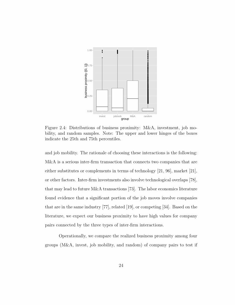
0.00

0.25

0.50

0.75

1.00

invest jobmob M&A randomgroup

busi

ness

pro

xim

ity (

[0, 1

])

Figure 2.4: Distributions of business proximity: M&A, investment, job mo-bility, and random samples. Note: The upper and lower hinges of the boxesindicate the 25th and 75th percentiles.

and job mobility. The rationale of choosing these interactions is the following:

M&A is a serious inter-firm transaction that connects two companies that are

either substitutes or complements in terms of technology [21, 96], market [21],

or other factors. Inter-firm investments also involve technological overlaps [78],

that may lead to future M&A transactions [73]. The labor economics literature

found evidence that a significant portion of the job moves involve companies

that are in the same industry [77], related [19], or competing [34]. Based on the

literature, we expect our business proximity to have high values for company

pairs connected by the three types of inter-firm interactions.

Operationally, we compare the realized business proximity among four

groups (M&A, invest, job mobility, and random) of company pairs to test if

24

the business proximity has a leading effect on the corresponding inter-firm in-

teractions. One may argue that high business proximity values could be the

results of various firm relationships. For example, after an M&A transaction

takes place, it is very likely that the acquiring company’s business description

will incorporate various aspects of the acquired company. To avoid this rever-

sal effect, we only consider inter-firm actions after the business proximity was

constructed (April 2013). Our inter-firm interaction dataset contains 394 com-

pany pairs associated to M&A transactions, 129 with inter-firm investments,

and 9, 792 with job mobility.5 Lastly, to construct the baseline, we randomly

select company pairs from the whole sample.

Figure 2.4 compares the business proximity values among the company

pairs constructed by M&A, investments, job mobility, and random. On aver-

age, the first three groups have more than three times higher proximity than

the randomly-paired group: M&A (0.293), investments (0.224), job mobility

(0.218), and random (0.068). Given the fact that M&A is a rare, significant

inter-firm transaction, it is intuitive to find that M&A-paired firms have higher

similarities than other two interaction types (investments and job mobility).

2.4.2 Empirical Application on M&A Networks

In this subsection, we demonstrate the business proximity measure’s

value for empirical modeling. Specifically, we apply it in analyzing high-tech

5For job mobility, if a person made a job transition from a company A to another oneB, then we consider A and B are associated.

25

M&As. Our objective is to document the relationship between the likelihood

of a pair of firms’ matching in an M&A transaction and their individual and

pairwise characteristics, among which the newly developed business proximity

is of our primary interest. We first summarize the theoretical basis for the

importance of business proximity as well as proximity in three other dimensions

in modeling M&As. Next, we briefly introduce the statistical network analysis

method and explain our empirical specifications. Lastly, we present estimation

results.

2.4.2.1 Proximity and M&A

The high-tech industry is characterized by active and rapid innovation,

significant geographic clustering (at a handful of high-tech hubs), rapid job

mobility, high concentration of ownership at the company level, and strong

influence of angel and venture investors. We posit that business proximity,

geographic vicinity, social linkage, and common ownership are associated with

the likelihood of two firms’ matching in an M&A transaction.

Business Proximity

Business proximity measures firms’ relatedness in the spaces of product,

market, and technology. It has been widely recognized in the literature that

the potential synergy in products, markets, and technologies is a key driver

for M&As [90] and is especially important in high-tech acquisitions [3]. The

central idea of business synergy is that economic surplus can be created from

26

novel recombination of the acquirer and target’s resources and capabilities.

Hence, one of the determinants for the matching of the acquirer and target

should be the recombination potential, which is in turn influenced by the

relatedness of the two firms’ products, markets, and technology (e.g., Cassiman

et al. 2005). Therefore, we expect the business proximity is associated with

the M&A matching likelihood.

Geographic Proximity

Geographic or spatial proximity refers to the closeness of physical loca-

tions and it has been shown to have a moderating effect in a diversity of finan-

cial transactions. In the M&A domain, Erel et al. [32] analyzed cross-border

mergers to show that, among other factors, geographic proximity increases the

likelihood of mergers between two countries. At the firm level, Chakrabarti

and Mitchell [22] found that chemical manufacturers prefer spatially proxi-

mate acquisition targets. The main reasoning behind these findings is that

information propagation is subject to spatial distance; geographic proximity

brings a higher level of knowledge exchange and hence a lower level of informa-

tion asymmetry. For the same reason, we predict that geographic proximity

is positively associated with the M&A likelihood.

We operationalize geographic proximity by measuring the great-circle

distance6 between two companies’ headquarters. First, we translate the street

address of each company’s headquarters into its latitude (φ) and longitude

6http://en.wikipedia.org/wiki/Great-circle_distance

27

(λ) coordinates by using Google Maps API.7 For companies whose full street

address is missing, we use the city center as an approximate. Next, we use

the latitude and longitude coordinates to calculate the great-circle distance.

Specifically, let (φi, λi) and (φj, λj) be the coordinates for companies i and j,

and ∆λ be the absolute difference in their longitudes. Then the geographic

proximity pg(i, j) between companies i and j is defined as

pg(i, j) = −R arccos(sinφi sinφj + cosφi cosφj cos ∆λ), (2.4.1)

where the constant R is the sphere radius of the earth. The negative sign is

to convert distance to proximity.

Social Proximity

Social proximity of two firms is defined according to the social link-

age between the individuals associated with the two firms. Personal linkage

is an important factor in coordinating transactions and promoting private

information exchange between business entities through mutual trust and kin-

ship [52, 28, 108]. We believe two factors about the high-tech industry greatly

contribute to the importance of personal linkage’s role in transmitting vital

information across companies. First, the U.S. high-tech industry, especially

the startup sphere of it, is characterized by high job mobility, which creates

the paths and opportunities for private information flow (Fallick et al. 2006).

Second, early-stage digital startups are mostly very small in size; thus, infor-

7https://developers.google.com/maps/

28

mation about them is often scarce outside the teams’ social circles. Moreover,

many startups intentionally stay in a “stealth mode” before their products and

technologies mature. Hence, we argue that companies with closer social prox-

imity are likely to be aware of each other’s products and intellectual property,

which would lead to a higher M&A probability.

We operationalize social proximity by using the “people” part of our

dataset. For each company, we observe the individuals who are or have previ-

ously been affiliated with it either as a (co)founder, or as a board member, or

as an employee. Let Si denote this set of individuals for company i. Then we

define the social proximity ps(i, j) between two companies i and j as

ps(i, j) = |Si ∩ Sj|, (2.4.2)

i.e., the number of people who are identified having experiences in both com-

panies.

Investor Proximity

Investment proximity is defined according to the common angel and

venture investors who have founded the firms. In the high-tech industry, star-

tups depend on external investments to support product development before

they establish a stable cash flow. As compared with other types of investors,

angel and venture investors often play a more active role in management and

can be highly influential on strategic decisions [6, 45], such as pursuing M&A

opportunities. Hence, common early investors of two high-tech companies can

29

form a critical information bridge or even an initiator and enabler of collabo-

ration between them, which we predict leads a higher likelihood of M&A.

Our operationalization of investor proximity is methodologically simi-

lar to that of social proximity. Given two companies i and j, their investor

proximity pf (i, j) is defined as

pf (i, j) = |Ii ∩ Ij|, (2.4.3)

where Ii and Ij are the sets of investors who have funded companies i and j

in any of the funding rounds respectively.

Correlation Analysis

We explore the realizations of the business, geographic, social, and

investor proximities in our CrunchBase dataset and analyze their correlations

with the matching of M&A. Note that we compute all proximity measures

using company data collected in April 2013 and only use the M&A transactions

that occurred between April 2013 and April 2015 to avoid any possible reversal

effect.

For each of the four proximity measures, we compare its different distri-

butions in two groups of company pairs: (1) group of M&A-matched company

pairs and (2) that of randomly selected pairs. Figure 2.5 shows the empirical

cumulative distribution functions (CDF) of the four proximity measures. For

the (b) geographic dimension, we plot the distance rather than proximity for

intuitiveness. Also note that the business and geographic proximity values

30

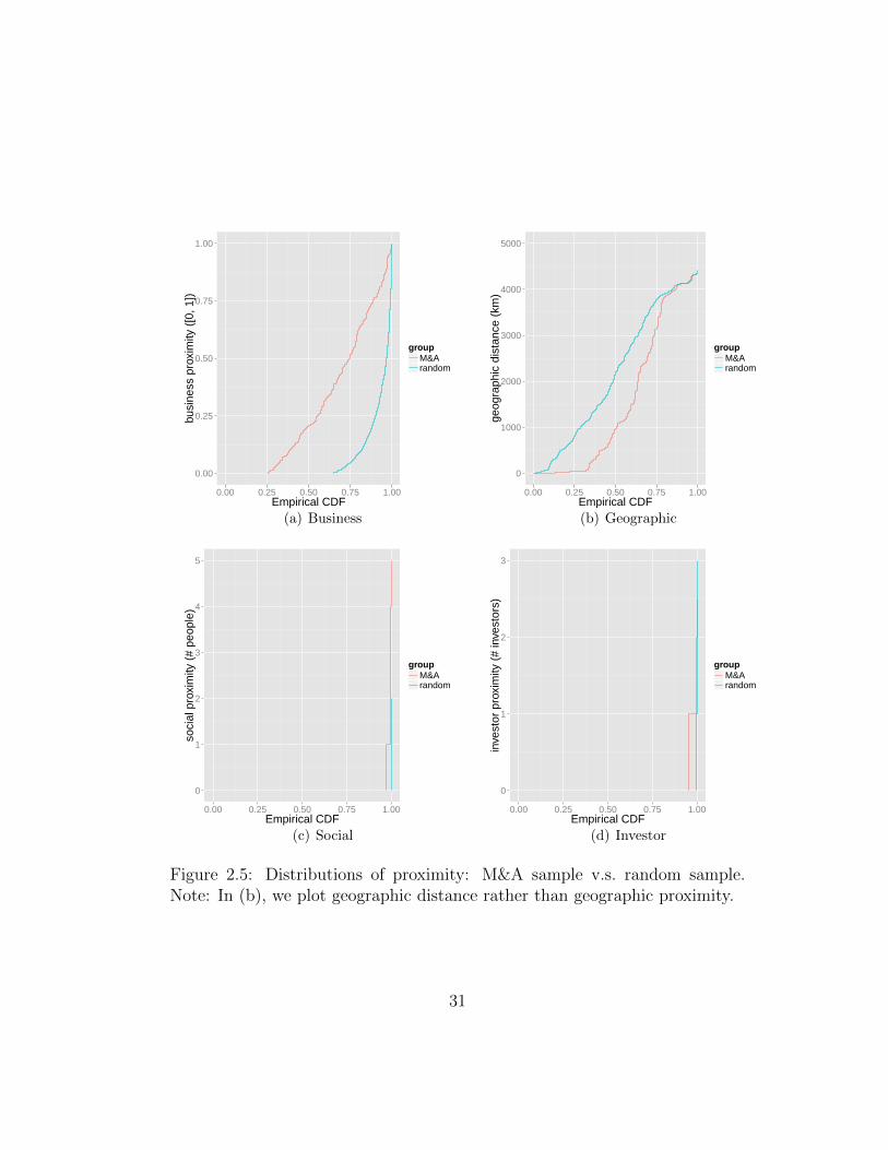
0.00

0.25

0.50

0.75

1.00

0.00 0.25 0.50 0.75 1.00Empirical CDF

busi

ness

pro

xim

ity (

[0, 1

])

groupM&Arandom

(a) Business

0

1000

2000

3000

4000

5000

0.00 0.25 0.50 0.75 1.00Empirical CDF

geog

raph

ic d

ista

nce

(km

)

groupM&Arandom

(b) Geographic

0

1

2

3

4

5

0.00 0.25 0.50 0.75 1.00Empirical CDF

soci

al p

roxi

mity

(#

peop

le)

groupM&Arandom

(c) Social

0

1

2

3

0.00 0.25 0.50 0.75 1.00Empirical CDF

inve

stor

pro

xim

ity (

# in

vest

ors)

groupM&Arandom

(d) Investor

Figure 2.5: Distributions of proximity: M&A sample v.s. random sample.Note: In (b), we plot geographic distance rather than geographic proximity.

31

are continuous, whereas the other two are discrete. In each subfigure, the

red line represents the distribution for the group of company pairs defined by

M&A transactions and the green line shows that of random pairs. For each

proximity measure, we observe a distinction between the two lines, suggest-

ing the existence of dependency between the proximity measures and M&A

transactions (the differences in the two lower subplots are visually less distinct

because both social and investor proximity measures are discrete and have a

large point mass at 0). Next, we appeal to a more rigorous statistical model

for further analysis.

2.4.2.2 Statistical Model

Using statistical terminology, the matching of a pair of firms is a binary

outcome: Either they are part of an M&A transaction or they are not. Thus it

could be tempting to use binary response econometric models such as logistic

regression for the empirical analysis. However, they are inappropriate in this

context due to the relational nature of the data. For example, an M&A trans-

action between firms i and j and that between i and k (which would be two

observations in a logistic regression) are correlated since they involve a com-

mon party, i.e. firm i. Hence, the key assumption of independent observations,

which underlies the binary response econometric models, is clearly violated.

So instead of treating the M&A transactions as independent observations, we

model all of them together as a network.

Exponential random graph models (ERGMs), also known as p∗ models,

32

have been developed in statistical network analysis over the past three decades

and recently have become perhaps the most important and popular class of

statistical models of network structure (see [43] for a survey of models in this

field). As far as we are aware, this modeling framework has not been widely

used in the information systems literature thus far, so we briefly introduce

it here.8 We also provide a list of important notations used in this and the

following sections in Table 2.2 for reference.

A network is a way to represent relational data in the form of a mathe-

matical graph. A graph consists of a set of nodes and a set of edges, where an

edge is a directed or undirected link between a pair of nodes. A network of n

nodes can also be mathematically represented by an n×n adjacency matrix Y ,

where each element Yij can be zero or one, with one indicating the existence of

the i-j edge and zero meaning otherwise. Self-edges are disallowed so Yii = 0

∀i. If edges are undirected (i.e., the i-j edge is not distinguished from the j-i

edge), then Yij = Yji ∀i, j (i.e., Y is a symmetric matrix).

In applications, the nodes in a network are used to represent economic

or social entities, and the edges are used to represent certain relations between

the entities. In this present research, the nodes and the edges are high-tech

companies and the M&A transactions between them respectively, and they

together form an M&A network. In terms of the adjacency-matrix represen-

8The only papers using ERGMs by information systems scholars that we are aware ofare [103] and [35].

33

Network graphY , Yij a random network graph matrix, its i, j elementY−ij all elements except i, j

Y the set of all possible graphs for a fixed set of nodesy, yij a realization of the random network graph and its i, j elementzk(y) a statistic of network graph y

Network statisticst total number of edgesd2 number of nodes which have at least 2 edges

hstas number of edges within state shcatc number of edges within category cpg sum of geographic proximity over all edgesps sum of social proximity over all edgespf sum of investor proximity over all edgespb sum of business proximity over all edges

Nodal characteristicssi state where i’s headquarter is locatedci category to which i belongs

Dyadic characteristicspg,ij geographic proximity of i and jps,ij social proximity of i and jpf,ij investor proximity of i and jpb,ij business proximity of i and j

Table 2.2: ERGM notations

34

tation, we define

Yij =

{1, if i and j are part of an M&A transaction,0, otherwise.

With this definition, the resultant M&A network is undirected.9

ERGMs treat network graph, or equivalently adjacency matrix Y , as

a random outcome. For a network of n nodes, the set of all possible graphs

(denoted Y) is finite. The observed network is one realization of the underly-

ing random graph generation process. For some y ∈ Y, the probability of it

occurring is assumed to be

P(Y = y) =1

Ψexp{

K∑k=1

θkzk(y)}, (2.4.4)

where K is the number of network statistics, zk(y) is the k-th network statistic,

the θk’s are parameters, and the denominator Ψ is a normalizing constant.10

The zk(y) terms capture certain properties of the network and are assumed to

affect the likelihood of its occurring. They are analogous to the independent

variables in a regression model. One common example of network statistics is

the total number of edges in the network (or a constant multiple of it). zk(y)

can be a function of not only the network graph y, but also other exogenous

covariates on the nodes. For example, suppose we have a categorical variable

9Alternatively, we could define a directed “acquisition network” where the edges areasymmetric. That is, we could distinguish the acquirer and the acquired. For our purposeof assessing the business proximity measure, the distinction is not very important sincebusiness proximity is symmetric (and it is also true for the other three proximity mea-sures). In addition, our assumption of undirected M&A network reduces the time neededfor computation when we perform the estimations.

10∑

y∈Y P(Y = y) = 1, so Ψ =∑

y∈Y exp{∑K

k=1 θkzk(y)}

35

on the nodes. Then one such statistic is the number of edges where the two

ending nodes belong to the same category. To interpret the parameters θk, we

can rewrite equation (2.4.4) in terms of log-odds of the conditional probability:

logit(P(Yij = 1|Y−ij)) =K∑k=1

θk∆zk, (2.4.5)

where Y−ij is all but the ij element in the adjacency matrix. Therefore, the

interpretation of θk is: If forming the i-j edge increases zk by 1 and the other

statistics stay constant, then the log-odds of it forming is θk.11 12

2.4.2.3 Specification

Our ERGM specification includes the statistics (zk’s) for degree distri-

bution, selective mixing, and proximity. We iterate them and explain their

interpretations in the M&A context in the following paragraphs. In the dis-

cussion, we translate the generic terms nodes and edges into the more specific

terms firms and transactions.

The degree distribution statistics include: t, the total number of M&A

11It is noteworthy that if the ∆zk’s do not depend on Y−ij ∀i, j, then the edges areindependent of each other, and hence the ERGM model reduces to a standard logisticregression where each edge is considered an independent observation.

12The above summarizes the basic formulation of ERGMs. Despite its relatively straight-forward interpretation and analytic convenience, applications had been limited until just afew years ago due to significant computational burdens. The difficulty lies in evaluating thenormalizing constant in the equation (2.4.4), which involves a sum over a very large samplespace even for a moderate n. It is not hard to see that the number of possible graphs is

2n(n−1) if the network is directed, and the number of possible graphs is 2n(n−1)

2 if the net-work is undirected. Recent advances in computing capability and Monte Carlo estimationtechniques [104, 47] have made possible the significant growth of ERGMs applications inacademic fields such as sociology and demography.

36

transactions, and d2, the number of firms that each are a party of at least

two different transactions. t measures the density of transactions in the M&A

network and its coefficient serves a similar role as the constant term in a re-

gression model. In fact, equation (2.4.5) implies that the coefficient of t is

the log-odds of transaction happening if t were the only statistic in the equa-

tion. Given the sparsity of the M&A network, we expect t’s coefficient to be

negative. The reason why we also include the d2 statistic is because it has

been demonstrated in the prior research that firms with different relational

capabilities [71] participate in significantly different levels of M&A activities.

Wang and Zajac [113] specifically showed that an acquisition is more likely to

occur if any of the two parties have prior acquisition experiences. Moreover,

we have found in the exploratory data analysis in Section 2.2 that the number

of M&A transactions in which a firm is a party follows the power-law distri-

bution. Hence we predict a transaction where either of the two parties that

has previously engaged in M&A transactions should have a different likelihood

than when neither has. The d2 statistic captures exactly this effect and we

expect its coefficient to be positive.

Selective mixing captures the matching of firms according to the combi-

nation of their nodal-level characteristics. In other words, these characteristics

are first defined at the individual firm level, and then combined to the pair level

and lastly aggregated to the corresponding network statistics. In the network

analysis literature, one widely adopted form of selective mixing is assortative

mixing: Social and economic entities tend to form relationships with others

37

that are “similar.” We include two groups of statistics that reflect an analo-

gous kind of selective mixing in M&As and they are constructed based on two

categorical covariates we have on the firms, i.e., state and industry sector. We

expect that a pair of firms belonging to the same category are more likely to

match than otherwise. Specifically, statistic hstas is the number of transactions

between two firms whose headquarters are both located in state s, where s is

one of the 50 states plus the District of Columbia; hsecc is the number of trans-

actions between two firms that belong to the same industry sector c, where c

is any of the 19 sectors described in Section 2.2. We also want to point out

that these two groups of statistics can serve as alternative operationalizations

of geographic and business proximity.

Lastly, the statistics of most interest are the four proximity measures

that capture the matching process based on dyadic-level characteristics. We

normalize the four proximity measures to ensure they have the same standard

deviation. The four statistics each equal the sum of the corresponding char-

acteristic values over all transactions. We use pg, ps, pf , and pb to denote

the sums of geographic proximity, social proximity, investor proximity, and

business proximity respectively. The rationale of including them has been dis-

cussed in Section 2.4.2.1. In the benchmark specification, we include a linear

term for pb. We also estimate an additional specification with a quadratic term

of pb to allow for a curvilinear effect of business proximity on matching.

38

To sum up, our benchmark model specification can be written:

P(Y = y) =1

Ψexp{θtt+θd2d2+

∑s

θstas hstas +∑c

θcatc hcatc +θgpg+θsps+θfpf+θbpb},

(2.4.6)

and the corresponding conditional form is

logit(P(Yij = 1|Y−ij))

=θt∆t+ θd2∆d2 +∑s

θstas ∆hstas +∑c

θcatc ∆hcatc + θg∆pg + θs∆ps + θf∆pf + θb∆pb

=θt + θd2∆d2 +∑s

θstas I(si = sj = s) +∑c

θcatc I(ci = cj = c)

+ θgpg,ij + θsps,ij + θfpf,ij + θbpb,ij.

(2.4.7)

where I(·) is an indicator function, and, for instance, I(si = sj = s) means

companies i and j are in the same state s and I(ci = cj = c) means i and j

belong to the same sector c.

2.4.2.4 Results

The final dataset contains a total of 24,382 companies. This seemingly

moderate number of nodes is actually huge for estimating network models,

since the number of potential edges — in our case un-ordered pairs — close to

300 million. Given our current computational capacity, we cannot handle the

whole dataset in one estimation procedure. To carry out the analysis, we decide

to randomly select 25% of the whole dataset for estimation and repeatedly do

so 100 times. Since the estimation for each subsample is an independent,

computation-intensive task, we parallelized the estimation job using Condor

39

Number of Number of MedianSamples with Samples with Coefficient

Expected Sign p-value Value< 1.0%

θt edges 100(<0) 98 -14.7837θd2 degree> 2 97(>0) 92 3.0064

Table 2.3: Degree distribution coefficients (100 samples)

system,13 which is a Big Data platform to support high throughput computing.

For each of the 100 different samples (6,096 companies each), we estimate

the model coefficients by using the Markov Chain Monte Carlo maximum

likelihood estimation procedure outlined in Hunter and Handcock [54].

We summarize the resultant 100 set of coefficients for the degree dis-

tribution, selective mixing, and proximity statistics in Tables 2.3, 2.4, and 2.5

respectively. For each statistic, we report the number of samples that yield a

coefficient with the expected sign, and the number(s) of samples that yield a

coefficient that has the expected sign and is statistically significant at one or

more selected confidence level(s). Also, to provide an example, we report the

full estimation result for one particular sample in Table 2.6.

Table 2.3 reports the coefficients of the degree distribution statistics.

Among the 100 samples, all θt coefficients are negative and 97 θd2 coefficients

are positive. At the 99.0% confidence level, 98 θt estimates are significant

and 92 θd2 estimates are significant. Hence the results for the two degree

distribution statistics are both consistent with our expectations. As discussed,

13http://research.cs.wisc.edu/htcondor/

40

(a) State

Number of Number of Number of Number of Number of Number ofSamples Samples Samples Samples Samples Samples

with Coefficient p-value with Coefficient p-valueCoefficients > 0 < 1.0% Coefficient > 0 < 1.0%

AK 0 - - MT 0 - -AL 0 - - NC 0 - -AR 0 - - ND 0 - -AZ 0 - - NE 0 - -CA 100 94 43 NH 5 5 3CO 7 7 7 NJ 4 4 3CT 0 - - NM 0 - -DC 5 5 4 NV 0 - -DE 0 - - NY 61 61 22FL 0 - - OH 0 - -GA 7 7 6 OK 0 - -HI 0 - - OR 0 - -IA 0 - - PA 0 - -ID 0 - - RI 0 - -IL 5 5 5 SC 0 - -IN 0 - - SD 0 - -KS 0 - - TN 0 - -KY 0 - - TX 19 19 13LA 0 - - UT 0 - -MA 28 28 16 VA 0 - -MD 6 6 5 VT 0 - -ME 0 - - WA 11 11 6MI 0 - - WI 0 - -MN 0 - - WV 0 - -MO 0 - - WY 0 - -MS 0 - -

(b) Category

Number of Number of Number of Number of Number of Number ofSamples Samples Samples Samples Samples Samples

with Coefficient p-value with Coefficient p-valueCoefficient > 0 < 1.0% Coefficient > 0 < 1.0%

advertising 26 25 7 mobile 28 26 11biotech 38 37 5 net hosting 7 6 6cleantech 11 11 6 other 0 - -consulting 11 10 3 pub rel 8 8 8ecommerce 13 13 3 search 0 - -education 0 - - security 0 - -enterprise 22 22 20 semiconductor 15 15 5games video 26 25 11 software 87 78 37hardware 32 31 25 web 76 66 21legal 0 - -

Table 2.4: Selective mixing coefficients (100 samples)

41

Number of Number of Number of Number of MedianSamples Samples Samples Samples Estimate

with with with with EstimateCoefficient p-value p-value p-value

> 0 < 5.0% < 1.0% < 0.1%

θg Geographic 46 8 5 3 -0.0173θs Social 79 73 70 69 0.1460θf Investor 62 52 51 46 0.0689θb Business 100 92 86 79 0.5315

Table 2.5: Proximity coefficients (100 samples)

the negativity of θt indicates only the overall small probability of an M&A

transaction occurring; the positive sign of θd2 means that an M&A transaction

of which firms with some M&A experience are involved is more likely to occur.

In part (a) of Table 2.4, we find most state-based selective mixing statis-

tics are dropped. This is due the sparsity of M&A transactions during the data

collection period — the likelihood that two same-state companies merged in

an individual sample is low for most states. Indeed, the states that yield the

most coefficients, namely CA, NY, and MA, are where well-known high-tech

hubs are located. In part (b) of Table 2.4, we observe that for almost all

category-based selective mixing statistics, an overwhelmingly large proportion

of the coefficient estimates are positive, but it turns out their statistical sig-

nificance, when using the 99.0% confidence level, is not strongly supported.

One possible explanation of their statistical insignificance is the inclusion of

our business proximity measure. As mentioned, the selective mixing statistics

based on industry sector can also be thought of as alternative, but coarser

operationalizations of business proximity. Therefore, when including both the

42

Coeff S.E. p-value Coeff S.E. p-valueGeographic -0.2699 0.3440 0.4326 NV - - -Social 0.0532 0.0108 0.0000 NY - - -Investor 0.0270 0.0522 0.6049 OH - - -Business 0.4635 0.1378 0.0008 OK - - -Edges -12.5625 3.7908 0.0009 OR - - -Degree> 2 2.4820 0.6438 0.0001 PA - - -State RI - - -

AL - - - SC - - -AR - - - SD - - -AZ - - - TN - - -CA 2.3899 0.8178 0.0035 TX - - -CO - - - UT - - -CT - - - VA - - -DC - - - VT - - -DE - - - WA - - -FL - - - WI - - -GA - - - WV - - -HI - - - WY - - -IA - - - CategoryID - - - advertising - - -IL - - - biotech - - -IN - - - cleantech - - -KS - - - consulting - - -KY - - - ecommerce - - -LA - - - education - - -MA 4.6361 1.1201 0.0000 enterprise 2.9201 0.8882 0.0010MD - - - games video 3.0284 1.0953 0.0057ME - - - hardware 3.7045 1.7912 0.0386MI - - - legal - - -MN - - - mobile 1.8611 1.2047 0.1223MO - - - network hosting - - -MS - - - other - - -MT - - - public relations - - -NC - - - search - - -NE - - - security - - -NH 9.7899 1.5931 0.0000 semiconductor - - -NJ 5.6899 1.6428 0.0005 software - - -NM - - - web -0.9020 2.1375 0.6731

Table 2.6: Model coefficients from Sample 1

43

selective mixing statistics and our business proximity measure in the ERGM

specification, the effect of the selective mixing statistics is superceded by the

effect of the more refined proximity measure, causing the model to produce

insignificant coefficients for the selective mixing statistics. To test the valid-

ity of this explanation, we also estimate another ERGM specification, which

excludes the business proximity measures and for which we report the corre-

sponding results for the selective mixing coefficients in Table 2.7. Comparing

the last columns of Tables 2.4 and 2.7, we find that when using the specifi-

cation without proposed business proximity, a much higher proportion of the

samples produces statistically significant (at the 1.0% significance level) esti-

mates for the selective mixing coefficients. This is thus supporting evidence

for the superiority of the proximity measures we use: They are correlated with

the alternative, coarser measures, but statistically more powerful in explaining

the matching in M&As.

In Table 2.5 we report the estimation results for the four proximity

measures. First and foremost, the new business proximity measure is found to

be strongly associated with the matching likelihood: All the samples produce

positive coefficients and among them 79 estimates are significant at the 99.9%

confidence level. Furthermore, when comparing the proximity measures across

the rows, we observe three among the four proximity measures (except θg ge-

ographic) are positively associated with the likelihood of matching in M&As,

and in particular, our newly developed business proximity measure also out-

performs the other three in terms of statistical significance. Moreover, since we

44

(a) Category

Number of Number of Number ofSamples Samples Samples

with Coefficient p-valueCoefficient > 0 < 1.0%

advertising 28 28 14biotech 37 37 32cleantech 12 12 10consulting 12 12 9ecommerce 12 12 6education 0 - -enterprise 22 22 20games video 28 28 16hardware 31 31 29legal 0 - -mobile 27 27 16net hosting 8 8 6other 0 - -pub rel 10 10 6search 0 - -security 0 - -semiconductor 17 17 14software 89 85 55web 78 70 22

Table 2.7: Category-based selective mixing coefficients (100 samples): Equa-tion (2.4.6) excluding θbpb

45

normalize the proximity measures, we can evaluate their economic significance

by comparing the magnitude of the coefficients. Using the median estimate

from the 100 samples (last column of Table 2.5), we find that the business

proximity measure has the largest effect on matching likelihood: A 1-standard-

deviation increase in business proximity has the same effect as a 3.64-standard-

deviation increase in social proximity, or a 6.89-standard-deviation increase in

investor proximity. These results thus support the value of business proximity

in modeling M&As. Interestingly, in our dataset, the geographic proximity

appears to play an insignificant role in identifying high-tech firms’ matching

in M&As.

The estimation result of equation (2.4.6) shows business proximity is

positively associated with the M&A matching likelihood. However, a linear

structure might not best capture the true relationship between business prox-

imity and M&A matching since the economic benefits of merging two firms’

businesses may result from not only their similarity but also their complemen-

tarity [27, 96]. The value of M&A could decrease in cases where two firms’

businesses are too similar but lack complementarity, so little value of synergy

can be achieved through merger. We test this hypothesis by estimating a speci-

fication that includes a squared term of business proximity, θb2pb2 = θb2∑p2b,ij,

and that is otherwise the same as equation (2.4.6). We expect θb2 to be neg-

ative and θb to be still positive. The estimation results on the proximity

measures (of the 100 samples) are reported in Table 2.8. We do observe that

for a large number of the samples business proximity is estimated to have a

46

Number of Number of Number of Number ofSamples with Samples with Samples with Samples with

Coefficient p-value p-value p-valueExpected Sign < 5.0% < 1.0% < 0.1%

θg Geographic 47(> 0) 6 4 2θs Social 85(> 0) 77 77 73θf Investor 67(> 0) 56 52 50θb Business 100(> 0) 86 76 61θb2 Business2 86(< 0) 42 28 13

Table 2.8: Proximity coefficients (100 samples):Equation (2.4.6) plus θb2pb2

curvilinear effect on the M&A matching likelihood. Specifically, for 86 out of

the 100 samples, the coefficient of the squared term is negative and that of the

linear term is positive, suggesting the matching likelihood first increases with

business proximity and then decreases after a certain point. This evidence is

thus consistent with our expectation. Meanwhile, we note that the evidence

for the statistical significance of the squared term is not as strong as that for

the linear term.

2.5 Platform Prototype: Information System for Indus-try Intelligence

During the recent boom of the high-tech industry, the media are often

full of reports about high-profile M&As involving startups.14 It is well known

that M&As are an important alternative to IPOs as an exit option for high-

tech entrepreneurs and early investors. Meanwhile, industry giants spend tens

of billions of dollars each year in acquiring smaller firms for market entrance,

14 http://www.statista.com/chart/1927/tech-acquisitions/

47

strategic intellectual property, and talented employees.15 Venture capitalists

also arrange mergers between their partially owned startups in order to con-

solidate resources and reduce competitive pressure.16 The fierce competition

in both demand and supply instantaneously creates the problem of matching

between an acquirer and a potential target, since the value (or disvalue) of an

M&A critically depends on the synergy of their products, technologies, and

markets. The other side of this problem is search for targets. While almost

everyone knows who the top competitors are in a particular space, it is a diffi-

cult and time consuming task to find the small companies in the vast startup

universe with the right products or technology. Observers have noted data

analytics can complement executives’ industry knowledge in alleviating some

of the problems in M&A matching and startup search — it is reported that

many large M&A players have already been investing heavily in analytics for

identifying the win-win matches by rendering the decision-making processes

more “data-driven.”17 Along these lines, our empirical analysis indicates the

potential practical value of the proposed business proximity measure as an

important metric in the analytics of M&A matching and startup search. To

show the practical application in a concrete way, we build a prototype for

15See “Internet Mergers and Takeovers: Platforms upon Platforms,” The Economist, May25, 2013.

16An example is the acquisition of Summize by Twitter in 2008. See “Finding A PerfectMatch,” Twitter Blog, https://blog.twitter.com/2008/finding-perfect-match andNick Bilton’s 2013 book Hatching Twitter: A True Story of Money, Power, Friendship,and Betrayal.

17See “Google Ventures Stresses Science of Deal, Not Art of the Deal,” New York Times,June 23, 2013.

48

Front end

Back end

Data collector (Python)

Raw data (MongoDB)Crunchbase

Topic model builder(Scala)

Processed data (MongoDB)

Webpages(HTML/CSS, Javascript)

Company meta info

(JSON)

Business proximity (JSON)

UsersSearch

Company info

API

Cloud DB(Google Datastore,

Google Cloud Storage)

API Engine(Google App

Engine)

Figure 2.6: Prototype architecture and components

a cloud-based information system that allows entrepreneurs, managers, and

analysts to explore the competitive landscape of the U.S. high-tech industry.

By incorporating business proximity and making it explicitly available to the

users in the search and navigation tools, the platform expedites the process

of startup search and competition analysis as well as facilitates efficient new

niche-market discovery. The system largely consists of two components as

shown in Figure 2.6: The back-end collects raw data from the data sources,

integrates and cleans the data, computes business proximity, and stores the

processed data in local databases. The front-end is a web application that

enables users to explore the data stored in a cloud-based database.

49

2.5.1 Back-End System

The back-end system comprises two modules and two databases. The

first module is the data collector written in Python to retrieve data from

CrunchBase API.18 The collector runs periodically to ensure our data is up-to-

date. The raw data is stored in a MongoDB19 database, which is a document-

oriented, NoSQL database that stores records in JSON format. The reason

why we do not use a relational database is that the structure of the com-

pany data may change over time, so the traditional relational database, which

requires a pre-defined schema, is not the best technology for our system. An-

other feature of MongoDB is that it supports scalability: As the data size

grows load balancing can be performed using the shrading mechanism. This

is a basis for the cloud-based information system.

The second module, the topic model builder, constructs and estimates

topic models using the textual company descriptions extracted from the raw

data in MongoDB. To run the LDA topic modeling algorithm, we use a Scala

implementation in Stanford Topic Model Toolkit.20 The topic model builder

produces two sets of results: First, each company’s profile is transformed into

a topic vector, which is stored in the database of processed data in MongoDB.

Next we compute the pairwise business proximity between all pairs of com-

panies using the methodology given in Section 2.3. Note that the number of

18https://developer.crunchbase.com.19https://www.mongodb.org.20http://www-nlp.stanford.edu/software/tmt/tmt-0.4/.

50

companies is relatively large and the number of pairs is even larger, so in-

stead of storing all the pairwise proximity values, the records of the N closest

companies for each firm are inserted into the database in JSON format.

2.5.2 Front-End System

The front-end is a cloud-based web application, available at http:

//146.6.99.242/bizprox, to let users explore various company information

with the proposed business proximity. Figure 2.7 shows the screenshots of the

user interface. Given a keyword from the user, the search results show the

topics and companies associated to the keyword. By selecting topics, the user

can interpret the topic with 20 (additional) relevant keywords and the signif-

icance of each. If a company is selected from the search results, the interface

provides (1) the basic information about the company along with the topic

distribution, and (2) a list of potential competitors of the focal company. The

basic information of a company includes the founding date, founders, head-

quarters, and a short business description. With the topic distribution, users

can recognize various business aspects of the company. Potential competitors

are sorted by the business proximity.

From the system architecture perspective, the front-end is a cloud-

based system leveraging platform-as-a-service (PaaS). The static webpages in

HTML/CSS are hosted by our local Apache Web Server. The server interacts

with the various user inputs such as keyword searches and page navigations.

51

(a) Search companies and topics of interest

(b) Search results

(c) Focal company with its competitors based on businessproximity

Figure 2.7: Prototype front end: User interface screenshots

52

Each webpage is instrumented with Google Analytics21 so that web analyt-

ics is performed to understand user engagement and potentially optimize the

service. An API Engine, deployed in Google App Engine,22 receives queries

from the HTML pages and returns relevant data from the cloud database. The

cloud database consists of two components: First, the dynamic data is man-

aged in Google Cloud Datastore,23 a cloud-based NoSQL database system;

second, the static data is stored in Google Cloud Storage,24 which provides

a cost-effective content distribution service for static information. The cloud-

based approach gives two main benefits: scalability (e.g., the system scales

automatically according to user demand and data size) and availability (e.g.,

almost no downtime due to replication).

2.6 Discussion and Conclusion

In this chapter, we set out with the task of developing a new approach

for measuring firms’ dyadic proximity in the business dimension. Using a

unique dataset of the U.S. high-tech industry, we detailed the process of us-

ing topic models to analyze the publicly available, unstructured descriptions

of company business and computing proximity according to the topic model

results. We then validated the new measure by relating it to simple category

classification and analyzing its statistical relationships with firm interactions

21http://www.google.com/analytics/.22https://developers.google.com/appengine/.23https://developers.google.com/datastore/.24https://cloud.google.com/products/cloud-storage/.

53

including M&A, investment, and job mobility. Through an empirical analysis,

we also demonstrated the new measure’s usefulness in modeling the matching

of M&As. Moreover, to show the practical value of the proposed measure,

we deployed various Big Data and analytics technologies to build a prototype

for a cloud-based information system that leverages business proximity for

competitive intelligence.

Broadly, this research sheds light on the value of leveraging data science

techniques in the development of novel measures for large-scale business ana-

lytics (e.g., Einav and Levin 2013). Our data-driven, analytics-based approach

requires no expert preprocessing, provides finer granularity (compared with the

SIC- or NAICS-based methods), is more comprehensive on quantifying firms’

positions in the product, market, and technology spaces (compared with the

patent- or customer-based methods), and is fully automated and scalable to

Big Data. Thus our general methodology greatly complements the toolkit for

measuring business proximity, and it is especially useful when researchers or

analysts are studying an already narrowly focused industry or when the firms

under study are small and privately held (e.g., startups) so industry classifi-

cation is largely unavailable. Meanwhile, we wish to stress that our measure

is not intended as a replacement for the existing methods in all scenarios.

For instance, when the research question is at a relatively macro level, only

firms’ broad industry membership is important, and all firms’ SIC or NAICS

codes are available, the researcher should not be hesitant to use the SIC- or

NAICS-based methods.

54

If further extended, the proposed method can have broader implications

for both industry intelligence practice and academic research. For analytics-

minded analysts and managers, firms’ relatedness in business is a very im-

portant metric for identifying potential partners, competitors, and alliance or

acquisition targets. The saying in management goes, “if you cannot measure

it, you cannot manage it.” As shown in our study, the new proximity measure

we developed provides finer granularity in quantifying a pair of firms’ related-

ness in spaces of product, market, and technology, and is proved to be effective

in high-tech M&A analytics. Our prototype can be the first step in building a

Business Intelligence (BI) platform to fully realize the new measure’s practical

potential. For business and economics scholars, our method can perhaps be

adapted and serve as an alternative approach of defining market boundary or

identifying industry rivals, which is a crucial step in the empirical research

of industrial organization. Additionally, future research can explore the pos-

sibility of combining topic model results and clustering algorithms to build

an industry hierarchy, which could be a data-driven alternative to the expert-

labeled systems that are currently in use. A data-driven approach is much

needed for industries such as high-tech because the underlying technology is

rapidly changing and the manually labeled industry classification system can

be stale.

In the empirical application on M&A, we adopted the statistical model-

ing framework of ERGMs to accommodate the relational nature of the match-

ing data. The network/graph approach has been fruitfully applied to analyzing

55

a variety of economic exchanges and markets (as surveyed in [31, 56]). How-

ever, whereas the literature is abundant with studies on how networks affect

the interaction and performance of firms, research using rigorous statistical

methods to analyze the structure of inter-firm networks is relatively underde-

veloped. To our knowledge, the M&A application in the study is one of the first

that uses a statistical network model to analyze relational transactions among

companies. We believe statistical network models are currently underutilized

by management scholars in their empirical research on inter-organizational

linkage despite the fact that relational data is actually not uncommon in the

studies of many very important questions. For example, strategic alliances,

investments, and patent license agreements among companies can all be visu-

alized and carefully analyzed as graphs/networks. We predict that with the

growing availability of network datasets and ongoing development of large-

scale computing technologies, statistical network models’ value in management

research will be increasingly recognized.

In closing, we wish to point out some additional caveats and limita-

tions of the research. First, since SIC- or NAICS-based industry classification

or patent data is unavailable in CrunchBase, we could not directly compare

the proposed business proximity measure with that based on industry hier-

archy [113] or the measure based on patent citation [107] in terms of their

explanatory power for M&A matching. Though this is less crucial for this

chapter, since our goal is not to search for the best empirical model for M&As,

it could be an interesting research project to find a suitable dataset where

56

all the new and traditional measures could be operationalized and compared

directly. Second, for our data-analytic approach, the number of topics in

LDA is a free parameter for users to choose. When performing topic mod-

eling on the CrunchBase descriptions, we selected a finite set of values for

this parameter. While choosing one fixed number of topics is sufficient for

our purpose of illustrating the general methodology, from a practical point of

view, it is worth investigating whether an “optimal” number of topics exists,

and if so, how it should be determined [110]. Third, in the machine learning

literature, there are several extensions to the LDA algorithm [110, 55] Future

research could investigate how these extensions could benefit understanding

company businesses through text analysis. Fourth, some important company-

level characteristics — notably company size and revenue — are unavailable

in our dataset, which inevitably limited our ability to extend our empirical

application on M&A matching. For instance, had we observed company size,

we would be able to study the moderating effect of companies’ size on the

relationship between business proximity and the matching likelihood. Lastly,

the model we employed in the empirical analysis is a static network model.

To deepen our understanding about the dependence structure of M&A trans-

actions, future research could examine the evolution of the M&A network by

using some dynamic network models [61].

57

Chapter 3

Matching Mobile Applications for Cross

Promotion

3.1 Introduction

The mobile ecosystem is one of the most successful markets in recent

years [85, 20, 119]. Millions of mobile applications (apps) are developed in

multiple mobile app markets such as Apple’s App Store, Google’s Play Store,

and Microsoft’s Windows Phone Store. Billions of people are adopting smart-

phones and tablets as their main Internet devices, so the demand for mobile

apps keeps increasing. This successful two-sided market is opening up a post-

PC era in the computing industry.

Product diversity is one of the key success factors in the mobile app

market. In addition to the first-party apps developed by the platform builders,

open application programming interface (API) allows third-party developers

to bring innovative products to the market. Of note is that a significant

number of third-party apps are developed by relatively small-sized startups

with the support of various platforms. New mobile apps can reach the global

market through well-established distribution channels, and new app services

0A preliminary version of this chapter was presented in the Conference on Big DataMarketing Analytics [62].

58

can support large user demands with cloud services without large investments

on infrastructure. As a result, we are experiencing a huge growth in mobile

app markets.

Our expectation of this market is that the mobile app popularity follows

a long-tail distribution [8]: many apps with small user bases contribute to a

significant portion of the total market share. However, recent studies have

found evidence that mobile app markets are actually experiencing a “winner-

takes-all” phenomenon [85, 121]. A recent TechCrunch report indicated that

54% of total app store revenue goes to only 2% of the developers and that

almost half of the developers earn less than $500 a month.1 This is a sharp

contrast to other online markets such as video streaming [8], auctions [53],

retail [70], and even music stores. Actually, many independent app developers

have already switched to more stable positions in established firms.2 Norumra

recently reported that even the Chinese mobile game market shows signs of

slowdown because no killer apps emerge in the market.3 We argue that this

phenomenon can compromise the vitality of the mobile app markets.

It is believed that this market inefficiency is due to the fact that app

advertising (ad) heavily relies on app marketplaces’ in-house ranking systems,

which provide lists of popular and growing apps in different ranking criteria.

Hence the developers’ primary goal is to somehow get into the rankings, rather

1http://techcrunch.com/2014/07/21/the-majority-of-todays-app-businesses-are-not-sustainable/2http://apple.slashdot.org/story/14/07/30/1838203/

is-the-app-store-broken3http://blogs.barrons.com/asiastocks/2014/09/08/nomura-tencent-qihoo-may-see-pressure-on-mobile-gaming/

59

than to produce high-quality software. Without an efficient app search mech-

anism, customers are mainly exposed to the top ranked apps, which cover only

a small fraction of the whole market. This trend calls for better marketing

strategies to promote mobile apps to potential active customers and to enable

users to search the right apps that fit their needs.

Cross promotion has recently emerged as a way to recommend new

apps to the users who are already using related established apps. For exam-

ple, game app developers can promote their new products to the active users

playing other games of a similar genre. For new app developers, this is an

effective ad channel to reach potential customers. For the established app

publishers, cross promotion provides a way to monetize their visibility. Poten-

tially established apps may even improve their reputations by providing good

app recommendations to their customers. Cross promotions incentivize users

to install and use new apps by providing credits (e.g., free game items) in the

apps they use.

Figure 3.1 shows a screenshot of a cross promotion event from IGA-

Works, a Korean mobile ad company. In this promotion, an app introduces

a list of other apps along with the rewards to give if users participate the

event by installing or using the apps. There are many active cross promotion

networks including AppFlood,4 Chartboost,5 Tapjoy,6 and LeadBolt.7 In a

4http://appflood.com/5https://www.chartboost.com/en/platform#cross-promotion6http://home.tapjoy.com/7http://www.leadbolt.com/developer-tools/

60

Figure 3.1: Screenshot of cross promotion campaigns (Source: IGAWorks)

61

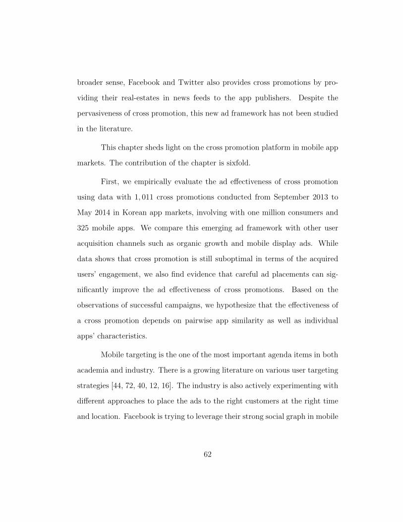
broader sense, Facebook and Twitter also provides cross promotions by pro-

viding their real-estates in news feeds to the app publishers. Despite the

pervasiveness of cross promotion, this new ad framework has not been studied

in the literature.

This chapter sheds light on the cross promotion platform in mobile app

markets. The contribution of the chapter is sixfold.

First, we empirically evaluate the ad effectiveness of cross promotion

using data with 1, 011 cross promotions conducted from September 2013 to

May 2014 in Korean app markets, involving with one million consumers and

325 mobile apps. We compare this emerging ad framework with other user

acquisition channels such as organic growth and mobile display ads. While

data shows that cross promotion is still suboptimal in terms of the acquired

users’ engagement, we also find evidence that careful ad placements can sig-

nificantly improve the ad effectiveness of cross promotions. Based on the

observations of successful campaigns, we hypothesize that the effectiveness of

a cross promotion depends on pairwise app similarity as well as individual

apps’ characteristics.

Mobile targeting is the one of the most important agenda items in both

academia and industry. There is a growing literature on various user targeting

strategies [44, 72, 40, 12, 16]. The industry is also actively experimenting with

different approaches to place the ads to the right customers at the right time

and location. Facebook is trying to leverage their strong social graph in mobile

62

app ads market.8 Google recently announced a new technology to track mobile

app usages along with mobile web behaviors for better ad targeting.9 Existing

approaches target users according to locations, times, and social relationships.

Our approach is to target potential active app users by selecting the right apps

where cross promotions are conducted. In doing so, we leverage topic model

based app similarity between apps hosting the promotions and those to be

promoted.

The second contribution of the work is to model ad placement in cross

promotion as a matching problem. Given the apps to promote and those

where ads can be placed, the cross promotion platform should arrange the most

effective matchings between apps to meet the requirements of the stakeholders.

Matching markets have been well studied in the economics literature with

many applications such as marriage and dating [38, 51], labor market [91, 92,

93], and school admission [1, 33]. To the best of our knowledge, our work is

the first to frame a matching problem in mobile app markets.

Third, we propose a novel app similarity measure constructed with

apps’ text descriptions. Specifically, we apply latent Dirichlet allocation (LDA)

topic modeling [18, 17] on the app description texts. The resulting topic

model gives the trending topics in the current app market and also transforms

individual apps into topic vectors. Then the app similarity is calculated by

8https://developers.facebook.com/docs/ads-for-apps9http://adage.com/article/digital/google-tie-mobile-web-app-trackers-ad-targeting/

294502/

63

the cosine similarity between topic vectors.

Next, we empirically estimate our model to identify the variables that

improve the ad effectiveness in cross promotion. Specifically, we are interested

in similarity between source apps (where the ads are placed) and target apps

(which are the ones to promote in the campaign). We find evidence that the

proposed app similarity has significantly positive effects to improve the ad ef-

fectiveness. In other words, a cross promotion is likely to be successful if source

and target apps are closely related. This can be a basis for a recommender

system for app markets.

Based on the empirical results, we design a matching mechanism for

cross promotions. Using the learned model, a linear programming (LP) based

algorithm is used to provide stable matchings. Our counterfactual analysis

shows that the matching obtained from the LP can improve the ad effectiveness

by 260%.

Lastly, this work can serve as an example of Big Data approach to

bring machine learning techniques and economic theory into the marketing

literature. Many ad frameworks can be modeled as matching problems as

done in the present chapter. Also, an unprecedented large amount of unstruc-

tured text information about products can be analyzed with machine learning

algorithms, as shown in this work.

The remainder of the chapter is organized as follows. In Section 3.2,

we describe the data on mobile apps and promotions, then compare the ad

64

effectiveness of different ad channels. In Section 3.3 we model ad placements

in cross promotion as a matching problem, and overview the independent vari-

ables in the model with the introduction on the novel app similarity measure

in Section 3.4. Empirical results are given in Section 3.5. Based on the ob-

servations, a stable matching algorithm is designed in Section 3.6. Section 3.7

concludes the chapter with future directions.

3.2 IGAWorks Data

We first describe data on mobile app markets, then compare the effec-

tiveness of three ad channels – organic growth, mobile display ads, and cross

promotions – in terms of user engagements.

3.2.1 Data Description

We use data from IGAWorks, a leading mobile advertising company in

Korea.10 The product line includes a mobile app analytics tool called Adbrix

and a mobile app monetization platform supporting various promotions such

as mobile display ads and cross promotions. It has the largest mobile ad

network in Korea, including hundreds of mobile apps and 2.4 million users.

The data was shared by the company using a secure channel. All personally

identifiable information (PII) is anonymized to preserve user privacy.

The data consists of three parts: app meta data, usage data, and funnel

10http://www.igaworks.com/en/

65

data. The meta data includes descriptive information about 383,896 mobile

apps in three major app markets in Korea: Apple’s App Store, Google’s Play

Store, and SK Telecom’s T-store. Play store and T-store provide Android apps,

whereas the App Store serves iOS apps. Each app record contains the app

name, text description, screenshots, developer, registration time, last update

time, price, number of ratings, average rate, and file size. Note that this

information is publicly available in the app markets.

Usage data includes detailed information about user engagements. This

user level data includes daily app session times (i.e., how long a customer uses

an app), daily connection counts (i.e., how many times a customer executes

an app), and daily buy activities (i.e., how many times a customer makes in-

app purchases). Usage data is available for 501 apps that adopted the Adbrix

analytic tool and a total of 1.1 million users’ activity data is captured over a

six-month period in our data. Note that buy activity is available only for apps

with in-app purchase options.

Lastly, funnel data provides information on promotions that IGAWorks

has executed with its clients (app developers). The promotions were conducted

from September 2013 to May 2014, involving 310, 183 users and 325 mobile

apps. Ad types include cross promotions and mobile display ads. The data

keeps track of user acquisition channels for each app. In other words, we

observe how and when a given user installed the promoting app, which is the

basis to evaluate the effectiveness of promotions.

66

3.2.2 Effectiveness of Ad Channels

We measure the effectiveness of a given ad campaign by combining

funnel and usage data. We divide user groups according to the acquisition

channels: organic growth, mobile display ads, and cross promotions. A user is

organic with respective to a mobile app if the app installation is not associated

to any ad campaigns. Users are associated to mobile display ads if they in-

stalled the app by clicking the banner ads placed in mobile websites or mobile

apps [16]. Lastly, a user is in cross promotion group if he or she installed the

app through a reward-based cross promotion conducted in another app. Note

that reward is the differentiator of cross promotion as compared with mobile

display ads placed in other mobile apps.

Ad effectiveness can be measured with various user engagement metrics

such as session times, connection counts, or buy activities. In our study, we

focus on session times and connection counts because buy activities are only

available in mobile apps with in-app purchase options. We say an ad channel

is effective if the users acquired through the channel show active engagements

(e.g., longer session time). We argue that the number of app downloads is not

a good metric of ad effectiveness because the users acquired from promotions

may not end up being active users.

Figure 3.2 shows the average user session times in three user acquisition

channels: organic, mobile display ads, and cross promotions. We observe that

organic users are the most active group. This finding is intuitive because an

app installation without any external inputs indicates the user’s strong moti-

67

0

5

10

15

20

total organic display cross cross_10% cross_1%channel

hour_avg

Figure 3.2: Ad effectiveness comparison

68

vation to use the app. User groups from display ads show 50% less engagement

than organic user groups. Lastly, we clearly observe that users acquired by

cross promotions are the least active group. Since the app installation in cross

promotion is incentivized by the rewards, users may install the promoting

apps but do not use them afterwards. This is an issue for both the promotion

platform and participating apps because the promotion yields a low return on

investment.

Next, we conduct an in-depth analysis within cross promotions. For a

given app to advertise (we call it target app), there are multiple apps where

the ads can be placed (we call them source apps). For a given target app,

we divide its users according to the specific acquisition subchannel (e.g., the

source app). Then for each source-target pair, we calculate the average user

engagement levels, then identify 1% and 10% best pairs for each target app.

We find that top 1% matches are 690% more effective than the average ones

and that the top 10% are 130% more effective than the average. Results also

show that the top 1% matches outperform the display ads in almost half of

the target apps (48%), and they even outperform organic acquisitions in 22%

of the samples. Based on these observations, we argue that the app matches

in cross promotion should be optimized so that the ads are targeted to the

right source apps which users are likely to be active in the target apps.

Given the large impact of source-target matching on the ad effective-

ness, the question is what makes a good match. We compare the list of good

matches with that of bad ones to find that a pair of apps with similar genres

69

and topics makes a good match. For example, a new poker game is actively

used by the users acquired from other similar gambling games. On the other

hand, bad matches involve two unrelated apps such as a celebrity photos app

and a utility app. Based on these observations, we hypothesize that app simi-

larity positively contributes to the ad effectiveness of cross promotions. In the

next section, we build a model of ad effectiveness in cross promotions. Then

we operationalize the app similarity measure in Section 3.4.2.

3.3 Modeling Cross Promotion Network

A cross promotion involves with three groups of entities: source app,

target app, and the promotion platform. App publishers who want to promote

their (target) apps make contracts with the platform to launch a campaign with

the specific number of app installations to acquire. Then the cross promotion

platform places the ads in the (source) apps that agreed to conduct cross

promotions. Note that source apps are mostly popular ones that already have

large user bases, whereas targets are usually new apps with limited awareness

in the market. Thus we assume no overlaps in source and target apps.

Source apps are paid by the targets according to the number of target

app installations they achieved and the promotion platform gets a cut on each

installation. Essentially, this is a cost-per-action (CPA) pricing model. A

campaign is finalized when the number of app installations reaches the goal.

One thing to note is that the utility of source apps and the platform is based

on app download counts, where the objective of target apps is to acquire active

70

users. This misalignment of these two objectives may explain the suboptimal

ad effectiveness of the current cross promotion data shown in Section 3.2.2. In

order for the promotion market to sustain, the objectives of sources, targets,

and the platform should be harmonized.

Another economic insight about cross promotion is that the platform

acts as an intermediary match maker to match source and target apps. Thus

cross promotion framework creates a two-sided matching market rather than a

commodity market. In a commodity market, it is assumed that sellers (source

apps in our case) and buyers (target apps in our case) have perfect information

about each other and that sellers and buyers can switch their roles in differ-

ent situations. Also, prices and transactions can be determined without any

intermediary. However, the cross promotion market has information asymme-

try issues: Source apps have superior information about the customers than

do target apps and they may only want to reveal private information to the

matched counterparts. Also, the platform has extensive knowledge about the

whole market. Thus the existence of the promotion platform as a match maker

is essential.

Matching markets have a strong theoretical foundation established in

the economics literature [38, 91, 92, 93, 1, 33, 51, 49]. The theory has been ap-

plied to many empirical studies involving with marriage [38], online dating [51],

labor market [91, 92, 93], and school admission [1, 33].

We frame the ad placement in cross promotion as a matching problem.

Let S be the set of source apps where ads can be placed and T be the set of

71

target apps to be advertised. Then let G =< V,E > be the bipartite graph

where V = S ∪ T and S ∩ T = ∅. For a given target app t ∈ T , the platform

should select a source app s ∈ S, creating an edge (s, t) ∈ E. Note that an

edge is not created within the same subset (S or T ) under our assumption.

The effectiveness of an app match u(s, t) is measured by the user en-

gagement levels in target t. Our hypothesis is that the effectiveness depends

on the individual characteristics of s and t and the pairwise similarity between

s and t. Thus the effectiveness of an app match is given by a linear functional

form:

u(s, t) = α0 + α1Xs + α2Xt + α3Ps,t + εs,t (3.3.1)

where Xs and Xt represent individual characteristic vectors of apps s and t

(e.g., popularity, quality, age). εs,t is the individual heterogeneity of a match s

and t, and is independent across all pairs (s, t). Then Ps,t is the symmetric app

similarity between apps s and t (Ps,t = Pt,s) and parameter α3 measures the

tendency that users engage in similar apps. In our context, the similarity mea-

sure is operationalized by apps’ text descriptions. Details on the independent

variables are described in Section 3.4.

3.4 Mobile App Characteristics and Similarity

In this section, we describe mobile apps’ individual characteristics con-

sidered in the model, then propose a novel pairwise app similarity measure by

72

applying a machine learning technique to apps’ text descriptions.

3.4.1 Individual App Characteristics

Recent empirical studies on app markets have shown that various app

characteristics (e.g., popularity, quality, age, complexity) affect the user pref-

erence [41, 65, 119]. To capture app popularity in our model, we use number

of ratings (Num Rates) reported in app markets. It is worth noting that the

number of app downloads is not publicly available in most markets [41]. Thus

we use rate count as a proxy for app popularity. Then we use the average rate

(between 1 and 5) to capture the latent app quality observed by the existing

app users (Avg Rate). We also consider two age-related variables: number of

days since the initial app registration (Days Regist) and number of days since

the last update (Days Update). One may argue that old apps are likely to lose

attention as people search for new things [36, 118]. On the other hand, we

may expect that apps that have survived a long time have some compelling fea-

tures that keep consistent user engagements. Recent update time reveals the

developer’s engagement level in the product: If an app does not have update

for a long period, it may indicate that developers lost interest in adding new

features. The last individual app characteristic is the file size in megabytes

(File Size). Large file size may indicate that the developer made significant

efforts and that the app has complex functionalities.

73

3.4.2 Topic Models and App Similarity

Besides individual app characteristics, we argue that app similarity

can positively affect the ad effectiveness in the model. Studies show that

people usually stick to a certain taste when they select products in online

shopping [70], music streaming [48], and mobile app usage [80]. Essentially,

customers’ tendencies to choose similar products is the basis for online rec-

ommender systems. One may argue that app genre can be used to measure

app similarity. However, this method can only provide binary relationships

between apps, which is not sufficient for our purpose to measure the degree of

closeness.

App similarity is operationalized by processing apps’ text descriptions.

Developers provide detailed app descriptions in the app market so that poten-

tial users can understand the features provided by the apps. A pair of apps

with similar descriptions is supposed to share common features such as game

genres, usage scenarios, and so on. The issue is how we process unstructured

text descriptions in a principled way to quantify the pairwise closeness.

Our approach is to use latent Dirichlet allocation (LDA) topic modeling

on the app description corpus [18, 17]. LDA is a natural language processing

technique that allows a set of documents to be explained by hidden topics,

which are sets of related keywords. LDA has been successfully used to analyze

documents in various domains such as scientific articles [46, 111, 17], music [48],

social media [89, 115, 63], and firms [99]. In our context, each app description

is a mixture of a small number of app features and each word in the description

74

is a realization of the app features. For details on LDA see [17].

We run LDA on the text descriptions of 195,956 mobile apps in Korean

market. We vary the number of topics to find that 100-topic model gives the

best result. Table 3.1 shows a partial list of 100-topic model.11 The keywords

in each topic are translated into English for readability. We believe that the

topics give a reasonable overview of the app market. Topics in the Korean app

market include music (topics 0, 27), social networks (topics 1, 14, 25, 41, 89),

kids (topics 6, 34), religion (topic 11), games (topics 16, 27), sports (topic 76),

online dating (topic 96), foreign language education (topics 19, 33, 81, 93),

e-commerce (topics 18, 29), and utilities (topics 10, 13, 48, 49, 97).

Once the topic model is built, an app i’s description can be represented

by a topic vector Vi =< Vi,1, Vi,2, ..., Vi,K >, where K is the number of topics,

Vi,k is the weight on the k-th topic, and the sum of weights is 1 (∑K

k=1 Vi,k = 1).

Given a pair of source s and target t and their topic vectors Vs and Vt, we define

the app similarity P (s, t) (Topic Similarity) to be the cosine similarity of

the two topic vectors as follows:

P (s, t) =Vs · Vt||Vs||||Vt||

=

∑Kk=1 Vs,kVt,k√∑K

k=1(Vs,k)2

√∑Kk=1(Vt,k)2

(3.4.1)

where the resulting values range from 0 to 1. For the extreme cases, P (s, t) = 0

if two apps do not share any common topics and P (s, t) = 1 if two apps have

11For full list of topics and keywords, see http://diamond.mccombs.utexas.edu/app.

topic.keywords.txt

75

Topic ID Top Keywords

0 piano, sskin, classic, flipfont, sound, symphony

1 Naver, Kakaotalk, subway, radio, radion, radic

3 color ring, background, service provider, copyright

6 kids, Cocomong, animation, hearts, master

8 icon, Hello Kitty, atom, screen, game, cute

10 LTE, contract, content, SK Telecom, SKT, promotion

11 hymn, copyright, bible, the Lord’s prayer

13 series, galaxy, final, system, fantasy, wifi

14 friends, facebook, play, graphics, developers

16 car, racing, simulation, parking, bicycle, place

18 point, gift card, reference, cookie run, content

19 Chinese, maker, content, foreign language, kids

25 camera, image, frame, emoticon, sticker, gallery

27 music island, epilus, mr karaoke, karaoke, hellip

28 lotto, tethering, seller, lottery, lottery number

29 social commerce, shopping mall, gifts, brand

33 English listening, smart teps, ted, smart

34 Pororo, friends, animation, sing, kids

36 what’s the number, poweramp, go locker, phone number

41 naver, dodol launcher, dodol home, blog, icon

42 kakao talk, alert, kakao story, passrod, theme

45 recruiting, job korea, resume, check card, saramin

48 calendar, anniversary, diary, point, day, time management

49 subway, bus stop, guide, public transportation, offline

51 Korean language, Korea, travel, tourism, smart wallet

53 fortune telling, 2014, love, money, content, new year

56 drama, vod, content, rate, youtube, high resolution

67 NFC, touch, USIM, smart, sd card, app, record

68 diet, calorie, recipe, stretching, fitness, trainer

76 sports, baseball, NBA, world cup, score, KBO, Spain

80 book 21, story, series, show, homepage, email

81 title, YBM, CNN, TOEIC, YFS, word, Japanese, network

85 mp3, battery, 50 songs, series, recorder, ebooks

89 naver, blog, post, mail, diary, NHN, content, navercc

93 Korean, Spanish, Chinese, French, German, Japanese, Italian

96 blind date, date, ideal, profile, social dating

97 wall paper, 7days, subway, love, image

99 vocab, megabox, vocabulary bible, traffic information

Table 3.1: A partial list of 100 topic model of mobile apps: Korean keywordstranslated into English for readers 76

identical topics. Similar approaches are used to measure user similarity in

social networks [63] and firms’ business proximity in high tech industry [99]

3.5 Empirical Analysis

In this section, we present the estimation results on the ad effectiveness

of cross promotions. We collect the list of target apps that have conducted

cross promotion campaigns along with the list of corresponding source apps

where the ads were placed. The cross promotion data includes 1,011 app

matches and 310,183 users. An app match in a promotion is said to be effective

if the promotion acquires active users with longer session times and higher

connection counts.

Table 3.2 shows the estimation results on user session times and Table

3.3 gives those on user connection counts. For a robustness check, we estimate

four different models by including and excluding various app characteristics.

Characteristics can be divided into two groups: customer-given and developer-

given. Customer-given variables include number of ratings (for popularity) and

average rates (for quality), and developer-given ones are registration time (for

age), update time (for responsiveness), and file size (for complexity).

We find strong evidence that the effect of app topic similarity, Topic Similarity,

on ad effectiveness is significantly positive. The results are consistent with all

models in both dependent variables. This result validates our hypothesis that

people tend to like target apps that are highly similar to sources. It means that

the user preference on app adoption is to some extent predictable based on

77

User session time of target apps (minutes)

(1) (2) (3) (4)

Topic Similarity (0˜1) 25.4915*** 5.801e+01*** 54.846372*** 6.116e+01***(<2e-16) (<2e-16) (<2e-16) (<2e-16)

Num Rates Source 1.538e-02*** 2.778e-03(0.000128) (0.7313)

Num Rates Target -1.302e-03 -2.218e-03*(0.268803) (0.0625)

Avg Rate Source (1˜5) 1.689e+01*** 2.280e+01***(<2e-16) (<2e-16)

Avg Rate Target (1˜5) 1.162e+01*** 1.434e+01***(4.44e-05) (7.34e-07)

Days Regist Source -0.087131*** 2.156e-02(<2e-16) (0.1919)

Days Regist Target 0.073222*** 6.567e-02***(<2e-16) (<2e-16)

Days Update Source 0.074570*** -3.822e-02(0.00919) (0.2231)

Days Update Target -0.230001*** -2.405e-01***(4.14e-13) (4.29e-14)

File Size Source -0.108862 -5.627e-01***(0.12014) (1.12e-09)

File Size Target 0.253022*** 2.338e-01***(<2e-16) (<2e-16)

Intercept 15.1479*** -1.117e+02*** 8.535493** -1.588e+02***(<2e-16) (<2e-16) (0.28598) (< 2e-16)

Observations 310,183 310,183 310,183 310,183

Table 3.2: Multivariate linear regression results on user session timea

aNote: This table shows the estimation result on ad effectiveness in an app match.Results show that the effect of app similarity is significantly positive. * indicates statisticalsignificance at the 10% level, ** at the 5% percent level, and *** at the 1% level.

78

User connection count of target apps

(1) (2) (3) (4)

Topic Similarity (0˜1) 5.1517*** 9.255e+00*** 8.018898*** 8.939e+00***(<2e-16) (<2e-16) (<2e-16) (<2e-16)

Num Rates Source -1.393e-03* 2.271e-03(0.0525) (0.116667)

Num Rates Target -4.128e-04** -3.627e-04*(0.0500) (0.088721)

Avg Rate Source (1˜5) 3.134e+00*** 3.650e+00***(<2e-16) (<2e-16)

Avg Rate Target (1˜5) 3.999e+00*** 4.259e+00***(3.94e-15) (<2e-16)

Days Regist Source -0.008145*** 1.146e-02***(5.65e-07) (0.000107)

Days Regist Target 0.006517*** 6.057e-03***(2.38e-09) (7.60e-08)

Days Update Source 0.029420*** 9.692e-03*(9.27e-09) (0.084234)

Days Update Target -0.053952*** -5.477e-02***(<2e-16) (<2e-16)

File Size Source 0.091901*** 3.489e-02**(2.26e-13) (0.034796)

File Size Target 0.022574*** 2.057e-02***(3.20e-06) (2.41e-05)

Intercept 4.0839*** -2.586e+01*** 2.164251*** -3.417e+01***(<2e-16) (<2e-16) (0.00144) (<2e-16)

Observations 310,183 310,183 310,183 310,183

Table 3.3: Multivariate linear regression results on user connection counta

aNote: This table shows the estimation result on ad effectiveness in an app match.Results show that the effect of app similarity is significantly positive. * indicates statisticalsignificance at the 10% level, ** at the 5% percent level, and *** at the 1% level.

79

the current apps they are using. This result can be a basis for a recommender

system to introduce new apps to users according to the topic similarity.

Empirical results also show that various individual app characteristics

have significant impacts on app engagement. First, the effects of average rat-

ings of both source (Avg Rate Source) and target (Avg Rate Target) apps are

significantly positive. This finding indicates that apps with better quality are

more attractive to the customers, which follows intuition. An interpretation

on the source app quality effect can be that promotions from high quality apps

are perceived to be more reliable to the customers, which leads to high user

engagements. A similar phenomenon can be found in job markets: applicants

recommended by well established people are more likely to be accepted by the

recruiters.

We do not observe consistent effects of app popularity on the ad effec-

tiveness (Num Rates Source and Num Rates Target). Target apps are usually

new in the market, so the rate counts may not matter. However, it is inter-

esting that even the source app’s popularity does not have consistent effects.

This may indicate that ads should be placed with the “right” apps, not the

“popular” ones.

Next we consider developer-given variables. The target app’s age (Days Regist Target)

has a significantly positive impact on user engagement. An interpretation can

be that apps that have survived in the market for a long time have intrinsic

values in them. The number of days since last update (Days Update Target)

has a significantly negative impact on engagement. In other words, target

80

apps with infrequent updates are less likely to keep the customer’s attention.

This may suggest that app developers should actively respond to their cus-

tomers’ feedback and add new features to their products. Results show that

source apps’ age-related variables do not have consistent effects. Lastly, the

file size of target apps (File Size Target) has a significantly positive effect

in all the models, indicating that well-made apps are more likely to increase

user engagements.

3.6 Matching Mechanism Design

We design a matching mechanism for cross promotions, followed by the

model introduced in Section 3.3. Given the set of target apps that want to

be advertised and the set of source apps who can provide real-estate for cross

promotions, the platform should decide an assignment to meet the require-

ments from sources and targets. We leverage the model on ad effectiveness

to calculate the expected utility of each app pair. There are three main is-

sues to consider in designing the matching mechanism: utility transferability,

information structure, and monogamy.

We first discuss the utility of matchings. In the literature on marriage

matching market [38], the utility of each side is separated as compensating

transfers are not allowed. However, in the cross promotion market, utility

can transferred from targets to sources according to the performance of the

promotions. This is similar to the model from Shapley and Shubik [97]. A

target app’s gained utility of a match can be interpreted as the engagement

81

levels of the users achieved by the matched cross promotions. The utility of

a source app is the reward it gets when one of its users installed the target.

Based on the empirical results in Section 3.5, we define the utility of a potential

app match to be the ad effectiveness given by Equation 3.3.1.

The next design issue is about the information structure. We assume

that perfect and cost-less information about potential matches is available

to all participants. In other words, each target (source) app is aware of the

potential utility achievable from all possible source (target) apps. This is a

reasonable assumption because all the variables (text descriptions, ratings,

ages, etc.) needed to estimate the ad effectiveness are public information

available in the app markets.

Lastly, we assume monogamous matching in cross promotions: one

target (source) can be assigned to at most one source (target). In most cases,

the platform should perform one-to-one matchings. However, some promotions

involve multiple target apps where a popular source app hosts multiple cross

promotions simultaneously. This scenario can be modeled as many-to-one

matchings as in job markets, where multiple employees can work for a single

company [60].

In summary, the app matching problem can be considered a frictionless

one-to-one matching with transferable utilities.

Now we formally design the matching mechanism. Let S be the set of

source apps where ads can be placed and let T be the set of target apps to

82

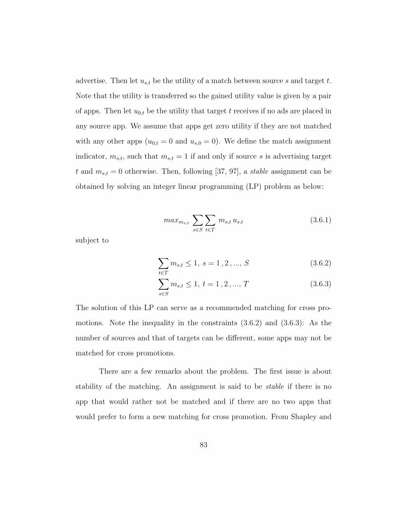
advertise. Then let us,t be the utility of a match between source s and target t.

Note that the utility is transferred so the gained utility value is given by a pair

of apps. Then let u0,t be the utility that target t receives if no ads are placed in

any source app. We assume that apps get zero utility if they are not matched

with any other apps (u0,t = 0 and us,0 = 0). We define the match assignment

indicator, ms,t, such that ms,t = 1 if and only if source s is advertising target

t and ms,t = 0 otherwise. Then, following [37, 97], a stable assignment can be

obtained by solving an integer linear programming (LP) problem as below:

maxms,t

∑s∈S

∑t∈T

ms,t us,t (3.6.1)

subject to

∑t∈T

ms,t ≤ 1, s = 1 , 2 , ..., S (3.6.2)∑s∈S

ms,t ≤ 1, t = 1 , 2 , ..., T (3.6.3)

The solution of this LP can serve as a recommended matching for cross pro-

motions. Note the inequality in the constraints (3.6.2) and (3.6.3): As the

number of sources and that of targets can be different, some apps may not be

matched for cross promotions.

There are a few remarks about the problem. The first issue is about

stability of the matching. An assignment is said to be stable if there is no

app that would rather not be matched and if there are no two apps that

would prefer to form a new matching for cross promotion. From Shapley and

83

Shubik [97], it is shown that the assignment obtained by solving the LP is

stable. In other terms, this app match assignment has the core property from

cooperative game theoretic perspective (Chapter 9 in [79]; [106])12 The core

is the set of assignments that cannot be improved by the deviation from any

subset of players. In other words, there are no source or target app developers

who can achieve better utility by deviating from the assignment proposed by

the platform. This property secures the authority of the platform.

One can actually assume that the assignment indicator, ms,t, can be

real numbers, instead of integers. Intuitively, ms,t can be interpreted as the

probability of source s being matched to target t. However, it is shown that

the constraint matrix of the LP assignment problem is totally unimodular,

thus all extreme points are integers [81]. In other words, the solution of the

LP always gives the results with all ms,t being zero or one.

The next remark is that the assignment problem is defined as a stan-

dard LP, where we want to find a vector that maximizes the objective function

(3.6.1) with the constraints (3.6.2) and (3.6.3). Therefore, we can use a stan-

dard tool of LP: duality theory, which says that every maximization problem,

called primal, can be converted into a dual minimization problem. Aggregate

utility maximization that decides the assignments is a dual cost minimization

12 In cooperative game theory, a subset of players form a coalition and the payoff of eachplayer is decided by the coalition. Mobile apps form coalitions in the cross promotions. Sidepayments are also possible within the matched app developers, which means that the utilityis transferable. These properties are different from the non-cooperative games where it isassumed that the players in the game cannot directly communicate each other and do notshare the utility.

84

problem that determines the set of possible divisions of the gained utility.

Specifically, we define a dual variable xs for each constraint (3.6.2) and a dual

variable yt for each constraint (3.6.3). Then the dual program is given as

follows:

minxt,ys (∑s∈S

xs +∑t∈T

yt) (3.6.4)

subject to

xs + yt ≥ us,t, s ∈ S, t ∈ T (3.6.5)

xs ≥ 0, yt ≥ 0 (3.6.6)

The optimal values of xs and yt can be interpreted as the prices of the

constraint in the original maximization problem (the primal). Then xs + yt =

us,t if the match is formed, and xs + yt ≥ us,t otherwise. This dual LP can

serve as a mechanism to recommend the prices of app matches according to

their competitive advantage. In other words, xs can be the price to pay the

source app in order to conduct a cross promotion and yt can be the price for

the target. Note that payments from targets to sources are conditional on the

number of downloads achieved, which is different from the fixed price case in

Kelso and Crowford [60].

With the proposed LP based matching mechanism, we conduct a coun-

terfactual analysis to produce optimal matching. From the empirical analysis

from Section 3.5, we learn the parameters for Equation 3.3.1 in Section 3.3.

85

We use this model to calculate the predicted utility values for all possible

matches (us,t). Using the GNU Linear Programming Kit (GLPK), we run the

primal LP to find the optimal assignment (ms,t). It turns out the assignment

obtained from the LP gives much higher predicted utility value than the cur-

rent matching in the promotion data: The existing matching in the data gives

an average utility of 0.189 for each app pair. As a comparison, the average

utility of all possible app pairs is 0.204, which shows the suboptimality of the

current matches. Furthermore, the matching obtained by the LP achieves an

average predicted utility value of 0.679, which is a 260% improvement from

the baseline. This counterfactual analysis shows that the proposed matching

algorithm can achieve both stability and improved effectiveness. One may

argue about the accuracy of the predicted utility values. Thus we plan to con-

duct a randomized field experiment to compare the performance of different

matchings.

3.7 Conclusion and Future Directions

In this chapter, we study cross promotion in the mobile app market.

As compared with other user acquisition channels such as organic growth and

mobile display ads, cross promotion shows suboptimal ad effectiveness in terms

of user engagement. However, it has also shown that carefully matches source

and target apps can significantly improve the ad effectiveness. We built a

model to identify significant factors that contribute to better app matching.

Empirical results show that app similarity, measured by app descriptions’ topic

86

model, has a significantly positive effect to improve tad effectiveness. Lastly,

we proposed a matching mechanism for cross promotions to achieve stable app

matching with improved ad effectiveness.

From the modeling perspective, we assume a frictionless one-to-one

matching in cross promotion markets. We plan to extend our studies by relax-

ing some assumptions. For the information structure, some variables related

to matching effectiveness can be privately shared. Also, source apps can host

multiple targets simultaneously, thus we may extend the model to the many-to-

one matching market. Eventually, we may consider many-to-many matching

markets as one target app can perform promotions on multiple source apps

and a single source app may advertise multiple targets.

Mobile app market is highly dynamic: new apps enter the market,

existing ones disappear or update themselves with new features, and app de-

mands change rapidly. Thus our matching model can be extended to capture

the dynamics of the market [7, 4].

87

Chapter 4

Strategic Network Formation in a

Location-Based Social Network: A Topic

Modeling Approach

4.1 Introduction

Social networks have long been regarded as a driving force in shaping

individual behavior. A large body of literature explored the role of social net-

works in product adoption [10, 83], peer-to-peer (P2P) lending [69], financial

markets [28], technology usage [114], prediction markets [87], music and video

consumption [39, 109, 14], and online dating [13]. In most of the previous lit-

erature, social networks are treated as exogenously given and remain fixed for

the duration of the studies. This assumption ignores the effects of the dynamic

nature of network formation in real-world social networks [50]. Therefore, it

is critical to understand the determinants of network formation.

In the chapter, we examine the main determinants of network forma-

tion in a location-based social network. Recently, mobile devices have offered

geographic localization capabilities that enables location sharing with their

friends [64, 88]. People check-in at restaurants using a mobile website, text

0A preliminary version of this chapter is published in the Proceedings of the Workshopon Information Technologies and Systems [63].

88

messaging, or a device-specific application in order to have their check-ins

posted on their social network accounts (e.g., Foursquare, Facebook Place, or

Google+). In this chapter, we focus on estimating a structural model for net-

work formation based on individual choices motivated by utility maximization.

This approach is on the basis of game-theoretic models of network formation,

also known as strategic network formation models [58, 57, 26, 98] or actor-

based models [105] in the literature. In our structural model, we assume that

a pair of users forms a link if both individuals view the link as beneficial and

that the social network is the equilibrium outcome of strategic interactions

among users.1 Essentially, the process of our network formation is a stable

matching [94].

In the computer science and statistical physics literature, network for-

mation has been studied as a link prediction problem rather than statistical

inference. Pioneer work from Liben-Nowell and Kleinberg [68] explored various

pairwise node proximity measures constructed from graph structures to predict

future links in online social networks. For link prediction in a location-based

social network, Scellato, Noulas, and Mascolo [95] used co-check-in records

to extract common interests of two users, and Allamanis, Scellato, and Mas-

colo [5] incorporated the geographic distance between users. Our work takes

one step forward to build topic model-based user proximity from users un-

structured text information.

1The equilibrium concept we use is pairwise stability [58]. A social network is pairwisestable if no pair of individuals has incentives to form a new link, and no individual has anincentive to sever an existing link.

89

The contribution of this chapter is threefold: We build a structural

model for strategic network formation, introduce various user similarity mea-

sures to support the model, and empirically estimate the statistical significance

of the introduced variables. As a result, we find evidence on homophily effect

in friendship creation of location-based social networks.

First, from the modeling perspective, we propose a structural model

of strategic network formation in location-based social networks. Compared

with other empirical approaches of network formation, such as exponential

random graph models (ERGMs), our structural model has several advantages.

(1) Strategic network formation has solid microfoundations: The links are the

results of individual choices, and the rule for forming a link requires that both

potential partners derive positive net utility from the link. The utility function

for each user is defined by individual characteristics as well as user similarity

measures. Therefore, a structural model based on strategic network formation

is more useful for policy evaluation and counterfactual analysis [98]. The es-

timated parameters of our strategic network formation model are consistent

by using the method of maximum likelihood estimation. In contrast, some

other empirical approaches of network formation do not consider the under-

lying economic incentives. Thus it is not clear why the parameters of these

models should remain the same in new settings with a different number of

nodes, or a different distribution of characteristics [26]. (2) The estimation

using other approaches may not be computationally feasible or consistent in a

large network [23].

90

The second contribution is to build four user similarity measures to cap-

ture various aspects of location-based social networks: unstructured biography

texts, geographic location, common check-in activities, and short messages

(i.e., tweets).

The first similarity measure is based on user biography texts. Many

social networks allow users to describe their interests in plain sentences. The

issue is how we incorporate the unstructured text information and produce

similarity metrics between users. Our novel approach is to apply latent Dirich-

let allocation [18] topic modeling to the text corpus of user biography texts.

With a topic model, each user can be presented as a topic vector, where each

topic is an automatically generated user feature dimension that can be eas-

ily understood. Then pairwise user similarity is constructed with the cosine

similarity between topic vectors. Joseph, Tan, and Carley [59] constructed

topic models of Foursquare check-in data to identify different user groups such

as tourists and local communities. Wu [116] computed the diversity of in-

formation content using the dissimilarities of the topics. Singh, Sahoo, and

Mukhopadhyay [102] analyzed the key words that occur in blog articles using

a topic-modeling approach. The next user proximity measure is based on geo-

graphic location of users to capture the unique feature of location-based social

networks. Specifically, we calculate pairwise user distances based on the coor-

dinates of the users hometowns. Many studies of social networks have found

the evidence of correlation between geographic distance and the likelihood

of friendship creation [11, 5]. Pool, Stoffman, and Yonker [86] constructed

91

a distance measure using residential addresses to proxy for social interaction

among fund managers. Zheng et al. [120] used GPS trajectory data to get user

similarities to better recommend friends and places.

Besides the home locations, the check-in records are used to the con-

struct our third proximity measure. The locations at which a user checks in

implicitly indicate the users taste [112]. And the commonality of check-in

points of a pair of users can be a good predictor of link formation [95]. Ac-

tually, this way of measuring common activities between users is the basis

for collaborative filtering-based recommender systems [70]. We use a simple

normalized check-in intersection measure to identify users with similar tastes.

The last user proximity metrics are based on tweets, which are short

messages users generate to express themselves. Recent studies show that re-

searchers can extract useful information from the content of tweets [84]. The

hypothesis is that if a pair of users say similar words and post about the same

topics, they are likely to be actual friends. Note that we do not claim the

causality of the two variables. We operationalize the tweet-based proximity

by following the same approach used in biography-based metric.

The third contribution is to empirically estimate the structural model

using a large data sample of a location-based social network: Gowalla. The

data includes more than 35 million check-in activities of 385,306 users at three

million different locations. The empirical analyses show statistical significance

of proposed similarity measures to the network formation. This is reminis-

cent of the importance of homophily [30, 9]: People with similar backgrounds

92

are more likely to form links with each other. Our empirical estimation goes

beyond location-based service and applies to other settings of social network

formation. For example, ResearchGate, a social network for scientists and re-

searchers, can use topic modeling to process titles and abstracts of research

papers, and can recommend new possible co-authorship links based on our

structural estimation [111]. In the context of online dating, biographic infor-

mation can be used in estimating a similar network formation model. The

present study is potentially useful for practitioners in understanding how to

predict and affect network formation. The business value of information tech-

nology has been documented in the literature [75, 15]. Our research highlights

the role of a tight integration of topic modeling and location-based technology

in providing friend recommendation.

The remainder of the chapter is organized as following: In Section 4.2,

we present our structural model for strategic network formation in location-

based social networks. Section 4.3 defines user proximity measures as the

independent variables for the model. Our Gowalla data collection is described

in Section 4.4. We show the results from the empirical analyses in Section 4.5

and conclude the chapter with future directions in Section 4.6.

4.2 Structural Model of Social Network Formation

In this section, we present a structural model for strategic network

formation. Users are linked to each other according to a location-based social

network. The undirected social graph Γ = (N,L) is given by a finite set of

93

nodes N = 1, 2, ..., n and a set of links L ⊆ N × N . Each node represents a

user using location-based services. The social connections between the users

are described by an n × n dimensional matrix denoted by g ∈ {0, 1}n×n such

that:

gij =

{1, if i and j are friends,0, otherwise.

. In other words, gij = 1 if and only if users i and j are friends; otherwise,

gij = 0. Let Ni(g) = j ∈ N : gij = 1 represent the set of friends of user i.

Given the current state of the location-based social network Γ, the

utility of consumer i is

Ui =n∑j=i

gijuij (4.2.1)

, where uij is the utility user i obtained if a link between users i and j is

formed. The utility uij is given by a linear functional form:

uij = α0 + α′1Xi + α′2Sij + εij (4.2.2)

where Xi represents individual characteristics of user i (e.g., hometown), and

εij is individual taste heterogeneity when users i and j form a link, and is

independent across all pairs (i, j). We assume that εij follows a type I ex-

treme value distribution. Each user can observe her own taste heterogeneity

εij, but the researcher cannot. The vector Sij captures the similarity between

consumers i and j, and it is symmetric that is, Sij = Sji. The parameter

α2 measures the effect of homophily: the tendency of individuals to associate

with others who are similar [30, 9]. In our context, the quantifiable similarity

measures include the geographical distance between individuals hometowns,

94

the user biography similarity constructed by topic models, the user preference

similarity exploited from the users check-in information, and the tweet-based

proximity. It is worthwhile noting that although users check-in information

could be a good predictor for network formation,2 constructing similarity mea-

sures using check-in data should be done with care. The endogeneity concern

arises when the current state of social network structures can also affect users

check-in behavior: A consumer is more likely to check in at the restaurants

her friends have visited before because of observational learning [88]. We will

describe how to construct this measure in detail, together with other similarity

measures, in Section 4.3.

For notation simplicity, we denote Ui = Ui(gij, g−ij, Xi, εi), where g−ij is

the network by removing link ij. The individual heterogeneity εi = (εi1, εi2, , εi,i−1, εi,i+1, , εin).

The marginal utility of user i of forming a link with user j is given by:

∆Uij = Ui(gij = 1, g−ij, Xi, εi)− Ui(gij = 0, g−ij, Xi, εi) = uij. (4.2.3)

Following the literature on strategic network formation [58, 98], the

decision of forming a link in a location-based social network is based on the

marginal utility derived from the link. Users i and j will form a link if both

of them obtain positive utility from the link: ∆Uij ≥ 0, and ∆Uji ≥ 0. This

equilibrium concept comes from pairwise stability [58]. Note that the concept

of pairwise stability is different from a Nash equilibrium. Even if ∆Uij ≥ 0, and

2Scellato, Noulas, and Mascolo [95] found that about 30% of all new links appear amongusers that checked in at the same places.

95

∆Uji ≥ 0, a user could choose not to form a link in a Nash equilibrium. The

reason is that rejection is always a weakly dominant strategy given the partner

chooses not to form a link. In the present study, we focus on the case that the

individual utility obtained from forming a link is not transferable. In other

words, the link formation rule requires the agreement of both users. Christakis

et al. [26] discussed the transferable case that allows for cooperative behavior

through the possibility of transfers. More specifically, in order to form a link,

a user can use her surplus to compensate her partner for the loss. It is also

worth noting that Comola and Fafchamps [29] pointed out a potential issue in

many empirical studies relying on self-reported survey questions to elicit social

networks: when two individuals are asked about the friendship link between

them, their responses might be discordant, that is, person A cites person B

but person B does not cite person A. It is not clear whether the underlying

link formation process is bilateral or unilateral. In contrast, an advantage of

our location-based social network is that it does not suffer from a lack of clarity

on link formation rule: links are generated by a bilateral network formation

process.3

Combining equations 4.2.2 and 4.2.3, we can obtain:

∆Uij = uij = α0 + α′1Xi + α′2Sij + εij. (4.2.4)

3Recently, the popularity of social media attracts advertisers to purchase Facebookfriends or Twitter followers [66]. In this case, the transferable link formation rule wouldapply.

96

Because εij follows a type I extreme value distribution,

lnPr(∆Uij ≥ 0)

1− Pr(∆Uij ≥ 0)= α0 + α′1Xi + α′2Sij. (4.2.5)

Therefore,

Pr(∆Uij ≥ 0) =exp[α0 + α′1Xi + α′2Sij]

1 + exp[α0 + α′1Xi + α′2Sij]. (4.2.6)

The probability of forming a link between users i and j is given by

Pr(∆Uij ≥ 0) · Pr(∆Uji ≥ 0) =

exp[α0 + α′1Xi + α′2Sij

]1 + exp

[α0 + α′1Xi + α′2Sij

] · exp[α0 + α′1Xj + α′2Sij

]1 + exp

[α0 + α′1Xj + α′2Sij

]We construct the log likelihood function to estimate the empirical model for

strategic network formation:

lnL(θ) =

lnn−1∏i=1

n∏j=i+1

[Pr(∆Uij ≥ 0) · Pr(∆Uji ≥ 0)

]gij · [1− Pr(∆Uij ≥ 0) · Pr(∆Uji ≥ 0)]1−gij ,

where gij = 1 if users i and j are friends; otherwise, gij = 0. Our estimates of

the parameters are chosen to satisfy:

θ = (α0, α1, α2) = arg maxα0,α1,α2

lnL(θ). (4.2.7)

To summarize, the parameters to estimate include a vector of coefficients of

individual characteristics, α1, a vector of coefficients estimating the effects of

similarity measures (homophily), α2, and a constant term α0.

97

4.3 User Proximity

In this section, we describe how various similarity measures in the

structural model are operationalized in the context of location-based social

networks. Specifically, four similarity or distance measures are defined with

the following user features: biography text, hometown location, check-in spots,

and tweets.

First, we introduce a user proximity measure based on topic models of

user biography texts, which is one of the novel contributions in the work. We

hypothesize that a pair of users with similar biographies is likely to form a link.

The challenge is how we quantify the similarity of unstructured texts. Our

approach is to use latent Dirichlet allocation [18] to construct topic models with

users biographies as the input corpus. Among various text analysis algorithms,

we use a topic modeling approach because it transfers documents into vectors

of topics, where each topic is an automatically defined user feature dimension

that can be easily interpreted.

Once the topic model is built, each users biography text can be trans-

formed to a vector where each entry represents the weight associated to a

specific topic. Given two users biography texts, a pairwise proximity value

can be calculated by cosine similarity of the topic vectors from biographies

(bio topic similarity). Shi, Lee, and Whinston [99] used a similar ap-

proach to quantify business proximity between firms. The resulting similarity

values range from 0 to 1, where larger values indicate that two user have simi-

lar biographies. Our expectation is that this similarity has positive impacts on

98

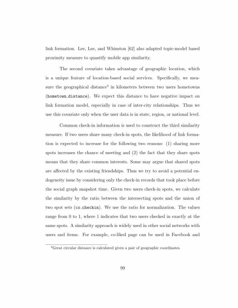
link formation. Lee, Lee, and Whinston [62] also adapted topic-model based

proximity measure to quantify mobile app similarity.

The second covariate takes advantage of geographic location, which

is a unique feature of location-based social services. Specifically, we mea-

sure the geographical distance4 in kilometers between two users hometowns

(hometown distance). We expect this distance to have negative impact on

link formation model, especially in case of inter-city relationships. Thus we

use this covariate only when the user data is in state, region, or national level.

Common check-in information is used to construct the third similarity

measure. If two users share many check-in spots, the likelihood of link forma-

tion is expected to increase for the following two reasons: (1) sharing more

spots increases the chance of meeting and (2) the fact that they share spots

means that they share common interests. Some may argue that shared spots

are affected by the existing friendships. Thus we try to avoid a potential en-

dogeneity issue by considering only the check-in records that took place before

the social graph snapshot time. Given two users check-in spots, we calculate

the similarity by the ratio between the intersecting spots and the union of

two spot sets (co checkin). We use the ratio for normalization. The values

range from 0 to 1, where 1 indicates that two users checked in exactly at the

same spots. A similarity approach is widely used in other social networks with

users and items. For example, co-liked page can be used in Facebook and

4Great circular distance is calculated given a pair of geographic coordinates.

99

co-purchased items can be used in Amazon.

The last user similarity is calculated by another source that reveals

a users interests: tweets. Location-based social networks encourage users

to connect their accounts to external social networks like Twitter. Follow-

ing a similar approach with biography similarity, we first build topic models

with tweets, then calculate cosine similarity between two tweet topic vectors

(tweet topic similarity). One thing to note is that all the tweets from one

user are combined to form a single document in the topic model.

4.4 Gowalla Data

Gowalla is the main data source for the empirical analysis of strategic

network formation. It was a location-based social network service, launched

in 2009 and closed in 2012 after Facebooks acquisition. With its mobile apps

available in major platforms, Gowalla allowed mobile users to check in at

spots5 that they visited and to share their check-in activities with friends.

Competitive services have included Foursquare, Brightkite, and Loopt (note

that Foursquare is the only one still available in the market). Larger social

networks such as Facebook and Google+ have also adopted check-in features.

Check-in is an on-demand event created by a user only when he or she

likes to share it with others. Thus a check-in reveals a lot about the individual.

For example, the category of the location (e.g., restaurant) can be used to infer

5Gowalla used the term spot to indicate locations. We use spots, locations, and venuesinterchangeably.

100

the users taste. Also, the geographic locations of the check-in points show the

users mobility pattern such as home, workplace, and frequently visited places.

Lastly, check-in times may reveal the diurnal and weekly patterns of users.

Gowallas social graph is undirected, as each friendship link is formed

with mutual agreements. This is different than the case of Twitter, where

users can follow others tweets even without the opponents approvals. Link

formation can be affected by individual characteristics, which can be observed

by check-in histories and user profiles. Conversely, the social network cre-

ates an environment of observational learning: People can explore previously

unknown places by observing friends check-in activities.

4.4.1 Data Collection

We used Gowallas API to collect data about users, spots, check-ins,

and the social graph. Firstly, we collected data of 385,306 users. Each user

data includes first and last name, hometown (city, state, and country), text

biography, website, Facebook identifier, Twitter identifier, friends count, and

various activity counts. Note that there are missing values as the user vol-

untarily gives the data. For the users without explicit home information, we

approximate the hometown by the location with the highest check-in count.

Secondly, we have a total of 3,101,620 spots in the database. Each

record consists of spot identifier, name, category, street address, city, state,

country, latitude, and longitude. Again, missing fields do exist but we observed

that spots in the U.S. mostly have complete information. Thus we focus on

101

U.S.-based users and locations in the analysis.

To our surprise, we were able to collect the whole trajectory of check-ins

in Gowalla. The very first check-in was by Gowallas co-founder on January

21, 2009 at his house and the last event took place in Bangkok, Thailand

on January 1, 2012. We collected 35,691,059 check-in records6 that created

a three-year time span. Each check-in entry indicates user identifier, spot

identifier, spot name, latitude, longitude, and check-in timestamp. On average,

each user checked in 92 times and each spot was visited more than 11 times.

Lastly, the social network, which is the dependent variable in our em-

pirical analysis, consists of 63,982 user nodes and 95,974 friendship edges. The

snapshot was taken over the course of May 2011.7 The graph has a density

of 0.0047%, as there are more than two billion possible pairs. In addition to

the Gowalla data, we collected tweets from Gowalla users to obtain richer text

information. A total of 100,946 Gowalla users linked their accounts to Twit-

ter to share their check-ins as tweets. Using Twitters API, 200 tweets from

79,979 users.8 are crawled, then 58,436 users tweets are used after filtering out

non-English tweets.

6Note that we could only collect public check-in records, not private ones that are pro-tected by users.

7Instant snapshot was not feasible due to the API rate limitation.8Some Twitter accounts are not available at the collection time due to account closure

or privacy settings.

102

4.4.2 User Sampling

User data is sampled in the link formation analysis to achieve computa-

tional feasibility. 9 In the analysis, we need to consider all possible user pairs,

comparing to the realized friendship. The number of pairs is quadratic to the

number of users, meaning that more than 74 billion pairs need to be analyzed

if we consider all the users in the analysis. Leskovec and Faloutsos [67] showed

that simple, uniform random node selection works well in graph sampling, and

we follow this direction in user sampling.

We construct the sample data in city, state, region, and national levels.

For city-level (Austin, TX; New York, NY; San Francisco, CA), we actually in-

clude all the users without sampling. In state-level analysis, we use the whole

user samples for the states of Georgia and Illinois. Fifty percent sampling is

used for the states of California and Texas. Then, user samples in regional

divisions are constructed by combining multiple states according to the defi-

nition from the United States Census Bureau.10 For region 1 (Northeast) and

2 (Midwest), the sampling rate is 50%, whereas the number is 20% for regions

3 (South) and 4 (West), due to large population in the data. Lastly, 10%

sampling is used to construct U.S. national level data.

9In case of user sampling, we test five different samples to check result consistency.10http://en.wikipedia.org/wiki/List_of_regions_of_the_United_States

103

4.4.3 Topic Models and User Proximity

We calculate four proximity measures based on the definitions in Sec-

tion 4.3. First, for biography topic similarity, we construct topic models with

22,139 users biographies as the input document collection. We vary the num-

ber of topics (10, 20, 30, 50, 100, 200) to find that the 200-topic model to yield

the best topics. Note that we did not remove the stop words from the raw

corpus to avoid bias issues. Table 4.1 gives a partial list of the resulting 200

topics along with the related keyword in each topic.11 Then the geographic

distance between users hometowns coordinates ranges from 0.0 km but does

not have the upper bounds. Large values observed are further than 3,000 km.

For co-check-in similarity measure, we consider only check-in records before

2011 because the social graph snapshot was taken in May 2011. Lastly, Ta-

ble 4.2 shows a partial list of topics and keywords from Gowalla users recent

tweets.12

To illustrate the relationship between our proposed topic-based user

similarities and friendship, we present two pairs of users who are friends and

share similar topics, as listed in Figure 4.1. As in the first example, user

#143496 and user #8122 are friends who show high similarity values in both

topic models (60% in biography and 42% in tweets). The specific topics that

contribute to the high similarity values are topic #187 (open, source, advocate,

11For the full list of topics and keywords from user biography, see http://diamond.

mccombs.utexas.edu/bio.topic.keywords.txt.12For the full list of topics and keywords from user tweets, see http://diamond.mccombs.

utexas.edu/tweet.topic.keywords.txt.

104

Topic Top Keywords0 mobile, technologies, work, focused, company, software

1 culture, pop, fashion, art, blog, sports, film, editor

2 married, wife, beautiful, work, son, years, kids

3 little, time, funny, big, pretty, baby, friends

4 information, health, visit, dental, cosmetic, treatment

5 high, doors, custom, site, luxury, road, wine, quality

6 hosting, online, popular, money, dedicated, host, support

7 loves, lives, travel, tourism, beautiful, works, london

8 manager, content, strategist, community, consultant

9 creative, agency, founder, interactive, firm, co-founder

10 enthusiast, junkie, blogger, fan, internet, foodie, dad

11 help, businesses, build, helping, small, companies, online

12 write, live, lot, drink, play, work, eat, laugh, travel, movies

13 store, shop, online, vintage, owner, items, cowboy, person

14 gowalla, use, don, account, official, foursquare, know, push

15 development, management, working, personal, project, learning

16 really, think, want, sense, know, good, humor, outside, places

17 local, community, news, information, events, destination

18 good, food, beer, wine, friends, travel, great, eat, order

19 experience, services, years, online, leading, industry

20 born, girl, city, town, raised, small, live, country, enjoys

21 user, mac, iphone, experience, software, android, blogger

22 entrepreneur, founder, creative, strategist, blogger

23 art, creative, artist, fine, interested, original, making

24 band, guitar, rock, playing, player, work, plays, called

25 team, street, gowalla, member, elite, need, fan, using

26 live, xbox, websites, make, action, 360, apps, cars, play

27 tea, chocolate, ice, coffee, blue, black, photography

28 dad, friend, writer, nerd, son, brother, evangelist ,fanatic

29 university, state, texas, science, research, studying

Table 4.1: A partial list of 200 topic model of 22,139 Gowalla users’ biographycorpus.

105

Topic Top Keywords0 google, apple, android, app, 2014, ios, phone, amazon, glass

1 win, enter, free, giveaway, chance, follow, entered, retweet

2 social, media, marketing, content, facebook, twitter, digital

3 kids, happy, family, little, school, birthday, baby, home, fun

4 beach, park, morning, sunset, beautiful, lake, view, travel

5 dallas, houston, texas, worth, nashville, rangers, dfw, fort

6 man, design, guys, yeah, app, @sketchapp, team, nice, dude

7 bitcoin, security, nsa internet, privacy, data, government, snowden

8 movie, star, film, episode, watch, wars, season, trailer

9 music, nowplaying, album, soundcloud, song, listening, live

10 help, join, support, share, donate, cancer, thx, water, world

11 washington, kansas, city, baltimore, virginia, lawrence

12 art, world, read, story, video, life, book, film, years

13 design, free, web, creative, nice, designers, awesome, app

14 oscars, watch, tonight, watching, happy, season, can’t, amazing

15 oklahoma, okc, live, pandora, city, thunder, tulsa, broadcasting

16 yelp, checked, endomondo, los, angeles, trakt, watched, walking

17 code, web, using, use, javascript, awesome, google, app, api, open

18 video, @youtube, liked, youtube, vimeo, added, playlist, favorited

19 women, gay, men, marriage, court, scotus, yesallwomen, lgbt, supreme

20 game, games, play, xbox, playing, ps4, live, gaming, awesome, steam

21 [pic]:, park, center, house, bar, grill, ave, cafe, starbucks

22 nike, run, nikeplus, ran, running, pace, finished, miles, route

23 tonight, come, week, tomorrow, join, free, night, event, 2014

24 data, big, open, @prismatic, analytics, science, research, map

25 space, science, video, mars, earth, nasa, solar, robot, launch

26 blog, post, business, marketing, tips, read, free, online, ways

27 austin, texas, sxsw, atx, antonio, san, acl, party, alamo, tacos

28 lastfm, artists, loved, soundhound, @hypem, tweeklyfm, shazam

29 vegas, las, phoenix, rewards, raleigh, casino, earning, arizona

Table 4.2: A partial list of 100 topic model of 58,436 Gowalla users’ tweetcorpus.

106

Figure 4.1: Examples of friends with similar topics in biographies and tweets

107

software) for biography and topic #17 (code, web, javascript) and topic #45

(right, did, pretty, better) in tweets. One can expect that this friendship is

related to web development and open software. The second pair of user #39875

and user #5279 has 42% similarity in biography and 62% in tweets. Sharing

topics are topic #177 (manager, community, founder, group, ceo, startup) in

biography and topic #2 (win, enter, free, giveaway) and topic #91 (twitter,

news, journalism, story).

4.5 Empirical Results

In this section, we present the empirical results estimated from our

structural model of strategic network formation. Table 4.3 shows the main

estimation results. As we introduced in Section 4.4, 10% sampling is used

to construct U.S. national level data in column 1 of Table 4.3. We find that

the effect of bio topic similarity, bio topic similarity, on network forma-

tion is significantly positive. This result confirms homophily in location-based

social networks: People with similar topic vectors from biographies are more

likely to form links with each other. In the estimation, we use the robust

z-statistics to deal with the concerns about the failure to meet standard re-

gression assumptions, such as unknown heteroskedasticity. Column 1 of Ta-

ble 4.3 also shows that the geographical distance between two users home-

towns, hometown distance, has a negative impact on link formation. This

result implies that physical distance matters in the case of intercity relation-

ships and is consistent with the results shown in the prior literature: Allama-

108

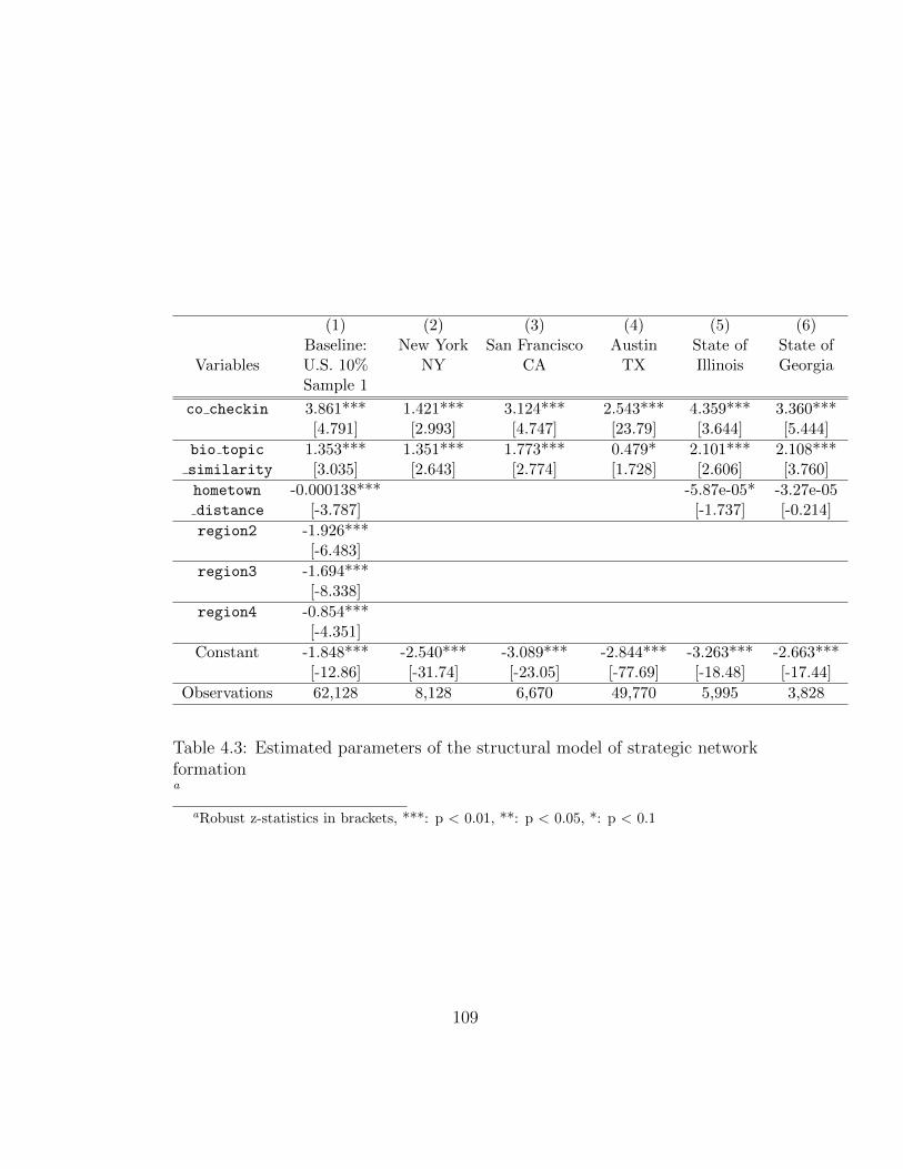
(1) (2) (3) (4) (5) (6)Baseline: New York San Francisco Austin State of State of

Variables U.S. 10% NY CA TX Illinois GeorgiaSample 1

co checkin 3.861*** 1.421*** 3.124*** 2.543*** 4.359*** 3.360***[4.791] [2.993] [4.747] [23.79] [3.644] [5.444]

bio topic 1.353*** 1.351*** 1.773*** 0.479* 2.101*** 2.108***similarity [3.035] [2.643] [2.774] [1.728] [2.606] [3.760]

hometown -0.000138*** -5.87e-05* -3.27e-05distance [-3.787] [-1.737] [-0.214]

region2 -1.926***[-6.483]

region3 -1.694***[-8.338]

region4 -0.854***[-4.351]

Constant -1.848*** -2.540*** -3.089*** -2.844*** -3.263*** -2.663***[-12.86] [-31.74] [-23.05] [-77.69] [-18.48] [-17.44]

Observations 62,128 8,128 6,670 49,770 5,995 3,828

Table 4.3: Estimated parameters of the structural model of strategic networkformationa

aRobust z-statistics in brackets, ***: p < 0.01, **: p < 0.05, *: p < 0.1

109

nis, Scellato, and Mascolo [5] showed that the geographic distance is critical in

predicting online social network formation. Lastly, we find that the similarity

measure based on co-check-in activities, co checkin, has a positive impact

on network formation. The intuition of this result is that users who share

similar location histories are likely to have common interests and behavior,

and therefore are more likely to become friends. The similarity between users

interests and behavior can be inferred from their location histories [95]. For

instance, people who enjoy the same museum or hiking the same mountain

can connect with each other to share their experiences. Oestreicher-Singer

and Sundararajan [83] examine the effect of a co-purchase relation on sales in

product networks. Our co-check-in similarity measure is conceptually similar

to the co-purchase relation described in Oestreicher-Singer and Sundarara-

jan [83]. It is worth noting that we cannot completely avoid the endogeneity

issue due to a lack of information on the time of each link formation: the link

formation between two users could also increase future co-check-in activities.

However, because we use only the check-in records that took place far ahead of

the time of our social graph snapshot to construct the measure, co checkin,

the endogeneity problem would be less of a concern.

In column 1 of Table 4.3, we also add U.S. regional dummies, which

take the value one if the hometown of a user is in a corresponding region,

and zero otherwise, as individual characteristics. In the analysis of city-level

and state-level samples, columns 2 - 6 of Table 4.3 show that our main results

are robust. A variety of additional robustness checks on the sample of state,

110

(1) (2) (3) (4)U.S. 10% U.S. 10% State CA State TX

Variables Sample 2 Sample 3 Sample Sample

co checkin 4.959*** 15.357*** 3.707*** 3.106***[9.679] [4.706] [7.502] [22.02]

bio topic 0.828** 1.685*** 1.723*** 0.793*similarity [1.987] [2.777] [3.016] [1.841]

hometown -0.000103*** -0.000129 -0.000187* -9.32e-05**distance [-2.705] [-0.833] [-1.767] [-2.059]

region2 -0.612 0.171[-1.562] [0.291]

region3 -0.320 0.634[-1.108] [1.231]

region4 0.670*** 0.0217[2.661] [0.0363]

Constant -3.326*** -4.139*** -3.518*** -3.266***[-13.08] [-6.957] [-28.45] [-60.53]

Observations 71,253 66,430 33,670 70,876

Table 4.4: Robustness checks of the structural estimation: U.S. and statesa

aRobust z-statistics in brackets, ***: p < 0.01, **: p < 0.05, * p: < 0.1

region, and national levels in Tables 4.4 and 4.5 are provided. Almost all of

the results are consistent with our expectation. The only exception is that

the coefficient on the geographic measure, hometown distance, in column 1

of Table 4.5 is positive, implying that the physical distance actually increases

the likelihood of link formation in region 1 (Northeast). A possible explanation

is that most of the users in this region are from the northeast megalopolis, the

most heavily urbanized region of the United States, and population mobility

is high within the megalopolis.

111

(1) (2) (3) (4)Region 1 Regions 2 Regions 3 Region 4

(Northeast) (Midwest) (South) (West)Variables 50% Sample 50% Sample 20% Sample 20% Sample

co checkin 2.017*** 4.393*** 2.912*** 5.571***[4.227] [5.229] [7.917] [6.077]

bio topic 1.538*** 1.349** 1.484** 1.324**similarity [3.244] [2.042] [2.333] [2.173]

hometown 0.000143*** -0.00112 -1.85e-05 -1.80e-05distance [3.521] [-1.468] [-0.202] [-0.453]

Constant -3.384*** -3.191*** -3.893*** -3.440***[-30.29] [-10.08] [-24.52] [-29.20]

Observations 21,945 36,315 45,150 23,220

Table 4.5: Robustness checks of the structural estimation: Regionsa

aRobust z-statistics in brackets, ***: p < 0.01, **: p < 0.05, *: p < 0.1

In Table 4.6, we further explore the effect of the tweet-wise similarity

measure based on topic models. As described in Section 4.3, we extract sim-

ilarity information from each users 200 recent tweets. Table 4.6 shows that

the effect of the tweet-wise similarity measure, tweet topic similarity, is

positive. Two points are worth noting. First, the sample size in Table 4.6

has been significantly decreased because only one-fifth of Gowalla users linked

their accounts to Twitter. Second, because of the restriction of Twitter API, 13

we can only collect the most recent tweets instead of specifying the time win-

dow of tweets. Therefore, the estimation of the effect of the tweet-wise sim-

ilarity measure might suffer from an endogeneity problem similar to the one

13https://dev.twitter.com/rest/public/rate-limiting

112

(1) (2) (3) (4) (5)U.S. San Francisco Austin State of State of

Variables 10% Sample CA TX California Texas

co checkin 3.928*** 3.375*** 3.210*** 5.116*** 3.262***[3.325] [3.192] [14.40] [8.256] [12.75]

bio topic 2.407*** 2.257*** 0.775** 2.179*** 0.141similarity [3.236] [2.915] [2.281] [4.005] [0.308]

hometown -0.000619* -3.48e-05 -3.99e-05distance [-1.933] [-0.326] [-1.226]

tweet topic 0.232 1.075** 2.014*** 1.017* 0.762***similarity [0.547] [2.277] [8.378] [1.742] [2.945]

region2 -0.416[-0.372]

region3 0.184[0.322]

region4 0.00215[0.00268]

Constant -3.228*** -3.689*** -3.682*** -3.942*** -3.036***[-4.434] [-10.74] [-24.61] [-11.44] [-22.58]

Observations 15,576 2,211 17,205 11,325 22,155

Table 4.6: Estimated parameters of the structural model of strategic networkformation: Tweet topic modelsa

aRobust z-statistics in brackets, ***: p < 0.01, **: p < 0.05, *: p < 0.1

113

(1) (2) (3)Actual number Average predicted Counterfactual

of number of numberformed links formed links (No homophily)

Col 1 in Table 4.5 97 98.030 80.766Col 1 in Table 4.6 80 78.378 64.970Col 2 in Table 4.5 52 52.019 43.340Col 3 in Table 4.5 21 21.344 13.030

Table 4.7: Comparison between the actual number and predicted number offormed linksa

aColumn 3 shows the counterfactual number of formed links generated from our structuralmodel when the coefficients on bio topic similarity and on co checkin are zero.

we discussed before: Network formation between users can affect their con-

tent of future tweets. In this sense, we do not claim that the coefficients

on tweet topic similarity in Table 4.6 are estimated causal effects. These

estimation results in Table 4.6 just provide an additional robustness check.

Like Christakis et al. [26], we compare the predicted networks with the

actual networks to evaluate the goodness of fit. First, we look at the number

of links formed by users. In columns 1 and 2 of Table 4.7, we compare the

number of formed links in the actual networks with the predicted number.

Note that in our structural model, the error terms εij and εji are drawn from

a type I extreme value distribution, so the predicted number of formed links

is affected by the randomness of the error terms. In order to compare with

the actual networks, we calculate the average predicted number of formed

links by drawing the error terms 100 times. The results in Table 4.7 show

114

that our structural model can predict accurately the mean number of formed

links. Next, we compare the degree distribution. The results are presented in

Tables 4.8, 4.9, 4.10, and 4.11. Although the predicted degree distribution is

a little less skewed than the actual degree distribution, the prediction works

well in general.

A major advantage of the structural approach is that it allows for inter-

esting counterfactual analysis that is simply not possible with reduced-form

regressions by recovering fundamental structural parameters [82]. A tight

integration of structural modeling and location-based technology allows us to

identify the parameters of the underlying individual choice model and conduct

counterfactual analysis on the effect of homophily. If homophily is important

in network formation, we would like to know what would happen if people

do not care about the proximity measures based on bio topics and check-in

records (no homophily exists), and evaluate the role of homophily. Column 3

of Table 4.7 shows the counterfactual number of formed links generated from

our structural model when the coefficients on bio topic similarity and on

co checkin are zero. We find that the number of formed links has been de-

creased by about 20% if the effect of homophily does not exist. In other words,

20% of links are formed because of homophily.

4.6 Conclusion and Managerial Implications

In this chapter, we studied the strategic network formation in a location-

based social network. We built a structural model for network formation with

115

Degree Actual Predicted

0 280 219.161 52 92.032 6 28.123 6 9.284 2 2.925 1 0.896 1 0.447 0 0.118 1 0.049 0 0.0110 1 0≥ 11 3 0

Average Degree of Users 0.550 0.555

Table 4.8: Actual degree distribution and predicted degree distribution: Socialnetwork shown in column 1 of Table 4.3

Degree Actual Predicted

0 304 254.511 54 93.432 11 23.323 4 5.264 1 1.255 0 0.176 0 0.047 2 0.028 1 0≥ 9 1 0

Average Degree of Users 0.423 0.429

Table 4.9: Actual degree distribution and predicted degree distribution: Socialnetwork shown in column 1 of Table 4.4

116

Degree Actual Predicted

0 95 56.761 16 46.412 5 18.323 4 5.414 2 0.895 2 0.26 0 0.018 2 014 1 0

Average Degree of Users 0.813 0.812

Table 4.10: Actual degree distribution and predicted degree distribution: So-cial network shown in column 2 of Table 4.3

Degree Actual Predicted

0 90 81.071 19 28.252 2 5.643 3 0.894 1 0.135 0 0.026 1 0

Average Degree of Users 0.362 0.369

Table 4.11: Actual degree distribution and predicted degree distribution: So-cial network shown in column 3 of Table 4.3

117

individual characteristics and pairwise user similarity. To construct the simi-

larity values, we constructed topic models with two sets of text corpus - biog-

raphy and tweets – that can reveal the users interest. In addition, geography-

based proximity measures were used to incorporate the unique nature of a

location-based social network. Based on the empirical analysis on Gowalla so-

cial network, we found evidence of the homophily effect on network formation.

The processes of network formation and peer influence are intercon-

nected. First, without full understanding of the process of network formation,

the observed relationship between network structure and influence could be

spurious [14]. Second, the interconnected nature of network formation and

peer influence has important managerial implications. If, for example, an in-

dividuals dining decision is significantly influenced by the characteristics and

behaviors of her friends, then social recommendation based on our model of

strategic network formation would have implications on the implementation

of restaurants seeding strategies. Our user proximity measures constructed by

topic modeling are statistically and economically relevant in friend recommen-

dation in location-based social networks.

A limitation in our empirical study is that in reality the benefit of form-

ing a link may depend on the presence of other links in the network – that

is, the current network structure [26]. In our model, the formation of links

depends only on individual user characteristics and pairwise user similarity

measures. In other words, we assume pairwise independence between network

links: The latent utility of forming each pairwise link is separable. Therefore,

118

in our maximum-likelihood estimation, the likelihood of the whole social net-

work is the product of likelihoods from all pairwise links. As a future research

direction, we can further examine the role of current network structures on

the dynamic formation of links.

Another research direction is to estimate peer effects and network for-

mation jointly under a unified model. When examining peer effects given an

exogenous social network, researchers need to correct for possible endogene-

ity biases due to friendship selection [9]. Our present model provides a basis

for understanding friendship selection, and a natural extension is to study a

more complete structural framework of peer effects with endogenous network

formation that can correct friendship selection biases.

119

Chapter 5

Conclusion

In this dissertation, we studied three link formation problems in mobile

and economic networks: (i) company matching for M&A and investment trans-

actions in the high-tech industry, (ii) mobile app matching for cross promotion

campaigns in the mobile app ad market, and (iii) online friendship formation

in the mobile social networks. Each problem can be modeled as link formation

problem in a graph, where nodes represent independent entities (e.g., compa-

nies, apps, users) and edges represent interactions (e.g., transactions, promo-

tions, friendships) among the nodes. First, based on the underlying properties

of each network, we proposed statistical models of link formations. Then, we

introduced various dyadic proximity measures that quantify the closeness be-

tween matching entities, including the novel proximity constructed from latent

Dirichlet allocation (LDA) topic models [18] of the entities’ text descriptions.

Finally, we conducted empirical analyses on large scale datasets (e.g., Crunch-

Base, IGAWorks, Gowalla) to find strong evidence that the proposed proximity

measures have statistically significant impact on the link formation procedures.

This dissertation can provide insights on understanding the emerging

mobile ecosystem in three different layers: users, apps, and firms. Our in-

120

ference results identified the determinants of the link formations in the three

networks. As a future direction, we can leverage proposed proximity measures

in predictive analytics to predict network evolution.

121

Bibliography

[1] Atila Abdulkadiroglu and Tayfun Sonmez. School choice: A mechanism

design approach. American Economic Review, 93(3):729–747, 2003.

[2] Gediminas Adomavicius and Alexander Tuzhilin. Toward the next

generation of recommender systems: A survey of the state-of-the-art

and possible extensions. IEEE Transactions on Knowledge and Data

Engineering, 17(6):734–749, 2005.

[3] Gautam Ahuja and Riitta Katila. Technological acquisitions and the

innovation performance of acquiring firms: A longitudinal study.

Strategic Management Journal, 22(3):197–220, 2001.

[4] Mohammad Akbarpour, Shengwu Li, and Shayan Oveis Gharan.

Dynamic matching market design. In Proceedings of the 15th ACM

Conference on Economics and Computation, EC ’14, pages 355–355,

New York, NY, USA, 2014. ACM.

[5] Miltiadis Allamanis, Salvatore Scellato, and Cecilia Mascolo. Evolution

of a location-based online social network: Analysis and models. In

Proceedings of the 12th ACM Internet Measurement Conference, pages

145–158, 2012.

122

[6] Raphael Amit, Lawrence Glosten, and Eitan Muller. Entrepreneurial

ability, venture investments, and risk sharing. Management Science,

36(10):1233–1246, 1990.

[7] Axel Anderson and Lones Smith. Dynamic matching and evolving

reputations. Review of Economic Studies, 77(1):3–29, 2010.

[8] Chris Anderson. The long tail: Why the future of business is selling

less of more. Hachette Digital, Inc., 2006.

[9] Sinan Aral, Lev Muchnik, and Arun Sundararajan. Distinguishing

influence-based contagion from homophily-driven diffusion in dynamic

networks. Proceedings of the National Academy of Sciences,

106(51):21544–21549, December 2009.

[10] Sinan Aral and Dylan Walker. Creating social contagion through viral

product design: A randomized trial of peer influence in networks.

Management Science, 57(9):1623–1639, 2011.

[11] Lars Backstrom, Eric Sun, and Cameron Marlow. Find me if you can:

Improving geographical prediction with social and spatial proximity. In

Proceedings of the 19th International Conference on World Wide Web,

WWW ’10, pages 61–70, New York, NY, USA, 2010. ACM.

[12] Bradley James Baker, Zheng Fang, and Xueming Luo. Hour-by-hour

sales impact of mobile advertising. Available at SSRN 2439396, 2014.

123

[13] Ravi Bapna, Jui Ramaprasad, Galit Shmueli, and Akhmed Umyarov.

One-way mirrors in online dating: A randomized field experiment. In

Proceedings of International Conference in Information Systems, 2013.

[14] Ravi Bapna and Akhmed Umyarov. Do your online friends make you

pay? A randomized field experiment in an online music social network.

Management Science, pages 1–19, 2015.

[15] Indranil R. Bardhan, Vish V. Krishnan, and Shu Lin. Research note -

Business value of information technology: Testing the interaction effect

of IT and R&D on Tobin’s Q. Information Systems Research,

24(4):1147–1161, 2013.

[16] Yakov Bart, Andrew T. Stephen, and Miklos Sarvary. Which products

are best suited to mobile advertising? A field study of mobile display

advertising effects on consumer attitudes and intentions. Journal of

Marketing Research, 51(3):270–285, 2014.

[17] David M. Blei. Probabilistic topic models. Communications of the

ACM, 55(4):77–84, 2012.

[18] David M. Blei, Andrew Y. Ng, and Michael I. Jordan. Latent Dirichlet

allocation. Journal of Machine Learning Research, 3:993–1022, March

2003.

[19] Ron Boschma, Rikard Eriksson, and Urban Lindgren. How does labour

mobility affect the performance of plants? The importance of

124

relatedness and geographical proximity. Journal of Economic

Geography, 9(2):169–190, 2009.

[20] Timothy Bresnahan and Shane Greenstein. Mobile computing: The

next platform rivalry. American Economic Review, 104(5):475–480,

2014.

[21] Bruno Cassiman, Massimo G. Colombo, Paola Garrone, and Reinhilde

Veugelers. The impact of M&A on the R&D process: An empirical

analysis of the role of technological- and market-relatedness. Research

Policy, 34(2):195–220, 2005.

[22] Abhirup Chakrabarti and Will Mitchell. The persistent effect of

geographic distance in acquisition target selection. Organization

Science, 24(6):1805–1826, 2013.

[23] Arun Chandrasekhar and Matthew O. Jackson. Tractable and

consistent random graph models. CoRR, abs/1210.7375, 2012.

[24] Hsinchun Chen, Roger H. L. Chiang, and Veda C. Storey. Business

intelligence and analytics: From big data to big impact. MIS

Quarterly, 36(4):1165–1188, December 2012.

[25] Roger H. L. Chiang, Paulo Goes, and Edward A. Stohr. Business

intelligence and analytics education, and program development: A

unique opportunity for the information systems discipline. ACM

125

Transactions on Management Information Systems, 3(3):12:1–12:13,

October 2012.

[26] Nicholas A. Christakis, James H. Fowler, Guido W. Imbens, and

Karthik Kalyanaraman. An empirical model for strategic network

formation. Working Paper 16039, National Bureau of Economic

Research, May 2010.

[27] Seungwha (Andy) Chung, Harbir Singh, and Kyungmook Lee.

Complementarity, status similarity and social capital as drivers of

alliance formation. Strategic Management Journal, 21(1):1–22, 2000.

[28] Lauren Cohen, Andrea Frazzini, and Christopher Malloy. The small

world of investing: Board connections and mutual fund returns.

Journal of Political Economy, University of Chicago Press,

116(5):951–979, October 2008.

[29] Margherita Comola and Marcel Fafchamps. Testing unilateral and

bilateral link formation. The Economic Journal, 124(579):954–976,

2014.

[30] Sergio Currarini, Matthew O. Jackson, and Paolo Pin. An economic

model of friendship: Homophily, minorities, and segregation.

Econometrica, 77(4):1003–1045, 07 2009.

[31] David Easley and Jon Kleinberg. Networks, crowds, and markets:

Reasoning about a highly connected world. Cambridge University Press,

126

2010.

[32] Isil Erel, Rose C. Liao, and Michael S. Weisbach. Determinants of

cross-border mergers and acquisitions. Journal of Finance,

67(3):1045–1082, 2012.

[33] Haluk Ergin and Tayfun Sonmez. Games of school choice under the

boston mechanism. Journal of Public Economics, 90(1):215–237, 2006.

[34] Bruce Fallick, Charles A. Fleischman, and James B. Rebitzer.

Job-hopping in Silicon Valley: Some evidence concerning the

microfoundations of a high-technology cluster. Review of Economics

and Statistics, 88(3):472–481, August 2006.

[35] Samer Faraj and Steven L. Johnson. Network exchange patterns in

online communities. Organization Science, 22(6):1464–1480, November

2011.

[36] Fred M. Feinberg, Barbara E. Kahn, and Leigh McAlister. Market

share response when consumers seek variety. Journal of Marketing

Research, 29(2):227–237, 1992.

[37] David Gale. The theory of linear economic models. University of

Chicago press, 1960.

[38] David Gale and Lloyd S. Shapley. College admissions and the stability

of marriage. American Mathematical Monthly, pages 9–15, 1962.

127

[39] Rajiv Garg, Michael Smith, and Rahul Telang. Measuring information

diffusion in an online community. Journal of Management Information

Systems, 28(2):11–38, October 2011.

[40] Anindya Ghose, Avi Goldfarb, and Sang Pil Han. How is the mobile

Internet different? Search costs and local activities. Information

Systems Research, 24(3):613–631, 2012.

[41] Anindya Ghose and Sang Pil Han. Estimating demand for mobile

applications in the new economy. Management Science, 2014.

[42] Anindya Ghose, Panagiotis G. Ipeirotis, and Beibei Li. Designing

ranking systems for hotels on travel search engines by mining

user-generated and crowdsourced content. Marketing Science,

31(3):493–520, May 2012.

[43] Anna Goldenberg, Alice X. Zheng, Stephen E. Fienberg, and

Edoardo M. Airoldi. A survey of statistical network models.

Foundations and Trends in Machine Learning, 2(2):129–233, 2010.

[44] Avi Goldfarb and Catherine Tucker. Online display advertising:

Targeting and obtrusiveness. Marketing Science, 30(3):389–404, 2011.

[45] Paul A. Gompers. Optimal investment, monitoring, and the staging of

venture capital. Journal of Finance, 50(5):1461–1489, 1995.

[46] Thomas L. Griffiths and Mark Steyvers. Finding scientific topics.

Proceedings of the National Academy of Sciences, 101:5228–5235, 2004.

128

[47] Mark S. Handcock, David R. Hunter, Carter T. Butts, Steven M.

Goodreau, and Martina Morris. statnet: Software tools for the

representation, visualization, analysis and simulation of network data.

Journal of Statistical Software, 24(1):1–11, 5 2008.

[48] Negar Hariri, Bamshad Mobasher, and Robin Burke. Context-aware

music recommendation based on latent topic sequential patterns. In

Proceedings of the 6th ACM Conference on Recommender systems,

pages 131–138. ACM, 2012.

[49] John William Hatfield, Scott Duke Kominers, Alexandru Nichifor,

Michael Ostrovsky, and Alexander Westkamp. Stability and

competitive equilibrium in trading networks. Journal of Political

Economy, 121(5):966–1005, 2013.

[50] Oliver Hinz, Bernd Skiera, Christian Barrot, and Jan U. Becker.

Seeding strategies for viral marketing: An empirical comparison.

Journal of Marketing, 75(6):55–71, 2011.

[51] Gunter J. Hitsch, Ali Hortacsu, and Dan Ariely. Matching and sorting

in online dating. American Economic Review, pages 130–163, 2010.

[52] Yael V. Hochberg, Alexander Ljungqvist, and Yang Lu. Whom you

know matters: Venture capital networks and investment performance.

Journal of Finance, 62(1):251–301, 2007.

129

[53] Wenyan Hu and Alvaro Bolivar. Online auctions efficiency: A survey

of eBay auctions. In Proceedings of the 17th International Conference

on World Wide Web, pages 925–934. ACM, 2008.

[54] David R. Hunter and Mark S. Handcock. Inference in curved

exponential family models for networks. Journal of Computational and

Graphical Statistics, 15:565–583, 2006.

[55] David Inouye, Pradeep Ravikumar, and Inderjit Dhillon. Admixture of

poisson MRFs: A topic model with word dependencies. In Proceedings

of the 31st International Conference on Machine Learning, pages

683–691, 2014.

[56] Matthew O. Jackson. Social and Economic Networks. Princeton

University Press, Princeton, NJ, USA, 2010.

[57] Matthew O. Jackson and Brian W. Rogers. Meeting strangers and

friends of friends: How random are social networks? American

Economic Review, pages 890–915, 2007.

[58] Matthew O. Jackson and Asher Wolinsky. A strategic model of social

and economic networks. Journal of Economic Theory, 71(1):44–74,

1996.

[59] Kenneth Joseph, Chun How Tan, and Kathleen M. Carley. Beyond

local, categories and friends: Clustering Foursquare users with latent

topics. In Proceedings of the 2012 ACM Conference on Ubiquitous

130

Computing, UbiComp ’12, pages 919–926, New York, NY, USA, 2012.

ACM.

[60] Alexander S. Kelso Jr. and Vincent P. Crawford. Job matching,

coalition formation, and gross substitutes. Econometrica, pages

1483–1504, 1982.

[61] Pavel N. Krivitsky and Mark S. Handcock. A separable model for

dynamic networks. Journal of the Royal Statistical Society: Series B

(Statistical Methodology), 76(1):29–46, 2014.

[62] Gene Moo Lee, Joowon Lee, and Andrew B. Whinston. Matching

mobile applications for cross promotion. In Conference on Big Data

Marketing Analytics, 2014.

[63] Gene Moo Lee, Liangfei Qiu, and Andrew B. Whinston. Strategic

network formation in a location based social network: A topic

modeling approach. In Proceedings of the Workshop on Information

Technologies and Systems, 2014.

[64] Gene Moo Lee, Swati Rallapalli, Wei Dong, Yi-Chao Chen, Lili Qiu,

and Yin Zhang. Mobile video delivery via human movement. In

Proceedings of 10th Annual IEEE Communications Society Conference

on Sensor, Mesh and Ad Hoc Communications and Networks, pages

406–414, 2013.

131

[65] Gun Woong Lee and T. Santanam Raghu. Determinants of mobile

apps success: Evidence from app store market. Journal of

Management Information Systems, 2014.

[66] Shun-Yang Lee, Liangfei Qiu, and Andrew B. Whinston.

Manipulation: Online platforms inescapable fate. In Proceedings of the

International Conference in Information Systems, 2014.

[67] Jure Leskovec and Christos Faloutsos. Sampling from large graphs. In

Proceedings of the 12th ACM SIGKDD International Conference on

Knowledge Discovery and Data Mining, KDD ’06, pages 631–636, New

York, NY, USA, 2006. ACM.

[68] David Liben-Nowell and Jon Kleinberg. The link-prediction problem

for social networks. Journal of the American Society for Information

Science and Technology, 58(7):1019–1031, May 2007.

[69] Mingfeng Lin, Nagpurnanand R. Prabhala, and Siva Viswanathan.

Judging borrowers by the company they keep: Friendship networks and

information asymmetry in online peer-to-peer lending. Management

Science, 59(1):17–35, January 2013.

[70] Greg Linden, Brent Smith, and Jeremy York. Amazon.com

recommendations: Item-to-item collaborative filtering. IEEE Internet

Computing, 7(1):76–80, 2003.

132

[71] Gianni Lorenzoni and Andrea Lipparini. The leveraging of interfirm

relationships as a distinctive organizational capability: A longitudinal

study. Strategic Management Journal, 20(4):317–338, 1999.

[72] Xueming Luo, Michelle Andrews, Zheng Fang, and Chee Wei Phang.

Mobile targeting. Management Science, 2013.

[73] Wayne H. Mikkelson and Richard S. Ruback. An empirical analysis of

the interfirm equity investment process. Journal of Financial

Economics, 14(4):523–553, December 1985.

[74] Stanislav Miskovic, Gene Moo Lee, Yong Liao, and Mario Baldi.

AppPrint: Automatic fingerprinting of mobile applications in network

traffic. In Proceedings of the 16th Passive and Active Measurement

Conference, pages 57–69, 2015.

[75] Sunil Mithas, Ali Tafti, Indranil Bardhan, and Jie Mein Goh.

Information technology and firm profitability: Mechanisms and

empirical evidence. MIS Quarterly, 36(1):205–224, March 2012.

[76] Hitoshi Mitsuhashi and Henrich R. Greve. A matching theory of

alliance formation and organizational success: Complementarity and

compatibility. Academy of Management Journal, 52(5):975–995, 2009.

[77] Giuseppe Moscarini and Kaj Thomsson. Occupational and job mobility

in the US. Scandinavian Journal of Economics, 109(4):807–836, 2007.

133

[78] David C. Mowery, Joanne E. Oxley, and Brian S. Silverman.

Technological overlap and interfirm cooperation: Implications for the

resource-based view of the firm. Research Policy, 27(5):507–523, 1998.

[79] Roger B. Myerson. Game Theory. Harvard University Press, 2013.

[80] Nagarajan Natarajan, Donghyuk Shin, and Inderjit S. Dhillon. Which

app will you use next? Collaborative filtering with interactional

context. In Proceedings of the 7th ACM Conference on Recommender

systems, pages 201–208. ACM, 2013.

[81] George L. Nemhauser and Laurence A. Wolsey. Integer and

combinatorial optimization, volume 18. Wiley New York, 1988.

[82] Aviv Nevo and Michael D. Whinston. Taking the dogma out of

econometrics: Structural modeling and credible inference. Journal of

Economic Perspectives, pages 69–81, 2010.

[83] Gal Oestreicher-Singer and Arun Sundararajan. The visible hand?

Demand effects of recommendation networks in electronic markets.

Management Science, 58(11):1963–1981, 2012.

[84] Onook Oh, Manish Agrawal, and H. Raghav Rao. Community

intelligence and social media services: A rumor theoretic analysis of

tweets during social crises. MIS Quarterly, 37(2):407–426, 2013.

[85] Thanasis Petsas, Antonis Papadogiannakis, Michalis Polychronakis,

Evangelos P Markatos, and Thomas Karagiannis. Rise of the planet of

134

the apps: A systematic study of the mobile app ecosystem. In

Proceedings of Internet Measurement Conference, pages 277–290.

ACM, 2013.

[86] Veronika K. Pool, Noah Stoffman, and Scott E. Yonker. The people in

your neighborhood: Social interactions and mutual fund portfolios.

Journal of Finance, Forthcoming.

[87] Liangfei Qiu, Huaxia Rui, and Andrew B. Whinston. Effects of social

networks on prediction markets: Examination in a controlled

experiment. Journal of Management Information Systems,

30(4):235–268, 2014.

[88] Liangfei Qiu, Zhan Shi, and Andrew B. Whinston. Learning from your

friends repeated check-ins: An empirical study of location-based social

networks. Working paper, University of Texas at Austin, 2014.

[89] Daniel Ramage, Susan T. Dumais, and Daniel J. Liebling.

Characterizing microblogs with topic models. In Proceedings of

International AAAI Conference on Web and Social Media, volume 10,

pages 1–1, 2010.

[90] Matthew Rhodes-Kprof and David T. Robinson. The market for

mergers and the boundaries of the firm. Journal of Finance,

63(3):1169–1211, 2008.

135

[91] Alvin E. Roth. The evolution of the labor market for medical interns

and residents: A case study in game theory. Journal of Political

Economy, pages 991–1016, 1984.

[92] Alvin E. Roth. A natural experiment in the organization of entry-level

labor markets: Regional markets for new physicians and surgeons in the

United Kingdom. American Economic Review, pages 415–440, 1991.

[93] Alvin E. Roth and Elliott Peranson. The redesign of the matching

market for american physicians: Some engineering aspects of economic

design. American Economic Review, 89(4):748–780, 1999.

[94] Alvin E. Roth, Tayfun Sonmez, and M. Utku Unver. Efficient kidney

exchange: Coincidence of wants in markets with compatibility-based

preferences. American Economic Review, pages 828–851, 2007.

[95] Salvatore Scellato, Anastasios Noulas, and Cecilia Mascolo. Exploiting

place features in link prediction on location-based social networks. In

Proceedings of the 17th ACM SIGKDD International Conference on

Knowledge Discovery and Data Mining, pages 1046–1054. ACM, 2011.

[96] Joshua Sears and Glenn Hoetker. Technological overlap, technological

capabilities, and resource recombination in technological acquisitions.

Strategic Management Journal, 35(1):48–67, 2014.

[97] Lloyd S. Shapley and Martin Shubik. The assignment game I: The

core. International Journal of Game Theory, 1(1):111–130, 1971.

136

[98] Shuyang Sheng. Identification and estimation of network formation

games. Working paper, University of Southern California, 2012.

[99] Zhan Shi, Gene Moo Lee, and Andrew B. Whinston. Towards a better

measure of business proximity: Topic modeling for analyzing M&As.

In Proceedings of the ACM Conference on Economics and

Computation, pages 565–565. ACM, 2014.

[100] Zhan Shi, Huaxia Rui, and Andrew B. Whinston. Content sharing in a

social broadcasting environment: Evidence from Twitter. MIS

Quarterly, 38(1):123–142, March 2014.

[101] Galit Shmueli and Otto R. Koppius. Predictive analytics in

information systems research. MIS Quarterly, 35(3):553–572, 2011.

[102] Param Vir Singh, Nachiketa Sahoo, and Tridas Mukhopadhyay. How

to attract and retain readers in enterprise blogging? Information

Systems Research, 25(1):35–52, 2014.

[103] Miha Skerlavaj, Vlado Dimovski, and Kevin C. Desouza. Patterns and

structures of intra-organizational learning networks within a

knowledge-intensive organization. Journal of Information Technology,

25(2):189–204, 06 2010.

[104] Tom A. B. Snijders. Markov chain Monte Carlo estimation of

exponential random graph models. Journal of Social Structure, 3, 2002.

137

[105] Tom A.B. Snijders, Johan Koskinen, and Michael Schweinberger.

Maximum likelihood estimation for social network dynamics. Annals of

Applied Statistics, 4(2):567–588, 2010.

[106] John Sorenson, John Tschirhart, and Andrew B. Whinston. A theory

of pricing under decreasing costs. American Economic Review, pages

614–624, 1978.

[107] Toby E. Stuart. Network positions and propensities to collaborate: An

investigation of strategic alliance formation in a high-technology

industry. Administrative Science Quarterly, 43(3):668–698, 1998.

[108] Toby E. Stuart and Soojin Yim. Board interlocks and the propensity

to be targeted in private equity transactions. Journal of Financial

Economics, 97(1):174 – 189, 2010.

[109] Anjana Susarla, Jeong-Ha Oh, and Yong Tan. Social networks and the

diffusion of user-generated content: Evidence from YouTube.

Information Systems Research, 23(1):23–41, 2012.

[110] Yee Whye Teh, Michael I. Jordan, Matthew J. Beal, and David M.

Blei. Hierarchical Dirichlet processes. Journal of the American

Statistical Association, 101, 2004.

[111] Chong Wang and David M. Blei. Collaborative topic modeling for

recommending scientific articles. In Proceedings of the 17th ACM

138

SIGKDD International Conference on Knowledge Discovery and Data

Mining, pages 448–456. ACM, 2011.

[112] Lei Wang, Ram Gopal, Ramesh Sankaranarayanan, and Joseph

Pancras. Predicting restaurant failure through Foursquare customer

check-ins. Working paper, University of Connecticut, 2014.

[113] Lihua Wang and Edward J. Zajac. Alliance or acquisition? A dyadic

perspective on interfirm resource combinations. Strategic Management

Journal, 28(13):1291–1317, 2007.

[114] Sunil Wattal, Pradeep Racherla, and Munir Mandviwalla. Network

externalities and technology use: A quantitative analysis of

intraorganizational blogs. Journal of Management Information

Systems, 27(1):145–174, 2010.

[115] Jianshu Weng, Ee-Peng Lim, Jing Jiang, and Qi He. TwitterRank:

finding topic-sensitive influential twitterers. In Proceedings of the ACM

International Conference on Web Search and Data Mining, pages

261–270. ACM, 2010.

[116] Lynn Wu. Social network effects on productivity and job security:

Evidence from the adoption of a social networking tool. Information

Systems Research, 24(1):30–51, 2013.

[117] Lizhen Xu, Jason A. Duan, and Andrew B. Whinston. Path to

purchase: A mutually exciting point process model for online

139

advertising and conversion. Management Science, 2014.

[118] Qiang Xu, Jeffrey Erman, Alexandre Gerber, Zhuoqing Mao, Jeffrey

Pang, and Shobha Venkataraman. Identifying diverse usage behaviors

of smartphone apps. In Proceedings of the 2011 ACM SIGCOMM

Conference on Internet Measurement Conference, pages 329–344.

ACM, 2011.

[119] Pai-Ling Yin, Jason P. Davis, and Yulia Muzyrya. Entrepreneurial

innovation: Killer apps in the iPhone ecosystem. American Economic

Review, 104(5):255–259, 2014.

[120] Yu Zheng, Lizhu Zhang, Zhengxin Ma, Xing Xie, and Wei-Ying Ma.

Recommending friends and locations based on individual location

history. ACM Transactions on the Web, 5(1):5, 2011.

[121] Nan Zhong and Florian Michahelles. Google Play is not a long tail

market: An empirical analysis of app adoption on the Google Play app

market. In Proceedings of the 28th Annual ACM Symposium on

Applied Computing, pages 499–504. ACM, 2013.

140

Vita

Gene Moo Lee was born in Seattle, Washington on July 7, 1981, the

son of Dr. Sang-Won Lee and Mrs. Kyung-Ja Hwang. He received a dual

Bachelor of Science degree in Computer Science and Mathematics from Korea

University in 2004 and a Master of Arts degree in Computer Science from

the University of Texas at Austin in 2006. He joined the Ph.D. program in

Computer Science at the University of Texas at Austin in Fall 2010.

His research topics include mobile ecosystems, social network analysis,

business analytics, and Internet security. He takes Big Data approaches with

various techniques from data mining, machine learning, and econometrics. His

works have been published in 8 refereed conference proceedings and 8 non-

refereed conference papers in the field of Computer Science and Information

Systems. He holds 10 patents and 7 patent applications.

He also has extensive industry experiences. In 2014, he co-founded

Topic Technologies,1 a business intelligence startup. He is the lead developer

for SpamRankings.net project2 since 2013. From 2006 to 2010, he was a re-

search engineer in Samsung Electronics (Suwon, Korea), where he designed

innovative mobile convergence services for various consumer electronics prod-

1http://www.topictechnologies.com2http://www.spamrankings.net

141

ucts such as smartphones, laptops, and smart TVs. He also has internship

experiences at Goldman Sachs (New York, NY), Intel (Austin, TX), AT&T

Labs (Florham Park, NJ), and Narus (Sunnyvale, CA).

Starting from Fall 2015, he will be an Assistant Professor in Depart-

ment of Information Systems and Operations Management at the University

of Texas at Arlington.

Permanent address: 6746 Deseo #112Irving, TX 75039

This dissertation was typeset with LATEX† by the author.

†LATEX is a document preparation system developed by Leslie Lamport as a specialversion of Donald Knuth’s TEX Program.

142