Copyright by Fahad Mohammed Alfadhli 2012
218
Copyright by Fahad Mohammed Alfadhli 2012
Transcript of Copyright by Fahad Mohammed Alfadhli 2012

Copyright
by
Fahad Mohammed Alfadhli
2012

The Dissertation Committee for Fahad Mohammed Alfadhli Certifies that this is the
approved version of the following dissertation:
Reducing Environmental Impacts of Petroleum Refining: A Case Study
of Industrial Flaring
Committee:
David T. Allen, Supervisor
Thomas F. Edgar
Elena McDonald-Buller
Michael Baldea
Vincent M. Torres

Reducing Environmental Impacts of Petroleum Refining: A Case Study
of Industrial Flaring
by
Fahad Mohammed Alfadhli, B.Ch.E; M.S.E.
Dissertation
Presented to the Faculty of the Graduate School of
The University of Texas at Austin
in Partial Fulfillment
of the Requirements
for the Degree of
Doctor of Philosophy
The University of Texas at Austin
August 2012

Dedication
Dedicated to my parents, wife, lovely daughter Shaikha and family

v
Acknowledgements
I would like to thank my supervisor, Dr. David T. Allen, for his guidance and
support; it has been a privilege to work with him. His guidance and patience have helped
me grow scientifically and professionally. My sincere gratitude is also goes to Dr.
Yosuke Kimura for his the technical supports he offered. My gratitude also extended to
Dr. Thomas Edgar, Dr. Elena McDonald-Buller, Dr. Michael Baldea and Mr. Vincent M.
Torres for serving on my committee.
I gratefully thank my parents, Mohammed Al-Fadhli and Shaikha Al-Khemsan
for their love, continuous encouragement, and motivational support throughout my life. I
am most thankful to my wife Asmaa Al-Fadgham and my daughter Shaikha for their
support and patience. My sincere thanks go to my family and friends for believing in me.
This work would not be possible without them.
Finally, a special thanks to Kuwait University for giving me the opportunity to
pursue my graduate study at the University of Texas at Austin.

vi
Reducing Environmental Impacts of Petroleum Refining: A Case Study
of Industrial Flaring
Fahad Mohammed Alfadhli, Ph.D.
The University of Texas at Austin, 2012
Supervisor: David T. Allen
Industrial flaring can have negative impacts on regional air quality and recent
studies have shown that flares are often operated at low combustion efficiency, which
exacerbates these air quality impacts. This thesis examines industrial flaring with the
objectives of (1) assessing the air quality impacts of flares operating at a variety of
conditions, (2) examining the extent to which improvements in flare operations could
reduce emissions, (3) identifying opportunities for recycling flared gases in fuel gas
networks, and (4) identifying opportunities for reducing the generation of flared gases,
using the improved control of catalytic cracking operations as a case study.
The work presented in this thesis demonstrates that flares operating at low
combustion efficiency can increase localized ambient ozone concentrations by more than
15 ppb under some conditions. The impact of flares on air quality depends most strongly
on combustion efficiency, the flow rates to the flares and the chemical composition
(photochemical reactivity) of the emissions. Products of incomplete combustion and
nitrogen oxides emissions from flaring generally had a smaller impact on air quality than
unburned flare gases.

vii
The combustion efficiency at which a flare can operate can be constrained by the
flare’s design. In a case study of an air-assisted flare, it was demonstrated that choices in
blower configurations could lead to emissions that were orders of magnitude greater or
less than those predicted using an assumed combustion efficiency of 98%. Designing
flares with air-assist rates that can be finely tuned can significantly reduce emissions.
Similarly, flaring can be reduced by integrating sources of waste gases into fuel gas
networks. Analyses for a petroleum refinery indicated that this integration can often be
accomplished with little net cost by expanding boiler capacities. Finally, flared gases can
be reduced at their source. A case study of a fluid catalytic cracking indicated that using
better temperature control could significantly minimize flared gases.

viii
Table of Contents
List of Tables ........................................................................................................ xii
List of Figures .................................................................................................... xviii
CHAPTER 1: Introduction ...................................................................................1
CHAPTER 2: Literature Review..........................................................................8
2.1 Impact of flare emissions on air quality .................................................8
2.2 Flare destruction efficiency ..................................................................12
2.3 Reducing flaring through fuel gas networks ........................................18
CHAPTER 3: Impact of Flare Destruction Efficiency and Products of Incomplete
Combustion on Ozone Formation in Houston, Texas ............................................23
3.1 Introduction ..........................................................................................23
3.2 Methodology ........................................................................................25
3.2.1 Industrial Flares ..........................................................................25
3.2.1.1 Petroleum refinery flares ..............................................25
3.2.1.2 Olefin flares ..................................................................28
3.2.2 Flare chemical compositions.......................................................31
3.2.3 Emissions scenarios ....................................................................33
3.2.3.1 VOC emissions .............................................................33
3.2.3.2 NOx emissions ..............................................................35
3.2.4 Photochemical modeling .............................................................35
3.3 Results and Discussion ........................................................................40
3.3.1 Base Case ....................................................................................40
3.3.2 Flare Emission Scenarios ............................................................42
3.3.2.1 Refinery Flare 1 ............................................................42
3.3.2.2 Refinery Flares 2 and 3 ................................................46
3.3.2.3 Olefin Flares .................................................................49
3.4 Conclusion ...........................................................................................52

ix
CHAPTER 4: Impact of Emissions of Nitrogen Oxides from Flares on Ozone
Formation in Houston, Texas .................................................................................53
4.1 Introduction ..........................................................................................53
4.2 Methods................................................................................................55
4.2.1 Emission factor ...........................................................................55
4.2.2 Air quality ...................................................................................58
4.2.2.1 Flare selection ..............................................................58
4.2.2.2 NOx emission scenarios ................................................58
4.2.2.3 Photochemical modeling ..............................................59
4.3 Results and Discussion ........................................................................60
4.4 Conclusion ...........................................................................................67
CHAPTER 5: Impacts of Air-Assist Flare Blower Configurations on Flaring
Emissions……… ...................................................................................................69
5.1 Introduction ..........................................................................................69
5.2 Methods................................................................................................71
5.2.1 Air-assisted flare experimental tests ...........................................71
5.2.2 Stochastic models........................................................................73
5.3 Results and Discussion ........................................................................78
5.3.1 Vent gas mixture with LHV of 350 Btu/scf ................................78
5.3.2 Vent gas mixture with LHV of 560 Btu/scf ................................83
5.4 Conclusion ...........................................................................................84
CHAPTER 6: Minimization of Refinery Flaring Through Integration with Fuel Gas
Networks……… ....................................................................................................85
6.1 Introduction ..........................................................................................85
6.2 Methods................................................................................................86
6.2.1 Flow rates ....................................................................................89
6.2.2 Energy demand ...........................................................................90
6.2.3 Non-isothermal and non-isobaric operations ..............................91
6.2.4 Fuel quality .................................................................................93
6.2.5 Physical features .........................................................................97
6.3 Case study of a petroleum refinery ....................................................101

x
6.3.1 Minimizing waste gases ............................................................106
6.3.1.1 Turbine fuels ..............................................................106
6.3.1.2 Flare gas and boiler fuel .............................................108
6.4 Conclusion .........................................................................................113
CHAPTER 7: Effect of Temperature Excursions in Catalytic Cracking Units on the
Generation of Flared gases ...................................................................................114
7.1 Introduction ........................................................................................114
7.2 Three-Lump model ............................................................................117
7.2.1 Kinetic model ............................................................................117
7.2.2 Comparing the Three-lump model with experimental data ......120
7.2.3 Temperature effect ....................................................................121
7.2.4 Coke formation .........................................................................122
7.3 Light gases scenarios .........................................................................123
7.4 Comparison between scenario results and FCC flare data .................127
7.5 Conclusion .........................................................................................137
CHAPTER 8: Findings, Outcomes and Recommmedations ............................138
8.1 Findings..............................................................................................138
8.1.1 Air quality impacts of flaring operations ..................................138
8.1.2 Improving flare operation .........................................................139
8.1.3 Minimization of refinery flaring through integration with fuel gas
networks ....................................................................................139
8.1.4 Impact of temperature excursions of FCC units on the light
gas/flared gas production. .........................................................140
8.2 Outcomes ...........................................................................................140
8.3 Future work ........................................................................................141
8.3.1 Air quality impacts of flaring operations ..................................141
8.3.2 Improving flare operation .........................................................141
8.3.3 Minimization of refinery flaring through integration with fuel gas
networks ....................................................................................141
8.3.4 Impact of temperature excursions of FCC units on the light
gas/flared gas production. .........................................................141

xi
Appendix A ..........................................................................................................142
Appendix B ..........................................................................................................158
Appendix C ..........................................................................................................160
Appendix D ..........................................................................................................181
References ............................................................................................................185
Vita .......................................................................................................................192

xii
List of Tables
Table 3-1: The 24 refinery flares with the highest VOC emissions, as reported
through a month-long 2006 inventory ......................................................... 26
Table 3-2: Petroleum refinery flares selected for photochemical modeling analyses ...... 26
Table 3-3: The 17 olefin manufacturing flares with the highest VOC emissions, as
reported through a month-long 2006 inventory ........................................... 29
Table 3-4: Olefin manufacturing flares selected for photochemical modeling analyses .. 29
Table 3-5: Composition of flared gases ............................................................................ 32
Table 3-6: Photochemical modeling scenarios performed for each flare ......................... 34
Table 3-7: daily maximum mass flow rate for the selected flares, daily maximum one-
hour average ozone concentrations during period of 2006 SI and whether
simulation files for 2 kilometers domain are exist or not ............................ 39
Table 3-8: Summary of Maximum ozone concentrations (ppb) for all DRE scenarios
applied on Refinery Flare 1 ......................................................................... 46
Table 3-9 : The difference in wide region maxima one-hour average ozone
concentrations (in ppb) and the maximum difference in one-hour
average ozone concentrations (in ppb) for all the flare DRE scenarios
applied to the three refinery flares compared to the base case .................... 48
Table 3-10 : The difference in wide region maxima one-hour average ozone
concentrations (in ppb) and the maximum difference in one-hour
average ozone concentrations (in ppb) for all the flare DRE scenarios
applied to the two olefin flares compared to the base.................................. 49
Table 3-11: The mass of the predicted ozone (ton) for all scenarios when the
maximum daily flow rates were used for the five flares. The maximum

xiii
daily flow rates for Refinery Flare 1, 2, 3, Olefin Flare 1 and 2 are 25.3,
4, 3.9, 3.5 and 4.1 tons/ hr respectively. The mass of the predicted ozone
was based on MIR values (Carter, 2011) ..................................................... 51
Table 3-12 : The absolute product all the scenarios in Table 3-11 divided by the base
case value ..................................................................................................... 51
Table 4-1: Photochemical modeling scenarios performed for Refinery Flare 1 ............... 59
Table 4-2 : The difference in maximum ozone concentration (DMOC), maximum
difference in ozone concentration (MaxDOC), and minimum difference
in ozone concentration (MinDOC) for all the scenarios with reduced
NOx compared to the base case. All ozone concentrations are in ppb. ........ 66
Table 4-3: The difference in maximum ozone concentration (DMOC), maximum
difference in ozone concentration (MaxDOC) and minimum difference
in ozone concentration (MinDOC) for all the scenarios with NOx based
on AP-42 compared to the base case with NOx based on AP-42 value. ...... 67
Table 5-1: Categorization of petroleum refinery flares in 2006 SI (Pavlovic et al.,
2012b). ......................................................................................................... 74
Table 5-2: Air-assist rates (ft3/min) for each air-assist design under different
stoichiometric air conditions ........................................................................ 76
Table 6-1: Data of the sources in the refinery problem .................................................. 103
Table 6-2: Data of the sinks in the refinery problem ...................................................... 104
Table 6-3: CAPEX and OPEX of auxiliary equipment and pipelines in the multi-
mode FGN.................................................................................................. 105
Table 6-4: CAPEX of the pipelines in the multi-mode FGN .......................................... 105
Table 6-5: optimum operating conditions for the first problem ..................................... 107

xiv
Table 6-6: Scenario results of the impact of hydrocarbon penalty constraint on the
TAC and the flaring amount ...................................................................... 109
Table 6-7: Scenario results of the impact of the sink flexibility on the TAC and the
flaring amount ............................................................................................ 110
Table 6-8: Scenario results of the impact of expanding the boiler capacity on the TAC
and the flaring amount ............................................................................... 111
Table 6-9: Scenario results of the impact of installing a new boiler on the TAC and
flaring amount ............................................................................................ 112
Table 6-10: Impact of utilizing the additional high pressure steam on the TAC. ........... 113
Table 7-1: The values of rates of reactions and catalyst decay coefficient (Weekman
Jr and Nace, 1970). .................................................................................... 121
Table 7-2: Mass rates of additional light gases from a FCC unit for different
temperature excursion scenario when the tc =5 min ................................. 126
Table 7-3 : Mass rates of additional light gases from a FCC unit for different
temperature excursion scenario when the tc = 1.25min ............................ 126
Table 7-4: The maximum temperature, the minimum temperature, and the maximum
temperature excursion for each scenario when tc =5 min ......................... 132
Table 7-5: The maximum temperature, the minimum temperature, and the maximum
temperature excursion for each scenario when tc =5 min ......................... 135
Table A-1: Summary of emission scenarios simulated for each flare ............................ 142
Table A-2: Summary of VOC emissions (tons/hr) for the base case, scenarios A, C, E
and G for Refinery Flare 1 ......................................................................... 143
Table A-3: Summary of NOx, unburned hydrocarbon (UHC) and products of
incomplete combustion (PICs) for the base case, scenarios B, D, F and
H for Refinery Flare 1 ............................................................................... 144

xv
Table A-4: Summary of VOC emissions (tons/hr) for the base case, scenarios A, C, E
and G for Refinery Flare 2 ......................................................................... 145
Table A-5: Summary of NOx, unburned hydrocarbon (UHC) and products of
incomplete combustion (PICs) for the base case, scenarios B, D, F and
H for Refinery Flare 2 ............................................................................... 146
Table A-6: Summary of VOC emissions (tons/hr) for the base case, scenarios A, C, E
and G for Refinery Flare 3 ......................................................................... 147
Table A-7: Summary of NOx, unburned hydrocarbon (UHC) and products of
incomplete combustion (PICs) for the base case, scenarios B, D, F and H
for Refinery Flare 3.................................................................................. 148
Table A-8 : Summary of VOC emissions (tons/hr) for the base case, scenarios A, C, E
and G for Olefin Flare 1 ............................................................................. 149
Table A-9: Summary of NOx, unburned hydrocarbon (UHC) and products of
incomplete combustion (PICs) for the base case, scenarios B, D, F and
H for Olefin Flare1 .................................................................................... 150
Table A-10: Summary of VOC emissions (tons/hr) for the base case, scenarios A, C,
E and G for Olefin Flare 2 ......................................................................... 151
Table A-11: Summary of NOx, unburned hydrocarbon (UHC) and products of
incomplete combustion (PICs) for the base case, scenarios B, D, F and
H for Olefin Flare 2 ................................................................................... 152
Table A-12: Average ratios of PICs to propylene (unburned flared gas) emissions in
air -assisted flare tests (lbs / lbs Propene) as function of DRE. The feed
to the flare was 80% Propene and 20% of Tulsa natural gas (Allen and
Torres, 2011b). ........................................................................................... 153

xvi
Table A-13: Average ratios of PICs to propylene (unburned flared gas) emissions in
steam-assisted flare tests (lbs / lbs Propene) as function of DRE. The
feed to the flare was 80% propylene and 20% of Tulsa natural gas (Allen
and Torres, 2011b). .................................................................................... 153
Table B-1: Photochemical modeling scenario performed for Refinery Flare 1 .............. 158
Table B-2: Summary of VOC emissions (tons/hr) for the base case, scenarios A, C, E
and G for Refinery Flare 1 ......................................................................... 159
Table C-1: Flaring emission of flare type 1 (natural, process, and fuel-fired equipment
flares–low variability) for all the average flow scenarios (vent gas with
350 Btu/scf)................................................................................................ 166
Table C-2: Flaring emission of flare type 2 (Natural, process, and fuel-fired
equipment flares–medium variability) for all the average flow scenarios
(vent gas with 350 Btu/scf) ........................................................................ 166
Table C-3: Flaring emission of flare type 3 (Natural, process, and fuel-fired
equipment flares–high variability) for all the average flow scenarios
(vent gas with 350 Btu/scf) ........................................................................ 167
Table C-4: Flaring emission of flare type 4 (Fluid catalytic cracking flares) for all the
average flow scenarios (vent gas with 350 Btu/scf) .................................. 167
Table C-5: Flaring emission of flare type 5 (Unclassified process flares–low
variability) for all the average flow scenarios (vent gas with 350 Btu/scf) 168
Table C-6: Flaring emission of flare type 6 (Unclassified process flares–high
variability) for all the average flow scenarios (vent gas with 350 Btu/scf) 168
Table C-7: Flaring emission of flare type 1 (Natural, process, and fuel-fired
equipment flares–low variability) for all the average flow scenarios
(vent gas with 560 Btu/scf) ........................................................................ 169

xvii
Table C-8: Flaring emission of flare type 2 (Natural, process, and fuel-fired
equipment flares–medium variability) for all the average flow scenarios
(vent gas with 560 Btu/scf) ........................................................................ 169
Table C-9: Flaring emission of flare type 3 (Natural, process, and fuel-fired
equipment flares–high variability) for all the average flow scenarios
(vent gas with 560 Btu/scf) ........................................................................ 170
Table C-10: Flaring emission of flare type 4 (Fluid catalytic cracking flares) for all
the average flow scenarios (vent gas with 560 Btu/scf) ............................ 170
Table C-11: Flaring emission of flare type 5 (Unclassified process flares–low
variability) for all the average flow scenarios (vent gas with 560 Btu/scf) 171
Table C-12: Flaring emission of flare type 6 (Unclassified process flares–high
variability) for all the average flow scenarios (vent gas with 560 Btu/scf) 171
Table D-1: Flow rates and LHV of the available sources in the refinery problem ......... 181
Table D-2: Flow rates and bounds on the LHV of the avaiable sink (Boiler) ................ 181

xviii
List of Figures
Figure 1-1: The geographical locations of petroleum refineries in the U.S. (DOE,
2006). ............................................................................................................. 2
Figure 1-2: Conceptual diagram of a typical refinery (DOE, 2007) ................................... 3
Figure 2-1: Flare CE versus steam to vent gas ratio when the LHV is 350 Btu/scf
(Torres et al., 2012a). ................................................................................... 15
Figure 2-2: Flare CE versus steam to vent gas ratio when the LHV is 600 Btu/scf
(Torres et al., 2012a). ................................................................................... 15
Figure 2-3: Flare CE versus steam to vent gas ratio when the LHV is 350 Btu/scf and
with no center steaming (Torres et al., 2012a). ........................................... 16
Figure 2-4: Flare CE versus air to vent gas ratio when the LHV is 350 Btu/scf. ............. 17
Figure 2-5: Flare CE versus air to vent gas ratio when the LHV is 560 Btu/scf. ............. 17
Figure 2-6: The superstructure of the FGN. ...................................................................... 20
Figure 3-1: Monitored hourly flow rate time series for Refinery Flare 1. ........................ 27
Figure 3-2: Monitored hourly flow rate time series for Refinery Flare 2. ........................ 27
Figure 3-3: Monitored hourly flow rate time series for Refinery Flare 3. ........................ 28
Figure 3-4: Monitored hourly flow rate time series for Olefin Flare 1. ............................ 30
Figure 3-5: Monitored hourly flow rate time series for Olefin Flare 2. ........................... 30
Figure 3-6: Full domain used in this study. The East US, East Texas, Houston-
Galveston-Beaumont-Port Arthur (HGBPA), and Houston Galveston
(HG) nested domains had 36, 12, 4 and 2 km resolution, respectively; in
this work the 2 km grid was flexi-nested to a 1 km resolution (TCEQ,
2010b). ......................................................................................................... 37

xix
Figure 3-7: Maximum one-hour ozone concentrations over HG (the red region in
Figure 3-6) for the base cases on August 20, 22 and September 4, 2006. ... 41
Figure 3-8: Ozone spatial distribution for base cases on August 20, 22 and September
4, 2006, where the white dots are the flare locations (3 flares on August
20, 1 flare on August 22 and 1 flare on September 4). Wind was from
the south-east on August 20 and 22, 2006 and from the northeast on
September 4, 2006. ...................................................................................... 41
Figure 3-9: (a) Maximum one-hour average ozone concentrations on August 22, 2006
resulting from applying different flare DRE on the Refinery Flare 1.
(b)The difference in the region-wide maxima one-hour average ozone
concentrations on August 22, 2006 resulting from applying different
flare DREs on Refinery Flare 1. .................................................................. 43
Figure 3-10: The spatial distribution for the differences in ozone concentrations from
8:00 am through 3:00 pm between the scenario when Refinery Flare 1
has 50% DRE and the base case, on August 22, 2006................................. 44
Figure 3-11: The maximum change in one-hour ozone concentrations compared to the
base case on August 22, 2006 resulting from applying different flare
DREs to Refinery Flare 1............................................................................. 45
Figure 4-1: The estimated NOx emission factor versus the combustion efficiency for
the steam-assisted flare. ............................................................................... 57
Figure 4-2: The estimated NOx emission factor versus the combustion efficiency for
the air-assisted flare. .................................................................................... 57
Figure 4-3: The changes in the region-wide maximum one-hour average ozone
concentrations on August 22, 2006, resulting from applying the three
scenarios with the reduced NOx to Refinery Flare 1. .................................. 60

xx
Figure 4-4: The spatial distribution for the differences in ozone concentration from
00:00 am through 7:00 am between the scenario of 98% DRE and NOx
reduced to 50% of the AP-42 value and the base case on August 22,
2006. ............................................................................................................ 62
Figure 4-5: The spatial distribution for the differences in ozone concentration from
1:00 am through 8:00 am between the scenario of 90% DRE and NOx
reduced to 25% of the AP-42 value and the base case on August 22,
2006. ............................................................................................................ 63
Figure 4-6: The spatial distribution for the differences in ozone concentration from
8:00 am through 3:00 pm between the scenario of 75% DRE and NOx
reduced to 25% of the AP-42 value and the base case on August 22,
2006. ............................................................................................................ 64
Figure 4-7: (a) The maximum positive changes in one-hour average ozone
concentrations compared to the base case on August 22, 2006 resulting
from applying the three scenarios to Refinery Flare 1. (b) The minimum
negative changes in one-hour ozone average concentrations compared to
the base case on August 22, 2006 resulting from applying the three
scenarios to Refinery Flare 1. ...................................................................... 65
Figure 5-1: Destruction removal efficiency (DRE) versus air-to-vent gas ratio for
flared gases with a lower heating value (LHV) of 560 Btu/Scf (upper)
and 350 Btu/Scf (lower) (Torres et al., 2012a). ........................................... 72
Figure 5-2: Flaring emission of flare type 2 of refinery flares (natural, process, and
fuel-fired equipment flares–medium variability) based on 98% DRE and
using single fixed speed and dual fixed speed blowers. The vent gas has
a LHV of 350 Btu/scf................................................................................... 80

xxi
Figure 5-3: Hourly emission rate of flare type 2 (maximum flow 1% of maximum
design capacity) based on DRE of 98% and LHV of 350 Btu/scf (upper)
and hourly emission rate of the same scenario when the single fixed
speed blower configuration is used (lower). ................................................ 81
Figure 5-4: Flaring emission of flare type 6 (unclassified process flares–high
variability) based on 98% DRE and using all the air-assist designs for all
the flow scenarios. The vent gas has a LHV of 350 Btu/scf. ....................... 82
Figure 5-5: Flaring emission of flare type 6 (unclassified process flares–high
variability) based on 98% DRE and using all the air-assist designs for all
the flow scenarios. The vent gas has a LHV of 560 Btu/scf. ....................... 83
Figure 6-1: The superstructure of the multi-mode FGN. .................................................. 87
Figure 6-2: Waste gases Flow rates time series from FCCU over a month of
operation. ................................................................................................... 102
Figure 7-1: Fluid Catalytic Cracking (FCC) process (DOE, 2007). ............................... 116
Figure 7-2: reaction scheme of catalytic cracking of the heavy gas oil. ......................... 118
Figure 7-3: The probability of the FCC’s reactor temperature for the base case. .......... 124
Figure 7-4 :The probability of the FCC’s reactor temperature for the scenario where
the hot spots average temperature is 830 K and represent 10% of the
reactor volume. .......................................................................................... 125
Figure 7-5: Monitored hourly flow rate time series of FCC flare over a month of
operation. ................................................................................................... 128
Figure 7-6 : Mass cumulative distribution function for the FCC flare flows. ................ 128
Figure 7-7: Histogram and time cumulative distribution for the FCC flare flows for a
month of operation. .................................................................................... 129

xxii
Figure 7-8: Hot spot temperature versus the production of additional light gases at
tc=5 min. ..................................................................................................... 130
Figure 7-9: Hot spot temperature versus the production of additional light gases at
tc=1.25min. ................................................................................................ 130
Figure 7-10: The cumulative distributions of the hot spot temperatures at three
different volume fractions of 2, 5 and 10% at tc of 5 min. ........................ 131
Figure 7-11: Time cumulative distribution and histogram of the temperature of the hot
spots at volume fraction of 2% when the tc =5 min. .................................. 132
Figure 7-12: Time cumulative distribution and histogram of the temperature of the hot
spots at volume fraction of 5% when the tc =5 min. .................................. 133
Figure 7-13: Time cumulative distribution and histogram of the temperature of the hot
spots at volume fraction of 10% when the tc =5 min. ................................ 133
Figure 7-14: The cumulative distributions of the hot spot temperatures at three
different volume fractions of 2, 5 and 10%, respectively, at catalyst
residence time of 1.25 min. ........................................................................ 134
Figure 7-15 : Time cumulative distribution and histogram of the temperature of the
hot spots at volume fraction of 2% when the tc =1.25 min. ...................... 135
Figure 7-16 : Time cumulative distribution and histogram of the temperature of the
hot spots at volume fraction of 5 % when the tc =1.25 min. ..................... 136
Figure 7-17: Time cumulative distribution and histogram of the temperature of the hot
spots at volume fraction of 10 % when the tc =1.25 min. ......................... 136
Figure A-1: Maximum one-hour average ozone concentrations on August 30, 2006
resulting from applying different flare DRE on the Refinery Flare2. ....... 154

xxiii
Figure A-2:The difference in the wide-region maxima one-hour average ozone
concentrations on August 30, 2006 resulting from applying different
flare DRE on the Refinery Flare2. ............................................................. 154
Figure A-3: The maximum change in one-hour ozone concentrations compared to the
base case on August 30, 2006 resulting from applying different flare
DREs to the Refinery Flare 2. .................................................................... 154
Figure A-4: Maximum one-hour average ozone concentrations on August 20, 2006
resulting from applying different flare DRE on the Refinery Flare3. ....... 155
Figure A-5: The difference in the wide-region maxima one-hour average ozone
concentrations on August 20, 2006 resulting from applying different
flare DRE on the Refinery Flare3. ............................................................. 155
Figure A-6: The maximum change in one-hour ozone concentrations compared to the
base case on August 20, 2006 resulting from applying different flare
DREs to the Refinery Flare 3. .................................................................... 155
Figure A-7: Maximum one-hour average ozone concentrations on August 20, 2006
resulting from applying different flare DRE on the Olefin Flare1. ........... 156
Figure A-8: The difference in the wide-region maxima one-hour average ozone
concentrations on August 20, 2006 resulting from applying different
flare DRE on the Olefin Flare1. ................................................................. 156
Figure A-9: The maximum change in one-hour ozone concentrations compared to the
base case on August 20, 2006 resulting from applying different flare
DREs to the Olefin Flare1. ........................................................................ 156
Figure A-10: Maximum one-hour average ozone concentrations on August 20, 2006
resulting from applying different flare DRE on the Olefin Flare2. ........... 157

xxiv
Figure A-11: The difference in the wide-region maxima one-hour average ozone
concentrations on August 20, 2006 resulting from applying different
flare DRE on the Olefin Flare2. ................................................................. 157
Figure A-12: The maximum change in one-hour ozone concentrations compared to
the base case on August 20, 2006 resulting from applying different flare
DREs to the Olefin Flare2. ........................................................................ 157
Figure C-1: Hourly emission rate of for flare type 2 (maximum flow 5% of maximum
design capacity) based on DRE of 98% and LHV of 350 Btu/scf (upper)
and hourly emission rate of the same scenario when the single fixed
speed blower configuration is used (lower). .............................................. 172
Figure C-2: Hourly emission rate of flare type 2 (maximum flow 10% of maximum
design capacity) based on DRE of 98% and LHV of 350 Btu/scf (upper)
and hourly emission rate of the same scenario when the single fixed
speed blower configuration is used (lower). .............................................. 173
Figure C-3: Hourly emission rate of flare type 2 (maximum flow 20% of maximum
design capacity) based on DRE of 98% and LHV of 350 Btu/scf (upper)
and hourly emission rate of the same scenario when the single fixed
speed blower configuration is used (lower). .............................................. 174
Figure C-4: Hourly emission rate of flare type 2 (maximum flow 100% of maximum
design capacity) based on DRE of 98% and LHV of 350 Btu/scf (upper)
and hourly emission rate of the same scenario when the single fixed
speed blower configuration is used (lower). .............................................. 175

xxv
Figure C-5: Hourly emission rate of flare type 2 (maximum flow 1% of maximum
design capacity) based on DRE of 98% and LHV of 560 Btu/scf (upper)
and hourly emission rate of the same scenario when the dual variable
speed blower configuration is used (lower). .............................................. 176
Figure C-6: Hourly emission rate of flare type 2 (maximum flow 5% of maximum
design capacity) based on DRE of 98% and LHV of 560 Btu/scf (upper)
and hourly emission rate of the same scenario when the dual variable
speed blower configuration is used (lower). .............................................. 177
Figure C-7: Hourly emission rate of flare type 2 (maximum flow 10% of maximum
design capacity) based on DRE of 98% and LHV of 560 Btu/scf (upper)
and hourly emission rate of the same scenario when the dual variable
speed blower configuration is used (lower). .............................................. 178
Figure C-8: Hourly emission rate of flare type 2 (maximum flow 20% of maximum
design capacity) based on DRE of 98% and LHV of 560 Btu/scf (upper)
and hourly emission rate of the same scenario when the dual variable
speed blower configuration is used (lower). .............................................. 179
Figure C-9: Hourly emission rate of flare type 2 (maximum flow 100% of maximum
design capacity) based on DRE of 98% and LHV of 560 Btu/scf (upper)
and hourly emission rate of the same scenario when the dual variable
speed blower configuration is used (lower). .............................................. 180
Figure D-1: Material reuse pinch diagram for the first operation mode in the refinery
problem using a flexible fixed capacity boiler of 0.2-0.25 MMscf/hr and
a flare as sinks. ........................................................................................... 182

xxvi
Figure D-2: Material reuse pinch diagram for the second operation mode in the
refinery problem using a flexible fixed capacity boiler of 0.2-0.25
MMscf/hr and a flare as sinks. ................................................................... 182
Figure D-3: Material reuse pinch diagram for the third operation mode in the refinery
problem using a flexible fixed capacity boiler of 0.2-0.25 MMscf/hr and
a flare as sinks.. .......................................................................................... 183
Figure D-4: Material reuse pinch diagram for the fourth operation mode in the
refinery problem using a flexible fixed capacity boiler of 0.2-0.25
MMscf/hr and a flare as sinks.. .................................................................. 183

1
CHAPTER 1: Introduction
Crude oil (petroleum) is a mixture of hydrocarbons in an unrefined form. This
mixture has no or little use in its crude form. In contrast, the refined products from crude
oil such as gasoline, kerosene and diesel fuels have multiple and important uses
worldwide. Petroleum derived fuels are the largest source of energy in the world, and
petroleum and its derivatives are the most traded commodities in the world (DOE, 2007).
In 2006, petroleum fuels accounted for 36 % of the total world’s energy consumption
(EIA, 2009a). In the United States, petroleum is the leading fuel source of energy,
representing approximately 38% of total energy consumption (EIA, 2009b).
The conversion of crude oil into a broad range of marketable products is called
petroleum refining and involves physical and chemical separations, molecular cracking,
physical and chemical treatments, and blending and reforming of organic hydrocarbon
molecules. A petroleum refinery is a complex, coupled and varied collection of processes
that are designed to be flexible in the products produced and the ability to manage a
variety of feedstocks (heavy or light oil), under a variety of market conditions and
environmental regulations.
The U.S. petroleum refining industry is the largest producer of petroleum
products in the world. In 2003, the total production of the U.S refining industry counted
for 23% of total world production (DOE, 2007). There are about 150 refining facilities in
the U.S., which are mapped in Figure 1-1. The majority of the large petroleum refineries
are distributed along the coast of the U.S. to facilitate access to sea transportation. The
total capacity of the U.S petroleum refineries is 18 million barrels per stream day of crude

2
oil. The capacity of processing the crude oil varies from 4,000 to 843,000 barrels per
stream day for refineries in the U.S. (DOE, 2006).
Figure 1-1: The geographical locations of petroleum refineries in the U.S. (DOE, 2006).
A petroleum refinery consists of many chemical process units. The types of
processes depend on the type of products desired and the available feedstocks, however,
the most common chemical processes are crude oil distillation, catalytic cracking,
alkylation, catalytic hydrotreating and catalytic reforming. These processes are shown in
a conceptual diagram of a typical refinery, in Figure 1-2.

3
Figure 1-2: Conceptual diagram of a typical refinery (DOE, 2007)

4
Most refineries have a crude oil distillation unit that receives crude oil as feed,
and then separates the crude oil into different mixtures or fractions of hydrocarbon (cuts)
according to their boiling points. Distillation is done at both atmospheric pressure and
under vacuum. Typically, atmospheric distillation is done first and the heavy residue
from the bottom of the atmospheric distillation is further processed by vacuum distillation
to recover gas oil under vacuum pressure (Parkash, 2003; Speight, 2005). Fractions
heavier than diesel or gasoline are often then chemically processed in the catalytic
cracking unit. Catalytic cracking breaks (cracks) heavy oil, with high molecular weight,
into lighter hydrocarbons, such as LPG, gasoline and diesel. The most common catalytic
cracking process used in petroleum refineries is fluid catalytic cracking. The catalyst is a
fine powder that behaves as fluid when it is mixed with vaporized feed. The catalyst
deactivates rapidly, and so is continuously circulated between a reactor and a regenerator
(DOE, 2006; Ertl et al., 2008; Parkash, 2003; Speight, 2005).
A variety of hydrotreating processes are used to remove nitrogen, sulfur and other
undesirable species from the refinery’s hydrocarbon products. The refinery streams to be
upgraded are contacted with hydrogen at high temperature and pressure in the presence of
catalysts (DOE, 2006; Speight, 2005). Other catalytic processes (e.g., catalytic reforming,
alkylation) are used to improve the octane number (or other fuel quality parameters) by
restructuring the molecules of the hydrocarbon compounds in the presence of catalysts
(DOE, 2006; Parkash, 2003).
Modern refineries are very efficient at converting increasingly heavy crude oils
into salable products, typically converting 99% of mass entering a refinery into products
that are either sold or used as fuels in the refining process (DOE, 2007; Speight, 2005).
Wastes (the 1% of the input material that is not converted into products) can be routinely

5
generated in processes such as distillation, fluid catalytic cracking and reforming (De
Carli et al., 2002). Wastes can also be associated with startup, shutdown, maintenance,
process upsets, and emergency releases. Wastes from refineries can be in the form of
liquids (mostly water), gases or solids. A typical waste distribution for a large refinery is
51% (by mass ) water with dilute contaminants, 33% solid and 12% gas (Allen and
Rosselot, 1997). Most of the waste gases such as flash gases, purged gas and off gas are
not commercial products and are frequently routed to flares for destruction.
The goal of this thesis will be to examine methods for reducing the environmental
impacts of waste gases from refineries. Waste gases are an appropriate area of focus
because they are typically combustible and therefore have heating value that can be used,
and because, as demonstrated later in this thesis, the emissions may have a significant
impact on regional air quality. The focus in the thesis will be on waste gases that are
currently flared.
Flares are essential units in petroleum refineries. Flares are designed to destroy
waste gases at very high efficiency (98-99% destruction) in a safe manner to protect the
environment from direct waste disposal. During process emergencies (process failure)
flares work as safety units to protect the plant operators and equipment by disposing of
the combustible gases (EPA, 1991). While safe operation of many chemical processes
(including refining) would not be feasible without flaring, previous studies have shown
that flaring emission have negative impacts on air quality (Murphy and Allen, 2005; Nam
et al., 2006; Nam et al., 2008; Pavlovic, 2009; Webster et al., 2007). These studies
demonstrate that flaring emissions can cause a significant increase in concentrations of
ground level ozone and other pollutants. Moreover, recent studies have shown that flare
destruction efficiency can often be significantly below the design value of 98-99%,

6
particularly at low flow conditions (Allen and Torres, 2011a; Cade and Evans, 2010;
Ewing et al., 2010). Most flares operate at low flow rate conditions for the majority of
their operating time and reach their maximum flow rate capacity just a few times every
few years (Cade and Evans, 2010; Ewing et al., 2010; Webster et al., 2007). Therefore,
these flares may work at poor destruction efficiency most of the time, potentially causing
significant air quality impacts.
The goals of this thesis will be:
i) Characterize the air quality impacts of flaring operations at a variety of
operating conditions
ii) Assess the extent to which improvements in flare operations could reduce
flaring emissions
iii) Identify opportunities for reusing currently flared gases in refinery or
ancillary processes
iv) Examine opportunities for reducing the generation of flared gases, using
the improved control of catalytic cracking operations as a case study
Chapter 2 will provide a literature review on industrial flaring operations.
Chapters 3 and 4 will describe the work on assessing the air quality impacts of flares.
Specifically, Chapter 3 will illustrate the impact of flare destruction removal efficiency
and products of incomplete combustion on the air quality. Chapter 4 will show the impact
of nitrogen oxide emissions from flares on regional air quality, using the area around
Houston, Texas as a case study. Chapter 5 will describe opportunities for improving flare
operation, and the emissions changes that could result from those improvements. Chapter
6 will report results on recycling of flared gases in petroleum refineries and Chapter 7

7
will describe preliminary analyses of the effect of temperature excursions in catalytic
cracking units on the generation of flared gases. Finally, Chapter 8 will summarize the
major findings of the work described in this thesis and will make recommendations for
future work.

8
CHAPTER 2: Literature Review
Flares are indispensable units in petroleum refineries that are used to dispose of
waste gases; however, flare emissions can have negative impacts on air quality.
Therefore, minimizing flaring is an important issue in petroleum refining. This chapter
reviews current understanding of the impacts of flare emissions on air quality, and the
potential for reduction of flaring.
2.1 IMPACT OF FLARE EMISSIONS ON AIR QUALITY
Although industrial flares are designed to handle waste gases from petrochemical
facilities safely, recent studies have shown that flaring emissions have the potential to
impact regional air quality. This section reviews recent studies of the impact industrial
flaring on air quality.
Murphy and Allen (2005) showed that emissions from industrial point sources,
such as flares, can exhibit significant temporal variability. Webster et al. (2007) studied
the impact of variability in flare emissions on regional air quality in the Houston-
Galveston (HG) area. For flares, the emissions were grouped into three categories: nearly
constant, routinely variable and allowable episodic emissions. A stochastic model was
developed based on data from a limited group of industrial point sources to generate
typical flare emissions (within the permitted level). Then, these variable emissions were
used in a photochemical model to simulate the impact of the emission variability on
ozone concentrations in the HG area. The air quality simulations showed that the
temporal variability in emissions could result in either a positive or negative change in
ozone concentrations, as compared to assumptions of continuous flare emissions.

9
Localized increases were up to 52 ppb and increases in the region wide ozone maxima
were up to 12 ppb (Webster et al., 2007).
The study of Webster et al. (2007) was based on only a few petrochemical flares.
Pavlovic et al. (2012b) extended the study of Webster et al. (2007) by characterizing the
temporal profiles of emissions from a much larger number of industrial flares. They
found that the emissions from virtually every flare examined had significant temporal
variability and stochastic behavior. Their study was focused on petroleum refinery flares
and flares at olefin manufacturing facilities. Their analysis was based on flared gas flow
rates from a data set referred to as the 2006 special inventory (2006 SI). The 2006 SI is a
collection of hourly data, from August 15, 2006 through September 15, 2006, of
emissions or emission surrogates for different types of emission point sources (flares,
stacks and fugitives) from 141 industrial sites in the HG area. For flares, the data set
reports hourly mass flow rates to the flares and emissions are estimated assuming either a
98% or 99% combustion efficiency of the flared gases. Pavlovic et al. (2012b) grouped
the flares based on industrial sector, process type and chemical compositions. Then,
flares were segregated into subcategories based on statistical parameters (relative
emission variability) of flare emissions. Pavlovic et al. (2012b) then developed a
stochastic model for each subcategory to generate flare emissions with the same temporal
variability as the actual flare flow rates.
Nam et al. (2008) used the stochastic models developed by Webster et al. (2007),
which were later refined by Pavlovic, et al. (2012b), to study the effectiveness of
emission control strategies on air quality in HG area. Specifically, they used regional
photochemical models to estimate the change in the one–hour average ozone
concentrations resulting from applying two approaches to reducing flaring emissions in

10
the HG area. The first method eliminated episodic emissions which are likely due to
activities such as start-ups and shut-downs. The second method decreased the nearly
constant emissions from flares. They also compared the impacts of reducing time varying
flare emissions (both episodic and continuous) to the estimated impacts of reducing
constant flare emissions. The simulations indicated that the benefits estimated from
reducing time varying emissions were higher than those estimated using a deterministic
inventory (constant average emissions), when the same total reduction in emissions was
simulated. Also, controlling episodic emissions was more effective than controlling the
nearly constant emissions in reducing very high localized ozone concentrations in HG
area (Nam et al., 2008).
These analyses all assumed that flare destruction efficiency is ideal (98-99%
destruction). However, there have been concerns that flares may not always perform at
the designed destruction efficiency. A group of full scale tests have demonstrated that, at
high flow rates, and under conditions above a threshold exit velocity, flares operate at
high combustion efficiencies (CE) (McDaniel, 1983; Pohl et al., 1986) However, a
number of field observations indicate that CE can fall below the targeted 98-99% values
under certain conditions. For example, combustion efficiencies below 85% were
measured for two flares (sweet and sour gas flares) in Alberta, under conditions of
relatively low flow and liquid carry-over (Strosher, 2000). During a field measurement
campaign in Houston, the CE of two flares, estimated using Solar Occultation Flux
techniques, were low at low flow rates (Mellqvist, 2001). Recent measurements of full
scale flares under controlled flaring conditions, reported by the University of Texas
(Allen and Torres, 2011a; Torres et al., 2012a; Torres et al., 2012b) have indicated that
for some types of flares, low flows and high steam or air assist rates lead to CEs

11
substantially below 98-99%. Low CEs were observed even under some conditions when
standard emission estimation algorithms would have predicted 98-99% CE. Recently,
field tests were conducted to measure the combustion efficiency of two industrial steam-
assisted flares at petroleum refineries in Texas City, Texas and Detroit, Michigan using
Passive Fourier Transform Infrared Spectroscopy. The tests showed results that were
qualitatively and quantitatively similar to the University of Texas studies. Increasing the
amount of steam assist at low flow can reduce the combustion efficiency dramatically
below 98% (Cade and Evans, 2010; Ewing et al., 2010). Computational studies have
shown similar results. Castiñeira and Edgar (2006) studied flare destruction removal
efficiency (DRE) using computational fluid dynamics simulations. The simulations
indicated that high steam/feed gas and air/feed gas ratios cause inefficient combustion
(decreasing the DRE). Waste gases with lower heating values (LHVs) below 200 Btu/scf
were predicted to cause a dramatic decrease in flare efficiency (Castiñeira and Edgar,
2006). Computational studies of the impact of wind speed indicated that cross winds
shortened the flame length, decreasing flame efficiency, and that increasing the exit
velocity of high momentum flames decreased the flare combustion efficiency under
crosswind conditions (Castiñeira and Edgar, 2008a; Castiñeira and Edgar, 2008b).
Overall, these studies indicate that low destruction efficiencies are possible in industrial
flaring, even when the flares are operated at conditions that may be expected to lead to
high DREs. These lower destruction efficiencies at low flows will influence the air
quality impacts of flare operation.
Al-Fadhli (2010) studied the impact of variation in flare CE on regional air
quality in the HG area. Stochastic models developed by Pavlovic et al. (2012b) were used
to generate variable VOC emissions for petroleum refinery and olefin flares. The VOC

12
emissions from stochastic models were initially based on ideal destruction efficiency (98-
99%). Then, based on assumptions that the CE would vary with flow rate, 100 different
forms of the relationship between CE and flow rate were applied to the hourly mass flow
rate of twenty-five flares in HG area to estimate the VOC emissions of theses flares. The
total VOC emissions resulting from applying different destruction efficiency scenarios
varied between 7.8 to 268 tons/day as compared to an average estimate of 6.3 tons/day of
VOC emissions for an assumed 98-99% CE. These new emissions were used in a
photochemical model to estimate air quality impacts. Meteorological data from August
25, 2000 was used in the model since this day is representative of conditions conducive to
ozone formation. The simulations results were compared to the base case scenario where
the flare destruction efficiency was assumed constant and equal to 98-99%. The air
quality results indicated that flare CE scenarios have the potential to increase ozone
concentrations from a few ppb up to 50 ppb (Al-Fadhli, 2009; Pavlovic et al., 2012a).
2.2 FLARE DESTRUCTION EFFICIENCY
The studies reviewed in the previous section have demonstrated that flare
emissions are highly variable and that both the temporal variability in flared gas flow and
the effectiveness of combustion in the flare can have significant impacts on regional air
quality. Reducing flare emissions will require an understanding of the processes that
generate flare gas and the operating conditions that lead to low combustion efficiencies.
This section addresses understanding the conditions that lead to poor combustion
efficiencies.
Understanding of the factors that lead to low combustion efficiencies in flares was
substantially improved through a recent measurement campaign conducted by the

13
University of Texas at the testing facilities of the John Zink Company. The campaign
examined flare CE and destruction removal efficiency (DRE, percentage of the flared
gases that react to form either products of complete or incomplete combustion) at low
flow rates under variety of industrial operation conditions. Two flares were tested in this
campaign: a steam-assisted flare and an air-assisted flare with flare tips of 36 inch and 24
inch diameters, respectively. The steam-assisted flare has both an upper ring and center
injecting nozzle to introduce stream into the combustion zone. The maximum design
capacity of the steam-assisted flare was 937,000 lb/hr while the air-assisted flare was
144,000 lb/hr. The flare tests were conducted at an outdoor flare facility under semi-
controlled environment (controlled flare conditions but uncontrolled weather conditions).
A series of tests were conducted at low flow conditions and with low heating value gases,
since previous studies, summarized in the last section, indicated that low flow of low
heating value gases represent particularly challenging conditions for flares. All the flare
operating tests were operated under conditions at which 98-99% combustion efficiency is
expected (i.e., in compliance with all criteria of 40 Code of Federal Regulation (CFR) §
60.18) (Allen and Torres, 2011a; Torres et al., 2012a).
A plume sample collector was used, suspended by a crane over the flare plume, to
extract gas samples from the flare plume. The extracted sample was sent to two sampling
vans that contained instruments that allowed measurement of unburned gases, and
products of complete and incomplete combustion. These measurements allowed CE and
DRE in the flare plume, downwind of the combustion zone, to be measured with a one
second resolution. Remote sensing technologies also were used to estimate CE. Vent gas
flow rates ranged from 0.1% to 0.25% of the maximum design capacity of the flares and

14
gases with heating values of 300-600 BTU/scf were used (Allen and Torres, 2011a;
Torres et al., 2012a; Torres et al., 2012b).
The campaign results showed that both flares could reach high CE and DRE at
low flow rates when they are working near the incipient smoke point (the point at which
smoke begins to persist multiple flame lengths from the flare tip); however, as the steam
or air to fuel ratio increases, the CE and DRE decrease dramatically which results in poor
flare CE and DRE (below 50%). Because operating a flare which produces smoke
violates regulations, most flare operators will not operate near the smoke point, and will
add steam or air until the smoke is extinguished. Unfortunately, reducing smoke can also
significantly lower CE and DRE. For the steam-assisted flare, the dependence of CE on
steam assist at low vent flow rates and relatively low LHV shows that CE greater than
98% for a limited range of steam to vent gas ratio. The CE decreases dramatically as
more steam is added. The ratio of steam to vent gas flow rate at which the CE and DRE
start to decline depends on the LHVs of the vent gas and the amount of steaming. As
shown in Figure 2-1, the flare CE starts to decline dramatically at a steam to vent gas
ratio of 0.5 when the LHV is 350 Btu/scf. In contrast, the flare CE starts to decrease at a
steam to vent gas ratio of 1 when the LHV is 600 Btu/scf as shown in Figure 2-2. Figure
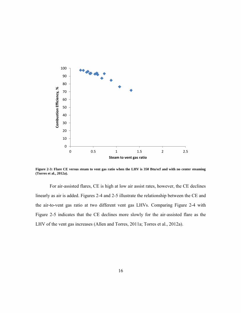
2-3 shows the relation between the flare CE and steam to vent gas ratio at LHV of 350
Btu/scf but with no center steaming. Comparing Figure 2-1 with Figure 2-3 shows that
center steaming impacts flare CE more than upper steam, where center steam indicates
steam added with the vent gas and upper steam indicates steam added at the flare tip.

15
Figure 2-1: Flare CE versus steam to vent gas ratio when the LHV is 350 Btu/scf (Torres et al., 2012a).
Figure 2-2: Flare CE versus steam to vent gas ratio when the LHV is 600 Btu/scf (Torres et al., 2012a).
0
10
20
30
40
50
60
70
80
90
100
0 0.5 1 1.5 2 2.5
Co
mb
ust
ion
Eff
icie
ncy
, %
Steam to vent gas ratio
0
10
20
30
40
50
60
70
80
90
100
0 0.5 1 1.5 2 2.5
Co
mb
ust
ion
Eff
icie
ncy
, %
Steam to vent gas ratio
16
Figure 2-3: Flare CE versus steam to vent gas ratio when the LHV is 350 Btu/scf and with no center steaming
(Torres et al., 2012a).
For air-assisted flares, CE is high at low air assist rates, however, the CE declines
linearly as air is added. Figures 2-4 and 2-5 illustrate the relationship between the CE and
the air-to-vent gas ratio at two different vent gas LHVs. Comparing Figure 2-4 with
Figure 2-5 indicates that the CE declines more slowly for the air-assisted flare as the
LHV of the vent gas increases (Allen and Torres, 2011a; Torres et al., 2012a).
0
10
20
30
40
50
60
70
80
90
100
0 0.5 1 1.5 2 2.5
Co
mb
ust
ion
Eff
icie
ncy
, %
Steam to vent gas ratio

17
Figure 2-4: Flare CE versus air to vent gas ratio when the LHV is 350 Btu/scf.
Figure 2-5: Flare CE versus air to vent gas ratio when the LHV is 560 Btu/scf.
0
10
20
30
40
50
60
70
80
90
100
0 50 100 150 200 250
Co
mb
ust
ion
Eff
icie
ncy
, %
Air-to-vent gas ratio
0
10
20
30
40
50
60
70
80
90
100
0 100 200 300 400 500
Co
mb
ust
ion
Eff
icie
ncy
, %
Air-to-vent gas ratio
18
The chemical composition of products of incomplete combustion (PICs) were also
reported. The PICs in the flare emissions include carbon monoxide formaldehyde,
ethylene, acetaldehyde, acrolein, acetylene, ethane, propylene-oxide, methanol, acetone,
propanol and butane isomers. However, the dominant species were carbon monoxide
formaldehyde, acetaldehyde, acetylene and ethylene (Allen and Torres, 2011a; Knighton
et al., 2012; Torres et al., 2012a). The chemical composition of the vent gas had some
impact on PICs, but little impact on the CE.
These detailed measurements provide new insights into methods that could be
used to reduce the air quality impacts of flares. This topic will be addressed in more
detail in Chapter 5.
2.3 REDUCING FLARING THROUGH FUEL GAS NETWORKS
The previous sections have demonstrated that flare emissions can have significant
air quality impacts. Those impacts can be mitigated by improving flare operation
(increasing CE and DRE), but a more effective strategy would be to prevent the gases
from being flared. One method for reducing flared gases is to incorporate the gases into
the fuel gas networks in refineries. This presents challenges, since as was documented in
previous sections, flared gas flows are highly variable. Nevertheless, as will be described
in Chapter 6, there are opportunities for integrating more flared gases into refinery fuel
gas networks. This section reviews previous work on fuel gas networks.
De Carli et al (2002) proposed a new management and control strategy to improve
the performance of the fuel gas network (FGN) without changing the existing
superstructure in a petroleum refinery. They discussed designing an advanced controller
for the management of the FGN with the following objectives: controlling pressure

19
variation within a prescribed range, minimizing the flared waste fuel gas, minimizing the
use of fuel oil and LPG, and stabilizing the fluid temperature. The simulations showed
good preliminary results on the performance of FGN after using the advanced controller
(De Carli et al., 2002).
Hasan et al.(2011) developed a fuel gas network (FGN) design methodology that
evaluates waste gases with fuel values from different sources (chemical processes) and
mixes them optimally to match the available fuel waste gases with various sinks ( boilers,
furnace, turbines, steam generator etc.) in a petroleum refinery or LNG plant. The
optimality of the mixing depends on the flows, chemical compositions, fuel quality of
waste gases, and fuel constraints (flow, chemical compositions and fuel qualities) of all
the potential sinks. These fuels can be used to provide steam, electricity and heat to onsite
and offsite units or plants. It is this approach to fuel gas network optimization that will be
used in this thesis to examine opportunities for minimizing flaring.
In the current formulation, the optimized FGN is a steady state model that
accounts for non-isothermal and non-isobaric operation, non-isothermal mixing,
treatment cost, utility and operating cost, the profit of using waste gases from all the
available sources and the cost of not using them. The superstructure of the FGN model
includes sources, sinks, headers (pools) for each sink and auxiliary equipment such as
heaters, coolers, compressors and valves to account for non-isothermal and non-isobaric
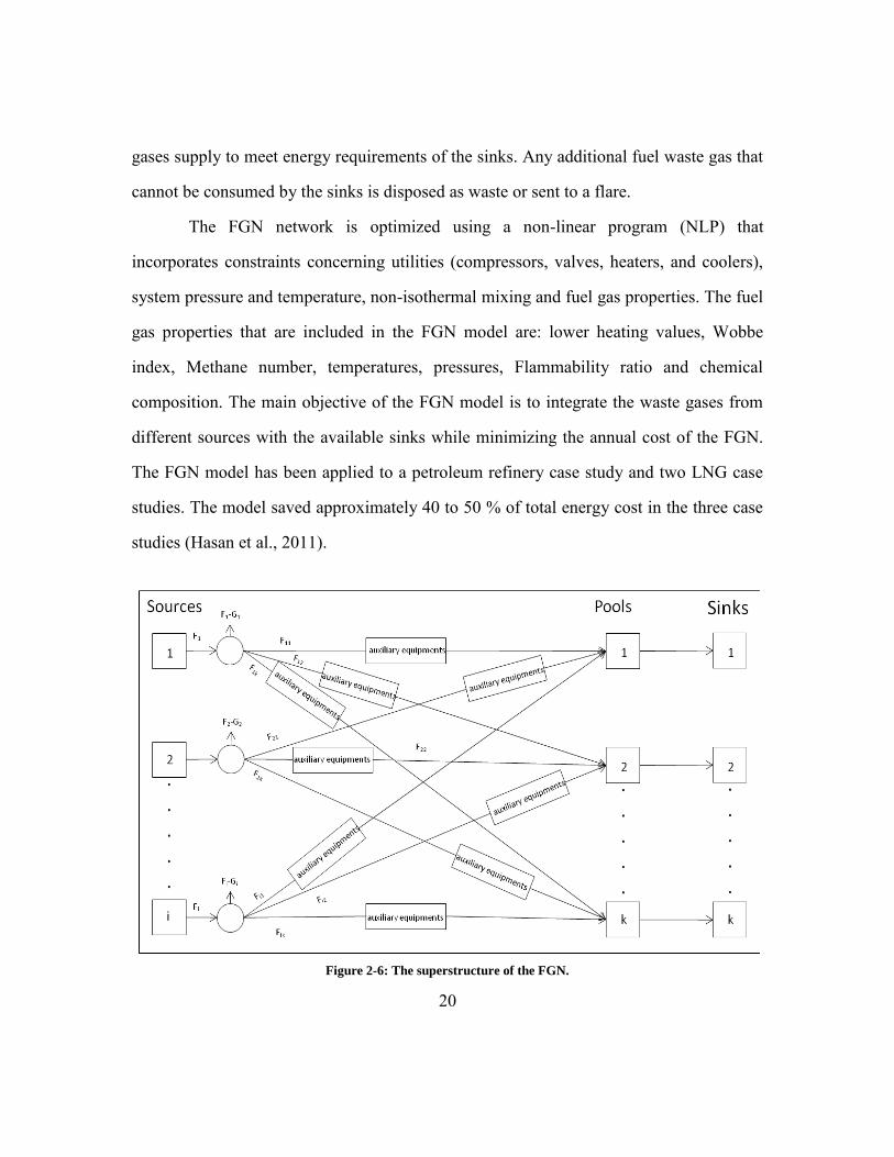
operation. Figure 2-6 shows the superstructure of the FGN. The header is used to mix the
fuels from different sources and supply the sinks with required amounts of gas. Also, a
standard fuel source was added to the superstructure of the FGN to assure the standard
fuel can be used, but with relatively higher cost, if there is any shortage in the waste
20
gases supply to meet energy requirements of the sinks. Any additional fuel waste gas that
cannot be consumed by the sinks is disposed as waste or sent to a flare.
The FGN network is optimized using a non-linear program (NLP) that
incorporates constraints concerning utilities (compressors, valves, heaters, and coolers),
system pressure and temperature, non-isothermal mixing and fuel gas properties. The fuel
gas properties that are included in the FGN model are: lower heating values, Wobbe
index, Methane number, temperatures, pressures, Flammability ratio and chemical
composition. The main objective of the FGN model is to integrate the waste gases from
different sources with the available sinks while minimizing the annual cost of the FGN.
The FGN model has been applied to a petroleum refinery case study and two LNG case
studies. The model saved approximately 40 to 50 % of total energy cost in the three case
studies (Hasan et al., 2011).
Figure 2-6: The superstructure of the FGN.

21
Broadly, the mixing and redistribution fuels in FGN is a well known problem in
the literature referred to as a pooling problem. In general, the pooling problem consists of
three main nodes. The first node represents the sources. The second node represents the
pools which are intermediate storage used to receive the streams from different sources
and distribute them to the products. These pools improve mixing flexibility; however,
impose more restrictions that introduce nonlinear constraints. The third node represents
the products. Connections among the sources, pools and the products are defined. Also,
the quality specifications of the source streams and the required characteristics of the
products are known. However, all flow rates among the sources, pools and product tanks
are unknown and are optimized subject to all the imposed constraints. Determining the
optimum flow rates between the three nodes to minimize the total cost or maximizing the
total revenue of the blending process is called the pooling problem.
Much research has been devoted to find the global solution of pooling problems
because of their importance in the petrochemical sector. Haverly (1978) proposed a
recursion approach to solve the pooling problem. However, whether the global optimum
will be found using this approach depends on the initial starting points (Haverly, 1978).
Lasdon et al. (1979) and his colleges solved the pooling problem proposed by Haverly
through nonlinear programming using generalized reduced gradient algorithms and
successive linear programming (Lasdon et al., 1979). A decomposition strategy to search
for the global optimum for the pooling problem with nonconvex bilinear terms was
proposed by Floudas and Aggarwal (1990). They applied their strategy to a pooling
problem introduced by Haverly. However, their approach cannot guarantee determining
the global optimum (Floudas and Aggarwal, 1990). Audet et al. (2004) formulated the
pooling problem into models that can be solved using the branch-and-cut quadratic

22
programming algorithm developed by Audet et al. (2000) (Audet et al., 2004; Audet et
al., 2000). Meyer and Floudas (2006) proposed a piecewise algorithm based on the
reformulation-linearization technique to determine the global solution of the pooling
problem. Their proposed approach has reduced the gap between the upper and the lower
bound to 1.2% when it was applied on a large complex industrial problem (Meyer and
Floudas, 2006). Pham et al.(2009) proposed a convex hull discretization approach to find
the global or the near global solution for the pooling problem. They solved the discretized
pooling problem as a mixed integer linear programming to determine the global
minimum flow rates among the sources, pools and the product tanks (Pham et al., 2009).
Minsener and Floudas (2010) used piecewise underestimation algorithms for the
nonconvex bilinear terms developed by(Wicaksono and Karimi, 2008), and (Gounaris et
al., 2009) to solve large scale pooling problems (Misener and Floudas, 2010)
This work will use the optimization approach utilized by Hasan, et al. (2011) to
minimize flared gases by incorporating these gases into the FGN in a refinery.
Specifically, this study will modify the FGN to accommodate the waste gases from a
fluidized catalytic cracking unit (FCCU) flare as a case study. Different scenarios will be
tested to minimize the flared from FCCU.
An alternative to incorporating flared gases into a FGN is to minimize the flared
gases at their source. As a case study of this approach, this thesis will examine
minimization of flared gases from FCC units. The approach will be to use kinetic models
of FCC units to estimate the quantity of gas generated at various operating temperatures,
then to use that information to assess the value (in minimized flare gases) of better
temperature control in FCC units. This topic is described in Chapter 7.

23
CHAPTER 3: Impact of Flare Destruction Efficiency and Products
of Incomplete Combustion on Ozone Formation in Houston, Texas
3.1 INTRODUCTION
Flares are designed to combust waste organic gases at very high efficiency. Most
flares are designed to have destruction removal efficiencies (DREs), defined as the
percentage of waste gas fed to the flare that is destroyed by complete or partial
combustion, of 98% or 99%. Flares are also designed to operate over a very large range
of flow rates. Emergency flares need to be able to handle the large volumes of gases that
may need to be disposed of very rapidly during a process upset or during a process start-
up or shut-down. Some of these emergency flares are also used to destroy much lower
flows of gases that occur during routine operation. Webster et al. (2007) have reported on
variability in the flow to a small sample of petrochemical flares; Pavlovic et al. (2012b)
have reported on flow variability for a much larger number of flares. Both of these
studies have confirmed that flow to flares varies over large ranges, and have presented
quantitative characterizations of variability in flare flows.
As described in Chapter 2, several studies have examined the impact of flow
variability in industrial flare emissions on ambient ozone concentrations, particularly
focusing on the Houston-Galveston area (Murphy and Allen, 2005; Nam et al., 2006;
Nam et al., 2008; Pavlovic, 2009; Webster et al., 2007). However, all of these studies
have assumed that the destruction efficiency in flares remains constant at 98-99%. As
also described in Chapter 2, low destruction efficiencies are possible in industrial flaring,
even when the flares are operated at conditions that may be expected to lead to high
DREs. These lower destruction efficiencies at low flows will influence the air quality
impacts of flare operation.

24
Previous analyses of the air quality impacts of flare emissions have assumed
constant destruction efficiencies; these studies have also generally assumed that unburned
hydrocarbons exiting the flare have the same composition as the waste gas. Recent
measurements have characterized products of incomplete combustion (PICs) in flares,
and these PICs include both highly reactive gases (e.g., formaldehyde and acetaldehyde)
and less reactive gases (e.g., CO) (Allen and Torres, 2011a; Herndon, 2011). These PICs
may also influence the air quality impacts of flare emissions.
This Chapter describes an extension of previous analyses of the air quality
impacts of flare emissions that uses results from recent studies of the DRE and PICs in
full scale flares. The impact on air quality of flare DREs that are less than 98-99% and
the impact on air quality, specifically ozone formation, of products of incomplete
composition (PICs), are examined.

25
3.2 METHODOLOGY
3.2.1 Industrial Flares
The first step in the analysis was to select specific flares for analysis. Flares from
petroleum refineries and from olefin manufacturing operations were chosen, as described
below.
3.2.1.1 Petroleum refinery flares
Detailed data on the flow rates to petroleum refinery flares have been examined
by Pavlovic (2009). These flares were classified into categories based on the sources of
the waste gas fed to the flare, the composition of the waste gas streams, and the
variability in the flow rates. Table 3-1 lists the 24 flares in the Houston-Galveston area,
reported with refinery source codes, with the highest reported flow rates. The flow data
are based on information from a month-long study period (August 15-September 15,
2006) during which hourly mass flows fed to the flares were reported. The flares are
grouped into five categories: natural gas flares, process gas flares, fuel fired equipment
flares, fluid catalytic cracking unit flares and unclassified flares.
This work will examine the potential air quality impacts of low destruction
efficiencies and PICs formation on three of these flares. These flares were selected based
on their relatively high average flow rates and the photochemical reactivity of the vent
gases. The three flares chosen are described in Table 3-2. Figures 3-1, 3-2 and 3-3 show
the monitored hourly flow rate time series for each of the flares selected for detailed
modeling, during the month-long data collection period starting on August 15 and ending
September 15, 2006 (768 hours).

26
Table 3-1: The 24 refinery flares with the highest VOC emissions, as reported through a month-long 2006
inventory
Process type Flow rate (Tons/32 day) Emissions, assuming
98 or 99% DRE (Tons/32day)
Natural Gas 2639.12 52.78
fuel fired equipment 1511.16 30.22
Process Gas 1515.42 15.15
Process Gas 716.18 14.32
Fluid Catalytic Cracking Unit 638.60 12.77
Natural Gas 462.22 9.24
Natural Gas 440.83 8.82
Natural Gas 333.52 6.67
Process Gas 321.03 6.42
Unclassified 311.80 6.24
Unclassified 305.56 6.11
Process Gas 302.46 6.05
Natural Gas 297.22 5.94
Unclassified 240.75 4.82
Unclassified 207.46 4.15
Unclassified 199.54 3.99
Unclassified 147.31 2.95
Unclassified 87.61 1.75
Unclassified 70.84 1.42
fuel fired equipment 69.16 1.38
fuel fired equipment 48.87 0.98
Process Gas 29.98 0.6
Fluid Catalytic Cracking Unit 14.60 0.29
Process Gas 2.18 0.04
DRE of 98 % or 99% can be assumed if a flare satisfies all criteria of 40 Code of Federal Regulation (CFR) § 60.18. If the flared gas is
alkane (butane +) and hydrogen, a DRE of 98% is assumed, and if the flared gas is propylene, propane, or ethylene, a DRE of 99% is
assumed (TCEQ, 2009).
Table 3-2: Petroleum refinery flares selected for photochemical modeling analyses
Flare identifier Flow rate
(Tons/32 day)
Emission assuming 98 or
99% DRE (Tons/32day)
Location
(lat, lon)
Average heat content
( Btu/Ib)
Refinery Flare 1 1511.16 30.22 29.717, -95.130 19300
Refinery Flare 2 1515.42 15.15 29.723, -95.209 19400
Refinery Flare 3 716.18 14.32 29.371, -94.927 19600 DRE of 98 % or 99% can be assumed if a flare satisfies all criteria of 40 Code of Federal Regulation (CFR) § 60.18. If the flared gas is alkane (butane +) and hydrogen, a DRE of 98% is assumed, and if the flared gas is propylene, propane, or ethylene, a DRE of 99% is
assumed (TCEQ, 2009)

27
Figure 3-1: Monitored hourly flow rate time series for Refinery Flare 1.
Figure 3-2: Monitored hourly flow rate time series for Refinery Flare 2.
0
5
10
15
20
25
30
0 200 400 600
Flo
w r
ate
(to
ns/
hr)
Hour of operation
0
1
2
3
4
5
6
0 200 400 600
Flo
w r
ate
(to
ns/
hr)
Hour of operation

28
Figure 3-3: Monitored hourly flow rate time series for Refinery Flare 3.
3.2.1.2 Olefin flares
Flares used in olefin (ethylene and propylene) manufacturing processes were
chosen for analysis because they have relatively high flow rates and because they emit
chemical species that have high photochemical reactivity. Table 3-3 lists the 17 flares
reported with olefin manufacturing source codes that had the highest flow rates during
the August 15 through September 15, 2006 reporting period (Pavlovic, 2009). Two of
these flares were chosen for detailed analysis (Table 3-4), based on their relatively high
flow rates and their physical location within a region in which photochemical models
with detailed spatial resolution were available. Figures 3-4 and 3-5 show the monitored
hourly flow rate time series for each of the flares selected for detailed photochemical
modeling.
0
0.5
1
1.5
2
2.5
3
3.5
4
4.5
0 200 400 600
Flo
w r
ate
(t
on
s/h
r)
Hour of operation

29
Table 3-3: The 17 olefin manufacturing flares with the highest VOC emissions, as reported through a month-
long 2006 inventory
Process type Flow rate (Tons/32day) Emissions at 98-99%
DRE (Tons/32day)
Ethylene: General 1666.88 33.34
Ethylene: General 499.13 9.98
Propylene: General 287.95 5.76
Not Classified 206.52 4.13
Ethylene: General 156.38 3.13
Ethylene: Flue Gas Vent 119.20 2.38
Ethylene: General 114.44 2.29
Ethylene: General 111.15 2.22
Ethylene: General 85.89 1.72
Propylene: Fugitive Emissions 58.58 1.17
Not Classified 55.88 1.12
Not Classified 35.01 0.7
Propylene: Fugitive Emissions 27.55 0.55
Not Classified 24.19 0.48
Ethylene: General 22.57 0.45
Not Classified 15.62 0.31
Ethylene: General 2.09 0.04 DRE of 98 % or 99% can be assumed if a flare satisfies all criteria of 40 Code of Federal Regulation (CFR) § 60.18. If the flared gas is
alkane (butane +) and hydrogen, a DRE of 98% is assumed, and if the flared gas is propylene, propane, or ethylene, a DRE of 99% is
assumed (TCEQ, 2009).
Table 3-4: Olefin manufacturing flares selected for photochemical modeling analyses
Flare identifier Flow rate
(Tons/32day)
Emission assuming 98 or
99% DRE (Tons/32day)
Location
(lat, lon)
Average heat content
( Btu/Ib flow rate)
Olefin Flare 1 499.13 9.98 29.752, -95.009 19200
Olefin Flare 2 287.95 5.76 29.858, -94.911 19500 DRE of 98 % or 99% can be assumed if a flare satisfies all criteria of 40 Code of Federal Regulation (CFR) § 60.18. If the flared gas is alkane (butane +) and hydrogen, a DRE of 98% is assumed, and if the flared gas is propylene, propane, or ethylene, a DRE of 99% is
assumed (TCEQ, 2009)

30
Figure 3-4: Monitored hourly flow rate time series for Olefin Flare 1.
Figure 3-5: Monitored hourly flow rate time series for Olefin Flare 2.
0
2
4
6
8
10
12
0 200 400 600
Flo
w r
ate
(to
ns/
hr)
Hour of operation
0
0.5
1
1.5
2
2.5
3
3.5
4
4.5
0 200 400 600
Flo
w r
ate
(to
ns/
hr)
Hour of operation

31
3.2.2 Flare chemical compositions
The chemical composition of the inlet flow was assumed constant for each flare,
and was based on the monthly average composition. Also, the composition of the VOCs
reported as unclassified in the flare composition data (ranging from 0 to 54.6% mass
fraction) was assumed to have a composition identical to the average composition of
identified species. Table 3-5 shows chemical compositions for each flare. The flared
gases contain a mixture of olefins and saturated alkanes, and therefore, the emissions
from these flares are expected to have a broad range of chemical reactivity. This
variability in the composition of flared gases also indicated that the flares service very
different chemical and petroleum processing operations. Further, the labeling of these
flares as refinery or olefin manufacturing should be regarded a broad source identifier.
Operations serviced by these flares include integrated refining and chemical
manufacturing operations, and the identifications used in this work are based on the
source code identifiers used in reporting the emissions.

32
Table 3-5: Composition of flared gases
Mass percentages in waste gases
Chemical species Refinery
Flare 1
Refinery
Flare 2
Refinery
Flare 3 Olefin Flare 1
Olefin Flare 2
1,3-BUTADIENE 7.81% 0.00% 0.00% 9.75% 0.00%
ACETYLENE 0.03% 0.00% 0.00% 0.01% 0.00%
BENZENE 0.00% 0.00% 0.00% 6.25% 0.00%
N-BUTANE 4.91% 10.14% 7.14% 4.72% 21.69%
BUTENE 0.00% 1.31% 1.45% 0.00% 0.00%
1-BUTENE 2.47% 0.00% 0.00% 0.00% 0.00%
2-METHYL-1-BUTENE 0.00% 0.00% 0.00% 2.63% 0.00%
3-METHYL-1-BUTENE 0.00% 0.00% 0.00% 0.92% 0.00%
CIS-2-BUTENE 1.17% 0.42% 0.00% 1.13% 0.04%
ETHYL BENZENE 0.00% 0.00% 0.00% 0.18% 0.00%
ETHYLENE 7.17% 0.81% 0.00% 3.54% 0.45%
HEPTANE 0.00% 0.00% 0.00% 1.76% 0.00%
HEXANE 0.00% 0.00% 7.47% 5.44% 0.00%
INDENE 0.00% 0.00% 0.00% 0.04% 0.00%
ISOBUTANE 3.39% 9.81% 9.35% 1.43% 36.26%
ISO-BUTENE 2.48% 0.00% 1.45% 0.00% 0.00%
ISOBUTYLENE 0.00% 0.00% 0.00% 5.12% 0.22%
ISO-PENTANE 0.00% 0.00% 7.26% 15.29% 0.00%
ISOPRENE 0.00% 0.00% 0.00% 5.45% 0.00%
NONANE 0.00% 0.00% 0.00% 0.50% 0.00%
OCTANE 0.00% 0.00% 0.00% 1.22% 0.00%
(E)-1,3-PENTADIENE 0.00% 0.00% 0.00% 1.48% 0.00%
1,4-PENTADIENE 0.00% 0.00% 0.00% 1.61% 0.00%
PENTANE 0.00% 0.00% 7.26% 4.15% 16.25%
N-PENTANE 0.00% 0.00% 0.00% 9.74% 0.00%
1-PENTENE 0.00% 0.00% 0.00% 3.62% 0.00%
PROPANE 1.27% 20.26% 44.01% 2.21% 15.99%
PROPYLENE 13.14% 2.26% 3.65% 4.46% 9.05%
STYRENE 0.00% 0.00% 0.00% 0.11% 0.00%
TOLUENE 0.00% 0.00% 0.00% 1.18% 0.00%
TRANS-2-BUTENE 1.60% 0.56% 0.00% 1.14% 0.06%
TRANS-2-PENTENE 0.00% 0.00% 0.00% 1.52% 0.00%
VINYL TOLUENE 0.00% 0.00% 0.00% 0.06% 0.00%
VOC-UNCLASSIFIED 54.56% 54.44% 10.96% 3.35% 0.00%
33
3.2.3 Emissions scenarios
3.2.3.1 VOC emissions
Flare DRE and the extent of PICs formation could be influenced by many factors,
such as high cross wind speed, over steaming, over aerating, and low heating value of the
waste gases. This analysis will examine the impacts on air quality for four assumed levels
of DRE (95%, 90%, 75% and 50%) for each of the five flares chosen for photochemical
modeling analyses. These DRE values will be applied to the inlet flow rate data for the
five flares to determine the flare emissions. For each flare and each DRE level, two
scenarios for PIC emissions will be examined. The first case assumes that VOC
emissions are just unburned hydrocarbons (no PICs formation) while the second case
assumes that the emissions are a combination of unburned hydrocarbons and PICs. The
ratio of unburned hydrocarbon to PICs was based on results reported in the University of
Texas flare studies (Allen and Torres, 2011a), and depended on DRE. Tables A-12 and
A-13 in the Appendix A summarize the measurement results of the PICs reported by the
University of Texas. In this work, it will be assumed that, in cases where the DRE is 95
or 90%, the ratio of unburned hydrocarbon to PIC is 1:1. For 75 and 50 % DREs, the
ratios of unburned hydrocarbons to PICs are assumed to be 4:1 and 9:1, respectively. In
all cases, the PICs are assumed to be 93% (carbon basis) carbon monoxide (CO), 5%
formaldehyde, and 2% acetaldehyde. This is a simplification of the full results of PIC
composition reported by Knighton et al. (2012), but captures the main features of the PIC
composition analysis. Much of the mass of PICs is CO, but the remainder includes highly
photochemically reactive species such as aldehydes. Taking into account all of the
assumed flare emission scenarios, for each of the 5 flares chosen for analysis, 8 scenarios

34
(in addition to the base case of 98 or 99% DRE) were examined. Table 3-6 summarizes
the 8 scenarios examined for each flare.
Table 3-6: Photochemical modeling scenarios performed for each flare
Flare emissions
Scenario DRE%
Unburned hydrocarbons PIC Ratio of hydrocarbon to PIC
A 95 yes no 1 : 0
B 95 yes yes 1 : 1
C 90 yes no 1 : 0
D 90 yes yes 1 : 1
E 75 yes no 1 : 0
F 75 yes yes 4 : 1
G 50 yes no 1 : 0
H 50 yes yes 9 : 1
These levels of DREs (95%, 90%, 75% and 50%) are within the range of
measurements reported in the University of Texas flare tests. At world-scale facilities,
refinery and olefin emergency flares can accommodate on the order of 500 tons /hr of
flow. The flow rates of the five flares selected for this analysis do not exceed 25 tons/hr
and for most of the time, the reported flows do not exceed 4.5 tons/hr (<1% expected
maxima for emergency flares). As reported by Pavlovic et al. (2012b) and Webster et al.
(2007), many flares work primarily at low flow rate conditions and may reach maximum
flow only once in several years of operation. The available flow rate data of the flares
examined in this work is for one month. Therefore, the flow rates examined in this work
could represent low flow conditions, subject to over-steaming, over-aerating and cross
wind impacts.

35
3.2.3.2 NOx emissions
Flare NOx emissions are formed by the fixation of atmospheric nitrogen at high
temperature or the reaction of hydrocarbon free radical with nitrogen in the combustion
zone (Wark et al., 1998). NOx emissions for the flares were estimated using the emission
factor from AP-42, 0.068 lb/106 BTU (EPA, 1991). Detailed information about the flare
emissions for each emission scenario is reported in the Appendix A and a more detailed
examination of the impacts of NOx emissions on air quality impacts is presented in
Chapter 4.
3.2.4 Photochemical modeling
A photochemical model was used to evaluate the impact of the flare emission
scenarios on predicted one-hour average ozone concentration in Houston, Texas. The
photochemical model used in the simulations was the Comprehensive Air Quality Model
with extension (CAMx). This model simulates the dispersion, advection, and physical
and chemical processes of pollutants in the troposphere by solving the continuity
equation for each chemical species in nested 3 dimensional grids. CAMx was selected for
this analysis since it is the photochemical model used by the State of Texas in developing
air quality management plans (State Implementation Plan or SIP). The model and input
data used in the simulations, except for the emissions of the specific flares being
examined, were the same model formulation and inputs being used by the State of Texas
in its SIP for the Houston area and are available from the Texas Commission on
Environmental Quality (TCEQ) web site (TCEQ, 2011). In this work, CAMx ready input
files were downloaded from TCEQ. These input files included initial and boundary
conditions, metrological data, emissions inventories input files, and land use data (TCEQ,

36
2010a). This base case model has undergone extensive performance evaluation, as
described by the TCEQ (TCEQ, 2011). Figure 3-6 shows the spatial domain for the
simulation and maps the horizontal grid resolutions used in the model.
Previous work had shown that the air quality impacts of flaring can be sensitive to
the horizontal grid resolution used in the modeling in the region immediately surrounding
the flare (Nam et al., 2006; Pavlovic, 2009; Webster et al., 2007). Therefore, for this
work, the minimum practicable horizontal grid resolution, 1 km, was used in the regions
in which the flares were located. A 1 km resolution was achieved by flexi-nesting
(Environ International corporation (Environ), 2010) the 2 km resolution grid provided by
the TCEQ.

37
Figure 3-6: Full domain used in this study. The East US, East Texas, Houston-Galveston-Beaumont-Port Arthur
(HGBPA), and Houston Galveston (HG) nested domains had 36, 12, 4 and 2 km resolution, respectively; in this
work the 2 km grid was flexi-nested to a 1 km resolution (TCEQ, 2010b).

38
Photochemical model predictions were made for different days for the five flares.
Days to be simulated were chosen based on three criteria. First, only days when the daily
maximum one-hour average ozone concentration in Houston exceeded 85 ppb were
considered. These days were chosen because they are meteorologically conducive to
ozone formation, and flare emissions on these days will have the greatest impact on air
quality management decisions. A second criterion was that the flow rate to the flare
would approach the observed maximum for the 2006 modeling period which is still
assumed to potentially represent low flow conditions. Finally, the availability of a high
spatial resolution photochemical modeling base case for the day of interest was
necessary. Table 3-7 shows the daily maximum mass flow rate for the selected flares,
daily maximum one-hour average ozone concentrations during the period when hourly
emissions were available, and whether high spatial resolution photochemical models
were available. Based on these data, the best simulation day for Refinery Flare 1 was
August 22, 2006, and the best day for Refinery Flare 2 was September 4, 2006; the best
day for simulation for the other flares was August 20, 2006.

39
Table 3-7: daily maximum mass flow rate for the selected flares, daily maximum one-hour average ozone
concentrations during period of 2006 SI and whether simulation files for 2 kilometers domain are exist or not
Daily maximum flow rate(ton/hr)
Date
Maximum ozone concentration(ppb)
Refinery
Flare1
Refinery
Flare2
Refinery
Flare3 Olefin Flare1
Olefin Flare2
Files of 2 Km domain
8/15/2006 98 8.6 0.2 1.3 1.6 0.6 yes
8/16/2006 141 3.5 0.1 2.2 1.1 3.1 yes
8/17/2006 158 2.4 0.1 3.3 2.1 0.7 yes
8/18/2006 106 0.1 0.1 3.1 0.9 0.5 yes
8/19/2006 69 0.5 0.4 1.7 1.4 2.0 yes
8/20/2006 107 3.3 2.8 3.9 3.5 4.1 yes
8/21/2006 102 8.7 2.1 1.6 0.9 0.6 yes
8/22/2006 93 25.3 3.8 1.4 0.8 0.8 yes
8/23/2006 75 3.8 3.9 1.3 0.9 0.6 no
8/24/2006 93 4.9 4.0 0.3 10.5 2.7 no
8/25/2006 51 3.4 3.4 1.0 8.1 2.0 no
8/26/2006 30 3.2 3.6 1.3 1.5 0.9 no
8/27/2006 36 9.5 3.8 1.1 1.0 0.8 no
8/28/2006 47 5.4 4.9 1.5 0.7 1.0 no
8/29/2006 103 2.9 3.0 1.7 1.1 1.9 yes
8/30/2006 95 3.0 3.2 1.5 1.9 0.9 yes
8/31/2006 147 4.6 3.9 1.4 0.5 1.3 yes
9/1/2006 161 0.1 3.7 1.7 0.5 0.7 yes
9/2/2006 90 0.2 3.4 2.5 0.8 1.0 yes
9/3/2006 107 0.2 3.0 1.3 1.0 1.5 yes
9/4/2006 101 0.1 4.0 1.5 0.8 0.3 yes
9/5/2006 82 4.0 3.5 1.5 0.4 1.5 yes
9/6/2006 101 3.7 3.7 1.4 0.5 2.1 yes
9/7/2006 153 4.2 3.3 1.4 0.9 0.5 yes
9/8/2006 102 7.9 3.3 1.4 0.7 0.7 yes
9/9/2006 54 6.1 3.3 1.4 0.4 0.8 no
9/10/2006 62 5.9 3.4 1.4 0.4 0.9 no
9/11/2006 68 6.3 3.5 1.4 0.4 0.4 no
9/12/2006 83 4.6 3.2 1.5 1.0 0.7 yes
9/13/2006 109 2.8 3.7 1.5 0.5 0.8 yes
9/14/2006 165 1.7 3.6 1.2 0.7 1.0 yes
9/15/2006 73 3.0 0.0 1.7 0.7 2.1 no

40
3.3 RESULTS AND DISCUSSION
Results will be reported as differences in ozone concentrations between a
photochemical modeling base case with high (98-99%) DRE and a photochemical
modeling scenario with lowered DRE, with and without PIC formation. The impact of the
flare emission scenarios on the region-wide ozone maximum and the maximum
difference in the one-hour average ozone concentrations resulting from the flare emission
scenarios will both be reported.
3.3.1 Base Case
Base cases with high flare DRE (98-99%) were simulated for August 20, 22 and
September 4, 2006. Region-wide maximum one-hour ozone concentrations of 120, 145
and 101 ppb occurred at 3:00 pm on August 20, 4:00 pm on August 22 and 2:00 pm on
September 4, respectively. Figure 3-7 shows the region-wide maximum one-hour average
ozone concentrations for each hour for the base cases on August 20, 22 and September 4,
2006. Figure 3-8 shows the spatial distribution of one-hour average ozone concentrations
for the times on the 3 days when the region-wide ozone maxima occurred.

41
Figure 3-7: Maximum one-hour ozone concentrations over HG (the red region in Figure 3-6) for the base cases
on August 20, 22 and September 4, 2006.
Figure 3-8: Ozone spatial distribution for base cases on August 20, 22 and September 4, 2006, where the white
dots are the flare locations (3 flares on August 20, 1 flare on August 22 and 1 flare on September 4). Wind was
from the south-east on August 20 and 22, 2006 and from the northeast on September 4, 2006.
0
20
40
60
80
100
120
140
160
0 5 10 15 20 25
August 20,2006
August 22,2006
September 4,2006

42
3.3.2 Flare Emission Scenarios
Eight emission scenarios, described in Table 3-6, were considered for each flare.
Results for each of the 5 flares are reported.
3.3.2.1 Refinery Flare 1
Changes in region-wide maximum one-hour average ozone concentrations on
August 22, 2006, resulting from applying different flare DREs on Refinery Flare 1, are
shown in Figure 3-9. This analysis assumes no PICs are formed. The predicted difference
in the region-wide maximum one-hour average ozone concentrations reaches 31.6 ppb
when the DRE is assumed to be 50%. The spatial distribution for differences in ozone
concentration, between the scenario when the Refinery Flare 1 has 50% DRE and the
base case on August 22, 2006, over the course of the day, is shown in Figure 3-10. The
largest difference in ozone concentrations occurs at 10 am, when the difference reaches
40.9 ppb. Figure 3-11 summarizes the maximum change in one-hour averaged ozone
concentrations, compared to the base case, for all DRE scenarios applied to Refinery
Flare 1.

43
Figure 3-9: (a) Maximum one-hour average ozone concentrations on August 22, 2006 resulting from applying
different flare DRE on the Refinery Flare 1. (b)The difference in the region-wide maxima one-hour average
ozone concentrations on August 22, 2006 resulting from applying different flare DREs on Refinery Flare 1.
0
20
40
60
80
100
120
140
160
180
0 5 10 15 20
Max
imu
m O
zon
e c
on
cen
trat
ion
(pp
b)
Time (hr)
DRE = 50%
DRE = 75%
DRE = 90%
DRE =95%
Base Case
( a )
0
5
10
15
20
25
30
35
0 5 10 15 20
Dif
fere
nce
in m
axim
um
ozo
ne
co
nce
ntr
atio
n(p
pb
)
Time (hr)
DRE = 50%
DRE = 75%
DRE = 90%
DRE =95%
( b )

44
Figure 3-10: The spatial distribution for the differences in ozone concentrations from 8:00 am through 3:00 pm
between the scenario when Refinery Flare 1 has 50% DRE and the base case, on August 22, 2006.

45
Figure 3-11: The maximum change in one-hour ozone concentrations compared to the base case on August 22,
2006 resulting from applying different flare DREs to Refinery Flare 1.
The results in Figures 3-9 to 3-11 assumed that the flare emissions contained just
unburned hydrocarbons. Including PICs in the photochemical modeling scenarios had
relatively little impact on ozone formation chemistry. Table 3-8 shows the region-wide
maximum one-hour average ozone concentrations on August 22, 2006 for each of the
DRE scenarios, with and without PICs. Since the PICs include relatively reactive
aldehydes, and relatively unreactive CO, the net impact of replacing some of the
unburned flare gases with PICs had a relatively small impact on the reactivity of the
emissions for this flare, and in fact, lowered the estimated ozone formation by
approximately one ppb.
0
5
10
15
20
25
30
35
40
45
0 5 10 15 20
Max
imu
m d
iffe
ren
ce in
ozo
ne
co
nce
ntr
atio
n(p
pb
)
Time (hr)
DRE = 50%
DRE = 75%
DRE = 90%
DRE =95%

46
Table 3-8: Summary of Maximum ozone concentrations (ppb) for all DRE scenarios applied on Refinery Flare 1
DRE % No PICs PICs
50 157.9 156.9
75 151.9 150.8
90 147.7 146.3
95 146.2 145.4
3.3.2.2 Refinery Flares 2 and 3
Predicted changes in region-wide maximum one-hour average ozone
concentrations on September 4, 2006, and August 20, 2006, resulting from applying
different flare DREs on Refinery Flares 2 and 3, respectively, are shown in Table 3-9.
Predicted ozone enhancements are much smaller than for Refinery Flare 1, with a
maximum difference in the one-hour ozone concentrations for the 50% DRE scenario of
4-5 ppb for both Refinery Flares 2 and 3. DRE scenarios with PICs and hydrocarbon
emissions have almost the same impact as DRE scenarios with no PICs emissions.
The difference in air quality impacts between Refinery Flare 1 and Refinery
Flares 2 and 3 is largely due to the chemical composition and the flow rate of flared
gases. A quantitative estimate of the relative role of the reactivity of flared gases can be
calculated based on the composition and the Maximum Incremental Reactivity (MIR) of
the individual gases. This approach has been used previously to assess the effectiveness
of reactivity-based emission trading programs in Houston (Wang et al., 2007). The
maximum incremental reactivity was calculated using data from the SAPRC-07 chemical
mechanism (Carter, 2011). The results indicate that each 100 g of Refinery Flare 1 gases

47
has the potential to produce 896 g of ozone. In contrast, each 100 g of Refinery Flare 2
and Refinery Flare 3 gases has the potential to form 207 and 153 g of ozone, respectively.
While these are likely not accurate absolute estimates of ozone production, previous work
has shown that, for Houston, they are reliable indicators of relative ozone formation
potential (Wang et al., 2007). Therefore, the Refinery Flare 1 gases are likely to be 4-6
times more reactive than Refinery Flares 2 or 3. This coupled with the higher flow rate of
Refinery Flare 1, accounts for much of the difference in ozone formation between the
flares. The remainder is likely due to different photochemistry on different days.

48
Table 3-9 : The difference in wide region maxima one-hour average ozone concentrations (in ppb) and the maximum difference in one-hour average ozone
concentrations (in ppb) for all the flare DRE scenarios applied to the three refinery flares compared to the base case
Difference in maximum ozone concentration(ppb)
Maximum difference in ozone concentration(ppb)
Refinery Flare 1
Refinery Flare 2
Refinery Flare 3
Refinery Flare 1
Refinery Flare 2
Refinery Flare 3
DRE %
No PIC
PIC No PIC
PIC No PIC
PIC No PIC
PIC No PIC
PIC No PIC
PIC
50 31.6 29.0 0.3 0.3 0.2 0.2 40.9 37.3 4.0 3.7 4.2 4.6
75 16.3 13.2 0.2 0.2 0.1 0.1 21.0 17.3 2.4 1.8 2.0 2.0
90 5.1 2.2 0.1 0.1 0.1 0.0 8.3 3.2 0.7 0.6 0.7 0.6
95 1.7 0.3 0.0 0.0 0.0 0.0 2.4 1.7 0.3 0.4 0.2 0.2

49
3.3.2.3 Olefin Flares
Results for the olefin flares were qualitatively similar to the results for the 3
refinery flares. One of the flares (Olefin Flare 1) exhibited relatively large impacts, while
the other flare had relatively low impacts. For Olefin Flare 1, the predicted maximum
difference in one-hour average ozone concentrations reach 17.2 ppb, compared to the
base case. Including PICs in the simulations reduced the maximum difference in one-
hour average ozone concentrations by a few ppb. In contrast, for Olefin Flare 2, the
maximum difference in ozone concentrations was 1.5 ppb. Table 3-10 summarizes the
difference in wide region maxima and maximum difference in one-hour average ozone
concentrations for two olefin flares, compared to the base case.
Table 3-10 : The difference in wide region maxima one-hour average ozone concentrations (in ppb) and the
maximum difference in one-hour average ozone concentrations (in ppb) for all the flare DRE scenarios applied
to the two olefin flares compared to the base
Difference in maximum ozone concentration(ppb)
Maximum difference in ozone concentration(ppb)
Olefin Flare1 Olefin Flare2 Olefin Flare1 Olefin Flare2
DRE % No PIC PIC No PIC PIC No PIC PIC No PIC PIC
50 2.8 2.5 0.4 0.4 17.2 15.7 1.3 1.5 75 1.1 0.9 0.2 0.2 6.5 5.5 0.8 0.8 90 0.4 0.2 0.1 0.1 2.0 1.0 0.4 0.4 95 0.1 0.0 0.0 0.0 0.5 0.2 0.3 0.3
This large difference in the air quality impacts of the two olefin flares could be
due to the same reasons as the refinery flares. Maximum incremental reactivity data
(Carter, 2011) for the flares gases from Olefin Flare 1 showed that each 100 g of flared
gases has the potential to form 515 g atmospheric ozone. In contrast, 100 g of vent gases

50
from Olefin Flare 2 has the potential to produce 211 g ozone. The flow rate of Olefin
Flare 1 is roughly double that of Olefin Flare 2. The remainder of the difference is likely
due to the different physical location of the flares.
Overall, flow and chemical reactivity explain much of the difference in ozone
formation differences among the flares considered in this work. Table 3-11 shows the
product of the mass of emissions, multiplied by the MIR of the emitted gases for each of
the flares. The maximum daily flow rates were used in the calculations. Table 3-12 shows
the absolute product of flow rate and reactivity (reported in Table 3-11) divided by the
base case value. This represents a relative increase in ozone formation potential. The
results suggest that the relative increase in ozone formation potential is reasonably
consistent among the flares as DRE is reduced and that a DRE of 50% can lead to an
increase in ozone formation potential of a factor of up to 20-50 (2000-5000%), relative to
the base case. (Al-Fadhli et al., 2012a)

51
Table 3-11: The mass of the predicted ozone (ton) for all scenarios when the maximum daily flow rates were used for the five flares. The maximum daily flow
rates for Refinery Flare 1, 2, 3, Olefin Flare 1 and 2 are 25.3, 4, 3.9, 3.5 and 4.1 tons/ hr respectively. The mass of the predicted ozone was based on MIR values
(Carter, 2011)
Refinery Flare1 Refinery Flare2 Refinery Flare3 Olefin Flare1 Olefin Flare2
DRE % No PIC PIC No PIC PIC No PIC PIC No PIC PIC No PIC PIC
50 113.4 103.8 4.1 3.9 3.0 2.9 9.1 8.4 4.4 4.2 75 56.7 47.0 2.0 1.9 1.5 1.4 4.5 3.9 2.2 2.0 90 22.7 13.0 0.8 0.7 0.6 0.5 1.8 1.1 0.9 0.7 95 11.3 6.5 0.4 0.3 0.3 0.3 0.9 0.6 0.4 0.4
Base Case 4.5 0.1 0.1 0.4 0.2
Table 3-12 : The absolute product all the scenarios in Table 3-11 divided by the base case value
Refinery Flare1 Refinery Flare2 Refinery Flare3 Olefin Flare1 Olefin Flare2
DRE % No PIC PIC No PIC PIC No PIC PIC No PIC PIC No PIC PIC 50 25.0 22.9 50.0 48.1 25.0 24.6 25.0 23.1 25.0 24.0 75 12.5 10.4 25.0 23.1 12.5 12.1 12.5 10.6 12.5 11.5 90 5.0 2.9 10.0 8.1 5.0 4.6 5.0 3.1 5.0 4.0 95 2.5 1.4 5.0 4.0 2.5 2.3 2.5 1.6 2.5 2.0

52
3.4 CONCLUSION
The impact of flare DRE on the ozone formation potential of flare emissions
varies among flares. Five flares were examined in this study. Two flares showed a
predicted increases in ozone concentrations in excess of 15 ppb when the DRE is
reduced. The other three flares showed smaller impacts on the ozone concentrations. The
flare DRE impact on ozone concentration depends on the amount of flare emissions and
chemical composition of the emissions. PICs have a modest impact on ozone
concentration because most of PIC mass is carbon monoxide which has low chemical
reactivity to form ozone.
The analyses reported here are intended to represent upper bounds on the ozone
formation potential of flare emissions. The flow rates analyzed were for days when flow
rates were reaching their maxima for the month-long study. Meteorological conditions
were conducive to ozone formation. Destruction efficiencies as low as 50% were
assumed, and while these low DREs have been observed, they may not be representative
for these flares at these flow conditions. VOC emissions that had unclassified
compositions were assumed to have the same composition as the average of the speciated
emissions; the true composition of these unclassified emissions may have a lower
reactivity than the speciated emissions. Nevertheless, the results indicate that for flares
burning photochemically reactive gases, ozone formation potential of flare emissions
could lead to increases in ozone concentrations in excess of 15 ppb. These results
reported here indicate that ensuring high DRE during flaring operations can be important
for regional air quality.

53
CHAPTER 4: Impact of Emissions of Nitrogen Oxides from Flares
on Ozone Formation in Houston, Texas
4.1 INTRODUCTION
Flares destruct waste gases by burning them at high temperature to produce
carbon dioxide and steam, with an efficiency that is designed to be 9899%. Oxides of
nitrogen (NOx, the sum of NO and NO2) are formed as a by-product of combustion (Wark
et al., 1998), and since NOx is a precursor for tropospheric ozone production (Seinfeld
and Pandis, 2006), emissions of NOx are inventoried in regions where ozone
concentrations are of concern. Typically, NOx emissions from flares are estimated using
methods outlined by the US Environmental Protection Agency (EPA) in the AP-42 series
of documents (EPA, 1991). Emissions are estimated by multiplying an emission factor by
an activity parameter:
( 4.1 )
where E is the emissions rate, A is the activity rate and EF is the emission factor.
For estimating NOx emissions from flares, current practice, based on information
documented in Section 13.5-1 of AP-42, is to assume a constant emission factor of 0.068
lb NOx per million BTU of heating value (lower heating value, LHV) of gases sent to the
flare. A slightly different set of emission factors is suggested in documentation from the
State of Texas (TCEQ, 2000). The Texas Commission on Environmental Quality (TCEQ)
suggests the use of one of four emission factors, two for low heating value gases (0.068
and 0.064 lb NOx per million BTU of heating value for steam- and air-assisted flares,
respectively) and two for high heating value gases (0.049 and 0.14 lb NOx per million
54
BTU of heating value for steam- and air-assisted flares, respectively). The emission
factors suggested by the TCEQ for low heating value gases are very similar to the AP-42
emission factor.
The activity factor in equation 4.1 is the flow rate of gases fed to the flare,
multiplied by their lower heating value. Emissions are estimated, as indicated in equation
4.1, by multiplying the activity factor by the emission factor. This approach to estimating
NOx emissions from flares, and the emission factors, are based largely on data collected
during full scale flare tests conducted in 1983, with flares generally operating at high
flow rates, with high heating value gases (McDaniel, 1983). During these tests,
combustion efficiencies (fraction of the feed gases converted to CO2 and water) were
high.
As stated in Chapter 2, if too much steam or air is added to flared gases (steam
and air-assist), particularly at low flow conditions and with low heating value gases being
flared, combustion efficiencies can be lower than the targeted values of 98-99%. Since
less heat of combustion is generated with low heating value gases, combustion
temperatures are lower than for high heating value gases, production of NOx may be
reduced. Further, if too much air or steam is added to the flared gases, destruction
efficiencies and combustion temperatures can be reduced, and NOx emissions may be
reduced. This Chapter presents NOx emission data for the steam-assisted and air-assisted
flare tests reported by Torres et al. (2012a) and Torres et al.(2012b). These tests were
conducted at low flow rates (0.1% to 0.25% of maximum flow), and with low heating
value gases (300-650 BTU LHV/scf). The NOx emission rates from the tests will be
shown to be generally lower than emissions calculated using existing procedures, and the

55
potential implications for region-wide NOx emission estimates and ozone formation in
the Houston area of these lower NOx emission rates from flares are quantified.
4.2 METHODS
4.2.1 Emission factor
NOx emissions from industrial flares have been estimated using an emission
factor of 0.068 lb of NOx/106 BTU of flared gas. Equation 4.2 (similar to equation 4.1)
uses the AP-42 NOx emission factor to estimate the NOx emission rate from burning
hydrocarbon gases using an industrial flare.
( 4.2 )
where Xi is the mass fraction of species i and LHVi is the lower heating value for species
i (BTU/lb).
The results of the University of Texas flare study showed that NOx emissions are
a function of the combustion efficiency of the flare. The NOx (lbmole) to total C
(lbmole) ratios were measured during flare tests done with propane as the flared gas
(Torres et al., 2012c). The propane was fed to the flares (steam- and air-assist) with
natural gas in a volume ratio of 4:1. The NOx emission factors were estimated based on
the measured NOx (lbmole) / C (lbmole) ratios using equation 4.3. The derivation of
equation 4.3 is described in detail in Torres et al. (2012c). The measured NOx (lbmole)
to C (lbmole) ratios showed that the NOx emission factor ranged from 10120% of the
factor reported in AP-42.

56
( 4.3 )
Figures 4-1 and 4-2 show the estimated NOx emission factor versus the
combustion efficiency of a steam-assisted flare and an air-assisted flare, respectively. As
shown in Figures 4-1 and 4-2, the air-assisted flare has higher NOx emissions than does
the steam-assisted flare. This suggests that the NOx emission factor for the air-assisted
flares should be higher than that for the steam-assisted flares. However, the NOx emission
factor is the same for both air- and steam-assisted flares in AP-42. Moreover, both
Figures (4-1and 4-2) indicate that the NOx emissions are high at high combustion
efficiency (9899%) and drop by a factor of 2 when combustion efficiency reaches 90%.
Then, the NOx emissions remain relatively constant as the combustion efficiency
decreases below 90%.

57
Figure 4-1: The estimated NOx emission factor versus the combustion efficiency for the steam-assisted flare.
Figure 4-2: The estimated NOx emission factor versus the combustion efficiency for the air-assisted flare.
-0.002
0.008
0.018
0.028
0.038
0.048
0.058
0.068
30 40 50 60 70 80 90 100
NO
x e
mis
sio
n f
acto
r (l
b N
Ox/
10
6 B
TU)
Combustion efficiency (%)
NOx factor based on AP-42
0
0.01
0.02
0.03
0.04
0.05
0.06
0.07
0.08
0.09
60 65 70 75 80 85 90 95 100
NO
x e
mis
sio
n f
acto
r (l
b N
Ox/
10
6 B
TU)
Combustion efficiency (%)
NOx factor based on AP-42

58
These results will be used to compare the impact of estimated NOx emissions,
based on the University of Texas flare study, with the impact of NOx emissions based on
the AP-42 emission factor, on the formation of ozone in Houston, Texas.
4.2.2 Air quality
4.2.2.1 Flare selection
Five industrial flares were considered for evaluating the impact of new NOx
emission factors on air quality. These are the same five flares examined in Chapter 3,
where they were used to estimate the impact of low flare DRE and products of
incomplete combustion on ozone formation in Houston, Texas. Of these five flares,
Refinery Flare 1 showed the highest increase in ozone concentrations (up to 40 ppb)
when its DRE was low. Therefore, Refinery Flare 1 is used in this analysis. Table 3-2
provides detailed information about Refinery Flare 1. The chemical composition of the
flared gases for Refinery Flare 1 is shown in Table 3-5.
4.2.2.2 NOx emission scenarios
To estimate the impact of the NOx emission factors for an industrial flare on
ozone formation, NOx emission scenarios were developed based on the results of the
University of Texas flare study. In this work, we assume that Refinery Flare 1 is a steam-
assisted flare because it is one of the largest refinery flares in the Houston area. Most of
the largest refinery flares are steam-assisted (EPA, 2000). Based on the results for the
steam-assisted flare reported in Figure 4-1, three NOx emission scenarios were developed
depending on the levels of the flare DRE. The first scenario assumes the NOx emission
factor is 50% of the AP-42 value at a DRE of 98%. The second and the third scenarios

59
assume that the NOx emissions are 25% of the estimated NOx emissions based on an AP-
42 value at flare DREs of 90% and 75%. These scenarios were applied to Refinery Flare
1. Table 4-1 summarizes the three scenarios. Detailed information about Refinery Flare 1
emissions for each NOx emission scenario is reported in Appendix B. A photochemical
model, described in Chapter 3, was used to predict changes in one-hour average ozone
concentrations resulting from each scenario.
Table 4-1: Photochemical modeling scenarios performed for Refinery Flare 1
Scenario DRE% NOx reduction compared to the AP-42 value
1 98 50%
2 90 25%
3 75 25%
4.2.2.3 Photochemical modeling
CAMx was used to predict one-hour average ozone concentrations resulting from
applying the NOx emission scenarios to Refinery Flare 1. Figure 3-6 (in Chapter 3) shows
the full spatial domain used by the photochemical model, where the red region is the
Houston area, which is modeled with 1 km grid resolution. In this work, all the input
files required by CAMx were downloaded from the TCEQ website, except the emission
from Refinery Flare 1. A simulation day of August 22, 2006 was selected based on three
criteria developed in Chapter 3. Additional information concerning the photochemical
model is also provided in Chapter 3.

60
4.3 RESULTS AND DISCUSSION
The simulation results will be reported as the difference in ozone concentrations
between the examined scenarios and the base case. The base case assumes the DRE of
Refinery Flare 1 is 98% and the NOx emissions are based on the AP-42 factor. The
simulation results of the base case are discussed in detail in Chapter 3.
The differences in the region-wide maximum one-hour average ozone
concentrations resulting from applying the three scenarios with the reduced NOx to
Refinery Flare 1 are shown in Figure 4-3. The first scenario (DRE of 98% with reduced
NOx) shows no change in the region-wide maxima compared to the base case. In contrast,
the second and the third scenarios (DREs of 90% and 75%, respectively, with the reduced
NOx) show positive increases in the predicted difference in the region-wide maximum
one-hour average ozone concentrations up to 5.1 and 16.4 ppb, respectively.
Figure 4-3: The changes in the region-wide maximum one-hour average ozone concentrations on August 22,
2006, resulting from applying the three scenarios with the reduced NOx to Refinery Flare 1.
0
2
4
6
8
10
12
14
16
18
0 5 10 15 20 25
Dif
fere
nce
in m
axim
um
ozo
ne
co
nce
ntr
atio
n(p
pb
)
Time (hr)
DRE = 75%
DRE = 90%
DRE =98%

61
Figures 4-4, 4-5, and 4-6 show the spatial distribution for the differences in the
one-hour average ozone concentrations between the three scenarios with reduced NOx
and the base case, over the course of August 22, 2006. Figure 4-4 (98% DRE, reduced
NOx) shows that the largest predicted difference in ozone concentrations occurred at 2 am
and reached 6.6 ppb. However, the reduction in ozone concentration was highly
localized around Refinery Flare 1. The largest predicted difference in ozone
concentrations in Figure 4-5 (90% DRE, reduced NOx) reached up to 9.4 ppb, and it
occurred at 3 am. The largest predicted difference in ozone concentrations in Figure 4-6
(75% DRE, reduced NOx) reached up to 21.0 ppb, and it occurred at 11 am. Figure 4-7
summarizes the maximum positive and the minimum negative changes in one-hour
average ozone concentrations for all the three scenarios compared to the base case. Table
4-2 summarizes the maximum difference in wide region maxima, maximum difference in
one-hour average ozone concentrations, and minimum difference in one-hour average
ozone concentrations for the three scenarios compared to the base case.

62
Figure 4-4: The spatial distribution for the differences in ozone concentration from 00:00 am through 7:00 am
between the scenario of 98% DRE and NOx reduced to 50% of the AP-42 value and the base case on August 22,
2006.

63
Figure 4-5: The spatial distribution for the differences in ozone concentration from 1:00 am through 8:00 am
between the scenario of 90% DRE and NOx reduced to 25% of the AP-42 value and the base case on August 22,
2006.

64
Figure 4-6: The spatial distribution for the differences in ozone concentration from 8:00 am through 3:00 pm
between the scenario of 75% DRE and NOx reduced to 25% of the AP-42 value and the base case on August 22,
2006.

65
Figure 4-7: (a) The maximum positive changes in one-hour average ozone concentrations compared to the base
case on August 22, 2006 resulting from applying the three scenarios to Refinery Flare 1. (b) The minimum
negative changes in one-hour ozone average concentrations compared to the base case on August 22, 2006
resulting from applying the three scenarios to Refinery Flare 1.
0
5
10
15
20
25
0 5 10 15 20 25
Max
imu
m d
iffe
ren
ce in
ozo
ne
co
nce
ntr
atio
n(p
pb
)
Time (hr)
DRE = 75%
DRE = 90%
DRE =98%
-7
-6
-5
-4
-3
-2
-1
0
0 5 10 15 20 25
Min
imu
m d
iffe
ren
ce in
ozo
ne
co
nce
ntr
atio
n(p
pb
)
Time (hr)
DRE = 75%
DRE = 90%
DRE =98%
A
(a)
A
(b)
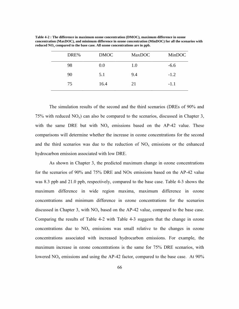
66
Table 4-2 : The difference in maximum ozone concentration (DMOC), maximum difference in ozone
concentration (MaxDOC), and minimum difference in ozone concentration (MinDOC) for all the scenarios with
reduced NOx compared to the base case. All ozone concentrations are in ppb.
DRE% DMOC MaxDOC MinDOC
98 0.0 1.0 -6.6
90 5.1 9.4 -1.2
75 16.4 21 -1.1
The simulation results of the second and the third scenarios (DREs of 90% and
75% with reduced NOx) can also be compared to the scenarios, discussed in Chapter 3,
with the same DRE but with NOx emissions based on the AP-42 value. These
comparisons will determine whether the increase in ozone concentrations for the second
and the third scenarios was due to the reduction of NOx emissions or the enhanced
hydrocarbon emission associated with low DRE.
As shown in Chapter 3, the predicted maximum change in ozone concentrations
for the scenarios of 90% and 75% DRE and NOx emissions based on the AP-42 value
was 8.3 ppb and 21.0 ppb, respectively, compared to the base case. Table 4-3 shows the
maximum difference in wide region maxima, maximum difference in ozone
concentrations and minimum difference in ozone concentrations for the scenarios
discussed in Chapter 3, with NOx based on the AP-42 value, compared to the base case.
Comparing the results of Table 4-2 with Table 4-3 suggests that the change in ozone
concentrations due to NOx emissions was small relative to the changes in ozone
concentrations associated with increased hydrocarbon emissions. For example, the
maximum increase in ozone concentrations is the same for 75% DRE scenarios, with
lowered NOx emissions and using the AP-42 factor, compared to the base case. At 90%

67
DRE, the positive change in the ozone concentrations is 9.4 ppb compared to the base
case, in which NOx emissions are lowered to 25% of the AP-42 value. Using the AP-42
NOx emission factor, at 90% DRE, results in an increase in ozone concentrations of up to
8.3 ppb, compared to the base case. Again, lowering the DRE of Refinery Flare 1 has a
greater impact on hydrocarbon emissions than on NOx emissions. In general, industrial
flares are located in complexes that have many sources of NOx emissions. Thus, the
hydrocarbon emissions from Refinery Flare 1 could react with NOx from other sources in
the facility or its NOx emissions.
Table 4-3: The difference in maximum ozone concentration (DMOC), maximum difference in ozone
concentration (MaxDOC) and minimum difference in ozone concentration (MinDOC) for all the scenarios with
NOx based on AP-42 compared to the base case with NOx based on AP-42 value.
DRE% DMOC MaxDOC MinDOC
90 5.1 8.3 -2.7
75 16.3 21 -1.0
4.4 CONCLUSION
The production of NOx from industrial flares is not constant. It depends on the
DRE of the flare. Lowering the flare DRE decreases the temperature of the combustion
zone. This reduction in the flame temperature leads to a reduction in formation of NOx
emissions. The results of the University of Texas flare study showed that the NOx
emission factor ranged from 10120% of the factor reported in the AP-42. Also, the
results showed that the air-assisted flare produced more NOx emissions than did the

68
steam-assisted flare. Photochemical modeling simulation indicated that lowering the NOx
emissions of a large refinery flare had small impacts on the ozone formation relative to
changes in ozone concentration associated with the enhanced hydrocarbon emissions at
low DRE. The change in ozone concentration resulting from changing the NOx emission
was highly localized around the refinery flare.

69
CHAPTER 5: Impacts of Air-Assist Flare Blower Configurations on
Flaring Emissions
5.1 INTRODUCTION
Flares burn waste gases at high temperature, in an open flame, to produce carbon
dioxide and steam. Flares are primarily safety devices designed to destroy waste gases
(vent gases) at a destruction removal efficiency (DRE, fraction of waste gases destroyed
by complete and incomplete combustion) of 9899%. As described in Chapter 2, flares
operating at low flow rates (<1% of designed maximum flow) and with low heating value
gases (<600 BTU/scf lower heating value (LHV)) can have low destruction efficiencies,
particularly when air-assist or steam-assist rates are high. Chapter 2 also described
studies that have demonstrated that, for vent gases with low heating values, there is, at
times, a narrow operating window of air assist-to-vent gas ratios and steam-to-vent gas
ratios that achieve both high destruction efficiencies and avoid flare generated smoke.
The purpose of the analyses presented in this Chapter is to examine how flare
configurations, particularly blower selection for air-assisted flares, may limit the ability
of a flare to operate in the targeted, but narrow, operating window that achieves low
smoke and high destruction efficiencies, and the potential implications for flare
emissions.
The air-assisted flare to be used as a case study in this work is the flare described
by Torres, et al (Allen and Torres, 2011a; TCEQ, 2010c; Torres et al., 2012a; Torres et
al., 2012b). This flare can accommodate a maximum vent gas flow rate of 144,000
pounds per hour when used with propylene and operated in compliance with 40 Code of
Federal Regulation §60.18. It would typically be operated with a blower or blowers that
can deliver 65,000 cfm of air assist (Kodesh, 2012). The blower(s) used in an air-assisted

70
flare can be either fixed or variable speed. Both fixed and variable speed blowers will be
considered in the analyses to be presented here, and two configurations of each type will
be examined. The fixed-speed motor designs are (a) a single blower (65,000 cfm) that has
a two-speed motor (off, half speed and full speed), and (b) dual blowers, each with two
speeds, delivering a combined maximum flow of 65,000 cfm. The variable-speed blowers
are assumed to operate with variable frequency drives (VFDs) capable of generating
flows of 5% to 100% of blower design capacity. Scenarios with single blowers and dual
blowers with VFDs are examined.

71
5.2 METHODS
5.2.1 Air-assisted flare experimental tests
Torres et al. reported full-scale air-assisted flare tests under low flow and low
heating value conditions (Torres et al., 2012a; Torres et al., 2012b). The air-assisted flare
used in the tests had a tip 24 inches in diameter and a maximum design capacity of
144,000 lb/hr. The chemical composition of the vent gas was a mixture of propylene and
natural gas, with nitrogen added as a diluent to reach low heating value conditions. The
volume ratio of the propylene to natural gas in the vent gas was 4:1 in all tests. Two
targeted LHVs (560 and 350 Btu/scf) were tested under low flow conditions (less than
0.7% of the maximum capacity). The test results showed that the air-assisted flare
achieves high DRE at low air-to-vent gas ratios, and the DRE drops linearly as the air-to-
vent gas ratio increases. Figure 5-1 shows the relationship between DRE and air-to-vent
gas ratio when the LHV was 560 Btu/scf and when the LHV was 350 Btu/scf.

72
Figure 5-1: Destruction removal efficiency (DRE) versus air-to-vent gas ratio for flared gases with a lower
heating value (LHV) of 560 Btu/Scf (upper) and 350 Btu/Scf (lower) (Torres et al., 2012a).
R² = 0.85
0
10
20
30
40
50
60
70
80
90
100
0 50 100 150 200
DR
E%
Air-to-vent gas ratio (mass basis)
DRE = -0.11 *(Air-to-vent ratio) + 102.9 (Air-to-vent ratio> 26.4 ) DRE = 99.9 (Air-to-vent ratio< 26.4)
R² = 0.88
0
10
20
30
40
50
60
70
80
90
100
0 20 40 60 80 100 120 140 160
DR
E %
Air to vent gas ratio (mass basis)
DRE = -0.25 *(Air-to-vent ratio) + 104.9 (Air-to-vent ratio> 19.6 ) DRE = 99.9 (Air-to-vent ratio< 19.6)

73
5.2.2 Stochastic models
To determine the DRE achievable with air-assisted flares with various blower
configurations, the air assist-to-vent gas ratio must be calculated (Figure 5-1). This
requires an understanding of the vent gas flow rates fed to the flare, along with the air
assist flows achievable using either fixed or variable speed blowers. In this study, models
of flare vent gas flows developed by Pavlovic et al. (2012b) for refinery flares are used to
estimate hourly flow rates of vent gas. These models were developed based on hourly
flow rates of a large number of refinery flares in Houston, Texas for a month-long period
in the summer of 2006. The modeled flows are therefore assumed to be representative of
the temporal variation in flows to refinery flares in Houston, Texas. Pavlovic et al.
(2012b) grouped refinery flares into three categories: (a) natural, process, and fuel-fired
equipment flares, (b) fluid catalytic cracking flares, and (c) unclassified process flares.
The natural, process, and fuel-fired equipment flares, and the unclassified process flares
were further divided into sub-categories based on their relative variability, defined as the
ratio of the standard deviation to the average flow rate. This results in the six groups of
refinery flares shown in Table 5-1.

74
Table 5-1: Categorization of petroleum refinery flares in 2006 SI (Pavlovic et al., 2012b).
Group
Number Group Name
1 Natural, process, and fuel-fired equipment flares–low variability
2 Natural, process, and fuel-fired equipment flares–medium variability
3 Natural, process, and fuel-fired equipment flares–high variability
4 Fluid catalytic cracking flares
5 Unclassified process flares–low variability
6 Unclassified process flares–high variability
In this analysis, the models for the hourly flow of vent gas to six types of refinery
flares were used to generate 240 hours (10 days) of simulated flow rates for each flare
type. Flow rates for ten days were generated to capture a broad range of variability in the
flow rates to each flare type. The models predicted normalized hourly flow rates (hourly
flow/time averaged flow), so hourly flare flow was predicted by multiplying normalized
hourly flow rates generated by the model by an average flow rate. In this work, five
average flow rate scenarios were developed for each of the 6 flare types. The first
scenario assumed that the maximum hourly flow (of the 240 hours of simulated flow)
was 1% of the maximum design capacity (1,440 lb/hr) of the air-assisted flare (maximum
design capacity of 144,000 lb/hr). The average flow for this scenario was calculated by
dividing the 1,440 lb/hr by the maximum normalized hourly flow predicted by the model
for the 240 hours of simulation. This average flow was then multiplied by the 240
normalized hourly flow rates to obtain the 240 hourly flow rates for this scenario.
Assuming that the maximum predicted flow over a 10 day period is 1% of flare capacity

75
is a feasible scenario because many flares only experience maximum flow once over a
period of multiple years. The flare vent gas flow data reported by Pavlovic, and which the
model is based on, are for only one month of operations, and it is unlikely that a flare
would reach its design flow limit during such a short sampling period. However,
assuming that the maximum flow achieved over one month of sampling is only 1% of
maximum flow may be too low. Therefore, four additional scenarios were examined
assuming that the maximum flows over 240 hours were 5, 10, 20 and 100%, respectively,
of the maximum design capacity of the air-assisted flare. Most of these scenarios were for
low flow conditions (maximum flow for the 240 simulated hours less than 20% of
maximum design capacity of 144,000 lb/hr) because most industrial flares work at low
flow conditions most of their operating time (ENVIRON International Corporation, 2009;
Pavlovic et al., 2012b). The 100% scenario was considered because during upset
conditions, flares may work near their maximum design flow; however, the primary focus
of this work is on low flow conditions. Overall, 5 scenarios for the flow to each flare
were considered, each with the same pattern of temporal variability, but scaled to
different average flows.
Calculating the air assist-to-vent gas ratio for each of the 30 flaring scenarios (6
flares, 5 average flow rates for each flare) requires that air assist rates be calculated. In
this work, it is assumed that the flare operator has perfect knowledge of the air
requirements of the vent gas being fed to the flare and the ability to respond to hourly
changes in vent gas flow rate, but that the ability to achieve the ideal air assist-to-vent gas
ratio is limited by blower configuration. For the single fixed speed blower, only three
options are available (0, 50% and 100% of full flow). For the dual fixed speed blowers,
with each blower sized to handle half of the total flow, five options are possible (0, 25,

76
50, 75 and 100% of full flow). The single variable speed blower can achieve between
10% and 100% of maximum flow. The dual variable speed blowers can achieve between
5% and 100% of maximum flow.
In this analysis, the desired air-assist flow rate was based on the stoichiometric air
required by the vent gas and the air-assist design. For example, if the stoichiometric air
required by the vent gas is less than 32,500 ft3/min (50% of maximum flow of 65,000
ft3/min) and the single fixed speed blower is used, then the air-assist rate is 32,500
ft3/min. For the same single fixed blower system, if the stoichiometric air required is
larger than 32,500 ft3/min, the air-assist rate is 65,000 ft
3/min. Table 5-2 summarizes all
conditions used to assign hourly air-assist rates for each air-assist design.
Table 5-2: Air-assist rates (ft3/min) for each air-assist design under different stoichiometric air conditions
Condition Single fixed
speed
Dual fixed
speed
Single variable
speed
Dual variable
speed
Stoichiometric air required is
less than 3,250 ft3/min
32,500 16,250 6,500 3,250
Stoichiometric air required is
higher than 3,250 and less than
6,500 ft3/min
32,500 16,250 6,500
Stoichiometric
air
Stoichiometric air required is
higher than 6,500 and less than
16,250 ft3/min
32,500 16,250
Stoichiometric
air
Stoichiometric
air
Stoichiometric air required is
higher than 16,250 and less than
32,500 ft3/min
32,500 32,500
Stoichiometric
air
Stoichiometric
air
Stoichiometric air required is
higher than 32,500 and less than
48,750 ft3/min
65,000 48,750
Stoichiometric
air
Stoichiometric
air
Stoichiometric air required is
larger than 48,750 ft3/min 65,000 65,000
Stoichiometric
air
Stoichiometric
air

77
In summary, 240 hourly flow rates for each of the six refinery flare types and for
the five average flow rates (30 flaring scenarios) were simulated. For each of the 30
flaring scenarios, two cases were tested (60 sets of simulations). The first case assumed
the LHV of the vent gas was 350 Btu/scf, and the second case assumed the LHV was 560
Btu/scf. For each of these 60 sets of simulations, four blower configurations were used to
estimate emissions (240 emission scenarios). A sample calculation of estimating the
hourly DRE of an air-assisted flare with the dual fixed speed blowers is provided in
Appendix C.
78
5.3 RESULTS AND DISCUSSION
The results for the 240 emission scenarios are presented in two major sections, the
first assuming the vent mixture has a LHV of 350 Btu/scf, and the second assuming the
vent mixture has a LHV of 560 Btu/scf. The focus is on presenting the main features
observed in the 240 emission scenarios. Emission estimates for all 240 emission
scenarios are presented in Appendix C.
5.3.1 Vent gas mixture with LHV of 350 Btu/scf
Typically, emissions from flares have been estimated assuming a DRE of 98%. In
this study, the estimated emissions based on a DRE of 98% are referred to as base case
emissions and alternative scenarios, limited by blower configurations, are compared to
the base case. Because the flare tests reported by Torres et al. (2012a, b) had DREs both
greater than and less than 98%, emission scenarios may have estimated emissions that are
greater than or less than the base case. In general, a greater ability to fine tune air assist
rates lowers emissions. Emission estimates based on using a fixed-speed motor results in
emission increases of more than an order of magnitude compared the base case at low-
flow conditions. For example, average flow scenario 1 (maximum flow is 1% of flare
design capacity) for group 2 of the refinery flares (natural, process, and fuel-fired
equipment flares–medium variability) results in an emission increase of 4200% when the
single fixed speed blower is used and 3600% when the dual fixed speed blower
configuration is used, compared to the base case over 10 days (240 hours). Figure 5-2
compares the estimated base case emissions of flare type 2 (natural, process, and fuel-
fired equipment flares–medium variability) to emissions based on using single and dual
fixed speed blowers for all of the average flow scenarios. Emissions are reported for a

79
time-integrated 10 day period. At low-flow conditions (maximum flow less than 20% of
maximum flare design capacity) emissions were lower in the base case than is achievable
using any of fixed speed blower configurations. This is because at low flows, the
minimum blower speed results in air assist-to-vent gas ratios that are higher than the
amount needed for 98% or higher DRE. However, at high flow conditions (maximum
flow is 100% of flare design capacity) the time averaged DRE of the air-assisted flare is
higher than 98%. For example, using the single fixed speed blower for flare type 2
(natural, process, and fuel-fired equipment flares–medium variability) at high flow
conditions results in a time averaged DRE of 99.1 % and using dual fixed speed blowers
results in a time averaged DRE of 99.7%. Figure 5-3 compares the base case emissions
time series for this flare type to the emissions predicted with maximum flow at 1% of
flare capacity and a single fixed speed blower. The comparison shows that relatively low
vent gas flow rates can lead to emissions that are predicted to be as high as the emissions
at maximum vent gas flow because of low DRE at high air assist-to-vent gas ratios.
Appendix C contains time series for many additional flaring and blower configuration
scenarios.

80
Figure 5-2: Flaring emission of flare type 2 of refinery flares (natural, process, and fuel-fired equipment flares–
medium variability) based on 98% DRE and using single fixed speed and dual fixed speed blowers. The vent gas
has a LHV of 350 Btu/scf.
0
2,000
4,000
6,000
8,000
10,000
12,000
14,000
16,000
0% 20% 40% 60% 80% 100%
Emis
sio
n (
Ib/1
0 d
ay)
Upper bound of flare flow compared to maximum design capacity
Emission using the single fixed speed blower
Emission using the dual fixed speed blowers
Emission based on DRE of 98%

81
Figure 5-3: Hourly emission rate of flare type 2 (maximum flow 1% of maximum design capacity) based on DRE
of 98% and LHV of 350 Btu/scf (upper) and hourly emission rate of the same scenario when the single fixed
speed blower configuration is used (lower).
0
1
2
3
4
5
6
7
0 50 100 150 200
Emis
sio
n (
Ib/h
r)
Time (hr)
0
10
20
30
40
50
60
70
80
90
0 50 100 150 200
Emis
sio
n (
Ib/h
r)
Time (hr)

82
Using single or dual variable speed blowers reduced predicted flaring emissions
compared to using the fixed speed blower(s) in all scenarios, however, low-flow
conditions (maximum flow 1% to 5% or 10% of design capacity) can still produce higher
emissions than the base case. Figure 5-4 compares base case, fixed speed blower and
variable speed blower flaring emissions for flare type 6 (unclassified process flares–high
variability). Figure 4 shows that at high flow conditions (maximum flow is 100% of flare
design capacity) the time averaged DRE of the air-assisted flare is predicted to be higher
than 98%. Using the variable speed blowers for this flare type results in a time averaged
DRE of 99.9%. Tables in Appendix C report predicted emissions for all of the flare types.
Figure 5-4: Flaring emission of flare type 6 (unclassified process flares–high variability) based on 98% DRE and
using all the air-assist designs for all the flow scenarios. The vent gas has a LHV of 350 Btu/scf.
0
2,000
4,000
6,000
8,000
10,000
12,000
14,000
16,000
0% 20% 40% 60% 80% 100%
Emis
sio
n (
Ib/1
0 d
ay)
Upper bound of flare flow compared to maximum design capacity
Emission using the single fixed speed blower
Emission using the dual fixed speed blowers
Emission based on DRE of 98%
Emission using the single variable speed blower
Emission using the dual variable speed blowers

83
5.3.2 Vent gas mixture with LHV of 560 Btu/scf
Results assuming a vent gas mixture of 560 Btu/scf were qualitatively similar to
the results based on a vent gas mixture of 350 Btu/scf. Using the single fixed speed
blower or the dual fixed speed blowers design resulted in a significant increase in
emissions compared to the base case at low-flow conditions, and using the variable speed
blowers reduced emissions compared to using a fixed-speed motor. Figure 5-5 shows the
estimated emissions of flare type 6 (unclassified process flares–high variability) for the
base case, fixed speed blowers and variable speed blowers. Emissions are lower than in
the 350 BTU/scf cases, however, operating with flows that peak at 1% of maximum
design capacity is still challenging. Using the dual variable speed blowers leads to
reductions in flaring emissions compared to other blower configurations. Tables
containing emission estimates for additional flare types are provided in Appendix C.
Figure 5-5: Flaring emission of flare type 6 (unclassified process flares–high variability) based on 98% DRE and
using all the air-assist designs for all the flow scenarios. The vent gas has a LHV of 560 Btu/scf.
0
5,000
10,000
15,000
20,000
25,000
0% 20% 40% 60% 80% 100%
Emis
sio
n (
Ib/1
0 d
ay)
Upper bound of flare flow compared to maximum design capacity
Emission using the single fixed speed blower
Emission using the dual fixed speed blowers
Emission based on DRE of 98%
Emission using the single variable speed blower
Emission using the dual fixed speed blowers

84
5.4 CONCLUSION
Air-assisted flares, operating under low flow conditions (<1% of maximum flow)
with low BTU gases, have relatively narrow bands of air-to-vent gas ratios that can
achieve DREs greater than 98%. If blower configurations are not able to operate within
these narrow bands, emissions may be greater than those predicted based on 98% DRE,
but if air-assist rates can be finely tuned, emissions much lower than those predicted
assuming 98% DRE are achievable. This work examined the potential impact on
emissions of using four different blower configurations (single fixed speed, dual fixed
speed, single variable speed, dual variable speed) on an air-assisted flare. Typical patterns
of flare vent gas flow rates were obtained from hourly data on vent gas flow rates from
Houston, Texas. The analyses indicate that flare emissions can be much greater than or
much less than the emissions assumed based on 98% DRE, depending on whether the
blowers are able to achieve desired assist air to vent gas ratios. Variable speed blower
configurations achieve lower predicted emissions than similarly sized fixed speed
blowers. The most cost effective blower configurations will depend on flared gas flow
rate, flow rate variability and composition. (Al-Fadhli et al., 2012b)

85
CHAPTER 6: Minimization of Refinery Flaring Through
Integration with Fuel Gas Networks
6.1 INTRODUCTION
Minimizing flaring emissions is an effective approach to reducing flaring impacts
on air quality. As will be described in this chapter, integrating flared gases into the fuel
gas network of a refinery can be an effective minimization strategy.
Refineries use internal fuel sources and purchase external fuel such as natural gas
to satisfy their needs. Waste gases with different pressures, temperatures, composition,
and heating values can be collected, rather than flared, and utilized as fuel in a refinery
fuel gas network. However, the quality (physical and chemical properties) and the
quantity of the waste gases must be matched to refinery needs. Designing a fuel network
that can consume the available waste gases and fuels in an optimal manner, can both
reduce flaring operation and the cost of purchasing fuels and consuming refinery fuel
products.
This chapter will examine the integration of time varying flare gas (waste gases)
flows into a refinery fuel gas network (Hasan et al., 2011). A modified version of the fuel
gas network (FGN) design methodology reported by Hasan et al (2011) will be used.

86
6.2 METHODS
Hasan et al. (2011) have developed a fuel gas network (FGN) design
methodology that matches multiple waste gas sources with refinery sinks. The optimal
configuration depends on the flows, chemical compositions, fuel quality of waste gases,
and fuel constraints (flow, chemical compositions and fuel qualities) of all the potential
sinks. The FGN designs reported by Hasan, et al (2011) assume steady state operation
and account for non-isothermal and non-isobaric operation, non-isothermal mixing,
treatment cost, utility and operating cost, the profit of using waste gases from all the
available sources and the cost of not using them. The superstructure of the FGN model
includes heaters, coolers, compressors, valves, sources, sinks and headers for each sink.
The model is a non-linear program (NLP) that incorporates constraints concerning
utilities (compressors, valves, heaters, and coolers), system pressure and temperature,
non-isothermal mixing and fuel gas properties.
As stated above, the model developed by Hasan et.al (2011) model was designed
for a static and steady state operation. However, operation in most petrochemical plants is
unsteady-state (dynamic). The flow rate of wastes gases is highly variable due to
variations in the operation modes. For example, previous chapters in this thesis have
shown that waste gases exhibit significant temporal variability. In this work the FGN is
modified to handle the dynamic behavior of waste gas flows.
The modified version of the FGN, called a multi-mode FGN, has been described
by Jagannath et. al (2012). This model assumes that a plant operates under P operating
modes. Each industrial operating mode is steady-state operation. Also, each operation
mode has a probability of occurrence during a year of operation.

87
The multi-mode FGN model consists of three main nodes. The first node consists
of all available sources with a fuel gas. The second node consists of mixing headers or
tanks, called pools, which are used to blend different source streams to meet the
requirements of the sinks. The third node consists of sinks where the fuel gases are used.
The model used in this work assumes that each pool is connected to only one sink.
Between the source and pool nodes, waste gases can pass through coolers or heaters,
valves or compressors. Figure 6-1 shows the superstructure of the multi-mode FGN,
where fuel gas from source (i) passes through utility exchangers (coolers and heaters) and
movers (compressors and valves) to pool (k) and then reaches to sink (k).
Figure 6-1: The superstructure of the multi-mode FGN.

88
In developing the mathematical formulation of the multi-mode FGN model,
several assumptions were made:
1. All source gases, internal and external fuels are ideal gases.
2. The lower heating value of the source gases, internal and external fuels is
constant and does not vary with temperature variation.
3. All gas expansions in the multi-mode FGN follow Joule–Thompson
expansion.
4. Only valves are used for expansion.
5. All gas compressions in the multi-mode FGN are adiabatic and single-
stage compressors are used.
6. No pressure drops in utility exchangers, mixers and transfer pipes.
7. No chemical reaction or phase change during the multi-mode FGN
operation.
8. Operation of the multi-mode FGN consist of several operating modes
(1,2,…p) with a known probability of occurrence during a year of
operation.
9. No limit on utility exchangers operation at any temperature.
10. All flow rates of gaseous fuel (MMscf/h) were calculated at 68 F and 14.7
psia.
The mathematical formulation of the multi-mode FGN imposes constraints on (i)
the flow rates of the sources and the sinks, (ii) the energy demand of the sinks, (iii)
pressure and temperature limits in the multi-mode FGN, (iv) fuel quality limits, and (v)
physical features of the multi-mode FGN. In specifying the mathematical formulation,
the index i is used to represent the source number while the index k is used to represent
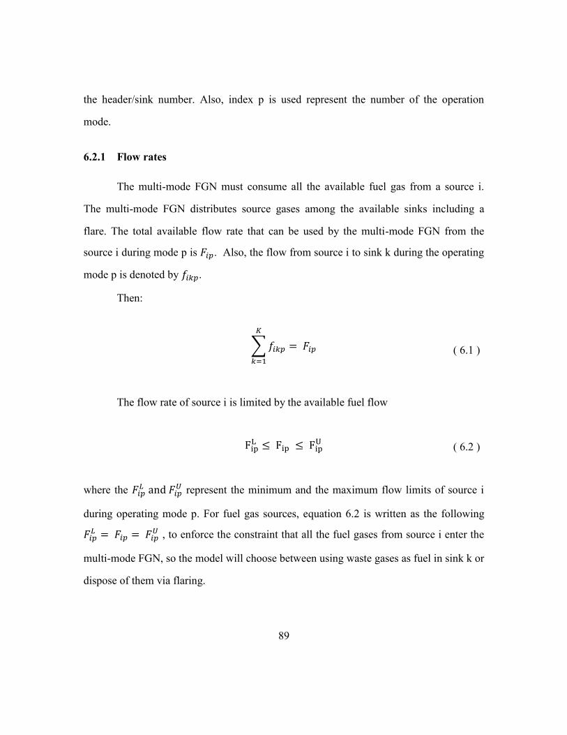
89
the header/sink number. Also, index p is used represent the number of the operation
mode.
6.2.1 Flow rates
The multi-mode FGN must consume all the available fuel gas from a source i.
The multi-mode FGN distributes source gases among the available sinks including a
flare. The total available flow rate that can be used by the multi-mode FGN from the
source i during mode p is . Also, the flow from source i to sink k during the operating
mode p is denoted by .
Then:
( 6.1 )
The flow rate of source i is limited by the available fuel flow
( 6.2 )
where the
represent the minimum and the maximum flow limits of source i
during operating mode p. For fuel gas sources, equation 6.2 is written as the following
, to enforce the constraint that all the fuel gases from source i enter the
multi-mode FGN, so the model will choose between using waste gases as fuel in sink k or
dispose of them via flaring.

90
The flow rates of the fuel gas that is received by the sink k should be within its
flow limits.
( 6.3 )
where the
represent the minimum and the maximum flow limits of sink k in
period p.
6.2.2 Energy demand
There are two types of sinks. The first type can use a fixed amount of energy
(fixed sink) while the second can use excess energy above its energy demand (flexible
sink). To account for these two types of sinks, the following constraints are developed.
( 6.4 )
( 6.5 )
where is the lower heating value of the waste gaseous fuel from source i and is
the energy demand for sink k during operating mode p.

91
6.2.3 Non-isothermal and non-isobaric operations
The multi-mode FGN accounts for the enthalpy, temperature and pressure
changes in the network that could occur because of the existence of coolers, heaters,
compressors or valves. The following constraints account for the non-isothermal and non-
isobaric operations in the multi-mode FGN.
Total temperature/enthalpy change of waste gases from source i to sink k:
( 6.6 )
Enthalpy change across the valve:
( 6.7 )
Enthalpy change across the compressor:
( 6.8 )
Pressure limits of sink k:
( 6.9 )

92
Temperature/enthalpy limits of source i:
( 6.10 )
( 6.11 )
Energy balance across the mixing header k:
( 6.12 )
( 6.13 )
where
are the enthalpy changes across the compressor,
the valve, the heater and the cooler from source i to sink k during mode p, is the
heat capacity of waste gases from source i in mode p, Pkp and Pip are pressure of sink k
and source i during mode p, respectively, and
are the minimum and the
maximum allowable pressure limits in sink k during mode p. is the temperature of

93
source i in period p, and and
are the upper and lower allowable temperature
bounds of gaseous fuel from source i. is the temperature of sink k during mode p.
and are the minimum and the maximum acceptable temperature by sink k during
mode p. Also, µip is the Joule-Thompson coefficient, Ƞip is the adiabatic compression
efficiency of source i during operating mode p, and R is the ideal gas constant.
6.2.4 Fuel quality
Each sink can consume fuel gas that satisfies its fuel quality requirements.
Therefore, the FGN accounts for the fuel quality limits for each sink. The following
section discuses the constraints on several fuel properties.
Specific gravity of gaseous fuel is the density ratio of fuel to the air. Both
densities are measured at the same conditions (pressure and temperature). However, for
an ideal gas fuel, the specific gravity is just the ratio of the molecular weight of the ideal
gas to the molecular weight of air. The following constraints are used to satisfy the
specific gravity requirement for each sink.
( 6.14 )
( 6.15 )

94
where is the specific gravity of gaseous fuel from source i to sink k, is the
specific gravity of sink k, and
are the minimum and the maximum
acceptable specific gravity of sink k.
A lower heating value (LHV) is an important property that characterizes the
energy content of gaseous fuels depending on their chemical composition. Sinks require a
fuel with a minimum LHV to work with high performance. For example, flares require
waste gas with a minimum LHV of 300 BTU/scf in order to maintain high combustion
efficiency (TCEQ, 2012). The following constraints provide each sink with the required
LHV.
( 6.16 )
( 6.17 )
where is the lower heating value of sink k, and
are the
minimum and the maximum acceptable lower heating value of sink k in operating mode
p.
Several sinks constrain the presence of chemical species in gaseous fuels. The
presence of chemicals above the acceptable level may cause corrosion or destruction to
the sink. Also, it could violate an environmental regulation by allowing the sink (e.g.
turbine) to emit hazardous emissions above allowable levels. Therefore, the following
constraint is used to ensure that the multi-mode FGN delivers gaseous fuel with
acceptable contaminant levels.

95
( 6.18 )
where is the fraction of species s in source i, and
are the minimum
and the maximum acceptable fraction of species s in sink k during mode p.
The Wobbe index (WI) is a measure of energy flow and interchangeability of fuel
gas. The heating value of gaseous fuel flowing through an orifice in a specific period
increases as the WI increases. The WI combines the LHV with SG as follows:
Two gaseous fuels with different LHV and composition, but with same WI,
exhibit similar combustion characteristics. The WI is not a linear fuel property, so the
following constraint is developed to account for the WI requirement for each sink.
( 6.19 )
where
are the minimum and the maximum WI limits for sink k.
The methane number is a fuel property that characterizes the knocking resistance
of a gaseous fuel. When fuel is purely methane, the methane number is 100. In contrast, if
the fuel is hydrogen, the methane number is 0. If the fuel is a mixture of 80% methane
and 20% hydrogen, the methane number would be 80. The methane number is mostly
used for gas turbines. Gas turbines can commonly use fuel gas with a minimum Methane

96
number of 80. The following constraint is used to account for a Methane number
requirement.
( 6.20 )
where and are the mole fraction
of methane, ethane, propane, butane, pentane and higher alkanes in source i during mode
p.
Moreover, more constraints were developed to prevent any condensation of fuel
gas in sink k. The two minimum superheat requirements of sink k are:
( 6.21 )
( 6.22 )
where MDPkp and HDPkp are moisture and hydrocarbon dew point temperatures for sink
k during mode p.

97
The multi-mode FGN distributes the waste gases to several sinks. One of the sinks
is a flare. The flare disposes of all the waste gases that cannot be economically consumed
by the sinks. A hydrocarbon penalty is introduced through constraint 6.23 to discourage
flaring which leads to a reduction in flare environmental footprints. The hydrocarbon
penalty constraint allows a limited amount of hydrocarbon to be flared without a fee.
However, if the amount of hydrocarbon exceeds the allowable amount, constraint 6.23
incurs a cost of the excess flared hydrocarbon.
( 6.23 )
where is the amount of flared hydrocarbon with emission fee (kg/hr), is the
amount of hydrocarbon in source i (Kg/MMscf) and flared hydrocarbon with no
emission fee (kg/hr) in mode p. The cost of the hydrocarbon penalty ($/kg) will be
imposed in the objective function.
6.2.5 Physical features
Designing a FGN for each operation mode is not a practical solution. In contrast,
designing a FGN with the same physical features but with varying operational details (e.g
flow rates, temperature, pressure) in all the operation modes is practically preferable.
Therefore, the following design constraints are developed to address this issue.
( 6.24 )
( 6.25 )

98
( 6.26 )
( 6.27 )
( 6.28 )
where is the maximum flow capacity through transfer line from source i to sink k,
,
, and
are the maximum ,
, and
from
source i to sink k.
The main objective of the multi-mode FGN model is to integrate the waste gases
from different sources with the available sinks while minimizing the total annualized cost
(TAC) of the multi-mode FGN with P operation modes. The TAC is comprised of three
parts. The first and the second part are the capital expenditure (CAPEX) and operating
expenditure (OPEX) of the multi-mode FGN. The third part is flaring cost in terms of
hydrocarbon penalty. The following equation is the multi-mode FGN objective function.

99
( 6.29 )
Where
: is an annualization factor.
: is the capital expenditure of the pipelines.
: is the capital expenditure of the compressors.
: is the capital expenditure of the heaters.
: is the capital expenditure of the coolers.
: is the capital expenditure of the valves.
: is the cost of installing a new sink if needed.
: is the cost of upgrading the capacity of an existent sink.
: is the working time in hours of the plant per year.
: is the probability of occurrence of operation mode p during a year of operation.

100
: is the cost of using the fuel gas from source i in $/MMscf.
: is the revenue from surplus energy produced from sink k in $/BTU.
: is the treatment cost in sink k in $/MMscf.
: is the cost of flaring additional hydrocarbon above the allowable limit in $/kg.
: is the operating cost of the pipelines.
: is the operating cost of the compressors.
: is the operating cost of the heaters.
: is the operating cost of the coolers.
: is the operating cost of the valves.
Since the flare flow is highly variable in time, the objective in this work will be to
use the multi-mode FGN model to identify FGN designs that minimize flaring operations.
A case study of a petroleum refinery is adapted from Jagannath et. al (2012) to illustrate
scenarios that would minimize flaring operation.

101
6.3 CASE STUDY OF A PETROLEUM REFINERY
This case study is adapted from Jagannath et. al (2012) . A petroleum refinery has
four potential sources of fuel gases that are normally sent to a flare. Also, the refinery has
two fuel sources: internal and external. The internal fuels are products of the refinery
units and it is considered a fuel from product (FFP). The external source is a purchased
natural gas fuel. The refinery has five sinks: 4 turbines and a boiler.
Minimizing the waste gas from fluid catalytic cracking unit (FCCU) is the initial
focus of this study. The waste gas flow rate from FCCU is highly variable. Figure 6-2
illustrates the waste gas flow rate time series from an FCCU flare over a month of
operation. This FCCU flare will replace one of the sources in the petroleum refinery
problems that are reported by Jagannath et al. (2012). Pavlovic et al. (2011) modeled and
characterized the FCCU flow shown in Figure 6-2. They showed that this FCCU has four
modes of operations. The average flow rates of the four operation modes are 0.01, 0.013,
0.015 and 0.02 MMscf/hr with probability of occurrence of 0.59, 0.16, 0.12 and 0.13
respectively. Consequently, these flow rates with their occurrence probability will be
used in the refinery case study.

102
Figure 6-2: Waste gases Flow rates time series from FCCU over a month of operation.
In summary, the refinery problem has 6 sources (including FCCU) and 6 sinks
(including a flare). Table 6-1 provides the flow, temperature, pressure, LHV, and other
properties of all sources in the refinery problem. Table 6-2 shows the flow range,
temperature, pressure, and other specifications required by all sinks in the refinery
problem.
In the refinery problem, we assume that all flow rates from all sources are
constant except the waste gases from the FCCU flare. Moreover, the probability of
occurrence of the FCCU flare operation modes is the same as the probability of the
refinery operation modes. Also, it is assumed that this refinery works 8000 hours per year
and the annualization factor in this problem is 10% (straight line 10 year capital
depreciation). Finally, Tables 6-3 and 6-4 provide the cost parameters (CAPEX and
OPEX) of the pipelines, compressors, valves, heaters, and coolers that are used in the
multi-mode FGN.
0
500
1000
1500
2000
2500
3000
3500
0 100 200 300 400 500 600 700
Mas
s fl
ow
rat
e(I
b/h
r)
Hour of operation

103
Table 6-1: Data of the sources in the refinery problem
Spec/Parameter Source 1 Source 2 (FFCU) Source 3 Source 4 FFP Natural gas
Flow (MMscf/h) – Mode 1 0.04 0.01 0.18 0.09 ≤5.00 ≤5.00
Flow (MMscf/h) – Mode 2 0.04 0.013 0.18 0.09 ≤5.00 ≤5.00
Flow (MMscf/h) – Mode 3 0.04 0.015 0.18 0.09 ≤5.00 ≤5.00
Flow (MMscf/h) – Mode 4 0.04 0.02 0.18 0.09 ≤5.00 ≤5.00
Temperature (K) 373 400 350 380 320 320
Pressure (psia) 50 35 25 50 25 50
Cp (kJ/MMscf K) 42791 122142 42270 44403 100626 46157
µ (K/psia) 0.03 0.028 0.03 0.028 0.028 0.028
Ƞ 0.75 0.75 0.75 0.75 0.75 0.75
R/Cp 0.2 0.2 0.17 0.17 0.18 0.2
LHV (MMBtu/MMscf) 880 2628 850 807 2659 1100
SG 0.769 0.74 0.769 0.772 1.425 0.909
Hydrocarbon content (Kg/MMscf) 21400 61099 20622 25358 62701 21665
Methane (mol%) 88 0 88 62 0 85
Ethane (mol%) 2 0 2 5 2 5
Propane (mol%) 0.5 0 0 4 56 4
C3+ (mol%) 1 100 0 2 42 2
Hydrogen (mol%) 0.5 0 4 1 0 0
Carbon Monoxide (mol%) 1 0 3 1 0 0.05
Nitrogen (%) 7 0 3 25 0 3.95
Sulfur (ppm) 55 0 55 65 65 65
H2S (ppm) 0.05 0 0.05 198 198 198
Price ($/MMscf) 0 0 0 0 500 800

104
Table 6-2: Data of the sinks in the refinery problem
Spec/Parameter Turbine 1 Turbine 2 Turbine3 Turbine4 Boiler Flare
Flow Range (MMscf/h) 0.08-0.11 0.09-0.145 0.10-0.13 0.09-0.12 0.20-0.25 ≥0
Temperature (K) 273-800 273-800 273-800 273-800 273-800 273-800
Pressure (psia) 25-360 25-360 25-360 25-360 25-360 14-17
Demand (MMBtu/h) 120 140 110 110 180 ≥0
WI 750-1590 750-1590 750-1590 750-1590 750-1590 -
MN >80 >80 >80 >80 >80 -
MDP(K) 277 277 277 277 277 -
HDP(K) 277 277 277 277 277 -
LHV (MMBtu/MMscf) 500-2000 500-2000 500-2000 500-2000 500-2000 300-2000
SG 0.5-1 0.5-1 0.5-1 0.5-1 0.5-1 0.5-1
Methane (mol%) >85 >85 >85 >85 - -
Ethane (mol%) <15 <15 <15 <15 - -
Propane (mol%) <15 <15 <15 <15 - -
C3+ (mol%) <5 <5 <5 <5 - -
Carbon Monoxide(mol%) <10 <10 <10 <10 - -
Nitrogen (mol%) <15 <15 <15 <15 - -
Sulfur (ppm) <500 <500 <500 <500 - -
H2S (ppm) <200 <200 <200 <200 - -
Handling Cost ($/MMscf) 0 0 0 0 0 5

105
Table 6-3: CAPEX and OPEX of auxiliary equipment and pipelines in the multi-mode FGN
Unit CAPEX ($/kW) OPEX ($/kWh)
Compressor 100000 0.1
Heater 50000 0.01
Cooler 50000 0.02
Valve 5000 0.001
Pipeline - 0.5 $ /MMscf
Table 6-4: CAPEX of the pipelines in the multi-mode FGN
CAPEX ($-h/MMscf) Turbine1 Turbine 2 Turbine 3 Turbine 4 Boiler Flare
Source 1 62500 64000 65000 63000 62500 62500
Source 2 62500 66000 65500 62500 63500 63000
Source 3 61000 64000 60000 62000 63500 63000
Source 4 62500 63500 64500 65500 67000 68500
Source 5 62500 64000 65000 66000 66500 68000
Source 6 61500 61000 60500 64000 64500 66000

106
6.3.1 Minimizing waste gases
To minimize waste gases that are normally sent to the flare, for these scenarios,
the sources and the sinks were divided into two problems. The first problem contains the
natural gas and FFP sources with the four turbines. Turbines are sensitive to the chemical
composition of the fuel gas. The presence of heavy hydrocarbon gas in the fuel with
unknown composition could cause severe turbine damage or explosion (Elliott et al.,
2004). Data on flared gas composition showed that waste gases contain considerable
amounts of heavy hydrocarbon which could impact turbine performance. Therefore,
natural gas and FFP were the only sources of fuel for the four turbines in this case study.
The second problem contains the four sources of the waste gases with the boiler and the
flare sinks. This effectively converts the problem of minimizing flared gases to a boiler
design problem. In the following sections, the solution to the turbine fuel feed problem is
briefly described, but the main focus is on the flare gas and boiler design scenarios.
6.3.1.1 Turbine fuels
In the turbine fuel problem, the only sources of fuel are commercial natural gas
and FFP and the sinks are four turbines.
Using the FGN model to solve the turbine fuel problem showed that no heater,
cooler or compressor is need for this problem. Only a single valve is needed. The model
uses a combination of natural gas and FFP to satisfy all the four turbine demands. Table
6-5 gives the optimum operating parameters for the turbine fuel problem.

107
Table 6-5: optimum operating conditions for the first problem
Flow (MMscf/h)
Flow from
Natural gas (MMscf/h)
Flow from
FFP (MMscf/h) LHV
(MMBtu/MMscf) Wobbe Index (MMBTU/MMscf)
Energy Flow (MMBTU/hr)
Pressure (Psia)
Temperature (K)
Turbine 1 0.107 0.099 0.008 933 959 120 25 319
Turbine 2 0.124 0.115 0.009 943 969 140 25 319
Turbine 3 0.1 0.094 0.006 916 945 110 25 319
Turbine 4 0.098 0.09 0.007 934 965 110 25 319

108
6.3.1.2 Flare gas and boiler fuel
The flare gas and boiler fuel problem contains four sources of waste gases and
two sinks (a boiler and a flare). The flow rates of the waste gases from three sources are
constant and the flow rate from the fourth source (FCCU flare) is variable. The flow rate
from the FCCU flare can be divided into 4 operation modes with their known
probabilities of occurrence during a year of operation. The objective of this work is to
determine the best scenarios to utilize all the waste gases instead of flaring them.
Three methods will be tested for the second problem. Then, impact of different
parameters on the TAC and the amount of flaring will be examined. The parameters to
be tested are: minimum flared hydrocarbon without emission fee ( , hydrocarbon
penalty ( , and sink flexibility. In the first method, the existing boiler with a limited
capacity and a flare will be the only sinks for the waste gases that are produced by the
four sources. The model will be used to assess sensitivity to parameters such as emission
fees. In the second and third methods, the capacity of the existing boiler will be expanded
assuming either an upgrade to the existing boiler or the construction of a new boiler, to
accommodate more fuel and produce more steam. Again, the model will be used to assess
sensitivity to network parameters.
6.3.1.2.1 Fixed capacity boiler
The existing boiler and a flare were the only sinks for the waste gases for these
scenarios. The existing boiler has a limited fuel flow capacity range of 0.2 to 0.25
MMscf/hr. In contrast, the flare can accommodate any amount of waste gases. A variety
of different scenarios for hydrocarbon penalties were examined, as summarized in Table
6-6. The fuel gas network was relatively insensitive to any changes in flaring penalties.
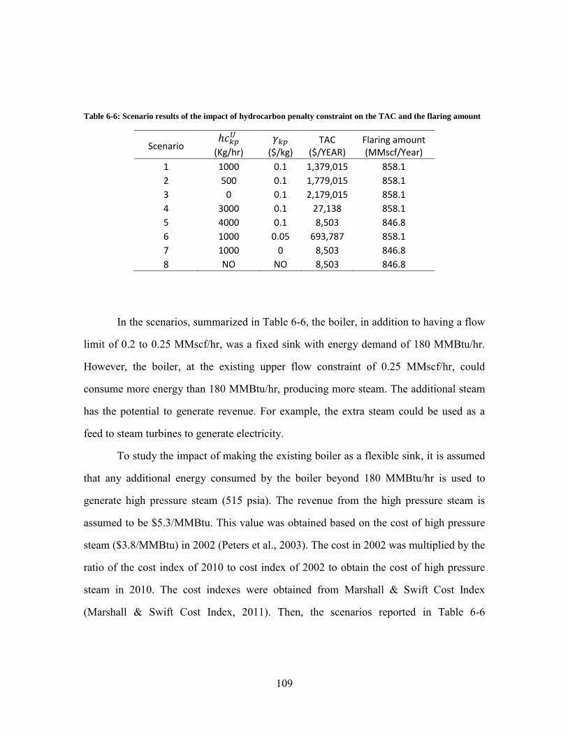
109
Table 6-6: Scenario results of the impact of hydrocarbon penalty constraint on the TAC and the flaring amount
Scenario
(Kg/hr)
($/kg) TAC
($/YEAR) Flaring amount (MMscf/Year)
1 1000 0.1 1,379,015 858.1
2 500 0.1 1,779,015 858.1
3 0 0.1 2,179,015 858.1
4 3000 0.1 27,138 858.1
5 4000 0.1 8,503 846.8
6 1000 0.05 693,787 858.1
7 1000 0 8,503 846.8
8 NO NO 8,503 846.8
In the scenarios, summarized in Table 6-6, the boiler, in addition to having a flow
limit of 0.2 to 0.25 MMscf/hr, was a fixed sink with energy demand of 180 MMBtu/hr.
However, the boiler, at the existing upper flow constraint of 0.25 MMscf/hr, could
consume more energy than 180 MMBtu/hr, producing more steam. The additional steam
has the potential to generate revenue. For example, the extra steam could be used as a
feed to steam turbines to generate electricity.
To study the impact of making the existing boiler as a flexible sink, it is assumed
that any additional energy consumed by the boiler beyond 180 MMBtu/hr is used to
generate high pressure steam (515 psia). The revenue from the high pressure steam is
assumed to be $5.3/MMBtu. This value was obtained based on the cost of high pressure
steam ($3.8/MMBtu) in 2002 (Peters et al., 2003). The cost in 2002 was multiplied by the
ratio of the cost index of 2010 to cost index of 2002 to obtain the cost of high pressure
steam in 2010. The cost indexes were obtained from Marshall & Swift Cost Index
(Marshall & Swift Cost Index, 2011). Then, the scenarios reported in Table 6-6

110
(scenarios 1 to 8) were re-examined, assuming that the existing boiler is flexible. Table
6-7 shows the impact of the sink flexibility on the TAC and the flaring amount.
Table 6-7: Scenario results of the impact of the sink flexibility on the TAC and the flaring amount
Scenario
(Kg/hr)
($/kg)
TAC ($/YEAR)
Flaring amount (MMscf/Year)
9 1000 0.1 -1,789,230 579.0
10 500 0.1 -1,389,230 579.0
11 0 0.1 -989,226 579.0
12 3000 0.1 -2,321,370 579.0
13 4000 0.1 -2,321,370 579.0
14 1000 0.05 -1,987,220 579.0
15 1000 0 -2,321,370 579.0
16 NO NO -2,321,370 579.0
The results of scenarios 9-16 indicate that the sink flexibility has a significant
impact on the TAC and the flaring. However, with an upper flow rate bound of 0.25
MMscf/hr, the sink flexibility did not eliminate flaring, only reduced the flaring amount.
Once again, emission fees have a negligible impact on network design.
Material reuse pinch analyses (described in detail in Appendix D) confirmed that,
for this maximum boiler flow rate, the minimum possible amount of flaring is 579
MMscf per year. These results further confirm that increasing the hydrocarbon penalty
will not reduce flaring. This led to a series of additional case studies which increase the
capacity of the boiler.

111
6.3.1.2.2 Variable capacity boilers
Two alternatives for expanding boiler capacity were examined: adding additional
capacity to an existing boiler and adding a new boiler. For the first alternative
(expanding the existing boiler) the proposed new fuel capacity limits are 0.22-0.33
MMscf/hr. The cost of the upgrading depends on whether high or low pressure steam is
generated. The costs of high pressure and low pressure steam boiler expansions were
assumed to be $400,000 and $200,000, respectively. Also, the revenues from producing
high pressure and low pressure steam were assumed to be $5.3 and $3.6 / MMBtu,
respectively.
Expanding the boiler capacity showed a significant impact on flaring, eliminating
all flaring in each of the tested scenarios. Table 6-8 shows the impact of upgrading the
boiler capacity (high and low pressure steam) on the TAC and the amount of gases flared.
Table 6-8: Scenario results of the impact of expanding the boiler capacity on the TAC and the flaring amount
Scenari
o Cost of
Expanding Steam Type
(Kg/hr)
($/kg) TAC
($/YEAR)
Flaring amount
(MMscf/Year)
17 400,000 High pressure 1000 0.1 -4,754,970 0
18 400,000 High pressure 1000 0.05 -4,754,970 0
19 400,000 High pressure 1000 0 -4,754,970 0
20 400,000 High pressure NO NO -4,754,970 0
21 200,000 Low pressure 1000 0.1 -3,235,660 0
22 200,000 Low pressure 1000 0.05 -3,235,660 0
23 200,000 Low pressure 1000 0 -3,235,660 0
24 200,000 Low pressure NO NO -3,235,660 0

112
An alternative configuration, which differs only in the capital cost assumed for
the boiler expansion, is the installation of a new boiler. In this scenario, there are three
sinks (2 boilers and a flare) for the waste gases. The maximum capacity of the new boiler
is 0.08 MMscf/hr. The cost of the new boiler depends on whether high or low pressure
steam is generated, with the costs of new high pressure and low pressure steam boilers set
at $1,000,000 and $ 600,000, respectively.
Installing a new boiler with the proposed capacity eliminates flaring in scenarios
25-32 (Table 6-9). Hydrocarbon penalties had no impact on the amount flared
Table 6-9: Scenario results of the impact of installing a new boiler on the TAC and flaring amount
Scenario Cost of
installing Steam Type
(Kg/hr)
($/kg) TAC
($/YEAR) Flaring amount (MMscf/Year)
25 1,000,000 High pressure 1000 0.1 -4,694,970 0
26 1,000,000 High pressure 1000 0.05 -4,694,970 0
27 1,000,000 High pressure 1000 0 -4,694,970 0
28 1,000,000 High pressure NO NO -4,694,970 0
29 600,000 Low pressure 1000 0.1 -3,155,660 0
30 600,000 Low pressure 1000 0.05 -3,155,660 0
31 600,,000 Low pressure 1000 0 -3,155,660 0
32 600,000 Low pressure NO NO -3,155,660 0
Installing a new boiler capacity, whether expansion or through the addition of a
new boiler, shows a net operating profit if all of the steam can be sold. However, it is
possible that the refinery may not use all the additional steam. Table 6-10 reports the cost
impacts of using only various fractions of the generated steam. The results demonstrate
that even if only a few percent of the steam generated by burning waste gas in the boiler
can be used, the design still shows a profit.

113
Table 6-10: Impact of utilizing the additional high pressure steam on the TAC.
Percentage of additional steam used
TAC ($/year)
100% -4,694,970.0
90% -4,215,060
40% -1,815,550
30% -1,335,650
10% -375,841
8% -79,115
3% -39,909
2% 8,081
1% 83,893
0% 104,062
6.4 CONCLUSION
Integrating sources of waste gases with the multi-mode FGN is an effective
approach to reducing flaring impacts on air quality. In the case studies reported here,
configurations that expanded boiler capacity, using waste gases to generate steam, were
estimated to be profitable. Including a hydrocarbon penalty constraint on flaring showed
little effect. Overall, upgrading and installing new sinks can minimize or eliminate
flaring.(Jagannath et al., 2012)

114
CHAPTER 7: Effect of Temperature Excursions in Catalytic
Cracking Units on the Generation of Flared gases
7.1 INTRODUCTION
A petroleum refinery is a complex facility, and detailed processing configurations
vary among refineries, but a central operation in most refineries is the fluid catalytic
cracking (FCC) unit. FCC is a chemical process used to break down large hydrocarbon
molecules in gas oils into more valuable products. The main products of the FCC are
gasoline and liquefied petroleum gas (LPG). In 1942, the first FCC unit was introduced to
the world of petroleum refining for the production of aviation gasoline. It was installed in
Baton Rouge, Louisiana. FCC units allowed more gasoline production, and enhanced the
fuel quality (Ertl et al., 2008; Parkash, 2003). In modern refineries, approximately half of
motor gasoline is produced from the FCC process. In 2004, the total worldwide capacity
of FCC was above 2 million tons per day, which is about 17% of the total crude oil unit
capacity in the world (Ertl et al., 2008). In 2006, U.S refineries processed around 6.3
million barrels per day of heavy oil in catalytic cracking units (DOE, 2007). The oil feed
capacity for a typical FCC unit is about 10,000 tons/day (100,000 BBL/day) (Ertl et al.,
2008). The traditional feed of FCC is the heavy vacuum gas oil, which is the middle
product from the vacuum distillation column. This feed is catalytically cracked through
the FCC unit to produce useful fuel (mainly gasoline) (Ertl et al., 2008; Parkash, 2003).
Due to the flexible operation of the FCC unit, some refineries use residual oil, the bottom
product of vacuum distillation, which contains high concentrations of aromatics and
asphaltenes. The catalytic cracking of these compounds may result in high coke
formation and could affect the FCC unit performance. Also, existence of some
contaminants in the feed, such as nickel and vanadium, can promote undesirable chemical
reactions and negatively impact catalyst performance (Ertl et al., 2008; Parkash, 2003).

115
Therefore, some refineries install hydrotreating units to decontaminate the FCC feed,
which leads to improved fuel quality and reduced pollutants emissions such as SOx, NOx
from FCC units. In the United States, approximately 37% of the FCC feed is hyrotreated
which is expected to increase in the future due to stringent environmental regulations; 35
% of the FCC worldwide feed is hydrotreated (Ertl et al., 2008).
A typical FCC unit diagram is shown in Figure 7-1. The FCC oil feed is
preheated by series of heat exchangers and then mixed with very hot regenerated catalyst
which vaporizes the oil. The gas oil with the catalyst travels up to the catalyst riser
(reactor) where the cracking reactions take place. A typical catalyst to oil ratio is around
6. The cracking reactions take place at high temperature, approximately 810 K(Ertl et al.,
2008; Parkash, 2003). The gaseous products from the cracking reactions are separated
from the catalyst by cyclones. A small fraction of the products formed in the reactor is
coke, which deposits on the catalyst surface. The gaseous products (super heated vapors)
are sent to a fractionator. The fractionator separates the cracking products into different
cuts (such as light gases, gasoline and heavy cycle oil) based on their boiling point
temperature. The separated catalyst from the cyclones travels down to the catalyst
regenerator. The used catalyst is regenerated by using hot air to burn off the deposited
coke on the catalyst surface. The flue gas from the combustion is separated from the
regenerated catalyst by cyclones. The regenerated hot catalyst is mixed again with oil
feed and then the cycle is repeated. Moreover, the regenerator and reactor are thermally
integrated. The thermal energy from the combustion of deposited coke is used to provide
heat for cracking reactions in the reactor. Also, the reactor provides the combustion fuel
(coke) to the regenerator (Ertl et al., 2008; Pariyani et al., 2010; Parkash, 2003).

116
Figure 7-1: Fluid Catalytic Cracking (FCC) process (DOE, 2007).
Fresh catalyst is added daily to the FCC unit. However, the fresh catalyst rate
varies depending on the mode of operation and the feed type. For example, the fresh
catalyst rate could reach to 0.3 kg of catalyst per ton feed for feedstock with high metal
concentration but the rate may drop to 0.03 kg of catalyst per ton feed for feedstock with
low metal residual (Ertl et al., 2008).
For this work, the objective is to understand the production of light gases by the
FCC unit, and their impact on flaring. Light gas formation could be influenced by hot
spots in the reactor (e.g., from fresh catalyst addition), the level of coke formation
(influencing the energy demand in the regenerator) or other factors. A three–lump kinetic
model will be used to predict the impact of the reactor temperature on the conversion of
the gas oil charged. Specifically, the model is used to estimate the change in the

117
production of light gases (C2-C4) resulting from temperature excursions in the fluid bed
reactor.
7.2 THREE-LUMP MODEL
In 1970, Weekman and his colleagues reported a kinetic model for the catalytic
cracking process which is called the three-lump model. The Three-lump model is a
mathematical model to estimate the gas oil conversion and its yields in fixed, moving and
fluid bed reactors. The model assumes an isothermal reactor that is working at steady
state condition. Also, the model counts for the catalyst decay by adding a decay function
in the reaction rates. The model can estimate the gasoline, light gases and coke yields
based on reactor temperature, space velocity, catalyst to gas oil ratio and catalyst
residence time (Weekman and Nace, 1970).
A number of advancements have been made to FCC modeling since the
development of the three-lump model, and modern reaction models use a concept called
structure oriented lumping (SOL), first reported by Liguras and Allen (Liguras and Allen,
1989a; Liguras and Allen, 1989b). While SOL dramatically improves the ability to
predict gasoline quantity and quality, it does little to change predictions of light gas
formation, the focus of this work. Therefore, this work will use the simpler, and far less
computationally intensive, 3-lump model.
7.2.1 Kinetic model
In the three-lump model, the wide range of catalytic cracking feed and products
are lumped into three components; gas oil, gasoline, and light gases (C2-C4) and coke.
The interconversion of these components is determined by the process variables, kinetic
and parameters. Figure 7-2 shows the reaction scheme among the three components.

118
Figure 7-2: reaction scheme of catalytic cracking of the heavy gas oil.
where Y1 is the weight fraction of unconverted gas oil charged, Y2 is the weight fraction
of gasoline formed and Y3 is the weight fraction of light gases (C2-C4) and coke yields.
The catalytic cracking of gas oil charged results in gasoline and other products (light
gases and coke). The cracking of gas oil has been proven to be a second order reaction
(Weekman, 1968). Moreover, the cracking of gasoline to light gases and coke is assumed
to be a first order reaction because gasoline does not have as much diversity in the
molecule types as the gas oil (Weekman, 1979; Weekman and Nace, 1970). Equations
7.1 and 7.2 show the rate of disappearance of gas oil and the rate of change in weight
fraction of gasoline. Equation 7.3 calculates the weight fraction of light gases and coke.
( 7.1 )
( 7.2 )
( 7.3 )
where to is the oil residence time and Ф is the catalyst decay function.

119
The catalyst affects the rate of reaction. The activity of the catalyst decays as the
reaction proceeds because coke deposits on the catalyst surface (active sites). Voorhies
(1945) showed that the rate of coke deposition on the catalyst surface is highly dependent
on the catalyst residence time and independent of the gas oil conversion or the space
velocity (Nace et al., 1971; Voorhies 1945). Therefore, the catalyst activity is a function
of the catalyst residence time in the reactor. Also, it is assumed that the catalyst decay
functions for gas oil and gasoline cracking reactions are equal, because the same catalyst
active sites crack both the gas oil and the gasoline (Weekman and Nace, 1970). Using a
simple exponential form to represent the catalyst decay function (Ф) is adequate for
catalytic cracking reactions (equation 7.4) (Weekman, 1979).
( 7.4 )
where α is catalyst decay coefficient and tc is the catalyst residence time.
Solving equation 7.1 and equation 7.2 simultaneously is not easily possible, so the
best practice is to divide equation 7.2 by equation 7.1 which results in equation 7.5.
Equation 7.5 relates the weight fraction of the gas oil charged (Y1) and the gasoline (Y2).
At the beginning of the cracking reaction there is only gas oil (Y1=1) and no initial
gasoline (Y2=0). Using this as a boundary condition, equation 7.5 can be solved in terms
of K0, K1 and K2. As can be shown from equation 7.5, the relationship between Y1 and
Y2 does not depend on the space velocity, the catalyst activity function, or the catalyst
residence time but it depends only on the selectivity ratio (K1/K0) and the over cracking
ratio (K2/K0) (Weekman and Nace, 1970).
( 7.5 )

120
The derivation of the conversion equations for fixed, moving and fixed bed
reactor are described in detail by Weekman (1968). Equation 7.6 is the conversion
equation for a fluid bed reactor, which will be used for this work.
( 7.6 )
where AO is the extent of the reaction group, λ is the extend of the catalyst decay group, S
is the space velocity, K0=K1+K3, β is the catalyst-to-oil ratio, FO is the mass flow rate for
the oil charge, ρl is density of the liquid charge at room temperature and Vr is the volume
of the reactor.
7.2.2 Comparing the Three-lump model with experimental data
Laboratory experimental data of catalytic cracking of gas oil were used to test the
ability of the three-lump model to predict the conversion of the gas oil, weight fraction of
gasoline formed, and the weight fraction of light gases and coke yields. A wide range of
gas oils with different properties and molecular compositions were catalytically cracked.
The paraffins, naphthenes and aromatics concentrations were varied in all the tested gas
oil types. The model successfully estimated the weight fractions of the three components
(Y1, Y2 and Y3) under different reaction conditions for all types of charge stocks (gas

121
oils) (Nace et al., 1971). The Three-lump model requires four constants (K0, K1, K2 and
α) to be determined experimentally. The gas oil data that will be used for this work is the
data for a Mid-Continent blend with a boiling range of 423 to 904o F that has API =
29.6o. Also, an activity coefficient (α) for a typical zeolite catalyst will be used. The
laboratory experiments of catalytic cracking of the Mid-Continent blend with zeolite
catalyst were carried out at 900o F (Weekman and Nace, 1970). Table 7-1 shows the
values of the four constants at T=900o F.
Table 7-1: The values of rates of reactions and catalyst decay coefficient (Weekman Jr and Nace, 1970).
constant Value
K0 22.9
K1 18.1
K2 1.7 α 42.7
7.2.3 Temperature effect
All the reaction rate constants are function of temperature. Therefore, the relation
between Y1 and Y2 is a function of the temperature. The activation energy of the catalytic
cracking of gas oil and gasoline were assumed to be 10000 cal/gmole and 18000
cal/gmole, respectively (Weekman and Nace, 1970). The temperature dependence on K0,
K1 and K2 is shown in equations 7.7, 7.8 and 7.9.
( 7.7 )
( 7.8 )
( 7.9 )

122
The impact of the process variables on gas oil conversion, light gas and coke
yields, and gasoline yields can be determined by combining equations 7.3, 7.6, 7.7, 7.8,
7.9 and the solution of equation 7.5.
7.2.4 Coke formation
The amount of coke deposited on the catalyst surface can be calculated using the
Voorhees (1945) relation (equation 7.10), which relates coke formation to the catalyst
residence time.
( 7.10 )
where C is weight percent of carbon on the catalyst, tc is the catalyst residence time, and a
and b are constants. The value of a increases as the aromatics concentration in the gas oil
increases. Therefore, as the concentration of aromatics increases in feed stock, more coke
will deposit on the catalyst surface, which increases the catalyst deactivation (Nace et al.,
1971).
The weight percent of the total coke yield can be estimated using correlations.
Jacob et al. (1976) slightly modified Voorhees’s relation by testing 95 sets of coke data.
Then the coke yield was estimated by multiplying a modified form of relation 7.10 by 1.1
which counts for ratio of the hydrogen to carbon in coke (Jacob et al., 1976). In this work
it is assumed that the coke yield only depends on the composition of the feed stock and
the catalyst residence time and does not depend on the reactor temperature. In other
words, the impact of the reactor temperature excursion on the Y3 lump changes the
weight fraction of only the light gas yield, not the coke.

123
7.3 LIGHT GASES SCENARIOS
The typical average temperature of an FCC reactor is 810 K, (Ertl et al., 2008)
however, there are some hot spots in the reactor that have higher temperatures. Therefore,
different scenarios are developed to determine the impact of temperature excursions on
the additional amount of light gases produced.
For this work, it is assumed that the nominal temperature of the reactor is 810 K,
the total oil feed capacity to the FCC is 10,000 tons /day and the catalyst to oil ratio is 6
(Ertl et al., 2008). The base case scenario was developed by assuming that the average
reactor temperature is 810 K and no hot spots exist in the reactor. Moreover, it is assumed
that the temperature is normally distributed throughout the reactor volume. The
probability density function of the reactor temperature is calculated using equation 7.11.
The full width at half maximum (FWHM) of the temperature distribution in the reactor is
assumed to be 10. Using equation 7.12, the standard deviation (σ) of the temperature
distribution is 4.25. Figure 7-3 shows the temperature probability distribution of the FCC
reactor temperature for the base case.
( 7.11 )
( 7.12 )
where T is reactor temperature, Tav is the average reactor temperature, V is the volume
fraction of the temperature distribution in the FCC reactor (V=1 for the base case), σ is
the standard deviation of temperature distribution in the reactor, and FWHM is the full
width at half maximum (FWHM) of the temperature distribution in the reactor.

124
Figure 7-3: The probability of the FCC’s reactor temperature for the base case.
The weight fraction of the light gases (WFLG) at different temperatures can
determined using equations 7.3, 7.6, 7.7, 7.8, 7.9 and the solution of equation 7.5. Then
equation 7.13 is used to evaluate the WFLG for the base case.
( 7.13 )
The FCC reactor could have hot spots that have higher temperatures than the
average reactor temperature. These hot spots normally represent a small fraction of the
reactor volume. Therefore, different scenarios are developed depending on the
temperature of the hot spots and the volume percent of the hot spots in the reactor. For
example, one of the tested scenarios assumed that the hot spots have an average
temperature of 830 K and represent 10 % of the reactor volume. Figure 7-4 shows the
temperature probability distribution of the FCC reactor for this scenario. Then, equation
0
0.01
0.02
0.03
0.04
0.05
0.06
0.07
0.08
0.09
0.1
780 790 800 810 820 830 840
Tem
pe
ratu
re p
rob
abili
ty
T (K)

125
7.14 is used to calculate the WFLG for this scenario. Tables 7-2 and 7-3 show the
additional light gases of a FCC unit resulting from an oil feed of 10,000 tons /day for
different scenarios. The scenarios in Table 7-2 and 7-3 assume the catalyst residence
times (tc) are 5 min and 1.25 min, respectively.
( 7.14 )
Figure 7-4 :The probability of the FCC’s reactor temperature for the scenario where the hot spots
average temperature is 830 K and represent 10% of the reactor volume.
0
0.01
0.02
0.03
0.04
0.05
0.06
0.07
0.08
0.09
780 790 800 810 820 830 840 850 860
Tem
pe
ratu
re p
rob
abili
ty
T (K)
90 % of the reactor volume
10 % of the reactor volume

126
Table 7-2: Mass rates of additional light gases from a FCC unit for different temperature excursion scenario
when the tc =5 min
Average T of hot spots
Volume % of the reactor
Additional
WFLG % Mass rate of additional
light gases (Ib/hr) 830 10% 0.55894% 4658 830 5% 0.27947% 2329 830 2% 0.11179% 932 820 10% 0.27070% 2256 820 5% 0.13535% 1128 820 2% 0.05414% 451 815 10% 0.13310% 1109 815 5% 0.06655% 555 815 2% 0.02662% 222 813 10% 0.07931% 661 813 5% 0.03966% 330 813 2% 0.01586% 132 812 10% 0.05269% 439 812 5% 0.02635% 220 812 2% 0.01054% 88
Table 7-3 : Mass rates of additional light gases from a FCC unit for different temperature excursion scenario
when the tc = 1.25min
Average T of hot spots
Volume % of the reactor
Additional
WFLG % Mass rate of additional
light gases (Ib/hr) 830 10% 0.37673% 3139 830 5% 0.18836% 1570 830 2% 0.07535% 628 820 10% 0.18107% 1509 820 5% 0.09053% 754 820 2% 0.03621% 302 815 10% 0.08874% 740 815 5% 0.04437% 370 815 2% 0.01775% 148 813 10% 0.05282% 440 813 5% 0.02641% 220 813 2% 0.01056% 88 812 10% 0.03507% 292 812 5% 0.01754% 146 812 2% 0.00701% 58

127
7.4 COMPARISON BETWEEN SCENARIO RESULTS AND FCC FLARE DATA
A FCC unit is a central and continuous process in all modern refineries.
Therefore, waste gases from the FCC unit are expected to be continuously generated.
These waste gases are normally sent to either the fuel gas network or a flare. Figure 7-5
shows the monitored hourly flow rate times series for a FCC flare in Houston, Texas.
These data was extracted from 2006 SI. The total flow rate of the FCC flare is 1,277,000
lb for a month of operation with an average of 1,665.2 lb/hr. The cumulative mass
distribution for the FCC flare flows is shown in Figure 7-6. Figure 7-6 indicates that
almost 50% of total mass flow rate is generated at flow rates less than 1,600 lb/hr. The
histogram and the time cumulative distribution of the waste gas flow rates from the FCC
unit for a month of operation are shown in Figure 7-7. Figure 7-7 shows the waste gas
flow rates was ranged between 1300 to 1600 lb/hr for more than half of the operating
time (32 days) with a frequency of 415 hours out of 767 hours. Also, the flow rate of the
generated waste gases from the FCC unites was less than 1600 lb/hr for 62 % of the total
operating time.

128
Figure 7-5: Monitored hourly flow rate time series of FCC flare over a month of operation.
Figure 7-6 : Mass cumulative distribution function for the FCC flare flows.
0
500
1000
1500
2000
2500
3000
3500
0 100 200 300 400 500 600 700
Mas
s fl
ow
rat
e(I
b/h
r)
Hour of operation
0%
10%
20%
30%
40%
50%
60%
70%
80%
90%
100%
90
0
10
00
11
00
12
00
13
00
14
00
15
00
16
00
17
00
18
00
19
00
20
00
21
00
22
00
23
00
24
00
25
00
26
00
27
00
28
00
29
00
30
00
31
00
Cu
mu
lati
ve D
istr
ibu
tio
n F
un
ctio
n (
%)
Mass flow rate (Ib/hr)

129
Figure 7-7: Histogram and time cumulative distribution for the FCC flare flows for a month of
operation.
Tables 7-2 and 7-3 showed the impact of the temperature and the volume fraction
of the hot spots inside the FCC’s reactor on the production of additional light gases at two
different catalyst residence times. Figures 7-8 and 7-9 illustrate the relation between the
hot spot temperatures and the production of the light gases at constant volume fractions
and catalyst residence times 5 and 1.25 min, respectively.
0 1 2 13
44
124
158
133
77
40 33
15 8 11 15
26 14 10
16 12 10 3 2 0
0%
10%
20%
30%
40%
50%
60%
70%
80%
90%
100%
0
20
40
60
80
100
120
140
160
≤ 9
9-1
0
10
-11
11
-12
12
-13
13
-14
14
-15
15
-16
16
-17
17
-18
18
-19
19
-20
20
-21
21
-22
22
-23
23
-24
24
-25
25
-26
26
-27
27
-28
28
-29
29
-30
30
-31
31
≤ Ti
me
Cu
mu
lati
ve D
istr
ibu
tio
n F
un
ctio
n %
Fre
qu
en
cy
Mass flow rate (102 Ib/hr)
Frequency
Time Cumulative Distribution Function %

130
Figure 7-8: Hot spot temperature versus the production of additional light gases at tc=5 min.
Figure 7-9: Hot spot temperature versus the production of additional light gases at tc=1.25min.
Figures 7-8 and 7-9 show that the relation between the hotspot temperatures and
the generation of additional light gases is a linear relationship. However, the slope of the
linear relationship depends on the volume fraction of the hot spots and the tc. The six
y = 46.917x - 38013 R² = 0.9998
y = 117.29x - 95033 R² = 0.9998
y = 234.58x - 190065 R² = 0.9998
0
500
1000
1500
2000
2500
3000
3500
4000
4500
5000
810 815 820 825 830 835
Mas
s ra
te o
f ad
dit
ion
al li
ght
gase
s (I
b/h
r)
Temperature (K)
Volume fraction = 2%
Volume fraction = 5%
Volume fraction = 10%
y = 31.667x - 25659 R² = 0.9997
y = 79.168x - 64148 R² = 0.9997
y = 158.34x - 128295 R² = 0.9997
0
500
1000
1500
2000
2500
3000
3500
810 815 820 825 830 835
Mas
s ra
te o
f ad
dit
ion
al li
ght
gase
s (I
b/h
r)
Temperature (K)
Volume fraction = 2%
Volume fraction = 5%
Volume fraction = 10%

131
scenarios in Figures 7-8 and 7-9 can be used to infer the characteristics (temperature and
volume) of the temperature hot spots that would be required to generate the waste gas
flow rates from the FCC unit reported in Figure 7-5. Figure 7-10 shows the cumulative
distribution of the hot spot temperatures at three different volume fractions of 2, 5 and
10% at tc of 5 min. When the scenario of 2% volume fraction of the hot spots is applied,
temperature excursions reached to of 30-70 K are required to generate the volumes of
waste gases observed. For the scenarios where the volume fractions are 5 and 10 %, the
much smaller temperature excursions (5-35 K) are required to generate the waste gases.
Note that all of these calculations assume that the base case leads to no flared gases.
Table 7-4 summarizes the maximum temperature, the minimum temperature, and the
maximum temperature excursion for each scenario, when tc =5 min, to replicate the
actual data of waste gases flow rates from FCC units in Figure 7-5. Figures 7-11, 7-12
and 7-13 show the time cumulative distribution and the histogram for the scenarios when
tc =5 min.
Figure 7-10: The cumulative distributions of the hot spot temperatures at three different volume fractions of 2, 5
and 10% at tc of 5 min.
0%
10%
20%
30%
40%
50%
60%
70%
80%
90%
100%
81
0
82
0
83
0
84
0
85
0
86
0
87
0
88
0
Cu
mu
lati
ve D
istr
ibu
tio
n F
un
ctio
n
(%)
Temperature (K)
Volume fraction = 2%
Volume fraction = 5%
Volume fraction = 10%
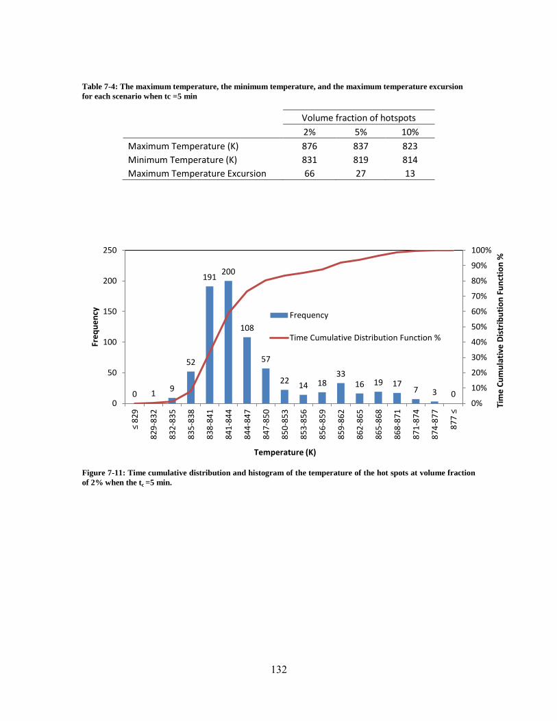
132
Table 7-4: The maximum temperature, the minimum temperature, and the maximum temperature excursion
for each scenario when tc =5 min
Volume fraction of hotspots
2% 5% 10%
Maximum Temperature (K) 876 837 823 Minimum Temperature (K) 831 819 814 Maximum Temperature Excursion 66 27 13
Figure 7-11: Time cumulative distribution and histogram of the temperature of the hot spots at volume fraction
of 2% when the tc =5 min.
0 1 9
52
191 200
108
57
22 14 18
33 16 19 17
7 3 0 0%
10%
20%
30%
40%
50%
60%
70%
80%
90%
100%
0
50
100
150
200
250
≤ 8
29
82
9-8
32
83
2-8
35
83
5-8
38
83
8-8
41
84
1-8
44
84
4-8
47
84
7-8
50
85
0-8
53
85
3-8
56
85
6-8
59
85
9-8
62
86
2-8
65
86
5-8
68
86
8-8
71
87
1-8
74
87
4-8
77
87
7 ≤
Tim
e C
um
ula
tive
Dis
trib
uti
on
Fu
nct
ion
%
Fre
qu
en
cy
Temperature (K)
Frequency
Time Cumulative Distribution Function %

133
Figure 7-12: Time cumulative distribution and histogram of the temperature of the hot spots at volume fraction
of 5% when the tc =5 min.
Figure 7-13: Time cumulative distribution and histogram of the temperature of the hot spots at volume fraction
of 10% when the tc =5 min.
0 1 8
24
120
180
158
73
49
23 11 12
18 28
16 15 12 14 3 2 0
0%
10%
20%
30%
40%
50%
60%
70%
80%
90%
100%
0
20
40
60
80
100
120
140
160
180
200
≤81
8
81
8-8
19
81
9-8
20
82
0-8
21
82
1-8
22
82
2-8
23
82
3-8
24
82
4-8
25
82
5-8
26
82
6-8
27
82
7-8
28
82
8-8
29
82
9-8
30
83
0-8
31
83
1-8
32
83
2-8
33
83
3-8
34
83
4-8
35
83
5-8
36
83
6-8
37
83
7≤
Tim
e C
um
ula
tive
Dis
trib
uti
on
Fu
nct
ion
%
Fre
qu
en
cy
Temperature (K)
Frequency
Time Cumulative Distribution Function %
0 3
110
342
144
47 27
44 26 21
3 0 0%
10%
20%
30%
40%
50%
60%
70%
80%
90%
100%
0
50
100
150
200
250
300
350
400
≤ 8
14
81
4-8
15
81
5-8
16
81
6-8
17
81
7-8
18
81
8-8
19
81
9-8
20
82
0-8
21
82
1-8
22
82
2-8
23
82
3-8
24
82
4 ≤
Tim
e C
um
ula
tive
Dis
trib
uti
on
Fu
nct
ion
%
Fre
qu
en
cy
Temperature (K)
Frequency
Time Cumulative Distribution Function %

134
Figure 7-14 shows the cumulative distribution of the hot spot temperatures at
three different volume fractions of 2, 5 and 10% at tc of 1.25 min. In these simulations,
larger temperature excursions are required to generate the waste gases since less coke is
formed at the shorter catalyst residence time. Table 7-5 summarizes the maximum
temperature, the minimum temperature, and the maximum temperature excursion for
each scenario, when tc =1.25 min, to replicate the actual data of waste gases flow rates
from FCC units in Figure 7-5. Figures 7-15, 7-16 and 7-17 show the time cumulative
distribution of and the histogram for the scenarios when the tc =1.25 min.
Figure 7-14: The cumulative distributions of the hot spot temperatures at three different volume fractions of 2, 5
and 10%, respectively, at catalyst residence time of 1.25 min.
0%
10%
20%
30%
40%
50%
60%
70%
80%
90%
100%
80
0
82
0
84
0
86
0
88
0
90
0
92
0
Cu
mu
lati
ve D
istr
ibu
tio
n F
un
ctio
n (
%)
Temperature (K)
Volume fraction = 2%
Volume fraction = 5%
Volume fraction = 10%

135
Table 7-5: The maximum temperature, the minimum temperature, and the maximum temperature excursion
for each scenario when tc =5 min
Volume fraction of hotspots
2% 5% 10%
Maximum Temperature (K) 908 849 830 Minimum Temperature (K) 841 823 816 Maximum Temperature Excursion 98 39 20
Figure 7-15 : Time cumulative distribution and histogram of the temperature of the hot spots at volume fraction
of 2% when the tc =1.25 min.
0 1 5 14
64
132 141
126
69
39 33
14 9 9 13
25 14 13 10 12 13
6 3 2 0 0%
10%
20%
30%
40%
50%
60%
70%
80%
90%
100%
0
20
40
60
80
100
120
140
160
≤ 8
40
84
0-8
43
84
3-8
46
84
6-8
49
84
9-8
52
85
2-8
55
85
5-8
58
85
8-8
61
86
1-8
64
86
4-8
67
86
7-8
70
87
0-8
73
87
3-8
76
87
6-8
79
87
9-8
82
88
2-8
85
88
5-8
88
88
8-8
91
89
1-8
94
89
4-8
97
89
7-9
00
90
0-9
03
90
3-9
06
90
6-9
09
90
9 ≤
Tim
e C
um
ula
tive
Dis
trib
uti
on
Fu
nct
ion
%
Fre
qu
en
cy
Temperature (K)
Frequency
Time Cumulative Distribution Function %

136
Figure 7-16 : Time cumulative distribution and histogram of the temperature of the hot spots at volume fraction
of 5 % when the tc =1.25 min.
Figure 7-17: Time cumulative distribution and histogram of the temperature of the hot spots at volume fraction
of 10 % when the tc =1.25 min.
0 0 2
27
157
238
134
62
25 13
32 27 19 19
8 4 0 0%
10%
20%
30%
40%
50%
60%
70%
80%
90%
100%
0
50
100
150
200
250
≤ 8
20
82
0-8
22
82
2-8
24
82
4-8
26
82
6-8
28
82
8-8
30
83
0-8
32
83
2-8
34
83
4-8
36
83
6-8
38
83
8-8
40
84
0-8
42
84
2-8
44
84
4-8
46
84
6-8
48
84
8-8
50
85
0 ≤
Tim
e C
um
ula
tive
Dis
trib
uti
on
Fu
nct
ion
%
Fre
qu
en
cy
Temperature (K)
Frequency
Time Cumulative Distribution Function %
0 1 20
143
240
148
66
24 14
29 29 18 21
10 4 0 0%
10%
20%
30%
40%
50%
60%
70%
80%
90%
100%
0
50
100
150
200
250
300
≤ 8
16
81
6-8
17
81
7-8
18
81
8-8
19
81
9-8
20
82
0-8
21
82
1-8
22
82
2-8
23
82
3-8
24
82
4-8
25
82
5-8
26
82
6-8
27
82
7-8
28
82
8-8
29
82
9-8
30
83
0 ≤
Tim
e C
um
ula
tive
Dis
trib
uti
on
Fu
nct
ion
%
Fre
qu
en
cy
Temperature (K)
Frequency
Time Cumulative Distribution Function %

137
7.5 CONCLUSION
The results from these scenarios suggest that reasonable scenarios for temperature
excursions in FCC reactors lead to the types of waste gas volumes reported for FCC
flares. This suggests that better temperature controls on FCC units could result in the
elimination of flared gases. Although the development of temperature control schemes
for FCC units is beyond the scope of this work, this analysis has demonstrated that the
goal of minimization of flaring may create additional economic incentives for improved
FCC temperature control.

138
CHAPTER 8: Findings, Outcomes and Recommmedations
This thesis has examined the impacts of industrial flaring and methods for
minimizing those impacts. Four primary topics were investigated. This Chapter
summarizes the main findings reported in this thesis, outcomes of this work and
recommendations of the future work in four areas:
i) Air quality impacts of flaring operations
ii) Improving flare operation
iii) Minimization of refinery flaring through integration with fuel gas
networks
iv) Impact of temperature excursions of FCC units on the light gas/flared gas
production.
8.1 FINDINGS
8.1.1 Air quality impacts of flaring operations
Flares operating at low DRE can increase localized ambient ozone
concentrations by more than 15 ppb under some conditions. The impact of
flare DRE on the ozone formation potential of flare emissions depends
largely on flow rate and composition of flared gases; Products of
incomplete combustion play a secondary role in the photochemistry driven
by flare emissions.
The production of NOx from industrial flares is not constant and depends
on the DRE of the flare; current emission factors may overstate NOx

139
emissions, however, NOx emissions from flares play a much smaller role
in the photochemistry of flare emissions than unburned hydrocarbons.
8.1.2 Improving flare operation
The analyses of improving flare operation focused on the implications of the
narrow operating range in which flares operating at low flow rate can achieve both high
combustion efficiency and low smoke production. A case study of how blower design for
an air-assisted flare impacts the ability to operate in this narrow regime was examined.
Flare emissions can be more than an order of magnitude greater than or
less than a base case assuming 98% DRE, depending on whether the
blowers are able to achieve desired assist-air to vent gas ratios.
Variable speed blower configurations achieve lower predicted emissions
than similarly sized fixed speed blowers.
8.1.3 Minimization of refinery flaring through integration with fuel gas networks
The protential for recycling flared gases was examined using a case study of a
petroleum refinery.
By expanding boiler (sink) size, flaring can be reduced significantly, and
recovered steam may offset much or all of the cost of boiler expansion.
Including a hydrocarbon penalty constraint on flaring showed little effect
on flaring.

140
8.1.4 Impact of temperature excursions of FCC units on the light gas/flared gas
production.
Temperature excursions in FCC reactors lead to the types of waste gas
volumes reported for FCC flares.
Better temperature controls on FCC units could result in the elimination of
flared gases.
8.2 OUTCOMES
This thesis represents:
1. The most comprehensive air quality analysis done to date of the air quality
impact of flare emissions, including products of incomplete combustion
and NOx emissions
2. The first assessment of the impact of blower configurations on flare
emissions
3. The first integration of time varying flare flows into refinery fuel gas
networks (a dynamic pooling problem)
4. The first assessment of flare prevention potential of temperature
excursions on FCC units
Collectively, the work is the first time that a comprehensive examination of
flaring has been performed, incorporating an understanding of environmental impacts,
and assessments of the relative merits of better flare operation, flare gas recycling and
preventing flare gas generation.

141
8.3 FUTURE WORK
8.3.1 Air quality impacts of flaring operations
The air quality analyses in this thesis represent the upper bounds on the ozone
formation potential of flare emissions. Using hourly flow data of flares in Houston Area,
with hourly resolved chemical compositions and using University of Texas Flare study
results to estimate the hourly DRE will be the focus of the future work.
8.3.2 Improving flare operation
A case study of an air-assisted flare was examined to improve its operation. For
the future work, a case study of a steam-assisted flare could be studied to determine the
best practices that maintain high performance.
8.3.3 Minimization of refinery flaring through integration with fuel gas networks
Determining new sinks in petroleum refineries that can use the flared gases will
be the focus of the future work. Also the possibility of integrating the waste gases from
refinery sources with other industrial facilities will be explored in the near future.
8.3.4 Impact of temperature excursions of FCC units on the light gas/flared gas
production.
Developing a temperature control schemes for FCC units to minimize temperature
excursions will be explored in more detail in the future. The ultimate goal of the
temperature control for FCC units is minimizing the production of waste gases.

142
Appendix A
This appendix contains tables summarizing the air quality modeling scenarios
presented in Chapter 3 and emissions for each flare for each scenario, including both
VOC and NOx emissions. A summary of the emissions of products of incomplete
combustion (PICs) reported in full scale flare tests by the University of Texas is included.
Also, this appendix contains the air quality simulation results for all flares except
Refinery Flare1.
Table A-1: Summary of emission scenarios simulated for each flare
Flare emissions
Scenario DE%
Unburned
hydrocarbons PIC Ratio of hydrocarbon to PIC
A 95 yes no 1 : 0
B 95 yes yes 1 : 1
C 90 yes no 1 : 0
D 90 yes yes 1 : 1
E 75 yes no 1 : 0
F 75 yes yes 4 : 1
G 50 yes no 1 : 0
H 50 yes yes 9 : 1

143
Table A-2: Summary of VOC emissions (tons/hr) for the base case, scenarios A, C, E and G for Refinery Flare 1
Base case Scenario A Scenario C Scenario E Scenario G
Time
(hr)
Mass flow
rate
(tons/hr)
NOx
(tons/hr)
VOC
emissions
(tons/hr)
VOC
emissions
(tons/hr)
VOC
emissions
(tons/hr)
VOC
emissions
(tons/hr)
VOC
emissions
(tons/hr)
0 6.03 0.00793 0.121 0.301 0.603 1.51 3.01
1 25.3 0.0333 0.506 1.265 2.531 6.33 12.7
2 23.1 0.0304 0.462 1.154 2.309 5.77 11.5
3 16.2 0.0214 0.325 0.811 1.623 4.06 8.11
4 2.54 0.00334 0.0508 0.127 0.254 0.635 1.27
5 2.44 0.00321 0.0487 0.122 0.244 0.609 1.22
6 2.35 0.00309 0.0469 0.117 0.235 0.586 1.17
7 2.27 0.00298 0.0453 0.113 0.227 0.566 1.13
8 2.68 0.00353 0.0537 0.134 0.268 0.671 1.34
9 3.76 0.00495 0.0752 0.188 0.376 0.940 1.88
10 0.130 0.000171 0.00260 0.00649 0.0130 0.0324 0.0649
11 0.101 0.000133 0.00203 0.00507 0.0102 0.0254 0.0507
12 1.63 0.00215 0.0327 0.0817 0.163 0.409 0.817
13 1.80 0.00237 0.0361 0.0902 0.180 0.451 0.901
14 2.19 0.00288 0.0438 0.109 0.219 0.547 1.09
15 1.85 0.00243 0.0369 0.0923 0.185 0.462 0.923
16 1.79 0.00235 0.0358 0.0894 0.179 0.447 0.894
17 1.99 0.00262 0.0398 0.0996 0.199 0.498 0.996
18 2.54 0.00334 0.0507 0.127 0.254 0.634 1.268
19 2.12 0.00279 0.0425 0.106 0.212 0.530 1.06
20 1.93 0.00254 0.0387 0.0967 0.193 0.483 0.967
21 2.19 0.00289 0.0439 0.110 0.219 0.548 1.10
22 1.63 0.00215 0.0326 0.0816 0.163 0.408 0.816
23 6.64 0.00874 0.133 0.332 0.664 1.661 3.32

144
Table A-3: Summary of NOx, unburned hydrocarbon (UHC) and products of incomplete combustion (PICs) for the base case, scenarios B, D, F and H for Refinery
Flare 1
Scenario B Scenario D Scenario F Scenario H
Time
(hr)
Mass flow
rate
(tons/hr)
NOx
(tons/hr)
UHC
(tons/hr)
PICs
(tons/hr)
UHC
(tons/hr)
PICs
(tons/hr)
UHC
(tons/hr)
PICs
(tons/hr)
UHC
(tons/hr)
PICs
(tons/hr)
0 6.03 0.00793 0.151 0.151 0.301 0.301 1.206 0.301 2.71 0.301
1 25.3 0.0333 0.633 0.633 1.27 1.27 5.06 1.27 11.4 1.27
2 23.1 0.0304 0.577 0.577 1.15 1.15 4.62 1.15 10.4 1.15
3 16.2 0.0214 0.406 0.406 0.811 0.811 3.25 0.811 7.30 0.811
4 2.54 0.00334 0.0635 0.0635 0.127 0.127 0.508 0.127 1.14 0.127
5 2.44 0.00321 0.0609 0.0609 0.122 0.122 0.487 0.122 1.1 0.122
6 2.35 0.00309 0.0586 0.0586 0.117 0.117 0.469 0.117 1.06 0.117
7 2.27 0.00298 0.0566 0.0566 0.113 0.113 0.453 0.113 1.02 0.113
8 2.68 0.00353 0.0671 0.0671 0.134 0.134 0.537 0.134 1.21 0.134
9 3.76 0.00495 0.0940 0.0940 0.188 0.188 0.752 0.188 1.69 0.188
10 0.130 0.000171 0.00324 0.00324 0.00649 0.00649 0.0260 0.00649 0.0583 0.00649
11 0.101 0.000133 0.00254 0.00254 0.00507 0.00507 0.0202 0.00507 0.0457 0.00507
12 1.63 0.00215 0.0409 0.0409 0.0817 0.0817 0.327 0.0817 0.736 0.0817
13 1.80 0.00237 0.0451 0.0451 0.0901 0.0901 0.361 0.0901 0.811 0.0901
14 2.19 0.00288 0.0547 0.0547 0.109 0.109 0.438 0.109 0.985 0.109
15 1.85 0.00243 0.0462 0.0462 0.0923 0.0923 0.369 0.0923 0.830 0.0923
16 1.79 0.00235 0.0447 0.0447 0.0894 0.0894 0.358 0.0894 0.804 0.0894
17 1.99 0.00262 0.0498 0.0498 0.0996 0.0996 0.398 0.0996 0.896 0.0996
18 2.54 0.00334 0.0633 0.0633 0.127 0.127 0.507 0.127 1.14 0.127
19 2.12 0.00279 0.0531 0.0531 0.106 0.106 0.424 0.106 0.955 0.106
20 1.93 0.00254 0.0484 0.0484 0.0967 0.0967 0.387 0.0967 0.870 0.0967
21 2.19 0.00289 0.0548 0.0548 0.110 0.110 0.439 0.110 0.987 0.110
22 1.63 0.00215 0.0408 0.0408 0.0816 0.0816 0.326 0.0816 0.734 0.0816
23 6.64 0.00874 0.166 0.166 0.332 0.332 1.33 0.332 2.99 0.332

145
Table A-4: Summary of VOC emissions (tons/hr) for the base case, scenarios A, C, E and G for Refinery Flare 2
Base case Scenario A Scenario C Scenario E Scenario G
Time
(hr)
Mass flow
rate
(tons/hr)
NOx
(tons/hr)
VOC
emissions
(tons/hr)
VOC
emissions
(tons/hr)
VOC
emissions
(tons/hr)
VOC
emissions
(tons/hr)
VOC
emissions
(tons/hr)
0 2.74 0.00361 0.05474 0.137 0.274 0.684 1.37
1 3.02 0.00398 0.06036 0.151 0.302 0.754 1.51
2 3.12 0.00411 0.06231 0.156 0.312 0.779 1.56
3 3.95 0.00522 0.07908 0.198 0.395 0.988 1.98
4 2.74 0.00362 0.05486 0.137 0.274 0.686 1.37
5 3.14 0.00414 0.06280 0.157 0.314 0.785 1.57
6 2.95 0.00389 0.05891 0.147 0.295 0.736 1.47
7 2.93 0.00387 0.05858 0.146 0.293 0.732 1.46
8 3.10 0.00409 0.06201 0.155 0.310 0.775 1.55
9 3.28 0.00433 0.06567 0.164 0.328 0.821 1.64
10 3.16 0.00417 0.06320 0.158 0.316 0.790 1.58
11 3.08 0.00407 0.06166 0.154 0.308 0.771 1.54
12 3.16 0.00417 0.06313 0.158 0.316 0.789 1.58
13 2.98 0.00393 0.05956 0.149 0.298 0.744 1.49
14 2.94 0.00388 0.05874 0.147 0.294 0.734 1.47
15 3.15 0.00415 0.06290 0.157 0.315 0.786 1.57
16 3.08 0.00407 0.06166 0.154 0.308 0.771 1.54
17 2.83 0.00374 0.05668 0.142 0.283 0.708 1.42
18 3.09 0.00407 0.06175 0.154 0.309 0.772 1.54
19 2.94 0.00388 0.05885 0.147 0.294 0.736 1.47
20 3.28 0.00433 0.06566 0.164 0.328 0.821 1.64
21 3.39 0.00447 0.06777 0.169 0.339 0.847 1.69
22 3.48 0.00459 0.06957 0.174 0.348 0.870 1.74
23 2.91 0.00385 0.05829 0.146 0.291 0.729 1.46

146
Table A-5: Summary of NOx, unburned hydrocarbon (UHC) and products of incomplete combustion (PICs) for the base case, scenarios B, D, F and H for Refinery
Flare 2
Scenario B Scenario D Scenario F Scenario H
Time
(hr)
Mass flow
rate
(tons/hr)
NOx
(tons/hr)
UHC
(tons/hr)
PICs
(tons/hr)
UHC
(tons/hr)
PICs
(tons/hr)
UHC
(tons/hr)
PICs
(tons/hr)
UHC
(tons/hr)
PICs
(tons/hr)
0 2.74 0.00361 0.0684 0.0684 0.137 0.137 0.547 0.137 1.232 0.137
1 3.02 0.00398 0.0755 0.0755 0.151 0.151 0.604 0.151 1.358 0.151
2 3.12 0.00411 0.0779 0.0779 0.156 0.156 0.623 0.156 1.402 0.156
3 3.95 0.00522 0.0989 0.0989 0.198 0.198 0.791 0.198 1.779 0.198
4 2.74 0.00362 0.0686 0.0686 0.137 0.137 0.549 0.137 1.234 0.137
5 3.14 0.00414 0.0785 0.0785 0.157 0.157 0.628 0.157 1.413 0.157
6 2.95 0.00389 0.0736 0.0736 0.147 0.147 0.589 0.147 1.325 0.147
7 2.93 0.00387 0.0732 0.0732 0.146 0.146 0.586 0.146 1.318 0.146
8 3.10 0.00409 0.0775 0.0775 0.155 0.155 0.620 0.155 1.395 0.155
9 3.28 0.00433 0.0821 0.0821 0.164 0.164 0.657 0.164 1.478 0.164
10 3.16 0.00417 0.0790 0.0790 0.158 0.158 0.632 0.158 1.422 0.158
11 3.08 0.00407 0.0771 0.0771 0.154 0.154 0.617 0.154 1.387 0.154
12 3.16 0.00417 0.0789 0.0789 0.158 0.158 0.631 0.158 1.420 0.158
13 2.98 0.00393 0.0745 0.0745 0.149 0.149 0.596 0.149 1.340 0.149
14 2.94 0.00388 0.0734 0.0734 0.147 0.147 0.587 0.147 1.322 0.147
15 3.15 0.00415 0.0786 0.0786 0.157 0.157 0.629 0.157 1.415 0.157
16 3.08 0.00407 0.0771 0.0771 0.154 0.154 0.617 0.154 1.387 0.154
17 2.83 0.00374 0.0709 0.0709 0.142 0.142 0.567 0.142 1.275 0.142
18 3.09 0.00407 0.0772 0.0772 0.154 0.154 0.617 0.154 1.389 0.154
19 2.94 0.00388 0.0736 0.0736 0.147 0.147 0.588 0.147 1.324 0.147
20 3.28 0.00433 0.0821 0.0821 0.164 0.164 0.657 0.164 1.477 0.164
21 3.39 0.00447 0.0847 0.0847 0.169 0.169 0.678 0.169 1.525 0.169
22 3.48 0.00459 0.0870 0.0870 0.174 0.174 0.696 0.174 1.565 0.174
23 2.91 0.00385 0.0729 0.0729 0.146 0.146 0.583 0.146 1.312 0.146

147
Table A-6: Summary of VOC emissions (tons/hr) for the base case, scenarios A, C, E and G for Refinery Flare 3
Base case Scenario A Scenario C Scenario E Scenario G
Time
(hr)
Mass flow
rate
(tons/hr)
NOx
(tons/hr)
VOC
emissions
(tons/hr)
VOC
emissions
(tons/hr)
VOC
emissions
(tons/hr)
VOC
emissions
(tons/hr)
VOC
emissions
(tons/hr)
0 1.88 0.00251 0.0376 0.0939 0.188 0.470 0.939
1 2.06 0.00276 0.0413 0.103 0.206 0.516 1.03
2 1.91 0.00256 0.0383 0.0957 0.191 0.479 0.957
3 2.11 0.00282 0.0423 0.10569 0.211 0.528 1.06
4 0.654 0.00087 0.0131 0.0327 0.0654 0.164 0.327
5 0.146 0.00020 0.00293 0.00732 0.0146 0.0366 0.0732
6 0.0179 0.00002 0.00036 0.00090 0.00179 0.00448 0.00895
7 0.297 0.00040 0.00594 0.0149 0.0297 0.0743 0.149
8 2.26 0.00301 0.0451 0.113 0.226 0.564 1.13
9 2.12 0.00284 0.0425 0.106 0.212 0.531 1.06
10 2.36 0.00315 0.0472 0.118 0.236 0.589 1.18
11 3.91 0.00522 0.0782 0.196 0.391 0.978 1.96
12 2.32 0.00309 0.0463 0.116 0.232 0.579 1.16
13 1.75 0.00234 0.0351 0.0877 0.175 0.439 0.877
14 0.662 0.00088 0.0132 0.0331 0.0662 0.165 0.331
15 0.755 0.00101 0.0151 0.0378 0.0755 0.189 0.378
16 0.654 0.00087 0.0131 0.0327 0.0654 0.164 0.327
17 0.568 0.00076 0.0114 0.0284 0.0568 0.142 0.284
18 0.535 0.00071 0.0107 0.0267 0.0535 0.134 0.267
19 0.654 0.00087 0.0131 0.0327 0.0654 0.163 0.327
20 0.616 0.00082 0.0123 0.0308 0.0616 0.154 0.308
21 0.755 0.00101 0.0151 0.0378 0.0755 0.189 0.378
22 0.869 0.00116 0.0174 0.0435 0.0869 0.217 0.435
23 1.45 0.00193 0.0289 0.0723 0.145 0.361 0.722

148
Table A-7: Summary of NOx, unburned hydrocarbon (UHC) and products of incomplete combustion (PICs) for the base case, scenarios B, D, F and H for Refinery
Flare 3
Scenario B Scenario D Scenario F Scenario H
Time
(hr)
Mass flow
rate
(tons/hr)
NOx
(tons/hr)
UHC
(tons/hr)
PICs
(tons/hr)
UHC
(tons/hr)
PICs
(tons/hr)
UHC
(tons/hr)
PICs
(tons/hr)
UHC
(tons/hr)
PICs
(tons/hr)
0 2.06 0.00251 0.0470 0.0470 0.0939 0.0939 0.376 0.0939 0.845 0.0939
1 1.91 0.00276 0.0516 0.0516 0.103 0.103 0.413 0.103 0.928 0.103
2 2.11 0.00256 0.0479 0.0479 0.0957 0.0957 0.383 0.0957 0.861 0.0957
3 0.654 0.00282 0.0528 0.0528 0.106 0.106 0.423 0.106 0.951 0.106
4 0.146 0.00087 0.0164 0.0164 0.0327 0.0327 0.131 0.0327 0.294 0.0327
5 0.0179 0.00020 0.00366 0.00366 0.00732 0.00732 0.0293 0.00732 0.0659 0.00732
6 0.297 0.00002 0.00045 0.00045 0.00089 0.00089 0.00358 0.00089 0.00805 0.00089
7 2.255 0.00040 0.00743 0.00743 0.0149 0.0149 0.0594 0.0149 0.13370 0.0149
8 2.12 0.00301 0.0564 0.0564 0.113 0.113 0.451 0.113 1.01 0.113
9 2.36 0.00284 0.0531 0.0531 0.106 0.106 0.425 0.106 0.955 0.106
10 3.91 0.00315 0.0590 0.0590 0.118 0.118 0.472 0.118 1.06 0.118
11 2.32 0.00522 0.0978 0.0978 0.196 0.196 0.782 0.196 1.76 0.196
12 1.75 0.00309 0.0579 0.0579 0.116 0.116 0.463 0.116 1.04 0.116
13 0.662 0.00234 0.0439 0.0439 0.0877 0.0877 0.351 0.0877 0.789 0.0877
14 0.755 0.00088 0.0165 0.0165 0.0331 0.0331 0.132 0.0331 0.298 0.0331
15 0.654 0.00101 0.0189 0.0189 0.0378 0.0378 0.151 0.0378 0.340 0.0378
16 0.568 0.00087 0.0164 0.0164 0.0327 0.0327 0.131 0.0327 0.294 0.0327
17 0.535 0.00076 0.0142 0.0142 0.0284 0.0284 0.114 0.0284 0.256 0.0284
18 0.654 0.00071 0.0134 0.0134 0.0267 0.0267 0.107 0.0267 0.241 0.0267
19 0.616 0.00087 0.0163 0.0163 0.0327 0.0327 0.131 0.0327 0.294 0.0327
20 0.755 0.00082 0.0154 0.0154 0.0308 0.0308 0.123 0.0308 0.277 0.0308
21 0.869 0.00101 0.0189 0.0189 0.0378 0.0378 0.151 0.0378 0.340 0.0378
22 1.45 0.00116 0.0217 0.0217 0.0435 0.0435 0.174 0.0435 0.391 0.0435
23 2.06 0.00193 0.0361 0.0361 0.0722 0.0722 0.289 0.0722 0.650 0.0722
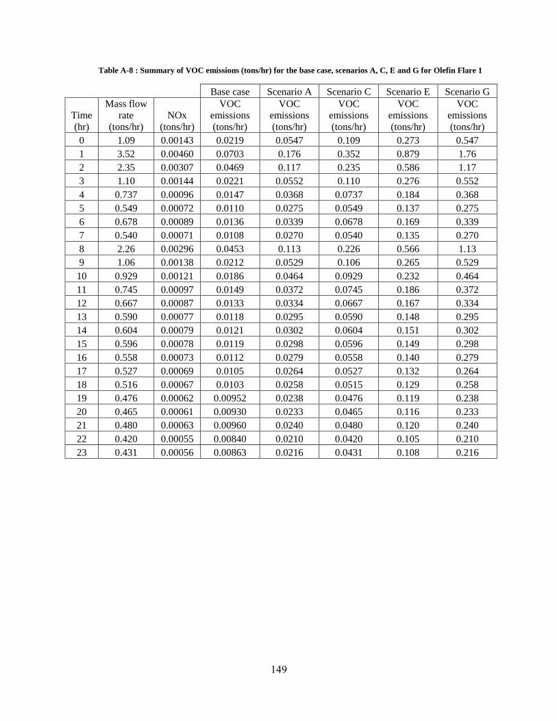
149
Table A-8 : Summary of VOC emissions (tons/hr) for the base case, scenarios A, C, E and G for Olefin Flare 1
Base case Scenario A Scenario C Scenario E Scenario G
Time
(hr)
Mass flow
rate
(tons/hr)
NOx
(tons/hr)
VOC
emissions
(tons/hr)
VOC
emissions
(tons/hr)
VOC
emissions
(tons/hr)
VOC
emissions
(tons/hr)
VOC
emissions
(tons/hr)
0 1.09 0.00143 0.0219 0.0547 0.109 0.273 0.547
1 3.52 0.00460 0.0703 0.176 0.352 0.879 1.76
2 2.35 0.00307 0.0469 0.117 0.235 0.586 1.17
3 1.10 0.00144 0.0221 0.0552 0.110 0.276 0.552
4 0.737 0.00096 0.0147 0.0368 0.0737 0.184 0.368
5 0.549 0.00072 0.0110 0.0275 0.0549 0.137 0.275
6 0.678 0.00089 0.0136 0.0339 0.0678 0.169 0.339
7 0.540 0.00071 0.0108 0.0270 0.0540 0.135 0.270
8 2.26 0.00296 0.0453 0.113 0.226 0.566 1.13
9 1.06 0.00138 0.0212 0.0529 0.106 0.265 0.529
10 0.929 0.00121 0.0186 0.0464 0.0929 0.232 0.464
11 0.745 0.00097 0.0149 0.0372 0.0745 0.186 0.372
12 0.667 0.00087 0.0133 0.0334 0.0667 0.167 0.334
13 0.590 0.00077 0.0118 0.0295 0.0590 0.148 0.295
14 0.604 0.00079 0.0121 0.0302 0.0604 0.151 0.302
15 0.596 0.00078 0.0119 0.0298 0.0596 0.149 0.298
16 0.558 0.00073 0.0112 0.0279 0.0558 0.140 0.279
17 0.527 0.00069 0.0105 0.0264 0.0527 0.132 0.264
18 0.516 0.00067 0.0103 0.0258 0.0515 0.129 0.258
19 0.476 0.00062 0.00952 0.0238 0.0476 0.119 0.238
20 0.465 0.00061 0.00930 0.0233 0.0465 0.116 0.233
21 0.480 0.00063 0.00960 0.0240 0.0480 0.120 0.240
22 0.420 0.00055 0.00840 0.0210 0.0420 0.105 0.210
23 0.431 0.00056 0.00863 0.0216 0.0431 0.108 0.216

150
Table A-9: Summary of NOx, unburned hydrocarbon (UHC) and products of incomplete combustion (PICs) for the base case, scenarios B, D, F and H for Olefin Flare1
Scenario B Scenario D Scenario F Scenario H
Time
(hr)
Mass flow
rate
(tons/hr)
NOx
(tons/hr)
UHC
(tons/hr)
PICs
(tons/hr)
UHC
(tons/hr)
PICs
(tons/hr)
UHC
(tons/hr)
PICs
(tons/hr)
UHC
(tons/hr)
PICs
(tons/hr)
0 1.09 0.00143 0.0273 0.0273 0.0547 0.0547 0.219 0.0547 0.492 0.0547
1 3.52 0.00460 0.0879 0.0879 0.176 0.176 0.703 0.176 1.58 0.176
2 2.35 0.00307 0.0586 0.0586 0.117 0.117 0.469 0.117 1.06 0.117
3 1.10 0.00144 0.0276 0.0276 0.0552 0.0552 0.221 0.0552 0.497 0.0552
4 0.737 0.00096 0.0184 0.0184 0.0368 0.0368 0.147 0.0368 0.332 0.0368
5 0.549 0.00072 0.0137 0.0137 0.0275 0.0275 0.110 0.0275 0.247 0.0275
6 0.678 0.00089 0.0169 0.0169 0.0339 0.0339 0.136 0.0339 0.305 0.0339
7 0.540 0.00071 0.0135 0.0135 0.0270 0.0270 0.108 0.0270 0.243 0.0270
8 2.26 0.00296 0.0566 0.0566 0.113 0.113 0.453 0.113 1.02 0.113
9 1.06 0.00138 0.0265 0.0265 0.0529 0.0529 0.212 0.0529 0.476 0.0529
10 0.929 0.00121 0.0232 0.0232 0.0464 0.0464 0.186 0.0464 0.418 0.0464
11 0.745 0.00097 0.0186 0.0186 0.0372 0.0372 0.149 0.0372 0.335 0.0372
12 0.667 0.00087 0.0167 0.0167 0.0334 0.0334 0.133 0.0334 0.300 0.0334
13 0.590 0.00077 0.0148 0.0148 0.0295 0.0295 0.118 0.0295 0.266 0.0295
14 0.604 0.00079 0.0151 0.0151 0.0302 0.0302 0.121 0.0302 0.272 0.0302
15 0.596 0.00078 0.0149 0.0149 0.0298 0.0298 0.119 0.0298 0.268 0.0298
16 0.558 0.00073 0.0140 0.0140 0.0279 0.0279 0.112 0.0279 0.251 0.0279
17 0.527 0.00069 0.0132 0.0132 0.0264 0.0264 0.105 0.0264 0.237 0.0264
18 0.516 0.00067 0.0129 0.0129 0.0258 0.0258 0.103 0.0258 0.232 0.0258
19 0.476 0.00062 0.0119 0.0119 0.0238 0.0238 0.0952 0.0238 0.214 0.0238
20 0.465 0.00061 0.0116 0.0116 0.0233 0.0233 0.0930 0.0233 0.209 0.0233
21 0.480 0.00063 0.0120 0.0120 0.0240 0.0240 0.0960 0.0240 0.216 0.0240
22 0.420 0.00055 0.0105 0.0105 0.0210 0.0210 0.0840 0.0210 0.189 0.0210
23 0.431 0.00056 0.0108 0.0108 0.0216 0.0216 0.0862 0.0216 0.194 0.0216

151
Table A-10: Summary of VOC emissions (tons/hr) for the base case, scenarios A, C, E and G for Olefin Flare 2
Base case Scenario A Scenario C Scenario E Scenario G
Time
(hr)
Mass
flow rate
(tons/hr)
NOx
(tons/hr)
VOC
emissions
(tons/hr)
VOC
emissions
(tons/hr)
VOC
emissions
(tons/hr)
VOC
emissions
(tons/hr)
VOC
emissions
(tons/hr)
0 0.230 0.000306 0.00460 0.0115 0.0230 0.0575 0.115
1 0.217 0.000289 0.00435 0.0109 0.0217 0.0543 0.109
2 0.203 0.000271 0.00407 0.0102 0.0203 0.0508 0.102
3 0.189 0.000252 0.00379 0.00947 0.0189 0.0473 0.0946
4 0.180 0.000239 0.00359 0.00898 0.0180 0.0449 0.0898
5 0.239 0.000319 0.00479 0.0120 0.0239 0.0599 0.120
6 0.243 0.000324 0.00486 0.0122 0.0243 0.0608 0.122
7 0.180 0.000240 0.00360 0.00901 0.0180 0.0451 0.0901
8 0.204 0.000272 0.00408 0.0102 0.0204 0.0511 0.102
9 0.205 0.000273 0.00411 0.0103 0.0205 0.0513 0.103
10 0.401 0.000534 0.00802 0.0201 0.0401 0.100 0.201
11 0.216 0.000287 0.00432 0.0108 0.0216 0.0540 0.108
12 0.265 0.000352 0.00529 0.0132 0.0265 0.0661 0.132
13 0.420 0.000559 0.00839 0.0210 0.0420 0.105 0.210
14 4.13 0.005501 0.0827 0.207 0.413 1.03 2.07
15 2.43 0.00324 0.0487 0.122 0.243 0.608 1.22
16 0.956 0.00127 0.0191 0.0478 0.0956 0.239 0.478
17 0.603 0.000803 0.0121 0.0302 0.0603 0.151 0.302
18 0.464 0.000618 0.00929 0.0232 0.0464 0.116 0.232
19 0.422 0.000561 0.00843 0.0211 0.0422 0.105 0.211
20 0.291 0.000387 0.00581 0.0145 0.0291 0.0726 0.145
21 0.201 0.000268 0.00403 0.0101 0.0201 0.0503 0.101
22 0.137 0.000182 0.00274 0.00684 0.0137 0.0342 0.0684
23 0.150 0.000200 0.00301 0.00752 0.0150 0.0376 0.0752

152
Table A-11: Summary of NOx, unburned hydrocarbon (UHC) and products of incomplete combustion (PICs) for the base case, scenarios B, D, F and H for Olefin Flare
2
Scenario B Scenario D Scenario F Scenario H
Time
(hr)
Mass flow
rate
(tons/hr)
NOx
(tons/hr)
UHC
(tons/hr)
PICs
(tons/hr)
UHC
(tons/hr)
PICs
(tons/hr)
UHC
(tons/hr)
PICs
(tons/hr)
UHC
(tons/hr)
PICs
(tons/hr)
0 0.230 0.000306 0.00575 0.00575 0.0115 0.0115 0.0460 0.0115 0.103 0.0115
1 0.217 0.000289 0.00543 0.00543 0.0109 0.0109 0.0435 0.0109 0.0978 0.0109
2 0.203 0.000271 0.00508 0.00508 0.0102 0.0102 0.0407 0.0102 0.0915 0.0102
3 0.189 0.000252 0.00473 0.00473 0.00946 0.00946 0.0379 0.00946 0.0852 0.00946
4 0.180 0.000239 0.00449 0.00449 0.00898 0.00898 0.0359 0.00898 0.0808 0.00898
5 0.239 0.000319 0.00599 0.00599 0.0120 0.0120 0.0479 0.0120 0.108 0.0120
6 0.243 0.000324 0.00608 0.00608 0.0122 0.0122 0.0486 0.0122 0.109 0.0122
7 0.180 0.000240 0.00451 0.00451 0.00901 0.00901 0.0360 0.0090 0.0811 0.00901
8 0.204 0.000272 0.00511 0.00511 0.0102 0.0102 0.0408 0.0102 0.0919 0.0102
9 0.205 0.000273 0.00513 0.00513 0.0103 0.0103 0.0411 0.0103 0.0924 0.0103
10 0.401 0.000534 0.0100 0.0100 0.0201 0.0201 0.0802 0.0201 0.181 0.0201
11 0.216 0.000287 0.00540 0.00540 0.0108 0.0108 0.0432 0.0108 0.0972 0.0108
12 0.265 0.000352 0.00662 0.00662 0.0132 0.0132 0.0529 0.0132 0.119 0.0132
13 0.420 0.000559 0.0105 0.0105 0.0210 0.0210 0.0839 0.0210 0.189 0.0210
14 4.13 0.005501 0.103 0.103 0.207 0.207 0.827 0.207 1.86 0.207
15 2.43 0.00324 0.06084 0.06084 0.122 0.122 0.487 0.122 1.10 0.122
16 0.956 0.00127 0.0239 0.0239 0.0478 0.0478 0.191 0.048 0.430 0.0478
17 0.603 0.000803 0.0151 0.0151 0.0302 0.0302 0.121 0.0302 0.272 0.0302
18 0.464 0.000618 0.0116 0.0116 0.0232 0.0232 0.0929 0.0232 0.209 0.0232
19 0.422 0.000561 0.0105 0.0105 0.0211 0.0211 0.0843 0.0211 0.190 0.0211
20 0.291 0.000387 0.00727 0.00727 0.0145 0.0145 0.0581 0.0145 0.131 0.0145
21 0.201 0.000268 0.00503 0.00503 0.0101 0.0101 0.0403 0.0101 0.0906 0.0101
22 0.137 0.000182 0.00342 0.00342 0.00684 0.00684 0.0274 0.00684 0.0616 0.00684
23 0.150 0.000200 0.00376 0.00376 0.00752 0.00752 0.0301 0.00752 0.0677 0.00752

153
Table A-12: Average ratios of PICs to propylene (unburned flared gas) emissions in air -assisted flare tests (lbs / lbs
Propene) as function of DRE. The feed to the flare was 80% Propene and 20% of Tulsa natural gas (Allen and Torres,
2011b).
Ratio of PICs to unburned propene (flared gas)
Species DRE>98% 95%<DRE<98 80%<DRE<95 DRE<80%
Acetylene 0.0625 0.0457 0.0433 0.0218
Ethylene 0.0307 0.0207 0.0180 0.0093
Propylene 1.0000 1.0000 1.0000 1.0000
Butene isomers 0.0002 0.0002 0.0017 0.0048
Formaldehyde 0.0463 0.0303 0.0247 0.0127
Acetaldehyde 0.0308 0.0192 0.0146 0.0069
Propanal 0.0010 0.0007 0.0007 0.0004
Acrolein 0.0186 0.0142 0.0099 0.0038
Methanol 0.0020 0.0014 0.0016 0.0012
Acetone 0.0012 0.0008 0.0008 0.0005
Propylene-Oxide 0.0014 0.0010 0.0006 0.0002
Methane 0.1318 0.1318 0.1318 0.1318
Ethane 0.0103 0.0103 0.0103 0.0103
Table A-13: Average ratios of PICs to propylene (unburned flared gas) emissions in steam-assisted flare tests (lbs / lbs
Propene) as function of DRE. The feed to the flare was 80% propylene and 20% of Tulsa natural gas (Allen and Torres,
2011b).
Ratio of PICs to unburned propylene (flared gas)
Species DRE>98% 95%<DRE<98 80%<DRE<95 DRE<80%
Acetylene 0.0228 0.0164 0.0162 0.0104
Ethylene 0.0388 0.0278 0.0199 0.0091
Propylene 1 1 1 1
Butene isomers 0.0003 0.0003 0.0021 0.0073
Formaldehyde 0.0588 0.0384 0.0265 0.0102
Acetaldehyde 0.0373 0.0226 0.0153 0.0054
Propanal 0.0011 0.0010 0.0009 0.0005
Acrolein 0.0289 0.0233 0.0125 0.0059
Methanol 0.0013 0.0013 0.0011 0.0008
Acetone 0.0013 0.0012 0.0010 0.0006
Propylene-Oxide 0.0016 0.0015 0.0007 0.0003
Methane 0.1318 0.1318 0.1318 0.1318
Ethane 0.0103 0.0103 0.0103 0.0103

154
Simulation results for Refinery Flare 2
Figure A-1: Maximum one-hour average ozone concentrations on August 30, 2006 resulting from applying
different flare DRE on the Refinery Flare2.
Figure A-2:The difference in the wide-region maxima one-hour average ozone concentrations on August 30,
2006 resulting from applying different flare DRE on the Refinery Flare2.
Figure A-3: The maximum change in one-hour ozone concentrations compared to the base case on August 30, 2006
resulting from applying different flare DREs to the Refinery Flare 2.
0
20
40
60
80
100
120
0 5 10 15 20 25
Max
imu
m O
zon
e
con
cen
trat
ion
(pp
b)
Time (hr)
DRE = 50%
DRE = 75%
DRE = 90%
DRE =95%
Base Case
0
0.05
0.1
0.15
0.2
0.25
0.3
0.35
0 5 10 15 20
Dif
fere
nce
in m
axim
um
o
zon
e c
on
cen
trat
ion
(pp
b)
Time (hr)
DRE = 50%
DRE = 75%
DRE = 90%
DRE =95%
0
1
2
3
4
5
0 5 10 15 20
Max
imu
m d
iffe
ren
ce in
o
zon
e c
on
cen
trat
ion
(pp
b)
Time (hr)
DRE = 50%
DRE = 75%
DRE = 90%
DRE =95%

155
Simulation results for Refinery Flare 3
Figure A-4: Maximum one-hour average ozone concentrations on August 20, 2006 resulting from applying
different flare DRE on the Refinery Flare3.
Figure A-5: The difference in the wide-region maxima one-hour average ozone concentrations on August 20,
2006 resulting from applying different flare DRE on the Refinery Flare3.
Figure A-6: The maximum change in one-hour ozone concentrations compared to the base case on August 20,
2006 resulting from applying different flare DREs to the Refinery Flare 3.
0
20
40
60
80
100
120
140
0 5 10 15 20
Max
imu
m O
zon
e
con
cen
trat
ion
(pp
b)
Time (hr)
DRE = 50%
DRE = 75%
DRE = 90%
DRE =95%
Base Case
0
0.05
0.1
0.15
0.2
0.25
0 5 10 15 20
Dif
fere
nce
in m
axim
um
o
zon
e c
on
cen
trat
ion
(pp
b)
Time (hr)
DRE = 50%
DRE = 75%
DRE = 90%
DRE =95%
0
1
2
3
4
5
0 5 10 15 20
Max
imu
m d
iffe
ren
ce in
o
zon
e c
on
cen
trat
ion
(pp
b)
Time (hr)
DRE = 50%
DRE = 75%
DRE = 90%
DRE =95%

156
Simulation results for Olefin Flare 1
Figure A-7: Maximum one-hour average ozone concentrations on August 20, 2006 resulting from applying
different flare DRE on the Olefin Flare1.
Figure A-8: The difference in the wide-region maxima one-hour average ozone concentrations on August 20,
2006 resulting from applying different flare DRE on the Olefin Flare1.
Figure A-9: The maximum change in one-hour ozone concentrations compared to the base case on August 20,
2006 resulting from applying different flare DREs to the Olefin Flare1.
0
20
40
60
80
100
120
140
0 5 10 15 20
Max
imu
m O
zon
e
con
cen
trat
ion
(pp
b)
Time (hr)
DRE = 50%
DRE = 75%
DRE = 90%
DRE =95%
Base Case
0
0.5
1
1.5
2
2.5
3
0 5 10 15 20
Dif
fere
nce
in m
axim
um
o
zon
e c
on
cen
trat
ion
(pp
b)
Time (hr)
DRE = 50%
DRE = 75%
DRE = 90%
DRE =95%
0
5
10
15
20
0 5 10 15 20
Max
imu
m d
iffe
ren
ce in
o
zon
e c
on
cen
trat
ion
(pp
b)
Time (hr)
DRE = 50%
DRE = 75%
DRE = 90%
DRE =95%

157
Simulation results for Olefin Flare 2
Figure A-10: Maximum one-hour average ozone concentrations on August 20, 2006 resulting from applying
different flare DRE on the Olefin Flare2.
Figure A-11: The difference in the wide-region maxima one-hour average ozone concentrations on August 20,
2006 resulting from applying different flare DRE on the Olefin Flare2.
Figure A-12: The maximum change in one-hour ozone concentrations compared to the base case on August 20,
2006 resulting from applying different flare DREs to the Olefin Flare2.
0
20
40
60
80
100
120
140
0 5 10 15 20
Max
imu
m O
zon
e
con
cen
trat
ion
(pp
b)
Time (hr)
DRE = 50%
DRE = 75%
DRE = 90%
DRE =95%
Base Case
0
0.1
0.2
0.3
0.4
0.5
0 5 10 15 20
Dif
fere
nce
in m
axim
um
o
zon
e c
on
cen
trat
ion
(pp
b)
Time (hr)
DRE = 50%
DRE = 75%
DRE = 90%
DRE =95%
0
0.5
1
1.5
0 5 10 15 20
Max
imu
m d
iffe
ren
ce in
o
zon
e c
on
cen
trat
ion
(pp
b)
Time (hr)
DRE = 50%
DRE = 75%
DRE = 90%
DRE =95%

158
Appendix B
This appendix contains tables summarizing the air quality modeling scenarios and
emissions for Refinery Flare 1 performed in Chapter 4, including both VOC and NOx
emissions.
Table B-1: Photochemical modeling scenario performed for Refinery Flare 1
Scenario DRE% NOx reduction compared to the AP-42 value
1 98 50%
2 90 25%
3 75 25%

159
Table B-2: Summary of VOC emissions (tons/hr) for the base case, scenarios A, C, E and G for Refinery Flare 1
Scenario 1 Scenario 2 Scenario 3
Time
Mass
flow rate
(tons/hr)
NOx
(tons/hr)
VOC
emissions
(tons/hr)
NOx
(tons/hr)
VOC
emissions
(tons/hr)
NOx
(tons/hr)
VOC
emissions
(tons/hr)
0 6.03 0.00397 0.121 0.00198 0.603 0.00198 1.507
1 25.31 0.01665 0.506 0.00832 2.531 0.00832 6.327
2 23.09 0.01519 0.462 0.00759 2.309 0.00759 5.772
3 16.23 0.01067 0.325 0.00534 1.623 0.00534 4.056
4 2.54 0.00167 0.051 0.00084 0.254 0.00084 0.635
5 2.44 0.00160 0.049 0.00080 0.244 0.00080 0.609
6 2.35 0.00154 0.047 0.00077 0.235 0.00077 0.586
7 2.27 0.00149 0.045 0.00075 0.227 0.00075 0.566
8 2.68 0.00177 0.054 0.00088 0.268 0.00088 0.671
9 3.76 0.00247 0.075 0.00124 0.376 0.00124 0.940
10 0.13 0.00009 0.003 0.00004 0.013 0.00004 0.032
11 0.10 0.00007 0.002 0.00003 0.010 0.00003 0.025
12 1.63 0.00108 0.033 0.00054 0.163 0.00054 0.409
13 1.80 0.00119 0.036 0.00059 0.180 0.00059 0.451
14 2.19 0.00144 0.044 0.00072 0.219 0.00072 0.547
15 1.85 0.00121 0.037 0.00061 0.185 0.00061 0.462
16 1.79 0.00118 0.036 0.00059 0.179 0.00059 0.447
17 1.99 0.00131 0.040 0.00065 0.199 0.00065 0.498
18 2.54 0.00167 0.051 0.00083 0.254 0.00083 0.634
19 2.12 0.00140 0.042 0.00070 0.212 0.00070 0.531
20 1.93 0.00127 0.039 0.00064 0.193 0.00064 0.483
21 2.19 0.00144 0.044 0.00072 0.219 0.00072 0.548
22 1.63 0.00107 0.033 0.00054 0.163 0.00054 0.408
23 6.64 0.00437 0.133 0.00218 0.664 0.00218 1.661

160
Appendix C
This Appendix demonstrates a sample calculation of estimating the hourly DRE
of an air-assisted flare with the dual fixed speed blowers and, summarizes predicted
emissions for all of the 240 emission scenarios described in Chapter 5. This Appendix
also contains time series of estimated emissions for all scenarios of flare type 2 (natural,
process, and fuel-fired equipment flares–medium variability) using the single fixed speed
blower configuration and the dual variable speed blower configuration.

161
Sample calculation
This sample calculation for flare type 3 (Natural, process and fuel fired flares-
highest variability) using duel fixed speed blowers and assuming a vent gas mixture of
560 Btu/scf.
1) Run the stochastic model to obtain normalized flow data for 10 days
2) Identify the maximum normalized flow during the 10 days. For this example, the
maximum normalized flow is 58.54
3) Calculate the average flow rate assuming the following scenarios
Scenario 1: Maximum normalized flow* Average flow rate = 1% of 144,000 lb/hr
Average flow rate = 24.60 lb/hr
Scenario 2: Maximum normalized flow* Average flow rate = 5% of 144,000 lb/hr
Average flow rate = 122.98 lb/hr
Scenario 3: Maximum normalized flow* Average flow rate = 10% of 144,000 lb/hr
Average flow rate = 245.96 lb/hr
Scenario 4: Maximum normalized flow* Average flow rate = 20% of 144,000 lb/hr
Average flow rate = 491.92 lb/hr

162
Scenario 5: Maximum normalized flow* Average flow rate = 100% of 144,000 lb/hr
Average flow rate = 2459.60 lb/hr
4) Calculate the flow rate of each hour for each scenario by multiplying the average flow
rate by the hourly normalized flow
5) Assume the composition of the vent gas is identical to test A4 and A6, where the
heating value is 560 Btu/scf. The chemical composition of the test A4 and A6 is
propylene, methane (4:1 volume ratio) with nitrogen as diluent.
6) Calculate the mass fraction of propylene, methane and nitrogen as the following:
LHVCH4 = (21,450 Btu/lb) (16 lb/lb-mole) (0.0026 lb-mole/scf) = 892.32 Btu/scf
LHVC3H6= (19,683 Btu/lb) (42 lb/lb-mole) (0.0026 lb-mole/scf) = 2,149.4 Btu/scf
LHVN2= 0 Btu/scf
LHVvent gas = XN2*LHVN2 + XHC (4/5) LHVC3H6 + XHC (1/5) LHVCH4= 560 Btu/scf
XHC = 0.3 (mole fraction of hydrocarbon (propylene and methane))
XN2 = 0.7 (mole fraction of nitrogen)
XC3H6 = 0.24 (mole fraction of C3H6)
XCH4= 0.06 (mole fraction of CH4)

163
Mass fractions (Y) of the species were calculated as the following:
MWT = molecular weight
7) Then, calculated the stoichiometric air required as the following:
Assume 16.667 lb-mole vent gas basis (including nitrogen diluent)
4 C3H6 + 18 O2 + 67.7 N2 12 CO2 + 12 H2O + 67.7 N2
CH4 + 2 O2 + 7.5 N2 CO2 + 2 H2O + 7.5 N2
Total mass of air = (20*32 + 75.2*28) = 2745.6 lb

164
Therefore
5.38 lb of air required for 1 lb of vent gas
8) Then, multiply 5.38 by each hourly flow rate to get the amount of hourly air required
9) Select the air assist rate using the following cases
0 < Stoichiometric air < 16,250 CFM
Then air-assist flow is 16,250 CFM
16,250 CFM < Stoichiometric air < 32,500 CFM
Then air-assist flow is 32,500 CFM
32,500 CFM < Stoichiometric air < 48,750 CFM
Then air-assist flow is 48,750 CFM
Stoichiometric air > 48,750 CFM
Then air-assist flow is 65, 000 CFM

165
10) Use the DRE vs air-to-vent gas ratio data from Torres et al. (2012) to obtain the
following equation
11) Then , use the DRE equation to estimate the DRE for each hourly flow
12) Calculate the hourly emission and the total emission during the 10 days data

166
Table C-1: Flaring emission of flare type 1 (natural, process, and fuel-fired equipment flares–low variability) for all the average flow scenarios (vent gas with 350
Btu/scf)
Scenario
Upper bound of
flare flow compared
to maximum design
capacity
Vent flow rate
(lb/10 day)
Emission based
on DRE of 98%
(lb/10 day)
Single fixed
speed
(lb/10 day)
Dual fixed
speed
(lb/10 day)
Single
variable
speed
(lb/10 day)
Dual
variable
speed
(lb/10 day)
1 1% 99,650 457 14,854 8,005 2,716 890
2 5% 498,252 2,283 13,582 4,451 759 268
3 10% 996,505 4,566 8,902 2,318 535 316
4 20% 1,993,010 9,131 4,636 1,368 632 489
5 100% 9,965,050 45,657 3,162 2,444 2,292 2,283
Table C-2: Flaring emission of flare type 2 (Natural, process, and fuel-fired equipment flares–medium variability) for all the average flow scenarios (vent gas with
350 Btu/scf)
Scenario
Upper bound of
flare flow compared
to maximum design
capacity
Vent flow rate
(lb/10 day)
Emission based
on DRE of 98%
(lb/10 day)
Single fixed
speed
(lb/10 day)
Dual fixed
speed
(lb/10 day)
Single
variable
speed
(lb/10 day)
Dual
variable
speed
(lb/10 day)
1 1% 25,092 115 4,982 4,267 2,707 1,430
2 5% 125,460 575 13,534 7,149 2,379 843
3 10% 250,920 1,150 14,298 6,363 1,685 498
4 20% 501,841 2,299 12,726 4,805 996 389
5 100% 2,509,204 11,497 4,980 1,945 1,001 744

167
Table C-3: Flaring emission of flare type 3 (Natural, process, and fuel-fired equipment flares–high variability) for all the average flow scenarios (vent gas with
350 Btu/scf)
Scenario
Upper bound of
flare flow compared
to maximum design
capacity
Vent flow rate
(lb/10 day)
Emission
based on DRE
of 98% (lb/10
day)
Single fixed
speed
(lb/10 day)
Dual fixed
speed
(lb/10 day)
Single
variable
speed
(lb/10 day)
Dual
variable
speed
(lb/10 day)
1 1% 7,613 35 1,341 1,169 1,004 814
2 5% 38,064 174 5,021 4,068 2,482 1,552
3 10% 76,129 349 8,135 5,665 3,103 1,480
4 20% 152,257 698 11,330 7,345 2,960 1,167
5 100% 761,285 3,488 14,801 5,833 1,435 367
Table C-4: Flaring emission of flare type 4 (Fluid catalytic cracking flares) for all the average flow scenarios (vent gas with 350 Btu/scf)
Scenario
Upper bound of
flare flow compared
to maximum design
capacity
Vent flow rate
(lb/10 day)
Emission
based on DRE
of 98% (lb/10
day)
Single fixed
speed
(lb/10 day)
Dual fixed
speed
(lb/10 day)
Single
variable
speed
(lb/10 day)
Dual
variable
speed
(lb/10 day)
1 1% 166,394 762 18,118 8,133 2,137 279
2 5% 831,970 3,812 10,684 1,397 191 191
3 10% 1,663,941 7,624 2,793 386 381 381
4 20% 3,327,881 15,247 771 762 762 762
5 100% 16,639,405 76,237 3,812 3,812 3,812 3,812

168
Table C-5: Flaring emission of flare type 5 (Unclassified process flares–low variability) for all the average flow scenarios (vent gas with 350 Btu/scf)
Scenario
Upper bound of
flare flow compared
to maximum design
capacity
Vent flow rate
(lb/10 day)
Emission
based on DRE
of 98% (lb/10
day)
Single fixed
speed
(lb/10 day)
Dual fixed
speed
(lb/10 day)
Single
variable
speed
(lb/10 day)
Dual
variable
speed
(lb/10 day)
1 1% 61,219 280 8,743 4,824 2,145 1,134
2 5% 306,096 1,402 10,725 5,668 1,929 852
3 10% 612,192 2,805 11,337 4,964 1,704 680
4 20% 1,224,384 5,610 9,928 4,461 1,361 483
5 100% 6,121,922 28,049 6,803 2,414 1,447 1,407
Table C-6: Flaring emission of flare type 6 (Unclassified process flares–high variability) for all the average flow scenarios (vent gas with 350 Btu/scf)
Scenario
Upper bound of flare
flow compared to
maximum design
capacity
Vent flow rate
(lb/10 day)
Emission
based on DRE
of 98% (lb/10
day)
Single fixed
speed
(lb/10 day)
Dual fixed
speed
(lb/10 day)
Single
variable
speed
(lb/10 day)
Dual
variable
speed
(lb/10 day)
1 1% 30,524 140 3,647 2,815 1,977 1,323
2 5% 152,619 699 9,884 6,615 2,612 1,052
3 10% 305,238 1,399 13,230 6,761 2,105 680
4 20% 610,476 2,797 13,522 5,761 1,360 309
5 100% 3,052,378 13,985 6,798 1,545 703 699

169
Table C-7: Flaring emission of flare type 1 (Natural, process, and fuel-fired equipment flares–low variability) for all the average flow scenarios (vent gas with 560
Btu/scf)
Scenario
Upper bound of flare
flow compared to
maximum design
capacity
Vent flow rate
(lb/10 day)
Emission based
on DRE of 98%
(lb/10 day)
Single fixed
speed
(lb/10 day)
Dual fixed
speed
(lb/10 day)
Single
variable
speed
(lb/10 day)
Dual
variable
speed
(lb/10 day)
1 1% 99,650 707 10,415 4,889 1,423 394
2 5% 498,252 3,536 7,117 1,969 414 247
3 10% 996,505 7,073 3,937 1,117 494 385
4 20% 1,993,010 14,145 2,234 1,120 770 716
5 100% 9,965,050 70,727 3,850 3,580 3,536 3,536
Table C-8: Flaring emission of flare type 2 (Natural, process, and fuel-fired equipment flares–medium variability) for all the average flow scenarios (vent gas with
560 Btu/scf)
Scenario
Upper bound of flare
flow compared to
maximum design
capacity
Vent flow rate
(lb/10 day)
Emission based
on DRE of 98%
(lb/10 day)
Single fixed
speed
(lb/10 day)
Dual fixed
speed
(lb/10 day)
Single
variable
speed
(lb/10 day)
Dual
variable
speed
(lb/10 day)
1 1% 25,092 178 6,195 4,337 1,888 862
2 5% 125,460 890 9,439 4,308 1,294 430
3 10% 250,920 1,781 8,615 3,561 859 299
4 20% 501,841 3,562 7,122 2,501 597 330
5 100% 2,509,204 17,809 2,987 1,649 1,128 968

170
Table C-9: Flaring emission of flare type 3 (Natural, process, and fuel-fired equipment flares–high variability) for all the average flow scenarios (vent gas with
560 Btu/scf)
Scenario
Upper bound of flare
flow compared to
maximum design
capacity
Vent flow rate
(lb/10 day)
Emission based
on DRE of 98%
(lb/10 day)
Single fixed
speed
(lb/10 day)
Dual fixed
speed
(lb/10 day)
Single
variable
speed
(lb/10 day)
Dual
variable
speed
(lb/10 day)
1 1% 7,613 54 1,769 1,583 1,162 794
2 5% 38,064 270 5,809 3,971 2,109 988
3 10% 76,129 540 7,943 5,082 1,976 816
4 20% 152,257 1,081 10,164 5,137 1,633 620
5 100% 761,285 5,403 8,164 3,100 718 292
Table C-10: Flaring emission of flare type 4 (Fluid catalytic cracking flares) for all the average flow scenarios (vent gas with 560 Btu/scf)
Scenario
Upper bound of flare
flow compared to
maximum design
capacity
Vent flow rate
(lb/10 day)
Emission based
on DRE of 98%
(lb/10 day)
Single fixed
speed
(lb/10 day)
Dual fixed
speed
(lb/10 day)
Single
variable
speed
(lb/10 day)
Dual
variable
speed
(lb/10 day)
1 1% 166,394 1,181 10,648 4,456 783 70
2 5% 831,970 5,905 3,915 351 295 295
3 10% 1,663,941 11,810 703 590 590 590
4 20% 3,327,881 23,620 1,181 1,181 1,181 1,181
5 100% 16,639,405 118,098 5,905 5,905 5,905 5,905

171
Table C-11: Flaring emission of flare type 5 (Unclassified process flares–low variability) for all the average flow scenarios (vent gas with 560 Btu/scf)
Scenario
Upper bound of flare
flow compared to
maximum design
capacity
Vent flow rate
(lb/10 day)
Emission based
on DRE of 98%
(lb/10 day)
Single fixed
speed
(lb/10 day)
Dual fixed
speed
(lb/10 day)
Single
variable
speed
(lb/10 day)
Dual
variable
speed
(lb/10 day)
1 1% 61,219 435 6,519 3,718 1,636 697
2 5% 306,096 2,173 8,178 3,487 1,162 511
3 10% 612,192 4,345 6,973 3,010 1,022 422
4 20% 1,224,384 8,690 6,020 2,685 845 486
5 100% 6,121,922 43,450 4,224 2,429 2,182 2,174
Table C-12: Flaring emission of flare type 6 (Unclassified process flares–high variability) for all the average flow scenarios (vent gas with 560 Btu/scf)
Scenario
Upper bound of flare
flow compared to
maximum design
capacity
Vent flow rate
(lb/10 day)
Emission based
on DRE of 98%
(lb/10 day)
Single fixed
speed
(lb/10 day)
Dual fixed
speed
(lb/10 day)
Single
variable
speed
(lb/10 day)
Dual
variable
speed
(lb/10 day)
1 1% 30,524 217 4,213 3,231 1,774 877
2 5% 152,619 1,083 8,872 4,383 1,473 542
3 10% 305,238 2,166 8,766 3,915 1,083 303
4 20% 610,476 4,333 7,831 3,053 606 237
5 100% 3,052,378 21,664 3,030 1,183 1,083 1,083

172
Figure C-1: Hourly emission rate of for flare type 2 (maximum flow 5% of maximum design capacity) based on
DRE of 98% and LHV of 350 Btu/scf (upper) and hourly emission rate of the same scenario when the single
fixed speed blower configuration is used (lower).
0
5
10
15
20
25
30
35
0 50 100 150 200
Emis
sio
n (
Ib/h
r)
Time (hr)
0
10
20
30
40
50
60
70
80
90
0 50 100 150 200
Emis
sio
n (
Ib/h
r)
Time (hr)

173
Figure C-2: Hourly emission rate of flare type 2 (maximum flow 10% of maximum design capacity) based on
DRE of 98% and LHV of 350 Btu/scf (upper) and hourly emission rate of the same scenario when the single
fixed speed blower configuration is used (lower).
0
10
20
30
40
50
60
70
0 50 100 150 200
Emis
sio
n (
Ib/h
r)
Time (hr)
0
10
20
30
40
50
60
70
80
90
0 50 100 150 200
Emis
sio
n (
Ib/h
r)
Time (hr)

174
Figure C-3: Hourly emission rate of flare type 2 (maximum flow 20% of maximum design capacity) based on
DRE of 98% and LHV of 350 Btu/scf (upper) and hourly emission rate of the same scenario when the single
fixed speed blower configuration is used (lower).
0
20
40
60
80
100
120
140
0 50 100 150 200
Emis
sio
n (
Ib/h
r)
Time (hr)
0
10
20
30
40
50
60
70
80
90
0 50 100 150 200
Emis
sio
n (
Ib/h
r)
Time (hr)

175
Figure C-4: Hourly emission rate of flare type 2 (maximum flow 100% of maximum design capacity) based on
DRE of 98% and LHV of 350 Btu/scf (upper) and hourly emission rate of the same scenario when the single
fixed speed blower configuration is used (lower).
0
100
200
300
400
500
600
700
0 50 100 150 200
Emis
sio
n (
Ib/h
r)
Time (hr)
0
10
20
30
40
50
60
70
80
90
0 50 100 150 200
Emis
sio
n (
Ib/h
r)
Time (hr)

176
Figure C-5: Hourly emission rate of flare type 2 (maximum flow 1% of maximum design capacity) based on
DRE of 98% and LHV of 560 Btu/scf (upper) and hourly emission rate of the same scenario when the dual
variable speed blower configuration is used (lower).
0
2
4
6
8
10
12
0 50 100 150 200
Emis
sio
n (
Ib/h
r)
Time (hr)
0
1
2
3
4
5
6
0 50 100 150 200
Emis
sio
n (
Ib/h
r)
Time (hr)

177
Figure C-6: Hourly emission rate of flare type 2 (maximum flow 5% of maximum design capacity) based on
DRE of 98% and LHV of 560 Btu/scf (upper) and hourly emission rate of the same scenario when the dual
variable speed blower configuration is used (lower).
0
10
20
30
40
50
60
0 50 100 150 200
Emis
sio
n (
Ib/h
r)
Time (hr)
0
1
2
3
4
5
6
0 50 100 150 200
Emis
sio
n (
Ib/h
r)
Time (hr)

178
Figure C-7: Hourly emission rate of flare type 2 (maximum flow 10% of maximum design capacity) based on
DRE of 98% and LHV of 560 Btu/scf (upper) and hourly emission rate of the same scenario when the dual
variable speed blower configuration is used (lower).
0
20
40
60
80
100
120
0 50 100 150 200
Emis
sio
n (
Ib/h
r)
Time (hr)
0
1
2
3
4
5
6
0 50 100 150 200
Emis
sio
n (
Ib/h
r)
Time (hr)

179
Figure C-8: Hourly emission rate of flare type 2 (maximum flow 20% of maximum design capacity) based on
DRE of 98% and LHV of 560 Btu/scf (upper) and hourly emission rate of the same scenario when the dual
variable speed blower configuration is used (lower).
0
50
100
150
200
250
0 50 100 150 200
Emis
sio
n (
Ib/h
r)
Time (hr)
0
2
4
6
8
10
12
0 50 100 150 200
Emis
sio
n (
Ib/h
r)
Time (hr)
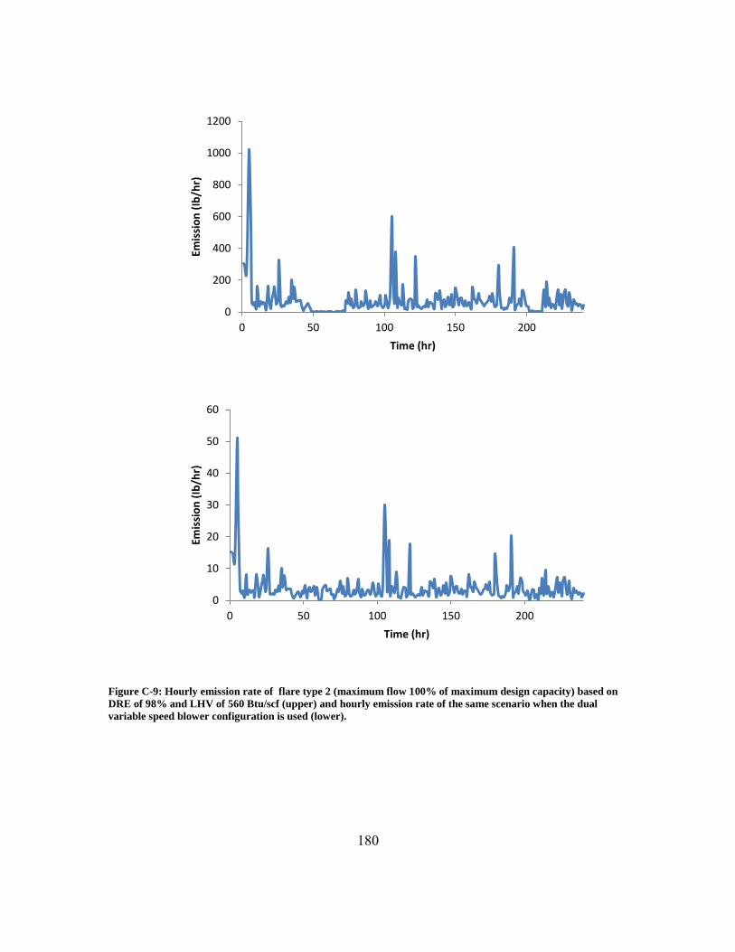
180
Figure C-9: Hourly emission rate of flare type 2 (maximum flow 100% of maximum design capacity) based on
DRE of 98% and LHV of 560 Btu/scf (upper) and hourly emission rate of the same scenario when the dual
variable speed blower configuration is used (lower).
0
200
400
600
800
1000
1200
0 50 100 150 200
Emis
sio
n (
Ib/h
r)
Time (hr)
0
10
20
30
40
50
60
0 50 100 150 200
Emis
sio
n (
Ib/h
r)
Time (hr)
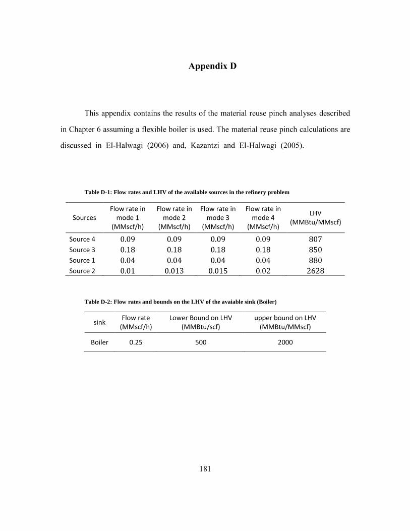
181
Appendix D
This appendix contains the results of the material reuse pinch analyses described
in Chapter 6 assuming a flexible boiler is used. The material reuse pinch calculations are
discussed in El-Halwagi (2006) and, Kazantzi and El-Halwagi (2005). (El-Halwagi,
2006; Kazantzi and El-Halwagi, 2005)..
Table D-1: Flow rates and LHV of the available sources in the refinery problem
Sources Flow rate in
mode 1 (MMscf/h)
Flow rate in mode 2
(MMscf/h)
Flow rate in mode 3
(MMscf/h)
Flow rate in mode 4
(MMscf/h)
LHV (MMBtu/MMscf)
Source 4 0.09 0.09 0.09 0.09 807
Source 3 0.18 0.18 0.18 0.18 850
Source 1 0.04 0.04 0.04 0.04 880
Source 2 0.01 0.013 0.015 0.02 2628
Table D-2: Flow rates and bounds on the LHV of the avaiable sink (Boiler)
sink Flow rate
(MMscf/h) Lower Bound on LHV
(MMBtu/scf) upper bound on LHV
(MMBtu/MMscf)
Boiler 0.25 500 2000

182
Figure D-1: Material reuse pinch diagram for the first operation mode in the refinery problem using a flexible
fixed capacity boiler of 0.2-0.25 MMscf/hr and a flare as sinks.
Figure D-2: Material reuse pinch diagram for the second operation mode in the refinery problem using a
flexible fixed capacity boiler of 0.2-0.25 MMscf/hr and a flare as sinks.
0
100
200
300
400
500
600
700
0 0.05 0.1 0.15 0.2 0.25 0.3 0.35
Ene
rgy
(MM
Btu
/h)
Flowrate (MMscf/h)
Sink composite curve
source composite curve
Minimum flaring = 0.07 MMscf/hr
0
100
200
300
400
500
600
700
0 0.05 0.1 0.15 0.2 0.25 0.3 0.35
Ene
rgy
(MM
Btu
/h)
Flowrate (MMscf/h)
Sink composite curve
source composite curve
Minimum flaring = 0.073 MMscf/hr
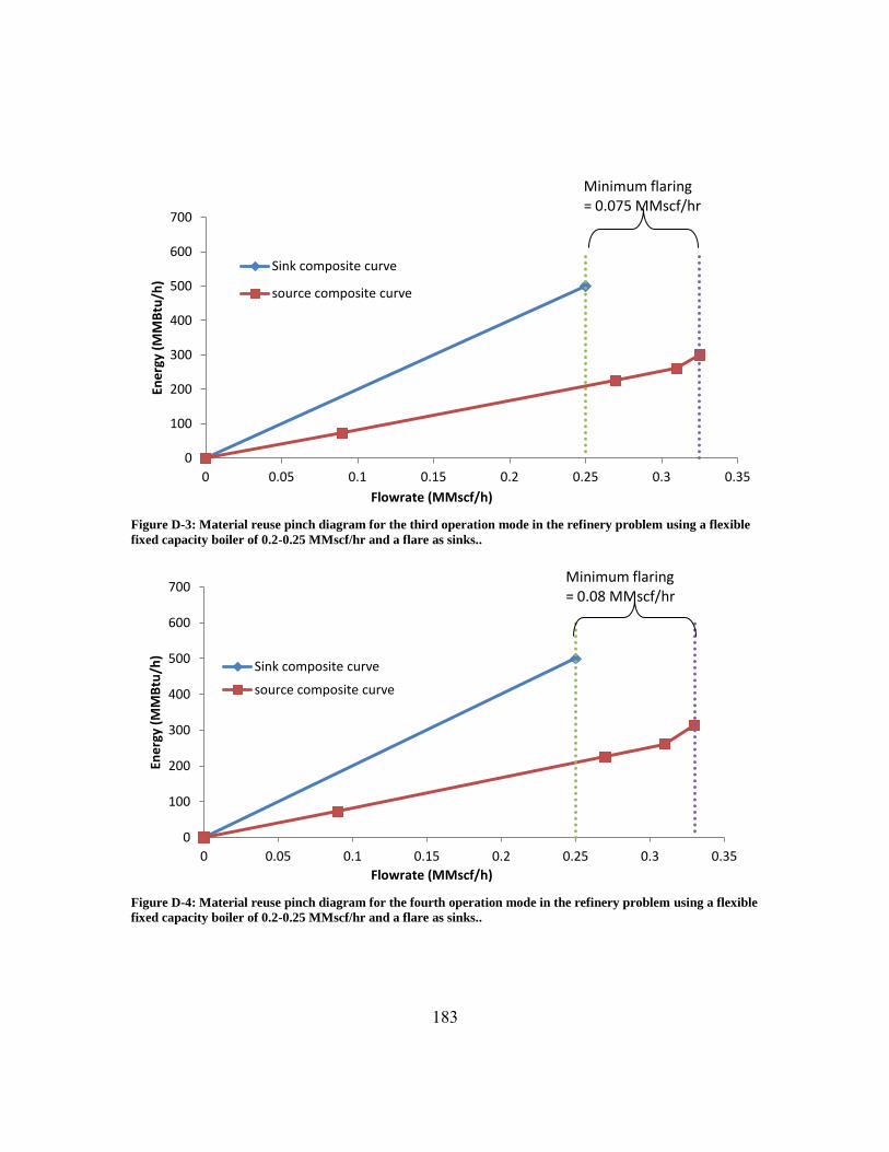
183
Figure D-3: Material reuse pinch diagram for the third operation mode in the refinery problem using a flexible
fixed capacity boiler of 0.2-0.25 MMscf/hr and a flare as sinks..
Figure D-4: Material reuse pinch diagram for the fourth operation mode in the refinery problem using a flexible
fixed capacity boiler of 0.2-0.25 MMscf/hr and a flare as sinks..
0
100
200
300
400
500
600
700
0 0.05 0.1 0.15 0.2 0.25 0.3 0.35
Ene
rgy
(MM
Btu
/h)
Flowrate (MMscf/h)
Sink composite curve
source composite curve
Minimum flaring = 0.075 MMscf/hr
0
100
200
300
400
500
600
700
0 0.05 0.1 0.15 0.2 0.25 0.3 0.35
Ene
rgy
(MM
Btu
/h)
Flowrate (MMscf/h)
Sink composite curve
source composite curve
Minimum flaring = 0.08 MMscf/hr

184

185
References
Al-Fadhli, F. 2009. "Impact of flare destruction effeciencies on ozone concentrations: a
case study for Houston, Texas" Master's Thesis. Master's MSThesis, University of
Texas at Austin.
Al-Fadhli, F. M., Kimura, Y., Mcdonald-Buller, E. C. & Allen, D. T. 2012a. Impact of
flare destruction efficiency and products of incomplete combustion on ozone
formation in Houston, Texas. Industrial & Engineering Chemistry Research,
DOI: 10.1021/ie201400z.
Al-Fadhli, F. M., Torres, V. M. & Allen, D. T. 2012b. Impacts of Air-Assist Flare Blower
Configurations on Flaring Emissions. Industrial & Engineering Chemistry
Research, DOI: 10.1021/ie3012209.
Allen, D. T. & Rosselot, K. S. 1997. Pollution prevention for chemical processes, Wiley
New York.
Allen, D. T. & Torres, V. M. 2011a. 2010 TCEQ Flare Study Project, Final Report.
Available:
http://www.tceq.texas.gov/assets/public/implementation/air/rules/Flare/TCEQ201
0FlareStudyDraftFinalReport.pdf [Accessed June 2011].
Allen, D. T. & Torres, V. M. 2011b. Appendix F of 2010 TCEQ Flare Study Project,
Final Report. Available:
http://www.tceq.texas.gov/assets/public/implementation/air/rules/Flare/ReportAp
pendices.pdf [Accessed June 2011]
Audet, C., Brimberg, J., Hansen, P., Le Digabel, S. & Mladenovi , N. 2004. Pooling
problem: Alternate formulations and solution methods. Management Science,
761-776.
Audet, C., Hansen, P., Jaumard, B. & Savard, G. 2000. A branch and cut algorithm for
nonconvex quadratically constrained quadratic programming. Mathematical
Programming, 87, 131-152.
Cade, R. & Evans, S. 2010. Performance Test of a Steam-Assisted Elevated Flare With
Passive FTIR. Final report. Texas City: Marathon Petroleum Company, LLCv &
Clean Air Engineering, Inc.
Carter, W. P. L. 2011. SAPRC Atmospheric Chemical Mechanisms and VOC Reactivity
Scales [Online]. Available: http://www.engr.ucr.edu/~carter/SAPRC/ [Accessed
20 June 2011].

186
Castiñeira, D. & Edgar, T. 2006. CFD for simulation of steam-assisted and air-assisted
flare combustion systems. Energy & Fuels, 20, 1044-1056.
Castiñeira, D. & Edgar, T. 2008a. CFD for Simulation of Crosswind on the Efficiency of
High Momentum Jet Turbulent Combustion Flames. Journal of Environmental
Engineering, 134, 561.
Castiñeira, D. & Edgar, T. 2008b. Computational Fluid Dynamics for Simulation of
Wind-Tunnel Experiments on Flare Combustion Systems. Energy & Fuels, 22,
1698-1706.
De Carli, A., Falzini, S., Liberatore, R. & Tomei, D. Year. Intelligent management and
control of fuel gas network. In, 2002. IEEE, 2921-2926 vol. 4.
DOE. 2006. U.S.Department of EnergyEnergy, "Bandwidth for Petroleum Refining
Processes". Prepared by Energetics Incorporated for the U.S. Department of
Energy, Office of Energy Efficiency and Renewable Energy, Industrial
Technologies Program. [Online]. Available:
http://www1.eere.energy.gov/industry/petroleum_refining/pdfs/bandwidth.pdf
[Accessed September 9, 2011].
DOE. 2007. U.S.Department of Energy," Energy and Environmental Profile of the U.S.
Petroleum Refining Industry ". Prepared by Energetics Incorporated for the U.S.
Department of Energy, Industrial Technologies Program. [Online]. Available:
http://www1.eere.energy.gov/industry/petroleum_refining/pdfs/profile.pdf
[Accessed September 17, 2011].
EIA. 2009a. Energy Information Agency, U.S. Department of Energy, International
Energy Annual 2006 [Online]. Available: http://www.eia.doe.gov/iea/ [Accessed
September 11 2011].
EIA. 2009b. Energy Information Agency, U.S. Department of Energy, Annual Energy
Review 2009 [Online]. Available: http://www.eia.gov/totalenergy/data/annual/
[Accessed September 11 2011].
El-Halwagi, M. M. 2006. Process Integration, Elsevier.
Elliott, F., Kurz, R., Etheridge, C. & O’Connell, J. 2004. Fuel system suitability
considerations for industrial gas turbines. Journal of engineering for gas turbines
and power, 126, 119.

187
ENVIRON International Corporation 2009. Control of HRVOC Emissions in Flares at
Low Flow Conditions-Project 2009-53. Available:
http://www.tceq.texas.gov/assets/public/implementation/air/rules/contracts/2009-
hrvoc-cost-analysis-final.pdf [Accessed April 2012].
Environ International corporation (Environ) 2010. User's Guide: Comprehensive Air
Quality Model with Extensions (CAMx) Document and model are available
online at http://www.camx.com.
EPA. 1991. U.S. Environmental Protection Agency, "AP 42 Emissions Factors "Chapter
13: Miscellaneous Sources" " [Online]. Available:
http://www.epa.gov/ttn/chief/ap42/index.html [Accessed 10 October 2010].
EPA. 2000. U.S. Environmental Protection Agency, "VOC Destruction Controls"
Section 3.2 : Flares [Online]. Available: http://www.epa.gov/ttncatc1/dir1/cs3-
2ch1.pdf [Accessed 11 January 2011].
Ertl, G., Knözinger, H., Schüth, F. & Weitkamp, J. 2008. Handbook of heterogeneous
catalysis, Wiley Online Library.
Ewing, B., Roesler, D. & Evans, S. 2010. Performance Test of a Steam-Assisted Elevated
Flare with Passive FTIR-Detroit. Final Report. Detroit: Marathon Petroleum
Company, LP & Clean Air Engineering, Inc.
Floudas, C. A. & Aggarwal, A. 1990. A decomposition strategy for global optimum
search in the pooling problem. INFORMS Journal on Computing, 2, 225.
Gounaris, C. E., Misener, R. & Floudas, C. A. 2009. Computational Comparison of
Piecewise- Linear Relaxations for Pooling Problems. Industrial & Engineering
Chemistry Research, 48, 5742-5766.
Hasan, M. M. F., Karimi, I. & Avison, C. M. 2011. Preliminary Synthesis of Fuel Gas
Networks to Conserve Energy & Preserve the Environment. Industrial &
Engineering Chemistry Research, 50, 7414–7427.
Haverly, C. A. 1978. Studies of the behavior of recursion for the pooling problem. ACM
SIGMAP Bulletin, 19-28.
Herndon, S. C. 2011. Products of incomplete combustion from full scale industrial flares
under low flow conditions. Industrial & Engineering Chemistry Research.
Jacob, S. M., Gross, B., Voltz, S. E. & Weekman Jr, V. W. 1976. A lumping and reaction
scheme for catalytic cracking. AIChE journal, 22, 701-713.
188
Jagannath, A., Hasan, M. M. F., Al-Fadhli, F. M., Karimi, I. & Allen, D. T. 2012.
Minimize Flaring via Integration with Fuel Gas Networks. Industrial &
Engineering Chemistry Research, DOI: 10.1021/ie300308g.
Kazantzi, V. & El-Halwagi, M. M. 2005. Targeting material reuse via property
integration. Chemical engineering progress, 101, 28-37.
Knighton, W. B., Herndon, S. C., Franklin, J. F., Wood, E. C., Wormhoudt, J., Brooks,
W., Fortner, E. C. & Allen, D. 2012. Direct measurement of volatile organic
compound emissions from industrial flares using real-time on-line techniques:
Proton Transfer Reaction Mass Spectrometry and Tunable Infrared Laser
Differential Absorption Spectroscopy. Industrial & Engineering Chemistry
Research, DOI: 10.1021/ie202695v.
Kodesh, Z. 2012. John Zink Company, personal communication.
Lasdon, L., Waren, A., Sarkar, S. & Palacios, F. 1979. Solving the pooling problem using
generalized reduced gradient and successive linear programming algorithms.
ACM SIGMAP Bulletin, 9-15.
Liguras, D. K. & Allen, D. T. 1989a. Structural models for catalytic cracking. 1. Model
compound reactions. Industrial & Engineering Chemistry Research, 28, 665-673.
Liguras, D. K. & Allen, D. T. 1989b. Structural models for catalytic cracking. 2.
Reactions of simulated oil mixtures. Industrial & Engineering Chemistry
Research, 28, 674-683.
Marshall & Swift Cost Index. 2011. last page of each issue of Chemical Engineering.
McDaniel, M. 1983. Flare efficiency study. NTIS, SPRINGFIELD, VA(USA).
Available:
http://www.epa.gov/ttn/chief/ap42/ch13/related/ref_01c13s05_jan1995.pdf
[Accessed June 2011].
Mellqvist, J. 2001. "Flare testing using the SOF method at Borealis Polyethylene in the
summer of 2000." Chalmers University of Technology.
http://www.fluxsense.se/reports/flarepaperfinal%201004.pdf [Accessed June
2011].
Meyer, C. A. & Floudas, C. A. 2006. Global optimization of a combinatorially complex
generalized pooling problem. AIChE journal, 52, 1027-1037.
Misener, R. & Floudas, C. A. 2010. Global optimization of large-scale generalized
pooling problems: Quadratically constrained MINLP models. Industrial &
Engineering Chemistry Research, 49, 5424-5438.
189
Murphy, C. & Allen, D. 2005. Hydrocarbon emissions from industrial release events in
the Houston-Galveston area and their impact on ozone formation. Atmospheric
Environment, 39, 3785-3798.
Nace, D. M., Voltz, S. & Weekman Jr, V. 1971. Application of a Kinetic Model for
Catalytic Cracking. Effects of Charge Stocks. Industrial & Engineering
Chemistry Process Design and Development, 10, 530-538.
Nam, J., Kimura, Y., Vizuete, W., Murphy, C. & Allen, D. 2006. Modeling the impacts
of emission events on ozone formation in Houston, Texas. Atmospheric
Environment, 40, 5329-5341.
Nam, J., Webster, M., Kimura, Y., Jeffries, H., Vizuete, W. & Allen, D. 2008.
Reductions in ozone concentrations due to controls on variability in industrial
flare emissions in Houston, Texas. Atmospheric Environment, 42, 4198-4211.
Pariyani, A., Seider, W. D., Oktem, U. G. & Soroush, M. 2010. Incidents Investigation
and Dynamic Analysis of Large Alarm Databases in Chemical Plants: A
Fluidized-Catalytic-Cracking Unit Case Study†. Industrial & Engineering
Chemistry Research.
Parkash, S. 2003. Refining processes handbook, Gulf Professional Publishing.
Pavlovic, R. 2009. "Impact of Variable Emissions on Ozone Formation in the Houston
Area",Ph.D. Dissertation. University of Texas at Austin.
Pavlovic, R., Al-Fadhli, F. M., Kimura, Y., Mcdonald-Buller, E. C. & Allen, D. T. 2012a.
Impact of Emission Variability and Flare Combustion Efficiency on Ozone
Formation in the Houston-Galveston-Brazoria Area. Industrial & Engineering
Chemistry Research, DOI: 10.1021/ie203052w.
Pavlovic, R., Allen, D. T. & Mcdonald-Buller, E. C. 2012b. Temporal Variability in
Flaring Emissions in the Houston-Galveston Area. Industrial & Engineering
Chemistry Research, DOI: 10.1021/ie2013357.
Peters, M. S., Timmerhaus, K. D. & West, R. E. 2003. Plant design and economics for
chemical engineers, McGraw-Hill Science/Engineering/Math.
Pham, V., Laird, C. & El-Halwagi, M. 2009. Convex hull discretization approach to the
global optimization of pooling problems. Industrial & Engineering Chemistry
Research, 48, 1973-1979.
Pohl, J., Lee, J., Payne, R. & Tichenor, B. 1986. Combustion efficiency of flares.
Combustion Science and Technology, 50, 217-231.
190
Seinfeld, J. H. & Pandis, S. N. 2006. Atmospheric Chemistry and Physics: From air
pollution to climate change, John Wiley & Sons, Inc.
Speight, J. G. 2005. Kirk-Othmer Encyclopedia of Chemical Technology " Petroleum
Refinery Processes ", Wiley-Interscience.
Strosher, M. 2000. Characterization of emissions from diffusion flare systems. Journal of
the Air & Waste Management Association, 50, 1723-1733.
TCEQ 2000. Texas Commission on Environmental Quality, Air Permits Division, Air
Permit Technical Guidance for Chemical Sources: Flares and Vapor Oxidizers,
RG-109 (Draft).
TCEQ. 2009. Texas Commission on Environmental Quality "New Source Review (NSR)
Emission Calculations" [Online]. Available:
http://www.tceq.texas.gov/assets/public/permitting/air/Guidance/NewSourceRevi
ew/emiss_calc_flares.pdf [Accessed 15 June 2009].
TCEQ. 2010a. Texas Commission on Environmental Quality " Houston-Galveston-
Brazoria 8-Hour Ozone SIP Modeling (2005/2006 Episodes) " [Online].
Available: http://www.tceq.texas.gov/airquality/airmod/data/hgb8h2/hgb8h2.html
[Accessed 10 October 2010].
TCEQ. 2010b. Texas Commission on Environmental Quality " Houston-Galveston-
Brazoria 8-Hour Ozone SIP Modeling (2005/2006 Episodes): CAMx Modeling
Domain " [Online]. Available:
http://www.tceq.texas.gov/airquality/airmod/data/hgb8h2/hgb8h2_camx_domain.
html [Accessed 1 October 2010].
TCEQ 2010c. Texas Commission on Environmental Quality. Flare Study Quality
Assurance Project Plan. Available:
http://www.tceq.texas.gov/assets/public/implementation/air/rules/Flare/QAPP.pdf
[Accessed April 2011].
TCEQ. 2011. Texas Commission on Environmental Quality "Revisions to the SIP"
[Online]. Available: http://www.tceq.texas.gov/airquality/sip/sipplans.html
[Accessed 17 June 2011].
TCEQ. 2012. § 60.18. General control device requirements [Online]. Available:
http://www.tceq.state.tx.us/assets/public/implementation/air/rules/Flare/Appendix
D_FTF_Draft_Report.pdf [Accessed 1 March 2012].

191
Torres, V. M., Herndon, S. C. & Allen, D. T. 2012a. Industrial flare performance at low
flow conditions: Part 2. Steam-and Air-Assisted Flares. Industrial & Engineering
Chemistry Research, DOI: 10.1021/ie202675f.
Torres, V. M., Herndon, S. C., Kodesh, Z. & Allen, D. T. 2012b. Industrial flare
performance at low flow conditions: Part 1. Study Overview. Industrial &
Engineering Chemistry Research, DOI: 10.1021/ie202674t.
Torres, V. M., Herndon, S. C., Wood, E., Al-Fadhli, F. M. & Allen, D. T. 2012c.
Emissions of Nitrogen Oxides from Flares Operating at Low Flow Conditions.
Industrial & Engineering Chemistry Research, DOI: 10.1021/ie300179x.
Voorhies , A. 1945. Carbon formation in catalytic cracking. Industrial & Engineering
Chemistry, 37, 318-322.
Wang, L., Thompson, T., McDonald-Buller, E. C., Webb, A. & Allen, D. T. 2007.
Photochemical modeling of emissions trading of highly reactive volatile organic
compounds in Houston, Texas. 1. Reactivity based trading and potential for ozone
hot spot formation. Environmental science & technology, 41, 2095-2102.
Wark, K., Warner, C. F. & T., D. W. 1998. Air pollution: its origin and control, Addison
Wesley Longman, Inc.
Webster, M., Nam, J., Kimura, Y., Jeffries, H., Vizuete, W. & Allen, D. 2007. The effect
of variability in industrial emissions on ozone formation in Houston, Texas.
Atmospheric Environment, 41, 9580-9593.
Weekman, V. 1968. Model of Catalytic Cracking Conversion in Fixed, Moving, and
Fluid-Bed Reactors. Industrial & Engineering Chemistry Process Design and
Development, 7, 90-95.
Weekman, V. W. 1979. Lumps, models, and kinetics in practice, American Institute of
Chemical Engineers.
Weekman, V. W. & Nace, D. M. 1970. Kinetics of catalytic cracking selectivity in fixed,
moving, and fluid bed reactors. AIChE journal, 16, 397-404.
Wicaksono, D. S. & Karimi, I. 2008. Piecewise MILP under and overestimators for
global optimization of bilinear programs. AIChE journal, 54, 991-1008.

192
Vita
Fahad M. Al-Fadhli was born in Doha, Kuwait on March 3, 1983. After
completing his work at Doha High School, he attended Kuwait University. He received
the degree of Bachelor of Science in Chemical Engineering with Class Honors from
Kuwait University in August 2005. After graduation, he worked at the Ministry of
Electricity and Water in State of Kuwait for three years. In 2008, he was awarded a
scholarship from Kuwait University to perform his graduate studies at the University of
Texas at Austin with an invitation to return to Kuwait University as a professor. In May
2010, he received his Master’s Degree in Chemical Engineering.
Permanent e-mail : [email protected]
This dissertation was typed by the author.