Copyright

by

Edoardo Angelo Di Napoli

2005

The Dissertation Committee for Edoardo Angelo Di Napolicertifies that this is the approved version of the following dissertation:

Quiver gauge theories, chiral rings and random matrix

models

Committee:

Vadim Kaplunovsky, Supervisor

Willy Fischler, Supervisor

Jacques Distler

Sonia Paban

Daniel S. Freed

Quiver gauge theories, chiral rings and random matrix

models

by

Edoardo Angelo Di Napoli, Dott.

DISSERTATION

Presented to the Faculty of the Graduate School of

The University of Texas at Austin

in Partial Fulfillment

of the Requirements

for the Degree of

DOCTOR OF PHILOSOPHY

THE UNIVERSITY OF TEXAS AT AUSTIN

August 2005

Dedicated to my past lovers, unjustly sacrificed on the altar of science.

Acknowledgments

I wish to thank the multitudes of people who helped me: all the fellow

students that contributed to a better understanding of physics during many

hours of discussion and intense work together; the professors of the Theory

Group and in particular my supervisor for his patience in listening to my

often incorrect arguments and putting up with my lack of knowledge; the

numerous administrative staff of the University of Texas that helped me with

bureaucratic and human issues an uncountable amount of times; all the friends

in Austin that have filled my personal life with joy and optimism; my past

fiancee to which I have caused more trouble than happiness but without whose

support I couldn’t have started such an enterprise; and above all my family

that never failed to believe in my endeavor and fueled me always with positive

energy and wise counseling. A bit of everyone is in this work and in the

achievement that represents. Even if their names do not appear written here

they are all forever printed in my memory.

v

Quiver gauge theories, chiral rings and random matrix

models

Publication No.

Edoardo Angelo Di Napoli, Ph.D.

The University of Texas at Austin, 2005

Supervisors: Vadim KaplunovskyWilly Fischler

Dimensional deconstruction of 5D SQCD with general nc, nf and kCS

gives rise to 4D N = 1 gauge theories with large quivers of SU(nc) gauge

factors. We first describe the spectrum of the model in the deconstructive limit

and show its properties. We then construct the chiral rings of such theories,

off-shell and on-shell. Anomaly equations for the various resolvents allowed by

the model permit us to calculate all the relevant chiral operators. The results

are broadly similar to the chiral rings of single U(nc) theories with both adjoint

and fundamental matter, but there are also some noteworthy differences such

as nonlocal meson-like operators where the quark and antiquark fields belong

to different nodes of the quiver. And because the analyzed gauge groups are

SU(nc) rather than U(nc), our chiral rings also contain a whole collection of

baryonic and antibaryonic operators. We then investigate the random matrix

model corresponding to such chiral ring. We find that bifundamental chiral

vi

operators correspond to unitary matrices. We derive the loop equations and

show that they are in perfect agreement with the anomaly equations of the

gauge model. An exact expression for the free energy is found in the large N

(rank of the matrix) limit. A formula for the effective superpotential is derived

and some examples are illustrated.

vii

Table of Contents

Acknowledgments v

Abstract vi

List of Tables x

List of Figures xi

Chapter 1. Introduction 1

1.1 Chiral ring, quivers and matrices . . . . . . . . . . . . . . . . . 1

1.1.1 Deconstructive quiver . . . . . . . . . . . . . . . . . . . 3

1.1.2 Random matrix model . . . . . . . . . . . . . . . . . . . 6

1.2 Presentation of the material . . . . . . . . . . . . . . . . . . . 7

Chapter 2. Chiral rings of deconstructive [SU(nc)]N 12

2.1 Deconstructive quiver theories and their classical vacua . . . . 12

2.1.1 Deconstruction summary . . . . . . . . . . . . . . . . . 12

2.1.2 The classical vacua . . . . . . . . . . . . . . . . . . . . . 17

2.1.3 Deforming the superpotential . . . . . . . . . . . . . . . 21

2.2 The non-baryonic chiral ring . . . . . . . . . . . . . . . . . . . 27

2.2.1 Generating the chiral ring . . . . . . . . . . . . . . . . . 29

2.2.2 Anomalous equations of motion and their solutions . . . 38

2.2.3 Analytic considerations . . . . . . . . . . . . . . . . . . 51

2.3 Baryons and other determinants . . . . . . . . . . . . . . . . . 63

2.3.1 Φ-baryons in the single SU(nc) theory . . . . . . . . . . 65

2.3.2 Baryonic operators of the [SU(nc)]N Quiver . . . . . . . 75

2.3.3 Determinants of link chains . . . . . . . . . . . . . . . . 87

viii

Chapter 3. The Random Matrix Model 99

3.1 Unitary matrices: why and how . . . . . . . . . . . . . . . . . 99

3.2 Loop equations for the Chiral Gauged Quiver . . . . . . . . . . 105

3.3 Solving for the Free Energy . . . . . . . . . . . . . . . . . . . . 112

3.4 Examples of Effective Superpotentials . . . . . . . . . . . . . . 123

3.4.1 One cut: SU(N) unbroken . . . . . . . . . . . . . . . . 126

Chapter 4. Open questions and conclusions 130

4.1 Chiral ring of the quiver theory . . . . . . . . . . . . . . . . . 130

4.2 Random matrix model . . . . . . . . . . . . . . . . . . . . . . 135

Appendix 137

Bibliography 147

Vita 151

ix

List of Tables

2.1 Charges of fields and parameters . . . . . . . . . . . . . . . . . 55

x

List of Figures

1.1 Diagram of the chiral quiver . . . . . . . . . . . . . . . . . . . 4

3.1 Branch cuts on the unit circle . . . . . . . . . . . . . . . . . . 119

3.2 Integration contour for FD on the cylinder . . . . . . . . . . . 121

3.3 Bi and Ai contours on the cylinder . . . . . . . . . . . . . . . 123

xi

Chapter 1

Introduction

1.1 Chiral ring, quivers and matrices

Regardless of their applicability to the weak scale phenomenology, su-

persymmetric gauge theories are important from the abstract QFT point of

view because they allow for exact calculation of some non-perturbative data.

In a 4D, N = 1 theory, the exactly-computable non-perturbative data form a

mathematical structure known as the chiral ring. Physically, this ring contains

invariant combinations of the scalar VEVs, gaugino condensates and abelian

gauge couplings; usually, these data are sufficient to completely determine the

phase structure of the theory and its moduli spaces, if any.

Two recent discoveries excited much interest in the chiral rings of

gauge theories with adjoint and fundamental matter fields: first, Dijkgraaf

and Vafa [1–3] found that the gaugino condensates and the abelian gauge cou-

plings of 4D, N = 1 gauge theories correspond to perturbative amplitudes of

matrix models without any spacetime or SUSY at all. Second, Cachazo, Dou-

glas, Seiberg and Witten [4],[5], [6] evaluated the entire on-shell chiral ring

of an U(Nc) theory with adjoint and fundamental matter using generalized

Konishi anomaly equations [7, 8]. In the process, they verified the Dijkgraaf-

Vafa conjecture by showing that the loop equation of the matrix model is

1

identical to the anomaly equation for a particular resolvent R(X) summariz-

ing the gaugino condensates. Both approaches — the matrix models and the

anomaly equations — are readily extended to the quiver theories with mul-

tiple gauge group factors “connected” by the bi-fundamental matter fields.

Thus far, most work on this subject concerned the non-chiral quivers where

the bi-fundamental fields come in (n,m) + (n, m) conjugate pairs; this is a

natural limitation of the matrix correspondence1 but the anomaly-equations

technology has no particular difficulties with 4D chirality [9]–[10].

In this dissertation we analyze the inherently chiral An quivers of one-

way arrows

which means that all the bi-fundamental fields are chiral (ni, ni+1) multi-

plets not accompanied by their (ni,ni+1) conjugates. Also, our quivers do

not have any adjoint matter fields — although the cyclic product of all the

bi-fundamental fields does act as some kind of a collective adjoint multiplet.

Finally, the individual gauge groups corresponding to our quivers’ nodes are

of the SU(nc) rather than U(nc) type, and this adds all kinds of baryonic

generators to the chiral ring of the theory.

1An un-constrained complex n×m matrix corresponds to a whole N = 2 hypermultipletin the bi-fundamental (n,m) representation of the SU(n) × SU(m), or in N = 1 termsto a conjugate pair (n,m) + (n, m) of chiral multiplets. A chiral bi-fundamental (n,m)multiplet not accompanied by its (n, m) conjugate corresponds to a matrix subject to non-linear constraints, which makes for a much more complicated matrix model. In particular,the chiral [SU(nc)]

N quiver theory presented in this dissertation corresponds to a modelof N unitary SU(nc) matrices. This matrix model — and its implications for the gauginocondensates — will be presented in the second chapter of this dissertation.

2

Specifically, our chiral quiver theories follow from the dimensional de-

construction of the 5D SQCD [11]–[12], hence the name deconstructive quiv-

ers. In general, dimensional deconstruction [11, 13] relates simple gauge the-

ories in spaces of higher dimension to more complicated theories in fewer di-

mensions of space: the extra dimensions of space are ‘deconstructed’ into

quiver diagrams of the ‘theory space’. For example, starting in 4 + 1 di-

mensions, we deconstruct the extra space dimension by discretizing the x4

coordinate into a lattice of small but finite spacing a and then interpreting

the result as a 4D gauge theory with a large quiver of gauge groups. In

order to have a finite number of 4D fields, the x4 is also compactified to a

large circle of length 2πR = Na (hence N lattice points), but eventually

one may take the N → ∞ limit and recover the uncompactified 5D physics.

In this limit, the lattice spacing a remains finite and serves as UV regula-

tor which breaks part of the 5D Lorentz symmetry as well as 4 out of 8

supercharges but preserves the (latticized) 5D gauge symmetry of the the-

ory.

1.1.1 Deconstructive quiver

The deconstruction of SQCD5 will be discussed in more detail in a

separate paper [12] (see also [14] for the quarkless case). From the 4D point

of view, the result is an N = 1 supersymmetric gauge theory with a quiver

diagram Each green circle of this diagram corresponds to a simple SU(nc)`

3

nc F F

nc

F

F

nc

F

F

nc

F

F

nc

F

F

nc

F

F

nc

FF

Figure 1.1: Diagram of the chiral quiver

factor of the net 4D gauge group

G4D =N∏

`=1

[SU(nc)] ` (1.1)

while the red and blue arrows denote the chiral superfields:

quarks Q`,f = ( `),

antiquarks Qf` = ( `),

bifundamental link fields Ω` = ( `+1, `), (1.2)

where f = 1, 2, . . . , F and ` = 1, 2, . . . , N is understood modulo N . From the

4D point of view, N is a fixed parameter of the quiver theory; in our analysis

4

we shall assume N to be large but finite.

Similar to many other deconstructed theories, the quiver (1.1) can be

obtained by orbifolding a simple 4D gauge theory with higher SUSY, namely

N = 2 SQCD with F flavors and N × nc colors: The ZN twist removes the

extra supercharges and reduces the gauge symmetry from SU(N × nc) down

to

S([U(nc)]N) = [SU(nc)]

N × [U(1)]N−1 . (1.3)

However, the abelian photons of the orbifold theory suffer from triangular

anomalies and therefore must be removed from the effective low-energy theory.

In string theory such removal is usually accomplished via the Green-Schwarz

terms [15], but at the field theory level we simply discard the abelian factors

of the orbifolded symmetry (1.3) and interpret the nodes (green circles) of the

quiver diagram (1.1) as purely non-abelian SU(nc)` factors.

In this dissertation we study chiral rings of deconstructed SQCD5 theo-

ries with generic numbers of colors and flavors, Chern-Simons levels, and sizes

of the compact fifth dimension. In 4D terms, this means [SU(nc)]N theories

with quiver diagrams of the general form (1.1), but with most general num-

bers nc, F , N , as well as generic quark masses; for the sake of 4D chirality we

assume N ≥ 3 quiver nodes. We shall see that the chiral rings of such theories

resemble the rings of refs. [4]–[6] but also have two novel features: first, our

rings have meson-like generators involving the quark and the antiquark fields

belonging to different nodes of the quiver. Such operators are non-local from

the 5D point of view, but in 4D terms they are legitimate generators of the

5

chiral ring. Second, in the absence of abelian gauge fields, all kinds of bary-

onic and antibaryonic operators are gauge-invariant and thus also belong to

the chiral ring; in fact, there is a whole zoo of such operators.

1.1.2 Random matrix model

To the chiral ring of the gauge model should correspond a random

matrix model of some kind. Until now it has been shown in a series of papers

[1–4] how a group of non-chiral gauge theories are well described by hermitian

random matrix models. Specifically, the great majority of such models contain

one or more scalar fields in the adjoint representation. Such fields typically

correspond to hermitian matrices or more generally matrices whose eigenvalues

are one variable holomorphic functions [16]. Chiral gauge models cannot be

described using hermitian matrices but have to rely on a different set of random

variables. The natural choice have fallen on the set of unitary matrices. In

particular to each bi-fundamental link variable Ω` correspond a unitary matrix

U`, while to the flavors Q`,f and Qf` correspond complex matrices B` and A`

(constrained by the condition B† = A). Such set, considered as a sub-manifold

of the set of all N × N complex matrices, admit a series of loop equations that

match perfectly the anomaly equations of the gauge theory.

Once established the correspondence a functional can be build for the

random matrix model using as action the superpotential of the gauge model.

First the flavor matrices are integrated out under the assumption that are

massive. Then a series of transformation reduce the integration over all the

U` to an integration over a single unitary matrix U. The model now can be

6

solved in the large N limit using standard resolvent techniques in complex

space. In such limit we recover an expression for the free energy made out

of two contribution: the sphere and the disk. Since the eigenvalues of the

unitary matrix U are on the unit circle a general expression for the free energy

is derived on the cylinder. From previous works presented by Cachazo et

Al. [4],[5],[6] a formula for the derivation of the effective superpotential for

the gaugino condensates is used. A particular simple example illustrates the

quasi-polynomial nature of such superpotential.

1.2 Presentation of the material

The main part of this dissertation (after this introduction) is organized

as follows: in section 2.1 we study the deconstructive [SU(nc)]N quiver theories

at the classical level. First, in section 2.1.1 we spell out the superpotentials

and explain how the 4D quiver theories deconstruct the 5D SQCD. Next, in

section 2.1.2 we survey the classical vacua of the quiver theories and find that

they form the same Coulomb, mesonic, and baryonic moduli spaces as the 5D

theories compactified on a large circle. And then in section 2.1.3 we break

the correspondence by deforming the 4D superpotentials in order to trigger

the gaugino condensation at the quantum level. This deformation is similar

to the adjoint field’s superpotential in the single-U(nc) theory and has similar

consequences for the classical vacua of a quiver theory: the Coulomb moduli

space breaks up into a large discrete set of isolated vacua.

In section 2.2 we study the fully-quantum [SU(nc)]N quiver theories and

7

derive their chiral rings, or rather the non-baryonic sub-rings. In section 2.2.1

we construct the off-shell chiral rings (un-constrained by the anomalous equa-

tions of motion). Similar to the single-U(nc) theory of [4]–[6], the non-baryonic

generators of the quivers’ off-shell rings combine into several resolvents where

the cyclic-ordered product ΩNΩN−1 · · ·Ω2Ω1 of the bi-fundamental link fields

plays the role of the adjoint field Φ. The main difference from the single-U(nc)

theory is a much richer set of mesonic generators and hence resolvents: in a

quiver theory, the quark and the antiquark fields of a meson-like chiral oper-

ator may belong to different quiver nodes as long as they are connected by a

chain of link fields which maintain the gauge invariance. From the 5D point

of view such operators are non-local and they create / annihilate un-bound qq

pairs, but in 4D they are local, chiral and gauge invariant and thus do belong

to the chiral ring.

In section 2.2.2 we turn to the on-shell chiral rings: we calculate the

generalized Konishi anomalies for suitable variations of the quark, antiquark

and link fields of the quiver theories and derive the anomalous equations of

motions for all the resolvents. We solve the equations in terms of a few poly-

nomials and find that all the on-shell resolvents are single-valued on the same

hyperelliptic Riemann surface Σ defined by the quadratic equation (2.103) for

the gaugino-bilinear resolvent. Physically, Σ is the Seiberg-Witten curve [17]

of the theory, and in section 2.2.3 we use analytic considerations to show that it

indeed looks like the SW curve of the SQCD5 compactified on a circle [18, 19].

We also find that this curve is completely determined at the level of one di-

agonal instanton, that is one instanton of the SU(nc)diag ≡ diag[SU(nc)N ] or

8

equivalently one instanton in each and every SU(nc)` factor of the total 4D

gauge group. Finally, we study the vacua of the quantum quiver theories and

show that in the weak coupling limit we have exactly the same Coulomb, Higgs,

pseudo-confining, etc., vacua as expected in a semisclassical theory, but in the

strong coupling regime all vacua with similar numbers of massless photons are

interchangeable by the monodromies in the parameter space of the theory.

In section 2.3 we complete the chiral rings by adding all kinds of bary-

onic, antibaryonic and other generators with non-trivial [U(1)B]N quantum

numbers. In section 2.3.1 we warm up by studying baryon-like generators in

a theory with a single SU(nc) gauge group, nf quarks and antiquarks and an

adjoint field Φ: Because the gauge group is SU(nc) rather than U(nc), the chi-

ral baryon operators are gauge invariant, and so are the Φ-baryons comprised

of nc quarks plus any number of adjoint fields Φ. Off-shell, such operators

exist for any nf ≥ 1, and we summarize them in baryonic resolvents. On-shell

however, the Φ-baryons follow from the ordinary baryons, hence no baryonic

VEVs whatsoever for nf < nc, and even for nf ≥ nc baryonic VEVs exist only

for the classical-like branches of the moduli space.

In section 2.3.2 we analyze the baryonic generators of the [SU(nc)]N

quiver theory. Off-shell, we find a whole zoo of baryon-like generators com-

prised of nc quarks belonging to different quiver nodes and connected to each

other by chains of link fields — and each chain may wrap a few times around

the whole quiver to emulate the Φ fields of Φ-baryons. Again, there is a big

pile of independent baryon-like operators for any nf ≥ 1, but only off-shell.

9

On-shell, we tame the zoo by solving the equations of motions for the bary-

onic resolvents and showing that all baryon-like VEVs follow from those of

ordinary baryonic operators (all quarks at the same node and no link fields).

Consequently, all baryonic VEVs of the quantum theory follow the classical

rules: they require nf ≥ nc as well as overdetermined Coulomb moduli of

the baryonic branch. However, the precise constraint on the quark masses

due to baryonic branch’s existence is subject to quantum corrections at the

one-diagonal-instanton level.

In section 2.3.3 we calculate quantum corrections to the determinants

of link chains,

det(Ω`2

· · ·Ω`1

)= det(Ω`2

) × · · · × det(Ω`2) + corrections. (1.4)

We find that for chains of less than N links the corrections come from in-

stantons in the individual SU(nc)` gauge groups rather than the diagonal in-

stantons, but the determinant det(ΩN · · ·Ω1) of the whole quiver is subject to

separate individual-instanton and diagonal-instanton corrections. We evaluate

the corrections and summarize their effect on the Coulomb moduli space of

a deconstructive quiver theory. A particularly technical part of our analysis

is removed to the 4.2 of this dissertation. We conclude the chapter with 4.1

where we discuss the open questions related to the present research.

In section 3.1 we explain why the choice of matrix valued random vari-

ables falls on the unitary set. We illustrate the guiding principles that lead

us to such a choice. The set up of the loop equations in this context is far

from trivial since the deformation of a generic matrix U brings us outside the

10

unitary manifold. This apparent problem is overcome forcing the deformation

to be holomorphic. The resulting loop equation will be, then, perfectly well

defined. We illustrate the general way of proceeding in the simplest case before

jumping to the quiver model.

In section 3.2 we derive the set of all loop equations for the quiver. We

deform in all possible allowed ways the matrices U , A and B inside the func-

tional Z. The set of equations derived matched perfectly with the anomaly

equations calculated in section 2.2.2. This result establish an exact correspon-

dence between the chiral quiver gauge theory and the proposed random matrix

model. This is the first case in which such correspondence is verified and gives

credibility to a larger duality that is believed to exist between gauge theories

and random matrix models.

In section 3.3 we solve for the free energy of the matrix model. We first

integrate out the massive degrees of freedom coming from the flavors. Then

we show how the functional integral reduces to a simpler one where all the

link matrices integrations are reduced to only one U. Since the eigenvalues

of the U lies on the unit circle we introduce a resolvent R(w) defined on it.

In the large N limit the steepest descent method can be used to derive an

integral expression for the free energy. The eigenvalues are then constrained

by the saddle point equation that corresponds to the first loop equation for

R(w) derived in section 3.2. A general expression for the free energy and the

superpotential is given in terms of contour integration on the cylinder.

Finally in section 3.4 a simple example of superpotential is calculated.

11

Chapter 2

Chiral rings of deconstructive [SU(nc)]N

2.1 Deconstructive quiver theories and their classicalvacua

Deconstruction of SQCD5 with general numbers of colors and flavors

will be explained in much detail in the companion paper [12]. In this section,

we summarize the salient features of the deconstructed theory from the 4D

point of view. In the immediately following section 2.1.1 we write down the

superpotential of the 4D theory and briefly explain how deconstruction works

for the most symmetric vacuum of the 5D theory. Of course, the [SU(nc)]N

quiver theory has many other classical vacua, and we describe them in sec-

tion 2.1.2. Finally, in section 2.1.3 we deform the quiver’s superpotential in

order to trigger some kind of a gaugino condensation and describe the effects of

this deformation on the quiver’s vacua. (The gaugino condensates themselves

will be discussed in the later section 2.2).

2.1.1 Deconstruction summary

The 4D gauge theory of the deconstructed SQCD5 is

G4D =N∏

`=1

[SU(nc)] ` (2.1)

12

with equal gauge couplings g` ≡ g for all the factors to assure discrete transla-

tion invariance in the x4 direction. The chiral superfields comprise the quarks,

the antiquarks, and the bilinear link fields specified in the table (1.2), and also

singlets s` (one for each ` = 1, 2, . . . , N). The superpotential has two distinct

parts, W = Whop + WΣ, where

Whop = γ

N∑

`=1

F∑

f=1

(Qf

`+1Ω`Q`,f − µf Qf` Q`,f

)(2.2)

facilitates the propagation of the (anti) quark fields in the x4 direction, while

WΣ = βN∑

`=1

s` (det Ω` − vnc) (2.3)

sets up an SL(nc, C) (AKA complexified SU(nc)) linear sigma model at each

link of the latticized 5D theory.1 Disregarding the massive “radial” mode, we

have

Ω`(x) = v × expPath

ordered

(∫ a(`+1)

a`

dx4(iA4(x) + φ(x)

))+ fermionic terms (2.4)

where Aµ(x) and φ(x) are the 5D vector fields and their scalar superpart-

ners. The simplest 5D vacuum with φ ≡ A4 ≡ 0 corresponds to the 4D field

configuration

〈Ω`〉 ≡ v × 1nc×nc(2.5)

which Higgses the 4D gauge symmetry [SU(nc)]N down to its diagonal sub-

group SU(nc)diag = diag(∏

` SU(nc)`). The rest of the 4D vectors acquire

1Although the β coupling is non-renormalizable for nc > 2, all the resulting divergencescan be regularized via higher-derivative lagrangian terms for the singlet fields s` withoutdisturbing the chiral ring of the theory.

13

masses

M2(k) = 4g2|v|2 sin2 πk

N=

4

a2sin2 aP4

2(2.6)

where the second equality follows from identifying the lattice spacing a as

a =1

g|v| (2.7)

and the lattice momentum P4 as

P4 =2πk

Na, k = 1, 2, . . . modulo N . (2.8)

In the large-N limit, the bottom end of the spectrum (2.6) becomes a Kaluza-

Klein tower

M2 ≈ P 24 =

(2πk

Na

)2

(2.9)

of a massless relativistic 5D vector field (compactified on a circle of length

2πR = Na); this is the momentum-space view of the dimensional deconstruc-

tion.

Similarly, the low-energy end of the 4D quark spectrum comprises

Kaluza-Klein towers for relativistic 5D hypermultiplets of masses mf (1/a).

Indeed, for a quark flavor of 4D mass γµf , the mass matrix for the Q`,f and

Qf` fields (` = 1, 2, . . . , N) has eigenvalues

M2(f, k) = |γ|2∣∣ve2πik/N − µf

∣∣2 , (2.10)

and for |µf | ≈ |v|, the bottom end of this spectrum becomes (in the large-N

limit)

M2 ≈ m25D + P 2

4 (2.11)

14

where

m5D = |γ| ×(|µf | − |v|

) 1

a, (2.12)

P4 =2πk

Na+ constant (Wilson line) , (2.13)

and

a =1

|γv| . (2.14)

The 4D quarks with |µf | 6≈ |v| do not have low-mass M 2 (1/a)2 modes

and do not deconstruct any 5D particles. For µf v, the 4D quark decou-

ples above the deconstruction threshold (1/a) and has no low-energy effect

whatsoever, but quarks with µf v decouple at the threshold itself and

modify the Chern-Simons interactions of the deconstructed SQCD5. Since the

Chern-Simons level kcs affects the moduli space geometry and even the phase

structure of the 5D theory, it must be deconstructed correctly. Thus, the

deconstructive quiver should have

F = nf + ∆F ≥ nf (2.15)

4D flavors, where nf is the number flavors in 5D,

∆F = nc −nf

2− kcs , 0 ≤ ∆F ≤ 2nc − nf , (2.16)

and

µf = v × exp(am5Df ) ∼ v for f ≤ nf but µf v for f > nf .

(2.17)

However, from the holomorphic, purely-4D point of view, there is no qualita-

tive difference between µf ∼ v and µf v, but there is a difference between

15

µf 6= 0 and between µf = 0. Hence, for the purposes of this article, we shall

assume

generic µf 6= 0 for f = 1, 2, . . . , nf

but µf = 0 for f = (nf + 1), . . . , F . (2.18)

Note that consistency between eqs. (2.7) and (2.14) requires equal gauge

and Yukawa couplings, g = |γ|. In a quantum theory, this means equality of

the renormalized physical couplings,

gphys = |γ|phys , (2.19)

or in non-perturbative terms, in the very low energy limit E (1/Na) the

effective theory (the diagonal SU(nc) with an adjoint field Φ and several quark

flavors) should be N = 2 supersymmetric. Without this condition, the decon-

structed theory would have quarks and gluons with different effective speed of

light in the x4 direction. This is a common problem in lattice theories with

some continuous dimensions (eg. hamiltonian lattice theories with continuous

time but discrete space), and the common solution is fine-tuning of the lat-

tice parameters. For the deconstructed SQCD5, the fine tuning involves the

Kahler parameters (such as coefficients of the quarks’, antiquarks’ and links’

kinetic-energy lagrangian terms) and does not affect any of the holomorphic

properties of the quiver such as its chiral ring. Consequently, in the present

article we may disregard eq. (2.19) and treat the holomorphic γ and the gauge

coupling g (or rather its dimensional transmutant Λ) as free parameters of the

quiver theory.

16

We conclude this section by acknowledging that there are many ways

to skin a cat or to deconstruct SQCD5 with given nc, nf and kcs. For example,

one can pack several 5D quark flavors into a single 4D flavor with a complicated

dispersion relation M4D(P4) by generalizing the hopping superpotential (2.2)

to allow the quark to hop over several lattice spacing at once. Indeed,

Whop =

p∑

q=0

Γp

N∑

`=1

Q`+qΩ`+q−1 · · ·Ω`Q` (2.20)

endows a single 4D flavor with p light modes when the polynomial

Hp(x) =

p∑

q=0

Γpxp (2.21)

has all p of its roots µ1, . . . , µp located close to the circle |x| = |v|. We found

however that such p-fold quarks are pretty much equivalent to p ordinary

flavors with masses µ1, . . . , µp. Consequently, we shall henceforth stick to

the p = 1 model (2.2) because of its twin virtues of relative simplicity and

renormalizability.

2.1.2 The classical vacua

As explained in [12], the classical moduli space of the [SU(nc)]N quiver

theory has exactly the same Coulomb, Higgs and mixed branches as the un-

deconstructed SQCD5. The Coulomb branch is distinguished by zero classical

values of the quark and antiquark scalars while the link fields have non-zero

VEVs subject to D/F term constraints

∀` : 〈Ω`〉† 〈Ω`〉 − 〈Ω`−1〉 〈Ω`−1〉† ∝ 1nc×nc, Det 〈Ω`〉 = vnc . (2.22)

17

Consequently, all the 〈Ω`〉 matrices are equal and diagonal modulo an `-

dependent gauge transform:

∀` : 〈Ω`〉 = diag (ω1, ω2, . . . , ωnc) (2.23)

for some complex moduli (ω1, ω2, . . . , ωnc) satisfying

∏j ωj = vnc . Note that

each ωj is gauge-equivalent to ωj × N√

1, hence the (ωN1 , ωN

2 , . . . , ωNnc

) makes a

better coordinate system for the moduli space, although it’s still redundant

with respect to permutations of the ωNj . Generically, all the ωN

j are distinct and

the 4D gauge symmetry is broken all the way down to the Cartan (U(1))nc−1

subgroup of the SU(nc)diag = diag[∏

` SU(nc)`

], but a non-abelian subgroup

SU(k) ⊂ SU(nc)diag survives un-Higgsed when k of the ωNj happen to coincide.

According to the deconstruction map (2.4),

ωj = v × exp(a(φj + iA4j)) (2.24)

where φj are the real 5D moduli scalars and A4j × Na are the Wilson lines of

the diagonal gauge fields around the deconstructed dimension. Of course, the

deconstruction works only for φj (1/a) =⇒ ωj ∼ v, but this restriction

does not affect the 4D theory as such.

Unlike the Coulomb branch which exists for any quark masses, the

Higgs and the mixed branches require coincidences between the µf or rather

among the non-zero µNf . For example, for µN

1 = µN2 6= 0 there is a mixed

mesonic branch where one of the ωNj is frozen at the same value. Indeed, let

ω1 = e2πik1/N µ1 = e2πik2/N µ2 (2.25)

18

for some integer (k1, k2); then the quark mass matrix due to the superpoten-

tial (2.2) allows for the squark VEVs

⟨Qj

`,f

⟩= e2πikf `/NQf ,

⟨Qf

`,j

⟩= e−2πikf `/NQf (2.26)

for j=1 and f=1,2 only, subject to F-term and D-term constraints

Q1 Q1 + Q2 Q2 = 0 , (2.27)

(|Q1|2 − |Q1|2) + (|Q2|2 − |Q2|2) = 0 . (2.28)

These VEVs Higgs the (SU(nc))N symmetry down to (SU(nc − 1))N , which

is further broken by the link VEVs 〈Ω`〉 down to a subgroup of the SU(nc −

1)diag = diag[∏

` SU(nc − 1)`

]. For generic values of the un-frozen Coulomb

moduli (ωN2 , . . . , ωN

nc), the surviving gauge symmetry is U(1)nc−2, but coinci-

dences among these moduli allow for un-Higgsing of a non-abelian SU(k) ⊂

SU(nc − 1)diag.

The mesonic branch of the quiver deconstructs the mesonic branch of

the SQCD5 where φ1 = m5D1 = m5D

2 . Although the deconstruction requires

φj (1/a) and hence m5D1,2 (1/a), this restriction does not affect the 4D

theory as such. In 4D, a coincidence µN1 = µN

2 gives rise to a a mesonic

branch regardless of whether µ1,2 is larger, smaller, or similar to v, as long

as µN1,2 6= 0. On the other hand, having two or more exactly massless 4D

flavors (i. e., ∆F ≥ 2) does not lead to a mesonic branch of the [SU(nc)]N

quiver because the link eigenvalues ωj cannot vanish. (Note the constraint

det(Ω`) = vnc 6= 0.)

19

Further coincidences among the µNf allow for multi-mesonic

mixed branches with more squark VEVs, more frozen Coulomb moduli ωNj

(eg., ωN1 = µN

1 = µN2 , ωN

2 = µN3 = µN

4 ), and a lower rank of the un-Higgsed

gauge symmetry. Such multi-mesonic branches work similarly to the single-

meson mixed branch, so we need not discuss them any further. Instead, let us

consider the purely-Higgs baryonic branch which exists for nf ≥ nc when nc

of the 5D quark masses add to zero, or in 4D terms, when the product of nc of

the µNf happens to equal to the (vnc)N . Indeed, for µN

1 ×µN2 ×· · ·×µN

nc= vNnc

we may freeze all of the Coulomb moduli at

ωj = e2πikj/N µj ∀j = 1, 2, . . . , nc , kj ∈ Z , (2.29)

which gives zero modes to all quark colors j = 1, . . . , nc for f = j and allows

non-zero VEVs

⟨Qj

`,f

⟩= δj

fe2πikj`/NQj ,

⟨Qf

`,j

⟩= δf

j e−2πikj`/N Qj (2.30)

subject to the D term constraint

same (|Qj|2 − |Qj|2) ∀j (2.31)

and the F-term constraint

∂W

∂Ωj`,j

= γe−2πikj/N QjQj + βs` ×vnc

ωj

= 0 . (2.32)

The simplest solutions to these constraints are either Qj ≡ 0, same Qj ≡ Q∀j

(baryonic VEVs only) or vice verse Qj ≡ 0, same Qj ≡ Q ∀j (antibaryonic

VEVs only), but thanks to the singlet fields s` enforcing the det Ω` = vnc

20

constraints, there are other solutions where both baryonic and antibaryonic

VEVs are present at the same time. In the deconstruction limit φj = m5Dj

(1/a) =⇒ ωj ≈ v (up to a phase) in eq. (2.32), we have Qj ≡ Q, Qj ≡ Q and

hence

⟨Qj

`,f

⟩= δj

fe2πikj`/N × Q ,

⟨Qf

`,j

⟩= δf

j e−2πikj`/N × Q (2.33)

for some arbitrary pair (Q, Q) of complex moduli which deconstruct the bary-

onic hyper-modulus of the SQCD5. Outside the deconstruction limit, the

4D baryonic branch exists anyway, albeit with more complicated anti/squark

VEVs. In any case, there are two complex moduli and the [SU(nc)]N gauge

symmetry is completely Higgsed down.

This completes our survey of the classical moduli space of the [SU(nc)]N

quiver. The bottom line is, all the classical vacua of this quiver are deconstruc-

tive, i. e. correspond to the SQCD5’s vacua according to the deconstruction

map (2.4) and the zero modes of the massless 5D gauge bosons match all the

massless 4D vector fields.

2.1.3 Deforming the superpotential

In the extreme infrared limit E (1/Na), the N = 1 quiver theory

reduces to the N = 2 SQCD4 with several flavors, and thanks to this extra

supersymmetry, the gauginos do not form bilinear condensates. According to

Cachazo, Douglas, Seiberg and Witten [4–6, 20], the gaugino condensates play

a key role in the chiral ring of the U(nc) theory with an adjoint chiral field Φ.

Indeed, the best way for understanding the N = 2 SQCD4 involves deforming

21

the theory to N = 1 (via superpotential tr W(Φ) for the adjoint field) in order

to turn on the gaugino condensation, although eventually, after solving the

anomaly equations of the chiral ring of the deformed theory (including the

chiral gaugino condensates) one may turn off the deformation and return to

N = 2 SUSY.

In the quiver theory, the role of the adjoint field Φ is played by the

quiver-ordered product (ΩN · · ·Ω2Ω1) of the link fields. Hence, to study the

chiral ring of the quiver, we need to temporarily deform the superpotential

according to

W = Whop + WΣ −→ W = Whop + WΣ + Wdef (2.34)

where

Wdef = tr W(ΩNΩN−1 · · ·Ω2Ω1)def=

d∑

k=1

νk

ktr((ΩNΩN−1 · · ·Ω2Ω1)

k)

. (2.35)

Although this deformation does not make any sense from the 5D point of view

— indeed, it is utterly non-local in the x4 direction — as well as grossly non-

renormalizable in 4D, it does lead to non-zero gaugino condensates which will

help us later in section 2.2. But before we study such non-perturbative effects,

we need to know the effect of the deformation (2.34) on the classical vacua of

the theory.

The general effect is similar to the deformed N = 2 SQCD4. The

Coulomb branch collapses to a discrete set of isolated vacua where each Coulomb

modulus ωNj takes one of d possible values (℘1, ℘2, . . . , ℘d), namely the roots

22

of the polynomial

W(X) =d∑

k=1

νkXk + β 〈s〉 vnc (2.36)

where 〈s〉 ≡ 〈s`〉 is the common expectation value of the singlet fields s` which

adjusts itself to assure∏

j ωj = vnc . Indeed, given the Coulomb VEVs (2.23),

∂W

∂ωj

=N

ωj

W(ωNj ) =⇒ ∀j : W(ωN

j ) = 0 . (2.37)

Note that each root ℘i of the W polynomial may capture several moduli ωNj , or

just one, or even none at all. The individual Coulomb vacua of the quiver are

distinguished by the ‘occupation numbers’ ni = #j : ωNj = ℘i = 0, 1, 2, . . .

for i = 1, . . . d; altogether,∑

i ni = nc. For any given set of the ni, the

surviving gauge symmetry of the [SU(nc)]N quiver theory is

Gunbroken = S

[∏

i

U(ni)

]⊂ SU(nc)diag (2.38)

where each ni ≥ 2 gives rise to a nonabelian factor SU(ni). In the quantum

theory, such nonabelian factors develop mass gaps due to pseudo-confinement2

and the ultimate low-energy limit of the theory has only the abelian photons.

The net number of such surviving photons is

nAbel = #i : ni 6= 0 − 1 ≤ nc − 1 . (2.39)

Besides the purely-Coulomb vacua, the deformed quiver also has dis-

crete mesonic vacua where the squark VEVs are determined by the deforma-

tion (2.35). In such vacua, some of the Coulomb moduli ωNj are frozen at

2Following the terminology of ref. [6] we call an SU(ni) gauge factor pseudo-confiningrather than confining because the overall quiver theory contains fields with anti/fundamentalquantum numbers (with respect to the SU(ni)) which prevent the complete confinement. Inthis terminology, the ordinary QCD with finite-mass quarks is also pseudo-confining ratherthan confining.

23

non-zero, non-degenerate µNf while the rest follow the roots ℘i of the deforma-

tion polynomial (2.36). For example, let ωN1 = µN

1 6= 0 while the (ωN2 , . . . , ωN

nc)

are captured by the ℘i. Then at this point, the D/F term constraints require

non-zero squark and antisquark VEVs for j = f = 1 only:

⟨Q1

`,1

⟩= e2πik`/NQ ,

⟨Q1

`,1

⟩= e−2πik`/NQ ,

|Q|2 = |Q|2 , QQ = −W(µN1 )

γµ1

6= 0 . (2.40)

In this vacuum∑

i ni = nc − 1 < nc, which reduces the unbroken gauge

symmetry according to eq. (2.38). Likewise, we may have fixed squark VEVs

for several distinct (j, f) pairs when the corresponding moduli ωNj are trapped

at the µNf 6= 0 instead of the roots ℘i; this results in even lower

∑i ni ≤ nc −2

and hence further Higgsing down of the gauge symmetry.

In the quantum theory, the Higgs mechanism is complementary to

pseudo-confinement and the two types of vacua are continuously connected

in the overall parameter/moduli space of the theory. The way this duality

works in the deformed N = 2 SQCD4 is explained in detail in [5, 6], and the

same arguments apply to the deconstructive quiver theories under discussion.

The bottom line is, all the Higgs and the pseudo-confining Coulomb vacua

(of the same theory) which have the same abelian rank nAbel are continuously

connected to each other in the quantum quiver theory. The purely-abelian

Coulomb vacua with no non-abelian factors at all form a separate class because

they have higher abelian rank than any Higgs or pseudo-confining vacuum.

Eventually, we shall un-deform the quiver theory by taking the limit

νk → 0 in the deformation superpotential (2.35). We should be careful to

24

maintain finite roots ℘i with ni > 0 and to allow them to move all over the

complex plane (subject to the constraint∏

i ℘ni

i = vNnc in the [SU(nc)]N case)

while the overall scale of the polynomial W(X) diminishes away. In this limit,

the purely-Coulomb vacua where each root ℘i captures a single modulus ωNi

span the whole Coulomb moduli space of the un-deformed quiver while each

individual vacuum state adiabatically recovers its un-deformed properties. At

the same time, the Higgs and the pseudo-confining vacua asymptote to the

Coulomb vacua we already have while losing their distinguishing features. For

example, the Higgs vacuum (2.40) loses the squark VEVs in the W(X) → 0

limit and becomes indistinguishable from a Coulomb vacuum which simply

happens to have ωN1 = µN

1 and hence a massless quark mode with j = f =

1. Likewise, the pseudo-confining vacuum with ωN1 = ωN

2 = ℘1 becomes

indistinguishable from the ordinary Coulomb vacuum with ℘1 ≈ ℘2 when the

SU(2) sector loses its mass gap in the un-deformed limit of the quiver.

Therefore, as far as the un-deformed deconstructive quiver theory is

concerned, the pseudo-confining and the isolated-Higgs vacua are artifacts of

the deformation and we should focus on the abelian Coulomb vacua with

ni = 1 (or 0) only. Nevertheless, the very existence of the pseudo-confining

and isolated-Higgs vacua of the deformed theory affects its chiral ring, and so

we will take them into consideration in section 2.2.

We conclude this section by discussing the mesonic and baryonic branches

of the deformed quiver theories, assuming the quark masses allow their exis-

tence in the first place. The mesonic branches are of mixed Coulomb+Higgs

25

type, and the two kinds of moduli sub-spaces are affected in two different ways:

the Coulomb subspace of a mesonic branch (the ωNj which are not frozen by

the squark VEVs) becomes discretized similarly to the main Coulomb branch,

but the Higgs subspace remains continuous, although its complex structure

may be deformed. For example, the mesonic Higgs branch (2.26) which exists

for evN1 = µN

1 = µN2 6= 0 has its F-term constraint (2.27) for the squark and

antisquark VEVs deformed to

Q1Q1 + Q2Q

2 = −W(µN1 )

γ µ1

, (2.41)

but despite this deformation, we still have continuously variable anti/squark

VEVs governed by two independent complex Higgs moduli. On the other

hand, the un-frozen Coulomb moduli (ωN2 , . . . , ωN

nc) of the deformed quiver

are no longer continuously variable but restricted to the discrete set of the ℘i

roots.

The multi-mesonic Coulomb+Higgs branches suffer similar effects: The

Coulomb moduli become discretized but the Higgs moduli remain continuously

variable, although the complex structure of the mesonic moduli space suffers

a deformation. Likewise, a baryonic Higgs branch of the [SU(nc)]N quiver sur-

vives as a continuous moduli space with two complex moduli, but its complex

structure is deformed as the F-term constraint (2.32) becomes

γe2πikj/N QjQj +β 〈s〉 vnc

ωj

+∑

k

νk ωkN−1j = 0 ∀j . (2.42)

This completes our summary of the classical quiver theories. The quan-

tum theories and their chiral rings will be addressed in the following sec-

tions 2.2 and 2.3.

26

2.2 The non-baryonic chiral ring

The main subject of this paper is the quantum chiral ring of the [SU(nc)]N

quiver theory from the purely D = 4, N = 1 point of view. Thus, we consider

the size N of the quiver as a fixed, finite parameter of the theory and allow

the superpotential deformation (2.35) despite its non-locality in the x4 direc-

tion. Using the techniques of Cachazo, Douglas, Seiberg and Witten [4]–[6],

we package the chiral ring’s generators into several resolvent functions of an

auxiliary complex variable X, and then derive and solve the anomaly equations

for these resolvents.

The new aspects of the present work (compared to Cachazo et al.) are

due to a more complicated object of study: a whole quiver of N gauge groups

instead of just one, and each gauge group is SU(nc) rather than U(nc). In this

section we focus on the quiver issues and study the non-baryonic generators

of the chiral ring. The baryons and other generators allowed by the SU(nc)

rather than U(nc) symmetries will be addressed in the following section 2.3.

Let us start with a brief review of the chiral ring basics. Most generally,

the chiral ring of a 4D N = 1 gauge theory is the Q cohomology in the algebra

of local gauge-invariant operators O(x) of the theory. That is, we consider

chiral operators [Qα,O = 0 and identify them modulo Q commutators,

O1cr= O2 ⇐⇒ O1 − O2 =

[Q

α,O′

(2.43)

where the operator O′(x) is also local and gauge invariant. In the superfield

formalism we may use the Dα

super-derivative instead of the Qα

supercharges,

27

thus chiral operators O(z) satisfy DαO = 0 and in the chiral ring

O1cr= O2 ⇐⇒ O1 − O2 = D

α(gauge-invariant O

′)

. (2.44)

In the chiral ring the spacetime location of an operator is irrelevant,

∂ααO =1

2iDα(DαO)

cr= 0 =⇒ ∀x1, x2 : O(x1)

cr= O(x2) , (2.45)

and therefore all operator products are also position independent,

O1(x1) O2(x2) · · ·On(xn)cr= same O1O2 · · ·On ∀x1, x2, . . . , xn . (2.46)

This position independence distinguishes the chiral ring from the more general

operator algebra of the quantum theory and makes it exactly solvable. It also

makes it a bona-fide ring, which simplifies the analysis: once we construct

all the independent generators from the fundamental fields of the theory, the

operator products (2.46) follow from the ring structure without any further

work.

Finally, note the distinction between the off-shell and the on-shell chi-

ral rings of the same theory: In the off-shell chiral ring the equivalence rela-

tions (2.44) must be operatorial identities of the quantum theory, but in the

on-shell chiral ring we use both the identities and the equations of motion.

Classically

∂W

∂φ=

1

4D

2(

∂K

∂φ

)cr= 0 (2.47)

for any independent chiral field φ, but at the quantum level eqs. (2.47) are

corrected by the generalized Konishi anomalies, cf. eq. (2.74) on page 38.

28

2.2.1 Generating the chiral ring

In this subsection we generate (i. e., construct independent generators

of) the off-shell chiral rings of the [SU(nc)]N quiver theories. Or rather the

almost off-shell rings where the operatorial identities of the theory are supple-

mented by the anomaly-free equations of motion for the singlet fields s`:

∀` :∂W

∂s`

cr= 0 =⇒ det(Ω`)

cr= vnc . (2.48)

We group these particular equations of motion with the operatorial identi-

ties because the s` fields do not do anything interesting besides imposing the

constraints (2.48) on the link fields to set up the SL(nc, C)` sigma models.

We begin with the chiral ring generators made from the link fields Ω`

and nothing else. Because of eqs. (2.48) we cannot form chiral gauge invariants

from the individual link fields; instead, we have to take traces

tr(ΩNΩN−1 · · ·Ω2Ω1)k of whole chains of links wrapped several times around

the quiver. Also, thanks to det(Ω`) 6= 0 the matrix inverses Ω−1` are well-

defined chiral operators; this allows us to takes traces tr(Ω−11 Ω−1

2 · · ·Ω−1N )k of

the inverse link chains wrapped around the quiver in the opposite direction.

Conveniently, both types of traces can be summarized via a single resolvent

T (X) = tr

(1

X − ΩN · · ·Ω1

)

=∞∑

k=0

1

Xk+1× tr (ΩNΩN−1 · · ·Ω2Ω1)

k

= −∞∑

k=1

Xk−1 × tr(Ω−1

1 Ω−12 · · ·Ω−1

N−1Ω−1N

)k. (2.49)

29

Classically, this resolvent has simple poles at the Coulomb moduli of the quiver

T (X) =nc∑

j=1

1

X − ωNj

(2.50)

and we may use contour integrals

n(C) =

∮

C

dX

2πiT (X) (2.51)

as gauge-invariant counts of the Coulomb moduli inside any particular con-

tour C; for example, ni = n(Ci) for a sufficiently small contour Ci surrounding

the deformation root ℘i.

In the quantum theory of the quiver, the resolvent (2.49) behaves sim-

ilarly to its tr( 1X−Φ

) analogue in the deformed N = 2 SQCD4: the poles at ℘i

become 2√

branch cuts, but the ni — defined as n(Ci) for suitable contours Ci

— remain exactly integer. And since the monodromies in the parameter space

of the deformed quiver theory can entangle a Ci with any other cycle of the

Riemann surface of the T (X), it follows that all closed-contour integrals (2.51)

of the link resolvent (2.49) must have integer values. Indeed, consider the dif-

ferential

T (X) dX = d tr log(X − ΩN · · ·Ω1) = d log det(X − ΩN · · ·Ω1) . (2.52)

Regardless of any quantum corrections to the determinant det(X−ΩN · · ·Ω1),

its logarithm will always have exactly integer × 2πi differences between its

branches. Consequently, the quantum quiver theory has exactly integer con-

tour integrals (2.51) for all contours C which are closed on the Riemann surface

of the T (X).

30

The readers who find the above argument too heuristic are referred to

Cachazo et al for a rigorous proof; the arguments of ref. [6] apply equally well

to the present case and we don’t see the need of repeating them here almost

verbatim.

Next, let us add the quark and antiquark fields to the picture and form

all kinds of chiral operators with mesonic quantum numbers. Besides the true

mesons

[M`]f ′

f = Qf ′

` Q`,f (2.53)

which are local in 5D as well as in 4D, there are other meson-like chiral gauge-

invariant operators where the quark and the antiquark are located at different

quiver nodes ` 6= `′ but are connected to each other by a chain of link fields, eg.,

Qf ′

`′ Ω`′−1 · · ·Ω`Q`,f . From the 5D point of view, these are bi-local operators

which create/annihilate un-bound pairs of quarks and antiquarks, while the

link chains deconstruct the un-physical Wilson strings which allow for manifest

gauge invariance of such bi-local operators:

[M(x2, x1)]f ′

f = Qf ′

(x2) × expPath

ordered

(i

∫ x2

x1

dxµ Aµ(x)

)× Qf (x1)

−→ Qf ′

`′ Ω`′−1Ω`′−2 · · ·Ω`+1Ω` Q`,f

for x0,1,2,31 = x0,1,2,3

2 , x41 = a` and x4

2 = a`′ . (2.54)

From the 4D point of view however, these operators are local, chiral and gauge

invariant — and therefore belong to the chiral ring of the quiver.3

3Actually, to make the chiral operator on the second line of eq. (2.54), the Wilson stringon the top line must be modified to incorporate the 5D scalar field φ(x) along with the

31

Besides the “split mesons” (2.54) where the link chain runs directly

from the quark to the antiquark, we may have the chain going several times

around the whole quiver, thus Qf ′

`′ Ω`′−1 · · ·Ω1(ΩN · · ·Ω1)kΩN · · ·Ω`+1Ω`Q`,f ,

or in reverse direction (via inverse links), thus Qf ′

`′ Ω−1`′ Ω−1

`′+1 · · ·Ω−1`−2Ω

−1`−1Q`,f

or even Qf ′

`′ Ω−1`′ Ω−1

`′+1 · · ·Ω−1N (Ω−1

1 · · ·Ω−1N )kΩ−1

1 · · ·Ω−1`−1Q`,f . To summarize all

these meson-like operators, we define mesonic resolvents

M`′,`(X) = Q`′Ω`′−1 · · ·Ω`

X − Ω · · ·Ω Q` (2.55)

where the flavor indices of the quarks and antiquarks are suppressed for no-

tational simplicity (or in other words, each M`′,`(X) is an F × F matrix), the

quiver indices are understood modulo N , and theΩ`′−1 · · ·Ω`

X − Ω · · ·Ω is a short-hand

for

Ω`′−1 · · ·Ω` ×1

X − Ω`−1 · · ·Ω1ΩN · · ·Ω`

=1

X − Ω`′−1 · · ·Ω1ΩN · · ·Ω`′× Ω`′−1 · · ·Ω` . (2.56)

The resolvents (2.55) with ` ≤ `′ < `+N suffice to generate all the meson-like

operators; for `′ = ` + N there is a periodicity equation

M`+N,`(X) = X × M`,`(X) − M` (2.57)

where the last (X-independent) term on the right hand side is the matrix of

the true mesons (2.53). Classically, the resolvents (2.55) have simple poles at

gauge field A4(X). Indeed, according to the deconstruction map (2.4),

Qf ′

`′ Ω`′−1Ω`′−2 · · ·Ω`+1Ω` Q`,f = Qf ′

`′ × exp Path

ordered

(∫ a`′

a`

dx4 (φ(x) + iA4(x))

)× Q`,f .

Despite this correction, the Wilson string remains un-physical and the quark-antiquark pairremains unbound.

32

X = µNf , but only for mesonic vacua with 〈Qf〉 , 〈Qf〉 6= 0. In the quantum

theory, such poles exist for all vacua, but only the mesonic vacua have them

on the “physical sheet” of the quiver’s spectral curve; we shall explain this

issue the following subsection 2.2.2.

Meanwhile, consider the chiral gaugino superfields W α` =λα

` +F αβ` θβ+ · · ·

∈ Adj(SU(nc)`) and their gauge-invariant combinations with the other chiral

fields of the quiver. Although there is a great multitude of such combinations,

most of them turn out to be total D2

super-derivatives and thus do not belong

to the chiral ring. This follows from the appearance of the tensor sum of all

gaugino superfields

Wα =

N⊕

`=1

W α` (2.58)

in the anti/commutation algebra of the gauge-covariant spinor derivatives ∇α

and ∇β:

[∇α,

∇β,∇γ

]= 4εαβWγ

=⇒ ∀ chiral Φ : −1

8∇2∇αΦ = W

αΦ, (2.59)

thus

−1

8∇2∇αQf

` = W α` Qf

` ,

−1

8∇2∇αQf

` = −Qf` W

α` ,

−1

8∇2∇αΩ` = W α

`+1Ω` − Ω`Wα` ,

−1

8∇2∇αW β

` = −1

8∇2∇βW α

` =

W α` ,W β

`

. (2.60)

Therefore, any gauge invariant combination of chiral superfields which includes

both gauginos and quarks or antiquarks is a total D2super-derivative — which

33

does not belong to the chiral ring. For example,

Q`′Ω`′−1 · · ·Ω`′′Wα`′′Ω`′′−1 · · ·Ω`Q` =

= −1

8D

2((Q`′Ω`′−1 · · ·Ω`′′)∇α (Ω`′′−1 · · ·Ω`Q`)

)cr= 0 . (2.61)

Furthermore, for any gauge-covariant combination Ξ`,`′ of gaugino and link

fields which transforms as ( `, `′), we have

tr (Ξ`,`′ Wα`′ Ω`′−1 · · ·Ω`) − tr (Ξ`,`′ Ω`′−1 · · ·Ω`W

α` ) =

= −1

8D

2(Ξ`,`′ ∇α (Ω`′−1 · · ·Ω`)

)cr= 0 . (2.62)

In particular, for any ` and `′,

tr(W α

` (Ω`−1 · · ·Ω`+1Ω`)k) cr

= tr(W α

`′ (Ω`′−1 · · ·Ω`′+1Ω`′)k)

(2.63)

and likewise

tr(W α

` (Ω−1` Ω−1

`+1 · · ·Ω−1`−1)

k) cr

= tr(W α

`′ (Ω−1`′ Ω−1

`′+1 · · ·Ω−1`′−1)

k), (2.64)

which means that all chiral ring’s generators which involve a single gaugino

operator are summarized in a single `-independent gaugino resolvent

Ψα(X)def=

1

4πtr

(W α

X − Ω · · ·Ω

)

≡ 1

4πtr

(W α

` × 1

X − Ω` · · ·Ω`−1

)〈〈same ∀`〉〉 . (2.65)

Physically, this resolvent encodes the exactly massless abelian photinos

of the [SU(nc)]N quiver. Indeed, contour integrals of the Ψ(X) yield traces

34

of the diagonal gaugino fields of the SU(nc)diag over a subspace where the

Coulomb moduli ωNj happen to lie inside the integration contour:∮

C

dX

2πiΨα(X) =

1

4πtr (W α|ωN inside C

) (2.66)

where the W α can be thought as belonging to the SU(nc)diag because any

W α` would yield the same generator of the chiral ring regardless of `. In

particular, for the Ci contour surrounding a deformation root ℘i (or in the fully

quantum theory, surrounding the branch cut near an ℘i), the integral (2.66)

restricts the gaugino fields W α to the U(ni) subgroup of the unbroken gauge

symmetry (2.38) — and then the trace extracts the abelian photino W αi in the

U(1)i center of the U(ni):

4π

∮

Ci

dX

2πiΨα(X) = tr

(W α|U(ni)

)= W α

i . (2.67)

Note that for the whole SU(nc)diag, tr(W α) = 0 and hence∑

i Wαi = 0; in

terms of the gaugino resolvent Ψα(X), it means no residue at X = ∞ and

Ψα(X) = O(1/X2) rather than O(1/X).

Next, consider the chiral ring generators involving two gaugino opera-

tors W α`1

and W β`2

inserted into a closed chain tr(ΩN · · ·Ω1)k of link operators.

Again, the specific points of insertion do not matter: For any `1 and `2 and

any k1 + k2 = k − 1,

tr(W α

`1(Ω`1−1 · · ·Ω`1)

k1 Ω`1−1 · · ·Ω`2 W β`2

(Ω`2−1 · · ·Ω`2)k2 Ω`2−1 · · ·Ω`1

)

cr= tr

(W α

`1W β

`1(Ω`1−1 · · ·Ω`1)

k)

cr= tr

(W α

` W β` (Ω`−1 · · ·Ω`)

k)

∀ other `

cr= −1

2εαβ × tr

(W 2

` (Ω`−1 · · ·Ω`)k)

(2.68)

35

where the last equality follows from the fourth eq. (2.60). Thanks to reversibil-

ity of the link matrices Ω` in the [SU(nc)]N quiver theory, eqs. (2.68) extend

to negative k1,2; in particular, for k1 + k2 + 1 = k = 0 we have

∀`1, `2 : tr(W 2

`1

) cr= tr

(W 2

`2

)(2.69)

without any link fields being involved at all (except at the intermediate stages).4

Consequently, all generators involving two gauginos are summarized in a single

`-independent “gaugino bilinear” resolvent

R(X)def=

1

32π2tr

(W 2

X − Ω · · ·Ω

)

≡ 1

32π2tr

(W α

` W`,α × 1

X − Ω`−1 · · ·Ω`

)〈〈same ∀`〉〉 . (2.70)

The contour integrals of this resolvent encode the “gaugino condensates” of

the non-abelian factors SU(ni) of the unbroken gauge symmetry (2.38):

Si ≡∮

Ci

dX

2πiR(X) =

1

32π2tr(

W αWα|U(ni)

). (2.71)

Or rather, the “gaugino condensation” in the SU(ni) factor is the leading

contribution to the Si for ni ≥ 2, in which case Si ∼ e−8π2/nig2diag develops at the

fractional instanton level 1/ni. For ni = 1 there is no gaugino condensation per

se, but the Si “condensate” develops anyway at the one-whole-instanton level

Si ∼ e−8π2/g2diag , thanks to coset instantons in the broken SU(nc)diag/ U(1)i.

4Strictly speaking, the identities (2.69) depend on the on-shell equations (2.48). Theoff-shell operatorial identities of the quiver’s chiral ring have form

det(Ω`) ×(tr(W 2

` ) − tr(W 2`+1)

) cr= 0

and imply eqs. (2.69) if and only if all det(Ω`) 6= 0.

36

In any case, we count instanton levels with respect to the diagonal SU(nc)

subgroup of the quiver; in terms of the whole [SU(nc)]N gauge group, one

diagonal instanton means one instanton in each SU(nc)` factor according to

exp

(− 8π2

g2diag

)=∏

`

exp

(−8π2

g2`

), (2.72)

or in un-deconstructed 5D terms, one euclidean 0time + 1space instanton brane

wrapped around the compactified x4 dimension. However, apart from this

quiver-specific instanton counting, the gaugino bilinear resolvent (2.70) be-

haves similarly to its tr(W αWα

X−Φ) analogue in the deformed N = 2 SQCD4.

Finally, the quiver’s chiral ring does not have any generators involv-

ing three or more gaugino fields. Indeed, let us insert W α`′ ,W

β`′′ , . . . ,W

γ`′′′ into

a closed chain tr(ΩN · · ·Ω1)k of the link operators. Applying eq. (2.62) sev-

eral times, we can move all the gaugino operators to the same quiver node

`, thus tr(W α` W β

` · · ·W γ` (Ω`−1 · · ·Ω`)

k), but then the fourth eq. (2.60) im-

plies W α` W β

` · · ·W γ` = ∇2

(something) and therefore, the whole shmeer =

D2(something else)

cr= 0 and does not belong to the chiral ring.

Altogether, we have constructed all the generators of the [SU(nc)]N

quiver’s chiral ring, except for the baryons, the antibaryons, and their multi-

local cousins comprised of nc quarks or antiquarks located at different quiver

nodes connected by chains of link operators. The [SU(nc)]N quiver has a whole

zoo of such multi-local baryon-like chiral operators, and we prefer to discuss

them in a separate section 2.3.2.

37

2.2.2 Anomalous equations of motion and their solutions

Thus far, we generated the (almost) off-shell chiral ring of the [SU(nc)]N

quiver. In this section, we focus on the on-shell chiral ring in which the resol-

vents T (X), M`′,`(X), Ψα(X) and R(X) satisfy the equations of motion of the

quantum quiver theory. Generically, such equations follow from infinitesimal

gauge-covariant field-dependent variations of the fundamental chiral fields of

the theory

Φ → Φ + δΦ (Φ, other chiral operators) . (2.73)

Classically, δW tree ≡ ∂W tree

∂Φ× δΦ

cr= 0, but in the quantum theory generalized

Konishi anomalies change this equation to

∂W tree

∂Φ× δΦ

cr=

1

32π2Tr

(W

αWα ∂δΦ

∂Φ

)(2.74)

where the trace on the right hand side is taken with respect to all indices of

the field Φ, color and flavor. As a specific example in the quiver context, let

Φ be the quark field Q`′ and consider the variation

δQ`′ =Ω`′−1Ω`′−2 · · ·Ω`

X − Ω · · ·Ω × Q` × ε (2.75)

where ε is an infinitesimal F ×F matrix in the flavor space. For this variation,

δW tree = δW hop = γ [tr (Q`′+1Ω`′ × δQ`′) − tr (µ × Q`′ × δQ`′)]

= γ[tr

(Q`′+1 ×

Ω`′Ω`′−1 · · ·Ω`

X − Ω · · ·Ω × Q` × ε

)−

− tr

(µ × Q`′ ×

Ω`′−1Ω`′−2 · · ·Ω`

X − Ω · · ·Ω × Q` × ε

)]

= γ tr((M`′+1,`(X) − µ × M`′,`(X)) × ε

)(2.76)

38

while the Konishi anomaly exists only for `′ = ` (otherwise δQ`′ does not

depend on the Q`′ itself) and amounts to

1

32π2Tr

(W α

`′ W`′,αδ`′,`

X − Ω`′−1 · · ·Ω`′⊗ ε

)cr= δ`′,` R(X) × tr(ε) . (2.77)

Substituting these formulæ into the generic eq. (2.74), we arrive at the anoma-

lous equations of motion for the on-shell mesonic resolvents: In F ×F matrix

notations,

M`′+1,`(X) − µ × M`′,`(X)cr= δ`′,` γ−1 R(X) × 1F×F . (2.78)

Consequently,

M`′,`(X)cr= µ`′−` × M`,`(X) + γ−1µ`′−`−1 × R(X) (2.79)

for ` < `′ ≤ ` + N and hence in light of the periodicity equation (2.57),

on shell:

M`′=`(X) =1

X − µN×(γ−1µN−1 R(X) + M`

),

M`′>`(X) =µ`′−`−1

X − µN×(γ−1 XR(X) + µ × M`

).

(2.80)

Thus, we have solved for all of the on-shell mesonic resolvents in terms of the

ordinary mesons M` and the gaugino bilinear resolvent R(X).

Likewise, starting with the infinitesimal antiquark variation

δQ` = ε × Q`′ ×Ω`′−1Ω`′−2 · · ·Ω`

X − Ω · · ·Ω (2.81)

we also arrive at anomalous equations of motion for the on-shell mesonic re-

solvents, but this time we have

M`′,`−1(X) − M`′,`(X) × µcr= δ`′,` γ−1 R(X) × 1F×F (2.82)

39

and consequently

on shell:

M`′=`(X) =(γ−1µN−1 R(X) + M`′

)× 1

X − µN,

M`′>`(X) =(γ−1 XR(X) + M`′ × µ

)× µ`′−`−1

X − µN.

(2.83)

Note that (2.82)–(2.83) are just as valid as (2.78)–(2.80), and to assure mutual

consistency of the two equation systems, all meson matrices M` — and hence

all the mesonic resolvent matrices M`′,`(X) — must commute with the µN

matrix and therefore must be block-diagonal in its eigenbasis. Furthermore,

if µf ′ = µf whenever µNf ′ = µN

f , then all the M` matrices must be equal to

each other, M` ≡ M ; otherwise M` = µ` × M × µ−`. In terms of the matrix

elements, we have

[M`]f ′

f = M f ′

f ×(

µf ′

µf

)`

for µNf ′ = µN

f 6= 0 only

[M`]f ′

f = 0 otherwise. (2.84)

In particular, the matrix elements with µf ′ = µf = 0 must vanish because

the on-shell mesonic resolvents of the [SU(nc)]N quiver cannot have poles at

X = 0. Indeed,

for X → 0 , M`′,`(X) → Q`′ Ω−1`′ Ω−1

`′+1 · · ·Ω−1`−1 Q` 6= ∞ (2.85)

because on shell det Ω` 6= 0 and the inverse links are well-defined chiral oper-

ators.

Next, let us vary a link field Ω` according to

δΩ` = εΩ`

X − Ω · · ·Ω (2.86)

40

where ε is now an infinitesimal number rather than a matrix. For this variation,

dδΩ` =ε

X − Ω` · · ·Ω`+1

× dΩ` ×X

X − Ω`−1 · · ·Ω`

(2.87)

while

WαWα dδΩ` = W α

`+1W`+1,α dδΩ` − 2W α`+1 dδΩ` W`,α + dδΩ` W α

` W`,α , (2.88)

hence the Konishi anomaly comes up to

1

32π2Tr

(W

αWα dδΩ`

dΩ`

)=

=εX

32π2Tr(W α

`+1W`+1,α

X − Ω · · ·Ω ⊗ 1

X − Ω · · ·Ω − 2W α

`+1

X − Ω · · ·Ω ⊗

⊗ W`,α

X − Ω · · ·Ω +1

X − Ω · · ·Ω ⊗ W α` W`,α

X − Ω · · ·Ω)

= εX(R(X) × T (X) − Ψα(X) × Ψα(X) + T (X) × R(X)) .

(2.89)

At the same time, the classical superpotential varies according to

δWhop = εγ tr

(Q`+1

Ω`

X − Ω · · ·Ω Q`

)≡ εγ tr

(M`+1,`(X)

), (2.90)

δWΣ = εβs` tr

(det Ω`

X − Ω · · ·Ω

)= εβs`

(det Ω` = vnc

)T (X) , (2.91)

δWdef = εd∑

k=1

νk tr

((Ω · · ·Ω)k

X − Ω · · ·Ω

)= ε[XW

′(X) T (X)]−

. (2.92)

where following the notations of [4], the [XW′(X)T (X)]− stands for the negative-

power part of the XW′(X)T (X) with respect to the power series expansion

around X = ∞. Thus, we arrive at an anomalous equation of motion

[W(X) T (X)

]−

+ γ tr(M`+1,`(X)

)cr= 2X R(X) T (X) − X Ψα(X) Ψα(X)

(2.93)

41

where W(X) = XW′(X) + βvncs` according to eq. (2.36) — and all singlets

are equal on shell, s` ≡ s. Solving eq. (2.93) for the on-shell link resolvent, we

have

T (X) =t(X) − γ tr M`+1,`(X) − XΨ2(X)

W(X) − 2XR(X)(2.94)

for some polynomial t(X) = [W(X) T (X)]+ of degree ≤ (d−1); we shall derive

a more specific formula later in this section.

The anomalous equation of motion for the gaugino resolvent Ψα(X)

also follows from varying a link field Ω`, but this time we have

δΩ` =Ω`

X − Ω · · ·Ω × W α` εα

4π(2.95)

where εα is an infinitesimal spinor. Consequently, δWhopcr= 0 (because of

anti/quark and gaugino operators present in the same expression) and

δWtreecr= δWdef + δWΣ =

[W(X)Ψα(X)εα

]−

(2.96)

while the Konishi anomaly is

1

32π2Tr(

WαWα dδΩ`

dΩ`

)=

=X

128π3Tr(W β

`+1W`+1,β

X − Ω · · ·Ω ⊗ W α` εα

X − Ω · · ·Ω − 2W β

`+1

X − Ω · · ·Ω ⊗

⊗ W α` εαW`,β

X − Ω · · ·Ω +1

X − Ω · · ·Ω ⊗ W α` εαW β

` W`,β

X − Ω · · ·Ω)

cr= X(R(X) × Ψα(X)εα+Ψβ(X) × R(X)εβ+T (X) × 0) , (2.97)

and hence[W(X)Ψα(X)

]−

cr= 2XR(X)Ψα(X) . (2.98)

42

This anomalous equation of motion has a particularly simple solution for the

on-shell gaugino resolvent:

Ψα(X) =ζα(X)

W(X) − 2XR(X)(2.99)

where ζα(X) = [W(X)Ψα(X)]+ is a spinor-valued polynomial of X of degree ≤

(d − 2). (Note Ψα(X) = O(1/X2) for X → ∞ because tr(W α` ) ≡ 0.)

Finally, consider yet another link variation

δΩ` =Ω`

X − Ω · · ·Ω × W α` W`,α × ε

32π2(2.100)

where ε is once again an infinitesimal c-number. This time, the Konishi

anomaly comes up to

1

32π2Tr

(W

αWα dδΩ`

dΩ`

)cr= εX

(R(X) × R(X) + 0 + 0

)(2.101)

while

δWtreecr=[W(X)R(X)ε

]−

, (2.102)

and therefore, the on-shell gaugino bilinear resolvent R(X) satisfies the quadratic

equation

X [R(X)]2 =[W(X)R(X)

]−≡ W(X) × R(X) − F (X) (2.103)

where F (X) = [W(X)R(X)]+ is yet another polynomial of X of degree ≤

(d − 1). Consequently,

R(X) =W(X) ∓

√W2(X) − 4XF (X)

2X(2.104)

43

and according to eqs. (2.80), (2.83), (2.94) and (2.99), all the on-shell resolvents

of the quiver theory — M`′,`(X), T (X), Ψα(X) and R(X) — are meromorphic

functions of the coordinates X and Y of the hyperelliptic Riemann surface Σ

of

Y 2 = W2(X) − 4XF (X) . (2.105)

In particular,

Ψα(X,Y ) =ζα(X)

Y(2.106)

which means that Σ is the Seiberg-Witten spectral curve encoding the abelian

gauge couplings of the quantum quiver theory modulo the Sp(nAbel, Z) elec-

tromagnetic duality group.

The sign choice in eq. (2.106) corresponds to

R(X,Y ) =W(X) − Y

2X. (2.107)

In the X → ∞ limit Y ≈ ±W(X) depending on the sheet of the Riemann

surface Σ; on the Y ≈ +W(X) sheet, the gaugino bilinear resolvent behaves

physically as R ≈ F (X)/W(X) = O(1/X) while on the other sheet we have

un-physical divergence R ≈ W(X)/X = O(Xd−1). Likewise, for X → 0 R is

regular on the first sheet but has an unphysical pole on the second sheet,

R(X,Y ) →X→0

finite on the Y ≈ +W(X) sheet,βvncs

Xon the Y ≈ −W(X) sheet,

(2.108)

so following Cachazo et al we shall refer to the two sheets of Σ “the physical

sheet” and “the unphysical sheet”. As in [5, 6], the distinction between the

two sheets is clear over most of the X plane in the weakly coupled regime

44

of the quiver but becomes blurred in the strongly coupled regime (except for

X → ∞ or X → 0).

By this point, we have solved the anomalous equations of motion for the

whole on-shell chiral ring of the quiver in terms of the three polynomials t(X),

ζα(X) and F (X) and one X-independent meson matrix M f ′

f . However, there

are additional constraints on these parameters following from a yet another

anomalous equation of motion due to quark-dependent variation of the link

field

δΩ` =Q`+1εQ`

X − Ω · · ·Ω (2.109)

where ε is an infinitesimal F × F matrix in the flavor space. This time, the

Konishi anomaly is

1

32π2Tr

(W

αWα dδΩ`

dΩ`

)cr=

cr=

1

32π2Tr

(0 + 0 +

Q`+1εQ`Ω`−1 · · ·Ω`+1

X − Ω · · ·Ω ⊗ W α` W`,α

X − Ω · · ·Ω

)

= tr(εM`+N,`+1(X)

)× R(X) (2.110)

while the tree-level superpotential varies according to

δWhop = γ tr(εM`,`(X) × M`+1) , (2.111)

δWdef =[W ′(X) tr (εM`+N,`+1(X))

]−

, (2.112)

δWΣ = βvncs tr (εM`,`+1(X))

=βvncs

Xtr(ε ×

(M`+N,`+1(X) − Q`Ω

−1` Q`+1

)). (2.113)

This gives us an anomalous equation

R(X,Y ) × M`+N,`+1(X,Y )cr=

45

cr= γM`,`(X,Y ) × M`+1 +

W(X)

X× M`+N,`+1(X,Y ) − C(X)

X(2.114)

where C(X) is yet another degree ≤ d − 1 polynomial of X. When combined

with the on-shell equations (2.80), (2.83) and (2.104) for the mesonic and

gaugino-bilinear resolvents, eq. (2.114) yields a quadratic equation for the

meson matrix M , namely

(γµM)2 +µN

XW(X) × (γµM) + µNF (X) = γµ2 X − µN

XC(X) . (2.115)

In the eigenbasis of the quark mass matrix µ (or rather of the µN) we may

sequentially substitute X = µNf and apply all the resulting equations at once

since the M matrix does not depend on X. Consequently, the right hand side

of eq. (2.115) vanishes regardless of the C(X) polynomial, while the left hand

side yields a matrix equation:

(γµM)2 + W(µN) × (γµM) + µNF (µN) = 0 . (2.116)

Now consider a quark flavor f with a non-degenerate µNf . According to

eq. (2.116), the on-shell value of the meson operator M ff satisfies a quadratic

equation which has two solutions

M ff =

−W(µNf ) ∓

√W2(µN

f ) − 4µNf F (µN

f )

2γµf

= − XR(X,∓Yphys)

γµf

∣∣∣∣X=µN

f

(2.117)

corresponding to two different vacua of the quiver. The physical identities

of these vacua become apparent in the weakly coupled regime of the theory

46

where XF (X) W2(X) over most of the complex X plane:5 For the upper-

sign solution of eq. (2.117) we have

M ff ≡ QfQf ≈ −

W(µNf )

γµf

(2.118)

precisely as in eq. (2.40) — which strongly suggest that this is the discrete

mesonic vacuum with one of the Coulomb moduli frozen at ωNj = µN

f by the

squark VEVs eq. (2.118).

To confirm the frozen Coulomb modulus in the fully-quantum language

of the chiral ring we turn to the link resolvent T (X,Y ) and check its analytic

structure near X = µN : according to eq. (2.51), a frozen Coulomb modulus

will manifest itself via a simple pole of residue exactly +1; more generally, k

Coulomb moduli frozen at the same value yield a pole of residue k. According

to eq. (2.94), the poles of T (X,Y ) at finite X follow from the poles of the

mesonic resolvent M`+1,`(X,Y ) at X = µNf and have residues

ResX=µN

f

[T (X,Y )

]= − γ

Y× Res

X=µNf

[tr M`+1,`(X)

]. (2.119)

By eq. (2.80)

= −γµfM

ff + XR(X,Y )

Y

∣∣∣∣∣X=µN

f

(2.120)

by eq. (2.117)

=

+1 on the physical sheet of Σ,0 on the unphysical sheet.

Note that in terms of the spectral curve Σ, X = µN describes two distinct

points but only one of them carries a pole of the link resolvent. For the upper-

sign solution (2.117) the pole is on the physical sheet, but it moves to the

5We shall see later in this section that F (X) = O(ΛN(2nc−F )).

47

unphysical sheet for the lower-sign solution where

ResX=µN

f

[T (X,Y )

]=

0 on the physical sheet of the Σ,+1 on the unphysical sheet.

(2.121)

Only the physical sheet of Σ is visible at the classical and perturbative levels

of the string theory, so the upper-sign solution (2.117) indeed has a Coulomb

modulus frozen at X = µNf but the lower-sign solution does not have any

frozen moduli. Classically, this goes along with the zero meson VEV, but the

quantum corrections generate M ff 6= 0; however, in the weak coupling regime

M ff ≡ QfQf ≈ −

µN−1f F (µN

f )

γW(µNf )

∝ ΛN(2nc−F ) −→ 0 . (2.122)

Now consider a degenerate pair of quark flavors, say µN1 = µN

2 6= 0. In

this case, the corresponding 2 × 2 block M2 of the meson matrix M satisfies

the quadratic equation (2.116) as a matrix, so each of the two block’s eigen-

value may independently choose either root (2.117). This gives us two discrete

solutions plus continuous family:

1. Both eigenvalues pick the bigger root (the upper sign in eq. (2.117)). This

is a discrete mesonic vacuum where two Coulomb moduli are frozen at

the same value ωN1 = ωN

2 = µN1,2 by two quark flavors.

2. One eigenvalue picks the bigger root and the other picks the smaller

root — which gives us a continuous family of solutions parameterizing

the spontaneous breakdown SU(2) → U(1) of the flavor symmetry. This

is the continuous mesonic branch of the quiver where two degenerate fla-

vors freeze one Coulomb modulus at ωN1 = µN

1,2. Classically, the M2 block

48

of the meson matrix satisfies rank(M2) = 1 as well as the trace condi-

tion (2.41); in the quantum theory, the M2 has two non-zero eigenvalues

but one of them is much smaller than the other (in the weak coupling

regime) while the trace condition remains unchanged.

3. Both eigenvalues pick the smaller root (the lower sign in eq. (2.117)).

This is a discrete Coulomb vacuum where none of the ωNj are frozen at

X = µN1,2, and in the weakly coupled regime, the whole M2 meson block

becomes small according to eq. (2.122).

To confirm our identification of the above vacua we calculate the poles of the

link resolvent T (X,Y ) at X = µN1,2 and find

ResX=µN

1,2

[T (X,Y )

]= −

γµ1,2 tr(M2) + 2XR(X,Y )

Y

∣∣∣∣X=µN

f

(2.123)

=

k on the physical sheet,2 − k on the unphysical sheet,

(2.124)

where k = 0, 1, 2 is the number of eigenvalues of M2 equal to the bigger root

of eq. (2.116). Again, the pole count on the physical sheet gives us the correct

number of frozen Coulomb vacua for each of the three solutions.

Likewise, for m > 2 degenerate flavors we have two discrete solutions

plus m− 1 continuous families distinguished by the number k = 0, 1, 2. . . . ,m

of meson eigenvalues which pick the bigger root of the quadratic equation.

The residue calculation yields

ResX=µN

1,2

[T (X,Y )

]=

k on the physical sheet,m − k on the unphysical sheet,

(2.125)

49

which confirms the physical meaning of k as the number of Coulomb moduli

frozen at X = µn. Classically, up to m moduli can be frozen at this point, and

this is exactly what we see in the quantum theory as well.

Note that all poles of the link resolvent T (X,Y ) on both sheets of the

spectral curve Σ have non-negative integer residues. (cf. (2.121)–(2.125)). For

the poles on the physical sheet this follows from the physical meaning of the

poles as frozen Coulomb moduli, the residue being the number of such moduli

frozen at the same point. The poles on the unphysical sheet do not have a clear

physical meaning — indeed the whole unphysical sheet of Σ does not exist at

the perturbative level of the quiver theory — but their residues are subject

to the same rules as the physical poles by reasons of analytic continuation:

as one wanders around the parameter space of the quiver theory — and in

particular changes the roots ℘i of the deformation W(X) — the point X = µNf

may cross the branch cut of the Riemann surface Σ and move the pole from

the unphysical sheet to the physical sheet or vice verse. Thus any pole is

physical somewhere in the parameter space of the theory — and that’s why in

eq. (2.125) the residue m − k on the unphysical sheet has the same spectrum

of values as the physical sheet’s residue k, namely m − k = 0, 1, 2, . . . ,m.

Actually, for the [SU(nc)]N quiver theory with some exactly massless

quark flavors (i. e., for ∆F > 0), the link resolvent T (X,Y ) has a pole stuck to

the unphysical sheet at X = 0. Indeed, because of the unphysical pole (2.108)

of the R(X,Y ) at (X = 0, Yunphys), the massless block of the mesonic resolvent

M`+1,` also have a pole of residue (+βvncs = −Y )γ−1δf ′

f at this point (cf.

50

eqs. (2.80) and (2.83)), and consequently

T (X,Y ) →X→0

finite on the physical sheet,∆F

Xon the unphysical sheet.

(2.126)

Note that despite its unphysical nature, this pole has a non-negative integer

residue anyway. Again, this is related to our ability to move the poles all

over the spectral curve Σ — including the physical sheet — by changing the

parameters of the theory. Indeed, having ∆F exactly massless quark flavors

is simply a choice of parameters µnf+1, . . . , µn

F+∆F , and once we change these

parameters to µ′ 6= 0, the pole (2.126) moves away from zero to X = µ′N ,

which may end up on the physical sheet when µ′N crosses a branch cut of the

spectral curve.

2.2.3 Analytic considerations

Having learned what we could from the anomaly equations of the

quiver, let us now consider the analytic properties of the link resolvent T (X,Y ).

As in [5, 6], the differential T (X,Y )dX is meromorphic, and has exactly integer

periods (in units of 2πi) for all closed contours on the Riemann surface Σ, in-

cluding the little contours around the poles at X = µNf as well as big contours

around the branch cuts of Σ over the X plane. Consequently,

T (X,Y ) dX =d Ξ

Ξ(2.127)

for some meromorphic function Ξ(X,Y ), and since all poles of T at finite X

have positive residues, it follows that Ξ(X,Y ) has zeros rather than poles at

X 6= ∞. Furthermore, the product Ξ(X, +Y ) × Ξ(X,−Y ) is a single-valued

51

function of X, has a simple zero at each X = µNf (regardless of the corre-

sponding pole of T (X,Y ) being on the physical or the unphysical sheet), and

has no essential singularity at X = ∞, which immediately implies polynomial

behavior

Ξ(X, +Y ) × Ξ(X,−Y ) = αB(X) ≡ αF∏

f=1

(X − µNf ) = α X∆F

nf∏

f=1

(X − µNf )

(2.128)

for some constant (i.e. X-independent) α. Also, for X → ∞ on the physical

sheet T (X,Y ) ≈ ncX−1, which translates to Ξ(X,Y ) ∝ Xnc — and therefore

on the unphysical sheet, Ξ(X,Y ) ∝ XF−nc . For F ≤ 2nc this means that

the sum Ξ(X, +Y ) + Ξ(X,−Y ) — which is also a single-valued holomorphic

function of X — grows like Xnc at X → ∞, hence

Ξ(X, +Y ) + Ξ(X,−Y ) = P (X) ≡nc∏

j=1

(X − $j) (2.129)

is another polynomial of X of degree nc with some roots $1, . . . , $nc— and

therefore

Ξ(X,Y ) =1

2

(P (X) ±

√P 2(X) − 4αB(X)

). (2.130)

Finally, to assure that this function is single-valued on Σ, the ratio

√P 2(X) − 4αB(X)

Y=

√P 2(X) − 4αB(X)

W2(X) − 4XF (X)

must be a rational function of X — which means polynomial factorization

W2(X) − 4XF (X) = H(X) × K2(X) , (2.131)

P 2(X) − 4αB(X) = H(X) × G2(X) , (2.132)

52

where H(X), K(X) and G(X) are three more polynomials of X of respective

degrees 2h, (d−h) and (nc−h) where d = deg(W) and h = 1, 2, . . . , min(d, nc)

depending on a particular vacuum of the quantum quiver theory. Specifically, a

vacuum which supports nfreephoton free massless photon abelian gauge fields should

have h = nfreephoton + 1 and the H(X) polynomial should have 2h distinct simple

roots. Indeed, according to eqs. (2.131) and (2.106), these are conditions for

the gaugino resolvent Ψ(X) to have precisely h branch cuts and therefore

h− 1 = nfreephoton independent zero modes corresponding to h− 1 species of free

massless photons.6

But regardless of a particular solution, (2.131)–(2.132) allow us to

rewrite the Seiberg-Witten curve of the quiver in terms of the parameters of

the link resolvent T (X) rather than gaugino condensate resolvent. Specifically,

for Y = G(X)2K(X)

Y +fW(X)

2we have

Σ = (X, Y ) : Y 2 − P (X) × Y + αB(X) = 0 (2.133)

which looks exactly like the SW curve [18, 19] of the N = 2 SQCD4 with nc

colors and F flavors. This similarity is no accident but a reflection of the ultra-

low energy limit of the quiver theory: For finite N , energies E 1/(Na) are

governed by the dimensional reduction of the deconstructed SQCD5 to 4D —

6In terms of the contour integrals∮

CΨα(X)dX, contours around branch cuts yield free

photons while contours around poles (if any) yield photons interacting with massless quarksand antiquarks (or monopoles and antimonopoles, dyons and antidyons, etc., etc. In thedeformed quiver theory, such massless quarks, etc., generally develop non-zero VEVs, soonly the free photons remain exactly massless. In terms of the resolvent Ψα(X) it means nopoles but only branch cuts, hence in eq. (2.106) the spinor-valued polynomial ζα(X) must

factorize as ζα(X) = K(X) × ζα(X) =⇒ Ψα(X) = ± ζα(X)√H(X)

where ζα(X) has rank h − 2

and hence h − 1 = nfreephoton independent spinor-valued coefficients =⇒ zero modes.

53

which is nothing but the N = 2 SQCD4 whose gauge symmetry is the diagonal

SU(nc) subgroup of the [SU(nc)]N quiver. In this effective N = 2 SQCD4,

the α parameter in eq. (2.133) is generated at the one-instanton level of the

diagonal SU(nc); in terms of the whole quiver, this means one instanton in each

and every SU(nc)` factor according to eq. (2.72). Indeed, it is easy to see that

were we to turn off quantum effects in a single SU(nc)` factor (by turning off

Λ` → 0), then the low-energy limit of the whole quiver theory would become

that classical SU(nc)` gauge theory with F quark flavors and an adjoint chiral

field Φ` made from Ω`−1 · · ·Ω1ΩN · · ·Ω`, and without the IR-visible quantum

effects we would have α = 0. Hence, in the fully-quantum quiver

α ∼ exp

(− 8π2

g2diag

)∼∏

`

Λ2nc−F` =

(Λ2nc−F

)N(2.134)

where the last equality assumes Λ` ≡ Λ, as required by the discretized trans-

lational invariance of the deconstructed SQCD5.

To verify that α 6= 0 is indeed generated at the one-diagonal-instanton

level — and also to determine the pre-exponential factors in eq. (2.134) —

we use the anomalous U(1)A × U(1)Ω × U(1)R symmetry of the quiver which

transforms both the chiral fields and the couplings according to the following

charge table: In light of these charges, the only allowed formula for α of the

type α = Λpower × something else is

α =(Λ2nc−F γF

)N × a numeric constant, (2.135)

so the one-diagonal-instanton level of eq. (2.134) is indeed correct.

54

FIELDS & CHARGESPARAMETERS qA qΩ qR

Q` 1 0 0Q` 1 0 0Ω` 0 1 0W α

` 0 0 1

µf 0 1 0γ -2 -1 2

Λ2nc−F` 2F 2nc −2F

X 0 N 0

W(X) 0 0 2F (X) 0 −N 4

α 0 (2nc − F )N 0

Table 2.1: Charges of fields and parameters

Finally, the numeric factor in eq. (2.135) follows from the decoupling of

ultra-heavy quark flavors from the low-energy chiral ring of the quiver. Indeed,

suppose one of the nf massive quark flavors of the quiver theory becomes

ultra-heavy, eg. γµ1 → ∞. In this limit, the chiral ring equations should

approximate those of the theory without the ultra-heavy flavor; in particular,

in eq. (2.128) we should have

∀ fixed finite X : αB(X)|nf−→ α′B′(X)|n′

f=n

f−1 =⇒ α′ = α × (−µN

1 ) .

(2.136)

At the same time, for each SU(nc)` gauge factor of the quiver we decouple one

ultra-heavy quark flavor of mass (−γµa) → ∞ out of nc + F effective flavors

altogether, hence

∀` : (Λ′`)

2nc−F+1 = (Λ`)2nc−F × (−γµa) . (2.137)

55

Consequently, mutual consistency of (2.135)–(2.137) completely determines

α = (−1)F((−γ)F Λ2nc−F

)N. (2.138)

For the N = 2 SQCD4, roots of the P (X) polynomial in eq. (2.133)

are the Coulomb moduli of the theory; classically, P = det(X − Φ) and the

roots are the eigenvalues of the adjoint field. The same holds true for the

[SU(nc)]N quiver theory: in the weak coupling limit α → 0, eq. (2.130) yields

Ξ(X,Y ) ≈ P (X) on the physical sheet of the spectral curve Σ — and therefore

T (X)| physical

sheet

≈nc∑

j=1

1

X − $j

, (2.139)

exactly as in the classical formula (2.50), with the roots $j of the P (X)

polynomial playing the role of the classical Coulomb moduli ωNj . In other

words, classically $j ≡ ωNj and P (X) = det(X − ΩN · · ·Ω1). In the quantum

theory, we need to redefine the Coulomb moduli because the link eigenvalues

ωj are no longer chiral gauge-invariant operators; in light of eq. (2.139), we

define the Coulomb moduli of the quantum quiver as the roots of the P (X),

ωNj

def= $j i.e. P (X) ≡

nc∏

j=1

(X − ωNj ) . (2.140)

For F < nc, this is equivalent to identifying P (X) with the det(X−ΩN · · ·Ω1)

operator in the quantum theory, but for F ≥ nc the relation is more compli-

cated; we shall return to this issue in section 2.3.3.

For a deformed quiver with W(X) 6≡ 0, the Coulomb moduli (2.140)

are constrained by the need to satisfy both (2.131)–(2.132) at the same time

56

as well as7

nc∏

j=1

ωNj ≡ (−1)ncP (X = 0) = V Nnc = [vnc + quantum corrections]N (2.141)

which translates the determinant constraint (2.48) into the language of the

Coulomb moduli (2.140). Consequently, the continuous moduli space of the

un-deformed deconstructive quiver breaks into a discrete set of solutions de-

scribing different vacua of the deformed quiver. For example, let us consider

the [SU(2)]N quiver with one quark flavor and degree d = 2 deformation su-

perpotential W(X) = ν2(12X2 + AX). For this quiver, we have one h = 2

solution and five h = 1 solutions. The h = 2 solution

P (X) = X2 + AX + V 2N ,

B(X) = X − µN ,

G(X) ≡ 1 , K(X) ≡ ν2 ,

βvncs = ν2

√V 4N + 4αµN ,

⇐=

W(X) = ν2

(X2 + AX +

√V 4N + 4αµN

),

F (X) =ν2

2

2

((√

V 4N + 4αµN − V 2N) × (X + A) + 2α)

, (2.142)

describes the unique discrete Coulomb vacuum with unbroken U(1) ⊂ SU(2)diag.

Classically, this calls for n1 = n2 = 1 ‘occupation numbers’ for the two roots

℘1,2 of the W(X) polynomial — and indeed, in the weak coupling limit α → 0

7According to eq. (2.264) in section 2.3.3, V Nnc = V Nnc

1 +V Nnc

2 , where V nc

1,2 are the tworoots of eq. (2.230).

57

we have W(X) ≈ ν2P (X) and hence ωN1 ≈ ℘1 and ωN

2 ≈ ℘2. Also, in this

limit

F (X) ∝ α =⇒ gaugino condensates S1,2 ∝ α (2.143)

as expected for a purely abelian Coulomb vacuum where gaugino bilinears

are generated by the coset instantons of the SU(2)diag/ U(1). Outside the

weak coupling limit, the Coulomb moduli ωN1,2 move away from the roots ℘1,2

of the W(X) polynomial and the occupation numbers n1,2 become ill-defined.

Nevertheless, me may identify the h = 2 solution with the Coulomb vacuum of

the quiver simply because h = 2 implies a Seiberg-Witten curve of genus g = 1

and hence a single exactly massless photon of the unbroken U(1) ⊂ SU(2)diag.

The h = 1 solutions describe mesonic and pseudo-confining vacua with-

out any massless photons whatsoever. The general form of these solutions is

given by

P (X) = X2 − (c + 2d)X + V 2N ,

B(X) = X − µN ,

G(X) = X − (c + d) ,

H(X) = (X − d)2 + 4e ,

K(X) = ν2(X + A + d) ,

βvncs = −ν2(A + d)√

d2 + 4e ,

⇐=

W(X) = ν2

[X2 + AX − (A + d)

√d2 + 4e

],

F (X) = −ν22e

[2(A + d)

d +√

d2 + 4e(X + A) + X + 2(A + d)

], (2.144)

58

where the parameters c, d, e satisfy a quintic equation system

c + d − e

c= µN , ce = α , 2e + cd + d2 = V 2N , (2.145)

hence five solutions. In the weak coupling limit α → 0, four solutions

d ≈ ±V N , c ≈ ±′

√α

±V N − µN, e ≈ ±′

√α(±V N − µN) ,

⇐=

P (X) ≈ (X ∓ V N)2 ∓′ 4√

α(±V N − µN) ,

W(X) ≈ ν2(X ∓ V N)(X + A ± V N) , (2.146)

describe two pairs of pseudo-confining vacua (i. e., two classical vacua solutions

denoted by the un-primed ± signs, each giving rise to two quantum vacuum

states denoted by the primed signs ±′ ), while the fifth solution

c ≈ µ2N − V 2N

µN, d ≈ V 2N

µN, e ≈ αµN

µ2N − V 2N,

⇐=

P (X) ≈(X − V 2N

µN

)×(X − µN

),

W(X) ≈ ν2

(X − V 2N

µN

)×(X + A +

V 2N

µN

)(2.147)

describes a discrete mesonic vacuum of the quiver. Indeed, the solutions (2.146)

has both Coulomb moduli / roots of P (X) captured by the same deformation

root, $1 ≈ $2 ≈ ℘1 =⇒ classically unbroken pseudo-confining SU(2)diag,

but the (2.147) solution has only one Coulomb modulus $1 ≈ ℘1 captured

by the deformation root while the other modulus is frozen at the quark mass,

$2 ≈ µN regardless of the deformation superpotential. Also, for the fifth so-

lution (2.147), T (X,Y ) has a pole at X = µN on the physical sheet — and

59

hence large mesonic VEV 〈M〉 according to eq. (2.118) — while the first four

solutions (2.146) have this pole on the un-physical sheet — and hence small

mesonic VEVs according to eq. (2.122).

For all five h = 1 solutions, the R(X) resolvent has a single branch

cut near the first deformation root ℘1 ≈ d while the second deformation root

℘2 remains unoccupied. In the weak coupling limit the branch cut becomes a

pole, and indeed all five solutions have

R(X)| physical

sheet

≈ F (X)

W(X)≈ −ν2e(2 + A/d)

X − d(2.148)

with a single pole of residue

S = −ν2

(2 +

A

d

)e =

O(

√α) for the first four solutions (2.146), and

O(α) for the fifth solution (2.147).

(2.149)

This gives us yet another way of distinguishing between the mesonic and the

pseudo-confining vacua of a weakly coupled quiver: the solutions with S ∝ α1/2

describe the pseudo-confining vacua with classically unbroken SU(2)diag which

produces the gaugino condensate at the half-instanton level, while the solu-

tion with S ∝ α1 describes the discrete mesonic vacuum where the SU(2)diag

is broken at the classical level and it takes a whole (diagonal) instanton to

generate S 6= 0.

For the strongly coupled quiver theory, the distinction between the

mesonic and the pseudo-confining h = 1 solutions becomes moot. Indeed, for

large α all five solutions have both Coulomb moduli / roots of P (X) nowhere

near deformation roots ℘1,2 or the quark mass µN , so the occupation numbers

60

are of no use. Likewise, all five solutions have large mesonic VEVs as well as

large gaugino condensates S which depend on α in a complicated way. Further-

more, all five solutions are permuted into each other by monodromies of the

(µN , α, V 2N) parameter space around the discriminant locus of eqs. (2.145),

hence it’s mathematically impossible to find any global distinction which re-

mains valid for all parameter values. Physically, this means that the difference

between the pseudo-confining and the mesonic vacua of the quantum quiver

theory is an artifact of the weak coupling approximation. At strong coupling,

there are simply five photon-less vacua, without any meaningful way of telling

which is mesonic and which is pseudo-confining: this is an example of the

confinement ↔ Higgs duality which shows up in all kinds of supersymmetric

gauge theories.

Other quiver theories with more colors and/or flavors exhibit the same

general behavior: in the weak coupling regime of the deformed quiver, the

solutions of (2.131)–(2.132) and (2.141) approximate the classical vacua dis-

cussed in section 2.1.3; in the α → 0 limit, the approximation becomes exact.

When the coupling becomes strong we still have exactly the same number of

solutions, but their physical identities become blurred and only the net abelian

rank nAbel = h− 1 and the number nmes of continuous mesonic moduli remain

clear. Generally, all vacua of the same nAbel and nmes are connected by the

monodromies of the parameter space and thus cannot be physically told apart

in the strongly coupled regime.

Finally, consider what happens when we un-deform a deconstructive

61

quiver by removing the deformation superpotential (2.35). Specifically, let us

take to zero the leading coefficient νd of the polynomial W(X) while keeping its

roots ℘1, . . . , ℘d finite. In this limit, eq. (2.131) yields K(X) ∝ νd, F (X) ∝ ν2d ,

hence Y ∝ νd, R(X) ∝ νd and therefore all gaugino condensates diminish as

O(νd). And according to eq. (2.117), all discrete mesonic VEVs also diminish

as O(νd). Thus, in the undeformed limit νd = 0, the pseudo-confining and the

discrete mesonic vacua lose their characteristic VEVs and become indistin-

guishable from the Coulomb vacua which just happen to have similar moduli

(ωN1 , . . . , ωN

nc).

Ultimately, for νd = 0 eq. (2.131) becomes a trivial 0 = 0 identity and

the roots (2.140) become free moduli of the continuous Coulomb moduli space.

For generic values of these moduli, the Seiberg-Witten spectral curve (2.133)

has maximal genus g = nc − 1 describing a purely-Coulomb vacuum with a

maximal number nAbel = nc−1 of massless photons. There are also interesting

curves of reduced genus, eg. g = nc−2 when B(X) has a double zero and P (X)

has a simple zero at exactly the same point — physically, this corresponds

to a mesonic vacuum family with a frozen Coulomb modulus at a degenerate

quark mass, ωN1 = µN

1 = µN2 . Finally, there are reduced-genus curves at special

loci in the Coulomb moduli space where some roots of the P 2(X) − 4αB(X)

just happen to coincide. In this case, the low-energy theory retains it full

complement of nAbel = nc − 1 photons but in addition some electrically or

magnetically charged particles become exactly massless, and the spectral curve

has a reduced rank g < nAbel because some photons are no longer free in the

infrared limit. This works exactly as in the N = 2 SQCD4 — and indeed the

62

very-low-energy limit of the [SU(nc)]N quiver theory is the N = 2 SQCD4 with

the SU(nc)diag gauge symmetry.8

This completes our study of the [SU(nc)]N quiver’s chiral ring — or

rather its sub-rings generated by the non-baryonic operators. The baryonic

and the anti-baryonic generators are presented in the following section 2.3.

2.3 Baryons and other determinants

In this section we complete the chiral ring of the [SU(nc)]N quiver theory

by adding all kinds of baryonic and antibaryonic generators. Note that besides

the ordinary baryonic operators B(`)f1,...,fnc

= εj1,...,jncQj1

`,f1· · ·Qjnc

`,fnccomprised of

nc quarks at the same quiver node `, there is a great multitude of baryon-like

gauge-invariant operators where the quarks sit at different nodes `1, `2, . . . , `nc

but are connected to each other via chains of link fields. Or rather each quark

is connected by a link chain Ω`−1Ω`−2 · · ·Ω`ito a common node ` where nc

quark indices of the SU(nc)` are combined into a gauge singlet,

B f1,f2,...,fnc(`; `1, `2, . . . , `nc

) = εj1,j2,...,jnc(Ω`−1 · · ·Ω`1Q`1,f1

)j1 ×(2.150)

×(Ω`−1 · · ·Ω`2Q`2,f2)j2 · · · (Ω`−1 · · ·Ω`nc

Q`nc ,fnc)jnc .

From the 5D point of view, these are multi-local operators which create/annihilate

un-bound sets of nc quarks while the link chains deconstructs the un-physical

8From the deconstruction point of view, this effective very-low-energy theory is theKaluza-Klein reduction of the SQCD5 on a circle of size 2πR = Na. and any 4D non-perturbative effects at E < (Na)−1 are artifacts of the finite-size compactification. How-ever, as far as a finite-N quiver is concerned, the non-perturbative effects associated withthe low-energy SU(nc)diag are just as important as any other non-perturbative effect in thetheory.

63

Wilson strings which allow for manifest gauge invariance of such multi-local

operators

[B(x; x1, . . . , xnc)]f1,...,fnc

= εj1,...,jnc

nc∏

i=1

expPath

ordered

(i

∫ x

xi

dxµAµ(x)

)ji

j′i

Qj′i`i,fi

−→ εj1,...,jnc

nc∏

i=1

(Ω`−1 · · ·Ω`iQ`i,fi

)ji (2.151)

for x0,1,2,3i ≡ x0,1,2,3 , x4 = a` and x4

i = a`i .

However, just like their mesonic counterparts (2.54), from the 4D point of view

these are local chiral gauge-invariant operators and we must include them in

the [SU(nc)]N quiver’s chiral ring.

Note that each of the nc link chains Ω`−1 · · ·Ω`imay wrap a few times

around the whole quiver (Ω`−1 · · ·Ω1(ΩN · · ·Ω1)kΩN · · ·Ω`i

), or go in reverse

direction (Ω−1` Ω−1

`+1 · · ·Ω−1`i+1 for `i > `), or both, and all these possibilities

give rise to a whole zoo of baryonic generators. To make sure the readers

do not get lost in this big zoo, we would like to begin our presentation with

a smaller menagerie of baryonic operators in a single SU(nc) gauge theory

with an adjoint field Φ as well as quarks and antiquarks. Once we explore

this menagerie in section 2.3.1 below, we shall return to the baryonic and

antibaryonic operators of the [SU(nc)]N quiver in section 2.3.2. Finally, in sec-

tion 2.3.3 we shall study quantum corrections to determinants of link chains

(as in det(Ω`′ · · ·Ω`) = det(Ω`′) · · · det(Ω`) + corrections). Of particular im-

portance is the determinant det(ΩN · · ·Ω1) of the whole quiver: it governs

quantum corrections to V nc = vnc + · · · in eq. (2.141) and affects the origin of

the quivers’ baryonic Higgs branch in the Coulomb moduli space.

64

2.3.1 Φ-baryons in the single SU(nc) theory

Consider the chiral ring of the N = 1 SU(nc) gauge theory with nf

chiral quark and antiquark fields Qf and Qf , a single adjoint field Φ, and the

superpotential

W = tr(W(Φ)

)+ Qf ′

m ff ′(Φ)Qf (2.152)

where m ff ′(Φ) is a matrix-valued polynomial of Φ of degree p ≥ 1. The non-

baryonic generators of this ring are exactly as in the U(nc) theory with the

same chiral fields: according to Cachazo et al [4–6, 20], all of these generators

are encoded in just four resolvents

T (X) = tr1

X − Φ, Ψα(X) =

1

4πtr

W α

X − Φ,

R(X) =1

32π2tr

W αWα

X − Φ, M

f ′

f (X) = Qf ′

1

X − ΦQf . (2.153)

Un-gauging the U(1) factor of the U(nc) makes all kinds of (anti) baryonic

chiral operators gauge-invariant and hence adds them to the chiral ring of the

SU(nc) theory. Note that besides the ordinary baryons

Bf1,...,fnc= εj1,...,jnc

Qj1f1· · ·Qjnc

fncmade of nc quarks and nothing else, there are

baryonic generators comprising nc quarks plus any number of the adjoint op-

erators Φ:

Bf1,f2,...,fnc(k1, k2, . . . , knc

) = εj1,j2,...,jnc

(Φk1Qf1

)j1(Φk2Qf2

)j2(Φknc Qfnc

)jnc

;

(2.154)

henceforth, we shall call such operators Φ-baryons. Likewise, the anti-baryonic

operators include the ordinary antibaryons as well as Φ-antibaryons

Bf1,f2,...,fnc (k1, k2, . . . , knc) = εj1,j2,...,jnc

(Qf1Φk1

)j1

(Qf2Φk2

)j2

(Qfnc Φknc

)jnc

.

(2.155)

65

Note that the Φ-baryons and the Φ-antibaryons are antisymmetric with respect

to simultaneous permutations of the flavor indices f1, f2, · · · , fncand the Φ-

numbers k1, k2, . . . , knc, but there is no antisymmetry with respect to the flavor

indices only. Consequently, the Φ-baryons and the Φ-antibaryons exist as non-

trivial generators of the (off-shell) chiral ring for any number of flavors nf ≥ 1,

unlike the ordinary baryons and antibaryons which exist only when nf ≥ nc.

Indeed, even for a single flavor we can build Φ-baryons such as

B(0, 1, 2, . . . , nc − 1) = εj1,j2,...,jnc(Q)j1(ΦQ)j2(Φ2Q)j3 · · · (Φnc−1Q)jnc , etc.

(2.156)

However, we shall see that all the baryonic and antibaryonic operators vanish

on shell unless nf × p ≥ nc. For the simplest case of (deformed) N = 2 SQCD

with linear quark masses mf ′

f = δf ′

f (Φ − µf ), this means no on-shell baryonic

or antibaryonic generators unless nf ≥ nc, and furthermore, all the on-shell Φ-

baryons are completely determined by the ordinary baryons of similar flavors,

and ditto for the Φ-antibaryons.

Similarly to the mesonic resolvent Mf ′

f (X) encoding both the ordinary

mesons and the Φ-mesons Qf ′

ΦkQf , we define the baryonic and antibaryonic

resolvents

Bf1,f2,...,fnc(X1, X2, . . . , Xnc

) = εj1,j2,...,jnc

nc∏

i=1

(1

Xi − ΦQfi

)ji

(2.157)

=∑

k1,k2,...,knc

Bf1,f2,...,fnc(k1, k2, . . . , knc

)

Xk1+11 Xk2+1

2 · · ·Xknc+1nc

,

Bf1,f2,...,fnc (X1, X2, . . . , Xnc

) = εj1,j2,...,jnc

nc∏

i=1

(Qfi

1

Xi − Φ

)

ji

(2.158)

66

=∑

k1,k2,...,knc

Bf1,f2,...,fnc (k1, k2, . . . , knc)

Xk1+11 Xk2+1

2 · · ·Xknc+1nc

encoding all kinds of baryonic and antibaryonic operators. Unlike the mesonic

resolvent, the (anti) baryonic resolvents depend on nc independent complex

variables X1, X2, . . . , Xnc— this is necessary to encode the (anti) baryonic

operators with arbitrary independent numbers k1, k2, . . . , kncattached to each

(anti) quark. By construction, the (anti) baryonic resolvents (2.158)–(2.159)

are antisymmetric with respect to simultaneous permutations of the flavor

indices f1, f2, . . . , fncand the arguments X1, X2, . . . , Xnc

but not under the

separate permutations; this allows for the non-trivial off-shell (anti) baryonic

resolvents for any flavor number nf ≥ 1.

The on-shell baryonic resolvents are subject to equations of motion

stemming from the quark-dependent variations of the antiquark fields, namely

δQfj =

(1

X1 − Φ

) j1

j

×εf,f2,...,fnc εj1,j2,...,jnc

(1

X2 − ΦQf2

)j2

· · ·(

1

Xnc− Φ

Qfnc

)jnc

(2.159)

where εf,f2,...,fnc is an infinitesimal tensor in the flavor space (nc indices, no

particular symmetry). This variation is anomaly free since the δQfj does not

depend on the antiquark field Qfj itself, hence the equation is simply

δWtree = δQfj × [m f1

f (Φ)]jj′Qj′

f1

= εf,f2,...,fnc εj1,j2,...,jnc

(m f1

f ′ (Φ)

X1 − ΦQf1

)j1

×

×(

1

X2 − ΦQf2

)j2

· · ·(

1

Xnc− Φ

Qfnc

)jnc

= εf,f2,...,fnc ×[m f1

f ′ (X1) Bf1,f2,...,fnc(X1, X2, . . . , Xnc

)]− wrt X1

67

cr= 0 (2.160)

where the subscript ‘− wrt X1’ means ‘the negative-power part of the power

series with respect to the X1 → ∞, but only with respect to the X1’. Hence,

m f1

f ′ (X1) × Bf1,f2,...,fnc(X1, X2, . . . , Xnc

)cr= (2.161)

cr= [m f1

f ′ (X1)Bf1,f2,...,fnc(X1, X2, . . . , Xnc

)]+wrtX1

= Polynomial(X1) of degree ≤ p − 1

with coefficients depending on X2, . . . , Xnc.

Furthermore, the X2 dependence of these coefficients is restricted in exactly

the same way as the X1 dependence of the baryonic resolvent itself, thus

m f1

f ′1(X1) m f2

f ′2(X2) × Bf1,f2,...,fnc

(X1, X2, . . . , Xnc)

cr= Polynomial(X1, X2)

(2.162)

with coefficients depending on the X3, . . . , Xnc. Iterating this argument, we

arrive at

m f1

f ′1(X1) m f2

f ′2(X2) · · ·m fnc

f ′nc

(Xnc) × Bf1,f2,...,fnc

(X1, X2, . . . , Xnc) (2.163)

being a polynomial of degree ≤ p − 1 with respect to each of the variables

X1, X2, . . . , Xnc; in other words, the on-shell baryon resolvent has form

Bf1,...,fnc(X1, . . . , Xnc

)cr= [m−1(X1)]

f ′1

f1· · · [m−1(Xnc

)]f ′

nc

fnc× (2.164)

×p−1∑

k1=0

· · ·p−1∑

knc=0

bf ′1,...,f ′

nc(k1, . . . , knc

) Xk1

1 · · ·Xkncnc

68

for some coefficients bf ′1,...,f ′

nc(k1, . . . , knc

). Likewise, the on-shell antibaryonic

resolvent has form

Bf1,...,fnc (X1, . . . , Xnc

)cr= [m−1(X1)]

f1

f ′1· · · [m−1(Xnc

)]fnc

f ′nc

× (2.165)

×p−1∑

k1=0

· · ·p−1∑

knc=0

bf ′1,...,f ′

nc (k1, . . . , knc) Xk1

1 · · ·Xkncnc

for some coefficients bf ′1,...,f ′

nc (k1, . . . , knc).

The total antisymmetry of the baryonic and antibaryonic resolvents un-

der simultaneous permutations of the flavor indices and the variables X1, . . . , Xnc

translates into the total antisymmetry of the bf ′1,...,f ′

nc(k1, . . . , knc

) and

bf ′1,...,f ′

nc (k1, . . . , knc) coefficient under simultaneous permutation of the flavors

and the power indices k1, . . . , knc. But each power index ki has only p allowed

values ki = 0, 1, . . . , (p−1) and hence each (ki, fi) index combination can take

only p×nf distinct values, which means we cannot possibly antisymmetrize nc

such index pairs unless nc ≤ p × nf . Thus, the baryonic and the antibaryonic

resolvents — and hence all the baryonic and the antibaryonic generators of

the chiral ring — vanish on shell unless p × nf ≥ nc. In particular, in the

(deformed) N = 2 SQCD with linear quark masses we have

Bf1,f2...,fnc(X1, X2, . . . , Xnc

)cr=

Bf1,f2,...,fnc

(X1 − µf1)(X2 − µf2

) · · · (Xnc− µfnc

),(2.166)

Bf1,f2...,fnc (X1, X2, . . . , Xnc

)cr=

Bf1,f2,...,fnc

(X1 − µf1)(X2 − µf2

) · · · (Xnc− µfnc

),(2.167)

where Bf1,f2,...,fncand Bf1,f2,...,fnc are the ordinary, Φ-less baryon and an-

tibaryon. And therefore, all the on-shell baryonic and antibaryonic generators

vanish unless nf ≥ nc.

69

Note that from the baryonic point of view, a theory with

non-renormalizable QΦpQ interactions of order p ≥ 2 behaves as an effective

N = 2 SQCD with nefff = nf × p flavors. Likewise, Cachazo et al showed [6]

that the Seiberg-Witten curve of a p ≥ 2 theory —

Y 2 − Y × P (X) + Λ2nc−pnf B(X) = 0 (2.168)

where P (X) is a polynomial of degree nc and B(X) = det(m(X)) is a poly-

nomial of degree p × nf — looks exactly like the N = 2 SQCD curve for the

same number nc of colors but nefff = p × nf flavors. Altogether, as far as the

chiral ring is concerned, a single quark flavor with QΦpQ interactions of order

p > 1 is physically equivalent to p ordinary quark flavors. And since many

formulæ look much more complicated for p ≥ 2 we shall henceforth limit our

presentation to the p = 1 case.9

Classically, the baryonic branches of the moduli space have overdeter-

9In the quiver theory we have a similar situation where a single quark flavor with a p-nodehopping superpotential (2.20) acts as p ordinary flavors with nearest-neighbor hopping (2.2).Indeed, classically such a p-node-hopping flavor deconstructs up to p light 5D flavors, and inthe fully-quantum chiral ring of the quiver it is physically equivalent to p ordinary flavors,although many formulæ become more complicated. For example, eq. (2.128) for the B(X)becomes

αB(X) = ΛN(2nc−pF ) × Det(X1/Nδ`′,`δ

ff ′ − (Γ`′−`)

ff ′

)

with respect to both `′, ` and f ′, f indices (2.169)

(this is actually a polynomial of X of degree pF because of the translational ZN invarianceof the quiver), while formulæ for the on-shell mesonic and baryonic resolvents would takepages simply to write down, never mind the derivations. Consequently, we have limited ourpresentation to the simpler case of the nearest-neighbor hopping.

70

mined Coulomb moduli:

Bf1,...,fnc6= 0 or Bf1,...,fnc 6= 0 requires ($1, . . . , $nc

) = (µf1, . . . , µfnc

) ,

(2.170)

which in turn requires µf1+ · · ·+µfnc

= 0 because $1 + · · ·+$nc= tr(Φ) = 0.

In the quantum theory, a non-zero on-shell value of a baryonic or an antibary-

onic operator also over-determines the Coulomb moduli, although their exact

values receive quantum corrections. To see how this works, consider a baryonic

resolvent Bf1,...,fnc(X1, . . . , Xnc

) at a point where the variables X1, . . . , Xncare

all equal to each other. By construction (2.158),

Bf1,...,fnc(X1 = · · · = Xnc

) = εj1,...,jnc

nc∏

i=1

(1

X − ΦQfi

)ji

= det

(1

X − Φ× Qf1,...,fnc

)(2.171)

where X denotes X1 = X2 = · · · = Xncand Qf1,...,fnc

is the nc × nc block

of the color × flavor quark matrix corresponding to flavors f1, . . . , fnc. Note

det(Qf1,...,fnc) = Bf1,...,fnc

and therefore

det

(1

X − Φ× Qf1,...,fnc

)= det

(1

X − Φ

)× Bf1,...,fnc

+ inst. corr.

cr= (quantum corr.) det

(1

X − Φ

)× Bf1,...,fnc

(2.172)

where the second equality follows from the fact that any instantonic term on

the first line must involve a baryonic operator with appropriate flavor indices

and all such operators are proportional to the Bf1,...,fnc. Consequently,

Bf1,...,fnc(X1 = · · · = Xnc

)cr= (quantum corrected) det

(1

X − Φ

)× Bf1,...,fnc

,

(2.173)

71

and comparing this equation with the on-shell formula (2.166) we immediately

see that a non-zero on-shell baryon Bf1,...,fnc6= 0 requires

(quantum corrected) det

(1

X − Φ

)=

nc∏

i=1

1

X − µfi

. (2.174)

Likewise, the antibaryonic resolvents satisfy

Bf1,...,fnc (X1 = · · · = Xnc

)cr= (quantum corrected) det

(1

X − Φ

)× Bf1,...,fnc ,

(2.175)

and hence in light of eq. (2.167), a non-zero on-shell antibaryon Bf1,...,fnc re-

quires exactly the same determinant condition (2.174) as a non-zero on-shell

baryon Bf1,...,fnc. In other words, eq. (2.174) is the quantum-corrected version

of the classical eq. (2.170) for the Coulomb moduli of the baryonic branches.

The trouble with eq. (2.174) is that in the quantum theory a deter-

minant of an operator-valued matrix has several definitions yielding different

results. For example, the definition

det1

(1

X − Φ

)def= exp

(tr

(log

1

X − Φ

))(2.176)

yields on-shell (for the T (X) resolvent given by eqs. (2.127) and (2.130))

det1

(1

X − Φ

)=

1

Ξ(X), (2.177)

but another definition

det2

(1

X − Φ

)def= Dnc

(tr

(1

X − Φ

), tr

(1

X − Φ

)2

, · · · , tr(

1

X − Φ

)nc

)

(2.178)

72

(where Dn(t1, t2, . . . , tn) is the Newton’s polynomial formula for the determi-

nant of an ordinary n × n matrix A in terms of the traces t1 = tr(A), t2 =

tr(A2), . . . , tn = tr(An)) yields

det2

(1

X − Φ

)=

1

Ξ(X)× 1

nc!

dncΞ

dXnc, (2.179)

and yet another definition

det3

(1

X − Φ

)def=

1

det(X − Φ)

def=

1

Dnc(tr(X − Φ), tr(X − Φ)2, . . . , tr(X − Φ)nc)

(2.180)

yields

det3

(1

X − Φ

)=

1

[Ξ(X)]+. (2.181)

However, all such definitions yields exactly the same on-shell determinant when

Ξ(X) happens to be a polynomial, and in light of 1/polynomial(X) expression

on the right hand side of eq. (2.174) it is clear that

Bf1,...,fnc6= 0 and/or Bf1,...,fnc 6= 0 requires Ξ(X) =

nc∏

i=1

(X − µfi

). (2.182)

Now consider the Seiberg-Witten curve (2.168) of the (deformed) N = 2

SQCD. In a classical baryonic vacuum, the SU(nc) is Higgsed down to nothing

by the quark and antiquark VEVs and there are no massless gluons or photons

whatsoever. In the quantum theory we likewise have no massless photons at

all, which means a Seiberg-Witten curve of zero genus. In other words,

Ξ(X,Y ) = Y =1

2

(P (X) +

√P 2(X) − 4Λ2nc−nf B(X)

)(2.183)

73

should have at most one branch cut over the complex X plane. Furthermore,

the spectral curves with h ≥ 1 branch cuts belong to the mesonic vacua with

non-zero classical VEVs of nc−h quark flavors (or to the non-classical pseudo-

confining vacua), but in the baryonic vacua all nc quark flavors develop non-

zero classical VEVs. This suggests h = 0 for the baryonic vacua, i. e. no branch

cuts whatsoever; in other words,

P 2(X) − 4Λ2nc−nf B(X) = K2(X) (2.184)

for some polynomial K(X), and Ξ(X) = 12(P (X)+K(X)) is also a polynomial

function of X. Of course, this whole argument is rather heuristic, but it serves

as a qualitative explanation why eq. (2.182) imposes a polynomial formula on

the Ξ(X).

It remains to solve eq. (2.182) for the Coulomb moduli of a baryonic

vacuum. Let us factorize

B(X) ≡nf∏

f=1

(X − µf ) = B1(X) × B2(X) (2.185)

where

B1(X) =∏

f=f1,...,fnc

(X −µf ) and B2(X) =∏

f 6=f1,...,fnc

(X −µf ) . (2.186)

Eq. (2.182) amounts to Ξ(X) = B1(X) while eq. (2.183) implies

P 2(X) − 4Λ2nc−nf B1(X)B2(X) = (2Ξ(X) − P (X))2 = (2B1(X) − P (X))2

(2.187)

and therefore

P (X) = B1(X) + Λ2nc−nf B2(X) . (2.188)

74

Thus, in the quantum theory, the Coulomb moduli of a baryonic vacuum with

Bf1,...,fnc6= 0 and/or Bf1,...,fnc 6= 0 are given by

nc∏

i=1

(X − $i) =∏

f=f1,...,fnc

(X − µf ) + Λ2nc−nf

∏

f 6=f1,...,fnc

(X − µf ) (2.189)

where the first term on the right hand side is the classical formula (2.170)

while the second term is due to single-instanton quantum effects. Remarkably,

there are no higher-order instantonic corrections.

Similar to its classical counterpart (2.170), eq. (2.189) over-determines

the Coulomb moduli ($i, . . . , $nc) because of the tracelessness constraint

tr(Φ) =

∮dX

2πiXT (X) =

∮X d Ξ(X)

2πi Ξ(X)= 0 . (2.190)

The Coulomb moduli (2.189) provide for Ξ(X) = B1(X) and hence the in-

tegral (2.190) evaluates to simply∑

i µfi. In other words, the existence of a

baryonic branch with

Bf1,...,fnc6= 0 or Bf1,...,fnc 6= 0 requires µf1

+ µf2+ · · · + µfnc

= 0 (2.191)

exactly as in the classical theory.

This completes our study of the baryonic aspects of the single SU(nc)

theory. In the following section 2.3.2 we shall see that the baryons of the

[SU(nc)]N quiver theory behave in a similar way.

2.3.2 Baryonic operators of the [SU(nc)]N Quiver

At this point, we are ready to face the whole zoo of chiral baryonic and

antibaryonic operators of the [SU(nc)]N quiver, so let us begin with the zoo’s

75

inventory. Most generally, a chiral baryonic operator of the quiver comprises

nc quarks Q1, . . . , Qnclocated at arbitrary quiver nodes `1, . . . , `nc

connected

by link chains to yet another quiver node ` where the color indices of the

SU(nc)` are combined together into a gauge singlet. Each of the nc quarks

Qi has an independent flavor index fi = 1, . . . , F , and each chain connecting

the ith

quark node `i to the combination node ` can wrap any number of

times around the quiver in either direction independently on any other chain.

Altogether, this gives us a very large family of chiral baryonic operators

Bf1,...,fnc(`; `1, . . . , `nc

; k1, . . . , knc) = (2.192)

= εj1,...,jnc

nc∏

i=1

((Ω`−1Ω`−2 · · ·Ω`)

ki Ω`−1Ω`−2 · · ·Ω`iQ`i,fi

)ji

where each ki runs from −∞ to +∞: A positive ki means the link chain from `i

to ` wraps ki times around the quiver in the forward direction while a negative

ki means the chain wraps backwards,

(Ω`−1Ω`−2 · · ·Ω`)(ki<0) × Ω`−1Ω`−2 · · ·Ω`i

=

=(Ω−1

` Ω−1`+1 · · ·Ω−1

`−1

)(−1−ki≥0) × Ω−1` Ω−1

`+1 · · ·Ω−1`i−1 . (2.193)

Note that the set of all possible baryonic operators (2.193) is redundant

in several ways. First, Bf1,...,fnc(`; `1, . . . , `nc

; k1, . . . , knc) is totally antisym-

metric with respect to permutations of the (fi, `i, ki) index triplets, i. e. with

respect to simultaneous permutations of the flavor, quark-node and chain-

wrap indices. This follows from the Bose statistics of the squark and link

operators and from the totally antisymmetric contraction of the color indices

76

j1, . . . , jnc. Nevertheless, there is no antisymmetry with respect to permu-

tations of the flavor indices alone, apart from the `i and ki indices, and

therefore the off-shell chiral baryonic operators (2.193) exist for any non-

zero flavor number F . However, similarly to the Φ-baryons of the single

SU(nc) theory, all the baryonic operators (2.193) of the [SU(nc)]N quiver

with nf < nc vanish on-shell ; we shall prove this statement later in this

section.

The second redundancy is due to quark locations `i being defined mod-

ulo N , hence in a baryonic operator, changing `i → `i ± N is equivalent to

changing the wrap number ki → ki∓1. Finally, letting the ki run from −∞ to

+∞ is redundant because any backward-wrapping link chain (2.193) is a linear

combination of all the forward-wrapping chains, and vice verse, any forward-

wrapping chain is a linear combination of the backward-wrapping chains. This

follows from the fact that a single meromorphic resolvent

Ω`−1 · · ·Ω`i

Xi − Ω · · ·Ω =∑

ki≥0

(1

Xi

)ki+1

× (Ω`−1Ω`−2 · · ·Ω`)ki Ω`−1Ω`−2 · · ·Ω`i

= −∑

ki<0

X−1−ki

i ×(Ω−1

` Ω−1`+1 · · ·Ω−1

`−1

)1−ki Ω−1` Ω−1

`+1 · · ·Ω−1`i−1 ,

summarizes both types of link chains but can be decomposed into a convergent

power series in terms of either only the forward-wrapping chains or else only

the backward-wrapping chains.

In light of the above redundancies, we can encode all the chiral baryonic

77

operators of the quiver in a family of baryonic resolvents

Bf1,...,fnc(`; `1, . . . , `nc

; X1, . . . , Xnc) = εj1,...,jnc

nc∏

i=1

(Ω`−1 · · ·Ω`i

Xi − Ω · · ·Ω Q`i,fi

)ji

(2.194)

where X1, . . . , Xncare independent complex numbers, and the resolvents are

totally antisymmetric with respect to simultaneous permutations of the flavor

indices fi, the quiver indices `i, and the arguments Xi. Similar to the mesonic

resolvents (2.55), the baryonic resolvents (2.194) of the quiver theory trade

the wrapping numbers k1, . . . , kncfor the complex arguments X1, . . . , Xnc

, but

now we also have to contend with the quiver indices `1, . . . , `ncand `. The

independent resolvents have all `i running from ` down to ` − N + 1; for the

`i outside of this range, there is a periodicity condition

B(`; . . . , `i = ` − N, . . . ; X1, . . . , Xnc) − Xi × B(`; . . . , `i = `, . . . ; X1, . . . , Xnc

)

= −εj1,...,jncQ

ji

`,fi×∏

ı′ 6=i

(Ω`−1 · · ·Ω`ı′

Xı′ − Ω · · ·Ω Q`ı′ ,fı′

)jı′

(2.195)

which does not depend on the Xi.

The antibaryonic chiral operators of the quiver theory comprise nc an-

tiquarks located at independent quiver nodes `i and connected by link chains

to yet another quiver node ` where the color indices are combined into a gauge

singlet. The most general operator of this kind has form

Bf1,...,fnc (`; `1, . . . , `nc; k1, . . . , knc

) =

= εj1,...,jnc

nc∏

i=1

(Q

fi

`iΩ`i−1Ω`i−2 · · ·Ω` (Ω`−1Ω`−2 · · ·Ω`)

ki

)ji

(2.196)

for some flavor indices fi, . . . , fnc, quiver-node indices `1, . . . , `nc

and `, and

wrapping numbers k1. . . . , knc. The antibaryonic operators (2.196) are subject

78

to the same redundancy conditions as the baryonic operators (2.193), thus we

may encode them in a similar family of the antibaryonic resolvents

Bf1,...,fnc (`; `1, . . . , `nc

; X1, . . . , Xnc) = εj1,...,jnc

nc∏

i=1

(Q

fi

`i

Ω`−1 · · ·Ω`i

Xi − Ω · · ·Ω

)

ji

.

(2.197)

Again, the X1, . . . , Xncare independent complex numbers, and the resolvents

are totally antisymmetric with respect to simultaneous permutations of the

flavor indices fi, the quiver indices `i, and the arguments Xi. The independent

antibaryonic resolvents have all the `i running from ` up to ` + N − 1; for the

`i outside of this range, there is a periodicity condition

B(`; . . . , `i = ` + N, . . . ; X1, . . . , Xnc) − Xi × B(`; . . . , `i = `, . . . ; X1, . . . , Xnc

) =

= −εj1,...,jnc Qfi

`,ji×∏

ı′ 6=i

(Q

fı′

`ı′

Ω`ı′−1 · · ·Ω`

Xı′ − Ω · · ·Ω

)

jı′

(2.198)

which does not depend on the Xi.

Thus far, we summarized the baryonic and antibaryonic generators

of the off-shell chiral ring of the [SU(nc)]N quiver. Note that the resol-

vents (2.194) and (2.197) are totally antisymmetric with respect to simultane-

ous permutations of the fi, the `i and the Xi, but there is no antisymmetry

with respect to flavor indices alone. Consequently, there are non-trivial off-

shell (anti) baryonic generators for any flavor number F ≥ 1.

The on-shell baryonic operators are constrained by equations of mo-

tions stemming from quark-dependent variations of the antiquark fields. Gen-

eralizing eq. (2.159) from the single SU(nc) theory to the [SU(nc)]N quiver,

79

consider

δQf`1,j = ε

(Ω`−1 · · ·Ω`1

X1 − Ω · · ·Ω

)j1

j

× εj1,...,jnc

nc∏

i=2

(Ω`−1 · · ·Ω`i

Xi − Ω · · ·Ω Q`i,fi

)ji

(2.199)

for an arbitrary combination of (anti) quark flavors f and f2, . . . , fnc. This

variation is anomaly-free since the δQf`1,j does not depend on the antiquark

field Qf`1,j itself, hence the resulting equation of motion is simply δWtree

cr= 0.

Or not so simply,

δWtree = γ δQf`1,j ×

[(Ω`1−1Q`1−1,f

)j − µfQj`1,f

]

= γε × εj1,j2,...,jnc

nc∏

i=2

(Ω`−1 · · ·Ω`i

Xi − Ω · · ·Ω Q`i,fi

)ji

×

×[(

Ω`−1 · · ·Ω`1

X1 − Ω · · ·ΩΩ`1−1Q`1−1,f

)j1

− µf

(Ω`−1 · · ·Ω`1

X1 − Ω · · ·Ω Q`1,f

)j1]

= γε ×[Bf,f2,...,fnc

(`; `1 − 1, `2, . . . , `nc; X1, X2, . . . , Xnc

) −

− µfBf,f2,...,fnc(`; `1, `2, . . . , `nc

; X1, X2, . . . , Xnc)]

cr= 0 . (2.200)

In other words, in the on-shell chiral ring, decreasing the `1 index of a baryonic

resolvent Bf1,...,fnc(`; `1, . . . , `nc

; X1, . . . , Xnc) by 1 simply multiplies the resol-

vent by µf1, regardless of the X1, . . . , Xnc

arguments. And since all nc quarks

of a baryon have equal status, decreasing any of the `i indices by 1 multiplies

the resolvent by the i th quark mass, namely µfi. Hence, by iteration

Bf1,...,fnc(`; `1, . . . , `nc

; X1, . . . , Xnc)

cr=

nc∏

i=1

µ`−`i

fi× B same fi

(all `i = `; same Xi)

(2.201)

80

for any `i ≤ `, and consequently, in light of the periodicity conditions (2.195),

Bf1,...,fnc(`; `1, . . . , `nc

; X1, . . . , Xnc)

cr=

nc∏

i=1

µ`−`i

fi

Xi − µNfi

× Bf1,...,fnc(`) (2.202)

where

Bf1,...,fnc(`) = εj1,...,jnc

Qj1`,f1

· · ·Qjnc

`,fnc

(2.203)

is the ordinary, local baryon at the quiver node `. Thus, on shell, all the

baryonic resolvents (2.193) of the quiver — and hence all the non-local baryon-

like chiral operators — are proportional to the ordinary local baryons (2.203).

Likewise, on-shell

Bf1,...,fnc (`; `1, . . . , `nc

; X1, . . . , Xnc)

cr=

nc∏

i=1

µ`i−`fi

Xi − µNfi

× Bf1,...,fnc (`) (2.204)

and all the antibaryonic resolvents (2.196) are proportional to the ordinary

antibaryons. And since the ordinary baryons and antibaryons have antisym-

metrized flavor indices, it follows that similarly to the deformed N = 2 SQCD

theory, all the baryonic and antibaryonic generators of the quiver’s chiral ring

vanish on shell unless F ≥ nc. Furthermore, we shall see momentarily that

baryonic branches of the quiver theory do not involve massless quark flavors,

so it takes at least nf ≥ nc massive quark flavors (cf. eqs. (2.15) and (2.18) to

get any anti/baryonic VEVs at all.

Indeed, similarly to the single SU(nc) theory of the previous section,

baryonic branches of the [SU(nc)]N quiver have overdetermined Coulomb mod-

uli. To derive this result, we again focus on the anti/baryonic resolvents with

equal arguments X1 = X2 = · · · = Xnc, but this time we also use equal quiver

81

indices `1 = `2 = · · · `nc= `. Thus,

Bf1,...,fnc(all `i = `; all Xi = X) =

= εj1,...,jnc

nc∏

i=1

( 1

X − Ω · · ·Ω Q`,fi

)ji

(cf. eq. (2.194))

= det

(1

X − Ω · · ·Ω × Qf1,...,fnc(`)

)

(on shell)

cr= det

(1

X − Ω · · ·Ω

)×[det(Qf1,...,fnc

(`))≡ Bf1,...,fnc

(`)]

+

+instantonic corrections

= Bf1,...,fnc(`) × (quantum corrected) det

(1

X − Ω · · ·Ω

), (2.205)

and comparing this result with the on-shell formula (2.202) for the same bary-

onic resolvent, we immediately see that a non-trivial baryonic

VEV 〈Bf1,...,fnc(`)〉 6= 0 requires

quantum corrected det

(1

X − Ω · · ·Ω

)=

nc∏

i=1

1

X − µNfi

. (2.206)

Likewise, for an antibaryonic resolvent with the same indices and arguments

we have

Bf1,...,fnc (all `i = `; all Xi = X) =

= εj1,...,jnc

nc∏

i=1

(Q

fi

`

1

X − Ω · · ·Ω

)

ji

cf. eq. (2.194)

= det

(Qf1,...,fnc (`) × 1

X − Ω · · ·Ω

)

(on shell)

cr=

[det(Qf1,...,fnc (`)

)≡ Bf1,...,fnc (`)

]× det

(1

X − Ω · · ·Ω

)+

82

+instantonic corrections

= Bf1,...,fnc (`) × (quantum corrected) det

(1

X − Ω · · ·Ω

), (2.207)

and comparing this result with the on-shell formula (2.204) we see that a

non-trivial antibaryonic VEV⟨Bf1,...,fnc (`)

⟩6= 0 requires exactly the same

determinant condition (2.206) as the baryonic VEV⟨Bf1,...,fnc

(`)⟩6= 0.

From the Coulomb moduli’s point of view, the determinant constraint

(2.206) of the quiver theory is precisely analogous to the determinant con-

straint (2.174) of the single SU(nc) theory, and its solution is precisely analo-

gous to eqs. (2.182) and (2.189). Specifically,

Bf1,...,fnc6= 0 and/or Bf1,...,fnc 6= 0 requires Ξ(X) =

nc∏

i=1

(X − µfi

), (2.208)

which means the Seiberg-Witten curve (2.133) of the quiver should have no

branch cuts at all, and the Coulomb moduli $i ≡ ωNi are given by

nc∏

i=1

(X − $i) =∏

f=f1,...,fnc

(X − µNf ) + α

∏

f 6=f1,...,fnc

(X − µNf ) (2.209)

where the first term on the right hand side describes the classical location

of the quiver’s baryonic branch (ωN1 = µN

f1, . . . , ωN

nc= µN

fnc) while the second

term is the instantonic correction. Note that all F quark flavors, massive

or massless alike, must appear in either product on the right hand side of

eq. (2.209). However, eq. (2.208) implies

T (X) =1

Ξ

dΞ

dX=

nc∑

i=1

1

X − µNfi

(2.210)

without any quantum corrections, and whereas the link resolvent of the

[SU(nc)]Nquiver must be regular at X = 0 on the physical sheet, it follows

83

that the quark flavors f1, . . . , fncinvolved in any anti/baryonic VEV must all

be massive, hence the nf ≥ nc requirement rather than just F ≥ nc.

Eq. (2.209) over-determines the Coulomb moduli of a baryonic branch

because only nc−1 of these moduli are independent while their product is con-

strained according to eq. (2.141). Consequently, the baryonic branch involving

quark flavors f1, . . . , fncexists if and only if

∏

f=f1,...,fnc

µNf + α(−1)F

∏

f 6=f1,...,fnc

µNf = V Nnc ≡ V Nnc

1 + V Nnc

2 (2.211)

where on the right hand side V nc

1 and V nc

2 are the two roots of eq. (2.230) as we

shall explain in the following section 2.3.3. Physically, V nc = vnc + quantum

corrections, and we shall see that the corrections vanish if the quiver has

massless quarks: for ∆F > 0, V nc

1 = vnc while V2 = 0 =⇒ V nc = vnc exactly.

At the same time, any µf = 0 kills the second product on the left hand side

of eq. (2.211), which leads us to the un-modified classical condition

∏

f=f1,...,fnc

µNf = vNnc . (2.212)

For ∆F = 0 (massive flavors only) the situation is more complicated: Both

products on the left hand side of eq. (2.211) have non-zero values, and likewise

both V1 6= 0 and V2 6= 0 on the right hand side. However, taking the second

eq. (2.230) to the N th power we have

V Nnc

1 × V Nnc

2 =

(Λ2nc−F (−γ)F

∏

all f

µf

)N

=

∏

f=f1,...,fnc

µNf

×

×

α(−1)F

∏

f 6=f1,...,fnc

µNf

(2.213)

84

(cf. eq. (2.138) for the α), and comparing this equation with eq. (2.211) we

immediately obtain a much simpler formula

∏

f=f1,...,fnc

µNf = V Nnc

1 or V Nnc

2 . (2.214)

In any case, the baryonic branch involving quark flavors f1, . . . , fncexists if and

only if the masses of these flavors satisfy the classical product condition (2.212)

for ∆F > 0 or the quantum-corrected product condition (2.214) for ∆F = 0.

This almost concludes our presentation of the baryonic aspects of the

[SU(nc)]N quiver theory, except for one minor point. Classically, a baryonic

branch of the quiver has `-independent VEVs 〈Bf1,...,fnc〉 and 〈Bf1,...,fnc 〉, mod-

ulo an e2πik`/N phase factor, but in the quantum theory eqs. (2.202) and (2.204)

seem to allow for arbitrary `-dependence of the ordinary baryons and an-

tibaryons. To plug this loophole, consider the baryonic resolvent with equal

arguments X1 = X2 = · · · = Xncand quiver indices `1 = `2 = · · · = `nc

= `−1:

Bf1,...,fnc(`; all `i = ` − 1; all Xi = X) =

= εj1,...,jnc

nc∏

i=1

(Ω`−1

X − Ω · · ·Ω Q`−1,fi

)ji

= det

(Ω`−1 ×

1

X − Ω · · ·Ω × Qf1,...,fnc(`)

)(on shell)

= det(Ω`−1) × det

(1

X − Ω · · ·Ω × Qf1,...,fnc(` − 1)

)+

+instantonic corrections

= (quantum corrected) det(Ω`−1) ×

×Bf1,...,fnc(` − 1; all `i = ` − 1; all Xi = X) , (2.215)

85

and comparing this formula with eq. (2.202), we arrive at

Bf1,...,fnc(`) =

µf1× µf2

× · · · × µfnc

(quantum corrected) det(Ω`−1)× Bf1,...,fnc

(` − 1) . (2.216)

Likewise, for the antibaryons we have

Bf1,...,fnc (`; all `i = ` + 1; all Xi = X) = (2.217)

Bf1,...,fnc (` + 1; all `i = ` + 1; all Xi = X) × (quantum corrected) det(Ω`) ,

and therefore

Bf1,...,fnc (`) =µf1

× µf2× · · · × µfnc

(quantum corrected) det(Ω`)× Bf1,...,fnc (` + 1) . (2.218)

In both eqs. (2.216) and (2.218) we have a quantum-corrected link determinant,

and while it may be hard to calculate the quantum corrections here, they

obviously do not depend on a particular link Ω`. Consequently,

∀` : Bf1,...,fnc(`) = C × Bf1,...,fnc

(` − 1) and

Bf1,...,fnc (`) = C × Bf1,...,fnc (` + 1) (2.219)

for some `-independent constant C, and by periodicity of the quiver we must

have CN = 1 =⇒ C = e2πik/N . In other words, the anti/baryonic VEVs of

the quantum quiver do follow the classical rule of

Bf1,...,fnc(`) = e+2πik`/N Bf1,...,fnc

and

Bf1,...,fnc (`) = e−2πik`/N Bf1,...,fnc . (2.220)

And this does complete our presentation of the baryonic issues.

86

2.3.3 Determinants of link chains

In this section we complete our study of the [SU(nc)]N quiver’s chiral

ring by calculating the quantum corrections to the determinants of link chains

det(Ω`2 · · ·Ω`1), especially the det(ΩN · · ·Ω1) which controls the parameter

V nc = vnc + · · · in eqs. (2.141) and (2.211). For simplicity, we focus on the

un-deformed deconstructive quivers.

In the quarkless case F = 0, the corrections follow from ‘local’ instan-

tons in the individual SU(nc)` gauge factors rather than the ‘global’ instantons

of the whole quiver. Iterating the Seiberg formula [21]

det(M) = BB + Λ2nc (2.221)

for the ordinary SQCD with nf = nc, Rodrıguez [22] and later Chang and

Georgi [23] found for an open link chain

det(Ω`2 · · ·Ω`1) = Poly

[`2∏

`=`1

det(Ω`) ×`2∏

`=`1+1

(1 +

Λ2nc

`

det(Ω`) det(Ω`−1)

)]

(2.222)

where Poly[· · ·] denotes the polynomial part of the expression in the square

brackets, that is, the terms without any net det(Ω`) factors in the denominator.

For example,

det(Ω4Ω3Ω2Ω1) = det(Ω4) det(Ω3) det(Ω2) det(Ω1) + det(Ω4) det(Ω3)Λ2nc

2 +

+ det(Ω4)Λ2nc

3 det(Ω1) + Λ2nc

4 det(Ω2) det(Ω1) +

+Λ2nc

4 Λ2nc

2 +det(Ω4)Λ

2nc

3 Λ2nc

2

det(Ω2)+

Λ2nc

4 Λ2nc

3 det(Ω1)

det(Ω3)

+Λ2nc

4 Λ2nc

3 Λ2nc

2

det(Ω3) det(Ω2). (2.223)

87

Likewise, the closed link chain wrapped around the whole quiver has determi-

nant

det(ΩN · · ·Ω1) = Poly

[N∏

`=1

det(Ω`) ×N∏

`=1

(1 +

Λ2nc

`

det(Ω`) det(Ω`−1)

)];

(2.224)

for the `-independent Λ` ≡ Λ and det(Ω`) ≡ vnc , this expression evaluates

to [14]

det(ΩN · · ·Ω1) = V Nnc

1 + V Nnc

2 (2.225)

where V nc

1 and V nc

2 are the two roots of the quadratic equation system

V nc

1 + V nc

2 = vnc , V nc

1 × V nc

2 = Λ2nc . (2.226)

In the deconstruction limit N → ∞ the right hand side of eq. (2.225) is dom-

inated by the larger root, hence the quantum corrections may be summarized

as v → V = max(V1, V2); as discussed in [14], this leads to (1/g25) ≥ 0 in the

deconstructed theory and prevents phase transitions. However, for the present

purposes we are interested in fixed-N quivers and exact holomorphic relations

in the chiral ring, so both roots of eqs. (2.226) are equally important.

In the quiver theories with quarks, the link chain determinants are

affected by both local and global instantonic effects. The local effects follow

from integrating out the massive (mass = γµf ) quark-antiquark pairs from

each individual SU(nc)` gauge group factor, thus

Λ2nc

` → Λ2nc−F` ×

F∏

f=1

(−γµf ) , (2.227)

88

and then proceeding exactly as in the quarkless case, hence

det(Ω`2 · · ·Ω`1) =

= Poly

[`2∏

`=`1

det(Ω`) ×`2∏

`=`1+1

(1 +

Λ2nc

`

∏f (−γµf )

det(Ω`) det(Ω`−1)

)]+ · · · , (2.228)

det(ΩN · · ·Ω1) =

= Poly

[N∏

`=1

det(Ω`) ×N∏

`=1

(1 +

Λ2nc

`

∏f (−γµf )

det(Ω`) det(Ω`−1)

)]+ · · ·

= V Nnc

1 + V Nnc

2 + · · · (2.229)

where

V nc

1 + V nc

2 = vnc , V nc

1 × V nc

2 = Λ2nc−F

F∏

f=1

(−γµf ) (2.230)

and the ‘· · ·’ stand for the non-local quantum corrections, if any. Note that the

products of quark masses in (2.227)–(2.230) involves all F quark flavors. When

some of the flavors are exactly massless (i. e., ∆F > 0) the local instanton

corrections to the determinants (2.222)–(2.224) go away.

The non-local effects arise from the quark and the antiquark fields prop-

agating between different quiver nodes according to the hopping superpoten-

tial (2.2). In a moment, we shall see that all such effects must be completely

global and involve all N quiver nodes at once, thus eg.

det(ΩN · · ·Ω1) = V Nnc

1 + V Nnc

2 + V Nnc

global where

V Nnc

global = O((Λ2nc−F γF )N

)≡ O(α) . (2.231)

Indeed, let us temporarily promote the gauge and the superpotential couplings

of the quiver theory to `-dependent background fields and allow for generic

89

flavor dependence of the quarks’ couplings and masses, thus separate Λ` for

each SU(nc)` factor and10

Wtree =N∑

`=1

(tr(Q`+1Ω`Q`Γ`) − tr(m`Q`Q`) + βs`(det Ω` − vnc

` ))

. (2.232)

The promoted theory has a separate [U(F )×U(F )×U(1)]` flavor symmetry for

each quiver node: for any 2N U(F ) matrices U` and U` and any N unimodular

complex numbers η` we may transform

Q′` = Q`U` , Q′

` = U`Q` , Ω′` = η`Ω` , s′` = η−nc

` s` ,(2.233)

m′` = U−1

` m`U−1` , Γ′

` = η−1` U−1

`+1Γ`U−1` , v′

` = η`v` , (2.234)

(Λ2nc−F` )′ = Λ2nc−F

` × ηnc

` ηnc

`−1 det(U`) det(U`) . (2.235)

All quantum effects in the promoted theory must transform covariantly under

this exact [U(F )×U(F )×U(1)]N symmetry, and this is a very strong constraint

on the holomorphic equations of the chiral ring. Indeed, there are only N + F

independent holomorphic invariant combinations of the background fields,11

for example

y` =Λ2nc−F

` det(m`)

vnc

` vnc

`−1

, ` = 1, . . . , N , (2.238)

10Note the Yukawa coupling γ being promoted to the matrices [Γ`]ff ′ and the quark masses

γµf to [m`]ff ′ .

11Generally,

#(invariants) = #(fields)−#(symmetries)+#(generically unbroken symmetries). (2.236)

The [U(F ) × U(F ) × U(1)]N symmetry of the promoted theory is mostly spontaneouslybroken by the non-zero values of the background fields m`, Γ`, v` and Λ`. Generically, onlythe U(1)F ⊂ U(F )diag = diag

([U(F )]2N

)flavor symmetry remains unbroken, hence

#(invariants) = N(F 2 + F 2 + 1 + 1) − N(F 2 + F 2 + 1) + F = N + F . (2.237)

90

and

Ck =αbk

(v1 · · · vN)2nc−k, k = 1, . . . , F , (2.239)

where

α = (−1)F

N∏

`=1

Λ2nc−F ×N∏

`=1

det(−Γ`) (2.240)

and bk are coefficient of the characteristic polynomial

B(X) ≡F∑

k=0

bkXk = det

(X − m1Γ

−11 m2Γ

−12 · · ·mNΓ−1

N

). (2.241)

Eventually, we will let the background fields take their usual values Γ` ≡

γ1F×F and m` ≡ γµ, and consequently eq. (2.240) would reduce to the

good old eq. (2.138) while the polynomial (2.241) would become exactly as

in eq. (2.128), thus

bF = 1 , bF−1 = −F∑

f=1

µNf , bF−2 = +

∑

f<f ′

µNf µN

f ′ , etc., etc.

(2.242)

For the moment, however, we need to keep the background fields completely

generic, and it is important to note that despite the appearance of Γ−1` in

eq. (2.241), the products αbk are actually polynomial in all the Γ` fields as

well as in the m` fields.

In general, the quantum corrections to link chain determinants may

depend on the Coulomb moduli $j of the quiver theory. The symmetry (2.233)

acts on the moduli according to $′j = $j × (η1 · · · ηN), hence most generally

det(Ω`2 · · ·Ω`1) = vnc

`2· · · vnc

`1×[1 + F

(y`, Ck,

$j

(v1v2 · · · vN)

)](2.243)

for some analytic function F. Actually, F has to be a polynomial of its argu-

ments because of the following considerations:

91

• In the un-deformed quiver theory there is no (pseudo) confinement or

gaugino condensation, hence the determinants (2.243) should be single-

valued functions of the Λ`2nc−F and the v`

nc as well as of the Γ` and m`

matrices.

• The determinants should not diverge for any finite values of the back-

ground fields m`, Γ`, vnc

` and Λ2nc−F` — and this includes regular behavior

for m` → 0, Γ` → 0, Λ2nc−F` → 0 and especially vnc

` → 0.

• Likewise, the moduli dependence of the determinants (2.243) should be

regular

throughout the Coulomb moduli space.

Furthermore, every term in vnc

`2· · · vnc

`1× F must carry a non-negative integer

power of every vnc

` parameter. Consequently, for open link chains of length

`2 − `1 + 1 < N

det(Ω`2 · · ·Ω`1) = vnc

`2· · · vnc

`1×[1 + F (y` only)

], (2.244)

while for the closed chain of length N (once around the quiver)

det(ΩN · · ·Ω1) = (v1 · · · vN)nc×[1 + F1(y`) + F2

(αbk

(v1 · · · vN)2nc−k,

$j

(v1 · · · vN)

)].

(2.245)

Physically, the O(y`) effects due to ‘local’ instantons in the individual SU(nc)`

factors, while the O(α) effects are due to ‘globally coordinated’ instanton ef-

fects in all the SU(nc)` factors at once — or equivalently, due to the ‘diagonal’

instantons in the SU(nc)diag. Thus, all quantum corrections to the determi-

nant (2.244) are solely due to the local instanton effects =⇒ the explicit part

92

of eq. (2.222) (without the ‘ + · · ·’ part) is actually exact. By comparison,

the determinant (2.245) suffers from two completely separate sets of quantum

corrections, one purely local and the other purely global. The local corrections

should be exactly as in eq. (2.224), hence in terms of eq. (2.231) the V1 and

V2 are exactly as in eq. (2.230) the global correction is given by

V Nnc

global = (v1 · · · vN)nc × F2

(αbk

(v1 · · · vN)2nc−k,

$j

(v1 · · · vN)

)

= α∑

k≥nc

bk × H(1)k ($) + α2

∑

k1+k2≥3nc

bk1bk2

× H(2)k1,k2

($) −

+α3∑

k1+k2+k3≥5nc

bk1bk2

bk3× H

(3)k1,k2,k3

($) + · · · (2.246)

where H(1)k , H

(2)k1,k2

, H(3)k1,k2,k3

, etc., are symmetric homogeneous polynomials of

the Coulomb moduli ($1, . . . , $nc) of respective degrees (k−nc), (k1+k2−3nc),

(k1 + k2 + k3 − 5nc), etc. Since the bk coefficients exist only for k ≤ F

(cf. (2.241)–(2.242), the flavor number F puts an upper limit on the sums in

eq. (2.246), which immediately gives us several general rules:

(A) For F < nc all sums are empty and V Nnc

global = 0, i. e. there is no global

correction.

(B) For F = nc there is only one valid term

V Nnc

global = α × bF × H(1)F=nc

= α × 1 × a numeric constant, (2.247)

hence the global correction exists but does not depend on the moduli $j.

(C) For F > nc there are several valid terms and the global correction be-

comes moduli dependent.

93

(D) For nc ≤ F < 32nc only the first sum (in eq. (2.246)) has valid terms,

hence ∆V Nnc ∝ α1 =⇒ the global corrections arises at the one diagonal

instanton level only.

(E) For 32nc ≤ F < 2nc several instanton levels contribute to the global

correction V Nnc

global, up to the maximum of⌊

nc

2nc−F

⌋diagonal instantons.

(F) Finally, for F = 2nc all instanton levels contribute to the global correc-

tion and eq. (2.246) becomes an infinite power series rather than a finite

polynomial.

To understand the physical significance of these rules we need to take a

closer look at the closed link chain ΩN · · ·Ω1. As a composite chiral field, the

closed chain has adjoint-like gauge quantum numbers, so the precise definition

of its determinant is somewhat ambiguous in the quantum theory. To under-

stand and resolve this ambiguity, consider the characteristic “polynomial”

χ(X) = det(X − ΩN · · ·Ω1

), (2.248)

which may actually be a non-polynomial function of X, depending on the

specific definition of the determinant on the right hand side. For example,

adapting the definitions (2.176)–(2.181) to the present situation, we have

det1(X − Ω · · ·Ω)def= exp

[tr(log(X − Ω · · ·Ω)

)], (2.249)

det2(X − Ω · · ·Ω)def= Dnc

(tr(X − Ω · · ·Ω), . . . , tr(X − Ω · · ·Ω)nc

),(2.250)

det3(X − Ω · · ·Ω)def=

[det2

(1

X − Ω · · ·Ω

)]−1

def=

[Dnc

(tr

1

X − Ω · · ·Ω , . . . , tr1

(X − Ω · · ·Ω)nc

)]−1

,(2.251)

94

which respectively yield on shell

the non-polynomial det1(X − Ω · · ·Ω) = Ξ(X) , (2.252)

the polynomial det2(X − Ω · · ·Ω) =[Ξ(X)

]+

, (2.253)

and the non-polynomial det3(X − Ω · · ·Ω) =nc! Ξ(X)

(d/dX)ncΞ(X).(2.254)

However, expanding the three functions (2.252)–(2.254) in power series of

X → ∞, we obtain exactly the same polynomial parts for all three functions

[det1(X−Ω · · ·Ω)

]+

=[det2(X−Ω · · ·Ω)

]+

=[det3(X−Ω · · ·Ω)

]+

=[Ξ(X)

]+

(2.255)

and only the negative-power parts are different. Although its dangerous to

generalize from just three data points, we believe eq. (2.255) should work

for all sensible definitions of the quantum determinant, and this gives us an

unambiguous formula for the polynomial part of the characteristic “polyno-

mial” (2.248), namely

[χ(X)

]+

=[Ξ(X)

]+

= P (X) −∑

d≥1

(2d − 2)!

d!(d − 1)!αd

[[B(X)]d

[P (X)]2d−1

]

+

(2.256)

where the second equality comes from expanding eq. (2.130) for the Ξ(X) in

powers of α. Physically, the P (X) term is the classical characteristic poly-

nomial of the quiver and the∑

d adds quantum corrections, the d th term

representing the effect of d diagonal instantons. Note that for F < 2nc the

sum stops at a finite instanton level dmax =⌊

nc

2nc−F

⌋, and for F < nc there are

no quantum corrections at all and χ(X) = P (X).

Classically,

(−1)nc det(ΩN · · ·Ω1) = free term of χ(X)cl= χ(0) (2.257)

95

but in the quantum theory we should reinterpret the free part of χ(X) as the

free part of the polynomial part [χ(X)]+ because only the polynomial part is

unambiguous. Or equivalently, we may identify the free term of χ(X) as the

coefficient of the X0 term in the power series expansion around X → ∞, thus

(−1)nc det(ΩN · · ·Ω1) =[χ(X)

]+

∣∣∣∣X=0

=[χ(X)

]0

=

∮dX χ(X)

2πiX(2.258)

where the integration contour is a very large circle on the physical sheet

of the Seiberg-Witten curve (2.133). Hence, following the instanton expan-

sion (2.256), we write

(−1)nc det(ΩN · · ·Ω1) =

= P (0) − α

∮dX B(X)

2πiXP (X)− α2

∮dX B2(X)

2πiXP 3(X)−−3α3

∮dX B3(X)

2πiXP 5(X)− · · ·(2.259)

= P (0) −∑

k≥nc

αbk × H(1)k ($) −

∑

k1+k2≥3nc

α2bk1bk2

× H(2)k1,k2

($) −

−∑

k1+k2+k3≥5nc

α3bk1bk2

bk3× H

(3)k1,k2,k3

($) − · · · (2.260)

where

H(1)k ($) =

∮dX Xk−1

2πi P (X),

H(2)k1,k2

($) =

∮dX Xk1+k2−1

2πi P 3(X),

H(3)k1,k2,k3

($) = 3

∮dX Xk1+k2+k3−1

2πi P 5(X),

. . . (2.261)

are homogeneous symmetric polynomial of the quiver’s moduli ($1, . . . , $nc)

of respective degrees (k − nc), (k1 + k2 − 3nc), (k1 + k2 + k3 − 5nc), etc. And

96

because these degrees are exactly as for the H(1)k ($), H

(2)k1,k2

, etc., polynomi-

als appearing in the expansion (2.246), the instanton expansion (2.260) must

satisfy exactly the same general rules (A) through (F). In particular,

(A) For F < nc

(−1)nc det(ΩN · · ·Ω1) = P (0) (2.262)

without any instantonic corrections whatsoever, and therefore

(−1)ncP (0) = V Nnc

1 + V Nnc

2 . (2.263)

In other words, the quantum-corrected constraint on the nc redundant

Coulomb moduli ωNi ≡ $i of the quiver is

nc∏

i=1

$i = V Nnc

1 + V Nnc

2 , exactly. (2.264)

(B) For F = nc there is a quantum correction at the one-diagonal-instanton

level but this correction is moduli independent,

(−1)nc det(ΩN · · ·Ω1) = P (0) − α . (2.265)

This formula exactly parallels eq. (2.247) up to an unknown numeri-

cal constant in the latter, and if that constant happens to be equal to

(−1)nc−1 then eq. (2.264) would remain valid for F = nc as well as for

F < nc.

(C) For F > nc the instantonic corrections become moduli dependent ac-

cording to the polynomials (2.261). Comparing eqs. (2.246) and (2.260)

97

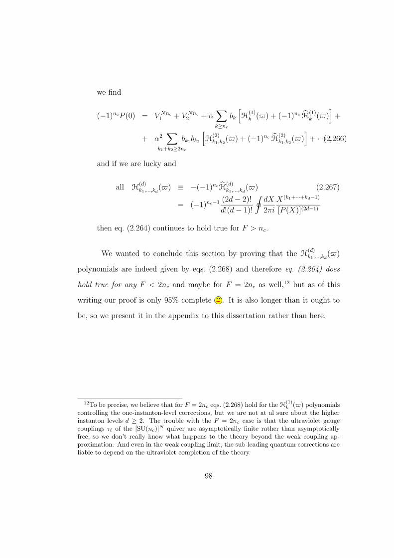
we find

(−1)ncP (0) = V Nnc

1 + V Nnc

2 + α∑

k≥nc

bk

[H

(1)k ($) + (−1)nc H

(1)k ($)

]+

+ α2∑

k1+k2≥3nc

bk1bk2

[H

(2)k1,k2

($) + (−1)nc H(2)k1,k2

($)]

+ · · · ,(2.266)

and if we are lucky and

all H(d)k1,...,kd

($) ≡ −(−1)ncH(d)k1,...,kd

($) (2.267)

= (−1)nc−1 (2d − 2)!

d!(d − 1)!

∮dX

2πi

X(k1+···+kd−1)

[P (X)](2d−1)

then eq. (2.264) continues to hold true for F > nc.

We wanted to conclude this section by proving that the H(d)k1,...,kd

($)

polynomials are indeed given by eqs. (2.268) and therefore eq. (2.264) does

hold true for any F < 2nc and maybe for F = 2nc as well,12 but as of this

writing our proof is only 95% complete . It is also longer than it ought to

be, so we present it in the appendix to this dissertation rather than here.

12To be precise, we believe that for F = 2nc eqs. (2.268) hold for the H(1)k ($) polynomials

controlling the one-instanton-level corrections, but we are not at al sure about the higherinstanton levels d ≥ 2. The trouble with the F = 2nc case is that the ultraviolet gaugecouplings τ` of the [SU(nc)]

N quiver are asymptotically finite rather than asymptoticallyfree, so we don’t really know what happens to the theory beyond the weak coupling ap-proximation. And even in the weak coupling limit, the sub-leading quantum corrections areliable to depend on the ultraviolet completion of the theory.

98

Chapter 3

The Random Matrix Model

3.1 Unitary matrices: why and how

In this dissertation we will focus on building matrix correspondents of

chiral models formed out of fields transforming in the bi-fundamental represen-

tation of a SU(nc)× SU(nc) gauge group. Since the gauge theory is anomaly

free there will be other chiral fields that we are temporarily leaving out of the

picture for sake of simplicity. In particular we want to buld the random matrix

model of the deconstructive quiver described in the previous chapter.

Similar correspondences have been established for fields in non-chiral

gauge theories. In [1, 4] have been conjectured and demonstrated that fields

transforming under the adjoint representation of the gauge group corresponds

to hermitian random matrix models. More precisely it has been shown [16]

that such models are realized as holomorphic random matrix models obtained

as a multidimensional contour integral in the space of complex matrices. In

the latest approach the hermitian matrix model is just a special case where the

contours are chosen to be lying on the real axis. Similarly it has been shown

[2, 24] that matter fields are in correspondence with complex matrices subject

to hermiticity constraints relating fields transforming in the fundamental rep-

resentation with the ones in the anti-fundamental. In building these models

99

two assumptions have been used: the symmetries and the degrees of freedom

of the matrix model have to be the same as the one for the fields in the gauge

theory. As an illustrative example let us take a U(nc) Yang-Mills model with

a field Φ in the adjoint and nf fields Qf , Qf respectively in the fundamental

and anti-fundamental representation of U(nc). Φ has n2c real degrees of free-

dom and real eigenvalues so the natural choice falls on an hermitian matrix

M transforming in the U(N) representation (N plays the role of color in the

matrix model). Similarly Qf and Qf have nc × nf complex degrees of free-

dom and correspond to a N × F complex matrix B and a F × N complex

matrix A. Since the two fields are in conjugate representations not all their

degrees of freedom are independent; this is easily expressed in the matrix lan-

guage imposing the constraint A = B†. As we can see these constraints are

purely linear in character and their imposition is what defines a sub-manifold

Γ ⊂ MatN(C) of the space of complex matrices. Clearly working out which

is the integration manifold is not the whole story. Until now we have only

illustrated the guiding principles to define the random matrix model corre-

sponding the a specific non-chiral gauge theory. This is not as saying this is

the correct one. There is one fundamental requirement to be satisfied by the

model besides the symmetry and degrees of freedom assumptions: the loop

equations of the matrix model and the anomaly equations of the gauge theory

have to match.

We can now start building a unitary one matrix model as a functional

integral on a subspace of the space of complex matrices. We use a construction

analogous to the one outlined in [16] and rely on the two assumptions just

100

illustrated. A bi-fundamental field Ω can be seen as one set of fields Qc, Qc

having half the degrees of freedom or equivalently having n2c real degrees of

freedom. This sounds similar to the hermitian case apart from the fact that

Ω doesn’t necessary has to have real eigenvalues (Ω 6= Ω†). The symmetry

requirements will define a manifold M ⊂ MatN(C) that is invariant under the

action of the symmetry group SU(N)L ⊗ SU(N)R and whose matrices have

non-zero distinct eigenvalues. In other words if U ∈ M then also LUR† ∈ M

with L ∈ SU(N)L and R ∈ SU(N)R. The manifold so defined is still too big

since dimCM = N2. According to the counting of degrees of freedom we want

a manifold Γ ⊂ M such that dimRΓ = dimCM = N2. Γ can be constructed

as follows: let γ : S1 → C be the map of the unit circle in the complex plane.

We can define

Γ = U ∈ M |σi ∈ γ (3.1)

This construction of Γ is equivalent to say that U is a unitary matrix and has

the advantage of making the symmetries of the model manifest. On the other

side the way Γ is “carved out” of M is far from unique, but this shouldn’t

trouble us since at the end of the day only an integration on eigenvalues will

be performed.

Once the integration manifold has been setup we can proceed to verify

if our model possess loop equations that match the anomaly equations of the

corresponding gauge theory. This operation will be less obvious than expected,

for unitary matrices, due to how the equations are derived from the matrix

action functional. The solution will be the definition of an holomorphic mea-

101

sure for the functional integral, or in other words an holomorphic deformation

of the maps γ used in the definition of Γ.

Let’s start with a generic unitary matrix model having an action func-

tional of the form

Z = e−N2

S2 F =1

V ol[SU(N)]

∫dN2

Ω e−N

SW(U) (3.2)

with

dN2

Ω =N∏

i,j=1

U−1ik dUkj = εa1···aN2 ωa1

· · ·ωaN2

ωai= Tr

[iU−1dUλai

](3.3)

the holomorphic Haar measure for the unitary (λaiis a chosen basis of matrices

spanning the SU(N)R symmetry group) matrix. W is exactly the superpo-

tential of the chiral gauge Lagrangian where the chiral fields are replaced by

their matrix correspondents. For normalization purposes we divide by the vol-

ume of the symmetry group. We also divide the coefficient of the exponent

of the integrand by S, a variable ultimately describing gaugino condensates.

In doing so we will satisfy a “quantization” condition for the density of the

eigenvalues of U to be defined later on. The action is clearly invariant under

SU(N)L ⊗ SU(N)R while the measure as a slightly larger invariance group:

SL(N , C)L ⊗ SU(N)R. Symmetry considerations become important when we

want to derive the loop equations of the model. As the Konishi anomaly equa-

tions are the consequence of generic holomorphic variations of the chiral field,

loop equations are derived by varying the correspondent unitary matrix within

102

the domain of integration Γ. In particular we want to impose infinitesimal uni-

tary left variations that are holomorphic

U −→ U ′ = LU = U + f(U). (3.4)

with f(U) an infinitesimal function of U . In general this may not be possible

since U ′ ∈ Γ while U + f(U) is not necessarily unitary. The solution to this

apparent problem is to deform the integration manifold Γ → Γ′ ⊂ M in a

way analog to the deformation of the unit circle in the simple case of a single

complex variable of integration. This is possible since the Haar measure is

actually SL(N , C) invariant and so it doesn’t require any modification.

Any generic function f(U) will make the job and since any function

can be locally expressed in power series we set f(U) = δU = εU k, with ε

an infinitesimal coefficient. The loop equation are retrieved imposing such

variation to the action and the measure and requiring that δZ = 0 when

integrated over Γ′. To simplify our notation let’s express U parametrically as

U =N∏

j=1

e−ixjλaj (3.5)

This choice implies that ωai= dxi so that formally the Jacobian coming from

the deformation of the holomorphic measure can be written as

J(ωai) = det

(d(xi + δxi)

dxj

)(3.6)

The formal structure of the loop equation then take the form

〈Trd δxi

dxj

〉 − N

S〈Tr(δU

dW

dU)〉 = 0. (3.7)

103

We have just written the linear part in ε of δZ = 0 where the second term

stems from the variation of the action W. The equation can be rendered more

explicit writing

d δxi =k∑

n=1

N∑

j=1

Tr[Unλ†

aiUk−nλaj

]d xj (3.8)

and chosing the specific basis for λai

λa ≡ (λαβ)ij ≡ δαiδβj (3.9)

The loop equation then becomes

〈k∑

n=1

Tr Un Tr Uk−n〉 − N

S〈Tr(δU

dW

dU)〉 = 0. (3.10)

To make this equation independent from the exponent k of the variation δU ,

we can write it as an equation for the resolvent

R(z) =S

N

∞∑

k=0

Tr(Uk)

zk+1. (3.11)

We will eventually obtain an equation for the unitary matrix that can be

compared, after having taken the large N limit, to the correspondent Konishi

anomaly equation. Its detailed form depends on the specifics of the action W

and can be generically expressed as

z 〈R(z)〉2 +S

N〈R(z)〉 − S

N〈Tr

[∞∑

k=0

Uk

zk+1

dW

dU

]〉 = 0. (3.12)

Clearly this is not the only possible loop equation for the unitary matrix U .

There are other possible variations depending on both the chiral fields left

over fro the chiral gauge model. Typically such variations will be functions of

104

complex matrices like A and B. The procedure, though, is exactly the same

and we will see it in detail only for the specific model we are going to analyze

in the next section.

3.2 Loop equations for the Chiral Gauged Quiver

As we already mentioned we are considering a matrix model with the

same formal symmetries of its correspondent gauge model. Essentially we are

considering the closed quiver of chapter 2 whose building blocks are a chain of

SU(nc) gauge symmetries. This is a 4D N = 1 theory with nf flavors Qf , Qf

for each block and a chiral bi-fundamental field Ω linking every block with the

next (Figure 1.1). The total gauge symmetry is then G4D =∏K

`=1 SU(nc)`1

, where the index ` refers to different blocks of the chain. The superpotential

of the quiver has three distinct parts W = WHop + WΣ + WDef . The first

part WHop = γ∑K

`=1 (Q`+1Ω`Q` − µQ`Q`) facilitates the propagation of the

(anti)quark fields in the x4 direction, the second WΣ = β∑K

`=1 s`(det Ω`−vnc)

is a Lagrange multiplier that implements the gauge symmetry at each site

and the third is a term WDef =∑d

p=1νp

ptr(ΩKΩK−1 · · ·Ω2Ω1)

p whose effect is

to deform the N = 2 SQCD4. This model has both deconstructive and non-

deconstructive phases [12, 14] and an interesting chiral ring structure studied

in detail in chapter 2. The subject of this and subsequent sections will be the

study of the random matrix model associated with it.

First we need to define the random matrix variables accordingly to

1In order to not confuse N , number of nodes, with N , rank of the matrices U`, we aregoing to use here K instead of N

105

the rules derived in the previous section. Accordingly to each hypermultiplet

corresponds a set of matrices A`, B`, and to each link a unitary matrix U`.

They transforms as

U` → S`+1US−1`

A` → AS−1`+1 S` ∈ SU`(N) (3.13)

B` → S`B

where in matrix language N is the number of colours and F is number of

flavours. The functional Z has K copies of (3.2) and the integration measure

is opportunely modified to include all the matrix variables

Z = e−N2

S2 F =1

V ol[SU(N)K ]

∫ K∏

`=1

dN2

Ω` dF NA` dNF B` e−N

SW(U,A,B). (3.14)

The expression for the matrix action has the same functional form of the

chiral superpotential of the quiver where field variables have been substituted

by their matrix correspondents. We omit the redundant term WΣ and think

of the matrices U` to be rescaled by the quantity vN . The functional action is

then

W(U,A,B, s) = WHop + WDef (3.15)

WHop =K∑

`=1

γ TrF (A`+1U`B` − µA`B`)

WDef =d∑

p=1

νp

pTrN(UK · · ·U1)

p.

Again WDef was introduced in the chiral gauge theory according to Dijkgraaf-

Vafa recipe in order to break N = 2 to N = 1 supersymmetry. We will see

106

how this term plays a major role in the expression for the loop equations;

the elliptic curve generated by one of them will have a topological structure

determined by the coefficents νp.

In this section we want to derive all the independent loop equations

generated by Z and compare them to the Konishi anomaly equations of sec-

tion 2.2.2. For the same reasons explained in the previous section we want to

have a holomorphic measure for the unitary matrices U` in order to allow for

non-unitary deformation the domain of integration Γ. Generic variations for

U` can be expressed in power series, the difference from the simpler example

of one matrix being that we have an ordered product of K unitary matrices.

The obvious generalization leads to two different possible deformations, the

second one including flavor matrices

δU` = ε(U` · · ·U`+1)kU` (3.16)

δU` = B`+1 εA`(U`−1 · · ·U`)k. (3.17)

The measure is readily modified using (3.3) for each dΩ`. Using (3.16) it is

easy to show that (3.10) becomes

〈k∑

n=1

Tr Cn Tr Ck−n〉 − N

S〈Tr(δU`

dW

dU`

)〉 = 0 (3.18)

with C = U`−1 · · ·U`. We can eliminate both the k and the ` dependence

rewriting the equation in terms the resolvent R(z) = S

N

∑∞

k=0Tr(Ck)zk+1 defined

out of the matrix valued variable C and using the explicit expression for W.

107

After some manipulation we have

z 〈R2(z)〉− S

N〈R(z)〉−γ

S

N

⟨∞∑

k=0

Tr(CkU`B`A`+1)

zk+1

⟩−z V ′(z)〈R(z)〉+〈P (z)〉 = 0.

(3.19)

where we have used the definitions

V (z) =d∑

p=1

νp

pzp ; P (z) =

S

N

d∑

p=1

νp

p−1∑

k=0

Tr(Ck)zp−k−1. (3.20)

We can keep only dominant terms in the large N limit so that in its final form

the loop equation for the resolvent of the ordered product C is

z 〈R(z)〉2 − z V ′(z)〈R(z)〉 + 〈P (z)〉 = 0. (3.21)

This is the first of series of equations. It can be solved in terms of the resolvent

R(z) to find that its domain of definition is a Riemannian surface with branch

cuts determined by the coefficients of the polynomial P (z).

The second variation (3.17) of U` generates an equation that impose

a constraint on the resolvent. The equation is obtained in exactly the same

fashion imposing the total variation of the functional action, Z, to be zero

〈k−1∑

n=0

Tr [εA`CnU`−1 · · ·U`+1B`+1]

(Tr Ck−n−1 − Tr I

)〉 − N

S〈Tr(δU`

dW

dU`

)〉 = 0.

(3.22)

In terms of the resolvents R(z) and M(z) this equation becomes

〈R(z)M`+K,`+1(z)〉+〈Q(z)〉z

=

(S + z V ′(z)

z

)〈M`+K,`+1(z)〉+γ 〈M`,`(z)M`+1〉

(3.23)

108

where we have defined the following quantities

M`,`′(z) =

[A`U`−1 · · ·U`′B`′

z − C

]

Ml = A`B` (3.24)

Q(z) =d∑

p=1

νp

p∑

k=1

A`Ck−1U`−1 · · ·U`+1B`+1 zp−k − γ(M`M`+1).

At first glance we can notice that the potential V (z) has been shifted by an

amount equal to the total fraction of the unitary eigenvalues S (the gaugino

condensate, in the field theory language). We believe that this is nothing than

an artifact coming from the deformation of the measure and can be reabsorbed

in the value that constraints the determinant of the unitary matrices. Here,

as for P (z) in equation (3.21), the polynomial Q(z) is at most of zp−1 order.

Notice also that we have written the equation in matrix valued form (F × F ),

so that it is independent of the variation parameter ε.

There are two remaining loop equations generated by variations of the

complex matrices A` and B` corresponding to the matter sector in field theory

language. Variations for these can be built in analogy with what just done for

U` giving the following expressions

δA` = εA`′ U`′−1 · · ·U`(U`−1 · · ·U`)k (3.25)

δB` = (U`−1 · · ·U`)kU`−1 · · ·U`′ B`′ ε (3.26)

where ε is just an infinitesimal F × F matrix. We can now impose each of this

variations independently on the functional integral and require that δZ = 0.

The formal expressions are very similar to (3.7)

〈Trd δA`

dA`

〉 − N

S〈Tr(δA`

dW

dA`

)〉 = 0, (3.27)

109

〈Trd δB`

dB`

〉 − N

S〈Tr(δB`

dW

dB`

)〉 = 0. (3.28)

Again the first term in the two expressions originates from the linear part of

the Jacobian while the second comes from the variation of the action. We can

treat these two equations on parallel grounds. Plugging in the variations (3.25,

3.26)

Tr(ε) Tr(Ck)δ`,`′ = γ[Tr(εA`′C

′kU`′−1 · · ·U`−1B`−1)

− µ Tr(εA`′U`′−1 · · ·U`CkB`)

](3.29)

Tr(ε) Tr(Ck)δ`′,` = γ[Tr(εA`+1U` · · ·U`′C

′kB`′)

− µ Tr(εA`CkU`−1 · · ·U`′B`′)

]. (3.30)

Note that C ′ is defined as C with the index ` substituted by `′. Written in

terms of the unitary resolvent R(z) and the meson resolvent M`,`′ , defined

in (3.24), we arrive at their final form

IF×F δ`,`′γ−1〈R(z)〉 = 〈M`′,`−1(z)〉 − µ〈M`′,`(z)〉 (3.31)

IF×F δ`′,`γ−1〈R(z)〉 = 〈M`+1,`′(z)〉 − µ〈M`,`′(z)〉 (3.32)

We have again written an F × F equation factorizing out the ε dependence.

At first glance these seem to be two distinct equations. Upon a more careful

look we see how the LHS of both is symmetric respect to the exchange of `

with `′. On the opposite the RHS seem to not respect such property. In fact

the two equations looks like they may be exchanged under this symmetry but

not quite. Indeed (3.31, 3.32) are two series of equations as ` varies for fixed `′.

We can summarize them in a more compact way if we write the first equation

110

as a system of equations with ` assuming values in the range `′ −K ≤ ` < `′ .

Analogously the second equation can be written as a system of equations with

values of ` now ranging in the interval `′ < ` ≤ `′ + K. In doing so we arrive

exactly at the same equation

〈M`′,`(z)〉 = γ−1µ`′−`−1〈R(z)〉 + µ`′−`〈M`′,`′(z)〉 (3.33)

valid for any value of ` 6= `′. This is the reason why we kept the delta symbol

on the RHS of (3.31, 3.32). This result shouldn’t be surprising since the

degrees of freedom encoded in A` and B` are not independent (A†` ≡ B`).

Consequently their variations are correlated and lead to the same equation.

We can elaborate a little more making use of the recurrence formula (coming

directly from definition (3.24))

〈M`′+N,`′(z)〉 = z〈M`′,`′(z)〉 − M`′ (3.34)

to determine

〈M`′=`(z)〉 =(γ−1µK−1〈R(z)〉 + M`′

) 1

z − µK(3.35)

〈M`′ 6=`(z)〉 =(z γ−1〈R(z)〉 + µM`′

) µ`′−`−1

z − µK(3.36)

These formulae exhaust the possible loop equations of our model.

Comparing them with the anomaly equations derived in section 2.2.2

we see that there is perfect agreement. This fact together with the arguments

expressed in section two makes the unitary random matrix model the dual of

our quiver chiral gauge model.

111

3.3 Solving for the Free Energy

In the last section we have proved that the quiver (1.1) corresponds to

the random matrix model (3.14). We have shown that the matrix model not

only possesses the same symmetry and degrees of freedom of the gauge theory

but also satisfy the same equations for various resolvents. In this section we

want to analyze this random matrix model further with the final objective of

obtaining an expression for the low energy effective potential, typically given

in terms of massless gaugino condensates. We are going to proceed in simple

steps. We will first integrate out massive matter degrees of freedom; the

resulting action will depend only on ordered products of K matrices U`. The

integration over the U` matrices will factorize into K − 1 trivial group volume

evaluation and and one integral with non-trivial integrand. The application of

standard saddle point method in the large N limit will lead to sphere and disk

contribution for the free energy F. A formal multi-cut solution will be derived

from which an expression for the effective superpotential is calculated.

We want to integrate massive modes A` and B` out of the (3.14) action

functional

Z = e−N2

S2 F =1

(V ol[SU(N)]

)K

ηNFK

∫ K∏

`=1

dN2

Ω` dF NA` dNF B` e−N

SW(U,A,B).

(3.37)

Notice that we are able to write the volume of the gauge group as a product

of volumes since the quiver symmetry groups are mutually independent. In

the large N limit the leading term of V ol[SU(N)] is equal to V ol[U(N)] and

112

can be written as [25]

V ol[SU(N)] =N2

2

(ln

2π

N+

3

2

)(3.38)

We have also introduced the normalization constant η defined as

∫d xd x e−

N

SγΛxx =

(2πS

NΛγ

).= η, (3.39)

where Λ is interpreted as the lightest mass scale of the 5D deconstructed quarks

and will serve as a cut-off parameter when expressing the free energy through

contour integrals. The only part of Z that is involved by the integrating out

process is

1

ηNFK

∫ K∏

`=1

dF NA` dNF B` e−N

SWHop = [Det D]−1

(2πS

Nγη

)NFK

(3.40)

where

D =

µ 0 0 · · · 0 UK

U1 µ 0 · · · 0 00 U2 µ · · · 0 0... · · · . . . . . .

......

0 · · · · · · · · · UK−1 µ

. (3.41)

The determinant is implicitly intended to be performed on all indices: quiver,

color and flavor. Here we are giving its explicit form only for quiver indices

deliberately leaving the rest in general form to be exploited later on

[Det D]−1

(2πS

Nγη

)NFK

=

[det

NF×NF

(K∏

`=1

U` − µK

)]−1

ΛNFK . (3.42)

This last expression depends on U` matrices only through their ordered product∏K

`=1 U`. The part of the action W of the matrix functional left untouched

by the integration (namely WDef ) depends on the ordered product of K U`

113

matrices as well. Consequently the entire matrix functional Z depends only

on∏K

`=1 U` and it naively seems that we can further integrate out K−1 of the

U` factors. This can be made precise making use of the large symmetry group

of the model to build a series of cascading changes of variables. Consider the

following chain of⊗

` SU`(N)R transformations

(1)

U

(1)K = UKVK

U(1)` = U` ` 6= K

VK = UK−1

......

(i)

U

(i)K = U

(i−1)K V

(i−1)K

U(i)` = U` ` 6= K

V(i−1)K = UK−i

......

(K − 1)

U

(K−1)K = U

(K−2)K V

(K−2)K

U(K−1)` = U` ` 6= K

V(K−2)K = U1

.

As a consequence of the chain of transformation we arrive at the result

K∏

`=1

U` = U(1)K UK−2 · · ·U1 = · · · = U

(i)K UK−i−1 · · ·U1

= · · · = U(K−2)K U1 = U

(K−1)K ≡ U. (3.43)

Then it is clear that their net effect is to have the action W depending only on

the variable U and completely independent of the other K−1 unitary matrices

U`, ` 6= K. In the same fashion the measure remains invariant under the listed

transformations. Take for example the (i + 1) transformation. The measure

transforms linearly

(i + 1)

d Ω(i+1)K =

[V

(i)K

]−1 (d Ω

(i+1)K − d ΩK−i−1

)V

(i)K

d Ω(i+1)` = d Ω` ` 6= K

114

so that the Jacobian matrix is lower triangular and its determinant is trivially

one. We can then integrate over all the non dynamical U` and eliminate

K − 1 powers of the volume of the gauge group that normalizes the functional

integral. What remains of Z expressed in the limit of large N (since that is

what matters when the saddle point method is used to find the free energy) is

Z = e−N2

S2 F =

∫U

−1dU e−N

SW(U)

W(U) = WDef (U) +S

Nln[det(U − µK

)]

+ S

[N

2

(ln

2π

N+

3

2

)− KF ln Λ

](3.44)

We are now reduced to the integration of a single unitary matrix vari-

able U. It is customary [26, 27] to use the residual SU(N) symmetry to express

the generic Haar measure in terms of more convenient variables. The new set

is given by the eigenvalues λk2 of U and its normalized off-diagonal compo-

nents θij. The cost of such transformation is the introduction of a Jacobian

solely dependent on λ’s and usually addressed as Vandermonde determinant

U−1dU −→ 4

N∏

k=1

d λk

∏

i<j

sin2

(λi − λj

2

)∏

i,j

d θij. (3.45)

The action W depends on U only through its eigenvalues so that we can in-

tegrate out the angular variables θij and get just a constant factor up front

that doesn’t contain any dynamical information. This factor can be readily

ignored since it doesn’t enter in any way in our analysis. Since the exponent of

2Actually the eigenvalues of U are eiλk but due to the form of the Haar measure its ex-pression in terms of the new variables depends directly on λ’s. Consequently the eigenvaluesassume values in the interval [0, 2π]

115

the integrand is proportional to N we can use the saddle point approximation

[26]. The eigenvalues are then constrained by the saddle point equation

∂W

∂λk

= 0, (3.46)

and in the large N limit the integral (3.44) is given by the dominant contribu-

tion in the N2 expansion. This is equivalent to the standard genus g expansion

N2−2g that we are familiar with from 2D gravity [28]: the first contribution

comes from the sphere meanwhile the sub-dominant term is given by the disk.

At the same time the eigenvalues assume continuum spectrum and can be ex-

pressed more elegantly introducing a density of eigenvalues ρ (λ). We end up

with an exact expression for the free energy F

e−N2

S2 F = exp

−N2

S2

[d∑

p=1

∫d λ ρ(λ)

νp

peiλp −

∫d λ ρ(λ) d λ′ ρ(λ′) ln sin2

(λ − λ′

2

)

+S2

2

(ln

2π

N+

3

2

)]− N

S

∫d λ ρ(λ) ln

[det(eiλ − µK)

ΛFK

]. (3.47)

Following the prescription of [20] we identify the two contributions to F. The

sphere, coming from WDef and the Vandermonde determinant, is defined as

FS = limN→∞ F

FS =

∫d λ ρ(λ) V (λ) −

∫d λ ρ(λ) d λ′ ρ(λ′) ln

[sin2

(λ − λ′

2

)]. (3.48)

On the other end the disk contribution arises from the matter sector and is

defined as FD = limN→∞N

S(F − FS)

FD =

∫d λ ρ(λ) ln

[det(eiλ − µK)

ΛFK

]. (3.49)

116

Notice that we have discarded from (3.47) any constant factor that doesn’t

depend on the eigenvalues density and ultimately won’t contribute to the ef-

fective potential.

The expressions (3.48)and (3.49) are still uncomplete solutions for the

free energy. In fact we have buried the crucial information in the density of

eigenvalues of which we have given just a very informal definition. Solving

for ρ(λ) means to solve for the saddle point equation (3.46) rewritten for a

continuum spectrum of eigenvalues limN→∞∂∂λ

∂F

∂ρ(λ)= 0. The limit procedure

is introduced so that we consider only dominant contributions, consistently

with the expression given for the free energy. The saddle point equation takes,

then, the simple form

V ′(λ) − 2

∫d λ′ ρ(λ′) cot

(λ − λ′

2

)= 0. (3.50)

This is just the loop equation (3.21) in disguised form. Multiplying both sides

by ρ(λ) cot(

w−λ2

)and integrating over λ we recover, after some algebra, the

loop equation for the resolvent R on the cylinder 3

R2(w) − R(w)V ′(w) + F (w) + S2 = 0 (3.51)

with

R(w) =

∫ 2π

0

d λ ρ(λ) cot

(w − λ

2

)(3.52)

F (w) =

∫ 2π

0

d λ ρ(λ) (V ′(w) − V ′(λ)) cot

(w − λ

2

). (3.53)

3The resolvent defined on the cylinder is related to the one on the complex plane through

the relation R(w) = NS

z R(z) − iS

117

The differences between (3.21) and (3.51) are a natural consequence stemming

from the dependence of all the expressions on the real variable λ and not eiλ.

We are then naturally lead to use a complex variable w that is related to the

complex plane through the cylinder map z = eiw. So the differences between

R(z) and R(w) are just an artifact of such map. Moreover the eigenvalue’s

density has to be periodic of 2π to ensure single valuedness of the resolvent.

For analogour reasons the function F (w) is not the same as P (z) but can be

rewritten in such a way that in the large N limit the two loop equations are

the same. In some sense the unitary matrix case can be seen as a special

case of hermitian model with compact, periodic support for its eigenvalues [2].

We have just reduced our model to solving a specific case of unitary circular

ensemble. Equation (3.51) directly determines the form of ρ(λ)

S =n∑

i=1

Si =n∑

i=1

∫ a+i

a−

i

d λρ(λ) (3.54)

where [a−i , a+

i ] are cuts on the fundamental interval [0, 2π] where eigenvalues

are condensed. These play exactly the same role of branch cuts on the real axis

in the hermitian matrix case. In order to see why is this so, let’s solve (3.51)

for R

R(w) =V ′(w) ± Y (w)

2; Y 2(w) = V ′2(w) − 4(F (w) + S2). (3.55)

This equations shows a two sheeted Riemann surface with branch cuts defined

by Y ; crossing a cut brings from one sheet to the other. It is now standard

procedure to show, with a simple contour integration argument, that

−2πiρ(λ) = R(λ + iζ) − R(λ − iζ). (3.56)

118

a−1

a+1

a−2

a+2

a−3

a+3

a−4

a+4

z = 0

A1

A2

A3

A4

Figure 3.1: Branch cuts on the unit circle

Thus the density of eigenvalues has support exactly on the branch cuts defined

by Y (3.1). Moreover a generic function f(λ), integrated along the cuts, is

equal to contour integrals Ai around the cuts

∫ 2π

0

d λ ρ(λ) f(λ) = − 1

2πi

n∑

i=1

∮

Ai

R(w) f(w)dw. (3.57)

A general formula expressing the effective superpotential Weff can be

recovered from the free energy adapting the procedure outlined by Cachazo

et Al. [5, 6] to the cylinder. According to their generic formula the effective

potential for S is (up to terms that involve two derivatives of the free energy)

Weff =n∑

i=1

Ni∂FS

∂Si

+ 2πi

n−1∑

i=1

biSi + FD. (3.58)

119

Here the bi are integers numbers arising from ambiguities in defining the

Veneziano-Yankielowicz superpotential and indicating a rotation from con-

finement to oblique confinement (equivalent to a shift in the theta angle for

the gluino condensate Si). The general expression for the sphere and disk con-

tributions can be recovered using the equations (3.57) and modifying carefully

the integration contours Ai. Performing contour integration on the cylinder

is essentially the same as doing it on the complex plane with one exception:

there may be potential problem arising from the undefined point z = 0 gen-

erated by the exponential map. These are avoided if we are careful to define

the integration contour. As an illustrative example we can derive an expres-

sion for the disk contribution FD. Let us define w = σ1 − iσ2 and write the

determinant in the logarithm of (3.49) as∏L

I=1 (eiw − eiwI ). Then

FD = − 1

2πi

L∑

I=1

n∑

i=1

∮

Ai

dw R(w) ln

(eiw − eiwI

ΛKF

)(3.59)

Modifying opportunely the contours this integral will give contributions

along the branch cuts originating from the points wI and extending to very

large σ2. We have to be careful to evaluate contributions coming from the

contours connecting very large positive values with very large negative val-

ues of σ2 running on both sides of the branch cut starting from σ2 = −∞.

Fortunately due to the single value definition of R the eigenvalue density is

periodic of 2π so that contribution from both contours cancel each other. The

remaining contours are simple integration along σ1 at very large |σ2| along

120

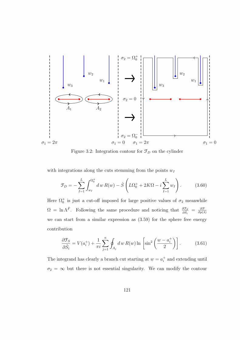
σ1 = 2π σ1 = 0

w3

w2

w1

σ1 = 2π σ1 = 0

w3

w2

w1

A1 A2

σ2 = 0

σ2 = Ω+0

σ2 = Ω−0

Figure 3.2: Integration contour for FD on the cylinder

with integrations along the cuts stemming from the points wI

FD = −L∑

I=1

∫ Ω+0

wI

dw R(w) − S

(LΩ+

0 + 2KΩ − iL∑

I=1

wI

). (3.60)

Here Ω+0 is just a cut-off imposed for large positive values of σ2 meanwhile

Ω = ln ΛF . Following the same procedure and noticing that ∂FS

∂Si= ∂F

∂ρ(λ)

we can start from a similar expression as (3.59) for the sphere free energy

contribution

∂FS

∂Si

= V (a+i ) +

1

πi

n∑

j=1

∮

Aj

dw R(w) ln

[sin2

(w − a+

i

2

)]. (3.61)

The integrand has clearly a branch cut starting at w = a+i and extending until

σ2 = ∞ but there is not essential singularity. We can modify the contour

121

again and arrive at an expression similar to (3.60) for the sphere contribution

∂FS

∂Si

= V (a+i ) + 2

∫ Ω+0

a+i

dw R(w) + 2S(Ω+

0 + Ω−0

). (3.62)

Ω−0 is a similar cut-off imposed on very large negative values of σ2. Taking

Ω−0 = −Ω+

0 the last term vanishes as we would expect since it is an artifact

of the singularity of the point z = 0. We can then plug in a solution for

R taking care of choosing the physical sheet where limσ2→∞ R = 1 Thus we

select the minus sign in (3.55) and substitute it in the expressions for ∂FS

∂Siand

FD. Assembling everything in the effective potential we arrive at the final

expression

Weff = −n∑

i=1

Ni

∫ Ω+0

a+i

dw Y (w) +1

2

L∑

I=1

∫ Ω+0

wI

dw Y (w) +1

2(2N − L)V (Ω+

0 )

+L∑

I=1

V (wI) +

(i

L∑

I=1

wI + 2KΩ − LΩ+0

)S + 2πi

n−1∑

i=1

biSi. (3.63)

The potential divergences limited by the cut-off Ω+0 are balanced by the nor-

malization constant Ω and define the bare coupling constant 2πiτ . Since Y (w)

vanishes at w = a+i we can write

∫ Ω+0

a+i

= 12

∫Bi

where Bi is a contour that goes

from Ω+0 , cross the ith cut and goes back to Ω+

0 on the second sheet.

Weff = −1

2

n∑

i=1

Ni

∫

Bi

dw Y (w) +1

2

L∑

I=1

∫ Ω+0

wI

dw Y (w) +1

2(2N − L)V (Ω+

0 )

+L∑

I=1

V (wI) +

(i

L∑

I=1

wI + 2πiτ

)S + 2πi

n−1∑

i=1

biSi. (3.64)

Notice that this is very similar to the result obtained in [6]. The only difference

being that the the bare coupling constant τ is shifted by an amount equal to

122

the eigenvalues of the matrix D (3.41). This is exactly what we would expect

since the introduction of extra 4D hypermultiplets change the Chern-Simons

level of the 5D coupling constant [12].

σ1 = 2π σ1 = 0

w3

w2

w1

σ1 = 2π σ1 = 0

w3

w2

w1

A1 A2A3

σ2 = 0

Ω+0 Ω+

0Ω+0 Ω+

0 Ω+0 Ω+

0

B1 B2 B3

Figure 3.3: Bi and Ai contours on the cylinder

3.4 Examples of Effective Superpotentials

At the end of last section we have given an explicit formula (3.64) ex-

pressing the effective superpotential. The only necessary ingredient needed is

the form of the tree superpotential of the gauge theory underlying the random

matrix model. Here we want to give some examples of such expression starting

from one of the simplest case possible. Due to the relative simplicity of the

cases considered we don’t use the (3.64) but a far direct even if less general

123

procedure [29]. The result of section 4 standing, we prefer to solve directly

for the free energy using an exact expression for the density ρ(λ). Such an

expression is derived from knowledge of the tree superpotential W and the

asymptotic behavior of the resolvent R(z) as well as from the number s of

branch cuts of Y . In general we can express this last quantity as

Y (z) =Q(z)

z

√σ(z) (3.65)

where Q(z) is an unknown polynomial. Generically Q(z) is determined by

inspection knowing that the resolvent R(z) ≈ Sz

for large z.

Q(z) = PolV ′(z)

z√

σ(z)(3.66)

Such condition determines also part of the unknowns of σ(z), namely the

endpoints of the branch cuts. If V (z) is of degree d then Q(z) is of degree

d − s (s ≤ d) and equation (3.66) gives d − s + s + 1 = d + 1 equations.

There remain s + 1 constants that are determined requiring the free energy is

minimal. In other words the system of cuts has to be stable and no eigenvalues

is permitted to migrate from one cut to the other. This is directly written in

integral form as ∫ a−

i+1

a+i

Q(z)

z

√σ(z) = 0 (3.67)

where the integral is performed between the endpoints of distinct branch cuts.

There are s − 1 independent integrals of this kind, giving the remaining con-

ditions required. Obviously this methods becomes a little cumbersome in the

case of several disjoint cuts, but it is easily applied to our simple examples.

124

Once Q(z) and all the endpoints are determined in terms of the coupling con-

stants of V (z) and the filling fractions (gluino condensates) Si we can express

the density of eigenvalues

ρ(x) =1

2πiY (x), (3.68)

plug it in the expression for the free energy and perform the integrations along

the branch cuts. In order to simplify such task we are going to rewrite the

expression for the sphere free energy FS so to avoid an overly complicated

double integration. Let’s take equation (3.50), integrate it between the two

intervals [θ−i , λ] and [λ, θ+i ] (with [θ+

i , θ−i ] a branch cut), and combine the two

results

∫ θ+i

θ−i

d λ′ ρ(λ′) ln

[sin2

(λ − λ′

2

)]=

V (λ)

2− 1

4

(V (θ−i ) + V (θ+

i ))

+1

2

∫ θ+i

θ−i

d λ′ ρ(λ′) ln

[sin2

(θ+

i − λ′

2

)sin2

(θ−i − λ′

2

)]. (3.69)

We can then take this expression and plug it in (3.48) to obtain a simplified

formula for the sphere free energy

FS =1

2

∑

i

∫ θ+i

θ−i

d λ′ ρ(λ′)

V (λ′) − Si ln

[sin2

(θ+

i − λ′

2

)sin2

(θ−i − λ′

2

)]

+Si

4

(V (θ−i ) + V (θ+

i )). (3.70)

Let’s now rewrite both FS and FD in terms of the complex integration variable

x = eiλ. This is just a technical stratagem that allows us to perform the

integral on the unit circle in a more readable fashion

FS =1

2

∑

i

∫ a+i

a−

i

d x

xρ(x)

V (x) − Si

[ln

∣∣∣∣a+

i − x

2

∣∣∣∣2

+ ln

∣∣∣∣a−

i − x

2

∣∣∣∣2]

125

+Si

4

(V (a−

i ) + V (a+i ))

(3.71)

FD =∑

i

∫ a+i

a−

i

d x

xρ(x)

[∑

flavors

ln(x − µK

)− FK ln Λ

], (3.72)

where a±i = eθ±i .

3.4.1 One cut: SU(N) unbroken

We want to consider the same example used in section 2.2.2 with d = 2

and F = 1

V (z) = α z +β

2z2 = βz(z − a) (3.73)

where a = −αβ

and |a| = 1, since we are on the unit circle. Classically since

zV ′(z) has only one zero, the gauge theory is described by an unbroken SU(nc)

gauge group. The quantum theory becomes interesting when this zero splits

to a cut on the unit circle. In this case Y (z) can be written as

Y (z) =Q(z)

z

√(z − a+)(z − a−) (3.74)

and a+ = a+2C a− = a−2C. The function Q(z) is determined as previously

described. If we write Q(z) = Az + B the fact that R(z) does not have terms

of O(z) and O(1) give A = β and B = α + β2(a+ + a−). The last constraint is

though redundant since (a++a−)2

= a implies B = 0. There is a third condition

coming from the O( 1z) term

(a+ − a−)2 =16

βS − 3

4a2. (3.75)

Through these conditions we can trade any dependence on the cut endpoints

for the other two independent variables: S and a. We will do this at the end

126

of the integration process for the free energy. We can now take the expression

for the density of eigenvalues (3.68)

ρ(x) =β

2πi

√(x − a+)(x − a−) (3.76)

and use it in (3.71),(3.72). There are essentially four integrals to be performed

I1 = − β

4π

∫ a+

a−

d x√

(x − a+)(x − a−)(α +β

2x)

I±2 = S

β

4π

∫ a+

a−

d x

x

√(x − a+)(x − a−) ln

∣∣∣∣a±

i − x

2

∣∣∣∣2

(3.77)

I3 = − β

2π

∫ a+

a−

d x

x

√(x − a+)(x − a−) ln

(x − µK

)

I4 = K ln Λβ

2π

∫ a+

a−

d x

x

√(x − a+)(x − a−)

I±2 and I3 cannot be straightforwardly calculated since the integrand contains

the function ln(c+x)x

. This is substantially different from the hermitian case

where there is no 1x

coefficient leading to a much simpler calculation. The only

way to perform the integration is to expand part of the integrand in an exact

power series. In this way these integrals can be reduced to a combination of a

series of terms originating from the logarithm asymptotic formula

ln(1 + x) =∞∑

k=1

(−1)k+1 xk

k. (3.78)

We can then define the k-index dependent integrals

Jk =

∫ a+

a−

d x√

(x − a+)(x − a−) xk−1, (3.79)

Hk =

∫ a+

a−

d x

x

√(x − a+)(x − a−)

×[cosk(i ln(x) − i ln(a+)) + cosk(i ln(x) − i ln(a−))

], (3.80)

127

and show that I1, I3 and I4 are given by a combination of Jk (for example

is fairly easy to see that I1 is given by J1 plus J2), while I±2 are given by an

infinite sum of Hk. It is convenient to introduce the following functions of S

and a

h(S, a) = (a+ − a−)2 =16

βS − 3

4a2

g(S, a) =√

a+a− =

√

−4S

β+

13

24a2 (3.81)

in order to express the integrals Jk and Hk only in terms of the specified

invariants With these conventions the first integrals of the series Jk and Hk

are

J0 = iπ(g(S, a) + a)

J1 =iπ

23h(S, a)

J2 =iπ

23h(S, a) a

J3 =iπ

27h(S, a)[24a2 + h(S, a)] (3.82)

J4 =iπ

27h(S, a)[24a3 + 3 a h(S, a)]

H1 =iπ

24g2(S, a)[−24a3 + 3 a h(S, a) + a2g(S, a)]

H2 =iπ

29g4(S, a)[17 · 25a5 − 13 · 24a3h(S, a) + 17 · 2 ah2(S, a)

+ 29a4g(S, a) + 9 · 25a2h(S, a)g(S, a) − 3 · 23h2(S, a)g(S, a)].

The first important fact is that all the integrals are polynomials of the invari-

ants a and S. This is not at all obvious and since the superpotential is directly

128

derived from the free energy through (3.58) it has to depend on S and a only

FS = − β

4π

αJ1 +

β

2J2 + S

[2 ln

1

2J0 −

∞∑

k=1

Hk

k

]

+S

4

(V (a−) + V (a+)

)(3.83)

FD = − β

2π

[(πi + K ln

µ

Λ

)J0 −

∞∑

k=1

Jk

k(µK)k

]. (3.84)

We can now use (3.58) adapted to the one cut case and derive the expression

for the effective superpotential

Weff = − β

2π

−nc

2πiS

βg(S, a)+ J0

(nc ln

1

2+ πi + K ln

µ

Λ

)−

∞∑

k=1

1

k

[1

2ncHk

+Jk

(µK)k

]− 1

2ncS

∂

∂S

(∞∑

k=1

Hk

k

)+

nc

4

(V (a−) + V (a+)

). (3.85)

Notice that we have discarded constant terms (indipendent of β) that can

always be absorbed.

129

Chapter 4

Open questions and conclusions

4.1 Chiral ring of the quiver theory

Having analyzed the chiral rings of deconstructive [SU(nc)]N quivers

in much detail, we would like to conclude this dissertation by discussing the

implications of the present research and the open questions it raises.

The most immediate implication of our rings concerns the quantum

effects in deconstructed SQCD5; this will be discussed at length in ref. [12],

but we would like to present a few highlights here. From the deconstruction

point of view, our most important results are the Seiberg-Witten curve (2.133)

and the quantum-corrected constraint (2.264) on the Coulomb moduli of the

quiver. In the large quiver size limit N → ∞ governed by the 4D ↔ 5D map

of moduli and parameters1

$i = V N × exp(Naφi) , (4.1)

µf = V × exp(amf ) , (4.2)

α =V 2ncN

∏f max(µN

f , V N)× exp

(−Na

8π2

g25D

)(4.3)

the 4D abelian gauge couplings encoded in the Seiberg-Witten curve (2.133)

1In the following (4.1)–(4.3), the φi denote the Coulomb moduli of the 5D SQCD, the mi

are the 5D quark masses, and the g25D is the 5D gauge coupling at the origin of the Coulomb

moduli space.

130

behave precisely as in a 5D gauge theory compactified on a large circle of size

2πR = Na. The 5D abelian couplings implied by this procedure — using

dimensional deconstruction as a UV completion of SQCD5 — are in perfect

agreement with those of SQCD5 embedded in string or M theory, which means

they are intrinsic properties of the 5D theory.

Furthermore, thanks to eq. (2.264), the V parameter in (4.1)–(4.3) is

the greater of V1, V2 roots of eq. (2.230). Consequently, for ∆F = 0 there is a

lower limit on the V/Λ ratio and hence according to eq. (4.3) the inverse 5D

gauge coupling also has a finite lower limit; on the other hand, for ∆F > 0

there are no limits and the g−25D ranges all the way from +∞ to −∞. In

5D terms this means that SQCD5 theories with maximal Chern-Simons levels

kcs = nc − 12nf have only the positive-coupling phase (see ref. [14] for the

nf = 0, kcs = nc case), but for lower Chern-Simons levels there are both

positive-coupling and negative-coupling phases.

We would like to extend our techniques from the deconstructed SQCD5

to other deconstructed 5D gauge theories, but this remains an open question.

Naively, the simplest extension is promoting the SU(nc) gauge theory to the

U(nc): Classically, all one has to do in 4D is to promote each [SU(nc)]` fac-

tor to a [U(nc)]`, dispense with the s` singlet fields and the WΣ part of the

superpotential (cf. eq. (2.3)), and expand the theory around a vacuum with

non-zero link VEVs 〈Ω`〉 ∝ 1nc×nc. Unfortunately, the abelian gauge fields of

131

such a [U(nc)]N quiver suffer from triangular anomalies

SU(nc)` or U(1)` Ω fields U(1)`+1 or U(1)`−1

(4.4)

and the quantum theory does not work. To cancel the anomalies we need

additional chiral superfields (cf. [30, 31] for the [U(1)]N quiver) with non-trivial

SU(nc)`, U(1)` and U(1)`±1 quantum numbers, for example

A` =(

` , (1−nc)`+1

)

B` =(

` , (1+nc)`−1

)

C` =((1−nc)` , (1

+nc)`+1

)

for all ` = 1, . . . , N . (4.5)

Then we need to endow all these fields with suitable superpotential couplings

and find a vacuum state of the theory where all the light particles correspond

to Kaluza-Klein modes of the 5D U(nc) theory compactified on a circle, and

nothing else. There will be of course all kinds of particles with O(V ) masses,

and we need to find their effects on the Chern-Simons interactions of the 5D

theory and perhaps adjust the number ∆F of massless quark flavors. At this

point we have a complicated 4D [U(nc)]N theory which is no longer described

by a simple quiver diagram (1.1), and now the real work begins: evaluating the

chiral ring of the theory and its implications for the quantum deconstruction.

A bigger open question concerns quantum deconstruction of other types

of 5D gauge theories, for example SO(n) or Sp(n). Again, one must first decon-

struct the 5D theory at the classical level and verify the quantum consistency

132

of the resulting 4D quiver theory, and then one must study the chiral ring in

all its glorious details. But the really big challenge comes from deconstructing

2 extra dimensions at once: start with a 6D SYM theory with 16 supercharges,

discretize the x4 and x5 coordinates into a 2D lattice, and interpret the result

as a 4D, N = 1 gauge theories with a complicated quiver. Classically, the

procedure is well known [32]; for example the SU(n) SYM theory in 6D de-

constructs to into the [SU(n)]N2

theory in 6D with a quiver diagram forming

a 2D triangular lattice

(4.6)

But at the quantum level, the chiral ring of this quiver poses a formidable

challenge because every closed loop on the lattice gives rise to an independent

generator of the ring, eg. Tr(Ω9Ω8 · · ·Ω2Ω1) for the loop of 9 links on the

133

following picture:

1 2

3

456

7

8 9 (4.7)

Another open question is finding a simple string model of the decon-

structed SQCD5 and investigating the string origin of the quantum effects

discussed in this paper at the 4D field theory level. Ironically, while some

complicated quiver theories do have simple string models — for example the

lattice quiver (4.6) deconstructing the 6D SYM obtains via nc ×N2 fractional

D3 branes at a C3/ZN × ZN orbifold point [32] — the simplest known string

model of the [SU(nc)]N quiver (1.1) involves brane webs on an orbifold [33].

The issue is not 5D versus 6D, and other, more complicated deconstructed 5D

gauge theories do have web-less string models. For example, 2N ×n fractional

D3 branes at the C3/Z2N [1, 1,−2] orbifold point give rise to the 4D theory

with the

(4.8)

quiver diagram which deconstructs an SU(n) × SU(n) theory in 5D. But this

134

theory has a very different chiral ring than the rings discussed in section 2.2–

section 2.3 of this dissertation, and it needs to be worked out in detail before

we can analyze its implications for the string theory.

4.2 Random matrix model

The random matrix portion of the model has shed light on the otherwise

uneasy task of calculating the effective superpotential of the gauge theory in

terms of gaugino condensates. In achieving this task we had to establish a

set of rules on how to realize the duality between bi-fundamental sets of fields

and bosonic random variables. In more precise words we had to identify which

integration manifold we had to choose for the corresponding matrices so that

the duality could be set in place. We have then, identified bi-fundamentals

with unitary matrices and confirmed the identifications of hyper-multiplets

with pairs of complex conjugate matrices.

In the process we have established similar results to the hermitian ran-

dom matrix case and have shown that the integration manifold has to be

holomorphically modified in order to accommodate for non-unitary variation

of the matrices representing bi-fundamentals of the quiver. We have shown

that the loop equations correspond to the anomaly equations of the quiver

theory and so lead to the same solutions. In the matrix model we do not have

the whole set of anomaly equations reproduced but a subset big enough to

guarantee the validity of the duality.

Having set the duality we have proceeded to calculate the effective su-

135

perpotential of the model in the large N limit using the saddle point approx-

imation. Such a calculation revealed that the matrix integral can be reduced

to a one-matrix integral only whose eigenvalues are concentrated on intervals

set on the unit circle. The overall expression of the free energy, from which the

superpotential is derived, is calculated as contour integrals on the cylinder and

support conclusions regarding the semiclassical limit of the superpotentials.

It is still unclear how to reproduce a fairly simple superpotential from

the example we have analyzed even if it should in principle possible. Our ex-

pression for the simple SU(nc) case is a little too clouded and needs some re-

fining but nonetheless is expressed in powers of the gaugino condensate and so

seems to reproduce a proper superpotential. This results conclude our analysis

of the quiver gauge theory, its chiral ring and its exact effective superpotential.

136

Appendix

An (almost) proof of the quantum corrections of the determi-

nants of link chains

In this appendix we (almost) prove that the H(d)k1,...,kd

($) polynomials

in eq. (2.246) are indeed given by eqs. (2.268) and therefore eq. (2.264) does

hold true for any F < 2nc and maybe for F = 2nc. Specifically we shall

prove that (1) the polynomials H(d)k1,...,kd

(nc; $1, . . . , $nc) have the same form

for all quivers with the same color number nc regardless of the quiver’s size

N or the flavor number F (as long as k1, . . . , kd ≤ F ≤ 2nc and N ≥ 2), and

(2) they are recursively related to the H(d)

k′1,...,k′

d(n′

c; $1, . . . , $n′c) polynomials

for smaller values of the k′1, . . . , k

′d indices and/or color numbers n′

c. These

relations are consistent with eqs. (2.268) and could be used to prove them

all by mathematical induction from a few special cases. Alas, verifying those

special cases remains a loophole; we hope to close it soon, but we have not

done it yet.

We begin by proving the N independence of the H(d)k1,...,kd

polynomials.

Consider what happens when one of the v` parameters of the promoted quiver

theory becomes very large, say v1 any other mass scale of the theory.

Physically, in the v1 → ∞ limit we have a high-energy threshold due to the

large semiclassical VEV 〈Ω1〉 = v1 × 1nc×nc(modulo gauge transforms): the

SU(nc)1 × SU(nc)2 gauge symmetry is Higgsed down to a single SU(nc)1+2

factor, the Ω1 chiral field is eaten up, and the Q1 quarks and Q2 antiquarks field

137

become massive. Integrating out these heavy fields we see that the effective

low-energy theory has the same quiver structure as the high-energy theory —

except for the N low = Nhigh − 1 — and the same coupling parameters except

for the2

Λ2nc−F1+2 = Λ2nc−F

1 Λ2nc−F2 ×det(v1Γ1)

v2nc

1

and m1+2 = m1×1

v1Γ1

×m2 . (9)

In terms of the α and bk parameters this means

αlow =αhigh

v2nc−F1

and blowk =

bhighk

vF−k1

(10)

while the Coulomb moduli of the low-energy and the high-energy theories are

related according to

$highj = v1 × $low

j . (11)

Consequently, eq. (2.246) of the low-energy theory becomes

[V Nnc

global

]low=

∑

d

(αlow)d∑

k1,...,kd

blowk1

· · · blowkd

× H(d) lowk1,...,kd

($lowj )

=∑

d

(αhigh)d∑

k1,...,kd

bhighk1

· · · bhighkd

× vP

k−2dnc

1 × H(d) lowk1,...,kd

(v−11 $high

j )

=1

vnc

1

×∑

d

(αhigh)d∑

k1,...,kd

bhighk1

· · · bhighkd

× H(d) lowk1,...,kd

($highj ) (12)

where the last equality follows from the H(d)k1,...,kd

being homogeneous polyno-

mials of respective degrees∑

k − (2d− 1)nc. By comparison, the high energy

theory has

[V Nnc

global

]high=∑

d

(αhigh)d∑

k1,...,kd

bhighk1

· · · bhighkd

× H(d)high

k1,...,kd($high

j ) (13)

2The quarks Q1+2,f ≈ Q2,f and the antiquarks Qf ′

1+2 ≈ Qf ′

1 of the low energy theory

acquire small masses [m1+2]f ′

f via the see-saw mechanism when the heavy fields Q1,f and

Qf ′

2 are integrated out.

138

regardless of the v1 parameter being large or small because the global correction

is completely independent of any of the v`. On the other hand, in the v1 → ∞

limit quantum effects associated with the Ω1 link field become small because

of asymptotic freedom (assuming F < 2nc), hence

det(ΩN · · ·Ω2Ω1) → det(ΩN · · ·Ω2) × vnc

1 (14)

and therefore the global corrections to these determinants should obey the

same scaling law[V Nnc

global

]high=[V Nnc

global

]low × vnc

1 . (15)

Consequently, substituting eqs. (12) and (13) into this formula and comparing

the moduli-dependent coefficients of similar (αhigh)dbhighk1

· · · bhighkd

we see that

we must have

H(d) highk1,...,kd

($j) = H(d) lowk1,...,kd

($j) ∀k1 + · · · + kd ≥ (2d − 1)nc . (16)

And therefore by induction, the polynomials H(d)k1,...,kd

($) have exactly the same

form for all quiver sizes N ≥ 2. Q. E. D.

Next, let us show that the flavor number F also does not affect the form

of the H(d)k1,...,kd

($) polynomials (as long as F ≥ k1, . . . , kd). For this purpose

we no longer need the `-dependent matrices of quark masses and Yukawa

couplings, so let [Γ`]f ′

f ≡ γδf ′

f and [m`]f ′

f ≡ γµfδf ′

f , and consider the limit in

which one of the quark flavors becomes very heavy, say µ1 → ∞. Again, we

integrate out the heavy fields and derive the low-energy effective theory which

has F low = F high − 1 and

[Λ2nc−F

`

]low=[Λ2nc−F

`

]high × (−γµ1) =⇒ αlow = −µN1 × αhigh . (17)

139

Let us keep the low-energy physics fixed while µ1 → ∞, thus fixed αlow and

fixed µ2, . . . , µF =⇒ fixed Blow(X). In terms of the high-energy theory, this

means

[αB(X)]high =X − µN

1

−µN1

× [αB(X)]low =⇒ [αbk]high →

µ1→∞[αbk]

low (18)

and therefore

[V Nnc

global

]high →µ1→∞

∑

d

(αlow)d∑

k1,...,kd

blowk1

· · · blowkd

× H(d)high

k1,...,kd($high

j ) . (19)

On the other hand, decoupling of the heavy quark flavor implies

[V Nnc

global

]high →µ1→∞

[V Nnc

global

]lowfor $low

j ≡ $highj (20)

=∑

d

(αlow)d∑

k1,...,kd

blowk1

· · · blowkd

× H(d) lowk1,...,kd

($highj ) .

Comparing (19)–(20) we immediately see that we should have

H(d) highk1,...,kd

($j) = H(d) lowk1,...,kd

($j) ∀F ≥ k1, . . . , kd (21)

and therefore by induction, the polynomials H(d)k1,...,kd

($) have exactly the same

form for all sufficiently large flavor numbers. Q. E. D.

Now let us relate quiver theories with different color numbers. To

integrate out a color we need each link field Ω` to have one very large eigenvalue

ω1 → ∞, or in gauge invariant terms we need a very large Coulomb modulus

$1 = ωN1 → ∞. To make sure this modulus stays large, we trap it on a

mesonic branch of the moduli space where $1 = µN1 = µN

2 and then take the

degenerate mass to infinity. Integrating out all fields which become superheavy

in this limit, we arrive at the effective low-energy theory which now has

F low = F high − 2 , nlowc = nhigh

c − 1 , and αlow = αhigh . (22)

140

Classically

det(ΩN · · ·Ω1)high cl

= ωN1 × det(ΩN · · ·Ω1)

low , (23)

but the quantum corrections may also have sub-leading contributions, thus we

look for[V Nnc

global

]high= $1 ×

[V Nnc

global

]low+ · · · (24)

where the ‘· · ·’ denote terms which do not grow in the $1 = µN1 = µN

2 → ∞

limit. To be precise, eq. (24) holds when we identify ($2, $2, . . . , $nc)high =

($1, $low) and

Bhigh(X) = (X−$1)2×Blow(X) =⇒ bhigh

k = blowk−2 − 2$1b

lowk−1 +$2blow

k . (25)

Let us plug these identifications and the respective eqs. (2.246) for both the

high-energy and the low energy theories into eq. (24). The result looks rather

messy, but grinding through the algebra and matching similar powers of αhigh =

αlow and similar products blowk1

· · · blowkd

on both sides we arrive at

H(1)highk ($1, $

low)−2$1H(1)highk−1 ($1, $

low)+$21H

(1)highk−2 ($1, $

low)=$1×H(1) lowk−2 ($low)+· · ·

(26)

for the one-diagonal-instanton level, and more generally

∑

q1,...,qd=0,1,2

(2

q1

)· · ·(

2

qd

)(−$1)

q1+···+qd × H(d) highk1−q1,...,kd−qd

($1, $low) =

= $1 × H(d) lowk1−2,...,kd−2($

low) + · · · (27)

where the ‘· · ·’ denotes terms independent of the $1 modulus.

Eqs. (27) give us recursive relations between the H polynomials of

quiver theories with different color numbers. It is easy to see that these rela-

tions are consistent with eqs. (2.268): Since the H(d)k1,...,kd

polynomials do not

141

depend on how the index sum K = k1 + · · ·+ kd is partitioned into individual

k1, . . . , kd indices, the left hand side of eq. (27) becomes

2d∑

Q=0

(2d

Q

)(−$1)

Q ×[H

(d) highK−Q ($1, $

low) = (−1)nc−1cd

∮dX

2πi

XK−Q−1

[P high(X)](2d−1)

]=

= (−1)nc−1cd

∮dX

2πi

XK−2d−1 × (X − $1)2d

[P high(X)](2d−1)

= (−1)nc−2cd

∮dX

2πi

($‘XK−2d−1 − Xk−21)

[P low(X)](2d−1)

= $1 × H(d) lowK−2d ($low) − H

(d) lowK−2d+1($

low) (28)

where cd = (2d−2)!d!(d−1)!

, the third line follows from P high(X) = (X−$1)×P low(X),

and the second term on the last line does not depend on the $1 modulus in

perfect agreement with the right hand side of eq. (27).

Working in the other direction, the recursive formulæ (27) allow us

to completely determine all of the H(d)k1,...,kd

(nc; $) polynomials for all color

numbers nc provided we already know a few of these polynomials. Indeed,

consider the one-instanton level and suppose we already know the H(1)k (nc −

1, $) polynomials for the nc − 1 colors. Then for the nc colors, eqs. (26)

consecutively determine all but one of the H(1)k (nc; $) polynomials according to

H(1)nc+1(nc; $1, $2, . . . , $nc

) = 2$1 × H(1)nc

(nc; $1, $2, . . . , $nc) + (29)

+$1 × H(1)nc−1(nc − 1; $2, . . . , $nc

)

+$1-independent ,

H(1)nc+2(nc; $1, $2, . . . , $nc

) = 2$1 × H(1)nc+1(nc; $1, $2, . . . , $nc

) − (30)

−$21 × H

(1)nc

(nc − 1; $1, $2, . . . , $nc)

+$1 × H(1)nc

(nc − 1; $2, . . . , $nc)

142

+$1-indep ,

H(1)nc+3(nc; $1, $2, . . . , $nc

) = 2$1 × H(1)nc+2(nc; $1, $2, . . . , $nc

) − (31)

−$21 × H

(1)nc+1(nc − 1; $1, $2, . . . , $nc

) +

+$1 × H(1)nc+1(nc − 1; $2, . . . , $nc

)

+$1-indep ,

H(1)2nc

(nc; $1, $2, . . . , $nc) = 2$1 × H

(1)2nc−1(nc; $1, $2, . . . , $nc

) − (32)

−$21 × H

(1)2nc−2(nc − 1; $1, $2, . . . , $nc

) +

+$1 × H(1)2nc−2(nc − 1; $2, . . . , $nc

)

+$1-indep , (33)

where the $1-independent term on the right hand side of each equation is

uniquely determined by the requirement that the polynomial on the left hand

side is homogeneous and totally symmetric in all of the Coulomb moduli

($1, $2, . . . , $nc). For example, suppose we already know that

H(1)3 (nc = 2) = −($2+$3) , H

(1)3 (nc = 3) = +1 , H

(1)4 (nc = 3) = +($1+$2+$3) ;

(34)

then eq. (30) tells us

H(1)5 (nc = 3) = $2

1 + $2($2 + $3) + $1-independent (35)

and the only homogeneous symmetric polynomial of this form is

H(1)5 (nc = 3) = ($2

1 + $22 + $2

4) + ($1$2 + $1$3 + $2$3) . (36)

The one exception to this method is the zero-degree case of k = nc

143

where eq. (26) reduces to a triviality

H(1)nc

(nc; $1, $2, . . . , $nc) = $1-independent (37)

and there is no symmetry argument to determine the numerical constant H(1)nc .

To plug this hole we need a separate recursive relation

H(1)nc

(nc) = −H(1)nc−1(nc − 1) , (38)

so let us cook up yet another integrating-out scheme. Consider the quiver

theory with F = nc in the limit of $1 = µN1 → ∞ while the remaining moduli

and quark masses remain finite.3 Integrating out the fields which become

superheavy in this limit we arrive at the low-energy theory with

F low = nlowc = F high − 1 = nhigh

c − 1 and αlow =−1

µN1

× αhigh . (39)

Consequently, according to eq. (2.247) for the low energy theory

[V Nnc

global

]low= αlow ×

[H

(1)nc

(nc)]low

(40)

and therefore

[V Nnc

global

]high= $1×

[V Nnc

global

]low+O(1) = −αhigh×

[H

(1)nc

(nc)]low

+O($−11 ) . (41)

On the other hand, we may apply eq. (2.247) to the high-energy theory itself

since it also has F = nc, thus

[V Nnc

global

]high= αhigh ×

[H

(1)nc

(nc)]high

, (42)

3We may force $1 ≡ µN1 while µ1 → ∞ by working with discrete Higgs vacua (2.40) of

the theory with a slightly deformed superpotential. We should allow for generic roots of thedeformation polynomial W(X) in order to keep the remaining Coulomb moduli $2, . . . , $nc

generic, but the overall magnitude of the deformation should be kept infinitesimal to assurethat the quantum corrections to the link chain determinants remains as in the undeformedtheory.

144

and comparing this formula to eq. (41) we immediately see that the H(1)nc

constants of the two theories must be related according to eq. (38).

Altogether, eqs. (38) and (29)–(32) allow us to derive all of the H(1)k ($)

polynomials for nc colors from the similar polynomials for nc−1 colors. Hence

by induction in nc, once we verify the induction base

H(1)2 (nc = 2) = −1 , H

(1)3 (nc = 2) = −($1+$2) , H

(1)4 (nc = 2) = −($2

1+$22+$1$2)

(43)

then all of the H(1)k polynomials for all color numbers must be exactly as in

eqs. (2.268).

At the higher instanton levels d ≥ 2 we have a similar situation: Once

we know the H(d)k1 ...,kd

(nc − 1, $) polynomials for nc − 1 colors, eqs. (27) let

us sequentially construct most of the H(d)k1 ...,kd

(nc, $) polynomials for nc colors

according to formulæ similar to (29)–(32). Again, the $1-independent terms

can be uniquely determined by the total symmetry of the polynomials in all nc

Coulomb moduli ($1, $2, . . . , $nc). And once again, in the zero-degree cases

of k1+· · ·+kd = (2d−1)nc the symmetry argument does not work and we need

an additional recursive formula like (38) to obtain the numerical constants

H(d)k1,...,kd

(nc; $1, $2, . . . , $nc) = (−1)nc−1 (2d − 2)!

d!(d − 1)!∀k1+· · ·+kd = (2d−1)nc .

(44)

Once we verify these constants we may use induction in nc, and given the

induction base

H(d)3,4,...,4(nc = 2) = − (2d − 1)!

d!(d − 1)!($1 + $2) ,

145

H(d)4,4,...,4(nc = 2) = − (2d − 1)!

d!(d − 1)!

(d($1 + $2)

2 − $1$2

), (45)

all of the H(d)k1 ...,kd

for all nc must be exactly as in eqs. (2.268) and eq. (2.264)

must hold true for all numbers of colors and flavors.

This completes our argument. To complete the proof we would need to

close the remaining loopholes, namely (A) verify the zero-degree formulæ (44)

for d ≥ 2 instantons, and (B) verify the induction base eqs. (43) and (45).

This work is in progress, but we have not yet finished it.

146

Bibliography

[1] R. Dijkgraaf and C. Vafa. Matrix models, topological strings, and super-

symmetric gauge theories. Nucl. Phys., B644:3, 2002. [hep-th/0206255].

[2] R. Dijkgraaf and C. Vafa. On geometry and matrix models. Nucl. Phys.,

B644:21, 2002. [hep-th/0207106].

[3] R. Dijkgraaf and C. Vafa. A perturbative windows into non-perturbative

physics. [hep-th/0208048].

[4] N. Seiberg F. Cachazo, M. Douglas and E. Witten. Chiral rings and

anomalies in supersymmetric gauge theory. JHEP, 12:071, 2002. [hep-

th/0211170].

[5] N. Seiberg F. Cachazo and E. Witten. Phases of N = 1 Supersymmetric

Gauge Theories. JHEP, 02:042, 2003. [hep-th/0301006].

[6] N. Seiberg F. Cachazo and E. Witten. Chiral rings and phases of super-

symmetric gauge theories. JHEP, 04:018, 2003. [hep-th/0303207].

[7] K. Konishi. Anomalous supersymmetry transformation of some compos-

ite operators in SQCD. Phys. Lett., B 135:439, 1984.

[8] K. Konishi and K. Shizuya. Functional integral approach to chiral anoma-

lies in supersymmetric gauge theories.

147

[9] Y. Meurice G.C. Rossi D. Amati, K. Konishi and G. Veneziano. Nonper-

turbative aspects in supersymmetric gauge theories.

[10] G. Ferretti R. Argurio and R. Heise. Chiral SU(N) gauge theories and

the konishi anomaly. JHEP, 07:044, 2003. [hep-th/0306125].

[11] A.G. Cohen N. Arkani-Hamed and H. Georgi. (De)constructing dimen-

sions. Phys. Rev. Lett., 86:4757, 2001. [hep-th/0104005].

[12] E. Di Napoli and V. Kaplunovsky. Quantum deconstruction of 5D SYM

with general nc, nf and kcs and their moduli space.

[13] S. Pokorski C.T. Hill and J. Wang. Gauge invariant effective lagrangian

for Kaluza-Klein modes. Phys. Rev., D 64:10505, 2001. [hep-th/0104035].

[14] A. Iqbal and V. Kaplunovsky. Quantum deconstruction of 5D SYM and

its moduli space. JHEP, 05:013, 2004. [hep-th/0212098].

[15] M.B. Green and J.H. Schwarz. Anomaly cancellation in supersymmetric

D = 10 gauge theory and superstring theory. Phys. Lett., B 149:117,

1984.

[16] C.I. Lazaroiu. Holomorphic matrix models. JHEP, 05:044, 2003. [hep-

th/0303008].

[17] N. Seiberg and E. Witten. Electric-magnetic duality, monopole condensa-

tion and confinement in N = 2 supersymmetric Yang-Mills theory. Nucl.

Phys., B 426:19, 1994. [hep-th/9407087].

148

[18] M. Billo et al. A search for nonperturbative dualities of local N = 2 Yang-

Mills theories from Calabi-Yau threefolds. Class. and Quant. Grav.,

13:831, 1996. [hep-th/9506075].

[19] M.R. Plesser P.C. Argyres and A.D. Shapere. The coulomb phase of

N = 2 supersymmetric QCD. Phys. Rev. Lett., 75:1699, 1995. [hep-

th/9505100].

[20] N. Seiberg. Adding fundamental matter to chiral rings and anomalies in

supersymmetric gauge theory. JHEP, 01:061, 2003. [hep-th/0212225].

[21] N. Seiberg. Exact results on the space of vacua of four-dimensional SUSY

gauge theories. Phys. Rev., D 49:6857, 1994. [hep-th/9402044].

[22] J. M. Rodrıguez. Vacuum structure of supersymmetric SU(N)K theories.

Ph. D. Thesis UMI–98–25065–mc, 1997.

[23] S. Chang and H. Georgi. Quantum modified mooses. Nucl. Phys., B

672:101, 2003. [hep-th/0209038].

[24] J. McGreevy. Adding flavor to Dijgraaf-Vafa. JHEP, page 047.

[25] H. Ooguri and C. Vafa. World sheet derivation of large N duality. Nucl.

Phys., B641:3, 2002. [hep-th/0205297].

[26] B. Eynard. Random Matrices. [Saclay-T01/014].

[27] M.L. Mehta. Random Matrices. Academic Press, rev. and enl. 2nd ed.

edition, 1990.

149

[28] P. Ginsparg P. Di Francesco and J. Zinn-Justin. 2D Gravity and random

matrices. Phys. Rep., 254:1, 1995. [hep-th/9306153].

[29] G. Ferretti R. Argurio and R. Heise. An introduction to supersymmetric

gauge theories and matrix models. [hep-th/0311066].

[30] A. Falkowski E. Dudas and S. Pokorski. Deconstructed U(1) and super-

symmetry breaking. Phys. Lett., B 568:281, 2003. [hep-th/0303155].

[31] M. Olechowski A. Falkowski, H. P. Nilles and S. Pokorski. Deconstructing

5D supersymmetric U(1) gauge theories on orbifolds. Phys. Lett., B

566:248, 2003. [hep-th/0212206].

[32] D.B. Kaplan A. Karch N. Arkani-Hamed, A.G. Cohen and L. Motl. De-

constructing (2, 0) and little string theories. JHEP, 01:083, 2003. [hep-

th/0110146].

[33] E. Poppitz J. Lykken and S.P. Trivedi. Chiral gauge theories from D-

branes. Phys. Lett., 416:286, 1998. [hep-th/9708134].

150

Vita

Edoardo Angelo Di Napoli was born in Rome, Italy on October 12,

1969, the son of Ing. Felice Di Napoli and Dott. Maria Grazia Vulpes. He

graduated from Liceo Scientifico “Ettore Majorana”, Rome Italy, in 1988 with

the highest grade cum laude. He enrolled in the Physics program of the 1st

University of Rome “La Sapienza” in Fall 1988. Between 1992 and 1994 he

worked as a sales manager for the company Al.P. In 1996 he entered in active

duty in the Italian Air Force and was stationed in Rome. He received his

Laurea degree in Physics from the 1st University of Rome in March 1997

after the end of his military service in January of the same year. In spring

1998 he was selected as recipient of the prestigious Fulbright scholarship for

the academic year 1999. From March 1998 until June 1999 he worked as an

external consultant in the Rome headquarters of the United Nation Agency

for Food and Agriculture (FAO). In 1999 Edoardo applied to the University of

Texas program in Physics and started graduate studies in August of the same

year.

Permanent address: 7122 Wood Hollow Dr Apt 88Austin, Texas 78731

This dissertation was typeset with LATEX† by the author.

†LATEX is a document preparation system developed by Leslie Lamport as a specialversion of Donald Knuth’s TEX Program.

151