Copyright

by

Chetan Kumar Jhurani

2009

The Dissertation Committee for Chetan Kumar Jhuranicertifies that this is the approved version of the following dissertation:

Multiscale Modeling Using Goal-oriented Adaptivity

and Numerical Homogenization

Committee:

Leszek F. Demkowicz, Supervisor

Todd Arbogast

J. Tinsley Oden

Robert A. van de Geijn

C. Grant Willson

Multiscale Modeling Using Goal-oriented Adaptivity

and Numerical Homogenization

by

Chetan Kumar Jhurani, B.Tech.

DISSERTATION

Presented to the Faculty of the Graduate School of

The University of Texas at Austin

in Partial Fulfillment

of the Requirements

for the Degree of

DOCTOR OF PHILOSOPHY

THE UNIVERSITY OF TEXAS AT AUSTIN

August 2009

To my family.

Acknowledgments

This dissertation would not be possible and the desire to work toward it

would be meaningless without the presence and support of my family, mentors,

teachers, friends, relatives, and colleagues over the years.

I would like to thank Professor Leszek Demkowicz for his professional

guidance, academic advice, and vision toward the goal. But most importantly

I thank him for his patience, care, and constant encouragement.

It has been a privilege to work with Professor J. Tinsley Oden in this

project. His desire and efforts to get to the truth are unmatched. Professor

C. Grant Willson provided the physical problem and has been very helpful and

encouraging throughout the project. The help of the dissertation committee

formed by Professor J. Tinsley Oden, Professor C. Grant Willson, Professor

Todd Arbogast, and Professor Robert A. van de Geijn has been crucial and

the discussions with them have been fruitful.

It has been a very good experience working and interacting with Paul T.

Bauman, David Fuentes, Jason Kurtz, Christian Michler, Serge Prudhomme,

and Elizabeth Collister. I would also like to thank all the participants of the

group meetings for Multiscale Modeling and hp-adaptivity for their critical

feedback.

v

It takes a department to complete a Ph.D. My thanks go to Cay Garcia,

Sue Hennigar, Donna Larson, Charlott Low, Stephanie Rodriguez, Lorraine

Sanchez, Kathleen Sparks, and the ICES Sysnet team for their administrative

help.

If it were not for the contributors to all the free software I have used,

this work would have been more work and less fun.

This work has been supported by a Department of Energy grant, a

Teaching Assistantship by the Department of Aerospace Engineering and En-

gineering Mechanics, and a Fellowship from University of Texas at Austin.

In the past, my teachers, mentors, and colleagues from Choithram

School (Indore), Indian Institute of Technology (Bombay), Geometric Soft-

ware, and McAfee Inc. have been very helpful. Specifically, I would like to

express my gratitude to Mrs. Neeta Arora, Professor S. Ghosh Moulic, Profes-

sor Ravi S. Nanjundiah, Yogesh Sajanikar, and Dr. Shailesh Deshpande.

I wish to thank Amanvir, Aniket, Aruna, Ashish, Bala, Bhoopesh,

Carla, Dolly, Easwar, Hirendra, Kapil, Neely, Pankaj, Preethi, Priya, Rachna,

Rajani, Raju, Rashmi, Richa, Richie, Sandeep, Sanjeev, Saurabh, Sena, Shailen-

dra, Shikha, Shilpa, Shreyas, Shubra, Siddhartha, Smita, Ujjwal, Ulka, Vid-

hya, and Vishy for their support and giving me some of the best times.

Finally, I would like to remember my family. My parents, my brother

Roopesh, all members of Jhurani family, Tahilramani family, and Gulati family

have supported me in every possible way. My wife Shilpa has been a constant

vi

source of love, encouragement, conversations, insights, and last but not the

least, delicious food. I am eternally grateful to all of you.

Chetan Kumar Jhurani

The University of Texas at Austin

August 2009

vii

Multiscale Modeling Using Goal-oriented Adaptivity

and Numerical Homogenization

Publication No.

Chetan Kumar Jhurani, Ph.D.

The University of Texas at Austin, 2009

Supervisor: Leszek F. Demkowicz

Modeling of engineering objects with complex heterogeneous material

structure at nanoscale level has emerged as an important research problem. In

this research, we are interested in multiscale modeling and analysis of mechan-

ical properties of the polymer structures created in the Step and Flash Imprint

Lithography (SFIL) process. SFIL is a novel imprint lithography process de-

signed to transfer circuit patterns for fabricating microchips in low-pressure

and room-temperature environments. Since the smallest features in SFIL are

only a few molecules across, approximating them as a continuum is not com-

pletely accurate. Previous research in this subject has dealt with coupling

discrete models with continuum hyperelasticity models. The modeling of the

post-polymerization step in SFIL involves computing solutions of large non-

linear energy minimization problems with fast spatial variation in material

viii

properties. An equilibrium configuration is found by minimizing the energy of

this heterogeneous polymeric lattice.

Numerical solution of such a molecular statics base model, which is

assumed to describe the microstructure completely, is computationally very

expensive. This is due to the problem size – on the order of millions of degrees

of freedom (DOFs). Rapid variation in material properties, ill-conditioning,

nonlinearity, and non-convexity make this problem even more challenging to

solve.

We devise a method for efficient approximation of the solution. Com-

bining numerical homogenization, adaptive finite element meshes, and goal-

oriented error estimation, we develop a black-box method for efficient solution

of problems with multiple spatial scales. The purpose of this homogenization

method is to reduce the number of DOFs, find locally optimal effective mate-

rial properties, and do goal-oriented mesh refinement. In addition, it smoothes

the energy landscape.

Traditionally, a finite element mesh is designed after obtaining material

properties in different regions. The mesh has to resolve material discontinu-

ities and rapid variations. In our approach, however, we generate a sequence

of coarse meshes (possibly 1-irregular), and homogenize material properties on

each coarse mesh element using a locally posed constrained convex quadratic

optimization problem. This upscaling is done using Moore-Penrose pseudoin-

verse of the linearized fine-scale element stiffness matrices, and a material in-

dependent interpolation operator. This requires solution of a continuous-time

ix

Lyapunov equation on each element. Using the adjoint solution, we compute

local error estimates in the quantity of interest. The error estimates also drive

the automatic mesh adaptivity algorithm. The results show that this method

uses orders of magnitude fewer degrees of freedom to give fast and approximate

solutions of the original fine-scale problem.

Critical to the computational speed of local homogenization is com-

puting Moore-Penrose pseudoinverse of rank-deficient matrices without using

Singular Value Decomposition. To this end, we use four algorithms, each

having different desirable features. The algorithms are based on Tikhonov

regularization, sparse QR factorization, a priori knowledge of the null-space

of the matrix, and iterative methods based on proper splittings of matrices.

These algorithms can exploit sparsity and thus are fast.

Although the homogenization method is designed with a specific molec-

ular statics problem in mind, it is a general method applicable for problems

with a given fine mesh that sufficiently resolves the fine-scale material proper-

ties. We verify the method using a conductivity problem in 2-D, with chess-

board like thermal conductivity pattern, which has a known homogenized

conductivity. We analyze other aspects of the homogenization method, for

example the choice of norm in which we measure local error, optimum coarse

mesh element size for homogenizing SFIL lattices, and the effect of the method

chosen for computing the pseudoinverse.

x

Table of Contents

Acknowledgments v

Abstract viii

List of Tables xv

List of Figures xvi

Chapter 1. Introduction 1

1.1 Motivation . . . . . . . . . . . . . . . . . . . . . . . . . . . . . 1

1.2 Multiscale methods and numerical homogenization . . . . . . . 4

1.3 Molecular mechanics . . . . . . . . . . . . . . . . . . . . . . . 5

1.4 Adaptivity and error estimation for elliptic problems . . . . . . 6

1.5 Computing Moore-Penrose pseudoinverse . . . . . . . . . . . . 8

1.6 Scope of this work . . . . . . . . . . . . . . . . . . . . . . . . . 10

Chapter 2. Description and Modeling of Step and Flash ImprintLithography 14

2.1 Description of the SFIL process . . . . . . . . . . . . . . . . . 15

2.2 Modeling polymerization in SFIL . . . . . . . . . . . . . . . . 17

2.2.1 Constituents of the etch barrier solution . . . . . . . . . 17

2.2.2 Polymerization reactions . . . . . . . . . . . . . . . . . . 18

2.2.3 Monte Carlo simulation of polymerization . . . . . . . . 19

2.3 Modeling densification in SFIL . . . . . . . . . . . . . . . . . . 20

2.3.1 Molecular statics base model . . . . . . . . . . . . . . . 20

2.3.2 Lattice equilibrium equation . . . . . . . . . . . . . . . 21

2.4 Numerical solution of the base model . . . . . . . . . . . . . . 23

2.5 Parameter estimation of molecular potentials . . . . . . . . . . 24

2.5.1 Experimental stress-strain relationship . . . . . . . . . . 24

xi

2.5.2 Formulation of the inverse problem . . . . . . . . . . . . 26

2.5.3 Numerical results . . . . . . . . . . . . . . . . . . . . . . 28

2.6 Remarks on the inverse problem approach . . . . . . . . . . . 28

Chapter 3. Goal-oriented hp-adaptivity for Dimensional Reduc-tion 31

3.1 Dimensional reduction . . . . . . . . . . . . . . . . . . . . . . 32

3.2 Dimensional reduction using hp-adaptivity . . . . . . . . . . . 33

3.3 Goal-oriented hp-adaptivity for elliptic problems . . . . . . . . 34

3.4 Numerical results . . . . . . . . . . . . . . . . . . . . . . . . . 37

3.4.1 1-D model with harmonic springs . . . . . . . . . . . . . 38

3.4.2 2-D linearized model . . . . . . . . . . . . . . . . . . . . 38

3.5 Dimensional reduction and homogenization . . . . . . . . . . . 42

Chapter 4. Local Numerical Homogenization 45

4.1 Using interpolation for dimensional reduction . . . . . . . . . . 46

4.2 Local numerical homogenization . . . . . . . . . . . . . . . . . 48

4.3 Locally best effective properties for a given load . . . . . . . . 52

4.3.1 Definition of local homogenization . . . . . . . . . . . . 52

4.3.2 Solution of the local homogenization problem . . . . . . 53

4.4 Locally best effective properties for all loads . . . . . . . . . . 56

4.4.1 A special case: minimum error in `2 norm . . . . . . . . 57

4.5 Constrained convex optimization for local homogenization . . . 57

4.6 Homogenization of pre-stress . . . . . . . . . . . . . . . . . . . 60

4.7 Remarks on local homogenization . . . . . . . . . . . . . . . . 62

4.8 An analytical example of local homogenization . . . . . . . . . 63

4.9 Computational aspects . . . . . . . . . . . . . . . . . . . . . . 66

4.9.1 Computation of Moore-Penrose pseudoinverse . . . . . . 66

4.9.2 Solution of the Lyapunov equation . . . . . . . . . . . . 68

4.10 Error estimation for goal-oriented adaptivity . . . . . . . . . . 69

4.11 Integration of homogenization, mesh adaptivity, and Newtoniterations for nonlinear problems . . . . . . . . . . . . . . . . . 71

xii

Chapter 5. Fast Algorithms for Moore-Penrose Pseudoinverse 73

5.1 Moore-Penrose pseudoinverse . . . . . . . . . . . . . . . . . . . 74

5.2 Computation of Moore-Penrose pseudoinverse . . . . . . . . . 74

5.3 Pseudoinverses and homogenization . . . . . . . . . . . . . . . 76

5.4 Sparse algorithms for Moore-Penrose pseudoinverse . . . . . . 78

5.4.1 Pseudoinverse using Tikhonov regularization . . . . . . 78

5.4.1.1 Approximation using a finite δ . . . . . . . . . . 79

5.4.1.2 Iterative improvement using a series representation 81

5.4.2 Pseudoinverse using a known null-space basis . . . . . . 82

5.4.3 Pseudoinverse using QR factorization . . . . . . . . . . 83

5.4.4 Pseudoinverse using proper splittings . . . . . . . . . . . 85

Chapter 6. Numerical Results 87

6.1 Verification of numerical homogenization . . . . . . . . . . . . 88

6.2 Alternatives in homogenization error functional . . . . . . . . . 93

6.3 Computational time for different element sizes . . . . . . . . . 95

6.4 Optimum element size for homogenization of a cubical lattice . 98

6.5 A comparison of Cholesky factorization and QR factorizationfor computing pseudoinverse . . . . . . . . . . . . . . . . . . . 104

6.6 Features of sparse algorithms for pseudoinverse . . . . . . . . . 107

6.7 Convergence rate of uniform mesh refinements . . . . . . . . . 108

6.8 Integration of homogenization with adaptivity and Newton it-erations . . . . . . . . . . . . . . . . . . . . . . . . . . . . . . . 110

6.8.1 Energy-oriented mesh adaptivity for a 2-D mesh . . . . 113

6.8.2 Goal-oriented mesh adaptivity for a 2-D mesh . . . . . . 118

6.8.3 Energy-oriented mesh adaptivity for a 3-D mesh . . . . 125

6.8.4 Goal-oriented mesh adaptivity for a 3-D mesh . . . . . . 131

Chapter 7. Concluding Remarks and Directions for Future Re-search 139

Appendices 143

xiii

Appendix A. Local Numerical Homogenization − The Station-ary Point of the Lagrangian 144

A.1 Derivatives of the linear terms . . . . . . . . . . . . . . . . . . 145

A.2 Derivatives of the quadratic terms . . . . . . . . . . . . . . . . 146

A.3 The stationarity conditions . . . . . . . . . . . . . . . . . . . . 147

Appendix B. Continuum Approximation of Nonlinear LatticeElasticity 148

B.1 Motivation . . . . . . . . . . . . . . . . . . . . . . . . . . . . . 148

B.2 Derivation of a hyperelasticity model from the lattice model . 149

B.2.1 Dimensional scaling of the lattice . . . . . . . . . . . . . 150

B.2.2 Continuum stored energy density and external work . . 152

B.3 Numerical results . . . . . . . . . . . . . . . . . . . . . . . . . 156

B.4 Conclusions . . . . . . . . . . . . . . . . . . . . . . . . . . . . 158

Appendix C. On Skew-symmetry of Outer Product of Two Vec-tors 159

Bibliography 161

Vita 174

xiv

List of Tables

2.1 Experimental data from the stress-strain experiments on PMMA. 25

xv

List of Figures

2.1 (a) A diagram of the SFIL process (not to scale) and (b) re-sulting patterns of size 40nm as seen using a scanning electronmicroscope. . . . . . . . . . . . . . . . . . . . . . . . . . . . . 15

2.2 Constituents of the etch barrier solution and SFIL process flow. 16

2.3 Reactions in free radical polymerization . . . . . . . . . . . . . 18

2.4 Steps of the Monte Carlo algorithm for polymer topology gen-eration are shown on a part of the lattice. (a) An initiatorcan change to a radical. (b) A bond can form between twomonomers or cross-linkers. (c) A molecule can move to anempty lattice site. . . . . . . . . . . . . . . . . . . . . . . . . 19

2.5 A single cell of the lattice showing edge and face bonds. . . . . 20

2.6 Part of the etch barrier modeled as a lattice of size 21×101×21in (a) pre-strained state and (b) equilibrium with fixed bottomlayer. The colors correspond to different constituent moleculesas shown in Figure 2.2. The solution was computed by Bau-man [14]. . . . . . . . . . . . . . . . . . . . . . . . . . . . . . . 24

2.7 Molecular structure of three constituents of the etch barrier(Figure 2.2) and PMMA. Acrylate groups are marked [41]. . . 25

2.8 PMMA sample used for the stress-strain experiments. . . . . . 26

2.9 Experimental stress-strain curve for a PMMA sample and thebest stress-strain curve for a lattice with 52 points in each side. 29

3.1 A piecewise polynomial is used to approximate the exact solu-tion on two elements. . . . . . . . . . . . . . . . . . . . . . . . 34

3.2 A one-dimensional spring network in static equilibrium. Bothend-points are fixed by Dirichlet boundary conditions. . . . . . 38

3.3 A piecewise smooth spring stiffness data shows that larger ele-ments are selected in regions of slow variation. The color-codedpolynomial scale is overlaid. . . . . . . . . . . . . . . . . . . . 39

3.4 Convergence of solution for a 1025 DOF spring system withdata shown in Figure 3.3. . . . . . . . . . . . . . . . . . . . . 40

3.5 Convergence history for exact and relative errors in energy normfor energy-oriented hp-adaptivity for data shown in Figure 3.3. 41

xvi

3.6 A 2-D rectangular lattice with a zoomed-in cell. . . . . . . . . 41

3.7 The 2-D lattice problem and its exact solution . . . . . . . . . 42

3.8 Final meshes for (a) energy-oriented and (b) goal-oriented hp-adaptivity. . . . . . . . . . . . . . . . . . . . . . . . . . . . . . 43

3.9 Convergence history for energy-oriented and goal-oriented hp-adaptivity. . . . . . . . . . . . . . . . . . . . . . . . . . . . . . 43

3.10 For rough material data, refinements happen everywhere with-out reducing the error appreciably. The mesh is overlaid on the1024 random spring constants uniformly distributed in [1,2].Compare Figure 3.3. . . . . . . . . . . . . . . . . . . . . . . . 44

4.1 N springs with a fixed leftmost particle and a force F on therightmost particle. . . . . . . . . . . . . . . . . . . . . . . . . 46

4.2 A 2-D lattice with fixed bottom layer is approximated with acoarse mesh. Effective local stiffness is computed on coarse ele-ments and used to create a global effective lattice. The diagonalbonds in the fine lattice are not shown for clarity. . . . . . . . 50

4.3 The homogenized pre-stress is the coarse-scale pre-stress thatwould give a deformation such that the fine-scale and coarse-scale lattices are approximately similar. . . . . . . . . . . . . . 61

4.4 We find the best effective k for the self-equilibrated systemshown on left. . . . . . . . . . . . . . . . . . . . . . . . . . . . 64

4.5 Structure of the Lyapunov equation after Schur decompositionof C. . . . . . . . . . . . . . . . . . . . . . . . . . . . . . . . . 68

4.6 Overall structure of integrating homogenization, mesh adaptiv-ity, and Newton iterations for nonlinearity. . . . . . . . . . . . 72

6.1 A 2-D domain with chess-board pattern of conductivities k1 andk2 has a limiting conductivity

√k1k2 as the width of the boxes

ε → 0. . . . . . . . . . . . . . . . . . . . . . . . . . . . . . . . 89

6.2 A square box of width 1 and flux boundary conditions on alledges. . . . . . . . . . . . . . . . . . . . . . . . . . . . . . . . 89

6.3 (a) The conductivity pattern for k1 = 1 and k2 = 10 and ε =0.125 in a box of width 1. (b) The plot shows a finite elementsolution for the temperature when the magnitude of the imposedflux is 1 and the square is discretized by 80× 80 bilinear quadelements. . . . . . . . . . . . . . . . . . . . . . . . . . . . . . . 90

6.4 (a) The finite element x derivative of the function shown inFigure 6.3(b). (b) The finite element y derivative of the samefunction. . . . . . . . . . . . . . . . . . . . . . . . . . . . . . . 91

xvii

6.5 A comparison between limiting conductivity√

k1k2 and homog-enized conductivity kε as k2 is varied and k1 = 1 fixed. . . . . 94

6.6 The four curves show the relative errors between homogenizedconductivity kε and analytic conductivity

√k1k2 for various

choices made in defining the homogenization error. See textin Section 6.2 for details. . . . . . . . . . . . . . . . . . . . . . 96

6.7 The figure shows computation time to homogenize a 2-D quadri-lateral element with 8 DOFs (2 per corner) as the element sizechanges. The element size is number of particles on each sideof the quadrilateral. Different pseudoinverse methods lead todifferent times. . . . . . . . . . . . . . . . . . . . . . . . . . . 98

6.8 The figure shows computation time to homogenize a 3-D hexa-hedral element with 24 DOFs (3 per corner) as the element sizechanges. The element size is number of particles on each sideof the cube. Different pseudoinverse methods lead to differenttimes. . . . . . . . . . . . . . . . . . . . . . . . . . . . . . . . 99

6.9 The best-fit power law constants A and B for homogenizationtime in 2-D (Figure 6.7) and 3-D (Figure 6.8). The computationtime is modeled by T (n) = 10−AnB, where n is the element size. 100

6.10 A fine-scale lattice with p particles on each side and a coarsemesh (homogenized lattice) with m elements, each containingn point particles. . . . . . . . . . . . . . . . . . . . . . . . . . 100

6.11 The time taken to homogenize a 2-D lattice of size 101×101 onceas a function of the coarse element size. Cholesky factorizationto compute pseudoinverse is the fastest for all element sizes.Compare Figure 6.12. . . . . . . . . . . . . . . . . . . . . . . . 102

6.12 The time taken to homogenize a 3-D lattice of size 101× 101×101 once as a function of the coarse element size. Choleskyfactorization to compute pseudoinverse is the fastest for smallelement sizes only. Compare Figure 6.11. . . . . . . . . . . . . 103

6.13 (a) The non-zero structure of a stiffness matrix K of a 3-D boxwith 13 particles on each side (total 2197 particles), and eachparticle connected to the 26 nearest neighbors. Each particlehas 1 DOF. (b) The non-zero structure of KT K + δI. . . . . . 104

6.14 (a) The non-zero structure of the permutation matrix P thatreduces fill-in for Cholesky factorization of KT K + δI. (b) Thenon-zero structure of the upper triangular Cholesky factor R ofKT K + δI such that P T (KT K + δI)P = RT R. . . . . . . . . 105

xviii

6.15 (a) The non-zero structure of the upper triangular Choleskyfactor R of KT K + δI such that KT K + δI = RT R. No permu-tation matrix is used. (b) The non-zero structure of the permu-tation matrix P for a sparse QR decomposition of K such thatKP = QR. See Figure 6.16. . . . . . . . . . . . . . . . . . . 106

6.16 (a) The non-zero structure of the orthogonal matrix Q for asparse QR decomposition of KP . See Figure 6.15(b) for P . (b)The non-zero structure of the upper triangular matrix R whereKP = QR. . . . . . . . . . . . . . . . . . . . . . . . . . . . . 106

6.17 Features of algorithms for computing Moore-Penrose pseudoin-verse discussed in Chapter 5. None of the algorithms is the bestamongst all depending on the kind of problem to be homogenized.108

6.18 A “random” 2-D lattice with 21 particles on each side. . . . . 109

6.19 An equilibrium solution for the lattice topology shown in Fig-ure 6.18 and fixed bottom layer. . . . . . . . . . . . . . . . . . 110

6.20 The global relative error in `2 norm for various levels of homog-enization shown in Figure 6.21. The exact solution is specifiedby 882 degrees of freedom. . . . . . . . . . . . . . . . . . . . . 110

6.21 An oblique view of the equilibrium solutions for the latticeshown in Figure 6.18 after homogenizing the lattice at variousresolutions. The bottom-right lattice is the non-homogenizedsolution taken from Figure 6.19. . . . . . . . . . . . . . . . . . 111

6.22 The figure shows a 2-D model with 16384 unit SFIL cells andfixed base. For goal-oriented adaptivity, the goal is the dis-tance between top-right corner and the center of top edge. Thenumerical results for this model are shown in Figures 6.24− 6.30.112

6.23 The figure shows a 3-D model with approximately 13000 unitSFIL cells and fixed base. For goal-oriented adaptivity, the goalis the distance between coordinates (12, 28, 4), shown by thewhite circle, and (12, 24, 4). The numerical results for thismodel are shown in Figures 6.34− 6.42. . . . . . . . . . . . . . 113

6.24 Energy-oriented mesh adaptivity for a 2-D lattice of size 128× 128 with fixed base boundary condition. Rest of the itera-tions are shown in Figure 6.25. Compare goal-oriented meshadaptivity in Figures 6.28− 6.29. . . . . . . . . . . . . . . . . 114

6.25 Energy-oriented mesh adaptivity for a 2-D lattice of size 128 ×128 with fixed base boundary condition. Previous iterations areshown in Figure 6.24. Compare goal-oriented mesh adaptivityin Figures 6.28− 6.29. . . . . . . . . . . . . . . . . . . . . . . 115

xix

6.26 The graphs show how the minimum energy and residual normchange as mesh is refined using energy-oriented adaptivity andNewton iterations proceed. (a) The kinks are present wheremesh is refined and the instantaneous rate of decrease of energyis higher. (b) The residual decreases with Newton iterations andgoes up again upon mesh refinements. This is because fine-scalebecomes more important. Compare with Figure 6.31. . . . . . 116

6.27 The graphs show the distribution of errors in various elementsand the decrease of error in energy with the increasing number ofDOFs for energy-oriented adaptivity. Compare with Figure 6.32. 117

6.28 Goal-oriented mesh adaptivity for a 2-D lattice of size 128 × 128with fixed base boundary condition. The goal is the distancebetween the top-right corner and center of top edge. Rest of theiterations are shown in Figure 6.29. Compare energy-orientedmesh adaptivity in Figures 6.24− 6.25. . . . . . . . . . . . . . 119

6.29 Goal-oriented mesh adaptivity for a 2-D lattice of size 128 × 128with fixed base boundary condition. The goal is the distancebetween the top-right corner and center of top edge. Previousiterations are shown in Figure 6.28. Compare energy-orientedmesh adaptivity in Figures 6.24− 6.25. . . . . . . . . . . . . . 120

6.30 Final meshes generated by energy-oriented adaptivity and goal-oriented adaptivity. The goal is the distance between top-rightcorner and the center of top edge. . . . . . . . . . . . . . . . . 121

6.31 The graphs show how the minimum energy and residual normchange as mesh is refined using goal-oriented adaptivity andNewton iterations proceed. (a) The kinks are present wheremesh is refined and the instantaneous rate of decrease of energyis higher. (b) The residual decreases with Newton iterations andgoes up again upon mesh refinements. This is because fine-scalebecomes more important. Compare with Figure 6.26. . . . . . 122

6.32 The graphs show the distribution of errors in various elementsand the decrease of error in energy with the increasing numberof DOFs for goal-oriented adaptivity. Compare with Figure 6.27.123

6.33 The decrease in error estimate for goal-oriented mesh adaptivityand components of error estimate as discussed in Section 4.10. 124

6.34 Energy-oriented mesh adaptivity for a 3-D lattice shown in Fig-ure 6.23 with fixed base boundary condition. Rest of the iter-ations are shown in Figure 6.35. Compare goal-oriented meshadaptivity in Figures 6.39− 6.40. . . . . . . . . . . . . . . . . 126

6.35 Energy-oriented mesh adaptivity for a 3-D lattice shown in Fig-ure 6.23 with fixed base boundary condition. Previous itera-tions are shown in Figure 6.34. Compare goal-oriented meshadaptivity in Figures 6.39− 6.40. . . . . . . . . . . . . . . . . 127

xx

6.36 Front, side, and top views of converged mesh generated byenergy-oriented adaptivity iterations shown in Figures 6.34 and6.35. Compare with Figure 6.41. . . . . . . . . . . . . . . . . . 128

6.37 The graphs show how the minimum energy and residual normchange as mesh is refined using energy-oriented adaptivity andNewton iterations proceed. (a) The kinks are present wheremesh is refined and the instantaneous rate of decrease of energyis higher. (b) The residual decreases with Newton iterations andgoes up again upon mesh refinements. This is because fine-scalebecomes more important. Compare with Figure 6.43. . . . . . 129

6.38 The graphs show the distribution of errors in various elementsand the decrease of error in energy with the increasing number ofDOFs for energy-oriented adaptivity. Compare with Figure 6.44. 130

6.39 Goal-oriented mesh adaptivity for a 3-D lattice shown in Fig-ure 6.23 with fixed base boundary condition. The goal is the dis-tance between the two blocks measured near the bottom. Restof the iterations are shown in Figure 6.40. Compare energy-oriented mesh adaptivity in Figures 6.34− 6.35. . . . . . . . . 131

6.40 Goal-oriented mesh adaptivity for a 3-D lattice shown in Fig-ure 6.23 with fixed base boundary condition. The goal is thedistance between the two blocks measured near the bottom.Previous iterations are shown in Figure 6.39. Compare energy-oriented mesh adaptivity in Figures 6.34− 6.35. . . . . . . . . 132

6.41 Front, side, and top views of converged mesh generated by goal-oriented adaptivity iterations shown in Figures 6.39 and 6.40.The goal is the distance between the two blocks measured nearthe bottom. Compare with Figure 6.36. . . . . . . . . . . . . . 133

6.42 Final meshes generated by energy-oriented adaptivity and goal-oriented adaptivity. The goal is the distance between the twoblocks measured near the bottom. . . . . . . . . . . . . . . . . 134

6.43 The graphs show how the minimum energy and residual normchange as mesh is refined using goal-oriented adaptivity andNewton iterations proceed. (a) The kinks are present wheremesh is refined and the instantaneous rate of decrease of energyis higher. (b) The residual decreases with Newton iterations andgoes up again upon mesh refinements. This is because fine-scalebecomes more important. Compare with Figure 6.37. . . . . . 135

6.44 The graphs show the distribution of errors in various elementsand the decrease of error in energy with the increasing numberof DOFs for goal-oriented adaptivity. Compare with Figure 6.38.137

6.45 The decrease in error estimate for goal-oriented mesh adaptivityand components of error estimate as discussed in Section 4.10. 138

xxi

B.1 A cuboidal lattice and (a) its enumeration/reference domainand (b) its physical domain for a particular deformation. Only“edge” bonds are shown. l is a characteristic bond length. . . 149

B.2 (a) Lattice in equilibrium with boundary points fixed by anaffine deformation and (b) Continuum with constant deforma-tion tensor equal to average lattice deformation tensor. . . . . 157

xxii

Chapter 1

Introduction

We describe a physical problem with multiple spatial scales, and a com-

putationally efficient solution technique for its mathematical model. A brief

literature review of multiscale methods, numerical homogenization, molecular

mechanics, adaptivity and error estimation for elliptic problems, and algo-

rithms for computing Moore-Penrose pseudoinverses is presented. Finally we

describe a goal-oriented and adaptive numerical homogenization method for

nonlinear optimization problems in heterogeneous physical media.

1.1 Motivation

All physical media are heterogeneous. Any homogeneous continuum

description stops being valid when the spatial scale reduces to atoms and

molecules. Even before reaching the smallest scale, engineering materials ex-

hibit a hierarchy of scales with different mechanical structure, properties, and

physical models. Multiscale or multilevel modeling and analysis methods try

to capture and describe these different scales in relation to each other.

Traditionally, however, we work at a single spatial or temporal scale.

Other scales are either not important or are explicitly ignored. Effective mate-

1

rial properties of a coarse-scale of interest are derived using physical or numer-

ical experiments on a Representative Volume Element that is much larger than

the small scales but still smaller than the large scales [82]. This approxima-

tion is justified for many problems when we are not interested in processes at

smaller scales. Even if one could simulate all the scales together, the problem

of acquiring input for the model is practically infeasible. In case of numerical

experiments, such an approximation is justified since it is simpler and limited

computational resources prohibit simulation of all the scales.

In last few decades, the technology to create small structures has im-

proved to reach nanoscale objects. Research in semiconductor technology has

been an important driving force in this progress [60]. Step and Flash Imprint

Lithography (SFIL) is an imprint lithography process designed to transfer cir-

cuit patterns to fabricate microchips in low-pressure and room-temperature

environments [10, 29, 9]. It has enabled imprinting of features smaller than 20

nanometers (nm). It has the inherent resolution necessary to define sub-10nm

geometries [75]. The main components of the SFIL process are the template,

etch barrier, transfer layer, and substrate. The process copies features from

the template onto the substrate by photopolymerizing the ultraviolet-sensitive

etch barrier solution. Photopolymerization is accompanied by densification

which affects the shape of imprinted features [30].

In this research, we are interested in the post-polymerization step of the

SFIL process. The object of interest is a glassy polymeric structure created

on an organic polymer layer which in turn is on a silicon substrate. We want

2

to model the changes in the mechanical structure of the polymeric pattern,

also referred to as densification. Typical dimensions of the patterns in the

structure are much larger than individual molecules, but the discreteness plays

an important role in modeling of such objects. In the context of SFIL, an

approach for coupling of discrete polymer elasticity models with continuum

hyperelasticity models has been presented in [14, 15].

Rapid increase in computational power has allowed large simulations

at atomistic and molecular level. Still, the capability of current computers

poses a limit on the size of such problems. Moreover, we are not interested

equally in every atom or molecule. An alternative approach is to find effective

properties of a group of molecules in some locations and work with fine-scale

properties where necessary. Such techniques of homogenization are frequently

used to model a heterogeneous continuum medium as a relatively homogeneous

medium on a coarser scale [82].

To efficiently simulate the large number of molecules forming the poly-

mer chains, we have to adapt the existing techniques of homogenization and

create new ones suitable to this problem. Our objective is to approximate

a nonlinear base model of the polymeric structure (molecular statics) by lo-

cal numerical homogenization and use goal-oriented adaptivity to change the

models spatially.

3

1.2 Multiscale methods and numerical homogenization

The desire to capture fundamental or more accurate small-scale models

into large-scale models has given rise to the field of multiscale methods [44].

Their applicability is shown in a wide range of fields where understanding of

heterogeneity is critical, for example in material sciences.

Resolution of fine scales is important for accuracy of the computed

solution. This is a demanding task because the coarse scales could be orders

of magnitude larger than the fine scales. This makes a typical multiscale

problem intractable unless the subgrid properties are taken into account using

auxiliary small problems. Hence, multiscale analysis is an active research area

and many numerical homogenization methods have been proposed recently.

Such methods find the approximate solution on a coarse mesh but use the fine

grid to construct the relevant information. They do not rely on the assumption

of periodicity that is typically used in classical homogenization.

Hughes et al. use concepts of variational multiscale and residual-free

bubbles to resolve the fine-scales [51, 26]. Engquist et al. use wavelet basis

to compute effective homogenized operators and use truncation for a sparse

approximation [43, 45]. Hou et al. compute operator-dependent basis func-

tions by solving local auxiliary problems [50]. For two-phase flow in porous

media, a numerical upscaling technique based on the assumption that net flux

between coarse elements occurs only on the coarse-scale has been introduced

by Arbogast [5]. In [58], Knapek introduced operator-dependent interpolation

in the context of multigrid methods.

4

The methods stated above are used on the continuum level. In molecu-

lar simulations, the fine-scale is made up of discrete entities but the coarse-scale

can be discrete or a continuum. If the coarse-scale is a continuum, additional

sophistication is needed to make the two models mathematically compatible.

Hence, in any coupling procedure of two models like these, extra care has to be

taken at the interface(s). This can be done by choosing an overlap for transfer

of information and enforcing continuity weakly. Many methods have been de-

veloped that take care of such problems, for example the Arlequin method to

couple particles and continuum [14, 15, 16], and the bridging domain method

of Xiao and Belytschko[81].

1.3 Molecular mechanics

Although the power of molecular models cannot be overestimated, their

simulation in itself is a challenging problem. The physical parameters required

to even pose the problem are hard to get, whether by ab initio quantum me-

chanical simulation, or an empirical method. After all this, prediction of the

minimum energy molecular structure is a highly non-convex optimization prob-

lem with a large number of local minima [23]. An assumption frequently made

is that the global minimum is the important and desired one [64]. Location of

the global minimum is obviously special, but whether it is reached in physi-

cal systems is difficult to ascertain. For non-convex problems, the location of

the global minimum is typically a discontinuous function of the input data.

Hence, solving for the location is ill-posed in the sense of Hadamard. This is

5

reflected in the fact that there does not exist any computationally competi-

tive and general-purpose algorithm for finding global minima of non-convex

functions. Nonetheless, a wide range of techniques have been tried for global

minimization of molecular structures [76, 23].

1.4 Adaptivity and error estimation for elliptic prob-lems

Critical to the accuracy, reliability and mesh adaptivity in finite element

methods is existence of good a posteriori error estimates. Such estimates not

only provide confidence in the solution on the current mesh but also indicate

elements to be refined further for an automatic refinement strategy. Use of

effective automatic refinement algorithms is essential to obtain an accurate

solution of problems in complex domains.

There have been many classes of a posteriori error estimators to esti-

mate the global error due to finite element approximation. Each estimator

utilizes the solution on the current mesh in a different way. Babuska and

Rheinboldt use the residual in the differential equation on each element and

jumps in normal derivatives across element boundaries to compute local error

indicators [8]. Other approaches involve solving auxiliary problems on each

element. Bank and Weiser solve a Neumann problem on each element with the

load coming from the residual and jumps on the element interface [12]. The

finite element space for the local problem uses polynomials of degree higher

than those of the original space. A similar approach, called the element resid-

6

ual method, was used by Oden et al. [68] for a posteriori error estimation. In

another paper [7], Babuska and Rheinboldt estimate the error by solving local

Dirichlet problem with boundary data coming from the current approximate

solution. The local finite element space is enriched by increasing the polyno-

mial degree. The difference of the two solutions provides a local estimate.

Many researchers have contributed to the vast field of a posteriori er-

ror estimation and mesh refinement. For a comprehensive introduction and

analysis of various methods, we refer to the monographs by Babuska and

Strouboulis [6] and by Oden and Ainsworth [1].

For many applications, interest is restricted to part of the full domain

or a goal represented by a functional of the solution. Usually, in the context of

linear problems, the goal is a bounded linear functional on the Hilbert space

containing the solution. Recently, many algorithms have been developed for

optimizing the mesh for reducing the error in a given quantity of interest

rather than in some energy norm. Such algorithms provide the basis for the

so-called goal-oriented adaptivity. The main tool behind such algorithms is

characterization of the error in the goal in terms of the solution of the adjoint

problem (which is driven by the goal). Amongst others, this approach was

taken by Becker and Rannacher [17] and Oden and Prudhomme [74].

These efforts for a posteriori error estimation work for h-adaptivity.

In the field of higher order finite elements and automatic hp-adaptivity, a

uniformly h and p refined grid has been used to decide between local h or p

refinements [38, 59]. The fine grid solution is a much better approximation

7

to the exact solution and eliminates the need of explicit a posteriori error

estimation. Goal-oriented adaptivity has also been extended to work with this

two-grid paradigm. It delivers accurate local error indicators and converges

exponentially [39, 71].

1.5 Computing Moore-Penrose pseudoinverse

Moore-Penrose pseudoinverse was discovered by E. H. Moore in 1906

in the context of projections associated with singular and rectangular matri-

ces [63]. It was rediscovered by Penrose in 1955 as the unique matrix satisfying

four algebraic matrix equations [73]. Quite a few articles and books have ap-

peared on the subject since then. There is a large bibliography in [67] and [19].

For an arbitrary dense matrix, Singular Value Decomposition (SVD)

is the most reliable algorithm to compute the pseudoinverse (or its action on

a vector). It is important to determine (or know) the numerical rank of a

matrix. This is because of the unusual perturbation properties of the pseu-

doinverse [48]. For this reason, general purpose linear algebra packages like

MATLAB R© use the SVD to compute the pseudoinverse. But the cost of

computing the SVD is high. It is O(n3) where n is the matrix size (assuming

a square matrix). However, SVD is useful for determination of the numeri-

cal rank, which is important to reliably compute pseudoinverse of arbitrary

matrices.

Despite its excellent numerical properties, use of SVD gives an impres-

sion that computation of pseudoinverse is inherently an iterative process just

8

like the computation of singular values or eigenvalues. This impression is not

correct. Entries of the pseudoinverse matrix are explicit rational functions

of the entries of the original matrix just like the entries of the inverse of an

invertible matrix. This is readily seen from the equivalent definition of the

pseudoinverse that uses Tikhonov regularization [19] or full-rank factoriza-

tions. Looking just at Tikhonov regularization, the entries of the inverse of

a non-singular matrix are rational polynomials in the entries of the original

matrix. Thus, the entries of the pseudoinverse matrix are limits of rational

polynomials expressions. In principle, they can be expressed as explicit func-

tions and are exactly computable unlike eigenvalues or singular values. We do

not use this observation for computing pseudoinverses, but mention it because

of its conspicuous absence in the literature. Moreover, this gives a hint that if

we know the rank of the matrix a priori, possibly using physical considerations,

then better algorithms can be devised, for example the one in [47].

As is common in the field of computational mathematics, much bet-

ter algorithms can be developed if one has additional information about the

problem input, or if one needs only an approximate solution, or if one has

to repeatedly compute something with moderate changes in data. All these

cases are possible for computing pseudoinverses in the context of multiscale

methods.

Since pseudoinverses are generalizations of inverses of square nonsin-

gular matrices, their computation usually involves solving linear equations or

obtaining matrix factorizations. Analogous to the plethora of direct and iter-

9

ative algorithms for solution of linear systems of equations, there is no single

algorithm that is the best choice for computing generalized inverses. There is a

variety of algorithms that can be used [19]. Moore-Penrose pseudoinverse can

be computed using full-rank factorization. The pseudoinverse of the original

matrix can be computed using pseudoinverses of the factors. There are other

direct algorithms too, for example Greville’s method discussed in [19]. We

focus only on a few that are most likely to be useful for our purposes. These

are presented as part of the next section and in detail in Chapter 5.

1.6 Scope of this work

In this dissertation, we desire to develop and implementation of a frame-

work for numerical homogenization and goal-oriented adaptivity for nonlinear

lattice elasticity problems. The method is developed with the polymer base

model of SFIL in mind, but is quite general and can be applied to contin-

uum problems with a given fine mesh that sufficiently resolves the fine-scale

material properties.

We describe the SFIL process, its modeling, and parameter estimation

in Chapter 2. In Section 2.5, we present the experimental method for estimat-

ing the bond parameters of the fine-scale lattice. In Chapter 3, we describe the

use of automatic hp-adaptivity to generate meshes suitable for approximating

solutions of linear lattice elasticity problems with smoothly varying mate-

rial properties. In Chapter 4, we present a local numerical homogenization

method based on Moore-Penrose pseudoinverse of element stiffness matrices.

10

We present fast algorithms for Moore-Penrose pseudoinverse of sparse singular

matrices in Chapter 5. Finally, in Chapter 6 we show numerical results of the

overall algorithm, which requires fast computation of pseudoinverses, integra-

tion of local numerical homogenization, goal-oriented adaptivity, and iterative

steps of a nonlinear optimization method.

Currently there is no general analytic or numerical technique with quan-

tifiable errors for homogenizing nonlinear elastic lattices. This research devel-

ops two different methods to achieve this goal.

In the first approximation method, presented in Appendix B, we use

a formal limit of the lattice energy and derive a lattice-dependent continuum

hyperelasticity model. The derived continuum model can be used on its own

or can be coupled with the exact lattice model in areas where higher accuracy

is desired.

The second method, which is the focus of this work, is detailed in

Chapters 4, 5, and 6. We use the theory of homogenization of continuous

periodic media as a guideline to obtain optimal effective properties of a mate-

rial with a discrete microstructure. The purpose of homogenization is to find

local effective properties and reduce number of DOFs for the global problem.

In addition, homogenization smooths the energy landscape. We also present

theoretical justifications for the choice of this method. Numerical experiments

prove the validity of our claims. An automatic goal-oriented adaptive mesh

h-refinement algorithm reduces the error due to coarsening.

11

The numerical homogenization method is related to G-convergence of

differential operators [78, 28] in the sense that it appropriately “averages”

an inverse to define the homogenized operator. The philosophy is similar to

various other multiscale approaches that upscale local information by solving

local problems, for example numerical subgrid upscaling [5], multiscale finite

element methods [50], and multigrid homogenization [58].

Traditionally, a finite element mesh is designed after obtaining material

properties in different regions. The mesh has to match material discontinuities.

In our approach we do exactly the opposite. A coarse mesh is selected first

and homogenization is done on each individual element of the mesh. In this

way, the coarse mesh and the fine-scale structure become naturally compatible.

On each element, the homogenization method works with the Moore-Penrose

pseudoinverse of the element stiffness matrix to produce pseudoinverse of the

local homogenized stiffness matrix as the output. This output depends on

the local load as well as a chosen local interpolation from the coarse to the

fine mesh. This process requires solving a continuous-time Lyapunov equation

on each element. The pseudoinverse of the homogenized stiffness matrix is

then pseudo-inverted to get the homogenized stiffness matrix for the assembly

phase. Computing homogenized stiffness matrices can be done on each element

independently of other elements. Use of the adjoint solution provides local

error estimates in the quantity of interest. These estimates indicate which

elements should to be h-refined for the next mesh. This process continues

until the error estimate in goal is below a required tolerance.

12

Local homogenization is the core part of the method and is done quite

frequently because of mesh refinement as well as nonlinearities. Critical to the

efficiency of the local homogenization is fast and approximate computation of

the pseudoinverse of a sparse element stiffness matrix. Thus, Singular Value

Decomposition is not the best choice. We present algorithms that are signifi-

cantly faster for sparse matrices. The first method uses the characterization of

the pseudoinverse as the limit of a Tikhonov regularized sequence [79, 19]. In

the second method, the knowledge of the null-space of a matrix can be used to

compute the pseudoinverse by direct or iterative linear solvers [47]. The third

method uses a sparse rank-revealing QR factorization of the matrix (or of a

suitable column permutation) to compute an “exact” pseudoinverse using the

matrix factors Q and R [24, 34]. Lastly, in the context of mesh refinement or

nonlinear problems, one might reuse an old pseudoinverse (actually its factor-

ized form) to compute pseudoinverse of a perturbed matrix. This can be done

using an iterative procedure based on ‘proper splittings’ [22, 66]. All these

algorithms are discussed in Chapter 5.

The work extends the existing goal-oriented h-refinement strategy [39]

to numerical homogenization where coarse-scale and fine-scale operators are

different. The adjoint solutions on coarse and fine meshes provide a basis

of automatic goal-oriented adaptivity. This gives rise to 1-irregular meshes

with hanging nodes. These are handled using the constrained approximation

techniques [37, 35].

13

Chapter 2

Description and Modeling of Step and Flash

Imprint Lithography

Advances in fabrication at nanoscale have led to faster computing chips

in the last few decades. A number of technologies are available and many

are being developed for creating and replicating structures at the molecular

level [60, 32] . Optical lithography, electron beam lithography, X-ray lithog-

raphy, and variations of nanoimprint lithography are a few examples. Within

these choices, optical lithography has remained the dominant technology for

creating circuit patterns on chips since the inception of the field. The wave-

length of ultra-violet (UV) light has characterized the size of the smallest fea-

tures. This limit has been reached, and faster techniques for smaller structures

are being developed in response to the demands of the market.

Step and Flash Imprint Lithography (SFIL) is a viable low-cost alterna-

tive to existing lithography techniques. This technique was initially developed

by the Willson Research Group at The University of Texas at Austin in the late

1990s [29]. It is designed for fabricating microchips in low-pressure and room-

temperature environments [10, 29, 9] . It has enabled imprinting of features

smaller than 20 nanometers (nm). Moreover, it has the inherent resolution

14

necessary to define sub-10 nm geometries [75] . Roughly speaking, a template

contains “negative” of the desired pattern. If liquid were to be trapped inside

these negative features and polymerized, on removal of the template, we would

obtain a polymer with the “positive” pattern. Figure 2.1 shows the basic idea

behind the process and the resulting geometry. This chapter describes the

process, the existing model of elasticity of polymeric lattices created in SFIL,

and parameter estimation for bond potentials. The lattice elasticity model is

described in detail in [14, 15].

2.1 Description of the SFIL process

(a) (b)

Figure 2.1: (a) A diagram of the SFIL process (not to scale) and (b) resultingpatterns of size 40nm as seen using a scanning electron microscope.

Multiple separate processes have to be carried out to complete the

15

Expose

Dispense

Imprint

Separate

Breakthrough Etch

Transfer Etch

UV Cure

TransferLayer

TemplateEtch Barrier

Release Layer

44% Gelest SIA-0210

37% t-Butyl Acrylate

15% Ethylene GlycolDiacrylate

1-4% Darocur 1173

Figure 2.2: Constituents of the etch barrier solution and SFIL process flow.

pattern transfer (Figure 2.2). To create a pattern layer, an organic polymer

layer (transfer layer) is spin-coated on a silicon substrate. A low viscosity,

photopolymerizable, organosilicon solution (etch barrier) is then distributed

on the wafer. A transparent template, which has patterned relief structures,

is placed over the coated silicon substrate. This displaces the etch barrier

solution which gets trapped in the pattern.

Once the pieces are in place, irradiation with UV light through the

backside of the template cures the etch barrier into a cross-linked polymer

film. A fluorocarbon release layer on the template allows separation from the

substrate, leaving an organosilicon relief image that is a replica of the template

pattern. A halogen etch is used to break through the undisplaced etch barrier

material (residual layer) exposing the underlying transfer layer [10].

16

The advantages of SFIL are that it does not use projection optics but

relies on photopolymerization chemistry and mechanical processes at room-

temperature and low pressure. Unlike other imprint lithography techniques,

it uses a low viscosity, photo-curable, organosilicon liquid and avoids high

temperatures and imprint pressures. The transparent rigid imprint template

allows flood exposure of the photopolymer to achieve cure, and enables classical

optical techniques for layer-to-layer alignment.

2.2 Modeling polymerization in SFIL

We briefly describe the existing model of formation of polymeric lattices

in SFIL. The details have been published elsewhere [61, 14, 15]. Free radical

polymerization of the etch barrier solution results in a glassy polymer struc-

ture with a shape dictated by the patterns on the template. A mathematical

polymerization model provides the topology of the polymer chains that form

the etch barrier.

2.2.1 Constituents of the etch barrier solution

We model the chemical reactions between the constituents of the etch

barrier solution when they are exposed to UV light. As seen in Figure 2.2,

the solution contains four different chemical compounds in different weight

proportions [42, 41] . Gelest SIA-0210 is a silicon containing monoacrylate

for etch resistance. We refer to it as “monomer 1”. It comprises 44% of the

solution. t-Butyl Acrylate (“monomer 2”) makes up for 37% of the solution

17

and is a reactive diluent to maintain low viscosity. Ethylene Glycol Diacrylate

is the cross-linker used for mechanical stability. It takes up 15% of the weight

of the solution. Darocur 1173 is the photoinitiator that forms free radicals on

exposure to UV light. It accounts for 1-4% of the solution.

2.2.2 Polymerization reactions

The polymers are formed by Radical Polymerization. There are three

main stages of such a reaction – initiation, chain propagation and chain ter-

mination. In the initiation stage, exposing the photoinitiator to UV light

splits it into two free radicals. In chain propagation, the radicals react with

other monomers or already radicalized polymer chains. This step leads to the

large chains in polymers. Termination occurs when two chains that have free

radicals react to form a single chain without a free radical.

Figure 2.3 shows the events that take place in free radical polymeriza-

tion. We represent the photoinitiator by I, the monomers by M , the radicals

by R •, radicalized polymers by P •, and the polymer chains formed by P .

Initiation

Termination by combination

Propagation

Ihν→

R• +R •

R• +M → P

•

P• +M → P

•

P• + P •

→ P

Figure 2.3: Reactions in free radical polymerization

18

2.2.3 Monte Carlo simulation of polymerization

A kinetic Monte Carlo algorithm simulates the chemical reactions that

take place in the etch barrier solution [61, 27] . The inputs to the Monte

Carlo algorithm are various reaction rates in form of probabilities and the ra-

tio of individual constituents [42, 41] . Its output is a lattice-like stochastic

cuboidal topology of monomers, cross-linker, initiator, substrate, and tem-

plate molecules interacting with each other by central pair potentials. Fig-

ure 2.4 shows the various steps that take place on randomly chosen lattice

sites. Empty lattice sites, also called voids, are introduced to facilitate motion

of molecules. There is good agreement in the statistics of degree of polymer-

ization between the simulations and experimentally observed quantities [57].

Monomer 1 or 2

Cross-Linker

Initiator

Void

(a) (b) (c)

R

Figure 2.4: Steps of the Monte Carlo algorithm for polymer topology gener-ation are shown on a part of the lattice. (a) An initiator can change to aradical. (b) A bond can form between two monomers or cross-linkers. (c) Amolecule can move to an empty lattice site.

19

2.3 Modeling densification in SFIL

Polymerization is accompanied by densification due to the change in

interaction potential between photopolymer precursors from Van der Waals

to covalent. Typical change in the feature volume is around 9% [30, 27].

Densification affects the shape of the resulting structure. It is a very slow

process compared to the reaction. Hence, polymerization is modeled separately

from the subsequent densification.

2.3.1 Molecular statics base model

The result of the Monte Carlo algorithm is just a topology of molecules

connected with different bonds. The molecules are treated as point masses

in this model. We still do not know an equilibrium position of this network.

Because of changes in bonds and the equilibrium lengths, pre-strain is built-

in to the problem. The equilibrium configuration with Dirichlet boundary

condition at the base (substrate) is found by letting the molecules relax to an

equilibrium configuration [72].

12 facediagonals

12 edges

(set 2)

(set 1)

Figure 2.5: A single cell of the lattice showing edge and face bonds.

The molecules are connected to nearest neighbors along edges and faces

20

of the cubical lattice (Figure 2.5). Each molecule, unless it is on the bound-

ary of the topology, is connected to 18 other molecules (assuming no “void”

molecules as neighbors). The face diagonal bonds simulate volume exclusion

and provide shear stiffness to the lattice. All of them are modeled by Lennard-

Jones potential. Edge bonds can be both covalent and non-covalent (Van der

Waals bonds). The Monte Carlo step provides this information. Covalent

bonds are modeled by a stiff harmonic potential.

2.3.2 Lattice equilibrium equation

Consider a cubical lattice with N1, N2, and N3 molecules in x, y, and z

directions respectively. Let A be the set of all molecules, and

x := xijkN1−1i=0 N2−1

j=0 N3−1k=0

be the set of all degrees of freedom (DOFs, coordinates of all the molecules).

Similarly, f is the set of point forces on all molecules and x is the set of the

initial guesses of the DOFs. Let D be the set of particles and directions with

Dirichlet boundary conditions.

D := (i, j, k, p) : xijkp = xijk

p is fixed in direction p

We can define the total potential energy J for this lattice as a function of x.

J(x) :=1

2

∑xijk ∈x

∑xlmn∈x

xlmn!xijk

E(∣∣∣∣xlmn − xijk

∣∣∣∣ ; (i, j, k) , (l,m, n))

−∑

xijk∈x

3∑p=1

(i,j,k,p)/∈D

f ijkp xijk

p (2.1)

21

The symbol ! means “is connected to”. Here E denotes a central

bond potential function that depends on the distance between any two given

molecules and the bond parameters. For a lattice with covalent bonds form-

ing the polymer chains, the bond parameters depend on the location of the

molecules in the lattice. For the sake of a simple expression for J , this de-

pendence of bond parameters is hidden in the expression for E by making E

a function that also depends on the lattice indices (i, j, k) and (l,m, n) . The

factor of half takes care of double counting of each bond in the summation

over neighbors.

The problem is to find an equilibrium position by minimizing the en-

ergy.

Minimize J(x) : xijkp = xijk

p ∀ (i, j, k, p) ∈ D.

We use a Newton trust-region method implemented in TAO/PETSc [11, 20]

to reach a local minimum starting from a given initial guess x. This requires

derivatives of J . The first derivative is

J ′|x =

∂J

∂xijkp

∣∣∣∣x

i,j,k,p

= g − f

where

gijkp =

∑xlmn∈x

xlmn!xijk

∂E

∂xijkp

(∣∣∣∣xlmn − xijk∣∣∣∣ ; (i, j, k) , (l,m, n)

)if (i, j, k, p) /∈ D

and 0 otherwise. The vector g represents the pre-strain. The second derivative

22

is

J ′′|x =

∂2J

∂xijkp ∂xlmn

q

∣∣∣∣∣x

i,j,k,p

l,m,n,q

=: H

where

H ijk,lmnp,q =

∂2E

∂xijkp ∂xlmn

q

(∣∣∣∣xlmn − xijk∣∣∣∣ ; (i, j, k) , (l,m, n)

)if (i, j, k, p) /∈ D and (l,m, n, q) /∈ D. Otherwise the matrix entries are 0.

2.4 Numerical solution of the base model

By the “base model” we mean the molecular statics model that uses

the exact information about the lattice topology. Numerical solution of such a

molecular statics base model, which is assumed to describe the microstructure

completely, is computationally very expensive. This is due to a large problem

size, on the order of millions of DOFs. Rapid variation in material proper-

ties, ill-conditioning, nonlinearity, and existence of multiple minima make this

problem even more challenging to solve.

Figure 2.6 shows a typical solution geometry visualized in VMD [52]

with the pre-strained fine-scale lattice and the lattice in equilibrium. The

biggest problem run so far had 3 millions DOFs (for a 100-cubed lattice).

The computation of equilibrium took 370 CPU hours (divided amongst 64

processors) and 25000 Newton iterations [14].

23

(a) (b)

Figure 2.6: Part of the etch barrier modeled as a lattice of size 21× 101× 21in (a) pre-strained state and (b) equilibrium with fixed bottom layer. Thecolors correspond to different constituent molecules as shown in Figure 2.2.The solution was computed by Bauman [14].

2.5 Parameter estimation of molecular potentials

In this section we describe an inverse problem approach to determine

the bond stiffness parameters of the molecular lattice from stress-strain exper-

iments on poly(methyl methacrylate) (PMMA).

2.5.1 Experimental stress-strain relationship

PMMA, sold by trade name Plexiglas amongst others, is easily available

in any desired form. The main reason why it is used to compute parameters

for the SFIL lattice is that the monomer unit is an acrylate except for two

methyl groups. Acrylates form the principle components of the compounds

used to produce the etch barrier [41], Figure 2.7.

The PMMA sample is a small dog-bone shaped object with length

1.25 cm and width 0.4 cm (Figure 2.8). The sample is pulled at both ends

24

by forces such that the strain increases by 0.25% at each step. The maximum

strain is 2.25% (Table 2.5.1). The experiments were conducted by Elizabeth

Collister from the Willson Research Group [31].

Force (kN) 0.35 0.65 1.1 1.35 1.75 1.9 2.2 2.3 2.45Stress (MPa) 7 13 22 27 35 38 44 46 49

Axial strain (%) 0.25 0.5 0.75 1 1.25 1.5 1.75 2 2.25

Table 2.1: Experimental data from the stress-strain experiments on PMMA.

Gelest SIA-0210

t-Butyl Acrylate

Ethylene GlycolDiacrylate

(CH2)3O Si

O

CHC CH2

O

O

O

SiMe3

SiMe3

Me3Si

OCH CH2C CH2H2C

O

CHC CH2

O

O

CH CH2t-BuO

O

Cpoly(methylmethacrylate)

C

Me

CH2

C O

O

Me

n

Acrylate group

Figure 2.7: Molecular structure of three constituents of the etch barrier (Fig-ure 2.2) and PMMA. Acrylate groups are marked [41].

25

0.5 cm2

Figure 2.8: PMMA sample used for the stress-strain experiments.

2.5.2 Formulation of the inverse problem

We determine the spring potential parameters for a cubical lattice by

using the data from the experimental stress-strain curve.

We use the superscript i to mark the ith experiment. The forces used

are F iNE=9i=1 . To keep the notation simple, we use the superscript 0 for the

quantities when no force is applied. Thus, i = 0, 1, 2, . . . , NE and F 0 = 0.

We take a cubical lattice with N1, N2, and N3 molecules in x, y, and z

directions respectively. A is the set of all molecules, and

x := xlmnN1−1l=0 N2−1

m=0 N3−1n=0

is the set of all molecular coordinates. Let xi denote the molecular coordinates

when force F i is used on the molecular lattice. We use the vector p to denote

the unknown lattice potential parameters. Thus, xi = xi(p).

Let L represent the length of the lattice in the direction of the force. L

is a linear functional of x defined using the average distance between the cube

surfaces perpendicular to direction of force. If the force is in x direction,

L(x) =1

N2N3

N2−1∑m=0

N3−1∑n=0

(x(N1−1)mn − x(0)mn

). (2.2)

26

The observed quantities are the strains εi. In terms of the lengths, the observ-

ables are

εi =L(xi)− L(x0)

L(x0).

Let qi be the experimentally observed strains. The misfit as a function

of the unknown parameters p is defined as

Q(p) =1

2

NE∑i=1

(εi − qi

)2.

Expanding the expression, we get

Q(p) =1

2

NE∑i=1

(L(xi(p))− L(x0(p))

L(x0(p))− qi

)2

.

We want to minimize the misfit as a function of p. Looking ahead, to

compute ∂Q∂p

, we need ∂L∂xi and ∂xi

∂p. We can compute the first quantity from the

definition of L in terms of x (Equation (2.2)). To compute the second quantity,

we need to know the equilibrium equation for the lattice. Let J = J(x, p) be

the total potential energy (Equation (2.1)) . At the minimum, ∂J∂x

= 0 ∀p.

Assuming sufficient regularity, we differentiate this constraint with re-

spect to p. Thus,

∂2J

∂x2

∂x

∂p+

∂2J

∂x∂p= 0.

We assume ∂2J∂x2 is positive-definite, which implies that the equilibrium configu-

ration x is a local minimum. Thus we can solve this linear system of equations

27

for ∂x∂p

. Finally, the gradient of Q can be computed as

∂Q∂p

=

NE∑i=1

εi − qi

L(x0)2

[(∂L∂x

(∂2J

∂x2

)−1∂2J

∂x∂p

)∣∣∣∣∣x0

L(xi)

−

(∂L∂x

(∂2J

∂x2

)−1∂2J

∂x∂p

)∣∣∣∣∣xi

L(x0)

].

All the quantities on the right hand side are computable. We use the steepest

descent method to get the optimum p.

2.5.3 Numerical results

We scaled the sample to match the area of a lattice with 51 cells on each

size. We determined two spring constants for a lattice with harmonic springs

for the covalent bond and the non-covalent bonds. Hence, p = (k1, k2). For

this lattice, the optimum values were 1320 N/m for the covalent bond and

1085 N/m for the non-covalent bond. The experimental and lattice stress-

strain data-points are shown in Figure 2.9.

2.6 Remarks on the inverse problem approach

The numerical results show that the bond parameters determined via

the inverse problem approach result in a stress-strain relationship that matches

well the experimentally determined stress-strain relationship. However, this

does not imply that the optimal bond parameters themselves are accurate.

This is because the experiments are carried out at length scale of centimeters

whereas the size of polymerized material is on a length scale less than mi-

28

0.0E+00

1.0E+07

2.0E+07

3.0E+07

4.0E+07

5.0E+07

6.0E+07

0 0.5 1 1.5 2 2.5

Strain (%)

Stress (Pa) Experimental

Axial Strain (%)

LatticeAxial Strain (%)

Figure 2.9: Experimental stress-strain curve for a PMMA sample and the beststress-strain curve for a lattice with 52 points in each side.

crometers. This is a physics based reason behind the possible inaccuracy. The

second reason, a mathematical one, is that the inputs to the inverse problem

are averaged forces and resulting strains (over the measurement surface). This

makes any inference of the microstructure inherently ill-conditioned.

To clarify using a simple 1-D example, consider two linear springs (of

possibly different stiffness) joined in series. It is impossible to determine the

two individual stiffness constants by applying forces on the end-points only and

measuring the relative displacement of the end-points. One can only determine

a quantity that is a function of the harmonic average. Thus, it would be best

to get the values of the bond parameters from an ab initio approach. This is

a challenging problem by itself and outside the scope of this dissertation.

We also note that the inverse problem gives deterministic values of

29

the bond parameters. The lattice, however, is stochastic in nature since it is

generated by a Monte Carlo simulation of the chemical reactions. Thus, one

may want to quantify this uncertainty using a probability distribution function

for unknown parameters. This requires multiple solution of the inverse problem

for a brute-force determination. We do not consider the stochastic case.

30

Chapter 3

Goal-oriented hp-adaptivity for Dimensional

Reduction

hp-adaptivity is a widely applicable mesh adaptivity technique for com-

puting approximate solutions of partial differential equations [38, 37, 39] .

This chapter describes an application of the hp-adaptivity algorithm for lat-

tice problems to achieve dimensional reduction of the problem space for an

approximate solution. The adaptivity algorithm chooses the mesh on top of

the lattice so that large elements with possibly high polynomial degree are

chosen in regions with mild variation in the solution. Elsewhere the mesh

resolves the rapid variation by h-refinements and it resembles the underlying

lattice. Both goal-oriented and energy-oriented local error estimates can be

used to drive the mesh adaptivity [53] .

Our dimensional reduction approach is similar to the Quasicontinuum

Method [62] and can be treated as its generalization. Instead of assuming

a uniform deformation gradient (via the Cauchy-Born rule, see [46]), we use

higher order polynomial interpolation within an element to kinematically con-

strain the masses and reduce the effective number of degrees of freedom.

31

3.1 Dimensional reduction

Let X := RN be the space of lattice DOFs. Let V ⊂ X be the space

of test vectors. The “stiffness matrix” K ∈ RN×N is symmetric and assumed

positive definite on V . uD ∈ X is the Dirichlet boundary condition. Vector

f ∈ X is the load. With this notation, the abstract variational formulation of

the lattice elasticity problem is

Find u ∈ uD + V such that vT Ku = vT f ∀ v ∈ V . (3.1)

The solution u can also be characterized as the element of X that minimizes

the energy functional J .

u = arg min J(v) where v ∈ uD + V and J(v) :=1

2vT Kv − vT f (3.2)

In the spirit of Finite Element Methods, we approximate the exact solution

by minimizing the energy in a subspace of X . Let Xhp be a subspace of X and

Vhp a subspace of V . The vector dimension of Xhp is M , such that M ≤ N .

The subspaces chosen are such that the Dirichlet boundary condition uD can

be imposed exactly. Let A be a global interpolation operator. A : Xhp → X .

Hence, as a matrix, A ∈ RN×M . Using the definition of A, the dimensionally

reduced solution is

uhp = arg min

(J(Avhp) =

1

2(Avhp)

T K(Avhp)− (Avhp)T f

)(3.3)

where hp ∈ uD + Vhp. It is readily seen that minimizing the energy in a

subspace means working with an effective stiffness matrix AT KA =: K ∈ SM+

32

and an effective load AT f =: f ∈ RM . Whether these effective properties lead

to an accurate approximation depends on the boundary conditions, spatial

variations in K and f , and the choice of A.

Once the subspace Xhp and the interpolation operator A are chosen,

the solution of Equation (3.3) is the best approximation of the solution of the

original fine-scale problem (Equation (3.2)) in the energy norm.

3.2 Dimensional reduction using hp-adaptivity

We use the automatic hp-adaptivity algorithm [37, 39] to construct and

automatically adapt the subspace Xhp. For simplicity, we explain hp meshes

for a lattice in 1-D. Groups of adjacent lattice cells form a single element. The

number of degrees of freedom in each original element gives the element size

h. Numerically h is the number of DOFs −1. The DOFs are constrained to

lie on a local polynomial of degree p. The goal of the hp-adaptivity algorithm

is to choose such a mesh automatically and optimally.

Consider a part of a 1-D lattice consisting of two adjacent elements

in Figure 3.1. For the element on left, we have used a p = 1 polynomial

to effectively constrain the node in the middle. For the element on right, a

p = 2 polynomial reduces the element DOFs from 5 to 3. The shape functions

to define the local polynomials are typical higher-order finite element shape

functions.

33

x

upj = 1

Exact solution

Constrained solutionpj+1 = 2

ki ki+5

hj = 2 hj+1 = 4

Figure 3.1: A piecewise polynomial is used to approximate the exact solutionon two elements.

3.3 Goal-oriented hp-adaptivity for elliptic problems

The approximation strategy presented in the previous section produces

solutions that have the least error measured in the energy norm. However,

many times we are interested in only a linear functional of the full solution [39].

For example, in case of the lattice, we may be interested in the average de-

formation of an edge. In such a case, local error estimates to refine the mesh

should reflect the error in the goal and not the energy. We describe this mod-

ification now.

We work with abstract variational forms in this section. Let the goal

G : X → R be a linear and continuous functional of the solution. Functional

G can be characterized by an element g in X . G(u) := (g, u) where (·, ·) is the

canonical inner product on X . Let B : X × X → R be a continuous, coercive

bilinear form and L : X → R be a continuous linear form. We keep track of

the interpolation operator A : Xhp → X also. This is done to compare the

34

error estimates obtained here with those obtained later in Section 4.10.

The exact primal problem is

Find u ∈ uD + V such that B(u, v) = L(v) ∀ v ∈ V .

The approximate primal problem is

Find uhp ∈ uD + Vhp such that B(Auhp, Avhp) = L(Avhp) ∀ vhp ∈ Vhp.

Let e := u− Auhp be the error due to this approximation. Let r ∈ X ′ be the

residual.

r(v) = B(e, v) ∀ v ∈ X .

Using Galerkin orthogonality, B(e, Avhp) = 0 ∀ v ∈ Vhp. Hence, r(vhp) =

0 ∀ v ∈ Vhp.

Let w : X ′ → R, w(r) := G(e). Functional w is called the influence

function. By reflexivity of X , r(w) = G(e). Hence, B(e, w) = G(e) ∀ e ∈ X .

Since B is self-adjoint, the variational form for the exact error in the goal is

Find w ∈ V such that B(w, e) = G(e) ∀ e ∈ V .

This is also known as the adjoint problem. The approximation of this adjoint

problem is

Find whp ∈ Vhp such that B(Awhp, Aehp) = G(Aehp) ∀ ehp ∈ Vhp.

We can express the exact error in the goal in terms of the primal and

adjoint solutions. The error is G(u) − G(Auhp) = G(u − Auhp). This is equal

35

to B(u−Auhp, w) using the adjoint problem. If we use Galerkin orthogonality

and subtract a term that is identically zero, we get B(u − Auhp, w − Awhp).

We can split this expression into a sum over elements.

G(u)− G(Auhp) =∑

elements j

Bj(u− Auhp, w − Awhp)

Bj is the same as B restricted to the jth element. Of course this expression is

usable only if we already know the exact primal and adjoint solutions.

We use this idea of computing the element-wise error estimates in the

following way. We work with two meshes, one coarse and one fine, where the

fine mesh is a uniformly refined version of the coarse mesh. The solution on

the fine mesh serves as a reference for the exact solution and it is used to

compute element-wise error estimates on the coarse mesh. These estimates

dictate which coarse mesh elements should actually be refined for the next

coarse mesh.

Let the superscripts f and c denote the fine and coarse meshes respec-

tively. Let uf and uc denote the fine and coarse mesh solutions projected to

the full lattice using fine and coarse mesh interpolation operators Af and Ac

respectively. We estimate the error in the goal by G(uf )−G(uc) = G(uf −uc).

Using the definition of the adjoint problem, this is equal to B(uf − uc, wf ).

Let Πc be the projection-based interpolation operator from X to the coarse

mesh [36] . Using Πc and Galerkin orthogonality, we can subtract a term that

is identically zero. The error then becomes B(uf − uc, wf − Πcwf ). If we use

the projection-based interpolation operator for the primal solution as well, the

36

error becomes

B(uf − uc, wf − Πcwf ) = B(uf − Πcuf , wf − Πcwf )

+ B(Πcuf − uc, wf − Πcwf ).

The second term is ignored 1 . We end up with following error estimate divided

element-wise.

∣∣B(uf − Πcwf , wf − Πcwf )∣∣ =

∣∣∣∣∣∣∑

elements j

Bj(uf − Πcuf , wf − Πcwf )

∣∣∣∣∣∣≤

∑elements j

∣∣∣∣uf − Πcuf∣∣∣∣Bj

∣∣∣∣wf − Πcwf∣∣∣∣Bj

Computing these estimates requires solving the primal and dual problems on

coarse and fine meshes. For comparison, the element-wise error estimate for

the energy-oriented adaptivity looks as follows.

∣∣∣∣uf − Πcuf∣∣∣∣2B = B(uf − Πcuf , uf − Πcuf ) =

∑elements j

∣∣∣∣uf − Πcuf∣∣∣∣2Bj

3.4 Numerical results

We present numerical results for a 1-D linear spring model with har-

monic springs and a 2-D linearized model. The 2-D model also shows results

for the goal-oriented adaptivity.

1This assumption is based largely on existing numerical experimentation [39] and existingestimates for the h version of Finite Element Methods.

37

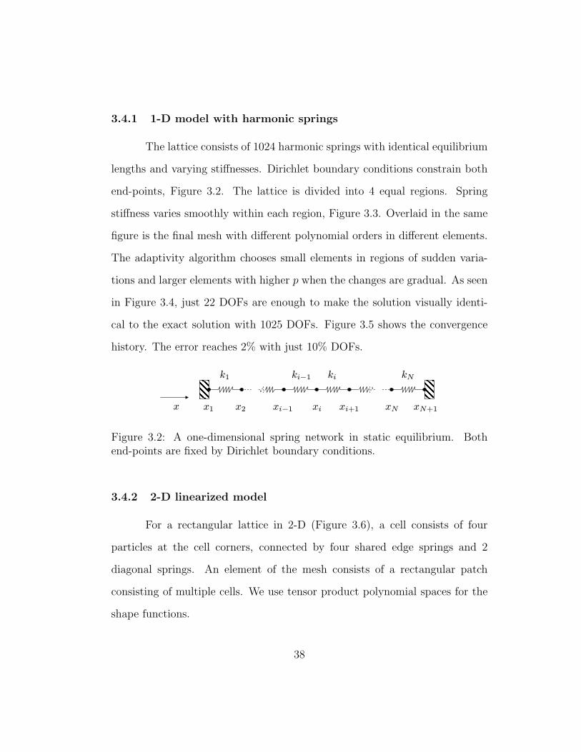
3.4.1 1-D model with harmonic springs

The lattice consists of 1024 harmonic springs with identical equilibrium

lengths and varying stiffnesses. Dirichlet boundary conditions constrain both

end-points, Figure 3.2. The lattice is divided into 4 equal regions. Spring

stiffness varies smoothly within each region, Figure 3.3. Overlaid in the same

figure is the final mesh with different polynomial orders in different elements.

The adaptivity algorithm chooses small elements in regions of sudden varia-

tions and larger elements with higher p when the changes are gradual. As seen

in Figure 3.4, just 22 DOFs are enough to make the solution visually identi-

cal to the exact solution with 1025 DOFs. Figure 3.5 shows the convergence

history. The error reaches 2% with just 10% DOFs.

x

k1 ki−1 ki kN

x1 x2 xi−1 xi xi+1 xN xN+1

Figure 3.2: A one-dimensional spring network in static equilibrium. Bothend-points are fixed by Dirichlet boundary conditions.

3.4.2 2-D linearized model

For a rectangular lattice in 2-D (Figure 3.6), a cell consists of four

particles at the cell corners, connected by four shared edge springs and 2

diagonal springs. An element of the mesh consists of a rectangular patch

consisting of multiple cells. We use tensor product polynomial spaces for the

shape functions.

38

0

0.2

0.4

0.6

0.8

1

1.2

0 128 256 384 512 640 768 896 1024

Spring s

tiffness c

onsta

nts

Spring index

Spring constants

Figure 3.3: A piecewise smooth spring stiffness data shows that larger elementsare selected in regions of slow variation. The color-coded polynomial scale isoverlaid.

Because of geometric nonlinearity, the equations for equilibrium are

not linear. In this example, we assume small strains and work with the

linearized model only. Let A be the set of all particles in the lattice. Let

Xα, α ∈ A denote the position vector of particle α and uα be its displacement

vector. Define (·)αβ = (·)α − (·)β for vectors. Let kαβ and lαβ be the stiffness

and equilibrium length respectively of the spring connecting α and β. Define

∆lαβ = ||Xαβ||− lαβ. Non-zero ∆lαβ implies existence of pre-strain in the par-

ticular spring. Let FEXTα be the external force on particle α. The linearized

39

0

50

100

150

200

250

300

0 128 256 384 512 640 768 896 1024

Spri

ng e

nd-p

oint

dis

plac

emen

ts

Spring index

Solution with 8 DOFsSolution with 22 DOFs

Exact Solution

Figure 3.4: Convergence of solution for a 1025 DOF spring system with datashown in Figure 3.3.

variational form for finding the displacements uηη∈A follows.

Find uηη∈A such that Dirichlet boundary conditions are satisfied and

B(uηη∈A , vζζ∈A

):=

∑α, β∈Aα!β

1

2

kαβ

||Xαβ||2(Xαβ · uαβ)(Xαβ · vαβ)

=

L(vζζ∈A

):=∑α∈A

FEXTα · vα −

∑α,β∈Aα!β

1

2

kαβ∆lαβ

||Xαβ||(Xαβ · vαβ)

∀ admissible vζζ∈A

“α ! β” means particle α is connected to particle β (by the spring

(kαβ, lαβ)).

We chose a square lattice consisting of 64 cells in each direction, Fig-

40

1

10

100

1000

1 10 100

%E

rror

Number of DOF

Exact error in energy normRelative error in energy norm

Figure 3.5: Convergence history for exact and relative errors in energy normfor energy-oriented hp-adaptivity for data shown in Figure 3.3.

x

y

Figure 3.6: A 2-D rectangular lattice with a zoomed-in cell.

ure 3.7(a). The bottom was fixed and a unit force in x direction was applied at

the top right corner. All spring constants were chosen to be 1. Edge springs

had a length 1 and diagonal springs had a length√

2. The equilibrium so-

lution for this configuration is shown in Figure 3.7(b). For the goal-oriented

41

algorithm, the goal is defined to be the x displacement of the top-left corner.

Figure 3.8 shows the hp-meshes using [35] with error less than 1% and num-

ber of DOFs almost 100 times fewer as compared to the fine-scale problem

size. The corresponding exact and approximate solutions are visually indis-

tinguishable at scale of the figures. Figure 3.9 shows the convergence histories

of energy-oriented and goal-oriented adaptivity.

F = 1

Initial Configuration

0

8

16

24

32

40

48

56

64

72

0 8 16 24 32 40 48 56 64 72 80 88

Y

X

Exact solution

(a) (b)

Figure 3.7: The 2-D lattice problem and its exact solution

3.5 Dimensional reduction and homogenization

Numerical results of the previous section show that adaptive mesh re-

finement can be used for dimensional reduction of lattice based problems. It

essentially amounts to solving the fine-scale model in a subspace. However,

42

6 7

22 23

34 35

46 47

48 49

37

25

9

x

y

z

6 7

22 23

34 35

46 47

48 49

37

25

58 59

60 61

x

y

z

(a) (b)

Figure 3.8: Final meshes for (a) energy-oriented and (b) goal-oriented hp-adaptivity.

0.1

1

10

100

0 10 20 30 40 50 60 70

Err

or

Number of DOFs per component

Actual % error in energyEstimated % error in energy

0.01

0.1

1

10

100

0 5 10 15 20 25 30 35 40 45 50 55

Err

or

Number of DOFs per component

Actual error in goalUpper bound for error in goal

(a) (b)

Figure 3.9: Convergence history for energy-oriented and goal-oriented hp-adaptivity.

if this approach is tried on a lattice model with fast varying “random” data,

we see that the mesh refinement algorithm keeps on refining without reduc-

ing the error appreciably. Every time an element is refined, more fine-scales

43

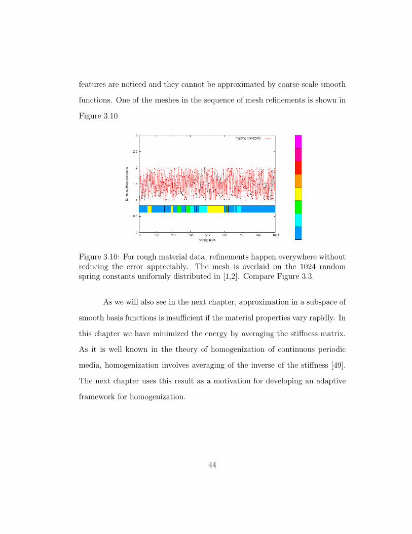
features are noticed and they cannot be approximated by coarse-scale smooth

functions. One of the meshes in the sequence of mesh refinements is shown in

Figure 3.10.

Figure 3.10: For rough material data, refinements happen everywhere withoutreducing the error appreciably. The mesh is overlaid on the 1024 randomspring constants uniformly distributed in [1,2]. Compare Figure 3.3.

As we will also see in the next chapter, approximation in a subspace of

smooth basis functions is insufficient if the material properties vary rapidly. In

this chapter we have minimized the energy by averaging the stiffness matrix.

As it is well known in the theory of homogenization of continuous periodic

media, homogenization involves averaging of the inverse of the stiffness [49].

The next chapter uses this result as a motivation for developing an adaptive

framework for homogenization.

44

Chapter 4

Local Numerical Homogenization

We describe a method for local numerical homogenization of nonlinear

lattice elasticity. There is no assumption of periodicity of material properties or

boundary conditions. The method will be applied to the problem of molecular

statics encountered in SFIL (Chapter 2). However, the method is general and

applicable for problems with a given fine mesh that sufficiently resolves the

fine-scale material properties.

Traditionally, a finite element mesh is designed after obtaining material

properties in different regions. The mesh has to match material discontinuities.

In our approach we do exactly the opposite. A coarse mesh is selected first

and homogenization is done on each individual element of the mesh. In this

way, the coarse mesh and the fine-scale structure become naturally compatible.

On each element, the homogenization method works with the Moore-Penrose

pseudoinverse of the element stiffness matrix to produce pseudoinverse of the

local homogenized stiffness matrix as the output. This output depends on

the local load as well as a chosen local interpolation from the coarse to the

fine mesh. This process requires solving a continuous-time Lyapunov equation

on each element. The pseudoinverse of the homogenized stiffness matrix is

45

then pseudo-inverted to get the homogenized stiffness matrix for the assembly

phase.

For computational efficiency of our method, we require fast and possibly

approximate algorithms for Moore-Penrose pseudoinverse. This is presented

in Chapter 5. Finally, we integrate the homogenization method with goal-

oriented mesh adaptivity and Newton iterations for linearizing the nonlinear

lattice elasticity problem. The numerical results are presented in Chapter 6.

4.1 Using interpolation for dimensional reduction

In Chapter 3, we extended hp-adaptivity to problems posed on lattices.

The method computed local effective material properties in form of a local

stiffness matrix. The approximate solutions matched the exact solutions very

well. However, in general, the resulting effective properties are incorrect. The

error becomes worse when the material properties have large variations. A

simple example in 1-D shows the discrepancy.

k1 ki kN

x1 xi−1 xi xi+1 xN

ki+1

x0

F

Figure 4.1: N springs with a fixed leftmost particle and a force F on therightmost particle.

As shown in Figure 4.1, let us have N harmonic springs, N ≥ 2, with

identical equilibrium lengths and variable stiffnesses kiNi=1. Assume the left

end-point is fixed at origin and that a force F is applied on the right end-

46

point. It is readily seen that the tension in each spring is F and hence the

displacement of the right end-point is F/k, where the effective stiffness k is

the harmonic mean of kiNi=1 times 1/N .

1

k=

N∑i=1

1

ki

. (4.1)

For this problem, the displacements uiNi=0 =: u can also be found by

minimizing the total potential energy J .

Minimize J(u) =1

2

N∑i=1

ki(ui − ui−1)2 − FuN such that u0 = 0. (4.2)

We can minimize J in a subspace. Let us consider all the springs to form a

single element and assume a linear constraint ui = (i/N)uN , where uN is the

only unknown. This interpolation scheme is independent of the specific values

of ki. The total potential energy in terms of a single unknown uN is

u2N

2N2

N∑i=1

ki − FuN .

The total energy is minimum when

uN =N2F∑N

i=1 ki

.

This shows that the effective stiffness, given by F/uN , is the arithmetic mean

of kiNi=1 times 1/N .

k =1

N2

N∑i=1

ki. (4.3)

For positive quantities, the harmonic mean is always less than the arith-

metic mean unless all the quantities are equal. This can be proved using in-

duction on N . Hence, in 1-D, if we minimize in a subspace using the typical

47

finite element shape functions, we always overestimate the effective stiffness.

The relative error due to this approximation is not bounded. For example,

take N = 2 and k1 = 1. In this case, the exact effective stiffness is always

less than 1 but the arithmetic mean stiffness can be made larger than any

arbitrary value by increasing k2.

Although this 1-D problem is simple, its analysis clearly shows the

pitfalls associated with homogenization. Problems in higher dimensions are

more complex and there may not be a simple effective property like in 1-D. In

fact, in the case presented above, the effective material property was just one of

the many possible ones. The one chosen was to match approximate end-point

displacement with the exact one. It does not tell us what happens as we move

away from the end-point. Thus, in a general case, homogenized properties will

also depends on volumetric forces and types of boundary conditions and their

distribution. In addition, the choice of a coarse mesh plays an important role

for the numerical homogenization.

We view this as a departure point and attempt local homogenization

from a different point of view. Our emphasis is on computing best local ma-

terial properties (best in a chosen norm or semi-norm) so that the upscaling

averages the inverse of the stiffness matrix.

4.2 Local numerical homogenization

We change our focus from the best energy norm solution in a simple

subspace. Our focus is on getting locally best effective material properties

48

from the linearized operator of the nonlinear lattice elasticity problem. For an

iterative numerical scheme, the material properties are the element stiffness

matrices that depend on the current coarse mesh and the current solution

guess.

We begin by introducing a coarse grid compatible with the lattice, as

illustrated in Figure 4.2. In each coarse element, the DOFs are displacements

of the corners. We find the effective stiffness for each element (Sections 4.3 and

4.4) in which every coarse DOF interacts with each other. The local effective

stiffness matrices are then assembled to form the global stiffness matrix and the

problem is solved using the standard Finite Element technology. The DOFs

corresponding to the hanging nodes are eliminated before the assembly stage.

Consider a lattice with a load provided by the built-in pre-strain, the

known external loads, and unknown reactions. Without solving the fine-scale

problem exactly we cannot know the forces on the masses forming a detached

coarse element. However, given the location of the masses, we can compute the

pre-strain in each element. To homogenize locally, we can use the pre-strain

as a particular load for which we want accurate homogenization. We may

also choose to homogenize without considering any particular load. We will

formulate the homogenization method using both choices (separately). For the

moment, we work with a known non-zero self-equilibrated load denoted by f ,

f ∈ RN . In Section 4.4 we consider the case f = 0 which can be understood

as homogenization for all loads.

Let K be a symmetric element stiffness matrix of size N . The local

49

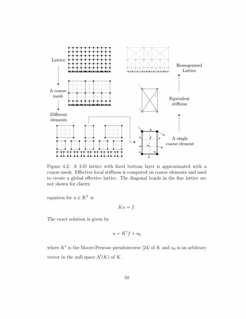
Lattice

A single

coarse element

Equivalent

stiffness

A coarse

mesh

Different

elements

Homogenized

Lattice

Figure 4.2: A 2-D lattice with fixed bottom layer is approximated with acoarse mesh. Effective local stiffness is computed on coarse elements and usedto create a global effective lattice. The diagonal bonds in the fine lattice arenot shown for clarity.

equation for u ∈ RN is

Ku = f.

The exact solution is given by

u = K†f + u0

where K† is the Moore-Penrose pseudoinverse [24] of K and u0 is an arbitrary

vector in the null space N (K) of K.

50

We mark the coarse-scale quantities with a hat. For M ≤ N , let

K ∈ RM×M , as yet unknown, represent the effective element stiffness for the

coarse element DOFs. Let f ∈ RM be the coarse-scale load. A ∈ RN×M is a

chosen interpolation operator. It is local to the element. Vector f = AT f is

the natural interpolation of the fine-scale load f .

In terms of the unknown K, the coarse-scale solution is

u = K†AT f + u0

where K† is the Moore-Penrose pseudoinverse of K and u0 ∈ N (K). When

compared to the fine-scale solution, the error is

u− Au = (K† − AK†AT )f + (u0 − Au0).

Hence, up to an arbitrary constant, the error e ∈ RN is

e := (K† − AK†AT )f.

Let B be a symmetric positive-definite matrix of size N . We will use B to mea-

sure the error e and in process define a homogenization problem to compute

K†.

B should not approximate energy norm. Suppose K is positive definite,

and B is chosen to be K. Then we are minimizing the error in the energy

norm in a round-about way, and as we have seen this results in an incorrect

homogenization when the interpolation operator A is a material independent.

Section 4.3 defines the local homogenization problem for a given self-

equilibrated load. If the load is not known, or is zero, we modify the local

51

homogenization procedure to compute best effective properties for arbitrary

loads. This takes care of forces on an element due to other elements. Homoge-

nization for all loads (by not using any given load) is explained in Section 4.4.

4.3 Locally best effective properties for a given load

We now define and solve the local homogenization problem for a given

non-zero and self-equilibrated load f .

4.3.1 Definition of local homogenization

Given K ∈ RN×N , K symmetric, A ∈ RN×M , B ∈ SN++, f ∈ RN − 0,

and ε > 0, the local homogenization problem is to find a symmetric K† that

minimizes E , where

E(K†) :=1

2

∣∣∣∣∣∣(K† − AK†AT )f∣∣∣∣∣∣2

B+

ε

2

∣∣∣∣∣∣K† − AK†AT∣∣∣∣∣∣2

F,B||f ||22 . (4.4)

The first term in the sum is 12||e||2B = 1

2eT Be and measures the error

in the solution. Symbol “F, B” in second term stands for Frobenius matrix

norm weighted with the matrix B. For X ∈ RN×N ,

||X||2F,B := trace(XT BX).

‘trace’ of a matrix is the sum of its diagonal elements. If B is the identity

matrix, then ||·||F,B is the standard Frobenius matrix norm.

In the limit ε → 0, this minimization problem can be interpreted as a

method to define a local effective stiffness K that provides the best solution

52

for arbitrary loads but subject to the constraint that for a particular load f

the error is the smallest possible.

We choose ε, a dimensionless parameter, a couple of magnitudes smaller

than 1. The second term is a regularization term and is included to obtain a

unique K†. We require regularization for two reasons.

• Firstly, the overall solution method is iterative due to mesh refinements

and Newton iteration steps. Hence f used for homogenization in a single

step represents only an approximation to an “exact” f .

• Secondly, without regularization, the minimization problem given by

Equation (4.4) is ill-posed (with infinitely many solutions). This hap-

pens because the action of operators K and K is used only for a single

load f . Thus regularization is necessary even if an “exact” f is known.

The “closure assumption” in this homogenization method is that local (to an

element) effective material properties are not affected by other elements [5].

4.3.2 Solution of the local homogenization problem

Equation (4.4) is a typical minimization problem with linear constraints

and a convex quadratic objective function in the entries of K†. Note that the

objective function is not quadratic in the entries of K. In fact, because of

the perturbation properties of the Moore-Penrose pseudoinverse, it is a highly

nonlinear and discontinuous function in the entries of K [24]. We will solve

53

for K† and obtain K by computing its pseudoinverse. We will see later in this

section that K† solves a continuous-time Lyapunov equation.

Symmetry of K implies (and is implied by) symmetry of K†. We use a

Lagrange multiplier matrix Λ to impose the symmetry condition. To keep the

notation simple we let the unknown K† be called X in the rest of this section.

The Lagrangian is

L(X, Λ) = E(X) + trace(ΛT (X −XT )). (4.5)

Stationarity of L(X, Λ) implies X = XT and

(AT BA)X(AT (ffT +ε ||f ||22 I)A)−AT BK†(ffT +ε ||f ||22 I)A = ΛT−Λ. (4.6)

I is the identity matrix of size compatible with f . The details of the derivation

of this equation are in Appendix A.

We define some intermediate matrices for simplification.

U := AT BA (4.7)

V := AT (ffT + ε ||f ||22 I)A (4.8)

W := AT BK†(ffT + ε ||f ||22 I)A (4.9)

Matrices U and V are symmetric. Using the definitions of U, V, and W , we

can write Equation (4.6) as

UXV −W = ΛT − Λ.

Since ΛT −Λ is skew-symmetric, so is UXV −W . Hence, we can eliminate Λ.

UXV −W + (UXV −W )T = 0. (4.10)

54

Assume ε > 0. We then use the Sherman-Morrison-Woodbury for-

mula [77] to express V −1.

V −1 =1

ε ||f ||22

((AT A)−1 − (AT A)−1AT ffT A(AT A)−1

ε ||f ||22 + fT A(AT A)−1AT f

)(4.11)

This exists if the following three conditions are true. Term ε ||f ||22 is positive,

(AT A)−1 exists, and the denominator of the second term is non-zero. The

second condition holds because columns of A are linearly independent. The

first and third conditions are true because ε ||f ||22 > 0 and A(AT A)−1AT is

positive semi-definite. In addition, V is positive-definite since it is invertible

and is sum of a positive definite matrix and a rank-1 positive semi-definite

matrix.

Using X = XT , invertibility of V , and symmetry of U and V , Equa-

tion (4.10) can be simplified to

(V −1U)X + X(V −1U)T = V −1(W + W T )V −1.

We define two more intermediate matrices.

C := V −1U (4.12)

D := V −1(W + W T )V −1 (4.13)

Hence, X solves

CX + XCT = D. (4.14)

This is a continuous-time Lyapunov equation, a linear matrix equation with

X as the unknown matrix. D is symmetric. If the sum of any two eigenvalues

55

of C is non-zero (which is satisfied if C is positive definite), then a unique

solution X exists and it is symmetric [80, 4].

4.4 Locally best effective properties for all loads

We now define and solve the local homogenization problem when the

load f is not given, or is 0, or we want to compute effective properties inde-

pendent of any self-equilibrated load.

Given K ∈ RN×N , K symmetric, A ∈ RN×M , and B ∈ SN++, the local

homogenization problem is to find a symmetric K† that minimizes E , where

E(K†) :=1

2

∣∣∣∣∣∣K† − AK†AT∣∣∣∣∣∣2

F,B. (4.15)

The notation is same as used in Equation (4.4). We can proceed to form a La-

grangian and minimize E(K†) for a symmetric K† as explained in Appendix A.

The only difference is that compared to the definitions of the intermediate ma-

trices in Section 4.3.2, the definitions of V and W are modified. U remains

the same.

U := AT BA, (4.16)

V := AT A, (4.17)

W := AT BK†A. (4.18)

Matrices C and D are defined as they were defined in Equations (4.12)–(4.13)

but in terms of these U, V, and W . We still have to solve a Lyapunov equation

(Equation (4.14)).

56

4.4.1 A special case: minimum error in `2 norm

If we want minimum error in the `2 norm and thus choose B = I, it

turns out that we don’t have to solve a Lyapunov equation because C becomes

identity. Note that in this case, U = V , and W = W T . Thus K† = X =

V −1WV −1.

K =((AT A)−1AT K†A(AT A)−1

)†=

(A†K†(A†)T

)†(4.19)

Compare this expression with the expression for K derived for least error in

energy norm in which K = AT KA (Equation (3.3)). These two expressions

are different in general.

It is readily seen that if the fine-scale stiffness matrix K is positive semi-

definite, then so is the coarse-scale stiffness matrix K. This can be shown

as follows. If K is positive semi-definite, then so is K†. This implies that

xT K†x ≥ 0 for any compatible vector x, in particular for u = (A†)T y. Thus,

((A†)T y)T K†((A†)T y) ≥ 0. Rearranging, we get yT (A†K†(A†)T )y ≥ 0. Thus,

A†K†(A†)T is positive semi-definite. This implies that its pseudoinverse K =

(A†K†(A†)T )† is positive semi-definite too.

4.5 Constrained convex optimization for local homoge-nization

In Section 4.3, the local problem to homogenize a single element was

posed using a regularization approach. We created a single error function,

57

which was a weighted sum of the error (due to homogenization) for a specific

non-zero load f and a norm of the difference of fine-scale compliance matrix

(K†) and interpolated compliance matrix (AK†AT ). This required choosing a

small weighing parameter ε > 0. The other constraint, of symmetry of X, was

imposed exactly using Lagrange multipliers.

In this section we formulate local homogenization as a (fully) con-

strained convex optimization problem that does not require the approximation

due to regularization.

There are two sets of constraints that the entries of the unknown matrix

X = K† must satisfy exactly. Firstly, X must be symmetric. Secondly, for

a specific non-zero load f the error due to homogenization should be the

minimum possible. The constrained optimization formulation is derived using

a two-step procedure. In the first step, the constraint equations are derived. In

the second step, while satisfying the constraints of first step, X must minimize

a norm of the difference of fine-scale compliance matrix (K†) and interpolated

compliance matrix (AXAT ).

The constraint equation for minimizing the error for a specific load

f can be derived from the first-order necessary optimality condition of the

following problem.

minX=XT

1

2

∣∣∣∣(K† − AXAT )f∣∣∣∣2

B

Using a Lagrange multiplier approach to impose X = XT as shown in Sec-

58

tion 4.3 and Appendix A we get the optimality condition.

AT BAXAT ffT A− AT BK†ffT A must be skew-symmetric.

Thus,

(AT BAXAT f − AT BK†f)(AT f)T must be skew-symmetric.

It can be shown that if the outer product of two vectors is skew-symmetric,

then at least one of the two vectors is zero. The proof is in Appendix C. Since

A is full-rank and f is assumed non-zero, it implies that AT f is non-zero. Thus

the first vector, AT BAXAT f−AT BK†f , is 0. Obviously this equation cannot

be used to fully determine X since it fixes the action of X only on a single

vector, AT f .

This leads us to the second stage of the optimization procedure.

minX

1

2

∣∣∣∣K† − AXAT∣∣∣∣2

F,Bsuch that AT BAXAT f = AT BK†f and X = XT

(4.20)

We define auxiliary matrices U, V,W, and f , where U = AT BA, V =

AT A, W = AT BK†, and f = AT f. Using Lagrange multipliers to impose the

two constraints, we can deduce the following first-order optimality condition. U ⊗ V + V ⊗ U U ⊗ f + f ⊗ U

U ⊗ fT + fT ⊗ U 0

[ vec(X)

µ

]=

[vec(WA + AT W T )

2 Wf

]

Here⊗ is the Kronecker product operation, “vec” is the vectorization operation

and µ is an unknown vector of Lagrange multipliers that constrain X to be the

59

best possible for the specific load f . The Lagrange multipliers for imposing

the symmetry of X have been eliminated. The (1, 2) block is the transpose

of (2, 1) block. Since the (1, 1) block (U ⊗ V + V ⊗ U) is symmetric positive

definite and the (2, 1) block (U⊗ fT + fT ⊗U) has full row-rank, the system is

invertible and characterizes the unique minimum X. The Kronecker products

are not computed. One should transform the system to a Lyapunov equation

like structure for fast solution. This is slightly more complicated than the

regularization approach of Section 4.3. Hence, we present all the results in

Chapter 6 using the simpler approach, but this derivation and the results

show that a unique solution can be found for exact local homogenization.

4.6 Homogenization of pre-stress

In case of polymer lattices of SFIL, even if there is no external force on

molecules, the lattice is not in equilibrium in general. This is because of the

residual forces due to a mismatch in inter-molecular distance and the length

at which the inter-molecular potential is minimum. Using the terminology

from continuum elasticity, we call the residual forces pre-stress. If a single

element is removed from the lattice, as shown in Figure 4.2, the pre-stress in

that element is self-equilibrated. This is because if a spring leads to a force

F on a particle, then it leads to a force −F on the corresponding neighbor.

Taking the sum and moment around any point, the total force as well as the

total moment is zero. This pre-stress leads to a pre-strain.

To homogenize correctly, we need to transfer the pre-stress (or pre-

60

strain) information in the fine-scale lattice to coarse-scale mesh. This is done

after determining the coarse-scale ‘material properties’ (K). Let p and u de-

note the fine-scale pre-stress and pre-strain, respectively. The corresponding

coarse-scale quantities are p and u. Figure 4.3 shows the transfer operation.

Fine-scaleNewton step

Coarse-scaleNewton step

Pre-stress p

⇐⇒

Pre-stress??

Figure 4.3: The homogenized pre-stress is the coarse-scale pre-stress thatwould give a deformation such that the fine-scale and coarse-scale latticesare approximately similar.

For a single iteration, we have

Ku = p =⇒ u = K†p

and

Ku = p =⇒ u = K†p.

We find u (and hence p too) by minimizing the error

||Au− u||2B ,

where A is the interpolation operator and B is a symmetric positive definite

matrix that forms the norm in which we measure the error. We will use B = I

61

here. Since A has full column-rank, the solution is simply u = A†u. Using the

expressions for u and u, the coarse-scale pre-stress is

p = KA†K†p. (4.21)

4.7 Remarks on local homogenization

The interpolation operator A is a parameter to play with and it can

be chosen to get better homogenized properties. Operator-dependent inter-

polation [50] should be a better choice but this is a speculation in context of

the current approach. We use the simple bilinear interpolant for lattice based

problems in 2-D (and trilinear in 3-D). We can also make the error E a func-

tion of A as well and look for the best A. This turns out to be a complicated

nonlinear problem with many more unknowns.

We have a choice of the matrix norm in the regularization term. Spec-

tral norm may be better but its use leads to a nonlinear problem with non-

smooth objective function. In contrast, weighted Frobenius norm leads to a

convex quadratic problem with linear equality constraints (due to the imposed

symmetry of K†).

Load-independent homogenization (Section 4.4) may not be correct for

problems involving layered media. Boundary loads and local material dis-

tribution influence the homogenized properties [2, p. 24]. For example, in

conductivity problems for layered media, if the flux is in parallel to the layers,

the effective conductivity is given by the arithmetic average. However, if the

62

flux is in the perpendicular direction, the effective conductivity is given by the

harmonic average [49, p. 13]. A local self-equilibrated load can be computed

by projecting the global known load.

The choice of B is critical. If we choose B = K (K should be positive

definite for this) then we don’t gain anything when compared to the minimiza-

tion in a subspace. The approximate solution of Equation (4.4) leads to the

arithmetic average rather than the harmonic average. Since our interpolation

operator is independent of the material properties, and we are not resolving

the variations, we should look for a “weaker” convergence. Here the theory of

homogenization for PDEs guides us to believe that B should be independent

of the operator and correspond to a discrete approximation of the L2 norm.

These alternatives, load dependent or independent homogenization and

possible values of the matrix B, are numerically explored and justified in Sec-

tion 6.2. In the next section we analytically compute effective properties in

1-D for a small element.

4.8 An analytical example of local homogenization

The local homogenization method of Section 4.3.1 is exemplified with

homogenization of 3 harmonic springs forming a single element of a 1-D lattice.

We homogenize the springs to create a single effective spring with spring

constant k (Figure 4.4). To keep the analysis simple, we first choose the matrix

B (used in Equation (4.4)) to be identity. Later on we use a different B to

63

reduce errors where we want. We recover the classical effective spring constant

given by the harmonic average.

k1u1 u2 u3 u4

k2 k3

f1 f2 f3 −f1 − f2 − f3

ku1 u2

f1

Homogenize

−f1

Figure 4.4: We find the best effective k for the self-equilibrated system shownon left.

The fine-scale system is described by displacements u ∈ R4, stiffness

matrix K ∈ R4×4, and load f ∈ R4 with f4 = −f1 − f2 − f3.

Ku =

k1 −k1 0 0−k1 k1 + k2 −k2 00 −k2 k2 + k3 −k3

0 0 −k3 k3

u1

u2

u3

u4

=

f1

f2

f3

f4

= f

The solution is u = K†f + (u0, u0, u0, u0)T where u0 is arbitrary and

K† =1

16

9k1

+ 4k2

+ 1k3

− 3k1

+ 4k2

+ 1k3

− 3k1− 4

k2+ 1

k3− 3

k1− 4

k2− 3

k3

− 3k1

+ 4k2

+ 1k3

1k1

+ 4k2

+ 1k3

1k1− 4

k2+ 1

k3

1k1− 4

k2− 3

k3

− 3k1− 4

k2+ 1

k3

1k1− 4

k2+ 1

k3

1k1

+ 4k2

+ 1k3

1k1

+ 4k2− 3

k3

− 3k1− 4

k2− 3

k3

1k1− 4

k2− 3

k3

1k1

+ 4k2− 3

k3

1k1

+ 4k2

+ 9k3

.

We use standard linear interpolation for the inner points. The interpolation

operator is

A =

[1 2

313

0

0 13

23

1

]T

.

For the homogenized element with a single spring, the effective stiffness matrix

is

K =

[k −k

−k k

].

64

Its pseudoinverse is

K† =1

4

[1bk − 1bk− 1bk 1bk

].

We will determine the best k by minimizing the error E (Equation (4.4)). We

choose B = I.

For an arbitrary load f and ε > 0, we can analytically solve for the

minimum. In the limit ε → 0 we get

k =10

9

(3f1 + 2f2 + f3)k1k2k3

3k1k2(f1 + f2 + f3) + 3k2k3(f1) + 4k3k1(f1 + f2).

To simplify the expression, let us use loads only at the end-points. Thus,

f1 = 1, f2 = 0, and f3 = 0. Then

k =10 k1k2k3

9 k1k2 + 12 k1k3 + 9 k2k3

.

Compare k with the classical effective spring constant

k =k1k2k3

k1k2 + k1k3 + k2k3

.

The expressions for k and k are not the same. However, we do get a

value very close to the one that is given by the harmonic average. Since we

chose B = I, the errors at the end-points were given equal emphasis as the

errors at interior points. In derivation of the classical effective constant, we

are only concerned with matching end-point displacements. This explains the

discrepancy between the two effective spring constants.

This discrepancy can be resolved by using B = diag(M, 1, 1, M), where

M 1, so that errors at end-points are penalized more. The best effective

65

stiffness can be computed to be

k =k1k2k3

(1−m)k1k2 + (1 + 2m)k1k3 + (1−m)k2k3

where m :=1

9M + 1→ 0 as M →∞. Hence, we recover the classical effective

stiffness by choosing an appropriate norm to measure the local error.

4.9 Computational aspects

Computing the homogenized material properties requires computation

of Moore-Penrose pseudoinverse of multiple matrices with different structural

properties. We discuss this topic briefly here in Section 4.9.1 and in detail in

Chapter 5 for large sparse matrices. In addition, we have to solve a dense Lya-

punov equation of a small size (number of DOFs in the coarse-scale element).

This is discussed in Section 4.9.2 below.

4.9.1 Computation of Moore-Penrose pseudoinverse

The pseudoinverse of a real matrix K can be defined and computed

in terms of the SVD [48, 24]. Let K have an SVD K = UΣV T , then the

pseudoinverse is K† = V Σ†UT where Σ† is formed by taking the reciprocal of

all non-zero singular values (diagonal entries in Σ) and applying a transpose

operation.

SVD is the most general and reliable procedure for computing pseu-

doinverses. However, it is an O(N3) procedure. It also ignores the sparsity

of the matrix. For these reasons, it is not the best method in the context

66

of numerical homogenization. In Chapter 5 we analyze faster algorithms for

computing the pseudoinverse. Numerical results are presented in Chapter 6.

For local homogenization, the pseudoinverse is needed in the following steps.

• We need pseudoinverses of the large and sparse fine-scale stiffness matrix

K. Actually, only the action of the pseudoinverse is needed on f and

columns of A (Equations (4.9) and (4.18)). See Chapter 5 for details.

• In case of Equation (4.19), we need the action of K† on columns of (AT )†.

See Chapter 5 for details.

• In case of Equation (4.19), we need the pseudoinverse of a dense A.

• Whether we homogenize for a particular load or not, we have to compute

the homogenized stiffness matrix from its pseudoinverse. Thus we need

to explicitly compute pseudoinverse of a symmetric matrix of a relatively

small fixed size (since it is on the coarse-scale). For example, for a 3-D

lattice elasticity problem with a cube forming the coarse-scale, the size

of effective stiffness matrices is 24× 24. In 2-D the size is 8× 8.

For a rectangular matrix of full column rank, for example the interpola-

tion matrix A, the pseudoinverse can be expressed using the normal equations.

A† = (AT A)−1AT

Since the number of columns of A is fixed and small, we can either use the

normal equations for computing A† or preferably use QR factorization of A.

67

4.9.2 Solution of the Lyapunov equation

Computing the pseudoinverse of the best local stiffness matrix requires

solving a Lyapunov equation (except for the special case mentioned above

for load-independent homogenization and when B is identity). This equation

arises in many different areas, for example control theory and stability analysis.

Many algorithms and implementations exist for its efficient solution [70, 4]. We

use the Bartels-Stewart algorithm [13] that uses lower real Schur decomposition

of the matrix C. Let C = QC ′QT , D = QD′QT , and X = QX ′QT , where

Q ∈ RM×M is a real orthonormal matrix, C ′ is real block lower triangular with

maximum block size 2. With these definitions, Equation (4.14) becomes

C ′X ′ + X ′C ′ T = D′.

+ =

Figure 4.5: Structure of the Lyapunov equation after Schur decomposition ofC.

Since C ′ has a special structure, the transformed equation can be

solved using a “forward-substitution” algorithm. We successively solve for

X ′11, X

′12, . . . , X

′1m, X ′

21, X′22 and so on where m is the number of blocks. Fi-

nally, we can compute X = QX ′QT .

68

4.10 Error estimation for goal-oriented adaptivity

We presented goal-oriented adaptivity for self-adjoint elliptic problems

in Section 3.3. We had used Galerkin orthogonality in the derivation of local

error estimates. The orthogonality condition is slightly different if the fine-

scale and coarse-scale operators are different. This is the case if the coarse-scale

operator is derived by local homogenization. We derive the corresponding error

estimates here. As before, quantities relevant on the coarse-scale are marked

with a hat and A is a global interpolation operator from the coarse-scale to

the fine-scale. We assume that the coarse-scale is chosen in such a way that

the Dirichlet boundary conditions are satisfied exactly.

The fine-scale primal problem is

Find u ∈ uD + V such that B(u, v) = L(v) ∀ v ∈ V .

The coarse-scale primal problem is

Find u ∈ uD + V such that B(u, v) = L(v) ∀ v ∈ V

where the coarse-scale load is defined by

L(v) = L(Av) ∀ v ∈ X .

Corresponding to a goal G ∈ X ′, we have the fine-scale and coarse-scale

adjoint problems. The fine-scale adjoint problem is

Find w ∈ V such that B(v, w) = G(v) ∀ v ∈ V .

69

The coarse-scale adjoint problem is

Find w ∈ V such that B(v, w) = G(v) ∀ v ∈ V

where the goal on the coarse-scale is defined by

G(v) = G(Av) ∀ v ∈ X .

The error in the goal is

G(u)− G(u) = G(u)− G(Au)

= G(u− Au)

= B(u− Au, w)

= B(u− Au, w − Aw) + B(u− Au, Aw)

= B(u− Au, w − Aw) + B(u, Aw)− B(Au, Aw).

In case of compatible fine-scale and coarse-scale bilinear forms, the last two

terms would have canceled each other. This is not true for our case. Instead,

we prove that B(u, Aw) = B(u, w) and simplify the error expression.

B(u, v) = L(v) ∀ v ∈ V⇒ B(u, Av) = L(Av) ∀ v ∈ V⇒ B(u, Av) = L(v) ∀ v ∈ V⇒ B(u, Av) = B(u, v) ∀ v ∈ V⇒ B(u, Aw) = B(u, w)

Finally, the error in the goal, G(u)− G(u), is

B(u− Au, w − Aw)︸ ︷︷ ︸Standard characterization

+ B(u, w)− B(Au, Aw)︸ ︷︷ ︸Incompatible bilinear forms

.

70

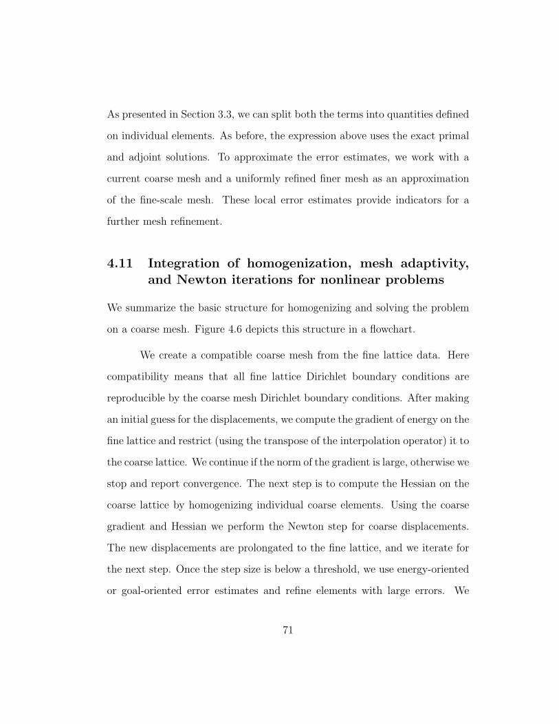
As presented in Section 3.3, we can split both the terms into quantities defined

on individual elements. As before, the expression above uses the exact primal

and adjoint solutions. To approximate the error estimates, we work with a

current coarse mesh and a uniformly refined finer mesh as an approximation

of the fine-scale mesh. These local error estimates provide indicators for a

further mesh refinement.

4.11 Integration of homogenization, mesh adaptivity,and Newton iterations for nonlinear problems

We summarize the basic structure for homogenizing and solving the problem

on a coarse mesh. Figure 4.6 depicts this structure in a flowchart.

We create a compatible coarse mesh from the fine lattice data. Here

compatibility means that all fine lattice Dirichlet boundary conditions are

reproducible by the coarse mesh Dirichlet boundary conditions. After making

an initial guess for the displacements, we compute the gradient of energy on the

fine lattice and restrict (using the transpose of the interpolation operator) it to

the coarse lattice. We continue if the norm of the gradient is large, otherwise we

stop and report convergence. The next step is to compute the Hessian on the

coarse lattice by homogenizing individual coarse elements. Using the coarse

gradient and Hessian we perform the Newton step for coarse displacements.

The new displacements are prolongated to the fine lattice, and we iterate for

the next step. Once the step size is below a threshold, we use energy-oriented

or goal-oriented error estimates and refine elements with large errors. We

71

Begin with a (fine) lattice,B.C., initial solution guess

Create any compatible coarse meshpartitions and restrict initial guess

Compute fine lattice gradient and Hessianon each element for current solution guess

Restrict the gradient to coarse mesh andhomogenize each partition independently

Assemble coarse mesh elementgradients and Hessians

Compute new solution guess on coarse mesh

Estimate error on the current coarse mesh

Estimate acceptable?

Subdivide the current coarse mesh elements with large error to create a finer

mesh

Reached minimum?

Replace the current coarse mesh and

prolongate the current solution to the new coarse

mesh

Replace the current solution guess and

prolongate to the fine lattice

DoneDoneDoneDone

YesYesYesYes

No

No

YesYesYesYes

Nonlinearity Adaptivity

Figure 4.6: Overall structure of integrating homogenization, mesh adaptivity,and Newton iterations for nonlinearity.

repeat the Newton iterations on the refined lattice until convergence. The

mesh is refined again if needed.

72

Chapter 5

Fast Algorithms for Moore-Penrose

Pseudoinverse

Local homogenization is the core part of the global solution method

and is done in each element. Moreover, because of mesh refinement and non-

linearities, each element can possibly have different stiffness matrix after each

step, and it may be required to upscale it again. Thus, critical to the compu-

tational efficiency of the whole method is fast and approximate computation

of the pseudoinverse of a sparse element stiffness matrix. For these reasons,

Singular Value Decomposition (SVD) is not the best choice here for computing

pseudoinverses.

We present algorithms that are significantly faster for sparse matrices.

The first one uses the characterization of the pseudoinverse as the limit of a

Tikhonov regularized matrix [79, 19]. In the second algorithm, the a priori

knowledge of the null-space of a matrix can be used to compute the pseu-

doinverse by direct or iterative linear solvers [47]. The third algorithm uses a

sparse rank-revealing QR factorization of the matrix (or of a suitable column

permutation) to compute an exact pseudoinverse using the matrix factors Q

and R [24, 34]. Lastly, in the context of mesh refinement or nonlinear prob-

73

lems, one might reuse an old pseudoinverse (actually its sparse factorized form)

to compute pseudoinverse of a perturbed matrix. This can be done using an

iterative procedure based on “proper splittings” [22, 66].

None of these algorithms is the perfect one for all situations. Depending

on the problem dimension, number of vector unknowns per DOF, element size,

condition numbers, and sparsity, one algorithm may be much better than the

others. These choices are analyzed in Sections 6.5 and 6.6.

5.1 Moore-Penrose pseudoinverse

Moore-Penrose pseudoinverse was discovered by E. H. Moore in 1906

in the context of projections associated with singular and rectangular matri-

ces [63]. It was rediscovered by Penrose in 1955 as the unique matrix satisfying

four algebraic matrix equations [73]. Quite a few articles and books have ap-

peared on the subject since then. There is a large bibliography in [67] and [19].

Moore-Penrose pseudoinverse is the most widely known special case

of generalized inverses or pseudoinverses. In this dissertation we exclusively

work with Moore-Penrose pseudoinverse and occasionally use the term pseu-

doinverse for it.

5.2 Computation of Moore-Penrose pseudoinverse

Since pseudoinverses are generalizations of inverses of square nonsin-

gular matrices, their computation usually involves solving linear equations or

74

obtaining matrix factorizations. Analogous to the plethora of direct and iter-

ative algorithms for solution of linear systems of equations, there is no single

algorithm that is the best choice for computing generalized inverses. There is

a variety of algorithms that can be used [19]. We focus only on a few that are

most likely to be useful for our purposes.

One of the most general and reliable computational method to compute

Moore-Penrose pseudoinverse is the SVD [48, 24]. The pseudoinverse of a real

matrix K can be defined and computed in terms of the SVD [48, 24]. Let

K have an SVD K = UΣV T , then the pseudoinverse is K† = V Σ†UT where

Σ† is formed by taking the reciprocal of all non-zero singular values (diagonal

entries in Σ) and applying a transpose operation. However, SVD is an O(N3)

procedure. Typical implementations also ignore the sparsity of the matrix. For

these reasons, SVD is not the best method in the context of homogenization.

However, SVD is useful for determination of the numerical rank, which is

important to reliably compute pseudoinverse of arbitrary matrices.

Despite its excellent numerical properties, use of SVD gives an impres-

sion that computation of pseudoinverse is inherently an iterative process just

like the computation of singular values or eigenvalues. This impression is not

correct. Entries of the pseudoinverse matrix are explicit rational functions

of the entries of the original matrix just like the entries of the inverse of an

invertible matrix. This is readily seen from the equivalent definition of the

pseudoinverse that uses Tikhonov regularization [19] or full-rank factoriza-

tions. Looking just at Tikhonov regularization, the entries of the inverse of

75

a non-singular matrix are rational polynomials in the entries of the original

matrix. Thus, the entries of the pseudoinverse matrix are limits of rational

polynomials expressions. In principle, they can be expressed as explicit func-

tions and are exactly computable unlike eigenvalues or singular values. We do

not use this observation for computing pseudoinverses, but mention it because

of its conspicuous absence in the literature. Moreover, this gives a hint that if

we know the rank of the matrix a priori, possibly using physical considerations,

then better algorithms can be devised, for example the one in [47].

5.3 Pseudoinverses and homogenization

Our focus is on computing Moore-Penrose pseudoinverses of the follow-

ing three categories of matrices.

1. A real, singular (hence square), sparse, symmetric matrix with almost

all eigenvalues being positive. The rank-deficiency is known in advance

and is small (typically between 1 and 6) and is independent of the matrix

size. The matrix size is variable, typical value being between 500 and

3000. These are element stiffness matrices coming from a finite element

discretization.

2. A real, dense, rectangular, full column-rank matrix with a small number

of columns, between 2 and 24, and a variable number of rows, typical

value being between 500 and 3000. These are interpolation matrices in

a finite element discretization.

76

3. A real, singular (hence square), dense, symmetric matrix. The matrix

size is small and will be between 2 and 24. These are pseudoinverses of

homogenized fine-scale matrices.

For the second category (the dense, rectangular, full column-rank ma-

trices) the pseudoinverse can be expressed and computed using the normal

equations.

A† = (AT A)−1AT

Since the number of columns of A is fixed and small and A is well-conditioned,

we can either use the normal equations for computing A† or preferably use

QR factorization of A to avoid loss of precision due to squaring of the con-

dition number. For the third category (the small, dense, symmetric, singular

matrices), we use the SVD. These are implemented in LAPACK [3].

The computational bottleneck of the homogenization process is com-

puting the pseudoinverses of the matrices of the first category (real, large,

sparse, singular matrices). SVD of a matrix of size 400 takes nearly a second

on current single core processor (as of year 2009). However, a sparse Cholesky

factorization of matrices of similar size and with a structure and properties of

the homogenization problem takes around 0.005 seconds, which is 200 times

faster. If the matrix size is greater, say 2500, the sparse factorization can be

3000 times faster than computing the SVD. Thus, if we can use sparse fac-

torization or sparse solution methods for linear systems instead of SVD for

pseudoinverse, we can hope to obtain a speedup of 100 to 1000 depending on

the matrix size.

77

Note that when we talk about computing pseudoinverse, in general we

do not want it in an explicit matrix form but want only its action on a set of

vectors. However, for the categories of matrices mentioned above, we do want

the pseudoinverse of the dense matrices explicitly. This is all right, since these

are small matrices.

5.4 Sparse algorithms for Moore-Penrose pseudoinverse

As mentioned above, using a sparse algorithm for computing pseudoin-

verse may be 2 or 3 orders of magnitude faster than the SVD for typical sparse

finite element matrices. We present three algorithms that exploit the sparsity.

In the end, we present an iterative algorithm that can compute pseudoinverse

of a perturbed matrix using the factorized form of the pseudoinverse of the

original matrix. This is useful when the element stiffness matrices change

slightly during mesh adaptivity steps and Newton step for nonlinearity.

5.4.1 Pseudoinverse using Tikhonov regularization

We can avoid the SVD by using a limit characterization for the pseu-

doinverse using Tikhonov regularization [79, 19]. For an arbitrary matrix K

K† = limδ→0

(KT K + δI)−1KT = limδ→0

KT (KKT + δI)−1. (5.1)

I is a size-compatible identity matrix. The limit always exists. The limit has

to be taken for the full expression and not just the matrix with the variable δ

((KKT + δI)−1 or (KT K + δI)). The proof is in [79, 19].

78

5.4.1.1 Approximation using a finite δ

We use a finite δ in Equation (5.1) to approximate K†. For an accurate

approximation, δ should be a small multiple of the σ2r , the square of the small-

est non-zero singular value of K. We can then use Equation (5.1) to compute

an approximate action of K† on any given vector g. An a priori error estimate

for δ > 0 can be proved [25, 19]

∣∣∣∣(KT K + δI)−1KT −K†∣∣∣∣2≤ δ

∣∣∣∣K†∣∣∣∣32.

We use the sparse direct Cholesky factorization method as implemented

in CHOLMOD [33]. If K is sparse or banded then KKT and KT K are sparse

too (although less so). For example, if K is tridiagonal, then KKT and KT K

are pentadiagonal. Moreover, they are positive semi-definite. Addition of a

positive diagonal makes the matrix to be inverted positive definite. Thus,

Cholesky factorization is a feasible algorithm for all K.

It is not necessary to use a general sparse factorization method for

the matrices we are interested in. If a typical nodal ordering is used to order

particles in a 2-D or 3-D box, the stiffness matrices are banded. For nd particles

and p DOFs per particle, where d is the space dimension and n is the “edge-

size” of an element, the matrix size is p nd and bandwidth is O(p nd−1). Thus

banded Cholesky solvers can also be competitive with general sparse Cholesky

solvers. Currently, we have used reordering based sparse direct solvers. A brief

comparison of the two methods is done in Section 6.5.

79

Because δ is finite, we lose a few digits in the computed vector K†g.

If δ is chosen appropriately, then the approximation is not detrimental to the

overall algorithm. It should not be too small (relative to σ2r) either since it

would lead to numerical singularity of KT K + δI. A large δ would lead to less

accuracy. We do need an estimate of σ2r for this problem, which is an O(N3)

procedure for an accurate estimate, but that is all right since it can be done

once and re-used for other elements.

This algorithm squares the (pseudo-)condition number by computing

KT K (or KKT ), and then adds a small diagonal perturbation to make the ma-

trix invertible. Hence, we do not use an iterative algorithm to invert. One can

use the QR factorization to compute the pseudoinverse for this damped least

squares problem [24] and avoid squaring of the condition number, but it would

be slower than sparse Cholesky factorization. And if one goes through the

trouble of implementing sparse QR factorization, one might as well compute

the pseudoinverse “exactly” using the algorithm presented in Section 5.4.3.

The advantage of sparse Cholesky factorization is its speed. For certain so-

lution regimes, this is the fastest of all the algorithms we will discuss. It is

inherently an approximate algorithm and will never obtain solutions with full

accuracy. This is not a big drawback because in the context of homogenization

with mesh adaptivity and nonlinearity, we need only an approximation of the

upscaled Hessian matrix and not its exact upscaling.

80

5.4.1.2 Iterative improvement using a series representation

The pseudoinverse can also be represented by the sum of a series [18].

K† =∞∑i=1

KT (KKT + I)−i (5.2)

Here KT must not be removed as a factor from the series (else the sum will

diverge). Using the property (αK)† = 1αK† for α 6= 0, it can be derived from

Equation (5.2) that

K† =∞∑i=1

KT δi−1(KKT + δI)−i ∀δ > 0.

Here δ = 1α2 . Since α 6= 0 is arbitrary, the representation is valid for all

δ > 0. Note that the first term in the summation is the last expression in

Equation (5.1) for a finite δ.

This representation effectively rescales the matrix K so that computing

the inverse of KKT +δI is not too badly-conditioned when K is rank-deficient

(and δ is chosen appropriately). A large δ would mean that the inverse can

be accurately computed, but then more terms in the series will be needed

to accurately approximate K†. If a smaller δ is chosen, then fewer terms

will be needed to achieve an acceptable accuracy, but the inverse will not be

accurately computed in finite precision. Thus, there is a built-in trade-off

between computation speed and high accuracy.

Once KKT + δI is factorized using a sparse Cholesky factorization, the

factors can be reused to compute the actions of (KKT +δI)−i for i ≥ 1. Thus,

81

the “inversion” step is required only once and rest of the terms can computed

cheaply.

We have not used this iterative improvement strategy in the context of

homogenization, but it can be used when the pseudoinverse is required with

higher accuracy.

5.4.2 Pseudoinverse using a known null-space basis

A less well-known result, presented in [47], is that computing pseudoin-

verse, or its action on a vector, can be transformed to solving linear algebraic

equations of same size (by either direct or iterative algorithms). One needs

the null space of the original matrix a priori. For many mathematical models

of physical problems the null-space is known from physical arguments.

For nonlinear lattice elasticity problems, the null-space of the stiffness

matrix contains the rigid body translations whether the lattice is in equilibrium

or not. If it is in equilibrium, rigid body rotations are also in the null-space [47].

Thus, the dimension of the null-space is independent of the size of the lattice,

and its basis is known.

Let R ∈ RN×P , 0 < P < N, be a matrix of columns-vectors that form

an orthonormal basis of the null-space of a symmetric K ∈ RN×N . R stands

for rigid body motion. Thus, P := In − RRT is the orthogonal projector on

the range of K. It is shown in [47] that P (K + RRT )−1 = (K + RRT )−1P is

the Moore-Penrose pseudoinverse of K.

Hence, if K and R are known, then computing u = K†g, for f ∈ RN ,

82

implies solving (K+RRT )u = Pg for u. Even if K is sparse, (K+RRT ) would

be dense in general. But it is a rank p update of a sparse matrix and p is small

compared to N . Thus the action of (K+RRT ) on any vector can be computed

with a little more effort than sparse matrix vector multiplication. Thus the

system can be efficiently solved by iterative solvers for symmetric matrices.

We use the iterative solvers (conjugate gradient and minimum residual meth-

ods) and preconditioners (Jacobi and Incomplete Cholesky) implemented in

PETSc [11]. A numerical comparison of these 4 combinations is presented in

Chapter 6.

5.4.3 Pseudoinverse using QR factorization

Let K ∈ RN×N have a rank-deficiency p, where 0 < p < n. In our

application, p will be a fixed number much smaller than n. We can compute

a rank-revealing QR factorization K = QR, where Q is orthonormal and R is

upper triangular. Partition Q and R as follows.

Q =[Q1 Q2

].

and

R =

[R11 R12

0 0

].

Here Q1 is n×(n−p), Q2 is n×p, R11 is (n−p)×(n−p), and R12 is (n−p)×p.

Define auxiliary matrices S and X.

S := R−111 R12

83

and

X := (ST S + I)−1ST R−111 QT

1 .

S is (n− p)× p, and X is p×n. The action of R−111 can be computed by back-

substitutions since R11 is a triangular matrix. In addition, the ‘inversion’ of a

p× p system (ST S + I) is needed to compute S and X.

Finally, using the QR factorization and the matrices S and X, it can

be shown [24]

K† =

[R−1

11 (QT1 −R12X)X

].

Note that this is just an expression and need not be computed explicitly. It

can be used to compute K†f for a known vector f . One should form QT1 f first

to compute X and K†f .

In general the factors Q and R are not as sparse as the original matrix

K. Moreover, a typical QR factorization algorithm will not exploit the sparsity

of K. For this, we can use a sparse QR factorization algorithm, for example

as implemented in [34].

The columns of K should be reordered before the QR factorization to

reduce fill-in. Thus, we need to form the Q and R factors of KP , where P is

a permutation matrix, usually chosen automatically [34]. If KP = QR, where

P is orthonormal, then it can be shown using SVD that K† = P (QR)†. This

expression is applicable for a permutation matrix P also because permutations

are orthonormal. (QR)† can be computed as shown above. The expressions

remain valid but the implementation takes advantage of the sparsity of Q and

84

R.

5.4.4 Pseudoinverse using proper splittings

In the context of homogenization for mesh-adaptivity and nonlineari-

ties, each of the algorithms to compute Moore-Penrose pseudoinverse presented

above recomputes the pseudoinverse of the element stiffness matrix whenever

needed. However, in some cases, material nonlinearity might not be strong

enough to change the element stiffness matrix appreciably when the mesh is

refined away from the element of interest. Hence, once pseudoinverse is com-

puted in an earlier step, its value may be useful in the new step if we do not

care for an exact upscaling. In a few steps, one could update the pseudoinverse

to avoid slower convergence in Newton steps (if observed). With this motiva-

tion, we can use an algorithm presented in [22, 66] to update the pseudoinverse

of a perturbed matrix by reusing the factorized form of the old pseudoinverse.

Analogous to additive splittings for solving nonsingular system of equa-

tions, one can use a proper splitting for computing pseudoinverses. A splitting

K = G −H of a matrix K is called proper if the range and null spaces of K

and G are equal. Using such a splitting, the iterative algorithm

u(n+1) = G†Hu(n) + G†f

converges to u = K†f as n →∞ iff the spectral norm of G†H is less than one.

This iteration can be useful if we know G†, the old pseudoinverse, in

factorized form using Cholesky factorization or QR factorization discussed

85

above. H is (negative of) the update of the element stiffness matrix due to

a new solution guess. One must make sure that the range and null space of

K and G are identical. In many cases this can be readily done using physical

arguments. In addition, if the update is small, only a few iterations will be

needed to converge to u.

Despite its appeal, this algorithm requires an independent algorithm

that computes the factorization of the pseudoinverse. Moreover, it is memory-

intensive because of extra storage that will be useful for just a few steps.

Finally, to ensure convergence a priori one needs an estimate of the spectral

norm of G†H or abort the computation if norm of u(n) is diverging to infinity.

We have not pursued this approach further in this dissertation. We mention

it because using this method may lead to faster computation at the expense

of more memory usage.

86

Chapter 6

Numerical Results

This chapter contains the numerical results of integration of the local

numerical homogenization method with mesh adaptivity for nonlinear lattice

elasticity problems. The results provide evidence of the accuracy, robustness in

presence of nonlinearities and mesh adaptivity, and fast computational speed of

the method. As mentioned in Section 4.10, this method extends the existing

goal-oriented h-refinement strategy [39] to numerical homogenization where

coarse-scale and fine-scale operators are different. The adjoint solutions on

coarse and fine meshes provide a basis of automatic goal-oriented adaptivity.

This gives rise to 1-irregular meshes with hanging nodes. These are handled

using the constrained approximation techniques. We present the details for

2-D and 3-D SFIL geometries in Section 6.8.

Before presenting the results on the full lattice geometries, we present

numerical results of the intermediate steps in detail. The homogenization

method is verified using a 2-D chessboard conductivity problem with a known

homogenized limit [56]. We compute the optimum element size for homoge-

nization of SFIL lattice. Optimum size means one that leads to fastest global

homogenization without taking loss of accuracy (due to large elements) into

87

consideration. Some of the algorithms for Moore-Penrose pseudoinverse dis-

cussed in Chapter 5 are analyzed for computational time as a function of space

dimension, element size, iterative method, and preconditioner. We compare

the computational times of the sparse Cholesky factorization method for ap-

proximate pseudoinverses with the exact QR factorization method. Based

on these results, we have created a feature matrix for different pseudoinverse

methods that could be useful for other applications.

6.1 Verification of numerical homogenization

We verify the local numerical homogenization algorithm presented in

Chapter 4 using a 2-D chessboard conductivity problem with a known homog-

enized limit [56]. If the conductivities of individual boxes of different colors

are k1 and k2, then the effective conductivity is√

k1k2 as box-width ε → 0,

Figure 6.1. This conductivity pattern has been used for operator-dependent

multigrid homogenization [58, 65]. However, in both the articles, the error due

to homogenization was large when the two conductivities differed significantly.

Using this analytical result, our goal is to form a pure Neumann prob-

lem with finite ε that also has a computable definition of effective conductivity.

We discretize this problem using finite elements and solve the resulting system

exactly. This gives us a value of effective conductivity that will, in general, be

different than√

k1k2 because of finite ε and discretization error. We then ap-

ply the local numerical homogenization method based on the Moore-Penrose

pseudoinverse of the stiffness matrix and compute an effective conductivity. A

88

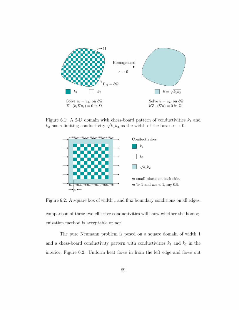
Ω

ΓD = ∂Ω

Homogenized

k1 k2 k =√k1k2

ǫ→ 0

Solve u = uD on ∂Ωk∇ · (∇u) = 0 in Ω

Solve uǫ = uD on ∂Ω∇ · (kǫ∇uǫ) = 0 in Ω

Figure 6.1: A 2-D domain with chess-board pattern of conductivities k1 andk2 has a limiting conductivity

√k1k2 as the width of the boxes ε → 0.

√k1k2

k1

k2

Conductivities

ǫ

m small blocks on each side.

m≫ 1 and mǫ < 1, say 0.9.

Figure 6.2: A square box of width 1 and flux boundary conditions on all edges.

comparison of these two effective conductivities will show whether the homog-

enization method is acceptable or not.

The pure Neumann problem is posed on a square domain of width 1

and a chess-board conductivity pattern with conductivities k1 and k2 in the

interior, Figure 6.2. Uniform heat flows in from the left edge and flows out

89

from the right edge. The magnitude of the flux is f . The top and bottom

edges are insulated. To avoid boundary effects a thin layer of material near

the boundary has conductivity equal to the homogenized limit√

k1k2. Since

this is a pure Neumann problem, we have to fix a datum. We choose the

minimum temperature in the domain to be exactly 0.

Figure 6.3(a) and Figure 6.3(b) show the conductivity pattern as a

function of x and y and the temperature profile for 8 small boxes on each side

(ε = 0.125) and each small box discretized by 10 bilinear quads. Conductivity

values are k1 = 1 and k2 = 10 and magnitude of imposed flux is 1.

(a) (b)

Figure 6.3: (a) The conductivity pattern for k1 = 1 and k2 = 10 and ε = 0.125in a box of width 1. (b) The plot shows a finite element solution for thetemperature when the magnitude of the imposed flux is 1 and the square isdiscretized by 80× 80 bilinear quad elements.

90

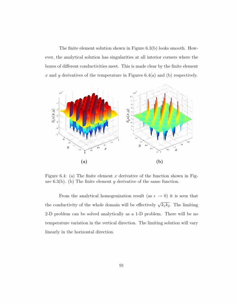
The finite element solution shown in Figure 6.3(b) looks smooth. How-

ever, the analytical solution has singularities at all interior corners where the

boxes of different conductivities meet. This is made clear by the finite element

x and y derivatives of the temperature in Figures 6.4(a) and (b) respectively.

(a) (b)

Figure 6.4: (a) The finite element x derivative of the function shown in Fig-ure 6.3(b). (b) The finite element y derivative of the same function.

From the analytical homogenization result (as ε → 0) it is seen that

the conductivity of the whole domain will be effectively√

k1k2. The limiting

2-D problem can be solved analytically as a 1-D problem. There will be no

temperature variation in the vertical direction. The limiting solution will vary

linearly in the horizontal direction.

91

The exact solution in the limit is

u(x, y) = (1− x)f√k1k2

, (6.1)

where u denotes the temperature, and f is the magnitude of boundary flux.

Using Equation (6.1), the maximum temperature in the box is at x = 0 and

is equal to f√k1k2

. Thus, a computable definition of effective conductivity is

keff :=f

maxx,y(u(x, y))−minx,y(u(x, y))=

f

maxx,y(u(x, y)). (6.2)

We compute keff for the finite element solution also. The local numer-

ical homogenization method is used to upscale the whole domain into a single

quad with bilinear shape functions. The output is a coarse-scale symmetric

“stiffness” matrix of size 4 (the number of DOFs in the coarse-scale element).

We can then extract the best conductivity from this stiffness matrix and com-

pare it with the keff for the finite element solution using Equation (6.2). De-

note the numerically homogenized conductivity kε (because it will vary with

ε).

For a bilinear quad with conductivity k and vertex nodes ordered as

[ 1 = (0,0), 2 = (1,0), 3 = (0,1), 4 = (1,1) ], the element stiffness matrix is

K = kK0 where K0 =1

6

4 −1 −1 −2

−1 4 −2 −1−1 −2 4 −1−2 −1 −1 4

The numerical homogenization algorithm will give the coarse-scale matrix K

of size 4× 4. In general it will not be proportional to K so we cannot extract

92

a conductivity kε for making a comparison. We use Frobenius matrix norm to

get the best kε such that∣∣∣∣∣∣K − K

∣∣∣∣∣∣2F

is minimum. This gives

kε =K0 : K

K0 : K0

=trace(KT

0 K)

trace(KT0 K0)

where ‘:’ is the matrix inner product induced by the Frobenius norm and

‘trace’ is the matrix trace. Note that this extraction of a single number k is

just for the comparison purposes of this section. For finite element assembly

in a “real” problem we use the matrix K obtained after homogenization.

For a fixed k1 = 1 and variable k2 > 1, Figure 6.5 shows the comparison

between the limiting conductivity (√

k2) and kε produced by the homogeniza-

tion method. k2 is varied from 1 to 100. The curves show that for this range

and a fixed number of elements (1600) to resolve the solution, the two values

are quite close. The difference increases for large contrast between k1 and k2

but it may be possible to rectify that by using smaller and more elements in

the mesh to resolve the singularities in the solution derivatives. We do not

attempt that here.

6.2 Alternatives in homogenization error functional

In Section 4.3 we formulated the local numerical homogenization prob-

lem when a local self-equilibrated load is known. In Section 4.4 we formulated

the same problem by treating all loads equally. In both cases we had used a

norm (given by a matrix B) to compare the local fine-scale and coarse-scale

compliance matrices. Thus, we have to make two choices − whether a known

93

Limiting and Numerical Conductivities as functions of k_2

1

10

1 10 100

k_2

Effective Conductivity

k_epsilon

sqrt(k_2)

Figure 6.5: A comparison between limiting conductivity√

k1k2 and homoge-nized conductivity kε as k2 is varied and k1 = 1 fixed.

load is used and which norm is used to compare coarse-scale and fine-scale so-

lutions. Using the chess-board conductivity problem of Section 6.1, we present

numerical evidence that the alternative in which the load is known, and we use

a norm that compares errors only on the boundary of the domain is a better

choice.

Consider the first choice, that the known local load be used. If we

minimize the homogenization error for a particular load, we should get a better

solution. This seems obvious. The choice in the case of norm needs a little

explanation. As will be shown, if we compare errors only on the boundary

(instead of the whole domain) we get a better solution. A finite element

interacts with the rest of the domain through the boundary. For example, in

94

the 1-D example of springs solved in Section 4.1, the process of homogenization

reduces the N spring constants to just one. The rest of the domain (or the

exterior) cannot know by interacting with an element what is there inside (at

least in this 1-D example). In that sense, homogenization is exact. But even

with the exact homogenization, the errors in the interior are not zero. Thus,

they should not be expected to be small, and should not be compared.

Figure 6.6 shows the errors made by making these choices. The curves

show the relative errors between kε and expected exact k =√

k1k2 while k1 = 1

fixed and k2 is varied between 1 and 25.

Symbol k F SN denotes the curve where the known self-equilibrated

“force” (or “load”) is used in conjunction with a special norm. Here we use

the boundary flux and the special weighs the errors in the interior as 100 times

less important than boundary errors. This idea is similar to the weighted `2

used in the end of Section 4.8. Symbol k SN denotes the curve where the load

is not used, but the special norm is. Symbol k F N denotes the curve where

the load is used, but the norm is the `2 norm. Symbol k N denotes the case

where no load is used and the norm is the `2 norm. As seen, using the known

load is better than not using it. Similarly, using the weighted norm is better

than not using the weighted norm.

6.3 Computational time for different element sizes

A typical mesh in the sequence of meshes generated for automatic mesh

adaptivity will have elements of all sizes. For allocating different elements

95

Relative Error for Various Homogenization Methods

(relative to k_epsilon)

-20

-15

-10

-5

0

5

10

1 2 3 4 5 6

k_epsilon

Relative Error (%)

k_F_SN

k_SN

k_F_N

k_N

Figure 6.6: The four curves show the relative errors between homogenizedconductivity kε and analytic conductivity

√k1k2 for various choices made in

defining the homogenization error. See text in Section 6.2 for details.

to different processors it is necessary to know in advance the time taken to

homogenize elements as a function of element size n (number of SFIL particles

in each element side). We compute homogenization time for hexahedral and

quadrilateral elements of polynomial degree 1 and identical number of cells in

each side.

The most expensive step is computing the pseudoinverse of the element

stiffness matrix. In Chapter 5 we presented a few algorithms for computing

Moore-Penrose pseudoinverses. Here, we compute pseudoinverses using two

kinds of algorithms − sparse Cholesky factorization of (Section 5.4.1) and

iterative methods based on known null space (Section 5.4.2).

For the iterative case, we choose the conjugate gradient (CG) and min-

imum residual (MINRES) methods. As preconditioners, we use Jacobi pre-

96

conditioner and Incomplete Cholesky (ICC). MINRES is also tried because

stiffness matrices in SFIL can be indefinite in a particular iteration. These

are implemented in PETSc [11]. The sparse Cholesky factorization is imple-

mented in CHOLMOD [33]. Thus, we analyze four different iterative schemes

and one direct scheme. The trends in homogenization times presented below

can be taken as trends in times taken to compute pseudoinverse (of the element

stiffness matrix) using these 5 different schemes.

Figures 6.7 and Figure 6.8 show the results for 2-D and 3-D respectively.

The computation time increases as a power law. For n as the element size, we

compute the best-fit homogenization time as a power law 10AnB. The best-fit

constants A and B are in Figure 6.9. We mention a few observations

For small elements, sparse Cholesky is better than iterative schemes.

In 2-D, it is much better, and never loses to the iterative schemes. In 3-D, for

small elements sparse Cholesky is better but not by much. Iterative schemes

are better beyond n = 8. This might be due to higher fill-in in 3-D.

Between the four iterative schemes, depending on element size n, the

best iterative scheme keeps on changing, but they are all very close together.

For small n, Jacobi preconditioner is better than ICC for both 2-D and 3-D

even though it leads to slower convergence (uses more iterations, not shown

here). ICC is more complicated to setup so it does not help much compared

to Jacobi unless n increases and the number of iterations taken increase a lot

with Jacobi.

97

0.0001

0.001

0.01

0.1

1

2 4 8 16 32

Tim

e (

se

co

nd

s)

Number of points in element side

Homogenization time in 2D

CG ICCCG Jacobi

Minres ICCMinres JacobiSparse Direct

Figure 6.7: The figure shows computation time to homogenize a 2-D quadri-lateral element with 8 DOFs (2 per corner) as the element size changes. Theelement size is number of particles on each side of the quadrilateral. Differentpseudoinverse methods lead to different times.

6.4 Optimum element size for homogenization of a cu-bical lattice

Given a cubical geometry with a fixed number of points p on each side,

we might want to divide the lattice into m elements on each side. If there are

n points in each element, we have a relation between p, m, and n.

p = m n−m + 1 or equivalently m =p− 1

n− 1

98

0.001

0.01

0.1

1

10

2 4 8 16

Tim

e (

se

co

nd

s)

Number of points in element side

Homogenization time in 3D

CG ICCCG Jacobi

Minres ICCMinres JacobiSparse Direct

Figure 6.8: The figure shows computation time to homogenize a 3-D hex-ahedral element with 24 DOFs (3 per corner) as the element size changes.The element size is number of particles on each side of the cube. Differentpseudoinverse methods lead to different times.

Figure 6.10 shows a 2-D cartoon of the fine and coarse lattices. We want

to decide n to minimize the computational cost of homogenizing the whole

cubical lattice into a coarse mesh.

Let H(n, p) be the total time to compute the homogenized Newton step

for the full lattice. It consists of md homogenizations and 1 linear solve using

99

2.63-5.09Cholesky

Sparse

Direct

2.82-4.90Minres

Jacobi

2.77-4.96Minres

ICC

2.72-4.82CG

Jacobi

2.73-4.95CG

ICC

BBBBAAAAMethodMethodMethodMethod

5.91-5.69Cholesky

Sparse

Direct

4.69-4.78Minres

Jacobi

4.14-4.19Minres

ICC

4.50-4.68CG

Jacobi

4.09-4.16CG

ICC

BBBBAAAAMethodMethodMethodMethod

Space dimension = 2 Space dimension = 3

Figure 6.9: The best-fit power law constants A and B for homogenization timein 2-D (Figure 6.7) and 3-D (Figure 6.8). The computation time is modeledby T (n) = 10−AnB, where n is the element size.

p points on each side m elements on each side,

each with n points

Original lattice Homogenized lattice

Figure 6.10: A fine-scale lattice with p particles on each side and a coarse mesh(homogenized lattice) with m elements, each containing n point particles.

100

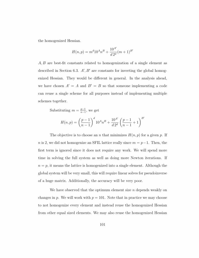
the homogenized Hessian.

H(n, p) = md10AnB +10A′

d 2d(m + 1)B′

A, B are best-fit constants related to homogenization of a single element as

described in Section 6.3. A′, B′ are constants for inverting the global homog-

enized Hessian. They would be different in general. In the analysis ahead,

we have chosen A′ = A and B′ = B so that someone implementing a code

can reuse a single scheme for all purposes instead of implementing multiple

schemes together.

Substituting m = p−1n−1

, we get

H(n, p) =

(p− 1

n− 1

)d

10AnB +10A′

d 2d

(p− 1

n− 1+ 1

)B′

The objective is to choose an n that minimizes H(n, p) for a given p. If

n is 2, we did not homogenize an SFIL lattice really since m = p−1. Then, the

first term is ignored since it does not require any work. We will spend more

time in solving the full system as well as doing more Newton iterations. If

n = p, it means the lattice is homogenized into a single element. Although the

global system will be very small, this will require linear solves for pseudoinverse

of a huge matrix. Additionally, the accuracy will be very poor.

We have observed that the optimum element size n depends weakly on

changes in p. We will work with p = 101. Note that in practice we may choose

to not homogenize every element and instead reuse the homogenized Hessian

from other equal sized elements. We may also reuse the homogenized Hessian

101

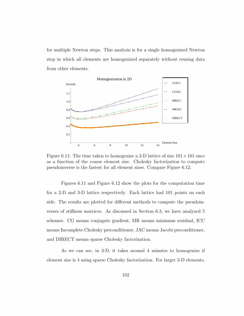
for multiple Newton steps. This analysis is for a single homogenized Newton

step in which all elements are homogenized separately without reusing data

from other elements.

4 6 8 10 12 14Element Size

0.2

0.4

0.6

0.8

1.0

1.2

Seconds

Homogenization in 2D

DIRECT

MRJAC

MRICC

CGJAC

CGICC

Figure 6.11: The time taken to homogenize a 2-D lattice of size 101×101 onceas a function of the coarse element size. Cholesky factorization to computepseudoinverse is the fastest for all element sizes. Compare Figure 6.12.

Figures 6.11 and Figure 6.12 show the plots for the computation time

for a 2-D and 3-D lattice respectively. Each lattice had 101 points on each

side. The results are plotted for different methods to compute the pseudoin-

verses of stiffness matrices. As discussed in Section 6.3, we have analyzed 5

schemes. CG means conjugate gradient, MR means minimum residual, ICC

means Incomplete Cholesky preconditioner, JAC means Jacobi preconditioner,

and DIRECT means sparse Cholesky factorization.

As we can see, in 3-D, it takes around 4 minutes to homogenize if

element size is 4 using sparse Cholesky factorization. For larger 3-D elements,

102

4 5 6 7 8 9 10Element Size

500

1000

1500

2000

Seconds

Homogenization in 3D

DIRECT

MRJAC

MRICC

CGJAC

CGICC

Figure 6.12: The time taken to homogenize a 3-D lattice of size 101 × 101 ×101 once as a function of the coarse element size. Cholesky factorization tocompute pseudoinverse is the fastest for small element sizes only. CompareFigure 6.11.

iterative schemes are faster than the sparse direct method. For 2-D, the sparse

direct method is always faster. The main reason why a sparse direct solver

came out as the best is due to multiple right hand sides. In 3-D, with 3 DOFs

per node, 24 (or 25 depending on if we use a known load) linear systems are

solved. For the given data, we see that the best idea is to choose n = 5 (4 cells

on each side), and use a sparse direct solver for local homogenization. Since

n− 1 is a power of 2, it will be beneficial for mesh adaptivity and refinements.

Thus, if initial mesh elements are too large, it is better to break them using

the optimum element size as a guideline.

103

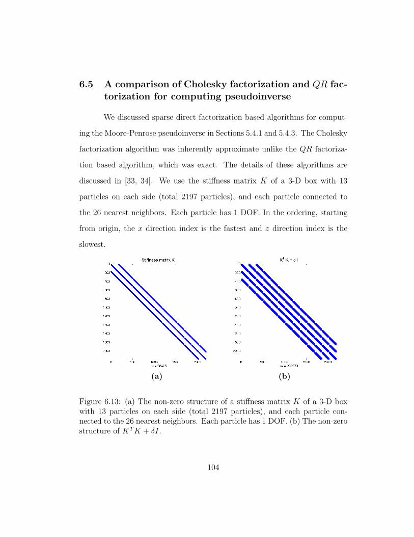
6.5 A comparison of Cholesky factorization and QR fac-torization for computing pseudoinverse

We discussed sparse direct factorization based algorithms for comput-

ing the Moore-Penrose pseudoinverse in Sections 5.4.1 and 5.4.3. The Cholesky

factorization algorithm was inherently approximate unlike the QR factoriza-

tion based algorithm, which was exact. The details of these algorithms are

discussed in [33, 34]. We use the stiffness matrix K of a 3-D box with 13

particles on each side (total 2197 particles), and each particle connected to

the 26 nearest neighbors. Each particle has 1 DOF. In the ordering, starting

from origin, the x direction index is the fastest and z direction index is the

slowest.

(a) (b)

Figure 6.13: (a) The non-zero structure of a stiffness matrix K of a 3-D boxwith 13 particles on each side (total 2197 particles), and each particle con-nected to the 26 nearest neighbors. Each particle has 1 DOF. (b) The non-zerostructure of KT K + δI.

104

Figures 6.13(a) and (b) show the stiffness matrix and the matrix KT K+

δI discussed in Section 5.4.1 used for Tikhonov regularization. Figures 6.14(a)

and (b) show the permutation matrix P and the upper triangular factor R such

that P T (KT K+δI)P = RT R. Figure 6.15(a) shows the upper triangular factor

R when no permutation is used (P = I). The factor has the same bandwidth

as the matrix (KT K + δI) and is dense within the band.

Figure 6.15(b) show the permutation (produced by COLAMD [34]) for

a fill-in reducing sparse QR factorization of K. Figures 6.16(a) and (b) show

the sparse orthogonal factor Q and the sparse upper triangular factor R such

that KP = QR.

0 500 1000 1500 2000

0

200

400

600

800

1000

1200

1400

1600

1800

2000

nz = 2197

Permutation matrix P for Cholesky factorization

(a) (b)

Figure 6.14: (a) The non-zero structure of the permutation matrix P thatreduces fill-in for Cholesky factorization of KT K + δI. (b) The non-zerostructure of the upper triangular Cholesky factor R of KT K + δI such thatP T (KT K + δI)P = RT R.

105

0 500 1000 1500 2000

0

200

400

600

800

1000

1200

1400

1600

1800

2000

nz = 2197

Permutation matrix P for sparse QR

(a) (b)

Figure 6.15: (a) The non-zero structure of the upper triangular Choleskyfactor R of KT K + δI such that KT K + δI = RT R. No permutation matrixis used. (b) The non-zero structure of the permutation matrix P for a sparseQR decomposition of K such that KP = QR. See Figure 6.16.

(a) (b)

Figure 6.16: (a) The non-zero structure of the orthogonal matrix Q for asparse QR decomposition of KP . See Figure 6.15(b) for P . (b) The non-zerostructure of the upper triangular matrix R where KP = QR.

106

On a 1.5 GHz single core processor, the sparse Cholesky factorization

with reordering took 0.235 seconds. The banded Cholesky factorization took

0.238 seconds. The difference is insignificant. However, the upper triangular

factor had 16% more non-zeroes for the banded factor. This would make

back-substitution slightly expensive.

The sparse QR factorization took 1.196 seconds, nearly 5 times slower

than Cholesky factorization. In addition, the number of non-zeroes in Q and

R combined was 4 times the number of non-zeroes in the Cholesky factor R.

6.6 Features of sparse algorithms for pseudoinverse

Finally, based on the results presented here and in Sections 6.3 and 6.5,

we have created a feature classification matrix for the various pseudoinverse

algorithms. This is presented in Figure 6.17. At least for the initial itera-

tions, the approximate pseudoinverse method using Tikhonov regularization

presented in Section 5.4.1 may be the best because of its speed.

We have not integrated sparse QR factorization with homogenization

yet. The features and classifications are based on analytical formulas and

preliminary code testing using [34].

These results are for a specific SFIL lattices, for a single step in the

Newton iterations, specific libraries (PETSc, CHOLMOD), and a typical re-

cent CPU (Intel Core 2 Duo, 1.5 GHz). However, for any changes in the

configuration, the time analysis can be done automatically for a few typical

107

Good

Null space

Depends

(iterative)

Medium

Multiple solves

Depends (If multiple RHS)

Null space basedNull space basedNull space basedNull space based

Good

No

Yes

High

Factorize once

Good

Sparse QRSparse QRSparse QRSparse QR

Bad (little better if Sparse QR used)

Smallest singular value magnitude

No

Medium

Factorize once

Fast

Regularize + Regularize + Regularize + Regularize + CholeskyCholeskyCholeskyCholesky

Exact (up to floating point)

Software complexity

Fast (although this is element dependent)

Conditioning

Prior information needed

Multiple RHS

Criterion and itsCriterion and itsCriterion and itsCriterion and its

importance (to us)importance (to us)importance (to us)importance (to us)

Not good

Good

Medium

Important Criterion

Figure 6.17: Features of algorithms for computing Moore-Penrose pseudoin-verse discussed in Chapter 5. None of the algorithms is the best amongst alldepending on the kind of problem to be homogenized.

elements and the best method can be chosen accordingly at run-time.

6.7 Convergence rate of uniform mesh refinements

We present the results of homogenization of a 2-D lattice with 21 par-

ticles on each side and “random” bonds. The bottom layer of particles is fixed

with equal inter-particle distance 1.3 and the lattice relaxes under zero exter-

nal forces. The objective is to compute the convergence rate of error in energy

norm as the coarse mesh element size is reduced to the fine-scale elements.

108

The steps of homogenization and nonlinear Newton iterations are integrated

as shown earlier in Figure 4.6. In this case, however, the mesh is always refined

uniformly in h.

Figure 6.18 shows the lattice topology. The lattice consists of two kinds

of harmonic bonds with different parameters (equilibrium length and stiffness).

The bonds are randomly distributed. The darker color represents the first kind

of bond with stiffness 0.4 and length 1.2. The lighter color signifies the second

kind with stiffness 1 and length 1. Figure 6.19 shows an equilibrium solution

starting from a square lattice as the initial guess.

Figure 6.18: A “random” 2-D lattice with 21 particles on each side.

We use various element sizes for the coarse mesh to homogenize the

lattice. Figure 6.21 shows the results. The nonlinear problem is homoge-

nized using load-independent homogenization (Section 4.4) with 1, 4, and 16

“square” elements with 400, 100, and 25 lattice “cells” in each element. As

seen, the solutions obtained after homogenization match the fine-scale solu-

tion very well. Figure 6.20 shows the global relative error in `2 norm when

compared to the non-homogenized fine-scale solution.

109

Figure 6.19: An equilibrium solution for the lattice topology shown in Fig-ure 6.18 and fixed bottom layer.

Error due to homogenization

50 DOFs

3.0% Error

18 DOFs

7.4% Error

8 DOFs

16.7% Error

1.0%

10.0%

100.0%

1 10 100

Degrees of Freedom

Percentage Error

1

0.93

Figure 6.20: The global relative error in `2 norm for various levels of homoge-nization shown in Figure 6.21. The exact solution is specified by 882 degreesof freedom.

6.8 Integration of homogenization with adaptivity andNewton iterations

In this section, we show results that combine automatic h-adaptivity

with nonlinear iterations and local homogenization for SFIL lattice problems.

110

Figure 6.21: An oblique view of the equilibrium solutions for the lattice shownin Figure 6.18 after homogenizing the lattice at various resolutions. Thebottom-right lattice is the non-homogenized solution taken from Figure 6.19.

These three techniques are integrated by the logic shown in Figure 4.6. We

present results for 2-D and 3-D lattices and compare meshes generated by

energy-oriented and goal-oriented adaptivity. In contrast, the results presented

in Chapter 3 were for automatic hp-adaptivity for linear problems with smooth

material data on cubic lattices and without local homogenization.

Although the real SFIL lattice model is in 3-D, we show the progress

of mesh refinements in 2-D first because of the clarity it provides. This 2-D

lattice model has 128× 128 cells. The base is fixed and the lattice is deformed

to its minimum energy configuration for a sequence of coarse meshes. We run

the algorithm two times but use a different strategy in both cases. First we

111

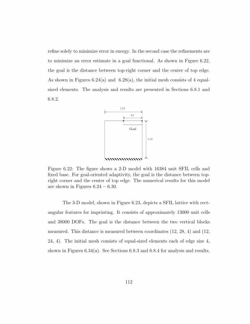
refine solely to minimize error in energy. In the second case the refinements are

to minimize an error estimate in a goal functional. As shown in Figure 6.22,

the goal is the distance between top-right corner and the center of top edge.

As shown in Figures 6.24(a) and 6.28(a), the initial mesh consists of 4 equal-

sized elements. The analysis and results are presented in Sections 6.8.1 and

6.8.2.

128

128

64

Goal

Figure 6.22: The figure shows a 2-D model with 16384 unit SFIL cells andfixed base. For goal-oriented adaptivity, the goal is the distance between top-right corner and the center of top edge. The numerical results for this modelare shown in Figures 6.24− 6.30.

The 3-D model, shown in Figure 6.23, depicts a SFIL lattice with rect-

angular features for imprinting. It consists of approximately 13000 unit cells

and 38000 DOFs. The goal is the distance between the two vertical blocks

measured. This distance is measured between coordinates (12, 28, 4) and (12,

24, 4). The initial mesh consists of equal-sized elements each of edge size 4,

shown in Figures 6.34(a). See Sections 6.8.3 and 6.8.4 for analysis and results.

112

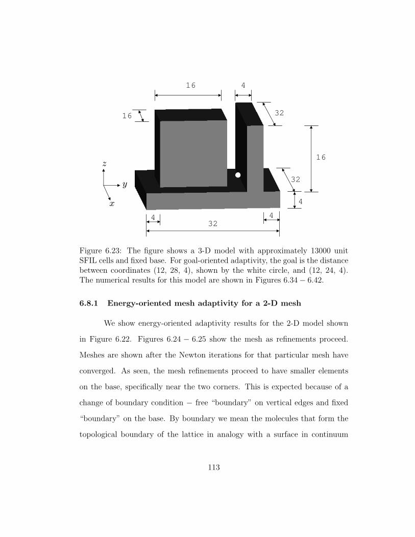
4

16

32

4

32

32

416

16

4

x

z

y

Figure 6.23: The figure shows a 3-D model with approximately 13000 unitSFIL cells and fixed base. For goal-oriented adaptivity, the goal is the distancebetween coordinates (12, 28, 4), shown by the white circle, and (12, 24, 4).The numerical results for this model are shown in Figures 6.34− 6.42.

6.8.1 Energy-oriented mesh adaptivity for a 2-D mesh

We show energy-oriented adaptivity results for the 2-D model shown

in Figure 6.22. Figures 6.24 − 6.25 show the mesh as refinements proceed.

Meshes are shown after the Newton iterations for that particular mesh have

converged. As seen, the mesh refinements proceed to have smaller elements

on the base, specifically near the two corners. This is expected because of a

change of boundary condition − free “boundary” on vertical edges and fixed

“boundary” on the base. By boundary we mean the molecules that form the

topological boundary of the lattice in analogy with a surface in continuum

113

material. The refinements are not necessarily symmetric in each step because

different bonds and molecules are randomly distributed, being generated by

the Monte-Carlo algorithm discussed in Section 2.2.3.

(a) Initial Guess (b) Iteration 1

(c) Iteration 2 (d) Iteration 3

Figure 6.24: Energy-oriented mesh adaptivity for a 2-D lattice of size 128 ×128 with fixed base boundary condition. Rest of the iterations are shown inFigure 6.25. Compare goal-oriented mesh adaptivity in Figures 6.28− 6.29.

114

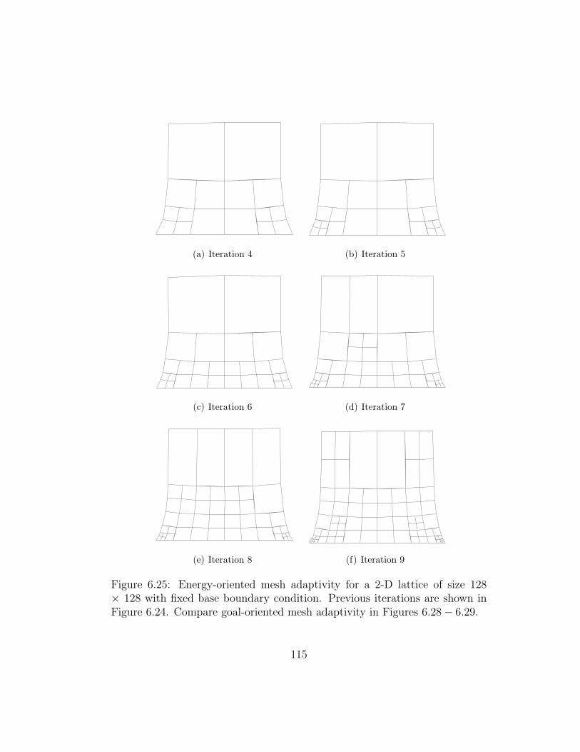
(a) Iteration 4 (b) Iteration 5

(c) Iteration 6 (d) Iteration 7

(e) Iteration 8 (f) Iteration 9

Figure 6.25: Energy-oriented mesh adaptivity for a 2-D lattice of size 128× 128 with fixed base boundary condition. Previous iterations are shown inFigure 6.24. Compare goal-oriented mesh adaptivity in Figures 6.28− 6.29.

115

0.1

1

10

100

1000

0 10 20 30 40 50 60 70

Iteration

Error in Energy (%)

(a) Error in energy (%)

0.001

0.01

0.1

1

10

0 10 20 30 40 50 60

Iteration

Homogenized Residual Norm per DOF

(b) Homogenized residual norm per DOF

Figure 6.26: The graphs show how the minimum energy and residual normchange as mesh is refined using energy-oriented adaptivity and Newton it-erations proceed. (a) The kinks are present where mesh is refined and theinstantaneous rate of decrease of energy is higher. (b) The residual decreaseswith Newton iterations and goes up again upon mesh refinements. This isbecause fine-scale becomes more important. Compare with Figure 6.31.

116

Error estimate for converged mesh

0

0.2

0.4

0.6

0.8

1

1.2

0 5 10 15 20 25 30 35 40 45

Element Number

Error estimate

(a) A posteriori error estimates in various elements

1

10

100

0 20 40 60 80 100 120

Number of DOFs

Error in Energy

(b) Error in energy versus number of DOFs

Figure 6.27: The graphs show the distribution of errors in various elementsand the decrease of error in energy with the increasing number of DOFs forenergy-oriented adaptivity. Compare with Figure 6.32.

117

Figure 6.26(a) shows convergence of error, measured as the difference

of energy for current mesh and the minimum energy, as Newton iterations

and mesh iterations proceed. The kinks are at iterations where the mesh is

refined because the solution has numerically converged for the current mesh.

Except while approaching the kinks (from the left) the reduction in error is

smooth. In Figure 6.26(b), we plot the homogenized residual per DOF at

each iteration. By homogenized residual we mean the vector that drives the

Newton iterations. We divide by the number of DOFs because the number of

DOFs increases as the mesh is refined. The residual goes up again upon mesh

refinements because further details of the fine-scale are seen. The solution is

the best in energy only for the coarser mesh.

Figure 6.27(a) shows a posteriori error estimates in various elements

for the last mesh. The variation in error in different elements is not too large,

which is a good sign. Figure 6.27(b) is a plot of absolute error versus number

of DOFs as the refinements proceed. The rate of decrease is almost constant

throughout the iterations. Compare this with the plot in Figure 6.32 for goal-

oriented adaptivity in which the corresponding curve is nearly flat.

6.8.2 Goal-oriented mesh adaptivity for a 2-D mesh

We show goal-oriented adaptivity results for the 2-D model shown in

Figure 6.22. Figures 6.28 − 6.29 show the mesh as refinements proceed. As

expected, the mesh refinements proceed to have smaller elements near the two

points that are needed to compute the goal.

118

(a) Initial Guess (b) Iteration 1

(c) Iteration 2 (d) Iteration 3

(e) Iteration 4 (f) Iteration 5

Figure 6.28: Goal-oriented mesh adaptivity for a 2-D lattice of size 128 ×128 with fixed base boundary condition. The goal is the distance between thetop-right corner and center of top edge. Rest of the iterations are shown inFigure 6.29. Compare energy-oriented mesh adaptivity in Figures 6.24− 6.25.

119

(a) Iteration 6 (b) Iteration 7

(c) Iteration 8 (d) Iteration 9

Figure 6.29: Goal-oriented mesh adaptivity for a 2-D lattice of size 128 ×128 with fixed base boundary condition. The goal is the distance betweenthe top-right corner and center of top edge. Previous iterations are shown inFigure 6.28. Compare energy-oriented mesh adaptivity in Figures 6.24− 6.25.

Figure 6.30 shows the meshes for the converged solution for energy-

oriented and goal-oriented adaptivity. Figure 6.31(a) shows convergence of

error, measured as the difference of energy for current mesh and the minimum

energy, as Newton iterations and mesh iterations proceed. The kinks are at

some of the iterations where the mesh is refined because the solution has

numerically converged for the current mesh. The curve is much flatter than

the curve shown in Figure 6.26(a) because the primary purpose of iterations

120

is to reduce the error in goal. In Figure 6.31(b), we plot the homogenized

residual per DOF at each iteration. By homogenized residual we mean the

vector that drives the Newton iterations. We divide by the number of DOFs

because as the mesh is refined the number of DOFs increases. The residual

goes up again upon mesh refinements because further details of the fine-scale

are seen. The solution is the best in energy only for the coarser mesh.

Figure 6.32(a) shows a posteriori error estimates in various elements

for the last mesh. The variation in error in different elements is not too large,

which is a good sign. Figure 6.32(b) is a plot of absolute error versus number of

DOFs as the refinements proceed. The error is almost constant throughout the

iterations. Compare this with the plot in Figure 6.27(b) for energy-oriented

adaptivity in which the corresponding curve does not have flat regions.

(a) Energy-oriented adaptivity (b) Goal-oriented adaptivity

Figure 6.30: Final meshes generated by energy-oriented adaptivity and goal-oriented adaptivity. The goal is the distance between top-right corner and thecenter of top edge.

121

1

10

100

1000

0 10 20 30 40 50

Iteration

Error in Energy (%)

(a) Error in energy (%)

0.001

0.01

0.1

1

10

0 10 20 30 40 50

Iteration

Homogenized Residual Norm per DOF

(b) Homogenized residual norm per DOF

Figure 6.31: The graphs show how the minimum energy and residual normchange as mesh is refined using goal-oriented adaptivity and Newton iterationsproceed. (a) The kinks are present where mesh is refined and the instantaneousrate of decrease of energy is higher. (b) The residual decreases with Newtoniterations and goes up again upon mesh refinements. This is because fine-scalebecomes more important. Compare with Figure 6.26.

122

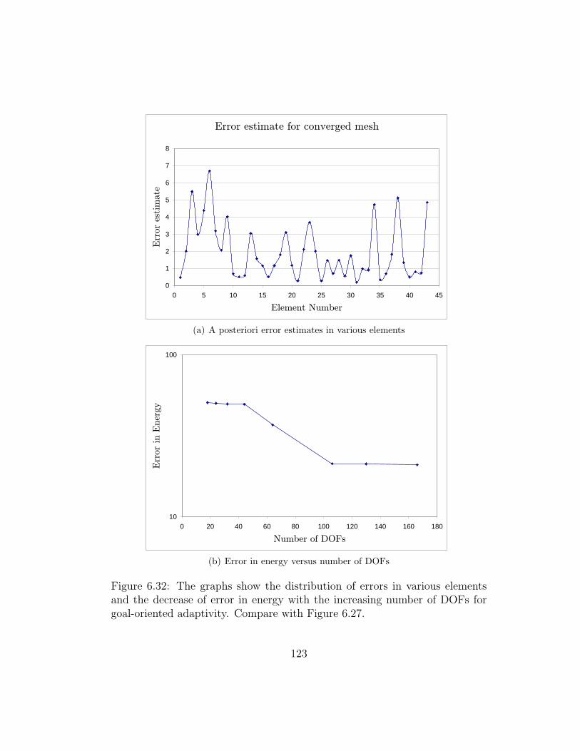
Error estimate for converged mesh

0

1

2

3

4

5

6

7

8

0 5 10 15 20 25 30 35 40 45

Element Number

Error estimate

(a) A posteriori error estimates in various elements

10

100

0 20 40 60 80 100 120 140 160 180

Number of DOFs

Error in Energy

(b) Error in energy versus number of DOFs

Figure 6.32: The graphs show the distribution of errors in various elementsand the decrease of error in energy with the increasing number of DOFs forgoal-oriented adaptivity. Compare with Figure 6.27.

123

10

100

1000

10 100 1000

Number of DOFs

Error Estimate for Goal

(a) Error estimate in goal versus number of DOFs

1.E-06

1.E-05

1.E-04

1.E-03

1.E-02

1.E-01

1.E+00

1.E+01

0 100 200 300

Element Number

Error Estim

ate for goal

StandardCharacterization

Error term due toHomogenization

(b) Components of error estimate as discussed in Section 4.10

Figure 6.33: The decrease in error estimate for goal-oriented mesh adaptivityand components of error estimate as discussed in Section 4.10.

124

The error estimate in goal, however, decreases uniformly as seen in

Figure 6.33(a). We also plot the error estimates for individual elements in

Figure 6.33(b). The estimate is divided into two parts − the standard charac-

terization and the term due to homogenization (Section 4.10). The error due

to homogenization is larger by around 1 order of magnitude.

6.8.3 Energy-oriented mesh adaptivity for a 3-D mesh

We show energy-oriented adaptivity results for the 3-D model shown

in Figure 6.23. Figures 6.34 − 6.35 show the mesh as refinements proceed.

Meshes are shown after the Newton iterations for that particular mesh have

converged. We start with a mesh that has equal elements of size 4. As seen,

the mesh refinements proceed to have smaller elements where the lattice has

abrupt changes, either in boundary conditions or the presence of topological

features like corners or edges. The first refinements just take care of the four

corners of the base (Figure 6.35(a)). Next come the four edges of the base and

the 4 corners of the block placed on the base (Figure 6.35(b)). Similar to the

2-D model in Figures 6.24− 6.25, the refinements happen near discontinuities

in the boundary and boundary conditions. The final mesh is shown more

clearly in Figure 6.36 with the view axis aligned to the coordinate axes.

Figure 6.37(a) shows convergence of error, measured as the difference

of energy for current mesh and the minimum energy, as Newton iterations

and mesh iterations proceed. The kinks are at iterations where the mesh is

refined because the solution has numerically converged for the current mesh.

125

Except while approaching the kinks (from the left) the reduction in error is

smooth. In Figure 6.37(b), we plot the homogenized residual per DOF at

each iteration. By homogenized residual we mean the vector that drives the

Newton iterations. We divide by the number of DOFs because as the mesh is

refined the number of DOFs increases. The residual goes up again upon mesh

refinements because further details of the fine-scale are seen. The solution is

the best in energy only for the coarser mesh. Figure 6.38(a) shows a posteriori

error estimates in various elements for the last mesh. The elements with lower

number are the initial mesh elements. Some of them have not been refined yet

and this explains larger error in the left of the graph. Figure 6.38(b) is a plot

of absolute error versus number of DOFs as the refinements proceed. The rate

of decrease is almost constant throughout the iterations. Compare this with

the almost flat curve in Figure 6.44 for goal-oriented adaptivity.

(a) Initial Guess (b) Iteration 1

Figure 6.34: Energy-oriented mesh adaptivity for a 3-D lattice shown in Fig-ure 6.23 with fixed base boundary condition. Rest of the iterations are shownin Figure 6.35. Compare goal-oriented mesh adaptivity in Figures 6.39− 6.40.

126

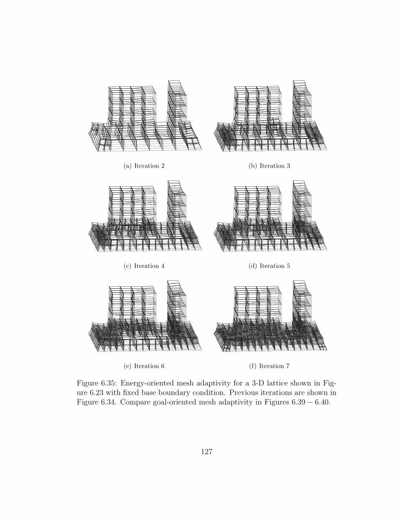
(a) Iteration 2 (b) Iteration 3

(c) Iteration 4 (d) Iteration 5

(e) Iteration 6 (f) Iteration 7

Figure 6.35: Energy-oriented mesh adaptivity for a 3-D lattice shown in Fig-ure 6.23 with fixed base boundary condition. Previous iterations are shown inFigure 6.34. Compare goal-oriented mesh adaptivity in Figures 6.39− 6.40.

127

(a) Front view

(b) Side view

(c) Top view

Figure 6.36: Front, side, and top views of converged mesh generated by energy-oriented adaptivity iterations shown in Figures 6.34 and 6.35. Compare withFigure 6.41.

128

1

10

100

1000

0 5 10 15 20 25 30

Iteration

Error in Energy (%)

(a) Error in energy (%)

1.00E-05

1.00E-04

1.00E-03

1.00E-02

1.00E-01

1.00E+00

0 5 10 15 20 25 30

Iteration

Homogenized Residual Norm per DOF

(b) Homogenized residual norm per DOF

Figure 6.37: The graphs show how the minimum energy and residual normchange as mesh is refined using energy-oriented adaptivity and Newton it-erations proceed. (a) The kinks are present where mesh is refined and theinstantaneous rate of decrease of energy is higher. (b) The residual decreaseswith Newton iterations and goes up again upon mesh refinements. This isbecause fine-scale becomes more important. Compare with Figure 6.43.

129

Error estimate for converged mesh

0

0.05

0.1

0.15

0.2

0.25

0.3

0.35

0 100 200 300 400 500 600

Element Number

Error estimate

(a) A posteriori error estimates in various elements

10

100

1000 1500 2000 2500 3000

Number of DOFs

Error in Energy

(b) Error in energy versus number of DOFs

Figure 6.38: The graphs show the distribution of errors in various elementsand the decrease of error in energy with the increasing number of DOFs forenergy-oriented adaptivity. Compare with Figure 6.44.

130

6.8.4 Goal-oriented mesh adaptivity for a 3-D mesh

We show energy-oriented adaptivity results for the 3-D model shown

in Figure 6.23. Figures 6.39 − 6.40 show the mesh as refinements proceed.

Meshes are shown after the Newton iterations for that particular mesh have

converged. We start with a mesh that has equal elements of size 4. The goal

is the distance between coordinates (12, 28, 4) and (12, 24, 4), see Figure 6.23.

The initial guess is shown in Figure 6.34(a). As expected, the mesh refinements

proceed to have smaller elements near these two points. Most of the larger

elements away from these two points are not refined, even though they need

to be refined for energy-oriented adaptivity (Figures 6.34 − 6.35). The final

mesh is shown more clearly in Figure 6.41 with the view axis aligned to the

coordinate axes.

(a) Iteration 1 (b) Iteration 2

Figure 6.39: Goal-oriented mesh adaptivity for a 3-D lattice shown in Fig-ure 6.23 with fixed base boundary condition. The goal is the distance betweenthe two blocks measured near the bottom. Rest of the iterations are shown inFigure 6.40. Compare energy-oriented mesh adaptivity in Figures 6.34− 6.35.

131

(a) Iteration 3 (b) Iteration 4

(c) Iteration 5 (d) Iteration 6

(e) Iteration 7 (f) Iteration 8

Figure 6.40: Goal-oriented mesh adaptivity for a 3-D lattice shown in Fig-ure 6.23 with fixed base boundary condition. The goal is the distance betweenthe two blocks measured near the bottom. Previous iterations are shown inFigure 6.39. Compare energy-oriented mesh adaptivity in Figures 6.34− 6.35.

132

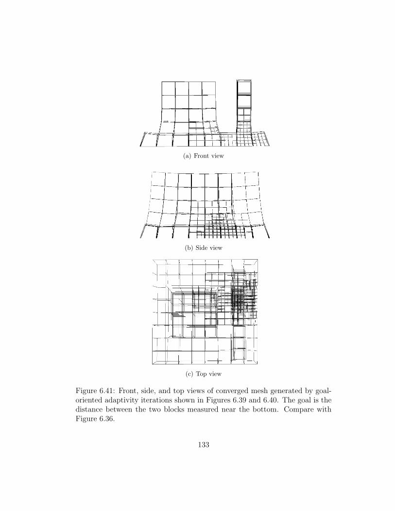
(a) Front view

(b) Side view

(c) Top view

Figure 6.41: Front, side, and top views of converged mesh generated by goal-oriented adaptivity iterations shown in Figures 6.39 and 6.40. The goal is thedistance between the two blocks measured near the bottom. Compare withFigure 6.36.

133

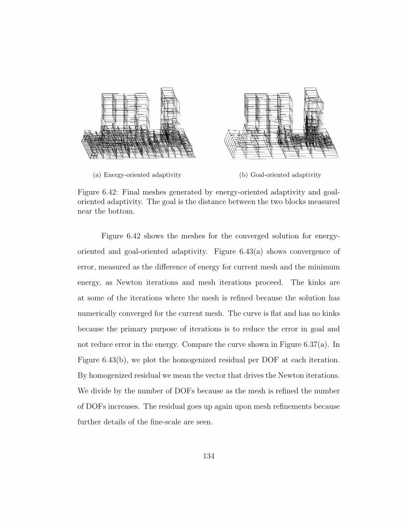
(a) Energy-oriented adaptivity (b) Goal-oriented adaptivity

Figure 6.42: Final meshes generated by energy-oriented adaptivity and goal-oriented adaptivity. The goal is the distance between the two blocks measurednear the bottom.

Figure 6.42 shows the meshes for the converged solution for energy-

oriented and goal-oriented adaptivity. Figure 6.43(a) shows convergence of

error, measured as the difference of energy for current mesh and the minimum

energy, as Newton iterations and mesh iterations proceed. The kinks are

at some of the iterations where the mesh is refined because the solution has

numerically converged for the current mesh. The curve is flat and has no kinks

because the primary purpose of iterations is to reduce the error in goal and

not reduce error in the energy. Compare the curve shown in Figure 6.37(a). In

Figure 6.43(b), we plot the homogenized residual per DOF at each iteration.

By homogenized residual we mean the vector that drives the Newton iterations.

We divide by the number of DOFs because as the mesh is refined the number

of DOFs increases. The residual goes up again upon mesh refinements because

further details of the fine-scale are seen.

134

1

10

100

1000

0 5 10 15 20 25 30

Iteration

Error in Energy (%)

(a) Error in energy (%)

1.00E-05

1.00E-04

1.00E-03

1.00E-02

1.00E-01

1.00E+00

0 5 10 15 20 25 30

Iteration

Homogenized Residual Norm per DOF

(b) Homogenized residual norm per DOF

Figure 6.43: The graphs show how the minimum energy and residual normchange as mesh is refined using goal-oriented adaptivity and Newton iterationsproceed. (a) The kinks are present where mesh is refined and the instantaneousrate of decrease of energy is higher. (b) The residual decreases with Newtoniterations and goes up again upon mesh refinements. This is because fine-scalebecomes more important. Compare with Figure 6.37.

135

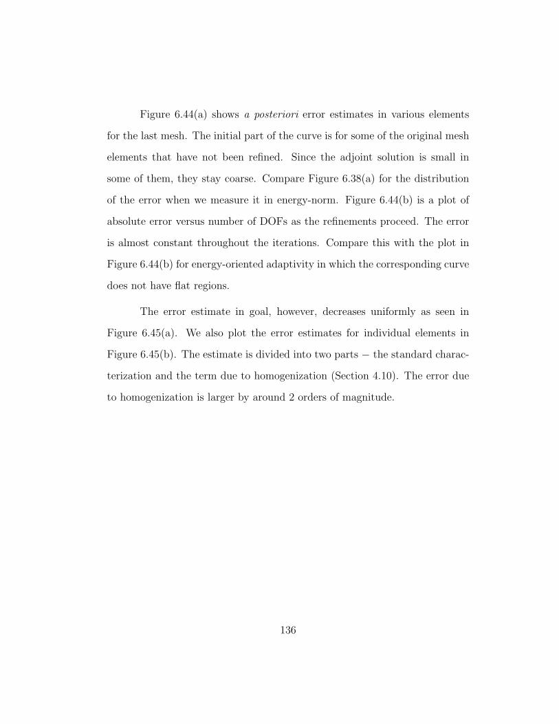
Figure 6.44(a) shows a posteriori error estimates in various elements

for the last mesh. The initial part of the curve is for some of the original mesh

elements that have not been refined. Since the adjoint solution is small in

some of them, they stay coarse. Compare Figure 6.38(a) for the distribution

of the error when we measure it in energy-norm. Figure 6.44(b) is a plot of

absolute error versus number of DOFs as the refinements proceed. The error

is almost constant throughout the iterations. Compare this with the plot in

Figure 6.44(b) for energy-oriented adaptivity in which the corresponding curve

does not have flat regions.

The error estimate in goal, however, decreases uniformly as seen in

Figure 6.45(a). We also plot the error estimates for individual elements in

Figure 6.45(b). The estimate is divided into two parts − the standard charac-

terization and the term due to homogenization (Section 4.10). The error due

to homogenization is larger by around 2 orders of magnitude.

136

Error estimate for converged mesh

0

0.002

0.004

0.006

0.008

0.01

0.012

0.014

0.016

0.018

0.02

0 50 100 150 200 250 300

Element Number

Error estimate

(a) A posteriori error estimates in various elements

20

22

24

26

28

30

32

34

36

38

40

1000 1200 1400 1600 1800 2000 2200 2400 2600

Number of DOFs

Error in Energy

(b) Error in energy versus number of DOFs

Figure 6.44: The graphs show the distribution of errors in various elementsand the decrease of error in energy with the increasing number of DOFs forgoal-oriented adaptivity. Compare with Figure 6.38.

137

0

2

4

6

8

10

12

1000 1200 1400 1600 1800 2000 2200 2400 2600

Number of DOFs

Error Estimate for Goal

(a) Error estimate in goal versus number of DOFs

1.E-09

1.E-08

1.E-07

1.E-06

1.E-05

1.E-04

1.E-03

1.E-02

0 500 1000 1500 2000 2500

Element Number

Error Estimate for goal

StandardCharacterization

Error term due toHomogenization

(b) Components of error estimate as discussed in Section 4.10

Figure 6.45: The decrease in error estimate for goal-oriented mesh adaptivityand components of error estimate as discussed in Section 4.10.

138

Chapter 7

Concluding Remarks and Directions for

Future Research

The objective of this dissertation was to develop and analyze a black-

box method for solving nonlinear problems with multiple scales due to rapidly

varying material data. We have achieved this using the following key ideas −

approximate mathematical models, error estimation with respect to the base

model, adaptive meshes, a local numerical homogenization method, and fast

algorithms for Moore-Penrose pseudoinverse.

Given a mesh that resolves the fine-scale, our method consists of creat-

ing a coarse mesh and numerically homogenizing the fine-scale material prop-

erties, that are linearized for a nonlinear problem, on each element separately.

For each coarse-mesh element, the numerically homogenized material proper-

ties are computed by solving a local constrained convex optimization problem.

The primary input is the Moore-Penrose pseudoinverse of local fine-scale stiff-

ness matrix. The solution of this problem is a coarse-scale material compliance

matrix. We refine the coarse-mesh based on an a posteriori error estimate until

convergence.

We have shown that the optimization problem that defines the local

139

homogenization method is well-posed and has a unique solution. We have also

shown that, for a certain choice of norm, homogenization preserves positive-

definiteness of the fine-scale operator. We verified the method for a material

with chess-board conductivity pattern. The possible choices for local homog-

enization were analyzed and it was seen that specific choices of local load and

norm can give better results. For computational feasibility, it was required that

we use fast algorithms for computing Moore-Penrose pseudoinverse of sparse

singular finite element matrices. We presented various algorithms that were

tailored for the purposes of this research. We studied the computational per-

formance of the method for various methods of computing pseudoinverses and

elements of various sizes. We derived optimal element sizes for homogenization

in the context of SFIL. Finally, we integrated mesh adaptivity and nonlinear

iterations with local homogenization. Convergence for both energy-oriented

and goal-oriented adaptivity was demonstrated.

This research was carried out with a specific physical problem in mind,

that of polymer shrinkage in Step and Flash Imprint Lithography process.

Moreover, the local homogenization method was used in a very specific way −

to create a coarse-scale Hessian matrix for finite element assembly. However,

this work can be applied to a wide class of problems in a variety of ways and

leads to many ideas for future research.

• As long as a suitable interpolation operator is used, it can be applied

to different kinds of finite elements. With further research, the method

140

developed here can be put to various other uses. For example, the coarse-

scale stiffness matrix can be used simply as a preconditioner for solving

the base model. Local homogenization can also be used as an indicator

to check whether locally the mesh is sufficiently refined (without solving

a global problem).

• Currently, the local constrained convex optimization problems are solved

approximately using a regularization approach using the parameter ε.

Although this has worked well and is justified due to the iterative nature

of the algorithm, it is not difficult to formulate the exact problem. It

is a linear system for constrained optimization with blocks consisting of

Kronecker product matrices. The problem how is to solve this efficiently

and look for any advantages it can provide. For example, each step of

the Newton iterations may be better in reducing the energy.

• We have fixed the choice of the local interpolation operator and norm

for measuring the local error using physical intuition. The accuracy of

these choices has been verified using numerical experiments. However,

it will be better if the intuition can be mathematically justified.

• Further analysis needs to be done to prove spectral properties of the ho-

mogenized stiffness matrix when the error is minimized in different norms

or whether the specific load formulation of the error is used. We have

proved that the homogenized stiffness matrix is positive semi-definite

141

when the fine-scale stiffness matrix is positive semi-definite and the er-

ror is minimized in the `2 norm and all loads are treated equally.

• Although we have tried three different algorithms for Moore-Penrose

pseudoinverse, we have not integrated the fourth one which uses “proper

splittings” to compute pseudoinverse of a modified matrix. It would

require more memory but it might make the overall method faster.

• We have implemented the algorithm for certain finite elements, specifi-

cally for quads and hexes with polynomial degree 1. To be widely ap-

plicable, we need to test and implement it for other elements and with

higher polynomial degrees.

• For larger systems, the homogenization can be done in parallel on mul-

tiple processors. We have done preliminary research to empirically de-

termine the optimal time to homogenize elements of various sizes. This

will be useful in allocating elements to different processors so that the

load is shared equally.

142

Appendices

143

Appendix A

Local Numerical Homogenization − The

Stationary Point of the Lagrangian

We derive conditions for stationarity of the Lagrangian, which is defined

in Equation (4.5), for the local homogenization problem (Section 4.3.2).

For K† ∈ RN×N , K† symmetric, A ∈ RN×M , X ∈ RM×M , B ∈ SN++,

f ∈ RN − 0, Λ ∈ RM×M , and ε > 0 the Lagrangian is

L(X, Λ) =1

2

∣∣∣∣(K† − AXAT )f∣∣∣∣2

B+

ε

2

∣∣∣∣K† − AXAT∣∣∣∣2

F,B||f ||22

+trace(ΛT (X −XT ))

=1

2fT K†BK†f +

ε

2||f ||22 trace

(K†BK†)

1

+ trace(ΛT (X −XT ))− fT K†BAXAT f − ε ||f ||22 trace(K†BAXAT

)2

+1

2fT AXT (AT BA)XAT f +

ε

2||f ||22 trace

(AXT (AT BA)XAT

).

3

Here 1, 2, and 3 denote the constant, linear, and quadratic terms respectively.

144

A.1 Derivatives of the linear terms

We differentiate L(X, Λ) with respect to Λij. δ denotes the Kronecker

delta symbol.

∂L∂Λij

=∂

∂Λij

(trace(ΛT (X −XT ))

)=

∂

∂Λij

(∑k,l

Λlk(Xlk −Xkl)

)=

∑k,l

δilδjk(Xlk −Xkl)

= Xij −Xji

Thus,∂L∂Λ

= X −XT and we recover the symmetry constraint on X.

We now differentiate the linear terms of L(X, Λ) with respect to Xij.

∂

∂Xij

(trace(ΛT (X −XT ))

)=

∂

∂Xij

(∑k,l

Λlk(Xlk −Xkl)

)=

∑k,l

Λlk(δliδkj − δkiδlj)

= Λij − Λji

Thus,∂

∂X

(trace(ΛT (X −XT ))

)= Λ− ΛT .

For u, v ∈ RM , we have

∂

∂Xij

(uT Xv

)=

∂

∂Xij

(∑k,l

Xklvluk

)=

∑k,l

δkiδljvluk

= uivj.

Thus,∂

∂X

(uT Xv

)= uvT .

145

For C ∈ RN×M and D ∈ RM×N , we have

∂

∂Xij

(trace(CXD)) =∂

∂Xij

(∑k,l,m

CklXlmDmk

)=

∑k,l,m

CklδliδmjDmk

=∑

k

CkiDjk

= (DC)ji

= (DC)Tij .

Thus,∂

∂X(trace(CXD)) = (DC)T = CT DT .

A.2 Derivatives of the quadratic terms

We now differentiate the quadratic terms of L(X, Λ) with respect to

Xij.

For v ∈ RM and F ∈ RM×M , we have

∂

∂Xij

(vT XT FXv

)=

∂

∂Xij

( ∑k,l,m,n

FklvmvnXlmXkn

)=

∑k,l,m,n

Fklvmvn (δilδjmXkn + δkiδjnXlm)

= 2∑k,n

FkivjvnXkn

= 2(FXv)ivj.

Thus,∂

∂X

(vT XT FXv

)= 2FXvvT .

146

For G ∈ RN×M and H ∈ RM×M , we have

∂

∂Xij

(trace(GXT HXGT )

)=

∂

∂Xij

( ∑k,l,m,n,p

GklGkpHmnXmlXnp

)=

∑k,l,m,n,p

GklGkpHmn(δmiδljXnp + δniδpjXml)

= 2∑k,n,p

GkjGkpHinXnp

= 2(HXGT G)ij.

Thus,∂

∂X

(trace(GXT HXGT )

)= 2HXGT G.

A.3 The stationarity conditions

Choosing

u = AT BK†f

v = AT f

C = K†BA

D = AT

F = AT BA

G = A

H = AT BA

in the equations above, we derive the stationarity conditions for the La-

grangian. We get X = XT and Equation (4.6), which is reproduced here.

(AT BA)X(AT (ffT + ε ||f ||22 I)A)− AT BK†(ffT + ε ||f ||22 I)A = ΛT − Λ

147

Appendix B

Continuum Approximation of Nonlinear

Lattice Elasticity

We derive an approximate continuum hyperelasticity model for nonlin-

ear elasticity of a lattice with particles interacting by central pair-potentials

with neighbors. As the number of lattice points increases in each spatial di-

rection, the lattice is approximated as a continuum.

B.1 Motivation

Many multiscale problems lack analytical macroscopic or coarse-scale

models. Individually tailored macroscopic models have to be derived from

the underlying precise but expensive fine-scale models. The derived coarse-

scale models can be used together with the fine-scale model by using many

coupling approaches [40, 81, 16, 21]. Model adaptivity can be used to choose

appropriate models, coarse or fine, in different spatial or temporal regions to

control the modeling error [69].

148

B.2 Derivation of a hyperelasticity model from the lat-tice model

For simplicity, we will work with harmonic potentials only. Other po-

tentials can be derived in a similar manner.

Consider a cuboidal lattice with n cells in each direction (Figure B.1).

Let A be the set of all particles. A = AI ∪ AS where AI is the set of interior

particles and AS is the set of surface particles. AI ∩ AS = φ. We have∣∣AI∣∣ = O(n3) and

∣∣AS∣∣ = O(n2).

n = 8 cells on each side-1 0 1 2 3 4 5 6 7 8 9

0 1 2 3 4 5 6 7 8 9 10

-1 0 1 2 3 4 5 6 7 8 9

D:/a.splot

x

y

Physical size ≈ nl

(a) (b)

Figure B.1: A cuboidal lattice and (a) its enumeration/reference domain and(b) its physical domain for a particular deformation. Only “edge” bonds areshown. l is a characteristic bond length.

Let xα, α ∈ A denote the unknown position vector of particle α. Let

kαβ and lαβ be the stiffness and equilibrium length respectively of the spring

connecting α and β. Let FEXTα stand for the external force on particle α. The

149

total potential energy of the lattice is

J(xαα∈A

)=

1

2

∑α∈A

∑β∈Aα!β

kαβ

2(||xα − xβ|| − lαβ)2

O(n3) terms

−∑α∈AI

FEXT, Iα · xα

O(n3) terms

−∑

α∈AS

FEXT, Sα · xα.

O(n2) terms

Hence, for large n, the total potential energy is O(n3kl2) + O(n3F I l) +

O(n2F Sl) where l is a characteristic spring length, k a characteristic spring

constant, F I a characteristic interior force, and F S a characteristic surface

force. As n increases, the physical dimensions of the lattice in each direction

grow as O(nl).

We want to approximate the hyperelastic behavior of the lattice as

n → ∞. But in this limit the total potential energy and other quantities are

infinite. To make further analysis possible, we scale the physical quantities

appropriately to derive a model with finite energy.

B.2.1 Dimensional scaling of the lattice

We have to scale the parameters appropriately in the total potential

energy function to keep the stored energy finite and keep the magnitude of

stored energy in balance with the external work done by the forces. We use a

hat to mark scaled quantities. The following scaling is the one that achieves

150

these constraints.xα/n = xα

lαβ/n = lαβ

kαβ/n = kαβ

FEXT, Iα /n2 = FEXT, I

α

FEXT, Sα /n2 = FEXT, S

α

J/n3 = J

These modifications change the expression for total potential energy to

J(xαα∈A

)=

1

2

∑α∈A

∑β∈Aα!β

kαβ

2

(||xα − xβ|| − lαβ

)2

︸ ︷︷ ︸

O(n3) terms

O(1/n3) each

−∑α∈AI

FEXT, Iα · xα︸ ︷︷ ︸

O(n3) terms

O(1/n3) each

−∑

α∈AS

FEXT, Sα · xα︸ ︷︷ ︸ .

O(n2) terms

O(1/n3) each

After applying the scaling, the physical dimensions of the lattice in each

direction become O(l) and the order of the scaled total potential energy J is

independent of n. Hence, as n → ∞, we will take limits of finite quantities.

Moreover, the summations in the expression for J look like Riemann sums for

volume and surface integrals.

151

B.2.2 Continuum stored energy density and external work

We derive integrals as formal limits of the summations present in the

expression for scaled total potential energy J . For simplicity and in anticipa-

tion of hyperelasticity equations, the notation is changed slightly.

In the unscaled lattice with n cells on each side (and hence n+1 par-

ticles on each side), we identify each particle by a triple of integers (i1, i2, i3)

where ij ∈ [0, n] , j = 1, 2, 3. For the scaled lattice, the particles are enu-

merated by scaled real numbers. The scaling in enumeration domain maps

particle (i1, i2, i3) to ξ := (l i1/n, l i2/n, l i3/n). Hence, apart from the physical

lattice remaining bounded as n → ∞, the reference domain is also bounded

(Figure B.1). We define the set of all particles

Ω =

ξ : ξ = (

l i1n

,l i2n

,l i3n

) where 0 ≤ ij ≤ n for j = 1, 2, 3

.

ΩI and ΩS represent interior and surface particles respectively.

Let x(ξ) be the position vector of particle ξ in a particular physical

configuration of the lattice; x : R3 → R3. Let X := x(ξ) : ξ ∈ Ω be the set

of physical coordinates.

Let Eξξ′ be the central potential function between particles ξ and ξ′.

For harmonic springs,

Eξξ′ (x(ξ), x(ξ′)) =1

2kξξ′

(||x(ξ′)− x(ξ)|| − l0ξξ′

)2

.

152

We can now express the total potential energy (TPE) as a function of X .

TPE(X ) =1

2

∑ξ∈Ω

∑ξ′∈Ωξ!ξ′

Eξξ′ (x(ξ), x(ξ′))−∑ξ∈ΩI

F (ξ) · x(ξ)−∑ξ∈ΩS

F (ξ) · x(ξ),

(B.1)

where F (ξ) is the force on particle ξ. For a lattice with nearest neighbors, we

have

ξ′ = ξ +

(l p1

n,l p2

n,l p3

n

)where p ∈ R3 represents the direction of the neighbor in the enumeration

domain (Figure 2.5). pj ∈ −1, 0, 1 for j = 1, 2, 3.

3∑j=1

|pj| =

1 for edges

2 for face diagonals

3 for cube diagonals

As n → ∞, ||ξ′ − ξ|| → 0. We formally extend x defined on Ω, which is a

discrete subset of [0, l]3, to the full cube [0, l]3 as n → ∞. We assume it is

twice continuously differentiable with respect to ξ ∈ [0, l]3 and use the Taylor

series expansion of x in ξ.∣∣∣∣∣∣∣∣x(ξ)− x(ξ′)− l

n

∂x

∂ξp

∣∣∣∣∣∣∣∣ ∼ 1

n2

∣∣∣∣∣∣∣∣∂2x

∂ξ2

∣∣∣∣∣∣∣∣ (B.2)

Here ∂x∂ξ

is the Jacobian (the deformation gradient). ∂2x∂ξ2 represents the second

order derivatives. Ignoring the higher order terms and using this approxima-

tion in the potential energy expression for the harmonic springs, we get

Eξξ′ (x(ξ), x(ξ′)) ≈ kξξ′

2n3

(l

∣∣∣∣∣∣∣∣∂x

∂ξp

∣∣∣∣∣∣∣∣− l0ξξ′

)2

. (B.3)

153

Expanding the norm inside, we get

∣∣∣∣∣∣∣∣∂x

∂ξp

∣∣∣∣∣∣∣∣ =√

pT Cp where

C =

(∂x

∂ξ

)T (∂x

∂ξ

)=

∂x/∂ξ1 · ∂x/∂ξ1 ∂x/∂ξ1 · ∂x/∂ξ2 ∂x/∂ξ1 · ∂x/∂ξ3

∂x/∂ξ2 · ∂x/∂ξ1 ∂x/∂ξ2 · ∂x/∂ξ2 ∂x/∂ξ2 · ∂x/∂ξ3

∂x/∂ξ3 · ∂x/∂ξ1 ∂x/∂ξ3 · ∂x/∂ξ2 ∂x/∂ξ3 · ∂x/∂ξ3

.

C(ξ) is the right Cauchy-Green deformation tensor at ξ in the reference domain

and x is interpreted as motion.

Looking at the expression for potential energy for a single bond in

Equation (B.3), we see n3 in the denominator. Since we have O(n3) bonds,

and each particle is connected to nearest neighbors only, the stored energy

summation can be converted to a volume integral. We have to split the sum-

mations into different parts with each corresponding to a different neighbor

type. As we do not have cube-diagonal neighbors in our model, we ignore that

part (Figure 2.5).

∑ξ∈Ω

∑ξ′∈Ωξ!ξ′

≡∑ξ∈Ω

∑6 edgebonds

+∑ξ∈Ω

∑12 facebonds

+

>

0∑ξ∈Ω

∑8 cubebonds

The sum for edge bonds with representative spring constant kE and represen-

tative equilibrium length l0E is

1

2

∑ξ∈Ω

∑6 edgebonds

Eξξ′ (x(ξ), x(ξ′)) =1

2n3

∑ξ∈Ω

3∑j=1

kE

(l√

Cjj − l0E

)2

.

The sum for face diagonal bonds with representative spring constant kF and

154

representative equilibrium length l0F is

1

2

∑ξ∈Ω

∑12 facebonds

Eξξ′ (x(ξ), x(ξ′)) =1

2n3

∑ξ∈Ω

kF

[

(l√

C11 + C22 + 2C12 − l0F

)2

+(l√

C11 + C22 − 2C12 − l0F

)2

+(l√

C22 + C33 + 2C23 − l0F

)2

+(l√

C22 + C33 − 2C23 − l0F

)2

+(l√

C33 + C11 + 2C31 − l0F

)2

+(l√

C33 + C11 − 2C31 − l0F

)2].

If we approximate the summations with integrals as for large n and

ignore o(1/n) terms, we get

TPE(x) =

∫V0

WL(C) dV0 −∫

V0

fEXT · x dV0 −∫

S0

tEXT · x dS0

where V0 is [0, l]3, S0 is its surface, and the stored energy density in terms of

the right Cauchy-Green deformation tensor is

(±1, 0,±1)

(0,±1,±1)

WL(C) =1

2[

(0,±1, 0)(±1, 0, 0)

(0, 0,±1)

(±1,±1, 0)

+ kE(l√C11 − l0E)2

+ kE(l√C22 − l0E)2

+ kE(l√C33 − l0E)2

+ kF (l√C11 + C22 − 2C12 − l0F )2

+ kF (l√C11 + C22 + 2C12 − l0F )2

+ kF (l√C22 + C33 − 2C23 − l0F )2

+ kF (l√C22 + C33 + 2C23 − l0F )2

+ kF (l√C33 + C11 − 2C31 − l0F )2

+ kF (l√C33 + C11 + 2C31 − l0F )2]

Direction set 1||p||

1= 1

Direction set 2||p||

1= 2

Since the lattice is stochastic and some edge bonds can be non-covalent,

there is no single kE or lE that would be valid everywhere. Hence, for the case

155

of interest, we still would have to determine the effective parameters in the

strain energy density. The purpose of this analysis was to provide the func-

tional form of the energy density that arises naturally from the lattice topology

and bond potentials. The expression for energy density can be expanded in

terms of unknown constants ai4i=1.

WL(C) = a1(C11 + C22 +C33)

+ a2(√C11 +

√C22 +

√C33)

+ a3(√C11 + C22 − 2C12 +

√C11 + C22 + 2C12)

+ a3(√C22 + C33 − 2C23 +

√C22 + C33 + 2C23)

+ a3(√C33 + C11 − 2C31 +

√C33 + C11 + 2C31)

+ a4

For a given discrete lattice, ai4i=1 will be determined through the inverse

analysis, by applying different boundary conditions and comparing energies of

the lattice and the continuum.

B.3 Numerical results

Although we derived the functional form of the stored energy density

for the continuum approximation of the lattice, we still have to compute the

unknown coefficients ai4i=1.

To this end, we choose a reasonably large cubical lattice and apply

affine deformations to its boundary points (Figure B.2). We let the lattice

relax to equilibrium and compute the total stored energy. Same deformation

156

is applied to the boundary of a cube that represents the continuum. We do

know the resulting deformation inside the cube and can compute the stored

energy for the continuum in terms of the coefficients ai4i=1. Using linear

least-squares matching of energies, the best coefficients can be obtained.

(a) (b)

Figure B.2: (a) Lattice in equilibrium with boundary points fixed by an affinedeformation and (b) Continuum with constant deformation tensor equal toaverage lattice deformation tensor.

We choose a lattice with 20 cells on each side and with spring pa-

rameters kE = 2, l0E = 0.8, kF = 0.5, l0F = 0.8√

2. The components of the

deformation gradient F range from 1 to 2 for diagonal entries and 0 to 0.5 for

xy and xz off-diagonal entries in four equal increments.

F =

1 : 2 0 : 0.5 0 : 0.50 1 : 2 00 0 1 : 2

This gives total 3125 data points to compute the best fit. The best ai4

i=1 are

determined to be 10088,−6188,−3838, 20810 and the average misfit error

between lattice and continuum energies for these best coefficients is 2.1%,

indicating an acceptable match.

157

B.4 Conclusions

We can derive a continuum hyperelasticity model for approximating a

lattice with nearest neighbors interacting via central potentials. This provides

a natural continuum model for large scale lattice features. The analytically

obtained form of the energy density depends on constants that can be found

by numerical solution of the fine-scale discrete lattice on a reasonably large

lattice.

158

Appendix C

On Skew-symmetry of Outer Product of Two

Vectors

We prove that if the outer product of two vectors is skew-symmetric,

then at least one of the two vectors is zero. We do not require the outer product

to be identically zero to deduce that at least one of the vectors is zero. We

only require a weaker condition (that the outer product be skew-symmetric).

Let u, v ∈ RN . Let uvT be skew-symmetric. Thus uvT + vuT = 0. We

show that either u = 0, or v = 0, or both can be zero, which is the trivial case.

Without loss of generality, assume u 6= 0. We have the following implications.

uvT + vuT = 0

⇒ (uvT + vuT )u = 0

⇒ u(vT u) + v ||u||22 = 0

⇒ u(uT v) + ||u||22 v = 0

⇒ (uuT + ||u||22 I)v = 0

Now ||u||22 I is symmetric positive definite and uuT is symmetric positive semi-

definite. Thus, their sum is symmetric positive definite and its action on a

vector can be zero iff the vector is 0. Hence v = 0 and we’re done.

A different (and more elementary) way to prove this result is to explic-

itly write the elements of uvT + vuT (in terms of ui and vi) and equate each of

159

them to 0 to deduce progressively that either all ui = 0, or all vi = 0, or both

vectors are 0. We skip the details.

160

Bibliography

[1] M. Ainsworth and J. T. Oden. A Posteriori Error Estimation in Finite

Element Analysis. Wiley-Interscience, 2000.

[2] G. Allaire. Shape Optimization by the Homogenization Method. Springer,

2002.

[3] E. Anderson, Z. Bai, C. Bischof, S. Blackford, J. Demmel, J. Dongarra,

J. Du Croz, A. Greenbaum, S. Hammarling, A. McKenney, and D. Sorensen.

LAPACK Users’ Guide. SIAM, Philadelphia, PA, third edition, 1999.

[4] A. C. Antoulas. Approximation of Large-Scale Dynamical Systems. Cam-

bridge University Press, 2005.

[5] T. Arbogast. Numerical subgrid upscaling of two-phase flow in porous

media. In Numerical Treatment of Multiphase Flows in Porous Media,

Lecture Notes in Physics, pages 35–49. Springer, 2000.

[6] I. Babuska and T. Strouboulis. The Finite Element Method and Its

Reliability. Oxford University Press, 2001.

[7] I. Babuska and W. C. Rheinboldt. A-posteriori error estimates for the

finite element method. International Journal for Numerical Methods in

Engineering, 12(10):1597–1615, 1978.

161

[8] I. Babuska and W. C. Rheinboldt. Error estimates for adaptive finite

element computations. SIAM Journal on Numerical Analysis, 15(4):736–

754, 1978.

[9] T. C. Bailey, M. Colburn, B. J. Choi, A. Grot, J. G. Ekerdt, and C. G. Will-

son S. V. Sreenivasan. Step and Flash Imprint Lithography. In Alter-

native Lithography: Unleashing the Potentials of Nanotechnology, Nanos-

tructure Science and Technology, pages 117–138. Springer, 2003. ISBN:

0306478587.

[10] T. C. Bailey, S. C. Johnson, S. V. Sreenivasan, J. G. Ekerdt, C. G. Will-

son, and D. J. Resnick. Step and Flash Imprint Lithography: An ef-

ficient nanoscale printing technology. Journal of Photopolymer Science

and Technology, 15(3):481–486, 2002.

[11] S. Balay, W. D. Gropp, L. C. McInnes, and B. F. Smith. PETSc users

manual. Technical Report ANL-95/11 - Revision 2.1.1, Mathematics and

Computer Science Division, Argonne National Laboratory, 2001.

[12] R. E. Bank and A. Weiser. Some a posteriori error estimators for elliptic

partial differential equations. Mathematics of Computation, 44(170):283–

301, 1985.

[13] R. H. Bartels and G. W. Stewart. Solution of the matrix equation

AX + XB = C. Communications of the ACM, 15(9):820–826, 1972.

162

[14] P. T. Bauman. Adaptive Multiscale Modeling of Polymeric Materials

Using Goal-Oriented Error Estimation, Arlequin Coupling, and Goals Al-

gorithms. PhD thesis, The University of Texas at Austin, 2008.

[15] P. T. Bauman, J. T. Oden, and S. Prudhomme. Adaptive multiscale

modeling of polymeric materials with Arlequin coupling and Goals al-

gorithms. Computer Methods in Applied Mechanics and Engineering,

198:799–818, 2009.

[16] P. T. Bauman, S. Prudhomme, and J. T. Oden. On the application of

the Arlequin Method to the coupling of particle and continuum models.

Technical Report ICES-07-28, Institute for Computational Engineering

and Sciences, The University of Texas at Austin, October 2007.

[17] R. Becker and R. Rannacher. Weighted a posteriori error control in FE

methods. In ENUMATH-95, Paris, 1995, Proc. ENUMATH-97, World

Sci. Pub.., 1995.

[18] A. Ben-Israel and A. Charnes. Contributions to the theory of generalized

inverses. Journal of the Society for Industrial and Applied Mathematics,

11(3):667–699, 1963.

[19] A. Ben-Israel and T. N. E. Greville. Generalized Inverses: Theory and

Applications. Springer, 2003.

[20] S. Benson, L. C. McInnes, and J. J. More. TAO users manual. Tech-

nical Report ANL/MCS-TM-242, Mathematics and Computer Science

163

Division, Argonne National Laboratory, 2000.

[21] M. Berezhnyy and L. Berlyand. Continuum limit for three-dimensional

mass-spring networks and discrete Korn’s inequality. Journal of the Me-

chanics and Physics of Solids, 54:635–669, 2006.

[22] A. Berman and R. J. Plemmons. Cones and iterative methods for best

least squares solutions of linear systems. SIAM Journal on Numerical

Analysis, 11(1):145–154, 1974.

[23] L. T. Biegler, T. F. Coleman, A. R. Conn, and F. N. Santosa, editors.

Large-Scale Optimization with Applications: Part III: Molecular Structure

and Optimization. Springer, 1997.

[24] A. Bjorck. Numerical Methods for Least Squares Problems. SIAM,

Philadelphia, 1996.

[25] Yu. E. Boyarintsev. Methods of Solving Singular Systems of Ordinary

Differential Equations. Wiley, Chichester, 1992.

[26] F. Brezzi, L.P. Franca, T. J. R. Hughes, and A. Russo. b =∫

g. Com-

puter Methods in Applied Mechanics and Engineering, 145:329–229, 1996.

[27] R. L. Burns, S. C. Johnson, G. M. Schmid, E. K. Kim, M. D. Dickey,

J. Meiring, S. D. Burns, N. A. Stacey, C. G. Willson, D. C., Yi Wei,

P. Fejes, K. A. Gehoski, D. P. Mancini, K. J. Nordquist, W. J. Dauksher,

and D. J. Resnick. Mesoscale modeling for SFIL simulating polymer-

ization kinetics and densification. In R. S. Mackay, editor, Emerging

164

Lithographic Technologies VIII. Edited by Mackay, R. Scott. Proceedings

of the SPIE, Volume 5374, pp. 348-360 (2004)., volume 5374 of Pre-

sented at the Society of Photo-Optical Instrumentation Engineers (SPIE)

Conference, pages 348–360, May 2004.

[28] D. Cioranescu and P. Donato. An Introduction to Homogenization. Ox-

ford University Press, 2000.

[29] M. Colburn, S. C. Johnson, M. D. Stewart, S. Damle, T. C. Bailey,

B. Choi, M. Wedlake, T. B. Michaelson, S. V. Sreenivasan, J. G. Ek-

erdt, and C. Grant Willson. Step and Flash Imprint Lithography: A new

approach to high-resolution patterning. In Y. Vladimirsky, editor, Pro-

ceedings of SPIE/Emerging Lithographic Technologies III, volume 3676,

pages 379–389, Santa Clara, 3 1999.

[30] M. Colburn, I. Suez, B. J. Choi, M. Meissl, T. Bailey, S. V. Sreenivasan,

J. G. Ekerdt, and C. G. Willson. Characterization and modeling of volu-

metric and mechanical properties for Step and Flash Imprint Lithography

photopolymers. Journal of Vacuum Science & Technology A: Vacuum,

Surfaces, and Films, 19(6):2685–2689, 2001.

[31] E. Collister. Stress-strain experiments on PMMA. private communica-

tion, 2006.

[32] Z. Cui. Micro-Nanofabrication: Technologies and Applications. Springer,

2006. ISBN: 3540289224.

165

[33] T. A. Davis. CHOLMOD users’ guide. Technical report, University of

Florida, 2005.

[34] T. A. Davis. Multifrontal multithreaded rank-revealing sparse QR fac-

torization. Technical report, University of Florida, 2009.

[35] L. Demkowicz. 2d hp-adaptive finite element package (2dhp90) version

2.0. Technical Report ICES-02-06, Institute for Computational Engineer-

ing and Sciences, The University of Texas at Austin, January 2002.

[36] L. Demkowicz. Projection-based interpolation. Technical Report ICES-

04-03, Institute for Computational Engineering and Sciences, The Uni-

versity of Texas at Austin, February 2004.

[37] L. Demkowicz. Computing with hp-ADAPTIVE FINITE ELEMENTS:

Volume I: One and Two Dimensional Elliptic and Maxwell Problems.

Chapman & Hall/CRC Press, 2006.

[38] L. Demkowicz, W. Rachowicz, and Ph. Devloo. A fully automatic hp-

adaptivity. Journal of Scientific Computing, 17:127–155, 2002.

[39] L. Demkowicz, W. Rachowicz, D. Pardo, M. Paszynski, J. Kurtz, and

A. Zdunek. Computing with hp-ADAPTIVE FINITE ELEMENTS: Vol-

ume II Frontiers: Three Dimensional Elliptic and Maxwell Problems with

Applications. Chapman & Hall/CRC Press, 2007.

166

[40] H. Ben Dhia and G. Rateau. The Arlequin method as a flexible en-

gineering design tool. International Journal for Numerical Methods in

Engineering, 62(11):1442–1462, 2005.

[41] M. D. Dickey, R. L. Burns, E. K. Kim, S. C. Johnson, N. A. Stacey, and

C. G. Willson. Study of the kinetics of Step and Flash Imprint Lithog-

raphy photopolymerization. AIChE Journal, 51(9):2547–2555, 2005.

[42] M. D. Dickey and C. G. Willson. Kinetic parameters for Step and Flash

Imprint Lithography photopolymerization. AIChE Journal, 52(2):777–

784, 2006.

[43] M. Dorobantu and B. Engquist. Wavelet-based numerical homogeniza-

tion. SIAM Journal on Numerical Analysis, 35(2):540–559, 1998.

[44] W. E, X. Li, and E. Vanden-Eijnden. Some recent progress in multi-

scale modeling. In Multiscale Modelling And Simulation, Lectures Notes

in Computational Science and Engineering, pages 3–22. Springer, 2003.

ISBN: 3540211802.

[45] B. Engquist and O. Runborg. Wavelet-based numerical homogenization

with applications. In T.J. Barth, T. F. Chan, and R. Haimes, editors,

Multiscale and Multiresolution Methods: Theory and Applications, Lec-

ture Notes in Computational Science and Engineering. Springer, 2002.

[46] J. L. Ericksen. The Cauchy and Born hypothesis for crystals. In Phase

167

transformations and material instabilities in solids, pages 61–77. Aca-

demic Press, 1984.

[47] C. A. Felippa, K. C. Park, and M. R. Justino Filho. The construction of

free-free flexibility matrices as generalized stiffness inverses. Computers

and Structures, 68:411–418, 1998.

[48] G. H. Golub and C. F. van Loan. Matrix Computations. Johns Hopkins,

third edition, 1996.

[49] U. Hornung. Homogenization and Porous Media. Springer, 1997.

[50] T. Y. Hou and X.-H. Wu. A multiscale finite element method for el-

liptic problems in composite materials and porous media. Journal of

Computational Physics, 134:169–189, 1997.

[51] T. J. R. Hughes. Multiscale phenomena - Green’s functions, the Dirichlet-

to-Neumann formulation, subgrid scale models, bubbles and the origins

of stabilized methods. Computer Methods in Applied Mechanics and

Engineering, 127:387–401, 1995.

[52] W. Humphrey, A. Dalke, and K. Schulten. VMD – Visual Molecular

Dynamics. Journal of Molecular Graphics, 14:33–38, 1996.

[53] C. Jhurani and L. Demkowicz. Dimensional reduction for a lattice-like

mass-spring polymer model using hp-adaptivity. Computer Methods in

Material Science, 6:161–170, 2006.

168

[54] C. Jhurani and L. Demkowicz. Derivation of continuum strain energy

density of a polymer lattice with central pair potentials. Conference

presentation, Ninth U.S. National Congress on Computational Mechanics,

San Francisco, CA, USA, 2007.

[55] C. Jhurani, L. Demkowicz, J. T. Oden, S. Prudhomme, and P. T. Bauman.

Dimensional reduction for molecular statics problems using hp-adaptivity.

Conference presentation, Seventh World Congress on Computational Me-

chanics, Los Angeles, CA, USA, 2006.

[56] V. V. Jikov, S. M. Kozlov, and O. A. Oleınik. Homogenization of differ-

ential operators and integral functionals. Springer-Verlag, Berlin, 1994.

[57] S. Johnson, R. Burns, E. K. Kim, M. Dickey, G. Schmid, J. Meiring,

S. Burns, C. G. Willson, D. Convey, Y. Wei, P. Fejes, K. Gehoski, D. Mancini,

K. Nordquist, W. J. Dauksher, and D. J. Resnick. Effects of etch bar-

rier densification on Step and Flash Imprint Lithography. Journal of

Vacuum Science & Technology B: Microelectronics and Nanometer Struc-

tures, 23(6):2553–2556, 2005.

[58] S. Knapek. Matrix-dependent multigrid homogenization for diffusion

problems. SIAM Journal on Scientific Computing, 20(2):515–533, 1999.

[59] J. Kurtz and L. Demkowicz. A fully automatic hp-adaptivity for elliptic

PDEs in three dimensions. Computer Methods in Applied Mechanics and

Engineering, 196:3534–3545, 2007.

169

[60] C. R. K. Marrian and D. M. Tennant. Nanofabrication. Journal of Vac-

uum Science & Technology A: Vacuum, Surfaces, and Films, 21(5):S207–

S215, 2003.

[61] J. E. Meiring. Mesoscale Simulation of the Photoresist Process and Hy-

drogel Biosensor Array Platform Indexed by Shape. PhD thesis, The

University of Texas at Austin, 2005.

[62] R. E. Miller and E. B. Tadmor. The Quasicontinuum method: Overview,

applications, and current directions. Journal of Computer-Aided Design,

9:203–239, 2002.

[63] E. H. Moore. On the reciprocal of the general algebraic matrix. Bull.

Amer. Math. Soc, 26:394–395, 1920.

[64] J. J. More and Z. Wu. Issues in large-scale global molecular optimization.

In L. T. Biegler et al., editor, Large-scale Optimization with Applications,

volume 94, pages 99–122, 1997.

[65] J. David Moulton, Jr. Joel E. Dendy, and James M. Hyman. The

black box multigrid numerical homogenization algorithm. Journal of

Computational Physics, 142(1):80–108, 1998.

[66] M. Zuhair Nashed. Perturbations and approximations for generalized

inverses and linear operator equations. In M. Zuhair Nashed, editor,

Generalized Inverses and Applications, pages 325–396, 8 1976.

170

[67] M. Zuhair Nashed and L. B. Rall. Annotated bibliography on generalized

inverses and applications. In M. Zuhair Nashed, editor, Generalized

Inverses and Applications, pages 771–1041, 8 1976.

[68] J. T. Oden, L. F. Demkowicz, T. Stroubolis, and P. Devloo. Adaptive

methods for problems in solid and fluid mechanics. In I. Babuska et al.,

editor, Accuracy Estimates and Adaptive Refinements in Finite Element

Computations, 1986.

[69] J. T. Oden and K. S. Vemaganti. Estimation of local modeling error and

goal-oriented adaptive modeling of heterogeneous materials. Journal of

Computational Physics, 164:22–47, October 2000.

[70] V. Sima P. Benner. Solving linear matrix equations with SLICOT. In

Proceedings of the European Control Conference, Cambridge, UK, 9 2003.

[71] D. Pardo, L. Demkowicz, C. Torres-Verdin, and L. Tabarovsky. A goal

oriented hp-adaptive finite element strategy with electromagnetic applica-

tions. Part I: Electrostatics. International Journal for Numerical Meth-

ods in Engineering, 65(8):1269–1309, 2006.

[72] M. Paszynski, A. Romkes, E. Collister, J. Meiring, L. F. Demkowicz, and

C. G. Willson. On the modeling of Step-and-Flash Imprint Lithography

using molecular statics models. Technical Report ICES-05-38, Institute

for Computational Engineering and Sciences, The University of Texas at

Austin, September 2005.

171

[73] R. Penrose. A generalized inverse for matrices. Proc. Cambridge Philos.

Soc., 51:406–413, 1955.

[74] S. Prudhomme and J. T. Oden. On goal-oriented error estimation for el-

liptic problems: application to the control of pointwise errors. Computer

Methods in Applied Mechanics and Engineering, 176:313–331, 1999.

[75] D. J. Resnick, G. Schmid, M. Miller, G. Doyle, C. Jones, and D. LaBrake.

Step and Flash Imprint Lithography template fabrication for emerging

market applications. In H. Watanabe, editor, Proceedings of SPIE Pho-

tomask and Next-Generation Lithography Mask Technology XIV, volume

6607, page 66070T, 5 2007.

[76] C.-S. Shao, R. Byrd, E. Eskow, and R. B. Schnabel. Global optimization

for molecular clusters using a new smoothing approach. Journal of Global

Optimization, 16:167–196, 2000.

[77] J. Sherman and W. J. Morrison. Adjustment of an inverse matrix corre-

sponding to changes in the elements of a given column or a given row of

the original matrix. Annals of Mathematical Statistics, 20:621, 1949.

[78] S. Spagnolo. Sul limite delle soluzioni di problemi di Cauchy relativi

all’equazione del calore. Annali della Scuola Normale Superiore di Pisa,

21:657–699, 1967.

[79] A. N. Tikhonov. Regularization of incorrectly posed problems. Soviet

Math., 4:1624–1627, 1963.

172

[80] J. Zhang W. Xing, Q. Zhang and Q. Wang. Some geometric properties

of Lyapunov equation and LTI system. Automatica, 37:313–316, 2001.

[81] S. P. Xiao and T. Belytschko. A bridging domain method for coupling

continua with molecular dynamics. Computer Methods in Applied Me-

chanics and Engineering, 193:1645–1669, 2004.

[82] T. I. Zohdi and P. Wriggers. Introduction to Computational Microme-

chanics. Springer, 2005.

173

Vita

Chetan Kumar Jhurani was born in Ujjain, India on November

13, 1978, the son of Jaishree Jhurani and Nanak Jhurani. He studied at the

Choithram School in Indore from 1982 to 1996. He received the degree of

Bachelor of Technology in Mechanical Engineering from Indian Institute of

Technology, Bombay in 2000. In his third year, he worked as an intern at the

Center for Atmospheric and Oceanic Sciences in Indian Institute of Science,

Bangalore. After graduating, he was a software engineer with Geometric Soft-

ware, a computer aided design company in Pune, for three years and McAfee

Inc., a network security company in Bangalore, for one year.

While working in Pune he met Shilpa Gulati, a student in the Depart-

ment of Mechanical Engineering in Indian Institute of Technology, Bombay.

They married on August 5, 2004. The same month, he joined the Univer-

sity of Texas at Austin to pursue his doctoral studies in the Computational

and Applied Mathematics (CAM) program in the Institute for Computational

Engineering and Sciences (ICES). He was awarded the Preemptive Fellowship

to incoming graduate students by University of Texas at Austin. Chetan has

accepted a job with CGGVeritas in Houston where he will be working as a

Seismic Imager.

174

Permanent address: c/o Mr. Suresh Tirthani209 Bairathi Colony No 2Indore MP 452001India

This dissertation was typeset with LATEX† by the author.

†LATEX is a document preparation system developed by Leslie Lamport as a specialversion of Donald Knuth’s TEX Program.

175