Copyright

by

Bryan John Lochman

2010

The Thesis Committee for Bryan John Lochman

Certifies that this is the approved version of the following thesis:

Technique for Imaging Ablation-Products Transported in High-Speed

Boundary Layers by using Naphthalene Planar Laser-Induced

Fluorescence

APPROVED BY

SUPERVISING COMMITTEE:

Noel T. Clemens

Venkatramanan Raman

Supervisor:

Technique for Imaging Ablation-Products Transported in High-Speed

Boundary Layers by using Naphthalene Planar Laser-Induced

Fluorescence

by

Bryan John Lochman, B.S.

Thesis

Presented to the Faculty of the Graduate School of

The University of Texas at Austin

in Partial Fulfillment

of the Requirements

for the Degree of

Master of Science in Engineering

The University of Texas at Austin

August, 2010

Dedication

For my loving wife and amazing parents who have always shown me the support and

encouragement that have pushed me to complete all the goals I have set before myself.

v

Acknowledgements

First and foremost I would like to thank my advisor Dr. Noel T. Clemens for

giving me the opportunity to work on this project. His advice and guidance has greatly

shaped this project’s success. I would also like to thank all others who have worked

directly on this project. Thank you to Dr. Zach Murphree who has helped tremendously

on the setup and data collection of the naphthalene fluorescence study. Thanks are also

due to Dr. Venkat Narayanaswamy for his diligent help on understanding naphthalene

spectroscopy. Thank you to Dr. Jeremy Jagodzinski for his initial work on this project. I

have also received invaluable support from Eddie Zihlman for his help in solving all

compressor related issues and Donna Soward for dealing with all last minute orders. I

would also like to thank staff members Timothy Valdez, Ricardo Palacios, and Travis

Crooks for all the generous help I have received. I also am very grateful for the help

from visiting professor Dr. Bulent Yuceil and fellow graduate students Kevin Marr, Ross

Burns, and Sumeet Trehan.

Finally, I would like to gratefully acknowledge the financial support offered by

NASA under cooperative agreement number NNX08AD03A.

August 2010

vi

Abstract

Technique for Imaging Ablation-Products Transported in High-Speed

Boundary Layers by using Naphthalene Planar Laser-Induced

Fluorescence

Bryan John Lochman, M.S.E.

The University of Texas at Austin, 2010

Supervisor: Noel T. Clemens

A new technique is developed that uses planar laser-induced fluorescence (PLIF)

imaging of sublimated naphthalene to image the transport of ablation products in a

hypersonic boundary layer. The primary motivation for this work is to understand scalar

transport in hypersonic boundary layers and to develop a database for validation of

computational models. The naphthalene is molded into a rectangular insert that is

mounted flush with the floor of a Mach 5 wind tunnel. The distribution of naphthalene in

the boundary layer is imaged by using PLIF, where the laser excitation is at 266 nm and

the fluorescence is collected in the range of 320 to 380 nm. To investigate the use of

naphthalene PLIF as a quantitative diagnostic technique, a series of experiments is

conducted to determine the linearity of the fluorescence signal with laser fluence, as well

vii

as the temperature and pressure dependencies of the signal. The naphthalene fluorescence

at 297 K is determined to be linear for laser fluence that is less than about 200 J/m2. The

temperature dependence of the naphthalene fluorescence signal is found at atmospheric

pressure over the temperature range of 297K to 525K. A monotonic increase in the

fluorescence is observed with increasing temperature. Naphthalene fluorescence lifetime

measurements were also made in pure-air and nitrogen environments at 300 K over the

range 1 kPa to 40 kPa. The results in air show the expected Stern-Volmer behavior with

decreasing lifetimes at increasing pressure, whereas nitrogen exhibits the opposite trend.

Preliminary PLIF images of the sublimated naphthalene are acquired in a Mach 5

turbulent boundary layer. Relatively low signal-to-noise-ratio images were obtained at a

stagnation temperature of 345 K, but much higher quality images were obtained at a

stagnation temperature of 380 K. The initial results indicate that PLIF of sublimating

naphthalene may be an effective tool for studying scalar transport in hypersonic flows.

viii

Table of Contents

List of Tables ...........................................................................................................x

List of Figures ........................................................................................................ xi

Nomenclature .........................................................................................................xv

Chapter 1: Introduction ............................................................................................1

Chapter 2: Literature Review ...................................................................................4

2.1 Ablation.....................................................................................................4

2.1.1 High Temperature Ablation ..........................................................4

2.1.2 Low Temperature Ablation ...........................................................7

2.2 Naphthalene as an Ablator and Tracer ......................................................9

2.3 Spectroscopic Measurements of Hydrocarbon Tracer-Molecules ..........12

2.4 Naphthalene Spectroscopy ......................................................................14

Chapter 3: Experimental Program .........................................................................22

3.1 Facilities ..................................................................................................22

3.1.1 Mach 5 Wind Tunnel Facility .....................................................22

3.1.2 Temperature Controlled Jet of Naphthalene Facility ..................24

3.2 Naphthalene Mach 5 Wind Tunnel Floor Model ....................................25

3.2.1 First Campaign Floor Model .......................................................25

3.2.2 Second Campaign Floor Model ..................................................28

3.3 Naphthalene LIF complimentary Investigations .....................................33

3.3.1 Fluorescence Linearity Measurement System ............................33

3.3.2 Temperature Dependence Measurement System ........................34

3.3.3 Pressure Dependence Measurement System ...............................35

3.4 Mach 5 Wind Tunnel PLIF System ........................................................37

3.4.1 Planar Laser Induced Fluorescence (PLIF) .................................37

3.4.2 PLIF System Setup .....................................................................38

3.4.3 Image Processing .......................................................................41

Chapter 4: Results ..................................................................................................42

ix

4.1 Mach 5 Naphthalene Ablation Results: First Campaign ........................45

4.2 Mass/Heat Transfer Analysis ..................................................................46

4.3 Complementary Investigations of Naphthalene LIF ...............................50

4.3.1 Naphthalene LIF Linearity ..........................................................50

4.3.2 Naphthalene LIF Temperature Dependence ...............................54

4.3.3 Naphthalene LIF Pressure Dependence ......................................57

4.3.3.1 Preliminary Fluorescence Study .....................................57

4.3.3.2 Fluorescence Lifetime Pressure Dependence .................59

4.4 Mach 5 Naphthalene Ablation Results: Second Campaign ....................66

4.4.1 Improvement of Naphthalene PLIF Images ................................66

4.4.2 Thermocouple Measurements .....................................................72

4.4.3 Average of Instantaneous PLIF Images ......................................74

4.4.4 Obtaining Quantitative Measurements .......................................76

Chapter 5: Conclusions and Future Work ..............................................................80

5.1 Conclusions ............................................................................................80

5.2 Future Work ............................................................................................81

Bibliography ..........................................................................................................83

Vita .......................................................................................................................88

x

List of Tables

Table 2.1: Physical Properties of Naphthalene ..................................................10

xi

List of Figures

Figure 1.1: Re-entry schematic..............................................................................1

Figure 2.1: Diagram of heat transfer effects in high temperature ablation ...........5

Figure 2.2: Absorption of naphthalene ..................................................................9

Figure 2.3: Emission of naphthalene ...................................................................10

Figure 2.4: Vibrational-electronic energy level diagram of gas-phase naphthalen.

There are two electronic systems, singlet and triplet, where each

electronic state is associated with a manifold of closely-spaced

vibrational levels ...............................................................................15

Figure 3.1: Schematic of the Mach 5 blowdown facility located at the Pickle

Research Campus of the University of Texas at Austin ...................23

Figure 3.2: Schematic of the first campaign naphthalene floor plug ..................26

Figure 3.3: Naphthalene crystals melting on a hot plate .....................................26

Figure 3.4: Naphthalene floor plug after molding plate is removed ...................27

Figure 3.5: Naphthalene floor plug installed into test section .............................27

Figure 3.6: Second campaign naphthalene floor plug installed in the Mach 5 wind

tunnel.................................................................................................28

Figure 3.7: Dimensions of the naphthalene plug and thermocouple/heat flux sensor

locations in the second campaign naphtalene floor plug ..................30

Figure 3.8: Dimensions of the downstream fused silica window in the second

campaign naphthalene floor plug ......................................................31

Figure 3.9: Second campaign naphthalene floor plug installed in the Mach 5 wind

tunnel test section ..............................................................................32

xii

Figure 3.10: Naphthalene LIF linearity measurement and temperature dependence

setup ..................................................................................................34

Figure 3.11: Naphthalene LIF pressure dependence measurement cell ................36

Figure 3.12: Naphthalene LIF pressure dependence measurement setup .............36

Figure 3.13: Schematic diagram of the naphthalene PLIF setup in the Mach 5 wind

tunnel. (a) Overall assembly and (b) inside the test section .............39

Figure 3.14: Back-illuminated CCD camera focusing on a field of view downstream

of the naphthalene plug in the Mach 5 test section ...........................40

Figure 3.15: Compact RIO System with thermocouples .......................................40

Figure 4.1: Example naphthalene instantaneous PLIF images from the first

campaign in the Mach 5 wind tunnel ................................................43

Figure 4.2: Composite of two instantaneous naphthalene PLIF images taken from

two adjacent locations at different times. Uncorrelated velocity field

image is displayed behind the images to show the boundary layer

thickness ............................................................................................44

Figure 4.3: Calculated temperature of the wall of the naphthalene plug as a function

of the stagnation temperature ............................................................48

Figure 4.4: Calculated heat flux through the naphthalene plug as a function of the

stagnation temperature ......................................................................49

Figure 4.5: Calculated naphthalene plug depth removal rate as function of

temperature .......................................................................................49

Figure 4.6: Beam profiles of naphthalene and air jet with varying input energy from

the laser .............................................................................................51

xiii

Figure 4.7: Dependence of naphthalene LIF signal on laser fluence at 297 K and 1

atm. The naphthalene is carried in air and the laser wavelength is

266nm ...............................................................................................53

Figure 4.8: Temperature dependence of the naphthalene LIF signal at atmospheric

pressure (T0=300K) ...........................................................................55

Figure 4.9: Temperature dependence of the naphthalene absorption cross-section at

atmospheric pressure (T0=300K) ......................................................56

Figure 4.10: Naphthalene jet exhausting into air with (a) nitrogen driving the flow,

(b) air driving the flow and (c) same image as in (b) except with a

rescaled color map that highlights the low signal range ...................58

Figure 4.11: Pressure dependence of the naphthalene (a) fluorescence lifetime and (b)

the natural logarithm of the fluorescence lifetime ............................60

Figure 4.12: Stern-Volmer plot of naphthalene vapor in a pure-air environment. Note

that the plot is linear at high pressure (>2 kPa), and deviation from

linearity can be seen close to 1 kPa. .................................................62

Figure 4.13: Fluorescence lifetime measurements for naphthalene diluted in nitrogen

and air................................................................................................64

Figure 4.14: Fluorescence lifetime measurements for naphthalene diluted in nitrogen

(current work) and argon (Beddard et al., 1973) ..............................64

Figure 4.15: Stagnation temperature during a typical run .....................................67

Figure 4.16: Instantaneous naphthalene PLIF images during (a) the first campaign

and (b) the second campaign.............................................................69

Figure 4.17: Instantaneous naphthalene PLIF images in a Mach 5 turbulent boundary

layer...................................................................................................70

xiv

Figure 4.18: Composite of two instantaneous naphthalene PLIF images taken at tow

adjacent locations at different times .................................................71

Figure 4.19: Naphthalene plug with thermocouples imbedded at varying

depths ................................................................................................72

Figure 4.20: Thermocouple measurements at different depths during a typical Mach 5

wind tunnel run .................................................................................73

Figure 4.21: Average of 18 instantaneous naphthalene PLIF images ...................74

Figure 4.22: Normalized average fluorescence signal through the Mach 5 boundary

layer with standard deviation ............................................................75

Figure 4.23: Normalized average fluorescence signal profiles through the Mach 5

boundary layer. Uncorrected signal and signal corrected for temperature

effects ................................................................................................79

xv

Nomenclature

Symbols

c = speed of light

Cf = skin friction coefficient

Cp = specific heat capacity

D = mass diffusivity

El = laser energy (J)

h = Plank’s constant

hh = heat transfer coefficient

hm = mass transfer coefficient

hsg = latent heat of vaporization

kf = rate of spontaneous emission

kint = rate of energy transfer from S1 not due to collisions

kQ = collisional quenching rate

''m = mass flux

n = total number density

ni = number density of colliding species i

M = Mach number

P = total pressure (Pa)

Pi = partial pressure of species i (Pa)

Pr = Prandtl number

r = recovery factor

Re∞ = free-stream Reynolds number

S0 = Singlet ground state

xvi

S1 = Singlet 1st electronic excited state

S2 = Singlet 2nd electronic excited state

Sf = fluorescence signal

Sc = Schmidt number

T = temperature (K)

Tr = recovery temperature (K)

Ts = surface temperature (K)

T∞ = free-stream temperature (K)

U∞ = free-stream velocity

ΔV = probe volume

Greek

α = thermal diffusivity

γ = specific heat ratio

δ99 = 99% velocity boundary layer thickness (m)

ηopt = collection optics collection efficiency

λ = wavelength (nm)

ν = kinematic diffusivity

= wavenumber (cm-1

)

Naiv

= mean relative speed between species i and naphthalene

ρvs = surface vapor density

ρ∞ = free-stream vapor density

σa = absorption cross-section

σi = quenching cross section of species i

τf = time-decay constant

υ = fluorescence yield

xvii

χi = mole fraction of species i

Subscripts

i = designates species i

r = recovery value

ref = reference value (300 K)

0 = stagnation value

∞ = free-stream value

1

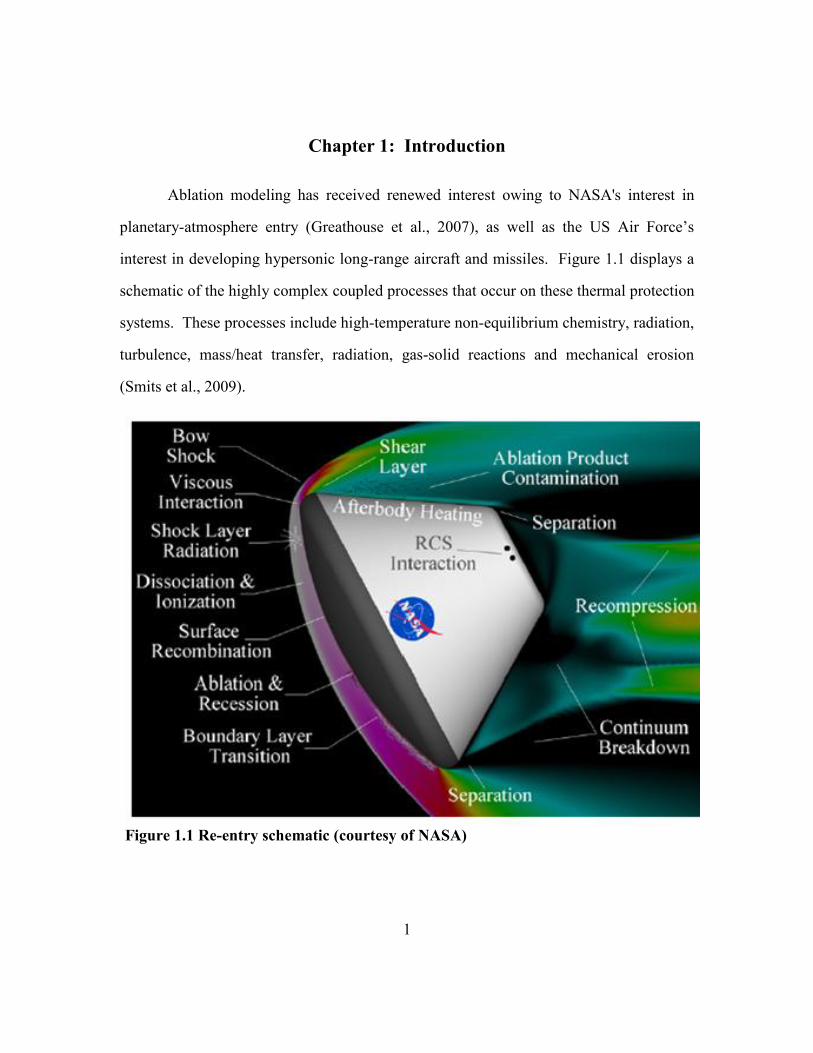
Figure 1.1 Re-entry schematic (courtesy of NASA)

Chapter 1: Introduction

Ablation modeling has received renewed interest owing to NASA's interest in

planetary-atmosphere entry (Greathouse et al., 2007), as well as the US Air Force’s

interest in developing hypersonic long-range aircraft and missiles. Figure 1.1 displays a

schematic of the highly complex coupled processes that occur on these thermal protection

systems. These processes include high-temperature non-equilibrium chemistry, radiation,

turbulence, mass/heat transfer, radiation, gas-solid reactions and mechanical erosion

(Smits et al., 2009).

2

The coupled nature of these thermophysical processes makes developing

computational models of ablation particularly challenging (Gnoffo et al., 1999). In

particular, modeling efforts are limited by the lack of suitable validation data acquired

under realistic conditions. For this reason, this study is aimed at considering a limited-

physics problem, where a low-temperature sublimating ablator is used to capture the

surface-gas transpiration and resulting transport of the ablation products in the turbulent

boundary layer. The sublimating ablator used is naphthalene, which has the particularly

useful property that it can be imaged using planar laser-induced fluorescence (PLIF).

A major goal of this work is the simultaneous acquisition of naphthalene PLIF

and particle image velocimetry (PIV) to enable the computation of the scalar/velocity

correlations that are used in Large Eddy Simulation (LES) and Reynolds Averaged

Navier-Stokes (RANS) model development. Large Eddy Simulations explicitly resolve

the large scale motion of the flow, while approximating the small scale structures of the

flow with an appropriate sub-grid scale model (Gatski et al., 1996).

The current investigation is focused on the development of the naphthalene

sublimation technique for investigating scalar transport of ablation products in low-

enthalpy hypersonic flows. The overall objective of the work is to develop a quantitative

diagnostic technique, so the photophysical properties of naphthalene were also studied.

This investigation has the following goals:

1. Make detailed measurements of naphthalene scalar fields in a Mach 5 turbulent

boundary layer using planar laser-induced fluorescence (PLIF)

2. Develop a method to measure temperature and heat flux through a naphthalene

floor plug while in the Mach 5 flow

3. Study the linearity of the naphthalene laser induced fluorescence signal (LIF) with

laser fluence in order to allow for sheet corrections to be made

3

4. Study the temperature dependence of the naphthalene LIF signal at varying

pressures

5. Study the pressure dependences of the naphthalene LIF signal

4

Chapter 2: Literature Review

2.1 ABLATION

2.1.1 High Temperature Ablation

The complex process of high temperature ablation that occurs on the thermal

protection systems of re-entry vehicles is characterized by several physical processes

including high-temperature non-equilibrium chemistry, radiation, turbulence, mass/heat

transfer, radiation, gas-solid reactions and mechanical erosion (Smits et al., 2009).

Figure 2.1 displays the detailed heat transfer process that occurs during high temperature

ablation. The thermochemical ablation involves the formation of a multilayer surface

that consists of a char layer, reaction layer and virgin material layer. The thermal

degradation of the material results in the formation of the char layer from the loss of solid

material in decomposition and the formation of carbonaceous char residue. The

production of decomposition gases occurs through this process and this gas escapes

through the porous char layer that forms. Through continuous heating, the char layer will

eventually be removed resulting in a recession-rate of the char layer. The temperature at

the surface will be maintained after the char layer begins being removed, thus this is the

point of the failure temperature of the material (Ho et al., 2007).

5

Fi

gure

2.1

Dia

gram

of

mas

s/h

eat

tran

sfer

eff

ects

in h

igh

tem

per

atu

re a

bla

tio

n

6

A large portion of testing high temperature ablators has gone into testing the

thermal properties of these materials in re-entry situations. A detailed survey of

experimental testing of high temperature ablation is given by Ho et al. (2007). An early

study by Vojvodich and Winkler (1963) studied the insulation efficiency of several

thermal protection materials in a high-energy arc-jet Mach 5.5 wind tunnel. Both low

conductive heating rates and high conductive heating rates were tested by varying the

model geometry. The materials tested were typical insulating charring materials and

were tested in both air and nitrogen environments. The materials were found to provide

better insulation efficiency when exposed for short duration run times with high heating

rates rather than for long duration run times with low heating rates. Recently, Milos and

Chen (2009) investigated the thermal properties of a Phenolic Impregnated Carbon

Ablator that is a candidate for use on the Orion Crew Module. Arc jet tests were

conducted over a range of stagnation heat flux and pressure conditions in order to

validate a thermal response property model.

In addition to the study of material thermal properties, past investigations have

focused on the char-recession rate. The char-recession rate and thermal response of five

phenolic-nylon-based materials were investigated by McLain et al. (1968). The

investigation was carried out in a Mach 5 arc-heated tunnel. Arc-heated tunnels are

heated through a magnetically rotated electric arc. Measured char-recession rates were

obtained through the analysis of motion-picture film and through testing the ablative

material for successively longer exposures. In addition, Covington et al. (2008)

evaluated surface recession rates of the Stardust spacecraft forebody heat shield in order

to obtain a measure for the ablative performance of the material. These tests were carried

out in a high-energy arc jet facility with conditions appropriate for the Stardust re-entry.

The data on the thermal performance of the PICA material forming the heat shield were

7

done through varying the model size and arc jet operating condition. The data were used

to correct computer models that predict the response of the re-entry vehicle.

2.1.2 Low Temperature Ablation

Since the 1950s low temperature ablation studies have been conducted so as to

create a limited physics problem that is more economical and easier to maintain in a test

environment. Materials used as low temperature ablators have included camphor, CO2

(dry-ice), water ice, naphthalene, ammonium chloride, and wax (Kohlman and

Richardson, 1969).

Similarly to high temperature ablation studies, recession rates have been a focus

of past investigations. Camphor and dry-ice have seen the most use in these studies.

Charwat (1968) used two low-temperature sublimating ablators, camphor and

naphthalene, to determine nose-tip recession rates of supersonic projectiles. Tests were

performed on cones with flat and hemispherical noses in a Mach 3 flow. The general

evolution of their profiles were traced using film records, which allowed for the

sublimation history of the tips and the occurrence of grooves, striations, and surface

markings to be extracted. Kohlman and Richardson (1969) investigated the viability of

using CO2 (dry-ice) models for studying ablation. They developed a fabrication method

for CO2 models and noted several advantages over other low temperature ablators: the

ablation products are safe, the sublimation rate is low in the sublimation temperature

range (-78º C to -130º C), and the low temperature vapor pressure is the same order of

magnitude as higher temperature ablators. Photographs were acquired a second apart to

measure the recession rate and imbedded thermocouples in the model were used to infer

the heat transfer. The use of camphor and dry ice models were used by Lipfert and

Genovese (1971) to simulating re-entry ablation. The models were steel-tipped 15º half-

angle cones mounted in a Mach 6 flow. Direct surface recession measurements were

8

made during each run. In addition, gas sampling probes as well as a boundary-layer

survey apparatus were used to make measurements of boundary layer parameters.

Camphor 5º half-angle cone models were also used by Griffith et al. (1977) to study the

ablation effects in laminar flow conditions.

Callaway et al. (2008) and Callaway et al. (2010) used dry-ice as a low

temperature ablating model material in a Mach 3 flow. Images were taken at 500 frames

per second to determine the ablation rate in the preliminary study and high speed

schlieren (1000 Hz) was used for visualization in the second study. Callaway et al.

(2010) developed a method to capture the surface topology during a run.

Photogrammetry was used to measure the 3D recessing surface. A dot projection

technique using a low power laser system and three to four laser grids measured the

recessing ablative surface. Two to three of the grids were focused on the model surface

and another grid was focused on the tunnel floor to provide anchor points and the scale of

the wind tunnel. The images were uploaded into PhotoModeler to extract measurements

and the shape change could be quantified with sub-millimeter accuracy.

In addition, water ice has been utilized in the past to study ablation onset times.

Silton and Goldstein (2000) investigated the effects of a forward-facing cavity on severe

heating and ablation onset times. Water ice was chosen as the low temperature ablative

material due to it being inexpensive, well characterized, nontoxic, neither flammable nor

corrosive, and having a low sublimation rate at low temperatures. A high speed video

camera operating at 30 Hz was used to characterize the ablation onset time.

Patterns created during ablation, such as streamwise striations and crosshatching

have also been studied using low-temperature ablators (Stock and Ginoux, 1971). Stock

and Ginoux (1971) used wax cones with pointed steel tips to investigate crosshatching

that occurs during re-entry. Stock (1975) investigated the cross-hatching phenomenon by

9

Figure 2.2 Absorption of naphthalene (Figure reproduced from Du (1998))

using camphor and wax models, and concluded that the viscosity of the ablation material

influences the streamwise spacing of the pattern that develops.

2.2 NAPHTHALENE AS AN ABLATOR AND TRACER

Naphthalene (C10H8) is a polycyclic aromatic hydrocarbon that sublimates at low

temperature. The naphthalene vapor absorbs light over a band extending from 220 nm to

310 nm (Figure 1.1) and it emits fluorescence over the range 300 nm to 400 nm (Figure

1.2), depending on the pump wavelength (Du, 1998). These absorption and emission

properties allow naphthalene to be imaged using planar laser-induced fluorescence

(PLIF). The naphthalene sublimation technique shares some characteristics with

techniques that transpire a non-reacting fluorescent gas such as nitric oxide into the heat-

shield boundary layer (Inman et al., 2008), but it adds the complexity that the ablation

products result from a true, albeit simplified, ablation process.

10

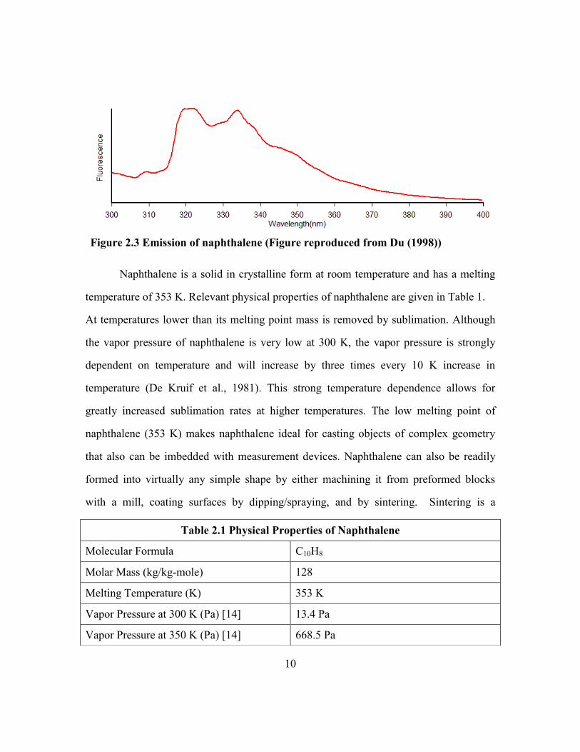
Figure 2.3 Emission of naphthalene (Figure reproduced from Du (1998))

Naphthalene is a solid in crystalline form at room temperature and has a melting

temperature of 353 K. Relevant physical properties of naphthalene are given in Table 1.

At temperatures lower than its melting point mass is removed by sublimation. Although

the vapor pressure of naphthalene is very low at 300 K, the vapor pressure is strongly

dependent on temperature and will increase by three times every 10 K increase in

temperature (De Kruif et al., 1981). This strong temperature dependence allows for

greatly increased sublimation rates at higher temperatures. The low melting point of

naphthalene (353 K) makes naphthalene ideal for casting objects of complex geometry

that also can be imbedded with measurement devices. Naphthalene can also be readily

formed into virtually any simple shape by either machining it from preformed blocks

with a mill, coating surfaces by dipping/spraying, and by sintering. Sintering is a

Table 2.1 Physical Properties of Naphthalene

Molecular Formula C10H8

Molar Mass (kg/kg-mole) 128

Melting Temperature (K) 353 K

Vapor Pressure at 300 K (Pa) [14] 13.4 Pa

Vapor Pressure at 350 K (Pa) [14] 668.5 Pa

11

necessary solution for objects that require greater structural strength due to the more

crystalline structure that is formed. In fact sintering can provides shear strength three

times that of a cast model as well as providing a more homogenous structure (Charwat,

1968).

In the past, sublimating ablators, such as naphthalene, have been extensively used

in low-speed flow applications to measure the convective heat transfer rate from surfaces.

The heat transfer rate is inferred from the ablation rate by using the heat-mass transfer

analogy. Essentially, the heat transfer rate is inferred from a measurement of the mass

loss, either by weighing the ablated material or by measuring the recession depth

(Goldstein et al., 1995). Furthermore, low-temperature sublimating ablators, such as

camphor and naphthalene, have been used to determine nose-tip recession rates of

supersonic projectiles (Charwat, 1968). Camphor has a higher melting temperature and

so is often preferred for shape-change studies in some higher-enthalpy supersonic wind

tunnels. Chartwat (1968) describes a method for sintering naphthalene by compressing it

to 4000 psi to improve the shear stress from 55 psi (when casted) to 160 psi.

Additionally, a procedure for measuring the local temperature of the surface of

naphthalene was developed. A fluorescent powder was added to the naphthalene before

sintering and was irradiated using an ultra-violet mercury lamp, which caused the surface

to fluoresce with varying intensity for different temperatures.

To date, naphthalene PLIF has not been used in supersonic flows, but it has seen

some use as a fuel marker in low-speed reacting flow experiments conducted by Kaiser et

al. (2003). Kaiser et al. (2003) added 5% of 1-methylnaphthalene to a fuel stream and

used PLIF to image the unburned fuel. The naphthalene fluorescence was excited using

the 4th harmonic of an Nd:YAG laser, and the fluorescence was imaged using an image-

intensified CCD camera (ICCD camera). In addition a two-color PLIF technique was

12

developed to measure temperature from a suitable ratio of different parts of the

fluorescence spectrum with a single excitation wavelength (Kaiser et al., 2005). This

technique was made viable by the measurements of Ossler et al. (2001), who showed that

the absorption coefficient of naphthalene at 266nm was insensitive to temperature.

In Kaiser et al. (2005) the quenching of naphthalene fluorescence was seen to be

dominated by oxygen at 500 K. In Ni and Melton (1996) the dependence of the

naphthalene PLIF signal on temperature was used to image the temperature of the

unreacted fuel in a jet flame. The fluorescence lifetime of naphthalene was found to

decrease from 180 ns at 25 ºC to 35 ns at 450 ºC, which was used to calculate the

temperature in oxygen-free environments. Lifetime-based thermometry techniques have

the advantage that the concentration (absolute or relative) of the excited species is not

required. Furthermore, a few studies have measured the rates of collisional quenching of

naphthalene fluorescence. For example, quenching rates for naphthalene in N2, O2, and

H2O were measured by Martinez et al. (2004). The effect of temperature on the lifetime

of naphthalene fluorescence was also studied in oxygen free environments by Ni and

Melton (1996). A more detailed discussion of the spectroscopy of naphthalene is given

in the section 2.4.

2.3 SPECTROSCOPIC MEASUREMENTS OF HYDROCARBON TRACER-MOLECULES

A great deal of insight into needed measurements can be obtained by consulting

studies that investigated the spectroscopy of other complex hydrocarbons, such as

acetone and 3-pentanone.

Ghandhi et al. (1996) and Grossmann et al. (1996) studied the pressure and

temperature dependence of LIF of two keytones, acetone and 3-pentanone. Ghandi et al.

(1996) studied the LIF signal in a temperature controlled jet and a motored engine. A

quadrupled Nd:YAG laser (266 nm) beam was focused onto the jet output using a 1 m

13

focal length lens while a thermocouple monitored the output temperature of the jet. The

fluorescence signal decreased with increasing temperature for both compounds, which

was argued to occur due to shifts in the absorption spectrum. However, the fluorescence

was found to be insensitive to pressure. Grossmann et al. (1996) studied the pressure and

temperature dependence of the keytones using a heated, high-pressure cell, which had

operating condtions of 383 to 650 K and 0 to 5000 kPa, and an excitation wavelength of

248, 277, and 312 nm. The pressure dependence for both molecules in synthetic air show

the fluorescence intensity rises initially and then decreases after the initially increase.

The authors argue that the initially increase is due to vibrational relaxation to levels with

higher fluorescence quantum yields and the later decrease is due to quenching of the S1

state with O2. The determined temperature dependence of the absorption strength was

used to measure the temperature using the ratio of the fluorescence intensity of two

different wavelengths

Acetone fluorescence temperature dependence has been thoroughly studied at six

excitation wavelengths by Thurber et al. (1998). The temperature dependence of the

absorption coefficient and fluorescence yield were extracted from measurements made of

the fluorescence signal by normalizing the signal for the acetone number density and

laser fluence. The temperature of the acetone seeded nitrogen jet was varied from 295 K

to 1000 K by using a furnace with an optically accessible flow cell mounted inside it.

Similar to Grossmann et al. (1996), Thurber et al. (1998) developed a technique to

measure temperature by using the ratio of fluorescence signals when pumped with

different excitation wavelengths. Specifically, five different excitation-wavelength

combinations were used to obtain different temperature dependencies of the ratio of

fluorescence signals.

14

Bryant et al. (2000) also investigated low temperature and low pressure effects of

acetone laser induced fluorescence. They used a static gas chamber which could be

cooled to 230 K and had a pressure range from .02 to 1 atm. The optically accessible cell

was cooled by liquid nitrogen which flowed through copper tubing coiled around the

exterior. Non-uniform cooling and icing and condensation of acetone vapor on the fused

quartz windows provided challenging problems in this investigation. The flow rate of the

liquid nitrogen had to be controlled around separate sections to reduce non-uniform

cooling, while dry air was utilized to prevent icing. A jet of room temperature air across

the windows was used to eliminate condensation on the windows.

2.4 NAPHTHALENE SPECTROSCOPY

The energy-level structure of the naphthalene molecule is complex because of the

presence of a large-number of vibronic states that are entangled with one another.

Figure 1 shows a simplified illustration of the energy levels that are close to the

photon energy of the fourth harmonic of the Nd:YAG laser (λ=266 nm or ν=37,600 cm-

1), since this is the excitation frequency that is used in the current investigation.

15

The first and second excited singlet electronic states, denoted as S1 and S2 respectively,

are located at an energy level of 32027 and 35815 cm-1

above the ground electronic state

(S0). Each electronic state is associated with a manifold of closely-spaced vibrational

energy levels. These vibrational levels are classified as either a “totally symmetric” (TS)

or “non-totally-symmetric” (NTS), depending on the symmetry of the vibration. In

general, the vibrational levels in the TS group have a shorter lifetime compared to the

NTS group (Behlen et al., 1981). In addition, since the energy level difference between

the S1 and the S2 states are quite small, the vibrational manifolds of the two states overlap

and form a larger entangled manifold.

There also exist excited triplet vibronic states T1 and T2, whose energy level

structure is very similar to the singlet levels S1 and S2. In Figure 2.1, the excitation by a

Figure 2.4 Vibrational-electronic energy level diagram of gas-phase naphthalene. There are two electronic systems, singlet and triplet, where each electronic state is

associated with a manifold of closely-spaced vibrational levels.

16

266 nm photon is illustrated, which excites the naphthalene molecule from the ground

state to the second excited state, S2. Almost all of the excited molecules undergo an

“internal conversion” to the vibrational levels of S1 (Laor and Ludwig, 1971). This

conversion from the higher singlet state to the lowest excited singlet state is a

radiationless process and is a purely intramolecular process (Watts and Strickler, 1966).

The internal conversion process takes place much faster than the fluorescence lifetime of

the S2→S0 transition (Stockburger et al.,1975b). Most of the fluorescence, therefore,

results from S1→S0 vibronic transitions even though the S2 state is pumped. Excitation to

the third excited state, S3, takes place at 42000 cm-1

. The radiative lifetimes observed

when exciting the S3 state is much different than when exciting the S1 and S2 state due to

vastly different processes regarding quantum yields, intersystem crossing, and emission

spectra (Laor and Ludwig, 1971).

A fraction of the molecules in the S1 and S2 states makes an “inter-system

transfer” to triplet vibronic states T1 and T2. The inter-system crossing from the S1 state

can best be described as a crossing from the S1 to T2 or other higher triplet state which is

then followed by an internal conversion from the T2 or higher state to the T1 state

(Ashpole et al., 1971). The rate of inter-system transfer increases with increasing

pressure. For example, the inter-system transfer is considerable for pressure over 150 torr

(Beddard et al., 1973). Soep et al. (1973) found that as the pressure of the gas decreases

the triplet yield of naphthalene decreases almost to zero and that the inter-system crossing

process in naphthalene appears to be practically irreversible. The molecules in the triplet

states T1 and T2 undergo both collisional de-excitation and radiative transition. The

radiative transitions from the triplet to the ground (singlet) state represent long-lived

phosphorescence with a lifetime of order milliseconds. The inter-system transfer,

however, is small for 266 nm excitation, and so the dominant emission is S1→S0.

17

Several studies have also investigated different aspects of naphthalene

fluorescence. The fluorescence signal with units of photons, under the assumption of

broadband detection and weak excitation, is given by:

),,,(),(),(/

),( inaphoptL

f PTTTPnVhc

ETPS

(2.1)

where EL is the laser fluence (J/m2), h is Planck’s constant, c is the speed of light, λ is the

wavelength of the laser, ηopt is the collection optics collection efficiency, ΔV is the probe

volume, χnaph is the napthalene mole fraction, n is the total number density, σ is the

absorption cross-section, φ is the fluorescence yield, P is pressure and T is temperature. If

we assume that the fluorescence results from the S1 state, and that the spontaneous

emission rate and electronic quenching rates are the same for each state, then we can

write the fluorescence yield as,

Qf

f

ikkk

kPT

int

),,,(

(2.2)

where kf is the rate of spontaneous emission, kint is the rate of de-excitation of S1 not due

to collisions, and kQ is the collisional quenching rate. Here we model the quenching rate

as,

Naii

iiQ vnk

(2.3)

where ni is the number density of colliding species i, σi is the is quenching cross section

of species i, and Nai

v

is the mean relative speed between species i and naphthalene.

18

When naphthalene is seeded in air, oxygen is the dominant quencher, as reported by

Martinez et al. (2004), and Kaiser and Long (2005). Thus we have:

NaOOOQ vnk

222 (2.4)

When the species is excited by a short-pulse laser, the fluorescence decay

typically follows an exponential form with time-decay constant. There are two electronic

systems, singlet and triplet, where each electronic state is associated with a manifold of

closely-spaced vibrational levels.

1

int )( Qff kkk (2.5)

The equations above are for an extended two-level model with broadband

detection, and they are reasonable approximations under some conditions, but take

caution that they can be highly inaccurate in others (e.g., low pressure).

A study by Sockburger et al. (1975a) has focused on understanding the single

vibrational level fluorescence at low pressure and at near absolute zero temperature. A

vibronic coupling theory is used to interpretate the vibrational structure. Gattermann and

Stockburger (1975) have investigated the intersystem transfer to the triplet states and the

corresponding phosphorescence. A triplet lifetime from the 0

00 band of 4.2 µs was

derived.

The fluorescence lifetimes and quantum yields of the first and higher excited

states have been studied by several groups. A detailed review of the studies on

fluorescence and non-radiative lifetimes and the quantum yields for different vibronic

states is given by Avouris et al. (1977). The fluorescence lifetimes and quantum yields

have been found to decrease with increasing excitation energy (Beddard et al., 1974). A

19

work by the same group, Beddard et al. (1973), observed naphthalene fluorescence decay

time as a function of pressure in argon gas. For short excitation wavelength (< 305 nm),

the lifetimes and yields were found to increase with increasing pressure, while they

decrease with increasing pressure for longer excitation wavelengths (> 305 nm). They

proposed that the increase in lifetimes and yields with increasing pressure for short

excitation wavelengths could be attributed to collisionally induced intramolecular

vibrational redistribution. The higher energy vibrational modes have a shorter

fluorescence lifetime, thus as the pressure increases the Boltzmann distribution of the S1

state forms and the lifetimes increase and become independent of pressure and

wavelength. The fluorescence decay waveform was reported to be bi-exponential by

Reyle and Brechignac (2000) and Behlen and Rice (1981). The bi-exponential trace is

because of the simultaneous decay of two types of vibronic states. The timescale of the

longer lifetime transitions was about 1 μs and the shorter lifetime ranged between 85 to

400 ns (Reyle and Brechignac, 2000).

The shorter duration decay corresponds to the fluorescence of the vibronic states

of S1 level. The range of lifetimes within the S1 vibronic states is because of the

differences in the lifetime of different groups of vibrational levels, which differ in their

symmetry. For the present investigation, the fluorescence decay corresponds to the

vibronic states of S1 level only. Most of the above fluorescence decay measurements

were performed in a vibrationally frozen condition (very low temperature) and at

extremely low pressures. At these conditions, the effect of collisional de-excitation is not

present. Suto et al. (1992) and Schlag et al. (1971a) performed fluorescence decay

measurements at a temperature of about 300 K. They reported a much smaller quantum

yield and fluorescence lifetime compared to the single vibrational level measurements.

Hsieh et al. (1974) and Lim and Huang (1973) observed the fluorescence lifetimes of

20

naphthalene in a collision-free conditions from which they extracted the nonradiative

decay rate. They reported a break in the nonradiative decay rates versus excitation

energy at photon energy corresponding to the S2 state. The authors suggested that the S2

to S1 internal conversion causes a change in the vibrational distribuition. This

distribuition is maintained through the time scale of the S1 radiationless decay, which

leads to the conclusion that the intramolecular vibrational energy redistribution is not a

fast process and collisions are necessary to affect the vibrational distribuition.

Only a few studies have focused on measuring electronic quenching rates of gas-

phase naphthalene. For example, quenching measurements of oxygen, nitrogen, methane,

noble gases and nitric oxide have been reported but only at a limited range of conditions

by Behlan and Rice (1981), Kaiser and Long (2005) and Martinez et al. (2004). Oxygen

is reported to be one of the major quenching agents of naphthalene and its quenching

effect was studied by Kaiser and Long (2005) and Martinez et al. (2004). Kaiser and

Long (2005) measured the quenching of naphthalene by oxygen and nitrogen at room

temperature and above. They reported that oxygen dominates the quenching process.

Similar conclusions were drawn by Martinez et al. (2004) who measured O2 and N2

quenching rates with an excitation at 308 nm at low pressure. They found that the O2

quenching cross-section is about an order of magnitude larger than that of N2. A study by

Ossler et al. (2001) observed the temperature dependence of the quenching cross-section

of naphthalene. The decay rate of naphthalene fluorescence was examined in the

temperature range of 400 to 1000 K and the quenching cross-section was extracted. In

addition, at temperatures below 540 K a Stern-Volmer behavior shows the decay rate of

naphthalene fluorescence was found to increase with an increase in the partial pressure of

oxygen, which was similarly observed by Kaiser et al. (2005) at 500 K. At higher

21

temperatures this Stern-Volmer behavior was seen to break down and a second order

dependence on the oxygen concentration appeared.

22

Chapter 3: Experimental Program

The following chapter details the experimental facilities, design and operation of

experiments, and the experimental techniques used to acquire all data in this

investigation.

3.1 FACILITIES

The wind tunnel experiments were conducted at the High-Speed Wind Tunnel

Laboratory located at the Pickle Research Campus of the University of Texas at Austin.

Complementary investigations of fluorescence linearity, and temperature/pressure

dependence were conducted in a temperature-controlled jet of naphthalene exhausting

into atmospheric conditions or a pressure-controlled cell.

3.1.1 Mach 5 Wind Tunnel Facility

The naphthalene ablation experiments were conducted in the blowdown Mach 5

wind tunnel facility as shown in Figure 3.1. The Mach 5 tunnel is driven by a 2550 psia

pressure tank that is charged either by a Worthington HB4 four-stage compressor or a

Norwalk four-stage compressor. The air was stored in eight high pressure tanks with total

volume of 4 m3 (140 ft

3). During each run the stagnation pressure was kept at 2.52 MPa

(360 psi) by a 1.5 in. Dahl valve operated by a Moore 352 controller and exhausts to the

atmosphere. The air is heated before the test section by two banks of 420 kW nichrome

wire resistive heaters controlled by a Love Controls 1543 controller to give a variable

stagnation temperature from 345 K to 380 K. The stagnation pressure was monitored by

a Setra 204 pressure transducer and the stagnation temperature was monitored by a J-type

thermocouple.

23

Figure 3.1 Schematic of the Mach 5 blowdown facility located at the Pickle

Research Campus of the University of Texas at Austin

24

The Mach 5 test section for the wind tunnel was 152 mm (6 in.) wide by 178 mm

(7 in.) tall by 762 mm (27 in.) long. The freestream Mach number was M∞ = 4.95,

Reynolds number was Re∞ = 49.5 x 106 m

-1 (15.1 x 10

6 ft

-1), and velocity was U∞ = 750

m/s. The freestream turbulence intensity is less than 0.3%. Optical access to the flow

was provided by a fused silica window mounted on the sidewall measuring 381 mm (15

in.) long, 51 mm (2 in.) tall, and 19 mm (.75 in.) thick

3.1.2 Temperature Controlled Jet of Naphthalene Facility

The investigations of naphthalene fluorescence linearity, and temperature/pressure

dependence were conducted in a temperature-controlled jet of naphthalene exhausting

into atmospheric conditions or a pressure-controlled cell. The naphthalene jet was driven

by a 90 psia pressure tank charged by the house air compressor or a compressed air bottle

of nitrogen, industrial air, breathing air, or ultra zero air. During each run the mass flow

rate was monitored using an Omega FMA-1610-NIST mass flow meter and controlled

using a needle valve. The pressure cell was made of a Kurt J. Lesker Company CF

flanged 6-way cross with tube outer diameter of 2 ¾ in. (Part No. C6-0275). The

pressure cell was drawn to a vacuum using a large vacuum reservoir drawn down by a

two stage Roots Connersville Rotary Positive Vacuum Pump. The pressure in the

pressure cell was monitored by a MKS Baratron Capacitance Manometer (Type 626) and

could be set between 1 kPa to 40 kPa. The temperature of the jet was controlled using a

Omegalux AHPF-102 In-Line Air Heater. The in-line heater was capable of heating the

jet from 297 K to 550 K by using a Staco Energy Products Variable Autotransformer

(Type 3PN1010) to control the voltage to the heater. The temperature of the jet was

monitored using a type-J thermocouple when exhausted to atmosphic conditions and

type-T thermocouple when exhausted to the pressure controlled cell.

25

The jet diameter was 12.7 mm (.5 in.) when exhausting into atmospheric

conditions and 19.1 mm (.75 in.) when exhausting into the pressure controlled cell.

Optical access to the flow was provided by a fused silica window measuring 38.1 mm

(1.5 in.) in diameter and 6.34 mm (.25 in.) thick.

3.2 NAPHTHALENE MACH 5 WIND TUNNEL FLOOR MODEL

The Mach 5 wind tunnel experimental models were flush mounted floor models.

There were two versions of the floor model created, one for a first campaign that was

very preliminary to show feasibility and the second for the second campaign that had

been optimized for improved diagnostics.

3.2.1 First-Campaign Floor Model

The original model contained a naphthalene plug that was 50.8 mm (2 in.) wide

by 25.4 mm (1 in) long. This model was developed in two stages. The first stage

consisted of a creating a model with a cavity that had no method to secure the

naphthalene plug in place after it had been poured. Testing this model in the wind tunnel

resulted in the naphthalene plug being sucked out of the cavity and into the flow.

Therefore, the design was modified by consisted of adding a 6.35 mm (.25 in.) lip around

the naphthalene to secure it in the plug. This model is shown in Figure 3.2. The model

was designed so the naphthalene would be cast inside it after a plate is installed over the

top. There were two fill holes that opened into the cavity, one of which allowed the

molten naphthalene to be poured into and the other allowed for air to escape.

The naphthalene pouring procedure was developed with the first floor model.

The naphthalene crystals were melted using a hot plate as seen in Figure 3.3. The

naphthalene was then poured into the floor model with the molding plate installed over

the open cavity, so as to seal the cavity. Once the naphthalene solidified the cover was

26

removed, and the resulting surface was relatively flat and smooth. The naphthalene was

allowed to solidify for approximately 12 hours before use. The molding plate was then

removed and any excess naphthalene that was not flush with the floor plug was sanded

down using fine grit sandpaper (800 grit or better). Once the naphthalene was sanded the

resulting surface was relatively flat and smooth, as shown in Figure 3.4. The model was

then ready to be installed into the wind tunnel as shown in Figure 3.5.

25.4 mm

50.8 mm

Upper Lip

Fill Holes

Figure 3.2 Schematic of the first campaign naphthalene floor plug

Figure 3.3 Naphthalene crystals melting on a hot plate

27

Figure 3.4 Naphthalene floor plug after molding plate is removed

Figure 3.5 Naphthalene floor plug installed into test section

28

3.2.2 Second-Campaign Floor Model

The second model design increased the size of the naphthalene plug to be 101.6

mm (4 in.) long by 57.2 mm (2.25 in.) wide. This design is shown schematically in

Figure 3.6. This model had a 6.35 mm (.25 in.) lip around the naphthalene so as to secure

it in the plug and prevent the plug from being sucked into the wind tunnel.

Figure 3.6 Second-campaign naphthalene floor plug installed in the Mach 5 wind tunnel

29

The naphthalene plug could be imbedded with up to 15 thermocouple equally

spaced in a 5 by 3 array 22.2 mm (.875 in) apart, with 5 installed length wise at three

span wise positions as seen in Figure 3.7. The closest the thermocouples could be to the

edge of the naphthalene plug was 6.35 mm (.25 in). This space prevented any non-

homogenous effects in the solidified naphthalene plug that could occur during pouring.

The thermocouples could be imbedded at the any depth within the naphthalene or at the

surface of the naphthalene plug at each position. In the design heat flux sensors could

replace two of the center line thermocouples and could be imbedded in the naphthalene.

In addition, a heat flux sensor or thermocouple could be installed 6.35 mm (.25 in.)

upstream and downstream of the naphthalene plug.

A fused silica window was added downstream of the naphthalene plug to allow

for the laser sheet to pass through the floor, thus reducing reflections. The optical access

enabled a field of view that ranged from 23.5 mm (.925 in.) to 264.8 mm (10.425 in)

downstream of the downstream edge of the naphthalene plug, as seen in Figure 3.8.

Moreover, the fused silica optical access from all sides of the test section enabled plan-

view imaging. The plan-view imaging can range from from 23.5 mm (.925 in.) to 264.8

mm (10.425 in) downstream of the downstream edge of the naphthalene plug, which is

identical to the side-view measurements.

30

Figure 3.7 Dimensions of the naphthalene plug and thermocouple/heat flux sensor locations in the second campaign naphthalene floor plug

31

Figure 3.8 Dimensions of the downstream fused silica window in the second campaign naphthalene floor plug

32

The naphthalene plug was formed using a similar molding procedure as in the

first campaign model. This procedure entailed heating solid naphthalene past its melting

point, then pouring it into the naphthalene plug. The fused silica window was removed

during the pouring procedure, so it would not become damaged, and the molding plate

was installed over the cavity. The thermocouples were installed before the molding

procedure and were positioned such that they were imbedded within the naphthalene after

it has solidified. After the naphthalene solidified, the molding plate was removed and the

plug was installed into the test section floor (Figure 3.9).

Figure 3.9 Second campaign naphthalene floor plug installed in the Mach 5 wind tunnel test section

Naphthalene Insert

Flow

Window

Imbedded

Thermocouples

33

3.3 NAPHTHALENE LIF COMPLEMENTARY INVESTIGATIONS

3.3.1 Fluorescence Linearity Measurement System

A jet of naphthalene-laden air exhausting into atmospheric conditions was used to

study the saturation effects of the naphthalene fluorescence. The schematic of the setup

is shown in Figure 3.10. Air from the house air compressor was passed through a cell

filled with naphthalene crystals. The naphthalene concentration was saturated at a

constant room temperature of 298 K. The flow rate was monitored and kept at 10 SLPM

using a needle valve. This vapor-laden flow was then passed through the in-line heater

(Omegalux AHPF-102), which was turned off during this investigation. A jet was

formed as the flow exits from a 12.7 mm (.5 in.) tube. To avoid condensation of the

naphthalene on the walls of a test cell, these measurements were made in a free jet. The

fluorescence was excited with a quadrupled Nd:YAG laser (Spectra- Physics Model PIV

400) operating at 266 nm. The beam was passed through a varying number of fused

silica flats, which are used to change the energy of the beam. A total of sixteen fused

silica flats were used. To obtain the lowest fluences, a 90 percent beam splitter was used

along with the fused silica flats. A 1m spherical lens was used to focus the beam in order

to reduce the beam diameter to significantly less than the outlet diameter of 12.7 mm.

The 1 m spherical lens was placed 292 mm away from the center of the jet. The beam

propagation direction was perpendicular to the axis of the jet. A PixelVision

SpectraVideo Model SV512V1 back-illuminated CCD camera (512 x 512 pixels) was

used to image the naphthalene fluorescence in the potential core of the jet. The camera

was shuttered to 99 ms so as to only capture one laser pulse per frame. The linearity of

the LIF signal was studied by changing the energy of the beam while keeping the

temperature constant.

34

3.3.2 Temperature Dependence Measurement System

In a related experiment the temperature dependence of the naphthalene

fluorescence from 297 K to 525 K was investigated by varying the temperature of the jet

while keeping the energy constant. The energy was kept low enough to be within the

linear regime using a fixed number of fused silica flats. The experimental setup is

displayed in Figure 3.13. The vapor-laden flow exiting the saturated naphthalene cell

was passed through the in-line heater (Omegalux AHPF-102) capable of heating the air to

525 K. A type-J thermocouple was used in conjunction with an Omega Type-J

Thermocouple Thermometer (Model 650) to monitor the outlet temperature of the jet.

Figure 3.10 Naphthalene LIF linearity measurement and temperature dependence setup

35

The jet issued into atmospheric pressure and the flow rate was maintained at 30 SLPM.

The inlet air temperature to the saturated naphthalene cell was monitored using the flow

meter, so the naphthalene concentration in air could be corrected for changing vapor

pressure.

3.3.3 Pressure Dependence Measurement System

The experiments to investigate the pressure dependence of the LIF signal were

conducted in a temperature controlled jet of naphthalene-vapor laden air exhausted into a

pressure controlled cell. The experimental setup is the same as in Figure 3.9 except

instead of exhausting into atmospheric conditions the jet is exhausted into a vacuum cell

(Kurt J. Lesker Company CF flanged 6-way cross with tube outer diameter of 2 ¾ in.,

Part No. C6-0275), as shown in Figure 3.11. The cell had fused silica windows on three

sides to allow for the 266nm laser beam to pass through and for imaging the fluorescence.

The cell was kept at a constant pressure (vacuum) by flowing the gas through a metering

valve and then into a large vacuum chamber kept at a vacuum using a two stage Roots

Connersville Rotary Positive Vacuum Pump. To determine the pressure dependence of

the naphthalene fluorescence decay, the pressure in the test cell was varied from 1 kPa to

40 kPa, while keeping the mass flow rate at 30 SPLM. The jet was kept at a constant

temperature of 297 K and was monitored by a type-T thermocouple. If not cleaned after

every run, the naphthalene would condense on the windows and would be burned by the

absorption of the laser light. The fluorescence decay signal was measured using a 1P28

photomultiplier tube (PMT) with a 60 mm fused silica focusing lens. Three Schott WG-

295 filters and two Schott UG-5 filter were used to transmit the fluorescence (in the range

295nm to 400nm), while rejecting most of the elastically scattered light. The laser energy

was set at few tens of micro joules to avoid non-linear effects in the PMT.

36

Figure 3.11 Naphthalene LIF pressure dependence measurement cell

Figure 3.12 Naphthalene LIF pressure dependence measurement setup

Pressure Cell

PMT

60 mm

Focusing Lens

Vacuum

37

3.4 MACH 5 WIND TUNNEL PLIF SYSTEM

Planar laser induced fluorescence (PLIF) was used to visualize the naphthalene

scalar field in the Mach 5 wind tunnel. A concise description of this method, the PLIF

system setup, and the image processing procedure, are discussed below.

3.4.1 Planar Laser Induced Fluorescence (PLIF)

Eckbreth (1988) has an in depth description of the PLIF technique that will be

truncated below. The planar laser-induced fluorescence (PLIF) technique typically

involves the excitation of atomic/molecular electronic transitions, which in this case

occurs at UV wavelengths for naphthalene as discussed in Chapter 1. The PLIF

technique utilizes a laser sheet which can be used to obtain quantitative information of

two-dimensional slice of the flowfield.

Laser induced fluorescence (LIF) is species specific and allows for the

measurement of minor species, such as naphthalene vapor from sublimation, in flows. In

this technique the absorption of a photon of light from a laser is used to excite the atom or

molecule from a lower energy state into a higher energy state. The excited state is in

non-equilibrium and thus will return to equilibrium, which for naphthalene the process is

outlined in section 2.4. In returning to ground state a photon of light may be emitted.

This can be imaged and can lead to quantitative information of the flowfield.

In general, LIF signals are a function of several flow variables, including pressure

and temperature. However, predicting the effect of pressure and temperature on the

signal can be challenging because this usually necessitates that a model be developed

describing the physics of the excitation/de-excitation processes. Therefore, developing an

understanding of the naphthalene LIF physics, and thus how the signal depends on

thermodynamic variables is one of the main objectives of complementary investigations.

38

3.4.2 PLIF System Setup

A schematic of the PLIF system setup in the Mach 5 wind tunnel is shown in

Figure 3.13. The naphthalene fluorescence was excited with a laser sheet from a

quadrupled Nd:YAG laser operating at 266 nm. Fused silica windows were downstream

of the naphthalene insert to enable the laser sheet to pass through the test section and

reduce reflections. An intensified CCD camera (Princeton Instruments PI-Max) imaged

the fluorescence through a fused silica window in the tunnel side wall during the use of

the first campaign floor model. A back-illuminated CCD camera (PixelVision

SpectraVideo Model SV512V1) imaged the fluorescence during the use of the second

campaign floor model. The image resolution was 512 x 267 pixels and the exposure time

was 80 ms, capturing one laser pulse per frame. The cameras were fitted with a 100 mm

focal length, f/2.8 UV lens (Eads Sodern Circo) operated at full aperture. Three Schott

WG-295 filters and one Schott UG-5 filter were used to pass the fluorescence (in the

range 295nm to 400nm), while rejecting most of the elastically scattered light. The

imaging field of view was 27 mm (1.06 in.) wide by 14 mm (.55 in.) tall. Figure 3.14

shows an image of the camera and naphthalene plug in the test section.

The sublimation rate at standard conditions is quite slow and no noticeable mass

is lost even if the insert sits for hours without flow. Only a small amount of ablation (less

than a fraction of a millimeter) is observed over the course of a 1 minute wind tunnel run.

Therefore the naphthalene plug does not need to be recast after each run. The plug was

recast after approximately every 7 to 10 runs

39

(a)

(b) Figure 3.13 Schematic diagram of the naphthalene PLIF setup in the Mach 5 wind tunnel. (a) Overall assembly and (b) inside the test section

40

Temperature measurements were obtained using type-T thermocouples imbedded

into the naphthalene. The stagnation temperature was also monitored using a type-J

thermocouple. These were recording using a National Instruments Compact RIO system

cRIO-9014 (controller), seen in Figure 3.15.

Figure 3.14 Back-illuminated CCD camera focusing on a field of view downstream of the naphthalene plug in the Mach 5 test section

Back-Illuminated CCD Camera

Model in Test Section

Figure 3.15 Compact RIO System with thermocouples

Thermocouples

41

3.4.3 Image Processing

The PLIF images were acquired using the PixelVision software. The raw images

were in 16-bit TIFF format. Each run acquired between 10 to 20 images depending on

run length and the amount of time it took for the stagnation temperature to remain

constant. The images were post-processed in MatLab. The instantaneous images were

filtered using a 3 x 3 median filter to reduce noise effects. All averaging and statistical

analyses were also performed using MatLab.

42

Chapter 4: Results

The experimental investigations of naphthalene ablation in the Mach 5 wind

tunnel and the complementary investigations of naphthalene fluorescence linearity,

temperature dependence and pressure dependence are presented in this chapter. First, the

first-campaign Mach 5 ablation investigation will be presented that proved the viability of

the technique. The complementary studies will then be presented, as the information

learned is necessary to obtain quantitative information from the measured naphthalene

PLIF signal. Finally, the second-campaign Mach 5 ablation investigation as well as the

extraction of quantitative information will be presented.

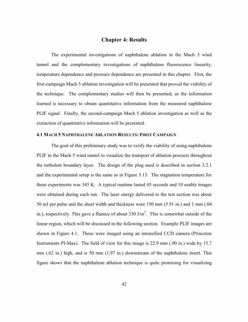
4.1 MACH 5 NAPHTHALENE ABLATION RESULTS: FIRST CAMPAIGN

The goal of this preliminary study was to verify the viability of using naphthalene

PLIF in the Mach 5 wind tunnel to visualize the transport of ablation procucts throughout

the turbulent boundary layer. The design of the plug used is described in section 3.2.1

and the experimental setup is the same as in Figure 3.13. The stagnation temperature for

these experiments was 345 K. A typical runtime lasted 45 seconds and 10 usable images

were obtained during each run. The laser energy delivered to the test section was about

50 mJ per pulse and the sheet width and thickness were 150 mm (5.91 in.) and 1 mm (.04

in.), respectively. This gave a fluence of about 330 J/m2. This is somewhat outside of the

linear region, which will be discussed in the following section. Example PLIF images are

shown in Figure 4.1. These were imaged using an intensified CCD camera (Princeton

Instruments PI-Max). The field of view for this image is 22.9 mm (.90 in.) wide by 15.7

mm (.62 in.) high, and is 50 mm (1.97 in.) downstream of the naphthalene insert. This

figure shows that the naphthalene ablation technique is quite promising for visualizing

43

the transport of ablation products, but we saw the signal-to-noise ratios are quite low (less

than 5). The observed mass loss is essentially negligible during a 60 to 100 second run.

Figure 4.1 Example naphthalene instantaneous PLIF images from the first campaign in the Mach 5 wind tunnel.

44

In addition, a second field of view closer to the naphthalene plug was observed.

The field of view for these images was 22.9 mm (.90 in.) wide by 15.7 mm (.62 in.) high,

and is 25.4 mm (1 in.) downstream of the naphthalene insert. Figure 4.2 shows a

composite image made from two different images captured at different locations and

times to reveal the spatial evolution of the scalar. An unrelated velocity field has been

added to this image to show the boundary layer thickness in comparison to the ablative

product.

The ablation products are seen to be confined quite close to the wall of the wind

tunnel. It appears though, that the scalar is transported out into the boundary layer in

bursts in accordance with known transport mechanisms in turbulent boundary layers.

Despite the modest quality of the data presented, the figures show that the technique is

quite promising.

Figure 4.2 Composite of two instantaneous naphthalene PLIF images taken from two adjacent locations at different times. Uncorrelated velocity field is displayed behind the images to show the boundary layer thickness

45

After observing the results of the first campaign it was apparent for the second

campaign experimental tests, the main object would be to improve the quality of the PLIF

imaging. The PLIF signal was improved in four important ways. The first was to increase

the size of the naphthalene plug (in the streamwise direction) so that more ablation

products were transpired into the flow. A new floor plug for the Mach 5 wind tunnel was

developed with an area of 101.6 mm (4 in.) long by 57.2 mm (2.25 in.) wide, as described

in section 3.2.3. The larger surface area led to a greater integrated amount of mass in the

boundary layer and hence higher fluorescence signal. The second way that the signal was

improved was to increase the tunnel stagnation temperature, since this increases the

naphthalene vapor pressure and hence its sublimation rate. The increase in vapor pressure

is not directly related to the increase in stagnation temperature because of the coupled

effects of heat and mass transfer that occurs due to the naphthalene sublimation. This

effect will be explored in the next section. and will be ignored, thus sublimative cooling

doesn’t affect the assumption of adiabatic flow. This coupled effect was explored in

section 3.2.2. The third improvement was to use a back-illuminated CCD camera

(PixelVision SpectraVideo Model SV512V1) with higher quantum efficiency compared

to the ICCD camera used in the first campaign. In this case the signal was shot noise

limited, so an increase in quantum efficiency led to an improvement in the signal-to-noise

ratio. The fourth was to increase the laser energy to increase the resultant fluorescence

signal. The amount the laser energy could be increased is limited by the fluence

(energy/area of the sheet) at which the LIF signal wa no longer linear. After this fluence,

sheet corrections are difficult to make. The linear regime of the fluence is discussed in

the following section. The effect of each of these techniques will be discussed in the

results of the second campaign in section 4.3.

46

4.2 Mass/Heat Transfer Analysis

The coupled effects of mass and heat transfer were then investigated in order to

obtain an estimate of the expected depth removal rate from the naphthalene plug during a

typical run in the Mach 5 wind tunnel. Ablation presents a coupled heat and mass

transfer problem as the mass flux from the surface cools the surface, while the heat flux

due to the recovery temperature heats the surface.

The sublimation process is very similar to evaporative cooling and an outline of

the coupled mass and heat transfer effects can be found in Incropera and DeWitt (2002).

The heat flux (in W/m2) is given by,

srh TThq '' (4.1)

where hh is the heat transfer coefficient, Ts is the surface temperature, and Tr is the

recovery temperature defined from White (2001) as,

2

2

11 MrTTr

(4.2)

where T∞ is the free stream temperature, γ is the specific heat ratio, M is the mach

number, and r is the recovery factor defined as a function of the Prandtl number as:

3/1Prr . The Prandtl number is the ratio of the kinematic viscosity, ν, to the thermal

diffusivity, α. The mass flux is given by,

svmhm '' , (4.3)

47

the heat and mass fluxes are related by,

svmsgsg hhhmq '''' , (4.4)

where hm is the mass transfer coefficient, ρsv is the surface vapor density, ρ∞ is the

freestream vapor density, and hsg is the latent heat of vaporization. The surface vapor

density is obtained using the ideal gas law and an equation for the vapor pressure from

Ambrose et al. (1975). This vapor pressure is dependent on the surface temperature, Ts,

thus the heat and mass flux equations are both dependent on the surface temperature. For

flow over a flat plate, Von Karmen (1939) derives the heat and mass transfer Stanton

numbers which can be related to the heat transfer and mass transfer coefficients,

respectively. The heat and mass transfer coefficients are given by,

141Pr5ln5Pr52/1

)2/(

f

fP

hC

CCuh

(4.5)

14)15ln(552/1

)2/(

ScScC

Cuh

f

f

m (4.6)

where u∞ is the freestream velocity, CP is the specific heat capacity, Cf is the skin friction

coefficient taken to be 7.7 x 10-4

in the Mach 5 wind tunnel, and Sc is the Schmidt

number. The Schmidt number is the ratio of the kinematic viscosity, ν, and mass

diffusivity, D. Goldstein (1995) reports the relationship for the Schmidt number for

naphthalene in air as,

1526.0

16.29828.2

TSc (4.7)

48

The surface temperature and heat flux may be solved for by equating the heat

transfer equation, Equation 4.1, and mass transfer equation, Equation 4.4. The

naphthalene plug surface temperature versus the stagnation temperature is shown in

Figure 4.3. The heat flux versus stagnation temperature is shown in Figure 4.4. In

addition these results allow for the calculation of the mass flux and thus the expected

depth removal rate from the surface of the plug, Figure 4.5. The expected mass loss

during a 60 second run at a stagnation temperature of 375 K was predicted to be 67µm.

The expected depth removal rate is consistent with the observed mass loss per run in the

first-campaign. Since the mass transfer is essentially negligible, the coupled effects of

heat and mass transfer that occurs due to the naphthalene sublimation can be ignored and

the assumption of adiabatic flow could be made.

340 360 380 400 420 440 460250

260

270

280

290

300

310

320

330

Stagnation Temperature (K)

Wa

ll T

em

pe

ratu

re (

K)

Figure 4.3 Calculated temperature of the wall of the naphthalene plug as a function of the stagnation temperature

49

340 360 380 400 420 440 4601300

1350

1400

1450

1500

1550

1600

1650

1700

1750

Stagnation Temperature (K)

He

at F

lux (

W/m

2)

Figure 4.4 Calculated heat flux through the naphthalene plug as a function of the stagnation temperature

340 360 380 400 420 440 4601.05

1.1

1.15

1.2

1.25

1.3

1.35

1.4

1.45

1.5

Stagnation Temperature (K)

De

pth

Re

mo

va

l Ra

te (

m/s

)

Figure 4.5 Calculated naphthalene plug depth removal rate as function of temperature

50

4.3 COMPLEMENTARY INVESTIGATIONS OF NAPHTHALENE LIF

The major objective of this study was to obtain quantitative information from the

PLIF images. In order to meet this objective, an understanding of the effect temperature

and pressure variations on fluorescence signal must be developed.

In addition, the linear regime of the LIF signal versus the fluence must also be

understood so that a valid sheet correction can be made.

4.3.1 Naphthalene LIF Linearity

To determine the effect of laser fluence on the fluorescence signal, the

fluorescence signal from the naphthalene jet was imaged on a back-illuminated CCD

camera at varying laser energy. The description of this setup is explained in section 3.3.1

and a schematic is shown in Figure 3.10. The frequency quadrupled Nd:YAG laser had a

pulse duration of about 20 ns. Here, we are ignoring the effect of pulse duration since it

is constant for this study. The laser energy was varied by passing the beam through a

variable number of fused silica flats to reflect different fractions of the energy. For the

lowest energy cases the fused silica flats were combined with a 90% beam splitter. The

laser energy was measured with a Joule meter (Coherent FieldmaxII-Top). The laser

beam was passed through the potential core of the air naphthalene jet and the resulting

fluorescence was imaged.

To obtain the area of the laser beam, intensity profiles were then extracted from

the images. Examples of the beam profiles extracted are displayed in Figure 4.3. The

fluence was then computed as the energy per pulse divided by the area of the laser beam.

The use of fused silica flats and a beam splitter kept the beam profile consistent during

each experiment. The area of the beam was assumed to correspond to that of a disk with

diameter equal to the full-width-at-quarter maximum of the fluorescence signal profiles.

Full width at quarter maximum was used instead of full width at half maximum due to a

51

plateau region in the beam profile near the half maximum point, which made the width

very sensitive to the exact value of maximum intensity used. This is visible in the beam

profiles in Figure 4.6. Typically, the areas derived from the full-width-at-quarter-max

points are about 1.56 times larger than those computed from the half-maximum points.

-5 0 50

0.2

0.4

0.6

0.8

1

Sf (

au

)

Length (mm)

17.17mJ

13.48mJ

10.83mJ

8.86mJ

7.32mJ

6.05mJ

4.86mJ

3.91mJ

3.17mJ

2.23mJ

Figure 4.6 Beam profiles of naphthalene and air jet with varying input energy from the laser.

52

The results are shown in Figure 4.7. The error bars represent a 95 percent

confidence interval determined from the standard error computed from six different sets

of experimental results, and the pre-factor obtained from the student’s t distribution.

Each data point of each set represents an average of 100 images over which the

fluorescence signal was spatially-averaged over the jet potential core.

Figure 4.7 shows that there is a region where the fluorescence signal is linear with

laser fluence but it levels off with increasing fluence. From the figure, the LIF signal

diverges from linear for fluences that are greater than about 200 J/m2. This value of

fluence that maintains linear behavior is relatively low as compared to other popular

tracers, such as acetone.

In PLIF imaging, we typically want to maintain linear behavior because this

improves our ability to make accurate sheet corrections. So say we use a 5 cm wide and

500 μm thick laser sheet with 10 ns pulse duration, then the maximum laser energy that

can be used is only 5 mJ. Now, approximately linear behavior is achieved for fluence

that is nearly twice this value, and the resultant bias error may be acceptable if achieving

higher signals is critically important. The data in Figure 4.7 were acquired at atmospheric

pressure, but the fluorescence linear regime may not be the same at the conditions of

interest in the Mach 5 wind tunnel (30 Torr), and so these measurements were checked at

lower pressures.

53

0 200 400 600 800 10000

0.2

0.4

0.6

0.8

1

Energy/Area (J/m2)

Sf (

au

)

Figure 4.7 Dependence of naphthalene LIF signal on laser fluence at 297 K and 1 atm. The naphthalene is carried in air and the laser wavelength is 266 nm.

54

4.3.2 Naphthalene LIF Temperature Dependence

The temperature dependence of naphthalene was determined by imaging the

fluorescence of a heated naphthalene-air jet. The description of this setup is explained in

section 3.3.2 and a schematic is shown in Figure 3.10. Here we normalize the

fluorescence signal by the room temperature value (Tref=300 K), i.e.

)()(

)()(

)(

)(

TTT

TTT

TS

TS

refref

ref

reff

f

(4.8)

In the quenching dominated limit where we assume the quenching cross-section is

constant over our temperature range then we have,

2/1

)(

)(

)(

)(

refreff

f

ref T

T

TS

TS

T

T

(4.9)

The temperature dependence of the fluorescence signal per unit-mole-fraction of

naphthalene is shown in Figure 4.5. These measurements represent the time- and

spectrally-integrated fluorescence signal. Four sets of data were collected to determine

the 95 percent confidence intervals. The pre-factor is obtained from the student’s t

distribution. The large uncertainty results from day-to-day variations in the naphthalene

vapor pressure. The data sets were collected by both increasing the temperature

throughout the run and decreasing it. Each point in the data sets consisted of an average

of 100 fluorescence images over which the fluorescence signal was spatially-averaged

over the jet potential core. The energy per pulse was in the linear regime of naphthalene

fluorescence at room temperature and verified at 525 K. The monitored energy per pulse

55

was used to correct the fluorescence signal. The temperature of the naphthalene

saturation cell was closely monitored, which was used to correct the fluorescence signal

for changing naphthalene vapor pressure (De Kruif et al., 1981), but there still seems to

be some lack of precision in this process. Figure 4.8 shows that the fluorescence increases

sharply at lower temperatures and levels off with higher temperatures, but this trend is

not entirely trustworthy considering the uncertainty. Future work will be directed at

reducing the uncertainty of these measurements.

250 300 350 400 450 500 5500.6

0.8

1

1.2

1.4

1.6

1.8

2

Temperature (K)

Sf (

T)

/ S

f (T

o)

Figure 4.8 Temperature dependence of the naphthalene LIF signal at atmospheric pressure (T0=300 K)

56

The normalized absorption cross-section is presented in Figure 4.6. The cross-

sections were obtained by multiplying the fluorescence signals by the temperature factor

as shown in Equation 4.9. Figure 4.9 shows that the cross-sections exhibit a monotonic

increase with temperature.

Similar measurements of other complex organic molecules, such as acetone, show

that the dependence of the signal on temperature will depend strongly on the excitation

wavelength (Thurber et al., 1998), and so these results are likely to be strongly dependent

on the wavelength of the laser used.

250 300 350 400 450 500 5500.6

0.8

1

1.2

1.4

1.6

1.8

2

2.2

2.4

Temperature (K)

(

T)

/

(T

o)

Figure 4.9 Temperature dependence of the naphthalene absorption cross-section at atmospheric pressure (T0=300 K)

57

4.3.3 Naphthalene LIF Pressure Dependence

4.3.3.1 Preliminary Fluorescence Study

A preliminary study of the fluorescence of naphthalene vapor was first

investigated through imaging a jet seeded with naphthalene vapor exhausting into

atmospheric conditions with an experimental setup similar to that in Figure 3.10. The jet

of naphthalene was formed using both air and nitrogen exhausting into air. The jet outlet

was 6.35 mm (.25 in.). Instead of a 266 nm laser beam as in Figure 3.10, a 266 nm laser

sheet was used at the exit to excite the entire jet. A back-illuminated CCD camera

(Micro Luminetics, Inc. Cryocam Model S5AB1660) with a resolution of 512 x 512

pixels was used to image the fluorescence. Figure 4.10 shows a comparison of the

fluorescence signal at constant laser energy when the naphthalene is seeded into air

versus nitrogen. All images represent an average of 50 instantaneous images that have

been background subtracted. For this preliminary case the fluence of the sheet was above

the linear regime, so a sheet correction was not performed. Since these were for

qualitative purposes rather than quantitative purposes this did not present a problem.

It was observed that the nitrogen case resulted in a signal that was approximately

20 times that of the air jet. This difference in fluorescence signal from the

air/naphthalene jet and the nitrogen/naphthalene jet is consistent with previous quenching

rate measurements by Martinez et al. (2004). The nitrogen jet also shows a

representation of the potential core of the naphthalene jet because as soon as the

naphthalene/nitrogen jet mixes with the air around it, the naphthalene fluorescence is

quenched by oxygen and thus the signal is dramatically reduced as compared to the

unmixed region.

58

(a) (b)

(c)

Figure 4.10 Naphthalene jet exhausting into air with (a) nitrogen driving the flow, (b) air driving the flow and (c) same image as in (b) except with a rescaled color map that highlights the lower signal range

59

4.3.3.2 Fluorescence Lifetime Pressure Dependence

To obtain more quantitative information regarding the pressure dependence of

naphthalene LIF, the fluorescence lifetime of naphthalene vapor was measured at

different pressures in a nitrogen environment and in a pure-air environment (ultra zero-

air). The experimental setup for this investigation is described in section 3.3.3. The

output of the PMT was monitored on a Tektronix oscilloscope with a sampling rate of 5

GS/s and a bandwidth of 500 MHz (TDS 3054). An on scope average of 128 images was

saved to a 3 ½ inch floppy disk to be analyzed. The quadrupled Nd:YAG laser operated

at 10 Hz and so a typical run took 12.8 seconds. Measurements were recorded over the

pressure range of 1 kPa to 7 kPa in an air/naphthalene jet and from 1 kPa to 40 kPa in a

nitrogen/naphthalene jet.

Since nitrogen is not an efficient quencher of naphthalene fluorescence, the

fluorescence decay in a nitrogen environment is due mainly to self-quenching

(naphthalene-naphthalene collisions) and natural decay (spontaneous emission and non-

radiative internal transfer). In contrast, the decay in an air environment is dominated by

oxygen quenching, which is very efficient as seen by the preliminary study and by

Beddard et al. (1973), Kaiser et al. (2005), and Martinez et al. (2004). The fluorescence

signal versus time for pressures ranging from 2 kPa to 6.7 kPa in air is displayed in

Figure 4.11a. This figure shows a decrease of fluorescence lifetimes with pressure. The

fluorescence lifetimes themselves were determined by taking the logarithm of the

fluorescence signal versus time curves, as shown in Figure 4.11b, and fitting the linear

region of the decay time. The fluorescence decay time-constant, τf (Equation 2.5), is

equal to the negative of the slope of this linear fit. It should be emphasized that the

measured fluorescence decay is the average of the radiative decay from different

vibrational levels; hence, fitting an exponential to the observed signal provides the

60

measure of the average lifetime of the different vibrational levels that participate in the

radiation.

0 20 40 60 80 1000

0.2

0.4

0.6

0.8

1

Time (ns)

Sf (

au

)

2.00 kPa

2.67 kPa

3.33 kPa

3.99 kPa

4.64 kPa

5.35 kPa

6.01 kPa

6.69 kPa

(a)

0 20 40 60 80 100-6

-5.5

-5

-4.5

-4

-3.5

-3

-2.5

-2

Time (ns)

Ln

[Sf]

(au

)

2.00 kPa

2.67 kPa

3.33 kPa

3.99 kPa

4.64 kPa

5.35 kPa

6.01 kPa

6.69 kPa

(b)

Figure 4.11 Pressure dependence of the naphthalene (a) fluorescence lifetime and (b) the natural logarithm of the fluorescence lifetime

Increasing Pressure

Increasing Pressure

61

Figure 4.11b also displays a bi-exponential behavior of the observed fluorescence

decay. There are two linear regions as the time increases that can be seen at pressures

greater than 3.33 kPa. These correspond to the two different fluorescence decay time-

constants. Bi-exponential behavior was observed in the past by Behlen and Rice (1981)

and Reyle and Brechignac (2000).

Figure 4.12 shows a Stern-Volmer plot of the quenching of the naphthalene vapor

by air. This plot is the variation of the reciprocal of the fluorescence decay time-constant

with pressure. It can be seen that the variation of the reciprocal time-constant is linear

with pressure for pressures greater than 2 kPa (40 torr). This linear variation indicates

that the fluorescence is dominated by quenching at these pressures. A straight line was

fitted to this linear region in order to determine the slope and the y-intercept of the line.

The quenching rate obtained from the slope of the Stern-Volmer plot was kQ = 0.0096

(kPa ns)-1

. For this fit the last two points at the low-pressure end were omitted. Since air

is composed of 21% O2, this gives a quenching rate of kQ = 0.046 (kPa ns)-1

for O2. This

value is reasonably close to the value of 0.06 (kPa ns)-1

measured by Martinez et al.

(2004) using 308 nm excitation.

In the linear curve fit of Figure 4.12, the y-intercept, which gives the sum of the

fluorescence decay and non-radiative non-collisional de-excitation, is estimated to give a

lifetime of about 123 ns. Although, the actual lifetime at zero-pressure is lower than this

as will be discussed below. The value of 123 ns can be considered an effective lifetime

that is appropriate for higher pressure conditions where the trend is linear.

An interesting feature is the deviation from the linear trend at low pressures. In

particular, it can be seen that the magnitude of the lifetime is less than that predicted by

the Stern-Volmer variation (i.e., the reciprocal of time is larger than the linear trend

would extrapolate to). This deviation indicates the role of internal de-excitation

62

mechanisms (kint) becomes important as the collisional de-excitation rate (kQ) approaches

zero. Therefore the internal quenching rate begins to dominate and the fluorescent decay

time constant behaves as:

intint

11

kkkkk fQf

f

(4.10)

1000 2000 3000 4000 5000 6000 70002

3

4

5

6

7

8x 10

7

Pressure (Pa)

1/

f (s)

Figure 4.12 Stern-Volmer plot of naphthalene vapor in a pure-air environment. Note that the plot is linear at high pressure (> 2 kPa), and deviation from linearity can be seen close to 1 kPa.

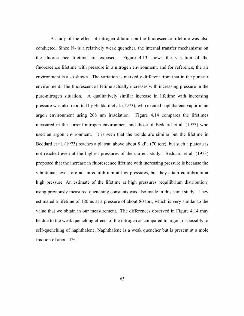
63

A study of the effect of nitrogen dilution on the fluorescence liftetime was also

conducted. Since N2 is a relatively weak quencher, the internal transfer mechanisms on

the fluorescence lifetime are exposed. Figure 4.13 shows the variation of the

fluorescence lifetime with pressure in a nitrogen environment, and for reference, the air

environment is also shown. The variation is markedly different from that in the pure-air

environment. The fluorescence lifetime actually increases with increasing pressure in the

pure-nitrogen situation. A qualitatively similar increase in lifetime with increasing

pressure was also reported by Beddard et al. (1973), who excited naphthalene vapor in an

argon environment using 268 nm irradiation. Figure 4.14 compares the lifetimes

measured in the current nitrogen environment and those of Beddard et al. (1973) who

used an argon environment. It is seen that the trends are similar but the lifetime in

Beddard et al. (1973) reaches a plateau above about 8 kPa (70 torr), but such a plateau is

not reached even at the highest pressures of the current study. Beddard et al. (1973)

proposed that the increase in fluorescence lifetime with increasing pressure is because the

vibrational levels are not in equilibrium at low pressures, but they attain equilibrium at

high pressure. An estimate of the lifetime at high pressures (equilibrium distribution)

using previously measured quenching constants was also made in this same study. They

estimated a lifetime of 180 ns at a pressure of about 80 torr, which is very similar to the

value that we obtain in our measurement. The differences observed in Figure 4.14 may

be due to the weak quenching effects of the nitrogen as compared to argon, or possibly to

self-quenching of naphthalene. Naphthalene is a weak quencher but is present at a mole

fraction of about 1%.

64

0 10 20 30 400

50

100

150

200

Pressure (kPa)

f (n

s)

Air

Nitrogen

Figure 4.13 Fluorescence lifetime measurements for naphthalene diluted in nitrogen and air

0 10 20 30 4040

60

80

100

120

140

160

180

200

Pressure (kPa)

f (n

s)

Current Study (N2)

Beddard et al. (Ar)

Figure 4.14 Fluorescence lifetime measurements for naphthalene diluted in nitrogen (current work) and argon (Beddard et al., 1973)

65

The collisional stabilization limit of Beddard et al. (1973) has apparently not been

established at the pressures tested for the case of nitrogen since a plateau has not yet been

reached. Other researchers have also reported non-equilibrium of the vibrational levels at

low pressures (Avouris et al., 1977, Stockburger et al., 1975b). Behlen and Rice (1981)

investigated the effect increasing excitation frequency (increasing photon energy) has on

the fluorescence lifetime, and found that the fluorescent lifetimes decreased with

increasing frequency, although the lifetimes demonstrated enormous variation from state

to state. They attributed it to an increase in population in higher vibrational levels with

increasing photon energy. This view was further corroborated by Schlag et al. (1971b),

who showed that the fluorescent lifetime decreases with increasing vibrational levels.

Avouris et al. (1977) and Schlag et al. (1971b) present a detailed discussion of the

lifetimes of different vibronic states.

The trend in the fluorescence lifetime found in the present experiments can be

explained with the above results. At low pressures, the laser pulse excites the molecules

to the S2 vibronic states, and the molecules undergo a rapid internal transfer to the S1

vibronic states (at rates of 1010

s-1

) (Schlag et al., 1971b). At low pressures, lack of

collisions locks the population in these upper vibrational states, whose fluorescent decay

times are short (on the order of 50 ns). However, at higher pressure, the upper states are

more thermalized and so the lower vibrational states are more highly populated. These

lower vibrational states have a longer decay time constant compared to the higher states,

which is seen as the increased fluorescence decay time-constant at higher pressures.

Figure 4.13 also shows that the lifetimes measured in the nitrogen environment and in

pure-air environment are very similar to one another as the pressure goes to zero. This of

course is expected, and provides some validation of the experimental technique

employed.

66

4.4 MACH 5 NAPHTHALENE ABLATION RESULTS: SECOND CAMPAIGN

4.4.1 Improvement of Naphthalene PLIF Images

The second campaign was focused on improving the PLIF signal levels. The

naphthalene PLIF signals were improved by four methods as outlined in section 4.1.

Since the fluorescence saturates at relatively low laser energy, it is not possible to

significantly improve the SNR by increasing the laser energy in a given pulse. Instead,

two laser pulses of laser light were used, separated in time by 100ns, so that more energy

could be delivered to the flow, but without increasing the laser intensity. Each laser pulse

had energy of 30 mJ per pulse delivered to the flow. The laser sheet was about 150 mm

wide and 1 mm thick. The resulting fluence was about 200 J/m2, which is within the

linear regime. Note that since the cameras integrate over the two pulses, the images are

slightly blurred due to flow motion. However, this blurring effect is negligible because

the flow convects a maximum of .08 mm, which is about one pixel width, between

pulses. The double-pulsing enabled us to obtain about a factor-of-two increase in signal,

but the main means of improving SNR was to increase the naphthalene concentration in

the boundary layer.

Another main improvement was to increase the size of the ablating surface. The

size of the insert was increased by about a factor of six and this design was described in

section 3.2.2. The original design was 25.4 mm (1 in.) long by 50.8 mm (2 in.) wide and

the new design was 101.6 mm (4 in.) long by 57.15 mm (2.25 in.) wide.

The largest improvement was obtained by increasing the stagnation temperature

of the tunnel from about 345 K to 380 K. The saturation pressure of naphthalene

increases by about a factor of 3 for each 10° C increase in temperature, and so heating is

potentially very effective at increasing the signal. Note, however, that the surface of the

naphthalene is not necessarily the same as the recovery temperature since the sublimation

67

process cools the surface, which is the purpose of an ablator. However, the amount of

mass loss is still quite small and so the sublimative cooling is expected to be small. It

was noted that as the stagnation temperature increased to its steady state value at the

beginning of each run, the fluorescence signal was seen to increase. This simply reflected

the increase in naphthalene vapor pressure with temperature. It took about 50 seconds for

the temperature to reach a semi steady state, and typically images were captured for about

30 seconds during this steady state period. The stagnation temperature was monitored

using a type-J thermocouple that was read by the Compact RIO and LabView and a

typical run is shown in Figure 4.15.

0 20 40 60 80 100 120280

300

320

340

360

380

400

Time (s)

Te

mp

era

ture

(K

)

Figure 4.15 Stagnation temperature during a typical run

68

Figure 4.16 shows a comparison between instantaneous naphthalene PLIF images

from the first campaign and from the second campaign. In this case the field of view

started 105 mm (x/δ99=5.4) downstream of the downstream edge of the naphthalene

insert. The size of the field of view was 27 mm (1.06 in.) wide by 14 mm (.55 in.) high as

seen in Figure 3.13b. The second campaign images were post-processed using a 3 x 3

median filter that was applied in MatLab. The images show that the fluorescence signal-

to-noise ratio is approximately 20, which represents a major improvement over the

images obtained in the first campaign.

Figure 4.17 shows several instantaneous naphthalene PLIF images after the

stagnation temperature had reached a steady state. The ablation products are seen to be

confined quite close to the wall of the wind tunnel, although the transport of the ablation

product through the boundary layer is evident.

To show the development of the scalar transport over a wider field of view,

Figure 4.18 shows a composite of two instantaneous (but uncorrelated) naphthalene PLIF

images. The total field of view spans 2.8 δ99 in the streamwise direction. The first image

starts 78 mm (x/δ99=3.98) downstream of the downstream edge of the naphthalene insert.

The capabilities of the plug allow for the field of view to span from 23.5 mm (x/δ99=1.24)

to 264.8 mm (x/δ99=13.94) downstream of the downstream edge of the naphthalene plug

(Figure 3.8).

69

(a)

(b) Figure 4.16 Instantaneous naphthalene PLIF images during (a) the first campaign and (b) the second campaign

70

Figure 4.17 Instantaneous naphthalene PLIF images in a Mach 5 turbulent boundary layer.

71

Fi

gure

4.1

8 C

om

po

site

of

two

inst

anta

ne

ou

s n

aph

thal

en

e P

LIF

imag

es

take

n a

t tw

o a

dja

cen

t lo

cati

on

s at

dif

fere

nt

tim

es

Figure 4.18 Composite of two instantaneous naphthalene PLIF images taken at two adjacent locations at different times

72

4.4.2 Thermocouple Measurements

The temperatures 1mm, 5.1mm, and 8.9mm below the surface of the naphthalene

plug were measured during each of these initial runs run at the center of the naphthalene

plug with type-T thermocouples. Figure 4.19 shows the schematic of the thermocouple

positions, while Figure 4.20 displays the readouts. These temperatures were found to be

steadily increasing. At 1mm below the surface, the sharp increase at the beginning and

ending of each run represent the normal shock passing over the naphthalene plug. The

heat flux through the surface from the combined effects of the recovery temperature near

the wind tunnel wall and mass transfer from the naphthalene plug is visible in the steady

increase of the thermocouples.

Figure 4.19 Naphthalene plug with thermocouples imbedded at varying depths

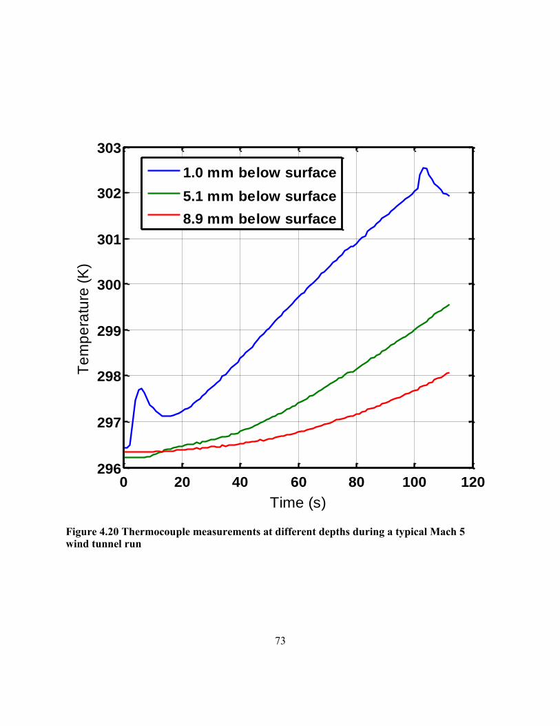
73

0 20 40 60 80 100 120296

297

298

299

300

301

302

303

Time (s)

Te

mp

era

ture

(K

)

1.0 mm below surface

5.1 mm below surface

8.9 mm below surface

Figure 4.20 Thermocouple measurements at different depths during a typical Mach 5 wind tunnel run

74

4.4.3 Average of Instantaneous PLIF Images

The mean fluorescence profile was computed from a set of 18 PLIF images

similar to that shown in Figure 4.17. Only 18 images were averaged due to a compressor

failure that ended this round of experiments. To improve the statistics, the pixel-columns

were averaged; i.e., the images were averaged in the streamwise direction as well as time.

Figure 4.21 shows the average image, while Figure 4.22 shows a plot of the normalized

mean LIF signal through the boundary layer and the standard deviation. Both the mean

LIF signal and standard deviation are normalized by the maximum mean LIF signal. The

naphthalene PLIF signal is seen to reach a peak at the wall and exhibit a gradual decrease

in magnitude with increasing distance from the wall.

x/

y/

5.4 5.6 5.8 6 6.2 6.4 6.6

0

0.1

0.2

0.3

0.4

0.5

0.6

0.7

0

0.1

0.2

0.3

0.4

0.5

0.6

0.7

0.8

0.9

1

Figure 4.21 Average of 18 instantaneous naphthalene PLIF images

75

0 0.2 0.4 0.6 0.8 10

0.1

0.2

0.3

0.4

0.5

0.6

0.7

0.8

Sf/S

f max

Wa

ll D

ista

nce

(y /

)

Mean

Standard Deviation

Figure 4.22 Normalized average fluorescence signal through the Mach 5 boundary layer with standard deviation

76

4.4.4 Obtaining Quantitative Measurements

The objective of the previously described spectroscopic studies was to enable us

to correct the measured naphthalene LIF signals to obtain quantitative measurements of

the naphthalene mole fraction. The dominant effect on the fluorescence signals will be

the temperature effect, since the mean pressure across the boundary layer is

approximately constant. For example, as the naphthalene is transported from the wall to

say the midpoint of the boundary layer it may cool from approximately the recovery

temperature of 370 K at the wall to 100 K. Although there currently is not spectroscopic

data at temperatures below 300 K, below we will develop a correction process that will

be used once the data are available. For example, currently there is data on the

temperature dependence of the fluorescence signal and absorption cross-section at

atmospheric pressure, for which the fluorescence is quenching dominated. In this case we

have,

)()()(

)()()(

)(

)(

TkTkTT

TkTkTT

TS

TS

Qreffref

refQfref

reff

f

(4.11)

If we assume that the spontaneous emission rate and quenching cross-section for

oxygen are temperature independent, then we have,

2/1

)(

)(

)(

)(

T

T

T

T

TS

TS ref

refreff

f

(4.12)

which we can use to obtain the temperature dependence of the cross-sections. Now, at the

conditions of the Mach 5 boundary layer, the pressure is 36 Torr (.7 psi) and the

77

fluorescence is not quenching dominated. In this case, for the same assumptions as above,

we can write,

),((

),((

))(/)((

)(/)(

)/(

)/(

)(

),(

int

maxint

max

max

maxmaxTPkkk

TPkkk

TT

TT

TT

TT

S

TPS

Qf

Qf

ref

ref

ref

ref

naph

naph

f

f

(4.13)

This equation can be used to obtain the normalized mole-fraction of naphthalene

vapor from the normalized fluorescence signal. Here we obtain the temperature profile in

the boundary layer from the Crocco-Busemann formula and the known mean velocity

profile. As outlined in White (1991), the energy equation can simplify to the Crocco-

Busemann formula after several approximations are made: (a) steady flow, (b) Pr = 1, (c)

adiabatic flow, (d) zero pressure gradient, and (e) boundary layer approximation hold (V

<< U and x / << y / ). The energy equation will then reduce to the familiar form of

the Crocco-Busemann relation:

PC

VUTT

2

)( 22

0

(4.14)

The assumption of adiabatic flow could be made due to negligible mass loss during a

typical run as explained in section 4.2. In this preliminary investigation the mean

velocity field is obtained from Pitot probe measurements in the Mach 5 boundary layer

Beresh (1999).

Since we do not have absorption cross-section data at lower temperatures, we

simply extrapolate the data in Figure 4.9 to lower temperatures. Obviously, this is a very

coarse assumption that will be checked in the future studies.

78

Finally, we take the quenching rate from the quenching measurements and the

assumed form as given in Equation 4.13. The corrected mean is shown in Figure 4.23.

This is only a proof-of-concept exercise to show how the fluorescence data can be

corrected to obtain quantitative results, provided the absorption data can be measured at

low-temperatures. In future work, the intention is to make the required LIF temperature-

dependence measurements.

It is clear that if this technique is to be made quantitative, it will be necessary to

have some idea of the local conditions, because the fluorescence signal is strongly

dependent on them. It is clear that having a simultaneous measurement of temperature is

critical. In the case of a boundary layer, the mean temperature can be achieved with a

separate velocity measurement (and Crocco-Busemann), but in cases where measuring

velocity is not possible then it may be possible to use a dual-line excitation method to

infer the temperature, as has been done with acetone (Thurber et al., 1998). In cases

where the freestream pressure varies widely, such as over the shoulder of a blunt re-entry

vehicle, it may be necessary to use simultaneously-acquired data from pressure taps, or

perhaps a numerical simulation, to obtain a first-order estimate for the local pressure.

79

0 0.2 0.4 0.6 0.8 10

0.1

0.2

0.3

0.4

0.5

0.6

0.7

0.8

Sf/S

f max

Wa

ll D

ista

nce

(y /

)

Original Signal

Corrected Signal

Figure 4.23 Normalized average fluorescence signal profiles through the Mach 5 boundary layer. Uncorrected signal and signal corrected for temperature effects.

80

Chapter 5: Conclusions and Future Work

5.1 CONCLUSIONS

Planar laser-induced fluorescence has been used to image the ablation products

given off by a sublimating ablator in the presence of a Mach 5 boundary layer.

Naphthalene is used as the ablator because its vapor is readily detected by the laser-

induced fluorescence technique with 266 nm excitation. The results show that excellent

signal-to-noise-ratio PLIF images can be obtained with this technique. Furthermore, it is

an objective of this work to conduct targeted spectroscopic studies to enable the

quantitative interpretation of the PLIF signal in terms of naphthalene mole fraction. Test-

cell measurements were made to determine the fluorescence signal and absorption cross-

section dependence on temperature, over the temperature range of 297 K to 525 K. On a

per-mole basis, the temperature dependence of naphthalene fluorescence increases

sharply at lower temperatures and levels off with higher temperatures, whereas the

absorption cross-section exhibits a more gradual increase with temperature. Stern-Volmer

plots show a linear variation of the inverse lifetime with pressure, which indicates the

fluorescence follows a conventional quenching model at pressures greater than 2 kPa (40

torr). It was further found that for the fluorescence remained linear with laser fluence

provided the laser fluence was less than about 200 J/m2.

To obtain quantitative concentration information in the Mach 5 turbulent

boundary layer, the naphthalene PLIF images will need to be corrected for temperature

effects since the boundary layer temperature can vary considerably with distance from the

wall. A correction procedure was demonstrated that used mean velocity data and the

Crocco-Busemann relation to obtain the needed temperature information. However, a

81

limitation of this process was the lack of absorption cross-section data at the lowest

temperatures encountered in the boundary layer.

5.2 SUGGESTED FUTURE WORK

Future work should be directed at finishing the spectroscopic study of

naphthalene LIF, expanding the database of images of naphthalene PLIF in the Mach 5

blow down wind tunnel, and obtaining simultaneous PIV and PLIF data in the Mach 5

wind tunnel. The temperature dependence of the absorption cross-section data will need

to be further investigated. The experimental setup to obtain the pressure dependence and

lifetime information of the naphthalene LIF will be used to obtain the absorption cross-

section data at low pressure. In addition, the absorption cross-section will need to be

investigated to the lowest temperature encountered in the boundary layer. One way to do

these low temperature measurements is to expand the naphthalene-laden gas through a

supersonic nozzle. The temperature effects on the quenching cross-section will also need

to be investigated. In this preliminary investigation the quenching cross-section was

assumed to be constant, but the validity of this assumption will need to be checked.

Expanding the database of naphthalene PLIF images is necessary in order to

obtain statistically converged data sets. A thousand images per position may be

necessary to compute the gradient of the mean scalar field. The gradient of the mean

scalar field will be used in validation of LES sub-filter models.

Simultaneous quantitative PLIF and PIV measurements in the Mach 5 turbulent

boundary layer is the overall goal of this entire investigation. The development of a PIV

system for the Mach 5 wind tunnel is currently in testing stages, which would allow for

these simultaneous diagnostics to begin. In the future, these data will be taken in

multiple side-view locations downstream of the naphthalene plug, as well as in multiple

82

plan-view locations. These results will give scalar/velocity correlations will also be used

in validation of LES sub-filter models.

83

Bibliography

Ambrose, D., Lawrenson, I. J., and Sparke, C. H. S., “The vapor pressure of naphthalene,” J. Chem. Thermodynam., 7: 1173-1176, 1975.

Ashpole, C. W., Formoshinho, S. J., and Porter, G., “Pressure dependence of intersysterm crossing in aromatic vapours,” Proc. Roy. Soc. Lond. A, 323: 11-28, 1971.

Avouris, P., Gelbart, W. M., and El-Sayed, M. A., “Nonradiative electronic relaxation under collision-free conditions”, Chemical reviews, 77 (6): 793–833, 1977.

Beddard, G. S., Fleming, G. R., Gijzeman, O. L. J., and Porter, G., “Vibrational energy dependence of radiationless conversion in aromatic vapours,” Proc. R. Soc. Lond. A, 340: 519-533, 1974.

Beddard, G. S., Formosinho, S. J., and Porter, G., “Pressure effects on the fluorescence from naphthalene vapour”, Chem. Phys. Letters, 22 (2): 235–238, 1973.

Behlen, M. F. and Rice, S. A., “Intersystem crossing in cold isolated molecules of naphthalene”, J. Chem. Phys. 75 (12): 5672–5684, 1981.

Bryant, R. A., Donbar, J. M., Driscoll, J. F., “Acetone laser induced fluorescence for low pressure/low temperature flow visualization,” Experiments in Fluids, 28: 471-478, 2000.

Callaway, D. W., Reeder, M. F., and Greendyke, R. B., “Experimental Studies of Low Temperature Ablation using Dry Ice,” AIAA 2008-2554, 15

th AIAA International

Space Planes and Hypersonic Systems and Technologies Conference, Dayton, Ohio, 2008.

Callaway, D. W., Reeder, M. F., Greendyke, R. B., and Gosse, R., “Photogrammetric Measurement of Recession Rates of Low Temperature Ablators in Supersonic Flow,” AIAA 2010-1216, 48

th AIAA Aerospace Sciences Meeting, Orlando,

Florida, 2010.

Charwat, A. F., “Exploratory studies on the sublimation of slender camphor and naphthalene models in a supersonic wind-tunnel,” 1968.

Clemens, N. T., “Flow Imaging,” Encyclopedia of Imaging Science and Technology, John Wiley and Sons, New York, 2002.

84

Covington, M. A., Heinemann, J. M., Goldstein, H. E., Chen, Y.-K., Terrazas-Salinas, I., Balboni, J. A., Olejniczak, J., and Martinez, E. R., “Performance of a Low Density Ablative Heat Shield Material,” Journal of Spacecraft and Rockets, 45 (4): 854-864, 2008.

De Kruif, C. G., Kuipers, T., Van Miltenburg, J. C., Schaake, R. C. F., and Stevens, G., “The vapor pressure of solid and liquid naphthalene,” J. Chem. Thermodynam, 13: 1081-1086, 1981.

Du, H., Fuh, R. A., Li, J., Corkan, A., and Lindsey, J. S., "PhotochemCAD: A computer-aided design and research tool in photochemistry," Photochemistry and Photobiology, 68: 141-142, 1998.

Eckbreth, A. C., Laser Diagnostics for Combustion Temperature and Species, Abacus Press, Cambridge, 1988.

Gatski, T. B., Hussaini, M. Y., and Lumley, J. L., Simulation and Modeling of Turbulent Flows, Oxford University Press, New York, 1996.

Gattermann, H. and Stockburger, M., “Spectroscopic studies on naphthalene in the vapor phase III, phosphorescence and intersystem crossing yields of single vibronic levels”, J. Chem. Phys., 63 (10): 4541–4545, 1975.

Ghandhi, J. B. and Felton, P. G., “On the fluorescent behavior of ketones at high temperatures,” Experiments in Fluids, 21: 143-144, 1996.

Gnoffo, P. A., Weilmuenster, K. J., and Hamiton II, H. H., “Computational aerothermo-dynamics design issues for hypersonic vehicles,” Journal of Spacecraft and Rockets, 36 (1): 21-43, 1999.

Goldstein, R. J. and Cho, H. H., “A review of mass transfer measurements using naphthalene sublimation,” Experimental Thermal and Fluid Science, 10: 416-434, 1995.

Greathouse, J. S., Kirk, B. S., Lillard, R. P, Truong, T. H., Robinson, P., and Cerimele, C. J., “Crew exploration vehicle (cev) crew module shape selection analysis and cev aeroscience project overview,” AIAA 2007-603, 45th AIAA Aerospace Sciences Meeting and Exhibit, Reno, Nevada, 2007.

Griffith, B. J., Edenfield, E. E., and Strike, W. T., “Wind-Tunnel Simulation of Ablation,” Journal of Spacecraft and Rockets, 14 (10): 593-599, 1977.

Grossman, F., Monkhouse, P. B., Ridder, M., Sick, V., and Wolfrum, J., “Temperature and pressure dependences of the laser-induced fluorescence of gas-phase acetone and 3-pentanone,” Applied Physics B, 62: 249-253, 1996.

85

Ho, D. W. K., Koo, J. H., Bruns, M. C., and Ezekoye, O. A., “A Review of Numerical and Experimental Characterization of Thermal Protection Materials – Part III. Experimental Testing,” AIAA 2007-5773, 43

rd AIAA/ASME/SAE/ASEE Joint

Propulsion Conference & Exhibit, Cincinnati, Ohio, 2007.

Hsieh, J. C., Huang, C., and Lim, E. C., “Radiationless singlet deactivation in isolated large molecules. I. Naphthalene, naphthol, and naphthylamine,” J. Chem. Phys., 60 (11): 4345-4353, 1974.

Incropera, F. P. and DeWitt, D. P., Fundamentals of Heat and Mass Transfer, John Wiley & Sons, 2002.

Inman, J. A. (Wilkes), Danehy, P. M., Alderfer, D. W., and Buck, G. M., “Plif imaging of capsule rcs jets and simulated forebody ablation,” AIAA 2008-248, 46th AIAA Aerospace Sciences Meeting and Exhibit, Reno, Nevada, 2008.

Kaiser, S., Kyritsis, D. C., Dobrowolski, P., Long, M. B., and Gomez, A., “The electrospray and combustion at the mesoscale,” J. Mass Spectrom. Soc Jpn., 51: 42-49, 2003.

Kaiser, S. A. and Long, M. B., “Quantitative planar laser-induced fluorescence of naphthalene as fuel tracers,” Proceedings of the Combustion Institute, 30: 1555-1563, 2005.

Kohlman, D. L. and Richardson, R. W., “Experiments on the use of dry ice ablating wind-tunnel models,” Journal of Spacecraft and Rockets, 6 (9): 1061-1063, 1969.

Laor, U. and Ludwig, P. K., “Fluorescence lifetimes of vibronic states of naphthalene vapor in the region of excitation from 3080 – 2150 A,” J. Chem. Phys., 54 (3): 1054–1057, 1971.

Lim E. C. and Huang C., “Radiationless transition in large isolated molecules: Variation of excess energy dependence of its decay rate with initially prepared electronic state,” J. Chem. Phys., 58 (3): 1247-1248, 1973.

Lipfert, F. and Genovese, J., “An experimental study of the boundary layers on low-temperature subliming ablators,” AIAA Journal, 9 (7): 1330-1337, 1971.

Martinez, M., Harder, H., Ren, X., Lesher, R. L., and Brune, W. H., “Measuring atmospheric naphthalene with laser-induced fluorescence,” Atmos. Chem. Phys. Discuss, 4: 343-363, 2004.

Milos, F. S. and Chen, Y.-K., “Ablation and Thermal Response Property Model Validation for Phenolic Impregnated Carbon Ablator,” AIAA 2009-262, 47

th

AIAA Aerospace Sciences Meeting, Orlando, Florida, 2009.

86

Ni, T. and Melton, L. A., “Two-dimensional gas-phase temperature measurements using fluorescence lifetime imaging,” Applied Spectroscopy, 50 (9): 1112-1116, 1996.

Ossler, F., Metz, T., and Aldén, M., “Picosecond laser-induced fluorescence from gas-phase polycyclic aromatic hydrocarbons at elevated temperatures. I. Cell measurements,” Appl. Phys. B., 72: 465-478, 2001.

Reyle, C. and Brechignac, P., “Fluorescence of jet-cooled naphthalene: emission spectra, lifetimes and quantum yields,” Eur. Phys. J. D, 8: 205–210, 2000.

Schlag, E. W., Schneider, S., and Chandler, D. W., “Fluorescence lifetimes of vibronic levels of naphthalene vapour,” Chem. Phys. Letters, 11 (4): 474–477, 1971a.

Schlag, E. W., Schneider, S., and Fischer, S. F., “Lifetimes in excited states,” Annual Review of Physical Chemistry, 22, 465-526, 1971b.

Silton, S. I. and Goldstein, D. B., “Ablation Onset in Unsteady Hypersonic Flow About Nose Tip with Cavity,” Journal of Thermophysics and Heat Transfer, 14 (3): 421-434, 2000.

Smits, A. J., Martin, M. P., and Girimaji, S., “Current status of basic research in hypersonic turbulence,” AIAA 2009-151, 47th AIAA Aerospace Sciences Meeting and Exhibit, Orlando, Florida, 2009.

Soep, B., Michel, C., Tramer, A., and Lindqvist, L., “Study of intersystem crossing in naphthalene and 1-methylnaphthalene in collision free conditions and pressure effects,” Chem. Phys., 2: 293-303, 1973.

Stock, H. W., “Surface Patterns on Subliming and Liquefying Ablation Materials,” AIAA Journal, 13 (9): 1217-1223, 1975.

Stock, H. W. and Ginoux, J. J., “Experimental Results on Crosshatched Ablation Paterns,” AIAA Journal, 9 (5): 971-973, 1971.

Stockburger, M., Gattermann, H., and Klusmann, W., “Spectroscopic studies of naphthalene in the vapor phase I ,” J. Chem. Phys., 63 (10): 4519 – 4529, 1975a.

Stockburger, M., Gattermann, H., and Klusmann, W., “Spectroscopic studies of naphthalene in the vapor phase II. Fluorescence quantum yields from single vibronic levels in the first excited singlet state – behavior of higher excited singlet states,” J. Chem. Phys., 63 (10): 4529–4540, 1975b.

Suto, M., Wang, X., Shan, J., and Lee, L. C., “Quantitative photoabsorption and fluorescence spectroscopy of benzene, naphthalene and some derivatives at 106 – 295 nm,” J. Quant. Spec. Radiat. Transfer, 48 (1): 79–89, 1992.

87

Thurber, M. C., Grisch, F., Kirby, B. J., Votsmeier, M., and Hanson, R. K., “Measurements and modeling of acetone laser-induced fluorescence with implications for temperature-imaging diagnostics,” Applied Optics, 37 (21): 4963-4978, 1998.

Vojvodich, N. S. and Winkler, E. L., “The Influence of Heat Rating and Test Stream Oxygen Content of the Insulation Efficiency of Charring Materials,” NASA TN D-1889, July 1963.

Von Karman, T. H., “The Analogy Between Fluid Friction and Heat Transfer,” Trans. ASME, 61: 705-510, 1939.

Watts, R. J. and Strickler, S. J., “Fluorescence and Internal Conversion in Naphthalene Vapor,” J. Chem. Phys., 44 (6): 2423-2426, 1966.

White, F. M., Viscous Fluid Flow, McGraw-Hill, Boston, 1991.

88

Vita

Bryan Lochman is the son of Mrs. Linda Lochman and Dr. John Lochman, and is

married to Natalie Busby. After graduating from Northridge High School in Tuscaloosa,

Alabama in 2004, he attended Northwestern University in Evanston, Illinois and received

his Bachelor of Science in Mechanical Engineering in June of 2008. In August of 2008

he enrolled into the Graduate School of the University of Texas at Austin in the

department of Aerospace Engineering and Engineering Mechanics pursuing a Master of

Science degree.

Permanent email address: bryan.lochman@gmail.com

This thesis was typed by the author.