Copyright by Bich-Thu Ngoc Nguyen 2013
271
Copyright by Bich-Thu Ngoc Nguyen 2013
Transcript of Copyright by Bich-Thu Ngoc Nguyen 2013

Copyright
by
Bich-Thu Ngoc Nguyen
2013
The Dissertation Committee for Bich-Thu Ngoc Nguyen certifies that
this is the approved version of the following dissertation:
Amine Volatility in CO2 Capture
Committee
____________________________ Gary T. Rochelle, Supervisor
_________________________________
Isaac C. Sanchez
_________________________________
Thomas M. Truskett
_________________________________
Ben A. Shoulders
_________________________________
Jim E. Critchfield
Amine Volatility in CO2 Capture
by
Bich-Thu Ngoc Nguyen, B.S.
Dissertation
Presented to the Faculty of the Graduate School of
The University of Texas at Austin
in Partial Fulfillment
of the Requirements
for the Degree of
Doctor of Philosophy
The University of Texas at Austin
May 2013

Dedication
To my Family
v
Acknowledgements
First I would like to extend my sincere gratitude and appreciation to Dr. Gary
Rochelle for being my research advisor and mentor throughout my entire graduate school
career. He is incredibly knowledgeable and experienced in the area of CO2 Capture. I
am always in awe of the breadth of his knowledge, and strive my best to emulate the high
level Ph.D. thinking process and analytical ability that he has taught me which will
undoubtedly be the most valuable tool to be utilized for the rest of my Chemical
Engineering career. Furthermore, Dr. Rochelle has inspired me to always have a thirst
for learning, and to maintain an inquisitive and open mind to new knowledge. Both of
these elements are essential and highly beneficial to my continuing growth as a Ph.D. for
years to come.
Next I want to thank the Luminant Carbon Management program for sponsoring
the Rochelle group’s CO2 Capture research. Without your generous contribution and
those of our other industrial sponsors, we would not have a means to pursue this exciting
research area which is so vital to the fate of our lives and natural environment. In
particular, I wish to acknowledge GTC Technology LLC, a first-rate technology
company in gas and oil processing, for both the research sponsorship and the employment
opportunity as a thermodynamic specialist – a role which has undoubtedly promoted my
passion and intellectual growth in the area of chemical thermodynamics, and furthermore,
has been seen to complement my CO2 thermodynamics research very well.
vi
Additionally, I need to thank my Ph.D. committee members, Dr. Isaac Sanchez,
Tom Truskett, Ben Shoulders, and Jim Critchfield, for their valuable guidance and inputs
for my work. They have always raised the bar for me to grow in my understanding of
thermodynamics and applied Chemical Engineering as a whole. Also, I want to thank
Maeve Cooney and others in the UT Austin Chemical Engineering staff, especially T.
Stockman, Kay Swift-Costales, for their assistance throughout my graduate school career.
Maeve in particular has been instrumental in editing all of my reports, presentations, as
well as helping me to meet many key deadlines and appointments which would otherwise
be rather stressful and overwhelming if it had not been for her assistance. Also Jim
Smitherman and Butch Cunningham in the Machine Shop have been my lifeline
whenever I run into hardware and/or instrumentation issues. No matter how serious the
problem was, they can always take care of it properly and expediently. Also, Eddie
Ibarra and Kevin Haynes had been superb in handling all procurement issues without any
glitch and expediently as well.
In terms of FTIR support, I am especially appreciative of Mark Nelson, the
technical sales representative of the former Gasmet Air Quality Analytical company. He
is a true FTIR expert and analytical chemist in his own right – the combination of which
has made him a highly valuable FTIR support resource for all instrumentation issues
ranging from hardware to chemical gas analysis. Mark was also supportive and
accessible in handling all of our queries and problems at all times, to which I am highly
grateful. And of course, there are the Rochelle group members which I must also thank.
Xi Chen for NMR support, Alex Voice for his innovative experimental inputs and

vii
solutions, Steven Fulks and Peter Frailie for their thermodynamic insights and modeling
support, respectively. Additionally, Mandana Ashouri, Lynn Li, Qing Xu, Jorge Plaza,
David Van Wagener, and the rest of the Rochelle group have been a pleasure to work
with and are always helpful.
Last but definitely not least, I am grateful beyond words to my loving parents who
have been my strongest supporters through my Ph.D. years, actually since as far back as I
can remember. They have always believed in me without fail, and are also a source of
strength and solace which I constantly turn to every time the going gets tough. I owe my
success, professional discipline, hard-working ethics, and sense of persistence to them
because of their love and guidance since I was very young. I feel very blessed to have
my parents be the people that they are in setting the good life examples, and I am proud
of the fact that I can see a reflection of them every day when I look in the mirror. Also I
would need to thank my four aunts and uncle in law for their unwavering love, support,
and patience through the years which have also gone a long way in helping me become
who I am today. Ultimately, I thank God for blessing me with the family that I have, the
opportunity to pursue a once-in-a-lifetime world class education, and most importantly,
for blessing me with the passion and appreciation to make the most of the opportunity I
am given to benefit not only myself and my family but also society in the years to come.
viii
Amine Volatility in CO2 Capture
Bich-Thu Ngoc Nguyen, Ph.D.
The University of Texas at Austin, 2013
Supervisor: Gary T. Rochelle
This work investigates the volatilities of amine solvents used in post-combustion
CO2 capture from coal-fired power plants. Amine volatility is one of the key criteria used
in screening an amine solvent for CO2 capture: (1) amine losses up the stack can react in
the atmosphere to form ozone and other toxic compounds; (2) volatility losses can result
in greater solvent make-up costs; (3) high losses will require the use of bigger water wash
units, and more water, to capture fugitive amines prior to venting - these translate to
higher capital and operating costs; (4) volatilities need to be measured and modeled in
order to develop more accurate and robust thermodynamic models.
In this work, volatility is measured using a hot gas FTIR which can determine
amine, water, and CO2 in the vapor headspace above a solution. The liquid solution is
speciated by NMR (Nuclear Magnetic Resonance). There are two key contributions
made by this research work: (1) it serves as one of the largest sources of experimental
data available for amine-water volatility; (2) it provides amine volatility for loaded
systems (where CO2 is present) which is a unique measurement not previously reported
in the literature.
ix
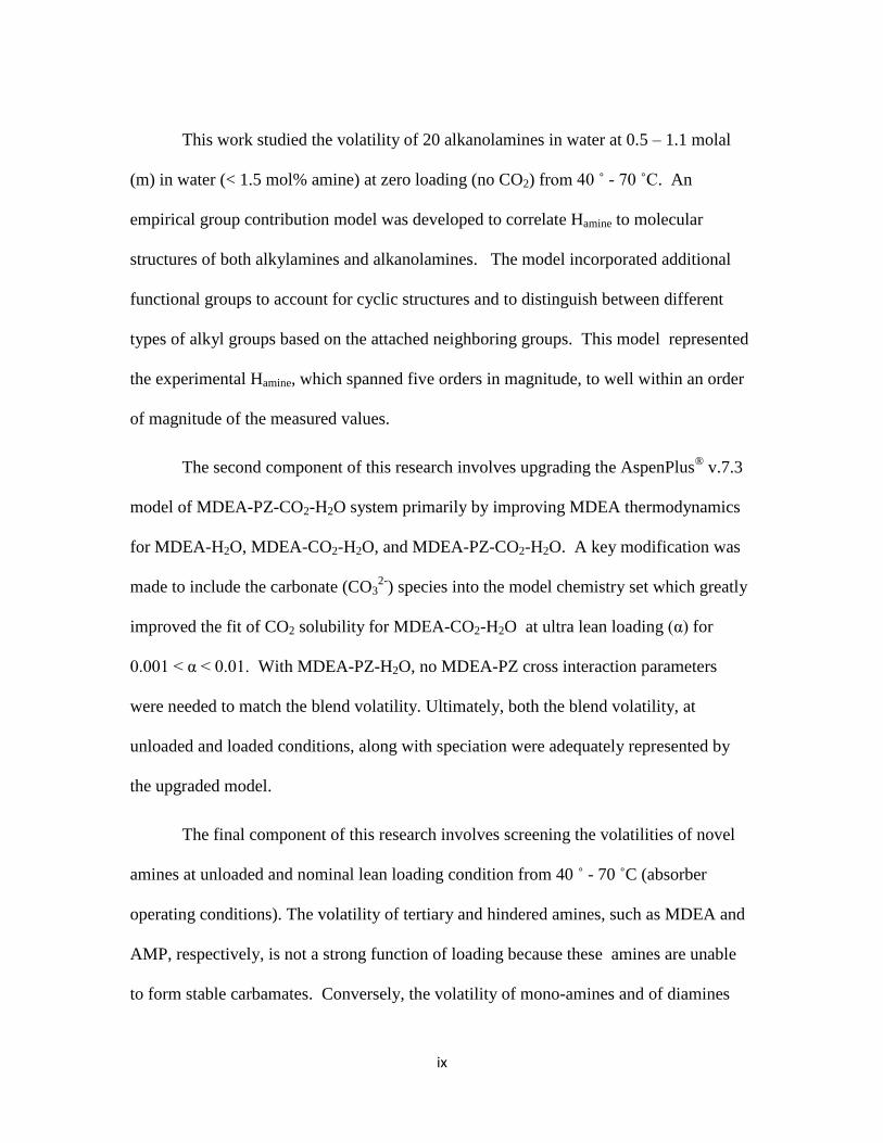
This work studied the volatility of 20 alkanolamines in water at 0.5 – 1.1 molal
(m) in water (< 1.5 mol% amine) at zero loading (no CO2) from 40 ˚ - 70 ˚C. An
empirical group contribution model was developed to correlate Hamine to molecular
structures of both alkylamines and alkanolamines. The model incorporated additional
functional groups to account for cyclic structures and to distinguish between different
types of alkyl groups based on the attached neighboring groups. This model represented
the experimental Hamine, which spanned five orders in magnitude, to well within an order
of magnitude of the measured values.
The second component of this research involves upgrading the AspenPlus®
v.7.3
model of MDEA-PZ-CO2-H2O system primarily by improving MDEA thermodynamics
for MDEA-H2O, MDEA-CO2-H2O, and MDEA-PZ-CO2-H2O. A key modification was
made to include the carbonate (CO32-
) species into the model chemistry set which greatly
improved the fit of CO2 solubility for MDEA-CO2-H2O at ultra lean loading (α) for
0.001 < α < 0.01. With MDEA-PZ-H2O, no MDEA-PZ cross interaction parameters
were needed to match the blend volatility. Ultimately, both the blend volatility, at
unloaded and loaded conditions, along with speciation were adequately represented by
the upgraded model.
The final component of this research involves screening the volatilities of novel
amines at unloaded and nominal lean loading condition from 40 ˚ - 70 ˚C (absorber
operating conditions). The volatility of tertiary and hindered amines, such as MDEA and
AMP, respectively, is not a strong function of loading because these amines are unable
to form stable carbamates. Conversely, the volatility of mono-amines and of diamines
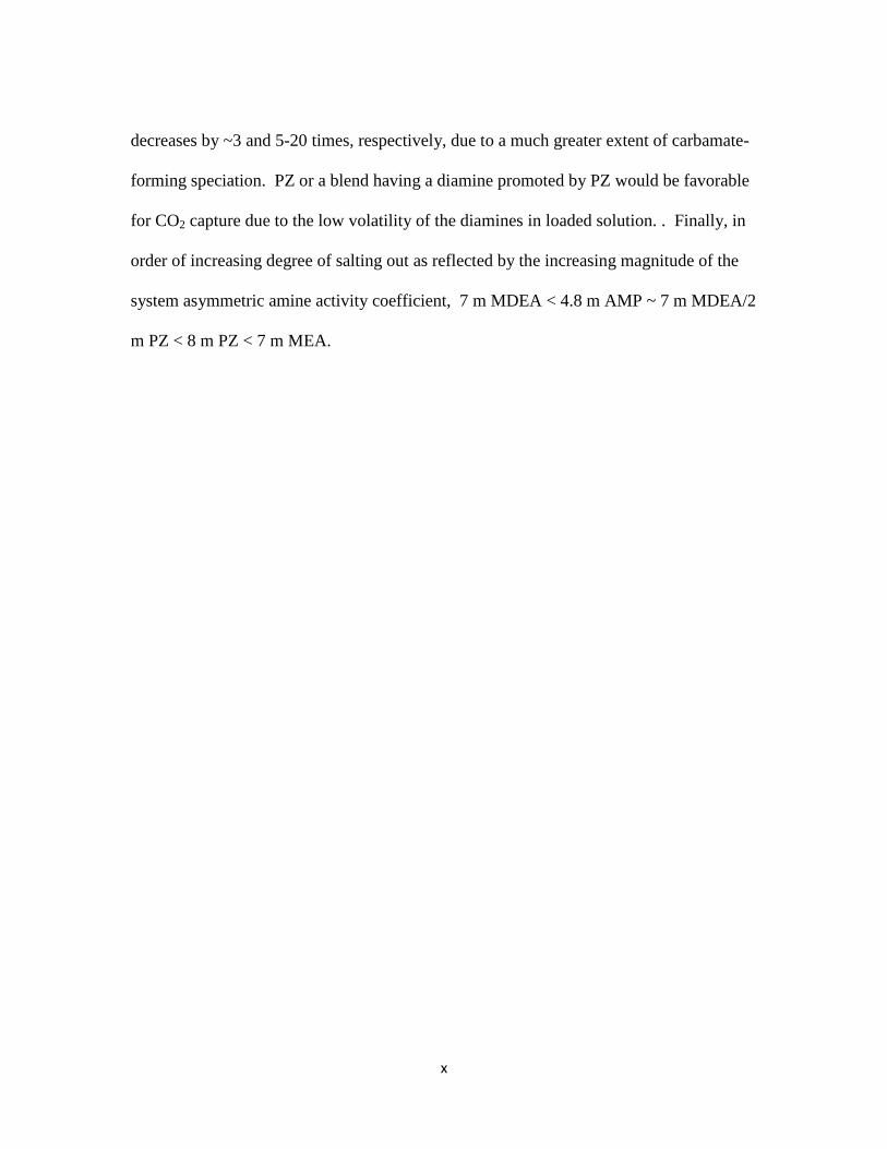
x
decreases by ~3 and 5-20 times, respectively, due to a much greater extent of carbamate-
forming speciation. PZ or a blend having a diamine promoted by PZ would be favorable
for CO2 capture due to the low volatility of the diamines in loaded solution. . Finally, in
order of increasing degree of salting out as reflected by the increasing magnitude of the
system asymmetric amine activity coefficient, 7 m MDEA < 4.8 m AMP ~ 7 m MDEA/2
m PZ < 8 m PZ < 7 m MEA.
xi
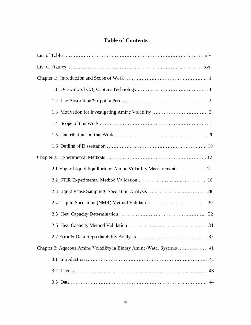
Table of Contents
List of Tables ………………………………………………………………………… xiv
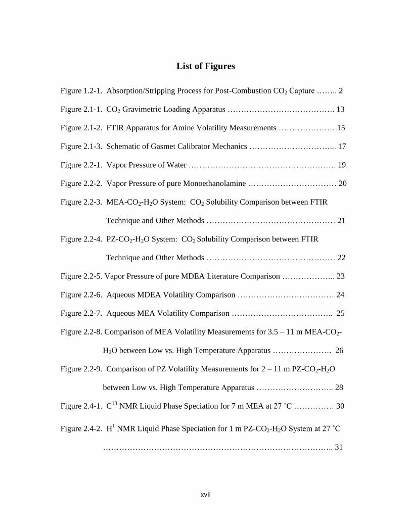
List of Figures ………………………………………………………………………...xvii
Chapter 1: Introduction and Scope of Work …………………………………………... 1
1.1 Overview of CO2 Capture Technology ……………………………………. 1
1.2 The Absorption/Stripping Process ………………………………………… 2
1.3 Motivation for Investigating Amine Volatility ……………………………. 3
1.4 Scope of this Work ………………………………………………………… 4
1.5 Contributions of this Work ………………………………………………… 9
1.6 Outline of Dissertation ……………………………………………………..10
Chapter 2: Experimental Methods ……………………………………………………. 12
2.1 Vapor-Liquid Equilibrium: Amine Volatility Measurements …………… 12
2.2 FTIR Experimental Method Validation ………………………………….. 18
2.3 Liquid Phase Sampling: Speciation Analysis …………………………….. 28
2.4 Liquid Speciation (NMR) Method Validation …………………………… 30
2.5 Heat Capacity Determination ……………………………………………. 32
2.6 Heat Capacity Method Validation ………………………………………... 34
2.7 Error & Data Reproducibility Analysis …………………………………... 37
Chapter 3: Aqueous Amine Volatility in Binary Amine-Water Systems ……………… 41
3.1 Introduction ……………………………………………………………….. 41
3.2 Theory ……………………………………………………………………... 43
3.3 Data ………………………………………………………………………... 44
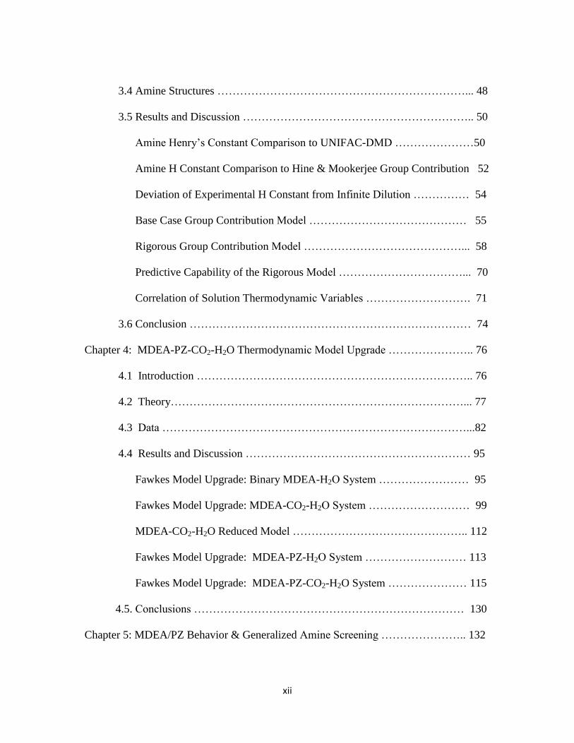
xii
3.4 Amine Structures …………………………………………………………... 48
3.5 Results and Discussion …………………………………………………….. 50
Amine Henry’s Constant Comparison to UNIFAC-DMD …………………50
Amine H Constant Comparison to Hine & Mookerjee Group Contribution 52
Deviation of Experimental H Constant from Infinite Dilution …………… 54
Base Case Group Contribution Model …………………………………… 55
Rigorous Group Contribution Model ……………………………………... 58
Predictive Capability of the Rigorous Model ……………………………... 70
Correlation of Solution Thermodynamic Variables ………………………. 71
3.6 Conclusion ………………………………………………………………… 74
Chapter 4: MDEA-PZ-CO2-H2O Thermodynamic Model Upgrade ………………….. 76
4.1 Introduction ……………………………………………………………….. 76
4.2 Theory……………………………………………………………………... 77
4.3 Data ………………………………………………………………………...82
4.4 Results and Discussion …………………………………………………… 95
Fawkes Model Upgrade: Binary MDEA-H2O System …………………… 95
Fawkes Model Upgrade: MDEA-CO2-H2O System ……………………… 99
MDEA-CO2-H2O Reduced Model ……………………………………….. 112
Fawkes Model Upgrade: MDEA-PZ-H2O System ……………………… 113
Fawkes Model Upgrade: MDEA-PZ-CO2-H2O System ………………… 115
4.5. Conclusions ……………………………………………………………… 130
Chapter 5: MDEA/PZ Behavior & Generalized Amine Screening ………………….. 132
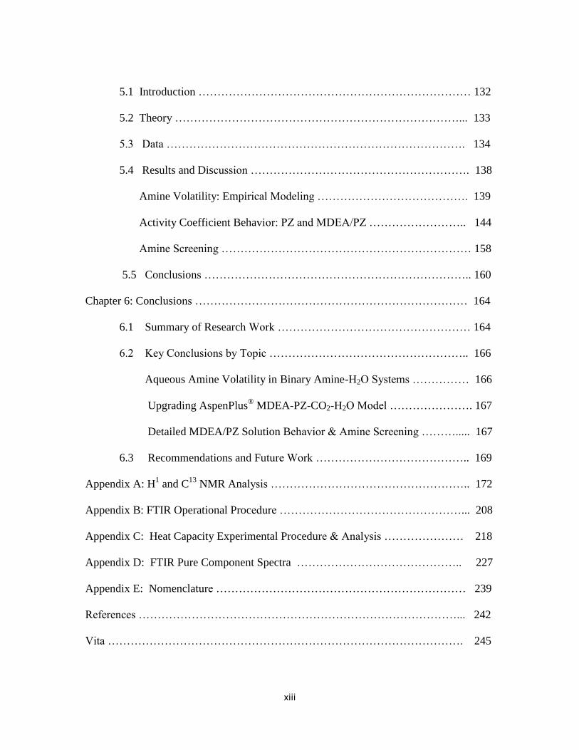
xiii
5.1 Introduction ……………………………………………………………… 132
5.2 Theory …………………………………………………………………... 133
5.3 Data ……………………………………………………………………. 134
5.4 Results and Discussion …………………………………………………. 138
Amine Volatility: Empirical Modeling …………………………………. 139
Activity Coefficient Behavior: PZ and MDEA/PZ …………………….. 144
Amine Screening ………………………………………………………… 158
5.5 Conclusions …………………………………………………………….. 160
Chapter 6: Conclusions ……………………………………………………………… 164
6.1 Summary of Research Work …………………………………………… 164
6.2 Key Conclusions by Topic …………………………………………….. 166
Aqueous Amine Volatility in Binary Amine-H2O Systems …………… 166
Upgrading AspenPlus® MDEA-PZ-CO2-H2O Model …………………. 167
Detailed MDEA/PZ Solution Behavior & Amine Screening ………..... 167
6.3 Recommendations and Future Work ………………………………….. 169
Appendix A: H1 and C
13 NMR Analysis …………………………………………….. 172
Appendix B: FTIR Operational Procedure …………………………………………... 208
Appendix C: Heat Capacity Experimental Procedure & Analysis ………………… 218
Appendix D: FTIR Pure Component Spectra …………………………………….. 227
Appendix E: Nomenclature ………………………………………………………… 239
References …………………………………………………………………………... 242
Vita …………………………………………………………………………………. 245
xiv
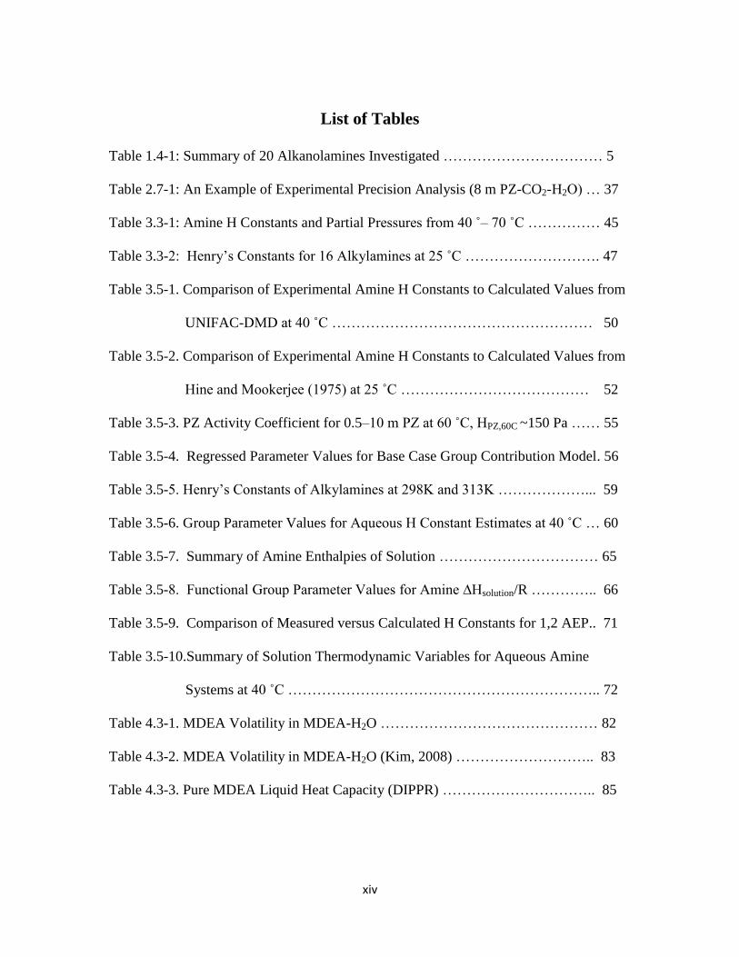
List of Tables
Table 1.4-1: Summary of 20 Alkanolamines Investigated …………………………… 5
Table 2.7-1: An Example of Experimental Precision Analysis (8 m PZ-CO2-H2O) … 37
Table 3.3-1: Amine H Constants and Partial Pressures from 40 ˚– 70 ˚C …………… 45
Table 3.3-2: Henry’s Constants for 16 Alkylamines at 25 ˚C ………………………. 47
Table 3.5-1. Comparison of Experimental Amine H Constants to Calculated Values from
UNIFAC-DMD at 40 ˚C ……………………………………………… 50
Table 3.5-2. Comparison of Experimental Amine H Constants to Calculated Values from
Hine and Mookerjee (1975) at 25 ˚C ………………………………… 52
Table 3.5-3. PZ Activity Coefficient for 0.5–10 m PZ at 60 ˚C, HPZ,60C ~150 Pa …… 55
Table 3.5-4. Regressed Parameter Values for Base Case Group Contribution Model. 56
Table 3.5-5. Henry’s Constants of Alkylamines at 298K and 313K ………………... 59
Table 3.5-6. Group Parameter Values for Aqueous H Constant Estimates at 40 ˚C … 60
Table 3.5-7. Summary of Amine Enthalpies of Solution …………………………… 65
Table 3.5-8. Functional Group Parameter Values for Amine ∆Hsolution/R ………….. 66
Table 3.5-9. Comparison of Measured versus Calculated H Constants for 1,2 AEP.. 71
Table 3.5-10.Summary of Solution Thermodynamic Variables for Aqueous Amine
Systems at 40 ˚C ……………………………………………………….. 72
Table 4.3-1. MDEA Volatility in MDEA-H2O ……………………………………… 82
Table 4.3-2. MDEA Volatility in MDEA-H2O (Kim, 2008) ……………………….. 83
Table 4.3-3. Pure MDEA Liquid Heat Capacity (DIPPR) ………………………….. 85
xv
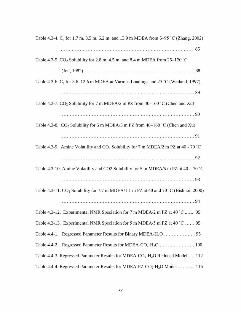
Table 4.3-4. Cp for 1.7 m, 3.5 m, 6.2 m, and 13.9 m MDEA from 5–95 ˚C (Zhang, 2002)
…………………………………………………………………………. 85
Table 4.3-5. CO2 Solubility for 2.8 m, 4.5 m, and 8.4 m MDEA from 25–120 ˚C
(Jou, 1982) ……………………………………………………………. 88
Table 4.3-6. Cp for 3.6–12.6 m MDEA at Various Loadings and 25 ˚C (Weiland, 1997)
…………………………………………………………………………. 89
Table 4.3-7. CO2 Solubility for 7 m MDEA/2 m PZ from 40–160 ˚C (Chen and Xu)
…………………………………………………………………………. 90
Table 4.3-8. CO2 Solubility for 5 m MDEA/5 m PZ from 40–160 ˚C (Chen and Xu)
…………………………………………………………………………. 91
Table 4.3-9. Amine Volatility and CO2 Solubility for 7 m MDEA/2 m PZ at 40 - 70 ˚C
…………………………………………………………………………. 92
Table 4.3-10. Amine Volatility and CO2 Solubility for 5 m MDEA/5 m PZ at 40 – 70 ˚C
…………………………………………………………………………. 93
Table 4.3-11. CO2 Solubility for 7.7 m MDEA/1.1 m PZ at 40 and 70 ˚C (Bishnoi, 2000)
…………………………………………………………………………. 94
Table 4.3-12. Experimental NMR Speciation for 7 m MDEA/2 m PZ at 40 ˚C ..…. 95
Table 4.3-13. Experimental NMR Speciation for 5 m MDEA/5 m PZ at 40 ˚C …… 95
Table 4.4-1. Regressed Parameter Results for Binary MDEA-H2O ……………….. 95
Table 4.4-2. Regressed Parameter Results for MDEA-CO2-H2O …………………. 100
Table 4.4-3. Regressed Parameter Results for MDEA-CO2-H2O Reduced Model …. 112
Table 4.4-4. Regressed Parameter Results for MDEA-PZ-CO2-H2O Model ……….. 116
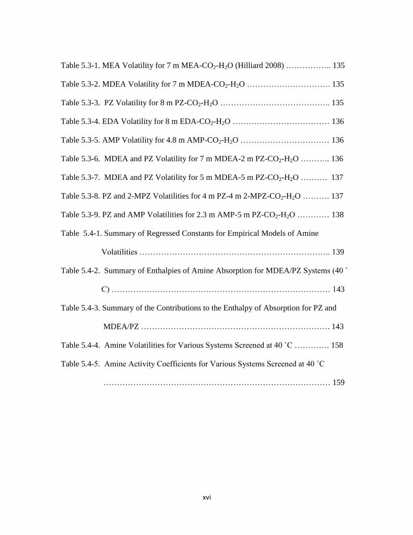
xvi
Table 5.3-1. MEA Volatility for 7 m MEA-CO2-H2O (Hilliard 2008) …………….. 135
Table 5.3-2. MDEA Volatility for 7 m MDEA-CO2-H2O …………………………. 135
Table 5.3-3. PZ Volatility for 8 m PZ-CO2-H2O ………………………………….. 135
Table 5.3-4. EDA Volatility for 8 m EDA-CO2-H2O ……………………………… 136
Table 5.3-5. AMP Volatility for 4.8 m AMP-CO2-H2O …………………………… 136
Table 5.3-6. MDEA and PZ Volatility for 7 m MDEA-2 m PZ-CO2-H2O ……….. 136
Table 5.3-7. MDEA and PZ Volatility for 5 m MDEA-5 m PZ-CO2-H2O ………. 137
Table 5.3-8. PZ and 2-MPZ Volatilities for 4 m PZ-4 m 2-MPZ-CO2-H2O ………. 137
Table 5.3-9. PZ and AMP Volatilities for 2.3 m AMP-5 m PZ-CO2-H2O ………… 138
Table 5.4-1. Summary of Regressed Constants for Empirical Models of Amine
Volatilities …………………………………………………………….. 139
Table 5.4-2. Summary of Enthalpies of Amine Absorption for MDEA/PZ Systems (40 ˚
C) ……………………………………………………………………… 143
Table 5.4-3. Summary of the Contributions to the Enthalpy of Absorption for PZ and
MDEA/PZ ……………………………………………………………. 143
Table 5.4-4. Amine Volatilities for Various Systems Screened at 40 ˚C …………. 158
Table 5.4-5. Amine Activity Coefficients for Various Systems Screened at 40 ˚C
………………………………………………………………………… 159
xvii
List of Figures
Figure 1.2-1. Absorption/Stripping Process for Post-Combustion CO2 Capture …….. 2
Figure 2.1-1. CO2 Gravimetric Loading Apparatus …………………………………. 13
Figure 2.1-2. FTIR Apparatus for Amine Volatility Measurements ………………….15
Figure 2.1-3. Schematic of Gasmet Calibrator Mechanics …………………………... 17
Figure 2.2-1. Vapor Pressure of Water ………………………………………………. 19
Figure 2.2-2. Vapor Pressure of pure Monoethanolamine …………………………… 20
Figure 2.2-3. MEA-CO2-H2O System: CO2 Solubility Comparison between FTIR
Technique and Other Methods ………………………………………… 21
Figure 2.2-4. PZ-CO2-H2O System: CO2 Solubility Comparison between FTIR
Technique and Other Methods ………………………………………… 22
Figure 2.2-5. Vapor Pressure of pure MDEA Literature Comparison ……………….. 23
Figure 2.2-6. Aqueous MDEA Volatility Comparison ……………………………… 24
Figure 2.2-7. Aqueous MEA Volatility Comparison ……………………………….. 25
Figure 2.2-8. Comparison of MEA Volatility Measurements for 3.5 – 11 m MEA-CO2-
H2O between Low vs. High Temperature Apparatus …………………. 26
Figure 2.2-9. Comparison of PZ Volatility Measurements for 2 – 11 m PZ-CO2-H2O
between Low vs. High Temperature Apparatus ……………………….. 28
Figure 2.4-1. C13
NMR Liquid Phase Speciation for 7 m MEA at 27 ˚C …………… 30
Figure 2.4-2. H1 NMR Liquid Phase Speciation for 1 m PZ-CO2-H2O System at 27 ˚C
………………………………………………………………………….. 31
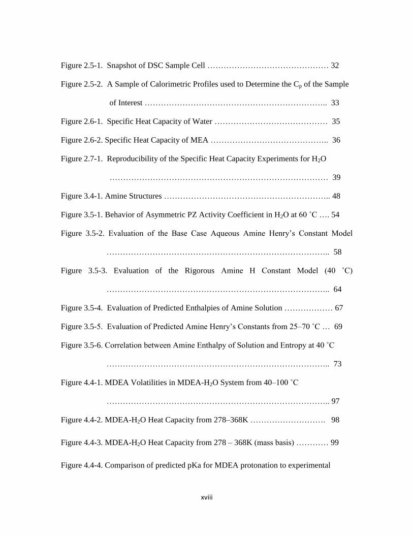
xviii
Figure 2.5-1. Snapshot of DSC Sample Cell ……………………………………… 32
Figure 2.5-2. A Sample of Calorimetric Profiles used to Determine the Cp of the Sample
of Interest ………………………………………………………….. 33
Figure 2.6-1. Specific Heat Capacity of Water …………………………………… 35
Figure 2.6-2. Specific Heat Capacity of MEA …………………………………….. 36
Figure 2.7-1. Reproducibility of the Specific Heat Capacity Experiments for H2O
……………………………………………………………………… 39
Figure 3.4-1. Amine Structures …………………………………………………….. 48
Figure 3.5-1. Behavior of Asymmetric PZ Activity Coefficient in H2O at 60 ˚C …. 54
Figure 3.5-2. Evaluation of the Base Case Aqueous Amine Henry’s Constant Model
……………………………………………………………………….. 58
Figure 3.5-3. Evaluation of the Rigorous Amine H Constant Model (40 ˚C)
……………………………………………………………………….. 64
Figure 3.5-4. Evaluation of Predicted Enthalpies of Amine Solution ……………… 67
Figure 3.5-5. Evaluation of Predicted Amine Henry’s Constants from 25–70 ˚C … 69
Figure 3.5-6. Correlation between Amine Enthalpy of Solution and Entropy at 40 ˚C
……………………………………………………………………….. 73
Figure 4.4-1. MDEA Volatilities in MDEA-H2O System from 40–100 ˚C
……………………………………………………………………….. 97
Figure 4.4-2. MDEA-H2O Heat Capacity from 278–368K ………………………. 98
Figure 4.4-3. MDEA-H2O Heat Capacity from 278 – 368K (mass basis) ………… 99
Figure 4.4-4. Comparison of predicted pKa for MDEA protonation to experimental
xix
values ……………………………………………………………….. 102
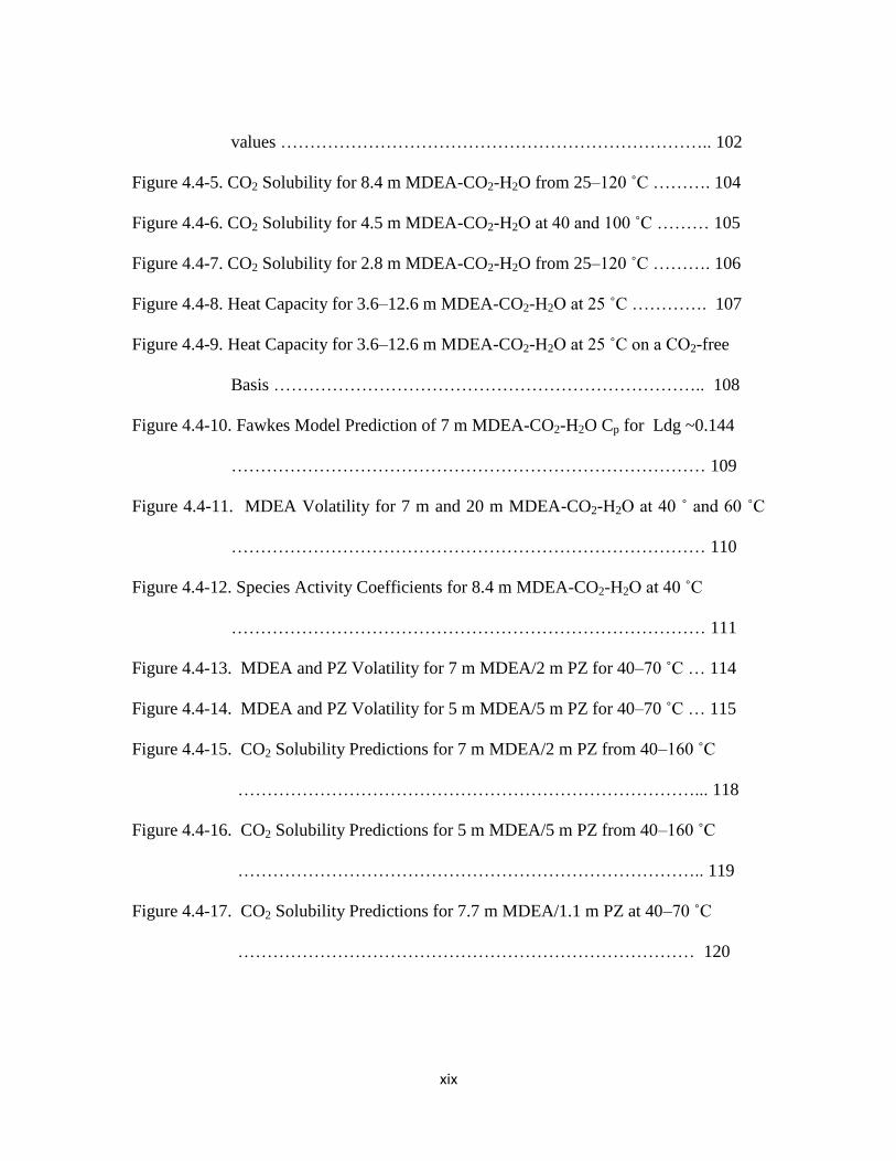
Figure 4.4-5. CO2 Solubility for 8.4 m MDEA-CO2-H2O from 25–120 ˚C ………. 104
Figure 4.4-6. CO2 Solubility for 4.5 m MDEA-CO2-H2O at 40 and 100 ˚C ……… 105
Figure 4.4-7. CO2 Solubility for 2.8 m MDEA-CO2-H2O from 25–120 ˚C ………. 106
Figure 4.4-8. Heat Capacity for 3.6–12.6 m MDEA-CO2-H2O at 25 ˚C …………. 107
Figure 4.4-9. Heat Capacity for 3.6–12.6 m MDEA-CO2-H2O at 25 ˚C on a CO2-free
Basis ……………………………………………………………….. 108
Figure 4.4-10. Fawkes Model Prediction of 7 m MDEA-CO2-H2O Cp for Ldg ~0.144
……………………………………………………………………… 109
Figure 4.4-11. MDEA Volatility for 7 m and 20 m MDEA-CO2-H2O at 40 ˚ and 60 ˚C
……………………………………………………………………… 110
Figure 4.4-12. Species Activity Coefficients for 8.4 m MDEA-CO2-H2O at 40 ˚C
……………………………………………………………………… 111
Figure 4.4-13. MDEA and PZ Volatility for 7 m MDEA/2 m PZ for 40–70 ˚C … 114
Figure 4.4-14. MDEA and PZ Volatility for 5 m MDEA/5 m PZ for 40–70 ˚C … 115
Figure 4.4-15. CO2 Solubility Predictions for 7 m MDEA/2 m PZ from 40–160 ˚C
……………………………………………………………………... 118
Figure 4.4-16. CO2 Solubility Predictions for 5 m MDEA/5 m PZ from 40–160 ˚C
…………………………………………………………………….. 119
Figure 4.4-17. CO2 Solubility Predictions for 7.7 m MDEA/1.1 m PZ at 40–70 ˚C
…………………………………………………………………… 120
xx
Figure 4.4-18. Amine Volatility Predictions for 7 m MDEA/2 m PZ at 40 ˚ and 60 ˚C
……………………………………………………………………. 121
Figure 4.4-19. Amine Volatility Predictions for 5 m MDEA/5 m PZ at 40 ˚and 60 ˚C
……………………………………………………………………. 122
Figure 4.4-20. Speciation for 7 m MDEA/2 m PZ at 40 ˚C …………………….. 123
Figure 4.4-21. Speciation for 5 m MDEA/5 m PZ at 40 ˚C …………………….. 124
Figure 4.4-22. Enthalpy of CO2 Absorption for 7 m MDEA/2 m PZ from 60 ˚– 150 ˚C
………........................................................................................... 125
Figure 4.4-23. Enthalpy of CO2 Absorption for 5 m MDEA/5 m PZ from 60 ˚ – 150 ˚C
………………………………………………………………….. 126
Figure 4.4-24. Cp Predictions for 7 m MDEA/2m PZ from 40 ˚ – 120 ˚C …….. 128
Figure 4.4-25. Cp Predictions for 5 m MDEA/5 m PZ from 40 ˚ – 120 ˚C ………129
Figure 5.4-1. Model Representation of 8 m PZ-CO2-H2O Volatility: Empirical vs.
Fawkes Model …………………………………………………… 140
Figure 5.4-2. Model Representation of PZ Volatility in 7 m MDEA/2 m PZ: Empirical
vs. Fawkes Model ………………………………………………… 141
Figure 5.4-3. Model Representation of MDEA Volatility in 7 m MDEA/2 m PZ:
Empirical vs. Fawkes Model …………………………………….. 142
Figure 5.4-4. PZ Volatility in 8 m PZ-CO2-H2O ………………………………… 144
Figure 5.4-5. PZ Volatility for 8 m, 10 m, 20 m PZ-CO2-H2O at 40 ˚C ………….145
Figure 5.4-6. PZ Volatility and PZ concentration in 8 m PZ-CO2-H2O at 60 ˚C
……………………………………………………………………. 146
xxi
Figure 5.4-7. Activity Coefficients of PZ in 8 m and 10 m PZ-CO2-H2O ……… 147
Figure 5.4-8. Amine Activity Coefficient in the Blend with Changing PZ Concentration
……………………………………………………………………. 148
Figure 5.4-9. Amine Activity Coefficient in the Blend with Changing MDEA
Concentration ……………………………………………………. 149
Figure 5.4-10. PZ and H2O Activity Coefficients in 7 m MDEA/2 m PZ ………. 151
Figure 5.4-11. MDEA Activity Coefficient in 7 m MDEA/2 m PZ ……………. 152
Figure 5.4-12. Amine Concentrations and Activity Coefficients for 7 m MDEA/2 m PZ
at 40 ˚C ………………………………………………………….. 153
Figure 5.4-13. PZ Activity Coefficient as a Function of Ionic Strength at 40 ˚C...154
Figure 5.4-14. MDEA Activity Coefficient as a Function of Ionic Strength at 40 ˚C
……………………………………………………………........... 156
Figure 5.4-15. Activity Coefficients of Electrolytes in 7 m MDEA/2 m PZ at 40 ˚C
…………………………………………………………………. 157
Figure A.1: Molecular Structure and Active Nuclei of Protons associated with PZ/PZH+
…………………………………………………………………. 173
Figure A.2: Molecular Structure and Active Nuclei of Protons associated with PZ(COO)-
/H
+PZ(COO) ……………………………………………………. 174
Figure A.3: Molecular Structure and Active Nuclei of Protons associated with
PZ(COO)22-
……………………………………………………… 174
Figure A.4: Molecular Structure and Active Nuclei of Protons associated with
MDEA/MDEAH+………………………………………………… 174
xxii
Figure A.5: Molecular Structure and Active Nuclei of Carbons associated with PZ/PZH+
………………………………………………………………………. 175
Figure A.6: Molecular Structure and Active Nuclei of Carbons associated with
PZH+/PZ(COO)
- ………………………………………………….. 175
Figure A.7: Molecular Structure and Active Nuclei of Carbons associated with
PZ(COO)22-
……………………………………………………….. 175
Figure A.8: Molecular Structure and Active Nuclei of Carbons associated with
MDEA/MDEAH+
………………………………………………… 176
Figure A.9: Molecular Structure and Active Nuclei of Carbons associated with HCO3-
/CO32-
……………………………………………………………… 176
Figure A.10: H1 NMR Spectrum of 8 m PZ-CO2-H2O, α = 0.25 mol CO2/mol total
alkalinity, 40 ˚C …………………………………………………… 177
Figure A.11: H1 NMR Spectrum of 8 m PZ-CO2-H2O, α = 0.30 mol CO2/mol total
alkalinity, 40 ˚C …………………………………………………… 178
Figure A.12: H1 NMR Spectrum of 8 m PZ-CO2-H2O, α = 0.40 mol CO2/mol total
alkalinity, 40 ˚C …………………………………………………….179
Figure A.13: C13
NMR Spectrum of 8 m PZ-CO2-H2O, α = 0.25 mol CO2/mol total
alkalinity, 40 ˚C (C12
peaks) ………………………………………. 180
Figure A.14: C13
NMR Spectrum of 8 m PZ-CO2-H2O, α = 0.25 mol CO2/mol total
alkalinity, 40 ˚C (C13
peaks) ………………………………………..181
Figure A.15: C13
NMR Spectrum of 8 m PZ-CO2-H2O, α = 0.30 mol CO2/mol total
alkalinity, 40 ˚C (C12
peaks) ………………………………………. 182
xxiii
Figure A.16: C13
NMR Spectrum of 8 m PZ-CO2-H2O, α = 0.30 mol CO2/mol total
alkalinity, 40 ˚C (C13
peaks) ……………………………………… 183
Figure A.17: C13
NMR Spectrum of 8 m PZ-CO2-H2O, α = 0.40 mol CO2/mol total
alkalinity, 40 ˚C (C12
peaks) ……………………………………… 184
Figure A.18: C13
NMR Spectrum of 8 m PZ-CO2-H2O, α = 0.40 mol CO2/mol total
alkalinity, 40 ˚C (C13
peaks) ……………………………………… 185
Figure A.19: H1 NMR Spectrum of 7 m MDEA-2 m PZ-CO2-H2O, α = 0.07 mol
CO2/mol total alkalinity, 40 ˚C …………………………………… 186
Figure A.20: H1 NMR Spectrum of 7 m MDEA-2 m PZ-CO2-H2O, α = 0.095 mol
CO2/mol total alkalinity, 40 ˚C …………………………………… 187
Figure A.21: H1 NMR Spectrum of 7 m MDEA-2 m PZ-CO2-H2O, α = 0.15 mol
CO2/mol total alkalinity, 40 ˚C …………………………………… 188
Figure A.22: H1 NMR Spectrum of 7 m MDEA-2 m PZ-CO2-H2O, α = 0.16 mol CO2/mol
total alkalinity, 40 ˚C …………………………………………….. 189
Figure A.23: C13
NMR Spectrum of 7 m MDEA-2 m PZ-CO2-H2O, α = 0.07 mol
CO2/mol total alkalinity, 40 ˚C (C12
peaks) ………………………. 190
Figure A.24: C13
NMR Spectrum of 7 m MDEA-2 m PZ-CO2-H2O, α = 0.07 mol
CO2/mol total alkalinity, 40 ˚C (C13
peaks) ……………………… 191
Figure A.25: C13
NMR Spectrum of 7 m MDEA-2 m PZ-CO2-H2O, α = 0.095 mol
CO2/mol total alkalinity, 40 ˚C (C12
peaks) ………………………. 192
Figure A.26: C13
NMR Spectrum of 7 m MDEA-2 m PZ-CO2-H2O, α = 0.095 mol
CO2/mol total alkalinity, 40 ˚C (C13
peaks) ………………………. 193
xxiv
Figure A.27: C13
NMR Spectrum of 7 m MDEA-2 m PZ-CO2-H2O, α = 0.15 mol
CO2/mol total alkalinity, 40 ˚C (C12
peaks) ……………………… 194
Figure A.28: C13
NMR Spectrum of 7 m MDEA-2 m PZ-CO2-H2O, α = 0.15 mol
CO2/mol total alkalinity, 40 ˚C (C13
peaks) ……………………… 195
Figure A.29: C13
NMR Spectrum of 7 m MDEA-2 m PZ-CO2-H2O, α = 0.16 mol
CO2/mol total alkalinity, 40 ˚C (C12
peaks) ……………………… 196
Figure A.30: C13
NMR Spectrum of 7 m MDEA-2 m PZ-CO2-H2O, α = 0.16 mol
CO2/mol total alkalinity, 40 ˚C (C13
peaks) …………………….. 197
Figure A.31: H1 NMR Spectrum of 5 m MDEA-5 m PZ-CO2-H2O, α = 0.096 mol
CO2/mol total alkalinity, 40 ˚C ………………………………….. 198
Figure A.32: H1 NMR Spectrum of 5 m MDEA-5 m PZ-CO2-H2O, α = 0.18 mol CO2/mol
total alkalinity, 40 ˚C ………………………………………………199
Figure A.33: H1 NMR Spectrum of 5 m MDEA-5 m PZ-CO2-H2O, α = 0.36 mol CO2/mol
total alkalinity, 40 ˚C …………………………………………….. 200
Figure A.34: C13
NMR Spectrum of 5 m MDEA-5 m PZ-CO2-H2O, α = 0.096 mol
CO2/mol total alkalinity, 40 ˚C (C12
peaks) ……………………… 201
Figure A.35: C13
NMR Peaks of 5 m MDEA-5 m PZ-CO2-H2O, α = 0.096 mol CO2/mol
total alkalinity, 40 ˚C (C13
peaks) ……………………………….. 202
Figure A.36: C13
NMR Spectrum of 5 m MDEA-5 m PZ-CO2-H2O, α = 0.18 mol
CO2/mol total alkalinity, 40 ˚C (C12
Peaks – Part 1) …………….. 203
Figure A.37: C13
NMR Spectrum of 5 m MDEA-5 m PZ-CO2-H2O, α = 0.18 mol
CO2/mol total alkalinity, 40 ˚C (C12
Peaks – Part 2) …………….. 204
xxv
Figure A.38: C13
NMR Spectrum of 5 m MDEA-5 m PZ-CO2-H2O, α = 0.18 mol
CO2/mol total alkalinity, 40 ˚C (C13
peaks) ………………………. 205
Figure A.39: C13
NMR Spectrum of 5 m MDEA-5 m PZ-CO2-H2O, α = 0.36 mol
CO2/mol total alkalinity, 40 ˚C (C12
peaks) ……………………… 206
Figure A.40: C13
NMR Spectrum of 5 m MDEA-5 m PZ-CO2-H2O, α = 0.36 mol
CO2/mol total alkalinity, 40 ˚C (C13
peaks) ……………………… 207
Figure B.1: Gasmet Calibrator …………………………………………………. 209
Figure B.2: Internal Gasmet Calibrator Setup ………………………………….. 210
Figure B.3: Jacketed 1000 mL Glass Reactor used for VLE Experiments ……… 213
Figure C.1. Snapshot of DSC Internal Chamber ……………………………….. 221
Figure C.2. Calorimetric Scan of Indium Sample (for Calibration of Cell Constant)
…………………………………………………………………….. 223
Figure C.3: Calorimetric Scan of Blank Sample ……………………………….. 223
Figure C.4: Calorimetric Scan of Al2O3 Sample ……………………………….. 224
Figure C.5: Calorimetric Scan of an Amine Sample ……………………………. 225
Figure D.1: Water (H2O) FTIR Reference Spectrum …………………………… 227
Figure D.2: Carbon Dioxide (CO2) FTIR Reference Spectrum …………………. 228
Figure D.3: Monoethanolamine (MEA) FTIR Reference Spectrum …………….. 228
Figure D.4: Piperazine (PZ) FTIR Reference Spectrum ………………………… 229
Figure D.5: N-Methyldiethanolamine (MDEA) FTIR Reference Spectrum ……. 229
Figure D.6: 2-Amino-2-Methyl-1-Propanol (AMP) FTIR Reference Spectrum …230
Figure D.7: Diethanolamine (DEA) FTIR Reference Spectrum ……………….. 230

xxvi
Figure D.8: Ethylenediamine (EDA) FTIR Reference Spectrum ………………. 231
Figure D.9: Hexamethylenediamine (HMDA) FTIR Reference Spectrum …….. 231
Figure D.10: 2-Methyl Piperazine (2-MPZ) FTIR Reference Spectrum ……….. 232
Figure D.11: 1,4-Dimethyl Piperazine (DMPZ) FTIR Reference Spectrum …… 232
Figure D.12: 2,2-Dimethylaminoethoxy Ethanol (2,2-DMAEE) FTIR Reference
Spectrum…………………………………………………………… 233
Figure D.13: Dimethylethanolamine (DMEA) FTIR Reference Spectrum …….. 233
Figure D.14: DL-Alaninol (ALA) FTIR Reference Spectrum …………………. 234
Figure D.15: 2-Hydroxyethyl Piperazine (HEP) FTIR Reference Spectrum ….. 234
Figure D.16: 1-Methyl Piperazine (1-MPZ) FTIR Reference Spectrum ……….. 235
Figure D.17: 1,2-Aminoethyl Piperazine (AEP) FTIR Reference Spectrum …… 235
Figure D.18: Diglycolamine® (DGA) FTIR Reference Spectrum ………………. 236
Figure D.19: 3-Methylamino Propylamine (MAPA) FTIR Reference Spectrum... 236
Figure D.20: 1,2-Diaminopropane (1,2-DAP) FTIR Reference Spectrum …….. 237
Figure D.21: Morpholine (MORPH) FTIR Reference Spectrum ……………….. 237
Figure D.22: Dimorpholino Diethyl Ether (DMORPH) FTIR Reference Spectrum
……………………………………………………………………… 238
1
Chapter 1: Introduction and Scope of Work
1.1. Overview of CO2 Capture Technology
Power generation is the biggest source of CO2 emission leading to global
warming, with coal-fired power plants producing up to ~81% of the CO2 that results from
worldwide electricity generation (EIA, 2008). The leading technology proposed to
capture CO2 from coal-fired power plants is a post-combustion absorption/stripping
process that makes use of aqueous amine. Post-combustion capture using aqueous amine
absorption has proven advantages compared to oxycombustion and pre-combustion
Integrated Gasification Combined Cycle (IGCC). These unmatched advantages include:
(1) amenability to be retrofitted onto an existing power plant as a tail-end process; (2)
maturity of the technology; and (3) lower capital and operating costs.
For the absorption process, 30 weight percent monoethanolamine (MEA) is
considered to be the baseline industry solvent and has been used for more than 70 years.
In an effort to develop solvents that are better performing, many novel amine solvents
have been screened to evaluate their absorption characteristics (such as capture capacity,
reaction rate, resistance to thermal/oxidative degradation, and volatility). Two of the
more promising new solvents screened are 8 molal (m) Piperazine (PZ) and 7 m MDEA
(n-methyldiethanolamine) / 2 m PZ blend. Based on studies from the Rochelle group,
both of these solvents have been shown to have excellent capacity, competitive rates, and
good resistance to degradation. It remains for this work to explore the volatilities of these
two solvents along with those of many other novel solvents.
2
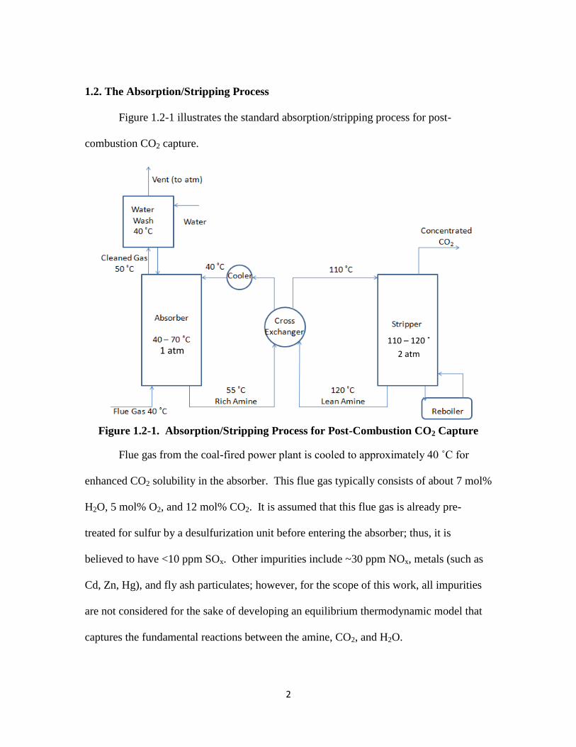
1.2. The Absorption/Stripping Process
Figure 1.2-1 illustrates the standard absorption/stripping process for post-
combustion CO2 capture.
Figure 1.2-1. Absorption/Stripping Process for Post-Combustion CO2 Capture
Flue gas from the coal-fired power plant is cooled to approximately 40 ˚C for
enhanced CO2 solubility in the absorber. This flue gas typically consists of about 7 mol%
H2O, 5 mol% O2, and 12 mol% CO2. It is assumed that this flue gas is already pre-
treated for sulfur by a desulfurization unit before entering the absorber; thus, it is
believed to have <10 ppm SOx. Other impurities include ~30 ppm NOx, metals (such as
Cd, Zn, Hg), and fly ash particulates; however, for the scope of this work, all impurities
are not considered for the sake of developing an equilibrium thermodynamic model that
captures the fundamental reactions between the amine, CO2, and H2O.
1 atm 110 – 120 ˚
2 atm
3
The flue gas enters the bottom of the absorber which operates within the range
from 40 ˚C – 70 ˚C throughout the length of the column and 1 atm. In a countercurrent
mode, this flue gas is contacted with the amine solvent coming into the top of the
absorber. The solvent comes in with a lean amount of CO2 (~0.5 kPa PCO2) due to
continuous cycling throughout the capture flow process. The amine absorbs CO2 from
the flue gas by means of chemical absorption. Upon reaching the bottom of the absorber,
the solvent is now loaded with a rich amount of CO2 (~5 kPa PCO2). The cleaned flue
gas, now with 90% of the CO2 removed by design, exits the top of the absorber and
enters into a water wash for amine recovery prior to being vented into the atmosphere.
The rich amine stream is pumped into a cross exchanger, designed with a ±5 ˚C
tempera- ture approach between its inlet and outlet streams (to ensure the optimum
equivalent work for the entire process), where it is heated to ~100 ˚ - 105 ˚C. The rich
stream then enters into the top of the stripper which operates between 110 ˚C – 120 ˚C
and 2 atm. Steam coming from the stripper reboiler contacts the rich amine counter-
currently and strips out the CO2 by reversing the absorption reaction. The amine is now
lean again as it exits the stripper and makes its way back to the absorber for continuous
capture operation. The steam/CO2 stream then exits the top of the stripper where water is
then condensed out as makeup water or it can be used for the amine wash if sufficient.
The CO2 is pressurized to 150 bars in preparation for sequestration.
1.3. Motivation for Investigating Amine Volatility
Amine volatility is one of the key criteria used to evaluate the viability of an
amine to be used as a solvent for CO2 capture. Volatility is important for environmental,
4
economic, and research & development purposes. First, amine volatility loss up the stack
can react in the atmosphere to form ozone and other toxic compounds. Currently there is
no set EPA regulation for amine emissions, but most CO2 capture processes aim to
reduce amine volatility to ~1 ppm for venting purposes per conversations with CO2
capture sponsors. From an economic standpoint, high volatility loss increases the solvent
makeup cost required to replenish the amine. For the more expensive amines such as PZ,
this cost can be substantial. Additionally, a large volatility loss will require the use of a
bigger water wash tower and more water to treat. Both of these factors will drive up the
capital and operating expenses of the CO2 capture operation. Finally, there is a research
& development need to quantify amine volatility and incorporate this type of data into the
framework of a thermodynamic model in order to build a more robust model.
Amine volatility is most crucial at two places in the process: (1) at the top of the
absorber (40 ˚ - 60 ˚C, 1 atm, nominal lean CO2 loading where loading = mol CO2/mol
total alkalinity) – this is the amount of amine that would have to be treated by the water
wash; (2) at the water wash (40 ˚C and 1 atm) – this is the amount of amine that will
eventually be vented into the environment. The scope of this work focuses mainly on
amine volatility at the top of the absorber.
1.4. Scope of this Work
There are three main areas of focus considered within the scope of this work: (1)
aqueous amine volatility in binary amine-water systems; (2) rigorous thermodynamic
model upgrade for MDEA-PZ-CO2-H2O; and (3) amine volatility screening for novel
solvents that are potentially viable for CO2 capture. The volatility of 20 amines was
5
measured in water. These amines were prepared at dilute concentrations ranging from
0.1 – 1.1 molal (<1.5 mol% amine) to approach the intrinsic vapor-liquid partition of the
amine at infinite dilution in water. At the low amine concentrations where the aqueous
volatilities were measured, these amines were considered to be diluted enough to
approximate the volatility at the condition of infinite dilution to within ±10%. Aqueous
amine volatilities were measured at 40 ˚- 70 ˚C and 1 atm which is representative of the
standard operating conditions of the absorber. Table 1.4-1 summarizes the 20
alkanolamines studied in this work.
Table 1.4-1. Summary of 20 Alkanolamines Investigated
Amine Class Amine Type Amine Acronym
Monoamines
Primary
Monoethanolamine MEA
Diglycolamine DGA
DL-Alaninol ALA
2-Amino-2-Methyl-1-
Propanol AMP
Secondary Diethanolamine DEA
Morpholine MORPH
Tertiary
N-Methyldiethanolamine MDEA
2,2-Dimethylethoxy Ethanol 2,2-DMAEE
N,N-Dimethylethanolamine DMMEA
Diamines
Primary
Hexamethylene Diamine HMDA
1,2-Diaminopropane DAP
Ethylenediamine EDA
Secondary Piperazine PZ
2-Methyl Piperazine 2-MPZ
Tertiary Dimorpholino Diethyl Ether DMORPH
1,4-Dimethylpiperazine 1,4-DMPZ
Mixed
Hydroxyethyl Piperazine HEP
3-Methylamino Propylamine MAPA
1-Methyl Piperazine 1-MPZ
Triamines Mixed 1,2-Aminoethyl Piperazine AEP
6
The aqueous amine volatilities were obtained experimentally as amine partial
pressures. However, for purposes of analytical representation, aqueous amine volatilities
will be expressed as amine Henry’s constants (H) in Pa units which represent the vapor-
liquid partition of the amine in terms of the ratio of the amine partial pressure to its liquid
mole fraction. The Henry’s constant was chosen as an intrinsic indicator of aqueous
amine volatility because it is referenced to the state of infinite dilution of amine in water.
By virtue of this reference state of infinite dilution, the H constant accounts for only the
intrinsic amine-water interaction as opposed to accounting for both amine-water and
amine-amine interactions as in the case of the amine activity coefficient.
This work also develops an empirical model to correlate the amine Henry’s
constants for 19 of the 20 alkanolamines studied, along with those of 16 alkylamines
from the literature, to their molecular structures in a group contribution method. The
model is also used to predict the experimental volatility of one of the amines (1,2-
Aminoethyl Piperazine), not used in the regression, to well within ±10%. This result
lends confidence that the model has excellent predictive capability for amines in addition
to just being able to capture the data.
This work also focuses on upgrading the existing thermodynamic model for
MDEA/PZ solvent system which was developed using the elecNRTL theory. The
original model, named Guy Fawkes, was developed by Peter Frailie (a Rochelle group
member) in 2010. This thermodynamic model for the quaternary system of MDEA-PZ-
CO2-H2O was developed by means of sequential regression in which one starts by
7
modeling the simplest subsystems (consisting of single pure components only) then onto
binary, tertiary, and ultimately the quaternary system. This work supplied various types
of experimental data, including CO2 solubility, amine volatility, heat capacity (Cp), and
speciation, needed to regress the parameters of this model. The upgrading effort done in
this work primarily consisted of improving the modeling of only MDEA, at all the levels
within the sequential regression hierarchy, as PZ was rather well-behaved for the most
part. There were two long standing issues with the original Fawkes model that were
effectively resolved in this upgrade: (1) the need to be able to match experimental
volatility data for MDEA/PZ blend; (2) the need to fit experimental speciation data for
the blend.
VLE and rate data have previously been developed for two blends: 7 m MDEA/2
m PZ and 5 m MDEA/5 m PZ. Both of these systems are believed to be superior
compared to the baseline 7 m MEA solvent for CO2 capture. In comparison to 7 m MEA,
the MDEA/PZ blends have almost twice the capture capacity (~0.8 mol CO2/kg
amine+H2O versus 0.47 mol CO2/kg amine+H2O) (Closmann 2011) within the optimum
operational loading range corresponding to ~0.5 and 5 kPa lean and rich CO2 partial
pressure, respectively; almost twice the rate of CO2 reaction at (~5.1x10⁷ mol/s*Pa*m2
versus 3.1 mol/s*Pa*m2) (Closmann 2011) at the nominal rich loading; much lower rate
of oxidative and thermal degradation; and are also 80% - 90% less volatile (0.47 Pa
PMDEA and 0.30 Pa PPZ versus 2.7 Pa PMEA at 40 ˚C) as reported in this work. Because of
these superior operating characteristics, extensive experimental work was performed to
investigate MDEA/PZ along with all its binary and ternary system constituents (0.5 m –
8
20 m MDEA-H2O, 0.5 m – 10 m PZ-H2O, 7 m MDEA-CO2-H2O, 8 m – 10 m PZ-CO2-
H2O, and 7 m/2 m and 5 m/5 m MDEA-PZ-H2O). The understanding gained from
performing a thorough study of MDEA/PZ will allow one to rationalize and predict the
behaviors of other amine solvents of interest. This ability lends itself to the pursuit of the
third objective within the scope of this work which is to analyze and generalize the
behavior of other amine systems screened as potentially viable solvents for CO2 capture.
With respect to the screening of amine solvents, this work explored a total of 9
amine systems: 7 m MEA (Hilliard 2008), 8 m PZ-CO2-H2O, 7 m MDEA-CO2-H2O, 7 m
MDEA/2 m PZ and 5 m MDEA/5 m PZ-CO2-H2O, 4 m PZ/4 m 2-MPZ-CO2-H2O, 4.8 m
AMP-CO2-H2O, 8 m EDA-CO2-H2O, and 2.3 m AMP / 5.0 m PZ-CO2-H2O. The
motivation behind screening these systems for volatility stemmed from the ongoing need
to formulate new solvents for CO2 capture with promising operational characteristics
which include large capture capacity, fast rates, strong resistance to oxidative and thermal
degradation, and low volatility. Cost is also a factor in the use of solvent, thus, certain
blends having other amines with PZ are used to reduce the high cost of using PZ alone.
These novel amine systems are screened for volatility at 40 ˚ - 70 ˚C, 1 atm, and nominal
lean CO2 loading (~0.5 kPa) which are the standard operating conditions at the top of the
absorber where volatility is of great concern. From the experiments, amine volatilities, in
terms of partial pressures, for these systems are obtained not only for comparative
purposes, but also to generalize the behavior of the system activity coefficients.
9
1.5. Contributions of this Work
This work is the first known investigation of amine volatility in CO2 systems.
While there had been many literature studies on amine volatility in binary amine-H2O
systems, there has not been any study of this kind for loaded CO2 systems. The
experimental method, developed by Hilliard (2008) , used to measure amine volatility is
also rather original in that uses an FTIR (Fourier Transform Infrared Spectroscopy)
technique, instead of the more common GC methods, to detect vapor composition down
to a resolution of 5-10 ppm.
Another important contribution of this work is that it serves as one of the largest
known collections of experimental data for aqueous volatility of alkanolamines used in
CO2 capture. While there are many studies to date on the volatilities of alkylamines or of
only a few alkanolamines applicable to CO2 capture, this work investigated a total of 20
alkanolamines. Furthermore, this work has successfully developed a group contribution
model to correlate aqueous amine volatilities to molecular structures. This model greatly
improves the predictions of aqueous volatilities for both alkanolamines (used for CO2
capture) and alkylamines, compared to existing group contribution methods such as
UNIFAC or that by Hine and Mookerjee (1979), because it is built on experimental data
from both types of amines. The other two methods are not able to successfully predict
the aqueous volatilities of CO2 capture alkanolamines because they are primarily
developed from the data of alkylamines not alkanolamines. The nitrogen functional
group in alkylamines are thought to have different interaction with water than the
nitrogen group in alkanolamines. This phenomenon is related to the type of neighboring
10
groups that are attached to nitrogen in alkylamines versus in alkanolamines. In
alkylamines, alkyl groups are the neighbors to the nitrogen, whereas in alkanolamines the
neighboring groups are often an alcohol or ether which influence how nitrogen interact
with water differently than alkyl groups. Lastly, the group contribution method of Hine
and Mookerjee (1975) also did not differentiate between aliphatic nitrogen and cyclic
nitrogen groups. This study has found that there is a clear difference in volatility between
these two nitrogen groups.
The most fundamental contribution of this research is that it truly illuminates the
solution behaviors of various amines in CO2 systems. This understanding allows for
effective modeling and simulation of system thermodynamics along with process designs
of the absorber.
1.6. Outline of Dissertation
The introduction chapter will be followed by the following chapters in this order:
Experimental Methods, Aqueous Amine Volatility in Binary Amine-H2O Systems,
MDEA/PZ/CO2/H2O Model Upgrade, MDEA/PZ Detailed Investigation & Generalized
Amine Screening, and Conclusions. The chapter on Experimental Methods discusses in
details the techniques for amine volatility measurements using FTIR, heat capacity
determination with Differential Scanning Calorimetry (DSC), and liquid speciation study
using Nuclear Magnetic Resonance technique (NMR). Other supporting lab techniques,
such as Total Inorganic Carbon (TIC) to verify the CO2 loading in solution and Amine
Titration to determine the amine concentration, are also covered. The body chapters are
presented in order of increasing system complexity, starting with simple binary system

11
analysis building up to the quaternary MDEA-PZ-CO2-H2O system which ultimately
leads to the generalization of other amine systems screened for CO2 capture.
12
Chapter 2: Experimental Methods
This chapter discusses the experimental methods used in this work to study (1)
vapor liquid equilibrium and (2) heat capacity of multi-component systems. MDEA and
PZ blends, along with their individual sub-systems, were extensively studied in both VLE
and calorimetry to develop a rigorous thermodynamic model for the blend. Other amine
systems were screened for their equilibrium volatility at the absorber operating condition
to determine their viability for use as CO2 capture solvents. All experiments were
typically run only once, not in replicates, because the main source of experimental
deviation from one run to the next lies with the precision of the instrument which does
not pose significant errors. An analysis of experimental precision, or data
reproducibility, will be presented in section 2.7. Accuracy of the different methods is
benchmarked by measuring known systems.
2.1. Vapor-Liquid Equilibrium: Amine Volatility Measurements
Solution Preparation
Approximately 525 – 550 g of solution was prepared for each experiment.
Solutions were prepared by dissolving pure, analytical-grade amine in water to achieve
the desired molality (m, moles of amine/kg water). . The chemical suppliers and purity
grades were: MEA (Acros Organics 99 %), PZ (Alfa Aesar 99 %), MDEA (Acros
Organics 99+ %), EDA (Strem Chemicals 99 %), AMP (Acros Organics 99 %), MAPA
(Acros Organics 98.5 – 100%), 2-Methyl PZ (Acros Organics 97.5 – 100%). High
concentrations of PZ were heated to dissolve anhydrous solid PZ in water. The solutions
13
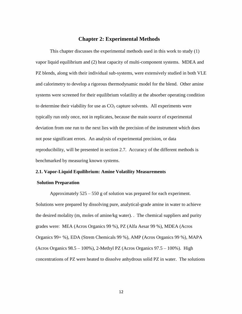
were loaded with CO2 by sparging CO2 in a glass cylinder on a balance to obtain a
gravimetric CO2 loading. Figure 2.1-1 shows the gravimetric loading apparatus.
Figure 2.1-1. CO2 Gravimetric Loading Apparatus
Amine solutions loaded with this technique produced CO2 loading within ± 5.0 %
of the target loading based on an analysis of the loaded solutions by TIC.
CO2 Loading Verification
The CO2 concentration in solution was verified by Total Inorganic Carbon (TIC)
analysis. The samples were diluted in H2O and injected into 30 wt % H3PO4 to release
CO2. The CO2 was carried by N2 to an infrared detector. The resulting voltage peak was
integrated and calibrated with a 1000 ppm inorganic carbon standard made from a
mixture of potassium carbonate and potassium bicarbonate (Ricca Chemical,
Pequannock, NJ). The reproducibility of this method is about 2%.

14
Amine Concentration Verification
The amine concentration was determined by acid titration with an automatic
Titrando series titrator with automatic equivalence point detection. A 300X diluted
sample was titrated with 0.1 N H2SO4 to a pH of 2.4. The amount of acid needed to reach
the equivalence point at a pH of 3.9 was used to calculate the total amine concentration.
The reproducibility of this method is about 1%.
Vapor Headspace Sampling: Amine Volatility Measurement
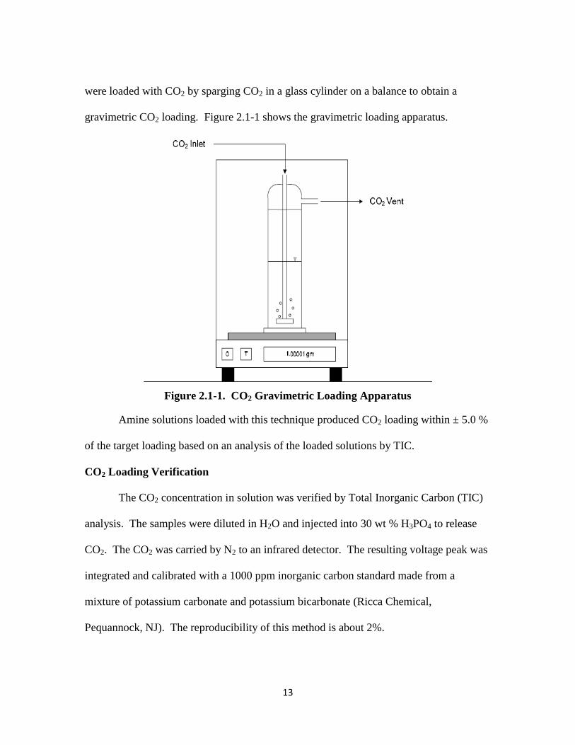
Amine volatility was measured in a stirred reactor coupled with a hot gas FTIR
analyzer (Fourier Transform Infrared Spectroscopy, Temet Gasmet DX-4000) as shown
in Figure 2.1-2. This unit has a 10 m gas cell path length with varying detection limits
between 0.1 ppm – 60 vol%+ depending on the absorption of the gas components
analyzed within the range of 900 – 4200 cm-1
wavenumber. The FTIR apparatus and
method were taken from Hilliard (2008). FTIR operation and procedure were followed
exactly as prescribed by Hilliard. Details regarding FTIR operation, including clean up,
are provided in Appendix B.
15
Figure 2.1-2. FTIR Apparatus for Amine Volatility Measurements
The 1L glass reactor was agitated at 350 rpm ± 5 rpm. This reactor is designed to
withstand up to 45 psig at 100 ˚C; however, given the experimental needs, only low
temperature experiments from 40 ˚ - 70 ˚C at atmospheric pressure are conducted as these
conditions are representative of the absorber operating conditions. Temperature in the
reactor was controlled to within ±0.1 °C by circulating heated dimethylsilicone oil in the
outer reactor jacket to and from the oil bath. The reactor was insulated with thick
16
insulation material. The temperature inside the reactor was measured with a digital
thermometer to within ±0.1 ˚C.
At the start of each experiment, the headspace in the reactor was swept with
excess N2. The reactor was maintained at ambient pressure by venting through a water
seal. The room pressure was measured with a barometer to ±0.1 mm Hg. Vapor from the
headspace of the reactor was circulated at a rate of ~5-10 L/min. by a heated sample
pump to the FTIR through a heated Teflon line. Both the line and analyzer were
maintained at 180 ºC to keep the material in vapor phase. The FTIR software, Calcmet,
directly measures amine, CO2, and water concentration in the gas by using a multiple
least squares algorithm that is based on the work of Saarinen and Kauppinen (1991). The
relative standard reproducibility in the vapor phase measurement was reported to be ±2%
by Goff (2005). The margin of error in the readings, however, is expected to increase
with detection of low concentration of material, and can be up to ±10% or greater for
concentrations <10 ppm. After the gas passed through the FTIR, it was returned to the
reactor through a heated line maintained at ~ 55 ºC hotter than the reactor (Treactor +
55˚C). The 55 ºC difference was necessary according to Hilliard (2008) to ensure that the
return gas can thermally equilibrate with the solution in the reactor, and also to
compensate for potential heat loss at the bottom of the reactor. Upon completion of an
experiment, approximately 25 mL of liquid sample was taken to verify both the loading
and amine concentration using TIC and amine titration, respectively.
FTIR calibration for each amine is performed using a Gasmet Calibrator. This
apparatus consists of a syringe pump, a manual needle valve, and a stainless steel
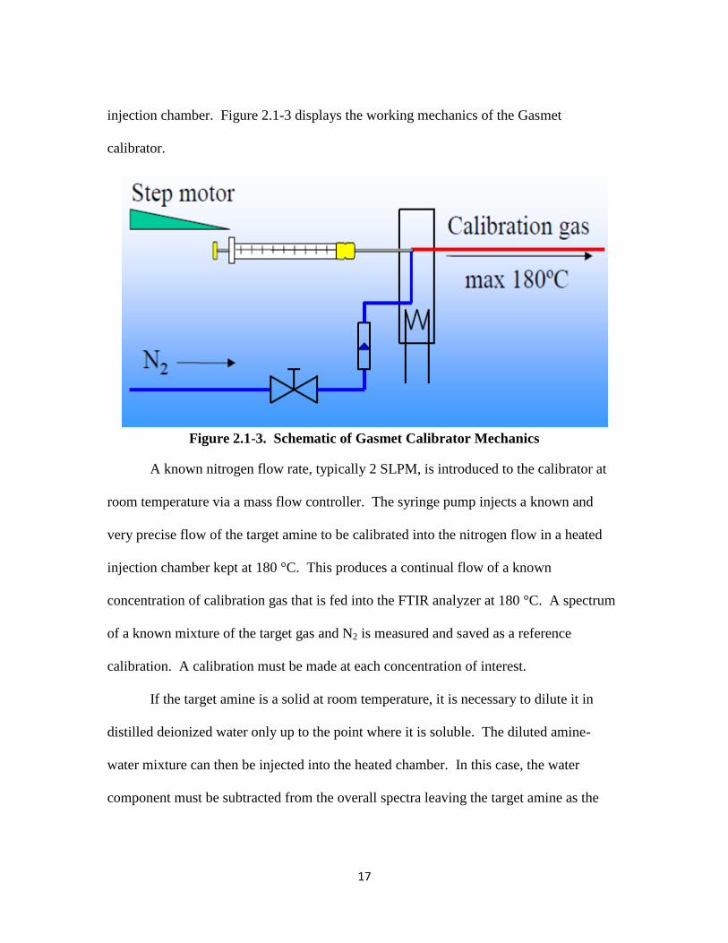
17
injection chamber. Figure 2.1-3 displays the working mechanics of the Gasmet
calibrator.
Figure 2.1-3. Schematic of Gasmet Calibrator Mechanics
A known nitrogen flow rate, typically 2 SLPM, is introduced to the calibrator at
room temperature via a mass flow controller. The syringe pump injects a known and
very precise flow of the target amine to be calibrated into the nitrogen flow in a heated
injection chamber kept at 180 °C. This produces a continual flow of a known
concentration of calibration gas that is fed into the FTIR analyzer at 180 °C. A spectrum
of a known mixture of the target gas and N2 is measured and saved as a reference
calibration. A calibration must be made at each concentration of interest.
If the target amine is a solid at room temperature, it is necessary to dilute it in
distilled deionized water only up to the point where it is soluble. The diluted amine-
water mixture can then be injected into the heated chamber. In this case, the water
component must be subtracted from the overall spectra leaving the target amine as the
18
remaining residual spectra. The amine residual can then be saved as a reference
calibration. PZ was calibrated by this method because it is a solid at room temperature.
Reference spectra for all the amines studied in this work are provided in Appendix D.
2.2. FTIR Experimental Method Validation
The FTIR experimental method was benchmarked by Hilliard (2008) by
measuring pure component vapor pressure (H2O, MEA) and CO2 solubility of loaded
amine systems (MEA-CO2-H2O and PZ-CO2-H2O). MDEA vapor pressure, MDEA-
H2O volatility, and MEA-H2O volatility were also compared to literature values.
Pure H2O System Benchmarking
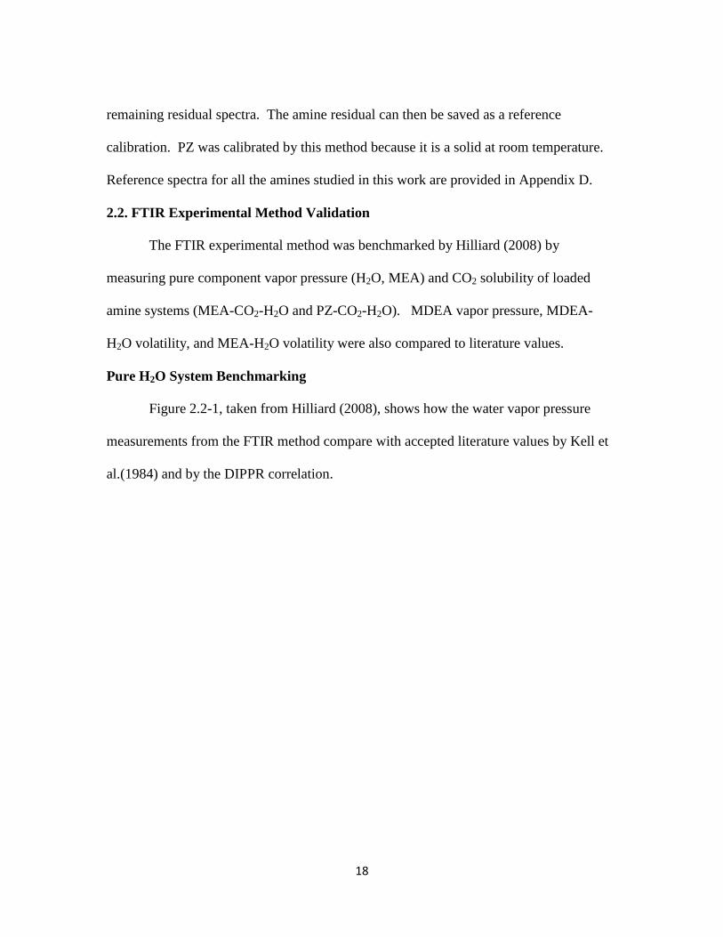
Figure 2.2-1, taken from Hilliard (2008), shows how the water vapor pressure
measurements from the FTIR method compare with accepted literature values by Kell et
al.(1984) and by the DIPPR correlation.
19
Figure 2.2-1. Vapor Pressure of Water. Points: ● Kell et al. (1984); ♦ Hilliard
(2008). Line: DIPPR Correlation
Kell et al. (1984) reported a relative standard uncertainty in the measurements as
< 0.2 %. Overall, measurements from the FTIR method were found to have an average
absolute relative uncertainty (AARD) of ±4.4 % with the exception of a few outliers.
Since the uncertainty associated with the FTIR analysis is ± 2.0 %, Hilliard (2008)
considered that an experimental AARD of ± 4.40 % was acceptable as compared to
estimated predictions from the DIPPR correlation based on the work of Kell et al. (1984).
20
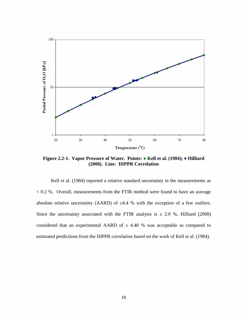
Pure MEA System Benchmarking
Figure 2.2-2, taken from Hilliard (2008), illustrates how the experimental MEA
vapor pressure obtained from the FTIR method compare to accepted values reported by a
number of literature sources.
Figure 2.2-2. Vapor Pressure of pure monoethanolamine. Points: ●, Matthews et al.
(1973), ♦, Engineering Sciences Data Unit (1979), ■,Hilliard (2008). Line: DIPPR
Correlation
Values estimated from the DIPPR correlation were reported with a relative
standard uncertainty of < 10 %. Measurements obtained from the FTIR method were
found to be adequate within an AARD of ±7.3 % with the exception of a few outliers.
MEA-CO2-H2O Benchmarking
CO2 solubility measurements for loaded MEA obtained from the FTIR technique
are compared to those reported by Jou et al. (1995) and Dugas (2009) in Figure 2.2-3.
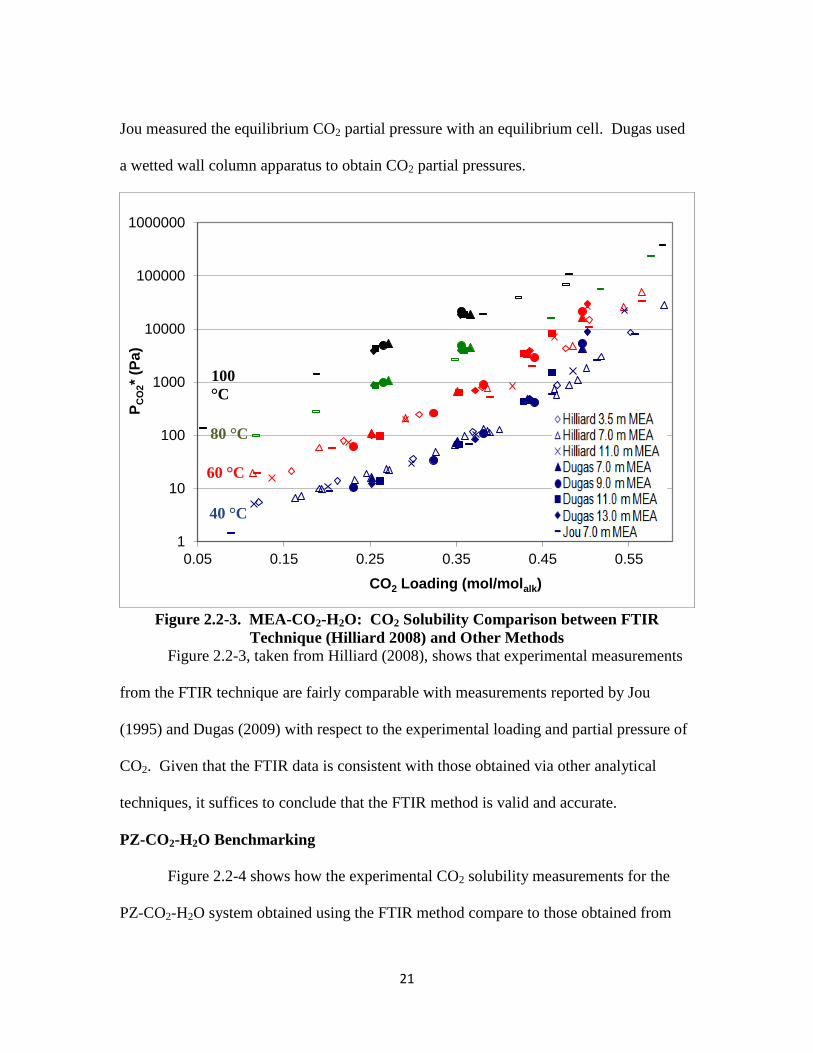
21
Jou measured the equilibrium CO2 partial pressure with an equilibrium cell. Dugas used
a wetted wall column apparatus to obtain CO2 partial pressures.
Figure 2.2-3. MEA-CO2-H2O: CO2 Solubility Comparison between FTIR
Technique (Hilliard 2008) and Other Methods
Figure 2.2-3, taken from Hilliard (2008), shows that experimental measurements
from the FTIR technique are fairly comparable with measurements reported by Jou
(1995) and Dugas (2009) with respect to the experimental loading and partial pressure of
CO2. Given that the FTIR data is consistent with those obtained via other analytical
techniques, it suffices to conclude that the FTIR method is valid and accurate.
PZ-CO2-H2O Benchmarking
Figure 2.2-4 shows how the experimental CO2 solubility measurements for the
PZ-CO2-H2O system obtained using the FTIR method compare to those obtained from
1
10
100
1000
10000
100000
1000000
0.05 0.15 0.25 0.35 0.45 0.55
PC
O2*
(Pa
)
CO2 Loading (mol/molalk)
40 °C
60 °C
80 °C
100
°C
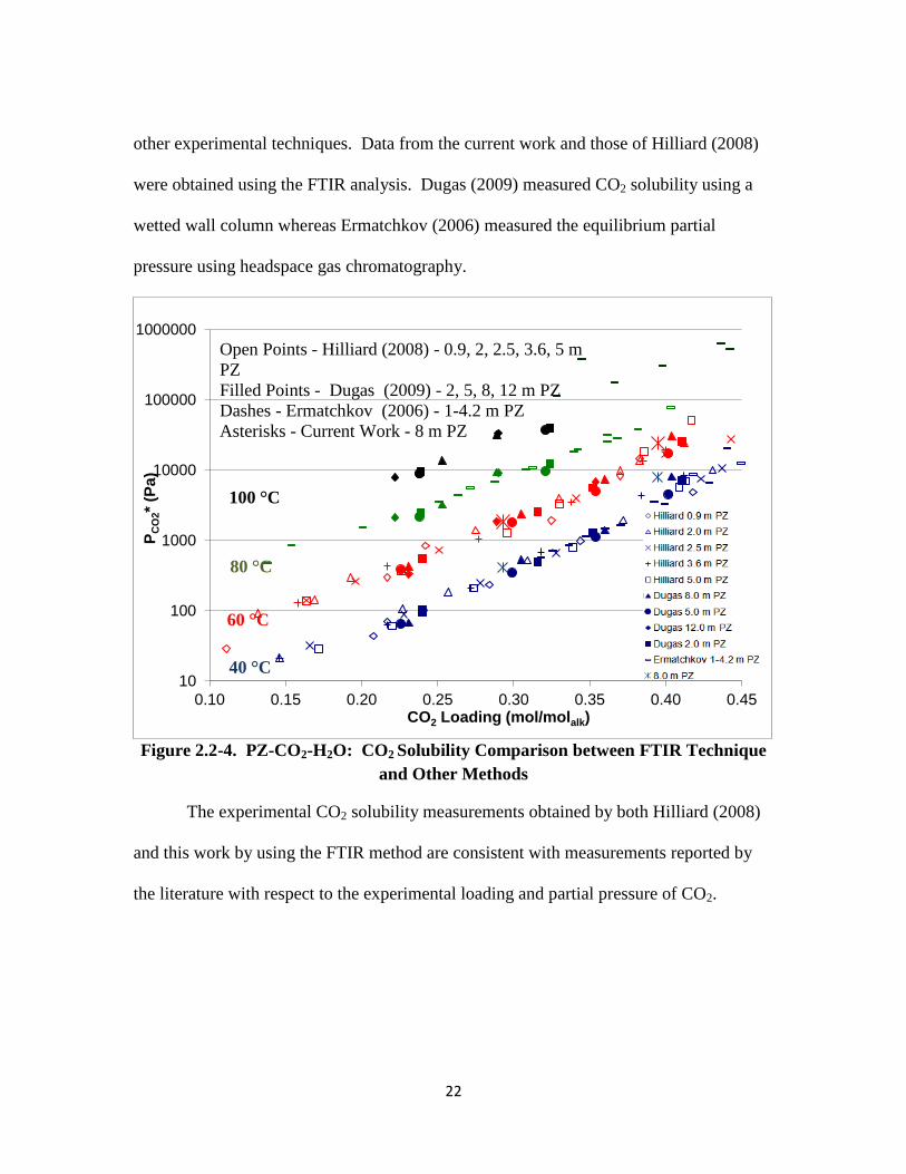
22
other experimental techniques. Data from the current work and those of Hilliard (2008)
were obtained using the FTIR analysis. Dugas (2009) measured CO2 solubility using a
wetted wall column whereas Ermatchkov (2006) measured the equilibrium partial
pressure using headspace gas chromatography.
Figure 2.2-4. PZ-CO2-H2O: CO2 Solubility Comparison between FTIR Technique
and Other Methods
The experimental CO2 solubility measurements obtained by both Hilliard (2008)
and this work by using the FTIR method are consistent with measurements reported by
the literature with respect to the experimental loading and partial pressure of CO2.
10
100
1000
10000
100000
1000000
0.10 0.15 0.20 0.25 0.30 0.35 0.40 0.45
PC
O2*
(Pa
)
CO2 Loading (mol/molalk)
Open Points - Hilliard (2008) - 0.9, 2, 2.5, 3.6, 5 m
PZ
Filled Points - Dugas (2009) - 2, 5, 8, 12 m PZ
Dashes - Ermatchkov (2006) - 1-4.2 m PZ
Asterisks - Current Work - 8 m PZ
40 °C
60 °C
80 °C
100 °C
23
Other Literature Comparisons
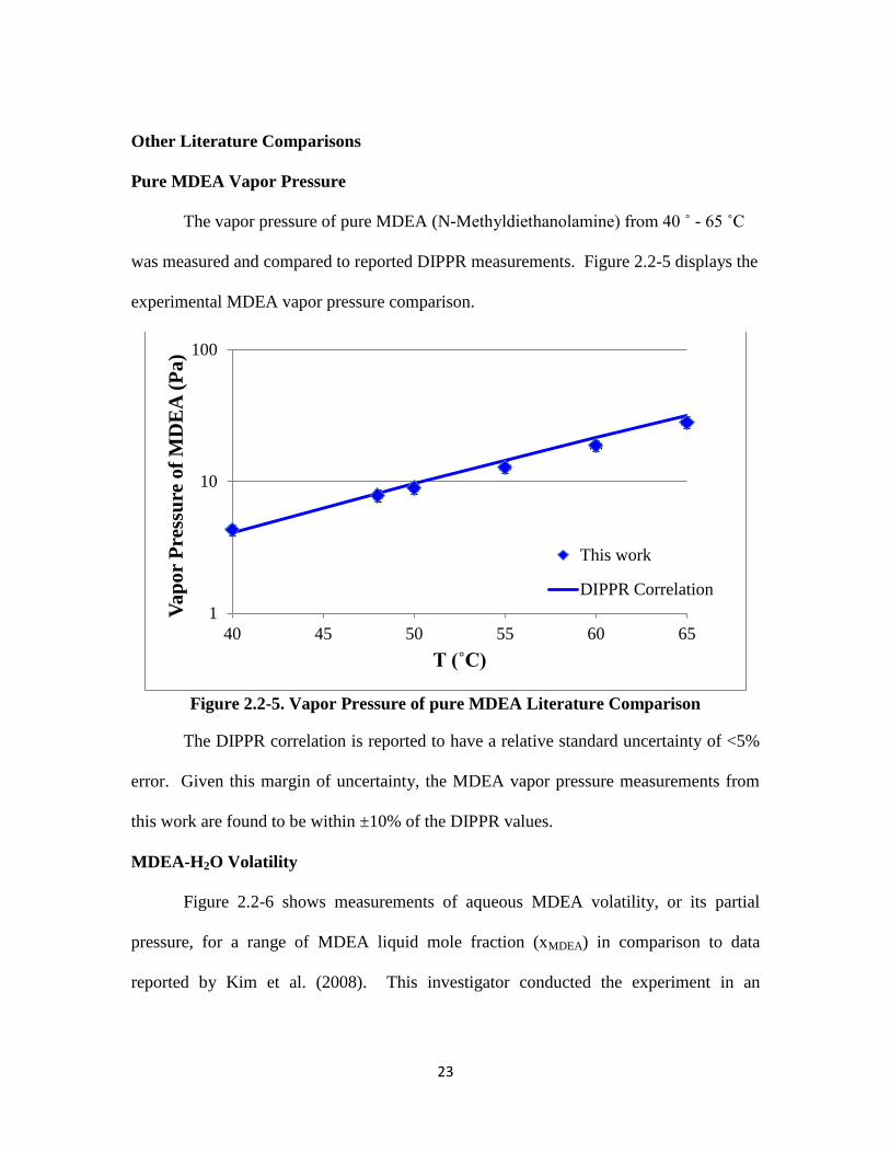
Pure MDEA Vapor Pressure
The vapor pressure of pure MDEA (N-Methyldiethanolamine) from 40 ˚ - 65 ˚C
was measured and compared to reported DIPPR measurements. Figure 2.2-5 displays the
experimental MDEA vapor pressure comparison.
Figure 2.2-5. Vapor Pressure of pure MDEA Literature Comparison
The DIPPR correlation is reported to have a relative standard uncertainty of <5%
error. Given this margin of uncertainty, the MDEA vapor pressure measurements from
this work are found to be within ±10% of the DIPPR values.
MDEA-H2O Volatility
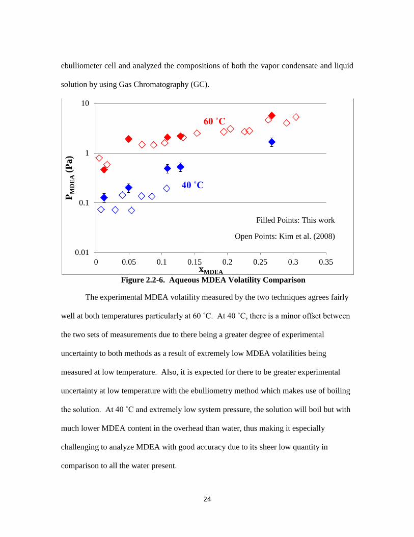
Figure 2.2-6 shows measurements of aqueous MDEA volatility, or its partial
pressure, for a range of MDEA liquid mole fraction (xMDEA) in comparison to data
reported by Kim et al. (2008). This investigator conducted the experiment in an
1
10
100
40 45 50 55 60 65
Va
po
r P
ress
ure
of
MD
EA
(P
a)
T (˚C)
This work
DIPPR Correlation
24
ebulliometer cell and analyzed the compositions of both the vapor condensate and liquid
solution by using Gas Chromatography (GC).
Figure 2.2-6. Aqueous MDEA Volatility Comparison
The experimental MDEA volatility measured by the two techniques agrees fairly
well at both temperatures particularly at 60 ˚C. At 40 ˚C, there is a minor offset between
the two sets of measurements due to there being a greater degree of experimental
uncertainty to both methods as a result of extremely low MDEA volatilities being
measured at low temperature. Also, it is expected for there to be greater experimental
uncertainty at low temperature with the ebulliometry method which makes use of boiling
the solution. At 40 ˚C and extremely low system pressure, the solution will boil but with
much lower MDEA content in the overhead than water, thus making it especially
challenging to analyze MDEA with good accuracy due to its sheer low quantity in
comparison to all the water present.
0.01
0.1
1
10
0 0.05 0.1 0.15 0.2 0.25 0.3 0.35
PM
DE
A (
Pa
)
xMDEA
40 ˚C
60 ˚C
Filled Points: This work
Open Points: Kim et al. (2008)
25
MEA-H2O Volatility
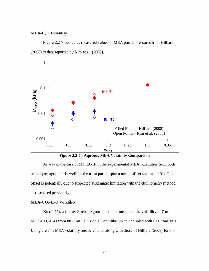
Figure 2.2-7 compares measured values of MEA partial pressures from Hilliard
(2008) to data reported by Kim et al. (2008).
Figure 2.2-7. Aqueous MEA Volatility Comparison
As was in the case of MDEA-H2O, the experimental MEA volatilities from both
techniques agree fairly well for the most part despite a minor offset seen at 40 ˚C. This
offset is potentially due to suspected systematic limitation with the ebulliometry method
as discussed previously.
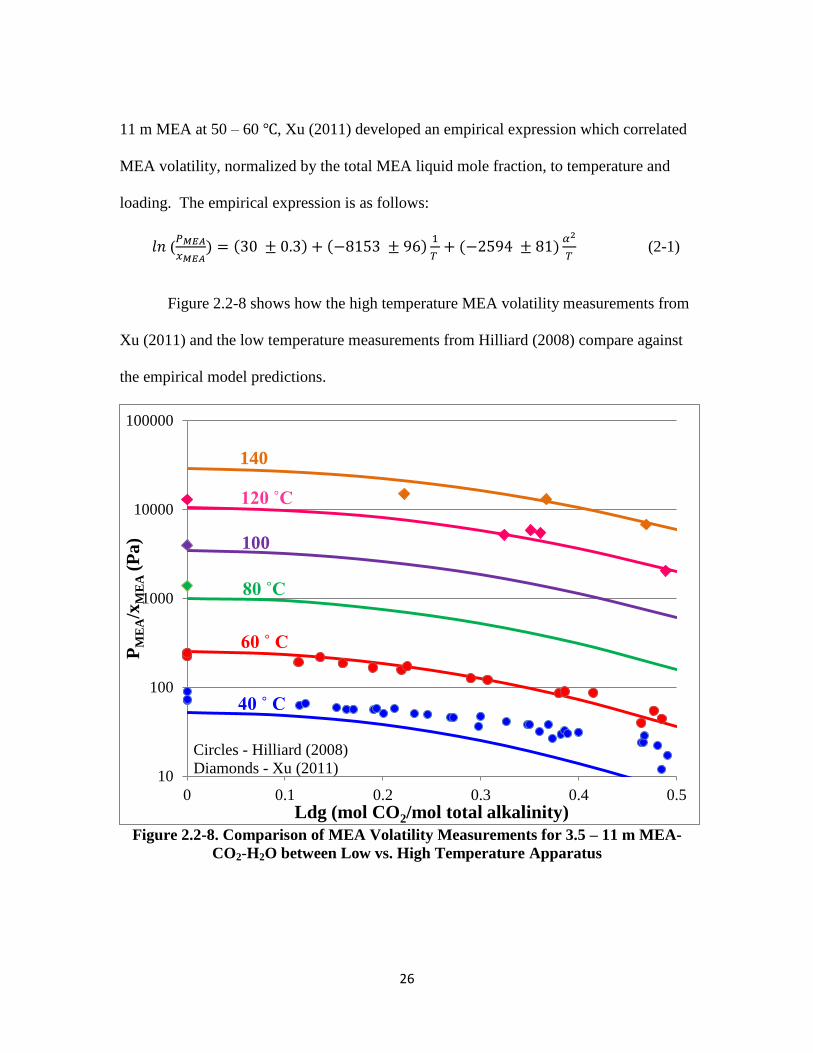
MEA-CO2-H2O Volatility
Xu (2011), a former Rochelle group member, measured the volatility of 7 m
MEA-CO2-H2O from 80 – 140 ˚C using a 2-equilibrium cell coupled with FTIR analysis.
Using the 7 m MEA volatility measurements along with those of Hilliard (2008) for 3.5 –
0.001
0.01
0.1
1
0.05 0.1 0.15 0.2 0.25 0.3 0.35
PM
EA (
kP
a)
xMEA
Filled Points - Hilliard (2008)
Open Points - Kim et al. (2008)
40 °C
60 °C
26
11 m MEA at 50 – 60 , Xu (2011) developed an empirical expression which correlated
MEA volatility, normalized by the total MEA liquid mole fraction, to temperature and
loading. The empirical expression is as follows:
(
( (
(
(2-1)
Figure 2.2-8 shows how the high temperature MEA volatility measurements from
Xu (2011) and the low temperature measurements from Hilliard (2008) compare against
the empirical model predictions.
Figure 2.2-8. Comparison of MEA Volatility Measurements for 3.5 – 11 m MEA-
CO2-H2O between Low vs. High Temperature Apparatus
10
100
1000
10000
100000
0 0.1 0.2 0.3 0.4 0.5
PM
EA/x
ME
A (
Pa
)
Ldg (mol CO2/mol total alkalinity)
40 ˚ C
60 ˚ C
80 ˚C
100
120 ˚C
140
Circles - Hilliard (2008)
Diamonds - Xu (2011)
27
The MEA volatility measurements for 3.5 – 11 m MEA-CO2-H2O at 40 ˚C by
Hilliard (2008) are not consistent with the rest of the measurements at other temperature.
Thus the 40 ˚C data were excluded from the empirical model regression. This data was
later considered to be erroneous due to faulty FTIR calibrations for low MEA
concentrations coupled with the fact that the low volatility measurements most likely
challenged the detection limit of the instrument. Other than this issue, the rest of the data
between the low and high temperature apparatus are internally consistent with each other
as evident by observation and the fact that they can both be modeled together by a
unifying empirical expression.
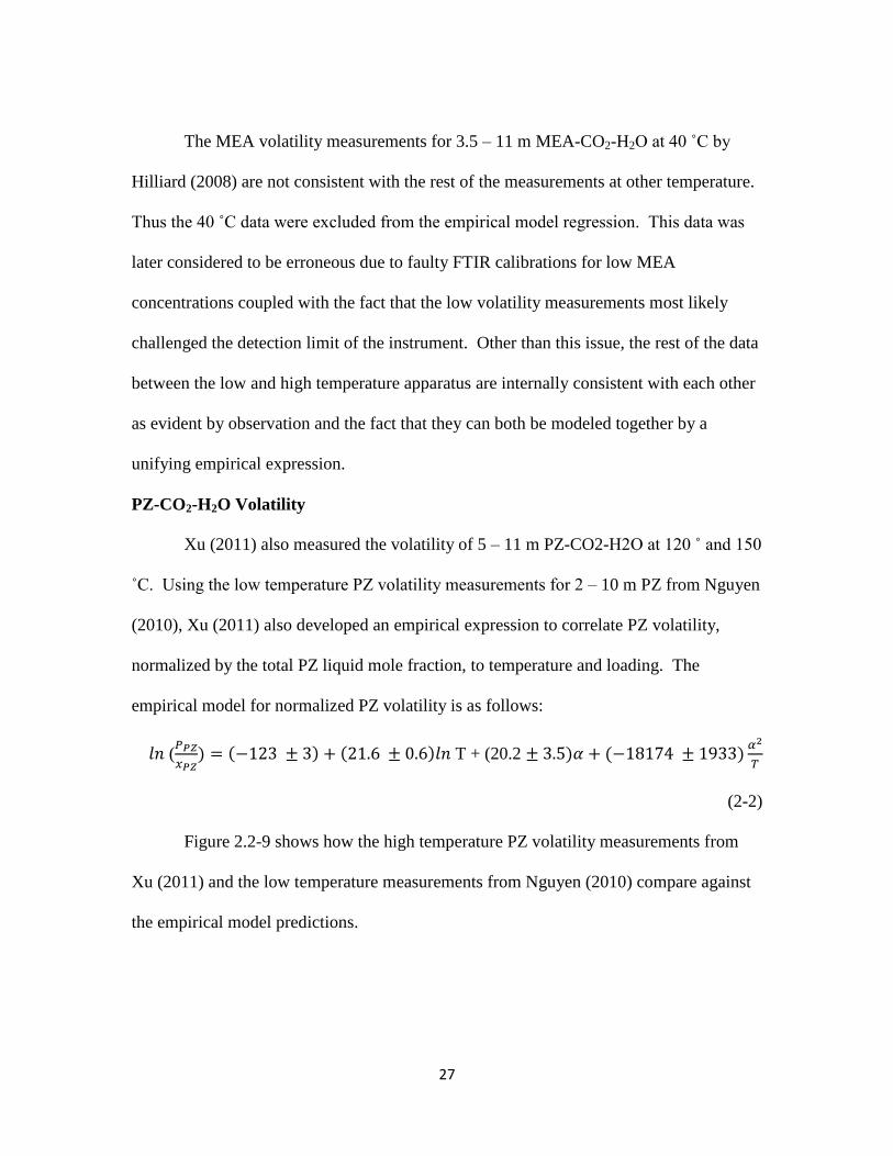
PZ-CO2-H2O Volatility
Xu (2011) also measured the volatility of 5 – 11 m PZ-CO2-H2O at 120 ˚ and 150
˚C. Using the low temperature PZ volatility measurements for 2 – 10 m PZ from Nguyen
(2010), Xu (2011) also developed an empirical expression to correlate PZ volatility,
normalized by the total PZ liquid mole fraction, to temperature and loading. The
empirical model for normalized PZ volatility is as follows:
(
( ( T + (20.2 (
(2-2)
Figure 2.2-9 shows how the high temperature PZ volatility measurements from
Xu (2011) and the low temperature measurements from Nguyen (2010) compare against
the empirical model predictions.
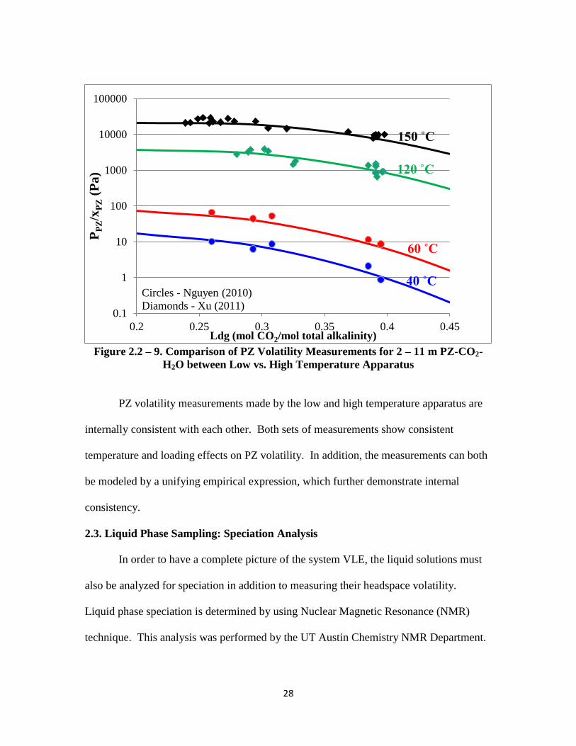
28
Figure 2.2 – 9. Comparison of PZ Volatility Measurements for 2 – 11 m PZ-CO2-
H2O between Low vs. High Temperature Apparatus
PZ volatility measurements made by the low and high temperature apparatus are
internally consistent with each other. Both sets of measurements show consistent
temperature and loading effects on PZ volatility. In addition, the measurements can both
be modeled by a unifying empirical expression, which further demonstrate internal
consistency.
2.3. Liquid Phase Sampling: Speciation Analysis
In order to have a complete picture of the system VLE, the liquid solutions must
also be analyzed for speciation in addition to measuring their headspace volatility.
Liquid phase speciation is determined by using Nuclear Magnetic Resonance (NMR)
technique. This analysis was performed by the UT Austin Chemistry NMR Department.
0.1
1
10
100
1000
10000
100000
0.2 0.25 0.3 0.35 0.4 0.45
PP
Z/x
PZ (
Pa
)
Ldg (mol CO2/mol total alkalinity)
40 ˚C
60 ˚C
120 ˚C
150 ˚C
Circles - Nguyen (2010)
Diamonds - Xu (2011)
29
Loaded solutions (whose volatilities were measured with the FTIR) cannot simply be
submitted for NMR analysis because they are not magnetically active. Unloaded aqueous
amine solutions were charged with 13
CO2 to enhance the NMR response.
The procedure for preparing NMR samples is as follows. A batch of amine-water
solution, approximately 5 – 10 g, was prepared and subsequently mixed with 1 wt % 1,4-
dioxane (Fisher ≥ 99.9% pure) and 10 wt % deuterium oxide (Cambridge Isotopes, ≥
99.9% pure). Dioxane serves as an internal reference, while the deuterium oxide acts as a
resonance lock for field stabilization to prevent the NMR signal of the sample from being
swamped by that of the solvent. The solution was then loaded with 13
CO2 (99% purity,
Cambridge Isotopes Laboratory) using a mini glass sparging apparatus until the desired
loading was achieved. Next, the loaded solution was transferred into an NMR tube
(Wilmad glass, 5 mm OD x 0.77 mm ID) which was sealed thermally. The NMR
analysis was performed with a Varian Inova 500 MHz NMR Spectrometer with variable
temperature control. Samples at 40 °C and 60 °C were thermally conditioned by heating
for at least 1 hour in a water bath at the temperature of interest prior to NMR analysis.
Both H1 and C
13 NMR analyses are used to determine the composition of the
liquid sample. Note that with either of these NMR techniques it is not possible to
distinguish a species from its protonated form (for example PZ and PZH+) due to the fast
exchange of proton between the unprotonated and protonated species. C13
NMR
uniquely provides the concentration of bicarbonate in the system, a species which cannot
be determined from H1 NMR since it is generated from
13CO2. For all the remaining
species in the system other than bicarbonate, both H1 and C
13 analyses provide close
30
results that match well within ±10% of each other. Details regarding NMR peak
assignment are provided in Appendix A.
2.4. Liquid Speciation (NMR) Method Validation
MEA-CO2-H2O Benchmarking
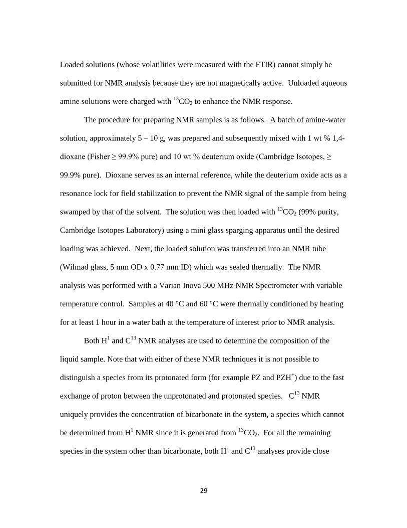
The experimental liquid speciation method used in this work was benchmarked by
Hilliard (2008) for 7 m MEA-CO2-H2O and 1 m PZ-CO2-H2O systems at 27 ˚C. Figure
2.4-1 illustrates how the speciation analysis from this work compares to the literature for
loaded 7 m MEA.
Figure 2.4-1. C13
NMR Liquid Phase Speciation for 7 m MEA at 27 ˚C. Closed
Points: Poplsteinova (2004). Open Points: Hilliard (2008).
It appears that the experimental speciation from Hilliard (2008) benchmarking
agrees well with that of Poplsteinova (2004) for loaded 7 m MEA at 27 ˚C. There is,
however, a minor discrepancy in the reported CO3-2
/HCO3-1
concentrations between
31
Hilliard (2008) and the literature. This offset was potentially attributed to the difficulty
of accurately measuring low concentrations at 0.01 – 0.1 mol/kg-H2O of the species.
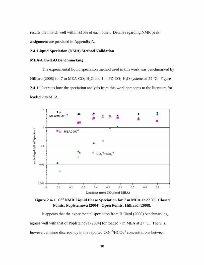
PZ-CO2-H2O Benchmarking
Hilliard (2008) also benchmarked the liquid speciation NMR method used in this
work with literature data for 1 m PZ-CO2-H2O system at 27 ˚C. Figure 2.4-2 displays the
comparison between the two sets of results.
Figure 2.4-2. H1 NMR Liquid Phase Speciation for 1 m PZ-CO2-H2O System at 27
˚C. Closed Points: Ermatchkov et al. (2003). Open Points: Hilliard (2008).
The experimental speciation results from Hilliard (2008) are seen to agree very
well with those of Ermatchkov et al. (2003). These results serve to validate the accuracy
of the Liquid Speciation NMR analysis used in this work.
32
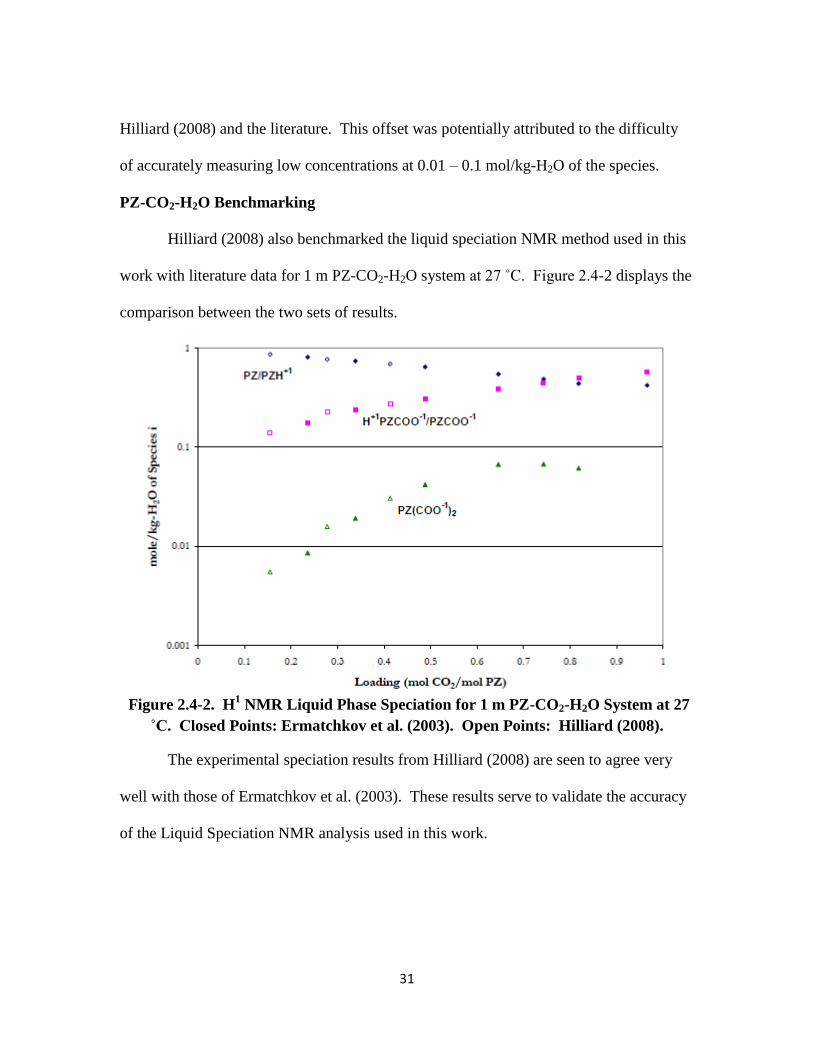
2.5. Heat Capacity Determination
A 304-stainless steel pan (Perkin Elmer #03190218) was filled to capacity with 60
μL of solution before being sealed with a lid and O-ring. When properly sealed, the
entire steel cell can withstand an internal pressure up to 150 bars. A vapor headspace of
roughly 5–10% in volume was estimated to exist in the sealed unit. The sample pan was
then placed against an empty reference pan inside a Differential Scanning Calorimeter
instrument (TA Instruments DSC-Q100) to measure the difference in the amount of heat
absorbed by the two pans. This amount of heat differential was subsequently used to
determine the heat capacity of the solution. Details regarding the Heat Capacity
experimental procedure and data interpretation are provided in Appendix C. Below is a
snapshot inside the DSC cell where the differential heat absorbed by a reference pan
compared to a sample pan is measured.
Figure 2.5-1. Snapshot of DSC Sample Cell
The cell constant and temperature response of the DSC instrument have to be
calibrated using Indium metal, which has a known melting point (156.6 ºC). The cell
constant is an internal machine parameter that is used to adjust for subtle differences in
33
the calorimetric response of the unit. In addition, temperature calibration is done to
ensure that the sample thermocouple is reading correctly under experimental conditions.
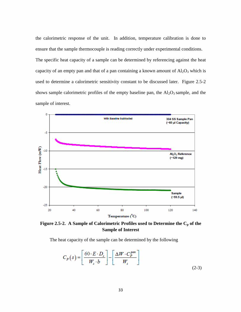
The specific heat capacity of a sample can be determined by referencing against the heat
capacity of an empty pan and that of a pan containing a known amount of Al2O3 which is
used to determine a calorimetric sensitivity constant to be discussed later. Figure 2.5-2
shows sample calorimetric profiles of the empty baseline pan, the Al2O3 sample, and the
sample of interest.
Figure 2.5-2. A Sample of Calorimetric Profiles used to Determine the Cp of the
Sample of Interest
The heat capacity of the sample can be determined by the following
(2-3)
34
where
Cp (s) is the specific heat capacity of the sample, kJ/kg-K,
E is the calorimetric sensitivity of the DSC apparatus,
b is the heat rate, 5 oC / min,
Ds is the vertical displacement between the empty sample pan and the sample DSC
thermal
curves at a given temperature, mW,
Ws is the mass of the sample, mg,
ΔW, is the difference in mass between the reference pan and the sample pan, and
Cppan
is the specific heat capacity of the 304 stainless steel pans
The calorimetric sensitivity constant E can be determined given the known heat
capacity of Al2O3 by using the expression below:
(2-4)
where
Dst is the vertical displacement between the empty sample pan and the Al2O3 DSC
thermal
curves at a given temperature,
Wst the mass of Al2O3 sample, mg, and
CpAl2O3
is the specific heat capacity of Al2O3
Details pertaining to the complete heat capacity procedure used in this work can
be referenced to Hilliard (2008).
2.6. Heat Capacity Method Validation
The experimental heat capacity method was benchmarked by measuring the heat
capacity of water, pure MEA, and that of MEA-H2O system for comparison against
literature. These benchmarking activities were performed and reported by Hilliard
(2008).
35
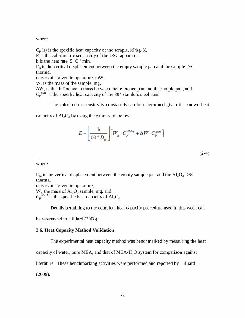
Pure H2O System Benchmarking
Figure 2.6-1, taken from Hilliard (2008), shows the experimental water heat
capacity measured by Hilliard (2008) in comparison to literature values.
Figure 2.6-1. Specific Heat Capacity of Water . Points: ♦ Kell et al. (1984); ■
Engineering Sciences Data (1966); ▲ Osborne et al. (1939); ●Chiu et al. (1999); ×
Hilliard (2008)
The experimental water heat capacity measurements from this method were found
to be ±0.4% of the average specific heat capacity of water reported in the literature.
Since the experimental measurements from this method tend to underestimate literature
data, it was estimated that the measurements would have ±2% (Hilliard 2008).
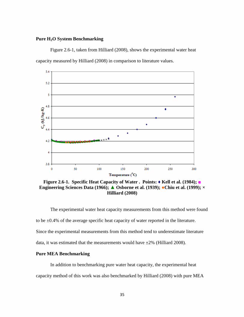
Pure MEA Benchmarking
In addition to benchmarking pure water heat capacity, the experimental heat
capacity method of this work was also benchmarked by Hilliard (2008) with pure MEA
36
heat capacity since these measurements were commonly established in the literature.
Figure 2.6-2 compares the experimental MEA Cp of this work to other sources.
Figure 2.6-2. Specific Heat Capacity of MEA. Points: ■ The Dow Chemical
Company (1981); ● Swanson and Chueh (1973); ♦ Chiu et al. (1999); ▲ Hilliard
(2008).
It appears that the experimental Cp of MEA measured by Hilliard (2008) agrees
well with that of the literature to within ±2%. Furthermore, the experimental Cp
measurements from Hilliard (2008) also show similar temperature dependence to the
literature.
MEA-H2O Heat Capacity
The Cp of 3.5 m and 7 m MEA-H2O at 40 ˚, 60 ˚, and 80 ˚C were also
benchmarked by Hilliard (2008) to the literature. Graphs will not be shown here due to
some of the original data being missing, but it was concluded that the experimental Cp for
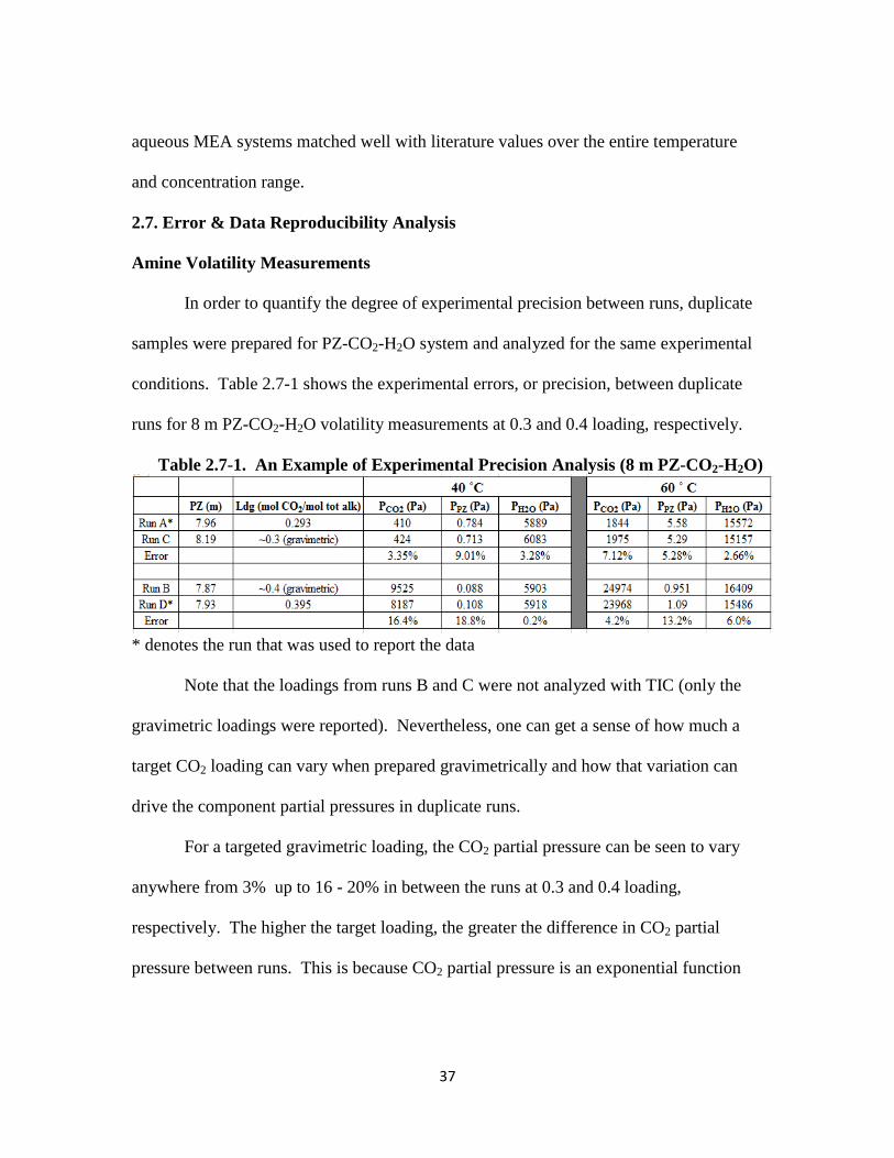
37
aqueous MEA systems matched well with literature values over the entire temperature
and concentration range.
2.7. Error & Data Reproducibility Analysis
Amine Volatility Measurements
In order to quantify the degree of experimental precision between runs, duplicate
samples were prepared for PZ-CO2-H2O system and analyzed for the same experimental
conditions. Table 2.7-1 shows the experimental errors, or precision, between duplicate
runs for 8 m PZ-CO2-H2O volatility measurements at 0.3 and 0.4 loading, respectively.
Table 2.7-1. An Example of Experimental Precision Analysis (8 m PZ-CO2-H2O)
* denotes the run that was used to report the data
Note that the loadings from runs B and C were not analyzed with TIC (only the
gravimetric loadings were reported). Nevertheless, one can get a sense of how much a
target CO2 loading can vary when prepared gravimetrically and how that variation can
drive the component partial pressures in duplicate runs.
For a targeted gravimetric loading, the CO2 partial pressure can be seen to vary
anywhere from 3% up to 16 - 20% in between the runs at 0.3 and 0.4 loading,
respectively. The higher the target loading, the greater the difference in CO2 partial
pressure between runs. This is because CO2 partial pressure is an exponential function
38
with respect to loading, therefore any small deviation in loading from one run to the next
would result in a big difference in CO2 partial pressure.
PZ partial pressures are seen to vary from 9% to 19% between the runs at 0.3 and
0.4 loading, respectively. The main source of discrepancy in PZ partial pressure between
runs is attributed to the difference in loading between the runs which drive the PZ
volatility accordingly. A different source for the discrepancy, which is not reflected in
the error analysis in Table 2.7-1, is the inherent variation in the FTIR analysis. An
analysis of the same sample can vary from 0.5% to 2%. Also the smaller the amine
partial pressure, the greater the error in the measurement which can also translate into
greater variation between different analyses of the same sample, or between different
runs with the same targeted gravimetric loading. Small amine partial pressures are more
difficult to detect than high partial pressures because the instrument is operating closer to
the detection limit (<10 ppm or < ~1 Pa).
Finally, differences in water partial pressures between the runs that are targeted to
have approximately the same gravimetric loading are typically much less than 10%. This
is because water partial pressures are very high in these systems, thus the relative
variation in these pressures among runs is relatively small. Also the FTIR is known to
provide very reliable water measurements. This is because water is the most dominant
species in the systems considered in this work and has the largest concentration.
The same level of experimental uncertainty between runs, along with the likely error
sources discussed above, can be expected for other amine systems as well.
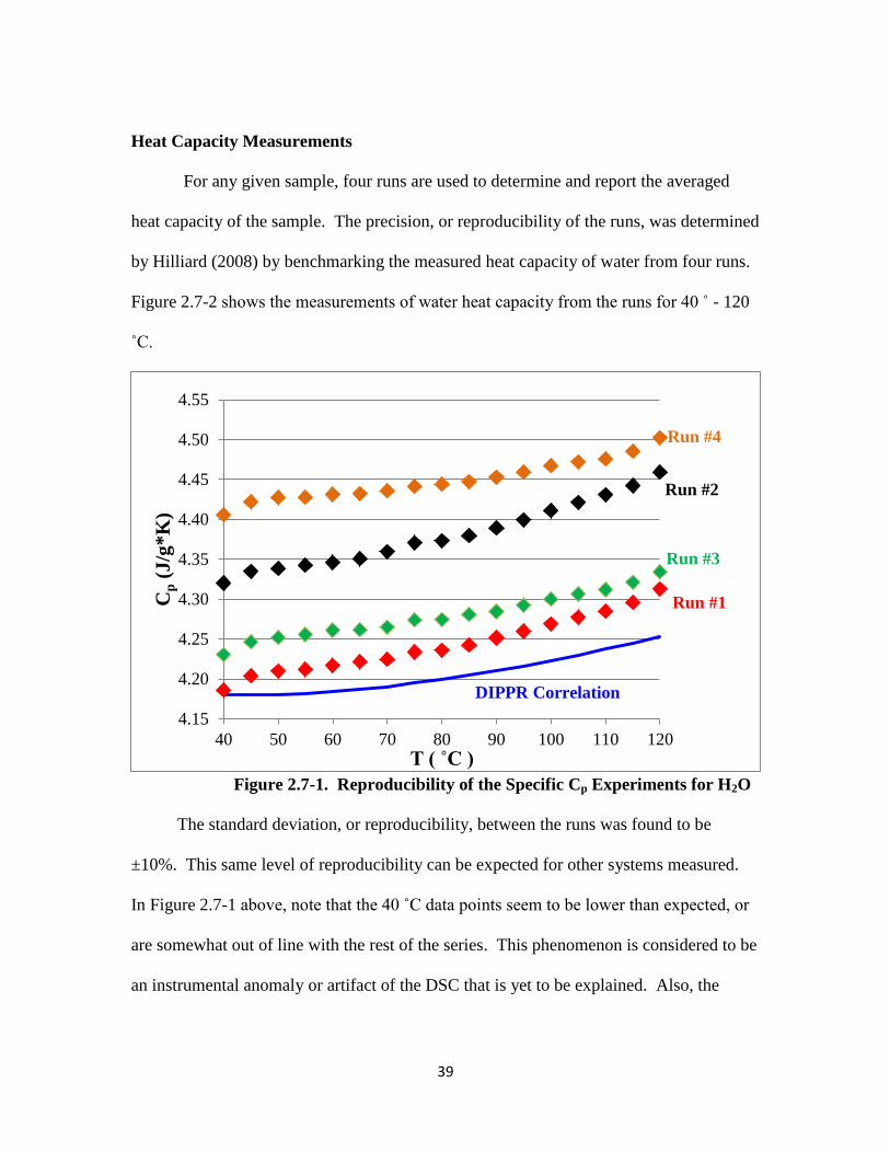
39
Heat Capacity Measurements
For any given sample, four runs are used to determine and report the averaged
heat capacity of the sample. The precision, or reproducibility of the runs, was determined
by Hilliard (2008) by benchmarking the measured heat capacity of water from four runs.
Figure 2.7-2 shows the measurements of water heat capacity from the runs for 40 ˚ - 120
˚C.
Figure 2.7-1. Reproducibility of the Specific Cp Experiments for H2O
The standard deviation, or reproducibility, between the runs was found to be
±10%. This same level of reproducibility can be expected for other systems measured.
In Figure 2.7-1 above, note that the 40 ˚C data points seem to be lower than expected, or
are somewhat out of line with the rest of the series. This phenomenon is considered to be
an instrumental anomaly or artifact of the DSC that is yet to be explained. Also, the
4.15
4.20
4.25
4.30
4.35
4.40
4.45
4.50
4.55
40 50 60 70 80 90 100 110 120
Cp (
J/g
*K
)
T ( ˚C )
Run #1
Run #2
Run #3
Run #4
DIPPR Correlation
40
temperature behavior of Run #2 from ~90 ˚ - 120 ˚C is steeper than what is known to be
according to the DIPPR water heat capacity correlation. This behavior is sometimes
observed in runs for other systems as well, and is attributed to the phenomenon of CO2,
amine, and water vaporization, or even partial boiling in this case with pure water, into
the small headspace above the solution. The degree of species vaporization into the
headspace is a function of both the species concentrations in solution and the headspace
volume, which is estimated to be anywhere from 10% - 15% of the entire sample cell.
This headspace is present as a result of the part of the lid that stands above the top of the
pan (filled to its maximum capacity ~ 60 μL).
In the analysis of samples, a correction has to be made to account for the
phenomenon of CO2 and H2O vaporization into the headspace at high temperature (~90 ˚
- 120 ˚C). The analysis used to correct for species vaporization involves determining the
gap space volume above the solution which would minimize the sum of squared residuals
between the measured heat capacities (with vaporization) and the calculated heat
capacities (estimated without vaporization). The calculated heat capacities are
determined from the true enthalpy of solution, Qsolution, which is estimated by subtracting
the heats associated with CO2 and H2O vaporization from the total measured enthalpy.
Using empirical models developed for CO2 solubility and H2O volatility, one can
calculate the partial pressure of these species above solution; subsequently the moles of
each species can be determined by using the Ideal Gas Law (assuming a gap space
volume) which can then be used to estimate the heats associated with the species
vaporization.
41
Chapter 3: Aqueous Amine Volatility in Binary Amine-Water System
3.1. Introduction
The study of amine volatility in dilute amine-water systems provides key
understanding that is crucial to the design of water wash units used in the CO2 capture
process. Typical water wash operations involve treating gas with only a few ppm of
amine and up to 15 mole % of water. Aqueous amine volatility at the water wash
condition also needs to be measured in order to quantify fugitive amine emission to the
atmosphere. There is also a scientific interest in having a better understanding of amine-
water interactions to generalize and predict the volatilities of a large number of amines
used in CO2 capture without the need for extensive experimentation.
While there are several published measurements on the VLE of amine-water
systems, only a few of them measure the vapor phase mole fraction of the amine. This
work measures the vapor composition of the amines, particularly at very dilute amine
concentration, to elucidate the intrinsic amine-water interactions. Furthermore, this work
is believed to provide one of the largest collections of experimental data of amine
volatility in water for as many as 20 amines that are relevant to CO2 capture.
Other work that investigated aqueous amine volatility will now be summarized.
Lenard et al. (1990) measured the gas phase composition of monoethanolamine (MEA) in
binary aqueous solution (343K and 363K) using gas chromatography. These data were
represented using a three-parameter Redlich-Kister expansion. Pappa et al. (2006) made
isobaric T-x-y measurements for the AMP-H2O system at 66.7, 80.0, and 101.3 kPa using
a modified Swietoslawski ebulliometer with sample compositions being determined using

42
a standard curve of refractive index for this system at 25 ˚C. Kim et al. (2008) used an
ebulliometer setup to determine the total pressure with the liquid and vapor mole
fractions of MEA, methyldiethanolamine (MDEA), and methylaminopropanolamine
(MAPA) analyzed using gas chromatography. Cai et al. (1996) measured isobaric VLE
at 101.3 kPa and 66 kPa (373K - 443K) of MEA in water using the standard curve of
refraction index versus the mole fraction of the binary mixture at 20 ºC. The liquid phase
activity coefficients were calculated with the UNIFAC group contribution model as
published by Larsen et al. (1987).
This work investigates the aqueous volatility of 20 amines that are potentially
viable for CO2 capture, including MEA, piperazine (PZ), and MDEA. The amine partial
pressure was obtained experimentally at the absorber operating conditions of 40 ˚– 70 ˚C
and 1 atm using a hot gas FTIR. Given the partial pressures, the amine Henry’s constants
can be determined and are used as the primary indicator of amine volatility. A group
contribution model is developed using experimental H constants from this work along
with those of 16 alkylamines obtained from the literature.
This model is believed to be more reliable and accurate in the prediction of amine
volatility for CO2 capture amines (alkanolamines) than existing group contribution
models such as UNIFAC and that of Hine and Mookerjee (1975). Although these other
models are regressed using a larger database of compounds, they are not able to
adequately predict the volatilities of alkanolamines since their functional group
parameters were largely regressed from alkylamine data. The alkanolamines used for
CO2 capture application are much more structurally complex than alkylamines. In the
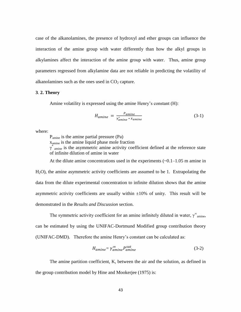
43
case of the alkanolamines, the presence of hydroxyl and ether groups can influence the
interaction of the amine group with water differently than how the alkyl groups in
alkylamines affect the interaction of the amine group with water. Thus, amine group
parameters regressed from alkylamine data are not reliable in predicting the volatility of
alkanolamines such as the ones used in CO2 capture.
3. 2. Theory
Amine volatility is expressed using the amine Henry’s constant (H):
(3-1)
where:
Pamine is the amine partial pressure (Pa)
xamine is the amine liquid phase mole fraction
γ* amine is the asymmetric amine activity coefficient defined at the reference state
of infinite dilution of amine in water
At the dilute amine concentrations used in the experiments (~0.1–1.05 m amine in
H2O), the amine asymmetric activity coefficients are assumed to be 1. Extrapolating the
data from the dilute experimental concentration to infinite dilution shows that the amine
asymmetric activity coefficients are usually within ±10% of unity. This result will be
demonstrated in the Results and Discussion section.
The symmetric activity coefficient for an amine infinitely diluted in water, γ∞
amine,
can be estimated by using the UNIFAC-Dortmund Modified group contribution theory
(UNIFAC-DMD). Therefore the amine Henry’s constant can be calculated as:
=
(3-2)
The amine partition coefficient, K, between the air and the solution, as defined in
the group contribution model by Hine and Mookerjee (1975) is:
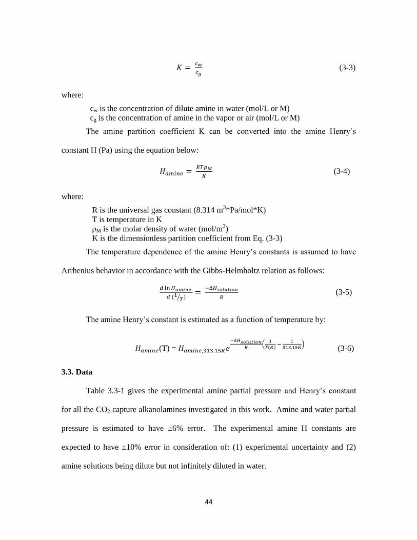
44
(3-3)
where:
cw is the concentration of dilute amine in water (mol/L or M)
cg is the concentration of amine in the vapor or air (mol/L or M)
The amine partition coefficient K can be converted into the amine Henry’s
constant H (Pa) using the equation below:
(3-4)
where:
R is the universal gas constant (8.314 m3*Pa/mol*K)
T is temperature in K
ρM is the molar density of water (mol/m3)
K is the dimensionless partition coefficient from Eq. (3-3)
The temperature dependence of the amine Henry’s constants is assumed to have
Arrhenius behavior in accordance with the Gibbs-Helmholtz relation as follows:
( ⁄
(3-5)
The amine Henry’s constant is estimated as a function of temperature by:
(T) =
(
(
) (3-6)
3.3. Data
Table 3.3-1 gives the experimental amine partial pressure and Henry’s constant
for all the CO2 capture alkanolamines investigated in this work. Amine and water partial
pressure is estimated to have ±6% error. The experimental amine H constants are
expected to have ±10% error in consideration of: (1) experimental uncertainty and (2)
amine solutions being dilute but not infinitely diluted in water.
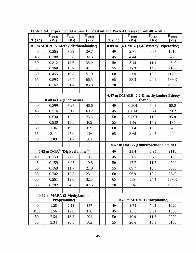
45
Table 3.3-1. Experimental Amine H Constant and Partial Pressure from 40 ˚– 70 ˚C
T ( C )
Pamine
(Pa)
PH2O
(kPa)
Hamine
(Pa) T ( C )
Pamine
(Pa)
PH2O
(kPa)
Hamine
(Pa)
0.5 m MDEA (N-Methyldiethanolamine) 0.09 m 1,4 DMPZ (1,4-Dimethyl Piperazine)
40 0.265 7.39 29.7 40 2.71 6.87 1510
45 0.288 9.38 32.3 45 4.44 8.63 2470
50 0.312 12.6 35.0 50 8.15 11.4 4540
55 0.369 15.9 41.4 55 12.9 14.8 7160
60 0.455 19.8 51.0 60 21.0 18.6 11700
65 0.593 25.4 66.5 65 33.8 24.1 18800
70 0.767 31.4 85.9 70 53.1 30.7 29500
0.48 m PZ (Piperazine) 0.47 m DMAEE (2,2-Dimethylamino Ethoxy
Ethanol)
40 0.399 7.27 46.6 40 0.504 7.05 60.0
45 0.516 9.17 60.2 45 0.614 8.74 73.2
50 0.630 12.2 73.5 50 0.803 11.5 95.8
55 0.930 15.5 109 55 1.46 14.9 174
60 1.36 19.3 159 60 2.04 18.8 243
65 2.11 25.0 246 65 3.69 24.3 440
70 3.09 31.7 361
0.57 m DMEA (Dimethylethanolamine)
0.45 m DGA® (Diglycolamine
®) 40 21.4 6.93 2110
40 0.153 7.06 19.1 45 31.5 8.72 3100
45 0.159 8.95 19.8 50 47.7 11.5 4700
50 0.169 11.7 21.0 55 69.7 15.0 6860
55 0.202 15.3 25.1 60 96.9 18.9 9540
60 0.261 19.0 32.5 65 139 24.4 13700
65 0.382 24.5 47.5 70 194 30.8 19200
0.49 m MAPA (3-Methylamino
Propylamine) 0.48 m MORPH (Morpholine)
40 1.28 9.11 147 40 8.78 7.05 1020
45.1 1.56 12.0 178 45 13.1 8.94 1530
50 2.54 16.3 291 50 19.0 11.8 2220
55 3.34 20.5 382 55 26.6 15.1 3100
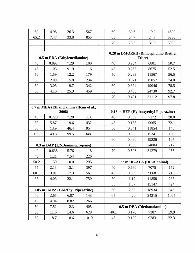
46
60 4.96 26.3 567 60 39.6 19.2 4620
65.2 7.47 33.8 855 65 54.7 24.7 6380
70 76.5 31.0 8930
0.5 m EDA (Ethylenediamine)
0.28 m DMORPH (Dimorpholino Diethyl
Ether)
40 0.892 7.29 100 40 0.254 6881 50.7
45 1.03 9.19 116 45 0.263 8675 52.5
50 1.59 12.2 179 50 0.283 11567 56.5
55 2.09 15.8 234 55 0.371 15057 74.0
60 3.05 19.7 342 60 0.394 19046 78.5
65 4.10 25.3 459 65 0.465 24730 92.7
70 0.491 31112 97.8
0.7 m MEA (Ethanolamine) (Kim et al.,
2008) 0.13 m HEP (Hydroxyethyl Piperazine)
40 0.728 7.28 60.0 40 0.089 7172 38.0
60 5.87 19.6 432 45 0.168 9065 72.1
80 13.9 46.4 954 50 0.341 11854 146
100 49.8 99.5 3481 55 0.393 15341 169
60 0.460 19226 197
0.3 m DAP (1,2-Diaminopropane) 65 0.506 24804 217
40 0.636 5.76 118 70 0.596 31279 255
45 1.21 7.54 226
50.2 1.59 10.0 295 0.22 m DL-ALA (DL-Alaninol)
55 2.13 13.1 397 40 0.680 7075 172
60.1 3.01 17.3 561 45 0.839 9068 213
65 4.03 22.1 750 50 1.12 11858 285
55 1.67 15147 424
1.05 m 1MPZ (1-Methyl Piperazine) 60 2.55 18934 645
40 2.65 6.87 143 65 4.20 24215 1065
45 4.94 8.82 266
50 7.51 12.3 405 0.5 m DEA (Diethanolamine)
55 11.6 14.6 628 40.1 0.178 7387 19.9
60 18.7 18.6 1010 45 0.199 9283 22.3
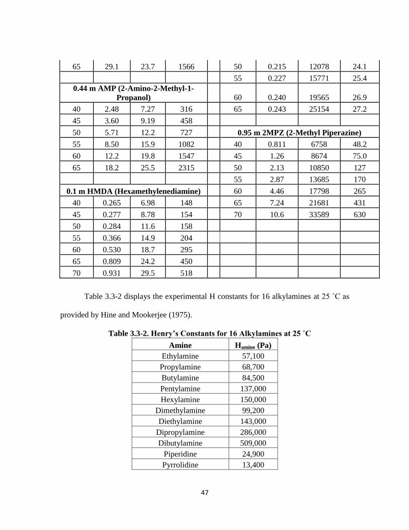
47
65 29.1 23.7 1566 50 0.215 12078 24.1
55 0.227 15771 25.4
0.44 m AMP (2-Amino-2-Methyl-1-
Propanol) 60 0.240 19565 26.9
40 2.48 7.27 316 65 0.243 25154 27.2
45 3.60 9.19 458
50 5.71 12.2 727 0.95 m 2MPZ (2-Methyl Piperazine)
55 8.50 15.9 1082 40 0.811 6758 48.2
60 12.2 19.8 1547 45 1.26 8674 75.0
65 18.2 25.5 2315 50 2.13 10850 127
55 2.87 13685 170
0.1 m HMDA (Hexamethylenediamine) 60 4.46 17798 265
40 0.265 6.98 148 65 7.24 21681 431
45 0.277 8.78 154 70 10.6 33589 630
50 0.284 11.6 158
55 0.366 14.9 204
60 0.530 18.7 295
65 0.809 24.2 450
70 0.931 29.5 518
Table 3.3-2 displays the experimental H constants for 16 alkylamines at 25 ˚C as
provided by Hine and Mookerjee (1975).
Table 3.3-2. Henry’s Constants for 16 Alkylamines at 25 ˚C
Amine Hamine (Pa)
Ethylamine 57,100
Propylamine 68,700
Butylamine 84,500
Pentylamine 137,000
Hexylamine 150,000
Dimethylamine 99,200
Diethylamine 143,000
Dipropylamine 286,000
Dibutylamine 509,000
Piperidine 24,900
Pyrrolidine 13,400
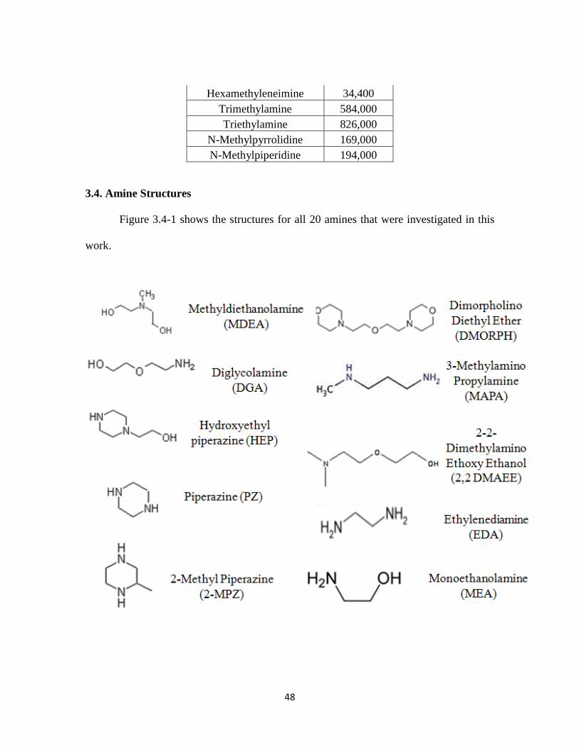
48
Hexamethyleneimine 34,400
Trimethylamine 584,000
Triethylamine 826,000
N-Methylpyrrolidine 169,000
N-Methylpiperidine 194,000
3.4. Amine Structures
Figure 3.4-1 shows the structures for all 20 amines that were investigated in this
work.
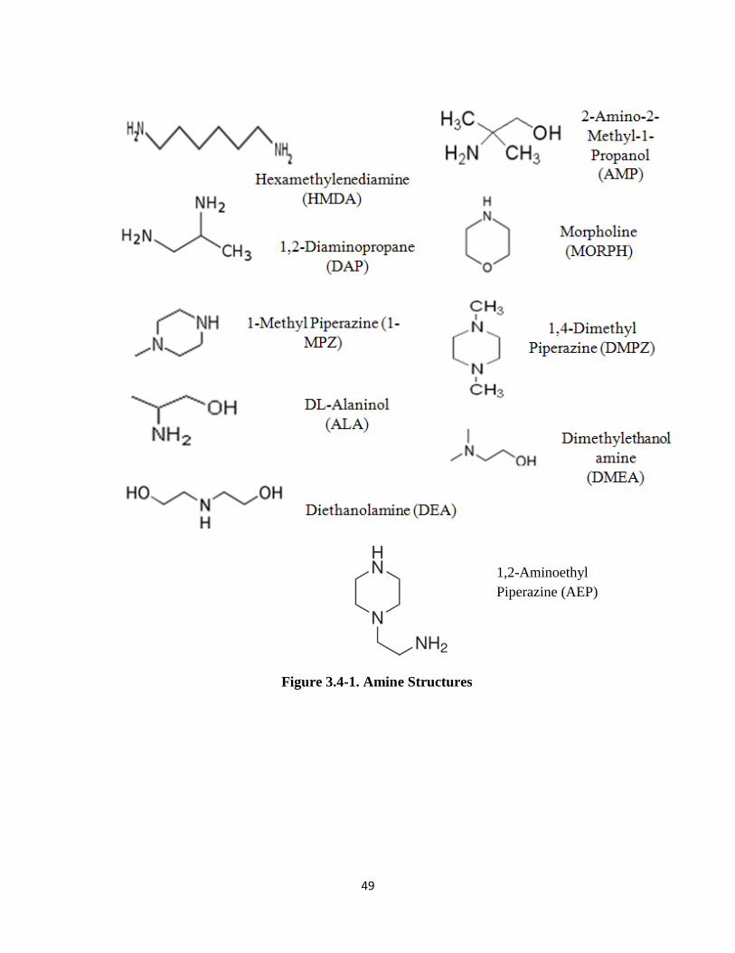
49
Figure 3.4-1. Amine Structures
1,2-Aminoethyl
Piperazine (AEP)
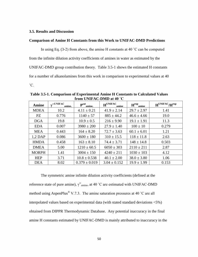
50
3.5. Results and Discussion
Comparison of Amine H Constants from this Work to UNIFAC-DMD Predictions
In using Eq. (3-2) from above, the amine H constants at 40 ˚C can be computed
from the infinite dilution activity coefficients of amines in water as estimated by the
UNIFAC-DMD group contribution theory. Table 3.5-1 shows the estimated H constants
for a number of alkanolamines from this work in comparison to experimental values at 40
˚C.
Table 3.5-1. Comparison of Experimental Amine H Constants to Calculated Values
from UNIFAC-DMD at 40 ˚C
Amine γ∞UNIFAC
amine, Psat
amine, HUNIFAC
amine Hexp
amine HUNIFAC
/Hexp
MDEA 10.2 4.11 ± 0.21 41.9 ± 2.14 29.7 ± 2.97 1.41
PZ 0.776 1140 ± 57 885 ± 44.2 46.6 ± 4.66 19.0
DGA 19.8 10.9 ± 0.5 216 ± 9.90 19.1 ± 1.91 11.3
EDA 0.007 3980 ± 200 27.9 ± 1.40 100 ± 10 0.279
MEA 0.443 164 ± 8.20 72.7 ± 3.63 60.1 ± 6.01 1.21
1,2 DAP 0.086 3600 ± 180 310 ± 15.5 118 ± 11.8 2.63
HMDA 0.458 163 ± 8.10 74.4 ± 3.71 148 ± 14.8 0.503
DMEA 5.00 1210 ± 60.5 6050 ± 303 2110 ± 211 2.87
MORPH 1.41 3004 ± 150 4240 ± 211 1030 ± 103 4.12
HEP 3.71 10.8 ± 0.538 40.1 ± 2.00 38.0 ± 3.80 1.06
DEA 8.02 0.379 ± 0.019 3.04 ± 0.152 19.9 ± 1.99 0.153
The symmetric amine infinite dilution activity coefficients (defined at the
reference state of pure amine), γ∞
amine, at 40 ˚C are estimated with UNIFAC-DMD
method using AspenPlus® V.7.3. The amine saturation pressures at 40 ˚C are all
interpolated values based on experimental data (with stated standard deviations <5%)
obtained from DIPPR Thermodynamic Database. Any potential inaccuracy in the final
amine H constants estimated by UNIFAC-DMD is mainly attributed to inaccuracy in the
51
estimated infinite dilution activity coefficients rather than to errors in the experimental
amine saturation pressures (which were stated to have low experimental uncertainties of
<5%). For the majority of amines shown in Table 3.5-1, the experimental H constants
from this work and those predicted by UNIFAC-DMD theory agree within an order of
magnitude.
HEP (hydroxyethyl piperazine) and MEA (monoethanolamine) show the closest
agreement between the experimental value and the UNIFAC-DMD prediction. This
observation serves to validate the accuracy of the experimental method of this work by
indicating that there is no systematic issue with the method, which could result in a gross
systematic discrepancy between UNIFAC-DMD and the experimental method for all
amines where one set of values is consistently higher or lower than the other.
PZ (piperazine) and DGA (diglycolamine) show the greatest discrepancy by more
than an order of magnitude between experimental versus estimated H constant values.
It is unexpected that DGA has a much greater estimated H constant (~216) compared to
MDEA (~41.9) according to UNIFAC-DMD. This observation implies that DGA is
more volatile than MDEA which seems rather counterintuitive as MDEA is believed to
be more nonpolar than DGA due to the presence of the methyl group, which should
increase its volatility due to unfavorable interaction with water. This hypothesis is
validated by experimental measurements which show that the measured H constant of
DGA is ~19.1 whereas that of MDEA is ~29.7. This translates to aqueous MDEA being
more volatile than aqueous DGA experimentally. Another important conclusion that can
be drawn from comparing MDEA to DGA is that aqueous amine volatility does not

52
necessarily correlate with pure component volatility. At 40 ˚C, although DGA has a
greater saturation pressure than MDEA, the latter is believed and shown experimentally
to have greater aqueous volatility. Due to the obvious discrepancy between UNIFAC-
DMD and experimental measurements, it is determined that it is crucial to investigate
alkanolamines extensively in order to elucidate the true interaction between amine and
water, which is the main driver of amine volatility.
Comparison of Amine Henry’s Constants from this Work to Hine and Mookerjee
Group Contribution Methodology (1975)
Table 3.5-2 summarizes the amine Henry’s constant, as determined from the
partition coefficient K estimated by using the group contribution method established by
Hine and Mookerjee (1975), and the experimental Henry’s constants measured by this
work at 25 ˚C.
Table 3.5-2. Comparison of Experimental Amine H Constants to Calculated Values from Hine and Mookerjee (1975) at 25 ˚C
HH&M
amine, 25C Hexp
amine, 25C HH&M
/Hexp
MDEA 1.38E-04 27.5 5.00E-6
PZ 37.9 40.4 9.40E-1
DGA 0.001 17.8 6.75E-5
MAPA 3.54 127 2.79E-2
EDA 9.98 87.8 1.14E-1
MEA 0.561 52.0 1.08E-2
1,2 DAP 4.16 103 4.05E-2
1-MPZ 158 118 1.34E+0
AMP 9.75 268 3.64E-2
HMDA 39.7 134 2.96E-1
1,4 DMPZ 659 1230 5.38E-1
2,2 DMAEE 0.021 50.9 4.19E-4
DMEA 9.98 1810 5.51E-3
MORPH 615 883 6.97E-1
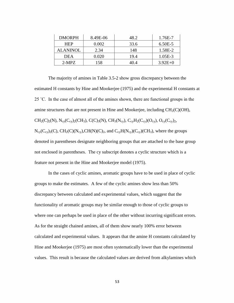
53
DMORPH 8.49E-06 48.2 1.76E-7
HEP 0.002 33.6 6.50E-5
ALANINOL 2.34 148 1.58E-2
DEA 0.020 19.4 1.05E-3
2-MPZ 158 40.4 3.92E+0
The majority of amines in Table 3.5-2 show gross discrepancy between the
estimated H constants by Hine and Mookerjee (1975) and the experimental H constants at
25 ˚C. In the case of almost all of the amines shown, there are functional groups in the
amine structures that are not present in Hine and Mookerjee, including CH2(C)(OH),
CH2(C)2(N), Ncy(Ccy)2(CH3), C(C)3(N), CH3(Ncy), CcyH2(Ccy)(Ocy), Ocy(Ccy)2,
Ncy(Ccy)2(C), CH2(C)(Ncy),CH(N)(C)2, and CcyH(Ncy)(Ccy)(CH3), where the groups
denoted in parentheses designate neighboring groups that are attached to the base group
not enclosed in parentheses. The cy subscript denotes a cyclic structure which is a
feature not present in the Hine and Mookerjee model (1975).
In the cases of cyclic amines, aromatic groups have to be used in place of cyclic
groups to make the estimates. A few of the cyclic amines show less than 50%
discrepancy between calculated and experimental values, which suggest that the
functionality of aromatic groups may be similar enough to those of cyclic groups to
where one can perhaps be used in place of the other without incurring significant errors.
As for the straight chained amines, all of them show nearly 100% error between
calculated and experimental values. It appears that the amine H constants calculated by
Hine and Mookerjee (1975) are most often systematically lower than the experimental
values. This result is because the calculated values are derived from alkylamines which
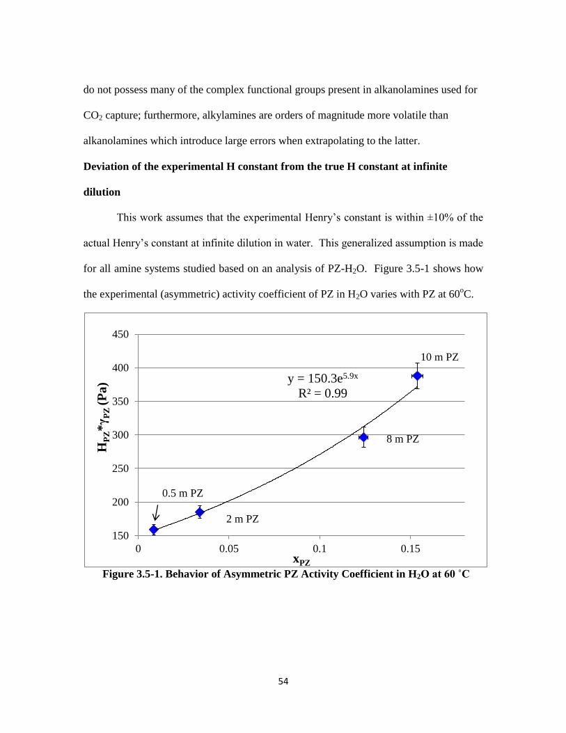
54
do not possess many of the complex functional groups present in alkanolamines used for
CO2 capture; furthermore, alkylamines are orders of magnitude more volatile than
alkanolamines which introduce large errors when extrapolating to the latter.
Deviation of the experimental H constant from the true H constant at infinite
dilution
This work assumes that the experimental Henry’s constant is within ±10% of the
actual Henry’s constant at infinite dilution in water. This generalized assumption is made
for all amine systems studied based on an analysis of PZ-H2O. Figure 3.5-1 shows how
the experimental (asymmetric) activity coefficient of PZ in H2O varies with PZ at 60oC.
Figure 3.5-1. Behavior of Asymmetric PZ Activity Coefficient in H2O at 60 ˚C
y = 150.3e5.9x
R² = 0.99
150
200
250
300
350
400
450
0 0.05 0.1 0.15
HP
Z*
γP
Z (
Pa
)
xPZ
0.5 m PZ
2 m PZ
8 m PZ
10 m PZ
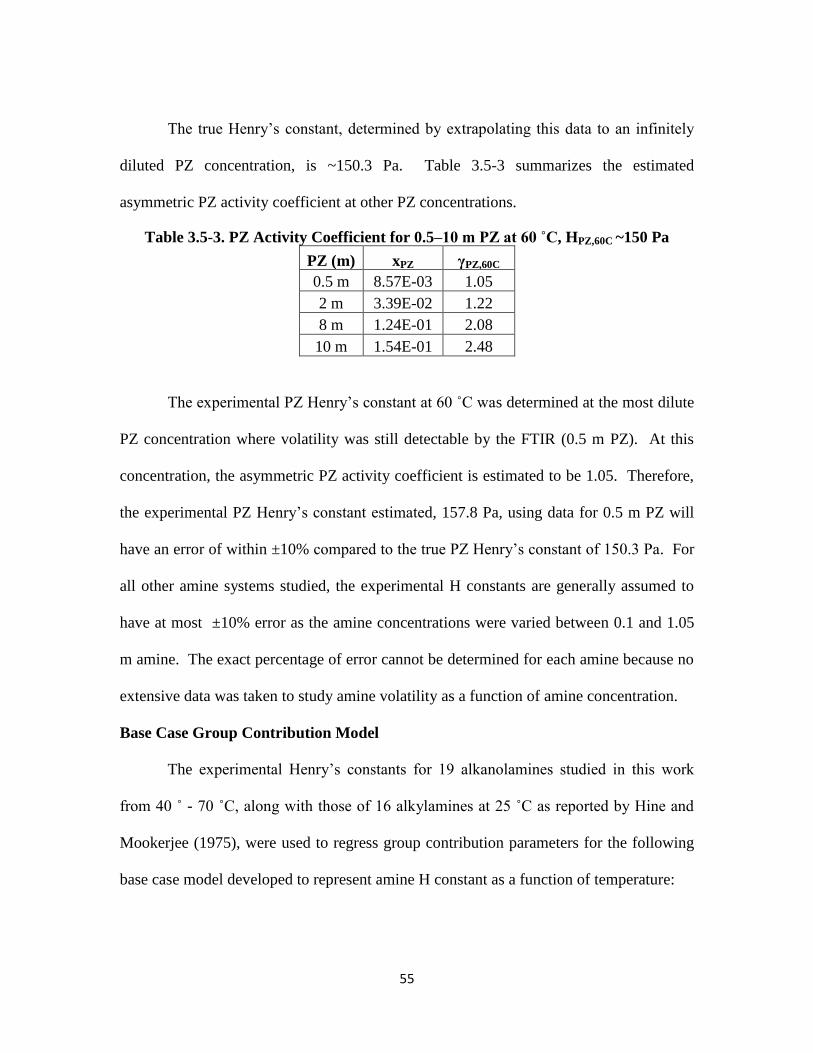
55
The true Henry’s constant, determined by extrapolating this data to an infinitely
diluted PZ concentration, is ~150.3 Pa. Table 3.5-3 summarizes the estimated
asymmetric PZ activity coefficient at other PZ concentrations.
Table 3.5-3. PZ Activity Coefficient for 0.5–10 m PZ at 60 ˚C, HPZ,60C ~150 Pa
PZ (m) xPZ γPZ,60C
0.5 m 8.57E-03 1.05
2 m 3.39E-02 1.22
8 m 1.24E-01 2.08
10 m 1.54E-01 2.48
The experimental PZ Henry’s constant at 60 ˚C was determined at the most dilute
PZ concentration where volatility was still detectable by the FTIR (0.5 m PZ). At this
concentration, the asymmetric PZ activity coefficient is estimated to be 1.05. Therefore,
the experimental PZ Henry’s constant estimated, 157.8 Pa, using data for 0.5 m PZ will
have an error of within ±10% compared to the true PZ Henry’s constant of 150.3 Pa. For
all other amine systems studied, the experimental H constants are generally assumed to
have at most ±10% error as the amine concentrations were varied between 0.1 and 1.05
m amine. The exact percentage of error cannot be determined for each amine because no
extensive data was taken to study amine volatility as a function of amine concentration.
Base Case Group Contribution Model
The experimental Henry’s constants for 19 alkanolamines studied in this work
from 40 ˚ - 70 ˚C, along with those of 16 alkylamines at 25 ˚C as reported by Hine and
Mookerjee (1975), were used to regress group contribution parameters for the following
base case model developed to represent amine H constant as a function of temperature:

56
( (
( ) ( ( ) ∑
(3-7)
where:
kj is the parameter value for functional group j
nj is the number of occurrences of group j in an amine structure
With this model form, all of the amines are assigned the same temperature
dependence, which is nonlinear in reciprocal temperature with two adjustable parameters.
Table 3.5-4 provides the regressed parameter values for Eq. (3-7).
Table 3.5-4. Regressed Parameter Values for Base Case Group Contribution Model
Parameter Value Standard Error
(±)
Ncy -3.90 0.38
N -2.87 0.36
OH -2.48 0.23
O -1.70 0.25
CH2, CH 0.216 0.08
Ccy 0.703 0.15
CH3-(C) 0.952 0.15
CH3-(N) 1.10 0.14
CH3-(Ncy) 1.60 0.19
B -139,458 17,863
C 1.36 0.17
Intercept (Pa) -417 54
12 parameters were used to represent both the functional group contributions and
temperature dependence of 35 amines from 40 ˚ - 70 ˚C (a total of 139 data points). This
model establishes two important distinctions: (1) cyclic (cy) versus non-cyclic structure –
this distinction is not found in the earlier group contribution model by Hine and
Mookerjee (1975) but is warranted in this work; (2) differentiation among different types
of methyl groups based on the neighboring groups attached to them – in this case, the
57
neighboring group attached to the methyl can either be a straight chained amine (N), a
cyclic amine (Ncy), or a straight chained carbon (C). Also, in contrast to other group
contribution models, this one does not distinguish between the different types of amine
group (primary, secondary, versus tertiary). Parameter N encompasses the total number
of nitrogens in a given straight chained amine. The parameter Ncy denotes the number of
nitrogens in a cyclic amine. The parameter O signifies the sum of ether groups in a given
amine regardless of whether that amine is cyclic or not. The goodness of fit statistic R2 is
~0.90 which indicates a robust fit of the experimental H. The parameter values are all
statistically significant as they are large compared to their corresponding standard errors.
In Table 3.5-4, the functional group parameters are ranked from top to bottom in
the order of most polar to most non-polar as given by their signed magnitudes. The
presence of polar groups tends to lower the tendency to volatilize into the vapor phase;
thus, polar groups are seen to have negative parameter values as they decrease the
magnitudes of the H constants. The opposite is true for the case of non-polar groups.
Figure 3.5-2 illustrates how the calculated H constants, obtained from the base
case model, compare to experimental values.
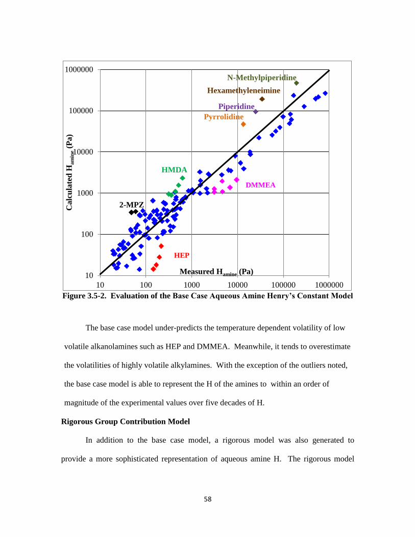
58
Figure 3.5-2. Evaluation of the Base Case Aqueous Amine Henry’s Constant Model
The base case model under-predicts the temperature dependent volatility of low
volatile alkanolamines such as HEP and DMMEA. Meanwhile, it tends to overestimate
the volatilities of highly volatile alkylamines. With the exception of the outliers noted,
the base case model is able to represent the H of the amines to within an order of
magnitude of the experimental values over five decades of H.
Rigorous Group Contribution Model
In addition to the base case model, a rigorous model was also generated to
provide a more sophisticated representation of aqueous amine H. The rigorous model
10
100
1000
10000
100000
1000000
10 100 1000 10000 100000 1000000
Calc
ula
ted
Ha
min
e (
Pa)
Measured Hamine (Pa)
HMDA
2-MPZ
Pyrrolidine
Piperidine
Hexamethyleneimine
N-Methylpiperidine
DMMEA
HEP
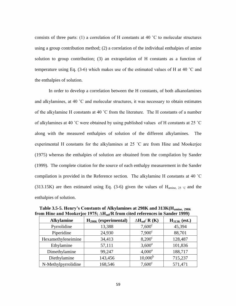
59
consists of three parts: (1) a correlation of H constants at 40 ˚C to molecular structures
using a group contribution method; (2) a correlation of the individual enthalpies of amine
solution to group contribution; (3) an extrapolation of H constants as a function of
temperature using Eq. (3-6) which makes use of the estimated values of H at 40 ˚C and
the enthalpies of solution.
In order to develop a correlation between the H constants, of both alkanolamines
and alkylamines, at 40 ˚C and molecular structures, it was necessary to obtain estimates
of the alkylamine H constants at 40 ˚C from the literature. The H constants of a number
of alkylamines at 40 ˚C were obtained by using published values of H constants at 25 ˚C
along with the measured enthalpies of solution of the different alkylamines. The
experimental H constants for the alkylamines at 25 ˚C are from Hine and Mookerjee
(1975) whereas the enthalpies of solution are obtained from the compilation by Sander
(1999). The complete citation for the source of each enthalpy measurement in the Sander
compilation is provided in the Reference section. The alkylamine H constants at 40 ˚C
(313.15K) are then estimated using Eq. (3-6) given the values of Hamine, 25 ˚C and the
enthalpies of solution.
Table 3.5-5. Henry’s Constants of Alkylamines at 298K and 313K(Hamine, 298K
from Hine and Mookerjee 1975; ∆Hsol/R from cited references in Sander 1999)
Alkylamine H298K (experimental) ∆Hsol/ R (K) H313K (est.)
Pyrrolidine 13,388 7,600c 45,394
Piperidine 24,930 7,900c 88,701
Hexamethyleneimine 34,413 8,200c 128,487
Ethylamine 57,111 3,600a 101,836
Dimethylamine 99,247 4,000a 188,717
Diethylamine 143,456 10,000b 715,237
N-Methylpyrrolidine 168,546 7,600c 571,471
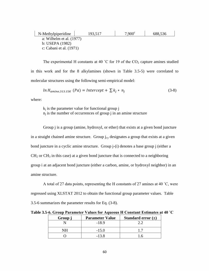
60
N-Methylpiperidine 193,517 7,900c 688,536
a: Wilhelm et al. (1977)
b: USEPA (1982)
c: Cabani et al. (1971)
The experimental H constants at 40 ˚C for 19 of the CO2 capture amines studied
in this work and for the 8 alkylamines (shown in Table 3.5-5) were correlated to
molecular structures using the following semi-empirical model:
( ∑ (3-8)
where:
kj is the parameter value for functional group j
nj is the number of occurrences of group j in an amine structure
Group j is a group (amine, hydroxyl, or ether) that exists at a given bond juncture
in a straight chained amine structure. Group jcy designates a group that exists at a given
bond juncture in a cyclic amine structure. Group j-(i) denotes a base group j (either a
CH2 or CH3 in this case) at a given bond juncture that is connected to a neighboring
group i at an adjacent bond juncture (either a carbon, amine, or hydroxyl neighbor) in an
amine structure.
A total of 27 data points, representing the H constants of 27 amines at 40 ˚C, were
regressed using XLSTAT 2012 to obtain the functional group parameter values. Table
3.5-6 summarizes the parameter results for Eq. (3-8).
Table 3.5-6. Group Parameter Values for Aqueous H Constant Estimates at 40 ˚C
Group j Parameter Value Standard error (±)
N -18.9 2.2
NH -15.0 1.7
O -13.8 1.6
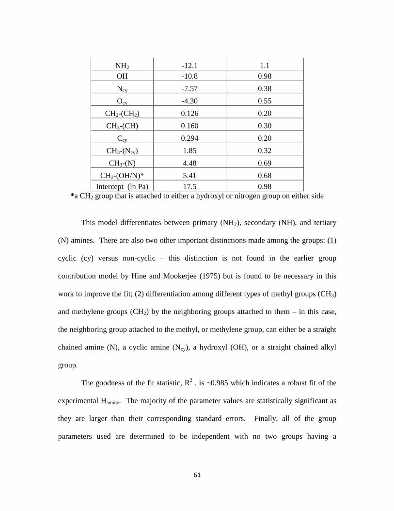
61
NH2 -12.1 1.1
OH -10.8 0.98
Ncy -7.57 0.38
Ocy -4.30 0.55
CH2-(CH2) 0.126 0.20
CH3-(CH) 0.160 0.30
Ccy 0.294 0.20
CH3-(Ncy) 1.85 0.32
CH3-(N) 4.48 0.69
CH2-(OH/N)* 5.41 0.68
Intercept (ln Pa) 17.5 0.98
*a CH2 group that is attached to either a hydroxyl or nitrogen group on either side
This model differentiates between primary (NH2), secondary (NH), and tertiary
(N) amines. There are also two other important distinctions made among the groups: (1)
cyclic (cy) versus non-cyclic – this distinction is not found in the earlier group
contribution model by Hine and Mookerjee (1975) but is found to be necessary in this
work to improve the fit; (2) differentiation among different types of methyl groups (CH3)
and methylene groups (CH2) by the neighboring groups attached to them – in this case,
the neighboring group attached to the methyl, or methylene group, can either be a straight
chained amine (N), a cyclic amine (Ncy), a hydroxyl (OH), or a straight chained alkyl
group.
The goodness of the fit statistic, R2 , is ~0.985 which indicates a robust fit of the
experimental Hamine. The majority of the parameter values are statistically significant as
they are larger than their corresponding standard errors. Finally, all of the group
parameters used are determined to be independent with no two groups having a
62
correlation greater than 0.9. The pair of parameters with the largest correlation though
still acceptable, ~0.865, is Ncy and Ccy. This is expected as both the nitrogen and carbon
are found to naturally exist on the same cyclic molecule side by side, thus it can be
rationalized that there is an overlap in their molecular functionalities that is difficult to
isolate to each individually. Other pairs of parameters showing high but acceptable
correlation are the CH2-(OH/N) with OH (~0.696), and CH3-(N) with N(~0.738). Again
the groups within each pair are adjacent neighbors thus resulting in a molecular overlap
that is difficult to isolate to each group individually. Not only is there a functional overlap
due to the group proximity to each other, there is also a mathematical overlap because the
hydrophilic groups (OH, N) are independent groups, thus to mathematically represent the
joint contribution of the polar group with an alkyl group can be confounding.
In Table 3.5-6, the functional group parameters are ranked from top to bottom in
the order of most polar to most non-polar as given by their signed magnitudes. Polar
groups, such as the amines and ether, are hydrophilic in nature. The presence of
hydrophilic groups tends to lower the tendency of an amine to volatilize into the vapor
phase; thus, hydrophilic groups are seen to have negative parameter values which
decrease the magnitudes of the H constants. Conversely, non-polar groups such as the
alkyl groups tend to increase the tendency of an amine to volatilize; therefore, they have
positive parameter values which increase the magnitudes of the H constants. Methyl or
methylene groups attached to hydrophilic groups (nitrogen or OH) appear especially
more hydrophobic than those that are attached to carbons. Although there is no definitive
scientific explanation for why this is the case, it can perhaps be hypothesized that
63
hydrophilic neighoring groups are more electronegative than carbon neighboring groups,
thus withdrawing electrons from the base methyl (or methylene) group to a greater extent
than the latter, which decreases the electronegativity difference between the atoms in the
base methyl (or methylene) group and thereby making the base group more nonpolar than
they would be otherwise.
The intercept used in the model is physically significant and has units of ln Pa.
Since the ln Hamine modeled has units of ln Pa, it follows that the intercept must also have
units and is needed to anchor the reference state of the system to infinite dilution in
water. Without the use of this intercept, the signs of the polar versus nonpolar groups
would be counterintuitive and consequently lose physical significance. If Hamine is
expressed as a unitless partition coefficient K using Eq. (3-4), then the model would be ln
K (unitless) = 1.24 + ∑kj*nj. The values of all the group parameters would be the same
as shown in Table 3.5-6. Given that K is the concentration of the amine in water divided
by its concentration in the gas, the polar groups would have positive values as they
increase the amine concentration in water due to favorable aqueous interactions, and vice
versa.
Figure 3.5-3 shows how the amine H constants calculated from the rigorous
model compare to experimental values at 40 ˚C.
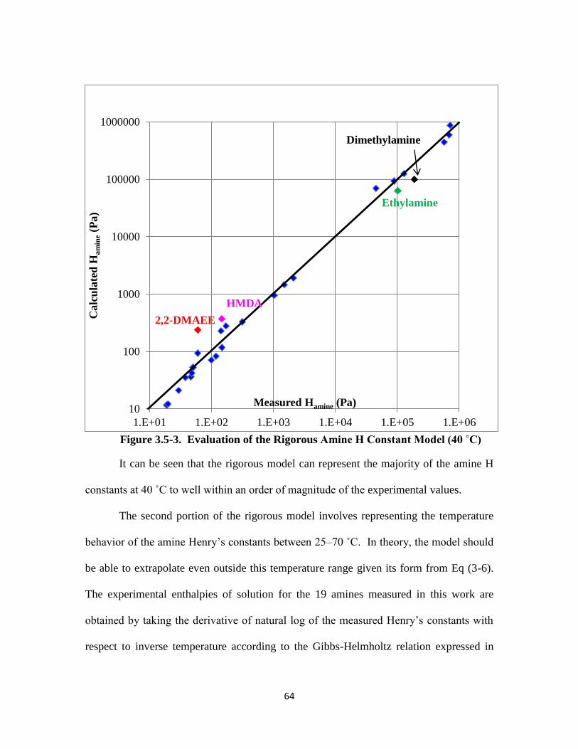
64
Figure 3.5-3. Evaluation of the Rigorous Amine H Constant Model (40 ˚C)
It can be seen that the rigorous model can represent the majority of the amine H
constants at 40 ˚C to well within an order of magnitude of the experimental values.
The second portion of the rigorous model involves representing the temperature
behavior of the amine Henry’s constants between 25–70 ˚C. In theory, the model should
be able to extrapolate even outside this temperature range given its form from Eq (3-6).
The experimental enthalpies of solution for the 19 amines measured in this work are
obtained by taking the derivative of natural log of the measured Henry’s constants with
respect to inverse temperature according to the Gibbs-Helmholtz relation expressed in
10
100
1000
10000
100000
1000000
1.E+01 1.E+02 1.E+03 1.E+04 1.E+05 1.E+06
Calc
ula
ted
Ha
min
e (
Pa)
Measured Hamine (Pa)
2,2-DMAEE
HMDA
Ethylamine
Dimethylamine
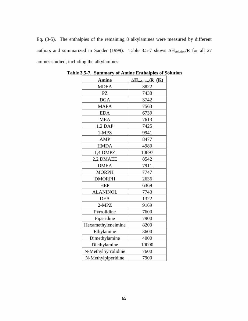
65
Eq. (3-5). The enthalpies of the remaining 8 alkylamines were measured by different
authors and summarized in Sander (1999). Table 3.5-7 shows ∆Hsolution/R for all 27
amines studied, including the alkylamines.
Table 3.5-7. Summary of Amine Enthalpies of Solution
Amine ∆Hsolution/R (K)
MDEA 3822
PZ 7438
DGA 3742
MAPA 7563
EDA 6730
MEA 7613
1,2 DAP 7425
1-MPZ 9941
AMP 8477
HMDA 4980
1,4 DMPZ 10697
2,2 DMAEE 8542
DMEA 7911
MORPH 7747
DMORPH 2636
HEP 6369
ALANINOL 7743
DEA 1322
2-MPZ 9169
Pyrrolidine 7600
Piperidine 7900
Hexamethyleneimine 8200
Ethylamine 3600
Dimethylamine 4000
Diethylamine 10000
N-Methylpyrrolidine 7600
N-Methylpiperidine 7900
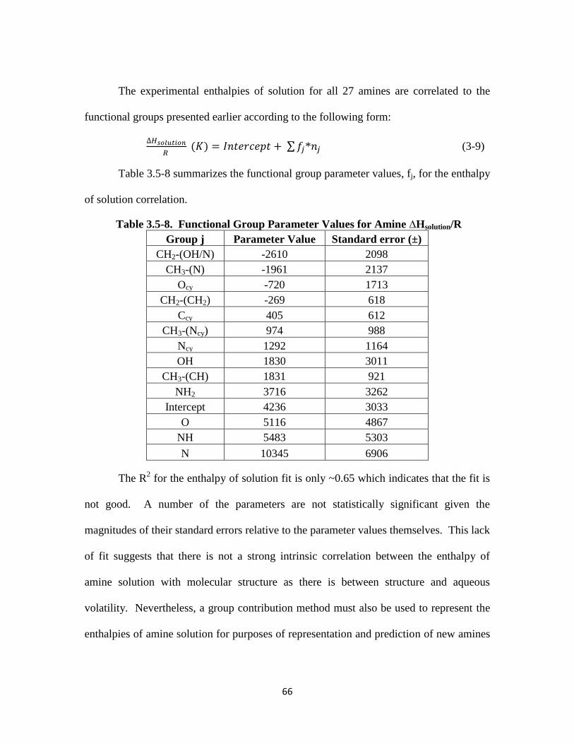
66
The experimental enthalpies of solution for all 27 amines are correlated to the
functional groups presented earlier according to the following form:
( ∑ * (3-9)
Table 3.5-8 summarizes the functional group parameter values, fj, for the enthalpy
of solution correlation.
Table 3.5-8. Functional Group Parameter Values for Amine ∆Hsolution/R
Group j Parameter Value Standard error (±)
CH2-(OH/N) -2610 2098
CH3-(N) -1961 2137
Ocy -720 1713
CH2-(CH2) -269 618
Ccy 405 612
CH3-(Ncy) 974 988
Ncy 1292 1164
OH 1830 3011
CH3-(CH) 1831 921
NH2 3716 3262
Intercept 4236 3033
O 5116 4867
NH 5483 5303
N 10345 6906
The R2 for the enthalpy of solution fit is only ~0.65 which indicates that the fit is
not good. A number of the parameters are not statistically significant given the
magnitudes of their standard errors relative to the parameter values themselves. This lack
of fit suggests that there is not a strong intrinsic correlation between the enthalpy of
amine solution with molecular structure as there is between structure and aqueous
volatility. Nevertheless, a group contribution method must also be used to represent the
enthalpies of amine solution for purposes of representation and prediction of new amines
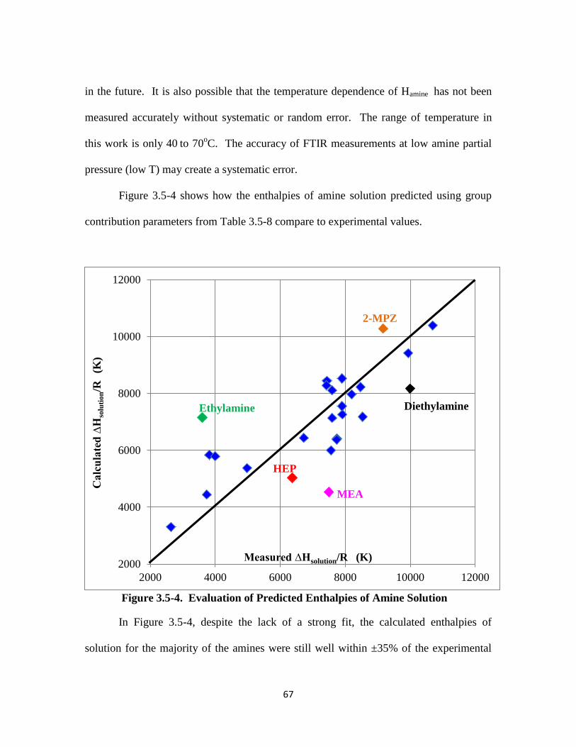
67
in the future. It is also possible that the temperature dependence of Hamine has not been
measured accurately without systematic or random error. The range of temperature in
this work is only 40 to 70
oC. The accuracy of FTIR measurements at low amine partial
pressure (low T) may create a systematic error.
Figure 3.5-4 shows how the enthalpies of amine solution predicted using group
contribution parameters from Table 3.5-8 compare to experimental values.
Figure 3.5-4. Evaluation of Predicted Enthalpies of Amine Solution
In Figure 3.5-4, despite the lack of a strong fit, the calculated enthalpies of
solution for the majority of the amines were still well within ±35% of the experimental
2000
4000
6000
8000
10000
12000
2000 4000 6000 8000 10000 12000
Calc
ula
ted
∆H
solu
tio
n/R
(
K)
Measured ∆Hsolution/R (K)
Ethylamine
HEP
2-MPZ
Diethylamine
MEA
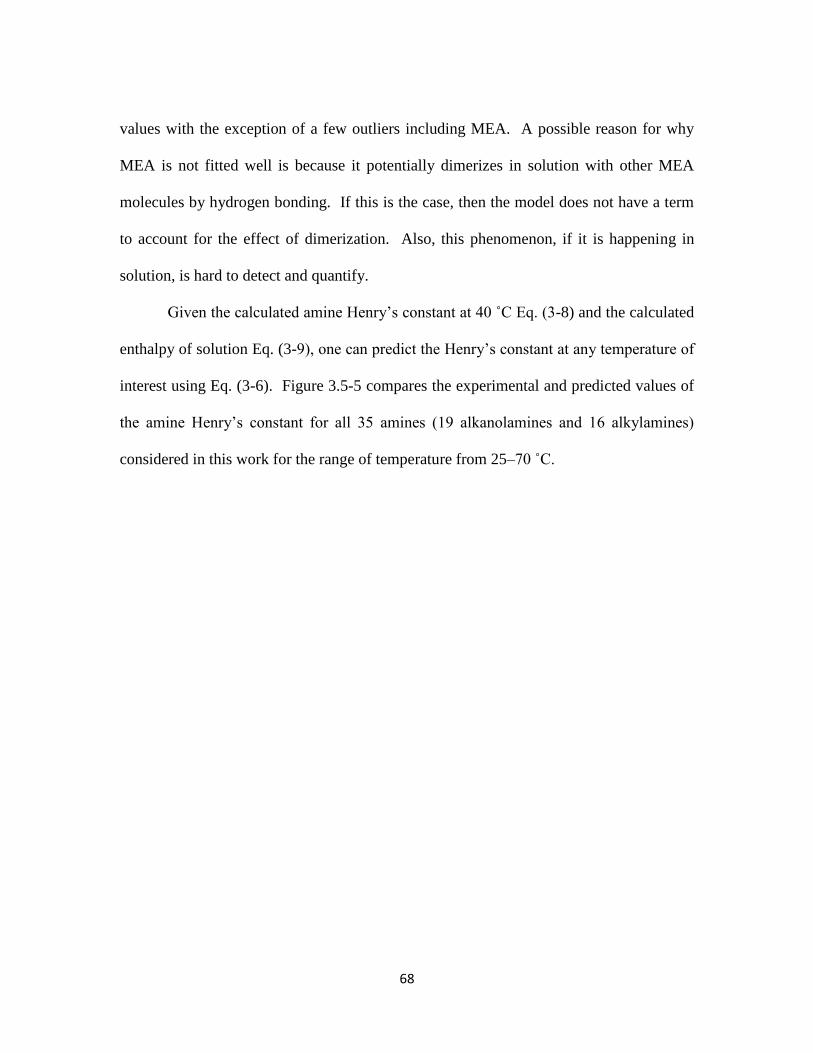
68
values with the exception of a few outliers including MEA. A possible reason for why
MEA is not fitted well is because it potentially dimerizes in solution with other MEA
molecules by hydrogen bonding. If this is the case, then the model does not have a term
to account for the effect of dimerization. Also, this phenomenon, if it is happening in
solution, is hard to detect and quantify.
Given the calculated amine Henry’s constant at 40 ˚C Eq. (3-8) and the calculated
enthalpy of solution Eq. (3-9), one can predict the Henry’s constant at any temperature of
interest using Eq. (3-6). Figure 3.5-5 compares the experimental and predicted values of
the amine Henry’s constant for all 35 amines (19 alkanolamines and 16 alkylamines)
considered in this work for the range of temperature from 25–70 ˚C.
69
Figure 3.5-5. Evaluation of Predicted Amine Henry’s Constants from 25 ˚–70 ˚C
It can be seen from Figure 3.5-5 that this rigorous model does a fair job of
representing most of the 35 amines from 25 ˚ - 70 ˚C to within an order of magnitude
with the exception of a few outliers as shown. Furthemore, the rigorous model appears to
be more accurate than the base case model in its representation of amine H constants due
to the appearance of a tighter data fit. In the region of low amine H constants, HEP
stands out as an entire temperature series (40 ˚ - 70 ˚C) that is not fitted as well as the
others. The inability to fit HEP mainly stems from the experimental scatter in the raw
volatility data. This results in a poor linear fit of HEP enthalpy of solution to the
1.E+01
1.E+02
1.E+03
1.E+04
1.E+05
1.E+06
1.E+01 1.E+02 1.E+03 1.E+04 1.E+05 1.E+06
Calc
ula
ted
Ha
min
e (
Pa)
Measured Hamine (Pa)
HEP
1,2 DAP, EDA
Ethyl, Propyl,
Butylamines
Trimethylamine
MAPA
70
Arrhenius temperature behavior (R2 ~ 0.87 only as compared to that of other amines). In
the case of the other outliers, such as 1,2-Diaminopropane, EDA, and MAPA, the
problem lies with not being able to fit compounds having two amino groups as well as
fitting monoamines. Also the confidence for alkyl group parameters attached to carbons
is not statistically significant which also contributed to a marginal fit. Nonetheless,
unlike with HEP, these diamines do show good fits of the temperature dependence due to
the fact that their experimental volatility data are much more linear with temperature than
HEP. In the case of the alkylamines, the model underestimated the H constants of the
alkylamine family, consisting of ethylamine through hexylamine, at 25 ˚C. It was
challenging to estimate both the H constant at 40 ˚C and the enthalpies of solution for
these alkylamines since only experimental data for ethylamine is available. To better
anchor the structural contribution of the alkyl groups in this alkylamine family, there
needs to be data for at least one more compound in this family such as propylamine in
addition to ethylamine.
Predictive Capability of the Rigorous Model
The rigorous model was used to predict the H constant of 1,2-Aminoethyl
Piperazine (AEP) from 40 ˚ - 65 ˚C. Note that this amine was not included in the model
regression earlier. Table 3.5-9 shows how the rigorous model predictions compare to the
experimental measurements.
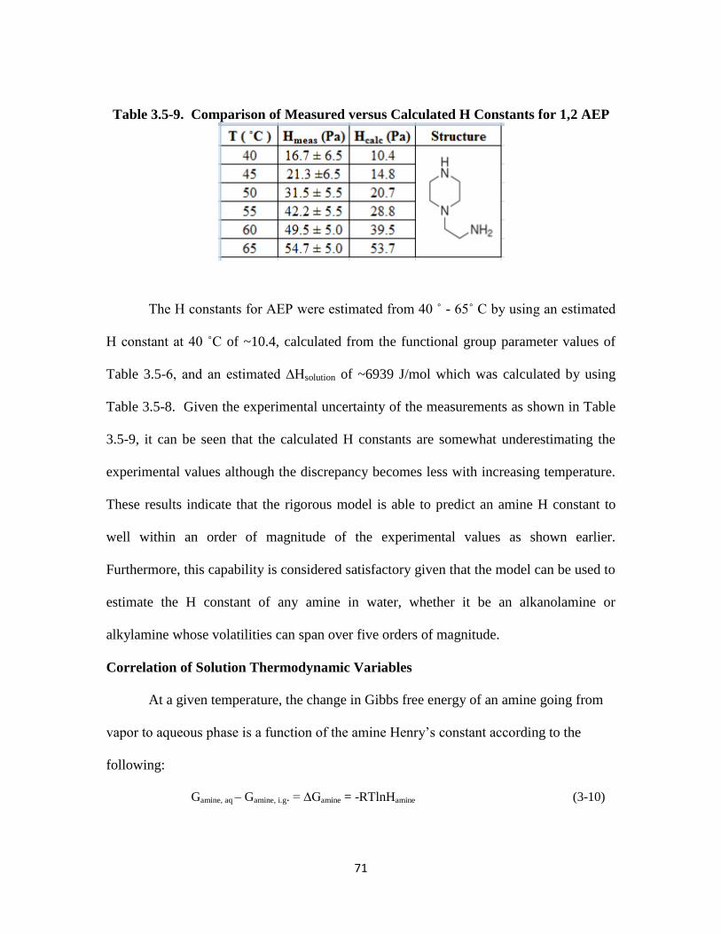
71
Table 3.5-9. Comparison of Measured versus Calculated H Constants for 1,2 AEP
The H constants for AEP were estimated from 40 ˚ - 65˚ C by using an estimated
H constant at 40 ˚C of ~10.4, calculated from the functional group parameter values of
Table 3.5-6, and an estimated ∆Hsolution of ~6939 J/mol which was calculated by using
Table 3.5-8. Given the experimental uncertainty of the measurements as shown in Table
3.5-9, it can be seen that the calculated H constants are somewhat underestimating the
experimental values although the discrepancy becomes less with increasing temperature.
These results indicate that the rigorous model is able to predict an amine H constant to
well within an order of magnitude of the experimental values as shown earlier.
Furthermore, this capability is considered satisfactory given that the model can be used to
estimate the H constant of any amine in water, whether it be an alkanolamine or
alkylamine whose volatilities can span over five orders of magnitude.
Correlation of Solution Thermodynamic Variables
At a given temperature, the change in Gibbs free energy of an amine going from
vapor to aqueous phase is a function of the amine Henry’s constant according to the
following:
Gamine, aq – Gamine, i.g. = ∆Gamine = -RTlnHamine (3-10)
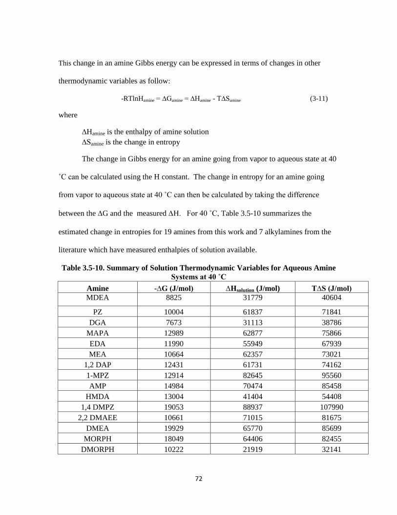
72
This change in an amine Gibbs energy can be expressed in terms of changes in other
thermodynamic variables as follow:
-RTlnHamine = ∆Gamine = ∆Hamine - T∆Samine (3-11)
where
∆Hamine is the enthalpy of amine solution
∆Samine is the change in entropy
The change in Gibbs energy for an amine going from vapor to aqueous state at 40
˚C can be calculated using the H constant. The change in entropy for an amine going
from vapor to aqueous state at 40 ˚C can then be calculated by taking the difference
between the G and the measured H. For 40 ˚C, Table 3.5-10 summarizes the
estimated change in entropies for 19 amines from this work and 7 alkylamines from the
literature which have measured enthalpies of solution available.
Table 3.5-10. Summary of Solution Thermodynamic Variables for Aqueous Amine
Systems at 40 ˚C
Amine -∆G (J/mol) ∆Hsolution (J/mol) T∆S (J/mol)
MDEA 8825 31779 40604
PZ 10004 61837 71841
DGA 7673 31113 38786
MAPA 12989 62877 75866
EDA 11990 55949 67939
MEA 10664 62357 73021
1,2 DAP 12431 61731 74162
1-MPZ 12914 82645 95560
AMP 14984 70474 85458
HMDA 13004 41404 54408
1,4 DMPZ 19053 88937 107990
2,2 DMAEE 10661 71015 81675
DMEA 19929 65770 85699
MORPH 18049 64406 82455
DMORPH 10222 21919 32141
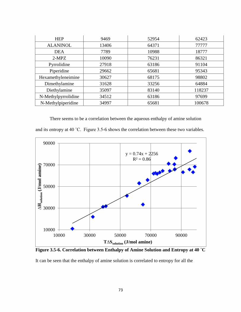
73
HEP 9469 52954 62423
ALANINOL 13406 64371 77777
DEA 7789 10988 18777
2-MPZ 10090 76231 86321
Pyrrolidine 27918 63186 91104
Piperidine 29662 65681 95343
Hexamethyleneimine 30627 68175 98802
Dimethylamine 31628 33256 64884
Diethylamine 35097 83140 118237
N-Methylpyrrolidine 34512 63186 97699
N-Methylpiperidine 34997 65681 100678
There seems to be a correlation between the aqueous enthalpy of amine solution
and its entropy at 40 ˚C. Figure 3.5-6 shows the correlation between these two variables.
Figure 3.5-6. Correlation between Enthalpy of Amine Solution and Entropy at 40 ˚C
It can be seen that the enthalpy of amine solution is correlated to entropy for all the
y = 0.74x + 2256
R² = 0.86
10000
30000
50000
70000
90000
10000 30000 50000 70000 90000
∆H
solu
tio
n (
J/m
ol
am
ine)
T∆Ssolution (J/mol amine)

74
amines studied at 40 ˚C. Given the expression of the linear trend fit, it can be seen that
the quantity of T∆S (x-variable) and ∆Hsolution (y-variable) are almost 1:1.
3.6. Conclusions
The experimental H constants of alkanolamines measured in this work are
compared to predictions from different group contribution theories in the literature. For
the majority of the amine systems studied, both the experimental H constants from this
work and those predicted by UNIFAC-DMD theory agree to within an order of
magnitude with the exception of PZ and DGA. In comparing the experimental amine H
constants to calculated values using the group contribution established by Hine and
Mookerjee (1975), it was seen that the calculated values are systematically one to many
orders of magnitude less than the experimental data.
Both the base case and rigorous models are able to estimate the H constants, for
the majority of amines, to well within an order of magnitude of the experimental values,
which span over five orders of magnitude in the temperature range from 25 ˚ - 70 ˚C.
The rigorous model is seen to provide a tighter fit of all the experimental data than the
base case model. The rigorous model was also demonstrated to have predictive
capability for estimating the H constant of an amine of interest (1,2-AEP) to within the
margin of experimental errors. In conclusion, the models developed in this work are
more reliable than UNIFAC-DMD and the Hine and Mookerjee group contribution
method for estimating H constants of alkanolamines, especially those of cyclic amines
such as PZ, which are used for CO2 capture.

75
Given the dilute working amine concentrations of this work, the measured amine
Henry’s constants are found to be ±10% from the true Henry’s constants at infinite
dilution of amine in water. From the base case model, it can be seen that the hydrophilic
strengths of the different polar groups are as followed: O < OH < N < Ncy. The rigorous
model has a similar ranking order of hydrophilic groups with further differentiation
between cyclic versus non-cyclic ether and between the different types of amine groups.
In order of increasing hydrophobicity, C < Ccy < CH3-( C ) < CH3-(N) < CH3-(Ncy). The
rigorous model also has similar ranking of hydrophobic groups with further
differentiation between methyl versus methylene groups based on whether they are
attached to a neighboring carbon or a polar group.
The enthalpies of solution of the different aqueous amine systems studied appear
to be adequately represented with Arrhenius temperature behavior which assumes a
constant enthalpy of solution over a range of temperature. Nonetheless, the base case
model shows an improved fit of the data with the use of an additional temperature term
which implies that the enthalpy of solution is a function of temperature to some extent.
Finally, it is seen that there is a correlation between the enthalpy of solution and the
entropy at 40 ˚C where ∆Hsolution = 0.74T∆Ssolution + 2256 (J/mol).
76
Chapter 4: MDEA-PZ-CO2-H2O Thermodynamic Model Upgrade
4.1. Introduction
The MDEA-PZ-CO2-H2O system was modeled in AspenPlus® v.7.3. by Peter
Frailie, a Rochelle group member, in 2010. The system was modeled using the liquid
activity method. The vapor phase of the system was represented using the Soave-
Redlich-Kwong (SRK) equation of state, whereas the liquid phase was modeled using
Electrolyte NRTL (eNRTL) theory. This MDEA-PZ model, named the Guy Fawkes
model, was built upon an earlier PZ-CO2-H2O model developed by Hilliard (2008) with
modifications to fit high concentration PZ systems made by Van Wagener (2010). The
2010 Fawkes model, while it provided a reasonably accurate representation of loaded PZ
systems, did not adequately capture MDEA thermodynamics. There were two primary
issues with the model: (1) inability to fit the MDEA and PZ volatilities for the blend
neither at unloaded or at loaded condition; (2) inability to match the experimental
speciation data for the blend.
Thus this work focused on resolving these two issues primarily by remodeling the
MDEA thermodynamics portion of the blend which includes the sub-systems: MDEA-
H2O and MDEA-CO2-H2O. Note that the sub-systems were modeled using a sequential
regression technique which involved first regressing data for the simplest systems
building on to the regression of the most complex system. In keeping with this regression
concept, the first system whose data was regressed was MDEA-H2O, followed by
MDEA-CO2-H2O, MDEA-PZ-H2O, and ultimately MDEA-PZ-CO2-H2O. The end goal
of this modeling effort is to be able to properly represent all the key thermodynamic
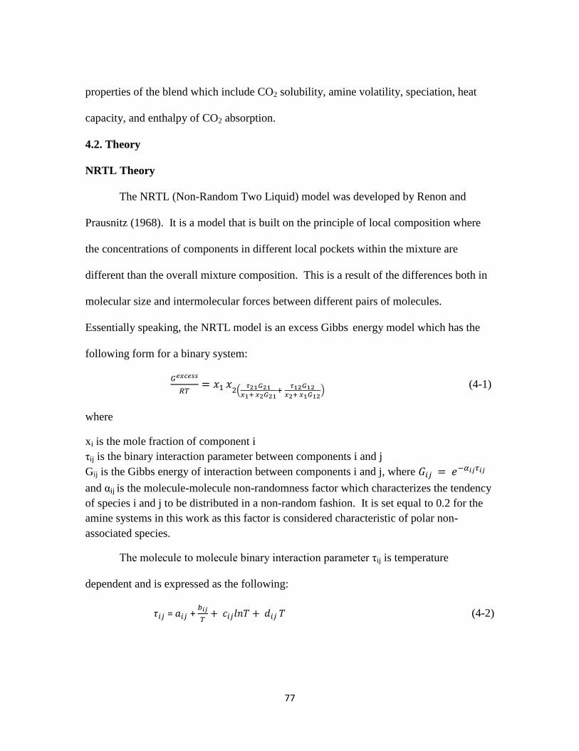
77
properties of the blend which include CO2 solubility, amine volatility, speciation, heat
capacity, and enthalpy of CO2 absorption.
4.2. Theory
NRTL Theory
The NRTL (Non-Random Two Liquid) model was developed by Renon and
Prausnitz (1968). It is a model that is built on the principle of local composition where
the concentrations of components in different local pockets within the mixture are
different than the overall mixture composition. This is a result of the differences both in
molecular size and intermolecular forces between different pairs of molecules.
Essentially speaking, the NRTL model is an excess Gibbs energy model which has the
following form for a binary system:
(
) (4-1)
where
xi is the mole fraction of component i
τij is the binary interaction parameter between components i and j
Gij is the Gibbs energy of interaction between components i and j, where
and αij is the molecule-molecule non-randomness factor which characterizes the tendency
of species i and j to be distributed in a non-random fashion. It is set equal to 0.2 for the
amine systems in this work as this factor is considered characteristic of polar non-
associated species.
The molecule to molecule binary interaction parameter τij is temperature
dependent and is expressed as the following:
= +
(4-2)
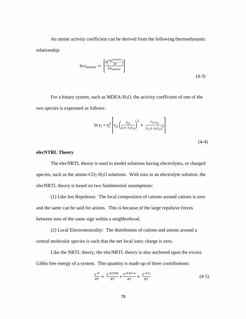
78
An amine activity coefficient can be derived from the following thermodynamic
relationship:
[ (
)
]
(4-3)
For a binary system, such as MDEA-H2O, the activity coefficient of one of the
two species is expressed as follows:
= [ (
)
( ) ]
(4-4)
elecNTRL Theory
The elecNRTL theory is used to model solutions having electrolytes, or charged
species, such as the amine-CO2-H2O solutions. With ions in an electrolyte solution, the
elecNRTL theory is based on two fundamental assumptions:
(1) Like Ion Repulsion: The local composition of cations around cations is zero
and the same can be said for anions. This is because of the large repulsive forces
between ions of the same sign within a neighborhood.
(2) Local Electroneutrality: The distribution of cations and anions around a
central molecular species is such that the net local ionic charge is zero.
Like the NRTL theory, the elecNRTL theory is also anchored upon the excess
Gibbs free energy of a system. This quantity is made up of three contributions:
+
(4-5)
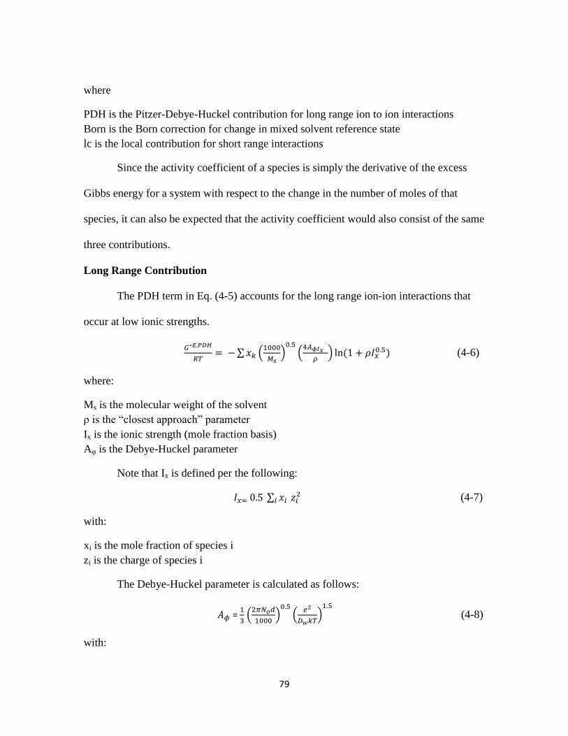
79
where
PDH is the Pitzer-Debye-Huckel contribution for long range ion to ion interactions
Born is the Born correction for change in mixed solvent reference state
lc is the local contribution for short range interactions
Since the activity coefficient of a species is simply the derivative of the excess
Gibbs energy for a system with respect to the change in the number of moles of that
species, it can also be expected that the activity coefficient would also consist of the same
three contributions.
Long Range Contribution
The PDH term in Eq. (4-5) accounts for the long range ion-ion interactions that
occur at low ionic strengths.
∑ (
)
(
) (
(4-6)
where:
Ms is the molecular weight of the solvent
ρ is the “closest approach” parameter
Ix is the ionic strength (mole fraction basis)
Aφ is the Debye-Huckel parameter
Note that Ix is defined per the following:
∑ (4-7)
with:
xi is the mole fraction of species i
zi is the charge of species i
The Debye-Huckel parameter is calculated as follows:
=
(
)
(
)
(4-8)
with:
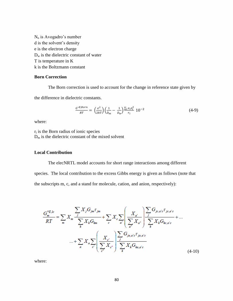
80
No is Avogadro’s number
d is the solvent’s density
e is the electron charge
Dw is the dielectric constant of water
T is temperature in K
k is the Boltzmann constant
Born Correction
The Born correction is used to account for the change in reference state given by
the difference in dielectric constants.
(
) (
)
∑
(4-9)
where:
ri is the Born radius of ionic species
Dm is the dielectric constant of the mixed solvent
Local Contribution
The elecNRTL model accounts for short range interactions among different
species. The local contribution to the excess Gibbs energy is given as follows (note that
the subscripts m, c, and a stand for molecule, cation, and anion, respectively):
(4-10)
where:
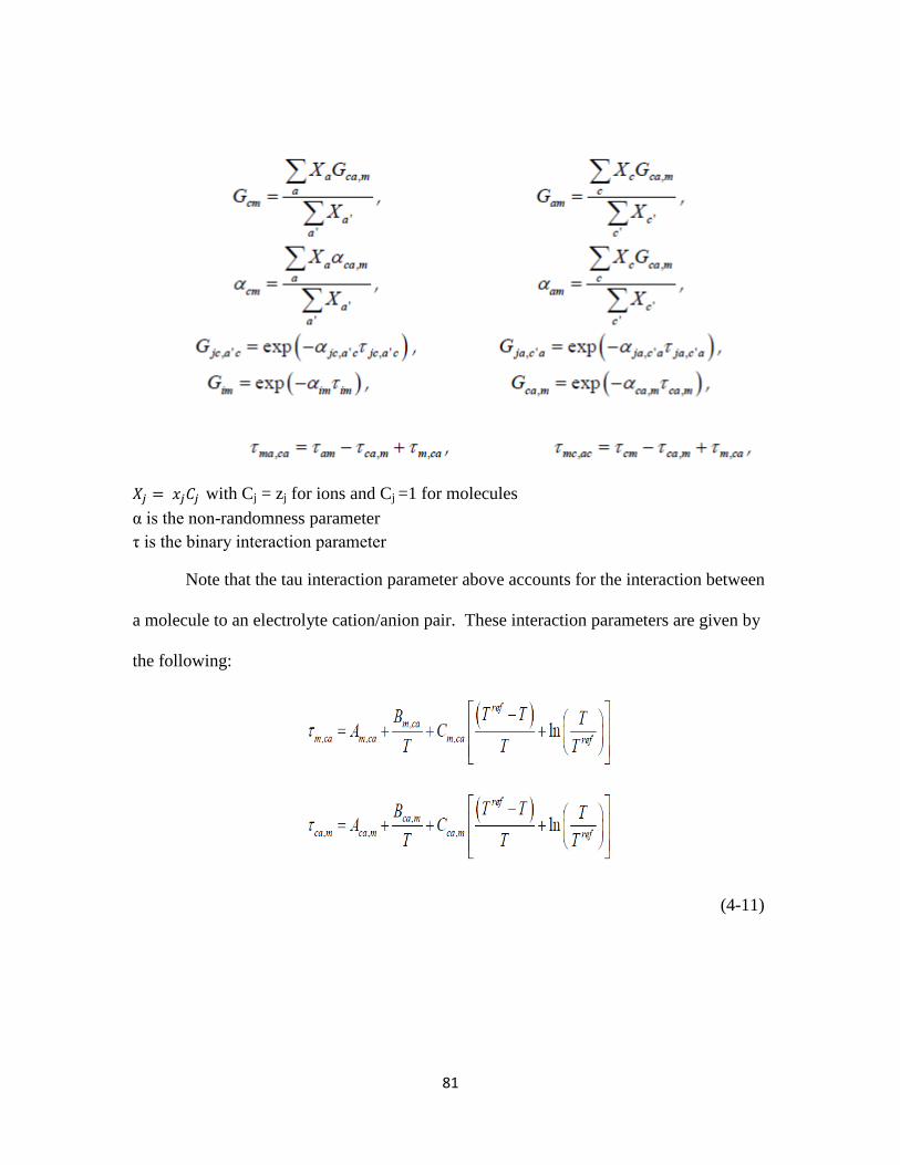
81
with Cj = zj for ions and Cj =1 for molecules
α is the non-randomness parameter
τ is the binary interaction parameter
Note that the tau interaction parameter above accounts for the interaction between
a molecule to an electrolyte cation/anion pair. These interaction parameters are given by
the following:
(4-11)
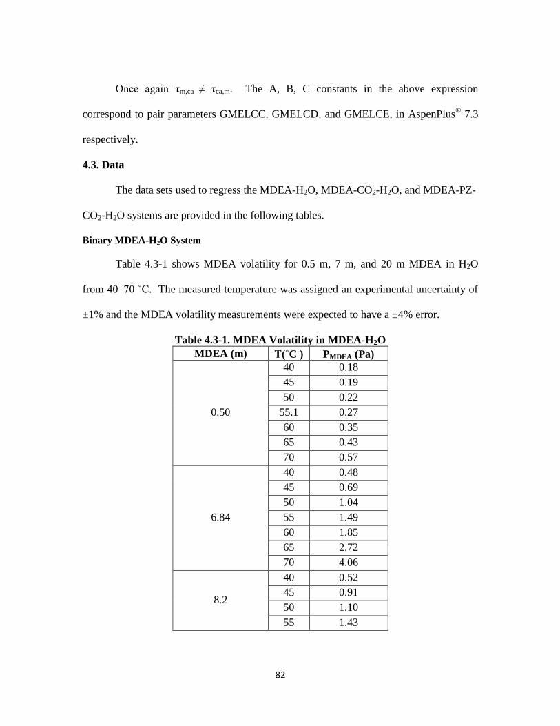
82
Once again τm,ca ≠ τca,m. The A, B, C constants in the above expression
correspond to pair parameters GMELCC, GMELCD, and GMELCE, in AspenPlus® 7.3
respectively.
4.3. Data
The data sets used to regress the MDEA-H2O, MDEA-CO2-H2O, and MDEA-PZ-
CO2-H2O systems are provided in the following tables.
Binary MDEA-H2O System
Table 4.3-1 shows MDEA volatility for 0.5 m, 7 m, and 20 m MDEA in H2O
from 40–70 ˚C. The measured temperature was assigned an experimental uncertainty of
±1% and the MDEA volatility measurements were expected to have a ±4% error.
Table 4.3-1. MDEA Volatility in MDEA-H2O
MDEA (m) T(˚C ) PMDEA (Pa)
0.50
40 0.18
45 0.19
50 0.22
55.1 0.27
60 0.35
65 0.43
70 0.57
6.84
40 0.48
45 0.69
50 1.04
55 1.49
60 1.85
65 2.72
70 4.06
8.2
40 0.52
45 0.91
50 1.10
55 1.43
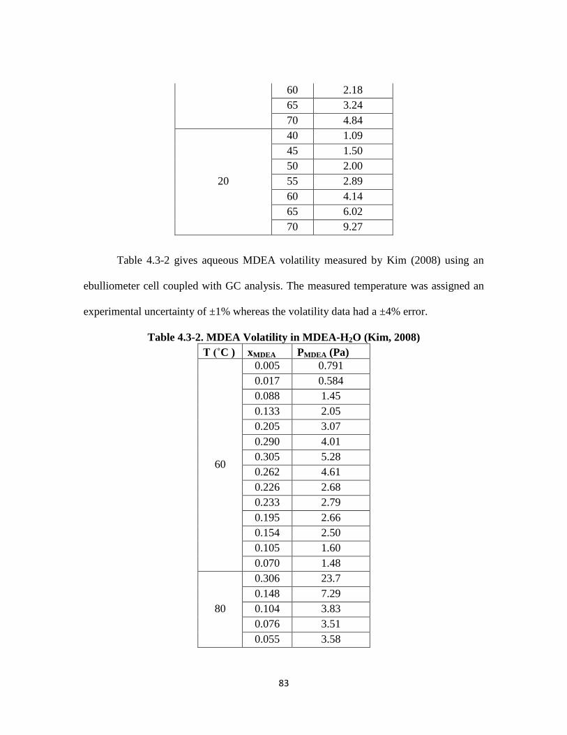
83
60 2.18
65 3.24
70 4.84
20
40 1.09
45 1.50
50 2.00
55 2.89
60 4.14
65 6.02
70 9.27
Table 4.3-2 gives aqueous MDEA volatility measured by Kim (2008) using an
ebulliometer cell coupled with GC analysis. The measured temperature was assigned an
experimental uncertainty of ±1% whereas the volatility data had a ±4% error.
Table 4.3-2. MDEA Volatility in MDEA-H2O (Kim, 2008)
T (˚C ) xMDEA PMDEA (Pa)
60
0.005 0.791
0.017 0.584
0.088 1.45
0.133 2.05
0.205 3.07
0.290 4.01
0.305 5.28
0.262 4.61
0.226 2.68
0.233 2.79
0.195 2.66
0.154 2.50
0.105 1.60
0.070 1.48
80
0.306 23.7
0.148 7.29
0.104 3.83
0.076 3.51
0.055 3.58
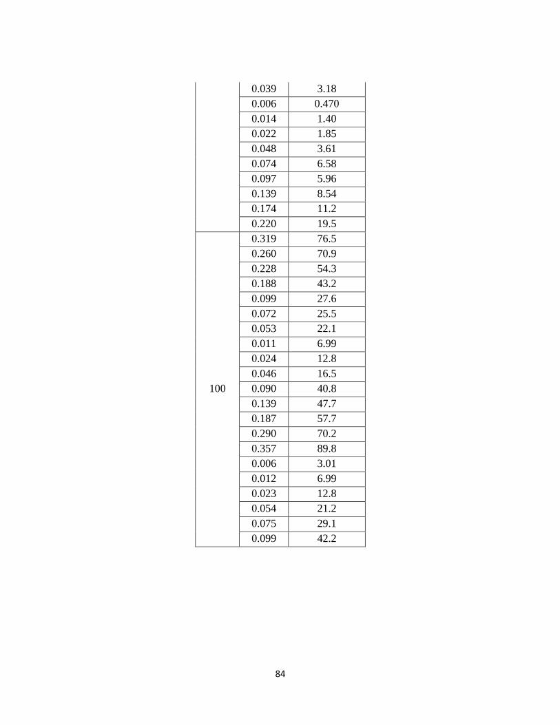
84
0.039 3.18
0.006 0.470
0.014 1.40
0.022 1.85
0.048 3.61
0.074 6.58
0.097 5.96
0.139 8.54
0.174 11.2
0.220 19.5
100
0.319 76.5
0.260 70.9
0.228 54.3
0.188 43.2
0.099 27.6
0.072 25.5
0.053 22.1
0.011 6.99
0.024 12.8
0.046 16.5
0.090 40.8
0.139 47.7
0.187 57.7
0.290 70.2
0.357 89.8
0.006 3.01
0.012 6.99
0.023 12.8
0.054 21.2
0.075 29.1
0.099 42.2
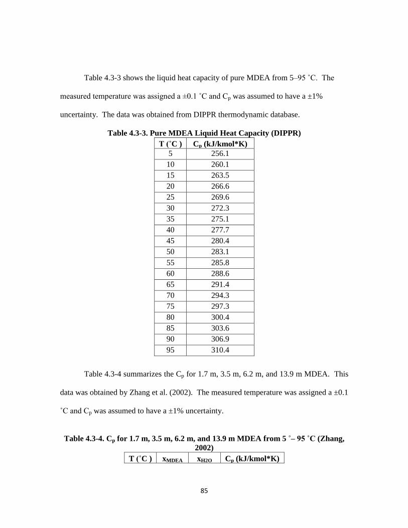
85
Table 4.3-3 shows the liquid heat capacity of pure MDEA from 5–95 ˚C. The
measured temperature was assigned a ±0.1 ˚C and Cp was assumed to have a ±1%
uncertainty. The data was obtained from DIPPR thermodynamic database.
Table 4.3-3. Pure MDEA Liquid Heat Capacity (DIPPR)
T (˚C ) Cp (kJ/kmol*K)
5 256.1
10 260.1
15 263.5
20 266.6
25 269.6
30 272.3
35 275.1
40 277.7
45 280.4
50 283.1
55 285.8
60 288.6
65 291.4
70 294.3
75 297.3
80 300.4
85 303.6
90 306.9
95 310.4
Table 4.3-4 summarizes the Cp for 1.7 m, 3.5 m, 6.2 m, and 13.9 m MDEA. This
data was obtained by Zhang et al. (2002). The measured temperature was assigned a ±0.1
˚C and Cp was assumed to have a ±1% uncertainty.
Table 4.3-4. Cp for 1.7 m, 3.5 m, 6.2 m, and 13.9 m MDEA from 5 ˚– 95 ˚C (Zhang,
2002)
T (˚C ) xMDEA xH2O Cp (kJ/kmol*K)
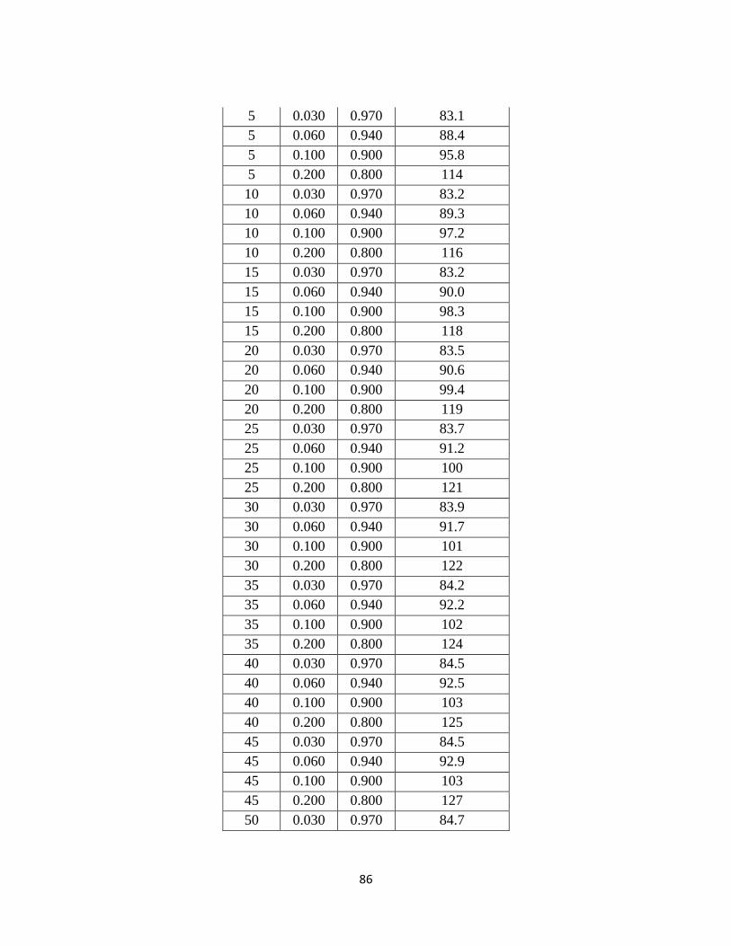
86
5 0.030 0.970 83.1
5 0.060 0.940 88.4
5 0.100 0.900 95.8
5 0.200 0.800 114
10 0.030 0.970 83.2
10 0.060 0.940 89.3
10 0.100 0.900 97.2
10 0.200 0.800 116
15 0.030 0.970 83.2
15 0.060 0.940 90.0
15 0.100 0.900 98.3
15 0.200 0.800 118
20 0.030 0.970 83.5
20 0.060 0.940 90.6
20 0.100 0.900 99.4
20 0.200 0.800 119
25 0.030 0.970 83.7
25 0.060 0.940 91.2
25 0.100 0.900 100
25 0.200 0.800 121
30 0.030 0.970 83.9
30 0.060 0.940 91.7
30 0.100 0.900 101
30 0.200 0.800 122
35 0.030 0.970 84.2
35 0.060 0.940 92.2
35 0.100 0.900 102
35 0.200 0.800 124
40 0.030 0.970 84.5
40 0.060 0.940 92.5
40 0.100 0.900 103
40 0.200 0.800 125
45 0.030 0.970 84.5
45 0.060 0.940 92.9
45 0.100 0.900 103
45 0.200 0.800 127
50 0.030 0.970 84.7
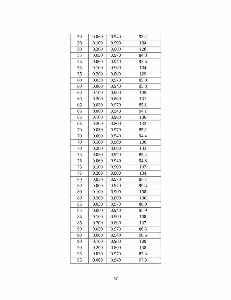
87
50 0.060 0.940 93.2
50 0.100 0.900 104
50 0.200 0.800 128
55 0.030 0.970 84.8
55 0.060 0.940 93.5
55 0.100 0.900 104
55 0.200 0.800 129
60 0.030 0.970 85.0
60 0.060 0.940 93.8
60 0.100 0.900 105
60 0.200 0.800 131
65 0.030 0.970 85.1
65 0.060 0.940 94.1
65 0.100 0.900 106
65 0.200 0.800 132
70 0.030 0.970 85.2
70 0.060 0.940 94.4
70 0.100 0.900 106
70 0.200 0.800 133
75 0.030 0.970 85.4
75 0.060 0.940 94.8
75 0.100 0.900 107
75 0.200 0.800 134
80 0.030 0.970 85.7
80 0.060 0.940 95.3
80 0.100 0.900 108
80 0.200 0.800 136
85 0.030 0.970 86.0
85 0.060 0.940 95.9
85 0.100 0.900 108
85 0.200 0.800 137
90 0.030 0.970 86.5
90 0.060 0.940 96.5
90 0.100 0.900 109
90 0.200 0.800 138
95 0.030 0.970 87.3
95 0.060 0.940 97.3
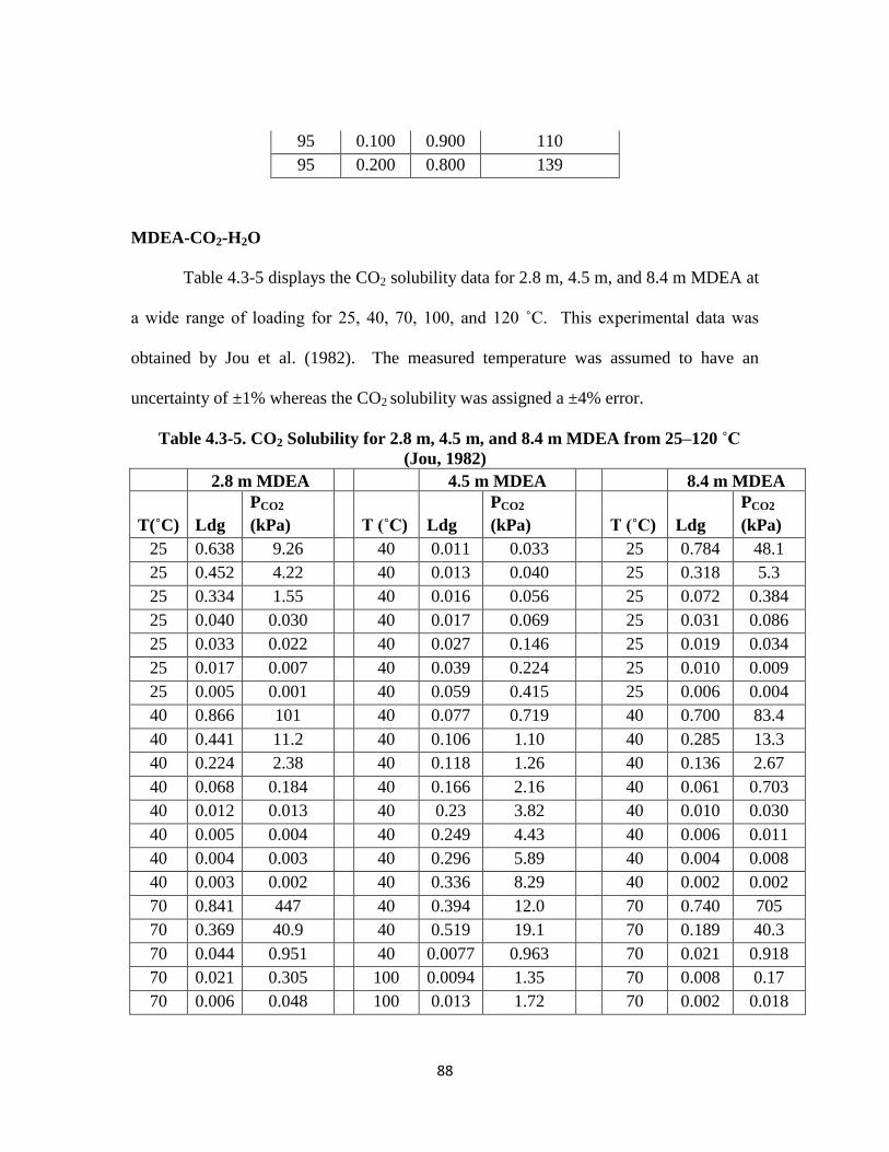
88
95 0.100 0.900 110
95 0.200 0.800 139
MDEA-CO2-H2O
Table 4.3-5 displays the CO2 solubility data for 2.8 m, 4.5 m, and 8.4 m MDEA at
a wide range of loading for 25, 40, 70, 100, and 120 ˚C. This experimental data was
obtained by Jou et al. (1982). The measured temperature was assumed to have an
uncertainty of ±1% whereas the CO2 solubility was assigned a ±4% error.
Table 4.3-5. CO2 Solubility for 2.8 m, 4.5 m, and 8.4 m MDEA from 25–120 ˚C
(Jou, 1982) 2.8 m MDEA 4.5 m MDEA 8.4 m MDEA
T(˚C) Ldg
PCO2
(kPa) T (˚C) Ldg
PCO2
(kPa) T (˚C) Ldg
PCO2
(kPa)
25 0.638 9.26
40 0.011 0.033
25 0.784 48.1
25 0.452 4.22
40 0.013 0.040
25 0.318 5.3
25 0.334 1.55
40 0.016 0.056
25 0.072 0.384
25 0.040 0.030
40 0.017 0.069
25 0.031 0.086
25 0.033 0.022
40 0.027 0.146
25 0.019 0.034
25 0.017 0.007
40 0.039 0.224
25 0.010 0.009
25 0.005 0.001
40 0.059 0.415
25 0.006 0.004
40 0.866 101
40 0.077 0.719
40 0.700 83.4
40 0.441 11.2
40 0.106 1.10
40 0.285 13.3
40 0.224 2.38
40 0.118 1.26
40 0.136 2.67
40 0.068 0.184
40 0.166 2.16
40 0.061 0.703
40 0.012 0.013
40 0.23 3.82
40 0.010 0.030
40 0.005 0.004
40 0.249 4.43
40 0.006 0.011
40 0.004 0.003
40 0.296 5.89
40 0.004 0.008
40 0.003 0.002
40 0.336 8.29
40 0.002 0.002
70 0.841 447
40 0.394 12.0
70 0.740 705
70 0.369 40.9
40 0.519 19.1
70 0.189 40.3
70 0.044 0.951
40 0.0077 0.963
70 0.021 0.918
70 0.021 0.305
100 0.0094 1.35
70 0.008 0.17
70 0.006 0.048
100 0.013 1.72
70 0.002 0.018
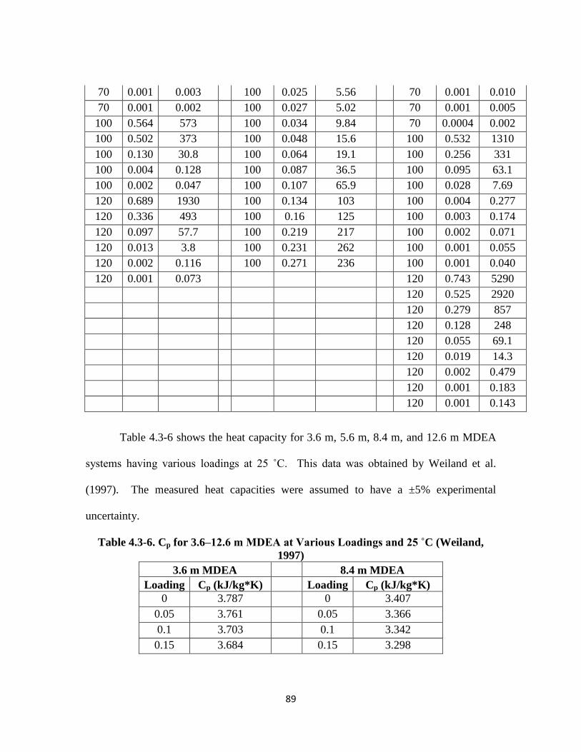
89
70 0.001 0.003
100 0.025 5.56
70 0.001 0.010
70 0.001 0.002
100 0.027 5.02
70 0.001 0.005
100 0.564 573
100 0.034 9.84
70 0.0004 0.002
100 0.502 373
100 0.048 15.6
100 0.532 1310
100 0.130 30.8
100 0.064 19.1
100 0.256 331
100 0.004 0.128
100 0.087 36.5
100 0.095 63.1
100 0.002 0.047
100 0.107 65.9
100 0.028 7.69
120 0.689 1930
100 0.134 103
100 0.004 0.277
120 0.336 493
100 0.16 125
100 0.003 0.174
120 0.097 57.7
100 0.219 217
100 0.002 0.071
120 0.013 3.8
100 0.231 262
100 0.001 0.055
120 0.002 0.116
100 0.271 236
100 0.001 0.040
120 0.001 0.073
120 0.743 5290
120 0.525 2920
120 0.279 857
120 0.128 248
120 0.055 69.1
120 0.019 14.3
120 0.002 0.479
120 0.001 0.183
120 0.001 0.143
Table 4.3-6 shows the heat capacity for 3.6 m, 5.6 m, 8.4 m, and 12.6 m MDEA
systems having various loadings at 25 ˚C. This data was obtained by Weiland et al.
(1997). The measured heat capacities were assumed to have a ±5% experimental
uncertainty.
Table 4.3-6. Cp for 3.6–12.6 m MDEA at Various Loadings and 25 ˚C (Weiland,
1997)
3.6 m MDEA 8.4 m MDEA
Loading Cp (kJ/kg*K)
Loading Cp (kJ/kg*K)
0 3.787
0 3.407
0.05 3.761
0.05 3.366
0.1 3.703
0.1 3.342
0.15 3.684
0.15 3.298
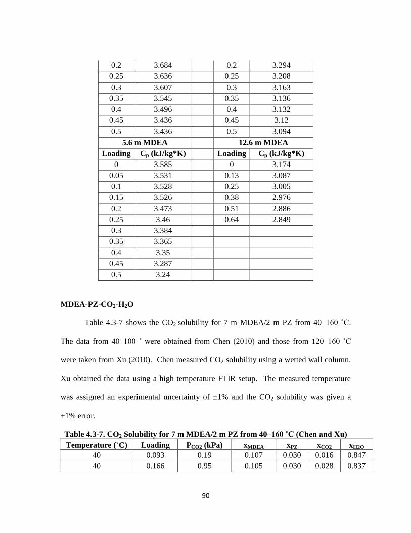
90
0.2 3.684
0.2 3.294
0.25 3.636
0.25 3.208
0.3 3.607
0.3 3.163
0.35 3.545
0.35 3.136
0.4 3.496
0.4 3.132
0.45 3.436
0.45 3.12
0.5 3.436
0.5 3.094
5.6 m MDEA
12.6 m MDEA
Loading Cp (kJ/kg*K)
Loading Cp (kJ/kg*K)
0 3.585
0 3.174
0.05 3.531
0.13 3.087
0.1 3.528
0.25 3.005
0.15 3.526
0.38 2.976
0.2 3.473
0.51 2.886
0.25 3.46
0.64 2.849
0.3 3.384
0.35 3.365
0.4 3.35
0.45 3.287
0.5 3.24
MDEA-PZ-CO2-H2O
Table 4.3-7 shows the CO2 solubility for 7 m MDEA/2 m PZ from 40–160 ˚C.
The data from 40–100 ˚ were obtained from Chen (2010) and those from 120–160 ˚C
were taken from Xu (2010). Chen measured CO2 solubility using a wetted wall column.
Xu obtained the data using a high temperature FTIR setup. The measured temperature
was assigned an experimental uncertainty of ±1% and the CO2 solubility was given a
±1% error.
Table 4.3-7. CO2 Solubility for 7 m MDEA/2 m PZ from 40–160 ˚C (Chen and Xu)
Temperature (˚C) Loading PCO2 (kPa) xMDEA xPZ xCO2 xH2O
40 0.093 0.19 0.107 0.030 0.016 0.847
40 0.166 0.95 0.105 0.030 0.028 0.837
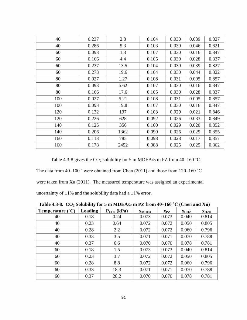
91
40 0.237 2.8 0.104 0.030 0.039 0.827
40 0.286 5.3 0.103 0.030 0.046 0.821
60 0.093 1.3 0.107 0.030 0.016 0.847
60 0.166 4.4 0.105 0.030 0.028 0.837
60 0.237 13.5 0.104 0.030 0.039 0.827
60 0.273 19.6 0.104 0.030 0.044 0.822
80 0.027 1.27 0.108 0.031 0.005 0.857
80 0.093 5.62 0.107 0.030 0.016 0.847
80 0.166 17.6 0.105 0.030 0.028 0.837
100 0.027 5.21 0.108 0.031 0.005 0.857
100 0.093 19.8 0.107 0.030 0.016 0.847
120 0.132 137 0.103 0.029 0.021 0.846
120 0.226 628 0.092 0.026 0.033 0.849
140 0.125 356 0.100 0.029 0.020 0.852
140 0.206 1362 0.090 0.026 0.029 0.855
160 0.113 785 0.098 0.028 0.017 0.857
160 0.178 2452 0.088 0.025 0.025 0.862
Table 4.3-8 gives the CO2 solubility for 5 m MDEA/5 m PZ from 40–160 ˚C.
The data from 40–100 ˚ were obtained from Chen (2011) and those from 120–160 ˚C
were taken from Xu (2011). The measured temperature was assigned an experimental
uncertainty of ±1% and the solubility data had a ±1% error.
Table 4.3-8. CO2 Solubility for 5 m MDEA/5 m PZ from 40–160 ˚C (Chen and Xu)
Temperature (˚C) Loading PCO2 (kPa) xMDEA xPZ xCO2 xH2O
40 0.18 0.24 0.073 0.073 0.040 0.814
40 0.23 0.64 0.072 0.072 0.050 0.805
40 0.28 2.2 0.072 0.072 0.060 0.796
40 0.33 3.5 0.071 0.071 0.070 0.788
40 0.37 6.6 0.070 0.070 0.078 0.781
60 0.18 1.5 0.073 0.073 0.040 0.814
60 0.23 3.7 0.072 0.072 0.050 0.805
60 0.28 8.8 0.072 0.072 0.060 0.796
60 0.33 18.3 0.071 0.071 0.070 0.788
60 0.37 28.2 0.070 0.070 0.078 0.781
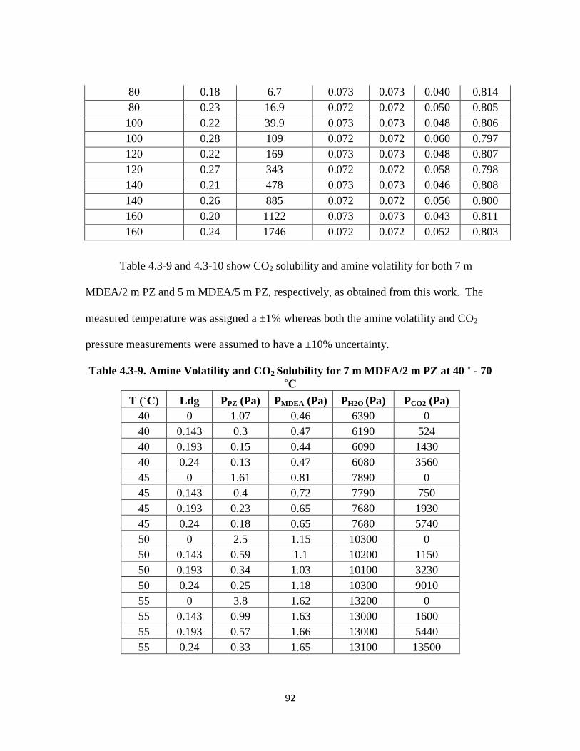
92
80 0.18 6.7 0.073 0.073 0.040 0.814
80 0.23 16.9 0.072 0.072 0.050 0.805
100 0.22 39.9 0.073 0.073 0.048 0.806
100 0.28 109 0.072 0.072 0.060 0.797
120 0.22 169 0.073 0.073 0.048 0.807
120 0.27 343 0.072 0.072 0.058 0.798
140 0.21 478 0.073 0.073 0.046 0.808
140 0.26 885 0.072 0.072 0.056 0.800
160 0.20 1122 0.073 0.073 0.043 0.811
160 0.24 1746 0.072 0.072 0.052 0.803
Table 4.3-9 and 4.3-10 show CO2 solubility and amine volatility for both 7 m
MDEA/2 m PZ and 5 m MDEA/5 m PZ, respectively, as obtained from this work. The
measured temperature was assigned a ±1% whereas both the amine volatility and CO2
pressure measurements were assumed to have a ±10% uncertainty.
Table 4.3-9. Amine Volatility and CO2 Solubility for 7 m MDEA/2 m PZ at 40 ˚ - 70
˚C
T (˚C) Ldg PPZ (Pa) PMDEA (Pa) PH2O (Pa) PCO2 (Pa)
40 0 1.07 0.46 6390 0
40 0.143 0.3 0.47 6190 524
40 0.193 0.15 0.44 6090 1430
40 0.24 0.13 0.47 6080 3560
45 0 1.61 0.81 7890 0
45 0.143 0.4 0.72 7790 750
45 0.193 0.23 0.65 7680 1930
45 0.24 0.18 0.65 7680 5740
50 0 2.5 1.15 10300 0
50 0.143 0.59 1.1 10200 1150
50 0.193 0.34 1.03 10100 3230
50 0.24 0.25 1.18 10300 9010
55 0 3.8 1.62 13200 0
55 0.143 0.99 1.63 13000 1600
55 0.193 0.57 1.66 13000 5440
55 0.24 0.33 1.65 13100 13500
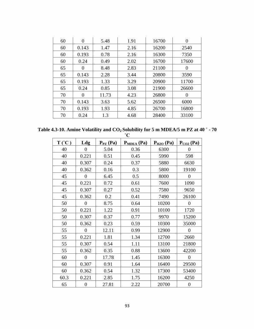
93
60 0 5.48 1.91 16700 0
60 0.143 1.47 2.16 16200 2540
60 0.193 0.78 2.16 16300 7350
60 0.24 0.49 2.02 16700 17600
65 0 8.48 2.83 21100 0
65 0.143 2.28 3.44 20800 3590
65 0.193 1.33 3.29 20900 11700
65 0.24 0.85 3.08 21900 26600
70 0 11.73 4.23 26800 0
70 0.143 3.63 5.62 26500 6000
70 0.193 1.93 4.85 26700 16800
70 0.24 1.3 4.68 28400 33100
Table 4.3-10. Amine Volatility and CO2 Solubility for 5 m MDEA/5 m PZ at 40 ˚ - 70
˚C
T (˚C ) Ldg PPZ (Pa) PMDEA (Pa) PH2O (Pa) PCO2 (Pa)
40 0 5.04 0.36 6300 0
40 0.221 0.51 0.45 5990 598
40 0.307 0.24 0.37 5880 6630
40 0.362 0.16 0.3 5800 19100
45 0 6.45 0.5 8000 0
45 0.221 0.72 0.61 7600 1090
45 0.307 0.27 0.52 7580 9650
45 0.362 0.2 0.41 7490 26100
50 0 8.75 0.64 10200 0
50 0.221 1.22 0.91 10100 1720
50 0.307 0.37 0.77 9970 15200
50 0.362 0.23 0.59 10300 35000
55 0 12.11 0.99 12900 0
55 0.221 1.81 1.34 12700 2660
55 0.307 0.54 1.11 13100 21800
55 0.362 0.35 0.88 13600 42200
60 0 17.78 1.45 16300 0
60 0.307 0.91 1.64 16400 29500
60 0.362 0.54 1.32 17300 53400
60.3 0.221 2.85 1.75 16200 4250
65 0 27.81 2.22 20700 0
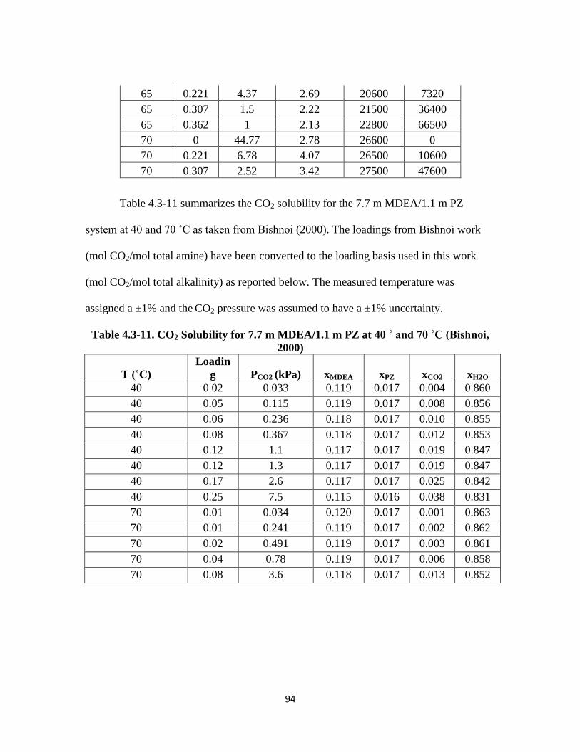
94
65 0.221 4.37 2.69 20600 7320
65 0.307 1.5 2.22 21500 36400
65 0.362 1 2.13 22800 66500
70 0 44.77 2.78 26600 0
70 0.221 6.78 4.07 26500 10600
70 0.307 2.52 3.42 27500 47600
Table 4.3-11 summarizes the CO2 solubility for the 7.7 m MDEA/1.1 m PZ
system at 40 and 70 ˚C as taken from Bishnoi (2000). The loadings from Bishnoi work
(mol CO2/mol total amine) have been converted to the loading basis used in this work
(mol CO2/mol total alkalinity) as reported below. The measured temperature was
assigned a ±1% and the CO2 pressure was assumed to have a ±1% uncertainty.
Table 4.3-11. CO2 Solubility for 7.7 m MDEA/1.1 m PZ at 40 ˚ and 70 ˚C (Bishnoi,
2000)
T (˚C)
Loadin
g PCO2 (kPa) xMDEA xPZ xCO2 xH2O
40 0.02 0.033 0.119 0.017 0.004 0.860
40 0.05 0.115 0.119 0.017 0.008 0.856
40 0.06 0.236 0.118 0.017 0.010 0.855
40 0.08 0.367 0.118 0.017 0.012 0.853
40 0.12 1.1 0.117 0.017 0.019 0.847
40 0.12 1.3 0.117 0.017 0.019 0.847
40 0.17 2.6 0.117 0.017 0.025 0.842
40 0.25 7.5 0.115 0.016 0.038 0.831
70 0.01 0.034 0.120 0.017 0.001 0.863
70 0.01 0.241 0.119 0.017 0.002 0.862
70 0.02 0.491 0.119 0.017 0.003 0.861
70 0.04 0.78 0.119 0.017 0.006 0.858
70 0.08 3.6 0.118 0.017 0.013 0.852
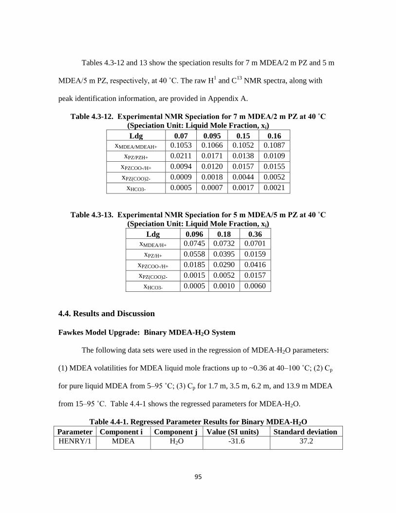
95
Tables 4.3-12 and 13 show the speciation results for 7 m MDEA/2 m PZ and 5 m
MDEA/5 m PZ, respectively, at 40 ˚C. The raw H1 and C
13 NMR spectra, along with
peak identification information, are provided in Appendix A.
Table 4.3-12. Experimental NMR Speciation for 7 m MDEA/2 m PZ at 40 ˚C
(Speciation Unit: Liquid Mole Fraction, xi)
Ldg 0.07 0.095 0.15 0.16
xMDEA/MDEAH+ 0.1053 0.1066 0.1052 0.1087
xPZ/PZH+ 0.0211 0.0171 0.0138 0.0109
xPZCOO-/H+ 0.0094 0.0120 0.0157 0.0155
xPZ(COO)2- 0.0009 0.0018 0.0044 0.0052
xHCO3- 0.0005 0.0007 0.0017 0.0021
Table 4.3-13. Experimental NMR Speciation for 5 m MDEA/5 m PZ at 40 ˚C
(Speciation Unit: Liquid Mole Fraction, xi)
Ldg 0.096 0.18 0.36
xMDEA/H+ 0.0745 0.0732 0.0701
xPZ/H+ 0.0558 0.0395 0.0159
xPZCOO-/H+ 0.0185 0.0290 0.0416
xPZ(COO)2- 0.0015 0.0052 0.0157
xHCO3- 0.0005 0.0010 0.0060
4.4. Results and Discussion
Fawkes Model Upgrade: Binary MDEA-H2O System
The following data sets were used in the regression of MDEA-H2O parameters:
(1) MDEA volatilities for MDEA liquid mole fractions up to ~0.36 at 40–100 ˚C; (2) Cp
for pure liquid MDEA from 5–95 ˚C; (3) Cp for 1.7 m, 3.5 m, 6.2 m, and 13.9 m MDEA
from 15–95 ˚C. Table 4.4-1 shows the regressed parameters for MDEA-H2O.
Table 4.4-1. Regressed Parameter Results for Binary MDEA-H2O
Parameter Component i Component j Value (SI units) Standard deviation
HENRY/1 MDEA H2O -31.6 37.2
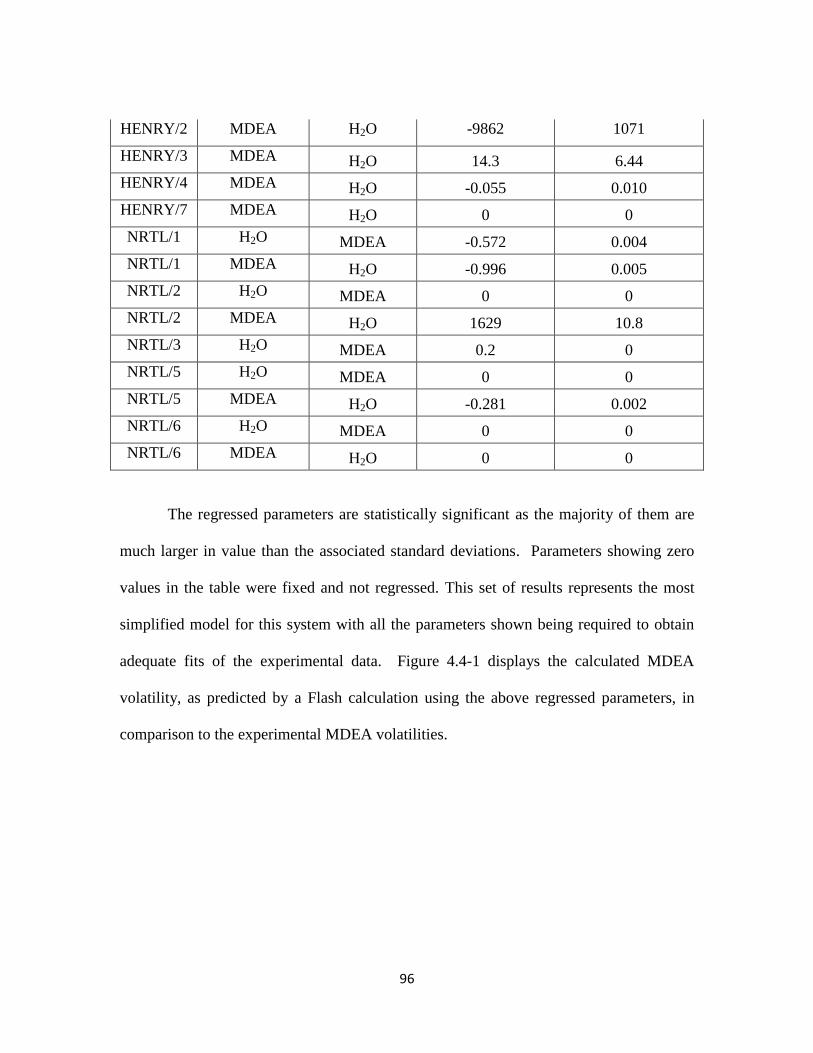
96
HENRY/2 MDEA H2O -9862 1071
HENRY/3 MDEA H2O 14.3 6.44
HENRY/4 MDEA H2O -0.055 0.010
HENRY/7 MDEA H2O 0 0
NRTL/1 H2O MDEA -0.572 0.004
NRTL/1 MDEA H2O -0.996 0.005
NRTL/2 H2O MDEA 0 0
NRTL/2 MDEA H2O 1629 10.8
NRTL/3 H2O MDEA 0.2 0
NRTL/5 H2O MDEA 0 0
NRTL/5 MDEA H2O -0.281 0.002
NRTL/6 H2O MDEA 0 0
NRTL/6 MDEA H2O 0 0
The regressed parameters are statistically significant as the majority of them are
much larger in value than the associated standard deviations. Parameters showing zero
values in the table were fixed and not regressed. This set of results represents the most
simplified model for this system with all the parameters shown being required to obtain
adequate fits of the experimental data. Figure 4.4-1 displays the calculated MDEA
volatility, as predicted by a Flash calculation using the above regressed parameters, in
comparison to the experimental MDEA volatilities.

97
Figure 4.4-1. MDEA Volatility in MDEA-H2O from 40–100 ˚C
The upgraded Fawkes model is able to represent both the temperature and the
effect of MDEA concentration. A separate thermodynamic model may still be required
to characterize MDEA volatility and related thermodynamics at very dilute amine
concentration typical of water wash operation.
Figure 4.4-2 shows the prediction of MDEA-H2O heat capacity relative to
experimentally measured Cp from 278–368 K.
0.01
0.1
1
10
100
0.004 0.04 0.4
PM
DE
A (
Pa)
xMDEA
60 ˚C
40 ˚C
80 ˚C
100 ˚C
Diamonds - This work
Circles - Kim (2008)
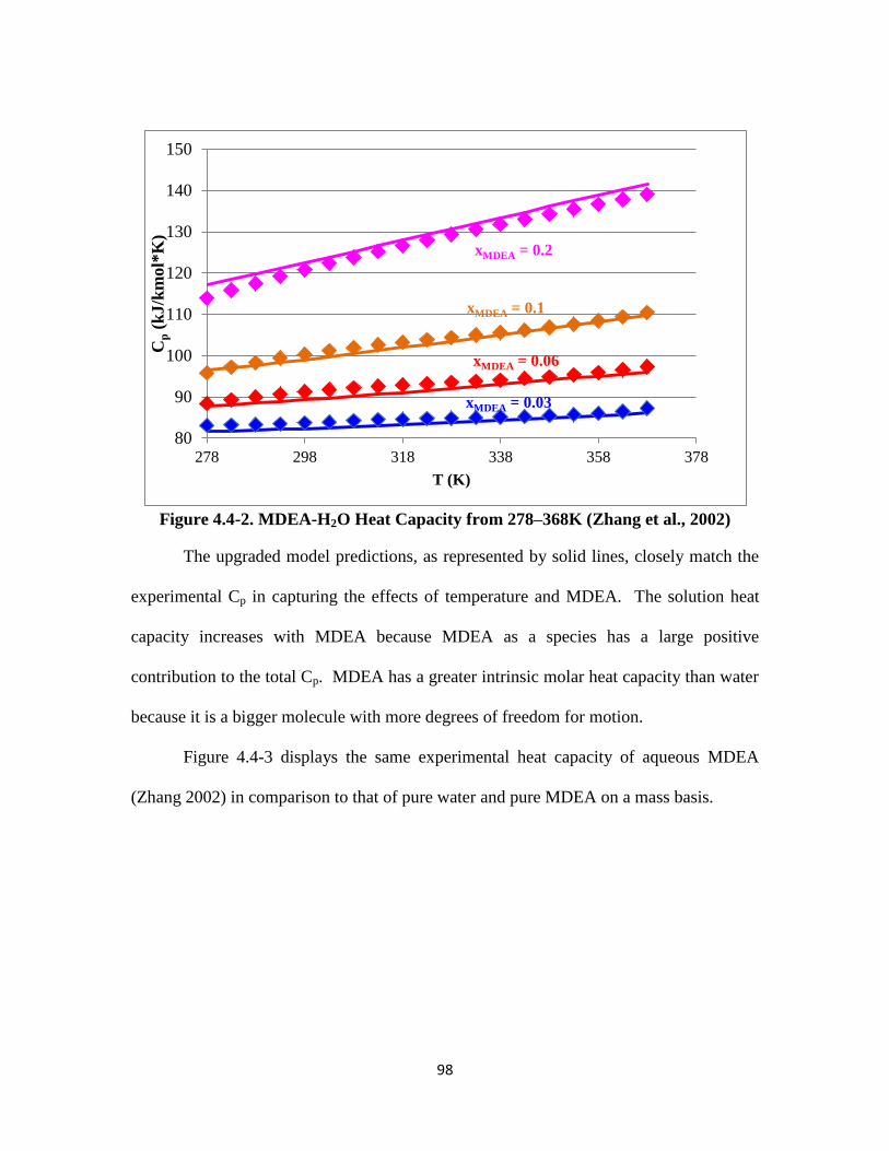
98
Figure 4.4-2. MDEA-H2O Heat Capacity from 278–368K (Zhang et al., 2002)
The upgraded model predictions, as represented by solid lines, closely match the
experimental Cp in capturing the effects of temperature and MDEA. The solution heat
capacity increases with MDEA because MDEA as a species has a large positive
contribution to the total Cp. MDEA has a greater intrinsic molar heat capacity than water
because it is a bigger molecule with more degrees of freedom for motion.
Figure 4.4-3 displays the same experimental heat capacity of aqueous MDEA
(Zhang 2002) in comparison to that of pure water and pure MDEA on a mass basis.
80
90
100
110
120
130
140
150
278 298 318 338 358 378
Cp (
kJ/k
mol*
K)
T (K)
xMDEA = 0.03
xMDEA = 0.06
xMDEA = 0.1
xMDEA = 0.2
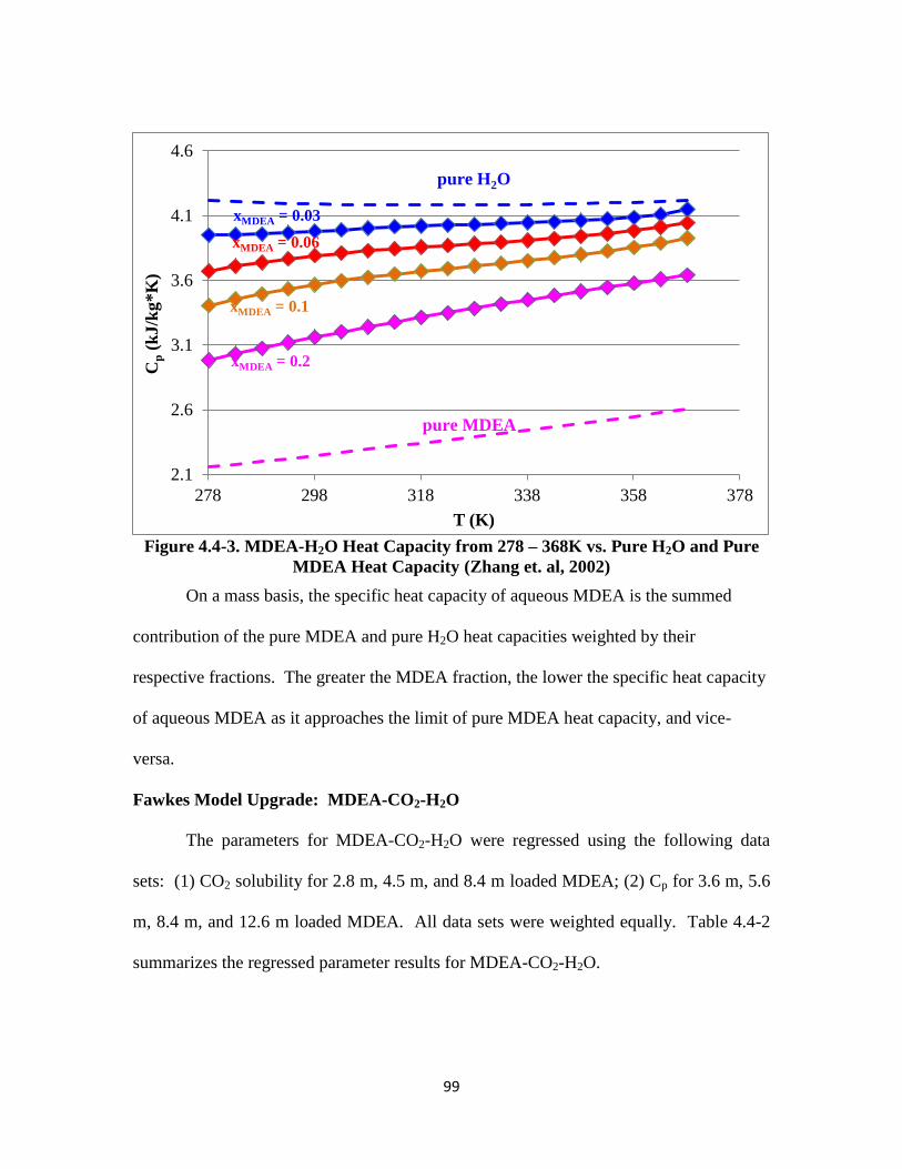
99
Figure 4.4-3. MDEA-H2O Heat Capacity from 278 – 368K vs. Pure H2O and Pure
MDEA Heat Capacity (Zhang et. al, 2002)
On a mass basis, the specific heat capacity of aqueous MDEA is the summed
contribution of the pure MDEA and pure H2O heat capacities weighted by their
respective fractions. The greater the MDEA fraction, the lower the specific heat capacity
of aqueous MDEA as it approaches the limit of pure MDEA heat capacity, and vice-
versa.
Fawkes Model Upgrade: MDEA-CO2-H2O
The parameters for MDEA-CO2-H2O were regressed using the following data
sets: (1) CO2 solubility for 2.8 m, 4.5 m, and 8.4 m loaded MDEA; (2) Cp for 3.6 m, 5.6
m, 8.4 m, and 12.6 m loaded MDEA. All data sets were weighted equally. Table 4.4-2
summarizes the regressed parameter results for MDEA-CO2-H2O.
2.1
2.6
3.1
3.6
4.1
4.6
278 298 318 338 358 378
Cp (
kJ/k
g*K
)
T (K)
pure H2O
xMDEA = 0.03
xMDEA = 0.06
xMDEA = 0.1
xMDEA = 0.2
pure MDEA
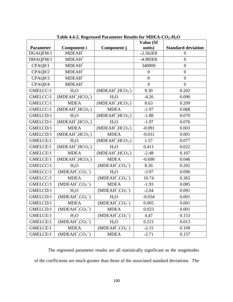
100
Table 4.4-2. Regressed Parameter Results for MDEA-CO2-H2O
Parameter Component i Component j
Value (SI
units) Standard deviation
DGAQFM/1 MDEAH+
-2.562E8 0
DHAQFM/1 MDEAH+
-4.985E8 0
CPAQ0/1 MDEAH+
340000 0
CPAQ0/2 MDEAH+
0 0
CPAQ0/3 MDEAH+
0 0
CPAQ0/4 MDEAH+
0 0
GMELCC/1 H2O (MDEAH+,HCO3
-) 9.30 0.202
GMELCC/1 (MDEAH+,HCO3
-) H2O -4.26 0.090
GMELCC/1 MDEA (MDEAH+,HCO3
-) 8.63 0.209
GMELCC/1 (MDEAH+,HCO3
-) MDEA -1.97 0.068
GMELCD/1 H2O (MDEAH+,HCO3
-) -1.88 0.070
GMELCD/1 (MDEAH+,HCO3
-) H2O -1.97 0.076
GMELCD/1 MDEA (MDEAH+,HCO3
-) -0.091 0.003
GMELCD/1 (MDEAH+,HCO3
-) MDEA -0.031 0.001
GMELCE/1 H2O (MDEAH+,HCO3
-) 1.57 0.077
GMELCE/1 (MDEAH+,HCO3
-) H2O 0.411 0.022
GMELCE/1 MDEA (MDEAH+,HCO3
-) -2.48 0.107
GMELCE/1 (MDEAH+,HCO3
-) MDEA -0.690 0.046
GMELCC/1 H2O (MDEAH+,CO3
--) 8.26 0.202
GMELCC/1 (MDEAH+,CO3
--) H2O -3.97 0.096
GMELCC/1 MDEA (MDEAH+,CO3
--) 10.74 0.365
GMELCC/1 (MDEAH+,CO3
--) MDEA -1.93 0.085
GMELCD/1 H2O (MDEAH+,CO3
--) -2.04 0.091
GMELCD/1 (MDEAH+,CO3
--) H2O -0.034 0.001
GMELCD/1 MDEA (MDEAH+,CO3
--) 0.005 0.001
GMELCD/1 (MDEAH+,CO3
--) MDEA 0.023 0.001
GMELCE/1 H2O (MDEAH+,CO3
--) 4.47 0.153
GMELCE/1 (MDEAH+,CO3
--) H2O 0.221 0.013
GMELCE/1 MDEA (MDEAH+,CO3
--) -2.15 0.109
GMELCE/1 (MDEAH+,CO3
--) MDEA -2.71 0.157
The regressed parameter results are all statistically significant as the magnitudes
of the coefficients are much greater than those of the associated standard deviations. The
101
correlation matrix for the above 24 parameters, constituting a total of 276 parameter
pairs, shows that no two parameters are strongly correlated as all of the correlation
factors are below 0.75. All of the above parameters are required to match the variety of
data types and sheer volume of data used. Nonetheless, a reduced model with fewer
parameters will be presented later. Parameters in the full model having negligible values
are zeroed out and again the model was regressed to obtain the reduced case. While the
elimination of parameters allows for the development of a simpler model, the ability to fit
certain data is compromised to some extent.
The free energy, enthalpy, and heat capacity parameters of the electrolyte
MDEAH+ were manually adjusted to simultaneously match: (1) the pKa of the reaction
which involves MDEA being protonated to form MDEAH+ and (2) all the rest of the data
types. The free energy parameter for this species, DGAQFM, was most crucial for
anchoring the pKa and CO2 solubility predictions at 25 ˚C whereas the enthalpy,
DHAQFM, was vital for obtaining the appropriate temperature behaviors of the pKa
extrapolation and of the CO2 solubility and Cp.
Figure 4.4-4 shows predicted pKa for MDEAH+ reaction as obtained by manually
adjusting the mentioned parameters. The experimental pKa measurements were obtained
by Hamborg and co-workers (2007).
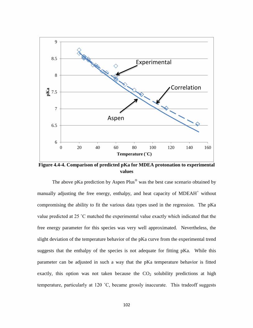
102
Figure 4.4-4. Comparison of predicted pKa for MDEA protonation to experimental
values
The above pKa prediction by Aspen Plus® was the best case scenario obtained by
manually adjusting the free energy, enthalpy, and heat capacity of MDEAH+ without
compromising the ability to fit the various data types used in the regression. The pKa
value predicted at 25 ˚C matched the experimental value exactly which indicated that the
free energy parameter for this species was very well approximated. Nevertheless, the
slight deviation of the temperature behavior of the pKa curve from the experimental trend
suggests that the enthalpy of the species is not adequate for fitting pKa. While this
parameter can be adjusted in such a way that the pKa temperature behavior is fitted
exactly, this option was not taken because the CO2 solubility predictions at high
temperature, particularly at 120 ˚C, became grossly inaccurate. This tradeoff suggests
6
6.5
7
7.5
8
8.5
9
0 20 40 60 80 100 120 140 160
pK
a
Temperature (˚C)
Experimental
Correlation
Aspen
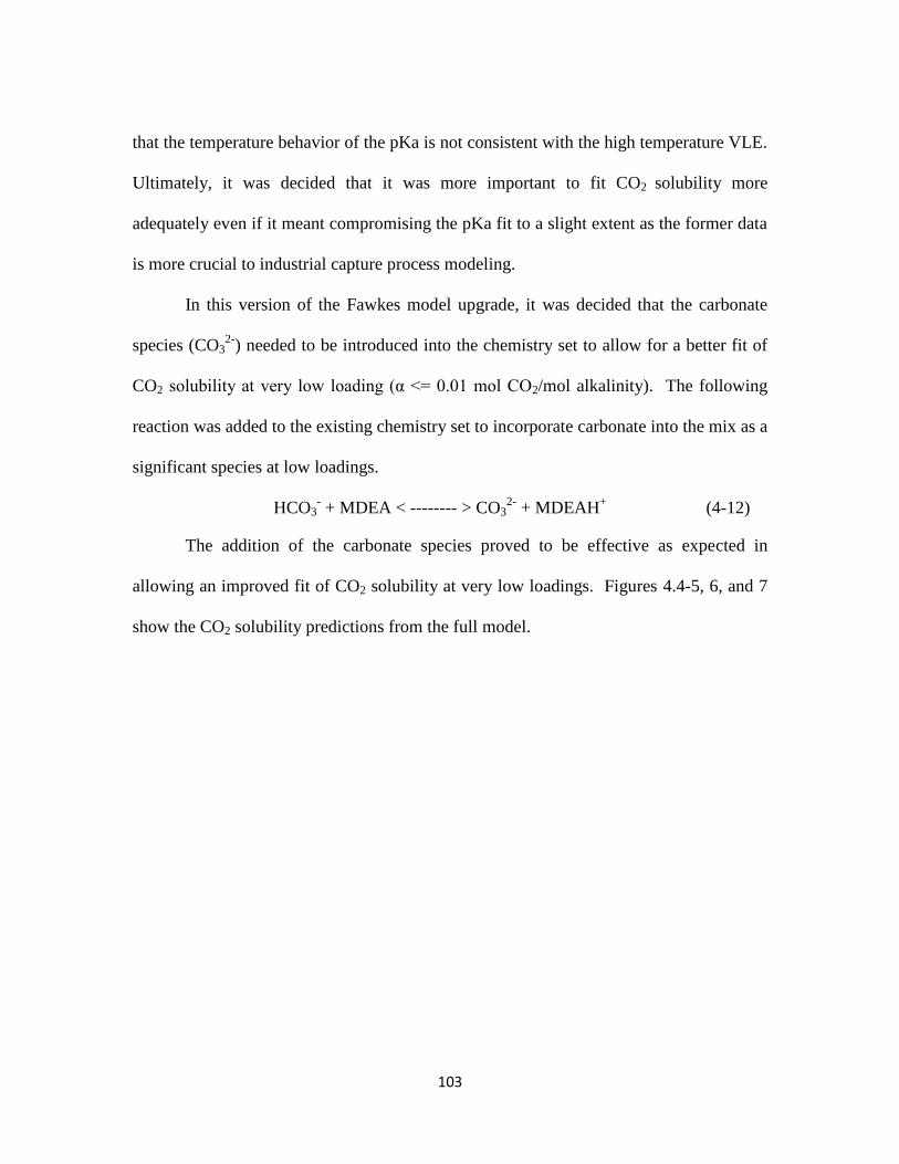
103
that the temperature behavior of the pKa is not consistent with the high temperature VLE.
Ultimately, it was decided that it was more important to fit CO2 solubility more
adequately even if it meant compromising the pKa fit to a slight extent as the former data
is more crucial to industrial capture process modeling.
In this version of the Fawkes model upgrade, it was decided that the carbonate
species (CO32-
) needed to be introduced into the chemistry set to allow for a better fit of
CO2 solubility at very low loading (α <= 0.01 mol CO2/mol alkalinity). The following
reaction was added to the existing chemistry set to incorporate carbonate into the mix as a
significant species at low loadings.
HCO3- + MDEA < -------- > CO3
2- + MDEAH
+ (4-12)
The addition of the carbonate species proved to be effective as expected in
allowing an improved fit of CO2 solubility at very low loadings. Figures 4.4-5, 6, and 7
show the CO2 solubility predictions from the full model.
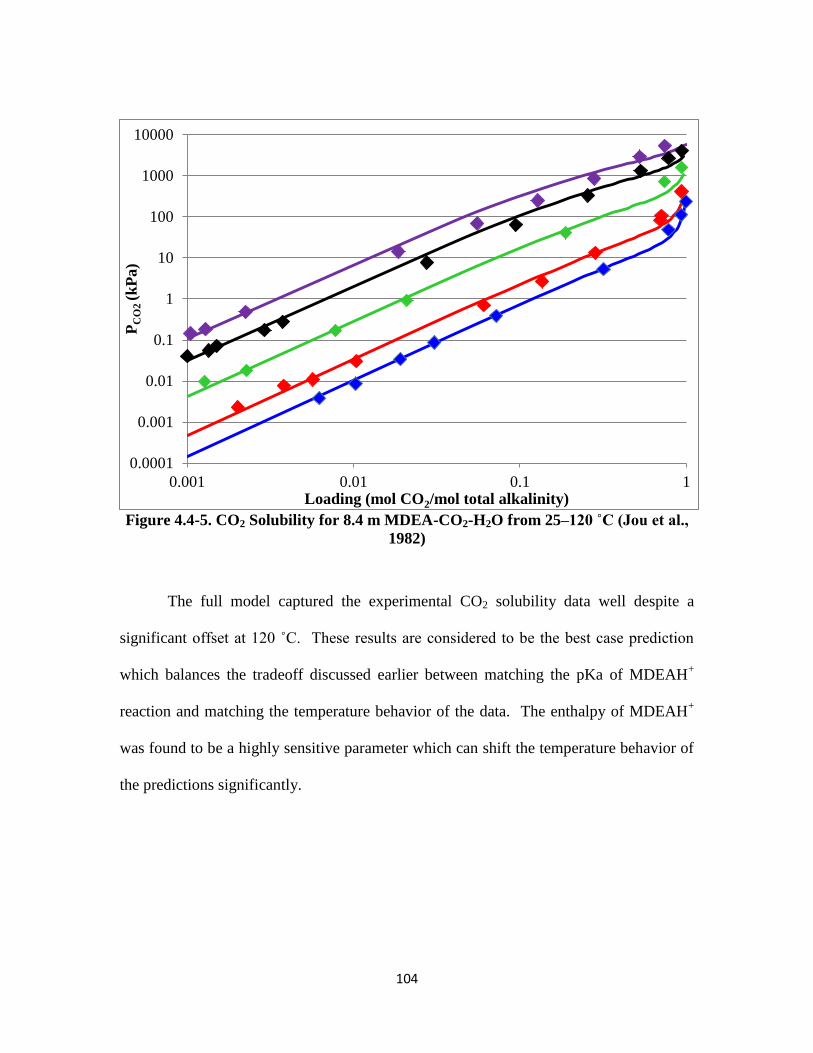
104
Figure 4.4-5. CO2 Solubility for 8.4 m MDEA-CO2-H2O from 25–120 ˚C (Jou et al.,
1982)
The full model captured the experimental CO2 solubility data well despite a
significant offset at 120 ˚C. These results are considered to be the best case prediction
which balances the tradeoff discussed earlier between matching the pKa of MDEAH+
reaction and matching the temperature behavior of the data. The enthalpy of MDEAH+
was found to be a highly sensitive parameter which can shift the temperature behavior of
the predictions significantly.
0.0001
0.001
0.01
0.1
1
10
100
1000
10000
0.001 0.01 0.1 1
PC
O2
(k
Pa)
Loading (mol CO2/mol total alkalinity)
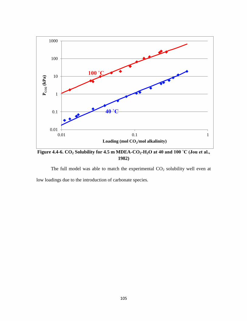
105
Figure 4.4-6. CO2 Solubility for 4.5 m MDEA-CO2-H2O at 40 and 100 ˚C (Jou et al.,
1982)
The full model was able to match the experimental CO2 solubility well even at
low loadings due to the introduction of carbonate species.
0.01
0.1
1
10
100
1000
0.01 0.1 1
PC
O2 (
kP
a)
Loading (mol CO2/mol alkalinity)
40 ˚C
100 ˚C
106
Figure 4.4-7. CO2 Solubility for 2.8 m MDEA-CO2-H2O from 25–120 ˚C (Jou et al.,
1982)
The full model was able to adequately represent the CO2 solubility data at 2.8 m
MDEA. It appears that the CO2 partial pressure at this concentration was even better
matched than at higher MDEA as the model is centered on an infinite dilution reference
state. Therefore dilute concentration data can be better fitted than concentrated data.
The Cp of MDEA-CO2-H2O was also regressed to obtain parameter results.
Figure 4.4-8 shows the upgraded Fawkes model predictions of heat capacity at 25 ˚C in
loaded MDEA compared to experimental values.
0.0001
0.001
0.01
0.1
1
10
100
1000
10000
0.001 0.01 0.1 1
PC
O2 (
kP
a)
Loading (mol CO2/mol alkalinity)
25 ˚C 40 ˚C
70 ˚C
100 ˚C
120 ˚C
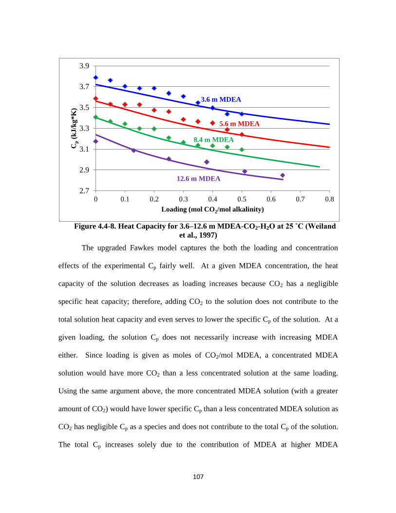
107
Figure 4.4-8. Heat Capacity for 3.6–12.6 m MDEA-CO2-H2O at 25 ˚C (Weiland
et al., 1997)
The upgraded Fawkes model captures the both the loading and concentration
effects of the experimental Cp fairly well. At a given MDEA concentration, the heat
capacity of the solution decreases as loading increases because CO2 has a negligible
specific heat capacity; therefore, adding CO2 to the solution does not contribute to the
total solution heat capacity and even serves to lower the specific Cp of the solution. At a
given loading, the solution Cp does not necessarily increase with increasing MDEA
either. Since loading is given as moles of CO2/mol MDEA, a concentrated MDEA
solution would have more CO2 than a less concentrated solution at the same loading.
Using the same argument above, the more concentrated MDEA solution (with a greater
amount of CO2) would have lower specific Cp than a less concentrated MDEA solution as
CO2 has negligible Cp as a species and does not contribute to the total Cp of the solution.
The total Cp increases solely due to the contribution of MDEA at higher MDEA
2.7
2.9
3.1
3.3
3.5
3.7
3.9
0 0.1 0.2 0.3 0.4 0.5 0.6 0.7 0.8
Cp (
kJ
/kg
*K
)
Loading (mol CO2/mol alkalinity)
3.6 m MDEA
5.6 m MDEA
8.4 m MDEA
12.6 m MDEA
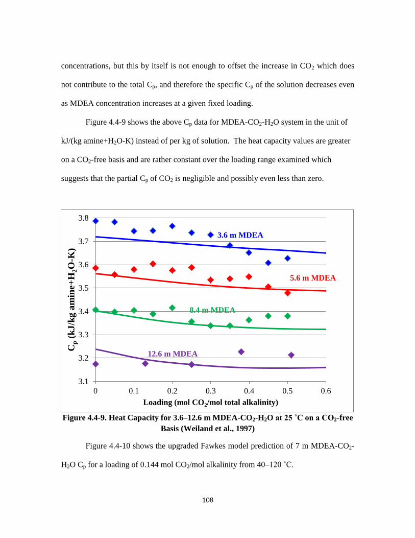
108
concentrations, but this by itself is not enough to offset the increase in CO2 which does
not contribute to the total Cp, and therefore the specific Cp of the solution decreases even
as MDEA concentration increases at a given fixed loading.
Figure 4.4-9 shows the above Cp data for MDEA-CO2-H2O system in the unit of
kJ/(kg amine+H2O-K) instead of per kg of solution. The heat capacity values are greater
on a CO2-free basis and are rather constant over the loading range examined which
suggests that the partial Cp of CO2 is negligible and possibly even less than zero.
Figure 4.4-9. Heat Capacity for 3.6–12.6 m MDEA-CO2-H2O at 25 ˚C on a CO2-free
Basis (Weiland et al., 1997)
Figure 4.4-10 shows the upgraded Fawkes model prediction of 7 m MDEA-CO2-
H2O Cp for a loading of 0.144 mol CO2/mol alkalinity from 40–120 ˚C.
3.1
3.2
3.3
3.4
3.5
3.6
3.7
3.8
0 0.1 0.2 0.3 0.4 0.5 0.6
Cp (
kJ
/kg
am
ine+
H2O
-K)
Loading (mol CO2/mol total alkalinity)
3.6 m MDEA
5.6 m MDEA
8.4 m MDEA
12.6 m MDEA
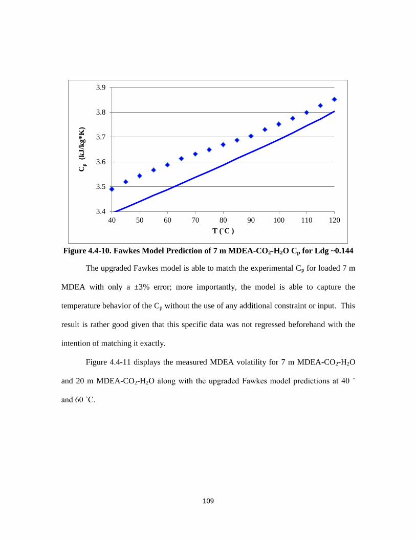
109
Figure 4.4-10. Fawkes Model Prediction of 7 m MDEA-CO2-H2O Cp for Ldg ~0.144
The upgraded Fawkes model is able to match the experimental Cp for loaded 7 m
MDEA with only a ±3% error; more importantly, the model is able to capture the
temperature behavior of the Cp without the use of any additional constraint or input. This
result is rather good given that this specific data was not regressed beforehand with the
intention of matching it exactly.
Figure 4.4-11 displays the measured MDEA volatility for 7 m MDEA-CO2-H2O
and 20 m MDEA-CO2-H2O along with the upgraded Fawkes model predictions at 40 ˚
and 60 ˚C.
3.4
3.5
3.6
3.7
3.8
3.9
40 50 60 70 80 90 100 110 120
Cp
(kJ
/kg
*K
)
T (˚C )
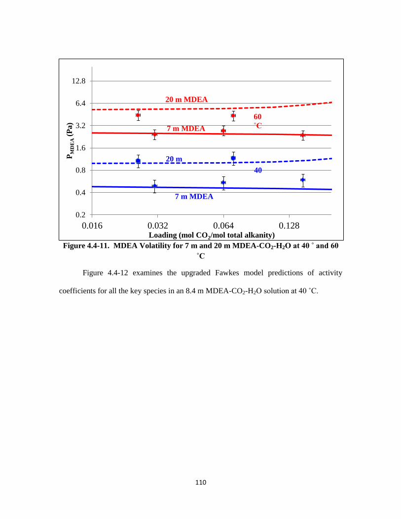
110
Figure 4.4-11. MDEA Volatility for 7 m and 20 m MDEA-CO2-H2O at 40 ˚ and 60
˚C
Figure 4.4-12 examines the upgraded Fawkes model predictions of activity
coefficients for all the key species in an 8.4 m MDEA-CO2-H2O solution at 40 ˚C.
0.2
0.4
0.8
1.6
3.2
6.4
12.8
0.016 0.032 0.064 0.128
PM
DE
A (
Pa)
Loading (mol CO2/mol total alkanity)
40
60
˚C 7 m MDEA
20 m
20 m MDEA
7 m MDEA
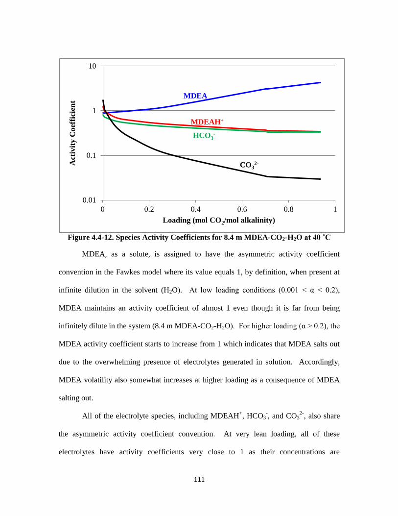
111
Figure 4.4-12. Species Activity Coefficients for 8.4 m MDEA-CO2-H2O at 40 ˚C
MDEA, as a solute, is assigned to have the asymmetric activity coefficient
convention in the Fawkes model where its value equals 1, by definition, when present at
infinite dilution in the solvent (H2O). At low loading conditions (0.001 < α < 0.2),
MDEA maintains an activity coefficient of almost 1 even though it is far from being
infinitely dilute in the system (8.4 m MDEA-CO2-H2O). For higher loading (α > 0.2), the
MDEA activity coefficient starts to increase from 1 which indicates that MDEA salts out
due to the overwhelming presence of electrolytes generated in solution. Accordingly,
MDEA volatility also somewhat increases at higher loading as a consequence of MDEA
salting out.
All of the electrolyte species, including MDEAH+, HCO3
-, and CO3
2-, also share
the asymmetric activity coefficient convention. At very lean loading, all of these
electrolytes have activity coefficients very close to 1 as their concentrations are
0.01
0.1
1
10
0 0.2 0.4 0.6 0.8 1
Act
ivit
y C
oef
fici
ent
Loading (mol CO2/mol alkalinity)
MDEA
MDEAH+
HCO3-
CO32-
112
practically negligible, though not infinitely dilute, due to the lack of CO2. At greater
loading, their activity coefficient start to drop due to interactions with increasing amounts
of like neighbors being generated with higher amounts of CO2. In other words, the
electrolytes species are salted in with other electrolytes unlike MDEA. In particular,
CO32-
activity coefficient drops significantly with loading as would be expected given
increasingly greater concentration of HCO3-/CO3
2- being generated.
MDEA-CO2-H2O Reduced Model
Certain parameters in the full model whose values were considered negligible
were eliminated in an attempt to develop a simpler model for MDEA-CO2-H2O. The
same data sets were regressed again using fewer parameters to fit the data. Table 4.4-3
summarizes the regressed parameter results for the reduced model.
Table 4.4-3. Regressed Parameter Results for MDEA-CO2-H2O Reduced Model
Parameter Component i Component j
Value (SI
units)
Standard
deviation
DGAQFM/1 MDEAH+
-256200000 0
DHAQFM/1 MDEAH+
-498500000 0
CPAQ0/1 MDEAH+
340000 0
CPAQ0/2 MDEAH+
0 0
CPAQ0/3 MDEAH+
0 0
CPAQ0/4 MDEAH+
0 0
GMELCC/1 H2O (MDEAH+,HCO3
-) 8.65 0.127
GMELCC/1 (MDEAH+,HCO3
-) H2O -3.96 0.058
GMELCC/1 MDEA (MDEAH+,HCO3
-) 8.40 0.124
GMELCC/1 (MDEAH+,HCO3
-) MDEA -2.08 0.069
GMELCD/1 H2O (MDEAH+,HCO3
-) -1.93 0.044
GMELCD/1 (MDEAH+,HCO3
-) H2O -1.97 0.037
GMELCD/1 MDEA (MDEAH+,HCO3
-) 0 0
GMELCD/1 (MDEAH+,HCO3
-) MDEA 0 0
GMELCE/1 H2O (MDEAH+,HCO3
-) 0.807 0.027
GMELCE/1 (MDEAH+,HCO3
-) H2O 0.119 0.005
113
GMELCE/1 MDEA (MDEAH+,HCO3
-) -0.807 0.044
GMELCE/1 (MDEAH+,HCO3
-) MDEA -0.651 0.027
GMELCC/1 H2O (MDEAH+,CO3
--) 8.05 0.226
GMELCC/1 (MDEAH+,CO3
--) H2O -3.85 0.076
GMELCC/1 MDEA (MDEAH+,CO3
--) 9.932 0.234
GMELCC/1 (MDEAH+,CO3
--) MDEA -1.98 0.048
GMELCD/1 H2O (MDEAH+,CO3
--) -1.96 0.049
GMELCD/1 (MDEAH+,CO3
--) H2O 0 0
GMELCD/1 MDEA (MDEAH+,CO3
--) 0 0
GMELCD/1 (MDEAH+,CO3
--) MDEA 0 0
GMELCE/1 H2O (MDEAH+,CO3
--) 0.240 0.011
GMELCE/1 (MDEAH+,CO3
--) H2O 0.151 0.007
GMELCE/1 MDEA (MDEAH+,CO3
--) -0.728 0.042
GMELCE/1 (MDEAH+,CO3
--) MDEA -0.360 0.014
The reduced model was able to adequately fit the regressed data almost as well as
the full model. The only two pieces of data that were not matched well were the CO2
solubility for 8.4 m MDEA-CO2-H2O at 120 ˚C and the loading effect on the isothermal
Cp for various MDEA concentrations at 25 ˚C. Nevertheless, the reduced model proved
to be robust overall and serves as a promising alternative to the full model as it allows
more flexibility, or more degrees of freedom, when it comes to fitting data for the more
complex MDEA-PZ blend. Ultimately the reduced MDEA-CO2-H2O model was
incorporated into the full model for the blend.
Fawkes Model Upgrade: MDEA-PZ-H2O
No additional parameter, namely cross parameters for MDEA-PZ interactions,
had to be used to match the MDEA/PZ volatility for either 7 m MDEA/2 m PZ or 5 m
MDEA/5 m PZ from 40 ˚–60 ˚C. In other words, the cross interaction parameters were
set to zero. The reason that this is the case is because the binary MDEA-H2O parameters
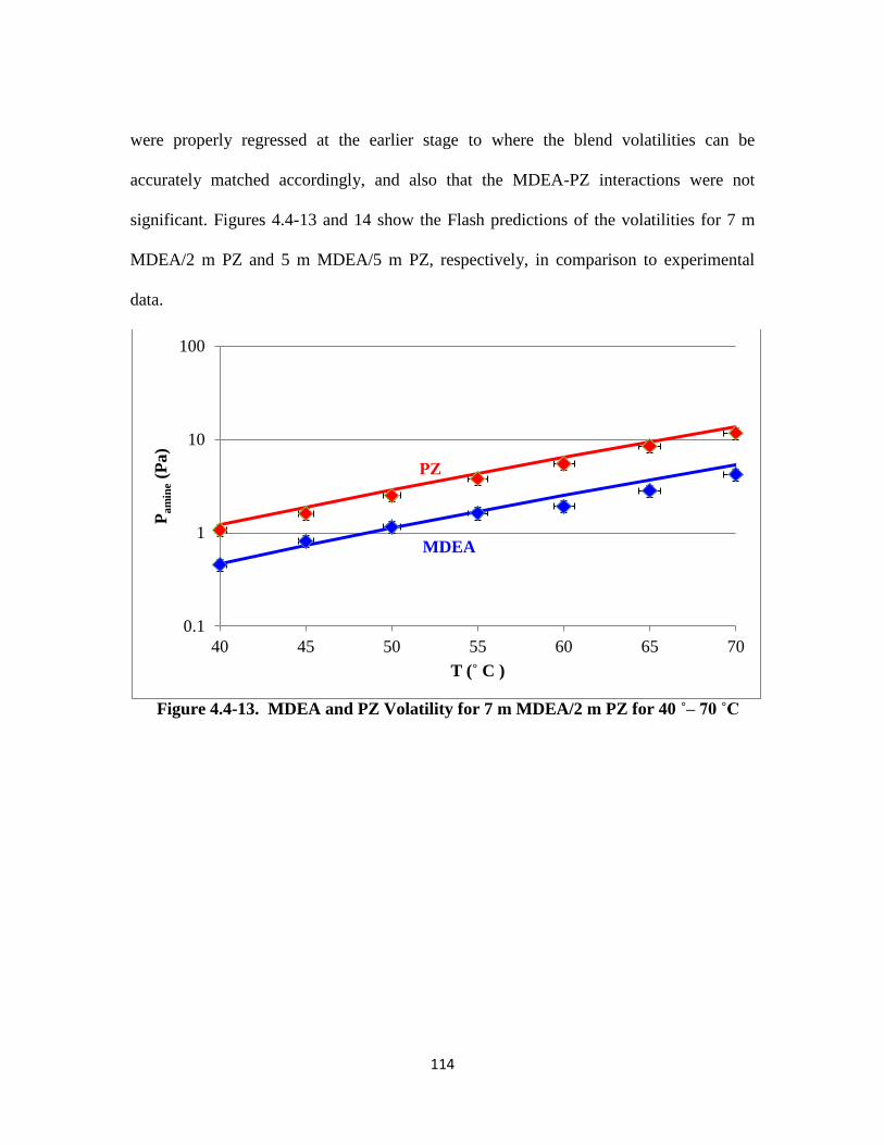
114
were properly regressed at the earlier stage to where the blend volatilities can be
accurately matched accordingly, and also that the MDEA-PZ interactions were not
significant. Figures 4.4-13 and 14 show the Flash predictions of the volatilities for 7 m
MDEA/2 m PZ and 5 m MDEA/5 m PZ, respectively, in comparison to experimental
data.
Figure 4.4-13. MDEA and PZ Volatility for 7 m MDEA/2 m PZ for 40 ˚– 70 ˚C
0.1
1
10
100
40 45 50 55 60 65 70
Pa
min
e (
Pa)
T (˚ C )
MDEA
PZ
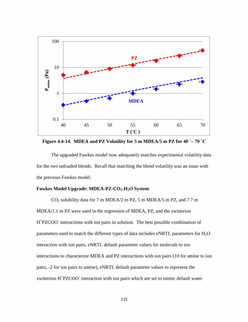
115
Figure 4.4-14. MDEA and PZ Volatility for 5 m MDEA/5 m PZ for 40 ˚– 70 ˚C
The upgraded Fawkes model now adequately matches experimental volatility data
for the two unloaded blends. Recall that matching the blend volatility was an issue with
the previous Fawkes model.
Fawkes Model Upgrade: MDEA-PZ-CO2-H2O System
CO2 solubility data for 7 m MDEA/2 m PZ, 5 m MDEA/5 m PZ, and 7.7 m
MDEA/1.1 m PZ were used in the regression of MDEA, PZ, and the zwitterion
H+PZCOO
- interactions with ion pairs in solution. The best possible combination of
parameters used to match the different types of data includes eNRTL parameters for H2O
interaction with ion pairs, eNRTL default parameter values for molecule to ion
interactions to characterize MDEA and PZ interactions with ion pairs (10 for amine to ion
pairs, -2 for ion pairs to amine), eNRTL default parameter values to represent the
zwitterion H+PZCOO
- interaction with ion pairs which are set to mimic default water
0.1
1
10
100
40 45 50 55 60 65 70
Pa
min
e (
Pa)
T (˚C )
MDEA
PZ
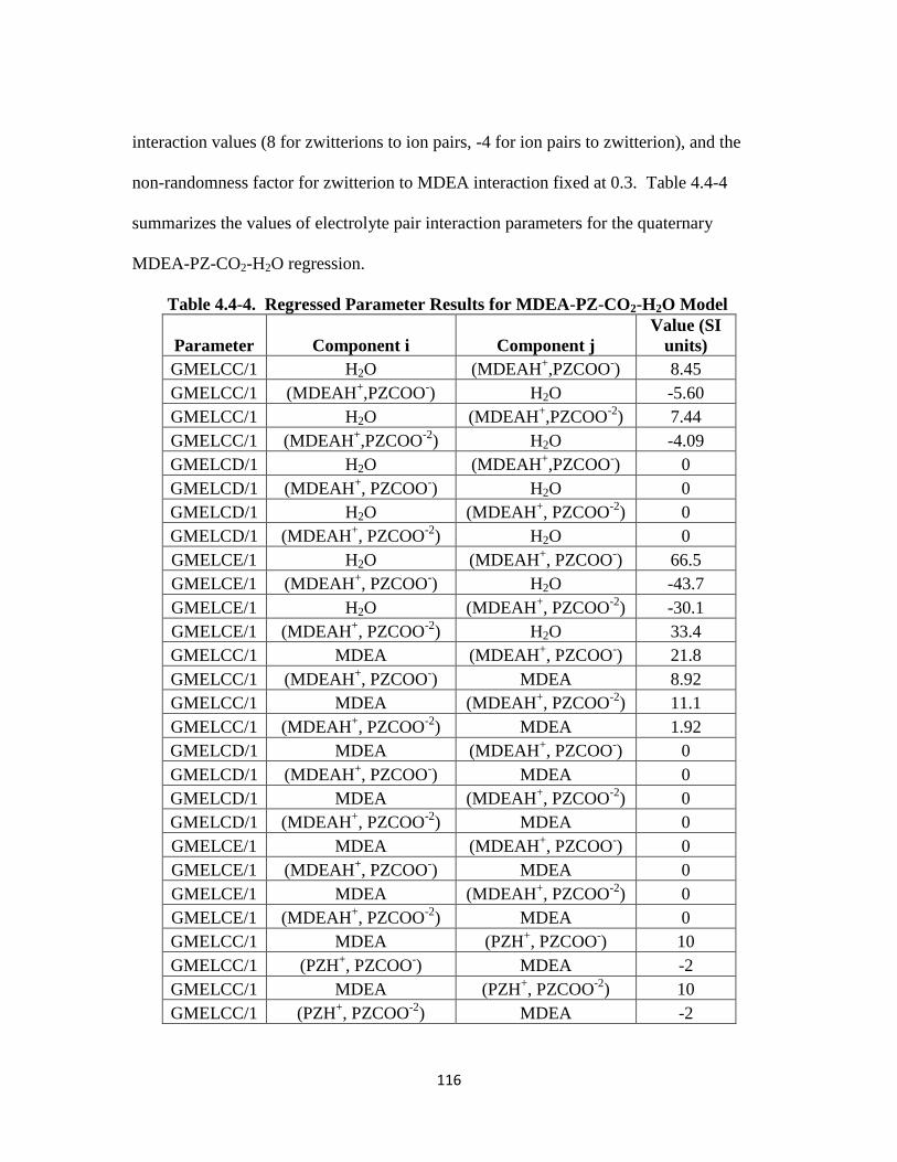
116
interaction values (8 for zwitterions to ion pairs, -4 for ion pairs to zwitterion), and the
non-randomness factor for zwitterion to MDEA interaction fixed at 0.3. Table 4.4-4
summarizes the values of electrolyte pair interaction parameters for the quaternary
MDEA-PZ-CO2-H2O regression.
Table 4.4-4. Regressed Parameter Results for MDEA-PZ-CO2-H2O Model
Parameter Component i Component j
Value (SI
units)
GMELCC/1 H2O (MDEAH+,PZCOO
-) 8.45
GMELCC/1 (MDEAH+,PZCOO
-) H2O -5.60
GMELCC/1 H2O (MDEAH+,PZCOO
-2) 7.44
GMELCC/1 (MDEAH+,PZCOO
-2) H2O -4.09
GMELCD/1 H2O (MDEAH+,PZCOO
-) 0
GMELCD/1 (MDEAH+, PZCOO
-) H2O 0
GMELCD/1 H2O (MDEAH+, PZCOO
-2) 0
GMELCD/1 (MDEAH+, PZCOO
-2) H2O 0
GMELCE/1 H2O (MDEAH+, PZCOO
-) 66.5
GMELCE/1 (MDEAH+, PZCOO
-) H2O -43.7
GMELCE/1 H2O (MDEAH+, PZCOO
-2) -30.1
GMELCE/1 (MDEAH+, PZCOO
-2) H2O 33.4
GMELCC/1 MDEA (MDEAH+, PZCOO
-) 21.8
GMELCC/1 (MDEAH+, PZCOO
-) MDEA 8.92
GMELCC/1 MDEA (MDEAH+, PZCOO
-2) 11.1
GMELCC/1 (MDEAH+, PZCOO
-2) MDEA 1.92
GMELCD/1 MDEA (MDEAH+, PZCOO
-) 0
GMELCD/1 (MDEAH+, PZCOO
-) MDEA 0
GMELCD/1 MDEA (MDEAH+, PZCOO
-2) 0
GMELCD/1 (MDEAH+, PZCOO
-2) MDEA 0
GMELCE/1 MDEA (MDEAH+, PZCOO
-) 0
GMELCE/1 (MDEAH+, PZCOO
-) MDEA 0
GMELCE/1 MDEA (MDEAH+, PZCOO
-2) 0
GMELCE/1 (MDEAH+, PZCOO
-2) MDEA 0
GMELCC/1 MDEA (PZH+, PZCOO
-) 10
GMELCC/1 (PZH+, PZCOO
-) MDEA -2
GMELCC/1 MDEA (PZH+, PZCOO
-2) 10
GMELCC/1 (PZH+, PZCOO
-2) MDEA -2
117
GMELCC/1 MDEA (PZH+,HCO3
-) 10
GMELCC/1 (PZH+, HCO3
-) MDEA -2
GMELCC/1 HPZCOO (MDEAH+, PZCOO
-) 8
GMELCC/1 (MDEAH+, PZCOO
-) HPZCOO -4
GMELCC/1 HPZCOO (MDEAH+, PZCOO
-2) 8
GMELCC/1 (MDEAH+, PZCOO
-2) HPZCOO -4
GMELCC/1 HPZCOO (MDEAH+, HCO3
-) 8
GMELCC/1 (MDEAH+, HCO3
-) HPZCOO -4
GMELCD/1 HPZCOO (MDEAH+, PZCOO
-) 0
GMELCD/1 (MDEAH+, PZCOO
-) HPZCOO 0
GMELCD/1 HPZCOO (MDEAH+, PZCOO
-2) 0
GMELCD/1 (MDEAH+, PZCOO
-2) HPZCOO 0
GMELCD/1 HPZCOO (MDEAH+, HCO3
-) 0
GMELCD/1 (MDEAH+, HCO3
-) HPZCOO 0
GMELCC/1 PZ (MDEAH+, PZCOO
-) 10
GMELCC/1 (MDEAH+, PZCOO
-) PZ -2
GMELCC/1 PZ (MDEAH+, PZCOO
-2) 10
GMELCC/1 (MDEAH+, PZCOO
-2) PZ -2
GMELCC/1 PZ (MDEAH+, HCO3
-) 10
GMELCC/1 (MDEAH+, HCO3
-) PZ -2
NRTL/1 MDEA HPZCOO 0
NRTL/1 HPZCOO MDEA 0
NRTL/2 MDEA HPZCOO 0
NRTL/2 HPZCOO MDEA 0
NRTL/3 HPZCOO MDEA 0.3
Figure 4.4-15 shows the upgraded model predictions for CO2 solubility in
comparison to experimental data for 7 m MDEA/2 m PZ from 40 ˚–160 ˚C.
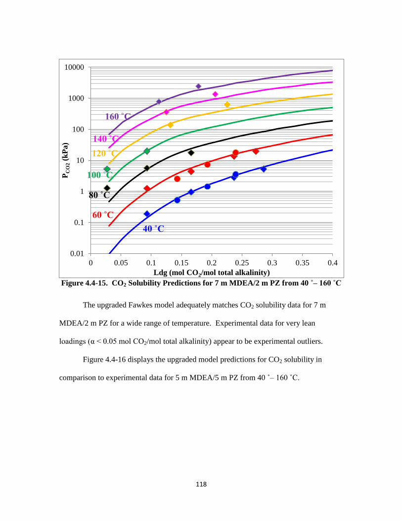
118
Figure 4.4-15. CO2 Solubility Predictions for 7 m MDEA/2 m PZ from 40 ˚– 160 ˚C
The upgraded Fawkes model adequately matches CO2 solubility data for 7 m
MDEA/2 m PZ for a wide range of temperature. Experimental data for very lean
loadings (α < 0.05 mol CO2/mol total alkalinity) appear to be experimental outliers.
Figure 4.4-16 displays the upgraded model predictions for CO2 solubility in
comparison to experimental data for 5 m MDEA/5 m PZ from 40 ˚– 160 ˚C.
0.01
0.1
1
10
100
1000
10000
0 0.05 0.1 0.15 0.2 0.25 0.3 0.35 0.4
PC
O2 (
kP
a)
Ldg (mol CO2/mol total alkalinity)
40 ˚C
60 ˚C
80 ˚C
100 ˚C
120 ˚C
140 ˚C
160 ˚C
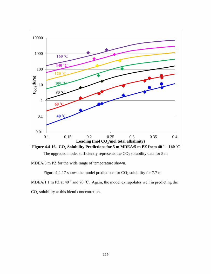
119
Figure 4.4-16. CO2 Solubility Predictions for 5 m MDEA/5 m PZ from 40 ˚ – 160 ˚C
The upgraded model sufficiently represents the CO2 solubility data for 5 m
MDEA/5 m PZ for the wide range of temperature shown.
Figure 4.4-17 shows the model predictions for CO2 solubility for 7.7 m
MDEA/1.1 m PZ at 40 ˚ and 70 ˚C. Again, the model extrapolates well in predicting the
CO2 solubility at this blend concentration.
0.01
0.1
1
10
100
1000
10000
0.1 0.15 0.2 0.25 0.3 0.35 0.4
PC
O2
(k
Pa)
Loading (mol CO2/mol total alkalinity)
40 ˚C
60 ˚C
80 ˚C
100 ˚C
120 ˚C
140 ˚C
160 ˚C
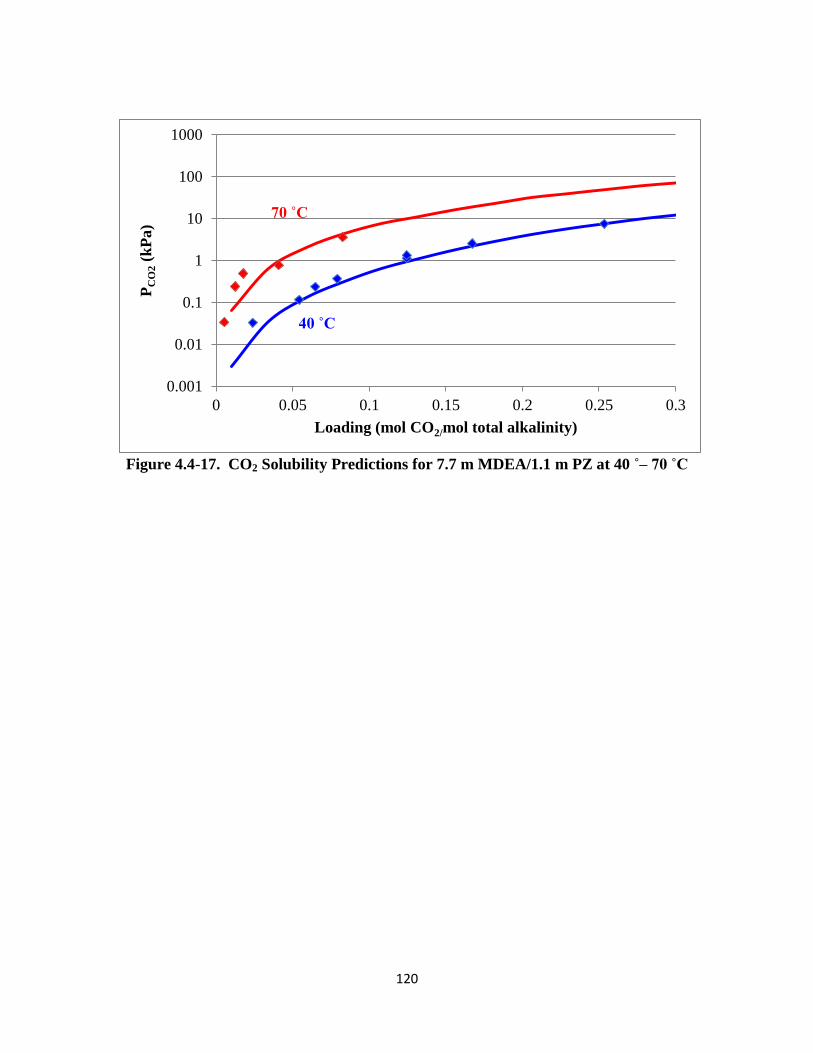
120
Figure 4.4-17. CO2 Solubility Predictions for 7.7 m MDEA/1.1 m PZ at 40 ˚– 70 ˚C
0.001
0.01
0.1
1
10
100
1000
0 0.05 0.1 0.15 0.2 0.25 0.3
PC
O2 (
kP
a)
Loading (mol CO2/mol total alkalinity)
40 ˚C
70 ˚C
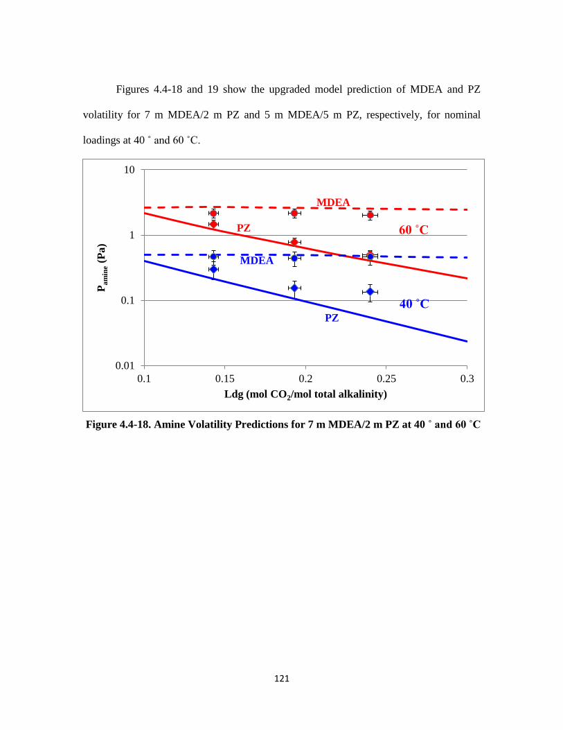
121
Figures 4.4-18 and 19 show the upgraded model prediction of MDEA and PZ
volatility for 7 m MDEA/2 m PZ and 5 m MDEA/5 m PZ, respectively, for nominal
loadings at 40 ˚ and 60 ˚C.
Figure 4.4-18. Amine Volatility Predictions for 7 m MDEA/2 m PZ at 40 ˚ and 60 ˚C
0.01
0.1
1
10
0.1 0.15 0.2 0.25 0.3
Pa
min
e (
Pa)
Ldg (mol CO2/mol total alkalinity)
40 ˚C
60 ˚C
PZ
MDEA
MDEA
PZ
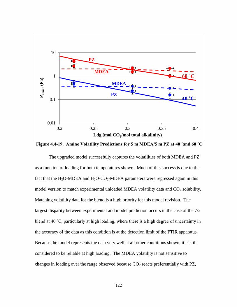
122
Figure 4.4-19. Amine Volatility Predictions for 5 m MDEA/5 m PZ at 40 ˚and 60 ˚C
The upgraded model successfully captures the volatilities of both MDEA and PZ
as a function of loading for both temperatures shown. Much of this success is due to the
fact that the H2O-MDEA and H2O-CO2-MDEA parameters were regressed again in this
model version to match experimental unloaded MDEA volatility data and CO2 solubility.
Matching volatility data for the blend is a high priority for this model revision. The
largest disparity between experimental and model prediction occurs in the case of the 7/2
blend at 40 ˚C, particularly at high loading, where there is a high degree of uncertainty in
the accuracy of the data as this condition is at the detection limit of the FTIR apparatus.
Because the model represents the data very well at all other conditions shown, it is still
considered to be reliable at high loading. The MDEA volatility is not sensitive to
changes in loading over the range observed because CO2 reacts preferentially with PZ,
0.01
0.1
1
10
0.2 0.25 0.3 0.35 0.4
Pa
min
e (
Pa)
Ldg (mol CO2/mol total alkalinity)
40 ˚C
60 ˚C
PZ
MDEA
PZ
MDEA
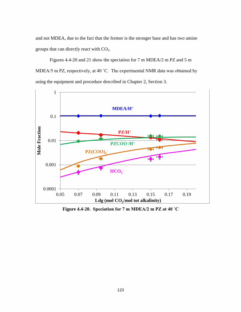
123
and not MDEA, due to the fact that the former is the stronger base and has two amine
groups that can directly react with CO2.
Figures 4.4-20 and 21 show the speciation for 7 m MDEA/2 m PZ and 5 m
MDEA/5 m PZ, respectively, at 40 ˚C. The experimental NMR data was obtained by
using the equipment and procedure described in Chapter 2, Section 3.
Figure 4.4-20. Speciation for 7 m MDEA/2 m PZ at 40 ˚C
0.0001
0.001
0.01
0.1
1
0.05 0.07 0.09 0.11 0.13 0.15 0.17 0.19
Mole
Fra
ctio
n
Ldg (mol CO2/mol tot alkalinity)
MDEA/H+
PZ/H+
PZCOO-/H+
PZ(COO)2-
HCO3-
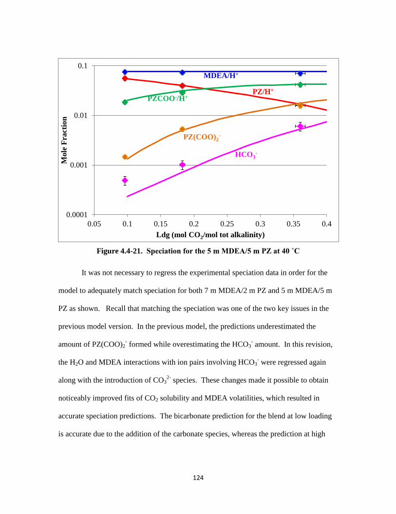
124
Figure 4.4-21. Speciation for the 5 m MDEA/5 m PZ at 40 ˚C
It was not necessary to regress the experimental speciation data in order for the
model to adequately match speciation for both 7 m MDEA/2 m PZ and 5 m MDEA/5 m
PZ as shown. Recall that matching the speciation was one of the two key issues in the
previous model version. In the previous model, the predictions underestimated the
amount of PZ(COO)2- formed while overestimating the HCO3
- amount. In this revision,
the H2O and MDEA interactions with ion pairs involving HCO3- were regressed again
along with the introduction of CO32-
species. These changes made it possible to obtain
noticeably improved fits of CO2 solubility and MDEA volatilities, which resulted in
accurate speciation predictions. The bicarbonate prediction for the blend at low loading
is accurate due to the addition of the carbonate species, whereas the prediction at high
0.0001
0.001
0.01
0.1
0.05 0.1 0.15 0.2 0.25 0.3 0.35 0.4
Mole
Fra
ctio
n
Ldg (mol CO2/mol tot alkalinity)
MDEA/H+
PZ/H+
PZCOO-/H+
PZ(COO)2-
HCO3-
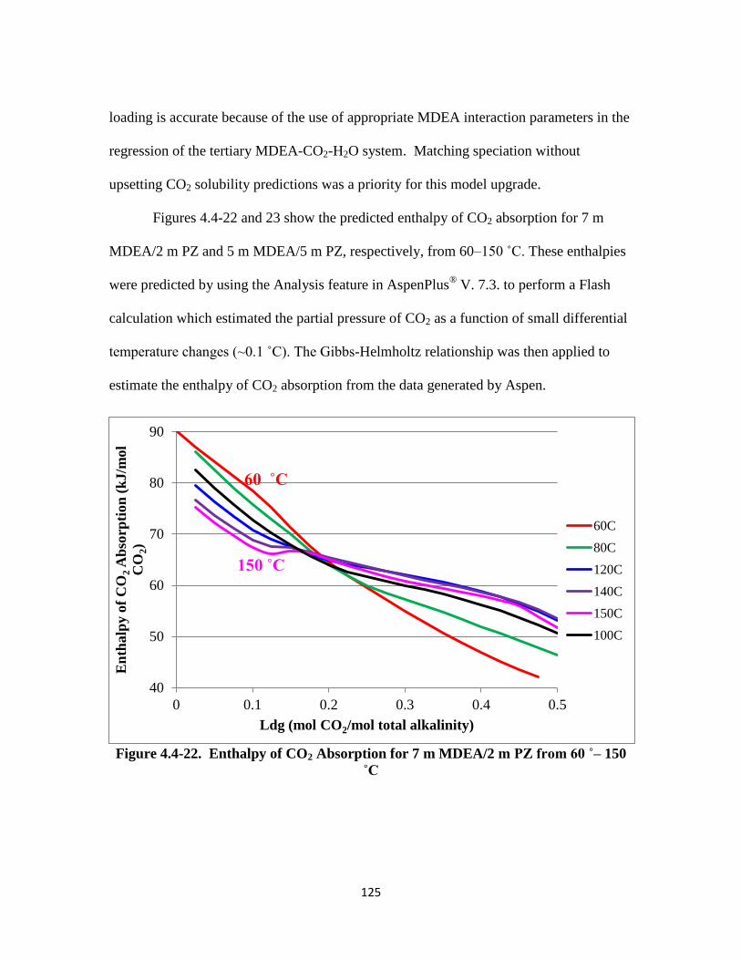
125
loading is accurate because of the use of appropriate MDEA interaction parameters in the
regression of the tertiary MDEA-CO2-H2O system. Matching speciation without
upsetting CO2 solubility predictions was a priority for this model upgrade.
Figures 4.4-22 and 23 show the predicted enthalpy of CO2 absorption for 7 m
MDEA/2 m PZ and 5 m MDEA/5 m PZ, respectively, from 60–150 ˚C. These enthalpies
were predicted by using the Analysis feature in AspenPlus® V. 7.3. to perform a Flash
calculation which estimated the partial pressure of CO2 as a function of small differential
temperature changes (~0.1 ˚C). The Gibbs-Helmholtz relationship was then applied to
estimate the enthalpy of CO2 absorption from the data generated by Aspen.
Figure 4.4-22. Enthalpy of CO2 Absorption for 7 m MDEA/2 m PZ from 60 ˚– 150
˚C
40
50
60
70
80
90
0 0.1 0.2 0.3 0.4 0.5
En
thalp
y o
f C
O2 A
bso
rpti
on
(k
J/m
ol
CO
2)
Ldg (mol CO2/mol total alkalinity)
60C
80C
120C
140C
150C
100C
60 ˚C
150 ˚C

126
Figure 4.4-23. Enthalpy of CO2 Absorption for 5 m MDEA/5 m PZ from 60 ˚ – 150
˚C
There is no experimental data available for the enthalpy of CO2 absorption in
MDEA/PZ system. Nevertheless, the model predicts well-behaved heat of absorption
that match expectations and are internally consistent. For both blends, the enthalpy of
CO2 absorption prediction flips temperature behavior at the critical loading where PZ is
saturated in both systems by stoichiometry (loading ~ 0.18 for 7/2; ~0.33 for 5/5). Before
reaching the critical loading point, CO2 reacts primarily with PZ, not MDEA, in an
exothermic reaction because PZ is a stronger base than MDEA. Since PZ reaction with
CO2 is exothermic, increasing the system temperature would tend to work against this
effect and result in a lower drive for the reaction to occur which is reflected in a smaller
enthalpy of CO2 absorption. This is the reason that absorbers require intercooling to
reduce the column temperature and thereby improving CO2 solubility, a process which
40
50
60
70
80
90
100
0 0.1 0.2 0.3 0.4 0.5
En
thalp
y of
CO
2 A
bso
rpti
on
(k
J/m
ol
CO
2)
Ldg (mol CO2/mol total alkalinity)
60C
80C
100C
120C
140C
150C
60 ˚C
150 ˚C
127
manifests in greater values of enthalpy of absorption. After the critical loading where
most of the PZ is saturated, CO2 now reacts with MDEA instead which has a different
enthalpy of CO2 absorption compared to PZ.
At less than 140 ˚C, the enthalpy of CO2 absorption tends to decrease with
loading because there is less free amine available to react with CO2. At temperature
higher than 140 ˚C, there is a competing effect between speciation and temperature on the
enthalpy of CO2 absorption, with the latter overriding the former, particularly for MDEA
where the reaction with CO2 is less exothermic. This behavior is so strong that it
compensates for the drop in ∆HCO2 due to lack of free amine (PZ); however, if one were
to project past a high enough loading (greater than 0.5), the enthalpy of absorption would
naturally decline again due to the MDEA running out and not being able to react with
CO2. In other words, speciation would dominate again as it tends to overall. Lastly, it
should be noted that predicting the enthalpy of CO2 absorption is not the primary scope
of this work, but is secondary to the needs of matching volatility and speciation. Thus it
is acceptable to end up with the enthalpy of CO2 absorption predictions shown provided
that the speciation and volatility are matched rather well.
Figures 4.4-24 and 25 illustrate the heat capacity predictions for 7 m MDEA/2 m
PZ and 5 m MDEA/5 m PZ, respectively, from 40 ˚- 120 ˚C. The experimental heat
capacity data were obtained by using the equipment and procedure described in Chapter 2
Section 5.
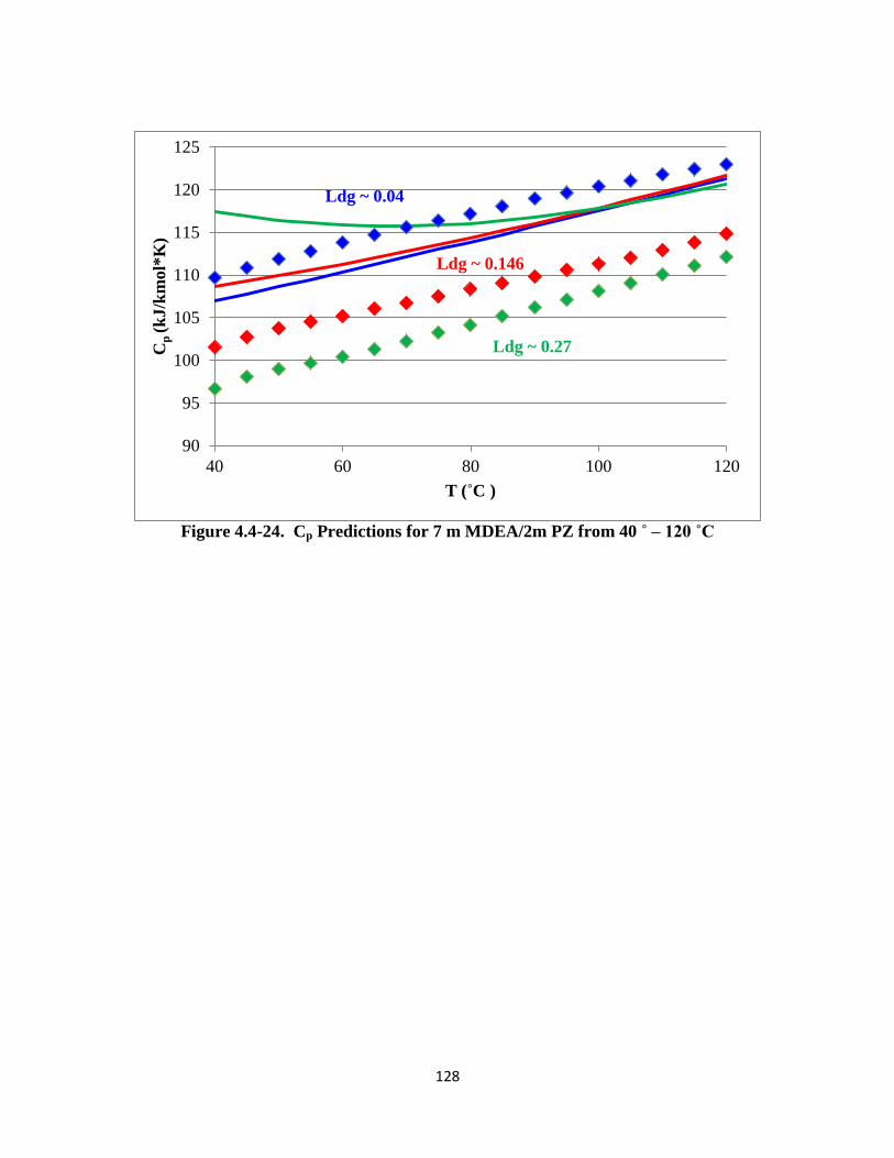
128
Figure 4.4-24. Cp Predictions for 7 m MDEA/2m PZ from 40 ˚ – 120 ˚C
90
95
100
105
110
115
120
125
40 60 80 100 120
Cp
(k
J/k
mol*
K)
T (˚C )
Ldg ~ 0.04
Ldg ~ 0.146
Ldg ~ 0.27
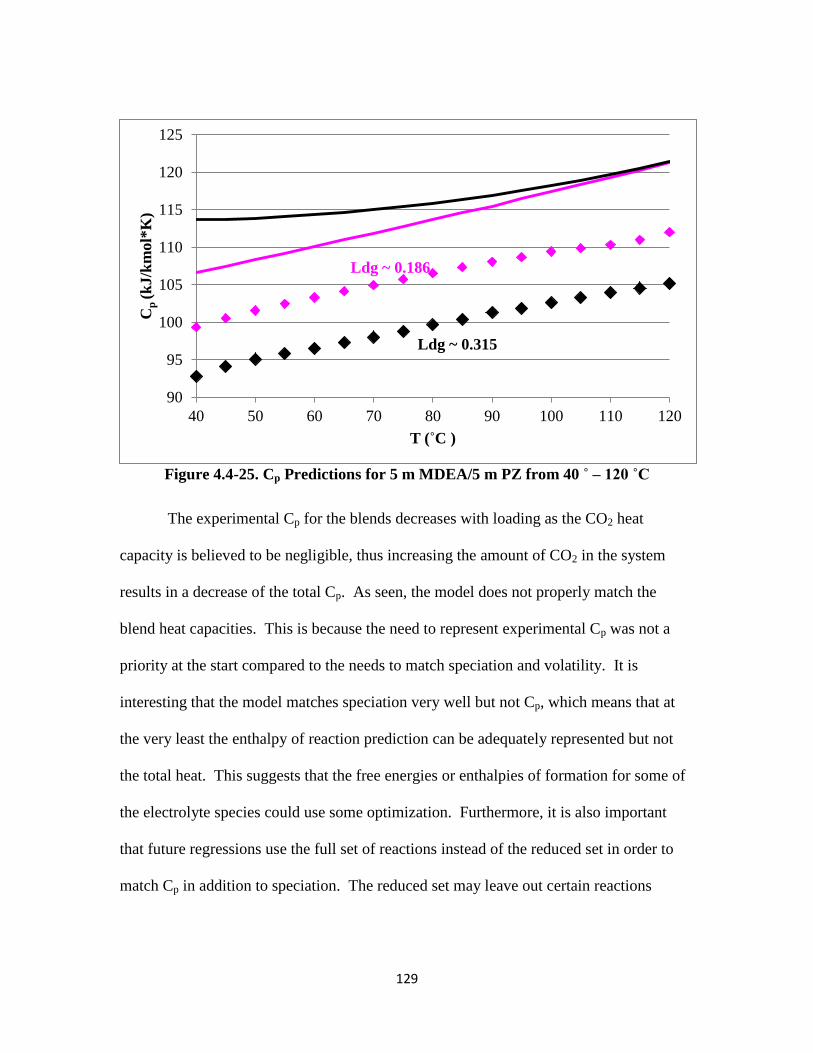
129
Figure 4.4-25. Cp Predictions for 5 m MDEA/5 m PZ from 40 ˚ – 120 ˚C
The experimental Cp for the blends decreases with loading as the CO2 heat
capacity is believed to be negligible, thus increasing the amount of CO2 in the system
results in a decrease of the total Cp. As seen, the model does not properly match the
blend heat capacities. This is because the need to represent experimental Cp was not a
priority at the start compared to the needs to match speciation and volatility. It is
interesting that the model matches speciation very well but not Cp, which means that at
the very least the enthalpy of reaction prediction can be adequately represented but not
the total heat. This suggests that the free energies or enthalpies of formation for some of
the electrolyte species could use some optimization. Furthermore, it is also important
that future regressions use the full set of reactions instead of the reduced set in order to
match Cp in addition to speciation. The reduced set may leave out certain reactions
90
95
100
105
110
115
120
125
40 50 60 70 80 90 100 110 120
Cp
(k
J/k
mol*
K)
T (˚C )
Ldg ~ 0.186
Ldg ~ 0.315

130
which may be highly relevant to capturing the system heat capacities though they may
not be significant enough to impact speciation.
4.5. Conclusions
In order to upgrade the existing Fawkes MDEA-PZ-CO2-H2O thermodynamic
model, it was necessary to remodel each subsystem within the blend starting with the
simplest subsystem and then building up to more complex subsystems.
For MDEA-H2O, both the MDEA volatility and Cp for 1.7–13.9 m MDEA-H2O
from 5 ˚– 95 ˚C (a total of over 250 points) were adequately fitted using 4 Henry’s
parameters and 4 binary NRTL parameters. The MDEA-H2O interaction has a
temperature dependence whereas the H2O-MDEA interaction does not in this regression
case.
For MDEA-CO2-H2O, the introduction of the carbonate species into the Fawkes
MDEA-CO2-H2O chemistry set allowed for an improved fit of CO2 solubility at ultra lean
loadings (0.001 < α < 0.01). The CO2 solubility for 2.8 m–8.4 m MDEA-CO2-H2O from
25˚ – 120 ˚C, Cp for nominal MDEA concentrations, and loaded MDEA volatility were
fitted very well using the free energy and enthalpy of MDEAH+ species along with all of
the pair parameters.
For MDEA-PZ-H2O subsystem, amine volatilities can be represented success-
fully without the need to regress any additional cross parameter for MDEA-PZ
interaction.
For MDEA-PZ-CO2-H2O, the best possible combination of parameters used to
represent the system includes: NRTL parameters for H2O interaction with ion pairs,

131
NRTL default parameter values for molecule to ion interactions to characterize MDEA
and PZ interactions with ion pairs (10 for amine to ion pairs, -2 for ion pairs to amine),
NRTL default parameter values to represent the zwitterion H+PZCOO
- interaction with
ion pairs which are set to mimic default water interaction parameter values (8 for
zwitterions to ion pairs, -4 for ion pairs to zwitterion), and the non-randomness factor for
the zwitterion to MDEA interaction fixed at 0.3. Both the amine volatility and speciation
for loaded 7/2 and 5/5 MDEA/PZ are successfully matched using the upgraded model.
Finally, it was seen that the upgraded model predicts rather well-behaved enthalpy
of CO2 absorption for the 7/2 blend but not for the 5/5 blend even though the general
temperature behaviors are represented as expected. Thus the upgraded model can be used
to qualitatively determine the enthalpy of CO2 absorption behaviors with respect to
loading and temperature. In regard to Cp, the new model was not able to capture the effect
of loading on Cp for a given temperature range. Recall that the original focus of this
work was given to matching volatility and speciation of the blend not so much Cp. In
order to improve the Cp fits, it is important to: (1) optimize the Gibbs energy and
enthalpies of formation for the electrolyte species and (2) perhaps use a full set of
reactions instead of the reduced set in future regression cases because the latter might
have possibly omitted certain reactions that maybe highly relevant to Cp even though they
may not be that significant to fitting speciation.
132
Chapter 5: MDEA/PZ Behavior & Generalized Amine Screening
5.1. Introduction
A number of novel amines were screened for amine volatility at nominal lean
loading to determine their viabilities for CO2 capture. Other amine characteristics,
including CO2 capture capacity, reaction rate, and resistance to oxidative and thermal
degradation, have been screened by other researchers. In addition to the need to screen
for amine volatility, it is also important to explore the VLE of novel amine systems to
generalize amine solution behavior in terms of activity coefficients. The trends in amine
activity coefficients can be further attributed to speciation, temperature, and the
phenomenon where the amine is being “salted out” due to its interactions with
surrounding electrolytes.
In this work, detailed analyses of activity coefficient behavior for PZ-CO2-H2O (8
– 10 m loaded PZ) and for MDEA-PZ-CO2-H2O (loaded 7 m MDEA/2 m PZ and 5 m
MDEA/5 m PZ) are used as the basis for interpreting the behavior of novel amines.
Other amine systems screened include loaded MEA, MDEA, EDA, AMP, PZ/2-MPZ,
and PZ/AMP. MDEA as a tertiary amine is known for its high CO2 capture capacity.
Blending MDEA with PZ serves to avoid PZ precipitation while taking advantage of fast
PZ kinetics. EDA, like PZ and any other diamine, was chosen for its high CO2 capacity
with two amine groups to react with CO2. EDA systems also have a high enthalpy of
CO2 absorption which is considered a favorable characteristic. In theory, a high enthalpy
of CO2 absorption results in high CO2 partial pressure at stripper conditions to reduce the
133
work needed for CO2 compression. Finally, AMP was also chosen for its high CO2
capture capacity since it is a hindered amine.
5.2. Theory
The amine liquid phase activity coefficient is defined by Henry’s Law as follows:
(5-1)
where:
Φamine is the amine fugacity coefficient
Pamine is the amine partial pressure (Pa)
xamine is the amine liquid phase mole fraction
Hamine is the amine Henry’s constant at a given temperature (Pa)
γamine is the asymmetric amine activity coefficient – defined at a reference state of
infinite dilution of amine in water
Since the total system pressure is atmospheric (low pressure), the vapor phase is
considered to be ideal; thus, no pressure correction is needed for the vapor phase. The
fugacity coefficient is ϕamine = 1.
The enthalpy of amine absorption can be estimated from the temperature
derivative of the amine partial pressure:
(
( ⁄
(5-2)
where:
Pamine is the amine volatility or partial pressure (Pa)
∆Habsorption is the enthalpy of amine absorption (J/mol amine)
Given that the existing system thermodynamics are anchored on the Henry’s
constant (referenced to infinite dilution of amine in water), the enthalpy of amine
absorption is the sum of three individual enthalpy contributions as follows:
∆Habsorption = ∆Hsolution + ∆Hreaction + ∆Hexcess (5-3)
where:

134
∆Hsolution is the enthalpy associated with dissolving amine in water at infinite
dilution (J/mol amine)
∆Hreaction is the enthalpy of reacting amine, water, and CO2 to form products
(J/mol amine)
∆Hexcess is the enthalpy associated with the non-ideality of the system (J/mol
amine)
Given the enthalpy of amine absorption at different loading and the associated
excess enthalpy, one can deduce the enthalpy of reaction by difference. Detailed analysis
of these enthalpy contributions will be provided for PZ and MDEA/PZ in the Results &
Discussion section.
The enthalpy of amine solution is given by:
(
( ⁄
(5-4)
where:
Hamine is the amine Henry’s constant (Pa)
R is the universal gas constant, 8.314 J/mol*K
The excess enthalpy of an amine can be determined as follows:
(
( ⁄ =
(5-5)
where:
γamine is the asymmetric amine activity coefficient
5.3. Data
Tables 5.3-1 through 5.3-9 show the amine volatility measured in the FTIR
apparatus for 7 m MEA-CO2-H2O, 7 m MDEA-CO2-H2O, 8 m PZ-CO2-H2O, 8 m EDA-
CO2-H2O, 4.8 m AMP-CO2-H2O, 7 m MDEA-2 m PZ-CO2-H2O, 5 m MDEA-5 m PZ-
CO2-H2O, 4 m PZ-4 m 2-MPZ-CO2-H2O, 2.3 m AMP-5 m PZ-CO2-H2O systems at
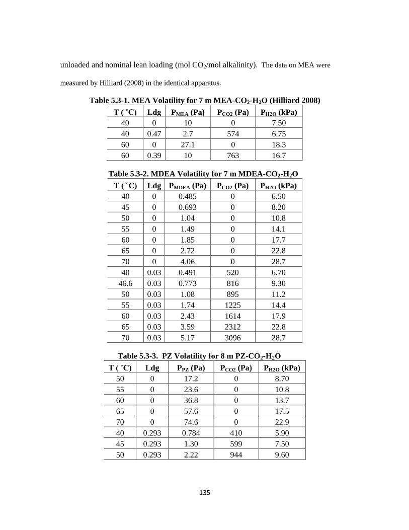
135
unloaded and nominal lean loading (mol CO2/mol alkalinity). The data on MEA were
measured by Hilliard (2008) in the identical apparatus.
Table 5.3-1. MEA Volatility for 7 m MEA-CO2-H2O (Hilliard 2008)
T ( ˚C) Ldg PMEA (Pa) PCO2 (Pa) PH2O (kPa)
40 0 10 0 7.50
40 0.47 2.7 574 6.75
60 0 27.1 0 18.3
60 0.39 10 763 16.7
Table 5.3-2. MDEA Volatility for 7 m MDEA-CO2-H2O
T ( ˚C) Ldg PMDEA (Pa) PCO2 (Pa) PH2O (kPa)
40 0 0.485 0 6.50
45 0 0.693 0 8.20
50 0 1.04 0 10.8
55 0 1.49 0 14.1
60 0 1.85 0 17.7
65 0 2.72 0 22.8
70 0 4.06 0 28.7
40 0.03 0.491 520 6.70
46.6 0.03 0.773 816 9.30
50 0.03 1.08 895 11.2
55 0.03 1.74 1225 14.4
60 0.03 2.43 1614 17.9
65 0.03 3.59 2312 22.8
70 0.03 5.17 3096 28.7
Table 5.3-3. PZ Volatility for 8 m PZ-CO2-H2O
T ( ˚C) Ldg PPZ (Pa) PCO2 (Pa) PH2O (kPa)
50 0 17.2 0 8.70
55 0 23.6 0 10.8
60 0 36.8 0 13.7
65 0 57.6 0 17.5
70 0 74.6 0 22.9
40 0.293 0.784 410 5.90
45 0.293 1.30 599 7.50
50 0.293 2.22 944 9.60
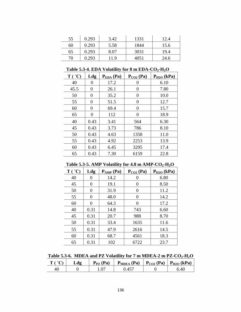
136
55 0.293 3.42 1331 12.4
60 0.293 5.58 1844 15.6
65 0.293 8.07 3031 19.4
70 0.293 11.9 4051 24.6
Table 5.3-4. EDA Volatility for 8 m EDA-CO2-H2O
T ( ˚C) Ldg PEDA (Pa) PCO2 (Pa) PH2O (kPa)
40 0 17.2 0 6.10
45.5 0 26.1 0 7.80
50 0 35.2 0 10.0
55 0 51.5 0 12.7
60 0 69.4 0 15.7
65 0 112 0 18.9
40 0.43 3.41 564 6.30
45 0.43 3.73 786 8.10
50 0.43 4.63 1358 11.0
55 0.43 4.92 2253 13.9
60 0.43 6.45 3295 17.4
65 0.43 7.30 6159 22.8
Table 5.3-5. AMP Volatility for 4.8 m AMP-CO2-H2O
T ( ˚C) Ldg PAMP (Pa) PCO2 (Pa) PH2O (kPa)
40 0 14.2 0 6.80
45 0 19.1 0 8.50
50 0 31.9 0 11.2
55 0 48.0 0 14.2
60 0 64.3 0 17.2
40 0.31 14.8 743 6.60
45 0.31 20.7 988 8.70
50 0.31 33.4 1635 11.6
55 0.31 47.9 2616 14.5
60 0.31 68.7 4561 18.3
65 0.31 102 6722 23.7
Table 5.3-6. MDEA and PZ Volatility for 7 m MDEA-2 m PZ-CO2-H2O
T ( ˚C) Ldg PPZ (Pa) PMDEA (Pa) PCO2 (Pa) PH2O (kPa)
40 0 1.07 0.457 0 6.40
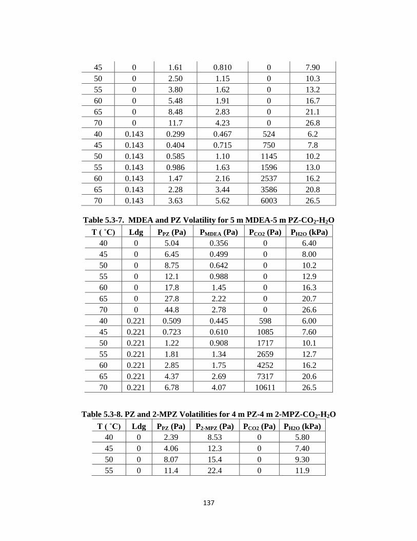
137
45 0 1.61 0.810 0 7.90
50 0 2.50 1.15 0 10.3
55 0 3.80 1.62 0 13.2
60 0 5.48 1.91 0 16.7
65 0 8.48 2.83 0 21.1
70 0 11.7 4.23 0 26.8
40 0.143 0.299 0.467 524 6.2
45 0.143 0.404 0.715 750 7.8
50 0.143 0.585 1.10 1145 10.2
55 0.143 0.986 1.63 1596 13.0
60 0.143 1.47 2.16 2537 16.2
65 0.143 2.28 3.44 3586 20.8
70 0.143 3.63 5.62 6003 26.5
Table 5.3-7. MDEA and PZ Volatility for 5 m MDEA-5 m PZ-CO2-H2O
T ( ˚C) Ldg PPZ (Pa) PMDEA (Pa) PCO2 (Pa) PH2O (kPa)
40 0 5.04 0.356 0 6.40
45 0 6.45 0.499 0 8.00
50 0 8.75 0.642 0 10.2
55 0 12.1 0.988 0 12.9
60 0 17.8 1.45 0 16.3
65 0 27.8 2.22 0 20.7
70 0 44.8 2.78 0 26.6
40 0.221 0.509 0.445 598 6.00
45 0.221 0.723 0.610 1085 7.60
50 0.221 1.22 0.908 1717 10.1
55 0.221 1.81 1.34 2659 12.7
60 0.221 2.85 1.75 4252 16.2
65 0.221 4.37 2.69 7317 20.6
70 0.221 6.78 4.07 10611 26.5
Table 5.3-8. PZ and 2-MPZ Volatilities for 4 m PZ-4 m 2-MPZ-CO2-H2O
T ( ˚C) Ldg PPZ (Pa) P2-MPZ (Pa) PCO2 (Pa) PH2O (kPa)
40 0 2.39 8.53 0 5.80
45 0 4.06 12.3 0 7.40
50 0 8.07 15.4 0 9.30
55 0 11.4 22.4 0 11.9
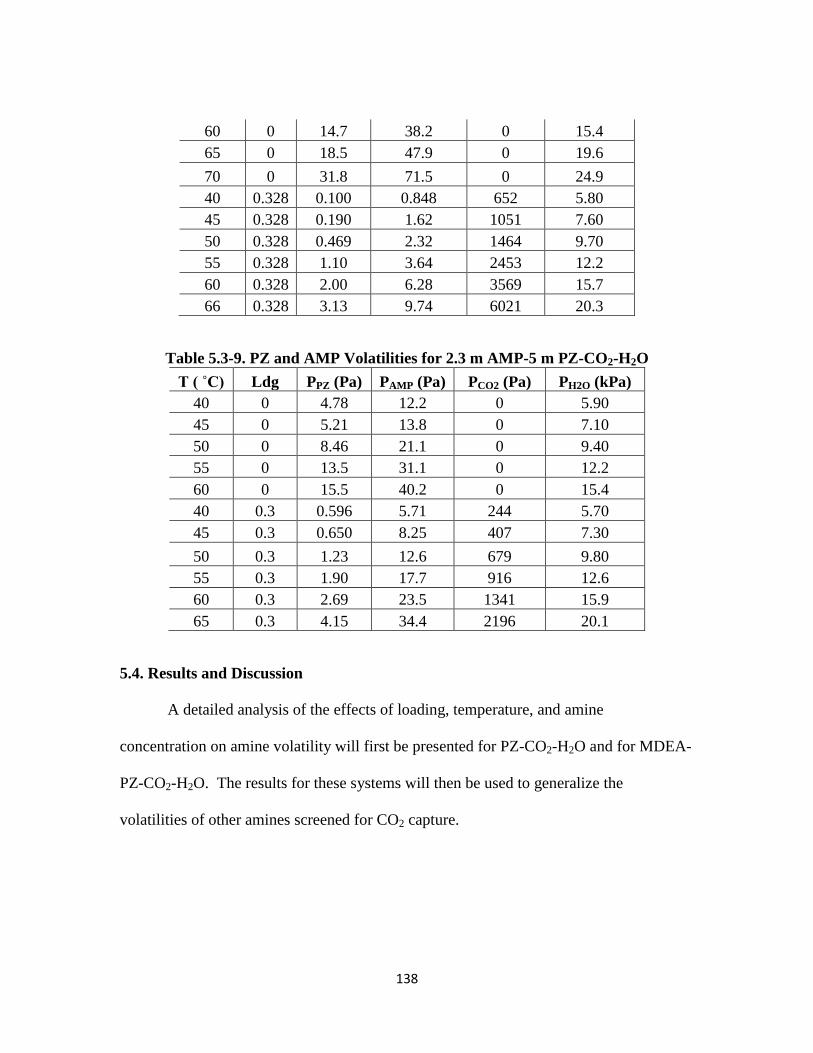
138
60 0 14.7 38.2 0 15.4
65 0 18.5 47.9 0 19.6
70 0 31.8 71.5 0 24.9
40 0.328 0.100 0.848 652 5.80
45 0.328 0.190 1.62 1051 7.60
50 0.328 0.469 2.32 1464 9.70
55 0.328 1.10 3.64 2453 12.2
60 0.328 2.00 6.28 3569 15.7
66 0.328 3.13 9.74 6021 20.3
Table 5.3-9. PZ and AMP Volatilities for 2.3 m AMP-5 m PZ-CO2-H2O
T ( ˚C) Ldg PPZ (Pa) PAMP (Pa) PCO2 (Pa) PH2O (kPa)
40 0 4.78 12.2 0 5.90
45 0 5.21 13.8 0 7.10
50 0 8.46 21.1 0 9.40
55 0 13.5 31.1 0 12.2
60 0 15.5 40.2 0 15.4
40 0.3 0.596 5.71 244 5.70
45 0.3 0.650 8.25 407 7.30
50 0.3 1.23 12.6 679 9.80
55 0.3 1.90 17.7 916 12.6
60 0.3 2.69 23.5 1341 15.9
65 0.3 4.15 34.4 2196 20.1
5.4. Results and Discussion
A detailed analysis of the effects of loading, temperature, and amine
concentration on amine volatility will first be presented for PZ-CO2-H2O and for MDEA-
PZ-CO2-H2O. The results for these systems will then be used to generalize the
volatilities of other amines screened for CO2 capture.
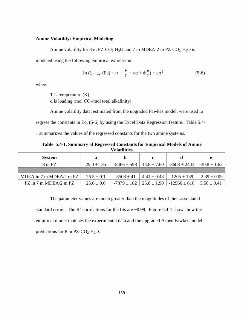
139
Amine Volatility: Empirical Modeling
Amine volatility for 8 m PZ-CO2-H2O and 7 m MDEA-2 m PZ-CO2-H2O is
modeled using the following empirical expression:
(Pa) =
+ cα + d(
+ e (5-6)
where:
T is temperature (K)
α is loading (mol CO2/mol total alkalinity)
Amine volatility data, estimated from the upgraded Fawkes model, were used to
regress the constants in Eq. (5-6) by using the Excel Data Regression feature. Table 5.4-
1 summarizes the values of the regressed constants for the two amine systems.
Table 5.4-1. Summary of Regressed Constants for Empirical Models of Amine
Volatilities
System a b c d e
8 m PZ 29.0 ±1.85 -8466 ± 598 14.8 ± 7.60 -3608 ± 2443 -30.8 ± 1.62
MDEA in 7 m MDEA/2 m PZ 26.5 ± 0.1 -8508 ± 41 4.41 ± 0.43 -1205 ± 139 -2.89 ± 0.09
PZ in 7 m MDEA/2 m PZ 25.6 ± 0.6 -7879 ± 182 25.8 ± 1.90 -12966 ± 616 5.58 ± 0.41
The parameter values are much greater than the magnitudes of their associated
standard errors. The R2 correlations for the fits are ~0.99. Figure 5.4-1 shows how the
empirical model matches the experimental data and the upgraded Aspen Fawkes model
predictions for 8 m PZ-CO2-H2O.
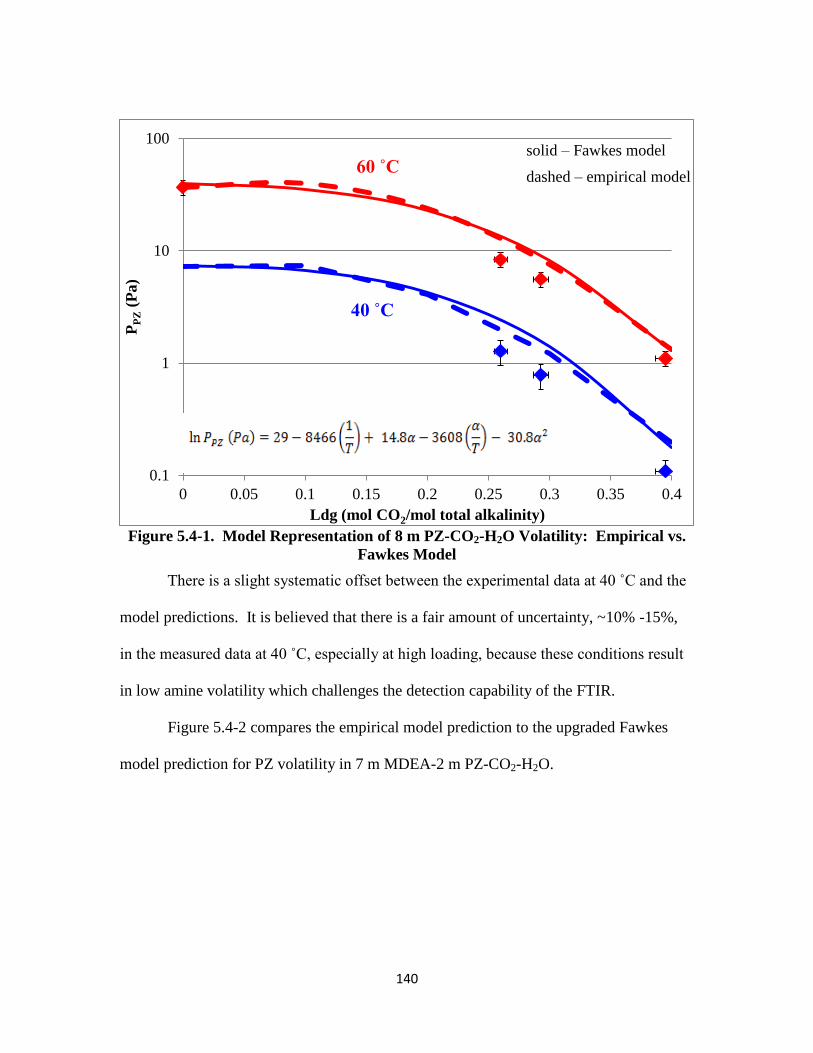
140
Figure 5.4-1. Model Representation of 8 m PZ-CO2-H2O Volatility: Empirical vs.
Fawkes Model
There is a slight systematic offset between the experimental data at 40 ˚C and the
model predictions. It is believed that there is a fair amount of uncertainty, ~10% -15%,
in the measured data at 40 ˚C, especially at high loading, because these conditions result
in low amine volatility which challenges the detection capability of the FTIR.
Figure 5.4-2 compares the empirical model prediction to the upgraded Fawkes
model prediction for PZ volatility in 7 m MDEA-2 m PZ-CO2-H2O.
0.1
1
10
100
0 0.05 0.1 0.15 0.2 0.25 0.3 0.35 0.4
PP
Z (
Pa)
Ldg (mol CO2/mol total alkalinity)
40 ˚C
60 ˚C solid – Fawkes model
dashed – empirical model
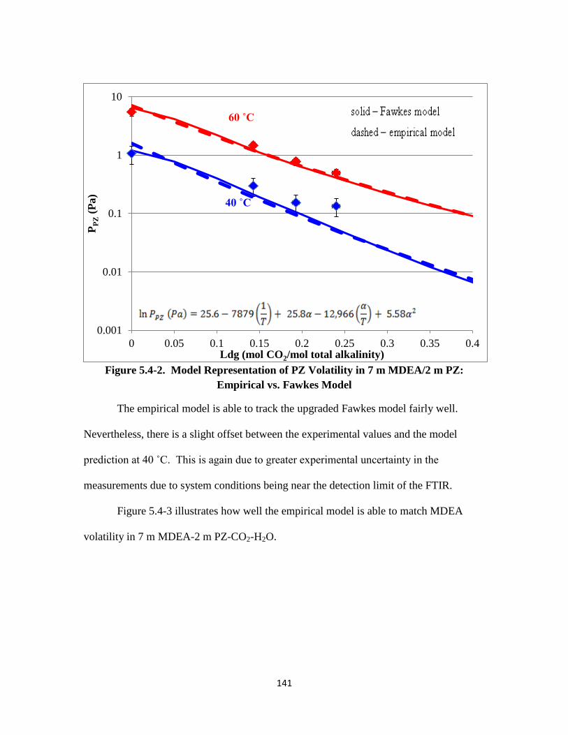
141
Figure 5.4-2. Model Representation of PZ Volatility in 7 m MDEA/2 m PZ:
Empirical vs. Fawkes Model
The empirical model is able to track the upgraded Fawkes model fairly well.
Nevertheless, there is a slight offset between the experimental values and the model
prediction at 40 ˚C. This is again due to greater experimental uncertainty in the
measurements due to system conditions being near the detection limit of the FTIR.
Figure 5.4-3 illustrates how well the empirical model is able to match MDEA
volatility in 7 m MDEA-2 m PZ-CO2-H2O.
0.001
0.01
0.1
1
10
0 0.05 0.1 0.15 0.2 0.25 0.3 0.35 0.4
PP
Z (
Pa)
Ldg (mol CO2/mol total alkalinity)
40 ˚C
60 ˚C
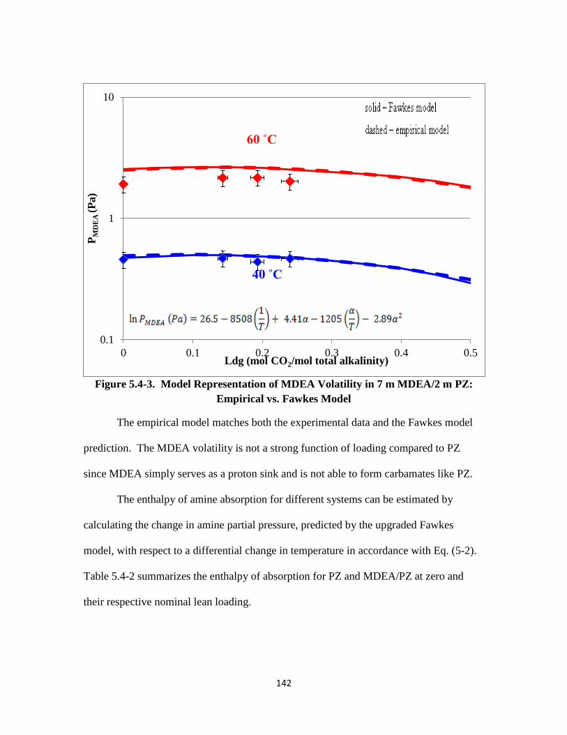
142
Figure 5.4-3. Model Representation of MDEA Volatility in 7 m MDEA/2 m PZ:
Empirical vs. Fawkes Model
The empirical model matches both the experimental data and the Fawkes model
prediction. The MDEA volatility is not a strong function of loading compared to PZ
since MDEA simply serves as a proton sink and is not able to form carbamates like PZ.
The enthalpy of amine absorption for different systems can be estimated by
calculating the change in amine partial pressure, predicted by the upgraded Fawkes
model, with respect to a differential change in temperature in accordance with Eq. (5-2).
Table 5.4-2 summarizes the enthalpy of absorption for PZ and MDEA/PZ at zero and
their respective nominal lean loading.
0.1
1
10
0 0.1 0.2 0.3 0.4 0.5
PM
DE
A (
Pa)
Ldg (mol CO2/mol total alkalinity)
40 ˚C
60 ˚C
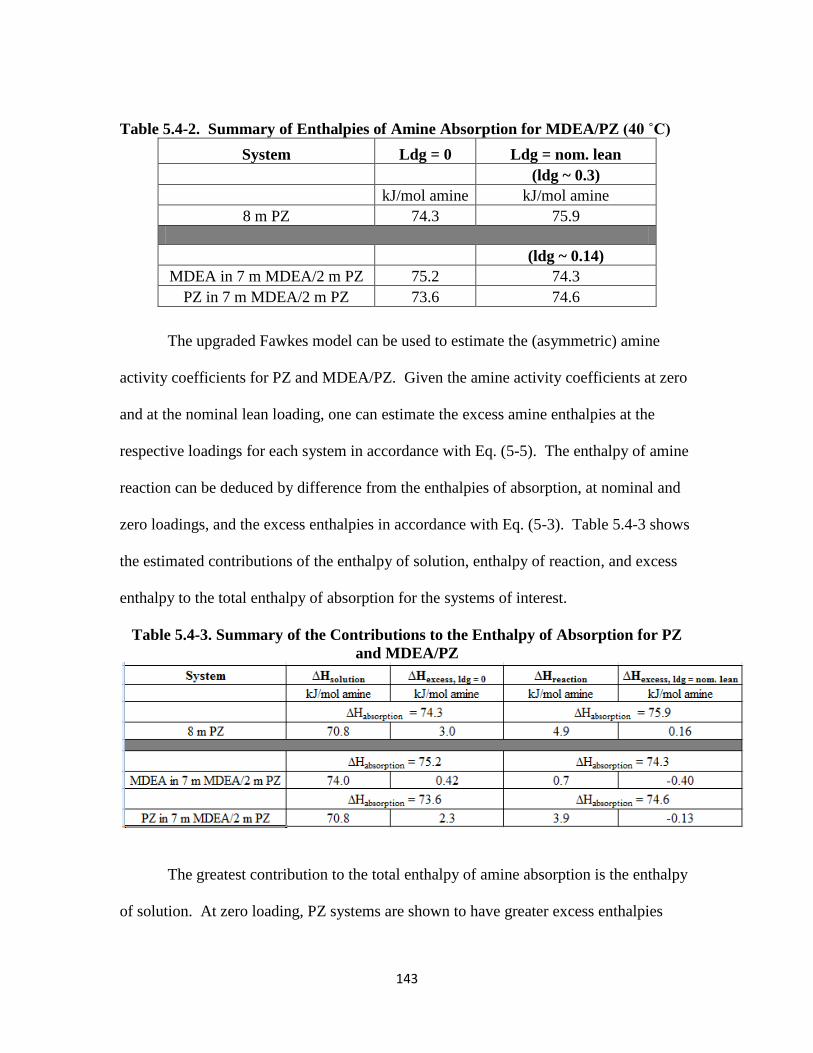
143
Table 5.4-2. Summary of Enthalpies of Amine Absorption for MDEA/PZ (40 ˚C)
System Ldg = 0 Ldg = nom. lean
(ldg ~ 0.3)
kJ/mol amine kJ/mol amine
8 m PZ 74.3 75.9
(ldg ~ 0.14)
MDEA in 7 m MDEA/2 m PZ 75.2 74.3
PZ in 7 m MDEA/2 m PZ 73.6 74.6
The upgraded Fawkes model can be used to estimate the (asymmetric) amine
activity coefficients for PZ and MDEA/PZ. Given the amine activity coefficients at zero
and at the nominal lean loading, one can estimate the excess amine enthalpies at the
respective loadings for each system in accordance with Eq. (5-5). The enthalpy of amine
reaction can be deduced by difference from the enthalpies of absorption, at nominal and
zero loadings, and the excess enthalpies in accordance with Eq. (5-3). Table 5.4-3 shows
the estimated contributions of the enthalpy of solution, enthalpy of reaction, and excess
enthalpy to the total enthalpy of absorption for the systems of interest.
Table 5.4-3. Summary of the Contributions to the Enthalpy of Absorption for PZ
and MDEA/PZ
The greatest contribution to the total enthalpy of amine absorption is the enthalpy
of solution. At zero loading, PZ systems are shown to have greater excess enthalpies
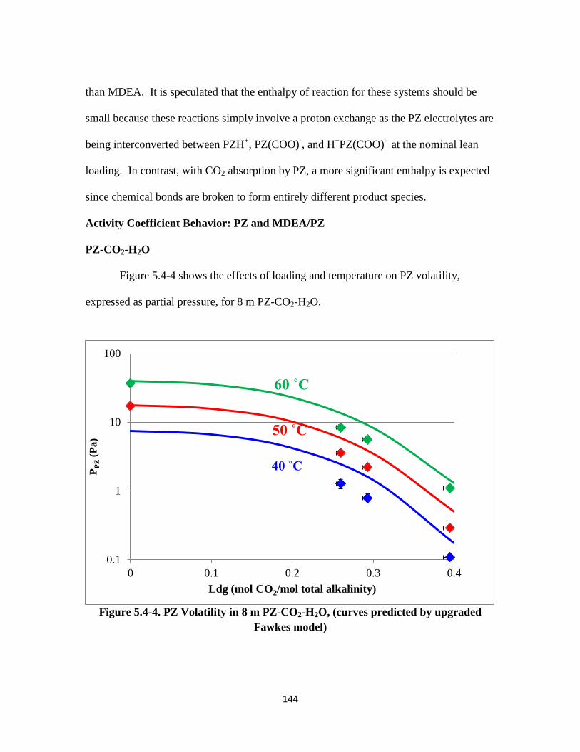
144
than MDEA. It is speculated that the enthalpy of reaction for these systems should be
small because these reactions simply involve a proton exchange as the PZ electrolytes are
being interconverted between PZH+, PZ(COO)
-, and H
+PZ(COO)
- at the nominal lean
loading. In contrast, with CO2 absorption by PZ, a more significant enthalpy is expected
since chemical bonds are broken to form entirely different product species.
Activity Coefficient Behavior: PZ and MDEA/PZ
PZ-CO2-H2O
Figure 5.4-4 shows the effects of loading and temperature on PZ volatility,
expressed as partial pressure, for 8 m PZ-CO2-H2O.
Figure 5.4-4. PZ Volatility in 8 m PZ-CO2-H2O, (curves predicted by upgraded
Fawkes model)
0.1
1
10
100
0 0.1 0.2 0.3 0.4
PP
Z (
Pa)
Ldg (mol CO2/mol total alkalinity)
40 ˚C
50 ˚C
60 ˚C

145
PZ volatility, or its partial pressure, decreases steadily as loading is increased because
there is less free PZ available with greater CO2 consumption. The majority of the
original PZ present is now converted into a number of PZ product species, or electrolytes,
such as PZH+, PZ(COO)
-, PZ(COO)2
-2.
Figure 5.4-5 illustrates how PZ volatility in PZ-CO2-H2O varies with PZ
concentration at a constant temperature (40 ˚C).
Figure 5.4-5. PZ Volatility for 8 m, 10 m, 20 m PZ-CO2-H2O at 40 ˚C (curves
predicted by upgraded Fawkes model)
PZ partial pressure increases with increasing PZ due to more free PZ being
available. Also, as discussed previously, at a given PZ concentration, PZ volatility
decreases with greater loading due to less free PZ available for volatilization.
1
10
100
1000
0 0.05 0.1 0.15 0.2 0.25 0.3 0.35 0.4
PP
Z (
Pa)
Ldg (mol CO2/mol total alkalinity)
8 m PZ
10 m PZ
20 m PZ
40 ˚C
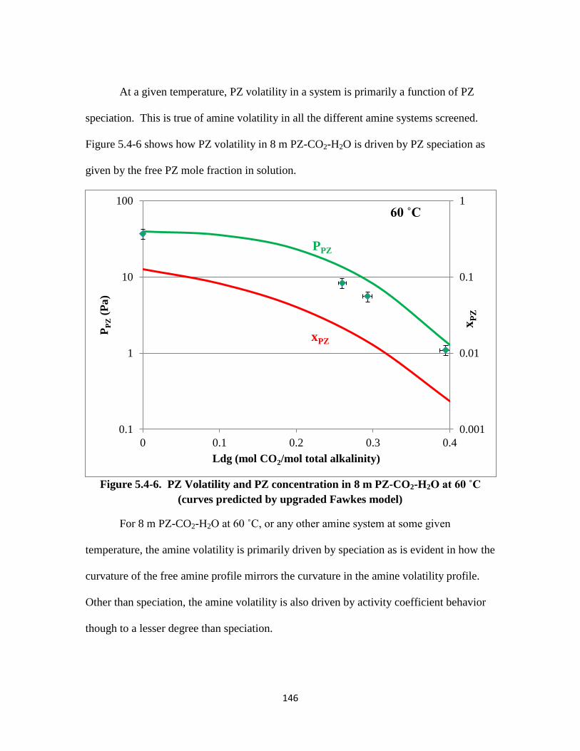
146
At a given temperature, PZ volatility in a system is primarily a function of PZ
speciation. This is true of amine volatility in all the different amine systems screened.
Figure 5.4-6 shows how PZ volatility in 8 m PZ-CO2-H2O is driven by PZ speciation as
given by the free PZ mole fraction in solution.
Figure 5.4-6. PZ Volatility and PZ concentration in 8 m PZ-CO2-H2O at 60 ˚C
(curves predicted by upgraded Fawkes model)
For 8 m PZ-CO2-H2O at 60 ˚C, or any other amine system at some given
temperature, the amine volatility is primarily driven by speciation as is evident in how the
curvature of the free amine profile mirrors the curvature in the amine volatility profile.
Other than speciation, the amine volatility is also driven by activity coefficient behavior
though to a lesser degree than speciation.
0.001
0.01
0.1
1
0.1
1
10
100
0 0.1 0.2 0.3 0.4
xP
Z
PP
Z (
Pa)
Ldg (mol CO2/mol total alkalinity)
xPZ
PPZ
60 ˚C
147
Figure 5.4-7 shows the activity coefficient of PZ in 8 m and 10 m PZ-CO2-H2O,
as a function of loading, as predicted by the upgraded Fawkes model.
Figure 5.4-7. Activity Coefficients of PZ in 8 m and 10 m PZ-CO2-H2O (curves
predicted by upgraded Fawkes model)
For both 8 m and 10 m PZ, PZ activity coefficient increases with loading because
PZ is being salted out of solution as electrolytes are being increasingly generated. The PZ
activity coefficient is greater for 10 m than for 8 m because PZ does not strongly interact
with itself as much as it does with water. Because PZ is known to form PZ hexahydrate
(PZ.6H2O), PZ is salted out at a higher PZ concentration because there is less water in 10
m PZ than in 8 m PZ to hydrate the PZ molecules. The PZ activity coefficient for 8 m
PZ-CO2-H2O is not seen to vary much going from 50 ˚C to 60 ˚C. Finally, it is not clear
2
3
4
5
0 0.1 0.2 0.3 0.4
Act
ivit
y C
oef
fici
ent
Ldg (mol CO2/mol total alkalinity)
PZ in 8 m PZ-CO2-H2O 50 ˚C
PZ in 8 m PZ-CO2-H2O 60 ˚C
PZ in 10 m PZ-CO2-H2O 60 ˚C
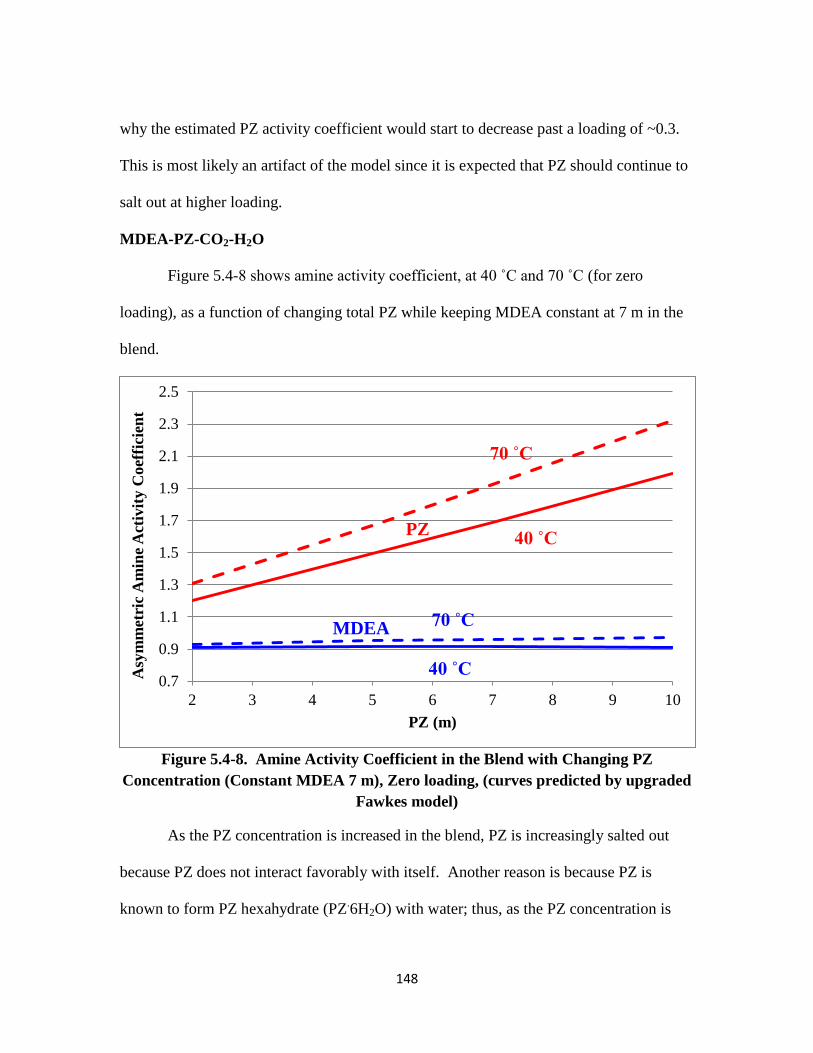
148
why the estimated PZ activity coefficient would start to decrease past a loading of ~0.3.
This is most likely an artifact of the model since it is expected that PZ should continue to
salt out at higher loading.
MDEA-PZ-CO2-H2O
Figure 5.4-8 shows amine activity coefficient, at 40 ˚C and 70 ˚C (for zero
loading), as a function of changing total PZ while keeping MDEA constant at 7 m in the
blend.
Figure 5.4-8. Amine Activity Coefficient in the Blend with Changing PZ
Concentration (Constant MDEA 7 m), Zero loading, (curves predicted by upgraded
Fawkes model)
As the PZ concentration is increased in the blend, PZ is increasingly salted out
because PZ does not interact favorably with itself. Another reason is because PZ is
known to form PZ hexahydrate (PZ.6H2O) with water; thus, as the PZ concentration is
0.7
0.9
1.1
1.3
1.5
1.7
1.9
2.1
2.3
2.5
2 3 4 5 6 7 8 9 10
Asy
mm
etri
c A
min
e A
ctiv
ity C
oef
fici
ent
PZ (m)
PZ
MDEA
40 ˚C
70 ˚C
40 ˚C
70 ˚C
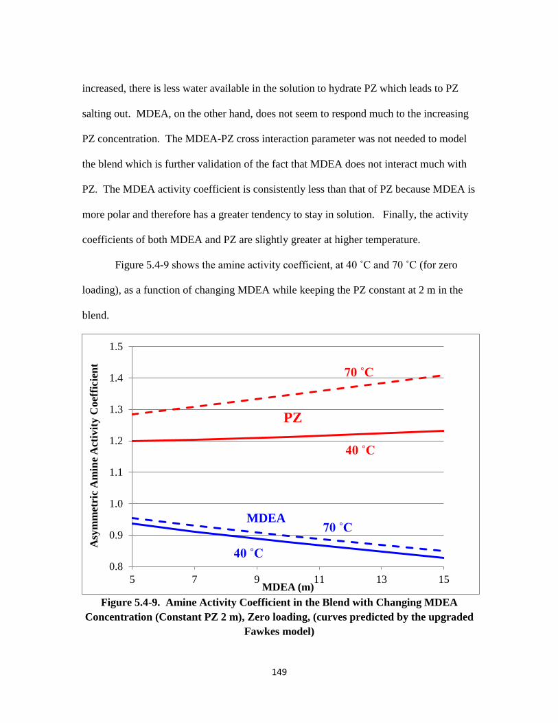
149
increased, there is less water available in the solution to hydrate PZ which leads to PZ
salting out. MDEA, on the other hand, does not seem to respond much to the increasing
PZ concentration. The MDEA-PZ cross interaction parameter was not needed to model
the blend which is further validation of the fact that MDEA does not interact much with
PZ. The MDEA activity coefficient is consistently less than that of PZ because MDEA is
more polar and therefore has a greater tendency to stay in solution. Finally, the activity
coefficients of both MDEA and PZ are slightly greater at higher temperature.
Figure 5.4-9 shows the amine activity coefficient, at 40 ˚C and 70 ˚C (for zero
loading), as a function of changing MDEA while keeping the PZ constant at 2 m in the
blend.
Figure 5.4-9. Amine Activity Coefficient in the Blend with Changing MDEA
Concentration (Constant PZ 2 m), Zero loading, (curves predicted by the upgraded
Fawkes model)
0.8
0.9
1.0
1.1
1.2
1.3
1.4
1.5
5 7 9 11 13 15
Asy
mm
etri
c A
min
e A
ctiv
ity C
oef
fici
ent
MDEA (m)
PZ
MDEA 70 ˚C
40 ˚C
40 ˚C
70 ˚C
150
As the MDEA concentration is increased, MDEA activity coefficient decreases
accordingly which suggests that MDEA is salting into the solution. Since MDEA
interacts favorably with itself due to hydrogen bonding, there is a greater tendency to stay
in solution unlike in the case of PZ. PZ, on the other hand, does not seem to respond
much to the changing MDEA concentration which is further confirmation of the
understanding that the two amines do not interact very much with each other. Again, the
amines interact with their own kinds much more strongly than they do with each other.
Lastly, the activity coefficients of both MDEA and PZ are greater at higher temperature
as shown previously.
Figure 5.4-10 shows the PZ and H2O activity coefficients in 7 m MDEA-2 m PZ-
CO2-H2O as predicted by the upgraded Fawkes model.
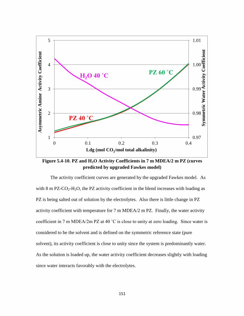
151
Figure 5.4-10. PZ and H2O Activity Coefficients in 7 m MDEA/2 m PZ (curves
predicted by upgraded Fawkes model)
The activity coefficient curves are generated by the upgraded Fawkes model. As
with 8 m PZ-CO2-H2O, the PZ activity coefficient in the blend increases with loading as
PZ is being salted out of solution by the electrolytes. Also there is little change in PZ
activity coefficient with temperature for 7 m MDEA/2 m PZ. Finally, the water activity
coefficient in 7 m MDEA/2m PZ at 40 ˚C is close to unity at zero loading. Since water is
considered to be the solvent and is defined on the symmetric reference state (pure
solvent), its activity coefficient is close to unity since the system is predominantly water.
As the solution is loaded up, the water activity coefficient decreases slightly with loading
since water interacts favorably with the electrolytes.
0.97
0.98
0.99
1.00
1.01
1
2
3
4
5
0 0.1 0.2 0.3 0.4
Sym
met
ric
Wate
r A
ctiv
ity C
oef
fici
ent
Asy
mm
etri
c A
min
e A
ctiv
ity C
oef
fici
ent
Ldg (mol CO2/mol total alkalinity)
PZ 40 ˚C
PZ 60 ˚C H2O 40 ˚C
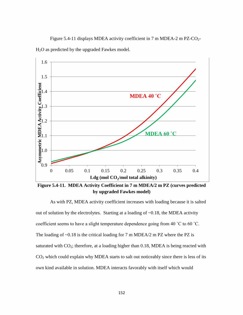
152
Figure 5.4-11 displays MDEA activity coefficient in 7 m MDEA-2 m PZ-CO2-
H2O as predicted by the upgraded Fawkes model.
Figure 5.4-11. MDEA Activity Coefficient in 7 m MDEA/2 m PZ (curves predicted
by upgraded Fawkes model)
As with PZ, MDEA activity coefficient increases with loading because it is salted
out of solution by the electrolytes. Starting at a loading of ~0.18, the MDEA activity
coefficient seems to have a slight temperature dependence going from 40 ˚C to 60 ˚C.
The loading of ~0.18 is the critical loading for 7 m MDEA/2 m PZ where the PZ is
saturated with CO2; therefore, at a loading higher than 0.18, MDEA is being reacted with
CO2 which could explain why MDEA starts to salt out noticeably since there is less of its
own kind available in solution. MDEA interacts favorably with itself which would
0.9
1.0
1.1
1.2
1.3
1.4
1.5
1.6
0 0.05 0.1 0.15 0.2 0.25 0.3 0.35 0.4
Asy
mm
etri
c M
DE
A A
ctiv
ity C
oef
fici
ent
Ldg (mol CO2/mol total alkinity)
MDEA 40 ˚C
MDEA 60 ˚C
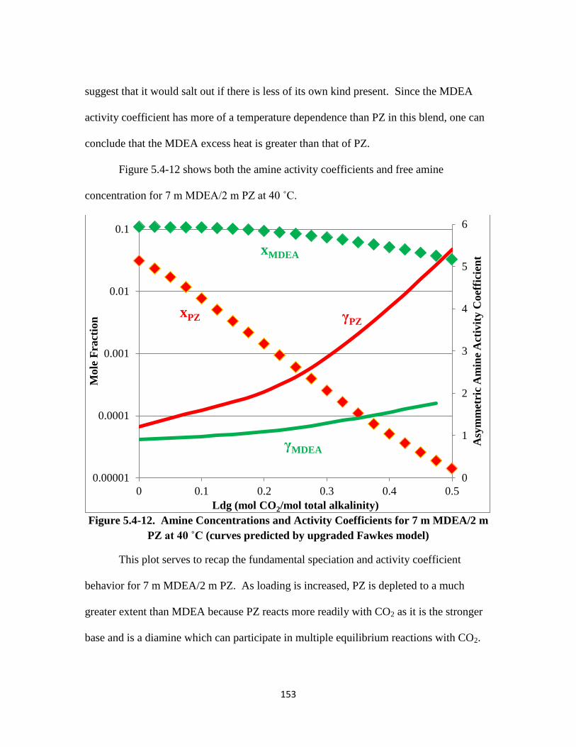
153
suggest that it would salt out if there is less of its own kind present. Since the MDEA
activity coefficient has more of a temperature dependence than PZ in this blend, one can
conclude that the MDEA excess heat is greater than that of PZ.
Figure 5.4-12 shows both the amine activity coefficients and free amine
concentration for 7 m MDEA/2 m PZ at 40 ˚C.
Figure 5.4-12. Amine Concentrations and Activity Coefficients for 7 m MDEA/2 m
PZ at 40 ˚C (curves predicted by upgraded Fawkes model)
This plot serves to recap the fundamental speciation and activity coefficient
behavior for 7 m MDEA/2 m PZ. As loading is increased, PZ is depleted to a much
greater extent than MDEA because PZ reacts more readily with CO2 as it is the stronger
base and is a diamine which can participate in multiple equilibrium reactions with CO2.
0
1
2
3
4
5
6
0.00001
0.0001
0.001
0.01
0.1
0 0.1 0.2 0.3 0.4 0.5
Asy
mm
etri
c A
min
e A
ctiv
ity C
oef
fici
ent
Mole
Fra
ctio
n
Ldg (mol CO2/mol total alkalinity)
xPZ γPZ
xMDEA
γMDEA
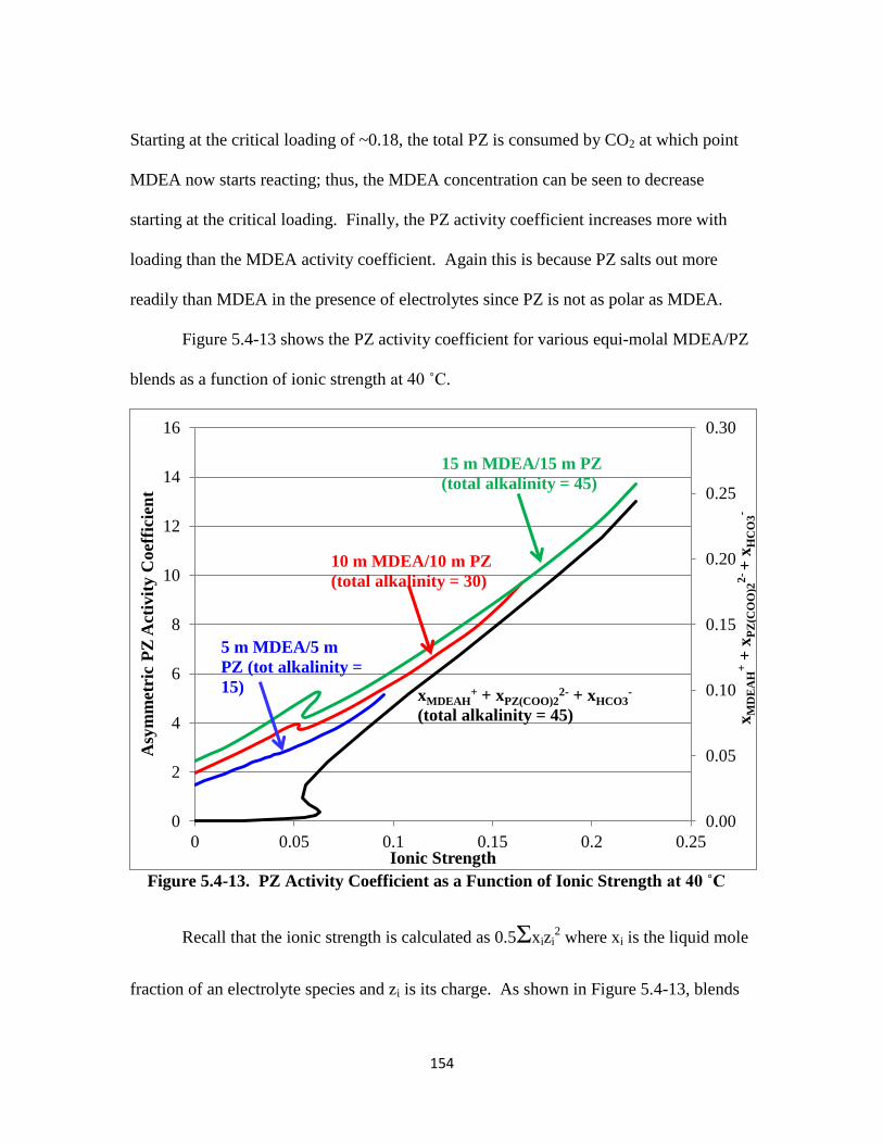
154
Starting at the critical loading of ~0.18, the total PZ is consumed by CO2 at which point
MDEA now starts reacting; thus, the MDEA concentration can be seen to decrease
starting at the critical loading. Finally, the PZ activity coefficient increases more with
loading than the MDEA activity coefficient. Again this is because PZ salts out more
readily than MDEA in the presence of electrolytes since PZ is not as polar as MDEA.
Figure 5.4-13 shows the PZ activity coefficient for various equi-molal MDEA/PZ
blends as a function of ionic strength at 40 ˚C.
Figure 5.4-13. PZ Activity Coefficient as a Function of Ionic Strength at 40 ˚C
Recall that the ionic strength is calculated as 0.5Σxizi2 where xi is the liquid mole
fraction of an electrolyte species and zi is its charge. As shown in Figure 5.4-13, blends
0.00
0.05
0.10
0.15
0.20
0.25
0.30
0
2
4
6
8
10
12
14
16
0 0.05 0.1 0.15 0.2 0.25
xM
DE
AH
+ +
xP
Z(C
OO
)22
- + x
HC
O3
-
Asy
mm
etri
c P
Z A
ctiv
ity C
oef
fici
ent
Ionic Strength
5 m MDEA/5 m
PZ (tot alkalinity =
15)
10 m MDEA/10 m PZ
(total alkalinity = 30)
15 m MDEA/15 m PZ
(total alkalinity = 45)
xMDEAH+ + xPZ(COO)2
2- + xHCO3-
(total alkalinity = 45)
155
with higher total alkalinity can be loaded to higher maximum ionic strengths. Most
importantly, the PZ activity coefficient increases with increasing ionic strength as PZ is
salted out of solution in the presence of increasing electrolyte generation. Additionally,
the PZ activity coefficient is greater with greater PZ concentration in a blend. Recall
from earlier that PZ does not interact favorably with its own kind due to competition to
bond with water to form PZ hexahydrate complexes; thus, at higher PZ concentration,
there is less water available to complex with PZ which results in PZ salting out. The PZ
activity coefficient behavior with respect to increasing ionic strength is mirrored by the
increasing total production of three key electrolyte species, xMDEAH+ + xPZ(COO)2
2- + xHCO3
-
, which drives greater ionic strength (as shown for the 15 m MDEA/15 m PZ case). In
light of this profile mirroring, to a first order, one can rationalize that PZ has a greater
tendency to salt out as a consequence of the increasing total presence of the electrolytes
mentioned.
Figure 5.4-14 displays the MDEA activity coefficient for various equi-molal
MDEA/PZ blends as a function of ionic strength at 40 ˚C.
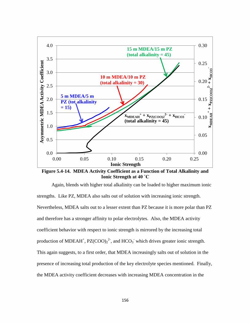
156
Figure 5.4-14. MDEA Activity Coefficient as a Function of Total Alkalinity and
Ionic Strength at 40 ˚C
Again, blends with higher total alkalinity can be loaded to higher maximum ionic
strengths. Like PZ, MDEA also salts out of solution with increasing ionic strength.
Nevertheless, MDEA salts out to a lesser extent than PZ because it is more polar than PZ
and therefore has a stronger affinity to polar electrolytes. Also, the MDEA activity
coefficient behavior with respect to ionic strength is mirrored by the increasing total
production of MDEAH+, PZ(COO)2
2-, and HCO3
- which drives greater ionic strength.
This again suggests, to a first order, that MDEA increasingly salts out of solution in the
presence of increasing total production of the key electrolyte species mentioned. Finally,
the MDEA activity coefficient decreases with increasing MDEA concentration in the
0.00
0.05
0.10
0.15
0.20
0.25
0.30
0.0
0.5
1.0
1.5
2.0
2.5
3.0
3.5
4.0
0.00 0.05 0.10 0.15 0.20 0.25
xM
DE
AH
+ +
xP
Z(C
OO
)22
- +
xH
CO
3-
Asy
mm
etri
c M
DE
A A
ctiv
ity C
oef
fici
ent
Ionic Strength
5 m MDEA/5 m
PZ (tot alkalinity
= 15)
10 m MDEA/10 m PZ
(total alkalinity = 30)
15 m MDEA/15 m PZ
(total alkalinity = 45)
xMDEAH+ + xPZ(COO)2
2- + xHCO3-
(total alkalinity = 45)
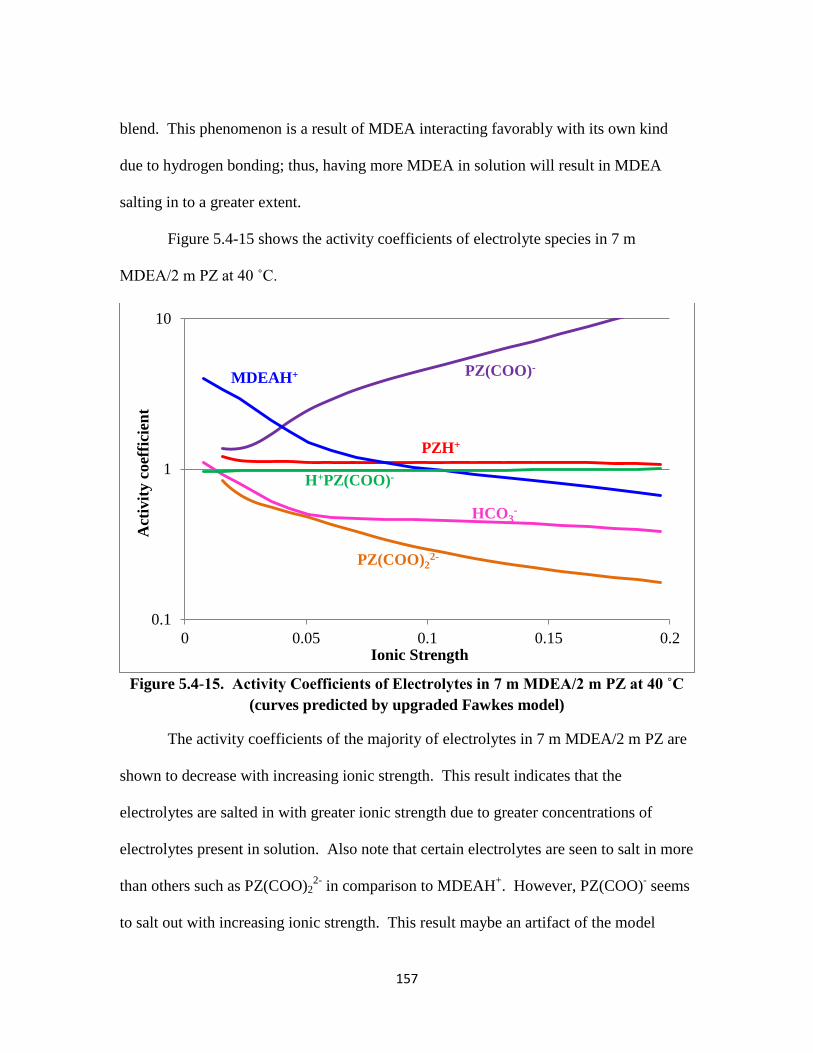
157
blend. This phenomenon is a result of MDEA interacting favorably with its own kind
due to hydrogen bonding; thus, having more MDEA in solution will result in MDEA
salting in to a greater extent.
Figure 5.4-15 shows the activity coefficients of electrolyte species in 7 m
MDEA/2 m PZ at 40 ˚C.
Figure 5.4-15. Activity Coefficients of Electrolytes in 7 m MDEA/2 m PZ at 40 ˚C
(curves predicted by upgraded Fawkes model)
The activity coefficients of the majority of electrolytes in 7 m MDEA/2 m PZ are
shown to decrease with increasing ionic strength. This result indicates that the
electrolytes are salted in with greater ionic strength due to greater concentrations of
electrolytes present in solution. Also note that certain electrolytes are seen to salt in more
than others such as PZ(COO)22-
in comparison to MDEAH+. However, PZ(COO)
- seems
to salt out with increasing ionic strength. This result maybe an artifact of the model
0.1
1
10
0 0.05 0.1 0.15 0.2
Act
ivit
y c
oef
fici
ent
Ionic Strength
PZ(COO)- MDEAH+
PZH+
H+PZ(COO)-
HCO3-
PZ(COO)22-
158
mathematics; nevertheless, it could be rationalized that PZ(COO)- is not as ionic as other
electrolytes since it possesses an organic PZ group at one end of the molecule. Because
of this characteristic, one could speculate that PZ(COO)- would perhaps tend salt out of
solution as opposed to other true electrolytes which salt in.
Amine Screening
Table 5.4-4 summarizes the amine volatility at 40 ˚C for various systems screened
for CO2 capture (with 7 m MEA data taken from Hilliard 2008).
Table 5.4-4. Amine Volatilities for Various Systems Screened at 40 ˚C
α = 0 α = nominal lean
Amine System
Pamine1
(Pa)
Pamine2
(Pa)
Pamine1
(Pa)
Pamine2
(Pa) Ldg
PCO2
(Pa)
7 m MDEA 0.48 0.47 0.03 520
4.8 m AMP 14.2 14.8 0.31 743
7 m MEA 10.0 2.70 0.47 574
8 m PZ 7.41 0.78 0.29 410
8 m EDA 17.2 3.41 0.43 564
7 m MDEA/2 m PZ 0.46 1.07 0.47 0.30 0.14 524
5 m MDEA/5 m PZ 0.36 5.04 0.45 0.51 0.22 598
4 m 2-MPZ/4 m PZ 8.53 2.39 0.85 0.10 0.33 652
2.3 m AMP/5 m PZ 12.2 4.78 5.71 0.61 0.30 244
The volatility of tertiary and hindered amines, such as MDEA and AMP,
respectively, does not vary much from zero to the nominal lean loading. This is because
tertiary and hindered amines are not able to react directly with CO2 to form charged
carbamates; therefore, the free amine concentrations do not significantly change upon
loading, which in turn result in a relatively constant volatility.
Carbamate forming monoamines, such as MEA, can participate in more
equilibrium reactions with CO2, thus resulting in the amine volatility dropping by a factor
159
of 3 or greater. Diamines, such as PZ and EDA, can participate in multiple equilibrium
reactions with CO2 to form various carbamate and protonated species; as a result, their
volatility decreases by a factor of 5, 10, or even more than 20 in some cases.
When PZ is added to make a blend, CO2 tends to react preferentially with it
because it is usually the stronger base of the two amines in the blend and has two amine
groups which can undergo extensive speciation. Based on these screening results, it
appears that PZ or any blend consisting of diamine promoted by PZ would make a choice
solvent for CO2 capture, at least from a volatility standpoint, given the low volatilities of
the amines at nominal loadings. (The PZ volatility for 8 m PZ at zero loading is a value
estimated by the upgraded MDEA/PZ Fawkes model. It was not possible to measure PZ
volatility at this condition due to solid precipitation.)
Table 5.4-5 displays the estimated (asymmetric) activity coefficients for the
different amine systems screened. The activity coefficients of systems forming complex
speciation were estimated from the upgraded Fawkes MDEA/PZ thermodynamic model.
Table 5.4-5. Asymmetric Amine Activity Coefficients for Various Systems
Screened at 40 ˚C (7 m MEA from Hilliard 2008)
α = 0
α = nominal lean
Salt Out Factor =
γamine,α=lean/γamine,α=0
System γamine1 γamine2 γamine1 γamine2 Ldg PCO2 amine1 amine2
7 m MDEA 0.906 0.911 0.03 520 1.01
4.8 m AMP 0.565 0.862 0.31 743 1.53
7 m MDEA/
2 m PZ 0.912 1.21 1.02 1.75 0.14 524 1.12 1.45
5 m MDEA/
5 m PZ 0.944 1.49 1.07 2.64 0.22 598 1.13 1.77
8 m PZ 1.81 3.8 0.29 410 2.10
7 m MEA 1.49 6.21 0.47 574 4.17
160
The salting out factor is defined as the ratio of the asymmetric amine activity
coefficients before and after loading. The degree to which an amine salts out of solution
essentially depends upon two factors: (1) the amount of salt or electrolytes generated in a
system at a particular loading; (2) how nonpolar the amine is which leads to it salting out
in the presence of polar charged electrolytes.
7 m MDEA and 4.8 m AMP show the least salting out. Given that MDEA is a
tertiary amine and AMP is a hindered amine, they are not able to react directly with CO2
to produce a significant amount of electrolytes. With little salt present in the system,
MDEA and AMP do not salt out appreciably. AMP salts out to a slightly greater extent
than MDEA because it is more nonpolar. In MDEA/PZ, MDEA salts out to a slightly
greater extent than in 7 m MDEA because there is more salt generated in the blend
coupled with the fact that MDEA has less favorable interactions with PZ. MDEA tends
to associate with itself due to hydrogen bonding. In 8 m PZ, a large amount of
electrolyte is formed due to PZ being a diamine; thus, PZ salts out noticeably in the
presence of high ionic strength. Additionally, the fact that PZ does not interact favorably
with its own kind also contributes to greater salting out. 7 m MEA appears to salt out
even more than PZ possibly because MEA is more nonpolar than PZ in the presence of
all the polar salt in the system.
5.5. Conclusions
The enthalpies of amine absorption, for PZ and for MDEA, at unloaded and
nominal lean loading conditions are 73 – 76 kJ/mol amine. The enthalpy of amine
solution (71 – 74 kJ/mol) provides the greatest contribution to the enthalpy of absorption,
161
followed by the enthalpy of reaction (~0.7 – 5 kJ/mol), and finally the amine excess
enthalpy (-0.1 - 3 kJ/mol). MDEA has a smaller enthalpy of reaction compared to PZ
because: (1) it is a tertiary amine which does not form carbamate and only serves as a
proton sink; (2) unlike PZ, it does not react much with CO2 at the nominal lean loading of
interest.
Amine volatility is most strongly a function of speciation, especially in the case of
PZ. PZ volatility decreases with increasing loading as proportional to the decrease in free
PZ. In 8 m PZ-CO2-H2O, as the loading is increased from zero to 0.4 mol CO2/mol total
alkalinity at 60 ˚C, both the PZ volatility and free PZ concentration drop by a factor of
50.
In the case of unloaded MDEA/PZ, as the PZ concentration increases by a factor
of 5 (while MDEA concentration is fixed), the PZ activity coefficient increases by a
factor of 1.5 – 1.7 because PZ does not interact favorably with its own species, partly due
to competition amongst each other to be hydrated in forming PZ hexahydrate. As the
MDEA concentration increases by a factor of 3 (while PZ concentration is fixed), the
MDEA activity coefficient decreases by a factor of ~1.1-1.2 because MDEA interacts
favorably with itself due to hydrogen bonding. As loading is increased from zero to
nominal lean loading, both MDEA and PZ activity coefficients increase since the amines
are being salted out of solution by the electrolytes; in particular, MDEAH+, PZ(COO)2
2-,
and HCO3- are the species that predominantly drive MDEA and PZ activity coefficient
behaviors.
162
Conversely, the electrolyte products are seen to salt in with increasing ionic
strength. PZ(COO)22-
and HCO3- salt in the most. PZ(COO)
- salts in the least, perhaps
because PZ carbamate has an organic PZ portion which makes it less polar than the other
electrolytes.
The volatilities of tertiary and hindered amines, such as MDEA and AMP,
respectively, do not vary much with respect to loading. This is because these amine types
are not able to form carbamates by reacting directly with CO2 like other amines;
moreover they tend to serve as proton sinks only. As a result of the limited extent of
reaction, their speciation does not change very much with loading which results in
seemingly constant volatilities. Mono-amines, such as MEA, show volatilities decreasing
by a factor of ~3 or greater upon loading the solutions to the nominal lean loadings. This
is because mono-amines can actually form stable carbamates with CO2 in addition to
being proton sinks. Finally, diamines such as EDA and PZ have volatilities that decrease
by a factor of 5 to as much as 20 times depending on the system. The volatilities of
diamines are very strong functions of loadings because diamines can participate in
multiple equilibrium reactions with CO2 due to having two amine groups.
PZ or any blend consisting of a diamine promoted by PZ would make a choice
solvent for CO2 capture, at least from a volatility standpoint, given the low volatilities of
the amines at nominal loadings.
In order of increasing salting out level at nominal lean loading and 40 ˚C: 7 m
MDEA < 4.8 m AMP ~ 7 m MDEA/2 m PZ < 8 m PZ < 7 m MEA. Tertiary and hindered
amines like MDEA and AMP, respectively, show negligible salting out since not much

163
salt is generated in these systems. Monoamines and diamines, such as MEA and PZ, salt
out more noticeably given higher amount of salt formed in these systems since these
amines can react directly with CO2 to make charged carbamates. Finally MEA salts out
more than PZ because it is more nonpolar.
164
Chapter 6. Conclusions and Recommendations
6.1. Summary of Research Scope and Background
This work investigated the volatilities of amine solvents used for post-combustion
CO2 capture from coal-fired power plants. Amine volatility is one of the key criteria used
to screen new solvents for a number of reasons: (1) volatility losses up the stack can
react in the atmosphere to form ozone and other toxic compounds; (2) high volatility
losses increase the costs spent for solvent make-up; (3) these high amine losses would
also require the use of a bigger water wash, and more water, to capture fugitive amines
which translate to higher capital and operating costs; (4) amine volatility measurements
are needed to construct more accurate and robust thermodynamic models of CO2 capture
systems.
The volatilities of amine solutions, at unloaded and loaded conditions, were
measured using the hot gas FTIR apparatus developed by Hilliard (2008). The amine
volatility measurements at loaded conditions are first of a kind and have not been made
outside the Rochelle group. Also this work is believed to be one of the largest sources of
experimental data for amine-water systems available.
The FTIR apparatus used to measure amine volatility is considered to be a fairly
novel technique used to determine vapor-liquid equilibrium. Other authors tend to use
more traditional experimental methods, such as those that involve a static cell or an
Othmer still coupled with Gas Chromatography (GC) analysis. These traditional methods
often involve boiling the solution to create a vapor phase for GC analysis, whereas the
FTIR method measures amine volatility above a sub-cooled solution. The FTIR method
165
is believed to be more versatile than existing experimental methods for vapor-liquid
equilibrium measurements because: (1) there is much more VLE data can be generated
when working with a sub-cooled liquid as opposed to boiling the solution; (2) ease of
operation – a definite advantage especially when it comes to working with high boiling
solvents. Traditional VLE methods sometime require pulling a vacuum to boil off these
high boiling solutions.
With the liquid phase analysis, the solutions are loaded with carbon 13 which
enable a Nuclear Magnetic Resonance (NMR) analysis of all the species present in
solution. Both the proton (H1) and carbon (C
13) NMR results are used to identify all of
the existing product species. These two sets of NMR results are often within ±10% of
one another which suggest consistency. Analysis of the liquid phase by NMR is used to
understand the speciation in the solution and is used to interpret the gas phase volatility
measurements made by the FTIR. For key amine systems such as PZ-CO2-H2O and
MDEA-PZ-CO2-H2O, heat capacity measurements are also made by using a Differential
Scanning Calorimeter (DSC). All of the thermodynamic measurements made by this
work, including amine volatility, speciation, and heat capacity, are used along with CO2
solubility measurements to construct rigorous thermodynamic models of the CO2 capture
systems. The thermodynamic models are built using AspenPlus®7.3. These models use
the Liquid Activity method to characterize system thermodynamics. The liquid phase is
modeled using elecNRTL (Electrolyte NRTL) method whereas the vapor phase is
modeled using SRK (Soave-Redlich-Kwong).
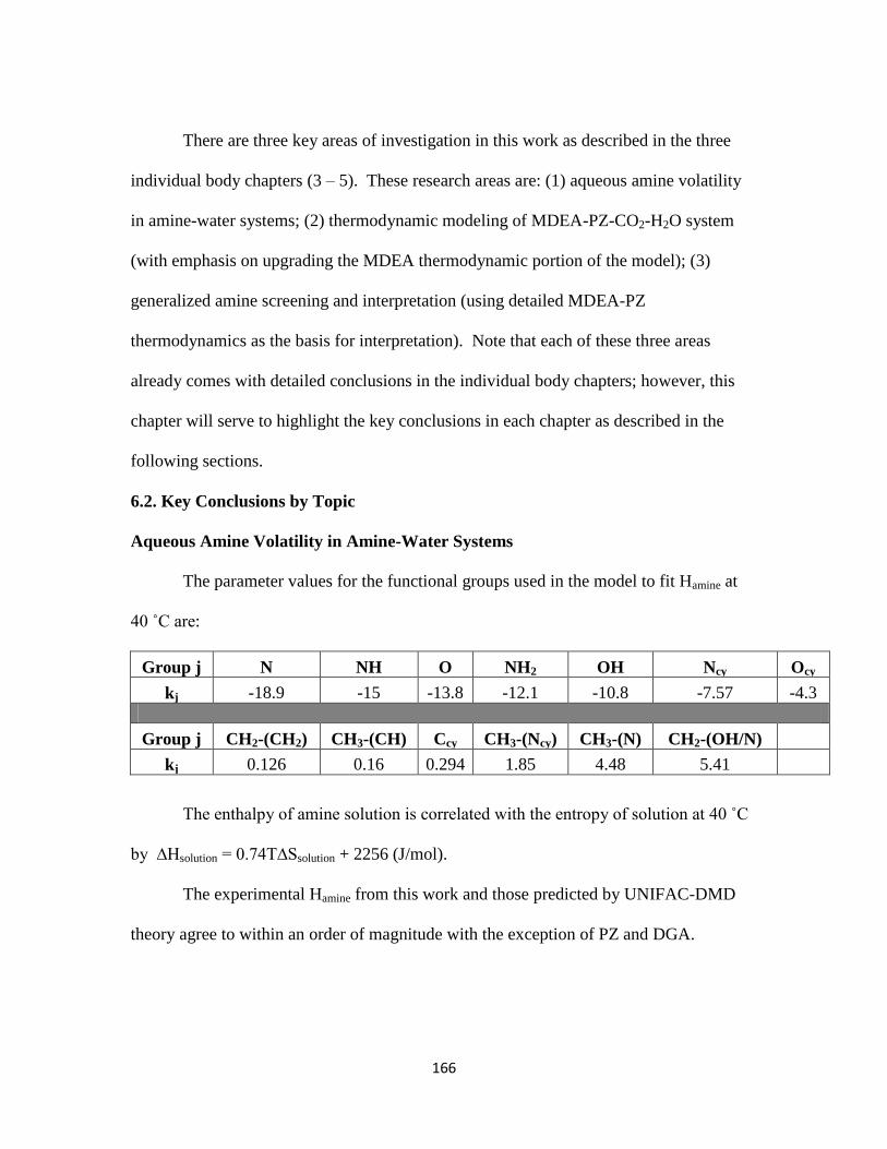
166
There are three key areas of investigation in this work as described in the three
individual body chapters (3 – 5). These research areas are: (1) aqueous amine volatility
in amine-water systems; (2) thermodynamic modeling of MDEA-PZ-CO2-H2O system
(with emphasis on upgrading the MDEA thermodynamic portion of the model); (3)
generalized amine screening and interpretation (using detailed MDEA-PZ
thermodynamics as the basis for interpretation). Note that each of these three areas
already comes with detailed conclusions in the individual body chapters; however, this
chapter will serve to highlight the key conclusions in each chapter as described in the
following sections.
6.2. Key Conclusions by Topic
Aqueous Amine Volatility in Amine-Water Systems
The parameter values for the functional groups used in the model to fit Hamine at
40 ˚C are:
Group j N NH O NH2 OH Ncy Ocy
kj -18.9 -15 -13.8 -12.1 -10.8 -7.57 -4.3
Group j CH2-(CH2) CH3-(CH) Ccy CH3-(Ncy) CH3-(N) CH2-(OH/N)
kj 0.126 0.16 0.294 1.85 4.48 5.41
The enthalpy of amine solution is correlated with the entropy of solution at 40 ˚C
by ∆Hsolution = 0.74T∆Ssolution + 2256 (J/mol).
The experimental Hamine from this work and those predicted by UNIFAC-DMD
theory agree to within an order of magnitude with the exception of PZ and DGA.
167
Hamine estimated by the group contribution method of Hine and Mookerjee (1975)
are systematically one to many orders of magnitude less than the experimental data.
At 0.1 to 1 m amine, the concentration range used to measure Hamine in this work,
the asym- metric activity coefficient of piperazine is 1.02 – 1.10.
The enthalpies of solution of the different aqueous amine systems studied appear
to be adequately represented with Arrhenius temperature behavior which assumes a
constant enthalpy of solution over a range of temperature.
Upgrading the AspenPlus® v.7.3 Fawkes MDEA-PZ-CO2-H2O Thermodynamic
Model
In the MDEA-CO2-H2O system, carbonate (CO32-
) is an important species as its
introduction into the chemistry set allowed for better fitting of CO2 solubility at ultra lean
loadings (0.001 < α < 0.01).
With the MDEA-PZ blend, MDEA-PZ cross interaction parameters were not
needed to adequately match the blend volatilities at unloaded condition. This observation
suggests that MDEA and PZ interact more strongly with their own species instead of with
each other.
Both the blend volatilities, at unloaded and loaded conditions, along with
speciation were adequately represented in the upgraded Fawkes model.
MDEA/PZ Behavior & Generalized Amine Screening
The enthalpies of amine absorption, for PZ and for MDEA, at unloaded and
nominal lean loading conditions are 73 – 76 kJ/mol amine. The enthalpy of amine
solution (71 – 74 kJ/mol) provides the greatest contribution to the enthalpy of absorption,
168
followed by the enthalpy of reaction (~0.7 – 5 kJ/mol), and finally the amine excess
enthalpy (-0.1 - 3 kJ/mol).
The volatilities of tertiary and hindered amines, such as MDEA and AMP,
respectively, do not vary significantly with respect to loading since they are unable to
form stable carbamates.
Monoamines, such as MEA, show volatilities decreasing by a factor of ~3 or
greater upon loading since they can form stable carbamates.
Diamines such as EDA and PZ have volatilities that decrease by a factor of 5 to as
much as 20 times depending on the system. The volatilities of diamines are very strong
functions of loading because diamines can participate in multiple equilibrium reactions
with CO2 due to having two amine groups.
PZ or a blend consisting of a diamine promoted by PZ would be favorable for
CO2 capture, at least from a volatility standpoint, given the low volatilities of the amines
at nominal loadings.
As loading is increased from zero to nominal lean loading, both MDEA and PZ
activity coefficients increase since the amines are being salted out of solution by the
electrolytes; in particular, MDEAH+, PZ(COO)2
2-, and HCO3
- are the species that
predominantly drive MDEA and PZ activity coefficient behaviors.
In order of increasing salting out level at nominal lean loading and 40 ˚C: 7 m
MDEA < 4.8 m AMP ~ 7 m MDEA/2 m PZ < 8 m PZ < 7 m MEA. The degree to which
an amine is salted out of solution depends on: (1) the amount of salt generated at a given
loading; (2) how nonpolar the amine is relative to the charged electrolytes.

169
6.3. Recommendations and Future Work
Future measurements of aqueous amine volatility, for the purpose of determining
the amine Henry’s constant, should involve a more rigorous analysis of the error
introduced by the asymmetric amine activity coefficient. The experimental deviation
from the condition of infinite dilution of amine in water is assumed to be ±10% for all
amines studied based on the analysis for PZ alone. In an effort to be more rigorous,
future measurements should entail measuring the amine volatilities for a series of dilute
amine concentrations in order to quantify the errors associated with experimenting at
dilute conditions that are not actually at infinite dilution. Nevertheless, this error should
be rather small, and therefore was not rigorously explored for every amine system studied
in this work in the interest of time.
Another experimental improvement that can be made to the study of aqueous
amine volatility in the future is to perhaps use a more sensitive analytical technique to
quantify ultra low volatility measurements. The margin of measurement error already
increases by about 15% - 30% for any measurement in the 10-20 ppm’s, and can only get
worse as one approaches even lower ppm concentrations in the neighborhood of the
detection limit (2-5 ppm). One can either upgrade to the next generation of FTIR
analysis with higher resolution or somehow use an advanced GC method, such as GC
Headspace Chromatography, that can perhaps be customized to the nature of these
experiments.
Another key experimental area that also requires optimization is the NMR
analysis of speciation. The existing NMR analysis method (using the Varian Inova 500
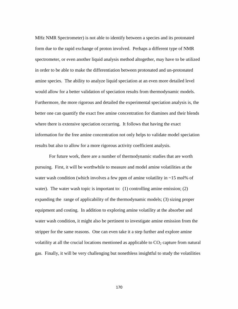
170
MHz NMR Spectrometer) is not able to identify between a species and its protonated
form due to the rapid exchange of proton involved. Perhaps a different type of NMR
spectrometer, or even another liquid analysis method altogether, may have to be utilized
in order to be able to make the differentiation between protonated and un-protonated
amine species. The ability to analyze liquid speciation at an even more detailed level
would allow for a better validation of speciation results from thermodynamic models.
Furthermore, the more rigorous and detailed the experimental speciation analysis is, the
better one can quantify the exact free amine concentration for diamines and their blends
where there is extensive speciation occurring. It follows that having the exact
information for the free amine concentration not only helps to validate model speciation
results but also to allow for a more rigorous activity coefficient analysis.
For future work, there are a number of thermodynamic studies that are worth
pursuing. First, it will be worthwhile to measure and model amine volatilities at the
water wash condition (which involves a few ppm of amine volatility in ~15 mol% of
water). The water wash topic is important to: (1) controlling amine emission; (2)
expanding the range of applicability of the thermodynamic models; (3) sizing proper
equipment and costing. In addition to exploring amine volatility at the absorber and
water wash condition, it might also be pertinent to investigate amine emission from the
stripper for the same reasons. One can even take it a step further and explore amine
volatility at all the crucial locations mentioned as applicable to CO2 capture from natural
gas. Finally, it will be very challenging but nonethless insightful to study the volatilities

171
of amine byproducts, such as nitrosamines, degraded amines, and such, that can also be
potentially released into the atmosphere.
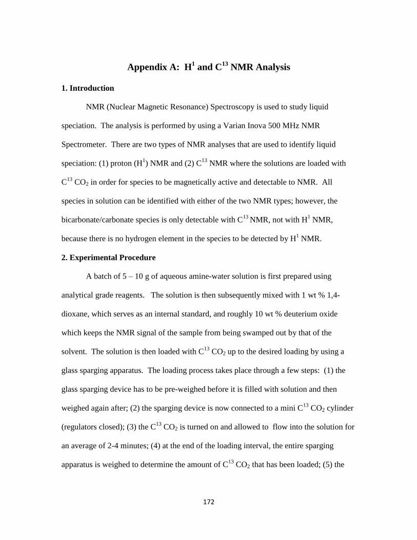
172
Appendix A: H1 and C
13 NMR Analysis
1. Introduction
NMR (Nuclear Magnetic Resonance) Spectroscopy is used to study liquid
speciation. The analysis is performed by using a Varian Inova 500 MHz NMR
Spectrometer. There are two types of NMR analyses that are used to identify liquid
speciation: (1) proton (H1) NMR and (2) C
13 NMR where the solutions are loaded with
C13
CO2 in order for species to be magnetically active and detectable to NMR. All
species in solution can be identified with either of the two NMR types; however, the
bicarbonate/carbonate species is only detectable with C13
NMR, not with H1 NMR,
because there is no hydrogen element in the species to be detected by H1 NMR.
2. Experimental Procedure
A batch of 5 – 10 g of aqueous amine-water solution is first prepared using
analytical grade reagents. The solution is then subsequently mixed with 1 wt % 1,4-
dioxane, which serves as an internal standard, and roughly 10 wt % deuterium oxide
which keeps the NMR signal of the sample from being swamped out by that of the
solvent. The solution is then loaded with C13
CO2 up to the desired loading by using a
glass sparging apparatus. The loading process takes place through a few steps: (1) the
glass sparging device has to be pre-weighed before it is filled with solution and then
weighed again after; (2) the sparging device is now connected to a mini C13
CO2 cylinder
(regulators closed); (3) the C13
CO2 is turned on and allowed to flow into the solution for
an average of 2-4 minutes; (4) at the end of the loading interval, the entire sparging
apparatus is weighed to determine the amount of C13
CO2 that has been loaded; (5) the
173
loading process is resumed, for several more 2-4 minute intervals with weighing in
between, until the desired loading is achieved as reflected by the total CO2 weight in
solution. Next, an aliquot of the loaded solution is transferred into an NMR tube
(Wilmad glass, 5 mm OD x 0.77 mm ID). It is recommended that the tube should only
be filled up to a height of 1.75 inch from the bottom of the tube to ensure that the solution
can be properly heated once inside the 1.75 inch tube holder within the NMR machine
chamber. After the NMR tube is filled, it is then sealed thermally by the glass shop prior
to being run on the Varian Inova 500 MHz NMR Spectrometer (with variable
temperature control). Samples that are to be run at 40 ˚C need to be thermally
conditioned for at least an hour before being run.
3. Amine Structural Identification and Peak Assignment
Proton (H1) Assignment
Figure A.1: Molecular Structure and Active Nuclei of Protons associated with
PZ/PZH+
H1
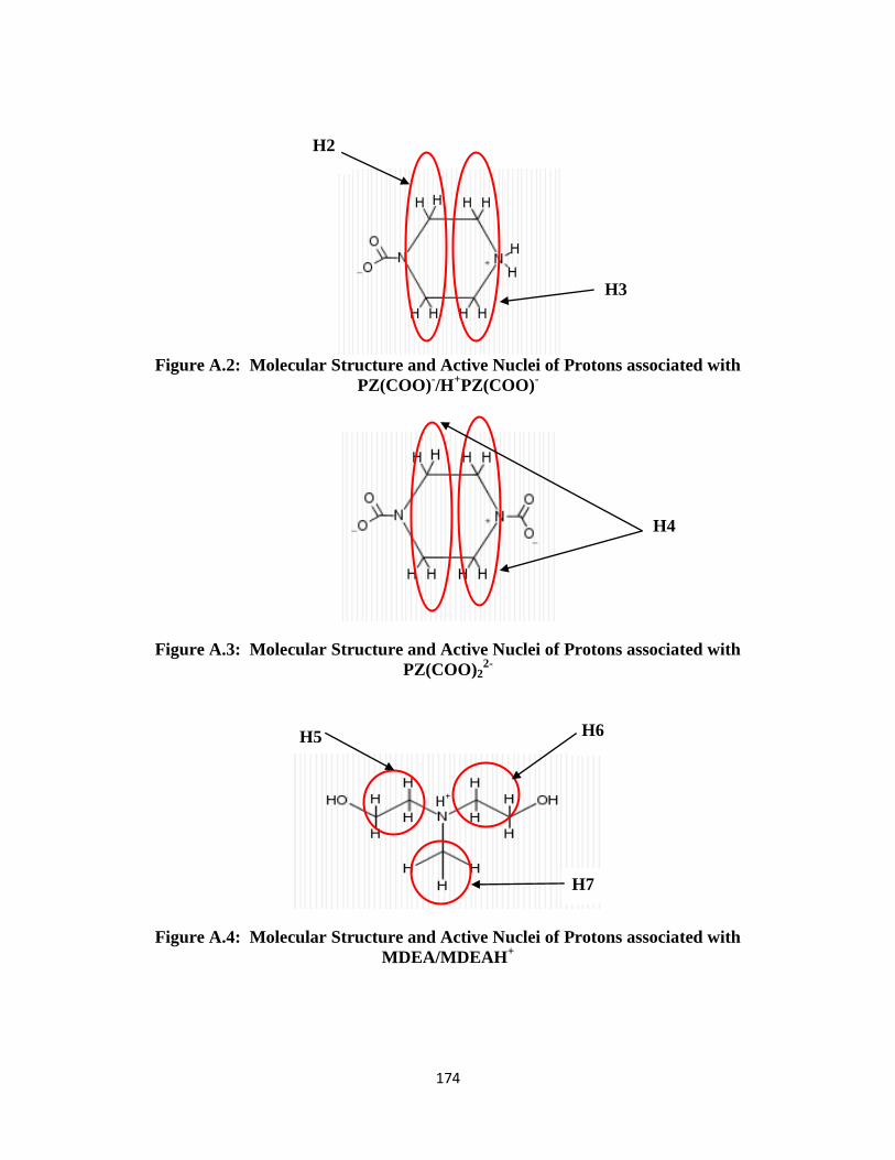
174
Figure A.2: Molecular Structure and Active Nuclei of Protons associated with
PZ(COO)-/H
+PZ(COO)
-
Figure A.3: Molecular Structure and Active Nuclei of Protons associated with
PZ(COO)22-
Figure A.4: Molecular Structure and Active Nuclei of Protons associated with
MDEA/MDEAH+
H2
H3
H4
H5 H6
H7
H+
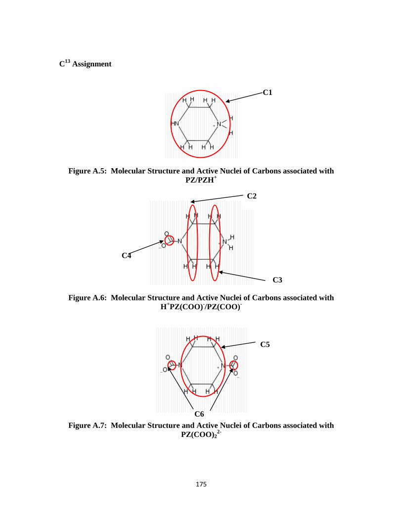
175
C13
Assignment
Figure A.5: Molecular Structure and Active Nuclei of Carbons associated with
PZ/PZH+
Figure A.6: Molecular Structure and Active Nuclei of Carbons associated with
H+PZ(COO)
-/PZ(COO)
-
Figure A.7: Molecular Structure and Active Nuclei of Carbons associated with
PZ(COO)22-
C1
C2
C3
C4
C5
C6
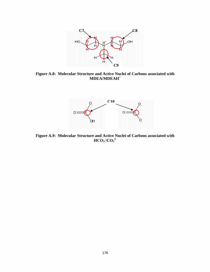
176
Figure A.8: Molecular Structure and Active Nuclei of Carbons associated with
MDEA/MDEAH+
Figure A.9: Molecular Structure and Active Nuclei of Carbons associated with
HCO3-/CO3
2-
C9
H+
C10
C7 C8
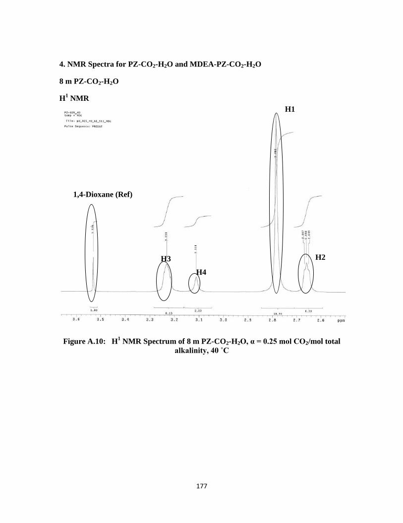
177
4. NMR Spectra for PZ-CO2-H2O and MDEA-PZ-CO2-H2O
8 m PZ-CO2-H2O
H1 NMR
Figure A.10: H1 NMR Spectrum of 8 m PZ-CO2-H2O, α = 0.25 mol CO2/mol total
alkalinity, 40 ˚C
1,4-Dioxane (Ref)
H1
H2 H3
H4
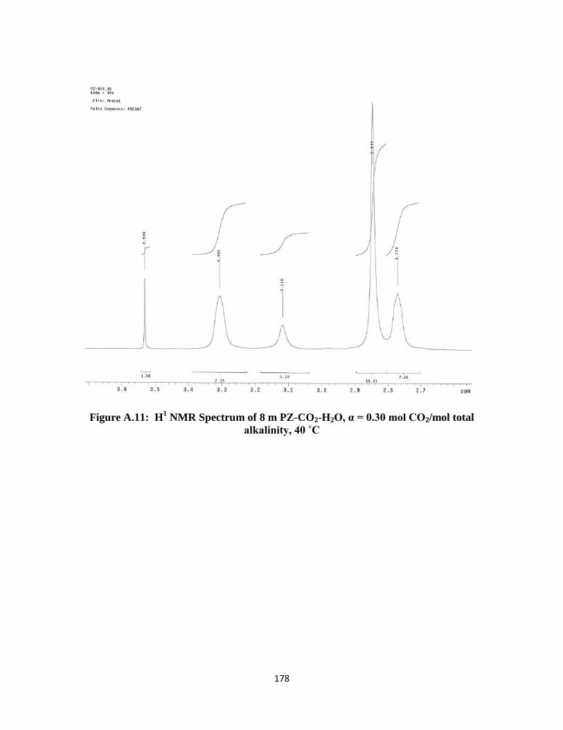
178
Figure A.11: H1 NMR Spectrum of 8 m PZ-CO2-H2O, α = 0.30 mol CO2/mol total
alkalinity, 40 ˚C
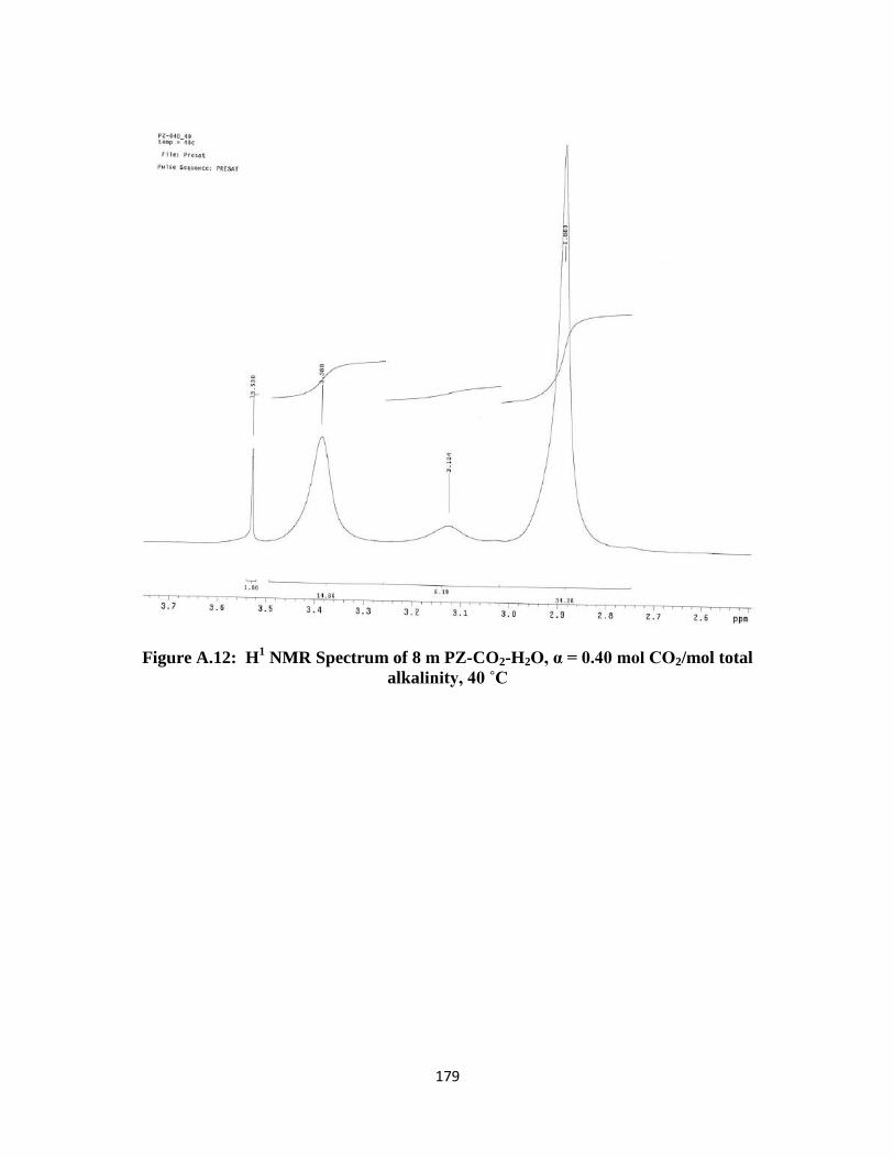
179
Figure A.12: H1 NMR Spectrum of 8 m PZ-CO2-H2O, α = 0.40 mol CO2/mol total
alkalinity, 40 ˚C
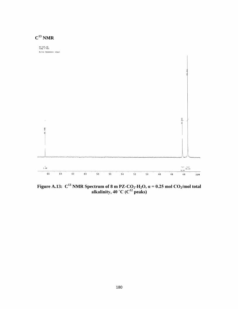
180
C13
NMR
Figure A.13: C13
NMR Spectrum of 8 m PZ-CO2-H2O, α = 0.25 mol CO2/mol total
alkalinity, 40 ˚C (C12
peaks)
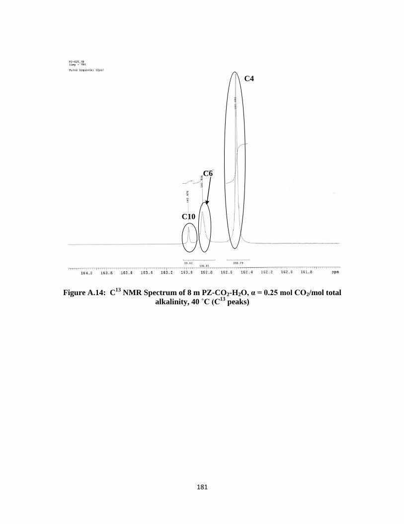
181
Figure A.14: C13
NMR Spectrum of 8 m PZ-CO2-H2O, α = 0.25 mol CO2/mol total
alkalinity, 40 ˚C (C13
peaks)
C4
C6
C10
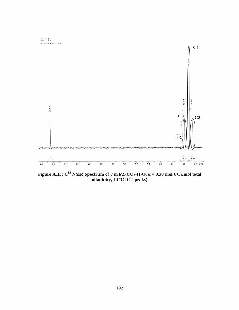
182
Figure A.15: C13
NMR Spectrum of 8 m PZ-CO2-H2O, α = 0.30 mol CO2/mol total
alkalinity, 40 ˚C (C12
peaks)
C1
C2 C3
C5
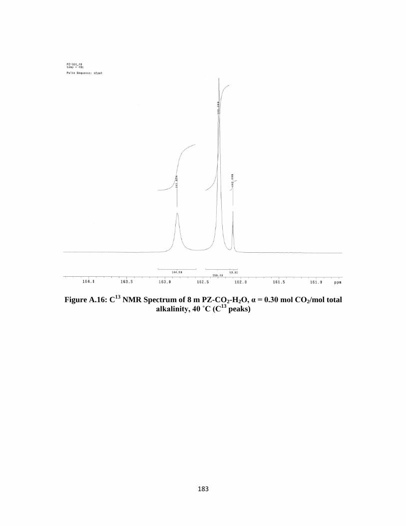
183
Figure A.16: C13
NMR Spectrum of 8 m PZ-CO2-H2O, α = 0.30 mol CO2/mol total
alkalinity, 40 ˚C (C13
peaks)
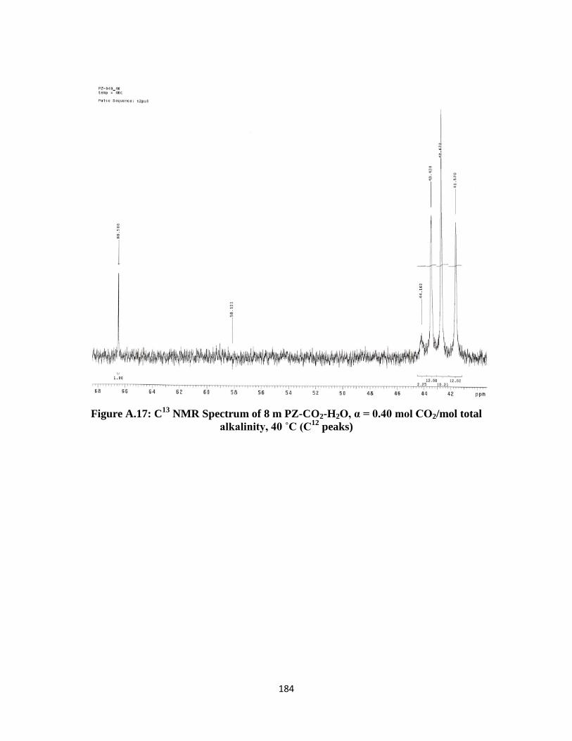
184
Figure A.17: C13
NMR Spectrum of 8 m PZ-CO2-H2O, α = 0.40 mol CO2/mol total
alkalinity, 40 ˚C (C12
peaks)
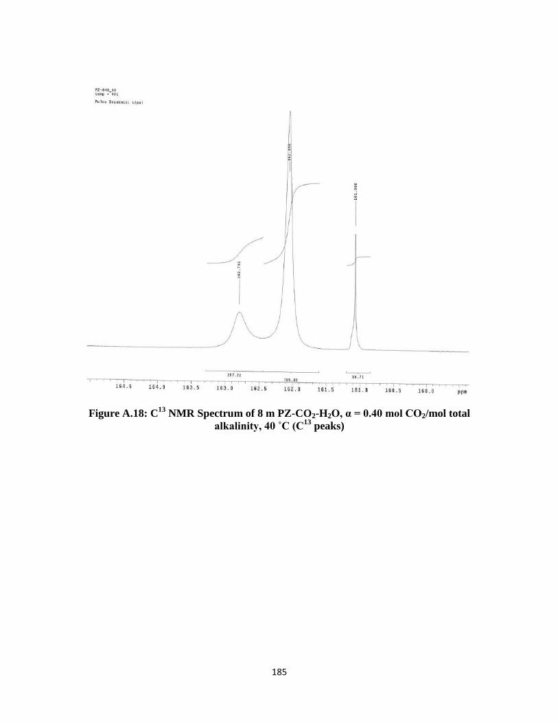
185
Figure A.18: C13
NMR Spectrum of 8 m PZ-CO2-H2O, α = 0.40 mol CO2/mol total
alkalinity, 40 ˚C (C13
peaks)
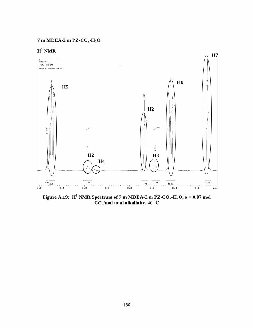
186
7 m MDEA-2 m PZ-CO2-H2O
H1 NMR
Figure A.19: H1 NMR Spectrum of 7 m MDEA-2 m PZ-CO2-H2O, α = 0.07 mol
CO2/mol total alkalinity, 40 ˚C
H5 H6
H7
H2 H3
H2
H4
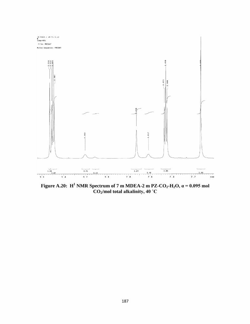
187
Figure A.20: H1 NMR Spectrum of 7 m MDEA-2 m PZ-CO2-H2O, α = 0.095 mol
CO2/mol total alkalinity, 40 ˚C

188
Figure A.21: H1 NMR Spectrum of 7 m MDEA-2 m PZ-CO2-H2O, α = 0.15 mol
CO2/mol total alkalinity, 40 ˚C
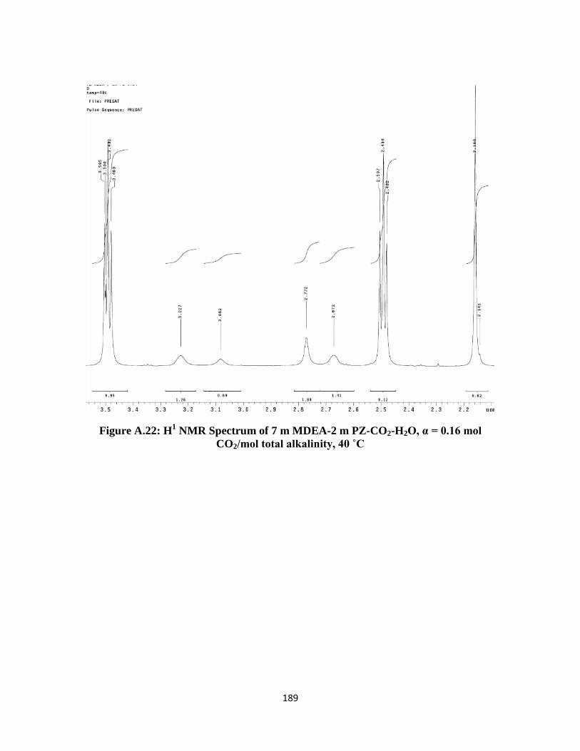
189
Figure A.22: H1 NMR Spectrum of 7 m MDEA-2 m PZ-CO2-H2O, α = 0.16 mol
CO2/mol total alkalinity, 40 ˚C
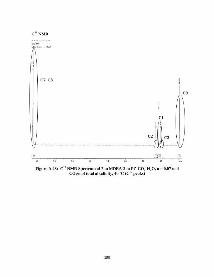
190
C13
NMR
Figure A.23: C13
NMR Spectrum of 7 m MDEA-2 m PZ-CO2-H2O, α = 0.07 mol
CO2/mol total alkalinity, 40 ˚C (C12
peaks)
C7, C8
C9
C2 C3
C1
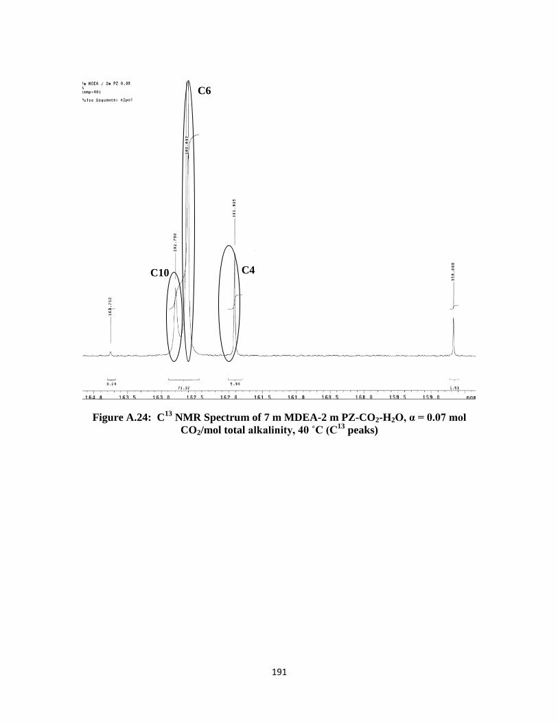
191
Figure A.24: C13
NMR Spectrum of 7 m MDEA-2 m PZ-CO2-H2O, α = 0.07 mol
CO2/mol total alkalinity, 40 ˚C (C13
peaks)
C4
C6
C10
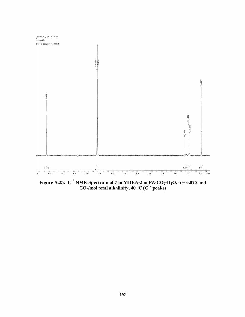
192
Figure A.25: C13
NMR Spectrum of 7 m MDEA-2 m PZ-CO2-H2O, α = 0.095 mol
CO2/mol total alkalinity, 40 ˚C (C12
peaks)
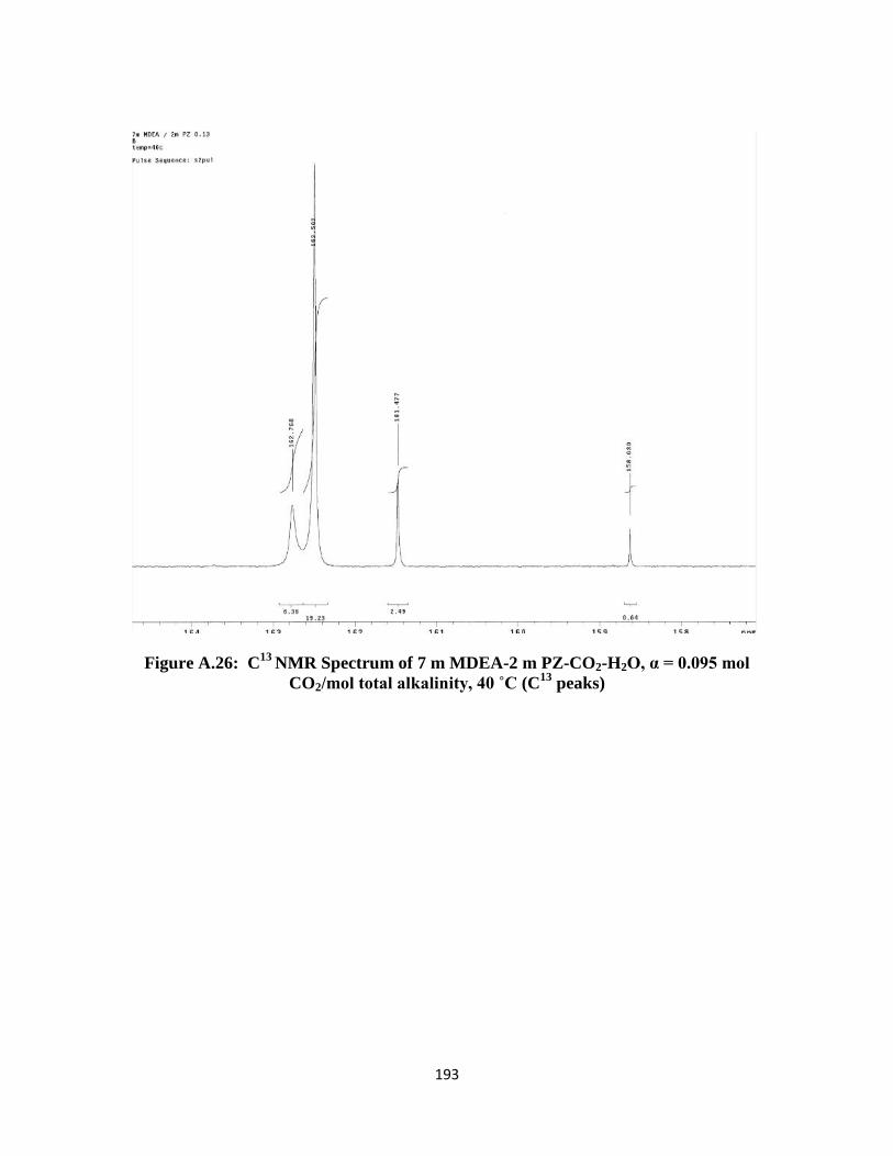
193
Figure A.26: C13
NMR Spectrum of 7 m MDEA-2 m PZ-CO2-H2O, α = 0.095 mol
CO2/mol total alkalinity, 40 ˚C (C13
peaks)
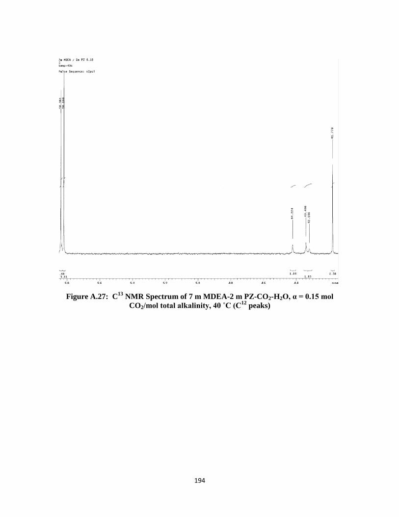
194
Figure A.27: C13
NMR Spectrum of 7 m MDEA-2 m PZ-CO2-H2O, α = 0.15 mol
CO2/mol total alkalinity, 40 ˚C (C12
peaks)
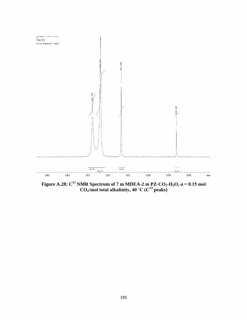
195
Figure A.28: C13
NMR Spectrum of 7 m MDEA-2 m PZ-CO2-H2O, α = 0.15 mol
CO2/mol total alkalinity, 40 ˚C (C13
peaks)
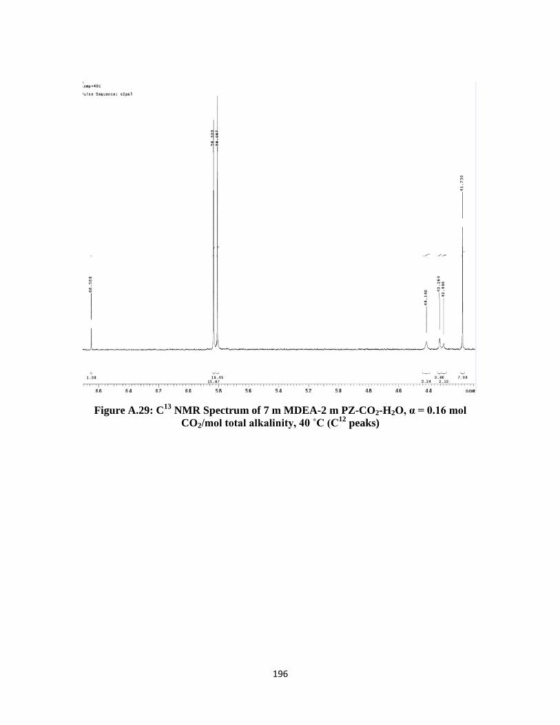
196
Figure A.29: C13
NMR Spectrum of 7 m MDEA-2 m PZ-CO2-H2O, α = 0.16 mol
CO2/mol total alkalinity, 40 ˚C (C12
peaks)
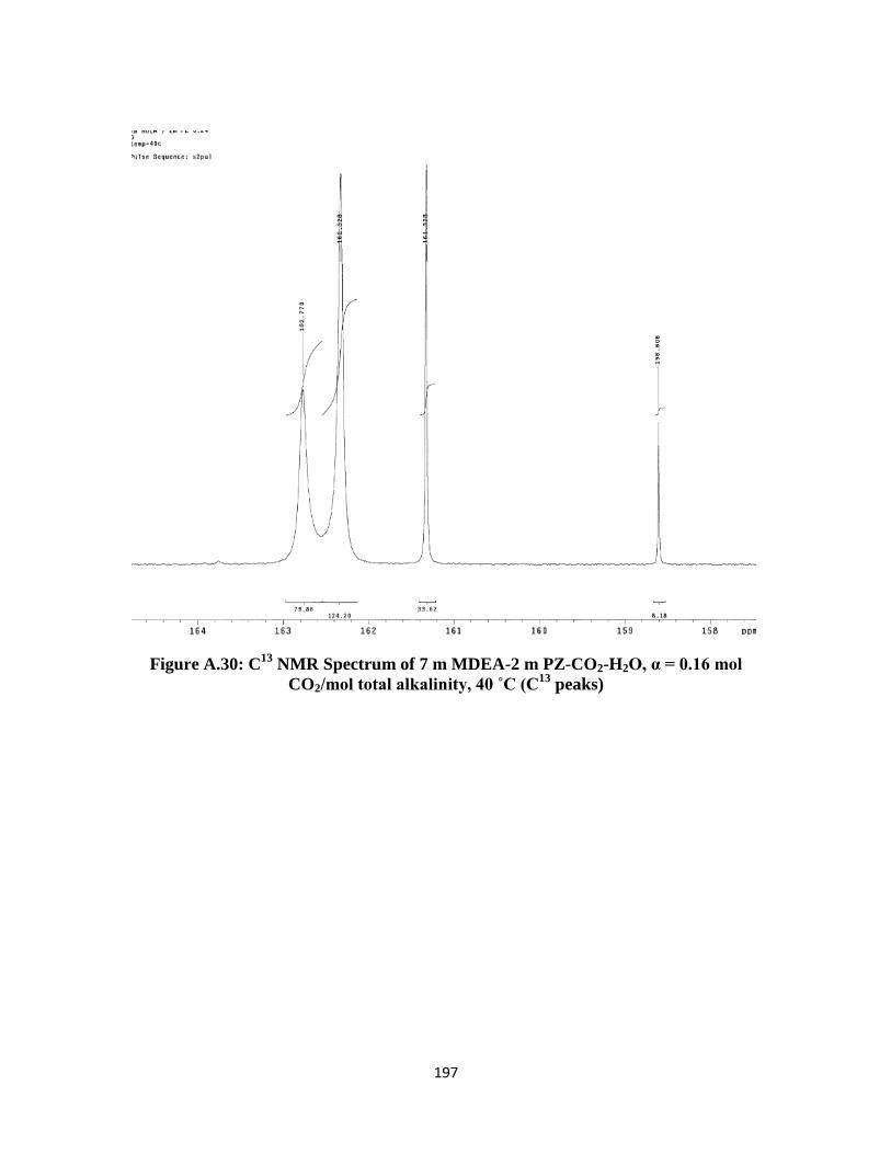
197
Figure A.30: C13
NMR Spectrum of 7 m MDEA-2 m PZ-CO2-H2O, α = 0.16 mol
CO2/mol total alkalinity, 40 ˚C (C13
peaks)
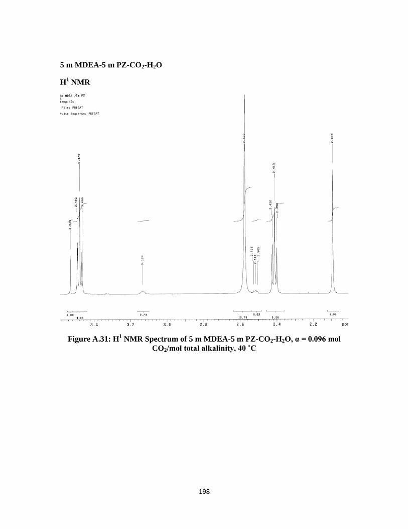
198
5 m MDEA-5 m PZ-CO2-H2O
H1 NMR
Figure A.31: H1 NMR Spectrum of 5 m MDEA-5 m PZ-CO2-H2O, α = 0.096 mol
CO2/mol total alkalinity, 40 ˚C
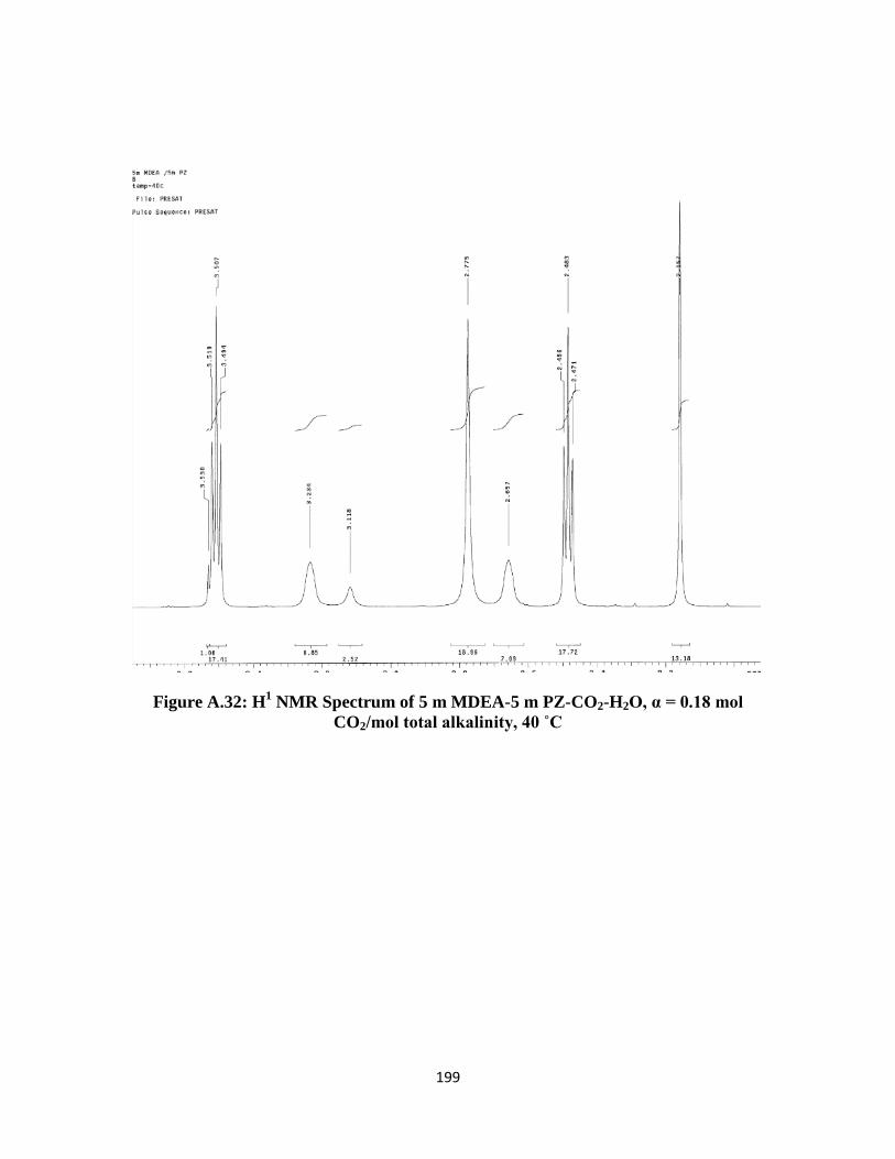
199
Figure A.32: H1 NMR Spectrum of 5 m MDEA-5 m PZ-CO2-H2O, α = 0.18 mol
CO2/mol total alkalinity, 40 ˚C
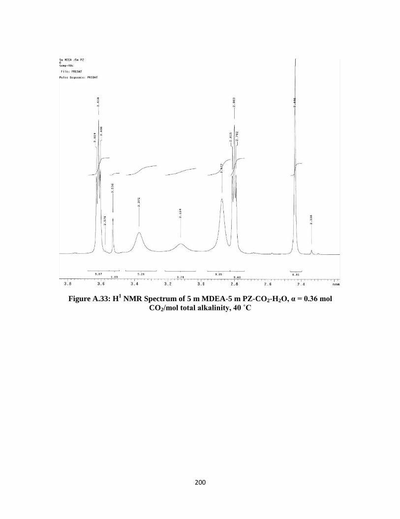
200
Figure A.33: H1 NMR Spectrum of 5 m MDEA-5 m PZ-CO2-H2O, α = 0.36 mol
CO2/mol total alkalinity, 40 ˚C
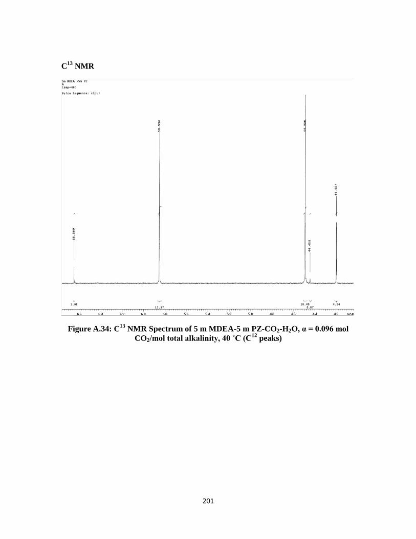
201
C13
NMR
Figure A.34: C13
NMR Spectrum of 5 m MDEA-5 m PZ-CO2-H2O, α = 0.096 mol
CO2/mol total alkalinity, 40 ˚C (C12
peaks)
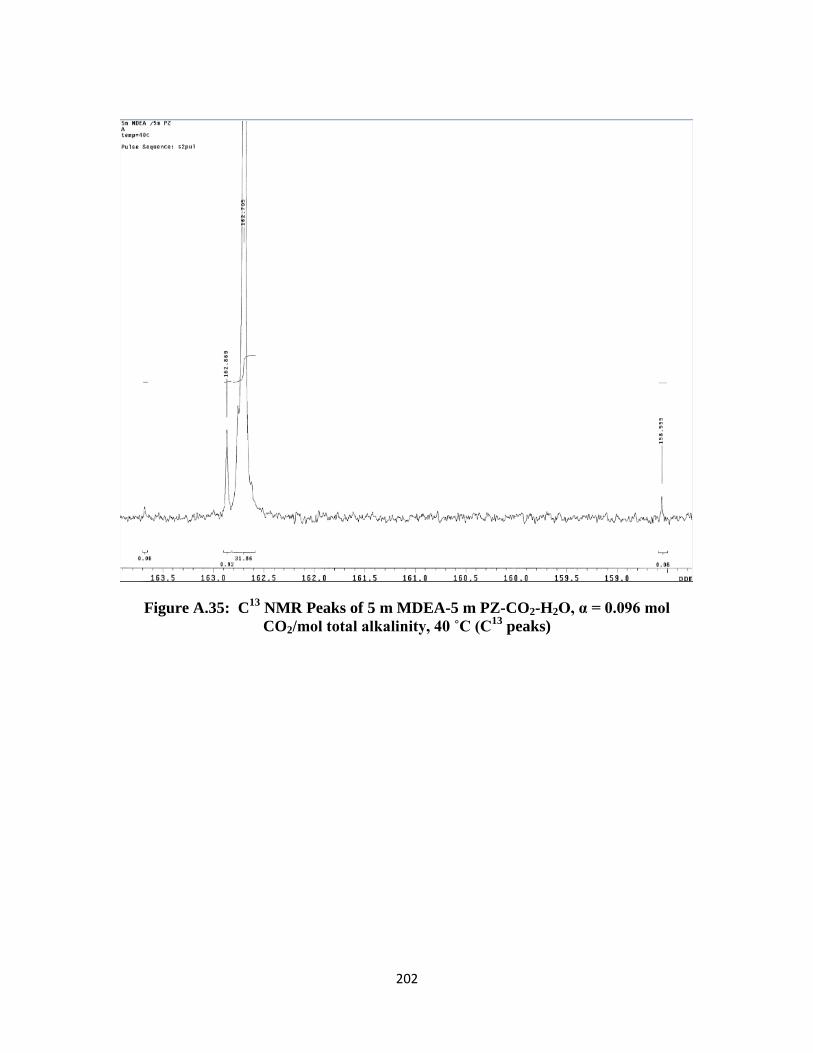
202
Figure A.35: C13
NMR Peaks of 5 m MDEA-5 m PZ-CO2-H2O, α = 0.096 mol
CO2/mol total alkalinity, 40 ˚C (C13
peaks)
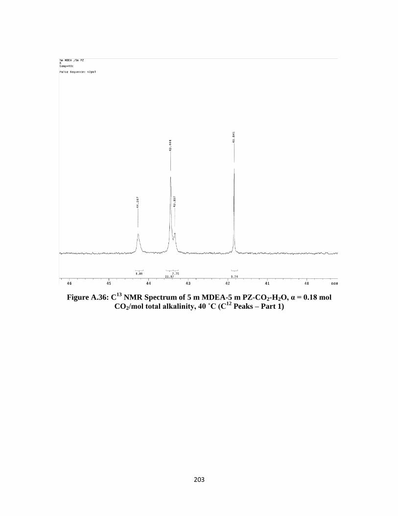
203
Figure A.36: C13
NMR Spectrum of 5 m MDEA-5 m PZ-CO2-H2O, α = 0.18 mol
CO2/mol total alkalinity, 40 ˚C (C12
Peaks – Part 1)
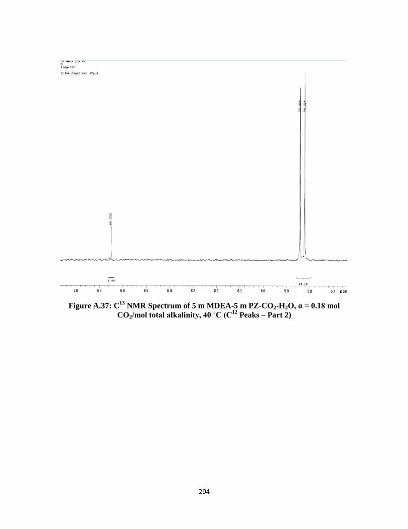
204
Figure A.37: C13
NMR Spectrum of 5 m MDEA-5 m PZ-CO2-H2O, α = 0.18 mol
CO2/mol total alkalinity, 40 ˚C (C12
Peaks – Part 2)
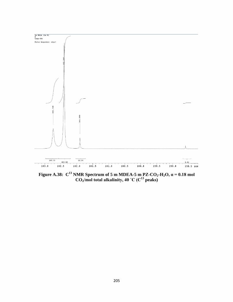
205
Figure A.38: C13
NMR Spectrum of 5 m MDEA-5 m PZ-CO2-H2O, α = 0.18 mol
CO2/mol total alkalinity, 40 ˚C (C13
peaks)
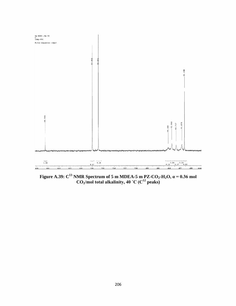
206
Figure A.39: C13
NMR Spectrum of 5 m MDEA-5 m PZ-CO2-H2O, α = 0.36 mol
CO2/mol total alkalinity, 40 ˚C (C12
peaks)

207
Figure A.40: C13
NMR Spectrum of 5 m MDEA-5 m PZ-CO2-H2O, α = 0.36 mol
CO2/mol total alkalinity, 40 ˚C (C13
peaks)

208
Appendix B: FTIR Operational Procedure
1. Introduction
The first part of this appendix discusses the procedure for calibrating pure
components for FTIR analysis (using the Gasmet DX-4000 analyzer). The latter part
describes how to operate the instrument for a standard VLE experimental run.
2. Procedure
Calibration of Pure Components
Pure components that are not already calibrated must be calibrated for FTIR
analysis. Calibration must be performed at each desired component concentration (ppm
or vol%). The calibration is done by using a Gasmet Calibrator Device that is specially
designed to calibrate pure components for Gasmet FTIR analyzers. Figure B.1 shows the
Gasmet Calibrator device.
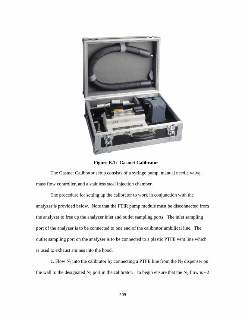
209
Figure B.1: Gasmet Calibrator
The Gasmet Calibrator setup consists of a syringe pump, manual needle valve,
mass flow controller, and a stainless steel injection chamber.
The procedure for setting up the calibrator to work in conjunction with the
analyzer is provided below. Note that the FTIR pump module must be disconnected from
the analyzer to free up the analyzer inlet and outlet sampling ports. The inlet sampling
port of the analyzer is to be connected to one end of the calibrator umbilical line. The
outlet sampling port on the analyzer is to be connected to a plastic PTFE vent line which
is used to exhaust amines into the hood.
1. Flow N2 into the calibrator by connecting a PTFE line from the N2 dispenser on
the wall to the designated N2 port in the calibrator. To begin ensure that the N2 flow is ~2

210
SLPM, with as little fluctuation as possible, as indicated by the digital flow indicator in
the calibrator.
2. Connect one end of the calibrator umbilical line to the outlet of the heated
oven chamber. Connect the other end of the umbilical line to the inlet sampling port of
the analyzer.
3. Set the temperature of both the umbilical line and of the heated oven chamber
to 180 ˚C. This is to prevent any species from condensing on the internals of the line and
apparatus. Do not perform any calibration injection until the setpoint of 180 ˚C is
reached.
Figure B.2. shows the internal calibrator setup as it is connected to the FTIR
analyzer.
Figure B.2: Internal Gasmet Calibrator Setup
4. Prepare the component to be injected for calibration. Fill up a Hamilton
gastight syringe with the component of interest to be calibrated. The concentration at
211
which the component will be injected into the calibrator will be determined by the rate at
which the component is to be injected (μL/hr) relative to the N2 carrier flow. Calculate
the appropriate injection rate relative to the N2 flow rate to obtain the desired calibration
concentration. Note that the N2 flow rate can be varied from 0.5 up to ~5 SLPM;
however, it is not recommended to flow N2 at too low or too high of a flow rate to avoid
frequent flow rate fluctuation.
5. Inject the calibration component into the heated oven inlet of the calibrator at
the appropriate injection rate as calculated. The injection rate is set by manually
selecting the flow settings in the calibrator flow display. Also ensure that the slider block
is properly rested against the syringe to secure the needle.
6. Set the N2 flow rate to the desired flow to achieve the component flow
concentration to be calibrated.
7. Observe the FTIR Calcmet live display of spectrum analysis. The display
should be showing no actual spectral feature, but only spectral noise, in the beginning
even after the component is injected as only N2 is flowing through the system at this
point. As the component is vaporized inside the heated chamber and is beginning to flow
into the analyzer, distinct spectral peaks should visibly emerge on the analysis window.
Some components may take longer than others to start showing peaks.
8. The peak signal should increase substantially with time even though it may
fluctuate somewhat due to flow irregularity. Ensure that the frequency of FTIR analysis
scan is set to every 5 second in order to observe the live changes in spectral peak
formation. Let the system equilibrate for as long as it takes, usually 20 – 30 minutes,
212
until the peak equilibrates to roughly a final constant value (peak height is seen to change
on the order of a hundredth or thousandth of a decimal).
9. When the peak height is relatively stable, set the FTIR scan frequency to 3
minutes to do a full peak integration.
10. Once the scan (integration) is completed, a reference spectra would have been
generated for the component at the desired concentration to be calibrated. Save this
spectra as a calibration spectra type (.REF) to be included in the Calcmet component
library. Specify the calibration conditions of the run (temperature and concentration) as
exactly as can be determined.
11. Repeat steps 4 – 10 to perform calibration for the same component at a
different concentration or for a different component. The reference concentration range
should ideally encompass the actual concentration range that is expected to be
encountered in an actual experiment.
Operation of the FTIR and Maintenance
The procedure below describes the steps taken to perform a VLE run on the FTIR
Gasmet DX-4000. Before any experiment is run, ensure that the umbilical lines, pump
modules, and analyzer are heated up to 180 ˚C and that a clean N2 background spectra
(~5 min. scan) is detected. It usually takes about 30 – 45 minutes to heat the lines to 180
˚C.
1. Prepare about ~525 – 550 g of the solution mixture to be studied. If it is
intended to study VLE at a given loading, then the solution needs to be loaded with CO2
up to the desired loading prior to running the FTIR experiment.
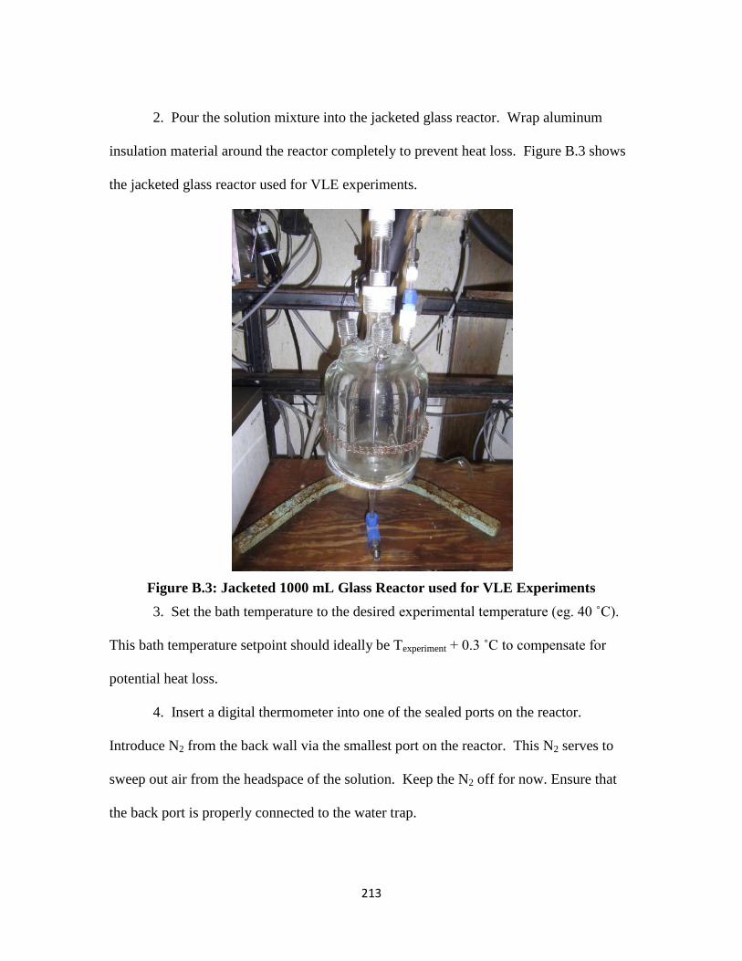
213
2. Pour the solution mixture into the jacketed glass reactor. Wrap aluminum
insulation material around the reactor completely to prevent heat loss. Figure B.3 shows
the jacketed glass reactor used for VLE experiments.
Figure B.3: Jacketed 1000 mL Glass Reactor used for VLE Experiments
3. Set the bath temperature to the desired experimental temperature (eg. 40 ˚C).
This bath temperature setpoint should ideally be Texperiment + 0.3 ˚C to compensate for
potential heat loss.
4. Insert a digital thermometer into one of the sealed ports on the reactor.
Introduce N2 from the back wall via the smallest port on the reactor. This N2 serves to
sweep out air from the headspace of the solution. Keep the N2 off for now. Ensure that
the back port is properly connected to the water trap.
214
5. Connect the plastic line and fittings from the remaining port on the reactor
with the FTIR umbilical line. Ensure that both the FTIR pump and line are set to 180 ˚C.
Do not run any experiment if these settings are below 180 ˚± 2˚C.
6. Connect the return umbilical line to the reactor outlet. Make sure that this line
is set to Treactor + 55 ˚C to prevent the returning gas from experiencing heat loss which
could upset equilibrium conditions in the reactor.
7. Turn on the agitator to a mixing speed of 350 ± 5 rpm. Use the tachometer to
verify that the mixing speed is as specified.
8. Turn on the FTIR pump. Also start the FTIR analysis scans (on Calcmet
software) with the 20 seconds scan for the beginning of the experiment.
9. Turn on N2 flow into the reactor for about 2 – 3 scan duration. This ensures
that the headspace of the reactor is fully evacuated.
10. Turn off the N2. Change the FTIR analysis scan rate to 1 minute for each
scan duration. Specify the components that are known to be in solution (eg. water,
amine, CO2). Make sure that there are reference spectra available for each component of
interest in the library method.
11. Allow for the experiment to run continuously up until the desired
experimental temperature is reached (eg. 40 ˚C). Given the standard heating rate of the
temperature bath, it should take ~ 1 hour to reach the desired experimental temperature
when starting from room temperature. Make sure that the digital thermometer reads that
the solution temperature has reach the desired target.

215
12. Record the equilibrium component concentrations from Calcmet. These
concentrations are the equilibrium concentrations of components in the gas phase. They
are used to determine the component volatilities at the experimental temperature.
13. Obtain a reading of the room pressure and record it. The room pressure is the
total pressure of the experiment. This number is also used to calculate the equilibrium
volatility.
14. Increase the water bath temperature to the next desired experimental
temperature. It is recommended to run experiments for every ∆T = 5 ˚C from 40 ˚C – 70
˚C (represent the absorber operating temperature).
15. Increase the temperature of the return umbilical line by 5 ˚C to match the
increase in water bath temperature. Maintain this new temperature for the return line for
the duration of this next run.
16. Save the data under a new file and resume the 1 minute analysis scans.
17. Run the experiment continuously until the desired experimental temperature
is reached (eg. 45 ˚C). Stop the analysis scan and record the equilibrium concentrations.
18. Repeat steps 13 – 16 until the final desired temperature is reached. On a
typical day, about 6 – 7 runs can be performed for temperature 40 ˚, 45 ˚, 50 ˚, 55 ˚, 60 ˚,
65 ˚, 70 ˚C.
19. After the final experiment of the day, drain out the content of the reactor and
dispose of properly in designated waste container. Disconnect all the lines from the
reactor ports. Make sure that the all the reactor ports are open to dry overnight.
216
20. Wash the interior of the reactor with ~1 gallon of distilled de-ionized water to
properly rinse it.
21. Lower the FTIR analyzer and line setpoints to 25 ˚C. This step is taken for
maintenance purposes to extend the life of the line and parts.
Cleaning the Umbilical Lines
It is recommended that the umbilical lines be cleaned every 2 – 3 weeks, or
perhaps even more frequently if there is excessive trace contaminants expected to build
up in the lines.
1. Disconnect the umbilical line from the inlet of the FTIR analyzer. Also
disconnect the return umbilical line from the back of the FTIR pump module. Connect
one end of the umbilical line to that of the return umbilical line so that form one long
continuous flow path.
2. Set the temperature of the umbilical lines to ~150 ˚C. Hot temperature
enhances cleaning and it helps to dry the lines faster after cleaning.
3. Connect a long ptfe line from the lab sink faucet to the free end of the
umbilical line. The free end of the return umbilical line should be directed into an empty
bucket.
4. Turn on the lab sink water and let flow through the connected umbilical lines.
Allow water to flow for ~30 minutes to properly rinse the lines.
5. Turn off the water. Connect the free end of the umbilical line to an air source
to blow dry the lines. Ensure that the lines are still heated at 150 ˚C. Let the air blow
through the lines for ~1.5 – 2 hours to ensure they are dried thoroughly.

217
6. Turn off the air and connect the umbilical and return lines to their appropriate
ports on the analyzer and the pump module.
218
Appendix C: Heat Capacity Experimental Procedure & Analysis
1. Introduction
Heat capacity measurements were needed for rigorous thermodynamic modeling
of amine systems, which ultimately becomes the key to proper process equipment design.
In this work, heat capacity was measured using a Differential Scanning Calorimeter
(DSC) from TA Instruments (model Q100) with automated controls provided by TA
Explorer DSC software . The following sections describe the experimental procedure for
obtaining heat capacity data along with how to analyze them.
2. Procedure
The following heat capacity procedure, which includes sample preparation, is in
accordance with standard ASTM Method E 1269-05 for determining heat capacity.
Preparing samples for Cp measurements
Four standard cells (reference, blank, Indium, Aluminum Oxide Al2O3) will have
to be prepared for any heat capacity experiment. Below is the procedure to prepare these
cells.
1. A cell consists of a pan, lid, and O-ring (Perkin Elmer #03190218 – 304
stainless steel with capacity of 60 μL). Weigh the pan, lid, and O-ring separately and
record their individual weights for the four cells.
2. Insert the O-ring into the lid of each cell. Make sure that the O-ring is properly
tucked inside the lid.
3. With the reference and blank cells, join the lid and pan together to make a cell
by using a Perkin Elmer Quick Press #0990-8467 device. When the cell has been
219
properly sealed, it is guaranteed to be able to withstand up to 150 bars of internal
pressure. Record the weights of the reference and blank cells.
4. Fill the Indium pan with ~5 mg of Indium sample. Join the Indium pan and its
lid to make the Indium cell. Record the weight of the Indium cell. Subtract this weight
from the total initial weight of its parts to determine the exact quantity of Indium in the
cell.
5. Fill the Al2O3 pan with ~120 mg of Al2O3 (Acros Organics, #40 sieve, 99.98 –
99.99% pure). Join the Al2O3 pan and its lid to make the Al2O3 cell. Record the weight
of the Al2O3 cell. Subtract this weight from the total initial weight of the parts to
determine the exact quantity of Al2O3 in the cell.
In regard to the sample cells, it is recommended that 4 sample cells are prepared
for each given loading. The need to have as many as 4 replicates of the same sample is to
ensure greater data reproducibility which accounts for fluctuations in the machine’s
calorimetric response.
6. Fill a given sample pan to the top (total capacity ~60 μL) with the sample
solution. Join the sample pan and its lid to make the sample cell. Record the weight of
the sample cell. Subtract this weight from the total initial weight of the parts to
determine the exact quantity of sample in the cell.
7. Repeat step 6 to make as many cells as needed (4 cells for each loading).
Place each cell inside a multi-cell container box and label each cell box with a number to
distinguish among the samples. Do not contaminate the cell with any type of residue as
this will affect the calorimetric measurement of the sample.
220
Measuring Sample Heat Capacity (on DSC Q100)
1. Start N2 flow from the cylinder into the DSC instrument. Set the N2 tank discharge
pressure at ~10 psia.
2. On the TA Explorer screen, select the N2 flow rate to be 50 mL/min. (Navigate to
“Notes” tab on the screen ---- > Mass Flow Controller entry field ---- > set to 50)
3. Turn on the Flange Cooler for the DSC and wait for the system to reach ~ -80 ˚C.
(Navigate to “Control” ----- > select Event ------ > choose On).
4. When the system is at -80 ˚C or below, calibrate the Indium metal sample. It
is recommended that the Indium sample not be used for calibration purposes for more
than 4 weeks. A fresh sample should be prepared after the 4 week timeframe to ensure
sample integrity. (Navigate to the DSC Calibration Wizard ----- > choose Heat Flow T4 -
----- > RCS for Cooling Unit ------ > select Cell Constant and Temperature Calibration ---
--- > fill in Indium for the Standard, sample weight, Other for the Pan Type ------ > select
Pre-Melt and specify the heating rate at 5 ˚C/min. Save the calibration under a new file
and then choose to Start Experiment. Note that this calibration exercise is used to
determine the drift in the machine’s calorimetric response and to have the system account
for it using an internal Cell Constant factor.
5. Once the Calibration is done, proceed to run the Heat Capacity experiments.
First load the sample pan into the DSC (On the instrument operating screen, independent
from the TA Explorer screen shown on the computer, select “Control Menu” and choose
“Open” Lid. Note that for safety reason it is not recommended to open the internal
chamber when the temperature is greater to 40 ˚C). Figure C.1. shows a snapshot of the
DSC internal chamber where the samples are stored.

221
Figure C.1. Snapshot of DSC Internal Chamber: Left (Reference Cell); Right
(Sample Cell)
6. Use uncontaminated tweezer to place the empty reference pan and the desired
sample plan into appropriate holder platforms (reference pan – left side platform; sample
pan – right side platform). Make sure that neither of the two pans will accidentally block
the central electrode which is used for heat sensing. Lid will automatically close once
the reference pan and sample pan have been properly placed inside the chamber.
7. Load the Heat Capacity Method (or Recipe) to run the experiments (Navigate
to the “Summary” tab ------ > select Mode -------- > specify Custom in regard to Standard
and Test ----- > Click Green arrow to run the experiment)
The Heat Capacity Method is given below:
Data Storage Off. Ramp at 10 ˚C/min. to 20 ˚C. Isothermal for 10 min. Data
Storage On. Ramp at 5 ˚C/min. to 125 ˚C. Date Storage Off. Ramp at 20 ˚C/min. to 25
˚C. Isothermal for 1 min.

222
8. Run the cells in this order: Blank, Al2O3, then all Samples. Be sure to always
place these cells on the right side platform. The reference cell should always be left on
the left side platform for each run. A typical run takes approximately 45 minute.
Shutting Down the Instrument
The following steps describe how to shut down the instrument at the end of each
day.
1. On the TA Explorer screen, navigate to the “Procedure” tab ----- > Open the
Folder icon ------ > Select a program called RCS Off and Open it ------- > Click Green
arrow to run it. It should take approximately 15 min. to run the shut down procedure.
2. Navigate to the “Notes” tab ------ > Set the Mass Flow Control to 0 mL/min. to
stop N2 flow into the DSC system.
3. Turn off the N2 from the tank.
3. Sample DSC Scans
Sample DSC scans are now provided for the Indium, Blank, Al2O3, and a given
sample. Note that all of these scans can be viewed with TA Universal Analysis software
(Version 4.2. E). Figure C.2. shows a standard Indium calorimetric scan.
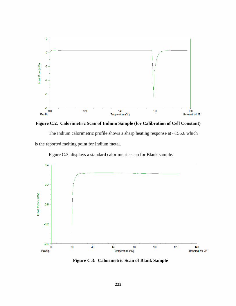
223
Figure C.2. Calorimetric Scan of Indium Sample (for Calibration of Cell Constant)
The Indium calorimetric profile shows a sharp heating response at ~156.6 which
is the reported melting point for Indium metal.
Figure C.3. displays a standard calorimetric scan for Blank sample.
Figure C.3: Calorimetric Scan of Blank Sample
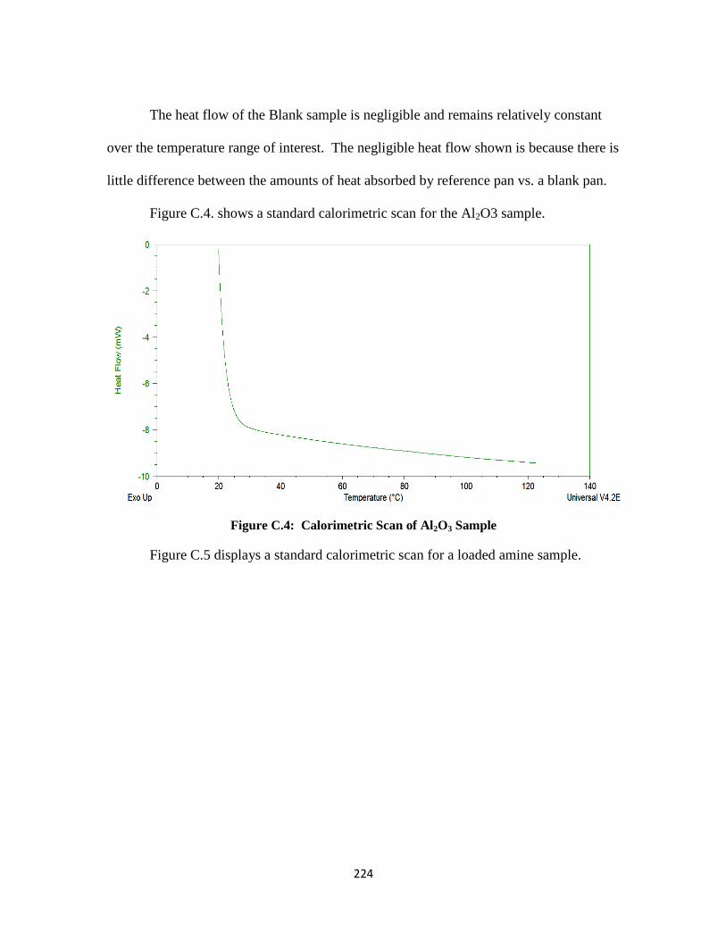
224
The heat flow of the Blank sample is negligible and remains relatively constant
over the temperature range of interest. The negligible heat flow shown is because there is
little difference between the amounts of heat absorbed by reference pan vs. a blank pan.
Figure C.4. shows a standard calorimetric scan for the Al2O3 sample.
Figure C.4: Calorimetric Scan of Al2O3 Sample
Figure C.5 displays a standard calorimetric scan for a loaded amine sample.
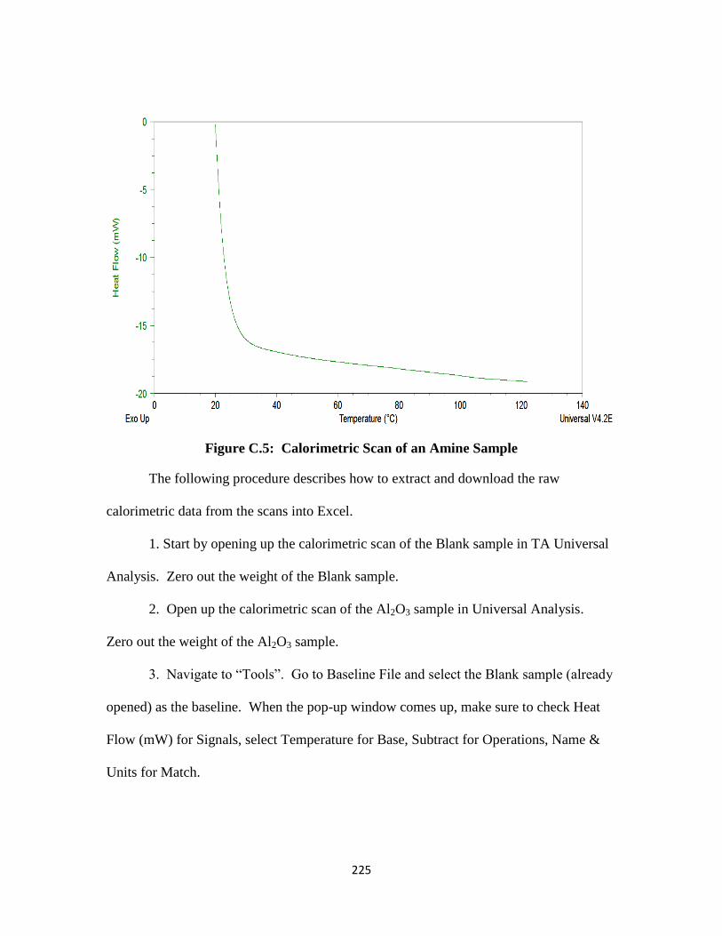
225
Figure C.5: Calorimetric Scan of an Amine Sample
The following procedure describes how to extract and download the raw
calorimetric data from the scans into Excel.
1. Start by opening up the calorimetric scan of the Blank sample in TA Universal
Analysis. Zero out the weight of the Blank sample.
2. Open up the calorimetric scan of the Al2O3 sample in Universal Analysis.
Zero out the weight of the Al2O3 sample.
3. Navigate to “Tools”. Go to Baseline File and select the Blank sample (already
opened) as the baseline. When the pop-up window comes up, make sure to check Heat
Flow (mW) for Signals, select Temperature for Base, Subtract for Operations, Name &
Units for Match.
226
4. Navigate to “View”. Go to Data Table and select Spreadsheet as the output
format. When the pop-up window comes up, specify the range of temperature for which
heat flow measurements are to be reported (40 ˚ - 120 ˚C) with an increment of 5 ˚C. Go
to Resolution, click on Temperature, and select round off to 3 significant figures. Choose
OK.
These steps will generate an Excel report of the heat flow data over the range of
temperature requested. These same steps must be followed to extract the calorimetry data
for the samples. The raw data are then used to calculate the sample heat capacity.
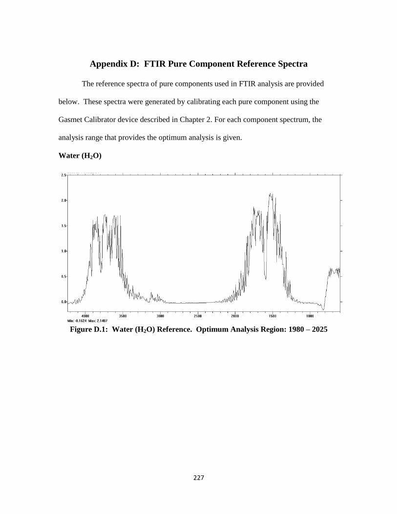
227
Appendix D: FTIR Pure Component Reference Spectra
The reference spectra of pure components used in FTIR analysis are provided
below. These spectra were generated by calibrating each pure component using the
Gasmet Calibrator device described in Chapter 2. For each component spectrum, the
analysis range that provides the optimum analysis is given.
Water (H2O)
Figure D.1: Water (H2O) Reference. Optimum Analysis Region: 1980 – 2025
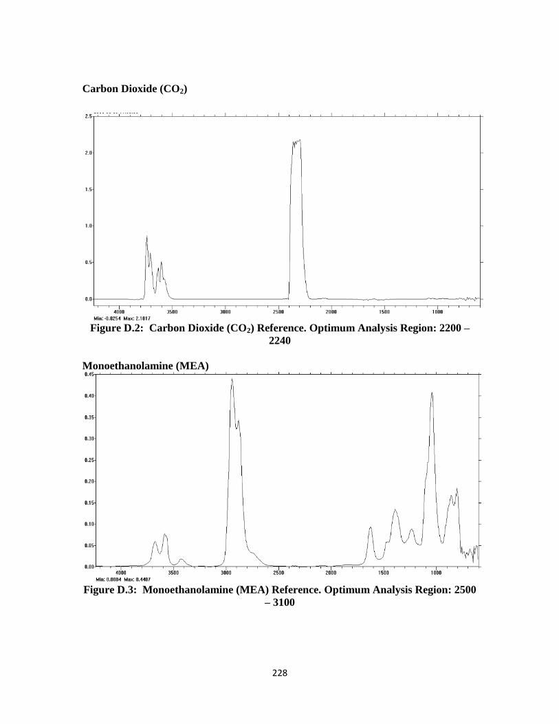
228
Carbon Dioxide (CO2)
Figure D.2: Carbon Dioxide (CO2) Reference. Optimum Analysis Region: 2200 –
2240
Monoethanolamine (MEA)
Figure D.3: Monoethanolamine (MEA) Reference. Optimum Analysis Region: 2500
– 3100
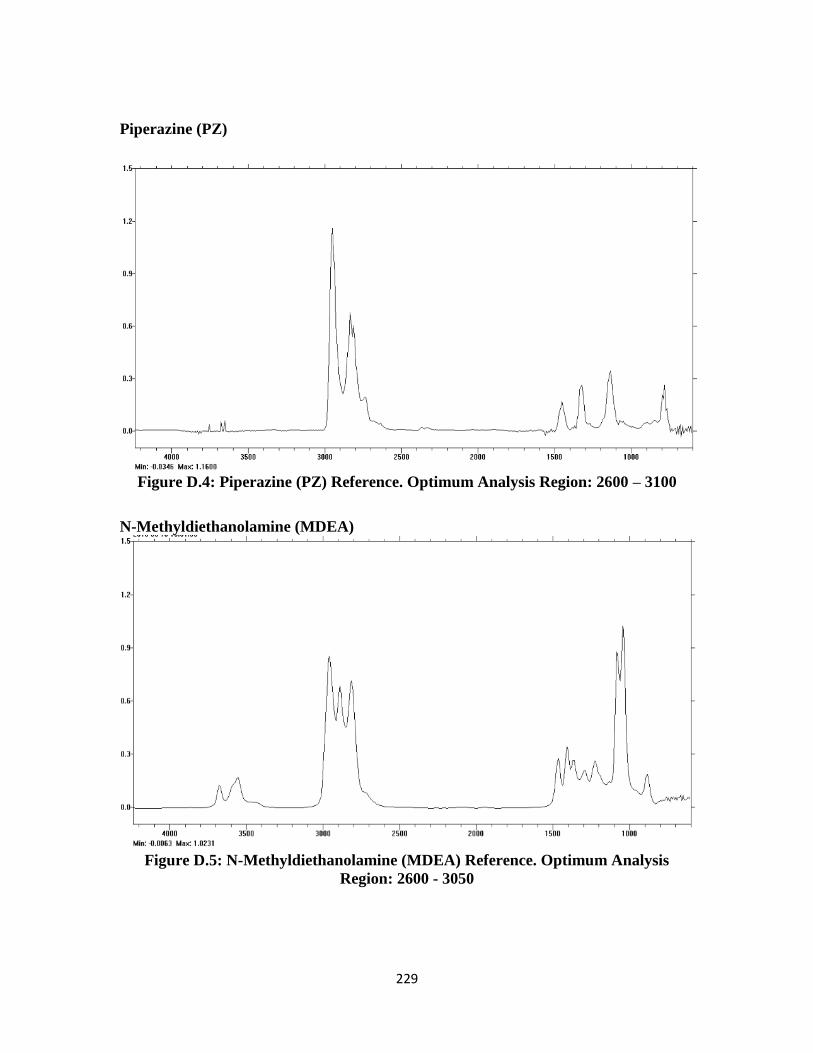
229
Piperazine (PZ)
Figure D.4: Piperazine (PZ) Reference. Optimum Analysis Region: 2600 – 3100
N-Methyldiethanolamine (MDEA)
Figure D.5: N-Methyldiethanolamine (MDEA) Reference. Optimum Analysis
Region: 2600 - 3050
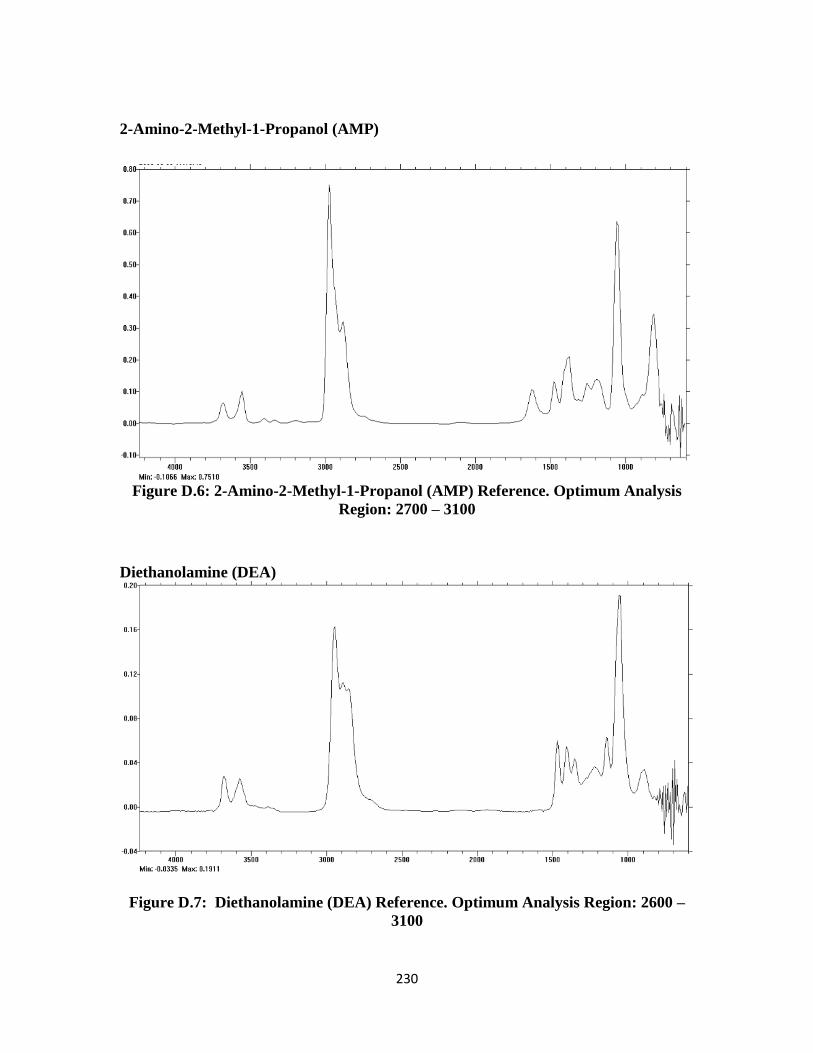
230
2-Amino-2-Methyl-1-Propanol (AMP)
Figure D.6: 2-Amino-2-Methyl-1-Propanol (AMP) Reference. Optimum Analysis
Region: 2700 – 3100
Diethanolamine (DEA)
Figure D.7: Diethanolamine (DEA) Reference. Optimum Analysis Region: 2600 –
3100
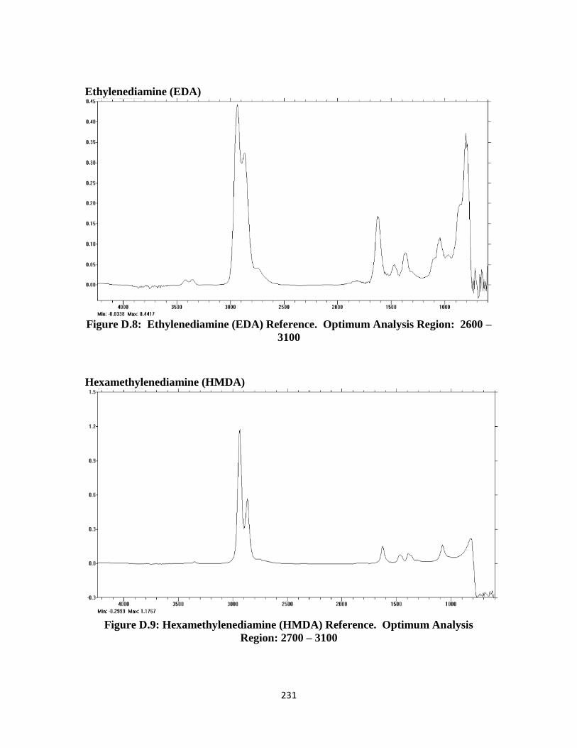
231
Ethylenediamine (EDA)
Figure D.8: Ethylenediamine (EDA) Reference. Optimum Analysis Region: 2600 –
3100
Hexamethylenediamine (HMDA)
Figure D.9: Hexamethylenediamine (HMDA) Reference. Optimum Analysis
Region: 2700 – 3100
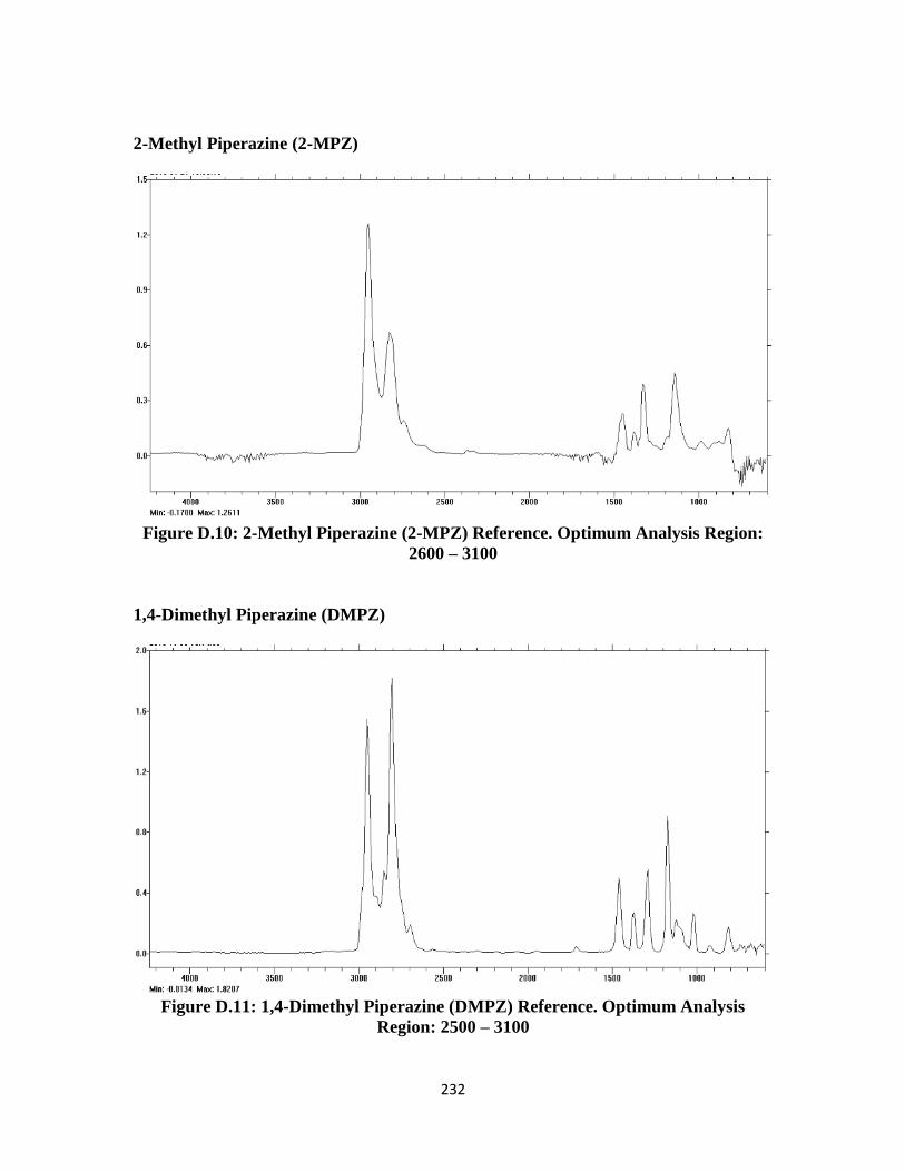
232
2-Methyl Piperazine (2-MPZ)
Figure D.10: 2-Methyl Piperazine (2-MPZ) Reference. Optimum Analysis Region:
2600 – 3100
1,4-Dimethyl Piperazine (DMPZ)
Figure D.11: 1,4-Dimethyl Piperazine (DMPZ) Reference. Optimum Analysis
Region: 2500 – 3100
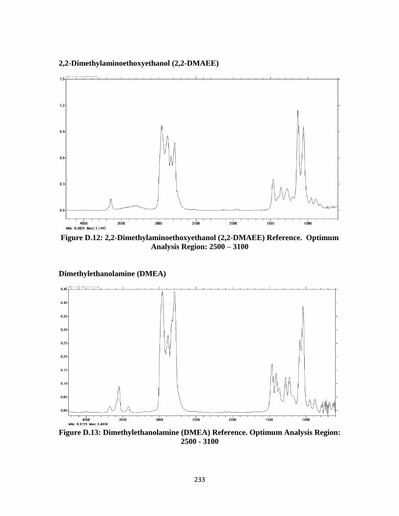
233
2,2-Dimethylaminoethoxyethanol (2,2-DMAEE)
Figure D.12: 2,2-Dimethylaminoethoxyethanol (2,2-DMAEE) Reference. Optimum
Analysis Region: 2500 – 3100
Dimethylethanolamine (DMEA)
Figure D.13: Dimethylethanolamine (DMEA) Reference. Optimum Analysis Region:
2500 - 3100
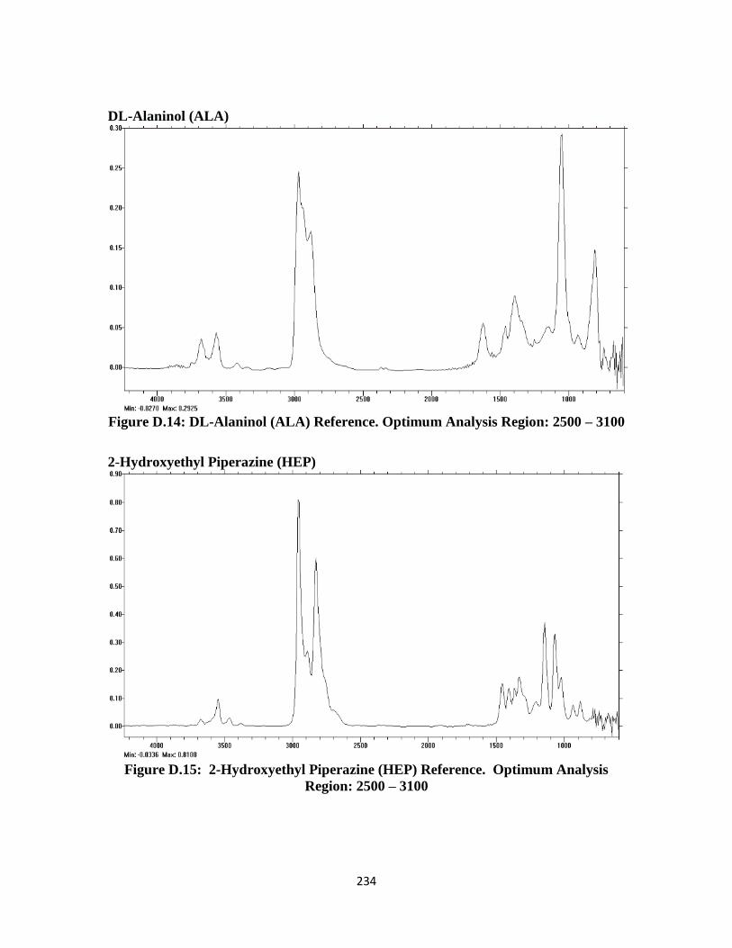
234
DL-Alaninol (ALA)
Figure D.14: DL-Alaninol (ALA) Reference. Optimum Analysis Region: 2500 – 3100
2-Hydroxyethyl Piperazine (HEP)
Figure D.15: 2-Hydroxyethyl Piperazine (HEP) Reference. Optimum Analysis
Region: 2500 – 3100
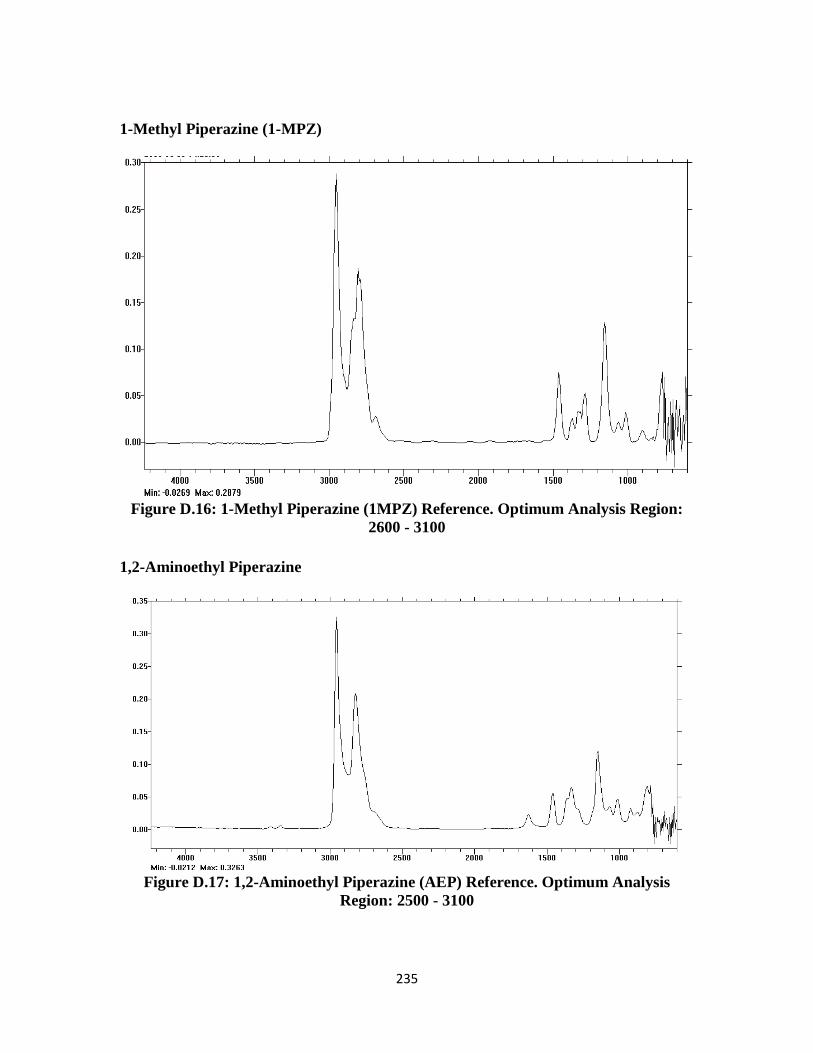
235
1-Methyl Piperazine (1-MPZ)
Figure D.16: 1-Methyl Piperazine (1MPZ) Reference. Optimum Analysis Region:
2600 - 3100
1,2-Aminoethyl Piperazine
Figure D.17: 1,2-Aminoethyl Piperazine (AEP) Reference. Optimum Analysis
Region: 2500 - 3100
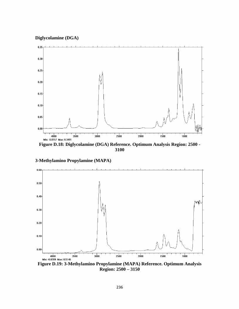
236
Diglycolamine (DGA)
Figure D.18: Diglycolamine (DGA) Reference. Optimum Analysis Region: 2500 -
3100
3-Methylamino Propylamine (MAPA)
Figure D.19: 3-Methylamino Propylamine (MAPA) Reference. Optimum Analysis
Region: 2500 – 3150
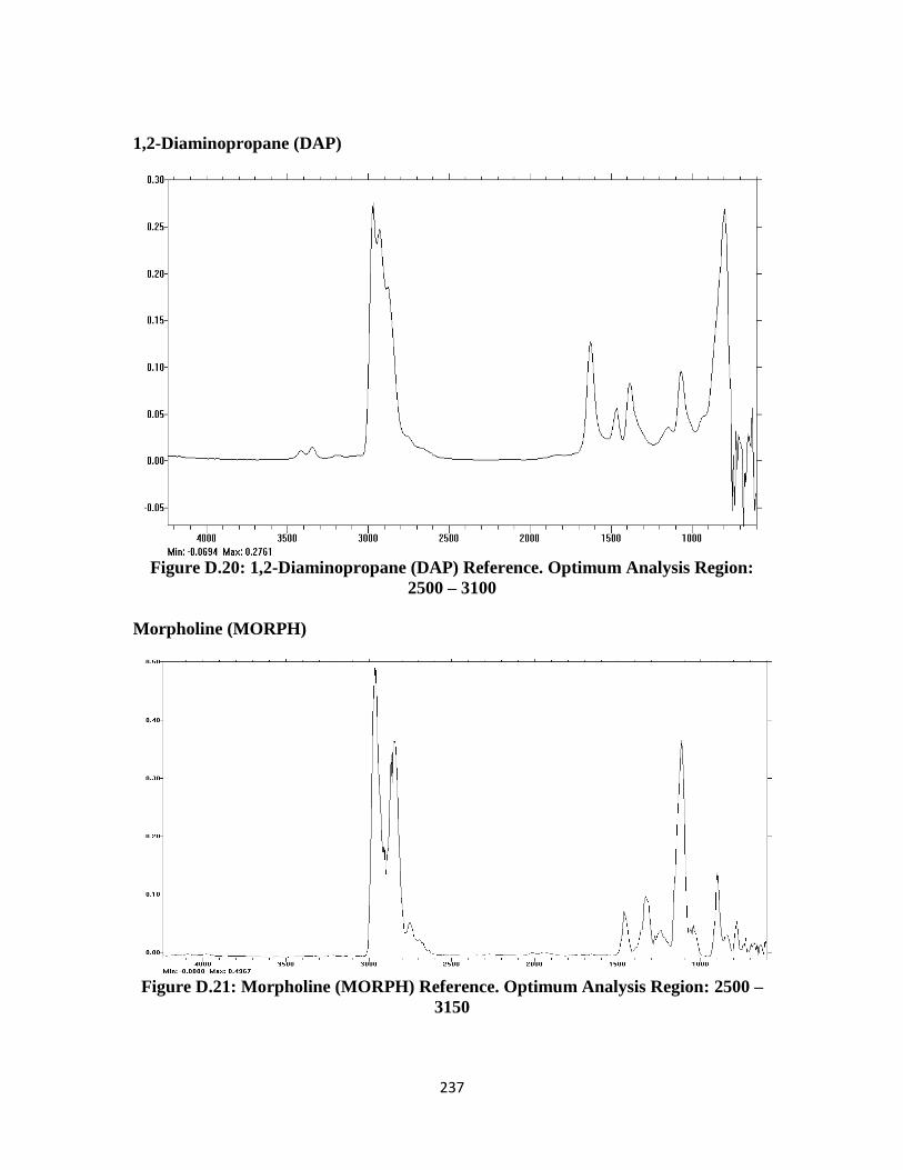
237
1,2-Diaminopropane (DAP)
Figure D.20: 1,2-Diaminopropane (DAP) Reference. Optimum Analysis Region:
2500 – 3100
Morpholine (MORPH)
Figure D.21: Morpholine (MORPH) Reference. Optimum Analysis Region: 2500 –
3150
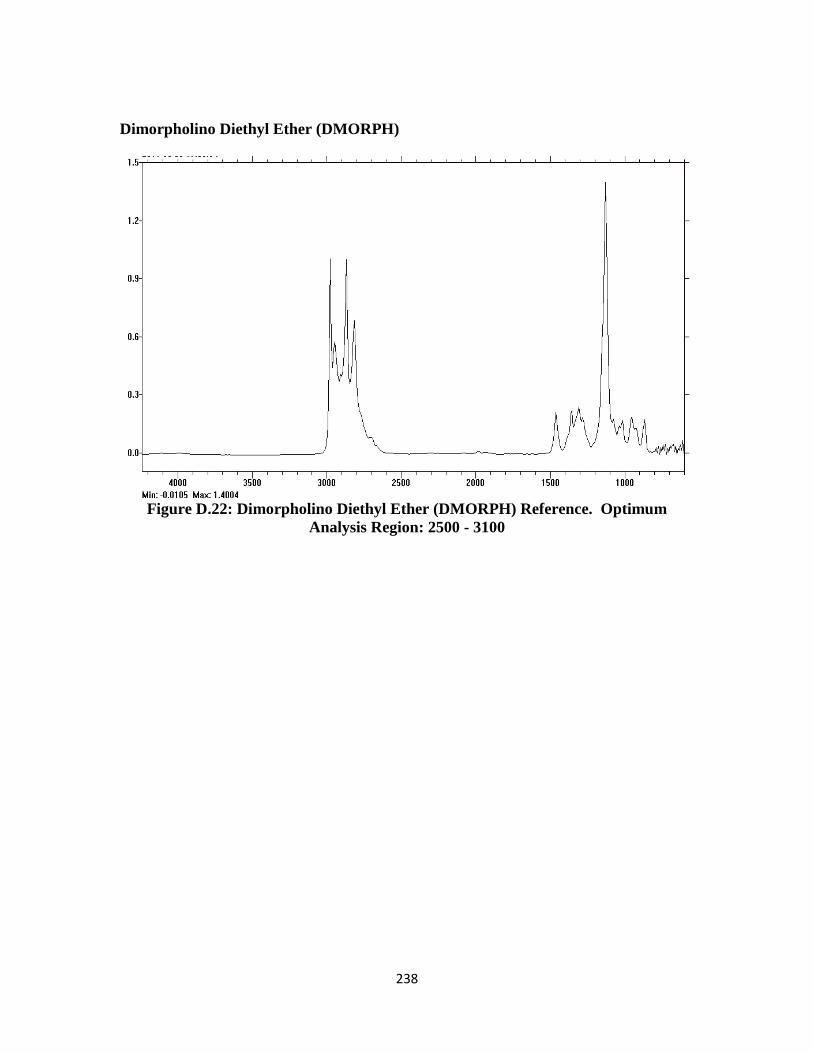
238
Dimorpholino Diethyl Ether (DMORPH)
Figure D.22: Dimorpholino Diethyl Ether (DMORPH) Reference. Optimum
Analysis Region: 2500 - 3100
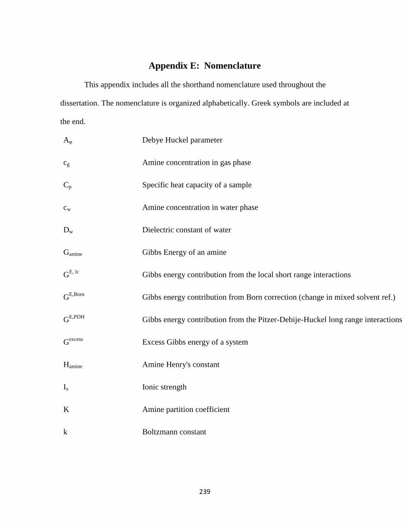
239
Appendix E: Nomenclature
This appendix includes all the shorthand nomenclature used throughout the
dissertation. The nomenclature is organized alphabetically. Greek symbols are included at
the end.
Aφ Debye Huckel parameter
cg Amine concentration in gas phase
Cp Specific heat capacity of a sample
cw Amine concentration in water phase
Dw Dielectric constant of water
Gamine Gibbs Energy of an amine
GE, lc
Gibbs energy contribution from the local short range interactions
GE,Born
Gibbs energy contribution from Born correction (change in mixed solvent ref.)
GE,PDH
Gibbs energy contribution from the Pitzer-Debije-Huckel long range interactions
Gexcess
Excess Gibbs energy of a system
Hamine Amine Henry's constant
Ix Ionic strength
K Amine partition coefficient
k Boltzmann constant
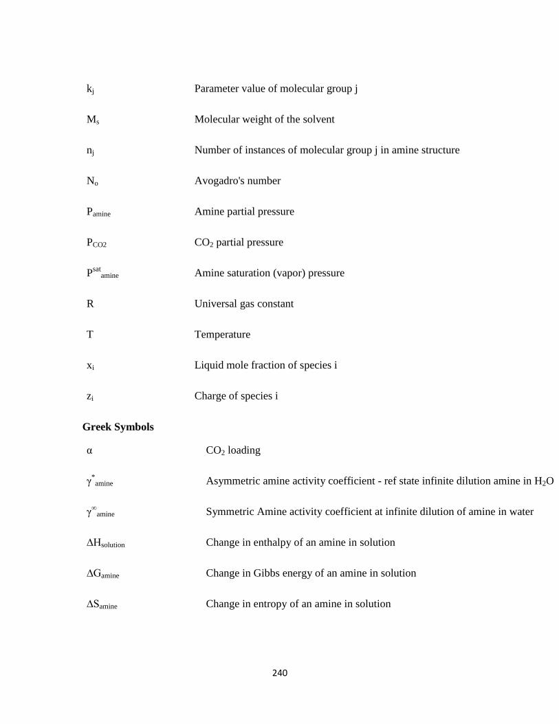
240
kj Parameter value of molecular group j
Ms Molecular weight of the solvent
nj Number of instances of molecular group j in amine structure
No Avogadro's number
Pamine Amine partial pressure
PCO2 CO2 partial pressure
Psat
amine Amine saturation (vapor) pressure
R Universal gas constant
T Temperature
xi Liquid mole fraction of species i
zi Charge of species i
Greek Symbols
α CO2 loading
γ*amine Asymmetric amine activity coefficient - ref state infinite dilution amine in H2O
γ∞
amine Symmetric Amine activity coefficient at infinite dilution of amine in water
∆Hsolution Change in enthalpy of an amine in solution
∆Gamine Change in Gibbs energy of an amine in solution
∆Samine Change in entropy of an amine in solution

241
τij Binary interaction parameter between component i and j
Gij Gibbs interaction energy between component i and j
φamine Fugacity coefficient of an amine
∆Hreaction Change in enthalpy of an amine in a reaction
∆Hexcess Change in excess enthalpy of an amine
ρM Molar density of water
242
References
Abbott, M.; O’Connell, J.P., Chem. Eng. Educ. 28 (1994) 18 – 23, 77.
Cabani, S., Conti, G., Lepori, L. Thermodynamic Study on Aqueous Dilute Solutions of
Organic Compounds. Part 1 – Cyclic Amines. Trans. Faraday Soc. 67 (1971)
1933 – 1942.
Cai, Z.; Xie, R.; Wu, Z., Binary Isobaric Vapor-Liquid Equilibria of Ethanolamines +
Water. J. Chem. Eng. Data. 41 (1996) 1101 – 1103.
Chiu, L. F.; Li, M. H., Heat Capacity of Alkanolamine Aqueous Solutions. Journal of
Chemical and Engineering Data 1999, 44, (6), 1396-1401.
Closmann, F.B., Oxidation and Thermal Degradation of
Methyldiethanolamine/Piperazine in CO2 Capture. Ph.D. Dissertation. The
University of Texas at Austin (2011).
DIPPR 801: Thermophysical Property Database for Pure Chemical Compounds.
Dugas, R.E., Carbon Dioxide Absorption, Desorption, and Diffusion in Aqueous
Piperazine and
Monoethanolamine. Ph.D. Dissertation. The University of Texas at Austin
(2009).
Ermatchkov, V.; Kamps, A. P.-S.; Speyer, D.; Maurer, G., Solubility of Carbon
Dioxide in Aqueous Solutions of Piperazine in the Low Gas Loading Region.
Journal
of Chemical and Engineering Data 2006, 51, (5), 1788-1796.
Ermatchkov, V.; Perez-Salado Kamps, A.; Maurer, G., Chemical Equilibrium
Constants for the Formation of Carbamates in (Carbon Dioxide + Piperazine +
Water)
from 1H NMR-Spectroscopy. Journal of Chemical Thermodynamics 35 (2003)
1277-1289.
Goff, G. S. Oxidative Degradation of Aqueous Monoethanolamine in CO2 Capture
Processes: Iron and Copper Catalysis, Inhibition, and O2 Mass Transfer. Ph.D.
Dissertation. The University of Texas at Austin, Austin, Texas, 2005.
Hamborg E, Niederer J, Versteeg G. “Dissociation Constants and Thermodynamic
Properties of Amino Acids used in CO2 Absorption from 293 to 353 K.” J Chem
Eng Data. 52 (2007) 2491-2502.
243
Hilliard, M.D., A Predictive Thermodynamic Model for an Aqueous Blend of Potassium
Carbonate, Piperazine, and Monoethanolamine for Carbon Dioxide Capture from
Flue Gas. Ph.D. Dissertation. The University of Texas at Austin (2008).
Hine, J; Mookerjee, P., The Intrinsic Hydrophilic Character of Organic Compounds.
Correlations in terms of Structural Contributions. J. Org. Chem. 40 (1975) 292 –
298.
Jou, F.-Y.; Mather, A. E.; Otto, F. D., The Solubility of CO2 in a 30 Mass Percent
Monoethanolamine Solution. The Canadian Journal of Chemical Engineering. 73
(1995)
140-146.
Jou, F-Y.; Mather, A.; Otto, F., Solubility of Hydrogen Sulfide and Carbon Dioxide in
Aqueous Methyldiethanolamine Solutions. Ind Eng Chem Process Des Dev. 21
(1982) 539-544.
Kell, G. S.; Haar, L.; Gallagher, J. S., NBS/NRC Steam Tables. Thermodynamic and
Transport Properties and Computer Programs for Vapor and Liquid States of
Water in SI Units. Hemisphere Publishing Corporation: Washington, (1984).
Kim, I.; Svendsen, H.F.; Borresen, E., Ebulliometric Determination of Vapor-Liquid
Equilibria for Pure Water, Monoethanolamine, N-Methyldiethanolamine, 3-
(Methylamino)-propylamine, and Their Binary and Ternary Solutions. J. Chem.
Eng. Data. 53 (2008) 2521-2531.
Larsen, B.; Rasmussen, P; Fredenslund, A., A Modified UNIFAC Group Contribution
Model for Prediction of Phase Equilibria and Heats of Mixing. Industrial &
Engineering Chemistry Research. 26 (1987) 2274-2286.
Lenard, J.; Rousseau, R.; Teja, A., Vapor-Liquid Equilibria for Mixtures of 2-
Aminoethanol + Water. AIChE Symposium Series. 86 (1990) 1-5.
Matthews, E.; Fried, V.; Boublik, T., The Vapour Pressures of Pure Substances. Elsevier:
New York, NY, (1973).
Osborne, N. S.; Stimson, H. F.; Ginnings, D. C., Measurements of Heat Capacity and
Heat of Vaporization of Water in the Range 0 oC to 100
oC. Journal of Research
of
the National Bureau of Standards (1939), 23, 197-260.
Pappa, G.; Anastasi, C.; Voutsas, E., Measurement and Thermodynamic Modeling of the
Phase Equilibrium of Aqueous 2-Amino-2-Methyl-1-Propanol Solutions. Fluid
Phase Equilibria. 243 (2006) 193-197.
244
Poplsteinova, J.; Krane, J.; Svendsen, H. F., Liquid-Phase Composition Determination in
CO2-H2O-Alkanolamine Systems: An NMR Study. Ind. Eng. Chem. Res. 2005,
44, 9894-9903.
Renon, H.; Prausnitz, J. M., Local Compositions in Thermodynamic Excess Functions for
Liquid Mixtures. AICHE J. 1968, 14, (1), 135-44.
Saarinen, P.; Kauppinen, J., Multicomponent Anaylsis of FT-IR Spectra. Applied
Spectroscopy. 45, 6 (1991) 953-963.
Sander, R., Compilation of Henry’s Law Constants for Inorganic and Organic Species of
Potential Importance in Environmental Chemistry. Version 3. (1999).
http://www.mpch-mainz.mpg.de/~sander/res/henry.html
Smith, J.; Van Ness, H.; Abbott, M., Introduction to Chemical Engineering
Thermodynamics, 6th
ed, McGraw-Hill Higher Education. (2001) 644.
Swanson, A. C.; Chueh, C. F., Estimating Liquid Heat Capacity. Chemical Engineering
Progress 1973, 69, 83.
U.S. Energy Information Administration (EIA). 2008. http://www.eia.gov/
USEPA. Air and Steam Stripping of Toxic Pollutants. Tech. Rep. EPA-68-03-002,
Industrial Environmental Research Laboratory, Cincinnati, OH, USA, 1982.
Van Wagener, D.H. Stripper Modeling for CO2 Removal Using Monoethanolamine and
Piperazine Solvents. Ph.D. Dissertation. The University of Texas at Austin
(2011).
Weiland, R.; Dingman, J.; Cronin, B., Heat Capacity of Aqueous Monoethanolamine,
Diethanolamine, N-Methyldiethanolamine, and N-Methyldiethanolamine-Based
Blends with Carbon Dioxide. J Chem Eng Data. 42 (1997) 1004-1006.
Wilhelm, E., Battino, R., Wilcock, R. Low Pressure Solubility of Gases in Liquid Water.
Chem. Rev. 77 (1977) 219 – 262.
Xu, Q. Thermodynamics of CO2 Loaded Aqueous Amines. Ph.D. Dissertation. The
University of Texas at Austin (2011).
Zhang, K.; Hawrylak, B.; Palepu, R.; Tremaine, P., Thermodynamics of Aqueous
Amines: Excess Molar Heat Capacities, Volumes, and Expansibilities of {Water +
Methyldiethanolamine (MDEA)} and {Water + 2-Amino-2-Methyl-1-Propanol
(AMP)}. J Chem Thermodynamics. 34 (2002) 679-710.
245
Vita
Thu Nguyen was born in Saigon, Vietnam to Dat-Vinh Nguyen and Ngoc-Oanh Pham.
After graduating from Lubbock High School in Lubbock, TX in May 1998, she enrolled
in The University of Texas at Austin. She received her B.S. in Chemical Engineering in
May 2003. After working for a number of years, she enrolled in graduate studies at The
University of Texas at Austin in July 2007 working in Dr. Gary Rochelle’s group on CO2
Capture. She has accepted full-time employment with GTC Technology, LLC in
Houston, TX.
Permanent Email: [email protected]
This dissertation was typed by the author.


![Diagram Koi Fish-Nguyen Ngoc Vu[HD]](https://static.fdocuments.us/doc/165x107/577c82381a28abe054aff17d/diagram-koi-fish-nguyen-ngoc-vuhd.jpg)