Copyright © 2007 Ramez Elmasri and Shamkant B. Navathe Slide 28- 1.

Copyright © 2007 Ramez Elmasri and Shamkant B. Navathe

Chapter 28

Data Mining Concepts


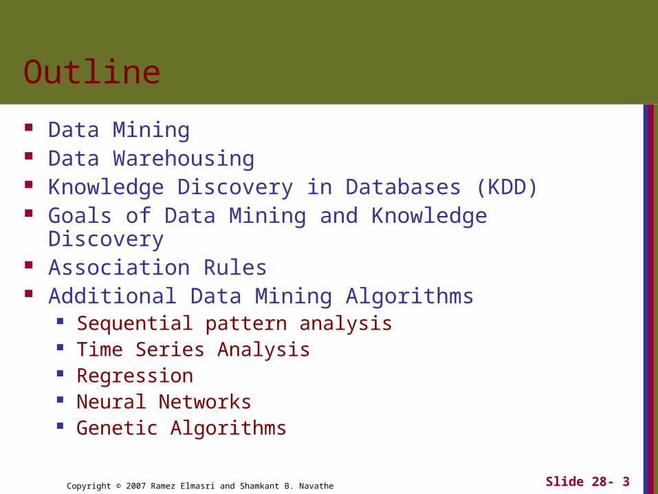
Outline

Data Mining Data Warehousing Knowledge Discovery in Databases (KDD) Goals of Data Mining and Knowledge Discovery Association Rules Additional Data Mining Algorithms

Sequential pattern analysis Time Series Analysis Regression Neural Networks Genetic Algorithms


Definitions of Data Mining

The discovery of new information in terms of patterns or rules from vast amounts of data.

The process of finding interesting structure in data.

The process of employing one or more computer learning techniques to automatically analyze and extract knowledge from data.


Data Warehousing

The data warehouse is a historical database designed for decision support.

Data mining can be applied to the data in a warehouse to help with certain types of decisions.

Proper construction of a data warehouse is fundamental to the successful use of data mining.


Knowledge Discovery in Databases (KDD)

Data mining is actually one step of a larger process known as knowledge discovery in databases (KDD).

The KDD process model comprises six phases Data selection Data cleansing Enrichment Data transformation or encoding Data mining Reporting and displaying discovered knowledge


Goals of Data Mining and Knowledge Discovery (PICO)

Prediction: Determine how certain attributes will behave in the

future. Identification:

Identify the existence of an item, event, or activity. Classification:

Partition data into classes or categories. Optimization:

Optimize the use of limited resources.


Types of Discovered Knowledge

Association Rules Classification Hierarchies Sequential Patterns Patterns Within Time Series Clustering


Association Rules

Association rules are frequently used to generate rules from market-basket data. A market basket corresponds to the sets of items a

consumer purchases during one visit to a supermarket. An association rule is of the form X=>Y

X is called antecedent (left-hand-side or LHS) and Y is called consequent (right-hand-side or RHS) of the rule.

For an association rule to be of interest, it must satisfy a

minimum support and confidence.


Example of rule

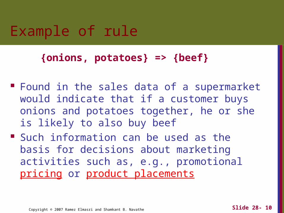
{onions, potatoes} => {beef}

Found in the sales data of a supermarket would indicate that if a customer buys onions and potatoes together, he or she is likely to also buy beef

Such information can be used as the basis for decisions about marketing activities such as, e.g., promotional pricing or product placements


Mathematical formulation of Rule

Let I={i1, i2, .., in} be a set of n binary attributes called items. Let D={t1, t2, .., tm} be a set of transactions called the database. Each transaction in D has a unique transaction ID and contains a

subset of the items in I. A rule is defined as an implication of the form XY where X∩Y= ∅

and X,Y⊆ I. Itemset

A collection of one or more items Example: {Milk, Bread, Bread}

k-itemset An itemset that contains k items


Example of association rule

Transaction ID

Milk Bread Butter Beef

1 1 1 0 0

2 0 1 1 0

3 0 0 0 1

4 1 1 1 0

5 0 1 0 0

I = {milk, bread, butter, beef}

D= {t1, t2, t3, t4, t5}


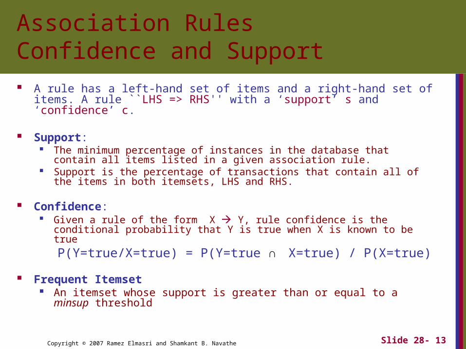
Association Rules Confidence and Support A rule has a left-hand set of items and a right-hand set of items. A rule ``LHS

=> RHS'' with a ‘support’ s and ‘confidence’ c.

Support: The minimum percentage of instances in the database that contain all items listed

in a given association rule. Support is the percentage of transactions that contain all of the items in both

itemsets, LHS and RHS.

Confidence: Given a rule of the form X Y, rule confidence is the conditional probability that

Y is true when X is known to be true

P(Y=true/X=true) = P(Y=true ∩ X=true) / P(X=true)

Frequent Itemset An itemset whose support is greater than or equal to a minsup threshold


Association Rules Confidence and Support

Transaction ID


1 1 1 1 1

2 0 1 1 0

3 1 1 0 1

4 1 1 1 0

5 0 1 0 0

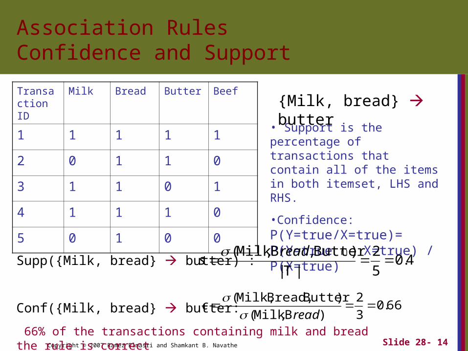
• Support is the percentage of transactions that contain all of the items in both itemset, LHS and RHS.

•Confidence: P(Y=true/X=true)= P(Y=true ∩ X=true) / P(X=true)

{Milk, bread} butter

Supp({Milk, bread} butter) :

Conf({Milk, bread} butter:

66% of the transactions containing milk and bread the rule is correct

4.05

2

|T|

)Butter,B,Milk(

reads

66.03

2

)B,Milk(

)ButterBread,Milk,(

readc


Generating Association Rules- Brute-force approach

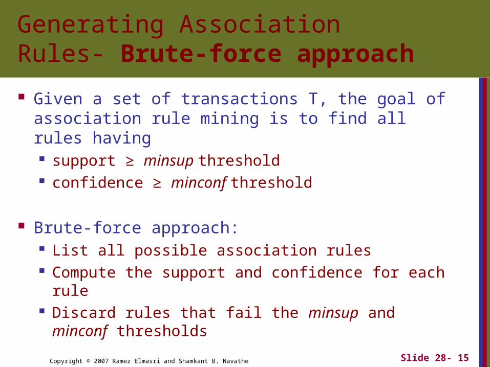
Given a set of transactions T, the goal of association rule mining is to find all rules having support ≥ minsup threshold confidence ≥ minconf threshold

Brute-force approach: List all possible association rules Compute the support and confidence for each rule Discard rules that fail the minsup and minconf

thresholds


Generating Association Rules- Brute-force approach

Observations: Rules originating from the same itemset have

identical support but can have different confidence

Slide 28- 16

Trans. ID


1 1 1 1 1

2 0 1 1 0

3 1 1 0 1

4 1 1 1 0

5 0 1 0 1

Example of Rules:

{Milk,Bread} {Beef} (s=0.4, c=0.66){Milk,Beef} {Bread} (s=0.4, c=1){Bread,Beef} {Milk} (s=0.4, c=0.66){Beef} {Milk,Bread} (s=0.4, c=0.66) {Bread} {Milk,Beef} (s=0.4, c=0.4) {Milk} {Bread,Beef} (s=0.4, c=0.66)


Generating Association Rules-Two steps approach

The general algorithm for generating association rules is a two-step process. Generate all itemsets that have a support

exceeding the given threshold. Itemsets with this property are called large or frequent itemsets.

Generate rules for each itemset as follows: For itemset X and Y a subset of X, let Z = X – Y; If support(X)/Support(Z) > minimum confidence, the

rule Z=>Y is a valid rule.


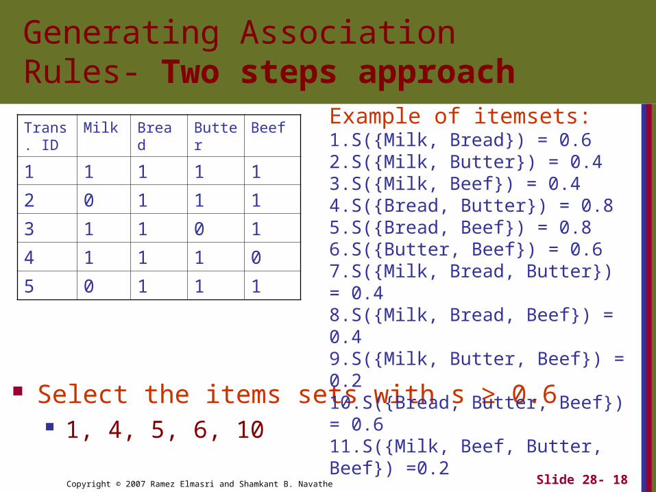
Generating Association Rules- Two steps approach

Select the items sets with s ≥ 0.6 1, 4, 5, 6, 10

Slide 28- 18

Trans. ID


1 1 1 1 1

2 0 1 1 1

3 1 1 0 1

4 1 1 1 0

5 0 1 1 1

Example of itemsets:1.S({Milk, Bread}) = 0.62.S({Milk, Butter}) = 0.43.S({Milk, Beef}) = 0.44.S({Bread, Butter}) = 0.85.S({Bread, Beef}) = 0.86.S({Butter, Beef}) = 0.67.S({Milk, Bread, Butter}) = 0.48.S({Milk, Bread, Beef}) = 0.49.S({Milk, Butter, Beef}) = 0.2 10.S({Bread, Butter, Beef}) = 0.611.S({Milk, Beef, Butter, Beef}) =0.2


Generating Association Rules- Two steps approach

Generate rules for each item set: Milk Bread, Bead Milk Bread Butter, Butter Bread Bread Beef, Beef Bread Butter Beef, Beef Butter Bread {Butter, Beef}, {Butter, Beef} Bread Butter {Beef, Bread}, {Beef, Bread} Butter Beef {Butter, Bread}, {Butter, Bread} Beef

Slide 28- 19

Trans. ID


1 1 1 1 1

2 0 1 1 1

3 1 1 0 1

4 1 1 1 0

5 0 1 1 1

Example of itemsets:1.S({Milk, Bread}) = 0.62.S({Bread, Butter}) = 0.83.S({Bread, Beef}) = 0.84.S({Butter, Beef}) = 0.65.S({Bread, Butter, Beef}) = 0.6


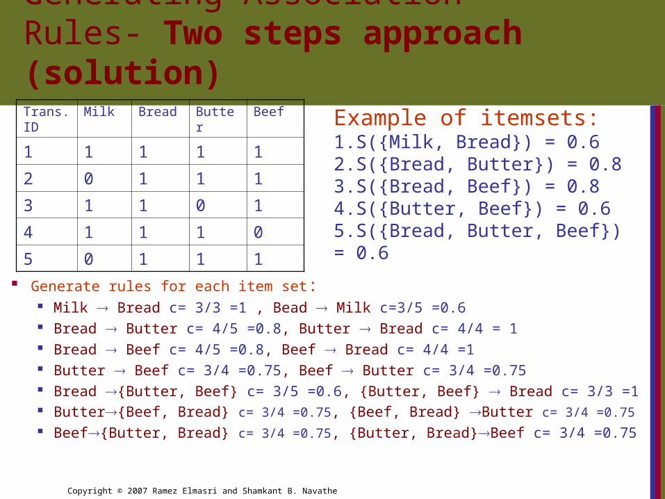
Generating Association Rules- Two steps approach (solution)

Generate rules for each item set: Milk Bread c= 3/3 =1 , Bead Milk c=3/5 =0.6 Bread Butter c= 4/5 =0.8, Butter Bread c= 4/4 = 1 Bread Beef c= 4/5 =0.8, Beef Bread c= 4/4 =1 Butter Beef c= 3/4 =0.75, Beef Butter c= 3/4 =0.75 Bread {Butter, Beef} c= 3/5 =0.6, {Butter, Beef} Bread c= 3/3 =1 Butter{Beef, Bread} c= 3/4 =0.75, {Beef, Bread} Butter c= 3/4 =0.75 Beef{Butter, Bread} c= 3/4 =0.75, {Butter, Bread}Beef c= 3/4 =0.75

Trans. ID


1 1 1 1 1

2 0 1 1 1

3 1 1 0 1

4 1 1 1 0

5 0 1 1 1

Example of itemsets:1.S({Milk, Bread}) = 0.62.S({Bread, Butter}) = 0.83.S({Bread, Beef}) = 0.84.S({Butter, Beef}) = 0.65.S({Bread, Butter, Beef}) = 0.6


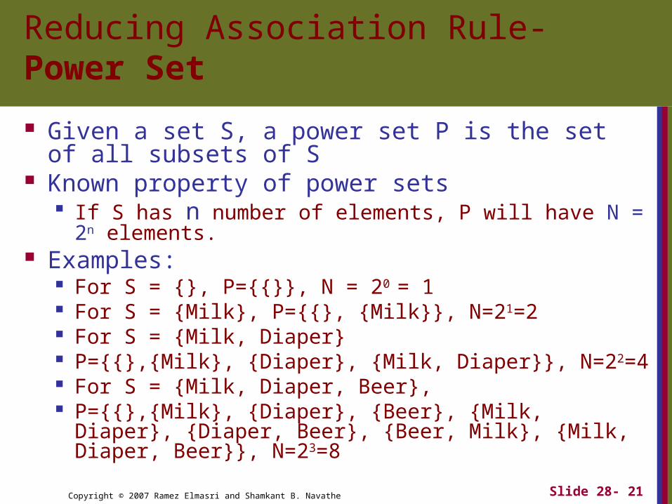
Reducing Association Rule- Power Set

Given a set S, a power set P is the set of all subsets of S

Known property of power sets If S has n number of elements, P will have N = 2n

elements. Examples:

For S = {}, P={{}}, N = 20 = 1 For S = {Milk}, P={{}, {Milk}}, N=21=2 For S = {Milk, Diaper} P={{},{Milk}, {Diaper}, {Milk, Diaper}}, N=22=4 For S = {Milk, Diaper, Beer}, P={{},{Milk}, {Diaper}, {Beer}, {Milk, Diaper}, {Diaper,

Beer}, {Beer, Milk}, {Milk, Diaper, Beer}}, N=23=8


Reducing Association Rule

For an itemset {milk, bread, butter}, we have 23 -1 = 7 subsets

Trans. ID


1 1 1 1 1

2 0 1 1 1

3 1 1 0 1

4 1 1 1 0

5 0 1 1 1

1-itemset

Itemset Count

Milk 3

Bread 5

Butter 4

2-itemset

Itemset Count

{Milk, Bread} 3

{Milk, Butter} 2

{Bread, Butter} 4

Itemset Count

{Milk, Bread, Butter} 2

3-itemset


Generating Association Rules:Apriori Algorithm

Apriori principle: If an itemset is frequent, then all of its subsets

must also be frequent

Apriori principle holds due to the following property of the support measure:

Support of an itemset never exceeds the support of its subsets

This is known as the anti-monotone property of support

)()()(:, YsXsYXYX


Generating Association Rules: Illustrating Apriori Principle

Slide 28- 24

Item Count Bread 4 Coke 2 Milk 4 Beer 3 Diaper 4 Eggs 1

Itemset Count{Bread,Milk} 3{Bread,Beer} 2{Bread,Diaper} 3{Milk,Beer} 2{Milk,Diaper} 3{Beer,Diaper} 3

Itemset Count {Bread,Milk,Diaper} 3

Items (1-itemsets)

Pairs (2-itemsets)

No need to generatecandidates involving Cokeor Eggs

Triplets (3-itemsets)

No need to generatecandidates involving {bread, beer} and {milk, beer}

Minimum frequency= 3

Write all possible 3-itemsets and prune the list based on infrequent 2-itemsets


Generating Association Rules: Apriori Algorithm

N= Nomber of attributes Attribute_list = all attributes

For i=1 to N

Frequent_item_set = generate item set of i attributes using

attribute_list

Frequent_item_set = remove all infrequent itemsets

Rule = Rule U generate rule using Frequent_item_set

Attribute_list = Only attributes contained in Frequent_item_set End For

Slide 28- 25


Generating Association Rules:The Sampling Algorithm

The sampling algorithm selects samples from the database of transactions that individually fit into memory. Frequent itemsets are then formed for each sample. If the frequent itemsets form a superset of the

frequent itemsets for the entire database, then the real frequent itemsets can be obtained by scanning the remainder of the database.

In some rare cases, a second scan of the database is required to find all frequent itemsets.


Generating Association Rules:Frequent-Pattern Tree Algorithm

The Frequent-Pattern Tree Algorithm reduces the total number of candidate itemsets by producing a compressed version of the database in terms of an FP-tree.

The FP-tree stores relevant information and allows for the efficient discovery of frequent itemsets.

The algorithm consists of two steps: Step 1 builds the FP-tree. Step 2 uses the tree to find frequent itemsets.


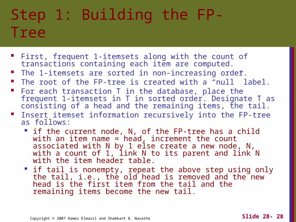
Step 1: Building the FP-Tree First, frequent 1-itemsets along with the count of transactions

containing each item are computed. The 1-itemsets are sorted in non-increasing order. The root of the FP-tree is created with a “null” label. For each transaction T in the database, place the frequent 1-itemsets

in T in sorted order. Designate T as consisting of a head and the remaining items, the tail.

Insert itemset information recursively into the FP-tree as follows: if the current node, N, of the FP-tree has a child with an item

name = head, increment the count associated with N by 1 else create a new node, N, with a count of 1, link N to its parent and link N with the item header table.

if tail is nonempty, repeat the above step using only the tail, i.e., the old head is removed and the new head is the first item from the tail and the remaining items become the new tail.


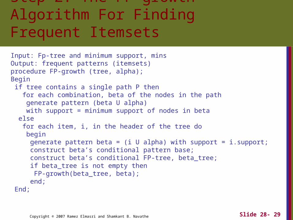
Step 2: The FP-growth Algorithm For Finding Frequent Itemsets

Input: Fp-tree and minimum support, minsOutput: frequent patterns (itemsets)procedure FP-growth (tree, alpha);Begin if tree contains a single path P then for each combination, beta of the nodes in the path generate pattern (beta U alpha) with support = minimum support of nodes in beta else for each item, i, in the header of the tree do begin generate pattern beta = (i U alpha) with support = i.support; construct beta’s conditional pattern base; construct beta’s conditional FP-tree, beta_tree; if beta_tree is not empty then FP-growth(beta_tree, beta); end; End;


Generating Association Rules:The Partition Algorithm

Divide the database into non-overlapping subsets.

Treat each subset as a separate database where each subset fits entirely into main memory.

Apply the Apriori algorithm to each partition. Take the union of all frequent itemsets from each

partition. These itemsets form the global candidate

frequent itemsets for the entire database. Verify the global set of itemsets by having their

actual support measured for the entire database.


Complications seen withAssociation Rules

The cardinality of itemsets in most situations is extremely large.

Association rule mining is more difficult when transactions show variability in factors such as geographic location and seasons.

Item classifications exist along multiple dimensions.

Data quality is variable; data may be missing, erroneous, conflicting, as well as redundant.


Classification

Classification is the process of learning a model that is able to describe different classes of data.

Learning is supervised as the classes to be learned are predetermined.

Learning is accomplished by using a training set of pre-classified data.

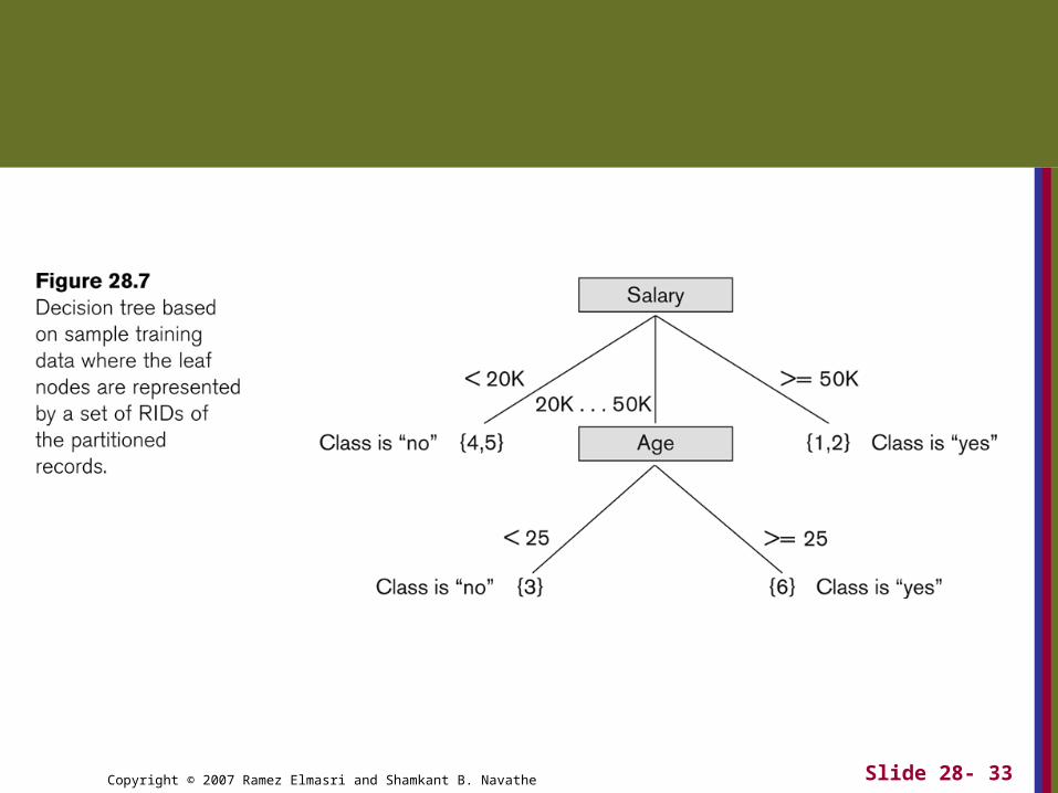
The model produced is usually in the form of a decision tree or a set of rules.


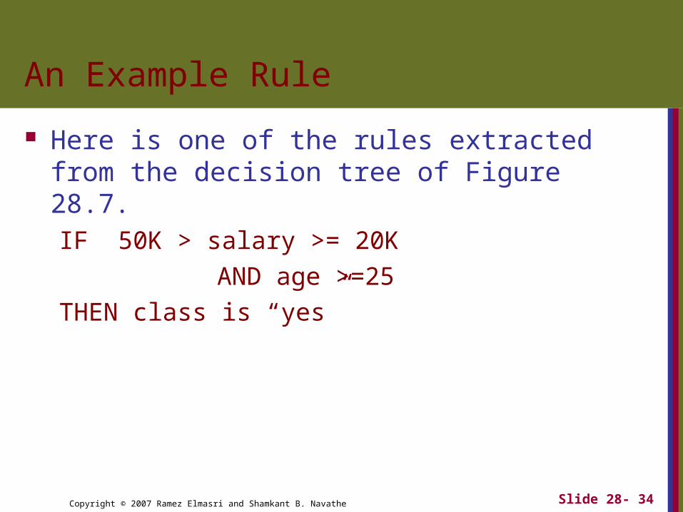
An Example Rule

Here is one of the rules extracted from the decision tree of Figure 28.7.IF 50K > salary >= 20K

AND age >=25

THEN class is “yes”


Clustering

Unsupervised learning or clustering builds models from data without predefined classes.

The goal is to place records into groups where the records in a group are highly similar to each other and dissimilar to records in other groups.

The k-Means algorithm is a simple yet effective clustering technique.


Additional Data Mining Methods



Sequential Pattern Analysis

Transactions ordered by time of purchase form a sequence of itemsets.

The problem is to find all subsequences from a given set of sequences that have a minimum support.

The sequence S1, S2, S3, .. is a predictor of the fact that a customer purchasing itemset S1 is likely to buy S2 , and then S3, and so on.


Time Series Analysis

Time series are sequences of events. For example, the closing price of a stock is an event that occurs each day of the week.

Time series analysis can be used to identify the price trends of a stock or mutual fund.

Time series analysis is an extended functionality of temporal data management.


Regression Analysis

A regression equation estimates a dependent variable using a set of independent variables and a set of constants.

The independent variables as well as the dependent variable are numeric.

A regression equation can be written in the form Y=f(x1,x2,…,xn) where Y is the dependent variable.

If f is linear in the domain variables xi, the equation is call a linear regression equation.


Neural Networks

A neural network is a set of interconnected nodes designed to imitate the functioning of the brain.

Node connections have weights which are modified during the learning process.

Neural networks can be used for supervised learning and unsupervised clustering.

The output of a neural network is quantitative and not easily understood.


Genetic Learning

Genetic learning is based on the theory of evolution.

An initial population of several candidate solutions is provided to the learning model.

A fitness function defines which solutions survive from one generation to the next.

Crossover, mutation and selection are used to create new population elements.


Data Mining Applications

Marketing Marketing strategies and consumer behavior

Finance Fraud detection, creditworthiness and investment

analysis Manufacturing

Resource optimization Health

Image analysis, side effects of drug, and treatment effectiveness


Recap

Data Mining Data Warehousing Knowledge Discovery in Databases (KDD) Goals of Data Mining and Knowledge Discovery Association Rules Additional Data Mining Algorithms


Copyright © 2007 Ramez Elmasri and Shamkant B. Navathe Slide 28- 1.

Documents

Transcript of Copyright © 2007 Ramez Elmasri and Shamkant B. Navathe Slide 28- 1.