Copyright ©2006 Brooks/Cole A division of Thomson Learning, Inc. Introduction to Probability and...

Copyright ©2006 Brooks/ColeA division of Thomson Learning, Inc.

Introduction to Probability Introduction to Probability and Statisticsand Statistics

Twelfth EditionTwelfth Edition

Robert J. Beaver • Barbara M. Beaver • William Mendenhall

Presentation designed and written by: Presentation designed and written by: Barbara M. BeaverBarbara M. Beaver


Introduction to Probability Introduction to Probability and Statisticsand Statistics

Twelfth EditionTwelfth Edition

Chapter 14

Analysis of Categorical Data

Some graphic screen captures from Seeing Statistics ®Some images © 2001-(current year) www.arttoday.com


IntroductionIntroduction

• Many experiments result in measurements that are qualitativequalitative or categorical categorical rather than quantitative.

– People classified by ethnic origin

– Cars classified by color

– M&M®s classified by type (plain or peanut)

• These data sets have the characteristics of a multinomial experimentmultinomial experiment.

mm

m m

m

m


The Multinomial ExperimentThe Multinomial Experiment

1. The experiment consists of nn identical trials. identical trials.2. Each trial results in one of one of kk categories. categories.3. The probability that the outcome falls into a

particular category i on a single trial is pi and remains constantremains constant from trial to trial. The sum of all k probabilities, pp11+p+p22 +…+ +…+ ppkk = 1 = 1.

4. The trials are independentindependent.5. We are interested in the number of outcomes in

each category, OO1, 1, OO2 ,2 ,… … OOkk with OO1 1 + + OO2 2 +… + +… + OOkk = = n.n.

mm

m m

m

m


The Binomial ExperimentThe Binomial Experiment• A special case of the multinomial

experiment with k = 2.

• Categories 1 and 2: success and failure

• p1 and p2: p and q

• O1 and O2: x and n-x• We made inferences about p

(and q = 1 - p)In the multinomial experiment, we make inferences about all the probabilities, p1, p2, p3 …pk.In the multinomial experiment, we make inferences about all the probabilities, p1, p2, p3 …pk.

mm

m m

m

m


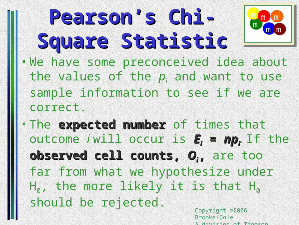
Pearson’s Chi-Square Pearson’s Chi-Square StatisticStatistic

• We have some preconceived idea about the values of the pi and want to use sample information to see if we are correct.

• The expected numberexpected number of times that outcome i will occur is EEii = = npnpii. If the

observed cell counts, observed cell counts, OOii,, are too far from what we hypothesize under H0, the more likely it is that H0 should be rejected.

mm

m m

m

m


Pearson’s Chi-Square Pearson’s Chi-Square StatisticStatistic

• We use the Pearson chi-square statistic:

• When H0 is true, the differences O-E will be small, but large when H0 is false.

• Look for large values of Xlarge values of X22 based on the chi-square distribution with a particular number of degrees of freedom.

i

ii

E

EOX

22 )(

i

ii

E

EOX

22 )(

mm

m m

m

m


Degrees of FreedomDegrees of Freedom• These will be different depending on the application.1. Start with the number of categories or cells in the experiment.

2. Subtract 1df for each linear restriction on the cell probabilities. (You always lose 1 df since pp11+p+p22 +…+ +…+ ppkk = 1 = 1.)

3. Subtract 1 df for every population parameter you have to estimate to calculate or estimate Ei.

mm

m m

m

m


The Goodness of Fit TestThe Goodness of Fit Test•The simplest of the applications.

•A single categorical variable is measured, and exact numerical values are specified for each of the pi.

•Expected cell counts are EEii = np = npii

•Degrees of freedom: df = k-df = k-11

i

ii

E

EOX

22 )(

:statistic Testi

ii

E

EOX

22 )(

:statistic Test


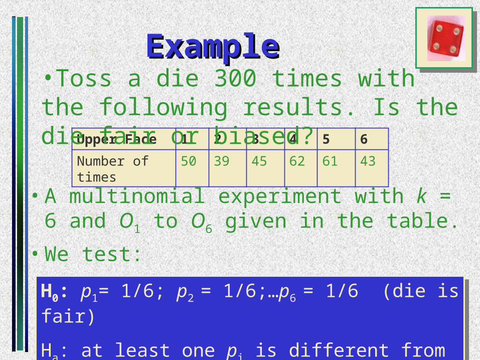
ExampleExample

• A multinomial experiment with k = 6 and O1 to O6 given in the table.

• We test:

Upper Face 1 2 3 4 5 6

Number of times 50 39 45 62 61 43

H0: p1= 1/6; p2 = 1/6;…p6 = 1/6 (die is fair)

Ha: at least one pi is different from 1/6 (die is biased)

H0: p1= 1/6; p2 = 1/6;…p6 = 1/6 (die is fair)

Ha: at least one pi is different from 1/6 (die is biased)

•Toss a die 300 times with the following results. Is the die fair or biased?


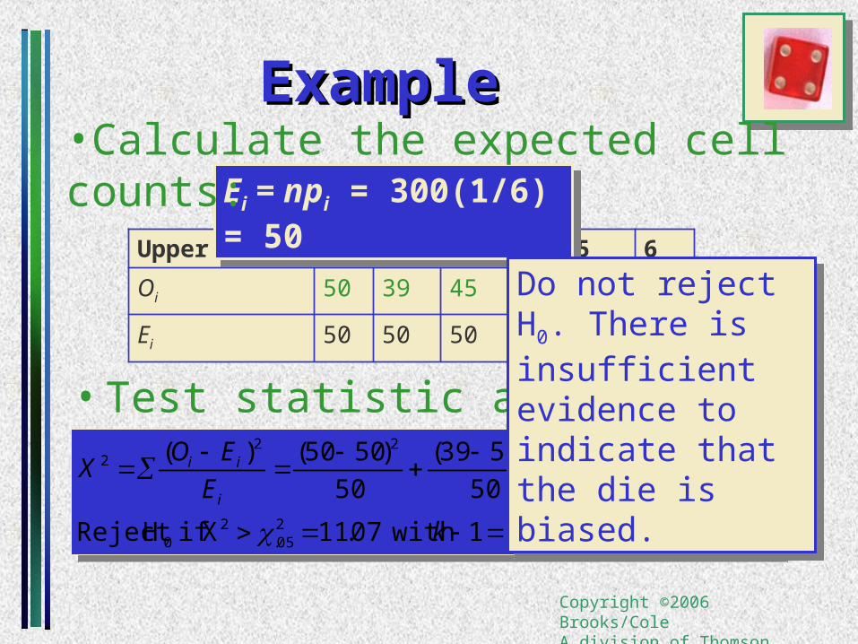
ExampleExample

Upper Face 1 2 3 4 5 6

Oi 50 39 45 62 61 43

Ei 50 50 50 50 50 50

Ei = npi = 300(1/6) = 50Ei = npi = 300(1/6) = 50

•Calculate the expected cell counts:

• Test statistic and rejection region:

df. withX if H Reject 20 516107.11

2.950

)5043(...

50

)5039(

50

)5050()(

205.

22222

k

E

EOX

i

ii

df. withX if H Reject 20 516107.11

2.950

)5043(...

50

)5039(

50

)5050()(

205.

22222

k

E

EOX

i

ii

Do not reject H0. There is insufficient evidence to indicate that the die is biased.

Do not reject H0. There is insufficient evidence to indicate that the die is biased.


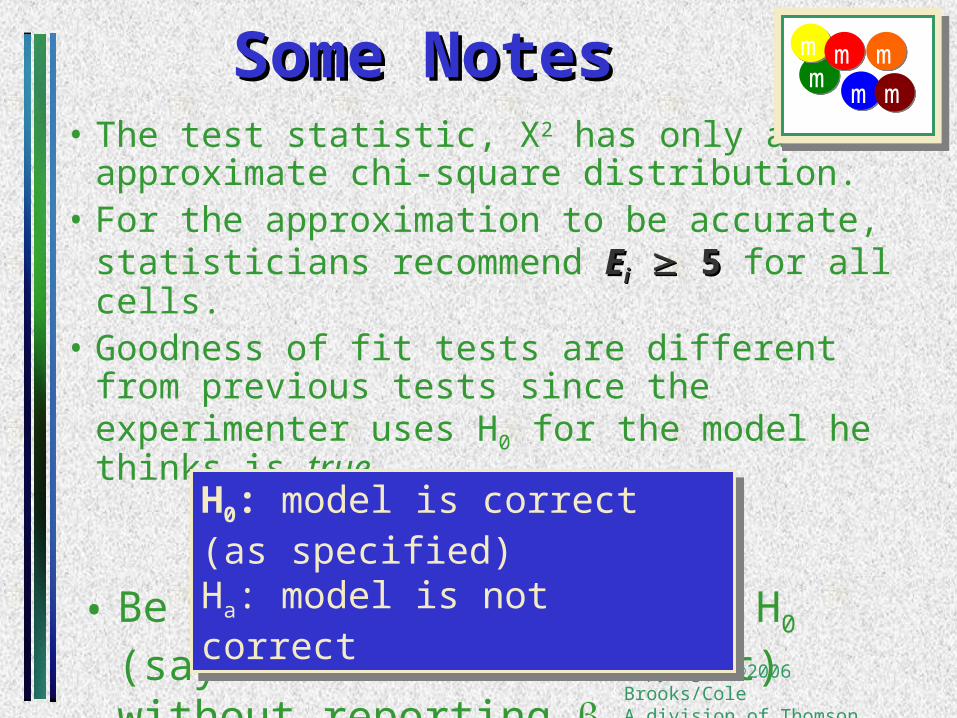
Some NotesSome Notes• The test statistic, X2 has only an

approximate chi-square distribution. • For the approximation to be accurate,

statisticians recommend EEii 5 5 for all cells.• Goodness of fit tests are different from previous

tests since the experimenter uses H0 for the model he thinks is true.

• Be careful not to accept H0 (say the model is correct) without reporting .

H0: model is correct (as specified)Ha: model is not correct

H0: model is correct (as specified)Ha: model is not correct

mm

m m

m

m


Contingency Tables: A Contingency Tables: A Two-Way ClassificationTwo-Way Classification

• The experimenter measures two qualitative two qualitative variablesvariables to generate bivariate databivariate data.

– Gender and colorblindness– Age and opinion– Professorial rank and type of university

• Summarize the data by counting the observed number of outcomes in each of the intersections of category levels in a contingency table.contingency table.


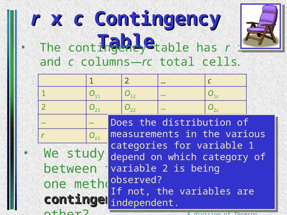
rr x x cc Contingency Table Contingency Table• The contingency table has r rows and c

columns—rc total cells. 1 2 … c

1 O11 O12 … O1c

2 O21 O22 … O2c

… … … … ….

r Or1 Or2 … Orc

• We study the relationship between the two variables. Is one method of classification contingentcontingent or dependentdependent on the other?

Does the distribution of measurements in the various categories for variable 1 depend on which category of variable 2 is being observed?If not, the variables are independent.

Does the distribution of measurements in the various categories for variable 1 depend on which category of variable 2 is being observed?If not, the variables are independent.


Chi-Square Test of Chi-Square Test of IndependenceIndependence

•Observed cell counts are OOijij for row i and column j.

•Expected cell counts are EEijij = np = npijij

If H0 is true and the classifications are independent, pij = pipj = P(falling in row i)P(falling in row j)

H0: classifications are independentHa: classifications are dependent

H0: classifications are independentHa: classifications are dependent


Chi-Square Test of Chi-Square Test of IndependenceIndependence

ij

ijji

E

EOX

ˆ)ˆ( 2

2

:statistic Testij

ijji

E

EOX

ˆ)ˆ( 2

2

:statistic Test

n

cr

n

c

n

rnE

n

c

n

rpp

jijiij

jiji

ˆ

. and with and Estimate

n

cr

n

c

n

rnE

n

c

n

rpp

jijiij

jiji

ˆ

. and with and Estimate

•The test statistic has an approximate chi-square distribution with df = df = ((r-r-1)(1)(cc-1).-1).


ExampleExampleFurniture defects are classified according to type of defect and shift on which it was made.

Shift

Type 1 2 3 Total

A 15 26 33 74

B 21 31 17 69

C 45 34 49 128

D 13 5 20 38

Total 94 96 119 309Do the data present sufficient evidence to indicate that the type of furniture defect varies with the shift during which the piece of furniture is produced? Test at the 1% level of significance.

Do the data present sufficient evidence to indicate that the type of furniture defect varies with the shift during which the piece of furniture is produced? Test at the 1% level of significance.

H0: type of defect is independent of shiftHa: type of defect depends on the shift

H0: type of defect is independent of shiftHa: type of defect depends on the shift


The Furniture ProblemThe Furniture Problem•Calculate the expected cell counts. For example: 99.22

309

)96(74ˆ 2112

n

crE 99.22

309

)96(74ˆ 2112

n

crE

Chi-Square Test: 1, 2, 3 Expected counts are printed below observed countsChi-Square contributions are printed below expected counts 1 2 3 Total 1 15 26 33 74 22.51 22.99 28.50 2.506 0.394 0.711

2 21 31 17 69 20.99 21.44 26.57 0.000 4.266 3.449

3 45 34 49 128 38.94 39.77 49.29 0.944 0.836 0.002

4 13 5 20 38 11.56 11.81 14.63 0.179 3.923 1.967

Total 94 96 119 309df. ( withX if H Reject

:statistic Test

20 6)1)(107.11

18.1963.14

)63.1420(...

99.22

)99.2226(

51.22

)51.2215(

ˆ)ˆ(

205.

222

22

cr

E

EOX

ij

ijij

df. ( withX if H Reject

:statistic Test

20 6)1)(107.11

18.1963.14

)63.1420(...

99.22

)99.2226(

51.22

)51.2215(

ˆ)ˆ(

205.

222

22

cr

E

EOX

ij

ijij

Chi-Sq = 19.178, DF = 6, P-Value = 0.004

Reject H0. There is sufficient evidence to indicate that the proportion of defect types vary from shift to shift.

Reject H0. There is sufficient evidence to indicate that the proportion of defect types vary from shift to shift.

APPLETAPPLETMY


Comparing Multinomial Comparing Multinomial PopulationsPopulations

• Sometimes researchers design an experiment so that the number of experimental units falling in one set of categories is fixed in advance.

• Example: An experimenter selects 900 patients who have been treated for flu prevention. She selects 300 from each of three types—no vaccine, one shot, and two shots. No Vaccine One Shot Two Shots Total

Flu r1

No Flu r2

Total 300 300 300 n = 900

The column totals have been fixed in advance!

The column totals have been fixed in advance!


Comparing Multinomial Comparing Multinomial PopulationsPopulations

• Each of the c columns (or r rows) whose totals have been fixed in advance is actually a single multinomial experiment.

• The chi-square test of independence with (r-1)(c-1) df is equivalent toequivalent to a test of the equality of c (or r) multinomial populations.

No Vaccine One Shot Two Shots Total

Flu r1

No Flu r2

Total 300 300 300 n = 900

Three binomial populations—no vaccine, one shot and two shots.Is the probability of getting the flu independent of the type of flu prevention used?

Three binomial populations—no vaccine, one shot and two shots.Is the probability of getting the flu independent of the type of flu prevention used?


ExampleExampleRandom samples of 200 voters in each of four wards were surveyed and asked if they favor candidate A in a local election.

Ward

1 2 3 4 Total

Favor A 76 53 59 48 236

Do not favor A 124 147 141 152 564

Total 200 200 200 200 800Do the data present sufficient evidence to indicate that the the fraction of voters favoring candidate A differs in the four wards?

Do the data present sufficient evidence to indicate that the the fraction of voters favoring candidate A differs in the four wards?

H0: fraction favoring A is independent of wardHa: fraction favoring A depends on the ward

H0: fraction favoring A is independent of wardHa: fraction favoring A depends on the ward

H0: p1 = p2 = p3 = p4

where pi = fraction favoring A in each of the four wards

H0: p1 = p2 = p3 = p4

where pi = fraction favoring A in each of the four wards

APPLETAPPLETMY


The Voter ProblemThe Voter Problem•Calculate the expected cell counts. For example:

59800

)200(236ˆ 2112

n

crE 59

800

)200(236ˆ 2112

n

crE

Chi-Square Test: 1, 2, 3, 4

Expected counts are printed below observed countsChi-Square contributions are printed below expected counts

1 2 3 4 Total 1 76 53 59 48 236 59.00 59.00 59.00 59.00 4.898 0.610 0.000 2.051

2 124 147 141 152 564 141.00 141.00 141.00 141.00 2.050 0.255 0.000 0.858

Total 200 200 200 200 800

df. 3)1)(1( with 81.7X if HReject

722.10141

)141152(...

59

)5953(

59

)5976(

ˆ)ˆ(

:statisticTest

205.

20

222

22

cr

E

EOX

ij

ijij

df. 3)1)(1( with 81.7X if HReject

722.10141

)141152(...

59

)5953(

59

)5976(

ˆ)ˆ(

:statisticTest

205.

20

222

22

cr

E

EOX

ij

ijij

Chi-Sq = 10.722, DF = 3, P-Value = 0.013

Reject H0. There is sufficient evidence to indicate that the fraction of voters favoring A varies from ward to ward.

Reject H0. There is sufficient evidence to indicate that the fraction of voters favoring A varies from ward to ward.

APPLETAPPLETMY


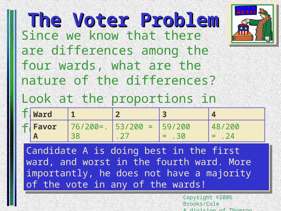
The Voter ProblemThe Voter ProblemSince we know that there are differences among the four wards, what are the nature of the differences?

Look at the proportions in favor of candidate A in the four wards.

Ward 1 2 3 4

Favor A 76/200=.38 53/200 = .27 59/200 = .30 48/200 = .24

Candidate A is doing best in the first ward, and worst in the fourth ward. More importantly, he does not have a majority of the vote in any of the wards!

Candidate A is doing best in the first ward, and worst in the fourth ward. More importantly, he does not have a majority of the vote in any of the wards!


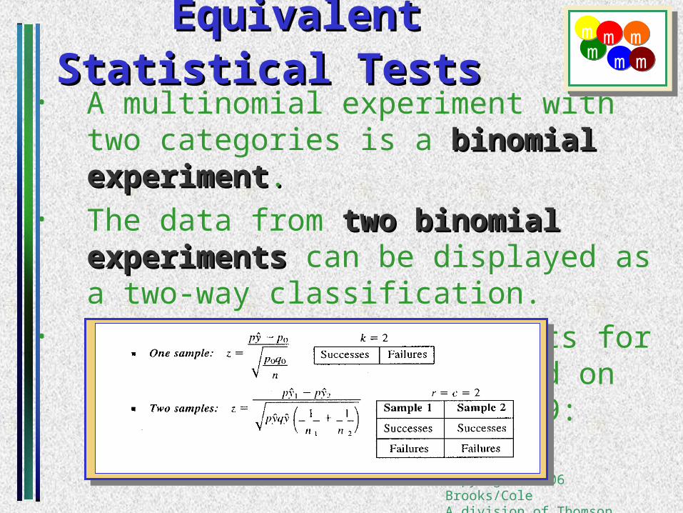
Equivalent Statistical TestsEquivalent Statistical Tests • A multinomial experiment with two categories

is a binomial experimentbinomial experiment..• The data from two binomial experimentstwo binomial experiments can

be displayed as a two-way classification.• There are statistical tests for these two

situations based on the statistic of Chapter 9:

mmm m

mm


Other Applications Other Applications Goodness-of-fit tests:Goodness-of-fit tests: It is possible to design

a goodness-of-fit test to determine whether data are consistent with data drawn from a particular probability distribution, possibly the normal, binomial, Poisson, or other distributions.

Time-dependent multinomialsTime-dependent multinomials: The chi square statistic can be used to investigate the rate of change of multinomial proportions over time.

mm

m m

m

m


Other Applications Other Applications Multidimensional contingency tablesMultidimensional contingency tables:

Instead of only two methods of classification, it is possible to investigate a dependence among three or more classifications.

Log-linear modelsLog-linear models: Complex models can be created in which the logarithm of the cell probability (ln pij) is some linear function of the row and column probabilities.

mm

m m

m

m


Assumptions Assumptions

Assumptions for Pearson’s Chi-Square:

1. The cell counts O1, O2, …,Ok must satisfy

the conditions of a multinomial experiment, or a set of multinomial experiments created by fixing either the row or the column totals.

2. The expected cell counts E1, E2, …, Ek

should equal or exceed five.

Assumptions for Pearson’s Chi-Square:

1. The cell counts O1, O2, …,Ok must satisfy

the conditions of a multinomial experiment, or a set of multinomial experiments created by fixing either the row or the column totals.

2. The expected cell counts E1, E2, …, Ek

should equal or exceed five.

mm

m m

m

m


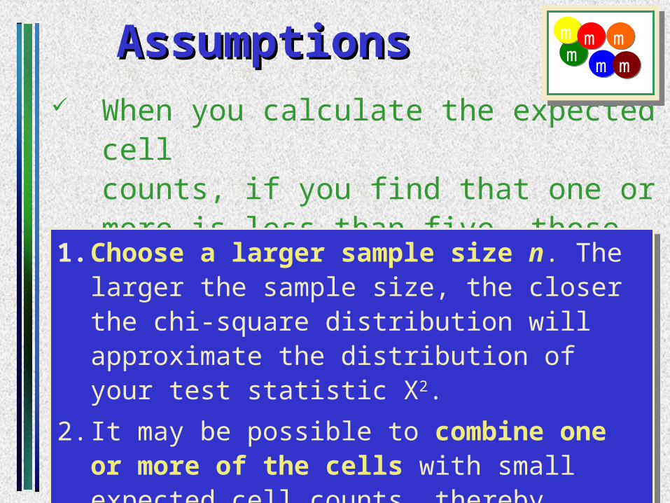
Assumptions Assumptions When you calculate the expected cell

counts, if you find that one or more is less than five, these options are available to you:

1. Choose a larger sample size n. The larger the sample size, the closer the chi-square distribution will approximate the distribution of your test statistic X2.

2. It may be possible to combine one or more of the cells with small expected cell counts, thereby satisfying the assumption.

1. Choose a larger sample size n. The larger the sample size, the closer the chi-square distribution will approximate the distribution of your test statistic X2.

2. It may be possible to combine one or more of the cells with small expected cell counts, thereby satisfying the assumption.

mm

m m

m

m


Key ConceptsKey ConceptsI.I. The Multinomial ExperimentThe Multinomial Experiment

1. There are n identical trials, and each outcome falls into one of k categories.

2. The probability of falling into category i is pi and remains

constant from trial to trial.

3. The trials are independent, pi 1, and we measure Oi , the

number of observations that fall into each of the k categories.

II.II. Pearson’s Chi-Square StatisticPearson’s Chi-Square Statistic

which has an approximate chi-square distribution with degrees degrees of freedomof freedom determined by the application.

npEE

EOii

i

ii e wher)( 2

2


Key ConceptsKey Concepts

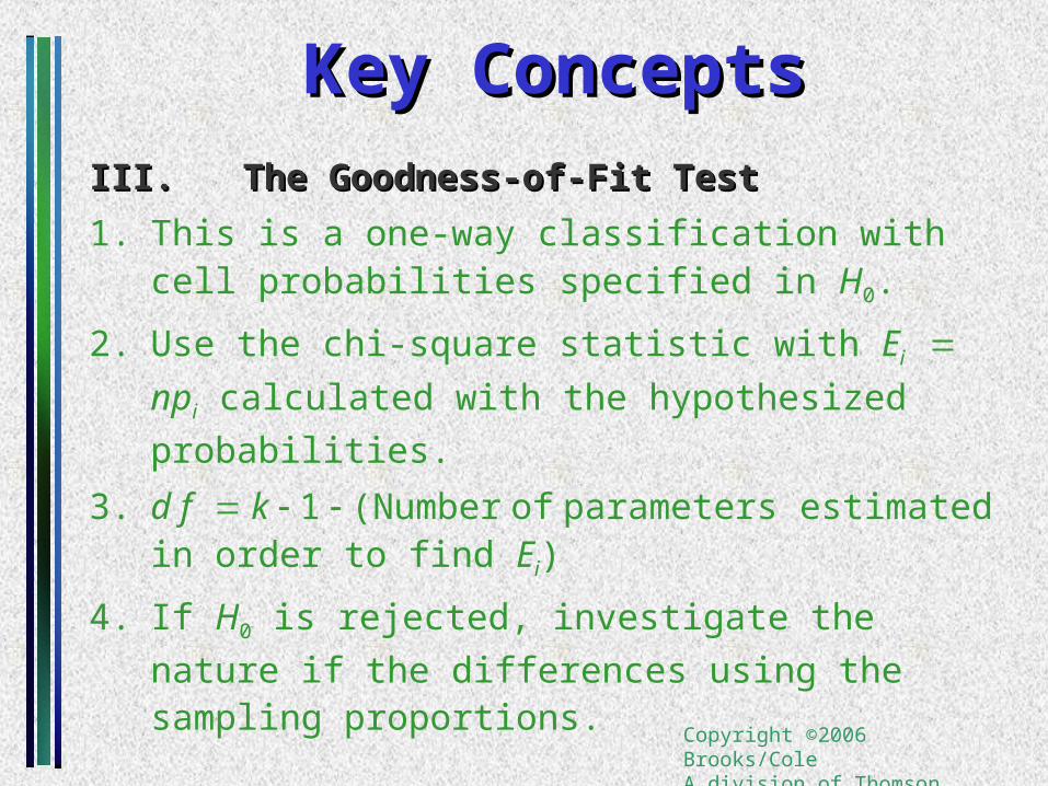
III.III. The Goodness-of-Fit TestThe Goodness-of-Fit Test

1. This is a one-way classification with cell probabilities specified in H0.

2. Use the chi-square statistic with Ei npi

calculated with the hypothesized probabilities.

3. d f k 1 (Number of parameters estimated in order to find Ei)

4. If H0 is rejected, investigate the nature if the

differences using the sampling proportions.


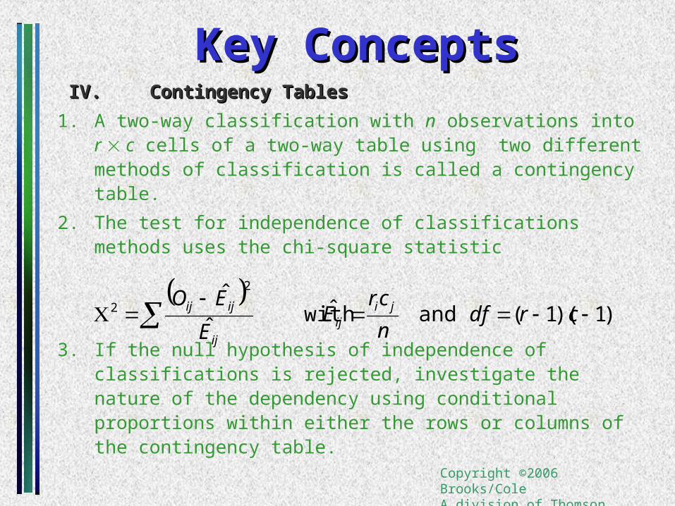
Key ConceptsKey Concepts IV.IV. Contingency TablesContingency Tables

1. A two-way classification with n observations into r c cells of a two-way table using two different methods of classification is called a contingency table.

2. The test for independence of classifications methods uses the chi-square statistic

3. If the null hypothesis of independence of classifications is rejected, investigate the nature of the dependency using conditional proportions within either the rows or columns of the contingency table.

)1)(1( and ˆ with

ˆ

ˆ 2

2

crdfn

crE

E

EO jiij

ij

ijij


Key ConceptsKey ConceptsV.V. Fixing Row or Column TotalsFixing Row or Column Totals

1. When either the row or column totals are fixed, the test of independence of classifications becomes a test of the homogeneity of cell probabilities for several multinomial experiments.

2. Use the same chi-square statistic as for contingency tables.

3. The large-sample z tests for one and two binomial proportions are special cases of the chi-square statistic.


Key ConceptsKey ConceptsVI. AssumptionsVI. Assumptions

1. The cell counts satisfy the conditions of a multinomial experiment, or a set of multinomial experiments with fixed sample sizes.

2. All expected cell counts must equal or exceed five in order that the chi-square approximation is valid.

Copyright ©2006 Brooks/Cole A division of Thomson Learning, Inc. Introduction to Probability and...

Documents

Transcript of Copyright ©2006 Brooks/Cole A division of Thomson Learning, Inc. Introduction to Probability and...