Copositive relaxation beats Lagrangian dual bounds

in quadratically and linearly constrained

quadratic optimization problems

Immanuel M. Bomze

ISOR, University of Vienna, Austria

Abstract

We study non-convex quadratic minimization problems under (pos-sibly non-convex) quadratic and linear constraints, and characterizeboth Lagrangian and Semi-Lagrangian dual bounds in terms of conicoptimization. While the Lagrangian dual is equivalent to the SDPrelaxation (which has been known for quite a while, although the pre-sented form, incorporating explicitly linear constraints, seems to benovel), we show that the Semi-Lagrangian dual is equivalent to a nat-ural copositive relaxation (and this has apparently not been observedbefore). This way, we arrive at conic bounds tighter than the usualLagrangian dual (and thus than the SDP) bounds. Any of the knowntractable inner approximations of the copositive cone can be used forthis tightening, but in particular, above mentioned characterizationwith explicit linear constraints is a natural, much cheaper, relaxationthan the usual zero-order approximation by doubly nonnegative (DNN)matrices, and still improves upon the Lagrangian dual bounds. Theseapproximations are based on LMIs on matrices of basically the originalorder plus additional linear constraints (in contrast to more familiarsum-of-squares or moment approximation hierarchies), and thus mayhave merits in particular for large instances where it is important to

employ only a few inequality constraints (eg., n instead of n(n−1)2 for

the DNN relaxation). Further we specify sufficient conditions for tight-ness of the Semi-Lagrangian relaxation and show that copositivity ofthe slack matrix guarantees global optimality for KKT points of thisproblem, thus significantly improving upon a well-known second-orderglobal optimality condition.

Key words: Copositive matrices, non-convex optimization, polynomial op-timization, quadratically constrained problem, global optimality condition,approximation hierarchies

April 25, 2015

1 Introduction and basic concepts

1.1 Motivation, innovative contentand organization of the paper

As is well known, the effectiveness of Lagrangian relaxation – and optimiza-tion methods in general – heavily depends on the formulation of the problem,and of the treatment of constraints. For instance, if the ground set is notthe full space but rather incorporates some (simpler) constraints, we arriveat Semi-Lagrangian relaxation yielding tighter bounds than the classic La-grangian relaxation which uses the full Euclidean space Rn as the groundset. However, Semi-Lagrangian dual bounds cannot always be calculatedefficiently.

Here we study non-convex quadratic minimization problems under (pos-sibly non-convex) quadratic and linear constraints, and characterize bothduals in terms of conic optimization. Due to their pivotal role for applica-tions, bounds for such type of problems receive currently much interest inthe optimization community, a for sure non-exhaustive list is [2, 19, 20, 26,28, 30, 31, 32, 34, 36, 42, 45].

In the absence of linear constraints, the full Lagrangian dual problemis equivalent to the direct semidefinite relaxation. Under additional linearconstraints, we arrive at an LMI description of the Lagrangian dual which isan extension thereof, while the Semi-Lagrangian dual can be shown to resultfrom a natural copositive relaxation. This way, we arrive at a full hierarchyof tractable conic bounds tighter than the usual Lagrangian dual (and thusthan the SDP) bounds. In particular, the usual zero-order approximationby doubly nonnegative matrices improves upon the Lagrangian dual bounds.Therefore we manage a tractable approximation tightening towards Semi-Lagrangian dual bounds.

The resulting approximation hierarchy is based upon LMIs on matrices ofbasically the original order plus relatively few additional linear constraints,in contrast to more familiar sum-of-squares hierarchies or moment approx-imation hierarchies. We also relate the new relaxation with an alternative,still tighter, relaxation earlier introduced by Burer who showed that hisformulation is indeed tight in an important subclass of the problem typestudied here, including all mixed-binary QPs satisfying the so-called keycondition. Further we study strong duality of the resulting conic problems,and also specify sufficient conditions for tightness of the Semi-Lagrangian(i.e. copositive) relaxation. We also show that copositivity of the slack ma-trix guarantees global optimality for KKT points of this problem. Finally,we address an alternative to replace all linear constraints by one convex

1

quadratic. Similar aggregation approaches have been tried recently alongdifferent roads [2, 10, 23, 32].

The paper is organized as follows: first, after briefly recapitulating basicconcepts, we review several variants of (Semi-)Lagrangian relaxations inthe preparatory Section 2. Section 3 presents a new perspective on the fullLagrangian duals as SDPs; in Subsection 3.1, for the readers’ convenience wepresent a summary of well-known results on all-quadratic problems withoutany linear constraint in a suitable context. Subsection 3.2 treats, apparentlyfor the first time in literature, linear constraints in an explicit way andmotivates the study of a cone which will serve in relaxation later on.

All these preparations will be essential in the central Section 4 wherewe incorporate the sign constraints into the ground set, and show that theresulting Semi-Lagrangian bounds exactly lead to the natural copositive re-laxation of the all-quadratic problem with linear constraints. Next, underwidely used strict feasibility conditions, we establish full strong duality ofthe primal-dual pair of copositive problems. However, for some formula-tions, strict feasibility does not hold for the original problem. Still, themajor implications like primal attainability and zero duality gap for theconic relaxation can be established. Section 5 contains conditions whichguarantee that the Semi-Lagrangian relaxation (and thus the copositive re-laxation) is tight, and discusses global optimality conditions for a KKT pointof the original problem. In Section 6 we address an alternative formulationwhich replaces all linear constraints by one convex quadratic, position theresulting bound to the previous natural one, and establish equivalence ofthis variant to Burer’s relaxation which was, albeit for problems withoutinequality constraints, first introduced in [17]. Finally, in Section 7, we alsobriefly explain how to tighten Lagrangian bounds by the resulting approx-imation hierarchies, which may be of particular interest in large instances,i.e., in regimes where every additional linear inequality constraint “hurts”in the conic problem, forcing us to employ as few of them as possible.

The roadmap outlined above already indicates the need to somehowmix innovative contributions with novel perspectives on already known re-sults, for presentational purposes. Therefore it may be of interest to high-light here what is new in this paper: a characterization and positioningof Semi-Lagrangian bounds within the copositive optimization framework,along with a detailed analysis of (strong) conic duality; introduction of anatural sub-zero level in approximation hierarchies, which reduces the num-ber of linear inequality constraints to avoid memory problems in tractablerelaxations; a Frank-Wolfe-type result on primal attainability of quadraticoptimization problems under linear and quadratic constraints; and newsecond-order global optimality conditions emerging from above approach.

2

Summarizing, this article shall, along with a new perspective on SDP re-laxations in context of more general/conic (i.e., copositive) optimization,shed new light on the question how copositivity can help in the theory andalgorithmic treatment of quadratic optimization problems.

1.2 Notation and terminology

We abbreviate by [m : n] := {m,m+ 1, . . . , n} the integer range betweentwo integers m,n with m ≤ n. By bold-faced lower-case letters we denotevectors in n-dimensional Euclidean space Rn, by bold-faced upper case let-ters matrices, and by > transposition. The positive orthant is denoted byRn+ := {x ∈ Rn : xi ≥ 0 for all i∈ [1 :n]}. In is the n×n identity matrix with

columns ei, i∈ [1 :n], while e :=n∑i=1

ei = [1, . . . , 1]> ∈ Rn and the compact

standard simplex is

∆ :={x ∈ Rn+ : e>x = 1

},

which of course satisfies R+∆ = Rn+. The letters o and O stand for zerovectors, and zero matrices, respectively, of appropriate orders. The set ofall n× n matrices is denoted by Rn×n, and the interior of a set S ⊂ Rn byS◦.

For a given symmetric matrix H = H>, we denote the fact that H ispositive-semidefinite by H � O. Sometimes we write instead ”H is psd.”Linear forms in symmetric matrices X will play an important role in thispaper; they are expressed by Frobenius duality 〈S,X〉 = trace(SX), whereS = S> is another symmetric matrix of the same order as X.

Given any cone C of symmetric n× n matrices,

C? :={S = S> ∈ Rn×n : 〈S,X〉 ≥ 0 for all X ∈ C

}denotes the dual cone of C. For instance, if C =

{X = X> ∈ Rn×n : X � O

},

then C? = C itself, an example of a self-dual cone. Trusting the sharp eyes ofmy readers, I chose a notation with subtle differences between the five-stardenoting a dual cone, e.g., C?, and the six-star, e.g. z∗, denoting optimal-ity. Generally, (combined) subscripts will distinguish reference to variousproblems; e.g. 2LD refers to the Lagrangian dual, and 2S to a semidefi-nite problem. When it comes to primal-dual conic pairs, the subscripts 2Drefer to the conic dual, and 2P to the primal conic problem. A subscript2C always refers to co(mpletely )positive problems in the most frequentlyused form: 2CD indicates the dual problem over the copositive cone while2CP refers to the primal problem over the completely positive cone; detaileddefinitions follow immediately. A subscript 2+ always indicates that linear

3

inequality constraints are treated in an explicit way. Finally, the matrixsymbols Z and M are reserved for a slack matrix in the various dual conicprograms, and the Shor relaxation matrix of a quadratic function, respec-tively.

The key notion used below is that of copositivity. Given a symmetricn× n matrix Q, we say that

Q is copositive if v>Qv ≥ 0 for all v ∈ Rn+ , and that

Q is strictly copositive if v>Qv > 0 for all v ∈ Rn+ \ {o} .

Strict copositivity generalizes positive-definiteness (all eigenvalues strictlypositive) and copositivity generalizes positive-semidefiniteness (no eigen-value strictly negative) of a symmetric matrix. Contrasting to positive-semidefiniteness, checking copositivity is NP-hard, see [22, 37].

The set of all copositive matrices forms a closed, convex cone, the copos-itive cone

C? ={Q = Q> ∈ Rn×n : Q is copositive

}with non-empty interior [C?]◦ which exactly consists of all strictly copositivematrices. However, the cone C? is not self-dual. Rather one can show(denoting sn := n for n ≤ 4 while sn := n(n+1)−8

2 for n ≥ 5) that C? is thedual cone of

C ={X = FF> : F has sn columns in Rn+

},

the cone of completely positive matrices. Note that the factor matrix Fhas many more columns than rows. The upper bound sn on the necessarynumber of columns was recently established by [43] and is asymptoticallytight as n→∞ [14]. Anyhow, a perhaps more amenable representation is

C = conv{xx> : x ∈ Rn+

},

where conv S stands for the convex hull of a set S ⊂ Rn. Caratheodory’stheorem then elucidates the quadratic character of sn.

2 Lagrangian duality for quadratic problems

2.1 Different problems and different formulations

Consider two problems with quadratic constraints:

z∗ := inf {q0(x) : x ∈ F} with F := {x ∈ Rn : qi(x) ≤ 0 , i∈ [1 :m]} (1)

4

where all qi(x) = x>Qix − 2b>i x + ci are quadratic functions (as the valueof c0 does not matter, we may mostly assume c0 = 0, but will deviate fromthis in the proof of Theorem 4.2 below) for i∈ [0 :m]; and

z∗+ := inf {q0(x) : x ∈ F ∩ P} with P :={x ∈ Rn+ : Ax = a

}. (2)

where a ∈ Rp and A is a p×n matrix of full row rank p (if P = Rn+, i.e., p = 0,we will simply drop all terms involving A, a or the multipliers w introducedbelow). We further impose a Slater condition on the linear constraints:

there is a point y ∈ P such that yj > 0 for all j∈ [1 :n] . (3)

This is not customary as linear constraints do not need qualifications in theusual context; however, we will need (3) here, and it poses no restrictionof generality, since we can test this condition by solving, in a preprocessingstep, for all j∈ [1 :n], the n LPs z∗j := sup {xj : x ∈ P}, and discard thevariable xj if z∗j = 0. The remaining variables (we rearrange their indices

again as all j∈ [1 :n]) now have the property that there is an x(j) ∈ P such

that x(j)j > 0. Taking the arithmetic mean of all x(j) yields the desired point

y ∈ P ∩ [R+n ]◦.

Neither of the optimal values z∗ of (1), or z∗+ of (2) need be attained,and they could also be equal to −∞ (in the unbounded case) or to +∞(in the infeasible case). Of course, we have z∗ ≤ z∗+ due to the additionallinear constraints. Considering Qi = O would also allow for linear inequalityconstraints. But it is often advisable to discriminate the functional form ofconstraints, and we will adhere to this principle in what follows. Thereforelinear inequality constraints are cast into above form x ∈ P by use of slackvariables, if necessary.

Note that defining Qm+1 = A>A, bm+1 = A>a and cm+1 = a>a, we mayrephrase the m linear constraints Ax = a into one homogeneous quadraticconstraint z>Mm+1z = ‖Ax− a‖2 = 0. We will return later to this formula-tion. Still, the resulting feasible set is not of the form of F , the differencebeing the sign constraints xj ≥ 0.

Finally note that binarity constraints xj ∈ {0, 1} can be recast into twoinequality constraints of the form xj ≤ 1 (this constraint would ensure Bu-rer’s key condition [12, 17]) and xj−x2

j ≤ 0. This fits into above formulation,but then one has to be careful with strict feasibility assumptions; also, in-troducing slacks for xj ≤ 1 will double the number of variables. We willaddress an alternative (Burer’s relaxation) later in Subsection 6.2.

5

2.2 The Lagrangian (dual) functions

Now consider multipliers u ∈ Rm+ of the inequality constraints qi(x) ≤ 0,2v ∈ Rn+ for the sign constraints x ∈ Rn+, and 2w ∈ Rp for the linear equalityconstraints Ax = a (again, the factors two are introduced for notationalconvenience only). Then the full Lagrangian function

L(x; u, v,w) := q0(x) +∑i

uiqi(x)− 2v>x + 2w>(a− Ax)

and its first two derivatives w.r.t. x are given by

L(x; u, v,w) = x>Hux− 2(du + v + A>w)>x + c>u + 2w>a ,

∇xL(x; u, v,w) = 2[Hux− (du + v + A>w)] and

D2xL(x; u, v,w) = 2Hu for all (x; u, v,w) ∈ Rn × Rm+ × Rn+ × Rp .

Here we denote by Hu = Q0 +m∑i=1

uiQi, by du = b0 +m∑i=1

uibi and by c =

[c1, . . . , cm]>. Abbreviating L0(x; u) = L(x; u, o, o), the Lagrangian dualfunction for problem (1) reads

Θ0(u) := inf {L0(x; u) : x ∈ Rn} , (4)

and the dual optimal value is

z∗LD := sup{

Θ0(u) : u ∈ Rm+}. (5)

Standard weak duality implies z∗LD ≤ z∗.

The full Lagrangian dual for problem (2) with additional linear con-straints reads instead

Θ(u, v,w) := inf {L(x; u, v,w) : x ∈ Rn} , (6)

with dual optimal value

z∗LD,+ := sup{

Θ(u, v,w) : (u, v,w) ∈ Rm+ × Rn+ × Rp}. (7)

The idea to incorporate some of the constraints defining F ∩ P into theground set, or equivalently, to relax only some of the constraints, leads to thecorresponding Semi-Lagrangian (sometimes also called partial Lagrangian)dual and is not new, see, e.g. [26] and references therein. However, previouswork has concentrated to do this with linear equality constraints, which thenleads to an SDP formulation similar to those treated in the previous section.Here, we take an alternative path, incorporating the sign (i.e., inequality)constraints into the ground set, and relax all other constraints.

6

So we arrive at the Semi-Lagrangian variant

Θsemi(u,w) := inf{L(x; u, o,w)) : x ∈ Rn+

}, (8)

with dual optimal value

z∗semi := sup{

Θsemi(u,w) : (u,w) ∈ Rm+ × Rp}. (9)

The relation between full and Semi-Lagrangian bounds is a general principle.For ease of reference, we repeat the argument here: for any v ∈ Rn+,

Θ(u, v,w) = inf {L(x; u, v,w) : x ∈ Rn}≤ inf

{L(x; u, v,w) : x ∈ Rn+

}= inf

{L(x; u, o,w)− 2v>x : x ∈ Rn+

}≤ inf

{L(x; u, o,w) : x ∈ Rn+

}= Θsemi(u,w) ,

as v>x ≥ 0 for all x ∈ Rn+. So we arrive at the following chain of inequalities

z∗LD,+ ≤ z∗semi ≤ z∗+ ,

where the last inequality above follows, again, from standard weak duality.

We also have z∗LD ≤ z∗LD,+ as Θ0(u) = Θ(u, o, o), but as z∗LD and z∗LD,+refer to different problems, their relation cannot be seen as a tightening, butrather as a reflection of the relation z∗ ≤ z∗+ of the optimal (primal) valuesof (1) and (2), respectively.

2.3 Consequences of an elementary observation

We conclude this section with a key observation which is well known inthe context of homogenizing polynomials, at least in the case without signconstraints. For the readers’ convenience, we adapt a short proof here forthe copositive case. The argument involves bordering of n× n matrices (inwhich context we always address the first row/column as the zeroth one. Tothis end, we denote by e0 = [1, 0, . . . , 0]> ∈ Rn+1, and by

J0 := e0e>0 =

[1 o>

o O

].

Lemma 2.1 Consider a quadratic function q(x) = x>Hx− 2d>x+γ definedon Rn, with q(o) = γ, ∇q(o) = −2d and D2q(o) = 2H (the factors 2 beinghere just for ease of later notation). Define the Shor relaxation matrix [44]

M(q) :=

[γ −d>−d H

]. (10)

Then for any µ ∈ R, we have

7

(a) q(x) ≥ µ for all x ∈ Rn if and only if M(q − µ) = M(q)− µJ0 � O.

(b) q(x) ≥ µ for all x ∈ Rn+ if and only if M(q − µ) = M(q)− µJ0 ∈ C?.

Proof. The identity M(q − µ) = M(q) − µJ0 is evident. Assertion (a) isproved, e.g., in [26, Lemma 1]. The argument for claim (b) is completelyanalogous: suppose that q(x) ≥ µ for all x ∈ Rn+. Then H must be copositive.Indeed, otherwise consider a y ∈ Rn+ such that y>Hy < 0 and look at x = ty.For large enough t > 0, we get

q(x) = q(ty) = t2y>Hy − 2td>y + γ < µ ,

contradicting the hypothesis. So we have [0, x>]M(q−µ)[0, x>]> = x>Hx ≥ 0for all x ∈ Rn+. On the other hand, we get

[1, x>]M(q − µ)

[1x

]= [1, x>]

[γ − µ −d>−d H

] [1x

]= q(x)− µ , (11)

and the latter is nonnegative for all x ∈ Rn+, by hypothesis. By homogeneity,we arrive at z>M(q−µ)z ≥ 0 for all z ∈ Rn+1

+ and one implication is shown.The converse follows readily from (11). 2

This observation implies the following identities with a duality flavor:

Corollary 2.1 For a quadratic function q(x) = x>Hx− 2d>x + γ,

(a) inf {q(x) : x ∈ Rn} = sup {µ ∈ R : M(q)− µJ0 � O}; and

(b) inf{q(x) : x ∈ Rn+

}= sup {µ ∈ R : M(q)− µJ0 ∈ C?}.

Note that above equalities hold, by the usual convention (sup ∅ = −∞), alsoif q(x) is unbounded from below on Rn or Rn+.

So quite naturally we are led to our first SDP, in (a), or copositiveoptimization problem, in (b): optimize a linear function of a variable µ underthe constraint that a matrix affine-linear in µ is either psd or copositive.More generally, in a copositive optimization problem, for surveys see, e.g. [8,11, 18, 24], we are given r ∈ Rm as well as m + 2 symmetric matrices{M0, . . . ,Mm, J0} of same order, and we have to maximize a linear functionof m + 1 variables ui ≥ 0 and y0 ∈ R such that the affine combinationM0 − y0J0 +

∑mi=1 uiMi ∈ C?:

z∗CD := sup(y0,u)∈R×Rm

+

{y0 − r>u : M0 − y0J0 +

m∑i=1

uiMi ∈ C?}. (12)

8

This convex program has no local, non-global solutions, and the formulationshifts complexity from global optimization towards sheer feasibility questions(is S ∈ C? ?). On the other hand, there are several hard non-convex programswhich can be formulated as copositive problems, among them mixed-binaryQPs or Standard QPs. The copositive formulation offers a unified view onsome key classes of (mixed) continuous and discrete optimization problems.Applications range from machine learning to several combinatorial problems,including the maximum-clique problem or the maximum-cut problem.

Unlike the more popular SDP case, problem (12) is the conic dual of aproblem involving a different matrix cone C. Here we have to minimize alinear function 〈M0,X〉 in a completely positive matrix variable X subject tolinear constraints 〈Mi,X〉 ≤ ri, i∈ [1 :m]:

z∗CP := infX∈C{〈M0,X〉 : 〈J0,X〉 = 1 , 〈Mi,X〉 ≤ ri , i∈ [1 :m]} . (13)

The reasons why we treat the one constraint with J0 separately, and whywe consider (13) as the primal problem, will be clear immediately.

Consider, for ease of exposition only, the all-quadratic optimization prob-lem over the positive orthant,

z∗+ := inf{q0(x) : qi(x) ≤ 0 , i∈ [1 :m] , x ∈ Rn+

}, (14)

where all qi are quadratic functions (resulting as a special case of (2) withempty A). Then z = [1, x>]> ∈ Rn+1

+ and X = zz> is completely positive.Further, for Mi = M(qi) as defined in (10), we get qi(x) = z>Miz for alli∈ [0 :m] by (11), so we can put r = o in (13) and (12); moreover 〈J0,X〉 = 1holds. Therefore, and by weak conic duality, we get

z∗CD ≤ z∗CP ≤ z∗+ .

Strong duality for the pair (12) and (13) follows by a reasoning standard forconvex problems: strict feasibility of (13) implies attainability of z∗CD, andstrict feasibility of (12) implies attainability of z∗CP . In either of these caseswe have zero duality gap, z∗CD = z∗CP . We will investigate, and formally de-fine, strict feasibility of these conic problems in more detail in Subsection 4.3below.

3 A new perspective on SDP relaxations

3.1 SDP and Lagrangian dual in absence of linear constraints

Dropping the sign constraints in (14), we arrive at problem (1), where, againA is empty, with its familiar SDP relaxation (see [42] in the convex case and

9

[28, 38, 41, 44] for nonconvex/binary variants)

z∗SD ≤ z∗SP ≤ z∗ ,

where

z∗SD := sup(y0,u)∈R×Rm

+

{y0 : M0 − y0J0 +

m∑i=1

uiMi � O

}(15)

which is very similar to (12), and which is the dual of the SDP

z∗SP := infX�O{〈M0,X〉 : 〈J0,X〉 = 1, 〈Mi,X〉 ≤ 0, i∈ [1 :m]} , (16)

the counterpart of (13). In [44] it is also shown (for the first time to theauthor’s belief), that z∗SD coincides with the Lagrangian dual for z∗.

For the readers’ convenience, we start this section with a recapitulation ofwell-known results on all-quadratic problems without any linear constraint,put into the current context.

We have Θ0(u) > −∞ if and only if (a) Hu � O; and (b) the linearequation system Hux = du has a solution. In this case Θ0(u) = L0(x; u) forany x with Hux = du, or

Θ0(u) = L0(x; u) = x>du − 2d>u x + c>u = c>u− d>u x .

So the Lagrangian dual problem can be written as a Wolfe dual with anadditional psd constraint, namely as

z∗LD = sup{L0(x; u) : (x, u) ∈ Rn × Rm+ ,Hu � O , Hux = du

}.

Unfortunately, the condition Θsemi(u,w) > −∞ does not allow for nice con-ditions similar to requiring Hu � O and solvability of Hux = du + A>w,which would now be the first-order condition ∇xL(x; u, o,w) = o. How-ever, for Θ0(u) these conditions played a key role for the equivalence resultz∗LD = z∗SD, cf. [38]. Here we will pass, also in light of the difficulties withΘsemi(u,w), to a different formulation of this semidefinite relaxation for theproblem (1) which immediately follows from Corollary 2.1:

Theorem 3.1 Consider problem (1) and its Lagrangian dual function asdefined in (4). Then

Θ0(u) = sup {µ : µ ∈ R , M(L0(·; u))− µJ0 � O}

andz∗LD = sup

{µ : (µ, u) ∈ R× Rm+ , M(L0(·; u))− µJ0 � O

}.

Further, we have z∗LD = z∗SD as defined in (15); so a zero duality gap z∗LD =z∗ occurs if and only if (a) the SDP relaxation has itself no positive dualitygap, and (b) the SDP relaxation is tight.

10

Proof. The first equation follows directly from Corollary 2.1(a), and thesecond equation is then immediate. But obviously

M(L0(·; u))− µJ0 = M(q0)− y0J0 +m∑i=1

uiM(qi)

when y0 = µ. Now, considering the equality constraint 〈J0,X〉 = 1 with mul-tiplier y0 ∈ R and the inequality constraints 〈M(qi),X〉 ≤ 0 with multiplierui ≥ 0, all i∈ [1 :m], we arrive at the dual SDP (15), exactly as required. Sowe arrive at

z∗LD = z∗SD ≤ z∗SP ≤ z∗

wherefrom the last assertion follows. 2

Thus the slack matrix of the conic relaxation for (1) is

Z(y) := M0 − y0J0 +

m∑i=1

uiMi =

[c>u− y0 −d>u−du Hu

], (17)

where y = (y0, u) ∈ R × Rm+ collects all dual variables. We will encounterupdates of these slack matrices in the sequel.

3.2 Full Lagrangian dual with linear constraints

There are several, a priori different, SDP formulations for the full Lagrangiandual of (2), some adapted to special subclasses; see, e.g. [26] and referencestherein. If any further structural properties are missing, the formulationsproposed here are general and seem to be most natural as they employa conic constraint where the following cone K� occurs, which will play asignificant role in terms of approximation hierarchies in Section 7 as a sub-zero level approximation of C:

K� := {X is psd : X0j ≥ 0 for all j∈ [1 :n]} . (18)

Its dual cone is given by

K?� :=

{P +

[0 v>

v O

]: P is psd , v ∈ Rn+

}. (19)

Theorem 3.2 Consider problem (2) and its Lagrangian dual function asdefined in (6). Then for all (u, v,w) ∈ Rm+ × Rn+ × Rp

Θ(u, v,w) = sup {µ : µ ∈ R , M(L(·; u, v,w))− µJ0 � O}

11

and the full Lagrangian dual problem of (2) can be written as

z∗LD,+ = sup{µ : (µ, u,w) ∈ R× Rm+ × Rp, M(L(·; u, o,w))− µJ0 ∈ K?�

}.

(20)

Proof. The first equation is again a direct consequence of Corollary 2.1(a).For the second, observe that

M(L(·; u, v,w))− µJ0 = M(L(·; u, o,w))− µJ0 −[

0 v>

v O

],

so that M(L(·; u, o,w)) − µJ0 ∈ K?� if and only if M(L(·; u, v,w)) − µJ0 � Ofor some v ∈ Rn+, by (19). The result follows. 2

Hence we can characterize also the full Lagrangian dual for (2) as anSDP, namely the dual of the natural SDP relaxation of (2): to this end, letus express the p linear equality constraints as r>k x = ak with rk ∈ Rn for allk∈ [1 :p]. So A> = [r1, . . . , rp]

> with r>k the kth row of A. For all k∈ [1 :p],we define the symmetric matrices of order n+ 1

Ak :=

[2ak −r>k−rk O

]. (21)

Theorem 3.3 For problem (2), let Mi = M(qi), i∈ [0 :m], and consider thefull Lagrangian dual z∗LD,+ as defined in (7) and expressed in Theorem 3.2.Then this is the conic dual of the SDP

z∗SP,+ := inf

{〈M0,X〉 : X=

[1 x>

x Y

]�O, x ∈ P, 〈Mi,X〉 ≤ 0, i∈ [1 :m]

},

(22)which can be easily seen as the natural SDP relaxation of (2). Therefore wehave

z∗LD,+ = z∗SD,+ ≤ z∗SP,+ ≤ z∗+ ,and the full Lagrangian relaxation is tight, z∗LD,+ = z∗+, if and only if (a)the SDP relaxation has zero duality gap, z∗SD,+ = z∗SP,+; and (b) the primalSDP relaxation (22) is tight.

Proof. Whenever the top (zeroth) row of X reads z> = [1, x>], we have, dueto (21), 2(ak − r>k x) = z>Akz = 〈Ak,X〉. Hence the constraint 〈Ak,X〉 = 0 isequivalent to r>k x = ak. So x ∈ P is equivalent to x ∈ Rn+ and 〈Ak,X〉 = 0for all k∈ [1 :p]. Therefore problem (22) can be alternatively written as

z∗SP,+ = infX�O,〈J0,X〉=1

〈M0,X〉 :〈Mi,X〉 ≤ 0 , i∈ [1 :m],−e>0 Xej ≤ 0 , j∈ [1 :n],〈Ak,X〉 = 0 , k∈ [1 :p]

. (23)

12

Now choose multipliers vj ≥ 0 for the sign constraints −e>0 Xej ≤ 0 andwk ∈ R for the equality constraints 〈Ak,X〉. Then, if we dualize the SDP (22)by the standard procedure, we arrive at the new slack matrix Z+(y,w) −[

0 v>

v O

]with

Z+(y,w) := Z(y) +

p∑k=1

wkAk =

[c>u− y0 + 2w>a −d>u − w>A−du − A>w Hu

], (24)

where Z(y) is defined as in (17). Now notice that for y0 = µ, we have

M(L(·, u, o,w))− µJ0 = Z+(y,w) if y = (µ, u) .

Hence the result follows by (20) and its proof. 2

3.3 Strict feasibility and strong duality for the SDP

It can easily be shown that strict feasibility of (1) implies strict feasibilityof (16). Moreover, if Qi is (strictly) positive-definite for at least one i∈ [1 :m],then also (15) is strictly feasible, so that full strong duality holds for theprimal-dual SDP pair; see [1, 38]. Under these assumptions, we arrive at

z∗LD = z∗SD = z∗SP ≤ z∗ .

Now we pass to the problem (2) with linear constraints. By analogousreasons, if at least one Qi is positive-definite and if there is a x ∈ P withqi(x) < 0 for all i∈ [1 :m], then strong duality for the SDP pair (22) andits dual (7) holds: both optimal objective values are attained and equal thedual full Lagrangian bound, z∗LD,+ = z∗SD,+ = z∗SP,+.

4 Semi-Lagrangian dual and copositive relaxation

4.1 A two-fold characterization of Semi-Lagrangian dual

Before we proceed to the Semi-Lagrangian case, we introduce the naturalcopositive relaxation of (2), in analogy to (23). Consider therefore Ak asin (21) and form the problem

z∗CP := infX∈C,〈J0,X〉=1

{〈M0,X〉 :

〈Mi,X〉 ≤ 0 , i∈ [1 :m],〈Ak,X〉 = 0 , k∈ [1 :p]

}(25)

13

and its dual

z∗CD := sup{y0 : Z+(y,w) ∈ C?, (y,w) = (y0, u,w) ∈ R× Rm+ × Rp

}(26)

with the slack matrix Z+(y,w) as defined in (24).

Theorem 4.1 Consider problem (2) and its Semi-Lagrangian dual functionas defined in (8), the dual z∗semi as defined in (9), as well as the copositiverelaxation (25) and (26). Then

Θsemi(u,w) = sup {µ : µ ∈ R , M(L(·; u, o,w))− µJ0 ∈ C?}

and the Semi-Lagrangian dual problem of (2) can be written as

z∗semi = sup{µ : (µ, u,w) ∈ R× Rm+ × Rp, M(L(·; u, o,w))− µJ0 ∈ C?

}.

Further, we have

z∗LD,+ ≤ z∗semi = z∗CD ≤ z∗CP ≤ z∗+ , (27)

and the Semi-Lagrangian relaxation is tight, z∗semi = z∗+, if and only if (a)the copositive relaxation has no positive duality gap, z∗CD = z∗CP , and (b)the copositive primal relaxation (25) is tight.

Proof. The first equation is now a direct consequence of Corollary 2.1(b).The remainder is as an immediate generalization of Theorem 3.3. 2

So we have characterized the Semi-Lagrangian dual in two ways: (a) asthe dual of the natural (primal) copositive relaxation for the problem (2);and (b) as the natural extension of the (dual) SDP relaxation for the sameproblem. But we can say more, in particular regarding potential computa-tional consequences, see Section 7.

4.2 Sufficient conditions for attainability of original problem

We will proceed to develop a similar theory as in Subsection 3.3 for thecopositive formulation. The aim is to replace (strict) positive-definitenessof one Qi with strict copositivity. This is not as straightforward as it mayseem at a superficial first glance, as not all relations carry over directlyfrom the (self-dual) psd cone to the pair of dual cones (C, C?). For instance,from complementary slackness 〈X,S〉 = 0 it follows that the matrix productXS = O in the SDP case but not in the copositive case.

14

The celebrated Frank-Wolfe theorem [27] states that any (also non-convex) quadratic function which is bounded below over a polyhedron alsoattains its minimum there, for a nice proof see [39]. There are many exten-sions, to cubic functions under the same assumptions, or to convex poly-nomial optimization problems under convex polynomial constraints; see,e.g. [6]. Here we deal with possibly non-convex quadratic optimization prob-lems under (possibly non-convex) quadratic constraints. [6, p.45] presentstwo examples of bounded non-convex quadratics under two convex quadraticconstraints where the minimum is not attained; another simple exampleis [39] inf

{x2

1 : x1x2 ≥ 1}

with convex objective and non-convex constraint.So additional conditions are necessary to ensure this in our framework. Wewill now prove that strict copositivity of at least one Qi guarantees attain-ability of (2), even without the assumption that the objective is boundedbelow on the feasible set. This result complements prior investigations [35]and a recent study [3]. Let us first establish the following auxiliary result:

Lemma 4.1 Given arbitrary d ∈ Rn and a symmetric n × n matrix H,consider q(x) = x>Hx− 2d>x. For any µ ∈ R define via (10)

Sµ := M(q) + µJ0 = M(q + µ) .

If H is strictly copositive, then

(a) there is a µ ≥ 0 such that Sµ are strictly copositive for all µ ≥ µ;

(b) q is bounded from below over Rn+.

Proof. (a) Since H is strictly copositive, σ := min{y>Hy : y ∈ ∆

}> 0.

Further define

µ :=2

σmax

{(d>y)2 + 1 : y ∈ ∆

}> 0 .

Now pick an arbitrary z = [x0, x>]> ∈ Rn+1

+ \ {o}. If x = o, then x0 > 0 andz>Sµz = µx2

0 > 0. If x 6= o, then y := 1e>x

x ∈ ∆ and y0 := 1e>x

x0 ≥ 0. Weconclude

z>Sµz = (e>x)2[µy20 − 2y0d

>y + y>Hy] ≥ (e>x)2[µy20 − 2y0d

>y + σ] .

Now the strictly convex function ψ(t) = µt2 − 2(d>y)t+ σ attains its mini-mum over the positive half-ray (t ≥ 0) either at t = 0 with value ψ(0) = σ,

or else at t = d>yµ with value ψ(t) = σ − (d>y)2

µ ≥ σ2 > 0. Hence

z>Sµz = (µ− µ)z20 + z>Sµz ≥ 0 + (e>x)2σ

2> 0 ,

15

and claim (a) follows. Assertion (b) then is a consequence of (a) and Corol-lary 2.1(b). 2

One may wonder whether there is a ”weak” version of Lemma 4.1(a).However, the example H = O and d = e shows that Sµ is never copositive,although H is. The corresponding observation and the ”strict” result forpositive-(semi)definiteness is folklore, but by passing from positive-definitematrices to strictly copositive matrices, we will strengthen these findings,and also derive a stronger version of (27) in the case of linear constraints.

So let us next consider primal attainability of the original problem (2).

Theorem 4.2 Suppose that the problem (2) is feasible, i.e., that F ∩P 6= ∅,and recall that Qi is the Hessian of the function qi.

(a) If for at least one i∈ [1 :m] the matrix Qi is strictly copositive, thenF ∩P is compact and z∗+ is attained: there is an x∗ ∈ F ∩P such thatq0(x∗) = z∗+.

(b) If Q0 is strictly copositive, then z∗+ is also attained even if F ∩ P isunbounded.

Proof. For any i∈ [0 :m] let Qi be strictly copositive, and define the compactset Ri :=

{y ∈ ∆ : b>i y ≥ 0 and y>(bib

>i − ciQi)y ≥ 0

}as well as

τi := max

b>i y +√y>(bib>i − ciQi)yy>Qiy

: y ∈ Ri

< +∞ .

Consider an arbitrary x = ty ∈ Rn+ with t := e>x ≥ 0 and y ∈ ∆. If nowqi(x) = t2y>Qiy − 2tb>i y + ci ≤ 0, we deduce that y ∈ Ri and that

t ≤b>i y +

√y>(bib>i − ciQi)yy>Qiy

,

and hence

x = ty , t ≥ 0 , y ∈ ∆ and qi(x) ≤ 0 imply t ≤ τi . (28)

For i∈ [1 :m], we deduce

F ∩ P ⊆{x ∈ Rn+ : qi(x) ≤ 0

}⊆{x ∈ Rn+ : e>x ≤ τi

}16

and thus z∗+ must be attained as a minimum of the continuous function q0

over the compact set F ∩ P . If i = 0, strict copositivity of the objectiveHessian matrix 2Q0 implies z∗+ > −∞ by Lemma 4.1(b). Since F∩P 6= ∅, wetherefore have a finite optimal value z∗+ ∈ R. Now we redefine c0 := −z∗+ andinfer from (28) that q0(x) > z∗+ whenever e>x > τ0 and x ∈ Rn+. Therefore

z∗+ = inf {q0(x) : x ∈ F ∩ P} = min{q0(x) : x ∈ F ∩ P , e>x ≤ τ0

},

and the latter minimum is attained as{x ∈ Rn+ : e>x ≤ τ0

}is compact. 2

Note that an obvious modification of [35, Example 2] with m = 2 demon-strates the need of additional conditions: even though both Q1 and Q2 arepsd so that the feasible region is convex (but unbounded), failure of strictcopositivity of Q0 allows for non-attainability.

4.3 Strong duality in the copositive relaxation

Now we turn to strong duality of the copositive problem.

Theorem 4.3 Consider the copositive relaxation (25) and (26) of (2).

(a) Suppose that Qi is strictly copositive for at least one i∈ [0 :m]. Thenthere is a y = (y0, u) ∈ R × Rm+ such that uj > 0 for all j∈ [1 :m]and such that the matrix Z(y) = Z+(y, o) is strictly copositive, andtherefore we have primal attainability and zero duality gap for the conicpair (25),(26).

(b) Suppose that there is an x ∈ Rn+ such that Ax = a and qi(x) < 0 forall i∈ [1 :m]. Then there is a matrix X in the interior of C such that〈J0,X〉 = 1 and 〈Mi,X〉 < 0 for all i∈ [1 :m].

(c) Under the assumptions of (a) and (b), full strong duality for the primal-dual conic pair (25),(26) holds: both optimal values are attained atcertain X∗ ∈ C and (y∗,w∗) ∈ R × Rm+ × Rp, and there is no dualitygap:

z∗CD = y∗0 = 〈M0,X∗〉 = z∗CP and 〈X∗,Z+(y∗,w∗)〉 = 0 .

Proof. (a) By assumption on Qi, the bound σ := min{x>Qix : x ∈ ∆

}> 0.

Further define

α := min

∑j 6=i

x>Qjx : x ∈ ∆

∈ R

17

and put ui = max{

1,−2ασ

}> 0. Then for all x ∈ ∆ we get by construction

x>(uiQi +∑j 6=i

Qj)x ≥ uiσ + α = max {−α, σ + α} > 0 .

By positive homogeneity, we arrive at strict copositivity of the matrix Hu =

Q0 +m∑j=1

ujQj by setting uj := 1 > 0 for all j 6= i if i ≥ 1, and else

uj := 1u0

> 0 if i = 0. By Lemma 4.1(a) and D2L0(x; u) = 2Hu, we inferthat the slack matrix Z+(y, o) = Z(y) = M(L0(·; u)) + tJ0 as defined in (17)is strictly copositive for y0 = c>u− t if t > 0 is large enough.(b) Given x as in the assumption, select y ∈ P ∩ [Rn+]◦ as in (3) and definex := (1 − ε)x + εy where ε > 0 is chosen so small that still qi(x) < 0holds for all i. This is possible by continuity of all qi. Then xj > 0 for allj∈ [1 :n] by construction and also x ∈ F ∩ P . Next put z = [1, x>]> andX = (1 − ε)zz> + εIn+1. If necessary, decrease ε > 0 further such that still〈Mi,X〉 < 0 holds; again, this is possible by continuity and because

〈Mi, zz>〉 = z>Miz = qi(x) < 0 for all i .

Hence we can write X = [f|B][f|B]> where f =√

1− ε z has all coordinatesstrictly positive and B =

√ε In+1 has full rank, and therefore X lies in

the interior of C due to the improved characterization in [21]. Of course,〈J0,X〉 = 1 by construction.The remaining assertions, in particular (c), follow from Slater’s theorem forconvex optimization. 2

Violation of the assumption in Theorem 4.3(b) will play a role in Sub-section 6.1 below.

5 Tightness and second-order optimality conditions

When is the Semi-Lagrangian/copositive bound tight ?

A first answer is given by Theorem 4.1. But how is this reflected interms of the original problem (2), i.e., of the (bordered) Hessian of theLagrangian? Below, we will give an answer which also reveals a second-order condition sufficient for global optimality, which is weaker than theconditions derived from tightness of the Lagrangian relaxation. Note thatneither F nor F ∩ P are, in general, convex, so strict feasibility would notimply the KKT conditions at a (local) solution, as Slater’s theorem doesnot apply. However, tightness of the relaxations basically enforces the KKT

18

conditions without any further constraint qualifications on (1) or on (2); inthe latter case with the Semi-Lagrangian dual in a moderately generalizedform though.

5.1 Recap: the full Lagrangian case, difficulty gap for SDP

Let us briefly go back to the problem (1) without linear constraints. Consideragain the conditions guaranteeing strong duality for its SDP relaxation,namely (a) at least one of the Qi is (strictly) positive-definite; and (b) thereis an x ∈ Rn such that qi(x) < 0 for all i. Under these conditions, [1] provedthat the following two properties (a) and (b) are equivalent: (a) tightness ofthe semidefinite relaxation for problem (1), i.e. the equality z∗SP = z∗; and(b) Z(q0(x∗), u∗) � O for some u∗ ∈ Rm+ which satisfies the KKT conditionsat a global solution x∗ of (1).

We can say even more: if (x, u) is a KKT pair of (1) such that Hu � O,then x is a global solution to (1). In case of the trust region problem wherem = 1 and Q1 � O, or of a co-centered problem with two constraints wherem = 2, Qi � O for i∈ [1 :2] and all bi = o, also the converse is true, sothat we have always z∗SP = z∗ in these cases, or, equivalently, for any globalsolution x∗ there is a multiplier u∗ ∈ Rm+ satisfying the KKT conditionssuch that Hu∗ � O. However, for the Celis-Dennis-Tapia (CDT) problemto minimize a nonconvex quadratic over the intersection of two ellipsoids(the inhomogeneous case of m = 2), the Hessian Hu can be indefinite atthe global optimum [5] for all KKT multipliers u at x∗ (generically but notalways u is unique), and then there is a positive gap, z∗SP < z∗, even thoughQi � O for i∈ [1 :2]. So the converse does not hold in general, not even forproblem (1) without linear constraints. For the co-centered case (generalm), one has at least the Approximate S-Lemma (see [7, Lemma A6] or [29,Theorem 4.6] to bound this gap, but for the general case even this seemsout of reach.

With minimal effort, one can translate above results to the full La-grangian dual of (2), and arrive at a similar sufficient global optimalitycondition: if at a KKT pair (x; u, v, w), the slack matrix Z+(q0(x), u, w) ∈ K?�,then x is a global solution to (2), a slight improvement over the result [31,Theorem 3.1]. The next subsection will present a much stronger result.

19

5.2 Semi-Lagrangian tightness andsecond-order optimality condition

Here, we go a step further and prove a counterpart of the above findingsfor the Semi-Lagrangian relaxation of problem (2). Again, this is not astraightforward generalization from positive-semidefiniteness to copositiv-ity. In fact, we need very recent results on complementary slackness at theboundaries of C and C?, and we need to relax the KKT conditions, too: letus say that the pair (x; u,w) ∈ (F ∩P )×Rm+ ×Rp is a generalized KKT pairfor (2) if and only if

xj(Hux− du − A>w)j = 0 for all j∈ [1 :n] ,

uiqi(x) = 0 for all i∈ [1 :m] and

wk(ak − rk>x) = 0 for all k∈ [1 :p] .

(29)

Let v := Hux − du − A>w; then (29) is equivalent to stipulating equation∇L(x; u, v,w) = o under the conditions vjxj = 0, wk(ak − r>k x) = 0 anduiqi(x) = 0 for all i, j, k, but without requiring vj ≥ 0 now.

Theorem 5.1 Consider the following properties of problem (2):

(a) There is an optimal solution x to (2), and for all optimal solutions x∗

to (2), there is a (u∗,w∗) ∈ Rm+ × Rp such that (x∗; u∗,w∗) is a gener-alized KKT pair and such that

Z+(y∗,w∗) ∈ C? for y∗ = (q0(x∗), u∗) ;

(b) there is a global solution x∗ to (2) and a (u∗,w∗) ∈ Rm+ × Rp such that(x∗; u∗,w∗) is a generalized KKT pair and such that

Z+(y∗,w∗) ∈ C? for y∗ = (q0(x∗), u∗) ;

(c) there is a generalized KKT pair (x; u, w) ∈ (F ∩P )×Rm+ ×Rp such that

Z+(y, w) ∈ C? for y = (q0(x), u) ;

(d) The Semi-Lagrangian relaxation is tight, z∗semi = z∗+, and there is anoptimal solution x to (2).

Then (a) =⇒ (b) =⇒ (c) =⇒ (d). Further, under the assumptions of Theo-rem 4.3(c), there is an optimal solution to (2), and all above assertions areequivalent.

20

Proof. The implications (a) =⇒ (b) =⇒ (c) are obvious. To show (c) =⇒ (d),put y0 := q0(x), y = [y0, u

>], and z> = [1, x>] as well as X = zz> ∈ C.By (29), we infer (du + A>w)>x = x>Hux, so that

y0 = q0(x) +∑m

i=1 uiqi(x) + 2∑p

k=1 wk(ak − r>k x)

= c>u + 2a>w − 2(du + A>w)>x + x>Hux ,

and therefore

0 = (c>u− y0 + 2a>w)− 2(du + A>w)>x + x>Hux = z>Z+(y, w)z .

Hence 〈X,Z+(y, w)〉 = z>Z+(y, w)z = 0, so that (X,Z+(y, w)) form an op-timal primal-dual pair for the copositive problem (25) and (26) with zeroduality gap. We conclude

z∗+ ≤ q0(x) = y0 = z∗CD = z∗CP = z∗semi ≤ z∗+

yielding tightness of the Semi-Lagrangian relaxation and optimality of x.Now, under the assumptions of Theorem 4.3(c), there exists an optimalsolution x∗ to (2) by Theorem 4.2. To show that (d) implies (a), form againX∗ = zz> ∈ C with z> = [1, (x∗)>] ∈ Rn+1

+ . Then 〈Mi,X∗〉 = qi(x

∗) ≤ 0 forall i∈ [1 :m] and 〈J0,X

∗〉 = 1, so that X∗ is feasible for (25). The (in)equalitychain

z∗+ = z∗semi = z∗CD = z∗CP ≤ 〈M0,X∗〉 = q0(x∗) = z∗+

establishes optimality of X∗. By strong duality due to Theorem 4.3(c),there is a dual-optimal (y∗,w∗) = (y∗0, u

∗,w∗) ∈ R × Rm+ × Rp such thatZ+(y∗,w∗) ∈ C? and 〈Z+(y∗,w∗),X∗〉 = 0. This complementary slacknessimplies, at first, that

u∗i qi(x∗) = u∗i 〈Mi,X

∗〉 = 0 for all i∈ [1 :m] and

w∗k(ak − r>k x∗) = w∗k〈Ak,X∗〉 = 0 for all k∈ [1 :p] .

}(30)

In particular, we get (a− Ax∗)>w∗ =p∑

k=1

w∗k(ak − rk>x∗) = 0, so that

Z+(y∗,w∗)X∗ =

[c>u∗ − y∗0 − d>u∗x

∗ + a>w∗ [c>u∗ − y∗0 − d>u∗x∗ + a>w∗](x∗)>

Hu∗x∗ − du∗ − A>w∗ [Hu∗x

∗ − du∗ − A>w∗](x∗)>

].

(31)But by [43, Thm.2.1(a)] we know that 〈Z+(y∗,w∗),X∗〉 = 0 also impliesdiag (Z+(y∗,w∗)X∗) = o, since X∗ ∈ C and Z+(y∗,w∗) ∈ C?, so we infery∗0 = c>u∗ − d>u∗x

∗ + a>w∗ and

x∗j (Hu∗x∗ − du∗ − A>w∗)j = 0 for all j∈ [1 :n] . (32)

(note that [43, Thm.2.1(b)] says that the j-th row of Z+(y∗,w∗)X∗ vanishesif either j = 0 or if x∗j > 0, which, by (31), exactly amounts to the same).

21

Hence (x∗; u∗,w∗) ∈ (F ∩P )×Rm+ ×Rp form a generalized KKT pair for (2).Now (32) also implies (x∗)>Hu∗x

∗ = (du∗ + A>w∗)>x∗ and therefore

y∗0 = c>u∗ − d>u∗x∗ + a>w∗

= c>u∗ + a>w∗ − d>u∗x∗ + (a− Ax∗)>w∗

= c>u∗ + 2a>w∗ − (du∗ + A>w∗)>x∗

= c>u∗ + 2a>w∗ − 2(du∗ + A>w∗)>x∗ + (x∗)>Hu∗x∗

= L(x∗; u∗, o,w∗) = q0(x∗)

by (30), and assertion (a) is established. 2

In fact, we have obtained the following sufficient second-order globaloptimality condition which need no further assumptions than stated.

Corollary 5.1 Let (x; u, w) ∈ (F ∩P )×Rm+ ×Rp be a generalized KKT pairfor (2). If the matrix[

c>u + 2a>w − q0(x), −(du + A>w)>

−(du + A>w), Hu

](33)

is copositive, then x is a global solution to (2).

Proof. Observe that in the proof of (c) ⇒ (d) of Theorem 5.1 above, wenever used one of the conditions in Theorem 4.3. So regardless of these,global optimality of x holds, along with tightness and zero duality gap,z∗semi = z∗+ = z∗CP = z∗CD = q0(x). 2

The significance of above result is that it considerably tightens previ-ously known second-order sufficient global optimality conditions; for therole of copositivity in second-order optimality conditions for general smoothoptimization problems, refer to [9]. While checking copositivity is NP-hard,the slack matrix may lie in a slightly smaller but tractable approximationcone (cf. Section 7 below), and then global optimality is guaranteed even incases where the slack matrix is indefinite.

Problem (2) may have many (generalized) KKT points x, some of whichcan be detected with not too much effort by local optimization procedures;cf. [45]. Next, we may solve the linear equations for (u, w), and then test asufficient copositivity criterion for the matrix in (33), to get a certificate forglobal optimality of x. The condition is weaker than that addressed at theend of Subsection 5.1 in two aspects: it deals with generalized KKT pairs,

22

and it requires only Z+(y, w) ∈ C? rather than Z+(y, w) ∈ K?�. Recall thatthe sub-zero level approximation cone K?� is much smaller than C?.

The difference can also be expressed in properties of the Hessian Hu of theLagrangian: indeed, the condition Z+(y, w) ∈ K?� (giving tightness z∗LD,+ =z∗+) implies that its lower right principal submatrix Hu has to be psd, andwe know this is too strong in some cases (recall Subsection 5.1), whereasZ+(y, w) ∈ C? (giving tightness z∗semi = z∗+), by the same argument, onlyyields copositivity of Hu. Of course, this happens with higher frequency thanpositive-definiteness of the Hessian, and the discrepancy is not negligible,see [13] for a related simulation study.

Example. For any n, consider an indefinite, but copositive matrix Q0 (e.g.,Q0 = ee> − 1

2 In). Further suppose that the origin o is feasible w.r.t. thequadratic constraints, i.e. qi(o) ≤ 0 for all i∈ [1 :m]. Here qi are (forease of exposition assumed to be) concave quadratic constraint functionsof arbitrary number m. Evidently, o is a critical point of the objectiveq0(x) := x>Q0x and so (o; o) is a KKT (in fact, optimal) pair of the problem

z∗+ := min{q0(x) : qi(x) ≤ 0 , i∈ [1 :m] , x ∈ Rn+

}.

However,

Z+(y0, o) =

[−y0 o>

o Q0

]/∈ K?� for all y0 ∈ R ,

because Q0 is indefinite. Moreover, for all y = (y0, u) ∈ R × Rm+ , we haveZ+(y) /∈ K?� for a similar reason: for no u ∈ Rm+ , the block Hu can be positive-semidefinite. Therefore there is a Lagrangian relaxation gap, z∗LD,+ = −∞ <0 = z∗+ while the semi-Lagrangian gap is closed; indeed,

z∗CD = sup

{y0 :

[−y0 o>

o Q0

]∈ C?

}= 0 = z∗+ .

If constraints qi are chosen instead such that F ⊆ x+Rn+ for some x ∈ [Rn+]◦

with qi(x) = 0, rendering some or all quadratic constraints binding, andsome or all linear ones non-binding, we can have the same effect with xinstead of o by shifting the objective: q0(x) = (x − x)>Q0(x − x), as thesecond-order properties remain unaffected by these changes.

23

6 Alternative copositive relaxations:aggregation and Burer’s approach coincide

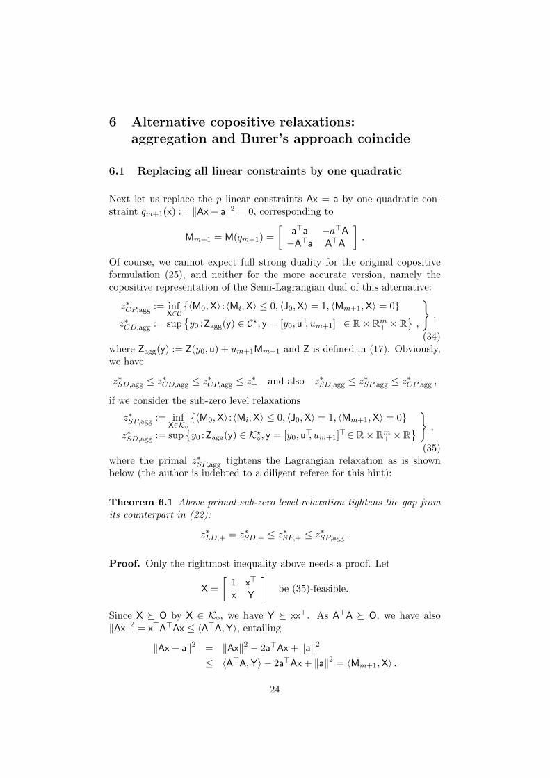
6.1 Replacing all linear constraints by one quadratic

Next let us replace the p linear constraints Ax = a by one quadratic con-straint qm+1(x) := ‖Ax− a‖2 = 0, corresponding to

Mm+1 = M(qm+1) =

[a>a −a>A−A>a A>A

].

Of course, we cannot expect full strong duality for the original copositiveformulation (25), and neither for the more accurate version, namely thecopositive representation of the Semi-Lagrangian dual of this alternative:

z∗CP,agg := infX∈C{〈M0,X〉 :〈Mi,X〉 ≤ 0, 〈J0,X〉 = 1, 〈Mm+1,X〉 = 0}

z∗CD,agg := sup{y0 :Zagg(y) ∈ C?, y = [y0, u

>, um+1]>∈ R× Rm+ × R},

},

(34)where Zagg(y) := Z(y0, u) + um+1Mm+1 and Z is defined in (17). Obviously,we have

z∗SD,agg ≤ z∗CD,agg ≤ z∗CP,agg ≤ z∗+ and also z∗SD,agg ≤ z∗SP,agg ≤ z∗CP,agg ,

if we consider the sub-zero level relaxations

z∗SP,agg := infX∈K�

{〈M0,X〉 :〈Mi,X〉 ≤ 0, 〈J0,X〉 = 1, 〈Mm+1,X〉 = 0}

z∗SD,agg := sup{y0 :Zagg(y) ∈ K?�, y = [y0, u

>, um+1]>∈ R× Rm+ × R} } ,

(35)where the primal z∗SP,agg tightens the Lagrangian relaxation as is shownbelow (the author is indebted to a diligent referee for this hint):

Theorem 6.1 Above primal sub-zero level relaxation tightens the gap fromits counterpart in (22):

z∗LD,+ = z∗SD,+ ≤ z∗SP,+ ≤ z∗SP,agg .

Proof. Only the rightmost inequality above needs a proof. Let

X =

[1 x>

x Y

]be (35)-feasible.

Since X � O by X ∈ K�, we have Y � xx>. As A>A � O, we have also‖Ax‖2 = x>A>Ax ≤ 〈A>A,Y〉, entailing

‖Ax− a‖2 = ‖Ax‖2 − 2a>Ax + ‖a‖2

≤ 〈A>A,Y〉 − 2a>Ax + ‖a‖2 = 〈Mm+1,X〉 .

24

Now X ∈ K� yields also x ∈ Rn+, so that 〈Mm+1,X〉 = 0 implies, by above,finally x ∈ P . Hence X is also (22)-feasible, and the inequality follows. 2

Evidently, for no x we can have qm+1(x) < 0. Still we have zero dualitygap and primal attainability for the conic pairs, if problem (2) is feasible atall, under mild conditions:

Theorem 6.2 Consider the case qm+1(x) = ‖Ax − a‖2. Suppose that atleast one Qi is strictly copositive for i∈ [0 :m+ 1] (note that Qm+1 = A>Ais so if and only if ker A ∩ Rn+ = {o}). Then both primal/dual conic pairs,(25)/(26) and (34), have zero duality gap and the primal optimal value isattained if there is an x ∈ F ∩ P :for some X∗ ∈ C such that 〈Mi,X

∗〉 ≤ 0 for all i∈ [1 :m] as well as 〈J0,X∗〉 = 1

and 〈Mm+1,X∗〉 = 0, we have

z∗CD,agg = z∗CP,agg = 〈M0,X∗〉 .

Proof. First note that the primal problem in (34) is feasible since X = zz>

with z> = [1, x>] satisfies all constraints. Next construct a strictly fea-sible Zagg(y) = Z(y) with um+1 = 0 from Z(y) as in the proof of Theo-rem 4.3(a). Now the result follows from Slater’s principle, applied to theconic primal/dual pair. 2

6.2 Burer’s relaxation and aggregation

We now pass to an alternative put forward by Burer in his seminal pa-per [17], although this is not made explicit there in full generality; but seethe more recent papers [19, 20]. Basically, he concentrated on mixed-binary,linearly constrained quadratic optimization problems, but extended the re-sults to problems with additional quadratic equality constraints, e.g., com-plementarity constraints. The focus of [17] was laid on reformulation ratherthan on relaxation, and the problem (2) with inequality constraints was nottreated there. However the approach in [17] can be easily extended to gen-eral quadratic inequality constraints, namely to complement the condition〈Ak,X〉 = 0 by another one resulting from squaring the linear constraintr>k x = ak: again, with X = [1, x>]>[1, x>], we have

〈rkr>k , xx>〉 = (r>k x)2 = a2

k ⇐⇒ 〈Bk,X〉 = 0 with Bk :=

[−a2

k o>

o rkr>k

].

25

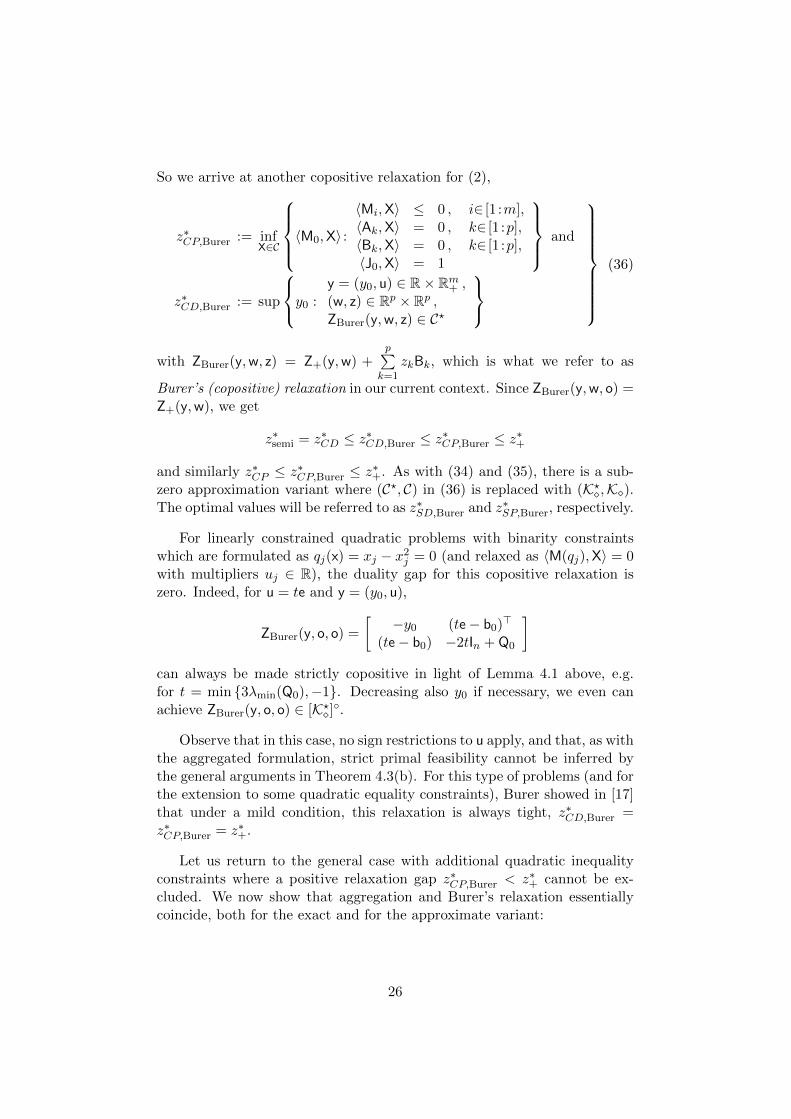
So we arrive at another copositive relaxation for (2),

z∗CP,Burer := infX∈C

〈M0,X〉 :

〈Mi,X〉 ≤ 0 , i∈ [1 :m],〈Ak,X〉 = 0 , k∈ [1 :p],〈Bk,X〉 = 0 , k∈ [1 :p],〈J0,X〉 = 1

and

z∗CD,Burer := sup

y0 :y = (y0, u) ∈ R× Rm+ ,(w, z) ∈ Rp × Rp ,ZBurer(y,w, z) ∈ C?

(36)

with ZBurer(y,w, z) = Z+(y,w) +p∑

k=1

zkBk, which is what we refer to as

Burer’s (copositive) relaxation in our current context. Since ZBurer(y,w, o) =Z+(y,w), we get

z∗semi = z∗CD ≤ z∗CD,Burer ≤ z∗CP,Burer ≤ z∗+

and similarly z∗CP ≤ z∗CP,Burer ≤ z∗+. As with (34) and (35), there is a sub-zero approximation variant where (C?, C) in (36) is replaced with (K?�,K�).The optimal values will be referred to as z∗SD,Burer and z∗SP,Burer, respectively.

For linearly constrained quadratic problems with binarity constraintswhich are formulated as qj(x) = xj − x2

j = 0 (and relaxed as 〈M(qj),X〉 = 0with multipliers uj ∈ R), the duality gap for this copositive relaxation iszero. Indeed, for u = te and y = (y0, u),

ZBurer(y, o, o) =

[−y0 (te− b0)>

(te− b0) −2tIn + Q0

]can always be made strictly copositive in light of Lemma 4.1 above, e.g.for t = min {3λmin(Q0),−1}. Decreasing also y0 if necessary, we even canachieve ZBurer(y, o, o) ∈ [K?�]◦.

Observe that in this case, no sign restrictions to u apply, and that, as withthe aggregated formulation, strict primal feasibility cannot be inferred bythe general arguments in Theorem 4.3(b). For this type of problems (and forthe extension to some quadratic equality constraints), Burer showed in [17]that under a mild condition, this relaxation is always tight, z∗CD,Burer =z∗CP,Burer = z∗+.

Let us return to the general case with additional quadratic inequalityconstraints where a positive relaxation gap z∗CP,Burer < z∗+ cannot be ex-cluded. We now show that aggregation and Burer’s relaxation essentiallycoincide, both for the exact and for the approximate variant:

26

Theorem 6.3 In the primal, Burer’s relaxation is equivalent to the aggre-gation one, and it (weakly) tightens the dual one; the same relations hold atsub-zero level of approximation:

z∗CD,agg ≤ z∗CD,Burer and z∗CP,Burer = z∗CP,agg ,

z∗SD,agg ≤ z∗SD,Burer and z∗SP,Burer = z∗SP,agg .

}(37)

Further, in the case of zero conic duality gap of the aggregated version, thefirst four of these bounds coincide, and likewise the last four ones:

z∗CD,agg = z∗CD,Burer = z∗CP,Burer = z∗CP,agg and

z∗SD,agg = z∗SD,Burer = z∗SP,Burer = z∗SP,agg .

}(38)

Proof. Let us start with the observation that

Ck := akAk + Bk =

[a2k −akr>k

−akrk rkr>k

]= [ak,−r>k ]>[ak,−r>k ] � O .

Hence all Ck are psd., so for any X ∈ K�, the conditions 〈Ck,X〉 = 0 for allk∈ [1 :p] are equivalent to

p∑k=1

〈Ck,X〉 = 0 ,

i.e., to a single homogeneous linear constraint. But

p∑k=1

Ck =

[a>a −a>A−A>a A>A

]= Mm+1 ,

so that the constraint 〈Mm+1,X〉 = 0 is simply an aggregated version ofthe constraints 〈Ck,X〉 = 0 which in turn follow from both 〈Ak,X〉 = 0and 〈Bk,X〉 = 0. On the other hand, we already know (cf. the proof ofTheorem 6.1) that 〈Mm+1,X〉 = 0 imply x ∈ P for all X ∈ K� ⊃ C, whichmeans 〈Ak,X〉 = 0 and, as argued above, also 〈Ck,X〉 = 0, which entails〈Bk,X〉 = 〈Ck,X〉 − ak〈Ak,X〉 = 0 for all k∈ [1 :p], i.e., X is (36)-feasible ifit was (34)-feasible, and vice versa. Since above arguments hold also at thesub-zero level, all the primal equalities follow. On the dual side, we have,by a similar argument, for all y = (y, um+1) ∈ R× Rm+ × R

Zagg(y) = Z(y) + um+1Mm+1 = ZBurer(y, um+1a, um+1e) ,

which establishes z∗CD,agg ≤ z∗CD,Burer. Finally, if z∗CD,agg = z∗CP,agg andlikewise z∗SD,agg = z∗SP,agg, then (37) yields (38). 2

27

A short summary of above results could be the following one: if Qi isstrictly copositive for at least one i∈ [0 :m+ 1], then

z∗LD,+ ≤ z∗semi = z∗CP ≤ z∗CP,Burer = z∗CP,agg ≤ z∗+ .

As an aside, one may note that the two inequality constraints 〈Ak,X〉 ≤ 0and 〈Bk,X〉 ≤ 0 already imply the equalities 〈Ak,X〉 = 〈Bk,X〉 = 0, wheneverX � O with 〈J0,X〉 = 1 and all ak ≥ 0. Indeed, if 0 ≤ ak ≤ r>k x, thensquaring this inequality, using again the fact Y � xx> and using 〈Bk,X〉 ≤ 0already entails

a2k ≤ (r>k x)

2 ≤ r>k Yrk ≤ a2k ,

so 〈Ak,X〉 = 〈Bk,X〉 = 0 follows.

Interestingly, the idea to aggregate constraints in copositive optimizationformulations recently emerged almost simultaneously and independently bythe different approaches in [2, 23, 32]. However, very recent and preliminaryempirical evidence on closely related problems [10] shows no clear advantageof either formulation, which is the reason why we mainly concentrated on thenon-aggregated versions in this paper. See Section 7 for further discussion.

6.3 A further global optimality condition

As done in Corollary 5.1 in Subsection 5.2, we can also derive a second-ordercondition which guarantees global optimality of a generalized KKT point.Again, the slack matrix has to be copositive, and all we need is to adapt tothe problem formulation with the redundant constraints a la Burer:

z∗+ = inf {q0(x) : x ∈ F ∩ P : qi(x) = 0 , i∈ [m+ 1:p]}

with qm+k(x) = (r>k x)2 − a2

k = 0 as k∈ [1 :p]. In this context, a pair(x; u,w, z) ∈ F ∩ P ×Rm+ ×R2p is called generalized KKT pair if and only if

xj [(Hu +∑k

zkrkr>k )x− du − A>w]j = 0 for all j∈ [1 :n] and

uiqi(x) = 0 for all i∈ [1 :m] .

}(39)

Again (39) is equivalent to requiring that x is a critical point of the La-grangian function, but without imposing sign constraints on the multipliersof the sign constraints xj ≥ 0.

Theorem 6.4 If at a generalized KKT pair (x; u, w, z) ∈ F ∩P ×Rm+ ×R2p

in the sense of (39), the matrix c>u−∑k

zka2k + 2a>w − q0(x), −(du + A>w)>

−(du + A>w), Hu +∑k

zk rkr>k

(40)

28

is copositive, then x is a global solution to (2).

Proof. The proof is similar to, but even simpler than, the proof of theimplication (c) =⇒ (d) in Theorem 5.1. In fact, condition (39) implieshere x>Hux = x>du, so that X = zz> with z> = [1, x>] forms an optimalprimal-dual pair (X; y, w, z) to the copositive problem (36), if we define y> =[q0(x), u>], in which case the matrix in (40) exactly is ZBurer(y, w, z). 2

As before, specializing w = um+1a and z = um+1e, the matrix in (40)simplifies to[

c>u + um+1‖a‖2 − q0(x), −(du + um+1A>a)>

−(du + um+1A>a), Hu + um+1A

>A

],

which exactly corresponds to the (generalized) KKT formulation for z+ =inf{x ∈ F ∩ Rn+ : ‖Ax− a‖2 = 0

}with multiplier um+1 for the last constraint.

7 Possible algorithmic implications

7.1 Update on approximation hierarchies

Both cones C and C? involved in the primal-dual pair (12) and (13) areintractable. So we need to approximate them by so-called hierarchies, i.e.,a sequence of tractable cones K?d such that K?d ⊂ K?d+1 ⊂ C? where d isthe level of the hierarchy, and

⋃∞d=0K?d = [C?]◦, i.e., every strictly copositive

matrix is contained in K?d for some d. On the dual side, Kd are also tractable,Kd+1 ⊂ Kd, and

⋂∞d=0Kd = C contains no matrix which is not completely

positive. For brevity of exposition, assume that z∗CD = z∗CP and furtherassume that strong duality also holds for the approximation:

z∗Kd:= min {〈M0,X〉 : 〈Mi,X〉 ≤ ri , i∈ [1 :m] , X ∈ Kd}

= max

{r>y : y ∈ Rm+ , M0 +

m∑i=1

yiMi ∈ K?d

}.

Then by above we get z∗Kd→ z∗CD = z∗CP as d → ∞. By now, there are

many possibilities explored for hierarchies (Kd)d, for a concise survey see [11].Many of these involve linear or psd constraints of matrices of order nd+2, e.g.the seminal ones proposed in [33, 40]. In particular for LMIs, matrices oflarger order pose a serious memory problem for algorithmic implementationseven for moderate d if n is large. LP-based hierarchies suffer less from thiscurse of dimensionality, and therefore we will follow a compromise between

29

LP-based and SDP-based hierarchies. We start with the usual zero-orderapproximation by the cone of doubly nonnegative (DNN) matrices

K0 = {X is psd : X has no negative entries} . (41)

For the dual cone

K?0 = {P + N : P is psd. and N has no negative entries} (42)

Florian Jarre (personal communication) very recently has coined the termnonnegative decomposable (NND) for matrices in K?0, using the duality cal-culus pun (DNN)? = NND. Anyhow, based upon this construction, wemay add valid linear inequalities, e.g., as done in [15, 16], yielding polyhe-dral inner approximations L?d of the copositive cone, and, on the dual side,polyhedral outer approximations Ld for the completely positive cone, andfinally define

Kd := K0 ∩ Ld , d ∈ {0, 1, 2, . . .} , (43)

or, by duality, the closure K?d of the Minkowski sum K?0 +L?d. Of course, thisapproximation satisfies above properties of exhaustivity, and involves LMIsonly for matrices of order linear in n; in fact, we only employ the matricesMi = M(qi) of order n+ 1.

A similar yet different approach is taken in [34] where a conic exactreformulation of problem (1) is proposed, using another intractable cone,and constructing tractable approximation hierarchies for this cone. Theexamples specified in [34] reduce again to the NND cone K?0 or its dual, theDNN cone K0. However for large n, even K0 may involve too many (namely(n−1)n

2 ) linear inequalities to allow for efficient computation. This problemcan be overcome by warmstarting as in [25], identifying or separating validlinear inequalities on the fly, or by the recently proposed tightening andacceleration method in [32].

The following proposal is an alternative: suppose that we only employ,say, n inequalities, e.g., by forbidding negative entries only in the first rowof a matrix, to proxy for complete positivity. Then we arrive at K� ={X is psd : X0j ≥ 0 for all j∈ [1 :n]} introduced in (18), and used in the SDPreformulation of the full Lagrangian dual in Subsection 3.2. Above discussionnow justifies the term sub-zero level approximation.

A possibly efficient hierarchy is then

K�,d = K� ∩ Ld , d ∈ {0, 1, 2, . . .} . (44)

While practical experience with this proposal is not yet available, we haveseen above that K�,d emerges quite naturally in the context of Lagrangianduality and thus can be seen as a conceptual way of selecting (few) linearinequality constraints to tighten the SDP bound.

30

7.2 Approximate copositive bounds dominateLagrangian dual bounds even at (sub-)zero level

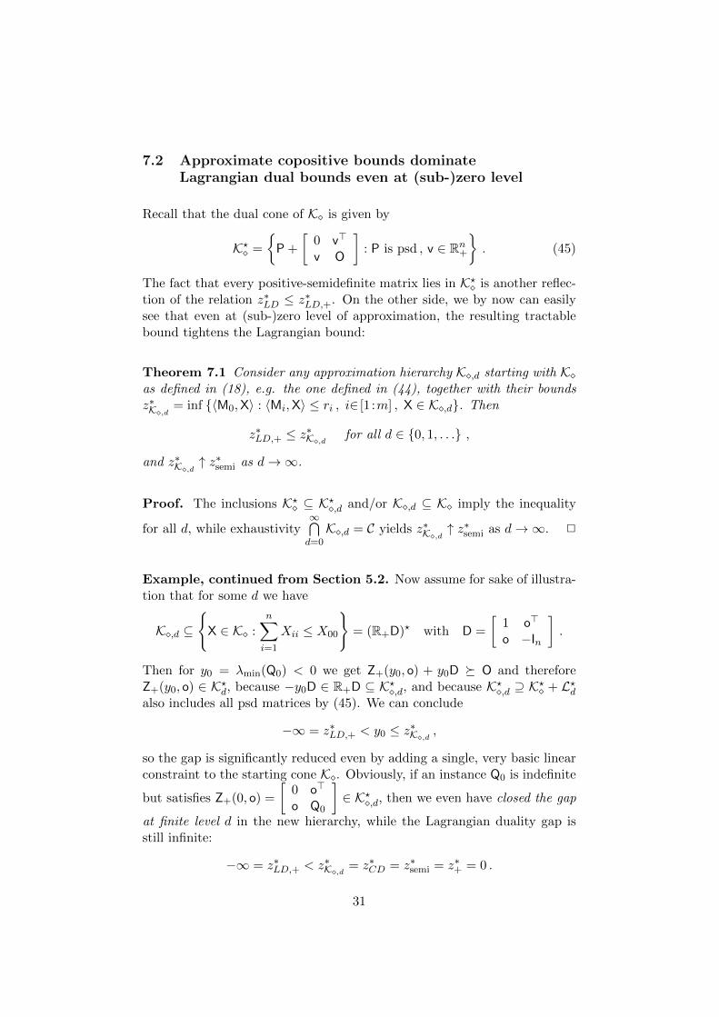
Recall that the dual cone of K� is given by

K?� =

{P +

[0 v>

v O

]: P is psd , v ∈ Rn+

}. (45)

The fact that every positive-semidefinite matrix lies in K?� is another reflec-tion of the relation z∗LD ≤ z∗LD,+. On the other side, we by now can easilysee that even at (sub-)zero level of approximation, the resulting tractablebound tightens the Lagrangian bound:

Theorem 7.1 Consider any approximation hierarchy K�,d starting with K�as defined in (18), e.g. the one defined in (44), together with their boundsz∗K�,d = inf {〈M0,X〉 : 〈Mi,X〉 ≤ ri , i∈ [1 :m] , X ∈ K�,d}. Then

z∗LD,+ ≤ z∗K�,d for all d ∈ {0, 1, . . .} ,

and z∗K�,d ↑ z∗semi as d→∞.

Proof. The inclusions K?� ⊆ K?�,d and/or K�,d ⊆ K� imply the inequality

for all d, while exhaustivity∞⋂d=0

K�,d = C yields z∗K�,d ↑ z∗semi as d→∞. 2

Example, continued from Section 5.2. Now assume for sake of illustra-tion that for some d we have

K�,d ⊆

{X ∈ K� :

n∑i=1

Xii ≤ X00

}= (R+D)? with D =

[1 o>

o −In

].

Then for y0 = λmin(Q0) < 0 we get Z+(y0, o) + y0D � O and thereforeZ+(y0, o) ∈ K?d, because −y0D ∈ R+D ⊆ K?�,d, and because K?�,d ⊇ K?� + L?dalso includes all psd matrices by (45). We can conclude

−∞ = z∗LD,+ < y0 ≤ z∗K�,d ,

so the gap is significantly reduced even by adding a single, very basic linearconstraint to the starting cone K�. Obviously, if an instance Q0 is indefinite

but satisfies Z+(0, o) =

[0 o>

o Q0

]∈ K?�,d, then we even have closed the gap

at finite level d in the new hierarchy, while the Lagrangian duality gap isstill infinite:

−∞ = z∗LD,+ < z∗K�,d = z∗CD = z∗semi = z∗+ = 0 .

31

Burer’s relaxation simply adds another constraint to every linear equal-ity constraint of the natural copositive formulation of the Semi-Lagrangianbound. Replacing C with Kd or C? with K?d, would therefore tighten theapproximate bounds even beyond the Semi-Lagrangian dual, at the cost ofdealing with additional constraints. As always in implementation, we haveto face a trade-off between quality and effort of obtaining tractable bounds.Hopefully some empirical evidence will be put forward soon.

8 Conclusion and outlook

This paper deals with problems to optimize a quadratic function subjectto quadratic and linear constraints, where the linear ones are treated sep-arately. By relaxing everything except the sign constraints, we arrived ata Semi-Lagrangian dual which apparently has not been analyzed before inthe literature. Here we have reformulated both the Lagrangian dual and theSemi-Lagrangian dual as conic optimization problems, and compared theresulting bounds to their counterparts when all linear equality constraintsare replaced by a single convex quadratic one. This alternative turned out tobe essentially equivalent to Burer’s copositive relaxation. While the Semi-Lagrangian dual is a copositive problem, the Lagrangian dual can be seenas a natural relaxation of the latter, namely arising from an approximationof the copositive problem at a sub-zero level. This low level is importantin regimes where every additional linear inequality constraint severely slowsdown algorithmic performance and/or creates memory problems, which istypical for interior-point methods when applied to very large problems, forinstance in the most familiar doubly-nonnegative relaxation. For an inter-esting review of these and related bounds (as known prior to 2011), we referto the survey article [4].

The development led us to propose a new variant building upon knownapproximation hierarchies which may avoid above drawbacks, with the hopethat a significant tightening of the bounds becomes tractable, because LMIsof higher order matrices can be avoided. Furthermore, we studied propertiesof the problem which ensure strong duality of the conic relaxations; specifiednecessary and sufficient copositivity-based conditions to guarantee that theSemi-Lagrangian relaxation is exact; and proposed a hierarchy of seeminglynew, sufficient, second-order global optimality conditions for a KKT pointof the original problem which can be tested in polynomial time if tractableapproximation hierarchies are employed. These conditions require much lessthan the familiar ones which require positive-semidefiniteness of the Hessianof the Lagrangian.

32

Building upon these findings, there are several directions of future re-search, among them:

• to tighten other variants of SDP formulations of the full Lagrangianrelaxation [26], and to interpret them in terms of properties of theLagrangian function of the original problem (in some formulation);

• to define a strategy which balances computational effort identifyingand using additional linear constraints (i.e., other than those definingK�), against efficient strengthening of the resulting bounds;

• to explore the quality of the relaxation if the Ak constraints are simplyreplaced by the Bk constraints, and to relate the result with above dualbounds.

Acknowledgement. The author is indebted to Associate Editor SamuelBurer and to three anonymous referees for their diligence and many sugges-tions which helped to significantly improve presentation of the paper. Iam grateful for valuable comments and stimulating discussions on an ear-lier draft of this paper, provided by Peter J.C. Dickinson and Luis Zuluaga.Thanks are also due to the Isaac Newton Institute at Cambridge Univer-sity for providing a stimulating environment when the author participatedas a visiting fellow in the Polynomial Optimization Programme 2013, orga-nized by Joerg Fliege, Jean Bernard Lasserre, Adam Letchford and MarkusSchweighofer.

References

[1] Wenbo Ai and Shuzhong Zhang. Strong duality for the CDT subproblem:a necessary and sufficient condition. SIAM J. Optim., 19(4):1735–1756, 2009.

[2] Naohiko Arima, Sunyoung Kim, and Masakazu Kojima. Simplified coposi-tive and Lagrangian relaxations for linearly constrained quadratic optimizationproblems in continuous and binary variables. Pacific J. Optimiz., 10(3):437–451, 2014.

[3] Lijie Bai, John E.Mitchell, and Jong-Shi Pang. On QPCCs, QC-QPs and completely positive programs. Preprint, RPI, http://www.

optimization-online.org/DB\_HTML/2014/01/4213.html, 2014.

[4] Xiaowei Bao, Nikolaos V. Sahinidis, and Mohit Tawarmalani. Semidefiniterelaxations for quadratically constrained quadratic programming: a review andcomparisons. Math. Program., 129(Ser. B):129–157, 2011.

[5] Amir Beck and Yonina Eldar. Strong duality in nonconvex quadratic optimiza-tion with two quadratic constraints. SIAM J. Optim., 17(3):844–860, 2006.

33

[6] Evgeny G. Belousov and Diethard Klatte. A Frank-Wolfe type theorem forconvex polynomial programs. Comput. Optim. Appl., 22(1):37–48, 2002.

[7] Aharon Ben Tal, Arkadi Nemirovski, and Cornelis Roos. Robust solutionsof uncertain quadratic and conic-quadratic problems. SIAM J. Optim.,13(2):535–560, 2002.

[8] Immanuel M. Bomze. Copositive optimization – recent developments and ap-plications. European J. Oper. Res., 216:509–520, 2012.

[9] Immanuel M. Bomze. Copositivity for second-order optimality conditions ingeneral smooth optimization problems. Preprint NI13033-POP, Isaac NewtonInstitute, Cambridge UK, 2013.

[10] Immanuel M. Bomze, Jianqiang Cheng, Peter J.C. Dickinson, and AbdelLisser. A fresh CP look at mixed-binary QPs: new formulations, relaxationsand penalizations. Preprint, LRI, Univ. Paris Sud, 2015 (in preparation).

[11] Immanuel M. Bomze, Mirjam Dur, and Chung-Piaw Teo. Copositive optimiza-tion. Optima – MOS Newsletter, 89:2–10, 2012.

[12] Immanuel M. Bomze and Florian Jarre. A note on Burer’s copositive repre-sentation of mixed-binary QPs. Optim. Lett., 4(3):465–472, 2010.

[13] Immanuel M. Bomze and Michael L. Overton. Narrowing the difficultygap for the Celis-Dennis-Tapia problem. Math. Program., to appear.DOI:10.1007/s10107–014–0836–3, 2015.

[14] Immanuel M. Bomze, Werner Schachinger, and Reinhard Ullrich. New lowerbounds and asymptotics for the cp-rank. SIAM J. Matrix Anal. Appl.,36(1):20–37, 2015.

[15] Stefan Bundfuss and Mirjam Dur. Algorithmic copositivity detection by sim-plicial partition. Linear Algebra Appl., 428(7):1511–1523, 2008.

[16] Stefan Bundfuss and Mirjam Dur. An adaptive linear approximation algorithmfor copositive programs. SIAM J. Optim., 20(1):30–53, 2009.

[17] Samuel Burer. On the copositive representation of binary and continuousnonconvex quadratic programs. Math. Program., 120(2, Ser. A):479–495, 2009.

[18] Samuel Burer. Copositive programming. In Miguel F. Anjos and Jean BernardLasserre, editors, Handbook of Semidefinite, Cone and Polynomial Optimiza-tion: Theory, Algorithms, Software and Applications, International Series inOperations Research and Management Science, pages 201–218. Springer, NewYork, 2012.

[19] Samuel Burer, Sunyoung Kim, and Masakazu Kojima. Faster, but weaker,relaxations for quadratically constrained quadratic programs. Comput. Optim.Appl., 59(1–2):27–45, 2014.

[20] Jieqiu Chen and Samuel Burer. Globally solving nonconvex quadratic pro-gramming problems via completely positive programming. Math. Program.Comput., 4(1):33–52, 2012.

[21] Peter J. C. Dickinson. An improved characterisation of the interior of thecompletely positive cone. Electron. J. Linear Algebra, 20:723–729, 2010.

34

[22] Peter J. C. Dickinson and Luuk Gijben. On the computational complexity ofmembership problems for the completely positive cone and its dual. Comput.Optim. Appl., 57(2):403–415, 2014.

[23] Peter J.C. Dickinson. The copositive cone, the completely positive cone andtheir generalisations. Ph.D. dissertation, University of Groningen, The Nether-lands, 2013.

[24] Mirjam Dur. Copositive programming — a survey. In Moritz Diehl, FrancoisGlineur, Elias Jarlebring, and Wim Michiels, editors, Recent Advances in Op-timization and its Applications in Engineering, pages 3–20. Springer, BerlinHeidelberg New York, 2010.

[25] Alexander Engau, Miguel F. Anjos, and Immanuel M. Bomze. Constraint se-lection in a build-up interior-point cutting-plane method for solving relaxationsof the stable-set problem. Math. Methods of OR, 78(1):35–59, 2013.

[26] Alain Faye and Frederic Roupin. Partial Lagrangian relaxation for generalquadratic programming. 4OR, 5:75–88, 2007.

[27] Marguerite Frank and Philip Wolfe. An algorithm for quadratic programming.Naval Res. Logistics Quarterly, 3:95–110, 1956.

[28] Tetsuya Fujie and Masakazu Kojima. Semidefinite programming relaxationfor nonconvex quadratic programs. J. Global Optim., 10(4):367–380, 1997.

[29] Simai He, Zhi-Quan Luo, Jiawang Nie, and Shuzhong Zhang. Semidefiniterelaxation bounds for indefinite homogeneous quadratic optimization. SIAMJ. Optim., 19(2):503–523, 2008.

[30] Vaithilingam Jeyakumar, Gue Myung Lee, and Guoyin Li. Alternative theo-rems for quadratic inequality systems and global quadratic optimization. SIAMJ. Optim., 20(2):983–1001, 2009.

[31] Vaithilingam Jeyakumar and Guoyin Li. Trust-region problems with linearinequality constraints: exact SDP relaxation, global optimality and robust op-timization. Math. Program., 147(Ser. A):171–206, 2014.

[32] Sunyoung Kim, Masakazu Kojima, and Kim-Chuan Toh. A Lagrangian-DNN relaxation: a fast method for computing tight lower bounds for aclass of quadratic optimization problems. Math. Program., to appear.DOI:10.1007/s10107–015–0874–5, 2015.

[33] Jean Bernard Lasserre. Global optimization with polynomials and the problemof moments. SIAM J. Optim., 11(3):796–817, 2000/01.

[34] Cheng Lu, Shu-Cherng Fang, Qingwei Jin, Zhengbo Wang, and WenxunXing. KKT solution and conic relaxation for solving quadratically constrainedquadratic programming problems. SIAM J. Optim., 21(4):1475–1490, 2011.

[35] Zhi-Quan Luo and Shuzhong Zhang. On extensions of the Frank-Wolfe theo-rems. Comput. Optim. Appl., 13(1-3):87–110, 1999.

[36] Jerome Malick and Frederic Roupin. On the bridge between combinatorialoptimization and nonlinear optimization: a family of semidefinite bounds for0-1 quadratic problems leading to quasi-Newton methods. Math. Program.,140(Ser. B):99–124, 2013.

35

[37] Katta G. Murty and Santosh N. Kabadi. Some NP-complete problems inquadratic and nonlinear programming. Math. Program., 39(2):117–129, 1987.

[38] Yuri Nesterov, Henry Wolkowicz, and Yinyu Ye. Nonconvex quadratic op-timization. In Henry Wolkowicz, Romesh Saigal, and Lieven Vandenberghe,editors, Handbook of Semidefinite Programming, pages 361–420. Kluwer, NewYork, 2000.

[39] Arnold Neumaier. Optimization – Theory and Algorithms. Preprint, http://www.mat.univie.ac.at/~neum/, 2014.

[40] Pablo A. Parrilo. Structured Semidefinite Programs and Semi-algebraic Geom-etry Methods in Robustness and Optimization. PhD thesis, California Instituteof Technology, Pasadena, CA, May 2000.

[41] Svatopluk Poljak, Franz Rendl, and Henry Wolkowicz. A recipe for semidefi-nite relaxation for (0,1)-quadratic programming. J. Global Optim., 7(1):51–73,1995.

[42] Motakuri Venkata Ramana. An Algorithmic Analysis of Multiquadratic andSemidefinite Programming Problems. Doctoral dissertation, Johns HopkinsUniversity, Baltimore, MD, 1993.

[43] Naomi Shaked-Monderer, Abraham Berman, Immanuel M. Bomze, FlorianJarre, and Werner Schachinger. New results on the cp rank and related prop-erties of co(mpletely )positive matrices. Linear Multilinear Algebra, 63(2):384–396, 2015.

[44] Naum Z. Shor. Quadratic optimization problems. Izv. Akad. Nauk SSSRTekhn. Kibernet., 222(1):128–139, 1987.

[45] Yinyu Ye. On the complexity of approximating a KKT point of quadraticprogramming. Math. Program., 80(Ser. A):195–211, 1998.

36