Coordinated Replenishments in a Multi-item Inventory ...

Coordinated Replenishments in aMulti-item Inventory System using a

g-revised Cost Method

January 31, 2018

By:

Ger Westra 2387565

University of Groningen

Abstract: Inventory control models have been studied extensively in the past. As items are oftenreplenished by the same supplier, research has focussed on joint ordering models in order to reducecosts. However, due the complexity of the problem, no exact solution method has been developed andtherefore research has focussed on approximations such as can-order and periodic review policies.This thesis focusses on a different solution method, namely the g-revised cost method. Using thismethod, we are able to solve the coordinate replenishment problem for both the deterministic and

stochastic setting. Numerical experiments show the importance of coordinated replenishment.Furthermore, the results show that this method outperforms the can-order policy in the two-item

setting, but this difference becomes insignificant in case the number of items is increased.Keywords: Coordinated replenishment, joint ordering, g-revised cost

G.Y. Westra

Master’s thesis for MSc Econometrics, Operations Research and Actuarial Studies

Supervisor:Co-assessor:Programme profile:

dr. N.D. van Foreestdr. O.A. KilicOperations Research

Page 1 of 32

G.Y. Westra CONTENTS

Contents

1 Introduction 3

2 Literature Review 42.1 Contribution by this thesis . . . . . . . . . . . . . . . . . . . . . . . . . . . . . . . 5

3 Problem Description 6

4 Solution Method 8

5 Deterministic Multi-item Setting 10

6 Stochastic Single-item Setting 15

7 Stochastic Multi-item Setting 16

8 Numerical Results 188.1 Single-item Setting . . . . . . . . . . . . . . . . . . . . . . . . . . . . . . . . . . . 18

8.1.1 EOQ model with unit demand . . . . . . . . . . . . . . . . . . . . . . . . . 188.1.2 Stochastic demand . . . . . . . . . . . . . . . . . . . . . . . . . . . . . . . . 20

8.2 Two-item Setting . . . . . . . . . . . . . . . . . . . . . . . . . . . . . . . . . . . . . 218.2.1 Testing . . . . . . . . . . . . . . . . . . . . . . . . . . . . . . . . . . . . . . . 218.2.2 Evaluation of the value function . . . . . . . . . . . . . . . . . . . . . . . 218.2.3 Basic policy . . . . . . . . . . . . . . . . . . . . . . . . . . . . . . . . . . . . 228.2.4 Numerical Results . . . . . . . . . . . . . . . . . . . . . . . . . . . . . . . . 24

8.3 Multi-item Setting . . . . . . . . . . . . . . . . . . . . . . . . . . . . . . . . . . . . 258.3.1 Testing . . . . . . . . . . . . . . . . . . . . . . . . . . . . . . . . . . . . . . . 258.3.2 Basic policy . . . . . . . . . . . . . . . . . . . . . . . . . . . . . . . . . . . . 268.3.3 Multi-item Setting . . . . . . . . . . . . . . . . . . . . . . . . . . . . . . . . 26

8.4 Comparison with other policies . . . . . . . . . . . . . . . . . . . . . . . . . . . . 278.4.1 Numerical results . . . . . . . . . . . . . . . . . . . . . . . . . . . . . . . . 28

9 Conclusion 29

Appendix 32

Page 2 of 32

G.Y. Westra 1 INTRODUCTION

1 Introduction

Inventory control systems have been a field of interest for researchers for many decades.That is caused by the fact that companies and shops do not want too many items in stockdue to the holding costs, however on the other hand, they do not want too few items in stockeither, due to the backorder costs or lost sales related to running out of stock. For this rea-son, inventory control models have been developed in order to analyse the optimal reorderand order-up-to points. The first models only focused on a single-item setting with determin-istic demand and this resulted in the well-known Economic Order Quantity (EOQ) model byFord W. Harris in 1913 [4]. Over the decades, the inventory control models became more so-phisticated and more complex problems could be solved, for example taking into account therandomness of demand using stochasticity and other interesting extension of the existingmodels, such as different lead-times, no-ordering periods and numerous other extensions.One of the extensions that has been studied, is the opportunity of joint ordering. The ideabehind joint ordering is the following. Consider a shop that sells multiple products whichare replenished by the same supplier. If the shop owner uses an independent replenishmentpolicy, this policy might suggest to reorder a certain product on one day and the next daya different product. Intuitively, this might not be the optimal reorder policy, since the tworeplenishments could have been combined resulting in a cost reduction in the fixed orderingcosts. Typically, the total order costs can be divided into two categories, namely fixed order-ing costs and item-dependent ordering costs. The fixed ordering costs are costs independentof the type of items replenished and the number of items ordered. An example of these costsare the costs corresponding to the truck and the driver which deliver the ordered items.The item-dependent ordering costs are costs associated with the item or number of itemsordered. An example can be costs corresponding to the labour required for inspection of theitems ordered.

In the previous decades, researchers have investigated inventory systems with coordi-nated replenishment. However, due to the complexity of the problem, no optimal solutionmethod has been developed. Previous research has focused on two solution methods, thefirst being can-order policies and the second periodic-review policies. The can-order policiesare characterised by defining for each item an individual must-order level, an order-up-tolevel and a can-order level. Next, when an item reaches its must-order level an order isplaced, but all items having inventory levels below their can-order level are combined in theorder and all items are replenished up to their order-up-to level. Periodic-review policiesare characterised by having fixed time intervals between the order decision. For each item,a multiple of the base cycle is determined at which this item is replenished (in general,these are power-of-two type of policies) and this result in a simple ordering policy. However,research has shown that both solution methods can result in non-optimal policies, even insimple cases.

In this thesis, the coordinated replenishment problem will be addressed using a differentmethod, namely a g-revised cost method suggested by Germs, Van Foreest and Kilic (2017)

Page 3 of 32

G.Y. Westra 2 LITERATURE REVIEW

[8]. Using this method, the coordinated replenishment problem can be solved in both the de-terministic and stochastic setting. However, due to numerical complexity of this method, thenumber of items considered is small, but the solution method is equivalent for coordinatedreplenishment problems with a larger number of items.

The remainder of this paper is organised as follows: Section 2 provides an overview ofthe relevant literature. In Section 3 a complete description of the coordinated replenish-ment problem is given, which is followed by the solution method in Section 4. Afterwards,this solution method is extended to the multi-item setting in Section 5. Consequently, thesolution method is described for the stochastic single-item and multi-item setting in Section6 and Section 7 respectively. Subsequently, Section 8 shows the numerical results of thissolution method and lastly, 9 provides the conclusion and fields of interest for the future.

2 Literature Review

Inventory control models have been studied extensively of the last century. The first modelsresulted in the well-known EOQ model and over the decades these models became moresophisticated, such that they could handle stochastic demands, differences in lead-times,no-order periods and numerous other extensions. Silver (1981) [17] provides an overviewof inventory management, including all relevant costs and minimisation problem related toinventory control models. Furthermore, solution methods are mentioned for solving theseproblems. Also, Axsäter (2015) [1] provides a great overview of inventory control modelsand existing solution methods. Furthermore, he provides a great number of practical ex-amples, applications and discusses several extensions of the models in his book. One of theextensions that has been studied, is the opportunity of joint ordering. The idea behind jointordering is mentioned before, namely that for all items that are ordered jointly, the fixed or-dering costs have to be paid only once and this could be potentially cost-reducing. However,finding a policy is not always straightforward as Ignall (1969) [10] conclude in a two itemsetting. Furthermore, he is able to find parameter spaces for which a given policy is optimalusing Markov Renewal programming. Federgruen et al. (1984) [5] focus on joint orderinginventory models subject to a service level constraint. They construct an algorithm whichsolves this problem, under the assumption of compound Poisson demand. Pantumsinchai(1992) [13] evaluates the performance of a joint ordering policy based on a group reorderpoint and a combined order quantity, where each item maintains its individual order-up-tolevel. He compares this policy to a can-order policy and a periodic review where the itemscan be ordered in fixed intervals. He concludes that no policy is superior to the other policiesbased on the long-run average costs. Sethi and Cheng (1997) [15] focus on the generalisationof (s,S) type of inventory policies with Markovian demand. Furthermore, they present pos-sible extensions of the model by incorporation seasonal demands, no-ordering periods andstorage and service level constraints. They conclude that (s,S) type of policies are optimalfor all models described above.

Page 4 of 32

G.Y. Westra 2 LITERATURE REVIEW

Due to the complexity of the problem, researchers have come up with different solutionmethods. A well-known solution method is the so-called can-order policy, which was firstsuggested by Balintfy (1964) [2]. These policies are known for their simplicity and flexi-bility. They can be used both in a deterministic and stochastic setting, as Goyal and Satir(1989) [9] show. Later, different types of can-order policies were suggested, for exampleby Melchiors (2002) [12]. He suggests a compensation approach in which the item thattriggers the order, receives a compensation from other items which benefit from this orderopportunity. He concludes that this can-order policy outperforms policies of the same typeon examples where the can-order policies perform better than the periodic replenishmentpolicies.

A different solution method for the joint ordering problem are the so-called periodic re-view policies. A well-known example of these type of policies are the power-of-two policies.In these type of policies, the ordering period for each item must be a multiple (or power-of-two) of the base cycle length. This results in a simple ordering policy, which is repetitiveafter some interval. These type of policies are related to Silver (1976) [16] where he sug-gests a method for determining a basic cycle time and determines for each item a multipleof this basic cycle length. Roundy (1985) [14] shows that these are widely applicable, due totheir flexibility and simplicity. Federgruen et al. (1992) [6] show that the best power-of-twopolicy, is at most 2% worse than the optimal policy. However, this optimal policy might benon-stationary and extremely difficult to find and for this reason, this power-of-two policyhas been suggested. Furthermore, due to their simplicity, relatively complex problems couldbe modelled. That is, Federgruen and Zheng (1993) [7] have managed to develop power-of-two policies where they take into account capacity constraints. Similarly, Chu and Shen(2010) [3] have developed policies with service level constraints and stochastic demandsand show that their algorithm is at most 1.26% more costly than the optimal policy.

In general, it is believed that can-order policies are more suitable when the major set-upcost is high (i.e. the fixed ordering cost is high) and periodic-review policies are more appro-priate when these costs are relatively low. However, Van Eijs (1994) [18] finds that there isno significant difference between the policies itself, but these differences are caused by themethod which is used for determining the parameter values. Johansen and Melchiors (2003)[11] conclude that under stochastic demands, the can-order policy is more appropriate.

2.1 Contribution by this thesis

In this thesis, the g-revised cost method suggested by Germs, Van Foreest and Kilic (2017)[8] will be used in order to analyse the joint ordering inventory model. This method in-troduces explicitly a parameter which denotes the compensation g. Afterwards, this com-pensation g can be used in order to evaluate the value function and the optimal startinginventory corresponding to minimum of this value function. This g-revised cost method isinvestigated in both the deterministic and stochastic setting.

Using this method, we are able to solve the coordinated replenishment problem in both

Page 5 of 32

G.Y. Westra 3 PROBLEM DESCRIPTION

the deterministic and stochastic setting. However, due to the numerical complexity of thisproblem, the number of items considered is small, but the solution method is equivalent forhigher dimensional problems. Computational experiments show the importance of coordi-nated replenishment. Furthermore, the results presented in this thesis suggest that thereis a significant difference between the can-order policy suggested by Balintfy (1964) [2] andthe policy constructed via the g-revised cost method in the two-item setting. However, thisdifferences becomes insignificant when the number of items is increased.

3 Problem Description

Inventory control models are used in order to keep inventory levels at acceptable levels.These acceptable levels could be determined by service level constraints and other type ofdemand fulfilment constraints. These inventory control models focus on construction ofa reorder policy, denoted by π(x), which depend on the current inventory level x. Basically,these order policies are decision rules, which determine whether an order will be placed, andhow many items will be replenished. Consider for example a shop which sells a particularitem and the shop uses an (s,S) type of policy. That is, an item will be ordered when itsinventory is smaller or equal to s and if an order is placed, it will order-up-to S items. Next,we can construct the order cycle that will occur under this policy π(x). That is, each orderwill start at the order-up-to level S and the cycle will start. Then over time, demand willarrive which is denoted by y≥ 0 and this will lower the inventory level. The inventory levelat time t is given by Equation 1, where Yt denotes the demand quantity at time t.

X t = X t−1 −Yt (1)

This process will continue until the inventory level equals the reorder level s. At that mo-ment a reorder will be placed and the item is replenished such that its inventory level equalsthe order-up-to level S. This is the end of the cycle and a new order cycle will start. Obvi-ously, the policy used for determining the reorder level and the order-up-to level will affectthe inventory level of each item. Furthermore, when demand Y and the starting inven-tory is known, we can determine the inventory levels at each time. Afterwards, we can usethese inventory in order to compare different policies in terms of costs, since there are costsrelated to the inventory levels.

Consider the multi-item setting in which we have m ∈N items. We assume that the costscorresponding to positive inventory of each item i is given by hi. Furthermore, we assumethat all unsatisfied demand is backordered for costs bi and this results in the followinginventory cost function:

h(x)=m∑

i=1hi max{xi,0}+bi max{−xi,0} (2)

where x is the vector with inventory level for each item. Next, as mentioned before, theitems have to be replenished in order to keep the inventory at an acceptable level. We

Page 6 of 32

G.Y. Westra 3 PROBLEM DESCRIPTION

assume that the replenishment arrives immediately upon arrival, that is, we have zero leadtime. The costs associated with a replenishment can be diversified into two categories. Firstwe have the fixed ordering costs K , which occur in every order, regardless of the number ofitems and which items we replenish. Second, there is an item-dependent ordering cost ki

which occurs when item i is present in the order. Therefore, the costs corresponding to asingle order j are given by

c j(y)= K +m∑

i=1ki I{yi>0} (3)

where y denotes the vector of items that can be ordered and I{yi>0} is the indicator functionwhich assesses whether item i is included in the order. Observe the order cost only dependon whether an item is included in the order, and it is independent of the number of itemswe order for a specific item i. The total costs are given by the summation of the inventorycosts and the ordering costs. Obviously, the policy π(x) influences the inventory levels andthe ordering costs and consequently the total costs. Since we aim for profit maximisationand consequently, cost minimisation, it follows that this problem is not straightforward.

In order to specify the cost of a policy, it is necessary to specify points in time at whichthe replenishments are made and the number of items that are ordered. Let the time oforders by denoted by σ j. Then, a reorder is characterised by its timing σ j and its reorderwhich is completely specified by inventory levels of the items, denoted by xt. The total costsof a policy π(x) up to time T are given by

Cπ(T)=∫ T

0h(xt)dt+

∞∑j=1

c j(yj) I{σ j<T} (4)

where yj denotes the vector of ordered items in order j and I{σ j} is the indicator functionwhether an order is placed before time T. We are interested in the long-run average costs

Cπ = limsupT→∞

Cπ(T)T

(5)

and the objective is to find the policy π∗(x) which minimises the long-run average costs,assuming this minimum exists. That is,

C∗π = inf

π{Cπ}= inf

π

{limsup

T→∞Cπ(T)

T

}(6)

We will focus on this problem for both the deterministic and the stochastic setting. Thedifference between those models is characterised by the demand Y . The former correspondsto the case in which demand y is known and it is equal in all periods. In this case, theinventory level process given in equation (1) is complete known beforehand. In the lattercase, the demand vector y is unknown, but is distribution is known. In this case the in-ventory level can be characterised over time as done in equation (1), but it is a stochasticprocess. However, this does not influence the structure of the minimisation problem givenin equation (6), although the computational complexity is influenced.

Page 7 of 32

G.Y. Westra 4 SOLUTION METHOD

4 Solution Method

In order to solve the minimisation problem described in the previous section, the g-revisedcost method suggested by Germs, Van Foreest and Kilic (2017) [8] will be used. We willexplain this solution method in the single-item deterministic setting and later expand thismodel to the multi-item setting and the stochastic setting. Consider the case in which thereis one item with deterministic demand d. For simplicity, we will drop the index i in thissingle-item case. Then, the g-revised cost method uses a simple inventory cost structure,which is given by:

h(x)− g = hmax{x,0}+bmax{−x,0}− g (7)

Observe that the g is introduced, to make it explicit that we deal with g-revised costs here.Next, the idea of this g-revised cost method is the following. Consider there is an en-

trepreneur who is given the choice to participate in a game, for which he has to pay startingprice K . If he accepts the offer, he has to decide on the starting inventory and then thegame starts. Each time period, e.g. a day, the entrepreneur has to pay holding and back-order costs h and b respectively for his inventory, according to the inventory cost functionintroduced above. On the other hand, each time period he receives a financial compensa-tion g at demand rate d. The entrepreneur has the option to quit the game at any time heprefers. Furthermore, the entrepreneur is aiming for profit maximisation, so all decisionwill be profit maximising. Naturally, three questions arise related to this game. First, willthe entrepreneur decide to enter the game? Second, what will be the starting inventory theentrepreneur selects? Third, when will the entrepreneur decide to stop the game? Obvi-ously, the answers to these questions will depend on the parameter values for K ,b,h, g andd.

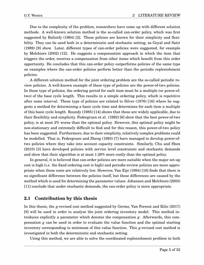
Due to the one-dimensionality of this game, we can depict the inventory cost functionof this game graphically, which is shown in Figure 1. We observe that the function h(·) isa piecewise linear function, which has a kink-point exactly at x = 0 or equivalently, whenthere is no inventory. Furthermore, we observe that this function attains its minimum atthis kink-point and it has value h(0) = −g. Due to its piecewise linearity, we find that theinventory cost function equals zero at two points, namely one where the inventory level isnegative and one where it is positive. That is

h(x)− g = 0 =⇒ x =−1b

g ∨ x = 1h

g (8)

We find that the marginal profit of the entrepreneur will be exactly zero at these points.Moreover, we find that any inventory level less than − 1

b g or greater than 1h g will result in a

negative marginal profit. Recall that the entrepreneur was profit maximising and it followsdirectly that these points will correspond to the starting and stopping inventory level theentrepreneur will select. Let these points be denoted by

s =−1b

g S = 1h

g

Page 8 of 32

G.Y. Westra 4 SOLUTION METHOD

−10 −5 0 5 10 15 20

−20

−10

010

20

Inventory level

Cos

ts

Figure 1: Inventory cost function h(x) and h(x)− g, given h = 1 and b = 9.

Now it remains to determine whether the entrepreneur will enter the game. In order todetermine this, we will first define the value function v(x). This function denotes the startingprice K minus the total compensation the entrepreneur receives given that he starts atinventory level x. This is given by

v(x)= K +∫ x

sh (z)− g dz (9)

= K +∫ τ

0h (xt)− g dt (10)

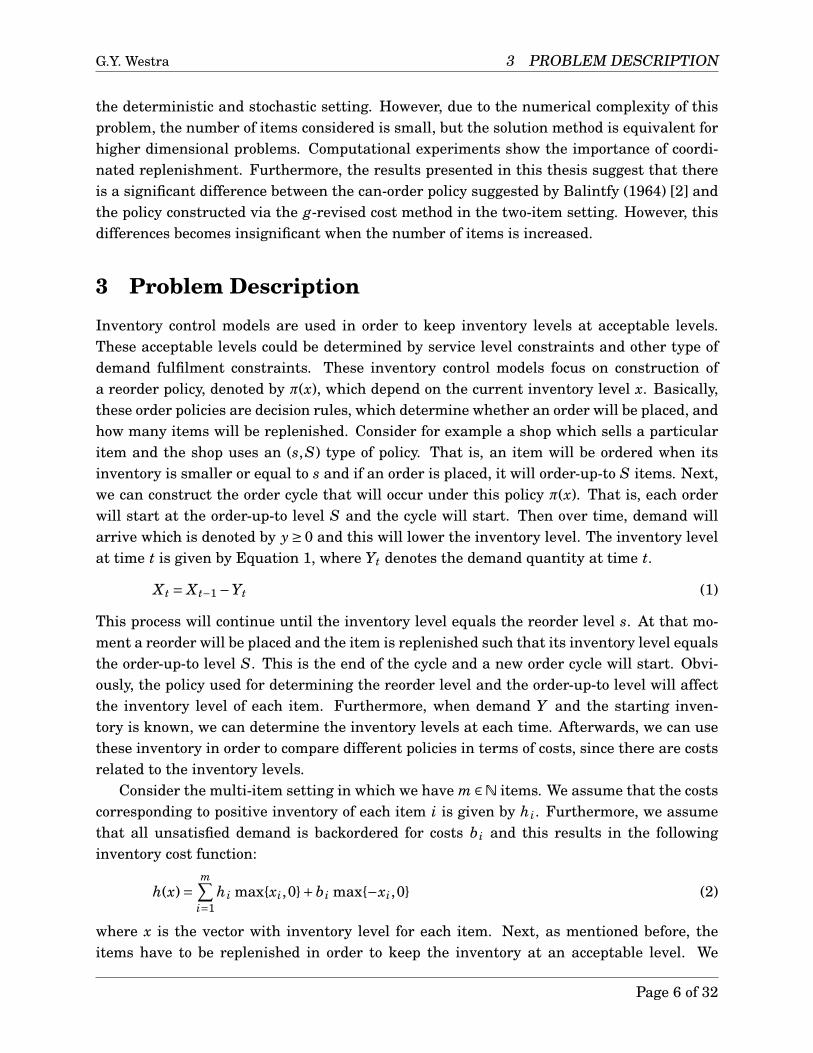
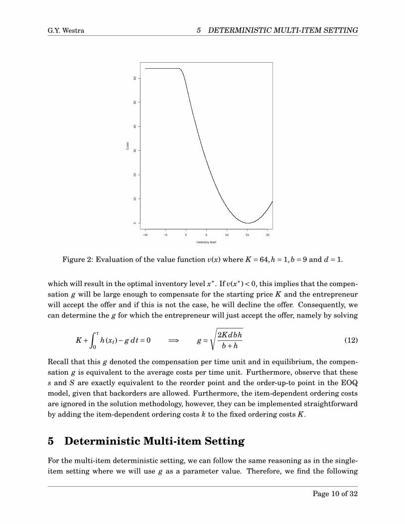
where τ denotes the time when the inventory level reaches s, given it starts at x. Next, foreach inventory level x ∈Swe can evaluate the value function and a graphical representationof this function is shown in Figure 2, where S denotes the set of all inventory levels.

Given that the entrepreneur is profit maximising, it will choose the starting inventory xwhich is most beneficial. This implies that he will minimise the value function and choosethe inventory level corresponding to this minimum. Therefore, rewriting the value functionsuch that x is the argument of the function is useful and more convenient. The entrepreneurwill solve

minx∈S

{v(x)}=minx∈S

{K +

∫ τ

0h (xt)− g dt

}(11)

Page 9 of 32

G.Y. Westra 5 DETERMINISTIC MULTI-ITEM SETTING

−10 −5 0 5 10 15 20

010

2030

4050

60

Inventory level

Cos

ts

Figure 2: Evaluation of the value function v(x) where K = 64,h = 1,b = 9 and d = 1.

which will result in the optimal inventory level x∗. If v(x∗)< 0, this implies that the compen-sation g will be large enough to compensate for the starting price K and the entrepreneurwill accept the offer and if this is not the case, he will decline the offer. Consequently, wecan determine the g for which the entrepreneur will just accept the offer, namely by solving

K +∫ τ

0h (xt)− g dt = 0 =⇒ g =

√2Kdbh

b+h(12)

Recall that this g denoted the compensation per time unit and in equilibrium, the compen-sation g is equivalent to the average costs per time unit. Furthermore, observe that theses and S are exactly equivalent to the reorder point and the order-up-to point in the EOQmodel, given that backorders are allowed. Furthermore, the item-dependent ordering costsare ignored in the solution methodology, however, they can be implemented straightforwardby adding the item-dependent ordering costs k to the fixed ordering costs K .

5 Deterministic Multi-item Setting

For the multi-item deterministic setting, we can follow the same reasoning as in the single-item setting where we will use g as a parameter value. Therefore, we find the following

Page 10 of 32


reorder and order-up-to points

si =− 1bi

g Si = 1hi

g

Consequently, for each item we can determine the cycle length. That is, the time corre-sponding to the inventory decreasing from the order-up-to level to the reorder level, giventhe demand rate di. That is,

ci = Si − si

di(13)

Next, we will analyse these cycles for each item. First, define the smallest cycle length asthe basic cycle length denoted by c

c = mini∈{1,..,m}

{ci} (14)

and afterwards, we will analyse whether all cycle lengths are multiples of this minimumcycle length. Mathematically, this is given by

∃ni ∈N s.t. ni c = ci ∀i ∈ {1, ...,m} (15)

Case 1: If we can find such an ni for each item i, it is a special case which we can solve.Since this is the deterministic setting, we know beforehand what will happen if all itemshave inventory level equal to the reorder points. That is, the time corresponding to an itemreaching its reorder level will always be exactly the same. Furthermore, we know that thecycle lengths for all items are multiples of some basic cycle length denoted as c. Next, wecan construct a policy corresponding to this basic cycle length. For each item which has cyclelength unequal to the basic cycle length, that is, ni > 1, we observe that we have a single ormultiple special reordering opportunities, which we will denote by r j.

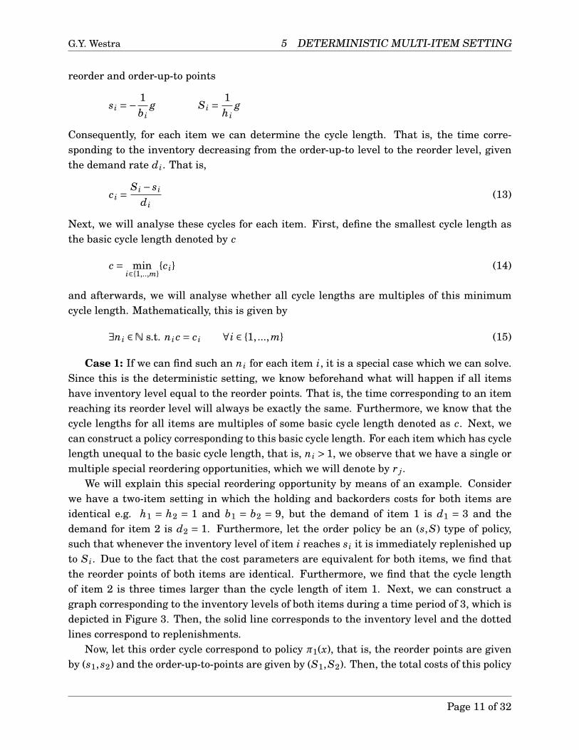
We will explain this special reordering opportunity by means of an example. Considerwe have a two-item setting in which the holding and backorders costs for both items areidentical e.g. h1 = h2 = 1 and b1 = b2 = 9, but the demand of item 1 is d1 = 3 and thedemand for item 2 is d2 = 1. Furthermore, let the order policy be an (s,S) type of policy,such that whenever the inventory level of item i reaches si it is immediately replenished upto Si. Due to the fact that the cost parameters are equivalent for both items, we find thatthe reorder points of both items are identical. Furthermore, we find that the cycle lengthof item 2 is three times larger than the cycle length of item 1. Next, we can construct agraph corresponding to the inventory levels of both items during a time period of 3, which isdepicted in Figure 3. Then, the solid line corresponds to the inventory level and the dottedlines correspond to replenishments.

Now, let this order cycle correspond to policy π1(x), that is, the reorder points are givenby (s1, s2) and the order-up-to-points are given by (S1,S2). Then, the total costs of this policy

Page 11 of 32


Inventory level of item 1

Inve

ntor

y le

vel o

f ite

m 2

s1 S1

s 2S

2

r 1r 2

Figure 3: Inventory levels over time

over one cycle can be determined using equation (4) and it follows that the average cost pertime unit is given by:

Cπ1 =13

(∫ 3

0h(xt)dt+

3∑j=1

c j(yj)

)(16)

= 13

(∫ 3

0h(xt)dt+3K +3k1 +k2

)Next, we have two different policies π2 and π3 in which the reorders points are equivalentto policy π1, however the order-up-to points will be different. These points will be given by(S1, r1) for policy π2 and (S1, r2) for policy π3. Observe that the cycle times for these policieswill be different in these cases, namely 1 and 2 for policy π2 and π3 respectively. The costscorresponding to these policies over time are given by:

Cπ2 =∫ 1

0h(xt)dt+

1∑j=1

c j(yj) (17)

=∫ 1

0h(xt)dt+K +k1 +k2

Cπ3 =12

(∫ 2

0h(xt)dt+

2∑j=1

c j(yj)

)(18)

Page 12 of 32


= 12

(∫ 2

0h(xt)dt+2K +2k1 +k2

)Next, the optimal policy can be found by selecting the policy which results in minimum costsover time. Observe, that the inventory cost function is an increasing function, and thereforethis is basically a trade-off between ordering costs and inventory costs. This reasoning usingthese special reordering opportunities can be generalised to more than one dimension. Themethod is exactly the same, however, more special reorder opportunity points needs to beexamined and difficulties may arise due to the complexity of the integral of the inventorycost function when the number of dimensions is higher.

Case 2: Now we focus on the case when not all cycle lengths are multiples of the basiccycle length. In this case, we cannot guarantee that there exists an optimal policy or that wecan find this policy, which makes it more difficult and complex than the previous case. First,we will focus on evaluation of the value function v(·). In order to do so, we will first analysethe area in which the value function is interesting. We define the set C as the set of allinventory levels, such that the inventory cost function is non-positive. We will refer to thisset as the continuation set C, since this set includes all inventory levels which correspond to‘no replenishment’ or equivalently, ‘continue’ and all other inventory levels outside this setcorrespond to the case in which a replenishment is made. This set is given by

C= {x ∈S : h(x)− g ≤ 0} (19)

A graphical representation of this set in two dimensions can be found in Figure 4.Furthermore, observe that this continuation set is not depending on demand and conse-

quently, this set is exactly the same in the deterministic and the stochastic setting. More-over, in the single-item deterministic setting, the optimal stopping point s was equivalentto the moment when the compensation g does not make up for the inventory costs h(x). Inother words, the optimal stopping point was on the boundary of the set C and the same rea-soning applies for multiple dimensions. Furthermore, due to equivalence of the set C, thesame applies for the stochastic setting. That is, the optimal stopping point inventory x canbe found by solving h(x)− g = 0.

However, it is more complicated to determine the optimal starting inventory for thisproblem, even in two dimensions. If the inventory level hits the boundary of the continua-tion set, we know an order will be placed, however we do not know how many items we order.Basically, there are three options. The first option corresponds to ordering both items. Sec-ond, only item 1 is ordered and third, only item 2 is ordered. In general, the optimal startinginventory can be found by selecting the inventory level which corresponds to the minimumof the value function. In the first two cases, we can choose any inventory level, where in thelatter two cases, the inventory level of the item that is not ordered should be kept constant.Moreover, since the reorder points are different, we also have to take into account the fu-ture value of the value function. Afterwards, we have to select the minimum of these casesand we have found the optimal starting inventory and consequently, the optimal orderingstrategy at x.

Page 13 of 32



Inve

ntor

y le

vel o

f ite

m 2

s1 0 S1

s 20

S2

Figure 4: Continuation set in the two-dimensional space

However, we also have to take into account the future value of the value function, as thestarting inventories will be different for all three cases. This will drastically complicate theproblem, since this future value is depending on the starting inventory and consequently,on the reordering policy chosen. Therefore, it is only possible to determine the optimalpolicy to iteratively determine the future value of the value function for all possible policies.Numerically, this is extremely complex, especially when the number of items increases tomore than 2. Then, the number of different order possibilities will increase exponentiallyand the numerical evaluation becomes extremely difficult.

For this reason, we need to simplify the problem in order to be able to solve the problemin the multi-item setting. Therefore, we simplify the model by setting all item-dependentorder costs equal to zero, i.e. ki = 0,∀i ∈ {1, ..,m}. In this case, the costs corresponding to anorder will always result in equivalent costs, namely K . This implies that we can replenishall items for equivalent costs and for this reason we will always choose to replenish all

Page 14 of 32

G.Y. Westra 6 STOCHASTIC SINGLE-ITEM SETTING

items. Consequently, this problem reduces to determining the optimal starting inventorydenoted by x∗ which can be found by choosing the inventory level which corresponds to theminimum of the value function as given in equation (11). In the remainder of this thesis, wemake the assumption that ki = 0,∀i ∈ {1, ..,m} and focus on determining the optimal startinginventory x∗.

6 Stochastic Single-item Setting

Next, the stochastic case will be analysed. Similar to the deterministic case we will firstfocus on the single-item setting and afterwards modify this to the multi-item setting. Fur-thermore, also in this case we will use the g-revised cost method in order to analyse thisproblem.

Consider the setting similar to the deterministic case, however where demand d is un-known but its distribution is known. For simplicity we will again drop the index i in thesingle-item setting. Now, we are interested in the value function v(x) as a function of thestarting inventory levels x, similar to the deterministic case. However, due to the fact thatwe have stochastic demand in this case, we cannot evaluate the value function by taking theintegral over the inventory cost function. Therefore, we have to evaluate this value func-tion numerically. In order to do so, we first have to define the demand distribution. Dueto the fact that Poisson and Compound Poisson demand distribution have infinite support,although with very small probabilities, it is more convenient to use a discrete distribution,which could be an approximation of the Poisson distribution and this discrete distributionshould have finite support.

We define p(x, y) as the pdf of this distribution and the arguments x and y are inventorycombinations in the state space S. Then p(x, y) denotes the transition probability frominventory level x to inventory level y. We assume that demand is non-negative, whichis given by p(x, y) = 0 if x < y. Observe that depending on the demand distribution, it ispossible that no demand occurs, which is equivalent to p(x, x)≥ 0. Furthermore, we assumethat only positive probabilities occur when both x and y are in the state space. That is,p(x, y)= 0 if x ∉S or y ∉S.

Next, we want to evaluate the value function v(x) for all x in the state space. First, weobserve that a for each x ∈ S we have a decision opportunity, whether an order should beplaced or not. The costs corresponding to an order are given by K and the costs for notordering are given by the inventory cost function h(x) minus the compensation g. However,we should also take into account the future value of the value function when we decide notto order. Therefore, the value function when no order is placed is given by

v(x)= h(x)− g+ ∑y∈S

p(x, y)v(y) (20)

In order to evaluate this summation, we can make use of the special structure of the valuefunction v(x). Due to the fact that demand is non-negative, it follows that we need the

Page 15 of 32

G.Y. Westra 7 STOCHASTIC MULTI-ITEM SETTING

evaluation of the value function of all y smaller than x in order to evaluate x, accordingto equation (20). Observe that p(x, x) can be greater than zero and in this case we have tocorrect for this. This can be done by dividing both the left and right hand side by 1− p(x, x).Furthermore, we know from the deterministic case that the continuation set C correspondsto set of all inventory levels for which the optimal decision was to ‘continue’ or equivalently,‘not ordering’. It follows that for all x to the left of the continuation set, the optimal decisionis to ‘order’ and consequently, the value function equals K in this case. We can use thesestarting values in order to evaluate the value function v(x) for all x ∈S. In order to do so, wecan construct an algorithm which iteratively solves the value function for x ∈S, which usesthe lower bound of the continuation set C as starting point.

Next, it remains to determine the optimal starting inventory x of this problem. Once wehave evaluate the value function for all x, the minimisation problem of the value functionas described in equation (11) is straightforward, since the optimal starting inventory x∗ isequivalent to the x that minimises the value function.

7 Stochastic Multi-item Setting

Next, we focus on a multi-item setting instead of the single-item setting. First, due to thecomplexity of the problem, we simplify the problem by setting all item-dependent orderingcosts ki equal to zero. This reduces the complexity of the problem drastically, and nowreorders can be seen as a decision problem, in which we have to choose the starting inventoryfor each item. Due to the fact that every reorder has the same costs, it follows that wheneveran order is placed, we will always order the items in such quantities such that we start atthe optimal starting inventory. This implies that this case simplifies to finding this optimalstarting inventory and determining when an order is placed.

Next, similar to the one-dimensional case, we can construct the set C for which the com-pensation g is larger than the inventory costs. Similar to the one-dimensional case, an orderwill be placed when at the boundary of the continuation set. Moreover, for all x in the lower-left quadrant of the continuation set C, it is optimal to place an order and consequently, thevalue function equals K for all these inventory levels. For all other inventory levels, we haveto numerically evaluate the value function using equation (20).

Consequently, if we evaluate the value function v(·) for all points in the subset x ∈S, wehave to determine which x is optimal or equivalently, which x maximises the value function.It follows that we can write this maximisation problem as:

maxx∈S

{v(x)}=maxx∈S

{h(x)− g+ ∑

y∈Sp(x, y)v(y)

}(21)

Observe that this maximisation problem is not straightforward, but we can solve this bymeans of an algorithm. We know that the value function of all x in the lower-left quadrantof the set C is equal to K . Furthermore, when this is combined with the fact that demand

Page 16 of 32

G.Y. Westra 7 STOCHASTIC MULTI-ITEM SETTING

is non-negative, we can iteratively evaluate the value function. That is, in order to eval-uate the value function x, we need the evaluations of all inventory levels in the lower-leftquadrant of x.

Lastly, we can prove that the optimal starting inventory is in the set C, which is a subsetof S. For this reason, we only have to assess the value function in a smaller set C in orderto find the optimal starting inventory. The proof of this claim can be found in the Appendix.

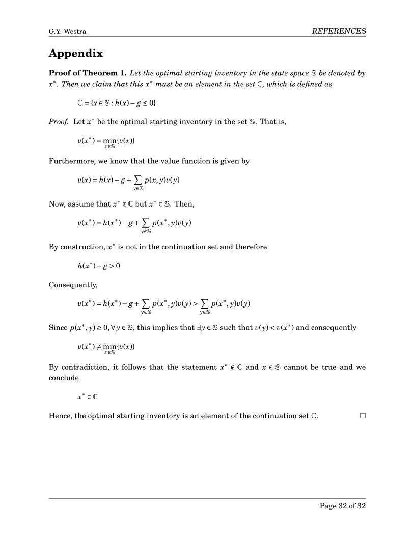
Theorem 1. Let the optimal starting inventory in the state space S be denoted by x∗. Thenwe claim that this x∗ must be an element in the set C, which is defined as

C= {x ∈S : h(x)− g ≤ 0}

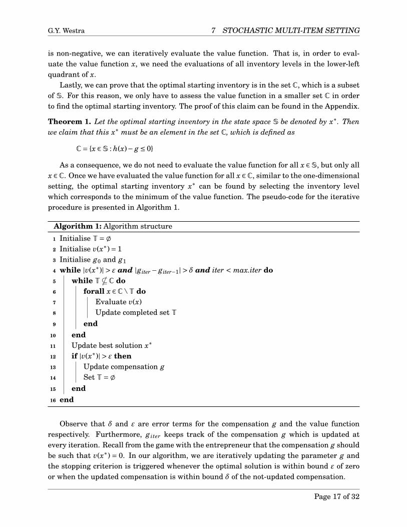
As a consequence, we do not need to evaluate the value function for all x ∈S, but only allx ∈C. Once we have evaluated the value function for all x ∈C, similar to the one-dimensionalsetting, the optimal starting inventory x∗ can be found by selecting the inventory levelwhich corresponds to the minimum of the value function. The pseudo-code for the iterativeprocedure is presented in Algorithm 1.

Algorithm 1: Algorithm structure

1 Initialise T=;2 Initialise v(x∗)= 13 Initialise g0 and g1

4 while |v(x∗)| > ε and |giter − giter−1| > δ and iter < max.iter do5 while T*C do6 forall x ∈C\T do7 Evaluate v(x)8 Update completed set T9 end

10 end11 Update best solution x∗

12 if |v(x∗)| > ε then13 Update compensation g14 Set T=;15 end16 end

Observe that δ and ε are error terms for the compensation g and the value functionrespectively. Furthermore, g iter keeps track of the compensation g which is updated atevery iteration. Recall from the game with the entrepreneur that the compensation g shouldbe such that v(x∗) = 0. In our algorithm, we are iteratively updating the parameter g andthe stopping criterion is triggered whenever the optimal solution is within bound ε of zeroor when the updated compensation is within bound δ of the not-updated compensation.

Page 17 of 32

G.Y. Westra 8 NUMERICAL RESULTS

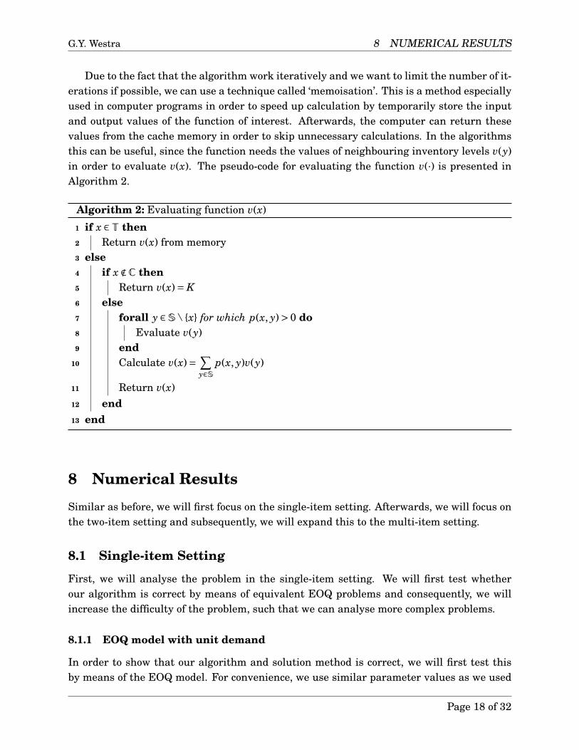
Due to the fact that the algorithm work iteratively and we want to limit the number of it-erations if possible, we can use a technique called ‘memoisation’. This is a method especiallyused in computer programs in order to speed up calculation by temporarily store the inputand output values of the function of interest. Afterwards, the computer can return thesevalues from the cache memory in order to skip unnecessary calculations. In the algorithmsthis can be useful, since the function needs the values of neighbouring inventory levels v(y)in order to evaluate v(x). The pseudo-code for evaluating the function v(·) is presented inAlgorithm 2.

Algorithm 2: Evaluating function v(x)

1 if x ∈T then2 Return v(x) from memory3 else4 if x ∉C then5 Return v(x)= K6 else7 forall y ∈S\{x} for which p(x, y)> 0 do8 Evaluate v(y)9 end

10 Calculate v(x)= ∑y∈S

p(x, y)v(y)

11 Return v(x)12 end13 end

8 Numerical Results

Similar as before, we will first focus on the single-item setting. Afterwards, we will focus onthe two-item setting and subsequently, we will expand this to the multi-item setting.

8.1 Single-item Setting

First, we will analyse the problem in the single-item setting. We will first test whetherour algorithm is correct by means of equivalent EOQ problems and consequently, we willincrease the difficulty of the problem, such that we can analyse more complex problems.

8.1.1 EOQ model with unit demand

In order to show that our algorithm and solution method is correct, we will first test thisby means of the EOQ model. For convenience, we use similar parameter values as we used

Page 18 of 32


for the EOQ model in Section 4, that is, K = 64,b = 9 and h = 1. Furthermore, we use thefollowing demand probability

p(x, y)=1, y= x−1

0, otherwise

Observe that in this setting, the demand always equals 1, which is equivalent to the EOQmodel with a demand of 1. For this EOQ model, we know that

g =√

2Kdbhb+h

= 10.733 s =−1b

g =−1.193 S = 1h

g = 10.733

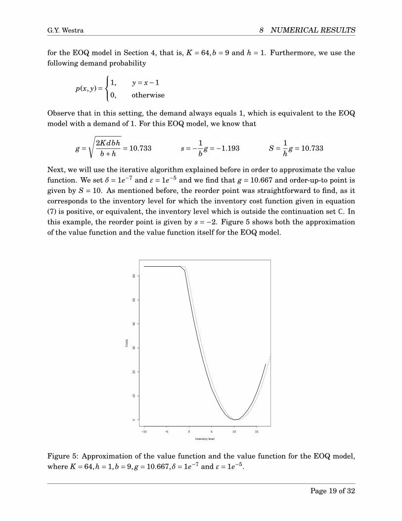
Next, we will use the iterative algorithm explained before in order to approximate the valuefunction. We set δ= 1e−7 and ε= 1e−5 and we find that g = 10.667 and order-up-to point isgiven by S = 10. As mentioned before, the reorder point was straightforward to find, as itcorresponds to the inventory level for which the inventory cost function given in equation(7) is positive, or equivalent, the inventory level which is outside the continuation set C. Inthis example, the reorder point is given by s = −2. Figure 5 shows both the approximationof the value function and the value function itself for the EOQ model.

−10 −5 0 5 10 15

010

2030

4050

60

Inventory level

Cos

ts

Figure 5: Approximation of the value function and the value function for the EOQ model,where K = 64,h = 1,b = 9, g = 10.667,δ= 1e−7 and ε= 1e−5.

Page 19 of 32


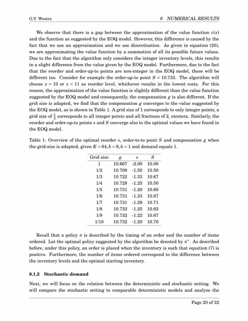
We observe that there is a gap between the approximation of the value function v(x)and the function as suggested by the EOQ model. However, this difference is caused by thefact that we use an approximation and we use discretisation. As given in equation (20),we are approximating the value function by a summation of all its possible future values.Due to the fact that the algorithm only considers the integer inventory levels, this resultsin a slight difference from the value given by the EOQ model. Furthermore, due to the factthat the reorder and order-up-to points are non-integer in the EOQ model, these will bedifferent too. Consider for example the order-up-to point S = 10.733. The algorithm willchoose x = 10 or x = 11 as reorder level, whichever results in the lowest costs. For thisreason, the approximation of the value function is slightly different than the value functionsuggested by the EOQ model and consequently, the compensation g is also different. If thegrid size is adapted, we find that the compensation g converges to the value suggested bythe EOQ model, as is shown in Table 1. A grid size of 1 corresponds to only integer points, agrid size of 1

2 corresponds to all integer points and all fractions of 2, etcetera. Similarly, thereorder and order-up-to points s and S converge also to the optimal values we have found inthe EOQ model.

Table 1: Overview of the optimal reorder s, order-to-to point S and compensation g whenthe grid-size is adapted, given K = 64,b = 9,h = 1 and demand equals 1.

Grid size g s S1 10.667 -2.00 10.00

1/2 10.708 -1.50 10.501/3 10.722 -1.33 10.671/4 10.728 -1.25 10.501/5 10.731 -1.20 10.601/6 10.731 -1.33 10.671/7 10.731 -1.29 10.711/8 10.732 -1.25 10.621/9 10.732 -1.22 10.67

1/10 10.732 -1.20 10.70

Recall that a policy π is described by the timing of an order and the number of itemsordered. Let the optimal policy suggested by the algorithm be denoted by π∗. As describedbefore, under this policy, an order is placed when the inventory is such that equation (7) ispositive. Furthermore, the number of items ordered correspond to the difference betweenthe inventory levels and the optimal starting inventory.

8.1.2 Stochastic demand

Next, we will focus on the relation between the deterministic and stochastic setting. Wewill compare the stochastic setting to comparable deterministic models and analyse the

Page 20 of 32


differences. We will use similar parameters as before, that is, K = 64,b = 9 and h = 1. Next,we use the following demand probability function, which described the demand probabilityat each time step:

p(x, y)=

12 , y= x−112 , y= x−2

0, otherwise

Observe that this stochastic setting is a combination of the deterministic EOQ models withdemand 1 and 2, respectively. Intuitively, the model should be in between the EOQ mod-els and therefore, the costs and the optimal starting inventory should be in between thesevalues as well. Similar as above, we find for the EOQ models these values are given by

EOQ with demand 1: g = 10.733 s =−1.193 S = 10.733

EOQ with demand 2: g = 15.179 s =−1.687 S = 15.179

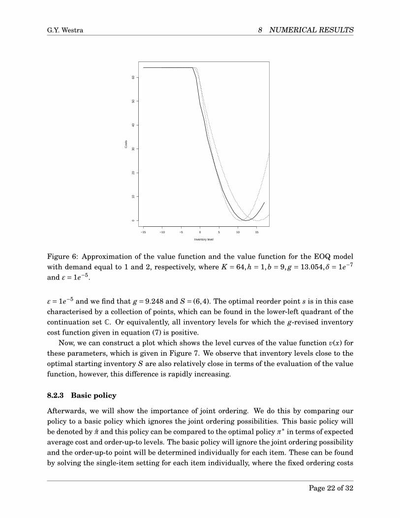
Next, we will use the iterative algorithm in order to solve the stochastic problem. We setδ = 1e−7 and ε = 1e−5 and we find that g = 13.054, s = −2 and S = 12. Figure 6 shows theapproximation the value function of this stochastic model and the value function suggestedby the EOQ model for both demand equals 1 and 2. As expected, the optimal inventory forthe stochastic model is in between the optimal inventory for the EOQ models. Furthermore,we find that the compensation g is in between these values as well.

8.2 Two-item Setting

In this subsection, we focus on the two-item setting. We start by performing some tests inother to evaluate whether the algorithm is correctly programmed. Afterwards, we will focuson the evaluation of the value function. Furthermore, we will construct instances for whichwe will compare our policy to other policies.

8.2.1 Testing

We start by setting all cost parameters for item 1 equal to zero, that is, b1 = h1 = 0. It followsthat item 1 does not affect the inventory cost as given in equation (2). This implies that theoptimal starting inventory should be independent of item 1 and consequently, this shouldequal the single-item case in which only item 2 is considered. We perform this test for bothitems. As expected, when we set all cost parameters for one item equal to zero, the solutionis independent of this item and this reduces to the single-item setting.

8.2.2 Evaluation of the value function

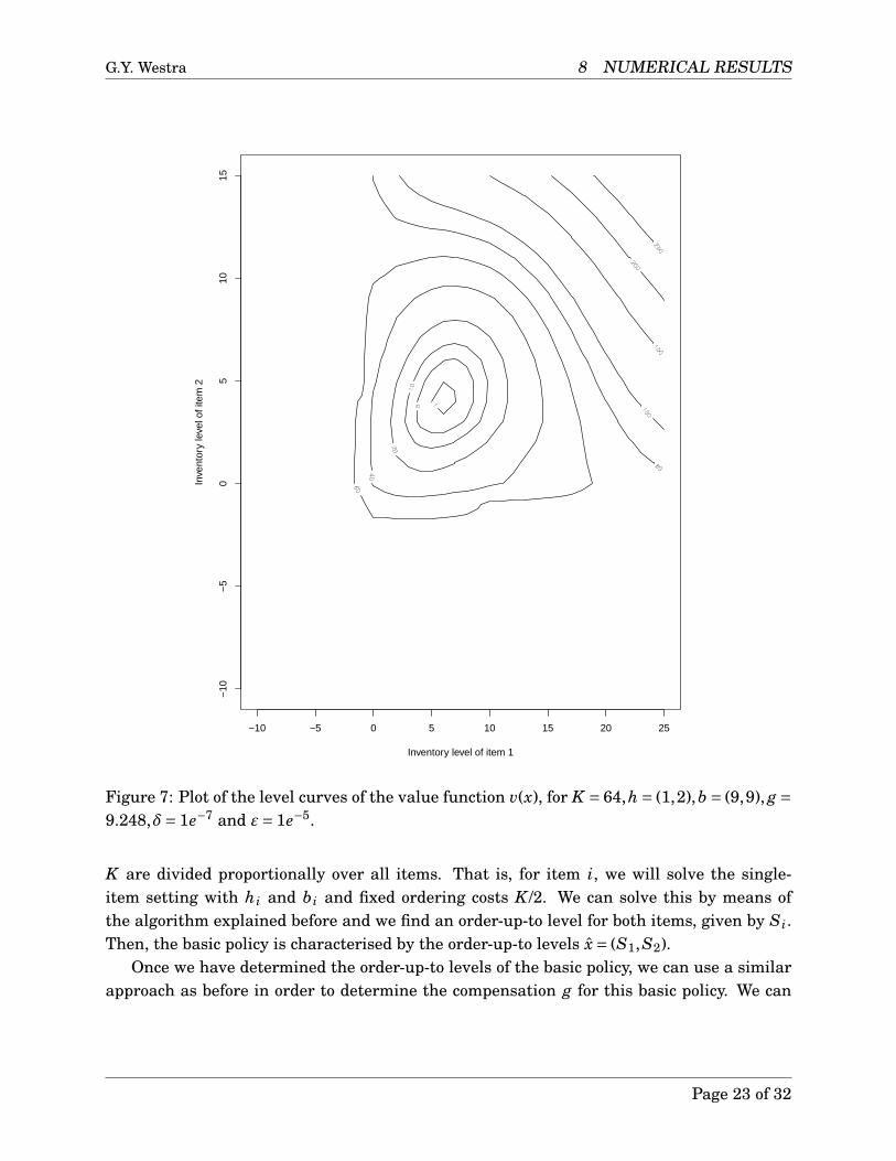
Afterwards, we focus on the analysis of the value function. We use the following parametervalues: K = 64,h = (1,2) and b = (9,9). Then, we can use the algorithm in order to approxi-mate the value function for all inventory combinations of both items. We use δ = 1e−7 and

Page 21 of 32


−15 −10 −5 0 5 10 15

010

2030

4050

60

Inventory level

Cos

ts

Figure 6: Approximation of the value function and the value function for the EOQ modelwith demand equal to 1 and 2, respectively, where K = 64,h = 1,b = 9, g = 13.054,δ = 1e−7

and ε= 1e−5.

ε= 1e−5 and we find that g = 9.248 and S = (6,4). The optimal reorder point s is in this casecharacterised by a collection of points, which can be found in the lower-left quadrant of thecontinuation set C. Or equivalently, all inventory levels for which the g-revised inventorycost function given in equation (7) is positive.

Now, we can construct a plot which shows the level curves of the value function v(x) forthese parameters, which is given in Figure 7. We observe that inventory levels close to theoptimal starting inventory S are also relatively close in terms of the evaluation of the valuefunction, however, this difference is rapidly increasing.

8.2.3 Basic policy

Afterwards, we will show the importance of joint ordering. We do this by comparing ourpolicy to a basic policy which ignores the joint ordering possibilities. This basic policy willbe denoted by π and this policy can be compared to the optimal policy π∗ in terms of expectedaverage cost and order-up-to levels. The basic policy will ignore the joint ordering possibilityand the order-up-to point will be determined individually for each item. These can be foundby solving the single-item setting for each item individually, where the fixed ordering costs

Page 22 of 32



Inve

ntor

y le

vel o

f ite

m 2

−10 −5 0 5 10 15 20 25

−10

−5

05

1015

Figure 7: Plot of the level curves of the value function v(x), for K = 64,h = (1,2),b = (9,9), g =9.248,δ= 1e−7 and ε= 1e−5.

K are divided proportionally over all items. That is, for item i, we will solve the single-item setting with hi and bi and fixed ordering costs K /2. We can solve this by means ofthe algorithm explained before and we find an order-up-to level for both items, given by Si.Then, the basic policy is characterised by the order-up-to levels x = (S1,S2).

Once we have determined the order-up-to levels of the basic policy, we can use a similarapproach as before in order to determine the compensation g for this basic policy. We can

Page 23 of 32


solve the following equality for the compensation g

v(x)= h(x)− g+ ∑y∈S

p(x, y)v(y)= 0 (22)

and this compensation corresponds to the average expected costs of the basic policy, whichwill be denoted by g.

Next, observe that the optimal reorder point can be found following the same procedureas before, namely an order is placed whenever the inventory level is not in the continuationset C. Notice that this set C is dependent on the compensation g, which is different to thecompensation of policy π∗. Therefore, the continuation sets will be different for both policiesand consequently, the reorder points will be different as well. However, the procedure inorder to check whether an order will be placed is equivalent.

8.2.4 Numerical Results

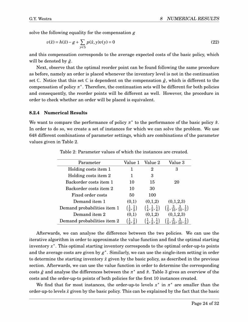
We want to compare the performance of policy π∗ to the performance of the basic policy π.In order to do so, we create a set of instances for which we can solve the problem. We use648 different combinations of parameter settings, which are combinations of the parametervalues given in Table 2.

Table 2: Parameter values of which the instances are created.

Parameter Value 1 Value 2 Value 3Holding costs item 1 1 2 3Holding costs item 2 1 3

Backorder costs item 1 10 15 20Backorder costs item 2 10 30

Fixed order costs 50 100Demand item 1 (0,1) (0,1,2) (0,1,2,3)

Demand probabilities item 1(1

2 , 12

) (14 , 1

2 , 14

) (15 , 3

10 , 310 , 1

5

)Demand item 2 (0,1) (0,1,2) (0,1,2,3)


2 , 12

) (14 , 1

2 , 14

) (15 , 3

10 , 310 , 1

5

)Afterwards, we can analyse the difference between the two policies. We can use the

iterative algorithm in order to approximate the value function and find the optimal startinginventory x∗. This optimal starting inventory corresponds to the optimal order-up-to pointsand the average costs are given by g∗. Similarly, we can use the single-item setting in orderto determine the starting inventory x given by the basic policy, as described in the previoussection. Afterwards, we can use the value function in order to determine the correspondingcosts g and analyse the differences between the π∗ and π. Table 3 gives an overview of thecosts and the order-up-to points of both policies for the first 10 instances created.

We find that for most instances, the order-up-to levels x∗ in π∗ are smaller than theorder-up-to levels x given by the basic policy. This can be explained by the fact that the basic

Page 24 of 32


Table 3: Optimal order-up-to points and the corresponding average costs for the policy π∗

and the basic policy π for the two-item problem.

Policy π∗ Basic policy πInstance Average costs Order-up-to points Average costs Order-up-to points

1 7.81 (3,3) 7.95 (4,4)2 9.30 (2,3) 9.61 (3,4)3 10.39 (3,3) 10.57 (2,4)4 10.39 (3,2) 10.57 (4,2)5 11.81 (2,2) 12.10 (3,2)6 12.89 (2,2) 12.89 (2,2)7 7.81 (3,3) 7.95 (4,4)8 9.30 (2,3) 9.61 (3,4)9 10.40 (2,3) 10.58 (2,4)

10 10.40 (3,2) 10.58 (4,2)

policy ignores the joint ordering opportunities and determines these levels independently.Consequently, the policies π∗ and π have different compensations, namely g∗ = 19.479 andg = 20.118 respectively. As mentioned before, these compensations can be interpreted as theaverage costs per time unit. Based on all 648 instances, we find that the policy π∗ performsbetter than the basic policy π and the average gap is given by 2.941%. Furthermore, weexpect that this gap will increase when the number of items increases. Intuitively, when thenumber of items increase, there are more opportunities to take advantage of joint orderingand we would expect that this results in a better performance of the policy π∗ than the basicpolicy π.

8.3 Multi-item Setting

In this subsection, we will focus on the multi-item setting where we will follow the sameprocedure as in the two-item setting. First, we will focus on the three-item setting, which issimilar to the two-item setting analysed in the previous section. We start by testing whetherthe algorithm is correct. Afterwards, we construct different instances in order to comparethe policy π∗ to the basic policy π.

8.3.1 Testing

First, we will perform some tests in other to check whether our algorithm is programmedcorrectly. This can be done using a similar procedure as before, namely by setting the costparameters for one or two of the items equal to zero and analyse whether the optimal policyis independent of this or these items. We find that this is indeed the case, and in those cases,the problem reduces to the single-item or two-item setting we have analysed before.

Page 25 of 32


8.3.2 Basic policy

Next, we will again focus on the difference between the policies π∗ and π. Recall that thebasic policy can be found by solving the single-item problem for each item individually,where the fixed ordering costs are divided proportionally over all items, i.e. each item hasto make up for 1

m of the fixed ordering costs. Let the order-up-to points be denoted by x forthis basic policy. Afterwards, we can analyse the difference between the policies π∗ and π.Again we create instances for which we will test the performance of both policies and Table4 provides an overview of the different parameter values used for creating those instances.

Table 4: Parameter values of which the instances are created.

Parameter Value 1 Value 2Holding costs item 1 1 2Holding costs item 2 2 3Holding costs item 3 3 5

Backorder costs item 1 5 10Backorder costs item 2 10 15Backorder costs item 3 25 30

Fixed order costs 100Demand item 1 (0,1) (0,1,2)


2 , 12

) (14 , 1

2 , 14

)Demand item 2 (0,1,2) (0,1,2,3)


4 , 12 , 1

4

) (15 , 3

10 , 310 , 1

5

)Demand item 3 (0,1,2,3) (0,1,2,3)


5 , 310 , 3

10 , 15

) ( 120 , 3

20 , 310 , 1

2

)Next, the algorithm and the value function can be used in order to determine the order-

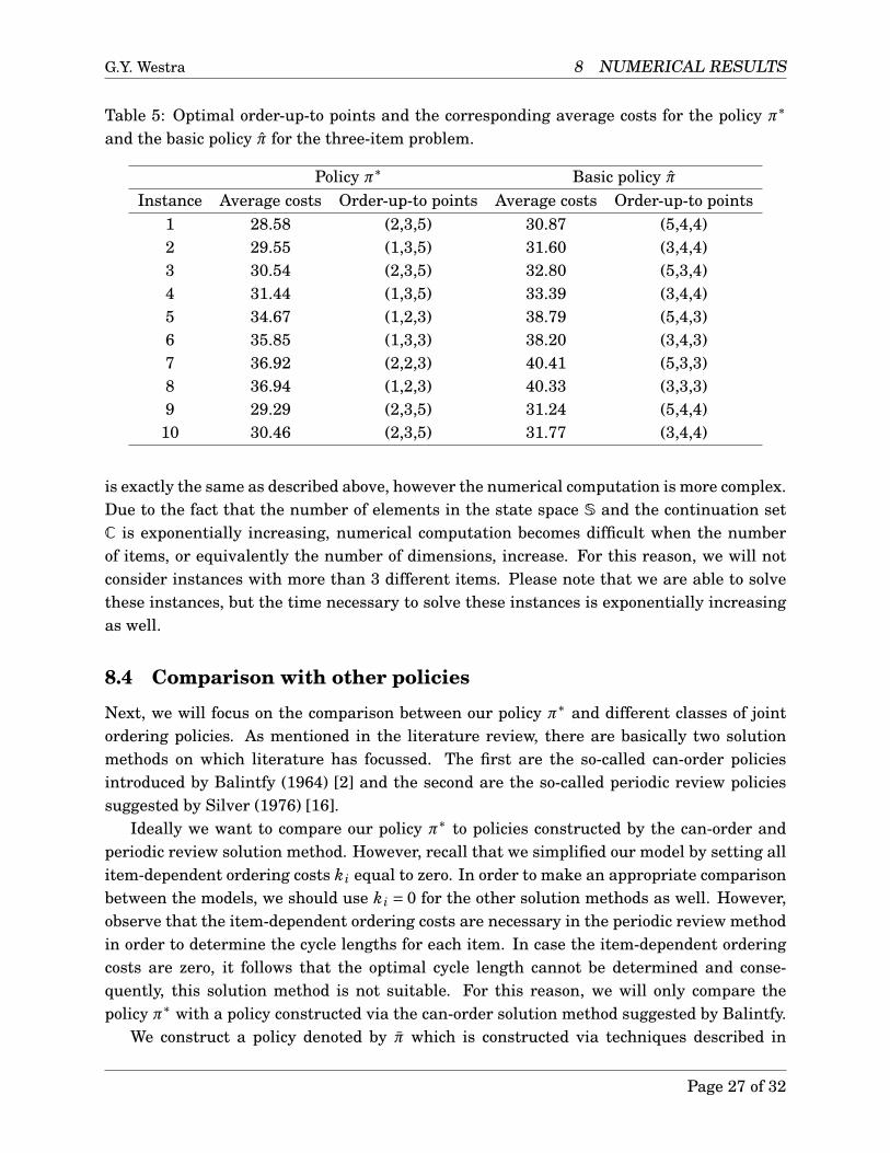
up-to points x and the compensation g for both policies. Table 5 provides an overview of theorder-up-to points and compensation for both policies of the first 10 instances.

In total, we solved 143 different instances and we observe that for most instances, theorder-up-to points suggested by the policy π∗ are lower than the order-up-to points suggestedby the basic policy π. The average compensation of the policy π∗ is given by g∗ = 34.783and for the basic policy this is given by g = 36.731. We find that there is an average gapof 5.665% between the policies which is significantly higher than in the two-item setting.This suggests that our expectation is correct and joint ordering is especially beneficial whenthe number of items is larger. In that case, we can take advantage of the joint orderingopportunities, which results in a cost reduction.

8.3.3 Multi-item Setting

Similar to the two-item setting and the three-item setting, we can create different instancesin order to compare the policy π∗ to the basic policy π. The procedure for solving this problem

Page 26 of 32


Table 5: Optimal order-up-to points and the corresponding average costs for the policy π∗

and the basic policy π for the three-item problem.

Policy π∗ Basic policy πInstance Average costs Order-up-to points Average costs Order-up-to points

1 28.58 (2,3,5) 30.87 (5,4,4)2 29.55 (1,3,5) 31.60 (3,4,4)3 30.54 (2,3,5) 32.80 (5,3,4)4 31.44 (1,3,5) 33.39 (3,4,4)5 34.67 (1,2,3) 38.79 (5,4,3)6 35.85 (1,3,3) 38.20 (3,4,3)7 36.92 (2,2,3) 40.41 (5,3,3)8 36.94 (1,2,3) 40.33 (3,3,3)9 29.29 (2,3,5) 31.24 (5,4,4)

10 30.46 (2,3,5) 31.77 (3,4,4)

is exactly the same as described above, however the numerical computation is more complex.Due to the fact that the number of elements in the state space S and the continuation setC is exponentially increasing, numerical computation becomes difficult when the numberof items, or equivalently the number of dimensions, increase. For this reason, we will notconsider instances with more than 3 different items. Please note that we are able to solvethese instances, but the time necessary to solve these instances is exponentially increasingas well.

8.4 Comparison with other policies

Next, we will focus on the comparison between our policy π∗ and different classes of jointordering policies. As mentioned in the literature review, there are basically two solutionmethods on which literature has focussed. The first are the so-called can-order policiesintroduced by Balintfy (1964) [2] and the second are the so-called periodic review policiessuggested by Silver (1976) [16].

Ideally we want to compare our policy π∗ to policies constructed by the can-order andperiodic review solution method. However, recall that we simplified our model by setting allitem-dependent ordering costs ki equal to zero. In order to make an appropriate comparisonbetween the models, we should use ki = 0 for the other solution methods as well. However,observe that the item-dependent ordering costs are necessary in the periodic review methodin order to determine the cycle lengths for each item. In case the item-dependent orderingcosts are zero, it follows that the optimal cycle length cannot be determined and conse-quently, this solution method is not suitable. For this reason, we will only compare thepolicy π∗ with a policy constructed via the can-order solution method suggested by Balintfy.

We construct a policy denoted by π which is constructed via techniques described in

Page 27 of 32


Federgruen et al. (1984) [5]. Using this method we determine a must-order level, a can-orderlevel and an order-up-to level which are denoted by si, ci and Si for each item respectively.Afterwards, we can determine the average costs for this can-order policy π which is denotedby g. We will compare this policy to the optimal policy π∗ in both the two-item and thethree-item setting.

8.4.1 Numerical results

First, we will compare the can-order policy π to the policy π∗ in the two-item setting. Weuse the same set of instances as before, for which the parameter values are given in Table 2.Table 6 provides an overview of the average costs, the must-order, can-order and order-up-tolevels for the first 10 instances. In total, we solved 450 instances and on average we findthat the can-order policy resulted in an average cost of g = 18.566. For the same instances,our policy π∗ resulted in an average cost of g∗ = 17.614. Furthermore, we find that there isan average gap of 6.837% in favour of our policy π∗ compared to the can-order policy π.

Table 6: Average costs and the optimal must-order, can-order and order-up-to level for thepolicy π for the two-item problem.

Policy πInstance Average costs Must-order levels Can-order levels Order-up-to levels

1 8.15 (-1,-1) (3,3) (4,4)2 10.21 (-1,-1) (1,3) (3,5)3 10.75 (-1,-1) (1,3) (2,4)4 11.01 (-1,-1) (2,1) (5,2)5 12.14 (-1,-1) (1,1) (3,2)6 13.23 (-1,-1) (1,1) (2,2)7 8.61 (-1,-1) (3,2) (4,5)8 10.43 (-1,-1) (2,2) (3,5)9 11.64 (-1,-1) (1,1) (2,5)

10 11.06 (-1,-1) (1,1) (5,2)

This difference can be explained by the fact that the ordering strategy and the order-up-to points are different. The can-order policy introduces a must-order level, a can-orderlevel and a order-up-to level for each item individually. This corresponds to a rectangularcontinuation set in the two-item setting, which is completely different compared to the con-tinuation set corresponding to policy π∗, as given in Figure 4. Furthermore, this differencecan be caused by discretisation. As mentioned before in Section 8.1.1, discretisation has aneffect on the numerical results, although it can be relatively small. However, due to the factthat in the can-order policy π we have to discretise both the must-order levels, the can-orderlevels and the order-up-to levels, this discretisation might amplify the difference betweenthe policies π∗ and π.

Page 28 of 32

G.Y. Westra 9 CONCLUSION

Next, we will focus on the three-item setting. Similar as the two-item setting, we willsolve the instances we created before for the three-item setting and the parameter settingsare given in Table 4. Table 7 provides an overview of the average costs, must-order, can-order and order-up-to levels for the first 10 instances.

Table 7: Average costs and the optimal must-order, can-order and order-up-to level for thepolicy π for the three-item problem.

Policy πInstance Average costs Must-order levels Can-order levels Order-up-to levels

1 29.06 (-1,-1,-1) (1,2,3) (5,5,5)2 29.89 (-2,-1,-1) (0,3,5) (3,5,6)3 30.75 (-1,-1,-1) (2,2,3) (4,4,5)4 31.87 (-2,-1,-1) (0,2,3) (3,4,5)5 33.76 (-1,-1,-1) (2,3,3) (5,5,4)6 34.34 (-2,-1,-1) (1,2,2) (3,5,4)7 36.19 (-1,-1,-1) (1,3,2) (6,4,4)8 36.43 (-2,-1,-1) (1,1,3) (3,4,4)9 29.37 (-1,-1,-1) (1,3,2) (5,5,5)

10 30.81 (-1,-1,-1) (1,2,4) (3,4,6)

In total, we solved 47 instances and the average costs for the can-order policy π aregiven by g = 33.313. On the same instances, the average costs corresponding to policy π∗

are given by g∗ = 33.166 and the average gap is given by 0.192%. Observe that in the three-item setting, there is no significant gap between the two policies, and their performanceis almost identical. This is remarkable, since the order-up-to points are different for bothmodels. As mentioned before, the policy π∗ makes use of the fact that each time an orderis placed, we can replenish all items for the same costs K . The can-order policy does notexploit this fact directly, instead, it introduces can-order levels for each item and items areordered jointly below this can-order level. However, these results suggest that the can-orderpolicy π are adequate in determining the most appropriate can-order levels as the resultsare close to results corresponding to the policy π∗.

9 Conclusion

Joint ordering inventory control models have been studied extensively in the past. How-ever, research has focussed on two solution methods, namely the can-order policies and theperiodic review policies. In this thesis, we focus on a different solution method, namely theso-called g-revised cost method suggested by Germs, Van Foreest and Kilic (2017) [8]. Weconstruct a value function which can be evaluated for all different inventory levels. After-wards, these evaluations can be used in order to construct an ordering policy π, which is

Page 29 of 32

G.Y. Westra REFERENCES

characterised by a reorder set and the order-up-to point. This can only be done under theassumption that all item-dependent ordering costs are set to zero, since in this case, theproblem reduces to a minimisation problem which can be solved in the multi-item setting.

Afterwards, we construct a set of sample instances in order to test the performance ofthe policy. The results show that the our policy outperforms policies which ignore the jointordering possibilities and therefore they should be considered, although computation timesare rapidly increasing in higher dimensions. Furthermore, when the policy π is comparedto the can-order policy, we find that the g-revised cost method outperforms the can-orderpolicy in the two-item setting, however this gap becomes insignificant when the number ofitems is increased.

Future research should be focussed on the implementation of the item-dependent order-ing costs in the solution method. In this thesis, we simplified the problem by setting thesecosts equal to zero. In general, these costs can be relevant and consequently should notbe ignored. However, numerically this problem is extremely complex and this should beaddressed in the future. Moreover, a point of interest in the numerical complexity of thesimplified model. As the value function needs to be evaluated for all relevant points in thestate space, computation times grow rapidly when the number of items increase. Futureresearch should be focussed on more efficient algorithms in order to reduce computationtimes. Then, this g-revised cost method can be used in order to solve the coordinated re-plenishment problem with numerous items.

References

[1] Sven Axsäter. Inventory Control. Springer International Publishing AG, third editionedition, 2015.

[2] Joseph L. Balintfy. On a basic class of multi-item inventory problems. ManagementScience, 10(2):287–297, 1964.

[3] Leon Yang Chu and Zuo-Jun Max Shen. A power-of-two ordering policy for one-warehouse multiretailer systems with stochastic demand. Operations Research,58(2):492–502, 2010.

[4] Donald Erlenkotter. Ford whitman harris and the economic order quantity model.Operations Research Society of America, 38(6):937–946, 1990.

[5] A. Federgruen, H. Groenevelt, and H.C. Tijms. Coordinated replenishments in amulti-item inventory system with compound poisson demands. Management Science,30(3):344–357, 1984.

[6] A. Federgruen, M. Queyranne, and Yu-Sheng Zheng. Simple power-of-two policies areclose to optimal in a general class of production / distribution networks with generaljoint setup costs. Mathematics of Operations Research, 17(4):951–963, 1992.

Page 30 of 32


[7] A. Federgruen and Yu-Sheng Zheng. Optimal power-of-two replenishment strate-gies in capacitated general production / distribution networks. Management Science,39(6):710–727, 1993.

[8] Remco Germs, Nicky D. van Foreest, and Onur A. Kilic. Production inventory systemswith constant and compound poisson demand. Working paper, 2017.

[9] Suresh K. Goyal and Ahmet T. Satir. Joint replenishment inventory control: Deter-ministic and stochastic models. European Journal of Operational Research, 38:2–13,1989.

[10] Edward Ignall. Optimal continuous review policies for two product inventory systemswith joint setup costs. Management Science, 15(6):278–283, 1969.

[11] S.G. Johansen and P. Melchiors. Can-order policy for the periodic-review joint replen-ishment problem. Journal of the Operational Research Society, 54:283–290, 2003.

[12] Philip Melchiors. Calculating can-order policies for the joint replenishment problem bythe compensation approach. European Journal of Operational Research, 141:587–595,2002.

[13] Pricha Pantumsinchai. A comparison of three joint ordering inventory policies. Deci-sion Sciences, 23(1):111–127, 1992.

[14] Robin Roundy. 98%-effective integer-ratio lot-sizing for one-warehouse multi-retailersystems. Management Science, 31(11):1416–1430, 1985.

[15] Suresh P. Sethi and Feng Cheng. Optimality of (s,S) policies in inventory models withmarkovian demand. Operations Research, 45(6):931–939, 1997.

[16] Edward A. Silver. A simple method of deterministic order quantities in joint replenish-ments under deterministic demand. Management Science, 22(12):1351–1362, 1976.

[17] Edward A. Silver. Operations research in inventory management: A review and cri-tique. Operations Research, 29(4):628–645, 1981.

[18] Marc J.G. van Eijs. On the determination of the control parameters of the optimalcan-order policy. Mathematical Methods of Operations Research, 39(3):289–304, 1994.

Page 31 of 32


Appendix

Proof of Theorem 1. Let the optimal starting inventory in the state space S be denoted byx∗. Then we claim that this x∗ must be an element in the set C, which is defined as

C= {x ∈S : h(x)− g ≤ 0}

Proof. Let x∗ be the optimal starting inventory in the set S. That is,

v(x∗)=minx∈S

{v(x)}

Furthermore, we know that the value function is given by

v(x)= h(x)− g+ ∑y∈S

p(x, y)v(y)

Now, assume that x∗ ∉C but x∗ ∈S. Then,

v(x∗)= h(x∗)− g+ ∑y∈S

p(x∗, y)v(y)

By construction, x∗ is not in the continuation set and therefore

h(x∗)− g > 0

Consequently,

v(x∗)= h(x∗)− g+ ∑y∈S

p(x∗, y)v(y)> ∑y∈S

p(x∗, y)v(y)

Since p(x∗, y)≥ 0,∀y ∈S, this implies that ∃y ∈S such that v(y)< v(x∗) and consequently

v(x∗) 6=minx∈S

{v(x)}

By contradiction, it follows that the statement x∗ ∉ C and x ∈ S cannot be true and weconclude

x∗ ∈C

Hence, the optimal starting inventory is an element of the continuation set C.

Page 32 of 32

Coordinated Replenishments in a Multi-item Inventory ...

Documents

Transcript of Coordinated Replenishments in a Multi-item Inventory ...