Coordinated Ocean-ice Reference Experiments...
46
Coordinated Ocean-ice Reference Experiments (COREs) Stephen M. Griffies a, * , Arne Biastoch b , Claus Böning b , Frank Bryan c , Gokhan Danabasoglu c , Eric P. Chassignet d , Matthew H. England e , Rüdiger Gerdes f , Helmuth Haak g , Robert W. Hallberg a , Wilco Hazeleger h , Johann Jungclaus g , William G. Large c , Gurvan Madec i , Anna Pirani j , Bonita L. Samuels a , Markus Scheinert b , Alex Sen Gupta e , Camiel A. Severijns h , Harper L. Simmons k , Anne Marie Treguier l , Mike Winton a , Stephen Yeager c , Jianjun Yin d a NOAA Geophysical Fluid Dynamics Laboratory, Princeton Forrestal Campus Rte. 1, 201 Forrestal Road, Princeton, NJ 08542-0308, USA b Leibniz IfM-GEOMAR, Kiel, Germany c National Center for Atmospheric Research, Boulder, USA d Center For Ocean-Atmospheric Prediction Studies, Florida State University, Tallahassee, USA e Climate Change Research Centre, University of New South Wales, Sydney, Australia f Alfred-Wegener-Institut für Polar- und Meeresforschung, Bremerhaven, Germany g Max-Planck-Institut für Meteorologie, Hamburg, Germany h Royal Netherlands Meteorological Institute (KNMI), de Bilt, The Netherlands i Laboratoire d’Océanographie et du Climat: Expérimentation et Approches Numériques, CNRS-UPMC-IRD, Paris, France j International CLIVAR, and Princeton University AOS Program, Princeton, USA k International Arctic Research Center, University of Alaska, USA l Laboratoire de Physique de Oceans, CNRS-IFREMER-UBO, Plouzané, France article info Article history: Received 10 December 2007 Received in revised form 31 July 2008 Accepted 4 August 2008 Available online 19 September 2008 Keywords: Global ocean-ice modelling Model comparison Experimental design Atmospheric forcing Analysis diagnostics Circulation stability World ocean abstract Coordinated Ocean-ice Reference Experiments (COREs) are presented as a tool to explore the behaviour of global ocean-ice models under forcing from a common atmospheric dataset. We highlight issues arising when designing coupled global ocean and sea ice experiments, such as difficulties formulating a consis- tent forcing methodology and experimental protocol. Particular focus is given to the hydrological forcing, the details of which are key to realizing simulations with stable meridional overturning circulations. The atmospheric forcing from [Large, W., Yeager, S., 2004. Diurnal to decadal global forcing for ocean and sea-ice models: the data sets and flux climatologies. NCAR Technical Note: NCAR/TN-460+STR. CGD Division of the National Center for Atmospheric Research] was developed for coupled-ocean and sea ice models. We found it to be suitable for our purposes, even though its evaluation originally focussed more on the ocean than on the sea-ice. Simulations with this atmospheric forcing are presented from seven global ocean-ice models using the CORE-I design (repeating annual cycle of atmospheric forcing for 500 years). These simulations test the hypothesis that global ocean-ice models run under the same atmospheric state produce qualitatively similar simulations. The validity of this hypothesis is shown to depend on the chosen diagnostic. The CORE simulations provide feedback to the fidelity of the atmo- spheric forcing and model configuration, with identification of biases promoting avenues for forcing data- set and/or model development. Published by Elsevier Ltd. 1. Introduction Simulations with global coupled ocean-ice models can be used to assist in understanding climate dynamics, and as a step towards the development of more complete earth system models. Unfortu- nately, there is little consensus in the modelling community regarding the design of global ocean-ice experiments, especially those run for centennial and longer time scales. In particular, there is no widely agreed method to force the models. Furthermore, some relatively small differences in forcing methods can lead to large deviations in circulation behaviour and sensitivities. Such dif- ficulties create practical barriers to comparing simulations from different modelling groups. 1.1. Purpose and scope of this paper A central purpose of this paper is to present Coordinated Ocean- ice Reference Experiments (COREs). COREs provide a common ref- erence point for research groups developing and analyzing global ocean-ice models. They do so by establishing a standard practice for the design of a baseline set of experiments that is useful for 1463-5003/$ - see front matter Published by Elsevier Ltd. doi:10.1016/j.ocemod.2008.08.007 * Corresponding author. Tel.: +1 609 452 6672; fax: +1 609 987 5063. E-mail address: stephen.griffi[email protected] (S.M. Griffies). Ocean Modelling 26 (2009) 1–46 Contents lists available at ScienceDirect Ocean Modelling journal homepage: www.elsevier.com/locate/ocemod
Transcript of Coordinated Ocean-ice Reference Experiments...
Ocean Modelling 26 (2009) 1–46
Contents lists available at ScienceDirect
Ocean Modelling
journal homepage: www.elsevier .com/ locate/ocemod
Coordinated Ocean-ice Reference Experiments (COREs)
Stephen M. Griffies a,*, Arne Biastoch b, Claus Böning b, Frank Bryan c, Gokhan Danabasoglu c,Eric P. Chassignet d, Matthew H. England e, Rüdiger Gerdes f, Helmuth Haak g, Robert W. Hallberg a,Wilco Hazeleger h, Johann Jungclaus g, William G. Large c, Gurvan Madec i, Anna Pirani j, Bonita L. Samuels a,Markus Scheinert b, Alex Sen Gupta e, Camiel A. Severijns h, Harper L. Simmons k, Anne Marie Treguier l,Mike Winton a, Stephen Yeager c, Jianjun Yin d
a NOAA Geophysical Fluid Dynamics Laboratory, Princeton Forrestal Campus Rte. 1, 201 Forrestal Road, Princeton, NJ 08542-0308, USAb Leibniz IfM-GEOMAR, Kiel, Germanyc National Center for Atmospheric Research, Boulder, USAd Center For Ocean-Atmospheric Prediction Studies, Florida State University, Tallahassee, USAe Climate Change Research Centre, University of New South Wales, Sydney, Australiaf Alfred-Wegener-Institut für Polar- und Meeresforschung, Bremerhaven, Germanyg Max-Planck-Institut für Meteorologie, Hamburg, Germanyh Royal Netherlands Meteorological Institute (KNMI), de Bilt, The Netherlandsi Laboratoire d’Océanographie et du Climat: Expérimentation et Approches Numériques, CNRS-UPMC-IRD, Paris, Francej International CLIVAR, and Princeton University AOS Program, Princeton, USAk International Arctic Research Center, University of Alaska, USAl Laboratoire de Physique de Oceans, CNRS-IFREMER-UBO, Plouzané, France
a r t i c l e i n f o a b s t r a c t
Article history:Received 10 December 2007Received in revised form 31 July 2008Accepted 4 August 2008Available online 19 September 2008
Keywords:Global ocean-ice modellingModel comparisonExperimental designAtmospheric forcingAnalysis diagnosticsCirculation stabilityWorld ocean
1463-5003/$ - see front matter Published by Elsevierdoi:10.1016/j.ocemod.2008.08.007
* Corresponding author. Tel.: +1 609 452 6672; faxE-mail address: [email protected] (S.M. Gr
Coordinated Ocean-ice Reference Experiments (COREs) are presented as a tool to explore the behaviour ofglobal ocean-ice models under forcing from a common atmospheric dataset. We highlight issues arisingwhen designing coupled global ocean and sea ice experiments, such as difficulties formulating a consis-tent forcing methodology and experimental protocol. Particular focus is given to the hydrological forcing,the details of which are key to realizing simulations with stable meridional overturning circulations.
The atmospheric forcing from [Large, W., Yeager, S., 2004. Diurnal to decadal global forcing for oceanand sea-ice models: the data sets and flux climatologies. NCAR Technical Note: NCAR/TN-460+STR.CGD Division of the National Center for Atmospheric Research] was developed for coupled-ocean andsea ice models. We found it to be suitable for our purposes, even though its evaluation originally focussedmore on the ocean than on the sea-ice. Simulations with this atmospheric forcing are presented fromseven global ocean-ice models using the CORE-I design (repeating annual cycle of atmospheric forcingfor 500 years). These simulations test the hypothesis that global ocean-ice models run under the sameatmospheric state produce qualitatively similar simulations. The validity of this hypothesis is shown todepend on the chosen diagnostic. The CORE simulations provide feedback to the fidelity of the atmo-spheric forcing and model configuration, with identification of biases promoting avenues for forcing data-set and/or model development.
Published by Elsevier Ltd.
1. Introduction
Simulations with global coupled ocean-ice models can be usedto assist in understanding climate dynamics, and as a step towardsthe development of more complete earth system models. Unfortu-nately, there is little consensus in the modelling communityregarding the design of global ocean-ice experiments, especiallythose run for centennial and longer time scales. In particular, thereis no widely agreed method to force the models. Furthermore,
Ltd.
: +1 609 987 5063.iffies).
some relatively small differences in forcing methods can lead tolarge deviations in circulation behaviour and sensitivities. Such dif-ficulties create practical barriers to comparing simulations fromdifferent modelling groups.
1.1. Purpose and scope of this paper
A central purpose of this paper is to present Coordinated Ocean-ice Reference Experiments (COREs). COREs provide a common ref-erence point for research groups developing and analyzing globalocean-ice models. They do so by establishing a standard practicefor the design of a baseline set of experiments that is useful for
2 S.M. Griffies et al. / Ocean Modelling 26 (2009) 1–46
model development and ocean-ice research. By standard practice,we envision an experimental protocol that satisfies the followinggoals:
– Provides model simulations that can be tested directly against abroad suite of ocean and sea ice observations;
– Is not specific to a particular model or model framework, facili-tating cooperation between groups and model communities;
– Is not so complex or computationally expensive so as to make ittoo onerous for smaller groups to implement;
– Can be incorporated into a more comprehensive model develop-ment or research program; e.g., by providing spun-up initialconditions for fully coupled climate simulations or controlexperiments in sensitivity studies;
– Facilitates sharing of expertise and reduces redundant efforts inforcing data set design.
Prior to the availability of atmospheric reanalysis products, a defacto standard practice existed in the ocean modelling community:wind stress was prescribed by the only widely available globaldataset (Hellerman and Rosenstein, 1983), and surface tempera-ture and salinity were damped toward observed conditions (seeSection 3.1). With the emergence of more comprehensive and real-istic atmospheric reanalysis and remote sensing products, thechoices have expanded but also become more complex. Our pro-posal for COREs does not provide the definitive resolution of theseforcing issues, but can provoke discussion and debate leading toimproved scientific convergence onto a common experimentalprotocol.
We distinguish the research focus of COREs from that of modelintercomparison projects. In an intercomparison project, simula-tions follow a strict protocol and output is generated for analysesby a broad community. Projects, such as the Atmospheric ModelIntercomparison Project (AMIP) (Gates, 1993), help document mod-el similarities and differences, and can be of great use for variousresearch and development purposes. Prior to deciding whether ananalogous global ocean-ice model intercomparison project (i.e., anOMIP) would be a useful exercise, it is important for the researchcommunity to converge to a baseline experimental design. Webelieve that COREs provide a useful step toward this convergence.
Given the broad selection of models participating in this study,the simulations presented here can provide some feedback to thefidelity of the atmospheric forcing. That is, places where each modelproduces a similar behaviour that is biased relative to observationsmay signal a problem with the atmospheric dataset, thus suggest-ing areas requiring reexamination. The common bias could, in con-trast, indicate a common problem amongst the full suite of modelsthat may highlight problems in the model fundamentals and/orconfigurations. Analogously, in the case where a single model pro-duces a widely varying behaviour, this outlier model may resultfrom problems in the model’s fundamentals and/or configuration.
1.2. Contents of this paper
This paper contains three main parts. The first part summarizesthe state of the art in global ocean-ice coupled modelling, and itstarts in Section 2, which highlights some uses of ocean-ice modelsand argues for the relevance of a reference experimental design.Section 3 reviews methods used to force the ocean-ice models, withemphasis on limitations of these methods. Section 4 then presentsour proposal for COREs. The second part of the paper is given in Sec-tions 5–16, where we consider a selection of diagnostics from sevenglobal ocean-ice simulations run with the CORE-I (repeating annualcycle) forcing. For each diagnostic, we provide rationalizations forwhy the diagnostic is useful to examine in global simulations; pres-ent guidance towards observational datasets that can be used for
model-observational comparisons; display model results; and offerhypotheses that could explain model differences and which couldbe followed-up with more focused studies. We do not provide acomplete mechanistic understanding of model differences for theexhibited diagnostics. Doing so is nontrivial from many perspec-tives, and would require a new study no less lengthy than the pres-ent. Section 17 closes the main paper with discussion andconclusions. The third part of this paper is comprised of appendicesthat detail aspects of the models used in this study; the experimen-tal protocol; the methods use to force the models; formulational as-pects of certain diagnostics; and acronyms used in the manuscript.
2. Uses of ocean-ice models
To study the earth’s climate, and possible climatic changes dueto anthropogenic forcing, various research teams have successfullybuilt realistic global climate or earth system models with interac-tive ocean, sea ice, land, atmosphere, biogeochemical, and ecosys-tem components (referred to as climate models in the following).These models are generally built incrementally, with componentsconsidered initially in isolation, then sub-groups of componentsare coupled, and finally the full set of components are brought to-gether in the climate model. This process requires a wide suite ofscientific and engineering methods, from reductionist processphysics and biogeochemical modelling, to wholistic climate sys-tems science methods.
Ice covered regions of the polar and sub-polar oceans are of par-ticular importance for the large scale circulation of the globaloceans. In particular, sea ice melt and formation alter the thermo-haline fluxes across the surface ocean, and greatly alter the buoy-ancy forcing affecting deep water formation and thus the largescale overturning circulation. Additionally, the presence of sea icegreatly alters the fluxes entering the ocean, due to the large inso-lating effects of ice cover relative to open ocean. Hence, realisticmodelling studies of global ocean climate include a realistic inter-active sea ice model coupled to the ocean.
Coupled ocean-ice models form an important sub-group in theclimate system. They are often developed together prior to cou-pling to other components such as the land and atmosphere. Fromthe perspective of a global climate modeller, the absence of anatmosphere and land component allows for a more focused assess-ment of the successes and limitations of the ocean-ice components.From the perspective of a global ocean modeller, introducing a seaice model provides a physically based interactive method to deter-mine high latitude ocean-ice fluxes, rather than the ad hocapproaches needed in global ocean-only models. Ocean-ice modelsalso admit more dynamical degrees of freedom than possible inocean-only simulations. In turn, running ocean-ice models is muchmore complex than ocean-only simulations, as they place a greaterneed on the accuracy required from surface boundary forcing,especially due to the ice-albedo feedback, whereby larger regionsof high albedos associated with snow and sea ice act to reducesolar heating, thus further increasing the earth’s albedo andcausing more snow and sea ice to form.
The incremental methodology of climate model development islargely pragmatic. Namely, the fully coupled system is far morecomplicated, computationally expensive, and the ocean and seaice components reflect errors in the modelled atmosphere. Addi-tionally, for many research groups, ocean-ice models representthe final stage in the development of a tool of use for addressingcertain scientific questions. For example, ocean-ice models formthe basis for many simulations in the high latitudes, with the regio-nal Arctic Ocean Model Intercomparison Project (AOMIP) providingone example with significant scientific impact (Proshutinsky et al.,2001; Holloway et al., 2007). In general, it is hoped that researchand development efforts focused on ocean-ice simulations success-
S.M. Griffies et al. / Ocean Modelling 26 (2009) 1–46 3
fully assist in understanding the behaviour of the more completeclimate system.
Although many useful insights can be garnered from studieswith ocean-ice models, it is critical to understand their limitations.Namely, it often remains difficult to ensure that results from theocean-ice subsystem carry over to the full climate system, whereclimate model behaviour, such as sensitivities to perturbations,can prove distinct from ocean-ice models (an example is providedin Section 16.1). Quite often, problems with ocean-ice models stemfrom unrealistic aspects of surface forcing from a non-interactiveatmosphere (Section 3). Nonetheless, even with their limitations,ocean-ice models remain a valuable climate science tool, and socan be used for fruitful scientific research and model developmentpurposes. We summarise here a few uses that motivate us to pro-pose a standard practice for running these models.
– Being less expensive than climate models, ocean-ice models canbe formulated with refined grid resolutions thus promotingsuperior representations of key physical, chemical, and biologi-cal processes as well as geographic features. Alternatively, theycan be run with a broader suite of algorithms and parameterisa-tions, which helps to develop an understanding of simulationsensitivity to model fundamentals.
– They provide a tool to study interactions between the ocean andsea ice as isolated from the complexities of atmospheric feed-backs and from biases that arise when coupling to a potentiallyinaccurate atmospheric model.
– Ocean-ice models using different atmospheric forcing provide ameans to assess implications on the ocean and sea ice climate ofvarious atmospheric reanalysis or observational products. As acomplement, many models run using the same atmosphericforcing, and which show similar ocean biases, may suggest thatthere are problems with the atmospheric forcing. In these ways,models feedback onto the development of atmospheric datasetsused to force ocean-ice models (e.g., Large and Yeager, 2008).
– There is great utility for model development by comparing sim-ulations from different ocean-ice models using the same atmo-spheric forcing. For example, comparisons often highlightdeficiencies in the representation of physical processes, whichthen guide efforts to improve simulation integrity.
– Bulk formulae are needed to produce ocean-ice fluxes given anatmospheric state and ocean-ice state. Ocean-ice models runwith the same atmospheric state yet with different bulk formu-lae allow one to assess the sensitivity of the simulation to thechosen bulk formulae.
– Run under realistic atmospheric forcing, models can be usedto reproduce the history of ocean and sea ice variables andhelp to interpret observations that are scarce in space andtime (e.g., Gerdes et al., 2005b). This approach provides amethod for ocean reanalysis unavailable with fully coupledclimate models. Notably, there are nontrivial issues of initialconditions and ocean drifts that need to be resolvedbefore obtaining unambiguous results from such reanalysisstudies.
– One can select particular temporal or spatial scales from withinthe forcing data for use in running ocean-ice models for pur-poses of understanding variability mechanisms.
– Coupled ocean-ice models provide a valuable engineering steptowards the development of more complete climate models. Forexample, many tools and methods needed to build climate mod-els are more easily prototyped in the simpler ocean-ice models.
1 Modellers tend to equate the temperature and salinity in the upper model gridcell with the sea surface temperature and sea surface salinity. This equality is notprecise, as the model grid cell values represent a grid cell averaged value, and so donot precisely reflect the surface skin values measured, say, from a satellite. See(Robinson, 2005) for more discussion.
3. Boundary fluxes for ocean-only and ocean-ice models
A coupled ocean-ice model requires momentum, heat, andhydrological exchanges with the atmosphere to drive the
simulated ocean and ice fields. These exchanges take the form ofstress from atmospheric winds, of radiative and turbulent fluxesof heat, and of precipitation, continental runoff and evaporation.Notably, evaporation has an associated turbulent latent heat fluxwhich links the thermal and hydrological fluxes. When decouplingthe ocean and sea ice models from the atmosphere, one must intro-duce a method to generate these fluxes. We briefly review certainpoints related to this issue, highlighting problems that arise withvarious approaches.
3.1. Thermohaline fluxes from restoring SST and SSS
Perhaps the simplest and oldest approach to developing fluxesfor ocean-only models is to specify a wind stress and to dampthe model’s upper layer temperature (SST) and upper layer salinity(SSS)1 to prescribed values (Cox and Bryan, 1984), such as from theclimatologies of Levitus (1982); Conkright et al. (2002), or Steeleet al. (2001). The thermohaline fluxes are thus generated withoutatmospheric information, and fluxes are non-zero only when modelpredicted SST and/or SSS differ from observations. With thisapproach, there is no direct link between the thermal and hydrolog-ical forcing present with latent heating and evaporation. Nonethe-less, fluxes generated from restoring provide a strong negativefeedback that limits the errors that can be realized in the simulatedsurface ocean properties. Hence, surface restoring of SST and SSSrenders a useful leading order understanding of the simulated oceancirculation, which in turn helps to identify egregious problems withocean model fundamentals. It has thus been commonly employed byocean modellers for many decades.
Damping the model predicted SST and SSS fields to pre-scribed values generates a restoring thermohaline flux for theocean model. Unfortunately, the resulting fluxes can be quiteunrealistic (Killworth et al., 2000), especially the freshwaterfluxes (Large et al., 1997). It can also produce distortions inthe simulated annual cycle (Killworth et al., 2000). Thermoha-line damping is typically associated with rather short dampingtime scales (i.e., strong restoring), which can suppress potentiallyinteresting internal modes of variability such as mesoscaleeddies represented in refined resolution models. Dampingbecomes more problematic for a coupled ocean-ice model,because there is no proven analogue for driving a sea-icemodel, and it is ambiguous how to restore to SST and SSS inregions with ice. Hence, thermohaline restoring with relativelystrong damping is not an ideal means for generating thermoha-line fluxes for ocean-ice climate modelling. An alternativeshould be considered.
3.2. Undamped thermohaline fluxes
Applying undamped thermohaline fluxes is a complementarymethod to the previous approach of damping SST and SSS.Consequently, it possesses complementary attributes, such asallowing surface tracers to evolve freely with no damping. Also,the prescribed surface fluxes can be adjusted to yield zero net gainof heat and freshwater by the ocean-ice system, and to give adesired equilibrium oceanic transport of heat and freshwater.
When using undamped fluxes, one must be more mindful ofdetails than in the restoring case. Here, there are three types ofthermohaline fluxes to consider:
4 S.M. Griffies et al. / Ocean Modelling 26 (2009) 1–46
– Turbulent fluxes for heat (sensible and latent), water (evapora-tion), and momentum (wind stress);
– Radiative heat fluxes (shortwave and longwave);– Water fluxes such as precipitation, river runoff, and sea ice for-
mation/melt.
Unfortunately, fluxes from observations and/or reanalysis prod-ucts have nontrivial uncertainties (Taylor, 2000; Large and Yeager,2004). Running ocean-ice models for decades or longer with suchlarge uncertainties can lead to unacceptable model drift in surfacetemperature and salinity (Rosati and Miyakoda, 1988). Addition-ally, SST anomalies do experience a negative feedback in the cli-mate system, whereby they are damped by interactions with theatmosphere. Hence, SST restoring is based on physical interactions(Haney, 1971), and the lack of a negative feedback exacerbatesproblems with the undamped fluxes. Consequently, the undampedflux forced simulations can experience unacceptable drift associ-ated with errors in the undamped fluxes and/or model errors, aswell as the absence of a feedback mechanism to suppress drift. Itis therefore generally not feasible nor physically relevant to runglobal ocean-ice models with undamped thermohaline fluxes formore than a few years.
3.3. Turbulent fluxes from bulk formulae
The turbulent sensible heat flux lost from the ocean is propor-tional to the sea-air temperature difference. As this differenceincreases (decreases), there is also more ocean heat loss (gain)through the latent heat flux. Thus, the air-sea interaction repre-sented by the turbulent heat fluxes tends to damp SST differencesfrom the air temperature. The damping strength can be determinedby numerically linearizing the thermal boundary condition (Haney,1971; Barnier et al., 1995; Rivin and Tziperman, 1997; Barnier,1998). It can be quite strong in regions of strong winds such asthe Southern Ocean and North Atlantic, where piston velocities2
can reach 1–2 m day�1, which corresponds to a coupling strengthof 50–100ðWm�2Þ=�K. More generally, Rahmstorf and Willebrand(1995) point out the scale dependence of the ocean-atmosphere heatflux coupling. Basin scale SST anomalies are damped at a muchslower rate ð� 5ðWm�2Þ=�KÞ, that is set by outgoing long wave radi-ation. They propose an approach with scale dependent bulk formu-lae for the ocean-atmosphere heat flux.
The feedback between the SSTs and the atmospheric state pro-vides a nontrivial space-time dependent damping of SSTs that actsto reduce model drift.3 As a means to model this and other air-seainteractions, in the absence of an interactive atmospheric model, acompromise can be made between the damped and undampedapproaches by prognostically computing turbulent fluxes for heat,moisture, and momentum using the evolving ocean surface state(SST and surface currents). In this case, turbulent fluxes are com-puted from bulk formulae, given a prescribed, time evolving atmo-spheric state (air temperature, humidity, sea level pressure, andwind velocity). This approach directly corresponds to that used inclimate models, where the atmospheric state is provided by a prog-nostic atmospheric model. In this way, the bulk formulae forcedocean-ice models are much more directly relevant to the coupledmodels than the other methods. They also properly link the latentheat flux and evaporation.
2 The piston velocity (units of length per time) refers to the multiplier that weightsthe difference between the ocean property (e.g., temperature) and atmosphereproperty (e.g., surface air temperature) for computing a tracer flux. Larger pistonvelocities yield a larger flux for a given difference. We have more to say regardingpiston velocity in Section B.3 of the Appendix.
3 Note that drifts in SST due to errors in the atmospheric forcing may actually leadto model drift.
3.4. Problems with ocean-ice models forced by a prescribedatmosphere
The basic assumption made when using an atmospheric datasetto force an ocean-ice model is that changes in the prescribed nearsurface atmospheric state accurately reflect the surface turbulentheat and moisture fluxes across the ocean-ice surface, plus thedivergence of all near surface internal atmospheric transport pro-cesses. The fundamental problem with the proposed bulk formulaeapproach is that in general this assumption is not valid, because oferrors in the ocean-ice models, errors in the bulk formulae, anderrors in atmospheric datasets. The latter represent only anapproximation to Nature, and the uncertainties can be large.Furthermore, there is no unambiguous way of separating modelerror from forcing error in the simulated ocean-ice system, anderrors can be both compensating and additive.
Even a perfect ocean-ice model is exposed to limitations inher-ent in the forcing and in the problems with decoupling from aninteractive atmosphere. For example, a prescribed wind precludesatmospheric feedbacks that, in particular, contribute to the devel-opment and evolution of ENSO. Additionally, a prescribed air tem-perature results in an atmosphere acting as a fluid with infiniteheat capacity, which is the opposite of the physically relevant limitwhere the ocean is more appropriately approximated as the slowclimate component with a huge heat capacity. We now detail fur-ther problems associated with thermohaline forcing. These prob-lems are intimately related, but we expose them here as separatemechanisms for clarity.
3.4.1. Mixed boundary conditions and corruption of the temperaturenegative feedback
The first problem relates to anticipated errors in the surfacefluxes for salinity or fresh water, especially precipitation. Theseerrors will force erroneous drift in ocean salinity. A relativelystrong salinity restoring, analogous to the effective restoring ofSSTs arising from bulk formulae, can control this drift in theocean-ice simulations. However, salinity restoring has no physicalbasis. That is, precipitation fluxes do not depend on local salinity,so there is no local negative feedback to mitigate the accumulationof flux errors. It is thus desirable physically to use at most a weaksalinity restoring. Weak restoring rather than strong restoringallows increased, and typically more realistic, variability in the sur-face salinity and deep circulation. Furthermore, the weak restoringcan be regarded as a correction to the precipitation.
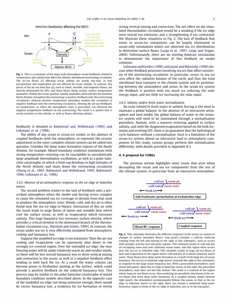
The widely differing time scales determining surface moistureand heat fluxes leads to the term mixed boundary condition ther-mohaline fluxes. As emphasized by Stommel (1961), the differingeffects of temperature and salinity on ocean density, as well astheir distinct air-sea interactions, present the ocean’s thermoha-line circulation with the possibility for multiple regimes ofcirculation (Bryan, 1986) and/or strong nonlinear oscillations(Zhang et al., 1993; Greatbatch and Peterson, 1996; Colin de Ver-dière and Huck, 1999). Consider a positive salinity anomaly mov-ing into the subpolar gyre region of the North Atlantic. Thisanomaly creates a positive density anomaly, which generally actsto support the large-scale overturning circulation with deepwater formation in the northern part of the North Atlantic. Thispositive feedback from salinity is counteracted by a negativefeedback from enhanced warm water advected northward, creat-ing a negative density anomaly. We illustrate these feedbacks inFig. 1. Unfortunately, the negative temperature feedback isaltered or removed when presenting the ocean with a prescribedatmospheric state which does not respond to the temperatureanomaly. In turn, the positive salinity feedback plays a spuri-ously large role in the ocean-ice simulations using a prescribedatmosphere. The sensitivity of simulations to these altered
cold water
cold air warm air
warm water
fresh icy
Add freshwater perturbation at ice/halocline edge
Coupled responseMixed BC response
cold water
cold air warm air
warm water
fresh icycold water
cold air warm air
warm water
fresh icy
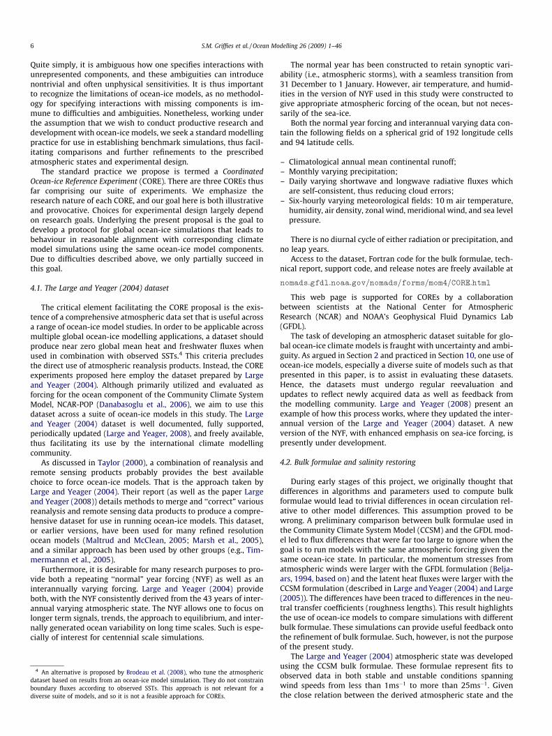
Fig. 2. This schematic illustrates the different responses of the ocean-ice system tochanges in surface boundary fluxes. (top panel) Consider a cold-air outbreak(coming from the left and moving to the right in this schematic), such as occurswith synoptic activity over sub-polar regions. This outbreak results in cold and dryair occupying some area over relatively warm water, and this region often occursnear the sea ice or halocline edge. This situation results in huge air-sea fluxes ofheat and evaporation in the region where cold and dry air is above relatively warmwater. These fluxes drive deep water formation as a result of the huge loss of oceanbuoyancy. The sea ice or halocline edge moves (towards the right in this schematic)in response to the large ocean buoyancy loss. With a prescribed atmospheric state(lower left panel), when the ice edge or halocline moves to the right, the prescribedatmospheric state does not feel this motion. The result is a removal of the regionwhere large air-sea fluxes occur, thus rendering an unrealistic shut down of the air-sea fluxes that drive deep water formation. In a coupled climate model (bottomright panel), the atmosphere predominantly follows the ocean, so that as the iceedge or halocline moves to the right, there can remain a nontrivial deep-waterformation region in front of the ice edge or halocline, just as in the top panel.
Fig. 1. This is a schematic of the large-scale atmosphere-ocean feedbacks related totemperature and salinity that affect the Atlantic meridional overturning circulation.The air-sea fluxes (F) affecting ocean salinity are nearly one-way, in thatprecipitation and evaporation are not affected by ocean salinity. In contrast, keypieces of the air-sea heat flux (Q), such as latent, sensible, and longwave fluxes, aredirectly determined by SSTs, and these fluxes damp oceanic surface temperatureanomalies. Within the ocean, positive salinity anomalies advected into the northernNorth Atlantic strengthen the overturning (a positive feedback onto the overturningcirculation), whereas positive temperature anomalies weaken the circulation (anegative feedback onto the overturning circulation). Altering the air-sea feedbackson temperature, as when the atmospheric state is prescribed, can diminish thenegative temperature feedback on the overturning. The result is a system that isoverly sensitive to the salinity, as well as fluxes affecting salinity.
S.M. Griffies et al. / Ocean Modelling 26 (2009) 1–46 5
feedbacks is detailed in Rahmstorf and Willebrand (1995) andLohmann et al. (1996).
The ability of any ocean or ocean-ice model, in the absence ofcoupled feedbacks with the atmosphere, to represent the oceanicadjustment in the more complete climate system can be called intoquestion. Consider the deep water formation regions of the NorthAtlantic, for example. Mixed boundary condition simulations withstrong temperature restoring can be susceptible to unrealisticallylarge amplitude thermohaline oscillations, as well as a polar halo-cline catastrophe, in which a fresh cap develops in high latitudes ofthe North Atlantic and shuts down the overturning circulation(Zhang et al., 1993; Rahmstorf and Willebrand, 1995; Rahmstorf,1996; Lohmann et al., 1996).
3.4.2. Absence of an atmospheric response as the ice edge or haloclinemoves
The second problem relates to the lack of feedback onto a pre-scribed atmosphere when the model and forcing errors conspireto cause the simulated sea ice coverage to deviate from that usedto produce the atmospheric state. Windy, cold, and dry air is oftenfound near the sea ice edge in Nature. Interaction of this air withthe ocean leads to large fluxes of latent and sensible heat whichcool the surface ocean, as well as evaporation which increasessalinity. This huge buoyancy loss increases surface density, whichprovides a critical element in the downward branch of the thermo-haline circulation (e.g., Marshall and Schott, 1999). In contrast, theocean under sea-ice is very effectively insulated from atmosphericcooling and buoyancy loss.
Suppose the modelled ice edge is too extensive. Then the air-seacooling and evaporation can be spuriously shut down in thewrongly ice-covered region. Over the extended ice edge, the nearfreezing water will be under relatively warm air and weaker winds,so there will be less overall buoyancy loss to drive vertical mixingand convection in the ocean, as well as a negative feedback effecttending to melt back the ice. As a result the water column canbecome prone to freshwater pooling at the surface, which couldprovide a positive feedback on the reduced buoyancy loss. Thisprocess may be similar to the polar halocline catastrophe of mixedboundary condition models described above. In the opposite caseof the modelled ice edge not being extensive enough, there wouldbe excess buoyancy loss, a tendency for ice formation or overly
strong vertical mixing and convection. The net effect on the simu-lated thermohaline circulation would be a weaking if the ice edgewere overall too extensive, and a strengthening if too contracted.We illustrate these situations in Fig. 2. The lack of feedback thatexists in ocean-ice simulations can be largely eliminated inocean-only simulations which use observed sea ice distributionsto determine surface fluxes (Large et al., 1997; Large and Yeager,2004). Unfortunately, there are no existing hindcast simulationsto demonstrate the importance of this feedback on modelsolutions.
Lohmann andGerdes (1998) and Jayne and Marotzke (1999) dis-cuss other feedback processes involving sea ice that affect sensitiv-ity of the overturning circulation. In particular, errors in sea icearea affect the radiation balance of the earth, and thus the totalmeridional heat transport in the climate system and its partition-ing between the atmosphere and ocean. In the ocean-ice systemthe feedback is positive with too much ice reducing the solarenergy input, and too little ice increasing the solar input.
3.4.3. Salinity and/or fresh water normalisationAn issue related to fresh water or salinity forcing is the need to
maintain a global balance. In the absence of an interactive atmo-sphere and land model, the global balance of water in the ocean-ice system will need to be maintained through a normalisationprocedure. Namely, with a nonzero restoring applied to surfacesalinity, and with the diagnosed evaporation based on the bulk for-mulae and evolving SST, there is no guarantee that the hydrologicalcycle balances without a normalisation. Such is a limitation of theocean-ice system absent an interactive land or atmospheric com-ponent. In this study, various groups perform this normalisationdifferently, with details provided in Appendix B.3.
4. A proposal for COREs
The previous section highlights some issues that arise whendecoupling the ocean and sea ice components from the rest ofthe climate system, in particular from an interactive atmosphere.
6 S.M. Griffies et al. / Ocean Modelling 26 (2009) 1–46
Quite simply, it is ambiguous how one specifies interactions withunrepresented components, and these ambiguities can introducenontrivial and often unphysical sensitivities. It is thus importantto recognize the limitations of ocean-ice models, as no methodol-ogy for specifying interactions with missing components is im-mune to difficulties and ambiguities. Nonetheless, working underthe assumption that we wish to conduct productive research anddevelopment with ocean-ice models, we seek a standard modellingpractice for use in establishing benchmark simulations, thus facil-itating comparisons and further refinements to the prescribedatmospheric states and experimental design.
The standard practice we propose is termed a CoordinatedOcean-ice Reference Experiment (CORE). There are three COREs thusfar comprising our suite of experiments. We emphasize theresearch nature of each CORE, and our goal here is both illustrativeand provocative. Choices for experimental design largely dependon research goals. Underlying the present proposal is the goal todevelop a protocol for global ocean-ice simulations that leads tobehaviour in reasonable alignment with corresponding climatemodel simulations using the same ocean-ice model components.Due to difficulties described above, we only partially succeed inthis goal.
4.1. The Large and Yeager (2004) dataset
The critical element facilitating the CORE proposal is the exis-tence of a comprehensive atmospheric data set that is useful acrossa range of ocean-ice model studies. In order to be applicable acrossmultiple global ocean-ice modelling applications, a dataset shouldproduce near zero global mean heat and freshwater fluxes whenused in combination with observed SSTs.4 This criteria precludesthe direct use of atmospheric reanalysis products. Instead, the COREexperiments proposed here employ the dataset prepared by Largeand Yeager (2004). Although primarily utilized and evaluated asforcing for the ocean component of the Community Climate SystemModel, NCAR-POP (Danabasoglu et al., 2006), we aim to use thisdataset across a suite of ocean-ice models in this study. The Largeand Yeager (2004) dataset is well documented, fully supported,periodically updated (Large and Yeager, 2008), and freely available,thus facilitating its use by the international climate modellingcommunity.
As discussed in Taylor (2000), a combination of reanalysis andremote sensing products probably provides the best availablechoice to force ocean-ice models. That is the approach taken byLarge and Yeager (2004). Their report (as well as the paper Largeand Yeager (2008)) details methods to merge and ‘‘correct” variousreanalysis and remote sensing data products to produce a compre-hensive dataset for use in running ocean-ice models. This dataset,or earlier versions, have been used for many refined resolutionocean models (Maltrud and McClean, 2005; Marsh et al., 2005),and a similar approach has been used by other groups (e.g., Tim-mermannn et al., 2005).
Furthermore, it is desirable for many research purposes to pro-vide both a repeating ‘‘normal” year forcing (NYF) as well as aninterannually varying forcing. Large and Yeager (2004) provideboth, with the NYF consistently derived from the 43 years of inter-annual varying atmospheric state. The NYF allows one to focus onlonger term signals, trends, the approach to equilibrium, and inter-nally generated ocean variability on long time scales. Such is espe-cially of interest for centennial scale simulations.
4 An alternative is proposed by Brodeau et al. (2008), who tune the atmosphericdataset based on results from an ocean-ice model simulation. They do not constrainboundary fluxes according to observed SSTs. This approach is not relevant for adiverse suite of models, and so it is not a feasible approach for COREs.
The normal year has been constructed to retain synoptic vari-ability (i.e., atmospheric storms), with a seamless transition from31 December to 1 January. However, air temperature, and humid-ities in the version of NYF used in this study were constructed togive appropriate atmospheric forcing of the ocean, but not neces-sarily of the sea-ice.
Both the normal year forcing and interannual varying data con-tain the following fields on a spherical grid of 192 longitude cellsand 94 latitude cells.
– Climatological annual mean continental runoff;– Monthly varying precipitation;– Daily varying shortwave and longwave radiative fluxes which
are self-consistent, thus reducing cloud errors;– Six-hourly varying meteorological fields: 10 m air temperature,
humidity, air density, zonal wind, meridional wind, and sea levelpressure.
There is no diurnal cycle of either radiation or precipitation, andno leap years.
Access to the dataset, Fortran code for the bulk formulae, tech-nical report, support code, and release notes are freely available at
nomads:gfdl:noaa:gov=nomads=forms=mom4=CORE:html
This web page is supported for COREs by a collaborationbetween scientists at the National Center for AtmosphericResearch (NCAR) and NOAA’s Geophysical Fluid Dynamics Lab(GFDL).
The task of developing an atmospheric dataset suitable for glo-bal ocean-ice climate models is fraught with uncertainty and ambi-guity. As argued in Section 2 and practiced in Section 10, one use ofocean-ice models, especially a diverse suite of models such as thatpresented in this paper, is to assist in evaluating these datasets.Hence, the datasets must undergo regular reevaluation andupdates to reflect newly acquired data as well as feedback fromthe modelling community. Large and Yeager (2008) present anexample of how this process works, where they updated the inter-annual version of the Large and Yeager (2004) dataset. A newversion of the NYF, with enhanced emphasis on sea-ice forcing, ispresently under development.
4.2. Bulk formulae and salinity restoring
During early stages of this project, we originally thought thatdifferences in algorithms and parameters used to compute bulkformulae would lead to trivial differences in ocean circulation rel-ative to other model differences. This assumption proved to bewrong. A preliminary comparison between bulk formulae used inthe Community Climate System Model (CCSM) and the GFDL mod-el led to flux differences that were far too large to ignore when thegoal is to run models with the same atmospheric forcing given thesame ocean-ice state. In particular, the momentum stresses fromatmospheric winds were larger with the GFDL formulation (Belja-ars, 1994, based on) and the latent heat fluxes were larger with theCCSM formulation (described in Large and Yeager (2004) and Large(2005)). The differences have been traced to differences in the neu-tral transfer coefficients (roughness lengths). This result highlightsthe use of ocean-ice models to compare simulations with differentbulk formulae. These simulations can provide useful feedback ontothe refinement of bulk formulae. Such, however, is not the purposeof the present study.
The Large and Yeager (2004) atmospheric state was developedusing the CCSM bulk formulae. These formulae represent fits toobserved data in both stable and unstable conditions spanningwind speeds from less than 1ms�1 to more than 25ms�1. Giventhe close relation between the derived atmospheric state and the
S.M. Griffies et al. / Ocean Modelling 26 (2009) 1–46 7
bulk formulae, we decided that all models in this study would em-ploy the CCSM formulae, rather than each group using their ownparticular formulae.
Salinity or fresh water forcing was a point of debate amongst theparticipants in this study, largely due to difficulties raised in Section3.4. The basic question is: how strongly should SSS be restored?Some simulations removed restoring under sea ice, whereas othersretained restoring. Some ran with extremely weak restoring withthe piston velocity of 50 m/4 years, and some explored a range ofrestoring scenarios. We have more to say on this issue in Section16. Quite generally, these issues highlight the utility of comple-menting ocean-ice simulations with fully coupled climate simula-tions, where ambiguities with salinity forcing are absent.
Choices made by each of the ocean and sea ice model for salinityrestoring and salt/water normalisation are detailed in Section B.3.They can be summarised as follows:
– Weak salinity restoring for NCAR-POP, FSU-HYCOM, and MPI;– Modestly strong salinity restoring for GFDL-MOM, GFDL-HIM,
and Kiel-ORCA;– Variable salinity restoring for KNMI-MICOM;– Salt/water normalisation for all, except FSU-HYCOM and KNMI-
MICOM.
In addition to surface salinity restoring, Kiel-ORCA simulationemployed restoring of temperature and salinity within the Medi-terranean and Red Seas (see Section A.7). No other model em-ployed internal damping of ocean temperature or salinity toobservations.
4.3. Three proposed COREs
We propose three COREs, whose basic elements are outlinedhere.
– CORE-I: This experiment is aimed at investigations of the clima-tological mean ocean and sea ice states realized using the ideal-ized repeating NYF of Large and Yeager (2004). Models shouldideally be run to quasi-equilibrium of the deep circulation,which is on the order of many hundreds to thousands of years(England, 1995; Stouffer, 2004).
– CORE-II: This experiment is aimed at investigations of the forcedresponse of the ocean and/or ocean hindcast. It therefore willemploy a more recent version of the interannually varying data-set from Large and Yeager (2008), rather than the idealizedrepeating normal year. CORE-II may also facilitate more directcomparisons with observations of time dependent phenomena,and thus be of direct use for ocean reanalysis. It is critical to notethat the utility of these experiments depends largely on theimpact of initial conditions as well as model drift. These issuesremain at the forefront of present research.
– CORE-III: This is a perturbation experiment involving ideas pro-posed by Gerdes et al. (2005a), Gerdes et al. (2006). Hereenhanced fresh water flux enters the North Atlantic in responseto increased meltwater runoff distributed around the Greenlandcoast. Response of the regional and global ocean and sea ice sys-tem on the decadal to centennial time scales is the focus ofCORE-III. This experimental design is motivated by possibleincreases in Greenland meltwater that may occur due to anthro-pogenic global warming.
We focus in this paper on CORE-I. During the early stages ofexploring CORE-I simulations, we hoped that 100 years would pro-vide a sufficient time to expose general model behaviour and mod-el differences. 100 years was the choice taken for the comparisonof German ocean-ice models discussed in Fritzsch et al. (2000)
which used the forcing from Röske (2006). Unfortunately, 100years proved insufficient for highlighting differences of overturn-ing circulation behaviour. In particular, drifts in the water massesin some of the simulations caused either the overturning circula-tion to drastically weaken within 100 years, or to experience unre-alistic oscillations after a few hundred years (Sections 15 and 16).Simulations of 500 years length exposed many of these issues,whereas 100 years was insufficient. Notably, even though manyissues were exposed only after multiple-century integrations, thereis no guarantee that 500 years is sufficient to sample the phasespace of the models run with the CORE-I design. 500 years is there-fore considered a pragmatic compromise amongst the participantsin this study.
4.4. Differences in methods
Use of the Large and Yeager (2004) NYF dataset and bulk formu-lae with no temperature restoring for 500 year ocean-ice simula-tions is basically what defines CORE-I. This experimental designleaves open many details for each group to choose based on theirjudgement. Consequently, as shown in the Appendices, experimen-tal design and model details followed by the groups differed inmany aspects. For various reasons based on specifics of numericalalgorithms, computational and human resources, and/or contraryscientific judgements, we were unable to remove all differences.Indeed, we did not put much effort at reducing these differences,as such would have sacrificed our ability to make progress towardsa common experimental framework.
Certainly some differences in methods are expected with com-parisons, and as such, can add to the strength of the project byexposing alternative approaches to the scrutiny of a larger groupof scientists. Nonetheless, differences in model formulation andimplementation of forcing add to the difficulty of uncoveringmechanisms for simulation disagreements. For example, no twomodels used precisely the same grid resolution; some models usedimplied salt fluxes while others used real water fluxes (see Appen-dix B.3 for details); and differences in ice albedo schemes werecommon. Such differences might be important for determiningwhy, as shown later, the models exhibit varying behaviours of theirsimulated Atlantic overturning circulations.
4.5. Models in this study
The ocean and sea ice models employed in this study includethe following (see Appendix A for details and references):
– NCAR-POP: This model is comprised of the ocean and sea icecomponents from the CCSM climate model using a zonal resolu-tion of roughly one degree, with enhanced meridional resolutionin the tropics. The ocean component uses geopotential verticalcoordinates.
– FSU-HYCOM: This model is comprised of the HYCOM oceanmodel code within the CCSM framework used in the NCAR-POP simulations, with the same horizontal grid resolution,coupler, and sea ice model. The ocean component uses hybridisopycnic-pressure coordinates, with pressure in the upperocean mixed layer and isopycnic beneath.
– GFDL-MOM: This model is comprised of the ocean and sea icecomponents from the GFDL climate model using a zonal resolu-tion of one degree, with enhanced meridional resolution in thetropics. The ocean component uses geopotential verticalcoordinates.
– GFDL-HIM: This model replaced the geopotential MOM codewith the isopycnal layered Hallberg Isopycnal Model (HIM), inwhich the vertical is discretized with potential density layers.
0 50 100 150 200 250 300 350 400 450 5001
1.5
2
2.5
3
3.5
4
4.5Global average temperature (C)
Year
Deg
C
NCAR−POPFSU−HYCOMGFDL−MOMGFDL−HIMKiel−ORCAMPIKNMI−MICOM
Fig. 3. Time series of the globally averaged annual mean liquid ocean temperaturefrom the CORE-I simulations. This diagnostic is computed as hhi ¼
PhdV=
PdV ,
with dV the grid cell volume, and the summation extending over the full liquidocean domain.
0 50 100 150 200 250 300 350 400 450 500
34.56
34.58
34.6
34.62
34.64
34.66
34.68
34.7
34.72
34.74
Global average salinity (psu)
Year
psu
NCAR−POPFSU−HYCOMGFDL−MOMGFDL−HIMKiel−ORCAMPIKNMI−MICOM
Fig. 4. Time series of the globally averaged annual mean liquid ocean salinity fromthe CORE-I simulations. This diagnostic is computed as hSi ¼
PSdV=
PdV , with dV
the grid cell volume, and the summation extending over the full liquid oceandomain.
8 S.M. Griffies et al. / Ocean Modelling 26 (2009) 1–46
The vertical and horizontal resolution is comparable to theGFDL-MOM simulation.
– KNMI-MICOM: This model is based on the MICOM isopycnalocean model with zonal resolution of two degrees and enhancedmeridional resolution in the tropics. The sea ice component isfrom Bentsen et al. (2004).
– MPI: This is the ocean and ice model components of the coupledclimate model from the Max-Planck-Institute. The horizontalresolution gradually varies between 12 km close to Greenlandand 150 km in the tropical Pacific. The ocean component usesgeopotential vertical coordinates.
– Kiel-ORCA: This model is comprised of the NEMO modelling sys-tem, with the OPA 9 ocean model coupled to the LIM sea icemodel with two degree zonal resolution, with enhanced merid-ional resolution in the tropics. The ocean component uses geo-potential vertical coordinates.
All geopotential models, as well as GFDL-HIM, employ the Bous-sinesq approximation, in which volume, not mass, of a fluid parcelis conserved, and thus steric effects are absent from the prognosticequations. In contrast, the KNMI-MICOM and FSU-HYCOM oceancodes are both non-Boussinesq.
4.6. Goals of the analysis
The following sections survey results from simulations run withthe ocean-ice models listed above using the CORE-I forcing. A keypurpose of this presentation is to be illustrative and provocativerather than thorough on all points. That is, the analysis fails to fullyassess each model’s ability to remain faithful to Nature’s ocean-icesystem. Furthermore, the analysis is insufficient to identify mech-anisms for model differences. Nonetheless, we do provide descrip-tions of the simulation features, and in certain places we offerhypotheses and criticisms that may help to explain model biases.
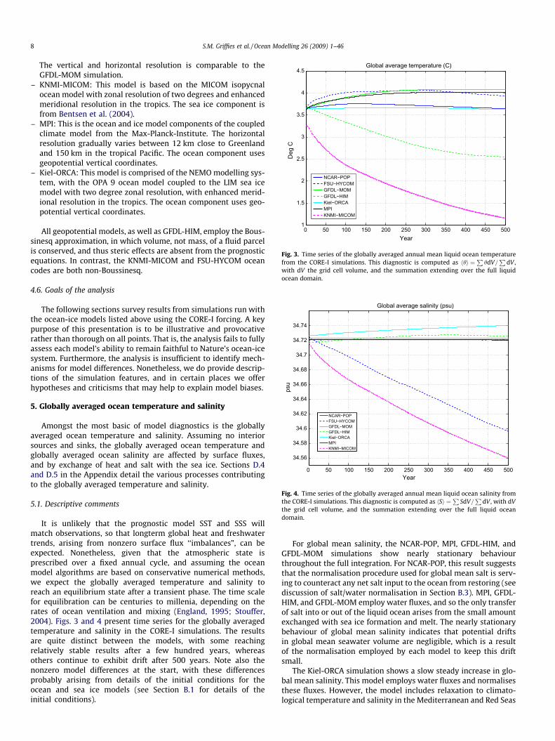
5. Globally averaged ocean temperature and salinity
Amongst the most basic of model diagnostics is the globallyaveraged ocean temperature and salinity. Assuming no interiorsources and sinks, the globally averaged ocean temperature andglobally averaged ocean salinity are affected by surface fluxes,and by exchange of heat and salt with the sea ice. Sections D.4and D.5 in the Appendix detail the various processes contributingto the globally averaged temperature and salinity.
5.1. Descriptive comments
It is unlikely that the prognostic model SST and SSS willmatch observations, so that longterm global heat and freshwatertrends, arising from nonzero surface flux ‘‘imbalances”, can beexpected. Nonetheless, given that the atmospheric state isprescribed over a fixed annual cycle, and assuming the oceanmodel algorithms are based on conservative numerical methods,we expect the globally averaged temperature and salinity toreach an equilibrium state after a transient phase. The time scalefor equilibration can be centuries to millenia, depending on therates of ocean ventilation and mixing (England, 1995; Stouffer,2004). Figs. 3 and 4 present time series for the globally averagedtemperature and salinity in the CORE-I simulations. The resultsare quite distinct between the models, with some reachingrelatively stable results after a few hundred years, whereasothers continue to exhibit drift after 500 years. Note also thenonzero model differences at the start, with these differencesprobably arising from details of the initial conditions for theocean and sea ice models (see Section B.1 for details of theinitial conditions).
For global mean salinity, the NCAR-POP, MPI, GFDL-HIM, andGFDL-MOM simulations show nearly stationary behaviourthroughout the full integration. For NCAR-POP, this result suggeststhat the normalisation procedure used for global mean salt is serv-ing to counteract any net salt input to the ocean from restoring (seediscussion of salt/water normalisation in Section B.3). MPI, GFDL-HIM, and GFDL-MOM employ water fluxes, and so the only transferof salt into or out of the liquid ocean arises from the small amountexchanged with sea ice formation and melt. The nearly stationarybehaviour of global mean salinity indicates that potential driftsin global mean seawater volume are negligible, which is a resultof the normalisation employed by each model to keep this driftsmall.
The Kiel-ORCA simulation shows a slow steady increase in glo-bal mean salinity. This model employs water fluxes and normalisesthese fluxes. However, the model includes relaxation to climato-logical temperature and salinity in the Mediterranean and Red Seas
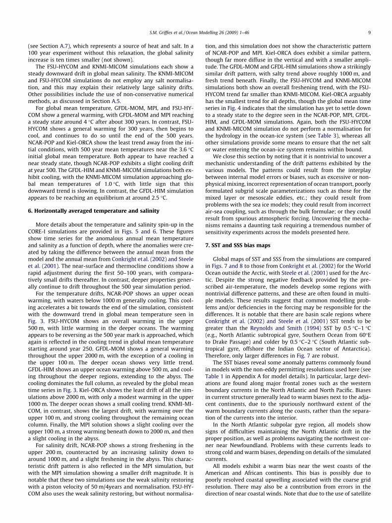
S.M. Griffies et al. / Ocean Modelling 26 (2009) 1–46 9
(see Section A.7), which represents a source of heat and salt. In a100 year experiment without this relaxation, the global salinityincrease is ten times smaller (not shown).
The FSU-HYCOM and KNMI-MICOM simulations each show asteady downward drift in global mean salinity. The KNMI-MICOMand FSU-HYCOM simulations do not employ any salt normalisa-tion, and this may explain their relatively large salinity drifts.Other possibilities include the use of non-conservative numericalmethods, as discussed in Section A.5.
For global mean temperature, GFDL-MOM, MPI, and FSU-HY-COM show a general warming, with GFDL-MOM and MPI reachinga steady state around 4 �C after about 300 years. In contrast, FSU-HYCOM shows a general warming for 300 years, then begins tocool, and continues to do so until the end of the 500 years.NCAR-POP and Kiel-ORCA show the least trend away from the ini-tial conditions, with 500 year mean temperatures near the 3.6 �Cinitial global mean temperature. Both appear to have reached anear steady state, though NCAR-POP exhibits a slight cooling driftat year 500. The GFDL-HIM and KNMI-MICOM simulations both ex-hibit cooling, with the KNMI-MICOM simulation approaching glo-bal mean temperatures of 1.0 �C, with little sign that thisdownward trend is slowing. In contrast, the GFDL-HIM simulationappears to be reaching an equilibrium at around 2.5 �C.
6. Horizontally averaged temperature and salinity
More details about the temperature and salinity spin-up in theCORE-I simulations are provided in Figs. 5 and 6. These figuresshow time series for the anomalous annual mean temperatureand salinity as a function of depth, where the anomalies were cre-ated by taking the difference between the annual mean from themodel and the annual mean from Conkright etal. (2002) and Steeleet al. (2001). The near-surface and thermocline conditions show arapid adjustment during the first 50–100 years, with compara-tively small drifts thereafter. In contrast, deeper properties gener-ally continue to drift throughout the 500 year simulation period.
For the temperature drifts, NCAR-POP shows an upper oceanwarming, with waters below 1000 m generally cooling. This cool-ing accelerates a bit towards the end of the simulation, consistentwith the downward trend in global mean temperature seen inFig. 3. FSU-HYCOM shows an overall warming in the upper500 m, with little warming in the deeper oceans. The warmingappears to be reversing as the 500 year mark is approached, whichagain is reflected in the cooling trend in global mean temperaturestarting around year 250. GFDL-MOM shows a general warmingthroughout the upper 2000 m, with the exception of a cooling inthe upper 100 m. The deeper ocean shows very little trend.GFDL-HIM shows an upper ocean warming above 500 m, and cool-ing throughout the deeper regions, extending to the abyss. Thecooling dominates the full column, as revealed by the global meantime series in Fig. 3. Kiel-ORCA shows the least drift of all the sim-ulations above 2000 m, with only a modest warming in the upper1000 m. The deeper ocean shows a small cooling trend. KNMI-MI-COM, in contrast, shows the largest drift, with warming over theupper 100 m, and strong cooling throughout the remaining oceancolumn. Finally, the MPI solution shows a slight cooling over theupper 100 m, a strong warming beneath down to 2000 m, and thena slight cooling in the abyss.
For salinity drift, NCAR-POP shows a strong freshening in theupper 200 m, counteracted by an increasing salinity down toaround 1000 m, and a slight freshening in the abyss. This charac-teristic drift pattern is also reflected in the MPI simulation, butwith the MPI simulation showing a smaller drift magnitude. It isnotable that these two simulations use the weak salinity restoringwith a piston velocity of 50 m/4years and normalisation. FSU-HY-COM also uses the weak salinity restoring, but without normalisa-
tion, and this simulation does not show the characteristic patternof NCAR-POP and MPI. Kiel-ORCA does exhibit a similar pattern,though far more diffuse in the vertical and with a smaller ampli-tude. The GFDL-MOM and GFDL-HIM simulations show a strikinglysimilar drift pattern, with salty trend above roughly 1000 m, andfresh trend beneath. Finally, the FSU-HYCOM and KNMI-MICOMsimulations both show an overall freshening trend, with the FSU-HYCOM trend far smaller than KNMI-MICOM. Kiel-ORCA arguablyhas the smallest trend for all depths, though the global mean timeseries in Fig. 4 indicates that the simulation has yet to settle downto a steady state to the degree seen in the NCAR-POP, MPI, GFDL-HIM, and GFDL-MOM simulations. Again, both the FSU-HYCOMand KNMI-MICOM simulation do not perform a normalisation forthe hydrology in the ocean-ice system (see Table 3), whereas allother simulations provide some means to ensure that the net saltor water entering the ocean-ice system remains within bound.
We close this section by noting that it is nontrivial to uncover amechanistic understanding of the drift patterns exhibited by thevarious models. The patterns could result from the interplaybetween internal model errors or biases, such as excessive or non-physical mixing, incorrect representation of ocean transport, poorlyformulated subgrid scale parameterizations such as those for themixed layer or mesoscale eddies, etc.; they could result fromproblems with the sea ice models; they could result from incorrectair-sea coupling, such as through the bulk formulae; or they couldresult from spurious atmospheric forcing. Uncovering the mecha-nisms remains a daunting task requiring a tremendous number ofsensitivity experiments across the models presented here.
7. SST and SSS bias maps
Global maps of SST and SSS from the simulations are comparedin Figs. 7 and 8 to those from Conkright et al. (2002) for the WorldOcean outside the Arctic, with Steele et al. (2001) used for the Arc-tic. Despite the strong negative feedback provided by the pre-scribed air-temperature, the models develop some regions withnontrivial difference patterns, and these are often found in multi-ple models. These results suggest that common modelling prob-lems and/or deficiencies in the forcing may be responsible for thedifferences. It is notable that there are basin scale regions whereConkright et al. (2002) and Steele et al. (2001) SST tends to begreater than the Reynolds and Smith (1994) SST by 0.5 �C–1 �C(e.g., North Atlantic subtropical gyre, Southern Ocean from 60�Eto Drake Passage) and colder by 0.5 �C–2 �C (South Atlantic sub-tropical gyre, offshore the Indian Ocean sector of Antarctica).Therefore, only larger differences in Fig. 7 are robust.
The SST biases reveal some anomaly patterns commonly foundin models with the non-eddy permitting resolutions used here (seeTable 1 in Appendix A for model details). In particular, large devi-ations are found along major frontal zones such as the westernboundary currents in the North Atlantic and North Pacific. Biasesin current structure generally lead to warm biases next to the adja-cent continents, due to the spuriously northward extent of thewarm boundary currents along the coasts, rather than the separa-tion of the currents into the interior.
In the North Atlantic subpolar gyre region, all models showsigns of difficulties maintaining the North Atlantic drift in theproper position, as well as problems navigating the northwest cor-ner near Newfoundland. Problems with these currents leads tostrong cold and warm biases, depending on details of the simulatedcurrents.
All models exhibit a warm bias near the west coasts of theAmerican and African continents. This bias is possibly due topoorly resolved coastal upwelling associated with the coarse gridresolution. There may also be a contribution from errors in thedirection of near coastal winds. Note that due to the use of satellite
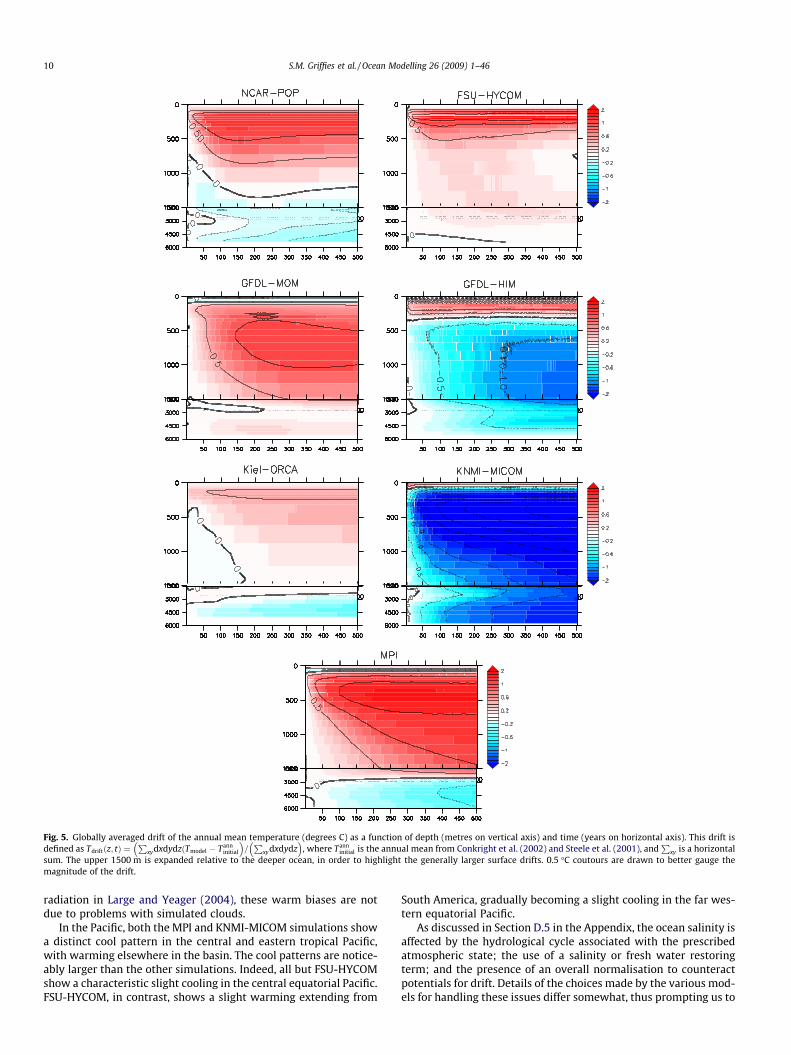
Fig. 5. Globally averaged drift of the annual mean temperature (degrees C) as a function of depth (metres on vertical axis) and time (years on horizontal axis). This drift isdefined as Tdriftðz; tÞ ¼
PxydxdydzðTmodel � Tann
initial
� �=P
xydxdydz� �
, where Tanninitial is the annual mean from Conkright et al. (2002) and Steele et al. (2001), and
Pxy is a horizontal
sum. The upper 1500 m is expanded relative to the deeper ocean, in order to highlight the generally larger surface drifts. 0.5 �C coutours are drawn to better gauge themagnitude of the drift.
10 S.M. Griffies et al. / Ocean Modelling 26 (2009) 1–46
radiation in Large and Yeager (2004), these warm biases are notdue to problems with simulated clouds.
In the Pacific, both the MPI and KNMI-MICOM simulations showa distinct cool pattern in the central and eastern tropical Pacific,with warming elsewhere in the basin. The cool patterns are notice-ably larger than the other simulations. Indeed, all but FSU-HYCOMshow a characteristic slight cooling in the central equatorial Pacific.FSU-HYCOM, in contrast, shows a slight warming extending from
South America, gradually becoming a slight cooling in the far wes-tern equatorial Pacific.
As discussed in Section D.5 in the Appendix, the ocean salinity isaffected by the hydrological cycle associated with the prescribedatmospheric state; the use of a salinity or fresh water restoringterm; and the presence of an overall normalisation to counteractpotentials for drift. Details of the choices made by the various mod-els for handling these issues differ somewhat, thus prompting us to
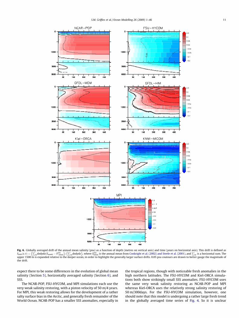
Fig. 6. Globally averaged drift of the annual mean salinity (psu) as a function of depth (metres on vertical axis) and time (years on horizontal axis). This drift is defined asSdriftðz; tÞ ¼
PxydxdydzðSmodel � Sann
initial
� �=P
xydxdydz� �
, where Sanninitial is the annual mean from Conkright et al. (2002) and Steele et al. (2001), and
Pxy is a horizontal sum. The
upper 1500 m is expanded relative to the deeper ocean, in order to highlight the generally larger surface drifts. 0.05 psu coutours are drawn to better gauge the magnitude ofthe drift.
S.M. Griffies et al. / Ocean Modelling 26 (2009) 1–46 11
expect there to be some differences in the evolution of global meansalinity (Section 5), horizontally averaged salinity (Section 6), andSSS.
The NCAR-POP, FSU-HYCOM, and MPI simulations each use thevery weak salinity restoring, with a piston velocity of 50 m/4 years.For MPI, this weak restoring allows for the development of a rathersalty surface bias in the Arctic, and generally fresh remainder of theWorld Ocean. NCAR-POP has a smaller SSS anomalies, especially in
the tropical regions, though with noticeable fresh anomalies in thehigh northern latitudes. The FSU-HYCOM and Kiel-ORCA simula-tions both show strikingly small SSS anomalies. FSU-HYCOM usesthe same very weak salinity restoring as NCAR-POP and MPIwhereas Kiel-ORCA uses the relatively strong salinity restoring of50 m/300days. For the FSU-HYCOM simulation, however, oneshould note that this model is undergoing a rather large fresh trendin the globally averaged time series of Fig. 4. So it is unclear
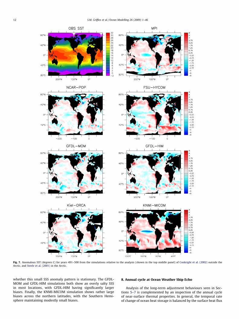
Fig. 7. Anomalous SST (degrees C) for years 491–500 from the simulations relative to the analysis (shown in the top middle panel) of Conkright et al. (2002) outside theArctic, and Steele et al. (2001) in the Arctic.
12 S.M. Griffies et al. / Ocean Modelling 26 (2009) 1–46
whether this small SSS anomaly pattern is stationary. The GFDL-MOM and GFDL-HIM simulations both show an overly salty SSSin most locations, with GFDL-HIM having significantly largerbiases. Finally, the KNMI-MICOM simulation shows rather largebiases across the northern latitudes, with the Southern Hemi-sphere maintaining modestly small biases.
8. Annual cycle at Ocean Weather Ship Echo
Analysis of the long-term adjustment behaviours seen in Sec-tions 5–7 is complemented by an inspection of the annual cycleof near-surface thermal properties. In general, the temporal rateof change of ocean heat storage is balanced by the surface heat flux
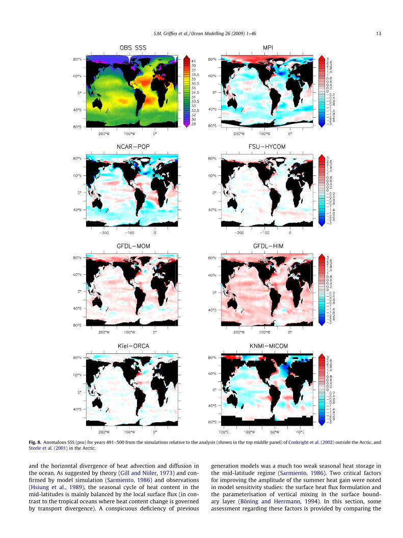
Fig. 8. Anomalous SSS (psu) for years 491–500 from the simulations relative to the analysis (shown in the top middle panel) of Conkright et al. (2002) outside the Arctic, andSteele et al. (2001) in the Arctic.
S.M. Griffies et al. / Ocean Modelling 26 (2009) 1–46 13
and the horizontal divergence of heat advection and diffusion inthe ocean. As suggested by theory (Gill and Niiler, 1973) and con-firmed by model simulation (Sarmiento, 1986) and observations(Hsiung et al., 1989), the seasonal cycle of heat content in themid-latitudes is mainly balanced by the local surface flux (in con-trast to the tropical oceans where heat content change is governedby transport divergence). A conspicuous deficiency of previous
generation models was a much too weak seasonal heat storage inthe mid-latitude regime (Sarmiento, 1986). Two critical factorsfor improving the amplitude of the summer heat gain were notedin model sensitivity studies: the surface heat flux formulation andthe parameterisation of vertical mixing in the surface bound-ary layer (Böning and Herrmann, 1994). In this section, someassessment regarding these factors is provided by comparing the
14 S.M. Griffies et al. / Ocean Modelling 26 (2009) 1–46
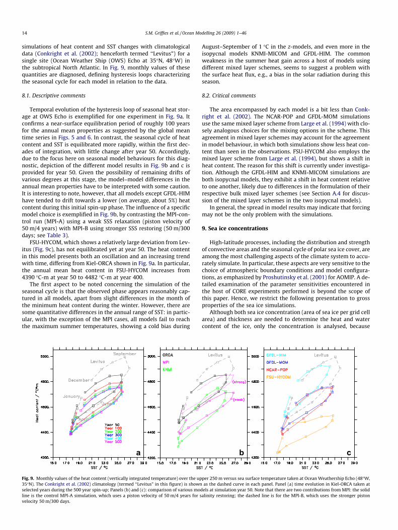
simulations of heat content and SST changes with climatologicaldata (Conkright et al. (2002); henceforth termed ‘‘Levitus”) for asingle site (Ocean Weather Ship (OWS) Echo at 35�N, 48�W) inthe subtropical North Atlantic. In Fig. 9, monthly values of thesequantities are diagnosed, defining hysteresis loops characterizingthe seasonal cycle for each model in relation to the data.
8.1. Descriptive comments
Temporal evolution of the hysteresis loop of seasonal heat stor-age at OWS Echo is exemplified for one experiment in Fig. 9a. Itconfirms a near-surface equilibration period of roughly 100 yearsfor the annual mean properties as suggested by the global meantime series in Figs. 5 and 6. In contrast, the seasonal cycle of heatcontent and SST is equilibrated more rapidly, within the first dec-ades of integration, with little change after year 50. Accordingly,due to the focus here on seasonal model behaviours for this diag-nostic, depiction of the different model results in Fig. 9b and c isprovided for year 50. Given the possibility of remaining drifts ofvarious degrees at this stage, the model–model differences in theannual mean properties have to be interpreted with some caution.It is interesting to note, however, that all models except GFDL-HIMhave tended to drift towards a lower (on average, about 5%) heatcontent during this initial spin-up phase. The influence of a specificmodel choice is exemplified in Fig. 9b, by contrasting the MPI-con-trol run (MPI-A) using a weak SSS relaxation (piston velocity of50 m/4 years) with MPI-B using stronger SSS restoring (50 m/300days; see Table 3).
FSU-HYCOM, which shows a relatively large deviation from Lev-itus (Fig. 9c), has not equilibrated yet at year 50. The heat contentin this model presents both an oscillation and an increasing trendwith time, differing from Kiel-ORCA shown in Fig. 9a. In particular,the annual mean heat content in FSU-HYCOM increases from4390 �C-m at year 50 to 4482 �C-m at year 400.
The first aspect to be noted concerning the simulation of theseasonal cycle is that the observed phase appears reasonably cap-tured in all models, apart from slight differences in the month ofthe minimum heat content during the winter. However, there aresome quantitative differences in the annual range of SST: in partic-ular, with the exception of the MPI cases, all models fail to reachthe maximum summer temperatures, showing a cold bias during
a
Fig. 9. Monthly values of the heat content (vertically integrated temperature) over the up35�N). The Conkright et al. (2002) climatology (termed ‘‘Levitus” in this figure) is shownselected years during the 500 year spin-up; Panels (b) and (c): comparison of various moline is the control MPI-A simulation, which uses a piston velocity of 50 m/4 years for svelocity 50 m/300 days.
August–September of 1 �C in the z-models, and even more in theisopycnal models KNMI-MICOM and GFDL-HIM. The commonweakness in the summer heat gain across a host of models usingdifferent mixed layer schemes, seems to suggest a problem withthe surface heat flux, e.g., a bias in the solar radiation during thisseason.
8.2. Critical comments
The area encompassed by each model is a bit less than Conk-right et al. (2002). The NCAR-POP and GFDL-MOM simulationsuse the same mixed layer scheme from Large et al. (1994) with clo-sely analogous choices for the mixing options in the scheme. Thisagreement in mixed layer schemes may account for the agreementin model behaviour, in which both simulations show less heat con-tent than seen in the observations. FSU-HYCOM also employs themixed layer scheme from Large et al. (1994), but shows a shift inheat content. The reason for this shift is currently under investiga-tion. Although the GFDL-HIM and KNMI-MICOM simulations areboth isopycnal models, they exhibit a shift in heat content relativeto one another, likely due to differences in the formulation of theirrespective bulk mixed layer schemes (see Section A.4 for discus-sion of the mixed layer schemes in the two isopycnal models).
In general, the spread in model results may indicate that forcingmay not be the only problem with the simulations.
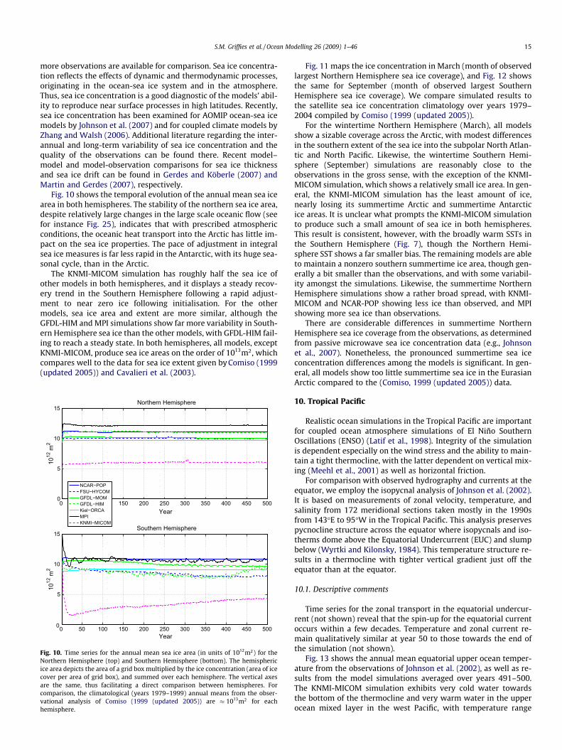
9. Sea ice concentrations
High-latitude processes, including the distribution and strengthof convective areas and the seasonal cycle of polar sea ice cover, areamong the most challenging aspects of the climate system to accu-rately simulate. In particular, these aspects are very sensitive to thechoice of atmospheric boundary conditions and model configura-tions, as emphasized by Proshutinsky et al. (2001) for AOMIP. A de-tailed examination of the parameter sensitivities encountered inthe host of CORE experiments performed is beyond the scope ofthis paper. Hence, we restrict the following presentation to grossproperties of the sea ice simulations.
Although both sea ice concentration (area of sea ice per grid cellarea) and thickness are needed to determine the heat and watercontent of the ice, only the concentration is analysed, because
b c
per 250 m versus sea surface temperature taken at Ocean Weathership Echo (48�W,as the dashed curve in each panel. Panel (a) time evolution in Kiel-ORCA taken at
dels at simulation year 50. Note that there are two contributions from MPI: the solidalinity restoring; the dashed line is for the MPI-B, which uses the stronger piston
S.M. Griffies et al. / Ocean Modelling 26 (2009) 1–46 15
more observations are available for comparison. Sea ice concentra-tion reflects the effects of dynamic and thermodynamic processes,originating in the ocean-sea ice system and in the atmosphere.Thus, sea ice concentration is a good diagnostic of the models’ abil-ity to reproduce near surface processes in high latitudes. Recently,sea ice concentration has been examined for AOMIP ocean-sea icemodels by Johnson et al. (2007) and for coupled climate models byZhang and Walsh (2006). Additional literature regarding the inter-annual and long-term variability of sea ice concentration and thequality of the observations can be found there. Recent model–model and model-observation comparisons for sea ice thicknessand sea ice drift can be found in Gerdes and Köberle (2007) andMartin and Gerdes (2007), respectively.
Fig. 10 shows the temporal evolution of the annual mean sea icearea in both hemispheres. The stability of the northern sea ice area,despite relatively large changes in the large scale oceanic flow (seefor instance Fig. 25), indicates that with prescribed atmosphericconditions, the oceanic heat transport into the Arctic has little im-pact on the sea ice properties. The pace of adjustment in integralsea ice measures is far less rapid in the Antarctic, with its huge sea-sonal cycle, than in the Arctic.
The KNMI-MICOM simulation has roughly half the sea ice ofother models in both hemispheres, and it displays a steady recov-ery trend in the Southern Hemisphere following a rapid adjust-ment to near zero ice following initialisation. For the othermodels, sea ice area and extent are more similar, although theGFDL-HIM and MPI simulations show far more variability in South-ern Hemisphere sea ice than the other models, with GFDL-HIM fail-ing to reach a steady state. In both hemispheres, all models, exceptKNMI-MICOM, produce sea ice areas on the order of 1013m2, whichcompares well to the data for sea ice extent given by Comiso (1999(updated 2005)) and Cavalieri et al. (2003).
0 50 100 150 200 250 300 350 400 450 5000
5
10
15Northern Hemisphere
1012
m2
Year
0 50 100 150 200 250 300 350 400 450 5000
5
10
15Southern Hemisphere
1012
m2
Year
NCAR−POPFSU−HYCOMGFDL−MOMGFDL−HIMKiel−ORCAMPIKNMI−MICOM
Fig. 10. Time series for the annual mean sea ice area (in units of 1012m2) for theNorthern Hemisphere (top) and Southern Hemisphere (bottom). The hemisphericice area depicts the area of a grid box multiplied by the ice concentration (area of icecover per area of grid box), and summed over each hemisphere. The vertical axesare the same, thus facilitating a direct comparison between hemispheres. Forcomparison, the climatological (years 1979–1999) annual means from the obser-vational analysis of Comiso (1999 (updated 2005)) are � 1013m2 for eachhemisphere.
Fig. 11 maps the ice concentration in March (month of observedlargest Northern Hemisphere sea ice coverage), and Fig. 12 showsthe same for September (month of observed largest SouthernHemisphere sea ice coverage). We compare simulated results tothe satellite sea ice concentration climatology over years 1979–2004 compiled by Comiso (1999 (updated 2005)).
For the wintertime Northern Hemisphere (March), all modelsshow a sizable coverage across the Arctic, with modest differencesin the southern extent of the sea ice into the subpolar North Atlan-tic and North Pacific. Likewise, the wintertime Southern Hemi-sphere (September) simulations are reasonably close to theobservations in the gross sense, with the exception of the KNMI-MICOM simulation, which shows a relatively small ice area. In gen-eral, the KNMI-MICOM simulation has the least amount of ice,nearly losing its summertime Arctic and summertime Antarcticice areas. It is unclear what prompts the KNMI-MICOM simulationto produce such a small amount of sea ice in both hemispheres.This result is consistent, however, with the broadly warm SSTs inthe Southern Hemisphere (Fig. 7), though the Northern Hemi-sphere SST shows a far smaller bias. The remaining models are ableto maintain a nonzero southern summertime ice area, though gen-erally a bit smaller than the observations, and with some variabil-ity amongst the simulations. Likewise, the summertime NorthernHemisphere simulations show a rather broad spread, with KNMI-MICOM and NCAR-POP showing less ice than observed, and MPIshowing more sea ice than observations.
There are considerable differences in summertime NorthernHemisphere sea ice coverage from the observations, as determinedfrom passive microwave sea ice concentration data (e.g., Johnsonet al., 2007). Nonetheless, the pronounced summertime sea iceconcentration differences among the models is significant. In gen-eral, all models show too little summertime sea ice in the EurasianArctic compared to the (Comiso, 1999 (updated 2005)) data.
10. Tropical Pacific
Realistic ocean simulations in the Tropical Pacific are importantfor coupled ocean atmosphere simulations of El Niño SouthernOscillations (ENSO) (Latif et al., 1998). Integrity of the simulationis dependent especially on the wind stress and the ability to main-tain a tight thermocline, with the latter dependent on vertical mix-ing (Meehl et al., 2001) as well as horizontal friction.
For comparison with observed hydrography and currents at theequator, we employ the isopycnal analysis of Johnson et al. (2002).It is based on measurements of zonal velocity, temperature, andsalinity from 172 meridional sections taken mostly in the 1990sfrom 143�E to 95�W in the Tropical Pacific. This analysis preservespycnocline structure across the equator where isopycnals and iso-therms dome above the Equatorial Undercurrent (EUC) and slumpbelow (Wyrtki and Kilonsky, 1984). This temperature structure re-sults in a thermocline with tighter vertical gradient just off theequator than at the equator.
10.1. Descriptive comments
Time series for the zonal transport in the equatorial undercur-rent (not shown) reveal that the spin-up for the equatorial currentoccurs within a few decades. Temperature and zonal current re-main qualitatively similar at year 50 to those towards the end ofthe simulation (not shown).
Fig. 13 shows the annual mean equatorial upper ocean temper-ature from the observations of Johnson et al. (2002), as well as re-sults from the model simulations averaged over years 491–500.The KNMI-MICOM simulation exhibits very cold water towardsthe bottom of the thermocline and very warm water in the upperocean mixed layer in the west Pacific, with temperature range
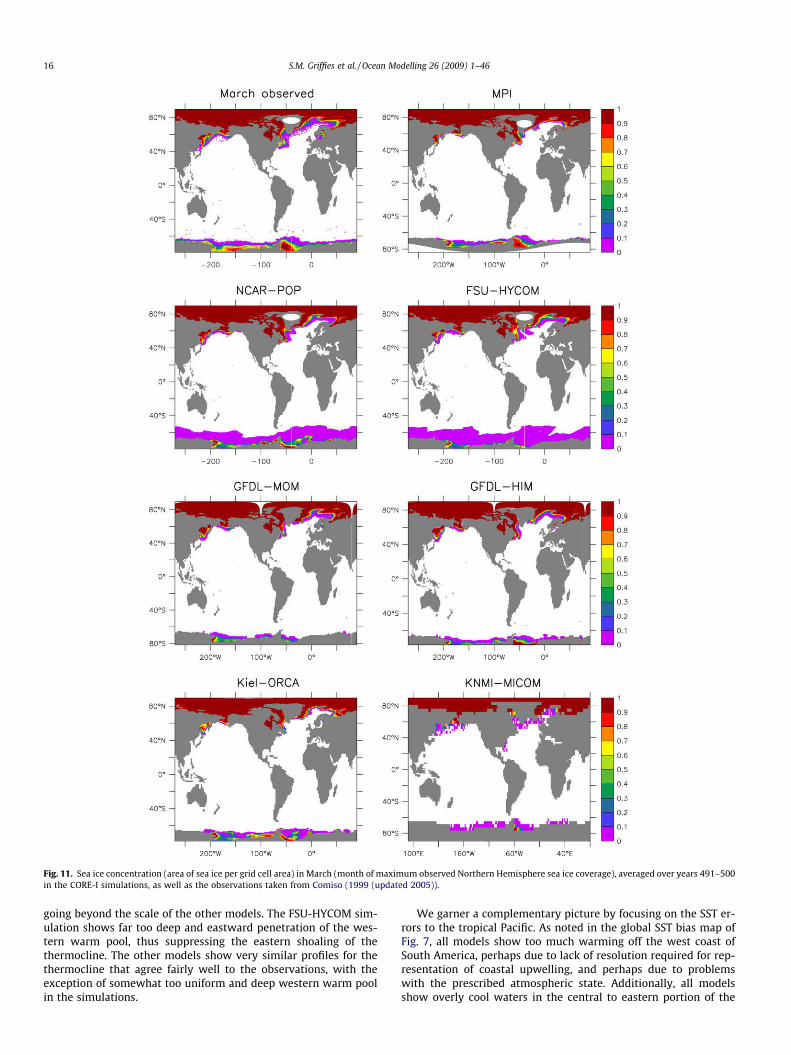
Fig. 11. Sea ice concentration (area of sea ice per grid cell area) in March (month of maximum observed Northern Hemisphere sea ice coverage), averaged over years 491–500in the CORE-I simulations, as well as the observations taken from Comiso (1999 (updated 2005)).
16 S.M. Griffies et al. / Ocean Modelling 26 (2009) 1–46
going beyond the scale of the other models. The FSU-HYCOM sim-ulation shows far too deep and eastward penetration of the wes-tern warm pool, thus suppressing the eastern shoaling of thethermocline. The other models show very similar profiles for thethermocline that agree fairly well to the observations, with theexception of somewhat too uniform and deep western warm poolin the simulations.
We garner a complementary picture by focusing on the SST er-rors to the tropical Pacific. As noted in the global SST bias map ofFig. 7, all models show too much warming off the west coast ofSouth America, perhaps due to lack of resolution required for rep-resentation of coastal upwelling, and perhaps due to problemswith the prescribed atmospheric state. Additionally, all modelsshow overly cool waters in the central to eastern portion of the
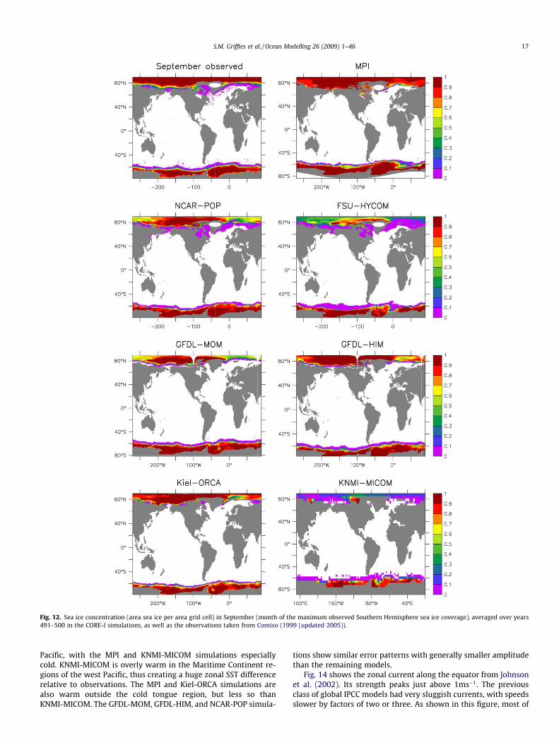
Fig. 12. Sea ice concentration (area sea ice per area grid cell) in September (month of the maximum observed Southern Hemisphere sea ice coverage), averaged over years491–500 in the CORE-I simulations, as well as the observations taken from Comiso (1999 (updated 2005)).
S.M. Griffies et al. / Ocean Modelling 26 (2009) 1–46 17
Pacific, with the MPI and KNMI-MICOM simulations especiallycold. KNMI-MICOM is overly warm in the Maritime Continent re-gions of the west Pacific, thus creating a huge zonal SST differencerelative to observations. The MPI and Kiel-ORCA simulations arealso warm outside the cold tongue region, but less so thanKNMI-MICOM. The GFDL-MOM, GFDL-HIM, and NCAR-POP simula-
tions show similar error patterns with generally smaller amplitudethan the remaining models.
Fig. 14 shows the zonal current along the equator from Johnsonet al. (2002). Its strength peaks just above 1ms�1. The previousclass of global IPCC models had very sluggish currents, with speedsslower by factors of two or three. As shown in this figure, most of
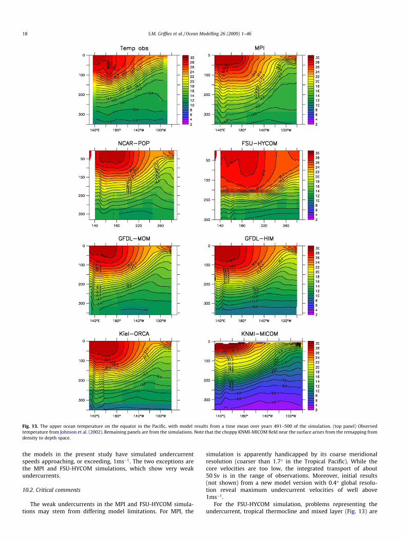
Fig. 13. The upper ocean temperature on the equator in the Pacific, with model results from a time mean over years 491–500 of the simulation. (top panel) Observedtemperature from Johnson et al. (2002). Remaining panels are from the simulations. Note that the choppy KNMI-MICOM field near the surface arises from the remapping fromdensity to depth space.
18 S.M. Griffies et al. / Ocean Modelling 26 (2009) 1–46
the models in the present study have simulated undercurrentspeeds approaching, or exceeding, 1ms�1. The two exceptions arethe MPI and FSU-HYCOM simulations, which show very weakundercurrents.
10.2. Critical comments
The weak undercurrents in the MPI and FSU-HYCOM simula-tions may stem from differing model limitations. For MPI, the
simulation is apparently handicapped by its coarse meridionalresolution (coarser than 1.7� in the Tropical Pacific). While thecore velocities are too low, the integrated transport of about50 Sv is in the range of observations. Moreover, initial results(not shown) from a new model version with 0.4� global resolu-tion reveal maximum undercurrent velocities of well above1ms�1.
For the FSU-HYCOM simulation, problems representing theundercurrent, tropical thermocline and mixed layer (Fig. 13) are
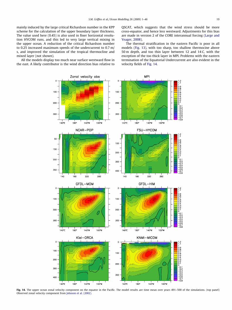
S.M. Griffies et al. / Ocean Modelling 26 (2009) 1–46 19
mainly induced by the large critical Richardson number in the KPPscheme for the calculation of the upper boundary layer thickness.The value used here (0.45) is also used in finer horizontal resolu-tion HYCOM runs, and this led to very large vertical mixing inthe upper ocean. A reduction of the critical Richardson numberto 0.25 increased maximum speeds of the undercurrent to 0.7 m/s, and improved the simulation of the tropical thermocline andmixed layer (not shown).
All the models display too much near surface westward flow inthe east. A likely contributor is the wind direction bias relative to
Fig. 14. The upper ocean zonal velocity component on the equator in the Pacific. TheObserved zonal velocity component from Johnson et al. (2002).
QSCAT, which suggests that the wind stress should be morecross-equator, and hence less westward. Adjustments for this biasare made in version 2 of the CORE interannual forcing (Large andYeager, 2008).
The thermal stratification in the eastern Pacific is poor in allmodels (Fig. 13), with too sharp, too shallow thermocine above50 m depth, and too thin layer between 12 and 14 C, with theexception of the too thick layer in MPI. Problems with the easterntermination of the Equatorial Undercurrent are also evident in thevelocity fields of Fig. 14.
model results are time mean over years 491–500 of the simulations. (top panel)
20 S.M. Griffies et al. / Ocean Modelling 26 (2009) 1–46
11. Mixed layer depths
The surface mixed layer is deepened by wind-driven mixingprocesses, Ekman-induced subduction, and convective overturnof gravitationally unstable water columns. It is the latter processthat is particularly important in the formation of SubantarcticMode Water (SAMW), North Atlantic Deep Water (NADW), andHigh Salinity Shelf Water around Antarctica. The mixed layer depth(MLD) attained in late winter is thus a crucial model diagnostic, asit reflects the depth of rapid overturn of surface waters, which isintimately related to water-mass formation and the regulation ofglobal climate via the air-sea exchange of heat, freshwater, andCO2.
In Section D.6 of the Appendix, we detail issues involved withevaluating the mixed layer depth in an ocean model. In particular,we note that the models used in this study do not compute themixed layer with the same algorithm. Hence, some of the differ-ences can be explained by different methodology, though manydifferences are large enough to be robust.
11.1. Observed mixed layer depth
The observed estimate of MLD (Fig. 15a) is derived from a long-term monthly mean climatology of h� S (described below). Thisapproach potentially underestimates the observed decade-longmaximum MLD as it (1) ignores interannual variability in the con-vective mixed layer, (2) derives MLD from a somewhat horizontallysmoothed h� S field, and (3) can be based on under-sampled win-tertime hydrography. However, alternate estimates, such as usingraw Argo and WOCE data, do not provide a complete global cover-age of mixed layer depth. Where data permitted, we compared thepatterns of MLD obtained using raw and climatological h� S. Ingeneral, both yield similar patterns of MLD, only with shallowermixed layers in the climatologically-derived estimates in the farNorth Atlantic and Labrador Sea.
A critical MLD benchmark is the distribution of maximumdepths of mixing attained during an annual cycle. This depthinfluences the rate of uptake of anthropogenic CO2 and the vig-our of the ocean thermohaline circulation. It also marks thegenesis of oceanic ventilation of thermocline (Stommel, 1979;Williams et al., 1995) and mode waters (McCartney, 1977). Anestimate of the observed distribution of maximum MLD isshown in Fig. 15a. This estimate is derived from the WorldOcean Atlas 2005 (WOA05) data set (Locarnini, 2006; Antonovet al., 2006), based on monthly mean density. The WOA05 data-set includes Argo data recorded up until the end of 2005. Themixed layer depth h is calculated as the depth where the buoy-ancy difference DB between the surface and h is 0:0003ms�2.Here, DB ¼ gð1� r0=rhÞ, where r is potential density. Data cov-erage is too sparse to derive the maximum MLD from anythingshorter than a monthly coverage of global density, whereas inmodel simulations the MLD can be diagnosed at each modeltimestep. The potential errors arising from deriving the maxi-mum MLD from a monthly climatology of h� S were itemizedabove. Generally speaking, the fields shown in Fig. 15a shouldbe viewed as a large-scale estimate of the horizontal variationsin global mixed layer depth, with highest values obtained in theformation regions for SAMW, NADW, and High Salinity ShelfWater around Antarctica.
11.2. Descriptive comments
In the observed analysis, deep winter mixed layers dominatethe subpolar North Atlantic Ocean associated with NADW over-turning. There is also a band of deep mixed layers or ‘pycnostads’associated with SAMW, extending along much of the northern
flank of the Antarctica Circumpolar Current (ACC) in the Indianand Pacific Oceans. Adjacent to Antarctica, particularly in the Wed-dell Sea, there is also evidence of deep mixed layers associatedwith the formation of High Salinity Shelf Water and, eventually,Antarctic Bottom Water. Only modest mixed layer depths areobserved over much of the remainder of the global ocean (of theorder of 50–100 m, consistent with typical open ocean wind-driven mixed layer depth).
All models, except KNMI-MICOM, simulate a band of deepmixed layers associated with SubAntarctic Mode Water (SAMW),although in GFDL-HIM these mixed layers are only seen in the In-dian Ocean and south of Australia. In FSU-HYCOM and MPI, theSAMW pycnostads are generally too broad and deep. To the south,many of the models simulate very deep mixed layers in the Wed-dell gyre, in contrast to observations where MLD is generally shal-low within the gyre, and deep at its southern edges. Deep mixedlayers are limited to the Antarctic margin in the Ross Sea in theobserved and most of the models, apart from the two GFDL simu-lations and MPI, wherein deep mixed layers are simulated withinthe polar gyres. In the North Atlantic all models capture a reason-ably good mixed layer field, apart from KNMI-MICOM where theMLD seems chronically too shallow over all regions of water-massformation. Overall, the NCAR-POP and Kiel-ORCA simulations yieldthe best general agreement with the observed estimate of maxi-mum MLD.
11.3. Critical comments
The model–model comparison for MLD is complicated by thefact that each simulation uses a slightly different diagnostic meth-od for calculating the depth of the mixed layer (see Section D.6 inthe Appendix). Ideally in a comparison study such as this, a methodfor diagnosing the surface mixed layer depth is agreed prior toexperimentation, so that a meaningful model–model analysis canbe made.
The two isopycnal models GFDL-HIM and KNMI-MICOM reportthe thickness of the layer with active surface wind and buoyancyinduced turbulence, with markedly different fields for the two sim-ulations. The KNMI-MICOM underestimates the MLD in all keyareas of water-mass formation, leaving its ocean interior poorlyventilated from surface waters, and therefore too cold and fresh(Section 12). In contrast, GFDL-HIM has relatively deep SouthernOcean and North Atlantic mixed layer depths, creating a muchmore ventilated simulation than KNMI-MICOM.
Among the z-level models, significant differences in simu-lated MLD are also noted. The GFDL-MOM and NCAR-POP sim-ulations employ the same mixed layer scheme from Large et al.(1994). Hence, there is likely another reason explaining theirdifferences, with treatment of the neutral physics scheme (Gentand McWilliams, 1990) perhaps the main reason. As docu-mented in Table 6 (Section D.3), GFDL-MOM chooses a spatiallydependent diffusivity which is a maximum of around 600m2s�1
in the centre of the ACC, and reduces to nearly 100� 200m2s�1
outside the main region of strong baroclinicity (Griffies et al.,2005, Fig. 14 of). NCAR-POP, in contrast, uses the larger valueof 600m2s�1 globally. Additionally, GFDL-MOM chooses to begintapering the neutral fluxes with a neutral slope of 1/500 (Gna-nadesikan et al., 2007), whereas NCAR-POP extends their fluxesuntapered until a slope of 3/10 (Danabasoglu et al., 2008). Boththe diffusivity and slope maximum differences provide a stron-ger tendency from Gent and McWilliams (1990) in NCAR-POPto relax the neutral slopes, thus shoaling the mixed layers,relative to GFDL-MOM. Recent tests with the GFDL-MOMcoupled climate model indicate that the mixed layer in theWeddell Sea is significantly reduced by allowing for a largermaximum slope.
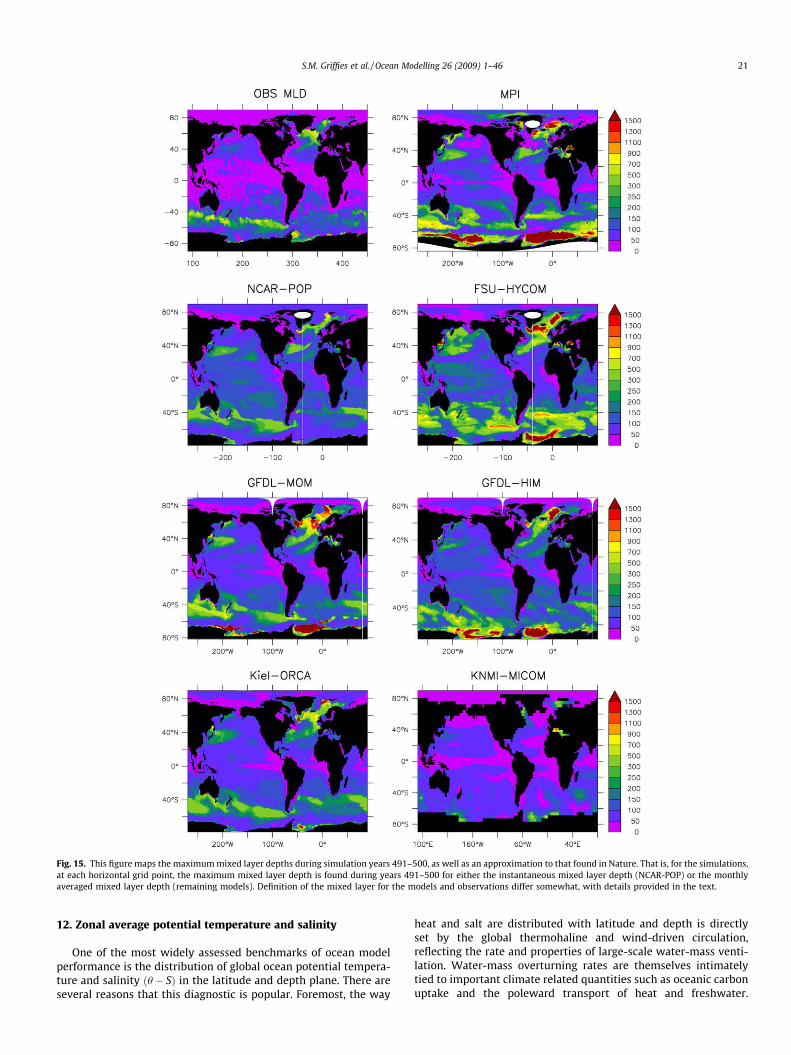
Fig. 15. This figure maps the maximum mixed layer depths during simulation years 491–500, as well as an approximation to that found in Nature. That is, for the simulations,at each horizontal grid point, the maximum mixed layer depth is found during years 491–500 for either the instantaneous mixed layer depth (NCAR-POP) or the monthlyaveraged mixed layer depth (remaining models). Definition of the mixed layer for the models and observations differ somewhat, with details provided in the text.
S.M. Griffies et al. / Ocean Modelling 26 (2009) 1–46 21
12. Zonal average potential temperature and salinity
One of the most widely assessed benchmarks of ocean modelperformance is the distribution of global ocean potential tempera-ture and salinity ðh� SÞ in the latitude and depth plane. There areseveral reasons that this diagnostic is popular. Foremost, the way
heat and salt are distributed with latitude and depth is directlyset by the global thermohaline and wind-driven circulation,reflecting the rate and properties of large-scale water-mass venti-lation. Water-mass overturning rates are themselves intimatelytied to important climate related quantities such as oceanic carbonuptake and the poleward transport of heat and freshwater.
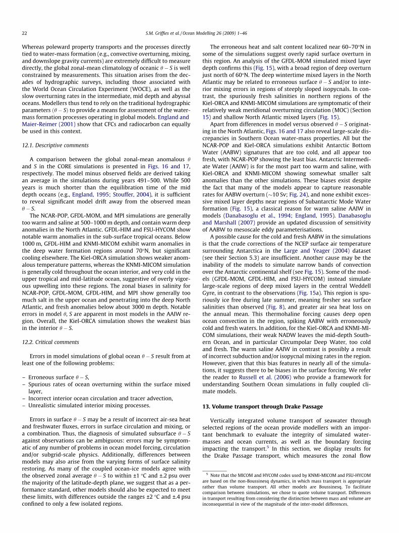
5 Note that the MICOM and HYCOM codes used by KNMI-MICOM and FSU-HYCOMare based on the non-Boussinesq dynamics, in which mass transport is appropriaterather than volume transport. All other models are Boussinesq. To facilitatecomparison between simulations, we chose to quote volume transport. Differencesin transport resulting from considering the distinction between mass and volume areinconsequential in view of the magnitude of the inter-model differences.
22 S.M. Griffies et al. / Ocean Modelling 26 (2009) 1–46
Whereas poleward property transports and the processes directlytied to water-mass formation (e.g., convective overturning, mixing,and downslope gravity currents) are extremely difficult to measuredirectly, the global zonal-mean climatology of oceanic h� S is wellconstrained by measurements. This situation arises from the dec-ades of hydrographic surveys, including those associated withthe World Ocean Circulation Experiment (WOCE), as well as theslow overturning rates in the intermediate, mid depth and abyssaloceans. Modellers thus tend to rely on the traditional hydrographicparameters ðh� SÞ to provide a means for assessment of the water-mass formation processes operating in global models. England andMaier-Reimer (2001) show that CFCs and radiocarbon can equallybe used in this context.
12.1. Descriptive comments
A comparison between the global zonal-mean anomalous hand S in the CORE simulations is presented in Figs. 16 and 17,respectively. The model minus observed fields are derived takingan average in the simulations during years 491–500. While 500years is much shorter than the equilibration time of the middepth oceans (e.g., England, 1995; Stouffer, 2004), it is sufficientto reveal significant model drift away from the observed meanh� S.
The NCAR-POP, GFDL-MOM, and MPI simulations are generallytoo warm and saline at 500–1000 m depth, and contain warm deepanomalies in the North Atlantic. GFDL-HIM and FSU-HYCOM shownotable warm anomalies in the sub-surface tropical oceans. Below1000 m, GFDL-HIM and KNMI-MICOM exhibit warm anomalies inthe deep water formation regions around 70�N, but significantcooling elsewhere. The Kiel-ORCA simulation shows weaker anom-alous temperature patterns, whereas the KNMI-MICOM simulationis generally cold throughout the ocean interior, and very cold in theupper tropical and mid-latitude ocean, suggestive of overly vigor-ous upwelling into these regions. The zonal biases in salinity forNCAR-POP, GFDL-MOM, GFDL-HIM, and MPI show generally toomuch salt in the upper ocean and penetrating into the deep NorthAtlantic, and fresh anomalies below about 3000 m depth. Notableerrors in model h, S are apparent in most models in the AAIW re-gion. Overall, the Kiel-ORCA simulation shows the weakest biasin the interior h� S.
12.2. Critical comments
Errors in model simulations of global ocean h� S result from atleast one of the following problems:
– Erroneous surface h� S,– Spurious rates of ocean overturning within the surface mixed
layer,– Incorrect interior ocean circulation and tracer advection,– Unrealistic simulated interior mixing processes.
Errors in surface h� S may be a result of incorrect air-sea heatand freshwater fluxes, errors in surface circulation and mixing, ora combination. Thus, the diagnosis of simulated subsurface h� Sagainst observations can be ambiguous: errors may be symptom-atic of any number of problems in ocean model forcing, circulationand/or subgrid-scale physics. Additionally, differences betweenmodels may also arise from the varying forms of surface salinityrestoring. As many of the coupled ocean-ice models agree withthe observed zonal average h� S to within ±1 �C and ±.2 psu overthe majority of the latitude-depth plane, we suggest that as a per-formance standard, other models should also be expected to meetthese limits, with differences outside the ranges ±2 �C and ±.4 psuconfined to only a few isolated regions.
The erroneous heat and salt content localized near 60–70�N insome of the simulations suggest overly rapid surface overturn inthis region. An analysis of the GFDL-MOM simulated mixed layerdepth confirms this (Fig. 15), with a broad region of deep overturnjust north of 60�N. The deep wintertime mixed layers in the NorthAtlantic may be related to erroneous surface h� S and/or to inte-rior mixing errors in regions of steeply sloped isopycnals. In con-trast, the spuriously fresh salinities in northern regions of theKiel-ORCA and KNMI-MICOM simulations are symptomatic of theirrelatively weak meridional overturning circulation (MOC) (Section15) and shallow North Atlantic mixed layers (Fig. 15).
Apart from differences in model versus observed h� S originat-ing in the North Atlantic, Figs. 16 and 17 also reveal large-scale dis-crepancies in Southern Ocean water-mass properties. All but theNCAR-POP and Kiel-ORCA simulations exhibit Antarctic BottomWater (AABW) signatures that are too cold, and all appear toofresh, with NCAR-POP showing the least bias. Antarctic Intermedi-ate Water (AAIW) is for the most part too warm and saline, withKiel-ORCA and KNMI-MICOM showing somewhat smaller saltanomalies than the other simulations. These biases exist despitethe fact that many of the models appear to capture reasonablerates for AABW overturn (�10 Sv; Fig. 24), and none exhibit exces-sive mixed layer depths near regions of Subantarctic Mode Waterformation (Fig. 15), a classical reason for warm saline AAIW inmodels (Danabasoglu et al., 1994; England, 1995). Danabasogluand Marshall (2007) provide an updated discussion of sensitivityof AABW to mesoscale eddy parameterisations.
A possible cause for the cold and fresh AABW in the simulationsis that the crude corrections of the NCEP surface air temperaturesurrounding Antarctica in the Large and Yeager (2004) dataset(see their Section 5.3) are insufficient. Another cause may be theinability of the models to simulate narrow bands of convectionover the Antarctic continental shelf (see Fig. 15). Some of the mod-els (GFDL-MOM, GFDL-HIM, and FSU-HYCOM) instead simulatelarge-scale regions of deep mixed layers in the central WeddellGyre, in contrast to the observations (Fig. 15a). This region is spu-riously ice free during late summer, meaning fresher sea surfacesalinities than observed (Fig. 8), and greater air sea heat loss onthe annual mean. This thermohaline forcing causes deep openocean convection in the region, spiking AABW with erroneouslycold and fresh waters. In addition, for the Kiel-ORCA and KNMI-MI-COM simulations, their weak NADW leaves the mid-depth South-ern Ocean, and in particular Circumpolar Deep Water, too coldand fresh. The warm saline AAIW in contrast is possibly a resultof incorrect subduction and/or isopycnal mixing rates in the region.However, given that this bias features in nearly all of the simula-tions, it suggests there to be biases in the surface forcing. We referthe reader to Russell et al. (2006) who provide a framework forunderstanding Southern Ocean simulations in fully coupled cli-mate models.
13. Volume transport through Drake Passage
Vertically integrated volume transport of seawater throughselected regions of the ocean provide modellers with an impor-tant benchmark to evaluate the integrity of simulated water-masses and ocean currents, as well as the boundary forcingimpacting the transport.5 In this section, we display results forthe Drake Passage transport, which measures the zonal flow
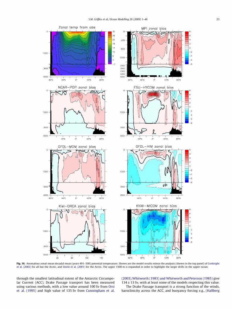
Fig. 16. Anomalous zonal-mean decadal mean (years 491–500) potential temperature. Shown are the model results minus the analysis (shown in the top panel) of Conkrightet al. (2002) for all but the Arctic, and Steele et al. (2001) for the Arctic. The upper 1500 m is expanded in order to highlight the larger drifts in the upper ocean.
S.M. Griffies et al. / Ocean Modelling 26 (2009) 1–46 23
through the smallest latitudinal extent of the Antarctic Circumpo-lar Current (ACC). Drake Passage transport has been measuredusing various methods, with a low value around 100 Sv from Orsiet al. (1995) and high value of 135 Sv from Cunningham et al.
(2003).Whitworth (1983) and Whitworth and Peterson (1985) give134 ± 13 Sv, with at least some of the models respecting this value.
The Drake Passage transport is a strong function of the winds,baroclinicity across the ACC, and buoyancy forcing e.g., (Hallberg
Fig. 17. Anomalous zonal-mean decadal mean (years 491–500) salinity. Shown are the model results minus the analysis (shown in the top panel) of Conkright et al. (2002) forall but the Arctic, and Steele et al. (2001) for the Arctic. The upper 1500 m is expanded in order to highlight the larger drifts in the upper ocean.
24 S.M. Griffies et al. / Ocean Modelling 26 (2009) 1–46
and Gnanadesikan, 2006) and references therein. It is thus very dif-ficult to determine the causes of model inaccuracies in simulatingthis transport. Nonetheless, comparing the simulated transportsbetween the models provides a useful diagnostic for this criticalpart of the ocean climate system (Russell et al., 2006).
13.1. Descriptive comments
Fig. 18 shows the time series for annual mean Drake Passagetransport from the CORE simulations. The transport in the KNMI-MI-COM simulation rapidly dives toward a very small value, reaching
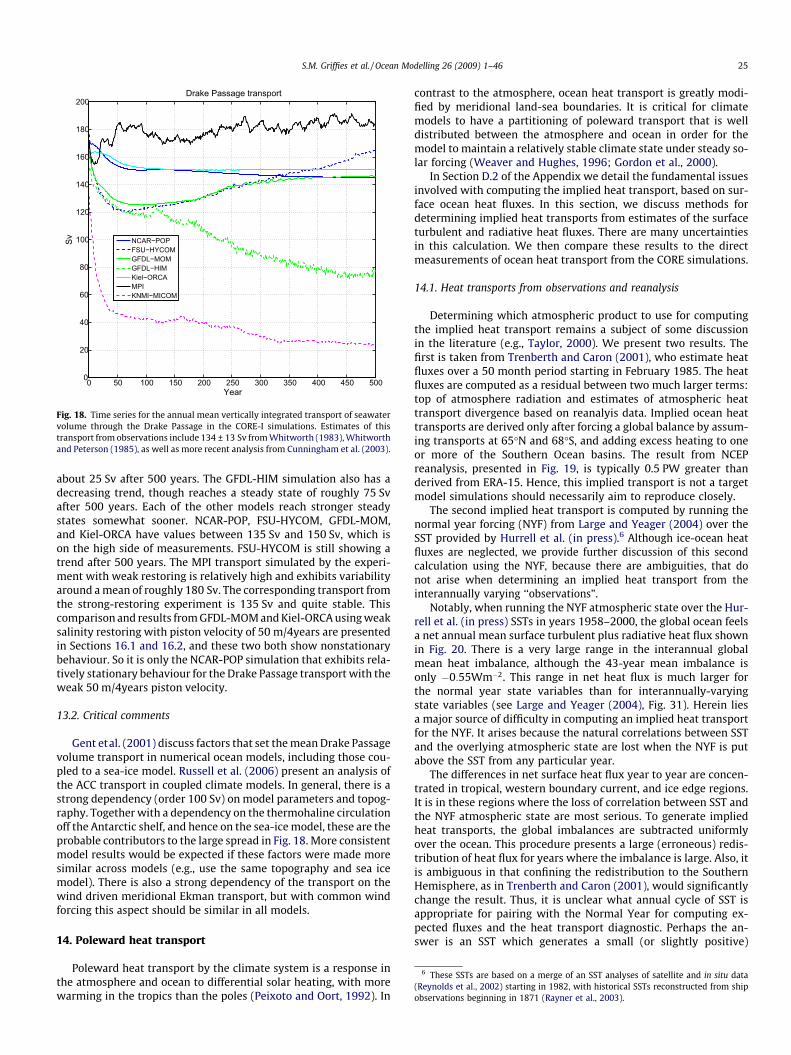
6 These SSTs are based on a merge of an SST analyses of satellite and in situ data(Reynolds et al., 2002) starting in 1982, with historical SSTs reconstructed from shipobservations beginning in 1871 (Rayner et al., 2003).
0 50 100 150 200 250 300 350 400 450 5000
20
40
60
80
100
120
140
160
180
200Drake Passage transport
Year
Sv NCAR−POPFSU−HYCOMGFDL−MOMGFDL−HIMKiel−ORCAMPIKNMI−MICOM
Fig. 18. Time series for the annual mean vertically integrated transport of seawatervolume through the Drake Passage in the CORE-I simulations. Estimates of thistransport from observations include 134 ± 13 Sv from Whitworth (1983), Whitworthand Peterson (1985), as well as more recent analysis from Cunningham et al. (2003).
S.M. Griffies et al. / Ocean Modelling 26 (2009) 1–46 25
about 25 Sv after 500 years. The GFDL-HIM simulation also has adecreasing trend, though reaches a steady state of roughly 75 Svafter 500 years. Each of the other models reach stronger steadystates somewhat sooner. NCAR-POP, FSU-HYCOM, GFDL-MOM,and Kiel-ORCA have values between 135 Sv and 150 Sv, which ison the high side of measurements. FSU-HYCOM is still showing atrend after 500 years. The MPI transport simulated by the experi-ment with weak restoring is relatively high and exhibits variabilityaround a mean of roughly 180 Sv. The corresponding transport fromthe strong-restoring experiment is 135 Sv and quite stable. Thiscomparison and results from GFDL-MOM and Kiel-ORCA using weaksalinity restoring with piston velocity of 50 m/4years are presentedin Sections 16.1 and 16.2, and these two both show nonstationarybehaviour. So it is only the NCAR-POP simulation that exhibits rela-tively stationary behaviour for the Drake Passage transport with theweak 50 m/4years piston velocity.
13.2. Critical comments
Gent etal. (2001) discuss factors that set the mean Drake Passagevolume transport in numerical ocean models, including those cou-pled to a sea-ice model. Russell et al. (2006) present an analysis ofthe ACC transport in coupled climate models. In general, there is astrong dependency (order 100 Sv) on model parameters and topog-raphy. Together with a dependency on the thermohaline circulationoff the Antarctic shelf, and hence on the sea-ice model, these are theprobable contributors to the large spread in Fig. 18. More consistentmodel results would be expected if these factors were made moresimilar across models (e.g., use the same topography and sea icemodel). There is also a strong dependency of the transport on thewind driven meridional Ekman transport, but with common windforcing this aspect should be similar in all models.
14. Poleward heat transport
Poleward heat transport by the climate system is a response inthe atmosphere and ocean to differential solar heating, with morewarming in the tropics than the poles (Peixoto and Oort, 1992). In
contrast to the atmosphere, ocean heat transport is greatly modi-fied by meridional land-sea boundaries. It is critical for climatemodels to have a partitioning of poleward transport that is welldistributed between the atmosphere and ocean in order for themodel to maintain a relatively stable climate state under steady so-lar forcing (Weaver and Hughes, 1996; Gordon et al., 2000).
In Section D.2 of the Appendix we detail the fundamental issuesinvolved with computing the implied heat transport, based on sur-face ocean heat fluxes. In this section, we discuss methods fordetermining implied heat transports from estimates of the surfaceturbulent and radiative heat fluxes. There are many uncertaintiesin this calculation. We then compare these results to the directmeasurements of ocean heat transport from the CORE simulations.
14.1. Heat transports from observations and reanalysis
Determining which atmospheric product to use for computingthe implied heat transport remains a subject of some discussionin the literature (e.g., Taylor, 2000). We present two results. Thefirst is taken from Trenberth and Caron (2001), who estimate heatfluxes over a 50 month period starting in February 1985. The heatfluxes are computed as a residual between two much larger terms:top of atmosphere radiation and estimates of atmospheric heattransport divergence based on reanalyis data. Implied ocean heattransports are derived only after forcing a global balance by assum-ing transports at 65�N and 68�S, and adding excess heating to oneor more of the Southern Ocean basins. The result from NCEPreanalysis, presented in Fig. 19, is typically 0.5 PW greater thanderived from ERA-15. Hence, this implied transport is not a targetmodel simulations should necessarily aim to reproduce closely.
The second implied heat transport is computed by running thenormal year forcing (NYF) from Large and Yeager (2004) over theSST provided by Hurrell et al. (in press).6 Although ice-ocean heatfluxes are neglected, we provide further discussion of this secondcalculation using the NYF, because there are ambiguities, that donot arise when determining an implied heat transport from theinterannually varying ‘‘observations”.
Notably, when running the NYF atmospheric state over the Hur-rell et al. (in press) SSTs in years 1958–2000, the global ocean feelsa net annual mean surface turbulent plus radiative heat flux shownin Fig. 20. There is a very large range in the interannual globalmean heat imbalance, although the 43-year mean imbalance isonly �0:55Wm�2. This range in net heat flux is much larger forthe normal year state variables than for interannually-varyingstate variables (see Large and Yeager (2004), Fig. 31). Herein liesa major source of difficulty in computing an implied heat transportfor the NYF. It arises because the natural correlations between SSTand the overlying atmospheric state are lost when the NYF is putabove the SST from any particular year.
The differences in net surface heat flux year to year are concen-trated in tropical, western boundary current, and ice edge regions.It is in these regions where the loss of correlation between SST andthe NYF atmospheric state are most serious. To generate impliedheat transports, the global imbalances are subtracted uniformlyover the ocean. This procedure presents a large (erroneous) redis-tribution of heat flux for years where the imbalance is large. Also, itis ambiguous in that confining the redistribution to the SouthernHemisphere, as in Trenberth and Caron (2001), would significantlychange the result. Thus, it is unclear what annual cycle of SST isappropriate for pairing with the Normal Year for computing ex-pected fluxes and the heat transport diagnostic. Perhaps the an-swer is an SST which generates a small (or slightly positive)
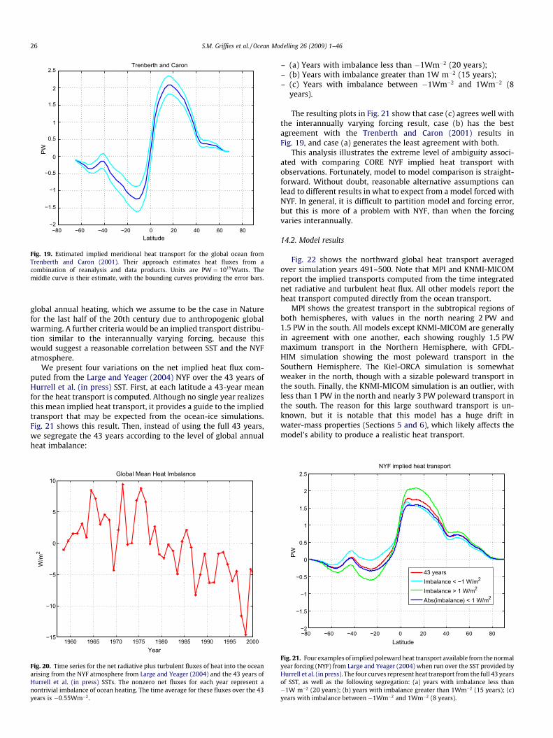
−80 −60 −40 −20 0 20 40 60 80−2
−1.5
−1
−0.5
0
0.5
1
1.5
2
2.5Trenberth and Caron
Latitude
PW
Fig. 19. Estimated implied meridional heat transport for the global ocean fromTrenberth and Caron (2001). Their approach estimates heat fluxes from acombination of reanalysis and data products. Units are PW ¼ 1015Watts. Themiddle curve is their estimate, with the bounding curves providing the error bars.
26 S.M. Griffies et al. / Ocean Modelling 26 (2009) 1–46
global annual heating, which we assume to be the case in Naturefor the last half of the 20th century due to anthropogenic globalwarming. A further criteria would be an implied transport distribu-tion similar to the interannually varying forcing, because thiswould suggest a reasonable correlation between SST and the NYFatmosphere.
We present four variations on the net implied heat flux com-puted from the Large and Yeager (2004) NYF over the 43 years ofHurrell et al. (in press) SST. First, at each latitude a 43-year meanfor the heat transport is computed. Although no single year realizesthis mean implied heat transport, it provides a guide to the impliedtransport that may be expected from the ocean-ice simulations.Fig. 21 shows this result. Then, instead of using the full 43 years,we segregate the 43 years according to the level of global annualheat imbalance:
1960 1965 1970 1975 1980 1985 1990 1995 2000−15
−10
−5
0
5
10Global Mean Heat Imbalance
Year
W/m
2
Fig. 20. Time series for the net radiative plus turbulent fluxes of heat into the oceanarising from the NYF atmosphere from Large and Yeager (2004) and the 43 years ofHurrell et al. (in press) SSTs. The nonzero net fluxes for each year represent anontrivial imbalance of ocean heating. The time average for these fluxes over the 43years is �0:55Wm�2.
– (a) Years with imbalance less than �1Wm�2 (20 years);– (b) Years with imbalance greater than 1W m�2 (15 years);– (c) Years with imbalance between �1Wm�2 and 1Wm�2 (8
years).
The resulting plots in Fig. 21 show that case (c) agrees well withthe interannually varying forcing result, case (b) has the bestagreement with the Trenberth and Caron (2001) results inFig. 19, and case (a) generates the least agreement with both.
This analysis illustrates the extreme level of ambiguity associ-ated with comparing CORE NYF implied heat transport withobservations. Fortunately, model to model comparison is straight-forward. Without doubt, reasonable alternative assumptions canlead to different results in what to expect from a model forced withNYF. In general, it is difficult to partition model and forcing error,but this is more of a problem with NYF, than when the forcingvaries interannually.
14.2. Model results
Fig. 22 shows the northward global heat transport averagedover simulation years 491–500. Note that MPI and KNMI-MICOMreport the implied transports computed from the time integratednet radiative and turbulent heat flux. All other models report theheat transport computed directly from the ocean transport.
MPI shows the greatest transport in the subtropical regions ofboth hemispheres, with values in the north nearing 2 PW and1.5 PW in the south. All models except KNMI-MICOM are generallyin agreement with one another, each showing roughly 1.5 PWmaximum transport in the Northern Hemisphere, with GFDL-HIM simulation showing the most poleward transport in theSouthern Hemisphere. The Kiel-ORCA simulation is somewhatweaker in the north, though with a sizable poleward transport inthe south. Finally, the KNMI-MICOM simulation is an outlier, withless than 1 PW in the north and nearly 3 PW poleward transport inthe south. The reason for this large southward transport is un-known, but it is notable that this model has a huge drift inwater-mass properties (Sections 5 and 6), which likely affects themodel’s ability to produce a realistic heat transport.
−80 −60 −40 −20 0 20 40 60 80−2
−1.5
−1
−0.5
0
0.5
1
1.5
2
2.5NYF implied heat transport
Latitude
PW
43 yearsImbalance < −1 W/m2
Imbalance > 1 W/m2
Abs(imbalance) < 1 W/m2
Fig. 21. Four examples of implied poleward heat transport available from the normalyear forcing (NYF) from Large and Yeager (2004) when run over the SST provided byHurrell et al. (in press). The four curves represent heat transport from the full 43 yearsof SST, as well as the following segregation: (a) years with imbalance less than�1W m�2 (20 years); (b) years with imbalance greater than 1Wm�2 (15 years); (c)years with imbalance between �1Wm�2 and 1Wm�2 (8 years).
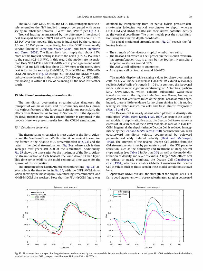
S.M. Griffies et al. / Ocean Modelling 26 (2009) 1–46 27
The NCAR-POP, GFDL-MOM, and GFDL-HIM transport most clo-sely resembles the NYF implied transport computed with yearsseeing an imbalance between �1Wm�2 and 1Wm�2 (see Fig. 21).
Tropical heating, as measured by the difference in northwardheat transport between 20�N and 20�S, ranges from about 2.3 to3.5 PW over the models. This range is bracketed by the values of2.0 and 3.5 PW given, respectively, from the CORE interannuallyvarying forcing of Large and Yeager (2004) and from Trenberthand Caron (2001). The fluxes from both imply that about 1 PWmore of this tropical heating is lost to the north (1.7–2.2 PW) thanto the south (0.3–1.3 PW). In this regard the models are inconsis-tent. Only NCAR-POP and GFDL-MOM are in good agreement, whileGFDL-HIM and MPI only lose about 0.3 PW more to the north. Moreheat is lost to the south by Kiel-ORCA, FSU-HYCOM and KNMI-MI-COM. All curves of Fig. 22, except FSU-HYCOM and KNMI-MICOM,indicate some heating in the vicinity of 50S. Except for GFDL-HIM,this heating is within 0.3 PW of balancing all the heat lost farthersouth.
15. Meridional overturning streamfunction
The meridional overturning streamfunction diagnoses thetransport of volume or mass, and it is commonly used to summa-rise various features of the large scale circulation, particularly theeffects from thermohaline forcing. In Section D.1 in the Appendix,we detail methods for how this streamfunction is computed in themodels. Here, we present results from the CORE-I simulations.
15.1. Descriptive comments
The thermohaline circulation is most active in the North Atlan-tic and the Southern Ocean. We thus find it convenient to examinethe former in the Atlantic MOC streamfunction (Fig. 23) and thelatter in the global streamfunction (Fig. 24), where each is timeaveraged over years 491–500 of the simulations. Additionally,Fig. 25 shows the time series for the maximum of the North Atlan-tic streamfunction at 45�N beneath the wind driven Ekman layer.This time series exhibits the multi-centennial time scales for thespin-up of this circulation.
The structure of the North Atlantic streamfunctions (Fig. 23) lar-gely reflects the time series in Fig. 25, with the GFDL-MOM simu-lation showing the most vigorous overturning streamfunction, andKNMI-MICOM the weakest. Note that the FSU-HYCOM figure was
−80 −60 −40 −20 0 20 40 60 80−2
−1.5
−1
−0.5
0
0.5
1
1.5
2
2.5Poleward heat transport
Latitude
PW
NCAR−POPFSU−HYCOMGFDL−MOMGFDL−HIM
Fig. 22. Northward heat transport for the global ocean as determined by the ocean modelresolved advective and SGS transport contributions. Units are PW ¼ 1015Watts.
obtained by interpolating from its native hybrid pressure-den-sity-terrain following vertical coordinates to depth, whereasGFDL-HIM and KNMI-MICOM use their native potential densityas the vertical coordinate. The other models plot the streamfunc-tion using their native depth coordinates.
The global meridional streamfunction (Fig. 24) reveals the fol-lowing features:
– The strength of the vigorous tropical wind-driven cells;– The Deacon Cell, which is a cell present in the Eulerian overturn-
ing streamfunction that is driven by the Southern Hemispheresubpolar westerlies around 60�S;
– The AABW cell adjacent to Antarctica;– An abyssal cell centred at around 20–40�S.
The models display wide-ranging values for these overturningcells. All z-level models as well as FSU-HYCOM exhibit reasonablyrealistic AABW cells of strength 5–10 Sv. In contrast, the isopycnalmodels show more vigorous overturning off Antarctica, particu-larly KNMI-MICOM, which exhibits substantial water-masstransformation at the high-latitude Southern Ocean, feeding anabyssal cell that ventilates much of the global ocean at mid-depth.Indeed, there is little evidence for northern sinking in this model,leaving its water-masses too cold and fresh almost everywhere(Figs. 16 and 17).
The Deacon cell is nearly absent when plotted in density-lati-tude space (Webb, 1994; Karoly et al., 1997), as seen in the isopyc-nal models. In depth-latitude space, the Deacon Cell takes values inexcess of 20 Sv in each of the z-level models, as well as in FSU-HY-COM. In general, the depth-latitude Deacon Cell is reduced in mag-nitude by the Gent and McWilliams (1990) parameterisation, withequatorward meridional velocity counteracted by polewardparameterised eddy induced velocity (Hirst and McDougall,1998). The strength of the reverse Deacon Cell arising from theGM streamfunction is set by parameters used in the SGS parame-terisation, such as the diffusivity and treatment of steep neutralslope regions (see Table 6 in Section D.3), as well as the model dis-tribution of density and layer thickness. A larger ‘‘GM-effect” actsto reduce, or nearly eliminate, the Deacon Cell (Danabasogluet al., 1994), whereas a smaller GM-effect maintains the DeaconCell at values such as those seen in the z-model simulations shownhere.
Apart from KNMI-MICOM, the strength of the abyssal cells is infairly good agreement with observed estimates, ranging between 6
−80 −60 −40 −20 0 20 40 60 80−2
−1.5
−1
−0.5
0
0.5
1
1.5
2
2.5Poleward heat transport
Latitude
PW
KNMI−MICOMKiel−ORCAMPI
s. Results are decadal means from model years 491–500, and the values include both
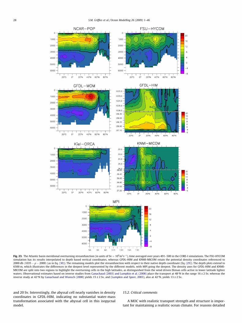
Fig. 23. The Atlantic basin meridional overturning streamfunction (in units of Sv ¼ 106m3s�1), time averaged over years 491–500 in the CORE-I simulations. The FSU-HYCOMsimulation has its results interpolated to depth based vertical coordinates, whereas GFDL-HIM and KNMI-MICOM retain the potential density coordinates referenced to2000 db ð1035� q� 2000Þ (as in Eq. (30)). The remaining models plot the streamfunction with respect to their native depth coordinate (Eq. (29)). The depth plots extend to6500 m, which illustrates the differences in the deepest level represented by the different models, with MPI going the deepest. The density axes for GFDL-HIM and KNMI-MICOM are split into two regions to highlight the overturning cells in the high latitudes, as distinguished from the wind driven Ekman cells active in lower latitude lighterwaters. Observational estimates based on inverse studies from Ganachaud (2003) and Lumpkin et al. (2008) place the transport at 48�N in the range 16 ± 2 Sv, whereas theinverse study at 42�N by Ganachaud and Wunsch (2000) yields 15 ± 2 Sv, and (Lumpkin and Speer, 2003), also at 42�N, yields 13 ± 2 Sv.
28 S.M. Griffies et al. / Ocean Modelling 26 (2009) 1–46
and 20 Sv. Interestingly, the abyssal cell nearly vanishes in densitycoordinates in GFDL-HIM, indicating no substantial water-masstransformation associated with the abyssal cell in this isopycnalmodel.
15.2. Critical comments
A MOC with realistic transport strength and structure is impor-tant for maintaining a realistic ocean climate. For reasons detailed
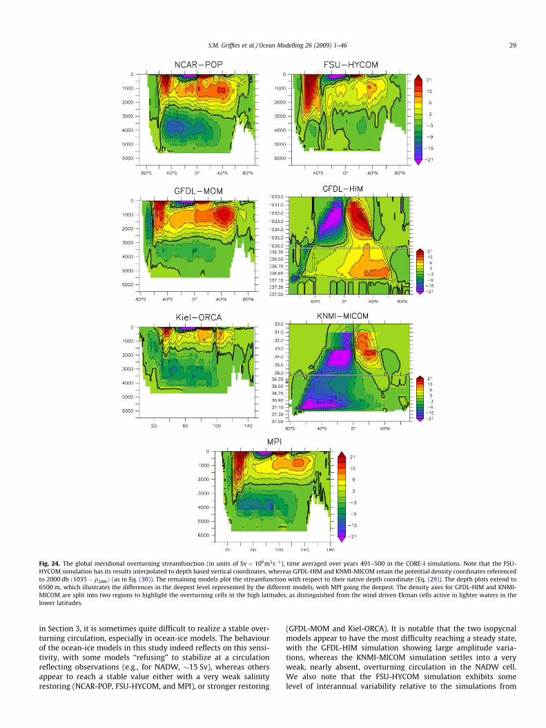
Fig. 24. The global meridional overturning streamfunction (in units of Sv ¼ 106m3s�1), time averaged over years 491–500 in the CORE-I simulations. Note that the FSU-HYCOM simulation has its results interpolated to depth based vertical coordinates, whereas GFDL-HIM and KNMI-MICOM retain the potential density coordinates referencedto 2000 db ð1035� q2000Þ (as in Eq. (30)). The remaining models plot the streamfunction with respect to their native depth coordinate (Eq. (29)). The depth plots extend to6500 m, which illustrates the differences in the deepest level represented by the different models, with MPI going the deepest. The density axes for GFDL-HIM and KNMI-MICOM are split into two regions to highlight the overturning cells in the high latitudes, as distinguished from the wind driven Ekman cells active in lighter waters in thelower latitudes.
S.M. Griffies et al. / Ocean Modelling 26 (2009) 1–46 29
in Section 3, it is sometimes quite difficult to realize a stable over-turning circulation, especially in ocean-ice models. The behaviourof the ocean-ice models in this study indeed reflects on this sensi-tivity, with some models ‘‘refusing” to stabilize at a circulationreflecting observations (e.g., for NADW, �15 Sv), whereas othersappear to reach a stable value either with a very weak salinityrestoring (NCAR-POP, FSU-HYCOM, and MPI), or stronger restoring
(GFDL-MOM and Kiel-ORCA). It is notable that the two isopycnalmodels appear to have the most difficulty reaching a steady state,with the GFDL-HIM simulation showing large amplitude varia-tions, whereas the KNMI-MICOM simulation settles into a veryweak, nearly absent, overturning circulation in the NADW cell.We also note that the FSU-HYCOM simulation exhibits somelevel of interannual variability relative to the simulations from
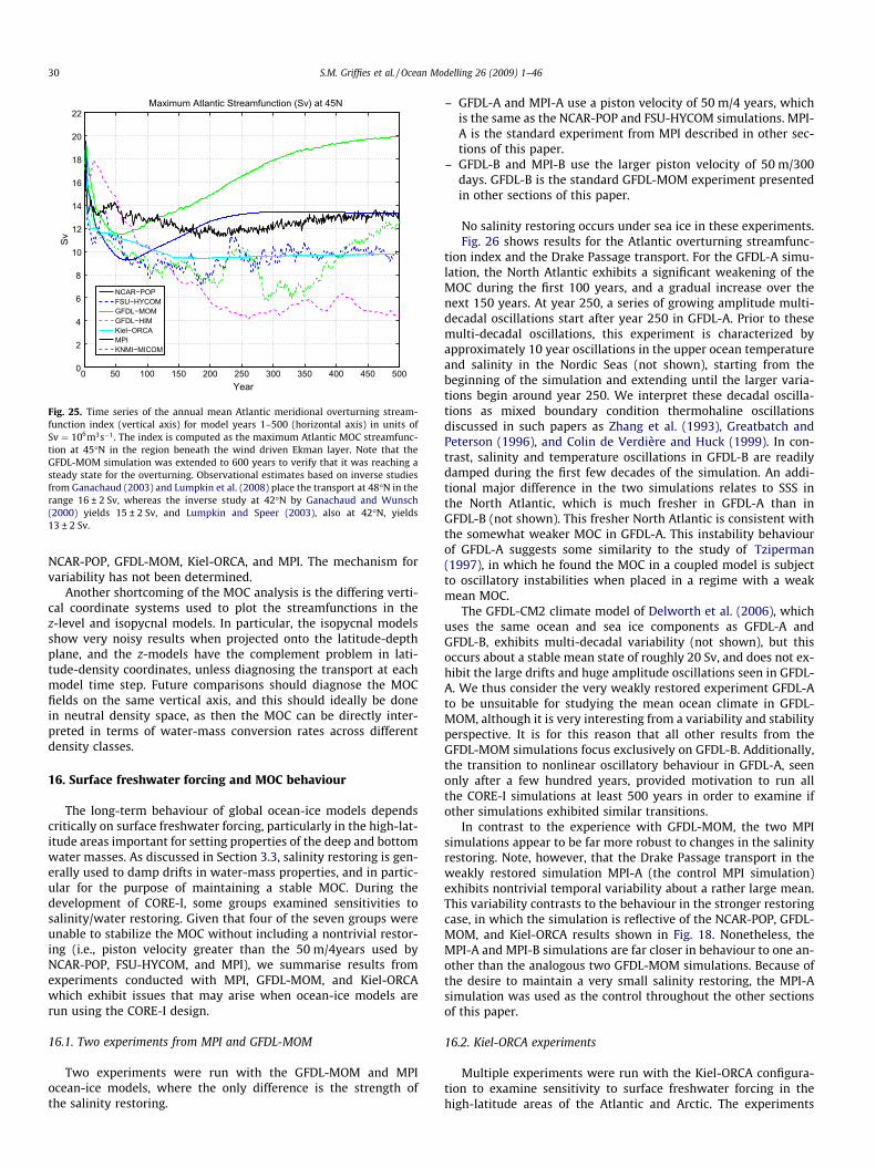
0 50 100 150 200 250 300 350 400 450 5000
2
4
6
8
10
12
14
16
18
20
22Maximum Atlantic Streamfunction (Sv) at 45N
Year
Sv
NCAR−POPFSU−HYCOMGFDL−MOMGFDL−HIMKiel−ORCAMPIKNMI−MICOM
Fig. 25. Time series of the annual mean Atlantic meridional overturning stream-function index (vertical axis) for model years 1–500 (horizontal axis) in units ofSv ¼ 106m3s�1. The index is computed as the maximum Atlantic MOC streamfunc-tion at 45�N in the region beneath the wind driven Ekman layer. Note that theGFDL-MOM simulation was extended to 600 years to verify that it was reaching asteady state for the overturning. Observational estimates based on inverse studiesfrom Ganachaud (2003) and Lumpkin et al. (2008) place the transport at 48�N in therange 16 ± 2 Sv, whereas the inverse study at 42�N by Ganachaud and Wunsch(2000) yields 15 ± 2 Sv, and Lumpkin and Speer (2003), also at 42�N, yields13 ± 2 Sv.
30 S.M. Griffies et al. / Ocean Modelling 26 (2009) 1–46
NCAR-POP, GFDL-MOM, Kiel-ORCA, and MPI. The mechanism forvariability has not been determined.
Another shortcoming of the MOC analysis is the differing verti-cal coordinate systems used to plot the streamfunctions in thez-level and isopycnal models. In particular, the isopycnal modelsshow very noisy results when projected onto the latitude-depthplane, and the z-models have the complement problem in lati-tude-density coordinates, unless diagnosing the transport at eachmodel time step. Future comparisons should diagnose the MOCfields on the same vertical axis, and this should ideally be donein neutral density space, as then the MOC can be directly inter-preted in terms of water-mass conversion rates across differentdensity classes.
16. Surface freshwater forcing and MOC behaviour
The long-term behaviour of global ocean-ice models dependscritically on surface freshwater forcing, particularly in the high-lat-itude areas important for setting properties of the deep and bottomwater masses. As discussed in Section 3.3, salinity restoring is gen-erally used to damp drifts in water-mass properties, and in partic-ular for the purpose of maintaining a stable MOC. During thedevelopment of CORE-I, some groups examined sensitivities tosalinity/water restoring. Given that four of the seven groups wereunable to stabilize the MOC without including a nontrivial restor-ing (i.e., piston velocity greater than the 50 m/4years used byNCAR-POP, FSU-HYCOM, and MPI), we summarise results fromexperiments conducted with MPI, GFDL-MOM, and Kiel-ORCAwhich exhibit issues that may arise when ocean-ice models arerun using the CORE-I design.
16.1. Two experiments from MPI and GFDL-MOM
Two experiments were run with the GFDL-MOM and MPIocean-ice models, where the only difference is the strength ofthe salinity restoring.
– GFDL-A and MPI-A use a piston velocity of 50 m/4 years, whichis the same as the NCAR-POP and FSU-HYCOM simulations. MPI-A is the standard experiment from MPI described in other sec-tions of this paper.
– GFDL-B and MPI-B use the larger piston velocity of 50 m/300days. GFDL-B is the standard GFDL-MOM experiment presentedin other sections of this paper.
No salinity restoring occurs under sea ice in these experiments.Fig. 26 shows results for the Atlantic overturning streamfunc-
tion index and the Drake Passage transport. For the GFDL-A simu-lation, the North Atlantic exhibits a significant weakening of theMOC during the first 100 years, and a gradual increase over thenext 150 years. At year 250, a series of growing amplitude multi-decadal oscillations start after year 250 in GFDL-A. Prior to thesemulti-decadal oscillations, this experiment is characterized byapproximately 10 year oscillations in the upper ocean temperatureand salinity in the Nordic Seas (not shown), starting from thebeginning of the simulation and extending until the larger varia-tions begin around year 250. We interpret these decadal oscilla-tions as mixed boundary condition thermohaline oscillationsdiscussed in such papers as Zhang et al. (1993), Greatbatch andPeterson (1996), and Colin de Verdière and Huck (1999). In con-trast, salinity and temperature oscillations in GFDL-B are readilydamped during the first few decades of the simulation. An addi-tional major difference in the two simulations relates to SSS inthe North Atlantic, which is much fresher in GFDL-A than inGFDL-B (not shown). This fresher North Atlantic is consistent withthe somewhat weaker MOC in GFDL-A. This instability behaviourof GFDL-A suggests some similarity to the study of Tziperman(1997), in which he found the MOC in a coupled model is subjectto oscillatory instabilities when placed in a regime with a weakmean MOC.
The GFDL-CM2 climate model of Delworth et al. (2006), whichuses the same ocean and sea ice components as GFDL-A andGFDL-B, exhibits multi-decadal variability (not shown), but thisoccurs about a stable mean state of roughly 20 Sv, and does not ex-hibit the large drifts and huge amplitude oscillations seen in GFDL-A. We thus consider the very weakly restored experiment GFDL-Ato be unsuitable for studying the mean ocean climate in GFDL-MOM, although it is very interesting from a variability and stabilityperspective. It is for this reason that all other results from theGFDL-MOM simulations focus exclusively on GFDL-B. Additionally,the transition to nonlinear oscillatory behaviour in GFDL-A, seenonly after a few hundred years, provided motivation to run allthe CORE-I simulations at least 500 years in order to examine ifother simulations exhibited similar transitions.
In contrast to the experience with GFDL-MOM, the two MPIsimulations appear to be far more robust to changes in the salinityrestoring. Note, however, that the Drake Passage transport in theweakly restored simulation MPI-A (the control MPI simulation)exhibits nontrivial temporal variability about a rather large mean.This variability contrasts to the behaviour in the stronger restoringcase, in which the simulation is reflective of the NCAR-POP, GFDL-MOM, and Kiel-ORCA results shown in Fig. 18. Nonetheless, theMPI-A and MPI-B simulations are far closer in behaviour to one an-other than the analogous two GFDL-MOM simulations. Because ofthe desire to maintain a very small salinity restoring, the MPI-Asimulation was used as the control throughout the other sectionsof this paper.
16.2. Kiel-ORCA experiments
Multiple experiments were run with the Kiel-ORCA configura-tion to examine sensitivity to surface freshwater forcing in thehigh-latitude areas of the Atlantic and Arctic. The experiments
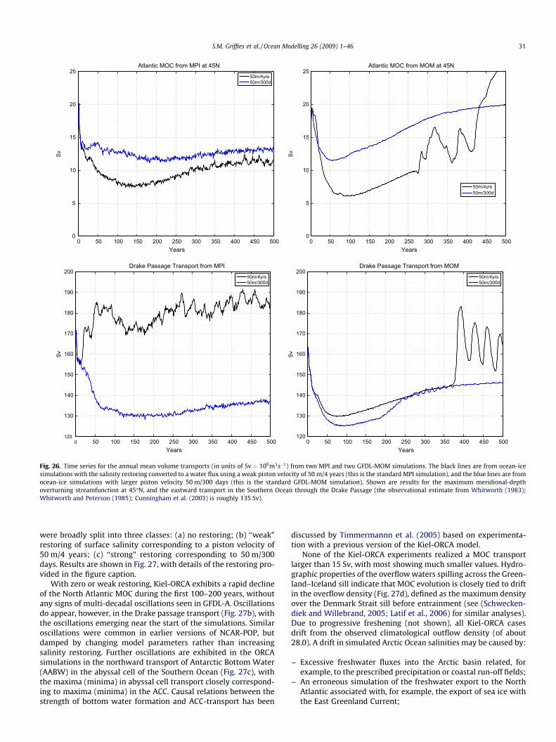
0 50 100 150 200 250 300 350 400 450 5000
5
10
15
20
25Atlantic MOC from MPI at 45N
Years
Sv
50m/4yrs50m/300d
0 50 100 150 200 250 300 350 400 450 5000
5
10
15
20
25Atlantic MOC from MOM at 45N
Years
Sv
50m/4yrs50m/300d
0 50 100 150 200 250 300 350 400 450 500120
130
140
150
160
170
180
190
200Drake Passage Transport from MPI
Years
Sv
50m/4yrs50m/300d
0 50 100 150 200 250 300 350 400 450 500120
130
140
150
160
170
180
190
200Drake Passage Transport from MOM
Years
Sv
50m/4yrs50m/300d
Fig. 26. Time series for the annual mean volume transports (in units of Sv ¼ 106m3s�1) from two MPI and two GFDL-MOM simulations. The black lines are from ocean-icesimulations with the salinity restoring converted to a water flux using a weak piston velocity of 50 m/4 years (this is the standard MPI simulation), and the blue lines are fromocean-ice simulations with larger piston velocity 50 m/300 days (this is the standard GFDL-MOM simulation). Shown are results for the maximum meridional-depthoverturning streamfunction at 45�N, and the eastward transport in the Southern Ocean through the Drake Passage (the observational estimate from Whitworth (1983);Whitworth and Peterson (1985); Cunningham et al. (2003) is roughly 135 Sv).
S.M. Griffies et al. / Ocean Modelling 26 (2009) 1–46 31
were broadly split into three classes: (a) no restoring; (b) ‘‘weak”restoring of surface salinity corresponding to a piston velocity of50 m/4 years; (c) ‘‘strong” restoring corresponding to 50 m/300days. Results are shown in Fig. 27, with details of the restoring pro-vided in the figure caption.
With zero or weak restoring, Kiel-ORCA exhibits a rapid declineof the North Atlantic MOC during the first 100–200 years, withoutany signs of multi-decadal oscillations seen in GFDL-A. Oscillationsdo appear, however, in the Drake passage transport (Fig. 27b), withthe oscillations emerging near the start of the simulations. Similaroscillations were common in earlier versions of NCAR-POP, butdamped by changing model parameters rather than increasingsalinity restoring. Further oscillations are exhibited in the ORCAsimulations in the northward transport of Antarctic Bottom Water(AABW) in the abyssal cell of the Southern Ocean (Fig. 27c), withthe maxima (minima) in abyssal cell transport closely correspond-ing to maxima (minima) in the ACC. Causal relations between thestrength of bottom water formation and ACC-transport has been
discussed by Timmermannn et al. (2005) based on experimenta-tion with a previous version of the Kiel-ORCA model.
None of the Kiel-ORCA experiments realized a MOC transportlarger than 15 Sv, with most showing much smaller values. Hydro-graphic properties of the overflow waters spilling across the Green-land–Iceland sill indicate that MOC evolution is closely tied to driftin the overflow density (Fig. 27d), defined as the maximum densityover the Denmark Strait sill before entrainment (see (Schwecken-diek and Willebrand, 2005; Latif et al., 2006) for similar analyses).Due to progressive freshening (not shown), all Kiel-ORCA casesdrift from the observed climatological outflow density (of about28.0). A drift in simulated Arctic Ocean salinities may be caused by:
– Excessive freshwater fluxes into the Arctic basin related, forexample, to the prescribed precipitation or coastal run-off fields;
– An erroneous simulation of the freshwater export to the NorthAtlantic associated with, for example, the export of sea ice withthe East Greenland Current;
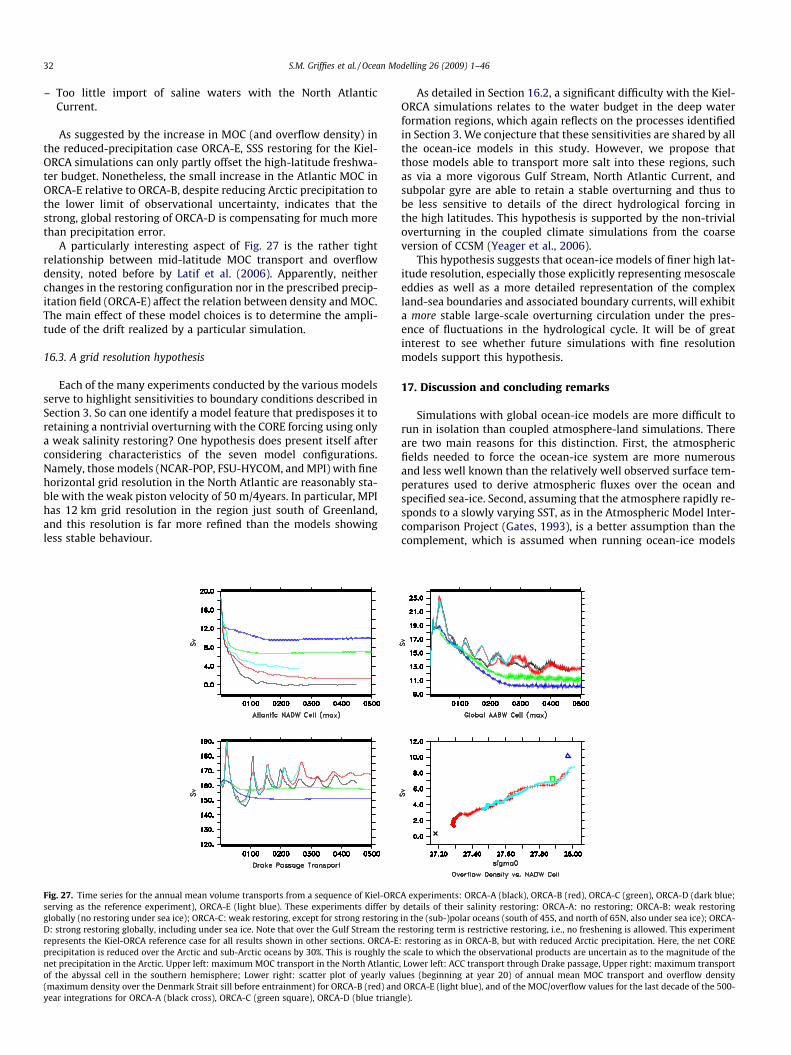
32 S.M. Griffies et al. / Ocean Modelling 26 (2009) 1–46
– Too little import of saline waters with the North AtlanticCurrent.
As suggested by the increase in MOC (and overflow density) inthe reduced-precipitation case ORCA-E, SSS restoring for the Kiel-ORCA simulations can only partly offset the high-latitude freshwa-ter budget. Nonetheless, the small increase in the Atlantic MOC inORCA-E relative to ORCA-B, despite reducing Arctic precipitation tothe lower limit of observational uncertainty, indicates that thestrong, global restoring of ORCA-D is compensating for much morethan precipitation error.
A particularly interesting aspect of Fig. 27 is the rather tightrelationship between mid-latitude MOC transport and overflowdensity, noted before by Latif et al. (2006). Apparently, neitherchanges in the restoring configuration nor in the prescribed precip-itation field (ORCA-E) affect the relation between density and MOC.The main effect of these model choices is to determine the ampli-tude of the drift realized by a particular simulation.
16.3. A grid resolution hypothesis
Each of the many experiments conducted by the various modelsserve to highlight sensitivities to boundary conditions described inSection 3. So can one identify a model feature that predisposes it toretaining a nontrivial overturning with the CORE forcing using onlya weak salinity restoring? One hypothesis does present itself afterconsidering characteristics of the seven model configurations.Namely, those models (NCAR-POP, FSU-HYCOM, and MPI) with finehorizontal grid resolution in the North Atlantic are reasonably sta-ble with the weak piston velocity of 50 m/4years. In particular, MPIhas 12 km grid resolution in the region just south of Greenland,and this resolution is far more refined than the models showingless stable behaviour.
Fig. 27. Time series for the annual mean volume transports from a sequence of Kiel-ORCserving as the reference experiment), ORCA-E (light blue). These experiments differ byglobally (no restoring under sea ice); ORCA-C: weak restoring, except for strong restoringD: strong restoring globally, including under sea ice. Note that over the Gulf Stream the rrepresents the Kiel-ORCA reference case for all results shown in other sections. ORCA-Eprecipitation is reduced over the Arctic and sub-Arctic oceans by 30%. This is roughly thenet precipitation in the Arctic. Upper left: maximum MOC transport in the North Atlanticof the abyssal cell in the southern hemisphere; Lower right: scatter plot of yearly va(maximum density over the Denmark Strait sill before entrainment) for ORCA-B (red) andyear integrations for ORCA-A (black cross), ORCA-C (green square), ORCA-D (blue triang
As detailed in Section 16.2, a significant difficulty with the Kiel-ORCA simulations relates to the water budget in the deep waterformation regions, which again reflects on the processes identifiedin Section 3. We conjecture that these sensitivities are shared by allthe ocean-ice models in this study. However, we propose thatthose models able to transport more salt into these regions, suchas via a more vigorous Gulf Stream, North Atlantic Current, andsubpolar gyre are able to retain a stable overturning and thus tobe less sensitive to details of the direct hydrological forcing inthe high latitudes. This hypothesis is supported by the non-trivialoverturning in the coupled climate simulations from the coarseversion of CCSM (Yeager et al., 2006).
This hypothesis suggests that ocean-ice models of finer high lat-itude resolution, especially those explicitly representing mesoscaleeddies as well as a more detailed representation of the complexland-sea boundaries and associated boundary currents, will exhibita more stable large-scale overturning circulation under the pres-ence of fluctuations in the hydrological cycle. It will be of greatinterest to see whether future simulations with fine resolutionmodels support this hypothesis.
17. Discussion and concluding remarks
Simulations with global ocean-ice models are more difficult torun in isolation than coupled atmosphere-land simulations. Thereare two main reasons for this distinction. First, the atmosphericfields needed to force the ocean-ice system are more numerousand less well known than the relatively well observed surface tem-peratures used to derive atmospheric fluxes over the ocean andspecified sea-ice. Second, assuming that the atmosphere rapidly re-sponds to a slowly varying SST, as in the Atmospheric Model Inter-comparison Project (Gates, 1993), is a better assumption than thecomplement, which is assumed when running ocean-ice models
A experiments: ORCA-A (black), ORCA-B (red), ORCA-C (green), ORCA-D (dark blue;details of their salinity restoring: ORCA-A: no restoring; ORCA-B: weak restoring
in the (sub-)polar oceans (south of 45S, and north of 65N, also under sea ice); ORCA-estoring term is restrictive restoring, i.e., no freshening is allowed. This experiment
: restoring as in ORCA-B, but with reduced Arctic precipitation. Here, the net COREscale to which the observational products are uncertain as to the magnitude of the
, Lower left: ACC transport through Drake passage, Upper right: maximum transportlues (beginning at year 20) of annual mean MOC transport and overflow density
ORCA-E (light blue), and of the MOC/overflow values for the last decade of the 500-le).
S.M. Griffies et al. / Ocean Modelling 26 (2009) 1–46 33
with a prescribed atmospheric state. These points largely accountfor the lack of a community supported Ocean Model Intercompar-ison Project (OMIP) 15 years after the initiation of AMIP.
17.1. Strategies for modelling the ocean-ice climate system
There are two general conclusions one can draw when recogniz-ing the difficulty running global ocean-ice models for climate pur-poses. First, one may choose to always run ocean-ice modelscoupled to a dynamical atmosphere and thus tolerate its inherentbiases. That is, to jettison the notion of running ocean-ice modelsaltogether, and thus to insist on only studying simulations fromrealistic climate models, where a prescribed atmosphere is unac-ceptable for the goals of, for example, climate change science. Itis notable that this trend is being followed by scientists at GFDL,NCAR, and the Hadley Centre, where ocean-ice simulations arebecoming less common than fully coupled climate simulations,even for purposes of developing ocean-ice models. Alternatively,one may consider realistic ocean-ice models coupled to atmo-spheric energy balance models, such as discussed for the CORE-IIIexperiments of Gerdes et al. (2005a, 2006). This approach requiresfar less overhead in atmospheric modelling expertise, and so ismore available to groups focused just on ocean and sea ice model-ling research. Either of these approaches which use a prognosticatmosphere precludes using the ocean-ice models for many ofthe purposes outlined in Section 2; most notably being an inabilityto perform reanalysis simulations aimed at interpreting the ob-served ocean record.
A second conclusion that can be drawn is to acknowledge thelimitations inherent with ocean-ice models, and to thus use themfor selected research studies within a hierarchy of numerical cli-mate science tools, ideally with a fully coupled climate model aspart of this hierarchy. This second conclusion is taken by many re-search groups, and it is used as motivation for our proposal ofCoordinated Ocean-ice Reference Experiments (COREs) in hope offacilitating collaborative research and model development. Thatis, we aim with CORE to bring the ocean-ice models onto a com-mon platform for experimental design and prescribed atmosphericstate, from which remaining model differences can be used to as-cribe reasons for diverging simulation behaviour.
Given our proposed CORE simulations, we illustrated resultsfrom seven ocean-ice models run with the CORE-I experimentaldesign, which involves running the models for 500 years withthe Normal Year Forcing from Large and Yeager (2004). These sim-ulations allowed us to test the hypothesis that global ocean-icemodels run under common forcing conditions will result in quali-tatively similar simulations. This paper finds this hypothesis not tobe valid in general, though the degree is very dependent on theparticular diagnostic chosen, and the model sub-set. The nontrivialdifferences arising from the simulations are often not related to theocean model vertical coordinate, which highlights the need to fur-ther examine the mechanisms accounting for the divergences.
17.2. Concerning the merit of model comparisons
A large part of this project was aimed at answering questionsabout the feasibility of bringing ocean-ice models onto a commondesign framework. A key reason for doing so is to ensure that dif-ferences between model simulations are not attributed to differ-ences in atmospheric forcing. These questions have beenanswered in the affirmative by the existence of seven contributinggroups having followed the CORE-I protocol. Questions regardingthe merit of this exercise have also been raised. What is gained?Comparison projects can be fraught with difficulties in bringingthe variety of model configurations into a reasonably controlledand understood setting. These difficulties make it tough to learn
anything new regarding mechanisms for simulation differences,and this point can be used to criticise a model comparison project.
However, these difficulties are not an argument for the dis-util-ity of comparisons. Instead, the utility of such ‘‘come as you are”comparisons, with the present paper falling somewhat into thiscategory, arise from the many new questions raised when simula-tions are compared and contrasted. Some questions relate to modelfundamentals and practice, each of which are brought to an ex-panded ‘‘table” when modellers using different codes collaborate.This is a healthy situation, which is handicapped when groups con-duct research in isolation. Many important questions generally gounasked in the absence of such collaborations and associated com-parisons, and such questions then motivate further focused studyconducted in a more controlled setting that aim to elucidatemechanisms.
In general, we propose that the preliminary experience withCORE-I documented in this paper provides a solid foundation fordeeper study of many important questions about ocean-ice simu-lations as well as the mechanisms affecting climate means, vari-ability, and stability. It also supports studies concerning thesuitability of a prescribed atmospheric state for running ocean-ice models, and in particular the utility of the Large and Yeager(2004, 2008) datasets, both the normal year and the interannuallyvarying versions.
17.3. COREs and coordination
CORE-I is one aspect of our envisioned coordinated suite of glo-bal ocean-ice experiments. It focuses on the longer term ocean cli-mate, with integration times sufficient for some models to reach aquasi-equilibrium. These simulations have direct relevance to thedevelopment of ocean-ice components of fully coupled climatemodels used for long term climate change simulations. Althoughfraught with the caveats detailed in Section 3, long term ocean-ice simulations from CORE-I render insights about the nature ofquasi-equilibrium ocean-ice solutions. In particular, long term sim-ulations provide a clear means to expose fundamental problemswith both the model algorithms and the experimental design.
A complement task is realized with the envisioned CORE-IIexperiment, whereby models are run with the interannually vary-ing atmospheric state from Large and Yeager (2008). These simula-tions are relevant for developing a mechanistic understanding ofthe observed ocean record compiled during the past few decades.Questions about how to initialize the models to minimise drift re-main a key aspect of the CORE-II experiment, with this nontrivialquestion largely ignored in the present focus on the longer timescale CORE-I simulations. Finally, a third aspect of the ocean-iceclimate system is addressed by considering the CORE-III experi-ment of Gerdes et al. (2005b), whereby the ocean is perturbed bya fresh water melt around Greenland, meant to emulate the possi-ble melt in a warming world. This experiment, which is similar inmany regards to those conducted as part of the Coupled ModelIntercomparison Project (see, for example, (Hewitt et al. (2006))),allows for an increased variety of ocean-ice participants, beyondthose running fully coupled climate models. It also presents theocean-ice system with an arguably more vigorous perturbation,which is both realistic and challenging to the model algorithms.
Each of the CORE-I, CORE-II, and CORE-III simulations benefitfrom coordination. This coordination assists by keeping groupsmore scientifically open. In particular, this openness promptsgroups to rationally address aspects of their simulation whichmay otherwise be ignored or overlooked. Quite literally, peer-pres-sure provides a positive element in moving modellers towards arational and robust platform. Coordination is also essential sincethe problems of ocean climate dynamics generally require teamsof scientists approaching the questions from many complementary
34 S.M. Griffies et al. / Ocean Modelling 26 (2009) 1–46
perspectives, and with differing tools. Such coordination generallyis necessary for the climate modelling community to garner robustunderstandings of climate mechanisms, which ultimately increaseour ability to rationally understand the past and to project into thefuture.
Acknowledgements
This paper was prompted by discussions occurring within theCLIVAR Working Group for Ocean Model Development (WGOMD)since the panel’s first meeting in 2000. The WGOMD sponsored aPilot-OMIP starting in 2001, with this project involving just a fewmodels. The Pilot-OMIP was itself based on an earlier comparisonof German ocean-ice models (Fritzsch et al., 2000). Both projectsused the forcing dataset compiled by Röske (2006). The culmina-tion of the Pilot-OMIP occurred at a CLIVAR workshop on ocean cli-mate modelling held June 16–18, 2004 at the Geophysical FluidDynamics Laboratory in Princeton USA. At the workshop, it wasdecided that a research project should be conducted to flesh outa benchmark simulation prior to stepping all the way towards anOMIP. This conclusion then set the stage for COREs.
We thank David Bi, Rainer Bleck, Torge Martin, Ge Peng, FrankRöske, and Ashwanth Srinivasan for critical support during variousparts of this project. We thank Laurent Brodeau for documenting theeffects of the code error in the bulk formulae calculation describedin Appendix C. David Baily provided annual mean sea ice areas forthe observational comparison in Fig. 10. Helene Banks, Riccardo Far-neti, Ron Stouffer, and two anonymous reviewers provided veryuseful comments on earlier drafts of this paper. SMG thanks CSIROMarine and Atmospheric Research in Australia for its hospitalityduring 2005, where the writing of this paper was initiated.
This paper is dedicated to the memory of Peter Killworth.
Appendix A. Contributing models
Table 1 summarises various aspects of the models used in thisstudy, and Table 2 details the model release and the date whenthe simulations were run. These models are examples of high-end global ocean-ice configurations that are actively being usedfor climate research, either in the ocean-ice configurations em-ployed in this paper, or as part of more complete climate or earthsystem models. Model details beyond those provided in thisappendix can be found in the cited references.
A.1. NCAR-POP
NCAR-POP is the ocean-ice component of the CommunityClimate System Model, CCSM3 (Collins et al., 2006). It consistsof the Los Alamos Parallel Ocean Program (POP) documentedby Smith and Gent (2004), which uses a z-coordinate for the ver-tical grid. This ocean is coupled to the Community Sea Ice Model(CSIM) that is documented by Briegleb et al. (2004). The resolu-tion is roughly one degree (320 zonal grid cells) with refinedmeridional spacing in the equatorial region (384 meridional gridcells) and 40 unevenly spaced cells in the vertical. The northcoordinate singularity is displaced over Greenland to avoid thetraditional spherical coordinate singularity at the geographicNorth Pole. This displacement also has the added feature ofrefining the grid resolution in the Labrador Sea deep water for-mation region (Smith et al., 1995). It has been hypothesized thatthis enhanced resolution in the deep water formation region isimportant for maintaining stability of the overturning circulationin the NCAR-POP CORE-I simulation (see Section 16.3). System-atic tests of this conjecture have only been performed at lowerresolution by Yeager et al. (2006).
The NCAR-POP ocean model component updates the tracer andbaroclinic velocity fields using a leap-frog for the inviscid portionof the equations with a 3600 s time step. The barotropic equationsare updated implicitly in time using a leap-frog for the tendencieswith 3600 s time step (Dukowicz and Smith, 1994). No water istransported across the ocean surface, thus necessitating salt fluxesrather than water fluxes.
Snow and ice albedos are important for computing the absorp-tion of shortwave radiation in snow and sea ice system, and hencefor setting the strength of the snow and ice albedo feedback. TheNCAR-POP sea ice model employs an albedo following the ap-proach documented in Briegleb et al. (2002). In particular, theNCAR-POP ice model distinguishes between visible (wavelengths<0.7 lm) and near-infrared (wavelengths >0.7 lm), since snowand ice spectral reflectivities are significantly higher in the visibleband than the near-infrared band. The zenith angle dependence ofsnow and ice is ignored, and therefore the distinction betweendownwelling direct and diffuse shortwave radiation is ignored.Snow and ice topography affect the scattering and transmissioninto the surface through shadowing effects and through variationsin the angle of the surface from the horizon. These topography af-fects are also ignored. For further details of the NCAR-POP albedo,refer to Briegleb et al. (2002). Although the ocean and sea ice com-ponents are the same as those used in the CCSM3.0 fully coupledclimate model (e.g., (Danabasoglu et al., 2006)), there were somemodifications made to the sea ice component parameters for usein the CORE simulations. The changes included slightly higher iceand snow albedos that are more in the middle of observed values.
The salinity of sea ice is 4 ppt. This affords a nonzero salt fluxbetween the ocean and sea ice as ice melts and forms.
A.2. FSU-HYCOM
FSU-HYCOM consists of the ocean-ice component to the Com-munity Climate System Model (Collins et al., 2006) with HYCOMversion 2.2 as the oceanic model. The horizontal grid and topogra-phy are identical to that of NCAR-POP, although the model vari-ables are arranged according to the Arakawa C-grid, rather thanthe B-grid used in NCAR-POP. FSU-HYCOM is configured with 32hybrid layers and each coordinate surface is assigned a referenceisopycnal. The model continually checks whether or not grid pointslie on their reference isopycnals and, if not, tries to move them ver-tically toward the latter (Bleck, 2002). However, the grid points arenot allowed to migrate when this would lead to excessive crowd-ing of coordinate surfaces. Thus, in the mixed layer or in shallowwater, vertical grid points are geometrically constrained to remainat a fixed pressure while being allowed to join and follow their ref-erence isopycnals over the adjacent deep ocean. Therefore, HYCOMbehaves like a pressure coordinate model in the mixed layer orother unstratified regions, like an isopycnic coordinate model instratified regions, and like a conventional terrain-following modelin very shallow and/or unstratified oceanic regions (Chassignetet al., 2003; Chassignet et al., 2006).
The HYCOM code advects salinity and density using a secondorder flux corrected transport scheme. The model baroclinic andbarotropic time steps are 2160 s and 36 s, respectively. The modeluses a nonslab K-profile parameterisation (KPP) mixed layer sub-model (Large et al., 1994) and virtual salt flux at the ocean surface.The sea ice model employed by FSU-HYCOM is the same version ofCSIM as used by NCAR-POP.
A.3. GFDL-MOM
This is the ocean-ice component of the GFDL climate model(Delworth et al., 2006; Griffies et al., 2005; Gnanadesikan et al.,2006) which uses the z-coordinate ocean code MOM4 documented
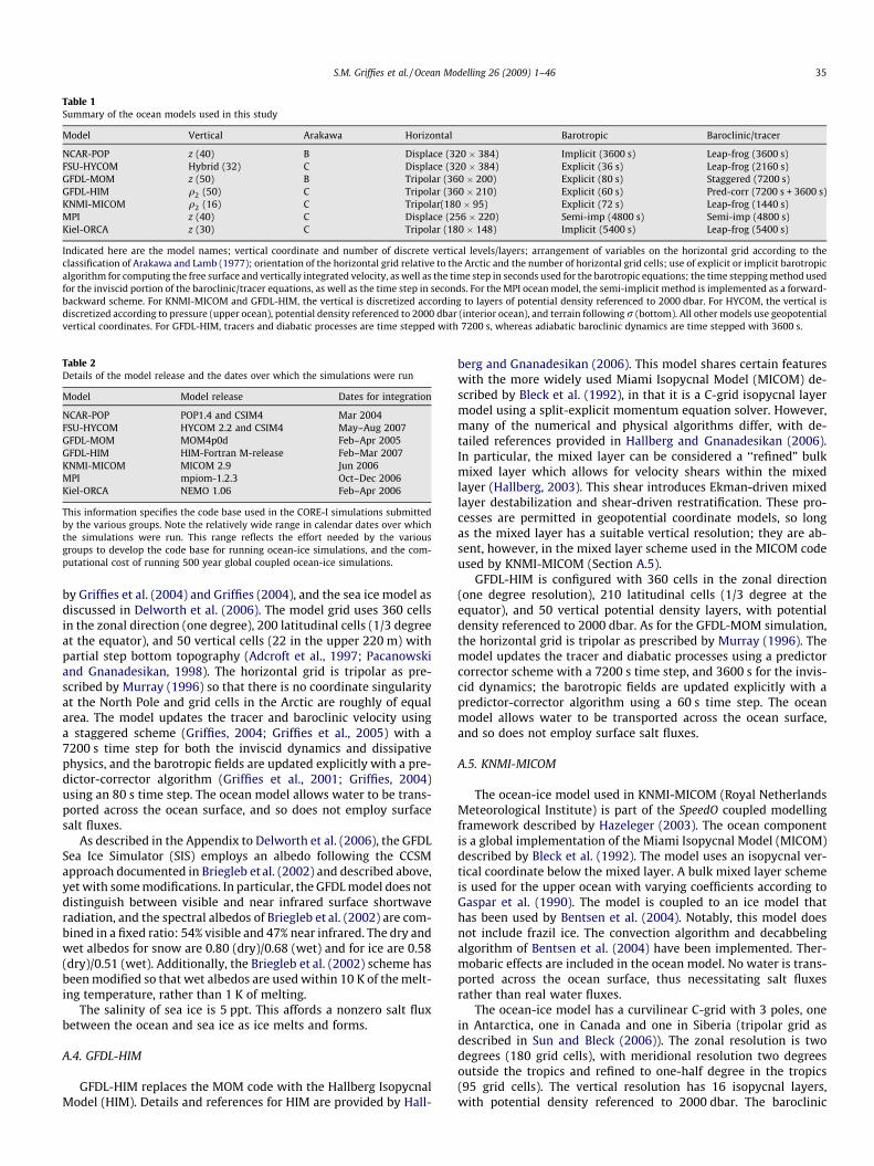
Table 1Summary of the ocean models used in this study
Model Vertical Arakawa Horizontal Barotropic Baroclinic/tracer
NCAR-POP z (40) B Displace (320 � 384) Implicit (3600 s) Leap-frog (3600 s)FSU-HYCOM Hybrid (32) C Displace (320 � 384) Explicit (36 s) Leap-frog (2160 s)GFDL-MOM z (50) B Tripolar (360 � 200) Explicit (80 s) Staggered (7200 s)GFDL-HIM q2 (50) C Tripolar (360 � 210) Explicit (60 s) Pred-corr (7200 s + 3600 s)KNMI-MICOM q2 (16) C Tripolar(180 � 95) Explicit (72 s) Leap-frog (1440 s)MPI z (40) C Displace (256 � 220) Semi-imp (4800 s) Semi-imp (4800 s)Kiel-ORCA z (30) C Tripolar (180 � 148) Implicit (5400 s) Leap-frog (5400 s)
Indicated here are the model names; vertical coordinate and number of discrete vertical levels/layers; arrangement of variables on the horizontal grid according to theclassification of Arakawa and Lamb (1977); orientation of the horizontal grid relative to the Arctic and the number of horizontal grid cells; use of explicit or implicit barotropicalgorithm for computing the free surface and vertically integrated velocity, as well as the time step in seconds used for the barotropic equations; the time stepping method usedfor the inviscid portion of the baroclinic/tracer equations, as well as the time step in seconds. For the MPI ocean model, the semi-implicit method is implemented as a forward-backward scheme. For KNMI-MICOM and GFDL-HIM, the vertical is discretized according to layers of potential density referenced to 2000 dbar. For HYCOM, the vertical isdiscretized according to pressure (upper ocean), potential density referenced to 2000 dbar (interior ocean), and terrain following r (bottom). All other models use geopotentialvertical coordinates. For GFDL-HIM, tracers and diabatic processes are time stepped with 7200 s, whereas adiabatic baroclinic dynamics are time stepped with 3600 s.
Table 2Details of the model release and the dates over which the simulations were run
Model Model release Dates for integration
NCAR-POP POP1.4 and CSIM4 Mar 2004FSU-HYCOM HYCOM 2.2 and CSIM4 May–Aug 2007GFDL-MOM MOM4p0d Feb–Apr 2005GFDL-HIM HIM-Fortran M-release Feb–Mar 2007KNMI-MICOM MICOM 2.9 Jun 2006MPI mpiom-1.2.3 Oct–Dec 2006Kiel-ORCA NEMO 1.06 Feb–Apr 2006
This information specifies the code base used in the CORE-I simulations submittedby the various groups. Note the relatively wide range in calendar dates over whichthe simulations were run. This range reflects the effort needed by the variousgroups to develop the code base for running ocean-ice simulations, and the com-putational cost of running 500 year global coupled ocean-ice simulations.
S.M. Griffies et al. / Ocean Modelling 26 (2009) 1–46 35
by Griffies et al. (2004) and Griffies (2004), and the sea ice model asdiscussed in Delworth et al. (2006). The model grid uses 360 cellsin the zonal direction (one degree), 200 latitudinal cells (1/3 degreeat the equator), and 50 vertical cells (22 in the upper 220 m) withpartial step bottom topography (Adcroft et al., 1997; Pacanowskiand Gnanadesikan, 1998). The horizontal grid is tripolar as pre-scribed by Murray (1996) so that there is no coordinate singularityat the North Pole and grid cells in the Arctic are roughly of equalarea. The model updates the tracer and baroclinic velocity usinga staggered scheme (Griffies, 2004; Griffies et al., 2005) with a7200 s time step for both the inviscid dynamics and dissipativephysics, and the barotropic fields are updated explicitly with a pre-dictor-corrector algorithm (Griffies et al., 2001; Griffies, 2004)using an 80 s time step. The ocean model allows water to be trans-ported across the ocean surface, and so does not employ surfacesalt fluxes.
As described in the Appendix to Delworth et al. (2006), the GFDLSea Ice Simulator (SIS) employs an albedo following the CCSMapproach documented in Briegleb et al. (2002) and described above,yet with some modifications. In particular, the GFDL model does notdistinguish between visible and near infrared surface shortwaveradiation, and the spectral albedos of Briegleb et al. (2002) are com-bined in a fixed ratio: 54% visible and 47% near infrared. The dry andwet albedos for snow are 0.80 (dry)/0.68 (wet) and for ice are 0.58(dry)/0.51 (wet). Additionally, the Briegleb et al. (2002) scheme hasbeen modified so that wet albedos are used within 10 K of the melt-ing temperature, rather than 1 K of melting.
The salinity of sea ice is 5 ppt. This affords a nonzero salt fluxbetween the ocean and sea ice as ice melts and forms.
A.4. GFDL-HIM
GFDL-HIM replaces the MOM code with the Hallberg IsopycnalModel (HIM). Details and references for HIM are provided by Hall-
berg and Gnanadesikan (2006). This model shares certain featureswith the more widely used Miami Isopycnal Model (MICOM) de-scribed by Bleck et al. (1992), in that it is a C-grid isopycnal layermodel using a split-explicit momentum equation solver. However,many of the numerical and physical algorithms differ, with de-tailed references provided in Hallberg and Gnanadesikan (2006).In particular, the mixed layer can be considered a ‘‘refined” bulkmixed layer which allows for velocity shears within the mixedlayer (Hallberg, 2003). This shear introduces Ekman-driven mixedlayer destabilization and shear-driven restratification. These pro-cesses are permitted in geopotential coordinate models, so longas the mixed layer has a suitable vertical resolution; they are ab-sent, however, in the mixed layer scheme used in the MICOM codeused by KNMI-MICOM (Section A.5).
GFDL-HIM is configured with 360 cells in the zonal direction(one degree resolution), 210 latitudinal cells (1/3 degree at theequator), and 50 vertical potential density layers, with potentialdensity referenced to 2000 dbar. As for the GFDL-MOM simulation,the horizontal grid is tripolar as prescribed by Murray (1996). Themodel updates the tracer and diabatic processes using a predictorcorrector scheme with a 7200 s time step, and 3600 s for the invis-cid dynamics; the barotropic fields are updated explicitly with apredictor-corrector algorithm using a 60 s time step. The oceanmodel allows water to be transported across the ocean surface,and so does not employ surface salt fluxes.
A.5. KNMI-MICOM
The ocean-ice model used in KNMI-MICOM (Royal NetherlandsMeteorological Institute) is part of the SpeedO coupled modellingframework described by Hazeleger (2003). The ocean componentis a global implementation of the Miami Isopycnal Model (MICOM)described by Bleck et al. (1992). The model uses an isopycnal ver-tical coordinate below the mixed layer. A bulk mixed layer schemeis used for the upper ocean with varying coefficients according toGaspar et al. (1990). The model is coupled to an ice model thathas been used by Bentsen et al. (2004). Notably, this model doesnot include frazil ice. The convection algorithm and decabbelingalgorithm of Bentsen et al. (2004) have been implemented. Ther-mobaric effects are included in the ocean model. No water is trans-ported across the ocean surface, thus necessitating salt fluxesrather than real water fluxes.
The ocean-ice model has a curvilinear C-grid with 3 poles, onein Antarctica, one in Canada and one in Siberia (tripolar grid asdescribed in Sun and Bleck (2006)). The zonal resolution is twodegrees (180 grid cells), with meridional resolution two degreesoutside the tropics and refined to one-half degree in the tropics(95 grid cells). The vertical resolution has 16 isopycnal layers,with potential density referenced to 2000 dbar. The baroclinic
36 S.M. Griffies et al. / Ocean Modelling 26 (2009) 1–46
and tracer time steps are 1440 s, and the barotropic time stepis 72 s.
As seen by the various model metrics in part 2 of this paper, theKNMI-MICOM simulation is an outlier, failing to match the physi-cal integrity of the other simulations for nearly all examined diag-nostics. Some fundamental problems with the MICOM version 2.9algorithms are mentioned here as possible reasons for the simula-tion difficulties.
– Thermobaricity and cabbeling:� Thermobaricity and cabbeling cause checkerboard-like insta-
bilities when the code is configured for refined vertical reso-lutions at high densities. These instabilities were suppressedby reducing the vertical resolution down to the 16 used here.Doing so, unfortunately, then led to poor representation ofdeep ocean processes. Note that Hallberg (2005) documentsthe problems with thermobaricity and cabbeling in isopycnalmodels, and provides a partial fix. The (Hallberg, 2005) fix isused in GFDL-HIM simulations, as required since GFDL-HIMuses a much finer vertical spacing with 50 layers.
� The decabbeling routine uses a very diffusive first orderupstream advection, which can create huge levels of spuriousdiapycnal mixing. In particular, there were large temperatureand salinity drifts between the deep and upper ocean due tocabbeling.
� Thermobaricity corrections are not globally defined. Instead,they use a region-dependent a priori temperature and salin-ity profile to calculate the thermobaricity corrections. Therewere large hydrography drifts within layers between adja-cent regions with different thermobaricity algorithms, mostnoticeably between the Southern Ocean and Atlantic.
7 The boundary layer is defined, for these purposes, as a region with verticaldiffusivity greater than 5 cm2 s�1.
– Advection: MICOM uses the MPDATA scheme of Smolarkiewicz(1984) for the horizontal advection of tracers. MICOM advectsdensity and spiciness rather than the traditional choice of poten-tial temperature and salinity. MPDATA, however, does not con-serve tracer. To maintain constant global tracer amounts,MICOM applies a global correction. This correction adds extrahorizontal and vertical diffusion between the layers, and it canexchange tracers between disconnected parts of a layer.
– Time filter: Another contribution to the highly diffusive simula-tion comes from the Robert–Asselin filter (e.g., (Haltiner andWilliams, 1980)) used to damp the splitting mode in the leapfrog time-stepping scheme.
A.6. MPI
MPI (Max-Planck-Institute) consists of the ocean-sea ice com-ponent from the MPI climate model (Roeckner et al., 2006; Jung-claus et al., 2006). The ocean model is a primitive equationmodel (C-Grid, z-coordinates, free surface) with a bottom boundarylayer scheme for the flow across steep topography (Marsland et al.,2003). The sea ice model is a dynamic/thermodynamic sea icemodel with a viscous-plastic rheology following Hibler (1979).The ocean model is configured with 40 vertical levels, with 20 inthe upper 600 m and the bottom topography is represented by par-tial steps (Adcroft et al., 1997; Pacanowski and Gnanadesikan,1998). The horizontal resolution of the bipolar grid with poles overGreenland and Antarctica gradually varies between a minimum of12 km close to Greenland and 190 km in the tropical Pacific. Themodel time stepping for tracers and velocity is formulated semi-implicitly with a time step of 4800 s. Sea ice has a salinity of5 psu. The ocean model allows water to be transported across theocean surface, thus does not employ surface salt fluxes. MPI’s seaice is initialised with thickness and concentration depending onthe initial sea surface temperature.
A.7. Kiel-ORCA
Kiel-ORCA is the ocean-ice component of the climate model atIPSL (Institut Pierre-Simon Laplace) in Paris. It uses the NEMOframework (Nucleus for European Modelling of the Ocean) version1.06, with the OPA9 z-coordinate ocean code (Madec et al., 1999)and LIM2 sea ice (Timmermannn et al., 2005).
The ocean model has 30 vertical levels (16 levels in the upper200 m) and a quasi-isotropic global tripolar grid, with two degreesresolution in the zonal direction and a meridional refinement atthe equator to 0.5� (180 � 149 � 30 grid cells). Topography is rep-resented with partial cells (Barnier et al., 2006). The model updatesthe tracer and baroclinic velocity using a leap-frog time step of5400 s for the inviscid dynamics and a forward step for dissipativephysics. The barotropic equations are updated implicitly in timeaccording to the algorithm of Roullet and Madec (2000) (usingthe same time steps as the baroclinic). The ocean model allowswater to be transported across the ocean surface, thus does notemploy surface salt fluxes.
In addition to the CORE-I surface boundary conditions em-ployed by the other models, the Kiel-ORCA simulation dampedtemperature and salinity towards climatology within the Mediter-ranean and Red Seas. The damping time scale is one day belowmodel level 18 (depth 272 m), and the damping is reduced towardszero from model level 17 up to the base of the planetary boundarylayer using a cosine function.7 Restoring is removed above theboundary layer base.
Appendix B. CORE-I experimental design
We summarise here the CORE-I experimental design. There arenotable details which differ between the models. Even in a cordialresearch collaboration such as this, we found it difficult to removeall differences, either because of incompatibilities between modelalgorithms, or scientific disagreements. It is conjectured that dif-ferences identified below are less important than the decision touse the same forcing, including the same bulk formulae, both basedon Large and Yeager (2004). This conjecture, however, remains un-proven without further sensitivity experiments which are beyondthe scope of this paper.
B.1. Initial conditions
We document here the methods used by the various modellingcentres for initialising their experiments. Ocean initial conditionsare thought to be of minor consequence on the multi-centennialtime scale of CORE-I. Shorter integrations, however, are influencedby the initial conditions, especially in deep water formationregions and regions of sea ice cover. For sea ice, in the absence ofrestoring of surface salinity, the initial sea ice can affect the totalsalt content in the ocean. For example, if starting with zero seaice, sea ice formation will increase ocean salinity due to the con-version of sea water from liquid to ice. As long as the sea ice doesnot fully melt again, this salinity bias will persist. The presence of asalinity restoring will dampen this bias.
Ocean models are initialised with zero velocity. The initial tem-perature and salinity fields are taken from the January temperatureand salinity profiles of Steele et al. (2001). The exception is thatKNMI-MICOM used initial conditions based on Levitus (1994).Temperature and salinity fields are interpolated to the respectiveocean model grid.
Ice models are initialised in the following manners.
S.M. Griffies et al. / Ocean Modelling 26 (2009) 1–46 37
– NCAR-POP: Zero initial ice concentration and zero ice volume.– FSU-HYCOM: Zero initial ice concentration and zero ice volume.– GFDL-HIM: Sea ice is taken from an earlier spinup.– GFDL-MOM: Sea ice is taken from an earlier spinup.– KNMI-MICOM: Zero initial ice concentration and zero ice
volume.– Kiel-ORCA: Initial sea ice has a uniform thickness of 1 m in the
Southern Hemisphere for grid boxes below freezing with a leadfraction of 10%, and 0 m in the Northern Hemisphere.
– MPI: Sea ice is initialised for SST values between �0.5 �C and thefreezing point of sea water, with linearly increasing 0 to 4 mthickness and a 100% concentration.
B.2. Fluxes from Large and Yeager (2004)
The normal year forcing for heat, moisture, and momentum areprovided by the Large and Yeager (2004) compilation of solar radi-ation, atmospheric state, and river runoff. The atmospheric state aswell as the model’s prognostic SST and surface currents determinethe turbulent momentum (wind stress), turbulent heat (sensibleand latent), and turbulent moisture (evaporation) fluxes. Thesefluxes are computed at each ocean-ice coupling time step usingthe CCSM bulk formulae described in Large and Yeager (2004)and Large (2005). Further details on the forcing are provided inAppendix C.
B.3. Salinity/water forcing
We provide here some details of the water or salinity forcingused in the models. The surface salinity or water restoring is notphysical, but is has been found necessary to prevent uncontrolleddrifts in salinity as a response to inaccurate precipitation. For mod-els using the salt flux boundary condition (NCAR-POP, FSU-HYCOM,and KNMI-MICOM), fresh water from precipitation, evaporation,and river runoff is converted to an implied salt flux via8
FðsaltÞðimpliedÞ ¼ qwSo; ð1Þ
where So is a global reference salinity. The NCAR-POP and FSU-HY-COM simulations set So ¼ 34:7 psu. Salinity restoring is applied tothe ocean according to the restoring salt flux
FðsaltÞðrestoreÞ ¼ VpistonðSðdataÞ � SSSÞ ð2Þ
with a nonnegative piston velocity Vpiston setting the strength of therestoring used for surface salinity/water forcing. Hence, when theprognostic surface salinity SSS is larger than monthly surface salin-ities SðdataÞ, a negative restoring salt flux FðsaltÞ
ðrestoreÞ is added to the topocean model grid cell.
The salinity field SðdataÞ is available at
http : ==nomads:gfdl:noaa:gov=nomads=forms=mom4=CORE:html:
This field is discussed in Section 4.7 of Large and Yeager (2004).Briefly, it is derived from the Conkright et al. (2002) and Steeleet al. (2001) monthly mean data. We averaged the top two verticallevels to remove overly fresh biases from river input. Because ofprocessing errors in the Foxe Basin, levels 1–4 were reset to level5, and Hudson Bay April level 1 was reset to level 2. Near the Ant-arctic, we use the Doney and Hecht (2002) recipe, which prescribesthe following.
– Where the bathymetric depth is less than or equal to 300 m, thecolumn-max salinity replaces the near-surface salinity.
8 Some authors refer to this salt flux as a virtual flux, since it is not present inNature (Huang, 1993).
– Where the depth is greater than this depth but less than or equalto 1000 m, the column-max salinity is blended with the near-surface salinity.
– Where the bathymetric depth is greater still, the near-surfacesalinity is used, without any enhancement.
The column-max salinity is derived from a search through all 12months, and not just from a search of the one particular month inquestion.
No restoring is applied under sea ice in the KNMI-MICOM sim-ulation, but note that grid cells may have partial ice cover such thatsome restoring does take place over those cells. The NCAR-POPsimulation used a salinity piston velocity of 50 m/4years in allregions of the ocean (including under sea ice), with the exceptionof enclosed marginal seas. The KNMI-MICOM simulation used aregionally dependent piston velocity: zero piston velocity in theregion 35�N–65�N, 275�E and 0�E (North Atlantic); 50 m/50daysnorth of 75�N; 50 m/30days south of 50�S; and 50 m/1500daysfor the remainder. Gradients between the different zones werelinearly interpolated in a 10� strip. The NCAR-POP simulationremoves the global mean restoring every time step, and multipliesprecipitation by a factor based on the global salinity change overthe previous year such that
net salt input ¼X
FðsaltÞðimpliedÞdxdy ð3Þ
is damped towards zero. This procedure compensates for the initialgrowth of sea ice. KNMI-MICOM and FSU-HYCOM do not apply anormalisation, and such may account for the fresh drift seen inthe salinity bias time series (Fig. 6).
The GFDL-HIM, GFDL-MOM, MPI, and Kiel-ORCA models trans-port water across the ocean surface, and thus add fresh water di-rectly to the volume conservation equation (i.e., the free surfaceheight evolution). Correspondingly, the restoring salt flux in equa-tion (2) is converted to a fresh water flux qrestore
w via
qrestorew ¼ �FðsaltÞ
ðrestoreÞ=SSS: ð4Þ
Hence, water is added ðqrestorew > 0Þ where the model’s prognostic
SSS is greater than SðdataÞ, and subtracted ðqrestorew < 0Þ where
SSS < SðdataÞ. For the Kiel-ORCA simulations, no extra water normal-isation is applied, and this may account for the fresh drift seen inthe salinity bias time series (Fig. 6). In the GFDL and MPI simula-tions, a global normalisation is applied at each time step so thatover the ocean surface,
net water input to ocean ¼XðP � Eþ Rþ qrestore
w Þ ð5Þ
is set to zero.9 This normalisation keeps the ocean volume constantyet has the unphysical effect of adding a water flux non-locally, evento a region that may have zero salinity bias. Nonetheless, it serves toavoid longterm drifts in the salinity and sea level.
Choices made for the models are summarised in Table 3.
Appendix C. Forcing the ocean-ice models
The ocean and sea ice systems are forced by air-sea and air-icefluxes, respectively, and coupled through ice-ocean fluxes. In acoupled ocean-ice model, the latter are internally computedaccording to the specific ice-model. The purpose of this appendixis to highlight details of computing the atmospheric forcing, whichhave proven important in setting up the CORE simulations.Although we focus on air-sea fluxes, many of the issues also
9 The GFDL-MOM simulations incorrectly included the sea ice melt as part of thenormalisation. It should not be included, since it is only the net water in the oceanplus ice systems that should be normalised to have a net zero sum.
Table 3Summary of choices made for the surface water/salt forcing in the various experiments
Experiment S/H2O flux Vpiston (m/d) Restore region Under ice Normal hydrology
NCAR-POP Salt 50/(4 � 365) Global Yes YesFSU-HYCOM Salt 50/(4 � 365) Global Yes NoGFDL-MOM-A Water 50/(4 � 365) Global No YesGFDL-MOM-B (ctrl) Water 50/(300) Global No YesGFDL-HIM Water 50/(300) Global Yes YesKNMI-MICOM Salt Regional Regional No NoMPI-A (ctrl) Water 50/(4 � 365) Global Fraction YesMPI-B Water 50/(300) Global Fraction YesKiel-ORCA Water 50/(300) Regional Yes Yes
All experiments were run for 500 years. Two experiments are mentioned for GFDL-MOM and MPI, corresponding to the perturbation experiments described in Section 16. Thecontrol experiments for both models are noted, as these are the settings used for all other sections. Column two indicates whether the experiment used salt fluxes or waterfluxes for hydrological forcing. Column three gives the piston velocity in metres per day, which determines the strength of the restoring used for surface salinity/waterforcing. Column four notes the region over which the salinity/water restoring fluxes are set. The Kiel-ORCA simulation used regionally varying restoring as discussed inFig. 27. The KNMI-MICOM simulations used the following regionally varying piston velocity: zero piston velocity in the region 35�N–65�N, 275�E and 0�E (North Atlantic);50 m/50 days north of 75�N; 50 m/30 days south of 50�S; and 50 m/1500 days for the remainder. Gradients between the different zones were linearly interpolated in a 10�strip. Column five indicates whether restoring was applied under sea ice. The ‘‘fraction” entry for MPI indicates the SSS restoring term was weighted by (1-ice concentration),so that no restoring was applied with 100% ice. Column six refers to whether the experiment normalised the precipitation minus evaporation plus runoff in some manner toreduce drift.
38 S.M. Griffies et al. / Ocean Modelling 26 (2009) 1–46
pertain to air-ice fluxes, and the similarities and differences in fluxcalculations over the two surfaces are detailed in Large (2005).
C.1. Air-sea fluxes
This section follows closely Section 2 from Large and Yeager(2008). The ocean is forced by fluxes of freshwater, Fs, heat, Q surf ,and momentum, s. In general, contributions come both from theopen ocean fraction, fo, and the sea-ice fraction, 1� fo:
s ¼ fosas þ ð1� foÞsio ð6ÞFs ¼ foFas þ ð1� foÞF io þ R ð7ÞQ surf ¼ foQ as þ ð1� foÞQ io; ð8Þ
where the subscript ‘‘as” refers to air-sea fluxes, ‘‘io” refers to ice-ocean, and R is the continental runoff. The air-sea heat and freshwa-ter fluxes have components:
Q as ¼ Q S þ Q L þ Q E þ Q H ð9ÞFas ¼ P þ E; ð10Þ
where all fluxes are positive when momentum, water, or heat enterthe ocean.
The shortwave solar radiation, QS, with wavelengths between0:3l and 3l, is computed from the solar insolation QI incidenton the ocean surface, minus that which is reflected from the oceansurface
Q S ¼ Q Ið1� aÞ ð11Þ
with the albedo a � 0:065 appropriate for the ocean (Payne, 1972).The net surface longwave solar
Q L ¼ Q A � rSST4 ð12Þ
results from a downwelling longwave flux QA from the atmosphere,minus the blackbody radiation from the ocean back to the atmo-sphere with r ¼ 5:67� 10�8Wm�2K�4 the Stefan–Boltzmannconstant.
Bulk formulae parameterise the turbulent fluxes (wind stress s,evaporation E, latent heat Q E, and sensible heat Q H) in terms of thenear surface atmospheric state (wind U, potential temperature h,specific humidity q, and density q) and surface ocean state (SSTand surface ocean current Uo).10 The air at the ocean surface is
10 The SST and ocean current are taken from the surface ocean model grid cellvalues. This is an appropriate choice, since the bulk formulae presented here aredeveloped from fits to bulk properties of the upper ocean, rather than skin properties.
assumed to be saturated at a specific humidity qsðSSTÞ that is afunction of the SST. The vapor pressure over seawater is about2% less than that over fresh water (see equation (5) in Large andYeager (2004)). This difference is not negligible compared to the20% subsaturation of marine air that drives evaporation. Conse-quently, the effect is included in the qsðSSTÞ function used by allmodels in the present comparison. A different function of surfacetemperature is used over sea-ice.
All models in this paper use the same bulk formulae and atmo-spheric state in a two step process. First, the meteorological dataare referenced to a common reference height. The bulk transfercoefficients are formulated at 10 m height and neutral stability,so the second step is to shift them to the atmospheric stabilityand the reference height. This step is often overlooked when forc-ing ocean and ocean-ice models, where sometimes data from dif-ferent heights (e.g., 10 m winds and 2 m temperature andhumidity from reanalyses) are used directly with the 10 m bulkformulae. For accuracy, it is essential to use a common height,and the height shifting and flux algorithms should be consistent,because they are closely related. The ocean state is provided bythe individual ocean models.
A reference height of d ¼ 10m was chosen for CORE-I, so thatthere would be no need for any height shift of either the wind data,or the transfer coefficients. The shift of air temperature and humid-ity to 10 m is done off-line using observed SST, so that the COREatmospheric state is given at 10 m (Table 4), where the dimension-less atmospheric stability is denoted as f10. The turbulent fluxes arethen given by
s ¼ qCDðf10ÞjDUjDU ð13ÞE ¼ qCEðf10Þ½q� qsðSSTÞ�jDUj ð14ÞQE ¼ KvE ð15ÞQH ¼ qcpCHðf10Þðh� SSTÞjDUj; ð16Þ
where cp � 1000:5J=kg is the specific heat capacity of air,Kv ¼ 2:5� 106J=kg is the latent heat of vaporization for water,and DU ¼ U� Uo is the difference between the atmospheric windsand ocean current (following Pacanowski (1987)).11
Large and Yeager (2004) detail the methodology for shiftingthe neutral 10 m transfer coefficients for drag, CD, sensible heat
11 Pacanowski (1987) noted that it is important to take into account surface oceancurrents in the computation of wind stress, especially where ocean currents reachlarge values, such as in the equatorial Pacific. Models in this study all follow thisapproach for computing the wind stress.

Table 4Summary of the forcing used in the CORE-I simulations as provided by Large and Yeager (2004) fields and CCSM bulk formulae
Field Available times Used to compute
Runoff Annual mean River runoff into oceanPrecipitation 12 months PrecipitationDownwelling short 365 days Ocean shortwave heatingDownwelling long 365 days Ocean longwave heating10 m air temp 6 hourly for 365 days Sensible heating (using air temp, SST, and bulk formulae)10 m humidity 6 hourly for 365 days Evap and latent heating (assume saturation over ocean water)10 m vector winds 6 hourly for 365 days Wind stress (from winds, surface currents, and bulk formulae)10 m vector winds 6 hourly for 365 days Sensible and latent heating, and evaporation (along with SST)Sea level pressure 6 hourly for 365 days Atmospheric loading on ocean and surface atmospheric density
Column 1 is the field provided by their dataset, column 2 is the temporal amount of data provided, column 3 is the quantity computed for use in the ocean-ice model forcing.Note that vector winds are listed twice due to their use in computing a large number of surface fluxes.
S.M. Griffies et al. / Ocean Modelling 26 (2009) 1–46 39
transfer, CH , and evaporation, CE, to the stability of the coefficientsin these equations, where
f10 ¼djg
ffiffiffiffiqpjsj3=2
QH
cphþ Q E
Kvðqþ :608�1Þ
!: ð17Þ
In this relation, d ¼ 10 m is the atmospheric reference height,j ¼ 0:4 is the von Karman constant, g is the gravitational acceler-ation, and
Mdry air
Mwater
� �� 1 ¼ :608; ð18Þ
with Mdry air ¼ 28:97 the molecular weight of dry air, andMwater ¼ 18:015 the molecular weight of fresh water. The stabilityshift is accomplished according to
CDðf10Þ ¼ CD 1�ffiffiffiffiffiffiCDp
jwmðf10Þ
� ��2
ð19Þ
CHðf10Þ ¼ CH
ffiffiffiffiffiffiffiffiffiffiffiffiffiffiffiffiCDðf10Þ
CD
s1� CH
jffiffiffiffiffiffiCDp whðf10Þ
� ��1
ð20Þ
CEðf10Þ ¼ CE
ffiffiffiffiffiffiffiffiffiffiffiffiffiffiffiffiCDðf10Þ
CD
s1� CE
jffiffiffiffiffiffiCDp whðf10Þ
� ��1
; ð21Þ
where wm and wh are empirical dimensionless momentum and heatflux profiles which are functions of stability with the followingbehaviour
wh ¼ �5f10 with f10 P 0ðstableÞ ð22Þwm ¼ �5f10 with f10 P 0ðstableÞ ð23Þwh > wm > 0 with f10 < 0ðunstableÞ: ð24Þ
Unfortunately, only the NCAR-POP and FSU-HYCOM fluxes werecomputed with the correct stability shift. The code used by theother models computed incorrect transfer coefficients at f10 forboth heat, CH , and moisture, CE, where the fractional error is givenby
CHCHðf10Þ
¼1�
ffiffiffiffiCD
pj wmðf10Þ
1� CH
jffiffiffiffiCD
p whðf10Þð25Þ
CECEðf10Þ
¼1�
ffiffiffiffiCD
pj wmðf10Þ
1� CE
jffiffiffiffiCD
p whðf10Þ: ð26Þ
Most of the ocean is cooled by negative Q H and QE, which makesf10 negative, the atmosphere unstable and wh more positive thanwm. Therefore, the fractional error is usually greater than unity,and largest in regions where high SST and low wind speeds com-bine to make a significantly unstable atmosphere, with wh typicallytwice wm. The heat flux error is greatest where these regions coin-cide with large latent heat flux loss, with the error increasing theloss. For example, using observed SST, the net heat flux into theocean is reduced by 8–10 W m�2 over much of the tropical Indian
and western Pacific oceans, over the western boundary currentswith the exception of the Brazil current, and off western Australia(Laurent Brodeau, personal communication, 2007). The expectedSST response would be for NCAR-POP and FSU-HYCOM to be war-mer in these regions by at most 0.3 �C. Elsewhere, the effect issmaller and poleward of about 40� degrees latitude, the heat fluxreduction is typically less than 3 W m�2.
C.2. The Large and Yeager (2004) dataset
Table 4 summarises the Large and Yeager (2004) dataset used tocompute the normal year forcing for heat, moisture, and momen-tum. This data includes monthly mean precipitation, daily shortand long solar radiation, 6 hourly atmospheric meteorological stateat 10 m (temperature, humidity, and vector wind), and annualmean river runoff. The atmospheric state as well as the model’sprognostic SST and surface currents determine the turbulentmomentum (wind stress), turbulent heat (sensible and latent),and turbulent moisture (evaporation) fluxes. These fluxes are com-puted at each ocean-ice coupling time step using the CCSM bulkformulae described in Large and Yeager (2004).
C.3. River runoff
The river runoff from Large and Yeager (2004) has a single timestep as it represents annual mean runoff. This data has been spreadout from the river mouths in a manner used in CCSM climate sim-ulations. This approach is thought to account for some unresolvedmixing that occurs at river mouths in Nature. A remapping schemeis provided at the GFDL web site quoted in Section 4.1. This schememaps the river data onto a model grid of differing resolution, solong as the new grid is logically rectangular (as all grids used in thisstudy).
Modellers are encouraged to test different runoff specifications,such as with a seasonal cycle as in (Röske, 2006). If doing so, werecommend that a correction be made to keep the total annual fluxof runoff similar to the value in the Large and Yeager (2004) datasetin order to facilitate comparisons.
C.4. Normalisation of moisture fluxes
As detailed in Section B.3, some models apply a normalisation tomaintain a balance in the globally integrated moisture flux (precip-itation minus evaporation plus river runoff plus restoring) equal tozero. This normalisation reduces long term drifts. We summarisethe choices made for the simulations in Table 3.
C.5. Use of sea level pressure
The sea level pressure is used to compute the air density (seeequation (24) of (Large and Yeager, 2004)). It also presents a loadon the ocean-ice models (the inverse barometer effect), which
Table 5Table indicating the manner that shortwave radiation is attenuated as it penetratesinto the ocean
Experiment Water type for shortwave
NCAR-POP Chlorophyll monthly climatologyFSU-HYCOM Chlorophyll monthly climatologyGFDL-MOM Chlorophyll monthly climatologyGFDL-HIM Chlorophyll monthly climatologyKNMI-MICOM Shortwave in mixed layerMPI Uniform Jerlov water type IKiel-ORCA Uniform Jerlov water type I
40 S.M. Griffies et al. / Ocean Modelling 26 (2009) 1–46
drives barotropic motion. However, all ocean-ice models in thisstudy discard this pressure loading, thus considering the atmo-sphere to be massless for purposes of ocean-ice dynamics.
C.6. High frequency meteorological data
It is desirable to use high frequency (6 hourly) meteorologicaldata as provided by Large and Yeager (2004). We ran a one monthAMIP model at GFDL to explore the flux errors associated with aver-aged meteorological states acting as inputs to the flux calculations.In the standard AMIP configuration, the model computes fluxesevery 30 min based on 30 min updates to the atmospheric state.Averages of these 30 min fluxes were then compared to fluxes com-puted using a less frequently updated atmospheric state.
With daily updated winds, temperatures, and humidities pro-viding the atmospheric state, the latent heat fluxes are under esti-mated broadly over the winter storm track band by some tens ofW m�2, relative to the latent heating computed with the 30 minfluxes. There was also a smaller underestimate located in the sum-mer storm track band. The nonlinear nature of storm track variabil-ity is the reason for the problems with low frequency updates tothe atmospheric state. Experiments that refined the temporal res-olution of the flux inputs individually showed that high frequencywinds are most important for reducing the flux error, but temper-ature and humidity frequency also contribute. When all inputs aregiven at 6 hourly frequency, the global RMS error is about 1 W m�2
versus near 8 W m�2 for daily inputs.
C.7. Treatment of saltwater vapor pressure
Models here use the same treatment of saltwater vapor pres-sure. The vapor pressure over seawater is about 2% less than thatover fresh water (see equation (5) in (Large and Yeager, 2004)).This difference is not negligible compared to the 20% subsaturationof marine air that drives evaporation. Consequently, the effectshould be included in all models participating in a comparison.
C.8. Shortwave penetration
The evolution of SST depends critically on the absorption of so-lar shortwave radiation and demands that this flux be separatedfrom the other heat fluxes (Rosati and Miyakoda, 1988). How thisradiation is attenuated into the ocean differs in the models. As de-scribed in Appendix B to Danabasoglu et al. (2006), shortwaveabsorption in NCAR-POP and FSU-HYCOM is based on monthlyand spatially varying SEAWIFS chlorophyll climatology followingOhlmann (2003). Similarly, GFDL-MOM and GFDL-HIM prescribethe chlorophyll climatology of Sweeney et al. (2005) and attenu-ates vertically according to Morel and Antoine (1994). KNMI-MI-COM places all of its shortwave radiation into the bulk mixedlayer. MPI and Kiel-ORCA use an e-folding dependency for theshortwave penetration as documented in Paulson and Simpson(1977), with clear water (type I in Jerlov (1968) classification).We summarise these choices in Table 5.
Appendix D. Diagnostics used to evaluate the simulations
All models in this study employ a generalized orthogonal grid inthe horizontal. As noted in Appendix A, four of the models employtripolar grids (GFDL-MOM, GFDL-HIM, KNMI-MICOM, and Kiel-ORCA), whereas FSU-HYCOM, NCAR-POP and MPI use a bipolar gridwith the North Pole displaced over Greenland. Generalized hori-zontal coordinates are commonly chosen for global models as theyremove the spherical coordinate singularity from the Arctic Ocean,and thus allow for improved simulation integrity in this region.Unfortunately, given the relative immaturity of software plottingpackages, non-spherical grids lead to difficulties directly compar-ing the simulations (e.g., making difference maps; producing polarprojections) in regions where the grid metric factors do not agree,such as the Arctic. We do not attempt to remedy this shortcoming,but instead choose to allow each model to plot results on their ownnative grid.
In the remainder of this section of the appendix, we formulatecertain of the diagnostics used to evaluate the model simulations.Some diagnostics used in this paper are compared to observations,and so represent metrics used to gauge the physical integrity of thesimulations.
D.1. Meridional overturning streamfunction
This section supplements the results from Section 15, where wepresented the meridional overturning streamfunctions for theAtlantic and World Oceans. The meridional overturning stream-function diagnoses the transport of volume poleward
Wðy; zÞ ¼ �Z
dxZ z
�Hdz0ðvþ vÞ; ð27Þ
where the minus sign reflects a convention. The overturningstreamfunction is commonly used to summarise various featuresof the large scale circulation, particularly effects from thermohalineforcing. In Eq. (27), the vertical limits extend from the ocean bottomat z ¼ �Hðx; yÞ to a depth z, and the zonal integral extends over theglobe or within a closed ocean basin. We include a possibly nonzerodivergence-free subgrid scale (SGS) velocity v. For the geopotentialcoordinate models used in this study, v is determined by theparameterisation of Gent et al. (1995), where
v ¼ �@zðjSyÞ; ð28Þ
with Sy ¼ �@yq=@zq the meridional slope of the neutral direction,and j > 0 a diffusivity (with units of squared length per time).The overturning streamfunction is thus given by the SGS plus Eule-rian terms
Wðy; zÞ ¼Z
dxjSy �Z
dxZ z
�Hdz0v; ð29Þ
where we set jSy ¼ 0 at the ocean bottom. The contribution fromthe Gent et al. (1995) parameterisation to both volume and tracertransport is most prominent in the Southern Ocean, where the basinis large and the neutral slopes generally steepen towards the pole.In other basins, such as the North Atlantic, its contribution is mod-est to negligible, depending on the chosen diffusivity.
For the isopycnal models employed by GFDL-HIM and KNMI-MICOM, the meridional overturning streamfunction is computedwith the vertical integral proceeding from the ocean bottomupwards to a surface of constant potential density, so that
Wðy;qÞ ¼ �Z
dxZ q
�Hdq0vð@z=@q0Þ; ð30Þ
where dz ¼ dq0ð@z=@q0Þ is the thickness between isopycnal layers.Since the product vð@z=@q0Þ is nonlinear, it is important for isopyn-cal models to retain this product over each time step when forming
12 This choice is suggested for precipitation in state-of-the-art coupled climatemodels, since the condensate in atmospheric models generally has zero heat capacity.Likewise, many river models do not carry the temperature of river water. There is anon-conservation of heat in the simulated global climate system due to theselimitations of the atmosphere and river components in coupled climate models.
S.M. Griffies et al. / Ocean Modelling 26 (2009) 1–46 41
the time average streamfunction. Otherwise, the resulting stream-function could suffer from aliasing problems.
Beneath the ocean surface, the no-normal flow condition on thevelocity field implies that the overturning streamfunction is a con-stant along land-sea boundaries, and choice of the referencestreamfunction value as chosen above leads to a vanishing stream-function on these boundaries. In a model run without water fluxforcing, the streamfunction vanishes along the surface as well. Incontrast, fresh water input means that the streamfunction is gen-erally nonzero at the ocean surface.
D.2. Poleward heat transport
For the ocean-ice system, the prescribed atmospheric state usedin CORE implies a poleward heat transport, given a sea surfacetemperature and a few assumptions. We summarise the formula-tion in order to highlight assumptions. For this purpose, start withthe vertically integrated temperature budget for a Boussinesqocean
@t
Z g
�Hdzh
� �¼ �r
Z g
�Hdzðuhþ FÞ
� �þ Q heat=ðqoCpÞ: ð31Þ
The left hand side represents transient storage of temperaturein a column of ocean fluid from the surface at z ¼ g to the bottomat z ¼ �H. This storage is affected by the convergence of heatthrough the vertically integrated resolved horizontal flow, uh,and parameterised SGS processes, F. For each of the models in thisstudy, the SGS parameterisations include the neutral diffusionscheme from Redi (1982) and the eddy induced advection fromGent and McWilliams (1990).
The storage term in Eq. (31) is also affected by heat transferacross the ocean surface
Q heat ¼ Q surf þ Q geo þ qoCp
XP;E;R
qwhw: ð32Þ
Q surf is the surface heat flux (positive into the ocean) arisingfrom interactions between the ocean and atmosphere, and oceanand sea ice
Q surf ¼ Qair-sea þ Q ice-sea: ð33Þ
These fluxes account for shortwave and longwave solar radia-tion, and turbulent fluxes from sensible and latent heating. Addi-tional ice-sea fluxes arise from the interaction between liquidseawater and frozen sea ice. For example, sea ice forms as liquidseawater is cooled below its freezing point. The cooling that wouldotherwise contribute to a sub-freezing liquid seawater is generallytransferred to the sea ice model as frazil is formed. This transferrepresents a sign definite heating of the liquid ocean, and it thusappears as part of the net heating in Eq. (32). Conversely, when fro-zen precipitation or calving land glaciers enter the liquid ocean, thelatent heat of fusion required to melt the frozen water acts as acooling for the liquid seawater.
The solid earth presents a heat source to the ocean which isincluded in the geothermal heating term. This heating is set tozero in all models except for the Kiel-ORCA simulation, where auniform value of 0.086 W m�2 is applied throughout the WorldOcean.
The final contribution to the heat flux in Eq. (32) arises from thetransfer across the ocean surface of water with a temperature hw.This transfer occurs with a volume per area per time due to precip-itation (P > 0 for water entering ocean), evaporation (E > 0 forwater leaving ocean), and river runoff (R > 0 for water enteringocean). This water heat flux is absent in virtual salt flux simula-tions (see Section B.3 and Table 3), since these models do notexchange water with other parts of the climate system. For themodels in this study using real water fluxes, hw for P; E, and R is
equated to the SST of the grid cell participating in the water trans-fer.12 For precipitation and evaporation, the term hwðP � EÞ generallyprovides a global net cooling of the ocean, since evaporation trans-fers water away from the ocean at a temperature typically higherthan precipitation adds water. This net heat loss must be compen-sated by ocean heat transfer.
If the ocean is in a steady state (say over annual or decadal timescales), then heating over these time scales will balance the diver-gence of heat throughout an ocean column. Now extend this bal-ance to a horizontal domain, in which the zonal boundaries areeither periodic or no-flow, and the southern boundary at y ¼ ys isno-flow (as for the Antarctic continent). Use of the Divergence The-orem indicates that meridional transport through the northernboundary balances heat input through the ocean surface
qoCp
ZdxZ g
�Hdzðvhþ FyÞ ¼
Z y
ys
dyZ
dxQ heat: ð34Þ
That is, in a steady state, the area integrated heat flux into the oceanover the region south of a given latitude (right hand side) is bal-anced by meridional transport of heat within the ocean at the spe-cific latitude (left hand side). For example, if there is a net surfaceflux of heat out of the ocean south of a chosen latitude (e.g., coldair over warmer water), then maintenance of a steady state requiresthat this surface heat loss is balanced by a transport of heat withinthe ocean towards the south across this latitude. A meridionalocean heat transport is thus implied by the net surface forcing. Thisresult allows us to estimate the meridional ocean heat transportthrough knowledge of just the surface fluxes.
As described by Large and Yeager (2004), knowledge of theatmospheric state and the sea surface temperature provide suffi-cient information to compute surface turbulent air-sea heat fluxesby using the bulk formulae. The radiative and turbulent heatingthen provide Qair-sea. The water transport term ðP � Eþ RÞhw isgenerally subdominant to Q surf . So it is common to estimate theimplied ocean heat transport just with Qair-sea. Hence, estimatesof the ocean heat transport implied from Q air-sea are useful if thefollowing assumptions hold:
– Ocean heat storage is small over the time scales of interest (i.e.,ocean has reached a steady state);
– Heat transport due to the movement of water across the oceansurface is ignored;
– Heat fluxes between ice-ocean are ignored;– Bottom heat fluxes (e.g., geothermal fluxes) are ignored.
These assumptions are made for the implied transports for theNormal Year Forcing shown in Fig. 21. Note that the missingQ ice-sea fluxes generally give more cooling toward the poles, imply-ing more poleward transport (steeper negative slopes) in bothhemispheres than shown in Fig. 21.
D.3. Comments on diagnosing heat and volume transport
As the ocean heat transport is a nonlinear product of terms, it isdesirable to compute the transport in a simulation at each timestep using the model numerics, and maintain a time average onlineduring the simulation. In Table 6, we note how the transport wascomputed by the models. For the overturning streamfunction(see Section D.1), the streamfunction is a nonlinear product whenthe thickness of a layer can change, as for a nonlinear free surface
42 S.M. Griffies et al. / Ocean Modelling 26 (2009) 1–46
z-model (GFDL-MOM) and for an isopycnal or hybrid model (GFDL-HIM, FSU-HYCOM, KNMI-MICOM).
The problem with using the mean velocity times the meanthickness for the overturning streamfunction, or mean velocitytimes the mean thickness times mean temperature for the heattransport, is that there tend to be very large correlations betweenthickness and the other two fields (especially near-surface). Soworking with time mean fields would be a very poor approxima-tion to the true fluxes.
In an isopycnal model, one complication is that the near-surfacelayers are non-isopycnal, and hence do not trivially map into thediscretized density space. GFDL-HIM uses the layer density over ashort interval (an hour to a few days) to partition the fluxes in thesevariable-density layers into the discrete density space matching thetarget densities for the interior layers. The total transport is exactlywhat the model uses, but there is a slight dependence on the fre-quency with which the fluxes are recast into pure density coordi-nates, and in the choice of the lateral mapping of densities ontovelocity points. Because for efficiency these are not calculated everytime-step, GFDL-HIM cannot simply use the ratio of the buoyancyflux to the volume flux to determine the buoyancy at which thefluxes occur. With the 2-h frequency used in the GFDL-HIM COREruns, it is expected that these uncertainties are negligible.
Finally, the transport arising from SGS mesoscale parameterisa-tion via neutral diffusion (Redi, 1982) and eddy induced advection(Gent and McWilliams, 1990) play a role in establishing the heattransport and meridional overturning streamfunction, especiallyin the Southern Ocean. Table 6 thus provides details regardinghow the models chose the parameters setting the strength of theseschemes.
D.4. Budget for volume averaged temperature
Integrating the heat budget (31) over the full extent of theWorld Ocean leads to an evolution equation for the globally inte-grated potential temperature
qoCp@t
XhdV
� �¼X
Q heatdA: ð35Þ
In this equation, dV is the grid cell volume, dA is the horizontalarea of a cell. Locally, the surface turbulent and radiative fluxestend to dominate heating from water transfer by one or two ordersof magnitude, with frazil yet another order of magnitude smaller.The turbulent and radiative terms, as well as the water term, haveboth positive and negative contributions, whereas frazil alwaysrepresents a heating of the liquid ocean. Hence, the global sum ofthese terms can be comparable and thus are important to retainin a budget analysis.
Note that models using real water fluxes have a seawater vol-ume that is generally nonconstant, given the ability to exchangewater between other components of the climate system. Thesemodels, however, generally implement a normalisation term sim-ilar to the salinity normalisation (Section B.3 and Table 3), thusminimising the drift. In general, drifts in volume averaged temper-ature and salinity may result from drifts in seawater volume.
One means of checking whether the model results are sensible isto consider a rough order of magnitude calculation to determine thetemperature trend that one may expect, given a net heat flux. Intro-ducing the mean temperature, hhi ¼
PhdV=
PdV , Eq. (35) indicates
that the global mean liquid ocean temperature evolves according to
ðVqoCpÞ@thhi ¼X
Q heatdA; ð36Þ
where V is the liquid ocean volume. Typical values for the WorldOcean yield VqoCp � 5:4� 1024J=�C and
PdA ¼ 3:6� 1014m2, lead-
ing to the decadal scale temperature trend
Dhhidecade
� 0:02Q heat: ð37Þ
For example, with a 1Wm�2 net heating of the ocean over thecourse of a decade, we expect a temperature trend of roughly0.02 �C per decade, or 0.2 �C per century.
D.5. Budget for volume averaged salinity
As a supplement to the results in Section 5, we note that theglobally integrated salinity in the liquid ocean evolves according to
@t
XSdV
� �¼X
Q saltdA; ð38Þ
where
Q salt ¼ Q ice þ vpistonðSSS� SobsÞ þ SoðP � Eþ RÞ þ normal ð39Þ
is the salt flux. Here, Q ice is the flux of salt passing between the li-quid ocean and sea ice, and vpiston is the piston velocity setting thestrength of the sea surface salinity (SSS) restoring to the observedvalues Sobs. The term SoðP � Eþ RÞ arises from the conversion ofwater flux to a salt flux, with So a global constant. The normalisationterm is used to minimise the salt drift, which would generally occurin its absence given that the globally integrated restoring term neednot be zero. The restoring term, the virtual salt flux term, and thenormalisation term are absent in models that use a real water flux.Instead, these models convert the restoring salt fluxes into an im-plied water flux, they insert water directly to the model, thuschanging its volume, and they introduce a normalisation for thesurface water forcing. Further details of this budget, as well as thechoices made by the various models, are provided in Section B.3and Table 3.
D.6. Mixed layer depths
The purpose of this section is to supplement the mixed layerdiagnostics presented in Section 11. We start by noting that thediagnosis of observed and model mixed layer depth (MLD) isambiguous. The mixed layer has near-zero gradients of h� S anddensity, as well as tracers such as CFCs. So most techniques to esti-mate the MLD rely on either a threshold gradient or a thresholdchange in one of these quantities, normally in potential tempera-ture h or density (Lorbacher et al., 2006, see, for example; De BoyerMontegut et al., 2004; Monterey and Levitus, 1997). Relying solelyon h has the advantage of good observational data coverage, butthis approach neglects salinity stratification associated with bar-rier layers (see e.g., (Sprintall and Tomczak, 1992)). In contrast,relying solely on density overlooks density-compensating changesin h� S, exaggerating the mixed layer depth. Given these caveats,with water-mass formation regulated by upper ocean stratificationand surface water overturn, an assessment of model MLD is extre-mely important.
There are two general classes of definitions for the diagnosedmixed layer used by the models in this study. The first is basedon meeting a buoyancy criteria, where the vertical buoyancy deriv-ative exceeds some critical value (as is used in the observed esti-mate of Fig. 15a). The second definition equates the mixed layerdepth to the depth over which vigorous turbulent mixing from sur-face wind and buoyancy forcing occurs. The following providesmore details of this diagnostic as used in each model. Note thatonce a mixed layer depth is determined within a particular model,the models all then report the maximum mixed layer depth at-tained for the years 491–500. In all models this is based on themaximum monthly mean value attained, except in NCAR-POP,wherein the maximum instantaneous MLD is reported. Thesedepths are presented in Fig. 15.
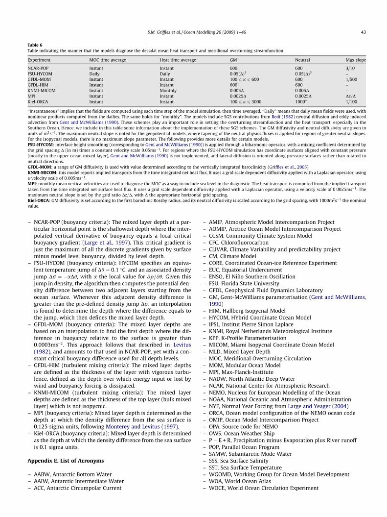
Table 6Table indicating the manner that the models diagnose the decadal mean heat transport and meridional overturning streamfunction
Experiment MOC time average Heat time average GM Neutral Max slope
NCAR-POP Instant Instant 600 600 3/10FSU-HYCOM Daily Daily 0:05ðDÞ3 0:05ðDÞ3 –GFDL-MOM Instant Instant 100 6 j 6 600 600 1/500GFDL-HIM Instant Instant 600 600 –KNMI-MICOM Instant Monthly 0:005D 0:005D –MPI Instant Instant 0:0025D 0:0025D Dz=DKiel-ORCA Instant Instant 100 6 j 6 3000 1000* 1/100
‘‘Instantaneous” implies that the fields are computed using each time step of the model simulation, then time averaged. ‘‘Daily” means that daily mean fields were used, withnonlinear products computed from the dailies. The same holds for ‘‘monthly”. The models include SGS contributions from Redi (1982) neutral diffusion and eddy inducedadvection from Gent and McWilliams (1990). These schemes play an important role in setting the overturning streamfunction and the heat transport, especially in theSouthern Ocean. Hence, we include in this table some information about the implementation of these SGS schemes. The GM diffusivity and neutral diffusivity are given inunits of m2s�1. The maximum neutral slope is noted for the geopotential models, where tapering of the neutral physics fluxes is applied for regions of greater neutral slopes.For the isopycnal models, there is no maximum slope parameter. The following provides more details for certain models.FSU-HYCOM: interface height smoothing (corresponding to Gent and McWilliams (1990)) is applied through a biharmonic operator, with a mixing coefficient determined bythe grid spacing D (in m) times a constant velocity scale 0:05ms�1. For regions where the FSU-HYCOM simulation has coordinate surfaces aligned with constant pressure(mostly in the upper ocean mixed layer), Gent and McWilliams (1990) is not implemented, and lateral diffusion is oriented along pressure surfaces rather than rotated toneutral directions.GFDL-MOM: a range of GM diffusivity is used with value determined according to the vertically integrated baroclinicity (Griffies et al., 2005).KNMI-MICOM: this model reports implied transports from the time integrated net heat flux. It uses a grid scale dependent diffusivity applied with a Laplacian operator, usinga velocity scale of 0:005ms�1.MPI: monthly mean vertical velocities are used to diagnose the MOC as a way to include sea level in the diagnostic. The heat transport is computed from the implied transporttaken from the time integrated net surface heat flux. It uses a grid scale dependent diffusivity applied with a Laplacian operator, using a velocity scale of 0:0025ms�1. Themaximum neutral slope is set by the grid ratio Dz=D, with D the appropriate horizontal grid spacing.Kiel-ORCA: GM diffusivity is set according to the first baroclinic Rossby radius, and its neutral diffusivity is scaled according to the grid spacing, with 1000m2s�1 the nominalvalue.
S.M. Griffies et al. / Ocean Modelling 26 (2009) 1–46 43
– NCAR-POP (buoyancy criteria): The mixed layer depth at a par-ticular horizontal point is the shallowest depth where the inter-polated vertical derivative of buoyancy equals a local criticalbuoyancy gradient (Large et al., 1997). This critical gradient isjust the maximum of all the discrete gradients given by surfaceminus model level buoyancy, divided by level depth.
– FSU-HYCOM (buoyancy criteria): HYCOM specifies an equiva-lent temperature jump of Dh ¼ 0:1 �C, and an associated densityjump Dr ¼ �aDh, with a the local value for @q=@h. Given thisjump in density, the algorithm then computes the potential den-sity difference between two adjacent layers starting from theocean surface. Whenever this adjacent density difference isgreater than the pre-defined density jump Dr, an interpolationis found to determine the depth where the difference equals tothe jump, which then defines the mixed layer depth.
– GFDL-MOM (buoyancy criteria): The mixed layer depths arebased on an interpolation to find the first depth where the dif-ference in buoyancy relative to the surface is greater than0:0003ms�2. This approach follows that described in Levitus(1982), and amounts to that used in NCAR-POP, yet with a con-stant critical buoyancy difference used for all depth levels.
– GFDL-HIM (turbulent mixing criteria): The mixed layer depthsare defined as the thickness of the layer with vigorous turbu-lence, defined as the depth over which energy input or lost bywind and buoyancy forcing is dissipated.
– KNMI-MICOM (turbulent mixing criteria): The mixed layerdepths are defined as the thickness of the top layer (bulk mixedlayer) which is not isopycnic.
– MPI (buoyancy criteria): Mixed layer depth is determined as thedepth at which the density difference from the sea surface is0.125 sigma units, following Monterey and Levitus (1997).
– Kiel-ORCA (buoyancy criteria): Mixed layer depth is determinedas the depth at which the density difference from the sea surfaceis 0.1 sigma units.
Appendix E. List of Acronyms
– AABW, Antarctic Bottom Water– AAIW, Antarctic Intermediate Water– ACC, Antarctic Circumpolar Current
– AMIP, Atmospheric Model Intercomparison Project– AOMIP, Arctice Ocean Model Intercomparison Project– CCSM, Community Climate System Model– CFC, Chlorofluorocarbon– CLIVAR, Climate Variability and predictability project– CM, Climate Model– CORE, Coordinated Ocean-ice Reference Experiment– EUC, Equatorial Undercurrent– ENSO, El Niño Southern Oscillation– FSU, Florida State University– GFDL, Geophysical Fluid Dynamics Laboratory– GM, Gent-McWilliams parameterisation (Gent and McWilliams,
1990)– HIM, Hallberg Isopycnal Model– HYCOM, HYbrid Coordinate Ocean Model– IPSL, Institut Pierre Simon Laplace– KNMI, Royal Netherlands Meteorological Institute– KPP, K-Profile Parameterisation– MICOM, Miami Isopycnal Coordinate Ocean Model– MLD, Mixed Layer Depth– MOC, Meridional Overturning Circulation– MOM, Modular Ocean Model– MPI, Max-Planck-Institute– NADW, North Atlantic Deep Water– NCAR, National Center for Atmospheric Research– NEMO, Nucleus for European Modelling of the Ocean– NOAA, National Oceanic and Atmospheric Administration– NYF, Normal Year Forcing from Large and Yeager (2004)– ORCA, Ocean model configuration of the NEMO ocean code– OMIP, Ocean Model Intercomparison Project– OPA, Source code for NEMO– OWS, Ocean Weather Ship– P � E + R, Precipitation minus Evaporation plus River runoff– POP, Parallel Ocean Program– SAMW, Subantarctic Mode Water– SSS, Sea Surface Salinity– SST, Sea Surface Temperature– WGOMD, Working Group for Ocean Model Development– WOA, World Ocean Atlas– WOCE, World Ocean Circulation Experiment
44 S.M. Griffies et al. / Ocean Modelling 26 (2009) 1–46
References
Adcroft, A., Hill, C., Marshall, J., 1997. Representation of topography by shaved cellsin a height coordinate ocean model. Mon. Weather Rev. 125, 2293–2315.
Antonov, J., Locarnini, R., Boyer, T., Mishonov, A., Garcia, H., 2006. World Ocean Atlas2005, vol. 2: Salinity. U.S. Government Printing Office 62, NOAA Atlas NESDIS,Washington, DC, 182 pp.
Arakawa, A., Lamb, V.R., 1977. The UCLA general circulation model. In: Chang, J.(Ed.), Methods in Computational Physics: General Circulation Models of theAtmosphere, vol. 17. Academic Press, pp. 174–265.
Barnier, B., 1998. Forcing the ocean. In: Chassignet, E.P., Verron, J. (Eds.), OceanModeling and Parameterization, vol. 516 of NATO ASI Mathematical andPhysical Sciences Series. Kluwer, pp. 45–80.
Barnier, B., Madec, G., Penduff, T., Molines, J., Treguier, A., Sommer, J.L., Beckmann,A., Biastoch, A., Böning, C., Dengg, J., Derval, C., Durand, E., Gulev, S., Remy, E.,Talandier, C., Theetten, S., Maltrud, M., McClean, J., Cuevas, B.D., 2006. Impact ofpartial steps and momentum advection schemes in a global ocean circulationmodel at eddy permitting resolution. Ocean Dyn. 56, 543–567.
Barnier, B., Siefridt, L., Marchesiello, P., 1995. Thermal forcing for a global oceancirculation model using a three-year climatology of ECMWF analyses. J. Mar.Res. 6, 363–380.
Beljaars, A., 1994. The parameterization of surface fluxes in large-scale modelsunder free convection. Q. J. Roy. Meteor. Soc. 121, 255–270.
Bentsen, M., Drange, H., Furevik, T., Zhou, T., 2004. Simulated variability of theAtlantic meridional overturning circulation. Clim. Dynam. 22, 701–720.
Bleck, R., 2002. Anoc eanic general circulation model framed in hybrid isopycnic-cartesian coordinates. Ocean Modell. 4, 55–88.
Bleck, R., Rooth, C., Hu, D., Smith, L.T., 1992. Salinity-driven thermocline transientsin a wind and thermohaline forced isopycnic coordinate model of the NorthAtlantic. J. Phys. Oceanogr. 22, 1486–1505.
Böning, C.W., Herrmann, P., 1994. Annual cycle of poleward heat transport in theoceans: results from high-resolution modeling of the Equatorial North Atlantic.J. Phys. Oceanogr. 24, 91–107.
Briegleb, B., Bitz, C., Hunke, E., Lipscomb, W., Holland, M., Schramm, J., Moritz, R.,2004. Scientific description of the sea ice component in the Community ClimateSystem Model, Version 3. NCAR Technical Report No. NCAR/TN-463+STRavailable online at http://www.ccsm.ucar.edu.
Briegleb, B., Hunke, E., Bitz, C.,, Lipscomb, W., 2002. Description of the CommunityClimate System Model Version 2 Sea Ice Model. NCAR Technical Reportavailable online at http://www.ccsm.ucar.edu, 60 pp.
Brodeau, L., Barnier, B., Treguier, A., Penduff, T., Gulev, S., 2008. An era40-basedatmospheric forcing for global ocean circulation models. Ocean Modell.Submitted for publication.
Bryan, F., 1986. High latitude salinity effects and interhemispheric thermohalinecirculations. Nature 323, 301–304.
Cavalieri, D., Parkinson, C., Vinnikov, K., 2003. 30-year satellite record revealsconrasting Arctic and Antarctic decadal variability. Geophys. Res. Lett. 30.doi:10.1029/2003GL018031.
Chassignet, E., Hurlburt, H., Smedstad, O., Halliwell, G., Wallcraft, A., Metzger, E.,Blanton, B., Lozano, C., Rao, D., Hogan, P., Srinivasan, A., 2006. Generalizedvertical coordinates for eddy-resolving global and coastal forecasting.Oceanography 19, 20–31.
Chassignet, E., Smith, L., Halliwell, G., Bleck, R., 2003. North Atlantic simulation withthe HYbrid Coordinate Ocean model (HYCOM): impact of the vertical coordinatechoice, reference density, and thermobaricity. J. Phys. Oceanogr. 33, 2504–2526.
Colin de Verdière, A., Huck, T., 1999. Baroclinic instability: a wavemaker for oceanicinterdecadal variability. J. Phys. Oceanogr. 29, 865–892.
Collins, W., Bitz, C., Blackmon, M., Bonan, G., Bretherton, C., Carton, J., Chang, P.,Doney, S., Hack, J., Henderson, T., Kiehl, J., Large, W., McKenna, D., Santer, B.,Smith, R., 2006. The community climate system model: CCSM3. J. Clim. 19,2122–2143.
Comiso, J., 1999 (updated 2005). Bootstrap sea ice concentrations for NIMBUS-7SMMR and DMSP SSM/I, June to September 2001. National Snow and Ice DataCenter Digital Media.
Conkright, M., Antonov, J., Baranova, O., Boyer, T., Garcia, H., Gelfeld, F., Johnson, D.,Locarnini, R., Murphy, P., O’Brien, T., Smolyar, I., Stephens, C., 2002. World OceanDatabase 2001, vol. 1: Introduction. NOAA Atlas NESDIS 42, U.S. GovernmentPrinting Office 13, NOAA, Washington, DC, 167 pp.
Cox, M., Bryan, K., 1984. A numerical model of the ventilated thermocline. J. Phys.Oceanogr. 14, 674–687.
Cunningham, S., Alderson, S., King, B., Brandon, M., 2003. Transport and variabilityof the Antarctic Circumpolar Current in Drake Passage. J. Geophys. Res. 108, Art.8084.
Danabasoglu, G., Ferrari, R., McWilliams, J.C., 2008. Sensitivity of an ocean generalcirculation model to a parameterization of near-surface eddy fluxes. J. Clim. 21,1192–1208.
Danabasoglu, G., Large, W.G., Tribbia, J.J., Gent, P.R., Briegleb, B.P., McWilliams, J.C.,2006. Diurnal coupling in the tropical oceans of CCSM3. J. Clim. 19, 2347–2365.
Danabasoglu, G., Marshall, J., 2007. Effects of vertical variations of thicknessdiffusivity in an oc ean general circulation model. Ocean Modell. 18, 122–141.
Danabasoglu, G., McWilliams, J., Gent, P., 1994. The role of mesoscale tracertransports in the global ocean circulation. Science 264, 1123–1126.
De Boyer Montegut, C., Madec, G., Fischer, A., Lazar, A., Iudicone, D., 2004. Mixedlayer depth over the global ocean: an examination of profile data and a profilebased climatology. J. Geophys. Res. 109. doi:10.1029/2004JC002378.
Delworth, T.L., Broccoli, A.J., Rosati, A., Stouffer, R.J., Balaji, V., Beesley, J.A., Cooke,W.F., Dixon, K.W., Dunne, J., Dunne, K.A., Durachta, J.W., Findell, K.L., Ginoux, P.,Gnanadesikan, A., Gordon, C., Griffies, S.M., Gudgel, R., Harrison, M.J., Held, I.M.,Hemler, R.S., Horowitz, L.W., Klein, S.A., Knutson, T.R., Kushner, P.J.,Langenhorst, A.L., Lee, H.-C., Lin, S., Lu, L., Malyshev, S.L., Milly, P.,Ramaswamy, V., Russell, J., Schwarzkopf, M.D., Shevliakova, E., Sirutis, J.,Spelman, M., Stern, W.F., Winton, M., Wittenberg, A.T., Wyman, B., Zeng, F.,Zhang, R., 2006. GFDL’s CM2 global coupled climate models – part 1:formulation and simulation characteristics. J. Clim. 19, 643–674.
Doney, S.C., Hecht, M.W., 2002. Antarctic bottom water formation and deep waterchlorofluorocarbon distributions in a global ocean climate model. J. Phys.Oceanogr. 32, 1642–1666.
Dukowicz, J.K., Smith, R.D., 1994. Implicit free-surface method for the Bryan–Cox–Semtner ocean model. J. Geophys. Res. 99, 7991–8014.
England, M.H., 1995. The age of water and ventilation timescales in a global oceanmodel. J. Phys. Oceanogr. 25, 2756–2777.
England, M.H., Maier-Reimer, E., 2001. Using chemical tracers to assess oceanmodels. Rev. Geophys. 39, 29–70.
Fritzsch, B., Gerdes, R., Hiller, W., Latif, M., Legutke, S., Maier-Reimer, E., Olbers, D.,Röske, F., 2000. The Ocean Model Intercomparison Project (OMIP). AlfredWegener Institude for Polar and Marine Research, Bemerhaven, and Max-Planck-Institute for Meteorology, Hamburg, 139 p.
Ganachaud, A., 2003. Large-scale mass transports, water mass formation, anddiffusivities estimated from World Ocean Circulation Experiment (WOCE)hydrographic data. J. Geophys. Res. 108. doi:10.1029/2002JC001565.
Ganachaud, A., Wunsch, C., 2000. Improved estimates of global ocean circulation,heat transport and mixing from hydrographic data. Nature 408, 453–456.
Gaspar, P., Gregoris, Y., Lefevre, J., 1990. A simple eddy kinetic energy model forsimulations of the oceanic vertical mixing: tests at station Papa and long-termupper ocean study site. J. Geophys. Res. 95, 16179–16193.
Gates, W., 1993. AMIP: the atmosphere model intercomparison project. Bull. Am.Meteorol. Soc. 73, 1962–1970.
Gent, P., Large, W., Bryan, F., 2001. What sets the mean transport through DrakePassage? J. Geophys. Res. 106, 2693.
Gent, P.R., McWilliams, J.C., 1990. Isopycnal mixing in ocean circulation models. J.Phys. Oceanogr. 20, 150–155.
Gent, P.R., Willebrand, J., McDougall, T.J., McWilliams, J.C., 1995. Parameterizingeddy-induced tracer transports in ocean circulation models. J. Phys. Oceanogr.25, 463–474.
Gerdes, R., Griffies, S., Hurlin, W., 2005a. Reaction of the oceanic circulation toincreased melt water flux from greenland – a test case for ocean generalcirculation models. Clivar Exchanges 10, 28–31.
Gerdes, R., Hurka, J., Karcher, M., Kauker, F., Köberle, C., 2005b. Simulated history ofconvection in the Greenland and Labrador Seas 1948–2001. In: Monograph, A.(Ed.), The Nordic Seas: An Integrated Perspective, vol. 158. AmericanGeophysical Union, Washington, DC, pp. 221–238.
Gerdes, R., Hurlin, W., Griffies, S., 2006. Sensitivity of a global ocean model toincreased run-off from greenland. Ocean Modell. 12, 416–435.
Gerdes, R., Köberle, C., 2007. Comparison of Arctic sea ice thickness variability inIPCC Climate of the 20th Century experiments and in ocean–sea ice hindcasts. J.Geophys. Res. 112 (C04S13). doi:10.1029/2006JC003616.
Gill, A.E., Niiler, P., 1973. The theory of the seasonal variability in the ocean. Deep-Sea Res. 20 (9), 57–64.
Gnanadesikan, A., Dixon, K.W., Griffies, S.M., Balaji, V., Beesley, J.A., Cooke, W.F.,Delworth, T.L., Gerdes, R., Harrison, M.J., Held, I.M., Hurlin, W.J., Lee, H.-C., Liang,Z., Nong, G., Pacanowski, R.C., Rosati, A., Russell, J., Samuels, B.L., Song, S.M.,Spelman, M.J., Stouffer, R.J., Sweeney, C.O., Vecchi, G., Winton, M., Wittenberg,A.T., Zeng, F., Zhang, R., 2006. GFDL’s CM2 global coupled climate models-part 2:the baseline ocean simulation. J. Clim. 19, 675–697.
Gnanadesikan, A., Griffies, S., Samuels, B., 2007. Effects in a climate model of slopetapering in neutral physics schemes. Ocean Modell. 17, 1–16.
Gordon, C., Cooper, C., Senior, C.A., Banks, H.J.M., Gregory, T.C.J., Mitchell, J.F.B.,Wood, R.A., 2000. The simulation of SST, sea ice extents and ocean heattransports in a version of the Hadley Centre coupled model without fluxadjustments. Clim. Dyn. 16, 147–168.
Greatbatch, R., Peterson, K., 1996. Interdecadal variability and oceanic thermohalineadjustment. J. Geophys. Res. 101, 20467–20482.
Griffies, S.M., 2004. Fundamentals of Ocean Climate Models. Princeton UniversityPress, Princeton, USA. 518+xxxiv p.
Griffies, S.M., Gnanadesikan, A., Dixon, K.W., Dunne, J.P., Gerdes, R., Harrison, M.J.,Rosati, A., Russell, J., Samuels, B.L., Spelman, M.J., Winton, M., Zhang, R., 2005.Formulation of an ocean model for global climate simulations. Ocean Sci. 1, 45–79.
Griffies, S.M., Harrison, M.J., Pacanowski, R.C., Rosati, A., 2004. A Technical Guide toMOM4. NOAA/Geophysical Fluid Dynamics Laboratory, Princeton, USA. 337 pp.
Griffies, S.M., Pacanowski, R., Schmidt, M., Balaji, V., 2001. Tracer conservation withan explicit free surface method for z-coordinate ocean models. Mon. WeatherRev. 129, 1081–1098.
Hallberg, R., 2005. A thermobaric instability in Lagrangian vertical coordinate oceanmodels. Ocean Modell. 8, 227–300.
Hallberg, R., Gnanadesikan, A., 2006. On the role of eddies in determining thestructure and response of the wind-driven southern hemisphere overturning:results from the Modeling Eddies in the Southern Ocean (MESO) project. J. Phys.Oceanogr. 36, 2232–2252.
Hallberg, R.W., 2003. The suitability of large-scale ocean models for adaptingparameterizations of boundary mixing and a description of a refined bulk mixed
S.M. Griffies et al. / Ocean Modelling 26 (2009) 1–46 45
layer model. In: Müller, P., Garrett, C. (Eds.), Near-Boundary Processes and TheirParameterization. Proceedings of the 13th’Aha Huliko’a Hawaiian WinterWorkshop. University of Hawaii at Manoa, pp. 187–203.
Haltiner, G.T., Williams, R.T., 1980. Numerical Prediction and Dynamic Meteorology.John Wiley and Sons, New York, USA.
Haney, R.L., 1971. Surface thermal boundary conditions for ocean circulationmodels. J. Phys. Oceanogr. 1, 241–248.
Hazeleger, W., Severijns, C., Haarsma, R., Selten, F., Sterl, A., 2003. Speedo – modeldescription and validation of a flexible coupled model for climate studies.KNMI-Technical Report R257, 1–38.
Hellerman, S., Rosenstein, M., 1983. Normal monthly wind stress over the WorldOcean with error estimates. J. Phys. Oceanogr. 13, 1093–1104.
Hewitt, C., Broccoli, A., Crucifix, M., Gregory, J., Mitchell, J., Stouffer, R., 2006. Theeffect of a large freshwater perturbation on the glacial North Atlantic Oceanusing a coupled general circulation model. J. Clim. 19, 4436–4447.
Hibler, W., 1979. A dynamic thermodynamic sea ice model. J. Phys. Oceanogr. 9,815–846.
Hirst, A., McDougall, T., 1998. Meridional overturning and dianeutral transport in az-coordinate ocean model including eddy-induced advection. J. Phys. Oceanogr.28, 1205–1223.
Holloway, G., Dupont, F., Golubeva, E., Hakkinen, S., Hunke, E., Jin, M., Karcher, M.,Kauker, F., Maltrud, M., Morales-Maqueda, M., Maslowski, W., Platov, G., Stark,D., Steele, M., Suzuki, T., Wang, J., Zhang, J., 2007. Water properties andcirculation in Arctic Ocean models. J. Geophys. Res. 112. doi:10.1029/2006JC003642.
Hsiung, J., Newell, R.E., Houghtby, T., 1989. The annual cycle of oceanic heat storageand oceanic meridional heat transport. Q. J. Roy. Meteor. Soc 115 (485), 1–28.
Huang, R.X., 1993. Real freshwater flux as a natural boundary condition for thesalinity balance and thermohaline circulation forced by evaporation andprecipitation. J. Phys. Oceanogr. 23, 2428–2446.
Hurrell, J.W., Hack, J.J., Shea, D., Caron, J.M., Rosinski, J., 2008. A new sea surfacetemperature and sea ice boundary data set for the Community AtmosphereModel. J. Clim. in press.
Jayne, S., Marotzke, J., 1999. A destabilizing thermohaline circulation-atmosphere-sea ice feedback. J. Clim. 12, 642–651.
Jerlov, N.G., 1968. Optical Oceanography. Elsevier.Johnson, G.C., Sloyan, B.M., Kessler, W.S., McTaggart, K.E., 2002. Direct
measurements of upper ocean currents and water properties across thetropical pacific during the 1990’s. Prog. Oceanogr. 52, 31–36.
Johnson, M., Gaffigan, S., Hunke, E., Gerdes, R., 2007. A comparison of Arctic Oceansea ice concentration among the coordinated AOMIP model experiments. J.Geophys. Res. 112 (C04S11). doi:10.1029/2006JC003690.
Jungclaus, J., Keenlyside, N., Botzet, M., Haak, H., Luo, J.-J., Latif, M., Marotzke, J.,Mikolajewicz, U., Roeckner, E., 2006. Ocean circulation and tropical variabilityin the coupled model ECHAM5/MPI-OM. J. Clim. 19, 3952–3972.
Karoly, D., McIntosh, P., Berrisford, P., McDougall, T.J., Hirst, A., 1997. Similarities ofthe Deacon cell in the Southern Ocean and Ferrel cells in the atmosphere. Q. J.Roy. Meteor. Soc. 123, 519–526.
Killworth, P.D., Smeed, D., Nurser, A., 2000. The effects on ocean models ofrelaxation toward observations at the surface. J. Phys. Oceanogr. 30, 160–174.
Large, W., Yeager, S., 2004. Diurnal to decadal global forcing for ocean and sea-icemodels: the data sets and flux climatologies. NCAR Technical Note: NCAR/TN-460+STR. CGD Division of the National Center for Atmospheric Research.
Large, W.B., 2005. Surface fluxes for practioners of global ocean data assimilation.In: Chassignet, E.P., Verron, J. (Eds.), Ocean Weather Forecasting: An IntegratedView of Oceanography, vol. 577. Springer, pp. 229–270.
Large, W.G., Danabasoglu, G., Doney, S.C., McWilliams, J.C., 1997. Sensitivity tosurface forcing and boundary layer mixing in a global ocean model: annual-mean climatology. J. Phys. Oceanogr. 27, 2418–2447.
Large, W.G., McWilliams, J.C., Doney, S.C., 1994. Oceanic vertical mixing: a reviewand a model with a nonlocal boundary layer parameterization. Rev. Geophys.32, 363–403.
Large, W.G., Yeager, S., 2008. The global climatology of an interannually varying air-sea flux data set. Clim. Dyn. accepted for pubication.
Latif, M., Anderson, D., Barnett, T., Cane, M., Kleeman, R., Leetmaa, A., O’Brien, J.,Rosati, A., Schneider, E., 1998. A review of the predictability and prediction ofENSO. J. Geophys. Res. 103 (C7), 14375–14393.
Latif, M., Böning, C., Willebrand, J., Biastoch, A., Dengg, J., Keenlyside, N., Madec, G.,Schweckendiek, U., 2006. Is the thermohaline circulation changing? J. Clim.,4631–4637.
Levitus, S., 1982. Climatological atlas of the world ocean. U.S. Government PrintingOffice 13, NOAA, Washington, DC, 163 pp.
Levitus, S., Burgett, R., Boyer, T., 1994. World Ocean Atlas 1994. vol 3: Salinity; vol.4: Temperature. NOAA Atlas NESDIS 3 and 4, NOAA, U.S. Dept. of Commerce,Washington, DC.
Locarnini, R., Mishonov, A., Antonov, J., Boyer, T., Garcia, H., 2006. World Ocean Atlas2005, volume 1: Temperature. U.S. Government Printing Office 61, NOAA AtlasNESDIS, Washington, DC, 182 pp.
Lohmann, G., Gerdes, R., 1998. Sea ice effects on the sensitivity of the thermohalinecirculation in simplified atmosphere-ocean-sea ice models. J. Clim. 11, 2789–2803.
Lohmann, G., Gerdes, R., Chen, D., 1996. Sensitivity of the thermohaline circulation incoupled oceanic gcm–atmospheric ebm experiments. Clim. Dyn. 12, 403–416.
Lorbacher, K., Dommenget, D., Niiler, P., Köhl, A., 2006. Ocean mixed layer depth: asubsurface proxy of ocean-atmosphere variability. J. Geophys. Res. 111, C07010.doi:10.1029/2003JC002157.
Lumpkin, R., Speer, K., 2003. Large-scale vertical and horizontal circulation in theNorth Atlantic Ocean. J. Phys. Oceanogr. 33, 1902–1920.
Lumpkin, R., Speer, K., Koltermann, K., 2008. Transport across 48�N in the AtlanticOcean. J. Phys. Oceanogr. 38, 733–752.
Madec, G., Delecluse, P., Imbard, M., Lévy, C., 1999. OPA 8.1 ocean generalcirculation model reference manual. In: Note du Pôle de modélisation. Paris,France, pp. 91.
Maltrud, M., McClean, J., 2005. An eddy resolving global 1/10� ocean simulation.Ocean Modell. 8, 31–54.
Marsh, R., de Cuevas, B., Coward, A., Nurser, A., Josey, S., 2005. Water masstransformation in the North Atlantic over 1985–2002 simulated in an eddy-permitting model. Ocean Sci. 1, 127–144.
Marshall, J., Schott, F., 1999. Open-ocean convection: observations, theory, andmodels. Rev. Geophys. 37, 1–64.
Marsland, S., Haak, H., Jungclaus, J., Latif, M., Röske, F., 2003. The Max-Planck-Institute global ocean/sea ice model with orthogonal curvilinear coordinates.Ocean Modell. 5, 91–127.
Martin, T., Gerdes, R., 2007. Sea ice drift variability in Arctic Ocean ModelIntercomparison Project models and observations. J. Geophys. Res. 112(C04S10). doi:10.1029/2006JC003617.
McCartney, M., 1977. Subantarctic mode water. In: Angel, M. (Ed.), A Voyage ofDiscovery: George Deacon 70th Anniversary Volume. Supplement to Deep-SeaResearch. Pergamon Press, Oxford, pp. 103–119.
Meehl, G., Gent, P.R., Arblaster, J., Otto-Bliesner, B., Brady, E., Craig, A., 2001. Factorsthat affect the amplitude of El Niño in global coupled climate models. Clim. Dyn.17, 515–526.
Monterey, G., Levitus, S., 1997. Climatological cycle of mixed layer depth in theworld ocean. U.S. government printing office, NOAA NESDIS, Washington, DC, 5pp.
Morel, A., Antoine, D., 1994. Heating rate within the upper ocean in relation to itsbio-optical state. J. Phys. Oceanogr. 24, 1652–1665.
Murray, R.J., 1996. Explicit generation of orthogonal grids for ocean models. J.Comput. Phys. 126, 251–273.
Ohlmann, J., 2003. Ocean radiant heating in climate models. JOC 16, 1337–1351.Orsi, A., Whitworth, T., Nowlin, W., 1995. On the meridional extent and fronts of the
antarctic circumpolar current. Deep-Sea Res. 42A, 641–673.Pacanowski, R.C., 1987. Effect of equatorial currents on surface stress. J. Phys.
Oceanogr. 17, 833–838.Pacanowski, R.C., Gnanadesikan, A., 1998. Transient response in a z-level ocean
model that resolves topography with partial-cells. Mon. Weather Rev. 126,3248–3270.
Paulson, E.A., Simpson, J.J., 1977. Irradiance measurements in the upper ocean. J.Phys. Oceanogr. 7, 952–956.
Payne, R., 1972. Albedo of the surface ocean. J. Atmos. Sci. 29, 959–970.Peixoto, J.P., Oort, A.H., 1992. Physics of Climate. American Institute of Physics.
520+xxxix pp.Proshutinsky, A., Steele, M., Zhang, J., Holloway, G., Steiner, N., Häkkinen, S., Holland,
D., Gerdes, R., Köberle, C., Karcher, M., Johnson, M., Maslowski, W., Zhang, Y.,Hibler, W., Wang, J., 2001. The Arctic Ocean Model Intercomparison Project(AOMIP). EOS 82, 637–644.
Rahmstorf, S., Marotzke, J., Willebrand, J., 1996. Stability of the thermohalinecirculation. In: Krauss, W. (Ed.), The Warmwatersphere of the North Atlantic.Borntraeger, pp. 129–157.
Rahmstorf, S., Willebrand, J., 1995. The role of temperature feedback in stabilizingthe thermohaline circulation. J. Phys. Oceanogr. 25, 787–805.
Rayner, N., Parker, D., Horton, E., Folland, C., Alexander, L., Rowell, D., Kent, E.,Kaplan, A., 2003. Global analyses of SST, sea ice and night marine airtemperature since the late nineteenth century. J. Geophys. Res. 108 (D14),4407. doi:10.1029/2002JD002670.
Redi, M.H., 1982. Oceanic isopycnal mixing by coordinate rotation. J. Phys.Oceanogr. 12, 1154–1158.
Reynolds, R.W., Rayner, N., Smith, T.M., Stokes, D., Wang, W., 2002. An improvedin situ and satellite SST analysis for climate. J. Clim. 15, 1609–1625.
Reynolds, R.W., Smith, T.M., 1994. Improved global sea surface temperatureanalyses using optimum interpolation. J. Clim. 7 (6), 929–948.
Rivin, I., Tziperman, E., 1997. On the sensitivity of air-sea fluxes to SSTperturbations. J. Clim. 11, 2431–2446.
Robinson, I., 2005. Satellite oceanography. In: Chassignet, E.P., Verron, J. (Eds.),GODEA Summer School. Springer/Kluwer.
Roeckner, E., Brokopf, R., Esch, M., Giorgetta, M., Hagemann, S., Kornblueh, L.,Manzini, E., Schlese, U., Schulzweida, U., 2006. Sensitivity of simulated climateto horizontal and vertical resolution in the ECHAM5 atmosphere model. J. Clim.19, 3771–3791.
Rosati, A., Miyakoda, K., 1988. A general circulation model for upper oceansimulation. J. Phys. Oceanogr. 18, 1601–1626.
Röske, F., 2006. A global heat and freshwater forcing dataset for ocean models.Ocean Modell. 11, 235–297.
Roullet, G., Madec, G., 2000. Salt conservation, free surface, and varying volume. Anew formulation for ogcms. JGR 105, 23927–23947.
Russell, J., Stouffer, R., Dixon, K., 2006. Intercomparison of the southern oceancirculations in the ipcc coupled model control simulations. J. Clim. 19, 4560–4575.
Sarmiento, J.L., 1986. On the North and Tropical Atlantic heat balance. J. Geophys.Res. 91 (C10), 11677–11690.
Schweckendiek, U., Willebrand, J., 2005. Mechanisms affecting the overturningresponse in global warming simulations. J. Clim. 18, 4925–4936.
46 S.M. Griffies et al. / Ocean Modelling 26 (2009) 1–46
Smith, R., Gent, P., 2004. Reference Manual for the Parallel Ocean Program (POP).Los Alamos Technical Report No. LAUR-02-2484.
Smith, R.D., Kortas, S., Meltz, B., 1995. Curvilinear coordinates for global oceanmodels. Los Alamos preprint LA-UR-95-1146.
Smolarkiewicz, P., 1984. A fully multidimensional positive definite advectiontransport algorithm with small implicit diffusion. J. Comput. Phys. 54, 325–362.
Sprintall, J., Tomczak, M., 1992. Evidence of the barrier layer in the surface layer ofthe tropics. J. Geophys. Res. 97, 7305–7316.
Steele, M., Morfley, R., Ermold, W., 2001. PHC: A global ocean hydrography with ahigh-quality Arctic Ocean. J. Clim. 14, 2079–2087.
Stommel, H., 1961. Thermohaline convection with two stable regies of flow. Tellus13, 224–228.
Stommel, H., 1979. Determination of water mass properties of water pumped downfrom the ekman layer to the geostrophic flow below. Proc. Nat. Acad. Sci. USA76, 3051–3055.
Stouffer, R.J., 2004. Time scales of climate response. J. Clim. 17, 209–217.Sun, S., Bleck, R., 2006. Multi-century simulations with the coupled GISS-HYCOM
climate model: control experiments. Clim. Dyn. 26, 407–428.Sweeney, C., Gnanadesikan, A., Griffies, S.M., Harrison, M., Rosati, A., Samuels, B.,
2005. Impacts of shortwave penetration depth on large-scale ocean circulationand heat transport. J. Phys. Oceanogr. 35, 1103–1119.
Taylor, P., 2000. Final Report of the Joint WCRP/SCOR Working Group on Air-Sea Fluxes: Intercomparison and validation of ocean-atmosphere energyflux fields. WCRP-112, WMO/TD-No.1036. World Climate ResearchProgramme, 303p.
Timmermannn, R., Goosse, H., Madec, G., Fichefet, T., Ethé, C., Duliére, V., 2005. Onthe representation of high latitude processes in the ORCA-LIM global coupledsea ice-ocean model. Ocean Modell. 8, 175–201.
Trenberth, K., Caron, J., 2001. Estimates of meridional atmosphere and ocean heattransports. J. Clim. 14, 3433–3443.
Tziperman, E., 1997. Inherently unstable climate behaviour due to weakthermohaline ocean circulation. Nature 386, 592–595.
Weaver, A.J., Hughes, T.M., 1996. On the incompatibility of ocean and atmospheremodels and the need for flux adjustments. Clim. Dyn. 13, 141–170.
Webb, D.J., 1994. The Deacon cell and the other meridional cells in the SouthernOcean. J. Phys. Oceanogr. 24, 429–442.
Whitworth, T., 1983. Monitoring the transport of the Antarctic Circumpolar Currentat Drake Passage. J. Phys. Oceanogr. 13, 2045–2057.
Whitworth, T., Peterson, R., 1985. Volume transport of the antarctic circumpolarcurrent from bottom pressure measurements. J. Phys. Oceanogr. 15, 810–816.
Williams, R., Spall, M., Marshall, J., 1995. Does Stommel’s mixed layer ‘demon’work? J. Phys. Oceanogr. 25, 3089–3102.
Wyrtki, K., Kilonsky, B., 1984. Mean water and current structure during the Hawaii-to-Tahiti shuttle experiment. J. Phys. Oceanogr. 14, 242–254.
Yeager, S.G., Shields, C.A., Large, W.G., Hack, J.J., 2006. The low-resolution CCSM3.J. Clim. 19, 2545–2566.
Zhang, S., Greatbatch, R., Lin, C., 1993. A re-examination of the polar haloclinecatastrophe and implications for coupled ocean-atmosphere models. J. Phys.Oceanogr. 23, 287–299.
Zhang, X., Walsh, J., 2006. Toward a seasonally ice-covered Arctic Ocean: scenariosfrom the IPCC AR4 model simulations. J. Clim. 19, 1730–1747.