Cooperatively Learning Footprints of Multiple Incumbent...

CooperativelyLearningFootprintsofMultipleIncumbentUsers

MihirLaghateandDanijelaCabric21st April2017

SupportedbyNSFGrant1527026:DynamicSpectrumAccessbyLearningPrimaryNetworkTopology

D. Markovic / Slide 2

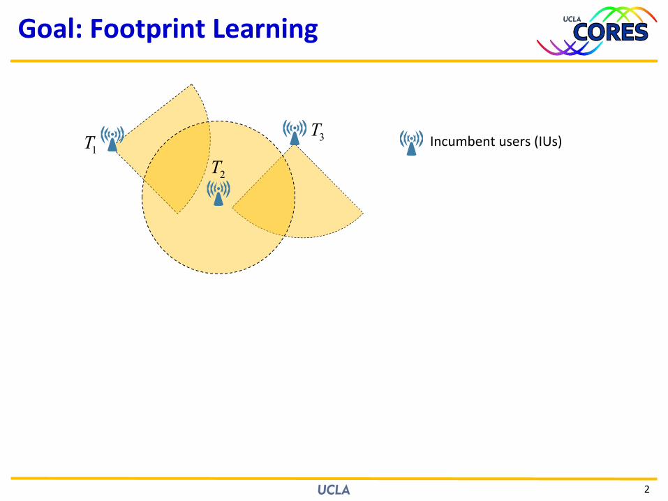
Goal:FootprintLearning

2

Incumbentusers(IUs)1T

2T

3T



3

CognitiveRadios(CRs)

Incumbentusers(IUs)1T

2T

3T



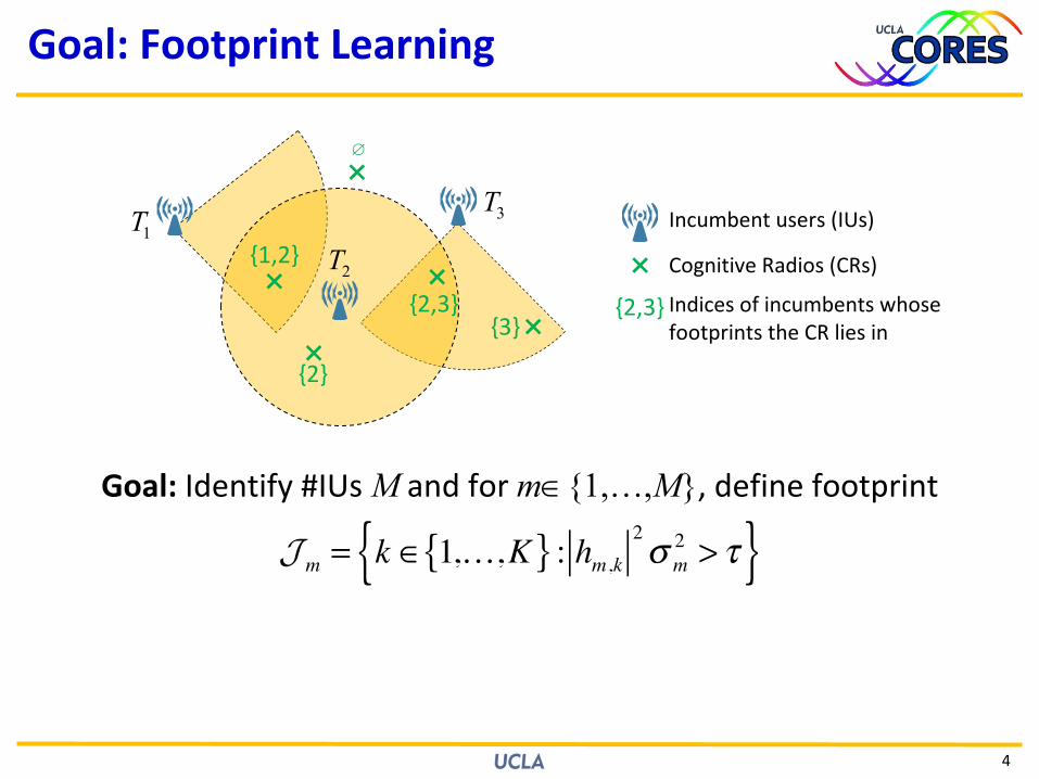
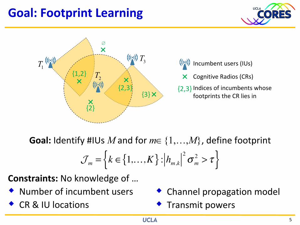
Goal: Identify#IUsM andformÎ{1,…,M},definefootprint

4


Incumbentusers(IUs)

{2,3} IndicesofincumbentswhosefootprintstheCRliesin

{2}

1T2T

3T

{2,3}{3}

{1,2}

∅

Jm = k ∈ 1,…,K{ } : hm,k2σ m2 > τ{ }



Goal: Identify#IUsM andformÎ{1,…,M},definefootprint

5


Incumbentusers(IUs)

{2,3} IndicesofincumbentswhosefootprintstheCRliesin

{2}

1T2T

3T

{2,3}{3}

{1,2}

∅

Jm = k ∈ 1,…,K{ } : hm,k2σ m2 > τ{ }

Constraints:Noknowledgeof…w Numberofincumbentusersw CR&IUlocations

w Channelpropagationmodelw Transmitpowers


ChallengesofDistinguishingIUs

w Anisotropicradiationpatterns– Directionalantennas– Beamforming

w Locationuncertainty

6

Incumbentusers

Example:Sectorized cellularnetwork

w Intermittenttransmissions

w Unknownnumberoftransmitters





7

Incumbentusers




Don’tuselocationinformation!





8

Incumbentusers

Example:Sectorized cellularnetworkDistinguishIUs



Don’tuselocationinformation!


ExistingMethodstoLearnFootprints

9

Based on Anisotropicfootprints

SpatialOverlap

BlindtoChannel Requires

Transmission protocols[1,2] ü ü ü

PriorInformationCyclicfrequency[6] ü ü ü

Channelmodel &location[3-5] û ü û

Angle ofArrival[7,8] ü ü û MultipleAntennasReceivedenergy[9,10] ü û ü BlindDistribution ofreceivedenergy ü ü ü BlindProposedmethod


Incumbentnetwork:w M transmittersindexed{1,…,M}w Transmitsw Fixedspatialradiationpatternw Spectrumoccupancy:am[n] = 1 iftransmitting,0 otherwise

Cognitivenetwork:w K CRreceiversw Slowfadingchannelhm,k frommth incumbenttokth CR

Receivedenergy:

w CRscancommunicatewithacentralserver

SystemModel

10

CognitiveRadios

Incumbenttransmitter


( )2[ ] ~ 0, mmx n sCN

2 2 2 2, 2

1

1~ [[ ]2

] | [ ]kk

M

m k m m Tm

h a ne n a n ns s c=

æ ö+ç ÷

è øå


GaussianMixtureModelofRxEnergy

w Component⇔ UniquesetofIUstransmittingsimultaneouslyw M transmitters⇔ #Components= 2M

11

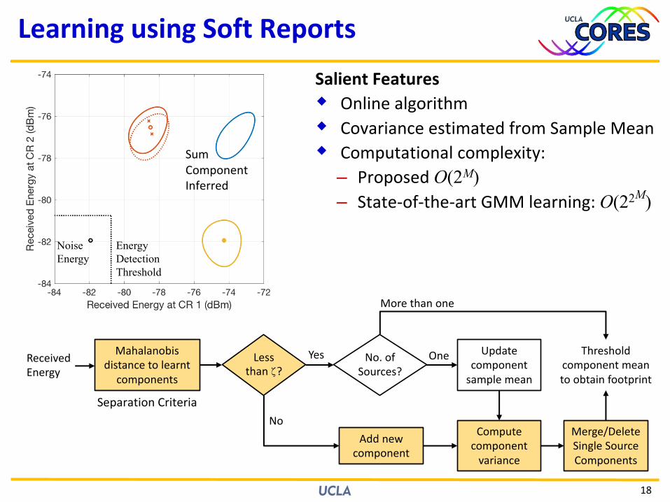
Example:Scatterplotofreceivedenergyat2CRsfrom2sources.Alsoshown:marginalconditionaldistributionsgiventransmitterID

2 2 2 2, 2

1

1~ [[ ]2

] | [ ]kk

M

m k m m Tm

h a ne n a n ns s c=

æ ö+ç ÷

è øå


LearningusingSoftReports

12

SalientFeaturesw Onlinealgorithmww

Energy Detection Threshold

Noise Energy



13

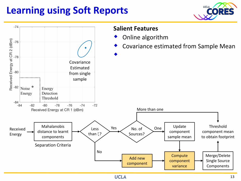
SalientFeaturesw Onlinealgorithmw CovarianceestimatedfromSampleMeanw

CovarianceEstimatedfromsinglesample

ReceivedEnergy

Mahalanobisdistancetolearnt

components

Lessthanζ?

No.ofSources?

Updatecomponentsamplemean

Thresholdcomponentmeantoobtainfootprint

Addnewcomponent

Computecomponentvariance

Merge/DeleteSingleSourceComponents

No

Yes One

Morethanone

SeparationCriteria


Noise Energy



14


NewSourceComponent

ReceivedEnergy


components

Lessthanζ?

No.ofSources?



Addnewcomponent



No

Yes One

Morethanone

SeparationCriteria


Noise Energy



15

SalientFeaturesw Onlinealgorithmw CovarianceestimatedfromSampleMeanwNewSample,

KnownComponent

ReceivedEnergy


components

Lessthanζ?

No.ofSources?



Addnewcomponent



No

Yes One

Morethanone

SeparationCriteria


Noise Energy



16


ComponentMeanUpdated

ReceivedEnergy


components

Lessthanζ?

No.ofSources?



Addnewcomponent



No

Yes One

Morethanone

SeparationCriteria


Noise Energy



17


NewSourceComponent

ReceivedEnergy


components

Lessthanζ?

No.ofSources?



Addnewcomponent



No

Yes One

Morethanone

SeparationCriteria


Noise Energy



18

SalientFeaturesw Onlinealgorithmw CovarianceestimatedfromSampleMeanw Computationalcomplexity:– ProposedO(2M)– State-of-the-artGMMlearning:O(22M)

SumComponentInferred

ReceivedEnergy


components

Lessthanζ?

No.ofSources?



Addnewcomponent



No

Yes One

Morethanone

SeparationCriteria


Noise Energy


SimulationofSlottedALOHA

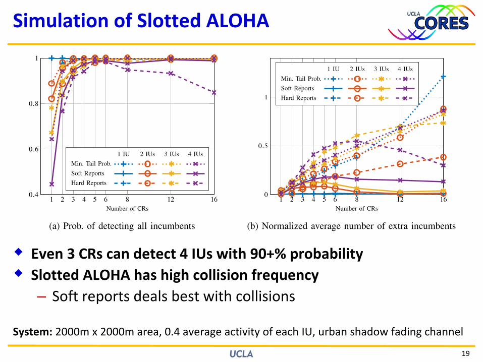
w Even3CRscandetect4IUswith90+%probabilityw SlottedALOHAhashighcollisionfrequency– Softreportsdealsbestwithcollisions

19

25

0.95 0.96 0.97 0.98 0.990.8

0.85

0.9

0.95

1

Threshold (⇣)

1 IU 2 IUs 3 IUs 4 IUsMin. Tail Prob.Soft ReportsHard Reports

(a) Prob. of detecting all incumbents

0.95 0.96 0.97 0.98 0.990

0.2

0.4

0.6

0.8

Threshold (⇣)


(b) Normalized average number of extra incumbents

Fig. 9. Effect on detection performance when threshold ⇣ is varied from 0.95 to 0.99. Parameters: M = 1 to 4 IUs, K = 4 CRs,

0.4 average activity, N = 200 frames of T = 32 samples each.

1 2 3 4 5 6 8 12 160.4

0.6

0.8

1

Number of CRs


(a) Prob. of detecting all incumbents

1 2 3 4 5 6 8 12 160

0.5

1

Number of CRs


(b) Normalized average number of extra incumbents

Fig. 10. Effect on detection performance when CRs are increased from 1 to 16 for up to 4 IUs with average activity 0.4. Hard

reports algorithm not run for 1 CR system. Parameters: N = 200 frames of T = 32 samples each.

C. Assumption of Constant Channel

An important assumption in our algorithm is that the channels between IUs and CRs are

constant, i.e., the channel coherence time is greater than the time required to collect N energy

measurements. We shall now estimate the measurement time for CRs using 6MHz wide bands,

similar to IEEE 802.22 [20], and find the minimum coherence time supported by our algorithm.

Time required to collect a single energy measurement of T samples is T/6µs, i.e., 5.33µs

for T = 32. To ensure that different IUs are transmitting in different energy measurements, we

assume a fixed time interval between successive measurements. A suitable sensing time interval

depends on the medium access control protocol of the IU systems because that controls the

transmission duration and interval between successive transmissions. For the sake of argument,

if the IUs belong to the commonly used IEEE 802.11 standards, the time interval between

System:2000mx2000marea,0.4averageactivityofeachIU,urbanshadowfadingchannel


Applications:AnisotropicAntennas

20

27

�1,000 0 1,000

�1,000

0

1,000

X-Coordinate (m)

Y-C

oord

inat

e(m

)

DBE [10]Hard ReportsTrue Footprints

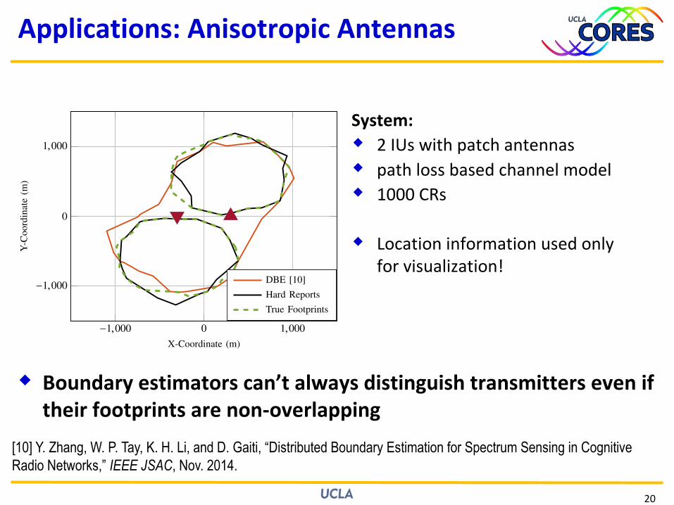
Fig. 12. Boundaries of the footprints of two IUs with patch antennas as detected by the hard reports algorithm and the DBE

algorithm proposed in [10]. Dots represent CR locations and triangles represent IU locations.

multiple 802.11n networks sharing a 20 MHz 802.11 channel in a square area of side 50m.

A simple log distance propagation loss model was used between IUs with exponent 3. 1000

network topologies were generated and simulated for 3 seconds each. By sampling the packet

traces every 150 µs, each topology provided 100 time sequences of 200 frames each. Each

network consists of 1 AP and 2 STAs. UDP flows are set up on both downlink and uplink. 2000

byte packets are generated at each radio at periodic intervals. To control the network load, these

intervals are chosen as multiples of the transmit times for an individual packet. Fig 11 shows

the performance of 6 CRs as this “load factor” is varied from 0.5 to 100. First, we note that

all three algorithms detect very few extra IUs. Secondly, the hard reports algorithm detects all

IUs with approximately the same probability as the soft reports algorithm. Both these properties

can be explained by the fewer number of collisions due to the collision avoidance mechanisms

of 802.11. Reducing number of collisions also explain why the probability of detecting all IUs

increases with increasing load factor. However, as the load factor reduces below 10, candidate

components may not get confirmed because of the low activity.

E. Comparison to Existing Work

Apart from [16], methods proposed in existing literature do not consider multiple IUs with spa-

tially overlapping footprints. For comparison on a simpler system, we implemented the distributed

boundary estimation (DBE) algorithm proposed in [10] that finds anisotropic non-overlapping

footprints. In addition to received energy, the DBE algorithm assumes geographical location for

clustering and pair wise communication channels for message exchanges. We simulated a single

IU located at the center of a 2000m ⇥ 2000m area with 100 CRs distributed uniformly around

System:w 2IUswithpatchantennasw pathlossbasedchannelmodelw 1000CRs

w Locationinformationusedonlyforvisualization!

[10] Y. Zhang, W. P. Tay, K. H. Li, and D. Gaiti, “Distributed Boundary Estimation for Spectrum Sensing in Cognitive Radio Networks,” IEEE JSAC, Nov. 2014.

w Boundaryestimatorscan’talwaysdistinguishtransmitterseveniftheirfootprintsarenon-overlapping


Applications:ExtendExistingAlgorithms

21

28

�1 �0.5 0 0.5 1

�1

�0.5

0

0.5

1

X-Coordinate (km)

Y-C

oordinate

(km

)

(a) Locations of all CRs (crosses) and IUs (triangles)

�1 �0.5 0 0.5 1�1

�0.5

0

0.5

1

�1 �0.5 0 0.5 1�1

�0.5

0

0.5

1

�1 �0.5 0 0.5 1�1

�0.5

0

0.5

1

�1 �0.5 0 0.5 1�1

�0.5

0

0.5

1

(b) Darker crosses mark CRs in footprint of IU, triangle marks

location of IU, and square marks estimated location of IU

Fig. 13. Weighted Centroid Localization of 4 IUs using 200 measurements at 64 CRs. The component means estimated by the

soft reports algorithm are used as input to the WCL algorithm.

it. The footprint detected by the hard reports algorithm had, on average, 8.16% error while the

footprint detected by the DBE algorithm had 24.45% error.

Furthermore, as the example in Fig. 12 shows, the DBE algorithm is not able to distinguish

two IUs even though their footprints do not overlap. For Fig. 12, we simulated two IUs with

patch antennas directed in opposite directions being sensed by 1000 CRs uniformly distributed

in a square area of side 3000m. A channel model with path loss exponent 4 and no fading was

used to ensure a compact footprint as modeled in [10].

F. Example Application: Localization of Multiple IUs

Localization of multiple IUs is a practical application of our proposed algorithms. The source

components’ sample means as estimated by the soft reports algorithm can be used as input for

received energy based localization algorithms. For our example scenario, we use the relative

weighted localization algorithm from [36]. We estimate the location of the mth IU as

lm ,KX

k=1

max(Cµ(m),k � �2

⌫k , 0)

pkPK

k=1 max(Cµ(m),k � �2

⌫k , 0) (41)

where pk 2 R2 is the location of the kth CR. An example of 4 IUs coexisting in space and

spectrum is shown in Fig. 13. Fig. 13(a) shows the locations of all the IUs and CRs and Fig. 13(b)

shows the identified footprints of each IUs and the estimated locations of the corresponding IUs.

SimultaneousWeightedCentroidLocalizationofMultipleIUs

System:w 4IUswithisotropicantennasw urbanshadowfadingchannel

modelw 64CRsw trianglemarkslocationofIUw squaremarksestimatedlocation

ofIU

w Originallyproposedforlocalizingasingletransmitter,ourproposedalgorithmextendsWCLtomultipletransmitters


ConclusionsandApplications

Conclusions:w Receivedenergycontainsmoreinformationthannoisevs.signalw Channelmodelandlocationarenotnecessaryfortransmitter

identification

Applications:w Higherlayerinferences– IUtrafficestimation– MAClayer– Networktopology

w RoutinginCRAdhocnetworks– QoS supportforrouting– Redundantrouting

22

0.7GHz TVWhitespace2.3GHz SatelliteRadio+LTE3.5GHz Naval Radar +LTE+WiFi5.9GHz DSRC +WiFi

UnderUtilizedLicensedChannels

UnlicensedChannels

2.4GHz Bluetooth+WiFi5.0GHz WiFi +LTE-Unlicensed


References

23

[1]I.Bisio,M.Cerruti,F.Lavagetto,M.Marchese,M.Pastorino,A.Randazzo,andA.Sciarrone,“Atrainingless WiFi fingerprintpositioningapproachovermobiledevices,”IEEEAntennasWirelessPropag.Lett.,vol.13,pp.832–835,2014.[2]M.IbrahimandM.Youssef,“CellSense:Anaccurateenergy-efficientGSMpositioningsystem,”IEEETrans.Veh.Technol.,vol.61,no.1,pp.286–296,Jan.2012.[3]J.Bazerque andG.Giannakis,“Distributedspectrumsensingforcognitiveradionetworksbyexploitingsparsity,”IEEETrans.SignalProcess.,vol.58,no.3,pp.1847–1862,Mar.2010.[4]H.Yilmaz,T.Tugcu,F.Alagoz,andS.Bayhan,“Radioenvironmentmapasenablerforpracticalcognitiveradionetworks,”IEEECommun.Mag.,vol.51,no.12,pp.162–169,Dec.2013.[5]S.Mishra,R.Tandra,andA.Sahai,“Coexistencewithprimaryusersofdifferentscales,”inIEEEDySPAN,Apr.2007,pp.158–167.[6]S.Chaudhari andD.Cabric,“Cyclicweightedcentroidlocalizationforspectrallyoverlappedsourcesincognitiveradionetworks,”inIEEEGLOBECOM,Dec.2014.[7]J.WangandD.Cabric,“AcooperativeDoA-basedalgorithmforlocalizationofmultipleprimary-usersincognitiveradionetworks,”inIEEEGLOBECOM,Dec.2012.[8]N.Bulusu,J.Heidemann,andD.Estrin,“GPS-lesslow-costoutdoorlocalizationforverysmalldevices,”IEEEPersonalCommun.Mag.,vol.7,no.5,pp.28–34,Oct.2000.[9]L.Bolea,J.Perez-Romero,R.Agusti,andO.Sallent,“Contextdiscoverymechanismsforcognitiveradio,”inIEEEVTC,May2011.[10]Y.Zhang,W.P.Tay,K.H.Li,andD.Gaiti,“Distributedboundaryestimationforspectrumsensingincognitiveradionetworks,”IEEEJSAC,Nov.2014.

Cooperatively Learning Footprints of Multiple Incumbent...

Documents

Transcript of Cooperatively Learning Footprints of Multiple Incumbent...