SAND REPORT

SAND2003-3653 Unlimited Release Printed December 2003 Cooperative Water Resources Modeling in the Middle Rio Grande Basin A collaboration between the Middle Rio Grande Water Assembly, the Mid-Region Council of Governments, the Utton Transboundary Resources Center, Sandia National Laboratories (SNL) Geoscience and Environment Center, the SNL Small Business Assistance Program, and the State of New Mexico Howard D. Passell, Vincent C. Tidwell, Stephen H. Conrad, Richard P. Thomas, and Jesse Roach

Prepared by Sandia National Laboratories Albuquerque, New Mexico 87185 and Livermore, California 94550 Sandia is a multiprogram laboratory operated by Sandia Corporation, a Lockheed Martin Company, for the United States Department of Energy’s National Nuclear Security Administration under Contract DE-AC04-94-AL85000. Approved for public release; further dissemination unlimited.

Issued by Sandia National Laboratories, operated for the United States Department of Energy by Sandia Corporation.

NOTICE: This report was prepared as an account of work sponsored by an agency of the United States Government. Neither the United States Government, nor any agency thereof, nor any of their employees, nor any of their contractors, subcontractors, or their employees, make any warranty, express or implied, or assume any legal liability or responsibility for the accuracy, completeness, or usefulness of any information, apparatus, product, or process disclosed, or represent that its use would not infringe privately owned rights. Reference herein to any specific commercial product, process, or service by trade name, trademark, manufacturer, or otherwise, does not necessarily constitute or imply its endorsement, recommendation, or favoring by the United States Government, any agency thereof, or any of their contractors or subcontractors. The views and opinions expressed herein do not necessarily state or reflect those of the United States Government, any agency thereof, or any of their contractors. Printed in the United States of America. This report has been reproduced directly from the best available copy. Available to DOE and DOE contractors from

U.S. Department of Energy Office of Scientific and Technical Information P.O. Box 62 Oak Ridge, TN 37831 Telephone: (865)576-8401 Facsimile: (865)576-5728 E-Mail: reports@adonis.osti.gov Online ordering: http://www.doe.gov/bridge

Available to the public from

U.S. Department of Commerce National Technical Information Service 5285 Port Royal Rd Springfield, VA 22161 Telephone: (800)553-6847 Facsimile: (703)605-6900 E-Mail: orders@ntis.fedworld.gov Online order: http://www.ntis.gov/help/ordermethods.asp?loc=7-4-0#online

SAND2003-3653 Unlimited Release

Printed December 2003

Cooperative Water Resources Modeling in the Middle Rio Grande Basin

Howard D. Passell, Vincent C. Tidwell, Stephen H. Conrad, and Richard P. Thomas

Sandia National Laboratories, P.O. Box 5800, Albuquerque, N.M., 87185

Jesse Roach University of Arizona, Tucson, Arizona, 85721

Contact: hdpasse@sandia.gov

Abstract The watersheds in which we live are comprised of a complex set of natural and social systems that interact over a range of spatial and temporal scales. These systems are continually evolving in response to changing climatic patterns, land use practices, and the increasing intervention of humans. Sustainable management of watersheds and their water resources benefits from the development and application of models that offer a comprehensive and integrated view of these complex systems and the demands placed upon them. The utility of these models is greatly enhanced if they are developed in a participatory process that incorporates the views and knowledge of decision-makers, resource managers, special interest groups, and the public. System dynamics provides a unique mathematical framework for integrating the natural and social processes important to watershed management and for providing an interactive interface for engaging the public. We have employed system dynamics modeling to assist in community-based water planning for a three-county region in north-central New Mexico. The planning region is centered on the Middle Rio Grande (MRG) Basin and includes the greater Albuquerque metropolitan area. Model development included close collaboration between the Middle Rio Grande Water Assembly, the Mid-Region Council of Governments, the Utton Transboundary Resources Center at the University of New Mexico School of Law, numerous regional agencies and experts, and Sandia National Laboratories. The challenge in the MRG Basin, which is common to other arid/semi-arid environments, is to balance a highly variable water supply among the demands posed by urban development, irrigated agriculture, river/reservoir evaporation, and riparian/in-stream uses. A description of the model and the planning process are given along with results and perspectives drawn from both. Key words: system dynamics, community-based water planning, modeling, Rio Grande

4

Acknowledgments

The authors gratefully acknowledge the long hours and personal sacrifice of the volunteers in the Middle Rio Grande Water Assembly, and their effort to balance the regional water budget. Their input, involvement, and review were invaluable to the model and planning process, and they are the unnamed authors of this report. We also appreciate the editing, formatting, and layout assistance provided by Leslie Lubin at Technically Write. Funding for this project was provided by Sandia National Laboratories Small Business Assistance Program, in collaboration with the State of New Mexico and through the Excellence in Engineering Fellowship with the University of Arizona supported by Laboratory Directed Research and Development. Sandia is a multiprogram laboratory operated by Sandia Corporation, a Lockheed Martin Company, for the United States Department of Energy.

5

Contents

1. Introduction............................................................................................................................. 9

2. Methods.................................................................................................................................. 12 2.1 Regional Water Planning Process........................................................................................ 12 2.2 Model Development Process ............................................................................................... 13 2.3 Model Architecture .............................................................................................................. 14 2.4 Role of the Model ................................................................................................................ 15

3. Conceptual Model ................................................................................................................. 16 3.1 Inflows ................................................................................................................................. 16 3.2 Outflows............................................................................................................................... 19 3.3 Conservation Alternatives.................................................................................................... 27

4. Results .................................................................................................................................... 37 4.1 Model Calibration ................................................................................................................ 37 4.2 No-Action Alternative ......................................................................................................... 39 4.3 Preferred Scenario................................................................................................................ 43

5. Discussion............................................................................................................................... 48 5.1 Providing a Quantitative Framework................................................................................... 48 5.2 Education and Outreach....................................................................................................... 49 5.3 Public Engagement .............................................................................................................. 50

6. References.............................................................................................................................. 52

6

Figures Figure 1. The Middle Rio Grande Basin...................................................................................... 10 Figure 2. Rio Grande Compact Schedule defining the middle region’s right to consume based on

Otowi Index flows (i.e., Otowi gage flows adjusted for upstream reservoir operation and SJC inflows). ......................................................................................................... 24

Figure 3. Price elasticity demand curves with data taken from a variety of locations. ............... 31 Figure 4. Each graph shows the historic data and the default model results for (A) Groundwater

depletion; (B) Rio Grande Compact balance; (C) Elephant Butte Reservoir volume; and (D) Rio Grande discharge at San Acacia. The legend is the same for all graphs.. 38

Figure 5. Graphs show results from 100 runs of the model with default settings for (A) Rio Grande Compact balance; and (B) Groundwater depletion. The 25th and 75th percentile values in Graph B are so close to the mean that they cannot be distinguished................................................................................................................. 40

Figure 6. Graphs show results from 100 runs of the model with the preferred scenario including no drought for (A) Rio Grande Compact balance; and (B) Groundwater depletion. ... 41

Figure 7. Graphs show results from 100 runs of the model with the preferred scenario including drought for (A) Rio Grande Compact balance; and (B) Groundwater depletion. ........ 42

Figure 8. Model results for water consumption in the MRG for (A) year 2000; (B) year 2050 under the default "no-action" scenario; and (C) year 2050 under the preferred scenario......................................................................................................................... 46

Tables Table 1. Sample statistics for stochastic model input. ................................................................. 17 Table 2. Data used to calculate evaporative losses. ..................................................................... 20 Table 3. Census data for the three-county region ........................................................................ 25 Table 4. Per capita water use in gallons per person per day ........................................................ 25 Table 5. Saline deposit locations and key assumptions. .............................................................. 35 Table 6. Model settings for the preferred scenario. ..................................................................... 44

7

Acronyms and Abbreviations af acre-feet °C degrees Celsius CMT cooperative modeling team CoA City of Albuquerque DWP Drinking Water Project ET evapotranspiration gpd gallons per day in inches ISC Interstate Stream Commission LUTA Land Use Trend Analysis m meter mg milligrams MJ/m2da millijouls per meter squared per day MRCOG Mid-Region Council of Governments MRG Middle Rio Grande MRGCD Middle Rio Grande Conservancy District MRGWA Middle Rio Grande Water Assembly NMSBA New Mexico Small Business Assistance Program ppm parts per million RGC Rio Grande Compact sec second SJC San Juan-Chama SNL Sandia National Laboratories TDS total dissolved solids USACE U.S. Army Corps of Engineers USBR U.S. Bureau of Reclamation USGS U.S. Geological Survey yr year

8

This page intentionally left blank.

1. Introduction The demand for water worldwide has more than tripled since 1950 and is projected to double again by 2035 (Postel, 1997). As many as 2.4 billion to 3.4 billion people may be living in water-scarce or water-stressed conditions by 2025 (Engelman et al., 2000), with the most susceptible populations living in arid environments. So far the growing demand has been met largely by improving and expanding storage capacity, and by mining fossil groundwater resources. However, both solutions have physical limits. Bringing future demand in line with available supplies will require increasingly efficient water management practices and greater conservation of water resources. The development of well-conceived, short-term, and long-term regional water management plans that include input from a broad array of stakeholders is one approach for working toward these goals. Developing management plans that are both scientifically sound and publicly acceptable, however, is fraught with difficulty. Water management solutions are complicated by the interplay (including cause and effect relationships, feedback loops, and time delays) of hydrological, ecological, social, and economic systems. Further, the urgency of water resources management issues around the world is drawing stakeholders with diverse technical and non-technical backgrounds into the management process, adding another set of players at the planning table.

Models built to tease apart and quantify the dynamics and the interplay of complex systems have long been a tool for scientists and water managers, but their operation, application, and utility can be obscure to the general public. An open and participatory planning process can help build confidence and acceptance in such models (Louks et al., 1985). Several examples of models used in regional water planning exist (e.g., Ford, 1996; Simonovic and Fahmy, 1999; Stave, 2003). However, there are few instances in which models have been created and implemented with direct public involvement (Wallace et al., 1988; Palmer et al., 1993). The Middle Rio Grande (MRG) Basin in north-central New Mexico (Figure 1) is a prime test bed for the development of a process and a tool that addresses the issues named above. Growing human population coupled with a current multi-year drought in this already semi-arid region have made water resources management a critical issue reaching across social, political, economic, and professional boundaries. The main regional challenge is balancing a limited supply of water, subject to wide seasonal and annual variation, with the disparate demands posed by urban development, riparian and in-stream uses, and irrigated agriculture. In this paper we describe a project aimed at building and applying a community-based, water resources planning model for a three-county region along the Rio Grande. The model is developed within the framework of system dynamics (Sterman, 2000; Forrester, 1990) for the purposes of (1) quantitatively exploring alternative water management strategies in terms of costs and water savings; (2) educating the public on the complexity of the regional water system; and (3) engaging the public in the decision process. Specifically, the model provides a means of screening alternative water management strategies and gauging public/political acceptance of the measures, while other more sophisticated modeling will be required to fully evaluate and design the leading alternatives.

10

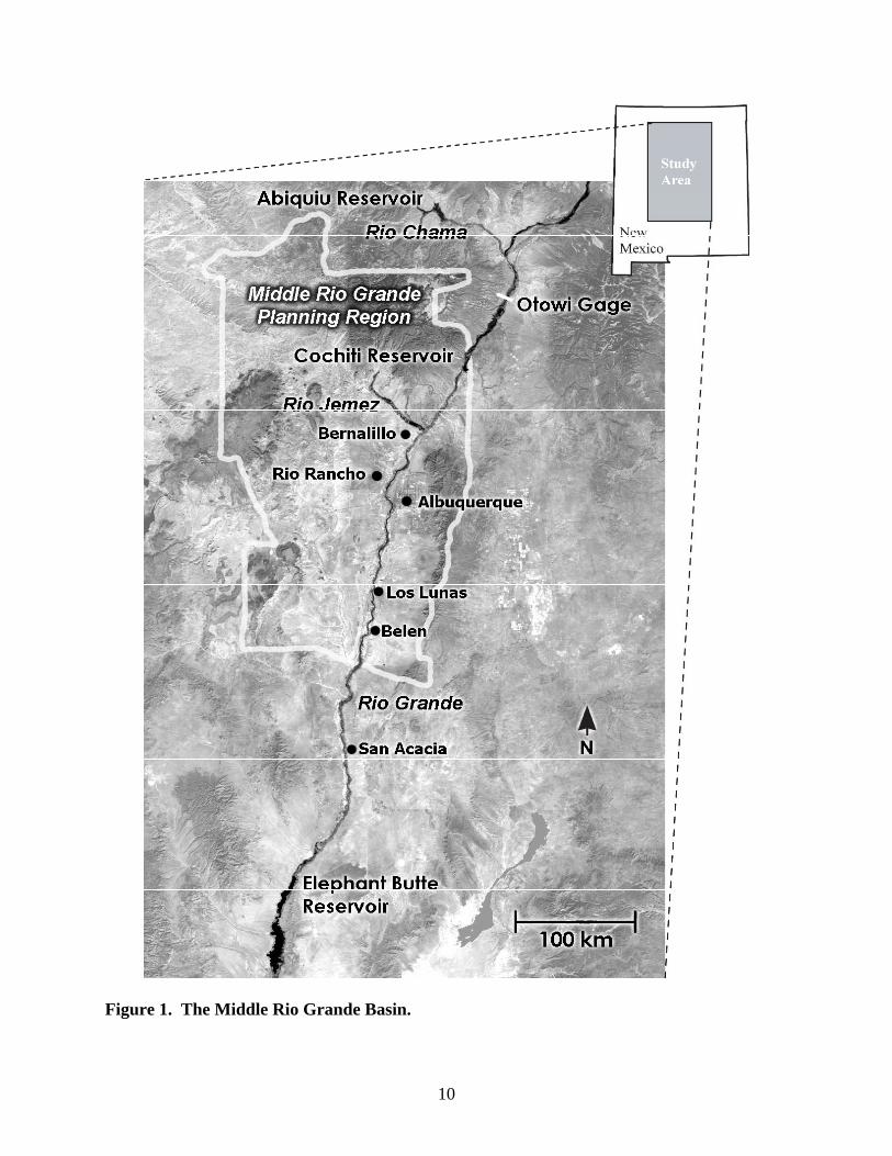
Figure 1. The Middle Rio Grande Basin.

11

The planning process will evolve as new data and new understanding of the system are both developed and as consequences unfold from historic and current management decisions. The model, periodically updated to include new data and understanding, can be a focal point in the ongoing process of resource management. Unique aspects of this work are (1) model development included the direct cooperation and involvement of the public; and (2) the model was subsequently used by the public along with local governments to develop a 50-year water plan for the region. The goal of the planning process was to balance regional consumption with projected supply in a publicly and politically acceptable manner. At the time of this writing, the model is fully engaged in the regional water planning process. This project represents collaboration between the Middle Rio Grande Water Assembly (MRGWA), the Mid-Region Council of Governments (MRCOG), the Utton Transboundary Resources Center at the University of New Mexico School of Law, and Sandia National Laboratories (SNL). Regional experts from city, county, state, and federal water management agencies, and from private consulting firms, contributed to the model development. SNL provided funding for this project through its New Mexico Small Business Assistance Program (NMSBA), which in turn is funded via a tax credit program administered by the New Mexico State Legislature. The NMSBA helps provide small New Mexico businesses with various kinds of technical tools and applications offered by SNL, but which are not available through the commercial public sector.

12

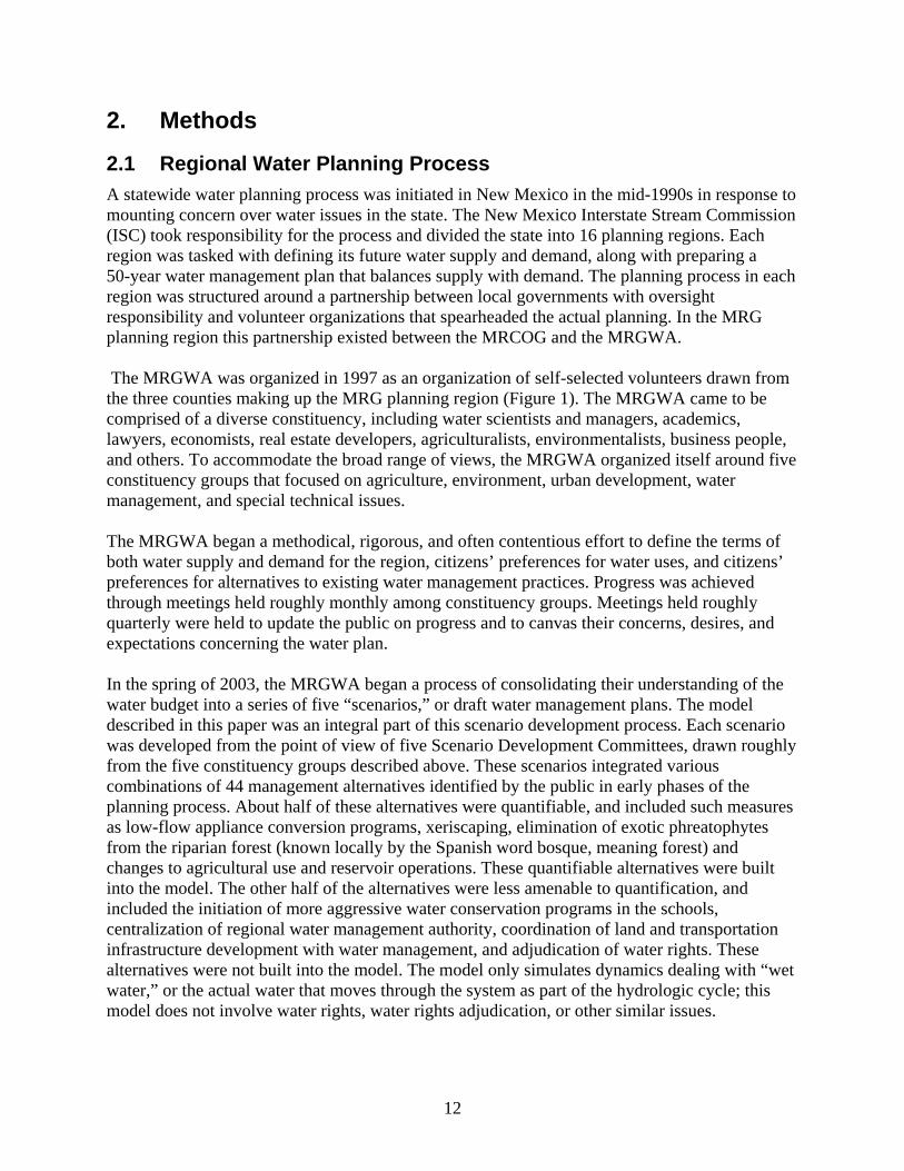
2. Methods

2.1 Regional Water Planning Process A statewide water planning process was initiated in New Mexico in the mid-1990s in response to mounting concern over water issues in the state. The New Mexico Interstate Stream Commission (ISC) took responsibility for the process and divided the state into 16 planning regions. Each region was tasked with defining its future water supply and demand, along with preparing a 50-year water management plan that balances supply with demand. The planning process in each region was structured around a partnership between local governments with oversight responsibility and volunteer organizations that spearheaded the actual planning. In the MRG planning region this partnership existed between the MRCOG and the MRGWA. The MRGWA was organized in 1997 as an organization of self-selected volunteers drawn from the three counties making up the MRG planning region (Figure 1). The MRGWA came to be comprised of a diverse constituency, including water scientists and managers, academics, lawyers, economists, real estate developers, agriculturalists, environmentalists, business people, and others. To accommodate the broad range of views, the MRGWA organized itself around five constituency groups that focused on agriculture, environment, urban development, water management, and special technical issues. The MRGWA began a methodical, rigorous, and often contentious effort to define the terms of both water supply and demand for the region, citizens’ preferences for water uses, and citizens’ preferences for alternatives to existing water management practices. Progress was achieved through meetings held roughly monthly among constituency groups. Meetings held roughly quarterly were held to update the public on progress and to canvas their concerns, desires, and expectations concerning the water plan. In the spring of 2003, the MRGWA began a process of consolidating their understanding of the water budget into a series of five “scenarios,” or draft water management plans. The model described in this paper was an integral part of this scenario development process. Each scenario was developed from the point of view of five Scenario Development Committees, drawn roughly from the five constituency groups described above. These scenarios integrated various combinations of 44 management alternatives identified by the public in early phases of the planning process. About half of these alternatives were quantifiable, and included such measures as low-flow appliance conversion programs, xeriscaping, elimination of exotic phreatophytes from the riparian forest (known locally by the Spanish word bosque, meaning forest) and changes to agricultural use and reservoir operations. These quantifiable alternatives were built into the model. The other half of the alternatives were less amenable to quantification, and included the initiation of more aggressive water conservation programs in the schools, centralization of regional water management authority, coordination of land and transportation infrastructure development with water management, and adjudication of water rights. These alternatives were not built into the model. The model only simulates dynamics dealing with “wet water,” or the actual water that moves through the system as part of the hydrologic cycle; this model does not involve water rights, water rights adjudication, or other similar issues.

13

During the summer of 2003 the MRGWA worked closely with the MRCOG to combine the individual scenarios developed by the different constituency groups into a unified water management plan. Each step in the water planning process was punctuated with a series of public meetings to gather feedback on the draft plans. 2.2 Model Development Process It became clear as the planning project grew in complexity that a model could assist in the planning process. In late 2001, a modeling project was initiated to:

1. provide a quantitative basis for comparing alternative water conservation strategies; 2. help the public understand the complexity inherent to the regional water system; and 3. engage the public in the decision process.

Construction of the model began in January 2002 and working versions of the model were released and applied to the regional planning process in the spring and summer of 2003. At the time of this report (early winter, 2003), use of the model in the planning process is ongoing. A community-based, participatory process for model development was adopted in an effort to build acceptance and confidence in the planning model. Model development involved collaboration between SNL, the MRGWA, the MRCOG, and the Utton Transboundary Resources Center of the University of New Mexico School of Law. SNL was responsible for model formulation and implementation within the system dynamics framework. The MRGWA was responsible for system conceptualization, identifying sources of subject expertise and data, model review, and for representing the views of the public and key constituency groups. The MRCOG represented the interests of the local governments that have ultimate responsibility for implementing the plan, and the Utton Center provided expertise in group facilitation. Individuals from each institution were organized into the Cooperative Modeling Team (CMT), which met roughly every other week throughout 2002 and early 2003 to develop the model. Starting in the spring of 2003, after the bulk of the modeling work was completed, the CMT began meeting monthly to review and update the model and to monitor the use of the model in the planning process. Model development followed a five-step process. First, the problem to be solved and the scope of analysis were both defined. Second, a description of the hydrological-ecological-economic system was developed. This step began by conceptualizing the broad structure of the system, followed by decomposing that broad structure into a series of manageable units defined by specific system sectors (e.g., agriculture, reservoirs). For each sector, a causal loop (schematic) diagram describing the inherent structure and feedbacks was developed and reviewed by the CMT. Subject experts were identified by the CMT who were then contacted for further clarification of the system and to gather necessary input data. In the third step the causal loop diagrams were converted into a system dynamics context, the model sectors were populated with appropriate data and mathematical relations, the model was calibrated against historic data, and a user-friendly interface was developed. Step four involved preliminary model review. The CMT reviewed each sector of the model both separately and as part of the broader model. Step five is ongoing and includes continual further review of the model both internally and by outside

14

experts and agencies, and continual modifications to the model as new data are generated or as new relationships are uncovered. The model development process also benefited from interactions with the community outside the CMT. Data and system understanding were gained from numerous meetings with water professionals and scientists from local, state, and federal agencies. The model also received close scrutiny by water experts from all those agencies, in many cases involving formal review. Public feedback was also gathered by way of public meetings in which draft versions of the model were previewed. Outreach targeted such venues as MRGWA public meetings, water forums, children’s water fairs, state and county fairs, civic, professional and academic groups, and students in various schools and universities whose teachers or professors requested a demonstration of the model. 2.3 Model Architecture Selection of the appropriate architecture for the planning model was based on two criteria. First, a model was needed that provided an “integrated” view of the watershed—one that coupled the complex physics governing water supply with the diverse social and environmental issues driving water demand. Second, a model was needed that could be taken directly to the public for involvement in the decision process and for educational outreach. For these reasons we adopted an approach based on the principles of system dynamics (Forrester, 1990; Sterman, 2000). System dynamics provides a unique framework for integrating the disparate physical and social systems important to water resource management, while providing an interactive environment for engaging the public. System dynamics is a systems-level modeling methodology developed at the Massachusetts Institute of Technology in the 1950s as a tool for business managers to analyze complex issues involving the stocks (e.g., inventories) and flows of goods and services. System dynamics is formulated on the premise that the structure of a system, or the network of cause and effect relations between system elements, governs system behavior (Sterman, 2000). According to Simonovic and Fahmy (1999), “The systems approach is a discipline for seeing wholes, a discipline for seeing the structures that underlie complex domains. It is a framework for seeing interrelationships rather than things, for seeing patterns of change rather than static snapshots, and for seeing processes rather than objects.” In the system dynamics approach, a problem is decomposed into a temporally dynamic, spatially aggregated system. The scale of the domain can range from the inner workings of a human cell to the operation of global commodity markets. Systems are modeled as a network of stocks and flows. For example, the change in volume of water stored in a reservoir is a function of the inflows less the outflows. Key to this framework is the feedback between the various stocks and flows comprising the system. In a reservoir, feedback occurs between evaporative losses and reservoir storage through the volume/surface area relation for the reservoir. Feedback is not always realized immediately but may be delayed in time, which represents another critical feature of dynamic systems. For example, effects of groundwater pumping on surface water flows can, in regions like the MRG, lag behind the actual groundwater pumping by decades.

There are a number of commercially available object-oriented simulation tools that provide a convenient environment for constructing system dynamics models. The construction process

15

proceeds within a graphical environment, using objects as building blocks. These objects are defined with specific attributes that represent individual physical or social processes. These objects are networked together so as to mimic the general structure of the system, as portrayed in a causal loop diagram. This provides a structured and intuitive environment for model development. The MRG planning model described in this paper is built in Studio Expert 2003, produced by Powersim, Inc. The model operates within a PC environment and requires less than 10 seconds to complete a simulation. Accompanying the model is a user interface for prescribing model input and viewing simulation results. Sixty-six variables can be manipulated by users in the model interface by slider bars or switches, allowing the comparison of multiple water management strategies. The model also includes textual explanations of the relevant regional water resource management issues, as well as definitions for how each slider bar or switch affects the simulated resource. Users can easily simulate various combinations of hydrological, economic, or demographic conditions, and then run the model and view output in near real-time. This allows users in private or public settings to experiment with competing management strategies and evaluate the comparative strengths and weaknesses of each. 2.4 Role of the Model Key to the cooperative modeling process is achieving consensus among all participants on the role of the model. Misconceptions can lead to misinterpretation of model results, antagonism between group members and/or the public, and eroded credibility in the model and modeling process. The primary functions of the model are to provide a tool for screening water management alternatives (i.e., the model can be used to quantitatively compare these different alternatives) as well as to provide a means for decision makers, stakeholders, and the public to make informed decisions. The model helps define basic trends in key metrics (e.g., Rio Grande Compact (RGC) balance, groundwater depletions, costs) over time, predicated on assumptions concerning population growth, the climate, and projected water demands. Likewise, the model helps define expected changes in these metrics in response to implementation of different water conservation measures. However, model results in absolute terms must be interpreted with care. Should one be interested in absolutes at a specific point in the basin or at a particular time, or want to design/implement a specific alternative, then more detailed and sophisticated modeling must be pursued. In fact, this systems-level planning model draws heavily on the inferences and results of many other more sophisticated models focused on particular aspects of the basin. The model should also be viewed as a vehicle to aid decision making, and not the means by which the decision is made. The model is designed to initiate dialogue among decision makers and the public and provide a consistent, scientific foundation for informing participants on issues and system behavior. The model is an effort to build a bridge linking science and policy. Any management decisions must consider other sources of information beyond the scope of the model, including the basic desires and attitudes of the stakeholders.

16

3. Conceptual Model The MRG planning region includes Bernalillo, Sandoval, and Valencia counties of north-central New Mexico (Figure 1). The region is characterized by basin and range topography with mountains along the east and arid valleys, and mesas central and west. The principle drainage for the basin is the Rio Grande. A deep alluvial aquifer, whose boundaries roughly coincide with that of the planning region, is in direct communication with the Rio Grande. Vegetation classes found within the region range from riparian along the Rio Grande to desert grassland, pinyon-juniper woodlands, and mixed coniferous forest at the higher mountain elevations. The planning region includes Albuquerque, the principle urban center of New Mexico, along with several smaller communities including Rio Rancho, Belen, Los Lunas, and Bernalillo. These communities are located along the Rio Grande while sparse rural populations characterize outlying areas. In the years 1900 to 2000, the population of the three-county region grew from about 51,000 to about 713,000 people (an increase of 1298%) according to the U.S. Census Bureau. The most recent doubling of population occurred from about 1970 to 2000.

The basic structure of the model is that of a dynamic water budget. Specifically, each supply and demand component is treated as a spatially aggregated, temporally dynamic variable. The spatial extent of the basin is delimited according to the boundaries of Bernalillo, Sandoval, and Valencia counties. Thus, the various water supply, demand, and conservation terms are aggregated over the three-county region; however, in some instances features outside the planning region must be simulated to accomplish these calculations (e.g., Elephant Butte Reservoir). Temporally, the model operates on an annual time step encompassing the period 1960–2050. This includes a 38-year calibration period (1960–1998) and the prescribed 50-year planning horizon (2000–2050).

At the highest level, the model is organized into two separate but interacting water budgets, one for surface water and the other for groundwater. In both budgets the water stored in the basin varies annually in response to changes in the associated inflows and outflows. Below we describe the basic elements contributing to these inflows and outflows. We also describe the modeling of 24 different water conservation strategies identified by the public as being important to regional planning efforts.

3.1 Inflows

3.1.1 Surface Water Surface water inflows to the planning region include the main stem of the Rio Grande, its associated tributaries (including storm water discharge), sewage return flows, and interbasin transfers from the Colorado River drainage. Rio Grande inflows are modeled at the Otowi gage located downstream of the confluence of the Rio Chama and the Rio Grande just north of the planning region boundary (Figure 1). Gaged tributary flows within the planning region include the Rio Jemez, Santa Fe River, Galisteo Creek, Tijeras Arroyo, and storm water flows from the City of Albuquerque (CoA).

For the period 1960–1998, the main stem and tributary flows are modeled using historic gage data (USGS, 2002). In cases where the record did not date back to 1960, the average flows (for

17

the available record) were used for pre-record years. Post-1998 stream flows are generated stochastically and based on realizations simulated from stream flow statistics derived from 1950–1998 gage data (Table 1). This period was selected as it provides both a period of significant drought (1950s) as well as an extended wet period (1980s and 1990s). The main stem and tributary time series were each fit with a unique distribution and appropriate statistics using the software package Crystal Ball 2000.2®, by Decisioneering, Inc. Correlation among the different tributary and main stem flows was also maintained where significant. Ten thousand random (i.e., lacking temporal correlation) realizations for each tributary distribution were simulated and then the seven tributary flows were aggregated for each realization. Ten thousand random realizations for the main stem were also simulated, and then the aggregate of the seven tributary inflows was added to the main stem inflow for each realization, resulting in 10,000 aggregated inflow values. Two hundred annual inflow values were then selected at random from the 10,000 values and input to Powersim as the distribution of future total inflow values. (Powersim will not allow the use of more than 200 values in this way.) Inflow sequences for the period of 1998–2050 are then generated for each run of the model by randomly selecting values from this set of 200 values.

Table 1. Sample statistics for stochastic model input.

Input Data Mean Standard Deviation Correlation Available

Record Otowi Index (af/yr) 963,570 490,194 1950–1998

Jemez River (af/yr) 45,866 29,236 Rio Grande (0.87) and Santa Fe River (0.73)

1950–1998

Santa Fe River (af/yr) 8470 951 Rio Grande (0.67) 1971–1998 Galisteo Creek (af/yr) 4469 2360 1970–1998 CoA Floodway (af/yr) 5094 5471 1988-1998 Tijeras Arroyo (af/yr) 332 232 1991–1998 Rio Puerco (af/yr) 28,538 22,208 1950–1998 Rio Salado (af/yr) 10,198 11,736 Rio Puerco (0.57) 1950–1998 Max Temp (°C) 21.4 0.8 Avg. Temp (0.86) 1950–1998 Min Temp (°C) 6.3 0.9 Avg. Temp (0.82) 1950–1998 Avg. Temp (°C) 13.8 0.7 1950–1998 Radiant Energy (MJ/m2da) 24.1 1.4 1950–1998

Relative Humidity 44 2.8 Rio Grande (0.62) and Precipitation (0.52)

1950–1998

Wind Speed (m/sec) 4.1 0.3 1950–1998 Precipitation (in.) 8.7 2.4 1950–1998 The user also has the option of modifying the inflow sequence to simulate the effects of drought. The current approach is simplistic in that the simulated inflows are reduced by some constant percentage from year to year defined as input into the model by the user. The user can control the year in which the drought begins and ends, and the intensity of the drought relative to historic inflow values. Long-term climatic changes can be modeled with these options as well. Sewage returns are disaggregated into four categories, including the population on publicly supplied water in each of the three counties and the population across all three counties on a

18

private water supply. Return flows are assumed to be equivalent to the total indoor water use for residential, commercial, and industrial customers on public systems. This equates roughly to 50% of the total municipal demand and is consistent with sewage outfall data for the three-county region (Papadopulos and Associates, 2000). In 1998, the total sewage discharge was 68,941 acre-feet (af). San Juan-Chama (SJC) Project water has been delivered to the MRG planning region since 1971 via a transmountain diversion from the San Juan River (in the Colorado River Basin) to the Chama River. Contracted SJC Project deliveries to the planning region equal 81,005 af annually, less a 2% conveyance loss. Of this, 48,200 af are contracted to the CoA, while the remaining water is contracted primarily to the Middle Rio Grande Conservancy District (MRGCD) (20,900 af) and to other city utilities. From 1971–1998, historic data are used to model actual deliveries. Future deliveries assume a constant delivery of 75,844 af/yr, based on average deliveries made over the period of 1990–1998 (Papadopulos and Associates, 2000). The model user has the option to reduce this delivery.

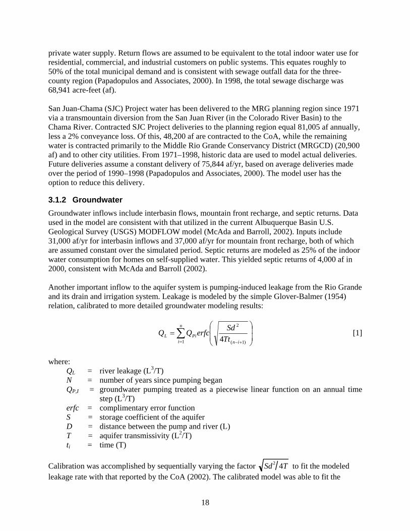
3.1.2 Groundwater Groundwater inflows include interbasin flows, mountain front recharge, and septic returns. Data used in the model are consistent with that utilized in the current Albuquerque Basin U.S. Geological Survey (USGS) MODFLOW model (McAda and Barroll, 2002). Inputs include 31,000 af/yr for interbasin inflows and 37,000 af/yr for mountain front recharge, both of which are assumed constant over the simulated period. Septic returns are modeled as 25% of the indoor water consumption for homes on self-supplied water. This yielded septic returns of 4,000 af in 2000, consistent with McAda and Barroll (2002). Another important inflow to the aquifer system is pumping-induced leakage from the Rio Grande and its drain and irrigation system. Leakage is modeled by the simple Glover-Balmer (1954) relation, calibrated to more detailed groundwater modeling results:

⎟⎟⎠

⎞⎜⎜⎝

⎛=

+−=∑

)1(

2

1 4 in

n

iPiL Tt

SderfcQQ [1]

where:

QL = river leakage (L3/T) N = number of years since pumping began QP,I = groundwater pumping treated as a piecewise linear function on an annual time

step (L3/T) erfc = complimentary error function S = storage coefficient of the aquifer D = distance between the pump and river (L) T = aquifer transmissivity (L2/T) ti = time (T)

Calibration was accomplished by sequentially varying the factor Sd2 4T to fit the modeled leakage rate with that reported by the CoA (2002). The calibrated model was able to fit the

19

CoA’s baseline leakage data to within 1%. Using the same calibrated parameters, the model was able to fit a reduced pumping scenario to within 10%. (The reduced pumping scenario simulated implementation of the CoA Drinking Water Project (DWP), which plans to use SJC Project water and is estimated to lead to a 60-75% reduction in Albuquerque pumping from the aquifer). Note that the modeled leakage is based on the difference between the river plus drain flows under current conditions versus that without the CoA pumping.

3.1.3 Socorro County As noted previously, a limited amount of modeling is necessary outside the boundaries of the planning region. This is particularly the case when calculating the RGC balance (Section 3.2.4). To calculate the Compact balance, the basic inflows to the Rio Grande that occur within Socorro County must be considered. Surface water inflows include the Rio Puerco, Rio Salado, and several ungaged tributaries. The Rio Puerco and Rio Salado flows were modeled in a manner consistent with that for other Rio Grande tributaries as described above (Table 1). Because of the lack of sufficient data, we have modeled the ungaged tributaries as a constant with a value of 28,200 af/yr (Papadopulos, S.S., and Associates, 2003). Other inflows to the Rio Grande include 1000 af/yr of sewage returns from Socorro (Papadopulos and Associates, 2002) and approximately 16,500 af/yr of groundwater discharge (Roybal, 1991), both of which are assumed constant. 3.2 Outflows Consumptive outflows can be distributed into four broad classes: open-water evaporation, bosque transpiration , agricultural evapotranspiration, and municipal consumption. Consumption in the region is roughly equally divided among the four groups. Each of the three evaporative losses are credited to the surface water system while municipal consumption is taken from the groundwater system; the CoA, however, has near term plans to utilize Rio Grande flows. Below we explore each of these outflow terms individually.

3.2.1 Surface Water 3.2.1.1 Open-Water Evaporation Open-water evaporation is calculated for the main stem of the Rio Grande and each of the modeled reservoirs. Because tributaries are gaged at their discharge to the Rio Grande, tributary evaporation does not need to be considered. Modeled reservoirs include Elephant Butte Reservoir, Cochiti Reservoir, and Abiquiu Reservoir (Figure 1). To estimate the evaporative losses, we begin by calculating the reference evapotranspiration (ET) rate, ETr. Reference ET rates are calculated using a modified form of the Penman-Monteith equation (Shuttleworth, 1993):

( ) DT

USRETr 275900

** +∗

⎟⎟⎠

⎞⎜⎜⎝

⎛∆+

++∆∆

=γ

γγ

[2]

where: ETr = reference evapotranspiration rate (L/T) ∆ = vapor pressure/temperature gradient (M/LT2degrees) γ = psychrometric constant (M/LT2degrees)

20

SR = net solar radiation (L/T) γ * = scaled psychrometric (M/LT2degrees) U = wind speed (L/T) T = temperature (degrees) D = vapor pressure deficit (M/LT2)

In this way, ETr accounts for the effects of climatic variability on evaporative losses. To determine the ET rate specific to an open-water body, rET is multiplied by an evaporation coefficient. Here we adopt the same open-water evaporation coefficient value (Table 2) as used in the ET Toolbox (USBR, 2002).

Table 2. Data used to calculate evaporative losses.

Evaporation Coefficient

Growing Days

1999 Acreage

Open Water 0.93 365 NA bosque 0.77 231 22,896 alfalfa 0.95 293 24,749 corn 0.77 205 2019 sorghum 0.65 186 576 wheat 0.57 123 209 oats 0.7 123 1722 fruit 0.71 365 711 nursery 0.71 365 209 melons 0.69 154 82 pasture/hay 0.9 293 19,118

For the period of 1960–1998, historic yearly averaged meteorological data are used in the Penman-Monteith equation. In later years, the meteorological parameters are stochastically generated in a manner equivalent to that used to simulate the Rio Grande/tributary flow data (Table 1). Where significant, historical correlations between the meteorological data and Otowi gage flows are preserved in the simulated time series. Total evaporative losses for the Rio Grande and associated saturated sand bars are calculated according to the empirical models developed by the U.S. Army Corps of Engineers (USACE, 2002). Losses are a function of the river discharge, river reach, and evaporation rate for that year. Average losses are on the order of 28,000 af/yr for the planning region.

Evaporative losses from large bodies of water, like reservoirs, must be handled in a slightly different manner. Lake evaporation, ETL is calculated according to the following relation given by Shuttleworth (1993): ( ) tAAUDETL ∆= − *****909.2 05.0 [3]

21

where:

ETL = reservoir evaporation (L3) D = vapor pressure deficit (M/LT2) U = wind speed (L/T) A = reservoir surface area (L2)

t∆ = number of evaporation days (i.e., number of days in the year) (T) Surface areas are computed from volume-surface area relationships specific to each lake (Mark Yuska, personal communication, 2003). 3.2.1.2. Bosque Transpiration According to the Land Use Trend Analysis (LUTA) performed by the U.S. Bureau of Reclamation (1997), there are 22,896 acres of bosque in the planning region. The riparian corridor along the Rio Grande is composed of a mosaic of cottonwood, willow, Russian olive, salt cedar, New Mexico privet, elm, and shrubs and grasses. In this analysis we are concerned with the phreatophyte communities that draw water directly from the shallow groundwater system in direct contact with the Rio Grande. For this reason, the model’s bosque acreage is limited to the LUTA classes of riparian woodland, salt cedar, riparian shrub, marsh, and bosque. Evaporative losses are determined by using the Penman-Monteith equation (Equation 2) to estimate the reference ET rate. Because of the diverse mixing of species throughout the bosque, we do not attempt to calculate ET rates for each individual vegetation class; rather, a single rate is used. Based on available data, an average transpiration rate of 3.62 af/acre/yr (Papadopulos, S.S., and Associates, 2003) was adopted. Total evaporative loses are calculated by multiplying the specific evaporation rate by the specific acreage and then by the number of growing days, estimated at 231 days (USBR, 2002). Average transpiration losses equal 83,000 af/yr throughout the planning region. As discussed below in more detail, the losses by specific transpiration are accounted directly against Rio Grande flows. Transpiration rates are adjusted annually for precipitation. An effective precipitation of four inches per year is assumed available (Papadopulos and Associates, 2000) to the specific vegetation. In this way, the yearly bosque ET rate, ETB, is calculated as:

ETB = 3.62ETr

ETa

⎡

⎣ ⎢ ⎢

⎤

⎦ ⎥ ⎥ − 0.33

PPa

⎡

⎣ ⎢ ⎢

⎤

⎦ ⎥ ⎥ [4]

where: ETB = bosque ET rate (L/T) ETr = reference ET rate (L/T)ETa = average reference ET rate (L/T) P = annual precipitation (L) Pa = 50-year average precipitation (8.75 in.)

Precipitation for 1960–1998 is modeled from historical data, while future precipitation is stochastically generated (as described above) and is correlated with main stem Rio Grande inflows (Table 1).

22

3.2.2 Irrigated Agriculture An average of 50,541 acres were irrigated annually in the three-county planning region in 2002 (MRGCD, 2001). A diversity of crops is grown in this region; however, forage crops like alfalfa and pasture hay represent about 80% of the irrigated acreage. The ease of growing forage crops, high demand by the strong local dairy industry, and lack of a market for most other crops are some of the reasons for the current cropping trends. Table 2 gives the estimated distribution of crops in 1999 for the planning region (based on data in USACE, 2002).

To maintain consistency, reference evaporation rates for the irrigated crops are calculated according to the Penman-Monteith equation. Evaporative losses specific to each crop are estimated by multiplying ETr by the evaporation coefficient, growing days, and acreage particular to each crop. These crop specific data are consistent with the ET Toolbox (USBR, 2002) and are shown in Table 2. As irrigated crops generally grow under some degree of water stress, the calculated ET rates must be adjusted for actual growing conditions. This involves reducing the calculated ET rates by a stress factor. A value of 0.75 was determined based on the reported average ET rate of 2.6 af/acre/yr for all irrigated acreage (which is based on a range of values given in Papadopulos and Associates, 2002). Accordingly, the current distribution of crops within the planning region consume an average of 131,000 af/yr. Yearly evaporative losses are adjusted according to Equation 4 for annual variations in rainfall.

In dry years water demand by agriculture is reduced. Specifically, 15% of the alfalfa farms are unable to reseed at the end of the year when Otowi gage flows drop below 550,000 af/yr (alfalfa must be reseeded every six years). Thus, in the following year wheat is grown in the place of alfalfa. This substitution continues until the farm can be reseeded (i.e., when flows exceed 550,000 af/yr). In these dry years it is also assumed that water consumption is reduced by 25% due to a lack of river flows in the last three months of the growing season. Alternatively, consumption is assumed to increase by 25% (equal to the potential ET rate) when Otowi gage flows exceed 2,000,000 af/yr. Between these flow limits, consumption is assumed to linearly decrease from 125% to 75%. Agricultural water is taken entirely from the Rio Grande and is predominantly administered by way of flood irrigation. In limited instances water is pumped from the shallow aquifer, which draws directly on the Rio Grande. A 763-mile network of canals, laterals, and ditches maintained by the MRGCD supplies the water (Papadopulos and Associates, 2002). When Rio Grande flows are sufficient, these canals run full from March 1 to October 31. Additionally, the MRGCD operates a series of riverside and exterior drains designed to capture tail water (unused irrigation water) and drain croplands along the river.

Besides the water directly consumed by the crops, several other losses from the irrigation system occur. First, there is a leakage loss of roughly 0.24 ft3/sec of water per mile of canal/ditch. This is assumed as a constant since the depth to groundwater and depth of water in the ditch are relatively consistent throughout the irrigation season. This loss represents about 91,000 af/yr (USACE, 2002). Second, riparian vegetation has grown up along much of the conveyance system that draws directly on the irrigation water. These losses are evaluated in a manner consistent with that for the bosque vegetation and result in average losses of 10,000 af/yr from 2,775 acres of ditch bank (adopted from Appendix I of Papadopulos and Associates, 2002; the

23

ditch bank is considered part of the 22,896 acres of bosque in the planning region). Third, roughly one acre-foot of water is lost per irrigated acre of land due to percolation below the root zone, which we term irrigation seepage. Finally, there are evaporative losses directly from the conveyance system that are on the order of 3,500 af/yr, which are calculated using Equation 2 and corresponding open-water loss coefficients. The total water diverted from the Rio Grande for irrigated agriculture is simply calculated by summing the individual losses. Specifically, the total diversion equals the sum of evapotranspiration from the crops, evaporative losses from the conveyance system, conveyance system leakage, irrigation seepage, and ditch bank evapotranspiration. Note that we do not attempt to model actual diversions and drain flows because of the complication of the system, poor supporting data, and its relative unimportance to the problem at hand.

3.2.3 Socorro County To calculate the RGC (Section 3.2.4), losses from the Rio Grande are modeled. Losses include evaporation from the Rio Grande, ET from the bosque and irrigated agriculture, and to a small degree pumping-induced river leakage. Evaporative losses from the Rio Grande and its associated sand bars are calculated according to the empirical models developed by the USACE (USACE, 2002), which average 26,000 af/yr. There are 40,598 acres of bosque in Socorro County above Elephant Butte Reservoir. Assuming an average ET rate of 3.88 af/acre/yr, 157,000 af of water are consumed by the bosque each year (Papadopulos, S.S., and Associates, 2003). Irrigated agriculture accounts for 54,000 af of consumption a year from 19,209 irrigated acres at a rate of 2.8 af/acre/yr (Papadopulos, S.S., and Associates, 2003). Both bosque and agricultural ET are modeled according to Equation 4 (with the appropriate substitution of the base ET rate). Finally, river leakage of 3300 af/yr is assumed due to municipal pumping by the city of Socorro (Papadopulos, S.S., and Associates, 2003).

3.2.4 Rio Grande Compact Colorado, New Mexico, and Texas signed the RGC in 1939 to apportion between them the Rio Grande water above Fort Quitman, Texas. Effectively, the Compact also apportions water among the upper, middle, and lower reaches of the Rio Grande in New Mexico. Our planning region falls in the middle reach, which extends from the Otowi gage in the north to Elephant Butte Reservoir in the south (Figure 1). Allowed depletions over this reach are qualified by a Compact schedule. At low flows (less than or equal to approximately 1 million af/y), New Mexico is entitled to deplete a maximum of 43% of the water passing the Otowi gage (Figure 2). Once annual flows at Otowi reach 1.1 million af, the marginal entitlement to deplete is zero. The maximum depletion by the middle reach is 405,000 af/yr. In this way, the middle region may consume the entitled native Rio Grande water plus any tributary or groundwater inflow that occurs over this reach. The middle reach is responsible for all depletions occurring between Otowi and Elephant Butte Reservoir, including all evaporative losses from Elephant Butte Reservoir. The annual Compact credit/deficit, VRGC, is calculated using Equation 5. CSDEBDDRGC VVVV −∆+= )( [5]

24

where: VRGC = Rio Grande Compact credit/deficit (L3) VDD = the actual downstream delivery from Elephant Butte Reservoir (L3)

EBV∆ = the change in Elephant Butte Reservoir storage (L3) VCSD = the Compact schedule delivery (based on Otowi gage flows) (L3).

Figure 2. Rio Grande Compact Schedule defining the middle region’s right to consume based on Otowi Index flows (i.e., Otowi gage flows adjusted for upstream reservoir operation and SJC inflows). In the case of New Mexico, the accrued deficit may not exceed an average of 200,000 af over six years, except when the debit may be caused by holdover storage in a northern reservoir. Water may be stored in northern reservoirs provided Elephant Butte Reservoir storage is not less than 400,000 af and adequate deliveries can be made downstream. In such instances, downstream users can call for a release of stored water. The target release from Elephant Butte Reservoir is 790,000 af/yr as prescribed by the RGC; however, over the last 40 years deliveries have averaged only 690,000 af/yr. RGC rules do not apply to SJC water. Modeling of the RGC begins by calculating the scheduled Compact delivery, subject to the Compact schedule (Figure 2), from the simulated Otowi gage flow. The annual credit/debit is then calculated according to Equation 5. Based on the credit/deficit and Elephant Butte Reservoir storage, the decision to store or release water from northern reservoirs is made. The credit/deficit is subsequently updated and the accrued status (cumulative annual Compact balance) is calculated. Releases from Elephant Butte Reservoir are made consistent with historic operations over the last 40 years. Specifically, if Elephant Butte Reservoir storage is above 1.5M af, then the full 790,000 af is delivered downstream. If storage is below 500,000 af, and inflows are also below 500,000 af then the delivery is set equal to the inflow. In all other cases a delivery of 690,000 af is made consistent with the 40-year average. Note that Compact storage does not

0

100

200

300

400

500

0 1000 2000 3000 4000 5000

Com

pact

Allo

catio

n (a

f x10

3 )

Otowi Index (af x10 3)

25

include credit water or SJC water stored in Elephant Butte Reservoir. If storage exceeds reservoir capacity, a spill is allowed and the accrued status is reset to zero.

3.2.5 Groundwater 3.2.5.1 Municipal Demand The U.S. Census Bureau estimated the population for the three-county planning region in year 2000 at 712,738 people. Within the model, population is disaggregated into four groups, including those using publicly supplied water in Bernalillo, Sandoval, and Valencia counties, plus a fourth group representing those in the planning region who use self-supplied domestic wells. The population associated with each group is given in Table 3.

Table 3. Census data for the three-county region1.

Group 2000 Population Average Annual Growth Rate, 2000-2050

Bernalillo 508,325 0.77 Sandoval 64,611 2.31 Valencia 33,084 2.01 Self Supplied (domestic wells) 106,718 1.59

1 U.S. Census Bureau, 2002; Wilson and Lucero, 1997 Municipal water use is calculated by multiplying the population by the corresponding per capita water demand. The per capita demand is broken into four different categories including residential, commercial, industrial, and institutional. These groups are further divided by indoor and outdoor water use. The per capita demand by category for each water use group is given in Table 4. The indoor demands are assumed constant, unless new conservation measures are instituted (see “Conservation Alternatives,” Section 3.3). Outdoor demands are allowed to fluctuate yearly in response to changing climatic conditions, as given in Equation 4.

Table 4. Per capita water use in gallons per person per day1.

Category Bernalillo Sandoval Valencia Self-Supplied Residential Indoor 61.1 61 61 64 Residential Outdoor 42.4 35 38 36 Commercial, Industrial, and Institutional Indoor 51.8 37.8 21.6 30

Commercial and Industrial Outdoor 16 9.6 6.4 12

Institutional Outdoor 13.2 9.6 7.6 0 Unaccounted for Water 11% 10% 11.3% 0 1 Wilson and Lucero, 1997; CoA, 2003 Additionally, each public water utility reports an additional water use category, termed unaccounted for water, that is roughly 10% of the total per capita demand. This category accounts for water distribution system leaks, inaccurate metering, and other unmeasured water

26

uses. In the model, the total water demand for each of the three publicly supplied water systems is simply increased by the percentage given in Table 4. Over the last 40 years, municipal demand has steadily grown, tracking the growth in population. Population growth is projected to continue throughout the basin for the next 50 years, resulting in a regional population of 1.27M people. This growth is modeled as )*(1 GRPopPopPop ttt +=+ [6] where:

Pop = population (People) GR = growth rate t = denotes the time step

Annual growth rates, shown in Table 3, are based on the projections from the University of New Mexico’s Bureau of Business and Economic Research (BBER, 2002). Historically, all municipal demand has been met through groundwater pumping. Municipal pumping grew from 37,700 af/yr in 1960 to 151,000 af/yr in 1999. This has resulted in significant groundwater level declines and limited ground subsidence in Albuquerque. In efforts to reduce this stress on the aquifer, Albuquerque plans to begin using their contracted allotment of SJC water. Beginning in 2006, the CoA will divert roughly 96,400 af/yr as part of their drinking water project and return 48,200 af/yr as treated sewage, resulting in a total consumption of 48,200 af/yr. This, in turn, will reduce Albuquerque’s dependence on groundwater by 96,400 af/yr. In dry years the CoA will curtail use of SJC water to maintain flows in the Rio Grande. Based on a regression of data in the CoA report (2002), we assume the CoA will take full use of their SJC allotment when Otowi gage flows are above 700,000 af/yr, will accept a 33% curtailment for flows below 475,000 af/yr, and will increase their curtailment linearly from 0 to 33% between these limits. Additionally, in the early years of the project, Albuquerque SJC water stored in Abiquiu Reservoir (from years prior to 2006) must be released to fully cover the CoA’s diversions from the Rio Grande. Releases are based on a balance between the CoA’s water use (96,400 af/yr for the drinking water project plus the CoA’s portion of the pump-induced river leakage) and the CoA’s water credits (48,200 af/yr SJC water, 23,300 af/yr of native Rio Grande water rights, and the CoA’s sewage return flows). 3.2.5.2 Groundwater Discharge Groundwater discharge to the Rio Grande occurs intermittently along the length of the basin and intermittently in time. Such discharge is principally captured by the drain system, which then conveys the water to the river. Groundwater discharge, Qgw, is calculated by the following balance: Bmfasclgw QQQQQ −++= )( [7] where:

Qgw = groundwater discharge (L3/T) Qcl = irrigation canal seepage (L3/T) Qas = agricultural seepage (L3/T) Qmf = mountain front recharge (L3/T) QB = bosque ET (L3/T)

27

Depending on the degree of bosque ET, Qgw can be positive or negative, denoting a net gain or loss to the river. The total loss or gain to the river is the sum of groundwater recharge Qgw and the pumping-induced river leakage (Equation 1). 3.3 Conservation Alternatives A variety of water conservation measures were modeled as part of the planning process. The purpose was to provide a quantitative basis for comparatively evaluating the alternatives in terms of the resulting water savings and cost to implement and maintain. A total of 24 alternatives were modeled, which are grouped according to six broad classes: residential/non-residential, bosque renovation, agriculture, reservoirs, desalination, and transfers. Each is described below. One important planning metric calculated by the model is the cost to implement and maintain a particular conservation measure. To provide a consistent basis of comparison, all costs are reported in year 2000 dollars. Yearly payments on large capital projects are calculated according to the following relation:

p

p

t

t

p IIIGC)1(1)1(

+−

+−= [8]

where: Cp = capital payments ($) I = interest rate G = principle ($) tp = repayment time horizon (T)

Additionally, all costs are adjusted to their net present value by way of

)2003()035.01(1

−+= tNPV [9]

where: NPV = net present value 0.035 = discount rate t = the year

3.3.1 Residential/Non-Residential This group of alternatives addresses potential water savings in the municipal sector. Modeled conservation measures include low-flow appliances, water re-use, xeriscaping, reduced landscaping, rooftop harvesting, and price controls. Indoor water use can be reduced by way of low-flow appliances and fixtures. Within the model, the user has the option of requiring all new homes (built after 2003) to be constructed with low-flow appliances, including toilets, showers, sinks, and washing machines. Additionally, the user can choose what percentage of existing homes will be retrofit with low-flow appliances. The model assumes homes will retrofit according to a constant compliance rate over the

28

user-specified time horizon. Water conservation is realized through reduced indoor per capita water use, which for the full package of appliances is roughly 43.6 gallons per person per day (gpd) compared to roughly 61 gpd (Table 4) (CoA, 2003). Water conservation is modeled by tracking separately the population with and without low-flow appliances and then multiplying each by the appropriate per capita water use statistic. By selecting either alternative it is assumed that all communities, as well as unincorporated rural areas, will comply equally with any new policy (CoA already requires low-flow appliances, excluding washing machines, in new construction). Note that the model limits the percent of homes to be retrofit by the number of existing homes that have low-flow appliances (<5%; CoA, 2003). Cost to retrofit a home with a package of low-flow appliances is about $425/person while the upgrade cost for a new home is $172/person (which is primarily the cost of a new washing machine). Costs are based on a survey of local vendors and assume 2.5 permanent residents per home. Similar options are available for the non-residential sector including commercial, industrial, and institutional properties. For these properties, low-flow appliances are limited to toilets and sinks, which reduces the per capita water use by 15%. Conservation is modeled exactly as above. Costs to retrofit are $100/person, while there are no additional costs for new construction. Residential homeowners also have the option of on-site gray water re-use. The user has the option of requiring gray water re-use in all new homes as well as retrofitting existing homes. For existing homes, only washing machine discharge (10 gpd) is allowed, while in new homes shower, dishwasher and washing machine discharge make up the gray water (30 gpd). Cost to retrofit is estimated at $75/person while in new homes it is $150/person. Additionally, maintenance of the system is assumed to cost $50/person annually. The re-used water both reduces the water needed to irrigate lawns as well as the volume of water returned as sewage. Outdoor water use can be curtailed by way of xeriscaping. The user has the option of requiring xeriscaping around all new home construction, and the option to retrofit a user-specified percentage of existing homes. Because of the broad variation in what is termed xeriscaping, the user is allowed to define the degree of water savings to be achieved. Additionally, the user has the option of reducing irrigated acreage in new home construction. Residential outdoor water use, Dro, is modeled as: redroxroxro AXRPopRPopPopD ))*(()( +−= [10] where:

Dro, = residential outdoor water use (L3) Pop = total population (Persons) Popx = xeriscaped population (Persons) Rro = per capita residential outdoor water demand (L3/Person) X = percent (%) reduction in water consumption by xeriscaped lawns Ared = percent (%) reduction in irrigated acreage

Again, selected options apply equally to all communities and rural populations. Costs to retrofit a lawn are estimated at $2000/person, while there are no added costs for new construction. Costs are based on a survey of local vendors and assume 2.5 permanent residents per home.

29

The same options are available for non-residential outdoor use including commercial and industrial properties. Water conservation by xeriscaping and reduced landscaping are calculated in a manner similar to Equation 10. Costs to xeriscape existing non-residential property are $400/person, with no costs for new construction. The xeriscaping option is not provided for institutional property as most of the landscaping is in the form of playing fields, golf courses and parks. Rather, the user has the option of reducing the irrigated acreage on a per capita basis for all new parks/golf courses (similar to the parameter Ared in Equation 10 above). The CoA has detailed plans to use non-potable water to irrigate new and existing parks and golf courses and for industrial re-use. Among these projects is the Industrial Re-Use Project, initiated in 2000, which provides 896 af/yr of industrial wastewater for irrigation and industrial re-use. Beginning in 2005, the CoA plans to use 2455 af of treated sewage water from the Southside Wastewater Reclamation Plant for non-potable irrigation, and in 2010 an additional 2095 af for irrigation in the Mesa Del Sol area in the southern part of the CoA. The CoA has also just begun using 3038 af/yr of their contracted SJC water to irrigate the Balloon Fiesta Park. After the CoA begins the DWP and thus exhausting their contracted SJC water, the irrigation water will be taken from the CoA’s stored SJC water or from rights freed up by reduced pump induced leakage. The user has the option of accepting or canceling these plans; this allows the user to see the water savings and costs associated with them. Capital costs for the project are $80M with an additional $400/af for additional water treatment costs and environmental monitoring (Stephens and Associates, 2003). Residential and non-residential customers also have the option of rooftop harvesting. The user has the choice of requiring harvesting on all new construction as well as retrofitting of existing properties. Harvested water is used to offset demand by irrigated landscaping. Volume of harvested water is simply a function of the annual rainfall and the acreage of rooftops. Actual harvested water available for irrigation is something less because of evaporative losses and water storage limitations. For this reason a 30% loss factor is used to reduce the captured volumes to that available for irrigation. Rooftop harvesting is assumed to have minimal impact on storm water discharge to the Rio Grande. The user can also explore the effects of the CoA’s DWP on water supply. The DWP allows the CoA to use its contracted San Juan-Chama water (48,200 af/yr) for municipal consumption, thus reducing dependence on the groundwater aquifer. This project is planned to start in 2006 and is the default in the model. However, the user can cancel the project to see the impact on the aquifer. Because this SJC water belongs to the CoA and cannot be used to satisfy RGC deliveries, this water is not shown to freely flow down the river when the DWP is not employed. Rather, that portion of the CoA’s contracted SJC water that is not able to be stored in Abiquiu Reservoir or is not used (i.e., as evaporation from Abiquiu Reservoir or to offset pumping-induced leakage) is tracked and reported separately from actual stream flows. This water must be beneficially used at the discretion of the CoA.

Rather than establishing “command and control” policies aimed at water conservation by requiring specific low-flow or conservation technologies as described above, a policy maker might also achieve water savings by increasing the price of water. According to economic

30

theory, consumers respond to an increase in the price of a good by reducing consumption of that good. The percent change in consumption resulting from a 1% increase in the price of a good is the price elasticity of demand for the good. A good with price elasticity between 0 and -1 (less than a 1% reduction in consumption after a 1% increase in price) is considered price inelastic, while a good with elasticity smaller than -1 is considered elastic (Michelsen et al., 1998). Most research suggests that water is price inelastic, with the majority of studies suggesting elasticity values between -0.02 and -0.75. Most of these studies however (including results for Albuquerque by Michelsen et al., 1998), report elasticities that are valid over a very narrow range of prices, making them essentially useless in predicting consumer response to significant price change (Brookshire et al., 2003). As a result, less specific data presented by Martin and Thomas (1986) are applicable over a wider range of prices, and were used to present price and demand data to the user. These data include price and demand information from a range of semi-arid cities, with possible constant elasticity demand curves superimposed as shown in Figure 3. The default elasticity for the model was set to -0.6 to most closely match the Martin and Thomas (1986) data. The change in demand for all residential/non-residential sectors resulting from a price change is calculated by the following equation:

ε)Price Price

(1initial

newD −=∆ [11]

where: D∆ = change in demand

Pricenew = modified price ($) Priceinitial = unmodified price ($) ε = the elasticity of demand

Due to lack of data concerning the difference between indoor use and outdoor use elasticity values over a significant price change, the total change in demand was split into changes in indoor and outdoor demand by assuming that the reduction would be proportional to the maximum conservation possible with no price change. For example, if the model predicted a 10% reduction in demand in each sector, but possible savings outdoors were double the possible savings indoors, two-thirds of the reduction would occur outside while one-third would occur inside.

31

Figure 3. Price elasticity demand curves with data taken from a variety of locations.

Inherent in the negative relationship between price and demand is the ability of consumers to change behavior and or technology to reduce demand as price rises. Because a change in price implies changes in behavior and/or technology to reduce demand, the price manipulation option in this model should not be mixed with other residential/non-residential conservation measures, as this might result in double counting potential sources of water conservation.

3.3.2 Bosque Renovation Changing water management practices, flood control, and fire suppression have changed the complexion of the bosque relative to pre-settlement conditions. These practices have lead to unnaturally dense stands of vegetation and a distinct shift in the forest composition. In particular, non-native species like salt cedar, Russian olive, and elm are displacing native cottonwood and willow. In this context, water conservation is achieved by removing non-native vegetation. This will not only reduce transpiration losses, but also improve the health and habitat of the riparian corridor and reduce the threat of wildfire. The model allows the user to choose how many acres should be treated in the planning region. Treated acreage is limited to the 16,897 acres on public and Indian land. Because this land is largely within the floodplain, we do not allow the option of converting this land to agricultural or urban use. By treatment we mean the removal of all non-native vegetation leaving the mature overstory of cottonwoods and sparse under story of willows and grasses. Some level of revegetation with native trees, shrubs, and grasses is also assumed. The result of thinning is to reduce bosque transpiration by 20% annually (Stephens and Associates, 2003). The desired level of treatment is assumed to follow a linear trend in time over a user-specified time horizon. Bosque thinning projects are in progress throughout the basin. Based on these efforts, costs to treat are estimated at $2000/acre the first year, with a maintenance cost of $500/acre in the next

Possible Water Demand Curves for Albuquerque

0

1

2

3

4

5

6

7

8

9

10

0 20 40 60 80 100 120 140 160 180 200Average Water Use (gpcd)

1998

Ave

rage

Pric

e ($

/100

0 ga

llons

) Elasticity = -0.6

Elasticity = -0.3

Elasticity = -0.15 (ModelDefault)

Perth, Australia 1981-82

Kuwait 1973-81

Tucson 1978-79

Albuquerque 1998

Albuquerque 1994

(Specific data points from: Martin, 1986 Albuquerque points from Sato, 1999)

Phoenix 1979

32

three years thereafter. This rate declines to $100/acre for year five and after. Revegetation costs are included in the treatment costs.

3.3.3 Agriculture Water for irrigated agriculture is taken predominately from the Rio Grande. Several options are available to the individual farmer as well as the MRGCD to reduce diversions from the river and reduce evaporative losses. Broadly, these options include upgrades to the conveyance system, improving on-farm irrigation efficiency, changing the crop distribution, and reducing irrigated acreage. Most of the 763 miles of mains, laterals, and ditches are unlined and uncovered. Resulting losses include leakage from the canals (which is largely returned to the Rio Grande through the shallow groundwater system), open water evaporation, and transpiration from vegetation growing on the ditch banks. The user has the option to choose the length of channel to line, or to line and cover. Lining is assumed to reduce leakage by 75% and likewise reduce ditch bank ET by 75%. Covering eliminates open water evaporation; however, it should be noted that covering might not be feasible from a ditch maintenance perspective. Costs to line are estimated at $35/ft, while costs to line and cover are $42/ft (Stephens and Associates, 2003). Water conservation on individual farms is possible through improved irrigation practices. Primary options include laser leveling, lining of delivery ditches and gates, and drip irrigation. Users have the option of choosing the number of acres for which each technology is implemented. Each measure will reduce the amount of water lost to agricultural seepage (which is returned to the Rio Grande through the shallow aquifer) and to a much lesser degree evaporative losses. Specifically, laser leveling reduces seepage losses by 40% and evaporative losses by 4%; lining delivery ditches reduces seepage by 40% and evaporation by 4%; and drip irrigation reduces seepage by 80% and evaporation by 8% (Craig Runyan, personal communication, 2002; Buller et al., 1988). Note that the same acreage should not be treated with both laser leveling and drip irrigation. Costs to laser level are $600/acre with an annual maintenance cost of $40/acre. Cost to line delivery ditches is estimated at $950/acre while the total maintenance cost is $25/acre annually. Finally, conversion to drip irrigation is estimated to cost $1500/acre with a cost of $150/acre to maintain (assumes replacement of full system every 10 years due to fouling by precipitates) (Corrine Brooks, personal communication, 2002). Note that the model does not consider improved yield, which might also result from these measures. Water use can also be reduced by eliminating some irrigated acreage or by changing the distribution of crops. A shift from alfalfa and pasture hay to lower water use crops can have a significant impact on water use. The model allows the acreage of each crop to be varied independently as well as the total irrigated acreage. Changes in evaporative losses for the new crop distribution are calculated as described above. Although there can be significant cost to convert to a new crop, there is too much uncertainty to accurately portray this value. As such, no costs are calculated for this alternative.

33

3.3.4 Reservoirs Evaporative losses from Elephant Butte Reservoir average 130,000 af annually and can run as high as 250,000 af when the reservoir is full. One means of reducing these losses is to transfer water out of Elephant Butte Reservoir to reservoirs at higher elevations or store it underground by way of artificial recharge. Such transfers depend on available storage capacity, the applied reservoir management practices, and requirements of the RGC. The model offers four different alternatives for storing water outside of Elephant Butte Reservoir. Two options pertain to existing capacity and the other two require construction. Of the four reservoirs north of Elephant Butte Reservoir only Abiquiu Reservoir, a flood and sediment control reservoir, can be configured to accept Compact water. Currently the CoA is allowed to store up to 170,900 af of SJC water in Abiquiu Reservoir. Thus, one option is to store Compact water equivalent to the unused storage capacity of the CoA. In this scenario the CoA has first right of use (i.e., Compact water is moved if the CoA needs the storage). The cost and time to implement this option are minimal. The other option involves the authorization of an additional 200,000 af of storage in Abiquiu Reservoir. Time to implement this option is left to the user to define, while a cost of $300,000/year is estimated for operation and maintenance fees and to purchase land easements during times of inundation (Stephens and Associates, 2003). New storage options consider both a new reservoir and artificial recharge. The new reservoir is assumed to be located at Wagon Wheel Gap in Colorado with a capacity of 500,000 af. It is left to the user to determine the time to design, authorize, and construct the reservoir with an associated cost of $900,000/year. Cost to construct the reservoir is estimated at $150M (Stephens and Associates, 2003). The artificial recharge option makes use of underground capacity created by CoA’s groundwater pumping. In this option, water is taken from the Rio Grande via infiltration galleries and then pumped to a 50-acre infiltration pond capable of recharging 20,000 af/yr. An evaporative loss rate of 1% is assessed to the infiltrating water. The time to authorize and construct is estimated at 10 years. Cost to build the pond and associated infrastructure is estimated at $20M with $1.5M/year for maintenance (Stephens and Associates, 2003). How the reservoirs are managed will dictate the realized water savings. According to the model default, water is only transferred to a northern reservoir when the middle region is running a net Compact credit (i.e., a positive annual RGC balance). Only the credit volume is transferred and only when capacity is available. Alternatively, water is released when the middle region is running a Compact deficit or Elephant Butte Reservoir storage drops below 400,000 af. Water is released until these deficits are met or the storage is exhausted. The model also provides for a more aggressive reservoir management approach. The principle difference is in the rule base for transferring water north, which is defined in Equation 12. VN =VEB + SEB − (VDD + ETEB + Smin) [12] where:

VN = water transferred north (L3) VEB = inflow to Elephant Butte Reservoir (L3) SEB = Elephant Butte Reservoir storage (L3)

34

VDD = downstream delivery (L3) ETEB = Elephant Butte Reservoir evaporation (L3) Smin = minimum allowable Elephant Butte Reservoir storage (L3)

Essentially, this scheme will work to maintain Elephant Butte Reservoir at its minimum allowable volume as prescribed by the RGC. Considering the effect of this aggressive management approach on Elephant Butte Reservoir, agreements with downstream users and the residents of Truth or Consequences will be needed. Also offered is the option to reduce the minimum pool requirement for Elephant Butte Reservoir. Such an option would require agreement by all RGC partners, which might be difficult and costly to accomplish. Note that this aggressive approach will result in an increased RGC debit, which is allowed as long as any debt over 200,000 af is covered by water stored upstream. In the model we do not show that portion of the debit covered by upstream storage to facilitate comparison with other alternatives.

3.3.5 Transfers Socorro and Sierra counties are located just south of the planning region. More importantly, these counties along with Bernalillo, Sandoval, and Valencia counties make up the middle region of the RGC. This geographic proximity can make transfers between the two planning regions easy. The model allows such transfers by way of treating bosque acreage and retiring irrigated acreage. There are 40,598 acres of bosque in Socorro and Sierra counties (north of Elephant Butte Reservoir) consuming 3.88 af/acre annually. Modeled transfers would take the form of treating the bosque (i.e., remove non-native vegetation) for Socorro and Sierra counties, thereby allowing the “saved“ water to be transferred to the Bernalillo, Sandoval, and Valencia planning region. Costs and water savings are modeled in an equivalent fashion as described above for the three-county planning region. Note that there is considerable uncertainty as to whether such transfers have any legal precedence. In the past, water rights have been purchased from farmers in Socorro and Sierra counties and transferred north. Similar transactions could occur in the future. As such, the model allows the user to determine the number of acres of farmland to retire and the cost per acre to purchase the land. There are 19,209 acres of irrigated agriculture in Socorro and Sierra counties, which consume an average of 2.8 af/acre of water.

3.3.6 Desalination Desalination of brackish groundwater may be one way to increase freshwater supply to the MRC planning region. Three brackish groundwater deposits in or near the MRG are considered possible sources for the desalination process. The location of those deposits and other key assumptions made about those locations are shown in Table 5.

35

Table 5. Saline deposit locations and key assumptions.

Location Water Depth (ft)

Elevation change between regions (ft)1

Distance (miles)2

Avg. Well Capacity (af/yr/well)

Albuquerque 1500 0 0 800 Estancia 500 1000 60 800 Tularosa 250 2000 200 800 1 Approximate elevation change between source and Albuquerque. 2 Approximate distance from source to Albuquerque. The extent of brackish groundwater resources within the MRG Basin are not well defined. Further, much of these groundwater resources generally underlay the fresh groundwater resources in the MRG. Drawing brackish groundwater from the MRG Basin therefore would most likely have a negative impact on fresh groundwater levels in the basin. To minimize impacts on fresh groundwater in the basin, brackish water from other basins or areas not connected to the MRG Basin are considered.

The two closest basins with known brackish groundwater resources are the Estancia and Tularosa Basins (Figure 1). The brackish water in these two basins has been identified from past studies (Hood and Kister, 1962; McLean 1970.) Both basins have relatively large supplies of brackish water (1500–3500 ppm TDS) near the surface in generally high permeability aquifers. Most of the brackish water in the Estancia Basin is on the east side of the basin, while in the Tularosa Basin the general availability of brackish water seems to increase in a southerly direction. The Tularosa Basin has very extensive brackish water resources. Therefore, in an effort to assess the potential of brackish water desalination we identified nominal aquifer locations, pumping depths, and the pipeline requirements in both the Estancia and Tularosa Basins to provide realistic supplies of desalinated brackish water to supplement the existing fresh water resources in the MRG Basin. The model assumes that the brackish water (TDS ~2500 ppm) is treated to drinking water standards (TDS <500 ppm.). The costs associated with desalination include: (a) groundwater pumping; (b) desalination plant construction and operations including concentrate disposal; and (c) finished water pipeline and pumping costs to the MRG region.

Groundwater pumping costs are calculated based on the number of wells required to fulfill the desired amount of desalinated water, depth to the water, the horsepower required for the pumping from each well, and the regional costs per kilowatt hour per horsepower in 2002, all following standard hydraulic engineering calculations (Israelsen and Hansen, 1962).

Costs for desalination plant construction are amortized over 20 years and include estimates based on industry-wide data on well development and plant construction ($2,000,000/mg/d), and includes the cost for reinjection of saline concentrate. Annual costs for operations and management of the desalination plant ($200,000/mg/d) are estimated from industry-wide data (RosTek Associates, 2002).

36

Pipeline costs for moving water from the source to the MRG region are calculated as the sum of the costs of laying the pipe ($750,000/mile) amortized over 20 years, plus an annual operations and management cost (10% of the capital costs). Pumping costs to the MRG region are based upon standard engineering calculations on the amount of water being pumped, the optimal size of the pipe for the amount of water, total transport head from different pumping locations, and regional electricity cost (Daugherty and Franzini, 1965). Electricity costs from 2002 were used in the calculation.

The model does not include any costs associated with land or water rights acquisition. It also does not include costs or consequences of land subsidence associated with deep aquifer pumping, or possible impacts on fresh water aquifers above the saline deposits. These issues will limit the amount of brackish water that can be sustainably pumped to supplement fresh water resources in the MRG Basin. For this reason the amount of water suggested for application through desalination was limited in the model. Actual long-term pumping of these brackish groundwaters will need to be investigated in much more detail if desalination is selected to become a major source of future fresh water supplies in the MRG Basin.

37

4. Results The MRG planning model was actively used by the MRGWA and the MRCOG to develop a water plan for the three-county region beginning in March 2003 and continuing into the winter of 2003–2004. Model results are provided in this section on model calibration, the no-action or default alternative, and the “preferred” 50-year water conservation plan for the region. As this report is being written, the model is being used in a sensitivity analysis of parameters contributing to the preferred scenario, and this sensitivity analysis is leading to a continued evolution of the preferred scenario. 4.1 Model Calibration The years 1960 to 1998 serve as the calibration period for the MRG water-planning model. The calibration process compares historical data with modeled data for four different variables, including the groundwater depletions, RGC balance, Rio Grande flows at the San Acacia gage (located just south of the planning region), and storage at Elephant Butte Reservoir (Figure 4). Historical groundwater depletions data are based on USGS MODFLOW modeling results for the basin aquifer (McAda and Barroll, 2002). These variables were selected for calibration because they integrate information from many other model variables. Also, in the case of the Compact balance and groundwater depletions, they represent two key metrics used to evaluate alternative conservation measures.

Figure 4 shows that in all four cases the model is able to accurately reproduce the 38-year trends evident in the historical data. However, year-to-year differences are also evident between the model and data. Note that these differences are less evident in the Rio Grande gage data and groundwater depletions because of the significant temporal variability in these processes (i.e., larger vertical scale on the graphs). Nevertheless, differences between the modeled data and historical tend to be less than 7% on average. These errors appear to be random in nature and reflect system complexity that is not fully represented in the model. Model calibration played an important role in the overall planning process. First, the calibration effort provided a sense of credibility and confidence that the model could reproduce historic trends and patterns. Second, the calibration results demonstrate that at a high level (i.e., at the level of aggregated surface and groundwater) the modeled terms in the water budget achieve balance. Considering that several of the terms in the budget are subject to considerable uncertainty, this “co-calibration” provides a rational means constraining that uncertainty. By “co-calibration” we mean calibrating the model not just to one variable but among multiple, interacting variables. Co-calibration causes the modeler to carefully consider whether data gathered from disparate sources are all measured and/or calculated in a self-consistent manner (e.g., with the same assumptions). Co-calibration of the surface and groundwater systems over an extended period of time is a unique aspect of this planning model.

38

Figure 4. Each graph shows the historic data and the default model results for (A) Groundwater depletion; (B) Rio Grande Compact balance; (C) Elephant Butte Reservoir volume; and (D) Rio Grande discharge at San Acacia. The legend is the same for all graphs.

-3,500 ,000

-3,000,000

-2,500,000

-2,000,000

-1,500,000

-1,000,000

-500,000

0

Acr

e-fe

et

Modeled

Historic

0

500,000

1,000,000

1,500,000

2,000,000

2,500,000

Acr

e-fe

et

0

500,000

1,000,000

1,500,000

2,000,000

2,500,000

1960 1970 1980 1990 2000 2010 2020 2030 2040 2050Year

Acr

e-fe

et

-1,200,000

-1,000,000

-800,000

-600,000

-400,000

-200,000

0

200,000

400,000

Acr

e-fe

et

A.

D.

C.

B.

39

At different times during the modeling development process and the development of the preferred scenario, there were critics who argued that a term in the water budget was too high or too low, and that the term should be changed. However, within the context of a co-calibrated model, any change made to one portion of the model requires an equal and opposite change to another part of the model. This increased the care with which advocates considered their proposed changes. More importantly, the co-calibration process made the team think more in the context of the whole system rather than the individual terms. 4.2 No-Action Alternative A key role of the MRG planning model was to help define and communicate trade-offs associated with alternative water resource management strategies. Toward this end the model helped quantify potential consequences resulting from a lack of any change in management strategies at all. Results for this “no-action,” or default alternative, derive from two important assumptions. First, water uses will follow the same rates and patterns through 2050 as those in effect during the period from 1995–2000. Second, population growth will proceed through 2050 at rates consistent with those proposed in 2002 by the Bureau of Business and Economic Research at the University of New Mexico (BBER, 2002). According to these rates, the population of the planning region will grow from about 713,000 people in 2000 to about 1.27 million people in 2050.

Figures 5A and 5B show the RGC balance and aquifer depletions for the no-action alternative. It should be noted that Figures 5A and 5B (as well as Figures 6 and 7) show the distribution of results for the years 1998–2050 from 100 runs of the model, with each run using a different set of projected annual values for surface water inflow to the basin. Each sequence of 52 annual future inflow values is generated stochastically from historic data, as described in Section 3.1. This approach leads to a much more robust set of results than can be achieved from any single run of the model, since the chances are very small that any single set of inflow values drawn stochastically from historical data will match actual future values. This approach accounts for the effect of variability in year-to-year sequencing of flows as well as slight variations (plus or minus 5%) in average stream flows between realizations. Figures 5 through 7 show the single highest and single lowest projections of the 100 model runs, the distribution of the middle 50% (between the 25th and 75th percentiles), and the mean values. Both water supply indicators in the no-action alternative (Figure 5) show trends that cause concern in the planning region. The RGC balance reaches a deficit of about 1 million af by the end of the planning horizon (Figure 5A). This reflects non-compliance with the RGC, since the Compact stipulates that deficits may not exceed 200,000 af for more than six years in a row except when the deficit may be caused by holdover storage in a northern reservoir. Another concern in the no-action alternative is that groundwater depletions in the model reach over 3 million af by 2050 (Figure 5B).

40

Figure 5. Graphs show results from 100 runs of the model with default settings for (A) Rio Grande Compact balance; and (B) Groundwater depletion. The 25th and 75th percentile values in Graph B are so close to the mean that they cannot be distinguished.

-2,500,000

-2,000,000

-1,500,000

-1,000,000

-500,000

0

500,000

1,000,000A

cre-

feet

High

25th percentile

Mean

75th percentile

Low

-3,500,000

-3,000,000

-2,500,000

-2,000,000

-1,500,000

-1,000,000

-500,000

0

1960 1970 1980 1990 2000 2010 2020 2030 2040 2050Year

Acr

e-fe

et

High25th percentileMean75th percentileLow

B.

A.

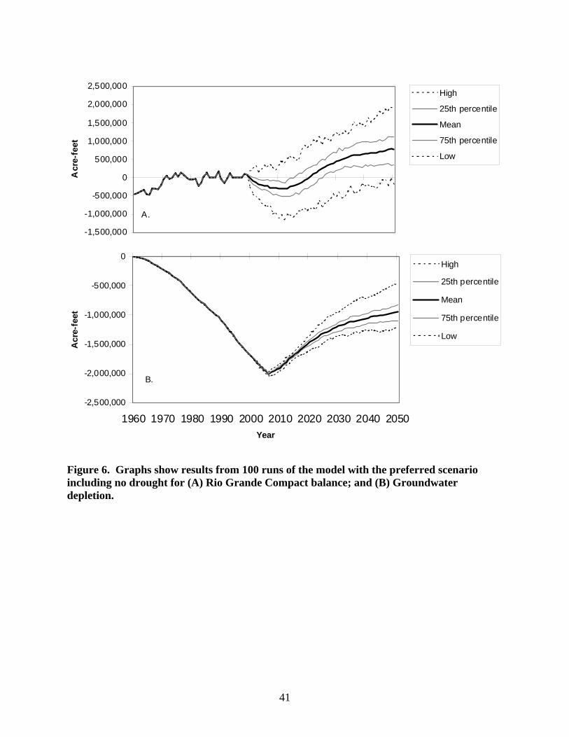
41

Figure 6. Graphs show results from 100 runs of the model with the preferred scenario including no drought for (A) Rio Grande Compact balance; and (B) Groundwater depletion.

-1,500,000

-1,000,000

-500,000

0

500,000

1,000,000

1,500,000

2,000,000

2,500,000A

cre-

feet

High

25th percentile

Mean

75th percentile

Low

A.

-2,500,000

-2,000,000

-1,500,000

-1,000,000

-500,000

0

1960 1970 1980 1990 2000 2010 2020 2030 2040 2050Year

Acr

e-fe

et

High

25th percentile

Mean

75th percentile

Low

B.

42

Figure 7. Graphs show results from 100 runs of the model with the preferred scenario including drought for (A) Rio Grande Compact balance; and (B) Groundwater depletion. Model results show that groundwater depletions occur every year from 1960 to 2006 (Figure 5B). More importantly, the rate of the depletion increases over this period of time. This trend continues until 2006 when the CoA begins using SJC water from the river for municipal supply and curtails its groundwater pumping. The reduction in groundwater pumping allows the aquifer levels to rebound briefly, but then increased demand for groundwater due to continued population growth starts driving a renewed decline. Important changes in the regional water budget are expressed in the temporal variation of the RGC balance (Figure 5A). The balance climbs out of a deficit situation in the 1960s and early 1970s, fluctuates around zero in the late 1970s through the early 1990s, and then moves increasingly into a deficit situation that reaches about 1 million af by 2050. The deficit condition in the early 1960s is a result of the severe drought of the 1950s. The rebound was fueled by increasing precipitation coupled with low lake levels in Elephant Butte Reservoir (i.e., low evaporation). Conversely, the 1980s and 1990s are some of the wettest years on record for the

-1,500,000

-1,000,000

-500,000

0

500,000

1,000,000

1,500,000

2,000,000

2,500,000A

cre-

feet

High25th percentileMean75th percentileLow

A.

-2,500,000

-2,000,000

-1,500,000

-1,000,000

-500,000

0

1960 1970 1980 1990 2000 2010 2020 2030 2040 2050Year

Acr

e-fe

et

High

25th percentile

Mean

75th percentile

Low

B.

43

planning region. These wet years combined with several spills of Elephant Butte Reservoir (which resets the RGC balance to zero) result in a Compact balance with little surplus or deficit.

The decline in the deficit after 2000 is caused by several factors. First, the climate moderates following the wet years of the 1980s and 1990s. Second, pump-induced river leakage exceeds sewage returns by 20,000–30,000 af/yr until after the CoA begins to curtail its pumping in 2006. Third, the CoA begins taking its full allotment of SJC water from the Rio Grande in 2006, some of which had been used in the past to assist farmers and others in times of drought. At the time of this writing it is unclear how drought will affect future irrigation consumption when the CoA’s SJC water is no longer available for supplemental use.

The RGC results shown in Figure 5A played an important role in making clear for the planning community the degree of difficulty they may face in meeting future RGC obligations. Previous to the MRG model, the only existing projections for the RGC were point estimates for the years 2000 and 2040 (Papadopulos and Associates, 2000). Papadopulos and Associates (2000) found that the MRG region ran on average a 13,500-af/yr credit in the year 2000 and estimated that the region will on average run a 29,800-af/yr deficit by 2040. The MRG planning model yields similar annual results to that of the Papadopulos report, with minor modifications to demand assumptions. The cumulative results of the model in the default run show the MRG balance dropping continually to about -1,000,000 af, which would represent extreme non-compliance with the RGC. The mean annual deficit of a 50-year, 1,000,000 af deficit is only 20,000 af, which is a small part of the total regional annual budget. In this case, viewing point estimates of a future annual deficit might not have carried the same impact as viewing the cumulative, 50-year deficit. 4.3 Preferred Scenario The main objective of the regional water planning process is to balance projected supply with demand. Operationally, the MRGWA set the objectives of ending groundwater depletion (i.e., balancing groundwater discharges with inflows) and maintaining the cumulative RGC balance so that it would not exceed a deficit of 200,000 af/year for more than six years.

A “preferred scenario” of future water management strategies was developed for achieving the region’s objectives and for ultimate inclusion in the state’s 50-year water plan. The development of the preferred scenario followed the process described in Section 2, Methods. Basic elements of the preferred scenario include municipal conservation through the installation of low-flow appliances, xeriscaping, rooftop harvesting, and reduction in landscaped acreages; improved irrigation efficiency through lining conveyance channels, laser leveling fields, and application of drip irrigation; bosque restoration; transfer of limited Elephant Butte Reservoir storage to Abiquiu Reservoir and to artificial recharge; expansion of the water supply through use of desalinated water; and water transfers from Socorro and Sierra counties. Specifics for each of these alternatives that comprise the preferred scenario are given in Table 6.

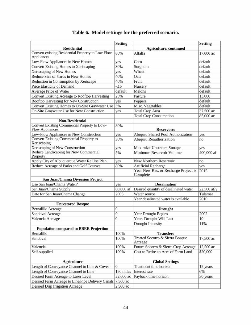
44

Table 6. Model settings for the preferred scenario.

Setting Setting Residential Agriculture, continued

Convert existing Residential Property to Low Flow Appliances

80% Alfalfa 17,000 ac

Low-Flow Appliances in New Homes yes Corn default Convert Existing Homes to Xeriscaping 30% Sorghum default Xeriscaping of New Homes yes Wheat default Reduce Size of Yards in New Homes 40% Oats default Reduction in Consumption by Xeriscape 40% Fruit default Price Elasticity of Demand -.15 Nursery default Average Price of Water default Melons default Convert Existing Acreage to Rooftop Harvesting 25% Pasture 13,000 Rooftop Harvesting for New Construction yes Peppers default Convert Existing Homes to On-Site Graywater Use 5% Misc. Vegetables default On-Site Graywater Use for New Construction yes Total Crop Area 37,500 ac Total Crop Consumption 85,000 ac

Non-Residential Convert Existing Commercial Property to Low-Flow Appliances

80% Reservoirs

Low-Flow Appliances in New Construction yes Abiquiu Shared Pool Authorization yes Convert Existing Commercial Property to Xeriscaping

30% Abiquiu Reauthorization no

Xeriscaping of New Construction yes Maximize Upstream Storage yes Reduce Landscaping for New Commercial Property

5% Minimum Reservoir Volume 400,000 af

Apply City of Albuquerque Water Re Use Plan yes New Northern Reservoir no Reduce Acreage of Parks and Golf Courses 80% Artificial Recharge yes Year New Res. or Recharge Project is

Complete 2015

San Juan/Chama Diversion Project Use San Juan/Chama Water? yes Desalination San Juan/Chama Supply 60,000 af Desired quantity of desalinated water 22,500 af/y Date for San Juan/Chama Change 2005 Water source Tularosa Year desalinated water is available 2010

Unrestored Bosque Bernalillo Acreage 0 Drought Sandoval Acreage 0 Year Drought Begins 2002 Valencia Acreage 0 Years Drought Will Last 10

Drought Intensity 11% Population compared to BBER Projection

Bernalillo 100% Transfers Sandoval 100% Treated Socorro & Sierra Bosque

Acreage 17,500 ac

Valencia 100% Future Socorro & Sierra Crop Acreage 12,500 ac Self-supplied 100% Cost to Retire an Acre of Farm Land $20,000

Agriculture Global Settings Length of Conveyance Channel to Line & Cover 0 Treatment time horizon 15 years Length of Conveyance Channel to Line 150 miles Interest rate 6% Desired Farm Acreage to Laser Level 22,000 ac Payback time horizon 30 years Desired Farm Acreage to Line/Pipe Delivery Canals 7,500 ac Desired Drip Irrigation Acreage 2,500 ac

45

Planners were concerned that the years from 2000 to 2050 might be dryer than the years from 1950 to 2000. These concerns were the product of multi-year drought conditions in the basin beginning around 1998, the identification of what appear to be long-term drought cycles in the Southwest corresponding to the existing drought conditions (Gray et al., 2003), and long-term tree ring analysis suggesting that drought conditions in the 1950s may actually be more representative of normal climatic conditions for the region (Grissino-Mayer et al., 2002). For these reasons two versions of the preferred scenario were developed, one without a significant long-term drought (Figure 6) and one with a drought (Figure 7). In both versions, the scenario described above remains the same except for the occurrence of the drought. In the drought version, the scenario assumes a drought beginning in 2002 and lasting for 10 years. The intensity of the drought reflects an 11% decrease in annual surface water inflows to the region, relative to average inflows from 1950–1998.

With or without a drought, the preferred scenario results in a mean RGC balance of about 600,000 af in 2050, representing a surplus in favor of the planning region (Figures 6A and 7A). However, with no drought the Compact balance drops into deficit territory around 2003 and falls to more than -300,000 af before moving to a surplus by about 2021. This period of deficit represents non-compliance with the Compact. With the drought, the deficit falls to about -500,000 af, and persists a year or two longer, also representing non-compliance with the compact.

With or without a drought, the preferred scenario results in an average aquifer depletion of approximately -1,000,000 af by 2050 (Figures 6B and 7B), and the depletion appears to continue decreasing (i.e., the aquifer continues refilling). Model results not shown here place the net present value for implementing all the management strategies in the preferred scenario at about $2.3 billion, and the cost per af of water saved as about $1190. Pie charts (Figure 8) show how consumption occurs by categories in the MRG according to model results for the year 2000, the year 2050 in the default scenario, and the year 2050 in the preferred scenario. It is noteworthy that the total consumption terms in 2000 and 2050 in the default scenario (about 479,600 and 477,400, respectively; Figures 8A and 8B) are nearly equal. However, in 2050 under the default (no-action) scenario the municipal consumption expands considerably relative to municipal consumption in 2000, and the Elephant Butte Reservoir evaporation declines considerably. Reduced Elephant Butte Reservoir evaporation, in this case, reflects low lake levels, which are related to low Rio Grande surface water flow levels and the large RGC deficit shown in Figure 5. (RGC obligations are met both by the amount of water released downstream from Elephant Butte Reservoir and the amount of water stored in the Reservoir.) So even though total consumption does not increase between 2000 and 2050 in the default scenario, the consumption patterns do not allow for compliance with the RGC, according to model results. In 2050 under the preferred scenario (Figure 8C), municipal, agricultural, and bosque consumption are all considerably lower compared to Figure 8B. This is the result of the numerous conservation strategies applied in the preferred scenario. However, Elephant Butte Reservoir evaporation increases considerably because the preferred scenario leaves more water in the river and more water in Elephant Butte, leading to increased evaporation from the

46

reservoir. The total consumption (414,412 af) is well below total consumption for either 2000 or 2050 in the default scenario, according to model results.

Figure 8. Model results for water consumption in the MRG for (A) year 2000; (B) year 2050 under the default "no-action" scenario; and (C) year 2050 under the preferred scenario.

79,719

119,038

76,649

166,506

37,735

ElephantButte Evap.

Bosque

Agriculture

Municipal

Rio Grande Evap.

A. Year 2000; total consumption = 479,647 af.

90,856

84,161

57,183

144,721

37,491

ElephantButte Evap.

Bosque

Agriculture

Municipal

Rio Grande Evap.

C. Year 2050, preferred scenario; total consumption = 414,412 af.

142,530

117,53175,840

104,049

37,491

ElephantButte Evap.

BosqueAgriculture

Municipal

Rio Grande Evap.

B. Year 2050, default; total consumption = 477,441 af.

47

As this report is being written, the model is being used in a sensitivity analysis of the parameters in the preferred scenario. This process includes the quantitative assessment of the strength of some of the more influential components in the preferred scenario. This analysis is contributing to the continued evolution of the preferred scenario for the MRG. In the course of developing the preferred scenario, the model helped identify three important lessons about the regional water system and the efficient management of that system. The first lesson was that there is no “silver bullet,” i.e., no single conservation measure can solve the region’s water budget deficit. In fact, even with extreme measures no single sector (i.e., municipal, agricultural, or environmental) can solve the regional deficit on its own. Rather, multiple conservation measures spread across different water use sectors are required. For example, groundwater depletions are due largely to municipal pumping. Thus, municipal conservation programs are the most important measures available to reduce groundwater depletions. Municipal conservation measures, however, provide little improvement to the RGC deficit over the short term. Alternatively, bosque restoration efforts directly improve the RGC deficit, yet treatment of all planning region acreage is insufficient to fully erase it. Combining bosque treatment and improved irrigation efficiencies can mitigate the RGC deficit, but they have no appreciable effect on the groundwater depletions. The second lesson was the stark realization of just how difficult balancing the groundwater budget and meeting RGC obligations will be, and that achieving balance will require strong measures and considerable cooperation across water use sectors. Over time these conservation measures will change the way the regional community looks and does business. The cities will take on more of a desert complexion as commercial and residential landscaping move to xeric vegetation. The bosque will be thinned considerably and the vegetation composition altered. Low-flow appliances and efficient irrigation practices will impact contractors and irrigators alike. There will also be a price tag associated with these measures, as seen in increased water bills, taxes, and costs to do business.

The third lesson involved timing of the water conservation programs. Note that in the preferred scenario, both with and without drought, the RGC deficit drops to more than -300,000 af very early within the planning period before beginning a recovery again in the mid-2020s. This occurs because of the lag between the time when new management and conservation programs are initiated and the time when water savings from those efforts are fully realized. In this scenario, it is assumed that 15 years are required to achieve full compliance with any conservation policy. These results make it clear that a shorter-term focus must be considered to offset the projected near-term deficits.

48

5. Discussion System dynamics modeling provides a powerful platform for cooperative, community-based water resource planning. These capabilities were demonstrated within the context of regional water planning for a three-county region in north-central New Mexico. A system dynamics model was developed to assist in preparing a 50-year water plan that balances available supply with growing demand. Unique to this effort was an open and participatory process in which the public was directly involved in model development and regional water planning. Both advantages and pitfalls were encountered in creating a model for use by people with both technical and non-technical backgrounds, and in a setting where data and modeling objectives are points of contention among differing interest groups. Here we share some perspective on the community-based model development and planning process in the context of our three modeling objectives, which were to: (1) provide a quantitative framework for evaluating alternative water conservation alternatives; (2) develop a tool for educating and reaching out to the public; and (3) use the model to engage the public in the planning process. 5.1 Providing a Quantitative Framework Our first modeling objective was to build a quantitative platform for exploring alternative water management strategies in terms of costs and water savings. A system dynamics model was created that incorporates 24 unique conservation alternatives and a no-action alternative. The model allows the user to select different alternatives and prescribe the degree of the impact (e.g., number of acres to treat) by moving slider bars and mouse-clicking on buttons from within a user-friendly interface. Within a matter of seconds results in graphical format are returned in terms of RGC balances, groundwater depletions, amount of water saved, costs, and other variables.

This interactive modeling environment proved valuable to the planning process, but a few reservations were registered by various reviewers. First, users have the power to make decisions in the model that could be considered unrealistic, or which require greater interpretation than can be provided on the pages of the model. For example, users can simulate the impact of a 100% conversion of existing homes to low-flow appliances. Some analysts would contend that achieving that rate of conversion is unrealistic; and unrealistic or not, it would require fiscal and/or legislative incentives not included in the model. Users can simulate the effect on evaporation by covering all 763 miles of agricultural conveyance channels in the planning region. But covering these conveyances would not allow easy maintenance, and so they could become clogged with debris within months or a few years. Users can also simulate the siting of a new dam and reservoir in southern Colorado at the headwaters of the Rio Grande, regardless of the political difficulties that will accompany such a project. Users could also simulate increased rates of population growth and, hence, groundwater pumping in the region. Increasing groundwater pumping to extreme levels could change fundamental dynamics in river seepage, which the current model might not capture. Particular care has been given to preclude these kinds of problems (i.e., many such options cannot be selected in the model). Nevertheless, this list underscores the idea that operation of the model must be accompanied by detailed instruction on the pages of the model, and/or expert facilitation during model use and the interpretation of results.

49

Another difficulty involved the disparity in understanding between modelers and the public on what a model is, and what a model should do. Early concerns about the modeling effort regarded the idea that the model would make decisions for the public, and that model results would drive the planning process. This concern was eventually allayed through the cooperative, transparent nature of the modeling process, and by many presentations of interim versions of the model (along with descriptions of the process) to many different groups. This concern was also allayed by making the distinction between the model as a predictive tool and as an instructive tool. Treating the model as a predictive tool created anxiety over its role in the planning process, while treating it as an instructive tool did not. Ultimately, the message that might have most helped the model find a secure place in the planning process was that the model, along with other kinds of information, allows the planners to better visualize both the problem and potential solutions, and to become better predictors themselves.

5.2 Education and Outreach Another reason for developing the model was to educate the public about the complexity of the regional water system. The hydrological-ecological-economic system portrayed in the model has many complex, interacting components. The model helps the user understand the system by breaking out and organizing individual components and their interactions in graphical ways. It allows users to actively experiment with different values for different variables, and it returns real-time, graphical results. The only other way to convey the same information is in spreadsheets and graphs, which might be inaccessible to some, or in prose, which may be equally inaccessible to others. The model adds a unique dimension to the educational process. At the highest level, the model effectively conveyed the basic elements of the water budget. It illustrates graphically and dynamically how municipal consumption rivals agricultural consumption in the basin, and how sizeable an element the bosque represented in the water budget. As discussed previously, the model was effective at conveying the idea that no single sector or alternative could solve regional problems with both groundwater depletions and RGC balance deficits, and that coordination and cooperation across the different water use sectors would be required. The model also helped convey the complexity of the regional water system. Though people can be good at observing the local structure of a system, they might have much more difficulty predicting how complex, interdependent systems will behave (Forrester, 1987). In particular, the model helped convey the impacts of time delays and feedbacks, which can be especially difficult dynamics to accurately conceptualize or communicate. The effects of time delays are visually evident in the graph of the RGC balance under the preferred scenario (Figure 6A). Difficulties in improving the RGC deficit in the early 2000s results from the time lag between program implementation and the time water savings are realized. Time delays are also integral to the cause and effect relation between groundwater pumping and river leakage, and these are demonstrated in the model.

In addition, the model helped illustrate feedback dynamics between system elements. Along these lines, the model played an important role in helping the public distinguish between consumed water and water transfers. For example, indoor municipal demand is met by groundwater pumping, and most of that water is returned to the Rio Grande as treated sewage

50

return flows. Indoor water is not consumed but transferred from the groundwater to the surface water system. This is important when indoor water conservation measures are adopted that result in reduced groundwater pumping (and thus reduced depletions) and reduced sewage return flows (and thus a reduced RGC balance). It is also interesting to note that a time delayed feedback helps offset the lost sewage returns with reduced pumping-induced river leakage.

Feedback also plays an important role in evaluating the transfer of stored water from Elephant Butte Reservoir to northern reservoirs where evaporative losses are reduced. Such transfers depend on available northern storage, the timing of RGC surpluses, and the storage at Elephant Butte Reservoir. Although this alternative looks good on paper, it is very difficult to find the water to transfer except in very wet years, which quickly overwhelms the limited storage capacity of northern reservoirs.

Unfortunately, public access to the model greatly limited educational opportunities. Because the model was developed on a commercial software package, direct access to the model was only available to those owning a Powersim license. The best option for increasing access is to post models on an internet site. This is part of the plan for the MRG model, but the resources required to transfer the model to the World Wide Web are considerable.

5.3 Public Engagement The third objective of the model was to engage the public in the water planning process. Over the course of the planning process a number of different “publics” interacted with the model. There was the MRGWA comprised of volunteers from the general public, most of whom had a particular vested interest in water (i.e., urban developers, irrigators, environmentalists, etc.). In addition, there was the general public who had enough interest in water to participate in public meetings. Local governments represented by MRCOG also engaged in the planning process along with various local, state, and federal water agencies. Interaction by these different groups with the model varied from a simple one-time viewing to supplying data and system understanding, model development, model review, and model utilization in the planning process. Perhaps the most important role of the model in the planning process was in promoting, initiating, and informing dialogue. In many cases the dialogue arose simply from the process of exploring the impacts of alternative water conservation measures. Participants were naturally drawn to offer their “what if” scenarios for testing. This led to questions and discussions of the pros and cons of the different alternatives. In many cases the questions led to discussions lasting weeks and months, which often led to greater understanding and clarity. These discussions often helped participants consider the broader, system-wide implications of proposed actions. Dialogue was also generated when unexpected results appeared. In many cases this served as an experience of discovery; i.e., the model helped users see something that had not been considered before. In other cases the result was counter to the preconceived mental model of the user. One example of this occurred with irrigators who know that they apply less water to laser leveled fields. But, counter to their expectation, laser leveling shows relatively little water savings. This is because leveling largely reduces water lost to infiltration, which is not consumed but returned to the river via the shallow ground water system.

51

Within the modeling environment, supplementary information was provided to help explain the difference between model results and users’ preconceived mental models. First, multiple intermediate results are graphed for each of the individual water balance terms. For the agricultural sector such variables as irrigation seepage, river diversions, drain return flows, crop evapotranspiration, and others are graphed to visually convey the reason for the result to the user. Accompanying explanatory text is also provided with the graphs. Second, efforts are made to reference the data and physical relations used in the model, hopefully with institutions and individuals trusted by the model user.

52

6. References Buller, O.H., H.L. Manges, L.R. Stone, and J.R. Williams, 1988. Benefits from improving flood

irrigation efficiency. Report of Progress 544, Kansas State University Agriculture Experiment Station, Manhattan, Kansas.

Brooks, C., 2002. Personal communication on October 30, 2002.

Brookshire, D.S., H.S. Burness, J.M. Chermak, K. Kraus, 2003. Western urban water demand. Natural Resources Journal 42(4): 873-898.

Bureau of Business and Economic Research, 2002. New Mexico Business Current Economic Report 23(7):8.

City of Albuquerque (CoA), 2003. Water conservation program website, accessed January 2003 at http://www.cabq.gov/waterconservation/.

City of Albuquerque (CoA), 2002. Hydrologic affects of the proposed City of Albuquerque drinking water project on the Rio Grande and the Rio Chama systems. City of Albuquerque Public Works Department Water Resources Study Implementation Final Report, May 2002. CH2M HILL, Inc., 6001 Indian School Rd. NE, Albuquerque, NM, 87110.

Daugherty, R.L., and J.R. Franzini, 1965. Fluid mechanics with engineering application. McGraw Hill, New York.

Engelman, R., R.P. Cincotta, B. Dye, T. Gardner-Outlaw, and J. Wisnewski, 2000. People in the balance: population and natural resources at the turn of the millennium. Population Action International, Washington D.C. http://populationaction.org/resources/publications/ peopleinthebalance/downloads/people_balance.pdf.

Ford, A., 1996. Testing the Snake River explorer. System Dynamics Review 12(4): 305-329.

Forrester, J.W., 1990. Principles of Systems. Productivity Press, Portland, Oregon.

Forrester, J.W., 1987. Lessons from system dynamics modeling. System Dynamics Review 3(2): 136-149.

Glover, R.R. and G.G. Balmer, 1954. River depletion resulting from pumping a well near a river. Transactions of the American Geophysical Union 35(3): 468-470.

Gray, S.T., J.L. Betancourt, C.L. Fastie, and S.T. Jackson, 2003. Patterns and sources of multidecadal oscillations in drought-sensitive tree-ring records from the central and southern Rocky Mountains. Geophysical Research Letters 30(6):1316-1320.

Grissino-Mayer, H.D., C.H. Baisan, K.A. Morino, and T.W. Swetnam, 2002. Multi-century trends in past climate for the Middle Rio Grande Basin, AD 622–1922. Final Report 28C4800. USDA Forest Service, Rocky Mountain Research Station, 333 Broadway SE, Suite 115, Alb., NM, 87102.

Hood, J.W. and L.R. Kister, 1962. Saline-water resources of New Mexico. U.S. Geological Survey, Water-Supply Paper 1601.

Israelsen, O.W and V. E. Hansen, 1962. Irrigation Principles and Practices. John Wiley and Sons, New York.

53

Louks, D.P., J. Kindler and K. Fedra, 1985. Interactive water resources modeling and model use: An overview. Water Resources Research 21(2): 95-102

Martin, W.E. and J.F. Thomas, 1986. Policy relevance in studies of urban residential water demand. Water Resources Research 22(13): 1735-1741.

McAda, D.P. and P. Barroll, 2002. Simulation of ground-water flow in the Middle Rio Grande Basin between Cochiti and San Acacia, New Mexico. U.S. Geological Survey Water-Resources Investigations Report 02-4200.

McLean, J.S., 1970. Saline ground-water resources of the Tularosa Basin, New Mexico. U.S. Department of the Interior, Office of Saline Water Report No. 561. July, 1970.

Michelsen, A.M., J.T. McGuckin, and D.M. Stumpf, 1998. Effectiveness of residential water conservation price and nonprice programs. American Water Works Research Foundation and American Water Works Association. Denver, Colorado.

Middle Rio Grande Conservancy District (MRGCD), 2001. Estimated Irrigated Acreage as of July 2000. Middle Rio Grande Conservancy District, Albuquerque, New Mexico.

Palmer, R.N., A.M. Keyes and S. Fisher, 1993. Empowering stakeholders through simulation in water resources planning. In: K. Hon, (ed.), Conference Proceedings: Water management in the ‘90s: a time for innovation. American Society of Civil Engineers Annual Conference, Seattle, WA, May 1-5, 1993.

Papadopulos, S.S., and Associates, 2000. Middle Rio Grande Water Supply Study. Report to the New Mexico Interstate Stream Commission, August 4, 2000. S.S. Papadopulos and Associates, Inc., 1877 Broadway, Suite 703, Boulder, Colorado, 80302-5245.

Papadopulos, S.S., and Associates, 2002. Evaluation of the Middle Rio Grande Conservancy District Irrigation System and Measurement Program to the New Mexico Interstate Stream Commission, December 2002. S.S. Papadopulos and Associates, Inc., 1877 Broadway, Suite 703, Boulder, Colorado, 80302-5245.

Papadopulos, S.S., and Associates, 2003. Middle Rio Grande Water Supply Study. Report to the New Mexico Interstate Stream Commission, Interim Draft Report, August 6, 2003. S.S. Papadopulos and Associates, Inc., 1877 Broadway, Suite 703, Boulder, Colorado, 80302-5245.Associates, Inc., 1877 Broadway, Suite 703, Boulder, Colorado, 80302-5245.

Postel, S., 1997. Last oasis: facing water scarcity. W.W. Norton & Co., New York. 239 pp.

RosTek Associates, 2002. Desalting handbook for planners, 3rd edition. RosTek Associates, Inc., U.S. Department of the Interior, Bureau of Reclamation, Water Treatment Engineering and Research Group.

Roybal, F.E., 1991. Groundwater Resources of Socorro, New Mexico, U.S. Geological Survey Water Resources Investigation Report 89-4083.

Runyan, C., 2002. Personal communication December 11, 2002.

Shuttleworth, W.J., 1993. Evaporation. In: D.R. Maidment (ed.), Handbook of Hydrology. McGraw-Hill, Boston.

Simonovic, S.P. and H. Fahmy, 1999. A new modeling approach for water resources policy analysis. Water Resources Research 35(1):295-304.

54

Stave, K.A., 2003. A system dynamics model to facilitate public understanding of water management options in Las Vegas, Nevada. Journal of Environmental Management 67:303-313.

Stephens, D.B., and Associates, 2003. Evaluation of alternative actions for technical, physical, hydrological and environmental feasibility; report to the Middle Rio Grande Water Assembly and the Mid Region Council of Governments. D.B. Stephens and Associates, Inc., 6020 Academy Road NE, Suite 100, Albuquerque, NM, 87109.

Sterman, J.D., 2000. Business dynamics, systems thinking and modeling for a complex world. McGraw-Hill, Boston. 982 pp.

U.S. Army Corps of Engineers (USACE), 2002. Upper Rio Grande water operations model, draft model documentation, technical review committee draft. U.S. Army Corps of Engineers, Albuquerque District.

U.S. Bureau of Reclamation (USBR), 1997. Middle Rio Grande water assessment: middle Rio Grande land use trend analysis geographic information system database. U.S. Bureau of Reclamation, Albuquerque Area Office, N.M.

U.S. Bureau of Reclamation (USBR), 2002. ET toolbox, evapotranspiration toolbox for the middle rio grande, accessed February 2002, http://www.usbr.gov/pmts/rivers/ awards/ettoolbox.html.

U.S. Geological Survey (USGS), 2002. Real-time data for New Mexico, accessed September 2002, http://waterdata.usgs.gov/nm/nwis/rt.

Wallace, S. D., F.H. Sancar and H. Fahriye, 1988. An integrative approach to water resource management: an application in Middleton, Wisconsin. Proceedings of the 1988 International Conference of the Systems Dynamics Society, La Jolla, California, International System Dynamics Society, 447-459.

Wilson, B.C. and A.A. Lucero, 1997. Water use by categories in New Mexico counties and river basins, and irrigated acreage in 1995. Technical Report 49, New Mexico Office of the State Engineer. 149 pp.

Yuska, Mark 2003. Personal communication on January 15, 2003.

55

DISTRIBUTION:

1 MS 9018 Central Technical Files, 8945-1

2 MS 0899 Technical Library, 9616

1 MS 0612 Review & Approval Desk, 9612 For DOE/OSTI

1 MS 1379 Dave Barber

1 MS 1373 David Betsill

1 MS 1373 Kent Biringer

1 MS 0323 Donna Chavez

2 MS 0451 Stephen Conrad

1 MS 0701 Peter Davies

1 MS0720 Darryl Drayer

4 MS 0735 Ray Finley

1 MS 0839 Jessica Glicken-Turnley

1 MS 0710 Mike Hightower

1 MS 0839 Curtis Johnson

1 MS 0749 Len Malczynski

1 MS 0749 Orman Paananen

170 MS 0735 Howard Passell

1 MS 0720 Phillip Pohl

1 MS 1373 Arian Pregenzer

2 MS 0451 Dick P. Thomas

2 MS 0735 Vince Tidwell

1 MS 0741 Marjorie Tatro

1 MS 0839 Gerry Yonas