Cooperative Motion Control of multiple autonomous robotic ... · patrulhas de seguranc¸a ou na...
85
Cooperative Motion Control of multiple autonomous robotic vehicles Collision Avoidance in Dynamic Environments S ´ ergio Alexandre Carrac ¸a Carvalhosa A thesis submitted to the Department of Electrotechnical Engineering in partial fulfillment of the requirements for the degree of Master of Science in Electrotechnical Engineering President: Doutor Carlos Jorge Ferreira Silvestre Advisor: Doutor Ant ´ onio Pedro Rodrigues de Aguiar Co-Advisor: Doutor Ant ´ onio Manuel dos Santos Pascoal Examiner: Doutor Miguel Afonso Dias de Ayala Botto October 2009
-
Upload
phungnguyet -
Category
Documents
-
view
215 -
download
0
Transcript of Cooperative Motion Control of multiple autonomous robotic ... · patrulhas de seguranc¸a ou na...

Cooperative Motion Control ofmultiple autonomous robotic vehicles
Collision Avoidance in Dynamic Environments
Sergio Alexandre Carraca Carvalhosa
A thesis submitted to the Department of Electrotechnical Engineering
in partial fulfillment of the requirements for the degree of
Master of Science in Electrotechnical Engineering
President: Doutor Carlos Jorge Ferreira Silvestre
Advisor: Doutor Antonio Pedro Rodrigues de Aguiar
Co-Advisor: Doutor Antonio Manuel dos Santos Pascoal
Examiner: Doutor Miguel Afonso Dias de Ayala Botto
October 2009

Abstract
The role of autonomous vehicles and robotics in aiding man in harsh environments has
become an increasing focus of interest over the last decade, as the technology that enables
this kind of systems becomes available. A particular area that has received special attention,
has been the study of coordination and control of various classes of unmanned autonomous
vehicles. The main motivation for this trend is the wide range of military and civilian
applications where teams of these vehicles working together exhibit better performance in
terms of flexibility, robustness and efficiency compared to the single heavily equipped vehicle
approach. For tasks such as space exploration, automated transport convoys, security
patrols or large object transportation, having a cooperative team of vehicles provides for
better area coverage as well has robustness to systems malfunctions. The completion of
missions of this nature often requires holding a desired geometrical formation pattern, that
is at the same time reactive and adaptive to an unknown environment, as for example to
prevent imminent collisions.
It is in this framework that this thesis proposes a collision avoidance system to be in-
tegrated in a cooperative motion control (CMC) architecture, enabling the autonomous
robotic vehicles that participate in a cooperative mission to automatically re-plan their
trajectories in order to avoid unknown obstacles. The first part of the thesis describes the
general architecture for CMC, that includes cooperative path following, where multiple ve-
hicles are required to follow pre-specified spatial paths while keeping a desired inter-vehicle
formation pattern. In the second part of the thesis we propose a Collision Avoidance sys-
tem (CAS) that is composed by two subsystems: the collision prediction, and the collision
avoidance module. For collision prediction we combine a bank of Kalman filters running in
parallel, each using a different model for target motion, to derive an unknown object’s veloc-
ity and estimate its probable trajectory, the vehicle pre-determined path is then checked for
possible interactions with the obstacle. Collision avoidance is achieved either by controlling
the speed of the vehicle along its assigned mission path, or through path re-planing using
harmonic potential fields. Because group coordination must be taken into consideration,
collision avoidance is implemented as part of a Behavior-based system, that is decentralized
and can be used with groups of heterogeneous vehicles. The proposed collision avoidance
ii

iii
system is then applied to a group of marine surface crafts, where simulation results are
presented trough the use of a Cooperative Motion Control Simulator developed to model
the key different aspects of cooperative multiple vehicle systems.
Keywords: Cooperative Motion Control, Collision Avoidance, Collision Prediction, Au-
tonomous Surface Crafts, Potential field theory, Kalman filter, Coordinated path-following,
Coordination control

Resumo
A utilizacao de veıculos autonomos na realizacao de tarefas em ambientes adversos, tem
na ultima decada merecido renovado interesse a medida que as tecnologias que permitem
realizar este tipo de sistemas se tornam disponıveis. Uma area em particular, foco de
especial atencao, e a pesquisa relacionada com o controlo e coordenacao de diferentes classes
de veıculos autonomos. O grande interesse neste tipo de sistemas deve-se ao vasto potencial
de aplicacao que possuem, tanto para fins comerciais como militares, onde a utilizacao de
equipas heterogeneas de veıculos autonomos em detrimento de um so veıculo fortemente
equipado, representa um aumento de desempenho do sistema em termos de flexibilidade,
robustez e eficiencia. Em tarefas como o transporte de objectos de elevadas dimensoes,
patrulhas de seguranca ou na exploracao espacial, recorrer a utilizacao de uma equipa de
veıculos autonomos em interaccao cooperativa, permite uma melhor cobertura da area da
missao e introduz uma maior robustez a avarias do sistema. E comum em missoes desta
natureza, que os veıculos intervenientes necessitem de manter uma determinada formacao
geometrica entre si, formacao essa que devera ser ao mesmo tempo flexıvel e reactiva, de
modo a por exemplo evitar colisoes com obstaculos desconhecidos.
E neste contexto, que se propoe nesta tese um sistema de evasao de colisoes a ser inte-
grado numa arquitectura de controlo cooperativo, munindo os veıculos autonomos partici-
pantes numa formacao com a capacidade de automaticamente replanearem uma trajectoria
com vista a evitar um obstaculo desconhecido. Na primeira parte da tese e apresentada
a estrutura geral de uma arquitectura de controlo cooperativo, a qual inclui o seguimento
coordenado de caminhos, onde multiplos veıculos seguem um caminho pre-designado en-
quanto mantem uma determinada formacao entre si. Na segunda parte desta tese e entao
proposto um sistema de evasao de colisoes composto por dois subsistemas: um preditor de
colisoes, e um modulo de evasao de colisoes.
Como primeiro passo para a predicao de uma colisao, e determinada a velocidade e
estimada a trajectoria de um obstaculo utilizando para tal um banco de filtros de Kalman
a correrem em paralelo, onde cada filtro emprega um modelo diferente para o movimento
do obstaculo. Esta trajectoria estimada e entao comparada com o caminho previsto para o
veıculo em busca de possıveis interaccoes.
iv

v
Com base na informacao adquirida no passo de predicao, e entao elaborada uma de duas
estrategias para evitar a colisao: correccao e controlo da velocidade ao longo do caminho
a percorrer, ou planeamento de um caminho alternativo baseado em campos de potencial
harmonico. Uma vez que se pretende integrar evasao de colisoes em equipas de veıculos
autonomos a funcionar em cooperacao, o sistema e implementado numa comutacao entre
dois modos distintos o de cooperacao e o de evasao, e pensado de forma a ser descentralizado
e aplicavel a diferentes tipos de veıculos.
O sistema de evasao de colisoes proposto e por fim aplicado a um grupo de veıculos
de superfıcie marinha, recorrendo para tal a um simulador de Controlo Cooperativo desen-
volvido no ambito desta tese.
Palavras Chave: Controlo Cooperativo, Evasao de Colisoes, Predicao de Colisoes, Teoria
de campos de potencial, Filtro de Kalman, Seguimento coordenado de caminhos, Veıculos
autonomos de superficie marinha.

Acknowledgements
The conclusion of the work reported in the present dissertation was attained thanks to the
contribution of several persons, in many different ways.
I would like to thank first of all professor Antonio Pedro Aguiar, for allowing me the
chance to pursue this study, and for all the support, advice and motivation he provided
throughout the course of this thesis. I would also like to thank professor Antonio Pascoal
and all the people at ISR, involved in GREX and COGS project, that were always ready
to share their knowledge and offer their advice whenever they could.
I thank my colleagues and friends at IST that bared with me many of the labors of
these last few years, and that I am sure will bare with many joys in the future to come.
Thank you Salvado, Renato, Rafa, Rui, Maria, Ines, Pica, Leite, Isacc, Dinis, Ze, Diogo,
Luis and surely I’m forgetting someone so I extend this thank you to every one that was
left out.
I couldn’t have reach this point in my academic life without the support of all my other
friends. I thank them first of all for their friendship, their many words of encouragement,
and for putting up with my lack of time in so many occasions. A special Thank you to
Antonio, Nuno, Eliana, Madeira for your friendship . Last but not least I would like to
thank my family: my brother Ricardo, and my parents Amandio and Adelaide. Its thanks
to their support and love that I was able to surpass many adversities in life, and its thanks
to them that I have a roll model to look up to. I dedicate this thesis to them.
A big thank you to you all!!!
vi

Contents
Abstract ii
Resumo iv
Acknowledgements vi
List of Figures ix
List of Tables xi
1 Introduction 1
1.1 Brief historical perspective . . . . . . . . . . . . . . . . . . . . . . . . . . . . 1
1.2 Problem statement . . . . . . . . . . . . . . . . . . . . . . . . . . . . . . . . 4
1.3 Previous work and contributions . . . . . . . . . . . . . . . . . . . . . . . . 5
1.3.1 Collision Prediction . . . . . . . . . . . . . . . . . . . . . . . . . . . 5
1.3.2 Collision Avoidance and Path planing . . . . . . . . . . . . . . . . . 6
1.3.3 Cooperative control of multiple ASC’s . . . . . . . . . . . . . . . . . 7
1.4 Thesis outline . . . . . . . . . . . . . . . . . . . . . . . . . . . . . . . . . . . 8
2 Cooperative Motion Control Architecture 9
2.1 Agents . . . . . . . . . . . . . . . . . . . . . . . . . . . . . . . . . . . . . . . 10
3 Collision Avoidance 13
3.1 Collision Avoidance System - An Overview . . . . . . . . . . . . . . . . . . 13
3.2 Prediction Module . . . . . . . . . . . . . . . . . . . . . . . . . . . . . . . . 17
3.2.1 Target Tracking . . . . . . . . . . . . . . . . . . . . . . . . . . . . . 17
3.2.2 Collision Prediction . . . . . . . . . . . . . . . . . . . . . . . . . . . 21
4 Collision Avoidance Module 26
4.1 Obstacle Avoidance using Harmonic Potential Functions . . . . . . . . . . . 26
4.1.1 The panel method . . . . . . . . . . . . . . . . . . . . . . . . . . . . 26
4.1.2 Uniform Flow . . . . . . . . . . . . . . . . . . . . . . . . . . . . . . . 33
vii

CONTENTS viii
4.1.3 Goal Sink . . . . . . . . . . . . . . . . . . . . . . . . . . . . . . . . . 33
4.1.4 Two Dimensional Robust Potential Field For Online Path Planing . 34
4.1.5 Stagnation Points and structural local minima . . . . . . . . . . . . 35
4.1.6 Path Planning for Multiple Mobile Robots . . . . . . . . . . . . . . . 36
4.2 Velocity Correction . . . . . . . . . . . . . . . . . . . . . . . . . . . . . . . . 37
4.2.1 Virtual target . . . . . . . . . . . . . . . . . . . . . . . . . . . . . . . 37
5 Cooperative Motion Control Simulator (CMCs) 41
5.1 Main Features . . . . . . . . . . . . . . . . . . . . . . . . . . . . . . . . . . . 41
5.2 Simulation . . . . . . . . . . . . . . . . . . . . . . . . . . . . . . . . . . . . . 42
5.3 Graphical User Interface and plotting tools . . . . . . . . . . . . . . . . . . 44
5.4 Visualizations and Plotting . . . . . . . . . . . . . . . . . . . . . . . . . . . 45
6 Simulation Results 47
6.1 Target tracking and Collision Prediction . . . . . . . . . . . . . . . . . . . . 47
6.2 Harmonic potential field based path planing . . . . . . . . . . . . . . . . . . 50
6.3 Velocity Correction . . . . . . . . . . . . . . . . . . . . . . . . . . . . . . . . 53
6.4 Collision Avoidance in a Cooperative Mission scenario . . . . . . . . . . . . 56
6.4.1 Dynamic Obstacle - Velocity Correction . . . . . . . . . . . . . . . . 57
6.4.2 Dynamic Obstacle - Static Virtual Obstacle solution . . . . . . . . . 59
6.4.3 Bottleneck scenario . . . . . . . . . . . . . . . . . . . . . . . . . . . . 61
6.5 Summary . . . . . . . . . . . . . . . . . . . . . . . . . . . . . . . . . . . . . 64
7 Conclusions and Further Research 65
7.1 Summary . . . . . . . . . . . . . . . . . . . . . . . . . . . . . . . . . . . . . 65
7.2 Future Directions . . . . . . . . . . . . . . . . . . . . . . . . . . . . . . . . . 66
A Potential Theory and Harmonic functions 67
A.1 Potential Theory . . . . . . . . . . . . . . . . . . . . . . . . . . . . . . . . . 67
A.2 Harmonic Functions . . . . . . . . . . . . . . . . . . . . . . . . . . . . . . . 68
A.2.1 Two-Dimensional Harmonic Potential Functions . . . . . . . . . . . 69
A.2.2 Constructing The Artificial Potential Field . . . . . . . . . . . . . . 69
Bibliography 72

List of Figures
1.1 DARPA . . . . . . . . . . . . . . . . . . . . . . . . . . . . . . . . . . . . . . 2
1.2 Terrestrial Planet Finder 21 mission . . . . . . . . . . . . . . . . . . . . . . 2
1.3 DelfimX performing a path-following , one of the key Vehicle Primitives
required in the scope of European project GREX . . . . . . . . . . . . . . . 3
1.4 The CO3-AUVs project: Assisted Human Diving Operations . . . . . . . . 4
1.5 Collision Avoidance scenario for a team of ASCs executing a path-following
mission . . . . . . . . . . . . . . . . . . . . . . . . . . . . . . . . . . . . . . 6
2.1 Functional architecture for Cooperative Mission Control . . . . . . . . . . . 9
2.2 Coordinated path-following control system architecture. . . . . . . . . . . . 11
2.3 Cooperative Motion Control of a group of autonomous vehicles: Path-Following
(left) and Target Tracking (right) . . . . . . . . . . . . . . . . . . . . . . . . 12
3.1 Collision avoidance scenario for a group of vehicles in a coordinated mission 13
3.2 Petri net representation of system architecture and hierichal relation . . . . 15
3.3 Fluxogram diagram for the Prediction and Collision Avoidance module in-
teraction, relating to the scenario depicted on Fig. 3.1 . . . . . . . . . . . . 16
3.4 Constant Velocity (CV) Model a) Constant Turn (CT) Model b) . . . . . . 18
3.5 Block diagram for the IMM-KF, source: M. Bayat and Aguiar (2009) . . . . 19
3.6 Different Collision scenarios in an environment with dynamic obstacles . . . 22
3.7 Collision scenario in which the obstacle behavior is interpreted has a static
virtual object (SVO) . . . . . . . . . . . . . . . . . . . . . . . . . . . . . . . 24
4.1 Potential of a source line segment(panel) . . . . . . . . . . . . . . . . . . . . 27
4.2 Panel geometry . . . . . . . . . . . . . . . . . . . . . . . . . . . . . . . . . . 29
4.3 Vehicle trajectory for different sets of Vi . . . . . . . . . . . . . . . . . . . . 34
4.4 Situation where the potential field between both vehicles is symmetric . . . 36
4.5 Velocity Correction: Virtual target concept . . . . . . . . . . . . . . . . . . 38
5.1 CMCs: Agent subsystems - configurable blocks . . . . . . . . . . . . . . . . 43
ix

LIST OF FIGURES x
5.2 CMCs: Vehicle Delfim inner model configurable parameters . . . . . . . . . 43
5.3 Graphical user interface: setting the Controllers for the Delfim Vehicle . . . 44
5.4 Graphical user interface: Setting the desired geometrical disposition of vehi-
cles in the formation . . . . . . . . . . . . . . . . . . . . . . . . . . . . . . . 45
5.5 Plotting Tools: Spacial evolution of vehicles and coordination analyses . . . 45
5.6 Plotting Tools: A 2D animation of the defined coordinated mission . . . . . 46
6.1 Target tracking and Collision Prediction . . . . . . . . . . . . . . . . . . . . 48
6.2 Target tracking and Collision Prediction . . . . . . . . . . . . . . . . . . . . 49
6.3 Harmonic potential field based path planing . . . . . . . . . . . . . . . . . . 51
6.4 Harmonic potential field based path planing - robust approach . . . . . . . 52
6.5 Velocity Correction . . . . . . . . . . . . . . . . . . . . . . . . . . . . . . . . 54
6.6 Velocity Correction . . . . . . . . . . . . . . . . . . . . . . . . . . . . . . . . 55
6.7 A team of three autonomous surface crafts performs a cooperative path-
following mission . . . . . . . . . . . . . . . . . . . . . . . . . . . . . . . . . 56
6.8 Team of ASC’s in a velocity correction maneuver . . . . . . . . . . . . . . . 57
6.9 Vehicle 1 and Vehicle 2 Prediction module results for interaction with the
incoming obstacle . . . . . . . . . . . . . . . . . . . . . . . . . . . . . . . . . 58
6.10 Velocity Correction undertaken by Vehicle 1 and 2 to avoid the incoming
obstacle . . . . . . . . . . . . . . . . . . . . . . . . . . . . . . . . . . . . . . 58
6.11 Vehicle 2 Prediction module results for interaction with the incoming obstacle 59
6.12 Vehicle 2 identifying path intersection as a Static Virtual Object in order to
avoid collision . . . . . . . . . . . . . . . . . . . . . . . . . . . . . . . . . . . 60
6.13 Path re-planning taking a Static Virtual Obstacle representation of the ob-
stacle trajectory . . . . . . . . . . . . . . . . . . . . . . . . . . . . . . . . . 61
6.14 Collision Avoidance System resolving spacial and temporal decoupling of
trajectories . . . . . . . . . . . . . . . . . . . . . . . . . . . . . . . . . . . . 62
6.15 Resultant inner map representation of the scenario to be used in potential
field path planing . . . . . . . . . . . . . . . . . . . . . . . . . . . . . . . . . 63
6.16 Velocity correction command issued to achieve inter vehicle coordenation . 64
A.1 Representation of a type sink harmonic function . . . . . . . . . . . . . . . 70
A.2 Representation of a Uniform flow Potential . . . . . . . . . . . . . . . . . . 71

List of Tables
6.1 IMM-KF parameters set for simulations 6.1 . . . . . . . . . . . . . . . . . . 50
6.2 Path planing simulations (b) and (c), and the resultant Vi and λi values . . 53
xi

Chapter 1
Introduction
This chapter introduces the problem of cooperative motion control of multiple autonomous
robotic vehicles. The thesis will address explicitly the collision avoidance problem in dy-
namic environments, and the integration of this fundamental module into the general control
architecture of decentralized cooperative motion control (CMC). To address the importance
of this topic, we start with a brief historical account of CMC for multiple autonomous
robotic vehicles. Next, we formulate the problem and provide a brief overview of the state-
of-the-art in collision avoidance and path planing. Together with this we highlight the main
contributions of this dissertation.
1.1 Brief historical perspective
The technological revolution that came along in these last decades with the advent of wire-
less communication brought a breadth of innovation and provided ways to efficiently share
information among systems in a robust manner. Interacting systems are no longer con-
strained to be physically connected. Thus, in several applications a single complex system
can be replaced by interacting multi-agent systems with simpler structures. In fact, a mul-
tiple vehicle framework (car-like robots, marine surface crafts or unmanned aerial vehicles
(UAVs)) with simple structures can result in an increase in terms of efficiency, performance,
flexibility and robustness over the single complex vehicle approach. Applications for this
type of systems extend trough a vast number of fields.
In the space industry, microsatellite clusters flying in formation are viewed has a fun-
damental stepping stone in achieving next-generation space exploration systems (System
F6 program, LISA Pathfinder, PROBA 3 (http://www.esa.int)). Autonomous Formation
Flight is intended to allow satellites to fly in formation using advanced positioning and
control systems technology.
Multiple spacecraft configurations enable the formation to reconfigure, adapt baselines
and acquire targets. Moreover, in case of failure of one satellite, it is easier to replace one
of the spacecrafts during the mission instead of repairing a subsystem of a big assembly
in space. An example of this, is NASA’s Terrestrial Planet Finder mission (see Fig. 1.2).
For Terrestrial Planet Finder, five spacecraft, flying in formation (Aung M., 2004) about
1

1.1. BRIEF HISTORICAL PERSPECTIVE 2
1 kilometer apart, will function as an optical interferometer. Optical interferometry com-
bines observations from multiple telescopes of the same target to achieve the results of a
much larger telescope. The further apart the individual telescopes are, the greater will be
the resolution. The components of the Terrestrial Planet Finder’s interferometer will be
connected virtually, rather than physically. Flying together in formation will allow them to
create something that can be informally classified as ”greater than the sum of its parts”.
Figure 1.1: System F6 modular satellitearchitecture (source: DARPA)
Figure 1.2: Terrestrial Planet Finder mis-sion (source: Aung M., 2004)
For land vehicles extensive research has been done regarding cooperative planing and
control ((Horowitz and Varaiya, 2000),(Ghabcheloo et al., 2007)). DARPA’s urban chal-
lenge for example, which is a robot-car race, is the culmination of a worldwide trend in
providing a car with the ability to automatically travel to a desired destination while in-
teracting with other land vehicles and avoiding potential collision situations.
In avionics, the recent advances in flight control techniques, and GPS-based navigation
have pushed Unmanned Aerial Vehicle technology to a point where they are commonly
used both in military and commercial applications. Formation flight control can therefore
be applied in a multitude of tasks, such as air-refueling or air reconnaissance. An example of
the later can be found in DARPA’s Heterogeneous Airborne Reconnaissance Team (HART)
project (A. and Pagels, 2008), which implements realtime coordinated planing and control
over teams of UAVs and ground vehicles, to ensure continuous and complete coverage of a
defined area for surveillance and other data gathering purposes.

1.1. BRIEF HISTORICAL PERSPECTIVE 3
The use of a team of autonomous surface crafts (ASC) and underwater vehicles(AUV)
in sea exploration and data gathering missions, has also been viewed with renewed in-
terest in the last few years, with several projects emerging. Cooperative Autonomous
Marine Vehicle Motion Control is one of the core ideas exploited in the EU GREX project(
http://www.grex-project.eu (Aguiar A.P. and F., 2009)), developed in partnership be-
tween IST-Institute for Systems and Robotics and other European R&D agencies, in the
scope of this project, path-following and coordination algorithms ((Aguiar and Pascoal,
2007a),(Aguiar and Hespanha, 2004)) are applied to unmanned marine vehicles in the ex-
ecution of cooperative multi-vehicle missions.
Figure 1.3: DelfimX performing a path-following mission under the scope of Europeanproject GREX(source: http://welcome.isr.ist.utl.pt)
Another example of multi-vehicle cooperation in a marine environment is the CO3-
AUVs project((Aguiar A. P., 2009)), which envisions the use of a formation of AUV’s in
the execution of missions in the realm of Cognitive Robotics. In a scenario referred as
Cooperative Control and Navigation of Multiple Marine Robots for Assisted Human Diving
Operations, robotic vehicles are required to maintain a formation around a human diver
and act as a navigation aid (see Fig. 1.4).

1.2. PROBLEM STATEMENT 4
Figure 1.4: The CO3-AUVs project: Assisted Human Diving Operations (source: AguiarA. P., 2009)
1.2 Problem statement
Research into coordinated teams of autonomous robotic vehicles spreads out in several
fields of study, and tackles a variety of problems that include navigation, guidance and
control. This thesis focuses on online Collision Avoidance(CA) for vehicles participating
in cooperative missions, where one or more vehicles are required to automatically avoid
an unexpected obstacle by planning and executing a maneuver that cannot possibly be
foreseen in advance. For each of the application areas reviewed in the previous section
different challenges arise regarding collision avoidance. There are however several common
threads that can be identified when providing vehicle formations with a Collision Avoidance
behavior:
i) The aim is to ensure automated systems safety
ii) In most cases Collision Avoidance is triggered in an unknown dynamical environment,
and therefore requires the use of fast algorithms;
iii) When planing an avoidance maneuver other teams members have to be taken in
consideration, so as to avoid inter-vehicle collisions.
The main purpose of CA is to ensure vehicle integrity while at the same time satisfying
the specified mission parameters. This implies seamlessly switching between mission execu-

1.3. PREVIOUS WORK AND CONTRIBUTIONS 5
tion and collision avoidance behavior. A vehicle needs to be able to identify a threat, plan
an evasion maneuver, and coordinate with the other formation members to achieve decon-
flicting trajectories. More precisely, following an architecture of the form of (Kyriakopoulos
and G.N.Saridis, 1992), the problem can be decomposed in two main tasks:
i) Collision Prediction, and
ii) Planing of a collision avoidance maneuver.
In collision prediction, the focus is to understand the nature of an obstacle and eval-
uate its threat level. In this case target tracking and trajectory estimation are the key
ingredients needed to test if the local configurations and velocities of the mobile robot and
the moving obstacle may lead to a collision. In the planning task of a collision avoidance
maneuver, the problem can be perceived has a trajectory deconfliction by speed correc-
tion, by path re-planing, or by both depending on the scenario. Motivated by the above
considerations, the past few years have witnessed an extensive research on reactive vehicle
formations, collision avoidance and trajectory planing. Few solutions do however cope with
vehicle formations working in environments with dynamic obstacles, or do so by relying on
a centralized approach.
It is against this backdrop of ideas that this thesis unfolds by proposing a Collision
Avoidance System that integrates easily with the cooperative mission architecture and
provides, for each vehicle in the formation, the ability to avoid collisions with unforeseen
obstacles in a coordinated and decentralized manner.
1.3 Previous work and contributions
1.3.1 Collision Prediction
Collision detection concerns the problems of determining if, when, and where two ob-
jects come into contact. Gathering information about when and where (in addition to the
Boolean collision detection result) is sometimes denoted collision determination. The terms
intersection detection and interference detection are sometimes used synonymously with col-
lision detection. Collision detection is fundamental to many varied applications, including
computer games, physically based simulations (such as computer animation), robotics, vir-
tual prototyping, and engineering simulations to name a few ( (Ericson, 2005)). Due to
this wide application base, numerous techniques have been developed to predict possible
collision situations. Velocity space based techniques, like The Dynamic Window approach
(DW) and Velocity Obstacles (VO) have been shown to realize collision avoidance taking
into account the future behavior of moving objects((Luis Martinez-Gomez, 2009),(Abe Ya-
suaki, 2001)). As a first step for prediction, the estimation of the target’s state has also been

1.3. PREVIOUS WORK AND CONTRIBUTIONS 6
Figure 1.5: Collision Avoidance scenario for a team of ASCs executing a cooperative path-following mission
a focus of study, where partially observable Markov decision process (POMDP)((Foka A.F.,
2002)) and extended Kalman filter (EKF)((Xu Y.W., 2009)) have successfully been imple-
mented in the collision detection between robotic vehicles and pedestrians. An extension
of the traditional Kalman filter is the Interactive Multiple Model Kalman filter (IMM-KF),
which combines a bank of Kalman filters running in parallel, each one using a different
model for target motion. In (M. Bayat and Aguiar, 2009) an IMM-KF is used to deter-
mine the curvature described by the trajectory of a tracked target. Borrowing from these
results, this thesis proposes a collision prediction scheme based on an IMM-KF to estimate
the targets state, and an intersection detection algorithm using a spherical approximation
for fast computation.
1.3.2 Collision Avoidance and Path planing
One way to realize Collision avoidance maneuvers is trough the implementation of path
planing methods with obstacle compliant geometry. Substantial research on these kind of
methods and algorithms for single robots working in environments with static obstacles can
be found in the literature. Examples include the geometrical methods like the road map,
cell decomposition, or methods based on potential field theory just to name a few. The
roadmap and cell decomposition methods rely on rules that are derived using the geometry
of the obstacle field. Many problems on motion planning for multiple robots (M., 2004) have

1.3. PREVIOUS WORK AND CONTRIBUTIONS 7
been solved using the geometrical methods. Different control theories have also been used
for path planning for groups of mobile robots. In (Hausler A.J., 2009) a centralized path
generation for a group of vehicles is realized using a polynomial-based approach, taking
into account spatial and temporal constraints. Ensuring inter-vehicle collision avoidance,
or even other criteria like simultaneous times of arrival. As mentioned, another approach
that has been extensively used for obstacle avoidance for single mobile vehicles, multiple
mobile vehicles, and dynamic obstacles is the potential field approach. In an artificial
potential field, the obstacles to be avoided are represented by a repulsive artificial potential,
and the goal is represented by an attractive potential so that a robot reaches the goal
without colliding with obstacles. This approach is computationally much less expensive
than the typical global approach and is therefore suited for real-time implementation. The
artificial potential approach, however, has been limited in use due to the existence of local
minima and its inability to deal with arbitrarily shaped obstacles. A local minimum can
attract and trap the robot, preventing it from reaching its final goal. Search methods have
been introduced to address this problem at a high computational cost (Yun X., 1997). In
(Pedro V. Fazenda, 2006) a potential field approach is used to maintain a desired formation
around an assigned leader, local minima are avoided by relocating the artificial potential
of the leader to previous known positions. In this thesis we propose the use of harmonic
functions and the panel method introduced in (Kim Jin-Ho, 1992), to overcome limitations
of previous formulations. Harmonic functions do not suffer from local minimum and lead
to unique solutions, allowing the potentials to be defined in Euclidean space rather than
the configuration space.
1.3.3 Cooperative control of multiple ASC’s
The research on formation control of automated marine vehicles has received special atten-
tion in the last few years. In (Aguiar and Hespanha, 2007) a method is proposed for the
control of autonomous surface crafts in path-following and trajectory tracking missions, in
(Francesco, 2007) coordination when in the presence of communication constraints is ad-
dressed, and a control approach to maintain a formation of underwater gliders and AUVs
minimizing energy consumption is introduced in (Kulkarni I. S., 2007).
In spite of significant progress in the area, much work remains to be done to develop
strategies capable of yielding robust performance of a fleet of vehicles in the presence of com-
plex vehicle dynamics, severe communication constraints, and partial vehicle failures. These
difficulties are specially challenging in the field of marine robotics, where the dynamics of
marine vehicles are often complex and cannot be simply ignored or drastically simplified for
control design purposes, and where the low bandwidth available for inter-vehicle commu-
nication introduces latency and asynchronism. Therefore, to solve the problem a number
of tools are required to be brought together to deal with trajectory planning, path follow-

1.4. THESIS OUTLINE 8
ing, and cooperative vehicle control in an integrated manner. The last contribution in this
thesis comes in the form of a Cooperative Motion Control Simulator, that takes in consid-
eration in its design the various characteristics of a cooperative multi-vehicle architecture.
The proposed simulator allows to test different algorithms related to formation control and
coordination, applied to various types of vehicles in different scenarios. We make use of
the simulator to test the results for the proposed Collision Avoidance system, integrating
it in a team of autonomous surface crafts (ASC) performing a coordinated path following
mission supported by the path-following controllers introduced in (Maurya P., 2008).
1.4 Thesis outline
The following is a brief description of the structure of this thesis.
Chapter 2 contains an overview on the Cooperative multi-vehicle control architecture
devised to coordinate a team of vehicles,
Chapter 3 presents the fundamental underlying design of the collision avoidance system,
and introduces the collision prediction module
Chapter 4 derives two collision avoidance schemes, path re-planing based on harmonic
potential fields, and velocity correction to be applied when facing dynamic obstacles
Chapter 5 introduces the Cooperative Motion Control simulator, and its main character-
istics
Chapter 6 illustrates the simulations that were run to test the control strategies devised
in the previous chapters.
Chapter 7 summarizes the results obtained and suggests directions for future research
work. investigation.

Chapter 2
Cooperative Motion Control Archi-tecture
This chapter describes the general architecture for Cooperative motion control for multiple
autonomous robotic vehicles. The fundamental underlying design was taken from (Vanni F.
and M., 2008) and (Aguiar and Pascoal, 2007b), where the main theoretical and practical is-
sues that arise in the process of developing advanced motion control systems for cooperative
multiple autonomous marine vehicles are tackled.
Agent 1
En
vir
on
men
t
Mis
sio
n P
lan
ne
r
VehicleMissionControl
Comms
CollisionAvoidance
+Mission
coordination
Figure 2.1: Functional architecture for Cooperative Mission Control
9

2.1. AGENTS 10
From a theoretical viewpoint, the problems that must be solved to achieve coordination
of multiple vehicles cover a vast number of fields, that include navigation, guidance and
control. To design a multi-vehicle solution there are several aspects that should be taken
into account so that the closed loop system can perform in a robust manner. Fig. 2.1
illustrates the systems functional architecture for a cooperative mission. It comprises the
three main systems around which the problem is formulated:
• the mission planner, where parameters and goals are set, and the missions formalized
• the agent, comprised of all the subsystems required for a vehicle to be able to follow
the mission parameters and coordinate with the rest of the team. These include i)The
dynamic model of the vehicle, ii)Mission Controllers and iii) Communications module
(hardware and protocol).
• the environment, the vehicles are to be deployed in an environment with its own set
of characteristics, that should be taken in consideration and modeled when designing
a Cooperative multi-vehicle solution. For example, in an underwater environment
a fleet of vehicles are required to achieve coordination by exchanging information
over a low bandwidth with short range communication channels that are plagued
with intermittent failures, multi-path effects, and distance-dependent delays. If we
hope to achieve coordination in this kind of environment, these constrains have to be
equationed.
The mission goals and the environment constrains directly define the desired character-
istics for each of these systems. If for example one wishes for a robotic vehicle to preform
automatic Collision Avoidance, the corresponding control algorithm has to be added in the
Mission Control system (Fig. 2.1).
2.1 Agents
An elaboration on the architecture described for the agent system is illustrated in Fig. 2.2.
Since Collision Avoidance is to be implemented within mission control, the fundamental
underlying designs for navigation, path-following, and coordination controllers are swiftly
introduced
i) Path-following controller a dynamical system whose inputs are a path Pvi , a desired
speed profile vri that is common to all agents, and the agents output yi. Its output
is the vehicles input ui, computed so as to make it follow the path at the assigned
speed, and a generalized path-variable γi. Further, it accepts corrective speed action
from the coordination controller via the signal vri. Notice that the dynamics of the

2.1. AGENTS 11
VehicleDynamics
i
Path-Following
CoordinationController
CommunicationSystem
y
u
i
i
~
vPvh ri i
vri
( )i( )
i ,
MissionControll
i
i^
Figure 2.2: Coordinated path-following control system architecture.
parameterizing variable γi are defined internally at this stage and play the role of an
extra design knob to tune the performance of the PF control law.
ii) Coordination Controller - the dynamical system that enforces coordination with other
team members, receiving has inputs the generalized path-variable γi, and estimates
γi of the generalized coordination states γj of the n agents it communicates with. It
passes on to Path-Following the planned path Pvi and its associated speed profile vri,
coupled with the correction speed signal vri which is used to synchronize agent i with
its neighbors.
The path planner is in this case responsible to generate the desired path Pvi(γi) : R →R
n parameterized by γi ∈ R, and feed it to the described controllers. Three main types of
multiple primitive missions are thought out to be implemented trough this architecture:
• Go to formation
Most cooperative missions require the vehicles to maintain a certain geometrical pat-
tern (formation). When the autonomous vehicles are initially deployed in the field,

2.1. AGENTS 12
however, this formation is in general not met. It is therefore imperative to have a
means of guiding the vehicles into the formation required for starting the mission,
with the immediate constraint that they all have to arrive at their respective pose
(coordinates and heading angle) within the formation at approximately the same time,
i.e., within an interval of time which is minimal under given initial conditions. This
is achieved through a Go-To-Formation behavior.
• Cooperative Target Tracking
A group of autonomous craft follows a target with (e.g. a fish, or a boat) by moving
along the spatial path generated by the target at a constant speed, while keeping
a desired formation pattern and if required a specified distance to the target. The
position of the target is not known in advanced and is either obtained through a
positioning system, or estimated by the leader vehicle, using for example acoustic
ranges.
• Cooperative Path-following
A group of autonomous marine vehicles are required to follow a desired path while
maintaining a specified formation, with no temporal specifications, that is, the vehicle
is not required to be a certain point at a desired time. (Fig. 2.3).
The proposed Collision Avoidance system (CAS) is to be implemented at the Path-
Following motion control level, together with the Coordination algorithm. When called
upon, CAS will feed a new path Pvi or a correction velocity vri has an input to the PF
controller, thus realizing the collision avoidance maneuver.
Figure 2.3: Cooperative Motion Control of a group of autonomous vehicles: Path-Following(left) and Target Tracking (right)

Chapter 3
Collision Avoidance
In this chapter the fundamental underlying design for the collision avoidance system and
its integration into cooperative mission control is introduced. In Section 3.1 the systems
intended behavior is explained, and the different modules that make up the system are
presented. In order to derive more efficient collision avoidance maneuvers, a Collision
prediction module that triggers the actual collision avoidance strategy is introduced in
Section 3.2.
3.1 Collision Avoidance System - An Overview
Figure 3.1: Collision avoidance scenario for a group of vehicles in a coordinated mission
To understand how collision avoidance behaves in the overall cooperative motion control
mission, we refer to the scenario depicted on Fig. 3.1. Has illustrated in the figure, three
unmanned marine vehicles are executing the mission of following an ’L’ shaped path, while
maintaining a triangular formation between them. Static and moving obstacles intersect
the vehicles trajectories, and it is therefore fundamental to take preemptive measures to
avoid collision.
13

3.1. COLLISION AVOIDANCE SYSTEM - AN OVERVIEW 14
In the description of this problem two main motivations can be interpreted
i) the main mission, where the vehicle is required to follow a specified trajectory com-
plying with a specific coordination algorithm
ii) a self preservation behavior, in any given scenario there is an obvious need for the
vehicle to maintain structural integrity, not only so equipment does not get damaged,
but so that the main mission can be concluded.
The collision avoidance system proposed is therefore intended to
• be able to predict possible collision situations;
• derive efficient collision avoidance measures, and seamlessly commute from a main
mission maneuver to a collision avoidance maneuver and vice-versa;
• achieve some degree of coordination with other team members while executing a
collision avoidance maneuver;
• and to do so in a decentralized manner, with minimum information exchange possible
between team members.
In order to realize collision avoidance it should be common for a vehicle to be required
to deviate from the original mission trajectory. For this reason it is important to define
a hierarchical relationship between mission control and collision avoidance to account for
these moments when conflicting outcomes from both navigation strategies occur. It is
assumed that for the majority of missions, self preservation is the priority, and therefore
if during a mission any command for collision avoidance is issued it will overwrite any
previous command for mission execution control. This behavior can be interpreted as the
transition between two states, a mission state, and a collision avoidance state.
In Fig. 3.2 the general high level system architecture is represented trough a Petri net,
and it can be described as follows:
i) In the presence of an obstacle in sensing range, target tracking is launched and kept
alive until the obstacle is out of range.
ii) Trough Target tracking a prediction of the trajectory that the obstacle will perform
can be derived. The Collision Prediction can then determine if collision is imminent,
and trigger the transaction to Collision Avoidance state.
iii) In collision avoidance state, one of the following two procedures will be taken: velocity
correction or path re-planing depending on the type of obstacle detected.

3.1. COLLISION AVOIDANCE SYSTEM - AN OVERVIEW 15
Hierarchy Model
Colision PredictionModule
Target tracking
Prediction
CooperativeMotion Control
CollisionAvoidance
Vehicle
Path FollowingController
CooperativeMotion Control
CollisionAvoidance
Figure 3.2: Petri net representation of system architecture and hierichal relation
iv) Mission execution state can resume once the maneuver is complete, and if no more
imminent collisions are present.
In this manner, CA module can alter both the path and the velocity profile planned for
the mission, and feed it to path following algorithms specific to the vehicle class.
For a closer look into the collision prediction and collision avoidance modules, consider
once again the scenario described in the beginning of this section, and illustrated in Fig. 3.1.
In this scenario one of the vehicles in the formation detects an unknown object obstructing
its path, and plans a new trajectory to avoid the obstacle and converge once again to
the mission path. Fig. 3.3 explains trough a fluxogram this behavior. After detecting
the collision threat, the prediction step defines what collision avoidance strategy to adopt
based on the time span ∆to, which is the estimated time that the object obstructs the
mission path. For the proposed scenario, given that the obstacle is static, path re-planing
is employed to overcome the obstacle.
The main algorithms that compose this system can now be presented in greater detail.

3.1. COLLISION AVOIDANCE SYSTEM - AN OVERVIEW 16
target trackingColision
Prediction
PathPlanning
VelocityCorrection
Path Following
Vehicle
>Δtth
Prediction
Module
Collision Avoidance
Module pathvel
vehicle state
path
obstacle
Δtob ΔPob
Figure 3.3: Fluxogram diagram for the Prediction and Collision Avoidance module inter-action, relating to the scenario depicted on Fig. 3.1

3.2. PREDICTION MODULE 17
3.2 Prediction Module
This section describes the method utilized to derive an obstacles expected trajectory, so
collisions can be predicted some time in advance enabling for smother and reliable collision
avoidance maneuvers. The estimation of an obstacle speed is achieved trough target track-
ing and is based on the algorithm proposed in (M. Bayat and Aguiar, 2009). The path of
the vehicle is then analyzed for possible interactions with the trajectory expected for the
obstacle, the data regarding these interactions will be used to determine which collision
strategy should be applied.
3.2.1 Target Tracking
The prediction module is responsible for triggering the collision avoidance strategies, by
identifying and gathering data relative to a possible future collision.
To this effect one has first to define the model to explain the obstacle motion, so its
trajectory can be extrapolated for the future time steps. The target is assumed to have a
two dimensional horizontal model described by:
X =
x
x
y
y
(3.1)
where (x, y) is the target position in Cartesian coordinates, and x and y are the linear
velocities along the x − axis and y − axis respectively. For the time window in which
trajectory is to be predicted, obstacles are assumed to have bounded linear v and angular
w velocities, and a dynamic motion given by:
x = vcos(θ)
y = vsin(θ)
θ = w
(3.2)
where θ denotes the obstacle velocity heading angle. This model is able to describe two
motions for the target, both of which are illustrated in Fig. 3.4:
• a rectilinear, constant velocity motion (v = const, w = 0), also known as Constant
Velocity (CV) Model, Li and Jilkov (2003).
• a circular, constant speed motion (v = const, w = const), or Constant Turn (CT)
Model with Known Turn Rate, Li and Jilkov (2003). The target is assumed to move
at a (nearly) constant speed v, but with a (nearly) constant angular velocity w.

3.2. PREDICTION MODULE 18
a) b)
!
v
v !
Figure 3.4: Constant Velocity (CV) Model a) Constant Turn (CT) Model b)
Now that a model is defined in (3.2) for the typical obstacle movement, target tracking
is used to estimate both v and w. To this effect, an Interactive Multiple Model Kalman
filter (IMM-KF) is developed to estimate the linear and angular velocities for the obstacle.
Since target tracking is not the focus of this thesis, only the general IMM-KF algorithm
will be described.
The IMM-KF is a nonlinear filter that combines a bank of Kalman filters running
in parallel(see Fig. 3.5), each one using a different model for target motion, with a dy-
namic system that computes the conditional probability of each KF. The output of the
IMM-KF is the state estimate given by a weighted sum of the state estimations produced
by each Kalman filter. Further details on the IMM-KF can be found in the book by
(Bar-Shalom Y. and X.R., 2002). For the implementation of the IMM-KF in the colli-
sion prediction module the solution developed in (M. Bayat and Aguiar, 2009) is applied.
Each Kalman filter j is designed according to the following discrete process model with a
constant sampling time Ts
xjk+1 = xj
k + TsVjk cosθ
jk
yjk+1 = yj
k + TsVjk sinθ
jk
θjk+1 = θj
k + Tswj + wj
θk
√Ts
V jk+1 = V j
k + wjV k
√Ts
(3.3)
where wj is the angular velocity and is set to be constant with a different value in each
model, ranging from −wmax to wmax including the origin(Constant Velocity Model). The
sequences wjθk and wj
V k are mutually independent, stationary zero mean white Gaussian
sequences of random variables, with covariances Qjθ and Qj
V respectively.

3.2. PREDICTION MODULE 19
Figure 3.5: Block diagram for the IMM-KF, source: M. Bayat and Aguiar (2009)
For each interaction cycle the Interactive Multiple Model Kalman filter works as follows:
i) Initialization: The initial state vector xj(0) for each model j is assumed to be a
Gaussian random variable with known mean
E{xj(0)
}= xj(0) (3.4)
and known covariance matrix
P j(0) = E{(xj(0) − xj(0))(xj(0) − xj(0))T
}. (3.5)
ii) Calculation of the mixing probabilities µ:
µi|j(k|k) =pijµi(k)
cj, (3.6)
where
cj =r∑
i=1
pijµi(k),
and P = [pij ]n×n is the Markov chain transition matrix between models. The proba-
bility of switching from model i to model j is represented by pij .

3.2. PREDICTION MODULE 20
iii) Mixed Initial condition for each jth model:
x0j(k|k) =r∑
i=1
xi(k|k)µi|j(k|k), (3.7)
P 0j(k|k) =
r∑
i=1
(µi|j(k|k)
Pi(k |k) +
r∑
j=1
[xi(k|k) − x0j(k|k)].[xi(k|k) − x0j(k|k)]T
]
iv) Propagation of state estimate and covariance matrix: Each mixed initial condition
(x0j(k|k), P 0j(k|k)) is used as the initial condition for its corresponding model j to
propagate the estimate xj(k + 1|k + 1) and the covariance matrix P j(k + 1|k + 1) as
follows:
xj(k + 1|k + 1) = xj(k + 1|k) +Kjk+1r
jk+1, (3.8)
P j(k + 1|k + 1) = (I −Kjk+1H
jk+1)P
j(k + 1|k),
where
xj(k + 1|k) = f(x0j(k|k), uk)
P j(k + 1|k) = Ajk+1P
0j(k|k)[Ajk+1]
T +Qj
Sjk+1 = Hj
k+1Pj(k + 1|k)[Hj
k+1]T +R
rjk+1 = yk+1 − h(xj(k + 1|k))
Kjk+1 = P j(k + 1|k)[Hj
k]T [Sjk+1]
−1
(3.9)
v) Mode-matched filtering: The Innovation or measurement residual rjk+1 and its corre-
sponding covariance matrix Sj
k+1|k of the Kalman filter j are used to generate mode-
matched filtering
Lj(k + 1) =
√∣∣∣Sjk+1
∣∣∣
(2π)ns2
e1
2(rj
k+1)T (Sj
k+1)−1r
j
k+1 , (3.10)
where ns represents the number of states, which is equal to 4 in this case.

3.2. PREDICTION MODULE 21
vi) Mode probability update:
µj(k + 1) =1
cLj(k + 1)cj , (3.11)
c =r∑
j=1
Lj(k + 1)cj .
vii) Estimate and covariance combination:
x(k + 1|k + 1) =r∑
j=1
xj(k + 1|k + 1) + µj(k + 1), (3.12)
P j(k + 1|k + 1) =r∑
j=1
(µj(k + 1){P j(k + 1|k + 1) + [xj(k + 1|k + 1) − (3.13)
x(k + 1|k + 1)].[xj(k + 1|k + 1) − x(k + 1|k + 1)
]T }).
The cycle keeps being repeated as long as the obstacle remains in sensor range.
3.2.2 Collision Prediction
Once the variables for the obstacle model X, v,w have been derived trough sensor acquisi-
tion and target tracking, it is now possible to make a reasonable estimate of its position in
a given time window into the future. From Knowing that our autonomous robotic vehicle is
performing a predefined mission path with a known velocity profile, we can test if the local
configurations and velocities of the vehicle and the moving obstacle may lead to a collision.
For that, several aspects have to be taken into account. One of them is the time window,
that is, how far into the future will the prediction reach. In this respect there are many
different variables to be taken into consideration:
- the dynamics of the vehicle, how fast can it react in the effort to avoid a collision,
- the nature of the obstacles to avoid, travel speed and movement model, and
- the computation resources available, given that the computation time will increase
with the increase of the time window to predict.
Notice that although a wider time window can result in greater anticipation to collisions,
it also has the disadvantage of increasing uncertainty on the obstacle estimated position.
This is specially serious for the case of obstacles with highly non-linear movement where
3.2. PREDICTION MODULE 22
Aob
rVh
tc
tc
Vvh
Vob
Aob
AVh
tc
Vvh
Vob
a)b)A
Vh
robrob
robrob
rVh
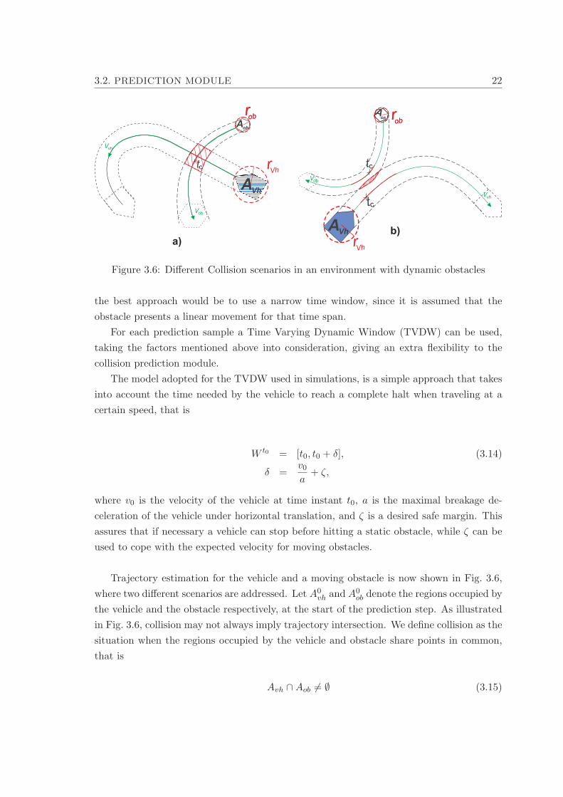
Figure 3.6: Different Collision scenarios in an environment with dynamic obstacles
the best approach would be to use a narrow time window, since it is assumed that the
obstacle presents a linear movement for that time span.
For each prediction sample a Time Varying Dynamic Window (TVDW) can be used,
taking the factors mentioned above into consideration, giving an extra flexibility to the
collision prediction module.
The model adopted for the TVDW used in simulations, is a simple approach that takes
into account the time needed by the vehicle to reach a complete halt when traveling at a
certain speed, that is
W t0 = [t0, t0 + δ], (3.14)
δ =v0a
+ ζ,
where v0 is the velocity of the vehicle at time instant t0, a is the maximal breakage de-
celeration of the vehicle under horizontal translation, and ζ is a desired safe margin. This
assures that if necessary a vehicle can stop before hitting a static obstacle, while ζ can be
used to cope with the expected velocity for moving obstacles.
Trajectory estimation for the vehicle and a moving obstacle is now shown in Fig. 3.6,
where two different scenarios are addressed. Let A0vh and A0
ob denote the regions occupied by
the vehicle and the obstacle respectively, at the start of the prediction step. As illustrated
in Fig. 3.6, collision may not always imply trajectory intersection. We define collision as the
situation when the regions occupied by the vehicle and obstacle share points in common,
that is
Avh ∩Aob 6= ∅ (3.15)

3.2. PREDICTION MODULE 23
where
Avh = Φv(xv(t), yv(t), A0vh), ∀t ∈W t
Aob = Φo(xo(t), yo(t), A0ob), ∀t ∈W t
here Φ denotes the operator that takes as arguments the position x(t), y(t) of the trajectory
at time instant t and a given region A0, and provides the region At at time t. For collision
prediction we are interested in a spacial and temporal correlation analysis of these regions.
Even thought knowing the intersection of the swept areas of Avh and Aob can be useful data
for collision avoidance, given that Φvh and Φob are functions of time, it will only be relevant if
some points in the intersection are time correlated. Furthermore the computational weight
of the algorithm that tests if condition (3.15) is verified for W t can be relevant depending
on the strategy chosen, and should only be used if necessary.
The process of checking the trajectories for intersections is therefore comprised of two
steps:
i) Temporal Correlation
This is the first step to evaluate if a collision actually occurs. Consider the following
simplification of the problem:
• let Cvh and Cob be two tight circles of radius Rvh and Rob respectively, such that
Avh ∈ Cvh and Aob ∈ Cob
• then if Avh ∩Aob 6= ∅ =⇒ Cvh ∩ Cob 6= ∅
To detect if Cvh and Cob share points in common during the time window W t, the
interesting feature to analyze is the euclidean distance from the centers of these two
circles that move along their respective paths, Pv(t) and Po(t). The strategy is to
compute the local minima of this distance in function of time, in the time window
W t, which we will denote by the pairs {t∗i , d∗(t∗i )}. We then define tc = min {t∗i } as
the time instant for the first minimum in which a collision might occur. It is known
that two circles intersect if the distance between their centers is smaller then the sum
of their radius. Therefore there exists a collision if
d(tc) = ‖Pv(tc) − Po(tc)‖ ≤ Rvh +Rob (3.16)
For the case that condition (3.16) is not verified, no more calculations are needed,
and so Collision Prediction module is done for the current time step.

3.2. PREDICTION MODULE 24
ii) Spatial Correlation
After a potential collision has been detected, more data can be extracted in order to
derive a more efficient collision avoidance maneuver. In this step, we are interested
in computing
- The region for which the obstacle will interact with the vehicle swept area Bvh
- The time interval in which that interaction occurs
It is assumed that for the chosen time window, if a overlapping of paths occurs it
will occur in a continuous time span ∆to = [ti, tf ] , where tc ∈ ∆to. This enables the
search for intersections between Avh and Aob to be narrowed to a window expanding
from tc.
Resorting to the same simplification taken to derive tc by considering only tight circles,
one can determine [ti, tf ] and the corresponding [Pv(ti), Pv(tf )](see Fig. 3.7).
AVh
Aob
tc
tiobtfob
SVO
Δtob
BVh
Figure 3.7: Collision scenario in which the obstacle behavior is interpreted has a staticvirtual object (SVO)

3.2. PREDICTION MODULE 25
The size of the estimated intersection period ∆to is a key variable in the decision of
what collision avoidance strategy should be employed, path re-planing or velocity correction.
This decision can be represented by the function:
σ(∆to) =
Path re-Planing for ∆to ≥ ∆ttreshold
Velocity Correction for ∆to < ∆ttreshold
(3.17)
where ∆ttreshold is defined as the maximum time span up to which an obstruction in the
vehicle path is tolerated. In the case of ∆to > ∆ttreshold, a representation of the obstacle
will be passed on to the Collision Avoidance inner map based on the obstacles swept area,
and path re-planing will take place. In this situation the obstacle is labeled as a Static
Virtual Obstacle(SVO), an example of which can be seen in Fig. 3.7.

Chapter 4
Collision Avoidance Module
In this chapter we present two strategies to achieve collision avoidance: path planing based
on potential fields theory and velocity correction. In Potential field based path planing,
harmonic potential functions are used to address the local minima predicament. In section
4.1.1 the panel method and the potential functions used in the creation of the potential
field are introduced, and the deduction of the velocity field used to construct the new path
is explained in section 4.1.1. The concept for velocity correction is presented in section 4.2,
where the main idea is to change the velocity along the nominal trajectory so that collisions
are avoided. A feedback control is developed, and the use of velocity correction as a means
to achieve inter-vehicle coordination explained.
4.1 Obstacle Avoidance using Harmonic Potential Functions
In this section,the panel method is introduced and path planing for multiple vehicles trough
the use of Harmonic Potential Functions is discussed. A complement to the traditional panel
method (Fahimi, 2009) is presented to generate a more effective harmonic potential field
for obstacle avoidance.
4.1.1 The panel method
To understand how collision avoidance can be realized trough the use of potential fields,
the panel method which has been used to solve the potential flow of a fluid around bodies
of arbitrary shape is introduced. In this method the surface of the body is first covered by
a finite number of small areas called panels, each of which is distributed with source or sink
singularities having uniform density. The distributed singularities are used to deflect the
incoming stream so that it will flow around the body. The requirement that the oncoming
flow be tangent to every panel at a particular location gives a set of equations that is used
to compute the singularity densities on every panel. Note that the path of a point mobile
vehicle matches the path of a single fluid particle through the stream.
26

4.1. OBSTACLE AVOIDANCE USING HARMONIC POTENTIAL FUNCTIONS 27
Potential of a Panel
Since the boundary of the obstacles in 2D space will be approximated by line segments
the corresponding potential, the potential of a line segment, also known as a panel in fluid
mechanics, must be defined.
The single panel in Fig. 4.1 is distributed with uniform sources, with strength per unit
length λ. The potential at any point (x, y) induced by the sources contained within the
small element dl of the panel at (0, l) is
dφ =λdl
2πln =
λdl
2πln
√x2 + (y − l)2 (4.1)
The induced potential function by the whole panel is
φ(x, y) =λ
4π
∫ L
−L
ln√x2 + (y − l)2dl. (4.2)
Figure 4.1: Potential of a source line segment(panel)

4.1. OBSTACLE AVOIDANCE USING HARMONIC POTENTIAL FUNCTIONS 28
A representation of the potential field defined for a line segment can be found in Fig.
Fig. 4.1. From the figure one can imagine that placing a particle(or a vehicle) on the surface
described by the potential field will cause the particle to roll away from the source panel.
This concept embodies two of the properties of harmonic function described in Chapter A,
the global maximum occurs on the panel itself (singularity), and there is no local minimum.
The velocity field generated by a line panel can be found by partial differentiation of
the potential field function. Differentiation with respect to x and y gives, respectively, the
expressions for velocity components:
ux(x, y) =∂φ
∂x=
λ
2π
(tan−1 y + L
x− tan−1 y − L
x
), (4.3)
uy(x, y) =∂φ
∂y=
λ
2πlnx2 + (y + L)2
x2 + (y − L)2. (4.4)
The limiting value of normal velocity ux(x, y) in (4.3) is ux(0−, y) = −λ/2 on the left
and ux(0+, y) = λ/2 on the right face of the panel. This shows that the source panel of
strength λ per unit length creates a uniform outward normal velocity of magnitude λ/2 at
the surface. The tangential velocity uy(x, y) on the panel starts from zero at the center of
panel and increases along the panel surface toward both edges, where the normal velocity
is not defined and the tangential velocity becomes infinite. That is, a single panel has a
singular point on each edge.
The normal velocity at the center of a panel is of great interest to us to derive a proper
potential field. In hydrodynamics, ux(0−, y) is set to 0 to satisfy the requirement that the
oncoming flow must be tangent to a panel. However, for our problem of obstacle avoidance,
this requirement must be modified as the normal velocity of a panel Vn must be greater
than or equal to zero. The requirement for obstacle avoidance can thus be represented as
Vn = −u(0−1, y) ≥ 0. (4.5)
As Vn increases so the fluid particle moves further away from the panel. This provides
a tradeoff between economy and safety. As Vi,becomes larger, a point vehicle will generally
have a longer but a safer path further away from obstacles. Apart from the normal velocity
on the left face of a panel recommended greater than zero there is another major difference
between the hydrodynamics and the obstacle avoidance problem. The obstacle avoidance
problem has a goal point that the vehicle must reach. Thus, the potential for the obstacle
avoidance will be composed of a uniform flow, distributed singularities on the panels (ob-
stacle boundaries), and a sink (a goal singularity). In the next section, we consider the use
of multiple panels to represent complex obstacles.

4.1. OBSTACLE AVOIDANCE USING HARMONIC POTENTIAL FUNCTIONS 29
Multiple panels
The typical obstacle is approximated by a set of panels, which are numbered clockwise.
The details of the panel geometry are shown in Fig. 4.2. Each panel has its own center
point with a desired outward normal velocity as an input variable. The boundary points
are the intersections of neighboring panels.
Figure 4.2: Panel geometry
The angle between line obstacle i and the x − axis is denoted by θi , and the angle
between the outward normal unit vector n of line obstacle i and the x− axis is denoted by
βi. Then βi = θi + π/2. Let m be the total number of panels. On each of the m panels,
whose lengths are usually not equal, sources/sinks of uniform density are distribute, and
λ1, λ2 . . . λm represent the source/sink strengths per unit length on these panels. In 2D the
potential field created by a panel j in any point (x, y) in space is given by
φp =λj
4π
∫
j
ln(Rj)dlj (4.6)
where Rj = (x− xj)2 + (y − yj)
2.
The obstacle avoidance problem consists on the ability to move a vehicle to a goal
position while maintaining a safe distance from obstacles. Therefore an attractive potential
is needed at the goal position so that the total artificial potential field has only one global
minimum. For this we refer to the potential functions introduced in Chapter A. A singular

4.1. OBSTACLE AVOIDANCE USING HARMONIC POTENTIAL FUNCTIONS 30
point sink is used at the goal to represent the attractive potential, acting like a drain in a
bathtub. Assuming the goal sink has a strength of λg > 0, then its potential is
φg =λ
2πln(Rg) (4.7)
where Rg =√
(x− xg)2 + (y − yg)2 is the distance between the point (x, y) and the goal
point (xg, yg). A potential of uniform flow, which tends to push the vehicle to the goal
can be added to the total field to derive a more efficient potential. From the notation in
Chapter A it is rewritten as
φu = −U(x cosα+ y sinα) (4.8)
where α is the angle between the x − axis and the direction of the uniform flow. The
obstacles, goal, and uniform flow generate a total potential as follows
φtotal = φg + φu + φob
= −U(xcosα+ ysinα) +λ
2πln(Rg)
+m∑
j=1
λ
4π
∫
j
ln(Rj)dlj (4.9)
wherem is the number of panels. Setting the strength of the uniform flow U and the strength
of the goal sink λg, the objective is then to derive the strengths of the m line obstacles.
We need at least m independent equations to solve this problem. These m equations are
derived from the given outward normal velocities on the m panels. Let Vi > 0 denote the
desired outward normal velocity at the center point (xic, yic) of panel i. Note that this
outward normal velocity is satisfied only at the center point of each panel. The resulting
m equations are
∂
∂niφ(xic, yic) = Vi, i = 1.2.....m (4.10)
These provide m linearly independent equations with variables of λ1, λ2 . . . λm. Recall-
ing (4.9), the potential at the center point (xic, yic) is
φ(xic, yic) = −U(xic cosα+ yic sinα) +λ
2πln(Rig) +
m∑
j=1
λ
4π
∫
j
ln(Rj)dlj (4.11)
where Rig is the distance between the goal and the center point of panel i, (xic, yic),
and Rij is the distance between (xic, yic) and a point on panel j as shown in Fig. 4.2. The

4.1. OBSTACLE AVOIDANCE USING HARMONIC POTENTIAL FUNCTIONS 31
substitution of (4.11) into (4.9), and recalling that the contribution to the normal velocity
on panel i by itself is λ/2 (as shown in the previous subsection), yields
λi
2+
m∑
j 6=1
λ
2πIij = Vi + U
∂
∂ni(xic cosα+ yic sinα)
−λg
2π
∂
∂niln(Rig), i = 1, 2 . . . ,m
(4.12)
where
Iij =
∫
j
∂
∂nilnRijdlj . (4.13)
Applying the geometrical relations
{xj = xj0 + lj cos θj
yj = yj0 + lj sin θj
Iij can be integrated to obtain
Iij =1
2C ln
[1 +
L2j + 2ALj
B
]− cos(θi − θj)
[tan−1 Lj +A
E− tan−1 A
E
]. for E 6= 0 (4.14)
= C
[ln
∣∣∣∣Lj +A
A
∣∣∣∣ −Lj
Lj +A
]
+D
[1
A− 1
Lj +A
], for E = 0 (4.15)
where
A = −(xic − xj0) cos θj − (yic − yj0) sin θj
B = (xic − xj0)2 + (yic − yj0)
2
C = sin(θi − θj)
D = −(xic − xj0) sin θi + (yic − yj0) cos θi
E = (xic − xj0) sin θj − (yic − yj0) cos θj

4.1. OBSTACLE AVOIDANCE USING HARMONIC POTENTIAL FUNCTIONS 32
The parameter E becomes zero when the center point of line obstacle i is on the exten-
sion of line obstacle j. The other terms of (4.12) result in
U(xic cosα+ yic sinα) = U sin(α− θi), (4.16)
U∂
∂nilnRgi =
λg
4π
∂
∂niln
((xic − xg)
2 + (yic − yg)2)
=λg
2π
−(xic − xg) sin θi + (yic − yg) cos θi
(xic − xg)2 + (yic − yg)2. (4.17)
We can now arrange equation (4.12) into
PΛ = q (4.18)
where P is an m×m of the form
Pij =
12 , for i = j
Iij
2πfor i 6= j
(4.19)
and q is a m× 1 vector, where each element is given by
qi = −Vi + U∂
∂ni(xiccosα+ yicsinα) +
m∑
j=1
λ
4π
∫
j
ln(Rj)dlj (4.20)
Solving (4.18) we obtain the panel strengths vector Λ = [λ1, λ2, . . . , λm]. Now that
the panel strengths have been defined, the trajectory for the mobile vehicle can be derived
following the negative gradient of the total potential field, taken from (4.9)
ux(x, y) =∂φtotal
∂x= U cosα− λg
2π
x− xg
(x− xg)2 + (y − yg)2− 1
2ln(1 +
L2j + 2LjA
B) cos θj
+(arctanLj +A
E− arctan
A
Esin θj), (4.21)
uy(x, y) =∂φtotal
∂y= U sinα− λg
2π
y − yg
(x− xg)2 + (y − yg)2− 1
2ln(1 +
L2j + 2LjA
B) sin θj
+(arctanLj +A
E− arctan
A
Ecos θj). (4.22)

4.1. OBSTACLE AVOIDANCE USING HARMONIC POTENTIAL FUNCTIONS 33
4.1.2 Uniform Flow
The uniform flow is added to derive a more effective potential field from the starting position
of the vehicle to the a final goal position. It will impel the vehicle towards the goal,
balancing the repulsive potential of obstacles when the vehicle is to far from the goal sink.
The direction of the uniform flow can be determined from
α =yg − ys
xg − xs, (4.23)
where (xs, ys) is the source coordinates of the vehicle. Increasing the strength of U , a
uniform flow, has the same effect on the resulting trajectory as decreasing the strength
of a source panel. Note that the strength of a uniform flow is an input variable, but the
strengths of panels are determined by (4.18), therefore an increase on U will result on an
increase on the panel strengths, satisfying the given normal velocities Vi.
4.1.3 Goal Sink
The goal sink provides the global minimum to the total artificial potential field. In other
words, the potential function of (4.9) has only one global minimum at the location of
this goal sink.For a vehicle to reach the goal, the strength of this goal sink must be large
enough. If not, like illustrated on Fig. 4.3, a vehicle may miss the goal by following the
uniform flow. To avoid the possibility of collision of the vehicle with obstacles and the
possibility of missing the goal, the strength of the goal sink and the source/sink panels of
the obstacle must satisfy the following inequality:
− λg > λob > 0 (4.24)
where we define obstacle strength λ, has
λob =m∑
i=1
λiLi (4.25)
If the obstacle strength λob is positive, one can conclude that there is more sink potential
than source potential in the line obstacles and the net effect of obstacle is attractive. The
vehicle will therefore be pulled into the obstacle, for this reason the set of values defined Vi
cannot be to small. On the other hand, if the velocities Vi are to large, it is possible that
−λg > λo. Then fluid particles created by obstacles may prevent fluid particles of uniform
flow from going into the goal sink. This implies that a vehicle cannot reach the goal and
will move to infinity following the uniform flow, Fig. 4.3. In conclusion inequality (4.24)
sets the bounds of Vi used to derive the strength of the panels. The trade off is that a large
V, implies a safer but less economical (longer trajectory) trajectory away from obstacles.

4.1. OBSTACLE AVOIDANCE USING HARMONIC POTENTIAL FUNCTIONS 34
Figure 4.3: Vehicle trajectory for different sets of Vi
4.1.4 Two Dimensional Robust Potential Field For Online Path Planing
Since the values for Vi that satisfy (4.24) cannot be defined by trial and error, specially in
unknown environments, a method for automatically adjusting the potential field parameters
based on the obstacle sizes is needed. A robust artificial potential field can be generated
for any sizes of obstacles by using the following method.
Recovering inequality (4.12) for the desired normal velocity Vi and the panel strengths
λi, we can rewrite it has
m∑
j=1
Pijλj = −Vi +Wi, (4.26)
where
Wi = U∂
∂ni(xic cosα+ yic sinα) +
m∑
j=1
λ
4π
∫
j
ln(Rj)dlj (4.27)
making J = P−1, where P was defined in (4.19), becomes
λi =m∑
j=1
Jij(−Vj +Wi) (4.28)

4.1. OBSTACLE AVOIDANCE USING HARMONIC POTENTIAL FUNCTIONS 35
substituting (4.28) into (4.25) the formula for the obstacle strength, results in
m∑
i=1
Li
m∑
j=1
JijVj < λg +m∑
i=1
Li
m∑
j=1
JijWj . (4.29)
If it is assumed that the outward normal velocity of a panel is proportional to its length,
that is,
Vj = αLj , (4.30)
then equation (4.29) can be reduced to
α < αmax, (4.31)
and
αmax =λg +
∑mi=1 Li
∑mj=1 JijWj∑m
i=1 Li
∑mj=1 JijLj
. (4.32)
Since all the parameters on the right hand side of (4.32) are known, one can simply
calculate αmax and choose a value for α that satisfies the inequality (4.31). Then, the
outward normal velocities that are guaranteed to satisfy (4.24) can be computed from
(4.30). We call parameter α the safety parameter. The larger α the larger Vi, which in
turn results in a safer but less economical path when avoiding an obstacle. αmax is the
maximum allowable safety parameter. We can then define the safety ratio r ∈ [0, 1], as an
input variable that represents this tradeoff
r =α
αmax(4.33)
4.1.5 Stagnation Points and structural local minima
For every panel in the configuration map, there is at leats one point where the potential
gradient is zero, this is called a stagnation point. A stagnation point(local maxima) is a
point where the velocity of a fluid particle becomes very close to zero, but this is an unstable
saddle point since the gradient of the potential in the vicinity of these points is negative.
This means that in practical applications position sensor noise can by itself disturb the
vehicle form a stagnation point, enabling it to continue its way toward the global minimum
of the potential.
Another issue to be taken into consideration is that in the computation of a desired
path the vehicle is often considered as a point without physical dimensions. With this
assumption, a planned trajectory among obstacles that is valid for a point vehicle may not

4.1. OBSTACLE AVOIDANCE USING HARMONIC POTENTIAL FUNCTIONS 36
be valid for a vehicle with real physical dimensions. This is known as the structural local
minimum. A common way to overcome this, is by extending the size of all the obstacles in
the map by at least half the diameter of the vehicle. This will cause for example, that an
opening between two obstacles the size of the vehicle will appear closed in the new map.
4.1.6 Path Planning for Multiple Mobile Robots
The method discussed in the previous section enabled us to extract two velocity components
ux and uy, that point the vehicle away from an obstacle and towards the goal. This resultant
velocity vector v = (ux, uy) is characterized by size and orientation, where the size is given
by V = (vTv)1
2 and orientation obtained from β = arctan(uy
ux). Starting from an initial
position Pvh(0), following this vector throughout the potential field for a chosen time window
[0, t] will result in an obstacle free path Pvh.
Pvh = P0 +
∫ t
0v(τ)dτ (4.34)
Once the path has been determined, it can be fed to a path-following controller, tuned
to the characteristics of the vehicle.
In the presence of dynamic environments, as the case of a team coordinated mission,
where each vehicle must consider the other vehicles of the group as moving obstacles it
is necessary to update the potential field as the vehicles move, and ensure that for every
recalculation of the potential field condition (4.24) is verified.
Figure 4.4: Situation where the potential field between both vehicles is symmetric
In this regard the overall architecture chosen for the proposed Collision Avoidance
system described in Section 3.2, enables us to skip constant recalculation of the potential
field, and only to do so when triggered by the collision prediction module. Therefore if
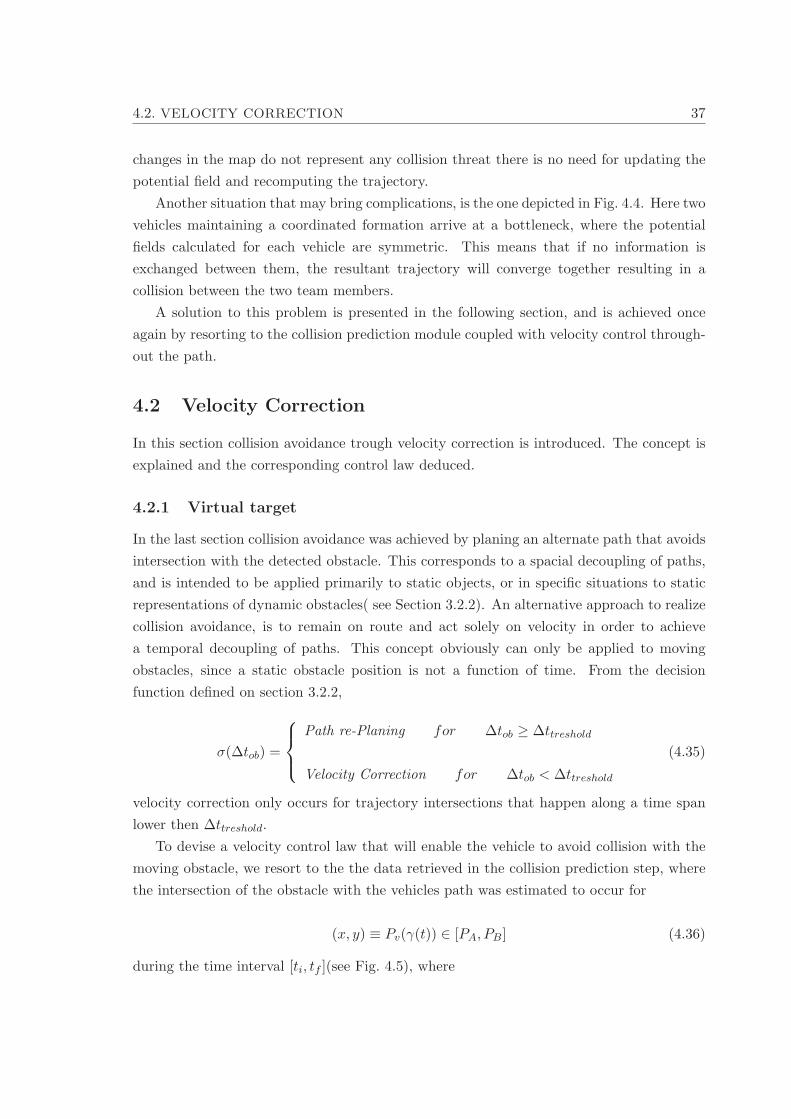
4.2. VELOCITY CORRECTION 37
changes in the map do not represent any collision threat there is no need for updating the
potential field and recomputing the trajectory.
Another situation that may bring complications, is the one depicted in Fig. 4.4. Here two
vehicles maintaining a coordinated formation arrive at a bottleneck, where the potential
fields calculated for each vehicle are symmetric. This means that if no information is
exchanged between them, the resultant trajectory will converge together resulting in a
collision between the two team members.
A solution to this problem is presented in the following section, and is achieved once
again by resorting to the collision prediction module coupled with velocity control through-
out the path.
4.2 Velocity Correction
In this section collision avoidance trough velocity correction is introduced. The concept is
explained and the corresponding control law deduced.
4.2.1 Virtual target
In the last section collision avoidance was achieved by planing an alternate path that avoids
intersection with the detected obstacle. This corresponds to a spacial decoupling of paths,
and is intended to be applied primarily to static objects, or in specific situations to static
representations of dynamic obstacles( see Section 3.2.2). An alternative approach to realize
collision avoidance, is to remain on route and act solely on velocity in order to achieve
a temporal decoupling of paths. This concept obviously can only be applied to moving
obstacles, since a static obstacle position is not a function of time. From the decision
function defined on section 3.2.2,
σ(∆tob) =
Path re-Planing for ∆tob ≥ ∆ttreshold
Velocity Correction for ∆tob < ∆ttreshold
(4.35)
velocity correction only occurs for trajectory intersections that happen along a time span
lower then ∆ttreshold.
To devise a velocity control law that will enable the vehicle to avoid collision with the
moving obstacle, we resort to the the data retrieved in the collision prediction step, where
the intersection of the obstacle with the vehicles path was estimated to occur for
(x, y) ≡ Pv(γ(t)) ∈ [PA, PB] (4.36)
during the time interval [ti, tf ](see Fig. 4.5), where

4.2. VELOCITY CORRECTION 38
t tfi
vd
A
B
P( )
P( )
virtual target
d
{ , t }00
Figure 4.5: Velocity Correction: Virtual target concept
PA = Pv(ti)
PB = Pv(tf )
The collision avoidance behavior can then be formalized as follows.
Problem: Consider the collision region given in (4.36), and let pd(γ) ∈ R2 be a desired
path parameterized by a continuous variable γ(t) ∈ R and vd(γ) ∈ R a desired speed
assignment. Suppose also that pd(γ) is sufficiently smooth and its derivatives with respect
to γ are bounded. Derive a control law such that
Pv(γ(t)) /∈ [PA, PB] ⇔ γ(t) /∈ [γA, γB],∀t ∈ [ti, tf ], (4.37)
which means the vehicle remains outside the collision area for the given time interval [ti, tf ].
It is easy to see that arriving at PB at time ti or at PA at time instant tf , verifies
condition (4.37) and assures that the vehicle avoids collision with the moving obstacle.
To derive the velocity control law for the vehicle, we imagine a virtual target traveling
along the path at a constant velocity Vd, such that at an intended time instant tg, the target
will be located at a goal position γg along the path(Fig. 4.5). The virtual target position
and velocity along the parameterized path are then given by
Vd =γg − γ0
tg − t0= cnst (4.38)

4.2. VELOCITY CORRECTION 39
γd(t) =
∫ t
t0
Vd dt
= Vd(t− t0) + γ0 (4.39)
The objective is now to make the vehicle track this virtual target. Defining the position
displacement between the target and the vehicle
e(t) = γ(t) − γd(t) (4.40)
and the velocity error
e(t) = v(t) − Vd (4.41)
one can easily derive a feedback law for V such that e = −ke, that is the error converges
to zero exponentially fast. The control law for velocity is then given by
v = Vd − k(γ − γd)
=γg − γ0
tg − t0− k(γ − γd) (4.42)
Choosing the goal (γg, tg) → (γA, tf ) or (γg, tg) → (γB, ti), will make the controller drive
the vehicle to decrease or increase velocity respectively, realizing collision avoidance.
Achieving Decentralization trough Right of Way
Now that the velocity control law was derived, we still need to define what will be the
vehicles behavior when encountering an obstacle. Two behaviors can be envisioned:
• The vehicle decreases its velocity and waits for the obstacle to pass (γg, tg → γA, tf )
• The vehicle increases its velocity passing the critical zone [PA, PB] in which collision
is set to occur
Trying to increase velocity comes with added risk, given that the velocity needed to
avoid collision may be beyond the set of reachable velocities of the vehicle, and that for
vehicles with high dynamics increasing the velocity along the path damages the performance
of path following controllers.
The primary drive for the vehicle is then to give right of way to an obstacle, that means
that once an obstacle is detected and is labeled as dynamic the vehicle will take the safest

4.2. VELOCITY CORRECTION 40
approach, which is to set γg, tg → γA, tf and let the obstacle pass, resuming the velocity
profile set for the mission once collision avoidance has been assured.
The only exception to this behavior will occur when the obstacle on collision course
is identified as another team member. In this situation, priority is set to be given to the
vehicle traveling on starboard tack. The task of decoupling the trajectory’s is therefore
carried on by the vehicle traveling on the left, which decreases velocity and enables the
passage of its team member.
This process enables the vehicles in the formation to achieve coordination within the col-
lision avoidance state, and present a solution to the scenario illustrated on Fig. 4.4 without
the need of exchanging information. Decentralized collision avoidance is thus realized.

Chapter 5
Cooperative Motion Control Simu-lator (CMCs)
This chapter presents an overview on the Matlab-based Cooperative Mission Control sim-
ulator developed during the study of multi-vehicle formations. The simulator aims for the
integration in a simulation environment of the key aspects that must be considered in a
Cooperative Motion Control(CMC) architecture discussed in Chapter 2. Its fundamental
underlying designed is introduced, and its main features addressed.The functionality of
the simulator is shown in Chapter 6 trough the presentation of simulation results for the
proposed Collision Avoidance System.
5.1 Main Features
During the development of new algorithms for control, it is critical to test them in simulation
using dynamic models of the robotic vehicles and environment, before their application on
real robots. This is specially important in the case of cooperative vehicle solutions, where
the communication topology and the complexity of the multi-vehicle interaction, can bring
fourth unexpected results for a designed controller. The software simulator could be a good
solution for these problems. A good simulator could provide many different environments
to help the researchers to find out problems in their algorithms in different kinds of mobile
robotic vehicles.
In order to facilitate the design of the controllers and models the simulator is almost
entirely supported through Matlab. Matlab is a widely used programing tool in engi-
neering simulation because of its graphic interface, mimic function-block and abundant
model library. Furthermore in later development Matlab’s automatic code generation func-
tion(RTW) frees the designers from the the tedious and debugging difficulty of manually
writing code.
41
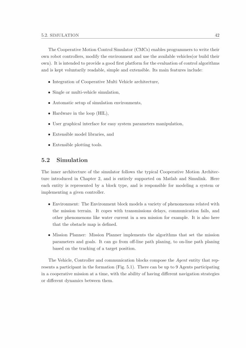
5.2. SIMULATION 42
The Cooperative Motion Control Simulator (CMCs) enables programmers to write their
own robot controllers, modify the environment and use the available vehicles(or build their
own). It is intended to provide a good first platform for the evaluation of control algorithms
and is kept voluntarily readable, simple and extensible. Its main features include:
• Integration of Cooperative Multi Vehicle architecture,
• Single or multi-vehicle simulation,
• Automatic setup of simulation environments,
• Hardware in the loop (HIL),
• User graphical interface for easy system parameters manipulation,
• Extensible model libraries, and
• Extensible plotting tools.
5.2 Simulation
The inner architecture of the simulator follows the typical Cooperative Motion Architec-
ture introduced in Chapter 2, and is entirely supported on Matlab and Simulink. Here
each entity is represented by a block type, and is responsible for modeling a system or
implementing a given controller.
• Environment: The Environment block models a variety of phenomenons related with
the mission terrain. It copes with transmissions delays, communication fails, and
other phenomenons like water current in a sea mission for example. It is also here
that the obstacle map is defined.
• Mission Planner: Mission Planner implements the algorithms that set the mission
parameters and goals. It can go from off-line path planing, to on-line path planing
based on the tracking of a target position.
The Vehicle, Controller and communication blocks compose the Agent entity that rep-
resents a participant in the formation (Fig. 5.1). There can be up to 9 Agents participating
in a cooperative mission at a time, with the ability of having different navigation strategies
or different dynamics between them.
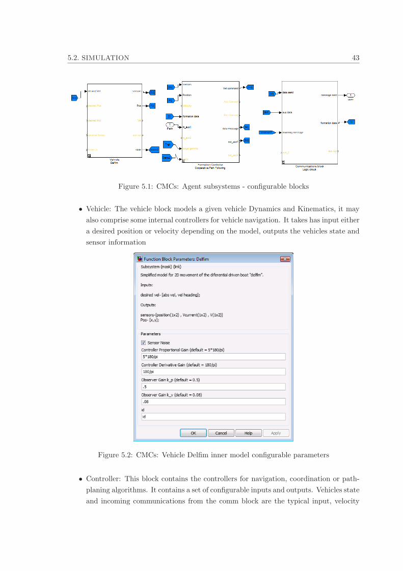
5.2. SIMULATION 43
Figure 5.1: CMCs: Agent subsystems - configurable blocks
• Vehicle: The vehicle block models a given vehicle Dynamics and Kinematics, it may
also comprise some internal controllers for vehicle navigation. It takes has input either
a desired position or velocity depending on the model, outputs the vehicles state and
sensor information
Figure 5.2: CMCs: Vehicle Delfim inner model configurable parameters
• Controller: This block contains the controllers for navigation, coordination or path-
planing algorithms. It contains a set of configurable inputs and outputs. Vehicles state
and incoming communications from the comm block are the typical input, velocity

5.3. GRAPHICAL USER INTERFACE AND PLOTTING TOOLS 44
and position commands are typically the product of the block computations
• Communications: Responsible for the implementation of the communication topology,
the communication block handles the exchange of data between vehicles. It takes
as inputs vehicle data and converts into the message format and vice versa. Here,
various parameters regarding communication protocol can be set, from frequency to
retransmission attempts.
Each one of these blocks is realized in the simulator trough library links. This enables
a user to choose from a list of available models inside the blocks library, and seamlessly set
different simulation environments. This format also enables in the future an easy integration
of more evolved communication and environment blocks for example.
5.3 Graphical User Interface and plotting tools
The simulator introduces a Graphical User Interface (GUI), that allows a high end user
not familiarized with simulink, to easily change between models for the various block types,
and effortlessly access their parameters.
Figure 5.3: Graphical user interface: setting the Controllers for the Delfim Vehicle
As Fig. 5.3 shows, the GUI automatically accesses the corresponding blocks library and
displays the available options. Once an option has been set in the GUI, it is automatically

5.4. VISUALIZATIONS AND PLOTTING 45
Figure 5.4: Graphical user interface: Setting the desired geometrical disposition of vehiclesin the formation
mimicked inside the simulators simulink model. In this manner the Graphical User Interface
frees the user from the tiring task of setting up new connections in simulink for each
modification in the vehicle formation structure.
5.4 Visualizations and Plotting
Figure 5.5: Plotting Tools: Spacial evolution of vehicles and coordination analyses
The access to block parameters (Fig. 5.2) and to plotting tools used for the evaluation
of the controllers can also be obtained thought the GUI. The available plotting tools are set

5.4. VISUALIZATIONS AND PLOTTING 46
to work for a group of known workspace variables. The extension of these tools is possible
to comprise new graphics for the testing of new developed controllers.
Figure 5.6: Plotting Tools: A 2D animation of the defined coordinated mission
At the current state the Cooperative Motion Control Simulator enables for the simula-
tion of teams of up to 9 coordinated marine vehicles. Delays in transmission are handled
inside the environment block, trough a simple model, that relates delays and transmission
losses with the distance between the vehicles. Path-following, Target tracking, and target
following missions and the respective controllers have been successfully tested through the
simulator.

Chapter 6
Simulation Results
This chapter illustrates via computer simulations the performance of the Collision Avoid-
ance System (CAS) proposed in this thesis. The first series of simulations are focused
in the analyses of each individual module. The first set of simulations (Section 6.1) tests
the Collision Prediction module (Tracking and Prediction) for dynamic and static obstacles.
Collision Avoidance schemes are then simulated. Potential field based path planing is tested
for different scenarios in Section 6.2, and Velocity Correction is applied to an Autonomous
Surface Craft(USC) in Section 6.3. Finally in Section 6.4, the proposed CMC simulator
described in Chapter 2 is used to test the overall behavior of the CAS in a Cooperative
multi-vehicle mission.
6.1 Target tracking and Collision Prediction
Collision Prediction is now tested for two scenarios, a moving obstacle and a static one. The
obstacle movement is described by the model defined in Section 3.2.1, where both v and w
are bounded. The target position is fed directly to the IMM-KF at every time step with a
zero mean and 0, 1 variance Gaussian error. The parameters for the IMM-KF can be found
in Table 6.1. For trajectory intersection calculations, the Timewindow for prediction is set
to 30 seconds, and treshold for obstruction(∆ttreshold) is set to 15 seconds. In simulations
both obstacle and vehicle areas are assumed to be contained in a circle of 2.5 meter radius,
adding a 1 meter safe distance. In this case collision is verified when the obstacles and
vehicles centers of mass are separated by less than 6 meters.
In this first simulation (see Fig. 6.1) an Autonomous Surface Craft(ASC) following a
predefined path runs into a collision course with a unknown target traveling with a linear
speed of 1.5m/s and an angular speed of 0.03rad/s. Target tracking starts once the obstacle
is at approximately 100 meters of the vehicle, and trajectory intersection is only computed
once the obstacle is in 20 meters range of the vehicle for performance purpouses. The
time span between the start of target tracking and the first collision prediction calculations
should be enough so v and w are fairly well estimated. For the trajectory intersection
prediction depicted in Fig. 6.1, v = 1.5723 and w = 0.0312 were the estimations for the
current time step. As Fig. 6.1 shows, the expected intersection occurs for a time span
47

6.1. TARGET TRACKING AND COLLISION PREDICTION 48
0 20 40 60 80 100-0.2
0
0.2
0.4
0.6
0.8
1
1.2
1.4
1.6
1.8
Time (t)
v (
m/s
)
True
Estimated
0 20 40 60 80 100-0.01
0
0.01
0.02
0.03
0.04
0.05
Time (t)
w (
rad/s
)
True
Estimated
0 20 40 60 80 1000
50
100
150
200
250
Time (t)
Ψ(º
degre
es)
True
Estimated
200 220 240 260 280 300 320140
160
180
200
220
240
260
x
yTarget Position
ti →
← tf
ti →
← tf
ti →
← tf
Target
Estimated
190 195 200 205 210 215 220 225 230 235
170
180
190
200
210
220
230
240
x(m)
y(m
)
Trajectory prediction and collision prediction
ti →
← tfvehicle planned trajectory
Predicted Time Window
obstacle position estimation
Target linear Velocity Target angular Velocity
Target heading
Figure 6.1: IMM-KF estimation of a dynamic obstacle state, and trajectory prediction fora 30 second time window. For this case the predicted intersection of trajectories results inthe creation of a Virtual obstacle, to be used in the collision avoidance stage
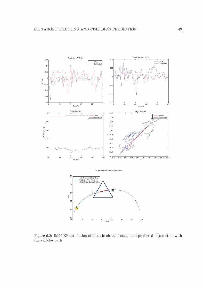
6.1. TARGET TRACKING AND COLLISION PREDICTION 49
0 20 40 60 80 100-0.015
-0.01
-0.005
0
0.005
0.01
Time (t)w
(ra
d/s
)
True
Estimated
0 20 40 60 80 1000
50
100
150
200
250
Time (t)
Ψ(º
de
gre
es)
True
Estimated
0 20 40 60 80 100-0.2
-0.15
-0.1
-0.05
0
0.05
0.1
0.15
Time (t)
v (
m/s
)
True
Estimated
20.5 20.6 20.7 20.8 20.9 21 21.1 21.2 21.3 21.430.4
30.5
30.6
30.7
30.8
30.9
31
31.1
31.2
31.3
31.4Target Position
x
y
Target
Estimated
-10 0 10 20 30 40 50 6015
20
25
30
35
40
x(m)
y(m
)
ti →← tf
vehicle planned trajectory
Predicted Time Window
obstacle position estimation
Target linear Velocity Target angular Velocity
Target heading
Trajectory and collision prediction
Figure 6.2: IMM-KF estimation of a static obstacle state, and predicted intersection withthe vehicles path

6.2. HARMONIC POTENTIAL FIELD BASED PATH PLANING 50
larger than ∆ttreshold(ti = 115.2s,tf = 130.4s). Thus the intersection is represented as a
virtual object derived from the obstacles path. This occurs because the vehicle didn’t take
any collision avoidance measures in the previous time steps. For dynamic obstacles the
initial trajectory intersection estimations should always be lower than ∆ttreshold triggering
Velocity correction.
The second simulation (see Fig. 6.2), describes a scenario where a static obstacle is
detected. In this case, as it was proposed in Section 3.2.2, the output of the prediction
module is again a Virtual obstacle, composed of panels that enclose the obstacles occupied
area on the map. The corresponding collision avoidance strategy to follow would therefore
be Path re-planing. Note that the lack of movement of the target, brings uncertainty to
the IMM-KF estimation for the target’s heading, which explains the difference in the real
and the estimated values for ψ.
Interactive Multi Model Kalman Filter
Number of Filters 7
w -0.05 -0.03 -0.01 0 0.01 0.03 0.05
minimum probability 2 × 10⁻³ Initial Probability 17
Table 6.1: IMM-KF parameters set for simulations 6.1
6.2 Harmonic potential field based path planing
This set of simulations was intended to test the proposed Path Planing algorithm under
different scenarios. In the scenario illustrated by Fig. 6.3 (a), the algorithm was run for
a team of three ASC placed inside a dock. Each ASC derives its path from a different
potential field, unique to the given vehicle. For this simulation the values for the normal
potential forces(Vi) in the center of each panel were set manually to illustrate the situation
described in Section 4.1.1, where for high Vi the resultant path might miss the goal. For
the next two simulations, the Robust Potential Field algorithm was applied. The bounds
for the values of Vi that guarantee convergence of the path to the goal position are derived
in the robust approach(equation (4.32)), as described in Section 4.1.4. Here a safety ratio
0 < r < 1 , is used, that establishes the tradeoff between wider but safer trajectories and
shorter but more economical ones. In Fig. 6.3, the paths generated for different values of
r are shown, for the maximum safety ratio r = 1 the path selected avoids the bottleneck
altogether. Note that to avoid structural minima the area of the vehicle is added to all the
obstacles in the map, this way every trajectory derived from the algorithm relates to an
unobstructed path in the real environment. The parameters set for the Robust Potential
Field simulations and the resultant values for Vi and λi can be found in Table 6.2.

6.2. HARMONIC POTENTIAL FIELD BASED PATH PLANING 51
0 10 20 30 40 50 60 70
-30
-20
-10
0
10
20
30
Path Planing
x (m)
y (
m)
safe ratio = 0.2
safe ratio = 0.3
safe ratio = 0.7
safe ratio = 1
-60 -40 -20 0 20 40 60 80 100 120-60
-40
-20
0
20
40
60
80
100
120
140
x
y
Path Planing - vehicle team
Vehicle 1 → Vi = 10
Vehicle 2 → Vi = 15
Vehicle 3 → Vi = 30
Vehicle 3 → Vi = 18
(a)
(b)
Vehicle 1
Vehicle 2
Vehicle 3
Figure 6.3: (a) Path planing for a group of ASC, where different values of Vi are set foreach vehicle Potential field (b)Robust Potential Field path planing for different safety ratiovalues (b)

6.2. HARMONIC POTENTIAL FIELD BASED PATH PLANING 52
-20 -15 -10 -5 0 5 10 15 20-20
-15
-10
-5
0
5
10
15
x (m)
y (
m)
Total Arteficial Potential Field
potential field gradient
Figure 6.4: Gradient of the total potential field created by the obstacles, uniform flow andgoal

6.3. VELOCITY CORRECTION 53
Simulation 6.2(b) 6.2(c)
λg = 30 , U = 1 λg = 70 , U = 1.85
r = 0.2 r = 0.3 r = 0.7 r = 1 r = 0.2
panel i Vi λi Vi λi Vi λi Vi λi Vi λi
1 0.1211 -0.7804 0.3634 -0.7228 0.848 -0.6076 1.2115 -0.5212 0.5547 -6.72262 0.1211 -9.783 0.3634 -10.1031 0.848 -10.7433 1.2115 -11.2234 1.0572 -6.51423 0.1211 -12.3228 0.3634 -12.5959 0.848 -13.1421 1.2115 -13.5517 1.0572 -4.66624 0.1211 -13.3712 0.3634 -13.6347 0.848 -14.1616 1.2115 -14.5568 0.5547 -5.7345 0.1211 -13.1361 0.3634 -13.3967 0.848 -13.918 1.2115 -14.309 0.5547 -2.4086 0.1211 -11.2735 0.3634 -11.4945 0.848 -11.9365 1.2115 -12.2681 0.5734 16.96377 0.1211 -0.4353 0.3634 -0.806 0.848 -1.5473 1.2115 -2.1033 0.5734 17.68868 0.1211 11.2839 0.3634 11.0628 0.848 10.6208 1.2115 10.2893 0.5547 -6.66579 0.1211 13.0179 0.3634 12.7573 0.848 12.236 1.2115 11.845 0.3786 -5.659810 0.1211 13.228 0.3634 12.9645 0.848 12.4376 1.2115 12.0424 0.8131 -9.540511 0.1211 12.1623 0.3634 11.8892 0.848 11.343 1.2115 10.9333 0.8131 -9.346212 0.1211 9.8308 0.3634 9.5107 0.848 8.8705 1.2115 8.3904 0.3786 -5.632313 0.1211 0.4408 0.3634 0.0702 0.848 -0.6711 1.2115 -1.2271 0.3786 -0.149114 0.1211 -10.5613 0.3634 -10.7824 0.848 -11.2244 1.2115 -11.5559 0.5572 15.37815 0.1211 -11.8159 0.3634 -12.0765 0.848 -12.5978 1.2115 -12.9888 0.5572 15.099516 0.1211 -11.8112 0.3634 -12.0747 0.848 -12.6017 1.2115 -12.9969 0.3786 -0.300717 0.1211 -10.78 0.3634 -11.0531 0.848 -11.5993 1.2115 -12.0089 0.5547 4.033418 0.1211 -8.5137 0.3634 -8.8338 0.848 -9.474 1.2115 -9.9541 1.0572 5.87819 0.1211 -0.8048 0.3634 -0.7472 0.848 -0.632 1.2115 -0.5455 1.0572 -17.857620 0.1211 8.5033 0.3634 8.1832 0.848 7.5431 1.2115 7.0629 0.5547 -10.878621 0.1211 10.5324 0.3634 10.2593 0.848 9.7131 1.2115 9.3034 0.5547 -6.955322 0.1211 11.5598 0.3634 11.2963 0.848 10.7694 1.2115 10.3741 0.5734 10.961623 0.1211 11.567 0.3634 11.3063 0.848 10.785 1.2115 10.3941 0.5734 14.036424 0.1211 10.1705 0.3634 9.9494 0.848 9.5074 1.2115 9.1759 0.5547 4.478625 0.5547 -11.885726 1.0572 -20.473427 1.0572 10.209228 0.5547 4.148229 0.5547 5.371830 0.5734 13.898831 0.5734 10.499632 0.5547 -7.7498
Table 6.2: Path planing simulations (b) and (c), and the resultant Vi and λi values
6.3 Velocity Correction
The control law derived in (4.42), for the speed at which the vehicle should follow a path
in order to avoid an imminent collision, is to be used as a command input in a path-
following controller. For these simulations the ASC path following controllers introduced
in (Maurya P., 2008) were implemented. The simulations depicted in Fig. 6.5 and Fig. 6.6
report to the same collision detection situation. In this case the output of the prediction
module is:
PA = (370, 100.6) ⇒ λA = 340.3
PB = (374.2, 114.46) ⇒ λB = 389
ti = 167s
tf = 198s

6.3. VELOCITY CORRECTION 54
150 200 250 300 350 400
0
50
100
150
200
250
x [m]
← PAPB →
← PAPB →
← PAPB →
150 160 170 180 190
-3.5
-3
-2.5
-2
-1.5
-1
-0.5
0
0.5
Position error
Time (s)
err
or
(γ)
150 160 170 180 190
-3
-2.5
-2
-1.5
-1
-0.5
0
0.5
Velocity Progression
Time (s)
Lin
ea
r V
elo
city (
m/s
)
Virtual target
Vehicle
150 160 170 180 190300
305
310
315
320
325
330
335
340
345
Spacial Progression
Time (s)
dis
tance (
γ)
Virtual target
Vehicle
Figure 6.5: Velocity Control problem, where the Vehicle is required to follow a virtualtarget set to reach point PA at time instant tf , Ts = 1 and Kv=2.
In the first simulation the goal is to reach point PA at the instant tf , decreasing velocity
to avoid collision, for this and like described in Section 4.2 a virtual target moving at a
constant velocity is followed. Triggering the controller for time the instant of t = 140s, con-
vergence to the targets position is obtained smoothly and rapidly and the vehicle succeeds
in avoiding the collision region for the time interval [ti, tf ]. For the second simulation, the
goal was set in reaching PB at time instant ti, increasing velocity. For this situation and
as expected the correction velocity goes outside the set of reachable velocities for the ASC,
the velocity command becomes saturated and the position error increases, which implies
that the vehicle is unable to avoid collision. Furthermore as depicted in Fig. 6.6, the Path-
following controller performance deteriorates with a high velocity profile, reinforcing the
strategy of preferably decreasing velocity when facing a moving obstacle. Note that for the
second simulation the trigger time for the controller was set at t = 130s to stress out the
flaws of the velocity increase strategy.

6.3. VELOCITY CORRECTION 55
135 140 145 150 155 160 165 170
2
4
6
8
10
12
14
16
18
Poicion error
Time (s)
err
or
(γ)
135 140 145 150 155 160 165 170
300
320
340
360
380
400
Spacial Progression
Time (s)
dis
tan
ce
(γ)
Virtual target
Vehicle
200 250 300 350 400
50
100
150
200
x [m]
y [m
]
← PA→ PB
← PA→ PB
← PA→ PB
130 135 140 145 150 155 160 165 170
5
10
15
20
Velocity Progression
Time (s)
Lin
ea
r V
elo
city (
m/s
)
Virtual target
Vehicle
Planed Path
Vehicle
Figure 6.6: Velocity Control problem, where the Vehicle is required to follow a virtualtarget set to reach point PB at time instant ti, Ts = 1 and Kv=2

6.4. COLLISION AVOIDANCE IN A COOPERATIVE MISSION SCENARIO 56
6.4 Collision Avoidance in a Cooperative Mission scenario
These last simulations are intended to demonstrate the behavior of the proposed colli-
sion avoidance system, in a cooperative multi-vehicle scenario, namely when the team
of vehicles faces a bottleneck situation. Since a Cooperative Motion Control architec-
ture brings together many different elements, for the following tests the simulator pro-
posed in Chapter 5 is used. Here three ASC’s travel in a line formation (see Fig. 6.7),
−100 0 100 200 300 400
−100
0
100
200
300
400
y [m]
x [m
]
0.01 m/s
t =299
Figure 6.7: A team of three autonomous surface crafts performs, numbered left to right, acooperative path-following mission
while performing a path-following mission. The vehicles maintain the formation by ex-
changing information regarding their respective positions on the parametrized path trough
the communications module. A coordination controller then uses this data to derive a
correction velocity so that the vehicle remains in formation with the rest of the team.
Collision Avoidance is triggered when the vehicles detected either static or dynamic ob-
stacles in their path, where it is assumed that once an obstacle is detected its radius is a
known variable. Three variations to the scenario depicted in Fig. 6.7 were used to test the
proposed collision avoidance system.
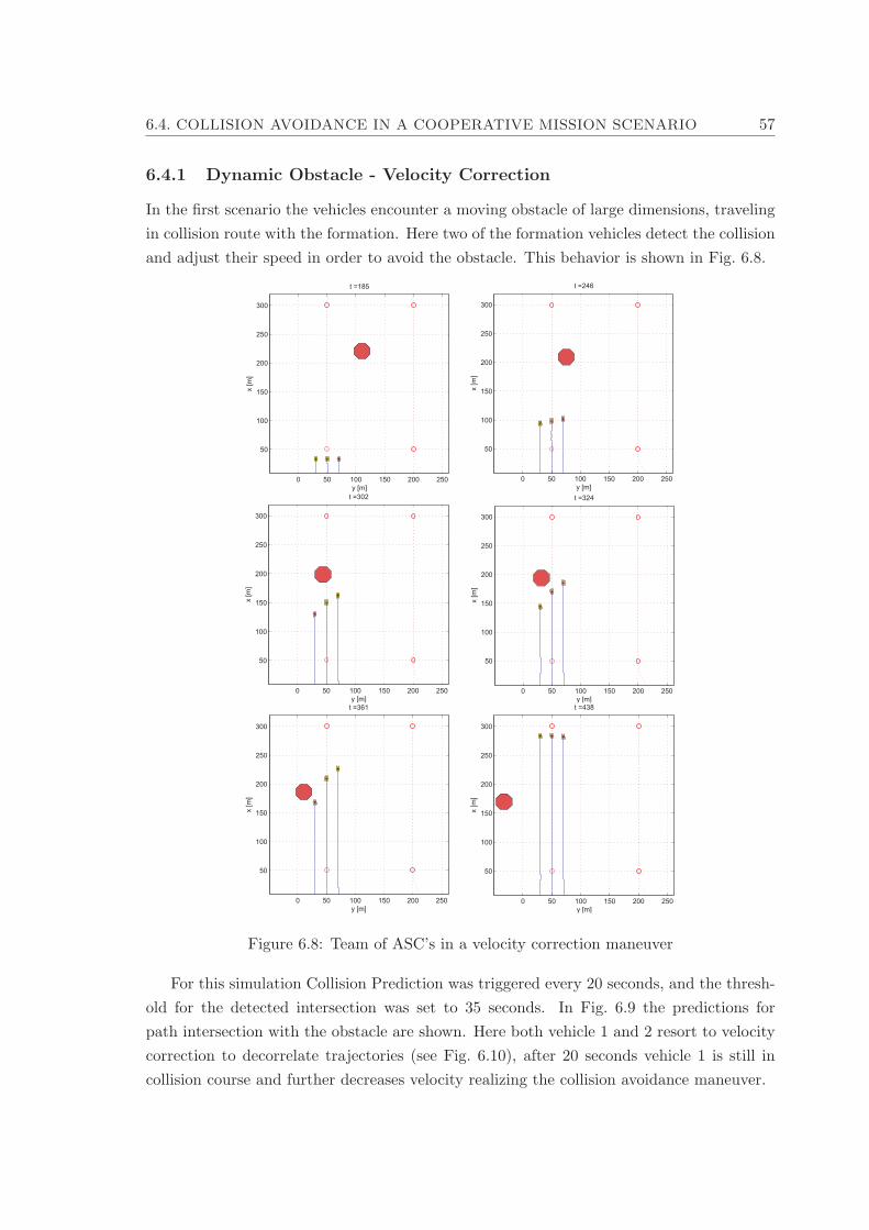
6.4. COLLISION AVOIDANCE IN A COOPERATIVE MISSION SCENARIO 57
6.4.1 Dynamic Obstacle - Velocity Correction
In the first scenario the vehicles encounter a moving obstacle of large dimensions, traveling
in collision route with the formation. Here two of the formation vehicles detect the collision
and adjust their speed in order to avoid the obstacle. This behavior is shown in Fig. 6.8.
0 50 100 150 200 250
50
100
150
200
250
300
y [m]
x [
m]
t =185
0 50 100 150 200 250
50
100
150
200
250
300
y [m]
x [
m]
t =246
0 50 100 150 200 250
50
100
150
200
250
300
y [m]
x [
m]
t =302
0 50 100 150 200 250
50
100
150
200
250
300
y [m]
x [
m]
t =324
0 50 100 150 200 250
50
100
150
200
250
300
y [m]
x [
m]
t =361
0 50 100 150 200 250
50
100
150
200
250
300
x [
m]
t =438
Figure 6.8: Team of ASC’s in a velocity correction maneuver
For this simulation Collision Prediction was triggered every 20 seconds, and the thresh-
old for the detected intersection was set to 35 seconds. In Fig. 6.9 the predictions for
path intersection with the obstacle are shown. Here both vehicle 1 and 2 resort to velocity
correction to decorrelate trajectories (see Fig. 6.10), after 20 seconds vehicle 1 is still in
collision course and further decreases velocity realizing the collision avoidance maneuver.

6.4. COLLISION AVOIDANCE IN A COOPERATIVE MISSION SCENARIO 58
20 40 60 80 100 120
100
150
200
250
t=220
ti →
← tf
20 40 60 80 100
100
150
200
250
t=240
ti →
← tf
20 40 60 80 100
100
150
200
250
t=220
ti →← tf
Vehicle 1 Vehicle 2
Figure 6.9: Vehicle 1 and Vehicle 2 Prediction module results for interaction with theincoming obstacle
240 260 280 300 320
30
40
50
60
70
80
90
100
110
120
Vehicle2 gamma progress
Time (s)
ga
mm
a (
m)
Virtual Target
Vehicle
240 260 280 300 320 340
0
0.1
0.2
0.3
0.4
0.5
0.6
0.7
0.8
0.9
1
Vehicle1 Velocity comand
V (
m/s
)
Virtual Target Speed
Velocity Command
Vehicle Speed
240 260 280 300 3200.3
0.4
0.5
0.6
0.7
0.8
0.9
1
Vehicle2 Velocity comand
V (
m/s
)
Virtual Target Speed
Velocity Command
Vehicle Speed
240 260 280 300 320 340 360
30
40
50
60
70
80
90
100
110
Vehicle1 gamma progress
ga
mm
a (
m)
Virtual Target
Vehicle
Figure 6.10: Velocity Correction undertaken by Vehicle 1 and 2 to avoid the incomingobstacle

6.4. COLLISION AVOIDANCE IN A COOPERATIVE MISSION SCENARIO 59
6.4.2 Dynamic Obstacle - Static Virtual Obstacle solution
The second scenario proposed addresses the situation where velocity correction by itself
does not assure collision avoidance with a dynamic obstacle. In this case, the obstacle
travels at a constant speed in direct collision course with Vehicle 2, both objects travel
in almost exact opposite directions. The performance of the formation when facing this
scenario is shown in Fig. 6.12.
45 50 55 60
100
150
200
t=220
ti → ← tf
40 50 6050
100
150
200
250t=240
ti →← tf
40 50 60100
120
140
160
180
200
220
240t=260
ti →← tf
40 50 60120
140
160
180
200
220t=280
ti →
← tf
100 200 300 400 500 600 700 8000
5
10
15
20
25
30
35
40Vehicle2 detected intersections/Time period for intersection (s)
Detection time
∆t for
inte
rsect
ion
Figure 6.11: Vehicle 2 Prediction module results for interaction with the incoming obstacle,and corresponding time span for the expected trajectory interaction

6.4. COLLISION AVOIDANCE IN A COOPERATIVE MISSION SCENARIO 60
-100 -50 0 50 100 150 200
50
100
150
200
250
300
350
y [m]
x [m
]t =204
-100 -50 0 50 100 150 200
50
100
150
200
250
300
350
y [m]
x [m
]
t =256
-100 -50 0 50 100 150 200
50
100
150
200
250
300
350
y [m]
x [m
]
t =292
-100 -50 0 50 100 150 200
50
100
150
200
250
300
350
y [m]
x [m
]t =325
-100 -50 0 50 100 150 200
50
100
150
200
250
300
350
y [m]
x [m
]
t =361
-100 -50 0 50 100 150 200
50
100
150
200
250
300
350
y [m]
x [m
]
t =481
Figure 6.12: Vehicle 2 identifying path intersection as a Static Virtual Object in order toavoid collision

6.4. COLLISION AVOIDANCE IN A COOPERATIVE MISSION SCENARIO 61
Figure 6.13: Path re-planning taking a Static Virtual Obstacle representation (blue) of theobstacle trajectory
To better understand the behavior depicted in Fig. 6.12 the Prediction module results
for this simulation are shown in Fig. 6.11. In this case Vehicle 2 detects three consecutive
collision situations, and performs velocity correction at the end of each prediction step. On
the fourth prediction the intersection occurs for a time span larger than the defined thresh-
old (35 seconds), and therefore path re-planning is triggered based on a virtual obstacle
interpretation of the obstacles trajectory(see Fig. 6.13).
6.4.3 Bottleneck scenario
In Fig. 6.14 the last set of simulations were run for a bottleneck situation, where the vehicles
were required to keep a safe distance of 15 meters from any obstacle trajectory.

6.4. COLLISION AVOIDANCE IN A COOPERATIVE MISSION SCENARIO 62
150 200 250
140
160
180
200
220
240
260
280
y [m]x [
m]
t =749
150 200 250
140
160
180
200
220
240
260
280
y [m]
x [
m]
t =721
150 200 250
140
160
180
200
220
240
260
280
x [
m]
t =773
140 160 180 200 220 240 260
140
160
180
200
220
240
y [m]
x [
m]
t =810
140 160 180 200 220 240 260
140
160
180
200
220
240
y [m]
x[m
]
t =836
140 160 180 200 220 240 260
140
160
180
200
220
240
y [m]
x [
m]
t =864
vehicle 2
vehicle 3 vehicle 1
Figure 6.14: Team of ASC’s avoiding unknown obstacle trough path re-planing and velocitycorrection

6.4. COLLISION AVOIDANCE IN A COOPERATIVE MISSION SCENARIO 63
The scenario shown in Fig. 6.14 is a representation of the situation first addressed in
Section 4.1.6, where the vehicles in the team are drowned into a bottleneck in order to avoid
collision with obstacles. Vehicle 1 and 3 are the first vehicles to detect a possible collision,
and given the fact that the obstacle is static, the collision avoidance strategy to follow
is path re-planing. In Fig. 6.15, the output of the path-planing subsystem is shown for
vehicle 1 and 3. Each vehicle has its own inner representation of the world map, where the
obstacles are represented by panels and are facing the vehicle in order to derive smoother
paths.
140 160 180 200 220 240 260150
160
170
180
190
200
210
220
230
240
250
x (m)
y (
m)
Path Planing - Vehicle 1 potential field
140 160 180 200 220 240 260150
160
170
180
190
200
210
220
230
240
250
x
y
Path Planing - Vehicle 3 potential field
Figure 6.15: Resultant inner map representation of the scenario to be used in potential fieldpath planing
The resultant paths drive vehicle 1 and 3 into a bottleneck, at which point collision
prediction detects possible trajectory intersections and triggers velocity correction. Since
all intersections detected are amongst team members, priority is given to the vehicle trav-
eling on starboard tack as proposed in Section 4.2. The results for the velocity correction
subsystem are shown in Fig. 6.16. Here only vehicle 1 and 2 perform the trajectory decou-
pling. In both cases velocity correction is first trigered at t = 720, and triggered a second
time for vehicle 1 at t = 725 in response to vehicle 2 change in velocity.

6.5. SUMMARY 64
720 740 760 780 800 820
500
510
520
530
540
550
Vehicle1 gamma progress
Time (s)
ga
mm
a (
m)
Virtual Target
Vehicle
720 730 740 750 760 770 780 790 800
500
510
520
530
540
550
560
Vehicle2 gamma progress
Time (s)
ga
mm
a (
m)
Virtual Target
Vehicle
720 740 760 780 800 820
-1.4
-1.2
-1
-0.8
-0.6
-0.4
-0.2
0
0.2
Vehicle1 Position error
Time (s)
gam
ma (
m)
720 730 740 750 760 770 780 790 800-0.8
-0.6
-0.4
-0.2
0
0.2
0.4
Vehicle2 Position error
Time (s)
gam
ma (
m)
720 740 760 780 800 820
-0.4
-0.2
0
0.2
0.4
0.6
Vehicle1 Velocity comand
Time (s)
V (
m/s
)
Virtual Target Speed
Velocity Command
Vehicle Speed
720 730 740 750 760 770 780 790 800
0.3
0.4
0.5
0.6
0.7
0.8
0.9
1
1.1
Vehicle2 Velocity comand
Time (s)
V (
m/s
)
Virtual Target Speed
Velocity Command
Vehicle Speed
Figure 6.16: Velocity correction command issued to achieve inter vehicle coordination dur-ing the collision avoidance maneuver
6.5 Summary
The simulations illustrated in this chapter show that the Collision Avoidance strategies
proposed in this thesis exhibit a good performance in a wide range of scenarios. The
results confirm that a prediction step can result in smother and more economical collision
avoidance maneuvers. Furthermore, it is shown how collision avoidance can be introduced
in a cooperative multi-vehicle architecture in a seamless and effective manner.

Chapter 7
Conclusions and Further Research
7.1 Summary
This thesis addressed the problem of motion control for multiple autonomous robotic vehi-
cles, taking explicitly into account the collision avoidance problem in dynamic environments.
To integrate collision avoidance in a typical cooperative motion control(CMC) architecture,
an hierarchical structure was devised. This approach allows for a team of autonomous ve-
hicles to have the ability to stray away from mission parameters to prevent collisions. The
problem was decoupled into a collision prediction problem that consists on interpreting an
obstacle movement by estimating its trajectory for a given time window, and a collision
avoidance maneuver derived trough a temporal or spacial deconfliction of the vehicle and
obstacle trajectories.
In Chapter 3, the fundamental underlying design for the collision avoidance system and
its integration into a CMC architecture were proposed. The solution consists in decouple
the vehicle behavior into two modes: a mission mode and a collision avoidance mode.
A vehicle performing a coordinated mission commutes to a collision avoidance behavior
when triggered by a Collision Prediction module. Collision Prediction is achieved first by
estimating the obstacles state trough the use of an Interactive Multi Model Kalman Filter,
and then by deriving its probable trajectory and checking it for interactions with the vehicle
pre-defined path.
In Chapter 4 two collision avoidance strategies were proposed to cope with dynamic
environments: a path re-planing algorithm and a velocity correction controller. The path
planing algorithm proposed based on Harmonic Potential Fields, was used to automatically
generate paths that realize collision avoidance and ensure convergence to a goal position.
The velocity correction controller, consists on changing the velocity along the pre-defined
path so that collisions are avoided.
The performance of each individual module was assessed through simulations, and the
behavior of the overall architecture bringing together prediction and collision avoidance
into a CMC mission was tested using the proposed Cooperative Motion Control Simula-
tor(Chapter 5). The system exhibits good behavior in terms of stability and convergence,
65

7.2. FUTURE DIRECTIONS 66
and is robust to a wide number of scenarios.
7.2 Future Directions
In the work presented thought out this thesis, several different problems were addressed
covering a vast number of fields. The results obtained are only preliminary, allowing to
point out areas that need future research.
Target tracking
In the process of tracking and classifying an unknown obstacle, GPS data regarding
the target is rarely a tool at the disposal of the system. Furthermore in a typical scenario,
information regarding the obstacle dimensions is not known in advance. Alternative meth-
ods for determining a target position and configuration must therefore be devised. Sensor
based target tracking has been addressed in several applications, trough the use of vision
based systems as well has acoustic ones, which in the case of underwater vehicles could be
considered very attractive strategies not only for target tracking, but for navigation control
purposes.
Cooperative navigation and mapping
The main idea here is to make use of the fact that each individual member of the group
could benefit from navigation and other sensory information obtained from other team
members. The use of a coordinated team of autonomous vehicles enables the distribution
of different sensors between team members, not all vehicles require to have complex and
expensive systems if they are to share the resources. This exchange of information can prove
to be useful not only for navigation, but for collision avoidance purposes, since a shared
knowledge of the surrounding environment enables better collision avoidance maneuvers.
Trajectory Optimization
Cooperative control of multiple autonomous vehicles, involves a multitude of different
tasks. One of the key features for the implementation of these systems is the availability of
efficient algorithms for multiple vehicle path planning that can take explicitly into account
the capabilities of each vehicle and other mission constraints. A trajectory planned for a
team of vehicles should for example minimize energy consumption, and at the same time
guarantee the best configuration possible for the performance of the mission( ex. target
following, data acquisition).

Appendix A
Potential Theory and Harmonic func-tions
This appendix is based on (Fahimi, 2009), and addresses the fundamental concepts related
with potential theory, and introduces the main properties of harmonic functions.
A.1 Potential Theory
Potential theory is used in describing many conservative systems such as irrotational fluid
flows. In the absence of viscous effects and rotational force, the originally irrotational flow
will remain so in the region around a body inside the flow field. Let the vectorial velocity
field in this region be defined by V. Vorticity vanishes when the flow is irrotational. That
is,
Vorticity = curlV = ∇× V = 0, (A.1)
This equation implies that the velocity field can be written as
V = −∇φ (A.2)
where φ is a scalar velocity potential. Furthermore, when the fluid is incompressible, the
velocity field must satisfy the continuity equation.
∇V = 0 (A.3)
Substituting Eq. A.2 into Eq. A.3, we get
∇2φ = 0 (A.4)
where ∇2 = ∇.∇ is the Laplacian operator. Equation (A.4) is called the Laplace or
potential equation, and its solutions are called harmonic or potential functions. In the
real world, many physical problems are described by the Laplace equation. An example is
the incompressible potential flow mentioned above. A steady-state temperature distribution
67

A.2. HARMONIC FUNCTIONS 68
also follows this Laplace equation. For this case, the temperature becomes the potential
function. A steady-state electric charge distribution is another example.
A.2 Harmonic Functions
Harmonic Functions gather a set of unique properties which makes them extremely useful in
solving several mathematical and engineering problems, some of which are now presented,
the proof for the following properties can be found in (S. Axler, 2001).
Property 1 - Superposition Property: Extension of the linearity of the Laplace equa-
tion, that is, if φ1 and φ2 are harmonic, then any linear combination of φ1 and φ2 is also
harmonic and a solution of the Laplace equation.
Property 2 - Mean-Value Property: For a two-dimensional potential function φ(x, y)
that is harmonic inside a circle centered at (x0, y0), there exists the mean-value property
of φ,
φ(x0, y0) =1
2π
∫ 2π
0φ(x0 + r cos θ.y0 + r sin θ)dθ (A.5)
the value of the potential at the center of any arbitrary circle is equal to the average of
the potential integrated over the circumference of the circle. This property is independent
of the radius r of the circle only if the function is harmonic inside the circle. A similar
result holds for an arbitrary number of dimensions. For example, in three dimensions, the
potential at (xo1 , xo2 , xo3 ) can be obtained by integration over the whole surface of a
sphere S.
φ(x0, y0, z0) =1
4π
∫ ∫φSdS (A.6)
The converse of the above property also holds, that is if φ(x, y) is continuous and has
the mean-value property for every circle in a domain, then φ, is harmonic. The above
mean-value property is an intrinsic property of a harmonic function. This property can be
used to prove the maximum and minimum principle of harmonic functions.
Property 3 - The Minimum Principle:The minimum of a non constant harmonic func-
tion occurs on the boundary, where the potential tends to infinity.
Property 4 -The Maximum Principle:The maximum of a non constant harmonic func-
tion also occurs on singular boundaries
Proof : Suppose that φ, is a non constant harmonic function and that the maximum
M of φ occurs at a non boundary point P . By imagining a circle centered at P inside of
the boundary, we can easily prove that the above assumption contradicts the mean-value
property because the point P must have mean value of the integration along the contour
of the circle.

A.2. HARMONIC FUNCTIONS 69
These properties of a harmonic function are very useful in building an artificial po-
tential field for the obstacle avoidance problem because the harmonic function completely
eliminates local minima.
A.2.1 Two-Dimensional Harmonic Potential Functions
An example of harmonic functions used to build the artificial potential field can now be
introduced. For this harmonic functions with spherical symmetry are used, these functions
are expressed in a spherical coordinate system, and to comply with spherical symmetry the
potential function must not depend on angular terms. It must only depend on r (distance
from the origin), e.g., φ = φ(r). The general n-dimensional expression of the Laplace
equation in spherical coordinate system can be written as
∇2φ = φrr +n− 1
rφr + angularterms, (A.7)
where φrr is the second partial derivative of φ with respect to r and φr is the first partial
derivative with respect to r. Since φ = φ(r), the angular terms in Eq.A.7 become zero.
Then the Laplace equation becomes
φrr
φr+n− 1
rφr = 0, (A.8)
Integration of Eq.A.8 once yields
φr =C1
rn−1. (A.9)
In 2 Dimensions, n = 2, integration of Eq.A.9 results in
φr = C1 ln r + C2. (A.10)
In A.9, and A.10, Ci’s are constant. From Eq. A.10, one can observe that every
harmonic function with spherical symmetry has its singularity at the origin and is not
harmonic at this singular point. Since the origin can be placed anywhere (the Laplace
equation is invariant under translation), we can always choose the origin outside the free
space for a autonomous vehicle. That is, by locating origins of the harmonic functions on
the surface of obstacles or inside obstacles, we can build an artificial potential field with no
local minimum and one global minimum in free space.
A.2.2 Constructing The Artificial Potential Field
In hydrodynamics, a harmonic function with spherical symmetry, is called a source or a
sink, depending on the sign of C1 in (A.10). A sink is similar to a drain in a bathtub and
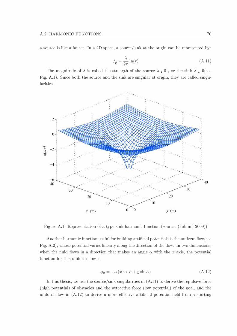
A.2. HARMONIC FUNCTIONS 70
a source is like a faucet. In a 2D space, a source/sink at the origin can be represented by:
φg =λ
2πln(r) (A.11)
The magnitude of λ is called the strength of the source λ ¡ 0 , or the sink λ ¿ 0(see
Fig. A.1). Since both the source and the sink are singular at origin, they are called singu-
larities.
Figure A.1: Representation of a type sink harmonic function (source: (Fahimi, 2009))
Another harmonic function useful for building artificial potentials is the uniform flow(see
Fig. A.2), whose potential varies linearly along the direction of the flow. In two dimensions,
when the fluid flows in a direction that makes an angle α with the x axis, the potential
function for this uniform flow is
φu = −U(x cosα+ y sinα) (A.12)
In this thesis, we use the source/sink singularities in (A.11) to derive the repulsive force
(high potential) of obstacles and the attractive force (low potential) of the goal, and the
uniform flow in (A.12) to derive a more effective artificial potential field from a starting

A.2. HARMONIC FUNCTIONS 71
Figure A.2: Representation of a Uniform flow Potential (source: (Fahimi, 2009))
position to a goal position. This uniform flow provides a linearly decreasing potential in
the direction a goal position for the unbounded environment.
Bibliography
A., Dr. Michael and Dr. Pagels (2008). Heterogeneous airborne reconnaissance team. Tech-
nical report. Information Processing Technology Office (DARPA). 2
Abe Yasuaki, Matsuo Yoshiki (2001). Collision avoidance method for multiple autonomous
mobile agents by implicit cooperation. ”IEEE Int. Conf. on Intelligent Robots and Sys-
tems. In press. 5
Aguiar, A. P. and A. M. Pascoal (2007a). Coordinated path-following control for nonlinear
systems with logic-based communication. In: 46th IEEE Conference on Decision and
Control (CDC’07). New Orleans, LO, USA. 3
Aguiar, A. P. and J. P. Hespanha (2004). Logic-based switching control for trajectory-
tracking and path-following of underactuated autonomous vehicles with parametric mod-
eling uncertainty. In: Proceedings of the American Control Conference (ACC2004). Vol. 4.
Boston, MA, USA. pp. 3004–3010. 3
Aguiar, A. P. and J. P. Hespanha (2007). Trajectory-tracking and path-following of under-
actuated autonomous vehicles with parametric modeling uncertainty. IEEE Transactions
on Automatic Control. In press. 7
Aguiar A. P., Pascoal A. (2009). Cooperative cognitive control for autonomous underwater
vehicles. Technical report. Institute for Systems and Robotics (ISR). 3, 4
Aguiar and Pascoal (2007b). Coordinated path-following control for nonlinear systems with
logic-based communication. CDC07 - 46th IEEE Conference on Decision and Control,
New Orleans. In press. 9
Aguiar A.P., Almeida J., Bayat M. Cardeira B. Cunha R. Hausler A.P. M. Oliveira A.
Pascoal A.M. Pereira A. Rufino M. Sebastiao L. Silvestre C. and Vanni F. (2009). Co-
operative autonomous marine vehicle motion control in the scope of the eu grex project:
Theory and practice.. Technical report. Instituto Superior Tecnico - Institute for Systems
and Robotics (IST/ISR). Lisbon, Portugal. 3
72

BIBLIOGRAPHY 73
Aung M., Ahmed A., Wette M. Scharf D. Tien J. Purcell G. Regehr M. Landin B. (2004).
An overview of formation flying technology development for the terrestrial planet finder
mission. Aerospace Conference,IEEE Proceedings. In press. 1, 2
Bar-Shalom Y., Kirubarajan T. and Li X.R. (2002). Estimation with Applications to Track-
ing and Navigation.. 3rd ed.. John Wiley and Sons. New York. 18
Ericson, Christer (2005). Real Time collision detection. 1st ed.. Morgan Kaufmann Pub-
lishers. San Francisco. 5
Fahimi, Farbod (2009). Autonomous Robots Modeling, Path Planning, and Control. 1st ed..
Springer. Canada. 26, 67, 70, 71
Foka A.F., Trahanias P.E. (2002). Predictive autonomous robot navigation. Intelligent
Robots and Systems, 2002. IEEE/RSJ International Conference on. In press. 6
Francesco, Vanni (2007). Coordinated motion control of multiple autonomous underwa-
tervehicles. Master’s thesis. Instituto Superior Tecnico - Dept. Electrical Engineering.
Lisbon, Portugal. 7
Ghabcheloo, R., A. M. Pascoal, C. Silvestre and I. Kaminer (2007). Nonlinear coordinated
path following control of multiple wheeled robots with bidirectional communication con-
straints. International Journal of Adaptive Control and Signal Processing 21(2-3), 133–
157. 2
Hausler A.J., Pascoal A., Aguiar A.P. Kaminer I. (2009). Temporally and spatially decon-
flicted path planning for multiple autonomous marine vehicles. Technical report. Institute
for Systems and Robotics (ISR). 7
Horowitz, R. and P. Varaiya (2000). Control design of an automated highway system.
Proceedings of the IEEE 88(7), 913–925. 2
Kim Jin-Ho, Khosla, P.K (1992). Real-time obstacle avoidance using harmonic potential
functions. Robotics and Automation, IEEE Transactions on. In press. 7
Kulkarni I. S., Pompili D. (2007). Coordination of autonomous underwater vehicles for
acoustic image acquisition. Intelligent Robots and Systems, 2002. IEEE/RSJ Interna-
tional Conference on. In press. 7
Kyriakopoulos, K.J. and G.N.Saridis (1992). An integrated collision prediction and avoid-
ance scheme for mobile robots in non-stationary environments. International conference
on Robotics and Automation. In press. 5

BIBLIOGRAPHY 74
Li, X. R. and V.P. Jilkov (2003). Part i. dynamic models, in aerospace and electronic
systems. IEEE Transactions. In press. 17
Luis Martinez-Gomez, Thierry Fraichard (2009). Collision avoidance in dynamic environ-
ments:an ics-based solution and its comparative evaluation. ”IEEE Int. Conf. on Robotics
and Automation. In press. 5
M. Bayat, F. Vanni A. and Pedro Aguiar (2009). Online mission planning for cooperative
target tracking of marine vehicles. Technical report. Institute for Systems and Robotics
(ISR). ix, 6, 17, 18, 19
M., SEUNGHO LEE; ADAMS Teresa (2004). Spatial model for path planning of multiple
mobile construction robots. Computer-aided civil and infrastructure engineering. In press.
6
Maurya P., Pascoal A., Aguiar A.P. (2008). Marine vehicle path following using inner-outer
loop control. Technical report. Institute for Systems and Robotics (ISR). 8, 53
Pedro V. Fazenda, Pedro U. Lima (2006). Non-holonomic robot formations with obstacle
compliant geometry. Technical report. Institute for Systems and Robotics (ISR). 7
S. Axler, W. Ramey, P. Bourdon (2001). Harmonic Function theory. 2nd ed.. Springer. San
Francisco. 68
Vanni F., Aguiar A. P. and Pascoal A. M. (2008). Cooperative path-following of underac-
tuated autonomous marine vehicles with logic-based communication. IFAC Workshop on
Navigation, Guidance and Control of Underwater Vehicles. In press. 9
Xu Y.W., Cao X.B., Li T. (2009). Extended kalman filter based pedestrian localization
for collision avoidance. Mechatronics and Automation, International Conference on. In
press. 6
Yun X., Tan K. (1997). Wall-following method for escaping local minima in potential field
based motion planning. In: Proceeding of the 8th International Conference on Advanced
Robotics. In press. 7