Performance Analysis of Cooperative Communication for Wireless

COOPERATIVE COMMUNICATION IN
WIRELESS LOCAL AREA NETWORKS
by
SAMIR GABER SAYED ABDEL GAWAD
A Thesis submitted in fulfilment of requirements for the degree ofDoctor of Philosophy of University College London
Communications and Information Systems GroupDepartment of Electronic and Electrical Engineering
University College Londonc⃝ 2010

Statement of Originality
I hereby declare that the research recorded in this thesis and the
thesis itself was composed and originated by myself in the Department of
Electronic and Electrical Engineering, University College London, except
where otherwise indicated.
Samir Gaber Sayed

Acknowledgements
I would like to express my deepest thanks to my supervisor, Dr. Yang
Yang, for his valuable advice, encouragement, patience, and his sugges-
tions and constant support during this research.
I would like to thank the Egyptian Government for the generous
scholarship which was awarded to me. Many thanks also go to the staff of
the Egyptian Educational and Cultural Bureau at London for their help and
support during the period of my study at the University College London.
I would like to express my sincere gratitude to Professor Izzat Dar-
wazeh for his valuable comments and insightful advice. I also would like to
thank my friends and colleagues, especially Ryan Grammenos and Ioannis
Kanaras, in the Department of Electronic and Electrical Engineering at the
University College London for their continuous help and encouragement.
I am grateful to Professor Mohamed Eladawy for his support and
help. I would like to thank Prof. Ahmed Abdelwahab for his help and sup-
port during my MSc degree. I am also very much indebted to my friend
Saad Roushdy for his help, support, understanding and friendly advice. My
thanks also go to my friend Eltayeb Abass for his help and support during
my stay in England.
Of course, my eternal thanks go to my parents, my wife, and my
sons Zyad and Gasser for their patience, support and love. Without their

iii
aid this work would never have come into existence. I dedicate this study
to them.
Last but certainly not least, I wish to thank the following close friends:
Amr Elsayed, Asem Shalaby, Ayman Ragab, Mohamed Saad, Raafat
Elshaer, Sameh Salah, Sameh Salem, and Walid Al-atabany.

Abstract
The concept of cooperative communication has been proposed to
improve link capacity, transmission reliability and network coverage in mul-
tiuser wireless communication networks. Different from conventional point-
to-point and point-to-multipoint communications, cooperative communi-
cation allows multiple users or stations in a wireless network to coordinate
their packet transmissions and share each other’s resources, thus achiev-
ing high performance gain and better service coverage.
According to the IEEE 802.11 standards, Wireless Local Area Net-
works (WLANs) can support multiple transmission data rates, depending
on the instantaneous channel condition between a source station and
an Access Point (AP). In such a multi-rate WLAN, those low data-rate sta-
tions will occupy the shared communication channel for a longer period
for transmitting a fixed-size packet to the AP, thus reducing the channel
efficiency and overall system performance.
This thesis addresses this challenging problem in multi-rate WLANs
by proposing two cooperative Medium Access Control (MAC) protocols,
namely Busy Tone based Cooperative MAC (BTAC) protocol and Coop-
erative Access with Relay’s Data (CARD) protocol. Under BTAC, a low
data-rate sending station tries to identify and use a close-by intermedi-
ate station as its relay to forward its data packets at higher data-rate to

v
the AP through a two-hop path. In this way, BTAC can achieve coopera-
tive diversity gain in multi-rate WLANs. Furthermore, the proposed CARD
protocol enables a relay station to transmit its own data packets to the AP
immediately after forwarding its neighbour’s packets, thus minimising the
handshake procedure and overheads for sensing and reserving the com-
mon channel. In doing so, CARD can achieve both cooperative diversity
gain and cooperative multiplexing gain. Both BTAC and CARD protocols
are backward compatible with the existing IEEE 802.11 standards.
New cross-layer mathematical models have been developed in this
thesis to study the performance of BTAC and CARD under different channel
conditions and for saturated and unsaturated traffic loads. Detailed simu-
lation platforms were developed and are discussed in this thesis. Extensive
simulation results validate the mathematical models developed and show
that BTAC and CARD protocols can significantly improve system through-
put, service delay, and energy efficiency for WLANs operating under real-
istic communication scenarios.

vi
Contents
Statement of Originality i
Acknowledgements ii
Abstract iv
List of Abbreviations xv
List of Symbols xix
1 Introduction 1
1.1 Problem Statement . . . . . . . . . . . . . . . . . . . . . . . . . . 2
1.2 Motivations and Objectives . . . . . . . . . . . . . . . . . . . . . 2
1.3 Thesis Contributions . . . . . . . . . . . . . . . . . . . . . . . . . . 4
1.4 Publications . . . . . . . . . . . . . . . . . . . . . . . . . . . . . . 5
1.5 Thesis Organisation . . . . . . . . . . . . . . . . . . . . . . . . . . 7
2 Background and State of the Art 9
2.1 IEEE 802.11 Standards . . . . . . . . . . . . . . . . . . . . . . . . 9
2.2 Network Architecture . . . . . . . . . . . . . . . . . . . . . . . . 12
2.3 IEEE 802.11 MAC Protocol . . . . . . . . . . . . . . . . . . . . . . 13
2.3.1 Distributed Coordination Function . . . . . . . . . . . . . 14
2.3.2 Frames Format . . . . . . . . . . . . . . . . . . . . . . . . 25

vii
2.3.3 Point Coordination Function (PCF) . . . . . . . . . . . . 33
2.4 IEEE 802.11 Physical Layer (PHY) . . . . . . . . . . . . . . . . . . 34
2.4.1 PHY Architecture . . . . . . . . . . . . . . . . . . . . . . . 34
2.4.2 PHY Frame Format . . . . . . . . . . . . . . . . . . . . . . 35
2.5 IEEE 802.11 Performance Metrics . . . . . . . . . . . . . . . . . . 38
2.6 Related Work . . . . . . . . . . . . . . . . . . . . . . . . . . . . . 39
2.7 Summary . . . . . . . . . . . . . . . . . . . . . . . . . . . . . . . . 45
3 BTAC: A Busy Tone Based Cooperative MAC Protocol 48
3.1 The BTAC Protocol . . . . . . . . . . . . . . . . . . . . . . . . . . 49
3.1.1 System Model . . . . . . . . . . . . . . . . . . . . . . . . . 49
3.1.2 Relay Selection Algorithm . . . . . . . . . . . . . . . . . . 50
3.1.3 BTAC Transmission Algorithm . . . . . . . . . . . . . . . . 53
3.1.4 Network Allocation Vector Setting . . . . . . . . . . . . . 56
3.1.5 The Hidden Relay Node Problem . . . . . . . . . . . . . 60
3.2 Enhanced BTAC (EBTAC) Protocol . . . . . . . . . . . . . . . . . 61
3.3 Performance Analysis . . . . . . . . . . . . . . . . . . . . . . . . 67
3.3.1 Markov Chain Model . . . . . . . . . . . . . . . . . . . . 68
3.3.2 Cross Layer MAC-Channel Model . . . . . . . . . . . . . 74
3.3.3 Throughput Analysis . . . . . . . . . . . . . . . . . . . . . 84
3.3.4 Energy Efficiency Analysis . . . . . . . . . . . . . . . . . . 88
3.3.5 Delay . . . . . . . . . . . . . . . . . . . . . . . . . . . . . . 94
3.4 Analytical and Simulation Results . . . . . . . . . . . . . . . . . 96
3.4.1 Throughput Results . . . . . . . . . . . . . . . . . . . . . . 97
3.4.2 Energy Efficiency Results . . . . . . . . . . . . . . . . . . . 102
3.4.3 Delay Results . . . . . . . . . . . . . . . . . . . . . . . . . 107
3.5 Conclusions . . . . . . . . . . . . . . . . . . . . . . . . . . . . . . 110
viii
4 CARD: Cooperative Access with Relay’s Data 113
4.1 The CARD Protocol . . . . . . . . . . . . . . . . . . . . . . . . . . 114
4.1.1 Source Node Algorithm . . . . . . . . . . . . . . . . . . . 115
4.1.2 Relay Node Algorithm . . . . . . . . . . . . . . . . . . . . 118
4.1.3 Access Point Algorithm . . . . . . . . . . . . . . . . . . . 120
4.1.4 Channel Access Procedure and NAV . . . . . . . . . . 122
4.2 Performance Analysis . . . . . . . . . . . . . . . . . . . . . . . . 126
4.2.1 Channel Packet Error Rate . . . . . . . . . . . . . . . . . 126
4.2.2 Markov Chain Model . . . . . . . . . . . . . . . . . . . . 133
4.2.3 Throughput . . . . . . . . . . . . . . . . . . . . . . . . . . 147
4.2.4 Energy Efficiency . . . . . . . . . . . . . . . . . . . . . . . 152
4.2.5 Delay . . . . . . . . . . . . . . . . . . . . . . . . . . . . . . 158
4.3 Analytical and Simulation results . . . . . . . . . . . . . . . . . . 160
4.3.1 Throughput Results . . . . . . . . . . . . . . . . . . . . . . 160
4.3.2 Energy Efficiency Results . . . . . . . . . . . . . . . . . . . 167
4.3.3 Delay Results . . . . . . . . . . . . . . . . . . . . . . . . . 171
4.4 Conclusions . . . . . . . . . . . . . . . . . . . . . . . . . . . . . . 176
5 Unsaturated Analysis of Cooperative MAC protocols 180
5.1 Non-saturated Markov Chain model . . . . . . . . . . . . . . . 181
5.1.1 Transition Probabilities . . . . . . . . . . . . . . . . . . . . 184
5.1.2 System Equations . . . . . . . . . . . . . . . . . . . . . . . 188
5.2 Performance Analysis . . . . . . . . . . . . . . . . . . . . . . . . 199
5.2.1 Throughput Analysis . . . . . . . . . . . . . . . . . . . . . 199
5.2.2 Delay Analysis . . . . . . . . . . . . . . . . . . . . . . . . . 201
5.2.3 Energy Efficiency . . . . . . . . . . . . . . . . . . . . . . . 204
5.3 Analytical and Simulation Results . . . . . . . . . . . . . . . . . 206
5.3.1 Throughput Results . . . . . . . . . . . . . . . . . . . . . . 207

ix
5.3.2 Energy Efficiency Results . . . . . . . . . . . . . . . . . . . 209
5.3.3 Delay Results . . . . . . . . . . . . . . . . . . . . . . . . . 211
5.4 Conclusions . . . . . . . . . . . . . . . . . . . . . . . . . . . . . . 211
6 Conclusions and Future Work 217
6.1 Conclusions . . . . . . . . . . . . . . . . . . . . . . . . . . . . . . 217
6.2 Future Work . . . . . . . . . . . . . . . . . . . . . . . . . . . . . . 220
A Node Distribution Probability 222
B Relay Probability 225
x
List of Figures
2.1 The IEEE 802.11 WLAN architecture (BSS, IBSS, DS). . . . . . . . 14
2.2 IEEE 802.11 standards. . . . . . . . . . . . . . . . . . . . . . . . . 15
2.3 DCF timing relationships . . . . . . . . . . . . . . . . . . . . . . . 17
2.4 Exponential increase of CW . . . . . . . . . . . . . . . . . . . . 20
2.5 DCF basic access mechanism. . . . . . . . . . . . . . . . . . . . 21
2.6 Hidden node and exposed node problems. . . . . . . . . . . . 22
2.7 DCF RTS/CTS access mechanism. . . . . . . . . . . . . . . . . . 24
2.8 IEEE 802.11 general frame format. . . . . . . . . . . . . . . . . . 26
2.9 Frame control field. . . . . . . . . . . . . . . . . . . . . . . . . . . 27
2.10 RTS frame. . . . . . . . . . . . . . . . . . . . . . . . . . . . . . . . 31
2.11 CTS frame. . . . . . . . . . . . . . . . . . . . . . . . . . . . . . . . 32
2.12 ACK frame. . . . . . . . . . . . . . . . . . . . . . . . . . . . . . . 32
2.13 MPDU frame. . . . . . . . . . . . . . . . . . . . . . . . . . . . . . 33
2.14 Anomaly performance. . . . . . . . . . . . . . . . . . . . . . . . 35
2.15 PLCP PPDU format. . . . . . . . . . . . . . . . . . . . . . . . . . . 36
3.1 Multi-rate IEEE 802.11b WLAN. . . . . . . . . . . . . . . . . . . . 50
3.2 Frame formats. . . . . . . . . . . . . . . . . . . . . . . . . . . . . 55
3.3 Access mechanism of BTAC protocol. . . . . . . . . . . . . . . 57
3.4 NAV setting in BTAC. . . . . . . . . . . . . . . . . . . . . . . . . . 59
3.5 NAV setting in EBTAC. . . . . . . . . . . . . . . . . . . . . . . . . 63
xi
3.6 Frame formats. . . . . . . . . . . . . . . . . . . . . . . . . . . . . 64
3.7 CTS corruption in EBTAC. . . . . . . . . . . . . . . . . . . . . . . . 65
3.8 DATA source to relay corruption in EBTAC. . . . . . . . . . . . . 66
3.9 MAC frame format. . . . . . . . . . . . . . . . . . . . . . . . . . . 67
3.10 BTAC cross layer Markov chain model. . . . . . . . . . . . . . . 70
3.11 Gilbert-Elliot channel model. . . . . . . . . . . . . . . . . . . . . 75
3.12 Throughput of IEEE802.11b, CoopMAC, and BTAC, L=1024 byte. 98
3.13 Collision and Relay probabilities versus number of nodes,
L=1024 byte. . . . . . . . . . . . . . . . . . . . . . . . . . . . . . . 99
3.14 Throughput gain, L=1024 byte. . . . . . . . . . . . . . . . . . . . 100
3.15 Throughput vs. packet length under ideal medium, L=1024
byte. . . . . . . . . . . . . . . . . . . . . . . . . . . . . . . . . . . 101
3.16 Throughput gain versus packet length, N=30. . . . . . . . . . . 102
3.17 Energy efficiency versus number of nodes, L=1024 byte. . . . 103
3.18 Energy efficiency performance versus number of nodes un-
der imperfect medium conditions, L=1024byte. . . . . . . . . . 104
3.19 Energy efficiency versus packet length, N=30. . . . . . . . . . . 105
3.20 Energy efficiency performance vs. packet length under im-
perfect channel conditions, N=30. . . . . . . . . . . . . . . . . 106
3.21 Delay performance versus number of nodes under ideal
medium, L=1024 byte. . . . . . . . . . . . . . . . . . . . . . . . . 108
3.22 Delay performance versus number of nodes under imperfect
medium, L=1024byte. . . . . . . . . . . . . . . . . . . . . . . . . 109
3.23 Delay performance versus packet length, N=30. . . . . . . . . 110
3.24 Delay performance vs. packet length under imperfect
medium, N=30. . . . . . . . . . . . . . . . . . . . . . . . . . . . . 111
4.1 Frame format. . . . . . . . . . . . . . . . . . . . . . . . . . . . . . 116
xii
4.2 Access mechanism of CARD protocol. . . . . . . . . . . . . . . 123
4.3 Network allocation vector (NAV). . . . . . . . . . . . . . . . . . 125
4.4 CARD protocol Markov chain model. . . . . . . . . . . . . . . . 137
4.5 Markov chain for backoff stage . . . . . . . . . . . . . . . . . . 153
4.6 Throughput vs. number of nodes under ideal channel, L =
1024 bytes. . . . . . . . . . . . . . . . . . . . . . . . . . . . . . . . 162
4.7 Throughput vs. number of nodes under imperfect channel,
L=1024 byte. . . . . . . . . . . . . . . . . . . . . . . . . . . . . . . 163
4.8 Throughput versus packet length under ideal channel, N=30
nodes. . . . . . . . . . . . . . . . . . . . . . . . . . . . . . . . . . 165
4.9 Throughput vs. packet length under imperfect channel, N=30. 166
4.10 Throughput versus number of nodes under ideal channel,
L=1024 byte. . . . . . . . . . . . . . . . . . . . . . . . . . . . . . . 167
4.11 Energy efficiency vs. number of nodes under ideal channel,
L=1024 bytes. . . . . . . . . . . . . . . . . . . . . . . . . . . . . . 168
4.12 Energy vs. number of nodes under imperfect channel, L=1024
byte. . . . . . . . . . . . . . . . . . . . . . . . . . . . . . . . . . . 170
4.13 Energy efficiency vs. packet length under ideal channel, N=30.171
4.14 Energy vs. packet length under imperfect channel, N=30. . . 172
4.15 Energy efficiency versus number of nodes under ideal
channel, L=1024 byte. . . . . . . . . . . . . . . . . . . . . . . . . 173
4.16 Service delay vs. number of nodes under ideal channel, L =
1024 bytes. . . . . . . . . . . . . . . . . . . . . . . . . . . . . . . . 174
4.17 Delay vs. number of nodes under imperfect channel, L=1024
byte. . . . . . . . . . . . . . . . . . . . . . . . . . . . . . . . . . . 175
4.18 Service delay vs. packet length under ideal channel, N=30. . 176
4.19 Delay vs. packet length under imperfect channel, N=30. . . . 177
xiii
4.20 Delay versus number of nodes under ideal channel, L=1024
byte. . . . . . . . . . . . . . . . . . . . . . . . . . . . . . . . . . . 178
5.1 Unsaturated Markov chain model. . . . . . . . . . . . . . . . . 183
5.2 Throughput performance versus total traffic load and number
of nodes, L = 1024 byte. . . . . . . . . . . . . . . . . . . . . . . . 208
5.3 Throughput performance versus total traffic load and packet
length, N = 30. . . . . . . . . . . . . . . . . . . . . . . . . . . . . 210
5.4 Energy efficiency performance versus total traffic load and
number of nodes, L = 1024 byte. . . . . . . . . . . . . . . . . . . 212
5.5 Energy efficiency performance versus total traffic load and
packet length, N = 30. . . . . . . . . . . . . . . . . . . . . . . . . 213
5.6 Delay performance versus total traffic load and number of
nodes, L = 1024 byte. . . . . . . . . . . . . . . . . . . . . . . . . . 214
5.7 Delay performance versus total traffic load and packet
length, N = 30. . . . . . . . . . . . . . . . . . . . . . . . . . . . . 215
B.1 Intersection area of two circles. . . . . . . . . . . . . . . . . . . 226
B.2 Relay regions of a node in zone-4. . . . . . . . . . . . . . . . . . 229

xiv
List of Tables
2.1 Dominant IEEE 802.11 standards . . . . . . . . . . . . . . . . . . 13
2.2 Interframe spaces values . . . . . . . . . . . . . . . . . . . . . . 18
2.3 The duration field of the RTS/CTS mechanism. . . . . . . . . . . 25
2.4 Type field value. . . . . . . . . . . . . . . . . . . . . . . . . . . . . 27
2.5 Subtype field value. . . . . . . . . . . . . . . . . . . . . . . . . . 28
2.6 To/From DS Combinations. . . . . . . . . . . . . . . . . . . . . . 28
2.7 Address field contents. . . . . . . . . . . . . . . . . . . . . . . . . 30
2.8 Signal field contents. . . . . . . . . . . . . . . . . . . . . . . . . . 37
2.9 Service field contents. . . . . . . . . . . . . . . . . . . . . . . . . 37
3.1 EBTAC Duration field contents . . . . . . . . . . . . . . . . . . . 65
3.2 Parameters used for both analytical results and simulation runs. 97
4.1 CARD Duration field contents . . . . . . . . . . . . . . . . . . . 124
4.2 PHY and MAC setup of the CARD protocol. . . . . . . . . . . . 160
5.1 System parameters under unsaturated conditions. . . . . . . . 206

xv
List of Abbreviations
ABI Allied Business Intelligence
ACK Acknowledgment
AP Access Point
ARF Auto Rate Fallback
BEB Binary Exponential Backoff
BER Bit Error Rate
BSS Basic Service Set
BSSID Basic Service Set Identifier
BTAC Busy Tone based Cooperative MAC
BTS Busy Tone Signal
CACK Cooperative ACK
CARD Cooperative Access with Relay’s Data
CCA Clear Channel Assignment
CCK Complementary Code Keying
CCTS Cooperative CTS
CFP Contention Free Period
CoopMAC Cooperative MAC
CRC Cyclic Redundancy Code
CRTS Cooperative RTS
CTS Clear To Send
CW Contention Window
xvi
DA Destination Address
DBPSK Differential Binary Phase Shift Keying
DCF Distributed Coordination Function
DFS Dynamic Frequency Selection
DIFS Distributed Interframe Space
DQPSK Quadrature Phase Shift Keying
DS Distributed System
DSSS Direct Sequence Spread Spectrum
EBTAC Enhanced BTAC
EDCF Enhanced Distributed Coordination Function
EIFS Extended Interframe Space
ESS Extended Service Set
FCC Federal Communications Commission
FCS Frame Check Sequence
FHSS Frequency Hopping Spread Spectrum
GHz Giga Hertz
HA Helper Address
HIPERLAN High-Performance Radio Local Area Network
HOL Head-Of-Line
HTS Helper-ready To Send
IBSS Independent Basic Service Set
IFS Interframe Space
IR Infrared
ISM Industrial, Scientific, and Medical
Kbps Kilo bit per second
LBT Listen Before Talk
MAC Medium Access Control
Mbps Mega bit per second

xvii
MF Mobile Framework
MHz Mega Hertz
MIMO Multiple Input Multiple Output
MPDU MAC Protocol Data Unit
MRTS Modified Request To Send
MSDU MAC service Data Unit
NACK Negative Acknowledgment
NAV Network Allocation Vector
OAR Opportunistic Auto Rate
OFDM Orthogonal Frequency Division Multiplexing
OMNET++ Objective Modular Network Testbed in C++
PBCC Packet Binary Convolutional Code
PC Point Coordinator
PCF Point Coordination Function
PDAs Personal Digital Assistants
pdf probability density function
PER Packet Error Rate
PHY Physical layer
PIFS Point Coordination Function Interframe Space
PLCP Physical Layer Convergence Procedure
PMD Physical Medium Dependent
PPDU PLCP Protocol Data Unit
PSDU PLCP Service Data Unit
PSM Power Saving Mechanism
QoS Quality of Service
RA Receiver Address
RAAR Relay-based Adaptive Auto Rate
xviii
RBAR Receiver Based Auto Rate
rDCF relay-enabled Distributed Coordination Function
rPCF relay-enabled Point Coordination Function
RRTS Relay Ready To Send
RSSI Received Signal Strength Intensity
RTH Ready To Help
RTS Request To Send
SA Source Address
SAP Service Access Point
SFD Frame Delimiter
SIFS Short Interframe Space
SNR Signal to Noise Ratio
TA Transmitter Address
TI Texas Instruments
TPC Transmitter Power Control
WEP Wired Equivalent Privacy
WFA Wi-Fi Alliance
WLANs Wireless Local Area Networks

xix
xx
List of Symbols
ACKtimeout Time out of an ACk packet.
BERrd Bite error rate at data-rate Rrd.
BERsd Bite error rate at data-rate Rsd.
BERsr Bite error rate at data-rate Rsr.
BERb Bit error rate at base data-rate Rb.
CTStimeout Time out of a CTS packet.
CWmax Maximum contention window size.
CWmin Minimum contention window size.
DCTS Duration field of a CTS packet in BTAC protocol.
Ddata1 Duration field of a data packet from a source to
a relay in BTAC protocol.
DMRTS Duration field of a MRTS packet.
DATAtimeout Time out a data packet.
E[Db,i] Average delay in the backoff stages.
E[Dc,i] Average delay due to packet collision.
E[De,i] Average delay due to erroneous transmission.
E[Do,i] average delay of overhearing during backoff.
E[Ds,i] Average delay due to a successful transmission.
E[Di] Average packet delay of node i, where i =
1, 2, ...N .
E[DT ] Average total delay of the network.
E[PL] Average payload size in octets.

xxi
E[TCi] Average collision duration at node i.
E[TCi] Average erroneous transmission duration at node
i.
E[TSi] Average successful transmission duration at node
i.
E[TC ] Average time that the channel is sensed busy due
to a collision.
E[TE] Average time the channel is sensed busy due to
an erroneous transmission.
E[TI ] Average duration of an empty slot time.
E[TS] Average time during which the channel is sensed
busy due to a successful transmission.
E(i)C Average energy consumption due to collision pe-
riod of a node i.
E(i)E Average energy consumption due to erroneous
transmission of a node i.
E(i)O Average energy consumption due to an over-
hearing transmission of a node i.
E(i)S Average energy consumption due to a successful
transmission of a node i.
Ece1 Energy consumption of a MRTS corruption.
Ece2 Energy consumption of a CTS corruption under
cooperative transmission.
Ece3 Energy consumption of a data packet (source-
relay) corruption.
Ece4 Energy consumption of a data packet (relay-AP)
corruption.
Ece5 Energy consumption of an ACK corruption under
BTAC protocol.

xxii
Ede1 Energy consumption of RTS corruption.
Ede2 Energy consumption of CTS corruption.
Ede3 Energy consumption of a data packet (source-
AP) corruption.
Ede4 Energy consumption of ACK corruption.
E(i)B Average energy consumption during backoff pe-
riod.
E(i)C Average energy consumption during collision pe-
riod.
E(i)E Average energy consumption during erroneous
transmission period.
Ee1 Energy consumption of RTS corruption.
Ee2 Energy consumption of CTS corruption.
Ee3 Energy consumption of a data packet (source-
AP) corruption.
Ee4 Energy consumption of an ACK corruption.
E(i)O Average energy consumption during overhearing
transmission period.
E(i)S Average energy consumption during successful
transmission period.
GR Rate gain.
K Maximum queue length of node i.
LACK ACK packet length in octets.
LCACK CACK packet length in octets.
LCCTS CCTS packet length in octets.
LCRTS CRTS packet length in octets.
LCTS CTS packet length in octets.

xxiii
LMRTS MRTS packet length in octets.
LPLCP Physical Layer Convergence Procedure header in
octets.
LRRTS RRTS packet length in octets.
LRTS RTS packet length in octets.
Lr Data packet length of relay node in octets.
Ls Data packet length of a source node in octets.
Nf,i Average number of slots during which node i
freezes its backoff counter due others transmis-
sions.
Ns,i Average number of time slots represents the suc-
cessful transmission period of node i.
Nu,i Average number of time slots represents the un-
successful transmission period of node i.
P (t) Stochastic transition matrix.
P ′(t) Derivative of P (t).
pce1 Corruption probability of a MRTS packet.
pce2 Corruption probability of a CTS packet.
pce3 Corruption probability of a data packet from a
source to a relay.
pce4 Corruption probability of a data packet from a
relay to the AP.
pce5 Corruption probability of an ACK packet in BTAC.
pde1 Corruption probability of a RTS packet.
pde2 Corruption probability of a CTS packet.
pde3 Corruption probability of a data packet from a
source to the AP.

xxiv
pde4 Corruption probability of an ACK from the AP to a
source.
Pb,i Probability the channel is sensed busy by a node
i.
Pc,i probability of collision of node i.
Pe,i Total packet error rate probability of node i.
PE,i Probability that at least one packet arrives in the
MAC queue during the following time slot condi-
tioning that the queue is empty at the beginning
of the slot.
pi,j(t0) Transition probability from state i to state j after t0
sec.
PIX Average power consumption in idle/sensing.
PRX Average power consumption in reception.
Ps,i Successful transmission probability of a node i.
P ′s,k Successful transmission probability of node k = i
of remaining N − 1 nodes.
Ptr Probability of at least one transmission occurs in a
slot time.
PTX Average power consumption in transmission.
Pu,i probability of unsuccessful packet transmission
from node i.
Ps Total successful transmission probability.
Q Infinitesimal generator or transition rate matrix.
qce1 probability that CRTS is corrupted given that no
CRTS collision.
qce2 probability that CCTS is corrupted and CRTS is cor-
rect given that no CRTS collision.

xxv
qce3 probability that RRTS is corrupted and both CRTS
and CCTS are correct given that no CRTS collision.
qce4 probability that DATA-S(source-relay) is corrupted
and CRTS, CCTS, and RRTS are correct given that
no CRTS collision.
qce5 probability that DATA-S (relay-destination) is cor-
rupted and CRTS, CCTS, RRTS, and DATA-S
(source-relay) are correct given that no CRTS col-
lision.
qce6 probability that DATA-R is corrupted and CRTS,
CCTS,RRTS, and DATA-S (source-relay) are correct
given that no CRTS collision.
qce7 probability that CACK is corrupted and CRTS,
CCTS,RRTS, DATA-S (source-relay), and at least
one of both DATA-S (relay-destination) and DATA-
R are correct given that no CRTS collision.
qi Probability that the there is at least one packet
available at the queue at the post-backoff stage.
Rrd Data-rate from a relay node to the AP in Mbps.
Rsr Data-rate from a source node to a relay node in
Mbps.
Rb Base data-rate in Mbps.
S Saturated throughput.
T cs,i Successful time duration due to cooperative tra-
nsmission of node i.
T ds,i Successful time duration due to direct tra-
nsmission of node i.
TACK Time duration of an ACK packet.
TBTS Duration of a BTS signal.
xxvi
TCACK Duration of a CACK.
TCCTS Duration of a CCTS.
TCRTS Duration of a CRTS.
TCTS Duration of a CTS.
TDIFS Duration of a DIFS slot.
TMRTS Duration of a MRTS.
Trd Duration of a data packet from a relay to the AP.
TRRTS Duration of RRTS.
TRTS Duration of a RTS.
T cs,i Successful transmission period of node i under co-
operative transmission.
T ds,i Successful transmission period of node i under di-
rect transmission.
Tsd Duration of a data packet from a source to the
AP.
TSIFS Duration of SIFS.
Tsr Duration of a data packet from a source to a re-
lay.
Tu,i Unsuccessful transmission period of node i due to
packet errors.
TACK Duration of ACK packet.
TB Average sojourn time in bad state.
Tc Collision time duration.
TG Average sojourn time in good state.
ud1 Corruption probability of a RTS packet given no
RTS collision in 802.11b.
ud2 Corruption probability of a CTS packet given no
RTS corruption and collision in 802.11b.
ud3 Corruption probability of a data packet given no
CTS and RTS corruption, and no RTS collision in
802.11b.

xxvii
ud4 Corruption probability of an ACK packet given no
RTS and CTS and data packets corruption, and
no RTS collision in 802.11b.
UF Final state probability vector.
UI Initial state probability vector.
v1 Probability a MRTS is corrupted given that a single
MRTS is transmitted.
v2 Probability a CTS is corrupted given that a MRTS is
received correctly.
v3 Probability a data packet from a source to a relay
is corrupted given that a CTS is received correctly.
v4 Probability a data packet from a relay to the AP
is corrupted given that a data packet from a
source to a relay is received correctly.
v5 Probability an ACK packet is corrupted given that
a data packet from a relay to the AP is received
correctly.
w1 Probability that CRTS is corrupted given that no
CRTS collision.
w2 Probability that CCTS is corrupted given that CRTS
is correct and no CRTS collision.
w3 probability that RRTS is corrupted given that both
CRTS and CCTS are correct and no CRTS collision.
w4 Probability that a data packet (source-relay) is
corrupted given that CRTS, CCTS, and RRTS are
correct and no CRTS collision.

xxviii
w5 Probability that a data packet (relay-AP) is cor-
rupted given that CRTS, CCTS, RRTS, and a data
packet (source-relay) are correct and no CRTS
collision.
w6 Probability that a data packet of a relay node
is corrupted given that CRTS, CCTS, RRTS, and a
data packet (source-relay) are correct and no
CRTS collision.
w7 probability that CACK is corrupted given that
CRTS, CCTS, RRTS, DATA-S (source-relay), and at
least one packet of both the source data packet
(relay-AP) and a relay data packet are correct
and no CRTS collision.
αk Probability that the channel is busy due to a tra-
nsmission from node k.
δ Channel propagation delay.
η Energy efficiency.
λ Packet arrival rate in packets per second.
λb Transition rate constant from bad state to good
state.
λg Transition rate constant from good state to bad
state.
N cek Average number of retries due to collisions.
No,i Average number of transmissions overheard by
the a node i.
Nr,i Average total number of retries.
Nc
e1 Average number of retries due to MRTS corrup-
tion.
Nc
e2 Average number of retries due to CTS corruption.

xxix
Nc
e3 average number of retries due to data packet
(source-relay) corruption.
Nc
e4 Average number of retries due to data packet
(relay-AP) corruption.
Nc
e5 Average number of retries due to ACK corruption
under BTAC.
Nd
e1 Average number of retries due to RTS corruption.
Nd
e2 Average number of retries due to CTS corruption.
Nd
e3 Average number of retries due to DATA-S (source-
AP) corruption.
Nd
e4 Average number of retries due to ACK corruption.
N b,i The average number of time slots during the
backoff duration.
N e1 Average number of retries due to RTS corruption.
N e2 Average number of retries due to CTS corruption.
N e3 Average number of retries due to data packet
(source-AP) corruption.
N e4 Average number of retries due to ACK corruption.
N idle,i Average number of consecutive idle slots be-
tween two consecutive busy slots.
πj,k Steady state probability of Markov chain in the
state (j, k).
πB Steady state probability for being in bad state.
πG Steady state probability of being in good state.
ρi Utilization factor.
σ Slot time duration.
τi Probability of successful transmission of node i in
a randomly chosen time slot.
Chapter 1
Introduction
In 1985, the United States Federal Communications Commission
(FCC) opened the experimental Industrial, Scientific and Medical (ISM)
spectral bands for license-free commercial applications of spread wire-
less spectrum technologies. During the last 20 years, Wireless Local Area
Networks (WLANs) have been widely deployed in educational institutions,
business buildings, public areas and even our homes to provide wireless
broadband access services, thanks to the popularity of Internet appli-
cations and the proliferation portable communication devices (such as
laptops and smart mobile phones). The dominant industrial standards for
WLANs are the IEEE 802.11 family [1] and its European counterpart High-
Performance Radio Local Area Network (HIPERLAN) [2]. The key advan-
tages of WLANs technologies include low costs (in deployment and main-
tenance), small size, ease of deployment and use, high speed, and cheap
and portable devices. According to the Allied Business Intelligence (ABI)
research [3], the world wireless market is predicted to grow from over 1.2
billion chipset unit shipments in 2009 to nearly 2.25 billion unit shipments in
2014.

1.1 Problem Statement 2
1.1 Problem Statement
According to the IEEE 802.11 standards, a WLAN can support mul-
tiple transmission data rates depending on the instantaneous wireless
channel condition between a device/station and an Access Point (AP).
To achieve the target Packet Error Rate (PER) in data transmission, a de-
vice/station transmits its packets to an AP at a low date rate when the
channel quality is poor. Heusse et al [4] show that the IEEE 802.11 WLANs
presents a performance anomaly whereby the presence of a low data-
rate device/station degrades the performance of a high data-rate de-
vices/stations. This is because, relative to the high data-rate stations, a
low data-rate station occupies the shared communication channel for
a longer period for transmitting the same size packet to the destination,
thus reducing the channel efficiency and overall system performance. To
demonstrate this negative effect, we evaluate the overall throughput and
delay performance of an IEEE 802.11b WLAN [5] consisting of 20 stations,
each with either a high transmission data rate of 11 Mbps or a low data
rate of 1 Mbps. When the number of low data-rate stations increases, the
overall throughput and delay performance degrades. For example, when
the number of low-data rate stations is three, the throughput decreases
by 34% and the delay increases by 39% relative to the values when the
number of low-data rate stations in zero.
1.2 Motivations and Objectives
The ubiquitous WLAN systems, based on the multi-rate IEEE 802.11
standards, lead to degradations in the performance of such networks. As

1.2 Motivations and Objectives 3
shown in pervious section, the overall system performance of a multi-rate
WLAN is determined by those low data-rate stations in the network. Recent
studies indicate that the IEEE 802.11 Medium Access Control (MAC) pro-
tocol is the main reason for this performance anomaly effect. Therefore,
it is fundamentally important to design or improve these MAC protocols
to utilise efficiently limited bandwidth and provide reliable system perfor-
mance, thus enabling WLANs to support many new applications such as
real-time multimedia communications. On the other hand, the IEEE 802.11
standards have been widely accepted and is now ubiquitous, it is then dif-
ficult to design a completely new MAC protocol that can succeed com-
mercially. Our aim in this thesis is to design backward compatible MAC
protocols, which can improve WLAN system performance with no signifi-
cant changes to current IEEE 802.11 standards.
The concept of cooperative communications has been recently
proposed to allow multiple users, devices or stations in a wireless network
to coordinate their packet transmissions and share each other’s resources
and capabilities, thus achieving cooperative diversity gain or cooperative
multiplexing gain. Specifically, cooperative diversity gain can be obtained
by using intermediate stations, termed relays, to forward a sender’s data
packets to its destination (an AP in WLANs). While cooperative multiplexing
gain can be achieved by enabling the relays to combine their own data
transmissions with those forwarding packets, i.e. reserve the medium for
additional data transmissions from the relays. In contrast to previous work,
mainly focusing on physical (PHY) layer performance optimisation, our ob-
jective in this thesis is to understand the impact of cooperative commu-
nications on MAC layer performance and then design new cooperative
MAC protocols to improve WLAN performance, in terms of system through-

1.3 Thesis Contributions 4
put, latency, and energy efficiency.
1.3 Thesis Contributions
The research reported here addresses a new area of engineering.
This research has resulted in several novel contributions outlined below:
• Design and verification of a new Busy Tone based Cooperative MAC
protocol, namely BTAC, is designed. BTAC has the advantage of im-
proving the system performance in terms of throughput, delay, and
energy efficiency, through achieving cooperative diversity gain. The
BTAC is detailed in Chapter 3.
• Design and verification of a novel cooperative medium access con-
trol (MAC) protocol, termed “Cooperative Access with Relay’s Data”
(CARD). CARD can achieve both cooperative diversity and cooper-
ative multiplexing gains and significantly improve the system through-
put, delay, and energy efficiency of multi-rate WLANs. The CARD pro-
tocol is detailed in Chapter 4.
• Development of mathematical models to evaluate the performance
of both BTAC and CARD protocols taking into account dynamic wire-
less channel conditions.
• Development of a new analytical energy efficiency model for both
BTAC and CARD protocols. This model consider the multi-rate,
channel conditions, cooperative transmission, and saturated traffic
load.
• Development of a new mathematical model to study the perfor-

1.4 Publications 5
mance of both BTAC and IEEE 802.11b protocols under unsaturated
traffic load and ideal channel conditions.
1.4 Publications
The work reported in this thesis resulted in the publications listed be-
low:
1. S. Sayed and Yang Yang, ” A new Cooperative MAC Protocol for Wire-
less LANs” in London Communication Symposium (LCS), September
2007.
2. S. Sayed and Yang Yang, ”BTAC: A busy tone based cooperative
MAC protocol for wireless local area networks,” in Proc. Third Inter-
national Conference on Communications and Networking in China
ChinaCom 2008, 2008, pp. 403-409.
3. S. Sayed and Yang Yang,”RID: Relay with integrated data for multi-
rate wireless cooperative networks,” in Proc. 5th International Con-
ference on Broadband Communications, Networks and Systems
BROADNETS ’08, 2008, pp. 383 - 388.
4. S. Sayed, Yang Yang, and Honglin Hu, ”CARD: Cooperative Access
with Relay’s Data for Multi-Rate Wireless Local Area Networks,” in
Proc. IEEE International Conference on Communications ICC ’09,
2009, pp. 1-6.
5. S. Sayed, Yang Yang, and Honglin Hu, ”Throughput Analysis of Coop-
erative Access Protocol for Multi-Rate WLANs,” in Proc. IEEE Wireless

1.4 Publications 6
Communications and Networking Conference (WCNC’09), 2009, pp.
1-6.
6. S. Sayed, Yang Yang, and Honglin Hu, ”Throughput Analysis of Coop-
erative Access with Relay’s Data Protocol for Unsaturated WLANs,” in
Proc. of the 2009 International Conference on Wireless Communica-
tions and Mobile Computing 2009 (IWCMC’09), 2009, pp. 790-794.
7. S. Sayed, Yang Yang, Haiyou Guo, and Honglin Hu, ”Energy Efficiency
Analysis of Cooperative Access with Relay’s Data Algorithm for Multi-
rate WLANs,” in Proc. IEEE Personal, Indoor and Mobile Radio Com-
munications Symposium 2009 (PIMRC’09), 2009.
8. S. Sayed, Yang Yang, Haiyou Guo, and Honglin Hu, ”Analysis of Energy
Efficiency of a Busy Tone Based Cooperative MAC Protocol for Multi-
rate WLANs,” accepted for publication in Proc. IEEE Wireless Commu-
nications and Networking Conference 2010 (WCNC’10), 2010.
9. S. Sayed, Yang Yang, Haiyou Guo, and Honglin Hu, ”BTAC: A busy
tone based cooperative MAC protocol for wireless local area net-
works,” accepted for publication in Mobile Networking and Applica-
tions (MONET), 2009.
10. Chi-Kin Chau, Fei Qin, Sayed Samir, Muhammad Husni Wahab and
Yang Yang, ”Harnessing Battery Recovery Effect in Wireless Sensor
Networks: Experiments and Analysis,” to appear in IEEE Journal on
Selected Areas in Communications (JSAC), Special Issue on Simple
Wireless Sensor Networking Solutions, 2010.
Also another paper titled ”CARD: Cooperative Access with Relay’s
Data for Multi-Rate Wireless Local Area Networks” is submitted to the IEEE

1.5 Thesis Organisation 7
Transaction on Wireless Communication.
1.5 Thesis Organisation
The thesis is organised as follows.
Chapter 2 reviews the background material and provides an
overview of the dominant IEEE 802.11 standards, specifically the standards
that have a common MAC protocol. The IEEE 802.11 WLANs structure is
then presented, including frequency bands, frame formats and MAC layer
access mechanisms. Some related work on the design and analysis of
802.11 MAC protocols is also reviewed.
Chapter 3 proposes and analyses a Busy Tone based cooperative
MAC protocol, namely BTAC, for multi-rate WLANs. The BTAC transmission
protocol is explained in detail and compared with the IEEE 802.11b [5]
standard to show its compatibility with the latter. A cross-layer analytical
model under dynamic channel conditions is developed to evaluate the
performance of BTAC in terms of throughput, energy efficiency, and ser-
vice delay. The proposed models and system performance are validated
by computer simulations.
Chapter 4 proposes a novel cooperative MAC protocol, namely Co-
operative Access with Relay’s Data (CARD), which comprises the design
of three algorithms for sender nodes, relay nodes and the AP, respec-
tively. Analytical models are then derived to analyse the throughput, de-
lay, and energy efficiency performance of the CARD protocol under dif-
ferent channel conditions. The models are validated by computer simula-
tions.
Chapter 5 presents an analytical model under ideal conditions and

1.5 Thesis Organisation 8
unsaturated traffic load. Subsequently, throughput, energy efficiency, and
delay analyses are given in details and computed for both IEEE 802.11b
and BTAC protocols. Furthermore, the analytical model is validated using
computer simulations.
Chapter 6 concludes this thesis and proposes some research direc-
tions for future work.

Chapter 2
Background and State of the Art
Nowadays, the IEEE 802.11 standards have been widely accepted
for deploying WLAN services. This chapter reviews Physical (PHY) layer and
Medium Access Control (MAC) layer defined in IEEE 802.11 standards, as
well as some related work on performance evaluation of WLANs.
The remainder of the chapter is organised as follows. Section 2.1 re-
views the IEEE 802.11 standards. In Section 2.2 the WLAN network structure
is presented. Section 2.3 explains the main features of the MAC layer in the
IEEE 802.11. The function of the PHY layer and the frame format of the IEEE
802.11 are explained in Section 2.4. The critical requirements of an efficient
MAC protocol are given in Section 2.5. The related work is given in Section
2.6, followed by summary in Section 2.7.
2.1 IEEE 802.11 Standards
In 1985, the United States Federal Communications Commission
(FCC) opened the experimental industrial, scientific, and medical (ISM)

2.1 IEEE 802.11 Standards 10
bands for commercial applications of spread spectrum technology with-
out a government licence. There are different parts for the IEEE 802.11
standard that are briefly outlined below.
• IEEE 802.11-legacy
The 802.11 study group was established under the IEEE Project 802 to
recommend the first international standard of the IEEE 802.11 [1] pro-
tocol, called IEEE 802.11 legacy. It was released in 1997 and clarified
in 1999. Due to the increasing commercial interest, the Wi-Fi Alliance
(WFA) was formed in 1999 to certify interoperability of WLANs devices
based on the IEEE 802.11 specifications. The legacy IEEE 802.11 [1]
specifies two data rates of 1 and 2 Mbps. It defines three PHY lay-
ers: Infrared (IR) operating at 1 Mbps, Frequency Hopping Spread
Spectrum (FHSS) operating at 1 or 2 Mbps, and Direct Sequence
Spread Spectrum (DSSS) operating at 1 or 2 Mbps. The FHSS and DSSS
technologies use the 2.4 GHz frequency band.
• IEEE 802.11a
The IEEE 802.11a [6] was ratified in 1999. It operates in the 5 GHz band
using Orthogonal Frequency-Division Multiplexing (OFDM) techniques
in PHY layer at a transmission data-rate up to 54 Mbps.
• IEEE 802.11b
The IEEE 802.11b standard [5] was released in 1999. The IEEE 802.11b
extended the transmission data-rate up to 11 Mbps using a DSSS PHY
layer at 2.4 GHz frequency band as the original IEEE 802.11. Despite
the 802.11a provides a transmission data-rate up to 54 Mbps, the IEEE
802.11b has become the most popular standard operating in the 2.4
GHz ISM band.

2.1 IEEE 802.11 Standards 11
• IEEE 802.11d
The IEEE 802.11d [7] was ratified in 2001. It is employed in some coun-
tries where systems using other standards in the IEEE 802.11 family are
not allowed to operate. It provides procedures to let the IEEE 802.11
networks operate compliantly to the regulations of these countries by
introducing regulatory domains.
• IEEE 802.11e
The IEEE 802.11 Working Group certified the IEEE 802.11e [8], in 2005,
to enhance the current standards. The IEEE 802.11e is based upon
IEEE 802.11a and supports applications with Quality of Service (QoS)
mechanisms.
• IEEE 802.11g
In order to provide a high data-rate as the 802.11a and a relatively
large coverage area as 802.11b, the IEEE 802.11g standard [9] was
released in 2003. The IEEE 802.11g operates in the 2.4 GHz band and
employs OFDM physical layer at a transmission data-rate up to 54
Mbps. It is fully compatible with the IEEE 802.11b standard.
• IEEE 802.11h
The IEEE 802.11h [10] is employed to provide Dynamic Frequency
Selection (DFS) and Transmitter Power Control (TPC). TPC protocol is
used to adapt the transmission power based on regulatory require-
ments.
• IEEE 802.11i
The IEEE 802.11i [11] is released to provide effective data security by
enhancing the Wired Equivalent Privacy (WEP) protocol.

2.2 Network Architecture 12
• IEEE 802.11j
The IEEE 802.11j [12] is released to allocate the Japanese spectrum in
the 4.9 to 5 GHz band for indoor, outdoor and mobile applications.
• IEEE 802.11-2007
The IEEE 802.11-2007 [13] standard was released, in 2007, to enhance
the existing MAC protocol and PHY layer functions such as data
link security. It also incorporates eight amendments which are IEEE
802.11a [6], IEEE 802.11b [5], IEEE 802.11d [7], IEEE 802.11e [8], IEEE
802.11g [9], IEEE 802.11h [10], IEEE 802.11i [11], and IEEE 802.11j [12].
• IEEE 802.11n
Recently, the IEEE 802.11n [14] standard has been released to im-
prove the transmission data-rate (up to 600 Mbps) and the coverage
area range over the previous standards, such as the IEEE 802.11a and
IEEE 802.11b/g. The IEEE 802.11n standard employs the Multiple-Input
Multiple-Output (MIMO) technique in the PHY layer and the frame
aggregation scheme to the MAC layer.
Comparisons for the most popular IEEE 802.11 standards, such as
802.11a, 802.11b, 802.11g, and 802.11n are illustrated in Table 2.1 [15–17].
2.2 Network Architecture
As shown in Fig. 2.1, a WLAN may contain several Basic Service Sets
(BSSs), each of them consists of an Access Point (AP) and a group of neigh-
bouring user stations. The function of the AP is to form a bridge between
wireless and wired network. When a station needs to communicate with

2.3 IEEE 802.11 MAC Protocol 13
802.11a 802.11b 802.11g 802.11n
Release date 1999 1999 2003 2009
Data-rate 54 Mbps 11 Mbps 54 Mbps 248 Mbps
Throughput 20 Mbps 5 Mbps 22 Mbps 144 Mbps
Frequency 5 GHz 2.4 GHz 2.4, 5 GHz 2.4, 5 GHz
Channel BW 20 MHz 20 MHz 20 MHz 20, 40 MHz
Modulation OFDM DSSS, CCK DSSS,CCK,OFDM DSSS,CCK,OFDM
Coverage 15-30m 45-90 m 45-90 m 75-150 m
Table 2.1: Dominant IEEE 802.11 standards
another station in the same BSS, the station sends first to the AP and then
the AP sends to the other station. The BSSs may be interconnected via
their APs through the Distributed System (DS). The whole interconnected
network including the BSSs and the DS is called an Extended Service Set
(ESS). As a basic 802.11 network type, Independent BSS (IBSS) supports at
least two stations to directly communicate with each other in an ad hoc
mode (i.e. without AP). Consequently, the medium access coordination
is distributed between all the stations. The IEEE 802.11 defines two layers,
which are the MAC and PHY layers. These two layers are explained in the
following two sections, respectively.
2.3 IEEE 802.11 MAC Protocol
The primary purpose of an IEEE 802.11 MAC protocol is to
regulate the access of multiple user stations to the shared wireless

2.3 IEEE 802.11 MAC Protocol 14
Figure 2.1: The IEEE 802.11 WLAN architecture (BSS, IBSS, DS).
channel/medium, thus achieving reliable data delivery and security [18].
The IEEE 802.11 standards [1] allocate the same MAC layer to operate on
top of one of several PHY layers 1. As shown in Fig. 2.2, the lower sub-
layer of the MAC layer is Distributed Coordination Function (DCF), which
provides a contention based service to access the shared medium. As
an optional choice, the Point Coordination Function (PCF) is a centralised
method exploiting the features in DCF sublayer to provide a contention-
free medium access service for users.
2.3.1 Distributed Coordination Function
DCF is the fundamental medium access method of the IEEE 802.11
standards [1], used in both infrastructure and ad hoc modes. DCF is based
on the Carrier Sense Multiple Access with Collision Avoidance (CSMA/CA)
protocol, which works as follows.
1The IEEE 802.11n standard has a different MAC Layer.

2.3 IEEE 802.11 MAC Protocol 15
Figure 2.2: IEEE 802.11 standards.
• Before transmitting a packet, a source station, senses the medium by
measuring the signal level at the carrier frequency.
• If the medium is found to be idle, the source waits a minimum speci-
fied duration called Distributed Interframe Space (DIFS).
• If the medium stays idle, the source station transmits its data packet
to the receiving station.
• If the medium is sensed busy, the source defers its transmission after a
random backoff delay.
• The source decrements the backoff interval counter while the
medium is idle, and freezes the counter when the medium is sensed
busy.
• The source will transmit its packet when its backoff counter reaches
zero.
2.3.1.1 Carrier Sense Mechanism
The carrier sense mechanism is used to determine the state of the
medium. There are two ways in which a carrier sense is performed: virtual
2.3 IEEE 802.11 MAC Protocol 16
carrier sense and physical carrier sense functions. When either function
indicates a busy medium, the MAC layer considers a busy medium; other-
wise the medium is considered idle.
The physical carrier sense is provided by the IEEE 802.11 PHY layer
in which a Clear Channel Assignment (CCA) is a logical function imple-
mented. The CCA procedure employs a single fixed power carrier sense
threshold. If a station detects a signal with Received Signal Strength Inten-
sity (RSSI) less than the threshold value, the channel is then assumed to be
idle. Otherwise, the medium is assumed to be busy and then unavailable
for transmission.
The virtual carrier sense is provided the IEEE 802.11 MAC layer. It
is referred to as the Network Allocation Vector (NAV). The NAV is a timer
maintained by all stations to indicate the time interval during which the
medium is reserved by other stations. The NAV timer decrements even
though the station’s CCA function indicates a busy medium. The NAV is set
after receiving a frame from another station in the network. Each frame
includes a duration field that indicates the required time period for the
following frame exchange. When either the CCA indicates the channel is
busy or the NAV is set, a station defers it transmissions.
2.3.1.2 Interframe Space
The Interframe Space (IFS) is the time duration between two MAC
frames. There are four different IFSs durations defined to access the wire-
less medium at different priority levels. These IFSs are the Short Interframe
Space (SIFS), the Point Coordination Function Interframe Space (PIFS), the
Distributed Coordination Function Interframe Space (DIFS), and the Ex-
tended Interframe Space (EIFS). Fig. 2.3 shows some of these IFSs.

2.3 IEEE 802.11 MAC Protocol 17
Figure 2.3: DCF timing relationships
• SIFS Interval
It is the time interval between a response frame and the frame that
requested the response, for example between a data frame and the
Acknowledgment (ACK) frame. The SIFS is the shortest of the inter-
frame spaces, but it is longer than the propagation delay and pro-
cessing time at PHY and MAC layers. This delay includes demodu-
lation and decoding the frame at the PHY layer, the MAC layer pro-
cessing time for the received frame and constructing the response
frame. The SIFS value for the 802.11b is 20 µs, and for the 802.11a,
802.11g, and 802.11n is 16 µs.
• PIFS Interval
It is the next highest priority following the SIFS interval. The PIFS is em-
ployed by stations operating under the PCF mode to gain priority ac-
cess to the wireless channel at the start of the Contention Free Period
(CFP).
• DIFS Interval
It is used by stations operating under the DCF mode. A station using
the DCF sends its frame if its backoff counter reaches zero and the
channel is sensed idle for the duration of the DIFS.

2.3 IEEE 802.11 MAC Protocol 18
Parameter Value
SIFS aSIFSTime = 20 µs (802.11b) and 16 µs (802.11a/g/n)
PIFS aSIFSTime + aSlotTime
DIFS aSIFSTime + 2× aSlotTime
EIFS aSIFSTime + ACKTxTime + DIFS
Table 2.2: Interframe spaces values
• EIFS Interval
It is used by a station operating under the DCF mode instead of the
DIFS interval when the received frame is incorrect. This occurs due to
imperfect channel conditions or when two or more stations transmit
at the same time (collision). The EIFS begins following the PHY layer
indication that the medium is sensed idle after detection of the er-
roneous frame. The EIFS is lowest access priority (longest IFS), which
gives the sending station a higher priority to access the medium. Ta-
ble 2.2 illustrates the values of the different interframe spaces; where
aSlotTime is the duration of a slot time. In 802.11b, aSlotTime is 10 µs.,
and in 802.11a/g/n is 9 µs. ACKTxTime is the duration of the ACK frame
at the lowest data-rate.
2.3.1.3 Random Backoff Algorithm
When the medium is sensed idle, two or more stations may trans-
mit at the same slot time. This is known as a collision. To minimise the
collision probability, a station performs the so-called backoff procedure
before starting transmission. If the medium is sensed busy, a station defers
until the channel becomes idle without interruption for a DIFS (or EIFS) inter-
val when the last frame is received correctly (or incorrectly). After this DIFS

2.3 IEEE 802.11 MAC Protocol 19
(or EIFS) idle period, the station selects a random backoff period, which is
a multiple of a slot time duration, and defers for that number of slot times.
Each station selects the backoff count from a uniform distribution over the
interval [0, CW-1], where CW is the Contention Window.
A station decreases its counter by one for every idle slot time. The
transmission is then started when the backoff counter reaches zero. If the
transmission is failed due to an erroneous transmission or a collision, the
CW is doubled until it reaches the maximum value aCWmax, where CW
takes the initial value of aCWmin. aCWmin = 31 and aCWmax = 1023 for the
DSSS technique, as shown in Fig. 2.4. If the maximum retry limit is reached,
which is six in Fig. 2.4, the frame should be dropped and the CW should
be reset to the initial value aCWmin. If the channel is sensed busy by the
CCA function, the station freezes its backoff counter until the medium be-
comes idle for a DIFS or EIFS once more a gain. The station then resumes its
counter and does not select a new backoff value. Thus, the station takes a
higher priority to access the channel in the following transmission. The pro-
cedure of doubling the CW is called the Binary Exponential Backoff (BEB)
algorithm [1]. This algorithm decreases the collision probability when there
are multiple stations trying to access the channel at the same slot time.
After each successful or dropped frame transmission, there is always
at least one backoff interval preceding (the initial attempt in Fig. 2.4) a
packet transmission even there is no other frame to send. This is referred
to as post-backoff. Alternatively, there is an exception to the essential rule
that an a packet from the upper layer has to be transmitted after perform-
ing the backoff mechanism. The packet arriving from the upper layer may
be transmitted immediately without waiting any time if the transmission
queue is empty, the latest post-backoff is finished, and at the same time

2.3 IEEE 802.11 MAC Protocol 20
Figure 2.4: Exponential increase of CW
the channel has been idle for at least one DCF or EIFS interval.
2.3.1.4 DCF Access Procedure
The DCF protocol describes two modes for packet transmission. The
mandatory scheme is referred to as a basic access or a two-way hand-
shaking scheme. In addition to the basic access, the other scheme is the
RTS/CTS [19, 20] mechanism, and is referred to as a four-way handshaking
mechanism and it is an optional mechanism.
Basic Access Mechanism
According to the CSMA/CA protocol, a station having a frame to
transmit should listen until the wireless channel becomes idle for a DCF pe-
riod when the last frame is received correctly, or an EIFS period when the
last frame is received in error due to collision or imperfect channel con-
ditions. After this DIFS or EIFS medium idle time, the station generates a

2.3 IEEE 802.11 MAC Protocol 21
Figure 2.5: DCF basic access mechanism.
random backoff interval according to the rules of the BEB algorithm. A
station transmits its data packet when the backoff timer reaches zero. If
the data packet is correctly received, the destination station then sends
an ACK frame immediately following a SIFS period. Otherwise, the des-
tination station defers for an EIFS interval. If the transmitting station does
not receive the ACK frame within a predefined ACKtimeout, it increases its
Retry Count by one for each unsuccessful transmission, rescheduling the
data frame retransmission according to the backoff rules. The CW should
be reset to its minimum value aCWmin after every successful transmission
or when retry count reaches the maximum value. The retry count is reset to
zero whenever an ACK frame is received correctly. The Frame exchange
sequence of the basic access mechanism is shown in Fig. 2.5.
Hidden Node And Exposed Node Problems
The basic access mechanism is inefficient in WLANs due to two
unique problems: the hidden node problem [21] and exposed node prob-
lem. These two problems are illustrated in Fig. 2.6. A hidden node (node C
in Fig. 2.6) is a node which is out of range of a sending node (node A in Fig.
2.6), but in the range of a receiving node (node B in Fig. 2.6). When the
node A is transmitting to the node B, the node C senses the channel to be
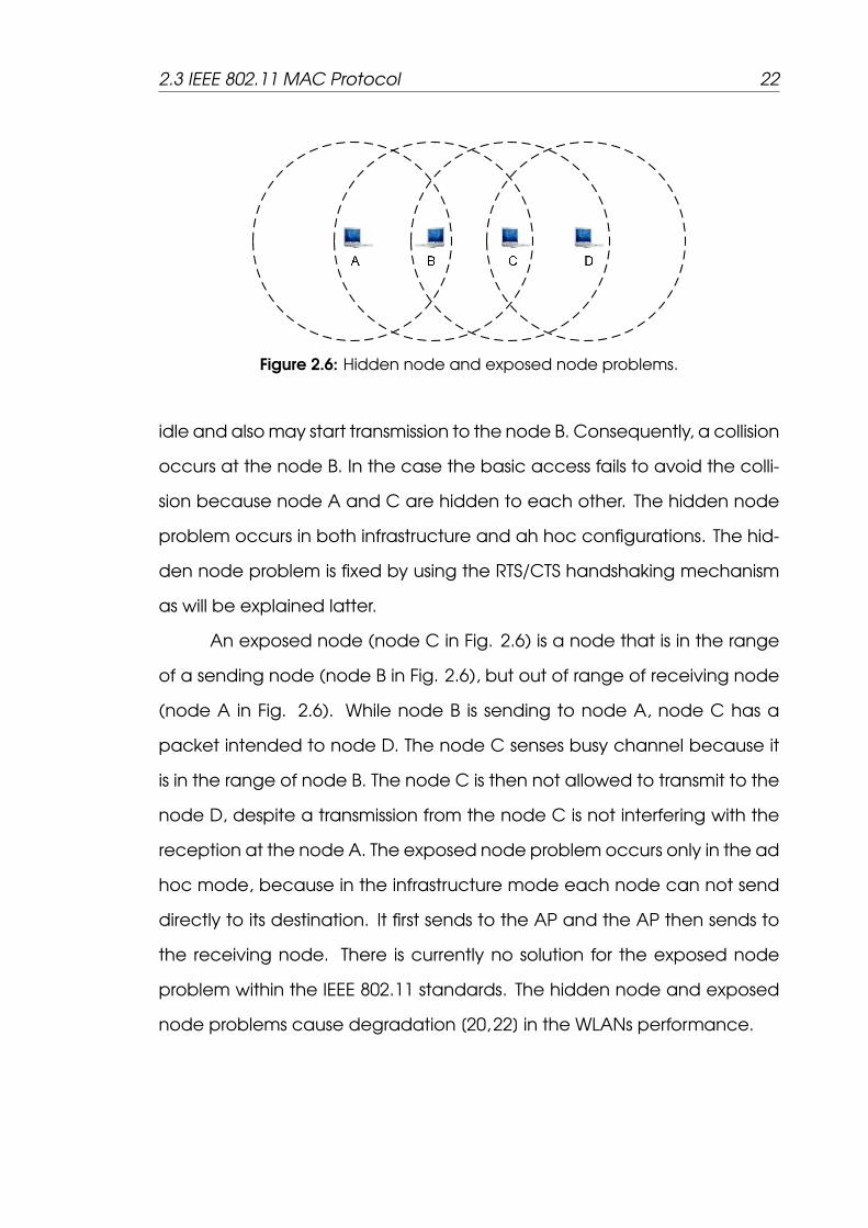
2.3 IEEE 802.11 MAC Protocol 22
Figure 2.6: Hidden node and exposed node problems.
idle and also may start transmission to the node B. Consequently, a collision
occurs at the node B. In the case the basic access fails to avoid the colli-
sion because node A and C are hidden to each other. The hidden node
problem occurs in both infrastructure and ah hoc configurations. The hid-
den node problem is fixed by using the RTS/CTS handshaking mechanism
as will be explained latter.
An exposed node (node C in Fig. 2.6) is a node that is in the range
of a sending node (node B in Fig. 2.6), but out of range of receiving node
(node A in Fig. 2.6). While node B is sending to node A, node C has a
packet intended to node D. The node C senses busy channel because it
is in the range of node B. The node C is then not allowed to transmit to the
node D, despite a transmission from the node C is not interfering with the
reception at the node A. The exposed node problem occurs only in the ad
hoc mode, because in the infrastructure mode each node can not send
directly to its destination. It first sends to the AP and the AP then sends to
the receiving node. There is currently no solution for the exposed node
problem within the IEEE 802.11 standards. The hidden node and exposed
node problems cause degradation [20,22] in the WLANs performance.
2.3 IEEE 802.11 MAC Protocol 23
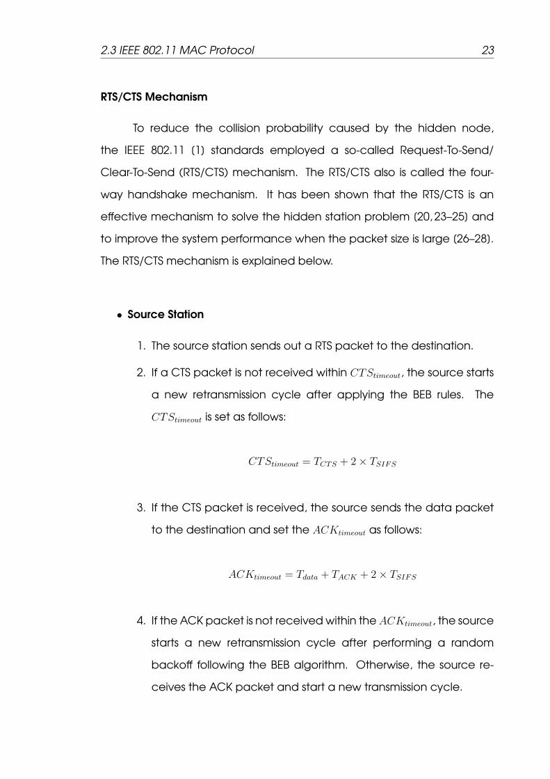
RTS/CTS Mechanism
To reduce the collision probability caused by the hidden node,
the IEEE 802.11 [1] standards employed a so-called Request-To-Send/
Clear-To-Send (RTS/CTS) mechanism. The RTS/CTS also is called the four-
way handshake mechanism. It has been shown that the RTS/CTS is an
effective mechanism to solve the hidden station problem [20, 23–25] and
to improve the system performance when the packet size is large [26–28].
The RTS/CTS mechanism is explained below.
• Source Station
1. The source station sends out a RTS packet to the destination.
2. If a CTS packet is not received within CTStimeout, the source starts
a new retransmission cycle after applying the BEB rules. The
CTStimeout is set as follows:
CTStimeout = TCTS + 2× TSIFS
3. If the CTS packet is received, the source sends the data packet
to the destination and set the ACKtimeout as follows:
ACKtimeout = Tdata + TACK + 2× TSIFS
4. If the ACK packet is not received within the ACKtimeout, the source
starts a new retransmission cycle after performing a random
backoff following the BEB algorithm. Otherwise, the source re-
ceives the ACK packet and start a new transmission cycle.

2.3 IEEE 802.11 MAC Protocol 24
Figure 2.7: DCF RTS/CTS access mechanism.
where TCTS, Tdata, and TACK stand for the duration of a CTS, a data,
and an ACK packet, respectively. TSIFS is the duration of a SIFS interval.
The reason that CTS packet may be unsuccessful is due to collision or im-
perfect channel conditions.
• Destination Station
1. If the RTS packet is successfully received, the destination transmits
a CTS packet back to the source following a SIFS interval. It sets
a DATAtimout as follows:
DATAtimout = Tdata + 2× TSIFS
2. If the data packet is received from the source within the
DATAtimout, the destination sends an ACK packet back to the
source after a SIFS interval. Otherwise, it assumes that the tra-
nsmission is terminated, and starts a new transmission cycle if
there is a packet ready for transmission in its buffer.
2.3 IEEE 802.11 MAC Protocol 25
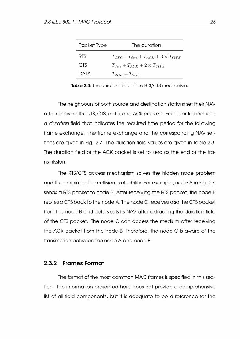
Packet Type The duration
RTS TCTS + Tdata + TACK + 3× TSIFS
CTS Tdata + TACK + 2× TSIFS
DATA TACK + TSIFS
Table 2.3: The duration field of the RTS/CTS mechanism.
The neighbours of both source and destination stations set their NAV
after receiving the RTS, CTS, data, and ACK packets. Each packet includes
a duration field that indicates the required time period for the following
frame exchange. The frame exchange and the corresponding NAV set-
tings are given in Fig. 2.7. The duration field values are given in Table 2.3.
The duration field of the ACK packet is set to zero as the end of the tra-
nsmission.
The RTS/CTS access mechanism solves the hidden node problem
and then minimise the collision probability. For example, node A in Fig. 2.6
sends a RTS packet to node B. After receiving the RTS packet, the node B
replies a CTS back to the node A. The node C receives also the CTS packet
from the node B and defers sets its NAV after extracting the duration field
of the CTS packet. The node C can access the medium after receiving
the ACK packet from the node B. Therefore, the node C is aware of the
transmission between the node A and node B.
2.3.2 Frames Format
The format of the most common MAC frames is specified in this sec-
tion. The information presented here does not provide a comprehensive
list of all field components, but it is adequate to be a reference for the

2.3 IEEE 802.11 MAC Protocol 26
Figure 2.8: IEEE 802.11 general frame format.
subjects discussed in this research. For a detailed list of the MAC frame
formats refer to the IEEE 802.11 [1, 5, 6, 8, 9, 14]. All stations is able to con-
struct frames for transmission and decode frames up on reception. Each
frame in the IEEE 802.11 standards [1] is composed by the following basic
components: A MAC header, a variable length frame body, and a frame
check sequence.
2.3.2.1 General MAC Frame Format
The IEEE 802.11 [1] standards specifies a general frame format as
shown in Fig. 2.8. The general MAC frame format consists of a set of the
fields that occur in a fixed order in all frames. The Address 2, Address 3,
Address 4, Sequence Control, and Frame body fields are only exist in a
certain frame types as will be explained latter. The following defines each
of the general MAC frame fields.
• Frame Control Field
It is two octets in length and is illustrated in Fig. 2.9. It consists of Proto-
col Version, Type, Subtype, To DS, From DS, More Fragments, Retry,
Power Management, More Data, Wired Equivalent Privacy (WEP),
and Order subfields.
– Protocol Version Field
It is two bits in length and represents the protocol version. The

2.3 IEEE 802.11 MAC Protocol 27
Figure 2.9: Frame control field.
b2 b3 Frame type
00 Management frame
01 Control frame
10 Data frame
11 Reserved
Table 2.4: Type field value.
value of the protocol version is zero for the current standards.
– Type Field
It is a two bits in length and defines whether the frame is a man-
agement, control, or data frame as indicated by Table 2.4.
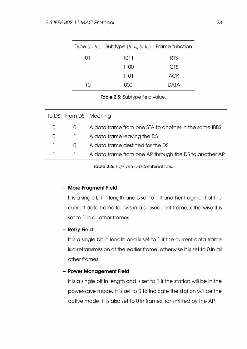
– Subtype Field
It is four bits in length and it defines the function of the frame.
Some Subtype field functions is shown in Table 2.5.
– To DS Field
It is a single bit in length and is set to 1 in any data frame destined
for the DS; otherwise, it is set to 0 in all other frames.
– From DS Field
It is a single bit in length and it is set to 1 in any data frame leaving
the DS; otherwise it is set to 0 in all other frames. The bit combi-
nations and their meanings of both To DS and From DS fields are
illustrated in Table 2.6.
2.3 IEEE 802.11 MAC Protocol 28
Type (b2 b3) Subtype (b4 b5 b6 b7) Frame function
01 1011 RTS
1100 CTS
1101 ACK
10 000 DATA
Table 2.5: Subtype field value.
To DS From DS Meaning
0 0 A data frame from one STA to another in the same IBBS
0 1 A data frame leaving the DS
1 0 A data frame destined for the DS
1 1 A data frame from one AP through the DS to another AP
Table 2.6: To/From DS Combinations.
– More Fragment Field
It is a single bit in length and is set to 1 if another fragment of the
current data frame follows in a subsequent frame; otherwise it is
set to 0 in all other frames.
– Retry Field
It is a single bit in length and is set to 1 if the current data frame
is a retransmission of the earlier frame; otherwise it is set to 0 in all
other frames.
– Power Management Field
It is a single bit in length and is set to 1 if the station will be in the
power-save mode. It is set to 0 to indicate the station will be the
active mode. It is also set to 0 in frames transmitted by the AP.

2.3 IEEE 802.11 MAC Protocol 29
– More Data Field
It is a single bit in length and is set to 1 if the AP has at least
one additional data frame for a station in the power-save mode;
otherwise it is set to 0 in the all other frames.
– Wired Equivalent Privacy (WEP) Field
It is a single bit in length and is set to 1 if the Frame Body field
of a data frame has been processed by the WEP algorithm (en-
crypted); otherwise it is set to 0 in all other frames.
– Order Field
It is a single bit in length and is set to 1 in any data frame that is
being sent using the StrictlyOrder service class. The StrictlyOrder
service class is used to tell the receiving station that the data
frames must be processed in order. The Order field is set to 0 in
all other frames.
• Duration/ID Field
It is a two octets in length and is used by a receiving station to set or
update its NAV when the frame is not addressed to that station. The
duration value represents the expected time duration during which
the medium is expected to be busy before another station can con-
tend for the medium.
• Address Fields
The IEEE 802.11 [1] standards defines the following address types
which are the Destination Address (DA), Receiver Address (RA),
Source Address (SA), Transmitter Address (TA), and Basic Service Set
Identifier (BSSID). The DA is the MAC address of the ultimate receiving
station that will handle the frame to the upper layers for processing.

2.3 IEEE 802.11 MAC Protocol 30
To DS From DS Address 1 Address 2 Address 3 Address 4
0 0 DA SA BSSID N/A
0 1 DA BSSID SA N/A
1 0 BSSID SA DA N/A
1 1 RA TA DA SA
Table 2.7: Address field contents.
The RA is the MAC address of a station (e.g. the AP) that should pro-
cess the frame. The SA is the MAC address of the original source of
the frame. The TA is the MAC address of a station that transmitted the
frame onto the medium. The content of Address fields of the MAC
frame is dependent upon the value of To DS and From DS fields and
given in Table 2.7.
• Sequence Control Field
It a two octet in length and consists of two subfields which are the
Fragment Number (the leftmost four bits) and Sequence Number
(the next 12 bits). The Fragment Number indicates the number of
each fragment of a data frame. It is set to zero and incremented by
one for each succeeding transmission. The Fragment Number is hav-
ing the same number in all retransmissions of the fragment. Sequence
Number specifies the sequence number of a data frame. Each data
frame is assigned a sequence number starting at zero and increment-
ing by one for data frame. The Sequence Number subfield remains
constant in each fragment or all retransmissions of the data frame.
• Frame Body Field
The Body Frame field has a variable length payload and contains
information that relates to the specific frame being sent.

2.3 IEEE 802.11 MAC Protocol 31
Figure 2.10: RTS frame.
• Frame Check Sequence (FCS) Field
The FCS is eight octets in length containing a 32-bit Cyclic Redun-
dancy Code (CRC). The CRC is used by a sending station to calcu-
late a checksum of all fields of the MAC frame. The receiving station
also calculates the CRC of the received frame and compares it with
the attached CRC. If the two CRCs are the same, the receiver veri-
fies that the frame has been received correctly; otherwise the frame
has been corrupted while in transmission due to collision or imperfect
channel conditions.
2.3.2.2 Common Frames Format
• Request To Send (RTS) Frame
The RTS frame format is illustrated in Fig. 2.10. The TA field of the RTS
frame is the address of the transmitting station and RA is the address
of the intended recipient of the frame (e.g. the AP in the infrastruc-
ture mode). The Duration field, in microseconds, is the time that the
sending station needs to transmit the data frame, plus one CTS frame,
plus one ACK frame, plus three SIFS intervals.
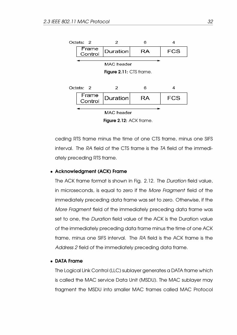
• Clear To Send (CTS) Frame
The CTS frame format is given in Fig. 2.11. The Duration field value,
in microseconds, is the Duration field value of the immediately pre-
2.3 IEEE 802.11 MAC Protocol 32
Figure 2.11: CTS frame.
Figure 2.12: ACK frame.
ceding RTS frame minus the time of one CTS frame, minus one SIFS
interval. The RA field of the CTS frame is the TA field of the immedi-
ately preceding RTS frame.
• Acknowledgment (ACK) Frame
The ACK frame format is shown in Fig. 2.12. The Duration field value,
in microseconds, is equal to zero if the More Fragment field of the
immediately preceding data frame was set to zero. Otherwise, if the
More Fragment field of the immediately preceding data frame was
set to one, the Duration field value of the ACK is the Duration value
of the immediately preceding data frame minus the time of one ACK
frame, minus one SIFS interval. The RA field is the ACK frame is the
Address 2 field of the immediately preceding data frame.
• DATA Frame
The Logical Link Control (LLC) sublayer generates a DATA frame which
is called the MAC service Data Unit (MSDU). The MAC sublayer may
fragment the MSDU into smaller MAC frames called MAC Protocol

2.3 IEEE 802.11 MAC Protocol 33
Figure 2.13: MPDU frame.
Data Units (MPDUs), as indicated in the IEEE 802.11 [1] standard. The
frame format of the MPDU is shown in Fig. 2.13. The Frame Body field
has a variable length from zero to 2312 octets, and the contents of
Address fields are specified in Table 2.7.
2.3.3 Point Coordination Function (PCF)
The PCF is an optional priority-based providing a contention-free
frame transfer. The PCF access method is only employable on infrastruc-
ture network configurations. The PCF uses a Point Coordinator (PC) which
exists in the AP to control the transmission of the stations. All stations follow
the PC by setting their NAV value at the beginning of each Contention-
Free Period (CFP). The PC senses the medium at the beginning of a CFP. If
the medium becomes free for the PIFS interval, the PC transmits a beacon
frame. All stations receiving the beacon frame set their NAV to the maxi-
mum duration of the CFP to lock out DCF-based access to the medium un-
til the end of the CFP. The difference between the DCF and PCF is that the
stations should contend to access the wireless medium in the DCF mode
while in the PCF mode, the PC controls the stations access to the medium.
The PCF has not been widely employed. The details of PCF access method
and frame formats are beyond the scope of this research. More detailed
information for the PCF access method can be found in [1,15,29].

2.4 IEEE 802.11 Physical Layer (PHY) 34
2.4 IEEE 802.11 Physical Layer (PHY)
The PHY layer is the second layer in the IEEE 802.11 WLAN architec-
ture shown in Fig. 2.2. The general operation of the PHYs is very similar.
The PHYs provides the following functions: carrier sense, transmission, and
reception on the wireless medium. The original IEEE 802.11 [1] standard
defines three different PHYs specifications. These three PHYs are 2.4 GHz
FHSS, 2.4 GHz DSSS, and Infrared (IR). There are additional three PHYs de-
fined in the 802.11a, 802.11b, 802.11g, and 802.11n standards. Except the
802.11b which is based on the DSSS and Complementary Code Keying
(CCK) [5] techniques, all the other PHYs are based on the OFDM scheme.
IEEE 802.11a [6] operates in the 5 GHz ISM band at data-rate up to 54 MHz.
The IEEE 802.11g [9] operates in the 2.4 GHz ISM band at data-rate up to
54 Mbps. The IEEE 802.11b [5] also operates in the 2.4 GHz ISM band at
data rat up to 11 Mbps. Finally, the IEEE 802.11n operates in either 2.4 GHz
or 5 GHz ISM band at data rate up to 248 Mbps. More details of these IEEE
802.11 PHY layers can be found in [18,29].
2.4.1 PHY Architecture
The architecture of PHY is shown in Fig. 2.14, and consists of two
sublayers which are Physical Layer Convergence Procedure (PLCP) and
Physical Medium Dependent (PMD). The PLCP sublayer maps the MPDUs
packet into a PLCP Service Data Units (PSDUs) that is suitable for the tra-
nsmission and reception on the wireless medium. The PMD sublayer is re-
sponsible for the frame transmission and reception on the wireless medium.
These responsibilities include modulation, demodulation, signal encoding,
and interacting with the wireless medium. The PLCP communicates with

2.4 IEEE 802.11 Physical Layer (PHY) 35
Figure 2.14: Anomaly performance.
MAC layer through a Service Access Point (SAP) called PHY SAP, and the
PLCP communicates with the PMD sublayer through the PMD SAP.
2.4.2 PHY Frame Format
The IEEE 802.11b [5] is employed here to explain the IEEE 802.11 PHY
frame. The other PHYs employ a similar frame format with slight changes
that beyond the scope of this work. The transmitted frame on the wireless
channel is called PLCP Protocol Data Unit (PPDU) shown in Fig. 2.15. It
consist of PLCP preamble, PLCP header, and PSDU fields.
• PLCP Preamble Field
The IEEE 802.11b defines two PPDU frames that differ only in the length
of the preamble. The long preamble, shown in Fig. 2.15(a), is a 144-
bit field including a 128-bit Sync field that enables the receiver to
synchronise with the transmitter and a 16-bit Start of Frame Delimiter
(SFD) field. The long preamble is the same as employed in the original
IEEE 802.11 [1]. The short preamble, illustrated in Fig. 2.15(b), is a 72-
bit field consists of a 56-bit Sync field and 16-bit SFD field. The short
preamble improves the performance efficiency. Both short and long
PLCP preambles are sent at data-rate of 1 Mbps using the Differential

2.4 IEEE 802.11 Physical Layer (PHY) 36
(a) Long Preamble PLCP PPDU format.
(b) Short Preamble PLCP PPDU format.
Figure 2.15: PLCP PPDU format.
Binary Phase Shift Keying (DBPSK) modulation technique.
• PLCP Header Field
It is a 48-bit field, and consists of Signal, Service, Length, and CRC
fields. It is sent at 1 Mbps with DBPSK modulation under long PLCP
preamble (Fig. 2.15(a)), and is sent at 2 Mbps with Differential
Quadrature Phase Shift Keying (DQPSK) modulation under the short
PLCP preamble (Fig. 2.15(b)).
– Signal Field
It describes the type of modulation that the receiving station
must employ to demodulate the received signal. The value of
the Signal field is equal to the data-rate divided by 100 Kbps. The
data-rates supported by the IEEE 802.11b [5] are 1, 2, 5.5, and 11
Mbps. The corresponding Signal field value is given in Table 2.8.
– Service Field
It is one octet in length, and is reserved for future use except
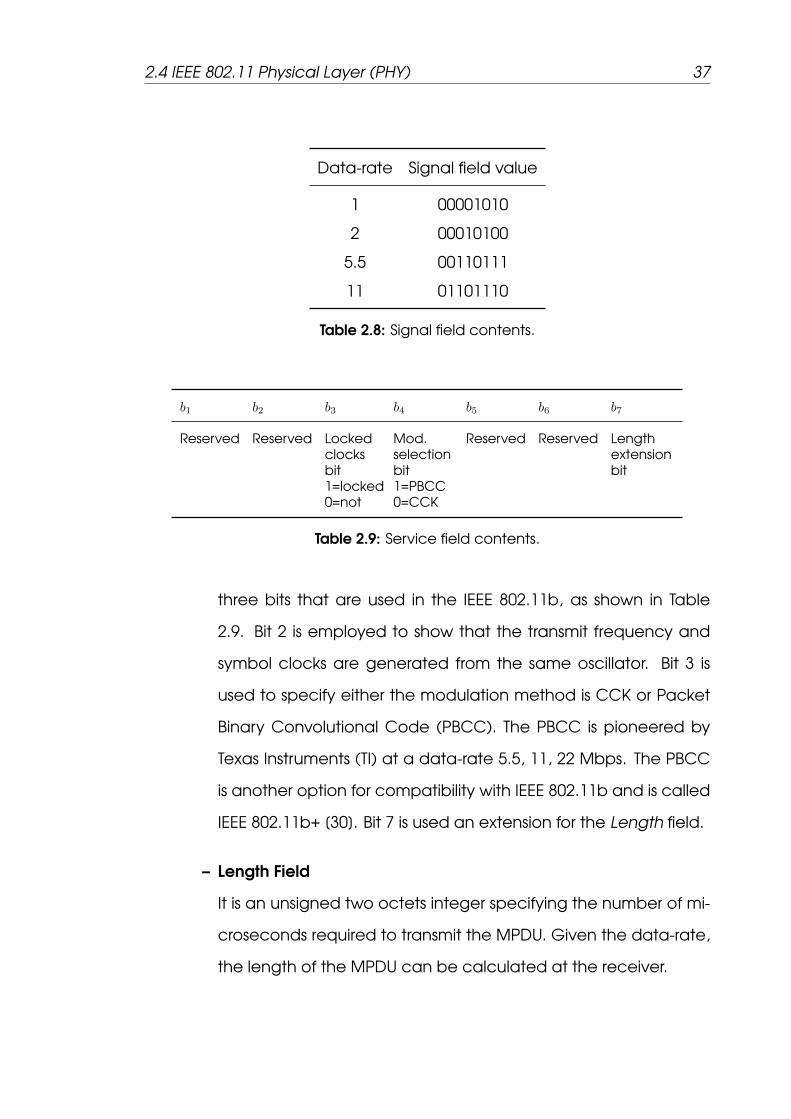
2.4 IEEE 802.11 Physical Layer (PHY) 37
Data-rate Signal field value
1 00001010
2 00010100
5.5 00110111
11 01101110
Table 2.8: Signal field contents.
b1 b2 b3 b4 b5 b6 b7
Reserved Reserved Lockedclocksbit1=locked0=not
Mod.selectionbit1=PBCC0=CCK
Reserved Reserved Lengthextensionbit
Table 2.9: Service field contents.
three bits that are used in the IEEE 802.11b, as shown in Table
2.9. Bit 2 is employed to show that the transmit frequency and
symbol clocks are generated from the same oscillator. Bit 3 is
used to specify either the modulation method is CCK or Packet
Binary Convolutional Code (PBCC). The PBCC is pioneered by
Texas Instruments (TI) at a data-rate 5.5, 11, 22 Mbps. The PBCC
is another option for compatibility with IEEE 802.11b and is called
IEEE 802.11b+ [30]. Bit 7 is used an extension for the Length field.
– Length Field
It is an unsigned two octets integer specifying the number of mi-
croseconds required to transmit the MPDU. Given the data-rate,
the length of the MPDU can be calculated at the receiver.
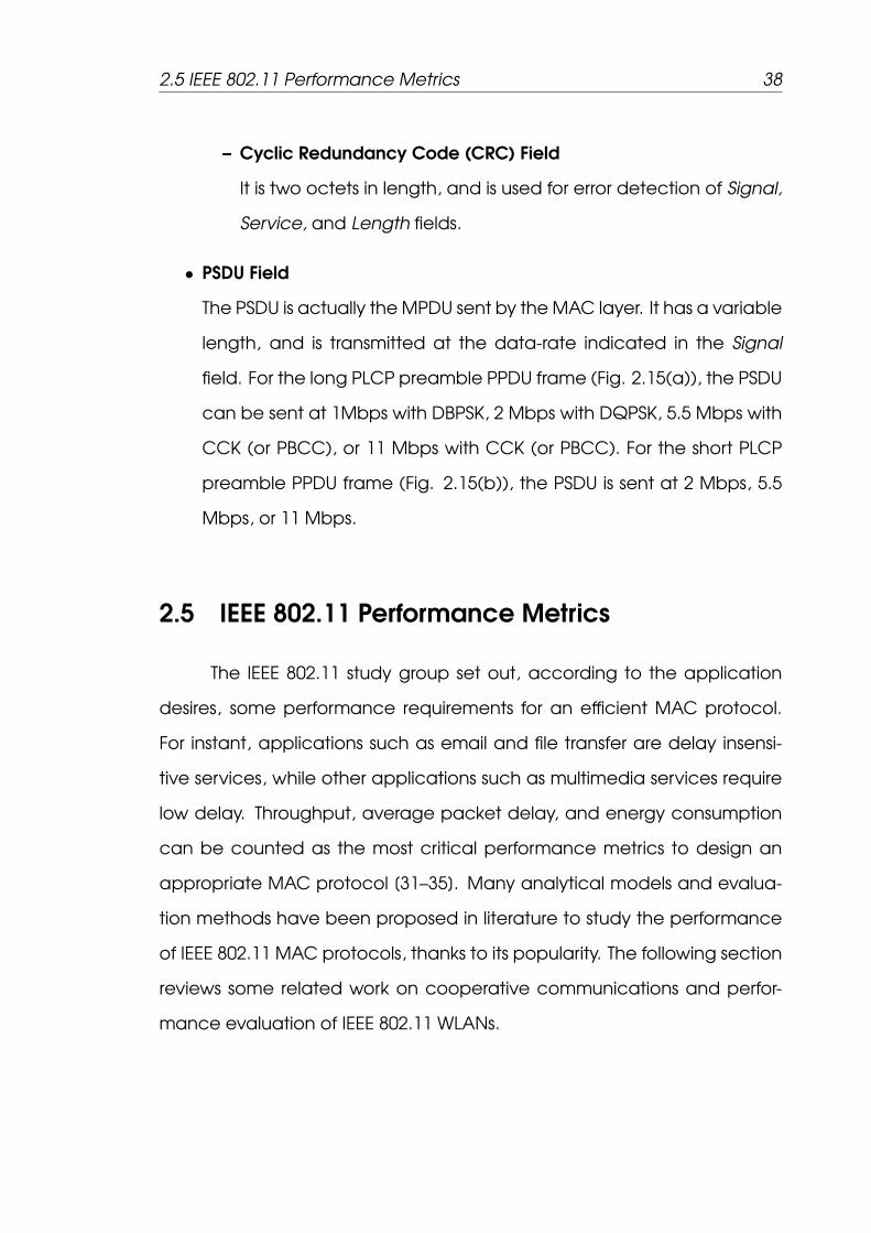
2.5 IEEE 802.11 Performance Metrics 38
– Cyclic Redundancy Code (CRC) Field
It is two octets in length, and is used for error detection of Signal,
Service, and Length fields.
• PSDU Field
The PSDU is actually the MPDU sent by the MAC layer. It has a variable
length, and is transmitted at the data-rate indicated in the Signal
field. For the long PLCP preamble PPDU frame (Fig. 2.15(a)), the PSDU
can be sent at 1Mbps with DBPSK, 2 Mbps with DQPSK, 5.5 Mbps with
CCK (or PBCC), or 11 Mbps with CCK (or PBCC). For the short PLCP
preamble PPDU frame (Fig. 2.15(b)), the PSDU is sent at 2 Mbps, 5.5
Mbps, or 11 Mbps.
2.5 IEEE 802.11 Performance Metrics
The IEEE 802.11 study group set out, according to the application
desires, some performance requirements for an efficient MAC protocol.
For instant, applications such as email and file transfer are delay insensi-
tive services, while other applications such as multimedia services require
low delay. Throughput, average packet delay, and energy consumption
can be counted as the most critical performance metrics to design an
appropriate MAC protocol [31–35]. Many analytical models and evalua-
tion methods have been proposed in literature to study the performance
of IEEE 802.11 MAC protocols, thanks to its popularity. The following section
reviews some related work on cooperative communications and perfor-
mance evaluation of IEEE 802.11 WLANs.
2.6 Related Work 39
2.6 Related Work
Heusse et al [4] showed that the IEEE 802.11 causes a performance
anomaly when in the same BSS exist stations with different data-rates due
to the channel conditions. In this case, the low data rate station reduces
the overall performance of the network below the level of the lower rate.
This is because, comparing to a high data rate stations, the low data-rate
stations will occupy the shared communication channel for a longer pe-
riod for transmitting a fixed-size packet to the AP, thus reducing the channel
efficiency and overall system performance.
This adverse performance can be mitigated by allowing both the
low and high data-rate stations to occupy the shared wireless medium
for the same time interval. Several research works have been proposed to
tackle this issue in different ways, with solutions at different levels of the pro-
tocols stack. Consequently, we review the most related researches, that
try to solve the performance anomaly by introducing minimum modifica-
tions in the MAC layer of the IEEE 802.11 standards.
The concept of cooperative communication has been proposed to
improve link capacity, transmission reliability and network coverage in mul-
tiuser wireless communication networks. Different from conventional point-
to-point and point-to-multipoint communications, cooperative communi-
cation allows multiple users or stations in a wireless network to coordinate
their packet transmissions and share each other’s resources, thus achiev-
ing cooperative diversity or user cooperative diversity [36–43]. Despite of
the extensive research is proposed for the physical layer of cooperative
communications [44], a small number of papers [45–52] considers the MAC
layer.
Wong et al [45] proposed a Relay-based Adaptive Auto Rate
2.6 Related Work 40
(RAAR) protocol using central control at the AP to select relay nodes. The
RAAR also employs a two-hop transmission through a suitable relay node.
The transmission rate is dynamically adjusted according to the channel
quality. The RAAR allows for transmission of multiple back to back (i.e. frag-
mentation) from the sender to the AP through the selected relay node and
hence affects the long term channel access fairness of the MAC.
Zhu et al [46] presented the relay-enabled Point Coordination Func-
tion (rPCF) MAC protocol. The rPCF exploits the physical multi-rate capabil-
ity allowing a low data-rate station to employ a neighbouring station as a
relay to forward its information to the AP. In rPCF, each mobile node reports
the sensed channel condition to the AP. Based on the collected informa-
tion, the AP decides and notifies the node at which rates to apply relay
through the polling packet. When the link from the sender and the AP sup-
ports a low data-rate, whereas the sender-relay link and the relay-AP link
can support a high transmission data-rate, the sender sends to the relay
instead of sending to the AP. The AP estimates the channel conditions be-
tween itself and each station, and notifies the stations which data-rate to
employ and whether to employ a relay station. This relay-type cooperative
communication can effectively improve network coverage, transmission
data rate and reliability, and system throughput in WLANs. The rPCF is cen-
tralised where the AP is responsible to establish the two-hop transmission.
In addition, the rPCF is designed to work in the PCF mode which is rarely
used due to implementation complexity.
Zhu et al [47, 48] and Panwar [49, 50] proposed independently two
similar protocols called relay-enabled Distributed Coordination Function
(rDCF) and Cooperative MAC (CoopMAC) protocols, respectively. These
two protocols are based on the IEEE 802.11 DCF mode which is the funda-
2.6 Related Work 41
mental transmission mode instead of the PCF mode in the rPCF protocol.
The rDCF and CoopMAC work in a distributed manner, since each station
contains a table of the potential relay nodes that can be used to forward
its information to the AP through a two-hop transmission. The rDCF enables
packet relaying in the ad hoc mode of 802.11 systems by requesting each
station to broadcast the rate information between stations explicitly. The
CoopMAC is applied in the infrastructure mode, and chooses the best
relay station to realize high rate two-hop transmissions, and then the over-
all system throughput can be improved. Later, the CoopMAC protocol
is implemented in a testbed and evaluated through experiments [53, 54].
CoopMAC and rDCF change is not fully compatible with the standard IEEE
802.11 protocols by introducing many changes in the IEEE 802.11 protocol.
In addition, CoopMAC and rDCF only achieve cooperative diversity gain
through two-hop transmission.
Chou et al [51] presented another MAC protocol to provide co-
operative communication in distributed manner. In order to select the
relay node among its neighbors, The proposed protocol employs a re-
lay selection with relay collision avoidance and three way handshaking
mechanism. The MAC performance metrics such as throughput, energy
efficiency, and service delay are not considered in the analysis.
Wang et al [52] presented a distributed cooperative MAC protocol
for multi-hop wireless networks based on the IEEE 802.11 DCF mode. The
relay selection criteria of this protocol is different from the rDCF and Coop-
MAC protocols. The relay selection in both rDCF and CoopMAC is selected
by the sender via a table of the potential relay stations, while the proto-
col in [52] employs a similar selection criteria as in [55]. The neighbouring
stations of the sender and destination monitor the channel conditions to-

2.6 Related Work 42
ward them through the received RTS and CTS packets. If the two-hop tra-
nsmission is better than the direct transmission, every willing station sends
out a busy tone followed by a random backoff period before sending a
Ready-To-Help (RTH) packet. If there is no collision between the compet-
ing relay stations, the sender transmits its information to the destination
through the relay station. Therefore, the two-hop transmission is initiated
by the relay node itself no by the sender or the destination, and then there
is no relay table as in the rDCF and CoopMAC protocols. The collision be-
tween relay station can cause a severe performance degradation. Con-
sequently, minimising the collision relay probability is still an open research
point.
Since bandwidth is a scarce resource in wireless networks, through-
put is then considered the most critical metric in the design of an appro-
priate MAC protocol. In order to enhance the bandwidth utilisation, it is
important to study the IEEE 802.11 throughput. There have been many
performance studies for the IEEE 802.11 standards. Binachi in his seminal
work [26–28] presents a Markov channel model to calculate the saturation
throughput of the IEEE 802.11 protocol assuming ideal channel conditions
and infinite number of retransmissions.
Ziouva et al [56], Xiao [57], and Ergen et al [58] extend the Bianchi’s
model taking into account the backoff counter suspension during a busy
wireless medium. However, it is assumed in [56] that there is no post-
backoff stage; this assumption is not compatible with the IEEE 802.11 stan-
dard. Wu et al [59] modifies Bianchi’s model through incorporating the
maximum number of retransmissions. The above mentioned analysis as-
sume ideal channel condition. Saturated throughput analysis in presence
of imperfect channel conditions is investigated in [56,60–66].

2.6 Related Work 43
The throughput analysis, in [67–77], has been shifted to the IEEE
802.11 WLANs under finite traffic conditions by extending the Markov chain
model proposed by Bianchi [27]. The performance analysis of the IEEE
802.11 taking into considerations the effect of the backoff window size is in-
vestigated in [78–84]. This analysis only considers a single-hop transmission
and do not consider the multi-rate capability supported by the IEEE 802.11
standards.
Delay is an important performance metric in the design an efficient
MAC protocol given that the IEEE 802.11 standards are applied not only
for asynchronous data service (i.e. best effort service), but also applied
for time-bounded multimedia applications such as voice and video. Con-
cerning the delay analysis of the IEEE 802.11, there is a lot of research in
modeling and studying delay performance [56, 85–98]. The delay analy-
sis mention above only considers a single-hop transmission, ideal channel
conditions, and do not consider the multi-rate capability supported by the
IEEE 802.11 standards.
The wireless clients are designed to be portable and/or mobile and
have limited battery power. The wireless clients must be designed to be
energy efficient. Therefore, energy efficiency is one of the important IEEE
802.11 parameters. Modeling the energy efficiency, in [99–110], can pro-
vide insights into the metrics that can improve the energy efficiency of the
IEEE 802.11-based networks. The energy efficeincy analysis mention above
only considers a single-hop transmission and do not consider the multi-rate
capability supported by the IEEE 802.11 standards.
The support of differentiated QoS has become one of the critical
requirements of the WLANs. The IEEE 802.11e [8] is then the solution of
the IEEE 802.11 study group to provide the required QoS for some applica-
2.6 Related Work 44
tions such as voice and video. There have been several theoretical studies
developed to address the problem of modeling and optimising the perfor-
mance of the IEEE 802.11e standards.
In [111–114], Bianchi’s model [28] is modified to analyse the En-
hanced Distributed Coordination Function (EDCF). The EDCF is the fun-
damental access method in the IEEE 802.11e [8]. In [115–117], the per-
formance of the IEEE 802.11e [8] is provided via simulations. The EDCF is
classified into three different kinds [118]: backoff, IFS, and hybrid priority
schemes. Readers may refer to [119–129] for the EDCF priority models. The
analysis of the IEEE 802.11e is applied for single-hop transmission and single
data rate. This assumption is not valid for the IEEE 802.11e standards.
IEEE 802.11 standards such as the IEEE 802.11a/b/g/n provide multi-
rate transmission capabilities. Consequently, design of a new MAC pro-
tocols taking into account this feature is required to achieve high perfor-
mance. There is a lot of research to design a MAC protocol, in [130–136],
considering the multi-rate capability provided by the IEEE 802.11 stan-
dards.
Kamerman et al [130] proposed the Auto Rate Fallback (ARF) proto-
col, in which the sending station increases the transmission rate after con-
secutive transmission successes and decreases its rate after transmission
failure. ARF does not work well when the channel condition becomes un-
stable.
Holland et al [131], designed the Receiver Based Auto Rate (RBAR)
protocol. The RBAR is different from the ARF protocol, since the receiver
measures the channel quality and feedbacks its to the sender. The RBAR
is then more accurate than the ARF protocol. Qiao et al [132, 133] investi-
gated that the link adaptation based on dynamic packet fragmentation

2.7 Summary 45
is efficient to enhance the performance of the IEEE 802.11a [6] WLANs.
Lung at el in [134], designed a protocol in which the transmission rate
of each packet is selected dynamically based on the estimated Signal
to Noise Ratio (SNR) of the pervious either received or transmitted frame.
Later, Sadeghi et al [135,136] proposed the Opportunistic Auto Rate (OAR)
protocol. In the OAR, the sending stations transmit multiple back-to-back
packets (i.e. packet fragmentation) to the receiving station whenever ac-
cess the medium. The OAR is better than the RBAR when the channel
quality is good between the sender and receiver. Other research studies
that consider the multi-rate capability to design of an efficient MAC pro-
tocol can be found in [137–141].
2.7 Summary
The IEEE 802.11 WLANs standards have been globally accepted and
adopted to provide wireless broadband access services in university cam-
pus, office, home and city hotspot areas. In this chapter, the concepts
behind the IEEE 802.11 standards that are used in WLANs are introduced.
The aim of these standards is to provide better performance and to extend
the coverage area of the WLANs. The most well known IEEE 802.11 stan-
dards are 802.11b, 802.11a, IEEE 802.11g, IEEE 802.11e, and IEEE 802.11n.
The IEEE 802.11a/.11g/.11b standards provide a best effort service, while
the IEEE 802.11e/.11n standards provide mechanisms to guarantee QoS
transmission. The IEEE 802.11 consists of two layers which are the MAC and
PHY layers. Except the IEEE 802.11n, the other IEEE 802.11 standards have
the same MAC layer with a different PHY layer. There are two MAC tra-
nsmission schemes in the IEEE 802.11 networks called the DCF and PCF.

2.7 Summary 46
The DCF is the fundamental access method, and provides a
contention-based service for delay insensitive traffic. The DCF employs the
CSMA/CA algorithm that requires each station listen to the channel before
transmission, and uses the BEB algorithm that can decrease the collision
probability. The DCF defines two modes for frame transmission over the
wireless medium. These modes are the basic access and RTS/CTS access
which is an optional scheme.
There are two unique problems in the WLANs called the hidden node
and exposed node problems. The hidden node is the node which is out
of sending node range, but in the receiving node range. The RTS/CTS
scheme is used to solve the hidden node problem that can occur in the
network and hence decreases the collision probability. On the other hand,
the exposed node is the node that is in the sending node range, but out of
the receiving node range. The exposed node problem occurs only in the
ad hoc network structure, and there is currently no solution to this problem.
The hidden and exposed node problems cause a reduction in the network
performance.
The PCF is an optional scheme that provides a contention free ser-
vice for delay sensitive traffic. The PCF is used only in the infrastructure
network configuration. The PCF uses a Point Coordinator (PC) existing in
the AP to control the transmission of the stations. The PCF is not widely
employed due to implementation complexity.
The function of the IEEE 802.11 PHY is to provide carrier sense, tra-
nsmission, and reception on the wireless medium. The IEEE 802.11 stan-
dards support different PHYs. The original IEEE 802.11 standard provide
three PHYs which are 2.4 GHz band with DSSS technique, 2.4 GHz band
with FHSS, and IR. The IEEE 802.11b is based on the DSSS and 2.4 GHz band.
2.7 Summary 47
The IEEE 802.11a/g/n are based on the OFDM scheme. The IEEE 802.11g
operates in the 2.4 GHz band, the IEEE 802.11a operates in 5 GHz band,
and the IEEE 802.11n operates in either 2.4 GHz or 5 GHz band.
Throughput, Delay, and energy efficiency are counted as the most
critical requirements to design an efficient MAC protocol in the IEEE 802.11
standards. This is due to the bandwidth limitations in wireless networks,
the increasing demand to support multimedia applications with guaran-
teed QoS, and the fact that wireless devices are typically portable and
have limited battery power. Therefore, modeling and analysing of these
requirements can provide insights into the metrics that can improve the
energy efficiency of the IEEE 802.11-based networks.
According to the IEEE 802.11 standards, WLANs can support multiple
transmission data rates depending on the instantaneous channel condi-
tion between the sender and the receiver. To achieve the target Packet
Error Rate (PER) in data transmission, the sender transmits its packets to the
receiver at a low date rate when the channel quality is poor. In this case,
the low data rate station reduces the overall performance of the network
below the level of the lower rate.
This adverse performance can be mitigated by using the concept of
cooperative communications at the MAC layer. The sender node can use
a neighboring node, called a relay, which has high-quality communica-
tion channels to both the sender and the receiver, to transmit its packets
to the latter at much higher data rate. This relay-type cooperative com-
munication can effectively improve network coverage, transmission data
rate and reliability, and system throughput in WLANs.
Chapter 3
BTAC: A Busy Tone Based
Cooperative MAC Protocol
Cooperative communications is the concept of engaging multiple
stations/nodes in a wireless network to share their resources and achieve
multi-user/spatial diversity gain. This gain is achieved through distributed
but cooperative transmissions, thus improving overall system performance
under dynamic wireless channel conditions. Many novel cooperative al-
gorithms and analytical models have been introduced in the literature for
the physical layer [36–43], Medium Access Control (MAC) layer [45–52], or
across multiple layers [142, 143]. Based on the cooperative communica-
tions concept, this chapter proposes and analyses a Busy Tone based co-
operative MAC protocol, namely BTAC, for multi-rate Wireless Local Area
Networks (WLANs). A cross-layer Markov chain model is then developed to
evaluate the performance of BTAC under dynamic wireless channel con-
ditions. Analytical and simulation results show that the BTAC protocol is
simple, robust, and fully compatible with the IEEE 802.11b standard [5].

3.1 The BTAC Protocol 49
Along with improvements in system throughput, BTAC can also achieve
better energy efficiency and media access delay than the standard Dis-
tributed Coordination Function (DCF) protocol and the recently proposed
CoopMAC protocol [50].
The remainder of the chapter is organised as follows. In Section 3.1,
the proposed BTAC protocol is described in detail and compared with the
IEEE 802.11b standard to show its compatibility with the latter. A cross-layer
analytical approach is developed in Section 3.3 to evaluate the perfor-
mance of BTAC in terms of throughput, energy efficiency, and service de-
lay. Section 3.4 presents and discusses the analytical and simulation results
for BTAC under different wireless channel conditions. Finally, conclusions
are presented in Section 3.5.
3.1 The BTAC Protocol
3.1.1 System Model
This research considers a typical IEEE 802.11b WLAN as can be seen
in Fig. 3.1, consisting of an Access Point (AP) at the center of the net-
work and N contending stations/nodes that are uniformly distributed in
four data-rate zones. It is assumed that a single physical channel is avail-
able for transmissions, and the channel is symmetric between the trans-
mitter and the receiver. Each node supports four different data-rates
R1 = 11 Mbps, R2 = 5.5 Mbps, R3 = 2 Mbps, and R4 = 1 Mbps, and maxi-
mum transmission ranges r1 < r2 < r3 < r4, respectively. The nodes in zone
I (0 ≤ r < r1) and zone II (r1 ≤ r < r2) are defined as the high data-rate
nodes, e.g. nodes A and B in Fig. 3.1, which can act as source and relay

3.1 The BTAC Protocol 50
Figure 3.1: Multi-rate IEEE 802.11b WLAN.
nodes and always communicate directly with the AP; while those in zone
III (r2 ≤ r < r3) and zone IV (r3 ≤ r < r4) are low data-rate nodes, e.g.
nodes C-F, which can only act as source nodes and each of them needs
a high data-rate relay station to improve its communication performance
with the AP. As described later, the low data-rate nodes continuously re-
evaluate their high data-rate neighbouring nodes in a distributed manner,
so as to select the best (in terms of effective throughput) potential relay
node.
3.1.2 Relay Selection Algorithm
The task of a relay selection algorithm is to find a relay node that pro-
vides the best end-to-end communication path between a source node
and its destination (the AP1). However, the selection criteria that operate
in a distributed manner and introduce a minimum overhead in terms of
complexity and delay are preferable. To achieve these requirements, in
1we consider only the infrastructure mode in this work.

3.1 The BTAC Protocol 51
the same way to existing work [47, 48, 50], each node maintains an up-
to-date list, named a Relay list of the high data-rate neighbouring (relay)
nodes. Each row in the list consists of five fields which are MAC identifier
(ID), i.e. MAC address, Rsr, Rrd, GR, and success rate of one potential relay
node. The two fields Rsr and Rrd stand for the data-rate between source
and relay, and data-rate between relay and AP, respectively. GR in equa-
tion (3.1) stands for the rate gain and is defined as the ratio between the
composite data-rate of a two-hop transmission to the data-rate of a direct
transmission rate, which is Rsd. The composite data-rate RC is calculated
by RC =1
1Rsr
+ 1Rrd
. A relay node is added to the Relay list when the two-
hop data transmission (via the relay) is more efficient than the direct data
transmission between the source node and the AP.
GR =RC
Rsd
% =RsrRrd
Rsd(Rsr +Rrd)% (3.1)
Each node creates and updates the Relay list by passively listen-
ing to all ongoing transmissions, e.g. Request-To-Send (RTS), Clear-To-Send
(CTS), acknowledgement (ACK), and data packets. Each node then de-
codes the control packets (i.e., RTS, CTS, and ACK), and the header of
the data packets to acquire the channel reservation information and re-
ceive the packets intended for itself. These packets are sent at the maxi-
mum power and at the base rate (e.g. 1 Mbps for 802.11b and 6Mbps for
802.11a/g). Considering a symmetric wireless channel condition in this re-
search, Rsd and Rsr can be estimated from the signal strengths of CTS/ACK
and RTS packets, respectively. Rrd can be extracted from the Physical
Layer Convergence Procedure (PLCP) header in a potential relay node’s
transmitted data packets. For example, node-E in Fig. 3.1 overhears a RTS
3.1 The BTAC Protocol 52
packet from node-A (which will be the potential relay node) to the AP. It
can calculate the achievable data rate Rsr between itself and node-A
by evaluating the channel quality between them. Upon receiving a CTS
packet from the AP, node-E can derive its feasible transmission data-rate
Rsd to the AP. It also calculates the data-rate Rrd between node-A and
the AP by extracting the piggy-backed transmission rate from the PLCP
header.
The success rate field in the Relay list is calculated as follows:
• Its value for a new added relay node is set to α1%.
• For an existing relay node, the success rate is increased by α2% for
each successful transmission via the selected relay, and decreased
by α2% when the transmission fails.
• The relay node is removed from the Relay list when its success rate is
less than α1%.
• If the GR value of a relay node is changed, the success rate of that
relay is reset to α1% as a new added relay.
• Each time a source node overhears the transmission from the relay
node to the AP, its success rate is increased (or decreased) by α3% for
each successful (or failed) transmission between them.
• A source node selects a relay which has a maximum GR value. When
multiple relay nodes have the same GR value, the one with a high
success rate will be selected to serve the user as a relay.
These percentage α1, α2, and α3 are design parameters optimized
based on the channel conditions and the data packet length. The source
node updates its Relay list for each successful transmission between any

3.1 The BTAC Protocol 53
neighbouring node and the AP. In order to reduce the control overhead,
the length of the Relay list can be limited for example to five entries. In
this way, each low data-rate node maintains an up-to-date list of high
data-rate neighbouring nodes with their IDs, rates (Rsr and Rrd), GR’s , and
success rates. Taking into account the IEEE 802.11b data-rates and the
rate gain in equation 3.1, only the nodes in zones III and IV at the data-
rates 2, 1 Mbps, respectively can benefit form the two-hop transmission
(i.e. GR > 1) when there is a relay node available. However, the nodes
in zone-II at data-rate Rsd = 5.5Mbps or nodes in zone-I at data-rate Rsd =
11Mbps use the standard DCF protocol for the IEEE 802.11b WLANs between
a source node and the AP. Considering backward compatibility with the
standard DCF and the principles given above, the next section describes
the principles of the BTAC protocol.
3.1.3 BTAC Transmission Algorithm
1. The source node sends a Modified RTS (MRTS) packet to the AP and
potential relay node at the base data rate, i.e. 1 Mbps for 802.11b.
2. Upon receiving the MRTS packet, the AP sends a CTS packet to the
source node at rate 1 Mbps. The selected relay node overhears the
CTS packet.
3. IF the selected relay is ready, THEN do the following:
(a) The relay sends a Busy-Tone-Signal (BTS) to both the source and
the AP.
(b) Upon receiving the BTS, the source sends its data packet “DATA-
S” to the relay at a high data-rate Rsr.
3.1 The BTAC Protocol 54
(c) Upon receiving “DATA-S” from the source, the relay forwards
“DATA-S” to the AP at a high data rate Rrd.
4. ELSE (no relay for the source): The source sends its data packet
“DATA-S” to the AP at a low data rate Rsd.
5. Upon successfully receiving “DATA-S”, the AP sends an “ACK” to the
source at rate 1 Mbps.
As shown in Fig. 3.2(b), the proposed Modified MRTS packet has the
same size as the standard RTS packet which in turn is shown in Fig. 3.2(a).
However, the six-byte Transmitter Address (TA) and Receiver Address (RA)
fields in a standard RTS packet are now replaced with TA⊕RA 2 and Helper
Address (HA), respectively. IEEE 802.11 [1] defines two fields: type and sub-
type fields in the frame control of the MAC header as shown in Fig. 3.2(c).
The type and subtype fields together identify the function of the frame.
There are three frame types: control, data, and management. The type
field value 01 is used for control frames (e.g., RTS, CTS, and ACK) and val-
ues from 0000 to 1001 of the subtype field are reserved. For example, in a
regular RTS, the type field value is 01 and the subtype field value is 1011.
To enable the AP and all the nodes in the network to recognise the new
MRTS packet, the same value of the type field of RTS packet is used but
the value 1001 is set in the subtype field. Thereby, each node in a Basic
Service Set (BSS) will be able to identify the MRTS packet in which the TA
field is bitwise XOR between the address of the source node and the ad-
dress of the AP. The duration field in both the MRTS and the RTS packet
provides the neighbours of the source node with the information required
to update their Network Allocation Vector (NAV) as explained later.
2The sign ⊕ represents bitwise XOR operation.
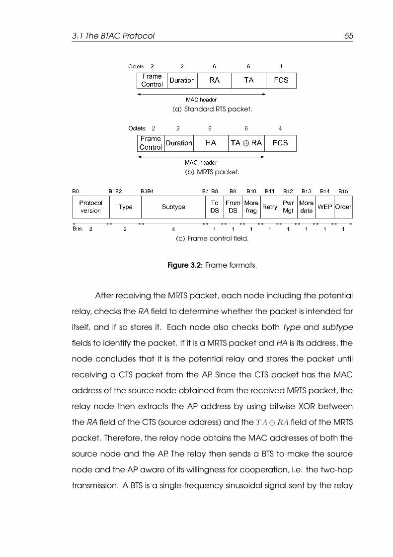
3.1 The BTAC Protocol 55
(a) Standard RTS packet.
(b) MRTS packet.
(c) Frame control field.
Figure 3.2: Frame formats.
After receiving the MRTS packet, each node including the potential
relay, checks the RA field to determine whether the packet is intended for
itself, and if so stores it. Each node also checks both type and subtype
fields to identify the packet. If it is a MRTS packet and HA is its address, the
node concludes that it is the potential relay and stores the packet until
receiving a CTS packet from the AP. Since the CTS packet has the MAC
address of the source node obtained from the received MRTS packet, the
relay node then extracts the AP address by using bitwise XOR between
the RA field of the CTS (source address) and the TA⊕RA field of the MRTS
packet. Therefore, the relay node obtains the MAC addresses of both the
source node and the AP. The relay then sends a BTS to make the source
node and the AP aware of its willingness for cooperation, i.e. the two-hop
transmission. A BTS is a single-frequency sinusoidal signal sent by the relay

3.1 The BTAC Protocol 56
node to both the AP and the source node at the same time. The duration
of a BTS is one or two slot times (e.g. 20 µs for 802.11b).
The AP also checks the type and subtype fields of the MRTS packet.
It uses its own address to execute the XOR operation with the “TA ⊕ RA”
field to obtain the TA, and sends a CTS packet back to the source node.
In this case, the AP can identify both the TA of the sender (source node)
and RA of its selected relay. Upon receiving a CTS packet, the neighbours
of the AP update their NAV by extracting the duration field information
available in a CTS packet.
After receiving both the CTS and the BTS from the AP and the relay
node, respectively, the source node updates its Relay list. The source node
calculates the data-rate Rsd and Rsr by estimating the Signal to Noise Ra-
tion (SNR) of both the CTS packet and the BTS, respectively. It then sends
its data packet (DATA-S) to the relay node at data-rate Rsr. If DATA-S is
received correctly, the relay node forwards DATA-S to the AP at data-rate
Rsr. The AP sends an ACK packet to the source node after receiving DATA-
S from the relay node to the AP.
The basic operation of BTAC protocol is illustrated in Fig. 3.3. This
handshake procedure of control packets, MRTS, CTS and BTS, is shown in
Fig. 3.3(a) and the data packets transmission from the source and relay
nodes to the AP is shown in Fig. 3.3(b).
3.1.4 Network Allocation Vector Setting
Fig. 3.4(a) shows the NAV setting of successfully transmitting a data
packet "DATA-S" via a selected relay node under the BTAC protocol. Sim-
ilarly to the standard IEEE 802.11b WLAN, two control packets, MRTS and
CTS, are used in BTAC to set the Network Allocation Vector (NAV), which

3.1 The BTAC Protocol 57
1
1
MRTS
MRTS
CTS
2
CTS2
3 3BTS
BTS
Relay
Source
AP
(a) Control packets handshake.
Source
4
DATA-S@
R sr
CTS
6
DATA-S@
Rrd
5
6
BTS
Relay
AP
(b) Data packets transmission.
Figure 3.3: Access mechanism of BTAC protocol.

3.1 The BTAC Protocol 58
stores the channel reservation information. This method can effectively
avoid the ”hidden relay node” problem which is explained later. The du-
ration field in a MRTS packet shown in Fig. 3.2(b), denoted by DMRTS, is
computed as follows:
DMRTS = TCTS +8Ls
Rsd
+8LPLCP
Rb
+ TACK + 5TSIFS + 6δ (3.2)
where TCTS, TACK , and TSIFS stand for the time duration for the CTS
packet, ACK packet, and the Short Inter-Frame Space (SIFS), respectively.
The data packet size is Ls octets and the PLCP header length, explained in
[Chapter 2, Section 2.4.2], is LPLCP octets. Rb and δ are the basic data-rate
and channel propagation delay, respectively. After receiving a MRTS, the
AP sends a CTS back to the source node after SIFS interval. The duration
field DCTS of a CTS packet is expressed as follows:
DCTS = DMRTS − (TCTS + TSIFS + δ) (3.3)
After exchanging both the MRTS and the CTS packets between a
source node and the AP, the communication channel is successfully re-
served. The selected relay node, which has overheard both the MRTS and
the CTS packets, transmits a one-time slot BTS signal to indicate its readi-
ness for relaying data packets. The source node then sends its data packet
“DATA-S” to the relay at a high data-rate Rsr. The duration field Ddata1 of
DATA-S (source-relay) is computed as follows:
Ddata1 =8Ls
Rrd
+8LPLCP
Rb
+ TACK + 2TSIFS + 2δ (3.4)

3.1 The BTAC Protocol 59
(a) NAV for BTAC-Relay available.
(b) NAV for BTAC-Relay not available.
Figure 3.4: NAV setting in BTAC.

3.1 The BTAC Protocol 60
The relay node forwards the DATA-S packet to the AP at a data-rate
Rrd. The duration field Ddata2 of the DATA-S (relay-AP) is the sum of the time
required to transmit the ACK packet plus one SIFS interval and the prop-
agation delay δ. The AP replies with an ACK packet when “DATA-S” from
the relay is correctly received. The duration field of the ACK is set to zero.
If the source node does not receive the BTS, it sends its “DATA-S” directly
to the AP at a low data rate Rsd as shown in Fig. 3.4(b). The duration field
of the DATA-S (source-AP) is the duration field of the immediately preced-
ing CTS packet given in equation (3.3) minus the time required to transmit
the DATA-S packet and one SIFS interval and propagation delay δ. If the
source node does not receive the CTS packet or the ACK packet from the
AP, it starts a new cycle of transmission after applying a Binary Exponential
Backoff algorithm (BEB) as in IEEE 802.11b [5].
3.1.5 The Hidden Relay Node Problem
In the CoopMAC protocol [50], the source node first sends a RTS
packet, a neighbouring relay node responds with a Helper- ready To Send
(HTS) packet, and then the AP sends a CTS packet to reserve the channel
for the upcoming data transmission. As some nodes cannot hear the on-
going packet transmission from the source and relay nodes, they may send
a RTS packet to the AP at the same time and cause a collision with the HTS
packet. This is defined as the “Hidden Relay Node Problem”. A packet col-
lision directly affects the channel reservation procedure and leads to the
failure of establishing a two-hop communication path with the relay node,
thus causing serious delays in the channel access and packet transmission.
As described in Section 3.1, in the BTAC protocol, the potential relay
responds with a BTS signal after receiving a MRTS packet from the source

3.2 Enhanced BTAC (EBTAC) Protocol 61
node and a CTS packet from the AP, i.e. after the channel reservation
procedure is completed. All the nodes in the network can hear the AP’s
CTS packet and will then defer their packet transmission requests, if any.
As a result, the BTS from the relay is guaranteed no collision and the two-
hop communication path will be successfully established after the BTS is
received by the source node and the AP. Therefore, the BTAC protocol
completely solves the “Hidden Relay Node Problem” and effectively en-
ables cooperative relay communication in WLANs.
3.2 Enhanced BTAC (EBTAC) Protocol
The dynamic channel condition may have significant impacts on
the performance of BTAC. In order to mitigate the impacts of dynamic
channel conditions, it is desirable to adaptively decide when to use two-
hop transmission according to the channel conditions. We design a heuris-
tically algorithm named Enhanced BTAC (EBTAC) which considers the dy-
namic nature of the wireless channel and bandwidth utilization.
EBTAC is intended to further improve the performance of the BTAC
protocol described in Section 3.1. However, performance of EBTAC is not
considered in this work. It is required to test EBTAC experimentally taking
into account the physical channel condition, and this beyond the scope
of this research.
In EBTAC, a new carrier sense mechanism is employed as shown in
Fig. 3.5. The source node sends a MRTS packet in which the duration field
carries the duration of the CTS packet and the BTS signal. After receiving
both the CTS and BTS, the source node calculates the data rates Rsr and
Rrd. The source node then sends its data packet (DATA-S) to the relay node
3.2 Enhanced BTAC (EBTAC) Protocol 62
with the actual transmission time in the duration field of the data packet.
In this way, the nodes within the transmission range of the source node
defer medium access for the exact transmission time. The source node
drops the data packet from its buffer after receiving DATA-S from the relay
to the AP. The DATA-S then works as an indirect ACK from the relay node to
the source node of receiving the data packet correctly. In this case, the
source node does not require to wait for receiving an ACK from the AP.
Similarly to the Receiver-Based Auto Rate (RBAR) scheme [131], the
AP after receiving the MRTS packet from the source node, estimates the
channel quality between itself and the source node and then calculates
the appropriate direct transmission data-rate Rsd. Following this the AP
sends a CTS packet, shown in Fig. 3.6(b), with a new field Rsd added,
which contains the data-rate between the source node and the AP. The
Rsd is a two bit field and uses encoding similar to the rate field in the PLCP
header in the IEEE 802.11a [6]. This method measures the Signal to Noise
Ratio (SNR) at the receiver at the time instant just before the data packet
transmission. Therefore, it is more accurate than adapting the transmission
rate based on the history of preceding transmission.
The neighbours of the AP extract the duration field information from
the received CTS packet to update their NAV. The AP uses the maximum
data packet length Lmax (e.g. 2312 octets for 802.11b) because the AP
has no sufficient information about the actual data packet length. These
settings will be cancelled after receiving the ACK packet with a zero dura-
tion field. After receiving DATA-S (relay-AP), the AP sends an ACK packet
back to the relay node to confirm correct receipt of the data packet. All
the nodes in the network start a new transmission cycle after receiving the
ACK from the AP.

3.2 Enhanced BTAC (EBTAC) Protocol 63
(a) NAV for EBTAC-Relay available.
(b) NAV for EBTAC-Relay not available.
Figure 3.5: NAV setting in EBTAC.

3.2 Enhanced BTAC (EBTAC) Protocol 64
(a) 802.11 CTS packet.
(b) EBTAC CTS packet.
Figure 3.6: Frame formats.
After receiving both the MRTS and CTS packets, the relay node es-
timates the channel quality and calculates the data-rate Rsr and Rrd be-
tween itself and both the source node and the AP, respectively. The relay
node also extracts data-rate Rsd (between the source and the AP) from
the received CTS packet. The relay node then sends a BTS if the two-hop
transmission is faster than the single-hop transmission. Otherwise, the re-
lay node updates its NAV by the reservation information available within
the duration field of the CTS packet. Therefore, this method can mitigate
frequent changes in the channel conditions and hence improve the per-
formance of the EBTAC protocol.
The relay node manages an additional queue containing the pack-
ets to be forwarded. This option is available in the IEEE 802.11 [8] stan-
dard. When the relay receives ”DATA-S” from the source node, it stores the
packet in this queue. The relay node forwards the received data packet
to the AP after updating the duration field within ”DATA-S” with the remain-
ing transmission time. The duration field for each packet used in EBTAC is
given in Table. 3.1, where other unlisted packets have zero durations.
On the other hand, if the CTS packet is corrupted at both the source

3.2 Enhanced BTAC (EBTAC) Protocol 65
Packet type The Duration
MRTS TCTS + TBTS + 3TSIFS + 3δ
CTS 8Lmax
Rsd+ 8LPLCP
Rb+ TACK + 2TSIFS + 2δ
DATA-S (source-relay) 8Ls
Rrd+ 8LPLCP
Rb+ TACK + 2TSIFS + 2δ
DATA-S (relay-AP) TACK + TSIFS + δ
DATA-S (source-AP) 8Ls
Rsd+ 8LPLCP
Rb+ TACK + 2TSIFS + 2δ
Table 3.1: EBTAC Duration field contents
Figure 3.7: CTS corruption in EBTAC.
and relay nodes due to imperfect channel condition, the Relay node does
not send a BTS signal. As a result, the source node stops its transmission.
The AP waits a two SIFS interval after sending the CTS packet. As shown
in Fig. 3.7, when there is no activity on the channel during this interval, it
broadcasts a Negative Acknowledgment (NACK) packet with zero dura-
tion field. The frame format of the NACK is similar to the frame format of
the ACK packet with no receiver address. All the nodes then reset their
NAV and start a new transmission cycle after receiving the NACK. There-
fore, the EBTAC protocol improves the bandwidth utilization under imper-
fect channel conditions.
If the CTS packet is corrupted at the source node only, the relay
node sends a BTS to the source node and the AP. The source concludes

3.2 Enhanced BTAC (EBTAC) Protocol 66
Figure 3.8: DATA source to relay corruption in EBTAC.
that the CTS packet is received correctly at the relay node which is ready
to receive the data packet from the source node. As discussed before
the relay node sends the BTS only when the two-hop transmission is faster
than the single-hop transmission. Consequently, the source node sends
the DATA-S packet to the relay node. The relay node forwards the DATA-S
to the AP and waits to receive either an ACK for successful transmission or
NACK for unsuccessful transmission.
If the DATA-S from the source to the relay is corrupted, as shown in
Fig. 3.8, the relay node does not forward this packet to the AP. The AP waits
for a two SIFS interval after receiving the DATA-S (source-relay). If the AP
does not receive the DATA-S packet from the relay node, it immediately
sends NACK to all of the node to start a new transmission cycle. Finally, if
the DATA-S (source-relay) is received correctly, the relay node forwards this
packet after a SIFS interval to the AP which in turn send an ACK packet for
successful transmission or a NACK for unsuccessful transmission.
In the standard IEEE 802.11 and the BTAC protocols, the data packet
header is sent at the base data-rate to allow all nodes in the transmission
range of the sender to decode the header upon reception. The frame
format of data packet under the IEEE 802.11 and BTAC is shown in Fig.
3.9(a). By contrast, the EBTAC follows modifies the data packet header as

3.3 Performance Analysis 67
(a) MAC frame format in BTAC and 802.11 [5].
(b) MAC frame format in rDCF [48] and EBTAC.
Figure 3.9: MAC frame format.
in [47, 48] by sending only frame control, duration, and Frame Check Se-
quence (FCS) fields at the base rate. All neighbours of the sender extract
the duration field and update their NAV values accordingly. The frame
format of a data packet in the EBTAC protocol is shown in Fig. 3.9. Since
the remainder of the header is sent at the same data rate as the frame
body, the data packet header overhead is smaller for the EBTAC than for
the BTAC. Therefore, taking into account the impact of multi-rate trans-
missions, bandwidth utilization, and the imperfect channel conditions due
to a fading, interference and noise, the EBTAC protocol compared to the
BTAC protocol improves the system performance.
3.3 Performance Analysis
In this section an analytical model is presented to study the perfor-
mance of the BTAC protocol under imperfect channel conditions. The per-

3.3 Performance Analysis 68
formance metrics considered in this chapter are the saturated throughput,
energy efficiency, and delay.
3.3.1 Markov Chain Model
The analysis presented in this section is an extension of Bianchi’s
work [27], where b(t) is defined as a random process representing the value
of the backoff counter for a given node at slot time t; while s(t) is a ran-
dom process representing the backoff stage j(j = 0, 1, ...,m) for the same
node at time t. Let Pu,i be the probability that a transmitted packet of
a given node i has failed. The probability Pu,i consists of two parts: the
collision probability Pc,i caused by collisions with transmissions from other
nodes, and the packet error rate probability (PER) Pe,i caused by imper-
fect channel conditions. The probability Pb,i is the probability that the
channel is busy, as sensed by a given node i during the backoff stages.
As in [56, 57], it is assumed that both Pb,i and Pu,i are independent of the
backoff algorithm. The state of a node can be described by {j, k}, where
j is the backoff stage taking values (0, 1, ...,m), and k is the backoff delay
taking values (0, 1, ...,Wj − 1) in time slots. Wj is the current Contention Win-
dow (CW) size, where Wj = 2jW0, CWmax = 2mW0, and m is the maximum
backoff stage.
In contrast to Bianchi’s model [27], Fig. 3.10 illustrates the following
differences:
1. The proposed model considers that the backoff counter is stopped
when the channel becomes busy, as in [56].
2. Fig. 3.10 takes into account the dynamic channel conditions, as in
[63], whereas Bianchi’s model assumes ideal channel conditions.

3.3 Performance Analysis 69
3. The proposed model considers the multi-rate capabilities, as in [144].
Bianchi’s model is applied for a single data-rate channel.
4. A finite retry limit is modeled, as in [59]. Bianchi’s model assumes an
infinite retry limit.
5. In the proposed model, the probability Pb,i, that the channel is sensed
busy and the probability Pu,i, that the packet is unsuccessful because
of collision or corruption are modeled, as in [56,57].
The probabilities Pc,i and Pe,i are assumed to be statistically indepen-
dent [63]. Therefore, the probability Pu,i, that a packet from a given node
i is unsuccessfully transmitted, is calculated as follows:
Pu,i = 1− (1− Pc,i)(1− Pe,i) = Pc,i + (1− Pc,i)Pe,i (3.5)
To analyse this Markov model, the steady state probability for a node
to be in state {j, k} is calculated. Let πj,k = limt→∞Pr{s(t) = j, b(t) = k} be
the stationary probability of the Markov model, and 0 ≤ j ≤ m, 0 ≤ k ≤ Wj−
1. In this Markov chain, the only non-null one step transition probabilities
are
P{j, k|j, k + 1} = 1− Pb,i 0 ≤ k ≤ Wj − 2 0 ≤ j ≤ m
P{j, k|j, k} = Pb,i 1 ≤ k ≤ Wj − 1 0 ≤ j ≤ m
P{0, k|j, 0} =1−Pu,i
W00 ≤ k ≤ W0 − 1 0 ≤ j ≤ m− 1
P{j, k|j − 1, 0} =Pu,i
Wj0 ≤ k ≤ Wj − 1 1 ≤ j ≤ m
P{0, k|m, 0} = 1W0
0 ≤ k ≤ W0 − 1
(3.6)
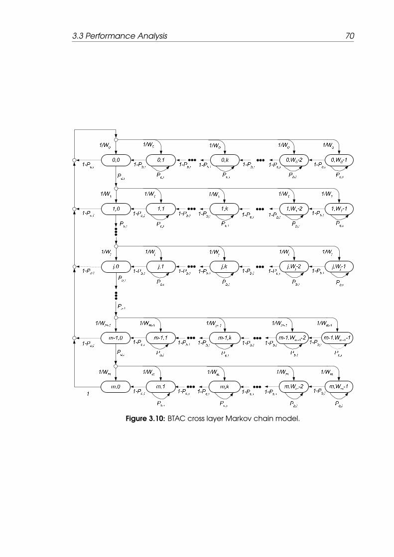
3.3 Performance Analysis 70
Figure 3.10: BTAC cross layer Markov chain model.

3.3 Performance Analysis 71
The first equation in (3.6) is the probability that the backoff counter
reduces by one when the channel becomes idle during a slot time. The
second equation is the probability that at the beginning of each slot time
the backoff counter freezes when the channel is sensed busy. A new back-
off delay of stage j = 0 is selected if the current packet is successfully
transmitted and is given by the third equation in (3.6). The other cases
model the system after unsuccessful transmission. As considered in the
fourth equation in (3.6), if an unsuccessful transmission occurs, the backoff
stage increases. Finally, the fifth equation in (3.6) models the fact that at
the last backoff stage, the CW will be reset when the transmission is unsuc-
cessful or restart the backoff stage for a new packet when the transmission
is successful.
In the steady state, the following equations hold for the Markov
chain illustrated in Fig. 3.10.
πj−1,0 · Pu,i = πj,0, then πj,0 = P ju,i · π0,0 0 ≤ j ≤ m (3.7)
Due to the regularities of the Markov chain, for each 1 ≤ k ≤ Wj − 1, the
probability πj,k is calculated as follows:
πj,k =Wj − k
Wj(1− Pb,i)
(1− Pu,i)
∑m−1x=0 πx,0 + πm,0 j = 0
Pu,iπi−1 0 < j ≤ m
(3.8)
By using (3.7) and using∑m−1
x=0 πx,0 =π0,0(1−Pm
u,i)
1−Pu,i, equation (3.8) can be rewrit-
ten as follows:
πj,k =Wj − k
Wj(1− Pb,i)πj,0 0 ≤ j ≤ m, 1 ≤ k ≤ Wj − 1 (3.9)

3.3 Performance Analysis 72
By using equations (3.7) and (3.9), the following equation is solved
by imposing the normalization condition for a stationary distribution. It is
calculated as follows.
1 =m∑j=0
Wj−1∑k=0
πj,k
=m∑j=0
πj,0
Wj−1∑k=1
Wj − k
Wj(1− Pb,i)+
m∑j=0
πj,0
=m∑j=0
π0,0Pju,i
Wj − 1
2(1− Pb,i)+
1− Pm+1u,i
1− Pu,i
π0,0
=π0,0
(1− Pb,i)
[m∑j=0
P ju,i
2jW0 − 1
2+
(1− Pb,i)(1− Pm+1u,i )
1− Pu,i
](3.10)
The second term between square practice on the R.H.S. is calcu-
lated as follows.
When m ≤ m′
m∑j=0
P ju,i
2jW0 − 1
2=
W0(1− (2Pu,i)m+1)
2(1− 2Pu,i)−
1− Pm+1u,i
2(1− Pu,i)(3.11)
When m > m′
m∑j=0
P ju,i
2jW0 − 1
2=
m′∑j=0
P ju,i
2jW0 − 1
2+
m∑j=m′+1
P ju,i
2m′W0 − 1
2
=W0(1− (2Pu,i)
m′+1)
2(1− 2Pu,i)−
1− Pm′+1u,i
2(1− Pu,i)
+(2m
′W0 − 1)(Pm′+1
u,i − Pm+1u,i )
2(1− Pu,i)(3.12)
By substituting equation (3.11) into equation (3.10) for m ≤ m′, we
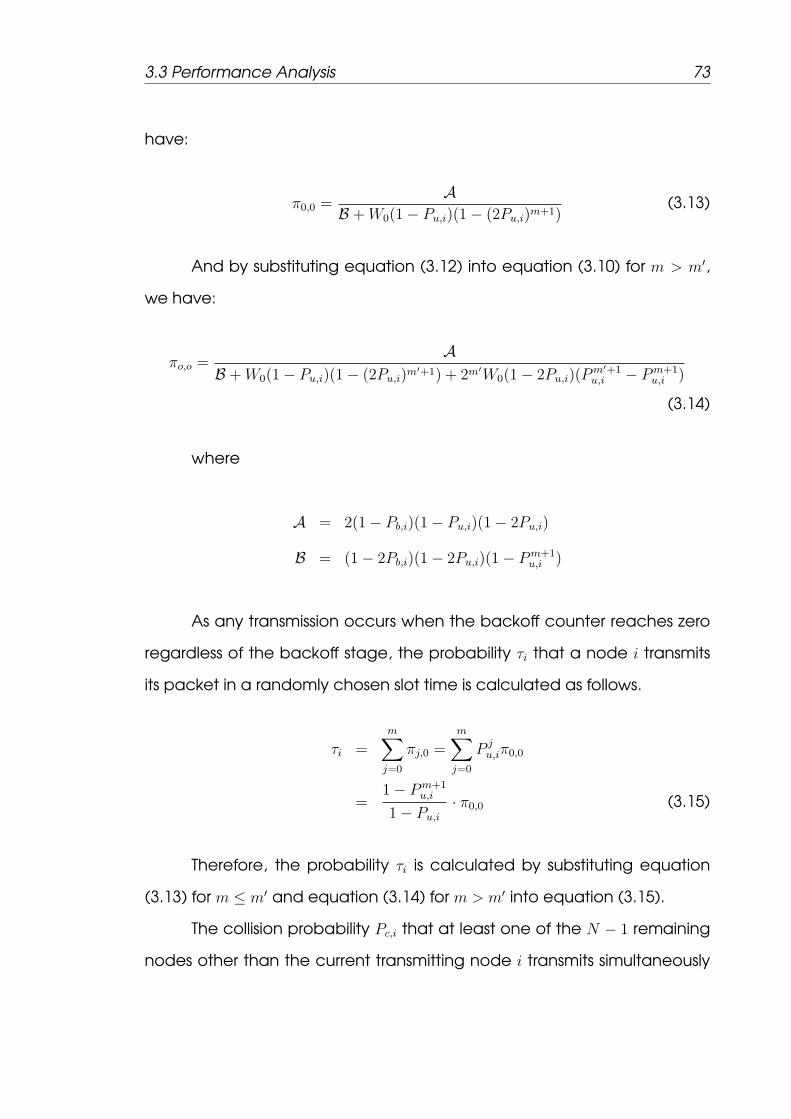
3.3 Performance Analysis 73
have:
π0,0 =A
B +W0(1− Pu,i)(1− (2Pu,i)m+1)(3.13)
And by substituting equation (3.12) into equation (3.10) for m > m′,
we have:
πo,o =A
B +W0(1− Pu,i)(1− (2Pu,i)m′+1) + 2m′W0(1− 2Pu,i)(P
m′+1u,i − Pm+1
u,i )
(3.14)
where
A = 2(1− Pb,i)(1− Pu,i)(1− 2Pu,i)
B = (1− 2Pb,i)(1− 2Pu,i)(1− Pm+1u,i )
As any transmission occurs when the backoff counter reaches zero
regardless of the backoff stage, the probability τi that a node i transmits
its packet in a randomly chosen slot time is calculated as follows.
τi =m∑j=0
πj,0 =m∑j=0
P ju,iπ0,0
=1− Pm+1
u,i
1− Pu,i
· π0,0 (3.15)
Therefore, the probability τi is calculated by substituting equation
(3.13) for m ≤ m′ and equation (3.14) for m > m′ into equation (3.15).
The collision probability Pc,i that at least one of the N − 1 remaining
nodes other than the current transmitting node i transmits simultaneously

3.3 Performance Analysis 74
in a chosen slot time can be expressed as follows.
Pc,i = 1−N∏j=1j =i
(1− τj) (3.16)
The probability Pb,i, that the channel is sensed busy by the given
node i due to the transmissions of the N−1 remaining nodes, is calculated
as follows.
Pb,i = 1−N−1∏j=1j =i
(1− τj) (3.17)
3.3.2 Cross Layer MAC-Channel Model
To calculate the packet error rate probability Pe,i (at node i), a sim-
ple and widely used model called ”Gilbert-Elliot model” [145, 146] is used
to capture the burst behavior of the wireless channel caused by fading.
Albeit this simplified model does not capture all the fading aspects, how-
ever it gives some indications of burst errors caused by deep fading. The
model is shown in Fig. 3.11 and it consists of two states, where one state
represents a good (G) channel condition and the other one represents a
bad (B) channel condition. In the simplest Gilbert model the probability of
packet loss in a good state is assumed to be zero, whereas in a bad state
the packet loss is assumed to be one.
In this model the state sojourn time (duration to be in a state) is a
random variable having a geometric distribution. For a high probability
of staying in one state, the sojourn time of the channel in state G (or B)
is modeled by an exponential distribution with probability density function
(pdf) λge−λgt (or λbe
−λbt); where λg and λb are the transition rate constants

3.3 Performance Analysis 75
Figure 3.11: Gilbert-Elliot channel model.
from state G to state B and from state B to state G, respectively. Hence
the average sojourn times TG and TB in a good state and in a bad state,
respectively are given by:
TG =1
λg
and TB =1
λb
(3.18)
From which the steady state probability, πG, of being in a state G is
calculated as follows:
πG =TG
TG + TB
(3.19)
Similarly, the steady state probability, πB, for being in a state B is
obtained as follows:
πB =TB
TG + TB
(3.20)
Substituting equation (3.18) into equations (3.19) and (3.20), we

3.3 Performance Analysis 76
have:
πG =λb
λg + λb
and πB =λg
λg + λb
(3.21)
Theorem 2.1.1 [147] is used to obtain the stochastic transition matrix
P (t) = (pij(t), i, j ∈ S), where S is the state set. This theorem shows that P(t)
satisfies the set of equations:
P ′(t) = QP (t) and P (0) = I (3.22)
And their solution is:
P (t) = P (0)eQt = eQt =∞∑k=0
(Qt)k
k!(3.23)
where I is the identity matrix and the matrix Q is called infinitesimal
generator, or transition rate matrix of the process and is given by:
Q =
−λg λg
λb −λb
If {X(t) : t ≥ 0} represents the channel state at time t, the transition prob-
abilities for all t, t0 ≥ 0 are given by:
pi,j(t0) = Pr(X(t+ t0) = j | X(t) = i) for all i, j ∈ S
= UTI P (t0)UF = UT
I eQt0UF (3.24)
where UI is the initial probability vector representing the initial distri-

3.3 Performance Analysis 77
bution, and UF is the final probability vector. The UI (or UF ) vector is simply
chosen with ith (or jth) entry equal to 1 and all other entries equal to 0.
When a source node i transmits a MRTS without collision, there are
still five events where the transmission could fail due to corruption. These
events include corruption of the MRTS, CTS, DATA-S from source to relay,
DATA-S from relay to AP, and ACK packets. It is assumed that there is no
BTS corruption, since it is a sinusoidal signal with no information to be cor-
rupted.
The probability v1, that a MRTS is corrupted given that only one MRTS
is transmitted (no collision), is calculated as follows:
v1 = Pr(MRTS corrupted|1 MRTS sent)
= 1− Pr(G state at MRTS start)Pr(G state duration > TMRTS + δ)
= 1− λb
λg + λb
e−λg(TMRTS+δ) (3.25)
where TMRTS = LMRTS
Rbis the duration of a MRTS packet, LMRTS is a
MRTS packet length, Rb is the base data-rate (e.g. 1Mbps in 802.11b), and
δ is the channel propagation delay.
The probability v2, that a CTS packet is corrupted given that a single
MRTS packet is successfully received, is expressed as follows:
v2 = Pr(CTS corrupted | MRTS is correct)
= Pr(B state at CTS start | G state at MRTS end)
+Pr(G state at CTS start and B state before CTS end | G state at MRTS end)
(3.26)
The second term on the R.H.S of equation (3.26) is expressed as fol-

3.3 Performance Analysis 78
lows:
Pr(G state at CTS start and B state before CTS end |G state at MRTS end)
= Pr(G state at CTS start | G state at MRTS end)Pr(G state duration < TCTS + δ)
= Pr(G state at CTS start | G state at MRTS end)(1− eλg(TCTS+δ)
)(3.27)
where TCTS = LCTS
Rbis the duration of a CTS packet, and LCTS is a CTS
packet length. From equations (3.27) and (3.24), we have:
Pr(G state at CTS start | G state at MRTS end) = Pr(X(t+ TSIFS) = G |X(t) = G)
= pgg(TSIFS) = UTI e
QTSIFSUF
(3.28)
where TSIFS is the duration of a SIFS interval, and
UI = UF =
1
0
Substituting equation (3.28) into equation (3.27), we have:
Pr(G state at CTS start and B state before CTS end |G state at MRTS end)
= UTI e
QTSIFSUF
(1− eλg(TCTS+δ)
)(3.29)
Recalling the first term on the R.H.S of equation (3.26), hence we

3.3 Performance Analysis 79
have:
Pr(B state at CTS start | G state at MRTS end) = pbg(TSIFS) = 1− pgg(TSIFS)
= 1− UTI e
QTSIFSUF (3.30)
Substituting equations (3.29) and (3.30) into equation (3.26), we
have:
v2 =(1− UT
I eQTSIFSUF
)+ UT
I eQTSIFSUF
(1− e−λg(TCTS+δ)
)(3.31)
The probability, v3, that a DATA-S packet from the source node to the
relay node is corrupted given that the CTS packet is received correctly, is
calculated as follows:
v3 = Pr(DATA-S corrupted|correct CTS) = Pr(B state at DATA-S start|G state at CTS end)
+Pr(G state at DATA-S start and B state before DATA-S end | G state at CTS end)
(3.32)
where the second term on the R.H.S. of equation (3.32) can be cal-
culated as follows:
Pr(G state at DATA-S start and B state before DATA-S end | G state at CTS end)
= Pr(G state at DATA-S start | G state at CTS end) · Pr(G state duration < TDATA−S + δ)
= Pr(G state at DATA-S start | G state at CTS end)(1− eλg(Tsr+δ)
)(3.33)
where Tsr = Ls
Rsr+ LPLCP
Rbis the duration of a DATA-S packet from the
source node to the relay node, Ls is the data packet length, LPLCP is the

3.3 Performance Analysis 80
PLCP header size, and Rb is the base data rate. Recalling equation (3.24)
and assuming no BTS corruption, we have:
Pr(G state at DATA-S start | G state at CTS end) = Pr(X(t+ T0) = G |X(t) = G)
= pgg(T0) = UTI e
QT0UF (3.34)
where T0 = TBTS + 2TSIFS, and TBTS is the BTS duration. Then substi-
tuting equation (3.34) into (3.33), we have:
Pr(G state at DATA-S start and B state before DATA-S end | G state at CTS end)
= UTI e
QT0UF
(1− eλg(Tsr+δ)
)(3.35)
Recalling the first term on the R.H.S. of equation (3.32), we have:
Pr(B state at DATA-S start | G state at CTS end) = pbg(T0) = 1− pgg(T0)
= 1− UTI e
QT0UF (3.36)
Substituting equations (3.35) and (3.36) into equation (3.32), we
have:
v3 =(1− UT
I eQT0UF
)+ UT
I eQT0UF
(1− e−λg(Tsr+δ)
)(3.37)
Similarly, the probability v4, that the DATA-S packet from the relay
node to the AP is corrupted given that the DATA-S from the source to the
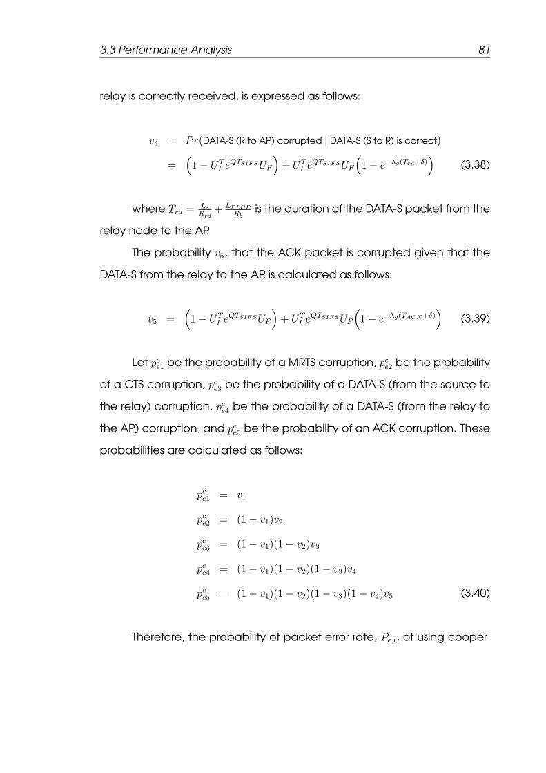
3.3 Performance Analysis 81
relay is correctly received, is expressed as follows:
v4 = Pr(DATA-S (R to AP) corrupted | DATA-S (S to R) is correct)
=(1− UT
I eQTSIFSUF
)+ UT
I eQTSIFSUF
(1− e−λg(Trd+δ)
)(3.38)
where Trd =Ls
Rrd+ LPLCP
Rbis the duration of the DATA-S packet from the
relay node to the AP.
The probability v5, that the ACK packet is corrupted given that the
DATA-S from the relay to the AP, is calculated as follows:
v5 =(1− UT
I eQTSIFSUF
)+ UT
I eQTSIFSUF
(1− e−λg(TACK+δ)
)(3.39)
Let pce1 be the probability of a MRTS corruption, pce2 be the probability
of a CTS corruption, pce3 be the probability of a DATA-S (from the source to
the relay) corruption, pce4 be the probability of a DATA-S (from the relay to
the AP) corruption, and pce5 be the probability of an ACK corruption. These
probabilities are calculated as follows:
pce1 = v1
pce2 = (1− v1)v2
pce3 = (1− v1)(1− v2)v3
pce4 = (1− v1)(1− v2)(1− v3)v4
pce5 = (1− v1)(1− v2)(1− v3)(1− v4)v5 (3.40)
Therefore, the probability of packet error rate, Pe,i, of using cooper-

3.3 Performance Analysis 82
ative (two-hop) transmission can be expressed as follows:
Pe,i = pce1 + pce2 + pce3 + pce4 + pce5 (3.41)
The time duration of these five different scenarios are denoted by
T ce1, T
ce2, T
ce3, T
ce4, and T c
e5, respectively, which can be expressed as follows:
T ce1 = TMRTS + TCTS + TSIFS + TDIFS + 2δ
T ce2 = TMRTS + TCTS + TSIFS + TDIFS + 2δ
T ce3 = TMRTS + TCTS + TBTS + Tsr + 4TSIFS + 4δ
T ce4 = TMRTS + TCTS + TBTS + Tsr + Trd + TACK + 3TSIFS + TDIFS + 6δ
T ce5 = TMRTS + TCTS + TBTS + Tsr + Trd + TACK + 3TSIFS + TDIFS + 6δ
(3.42)
where TDIFS is the duration of the Distributed Inter-Frame Space
(DIFS). In the same manner, Pe,i can be calculated for a node which uses
a direct transmission scheme. Let ud1 be the probability of a RTS corruption
given that a single RTS is sent, ud2 be the probability of a CTS corruption
given that a RTS is correct, ud3 be the probability of a DATA-S (source-AP)
corruption given that a CTS is correct, and ud4 be the probability of an ACK
corruption given that a DATA-S is correct. These probabilities are calcu-

3.3 Performance Analysis 83
lated as follows:
ud1 = 1− λg
λg + λb
eTRTS+δ
ud2 =
(1− UT
I eQTSIFSUF
)+ UT
I eQTSIFSUF
(1− e−λg(TCTS+δ)
)ud3 =
(1− UT
I eQTSIFSUF
)+ UT
I eQTSIFSUF
(1− e−λg(Tsd+δ)
)ud4 =
(1− UT
I eQTSIFSUF
)+ UT
I eQTSIFSUF
(1− e−λg(TACK+δ)
)(3.43)
where TRTS is the duration of a RTS packet, and Tsd = Ls
Rsd+ LPLCP
Rb
is the duration of the DATA-S packet from the source node to the AP. We
define that pde1 is the probability of a RTS corruption, pde2 is the probability of
a CTS corruption, pde3 be the probability of a DATA-S (source-AP) corruption,
and pde4 be the probability of an ACK corruption given that exactly one RTS
is sent. These probabilities are then expressed as follows:
pde1 = ud1
pde2 = (1− ud1)u
d2
pde3 = (1− ud1)(1− ud
2)ud3
pde4 = (1− ud1)(1− ud
2)(1− ud3)u
d4 (3.44)
Therefore, the probability Pe,i of the node i, that uses a direct tra-
nsmission, is calculated as follows:
Pe,i = pde1 + pde2 + pde3 + pde4 (3.45)
The corresponding time durations of the events identified in equa-
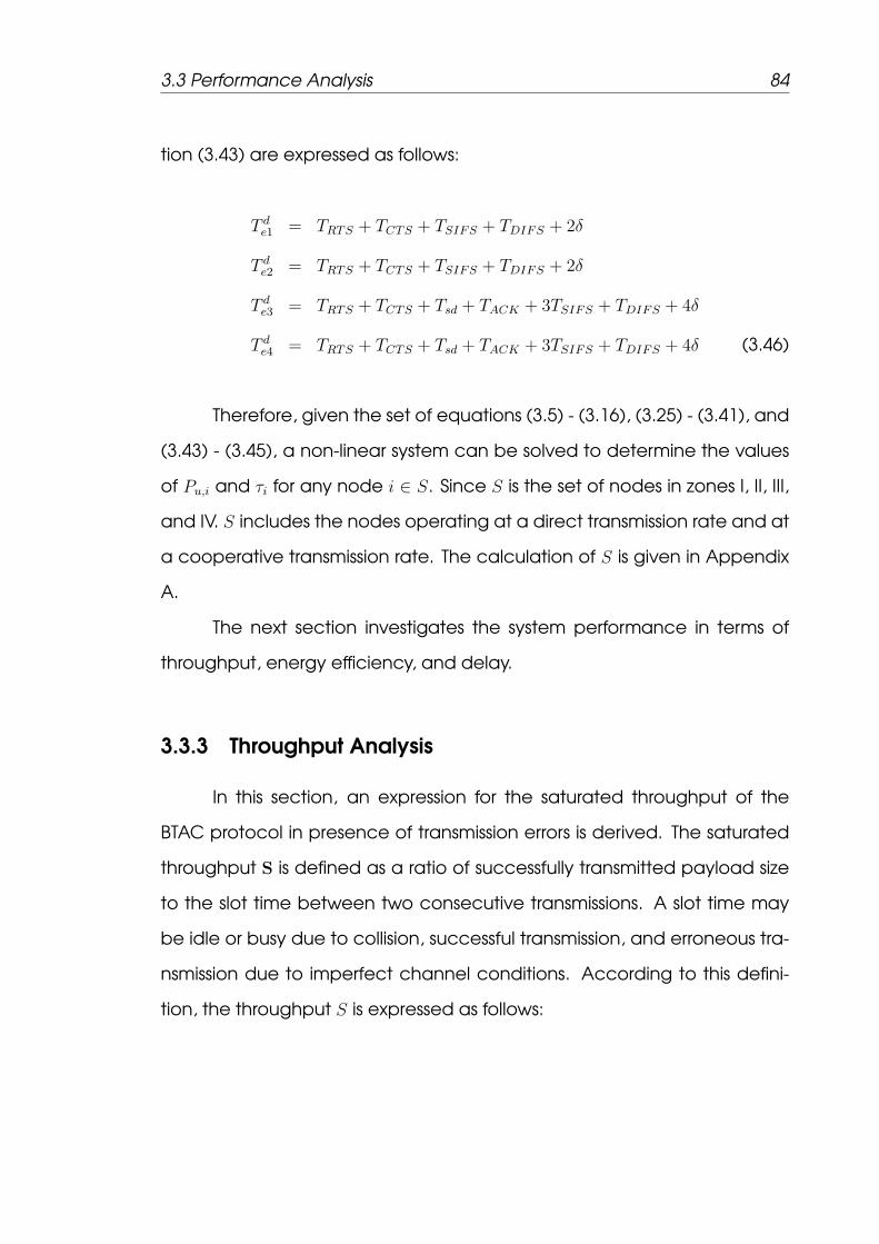
3.3 Performance Analysis 84
tion (3.43) are expressed as follows:
T de1 = TRTS + TCTS + TSIFS + TDIFS + 2δ
T de2 = TRTS + TCTS + TSIFS + TDIFS + 2δ
T de3 = TRTS + TCTS + Tsd + TACK + 3TSIFS + TDIFS + 4δ
T de4 = TRTS + TCTS + Tsd + TACK + 3TSIFS + TDIFS + 4δ (3.46)
Therefore, given the set of equations (3.5) - (3.16), (3.25) - (3.41), and
(3.43) - (3.45), a non-linear system can be solved to determine the values
of Pu,i and τi for any node i ∈ S. Since S is the set of nodes in zones I, II, III,
and IV. S includes the nodes operating at a direct transmission rate and at
a cooperative transmission rate. The calculation of S is given in Appendix
A.
The next section investigates the system performance in terms of
throughput, energy efficiency, and delay.
3.3.3 Throughput Analysis
In this section, an expression for the saturated throughput of the
BTAC protocol in presence of transmission errors is derived. The saturated
throughput S is defined as a ratio of successfully transmitted payload size
to the slot time between two consecutive transmissions. A slot time may
be idle or busy due to collision, successful transmission, and erroneous tra-
nsmission due to imperfect channel conditions. According to this defini-
tion, the throughput S is expressed as follows:
3.3 Performance Analysis 85
S =E[PL]
E[TI ] + E[TC ] + E[TS] + E[TE](3.47)
where E[PL] is the average payload size, E[TI ] is the average du-
ration of an empty slot time, E[TC ] is the average time that the channel
is sensed busy due to a collision, E[TS] is the average time the channel is
sensed busy due to a successful transmission, and E[TE] is the average time
that the channel is sensed busy due to an erroneous transmission. Mathe-
matical relations defining the average slot durations are expressed in the
following analysis.
Let Ptr be the probability at least one transmission occurs in the con-
sidered slot time. Since N nodes contend the channel with probability τi,
where i = 1, 2, ..., N , Ptr is then calculated as follows:
Ptr = 1−N∏i=1
(1− τi) (3.48)
Given a transmission on the channel from any node i, let Ps,i be the
probability that a successful transmission occurs in a slot time. Ps,i is then
expressed as follows:
Ps,i = τi
N∏j=1j =i
(1− τj), i = 1, 2, ..., N (3.49)
The total successful probability Ps that there is a successful transmission on

3.3 Performance Analysis 86
the channel, is calculated as follows:
Ps =N∑i=1
Ps,i (3.50)
The average idle slot duration before a transmission takes place is
calculated as follows:
E[TI ] = (1− Ptr)σ (3.51)
where 1 − Ptr is the probability that the chosen slot time is empty, and σ is
the duration of an empty slot time (e.g. 20 µs in 802.11b). The probability
that the channel is neither idle nor busy due to a successful transmission
in the considered slot time is defined as the collision probability which is
[1− (1− Ptr)− Ps] = Ptr − Ps. The average collision duration E[TC ] can then
be calculated as follows:
E[TC ] = (Ptr − Ps) · Tc (3.52)
where Tc stands for the collision time duration between either at least two
RTS packet, two MRTS, or RTS and MRTS packets. Tc is the same for all cases
because both RTS and MRTS have the same packet length. The Tc is then
expressed as follows:
Tc = TRTS/TMRTS + TCTS + TSIFS + TDIFS + δ (3.53)
The average slot duration of a successful transmission of a node, that
uses either a single-hop transmission or a two-hop transmission is calcu-

3.3 Performance Analysis 87
lated as follows:
E[TS] =N∑i=1
Ps,i(1− Pe,i)
[I(i ∈ Sd)T d
s,i + I(i ∈ Sc)T cs,i
](3.54)
where Sc = {Sc1 ∪ Sc
2} is the set of nodes operating at two-hop tra-
nsmission. Sc1 and Sc
2 are the set of nodes in zone IV (at data-rate 1
Mbps) and zone III (at data-rate 2Mbps), respectively using a two-hop tra-
nsmission. The set Sd is the set of nodes in zones IV, III, II, and I operating at
a direct transmission rate 1, 2, 5.5, and 11 Mbps, respectively. The sets Sd,
Sc1, and Sc
2 are given in Appendix A. The probability Ps,i(1−Pe,i) is the prob-
ability that the transmitted packet is received correctly by the receiving
node. I(x) is 1 if x is true, and is 0 otherwise. T ds,i and T c
s,i stand for the av-
erage time the channel is sensed busy because of successful transmission
under single-hop and two-hop transmission, respectively. It is calculated
as follows:
T ds,i = TRTS + TCTS + T
(i)sd + TACK + 3TSIFS + TDIFS + 4δ (3.55)
T cs,i = TMRTS + TCTS + TBTS + T (i)
sr + T(i)rd + TACK + 3TSIFS + TDIFS + 6δ (3.56)
The transmitted packet may be corrupted due to imperfect channel
conditions. Consequently, the average time E[TE] that the channel be-
comes busy due to an erroneous transmission is expressed as follows:
E[TE] =N∑i=1
Ps,i
[I(i ∈ Sd)
4∑j=1
pdejTdej + I(i ∈ Sc)
5∑j=1
pcejTcej
](3.57)

3.3 Performance Analysis 88
where pcej, Tcej, p
dej, and T d
ej are given in equations (3.40), (3.42), (3.44),
and (3.46), respectively.
The average payload size E[PL] is calculated as follows:
E[PL] = 8LN∑i=1
Ps,i(1− Pe,i) (3.58)
Finally, given the average slot durations and the payload size, the
saturated throughput can be calculated from equation (3.47).
3.3.4 Energy Efficiency Analysis
The energy efficiency, denoted by η, is defined as the ratio of the
successfully transmitted data bits to the total energy consumed [99, 100];
the unit of energy efficiency is bits/joule. In the IEEE 802.11 DCF, two man-
agement mechanisms are supported: active and Power Saving Mecha-
nism (PSM). In this research, only the active mechanism is considered, in
which a node may be in transmit, receive, and sense/idle modes. Under a
wireless fading channel, an unsuccessful transmission occurs not only due
to collision, but also due to channel errors. Thus, there is extra energy con-
sumption due to transmission errors. Let any node i = 1, 2, ...N act as a
generic node. The total energy consumed by this node i in the network
can be classified into five parts: the energy consumption during the back-
off period, denoted by E(i)B , the energy consumption during the collision
period, denoted by E(i)C , the energy consumption during the overhearing
transmissions, denoted by E(i)O , the energy consumption when there is no
packet collision but there are transmission errors, denoted by E(i)E , and the
energy consumption during the successful transmission (neither collision

3.3 Performance Analysis 89
nor errors), denoted by E(i)S . It is assumed that a node consumes power
PTX for transmitting, PRX for receiving, and PIX for sensing or being idle, re-
spectively. Consequently, for an average packet length E[L], the energy
efficiency, η, can be written as follows:
η =E[L]
N∑i=1
(E
(i)B + E
(i)C + E
(i)O + E
(i)E + E
(i)S
) (3.59)
Let Nb,i represent the average total number of backoff slots, which
the node i encounters without considering the case when the counter
freezes. Nb,i is calculated as follows:
Nb,i =m∑j=0
P ju,i(1− Pu,i)
1− Pm+1u,i
j∑k=0
Wk − 1
2, i = 1, 2, ..., N (3.60)
wherej∑
k=0
Wk−12
is the average number of backoff slots required by
the node i in order to transmit its packet successfully after j retries. 1−Pm+1u
is the probability that the packet is not dropped.P ju,i(1−Pu,i)
1−Pm+1u,i
is the successful
transmission probability after the jth backoff stage conditioned that the
packet is not dropped.
Hence, given the duration of empty slot σ and the idle power con-
sumption PIX , the energy that the node i spends during the backoff stage
can be calculated as follows:
E(i)B = σ · PIX ·Nb,i, i = 1, 2, ..., N (3.61)
Let N idle,i be the average number of consecutive idle slots between
two consecutive busy slots of the N − 1 remaining nodes. N idle,i is then
3.3 Performance Analysis 90
calculated as follows:
N idle,i =∞∑j=0
j(1− Pb,i)jPb,i =
1
Pb,i
− 1 (3.62)
The average number of transmissions No,i overheard by the node i
from the other N − 1 nodes during the backoff process is calculated as
follows:
No,i =Nb,i
N idle,i
=Nb,i
1− Pb,i
Pb,i (3.63)
Both Nb,i and No,i can be treated as the total number of idle and
busy slots that a packet encounters during the backoff stages, respec-
tively. The generic node i overhears collisions, successful transmissions, and
erroneous transmissions.
The energy E(i)O , that the node i consumes in overhearing transmis-
sions of other nodes during the backoff stages is calculated as follows:
E(i)O = No,iPRX
[E[TCi
] + E[TSi] + E[TEi
]
](3.64)
where E[TCi], E[TSi
], and E[TEi] stand for average collision dura-
tion, average successful transmission duration, and average erroneous tra-
nsmission duration given that at least one of the N − 1 nodes transmits dur-
ing the backoff process of the node i. Thus, we have:
E[TC,i] =
[1−
N−1∑j=1j =i
P ′s,j
]Tc (3.65)
where P ′s,k is the successful transmission probability of node k of the
3.3 Performance Analysis 91
N−1 remaining nodes given that the channel is sensed busy by the generic
node i. P ′s,k is expressed as follows:
P ′s,k =
τkN−1∏
j=1,j =k
(1− τj)
Pb,i
(3.66)
The average successful transmission duration E[TS,i] is computed as follows:
E[TS,i] =N−1∑j=1j =i
P ′s,j(1− Pe,j)
[I(j ∈ Sd)T d
s,j + I(j ∈ Sc)T cs,j
](3.67)
where T ds,j and T c
s,j are given in equations (3.55) and (3.56), respec-
tively. The average erroneous transmission duration, E[TE,i], is expressed as
follows:
E[TE,i] =N−1∑j=1j =i
P ′s,j
[I(j ∈ Sd)
4∑j=1
pdejTdej + I(j ∈ Sc)
5∑j=1
pcejTcej
](3.68)
The average number of retries Nr,i that the generic node i encoun-
ters before delivering its packet correctly to the AP, is calculated as follows:
Nr,i =m∑k=0
kP ku,i(1− Pu,i)
1− Pm+1u,i
=1− Pu,i
1− Pm+1u,i
[Pu,i
(1− Pu,i)2(1− Pm
u,i)−mPm+1
u,i
1− Pu,i
](3.69)
The Nr,i is the sum of retries due to both collision and erroneous tra-
nsmission. From equation (3.5),Pc,i
Pu,i
is the fraction of the total retries due to
collisions. Hence the average number of retries Nc,i due to collisions in the
3.3 Performance Analysis 92
total retries is expressed as follows:
Nc,i = Nr,iPc,i
Pu,i
(3.70)
Consequently, the energy consumption due to collisions is calculated as
follows:
E(i)C = Nc,i
[PTXTRTS/MRTS + PRXTCTS + PIX(TDIFS + TSIFS + δ)
](3.71)
The fraction of the total retries due to packet corruption is(1− Pc,i)p
cek
Pu,i
, where k ∈ (1, 5) in a two-hop transmission. Let N cek, where
k = 1, 2, ...5 be the average number of retries due to corruption of MRTS,
CTS, DATA-S (source to relay), DATA-S (relay to AP), and ACK , respectively.
N cek is calculated as follows:
N cek = Nr,i
(1− Pc,i)pcek
Pu,i
, k = 1, 2, ...5 (3.72)
The calculations are similar in the case of a direct transmission. Let
Ndek, k ∈ (1, 4) be the average number of retries due to corruption of the
RTS, CTS, DATA-S (source to AP), and ACK packets given successful RTS
contention, respectively. we have:
Ndek = Nr,i
(1− Pc,i)pekPu,i
, k = 1, 2, ...4 (3.73)
Let Ece1, E
ce2, ..., and Ec
e5 be the energy consumption during the time
durations T ce1, T
ce2, ..., and T c
e5 in equation (3.42), respectively. These energy

3.3 Performance Analysis 93
values are calculated as follows:
Ece1 = PTXTMRTS + PIX(TCTS + TSIFS + TDIFS + 2δ)
Ece2 = PTXTMRTS + PRXTCTS + PIX(TSIFS + TDIFS + 2δ)
Ece3 = PTX(TMRTS + Tsr) + PRX(TCTS + TBTS) + PIX(4TSIFS + TDIFS + 5δ)
Ece4 = PTX(TMRTS + Tsr) + PRX(TCTS + TBTS + Trd) + PIX(TACK + 5TSIFS + TDIFS + 6δ)
Ece5 = PTX(TMRTS + Tsr) + PRX(TCTS + TBTS + Trd + TACK) + PIX(5TSIFS + TDIFS + 6δ)
(3.74)
For direct transmission, Edek, where k ∈ (1, 4) stand for the RTS, CTS,
DATA-S (source-AP), and ACK packets corruption, respectively. These val-
ues is computed as follows:
Ede1 = PTXTRTS + PIX(TCTS + TSIFS + TDIFS + 2δ)
Ede2 = PTXTRTS + PRXTCTS + PIX(TSIFS + TDIFS + 2δ)
Ede3 = PTX(TRTS + Tsd) + PRXTCTS + PIX(4TSIFS + TDIFS + TACK + 5δ)
Ede4 = PTX(TRTS + Tsd) + PRX(TCTS + TACK) + PIX(4TSIFS + TDIFS + 5δ)
(3.75)
Therefore, the energy consumption due to erroneous transmission is
expressed as follows:
E(i)E = I(i ∈ Sd)
4∑k=1
NdekE
dek + I(i ∈ Sc)
5∑k=1
N cekE
cek (3.76)
The energy consumed by the generic node i under a successful two-

3.3 Performance Analysis 94
hop transmission is calculated as follows:
EcS = PTX(TMRTS + Tsr) + PRX(TCTS + TBTS + Trd + TACK)
+PIX(5TSIFS + TDIFS + 6δ) (3.77)
EdS in a single-hop transmission is computed as follows:
EdS = PTX(TRTS + Tsd) + PRX(TCTS + TACK) + PIX(4TSIFS + TDIFS + 5δ)
(3.78)
Hence the energy consumption during a successful transmission is
expressed as follows:
E(i)S = I(i ∈ Sd)Ed
S + I(i ∈ Sc)EcS (3.79)
Finally, the average packet length E[L] =∑N
i=1 8L assuming a fixed
packet length. Therefore, the energy efficiency η can be calculated from
(3.59).
3.3.5 Delay
The average packet delay is defined as the duration of time from
the time instant the packet is at the Head-Of-Line (HOL), i.e. it becomes
head of its MAC queue ready for transmission, to the time instant when the
packet is acknowledged for a successful transmission. Average packet
delay includes the backoff delay, the transmission delay, and the inter-
frame spaces. The backoff delay depends on the value of a node’s back-
3.3 Performance Analysis 95
off counter and the duration when the counter freezes due to a busy
channel.
Let Di (i = 1, 2, ..., N) denote a random variable representing a
packet delay of a generic node i. The average packet delay E[Di] can
be expressed as follows:
E[Di] = E[Db,i] + E[Dc,i] + E[Do,i] + E[De,i] + E[Ds,i] (3.80)
where E[Db,i], E[Dc,i], E[Do,i], E[De,i], and E[Ds,i] stand for the aver-
age delay in backoff stages, the average delay due to collisions, the aver-
age delay of overhearing during the backoff process, the average delay
due to an erroneous transmission, and the average delay of a successful
transmission, respectively. It is calculated as follows:
E[Db,i] = σNb,i
E[Dc,i] = Nc,iTc
E[Do,i] = No,i
[E[TCi
] + E[TSi] + E[TEi
]
]E[De,i] = P ′
s,i
[I(i ∈ Sd)
4∑k=1
Ndekp
dekT
dek + I(i ∈ Sc})
5∑k=1
N cekp
cekT
cek
]E[Ds,i] = I(i ∈ Sd)T d
s,i + I(i ∈ Sc)T cs,i (3.81)
where Nb,i and Nc,i are given in equations (3.60) and (3.63), respec-
tively. E[TCi], E[TSi
], and E[TEi] are given in equations (3.65), (3.67), and
(3.68), respectively. Tc, T ds,i, and T c
s,i are given in (3.53), (3.55), and (3.56),
respectively. T cek and T d
ek are given in (3.42) and (3.46), respectively. N cek
and Ndek are given in (3.72) and (3.73), respectively. Therefore, the total
3.4 Analytical and Simulation Results 96
average delay of the network is computed as follows:
E[DT ] =1
N
N∑i=1
E[Di] (3.82)
3.4 Analytical and Simulation Results
To validate the above analysis, a custom event driven simulator de-
veloped by using the Mobile Framework (MF) of the OMNET++ [148] pack-
age written in C++ programming language. The parameters used in simu-
lation and analysis are set to the default values specified in IEEE 802.11b
standard which are summarized in Table 3.2. The performance of the
proposed protocols is evaluated assuming static network topologies. The
curves presented hereafter were averaged over 50 runs, each of which
had a different topology and ran for a period of time that was long enough
to get stabilised results. Packets are transmitted at different rates, depend-
ing on the location of the nodes with respect to the AP. Specifically, the dis-
tance thresholds for 11Mbps, 5.5Mbps, 2Mbps and 1Mbps are set to 50m,
65m, 75m and 100m, respectively. Whereas the data rates versus distances
are used for demonstration purposes, which can be varied in reality. The
traffic is uniformly distributed across all the nodes in the network, and the
packets arrive in the network according to the Poisson distribution.
In the following figures, solid lines are fro the analytical model results
through Matlab software package. Whereas dot-dashed lines are for the
simulation results through OMNET++ software package.

3.4 Analytical and Simulation Results 97
Parameter Value Parameter ValueMAC header 272 bits Slot time, δ 20, 1 µs
PHY header 192 bits SIFS 10 µs
RTS 352 bits DIFS 50 µs
CTS 304 bits BTS 20 µs
ACK 304 bits CWmin 31 slotsPLCP data-rate 1 Mbps CWmax 1023 slotsPTX , PRX , PIX 1.0,0.8,0.8 W m′,m 5,7
Table 3.2: Parameters used for both analytical results and simulation runs.
3.4.1 Throughput Results
Fig. 3.12 shows the simulation and analytical results of the saturated
throughput of the BTAC, CoopMAC and IEEE 802.11b protocols against
the number of nodes under ideal channel conditions. It is assumed that
the data packet length is fixed and is set to be 1024 bytes. As illustrated
in Fig. 3.12, there is a good agreement between the analytical model
and simulation results. As the network size increases, the throughput of
the IEEE 802.11b decreases while the throughput of both the BTAC and
CoopMAC protocols increases. However, the BTAC protocol achieves a
higher throughput than the CoopMAC protocol. Since the throughput of
the BTAC increases from 2.0 Mbps to 2.41 Mbps, and the throughput of the
CoopMAC increases from 1.84 Mbps to 2.06 Mbps as the network size in-
creases. The reason is that the overhead control in the BTAC is less that the
overhead control in the CoopMAC protocol.
From Fig. 3.13, it can be seen that the collision probability increases
as the network size increases. For this reason the throughput of the 802.11
decreases as the number of node increases. On the other hand, as the
network size increases, the probability of a low data-rate node finding a
relay node increases, as illustrated in Fig. 3.13. Consequently, the low

3.4 Analytical and Simulation Results 98
8 10 12 14 16 18 20 22 24 26 28 30 32 34 36 38 400
0.2
0.4
0.6
0.8
1.0
1.2
1.4
1.6
1.8
2.0
2.2
2.4
2.6
Number of nodes
Thro
ughp
ut (M
bps)
801.11b−Analysis
CoopMAC−Analysis
BTAC−Analysis
801.11b−Simulation
CoopMAC−Simulation
BTAC−Simulation
Figure 3.12: Throughput of IEEE802.11b, CoopMAC, and BTAC, L=1024 byte.
data-rate node can send its data packet to the AP in a two-hop tra-
nsmission, and hence the transmission time decreases. The reduction in
the transmission time not only compensates the increasing in the collision
time, but also increases the overall throughput of the network.
The effect of the imperfect channel conditions on the throughput
performance is investigated in Fig. 3.14. Fig. 3.14 shows the relation-
ship between the throughput gain of both BTAC and CoopMAC proto-
cols and number of nodes under imperfect channel conditions and fixed
data packet length. The throughput gain is defined as the throughput of
the BTAC and CoopMAC protocols related to the throughput of the IEEE
802.11b protocol. The Good and Bad durations (TG and TB, respectively)
are assumed to be 50ms and 5ms, and 10ms and 1ms, respectively. As
expected, the lower the Good duration, the lower the throughput gain.
The reason is that as the Good duration decreases, the probability of the
packet error increases and so on the throughput decreases. The BTAC
protocol outperforms the CoopMAC protocols even under the imperfect

3.4 Analytical and Simulation Results 99
5 10 15 20 25 30 35 40 45 500
0.1
0.2
0.3
0.4
0.5
0.6
0.7
Number of Nodes
Prob
abilit
y
Collision Probability
Relay Probability
Figure 3.13: Collision and Relay probabilities versus number of nodes, L=1024 byte.
channel conditions.
As shown in Fig. 3.14 the throughput gain of the BTAC protocol under
the case of TG = 10ms is higher than the throughput gain of the CoopMAC
protocol under the case of TG = 100ms. In addition to the reduction in the
overhead of the BTAC protocol, the busy tone signal used in the BTAC is
better than the helper ready to send packet used in the CoopMAC pro-
tocol. Therefore, the BTAC is more reliable than the CoopMAC protocol
under both ideal and imperfect channel conditions.
It is well known that the packet length has a major effect on the
performance of WLANs. The relationship between the throughput and the
packet length under error free wireless medium and at a fixed number of
nodes which is chosen to be 30 nodes is illustrated in Fig. 3.15. The packet
size is changed from 400 bytes, which the threshold to use RTS/CTS tra-
nsmission in the standard IEEE 802.11, to 2000 byte, which is approximately
the maximum packet length supported by the IEEE 802.11b. It can be seen
that the analytical results match well the simulation results. As the packet
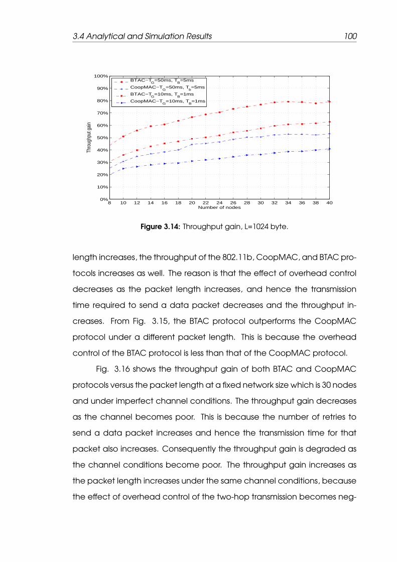
3.4 Analytical and Simulation Results 100
8 10 12 14 16 18 20 22 24 26 28 30 32 34 36 38 400%
10%
20%
30%
40%
50%
60%
70%
80%
90%
100%
Number of nodes
Thro
ughp
ut g
ain
BTAC−T
G=50ms, T
B=5ms
CoopMAC−TG
=50ms, Tb=5ms
BTAC−TG
=10ms, TB=1ms
CoopMAC−TG
=10ms, TB=1ms
Figure 3.14: Throughput gain, L=1024 byte.
length increases, the throughput of the 802.11b, CoopMAC, and BTAC pro-
tocols increases as well. The reason is that the effect of overhead control
decreases as the packet length increases, and hence the transmission
time required to send a data packet decreases and the throughput in-
creases. From Fig. 3.15, the BTAC protocol outperforms the CoopMAC
protocol under a different packet length. This is because the overhead
control of the BTAC protocol is less than that of the CoopMAC protocol.
Fig. 3.16 shows the throughput gain of both BTAC and CoopMAC
protocols versus the packet length at a fixed network size which is 30 nodes
and under imperfect channel conditions. The throughput gain decreases
as the channel becomes poor. This is because the number of retries to
send a data packet increases and hence the transmission time for that
packet also increases. Consequently the throughput gain is degraded as
the channel conditions become poor. The throughput gain increases as
the packet length increases under the same channel conditions, because
the effect of overhead control of the two-hop transmission becomes neg-

3.4 Analytical and Simulation Results 101
400 600 800 1000 1200 1400 1600 1800 20000.5
1
1.5
2
2.5
3
3.5
Packet length (byte.)
Thro
ughp
ut (M
bps)
801.11b−AnalysisCoopMAC−AnalysisBTAC−Analysis801.11b−SimulationCoopMAC−SimulationBTAC−Simulation
Figure 3.15: Throughput vs. packet length under ideal medium, L=1024 byte.
ligible. When the packet length increases, the throughput that can be
achieved by the BTAC protocol is higher than that can be achieved by
CoopMAC protocol. The reason is that the error probability of the BTAC
is less than the CoopMAC due to replacing the helper reday to send
packet by thee busy tone signal. Consequently, when the channel be-
comes poor, the BTAC protocol becomes more reliable than the Coop-
MAC protocol. Another point is that as the packet length increases, the
effect of the channel conditions becomes effective. This is because as the
packet length increases, the probability of the packet error increases and
hence the number of retries to send a data packet increases. Hence, the
throughput performance of both the BTAC and the CoopMAC protocols
decreases.

3.4 Analytical and Simulation Results 102
400 600 800 1000 1200 1400 1600 1800 20000%
20%
40%
60%
80%
100%
120%
Packet length (byte)
Thro
ughp
ut g
ain
BTAC−T
G=50ms,TB=5ms
CoopMAC−TG
=50ms,TB=5ms
BTAC−TG
=10ms,TB=1ms
CoopMAC−TG
=10ms,TB=1ms
Figure 3.16: Throughput gain versus packet length, N=30.
3.4.2 Energy Efficiency Results
The energy efficiency is counted as one of the most important re-
quirements to design an efficient MAC protocol. The energy efficiency of
the 802.11b, CoopMAC, and BTAC protocols versus the number of nodes
under ideal channel conditions and fixed packet length is shown in Fig.
3.17. The energy efficiency of both the BTAC and CoopMAC protocols
is better than the energy efficiency of the 802.11b protocol due to the
advantage of using the two-hop transmission. The energy efficiency de-
creases as the number of nodes increases due to two different reasons.
The first reason is that as the number of nodes increases, the collision prob-
ability increases as shown in Fig. 3.13. As the collision probability increases,
the retransmission probability increases. Therefore, the node consumes
more energy on the retransmissions, receiving and sensing the medium.
The second reason is that the overhearing energy consumption increases
as the number of nodes increases. Consequently, the energy efficiency

3.4 Analytical and Simulation Results 103
8 10 12 14 16 18 20 22 24 26 28 30 32 34 36 38 400
0.05
0.1
0.15
0.2
0.25
0.3
0.35
Number of nodes
Ene
rgy
effic
ienc
y (M
b/J)
801.11b−AnalysisCoopMAC−AnalysisBTAC−Analysis801.11b−SimulationCoopMAC−SimulationBTAC−Simulation
Figure 3.17: Energy efficiency versus number of nodes, L=1024 byte.
decreases as the number of nodes increases. The BTAC protocol achieves
higher energy efficiency than the CoopMAC protocol due to the lower
overhead control of the BTAC protocol.
The effect of the channel conditions on the energy efficiency ver-
sus the number of nodes is shown in Fig. 3.18. In Fig. 3.18(a), the good
and bad durations are assumed to be TG = 50ms and TB = 5ms, respec-
tively, where in Fig. 3.18(b), it is assumed that TG = 10ms and TB = 1ms.
When the channel quality becomes poor, the energy efficiency decreases
for the same number of nodes. The reason is that under the imperfect
channel conditions, the number of retransmission retries increases causing
increasing in the energy consumption of sending, receiving, overhearing,
and sensing. The energy efficiency of the BTAC protocol is better than the
802.11b and CoopMAC protocols under different channel conditions. This
is because of using a two-hop transmission with lower control overhead
than the CoopMAC protocol.
The effect of packet length on the energy efficiency at a fixed num-

3.4 Analytical and Simulation Results 104
8 10 12 14 16 18 20 22 24 26 28 30 32 34 36 38 400
0.05
0.1
0.15
0.2
0.25
0.3
0.35
Number of nodes
Ene
rgy
effic
ienc
y (M
b/J)
801.11b−AnalysisCoopMAC−AnalysisBTAC−Analysis801.11b−SimulationCoopMAC−SimulationBTAC−Simulation
(a) Energy efficiency vs. number of nodes at TG = 50ms and TB = 5ms.
8 10 12 14 16 18 20 22 24 26 28 30 32 34 36 38 400.02
0.04
0.06
0.08
0.1
0.12
0.14
0.16
0.18
0.2
Number of nodes
Ene
rgy
effic
ienc
y (M
b/J)
801.11b−AnalysisCoopMAC−AnalysisBTAC−Analysis801.11b−SimulationCoopMAC−SimulationBTAC−Simulation
(b) Energy efficiency vs. number of nodes at TG = 10ms and TB = 1ms.
Figure 3.18: Energy efficiency performance versus number of nodes under imper-fect medium conditions, L=1024byte.
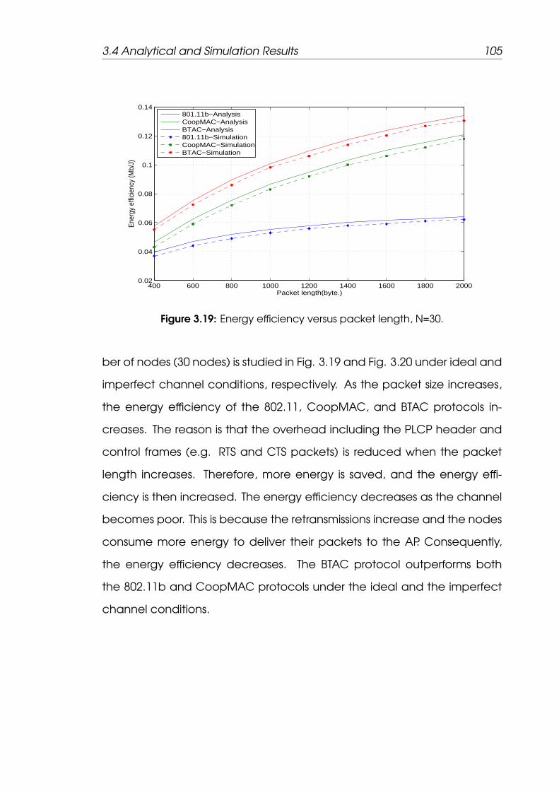
3.4 Analytical and Simulation Results 105
400 600 800 1000 1200 1400 1600 1800 20000.02
0.04
0.06
0.08
0.1
0.12
0.14
Packet length(byte.)
Ener
gy e
ffici
ency
(Mb/
J)
801.11b−AnalysisCoopMAC−AnalysisBTAC−Analysis801.11b−SimulationCoopMAC−SimulationBTAC−Simulation
Figure 3.19: Energy efficiency versus packet length, N=30.
ber of nodes (30 nodes) is studied in Fig. 3.19 and Fig. 3.20 under ideal and
imperfect channel conditions, respectively. As the packet size increases,
the energy efficiency of the 802.11, CoopMAC, and BTAC protocols in-
creases. The reason is that the overhead including the PLCP header and
control frames (e.g. RTS and CTS packets) is reduced when the packet
length increases. Therefore, more energy is saved, and the energy effi-
ciency is then increased. The energy efficiency decreases as the channel
becomes poor. This is because the retransmissions increase and the nodes
consume more energy to deliver their packets to the AP. Consequently,
the energy efficiency decreases. The BTAC protocol outperforms both
the 802.11b and CoopMAC protocols under the ideal and the imperfect
channel conditions.

3.4 Analytical and Simulation Results 106
400 600 800 1000 1200 1400 1600 1800 20000.03
0.04
0.05
0.06
0.07
0.08
0.09
0.1
0.11
0.12
0.13
Packet length(byte.)
Ene
rgy
effic
ienc
y (M
b/J)
801.11b−AnalysisCoopMAC−AnalysisBTAC−Analysis801.11b−SimulationCoopMAC−SimulationBTAC−Simulation
(a) Energy efficiency vs. packet length at TG = 50ms and TB = 5ms.
400 600 800 1000 1200 1400 1600 1800 20000.03
0.04
0.05
0.06
0.07
0.08
0.09
0.1
0.11
Packet length(byte.)
Ener
gy e
ffici
ency
(Mb/
J)
801.11b−AnalysisCoopMAC−AnalysisBTAC−Analysis801.11b−SimulationCoopMAC−SimulationBTAC−Simulation
(b) Energy efficiency vs. packet length at TG = 10ms and TB = 1ms.
Figure 3.20: Energy efficiency performance vs. packet length under imperfectchannel conditions, N=30.

3.4 Analytical and Simulation Results 107
3.4.3 Delay Results
The improvement in the system throughput also transforms into a bet-
ter delay performance. The relation between the service delay and the
network size under ideal channel conditions and a fixed packet size which
is 1024 bytes is shown in Fig. 3.21. The delay increases as the number of
nodes increases. This due to collision probability increases as the number
of nodes increases as illustrated in Fig. 3.13. Subsequently, the number
of retries to send a data packet from a source node to the AP increases
which causes increasing the service delay. On the other hand, both BTAC
and CoopMAC protocols outperform the 802.11b protocol as the number
of nodes increases. This because the probability of finding a relay node
increases (Fig. 3.13) as the number of nodes increases. As explained, the
transmission time of the two hop transmission is less that that of a single hop
transmission, Therefore, the service delay of both the BTAC and CoopMAC
protocols is less that that of the 802.11b. The delay of the BTAC is less than
the delay of the CoopMAC protocol. The reason is that the overhead of
the BTAC protocol is less than that of the CoopMAC protocol.
The effect of the channel conditions on the delay performance is
shown in Fig. 3.22. The delay performance under TG = 50ms and TB =
5ms, and under TG = 10ms and TB = 1ms is illustrated in Fig. 3.22(a) and
Fig. 3.22(b), respectively. As the channel conditions becomes poor, the
service delay increases due to increasing number of retries to deliver a
data packet from the sender to AP. On the other hand, the degradation
in the delay performance of both the BTAC and the CoopMAC protocols
is less than that of the 802.11b. This is due to the advantage of the two-
hop transmission under which the transmission time decreases and then
the service delay decreases.

3.4 Analytical and Simulation Results 108
8 10 12 14 16 18 20 22 24 26 28 30 32 34 36 38 400
0.05
0.1
0.15
0.2
0.25
0.3
0.35
Number of nodes
Del
ay (s
ec.)
801.11b−Analysis
CoopMAC−Analysis
BTAC−Analysis
801.11b−Simulation
CoopMAC−Simulation
BTAC−Simulation
Figure 3.21: Delay performance versus number of nodes under ideal medium,L=1024 byte.
The effect of the packet length on the service delay under ideal
channel conditions is shown in Fig. 3.23. As the packet length increases,
the service delay of the 802.11b, the CoopMAC, and the BTAC protocols
also increases. The delay is defined as the time from the packet ready
for transmission until receiving acknowledge packet from the AP, where
the transmission time of a data packet is included in the calculations of
the delay. Hence, as the packet length increases, the transmission time
increases and the delay increases. Both the CoopMAC and the BTAC pro-
tocols achieve lower delay performance than the 802.11b protocol. This
due the fact that under the two-hop transmission, the transmission rate in-
creases and then the transmission time decreases. On the other hand, the
BTAC has lower delay than the CoopMAC protocol due to the reduction
in the control overhead of the BTAC protocol.
The effect of the channel conditions on the delay performance ver-
sus the packet length is shown in Fig. 3.24. As the channel becomes poor,
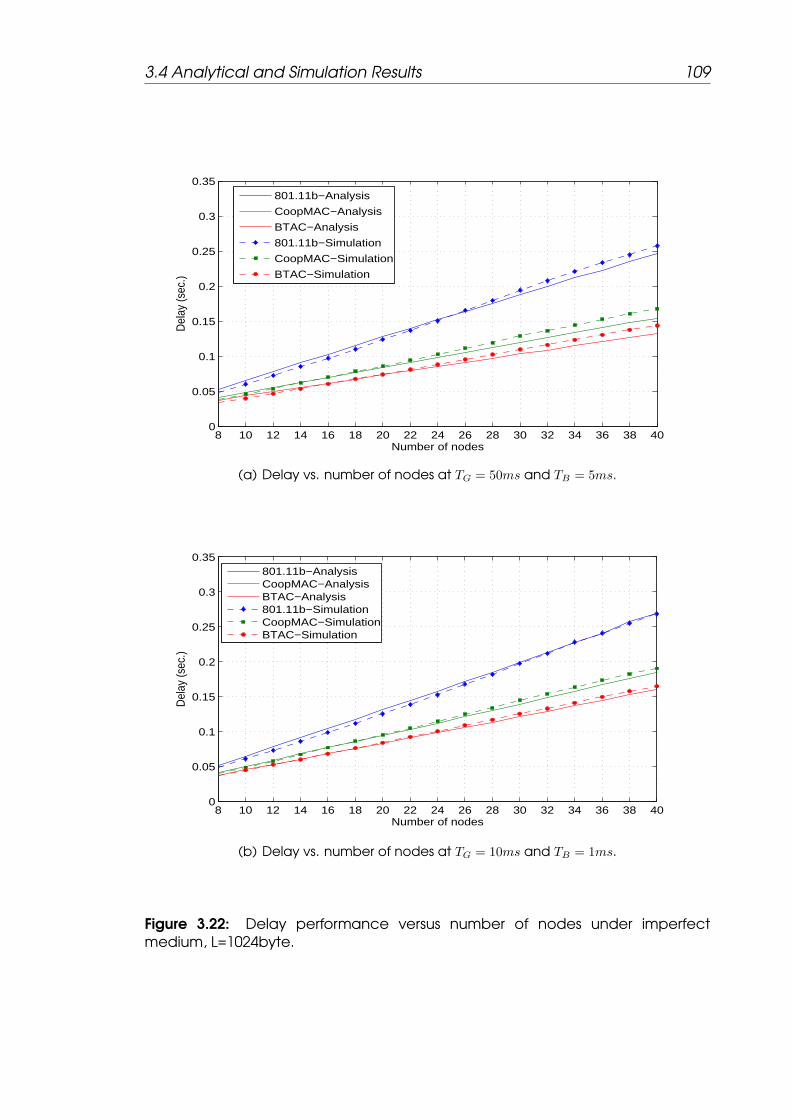
3.4 Analytical and Simulation Results 109
8 10 12 14 16 18 20 22 24 26 28 30 32 34 36 38 400
0.05
0.1
0.15
0.2
0.25
0.3
0.35
Number of nodes
Del
ay (s
ec.)
801.11b−Analysis
CoopMAC−Analysis
BTAC−Analysis
801.11b−Simulation
CoopMAC−Simulation
BTAC−Simulation
(a) Delay vs. number of nodes at TG = 50ms and TB = 5ms.
8 10 12 14 16 18 20 22 24 26 28 30 32 34 36 38 400
0.05
0.1
0.15
0.2
0.25
0.3
0.35
Number of nodes
Del
ay (s
ec.)
801.11b−AnalysisCoopMAC−AnalysisBTAC−Analysis801.11b−SimulationCoopMAC−SimulationBTAC−Simulation
(b) Delay vs. number of nodes at TG = 10ms and TB = 1ms.
Figure 3.22: Delay performance versus number of nodes under imperfectmedium, L=1024byte.
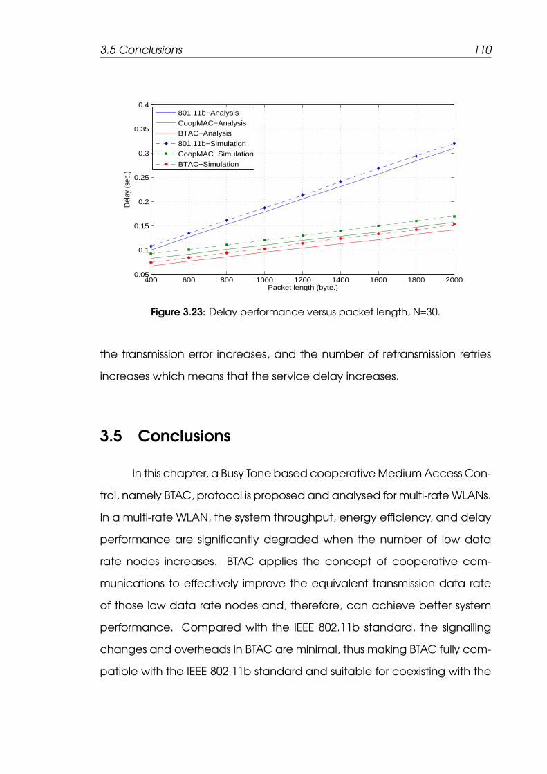
3.5 Conclusions 110
400 600 800 1000 1200 1400 1600 1800 20000.05
0.1
0.15
0.2
0.25
0.3
0.35
0.4
Packet length (byte.)
Del
ay (s
ec.)
801.11b−Analysis
CoopMAC−Analysis
BTAC−Analysis
801.11b−Simulation
CoopMAC−Simulation
BTAC−Simulation
Figure 3.23: Delay performance versus packet length, N=30.
the transmission error increases, and the number of retransmission retries
increases which means that the service delay increases.
3.5 Conclusions
In this chapter, a Busy Tone based cooperative Medium Access Con-
trol, namely BTAC, protocol is proposed and analysed for multi-rate WLANs.
In a multi-rate WLAN, the system throughput, energy efficiency, and delay
performance are significantly degraded when the number of low data
rate nodes increases. BTAC applies the concept of cooperative com-
munications to effectively improve the equivalent transmission data rate
of those low data rate nodes and, therefore, can achieve better system
performance. Compared with the IEEE 802.11b standard, the signalling
changes and overheads in BTAC are minimal, thus making BTAC fully com-
patible with the IEEE 802.11b standard and suitable for coexisting with the

3.5 Conclusions 111
400 600 800 1000 1200 1400 1600 1800 20000.05
0.1
0.15
0.2
0.25
0.3
0.35
0.4
Packet length (byte.)
Del
ay (s
ec.)
801.11b−AnalysisCoopMAC−AnalysisBTAC−Analysis801.11b−SimulationCoopMAC−SimulationBTAC−Simulation
(a) Delay vs. packet length at TG = 50ms and TB = 5ms.
400 600 800 1000 1200 1400 1600 1800 20000.05
0.1
0.15
0.2
0.25
0.3
0.35
0.4
0.45
0.5
Packet length (byte.)
Del
ay (s
ec.)
801.11b−AnalysisCoopMAC−AnalysisBTAC−Analysis801.11b−SimulationCoopMAC−SimulationBTAC−Simulation
(b) Delay vs. packet length at TG = 10ms and TB = 1ms.
Figure 3.24: Delay performance vs. packet length under imperfect medium,N=30.

3.5 Conclusions 112
standard DCF protocols. In addition, the BTAC is simple and robust, since
the Busy Tone Signal is easy to generate and detect, thus minimizing the
overhead of exchanging control messages between the relay and the
source node. The BTAC protocol completely avoids the hidden relay prob-
lem that may occur in the CoopMAC protocol.
To select the appropriate relay node by the source node, a dis-
tributed relay selection algorithm is proposed. This algorithm operates in a
distributed manner and introduces a minimum overhead in terms of com-
plexity and delay. On the other hand, taking into account the impact of
multi-rate transmissions, bandwidth utilization, and the imperfect channel
conditions due to the fading, interference, and noise, an enhanced ver-
sion of BTAC, named EBTAC, is proposed. The EBTAC protocol compared
to the BTAC protocol improves the system performance.
A cross-layer analytical approach is developed to evaluate the per-
formance of BTAC under dynamic wireless channel conditions. A simple
and widely used model, called ”Gilbert-Elliot model”, is used to capture
the burst behavior of the wireless channel caused by fading. Analytical
and simulation results show that, compared with other cooperative MAC
protocols, our BTAC protocol can achieve better throughput gain, and
acceptable energy efficiency and service delay performance.

Chapter 4
CARD: Cooperative Access with
Relay’s Data
In this chapter, a new Medium Access Control (MAC) protocol,
called Cooperative Access with Relay’s Data (CARD) for multi-rate wire-
less local area networks (WLANs) is proposed. The CARD protocol allows
remote nodes to transmit their information at a higher data rate to Ac-
cess Point (AP) by using intermediate nodes as relays. Particularly, under
the CARD protocol, a relay node sends its own data packet after forward-
ing a packet from the original source node, thus to improve system per-
formance. A Markov chain model is proposed taking into account the
multi-rate transmissions and the wireless channel conditions. The analyti-
cal and simulation results show that the CARD protocol can significantly
improve the system quality of service (QoS) in terms of throughput, service
delay and energy efficiency under different channel conditions. As a result
the CARD protocol can achieve: (1) potential benefits for the relay node
in cooperative communications; (2) both cooperative diversity gain and

4.1 The CARD Protocol 114
multiplexing gain in MAC layer; (3) further increasing in system throughput
and substantial service delay improvement; (4) energy efficiency improve-
ment
The remainder of the chapter is organised as follows. The proposed
CARD protocol with three algorithms for source nodes, relay nodes and the
AP is described in detail in Section 4.1. An analytical model is then derived
to analyse the throughput, delay, and energy efficiency performance of
the CARD protocol in Section 4.2. The analytical and simulation results
are presented and discussed in Section 4.3. Section 4.4 concludes the
chapter.
4.1 The CARD Protocol
This section describes the proposed CARD protocol based on physi-
cal specifications of IEEE 802.11b standard [5]. As described in [Sec. 3.1.1,
pp. 49] each node supports transmission data-rates of 1, 2, 5.5, 11 Mbps,
and the maximum transmission ranges r4 > r3 > r2 > r1, respectively.
Without loss of compatibility with standard WLAN protocols, the standard
Request-To-Send (RTS), Clear-To-Send (CTS) and Acknowledgment (ACK)
packets are slightly modified to create a Cooperative RTS (CRTS), a Relay-
Ready-To-Send (RRTS), a Cooperative CTS (CCTS) and a Cooperative ACK
(CACK) packets for the proposed CARD protocol. The frame formats of
these standard and cooperative control packets are shown in Fig. 4.1. In
particular, the Relay ID field in a CRTS packet specifies the MAC address
of the most appropriate neighbouring station selected by a low data-rate
source node. Hence, the source node uses the CRTS packet to reserve the
shared communication channel for its upcoming data packet transmission

4.1 The CARD Protocol 115
and, more importantly, to request the selected high data-rate neighbour-
ing node to serve as its relay node. The RRTS packet has the same format
as the CTS packet in the IEEE 802.11b standard [5]. The 2-bit flag field in
a CACK packet indicates if the two data packets from the source and
relay stations have been successfully received by the AP. If not, the corre-
sponding source or relay station requires to retransmit one or both packets
accordingly to the AP. The details are given in Section 4.1.3. With these
new control packets, the proposed CARD protocol consists of three algo-
rithms for the source nodes, the relay nodes and the AP. The following three
subsections describe the principles of these algorithms.
4.1.1 Source Node Algorithm
1. As soon as a data packet “DATA-S” is ready to transmit, the source
node senses the shared communication channel to the AP.
2. IF the channel is busy, THEN the source node waits until it becomes
idle.
3. IF the source node is located in zones III or IV, i.e. low data-rate zones,
THEN it checks the rate-gain GR of neighbouring high data-rate nodes
and identifies the most appropriate one as its relay node.
4. IF the source node is located in zones I or II, i.e. high data-rate zones,
or IF no relay node is identified in Step (3), THEN the source node uses
the standard RTS/CTS protocol to directly transmit its data packet to
the AP. Go to Step (7).
5. The source node sends a CRTS packet to the selected relay node
and the AP.

4.1 The CARD Protocol 116
(a) RTS frame.
(b) CRTS frame.
(c) CTS frame.
(d) CCTS frame.
(e) ACK frame.
(f) CACK frame.
Figure 4.1: Frame format.
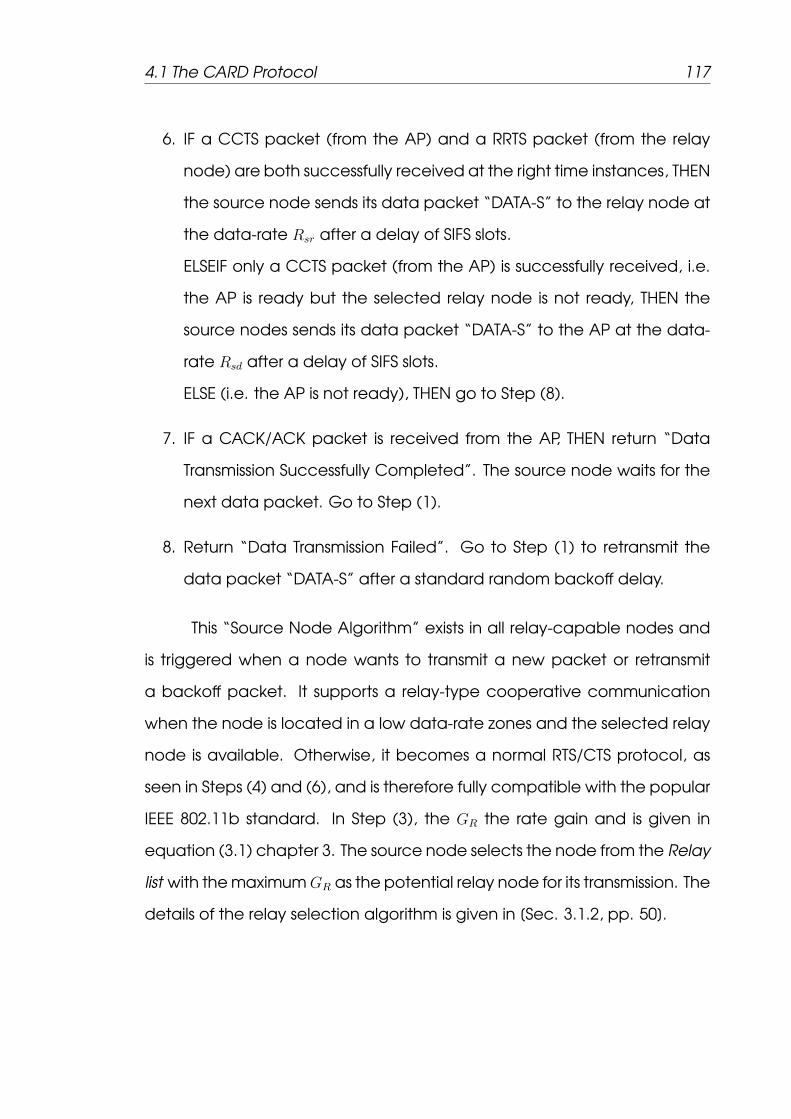
4.1 The CARD Protocol 117
6. IF a CCTS packet (from the AP) and a RRTS packet (from the relay
node) are both successfully received at the right time instances, THEN
the source node sends its data packet “DATA-S” to the relay node at
the data-rate Rsr after a delay of SIFS slots.
ELSEIF only a CCTS packet (from the AP) is successfully received, i.e.
the AP is ready but the selected relay node is not ready, THEN the
source nodes sends its data packet “DATA-S” to the AP at the data-
rate Rsd after a delay of SIFS slots.
ELSE (i.e. the AP is not ready), THEN go to Step (8).
7. IF a CACK/ACK packet is received from the AP, THEN return “Data
Transmission Successfully Completed”. The source node waits for the
next data packet. Go to Step (1).
8. Return “Data Transmission Failed”. Go to Step (1) to retransmit the
data packet “DATA-S” after a standard random backoff delay.
This “Source Node Algorithm” exists in all relay-capable nodes and
is triggered when a node wants to transmit a new packet or retransmit
a backoff packet. It supports a relay-type cooperative communication
when the node is located in a low data-rate zones and the selected relay
node is available. Otherwise, it becomes a normal RTS/CTS protocol, as
seen in Steps (4) and (6), and is therefore fully compatible with the popular
IEEE 802.11b standard. In Step (3), the GR the rate gain and is given in
equation (3.1) chapter 3. The source node selects the node from the Relay
list with the maximum GR as the potential relay node for its transmission. The
details of the relay selection algorithm is given in [Sec. 3.1.2, pp. 50].
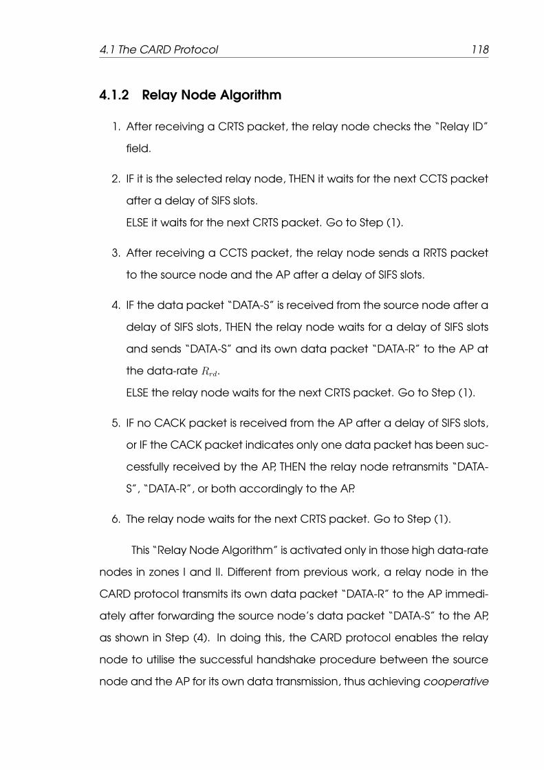
4.1 The CARD Protocol 118
4.1.2 Relay Node Algorithm
1. After receiving a CRTS packet, the relay node checks the “Relay ID”
field.
2. IF it is the selected relay node, THEN it waits for the next CCTS packet
after a delay of SIFS slots.
ELSE it waits for the next CRTS packet. Go to Step (1).
3. After receiving a CCTS packet, the relay node sends a RRTS packet
to the source node and the AP after a delay of SIFS slots.
4. IF the data packet “DATA-S” is received from the source node after a
delay of SIFS slots, THEN the relay node waits for a delay of SIFS slots
and sends “DATA-S” and its own data packet “DATA-R” to the AP at
the data-rate Rrd.
ELSE the relay node waits for the next CRTS packet. Go to Step (1).
5. IF no CACK packet is received from the AP after a delay of SIFS slots,
or IF the CACK packet indicates only one data packet has been suc-
cessfully received by the AP, THEN the relay node retransmits “DATA-
S”, “DATA-R”, or both accordingly to the AP.
6. The relay node waits for the next CRTS packet. Go to Step (1).
This “Relay Node Algorithm” is activated only in those high data-rate
nodes in zones I and II. Different from previous work, a relay node in the
CARD protocol transmits its own data packet “DATA-R” to the AP immedi-
ately after forwarding the source node’s data packet “DATA-S” to the AP,
as shown in Step (4). In doing this, the CARD protocol enables the relay
node to utilise the successful handshake procedure between the source
node and the AP for its own data transmission, thus achieving cooperative
4.1 The CARD Protocol 119
multiplexing gain and benefiting the relay node and the whole system in
terms of throughput and energy efficiency, as demonstrated by the an-
alytical and simulation results in Section 4.3. In Step (3), a RRTS packet is
transmitted for two purposes: (i) it serves as an acknowledgement mes-
sage for the source node to know that the relay node is ready to receive
the data packet “DATA-S”, and (ii) it serves as a request-to-send message
for the AP to know that the relay node is transmitting its own data packet
“DATA-R”.1 The RRTS packet is sent after sending the CCTS packet, i.e. af-
ter the channel reservation procedure is completed, for two reasons. First,
to solve the ” Hidden Relay Node Problem” that is discussed in [ch. 3 pp.
60]. As some nodes cannot hear the ongoing packet transmission from the
relay node, they may send a RTS packet to the AP at the same time and
cause a collision with the RRTS packet. All the nodes in the network can
hear the AP’s CCTS packet and will then defer their packet transmission
requests, if any. As a result, the RRTS packet from the relay node is guaran-
teed no collision and the two-hop communication path will be successfully
established after the RRTS packet is received by the source node and the
AP.
Therefore, the CARD protocol completely solves the “Hidden Relay
Node Problem” and effectively enables cooperative relay communica-
tion in WLANs. The second reason is that after receiving the CCTS packet,
the relay node extracts Rsd (the data rate between the source and the
AP) and estimates Rrd (the data rate between the relay and the AP). The
relay node also estimates Rsr (the data rate between the source and the
relay) of the received CRTS packet from the source node. In this case, it
1If the relay node does not have a data packet to transmit, CARD becomes a normalrelay protocol and, after a RRTS packet, only the packet “DATA-S” will be forwarded fromthe relay node to the AP.

4.1 The CARD Protocol 120
sends a RRTS packet only when a two-transmission is faster than a single-
hop transmission. This method improves bandwidth utilization under dy-
namic channel conditions.
To support packet retransmissions in Step (5), the relay node needs to
maintain two buffers (as in IEEE 802.11e [8]) for its own data packet and the
source node’s relayed packet, respectively. They are updated/empted
in parallel according to the flag field in the CACK packet for each
(re)transmission.
4.1.3 Access Point Algorithm
1. After receiving a CRTS packet (from a low data-rate node that re-
quests a relay node) or a standard RTS packet (from a node that
does not request a relay node), the AP checks the “Transmitter Ad-
dress” (TA) field and sends a CCTS packet or a standard CTS packet,
accordingly, to the source node after a delay of SIFS slots.
2. IF a CRTS packet is received in Step (1), THEN the AP waits for a RRTS
packet after a delay of SIFS slots.
ELSE (a standard RTS packet is received in Step (1)) the AP waits for
the data packet “DATA-S” from the source node after a delay of SIFS
slots. Go to Step (6).
3. IF a RRTS packet is received, THEN the AP waits for two data packets,
i.e. “DATA-S” and “DATA-R”, from the relay node after a delay of SIFS
slots.
ELSE the AP waits for the data packet “DATA-S” from the source node
after a delay of SIFS slots. Go to Step (6).
4. IF both “DATA-S” and “DATA-R” are successfully received, THEN the

4.1 The CARD Protocol 121
AP sets the flag field to ”11” and sends a CACK packet to the source
and relay nodes after a delay of SIFS slots.
ELSEIF only “DATA-S” is successfully received, THEN the AP sets the flag
field to ”10” and sends a CACK packet to the source and relay nodes
after a delay of SIFS slots.
ELSEIF only “DATA-R” is successfully received, THEN the AP sets the flag
field to ”01” and sends a CACK packet to the source and relay nodes
after a delay of SIFS slots.
ELSE (neither “DATA-S” nor “DATA-R” is received) the AP does not send
a CACK packet.
5. IF “DATA-S”, “DATA-R” or both are received after a delay of DIFS slots
(packet retransmission), THEN the AP updates the flag field and sends
a new CACK packet to the source and relay nodes after a delay of
SIFS slots. Go to Step (5). ELSE go to Step (7).
6. IF “DATA-S” is successfully received, THEN the AP sends an ACK packet
to the source nodes after a delay of SIFS slots.
ELSE the AP does not send an ACK packet.
7. A new contention-based random access period starts. The AP waits
for the next CRTS/RTS packet. Go to Step (1).
In Step (1), the AP may receive a standard RTS packet (without a re-
lay node request) from a high data-rate node that does not need a relay
node, a low data-rate node that does not have any high data-rate neigh-
bouring nodes as its potential relay nodes, or a legacy node that does
not support a relay-type cooperative communication. In this case, as well
the case when no RRTS packet is received in Step (3), the source node

4.1 The CARD Protocol 122
directly sends its data packet “DATA-S” to the AP at the data-rate Rsd. In
this way, the CARD protocol can accommodate both new relay-capable
nodes and legacy nodes in the same network and, hence, is compatible
with the IEEE 802.11b standard. Connecting Step (5) in this algorithm, Step
(5) in the “Relay Node Algorithm” and Step (8) in the “Source Node Al-
gorithm”, packet retransmissions are conducted by the relay node when
the received CACK packet has an incomplete flag field (i.e. flag = 11), or
when no CACK packet is correctly received (i.e. no CACK packet is trans-
mitted at all, or the transmitted CACK packet is destroyed under unreliable
radio channel condition).
The basic operation of CARD protocol is illustrated in Fig. 4.2. This
handshake procedure of control packets, CRTS, CCTS and RRTS, is shown
in Fig. 4.2(a) and the data packets transmission from the source and relay
nodes to the AP is shown in Fig. 4.2(b).
4.1.4 Channel Access Procedure and NAV
As an example, the combined channel access procedure with the
control and data packets in the CARD protocol is shown in Fig. 4.3(a),
where a low data-rate source node successfully establishes a two-hop
communication path through a high data-rate relay node for effectively
transmitting two data packets, “DATA-S” (from the source node) and
“DATA-R” (from the relay node), to the AP. If the source node does not re-
ceive a RRTS packet, i.e. the selected relay node is not available, it directly
sends the data packet “DATA-S” to the AP at the low data-rate Rsd and
then waits for an ACK packet, as shown in Fig. 4.3(b). For a legacy source
node that does not support relay communication in the CARD protocol,
its channel access procedure will be the same as the standard RTS/CTS

4.1 The CARD Protocol 123
(a) Control packets handshake.
(b) Data packets transmission.
Figure 4.2: Access mechanism of CARD protocol.

4.1 The CARD Protocol 124
Packet type The Duration
CRTS TCCTS + TRRTS + 3TSIFS + δ
CCTS 8Ls
Rsd+ TPLCP + 2TSIFS + TACK + 2δ
RRTS 8Ls
Rsr+ 8Ls+8Lr
Rrd+ 3TPLCP + 4TSIFS + TCACK + 4δ
DATA-S (source-relay) 16LRrd
+ 2TPLCP + 3TSIFS + TCACK + 3δ
DATA-S (relay-AP) 8LRrd
+ TPLCP + 2TSIFS + TCACK + 2δ
DATA-R TCACK + TSIFS + δ
RTS TCTS + 2TSIFS + δ
CTS 8LRsd
+ TPLCP + 2TSIFS + TACK + 2δ
DATA-S (source-AP) TACK + TSIFS + δ
Table 4.1: CARD Duration field contents
protocol in IEEE 802.11b WLANs. Therefore, the proposed CARD protocol
can flexibly support both relay-capable nodes and legacy nodes, and is
fully compatible with the IEEE 802.11b standard.
As described in Section 4.1.1, the transmission data rates between
a source node, a relay node and the AP, i.e. Rsd, Rsr, and Rrd, can be
estimated at the source node by overhearing a few recent packet trans-
missions. As all control packets are transmitted at the basic data-rate, the
source node can easily calculate the transmission time of RTS/CRTS, RRTS,
CTS/CCTS and ACK/CACK packets. Furthermore, the corresponding Net-
work Allocation Vectors (NAVs) can be estimated, as seen in Fig. 4.3, for
the CARD protocol.
The Duration field value is expressed in Table 4.1. where Ls and Lr are
the data packet length in octets of the source and the relay, respectively.
δ is the channel propagation delay, and TPLCP is the time duration of the
PLCP header. TRTS, TCTS, TACK , TCRTS, TCCTS, TRRTS, and TCACK stand for
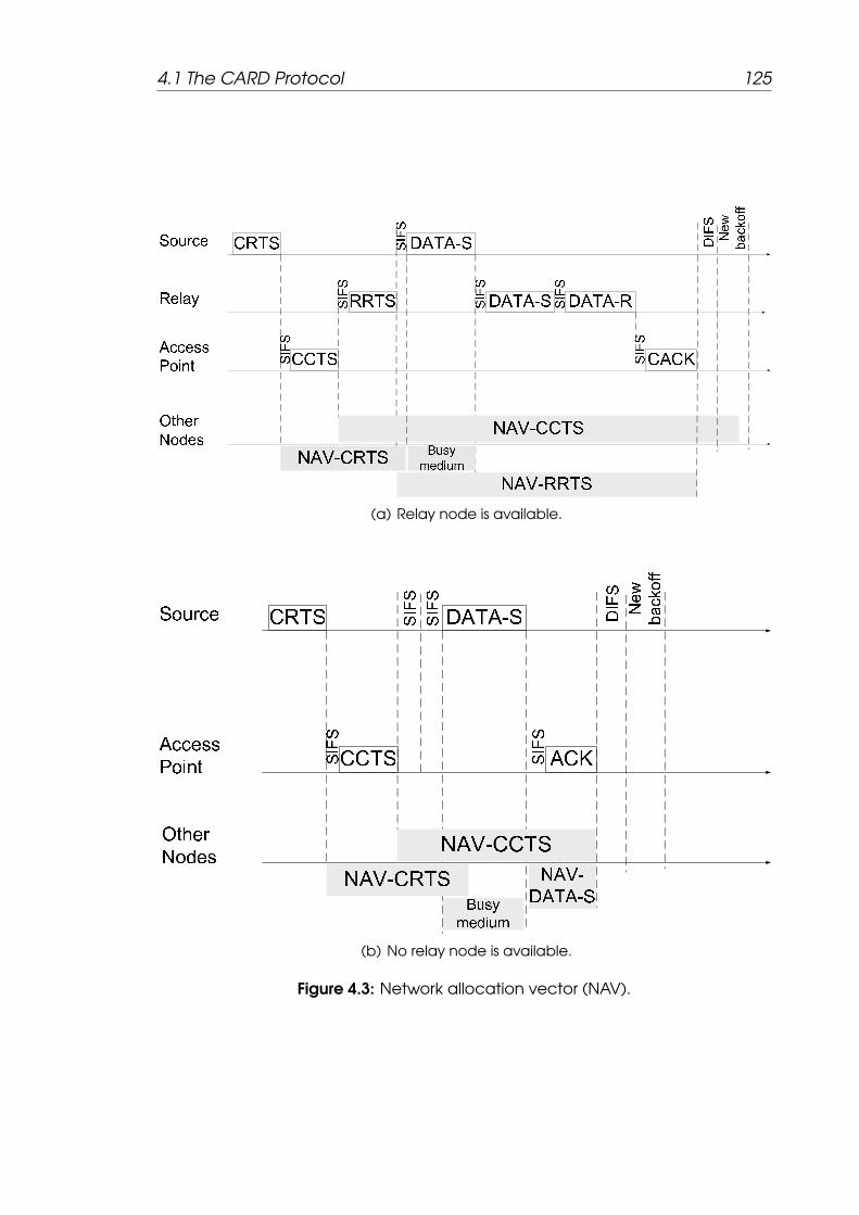
4.1 The CARD Protocol 125
(a) Relay node is available.
(b) No relay node is available.
Figure 4.3: Network allocation vector (NAV).

4.2 Performance Analysis 126
the duration of the RTS, CTS, ACK, CRTS, CCTS, RRTS, and CACK packets,
respectively.
4.2 Performance Analysis
4.2.1 Channel Packet Error Rate
Over the wireless channel, the multipath fading, interference, and
noise produce high error rates depending on the channel conditions and
transmission data rate. For a generic node i, let Pe,i be the probability of
packet error rate (PER) due to imperfect channel conditions. Under the
CARD protocol a source node can use a single-hop transmission when it is
located either in zone I or zone II. When a source node is located either in
zone III or zone IV and there is no relay available, the source node uses also
a single-hop transmission to send its packet to the AP. Otherwise, when a
source node is located either in zone III or zone IV and there is a relay node
available, it uses a two-hop transmission. In the following Pe,i is derived for
single-hop and two-hop transmission.
4.2.1.1 Direct Transmission
In this case, ageneric node i is located either in zone I, zone II, or
in zone III or zone IV where there is no relay available. It then sends its
packet directly to the AP at a data-rate Rsd = {1, 2, 5.5, 11} Mbps depend-
ing on the channel conditions. After sending a RTS packet with no collision
to the AP, the wireless channel undergoes one of the following four events
causing transmission failure. These events are RTS corruption, CTS corrup-
tion, DATA-S (source-AP) corruption, and ACK corruption. Consequently,

4.2 Performance Analysis 127
the probability that the RTS packet is corrupted given that there is no RTS
collision is calculated as follows:
u1 = Pr(RTS is corrupted | no RTS collision)
= 1− (1−BERb)8LRTS (4.1)
where BERb is the Bit Error Rate (BER) at the base data-rate (e.g.
1Mbps in 802.11b). The control packet, e.g. RTS, CTS, ACK, etc., are sent
also at the base data-rate . LRTS is the RTS packet length in octets. The
probability u2 that the CTS packet is corrupted given that the RTS packet is
successfully transmitted and there is no RTS collision is calculated as follows:
u2 = Pr(CTS is corrupted | no RTS corruption, no RTS collision)
= 1− (1−BERb)8LCTS (4.2)
where LCTS is the CTS packet length in octets. Similarly, the proba-
bility u3 that the DATA-S packet from a source to the AP is corrupted given
that both the RTS and CTS are successful, and exactly one RTS is transmit-
ted is expressed as follows:
u3 = 1− (1−BERsd)8Ls(1−BERb)
8LPLCP (4.3)
where Ls is the data packet length of the source node in octets.
LPLCP is the PLCP header size in octets. BERsd is bit error rate of the DATA-S
from a source node to the AP at the data-rate Rsd. The ACK corruption
4.2 Performance Analysis 128
probability u4 is computed as follows:
u4 = 1− (1−BERb)8LACK (4.4)
where LACK is the ACK packet length in octets. Let pde1 be the porta-
bility of the RTS corruption, pde2 be the portability of the CTS corruption, pde3
be the portability of the DATA-S corruption, and pde4 be the portability of
the ACK corruption under direct transmission. These probabilities are com-
puted as follows:
pde1 = u1
pde2 = (1− u1)u2
pde3 = (1− u1)(1− u2)u3
pde4 = (1− u1)(1− u2)(1− u3)u4 (4.5)
The corresponding time duration of these events are denoted by
T de1, T
de2, T
de3, and T d
e4, respectively. These time durations are calculated as
follows:
T de1 = TRTS + TCTS + TSIFS + TDIFS + 2δ
T de2 = TRTS + TCTS + TSIFS + TDIFS + 2δ
T de3 = TRTS + TCTS +
8Ls
Rsd
+LPLCP
Rb
+ TACK + 3TSIFS + TDIFS + 4δ
T de4 = TRTS + TCTS +
8Ls
Rsd
+LPLCP
Rb
+ TACK + 3TSIFS + TDIFS + 4δ (4.6)
where δ is the propagation delay, TDIFS is the duration of the Dis-
tributed Inter-Frame Space (DIFS), and TSIFS is the duration of Short Inter-
4.2 Performance Analysis 129
Frame Space (SIFS).
From equation (4.5), the probability Pe,i of the node i that uses a
single-hop transmission is expressed as follows:
Pe,i = pde1 + pde2 + pde3 + pde4 (4.7)
4.2.1.2 Cooperative Transmission
In this scenario, a source node transmits its data packet to the
AP via a relay node. The source node transmits its data packet at
a data-rate Rsr Mbps to the relay node. The relay then forwards the
data packet of the source to the AP at a data-rate Rrd Mbps. When
a source node is at data-rate 1 Mbps, it can use a two-hop data-rates
(Rsr, Rrd) = {(11, 11), (5.5, 11), (11, 5.5), (5.5, 5.5), (2, 11), (11, 2), (2, 5.5), (5.5, 2)}.
Otherwise, when the data-rate is 2 Mbps, a source node uses a two-hop
data-rate (Rsr, Rrd) = {(11, 11), (5.5, 11), (11, 5.5), (5.5, 5.5)}.
In the same manner as the single-hop transmission, after transmitting
a CRTS packet with no collision, there are seven events at which the tra-
nsmission may fail due to imperfect channel conditions. These events are
a CRTS, a CCTS, a RRTS, a DATA-S from the source to the relay, a DATA-S
from the relay to the AP, a DATA-R from the relay to the AP, and a CACK
packets corruption. The probability w1, that a CRTS is corrupted given that
there is exactly one CRTS is transmitted, is calculated as follows:
w1 = Pr(CRTS is corrupted|no CRTS collision)
= 1− (1−BERb)8LCRTS (4.8)

4.2 Performance Analysis 130
where LCRTS is the CRTS packet length in octets. The probability
w2, that a CCTS is corrupted given no CRTS collision and corruption, is ex-
pressed as follows:
w2 = 1− (1−BERb)8LCCTS (4.9)
where LCCTS is the CCTS packet length in octets. The probability w3,
that a RRTS is corrupted after receiving both CRTS and CCTS correctly, is as
follows:
w3 = 1− (1−BERb)8LRRTS (4.10)
where LRRTS is the RRTS packet length in octets. The probability that
a DATA-S from the source to the relay is corrupted after correct CRTS, CCTS
and RRTS, denoted by w4, is calculated as follows:
w4 = 1− (1−BERsr)8Ls(1−BERb)
8LPLCP (4.11)
where BERsr is the bit error rate of the data packet (source-relay) at
the data-rate Rsr. The probability w5, that a DATA-S (relay-AP) is corrupted
given that CRTS, CCTS, RRTS, and DATA-S (source-relay) are successfully
received and given that there is no CRTS collision, is computed as follows:
w5 = 1− (1−BERrd)8Ls(1−BERb)
8LPLCP (4.12)
where BERrd is the bit error rate between the relay and the AP of
the data packet sent at data-rate Rrd. The relay node sends a DATA-R

4.2 Performance Analysis 131
after sending a DATA-S (relay-AP) immediately even if a DATA-S is received
incorrectly. The probability w6, that a DATA-R is not successfully received
after receiving CRTS, CCTS, RRTS, DATA-S (source-relay) correctly where it
is independent on DATA-S (relay-AP), is expressed as follows:
w6 = 1− (1−BERrd)8Lr(1−BERb)
8LPLCP (4.13)
where Lr is the data packet length of the relay node in octets. The
AP sends a CACK if at least one the two packets DATA-S (relay-AP) and
DATA-R is received correctly. The probability w7, that a CACK is corrupted
after receiving CRTS, CCTS, RRTS, DATA-S (source-relay), and at least one of
both DATA-S (relay-AP) and DATA-R correctly, is then expressed as follows:
w7 = 1− (1−BERb)LCACK (4.14)
where LCACK is the CACK packet length in octets. Let qce1 be the
probability of a CRTS corruption, qce2 be the probability of a CCTS corrup-
tion, qce3 be the probability of a RRTS corruption, qce4 be the probability of a
DATA-S (from the source to the relay) corruption, qce5 be the probability of
a DATA-S (from the relay to the AP) corruption, qce6 be the probability of a
DATA-R corruption, and qce7 be the probability of a CACK corruption. These

4.2 Performance Analysis 132
probabilities are calculated as follows:
qce1 = w1
qce2 = (1− w1)w2
qce3 = (1− w1)(1− w2)w3
qce4 = (1− w1)(1− w2)(1− w3)w4
qce5 = (1− w1)(1− w2)(1− w3)(1− w4)w5
qce6 = (1− w1)(1− w2)(1− w3)(1− w4)w6
qce7 = (1− w1)(1− w2)(1− w3)(1− w4)(1− w5w6)w7 (4.15)
where 1−w5w6 is the probability that at least one of the DATA-S (relay-
AP) and DATA-R packets is received correctly by the AP. The time duration
of these seven different events are denoted by T ce1, T
ce2, T
ce3, T
ce4, T
ce5, T
ce6, and
T ce7, respectively. These time durations are calculated as follows:
T ce1 = TCRTS + TCCTS + TSIFS + TDIFS + 2δ
T ce2 = TCRTS + TCCTS + TSIFS + TDIFS + 2δ
T ce3 = TCRTS + TCCTS + TRRTS + 2TSIFS + TDIFS + 3δ
T ce4 = TCRTS + TCCTS + TRRTS +
8Ls
Rsr
+ TPLCP + 4TSIFS + TDIFS + 4δ
T ce5 = TCRTS + TCCTS + TRRTS +
8Ls
Rsr
+8(Ls + Lr)
Rrd
+ 3TPLCP + TCACK
+6TSIFS + TDIFS + 7δ
T ce6 = T c
e7 = T ce5 (4.16)
From equation (4.15), the probability Pe,i of the node i that uses a

4.2 Performance Analysis 133
two-hop transmission is calculated as follows:
Pe,i = qce1 + qce2 + qce3 + qce4 + qce5 + qce6 + qce7 (4.17)
4.2.2 Markov Chain Model
In this subsection, a discrete Markov chain model is introduced to
study the behaviour of the CARD protocol under assumptions of saturated
conditions, multi-rate transmissions, imperfect channel conditions, and IEEE
802.11b physical layer with 4 way (i.e., RTS/CTS) handshaking mechanism.
The analysis can be easily extended to IEEE 802.11a/g and later physical
layer extensions. Before presenting the analysis of the proposed model,
it helps to highlight some of the key differences between the proposed
model and other models proposed in the literature.
1. A finite retransmission limit (retry limit) defined in [1,5,6,8] is modelled
while the Bianchi’s model [27] assumes an infinite retry limit which is
not consistent with the IEEE 802.11 standards.
2. In the proposed model, the node suspends its backoff counter decre-
ment if the radio channel becomes busy whereas the Bianchi’s
model [27] assumes that the backoff counter decreases during a
busy slot time.
3. The proposed model in Fig. 4.4 considers the packet transmission
failures due to imperfect channel conditions, whereas the Bianchi’s
model assumes ideal channel transmission.
4. The proposed model takes into account the multi-rate transmissions
while Bianchi’s model considers a single rate transmission.

4.2 Performance Analysis 134
5. The Bianchi’s model is a two-dimensional model whereas the pro-
posed model introduces a third dimension specifying the remaining
time duration during a successful transmission, an unsuccessful tra-
nsmission including both erroneous and collision transmissions, and
frozen transmission due to a busy slot time.
6. In the proposed model the probability that the channel is sensed busy
and the probability that the packet is unsuccessful due to erroneous
and collision transmissions are different from each other.
Following the same consideration of the Bianchi’s model [27], the
time is considered to be slotted and at the end of each slot time an
event that activates a transition to another state occurs [149]. Let b(t)
be a stochastic process representing the value of the backoff counter for
a given node at time t. Let s(t) be a random process representing the
backoff stage j at time t, where 0 ≤ j ≤ m, where for each node there are
m + 1 stages of the backoff delay. The third dimension u(t) specify the re-
maining time during a successful transmission, an unsuccessful transmission
including both an erroneous and a collision transmissions, and a frozen tra-
nsmission due to a busy slot time. The value of the backoff counter in stage
j is uniformly chosen in the range of (0, 1, ...,Wj − 1), where Wj is given as
follows [5]:
Wj =
2jW0 j ≤ m′
2m′W0 j > m′
(4.18)
where m′ is the maximum number of retries using different contention win-
dow (CW) size. All the parameters assigned in this chapter is for the
Direct Sequence Spread Spectrum (DSSS) PHY layer in the IEEE 802.11.

4.2 Performance Analysis 135
W0 = CWmin + 1 and 2m′W0 = CWmax + 1, where Wmin = 31, Wmax = 1023,
and m′ = 5 for the IEEE 802.11b [5]. The analysis can be applied in all other
IEEE 802.11 PHY layer standards. As shown in Fig. 4.4, the three dimensional
process {s(t), b(t), u(t)} is a discrete-time Markov chain under assumption
that the probability Pu,i, that the transmitted frame is corrupted due to
a collision or an erroneous transmission and the probability Pb,i, that the
channel is sensed busy are independent. It is referred to a generic node
with index i ∈ S = {Sd ∪ Sc1 ∪ Sc
2}; where Sd is the set of nodes that employ
a single-hop transmission, Sc1 is the set of nodes at a data-rate 1 Mbps and
employing a two-hop transmission, and Sc2 is the set of nodes at a data-rate
2 Mbps and employing a two-hop transmission. The details of these node
sets is given in Appendix A. The state of each node can be described by
{j, k, ℓ}, where j is the backoff stage, j = 0, 1, ...,m (j = −1 represents a suc-
cessful transmission stage) and k is the backoff counter taking values from
[0,Wj−1] in time slots. The third index ℓ specifies the following:
• The remaining time for the successful transmission states
(−1, 0, ℓ) 1 ≤ ℓ ≤ Ns,i
• The remaining time for the unsuccessful transmission states (due to
either a collision or an erroneous transmission)
(j, 0, ℓ) 1 ≤ ℓ ≤ Nu,i 0 ≤ j ≤ m
• The remaining time for the frozen transmission period states
(j, k, ℓ), 1 ≤ ℓ ≤ Nf,i 1 ≤ k ≤ Wj − 1 0 ≤ j ≤ m

4.2 Performance Analysis 136
where Ns,i, Nu,i, and Nf,i stand for a successful transmission period,
an unsuccessful transmission period, and a frozen transmission period in a
time slot units, respectively. In relation to the generic node i in the net-
work, it is assumed that the collision probability that at least two nodes
send in the same slot time is denoted by Pc,i. The probability Pe,i, that the
transmission is unsuccessful due to imperfect channel conditions, is cal-
culated in equations (4.7) and (4.17) for a single-hop transmission and a
two-hop transmission, respectively. It is assumed that both a collision and
an erroneous transmission probabilities are statistically independent. The
probability Pu,i, that a transmitted packet from the node i is unsuccessful
due to a collision or an erroneous transmission, is calculated as follows:
Pu,i = 1− (1− Pc,i)(1− Pe,i) = Pc,i + (1− Pc,i)Pe,i (4.19)
4.2.2.1 Transition Probabilities
In this model the one step transition probabilities are described as follows:
1. At the beginning of each slot time, the backoff counter freezes for
Nf,i slots when the channel is sensed busy.
Pr{j, k,Nf,i|j, k, 0} = Pb,i 1 ≤ k ≤ Wj − 1 0 ≤ j ≤ m
2. During the frozen period, the counter decreases by one for each slot
time.
Pr{j, k, ℓ− 1|j, k, ℓ} = 1 2 ≤ ℓ ≤ Nf,i 0 ≤ k ≤ Wj − 1 0 ≤ j ≤ m

4.2 Performance Analysis 137
Figure 4.4: CARD protocol Markov chain model.

4.2 Performance Analysis 138
3. At the end of the frozen period, a node reactivities its backoff
counter.
Pr{j, k − 1, 0|j, k, 1} = 1 1 ≤ k ≤ Wj − 1 0 ≤ j ≤ m
4. The backoff counter decrements when the channel becomes idle.
Pr{j, k − 1, 0|j, k, 0} = 1− Pb,i 1 ≤ k ≤ Wj − 1 0 ≤ j ≤ m
5. When the backoff counter reaches zero and no other node tries to
transmit, the transmission is successful.
Pr{−1, 0, Ns,i|j, 0, 0} = 1− Pu,i 0 ≤ j ≤ m
6. During a successful transmission interval the counter decreases by
one for each slot time.
Pr{−1, 0, ℓ− 1| − 1, 0, ℓ} = 1 2 ≤ ℓ ≤ Ns,i
7. A new backoff delay of stage 0 is selected after the successful tra-
nsmission.
P{0, k, 0| − 1, 0, 1} =1
W0
0 ≤ k ≤ W0 − 1
8. When an unsuccessful transmission occurs due to a collision or an
erroneous transmission, a node inters the unsuccessful interval.
Pr{j, 0, Nu,i|j, 0, 0} = Pu,i 0 ≤ j ≤ m

4.2 Performance Analysis 139
9. During the unsuccessful transmission period the counter decreases by
one for each slot time.
P{j, 0, ℓ− 1|j, 0, ℓ} = 1 0 ≤ j ≤ m 2 ≤ ℓ ≤ Nc,i
10. After the counter of unsuccessful transmission period reaches zero,
the node doubles the contention window and inters the next backoff
stage.
Pr{j + 1, k, 0|j, 0, 1} =1
Wj+1
0 ≤ j ≤ m− 1
11. If there is an unsuccessful transmission after m retries, the current
packet is discarded and the node starts a new packet transmission
at the end of the unsuccessful transmission period.
Pr{0, k, 0|m, 0, 1} =1
W0
0 ≤ k ≤ W0 − 1
4.2.2.2 Steady State Probabilities
At this point, we calculate the steady state probability that a node
is at state {j, k, ℓ}. Let πj,k,ℓ = limt→∞P{s(t) = j, b(t) = k, u(t) = ℓ} be the sta-
tionary distribution of the Markov chain model. In the steady state, similar
to [26,27], the following equations hold for the Markov chain model given
in Fig. 4.4.
πj−1,0,0 · Pu,i = πj,0,0 0 < j ≤ m (4.20)

4.2 Performance Analysis 140
πj,0,0 = P ju,i · π0,0,0 0 ≤ j ≤ m (4.21)
Due to the regularities of the Markov chain, thus for each 1 ≤ k ≤ Wj − 1,
all the following relations hold:
πj,k,0 =Wj − k
Wj
(1− Pu,i)
∑mx=0 πx,0,0 + Pu,iπm,0,0 j = 0
Pu,iπj−1,0,0 0 < j ≤ m
(4.22)
By substituting equation (4.20) into equations (4.21) and (4.22), and using∑m−1x=0 πx,0,0 =
π0,0,0(1−Pmu,i)
1−Pu,i, equation (4.22) can be rewritten as follows:
πj,k,0 =Wj − k
Wj
P ju,iπ0,0,0 0 ≤ j ≤ m, 0 ≤ k ≤ Wj − 1 (4.23)
For the third dimension, during the successful transmission interval
the following relations can be expressed.
π−1,0,ℓ = π−1,0,Ns,i1 ≤ ℓ ≤ Ns,i (4.24)
π−1,0,Ns,i=
m∑j=0
(1− Pu,i)πj,0,0 (4.25)
Substituting equation (4.21) into equation (4.25), we have:
π−1,0,Ns,i=
m∑j=0
(1− Pu,i)Pju,iπ0,0,0 = (1− Pm+1
u,i )π0,0,0 (4.26)

4.2 Performance Analysis 141
By substituting equation (4.26) into equation (4.24), we have:
π−1,0,ℓ = (1− Pm+1u,i )π0,0,0 1 ≤ ℓ ≤ Ns,i (4.27)
During the unsuccessful transmission interval, the steady state prob-
abilities can be expressed as follows:
πj,0,ℓ = Pu,iπj,0,0 1 ≤ ℓ ≤ Nu,i 0 ≤ j ≤ m (4.28)
Similarly, during the frozen transmission period, we have:
πj,k,ℓ = Pb,iπj,k,0 1 ≤ ℓ ≤ Nf,i 1 ≤ k ≤ Wj − 1 0 ≤ j ≤ m (4.29)
Finally, π0,0,0 can be derived by imposing the normalization condition
for the stationary distribution. π0,0,0 is calculated as follows:
1 =
Ns,i∑ℓ=1
π−1,0,ℓ +m∑j=0
Nu,i∑ℓ=0
πj,0,ℓ +m∑j=0
Wj−1∑k=1
Nf,i∑ℓ=0
πj,k,ℓ (4.30)
From (4.27) and the first term on the R.H.S. of (4.30), we have:
Ns,i∑ℓ=1
π−1,0,ℓ = Ns,i(1− Pm+1u,i )π0,0,0 (4.31)
From (4.28), the second term on the R.H.S. of (4.30) is expressed as

4.2 Performance Analysis 142
follows:
m∑j=0
Nu,i∑ℓ=0
πj,0,ℓ =m∑j=0
[Nu,i∑ℓ=1
Pu,iπj,0,0 + πj,0,0
]
= (1 +Nu,iPu,i)m∑j=0
πj,0,0
= (1 +Nu,iPu,i)1− Pm+1
u,i
1− Pu,i
π0,0,0 (4.32)
From equation (4.29), the third term on the R.H.S. of equation (4.30)
can be calculated as follows:
m∑j=0
Wj−1∑k=1
Nf,i∑ℓ=0
πj,k,ℓ =m∑j=0
Wj−1∑k=1
[Nf,i∑ℓ=1
Pb,iπj,k,0 + πj,k,0
]
=m∑j=0
Wj−1∑k=1
(1 +Nf,iPb,i)πj,k,0 (4.33)
Substituting equation (4.23) into equation (4.33), we have:
m∑j=0
Wj−1∑k=1
Nf,i∑ℓ=0
πj,k,ℓ = (1 +Nf,iPb,i)m∑j=0
Wj−1∑k=1
Wj − k
Wj
P ju,iπ0,0,0
= (1 +Nf,iPb,i)π0,0,0
m∑j=0
Wj − 1
2P ju,i (4.34)
By substituting equations (4.31), (4.32), and (4.34) into (4.30), we
have:
1 = π0,0,0
[Ns,i(1− Pm+1
u,i ) + (1 +Nu,iPu,i)1− Pm+1
u,i
1− Pu,i
+ (1 +Nf,iPb,i)m∑j=0
Wj − 1
2P ju,i
]

4.2 Performance Analysis 143
Therefore, π0,0,0 can be expressed as follows:
π0,0,0 =
[Ns,i(1− Pm+1
u,i ) + (1 +Nu,iPu,i)1− Pm+1
u,i
1− Pu,i
+ (1 +Nf,iPb,i)m∑j=0
Wj − 1
2P ju,i
]−1
(4.35)
4.2.2.3 System Equations
Let τi be the probability that the node i transmits during a randomly
chosen slot time. The node accesses the medium when its backoff counter
reaches zero, regardless of the backoff stage. τi can be calculated as
follows:
τi =m∑j=0
πj,0,0 =1− Pm+1
u,i
1− Pu,i
π0,0,0 (4.36)
Substituting equation (4.35) into equation (4.36), τi is then calculated
as follows:
When m ≤ m′
τi =2(1− Pm+1
u,i
)(1− 2Pu,i)
W0(1 +Nf,iPb,i)(1− (2Pu,i)m+1
)(1− Pu,i) +A
(4.37)
When m > m′
τi =2(1− Pm+1
u,i
)(1− 2Pu,i)
W0(1 +Nf,iPb,i)[(1− (2Pu,i)m
′+1)(1− Pu,i) + B
]+A
(4.38)
4.2 Performance Analysis 144
where
A =(1− Pm+1
u,i
)(1− 2Pu,i)
[2Ns,i(1− Pu,i) + 2(1 +Nu,iPu,i)− (1 +Nf,iPb,i)
]B = 2m
′(1− 2Pu,i)
(Pm′+1u,i − Pm+1
u,i
)
Therefore, the transmission probability τi can be calculated when
the values of W0, m, m′, Nc,i, Nf,i, Ns,i, Pb,i, and Pu,i are known. The values of
W0, m, m′ are known, but the values of Pb,i, Pu,i, Ns,i, Nc,i, and Nf,i must be
calculated.
The probability αk, that the channel becomes busy due to either an
unsuccessful or a successful transmission of a node k = i, is calculated as
follows:
αk =
Ns,k∑ℓ=1
π−1,0,ℓ +m∑j=0
Nu,k∑ℓ=0
πj,0,ℓ
= τk
[Ns,k(1− Pu,k) +Nu,kPu,k + 1
](4.39)
For the node i, the probability Pb,i, that the channel is sensed busy
when it is occupied by at least one node, is calculated as follows:
Pb,i = 1−N∏k=1k =i
(1− αk), i = 1, 2, ..., N (4.40)
The collision probability Pc,i, that at least one of the N − 1 remaining
nodes and the node i transmit at the same time slot, is expressed as follows:
Pc,i = 1−N∏j=1j =i
(1− τj), i = 1, 2, ..., N (4.41)

4.2 Performance Analysis 145
By substituting equation (4.7) (or (4.17)) and equation (4.41) into
equation (4.19), the unsuccessful probability Pu,i is calculated for single-
hop (or two-hop) transmission.
The average number of time slots Ns,i, that represents the successful
transmission period, is calculated as follows:
Ns,i =
⌈I(i ∈ Sd)T d
s,i + I(i ∈ Sc)T cs,i
σ
⌉(4.42)
where ⌈x⌉ is the smallest integer larger than x. I(x) is 1 if x is true, and is 0
otherwise. σ is the slot time size. T ds,i and T c
s,i stand for the successful tra-
nsmission period for a single-hop and a two-hop transmission, respectively.
T ds,i and T c
s,i is expressed as follows:
T ds,i = TRTS + TCTS +
8Ls
R(i)sd
+ TPLCP + TACK + 3TSIFS + TDIFS + 4δ (4.43)
T cs,i = TCRTS + TCCTS + TRRTS +
8Ls
R(i)sr
+8(Ls + Lr)
R(i)rd
+ 3TPLCP + TCACK + 6TSIFS
+TDIFS + 7δ (4.44)
The average number of time slots Nu,i that represents the unsuccess-
ful period can be expressed as follows:
Nu,i =
⌈Tu,i
σ
⌉(4.45)
where the unsuccessful transmission period Tu,i is calculated as fol-
4.2 Performance Analysis 146
lows:
Tu,i =Pc,i
Pu,i
Tcol +1− Pc,i
Pu,i
[I(i ∈ Sd)
4∑j=1
pdeiTdei + I(i ∈ Sc)
7∑j=1
pceiTcei
](4.46)
where Tc is the collision time between at least two nodes. To simplify
the analysis, it is assumed that Tc is the same for the single-hop and two-
hop transmission and is calculated as follows:
Tc = TRTS + TCTS + TSIFS + TDIFS + δ (4.47)
The node i freezes its backoff counter for Nf,i slots due to collisions,
successful transmissions, and erroneous transmissions. The average num-
ber of slots Nf,i can then be expressed as follows:
Nf,i =
⌈Tf,i
σ
⌉(4.48)
where
Tf,i = E[TCi] + E[TSi
] + E[TEi] (4.49)
E[TCi], E[TSi
], and E[TEi] stand for the average collision duration, the
average successful duration, and the average erroneous transmission du-
ration given that at least one of the N −1 nodes transmits during the back-
off process of the intended node i. Consequently, we have:
E[TC,i] =
[1−
N−1∑j=1j =i
Ps,j
]Tc (4.50)
4.2 Performance Analysis 147
where Ps,j is the successful transmission probability of node j = i
when no other node of the remaining N − 1 transmits. It is expressed as
follows:
Ps,j =
N−1∏k=1,k =j
(1− αk)
Pb,i
Ns,j∑ℓ=1
π−1,0,ℓ =
N−1∏k=1,k =j
(1− αk)
1−N∏
k=1,k =i
(1− αk)
·Ns,j(1− Pu,j)τj (4.51)
The average successful duration E[TS,i] is expressed as follows:
E[TS,i] =N−1∑j=1j =i
Ps,j(1− Pe,j)
[I(j ∈ Sd)T d
s,j + I(j ∈ Sc)T cs,j
](4.52)
where T ds,j and T c
s,j are given in equations (4.43) and (4.44), respec-
tively. The average erroneous transmission duration E[TE,i] is calculated as
follows:
E[TE,i] =N−1∑j=1j =i
Ps,j
[I(j ∈ Sd)
4∑k=1
pdekTdek + I(j ∈ Sc)
7∑k=1
qcekTcek
](4.53)
Finally, given the set of equations (4.19) and (4.35)-(4.53), a non-
linear system can be solved to determine Pu,i and τi (∀ i = 1, 2, ..., N).
Therefore, in the following sections, we can then derive throughput, en-
ergy efficiency, and delay.
4.2.3 Throughput
In this section, we drive an expression for the saturated throughput of
CARD protocol in presence of transmission errors. The saturated through-
4.2 Performance Analysis 148
put S is defined as a ratio of successfully transmitted payload size over a
randomly chosen slot time duration:
S =E[PL]
E[TI ] + E[TC ] + E[TS] + E[TE](4.54)
where E[PL] is the average payload size, E[TI ] is the average idle
slot duration, E[TC ] is the average collision slot duration, E[TS] is the av-
erage successful transmission slot duration, and E[TE] is the average slot
duration due to erroneous transmission.
Let Ptr be the probability that there is at least one transmission occurs
in a randomly chosen slot time. Each node occupies the channel with
probability αi, where i = 1, 2, ..., N . Ptr is calculated as follows:
Ptr = 1−N∏i=1
(1− αi) (4.55)
where αi is given in equation (4.39). Given a transmission on the
channel from a generic node i, the probability Ps,i, that a transmission is
successful, is calculated as follows:
Ps,i =
Ns,i∑ℓ=1
π−1,0,ℓ ·N∏k=1k =i
(1− αk)
= Ns,i(1− Pu,i)τi ·N∏k=1k =i
(1− αk) (4.56)
The average idle slot duration before a transmission takes place is

4.2 Performance Analysis 149
computed as follows:
E[TI ] = (1− Ptr)σ (4.57)
where 1 − Ptr is the probability that the chosen slot time is empty. In
order to calculate the average collision slot duration, let T dcol and T c
col stand
for the time duration during which the channel is sensed busy for a single-
hop and a two-hop transmission, respectively. T dc and T c
c are computed as
follows:
T dc = TRTS + TCTS + TSIFS + TDIFS + δ (4.58)
T cc = TCRTS + TCCTS + TSIFS + TDIFS + δ (4.59)
where T cc > T d
c . There are two different collisions: (1) the collision oc-
curs with probability P dc1 (or P c
c1) between at least two RTS (or CRTS) packets
for a single (or a two)-hop transmission. (2) the collision occurs with prob-
ability P dc2 (or P c
c2) between at least one RTS (or CRTS) packet and at least
one CRTS (or RTS) packet. Let the number of nodes that employ a single
transmission be Nd = |Sd| and those employ a two hop transmission be
Nc = |Sc|, where N = Nd +Nc. The probability Pd/cc1 is calculated as follows:
Pd/cc1 =
∏i∈ Nc/d
(1− τi)
[1−
[ ∏i∈ Nd/c
(1− τi) +∑
i∈ Nd/c
τi∏
j∈ Sd/c
j =i
(1− τj)
]](4.60)
where the right hand side is the probability that the nodes employ-
ing a single/two hop transmission do not transmit times the probability that
4.2 Performance Analysis 150
there are at least two nodes using single/two hop transmission transmit on
the channel at the same time. The collision probability P cc2 between at least
one CRTS packet and at least one RTS packet is calculated as follows:
P cc2 =
[1−
∏i∈ Nc
(1− τi)
][1−
∏k∈ Nd
(1− τk)
](4.61)
The collision duration in this case is T ccol. In the case of single-hop, the
probability P dc2 = 0. The probabilities P d
c and P cc are calculated as follows:
P dc = P d
c1 (4.62)
P cc = P c
c1 + P cc1 (4.63)
The average collision slot duration E[TC ] is calculated as follows:
E[TC ] = P dc T
dc + P c
c Tcc (4.64)
The average slot duration of a successful transmission E[TS] depends
on the transmission technique (single or two hop). In the case of a single-
hop transmission, i.e. the nodes in zone I and II, and those in zones III and IV
with no relay node available, the average successful transmission period
E[T dS ] is expressed as follows:
E[T dS ] =
4∑j=1
T ds,j
Ndi∑
k=1
Ps,k(1− Pe,k) (4.65)
where T ds,j is given in equation (4.43). The remaining nodes in zone

4.2 Performance Analysis 151
III and IV employ a two-hop transmission to deliver their packet to the AP.
Let E[T cS1] and E[T c
S2] are the average slot duration of a successful two-hop
transmission of nodes located in zone IV and III, respectively. E[T cS1] and
E[T cS2] are expressed as follows:
E[T cS1] =
3∑i=1
3∑j=1
[N4(i,j)∑k=1
T cs,kPs,k(1− Pe,k)
], at i = 3 j = 3 (4.66)
E[T cS2] =
2∑i=1
2∑j=1
[N3(i,j)∑k=1
T cs,kPs,k(1− Pe,k)
](4.67)
where T cs,i is given in equation (4.44). Therefore, the average slot
duration of a successful transmission is computed as follows:
E[TS] = E[T dS ] + E[T c
S1] + E[T cS2] (4.68)
The average duration of the slot due to erroneous transmissions is:
E[TE] =N∑i=1
Ps,i
[I(i ∈ Sd)
4∑k=1
pdeiTdei + I(i ∈ Sc)
7∑k=1
qceiTcei
](4.69)
In the case of a single-hop transmission pei and T dei are given in equa-
tions (4.5) and (4.6) respectively. On the other hand for a two-hop tra-
nsmission qcei and T cei are given in equations (4.15) and (4.16), respectively.

4.2 Performance Analysis 152
The average payload size E[PL] is calculated as follows:
E[PL] = 8Ls
4∑i=1
Ndi∑
j=1
Ps,j(1− Pe,j) + 8(Ls + Lr)
[3∑
i=1
3∑j=1
N4(i,j)∑k=1
Ps,k(1− Pe,k)
+2∑
i=1
2∑j=1
N3(i,j)∑k=1
Ps,k(1− Pe,k)
](4.70)
Given the average slot durations and average payload size derived
in above, the saturated throughput is calculated from equation (4.54).
4.2.4 Energy Efficiency
The energy efficiency η, is defined as the ratio of the successfully
transmitted data bits to the total energy consumed [99, 100]. η, is written
as follows:
η =E[L]
N∑i=1
(E
(i)B + E
(i)C + E
(i)O + E
(i)E + E
(i)S
) (4.71)
where E(i)B is the energy consumption during the backoff period. E(i)
C
is the energy consumption during the collision transmission period. E(i)O is
the energy consumption during the overhearing transmission period. E(i)E
is the energy consumption during the erroneous transmission period. E(i)S is
the energy consumption during the successful transmission period. E[L] is
the average payload size.
The probability P (s = j), that the generic node i accesses the
channel when the backoff counter in stage j reaches zero as shown in
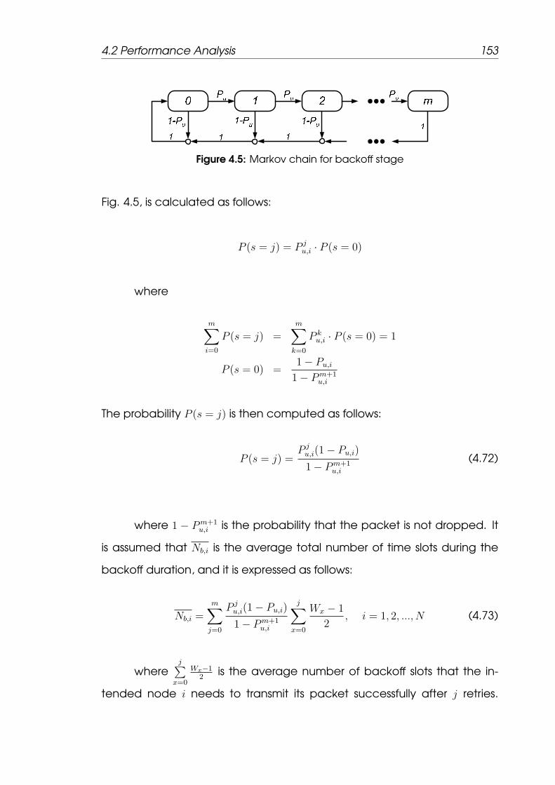
4.2 Performance Analysis 153
Figure 4.5: Markov chain for backoff stage
Fig. 4.5, is calculated as follows:
P (s = j) = P ju,i · P (s = 0)
where
m∑i=0
P (s = j) =m∑k=0
P ku,i · P (s = 0) = 1
P (s = 0) =1− Pu,i
1− Pm+1u,i
The probability P (s = j) is then computed as follows:
P (s = j) =P ju,i(1− Pu,i)
1− Pm+1u,i
(4.72)
where 1 − Pm+1u,i is the probability that the packet is not dropped. It
is assumed that Nb,i is the average total number of time slots during the
backoff duration, and it is expressed as follows:
Nb,i =m∑j=0
P ju,i(1− Pu,i)
1− Pm+1u,i
j∑x=0
Wx − 1
2, i = 1, 2, ..., N (4.73)
wherej∑
x=0
Wx−12
is the average number of backoff slots that the in-
tended node i needs to transmit its packet successfully after j retries.

4.2 Performance Analysis 154
P ju,i(1 − Pu,i) is the probability that the transmission of the node i is suc-
cessful after j retries (backoff stages). Consequently, given the duration of
an empty slot σ and the idle power consumption PIX , the energy that the
node i consumes during the backoff stage, is calculated as follows:
E(i)B = σ · PIX ·Nb,i, i = 1, 2, ..., N (4.74)
Notice that in equation (4.73) only the successful packet transmis-
sions are considered. Let N idle,i be the average number of consecutive
idle slots between two consecutive busy slots of the N−1 remaining nodes.
N idle,i is then calculated as follows:
N idle,i =∞∑j=0
j(1− Pb,i)jPb,i =
1
Pb,i
− 1 (4.75)
The average number of transmissions No,i overheard by the generic
node i from the other N−1 nodes during the backoff process is calculated
as follows:
No,i =Nb,i
N idle,i
=Nb,i
1− Pb,i
Pb,i (4.76)
where Pb,i is given in equation (4.40). Both Nb,i and No,i can be
treated as the total number of idle and busy slots that a packet encoun-
ters during the backoff stages, respectively. The intended node i overhears
the collisions, the successful transmissions, and the erroneous transmissions
of the N−1 nodes. Therefore, the energy that the node i consumes in over-
hearing other nodes transmission during the backoff stages is calculated

4.2 Performance Analysis 155
as follows:
E(i)O = No,iPRXTf,i (4.77)
where Tf,i is given in equation (4.49), and PRX is the receiving power
consumption. The average number of retries Nri that the node i encoun-
ters before delivering its packet correctly to its destination, is calculated as
follows:
Nri =m∑i=0
iP iu,i(1− Pu,i)
1− Pm+1u,i
=1− Pu,i
1− Pm+1u,i
[Pu,i
(1− Pu,i)2(1− Pm
u,i)−mPm+1
u,i
1− Pu,i
](4.78)
The Nri is the sum of retries due to both collision and erroneous tra-
nsmission. From equation (4.19), Pc,i
Pu,iis the fraction of the total retries due to
a collision transmission, and the average number of retries Nci that is due
to a collision transmission in the total retries is calculated as follows:
Nci = Nri
Pc,i
Pu,i
(4.79)
Consequently, the energy consumption due to collision is computed
as follows:
E(i)C = Nci
[PTXTRTS/CRTS + PRXTCTS/CCTS + PIX(TDIFS + TSIFS)
](4.80)
where PTX is the power consumption during transmission. The frac-
tion of the total retries due to an erroneous transmission is: (1−Pc,i)qcek
Pu,i, where
k ∈ (1, 7) for a two-hop transmission, and (1−Pc,i)pekPu,i
, where k ∈ (1, 4) for a
single-hop transmission. Let N cek, where k = 1, 2, ..., 7 be the average num-
4.2 Performance Analysis 156
ber of retries due to the corruption of CRTS, CCTS, RRTS, DATA-S (source-
relay), DATA-S (relay-AP), DATA-R, and ACK, respectively. It is then calcu-
lated as follows:
N cek = Nri
(1− Pc,i)qcek
Pu,i
, k = 1, 2, ...7 (4.81)
Similarly, in the case of a single-hop transmission Ndek, where k ∈ (1, 4)
stands for the average number of retries due to the corruption of RTS, CTS,
DATA-S (source-AP), and ACK, respectively given that exactly one RTS is
transmitted. Thus, we have:
Ndek = Nri
(1− Pc,i)pekPu,i
, k = 1, 2, 3, 4 (4.82)
To calculate the energy consumption during an erroneous tra-
nsmission, it is assumed that Edek, where k = 1, 2, ...4 is the erroneous en-
ergy consumption during the corruption transmission of RTS, CTS, DATA-
S (source-AP), and ACK packets, respectively under a single-hop tra-
nsmission. Edek is expressed as follows:
Ede1 = PTXTRTS + PIX(TCTS + TSIFS + TDIFS + 2δ)
Ede2 = PTXTRTS + PRXTCTS + PIX(TSIFS + TDIFS + 2δ)
Ede3 = PTX(TRTS +
8Ls
Rsd
+ TPLCP ) + PRXTCTS + PIX(TACK + 3TSIFS + TDIFS + 4δ)
Ede4 = PTX(TRTS +
8Ls
Rsd
+ TPLCP ) + PRXTCTS + PIX(TACK + 3TSIFS + TDIFS + 4δ)
(4.83)
Similarly, if the intended node i employs a two-hop transmission, the
energy consumption during an erroneous transmission is defined as Ecek,

4.2 Performance Analysis 157
where k = 1, 2, ...7. It is the energy consumption during the corruption
transmission of CRTS, CCTS, RRTS, DATA-S (source-relay), DATA-S (relay-AP),
DATA-R, and CACK, respectively. Ecek is expressed as follows:
Ece1 = PTXTCRTS + PIX(TCCTS + TSIFS + TDIFS + 2δ)
Ece2 = PTXTCRTS + PRXTCCTS + PIX(TSIFS + TDIFS + 2δ)
Ece3 = PTXTCRTS + PRX(TCCTS + TRRTS) + PIX(2TSIFS + TDIFS + 3δ)
Ece4 = PTX(TCRTS +
8Ls
Rsr
+ TPLCP ) + PRX(TCCTS + TRRTS)
+PIX(4TSIFS + TDIFS + 5δ)
Ece5 = PTX(TCRTS +
8Ls
Rsr
+ TPLCP ) + PRX(TCCTS + TRRTS +8Ls
Rrd
+8Lr
Rrd
+ 2TPLCP ) + PIX(TCACK + 6TSIFS + TDIFS + 7δ)
Ece6 = PTX(TCRTS +
8Ls
Rsr
+ TPLCP ) + PRX(TCCTS + TRRTS +8Ls
Rrd
+8Lr
Rrd
+ 2TPLCP ) + PIX(TCACK + 6TSIFS + TDIFS + 7δ)
Ece7 = PTX(TCRTS +
8Ls
Rsr
+ TPLCP ) + PRX(TCCTS + TRRTS +8Ls
Rrd
+8Lr
Rrd
+ 2TPLCP + TCACK) + PIX(6TSIFS + TDIFS + 7δ) (4.84)
Therefore, the total energy consumption E(i)E , that the intended
node i contends successfully but the packet is corrupted at the receiver,
is calculated as follows:
E(i)E = I(i ∈ Sd)
4∑i=1
NdekE
dek + I(i ∈ Sc)
7∑i=1
N cekE
cek (4.85)
The energy consumption for a successful single-hop transmission, EdS,

4.2 Performance Analysis 158
is computed as follows:
EdS = PTX(TRTS +
8Ls
Rsd
+ TPLCP ) + PRXTCTS + PIX(TACK + 3TSIFS + TDIFS + 4δ)
(4.86)
for a successful two-hop transmission, we have:
EcS = PTX(TCRTS +
8Ls
Rsr
+ TPLCP ) + PRX(TCCTS + TRRTS +8Ls
Rrd
+8Lr
Rrd
+ 2TPLCP ) + PIX(TCACK + 6TSIFS + TDIFS + 7δ) (4.87)
The energy consumption during a successful transmission of the in-
tended node i is computed as follows:
E(i)S = I(i ∈ Sd)Ed
S + I(i ∈ Sc)EcS (4.88)
Finally the average payload size E[L] is given as follows:
E[L] = 8Ls
4∑i=1
Ndi + 8(Ls + Lr)
[3∑
i=1
3∑j=1
N4(i,j) +2∑
i=1
2∑j=1
N3(i,j)
](4.89)
4.2.5 Delay
The average packet delay is the time interval between two suc-
cessful transmissions at a node. If the packet is discarded because it has
reached the retry limit, the delay for this packet will not be included in the
computing of the average delay. Let Di (i = 1, 2, ..., N) denote a random
variable representing a packet delay of the intended node i. Thus, the
average packet delay E[Di] is expressed as follows:

4.2 Performance Analysis 159
E[Di] = E[Db,i] + E[Dc,i] + E[Do,i] + E[De,i] + E[Ds,i] (4.90)
where E[Db,i], E[Dc,i], E[Do,i], E[De,i], and E[Ds,i] stand for the aver-
age delay during decreasing the backoff counter, the average delay due
to a collision transmission, the average delay due to freezing the backoff
counter during the transmissions of the other nodes, the average delay
due to an erroneous transmission, and the average delay of a successful
transmission, respectively. These average delay values are calculated as
follows:
E[Db,i] = σNb,i
E[Dc,i] = Nc,iTc
E[Do,i] = No,iTf,i
E[De,i] = Ps,i
[I(i ∈ Sd)
4∑k=1
N ekpekTek + I(i ∈ Sc)7∑
k=1
N cekq
cekT
cek
]E[Ds,i] = I(i ∈ Sd)T d
s,i + I(i ∈ Sc)T cs,i (4.91)
where Nb,i and No,i are given in equations (4.73) and (4.76), respec-
tively. Tf,i is given in equation (4.48). T ds,i, T
cs,i, and Tc are given in (4.43),
(4.44), and (4.47), respectively. T dek and T c
ek are given in (4.6) and (4.16),
respectively. N cek and Nd
ek are given in (4.81) and (4.82), respectively. There-
fore, the total average delay of the network is calculated as follows:
E[DT ] =1
N
N∑i=1
E[Di] (4.92)

4.3 Analytical and Simulation results 160
Parameter Value Parameter ValueMAC header 272 bits Slot time 20 µs
PHY header 192 bits SIFS 10 µs
RTS 352 bits DIFS 50 µs
CTS 304 bits CRTS 400 bits µsACK 304 bits CCTS 306 bits
CWmin 31 slots RRTS 304 bitsCWmax 1023 slots CACK 306 bits
PLCP rate 1 Mbps PIX , PRX , PTX 0.8,0.8,1.0 Watt
Table 4.2: PHY and MAC setup of the CARD protocol.
4.3 Analytical and Simulation results
To validate the above analysis, a custom event driven simulator de-
veloped by using the Mobile Framework (MF) of the OMNET++ [148] pack-
age written in C++ programming language. The parameters used in sim-
ulation and analysis are set to the default values specified in IEEE 802.11b
standard which are summarized in Table 4.2. The network setting is the
same as given in [Chapter 3, Section 3.4]. In all following figures, solid
lines are results of the analytical model results through Matlab software
package. Whereas dot-dashed lines are for the simulation results through
OMNET++ software package.
4.3.1 Throughput Results
In Fig. 4.6, we compare the saturated throughput achieved by the
CARD, CoopMAC, and IEEE 802.11b protocols under ideal channel condi-
tions. As the network size, i.e. number of nodes, increases, the through-
put for 802.11b decreases due to collisions. This is because of increas-
ing the number of nodes causes increasing the collision probability, and

4.3 Analytical and Simulation results 161
hence the overall throughput degrades. On the other hand, the through-
put achieved by both the CARD and CoopMAC protocols increases ex-
ponentially as the number of nodes increases. The reason is that as the
number of nodes increases, the probability of a low data-rate node find-
ing a relay node increases. The two-hop transmission between a source
node and the AP can be established via a relay node, and the data-
rate from a source node to the AP increases. Therefore, the cooperative
transmission not only compensates the collision probability caused by in-
creasing the number of nodes, but also solves the performance anomaly
caused by the low data-rate nodes; for this reason the throughput of both
the CARD and CoopMAC protcols increases as the number of nodes in-
creases. However, the CARD protocol achieves a higher throughput than
the CoopMAC protocol.
As shown in Fig. 4.6, the CARD protocol can achieve throughput up
to 42% more than that can be achieved by the CoopMAC protocol when
the number of nodes is more than 30 nodes. This is because the CARD
protocol achieves both cooperative diversity gain and cooperative multi-
plexing gain. The relay node shares the handshake procedure between
a source node and the AP and transmits its own data immediately after
forwarding the source station’s information to the AP. On the contrary, the
CoopMAC protocol achieves only cooperative diversity gain; where the
relay node forwards only the information of the source node to the AP.
The channel conditions is one of the critical parameters that can
affect the performance of the WLANs. It is then important to study the ef-
fect of the imperfect channel conditions on the throughput that can be
achieved by the CARD protocol. Fig. 4.7 shows the relationship between
throughput and network size under different channel conditions for the

4.3 Analytical and Simulation results 162
8 10 12 14 16 18 20 22 24 26 28 30 32 34 36 38 400
0.5
1
1.5
2
2.5
3
3.5
Number of nodes
Thro
ughp
ut (M
bps)
801.11b−AnalysisCoopMAC−AnalysisCARD−Analysis801.11b−SimulationCoopMAC−SimulationCARD−Simulation
Figure 4.6: Throughput vs. number of nodes under ideal channel, L = 1024 bytes.
802.11b, CoopMAC, and CARD protocols. The throughput performance
under BER = 2 × 10⁻⁵ and under BER = 6 × 10⁻⁵ is given in Fig. 4.7(a)
and Fig. 4.7(b), respectively. As the channel quality becomes poor, the
throughput of the three protocols decreases. The reason is that the proba-
bility of packet errors increases as the channel conditions becomes poor.
Consequently, the number of retransmission retries, and the transmission
time to deliver the data packet to the AP also increases. Even if the
channel conditions becomes imperfect, the CARD protocol outperforms
both the 802.11b and CoopMAC protocols. For example the throughput
that can be achieved by the CARD when the BER = 6×10⁻⁵ is higher than
the throughput that can be achieved by the CoopMAC protocol under
ideal channel conditions. Therefore, the CARD protocol is more reliable
than the existing 802.11b and CoopMAC protocols.
It is well known that the packet length has a major effect on the
performance of any MAC protocol. Therefore, in Fig. 4.8, we study the ef-
fect of the packet length on the throughput performance of the 802.11b,
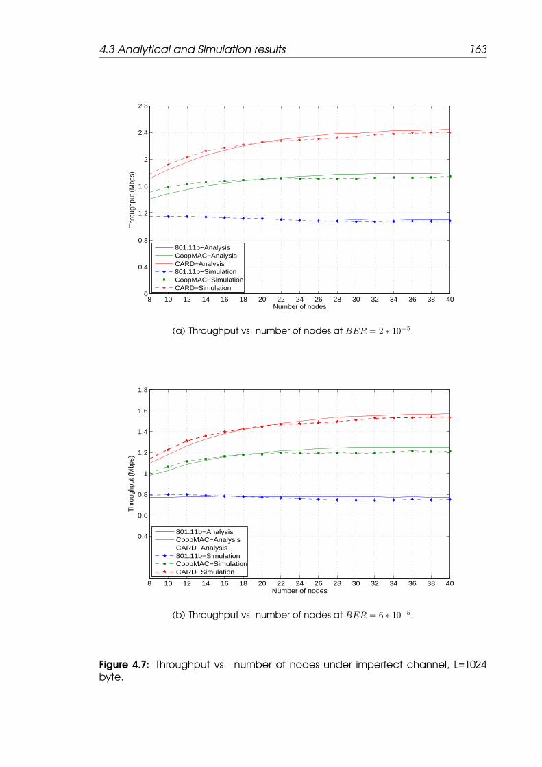
4.3 Analytical and Simulation results 163
8 10 12 14 16 18 20 22 24 26 28 30 32 34 36 38 400
0.4
0.8
1.2
1.6
2
2.4
2.8
Number of nodes
Thr
ough
put (
Mbp
s)
801.11b−AnalysisCoopMAC−AnalysisCARD−Analysis801.11b−SimulationCoopMAC−SimulationCARD−Simulation
(a) Throughput vs. number of nodes at BER = 2 ∗ 10−5.
8 10 12 14 16 18 20 22 24 26 28 30 32 34 36 38 40
0.4
0.6
0.8
1
1.2
1.4
1.6
1.8
Number of nodes
Thro
ughp
ut (M
bps)
801.11b−AnalysisCoopMAC−AnalysisCARD−Analysis801.11b−SimulationCoopMAC−SimulationCARD−Simulation
(b) Throughput vs. number of nodes at BER = 6 ∗ 10−5.
Figure 4.7: Throughput vs. number of nodes under imperfect channel, L=1024byte.
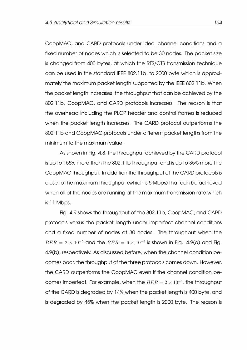
4.3 Analytical and Simulation results 164
CoopMAC, and CARD protocols under ideal channel conditions and a
fixed number of nodes which is selected to be 30 nodes. The packet size
is changed from 400 bytes, at which the RTS/CTS transmission technique
can be used in the standard IEEE 802.11b, to 2000 byte which is approxi-
mately the maximum packet length supported by the IEEE 802.11b. When
the packet length increases, the throughput that can be achieved by the
802.11b, CoopMAC, and CARD protocols increases. The reason is that
the overhead including the PLCP header and control frames is reduced
when the packet length increases. The CARD protocol outperforms the
802.11b and CoopMAC protocols under different packet lengths from the
minimum to the maximum value.
As shown in Fig. 4.8, the throughput achieved by the CARD protocol
is up to 155% more than the 802.11b throughput and is up to 35% more the
CoopMAC throughput. In addition the throughput of the CARD protocols is
close to the maximum throughput (which is 5 Mbps) that can be achieved
when all of the nodes are running at the maximum transmission rate which
is 11 Mbps.
Fig. 4.9 shows the throughput of the 802.11b, CoopMAC, and CARD
protocols versus the packet length under imperfect channel conditions
and a fixed number of nodes at 30 nodes. The throughput when the
BER = 2 × 10⁻⁵ and the BER = 6 × 10⁻⁵ is shown in Fig. 4.9(a) and Fig.
4.9(b), respectively. As discussed before, when the channel condition be-
comes poor, the throughput of the three protocols comes down. However,
the CARD outperforms the CoopMAC even if the channel condition be-
comes imperfect. For example, when the BER = 2× 10⁻⁵, the throughput
of the CARD is degraded by 14% when the packet length is 400 byte, and
is degraded by 45% when the packet length is 2000 byte. The reason is

4.3 Analytical and Simulation results 165
400 600 800 1000 1200 1400 1600 1800 20000.5
1
1.5
2
2.5
3
3.5
4
Packet length (byte)
Thr
ough
put (
Mbp
s)
801.11b−AnalysisCoopMAC−AnalysisCARD−Analysis801.11b−SimulationCoopMAC−SimulationCARD−Simulation
Figure 4.8: Throughput versus packet length under ideal channel, N=30 nodes.
that as the packet length increases, the probability of packet error rate
also increases, and hence the number retransmission retries increases. As
a result, the throughput is degraded as the packet length increases. As
show also in Fig. 4.9(b), as the packet length increases the throughput
increases until the packet length becomes around 1200 byte, after that
the throughput decreases as the packet length increases. As the packet
length increases, the throughput increases and also the packet error rate
also increases, and then the throughput decreases. For this reason, the
throughput improvement is reduced by the packet error as the packet
length increases. Under all the channel conditions, the CARD protocol
outperforms the CoopMAC protocol.
The throughput versus number of nodes under ideal channel con-
ditions of both BTAC and CARD protocols is shown in Fig. 4.10. The CARD
protocol outperforms the BTAC protocol, since the throughput of the CARD
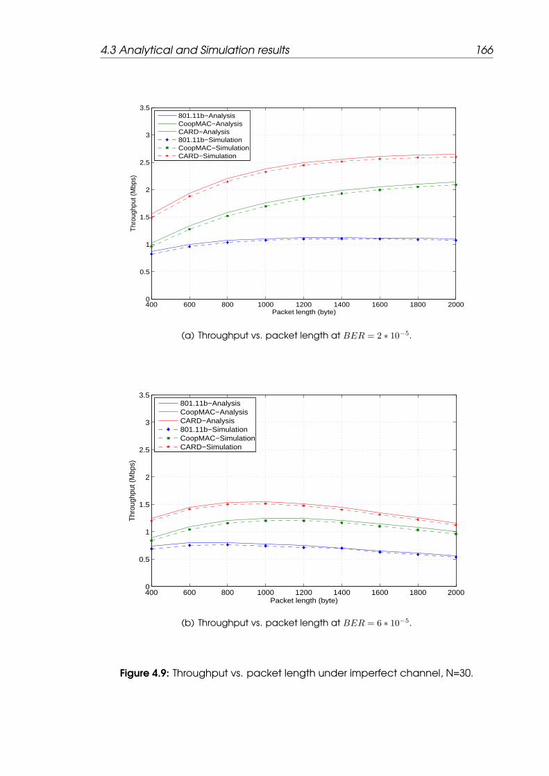
4.3 Analytical and Simulation results 166
400 600 800 1000 1200 1400 1600 1800 20000
0.5
1
1.5
2
2.5
3
3.5
Packet length (byte)
Thro
ughp
ut (M
bps)
801.11b−AnalysisCoopMAC−AnalysisCARD−Analysis801.11b−SimulationCoopMAC−SimulationCARD−Simulation
(a) Throughput vs. packet length at BER = 2 ∗ 10−5.
400 600 800 1000 1200 1400 1600 1800 20000
0.5
1
1.5
2
2.5
3
3.5
Packet length (byte)
Thro
ughp
ut (M
bps)
801.11b−AnalysisCoopMAC−AnalysisCARD−Analysis801.11b−SimulationCoopMAC−SimulationCARD−Simulation
(b) Throughput vs. packet length at BER = 6 ∗ 10−5.
Figure 4.9: Throughput vs. packet length under imperfect channel, N=30.
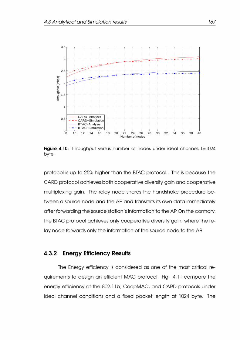
4.3 Analytical and Simulation results 167
8 10 12 14 16 18 20 22 24 26 28 30 32 34 36 38 400
0.5
1
1.5
2
2.5
3
3.5
Number of nodes
Thro
ughp
ut (M
bps)
CARD−AnalysisCARD−SimulationBTAC−AnalysisBTAC−Simulation
Figure 4.10: Throughput versus number of nodes under ideal channel, L=1024byte.
protocol is up to 25% higher than the BTAC protocol.. This is because the
CARD protocol achieves both cooperative diversity gain and cooperative
multiplexing gain. The relay node shares the handshake procedure be-
tween a source node and the AP and transmits its own data immediately
after forwarding the source station’s information to the AP. On the contrary,
the BTAC protocol achieves only cooperative diversity gain; where the re-
lay node forwards only the information of the source node to the AP.
4.3.2 Energy Efficiency Results
The Energy efficiency is considered as one of the most critical re-
quirements to design an efficient MAC protocol. Fig. 4.11 compare the
energy efficiency of the 802.11b, CoopMAC, and CARD protocols under
ideal channel conditions and a fixed packet length at 1024 byte. The

4.3 Analytical and Simulation results 168
8 10 12 14 16 18 20 22 24 26 28 30 32 34 36 38 400
0.05
0.1
0.15
0.2
0.25
0.3
0.35
Number of nodes
Ene
rgy
effic
ienc
y (M
b/J)
801.11b−AnalysisCoopMAC−AnalysisCARD−Analysis801.11b−SimulationCoopMAC−SimulationCARD−Simulation
Figure 4.11: Energy efficiency vs. number of nodes under ideal channel, L=1024bytes.
CARD protocol outperforms both the 802.11b and CoopMAC protocols.
Since the energy efficiency of the CARD protocol is up to 30% and up to
80% higher than the CoopMAC and 802.11b protocols, respectively. As
shown in Fig. 4.11, when the number of nodes increases, the energy ef-
ficiency decreases. The energy efficiency decreases as the number of
node increases due to increasing the probability of collisions. Whereas the
number of retransmissions increases as the collision probability increases.
Hence, a node consumes more energy on the retransmission, receiving,
overhearing, and sensing the medium.
The effect of the medium status on the energy efficiency versus the
number of nodes is shown in Fig. 4.12 at a fixed packet length 1024 byte. As
the medium becomes worst, the energy efficiency of the 802.11b, Coop-
MAC, and CARD protocols decreases, where the number of retransmission
retries increases and a node consumes more energy on the retransmission,
4.3 Analytical and Simulation results 169
overhearing, receiving, and sensing the medium. The CARD protocol is
better than the 802.11b and CoopMAC protocols under different channel
conditions. The CARD at BER = 6× 10⁻⁵, shown in Fig. 4.12(b) has energy
efficiency higher than that of the CoopMAC protocol at BER = 2 × 10⁻⁵
shown in Fig. 4.12(a). Therefore, the CARD protocol is more reliable than
the CoopMAC protocol against the channel conditions.
The effect of packet length on the energy efficiency at a fixed num-
ber of nodes (30 nodes) is studied in Fig. 4.13 and Fig. 4.14 under ideal and
imperfect channel conditions, respectively. As the packet size increases,
the energy efficiency of the 802.11, CoopMAC, and CARD protocols in-
creases. The reason is that the overhead including the PLCP header and
control frames is reduced when the packet length increases. Therefore,
more energy is saved, and the energy efficiency is then increases. The en-
ergy efficiency decreases as the channel becomes poor. This is because
the number retransmissions increases and a node consumes more energy
to deliver its data packets to the AP. Consequently, the energy efficiency
decreases. As shown in Fig. 4.14, the energy efficiency of the CARD proto-
col at BER = 6 × 10⁻⁵ shown in Fig. 4.12(b) is approximately equal to the
energy efficiency of the CoopMAC protocol at the ideal channel condi-
tions.
Fig. 4.15 compare the energy efficiency of both BTAC and CARD
protocols under ideal channel conditions and a fixed packet length at
1024 byte. The CARD protocol outperforms BTAC protocol. Since the en-
ergy efficiency of the CARD protocol is up to 20% higher than the BTAC
protocol.

4.3 Analytical and Simulation results 170
8 10 12 14 16 18 20 22 24 26 28 30 32 34 36 38 400
0.05
0.1
0.15
0.2
0.25
0.3
0.35
Number of nodes
Ene
rgy
effic
ienc
y (M
b/J)
801.11b−AnalysisCoopMAC−AnalysisCARD−Analysis801.11b−SimulationCoopMAC−SimulationCARD−Simulation
(a) Energy vs. number of nodes at BER = 2 ∗ 10−5.
8 10 12 14 16 18 20 22 24 26 28 30 32 34 36 38 400.02
0.04
0.06
0.08
0.1
0.12
0.14
0.16
0.18
0.2
Number of nodes
Ene
rgy
effic
ienc
y (M
b/J)
801.11b−Analysis
CoopMAC−Analysis
CARD−Analysis
801.11b−Simulation
CoopMAC−Simulation
CARD−Simulation
(b) Energy vs. number of nodes at BER = 6 ∗ 10−5.
Figure 4.12: Energy vs. number of nodes under imperfect channel, L=1024 byte.

4.3 Analytical and Simulation results 171
400 600 800 1000 1200 1400 1600 1800 20000.02
0.04
0.06
0.08
0.1
0.12
0.14
0.16
0.18
Packet length (byte)
Ene
rgy
effic
ienc
y (M
b/J)
)
801.11b−AnalysisCoopMAC−AnalysisCARD−Analysis801.11b−SimulationCoopMAC−SimulationCARD−Simulation
Figure 4.13: Energy efficiency vs. packet length under ideal channel, N=30.
4.3.3 Delay Results
The improvement in system throughput also transforms into a bet-
ter a packet delay performance. The relation between the service delay
and the number of nodes for a successful packet transmission and a fixed
packet length (1024 byte) is shown in Fig. 4.16. As the number of nodes
increases, the service delay also increases. This is due to the collision prob-
ability increases as the number of node increases, and hence the number
of retries increases. As a result, the service delay which is the time re-
quired to deliver the packet to the AP increases. However, the service
delay for the CARD protocol is substantially lower than that for both the
802.11b MAC and CoopMAC protocols under ideal channel conditions.
As shown in Fig. 4.16, the service delay of the CARD protocol is up to 150%
and up to 50% less than the service delay of the 802.11b and CoopMAC
protocols, respectively. This is because the CARD protocol achieves both
cooperative diversity gain and cooperative multiplexing gain. On the con-
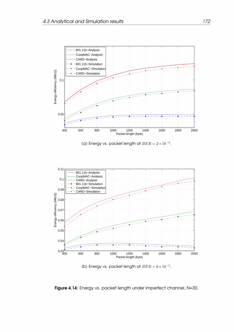
4.3 Analytical and Simulation results 172
400 600 800 1000 1200 1400 1600 1800 2000
0.05
0.1
Packet length (byte)
Ene
rgy
effic
ienc
y (M
b/J)
)
801.11b−Analysis
CoopMAC−Analysis
CARD−Analysis
801.11b−Simulation
CoopMAC−Simulation
CARD−Simulation
(a) Energy vs. packet length at BER = 2 ∗ 10−5.
400 600 800 1000 1200 1400 1600 1800 20000.03
0.04
0.05
0.06
0.07
0.08
0.09
0.1
0.11
Packet length (byte)
Ene
rgy
effic
ienc
y (M
b/J)
)
801.11b−AnalysisCoopMAC−AnalysisCARD−Analysis801.11b−SimulationCoopMAC−SimulationCARD−Simulation
(b) Energy vs. packet length at BER = 6 ∗ 10−5.
Figure 4.14: Energy vs. packet length under imperfect channel, N=30.
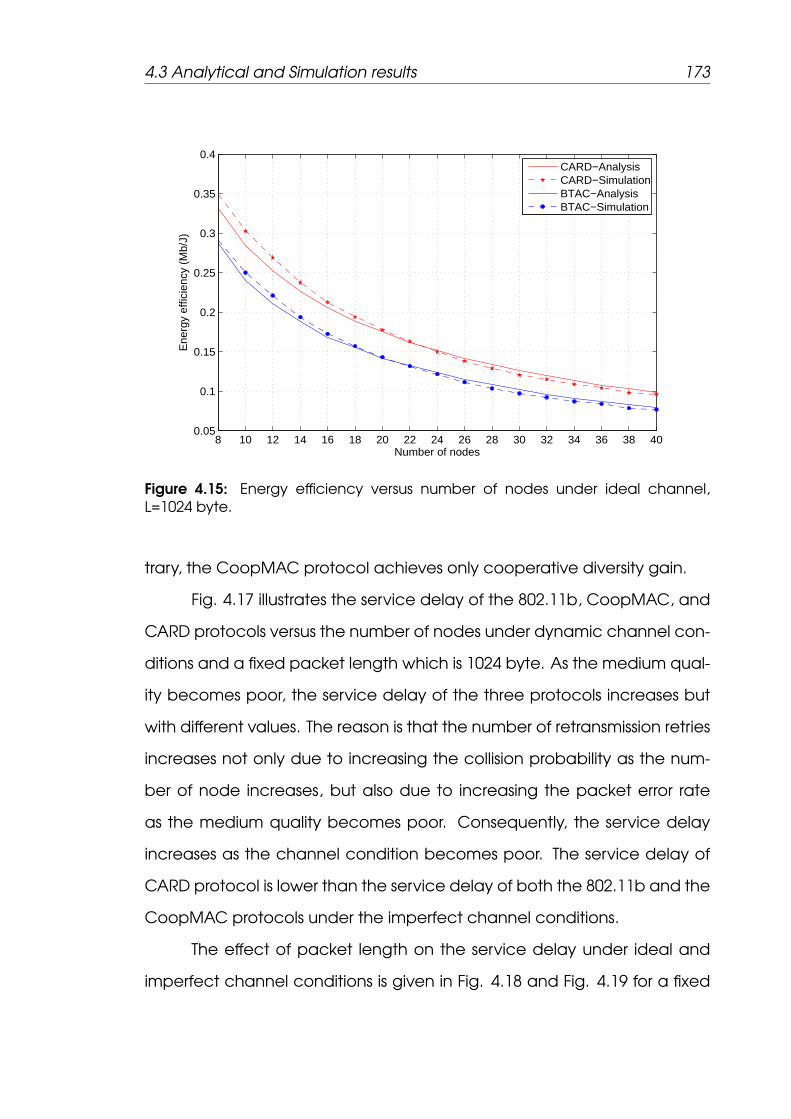
4.3 Analytical and Simulation results 173
8 10 12 14 16 18 20 22 24 26 28 30 32 34 36 38 400.05
0.1
0.15
0.2
0.25
0.3
0.35
0.4
Number of nodes
Ene
rgy
effic
ienc
y (M
b/J)
CARD−AnalysisCARD−SimulationBTAC−AnalysisBTAC−Simulation
Figure 4.15: Energy efficiency versus number of nodes under ideal channel,L=1024 byte.
trary, the CoopMAC protocol achieves only cooperative diversity gain.
Fig. 4.17 illustrates the service delay of the 802.11b, CoopMAC, and
CARD protocols versus the number of nodes under dynamic channel con-
ditions and a fixed packet length which is 1024 byte. As the medium qual-
ity becomes poor, the service delay of the three protocols increases but
with different values. The reason is that the number of retransmission retries
increases not only due to increasing the collision probability as the num-
ber of node increases, but also due to increasing the packet error rate
as the medium quality becomes poor. Consequently, the service delay
increases as the channel condition becomes poor. The service delay of
CARD protocol is lower than the service delay of both the 802.11b and the
CoopMAC protocols under the imperfect channel conditions.
The effect of packet length on the service delay under ideal and
imperfect channel conditions is given in Fig. 4.18 and Fig. 4.19 for a fixed

4.3 Analytical and Simulation results 174
8 10 12 14 16 18 20 22 24 26 28 30 32 34 36 38 400
0.05
0.1
0.15
0.2
0.25
0.3
0.35
Number of nodes
Del
ay (s
ec.)
801.11b−Analysis
CoopMAC−Analysis
CARD−Analysis
801.11b−Simulation
CoopMAC−Simulation
CARD−Simulation
Figure 4.16: Service delay vs. number of nodes under ideal channel, L = 1024bytes.
number of nodes which is 30 nodes. As the packet length increases, the
service delay of the three protocols increases. The reason is that the tra-
nsmission time increases as the packet length increases, and hence the
service delay increases. The service delay of the CARD protocol is lower
than that the service delay of both the 802.11b and CoopMAC protocols
under different channel conditions.
The relation between the service delay and the number of nodes for
a successful packet transmission and a fixed packet length (1024 byte) is
shown in Fig. 4.20. The service delay for the CARD protocol is substantially
lower than that for both the BTAC protocol under ideal channel condi-
tions. As shown in Fig. 4.20, the service delay of the CARD protocol is up
to 32% less than the service delay of the BTAC protocol. This is because
the CARD protocol achieves both cooperative diversity gain and cooper-
ative multiplexing gain. On the contrary, the BTAC protocol achieves only
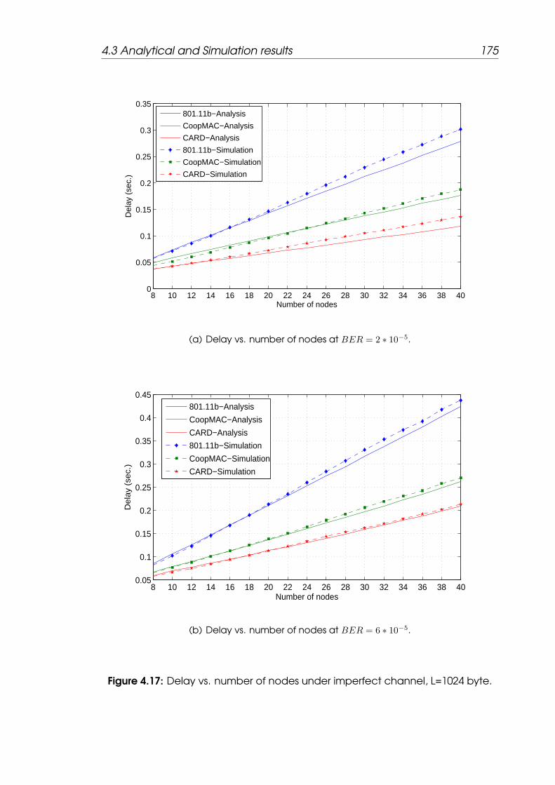
4.3 Analytical and Simulation results 175
8 10 12 14 16 18 20 22 24 26 28 30 32 34 36 38 400
0.05
0.1
0.15
0.2
0.25
0.3
0.35
Number of nodes
Del
ay (
sec.
)
801.11b−Analysis
CoopMAC−Analysis
CARD−Analysis
801.11b−Simulation
CoopMAC−Simulation
CARD−Simulation
(a) Delay vs. number of nodes at BER = 2 ∗ 10−5.
8 10 12 14 16 18 20 22 24 26 28 30 32 34 36 38 400.05
0.1
0.15
0.2
0.25
0.3
0.35
0.4
0.45
Number of nodes
De
lay
(se
c.)
801.11b−Analysis
CoopMAC−Analysis
CARD−Analysis
801.11b−Simulation
CoopMAC−Simulation
CARD−Simulation
(b) Delay vs. number of nodes at BER = 6 ∗ 10−5.
Figure 4.17: Delay vs. number of nodes under imperfect channel, L=1024 byte.

4.4 Conclusions 176
400 600 800 1000 1200 1400 1600 1800 20000.05
0.1
0.15
0.2
0.25
0.3
0.35
0.4
Packet length (byte.)
Del
ay (s
ec.)
801.11b−Analysis
CoopMAC−Analysis
CARD−Analysis
801.11b−Simulation
CoopMAC−Simulation
CARD−Simulation
Figure 4.18: Service delay vs. packet length under ideal channel, N=30.
cooperative diversity gain.
4.4 Conclusions
In this chapter, we propose a new MAC protocol, called Coopera-
tive Access with Relay’s Data (CARD) for multi-rate WLANs. CARD uses the
best relay node to improve the overall transmission rate for low data-rate
nodes. More importantly, CARD enables a relay node to transmit its own
data packet without the handshake procedure for accessing the channel.
In doing so, CARD for first time provides a novel transmission mechanism for
the relay node and therefore can achieve both cooperative diversity gain
and multiplexing gain. Compared with the IEEE 802.11b standard, the sig-
nalling changes and overheads in CARD are minimum, thus making CARD
fully compatible with the IEEE 802.11b standard and suitable for coexisting
with the standard DCF protocols.
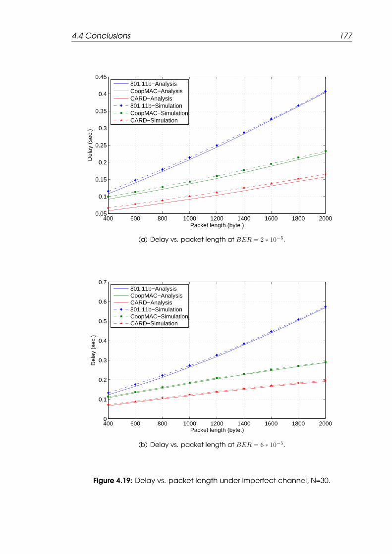
4.4 Conclusions 177
400 600 800 1000 1200 1400 1600 1800 20000.05
0.1
0.15
0.2
0.25
0.3
0.35
0.4
0.45
Packet length (byte.)
Del
ay (
sec.
)
801.11b−AnalysisCoopMAC−AnalysisCARD−Analysis801.11b−SimulationCoopMAC−SimulationCARD−Simulation
(a) Delay vs. packet length at BER = 2 ∗ 10−5.
400 600 800 1000 1200 1400 1600 1800 20000
0.1
0.2
0.3
0.4
0.5
0.6
0.7
Packet length (byte.)
Del
ay (
sec.
)
801.11b−AnalysisCoopMAC−AnalysisCARD−Analysis801.11b−SimulationCoopMAC−SimulationCARD−Simulation
(b) Delay vs. packet length at BER = 6 ∗ 10−5.
Figure 4.19: Delay vs. packet length under imperfect channel, N=30.
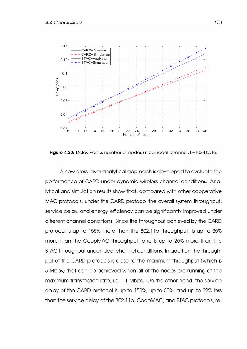
4.4 Conclusions 178
8 10 12 14 16 18 20 22 24 26 28 30 32 34 36 38 400.02
0.04
0.06
0.08
0.1
0.12
0.14
Number of nodes
Del
ay (s
ec.)
CARD−AnalysisCARD−SimulationBTAC−AnalysisBTAC−Simulation
Figure 4.20: Delay versus number of nodes under ideal channel, L=1024 byte.
A new cross-layer analytical approach is developed to evaluate the
performance of CARD under dynamic wireless channel conditions. Ana-
lytical and simulation results show that, compared with other cooperative
MAC protocols, under the CARD protocol the overall system throughput,
service delay, and energy efficiency can be significantly improved under
different channel conditions. Since the throughput achieved by the CARD
protocol is up to 155% more than the 802.11b throughput, is up to 35%
more than the CoopMAC throughput, and is up to 25% more than the
BTAC throughput under ideal channel conditions. In addition the through-
put of the CARD protocols is close to the maximum throughput (which is
5 Mbps) that can be achieved when all of the nodes are running at the
maximum transmission rate, i.e. 11 Mbps. On the other hand, the service
delay of the CARD protocol is up to 150%, up to 50%, and up to 32% less
than the service delay of the 802.11b, CoopMAC, and BTAC protocols, re-
4.4 Conclusions 179
spectively under ideal channel conditions. The energy efficiency of the
CARD protocol under ideal channel conditions is up to 20%, up to 30%,
and up to 80% higher than the BTAC, the CoopMAC, and 802.11b proto-
cols, respectively. The CARD protocol achieves better throughput, service
delay, and energy efficiency than the CoopMAC protocol under imper-
fect channel conditions. As a result, the CARD protocol is more reliable
than the CoopMAC protocol under dynamic channel conditions.

Chapter 5
Unsaturated Analysis of
Cooperative MAC protocols
In chapters 3 and 4 both the BTAC and CARD protocols are stud-
ied assuming saturated conditions, i.e. each node always has a packet
waiting for transmission. The studies on saturated conditions are essential
for gaining insights into the behavior of both protocols. However, the sat-
urated assumption is impractical for networks providing real-time applica-
tions such as web, email and voice. In such cases, a saturated assump-
tion is not appropriate [150–152]. Therefore, the aim of this chapter is to
propose a mathematical model for both the BTAC and the standard IEEE
802.11 protocols under unsaturated conditions.
The remainder of the chapter is organized as follows. Section 5.1
presents the proposed Markov chain model for the unsaturated condi-
tions. Throughput, energy efficiency, and delay analysis are given in Sec-
tion 5.2. In Section 5.3 the analytical model is validated using OMNET++
[148] simulations. Finally, some conclusion remarks are given in Section 5.4.

5.1 Non-saturated Markov Chain model 181
5.1 Non-saturated Markov Chain model
The Markov chain model given in [Sec. 4.2.2, pp. 133] is modified
to study the behaviour of the DCF under the assumption of unsaturated
conditions, error free channel, and multi-rate transmissions. Under the IEEE
802.11 standard, it is mandatory that the backoff mechanism is performed
after each successful transmission even if there is no other MAC Service
Data Unit (MSDU) to be transmitted. This referred to as ”post-backoff”. The
post-backoff guarantees that there is always at least one backoff interval
preceding a packet transmission. Alternatively, there is an exception to
the essential rule that an MSDU from the upper layer has to be transmit-
ted after performing the backoff mechanism. The MSDU arriving from the
upper layer may be transmitted immediately without waiting any time if
the transmission queue is empty, the latest post-backoff is finished, and at
the same time the channel has been idle for at least one DCF interval.
In the proposed model this exceptional case and the unsaturated traffic
conditions are taken into account by introducing a new state (idle state)
labelled (0,−1, 0) explained later.
Let m′ be the maximum number of retransmissions using different
contention window (CW) size. Let m be the maximum number of retries
after which the packet is discarded even if it is not received correctly.
Let s(t) be a random process representing the backoff stage j at time t,
where 0 ≤ j ≤ m. Let b(t) be a stochastic process representing the value of
the backoff counter for a given node at time t. The value of the backoff
5.1 Non-saturated Markov Chain model 182
counter is uniformly chosen from [0,Wj − 1]; Wj is given as follows [1]:
Wj =
2jW0 j ≤ m′
2m′W0 j > m′
(5.1)
The third dimension u(t) specify the remaining time during a success-
ful transmission, a collision transmission, and a frozen transmission. As shown
in Fig. 5.1, the three dimensional process {s(t), b(t), u(t)} is a discrete-time
Markov chain under assumption that the collision probability Pc,i and the
probability Pb,i, that the channel is busy are independent. It is referred to a
generic node with index i ∈ S = {Sd ∪ Sc1 ∪ Sc
2}; where Sd is the set of nodes
that employ a single-hop transmission, Sc1 is the set of nodes at rate 1 Mbps
and employing a two-hop transmission, and Sc2 is the set of nodes at rate 2
Mbps and employing a two-hop transmissions. The details of these sets are
given in Appendix A. The state of each node can be described by {j, k, ℓ}.
j is the backoff stage, j = 0, 1, ...,m, and j = −1 represents a successful tra-
nsmission stage. k is the backoff counter taking values from [0,Wj−1] in time
slots, and k = −1 stands for idle state (i.e. empty queue) during the backoff
stage 0. The third index ℓ specifies the following:
• The remaining time for the successful transmission states
(−1, 0, ℓ) 1 ≤ ℓ ≤ Ns,i
• The remaining time for the collision transmission states
(j, 0, ℓ) 1 ≤ ℓ ≤ Nc,i 0 ≤ j ≤ m

5.1 Non-saturated Markov Chain model 183
Figure 5.1: Unsaturated Markov chain model.

5.1 Non-saturated Markov Chain model 184
• The remaining time for the frozen transmission period states
(j, k, ℓ), 1 ≤ ℓ ≤ Nf,i 1 ≤ k ≤ Wj − 1 0 ≤ j ≤ m
(0,−1, ℓ), 1 ≤ ℓ ≤ Nf,i
where Ns,i, Nc,i, and Nf,i stand for a successful transmission period, a
collision transmission period, and a frozen transmission period in a slot time
units, respectively.
5.1.1 Transition Probabilities
In this model the one step transition probabilities are expressed as follows:
1. At the beginning of each slot time, the backoff counter freezes for
Nf,i slots when the channel becomes busy.
Pr{j, k,Nf,i|j, k, 0} = Pb,i 1 ≤ k ≤ Wj − 1 0 ≤ j ≤ m
2. The node suspends its transmission for Nf,i slots during a busy channel
while the node resides in the idle state and at least one packet arrives
with probability 1− PE,i
Pr{0,−1, Nf,i|0,−1, 0} = Pb,i(1− PE,i)
3. During the frozen period, the counter decreases by one for each slot

5.1 Non-saturated Markov Chain model 185
time.
Pr{j, k, ℓ− 1|j, k, ℓ} = 1 2 ≤ ℓ ≤ Nf,i 0 ≤ k ≤ Wj − 1 0 ≤ j ≤ m
Pr{0,−1, ℓ− 1|0,−1, ℓ} = 1 2 ≤ ℓ ≤ Nf,i
4. At the end of the frozen period, the node reactivities its backoff
counter.
Pr{j, k − 1, 0|j, k, 1} = 1 1 ≤ k ≤ Wj − 1 0 ≤ j ≤ m
5. The node accesses the medium at the end of the frozen interval of
the idle state after receiving at least one packet from the upper layer.
The transmission is successful if there is no other node tries to transmit.
Pr{−1, 0, Ns,i|0,−1, 1} = 1− Pc,i
6. If the node’s buffer is not empty, the transmission is unsuccessful due
to a collision with other nodes at the end of the frozen period.
Pr{0, 0, Nc,i|0,−1, 1} = Pc,i
7. The node stays in the idle state if the buffer is empty.
Pr{0,−1, 0|0,−1, 0} = PE,i
8. If the channel is idle and there is at least one packet arrival during

5.1 Non-saturated Markov Chain model 186
the idle state, the transmission is unsuccessful due to a collision.
Pr{0, 0, Nc,i|0,−1, 0} = (1− PE,i)(1− Pb,i)Pc,i
9. During the idle state if there is at least one packet arrival from the up-
per layer and the channel becomes idle, the transmission is successful
when other nodes are listening.
Pr{0, 0, Ns,i|0,−1, 0} = (1− PE,i)(1− Pb,i)(1− Pc,i)
10. When the backoff counter reaches zero in stage 0, the node inters
the idle state if its buffer is empty.
Pr{0,−1, 0|0, 0, 0} = 1− qi
11. The transmission is successful at the end of stage 0 if the channel is
idle and the buffer is not empty.
Pr{−1, 0, Ns,i|0, 0, 0} = qi(1− Pc,i)
12. When the node’s buffer is not empty at the end of backoff stage 0,
the transmission is unsuccessful due to a collision with other nodes.
Pr{0, 0, Nc,i|0, 0, 0} = qiPc,i
13. The backoff counter is decrementing when the channel is sensed
idle.

5.1 Non-saturated Markov Chain model 187
Pr{j, k − 1, 0|j, k, 0} = 1− Pb,i 1 ≤ k ≤ Wj − 1 0 ≤ j ≤ m
14. When the backoff counter reaches zero and no other node tries to
transmit, the transmission is successful.
Pr{−1, 0, Ns,i|j, 0, 0} = 1− Pc,i 1 ≤ j ≤ m
15. During a successful transmission interval the counter decreases by
one for each slot time.
Pr{−1, 0, ℓ− 1| − 1, 0, ℓ} = 1 2 ≤ ℓ ≤ Ns,i
16. A new backoff delay of stage 0 is selected after the successful tra-
nsmission.
P{0, k, 0| − 1, 0, 1} =1
W0
0 ≤ k ≤ W0 − 1
17. When an unsuccessful transmission occurs due to a collision, the node
inters the unsuccessful interval.
Pr{j, 0, Nc,i|j, 0, 0} = Pc,i 1 ≤ j ≤ m
18. During the unsuccessful transmission period the counter decreases by
one for each slot time.
P{j, 0, ℓ− 1|j, 0, ℓ} = 1 0 ≤ j ≤ m 2 ≤ ℓ ≤ Nc,i
19. After the counter of unsuccessful transmission period reaches zero,
5.1 Non-saturated Markov Chain model 188
the node doubles the contention window and inters the next backoff
stage.
Pr{j + 1, k, 0|j, 0, 1} =1
Wj+1
0 ≤ j ≤ m− 1
20. If there is an unsuccessful transmission after m retries, the current
packet is discarded and the node starts a new packet transmission
at the end of the unsuccessful transmission period.
Pr{0, k, 0|m, 0, 1} =1
W0
0 ≤ k ≤ W0 − 1
where qi is the probability that there is at least one packet waiting for
transmission in the queue of the generic node i after completing the post-
backoff of a pervious transmission. At the idle state (i.e. empty queue),
PE,i is the probability that the generic node i stays in the idle state until at
least one packet arrives from the upper layer.
5.1.2 System Equations
Let πj,k,ℓ = limt→∞P{s(t) = j, b(t) = k, u(t) = ℓ} be the stationary distri-
bution of the model. In the steady state, the following equations hold for
the Markov chain model given in Fig. 5.1.
π0,−1,1 = Pb,i(1− PE,i)π0,−1,0
(1− PE,i)π0,−1,0 = (1− qi)π0,0,0 (5.2)
From which, we have:
π0,−1,1 = Pb,i(1− qi)π0,0,0 (5.3)

5.1 Non-saturated Markov Chain model 189
From the model we also have:
π0,0,Nc,i= Pc,i
[qiπ0,0,0 + (1− Pb,i)(1− PE,i)π0,−1,0 + π0,−1,1
](5.4)
By substituting equations (5.2) and (5.3) into equation (5.4) we have:
π0,0,Nc,i= Pc,iπ0,0,0 (5.5)
where
πj,0,ℓ = πj,0,Nc,i0 ≤ j ≤ m 1 ≤ ℓ < Nc,i (5.6)
and
π1,0,0 = π0,0,1 (5.7)
Substituting equations (5.5) and (5.6) into equation (5.7), we have:
π1,0,0 = Pc,iπ0,0,0 (5.8)
Thus, we have:
πj,0,0 = Pc,i · πj−1,0,0 → πj,0,0 = P jc,iπ0,0,0 0 ≤ j ≤ m (5.9)
Due to the regularities of the Markov chain, thus for each 1 ≤ k ≤

5.1 Non-saturated Markov Chain model 190
Wj − 1, all the following relations hold:
πj,k,0 =Wj − k
Wj
(1− Pc,i)
∑mx=0 πx,0,0 + Pc,iπm,0,0 j = 0
Pc,iπj−1,0,0 0 < j ≤ m
(5.10)
By substituting equation (5.9) into equation (5.10), and using∑mx=0 πx,0,0 =
π0,0,0(1−Pm+1c,i )
1−Pc,i, equation (5.10) is rewritten as follows:
πj,k,0 =Wj − k
Wj
P jc,iπ0,0,0 0 ≤ j ≤ m, 0 ≤ k ≤ Wj − 1 (5.11)
For the third dimension, during the successful transmission interval
the following relation is expressed:
π−1,0,ℓ =m∑j=0
(1− Pc,i)πj,0,0 1 ≤ ℓ ≤ Ns,i (5.12)
By substituting equation (5.9) into equation (5.12), we have:
π−1,0,ℓ =m∑j=0
(1− Pc,i)Pjc,iπ0,0,0
= (1− Pm+1c,i )π0,0,0 1 ≤ ℓ ≤ Ns,i (5.13)
Du to the collision transmission, we have:
πj,0,ℓ = Pc,iπj,0,0 1 ≤ ℓ ≤ Nc,i 0 ≤ j ≤ m (5.14)
Due the frozen transmission and the node has a packet ready for

5.1 Non-saturated Markov Chain model 191
transmission, we have:
πj,k,ℓ = Pb,iπj,k,0 1 ≤ ℓ ≤ Nf,i 1 ≤ k ≤ Wj − 1 0 ≤ j ≤ m (5.15)
On the other hand, if the node’s buffer is empty and at least one
packet arrives from the upper layer, and at the same time the channel
becomes busy, we have:
π0,−1,ℓ = Pb,i(1− PE,i)π0,−1,0
= Pb,i(1− qi)π0,0,0 1 ≤ ℓ ≤ Nf,i (5.16)
Thus, πj,k,ℓ can be expressed as a function of π0,0,0. By imposing the
normalization condition for the stationary distribution, π0,0,0 is calculated as
follows:
1 =
Ns,i∑ℓ=1
π−1,0,ℓ +
Nf,i∑ℓ=0
π0,−1,ℓ +m∑j=0
Nc,i∑ℓ=0
πj,0,ℓ +m∑j=0
Wj−1∑k=1
Nf,i∑ℓ=0
πj,k,ℓ (5.17)
From equation (5.13) and the first term on the R.H.S. of equation
(5.17), we have:
Ns,i∑ℓ=1
π−1,0,ℓ =
Ns,i∑ℓ=1
(1− Pm+1c,i )π0,0,0
= Ns,i(1− Pm+1c,i )π0,0,0 (5.18)
From equations (5.2) and (5.16), and the second term on the R.H.S.
of equation (5.17), we have:
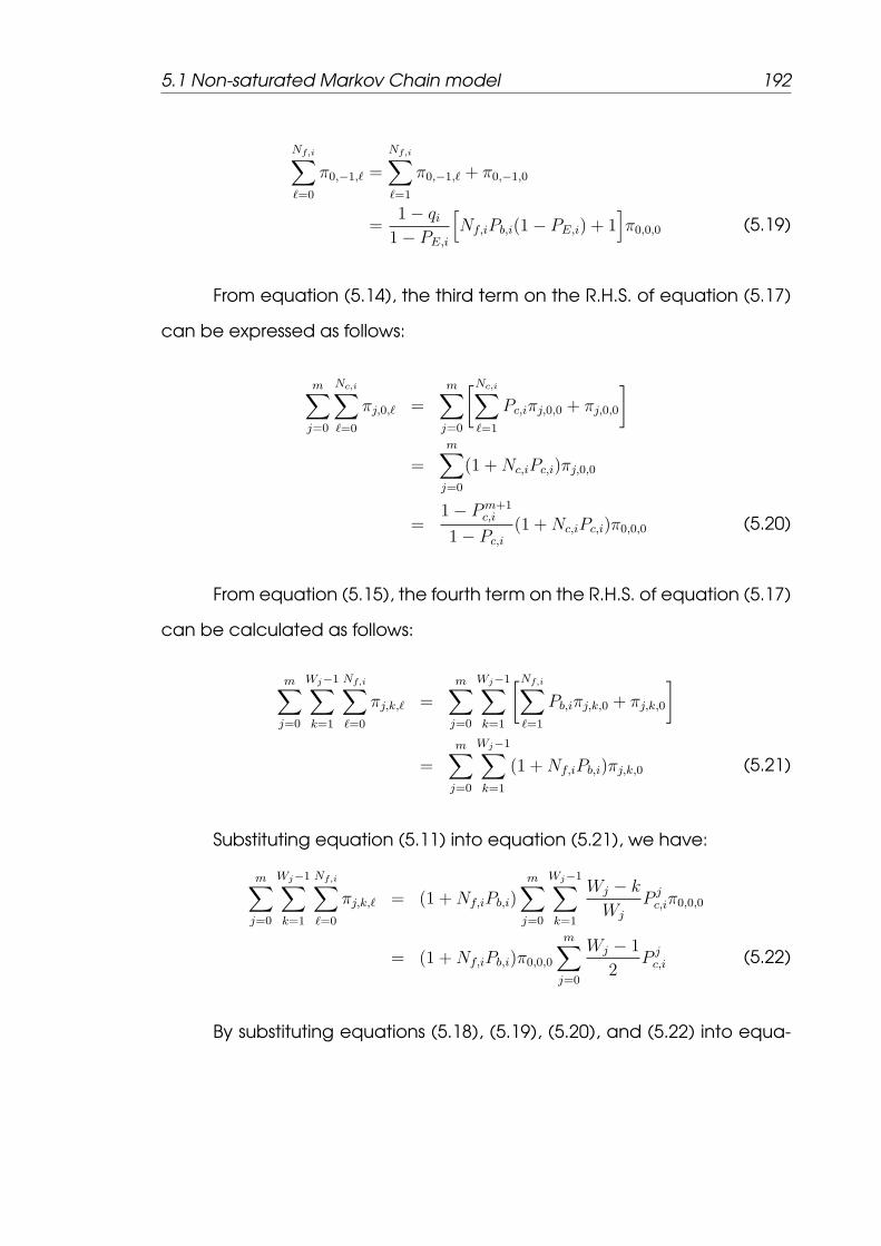
5.1 Non-saturated Markov Chain model 192
Nf,i∑ℓ=0
π0,−1,ℓ =
Nf,i∑ℓ=1
π0,−1,ℓ + π0,−1,0
=1− qi1− PE,i
[Nf,iPb,i(1− PE,i) + 1
]π0,0,0 (5.19)
From equation (5.14), the third term on the R.H.S. of equation (5.17)
can be expressed as follows:
m∑j=0
Nc,i∑ℓ=0
πj,0,ℓ =m∑j=0
[Nc,i∑ℓ=1
Pc,iπj,0,0 + πj,0,0
]
=m∑j=0
(1 +Nc,iPc,i)πj,0,0
=1− Pm+1
c,i
1− Pc,i
(1 +Nc,iPc,i)π0,0,0 (5.20)
From equation (5.15), the fourth term on the R.H.S. of equation (5.17)
can be calculated as follows:
m∑j=0
Wj−1∑k=1
Nf,i∑ℓ=0
πj,k,ℓ =m∑j=0
Wj−1∑k=1
[Nf,i∑ℓ=1
Pb,iπj,k,0 + πj,k,0
]
=m∑j=0
Wj−1∑k=1
(1 +Nf,iPb,i)πj,k,0 (5.21)
Substituting equation (5.11) into equation (5.21), we have:
m∑j=0
Wj−1∑k=1
Nf,i∑ℓ=0
πj,k,ℓ = (1 +Nf,iPb,i)m∑j=0
Wj−1∑k=1
Wj − k
Wj
P jc,iπ0,0,0
= (1 +Nf,iPb,i)π0,0,0
m∑j=0
Wj − 1
2P jc,i (5.22)
By substituting equations (5.18), (5.19), (5.20), and (5.22) into equa-

5.1 Non-saturated Markov Chain model 193
tion (5.17), we have:
π0,0,0 =
[(1− Pm+1
c,i )Ns,i +1− qi1− PE,i
(1 + (1− PE,i)Nf,iPb,i
)+ (1 +Nc,iPc,i)
1− Pm+1c,i
1− Pc,i
+ (1 +Nf,iPb,i)m∑j=0
Wj − 1
2P jc,i
]−1
(5.23)
Let τi be the probability that the generic node i transmits during a
slot time. The node transmits when its backoff counter reaches zero and
there is a packet in its queue regardless of the backoff stage. The node
accesses the channel also from the idle state when a packet arrives from
the upper layer and at the same time the channel is idle. Consequently,
we have:
τi =m∑j=1
πj,0,0 + qiπ0,0,0 + (1− PE,i)(1− Pb,i)π0,−1,0 + π0,−1,1 (5.24)
From equations (5.4) and (5.5), we have:
qiπ0,0,0 + (1− PE,i)(1− Pb,i)π0,−1,0 + π0,−1,1 = π0,0,0 (5.25)
By substituting equation (5.25) into equation (5.24), we have:
τi =m∑j=0
πj,0,0 =1− Pm+1
c,i
1− Pc,i
π0,0,0 (5.26)
Substituting equation (5.23) into equation (5.26), τi is then calculated
as follows:

5.1 Non-saturated Markov Chain model 194
When m ≤ m′
τi =2(1− Pm+1
c,i
)(1− 2Pc,i)
W0(1 +Nf,iPb,i)(1− (2Pc,i)m+1
)(1− Pc,i) +A+ B
(5.27)
When m > m′
τi =2(1− Pm+1
c,i
)(1− 2Pc,i)
W0(1 +Nf,iPb,i)[(1− (2Pc,i)m
′+1)(1− Pc,i) + C
]+A+ B
(5.28)
where
A =(1− Pm+1
c,i
)(1− 2Pc,i)
[2Ns,i(1− Pc,i) + 2(1 +Nc,iPc,i)− (1 +Nf,iPb,i)
]B =
2(1− qi)(1− Pc,i)(1− 2Pc,i)
1− PE,i
(1 + (1− PE,i)Nf,iPb,i
)C = 2m
′(1− 2Pc,i)
(Pm′+1c,i − Pm+1
c,i
)
Therefore, the transmission probability τi can be calculated when
the values of W0, m, m′, Nc,i, Nf,i, Ns,i, Pb,i, PE,i, qi, and Pc,i are known. The
values of W0, m, m′ are known, but the values of Pb,i, Pc,i, Ns,i, Nc,i, Nf,i, PE,i,
and qi must be calculated. The probability αk, that the channel is busy due
to either a collision transmission or a successful transmission of a node k = i,
is calculated as follows:
αk = (qkπ0,0,0 + (1− PE,k)(1− Pb,k)π0,−1,0 + π0,−1,1) +
Nc,k∑ℓ=1
π0,0,ℓ
+
Ns,k∑ℓ=1
π−1,0,ℓ +m∑j=1
Nc,k∑ℓ=0
πj,0,ℓ (5.29)

5.1 Non-saturated Markov Chain model 195
Substituting equation (5.25) into equation (5.29), we have:
αk =
Ns,k∑ℓ=1
π−1,0,ℓ +m∑j=0
Nc,k∑ℓ=0
πj,0,ℓ
= τk
[Ns,k(1− Pc,k) +Nc,kPc,k + 1
](5.30)
For the node i, the probability Pb,i, that the channel is sensed busy
when it is occupied by at least one node, is calculated as follows:
Pb,i = 1−N∏k=1k =i
(1− αk), i = 1, 2, ..., N (5.31)
The collision probability Pc,i, that at least one of the N − 1 remaining
nodes and the node i transmit at the same time slot, is expressed as follows:
Pc,i = 1−N∏j=1j =i
(1− τj), i = 1, 2, ..., N (5.32)
The average number of time slots Nc,i that represents the collision
period can be expressed as follows:
Nc,i =
⌈Tc
σ
⌉(5.33)
where ⌈x⌉ is the smallest integer larger than x. σ is the slot time size.
Tc is the collision time between at least two nodes. The value of Tc depends
on the employed MAC protocol. In this chapter the analysis is based on
the BTAC protocol. The analysis can be easily extended for the CARD pro-
tocol and the other MAC protocols. However, the simulation results in ad-
dition to the BTAC protocol can be applied to both the IEEE 802.11b [5]

5.1 Non-saturated Markov Chain model 196
and the CARD protocols. Therefore, Tc is computed as follows:
Tc = TMRTS + TCTS + TSIFS + TDIFS + δ (5.34)
where TMRTS, TCTS, TSIFS, and TDIFS stand for the time duration of
MRTS, CTS, SIFS, and DIFS, respectively. δ is the channel propagation delay.
The number of time slots Ns,i, that represents the successful transmission
period, is calculated as follows:
Ns,i =
⌈I(i ∈ Sd)T d
s,i + I(i ∈ Sc)T cs,i
σ
⌉(5.35)
where I(x) is 1 if x is true, and is 0 otherwise. T ds,i and T c
s,i stand for the
successful transmission period for a single-hop and a two-hop transmission,
respectively. T ds,i and T c
s,i can be expressed as follows:
T ds,i = TRTS + TCTS +
8L
Rsd
+ TPLCP + TACK + 3TSIFS + TDIFS + 4δ (5.36)
T cs,i = TMRTS + TCTS + TBTS +
8L
Rsr
+8L
Rrd
+ 2TPLCP + TACK + 5TSIFS
+TDIFS + 6δ (5.37)
where L is the data packet length in octets, Rsd is the data-rate
between a source node i and the AP. TPLCP is the time duration of the
PLCP header, and TACK is the time duration of the ACK packet. TBTS is
the time duration of the Busy-Tone-Signal (BTS). Rsr and Rrd are the data-
rate between the source and the relay and between the relay and the AP,
respectively. Sd and Sc are the set of nodes employing a single-hop and a

5.1 Non-saturated Markov Chain model 197
two-hop transmission, respectively.
The generic node i freezes its backoff counter for Nf,i time slots due
to collision and successful transmissions of the other N − 1 nodes under
condition that the channel is sensed busy. The average number of slots
Nf,i can be expressed as follows:
Nf,i =
⌈Tf,i
σ
⌉(5.38)
where Tf is the freezing duration during which the backoff counter
is frozen, and it is computed as follows:
Tf,i = E[TCi] + E[TSi
] (5.39)
E[TCi] and E[TSi
] stand for the average collision duration and the
average successful duration under condition that the channel is busy, re-
spectively. Consequently, we have:
E[TC,i] =
[1−
N∑j=1j =i
Ps,j
]Tc (5.40)
where Ps,j is the successful transmission probability of node j = i
when no other node of the remaining N − 1 transmits. It is expressed as
follows:
Ps,j =
N−1∏k=1,k =j
(1− αk)
Pb,i
Ns,j∑ℓ=1
π−1,0,ℓ =
N−1∏k=1,k =j
(1− αk)
1−N∏
k=1,k =i
(1− αk)
·Ns,j(1− Pc,j)τj (5.41)

5.1 Non-saturated Markov Chain model 198
The average successful duration E[TS,i] is expressed as follows:
E[TS,i] =N∑j=1j =i
Ps,j
[I(j ∈ Sd)T d
s,j + I(j ∈ Sc)T cs,j
](5.42)
where T ds,j and T c
s,j are given in equations (5.36) and (5.37), respec-
tively. The next step is to calculate the values of qi and PE,i. In this chap-
ter, it is assumed that the packet arrivals at each node follow the Poisson
process with a mean rate λ packet per second equal for all nodes. Let
E[Tservice,i] is the average MAC service time of the generic node i. The
MAC service time is the time interval from the time instant that a packet
becomes the head of the queue to the time instant when the post-backoff
completed by reaching either the state (0, 0, 0) or (−1, 0, 0) if the queue is
either busy or empty, respectively. Notice that the service time considers
the time either the packet is acknowledged for a successful transmission
or the packet is discarded. It is shown in [153] that the exponential distribu-
tion is a good approximation model for the MAC layer service time. Con-
sequently, a single node could be represented as an M/M/1/K queuing
system, in which K is the maximum queue length. Thus, the probability qi,
that there is at least one packet available at the end of the post-backoff
stage, is given as follows [154]:
qi =
1− 1−ρi
1−ρK−1i
ρi < 1
1 ρi ≥ 1
(5.43)
5.2 Performance Analysis 199
where ρi is the utilization factor and is given as follows:
ρi = λE[Tservice,i] (5.44)
This requires knowing the average service time E[Tservice,i], which is
derived in Section 5.2.2. Assuming the packets arrive at the MAC in a
Poisson process with rate λ, the probability PE,i, that the MAC queue is
empty the following generic time slot conditioning that the queue is empty
at the beginning of the slot, is calculated as follows:
PE,i = Pb,i
[( 1
Pb,i
− 1)e−λσ +
N∑j=1j =i
Ps,je−λTs,j +
(1−
N∑j=1j =i
Ps,j
)e−λTc
](5.45)
5.2 Performance Analysis
In this section the throughput, delay, and energy efficiency are stud-
ied under unsaturated conditions. The analysis could be applied to the
IEEE 802.11 standard protocols, the BTAC protocol, the CARD protocol, and
any other MAC protocols. In this chapter the BTAC protocol is considered.
5.2.1 Throughput Analysis
The throughput S is calculated as follows:
S =E[PL]
E[TI ] + E[TC ] + E[TS](5.46)
where E[PL] is the average payload size, E[TI ] is the average idle
slot duration, E[TC ] is the average collision slot duration, and E[TS] is the

5.2 Performance Analysis 200
average successful transmission slot duration
Let Ptr be the probability that there is at least one transmission occurs
in a randomly chosen time slot. Each node occupies the channel with
probability αi, where i = 1, 2, ..., N . Ptr is then calculated as follows:
Ptr = 1−N∏i=1
(1− αi) (5.47)
where αi is given in equation (5.30). Given a transmission on the
channel from any node i, the probability Ps,i, that the transmission is suc-
cessful, is calculated as follows:
Ps,i =
Ns,i∑ℓ=1
π−1,0,ℓ ·N∏k=1k =i
(1− αk)
= Ns,i(1− Pc,i)τi ·N∏k=1k =i
(1− αk) (5.48)
The average idle slot duration before a transmission takes place is
computed as follows:
E[TI ] = (1− Ptr)σ (5.49)
where 1−Ptr is the probability that the chosen slot time is empty. The
average collision slot duration E[TC ] is expressed as follows:
E[TC ] =(Ptr −
N∑i=1
Ps,i
)Tc (5.50)
where Tc is given in equation (5.34). The average successful duration
5.2 Performance Analysis 201
E[TS] is expressed as follows:
E[TS] =N∑i=1
Ps,i
[I(i ∈ Sd)T d
s,i + I(i ∈ Sc)T cs,i
](5.51)
where T ds,i and T c
s,i are given in equations (5.36) and (5.37), respec-
tively. For a fixed packet length L, the average payload size E[PL] is com-
puted as follows:
E[PL] = 8LN∑i=1
Ps,i (5.52)
Finally, the throughput S can calculated by substituting equations
(5.49), (5.50), (5.51), and (5.52) into equation (5.46).
5.2.2 Delay Analysis
In this subsection two kinds of delay are studied. The first kind is the
average service delay E[Tservice,i] that is used to calculate ρi in equation
(5.44). The second kind is the average medium access delay E[Di] that
is defined as the time interval from the time instant the packet becomes
head of the queue ready for transmission to the time instant when the
packet is acknowledged for a successful transmission. Let Di (i = 1, 2, ..., N)
denote a random variable representing a packet delay of a generic node
i. Thus, the average packet delay E[Dsuc,i] is expressed as follows:
E[Dsuc,i] = E[Db,i] + E[Dc,i] + E[Do,i] + E[Ds,i] (5.53)

5.2 Performance Analysis 202
where E[Db,i], E[Dc,i], E[Do,i], and E[Ds,i] stand for the average de-
lay during decreasing backoff counter, the average delay due to a colli-
sion transmission, the average delay due to freezing the backoff counter
during the transmissions of the other nodes, and the average delay of a
successful transmission, respectively. These average delay values are cal-
culated as follows:
E[Db,i] = Nb,iσ
E[Dc,i] = Nc,iTc
E[Do,i] = No,iTf,i + (1− PE,i)Pb,iTf,i
E[Ds,i] = I(i ∈ Sd)T ds,i + I(i ∈ Sc)T c
s,i (5.54)
where Tc, T ds,i, T c
s,i, and Tf,i are given in (5.34), (5.36), (5.37), and
(5.39), respectively. Nb,i is the average number of backoff slots that the
node i needs to transmit its packet successfully, without taking into ac-
count the time the counter is stopped. Nc,i is the average number of colli-
sions that the node i encounters before the packet is sent successfully. No,i
is the average number of transmissions overheard by the node i during the
backoff process. The average number Nb,i is calculated as follows:
Nb,i =m∑j=0
P jc,i(1− Pc,i)
1− Pm+1c,i
j∑k=0
Wk − 1
2(5.55)
whereP jc,i(1−Pc,i)
1−Pm+1c,i
is the successful transmission probability after the jth
backoff stage conditioned that the packet is not dropped, and the corre-
sponding average number of the backoff slots is∑j
k=0Wk−1
2. The average
number of collisions Nc,i is calculated as follows:

5.2 Performance Analysis 203
Nc,i =m∑i=0
iP ic,i(1− Pc,i)
1− Pm+1c,i
=1− Pc,i
1− Pm+1c,i
[Pc,i
(1− Pc,i)2(1− Pm
c,i)−mPm+1
c,i
1− Pc,i
](5.56)
Let N idle,i be the average number of consecutive idle slots between
two consecutive busy slots of the N − 1 remaining nodes. N idle,i is calcu-
lated as follows:
N idle,i =∞∑j=0
j(1− Pb,i)jPb,i =
1
Pb,i
− 1 (5.57)
Consequently, the average number of transmissions No,i overheard
by the node i is calculated as follows:
No,i =Nb,i
max(N idle,i, 1)− 1 (5.58)
Therefore, the delay E[Dsuc,i] can be calculated by substituting
equations (5.55), (5.56), and (5.58) into equation (5.53). For the reason
that E[Tservice,i] includes the time duration of the successful and dropped
packets, E[Tservice,i] is calculated as follows:
E[Tservice,i] = (1− Pm+1c,i )E[Dsuc,i] + Pm+1
c,i E[Ddrop,i] (5.59)
where E[Ddrop,i] is the average delay in the case of the packet being
dropped. Hence, E[Ddrop,i] is computed as follows:
E[Ddrop,i] =m∑j=0
Wj − 1
2
(σ +
Pb,i
1− Pb,i
Tf,i
)+ (1− PE,i)Pb,i + (m+ 1)Tc (5.60)
Finally, the total average medium access delay is calculated as fol-

5.2 Performance Analysis 204
lows:
E[DT ] =1
N
N∑i=1
E[Dsuc,i] (5.61)
5.2.3 Energy Efficiency
The energy efficiency η, is defined as the ratio of the successfully
transmitted data bits to the total energy consumed [99,100]. η is written as
follows:
η =E[L]
N∑i=1
(E
(i)B + E
(i)C + E
(i)O + E
(i)S
) (5.62)
where E(i)B is the energy consumption during the backoff period. E(i)
C
is the energy consumption during the collision transmission period. E(i)O is
the energy consumption during the overhearing transmission period. E(i)S
is the energy consumption during the successful transmission period. E[L]
is the average payload size.
Given the duration of an empty slot σ and the idle power consump-
tion PIX , the energy, that the node i consumes during the backoff stage,
is calculated as follows:
E(i)B = σ · PIX ·Nb,i, i = 1, 2, ..., N (5.63)
where Nb,i is given in equation (5.55). The node i overhears the colli-
sion and the successful transmissions. Therefore, the energy, that the node

5.2 Performance Analysis 205
i consumes in overhearing other nodes transmission during the backoff
stages, is calculated as follows:
E(i)O = PRX
[No,iTf,i + (1− PE,i)Pb,iTf,i
](5.64)
where Pbi, Tf,i, PE,i, , and No,i are given in equations (5.31), (5.39),
(5.45), and (5.58), respectively. PRX is the receiving power consumption.
The energy consumption due to collision is calculated as follows:
E(i)C = Nc,i
[PTXTRTS + PRXTCTS + PIX(TDIFS + TSIFS)
](5.65)
where PTX is the power consumption during transmission, and Nc,i
is the average number of collisions given in equation (5.56). The energy
consumption for a successful single-hop transmission, EdS,i, is computed as
follows:
EdS,i = PTX
(TRTS +
8L
Rsd
+ TPLCP
)+ PRXTCTS + PIX
(TACK + 3TSIFS + TDIFS + 4δ
)(5.66)
For a successful two-hop transmission, the energy consumption EcS,i
is computed as follows:
EcS,i = PTX
(TMRTS +
8L
Rsr
+ TPLCP
)+ PRX
(TCTS + TBTS +
8L
Rrd
+ TPLCP
)+PIX
(TACK + 5TSIFS + TDIFS + 6δ
)(5.67)
The energy consumption during a successful transmission of the

5.3 Analytical and Simulation Results 206
Parameter Value Parameter ValueMAC header 272 bits Slot time 20 µs
PHY header 192 bits SIFS 10 µs
RTS 352 bits DIFS 50 µs
CTS 304 bits Busy Tone 20 µs
ACK 304 bits CWmin 31 slotsPLCP data-rate 1 Mbps CWmax 1023 slotsData-rate 1, 2, 5.5, 11 Mbps PIX , PRX , PTX 0.8, 0.8, 1.0 Watt
Table 5.1: System parameters under unsaturated conditions.
generic node i is then computed as follows:
E(i)S = I(i ∈ Sd)Ed
S,i + I(i ∈ Sc)EcS,i (5.68)
Finally, the average packet length E[L] =∑N
i=1 8L assuming a fixed
packet length. Therefore, the energy efficiency η can be calculated using
equation (5.62).
5.3 Analytical and Simulation Results
To validate the above analysis, a custom event driven simulator de-
veloped by using the Mobile Framework (MF) of the OMNET++ [148] pack-
age written in C++ programming language. The parameters used in sim-
ulation and analysis are set to the default values specified in IEEE 802.11b
standard which are summarized in Table 5.1. The network setting is the
same as given in [Chapter 3, Section 3.4]. In all following figures, solid
lines are for the analytical model results through Matlab software pack-
age. Whereas dot-dashed lines are for the simulation results through OM-
NET++ software package.

5.3 Analytical and Simulation Results 207
5.3.1 Throughput Results
Fig. 5.2 shows the relationship between the total mean offered load,
the number of nodes, and the overall throughput of both the 802.11b and
the BTAC protocols at a fixed payload size which is 1024 byte. Since Fig.
5.2(a) and Fig. 5.2(b) show the results for 10 and 30 nodes, respectively.
Under 802.11b protocol, the relationship between throughput and offered
load is linear when λtotoal ≤ 120 and throughout is saturated when λtotoal ≥
300 when the number of nodes is 10 or 30 nodes. On the other hand, the
relationship between throughput of the BTAC protocol and offered load is
linear when λtotoal ≤ 200 and λtotoal ≤ 300 for the number of node 10 and
30 nodes, respectively, whereas throughput is saturated at λtotoal ≥ 400 for
both N = 10 and N = 30 nodes.
The reason of the linear relationship between throughput and a low
offered load is that at a low offered load the probability of accessing the
medium is low, the collision probability then becomes negligible. There-
fore, the probability to send a data packet successfully is very high and
then the overall throughput is equal to λtotal × L, where L is the packet
length in bits. As the number of nodes increases, the linear relationship
between throughput and offered load also increases under the BTAC pro-
tocol and becomes constant under the 802.11b protocol. This is because
the probability of finding relay node increases as the number of nodes in-
creases. Consequently, the time required to send a data packet from the
source to the AP decreases due to the high data rate through the two-
hop transmission. Therefore, the occupation time of channel becomes less
than the arrival rate of data packets at each node. For this reason, the col-
lision probability decrease and hence the relationship between through-
put and offered load is linear.
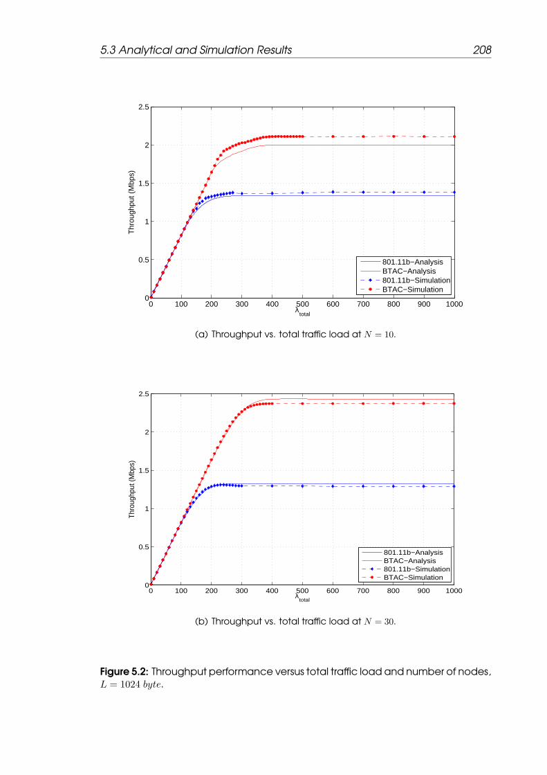
5.3 Analytical and Simulation Results 208
0 100 200 300 400 500 600 700 800 900 10000
0.5
1
1.5
2
2.5
λtotal
Thr
ough
put (
Mbp
s)
801.11b−AnalysisBTAC−Analysis801.11b−SimulationBTAC−Simulation
(a) Throughput vs. total traffic load at N = 10.
0 100 200 300 400 500 600 700 800 900 10000
0.5
1
1.5
2
2.5
λtotal
Thro
ughp
ut (M
bps)
801.11b−AnalysisBTAC−Analysis801.11b−SimulationBTAC−Simulation
(b) Throughput vs. total traffic load at N = 30.
Figure 5.2: Throughput performance versus total traffic load and number of nodes,L = 1024 byte.

5.3 Analytical and Simulation Results 209
Fig. 5.3 shows the results for L = 1024 and L = 1500 byte of through-
out versus offered load at a fixed number of nodes which is 30 nodes. In
Fig. 5.3(a), the BTAC is saturated at λtotal = 400, where in Fig. 5.3(b), it is
saturated at λtotal = 300. The reason is that as the packet length increases,
the occupation time of the medium increases. Hence, probability of node
to have a packet in its queue increases and the probability to access the
medium also increases. For this reason the collision probability increases
and causes the throughput to saturated at a low traffic load as the packet
length increases. As the packet length increases, the saturated through-
put increases. This because the effect of the control overhead becomes
noneligible as the packet length increases, the saturated throughout then
increases as the packet length increases.
5.3.2 Energy Efficiency Results
The energy efficiency is counted as one of the most important re-
quirements to design an efficient MAC protocol. Hence, the energy ef-
ficiency of the 802.11b and BTAC protocols versus the offered load un-
der different number of nodes and fixed packet length and under differ-
ent packet length and fixed number of nodes is shown in Fig. 5.4 and
Fig. 5.5, respectively. As the offered load increases, the collision probabil-
ity increases. As a result, the number of retries to deliver a data packet
from source node to the AP increases. This causes increasing in the tra-
nsmission, the receiving, overhearing, and sensing energy. Therefore, the
node consumes more energy on the retransmissions, receiving and sens-
ing the medium. Consequently, the energy efficiency decreases as the
offered load increases. The BTAC protocol achieves higher energy effi-
ciency than the 802.11b protocol due to advantage of using a two-hop

5.3 Analytical and Simulation Results 210
0 100 200 300 400 500 600 700 800 900 10000
0.5
1
1.5
2
2.5
λtotal
Thro
ughp
ut (M
bps)
801.11b−AnalysisBTAC−Analysis801.11b−SimulationBTAC−Simulation
(a) Throughput vs. total traffic load at L = 1024.
0 100 200 300 400 500 600 700 800 900 10000
0.5
1
1.5
2
2.5
3
λtotal
Thro
ughp
ut (M
bps)
801.11b−AnalysisBTAC−Analysis801.11b−SimulationBTAC−Simulation
(b) Throughput vs. total traffic load at L = 1500.
Figure 5.3: Throughput performance versus total traffic load and packet length,N = 30.

5.4 Conclusions 211
transmission.
5.3.3 Delay Results
It is important to consider the delay experienced by a data packet
in the MAC layer as well as throughput. Fig. 5.6 and Fig. 5.7 show the
results of delay versus offered load at N = 10, N = 30 and L = 1024 and
at L = 1024, L = 1500 byte and N = 30, respectively. As the offered load
increases, the collision probability increases, and hence the delay (associ-
ated with medium contention and collisions) increases. The BTAC protocol
outperforms the 802.11b protocol under all traffic conditions, number of
nodes, and packet length. This is due to using the tow-hop transmission.
5.4 Conclusions
In this chapter, a Markov chain model is proposed taking the traffic
characteristic and multi-rate transmissions into account. The model also
considers the post-backoff that there is always at least one backoff inter-
val preceding a packet transmission. Alternatively, there is an exception
to the essential rule that an a packet from the upper layer has to be trans-
mitted after performing the backoff mechanism. The packet arriving from
the upper layer may be transmitted immediately without waiting any time
if the transmission queue is empty, the latest post-backoff is finished, and
at the same time the channel has been idle for at least one DCF interval.
In the proposed model this exceptional case is considered. The M/M/1/K
queuing model is introduced in this chapter to study the various perfor-
mance metrics of WLAN in the non-saturated state which is the desired

5.4 Conclusions 212
0 100 200 300 400 500 600 700 800 900 10000
0.2
0.4
0.6
0.8
1
1.2
1.4
1.6
1.8
λtotal
Ene
rgy
effic
ienc
y (M
b/J)
801.11b−AnalysisBTAC−Analysis802.11b−SimulationBTAC−Simulation
(a) Energy efficiency vs. total traffic load at N = 10.
0 100 200 300 400 500 600 700 800 900 10000
0.5
1
1.5
2
2.5
λtotal
Ene
rgy
effic
ienc
y (M
b/J)
801.11b−AnalysisBTAC−Analysis801.11b−SimulationBTAC−Simulation
(b) Energy efficiency vs. total traffic load at N = 30.
Figure 5.4: Energy efficiency performance versus total traffic load and number ofnodes, L = 1024 byte.

5.4 Conclusions 213
0 100 200 300 400 500 600 700 800 900 10000
0.5
1
1.5
2
2.5
λtotal
Ene
rgy
effic
ienc
y (M
b/J)
801.11b−AnalysisBTAC−Analysis801.11b−SimulationBTAC−Simulation
(a) Energy efficiency vs. total traffic load at L = 1024.
0 100 200 300 400 500 600 700 800 900 10000
0.5
1
1.5
2
2.5
3
λtotal
Ene
rgy
effic
ienc
y (M
b/J)
801.11b−AnalysisBTAC−Analysis801.11b−SimulationBTAC−Simulation
(b) Energy efficiency vs. total traffic load at L = 1500.
Figure 5.5: Energy efficiency performance versus total traffic load and packetlength, N = 30.

5.4 Conclusions 214
0 100 200 300 400 500 600 700 800 900 10000
0.01
0.02
0.03
0.04
0.05
0.06
0.07
λtotal
Del
ay (
sec.
)
801.11b−AnalysisBTAC−Analysis801.11b−SimulationBTAC−Simulation
(a) Delay vs. total traffic load at N = 10.
0 100 200 300 400 500 600 700 800 900 10000
0.02
0.04
0.06
0.08
0.1
0.12
0.14
0.16
0.18
0.2
λtotal
Del
ay (
sec.
)
801.11b−AnalysisBTAC−Analysis801.11b−SimulationBTAC−Simulation
(b) Delay vs. total traffic load at N = 30.
Figure 5.6: Delay performance versus total traffic load and number of nodes,L = 1024 byte.

5.4 Conclusions 215
0 100 200 300 400 500 600 700 800 900 10000
0.02
0.04
0.06
0.08
0.1
0.12
0.14
0.16
0.18
0.2
λtotal
Del
ay (
sec.
)
801.11b−AnalysisBTAC−Analysis801.11b−SimulationBTAC−Simulation
(a) Delay vs. total traffic load at L = 1024.
0 100 200 300 400 500 600 700 800 900 10000
0.05
0.1
0.15
0.2
0.25
0.3
λtotal
Del
ay (
sec.
)
801.11b−AnalysisBTAC−Analysis801.11b−SimulationBTAC−Simulation
(b) Delay vs. total traffic load at L = 1500.
Figure 5.7: Delay performance versus total traffic load and packet length, N = 30.

5.4 Conclusions 216
state for some applications.
An analytical model is then presented to study the performance of
the IEEE 802.11 and BTAC protocols under non-saturation traffic conditions
in terms of throughput, medium access and service delay, and energy ef-
ficiency. The results show that the performance of both the 802.11b and
the BTAC protocols depends on the traffic conditions. Since under the very
low offered load, the throughput performance of the BTAC protocol is sim-
ilar to the 802.11b, whereas the delay and energy efficiency of the BTAC
protocol is better than that of the 802.11b protocol. On the other hand,
the BTAC protocol outperforms the 802.11b under a medium and high of-
fered load in terms of throughput, delay, and energy efficiency. Therefore,
the two-hop transmission technique used by the BTAC protocol is suitable
to apply under both light and heavy traffic load.

Chapter 6
Conclusions and Future Work
6.1 Conclusions
According to the IEEE 802.11 standards, Wireless Local Area Net-
works (WLANs) can support multiple transmission data rates depending
on the instantaneous channel conditions between the source station and
the Access Point (AP). To achieve the target Packet Error Rate (PER) in
data transmissions, a source station transmits its data packets to the AP
at a low date rate when the channel quality is poor. In such a multi-rate
WLAN, those low data-rate stations will occupy the shared communica-
tion channel for a longer period for packet transmissions, thus reducing
the channel efficiency and overall system performance.
Performance degradation can be mitigated by using the concept
of cooperative communication at Medium Access Control (MAC) layer.
A source station can use a neighbouring node, called relay, which has
high quality communication channels to both source station and the AP.
This relay-based cooperative communication can effectively improve net-

6.1 Conclusions 218
work coverage, transmission data rate, reliability, and overall system per-
formance.
This thesis addresses the channel efficiency problem in multi-rate
WLANs by adopting the concept of cooperative communications in the
development and evaluation of two cooperative Medium Access Con-
trol (MAC) protocols, namely Busy Tone based Cooperative MAC (BTAC)
protocol and Cooperative Access with Relay’s Data (CARD) protocol. Un-
der BTAC, a low data-rate source station uses a close-by intermediate sta-
tion as its relay to forward its data packets at higher data-rates to the AP
through a two-hop path. In this way, BTAC can achieve cooperative di-
versity gain in multi-rate WLANs. Furthermore, the proposed CARD proto-
col enables a relay station to transmit its own data packets to the AP im-
mediately after forwarding its neighbour’s packets, thus saving the hand-
shake procedure and overheads for sensing and reserving the common
channel. In doing so, CARD can achieve both cooperative diversity gain
and cooperative multiplexing gain. Both BTAC and CARD protocols are
backward compatible with the existing IEEE 802.11 standards.
Accordingly, new cross-layer analytical approaches have been de-
veloped in this thesis to study the performance of BTAC and CARD un-
der different channel conditions and traffic loads, i.e. saturated and un-
saturated traffics. Analytical results, verified by extensive simulation re-
sults, show that BTAC and CARD protocols can significantly improve sys-
tem throughput, service delay, and energy efficiency performance in re-
alistic communication scenarios. Compared with traditional IEEE 802.11b
MAC protocol, BTAC can greatly improve system performance by up to
88%, 40% and 84% in terms of throughput, energy efficiency and service
delay, respectively. Further, by enabling relay nodes to insert their own

6.1 Conclusions 219
packet transmissions without an additional handshake procedure, CARD
can achieve up to 165% throughput gain over the IEEE 802.11b MAC pro-
tocol. In addition, the throughput of CARD is approaching the maximum
value (i.e. 5 Mbps) when all the nodes have high-quality communication
channels for packet transmissions, i.e. 11 Mbps. In addition, the energy
efficiency and service delay performance of CARD are about 90% and
140% better than those of the IEEE 802.11b MAC protocol.
In order to support both BTAC and CARD protocols in real WLAN im-
plementations, some minor modifications related to relay packet trans-
missions and control frames (e.g. BTS under BTAC and RRTS under CARD)
are needed to enhance the current IEEE 802.11 standards. However, this
implementation complexity is considered quite low compared to the sig-
nificant performance gains of BTAC and CARD protocols. A general draw-
back of relay-based cooperative MAC protocols is the power consump-
tion of a relay station, which may consume much more energy than other
stations in receiving and forwarding neighbouring stations’ data packets
at high data rates. This problem is partially offset in CARD protocol by
enabling a relay station to transmit its own data packets to the AP im-
mediately after forwarding its neighbour’s packets, thus saving handshake
procedure and power consumption of a relay station. To further reduce
the energy consumption of a relay in BTAC and CARD protocols, when
multiple relay stations are available, we can use their remaining energy
levels to make a choice of the most suitable relay station.

6.2 Future Work 220
6.2 Future Work
A number of possible areas are identified for future work of this re-
search.
It will be important to extend the study of BTAC and CARD protocols
under more realistic channel models, e.g. Rayleigh fading channel model
[155]. In this thesis, the same bit error rate (BER) is assumed for different
data transmission rates. In reality, BER performance depends on channel
models, data rates, modulation and coding schemes. In addition to the
Poisson traffic model used in this thesis, it will be useful to evaluate the
performance of BTAC and CARD protocols under unsaturated conditions
with more sophisticated traffic models, such as Markov Modulated Poisson
Process (MMPP) model [156]. Further, research may be extended to the
newly emerging IEEE 802.11n standard, which has a different MAC layer
comparing to the IEEE 802.11a/b/g standards.
In this thesis the BTAC and CARD protocols were examined in two-
hop networks. The schemes and analytical methods presented here can
be extended to more complicated multi-hop scenarios and with mobile
relays. Also, it will be interesting to study the system performance of BTAC
and CARD protocols under real time applications such as video traffic.
These results will help in developing a deeper understanding of BTAC and
CARD protocols and their superior performance.
The security issue of MAC protocols is not considered in this research.
The proposed BTAC and CARD protocols may suffer from security attacks.
For example, a malicious relay station could drop some to-be-forwarded
data packets. On the other hand, a malicious relay station could modify
the data packets received from the source station before forwarding it
to the AP. Therefore, it is very important to develop a secure protection

6.2 Future Work 221
mechanism for supporting reliable data transmissions in BTAC and CARD
protocols.

Appendix A
Node Distribution Probability
In the following paragraphes the average number of nodes located
in different zones is derived. Let Nd1 , Nd
2 , Nd3 , and Nd
4 stand for the average
number of nodes in zones I, and II, III, and IV operating at the direct tra-
nsmission data-rates 1, 2, 5.5, and 11 Mbps, respectively. These average
number of nodes are computed as follows:
Ndu = NPu (A.1)
where Pu, u = 1, 2, 3, 4 is the fraction of nodes in zones I,
II, III, and IV, respectively that communicate directly with the AP.
It is assumed that only the nodes in zone III and IV can benefit
from cooperative transmission. If a source node is located in zone
IV (at data-rate 1 Mbps) and there is relay node available, this
source node can employ a two-hop transmission. Depending on
the channel quality, the supported data-rates are given by the set
(Rsr, Rrd) = {(11, 11), (5.5, 11), (11, 5.5), (5.5, 5.5), (2, 11), (11, 2), (2, 5.5), (5.5, 2)}.

A. Node Distribution Probability 223
Let N4(u,v) be the average number of nodes in zone IV at first-hop
rate Ru Mbps and second-hop rate Rv Mbps. The average number N4(u,v)
is then expressed as follows.
N4,(u,v) = NP4(u,v) u, v = 1, 2, 3 at u = 3 v = 3 (A.2)
where P4(u,v) is the fraction of nodes in zone IV employing a
two-hop transmission at data-rates Ru and Rv. Similarly, if a source
node is located in zone III (at data-rate 2 Mbps) and there is a
relay node available, the set of supported data-rates is given by
(Rsr, Rrd) = {(11, 11), (5.5, 11), (11, 5.5), (5.5, 5.5)}.
The average number of nodes N3(u,v) in zone III at two-hop data rates
Ru and Rv, is then calculated as follows.
N3,(u,v) = NP3(u,v) u, v = 1, 2 (A.3)
where P3(u,v) is the fraction of nodes in zone IV using two-hop
transmission at rates Ru and Rv. Pu, P3(u,v), and P4(u,v) are given in Appendix
B.
Therefore, the total set of nodes S = {Sd, Sc1, S
c2} includes three differ-
ent sets of nodes. The set Sd = {Ndu ∀ u = 1, 2, 3, 4} contains the nodes that
use a direct transmission scheme. The set Sc1 = {N4(u,v) ∀ u, v = 1, 2, 3}
contains the nodes at data-rate 1 Mbps and are located in zone IV.
These nodes use a two-hop transmission scheme. Finally, the set Sc2 =
{N3(u,v) ∀ u, v = 1, 2} is the set of nodes that are located in zone

A. Node Distribution Probability 224
III (at data-rate 2Mbps) and use a two-hop transmission. Notice that
|Sd|+ |Sc1|+ |Sc
2| = N , where | · | is the cardinality of the set.

Appendix B
Relay Probability
Consider a one cell wireless local area network (WLAN) consisting
of an access point (AP) and N nodes. The network supports M different
data-rates, denoted by Rm, where m = 1, 2, ...,M , and R1 > R2 > ...RM . For
simplicity, we only consider path loss [155], which means that the signal
strength mainly depends on the distance between the transmitter and the
receiver for a given transmission power. The maximum transmission radius
of a node at data-rate Rm is rm, where r1 < r2 < ... < rM . The AP is located
at the center of the cell of a radius R, where R = rM . The nodes are as-
sumed to be uniformly distributed within the coverage area of the cell. In
this work, we consider the case of one relay node and four different tra-
nsmission data-rates (M=4), where the analysis can be extended to larger
number of data-rates.
We define Ax,y(r) as the area of a region in which a node must be
located to work as a relay for another node (source node) which at a
distance r from the AP. As shown in Fig. B.1, the relay node is within a
distance rx from the source node and within a distance ry from the AP;
the data rate of the first hop (source to relay) is Rx and of the second hop
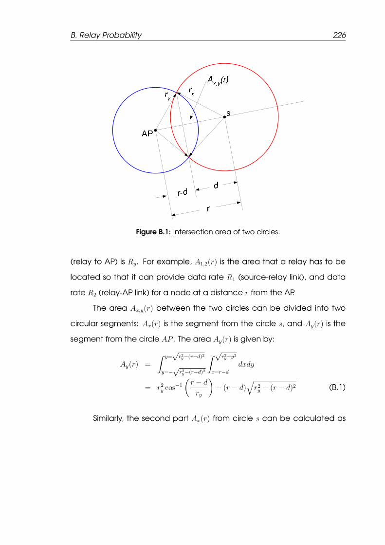
B. Relay Probability 226
Figure B.1: Intersection area of two circles.
(relay to AP) is Ry. For example, A1,2(r) is the area that a relay has to be
located so that it can provide data rate R1 (source-relay link), and data
rate R2 (relay-AP link) for a node at a distance r from the AP.
The area Ax,y(r) between the two circles can be divided into two
circular segments: Ax(r) is the segment from the circle s, and Ay(r) is the
segment from the circle AP . The area Ay(r) is given by:
Ay(r) =
∫ y=√
r2y−(r−d)2
y=−√
r2y−(r−d)2
∫ √r2y−y2
x=r−d
dxdy
= r2y cos−1
(r − d
ry
)− (r − d)
√r2y − (r − d)2 (B.1)
Similarly, the second part Ax(r) from circle s can be calculated as
B. Relay Probability 227
follows:
Ax(r) =
∫ y=√
r2x−d2
y=−√
r2x−d2
∫ √r2x−y2
x=d
dxdy
= r2x cos−1
(d
rx
)− d√
r2x − d2 (B.2)
where d =r2+r2y−r2x
2r. Therefore, from (B.1) and (B.2) the intersection
area Ax,y(r) can be calculated as follows:
Ax,y(r) = Ax(r) + Ay(r)
= r2x cos−1
(r2 + r2x − r2y
2rxr
)+ r2y cos
−1
(r2 − r2x + r2y
2ryr
)−1
2
√(rx + ry − r)(rx − ry + r)(ry − rx + r)(rx + ry + r)
(B.3)
The probability that a source node can be able to send its informa-
tion to the AP via a relay node, is equivalent to to the probability that
there is at least one node in its relay area Ax,y(r). Assuming the data-rate
from source node to relay node (first hop) is Rx, the data-rate from relay
node to the AP (second hop) is Ry, and the data-rate from source node to
the AP (direct transmission) is Rz. Consequently, in order for a node to act
as a relay for a source node, the following condition must be satisfied, the
source to relay transmission time (1/Rx) plus the relay to the AP transmission
time (1/Ry) is less than the transmission time (1/Rz) from the source to the
AP. Then, we have:
1
Rx
+1
Ry
<1
Rz
(B.4)

B. Relay Probability 228
where the packet length is assumed to be fixed. Assuming the N
nodes are uniformly distributed within the cell, then the probability density
function (PDF) of a node at a distance r from the AP is given by:
pr(r) =2r
R2, 0 ≤ r ≤ R (B.5)
and the node’s angle is uniformly distributed between [0, π). Fig. B.2 shows
the relaying regions for our proposed method, where the analysis given in
[157] is extended for four transmission data-rates. It is assumed that nodes
located only in zone-3 (r2 ≤ r < r3) and zone-4 (r3 ≤ r < r4) can benefits
from relaying, where nodes in zone-1 (0 ≤ r < r1) and zone-2 (r1 ≤ r < r2)
transmit directly at a high data-rate to the AP. Then, the fraction of nodes
at data-rate R1 and R2 is given, respectively as follows:
P1 =
∫ r1
r=0
2r
R2dr =
r21R2
P2 =
∫ r2
r=r1
2r
R2dr =
r22 − r21R2
(B.6)
We define P4(x,y) as the expected fraction of nodes in zone-4 that
can benefit from relaying provided by a relay node placed within area
Ax,y(r). Not that this for a first hop data-rate Rx and a second hop data-
rate Ry. Analogously, P3(x,y) gives the proportion of nodes in zone-3 that
can benefit from a relay within area Ax,y(r) with data-rate Rx for first hop
and data-rate Ry for second hop. For instant, P4(2,1) is the fraction of nodes
in zone-4 uses a relay node with a first hop (source-relay) data-rate R2 and
second hop (relay-AP) data-rate R1. where P3(1,2) is the fraction of nodes
in zone-3 that benefits from relaying with data-rate R1 for the first hop and

B. Relay Probability 229
Figure B.2: Relay regions of a node in zone-4.
data-rate R2 for the second hop. Therefore, we have
P4(1,1) is given as follows:
P4(1,1) = I(r3 < 2r1)
[∫ min(2r1,R)
r=r3
2r
R2
(1−
(1− A1,1(r)
πR2
)N−1)dr
](B.7)
where I(x) is 1 if x is true, and is 0 otherwise. The fraction P4(2,1) is
given as:
P4(2,1) = I(r3 < r1 + r2)
[∫ min(r1+r2,R)
r=r3
2r
R2
(1−
(1− A2,1(r)
πR2
)N−1)dr
]− P1,1
(B.8)

B. Relay Probability 230
P4(1,2) is calculated by:
P4(1,2) = I(r3 < 2r1)
[∫ 2r1
r=r3
2r
R2
(1−
(1− 2A1,2(r)− A1,1(r)
πR2
)N−1)dr
+
∫ min(r1+r2,R)
r=2r1
2r
R2
(1−
(1− 2A1,2(r)
πR2
)N−1)dr
]
+I(2r1 < r3 < r1 + r2)
[∫ min(r1+r2,R)
r=r3
2r
R2
(1−
(1− 2A1,2(r)
πR2
)N−1)dr
]
−[P1,1 + P2,1
](B.9)
P4(2,2) is given as follows:
P4(2,2) = I(r3 < 2r2)
[∫ min(2r2,R)
r=r3
2r
R2
(1−
(1− A2,2(r)
πR2
)N−1)dr
]
−[P4(1,1) + P4(2,1) + P4(1,2)
](B.10)

B. Relay Probability 231
P4(3,1) is calculated as follows:
P4(3,1) = I(r3 < r1 + r2)
[∫ r1+r2
r=r3
2r
R2
(1−
(1− A2,2(r) +A3,1(r)−A2,1(r)
πR2
)N−1)dr
+I(2r2 < r1 + r3)
[∫ 2r2
r=r1+r2
2r
R2
(1−
(1− A2,2(r) +A3,1(r)
πR2
)N−1)dr
+
∫ min(r1+r3,R)
r=2r2
2r
R2
(1−
(1− A3,1(r)
πR2
)N−1)dr
]
+I(2r2 > r1 + r3)
[∫ r1+r3
r=r1+r2
2r
R2
(1−
(1− A2,2(r) +A3,1(r)
πR2
)N−1)dr
+
∫ min(2r2,R)
r=r1+r3
2r
R2
(1−
(1− A2,2(r)
πR2
)N−1)dr
]]
+I(r3 > r1 + r2)
[I(2r2 < r1 + r3)
[∫ 2r2
r=r3
2r
R2
(1−
(1− A2,2(r) +A3,1(r)
πR2
)N−1)dr
+
∫ min(r1+r3,R)
r=2r2
2r
R2
(1−
(1− A3,1(r)
πR2
)N−1)dr
]
+I(2r2 > r1 + r3)
[∫ r1+r3
r=r3
2r
R2
(1−
(1− A2,2(r) +A3,1(r)
πR2
)N−1)dr
+
∫ min(2r2,R)
r=r1+r3
2r
R2
(1−
(1− A2,2(r)
πR2
)N−1)dr
]]
−[P4(1,1) + P4(2,1) + P4(1,2) + P4(2,2)
](B.11)

B. Relay Probability 232
P4(1,3) is given by:
P4(1,3) = I(r3 < r1 + r2)
[∫ r1+r2
r=r3
2r
R2
(1−
(1− A2,2(r) + 2A1,3(r)− 2A1,2(r)
πR2
)N−1)dr
+I(2r2 < r1 + r3)
[∫ 2r2
r=r1+r2
2r
R2
(1−
(1− A2,2(r) + 2A1,3(r)
πR2
)N−1)dr
+
∫ min(r1+r3,R)
r=2r2
2r
R2
(1−
(1− 2A1,3(r)
πR2
)N−1)dr
]
+I(2r2 > r1 + r3)
[∫ r1+r3
r=r1+r2
2r
R2
(1−
(1− A2,2(r) + 2A1,3(r)
πR2
)N−1)dr
+
∫ min(2r2,R)
r=r1+r3
2r
R2
(1−
(1− A2,2(r)
πR2
)N−1)dr
]]
+I(r3 > r1 + r2)
[I(2r2 < r1 + r3)
[∫ 2r2
r=r3
2r
R2
(1−
(1− A2,2(r) + 2A1,3(r)
πR2
)N−1)dr
+
∫ min(r1+r3,R)
r=2r2
2r
R2
(1−
(1− 2A1,3(r)
πR2
)N−1)dr
]
+I(2r2 > r1 + r3)
[∫ r1+r3
r=r3
2r
R2
(1−
(1− A2,2(r) + 2A1,3(r)
πR2
)N−1)dr
+
∫ min(2r2,R)
r=r1+r3
2r
R2
(1−
(1− A2,2(r)
πR2
)N−1)dr
]]
−[P4(1,1) + P4(2,1) + P4(1,2) + P4(2,2) + P4(3,1)
](B.12)

B. Relay Probability 233
P4(3,2) is given as follows:
P4(3,2) = I(r3 < r1 + r2)
[∫ r1+r2
r=r3
2r
R2
(1−
(1− A3,2(r) +A3,1(r)−A1,2(r)
πR2
)N−1)dr
+
∫ r1+r3
r=r1+r2
2r
R2
(1−
(1− A3,2(r) +A3,1(r)
πR2
)N−1)dr
+
∫ min(r2+r3,R)
r=r1+r3
2r
R2
(1−
(1− A3,2(r)
πR2
)N−1)dr
]
+I(r3 > r1 + r2)
[∫ r1+r3
r=r3
2r
R2
(1−
(1− A3,2(r) +A3,1(r)
πR2
)N−1)dr
+
∫ min(r2+r3,R)
r=r1+r3
2r
R2
(1−
(1− A3,2(r)
πR2
)N−1)dr
]
−[P4(1,1) + P4(1,2) + P4(2,1) + P4(2,2) + P4(3,1) + P4(1,3)
](B.13)
P4(2,3) is calculated as follows:
P4(2,3) = I(r3 < 2r2)
[∫ 2r2
r=r3
2r
R2
(1−
(1− 2A2,3(r)−A2,2(r)
πR2
)N−1)dr
+
∫ min(r2+r3,R)
r=2r2
2r
R2
(1−
(1− 2A2,3(r)
πR2
)N−1)dr
]
+I(r3 > 2r2)
[∫ min(r2+r3,R)
r=r3
2r
R2
(1−
(1− 2A3,2(r)
πR2
)N−1)dr
]
−[P4(1,1) + P4(2,1) + P4(1,2) + P4(2,2) + P4(3,1) + P4(1,3) + P4(3,2)
](B.14)
Finally, the fraction of nodes P4 in zone-4 that can not benefit from
relaying is given as follows:
P4 =r24 − r23R2
−[P4(1,1) + P4(2,1) + P4(1,2) + P4(2,2) + P4(3,1) + P4(1,3) + P4(3,2) + P4(2,3)
](B.15)

B. Relay Probability 234
In a similar way, the fraction of nodes in zone-3 that can take the advan-
tage of relaying can be calculated as follows.
P3(1,1) is calculated by:
P3(1,1) = I(r2 < 2r1)
[∫ min(2r1,r3)
r=r2
2r
R2
(1−
(1− A1,1(r)
πR2
)N−1)dr
](B.16)
P3(2,1) is given as:
P3(2,1) =
∫ min(r1+r2,r3)
r=r2
2r
R2
(1−
(1− A2,1(r)
πR2
)N−1)dr − P3(1,1) (B.17)
P3(1,2) is given as follows:
P3(1,2) = I(r2 < 2r1)
[∫ 2r1
r=r2
2r
R2
(1−
(1− 2A1,2(r)− A1,1(r)
πR2
)N−1)dr
+
∫ min(r1+r2,r3)
r=2r1
2r
R2
(1−
(1− 2A1,2(r)
πR2
)N−1)dr
]
+I(r2 > 2r1)
[∫ min(r1+r2,r3)
r=r2
2r
R2
(1−
(1− 2A1,2(r)
πR2
)N−1)dr
]−[
P3(1,1) + P3(2,1)
](B.18)
P3(1,2) is given as follows:
P3(2,2) =
∫ min(2r2,r3)
r=r2
2r
R2
(1−
(1− A2,2(r)
πR2
)N−1)dr −
[P3(1,1) + P3(2,1) + P3(1,2)
](B.19)
Finally, the fraction of nodes P3 that uses direct transmission at data

B. Relay Probability 235
rate R3 is given as follows:
P3 =r23 − r22
R−[P3(1,1) + P3(2,1) + P3(1,2) + P3(2,2)
](B.20)

236
Bibliography
[1] IEEE Std. 802.11-1999, Part 11: Wireless LAN Medium Access Control
(MAC) and Physical Layer (PHY) specifications, 1999.
[2] ETSI, ETS, Radio Equipment and Systems (RES); High Performance Ra-
dio Local Area Network (HIPERLAN), Type 1 Functional Specification,
1st ed., 1996.
[3] ABIresearch. [Online]. Available: http://www.abiresearch.com/press/
1570-Mobile+Device+Shipments+Will+Nearly+Double+Before+2015
[4] M. Heusse, F. Rousseau, G. Berger-Sabbatel, and A. Duda, “Per-
formance anomaly of 802.11b,” in Proc. INFOCOM 2003. Twenty-
Second Annual Joint Conference of the IEEE Computer and Com-
munications. IEEE Societies, vol. 2, 2003, pp. 836–843 vol.2.
[5] IEEE Std. 802.11b-1999, Part 11: Wireless LAN Medium Access Control
(MAC) and Physical Layer (PHY) specifications: High-Speed Physical
Layer Extension in the 2.4GHz Band, 1999.
[6] IEEE Std 802.11a-1999, Part 11: Wireless LAN Medium Access Control
(MAC) and Physical Layer (PHY) specifications: High Speed Physical
Layer in the 5GHz Ban, 1999.

Bibliography 237
[7] IEEE Std 802.11d-2001, Part 11: Wireless LAN Medium Access Control
(MAC) and Physical Layer (PHY) Specifications, 2001.
[8] IEEE Std 802.11e-2005, Part 11: Wireless Medium Access Control
(MAC) and physical layer (PHY) specifications: Medium Access
Conitrol (MAC) Enthancements for Quality of Service (QoS), 2005.
[9] IEEE Std 802.11g-2003, Part 11: Wireless LAN Medium Access Control
(MAC) and Physical Layer (PHY) specifications: Further Higher Data
Rate Extension in the 2.4GHz Band, 2003.
[10] IEEE Std 802.11h-2003, Part 11: Wireless LAN Medium Access Con-
trol (MAC) and Physical Layer (PHY) Specifications: Spectrum and
Transmit Power Management extensions in the 5 GHz band in Eu-
rope, 2003.
[11] IEEE Std 802.11i-2004, Part 11: Wireless Medium Access Control (MAC)
and physical layer (PHY) specifications: Medium Access Conitrol
(MAC) Enthancements for Quality of Service (QoS), 2005.
[12] IEEE Std 802.11j-2004, Part 11: Wireless LAN Medium Access Control
(MAC) and Physical Layer (PHY) specifications: 4.9 GHz - 5 GHz Op-
eration in Japan, 2004.
[13] IEEE Std 802.11-2007, Part 11: Wireless LAN Medium Access Control
(MAC) and Physical Layer (PHY) Specifications, 2007.
[14] IEEE Std 802.11n-2009, Part 11: Wireless LAN Medium Access Control
(MAC) and Physical Layer (PHY) specifications: Enhancements for
Higher Throughput, 2009.
[15] M. S. Gast, 802.11 Wireless Networks: The Definitive Guide. O’Reilly,
2005.

Bibliography 238
[16] [Online]. Available: http://www.cisco.com/en/US/products/hw/wireless/
ps4570/products_white_paper09186a00801d61a3.shtml
[17] S. M. Lars Berlemann, Cognitive Radio and Dynamic Spectrum Ac-
cess. John Wiley & Sons, Ltd, 2009.
[18] W. Stallings, Data and Computer Communications, 8th ed., 2007.
[19] P. Karn, “MACA a new channel access method for packet radio,” in
Computer Networking Conference, vol. 9th, 1990, pp. 134–140.
[20] V. Bharghavan, A. Demers, S. Shenker, and L. Zhang, “MACAW: a me-
dia access protocol for wireless LAN’s,” in SIGCOMM ’94: Proceed-
ings of the conference on Communications architectures, protocols
and applications. New York, NY, USA: ACM, 1994, pp. 212–225.
[21] F. Tobagi and L. Kleinrock, “Packet Switching in Radio Channels: Part
II–The Hidden Terminal Problem in Carrier Sense Multiple-Access and
the Busy-Tone Solution,” IEEE Trans. Commun., vol. 23, no. 12, pp.
1417–1433, 1975.
[22] M. Natkaniec and A. R. Pach, “A Performance Analysis of IEEE 802.11
Networks in the Presence of Hidden Stations,” in PWC ’00: Proceed-
ings of the IFIP TC6/WG6.8 Working Conference on Personal Wire-
less Communications. Deventer, The Netherlands, The Netherlands:
Kluwer, B.V., 2000, pp. 157–168.
[23] C. Fullmer and J. Garcia-Luna-Aceves, “Complete single-channel
solutions to hidden terminal problems in wireless LANs,” in Proc. ’To-
wards the Knowledge Millennium’ Communications ICC 97 Montreal
1997 IEEE International Conference on, vol. 2, 1997, pp. 575–579 vol.2.

Bibliography 239
[24] C. L. Fullmer and J. J. Garcia-Luna-Aceves, “Solutions to hidden ter-
minal problems in wireless networks,” SIGCOMM Comput. Commun.
Rev., vol. 27, no. 4, pp. 39–49, 1997.
[25] H. Zhai and Y. Fang, “A Solution to Hidden Terminal Problem Over a
Single Channel in Wireless AD HOC Networks,” in Proc. IEEE Military
Communications Conference MILCOM 2006, 2006, pp. 1–7.
[26] G. Bianchi, “IEEE 802.11-saturation throughput analysis,” IEEE Com-
mun. Lett., vol. 2, no. 12, pp. 318–320, 1998.
[27] ——, “Performance Analysis of the IEEE 802.11 Distributed Coordina-
tion Function,” IEEE Journal on Selected Areas in Communications,
vol. 18, no. 3, pp. 535–547, March 2000.
[28] G. Bianchi and I. Tinnirello, “Remarks on IEEE 802.11 DCF Performance
Analysis,” IEEE Communications Letters, vol. 9, no. 8, pp. 765–767, Au-
gust 2005.
[29] S. M. Bernhard H. Walke and L. Berlemann, IEEE 802 Wireless Systems:
Protocols, Multi-Hop Mesh/Relaying, Performance and Spectrum
Coexistence. John Wiley & Sons,Ltd, 2006.
[30] D. D. Coleman and D. A. Westcott, CWNA Certified Wireless Network
Administrator Official Study Guide: Exam PW0-104, 1st ed. John
Wiley & Sons,Ltd, 2009.
[31] D. Bantz and F. Bauchot, “Wireless LAN design alternatives,” IEEE Net-
work, vol. 8, no. 2, pp. 43–53, March–April 1994.
[32] K.-C. Chen, “Medium access control of wireless LANs for mobile com-
puting,” IEEE Network, vol. 8, no. 5, pp. 50–63, Sept.–Oct. 1994.

Bibliography 240
[33] R. Kohno, R. Meidan, and L. Milstein, “Spread spectrum access meth-
ods for wireless communications,” IEEE Commun. Mag., vol. 33, no. 1,
pp. 58–67, Jan. 1995.
[34] B. Crow, I. Widjaja, L. Kim, and P. Sakai, “IEEE 802.11 Wireless Local
Area Networks,” IEEE Commun. Mag., vol. 35, no. 9, pp. 116–126,
Sept. 1997.
[35] F. J. L.-H. Asuncion Santamaria, Wireless LAN Standards and Applica-
tions, 1st ed. Artech House Publishers, 2001.
[36] J. N. Laneman and G. W. Wornell, “Distributed space-time coded
protocols for exploiting cooperative diversity in wireless networks,”
IEEE Trans. Inform. Theory, vol. 49, pp. 2415–2425, Oct. 2003.
[37] J. N. Laneman, D. N. C. Tse, and G. W. Wornel, “Cooperative diversity
in wireless networks: efficient protocols and outage behavior,” IEEE
Trans. Inf. Theory, vol. 50, no. 12, pp. 3062–3080, Dec 2004.
[38] A. Sendonaris, E. Erkip, and B. Aazhang, “User cooperation diversity-
Part I: system description,” IEEE Trans. Comm., vol. 51, pp. 1927–1938,
Nov. 2003.
[39] ——, “User cooperation diversity- Part II: implementation aspects
and performance analysis,” IEEE Trans. Comm., vol. 51, pp. 1939–
1948, Nov. 2003.
[40] T. E. Hunter and A. Nosratinia, “Cooperation diversity through cod-
ing,” in Proc. IEEE ISIT, Laussane, Switzerland, July 2002, p. 220.
[41] M. Janani, A. Hedayat, T. E. Hunter, and A. Nostratinia, “Coded co-
operation in wireless communications: space-time transmission and

Bibliography 241
iterative decoding,” IEEE Trans. Signal Processing, vol. 52, no. 1, pp.
362–371, Feb. 2004.
[42] T. Hunter and A. Nosratinia, “Coded cooperation under slow fading,
fast fading and power control,” Asilomar Conferencce on Signals,
Systems, and Computers, Nov. 2002.
[43] T. Hunter, S. Sanayei, and A. Nosratinia, “Outage analysis of coded
cooperation,” IEEE Trans. Info. Theory, vol. 52, pp. 375–391, Feb. 2006.
[44] G. Kramer, I. Maric, and R. D. Yates, “Cooperative Communications,”
Found. Trends Netw., vol. 1, no. 3, pp. 271–425, 2006.
[45] J.-S. Liu and Y. chang Wong, “A relay-based multirate protocol in
infrastructure wireless LANs,” in Proc. 12th IEEE International Confer-
ence on Networks (ICON 2004), vol. 1, 16–19 Nov. 2004, pp. 201–206.
[46] H. Zhu and G. Cao, “On Improving the Performance of IEEE
802.11 with Relay-Enabled PCF,” Mobile Networking and Applica-
tions (MONET), vol. 9, pp. 423–434, 2004.
[47] ——, “rDCF: a relay-enabled medium access control protocol for
wireless ad hoc networks,” in Proc. IEEE 24th Annual Joint Confer-
ence of the IEEE Computer and Communications Societies INFO-
COM 2005, vol. 1, 2005, pp. 12–22 vol. 1.
[48] ——, “rDCF: A Relay-Enabled Medium Access Control Protocol for
Wireless Ad Hoc Networks,” vol. 5, no. 9, pp. 1201–1214, 2006.
[49] P. Liu, Z. Tao, and S. Panwar, “A cooperative MAC protocol for wire-
less local area networks,” in Proc. IEEE International Conference on
Communications ICC 2005, vol. 5, 2005, pp. 2962–2968 Vol. 5.

Bibliography 242
[50] P. Liu, Z. Tao, S. Narayanan, T. Korakis, and S. S. Panwar, “CoopMAC: A
Cooperative MAC for Wireless LANs,” IEEE Journal on Selected Areas
in Communications, vol. 25, no. 2, pp. 340–354, February 2007.
[51] C.-T. Chou, J. Yang, and D. Wang, “Cooperative MAC Protocol with
Automatic Relay Selection in Distributed Wireless Networks,” in PER-
COMW ’07: Proceedings of the Fifth IEEE International Conference
on Pervasive Computing and Communications Workshops. Wash-
ington, DC, USA: IEEE Computer Society, 2007, pp. 526–531.
[52] H. Shan, W. Zhuang, and Z. Wang, “Distributed cooperative MAC for
multihop wireless networks,” IEEE Commun. Mag., vol. 47, no. 2, pp.
126–133, February 2009.
[53] T. Korakis, S. Narayanan, A. Bagri, and S. Panwar, “Implementing a
Cooperative MAC Protocol for Wireless LANs,” in Proc. IEEE Interna-
tional Conference on Communications ICC ’06, vol. 10, 2006, pp.
4805–4810.
[54] O. Alay, Z. Xu, T. Korakis, Y. Wang, and S. Panwar, “Implementing a
Cooperative MAC Protocol for Wireless Video Multicast,” in Proc. IEEE
Wireless Communications and Networking Conference WCNC 2009,
2009, pp. 1–6.
[55] A. Bletsas, A. Khisti, D. Reed, and A. Lippman, “A simple Cooperative
diversity method based on network path selection,” IEEE J. Select.
Areas Commun., vol. 24, no. 3, pp. 659–672, 2006.
[56] E. Ziouva and T. Antonakopoulos, “CSMA/CA performance under
high traffic conditions: throughput and delay analysis,” Computer
Communications, vol. 25, no. 3, pp. 313–321, Feb. 2002.

Bibliography 243
[57] Y. Xiao, “A simple and effective priority scheme for IEEE 802.11,” IEEE
Commun. Lett., vol. 7, no. 2, pp. 70–72, 2003.
[58] M. Ergen and P. Varaiya, “Throughput analysis and admission control
for IEEE 802.11a,” Mob. Netw. Appl., vol. 10, no. 5, pp. 705–716, 2005.
[59] H. Wu, Y. Peng, K. Long, S. Cheng, and J. Ma, “Performance of re-
liable transport protocol over IEEE 802.11 wireless LAN: analysis and
enhancement,” in Proc. IEEE Twenty-First Annual Joint Conference of
the IEEE Computer and Communications Societies INFOCOM 2002,
vol. 2, 2002, pp. 599–607.
[60] P. Chatzimisios, A. Boucouvalas, and V. Vitsas, “Influence of channel
BER on IEEE 802.11 DCF,” Electronics Letters, vol. 39, no. 23, pp. 1687–
9–, 2003.
[61] N. Gupta and P. R. Kumar, “A performance analysis of the 802.11
wireless LAN medium access control,” Communications in Informa-
tion and Systems, vol. 3, no. 4, pp. 279–304, September 2004.
[62] X. Dong and P. Varaiya, “Saturation throughput analysis of IEEE 802.11
wireless LANs for a lossy channel,” IEEE Commun. Lett., vol. 9, no. 2,
pp. 100–102, 2005.
[63] Q. Ni, T. Li, T. Turletti, and Y. Xiao, “Saturation throughput analysis of
error-prone 802.11 wireless networks: Research Articles,” Wirel. Com-
mun. Mob. Comput., vol. 5, no. 8, pp. 945–956, 2005.
[64] H. C. Lee, “Impact of Bit Errors on the DCF Throughput in Wireless LAN
over Ricean Fading Channels,” in Proc. International Conference on
Digital Telecommunications, ICDT ’06, 2006, pp. 37–37.

Bibliography 244
[65] Y. Zheng, K. Lu, D. Wu, and Y. Fang, “Performance Analysis of IEEE
802.11 DCF in Imperfect Channels,” IEEE Trans. Veh. Technol., vol. 55,
no. 5, pp. 1648–1656, 2006.
[66] F. Daneshgaran, M. Laddomada, F. Mesiti, M. Mondin, and
M. Zanolo, “Saturation throughput analysis of IEEE 802.11 in the pres-
ence of non ideal transmission channel and capture effects,” IEEE
Trans. Commun., vol. 56, no. 7, pp. 1178–1188, 2008.
[67] G. R. Cantieni, Q. Ni, C. Barakat, and T. Turletti, “Performance analysis
under finite load and improvements for multirate 802.11,” Comput.
Commun., vol. 28, no. 10, pp. 1095–1109, 2005.
[68] K. Duffy, D. Malone, and D. Leith, “Modeling the 802.11 distributed
coordination function in non-saturated conditions,” IEEE Commun.
Lett., vol. 9, no. 8, pp. 715–717, Aug 2005.
[69] Y. S. Liaw, A. Dadej, and A. Jayasuriya, “Performance Analysis of IEEE
802.11 DCF under Limited Load,” in Proc. Asia-Pacific Conference on
Communications, 5–5 Oct. 2005, pp. 759–763.
[70] J. Sudarev, L. White, and S. Perreau, “Performance analysis of 802.11
CSMA/CA for infrastructure networks under finite load conditions,” in
Proc. 14th IEEE Workshop on Local and Metropolitan Area Networks
LANMAN 2005, 18–18 Sept. 2005, pp. 6pp.–6.
[71] F. Daneshgaran, M. Laddomada, F. Mesiti, and M. Mondin, “On
the Linear Behaviour of the Throughput of IEEE 802.11 DCF in Non-
Saturated Conditions,” IEEE Commun. Lett., vol. 11, no. 11, pp. 856–
858, November 2007.
Bibliography 245
[72] E. Daneshgaran, M. Laddomada, F. Mesiti, and M. Mondin, “A Model
of the IEEE 802.11 DCF in Presence of Non Ideal Transmission Channel
and Capture Effects,” in Proc. IEEE Global Telecommunications Con-
ference GLOBECOM ’07, 26–30 Nov. 2007, pp. 5112–5116.
[73] D. Malone, K. Duffy, and D. Leith, “Modeling the 802.11 Distributed
Coordination Function in Nonsaturated Heterogeneous Conditions,”
IEEE/ACM Trans. Networking, vol. 15, no. 1, pp. 159–172, Feb. 2007.
[74] N. Dao and R. Malaney, “A New Markov Model for Non-Saturated
802.11 Networks,” in Proc. 5th IEEE Consumer Communications and
Networking Conference CCNC 2008, 10–12 Jan. 2008, pp. 420–424.
[75] F. Daneshgaran, M. Laddomada, F. Mesiti, and M. Mondin, “Unsat-
urated Throughput Analysis of IEEE 802.11 in Presence of Non Ideal
Transmission Channel and Capture Effects,” IEEE Trans. Wireless Com-
mun., vol. 7, no. 4, pp. 1276–1286, April 2008.
[76] K. Ghaboosi, M. Latva-aho, and Y. Xiao, “Finite Load Analysis of IEEE
802.11 Distributed Coordination Function,” in Proc. IEEE International
Conference on Communications ICC ’08, 19–23 May 2008, pp. 2561–
2565.
[77] H. Y. Hwang, J. K. Kwon, J. W. Yang, and D. K. Sung, “Goodput anal-
ysis of a WLAN with hidden nodes under a non-saturated condition,”
IEEE Trans. Wireless Commun., vol. 8, no. 5, pp. 2259–2264, May 2009.
[78] F. Cali, M. Conti, and E. Gregori, “Dynamic tuning of the IEEE 802.11
protocol to achieve a theoretical throughput limit,” IEEE/ACM Trans.
Networking, vol. 8, no. 6, pp. 785–799, Dec. 2000.

Bibliography 246
[79] A. Khalaj, N. Yazdani, and M. Rahgozar, “The effect of decreasing
CW size on performance IEEE 802.11 DCF,” in Proc. 13th IEEE Inter-
national Conference on Networks Jointly held with the 2005 IEEE 7th
Malaysia International Conference on Communication, vol. 1, 16–18
Nov. 2005, p. 5pp.
[80] Y. Peng, S.-D. Cheng, and J.-L. Chen, “RSAD: a robust distributed
contention-based adaptive mechanism for IEEE 802.11 wireless
LANs,” J. Comput. Sci. Technol., vol. 20, no. 2, pp. 282–288, 2005.
[81] Q. Xia and M. Hamdi, “Contention Window Adjustment for IEEE
802.11 WLANs: A Control-Theoretic Approach,” in Proc. IEEE Interna-
tional Conference on Communications, vol. 9, June 2006, pp. 3923–
3928.
[82] H. Anouar and C. Bonnet, “Optimal Constant-Window Backoff
Scheme for IEEE 802.11 DCF in Single-Hop Wireless Networks Under Fi-
nite Load Conditions,” Wirel. Pers. Commun., vol. 43, no. 4, pp. 1583–
1602, 2007.
[83] A. Khalaj, N. Yazdani, and M. Rahgozar, “Effect of the contention
window size on performance and fairness of the IEEE 802.11 stan-
dard,” Wirel. Pers. Commun., vol. 43, no. 4, pp. 1267–1278, 2007.
[84] S. Choudhury and J. Gibson, “Throughput Optimization for Wireless
LANs in the Presence of Packet Error Rate Constraints,” IEEE Commun.
Lett., vol. 12, no. 1, pp. 11–13, January 2008.
[85] Y. Xiao and J. Rosdahl, “Throughput and delay limits of IEEE 802.11,”
IEEE Commun. Lett., vol. 6, no. 8, pp. 355–357, Aug. 2002.
Bibliography 247
[86] M. M. Carvalho and J. J. Garcia-Luna-Aceves, “Delay Analysis of IEEE
802.11 in Single-Hop Networks,” in ICNP ’03: Proceedings of the 11th
IEEE International Conference on Network Protocols. Washington,
DC, USA: IEEE Computer Society, 2003, p. 146.
[87] P. Chatzimisios, A. Boucouvalas, and V. Vitsas, “IEEE 802.11 packet
delay–a finite retry limit analysis,” in IEEE Global Telecommunications
Conference (GLOBECOM ’03), vol. 2, San Francisco, Calif, USA, De-
cember 2003., Dec. 2003, pp. 950–954.
[88] Z. Hadzi-Velkov and B. Spasenovski, “Saturation throughput - delay
analysis of IEEE 802.11 DCF in fading channel,” in Proc. IEEE Interna-
tional Conference on Communications ICC ’03, vol. 1, 2003, pp. 121–
126 vol.1.
[89] G. Wang, Y. Shu, L. Zhang, and O. Yang, “Delay analysis of the IEEE
802.11 DCF,” in Proc. 14th IEEE on Personal, Indoor and Mobile Radio
Communications PIMRC 2003, vol. 2, 2003, pp. 1737–1741.
[90] H. Zhai and Y. Fang, “Performance of wireless LANs based on IEEE
802.11 MAC protocols,” in Proc. 14th IEEE on Personal, Indoor and
Mobile Radio Communications PIMRC 2003, vol. 3, 2003, pp. 2586–
2590.
[91] I. Vukovic and N. Smavatkul, “Delay analysis of different backoff al-
gorithms in IEEE 802.11,” in Proc. VTC2004-Fall Vehicular Technology
Conference 2004 IEEE 60th, vol. 6, 2004, pp. 4553–4557 Vol. 6.
[92] P. Raptis, V. Vitsas, K. Paparrizos, P. Chatzimisios, and A. C. Boucou-
valas, “Packet Delay Distribution of the IEEE 802.11 Distributed Coor-
dination Function,” in WOWMOM ’05: Proceedings of the Sixth IEEE

Bibliography 248
International Symposium on World of Wireless Mobile and Multime-
dia Networks. Washington, DC, USA: IEEE Computer Society, 2005,
pp. 299–304.
[93] A. Zanella and F. De Pellegrini, “Statistical characterization of the
service time in saturated IEEE 802.11 networks,” IEEE Commun. Lett.,
vol. 9, no. 3, pp. 225–227, March 2005.
[94] A. Banchs, P. Serrano, and A. Azcorra, “End-to-end delay analysis
and admission control in 802.11 DCF WLANs,” Comput. Commun.,
vol. 29, no. 7, pp. 842–854, 2006.
[95] B. Sikdar, “An Analytic Model for the Delay in IEEE 802.11 PCF MAC-
Based Wireless Networks,” IEEE Trans. Wireless Commun., vol. 6, no. 4,
pp. 1542–1550, April 2007.
[96] G. Sun and B. Hu, “Delay Analysis of IEEE 802.11 DCF with Back-off Sus-
pension,” in FGCN ’07: Proceedings of the Future Generation Com-
munication and Networking. Washington, DC, USA: IEEE Computer
Society, 2007, pp. 148–151.
[97] J. S. Vardakas, I. Papapanagiotou, M. D. Logothetis, and S. A. Kot-
sopoulos, “On the End-to-End Delay Analysis of the IEEE 802.11 Dis-
tributed Coordination Function,” in ICIMP ’07: Proceedings of the
Second International Conference on Internet Monitoring and Pro-
tection. Washington, DC, USA: IEEE Computer Society, 2007, p. 16.
[98] O. Tickoo and B. Sikdar, “Modeling queueing and channel access
delay in unsaturated IEEE 802.11 random access MAC based wireless
networks,” IEEE/ACM Trans. Netw., vol. 16, no. 4, pp. 878–891, 2008.

Bibliography 249
[99] A. Chockalingam, W. Xu, M. Zorzi, and L. Milstein, “Energy efficiency
analysis of a multichannel wireless access protocol,” Proceedings
of IEEE International Symposium Personal, Indoor and Mobile Radio
Communications (PIMRC), vol. 3, pp. 1096–1100, 1998.
[100] P. Lettieri and M. Srivastava, “Adaptive frame length control for im-
proving wireless network link throughput, range and energy effi-
ciency,” Proceedings of the IEEE INFOCOM, vol. 2, pp. 564–571, 1998.
[101] R. Bruno, M. Conti, and E. Gregori, “Optimization of efficiency and
energy consumption in p-persistent CSMA-based wireless LANs,”
vol. 1, no. 1, pp. 10–31, Jan.–March 2002.
[102] A. Zanella and F. D. Pellegrini, “Mathematical Analysis of IEEE 802.11
Energy Efficiency,” in Wireless Personal Multimedia Communications
WPMC’04, Abano Terme (Padova), Sept. 2004.
[103] J. Yin, X. Wang, and D. Agrawal, “Energy efficiency evaluation of
wireless LAN over bursty error channel,” in Global Telecommunica-
tions Conference, 2005. GLOBECOM ’05. IEEE, vol. 6, 2-2 Dec. 2005,
pp. 5pp.–3632.
[104] A. M. Tsung-Han Lee and B. Zhou, “Modeling Energy Consumption
in error-prone IEEE 802.11-based Wireless Ad-Hoc Networks,” in 9th
IFIP/IEEE International Conference on Management of Multimedia
and Mobile Networks & Services, MMNS 2006, Dublin, Ireland, 25-27
Oct. 2006.
[105] X. Wang and D. Agrawal, “Analysis and optimization of energy effi-
ciency in 802.11 distributed coordination function,” in Proc. IEEE In-

Bibliography 250
ternational Conference on Performance, Computing, and Commu-
nications, 2004, pp. 707–712.
[106] X. Wang, J. Yin, and D. P. Agrawal, “Analysis and optimization of the
energy efficiency in the 802.11 DCF,” Mob. Netw. Appl., vol. 11, no. 2,
pp. 279–286, 2006.
[107] O. Bouattay, T. Chahed, M. Frikha, and S. Tabbane, “Modeling
and Analysis of Energy Consumption in IEEE802.11e Networks,” in
Proc. Fourth European Conference on Universal Multiservice Net-
works ECUMN ’07, Feb. 2007, pp. 145–151.
[108] W.-K. Kuo, “Energy efficiency modeling for IEEE 802.11 DCF system
without retry limits,” Comput. Commun., vol. 30, no. 4, pp. 856–862,
2007.
[109] E. Rantala, A. Karppanen, S. Granlund, and P. Sarolahti, “Modeling
energy efficiency in wireless internet communication,” in MobiHeld
’09: Proceedings of the 1st ACM workshop on Networking, systems,
and applications for mobile handhelds. New York, NY, USA: ACM,
2009, pp. 67–68.
[110] Y. Xu, J. C. S. Lui, and D.-M. Chiu, “Improving energy efficiency via
probabilistic rate combination in 802.11 multi-rate wireless networks,”
Ad Hoc Netw., vol. 7, no. 7, pp. 1370–1385, 2009.
[111] Y. Xiao, “Enhanced DCF of IEEE 802.11e to support QoS,” in Proc. IEEE
Wireless Communications and Networking WCNC 2003, vol. 2, 2003,
pp. 1291–1296 vol.2.
Bibliography 251
[112] Z.-n. Kong, D. Tsang, B. Bensaou, and D. Gao, “Performance analysis
of IEEE 802.11e contention-based channel access,” IEEE J. Select.
Areas Commun., vol. 22, no. 10, pp. 2095–2106, 2004.
[113] J. Robinson and T. Randhawa, “Saturation throughput analysis of IEEE
802.11e enhanced distributed coordination function,” IEEE J. Select.
Areas Commun., vol. 22, no. 5, pp. 917–928, 2004.
[114] I. Inan, F. Keceli, and E. Ayanoglu, “Saturation Throughput Analysis
of the 802.11e Enhanced Distributed Channel Access Function,” in
Proc. IEEE International Conference on Communications ICC ’07,
2007, pp. 409–414.
[115] S. Mangold, G. Hiertz, and B. Walke, “IEEE 802.11e wireless LAN - re-
source sharing with contention based medium access,” in Proc. 14th
IEEE on Personal, Indoor and Mobile Radio Communications PIMRC
2003, vol. 3, 2003, pp. 2019–2026 vol.3.
[116] Y. Xiao, “Performance analysis of IEEE 802.11e EDCF under saturation
condition,” in Proc. IEEE International Conference on Communica-
tions, vol. 1, 2004, pp. 170–174.
[117] Q. Ni, “Performance analysis and enhancements for IEEE 802.11e
wireless networks,” IEEE Network, vol. 19, no. 4, pp. 21–27, 2005.
[118] Y. Xiao, “Performance analysis of priority schemes for IEEE 802.11 and
IEEE 802.11e wireless LANs,” IEEE Trans. Wireless Commun., vol. 4, no. 4,
pp. 1506–1515, 2005.
[119] Y. Chen, Q.-A. Zeng, and D. Agrawal, “Performance analysis of
IEEE 802.11e enhanced distributed coordination function,” in Proc.

Bibliography 252
ICON2003 Networks The 11th IEEE International Conference on, 2003,
pp. 573–578.
[120] H. Zhu and I. Chlamtac, “An analytical model for IEEE 802.11e EDCF
differential services,” in Proc. 12th International Conference on Com-
puter Communications and Networks ICCCN 2003, 2003, pp. 163–
168.
[121] J. Hui and M. Devetsikiotis, “Performance analysis of IEEE 802.11e
EDCA by a unified model,” in Proc. IEEE Global Telecommunications
Conference GLOBECOM ’04, vol. 2, 2004, pp. 754–759 Vol.2.
[122] ——, “A unified model for the performance analysis of IEEE 802.11e
EDCA,” IEEE Trans. Commun., vol. 53, no. 9, pp. 1498–1510, 2005.
[123] J. Tantra, C. H. Foh, and A. Mnaouer, “Throughput and delay analysis
of the IEEE 802.11e EDCA saturation,” in Proc. IEEE International Con-
ference on Communications ICC 2005, vol. 5, 2005, pp. 3450–3454.
[124] H. Zhu and I. Chlamtac, “Performance analysis for IEEE 802.11e EDCF
service differentiation,” IEEE Trans. Wireless Commun., vol. 4, no. 4,
pp. 1779–1788, 2005.
[125] Z. Tao and S. Panwar, “Throughput and delay analysis for the IEEE
802.11e enhanced distributed channel access,” IEEE Trans. Com-
mun., vol. 54, no. 4, pp. 596–603, April 2006.
[126] L. Xiong and G. Mao, “Performance Analysis of IEEE 802.11 DCF with
Data Rate Switching,” IEEE Commun. Lett., vol. 11, no. 9, pp. 759–761,
2007.
[127] ——, “Saturated throughput analysis of IEEE 802.11e EDCA,” Comput.
Netw., vol. 51, no. 11, pp. 3047–3068, 2007.

Bibliography 253
[128] X. Ma and X. Chen, “Performance Analysis of IEEE 802.11 Broadcast
Scheme in Ad Hoc Wireless LANs,” IEEE Trans. Veh. Technol., vol. 57,
no. 6, pp. 3757–3768, 2008.
[129] H. Y. Hwang, S. J. Kim, D. K. Sung, and N.-O. Song, “Performance
Analysis of IEEE 802.11e EDCA With a Virtual Collision Handler,” IEEE
Trans. Veh. Technol., vol. 57, no. 2, pp. 1293–1297, 2008.
[130] A. Kamerman and L. Monteban, “WaveLAN-II: A High-Performance
Wireless LAN for the Unlicensed Band,” Bell Labs Technical Journal,
vol. 2, no. 3, pp. 118–133, August 1997.
[131] G. Holland, N. Vaidya, and P. Bahl, “A rate-adaptive MAC protocol
for multi-Hop wireless networks,” in MobiCom ’01: Proceedings of the
7th annual international conference on Mobile computing and net-
working. New York, NY, USA: ACM, 2001, pp. 236–251.
[132] D. Qiao and S. Choi, “Goodput enhancement of IEEE 802.11a wire-
less LAN via link adaptation,” in Proc. IEEE International Conference
on Communications ICC 2001, vol. 7, 11–14 June 2001, pp. 1995–
2000.
[133] D. Qiao, S. Choi, and K. Shin, “Goodput analysis and link adaptation
for IEEE 802.11a wireless LANs,” vol. 1, no. 4, pp. 278–292, Oct.–Dec.
2002.
[134] J.-L. Wu, H.-H. Liu, and Y.-J. Lung, “An adaptive multirate IEEE 802.11
wireless LAN,” in Proc. 15th International Conference on Information
Networking, 31 Jan.–2 Feb. 2001, pp. 411–418.
[135] B. Sadeghi, V. Kanodia, A. Sabharwal, and E. Knightly, “Opportunis-
tic media access for multirate ad hoc networks,” in MobiCom ’02:
Bibliography 254
Proceedings of the 8th annual international conference on Mobile
computing and networking. New York, NY, USA: ACM, 2002, pp.
24–35.
[136] ——, “OAR: An Opportunistic Autorate Media Access Protocol for Ad
Hoc Networks,” Wireless Networks, vol. 11, no. 1-2, pp. 39–53, 2005.
[137] M. Lacage, M. H. Manshaei, and T. Turletti, “IEEE 802.11 rate adap-
tation: a practical approach,” in MSWiM ’04: Proceedings of the 7th
ACM international symposium on Modeling, analysis and simulation
of wireless and mobile systems. New York, NY, USA: ACM, 2004, pp.
126–134.
[138] L.-C. Wang, Y.-W. Lin, and W.-C. Liu, “Cross-layer goodput analysis
for rate adaptive IEEE 802.11a WLAN in the generalized Nakagami
fading channel,” in Proc. IEEE International Conference on Commu-
nications, vol. 4, 20–24 June 2004, pp. 2312–2316.
[139] E. Ancillotti, R. Bruno, and M. Conti, “Design and performance evalu-
ation of throughput-aware rate adaptation protocols for IEEE 802.11
wireless networks,” Perform. Eval., vol. 66, no. 12, pp. 811–825, 2009.
[140] Y. Rong, A. Y. Teymorian, L. Ma, X. Cheng, and H.-A. Choi, “A
novel rate adaptation scheme for 802.11 networks,” Trans. Wireless.
Comm., vol. 8, no. 2, pp. 862–870, 2009.
[141] H. Wang and C.-C. Tsou, “A Rate Adaptation Scheme with Loss Dif-
ferentiation for WLAN,” in HIS ’09: Proceedings of the 2009 Ninth In-
ternational Conference on Hybrid Intelligent Systems. Washington,
DC, USA: IEEE Computer Society, 2009, pp. 108–112.

Bibliography 255
[142] P. Liu, Z. Tao, Z. Lin, E. Erkip, and S. Panwar, “Cooperative Wireless
Communications: A cross-Layer Approach,” IEEE Wireless Commun.
Mag., vol. 13, no. 4, pp. 84–92, Aug. 2006.
[143] W. Z. H. Shan, P. Wang and Z. Wang, “Cross-layer cooperative triple
busy tone multiple access for wireless networks,” in Proc. IEEE Globe-
com’08, Nov.-Dec. 2008.
[144] F. Daneshgaran, M. Laddomada, F. Mesiti, and M. Mondin, “Mod-
elling and Analysis of the Distributed Coordination Function of IEEE
802.11 with Multirate Capability,” in Proc. IEEE Wireless Communica-
tions and Networking Conference WCNC 2008, 2008, pp. 1344–1349.
[145] E. N. Gilbert, Capacity of a burst-noise channel. Bell Syst. Tech. J.,
Sept. 1960, vol. 39.
[146] E. O. Elliott, Estimates of error rates for codes on burst-noise channels.
Bell Syst. Tech. J., Sept. 1963, vol. 42.
[147] J. Norris, Markov Chains, Cambridge Series in Statistical and Proba-
bilistic Mathematics. Cambridge U. Press, 1997.
[148] Objective Modular Network Testbed in C++ (OMNET++). [Online].
Available: http://www.omnetpp.org/index.php
[149] T. G. Robertazzi, Computer Networks and Systems Queueing Theory
and Performance Evaluation, 3rd ed. Springer-Verlag, 2000.
[150] L. Cai, X. Shen, J. Mark, L. Cai, and Y. Xiao, “Voice capacity analysis
of WLAN with unbalanced traffic,” IEEE Trans. Veh. Technol., vol. 55,
no. 3, pp. 752–761, May 2006.
Bibliography 256
[151] A. Chan and S. C. Liew, “VoIP Capacity over Multiple IEEE 802.11
WLANs,” in Proc. IEEE International Conference on Communications
ICC ’07, 24–28 June 2007, pp. 3251–3258.
[152] S. Ahmed, X. Jiang, and S. Horiguchi, “Voice Capacity Analysis and
Enhancement in Wireless LAN,” in Proc. IEEE Wireless Communica-
tions and Networking Conference WCNC 2008, March 31 2008–April
3 2008, pp. 2153–2157.
[153] Y. K. Hongqiang Zhai and Y. Fang, “Performance analysis of IEEE
802.11 MAC protocols in wireless LANs:Research Articles,” Wireless
Communications and Mobile Computing, vol. 4, pp. 917–931, 2004.
[154] D. Bertsekas and R. Gallager, Data Networks, 2nd ed. Prentice Hall,
1992.
[155] T. Rappaport, Wireless Communications: Principle and Practice.
Prentice Hall, 1996.
[156] O. C. Ibe, Markov Processes for Stochastic Modeling. Academic
Press, September 2008.
[157] L. M. Feeney, D. Hollos, M. Kubisch, S. Mengesha, and H. Karl, “A Ge-
ometric Derivation of the Probability of Finding a Relay in Multi-rate
Networks,” Networking 2004, networking technologies, services, and
protocols; performance of computer and communication networks;
mobile and wireless communications, pp. 1312–1317, 2004.