Convolution - Rutgers Universityeceweb1.rutgers.edu/~gajic/solmanual/slides/chapter6C.pdfConvolution...

Convolution

Convolution is one of the primary conceptsof linear systemtheory. It gives

the answerto the problem of finding the systemzero-stateresponsedue to any

input—the most important problem for linear systems. The main convolution

theoremstatesthat the response of a system at rest (zero initial conditions) due

to any input is the convolution of that input and the system impulse response. We

havealreadyseenandderivedthis result in the frequencydomainin Chapters3, 4,

and5, hence,the mainconvolutiontheoremis applicableto , and domains,

that is, it is applicableto both continuous-anddiscrete-timelinear systems.

In this chapter,we study the convolutionconceptin the time domain.

The slides contain the copyrighted material from Linear Dynamic Systems and Signals, Prentice Hall, 2003. Prepared by Professor Zoran Gajic 6–1

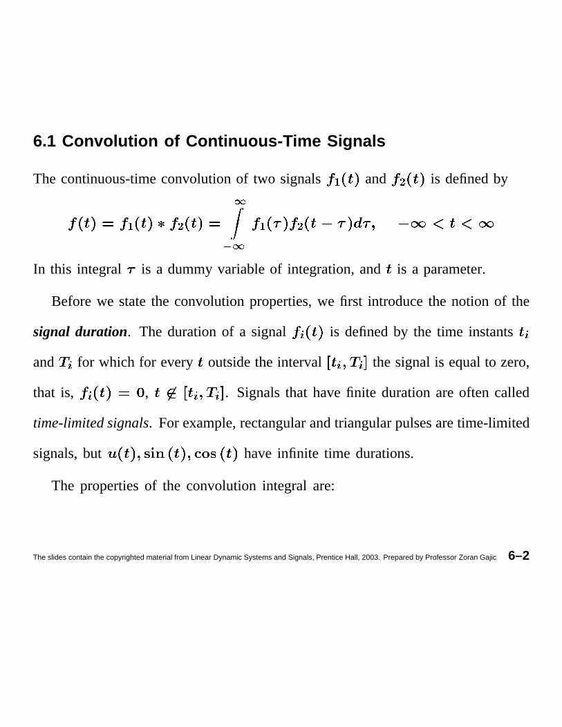
6.1 Convolution of Continuous-Time Signals

The continuous-timeconvolutionof two signals � and � is definedby

� ��

� ��

In this integral is a dummyvariableof integration,and is a parameter.

Before we statethe convolutionproperties,we first introducethe notion of the

signal duration. The durationof a signal � is definedby the time instants �and � for which for every outsidethe interval � � the signalis equalto zero,

that is, � , � � . Signalsthat havefinite durationareoften called

time-limited signals. For example,rectangularandtriangularpulsesaretime-limited

signals,but haveinfinite time durations.

The propertiesof the convolution integral are:


1) Commutativity

� � � �2) Distributivity

� � � � � � �3) Associativity

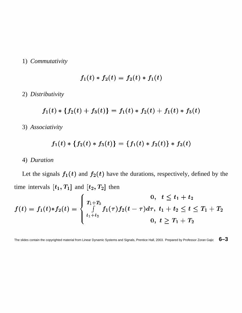
� � � � � �4) Duration

Let the signals � and � havethe durations,respectively,definedby the

time intervals � � and � � then

� ��

� � � � � � � � � ��


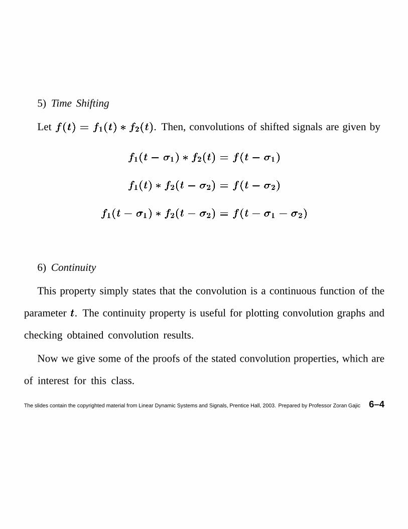
5) Time Shifting

Let � � . Then,convolutionsof shiftedsignalsaregiven by

� � � ��

� � � � � �

6) Continuity

This propertysimply statesthat the convolutionis a continuousfunction of the

parameter . The continuity propertyis useful for plotting convolutiongraphsand

checkingobtainedconvolution results.

Now we give someof the proofsof thestatedconvolutionproperties,which are

of interest for this class.


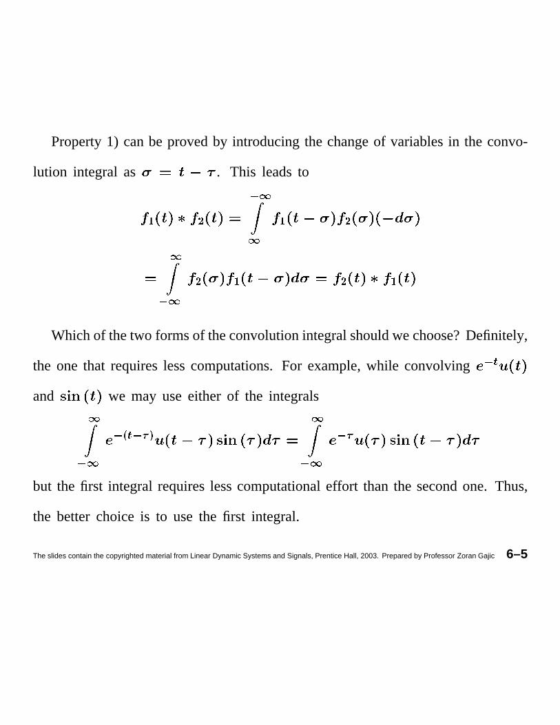
Property1) canbe provedby introducingthe changeof variablesin the convo-

lution integral as . This leadsto

� ��

� ��

��

Whichof thetwo formsof theconvolutionintegralshouldwechoose?Definitely,

the one that requireslesscomputations.For example,while convolving��

and we may useeither of the integrals��

��

� �

but the first integral requireslesscomputationaleffort than the secondone. Thus,

the better choice is to use the first integral.


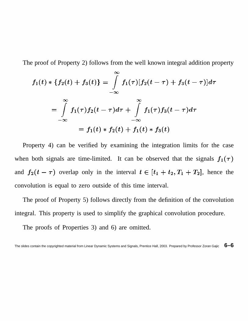
Theproof of Property2) follows from thewell knownintegraladditionproperty

! " #$

% $! " #

$

% $! "

$

% $! #

! " ! #Property 4) can be verified by examining the integration limits for the case

when both signals are time-limited. It can be observedthat the signals !and " overlap only in the interval ! " ! " , hencethe

convolutionis equalto zero outsideof this time interval.

The proof of Property5) follows directly from the definition of the convolution

integral. This propertyis usedto simplify the graphicalconvolutionprocedure.

The proofs of Properties3) and 6) are omitted.


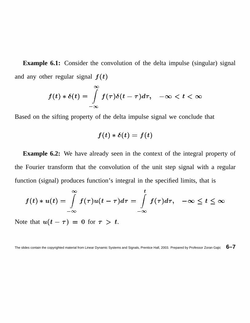
Example 6.1: Considerthe convolutionof the delta impulse(singular)signal

and any other regular signal &

' &Basedon the sifting propertyof the delta impulsesignalwe concludethat

Example 6.2: We havealreadyseenin the contextof the integral propertyof

the Fourier transformthat the convolution of the unit step signal with a regular

function (signal) producesfunction’s integral in the specifiedlimits, that is&

' &

(

' &Note that for .


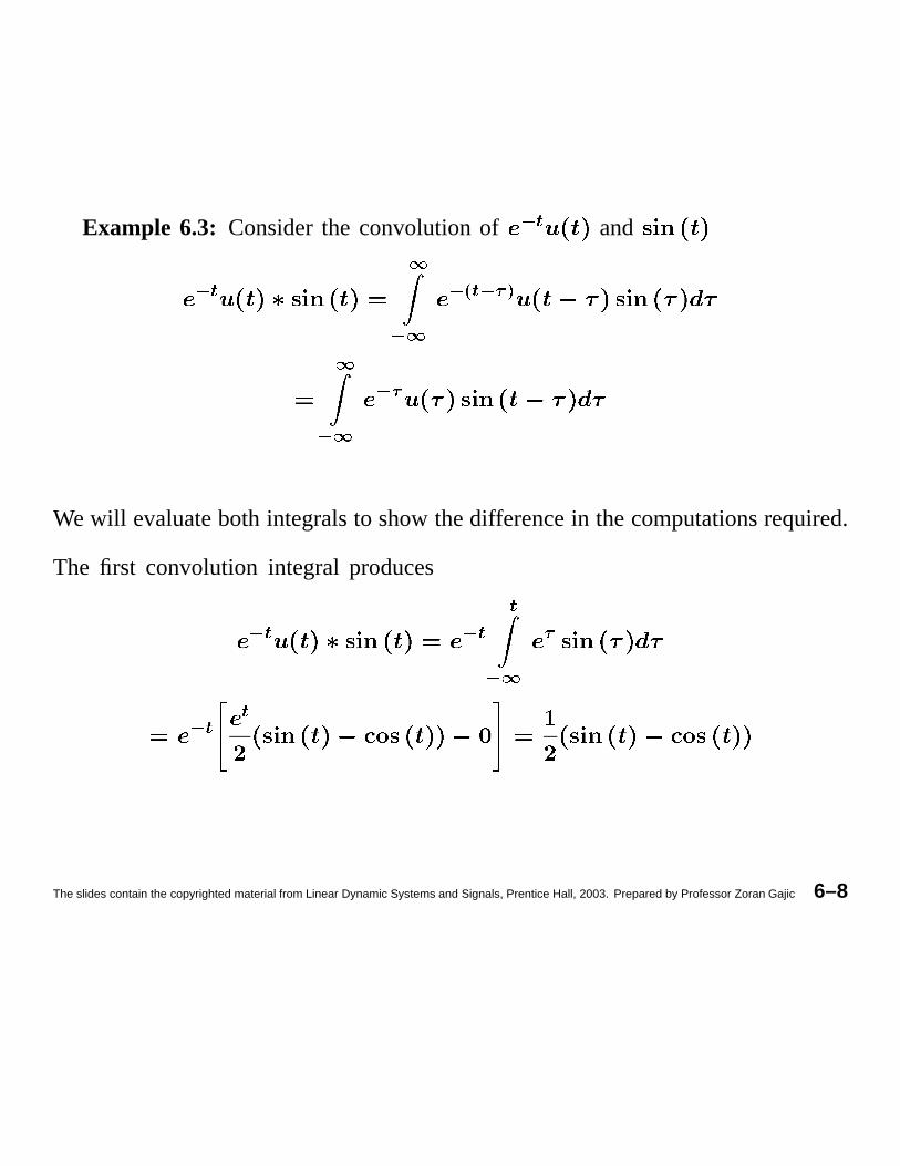
Example 6.3: Considerthe convolutionof )�* and

)�*+

) +)-,.*/)�021

+

) +) 0

We will evaluateboth integralsto showthedifferencein thecomputationsrequired.

The first convolution integral produces

)�* )�* *) +

0

)�* *


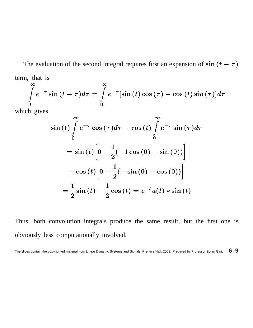
The evaluationof thesecondintegralrequiresfirst anexpansionof

term, that is34

5 634

5 6

which gives 34

5 634

5 6

5�7

Thus, both convolution integrals produce the same result, but the first one is

obviously lesscomputationallyinvolved.


6.1.1 Graphical Convolution

Thegraphicalpresentationof theconvolutionintegralhelpsin theunderstandingof

every stepin the convolutionprocedure.According to the definition integral, the

convolutionprocedureinvolves the following steps:

Step 1: Apply the convolutiondurationpropertyto identify intervalsin which

the convolution is equal to zero.

Step 2: Flip abouttheverticalaxisoneof thesignals(theonethathasa simpler

form (shape)since the commutativityholds), that is, representone of the signals

in the time scale .

Step 3: Vary the parameter from to , that is, slide the flipped signal

from the left to the right, look for the intervals where it overlapswith the other

signal,andevaluatethe integralof the productof two signalsin the corresponding

intervals.


In the abovestepsonecanalsoincorporate(if applicable)the convolutiontime

shifting propertysuchthat all signalsstart at the origin. In sucha case,after the

final convolutionresult is obtainedthe convolutiontime shifting formula shouldbe

appliedappropriately.In addition,theconvolutioncontinuitypropertymaybeused

to checkthe obtainedconvolutionresult,which requiresthat at the boundariesof

adjacentintervalstheconvolutionremainsa continuousfunctionof theparameter .

Wepresentseveralgraphicalconvolutionproblemsstartingwith thesimplestone.

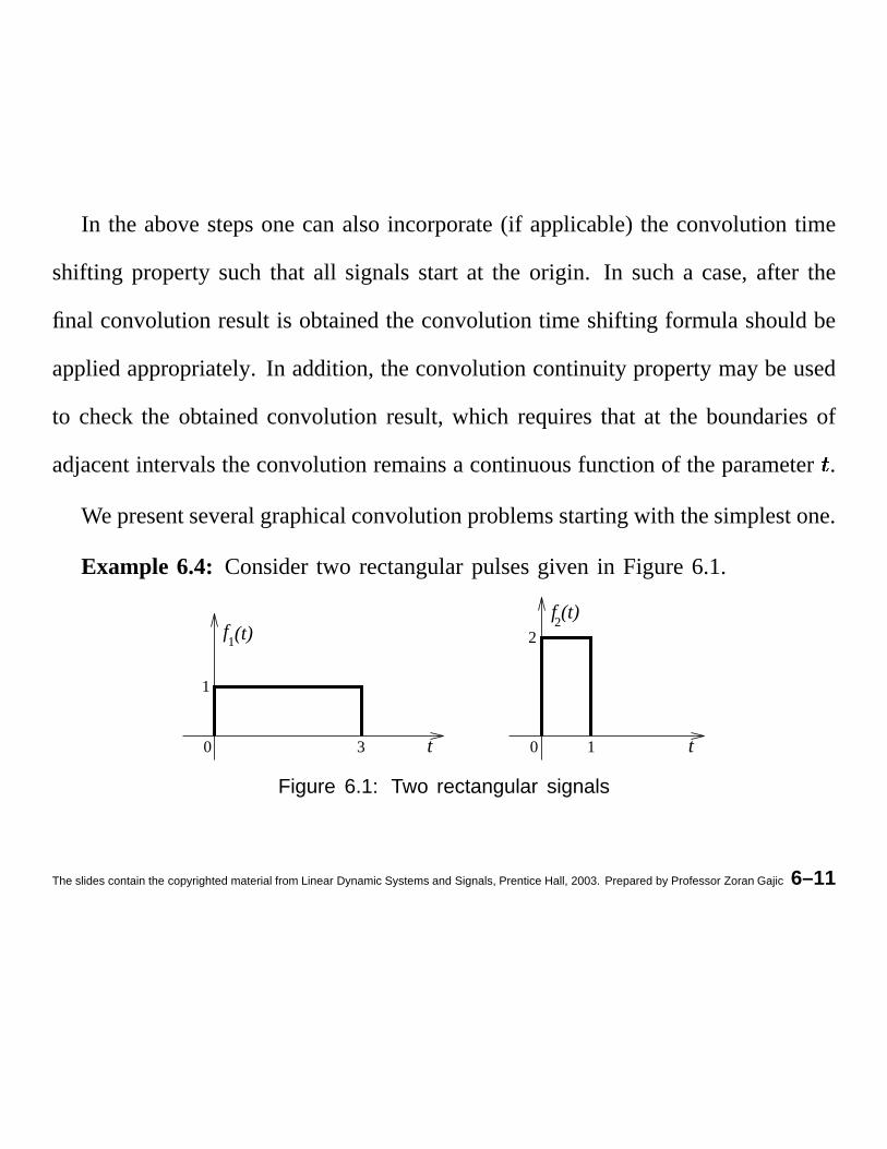
Example 6.4: Considertwo rectangularpulsesgiven in Figure6.1.

f1(t)

f2(t)

t t0 3 0 1

2

1

Figure 6.1: Two rectangular signals


Since the durationsof the signals 8 and 9 are respectivelygiven by

8 8 and 9 9 , we concludethat the convolutionof these

two signalsis zero in the following intervals (Step1)

8 9 8 98 9 8 9

Thus,we needonly to evaluatethe convolutionintegral in the interval .

In the secondstep,we flip aboutthe verticalaxis thesignalwhich hasa simpler

shape.Sincein this caseboth signalsare rectangularpulsesit is irrelevantwhich

one is flipped. Let us flip 9 . Note that the convolution is performedin the

time scale . In Figure6.2 we presentthe signals 8 and 9 . Figure6.2

correspondsto the convolution for .


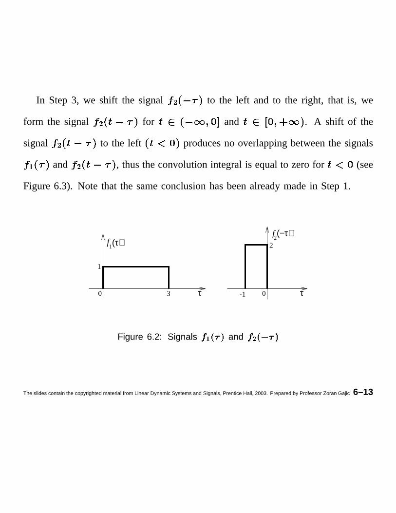
In Step3, we shift the signal : to the left and to the right, that is, we

form the signal : for and . A shift of the

signal : to the left producesno overlappingbetweenthe signals

; and : , thustheconvolutionintegralis equalto zerofor (see

Figure6.3). Note that the sameconclusionhasbeenalreadymadein Step1.

f2(−τ)

0 3

1

f1(τ)

τ 0 τ

2

-1

Figure 6.2: Signals <=?>A@CB and <EDF>HGI@CB


f1(τ)

-1+ t

0 3

1

τ

0 τ

f2

t

(t-τ)

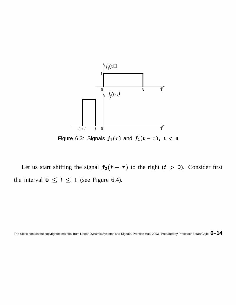
Figure 6.3: Signals J KMLANPO and JEQRLTS�U NVOXWYS[Z \

Let us start shifting the signal ] to the right ( ). Considerfirst

the interval (seeFigure 6.4).


f1(τ)

f2(t-τ)

-1+ t

0 3

1

τ

τ0

t

t

1

1

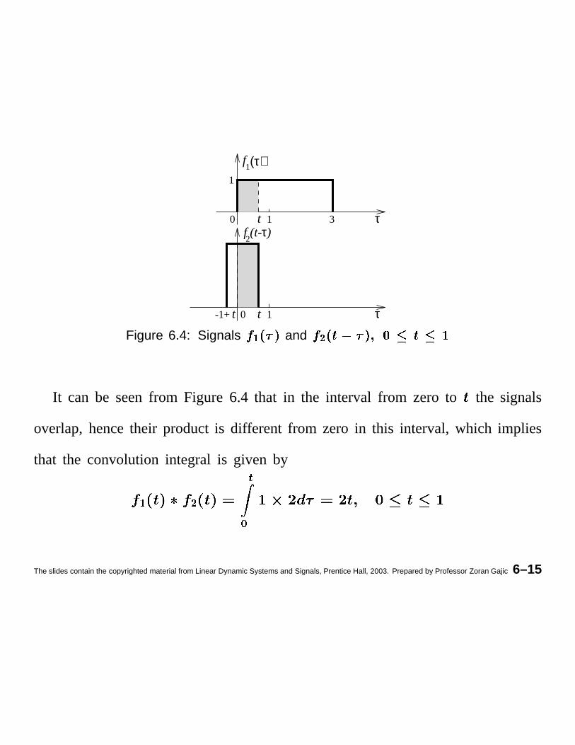
Figure 6.4: Signals ^_M`AaPb and ^dc�`fehg aPbjilknm eom p

It can be seenfrom Figure 6.4 that in the interval from zero to the signals

overlap,hencetheir product is different from zero in this interval, which implies

that the convolution integral is given by

q rst


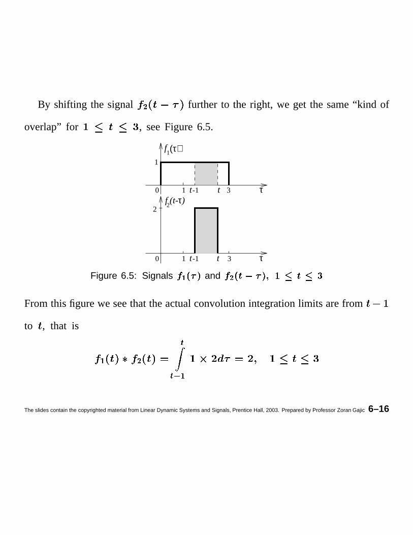
By shifting the signal u further to the right, we get the same“kind of

overlap” for , seeFigure 6.5.

f1(τ)

f (t-τ)2

t-1

t-10 3

1

τ

τt

t

2

0 31

1

Figure 6.5: Signals vwMxAyPz and vd{�xf|h} yPzj~�� |o� �Fromthis figurewe seethat theactualconvolutionintegrationlimits arefrom

to , that is

� ��

��-�


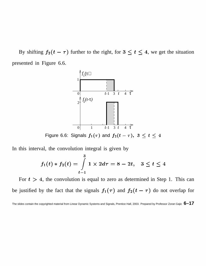
By shifting � further to the right, for , we get the situation

presentedin Figure 6.6.

t-1

t-1

f1(τ)

4

4

f2(t-τ)

0 3

1

τ

0 τt

t

1 3

2

Figure 6.6: Signals ��M�A�P� and �d��f�h� �P�j�l�n� �o� �In this interval, the convolution integral is given by

� ��

�/�-�For , the convolutionis equalto zeroas determinedin Step1. This can

be justified by the fact that the signals � and � do not overlap for


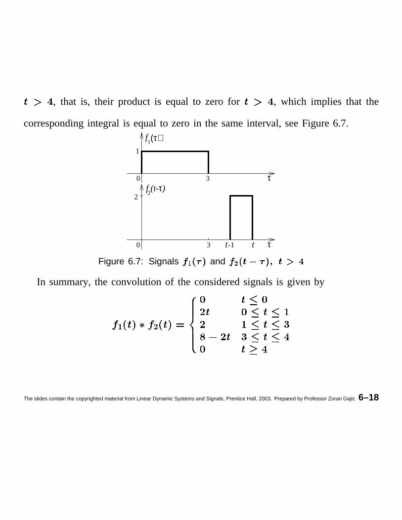
, that is, their product is equal to zero for , which implies that the

correspondingintegral is equalto zero in the sameinterval, seeFigure6.7.f1(τ)

f (t-τ)2

t-1 t

0 3

1

2

0 3

τ

τ

Figure 6.7: Signals � �M�A�P� and �E R�T¡�¢ �V�X£Y¡[¤ ¥In summary,the convolutionof the consideredsignalsis given by

¦ §


Note that from the convolution continuity property, the convolution signal

obtainedis a continuousfunction of . This canbe easilycheckedasfollows. For

the expression produceszero. At we seethat ,

also for we have , and finally for we

get . Thus the function obtained, ¨ © , is a

continuousfunction of the parameter .

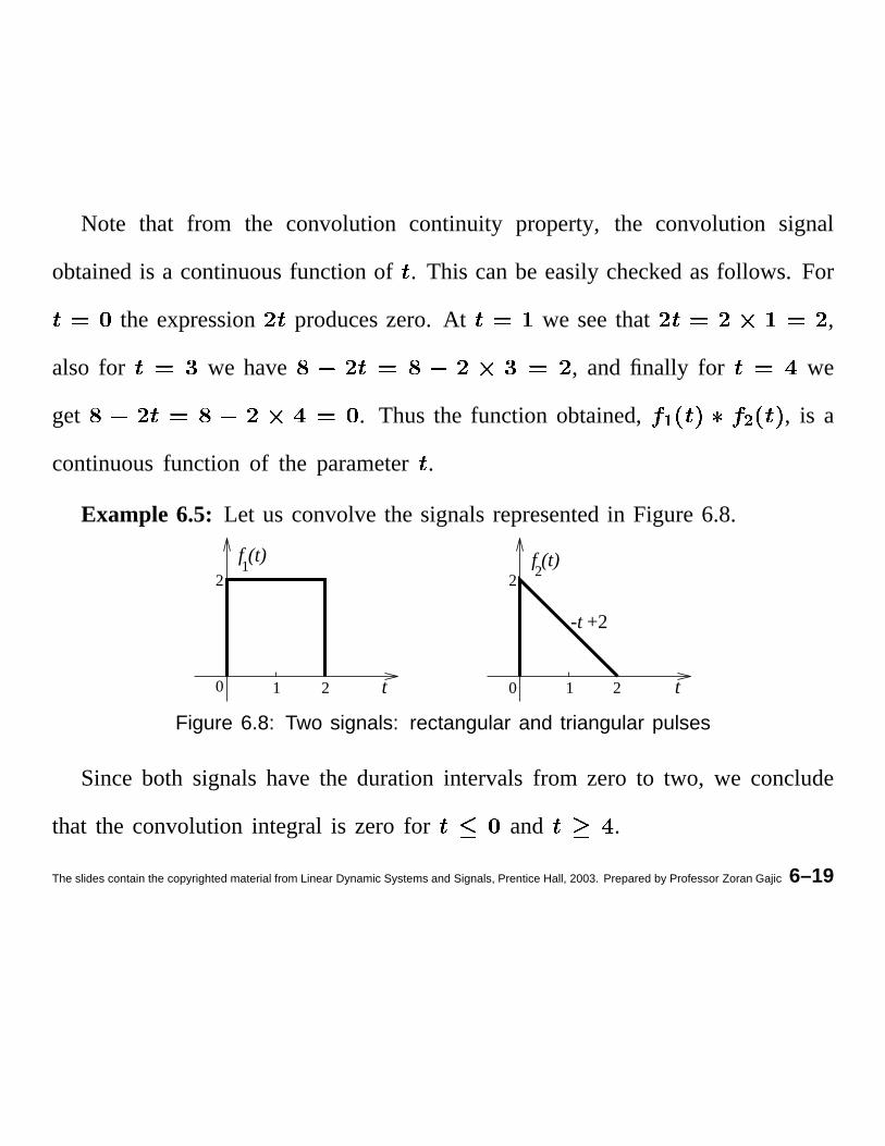
Example 6.5: Let us convolvethe signalsrepresentedin Figure6.8.

f1(t) f (t)

2

t t0 1 2

2

210

2

-t +2

Figure 6.8: Two signals: rectangular and triangular pulses

Sinceboth signalshave the duration intervals from zero to two, we conclude

that the convolutionintegral is zero for and .


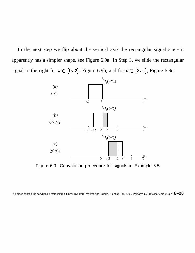
In the next step we flip about the vertical axis the rectangularsignal since it

apparentlyhasa simplershape,seeFigure6.9a. In Step3, we slide the rectangular

signal to the right for , Figure6.9b,and for , Figure6.9c.

t -2

f1(t−τ)

f1(t−τ)

t=0

<0 <2t

<2 <4t

τ

τ

τ

f

-2

1(−τ)

2t0

0

-2

0 2 4t

(a)

(b)

(c)

-2+t

Figure 6.9: Convolution procedure for signals in Example 6.5


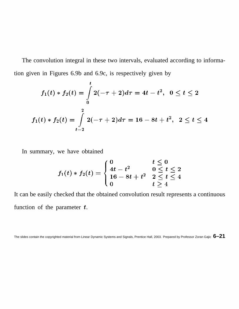
The convolutionintegralin thesetwo intervals,evaluatedaccordingto informa-

tion given in Figures6.9b and 6.9c, is respectivelygiven by

ª «¬

«

ª ««

¬�®�««

In summary,we have obtained

ª « « «

It canbeeasilycheckedthattheobtainedconvolutionresultrepresentsa continuous

function of the parameter .


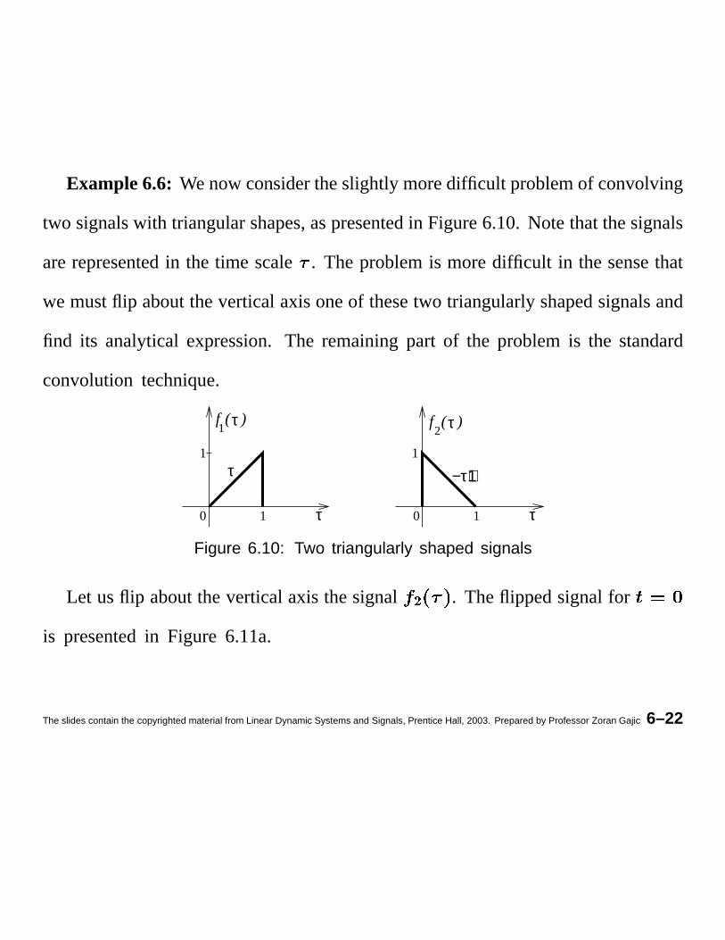
Example 6.6: Wenowconsidertheslightly moredifficult problemof convolving

two signalswith triangularshapes,aspresentedin Figure6.10. Notethatthesignals

arerepresentedin the time scale . The problemis moredifficult in the sensethat

we mustflip abouttheverticalaxisoneof thesetwo triangularlyshapedsignalsand

find its analyticalexpression.The remainingpart of the problem is the standard

convolution technique.

f2(τ )f

1(τ )

ττ

1

0 1 0 1

−τ+1τ1

Figure 6.10: Two triangularly shaped signals

Let usflip abouttheverticalaxis thesignal ¯ . Theflippedsignalfor

is presentedin Figure 6.11a.


f2(t−τ)

f2(t−τ)

f2(−τ)

τ+1−t

-1t

<1<0 t

<2<1 t

t=0

τ

τ

10

1

t

-1

-1 0

τ+1

t

τ

0

2

(a)

(b)

(c)

-1+t

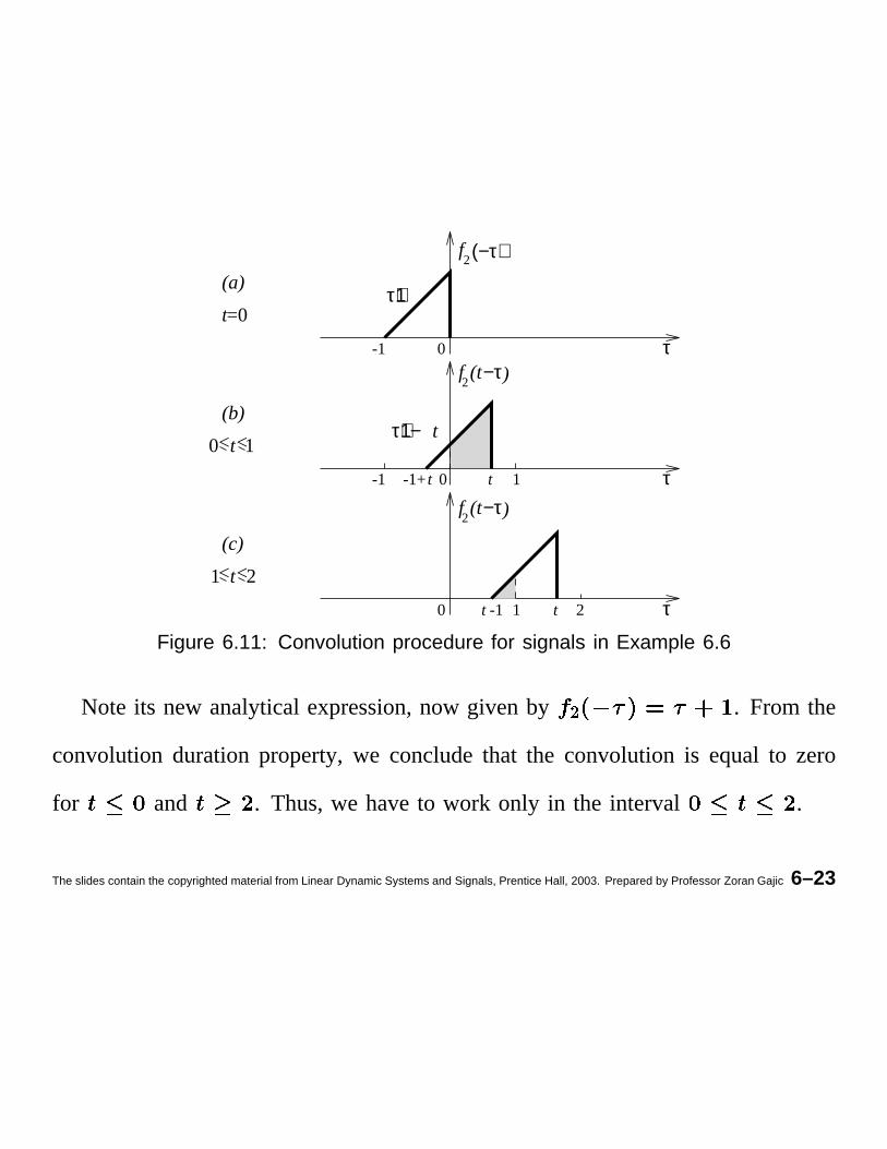
Figure 6.11: Convolution procedure for signals in Example 6.6

Note its new analyticalexpression,now given by ° . From the

convolutiondurationproperty,we concludethat the convolution is equal to zero

for and . Thus,we haveto work only in the interval .


Considerthe interval . In this interval, thesignal ± is given

by ± , seeFigure11.b. Sincethesignal ² overlapswith

the signal ± in the interval from zero to , the convolutionis given by

² ±³´

µ ±

For , the signal ± , presentedin Figure6.11c,overlapswith

the signal ² in the interval from to . Here,theconvolutionis givenby

² ±²

³/¶ ²µ


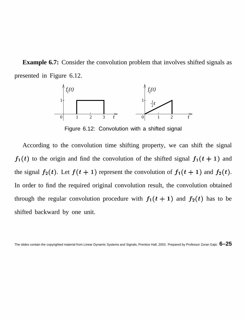
Example 6.7: Considertheconvolutionproblemthat involvesshiftedsignalsas

presentedin Figure 6.12.

211

0 2 0

1

1 21 3

f2

t

(t)

tt

f1(t)

Figure 6.12: Convolution with a shifted signal

According to the convolution time shifting property, we can shift the signal

· to the origin and find the convolutionof the shifted signal · and

the signal ¸ . Let representthe convolutionof · and ¸ .

In order to find the requiredoriginal convolutionresult, the convolutionobtained

through the regular convolution procedurewith · and ¸ has to be

shifted backwardby one unit.


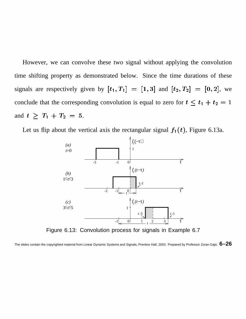
However,we can convolve thesetwo signal without applying the convolution

time shifting property as demonstratedbelow. Since the time durationsof these

signals are respectivelygiven by ¹ ¹ and º º , we

concludethat the correspondingconvolutionis equalto zero for ¹ ºand ¹ º .

Let us flip aboutthe vertical axis the rectangularsignal ¹ , Figure6.13a.

f1(t−τ)

f1(t−τ)

f1(−τ)

τ

1

-3 -1 0

<3<1 t

t=0

<3 <5t

τ

τ-1

1

-1-2

0 1 2 3

0

t

t

(c)

(a)

(b)

t

tt

-1

-3 -1

Figure 6.13: Convolution process for signals in Example 6.7


In the interval , the convolutionis given by (seeFigure6.13b)

» ¼½/¾-»¿

¼

In the interval , we havefrom Figure 6.13c

» ¼¼

½/¾�À

In the next sectionwe apply the convolutionformula to linear continuous-time

invariantsystemsandshowthat the systemresponseto any input is given in terms

of theconvolutionintegral. To thatend,we will usetheconceptsof systemtransfer

function andsystemimpulseresponseintroducedin Chapters3 and4.


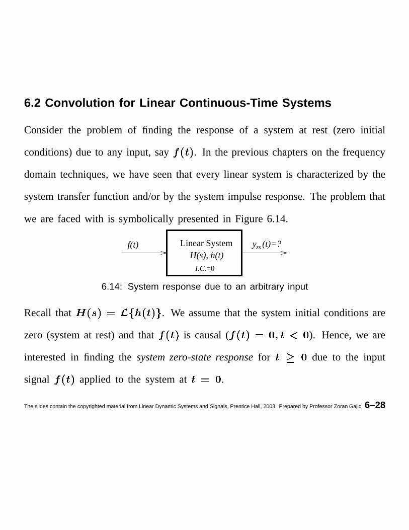
6.2 Convolution for Linear Continuous-Time Systems

Consider the problem of finding the responseof a systemat rest (zero initial

conditions)due to any input, say . In the previouschapterson the frequency

domaintechniques,we haveseenthat every linear systemis characterizedby the

systemtransferfunction and/orby the systemimpulseresponse.The problemthat

we are facedwith is symbolically presentedin Figure 6.14.

f(t) Linear SystemH(s), h(t)

y (t)=?zs

I.C.=0

6.14: System response due to an arbitrary input

Recall that . We assumethat the systeminitial conditionsare

zero (systemat rest) and that is causal( ). Hence,we are

interestedin finding the system zero-state response for due to the input

signal applied to the systemat .


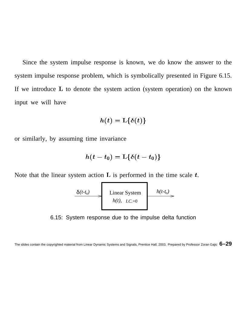
Since the systemimpulse responseis known, we do know the answerto the

systemimpulseresponseproblem,which is symbolicallypresentedin Figure6.15.

If we introduce to denotethe systemaction (systemoperation)on the known

input we will have

or similarly, by assumingtime invariance

Á Á

Note that the linear systemaction is performedin the time scale .

o) o)(t-tδ h(t-tLinear System

h(t), I.C.=0

6.15: System response due to the impulse delta function


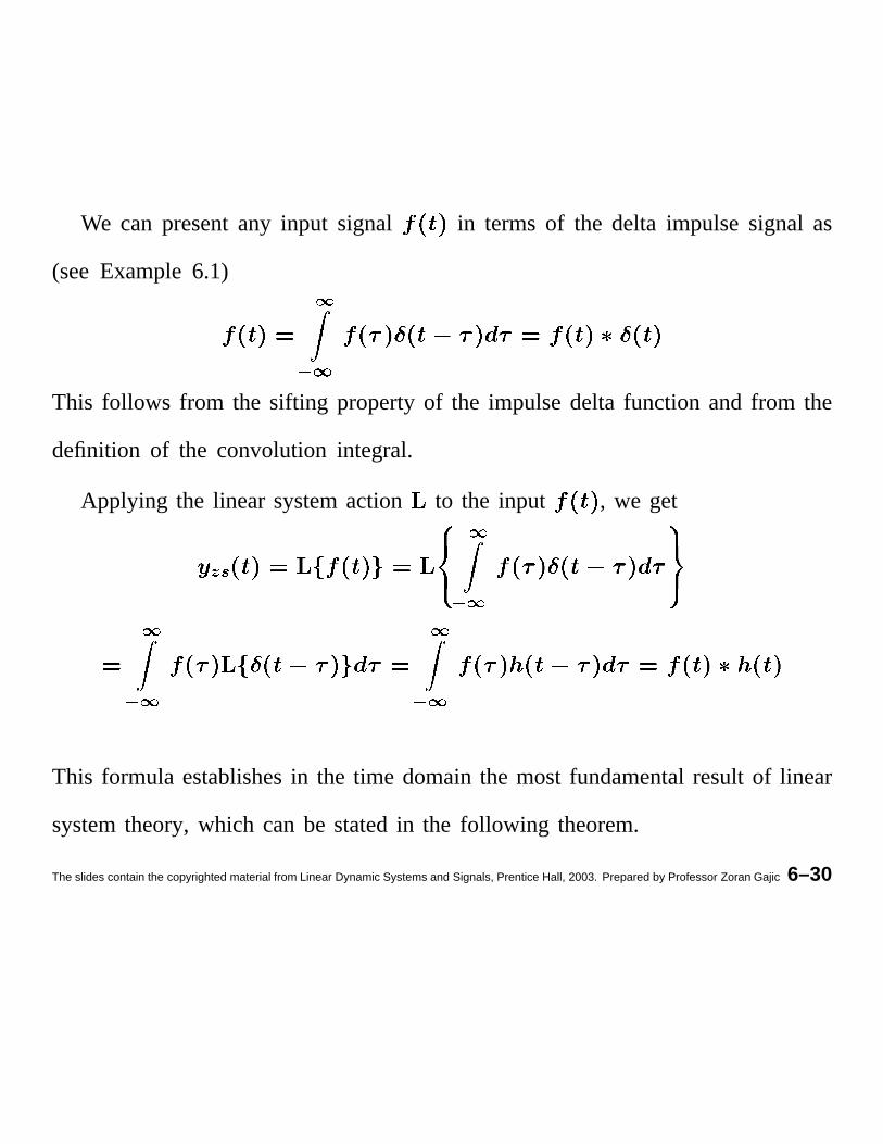
We can presentany input signal in termsof the delta impulsesignal as

(seeExample6.1) Â

Ã ÂThis follows from the sifting propertyof the impulsedelta function and from the

definition of the convolution integral.

Applying the linear systemaction to the input , we get

ÄRÅÂ

Ã ÂÂ

Ã ÂÂ

Ã Â

This formula establishesin the time domainthe most fundamentalresult of linear

systemtheory,which can be statedin the following theorem.


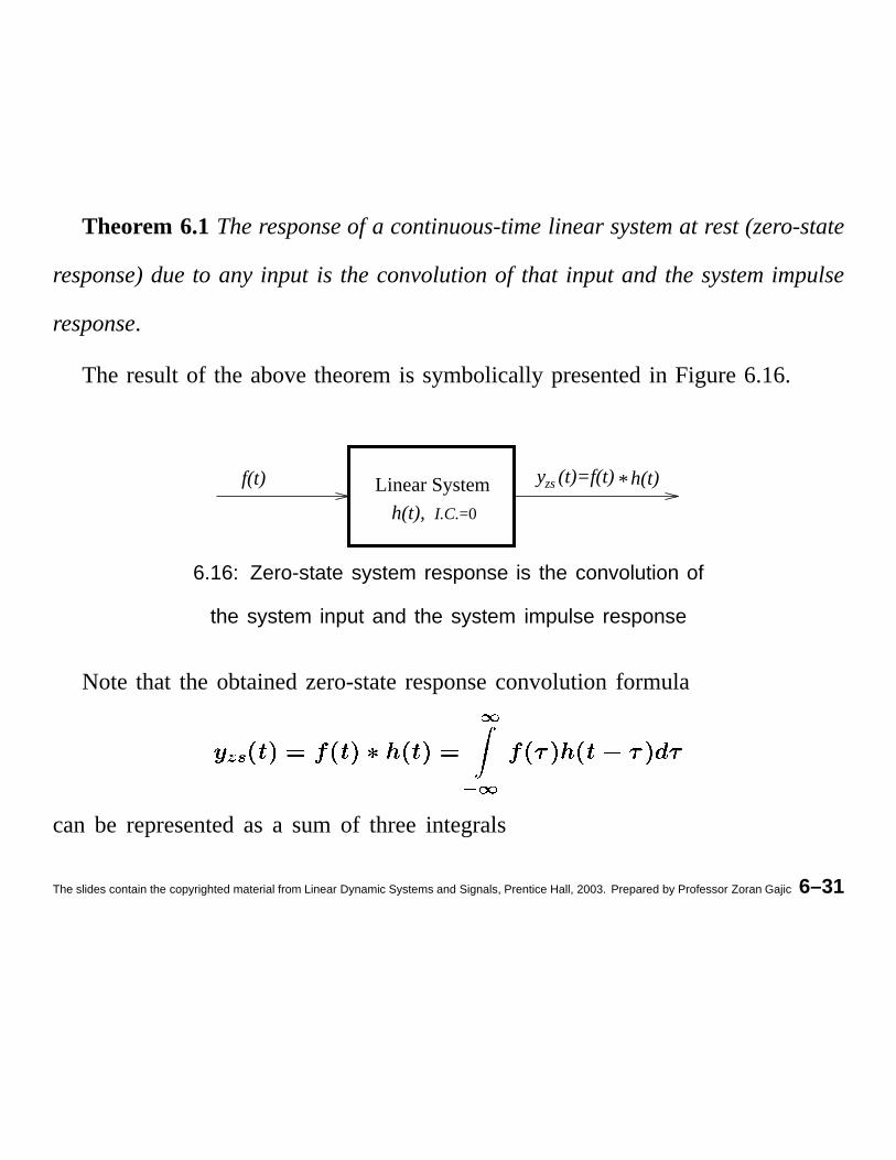
Theorem 6.1 The response of a continuous-time linear system at rest (zero-state

response) due to any input is the convolution of that input and the system impulse

response.

The resultof the abovetheoremis symbolicallypresentedin Figure6.16.

Linear System y (t)=f(t) * h(t)f(t) zs

h(t), I.C.=0

6.16: Zero-state system response is the convolution of

the system input and the system impulse response

Note that the obtainedzero-stateresponseconvolutionformula

ÆRÇÈ

É Ècan be representedas a sum of three integrals


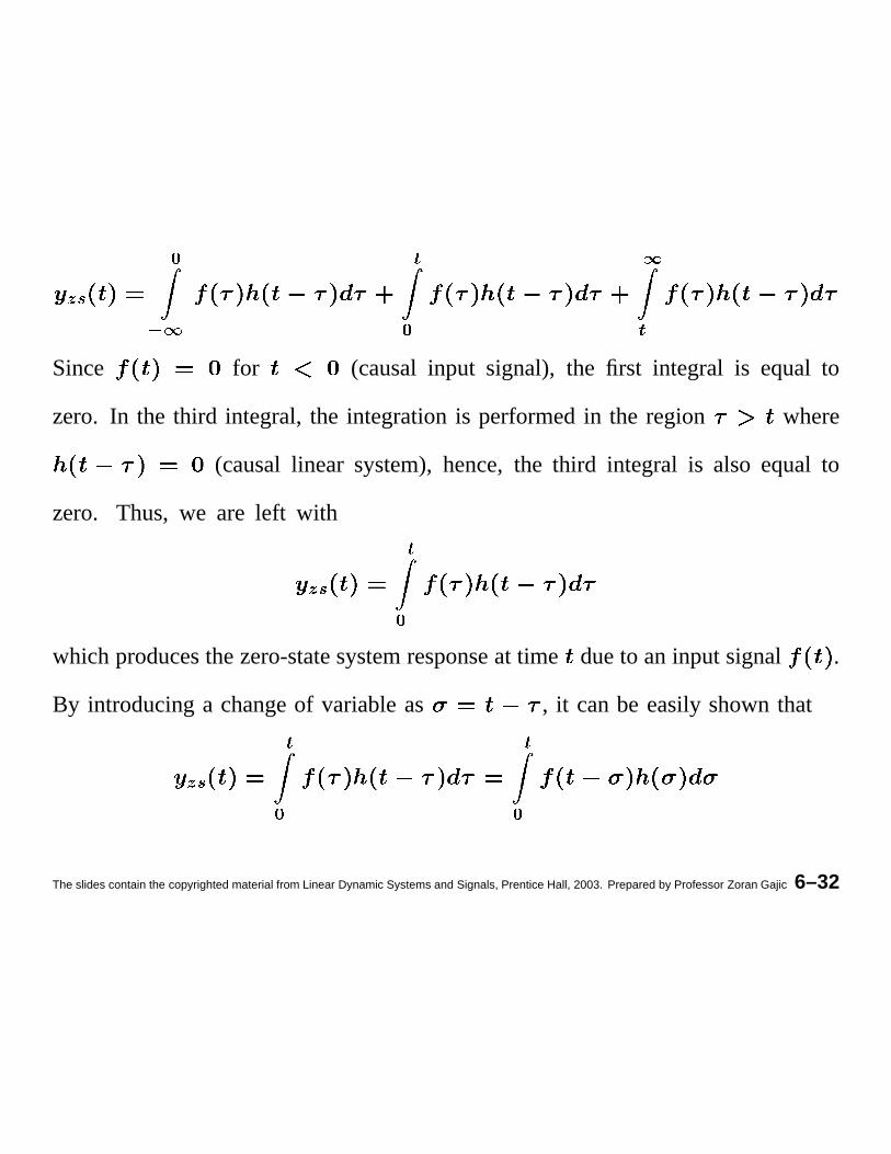
ÊRËÌ

Í�Î

ÏÌ

ÎÏ

Since for (causalinput signal), the first integral is equal to

zero. In the third integral, the integrationis performedin the region where

(causallinear system),hence,the third integral is also equal to

zero. Thus, we are left with

ÊRËÏÌ

which producesthezero-statesystemresponseat time dueto aninput signal .

By introducinga changeof variableas , it canbe easilyshownthat

ÊRËÏÌ

ÏÌ


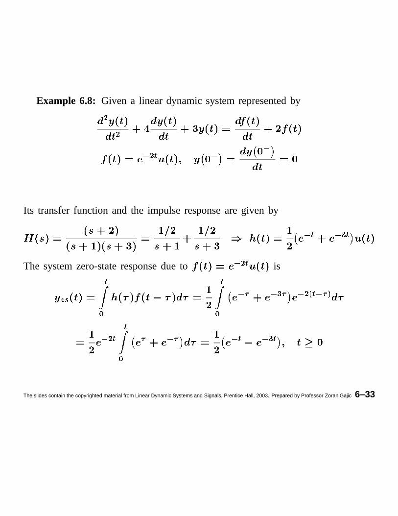
Example 6.8: Given a linear dynamicsystemrepresentedbyÐÐ

Ñ ÐHÒ Ñ Ñ

Its transferfunction and the impulseresponseare given by

Ñ Ò Ñ Ó Ò

The systemzero-stateresponsedue toÑ ÐHÒ

is

ÔFÕÒÖ

ÒÖ

Ñ × Ñ ÓØ× Ñ ÐMÙ.Ò Ñ × Ú

Ñ ÐHÒÒÖ

× Ñ × Ñ Ò Ñ Ó Ò


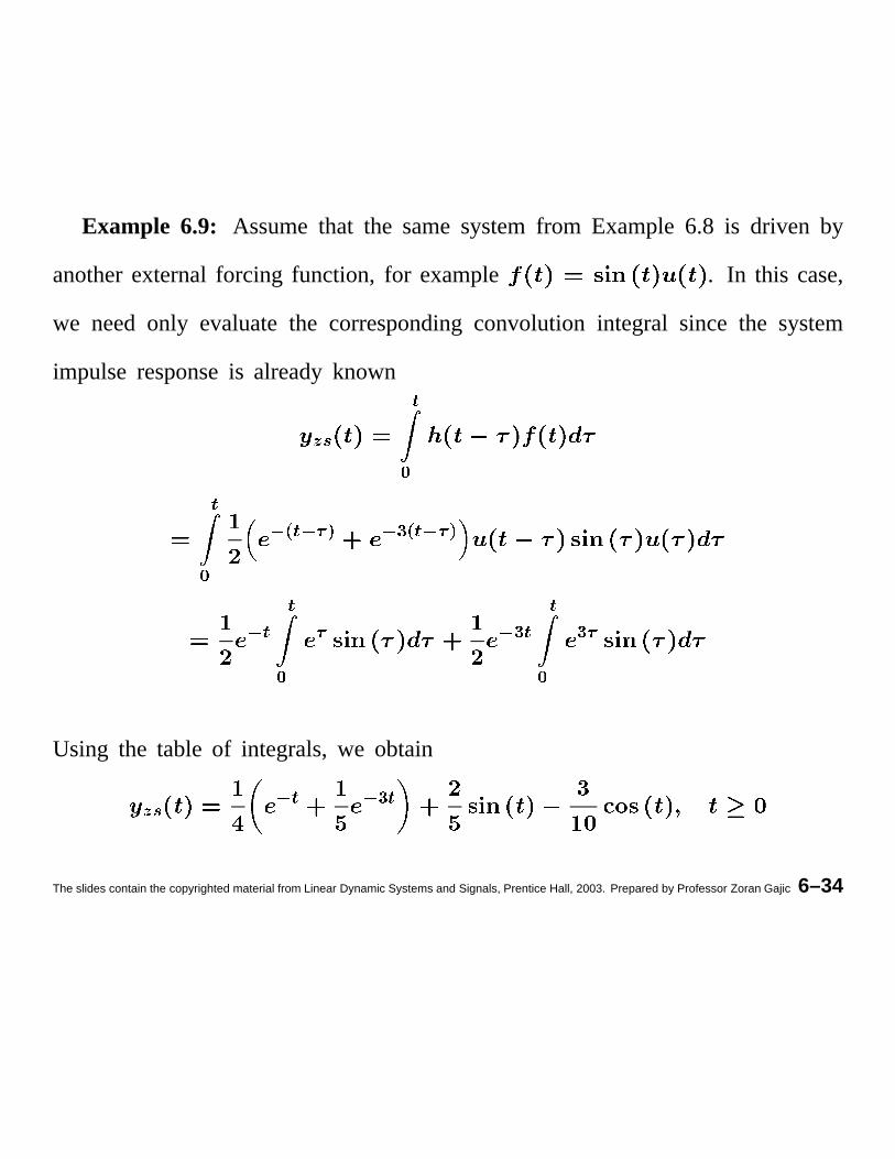
Example 6.9: Assumethat the samesystemfrom Example6.8 is driven by

anotherexternalforcing function, for example . In this case,

we need only evaluatethe correspondingconvolution integral since the system

impulse responseis alreadyknown

ÛRÜÝÞ

ÝÞ

ß�à Ý ß�á2â ßäãRà Ý ß á â

ß ÝÝÞ

á ß ã ÝÝ

ÞãØá

Using the table of integrals,we obtain

ÛRÜ ß Ý ß ã Ý


Convolution - Rutgers Universityeceweb1.rutgers.edu/~gajic/solmanual/slides/chapter6C.pdfConvolution...

Documents

Transcript of Convolution - Rutgers Universityeceweb1.rutgers.edu/~gajic/solmanual/slides/chapter6C.pdfConvolution...