Convex polyhedron learning and its applications
109
Convex polyhedron learning and its applications PhD thesis G´ abor Tak´ acs submitted to Budapest University of Technology and Economics, Budapest, Hungary Faculty of Electrical Engineering and Informatics October, 2009
Transcript of Convex polyhedron learning and its applications

Convex polyhedron learningand its applications
PhD thesis
Gabor Takacs
submitted to
Budapest University of Technology and Economics, Budapest, Hungary
Faculty of Electrical Engineering and Informatics
October, 2009

c© 2009 Gabor Takacs
Budapest University of Technology and EconomicsFaculty of Electrical Engineering and Informatics
Department of Measurement and Information Systems


Contents
1 Introduction 111.1 Classification . . . . . . . . . . . . . . . . . . . . . . . . . . . . . . . . . . . . . . 12
1.1.1 Linear classification . . . . . . . . . . . . . . . . . . . . . . . . . . . . . . 131.1.2 Fisher discriminant analysis . . . . . . . . . . . . . . . . . . . . . . . . . . 141.1.3 Logistic regression . . . . . . . . . . . . . . . . . . . . . . . . . . . . . . . 141.1.4 Artificial neuron . . . . . . . . . . . . . . . . . . . . . . . . . . . . . . . . 151.1.5 Linear support vector machine . . . . . . . . . . . . . . . . . . . . . . . . 161.1.6 Nonlinear classification . . . . . . . . . . . . . . . . . . . . . . . . . . . . . 161.1.7 K nearest neighbors . . . . . . . . . . . . . . . . . . . . . . . . . . . . . . 161.1.8 ID3 decision tree . . . . . . . . . . . . . . . . . . . . . . . . . . . . . . . . 171.1.9 Multilayer perceptron . . . . . . . . . . . . . . . . . . . . . . . . . . . . . 181.1.10 Support vector machine . . . . . . . . . . . . . . . . . . . . . . . . . . . . 181.1.11 Convex polyhedron classification . . . . . . . . . . . . . . . . . . . . . . . 20
1.2 Regression . . . . . . . . . . . . . . . . . . . . . . . . . . . . . . . . . . . . . . . . 201.2.1 Linear regression . . . . . . . . . . . . . . . . . . . . . . . . . . . . . . . . 211.2.2 Nonlinear regression . . . . . . . . . . . . . . . . . . . . . . . . . . . . . . 21
1.3 Techniques against overfitting . . . . . . . . . . . . . . . . . . . . . . . . . . . . . 221.4 Collaborative filtering . . . . . . . . . . . . . . . . . . . . . . . . . . . . . . . . . 23
1.4.1 Double centering . . . . . . . . . . . . . . . . . . . . . . . . . . . . . . . . 241.4.2 Matrix factorization . . . . . . . . . . . . . . . . . . . . . . . . . . . . . . 241.4.3 BRISMF . . . . . . . . . . . . . . . . . . . . . . . . . . . . . . . . . . . . 251.4.4 Neighbor based methods . . . . . . . . . . . . . . . . . . . . . . . . . . . . 271.4.5 Convex polyhedron methods . . . . . . . . . . . . . . . . . . . . . . . . . 30
1.5 Other machine learning problems . . . . . . . . . . . . . . . . . . . . . . . . . . . 301.5.1 Clustering . . . . . . . . . . . . . . . . . . . . . . . . . . . . . . . . . . . . 301.5.2 Labeled sequence learning . . . . . . . . . . . . . . . . . . . . . . . . . . . 311.5.3 Time series prediction . . . . . . . . . . . . . . . . . . . . . . . . . . . . . 31
2 Algorithms 332.1 Linear programming basics . . . . . . . . . . . . . . . . . . . . . . . . . . . . . . 332.2 Algorithms for determining separability . . . . . . . . . . . . . . . . . . . . . . . 35
2.2.1 Definitions . . . . . . . . . . . . . . . . . . . . . . . . . . . . . . . . . . . 352.2.2 Algorithms for linear separability . . . . . . . . . . . . . . . . . . . . . . . 362.2.3 Algorithms for convex separability . . . . . . . . . . . . . . . . . . . . . . 40
2.3 Algorithms for classification . . . . . . . . . . . . . . . . . . . . . . . . . . . . . . 422.3.1 Known methods . . . . . . . . . . . . . . . . . . . . . . . . . . . . . . . . 422.3.2 Smooth maximum functions . . . . . . . . . . . . . . . . . . . . . . . . . . 432.3.3 Smooth maximum based algorithms . . . . . . . . . . . . . . . . . . . . . 48
2.4 Algorithms for regression . . . . . . . . . . . . . . . . . . . . . . . . . . . . . . . 542.5 Algorithms for collaborative filtering . . . . . . . . . . . . . . . . . . . . . . . . . 54
3 Model complexity 573.1 Definitions . . . . . . . . . . . . . . . . . . . . . . . . . . . . . . . . . . . . . . . . 57
3.1.1 Convex polyhedron function classes . . . . . . . . . . . . . . . . . . . . . . 583.2 Known facts . . . . . . . . . . . . . . . . . . . . . . . . . . . . . . . . . . . . . . . 593.3 The VC dimension of MINMAX2,K . . . . . . . . . . . . . . . . . . . . . . . . . . 61
3.3.1 Concepts for the proof . . . . . . . . . . . . . . . . . . . . . . . . . . . . . 62
1

CONTENTS
3.3.2 The proof . . . . . . . . . . . . . . . . . . . . . . . . . . . . . . . . . . . . 623.4 New lower bounds . . . . . . . . . . . . . . . . . . . . . . . . . . . . . . . . . . . 68
4 Applications 734.1 Determining linear and convex separability . . . . . . . . . . . . . . . . . . . . . 73
4.1.1 Datasets . . . . . . . . . . . . . . . . . . . . . . . . . . . . . . . . . . . . . 734.1.2 Algorithms . . . . . . . . . . . . . . . . . . . . . . . . . . . . . . . . . . . 744.1.3 Types of separability . . . . . . . . . . . . . . . . . . . . . . . . . . . . . . 764.1.4 Running times . . . . . . . . . . . . . . . . . . . . . . . . . . . . . . . . . 79
4.2 Experiments with classification . . . . . . . . . . . . . . . . . . . . . . . . . . . . 844.2.1 Comparing the variants of SMAX . . . . . . . . . . . . . . . . . . . . . . 864.2.2 Comparing SMAX with other methods . . . . . . . . . . . . . . . . . . . . 88
4.3 Experiments with collaborative filtering . . . . . . . . . . . . . . . . . . . . . . . 93
List of publications 101
Bibliography 103
2

List of Figures
1.1 The structure of an MLP with one hidden layer. . . . . . . . . . . . . . . . . . . 191.2 The red dots represent training examples and the black squares new examples in
a regression problem. The green curve and the blue line represent two predic-tors. The green predictor fits perfectly to the training examples, but the blue onegeneralizes better. . . . . . . . . . . . . . . . . . . . . . . . . . . . . . . . . . . . 22
1.3 Training algorithm for BRISMF. . . . . . . . . . . . . . . . . . . . . . . . . . . . 261.4 Training algorithm for NSVD1. . . . . . . . . . . . . . . . . . . . . . . . . . . . . 29
2.1 Examples for linearly separable (a), mutually convexly separable (b), convexlyseparable (c), and convexly nonseparable (d) point sets. . . . . . . . . . . . . . . 36
2.2 The maximum function in 2 dimensions. . . . . . . . . . . . . . . . . . . . . . . . 452.3 Smooth maximum functions in 2 dimensions (α = 2). . . . . . . . . . . . . . . . . 462.4 The error of smooth maximum functions in 2 dimensions (α = 2). . . . . . . . . . 472.5 Stochastic gradient descent with momentum for training the convex polyhedron
classifier. . . . . . . . . . . . . . . . . . . . . . . . . . . . . . . . . . . . . . . . . . 512.6 Newton’s method for training the convex polyhedron classifier. . . . . . . . . . . 532.7 Stochastic gradient descent for training the convex polyhedron predictor. . . . . 56
3.1 How to choose the independent faces based on the label of the extra points. Notethat some faces are never chosen. . . . . . . . . . . . . . . . . . . . . . . . . . . . 60
3.2 A point set in convex position. The red and a blue signs cannot be separated witha triangle, because for this we should intersect all edges of a convex 8-gon with 3lines. . . . . . . . . . . . . . . . . . . . . . . . . . . . . . . . . . . . . . . . . . . . 62
3.3 A point set in tangled position. The red and the blue signs can never be separatedwith a convex K-gon, regardless of the value of K. . . . . . . . . . . . . . . . . . 62
3.4 The 14 regions generated by placing two points into a triangle. . . . . . . . . . . 643.5 The 13 regions generated by placing the third point into R13. . . . . . . . . . . . 653.6 Regions in BCDEF , case I. . . . . . . . . . . . . . . . . . . . . . . . . . . . . . . 663.7 Regions in BCDEF , case II. . . . . . . . . . . . . . . . . . . . . . . . . . . . . . 663.8 Regions in BCDEFG. . . . . . . . . . . . . . . . . . . . . . . . . . . . . . . . . . 673.9 The vertex adjacency graph of the 600-cell. . . . . . . . . . . . . . . . . . . . . . 71
4.1 Examples from the MNIST28 database. . . . . . . . . . . . . . . . . . . . . . . . 744.2 The TOY dataset. . . . . . . . . . . . . . . . . . . . . . . . . . . . . . . . . . . . 844.3 The V distribution with settings d = 2, α = 0.05 (a) and d = 3, α = 0.05 (b).
The optimal decision boundary is indicated with green. . . . . . . . . . . . . . . 844.4 The train–test split and the naming convention of the NETFLIX dataset (after
[Bell et al., 2007]) . . . . . . . . . . . . . . . . . . . . . . . . . . . . . . . . . . . . 94
3


List of Tables
4.1 Types of separability in the MNIST28 dataset. . . . . . . . . . . . . . . . . . . . 774.2 Types of separability in the MNIST14 dataset. . . . . . . . . . . . . . . . . . . . 774.3 Types of separability in the MNIST7 dataset. . . . . . . . . . . . . . . . . . . . . 784.4 Types of separability in the MNIST4 dataset. . . . . . . . . . . . . . . . . . . . . 784.5 Number of examples from Class 1 contained in the convex hull of Class 2 in the
MNIST4 dataset. . . . . . . . . . . . . . . . . . . . . . . . . . . . . . . . . . . . . 794.6 Running times of basic algorithms for determining linear separability. . . . . . . 804.7 Running times of LSEPX, LSEPY, and LSEPZ. . . . . . . . . . . . . . . . . . . . 814.8 Running times of LSEPZX and LSEPZY. . . . . . . . . . . . . . . . . . . . . . . 814.9 Running times of basic algorithms for determining convex separability. . . . . . . 824.10 Percentage of outer points cut by the centroid method (CSEPC). . . . . . . . . . 824.11 Running times of the centroid method (CSEPC). . . . . . . . . . . . . . . . . . . 834.12 Running times of enhanced algorithms for determining convex separability. . . . 834.13 Results of SMAX training on the TOY dataset. . . . . . . . . . . . . . . . . . . . 874.14 Results of classification algorithms on the V2 dataset. . . . . . . . . . . . . . . . 894.15 Results of classification algorithms on the V3 dataset. . . . . . . . . . . . . . . . 904.16 Results of classification algorithms on the ABALONE dataset. . . . . . . . . . . 904.17 Results of classification algorithms on the BLOOD dataset. . . . . . . . . . . . . 914.18 Results of classification algorithms on the CHESS dataset. . . . . . . . . . . . . . 924.19 Results of classification algorithms on the SEGMENT dataset. . . . . . . . . . . 924.20 Results of collaborative filtering algorithms on the NETFLIX dataset. . . . . . . 964.21 Results of linear blending on the NETFLIX dataset. . . . . . . . . . . . . . . . . 97
5


Acknowledgements
I would like to thank Bela Pataki, my advisor, for initiating me into research and guiding meover the years. I am grateful to him not only for his constant help and valuable advice, but alsofor his friendly character and good humor.
I would like to thank Gabor Horvath, my teacher, for giving me interesting tasks that greatlyinfluenced my interest. His neural networks course remains an unforgettable part of my under-graduate studies.
I would like to thank Istvan Pilaszy, Bottyan Nemeth, and Domonkos Tikk, the members ofteam Gravity, for their sincere enthusiasm to machine learning. I still enjoy the discussions withthem about scientific and other topics.
I would like to thank Zoltan Horvath, my senior colleague for listening me many times andasking good questions. I am also grateful to him for teaching me some cool mathematical tricksand helping me to meet people with particularly great knowledge.
I would like to thank my parents for bringing me up and encouraging me in my studies. Thiswork would not have been possible without their support.
Finally, I would like to thank my wife, Katalin for her never ending love and patience. Shekept me motivated constantly, and comforted me when I was down. I dedicate this thesis to herand to the fruit of our love, the little Agnes.
7


Abstract
From a possible engineer’s point of view learning can be considered as discovering the relationshipbetween the features of a phenomenon. Machine learning (data mining) is a variant of learning, inwhich the observations about the phenomenon are available as data, and the connection betweenthe features is discovered by a program.
In the case of classification the phenomenon is modeled by a random pair (X, Y ), where thed-dimensional continuous X is called input, and the discrete (often binary) Y is called label. Inthe case of collaborative filtering the phenomenon is modeled by a random triplet (U, I,R), wherethe discrete U is called user identifier, the discrete I is called item identifier, and the continuousR is called rating value.
Unbalanced problems i.e. in which one class label occurs much more frequently than the otherform an interesting subset among binary classification problems. In practice such problems oftenarise for example in the field of medical and technical diagnostics.
A convex polyhedron classifier is a function g : Rd 7→ {+1,−1} with the property that the
decision region {x ∈ Rd : g(x) = 1} is a convex polyhedron. At classifying an input x ∈ R
d, wehave to substitute x into the linear functions defining the polyhedron. If any of the substitutionsgives a negative number, then we can stop the computation immediately, since the class labelwill be necessarily −1 in this case. As a consequence, convex polyhedron classifiers fit well tounbalanced problems.
The convex polyhedron based approach has its analogous variant for collaborative filteringtoo. In this case the utility of the approach is that it gives a unique solution of the problem thatcan be a useful component of a blended solution involving many different models.
A related problem to classification is determining the convex separability of point sets. Letus assume that P and Q are finite sets in R
d. The task is to decide whether there exist a convexpolyhedron S that contains all element of P, but no elements from Q.
In a practical data mining project typically many experiments are run and many models arebuilt. It is non-trivial to decide which of them should be used for prediction in the final system.Obviously, if two models achieve the same accuracy on the training set, then it is reasonableto choose the simpler one. The Vapnik–Chervonenkis dimension is a widely accepted modelcomplexity measure in the case of binary classification.
The first chapter of the thesis (Introduction) briefly introduces the field of machine learningand locates convex polyhedron learning in it. Then, without completeness it overviews a setknown learning algorithms. The part dealing with collaborative filtering contains novel resultstoo.
The second chapter of the thesis (Algorithms) is about algorithms that use convex polyhe-drons for solving various machine learning problems. The first part of the chapter deals withthe problem of linear and convex separation. The second part of the chapter gives algorithmsfor training convex polyhedron classifiers. The third part of the chapter introduces a convexpolyhedron based algorithm for collaborative filtering.
The third chapter of the thesis (Model complexity) collects the known facts about the Vapnik–Chervonenkis dimension of convex polyhedron classifiers and proves new results. The fourthchapter (Applications) presents the experiments performed with the proposed algorithms.
9


Example isn’t another way to
teach, it is the only way to teach.
Albert Einstein
1Introduction
Learning from examples is a characteristic ability of human intelligence. For us, learning is asnatural as breathing. We not only observe the world, but inherently try to find relationshipsbetween our observations. From this point of view, a child learning to ride a bike discovers theconnection between his/her perception and traveling safely. A student preparing for an examtries to understand the connection between the possible questions and the correct answers. Inthis thesis, learning will be considered as discovering the relationship between the features of aphenomenon.
If the features are encoded as numbers, and the relationship between them is discovered byan algorithm, then we talk about machine learning (ML) 1. The input of machine learning is adataset that was collected by observing the phenomenon. The output is a program that is ableto answer certain questions about the phenomenon.
On the map of scientific disciplines machine learning could be placed into the intersection ofstatistics and computer science. Machine learning aims at inferring from data reliably, thereforeit can be viewed as a subfield of statistics. However, machine learning puts great emphasis oncomputer architectures, data structures, algorithms, and complexity, therefore it can be consid-ered as a subfield of computer science.
One might ask: “Why is it useful if machines learn?” There are plenty of reasons for it:
• In many real world problems it is difficult to formalize the connection between the inputand the output, however it is easy to collect corresponding input–output pairs (e.g. facerecognition, driving a car). In such cases, ML might be the only way to solve the problem.
• The raw ML solution consists of two simple and automatable steps: collecting data andfeeding a learning algorithm with it. Therefore with ML it is possible to get an initialsolution quickly. This may significantly reduce development time and cost.
• It happens quite often in engineering practice that the environment of the designed systemchanges over time. In such cases the adaptiveness of the ML solution is beneficial.
• There are sources that are quickly and continuously producing data (e.g. video cameras,web servers). Often, the data just lies unutilized after storing. ML algorithms may extractvaluable information from the available huge amount of unprocessed data.
• ML experiments can help us to understand better how human learning and human intelli-gence works.
1Another popular name of the discipline is data mining.
11
CHAPTER 1. INTRODUCTION
Now let us introduce the problem more formally. The phenomenon is modeled by the randomvector Z. The components of Z are called the features. The distribution of Z denoted by PZ
describes the frequency of encountering particular realizations of Z in practice.PZ is typically unknown, but in some cases one may have some partial knowledge about it
(e.g. one might assume that Z has multinormal distribution). The phenomenon can be eitherfully observable which means that all features are observable, or partially observable which meansthat some features are observable and some are not.
The goal is to estimate PZ or a well defined part of it, based on a finite sample generatedaccording to PZ. The elements of the sample are called training examples, and the sample itselfis called the training set.
In the rest of this chapter we will overview some special cases of the machine learning problemand investigate a selected subset of known learning algorithms. Furthermore, it will be revealedto the Reader what “convex polyhedron learning” means and why is it useful. I emphasize thatthe survey about algorithms does not want to be exhaustive. The main selection criterion wasthe degree of connection to the rest of the thesis.
1.1 Classification
In the problem of classification the phenomenon is a fully observable pair (X, Y ), where
• X taking values from Rd is called input, and
• Y taking values from C = {c1, . . . , cM},M ≥ 2 is called label. If M = 2, then the problemis termed binary classification, otherwise it is termed multiclass classification.
The goal is to predict Y from X with a function2 g : Rd 7→ C called classifier such that the
probability of errorL(g) = P{g(X) 6= Y }
is minimal. Theory says that the minimum of L(g) exists for every distribution of (X, Y ). Thebest possible classifier is the Bayes classifier3 [Devroye et al., 1996]:
g∗(x) = arg maxy∈C
P{Y = y|X = x}.
The minimal probability of error L∗ = L(g∗) is called the Bayes error. If L∗ = 0, then theproblem is called separable, otherwise it is called inseparable. In the separable case it is possibleto construct a classifier that (almost) never errs. In contrast, in the inseparable case the inputdoes not contain enough information to predict the label without error. Note that in the case ofbinary classification L∗ cannot be larger than 0.5, and L∗ = 0.5 means that for (almost) everyX the corresponding Y is generated by a coin toss .
Typically, the distribution of (X, Y ) is unknown, so that g∗ and L∗ is unknown too. We onlyhave a finite sequence of corresponding input–label pairs from the past
T = ((X1, Y1), . . . , (Xn, Yn)),
called training set. It is assumed that these pairs were drawn independently from the unknowndistribution of (X, Y ), and also that (X, Y ) and T are independent. In practice we usually
2Functions are always assumed to be measurable in this thesis. Otherwise the function of a random variablewould not necessarily be a random variable.
3The optimum is not unique. Perturbed variants of the Bayes classifier are also optimal, if the probability ofperturbation is zero.
12

1.1. CLASSIFICATION
observe only one realization of T denoted by t = ((x1, y1), . . . , (xn, yn)). This is our data athand that we have to live with.
The task is to estimate the Bayes classifier g∗ on the basis of T. In other words we want toconstruct a function gn : R
d × (Rd × C)n 7→ C, called n-classifier. This description incorporatesthe recipe of constructing the classifier from the training set: if we bind all variables except thefirst d, then we get a classifier. The error of an n-classifier gn is defined as
L(gn) = P{gn(X,T) 6= Y |T}.
Note that L(gn) is a random variable because of the random T in the condition. The quantityE{L(gn)} is also interesting. This number indicates the quality of the n-classifier on an averagetraining set, not your training set.
The disadvantage of an n-classifier is that it predefines the number of training examples. Itis useful to introduce a related concept that handles arbitrary training set size. A classificationalgorithm is a sequence of functions such that the n-th function is an n-classifier.
A good classification algorithm should produce a good classifier for any distribution of (X, Y ),if the training set is large enough. This requirement can be formalized with the following defini-tion: a classification algorithm {gn} is said to be universally consistent, if
limn→∞
E{L(gn)} = L∗
with probability one for any distribution of (X, Y ).Some interesting facts about classification algorithms [Devroye et al., 1996]:
• No universally consistent classification algorithm was known until 1977, when Stone provedthat under certain conditions the K nearest neighbors algorithm has this property [Stone,1977].
• For any universally consistent classification algorithm {gn} there exist a distribution of(X, Y ) for which E{L(gn)} converges to L∗ arbitrarily slowly. As a consequence, there isno guarantee that a universally consistent algorithm will perform well in practice.
• For any two n-classifiers gn and hn, if E{L(gn)} < E{L(hn)} for a distribution of (X, Y ),then there necessarily exists another distribution of (X, Y ) for which E{L(hn)} < E{L(gn)}.This means that no n-classifier can be inherently superior to any other and there is no bestn-classifier.
In the next subsections we will overview a selected subset of known classification algorithms.
1.1.1 Linear classification
Linear classification algorithms are simple, old, and extensively studied. Some of them werealready used in 1936, but they are still popular today. They are applied both directly and ascomponent of more complex learning machines.
A set S ⊂ Rd is called a half-space, if it can be given in the following form:
S = {x ∈ Rd : wT x + b ≥ 0,w ∈ R
d, b ∈ R}.
A binary classifier g : Rd 7→ {c1, c2} is termed linear, if {x ∈ R
d : g(x) = c1} is a half-space. Anequivalent definition is the following: a linear classifier is a function g : R
d 7→ {c1, c2} that canbe written in the following form:
g(x) = th(wT x + b),�
�
�
�1.1
13

CHAPTER 1. INTRODUCTION
where w ∈ Rd and b ∈ R are the parameters of the classifier, and
th(y) =
{c1 if y ≥ 0c2 if y < 0
is the threshold function. Unless otherwise stated we will always assume that c1 = 1 and c2 = 0.A classification algorithm is called linear, if it produces linear classifiers. The set {x ∈ R
d :wT x+b = 0}, is called the decision hyperplane. The various linear classification algorithms differin the way of determining w and b.
1.1.2 Fisher discriminant analysis
Fisher discriminant analysis (FDA) [Fisher, 1936] is probably the oldest recipe for determiningw. Its idea is that the scalar product wT x can be viewed as the projection of the input x to onedimension. Let us introduce the notations
nc =
n∑
i=1
I{yi = c},
mc =1
nk
n∑
i=1
I{yi = c}xi,
Rc =1
nk − 1
n∑
i=1
I{yi = c}(xi −mk)(xi −mk)T
for the elementary statistics of the classes (c = 0, 1). Then the empirical means and variancesof the projected classes can be written as wT mc and wT Rcw (c = 0, 1). The goal of FDA is tofind a vector w for which
F(w) =(wT m1 −wT m0)
2
wT R1w + wT R0w
�
�
�
�1.2
the so called Fisher criterion is maximal. In other words, FDA wants to obtain a large between-class variance and a small within-class variance simultaneously. Note that the maximum is notunique, since F(w) = F(αw) for any α ∈ R \ {0}.
It can be shown that F is maximal at4
w∗ = (R1 + R0)−1(m1 −m0).
�
�
�
�1.3
It is also true that w∗m1 ≥ w∗m0, therefore w∗ can be used in (1.1) without flipping the sign.The original FDA algorithm does not say anything about the offset b. A simple heuristic is
setting it to (w∗m1 −w∗m0)/2.
1.1.3 Logistic regression
Logistic regression (LOGR) [Wilson and Worcester, 1943] is a classical statistical method that isfrequently used in medical and social sciences. It assumes the following interdependency betweenX and Y :
P{Y = 1|X = x} = sgm(wT x + b),�
�
�
�1.4
where sgm(z) = 1/(1 + exp(−z)) is the logistic sigmoid function. When classifying a new inputx, logistic regression answers the class with higher probability:
g(x) = th(P{Y = 1|X = x} − 0.5) = th(wT x + b).
4If the inverse exists.
14

1.1. CLASSIFICATION
Note that logistic regression is more than a simple “black box”: besides classifying the input italso gives the probability of the classes.
In the training phase, the parameters w and b are calculated via maximum likelihood esti-mation. This means that w and b are set such that the conditional probability
P{Yi = yi, . . . , Yn = yn|Xi = xi, . . . ,Xn = xn}�
�
�
�1.5
is maximal. In other words we want to find the model for which the probability of gettingthe training labels given the training inputs is maximal. Maximizing (1.5) is equivalent withminimizing
L(w, b) = − lnP{Y1 = y1, . . . , Yn = yn|X1 = x1, . . . ,Xn = xn}�
�
�
�1.6
=
n∑
i=1
(ln(1 + exp(wT xi + b))− yi(w
T xi + b)),
the negative log-likelihood.L is convex, therefore its minimum can be approximated well by iterative optimization algo-
rithms (e.g. gradient descent, Newton’s method).
1.1.4 Artificial neuron
The linear classifier g(x) = th(wT x + b) can also be viewed as a simple model of the biologicalneuron [McCullogh and Pitts, 1943]. In this interpretation the elements of w are input connectionstrengths. Stimulating the neuron with input x causes an activation wT x in the neuron. If theactivation level is greater than b, then neuron “fires” and emits a signal on its output.
It is a natural idea that training should be done by minimizing
N (w, b) =
n∑
i=1
I{th(wT xi + b) 6= yi},
the number of misclassifications in the training set.Unfortunately, the minimization of N is difficult, because the functions I and th are not
differentiable. A straightforward way to overcome this difficulty is replacing them by smoothfunctions. The replacements will assume that the class labels are c1 = 1 and c2 = 0.
If I{α 6= β} is replaced by − ln(αβ(1 − α)1−β) and th(γ) by sgm(γ), then we get logisticregression. However, this is not the only possible choice.
Smooth perceptron
If I{α 6= β} is replaced by (α − β)2 and th(γ) by sgm(γ), then we get the smooth variant ofRosenblatt’s perceptron [Rosenblatt, 1962], referred as smooth perceptron (SPER). In this casethe function to minimize is the following:
P(w, b) =
n∑
i=1
(sgm(wT xi + b)− yi)2.
Finding the global minimum of P is difficult, because P is nonconvex. However, a localminimum can be computed easily with iterative methods, and this is often sufficient in practice.
15

CHAPTER 1. INTRODUCTION
Adaptive linear neuron
If I{α 6= β} is replaced by (α− β)2 and th(γ) by γ + 0.5, then we get the adaptive linear neuron(ALN) [Widrow, 1960]. Now the function to minimize is the following:
A(w, b) =
n∑
i=1
(wT xi + b + 0.5− yi)2.
A is convex and quadratic, therefore the minimization can be done efficiently. A disadvantageis that A is quite different from the original function N . As a consequence, ALN classifiers tendto be less accurate than other linear classifiers.
1.1.5 Linear support vector machine
Support vector machine (SVM) [Boser et al., 1992] is quite a new invention in machine learning.The linear variant of SVM (LSVM) is a linear classification algorithm. The goal of LSVM toseparate the classes from each other such that the distance between the decision hyperplane andthe closest training examples (called margin) is maximal. Assuming class labels c1 = +1 andc2 = −1 the requirement can be formalized as the following quadratic programming problem:
variables: w ∈ Rd, b ∈ R, ξ ∈ R
n
minimize:1
2wT w + C
n∑
i=1
ξi
�
�
�
�1.7
subject to: (wT xi + b)yi ≥ 1− ξi, ξi ≥ 0, i = 1, . . . , n.
The role of variable ξ is to make the problem feasible for every training set. The parameter Ccan be used as a tradeoff between training set classification accuracy and maximizing the margin.For solving (1.7) one can use a general quadratic programming solver or a specialized algorithmlike sequential minimal optimization (SMO) [Platt, 1999].
1.1.6 Nonlinear classification
In many real world training sets, the classes cannot be separated from each other with a hy-perplane. One possible solution is to consider this as an effect of noise and still apply a linearclassifier. A different and often more accurate approach is to apply a nonlinear classifier. Inthe following subsections we will overview a very limited subset of known nonlinear classificationalgorithms.
1.1.7 K nearest neighbors
The K nearest neighbors (KNN) [Fix and Hodges, 1951] approach is based on the assumptionthat if two inputs are similar, then their labels are probably identical. Let δ : R
d × Rd 7→ R be
a distance function. In the training phase KNN just memorizes the training examples. Then anew input x is classified as follows:
1. Calculate the distance between x and all training inputs with respect to δ.
2. Determine the indices of the K closest training inputs to x, and denote them by i1, i2, . . . , iK .
3. Return the most frequent label (or one of the most frequent labels) from {yi1 , yi2 , . . . , yiK}.
16

1.1. CLASSIFICATION
An appealing property of KNN classifiers is that they provide a nice explanation to theirdecision (e.g. “Joe was classified as a beer lover, because the most similar person in the database,Tom, is also one.”). The weak point of most KNN implementations is limited scalability (becauseone has to iterate over the training examples to classify an input).
1.1.8 ID3 decision tree
The key idea of decision tree algorithms is “divide and conquer”. The outline of the approach isthe following:
• In the training phase, the training set is partitioned by applying a splitting rule recursively.
• In the classification phase, the partition of the input is determined, and the most frequentlabel (or one of the most frequent labels) in the selected partition is returned.
Here we overview a simple decision tree variant called iterative dichotomizer 3 (ID3) [Quinlan,1986]. At first let us assume that all features are categorical. The entropy of a dataset D ={(x1, y1), . . . , (xn, yn)} denoted by H(D) is defined as
pk =1
n + Mβ
(β +
n∑
i=1
I{yi = ck})
, k = 1, . . . ,M,
H(D) = −M∑
k=1
pk log2(pk),
where β > 0 is called the Laplace smoothing term.Assume that the possible values of the j-th feature are v1, . . . , vN . Splitting D along the j-th
feature means that the following sub datasets are created:
Dl = {(x, y) ∈ D : xj = vl}, l = 1, . . . , N.
The information gain of the split is defined as
G = H(D)−N∑
l=1
|Dl||D| H(Dl).
�
�
�
�1.8
Originally, ID3 was designed for categorical features, but it can be extended to handle con-tinuous features too. Splitting dataset D along continuous feature j using value α results thefollowing sub datasets:
D1(α) = {(x, y) ∈ D : xj ≤ α},D2(α) = {(x, y) ∈ D : xj > α}.
The information gain of the split is defined as
G = maxα∈R
H(D)−2∑
l=1
|Dl(α)||D| H(Dl(α)).
�
�
�
�1.9
In practice it is often too expensive to try every possible value of α. A simple solution is toconsider only K values, α1, . . . , αK chosen so that the partitions {(x, y) ∈ D : αk < xj ≤ αk+1}are (nearly) equally sized.
17

CHAPTER 1. INTRODUCTION
The ID3 rule splits the dataset along the feature that gives the highest information gain. ID3training applies this rule recursively until the information gain is not lower than a predefinedlimit Gmin. The split features (and α values) found by the algorithm can be stored in a treestructure such that each node corresponds to a sub dataset. The class frequencies of the subdatasets can also be stored in the tree.
Using this tree structure, the classification of a new input can be done in O(L) time, whereL is the depth of the tree. Note that the time requirement does not depend on the number offeatures d, and only very elementary operations are needed (array indexing, scalar comparison).Therefore, ID3 classifiers can be faster than even linear classifiers in the classification phase.
Another strong point of the ID3 is user friendly explanation generation. The path to theselected leaf node can be viewed as a conjunction of simple statements (e.g. “you will probablylike this French restaurant, because you like wine and your favorite city is Paris.”) A disadvantageof ID3 is that it tends to be inaccurate on problems with continuous features.
1.1.9 Multilayer perceptron
Multilayer perceptron (MLP) is one of the most popular artificial neural networks [Haykin, 2008].An MLP consists of simple processing units called neurons that are arranged in layers. The firstlayer is called input and the last is called output layer. The layers between them are termedhidden layers.
Two neurons are connected if and only if they are in consecutive layers. A weight is associatedwith each connection. The neurons of the input layer contain the identity function. Every otherneuron consists of a linear combiner and a nonlinear activation function.
Assuming one hidden layer and logistic activation function, the answer of the network toinput x denoted by g(x) is the following:
hk = sgm
bk +d∑
j=1
wjkxj
, k = 1, . . . ,K,�
�
�
�1.10
g(x) = th
(sgm
(c +
K∑
k=1
hkvk
)− 0.5
),
where wjk, vk ∈ R called weights and bk, c ∈ R called biases are the parameters of the model(j = 1, . . . , d, k = 1, . . . ,K). The structure of this network is shown in Figure (1.1).
Denote the matrix of wjk values by W, the vector of bk values by b, and the vector of vk
values by v. Training can be done by minimizing
M(W,b,v, c) =
n∑
i=1
yi −n∑
i=1
sgm
c +
K∑
k=1
sgm
bk +
d∑
j=1
wjkxij
vk
2
,
the sum of squared errors between the label and the raw output of the network.A local minimum of M can be found with the backpropagation algorithm [Werbos, 1974]
which is an efficient implementation of gradient descent for this particular objective function.
1.1.10 Support vector machine
The nonlinear support vector machine (SVM) [Boser et al., 1992] can be obtained from linearSVM by rewriting the original optimization problem and replacing the scalar product with a
18

1.1. CLASSIFICATION
1 1
x1
xd
b1
w11
w1K
bK
wd1
wdK
c
v1
vK
h1
hK
g
Figure 1.1: The structure of an MLP with one hidden layer.
kernel function K : Rd × R
d 7→ R. This learning machine has nice theoretical properties and itoften shows outstanding performance in practice, therefore it has become very popular recently.Here I only give a very brief overview of SVM. Those who are interested can find more detailse.g. in [Burges, 1998].
Let us assume class labels c1 = +1 and c2 = −1. The answer of the SVM classifier for inputx is the following5:
g(x) = th
(n∑
i=1
αiyiK(x,xi)
).
�
�
�
�1.11
Training examples for which the corresponding αi is not zero are called support vectors. Thetraining procedure consists of solving the following constrained optimization problem:
variables: α ∈ Rn
maximize:
n∑
i=1
αi −1
2
n∑
i=1
n∑
j=1
αiαjyiyjK(xi,xj)�
�
�
�1.12
subject to: 0 ≤ αi ≤ C, i = 1, . . . , n.
Two common choices for K are:
• Polynomial kernel: K(xi,xj) = (xTi xj + 1)p,
• Gaussian kernel: K(xi,xj) = exp(−‖xi − xj‖2/2σ2).
In both cases, the objective function of (1.12) is convex quadratic, therefore the problem tosolve is a quadratic program. Similarly to linear SVM, for computing the solution one can use ageneral quadratic programming solver or a specialized algorithm like SMO [Platt, 1999].
Most algorithms appearing in this thesis are so simple that they can be easily implementedfrom scratch, but this is not true for SVM (and linear SVM). In most cases it is worthwhileto use an existing fine-tuned SVM implementation like svm-light [Joachims, 1999] or libsvm[Chang and Lin, 2001].
5It is possible to also include a bias term in the model. Here the bias was omitted for simplicity.
19

CHAPTER 1. INTRODUCTION
1.1.11 Convex polyhedron classification
Many interesting classification problems arising in practice are unbalanced, which means that thedistribution of labels is far from uniform. For example, in the case of breast cancer screening mostpatients are (fortunately) healthy. This results that in the corresponding binary classificationproblem most training examples belong to the “healthy” class. Convex polyhedron classifiers arespecial nonlinear classifiers that fit well to unbalanced problems.
Let us consider an unbalanced binary classification problem with labels c1 and c2. Let uscall c1 the positive and c2 the negative class, and assume that the class with higher probabilityis the negative class. A convex K-polyhedron (polyhedron) is the intersection of K half-spaces(any number of half-spaces).
A convex polyhedron (K-polyhedron) classifier is a function g : Rd 7→ {c1, c2} such that
{x ∈ Rd : g(x) = c1} is a convex polyhedron (K-polyhedron). An equivalent definition is the
following: A function g : Rd 7→ {c1, c2} is called a convex K-polyhedron classifier, if it can be
written as
g(x) =th(min{wT1 x + b1, . . . ,w
TKx + bK})
�
�
�
�1.13
=th(−max{−wT1 x− b1, . . . ,−wT
Kx− bK}),
where w1, . . . ,wK are called weight vectors and b1, . . . , bK are termed biases.When classifying an input x, we iterate over the weight vectors. If wT
k x + bk < 0 for anyk ∈ {1, . . . ,K}, then the input can be classified as negative immediately. As a consequence,convex polyhedron classifiers tend to classify negative examples quickly. This property makesthe approach particularly suitable for unbalanced problems.
1.2 Regression
In the problem of regression the phenomenon is a fully observable pair (X, Y ), where
• X taking values from Rd is called input, and
• Y taking values from R is called target.
The goal is to predict Y from X with a function g : Rd 7→ R called predictor such that the
mean squared error
L(g) = E{(g(X)− Y )2}is minimal. Some commonly used alternative error measures are the following:
• Mean absolute error: E{|g(X)− Y )|},
• Mean percentage error: E{|g(X)/Y − 1| · 100}.
It is true again that the minimum of L(g) exists for every distribution of (X, Y ). The bestpossible predictor is the regression function6 [Gyorfi et al., 2002]:
g∗(x) = E{Y |X = x}.
The minimal mean squared error L∗ = L(g∗) is called the noise level.
6The optimum is not unique. Perturbed versions of the regression function are also optimal, if the probabilityof perturbation is zero.
20

1.2. REGRESSION
Analogously with classification, we can introduce the concepts n-predictor and regressionalgorithm. An n-predictor is a function that maps from R
d × (Rd × C)n to R. A regressionalgorithm is a sequence of functions such that the n-th function is an n-predictor. The error ofan n-predictor gn is defined as
L(gn) = E{(gn(X,T)− Y )2|T}.A regression algorithm {gn} is said to be universally consistent, if
limn→∞
E{L(gn)} = L∗
with probability one for all distributions of (X, Y ).
1.2.1 Linear regression
Linear regression (LINR) is probably the oldest machine learning technique. According to[Pearson, 1930], the first regression line was plotted at a lecture by Galton in 1877. The rigorousdescription of the algorithm appeared first in [Pearson, 1896].
A predictor g : Rd 7→ R is called linear if it can be written in the following form:
g(x) = wT x + b.�
�
�
�1.14
The goal of linear regression is to minimize
L(w, b) =n∑
i=1
(wT xi + b− yi)2,
the sum of squared errors on the training set. With differentiation it can be shown that theminimum of L is located at7
w∗1...
w∗d
b∗
=
n∑i=1
xi1xi1 · · ·n∑
i=1
xidxi1
n∑i=1
xi1
.... . .
......
n∑i=1
xi1xid · · ·n∑
i=1
xidxid
n∑i=1
xid
n∑i=1
xi1 · · ·n∑
i=1
xid
n∑i=1
1
−1
n∑i=1
xi1yi
...n∑
i=1
xidyi
n∑i=1
yi
�
�
�
�1.15
1.2.2 Nonlinear regression
All of the discussed nonlinear classification algorithms (KNN, ID3, MLP, SVM) can be used asnonlinear regression techniques after some modifications:
• KNN: at prediction return the average of the neighbors’ target value.
• ID3: at prediction return the average target value of the partition, at training use varianceinstead of entropy.
• MLP: omit the sigmoid function from the output neuron, and omit the threshold functionfrom the prediction formula.
• SVM: omit the threshold function, and replace the per example loss function to the ǫ-insensitive loss (see [Burges, 1998]).
7If the inverse exists.
21

CHAPTER 1. INTRODUCTION
Figure 1.2: The red dots represent training examples and the black squares new examples ina regression problem. The green curve and the blue line represent two predictors. The greenpredictor fits perfectly to the training examples, but the blue one generalizes better.
Convex polyhedron regression
Convex polyhedron regression can be introduced analogously with convex polyhedron classifi-cation. A convex K-polyhedron predictor is a function g : R
d 7→ R that can be written in thefollowing form:
g(x) = min{wT1 x + b1, . . . ,w
TKx + bK}
�
�
�
�1.16
=−max{−wT1 x− b1, . . . ,−wT
Kx− bK}.The only difference from convex the K-polyhedron classifier is that the threshold function ismissing. The reason behind using the term “convex polyhedron” here is that the set {(x, y) ∈R
d+1 : y ≤ g(x)} is a convex polyhedron in Rd+1.
1.3 Techniques against overfitting
If a learning machine performs well on the training set but poorly (or not so well) on newexamples, then we talk about overfitting. Figure (1.2) illustrates the phenomenon in the case ofregression.
Overfitting is a natural consequence of using a finite training set, therefore it is an issue inalmost every machine learning project. The question is not how to eliminate it completely buthow to handle it well. Fighting against overfitting to aggressively may lead to underfitting, whichmeans that the learning machine performs poorly both on training and new examples.
As we have seen previously, the training procedure of a learning machine often means theunconstrained minimization of a differentiable objective function. In this case some usual tech-niques against overfitting are the following:
• L2 regularization: The term 12λ||p||2L2 = 1
2λ∑K
k=1 p2k is added to the objective function,
where the vector p = (p1, . . . , pK) contains a subset of the model’s parameters and the
22

1.4. COLLABORATIVE FILTERING
scalar λ is called the regularization coefficient. Introducing this term penalizes the largemagnitude of model parameters.
• L1 regularization: The term λ||p||L1 = λ∑K
k=1 |pk| is added to the objective function.Introducing this term may cause that the optimal value of some parameters will be exactlyzero.
• Early stopping: The iterative minimization algorithm is stopped before reaching a station-ary point of the loss function.
• It is often useful to apply both regularization and early stopping.
Without completeness, some other common techniques against overfitting are the following:
• In the case of FDA a convenient way to decrease overfitting is to add λwT w to the denom-inator of the objective function.
• In the case of KNN overfitting can be decreased by increasing the number of relevantneighbors K.
• In the case of ID3 overfitting can be decreased by increasing the Laplace smoothing termβ or the information gain threshold Gmin.
• In the case of SVM and LSVM overfitting can be decreased by decreasing the tradeoffparameter C.
1.4 Collaborative filtering
In collaborative filtering, the phenomenon is a fully observable triplet (U, I,R), where
• U taking values from {1, . . . , NU} is called the user identifier,
• I taking values from {1, . . . , NI} is called the item identifier, and
• R taking values from R is called the rating value.
A realization of (U, I,R) denoted by (u, i, r) means that the u-th user rated the i-th item withvalue r. The goal is to predict R from (U , I) with a function g : {1, . . . , NU}× {1, . . . , NI} 7→ R
such that mean squared errorL(g) = E{(g(U, I)−R)2}
is minimal. The most commonly used alternative error measure is E{|g(U, I) − R|}, the meanabsolute error.
Collaborative filtering can be viewed as a special case of regression. However, classical re-gression techniques are not suitable for solving collaborative filtering problems, because of theunique characteristics of the input variables.
Denote the random training set by T = ((U1, I1, R1), . . . , (Un, In, Rn)), and its realization byt = ((u1, i1, r1), . . . , (un, in, rn)). Denote the set of user–item pairs appearing in the training setby T = {u, i : ∃k : uk = u, ik = i}.
In real life, if a user has rated an item, then it is unlikely that he/she will rate the same itemagain. Therefore it is unrealistic to assume that the elements of the training set are independent.A more reasonable assumption is
P{Uk = uk, Ik = ik, Rk ≤ rk} =
P{U = uk, I = ik, R ≤ rk| ∩k−1l=1 (U 6= ul, I 6= il)},
23

CHAPTER 1. INTRODUCTION
which means that the training set is generated by a “sampling without replacement” procedure.If this assumption holds, then the training data can be represented as a partially specified
matrix R ∈ RNU×NI called rating matrix, where the matrix elements are known in positions
(u, i) ∈ T , and unknown in positions (u, i) /∈ T . The value of the matrix R at position (u, i) ∈ T ,denoted by rui, stores the rating of user u for item i.
When we predict a given rating rui, we refer to the user u as active user and to the item ias active item. The (u, i) pair of active user and active item is termed query. The set of itemsrated by user u is denoted by Tu = {i : ∃u : (u, i) ∈ T }. The set of users who rated item i isdenoted by T (i) = {u : ∃i : (u, i) ∈ T }.
1.4.1 Double centering
Double centering (DC) is a very basic approach that gives a rough solution to the problem. Theanswer of DC for user u and item i is
g(u, i) = bu + ci,
where b1, . . . , bNUcalled user biases and c1, . . . , cNI
called item biases are the parameters of themodel. Training can be done by minimizing
D(b, c) =∑
(u,i)∈T((bu + ci)− rui)
2,
the sum of squared errors on the training set.D is convex and quadratic therefore its minimum can be expressed in closed form. The
difficulty is that typically D has so many variables that computing the closed form solution isintractable. A faster method that produces an approximate solution is the following:
1. Initialize b to 0.
2. Repeat E times:
– Compute the c that minimizes D for fixed b:ci ←
∑u∈T (i)(rui − bu)/|T (i)|, for i = 1, . . . , NI .
– Compute the b that minimizes D for fixed c:bu ←
∑i∈Tu
(rui − ci)/|Tu|, for u = 1, . . . , NU .
Thus, we are alternating between minimizing the objective function in c and in b. Note thatgenerally there is no guarantee for the speed of convergence. A possible tool for reducing thenumber of iterations is the Hooke–Jeeves pattern search algorithm [Hooke and Jeeves, 1961]. Ialso mention that an alternative approach for the fast approximate minimization of D is theconjugate gradient method [Shewchuk, 1994].
1.4.2 Matrix factorization
The idea behind matrix factorization (MF) techniques is simple: we approximate the ratingmatrix R as the product of two matrices:
R ≈ PQ,
where P is an NU × L and Q is an L×NI matrix. We call P the user factor matrix and Q theitem factor matrix, and L is the rank of the given factorization.
24

1.4. COLLABORATIVE FILTERING
The prediction for user u and item i is the (u, i)-th element of PQ:
g(u, i) =
L∑
l=1
pulqli.
The training can be done by minimizing
M(P,Q) =∑
(u,i)∈T
((L∑
l=1
pulqli
)− rui
)2
,
the sum of squared errors at the known positions of the rating matrix.
M is a polynomial of degree 4. It is convex in P and convex in Q, but it is not necessarilyconvex in (P,Q). The approximate minimization of M can be done e.g. by stochastic gradientdescent [Takacs et al., 2007] or alternating least squares [Bell and Koren, 2007].
1.4.3 BRISMF
In this section, I propose a practical and efficient variant of MF, called biased regularized in-cremental simultaneous matrix factorization (BRISMF) [Takacs et al., 2009]. The prediction ofBRISMF for user u and item i is
g(u, i) = bu + ci +L∑
l=1
pulqli,
Contrary to basic MF, now the model contains user biases b1 . . . bNUand item biases c1 . . . cNI
too. The function to minimize is
M(P,Q,b, c) =∑
(u,i)∈T
((g(u, i)− rui)
2+ λU
L∑
l=1
p2ul + λI
L∑
l=1
q2li
).
The difference from basic MF is that now the objective function contains regularization terms too(λU and λI are called user and item regularization coefficients). The minimization ofM is doneby stochastic (aka incremental) gradient descent. The pseudo-code of the training algorithm canbe seen in Figure 1.3.
The meanings of the algorithm’s meta-parameters are as follows:
• R ∈ R: range of random number generation at model initialization,
• E ∈ N: number of epochs (iterations over the training set),
• ηU , ηI ∈ R: user and item learning rates8 — they control the step size at model update,
• λU , λI ∈ R: user and item regularization coefficients — they control how aggressively thefactors are pushed towards zero,
• D ∈ {0, 1}: ordering flag — controls whether ordering by date should be used within users.
8The idea of using different meta-parameters for users and items was suggested by my colleague, Istvan Pilaszy.
25

CHAPTER 1. INTRODUCTION
Input: rui : (u, i) ∈ T , |T | = n // the training set
Input: R, E, ηU , ηI , λU , λI , D // meta-parameters
Output: P, Q, b, c // the trained model
P, Q, b, c ← uniform random numbers from [−R,R] // initialization1
for e ← 1 to E do // for all epochs2
for u ← 1 to NU do // for all users3
Tu ← {i : ∃u : (u, i) ∈ T }4
I ← a random permutation of the elements of Tu5
if D = 1 and dates are available for ratings then6
I ← the elements of Tu sorted by rating date (in ascending order)7
end8
for i in I do // for user’s ratings9
a ← bu + ci +∑L
l=1 pulqli // calculate answer10
ε← a− yi // calculate error11
bu ← bu − ηUε // update biases12
ci ← ci − ηIε13
for l ← 1 to L do // update factors14
p ← pul // save current value15
pul ← pul − ηU (εqli + λUpul)16
qli ← qli − ηI(εp + λIqli)17
end18
end19
end20
end21
Figure 1.3: Training algorithm for BRISMF.
26

1.4. COLLABORATIVE FILTERING
In the time dependent version of collaborative filtering a time attribute is also given for eachrating, and a task is to predict future ratings from past ones. The setting D = 1 makes thealgorithm able to deal with this variant of the problem in a simple and computationally efficientway.
It is important that P and Q are initialized randomly. For example, if they were initial-ized with zeros, then they would not change during the training. The time requirement of thealgorithm is O(EL|T |), therefore it is able to deal with very large datasets.
BRISMF differs from other MF techniques in a few important aspects. Here is a summaryof differences from the most common alternatives:
• Simon Funk’s MF [Funk, 2006]: Simon Funk’s approach applies a sequence of rank 1approximations instead of updating all factors simultaneously. It is not specified when thelearning procedure has to step to the next factor. His approach converges slower thanBRISMF, because it iterates over R more times. Moreover, Simon Funk’s MF does notcontain bias terms.
• Paterek’s MF [Paterek, 2007]: The idea of user and item bias appeared at the same timein Paterek’s work (in section “Improved regularized SVD”) and in [Takacs et al., 2007] (insection “Constant values in matrices”). Paterek’s MF variant shares some common featureswith BRISMF, but it uses Simon Funk’s approach to update factors.
• BellKor’s MF [Bell and Koren, 2007]: BellKor’s MF does not contain bias terms, and ituses alternating least squares for the approximate minimization of the objective function.This means that P and Q are initialized randomly, one of them is recomputed using a leastsquares solver while the other is constant, then the other is recomputed, and these twoalternating steps are performed E times. The time requirement of alternating least squaresis O(E(NU + NI)L
3 + EL2|T |), and this upper bound is close to the true computationalcomplexity. Therefore, BellKor’s MF is less scalable than BRISMF.
• None of the previous three MF variants apply ordering by date within user ratings.
1.4.4 Neighbor based methods
Neighbor based methods exploit the observation that similar users rate similar items similarly. Inthe item neighbor based version of the approach, the prediction formula contains the similaritiesbetween the active item and other items rated by the active user.
Here I present an elegant and efficient item neighbor based method (referred as NSVD1) thatinfers the similarity measure from the data. The earliest variant of the approach appeared inPaterek’s pioneering work [Paterek, 2007].
The answer of a basic neighbor based method for user u and item i is
g(u, i) = bu + ci +1√|Tu|
∑
j∈Tu
sji,
where b1, . . . , bNUand c1, . . . , cNI
are user and item biases as usual, and Tu is the set of itemsrated by user u. The sji ∈ R values can be interpreted as similarities between items in a sense:sji > 0 (sji < 0) means that if a user has rated item j, than he/she will probably like (dislike)item i more than an average user, and sji = 0 means that there is no such connection betweenitems j and i.
If all sji values are 0 in the sum, then the prediction will be bu + ci, therefore bu + ci can be
considered as the default answer of the model. The role of the normalization factor 1/√|Tu| is
27

CHAPTER 1. INTRODUCTION
to control the deviation of the output around bu + ci. If we used 1/|Tu|0 = 1 instead, then itwould be difficult to keep the answer in a reasonable range. If we used 1/|Tu|, then the modelwould be too conservative for users with many ratings.
The matrix of sji values denoted by S can be called the item–item similarity matrix (j is therow and i is the column index). It is possible to consider S as the parameter of the model, anddo the training via stochastic gradient descent [Paterek, 2007]. However, this approach is ofteninefficient, since S has N2
I elements, and in a typical collaborative filtering setting NI is large.The key idea of NSVD1 is to approximate the similarity matrix as S ≈WQ, the product of
two lower-rank matrices. We call Q ∈ RL×NI as the primary item factor matrix and W ∈ R
NI×L
the secondary item factor matrix.If we introduce the the notation
pul =
1√|Tu|
∑
j∈Tu
wjl
,
then the answer of NSVD1 for user u and item i can be written as
g(u, i) = bu + ci +L∑
l=1
pulqli.
Thus, the prediction formula is the same as in the case of BRISMF. The difference is that nowthe pul values are not parameters of the model. They are instead functions of the secondary itemfactors. From now we will refer to the pul values as virtual user factors.
Training can be done by minimizing
N (Q,W,b, c) =∑
(u,i)∈T
((g(u, i)− rui)
2+ λU
L∑
l=1
p2ul + λI
L∑
l=1
q2li
),
the regularized sum of squared errors on the training examples.For the approximate minimization of N , there exist different variants of stochastic gradient
descent. Figure 1.4 presents the pseudo-code of my proposed variant that was introduced in[Takacs et al., 2008].
The meta-parameters of the algorithm are the same as in the case of BRISMF. Note that thenaive implementation of stochastic gradient descent would be inefficient, since it would iterateover all ratings of the given user at each training example. The presented algorithm overcomesthis difficulty by processing the training examples user-wise, and iterating over the ratings ofeach user three times:
• In the first iteration, the virtual user factors are computed.
• In the second iteration, the virtual user factors and the primary item factors are updated.
• In the third iteration, the change of the virtual user factors is distributed among thesecondary item factors.
The derivation of the update formula for pul is the following: If we differentiate the (u, i)-thterm of N with respect to wjl, then we get
21√|Tu|
(qli + λUpul).
28

1.4. COLLABORATIVE FILTERING
Input: rui : (u, i) ∈ T , |T | = n // the training set
Input: R, E, ηU , ηI , λU , λI // meta-parameters
Output: P, Q, b, c // the trained model
P, Q, b, c ← uniform random numbers from [−R,R] // initialization1
for e ← 1 to E do // for all epochs2
for u ← 1 to NU do // for all users3
Tu ← {i : ∃u : (u, i) ∈ T } // set of rated items4
I ← a random permutation of the elements of Tu5
if D = 1 and dates are available for ratings then6
I ← the elements of Tu sorted by rating date (in ascending order)7
end8
pu1, . . ., puL, ← zeros // initialize virtual user factors9
for i in I do // calculate virtual user factors10
for l ← 1 to L do11
pul ← pul + wil/|√Tu|12
poldul ← pul13
end14
end15
for i in I do16
a ← bu + ci +∑L
l=1 pulqli // calculate answer17
ε← a− yi // calculate error18
for l ← 1 to L do19
p ← pul20
pul ← pul − ηU (εqli + λUpul) // update virtual user factor21
qli ← qli − ηI(εp + λIqli) // update primary item factor22
end23
end24
for i in I do // update secondary item factors25
for l ← 1 to L do26
wil ← wil + rui(pul − poldul )/
√|Tu|27
end28
end29
end30
end31
Figure 1.4: Training algorithm for NSVD1.
29

CHAPTER 1. INTRODUCTION
Thus, the change of wjl after making a step into the direction the negative gradient is
∆wjl = −ηU1√|Tu|
(qli + λUpul).
Consequently, the update formula for pul is
pul ← pul +
1√|Tu|
∑
j∈Tu
ruj∆wjl
= pul + ηU (qli + λUpul)
∑j∈Tu
1
|Tu|.
1.4.5 Convex polyhedron methods
With the generalization of matrix factorization it is possible introduce convex polyhedron modelsfor collaborative filtering. Assume that we have K user factor matrices P(1), . . . ,P(K), an itemfactor matrix Q, a user bias vector b and an item bias vector c. The answer of the convexpolyhedron predictor for user u and item i can be defined as
g(u, i) = bu + ci + min
{(L∑
l=1
p(1)ul qli
), . . . ,
(L∑
l=1
p(K)ul qli
)}�
�
�
�1.17
= bu + ci −max
{−(
L∑
l=1
p(1)ul qli
), . . . ,−
(L∑
l=1
p(K)ul qli
)}.
An analogous variant can be obtained, if we have one user factor matrix P and K item factormatrices Q(1), . . . ,Q(K):
g(u, i) = bu + ci + min
{(L∑
l=1
pulq(1)li
), . . . ,
(L∑
l=1
pulq(K)li
)}�
�
�
�1.18
= bu + ci −max
{−(
L∑
l=1
pulq(1)li
), . . . ,−
(L∑
l=1
pulq(K)li
)}.
Training such models is not easy because of the non differentiable minimum (maximum)function appearing in the formulae.
1.5 Other machine learning problems
The rest of the thesis will focus on convex polyhedron algorithms for classification and collab-orative filtering. Having said this, here I briefly sketch some other machine learning problemstoo, in order to demonstrate the richness of the discipline.
1.5.1 Clustering
In the problem of clustering the phenomenon is a partially observable pair (X, Y ), where
• the observable X taking values from Rd is called input, and
• the unobservable Y taking values from C = {c1, . . . , cM},M ≥ 2 is called label.
The goal is to estimate the joint distribution of (X, Y ). We have to make assumptions aboutthe distribution of (X, Y ), otherwise the problem is ill-defined.
30

1.5. OTHER MACHINE LEARNING PROBLEMS
1.5.2 Labeled sequence learning
In the problem of labeled sequence learning the phenomenon is a fully observable triplet (X, Y, T ),where
• X taking values from Rd is called input,
• Y taking values from Y taking values from C = {c1, . . . , cM},M ≥ 2 is called label, and
• T taking values from N is called time.
It is assumed that the event T = t has nonzero probability for all t ∈ N. The goal is topredict Y from (X, T ) with a function g : R
d × N 7→ C called classifier such that the long termerror probability
L(g) =∞∑
t=0
P{g(X, t) 6= Y |T = t}
is minimal.
1.5.3 Time series prediction
In the problem of time series prediction the phenomenon is a fully observable triplet (X, Y, T ),where
• X taking values from Rd is called input,
• Y taking values from Y taking values from R is called target, and
• T taking values from N is called time.
It is assumed that the event T = t has nonzero probability for all t ∈ N. The goal is topredict Y from (X, T ) with a function g : R
d × R 7→ C called predictor such that the long termmean squared error
L(g) =
∞∑
t=0
E{(g(X, t)− Y )2|T = t}
is minimal.
31


Beware of bugs in the above code;
I have only proved it correct, not
tried it.
Donald Knuth 2Algorithms
In this chapter I will propose novel algorithms that use convex polyhedrons for solving variousmachine learning problems. At first, let us consider the problem of convex separability. Assumethat P and Q are two finite point sets in R
d. One may ask different questions about separatingP and Q:
A) Is there a half-space S ⊂ Rd such that P ⊂ S and Q ⊂ S?1
B) Is there a convex polyhedron S ⊂ Rd such that P ⊂ S and Q ⊂ S?
C) For fixed K, is there a convex K-polyhedron S ⊂ Rd such that P ⊂ S and Q ⊂ S?
Question A is known as the problem of linear separability and question B as the problemof convex separability. We will see that both can be decided in polynomial time. In contrast,answering question C is NP hard2. The only easy case is K = 1, where the task is to determinelinear separability. It is interesting that even the case K = 2 called wedge separation is NP hard[Megiddo, 1988, Arkin et al., 2006].
Roughly speaking, this implies the following for convex polyhedron classification: if an al-gorithm using K hyperplanes wants to exactly minimize the number of misclassifications in thetraining set, then it has to be slow. Only approximate algorithms can be efficient in terms ofrunning time, if the number of hyperplanes is fixed.
I underline that convex separability and convex polyhedron classification are different prob-lems. A convex separability algorithm has only to say a simple yes or no answer. If the algorithmis constructive (shows a polyhedron if the answer is yes), then the only requirement for the con-structed polyhedron is to demonstrate convex separability.
In contrast, the output of a convex polyhedron classification algorithm is always a convexpolyhedron. The goal is not to separate the classes perfectly in the training set, but to minimizethe error probability for future examples. Sometimes it is worthwhile to commit errors in thetraining set in order to achieve better generalization.
2.1 Linear programming basics
The next section of this chapter will use elements from the theory of linear programming. Forthose ones who are less familiar with the topic, this section gives an overview about some basicconcepts and results (for more details see e.g. [Chvatal, 1983] or [Ferguson, 2004]).
1S means Rd \ S, the complement of S.
2It is important to note that the dimension d is not fixed.
33

CHAPTER 2. ALGORITHMS
In a constrained optimization problem the task is to maximize or minimize an objective func-tion subject to constraints on the possible values of the variables. A vector of variables is calledfeasible, if it satisfies the constraints. The set of feasible vectors is called the feasible set. Aconstrained optimization problem is said to be feasible, if its feasible set is not empty; other-wise it is termed infeasible. A constrained maximization (minimization) problem is said to beunbounded, if its objective function can assume arbitrarily large positive (negative) values atfeasible vectors; otherwise it is termed bounded. Note that infeasible problems are considered asbounded according to the definition.
A linear program is a constrained optimization problem, in which the objective function islinear, and the constraints are linear inequalities or equalities. The standard maximum form ofa linear program is the following:
variables: x ∈ Rd
maximize: cT x�
�
�
�2.1
subject to: Ax ≤ b
x ≥ 0,
where x ∈ Rd contains the variables that should be set, and A ∈ R
n×d, b ∈ Rn, c ∈ R
d containfixed, known values. It is easy to show that every linear program can be transformed to standardmaximum form:
• The minimization of function f is equivalent with the maximization of −f .
• The constraint α ≥ β is equivalent with −α ≤ −β.
• The constraint α = β is equivalent with α ≤ β, −α ≤ −β.
• An unrestricted variable can be represented as the difference of two non-negative ones.
If maximization is replaced by minimization and Ax ≤ b is replaced by Ax ≥ b, then we getthe standard minimum form. A linear program in standard maximum (minimum) form is alsocalled a standard maximum (minimum) problem.
The dual of the standard maximum problem (2.1) is defined as the following standard mini-mum problem:
variables: y ∈ Rn
minimize: bT y�
�
�
�2.2
subject to: AT y ≥ c
y ≥ 0,
The original standard maximum problem is referred as primal in this relation. If we transform(2.2) to standard maximum form (by multiplying A, c, and c by −1), then its dual by definitionis (2.1), transformed to standard minimum form. Therefore, it is rightful to say that (2.1) and(2.2) are the duals of each other.
If a vector z is a feasible for the primal (dual) problem, then it termed primal (dual) feasible.The weak duality theorem says that for any primal feasible x and dual feasible y
cT x ≤ bT y.
The theorem is a straightforward consequence of the definitions:
34

2.2. ALGORITHMS FOR DETERMINING SEPARABILITY
1. cT x ≤ yT Ax, because c ≤ AT y and x ≥ 0.
2. yT Ax ≤ bT y, because Ax ≤ b and y ≥ 0.
It follows directly from the theorem that if the primal and the dual problems are both feasible,then both are bounded too. Moreover, if there exist a primal feasible x∗ and a dual feasible y∗
so that cT x∗ = bT y∗ then x∗ is optimal for the primal and y∗ for the dual problem.The strong duality theorem says that if a standard maximum problem is feasible and bounded,
then so its dual, and there exists a primal feasible x∗ and a dual feasible y∗ so that cT x∗ = bT y∗.The proof (that can be found e.g. in [Chvatal, 1983]) is not as straightforward as the weak dualitytheorem’s.
Now we introduce the concept of equivalence between linear programs in order to obtain amore general definition of duality. Let P1 and P2 be linear programs with d1 and d2 variables.P1 and P2 are equivalent, if there exists a bijection between R
d1 and Rd2 so that the feasible sets
correspond to each other, and
• the objective function values are the same for corresponding vectors, if P1 and P2 are bothmaximization or minimization problems,
• the objective function values equal −1 times each other for corresponding vectors, one ofthe problems is a maximization and the other is a minimization problem.
For example, let us consider the following linear program:
variables: x ∈ Rd, s ∈ R
n
maximize: cT x
subject to: Ax + s = b
x ≥ 0, s ≥ 0.
It is easy to see that this is equivalent with the standard maximum problem (2.1). The bijectionis given by the formulae z = x and s = Ax − b. I remark that this formulation is called theaugmented form of the standard maximum problem, and the variables s1, . . . , sn are called slackvariables.
Now we are ready introduce the more general definition of duality. Let P and Q be two linearprograms. Q is said to be the dual of P, if a standard minimum equivalent of Q is the dual of astandard maximum equivalent of P.
2.2 Algorithms for determining separability
In this section I will introduce definitions and overview conventional approaches for determininglinear and convex separability. I will also propose two new families of methods: one for linear andone for convex separability. In the Applications chapter it will be demonstrated by experimentsthat the proposed algorithms compare favorably in running time with the existing ones.
2.2.1 Definitions
Let T be a subset of Rd. The convex hull of T denoted by conv(T ) is the minimal convex subset
of Rd that contains T . If T is finite, then conv(T ) is a convex polyhedron. A convex polyhedron
in Rd can be given either by its vertices or its (d − 1)-dimensional facets. The former is called
vertex representation, and the latter is called half-space representation. In high dimensions it is
35

CHAPTER 2. ALGORITHMS
(a) (b) (c) (d)
Figure 2.1: Examples for linearly separable (a), mutually convexly separable (b), convexly sep-arable (c), and convexly nonseparable (d) point sets.
typically difficult to change from a given representation to the other, because the convex hull ofpoints can have intractably many facets, and the intersection of half-spaces can assign intractablymany extremal points.
Let P = {p1, . . . ,pm} ⊂ Rd and Q = {q1, . . . ,qn} ⊂ R
d be two finite point sets.
Definition 2.1. P and Q are linearly separable if and only if conv(P) ∩ conv(Q) = ∅.Definition 2.2. P and Q are convexly separable if and only if P∩conv(Q) = ∅ or Q∩conv(P) =∅. If P ∩ conv(Q) and Q∩ conv(P) are both empty, then P and Q are called mutually convexlyseparable. If Q ∩ conv(P) is empty, but P ∩ conv(Q) is not, then P is called the inner set andQ the outer set.
Figure 2.1 shows examples for different types of separability. Note that linear separabilityimplies mutual convex separability, but the reverse is not true.
2.2.2 Algorithms for linear separability
The question of linear separability can be formulated as a linear programming problem:
variables: w ∈ Rd, b ∈ R
minimize: 1�
�
�
�2.3
subject to: wT pi + b ≥ +ε, i = 1, . . . ,m
wT qj + b ≤ −ε, j = 1, . . . , n
where ε is an arbitrary positive constant. The constraints express that the elements of P and Qhave to be on the opposite sides of the hyperplane wT x + b = 0. P and Q are linearly separableif and only if the problem is feasible. This basic and straightforward method will be referred asLSEP1.
Maybe it is a bit unusual in LSEP1 that the function to minimize is constant. By introducingslack variables we can obtain a formulation that has a non-constant objective function, and thatalways has a feasible and bounded solution:
variables: w ∈ Rd, b ∈ R, s ∈ R
m, t ∈ Rn
minimize:m∑
i=1
si +n∑
j=1
tj�
�
�
�2.4
subject to: wT pi + b ≥ +ε− si, si ≥ 0, i = 1, . . . ,m
wT qj + b ≤ −ε + tj , tj ≥ 0, j = 1, . . . , n
36

2.2. ALGORITHMS FOR DETERMINING SEPARABILITY
P and Q are linearly separable if and only if the solution is s = 0, t = 0. Linear programmingproblems can be solved in polynomial time e.g. by using Karmarkar’s algorithm [Karmarkar,1984], therefore linear separability can be decided in polynomial time.
The dual of the LSEP1 formulation (referred as LSEP∗1) is the following:
variables: α ∈ Rm, β ∈ R
n
maximize: ε
m∑
i=1
αi +
n∑
j=1
βj
�
�
�
�2.5
subject to:m∑
i=1
αipi =n∑
j=1
βjqj
m∑
i=1
αi =
n∑
j=1
βj , α,≥ 0, β ≥ 0
Note that the problem is always feasible. If α and β are not zero vectors, then the constraints areexpressing that the conv(P) and conv(Q) have a common point. P and Q are linearly separableif and only if the solution is α = 0, β = 0. If P and Q are not linearly separable, then thesolution is unbounded.
It is natural to introduce a slightly modified version of LSEP∗1 (referred as LSEP+
1 ):
variables: α ∈ Rm, β ∈ R
n
maximize: ε
m∑
i=1
αi +
n∑
j=1
βj
�
�
�
�2.6
subject to:m∑
i=1
αipi =n∑
j=1
βjqj
m∑
i=1
αi =
n∑
j=1
βj = 1, α,≥ 0, β ≥ 0
The difference from LSEP∗1 is that now the components must sum to 1 in α and β. P and Q are
linearly separable if and only if the problem is infeasible. If P and Q are not linearly separable,then the problem has a feasible solution.
An interesting modification of LSEP1 (referred as LSEP2) tries to find a separating hyperplanewith a small norm:
variables: w,v ∈ Rd, b ∈ R
minimize:
d∑
k=1
(wk + vk)�
�
�
�2.7
subject to: (w − v)T pi + b ≥ +ε, i = 1, . . . ,m
(w − v)T qj + b ≤ −ε, j = 1, . . . , n
w ≥ 0, v ≥ 0
P and Q are linearly separable if and only if the problem is feasible. The price of penalizing theL1 norm of w and v is that LSEP2 has (nearly) twice as many variables as LSEP1. We will seethat this extra computational cost can pay off in certain cases.
37

CHAPTER 2. ALGORITHMS
The dual of LSEP2 (referred as LSEP∗2) is the following:
variables: α ∈ Rm, β ∈ R
n
maximize: ε
m∑
i=1
αi +
n∑
j=1
βj
�
�
�
�2.8
subject to: − 1 ≤m∑
i=1
αipi −n∑
j=1
βjqj ≤ 1
m∑
i=1
αi =
n∑
j=1
βj , α,≥ 0, β ≥ 0
where 1 denotes the all-one vector. P and Q are linearly separable if and only if the solution isα = 0, β = 0.
Finally, a quadratic programming based formulation (referred as LSEPS) is the following:
variables: w ∈ Rd, b ∈ R, s ∈ Rm, t ∈ R
n
minimize:1
2wT w + C
m∑
i=1
si +
n∑
j=1
tj
�
�
�
�2.9
subject to: wT pi + b ≥ +1− si, si ≥ 0, i = 1, . . . ,m
wT qj + b ≤ −1 + tj , tj ≥ 0, j = 1, . . . , n
Note that this is equivalent with linear SVM training. P and Q are linearly separable if and onlyif there exist a C > 0 for which the solution has the following property: s1, . . . , sm, t1, . . . , tn < 1.In practice it is not possible to check this property for all C values, just for a reasonably largeone. Therefore, we cannot completely rely on the answer, if LSEPS says no.
Recall that if the point sets are linearly separable (and there are no slack variables), thenminimizing 1
2wT w means maximizing the distance between the separating hyperplane and the
closest points. Obviously, introducing this quadratic term into the objective function makesthe optimization problem harder. The rationale behind this formulation is that for linear SVMtraining there exist efficient solving algorithms and fine-tuned software.
Proposed new methods
The algorithms presented so far try to solve the full problem in one step. Here I propose a novelapproach (referred as LSEPX) that is incremental:
1. Let P1, . . . ,PL and Q1, . . . ,QL be two systems of sets such that P1 ⊂ · · · ⊂ PL = P andQ1 ⊂ · · · ⊂ QL = Q.
2. For k = 1, . . . , L:
– Check whether Pk and Qk are separable using LSEP1, or LSEP2. The result of thisstep is a yes or no answer and a separating hyperplane wT
k x + bk = 0 if the answer isyes.
– If the answer is no, then P and Q are not linearly separable.
– If the hyperplane wTk x + bk = 0 separates P and Q, then P and Q are linearly
separable.
38

2.2. ALGORITHMS FOR DETERMINING SEPARABILITY
Pk and Qk can be called the active sets in the k-th iteration. The last iteration is equivalentwith solving the full problem. The advantage of the approach is that there is a chance of gettingthe answer before the last iteration. However, there is no guarantee for that. A reasonableheuristic for defining the active sets is the following:
1. P1, Q1 ← random min{d, |P|} and min{d, |Q|} element subsets of P and Q.
2. At the k-th iteration:
– For each x ∈ P ∪Q calculate δk(x) = (wTk x + b)(−1)I{x∈Q}.
– Denote the set of γk points with smallest δk values by Uk.
– Pk+1 ← Pk ∪ (Uk ∩ P), Qk+1 ← Qk ∪ (Uk ∩Q).
Thus, in each iteration the points with largest “errors” are added to the active sets. Somepossible choices for γk are γk ≡ 1, γk ≡ d, or γk = 2kd.
A possible disadvantage of LSEPX is that points are never removed from the active sets. Asa consequence, the active sets may contain redundant elements, which can increase running time.On the other hand, if we allow removals from the active sets without restrictions, then there isno guarantee for stopping. A simple solution to the dilemma is to allow removing points onlyonce.
The modified version of LSEPX (referred as LSEPY) defines the active sets as follows:
1. P1, Q1 ← random min{d, |P|} and min{d, |Q|} element subsets of P and Q.
2. At the k-th iteration:
– For each x ∈ P ∪Q calculate δk(x) = (wTk x + b)(−1)I{x∈Q}.
– Denote the set of γk points with smallest δk values by Uk.
– Denote the set of points with δk value greater than ε2 > 0 by Vk.
– Vk ← Vk \(∪k−1
l=1 Vl
), in order to avoid multiple removals.
– Denote the element of P and Q with minimal δk value by p′ and q′. Remove p′ andq′ from Vk, in order to keep at least 1 point from P and Q.
– Pk+1 ← Pk ∪ (Uk ∩ P) \ (Vk ∩ P), Qk+1 ← Qk ∪ (Uk ∩Q) \ (Vk ∩Q).
It is also possible to introduce an incremental method based on the dual based formulationLSEP+
1 . The outline of the algorithm (referred as LSEPZ) is the following:
1. Create reduced versions of P and Q by keeping only γ randomly selected coordinates(features). Denote the result by P1 and Q1.
2. For k = 1, . . . n:
– Check whether Pk and Qk are separable using LSEP+1 . The result of this step is a
yes or no answer and an α and a β vector, if the answer is no.
– If the answer is yes, then P and Q are linearly separable.
– If the answer is no, then:
∗ If Pk = P and Qk = Q, then P and Q are not linearly separable.
∗ Calculate s =∑m
i=1 αipi −∑n
j=1 βjqj , where pi-s and qj-s are from the originalP and Q sets.
∗ Denote the coordinates with largest |sk| values by Uk.
39

CHAPTER 2. ALGORITHMS
∗ Define Pk+1 and Qk+1 as the extension of Pk and Qk with the coordinates in Uk.
It is interesting to observe that the dual based LSEPZ is not perfectly “symmetric” to theprevious two primal based approaches. While LSEPX and LSEPY are able to achieve a speedupboth in the separable and the nonseparable case, LSEPZ is capable of that only in the nonsepa-rable case. Note that only LSEP+
1 can be used among the dual based basic methods in LSEPZ,since LSEP∗
1 and LSEP∗2 can have unbounded solution in the nonseparable case.
Finally, I would like to mention that it is possible to define hybrid methods (referred asLSEPZX and LSEPZY) based on the previous algorithms:
1. Run LSEPZ and try to reduce the number of coordinates (features).
2. If the answer of LSEPZ is yes, then run LSEPX or LSEPY on the reduced dataset.
2.2.3 Algorithms for convex separability
Recall that P andQ are called convexly separable, if and only if P∩conv(Q) = ∅ orQ∩conv(P) =∅. Without loss of generality assume that we want to decide whether Q∩ conv(P) is empty. Theother property can be checked exactly the same way.
At first we overview a naive approach with exponential time complexity:
1. Compute a half-space representation of conv(P). This yields wk-s and bk-s (k = 1, . . . , r)such that conv(P) = {x ∈ R
d : wT1 x ≥ b1, . . . ,w
Tr x ≥ br}.
2. Q∩ conv(P) = ∅ if and only if maxj=1,...,n{mink=1,...,r{wTk qj − bk}} < 0.
The problem with this algorithm is that the size of half-space representation r typically growsexponentially with d.
The methods presented from now will all have polynomial time complexity. A basic andstraightforward approach (referred as CSEP) is to separate each element ofQ from P individually.The primal based version of the algorithm is the following:
1. U ← ∅, q← a random element of Q.
2. For k = 1, . . . , n:
– Check whether P and {q} are linearly separable using LSEP1, or LSEP2, LSEPX,LSEPY, LSEPZX or LSEPZY. The result of this step is a yes or no answer and aseparating hyperplane wT
k x + bk = 0 if the answer is yes.
– If the answer is no, then P and Q are not convexly separable.
– If the answer is yes, then:
∗ If U = Q, then P and Q are convexly separable
∗ For each x ∈ Q \ U calculate δk(x) = −(wTk x + bk).
∗ If the smallest δk value is greater than 0, then P and Q are convexly separable.
∗ Add the point with smallest δk value to U .
The dual based version of CSEP is the following:
1. For k = 1, . . . , n:
– Check whether P and {qk} are linearly separable using LSEP∗1, LSEP+
1 , LSEP∗2, or
LSEPZ. The result of this step is a yes or no answer.
40
2.2. ALGORITHMS FOR DETERMINING SEPARABILITY
– If the answer is no, then P and Q are not convexly separable.
2. P and Q are convexly separable.
Note that the primal based version is able to finish in less than n iterations both in the sepa-rable and the nonseparable case. In contrast, the dual based version always runs |Q| iterations,if P and Q are convexly separable.
A proposed new method
At first I introduce a fast algorithm (referred as CSEPC) that performs approximate convexseparation:
1. V ← ∅. s1, . . . , sn ←∞.
2. Compute the centroid of P as p← 1m (p1 + · · ·+ pm).
3. Choose qk from Q such that k = arg maxj=1,...,n{sj}.
4. If sk ≤ 0, then return V.
5. Compute w← (p− qk)/‖p− qk‖ and b← mini=1,...,m{wT pi}.
6. V ← V ∪ {(w, b)}.
7. For all sj > 0: sj ← min{sj , wT qj − b}. sk ← 0.
8. Go to step 4.
The idea of the algorithm is to define hyperplanes by connecting the elements of Q withthe centroid of P, and translate the hyperplanes to the boundary of conv(P). Therefore thealgorithm can be called the centroid method. The centroid method is often able to separate mostof the elements of Q from conv(P). However, it does not guarantee to find a convex separationeven for for convexly separable point sets.
Now I propose an exact algorithm (referred as CSEPX) that uses the centroid method as apreprocessor:
1. Run CSEPC on P,Q. The result of this step is a set of weight–bias pairs V = {(w1, b1), . . . ,(wr, br)} and a set of not separated points Q′ = {q ∈ Q : mink=1,...,r{wT
k q + bk} ≥ 0}.
2. Run CSEP on P,Q′. The result of this step is a yes or no answer A indicating whetherQ′ ∩ conv(P) is empty, and a set of weight–bias pairs W, if the answer is yes.
3. If A is no, then answer no. If A is yes, then answer yes and return V ∪W.
CSEPC and CSEPX were first published in [Takacs and Pataki, 2007a]. In many practicalcases CSEPX can achieve a large speedup over the other presented methods. The efficiency ofthe algorithm will demonstrated by experiments in the Applications chapter.
41

CHAPTER 2. ALGORITHMS
2.3 Algorithms for classification
Recall, that a convex K-polyhedron classifier is function g : Rd 7→ {c1, c2} that can be written
in the following form:
g(x) = th(min{wT1 x + b1, . . . ,w
TKx + bK})
= th(−max{−wT1 x− b1, . . . ,−wT
Kx− bK}),
where w1, . . . ,wK ∈ Rd are called weight vectors and b1, . . . , bK ∈ R are called biases. The class
associated with c1 is called the positive, and the class associated with c2 the negative class. It isassumed that the labels are c1 = 1, c2 = 0, and also that the negative class has higher probability(P{Y = 0} > P{Y = 1}).
If wTk x < −bk for any k ∈ {1, . . . ,K}, then the input x can be classified as negative immedi-
ately. Therefore, convex polyhedron classifiers tend to classify negative examples quickly, whichmakes the approach particularly suitable for unbalanced problems.
Despite this appealing property, convex polyhedron classifiers are not frequently used in prac-tice currently. The main reason for that is the lack of efficient and practical training algorithms.In the next section we will overview the small literature of the area. Then, I will propose novelalgorithms that attempt to make the convex polyhedron classifier a practical tool.
2.3.1 Known methods
Probably the best known work that applied convex polyhedron classifiers for solving a practicalproblem is [Elad et al., 2001]. In this paper the authors propose the maximal rejection (MR)approach that can be applied for training convex polyhedron classifiers. The key idea of MR isdefining the criterion function
M(w) =(wT m1 −wT m0)
2 + wT R1w + wT R0w
wT R1w + λwT w,
�
�
�
�2.10
where m1, m0, R1 and R0 are the empirical means and covariances of the classes (see thedescription of Fisher discriminant analysis on page 14 for the details), and λ is the regularizationcoefficient. If we introduce the notation Q = (m1 −m0)(m1 −m0)T + R1 + R0, then M canbe written as
M(w) =wT Qw
wT (R1 + λI)w,
where I is the d× d identity matrix.It can be shown that the w that maximizesM is an eigenvector of (R1+λI)−1Q corresponding
to the largest eigenvalue. Note that the maximum is not unique, sinceM(w) =M(αw) for everyα 6= 0.
The outline of MR training is the following3:
• For k = 1, . . . ,K:
– Set wk to arg maxw∈RM(w).
– If∑
i:yi=1 wTk xi/
∑i yi <
∑i:yi=0 wT
k xi/∑
i(1− yi), then flip the sign of wk.
– Define gk(x) as th(min{wT1 x + b1, . . . ,w
Tk x + bk}).
– Set bk by minimizing∑
i:yi=1 I{gk(xi) 6= yi}+ β∑
i:yi=0 I{gk(xi) 6= yi}.3This variant is a bit more flexible than the original one.
42

2.3. ALGORITHMS FOR CLASSIFICATION
– Exclude examples from the training set for which gk(xi) = 0.
The output of training is a convex K-polyhedron classifier. The parameter β > 0 expresses ourwillingness to tolerate false negative classifications (larger β results more false negatives and lessfalse positives).
There also exist other known methods for training convex polyhedron classifiers, but they areless practical than MR. Some of the alternatives are the following:
• [Pilaszy and Dobrowiecki, 2007] tries to separate each negative example from the positiveclass individually with an adaptation of the multiclass SVM method [Crammer and Singer,2001]. The algorithm can be used only for small problems due to its large computationalcomplexity.
• The ID3 algorithm (see page 17) can also be used for training convex polyhedron classifiers,if we introduce the following restrictions: all features have to be continuous or binary, andone of the partitions has to be labeled as negative after each split. Unfortunately, themodeling power of this approach is quite limited.
• The hinging hyperplanes approach [Breiman, 1993] describes one of the classes as the unionof convex 2-polyhedrons. A hinge function is the maximum (or minimum) of two linearfunctions and the hinge is the intersection of the two hyperplanes defined by the linearfunctions. The classification formula consists of a threshold function applied on the sum ofhinge functions. Training is done by iterating over the hinge functions, and setting theirparameters separately. The disadvantage of the approach is that it does not deal withK-polyhedrons, and it allows only axis-parallel hinge directions.
• In the literature of probably approximately correct learning (PAC learning) [Valiant, 1984]one can find theoretical works related to convex polyhedron classification, for example[Fischer, 1995, Vempala, 1997, Kwek and Pitt, 1998, Klivans et al., 2004]. PAC is a for-malism for determining how much data is needed for a given classification algorithm toachieve a given accuracy on a given fraction of test examples. Unfortunately, the con-vex polyhedron classification algorithms published in the PAC papers are not practicalmethods. They are instead tools for proving theorems about PAC-learnability.
2.3.2 Smooth maximum functions
One of the factors that make the training of convex K-polyhedron classifiers hard is the non-differentiable maximum function appearing in the definition formula. One possible way of han-dling the difficulty is approximating maximum taking with a smooth4 function.
Let us start the discussion with a simple observation. Assume that we have K different realnumbers u1, . . . , uK , and a function f : R 7→ R with the following property:
∀u ∈ R : lim∆→∞
f(u + ∆)
f(u)=∞.
Denote the largest number by umax = max{u1, . . . , uK}, and the smallest number by umin =min{u1, . . . , uK}. Let us apply f on the numbers and investigate the values f(u1), . . . , f(uK). Ifthe difference between umax and the other numbers is large enough, then the following approxi-mation is admissible:
f(uj)
f(umax)=
f(uj)
f(uj + (umax − uj))≈{
0 if uj 6= umax,1 if uj = umax.
�
�
�
�2.11
4Infinitely many times differentiable.
43

CHAPTER 2. ALGORITHMS
It follows from (2.11) that
f(uj)∑Kk=1 f(uk)
=f(uj)/f(umax)∑K
k=1 f(uk)/f(umax)≈{
0 if uj 6= umax,1 if uj = umax.
�
�
�
�2.12
If f is monotonically increasing and smooth, then based on (2.12) it is possible to definesmooth approximations for the maximum function:
A) max{u1, . . . , uK} ≈ f−1
(K∑
k=1
f(uk)
),
B) max{u1, . . . , uK} ≈ f−1
(1
K
K∑
k=1
f(uk)
),
�
�
�
�2.13
C) max{u1, . . . , uK} ≈K∑
j=1
f(uj)∑Kk=1 f(uk)
uj .
Schemes A and B are similar: the only difference between them is the 1K factor appearing in
B. An advantage of A over B is that it approximates the max function better, if the differencebetween umax and the other numbers is large. An advantage of B over A is that its result isalways between umin and umax. Scheme C is an interesting one: it calculates the answer byassigning a weight to each variable, and it does not need the inverse of f . It is also true for Cthat the output is always between umin and umax.
The most natural choice for f is the exponential function f(u) = exp(αu), α > 0. Thepower function f(u) = uα, α > 1 is also suitable in the nonnegative domain. With the givenapproximation schemes and f functions we can define 6 different smooth maximum functions:
smaxA1(u) =1
αln
(K∑
k=1
exp(αuk)
)
smaxA2(u) =
(K∑
k=1
uαk
)1/α
smaxB1(u) =1
αln
(1
K
K∑
k=1
exp(αuk)
)�
�
�
�2.14
smaxB2(u) =
(1
K
K∑
k=1
uαk
)1/α
smaxC1(u) =K∑
j=1
exp(αuj)∑Kk=1 exp(αuk)
uj
smaxC2(u) =K∑
j=1
uαj∑K
k=1 uαk
uj
where u = [u1, . . . , uK ] denotes the vector containing all numbers. Parameter α can be usedto control the “degree of smoothness” (larger α results better approximation, but less smoothfunctions). Note that smaxA1 and smaxB1 differ only in a constant, and smaxA2, smaxB2,
44

2.3. ALGORITHMS FOR CLASSIFICATION
0
1
2
0
1
2 0
1
2
3
u1u2
max
Figure 2.2: The maximum function in 2 dimensions.
smaxC2 are admissible only if u1, . . . , uK are all non-negative 5. The surface plot of the maximumfunction in 2 dimensions can be seen in Figure (2.2). The presented smooth maximum functionsare depicted in Figure (2.3) and their difference from max in Figure (2.4).
Two simple properties of the maximum function are interchangeability with constant additionand non-negative constant multiplication:
max{u1 + C, . . . , uK + C} = max{u1, . . . , uK}+ C,
max{CuK , . . . , CuK} = C max{u1, . . . , uK},
where C is an arbitrary constant in the first case and a non-negative constant in the second case.Interestingly, for 5 of the given smooth maximum functions exactly one of these properties is true(smaxA1, smaxB1 and smaxC1 have the first, smaxB2 and smaxC2 have the second property).
Let us introduce the following abbreviation (j = 1, . . . ,K):
pj =f(uj)∑K
k=1 f(uk).
The quantity pj can be interpreted as a “measure of dominance” of the j-th number over the
others. If f(u) = exp(αu), then pj =exp(αuj)
P
Kk=1 exp(αuk)
. If f(u) = uα, then pj =uα
jP
Kk=1 uα
k
.
5smaxC2(0) can be defined as zero.
45

CHAPTER 2. ALGORITHMS
0
1
2
0
1
2 0
1
2
3
u1u2
smax
A1
(a)
0
1
2
0
1
2 0
1
2
3
u1u2
smax
A2
(b)
0
1
2
0
1
2 0
1
2
3
u1u2
smax
B1
(c)
0
1
2
0
1
2 0
1
2
3
u1u2
smax
B2
(d)
0
1
2
0
1
2 0
1
2
u1u2
smax
C1
(e)
0
1
2
0
1
2 0
1
2
3
u1u2
smax
C2
(f)
Figure 2.3: Smooth maximum functions in 2 dimensions (α = 2).
46

2.3. ALGORITHMS FOR CLASSIFICATION
0
1
2
0
1
2 −1
−0.5
0
0.5
1
u1u2
smax
A1−
max
(a)
0
1
2
0
1
2 −1
−0.5
0
0.5
1
u1u2
smax
A2−
max
(b)
0
1
2
0
1
2 −1
−0.5
0
0.5
1
u1u2
smax
B1−
max
(c)
0
1
2
0
1
2 −1
−0.5
0
0.5
1
u1u2
smax
B2−
max
(d)
0
1
2
0
1
2 −1
−0.5
0
0.5
1
u1u2
smax
C1−
max
(e)
0
1
2
0
1
2 −1
−0.5
0
0.5
1
u1u2
smax
C1−
max
(f)
Figure 2.4: The error of smooth maximum functions in 2 dimensions (α = 2).
47

CHAPTER 2. ALGORITHMS
The partial derivatives of the proposed smooth maximum functions are (j = 1, . . . ,K):
smax′j,A1(u) =
∂smaxA1
∂uj(u) = pj ,
smax′j,A2(u) =
∂smaxA2
∂uj(u) = pj
s
uj,
smax′j,B1(u) =
∂smaxB1
∂uj(u) = pj ,
�
�
�
�2.15
smax′j,B2(u) =
∂smaxB2
∂uj(u) = pj
s
Kuj,
smax′j,C1(u) =
∂smaxC1
∂uj(u) = pj (1 + α(uj − s)) ,
smax′j,C2(u) =
∂smaxC2
∂uj(u) = pj
(1 + α
(1− s
uj
)),
where s is the value of smax at u (always the same smooth max type is used as on the corre-sponding left hand side).
Interestingly, each derivative contains the factor pj . In the case of power function basedapproximations (smaxA2, smaxB2 and smaxC2), the derivative also depends on the ratio of theapproximated maximum and the j-th number. In the case of smaxC1, the derivative also dependson the difference of the approximated maximum and the j-th number.
The second partial derivatives are the following (j, k = 1, . . . ,K):
smax′′jk,A1(u) =
∂2smaxA1
∂uj∂uk(u) = (−pjpk + δjkpj)α,
smax′′jk,A2(u) =
∂2smaxA2
∂uj∂uk(u) = (−pjpk + δjkpj)
(α− 1)s
ujuk,
smax′′jk,B1(u) =
∂2smaxB1
∂uj∂uk(u) = (−pjpk + δjkpj)α,
�
�
�
�2.16
smax′′jk,B2(u) =
∂2smaxB2
∂uj∂uk(u) = (−pjpk + δjkpj)
(α− 1)s
K2ujuk,
smax′′jk,C1(u) =
∂2smaxC1
∂uj∂uk(u) =
(−pjs
′k − pks′j + δjk(s′j + pj)
)α,
smax′′jk,C2(u) =
∂2smaxC2
∂uj∂uk(u) =
(−pjs
′k
uj−
pks′juk
+ δjk
(s′juj
+pjs
u2j
))α,
where δjk = I{j = k} is the Kronecker delta symbol and s′j is the value of ∂smax∂uj
at u (always
the same smooth max type is used as on the corresponding left hand side).
2.3.3 Smooth maximum based algorithms
A large family of training algorithms can be introduced for convex polyhedron classifiers withthe help of smooth maximum functions. One branching point is what smooth maximum type touse. Another is how to approximate the convex polyhedron classifier itself.
48

2.3. ALGORITHMS FOR CLASSIFICATION
Let us introduce the notation z = [z1, . . . , zK ] = [wT1 x+ b1, . . . ,w
TKx+ bK ]. Three equivalent
forms of the convex polyhedron classifier are:
g(x) = th(min{z1, . . . , zK})= min{th(z1), . . . , th(zK)}= min{th(z1)− 1, . . . , th(zK)− 1}+ 1
Using the maximum function the previous formulae can be written as
g(x) = th(−max{−z1, . . . ,−zK})= −max{−th(z1), . . . ,−th(zK)}= −max{1− th(z1), . . . , 1− th(zK)}+ 1.
Note that in the third case we always take the maximum of positive numbers.Now we are ready to introduce smooth versions of g, since max can be replaced with a smooth
max and th(γ) with sgm(γ) or γ + 0.5. After filtering out some irrelevant combinations we getthe following smooth versions of g:
hA(x) = sgm(−smax(−z1, . . . ,−zK)),
hB(x) = −smax(−z1, . . . ,−zK) + 0.5,
hC(x) = −smax(1− sgm(z1), . . . , 1− sgm(zK)) + 1.
In the first two cases, smax takes value from {smaxA1, smaxB1, smaxC1}. In the third case, smaxtakes value from {smaxA1, smaxA2, smaxB1, smaxB2, smaxC1, smaxC2}.
It will be useful to unify the three branches by decomposing h functions into three parts:
h(x) = h2(smax(h1(z1), . . . , h1(zK))),
where h1 and h2 are R 7→ R mappings. The h1 and h2 parts of the given h functions are thefollowing:
hA1(z) = −z, hA2(s) = sgm(−s),
hB1(z) = −z, hB2(s) = −s + 0.5,�
�
�
�2.17
hC1(z) = 1− sgm(z), hC2(s) = −s + 1.
The first and the second derivatives of the above functions are:
h′A1(z) = −1, h′
A2(s) = −hA2(s)(1− hA2(s)),
h′B1(z) = −1, h′
B2(s) = −1,�
�
�
�2.18
h′C1(z) = −hC1(z)(1− hC1(z)), h′
C2(s) = −1,
h′′A1(z) = 0, h′′
A2(s) = −h′A2(s)(1− 2hA2(s)),
h′′B1(z) = 0, h′′
B2(s) = 0,�
�
�
�2.19
h′′C1(z) = h′
C1(z)(1− 2hC1(z)), h′′C2(s) = 0.
Let us denote the output of h for input x by a = h(x). The error of the classifier on example(x, y) can be measured with differentiable loss functions. Two possible choices are the squaredloss and the logistic loss:
lossS(a, y) = 12 (a− y)
2,
�
�
�
�2.20
lossL(a, y) = − ln(ay(1− a)1−y
).
49

CHAPTER 2. ALGORITHMS
In the first case, h takes value from {hA, hB , hC}. In the second case, a has to fall into [0, 1],therefore h takes value from {hA, hC}, but if h = hC , then the smooth maximum function cannotbe smaxA1 or smaxA2.
The first and the second derivatives of the proposed loss functions with respect to a are:
loss′S(a, y) =∂lossS
∂a(a, y) = a− y,
�
�
�
�2.21
loss′L(a, y) =∂lossL
∂a(a, y) =
1− y
1− a− y
a,
loss′′S(a, y) =∂2lossS
∂2a2(a, y) = 1,
�
�
�
�2.22
loss′′S(a, y) =∂2lossL
∂2a2(a, y) =
1− y
(1− a)2− y
a2.
Based on the per example loss, the regularized total loss can be defined as
L(b1,w1, . . . , bK ,wK) =
(n∑
i=1
loss(h(xi), yi)
)+ λ
1
2
K∑
j=1
wTj wj
,�
�
�
�2.23
where loss ∈ {lossS , lossL}, and λ is called regularization coefficient. The number of allowedchoices for (smax, h, loss) is 19. In every case, a local minimum of L can be found by derivativebased algorithms. This proposed approach of training convex polyhedron classifiers will bereferred SMAX in the rest of the thesis.
It is worthwhile to mention that SMAX contains various linear classification methods asspecial cases:
• If K = 1, h ∈ {hA, hC}, and loss = lossL, then SMAX is equivalent with LOGR.
• If K = 1, h ∈ {hA, hC}, and loss = lossS , then SMAX is equivalent with SPER.
• If K = 1, h = hB , and loss = lossS , then SMAX is equivalent with ALN.
It is important to note that smooth approximations are used only during the training. Inthe classification phase, the original formula of the convex polyhedron classifier is applied. Ob-viously, using different prediction formulae at training and classification may deteriorate theaccuracy. A possible way to to handle this problem is to gradually decrease the smoothness ofthe approximation during the training by increasing the value of α.
The first proposed training method uses stochastic gradient descent for the approximateminimization of L. The pseudo-code of the algorithm can be seen in Figure (2.5).
The meanings of the algorithm’s meta-parameters are as follows:
• smax ∈ {smaxA1, smaxA2, smaxB1, smaxB2, smaxC1, smaxC2}: smooth max function,
• α ∈ R: initial value of the smoothness parameter,
• h ∈ {hA, hB , hC}: smooth replacement of g,
• loss ∈ {lossS , lossL}: per example loss function,
• K ∈ N: number of hyperplanes in the convex polyhedron classifier,
50

2.3. ALGORITHMS FOR CLASSIFICATION
Input: (x1, y1), . . . , (xn, yn) // the training set
Input: smax, α, h, loss, K, R, E, B, η, µ, λ, A0, A1 // meta-parameters
Output: (w1, b1), . . . , (wK , bK) // the trained model
(w1, b1), . . . , (wK , bK) ← uniform random numbers from [−R,R] // initialization1
(wold1 , bold
1 ), . . . , (woldK , bold
K ) ← (w1, b1), . . . , (wK , bK)2
(w′1, b
′1), . . . , (w
′K , b′K) ← zeros3
macro AccumlateGradient(i) begin4
for j ← 1 to K do zj ← wTj xi + bj // calculate branch activations5
u ← [h1(z1), . . . , h1(zK)]T6
s ← smax(u)7
a ← h2(s) // calculate answer8
for j ← 1 to K do // update gradient9
c′j ← loss′(a, yi) · h′2(s) · smax′
j(u) · h′1(zj)10
w′j ← w′
j + c′jxi + λwj/n11
b′j ← b′j + c′j12
end13
end14
for e← 1 to E do // for all epochs15
α ← A1α + A0 // update smoothness16
for i ← 1 to n do // for all examples17
AccumlateGradient(i)18
if i ≡ 0 (mod B) then // update model19
for j ← 1 to K do20
∆ ← wj −woldj , wold
j ← wj21
wj ← wj − ηw′j + µ∆22
∆ ← bj − boldj , bold
j ← bj23
bj ← bj − ηb′j + µ∆24
end25
(w′1, b
′1), . . . , (w
′K , b′K) ← zeros // reset gradient26
end27
end28
end29
Figure 2.5: Stochastic gradient descent with momentum for training the convex polyhedronclassifier.
51

CHAPTER 2. ALGORITHMS
• R ∈ R: range of random number generation at model initialization,
• E ∈ N: number of epochs (iterations over the training set),
• B ∈ N: batch size — the model is updated after each B example,
• η ∈ R: learning rate — step size at model update,
• µ ∈ R: momentum factor — the weight of the previous update in the current one,
• λ ∈ R: regularization coefficient — how aggressively the weights are pushed towards 0,
• A0, A1 ∈ R: coefficients for controlling the change of α.
The time requirement of one iteration is O(ndK), and the time requirement of the algorithmis O(EndK), therefore the algorithm can be run on very large problems. In practice it is notalways necessary to find a local minimum. It is often enough to reach a sufficiently small objectivefunction value. Of course, there is no guarantee that the trained model will be acceptable aftera modest number of iterations, but at least we are able to test it.
The second proposed training algorithm uses Newton’s method for the approximate minimiza-tion of L. The pseudo-code of the algorithm can be seen in Figure (2.6). The meta-parametersof the algorithm are the same as before except that there is no batch size B, learning rate η,and momentum factor µ, and there is a new parameter S, the number of step sizes tried beforemodel update. The role of parameter S is to make the algorithm more stable. In the presentedversion of the algorithm the S step sizes does not depend on each other. Of course it would bepossible to replace this simple solution to a more sophisticated one like golden section search[Kiefer, 1953].
The time requirement of one iteration is O(nd2K2 + d3K3) and the time requirement of thealgorithm is O(End2K2 + Ed3K3). An advantage of Newton’s method over stochastic gradientdescent is better accuracy. A disadvantage is the substantially increased time complexity ofiterations. It may happen that we are unable to run even one iteration.
It is also true that Newton’s method is typically less robust than gradient method. It is moresensible to stuck in minor local minima, and also it is more prone to diverge. A possible way toovercome these difficulties is to introduce a hybrid approach that starts the minimization withgradient method, and then switches to Newton’s method.
Handling missing data
The previous algorithms assume that the phenomenon is fully observable. However, there aremany real-world problems (e.g. in the medical domain) in which this assumption is not true,and the training examples contain unknown feature values.
Finding a specialized technique for handling this difficulty that fits well to convex polyhedronclassifiers is out of the scope of this thesis. If the training set is incomplete, then I recommendto use a well-known, simple heuristic for handling missing data. Some possible choices are:
• Replacing the missing values with zero.
• Replacing the missing values with the empirical mean or median of the given feature.
• Using one of the previous methods and introducing new binary features that indicate if thevalue of the original feature was known.
52

2.3. ALGORITHMS FOR CLASSIFICATION
Input: (x1, y1), . . . , (xn, yn) // the training set
Input: smax, α, h, loss, K, R, E, λ, A0, A1, S // meta-parameters
Output: (w1, b1), . . . , (wK , bK) // the trained model
(w1, b1), . . . , (wK , bK) ← uniform random numbers from [−R,R] // initialization1
(w′1, b
′1), . . . , (w
′K , b′K), H, g ← zeros2
Lmin ← ∞3
macro AccumlateHessian(i) begin4
xi0 ← 1 // consider the 0-th coordinate as 15
for j ← 1 to K do6
for k ← 1 to K do7
c′′jk ← loss′′(a, yi) · h′2(s)
2 · smax′j(u)smax′
k(u) · h′1(zj)h
′1(zk) +8
loss′(a, yi) · h′′2(s) · smax′
j(u)smax′k(u) · h′
1(zj)h′1(zk) +9
loss′(a, yi) · h′2(s) · smax′′
jk(u) · h′1(zj)h
′1(zk) +10
loss′(a, yi) · h′2(s) · smax′
j(u)δjk · h′′1(zj)δjk11
for l ← 0 to d do // update Hessian12
for m ← 0 to d do13
j ← (j − 1)(d + 1) + l + 114
k ← (k − 1)(d + 1) + m + 115
hbjbk ← h
bjbk + c′′jkxilxim + λδl0δm016
end17
end18
end19
end20
end21
for e ← 1 to E do // for all epochs22
α ← A1α + A0 // update smoothness23
for i ← 1 to n do // for all examples24
AccumlateGradient(i)25
AccumlateHessian(i)26
end27
v ← [(b1w11 · · ·w1d) · · · (bKwK1 · · ·wKd)]T
28
g ← [(b′1w′11 · · ·w′
1d) · · · (b′Kw′K1 · · ·w′
Kd)]T
29
for σ in {1, 2−1, . . . , 2−S+2, 0} do // try S step sizes30
vnew ← v − σH−1g31
Lnew ← L(vnew) // use (2.23)32
if Lnew < Lmin then Lmin ← Lnew, vbest ← vnew33
end34
[(b1w11 · · ·w1d) · · · (bKwK1 · · ·wKd)] ← vTbest // update model35
(w′1, b
′1), . . . , (w
′K , b′k), H, g ← zeros // reset gradient and Hessian36
end37
Figure 2.6: Newton’s method for training the convex polyhedron classifier.
53
CHAPTER 2. ALGORITHMS
2.4 Algorithms for regression
Recall that a convex K-polyhedron predictor is a function g : Rd 7→ R that can be written in the
following form:g(x) = −max{−wT
1 x− b1, . . . ,−wTKx− bK}.
Analogously with classification, we can define smooth maximum based algorithms for training.The only difference is that now the only reasonable choice for h and loss is hB and lossS , becausethe target takes value from R. Apart from this restriction, the training algorithms remain thesame.
Note that in the case of regression we always have to evaluate all scalar products at prediction.Therefore, unlike the case of classification, there is no extra speedup in the prediction phase,however, the prediction is still not slow. Applying a convex polyhedron predictor can be areasonable choice, if we know a priori that the optimal predictor g∗ is convex.
2.5 Algorithms for collaborative filtering
Recall that in the case of collaborative filtering the answer of the convex polyhedron predictorfor user u and item i is
g(u, i) = bu + ci −max
{−(
L∑
l=1
p(1)ul qli
), . . . ,−
(L∑
l=1
p(K)ul qli
)},
where P(k) ∈ RNU×L, [P(k)]ul = p
(k)ul , k = 1, . . . ,K called user factor matrices, Q ∈ R
L×NI ,[Q]li = qli called item factor matrix, b ∈ R
NU called user bias vector, and c ∈ RNI called item
bias vector are the parameters of the model.An analogous variant can be obtained, if we have one user factor matrix P and K item factor
matrices Q(1), . . . ,Q(K):
g(u, i) = bu + ci −max
{−(
L∑
l=1
pulq(1)li
), . . . ,−
(L∑
l=1
pulq(K)li
)}.
Let us assume the first variant and introduce the notation z = [z1, . . . , zK ], zk =∑L
l=1 p(k)ul qli
(k = 1, . . . ,K). The smooth version of g can be obtained as
h(u, i) = bu + ci + smax(z),
where smax ∈ {smaxA1, smaxB1, smaxC1}.Now it is possible measure the error at example (u, i) with a differentiable loss function:
Lui(w) =1
2(h(u, i)− rui)
2+ λU
1
2
K∑
k=1
L∑
l=1
(p(k)ul
)2
+ λI1
2
L∑
l=1
(qli)2,
where w denotes the vector containing all parameters of the model (P(1), . . . ,P(K),Q,b, c), andλU , λI are the regularization coefficients. The total loss on the training set is the sum of the perexample losses:
L(w) =∑
(u,i)∈TLui(w).
54

2.5. ALGORITHMS FOR COLLABORATIVE FILTERING
Similarly to classification and regression, the approximate minimization of L can be donewith stochastic gradient descent. This approach of training the convex polyhedron predictorwill be referred as SMAXCF. Note that in the case of collaborative filtering the typical problemsize is large (say NU , NI > 1000, L > 10), therefore Newton’s method is computationally tooexpensive.
The partial derivatives of Lui can be written as
∂Lui
∂p(k)ul
(w) = (h(u, i)− rui)(smax′k(z)qui) + λUp
(k)ul ,
∂Lui
∂qli(w) = (h(u, i)− rui)
(K∑
k=1
smax′k(z)p
(k)ul
)+ λIqli,
�
�
�
�2.24
∂Lui
∂bu(w) = h(u, i)− rui,
∂Lui
∂ci(w) = h(u, i)− rui,
Note that the second equation builds upon the assumption smax ∈ {smaxA1, smaxB1, smaxC1},and it would not be true, if smax was an arbitrary differentiable function.
The pseudo-code of stochastic gradient descent based training can be seen in Figure (2.7).The meanings of the meta-parameters are the same as before, except that now we have differentlearning rate and regularization coefficient for users and items. The role of parameter D is tocontrol whether ordering by date within user ratings should be used.
Relationship with Mangasarian’s results
If we are talking about optimization techniques applied to solve machine learning problems,then we should definitely mention the work of Mangasarian and his colleagues. They have beenworking in this field since long ago, and they have published many interesting results. Anincomplete survey about their results can be found e.g. in [Bradley et al., 1999].
Although there are some intersections between that article and this thesis, generally the twoworks investigate different problems. The main differences are the following:
• This thesis contains numerous algorithms for determining the linear and convex separabilityof point sets. That paper contains some basic algorithms for linear separability, but insteadof separability they mainly focus on classification, regression, clustering, and dependencymodeling.
• They do not investigate the problem of convex separability.
• They usually formulate learning algorithms as constrained optimization problems. In thisthesis the proposed classification and regression algorithms are all formulated as uncon-strained optimization problems.
• They propose several interesting algorithms for training linear models but they do not dealwith training convex polyhedron models.
55

CHAPTER 2. ALGORITHMS
Input: rui : (u, i) ∈ T , |T | = n // the training set
Input: smax, α, K, R, E, ηU , ηI , λU , λI , D, A0, A1 // meta-parameters
Output: P(1), . . . ,P(K),Q // the trained model
P(1), . . . ,P(K), Q, b, c ← uniform random numbers from [−R,R] // initialization1
for e ← 1 to E do // for all epochs2
α ← A1α + A0 // update smoothness3
for u ← 1 to NU do // for all users4
Tu ← {i : ∃u : (u, i) ∈ T }5
I ← a random permutation of the elements of Tu6
if D = 1 and dates are available for ratings then7
I ← the elements of Tu sorted by rating date (in ascending order)8
end9
for i in I do // for user’s ratings10
for k ← 1 to K do zk ←∑L
l=1 p(k)ul qli11
for k ← 1 to K do s′k ← smax′k(−z)12
a ← bu + ci − smax(−z) // calculate answer13
ε ← a− yi // calculate error14
bu ← bu − ηUε // update biases15
ci ← ci − ηIε16
for l ← 1 to L do // update factors17
p ← ∑Kk=1 s′kpk
ul18
for k ← 1 to K do p(k)ul ← p
(k)ul − ηU (εs′kqli + λUp
(k)ul )19
qli ← qli − ηI(εp + λIqli)20
end21
end22
end23
end24
Figure 2.7: Stochastic gradient descent for training the convex polyhedron predictor.
56

Technical skill is a mastery of com-
plexity, while creativity is a mas-
tery of simplicity.
Erik Christopher Zeeman 3Model complexity
From a point of view, machine learning can be seen as modeling. The input is a dataset thatwas collected by observing a phenomenon. The output is a model that explains certain aspectsof the phenomenon, and that can be used for making prediction.
In a typical machine learning project many experiments are performed and many models arecreated. It is non-trivial to decide which of them should be used for prediction in the final system.Obviously, if two models achieve the same accuracy on the training set, then it is reasonable tochoose the simpler one. The question is how to characterize the complexity of machine learningmodels in a well-defined way.
The Vapnik–Chervonenkis dimension [Vapnik and Chervonenkis, 1971] is a widely acceptedmodel complexity measure for sets of binary classifiers. The first part of this chapter will intro-duce the concept and show its utility in machine learning. Then, I will present known and newresults about the Vapnik–Chervonenkis dimension of convex polyhedron classifiers.
3.1 Definitions
Recall that a binary classifier is an Rd 7→ {c1, c2} mapping, where the values c1, c2 ∈ R are called
labels. Without loss of generality assume that c1 = 1 and c2 = 0. Suppose that we have a set ofbinary classifiers G and a finite set of points P ⊂ R
d. We say that G shatters P, if the elementsof P can be arbitrarily labeled by the elements of G.
For example, if d = 1, G = {g1(x) = th(x−5), g2(x) = −th(x−3), g3(x) = −th(3−x), g4(x) =−th(5 − x)}, and P = {2, 4}, then G shatters P, because classifier g1 produces the labeling(2 → 0, 4 → 0), g2 produces (2 → 0, 4 → 1), g3 produces (2 → 1, 4 → 0), and g4 produces(2→ 1, 4→ 1). If G is the same as before, and P = {2, 4, 6}, then G does not shatter P, becausee.g. the labeling (2→ 0, 4→ 1, 6→ 0) cannot be obtained.
The m-th shatter coefficient of G denoted by s(G,m) is the maximum number of differentlabelings that can be produced with the members of G over m points. The 0-th shatter coefficientis defined as 1 for any G. In the previous example s(G, 0) = 1, s(G, 1) = 2, and s(G,m) = 4, ifm ≥ 2.
The Vapnik–Chervonenkis (VC) dimension of G, denoted by h(G), is the maximum numberof points that can be shattered by G. If G can shatter arbitrarily many points, then h(G) isdefined as ∞. With shatter coefficients h(G) can be expressed as
h(G) = max{m ∈ N : s(G,m) = 2m}.
The VC dimension of G in the previous example is 2, because there exist a 2-element point setthat can be shattered by G, but there is no such 3-element point set.
57

CHAPTER 3. MODEL COMPLEXITY
The concept was originally defined by Vapnik and Chervonenkis [Vapnik and Chervonenkis,1971]. It can be viewed as a measure of complexity for binary classification models. The mainutility of the concept is that we can obtain an upper bound on the error probability of a classifieron new examples with the help of it.
Given a binary classifier g, there is no general connection between its test error probabilityL(g) = P{g(X) 6= Y } and its training error rate Ln(g) = 1
n
∑ni=1 I{g(xi) 6= yi}. However, if we
know a priori that g ∈ G and h(G) <∞, then with probability 1− δ:
L(g) ≤ Ln(g) +
√8h(G) ln(2en/h(G)) + ln(2/δ)
n.
�
�
�
�3.1
A nice consequence of the above inequality is that if the VC dimension is finite, then we areable to bound the test error without using a test set. The proof of the theorem can be found e.g.in [Bousquet et al., 2004], along with other interesting results.
3.1.1 Convex polyhedron function classes
Recall that a function g : Rd 7→ {1, 0} is a linear classifier, if it can be written as
g(x) = th(wT x + b),
where w ∈ Rd and b ∈ R are the parameters of the model. Let LINd denote the set of all
d-dimensional linear classifiers.
We get a richer function class, if the label is decided by combining the outputs of K linearclassifiers:
g(x) = f(l1(x), . . . , lK(x)),
lk(x) = th(wTk x + bk), k = 1, . . . ,K,
where f is an arbitrary {1, 0}K 7→ {1, 0} mapping called composition function. Classifiers thatcan be expressed in this form are called polyhedron classifiers. Let POLd,K denote the set of alld-dimensional polyhedron classifiers using K linear decisions. The function class ∪∞k=1POL(d, k)is quite extensive: among others it contains all d-dimensional linear classifiers, ID3 decision treesand nearest neighbor classifiers.
We obtain interesting subsets of POLd,K , if we restrict the composition function to minimumand maximum taking:
MINd,K = {g : g ∈ POLd,K , f = min},MAXd,K = {g : g ∈ POLd,K , f = max},
MINMAXd,K = {g : g ∈ POLd,K , f ∈ {min,max}}.
It is true for all of the above cases that the decision boundary is the surface of a d-dimensionalconvex K-polyhedron. The label of the inner (convex) region is always 1 in MINd,K always 0in MAXd,K , and unrestricted in MINMAXd,K . Therefore, MINd,K and MAXd,K refer to thecase in which we know in advance what the label of the inner class is, and MINMAXd,K to thegeneral case of convex polyhedron classification. Note that the decision boundary belongs to theinner region in the case of MINd,K and to the outer region in the case of MAXd,K .
58

3.2. KNOWN FACTS
3.2 Known facts
In this section, we will overview some known facts about the VC dimension MINd,K , MAXd,K ,and MINMAXd,K . Clearly, h(MINd,K) = h(MAXd,K), therefore it is enough to state theoremsfor MINd,K and MINMAXd,K .
Let us start with the simplest special cases. If d = 1 and K = 1, then h(MINd,K) =h(MINMAXd,K) = 2. If d = 1 and K > 1, then h(MINd,K) = 2 and h(MINMAXd,K) = 3. IfK = 1, then MINd,K , MINMAXd,K , and LINd are identical. It is known since long ago thath(LINd) = d + 1. For showing this, we will use a simple lemma [Rodrıguez, 2004].
Lemma 3.1. Let F be a set of Rd 7→ R functions, and let G be the set of binary classifiers
that can be written as g(x) = th(f(x)), f ∈ F . If F is an m-dimensional vector space, thenh(G) ≤ m.
Proof. Assume that we have m + 1 arbitrary points p1, . . . ,pm+1 ∈ Rd. Consider the linear
transformation L : F 7→ Rm+1 defined by
L(f) = [f(p1), . . . , f(pm+1)] .
Since the image space LF is of dimension m, there must exist a nonzero vector α ∈ Rm
orthogonal to LF . Thus, there exist scalars α1, . . . , αm+1 not all zero such that
m+1∑
i=1
αif(pi) = 0, for all f ∈ F .
Separate the sum above according to whether αi is negative (i ∈ I−) or not (i ∈ I+), toobtain ∑
i∈I+
αif(ii) =∑
i∈I−
−αif(pi).
Without loss of generality we can assume that I− is not empty. G does not shatter P, becauseit is impossible to obtain f(pi) ≥ 0 for all i ∈ I+ and f(pi) < 0 for all i ∈ I−. (For this weshould make the left hand side of the above equation greater or equal zero, and the right handside less than zero.)
Now we are ready to prove the classical result about h(LINd).
Theorem 3.1. h(LINd) = d + 1.
Proof. Let us consider the point set P = {p0, . . . ,pd} ⊂ Rd, where p0 = 0, and pi is the i-th
unite vector, for i ≥ 1. The system of linear equations wT pi +b = yi (i = 0, . . . , d) has a solutionfor every y0, . . . , yd ∈ R, therefore P can be arbitrarily labeled by the elements of LINd. Thisproves h(LINd) ≥ d + 1.
Let F denote the set of linear functions in d variables. F is (d+1)-dimensional vector space,and the elements of LINd can be written as g(x) = th(f(x)). Applying the previous lemmaproves h(LINd) ≤ d + 1.
For MIN2,K , MIN3,K , and MIN3,4 we can find results in [Dobkin and Gunopulos, 1995].
Theorem 3.2. If K ≥ 2, then h(MIN2,K) = 2K + 1.
Proof. If we place 2K + 1 points into the vertices of a regular (2K + 1)-gon, then every labelingcan be produced with K lines. This implies h(MIN2,K) ≥ 2K +1. For proving the upper bound,consider an arbitrary point set P of size (2K+2). If one of the points is located inside the convex
59
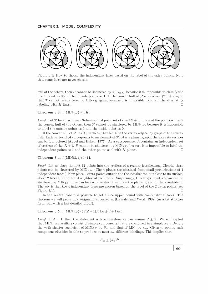
CHAPTER 3. MODEL COMPLEXITY
Figure 3.1: How to choose the independent faces based on the label of the extra points. Notethat some faces are never chosen.
hull of the others, then P cannot be shattered by MIN2,K , because it is impossible to classify theinside point as 0 and the outside points as 1. If the convex hull of P is a convex (2K + 2)-gon,then P cannot be shattered by MIN2,K again, because it is impossible to obtain the alternatinglabeling with K lines.
Theorem 3.3. h(MIN3,K) ≤ 4K.
Proof. Let P be an arbitrary 3-dimensional point set of size 4K +1. If one of the points is insidethe convex hull of the others, then P cannot be shattered by MIN3,K , because it is impossibleto label the outside points as 1 and the inside point as 0.
If the convex hull of P has |P| vertices, then let A be the vertex adjacency graph of the convexhull. Each vertex of A corresponds to an element of P. A is a planar graph, therefore its verticescan be four colored [Appel and Haken, 1977]. As a consequence, A contains an independent setof vertices of size K + 1. P cannot be shattered by MIN3,K , because it is impossible to label theindependent points as 1 and the other points as 0 with K planes.
Theorem 3.4. h(MIN(3, 4)) ≥ 14.
Proof. Let us place the first 12 points into the vertices of a regular icosahedron. Clearly, thesepoints can be shattered by MIN3,4. (The 4 planes are obtained from small perturbations of 4independent faces.) Now place 2 extra points outside the the icosahedron but close to its surface,above 2 faces that are third neighbor of each other. Surprisingly, this larger point set can still beshattered by MIN3,4. This can be easily verified if we draw the planar graph of the icosahedron.The key is that the 4 independent faces are chosen based on the label of the 2 extra points (seeFigure 3.1).
In the general case it is possible to get a nice upper bound with combinatorial tools. Thetheorem we will prove now originally appeared in [Haussler and Welzl, 1987] (in a bit strongerform, but with a less detailed proof).
Theorem 3.5. h(MINd,K) < 2(d + 1)K log2((d + 1)K).
Proof. If d = 1, then the statement is true therefore we can assume d ≥ 2. We will exploitthat MINd,K classifiers consist of simple components that are combined in a simple way. Denotethe m-th shatter coefficient of MINd,K by Sm and that of LINd by sm. Given m points, eachcomponent classifier is able to produce at most sm different labelings. This implies that
Sm ≤ (sm)K .
60

3.3. THE VC DIMENSION OF MINMAX2,K
From Sauer’s lemma [Sauer, 1972] we know that
sm ≤d+1∑
i=0
(m
i
).
If m ≥ d + 1, then the sum of binomial coefficients can be bounded from above as
d+1∑
i=0
(m
i
)≤(
m
d + 1
)d+1[
d+1∑
i=0
(m
i
)(d + 1
m
)i]≤
(m
d + 1
)d+1(1 +
d + 1
m
)m
<
(em
d + 1
)d+1
.
If d ≥ 2, then (em
d + 1
)d+1
< md+1.
Putting the inequalities together yields
Sm ≤ (sm)K < m(d+1)K .
Let us introduce the notation x = (d + 1)K. If m = 2x log2(x) and x ≥ 2, then it can beshown that m(d+1)K ≤ 2m. Rewriting m and (d + 1)K yields
[2x log2(x)]x ≤
[x2]x
.
The above inequality is true for all x ≥ 2, therefore m(d+1)K ≤ 2m.Moreover, it follows easily that m(d+1)K ≤ 2m is true also for m = ⌈2x log2(x)⌉, if m ≥ 2. We
got that the m-th shatter coefficient of MINd,K is smaller than 2m, if m = ⌈2(d + 1)K log2((d +1)K)⌉. Therefore, h(MINd,K) < 2(d + 1)K log2((d + 1)K).
The straightforward way of obtaining results for h(MINMAXd,K) is applying Assouad’slemma [Assouad, 1983]. The lemma states that for any function classes F and G with finite VCdimension, h(F ∪G) ≤ h(F) + h(G) + 1. As a consequence, h(MINMAXd,K) ≤ 2h(MINd,K) + 1.
In the cases studied so far we get the following upper bounds:
• h(MINMAX2,K) ≤ 4K + 3, if K ≥ 2,
• h(MINMAX3,K) ≤ 8K + 1,
• h(MINMAXd,K) ≤ 4(d + 1)K log2((d + 1)K) + 1.
3.3 The VC dimension of MINMAX2,K
We have seen previously that h(MIN2,K) = 2K + 1. Determining the Vapnik–Chervonenkis di-mension of MINMAX2,K is a substantially harder problem. Now I will show that MINMAX2,K =2K + 2, if K ≥ 2. I remark that the proof first appeared in [Takacs, 2007].
Theorem 3.6.
h(MINMAX2,K) =
{3 if K = 1,2K + 2 if K ≥ 2.
61

CHAPTER 3. MODEL COMPLEXITY
Figure 3.2: A point set in convex position. Thered and a blue signs cannot be separated witha triangle, because for this we should intersectall edges of a convex 8-gon with 3 lines.
Figure 3.3: A point set in tangled position.The red and the blue signs can never be sep-arated with a convex K-gon, regardless of thevalue of K.
3.3.1 Concepts for the proof
Definition 3.1. A planar point set is said to be in convex position, if its elements are the verticesof a convex polygon.
In other words, P does not have two distinct subsets Q1 and Q2 such that the convex hull ofQ1 contains a point from Q2. The following simple properties will also be used in the proof:
• P is in convex position, if and only if every 4-element subset of P is in convex position.
• A 2-element subset of P is called an edge, if the line segment connecting the two pointsis an edge of the convex hull of P. P is in convex position, if and only if every 5-elementsubset of P containing an edge is in convex position.
Note that MINMAX2,K cannot shatter 2K + 2 convexly positioned points, because for thealternating labeling we should intersect all edges of a convex (2K + 2)-gon with K lines (seeFigure 3.2). This is also true for MIN2,K , moreover it implies that h(MIN2,K) ≤ 2K + 1, sinceMIN2,K can shatter only convexly positioned point sets. The main difference between the twofunction classes is that MINMAX2,K is able to shatter non-convexly positioned point sets too.
Definition 3.2. A planar point set P is said to be in tangled position, if it has two distinctsubsets Q1 and Q2, such that the convex hull of Q1 contains a point from Q2 and the convexhull of Q2 contains a point from Q1.
Q1 and Q2 are called the tangled subsets. If P is not in tangled position, then it is said to betangle-free. Note that for any K, a tangled set of points cannot be shattered by MINMAX2,K ,because it is impossible to separate Q1 from Q2 (see Figure 3.3).
3.3.2 The proof
The case K = 1 is trivial, therefore we consider only the case K ≥ 2. We want to prove thath(MINMAX2,K) = 2K + 2. It is easy to see that h(MINMAX2,K) ≥ 2K + 2. For this we shouldjust place 2K + 1 points along a circle, in the vertices of a regular (2K + 1)-gon and put anadditional point in the center.
Consider an arbitrary labeling of these 2K + 2 points. We will refer to the points that havethe same label as the center as red points while to the others as blue points. There can be atmost K blue sequences along the circle. If the longest blue sequence is at most K long, then
62

3.3. THE VC DIMENSION OF MINMAX2,K
each blue sequence can be separated from the red points with 1 line. If the length of the longestblue sequence is more than K, then that blue sequence can be separated from the red pointswith 2 lines, and each remaining one with 1 line. The number of the remaining blue sequencesis not greater than K − 2 (assuming K ≥ 2). Therefore, K lines are always enough.
Proving the upper bound h(MINMAX2,K) ≤ 2K + 2 is somewhat more difficult. We shouldshow that no 2K + 3 points can be shattered by MINMAX2,K . It suffices to consider point setin which no 3 points are co-linear. If there is a point set that can be shattered by MINMAX2,K ,then there also exists a generally positioned point set of the same size that can be shattered byMINMAX2,K . (The second point set can be constructed from the first with small perturbations.)
Assume that MINMAX2,K shatters a generally positioned point set P. So far we know twonecessary conditions for this:
• P does not contain 2K + 2 points that are in convex position.
• P is tangle-free.
In the rest of the proof we will show that if K ≥ 2 and |P| ≥ 2K + 3, then these requirementsare contradictory, therefore no 2K + 3 points can be shattered by MINMAX2,K .
Theorem 3.7. Let P be a planar point set in general position. If P is tangle-free and |P| 6= 6,then P contains |P| − 1 points that are in convex position.
Corollary 3.1. If |P| = 2K +3, and K ≥ 2, then P is in tangled position or it contains 2K +2convexly positioned points. Therefore, P cannot be shattered by MINMAX2,K .
Proof. Denote the convex hull of P by conv(P). If conv(P) is a point or a line segment, then thestatement is trivial. The other cases are not so easy, because we can put arbitrarily many pointsinto conv(P) such that the requirements of the theorem are fulfilled. Along the property of beinga vertex of conv(P) or not, the elements of P can be classified as outside or inside points.
At first consider the case when conv(P) is a triangle. Denote the 3 outside points by A, B,and C. If |P| ≤ 5, then the statement of the theorem can be easily verified. Therefore we canassume that |P| ≥ 7, and we have at least 4 inside points.
Now select two arbitrary inside points and denote them by D and E. The line DE intersectstwo edges of the triangle ABC. Without loss of generality we can assume that the line DEintersects the edge AB in the direction of D and intersects the edge AC in the direction of E.Draw the following line segments into the triangle ABC:
• Segment DE, extended to the edges AB and AC,
• Segment BD, extended to the edge AC,
• Segment CE, extended to the edge AB,
• The extension of segment AD in the direction of D,
• The extension of segment AE in the direction of E,
• Segment BE,
• Segment CD.
These line segments partition the triangle ABC into 14 distinct regions (R1,R2, . . . ,R14).Number them according to Figure 3.4. Now try to put a third inside point F into the triangleABC without introducing a tangle.
63

CHAPTER 3. MODEL COMPLEXITY
1
23
4
5
6
7
8 910
11
12
13 14
A
B
C
DE
Figure 3.4: The 14 regions generated by placing two points into a triangle.
Lemma 3.2. If F /∈ R3 ∪R5 ∪R11 ∪R13, then P is in tangled position.
Proof.
• If F ∈ R1 ∪R2, then Q1 = {A,C,D} and Q2 = {B,E, F} are the tangled subsets.
• If F ∈ R1 ∪R4, then Q1 = {A,B,E} and Q2 = {C,D,F}.
• If F ∈ R6 ∪R7 ∪R8, then Q1 = {B,D,E} and Q2 = {A,C, F}.
• If F ∈ R8 ∪R9 ∪R10, then Q1 = {C,D,E} and Q2 = {A,B, F}.
• If F ∈ R6 ∪R12, then Q1 = {B,C,D} and Q2 = {A,E, F}.
• If F ∈ R10 ∪R14, then Q1 = {B,C,E} and Q2 = {A,D,F}.
Lemma 3.3. If F ∈ R13, then P is in tangled position.
Proof. If F ∈ R13, then lines DE, DF and EF partition the triangle ABC into 13 distinctregions (S1,S2, . . . ,S13). Number them according to Figure 3.5. Now try to place a 4th insidepoint G without introducing a tangle.
• If G ∈ S1∪S2∪S4∪S5∪S6∪S10∪S11∪S12∪S13, then P is in tangled position by Lemma3.2.
• If G ∈ S3 ∪ S8, then Q1 = {A,D,E, F} and Q2 = {B,C,G} are the tangled subsets.
• If G ∈ S7 ∪ S8, then Q1 = {B,D,E, F} and Q2 = {A,C,G}.
64

3.3. THE VC DIMENSION OF MINMAX2,K
A
B
C
DE
F
1
2 3
4
810
67
9
5
1112 13
Figure 3.5: The 13 regions generated by placing the third point into R13.
• If G ∈ S8 ∪ S9, then Q1 = {C,D,E, F} and Q2 = {A,B,G}.
Remark. If F is a non-boundary point of R13, then {A,B,C,D,E, F} is tangle-free, but hasno 5-element subset in convex position. This is why the restriction |P| 6= 6 had to be made.However, by Lemma 3.3 this arrangement is an irrelevant branch that cannot be continued.
The following fact is a simple consequence of Lemma 3.2 and Lemma 3.3:
Corollary 3.2. If a set of two outside and three inside points is not in convex position, thenthen P is in tangled position.
Now we are ready to finish the special case, when conv(P) is a triangle.
Lemma 3.4. Let P be a planar point set in general position. If P is tangle-free, |P| 6= 6 andconv(P) is a triangle, then we can select |P| − 1 points from P that are in convex position.
Proof. Let us analyze the situation after placing m inside points. Denote the union of {B,C}and the first m inside points with Tm. We know that T2 is in convex position. We will showthat if m ≥ 2, then the convex position of Tm implies the convex position of Tm+1. To verifythis assume indirectly that Tm is in convex position but Tm+1 is not. Since {B,C} is alwaysan edge of conv(Tm+1) and m ≥ 2, this means that Tm+1 has a 5-element subset that contains{B,C} and is not in convex position. Then by Corollary 3.2, P is in tangled position, which isa contradiction. Thus the convex position of Tm+1 follows from the convex position of Tm. As aconsequence, the set T|P|−3 = P \ {A} is also in convex position.
Remark. If we prohibit to place the third inside point into R13, then the condition |P| 6= 6 canbe omitted.
65

CHAPTER 3. MODEL COMPLEXITY
A
B
C
D
FE
1
23
Figure 3.6: Regions in BCDEF , case I.
3
A
B
C
D
FE
1
2
4
Figure 3.7: Regions in BCDEF , case II.
Now consider the case when conv(P) is a quadrangle. Denote the 4 outside points with A,B, C and D. If |P| ≤ 5, then the statement is trivial, therefore we can assume that we have atleast two inside points. Select two arbitrary inside points and denote them by E and F . The lineEF intersects two adjacent edges of the quadrangle ABCD, because otherwise P would be intangled position. Without loss of generality we can assume that the line EF intersects the edgeAB in the direction of E and intersects the edge AC in the direction of F . Now try to place athird inside point G into the quadrangle ABCD.
Lemma 3.5. If G is inside the pentagon BCDEF , then P is in tangled position.
Proof. There are two possible cases:
1. The extension of AD in the direction of D and the extension of AE in the direction Eintersect different edges of the quadrangle ABCD.
2. The extension of AD in the direction of D and the extension of AE in the direction Eintersect the same edge of the quadrangle ABCD. We can assume without loss of generalitythat the intersected edge is BD.
In the first case, the line segments DE and DF partition the pentagon BCDEF into 3distinct regions (R1, R2, R3), as it can be seen in Figure 3.6. If G ∈ R1∪R2, then {B,D,E, F}and {A,C,G} are the tangled subsets. If G ∈ R2 ∪R3, then {C,D,E, F} and {A,B,G} are thetangled subsets.
In the second case, DE and the extension of AF in the direction of F partitions the pentagonBCDEF into 4 distinct regions (S1, S2, S3, S4), as it can be seen in Figure 3.7. If G ∈ S1 ∪ S2,then {B,D,E, F} and {A,C,G} are the tangled subsets. If G ∈ S2 ∪ S3, then {C,D,E, F} and{A,B,G} are the tangled subsets. If G ∈ S4, then {B,C,D, F} and {A,E,G} are the tangledsubsets.
By Lemma 3.5, inside points up from the third can be placed only into the region ABC \BCEF without introducing a tangle. This and Lemma 3.4 (applied to P \ {D}) implies that
66

3.3. THE VC DIMENSION OF MINMAX2,K
A
B
C
E
GF
1
2
3
D4
Figure 3.8: Regions in BCDEFG.
P \ {A,D} is in convex position. The restriction |P \ {D}| 6= 6 can be now omitted, because thequadrangle BCEF is a forbidden area. If P \ {A,D} is in convex position, then P \ {A} is too.This completes the proof of the special case when conv(P) is a quadrangle.
Now consider the case when conv(P) is a pentagon. Denote the 5 outside points by A, B, C,D and E. Using the same reasoning as before we can assume that we have at least two insidepoints. Pick two arbitrary inside points F and G. The line FG intersects two adjacent edgesof the pentagon ABCDE, because otherwise P would be in tangled position. Without loss ofgenerality assume that the line FG intersects the edge AB in the direction of F , intersects theedge AC in the direction of G, moreover BD and CE are edges of the pentagon ABCDE. Nowtry to place a third inside point H into the pentagon ABCDE.
Lemma 3.6. If H is inside the hexagon BCDEFG, then P is in tangled position.
Proof. Line segments BE and CD partition the hexagon BCDEFG into 4 distinct regions(R1,R2,R3,R4), as it can be seen in Figure 3.8. If H ∈ R1 ∪ R2 ∪ R3, then P is in tangledposition by Lemma 3.5. If H ∈ R4, then P is tangled too, because there exists a line connectingtwo inside points that intersects non-adjacent edges of conv(P). For example the line FH cannotintersect adjacent edges of conv(P).
By Lemma 3.6, inside points up from the third can be placed only into the region ABC \BCFG without introducing a tangle. This and Lemma 3.4 (applied to P \ {D,E}) implies thatP \ {A,D,E} and this wise P \ {A} is in convex position.
Finally consider the case when conv(P) is a k-gon (k ≥ 6). Denote the outside points byA1, A2, . . . , Ak and the inside points by B1, B2, . . . , Bm. The line B1B2 intersects again twoadjacent edges of conv(P). Without loss of generality assume that the line B1B2 intersects theedges A1Ak and A1Ak. No inside point can be located in the (k + 1)-gon A2A3 . . . AkB1B2,because otherwise P would be in tangled position by Lemma 3.6. But then it follows as beforethat {A2, Ak} ∪ {B1, B2, . . . , Bm} = P \A1 is in convex position.
67

CHAPTER 3. MODEL COMPLEXITY
3.4 New lower bounds
This section contains new lower bounds on the Vapnik–Chervonenkis dimension of various convexpolyhedron classifier types. The results presented here first appeared in [Takacs and Pataki,2007b].
Let us start with two easily obtainable lower bounds for h(MINd,K) and h(MINMAXd,K).
Theorem 3.8 (sphere slicing). h(MINd,K) ≥ dK.
Proof.We have to arrange dK points such that they can be shattered by MINd,K . At first cut Kdistinct slices from a d-dimensional hypersphere with K hyperplanes. Denote the i-th hyperplanewith Hi and denote the intersection of the hypersphere surface and the i-th hyperplane with Ci.
Now define the point set P by assigning d different points in each Ci. Points belonging tothe same Ci can be shattered by one hyperplane, moreover, it can be required too, that the labelof all the other points have to be 1 according to this hyperplane. (The i-th hyperplane of theMINd,K classifier is obtained from a small perturbation of Hi.) Because of the requirement, thei-th hyperplane influences only the the labeling of the i-th group, therefore P can be arbitrarilylabeled by the members of MINd,K .
Theorem 3.9. h(MINMAXd,K) ≥ dK + 1.
Proof. Arrange the first dK points as in the proof of the previous theorem, but now put anadditional point into the center of the hypersphere. The previous theorem implies that the firstdK points can be shattered by both MINd,K and MAXd,K . In the first case, the label of thecentral point is always 1, in the second case it is always 0. This means, that the dK + 1 pointscan be arbitrarily labeled by the members of MINMAXd,K . (The label of the central pointdetermines whether to use a MINd,K or a MAXd,K classifier.)
The previous proofs are so simple that h(MINd,K) ≥ dK and h(MINMAXd,K) ≥ dK + 1 willbe referred as the basic lower bounds. The following theorem improves the basic lower boundsby one:
Theorem 3.10. If K ≥ 2, then h(MINd,K) ≥ dK + 1 and h(MINMAXd,K) ≥ dK + 2.
Proof. We begin with the proof of the first statement in the special case d = 3. Denote thecoordinates by x, y, and z. Place the first 5 points p1, . . . ,p5 on the plane xy, into the verticesof an origin-centered regular pentagon. On the plane xy these points can be shattered by 2 lines,moreover, the following constraints can be satisfied too:
• The lines have to be parallel.
• The lines cannot be axis-parallel.
• For any labeling, there exists an ε0 > 0 such that the circle of radius ε0 around the originmust belong to the inner region.
Place the next 2 points into p6 = [1 0 1] and p7 = [−1 0 1]. Now we show that thefirst 7 points can be arbitrarily labeled by the members of MIN3,2, even if we require that anε0-ball around the origin have to belong to the inner region.
Consider an arbitrary labeling p1 → y1, . . . ,p7 → y7 that we want to obtain with a memberof MIN3,2. Recall that a MIN3,2 classifier can be given by 8 parameters: (w11, w12, w13, b1) and(w21, w22, w32, b2).
If the input is one of the first 5 points, then the answer of the classifier is fully determined bythe parameters (w11, w12, b1) and (w21, w22, b2). Adjust these parameters such that the classifierlabels the first 5 points as desired. This can be done, moreover the following constraints can besatisfied too (i = 1, 2):
68
3.4. NEW LOWER BOUNDS
• w2i = −w1i 6= 0 (the lines are parallel but not axis-parallel),
• ∀δ21 +δ2
2 ≤ ε20 : mini{δ1wi1 +δ2wi2 +bi} ≥ 0 (the ball of radius ε0 around the origin belongs
to the inner region).
Based on y6 and y7 there are 4 possible cases (i = 1, 2):
• If y6 = y7 = 1, then the desired labeling can be obtained by wi3 ≫ 0.
• If y6 = y7 = 0, then the desired labeling can be obtained by wi3 ≪ 0.
• If y6 = 1, y7 = 0, then the desired labeling can be obtained by wi3 = −wi1 − bi + |wi1|.
• If y6 = 0, y7 = 1, then the desired labeling can be obtained by wi3 = +wi1 − bi + |wi1|.
If we choose a sufficiently small ε, then the ε-ball around the origin belongs to the innerregion in all of the 4 cases.
Now define a sphere surface that encloses the 7 points arranged so far and passes through thepoint [0 0 −ε/2]. On this surface there exist a segment, that belongs to the inner region ateach labeling of the first 7 points. Let us place the remaining 3(K−2) points onto this subsurfacein 3-element groups with the sphere slicing method. Each group can be shattered by one plane,moreover it can be assured, that the planes does not affect the labeling of the other groups andthe first 7 points. Therefore the 7 + 3(K − 2) = 3K + 1 points can be shattered by MIN3,K .
The proof of the d-dimensional case is analogous with the 3-dimensional one. Now the first 5points are placed onto the plane of the first 2 coordinates. The next 2(d−2) points are arrangedin the following way:
p6 = [+1 0 1 0 0 . . . 0],
p7 = [−1 0 1 0 0 . . . 0],
p6 = [+1 0 0 1 0 . . . 0],
p9 = [−1 0 0 1 0 . . . 0],
...
p2d = [+1 0 0 0 . . . 0 1],
p2d+1 = [−1 0 0 0 . . . 0 1].
It can be shown (exactly the same way as in the case d = 3) that the first 2d + 1 points can beshattered by MINd,2, moreover it can be required too that an ε-ball around the origin have tobelong to the inner region at each labeling. Then a hypersphere surface is defined that enclosesthe first 2d + 1 points and passes through the point [0 0 −ε/2 . . . −ε/2]. There exist asegment on this surface that belongs to the inner region at each labeling. The remaining d(K−2)points are placed onto this subsurface with the sphere slicing method.
The statement on MINMAXd,K can be proved with the same construction with an additionalpoint in the origin. The label of this point determines whether to use a MINd,K or a MAXd,K
classifier.
The bound h(MINd,K) ≥ dK +1 is not tight, if d > 2. For example, in the case d = 3,K = 4it states that h(MIN3,4) ≥ 13 We have seen previously that even h(MIN3,4) ≥ 14 can be provedwith the help of an icosahedron-based arrangement [Dobkin and Gunopulos, 1995]. This betterbound can easily be extended to the case d = 3,K > 4.
69

CHAPTER 3. MODEL COMPLEXITY
Theorem 3.11. If K > 4, then h(MIN3,K) ≥ 3K + 2 and h(MINMAX3,K) ≥ 3K + 3.
Proof. Place the first 14 points exactly as in the proof of Theorem 3.4. From the proof ofTheorem 3.4 we know that these points can be shattered by MIN3,4, and there exist a face of theicosahedron that is never selected. This means that we can define a sphere surface that enclosesthe first 14 points and has a segment that is always in the inner region. If we place the remaining3(K − 4) points on this subsurface with the sphere slicing method, then this point set of size14 + 3(K − 4) = 3K + 2 can be shattered by MIN3,K .
The second statement of the theorem can be proved the same way. The only difference isthat if we can use MAX3,K classifiers too, then we can put an additional point into the centerof the icosahedron.
We got that in R3 the basic lower bounds can be improved by 2. With a more sophisticated
version of the icosahedron trick it is possible to improve the basic lower bounds by 4 in R4.
Theorem 3.12. If K ≥ 30, then h(MIN4,K) ≥ 4K + 4 and h(MINMAX4,K) ≥ 4K + 5.
Proof. Let us consider a 600-cell, which is a finite regular 4-dimensional polytope, containing600 tetrahedral cells (with 5 to an edge), 1200 triangular faces, 720 edges, and 120 vertices. The600-cell is also called hypericosahedron, because it can be viewed as the 4-dimensional analog ofthe 3-dimensional icosahedron.
The vertices of an origin-centered 600-cell with edges of length 1/φ (where φ = 1+√
52 is the
golden ratio) can be given as follows:
• 16 vertices of the form [± 12 ± 1
2 ± 12 ± 1
2 ].
• The 8 possible permutations of [±1 0 0 0].
• 96 vertices, obtained from the even permutations of [± 12 ± 1
2φ ± 12φ−1 0].
The topological structure of the 600-cell is a system of subsets over the 120 vertices that giveswhich k vertices form a k-facet (k = 2, 3, 4; 2-facets are called edges, 3-facets are called facesand 4-facets are called cells). The topological structure of the 600-cell can be computed easily.At first we should generate the coordinates of the 120 vertices according to the previous scheme.Then we should identify the k-facets by examining every possible k vertices an checking whetherthey are at distance 1/φ from each other not. The vertex adjacency graph of the 600-cell can beseen in Figure 3.9.
We say that 2 cells are adjacent, if they have at least 1 common vertex and 2 cells areindependent, if they have no common vertices. The cell adjacency graph of the 600-cell can beeasily obtained from its topological structure.
Remember that in the 3-dimensional case we tried to cover the vertices of the icosahedronwith independent facets in many different ways. Now we want to cover the vertices of the600-cell with independent cells in many possible ways. This means that we want to find manyindependent points in the cell adjacency graph.
With a simple program performing brute force computation, it is possible to find 1920 differentcoverings.1 These coverings can be represented as a 1920-by-600 binary matrix C so that theelement at position (i, j) is 1 if the i-th covering contains the j-th cell and 0 otherwise.
Now let us turn back to the statement h(MIN4,K) ≥ 4K + 4, if K ≥ 30. Place the first 120points into the vertices of a 600-cell. These points can be shattered by MIN4,30, because it is
1The topological structure of the 600-cell, the cell adjacency graph and the coverings can be found athttp://www.sze.hu/~gtakacs/600cell.html. It is difficult to verify these results by hand but it is easy to writea program that performs this.
70
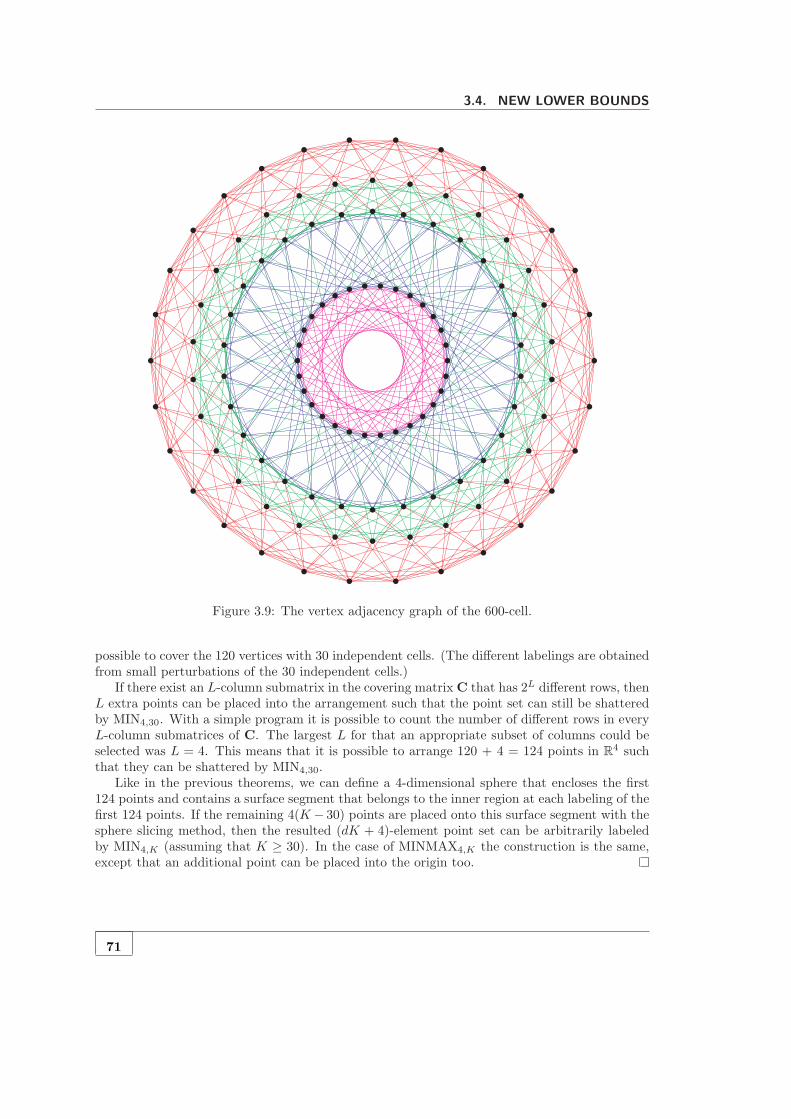
3.4. NEW LOWER BOUNDS
Figure 3.9: The vertex adjacency graph of the 600-cell.
possible to cover the 120 vertices with 30 independent cells. (The different labelings are obtainedfrom small perturbations of the 30 independent cells.)
If there exist an L-column submatrix in the covering matrix C that has 2L different rows, thenL extra points can be placed into the arrangement such that the point set can still be shatteredby MIN4,30. With a simple program it is possible to count the number of different rows in everyL-column submatrices of C. The largest L for that an appropriate subset of columns could beselected was L = 4. This means that it is possible to arrange 120 + 4 = 124 points in R
4 suchthat they can be shattered by MIN4,30.
Like in the previous theorems, we can define a 4-dimensional sphere that encloses the first124 points and contains a surface segment that belongs to the inner region at each labeling of thefirst 124 points. If the remaining 4(K − 30) points are placed onto this surface segment with thesphere slicing method, then the resulted (dK + 4)-element point set can be arbitrarily labeledby MIN4,K (assuming that K ≥ 30). In the case of MINMAX4,K the construction is the same,except that an additional point can be placed into the origin too.
71


No amount of experimentation can
ever prove me right; a single exper-
iment can prove me wrong.
Albert Einstein 4Applications
This chapter contains experiments demonstrating the utility of the algorithms proposed in thethesis. The organization of the chapter is the following: The first part will be about determiningthe linear and convex separability of point sets. The second part will deal with convex polyhedronmethods for classification. The third part will be about convex polyhedron and other methodsfor collaborative filtering.
4.1 Determining linear and convex separability
4.1.1 Datasets
The datasets involved in the experiments were the following:
• VOTES: This dataset is part of the UCI (University of California, Irvine) machine learningrepository [Asuncion and Newman, 2007], which is a well known collection of benchmarkproblems for testing machine learning algorithms. The dataset includes votes for each ofthe U.S. House of Representatives Congressmen on the d = 16 key votes identified by theCongressional Quarterly Almanac (98th Congress, 2nd session, 1984). The CongressionalQuarterly Almanac lists nine different types of votes: voted for, paired for, and announcedfor (these three are encoded as 1), voted against, paired against, and announced against(these three are encoded as −1), voted present, voted present to avoid conflict of interest,and did not vote or otherwise make a position known (these three are encoded as 0). Thedataset contains M = 2 classes (democrat or republican) and n = 435 examples (267democrat, 168 republican).
• WISCONSIN: This dataset is also part of the UCI machine learning repository. It wasoriginally obtained from the University of Wisconsin Hospitals, Madison, Wisconsin. Thetask to solve is to determine the benignness or malignancy (M = 2) of tumors based ond = 9 features extracted from mammograms. After removing examples with missing featurevalues the number of examples is n = 683 (444 benign, 239 malignant).
• MNIST28: This dataset is the training set part of the MNIST handwritten digit recogni-tion database [LeCun and Cortes, 1999]. The d = 784 features represent pixel intensitiesof 28× 28 sized images. The classes are associated with the digits, therefore the number ofclasses is M = 10. The number of examples is n = 60000 (5923 zeros, 6742 ones, 5958 twos,6131 threes, 5842 fours, 5421 fives, 5918 sixes, 6265 sevens, 5851 eights, 5949 nines). Fig-ure 4.1 shows some example images from the database. The dataset is sparse, the averagefrequency of 0 as a feature value is 80.9 %.
73

CHAPTER 4. APPLICATIONS
Figure 4.1: Examples from the MNIST28 database.
• MNIST14: This dataset was extracted from the MNIST28 by reducing image size to14×14 pixels. Intensity values of the 14×14 images were obtained by averaging intensitiesin the corresponding 2× 2 part of the original image. The average frequency 0 as a featurevalue is 74.4 %
• MNIST7: This dataset was extracted from the MNIST28 by reducing image size to 7× 7pixels. Intensity values of the 7 × 7 images were obtained by averaging intensities in thecorresponding 4 × 4 part of the original image. The average frequency of 0 as a featurevalue is 62.3 %
• MNIST4: This dataset was extracted from the MNIST28 by reducing image size to 4× 4pixels. Intensity values of the 4 × 4 images were obtained by averaging intensities in thecorresponding 7 × 7 part of the original image. The average frequency of 0 as a featurevalue is 41.3 %
If we want to refer to the subset of an MNIST dataset containing only classes A and B, thenwe will use postfix /AB (e.g. MNIST04/49).
4.1.2 Algorithms
This subsection overviews the algorithms that were used in the experiments. For determininglinear separability the following basic algorithms were tested:
• LSEP1: The most straightforward, linear programming based method. It tries to find anarbitrary separating hyperplane (see page 36 for the details).
• LSEP∗1: The dual formulation of LSEP1 (see page 37).
• LSEP+1 : A modified version of LSEP∗
1 (see page 37).
• LSEP2: An alternative linear programming based method that tries to find a solutionwith small norm (see page 37).
• LSEP∗2: The dual formulation of LSEP2 (see page 38).
• LSEPS : The support vector machine based method (see page 38). In the experiments itwas used with setting C = 106.
All of these algorithms try to answer the question whether two point sets are linearly separableor not. The primal based methods (LSEP1, LSEP2) are constructive in the sense that they also
74

4.1. DETERMINING LINEAR AND CONVEX SEPARABILITY
provide a separating hyperplane, if the answer is yes. The dual based methods (LSEP∗1, LSEP+
1
and LSEP∗2) cannot do this, but they are able to output an easily verifiable proof, if the answer
is no. The parameter ε was always set to 0.001 in the experiments.The support vector based approach (LSEPS) can only be considered as an approximate
method, because C cannot be set to ∞, therefore the answer is not perfectly reliable in thenonseparable case.
For determining linear separability the following enhanced algorithms were tested:
• LSEPX1, LSEPX2: The first proposed method (see page 38). It tries to solve the problemincrementally. The index indicates which basic method (LSEP1, LSEP2) is used for solvingsubproblems.
• LSEPY1, LSEPY2: The modified version of the previous method (see page 39). It triesto further reduce running time by removing points from the active sets.
• LSEPZ: A dual based alternative of the previous two approaches (see page 39). It usesLSEP+
1 for solving subproblems. It can be able to reduce the number of features in thelinearly separable case.
• LSEPZX1, LSEPZX2, LSEPZY1, LSEPZY2: A hybrid method that tries to reducethe number of features with LSEPZ first, and then runs LSEPX1, LSEPX2, LSEPY1, orLSEPY2 on the reduced dataset (see page 40).
The variants of LSEPX, LSEPY, LSEPZX and LSEPZY are constructive methods, whileLSEPZ is not. LSEPX and LSEPY was always run with setting γk ≡ d. The parameter ε wasalways set to 0.001 and ε2 to 0.002.
For determining convex separability the following algorithms were tested:
• CSEPX2, CSEPY 2, CSEPZX2, CSEPZY 2: Straightforward, linear programming basedapproach that tries to separate each outer point from the inner set individually (see page40). The indices indicate which primal based method is used for the individual linearseparations.
• CSEP∗2, CSEPZ : The dual based version of the the previous approach (see page 40). The
indices indicate which dual based method is used for the individual linear separations.
• CSEPC: Proposed method for approximate convex separation (see page 41). It consid-ers the lines connecting the centroid of the inner set with the outer points, and placeshyperplanes perpendicular to these lines.
• CSEPXX2, CSEPXY 2, CSEPXZX2, CSEPXZY 2, CSEPX∗2, CSEPXZ : Proposed
method for fast and exact convex separation (see page 41). At first it tries to reducethe size of the outer set by applying CSEPC, and then it runs a variant of CSEP on thereduced dataset. The indices indicate which version of CSEP is used in the second phase.
All algorithms were implemented in Python [Rossum, 2006], using the numerical (NumPy)[Ascher et al., 2001] and the scientific (SciPy) [Jones et al., 2001] modules. The internal lin-ear programming solver was the primal simplex method of the GNU Linear Programming Kit(GLPK) [Makhorin, 2009]. The reasons behind this choice were the following:
• GLPK is not the most sophisticated library for linear programming, but it is free, very welldocumented, and easy to use.
75

CHAPTER 4. APPLICATIONS
• The primal simplex method is a bit old fashioned and slow, but it is suitable for ourpurposes. The main goal is not to achieve the lowest possible running times but to comparedifferent separation approaches.
• I did some experiments on small problems with the built-in interior point method of GLPK,and also with an own interior point solver written from scratch, but the running times werenot promising. (However it is likely that a sophisticated interior point solver would beatthe primal simplex method on large problems.)
GLPK was accessed from Python via the PyGLPK interface [Finley, 2008]. The internalsupport vector machine implementation was libsvm [Chang and Lin, 2001]. The hardware envi-ronment was a notebook PC with Intel Pentium M 2 GHz CPU and 1 Gb memory.
4.1.3 Types of separability
As we have seen previously, if we have point sets P and Q, then it is possible to define differenttypes of separability between them:
• S0: P and Q are (convexly) inseparable, if P ∩ conv(Q) 6= ∅ and Q∩ conv(P) 6= ∅.
• S1: P and Q are convexly separable, if P ∩ conv(Q) = ∅ or Q∩ conv(P) = ∅.
• S2: P and Q are mutually convexly separable, if P ∩ conv(Q) = ∅ and Q∩ conv(P) = ∅.
• S3: P and Q are linearly separable, if conv(P) ∩ conv(P) = ∅.
Note that S3 implies S2, and S2 implies S1, therefore S3 can be considered as the strongestand S1 as the weakest type of separability. Also observe that S1 is the opposite of S0.
In the following experiments the type of separability is determined for each pair of classes inthe given datasets. At first, linear separability was checked with the LSEPZ method. If the pointsets were not linearly separable, then also convex separability was checked with the CSEPXX2
method.The type of separability in the VOTES and the WISCONSIN dataset turned out to be S1.
The results for the MNIST28 dataset can be seen in Table 4.1, for the MNIST 14 dataset inTable 4.2, for the MNIST7 dataset in Table 4.3, and for the MNIST4 dataset in Table 4.4.
In the case of the MNIST28 dataset 38 of the subproblems are S3- and 7 are S2-type. Thismeans that the majority of the 2-class subproblems are linearly separable, therefore it would bereasonable to use simple models, if we wanted to build classifiers.
If we reduce the size of the images, then it is natural to expect that the subproblems willbecome less separable. In the case of the MNIST14 dataset 18 of the subproblems are S3- and 27are S2-type. In the case of the MNIST7 dataset 2 of the subproblems are S3- and 43 are S2-type.In the case of the MNIST4 dataset 2 of the subproblems are S2-, 3 are S1- and 40 are S0-type.An interesting observation is that S2 (mutual convex separability) occurs more frequently thanS1 (non-mutual convex separability).
If two point set are not convexly separable (or not mutually convexly separable), then it isnatural to ask that how far they are from convex separability (mutual convex separability). Apossible measure of inseparability is IPQ = |P ∩ conv(Q)|, the number of points from P that arecontained in the convex hull Q.
The original versions of the presented convex separability algorithms are not able to determinethe value of IPQ, because they exit when the first inseparable outer point is found. However,it is trivial to modify the algorithms so that they calculate IPQ. We just have to introduce acounter for the inseparable outer points and not exit when we find one.
76

4.1. DETERMINING LINEAR AND CONVEX SEPARABILITY
Class 1 Class 2
1 2 3 4 5 6 7 8 9
0 S3 S3 S3 S3 S3 S3 S3 S3 S3
1 S3 S3 S3 S3 S3 S3 S3 S3
2 S2 S3 S3 S3 S3 S2 S3
3 S3 S2 S3 S3 S2 S3
4 S3 S3 S3 S3 S2
5 S3 S3 S2 S3
6 S3 S3 S3
7 S3 S2
8 S3
Table 4.1: Types of separability in the MNIST28 dataset.
Class 1 Class 2
1 2 3 4 5 6 7 8 9
0 S3 S2 S2 S3 S2 S2 S3 S2 S2
1 S2 S2 S3 S3 S3 S3 S2 S2
2 S2 S3 S3 S3 S3 S2 S3
3 S2 S2 S2 S2 S2 S2
4 S3 S3 S3 S3 S2
5 S2 S2 S2 S2
6 S3 S2 S3
7 S2 S2
8 S2
Table 4.2: Types of separability in the MNIST14 dataset.
77

CHAPTER 4. APPLICATIONS
Class 1 Class 2
1 2 3 4 5 6 7 8 9
0 S3 S2 S2 S2 S2 S2 S2 S2 S2
1 S2 S2 S2 S2 S2 S2 S2 S2
2 S2 S2 S2 S2 S2 S2 S2
3 S2 S2 S2 S2 S2 S2
4 S2 S2 S2 S2 S2
5 S2 S2 S2 S2
6 S3 S2 S2
7 S2 S2
8 S2
Table 4.3: Types of separability in the MNIST7 dataset.
Class 1 Class 2
1 2 3 4 5 6 7 8 9
0 S0 S0 S0 S1 S0 S0 S1 S0 S0
1 S0 S0 S0 S0 S0 S0 S0 S0
2 S0 S1 S0 S0 S0 S0 S0
3 S0 S0 S2 S0 S0 S0
4 S0 S0 S0 S0 S0
5 S0 S0 S0 S0
6 S2 S0 S0
7 S0 S0
8 S0
Table 4.4: Types of separability in the MNIST4 dataset.
78

4.1. DETERMINING LINEAR AND CONVEX SEPARABILITY
Class 1 Class 2
0 1 2 3 4 5 6 7 8 9
0 5923 57 36 67 3 110 22 0 389 21
1 36 6742 43 228 14 21 14 126 260 109
2 1 6 5958 34 0 3 3 4 16 2
3 1 74 151 6131 7 65 0 119 41 58
4 0 13 15 4 5842 27 17 102 9 490
5 1 8 1 34 4 5421 5 11 27 13
6 5 7 22 0 7 8 5918 0 13 2
7 1 17 7 44 50 1 0 6265 4 372
8 273 310 162 498 2 458 9 69 5851 160
9 2 66 5 129 933 42 3 945 65 5949
Table 4.5: Number of examples from Class 1 contained in the convex hull of Class 2 in theMNIST4 dataset.
The IPQ values for the MNIST4 dataset calculated by modified CSEPXX2 are shown inTable 4.5. It is true to a certain degree that digit pairs considered to be more similar by humanshave higher values. For example, there are 490 fours in the convex hull of nines and 933 nines inthe convex hull of fours, but only 1 seven in the convex hull of zeros and 0 zeros in the convexhull of sevens.
4.1.4 Running times
Linear separability
The running times of basic methods for determining linear separability can be seen in Table4.6. We get a measure of relative efficiency, if we rank the algorithms by running time for eachproblem, and then calculate the average rank of each algorithm 1. According to this measurethe order of basic methods on the given problems is the following: 1. LSEP∗
2 (1.95), 2. LSEP∗1
(2.2), 3. LSEP+1 (2.45), 4. LSEP1 (4.5), 5. LSEPS (4.6), 6. LSEP2 (5.3). The first 3 methods
are the dual based ones. The fastest primal based method was LSEP1.
It is interesting that sometimes LSEPS was the fastest method, however its performancewas not very stable. The running time of LSEPS was more than 1800 seconds in every linearlynonseparable case (and even in some linearly separable ones).
The running times of the proposed incremental algorithms (LSEPX, LSEPY, and LSEPZ)are shown in Table 4.7. The order of the methods according to the average rank measure is: 1.LSEPX2 (2.3), 2. LSEPY2 (2.5), 3. LSEPX1 (2.6), 4. LSEPY1 (3.6), 5. LSEPZ (4.2).
If we consider the average running time instead of the average rank, then the superiorityof LSEPX2 and LSEPY2 is even stronger. For example, on the MNIST14/01 dataset LSEPX2
was 12 times faster than LSEPX1, and LSEPY2 was 17 times faster than LSEPY1. Recall thatamong the basic methods LSEP2 was always slower than LSEP1 (since LSEP2 tries to find a
1If there is a tie from position A to position B, then the rank is considered as (A + B)/2.
79

CHAPTER 4. APPLICATIONS
Problem Running time (seconds)
LSEP1 LSEP∗1 LSEP+
1 LSEP2 LSEP∗2 LSEPS
VOTES S1 0.089 0.035 0.039 0.134 0.034 >1800
WISCONSIN S1 0.177 0.033 0.034 0.228 0.032 >1800
MNIST04/24 S1 122.0 1.01 0.89 135.9 1.03 >1800
MNIST04/49 S0 87.3 0.94 0.91 97.0 0.87 >1800
MNIST07/01 S3 259.7 2.10 2.06 299.6 2.03 15.1
MNIST07/02 S2 310.1 2.54 2.59 333.1 2.59 >1800
MNIST14/01 S3 744.0 9.56 9.60 1010.3 9.91 19.7
MNIST14/02 S2 872.0 13.0 14.8 1243.5 14.9 >1800
MNIST28/01 S3 >1800 97.9 107.7 >1800 56.3 36.3
MNIST28/02 S3 >1800 232.7 232.2 >1800 179.9 52.7
Table 4.6: Running times of basic algorithms for determining linear separability.
small norm solution, and uses nearly twice as many variables to achieve this). It is interestingto see that it can pay off to apply the slower basic method in the incremental algorithm. Thereason for that is that the hyperplanes found by LSEP2 have larger margin, and therefore lessof them are needed.
On the largest datasets (MNIST28/01 and MNIST28/02) LSEPY2 was significantly fasterthan LSEPX2. This demonstrates that removing points from the active sets can convey largespeedups in certain cases. It can also be observed that on the largest datasets the dual basedLSEPZ was the fastest method, while on the other datasets it was the slowest one.
The running times of the proposed hybrid algorithms (LSEPZX and LSEPZY) are shownin Table 4.8. The order of the methods according to the average rank is: 1. LSEPZY2 (1.9),2. LSEPZX1 (2.25), 3. LSEPZX2 (2.6), 4. LSEPZY2 (3.25). The differences between therunning times are not as drastic as in the previous experiments. This is because the first stepof the algorithm is the same in each case: running LSEPZ and possibly reducing the number offeatures. The unique second step is run only on the reduced dataset.
If we compare primal based basic methods with the proposed ones, then it turns out that theproposed algorithms are better. Typically, the speedup factor between a basic method and itscorresponding LSEPX/LSEPY/LSEPZX/LSEPZY variant is greater than 100.
The dual based basic methods (LSEP∗1, LSEP+
1 and LSEP∗2) are sometimes slightly faster than
the proposed LSEPX/LSEPY/LSEPZX/LSEPZY algorithms, but in contrast with the proposedmethods they do not construct a separating hyperplane in the separable case.
Convex separability
The running times of basic methods for determining convex separability can be seen in Table4.9. Each experiment consisted of two runs: at first the first class was the inner set, and then thesecond. The numbers shown in the table are the summed running times of the two runs (givenin seconds).
80

4.1. DETERMINING LINEAR AND CONVEX SEPARABILITY
Problem Running time (seconds)
LSEPX1 LSEPX2 LSEPY1 LSEPY2 LSEPZ
VOTES S1 0.029 0.041 0.029 0.038 0.11
WISCONSIN S1 0.049 0.031 0.048 0.055 0.081
MNIST04/24 S1 0.27 0.28 0.47 0.37 2.63
MNIST04/49 S0 0.26 0.36 0.36 0.36 2.37
MNIST07/01 S3 1.08 0.68 1.55 0.69 4.52
MNIST07/02 S2 0.39 0.49 0.67 1.57 12.7
MNIST14/01 S3 31.2 2.44 36.2 2.10 7.45
MNIST14/02 S2 5.38 3.59 5.67 4.78 133.5
MNIST28/01 S3 >1800 388.0 >1800 88.1 14.8
MNIST28/02 S3 >1800 640.6 >1800 284.9 143.2
Table 4.7: Running times of LSEPX, LSEPY, and LSEPZ.
Problem Running time (seconds)
LSEPZX1 LSEPZX2 LSEPZY1 LSEPZY2
VOTES S1 0.11 0.11 0.11 0.11
WISCONSIN S1 0.088 0.083 0.093 0.083
MNIST04/24 S1 2.61 2.96 3.01 2.70
MNIST04/49 S0 2.39 2.49 2.37 2.74
MNIST07/01 S3 5.70 5.40 5.54 5.17
MNIST07/02 S2 12.7 12.9 12.6 13.6
MNIST14/01 S3 10.2 16.3 15.9 8.24
MNIST14/02 S2 136.1 151.2 160.5 161.0
MNIST28/01 S3 26.1 27.0 31.1 15.5
MNIST28/02 S3 338.1 228.8 378.0 215.0
Table 4.8: Running times of LSEPZX and LSEPZY.
81

CHAPTER 4. APPLICATIONS
Problem Running time (seconds)
CSEPX2 CSEPY 2 CSEPZX2 CSEPZY 2 CSEP∗
2 CSEPZ
VOTES S1 0.78 0.80 1.47 1.48 4.38 5.36
WISCONSIN S1 0.62 0.53 0.89 0.92 5.42 4.13
MNIST04/24 S1 44.0 49.4 136.8 143.4 >1800 >1800
MNIST04/49 S0 4.63 5.65 11.8 24.7 >1800 >1800
MNIST07/01 S3 10.3 10.8 29.2 29.4 >1800 >1800
MNIST07/02 S2 58.1 58.8 152.6 170.3 >1800 >1800
MNIST14/01 S3 54.6 51.8 68.7 67.8 >1800 >1800
MNIST14/02 S2 >1800 >1800 310.5 375.1 >1800 >1800
MNIST28/01 S3 >1800 >1800 221.3 222.4 >1800 >1800
MNIST28/02 S3 >1800 >1800 >1800 >1800 >1800 >1800
Table 4.9: Running times of basic algorithms for determining convex separability..
Problem Pruning efficiency Problem Pruning efficiency
VOTES S1 98.92 % MNIST07/02 S2 98.91 %
WISCONSIN S1 93.24 % MNIST14/01 S3 99.99 %
MNIST04/24 S1 47.62 % MNIST14/02 S2 100 %
MNIST04/49 S0 12.69 % MNIST28/01 S3 100 %
MNIST07/01 S3 99.73 % MNIST28/02 S3 100 %
Table 4.10: Percentage of outer points cut by the centroid method (CSEPC).
The order of the basic methods according to the average rank measure is: 1. CSEPX2 (2.15),2. CSEPY 2 (2.45), 3. CSEPZX2 (2.75), 4. CSEPZY 2 (3.45), 5–6. CSEP∗
2, CSEPZ (5.1). Thedual based methods (CSEP∗
2 and CSEPZ) performed much worse than the other ones. This isbecause the dual based methods are not able to cut more than 1 outer point in 1 iteration. Noneof the basic methods was able to finish on MNIST28/02 in less than 1800 seconds.
The proposed CSEPX approach consist of two steps: at first the outer set is pruned byrunning the centroid (CSEPC) method, and then a basic method (CSEP) is run on the pruneddataset. The more outer points CSEPC can cut, the smaller problem the CSEP step has to solve,therefore the “pruning efficiency” of the CSEPC step can greatly influence the running time ofCSEPX.
Table 4.10 shows the percentage of outer points cut by CSEPC for each dataset. (In eachcell the values of the corresponding 2 runs are averaged.) We can see that the pruning efficiencywas typically high on the given problems: in 8 cases it was greater than 90 %, and in 3 cases itwas 100 %.
The running times of the proposed CSEPC and CSEPX methods can be seen in Table 4.11
82

4.1. DETERMINING LINEAR AND CONVEX SEPARABILITY
Problem Running time Problem Running time
VOTES S1 0.043 MNIST07/02 S2 1.69
WISCONSIN S1 0.041 MNIST14/01 S3 0.40
MNIST04/24 S1 11.3 MNIST14/02 S2 2.47
MNIST04/49 S0 15.2 MNIST28/01 S3 0.85
MNIST07/01 S3 0.26 MNIST28/02 S3 6.26
Table 4.11: Running times of the centroid method (CSEPC).
Problem Running time (seconds)
CSEPXX2 CSEPXY 2 CSEPXZX2 CSEPXZY 2 CSEPX∗
2 CSEPXZ
VOTES S1 0.14 0.17 0.24 0.26 0.080 0.13
WISCONSIN S1 0.60 0.53 0.80 0.84 0.51 0.61
MNIST04/24 S1 53.9 51.4 111.6 116.8 >1800 >1800
MNIST04/49 S0 22.2 23.8 50.4 44.2 >1800 >1800
MNIST07/01 S3 3.21 3.48 11.6 12.0 20.3 13.1
MNIST07/02 S2 21.0 20.1 58.4 58.5 125.5 62.2
MNIST14/01 S3 0.86 0.86 1.18 1.25 1.98 1.04
MNIST14/02 S2 2.47 2.47 2.47 2.47 2.47 2.47
MNIST28/01 S3 0.85 0.85 0.85 0.85 0.85 0.85
MNIST28/02 S3 6.26 6.26 6.26 6.26 6.26 6.26
Table 4.12: Running times of enhanced algorithms for determining convex separability.
and Table 4.12. The order of CSEPX variants according to the average measure rank is: 1–2.CSEPXX2, CSEPXY 2 (2.4), 3. CSEPXZX2 (3.75), 4. CSEPXZ (4.05), 5. CSEPX∗
2 (4.15), 6.CSEPXZY 2 (4.25). The difference between the running times is smaller than in the case of basicmethods, since each CSEPX variant runs CSEPC as the first step.
If we compare the best basic method (CSEPX2) with the best proposed one (CSEPXX2),then we can observe the following: In the case of the S0-typed MNIST04/49 problem the basicmethod was ∼5 times faster, and in the case of the S1-typed MNIST04/24 it was slightly faster.This situation can happen, because CSEPX2 exits immediately after finding an inseparable outerpoint, while the CSEPC step of CSEPXX2 cannot do this. In every other cases, CSEPXX2 wasfaster than CSEPX2, often with orders of magnitude. For example, in the case of S3-typedMNIST14/01 the speedup factor was ∼60, and in the case of MNIST28/01 it was more than2000. In terms of average and maximal running time the proposed CSEPXX2 method is farbetter than CSEPX2, indicating that the performance of the proposed method is more stable.
83

CHAPTER 4. APPLICATIONS
Figure 4.2: The TOY dataset.
−1 −0.5 0 0.5 1−1
−0.5
0
0.5
1
(a)
−1
0
1
−1
0
1−1
0
1
2
(b)
Figure 4.3: The V distribution with settings d = 2, α = 0.05 (a) and d = 3, α = 0.05 (b). Theoptimal decision boundary is indicated with green.
4.2 Experiments with classification
In this section, we will compare convex polyhedron classification algorithms with other methodsboth on artificial and real-life datasets. The artificial datasets involved in the experiments arethe following:
• TOY: This dataset contains 6 examples: x1 = [−1, 2], y1 = 1, x2 = [0, 1], y2 = 1, x3 =[1, 2], y3 = 1, x4 = [−1, 1], y4 = 0, x5 = [0, 0], y5 = 0, x6 = [1, 2], y6 = 0. The classes canbe separated from each other with 2 lines (see Figure 4.2). One may find it interestingto analyze the differences between the many proposed training algorithms on such anextremely simple dataset.
• V2: Let us define the V distribution as the following: The components of the inputvector X are drawn independently, according to uniform distribution over [−1,+1]. If
Xd ≥∑d−1
j=1 |Xj |, then the class label Y is set to 1, otherwise it is set to 0. Finally, the valueof Y is flipped with probability α. Note, that the Bayes classifier for the V distribution isa convex 2d−1-polyhedron classifier. The V2 dataset contains n = 105 examples generatedaccording to the V distribution with settings d = 2 and α = 0.05 (see Figure 4.3).
• V3: The 3-dimensional (d = 3, n = 105) version of the previous dataset (see Figure 4.3).
The real-life datasets involved in the experiments were extracted from the UCI machinelearning repository [Asuncion and Newman, 2007]. Convex polyhedron classification assumes
84

4.2. EXPERIMENTS WITH CLASSIFICATION
two classes, therefore all problems were transformed to binary ones by merging classes. Thespecific datasets were the following:
• ABALONE: Here the task is to predict from various physical characteristics (e.g. length,diameter, height) whether the number of rings of an abalone is greater than 12. Thenumber of input features in the dataset after variable encoding is d = 10, and the numberof of examples is n = 4177 (16.6 % of the examples belong to the positive class).
• BLOOD: This dataset originates from the donor database of Blood Transfusion ServiceCenter in Hsin-Chu City, Taiwan. The goal is to predict whether a donor donated blood ata given date in 2007. The dataset contains d = 4 input features (months since last donation,total number of donations, total blood donated in c.c., months since first donation), andn = 748 examples (23.8 % positives).
• CHESS: This dataset came from the domain of chess endgames. The d = 6 input featuresare integers, representing the location of the white king, the white rook and the black king.The task is to decide whether black can escape from being mated in 14 (or less) moves.The number of examples is n = 28056 (9.1 % positives).
• SEGMENT: The instances were drawn randomly from a database of 7 outdoor images.The images were hand-segmented to create a classification for every pixel. The task is topredict whether a pixel is part of a window object in the image. The number of features isd = 19, and the number of examples is n = 2310 (14.3 % positives).
The classification algorithms included in the comparison were the following:
• FDA: Fisher discriminant analysis (see page 14 for the description). Regularization wasdone by adding the term λwT w to the denominator of the objective function. The soleparameter of the algorithm is the regularization coefficient λ (default value: 10−6).
• LOGR: Logistic regression (see page 14) with L2 regularization applied on the weightvector w (see page 22). The minimization of the objective function was done by Newton’smethod. The starting point was the zero vector. The algorithm has 2 parameters: theregularization coefficient λ (default value: 10−6) and the number of iterations E.
• SPER: Smooth perceptron (see page 15) with L2 regularization applied on the weightvector w. The minimization of the objective function was done by Newton’s method. Thestarting point was the all-zero vector. The algorithm has 2 parameters: the regularizationcoefficient λ (default value: 10−6) and the number of iterations E.
• ALN: Adaptive linear neuron (see page 16) with L2 regularization applied on the weightvector w. The only parameter of the algorithm is the regularization coefficient λ (defaultvalue: 10−6).
• LSVM: Linear support vector machine (see page 16). The algorithm has one parameter:the tradeoff coefficient C.
• KNN: K nearest neighbors (see page 16). The only parameter of the approach is thenumber of relevant neighbors K.
• ID3: ID3 decision tree (see page 17). All features were treated as continuous ones. Thealgorithm has 3 parameters: the number of splitting values tried K (default value: 10), theLaplace smoothing term β, and the information gain threshold Gmin.
85

CHAPTER 4. APPLICATIONS
• MLP: Multilayer perceptron (see page 18) with L2 regularization applied on matrix W andvector v. The objective function was minimized by batch gradient descent with momentum.The parameters of the algorithm are the regularization coefficient λ (default value: 10−6),the number of hidden units K (default value: 5), the range of random initialization R, thenumber of epochs E, the learning rate η, and the momentum factor µ.
• SVM: Support vector machine with Gaussian kernel (see page 18). The only parameterof the algorithm is the tradeoff coefficient C.
• MR: Convex polyhedron classifier with maximal rejection based training (see page 42).The parameters of the algorithm are the number of hyperplanes K, and the tolerance β.
• SMAX: The proposed smooth maximum function based approach for convex polyhedronclassification (see page 42). The parameters of the algorithm are the training method (G:gradient method, see page 51, N: Newton’s method, see page 53, G+N: start with gradientmethod, and then continue with Newton’s method — default: G+N), the smooth maxfunction (smaxA1, smaxA2, smaxB1, smaxB2, smaxC1, or smaxC2 — default: smaxA1), thesmoothness parameter α (default value: 2), the smoothness change coefficients A1 and A0
(default values: A1 = 1, A0 = 0) the h function (hA, hB , or hC — default: hA), the perexample loss function (lossS or lossL — default: lossS), the number of hyperplanes K, therange of random initialization R, the number of epochs in the G phase E, the number ofepochs in the N phase E2, the batch size B (default value: n, which means batch mode),the regularization coefficient λ (default value: 10−6), the learning rate η, the momentumfactor µ (default value: 0.95), and the number of step sizes tried before Newton updates S(default value: 10).
For LSVM and SVM the libsvm [Chang and Lin, 2001] implementation was used, via thebuilt-in Python interface. All other algorithms were implemented from scratch in Python[Rossum, 2006], using the NumPy [Ascher et al., 2001] module. The hardware environmentwas a notebook PC with Intel Pentium M 2 GHz CPU and 1 Gb memory. If the value of aparameter is not specified, then the default value is used.
4.2.1 Comparing the variants of SMAX
In these experiments I ran the variants of SMAX training on the TOY dataset. Every validcombination of optimization method, loss, h and smax were tested with the 3 different optimiza-tion methods (G, N, G+N). The parameters E (number of epochs in the G phase), η (learningrate), E2 (number of epochs in the N phase), and R (range of random initialization) were setheuristically via “trial and error” for each setting. The other parameters were kept fixed at theirdefault values. The results can be seen in Table 4.13. The meaning of the last 3 columns are:
• ‖W‖: The Frobenius norm of weight matrix part of the solution (√∑K
k=1
∑dj=1 w2
kj).
• L01: The number of training examples misclassified by the trained model.
• L: The value of the regularized total loss at the solution.
It can be seen, that the G and the G+N methods were always able to build a classifier thatdoes not err on the training set. In contrast, the N method sometimes converged to local minimawith relatively high L value. This is because gradient descent with momentum is less prone tostuck in local minima than Newton’s method (however, it needs more iterations to converge).
If we consider the categories defined by the second and third columns, then we can observethe following:
86

4.2. EXPERIMENTS WITH CLASSIFICATION
variant loss h smax method parameters ‖W‖ L01 L
#1 S A A1 G E = 1000, η = 0.1, R = 1 9.6 0 0.0478#2 S A A1 N E2 = 10, R = 0.5 4.8 1 0.3493#3 S A A1 G+N E = 50, η = 0.1, E2 = 10, R = 1 9.6 0 0.0474#4 S A B1 G E = 1000, η = 0.1, R = 1 9.6 0 0.0487#5 S A B1 N E2 = 10, R = 1 9.6 0 0.0483#6 S A B1 G+N E = 50, η = 0.1, E2 = 10, R = 1 9.6 0 0.0483#7 S A C1 G E = 1000, η = 0.1, R = 1 9.3 0 0.0478#8 S A C1 N E2 = 10, R = 0.5 9.3 0 0.0449#9 S A C1 G+N E = 50, η = 0.1, E2 = 10, R = 1 9.3 0 0.0476
#10 S B A1 G E = 1000, η = 0.001, R = 1 2.4 0 0.0013#11 S B A1 N E2 = 10, R = 1 2.4 0 0.0014#12 S B A1 G+N E = 200, η = 0.001, E2 = 10, R = 1 2.4 0 0.0013#13 S B B1 G E = 1000, η = 0.001, R = 1 2.4 0 0.0015#14 S B B1 N E2 = 10, R = 1 2.4 0 0.0015#15 S B B1 G+N E = 100, η = 0.001, E2 = 10, R = 1 2.4 0 0.0014#16 S B C1 G E = 1000, η = 0.001, R = 1 2.0 0 0.0011#17 S B C1 N E2 = 10, R = 1 0.7 1 0.3533#18 S B C1 G+N E = 200, η = 0.001, E2 = 10, R = 1 2.0 0 0.0011
#19 S C A1 G E = 1000, η = 0.1, R = 1 10.2 0 0.2362#20 S C A1 N E2 = 20, R = 1 10.2 0 0.2362#21 S C A1 G+N E = 200, η = 0.1, E2 = 10, R = 1 10.2 0 0.2362#22 S C A2 G E = 1000, η = 0.1, R = 1 9.5 0 0.0488#23 S C A2 N E2 = 20, R = 1 9.5 0 0.0488#24 S C A2 G+N E = 50, η = 0.1, E2 = 10, R = 1 9.5 0 0.0488#25 S C B1 G E = 1000, η = 0.1, R = 1 10.5 0 0.1442#26 S C B1 N E2 = 10, R = 0.5 10.4 0 0.1440#27 S C B1 G+N E = 100, η = 0.1, E2 = 10, R = 1 10.5 0 0.1442#28 S C B2 G E = 1000, η = 0.1, R = 1 8.7 0 0.1628#29 S C B2 N E2 = 20, R = 0.5 9.8 0 0.1576#30 S C B2 G+N E = 200, η = 0.1, E2 = 10, R = 1 8.8 0 0.1623#31 S C C1 G E = 1000, η = 0.1, R = 1 10.0 0 0.0714#32 S C C1 N E2 = 10, R = 1 4.0 1 0.3665#33 S C C1 G+N E = 50, η = 0.1, E2 = 10, R = 1 10.0 0 0.0714#34 S C C2 G E = 1000, η = 0.1, R = 1 9.3 0 0.0464#35 S C C2 N E2 = 10, R = 0.5 4.0 1 0.3117#36 S C C2 G+N E = 50, η = 0.1, E2 = 10, R = 1 9.3 0 0.0464
#37 L A A1 G E = 1000, η = 0.05, R = 1 17.5 0 0.1652#38 L A A1 N E2 = 10, R = 1 17.5 0 0.1620#39 L A A1 G+N E = 200, η = 0.05, E2 = 10, R = 1 17.5 0 0.1620#40 L A B1 G E = 1000, η = 0.05, R = 1 17.5 0 0.1662#41 L A B1 N E2 = 10, R = 1 17.5 0 0.1592#42 L A B1 G+N E = 50, η = 0.05, E2 = 10, R = 1 17.5 0 0.1639#43 L A C1 G E = 1000, η = 0.05, R = 1 17.2 0 0.1643#44 L A C1 N E2 = 10, R = 1 17.2 0 0.1508#45 L A C1 G+N E = 50, η = 0.05, E2 = 10, R = 1 17.2 0 0.1638
#46 L C B1 G E = 1000, η = 0.05, R = 1 17.1 0 0.8212#47 L C B1 N E2 = 10, R = 0.5 11.3 0 1.3688#48 L C B1 G+N E = 50, η = 0.05, E2 = 10, R = 1 17.1 0 0.8210#49 L C B2 G E = 1000, η = 0.05, R = 1 14.8 0 0.8795#50 L C B2 N E2 = 10, R = 0.5 7.5 2 3.2423#51 L C B2 G+N E = 100, η = 0.05, E2 = 10, R = 1 14.8 0 0.8783#52 L C C1 G E = 1000, η = 0.05, R = 1 17.1 0 0.4095#53 L C C1 N E2 = 10, R = 0.5 8.4 1 1.9603#54 L C C1 G+N E = 50, η = 0.05, E2 = 10, R = 1 17.1 0 0.4094#55 L C C2 G E = 1000, η = 0.05, R = 1 17.2 0 0.1583#56 L C C2 N E2 = 10, R = 0.5 8.4 1 1.9607#57 L C C2 G+N E = 50, η = 0.05, E2 = 10, R = 1 17.3 0 0.1582
Table 4.13: Results of SMAX training on the TOY dataset.
87

CHAPTER 4. APPLICATIONS
• SA (loss = lossS , h = hA): In this category the G+N method required a relatively shortG phase. The lowest L value was achieved by smax = smaxC1.
• SB (loss = lossS , h = hB): This category required 2 magnitudes smaller learning ratesthan the other ones. (This is because in the case of hB the changes of the weights arenot “dampened” by the sigmoid function.) The ‖W‖ values were relatively small. TheG+N method required a relatively long G phase. The lowest L value was achieved bysmax = smaxC2.
• SC (loss = lossS , h = hC): The L value was typically higher than in SA and SB. Thelowest L value was achieved by smax = smaxC2.
• LA (loss = lossL, h = hA): In this category the pure N method was more stable than inthe other categories: it was always able to achieve zero misclassifications. The lowest Lvalue was achieved by smax = smaxC1.
• LC (loss = lossL, h = hC): In this category the pure N method performed poorly in termsof misclassifications. The L value was typically higher than in LA. The lowest L value wasachieved by smax = smaxC2.
4.2.2 Comparing SMAX with other methods
In the next experiments we will compare the proposed SMAX approach with other classificationalgorithms. The algorithms were tested on the given problems using 10-fold cross validation.This means that each dataset was partitioned randomly into 10 parts. Then, each algorithm wasrun on each problem 10 times, so that in the i-th run the i-th part was used as the test set, andthe other parts as the training set.
The performance measures used in the experiments were the following:
• AUC: The area under the receiver operating characteristics [Egan, 1975]. Given a predictorg and a test dataset (x1,y1), . . . , (xm, ym) the AUC value can be obtained as follows: Atfirst, the values g(x1), . . . , g(xm) are calculated, and sorted in descending order. If wedenote the indices of the sorted sequence by (1), . . . , (m), and introduce the notations
TP0 = 0, FP0 = 0, TPk =∑k
i=1 y(i)/∑m
i=1 yi, and FPk =∑m
i=k+1 y(i)/∑m
i=1(1 − yi)(k = 1 . . . ,m), then the AUC value can be written as:
AUC =
m∑
k=1
(FPk − FPk−1)(TPk + TPk−1)/2.
In each experiment, we measure the empirical mean and standard deviation of the AUCvalues obtained from the 10 runs.
• ∆AUC: The difference of the AUC value from the value from the AUC of FDA, which istreated as the baseline result. Again, we measure the empirical mean and the standard de-viation of the ∆AUC values obtained from the 10 runs. Note that the standard deviation ofAUC and ∆AUC provide different information about the uncertainty of the measurement.The second value is typically smaller than the first, and it is more useful for comparingalgorithms.
• TTIME: Training time in seconds, summed over the 10 runs.
• VTIME: Validation time in seconds, summed over the 10 runs.
88
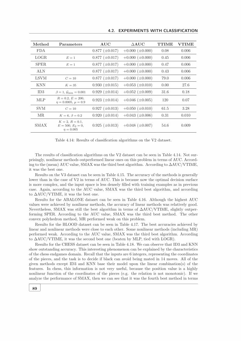
4.2. EXPERIMENTS WITH CLASSIFICATION
Method Parameters AUC ∆AUC TTIME VTIME
FDA 0.877 (±0.017) +0.000 (±0.000) 0.08 0.006
LOGR E = 1 0.877 (±0.017) +0.000 (±0.000) 0.45 0.006
SPER E = 1 0.877 (±0.017) +0.000 (±0.000) 0.47 0.006
ALN 0.877 (±0.017) +0.000 (±0.000) 0.43 0.006
LSVM C = 10 0.877 (±0.017) +0.000 (±0.000) 79.0 0.006
KNN K = 35 0.930 (±0.015) +0.053 (±0.010) 0.00 27.6
ID3 β = 1, Gmin = 0.001 0.929 (±0.014) +0.052 (±0.009) 31.6 0.18
MLP R = 0.2, E = 200,η = 0.0005, µ = 0.9
0.923 (±0.014) +0.046 (±0.005) 120 0.07
SVM C = 10 0.927 (±0.013) +0.050 (±0.010) 61.5 3.28
MR K = 6, β = 0.2 0.920 (±0.014) +0.043 (±0.006) 0.31 0.010
SMAXK = 2, R = 0.1,E = 500, E2 = 0,
η = 0.0050.925 (±0.013) +0.048 (±0.007) 54.6 0.009
Table 4.14: Results of classification algorithms on the V2 dataset.
The results of classification algorithms on the V2 dataset can be seen in Table 4.14. Not sur-prisingly, nonlinear methods outperformed linear ones on this problem in terms of AUC. Accord-ing to the (mean) AUC value, SMAX was the third best algorithm. According to ∆AUC/VTIME,it was the best one.
Results on the V3 dataset can be seen in Table 4.15. The accuracy of the methods is generallylower than in the case of V2 in terms of AUC. This is because now the optimal decision surfaceis more complex, and the input space is less densely filled with training examples as in previouscase. Again, according to the AUC value, SMAX was the third best algorithm, and accordingto ∆AUC/VTIME, it was the best one.
Results for the ABALONE dataset can be seen in Table 4.16. Although the highest AUCvalues were achieved by nonlinear methods, the accuracy of linear methods was relatively good.Nevertheless, SMAX was still the best algorithm in terms of ∆AUC/VTIME, slightly outper-forming SPER. According to the AUC value, SMAX was the third best method. The otherconvex polyhedron method, MR performed weak on this problem.
Results for the BLOOD dataset can be seen in Table 4.17. The best accuracies achieved bylinear and nonlinear methods were close to each other. Some nonlinear methods (including MR)performed weak. According to the AUC value, SMAX was the third best algorithm. Accordingto ∆AUC/VTIME, it was the second best one (beaten by MLP, tied with LOGR).
Results for the CHESS dataset can be seen in Table 4.18. We can observe that ID3 and KNNshow outstanding accuracy. This interesting phenomenon can be explained by the characteristicsof the chess endgames domain. Recall that the inputs are 6 integers, representing the coordinatesof the pieces, and the task is to decide if black can avoid being mated in 14 moves. All of thegiven methods except ID3 and KNN base their model upon the linear combination(s) of thefeatures. In chess, this information is not very useful, because the position value is a highlynonlinear function of the coordinates of the pieces (e.g. the relation is not monotonic). If weanalyze the performance of SMAX, then we can see that it was the fourth best method in terms
89

CHAPTER 4. APPLICATIONS
Method Parameters AUC ∆AUC TTIME VTIME
FDA 0.846 (±0.017) +0.000 (±0.000) 0.08 0.006
LOGR E = 1 0.846 (±0.017) +0.000 (±0.000) 0.45 0.006
SPER E = 1 0.846 (±0.017) +0.000 (±0.000) 0.47 0.006
ALN 0.846 (±0.017) +0.000 (±0.000) 0.43 0.006
LSVM C = 10 0.846 (±0.018) +0.000 (±0.000) 60.7 0.006
KNN K = 35 0.887 (±0.020) +0.041 (±0.010) 0.00 27.5
ID3 β = 1, Gmin = 0.001 0.877 (±0.019) +0.031 (±0.009) 22.1 0.19
MLP R = 0.2, E = 200η = 0.0005, µ = 0.9
0.877 (±0.016) +0.031 (±0.005) 120 0.07
SVM C = 10 0.888 (±0.015) +0.041 (±0.007) 125 3.17
MR K = 12, β = 0.2 0.867 (±0.017) +0.021 (±0.006) 0.47 0.012
SMAXK = 6, R = 0.1,E = 500, E2 = 0,
η = 0.0050.884 (±0.017) +0.038 (±0.007) 105 0.011
Table 4.15: Results of classification algorithms on the V3 dataset.
Method Parameters AUC ∆AUC TTIME VTIME
FDA 0.844 (±0.018) +0.000 (±0.000) 0.067 0.004
LOGR E = 1 0.849 (±0.018) +0.006 (±0.002) 0.206 0.004
SPER E = 2 0.852 (±0.018) +0.009 (±0.005) 0.256 0.004
ALN 0.849 (±0.018) +0.006 (±0.002) 0.195 0.004
LSVM C = 10 0.850 (±0.021) +0.007 (±0.005) 16.47 0.004
KNN K = 25 0.847 (±0.017) +0.003 (±0.007) 0.000 7.037
ID3 β = 2, Gmin = 0.001 0.821 (±0.024) −0.023 (±0.011) 164.2 0.153
MLP R = 0.2, E = 500η = 0.002, µ = 0.95
0.866 (±0.017) +0.022 (±0.006) 138.1 0.031
SVM C = 1000 0.863 (±0.015) +0.019 (±0.007) 30.23 1.517
MR K = 6, β = 0.2 0.748 (±0.030) −0.095 (±0.020) 0.481 0.007
SMAXK = 5, R = 0.2,
E = 5000, E2 = 5,η = 0.01
0.855 (±0.019) +0.012 (±0.008) 430.1 0.007
Table 4.16: Results of classification algorithms on the ABALONE dataset.
90
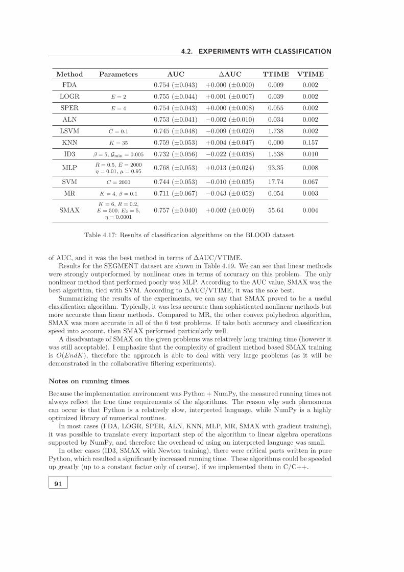
4.2. EXPERIMENTS WITH CLASSIFICATION
Method Parameters AUC ∆AUC TTIME VTIME
FDA 0.754 (±0.043) +0.000 (±0.000) 0.009 0.002
LOGR E = 2 0.755 (±0.044) +0.001 (±0.007) 0.039 0.002
SPER E = 4 0.754 (±0.043) +0.000 (±0.008) 0.055 0.002
ALN 0.753 (±0.041) −0.002 (±0.010) 0.034 0.002
LSVM C = 0.1 0.745 (±0.048) −0.009 (±0.020) 1.738 0.002
KNN K = 35 0.759 (±0.053) +0.004 (±0.047) 0.000 0.157
ID3 β = 5, Gmin = 0.005 0.732 (±0.056) −0.022 (±0.038) 1.538 0.010
MLP R = 0.5, E = 2000η = 0.01, µ = 0.95
0.768 (±0.053) +0.013 (±0.024) 93.35 0.008
SVM C = 2000 0.744 (±0.053) −0.010 (±0.035) 17.74 0.067
MR K = 4, β = 0.1 0.711 (±0.067) −0.043 (±0.052) 0.054 0.003
SMAXK = 6, R = 0.2,E = 500, E2 = 5,
η = 0.00010.757 (±0.040) +0.002 (±0.009) 55.64 0.004
Table 4.17: Results of classification algorithms on the BLOOD dataset.
of AUC, and it was the best method in terms of ∆AUC/VTIME.Results for the SEGMENT dataset are shown in Table 4.19. We can see that linear methods
were strongly outperformed by nonlinear ones in terms of accuracy on this problem. The onlynonlinear method that performed poorly was MLP. According to the AUC value, SMAX was thebest algorithm, tied with SVM. According to ∆AUC/VTIME, it was the sole best.
Summarizing the results of the experiments, we can say that SMAX proved to be a usefulclassification algorithm. Typically, it was less accurate than sophisticated nonlinear methods butmore accurate than linear methods. Compared to MR, the other convex polyhedron algorithm,SMAX was more accurate in all of the 6 test problems. If take both accuracy and classificationspeed into account, then SMAX performed particularly well.
A disadvantage of SMAX on the given problems was relatively long training time (however itwas still acceptable). I emphasize that the complexity of gradient method based SMAX trainingis O(EndK), therefore the approach is able to deal with very large problems (as it will bedemonstrated in the collaborative filtering experiments).
Notes on running times
Because the implementation environment was Python + NumPy, the measured running times notalways reflect the true time requirements of the algorithms. The reason why such phenomenacan occur is that Python is a relatively slow, interpreted language, while NumPy is a highlyoptimized library of numerical routines.
In most cases (FDA, LOGR, SPER, ALN, KNN, MLP, MR, SMAX with gradient training),it was possible to translate every important step of the algorithm to linear algebra operationssupported by NumPy, and therefore the overhead of using an interpreted language was small.
In other cases (ID3, SMAX with Newton training), there were critical parts written in purePython, which resulted a significantly increased running time. These algorithms could be speededup greatly (up to a constant factor only of course), if we implemented them in C/C++.
91

CHAPTER 4. APPLICATIONS
Method Parameters AUC ∆AUC TTIME VTIME
FDA 0.853 (±0.005) +0.000 (±0.000) 0.353 0.013
LOGR E = 5 0.854 (±0.005) +0.001 (±0.002) 1.949 0.013
SPER E = 6 0.854 (±0.005) +0.001 (±0.001) 2.711 0.013
ALN 0.832 (±0.006) −0.020 (±0.004) 1.282 0.013
LSVM C = 0.001 0.651 (±0.123) −0.201 (±0.120) 106.9 0.013
KNN K = 15 0.982 (±0.002) +0.129 (±0.005) 0.000 279.5
ID3 β = 0.1, Gmin = 0.001 0.993 (±0.003) +0.140 (±0.006) 192.9 0.700
MLP R = 0.01, E = 500η = 0.0002, µ = 0
0.836 (±0.006) −0.017 (±0.004) 916.1 0.178
SVM C = 100 0.955 (±0.006) +0.102 (±0.007) 277.5 18.76
MR K = 6, β = 0.2 0.916 (±0.008) +0.063 (±0.008) 0.783 0.026
SMAXK = 6, R = 0.2,
E = 1000, E2 = 5,η = 0.0002
0.937 (±0.006) +0.085 (±0.009) 2231 0.026
Table 4.18: Results of classification algorithms on the CHESS dataset.
Method Parameters AUC ∆AUC TTIME VTIME
FDA 0.930 (±0.019) +0.000 (±0.000) 0.077 0.003
LOGR E = 10 0.945 (±0.017) +0.015 (±0.009) 0.420 0.003
SPER E = 10 0.942 (±0.020) +0.012 (±0.011) 0.448 0.003
ALN 0.931 (±0.024) +0.001 (±0.011) 0.127 0.003
LSVM C = 10 0.939 (±0.024) +0.009 (±0.014) 5.519 0.003
KNN K = 15 0.988 (±0.009) +0.058 (±0.019) 0.000 2.748
ID3 β = 0.01, Gmin = 0.001 0.987 (±0.005) +0.057 (±0.018) 39.09 0.045
MLP R = 0.01, E = 500η = 5 · 10−6, µ = 0.95
0.858 (±0.026) −0.072 (±0.025) 76.75 0.018
SVM C = 5 · 105 0.989 (±0.010) +0.058 (±0.019) 84.82 0.260
MR K = 8, β = 0.2 0.973 (±0.013) +0.042 (±0.017) 0.342 0.006
SMAXK = 6, R = 0.05,E = 500, E2 = 5,
η = 0.0080.989 (±0.010) +0.059 (±0.016) 195.6 0.006
Table 4.19: Results of classification algorithms on the SEGMENT dataset.
92

4.3. EXPERIMENTS WITH COLLABORATIVE FILTERING
In the case of the support vector machines (LSVM, SVM), Python was used only as a wrapper.Most of the computation was done by the highly optimized libsvm library, therefore, the measuredrunning times can be considered as “state of the art”.
Notes on setting meta-parameters
Many of the algorithms involved in the experiments have meta-parameters that should be setappropriately in order to get a reasonable performance. For doing this, I generally applied thefollowing heuristic greedy search method:
1. Choose a meta-parameter to optimize based on intuition, or draw it randomly, if we haveno guess!
2. Optimize the value of the selected meta-parameter by “doubling and halving” (if it isnumerical) or by exhaustive search (if it is categorical)!
3. Go to step 1, if we want to continue optimizing!
It is important to note that meta-parameter optimization should use a different dataset orat least a different cross-validation split as the main experiment (in this work the latter solutionwas applied).
One may notice that the proposed SMAX approach has more meta-parameters than the otheralgorithms involved in the comparison. This is true, but I have found that for the given testproblems the performance is not very sensitive to the values of most meta-parameters. Themeta-parameters with largest influence on performance are the number of hyperplanes K, therange of random initialization R, the learning rate η, and the number of epochs E.
4.3 Experiments with collaborative filtering
The NETFLIX dataset
This collaborative filtering dataset is currently one of the largest publicly available machinelearning datasets. It contains about 100 million rating from over 480 thousand users on nearly18 thousand items (movies). The dataset was provided generously by Netflix, the popular movierental service, for the Netflix Prize (NP) competition [Bennett and Lanning, 2007].
The examples are (u, i, r, d) quadruplets, representing that user u rated item i as r on dated. The ratings values are integers from 1 to 5, where 1 is the worst, and 5 is the best. Thedata were collected between October, 1998 and December, 2005 and reflect the distribution ofall ratings received by Netflix during this period. The collected data was released in a train–testsetting in the following manner (see also Figure 4.4).
Netflix selected a random subset of users from their entire customer base with at least 20ratings in the given period. A Hold-out set was created from the 9 most recent ratings of theusers, consisting of about 4.2 million ratings. The remaining data formed the Training set. Theratings of the Hold-out set were split randomly with equal probability into three subsets of equalsize: Quiz, Test and Probe. The Probe set was added to the Training set and was released withratings. The ratings of the Quiz and Test sets were withheld as a Qualifying set to evaluatecompetitors. The Quiz/Test split of the qualifying set is unknown to the public. I remarkthat the date based partition of the entire NP dataset into train–test sets reflects the originalaim of recommender systems, which is the prediction of future interest of users from their pastratings/activities.
93

CHAPTER 4. APPLICATIONS
Known ratings Ratings withheld byNetflix for scoring
Random 3-way split
Training Data Probe Quiz Test
All Data(~100 M user item pairs)
Training Data
Held-Out Set(last 9 ratingfor each user:4.2 M pairs)
Figure 4.4: The train–test split and the naming convention of the NETFLIX dataset (after[Bell et al., 2007])
As the aim of the competition is to improve the prediction accuracy of user ratings, Netflixadopted RMSE (root mean squared error) as evaluation measure. The goal of the competitionis to reduce the RMSE on the Test set by at least 10 percent, relative to the RMSE achieved byNetflix’s own system Cinematch.2 The contestants have to submit predictions for the Qualifyingset. The organizers return the RMSE of the submissions on the Quiz set, which is also reportedon a public leaderboard.3 Note that the RMSE on the Test set is withheld by Netflix.
There are some interesting characteristics of the data and the set-up of the competition thatpose a difficult challenge for prediction:
• The distribution over the time of the ratings of the Hold-out set is quite different from theTraining set. As a consequence of the selection method, the Hold-out set does not reflectthe skewness of the movie-per-user, observed in the much larger Training set. Therefore theQualifying set contains approximately equal number of queries for often and rarely ratingusers.
• The designated aim of the release of the Probe set is to facilitate unbiased estimation ofRMSE for the Quiz/Test sets despite of the different distributions of the Training and theHold-out sets. In addition, it permits off-line comparison of predictors before submission.
• We already mentioned that users’ activity at rating is skewed. To put this into numbers,ten percent of users rated 16 or fewer movies and one quarter rated 36 or fewer. Themedian is 93. Some very active users rated more than 10,000 movies. A similar biasedproperty can be observed for movies: The most-rated movie, Miss Congeniality was rated
2The first team achieving the 10 percent improvement is promised to be awarded by a Grand Prize of $1million by Netflix. Not surprisingly, this prospective award drawn much interest towards the competition. So far,more than 3 000 teams submitted entries for the competition.
3http://www.netflixprize.com/leaderboard
94

4.3. EXPERIMENTS WITH COLLABORATIVE FILTERING
by almost every second user, but a quarter of titles were rated fewer than 190 times, anda handful were rated fewer than 10 times [Bell et al., 2007].
• The variance of movie ratings is also very different. Some movies are rated approximatelyequally by the user base (typically well), and some partition the users. The latter onesmay be more informative in predicting the taste of individual users.
Experiments
The algorithms involved in the experiments were the following:
• DC: Double centering (see page 24 for the details). The only parameter of the algorithmis the number of epochs E (default value: 2).
• BRISMF: Biased regularized incremental simultaneous matrix factorization (see page 25).The parameters of the algorithm are the number of epochs E, the number of factors L, theuser learning rate ηU (default value: 0.016), the item learning rate ηI (default value: 0.005),the user regularization coefficient λU (default value: 0.015), and the item regularizationcoefficient λI (default value: 0.015).
• NSVD1: Item neighbor based approach with factorized similarity (see page 27). Theparameters of the algorithm are the number of epochs E, the number of factors L, the userlearning rate ηU (default value: 0.005), the item learning rate ηI (default value: 0.005),the user regularization coefficient λU (default value: 0.015), and the item regularizationcoefficient λI (default value: 0.015).
• SMAXCF: The proposed smooth maximum based convex polyhedron approach (see page54). The parameters of the algorithm are the smooth max function (default value: smaxA1),the smoothness parameter α (default value: 2), the smoothness change parameters A1 andA0 (default value: A1 = 1, A0 = 0.25), the number of epochs E, the number of factorsL, the user learning rate ηU (default value: 0.016), the item learning rate ηI (defaultvalue: 0.005), the user regularization coefficient λU (default value: 0.015), and the itemregularization coefficient λI (default value: 0.015).
All algorithms were implemented in C++ from scratch. The hardware environment was aserver PC with Intel Pentium Q9300 2.5 GHz CPU and 3 Gb memory.
Let us denote the NETFLIX Training set by T = {(u1, i1, r1, d1), . . . , (un, in, rn, dn)}, andthe Probe set by P = {(u1, i1, r1, d1), . . . , (um, im, rm, dm)}. The exact sizes of the sets aren = 100, 480, 507 and m = 1, 408, 395. All algorithms were trained using T \ P, and then theProbe RMSE of the trained predictor g was calculated as
Probe RMSE =
√√√√ 1
|P|∑
(u,i,r,d)∈P(g(u, i)− r)2.
The results of individual algorithms are shown in Table 4.20. Recall that SMAXCF can beconsidered as a generalization of BRISMF. We can see, that the SMAXCF approach was able toboost the accuracy of BRISMF, however if we used more factors, then the benefit was smaller.The NSVD1 approach was less accurate than than BRISMF and SMAXCF, and not surprisingly,DC was the worst in terms of RMSE. It is true for all of BRISMF, NSVD1, and SMAXCF thatthe accuracy was increasing with introducing more factors.
Each experiment consists of three main phases: data loading, training, and validation. Thelast column of the table shows the total running time of the experiments in seconds. If we take
95

CHAPTER 4. APPLICATIONS
No. Method Parameters Probe RMSERunning time
(seconds)
#1 DC 0.9868 11
#2 BRISMF L = 10, E = 13 0.9190 161
#3 BRISMF L = 20, E = 12 0.9125 263
#4 BRISMF L = 50, E = 12 0.9081 598
#5 NSVD1 L = 10, E = 26 0.9492 568
#6 NSVD1 L = 20, E = 24 0.9459 1057
#7 NSVD1 L = 50, E = 22 0.9435 1900
#8 SMAXCF L = 10, E = 18 0.9169 861
#9 SMAXCF L = 20, E = 18 0.9114 1234
#10 SMAXCF L = 50, E = 18 0.9079 2692
Table 4.20: Results of collaborative filtering algorithms on the NETFLIX dataset.
into account that more than 99 million examples were used for training, then we can concludethat all of the presented algorithms are efficient in terms of time requirement.
In the last experiments the predictions of the previous methods for the Probe set were blendedwith L2 regularized linear regression (LINR, see page 21). The value of the regularization coef-ficient was λ = 1.4. The results can be seen in Table 4.21.
The last column shows the 10-fold cross validation Probe RMSE of the optimal linear com-bination of the inputs. The reason why the single-input blends (#11, #12, and #13) have lowerRMSE than the inputs themselves is that the LINR blender introduces a bias term too. We cansee that the SMAXCF approach was able to improve the result of the combination of BRISMFand NSVD1 models. This indicates that SMAXCF was able to capture new aspects of the datathat was not captured by BRISMF and NSVD1.
96

4.3. EXPERIMENTS WITH COLLABORATIVE FILTERING
No. Inputs Probe RMSE
#11 #4 0.9069
#12 #7 0.9430
#13 #10 0.9069
#14 #2+#3+#4 0.9065
#15 #5+#6+#7 0.9429
#16 #8+#9+#10 0.9068
#17 #14+#15 0.9035
#18 #14+#16 0.9050
#19 #15+#16 0.9033
#20 #14+#15+#16 0.9021
Table 4.21: Results of linear blending on the NETFLIX dataset.
97


Conclusion
This thesis was about convex polyhedron based methods for machine learning. The first chapter(Introduction) briefly introduced the field of machine learning and located convex polyhedronlearning in it. The second chapter (Algorithms) dealt with the problem of linear and convexseparation, and gave algorithms for training convex polyhedron classifiers and predictors. Thethird chapter (Model complexity) collected known facts about the Vapnik–Chervonenkis dimen-sion of convex polyhedron classifiers and proved new results. The fourth chapter (Applications)presented experiments with the given algorithms on real and artificial datasets.
The summary of new scientific results contained in the thesis is the following:
• Direct and incremental approaches were investigated for determining the linear separabilityof point sets. Heuristics were proposed for choosing the active constraints and variablesof the next step (LSEPX, LSEPY, LSEPZX, LSEPZY). A novel algorithm with low timerequirement was given for the approximate convex separation of point sets (CSEPC). Anovel exact algorithm with low expected time requirement was introduced for determiningthe convex separability of point sets (CSEPX).
• The possibility of approximating the maximum operator by smooth functions was inves-tigated, and six, parameterizable smooth maximum function families were introduced. Anovel, smooth maximum function based approach was introduced for training convex poly-hedron classifiers (SMAX). A novel, smooth maximum function based algorithm was givenfor training convex polyhedron models in the case of collaborative filtering (SMAXCF).
• The Vapnik–Chervonenkis dimension of 2-dimensional convex K-gon classifiers was deter-mined so that the label of the inner (convex) region is unrestricted. A new lower boundwas proved for the Vapnik–Chervonenkis dimension of d-dimensional convex K-polyhedronclassifiers. In the special cases d = 3 and d = 4 the bound was further improved.
• Scalable and accurate algorithms were introduced for collaborative filtering. A novel matrixfactorization technique called BRISMF (biased regularized incremental simultaneous ma-trix factorization) was introduced. A new training algorithm for Paterek’s NSVD1 modelwas given.
99


List of publications
[P1] G. Takacs, I. Pilaszy, B. Nemeth, and D. Tikk. Scalable collaborative filtering approachesfor large recommender systems. Journal of Machine Learning Research (Special Topic onMining and Learning with Graphs and Relations), 10: 623–656, 2009.
[P2] G. Takacs, I. Pilaszy, B. Nemeth, and D. Tikk. Matrix factorization and neighbor basedalgorithms for the Netflix Prize problem. Proc. of the 2008 ACM Conference on Recom-mender Systems (RECSYS’08), pages 267–274, Lausanne, Switzerland, 2008.
[P3] G. Takacs, I. Pilaszy, B. Nemeth, and D. Tikk. Investigation of various matrix factorizationmethods for large recommender systems. Proc. of the 2nd KDD Workshop on Large ScaleRecommender Systems and the Netflix Prize Competition, Las Vegas, Nevada, USA, 2008.
[P4] G. Takacs, I. Pilaszy, B. Nemeth, and D. Tikk. A unified approach of factor models andneighbor based methods for large recommender systems. Proc. of the 1th IEEE ICADIWTWorkshop on Recommender Systems and Personalized Retrieval, pages 186–191, Ostrava,Czech Republic, 2008.
[P5] G. Takacs, I. Pilaszy, B. Nemeth, and D. Tikk. Major components of the Gravity Recom-mendation System. ACM SIGKDD Explorations Newsletter, 9(2): 80–83, 2007.
[P6] G. Takacs, I. Pilaszy, B. Nemeth, and D. Tikk. On the Gravity Recommendation System.Proc. of the KDD Cup and Workshop 2007, pages. 22–30, San Jose, California, USA, 2007.
[P7] G. Takacs and B. Pataki. Case-level detection of mammographic masses. InternationalJournal of Applied Electromagnetics and Mechanics, 25(1–4): 395–400, 2007.
[P8] G. Takacs. The Vapnik–Chervonenkis dimension of convex n-gon classifiers. HungarianElectronic Journal of Sciences, 2007.
[P9] G. Takacs and B. Pataki. Lower bounds on the Vapnik–Chervonenkis dimension of convexpolytope classifiers. Proc. of the 11th International Conference on Intelligent EngineeringSystems (INES 2007), Budapest, Hungary, 2007.
[P10] G. Takacs and B. Pataki. Deciding the convex separability of pattern sets. Proc. ofthe 4th IEEE Workshop on Intelligent Data Acquisition and Advanced Computing Systems(IDAACS’2007), Dortmund, Germany, 2007.
[P11] G. Takacs and B. Pataki. An efficient algorithm for deciding the convex separability ofpoint sets. Proc. of the 14th PhD Mini-Symposium, Budapest University of Technology andEconomics, Department of Measurement and Information Systems, pages 54–57, Budapest,Hungary, 2007.
[P12] G. Takacs and B. Pataki. Nearest local hyperplane rules for pattern classification. AI*IA2007: Artificial Intelligence and Human-Oriented Computing, pages 302–313, Rome, Italy,2007.
[P13] G. Takacs and B. Pataki. A lepcsozetes donteshozas elvenek muszaki alkalmazasai, (inHungarian). Elektronet, 16(8): 76–78, 2007.
[P14] M. Altrichter, G. Horvath, B. Pataki, Gy. Strausz, G. Takacs and J. Valyon. Neuralishalozatok, (in Hungarian). Panem, 2006.
101

CHAPTER 4. APPLICATIONS
[P15] G. Takacs and B. Pataki. Local hyperplane classifiers. Proc. of the 13th PhD Mini-Symposium, Budapest University of Technology and Economics, Department of Measure-ment and Information Systems, pages 44–45, Budapest, Hungary, 2006.
[P16] G. Takacs and B. Pataki. Fast detection of masses in mammograms with difficult caseexclusion. International Scientific Journal of Computing, 4(3): 70–75, 2005.
[P17] G. Takacs and B. Pataki. Case-level detection of mammographic masses. Proc. of the 12thInternational Symposium on Interdisciplinary Electromagnetic, Mechanic and BiomedicalProblems (ISEM 2005), pages 214–215, Bad Gastein, Austria, 2005.
[P18] G. Takacs and B. Pataki. Fast detection of mammographic masses with difficult caseexclusion. Proc. of the 3rd IEEE Workshop on Intelligent Data Acquisition and AdvancedComputing Systems (IDAACS’2005), pages 424–428, Sofia, Bulgaria, 2005.
[P19] G. Takacs and B. Pataki. Computer-aided detection of mammographic masses. Proc. ofthe 12th PhD Mini-Symposium, Budapest University of Technology and Economics, Depart-ment of Measurement and Information Systems, pages 24–25, Budapest, Hungary, 2005.
[P20] N. Toth, G. Takacs, and B. Pataki. Mass detection in mammograms combining two meth-ods. Proc. of the 3rd European Medical & Biological Engineering Conference (EMBEC’05),Prague, Czech Republic, 2005.
[P21] G. Horvath, B. Pataki, A. Horvath, G. Takacs, and G. Balogh. Detection of microcalcifi-cation clusters in screening mammography. Proc. of the 3rd European Medical & BiologicalEngineering Conference (EMBEC’05), Prague, Czech Republic, 2005.
[P22] G. Takacs. The smooth maximum classifier. Accepted at: Second Gyor Symposium onComputational Intelligence, 2009.
[P23] G. Takacs. Smooth maximum based algorithms for classification, regression, and collabora-tive filtering. Accepted at: Acta Technica Jaurinensis, Series Intelligentia Computatorica,2009.
[P24] G. Takacs. Efficient algorithms for determining the linear and convex separability of pointsets. Accepted at: Acta Technica Jaurinensis, Series Intelligentia Computatorica, 2009.
[P25] G. Takacs, I. Pilaszy, B. Nemeth, and D. Tikk. Unifying collaborative filtering approaches.Veszprem Optimization Conference: Advanced Algorithms (VOCAL 2008), Veszprem,Hungary, 2008.
[P26] R. Horvath-Bokor, Z. Horvath, and G. Takacs. Kockazatelemzes logisztikus regressziovalnagy adathalmazokon, (in Hungarian). 28. Magyar Operaciokutatasi Konferencia, Bala-tonoszod, Hungary, 2009.
102

Bibliography
K. Appel and W. Haken. Every planar map is four colorable. Ilinois Journal of Mathematics,21:439–567, 1977.
E.M. Arkin, F. Hurtado, J.S.B. Mitchell, C. Seara, and S.S. Skiena. Some lower bounds ongeometric separability problems. International Journal of Computational Geometry and Ap-plications, 161:1–26, 2006.
D. Ascher, P.F. Dubois, K. Hinsen, J. Hugunin, and T. Oliphant. Numerical Python, 2001.URL: http://www.numpy.org/.
P. Assouad. Densite et dimension. Annales de l’Institut Fourier, 33:233–282, 1983.
A. Asuncion and D.J. Newman. UCI Machine Learning Repository, 2007.URL: http://www.ics.uci.edu/~mlearn/MLRepository.html.
R. Bell and Y. Koren. Improved neighborhood-based collaborative filtering. In Proc. of the KDDCup and Workshop 2007, pages 7–14, 2007.
R. Bell, Y. Koren, and C. Volinsky. Chasing $1,000,000: How we won the Netflix Progress Prize.ASA Statistical and Computing Graphics Newsletter, 18(2):4–12, 2007.
J. Bennett and S. Lanning. The Netflix Prize. In Proc. of the KDD Cup and Workshop 2007,pages 3–6, 2007.
B. Boser, I. Guyon, and V. Vapnik. A training algorithm for optimal margin classifiers. In Proc.of the Fifth Annual Workshop on Computational Learning Theory, pages 144–152, 1992.
O. Bousquet, S. Boucheron, and G. Lugosi. Introduction to statistical learning theory. LectureNotes in Artificial Intelligence, 3176:169–207, 2004.
P.S Bradley, U.M. Fayyad, and O.L. Mangasarian. Mathematical programming for data mining:Formulations and challenges. INFORMS Journal on Computing, 11(3):217–238, 1999.
L. Breiman. Hinging hyperplanes for regression, classification, and function approximation. IEEETransactions on Information Theory, 39(3):999–1013, 1993.
C. Burges. A tutorial on support vector machines for pattern recognition. Data Mining andKnowledge Discovery, 2(2):121–167, 1998.
C. Chang and C. Lin. LIBSVM: a library for support vector machines. National Taiwan Univer-sity, 2001. URL: http://www.csie.ntu.edu.tw/~cjlin/libsvm/.
V. Chvatal. Linear programming. W. H. Freeman & Co., 1983.
K. Crammer and Y. Singer. On the algorithmic implementation of multiclass kernel-based vectormachines. Journal of Machine Learning Research, 2:265–292, 2001.
L. Devroye, L. Gyorfi, and G. Lugosi. A probabilistic theory of pattern recognition. Springer,New York, 1996.
D.P. Dobkin and D. Gunopulos. Concept learning with geometric hypotheses. In Proc. 8th AnnualConference on Computational Learning Theory, pages 329–336. ACM Press, New York, 1995.
J.P. Egan. Signal detection theory and ROC analysis. Academic Press, New York, 1975.
103
BIBLIOGRAPHY
M. Elad, Y. Hel-Or, and R. Keshet. Pattern detection using a maximal rejection classifier. InProc. of the 4th International Workshop on Visual Form, pages 514–524, 2001.
T.S. Ferguson. Linear programming – A concise introduction, 2004.URL: http://www.math.ucla.edu/~tom/LP.pdf.
T. Finley. PyGLPK, version 0.3, 2008.URL: http://www.cs.cornell.edu/~tomf/pyglpk/.
P. Fischer. More or less efficient agnostic learning of convex polygons. In Proc. of the 8th AnnualConference on Computational Learning Theory, pages 228–236. ACM Press, New York, 1995.
R.A. Fisher. The use of multiple measurements in taxonomic problems. Annals of Eugenics, 7:179–188, 1936.
E. Fix and J.L. Hodges. Discriminatory analysis: Non-parametric discrimination: Consistencyproperties. Technical Report 4, US Air Force School of Aviation Medicine, 1951.
S. Funk. Netflix update: Try this at home, 2006.URL: http://sifter.org/~simon/journal/20061211.html.
L. Gyorfi, M. Kohler, A. Krzyzak, and H. Walk. A distribution-free theory of nonparametricregression. Springer, New York, 2002.
D. Haussler and E. Welzl. Epsilon nets and simplex range queries. Discrete ComputationalGeometry, 2:127–151, 1987.
S. Haykin. Neural networks and learning machines. Prentice Hall, 3rd edition, 2008.
R. Hooke and T.A. Jeeves. “direct search” solution of numerical and statistical problems. Journalof the ACM, 8(2):212–229, 1961.
T. Joachims. Making large-scale SVM learning practical. In B. Schlkopf, C. Burges, and A. Smola,editors, Advances in kernel methods - Support vector learning. MIT Press, 1999.
E. Jones, T. Oliphant, P. Peterson, et al. SciPy: Open source scientific tools for python, 2001.URL: http://www.scipy.org/.
N. Karmarkar. A new polynomial-time algorithm for linear programming. Combinatorica, 4:373–395, 1984.
J. Kiefer. Sequential minimax search for a maximum. Proceedings of the American MathematicalSociety, 4(1):502–506, 1953.
A.R. Klivans, R. O’Donnell, and R.A. Servedio. Learning intersections and thresholds of halfs-paces. Journal of Computer and System Sciences, 68(4):804–840, 2004.
S. Kwek and L. Pitt. PAC learning intersections of halfspaces with membership quieries. Algo-rithmica, 22:53–75, 1998.
Y. LeCun and C. Cortes. The MNIST database of handwritten digits, 1999.URL: http://yann.lecun.com/exdb/mnist/.
A. Makhorin. GNU Linear Programming Kit, version 4.37, 2009.URL: http://www.gnu.org/software/glpk/.
104

BIBLIOGRAPHY
W. McCullogh and W. Pitts. A logical calculus of the ideas immanent in nervous activity.Biophysics, 7:115–133, 1943.
N. Megiddo. On the complexity of polyhedral separability. Discrete and Computational Geome-try, 3:325–337, 1988.
A. Paterek. Improving regularized singular value decomposition for collaborative filtering. InProc. of the KDD Cup and Workshop 2007, pages 39–42, 2007.
K. Pearson. The life, letters and labors of Francis Galton. Cambridge University Press, 1930.
K. Pearson. Mathematical contributions to the theory of evolution. III. Regression, heredity andpanmixia. Philosophical Transactions of the Royal Society of London, 187:253–318, 1896.
I. Pilaszy and T. Dobrowiecki. Constructing large margin polytope classifiers with a multiclassclassification algorithm. In Proc. of the 4th IEEE Workshop on Intelligent Data Acquisitionand Advanced Computing Systems (IDAACS’2007), pages 261–264, 2007.
J.C. Platt. Fast training of support vector machines using sequential minimal optimization, pages185–208. MIT Press, 1999.
J.R. Quinlan. Induction of decision trees. Machine Learning, 1(1), 1986.
C.C. Rodrıguez. Learning theory notes, VC dimension: Examples and tools, 2004.URL: http://omega.albany.edu:8008/ml/.
F. Rosenblatt. Principles of neurodynamics: Perceptrons and the theory of brain mechanisms.Spartan Books, Washington D.C., 1962.
G. van Rossum. An introduction to Python, 2006.URL: http://www.network-theory.co.uk/docs/pytut/.
N. Sauer. On the density of families of sets. Journal of Combinatorial Theory (A), 13:145–147,1972.
J.R. Shewchuk. An introduction to the conjugate gradient method without the agonizing pain.Technical Report CMU-CS-94-125, Carnegie Mellon University, School of Computer Science,1994.
C. Stone. Consistent nonparametric regression. Annals of Statistics, 8:1348–1360, 1977.
G. Takacs. The Vapnik–Chervonenkis dimension of convex n-gon classifiers. Hungarian ElectronicJournal of Sciences, 2007.
G. Takacs and B. Pataki. Deciding the convex separability of pattern sets. In Proc. ofthe 4th IEEE Workshop on Intelligent Data Acquisition and Advanced Computing Systems(IDAACS’2007), pages 278–80, 2007a.
G. Takacs and B. Pataki. Lower bounds on the Vapnik–Chervonenkis dimension of convexpolytope classifiers. In Proc. of the 11th International Conference on Intelligent EngineeringSystems (INES 2007), 2007b.
G. Takacs, I. Pilaszy, B. Nemeth, and D. Tikk. On the Gravity Recommendation System. InProc. of the KDD Cup and Workshop 2007 (KDD 2007), pages 22–30, 2007.
105

BIBLIOGRAPHY
G. Takacs, I. Pilaszy, B. Nemeth, and D. Tikk. A unified approach of factor models and neighborbased methods for large recommender systems. In Proc. of the 1st IEEE ICADIWT Workshopon Recommender Systems and Personalized Retrieval, pages 186–191, 2008.
G. Takacs, I. Pilaszy, B. Nemeth, and D. Tikk. Scalable collaborative filtering approaches forlarge recommender systems. Journal of Machine Learning Research (Special topic on Miningand Learning with Graphs and Relations), 10:623–656, 2009.
L.G. Valiant. A theory of the learnable. Communications of the ACM, 27(11):1134–1142, 1984.
V. Vapnik and A. Chervonenkis. On the uniform convergence of relative frequencies of events totheir probabilities. Theory of Probability and its Applications, 16(2):264–280, 1971.
S. Vempala. A random sampling based algorithm for learning the intersection of half-spaces.In Proc. of the 38th Annual Symposium on Foundations of Computer Science, pages 508–513,1997.
P.J. Werbos. Beyond regression: New tools for prediction and analysis in the behaviour sciences.PhD thesis, Harvard University, Cambridge, MA, 1974.
B. Widrow. An adaptive “adaline” neuron using chemical “memistors”. Technical Report 1553-2,Stanford Electronics Laboratories, 1960.
E.B. Wilson and J. Worcester. The determination of L.D.50 and its sampling error in bio-assay.Proceedings of the National Academy of Sciences, 29:79–85, 1943.
106