Convex Energy Functions for Power Systems...

Convex Energy Functions for Power Systems Analysis

K. Dvijotham1 Steven Low1 M. Chertkov2

1California Institute of Technology

2Center for Nonlinear Studies and Theoretical DivisionLos Alamos National Laboratory

LANL Grid Science ConferenceJanuary 15, 2015

Figure

/2014

K. Dvijotham (Caltech) 1 / 45

Table of Contents

1 Introduction

2 Energy Functions for Power Systems

3 Applications of Convex Energy Functions

4 Convexity of Energy Function

5 Conclusions and Future Work


Table of Contents

1 Introduction






Power System Operations

Power System Operations

Generator Control

State EstimationPower Flow Analysis

Generator Control Transient Stability Analysis


Power System Operations: Typical Assumptions

Traditional Assumptions and Approach

Predictable Loads and Generation

Power Flow Directions mostly known

Linearized Analysis+Real-time simulations/monitoring

Heuristic Approaches to Nonlinearities


Power Grids: The Future

The grid is changing:

1 large number of distributed power sources

2 increasing adoption of renewables

⇒ large-scale, complex, & heterogeneousnetworks with stochastic disturbances

Implications

Linearized Analysis (DC Power Flow) no longer sufficiently accurate

Need efficient and reliable algorithms for “nonlinear” power systemsanalysis


Notation

Notation

Nodes=Buses i , Edges=Lines (i , j) ∈ E

Voltage phasor Vi exp (iθi ), V = {Vi exp (iθi )}

Complex Admittance Yij = Gij + iBij

Complex Power Injection Si = Pi + iQi

Complex Current Injection Ii , ρi = log (Vi ) , ρij = ρi − ρj , θij = θi − θj

Bus Types

Bus Type Fixed Quantities Variable Quantities(P,V ) buses (Generators) Pi ,Vi = vi Pi , θi

(P,Q) buses (Loads) Pi ,Qi Vi , θiSlack Bus θS , ρS = 0 Pi ,Qi


Why is Power Systems Analysis Hard?

Linear Circuits Analysis

I given, find V

I = YV

Linear Equation, Easy

Power Flow Analysis

S given, find v

S = V. ∗ I = V. ∗(YV)

Multivariate QuadraticEquations: Hard!


Power Flow Equations in Polar Coordaintes

Power Flow Equations

Pi =∑j

ViVj (Bij sin (θi − θj) + Gij cos (θi − θj)) ∀i

Qi =∑j

ViVj (Gij sin (θi − θj)− Bij cos (θi − θj)) ∀i ∈ pq

Vi = vi ∀i ∈ pv

Traditional Solution Methods

Multivariate nonlinear equationsSolved via Iterative Linearization: Newton-Raphson

Works well under “nice conditions”What if solver fails? No solution?


Our Solution: Use the physics!

1 Use energy function as analysis tool

2 Variational formulation of power flowequations

3 Computational tractability via convexity

Optimal Power Flow

Power Flow AnalysisTransient Stability Analysis

State Estimation

Energy Function


Table of Contents

1 Introduction






Variational Formulation for Resistive DC Networks

Loss Minimization in Resistive Network

Minimize{Iij :(i ,j)∈E}

∑(i ,j)∈E

1

2I 2ijRij (Resistive Losses)

Subject to Ii =∑

j :(i ,j)∈E

Iij −∑

j :(j ,i)∈E

Iji (Conservation of Current)

Solution of Loss Minimization

L (I ,V ) =∑

(i ,j)∈E

I 2ijRij + (Vj − Vi ) Iij −∑i

IiVi

∂L

∂Iij= 0 ≡ Iij =

Vi − Vj

Rij≡ Ohm’s Law!


Variational Formulation for Lossless AC Networks

Reactive Loss Minimization in a Lossless AC Network

Minimize{Iij :(i ,j)∈E}

∑(i ,j)∈E

Bij

∫ fijBij

−π2

arcsin (y) d y (Reactive Losses?)

Subject to Pi =∑

j :(i ,j)∈E

fij −∑

j :(j ,i)∈E

fji (Conservation of Active Power)

|fij | ≤ Bij

Solution of Reactive Loss Minimization

L (f , θ) =∑

(i ,j)∈E Bij

∫ fijBij

−π2

arcsin (y) d y + (θj − θi ) fij∂L∂fij

= 0 ≡ fij = Bij sin (θi − θj) ≡ Active Power

[Bent et al., 2013][Boyd and Vandenberghe, 2009]


Variational Formulation for Lossless AC Networks

Dual Form

Minimizeθ

∑(i ,j)∈E

−Bij cos (θi − θj)−∑i

Piθi

Subject to |θi − θj | ≤π

2

[Bergen and Hill, 1981]


Energy Functions for Power Systems - History

1958 2/3-bus case Aylett

1960-1980

Kron ReductionIgnore transferconductances

VariousauthorsSummarizedin Pai, 1981

1981-1990

Structurepreservingmodels

Bergen/HillVaraiya et alVan Cutsemet al


Energy Function for Lossless Power Systems

Main Assumption

Transmission lines purely inductive Gij = 0

Energy Function for Power Systems

E (ρ, θ) = −∑i

Piθi −∑i∈pq

Qiρi −1

2

∑j ,k

Bjk exp (ρi + ρj) cos (θi − θj)

[Cutsem and Ribbens-Pavella, 1985][Narasimhamurthi and Musavi, 1984]


Energy Function Properties

Stationary Points ≡ Power Flow Equations

∂E (ρ, θ)

∂θi= 0 ≡ Pi =

∑j 6=i

Bij exp (ρi + ρj) sin (θi − θj)

∂E (ρ, θ)

∂ρi= 0 ≡ Qi =

∑j 6=i

Bij (exp (ρi + ρj) cos (θi − θj)− exp (2ρi ))


Table of Contents

1 Introduction






Convexification Roadmap

Determine Region of Convexity C of E (ρ, θ)

Operational Constraints ⊂ C

Variationally enforce power flow constraints in convex way


Convexity Region and Power Flow Solutions

Why seek solutions in Convexity Region?

Solutions guaranteed to be locally stable with respect to SwingEquation Dynamics.

Boundary of convexity region, Hessian singular =⇒ Jacobian ofpower flow equations singular

For tree networks, PF solvable if and only if PF solvable in ConvexityRegion

Related to “Principal Singular Surfaces”, “Stable Region” [C.J.Tavoraand O.J.M.Smith, 1972] [Araposthatis et al., 1981] (all (P,V ) buses)


Convex Power Flow Solvers

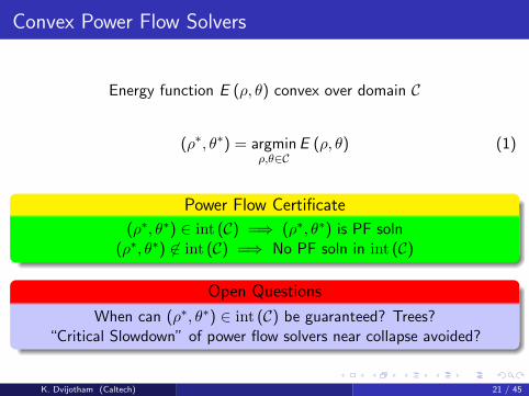
Energy function E (ρ, θ) convex over domain C

(ρ∗, θ∗) = argminρ,θ∈C

E (ρ, θ) (1)

Power Flow Certificate

(ρ∗, θ∗) ∈ int (C) =⇒ (ρ∗, θ∗) is PF soln(ρ∗, θ∗) 6∈ int (C) =⇒ No PF soln in int (C)

Open Questions

When can (ρ∗, θ∗) ∈ int (C) be guaranteed? Trees?“Critical Slowdown” of power flow solvers near collapse avoided?


Convex Optimal Power Flow Solvers

Optimal Power Flow

MinimizeP,Q,ρ,θ

c (P,Q) (Strictly convex generation cost) (2)

Subject to∇θE (ρ, θ;P,Q) = 0,∇ρE (ρ, θ;P,Q) = 0 Nonconvex PF Eqn

(ρ, θ) ∈ S Operational Constraints, Convex

Energy function E (ρ, θ;P,Q) strictly convex over domain C, S ⊂ C

Convex-Concave Saddle Point OPF

(P∗,Q∗, ρ∗, θ∗) = argmaxP,Q

argminρ,θ∈S

λE (ρ, θ;P,Q)− c (P,Q)


Convex Optimal Power Flow Solvers

Optimal Power Flow Certificate (λ→ 0)

(ρ∗, θ∗) ∈ int (S) =⇒ (P∗,Q∗, ρ∗, θ∗) is soln to (2)(2) has soln with (ρ∗, θ∗) ∈ int (S) =⇒ soln optimal for Saddle Point

OPF

Open Questions

What operational constraints can be encoded in S? Apparent power,voltage magnitude bounds . . .

When is S subset of C?Relationship to SDP/SOCP relaxations of OPF?

A general strategy for classes of QCQPs? Polar vs Cartesian


Topology Estimation

Sparse Topology Estimation from Phasor Measurements

Measurements {(ρi , θi

)}ki=1

Unknown Bij

min∑i

E(ρi , θi ;B

)− min

(ρ,θ)E (ρ, θ;B) + λ ‖B‖1


Table of Contents

1 Introduction






Intuition from 2-bus case

Slack bus Load0 1

p1 p1q1

Energy Function for 2-bus case

E (ρ1, θ1) = b

(1

2exp (2ρ1)− v0 exp (ρ1) cos (θ1)

)− p1θ1 − q1ρ1



(a) p = q = .01 (b) p = q = .1



(a) p = q = .2 (b) p = q = .25


Convexity of 2-bus case

Hessian of Energy Function

∇2E (θ1, ρ1) = b

(2 exp (2ρ1)− v0 exp (ρ1) cos (θ1) v0 exp (ρ1) sin (θ1)

v0 exp (ρ1) sin (θ1) v0 exp (ρ1) cos (θ1)

)This matrix is positive semidefinite if and only if

cos (θ1) ≥ v0 exp (−ρ1)

2=

1

2

V0

V1

Condition eliminates low-voltage solution


No (P ,Q) nodes connected

Special topology: No transmission lines connecting (P,Q) nodes.

Condition for Convexity

cos (θi − θj) ≥vi exp (−ρj)

2=

exp (ρi − ρj)2

∀(i , j) ∈ E , i ∈ pv, j ∈ pq

Let vi = 1pu at all i ∈ pv.

|θi − θj | ≤ 45 deg,Vj ≥1√2≈ .7 suffices for convexity


General Topologies

Condition for Convexity: Nonlinear Convex Matrix Inequality

M (ρ, θ) � 0,M ∈ S |pq|

[M (ρ, θ)]ii = 2∑j 6=i

Bij −∑j 6=i

Bijvj exp (ρj − ρi )cos (θij)

[M (ρ, θ)]ij = −Bij

cos (θij)∀(i , j) ∈ E , i , j ∈ pq


Conservatism in Convexity Region Estimate

Condition for Convexity: Sufficient, but Necessary?

For tree networks, yes

In general, unknown: Initial numerical tests show necessity for smallnetworks

Holds for all test systems available in MATPOWER

“Almost all” power flow solutions within convexity domain

Open Questions

Relationship to existence of power flow solutions: Answered for trees

Closing the gap for non-tree networks


Estimated vs Actual Regions of Convexity: 3-bus network

Slack bus

LoadLoad

0

21

p1 + p2

p2q2p1q1

B02B01

B12

Reduced Energy Function

Solve for ρ as a function of θPlug into energy function E (ρ (θ) , θ)



θ1

θ2

Convexity Region: No (P,Q) buses connected

−50 0 50

−60

−40

−20

0

20

40

60

(a) No (P,Q) connected

θ1

θ2

Convexity Region: Normal Loading

−50 0 50

−60

−40

−20

0

20

40

60

(b) Base Load

Figure: Theoretical Convexity Region=Numerical Convexity Region



θ1

θ2

Convexity Region: High Loading

−50 0 50

−60

−40

−20

0

20

40

60

(a) 10xBase Load

θ1

θ2

Convexity Region: Over critical load

−50 0 50

−60

−40

−20

0

20

40

60

(b) Critical Overload



Distance to Insolvability: IEEE 14 bus

Scale injections κP, δκQ. Detect Insolvability using SDP relaxation[Molzahn et al., 2012]


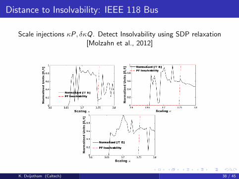
Distance to Insolvability: IEEE 118 Bus

Scale injections κP, δκQ. Detect Insolvability using SDP relaxation[Molzahn et al., 2012]


Convexity Region Operational Constraints

Fix bound on max(ViVj,Vj

Vi

)= exp (|ρi − ρj |)∀ (i , j) ∈ E .

Find maximum δ such that |θi − θj | ≤ δ∀ (i , j) ∈ E =⇒ (ρ, θ) ∈ C.


Table of Contents

1 Introduction






Summary

Summary

Power of Energy Function as an Analysis Tool

Several Applications in Different Power System Problem Domains

”Nice” power flow solutions easy to find

Convexity Analysis =⇒ Computational Tractability

Optimal Power Flow

Power Flow AnalysisTransient Stability Analysis

Estimation

Energy Function

Convexity

Tractability


Ongoing and Future Work

Ongoing Work

Extensions to Lossy case: Fixed BG ratio already works

Networks with small BG ratios - Initialized to region of convergence of

Newton’s method

Algorithmic developments and testing on IEEE benchmarks/realsystems

Relationship to Exactness of Convex Relaxations

Future Work

Scaling up algorithms - ADMM, Cutting plane etc.

Other Infrastructure Networks: Gas, Transportation etc.?

Variational modeling principles


Variational Modeling for Convexity

Nonconvex Formulation

Control Variables: u , Dependent Physical Variables: x

Minimizeu,x

f (u)︸︷︷︸Convex Control Cost

Subject to h (u, x) = 0︸︷︷︸Physics

, x ∈ S︸︷︷︸Safety Constraints

Convexity via Variational Prinicple

Variational Principle: h (u, x) = 0 ≡ ∇xE (u, x) = 0

Minimizeu,x

f (u) + λE (u, x) (λ << 1)

Subject to x ∈ S


Acknowledgements

Ian Hiskens, Scott Backhaus for initial discussions leading to this work

Anders Rantzer for saddle point interpretation of OPF convexification

Enrique Mallada, Dan Molzahn for useful comments

Misha Chertkov/Florian Dorfler for images used in slides


References/Questions

Older version under review at ACC

Journal version under development, posted to ArXiv soon.

http://www.its.caltech.edu/∼[email protected]

Questions?


A Araposthatis, S Sastry, and P Varaiya. Analysis of power-flow equation.International Journal of Electrical Power & Energy Systems, 3(3):115–126, 1981.

Russell Bent, Daniel Bienstock, and Michael Chertkov.Synchronization-aware and algorithm-efficient chance constrainedoptimal power flow. In Bulk Power System Dynamics and Control-IXOptimization, Security and Control of the Emerging Power Grid (IREP),2013 IREP Symposium, pages 1–11. IEEE, 2013.

A.R. Bergen and D.J. Hill. A structure preserving model for power systemstability analysis. Power Apparatus and Systems, IEEE Transactions on,PAS-100(1):25–35, Jan 1981. ISSN 0018-9510. doi:10.1109/TPAS.1981.316883.

Stephen Boyd and Lieven Vandenberghe. Convex optimization. Cambridgeuniversity press, 2009.

C.J.Tavora and O.J.M.Smith. Equilibrium analysis of power systems. IEEETransactions on Power Systems and Apparatus, 91(3):1131–1137, 1972.

Th. Van Cutsem and M. Ribbens-Pavella. Structure preserving directmethods for transient stability analysis of power systems. In Decision


and Control, 1985 24th IEEE Conference on, volume 24, pages 70–76,Dec 1985. doi: 10.1109/CDC.1985.268475.

Daniel K Molzahn, Bernard C Lesieutre, and Christopher L DeMarco. Asufficient condition for power flow insolvability with applications tovoltage stability margins. arXiv preprint arXiv:1204.6285, 2012.

Natarajan Narasimhamurthi and M Musavi. A generalized energy functionfor transient stability analysis of power systems. Circuits and Systems,IEEE Transactions on, 31(7):637–645, 1984.


Convex Energy Functions for Power Systems...

Documents

Transcript of Convex Energy Functions for Power Systems...