
converter station with CSCs. -...
69
7 2. LITERATURE SURVEY 2.1 HVDC Technologies in Recent Days Two basic converter technologies are used in modern HVDC transmission systems. These are conventional line-commutated current source converters (CSCs) and self- commutated voltage source converters (VSCs). Figure 2.1 shows a conventional HVDC converter station with CSCs. Figure 2.1: Conventional HVDC with Current Source Converters 2.1.1 Line-commutated current source converter Conventional HVDC transmission employs line-commutated CSCs with thyristor valves. Such converters require a synchronous voltage source in order to operate. The basic building block used for HVDC conversion is the three phase, full-wave bridge referred to as a six-pulse or Graetz bridge. The term six-pulse is due to six commutations or switching operations per period resulting in a characteristic harmonic ripple of six times the fundamental frequency in the DC output voltage. Each six-pulse bridge is comprised of six controlled switching elements or thyristor valves. Each valve is comprised of a suitable number of series-connected thyristors to achieve the desired DC voltage rating. The DC terminals of two six-pulse bridges with AC voltage sources phase displaced by 30 0 can be connected in series to increase the DC voltage and eliminate some of the characteristic AC current and DC voltage harmonics. Operation in this manner is referred to as 12-pulse
Transcript of converter station with CSCs. -...

7
2. LITERATURE SURVEY
2.1 HVDC Technologies in Recent Days
Two basic converter technologies are used in modern HVDC transmission systems.
These are conventional line-commutated current source converters (CSCs) and self-
commutated voltage source converters (VSCs). Figure 2.1 shows a conventional HVDC
converter station with CSCs.
Figure 2.1: Conventional HVDC with Current Source Converters
2.1.1 Line-commutated current source converter
Conventional HVDC transmission employs line-commutated CSCs with thyristor
valves. Such converters require a synchronous voltage source in order to operate. The basic
building block used for HVDC conversion is the three phase, full-wave bridge referred to as
a six-pulse or Graetz bridge. The term six-pulse is due to six commutations or switching
operations per period resulting in a characteristic harmonic ripple of six times the
fundamental frequency in the DC output voltage. Each six-pulse bridge is comprised of six
controlled switching elements or thyristor valves. Each valve is comprised of a suitable
number of series-connected thyristors to achieve the desired DC voltage rating. The DC
terminals of two six-pulse bridges with AC voltage sources phase displaced by 300 can be
connected in series to increase the DC voltage and eliminate some of the characteristic AC
current and DC voltage harmonics. Operation in this manner is referred to as 12-pulse

8
operation. In 12-pulse operation, the characteristic AC current and DC voltage harmonics
have frequencies of 12n+1 and 12n, respectively.
The 300 phase displacement is achieved by feeding one bridge through a transformer
with a wye-connected secondary and the other bridge through a transformer with a delta-
connected secondary. Most modern HVDC transmission schemes utilize 12-pulse converters
to reduce the harmonic filtering requirements required for six-pulse operation; e.g. , fifth and
seventh on the AC side and sixth on the DC side.
This is because, although these harmonic currents still flow through the valves and
the transformer windings, they are 1800 out of phase and cancel out on the primary side of
the converter transformer.
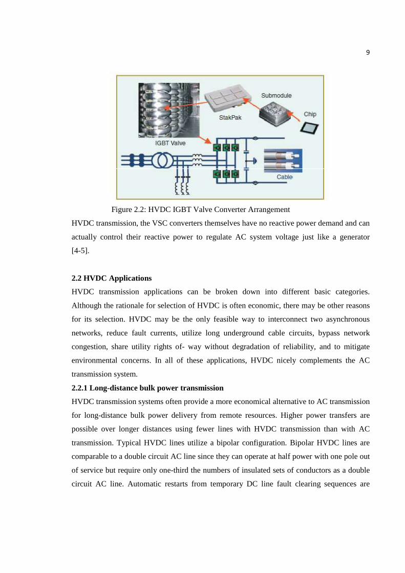
2.1.2 Self-commutated voltage source converter
HVDC transmission using VSCs with pulse-width modulation (PWM), commercially
known as HVDC Light, was introduced in the late 1990s. Since then the progression to
higher voltage and power ratings for these converters has roughly paralleled that for thyristor
valve converters in the 1970s. These VSC-based systems are self commutated with insulated-
gate bipolar transistor (IGBT) valves and solid-dielectric extruded HVDC cables. Figure
illustrates solid-state converter development for the two different types of converter
technologies using thyristor valves and IGBT valves.
HVDC transmission with VSCs can be beneficial to overall system performance.
VSC technology can rapidly control both active and reactive power independently of one
another. Reactive power can also be controlled at each terminal independent of the DC
transmission voltage level.
This control capability gives total flexibility to place converters anywhere in the AC
network since there is no restriction on minimum network short-circuits capacity. Self-
commutation with VSC even permits black start; i.e., the converter can be used to synthesize
a balanced set of three phase voltages like a virtual synchronous generator.
The dynamic support of the AC voltage at each converter terminal improves the
voltage stability and can increase the transfer capability of the sending- and receiving-end
AC systems, thereby leveraging the transfer capability of the DC link.
9
Figure 2.2: HVDC IGBT Valve Converter Arrangement
HVDC transmission, the VSC converters themselves have no reactive power demand and can
actually control their reactive power to regulate AC system voltage just like a generator
[4-5].
2.2 HVDC Applications
HVDC transmission applications can be broken down into different basic categories.
Although the rationale for selection of HVDC is often economic, there may be other reasons
for its selection. HVDC may be the only feasible way to interconnect two asynchronous
networks, reduce fault currents, utilize long underground cable circuits, bypass network
congestion, share utility rights of- way without degradation of reliability, and to mitigate
environmental concerns. In all of these applications, HVDC nicely complements the AC
transmission system.
2.2.1 Long-distance bulk power transmission
HVDC transmission systems often provide a more economical alternative to AC transmission
for long-distance bulk power delivery from remote resources. Higher power transfers are
possible over longer distances using fewer lines with HVDC transmission than with AC
transmission. Typical HVDC lines utilize a bipolar configuration. Bipolar HVDC lines are
comparable to a double circuit AC line since they can operate at half power with one pole out
of service but require only one-third the numbers of insulated sets of conductors as a double
circuit AC line. Automatic restarts from temporary DC line fault clearing sequences are
10
routine even for generator outlet transmission. No synchro-checking is required as for
automatic reclosures following AC line faults since the DC restarts do not expose turbine
generator units to high risk of transient torque amplification from closing into faults or across
high phase angles. The controllability of HVDC links offer firm transmission capacity
without limitation due to network congestion or loop flow on parallel paths. Controllability
allows the HVDC to “leap-frog” multiple “choke-points” or bypass sequential path limits in
the AC network. Therefore, the utilization of HVDC links is usually higher than that for extra
high voltage AC transmission, lowering the transmission cost per MWh. This controllability
can also be very beneficial for the parallel transmission since, by eliminating loop flow, it
frees up this transmission capacity for its intended purpose of serving intermediate load and
providing an outlet for local generation.
Whenever long-distance transmission is discussed, the concept of “break-even
distance” frequently arises. This is where the savings in line costs offset the higher converter
station costs. A bipolar HVDC line uses only two insulated sets of conductors rather than
three. This results in narrower rights-of-way, smaller transmission towers, and lower line
losses than with AC lines of comparable capacity. A rough approximation of the savings in
line construction is 30%. Although break-even distance is influenced by the costs of right-of-
way and line construction with a typical value of 500 km, the concept itself is misleading
because in many cases more AC lines are needed to deliver the same power over the same
distance due to system stability limitations. Furthermore, the long-distance AC lines usually
require intermediate switching stations and reactive power compensation. This can increase
the substation costs for AC transmission to the point where it is comparable to that for
HVDC transmission.
For example, the generator outlet transmission alternative for the ±250-kV, 500- MW
Square Butte Project was two 345-kV series-compensated AC transmission lines. The first
6,000-MW stage of the transmission for the Three Gorges Project in China would have
required 5×500-kV AC lines as opposed to 2 ×±500-kV, 3,000-MW bipolar HVDC lines.
2.2.2 Underground and submarine cable transmission
Unlike the case for AC cables, there is no physical restriction limiting the distance or
power level for HVDC underground or submarine cables. Underground cables can be used
on shared rights-of way with other utilities without impacting reliability concerns over use of
11
common corridors. For underground or submarine cable systems there is considerable
savings in installed cable costs and cost of losses when using HVDC transmission.
Depending on the power level to be transmitted, these savings can offset the higher
converter station costs at distances of 40 km or more. Furthermore, there is a drop-off in
cable capacity with AC transmission over distance due to its reactive component of charging
current since cables have higher capacitances and lower inductances than AC overhead lines.
Although this can be compensated by intermediate shunt compensation for underground
cables at increased expense, it is not practical to do so for submarine cables. For a given
cable conductor area, the line losses with HVDC cables can be about half those of AC cables.
This is due to AC cables requiring more conductors (three phases), carrying the reactive
component of current, skin-effect, and induced currents in the cable sheath and armor. With a
cable system, the need to balance unequal loadings or the risk of postcontingency overloads
often necessitates use of a series-connected reactors or phase shifting transformers. These
potential problems do not exist with a controlled HVDC cable system. Extruded HVDC
cables with prefabricated joints used with VSC-based transmission are lighter, more flexible,
and easier to splice than the mass-impregnated oil-paper cables (MINDs) used for
conventional HVDC transmission, thus making them more conducive for land cable
applications where transport limitations and extra splicing costs can drive up installation
costs. The lower-cost cable installations made possible by the extruded HVDC cables and
prefabricated joints makes long-distance underground transmission economically feasible for
use in areas with rights-of-way constraints or subject to permitting difficulties or delays with
overhead lines.
2.2.3 Asynchronous ties
With HVDC transmission systems, interconnections can be made between
asynchronous networks for more economic or reliable system operation. The asynchronous
interconnection allows interconnections of mutual benefit while providing a buffer between
the two systems. Often these interconnections use back-to-back converters with no
transmission line. Asynchronous HVDC links act as an effective “firewall” against
propagation of cascading outages in one network from passing to another network.
Asynchronous ties can eliminate market “electrical seams” while retaining natural
points of separation. Interconnections between asynchronous networks are often at the
12
periphery of the respective systems where the networks tend to be weak relative to the
desired power transfer. Higher power transfers can be achieved with improved voltage
stability in weak system applications using CCCs. The dynamic voltage support and
improved voltage stability offered by VSC-based converters permits even higher power
transfers without as much need for AC system reinforcement. VSCs do not suffer
commutation failures, allowing fast recoveries from nearby AC faults. Economic power
schedules that reverse power direction can be made without any restrictions since there is no
minimum power or current restrictions.
2.2.4 Multiterminal systems
Most HVDC systems are for point-to-point transmission with a converter station at
each end. The use of intermediate taps is rare. Conventional HVDC transmission uses
voltage polarity reversal to reverse the power direction. Polarity reversal requires no special
switching arrangement for a two terminal system where both terminals reverse polarity by
control action with no switching to reverse power direction. Special DC-side switching
arrangements are needed for polarity reversal in a multiterminal system, however, where it
may be desired to reverse the power direction at a tap while maintaining the same power
direction on the remaining terminals. For a bipolar system this can be done by connecting the
converter to the opposite pole. VSC HVDC transmission, however, reverses power through
reversal of the current direction rather than voltage polarity. Thus, power can be reversed at
an intermediate tap independently of the main power flow direction without switching to
reverse voltage polarity.
2.2.5 Power delivery to large urban areas
Power supply for large cities depends on local generation and power import
capability. Local generation is often older and less efficient than newer units located
remotely. Often, however, the older, less-efficient units located near the city center must be
dispatched out-of merit because they must be run for voltage support or reliability due to
inadequate transmission. Air quality regulations may limit the availability of these units. New
transmission into large cities is difficult to site due to right-of-way and land-use constraints.
Compact VSC-based underground transmission circuits can be placed on existing dual-use
rights-of-way to bring in power as well as to provide voltage support, allowing a more
economical power supply without compromising reliability. The receiving terminal acts like
13
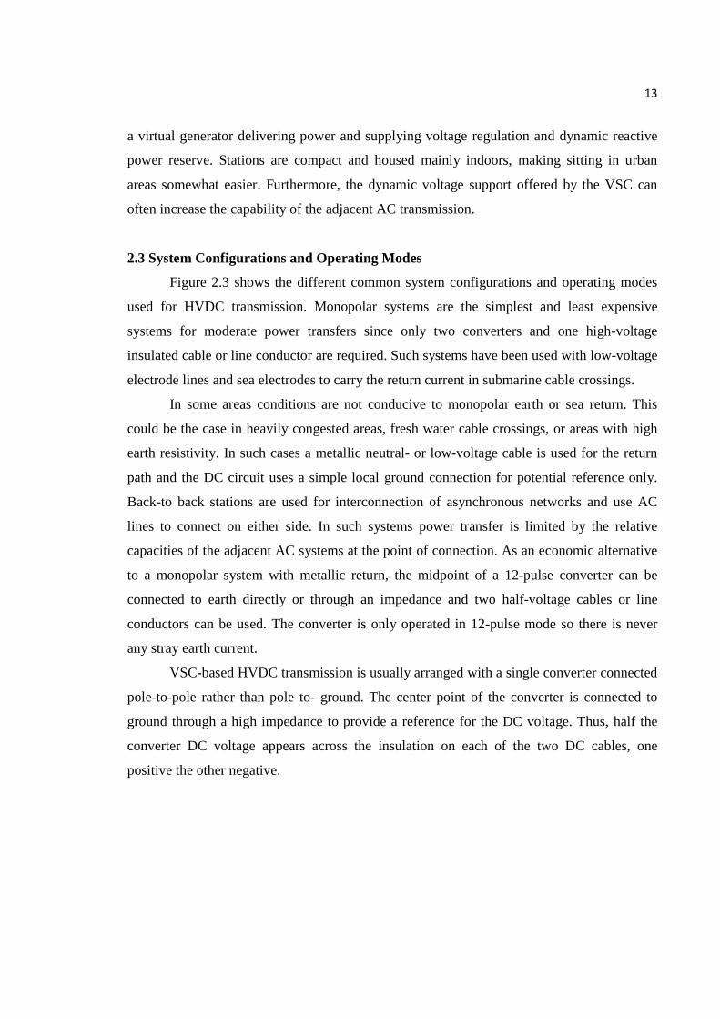
a virtual generator delivering power and supplying voltage regulation and dynamic reactive
power reserve. Stations are compact and housed mainly indoors, making sitting in urban
areas somewhat easier. Furthermore, the dynamic voltage support offered by the VSC can
often increase the capability of the adjacent AC transmission.
2.3 System Configurations and Operating Modes
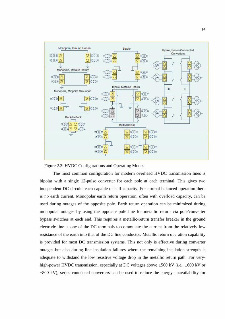
Figure 2.3 shows the different common system configurations and operating modes
used for HVDC transmission. Monopolar systems are the simplest and least expensive
systems for moderate power transfers since only two converters and one high-voltage
insulated cable or line conductor are required. Such systems have been used with low-voltage
electrode lines and sea electrodes to carry the return current in submarine cable crossings.
In some areas conditions are not conducive to monopolar earth or sea return. This
could be the case in heavily congested areas, fresh water cable crossings, or areas with high
earth resistivity. In such cases a metallic neutral- or low-voltage cable is used for the return
path and the DC circuit uses a simple local ground connection for potential reference only.
Back-to back stations are used for interconnection of asynchronous networks and use AC
lines to connect on either side. In such systems power transfer is limited by the relative
capacities of the adjacent AC systems at the point of connection. As an economic alternative
to a monopolar system with metallic return, the midpoint of a 12-pulse converter can be
connected to earth directly or through an impedance and two half-voltage cables or line
conductors can be used. The converter is only operated in 12-pulse mode so there is never
any stray earth current.
VSC-based HVDC transmission is usually arranged with a single converter connected
pole-to-pole rather than pole to- ground. The center point of the converter is connected to
ground through a high impedance to provide a reference for the DC voltage. Thus, half the
converter DC voltage appears across the insulation on each of the two DC cables, one
positive the other negative.
14
Figure 2.3: HVDC Configurations and Operating Modes
The most common configuration for modern overhead HVDC transmission lines is
bipolar with a single 12-pulse converter for each pole at each terminal. This gives two
independent DC circuits each capable of half capacity. For normal balanced operation there
is no earth current. Monopolar earth return operation, often with overload capacity, can be
used during outages of the opposite pole. Earth return operation can be minimized during
monopolar outages by using the opposite pole line for metallic return via pole/converter
bypass switches at each end. This requires a metallic-return transfer breaker in the ground
electrode line at one of the DC terminals to commutate the current from the relatively low
resistance of the earth into that of the DC line conductor. Metallic return operation capability
is provided for most DC transmission systems. This not only is effective during converter
outages but also during line insulation failures where the remaining insulation strength is
adequate to withstand the low resistive voltage drop in the metallic return path. For very-
high-power HVDC transmission, especially at DC voltages above ±500 kV (i.e., ±600 kV or
±800 kV), series connected converters can be used to reduce the energy unavailability for

15
individual converter outages or partial line insulation failure. By using two series-connected
converters per pole in a bipolar system, only one quarter of the transmission capacity is lost
for a converter outage or if the line insulation for the affected pole is degraded to where it can
only support half the rated DC line voltage. Operating in this mode also avoids the need to
transfer to monopolar metallic return to limit the duration of emergency earth return.
2.4 Economic Considerations
A study for Oak Ridge National Laboratory reported on a survey to 3 suppliers of
HVDC equipment for quotations of turnkey costs to supply two bipolar substations for four
representative systems. Each substation requires one DC electrode and interfaces to an AC
system with a short circuit capacity four times the rating of the HVDC system. The four
representative systems are summarized in Table 1. Table 2 provides a major component
breakdown based on average values derived from the responses of the suppliers. The turnkey
costs are in 1995/96 US dollars and are for one terminal only with the assumption that both
terminals would be provided by the same supplier. The back-to-back DC link cost is for the
complete installation. Transmission line costs cannot be so readily defined. Variations
depend on the cost of use of the land, the width of the right-of-way required, labor rates for
construction, and the difficulty of the terrain to be crossed. A simple rule of thumb may be
applied in that the cost of a DC transmission line may be 80% to 100% of the cost of an AC
line whose rated line voltage is the same as the rated pole-to-ground voltage of the DC line.
The cost advantage of DC transmission for traversing long distances is that it may be rated at
twice the power flow capacity of an AC line of the same voltage.
Table 2.1: Four Representative HVDC Systems for Substation Cost Analysis
System no. D.C. voltage Capacity A.C. Voltage
1. +250 kV 500 MW 230 kV
2. +350 kV 1000 MW 345 kV
3. +500 kV 3000 MW 500 kV
4. Back – to – back 200 MW 230 kV
16
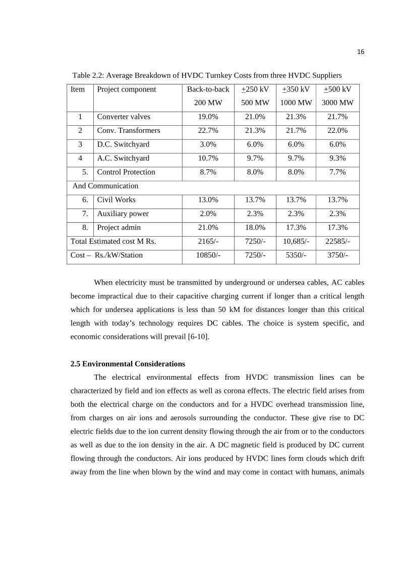
Table 2.2: Average Breakdown of HVDC Turnkey Costs from three HVDC Suppliers
Item Project component Back-to-back
200 MW
+250 kV
500 MW
+350 kV
1000 MW
+500 kV
3000 MW
1 Converter valves 19.0% 21.0% 21.3% 21.7%
2 Conv. Transformers 22.7% 21.3% 21.7% 22.0%
3 D.C. Switchyard 3.0% 6.0% 6.0% 6.0%
4 A.C. Switchyard 10.7% 9.7% 9.7% 9.3%
5. Control Protection 8.7% 8.0% 8.0% 7.7%
And Communication
6. Civil Works 13.0% 13.7% 13.7% 13.7%
7. Auxiliary power 2.0% 2.3% 2.3% 2.3%
8. Project admin 21.0% 18.0% 17.3% 17.3%
Total Estimated cost M Rs. 2165/- 7250/- 10,685/- 22585/-
Cost – Rs./kW/Station 10850/- 7250/- 5350/- 3750/-
When electricity must be transmitted by underground or undersea cables, AC cables
become impractical due to their capacitive charging current if longer than a critical length
which for undersea applications is less than 50 kM for distances longer than this critical
length with today’s technology requires DC cables. The choice is system specific, and
economic considerations will prevail [6-10].
2.5 Environmental Considerations
The electrical environmental effects from HVDC transmission lines can be
characterized by field and ion effects as well as corona effects. The electric field arises from
both the electrical charge on the conductors and for a HVDC overhead transmission line,
from charges on air ions and aerosols surrounding the conductor. These give rise to DC
electric fields due to the ion current density flowing through the air from or to the conductors
as well as due to the ion density in the air. A DC magnetic field is produced by DC current
flowing through the conductors. Air ions produced by HVDC lines form clouds which drift
away from the line when blown by the wind and may come in contact with humans, animals
17
and plants outside the transmission line right-of -way or corridor. The corona effects may
produce low levels of radio interference, audible noise and ozone generation.
2.5.1 Field and corona effects
The field and corona effects of transmission lines largely favor DC transmission over AC
transmission. The significant considerations are as follows:
1. For a given power transfer requiring extra high voltage transmission, the DC transmission
line will have a smaller tower profile than the equivalent AC tower carrying the same
level of power. This can also lead to less width of right-of-way for the DC transmission
option.
2. The steady and direct magnetic field of a DC transmission line near or at the edge of the
transmission right-of-way will be about the same value in magnitude as the earth’s
naturally occurring magnetic field. For this reason alone, it seems unlikely that this small
contribution by HVDC transmission lines to the background geomagnetic field would be
a basis for concern.
3. The static and steady electric field from DC transmission at the levels experienced
beneath lines or at the edge of the right-of-way have no known adverse biological effects.
There is no theory or mechanism to explain how a static electric field at the levels
produced by DC transmission lines could effect human health. The electric field level
beneath a HVDC transmission line is of similar magnitude as the naturally occurring
static field which exists beneath thunder clouds. Electric fields from AC transmission
lines have been under more intense scrutiny than fields generated from DC transmission
lines.
4. The ion and corona effects of DC transmission lines lead to a small contribution of ozone
production to higher naturally occurring background concentrations. Exacting long term
measurements are required to detect such concentrations. The measurements taken at
cross-sections across the Nelson River DC lines in Canada failed to distinguish
background from downwind levels. While solar radiation influences the production of
ozone even in a rural environment, thereby maintaining its level, any incremental
contribution from a DC line source is subject to breakdown, leading to a resumption of
background levels downwind from the line. Investigations of ozone for indoor conditions

18
indicate that in well mixed air, the half-life of ozone is 1.5 minutes to 7.9 minutes.
Increases in temperature and humidity increase the rate of decay.
5. If ground return is used with monopolar operation, the resulting DC magnetic field can
cause error in magnetic compass readings taken in the vicinity of the DC line or cable.
This impact is minimized by providing a conductor or cable return path (known as
metallic return) in close proximity to the main conductor or cable for magnetic field
cancellation. Another concern with continuous ground current is that some of the return
current may flow in metallic structures such as pipelines and intensify corrosion if
cathodic protection is not provided. When pipelines or other continuous metallic
grounded structures are in the vicinity of a DC link, metallic return may be necessary
[11-19].
2.6 Station Design and Layout
The converter station layout depends on a number of factors such as the DC system
configuration (i.e., monopolar, bipolar, or back-to-back), AC filtering, and reactive power
compensation requirements. The thyristor valves are air-insulated, water-cooled, and
enclosed in a converter building often referred to as a valve hall. For back-to-back ties with
their characteristically low DC voltage, thyristor valves can be housed in prefabricated
electrical enclosures, in which case a valve hall is not required. To obtain a more compact
station design and reduce the number of insulated high-voltage wall bushings, converter
transformers are often placed adjacent to the valve hall with valve winding bushings
protruding through the building walls for connection to the valves. Double or quadruple
valve structures housing valve modules are used within the valve hall. Valve arresters are
located immediately adjacent to the valves. Indoor motor-operated grounding switches are
used for personnel safety during maintenance. Closed-loop valve cooling systems are used to
circulate the cooling medium, deionized water or water-glycol mix, through the indoor
thyristor valves with heat transfer to dry coolers located outdoors. Area requirements for
conventional HVDC converter stations are influenced by the AC system voltage and reactive
power compensation requirements where each individual bank rating may be limited by such
system requirements as reactive power exchange and maximum voltage step on bank
19
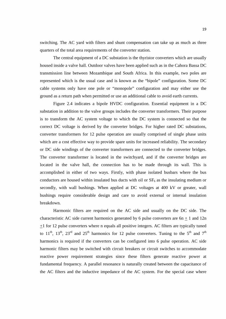
switching. The AC yard with filters and shunt compensation can take up as much as three
quarters of the total area requirements of the converter station.
The central equipment of a DC substation is the thyristor converters which are usually
housed inside a valve hall. Outdoor valves have been applied such as in the Cahora Bassa DC
transmission line between Mozambique and South Africa. In this example, two poles are
represented which is the usual case and is known as the “bipole” configuration. Some DC
cable systems only have one pole or “monopole” configuration and may either use the
ground as a return path when permitted or use an additional cable to avoid earth currents.
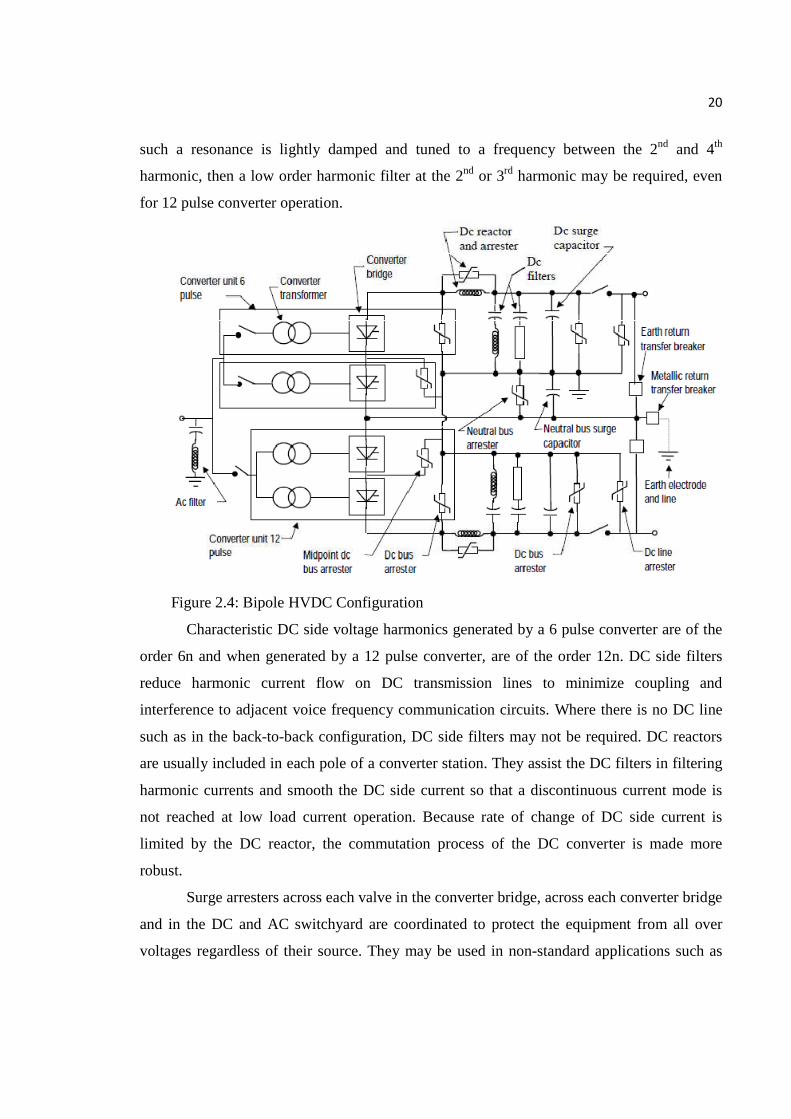
Figure 2.4 indicates a bipole HVDC configuration. Essential equipment in a DC
substation in addition to the valve groups includes the converter transformers. Their purpose
is to transform the AC system voltage to which the DC system is connected so that the
correct DC voltage is derived by the converter bridges. For higher rated DC substations,
converter transformers for 12 pulse operation are usually comprised of single phase units
which are a cost effective way to provide spare units for increased reliability. The secondary
or DC side windings of the converter transformers are connected to the converter bridges.
The converter transformer is located in the switchyard, and if the converter bridges are
located in the valve hall, the connection has to be made through its wall. This is
accomplished in either of two ways. Firstly, with phase isolated busbars where the bus
conductors are housed within insulated bus ducts with oil or SF6 as the insulating medium or
secondly, with wall bushings. When applied at DC voltages at 400 kV or greater, wall
bushings require considerable design and care to avoid external or internal insulation
breakdown.
Harmonic filters are required on the AC side and usually on the DC side. The
characteristic AC side current harmonics generated by 6 pulse converters are 6n + 1 and 12n
+1 for 12 pulse converters where n equals all positive integers. AC filters are typically tuned
to 11th, 13th, 23rd and 25th harmonics for 12 pulse converters. Tuning to the 5th and 7th
harmonics is required if the converters can be configured into 6 pulse operation. AC side
harmonic filters may be switched with circuit breakers or circuit switches to accommodate
reactive power requirement strategies since these filters generate reactive power at
fundamental frequency. A parallel resonance is naturally created between the capacitance of
the AC filters and the inductive impedance of the AC system. For the special case where
20
such a resonance is lightly damped and tuned to a frequency between the 2nd and 4th
harmonic, then a low order harmonic filter at the 2nd or 3rd harmonic may be required, even
for 12 pulse converter operation.
Figure 2.4: Bipole HVDC Configuration
Characteristic DC side voltage harmonics generated by a 6 pulse converter are of the
order 6n and when generated by a 12 pulse converter, are of the order 12n. DC side filters
reduce harmonic current flow on DC transmission lines to minimize coupling and
interference to adjacent voice frequency communication circuits. Where there is no DC line
such as in the back-to-back configuration, DC side filters may not be required. DC reactors
are usually included in each pole of a converter station. They assist the DC filters in filtering
harmonic currents and smooth the DC side current so that a discontinuous current mode is
not reached at low load current operation. Because rate of change of DC side current is
limited by the DC reactor, the commutation process of the DC converter is made more
robust.
Surge arresters across each valve in the converter bridge, across each converter bridge
and in the DC and AC switchyard are coordinated to protect the equipment from all over
voltages regardless of their source. They may be used in non-standard applications such as

21
filter protection. Modern HVDC substations use metal-oxide arresters and their rating and
selection is made with careful insulation coordination design [5,20].
2.7 Series Capacitors with DC Converter Substations
HVDC transmission systems with long DC cables are prone to commutation failure
when there is a drop in DC voltage Ud at the inverter. The DC cable has very large
capacitance which will discharge current towards the voltage drop at the inverter. The
discharge current is limited by the DC voltage derived from the AC voltage of the
commutating bus as well as the DC smoothing reactor and the commutating reactance. If the
discharge current of the cable increases too quickly, commutation failure will occur causing
complete discharge of the cable. To recharge the cable back to its normal operating voltage
will delay recovery.
The converter bridge firing controls can be designed to increase the delay angle α
when an increase in DC current is detected. This may be effective until the limit of the
minimum allowable extinction angle γ is reached.
Another way to limit the cable discharge current is to operate the inverter bridge with
a three phase series capacitor located in the AC system on either side of the converter
transformer. Any discharge current from the DC cable will pass into the AC system through
the normally functioning converter bridge and in doing so, will pass through the series
capacitor and add charge to it. As a consequence, the voltage of the series capacitor will
increase to oppose the cable discharge and be reflected through the converter bridge as an
increase in DC voltage Ud. This will act as a back emf and limit the discharge current of the
cable, thereby avoiding the commutation failure.
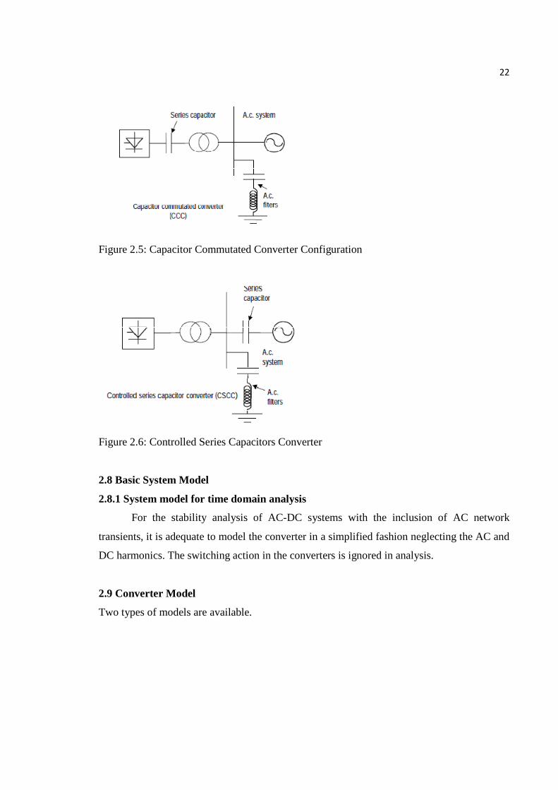
The proposed locations of the series capacitor are shown in figure 2.5 and figure 2.6
in single line diagram form. With the capacitor located between the converter transformer
and the valve group, it is known as a capacitor commutated converter (CCC). With the
capacitor located on the AC system side of the converter transformer, it is known as a
controlled series capacitor converter (CSCC). Each configuration will improve commutation
performance of the inverter but the CSCC requires design features to eliminate
ferroresonance between the series capacitor and the converter transformer if it should be
instigated [21-26].
22
Figure 2.5: Capacitor Commutated Converter Configuration
Figure 2.6: Controlled Series Capacitors Converter
2.8 Basic System Model
2.8.1 System model for time domain analysis
For the stability analysis of AC-DC systems with the inclusion of AC network
transients, it is adequate to model the converter in a simplified fashion neglecting the AC and
DC harmonics. The switching action in the converters is ignored in analysis.
2.9 Converter Model
Two types of models are available.

23
2.9.1 Simplified continuous time model
Figure 2.7: Simplified Continuous Time Equivalent Circuit of a Bridge
2.9.2 Detailed model of the converter
For detailed dynamic simulation of HVDC systems, it is necessary to represent the
switching action in the valves, assuming that the valves can be modeled as ideal switches.
The switch is turned on at the instant of firing which in turn is determined by the converter
control system including gate pulse firing control. The switch turns off when the current in
the valve goes to zero. The turn-off time required can be simulated by closing the switch if a
forward voltage appears within the turn-off time.
Figure 2.8: The Equivalent Circuit for the Transient Simulation of a Bridge
The converter bridge has been modeled by the equivalent circuit shown in figure 2.8.
This is a variable voltage source behind a variable inductance. This applies for the case when
transformer winding resistances are neglected and the leakage reactances in all the phases are
assumed to be identical.
24
The transition from two valves to three valve conduction occurs at the firing of a
valve, it is assumed that there is a forward voltage across the incoming valve. α is delay
angle. The angle of advance β is related in degrees to the angle of delay a by:
β = 180.0 - α …2.1
Extinction angle γ depends on the angle of advance β and the angle of overlap µ and
is determined by the relation:
γ = β - µ …2.2
The transition from three to two valve conduction can be estimated from
( )LL
dd
E
iiXct
2coscos 21 +=− ωα
…2.3
Where, id1 is the DC current at the firing of the incoming valve and id2 is the current at the
transition. ELL is the rms value of the commutation voltage of the incoming valve. It is
assumed that at the instant t = 0, the commutation voltage becomes positive. Equation 2.3 is
based on the assumption of sinusoidal commutation voltages [27-29].
2.9.3 Modeling of DC network
The DC network is assumed to consist of smoothing reactor, DC filters and the
transmission line. The smoothing reactor and DC filters can be represented by lumped
parameter linear elements. The DC line can also be modeled as a T or π equivalent if the
higher frequency behavior is not of interest.
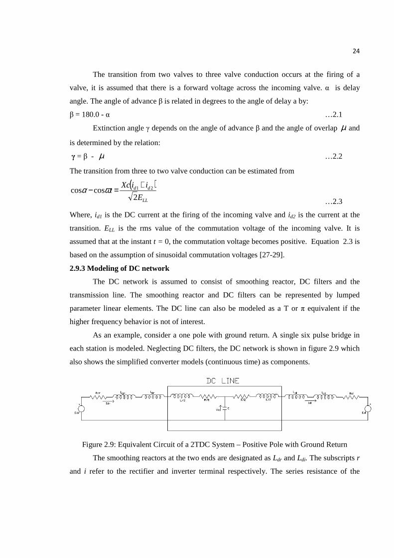
As an example, consider a one pole with ground return. A single six pulse bridge in
each station is modeled. Neglecting DC filters, the DC network is shown in figure 2.9 which
also shows the simplified converter models (continuous time) as components.
Figure 2.9: Equivalent Circuit of a 2TDC System – Positive Pole with Ground Return
The smoothing reactors at the two ends are designated as Ldr and Ldi. The subscripts r
and i refer to the rectifier and inverter terminal respectively. The series resistance of the
25
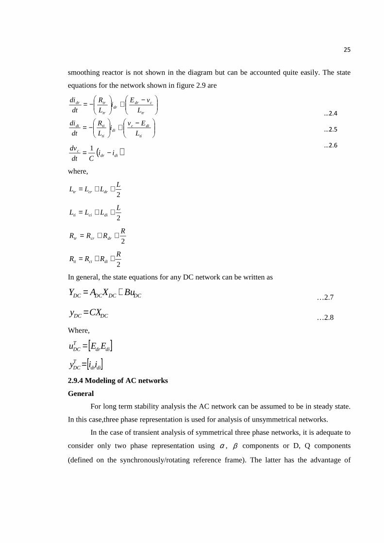
smoothing reactor is not shown in the diagram but can be accounted quite easily. The state
equations for the network shown in figure 2.9 are
−+
−=
−+
−=
ti
dicdi
ti
tidi
tr
cdrdr
tr
trdr
L
Evi
L
R
dt
di
L
vEi
L
R
dt
di
( )didrc ii
Cdt
dv −= 1
where,
2
LLLL drcrtr ++=
2
LLLL diciti ++=
2
RRRR drcrtr ++=
2
RRRR diciti ++=
In general, the state equations for any DC network can be written as
DCDCDCDC BuXAY += …2.7
DCDC CXy = …2.8
Where,
[ ]didrTDC EEu =
[ ]didrTDC iiy =
2.9.4 Modeling of AC networks
General
For long term stability analysis the AC network can be assumed to be in steady state.
In this case,three phase representation is used for analysis of unsymmetrical networks.
In the case of transient analysis of symmetrical three phase networks, it is adequate to
consider only two phase representation using α , β components or D, Q components
(defined on the synchronously/rotating reference frame). The latter has the advantage of
…2.4
…2.5
…2.6
26
eliminating the time-varying coupling between AC and DC system, and, hence, is convenient
for analytical studies. It also has the advantage that, in steady state D, Q components is
constants and is related to the phasors in load flow analysis.
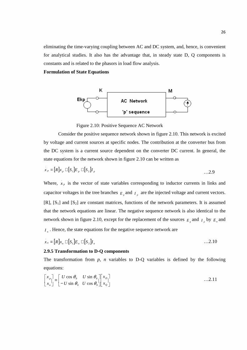
Formulation of State Equations
Figure 2.10: Positive Sequence AC Network
Consider the positive sequence network shown in figure 2.10. This network is excited
by voltage and current sources at specific nodes. The contribution at the converter bus from
the DC system is a current source dependent on the converter DC current. In general, the
state equations for the network shown in figure 2.10 can be written as
[ ] [ ] [ ] pppp ISESxRx 21
.
++= …2.9
Where, px.
is the vector of state variables corresponding to inductor currents in links and
capacitor voltages in the tree branches pE and
pI are the injected voltage and current vectors.
[R], [S1] and [S2] are constant matrices, functions of the network parameters. It is assumed
that the network equations are linear. The negative sequence network is also identical to the
network shown in figure 2.10, except for the replacement of the sources pE and
pI by nE and
nI . Hence, the state equations for the negative sequence network are
[ ] [ ] [ ] nnnn ISESxRx 21
.
++= …2.10
2.9.5 Transformation to D-Q components
The transformation from p, n variables to D-Q variables is defined by the following
equations:
−=
Q
D
n
p
x
x
U
U
U
U
x
x
0
0
0
0
cos
sin
sin
cos
θθ
θθ …2.11
27
Where, U is the identity matrix of dimension equal to the order of pX or nX . 0θ is the
angle by which the D axis leads a stationary axis. It is to be noted that
00 ωθ =
dt
d …2.12
is assumed to be constant.
Substituting equation 2.11 in equation 2.9 and 2.10 leads to the following equations
[ ] [ ] [ ] DDQDD ISESxxRx 210
.
++−= ω …2.13
[ ] [ ] [ ] QQDQQ ISESxxRx 210
.
+++= ω …2.14
Where, ED, EQ and ID, IQ are the D, Q components of the voltage and current sources
respectively.
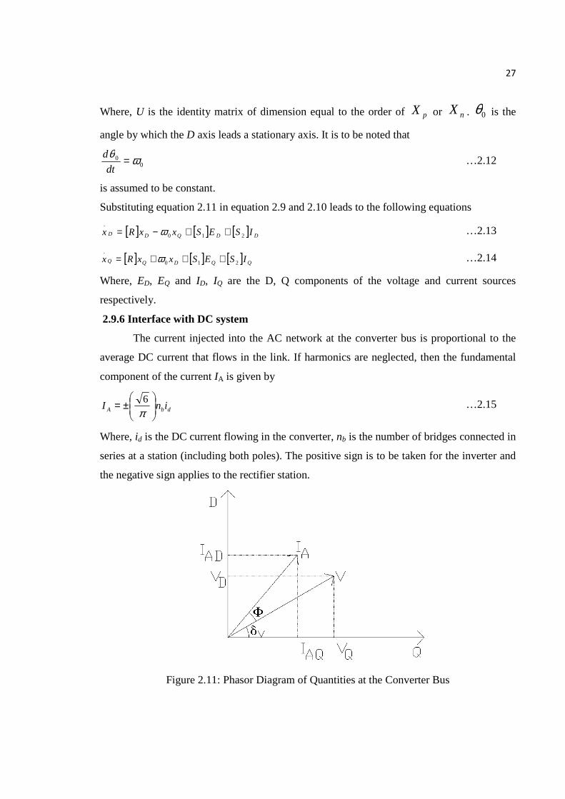
2.9.6 Interface with DC system
The current injected into the AC network at the converter bus is proportional to the
average DC current that flows in the link. If harmonics are neglected, then the fundamental
component of the current IA is given by
dbA inI
±=
π6 …2.15
Where, id is the DC current flowing in the converter, nb is the number of bridges connected in
series at a station (including both poles). The positive sign is to be taken for the inverter and
the negative sign applies to the rectifier station.
Figure 2.11: Phasor Diagram of Quantities at the Converter Bus

28
The injected current IA in steady state leads the converter bus voltage by an angle φ . The
phasor diagram shown in figure 2.11 gives the relative position of the current and voltage
phasors in D-Q reference frame. From this, the following equations can be derived.
( )vAAD II δφ+= sin …2.16
( )vAAQ II δφ+= cos …2.17
The angle vδ by which the converter bus voltage phasor V leads the Q axis, is given by
Q
Dv V
V=δtan …2.18
The angle φ is defined by
= −
aV
vd1cosφ …2.19
for the inverter, and by
πφ +
−= −
aV
vd1cos …2.20
For the rectifier, Vd is the average DC voltage across a converter bridge. It is to be
noted that equations 2.16 to 2.20 are nonlinear and have to be linearized for the analysis of
stability of the equilibrium (operating) state of the AC/DC system. In equidistant pulse firing
scheme, the delay angle is not only determined by the current controller but is also affected
by the angle vδ . As the angle vδ increases, the delay angle increases (as the voltage phasor
has increased lead), even if the change in delay angle demanded by the current controller is
zero.
2.9.7 Modeling of a synchronous generator
The state equations of a synchronous machine are written in terms of the phase
variables (three phase currents or flux linkages). However, these equations are nonlinear and
time-varying due to the dependence of inductance coefficients on the rotor angle. The time-
varying system equations can be transformed into the time-invariant form by Park's
transformation. However, the direct use of equations in Park's variables (in d-q components)
is not feasible in multi-machine systems due to the existence of multiple Park's reference
29
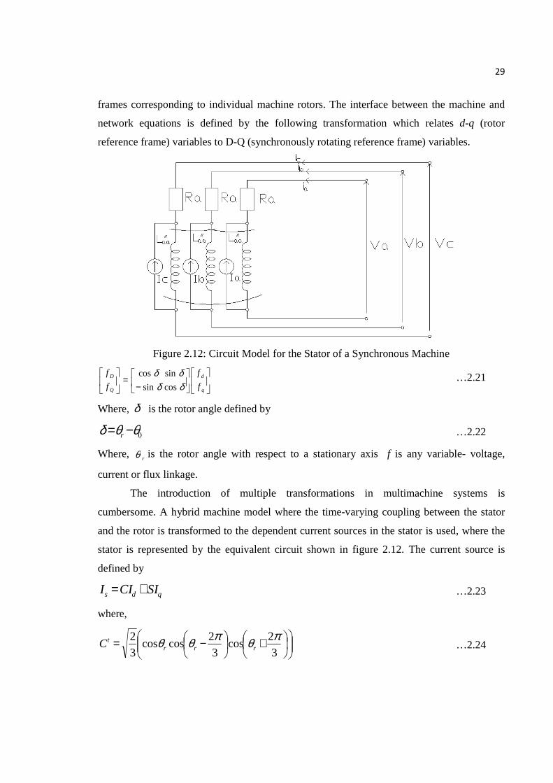
frames corresponding to individual machine rotors. The interface between the machine and
network equations is defined by the following transformation which relates d-q (rotor
reference frame) variables to D-Q (synchronously rotating reference frame) variables.
Figure 2.12: Circuit Model for the Stator of a Synchronous Machine
−=
q
d
Q
D
f
f
f
f
δδ
δδ
cos
sin
sin
cos …2.21
Where, δ is the rotor angle defined by
0θθδ −= r …2.22
Where, rθ is the rotor angle with respect to a stationary axis f is any variable- voltage,
current or flux linkage.
The introduction of multiple transformations in multimachine systems is
cumbersome. A hybrid machine model where the time-varying coupling between the stator
and the rotor is transformed to the dependent current sources in the stator is used, where the
stator is represented by the equivalent circuit shown in figure 2.12. The current source is
defined by
qds SICII += …2.23
where,
+
−=3
2cos
3
2coscos
3
2 πθπθθ rrrtC …2.24
30
+
−=3
2sin
3
2sinsin
3
2 πθπθθ rrrtS …2.25
( )cbats IIII =
dI and qI are defined by
rtdd kI ψ= , ccr
tqq kkI ψψ += …2.26
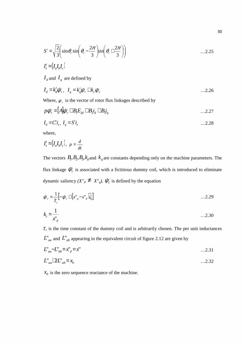
Where, rψ is the vector of rotor flux linkages described by
[ ] qdfdrr iBiBEBAp 321 +++= ψψ …2.27
st
d iCI = , st
q iSI = …2.28
where,
( )cbats IIII = ,
dt
dp =
The vectors dkBBB ,,, 321 and qk are constants depending only on the machine parameters. The
flux linkage cψ is associated with a fictitious dummy coil, which is introduced to eliminate
dynamic saliency (X"d ≠ X"q). cψ is defined by the equation
( )[ ]qdqcc
c ixxT
""1.
−+−= ψψ …2.29
dc x
k"
1= …2.30
Tc is the time constant of the dummy coil and is arbitrarily chosen. The per unit inductances
aaL" and abL" appearing in the equivalent circuit of figure 2.12 are given by
"""" xxLL dbbaa ==− …2.31
0"2" xLL abaa =+ …2.32
0x is the zero sequence reactance of the machine.
31
The advantage of this hybrid model is that the stator is represented by an equivalent circuit
with constant parameters. The phase variables can now be transformed into 0αβ variables as
follows
[ ] 01 pns iCi = …2.33
where,
( )00' iiii nppn β=
[ ]
−−=1
1
1
2
32
30
2
12
12
3
11C …2.34
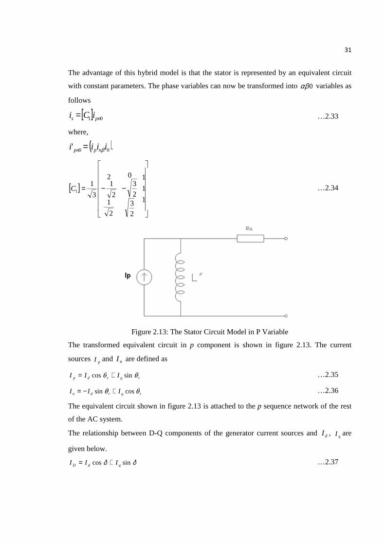
Figure 2.13: The Stator Circuit Model in P Variable
The transformed equivalent circuit in p component is shown in figure 2.13. The current
sources pI and nI are defined as
rqrdp III θθ sincos += …2.35
rqrdn III θθ cossin +−= …2.36
The equivalent circuit shown in figure 2.13 is attached to the p sequence network of the rest
of the AC system.
The relationship between D-Q components of the generator current sources and dI , qI are
given below.
δδ sincos qdD III += …2.37

32
δδ cossin qdQ III +−= …2.38
the electrical torque eT on the generator rotor is given by the following expression
( ) ( )QDDQqddqe IiIixIiIixT −=−= "" …2.39
The variablesaI , qI are related to the d-q components of stator flux linkages by the
following equations
( )ddd Iix += "ψ , ( )qqq Iix += "ψ …2.40
The hybrid model is used for stability analysis or transient analysis directly.
2.10 Basic System Model for Frequency Domain Analysis
The configuration of the HVDC transmission system model is as shown in figure
2.14. The linearized model is formed in a three-step process. The division of the system into
a number of smaller subsystems, the description of each sub system using a linearized model,
and, finally, the interconnection of the subsystems. This approach relies on the principle of
superposition for linear or linearized systems, and is a simpler approach than linearizing the
nonlinear equations which describe the system directly.
Figure 2.14 Model used for frequency Domain Analysis
The HVDC system is modeled using nine subsystems, which are the rectifier and
inverter AC systems, the rectifier and inverter AC filters and shunts capacitors, the DC
system, the rectifier and inverter HVDC converters, and the rectifier and inverter PLLs. The
firing angle-control inputs are left uncontrolled in the system. This model is used for the
representation of the general dynamics of an HVDC system in the frequency range between 2
and 200 Hz on the DC side.

33
2.10.1 State model formation
In order for the HVDC system to be represented in state model form, it is necessary
that a linear state model of each subsystem is available. A linear time-invariant state model
dynamically relates the subsystem inputs, outputs, and states using a state equation 2.41 and
an output equation 2.42, which are specified by the constant matrices. In the situation where
a state model is obtained by linearizing a system around an operating point, the input, output
and state variables represent the deviation of the system variables from their operating point
values.
BuAxx += …2.41
DuCxy += …2.42
The inputs and outputs of the state model are either signal or electrical variables.
Signal variables are associated with the measurement of electrical variables and control
subsystems, while electrical variables occur as voltage–current pairs, and are associated with
the electrical terminals of the subsystems. When connecting electrical subsystems together at
a busbar, only one subsystem can be represented in current-input voltage-output (impedance)
form, while all others must be represented in voltage-input current-output (admittance) form.
The subsystem in impedance form provides the voltage input for all of the subsystems in
admittance form, while the addition of the current outputs of the subsystems in admittance
form provides the current input to the subsystem in impedance form. A convention is adopted
where the flow of current into an electrical terminal is assumed to be of positive sign. It is
important to correctly choose the inputs and outputs of electrical subsystems such that firstly,
the inputs and outputs, which are to be connected together, are compatible, and secondly the
subsystems are proper. Only those systems which are proper, meaning the transfer functions
between the inputs and outputs of the system have at least as many poles as zeros, are able to
be described in the above state model form. If it is not possible to accommodate an improper
electrical subsystem (more zeros than poles) by interchanging inputs and outputs, then a
proper subsystem can be formed by adding extra poles above the frequency range of interest
to the system. Since standard methods are available to convert between proper–domain
transfer functions and state model representations, with respect to the input and output
relationships of the system, these two representations are equivalent. In cases where
subsystems are defined in terms of frequency response data, it is necessary to fit an s-domain
34
transfer function to the frequency response data. For simple frequency responses, an s-
domain representation can be obtained by inspection, while for more complicated frequency
responses, transfer-function fitting algorithms are available.
When forming system models, it is likely that a particular type of component, such as
the PLL and HVDC converter subsystems in the case described, will occur in multiplicity. In
this situation, it is of significant advantage to adopt a modular approach where the state
model of the component is specified as the output of a function. The subsystem state model
functions collectively form a library of components which may be called repeatedly during
the formation of system models. After proper defining the subsystems, they are connected
together to form a state model of the overall system.
2.10.2 Converter frequency-conversion process model
The conversion of electrical energy between AC and DC frequency is achieved by the
periodic firing of the HVDC converter thyristor valves. The switching action is the direct
cause of HVDC system nonlinearity, and the linearized representation of this process is of
significant importance to the system model. The converter is a complex single-frequency
input multiple frequency output modulators. A number of interactions, due to the frequency-
conversion process, occur between different frequencies on the AC and DC sides. An
arbitrary frequency on the DC side of the converter is related to two frequencies on the AC
side, separated by twice the fundamental frequency, positive sequence frequency, and
negative sequence frequency. A model which considers only these interactions is referred to
as a three-port model and is essentially of the describing function type. The zero-sequence
component of the AC system waveforms are omitted from the system models as they are
neither generated by nor affect the operation of three-phase power-electronic devices, such as
the HVDC converter.
Frequency conversion exhibits time-variance and cannot be directly represented in the
required state model form. In order to model the system in a time-invariant manner, it is
necessary to decouple the frequency-conversion process from the model of the converter.
The effect of the frequency-conversion process is accounted for by frequency shifting the
equations which describe the dynamics of the subsystems on the AC side of the converter.
Even though frequency conversion does not appear explicitly in the analysis, the interactions
are correctly represented through the altered subsystem dynamics. The dynamics of the

35
subsystems on the AC side of the converter can be frequency shifted using Park’s
transformation, or the transfer function zero-pole shifting approach.
2.10.3 AC system variable representation
As usual, three distinct representations of three-phase AC system voltage and current
variables are useful for the purposes of system modeling and control. The representations are
positive and negative sequence ( )pn components, direct and quadrature ( )DQ components,
and magnitude and angle ( )ma components. The transformations between the three AC
variable representations are described. The DQ and ma representations are with respect to a
synchronously rotating frame of reference, while sequence components may be at their actual
frequency or referred to their equivalent DC side frequency, depending on the context in
which they are used.
2.10.4 AC system variable transformations
The transform between DQ and PN components in equation 2.43 is obtained by
applying Park’s transformation to positive and negative sequence distortions. In this case, the
direct axis is referenced to a phase angle of zero, and the quadrature axis has been chosen to
lead the direct axis. If the frequency conversions involved with the transform are assumed to
be implicit, then the transform is considered linear
−=
n
p
Q
D
X
Xii
X
X
11 …2.43
The linearization of the transform between ma and DQ components in the synchronous
reference frame is given in equation 2.44
Where, XmD and XaD are the operating point magnitude and angle of the AC variable.
( ) ( )( ) ( )
∆∆
−=
∆∆
a
m
amoa
amoa
Q
D
X
X
XXX
XXX
X
X
0cos0sin
0sin0cos …2.44
2.10.5 Algorithm for the interconnection of the subsystems
The first step of the algorithm requires that the state models be diagonally appended.
The appended system, represented using capital letters for the inputs, outputs, and states, is
then rearranged so that all inputs/outputs, which are to be left unconnected, are grouped
together (indicated by the subscript 1), and all inputs/outputs which are to be connected are
grouped together (indicated by the subscript 2)

36
Using the matrix , which specifies the connections between the outputs and the inputs,
[ ]
=
2
121 U
UBBAXX …2.45
=
2
1
2221
1211
2
1
2
1 U
U
DD
DD
C
C
Y
Y …2.46
22 YHU =
the variables U2 and Y2 are eliminated from 2.49 and 2.50, resulting in a state model of the
form
( )[ ] ( )[ ] 1211
222121
222 11 UDHDHBBXCHDHBAX −− −++−+= …2.47
( )[ ] ( )[ ] 12122121121
221211 111 UDHDHDDXCHDHDCY −−++−+= − …2.48
Where, ‘I’ is the identity matrix.
2.10.6 AC system and filters
The rectifier and inverter AC systems and filters are represented using frequency
dependent equivalents which describe their electrical characteristics as seen from the AC
terminals of the converters. The HVDC converter uses AC voltage as an input, while the
nature of the AC system (series inductance) and the AC filters (shunt capacitance) means that
these subsystems are most appropriately represented in admittance and impedance forms,
respectively. To enable the connection of the subsystems at the AC terminals of the
converters without the need for variable transformations, a common sequence component is
chosen to represent the AC variables. The relationships between the inputs and outputs of the
AC system model are described by 2.48. It is assumed that the positive and negative
sequence admittances of the AC system acY are equal, and that there is no coupling between
the sequences
=
acn
acp
ac
ac
acn
acp
V
V
Y
Y
I
I …2.49
The frequency-conversion process of the converter is accounted for by frequency
shifting the AC system equations. This is achieved by representing the admittance acY in
zero-pole transfer function form, and then adding oj ω± to the values of the zeros and poles,
as described by equation 2.49 and 2.50. As the transfer-function zeros and poles have been
37
shifted in opposite directions, the poles of the subsystem still form complex conjugate pairs.
The AC filters are modeled in impedance form using the same process described
( )0)( ωjsYsY acacp += …2.50
( )0)( ωjsYsY acacn −= …2.51
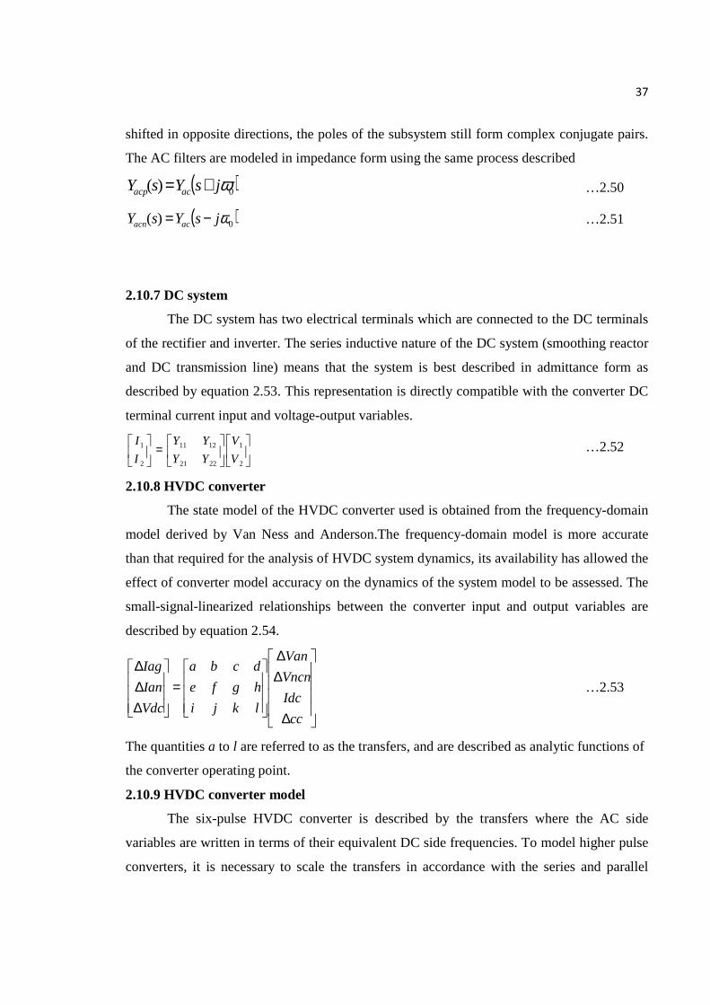
2.10.7 DC system
The DC system has two electrical terminals which are connected to the DC terminals
of the rectifier and inverter. The series inductive nature of the DC system (smoothing reactor
and DC transmission line) means that the system is best described in admittance form as
described by equation 2.53. This representation is directly compatible with the converter DC
terminal current input and voltage-output variables.
=
2
1
2221
1211
2
1
V
V
YY
YY
I
I …2.52
2.10.8 HVDC converter
The state model of the HVDC converter used is obtained from the frequency-domain
model derived by Van Ness and Anderson.The frequency-domain model is more accurate
than that required for the analysis of HVDC system dynamics, its availability has allowed the
effect of converter model accuracy on the dynamics of the system model to be assessed. The
small-signal-linearized relationships between the converter input and output variables are
described by equation 2.54.
∆
∆∆
=
∆∆∆
cc
Idc
Vncn
Van
lkji
hgfe
dcba
Vdc
Ian
Iag
…2.53
The quantities a to l are referred to as the transfers, and are described as analytic functions of
the converter operating point.
2.10.9 HVDC converter model
The six-pulse HVDC converter is described by the transfers where the AC side
variables are written in terms of their equivalent DC side frequencies. To model higher pulse
converters, it is necessary to scale the transfers in accordance with the series and parallel
38
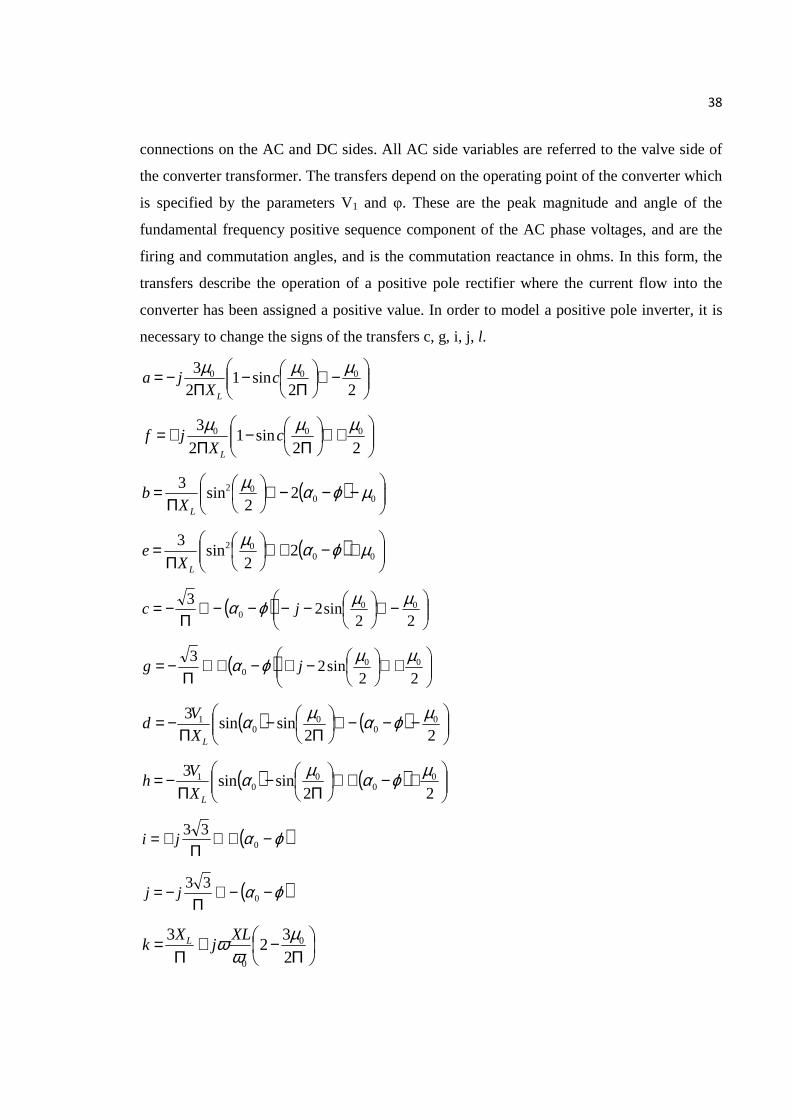
connections on the AC and DC sides. All AC side variables are referred to the valve side of
the converter transformer. The transfers depend on the operating point of the converter which
is specified by the parameters V1 and φ. These are the peak magnitude and angle of the
fundamental frequency positive sequence component of the AC phase voltages, and are the
firing and commutation angles, and is the commutation reactance in ohms. In this form, the
transfers describe the operation of a positive pole rectifier where the current flow into the
converter has been assigned a positive value. In order to model a positive pole inverter, it is
necessary to change the signs of the transfers c, g, i, j, l.
−∠
Π−
Π−=
22sin1
23 000 µµµ
cX
jaL
+∠
Π−
Π+=
22sin1
2
3 000 µµµc
Xjf
L
( )
−−−∠
Π= 00
02 22
sin3 µϕαµ
LXb
( )
+−+∠
Π= 00
02 22
sin3 µϕαµ
LXe
( )
−∠
−−−−∠Π
−=22
sin23 00
0
µµϕα jc
( )
+∠
−+−+∠Π
−=22
sin23 00
0
µµϕα jg
( ) ( )
−−−∠
Π−
Π−=
22sinsin
3 00
00
1 µϕαµαLX
Vd
( ) ( )
+−+∠
Π−
Π−=
22sinsin
3 00
00
1 µϕαµαLX
Vh
( )ϕα −+∠Π
+= 0
33ji
( )ϕα −−∠Π
−= 0
33jj
Π−+
Π=
23
23 0
0
µω
ω XLj
Xk L
39
( )01 sin
33 αΠ
−= Vl
The change in the HVDC system dynamics resulting from the use of converter
models, which take into account varying degrees of frequency dependence in the transfers,
indicates that a model where the transfers are approximated as constants is of sufficient
accuracy. The constants are naturally chosen to be the value of the frequency-domain
transfers at zero frequency on the DC side, and are consistent with the differentiation of the
standard steady-state converter equations. Transfer �, ���� � �� � as the form of a
zero and is the only case where a constant approximation is inappropriate. The constant
component of this transfer is the value which is obtained by differentiating the converter
steady-state equations, while the frequency-dependent component is the time-averaged value
of the commutation reactance seen from the DC side.
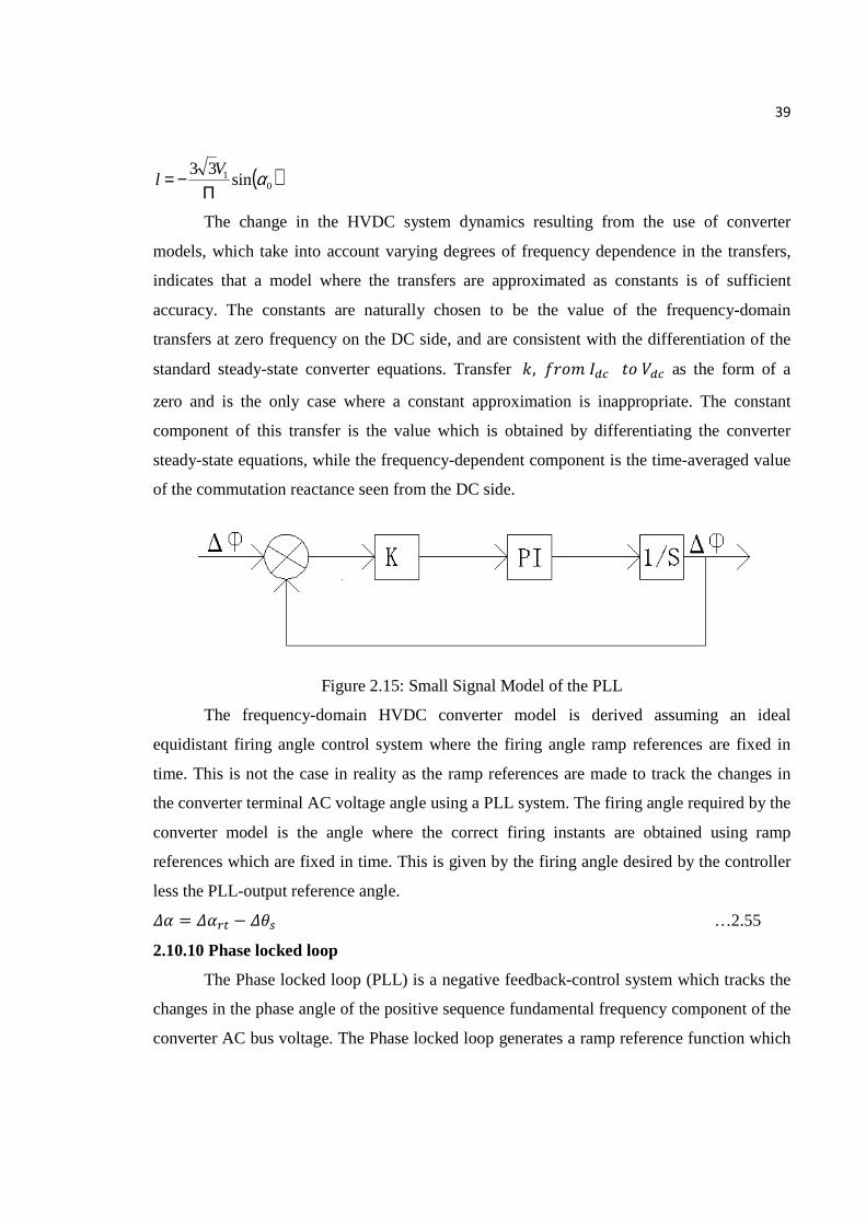
Figure 2.15: Small Signal Model of the PLL
The frequency-domain HVDC converter model is derived assuming an ideal
equidistant firing angle control system where the firing angle ramp references are fixed in
time. This is not the case in reality as the ramp references are made to track the changes in
the converter terminal AC voltage angle using a PLL system. The firing angle required by the
converter model is the angle where the correct firing instants are obtained using ramp
references which are fixed in time. This is given by the firing angle desired by the controller
less the PLL-output reference angle.
� = ��� − �� …2.55
2.10.10 Phase locked loop
The Phase locked loop (PLL) is a negative feedback-control system which tracks the
changes in the phase angle of the positive sequence fundamental frequency component of the
converter AC bus voltage. The Phase locked loop generates a ramp reference function which

40
is synchronized to the AC voltage. This output is used to define the ramp reference
associated with each of the converter thyristors and ensures that the firing instants are
synchronized to the AC voltage.
The PLL system modeled is of the DQZ type, the three major components of which
are an error signal calculator, PI controller, and voltage-controlled oscillator (VCO). The
error signal is calculated as the component of the AC voltage with respect to a sinusoidal
representation of the PLL-output ramp reference. This signal, which in the small-signal case
is proportional to the phase difference between the AC voltage and output reference, is used
to slow down or speed up the VCO so that the component and, hence, phase difference
between the AC voltage and PLL output become zero. The small-signal dynamics of the PLL
system are represented by the block diagram of figure 2.15.
The input to the model is the angle component of the AC bus voltage in the
synchronous reference frame, which is obtained from a sequence or component
representation of the AC voltage using the transforms described above. The open-loop
transfer function consists of the series combination of a gain, which is the operating point
magnitude component of the AC voltage, a PI controller, and an integrator which represents
the operation of the VCO. Controller integral action is required so that the PLL is able to
track changes in the frequency of the AC bus voltage with zero steady-state error. The
parameters of the PI controller are normally chosen such that the output reference angle is
only able to follow changes in the AC voltage angle which are slower than approximately
5Hz. Since the modes of oscillation resulting from the interconnection of the electrical
subsystems are usually at significantly higher frequencies than 5 Hz, the inclusion of the PLL
has only a very limited effect on the these modes. Despite this, the representation of the PLL
is still of importance, particularly at the inverter where a low-frequency instability arises
when the inverter AC system has a very low SCR [30-32].
2.11 System Stability
The stability of an interconnected power system is its ability to return to normal or
stable operation after having been subjected to some form of disturbance. Conversely,
instability means a condition denoting loss of synchronism or falling out of step. Stability
considerations have been recognized as an essential part of power system planning for a long

41
time. With interconnected systems continually growing in size and extending over vast
geographical regions, it is becoming increasingly more difficult to maintain synchronism
between various parts of a power system.
The dynamics of a power system are characterized by its basic features given below:
1. Synchronous tie exhibits the typical behavior that as power transfer is gradually increased
a maximum limit is reached beyond which the system cannot stay in synchronism, i.e., it
falls out of step.
2. The system is basically a spring-inertia oscillatory system with inertia on the mechanical
side and spring action provided by the synchronous tie wherein power transfer is
proportional to sin δ or δ (for small δ; δ being the relative internal angle of machines).
3. Because of power transfer being proportional to sin δ, the equation determining system
dynamics is nonlinear for disturbances causing large variations in angle δ. Stability
phenomenon peculiar to non-linear systems as distinguished from linear systems is
therefore exhibited by power systems (stable upto a certain magnitude of disturbance and
unstable for larger disturbances).
Stability Improvement
PSS and HVDC stabilizers are both the powerful control methodologies for power
swings in power system. Being the traditional damping controllers, Power System Stabilizers
(PSS) have also been proved to be the effective means to suppress electromechanical power
swings in power system. The HVDC system is assumed to have infinitely fast dynamics with
respect to the AC system. The fast power modulation capability of an HVDC link has been
utilized to improve the damping of electromechanical mode oscillations in a parallel AC-DC
power system for a long time. By modulating the transmitted power on the DC line, the
damping of electromechanical swings between systems interconnected by parallel AC and
DC interties are greatly improved.
Power system stability problems are classified into three basic types
� Steady state stability
� Transient stability
� Dynamic stability
42
2.12 Stability Analysis
The transient stability analysis is used to investigate the stability of a power system
under sudden and large disturbances such as faults followed by their clearing under the action
of protective relays. A methodology for the solution of system equations involves differential
equations for the dynamic system including generator and controllers and algebraic equations
describing the network. A major assumption in the transient stability analysis is to neglect
line transients and consider only the fundamental frequency behavior of the AC network.
This assumption is valid for the simulation of low frequency (below 5Hz) transients,
although not applicable for the simulation of subsynchronous frequency transients.
2.12.1 Stability analysis using simplified converter model
Transient stability analysis is conducted with the help of simplified model. The valve
switching is neglected and the converter is represented by the average DC voltage equation
dcd IRaUU −= θcos
Where, θ is either delay angle (α) for a rectifier or extinction angle (γ) for the inverter. The
coefficient 'α' includes the effect of on-load tap changer. U is the converter bus AC voltage.
This model is similar to that used in power flow analysis. However, there are some
differences. The transformer tap is assumed to be constant (at the value prior to the initiation
of the disturbance) as the tap changer dynamics is very slow.
The power or reactive power is not specified as the power controller is not fast acting.
-Instead, the dynamics of power (and auxiliary) controller including VDCOL, are
represented. The current order (reference value) is obtained as the output of the power
controller.
During a transient, it is possible to reverse the power flow under the action of an
emergency controller. The converter may be blocked following fault and unblocked after a
time delay.
2.12.2 Response type converter controller
Controller is represented with detailed or response type model. In case of response
type model of converter controller, the dynamics of the current/extinction angle and firing
controllers are neglected and only the steady-state controller (Ud -Id) characteristics are
represented.
43
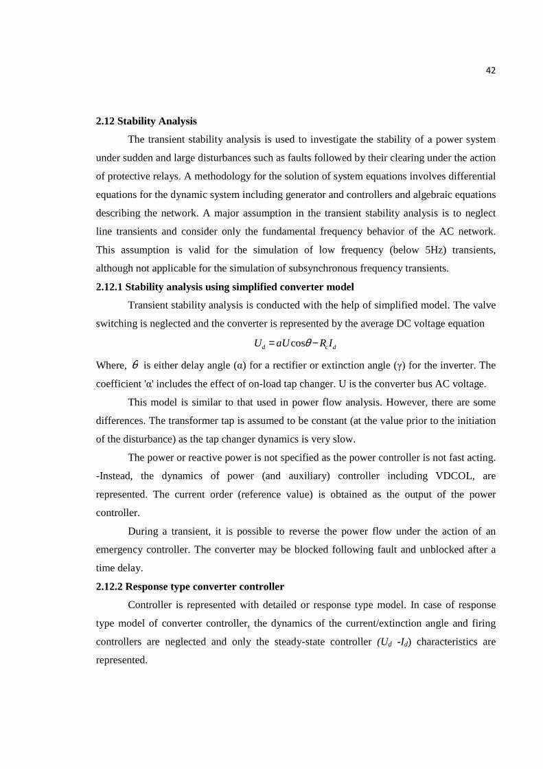
2.12.3 DC network
The DC network is represented as a resistive network, a single resistance ignoring energy
storage elements.
Figure 2.16: DC Network Represented as Resistive Network
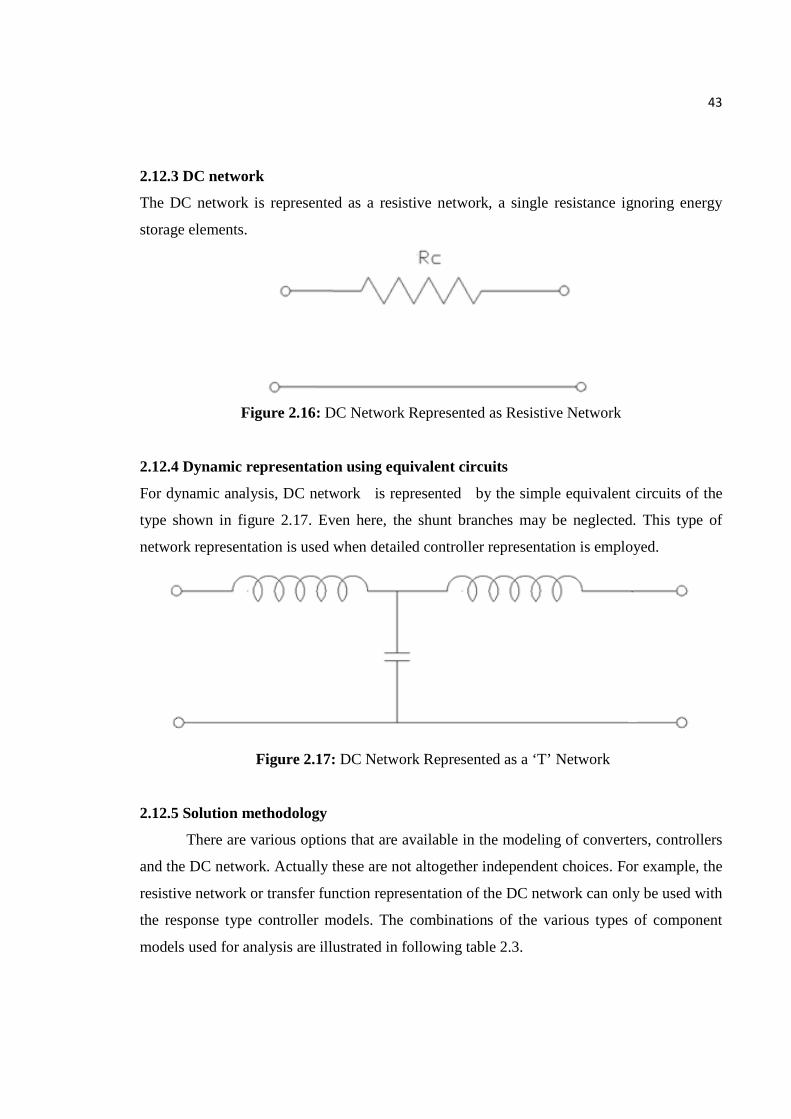
2.12.4 Dynamic representation using equivalent circuits
For dynamic analysis, DC network is represented by the simple equivalent circuits of the
type shown in figure 2.17. Even here, the shunt branches may be neglected. This type of
network representation is used when detailed controller representation is employed.
Figure 2.17: DC Network Represented as a ‘T’ Network
2.12.5 Solution methodology
There are various options that are available in the modeling of converters, controllers
and the DC network. Actually these are not altogether independent choices. For example, the
resistive network or transfer function representation of the DC network can only be used with
the response type controller models. The combinations of the various types of component
models used for analysis are illustrated in following table 2.3.
44
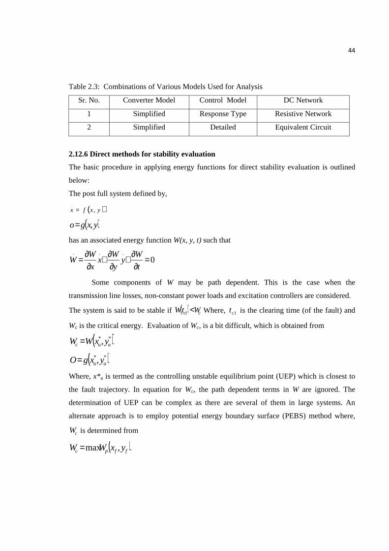
Table 2.3: Combinations of Various Models Used for Analysis
Sr. No. Converter Model Control Model DC Network
1 Simplified Response Type Resistive Network
2 Simplified Detailed Equivalent Circuit
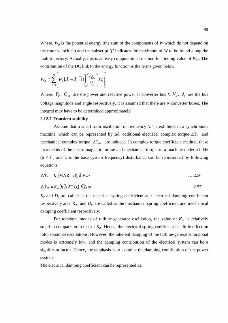
2.12.6 Direct methods for stability evaluation
The basic procedure in applying energy functions for direct stability evaluation is outlined
below:
The post full system defined by,
( )yxfx ,.
=
( )yxgo ,=
has an associated energy function W(x, y, t) such that
0...
=∂
∂+∂∂+
∂∂=
t
Wy
y
Wx
x
WW
Some components of W may be path dependent. This is the case when the
transmission line losses, non-constant power loads and excitation controllers are considered.
The system is said to be stable if ( ) cc WtW <1 Where, 1ct is the clearing time (of the fault) and
Wc is the critical energy. Evaluation of Wc, is a bit difficult, which is obtained from
( )** , uuc yxWW =
( )** , uu yxgO=
Where, x*u is termed as the controlling unstable equilibrium point (UEP) which is closest to
the fault trajectory. In equation for Wc, the path dependent terms in W are ignored. The
determination of UEP can be complex as there are several of them in large systems. An
alternate approach is to employ potential energy boundary surface (PEBS) method where,
cW is determined from
( )ffpc yxWW ,max=
45
Where, Wp is the potential energy (the sum of the components of W which do not depend on
the rotor velocities) and the subscript ‘f’ indicates the maximum of W to be found along the
fault trajectory. Actually, this is an easy computational method for finding value of Wc,. The
contribution of the DC link to the energy function is the terms given below
( )∑ ∫=
+−=
N
kk
v
v k
dkkokdkdc dV
V
QPW
k
ko1
δδ
Where, dkP , dkQ are the power and reactive power at converter bus k, kV , kδ are the bus
voltage magnitude and angle respectively. It is assumed that there are N converter buses. The
integral may have to be determined approximately.
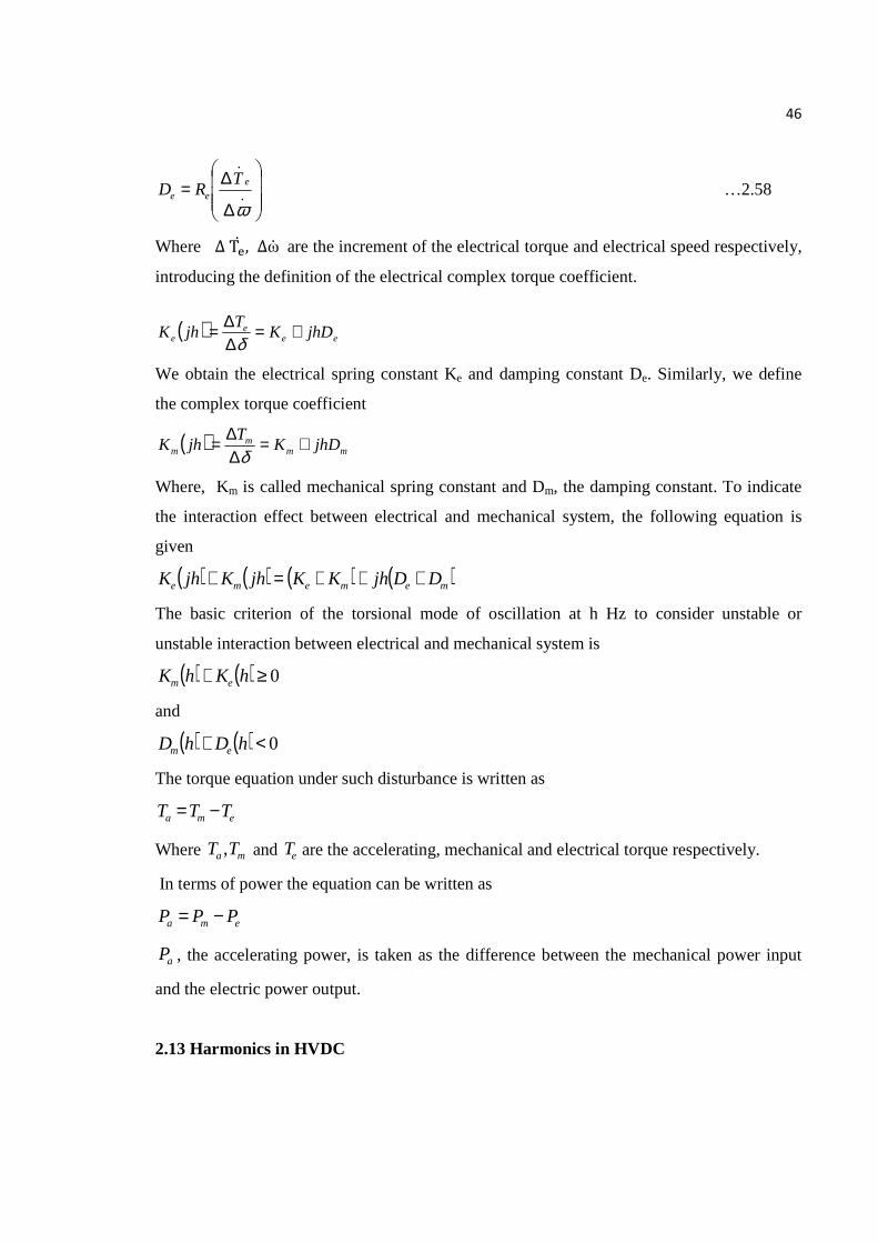
2.12.7 Transient stability
Assume that a small rotor oscillation of frequency ‘h’ is exhibited in a synchronous
machine, which can be represented by ∆δ, additional electrical complex torque ∆Te and
mechanical complex torque ∆Tm are induced. In complex torque coefficient method, these
increments of the electromagnetic torque and mechanical torque of a machine under a h Hz
(h < f , and f, is the base system frequency) disturbance can be represented by following
equations
( ) ( )...
ωδ ∆+∆=∆ hDhKT eee ….2.56
( ) ( )...
ωδ ∆+∆=∆ hDhKT mmm ….2.57
Ke and De are called as the electrical spring coefficient and electrical damping coefficient
respectively and Km, and Dm are called as the mechanical spring coefficient and mechanical
damping coefficient respectively.
For torsional modes of turbine-generator oscillation, the value of Ke, is relatively
small in comparison to that of Km. Hence, the electrical spring coefficient has little effect on
rotor torsional oscillations. However, the inherent damping of the turbine-generator torsional
modes is extremely low, and the damping contribution of the electrical system can be a
significant factor. Hence, the emphasis is to examine the damping contribution of the power
system.
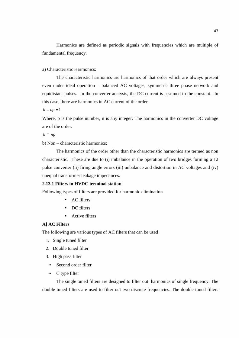
The electrical damping coefficient can be represented as:
46
∆
∆= .
.
ω
e
ee
TRD …2.58
Where ∆ T�� , ∆ω� are the increment of the electrical torque and electrical speed respectively,
introducing the definition of the electrical complex torque coefficient.
( ) eee
e jhDKT
jhK +=∆∆=
δ
We obtain the electrical spring constant Ke and damping constant De. Similarly, we define
the complex torque coefficient
( ) mmm
m jhDKT
jhK +=∆∆=
δ
Where, Km is called mechanical spring constant and Dm, the damping constant. To indicate
the interaction effect between electrical and mechanical system, the following equation is
given
( ) ( ) ( ) ( )mememe DDjhKKjhKjhK +++=+
The basic criterion of the torsional mode of oscillation at h Hz to consider unstable or
unstable interaction between electrical and mechanical system is
( ) ( ) 0≥+ hKhK em
and
( ) ( ) 0<+ hDhD em
The torque equation under such disturbance is written as
ema TTT −=
Where ma TT , and eT are the accelerating, mechanical and electrical torque respectively.
In terms of power the equation can be written as
ema PPP −=
aP , the accelerating power, is taken as the difference between the mechanical power input
and the electric power output.
2.13 Harmonics in HVDC
47
Harmonics are defined as periodic signals with frequencies which are multiple of
fundamental frequency.
a) Characteristic Harmonics:
The characteristic harmonics are harmonics of that order which are always present
even under ideal operation – balanced AC voltages, symmetric three phase network and
equidistant pulses. In the converter analysis, the DC current is assumed to the constant. In
this case, there are harmonics in AC current of the order.
1±= nph
Where, p is the pulse number, n is any integer. The harmonics in the converter DC voltage
are of the order.
nph =
b) Non – characteristic harmonics:
The harmonics of the order other than the characteristic harmonics are termed as non
characteristic. These are due to (i) imbalance in the operation of two bridges forming a 12
pulse converter (ii) firing angle errors (iii) unbalance and distortion in AC voltages and (iv)
unequal transformer leakage impedances.
2.13.1 Filters in HVDC terminal station
Following types of filters are provided for harmonic elimination
� AC filters
� DC filters
� Active filters
A] AC Filters
The following are various types of AC filters that can be used
1. Single tuned filter
2. Double tuned filter
3. High pass filter
• Second order filter
• C type filter
The single tuned filters are designed to filter out harmonics of single frequency. The
double tuned filters are used to filter out two discrete frequencies. The double tuned filters

48
are used to filer out two discrete frequencies, instead of using two single tuned filters. Their
main advantages are (i) only one inductor is subject to full line impulse voltage and
(ii) power loss at the fundamental frequency is considerably reduced.
The second order high pass filters are designed to filter out the higher harmonics.
The tuning of these filters is not critical. The losses at the fundamental frequency can be
reduced by using a C type filter where the capacitor C in series with L, provides a low
impedance path to the fundamental component of current.
A typical converter system with 12 pulse converters has double tuned (or two single
tuned) filter banks to filter out 11th and 13th harmonics and a high pass filter bank to filter out
the rest of harmonics. A third harmonics filter is included to filter out the non- characteristic
harmonic of the third order (particular with weak AC systems where some voltage unbalance
is expected).
All the filter branches appear capacitive at fundamental frequency and supply reactive
power.
B] DC filters
The harmonics in the DC voltage across the converter contain both characteristic and
non-characteristic orders. These harmonics result in current harmonics in DC lines and cause
noise in telephone circuits.
The harmonic current generated in the line can be computed from the knowledge of
harmonic voltage sources at the conveners, smoothing reactor, DC filter and line parameters.
The harmonic current varies with the distance (from the converter station) along the line.
The DC filters are also of single or double tuned type. The choice of DC filters
affect over voltages due to DC line resonances and line faults. The smoothing reactor and
the surge capacitor play a role in the first and the second case respectively, It is found that
DC filters help in limiting the over voltage at the DC terminals caused by monopolar DC line
faults. The DC filters are stressed by direct voltages in addition to harmonic voltages.
C] Active Filter
The principle of the active DC filter is to inject a current generated by a power
amplifier into the DC circuit with such amplitude and phase that it cancels the DC side
harmonics coming from the converter. The amplifier is controlled by a high speed signal

49
processor controller, taking its input from the measured harmonic current entering the DC
line.
The current entering the DC line is measured by the harmonic current transducer. The
PWM amplifier is protected against transient over voltages and over currents by the thyristor
protection.
2.14 Design of AC Filter
2.14.1 Criteria of design of filter
The AC harmonic filters constitute a significant proportion in the capital cost of the
HVDC terminal substation. A large area in converter substation in covered by AC filters.
The criterion of choice of filter size depends on
• Harmonic elimination
• Reactive power requirement.
• Permissible deviation in sinusoidal waveform
• Permissible telephone interference
• Cost of AC filters
2.14.2 Performance parameters
The major design objective of AC filters is to reduce the telephone interference. This
can be measured by the following performance indices.
Harmonics Distortion
This can be measured in different distortion
D = 1002 xE
ZI
I
m
nnn∑
=
In percentage where In, Zn and E1 are the harmonics current injected, the harmonics
impedance of the system and the fundamental component of the line to neutral voltage
respectively, m is the highest harmonics considered.
Total Effective Distortion
Deff = ( )
100
2
1
2
2
xE
ZI
I
m
nnn
∑
=
50
Individual Harmonics Distortion
In some cases, the harmonics distortion can be defined individually for a single harmonics as
Dn =
1E
InZn x 100
Telephone Influence Factor
This is an index of possible telephone interference and is defined as
TIF =
( )
I
m
nnnn
E
FZI2
1
2
2
∑
=
Where, Fn = 5nf1Pn
Pn is the C message weighting used by Bell Telephone System (BTS) and Edison Electric
Institute (EEI) in USA. This weighting reflects the frequency dependent sensitivity of the
human ear and has a maximum value at the frequency of 1000 Hz.
Telephone Harmonics Form Factor (THFF)
This is analogous to TIF except that
Fn = 800
1nfWn
Where Wn is the psophometric weight at the harmonics order n, as defined by the
Consultative Commission on Telephone and Telegraph System (CCITT).
IT product
In BTS-EEI system, there is another index called IT product and is defined by
IT = ( ) 2
1
2
2
∑
=
m
nnnFI
KIT product is defined as: KIT = 1000
IT
Although there are no specific standards on the performance requirements, the
suggested values of the above mentioned indices are given in table [33-35].
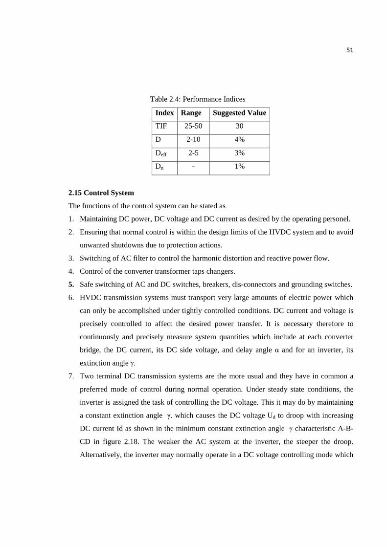
51
Table 2.4: Performance Indices
Index Range Suggested Value
TIF 25-50 30
D 2-10 4%
Deff 2-5 3%
Dn - 1%
2.15 Control System
The functions of the control system can be stated as
1. Maintaining DC power, DC voltage and DC current as desired by the operating personel.
2. Ensuring that normal control is within the design limits of the HVDC system and to avoid
unwanted shutdowns due to protection actions.
3. Switching of AC filter to control the harmonic distortion and reactive power flow.
4. Control of the converter transformer taps changers.
5. Safe switching of AC and DC switches, breakers, dis-connectors and grounding switches.
6. HVDC transmission systems must transport very large amounts of electric power which
can only be accomplished under tightly controlled conditions. DC current and voltage is
precisely controlled to affect the desired power transfer. It is necessary therefore to
continuously and precisely measure system quantities which include at each converter
bridge, the DC current, its DC side voltage, and delay angle α and for an inverter, its
extinction angle γ.
7. Two terminal DC transmission systems are the more usual and they have in common a
preferred mode of control during normal operation. Under steady state conditions, the
inverter is assigned the task of controlling the DC voltage. This it may do by maintaining
a constant extinction angle γ. which causes the DC voltage Ud to droop with increasing
DC current Id as shown in the minimum constant extinction angle γ characteristic A-B-
CD in figure 2.18. The weaker the AC system at the inverter, the steeper the droop.
Alternatively, the inverter may normally operate in a DC voltage controlling mode which
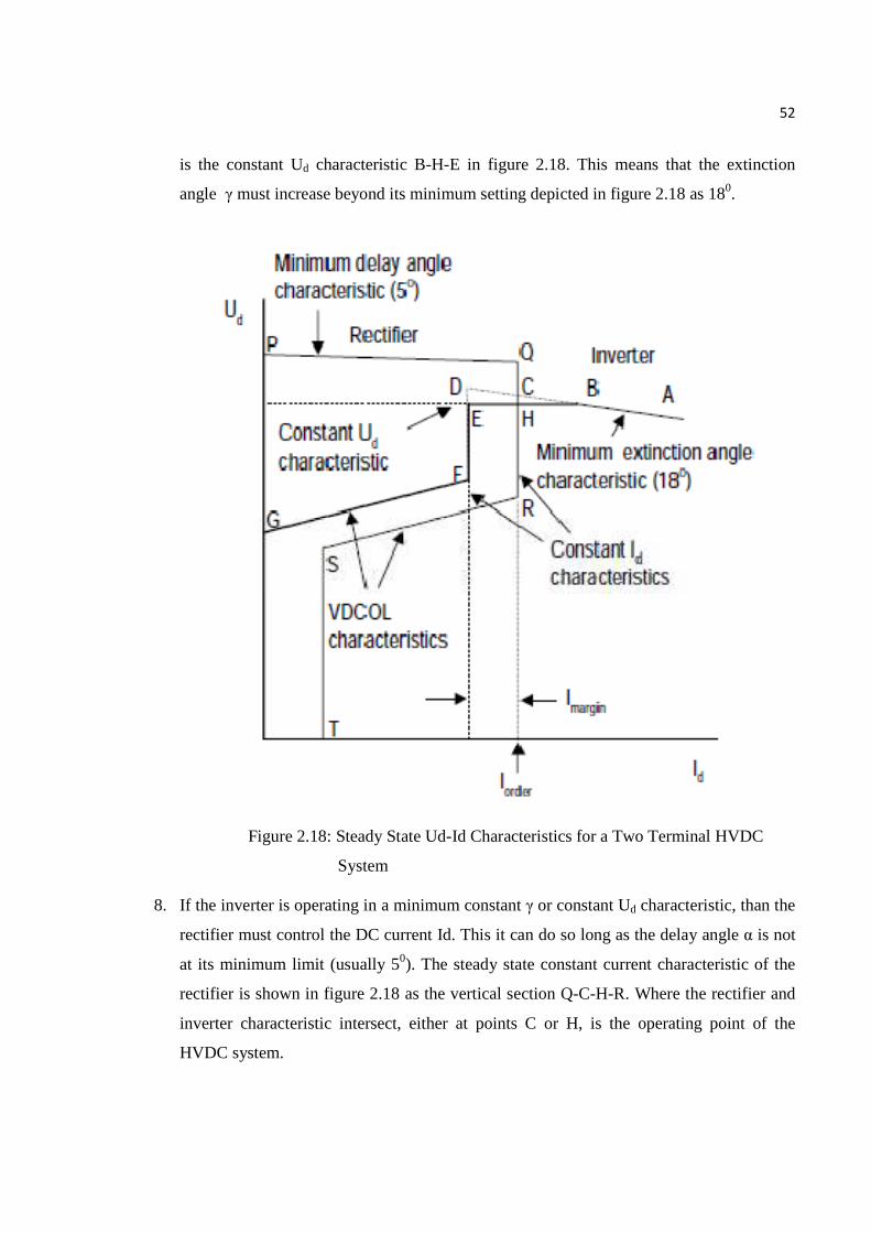
52
is the constant Ud characteristic B-H-E in figure 2.18. This means that the extinction
angle γ must increase beyond its minimum setting depicted in figure 2.18 as 180.
Figure 2.18: Steady State Ud-Id Characteristics for a Two Terminal HVDC
System
8. If the inverter is operating in a minimum constant γ or constant Ud characteristic, than the
rectifier must control the DC current Id. This it can do so long as the delay angle α is not
at its minimum limit (usually 50). The steady state constant current characteristic of the
rectifier is shown in figure 2.18 as the vertical section Q-C-H-R. Where the rectifier and
inverter characteristic intersect, either at points C or H, is the operating point of the
HVDC system.

53
9. The operating point is reached by action of the on-line tap changers of the converter
transformers. The inverter must establish the DC voltage Ud by adjusting its on-line tap
changer to achieve the desired operating level if it is in constant minimum γ control. If in
constant Ud control, the on-line tap changer must adjust its tap to allow the controlled
level of Ud be achieved with an extinction angle equal to or slightly larger than its
minimum setting of 180 in this case.
10. The on-line tap changers on the converter transformers of the rectifier are controlled to
adjust their tap settings so that the delay angle α has a working range at a level between
approximately 100 and 150 for maintaining the constant current setting Iorder (see figure
2.18). If the inverter is operating in constant DC voltage control at the operating point H,
and if the DC current order Iorder is increased so that the operating point H moves
towards and beyond point B, the inverter mode of control will revert to constant
extinction angle γ control and operate on characteristic A-B. DC voltage Ud will be less
than the desired value, and so the converter transformer on-line tap changer at the
inverter will boost its DC side voltage until DC voltage control is resumed.
11. Not all HVDC transmission system controls have a constant DC voltage control such as
is depicted by the horizontal characteristic B-H-E in figure 2.18. Instead, the constant
extinction angle γ control of characteristic A-B-C-D and the tap changer will provide the
DC voltage control.
2.15.1 Current margin
The DC current order Iorder is sent to both the rectifier and inverter. It is usual to
subtract a small value of current order from the Iorder sent to the inverter. This is known as
the current margin Imargin and is depicted in figure 2.18.
The inverter also has a current controller and it attempts to control the DC current Id
to the value Iorder - Imargin but the current controller at the rectifier normally overrides it to
maintain the DC current at Iorder. This discrepancy is resolved at the inverter in normal steady
state operation as its current controller is not able to keep the DC current to the desired value
of Iorder - Imargin and is forced out of action. The current control at the inverter becomes active
only when the current control at the rectifier ceases when its delay angle α is pegged against
its minimum delay angle limit. This is readily observed in the operating characteristics of
figure 2.18, where the minimum delay angle limit at the rectifier is characteristic P-Q. If for
54
some reason or other such as a low AC commutating voltage at the rectifier end, the P-Q
characteristic falls below points D or E, the operating point will shift from point H to
somewhere on the vertical characteristic D-E-F where it is intersected by the lowered P-Q
characteristic.
The inverter reverts to current control, controlling the DC current Id to the value Iorder
- Imargin and the rectifier is effectively controlling DC voltage so long as it is operating at its
minimum delay angle characteristic P-Q. The controls can be designed such that the
transition from the rectifier controlling current to the inverter controlling current is automatic
and smooth.
2.15.2 Converter control
For the sake of convenience, the overall control can be divided into three categories:
1. Power control, auxiliary control and voltage dependent current order limiter (VDCOL).
The output of this block is the current order.
2. Constant Current (CC) and Constant Extinction Angle (CEA) controls. These are usually
of feedback type but the extinction angle control can also be of predictive (open loop) type.
The output of these controllers is a control voltage that determines the instant of gate pulse
generation. The input is taken as the current order (generated locally or at the remote station)
or the extinction angle reference (generated locally). The communication delay in
transmitting the current order may have to be represented.
3. Gate pulse generator which has input from the CC or CEA controller and determines the
instant of gate pulse generation for each valve. There are basically two types of firing control
schemes.
i) Individual phase control (IPC)
ii) Equidistant Pulse Control (EPC)
a)Pulse Frequency Control (PFC)
b)Pulse Phase Control (PPC)
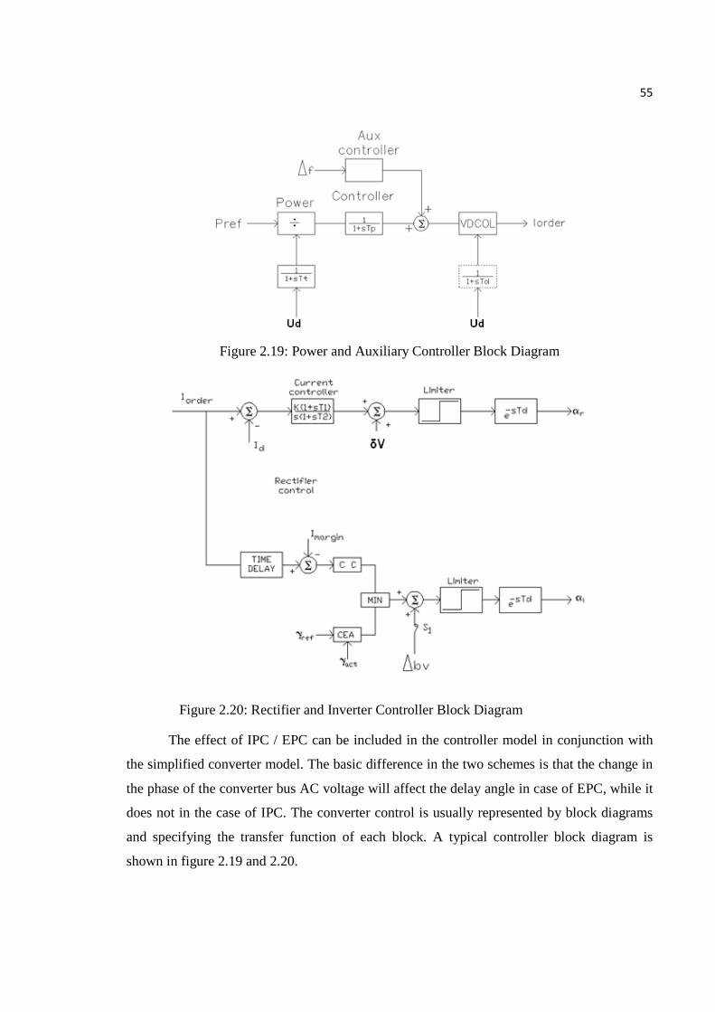
55
Figure 2.19: Power and Auxiliary Controller Block Diagram
Figure 2.20: Rectifier and Inverter Controller Block Diagram
The effect of IPC / EPC can be included in the controller model in conjunction with
the simplified converter model. The basic difference in the two schemes is that the change in
the phase of the converter bus AC voltage will affect the delay angle in case of EPC, while it
does not in the case of IPC. The converter control is usually represented by block diagrams
and specifying the transfer function of each block. A typical controller block diagram is
shown in figure 2.19 and 2.20.
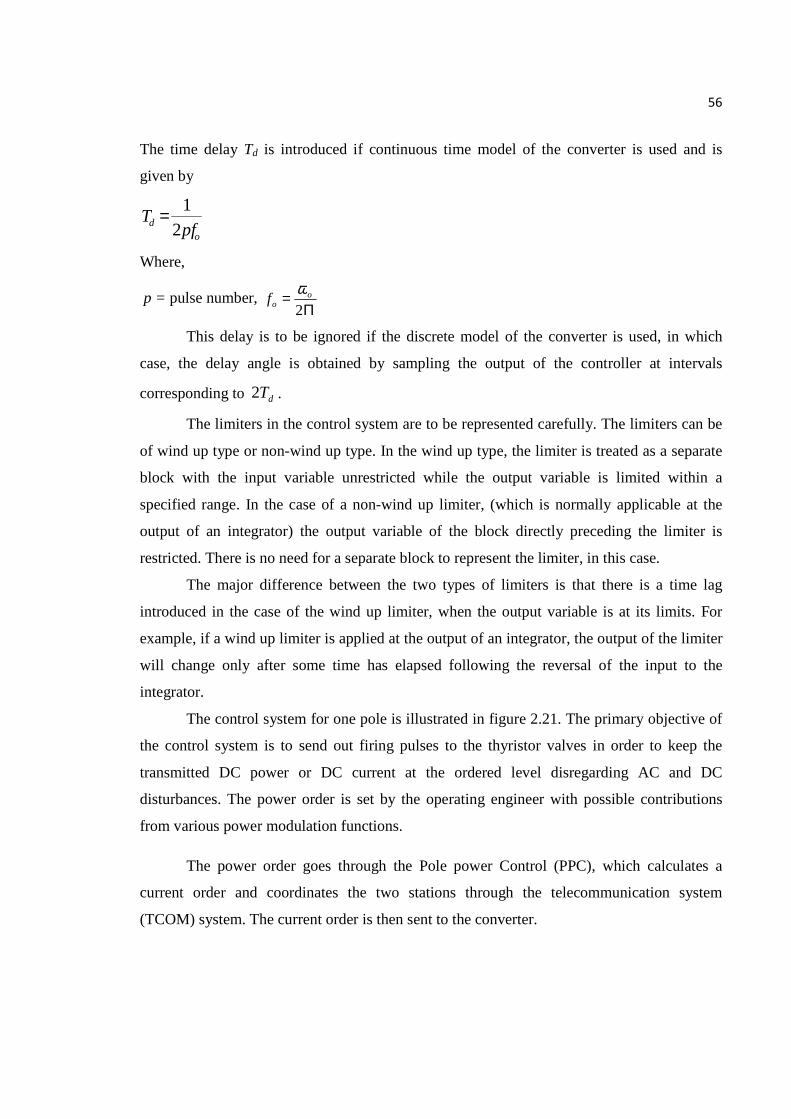
56
The time delay Td is introduced if continuous time model of the converter is used and is
given by
od pf
T2
1=
Where,
p = pulse number, Π
=2
oof
ω
This delay is to be ignored if the discrete model of the converter is used, in which
case, the delay angle is obtained by sampling the output of the controller at intervals
corresponding to dT2 .
The limiters in the control system are to be represented carefully. The limiters can be
of wind up type or non-wind up type. In the wind up type, the limiter is treated as a separate
block with the input variable unrestricted while the output variable is limited within a
specified range. In the case of a non-wind up limiter, (which is normally applicable at the
output of an integrator) the output variable of the block directly preceding the limiter is
restricted. There is no need for a separate block to represent the limiter, in this case.
The major difference between the two types of limiters is that there is a time lag
introduced in the case of the wind up limiter, when the output variable is at its limits. For
example, if a wind up limiter is applied at the output of an integrator, the output of the limiter
will change only after some time has elapsed following the reversal of the input to the
integrator.
The control system for one pole is illustrated in figure 2.21. The primary objective of
the control system is to send out firing pulses to the thyristor valves in order to keep the
transmitted DC power or DC current at the ordered level disregarding AC and DC
disturbances. The power order is set by the operating engineer with possible contributions
from various power modulation functions.
The power order goes through the Pole power Control (PPC), which calculates a
current order and coordinates the two stations through the telecommunication system
(TCOM) system. The current order is then sent to the converter.

57
Figure 2.21.docx

58
Figure 2.22.docx
59
firing control (CFC), which calculates the corresponding alpha and sends out firing pulses.
The CFC also ensures that the firing is done within the limits of the thyristor valves.
Alpha (α), Gamma (γ) and Ud are also superevised and controlled to be within their
respective design limits. This is achieved in the voltage and reactive control (VARC)
function which as outputs gives a Gamma reference to the CFC and Ud, Alpha, and Gamma
references to the tap changer control (TCC). The TCC controls the tap changers on the
converter transformers in order to, within the limits of the design, follow the Ud, Alpha and
Gamma references.
The reactive power balance of the HVDC converter stations is controlled by the
Reactive Power Control (RPC), which switches AC filters in order to keep the reactive power
balance, as well as harmonics generated by the HVDC stations, within design limits.
The tasks of the pole sequences (FSQ) are primarily to assist the operating engineers
for changing control modes, ensure safe switching of DC disconnectors and DC breakers at
connection and disconnection of a pole, changes of modes of operation e.g. Monopolar
earth return/metallic return. Coordination between the stations is done by the PSQ through
the TCOM.
2.16 Functions in HVDC Control System
2.16.1 Pole power control system
The main purpose of the Pole Power Control system is to calculate a current order
and thereby keep the transmitted DC power or DC current constant at the ordered level
disregarded AC and DC disturbances, while still maintaining the stability of the DC system.
Two different modes exist, either power or current control mode.
2.16.2 Power control mode
The power control mode keeps the DC power transmitted equal to the power order
given by the operating engineer. The power order and the power ramp are given to a stepping
logic function, which ramps the power order. In order to keep the power constant, variations
in the DC voltage are compensated for, by adjusting the current order accordingly. To the
60
power order obtained in this way, different additional contributions can be added from
various power modulation functions. The current order is obtained by dividing the total
power order by the direct voltage response measured at the DC high voltage divider. This is
the main mode of operation.
2.16.3 Power modulations
The inherent high speed power control capability of the HVDC transmission system
can be utilized for stabilization and/or frequency control of the surrounding AC systems. The
contribution from power modulation control functions is therefore, superimposed on the
normal operating engineer set power order. The PPC handles four different types of power
order modulations. The contribution from various power modulation functions could either
be seen as a strict additional power order or as an additional power order with an update of
the Stepping Logic Function. The former is useful for power frequency modulations which
do not normally give a permanent contribution. The latter is useful for modulation functions
that do give a permanent contribution or when the contribution is intended to be permanent.
Activation and deactivation of power modulation may cause smooth power change if the
scenario is such that the modulation function is active while being turned on or off. If the
modulation function updates the Stepping Logic Function there will not be a power change
when turned off.
Damping Control
The Damping control will normally always be activated. The Damping Control
receives the AC frequency from both stations, and gives a power contribution to the PPC in
order to damp oscillations in the AC network. Damping control will be available in power
control, normal power direction but not in islanded operation.
Frequency Control
The Frequency control is active while in islanded operation. The frequency control
receives the AC frequency from both stations, and gives a power contribution to the PPC in
order to maintain the frequencies in both stations at islanded operation. Frequency control
will be available in power control, normal power direction and in islanded operation.
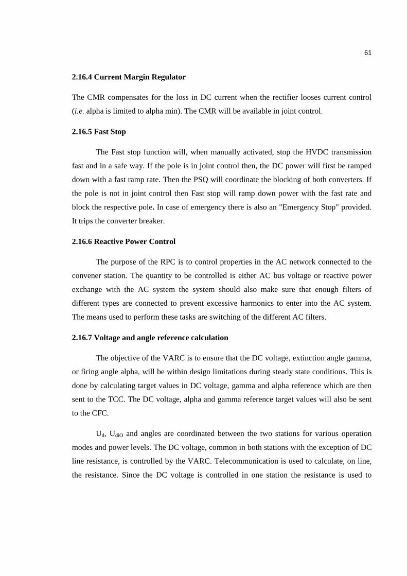
61
2.16.4 Current Margin Regulator
The CMR compensates for the loss in DC current when the rectifier looses current control
(i.e. alpha is limited to alpha min). The CMR will be available in joint control.
2.16.5 Fast Stop
The Fast stop function will, when manually activated, stop the HVDC transmission
fast and in a safe way. If the pole is in joint control then, the DC power will first be ramped
down with a fast ramp rate. Then the PSQ will coordinate the blocking of both converters. If
the pole is not in joint control then Fast stop will ramp down power with the fast rate and
block the respective pole. In case of emergency there is also an "Emergency Stop" provided.
It trips the converter breaker.
2.16.6 Reactive Power Control
The purpose of the RPC is to control properties in the AC network connected to the
convener station. The quantity to be controlled is either AC bus voltage or reactive power
exchange with the AC system the system should also make sure that enough filters of
different types are connected to prevent excessive harmonics to enter into the AC system.
The means used to perform these tasks are switching of the different AC filters.
2.16.7 Voltage and angle reference calculation
The objective of the VARC is to ensure that the DC voltage, extinction angle gamma,
or firing angle alpha, will be within design limitations during steady state conditions. This is
done by calculating target values in DC voltage, gamma and alpha reference which are then
sent to the TCC. The DC voltage, alpha and gamma reference target values will also be sent
to the CFC.
Ud, UdiO and angles are coordinated between the two stations for various operation
modes and power levels. The DC voltage, common in both stations with the exception of DC
line resistance, is controlled by the VARC. Telecommunication is used to calculate, on line,
the resistance. Since the DC voltage is controlled in one station the resistance is used to
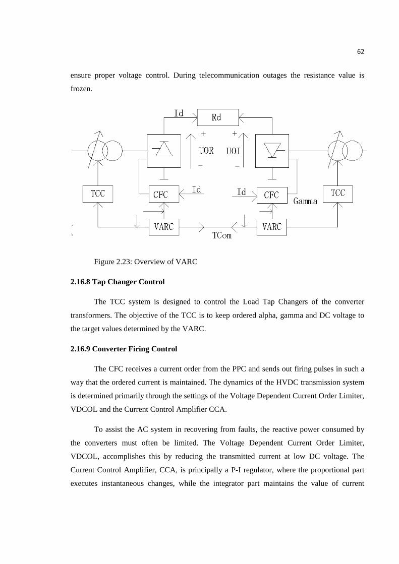
62
ensure proper voltage control. During telecommunication outages the resistance value is
frozen.
Figure 2.23: Overview of VARC
2.16.8 Tap Changer Control
The TCC system is designed to control the Load Tap Changers of the converter
transformers. The objective of the TCC is to keep ordered alpha, gamma and DC voltage to
the target values determined by the VARC.
2.16.9 Converter Firing Control
The CFC receives a current order from the PPC and sends out firing pulses in such a
way that the ordered current is maintained. The dynamics of the HVDC transmission system
is determined primarily through the settings of the Voltage Dependent Current Order Limiter,
VDCOL and the Current Control Amplifier CCA.
To assist the AC system in recovering from faults, the reactive power consumed by
the converters must often be limited. The Voltage Dependent Current Order Limiter,
VDCOL, accomplishes this by reducing the transmitted current at low DC voltage. The
Current Control Amplifier, CCA, is principally a P-I regulator, where the proportional part
executes instantaneous changes, while the integrator part maintains the value of current

63
during steady state conditions. The current control amplifier will have a high enough gain
and suitable dynamics to reach the demands regarding speed and stability. The output signal
from the current control amplifier is a reference for the firing angle and used as an input
order to the firing control system.
Figure 2.24: Overview of CFC
Firing Control
The objective of the firing control is to convert the ordered alpha into corresponding
firing pulses. The allowed changes of the firing angle are dependent upon the operation
mode. An alpha rate of change limiter is therefore included in order to avoid too fast changes.
Especially in regions where the commutations may become unsuccessful, i.e. low gamma.
One important task of the Firing Control is to secure that the firing instant does occur
within the time limitations which are set with regard to design limitations of the converter
bridge and thyristor valves. This is accomplished through the following features. The voltage
has to reach a certain level (UMIN, corresponding to. approximately 50 at normal voltages)
across the thyristor valve to enable firing. For inverter operation the value (ALPHA MIN) is
set to around 1000 in order to prevent reversed voltage, and thereby reversed power.
Predictive commutation margin (AMIN) control ensures that the extinction angle, is kept
above the minimum value, normally 170, in order to minimize the risk for commutation
failures.

64
Figure 2.25: Overview of the firing control
Control Pulse Generator
Control Pulse Generator distributes the control pulses to the correct thyristor valves.
One control pulse per valve is sent, i.e. 12 for a twelve pulse bridge per cycle. furthermore,
block, block with bypass pair, deblock and selection of bypass pair are performed in this
system. The orders are received from either the pole sequences or from protections.
Sub Synchronous Damping Controller
Torsional modes of oscillation of nearby generators will modulate the frequency of
the AC system. The SSDC will ensure that the HVDC provides positive damping for these
oscillations
The SSDC is integrated in the convener firing control. The controller modulates the
firing angle (α) directly inside the firing control system.
Figure 2.26: Sub Synchronous Damping Controller

65
2.16.10 Pole Sequences Control System
The pole sequences control system contains control functions for control of switching
at operation mode changes, start and stop of the transmission and control mode changes such
as joint and separate. The sequence control functions are divided into two parts, the
interlocking part and the coordination part.
2.16.11 Valve Control
The valve control receives electrical pulses (CP) from the pole control and converts
them to optical firing pulses (FP) which are sent to each thyristor in the valves. The status of
the thyristors are monitored and sent via bitbus to the Thyristor Monitoring (THM) in the
pole control system.
2.16.12 Pole Control Communication System
The pole control communicates between the stations through the telecommunication
system. The pole control communicates within each station between different control
cubicles through bitbus systems. This can also be done through high speed links.
2.17 Voltage Control
The voltage control function consists of three functions named:
• Open Line Test Control.
• Overvoltage Limiter (only in rectifier operation).
• Voltage Regulator
2.17.1 Open Line Test Control (OLTC)
Open Line Test is a test function, which is used manually by the operators to energize
the DC side with direct voltage. The test function is used for testing the isolation on the DC
side after a longer period of deenergization. Open Line Test is activated manually. The DC
voltage can be set by the operator to a desired level. The rectifier terminal generates a DC
voltage with normal polarity, while the inverter generates a voltage of reversed polarity. The
direct voltage from a 12-pulsc bridge at peak rectification can be written as:
( )60cos**3
*3
4 −= απUdiOUd
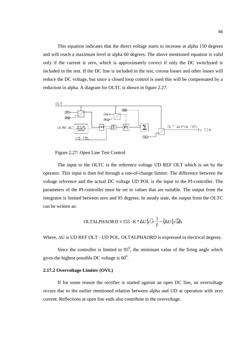
66
This equation indicates that the direct voltage starts to increase at alpha 150 degrees
and will reach a maximum level at alpha 60 degrees. The above mentioned equation is valid
only if the current is zero, which is approximately correct if only the DC switchyard is
included in the test. If the DC line is included in the test, corona losses and other losses will
reduce the DC voltage, but since a closed loop control is used this will be compensated by a
reduction in alpha. A diagram for OLTC is shown in figure 2.27.
Figure 2.27: Open Line Test Control
The input to the OLTC is the reference voltage UD REF OLT which is set by the
operator. This input is then fed through a rate-of-change limiter. The difference between the
voltage reference and the actual DC voltage UD POL is the input to the PI-controller. The
parameters of the PI-controller must be set to values that are suitable. The output from the
integrator is limited between zero and 95 degrees. In steady state, the output from the OLTC
can be written as:
( ) ( )( )dssUT
tU ∆−−∆= 1*K-155DOLTALPHAOR
Where, ∆U is UD REF OLT - UD POL. OLTALPHAORD is expressed in electrical degrees.
Since the controller is limited to 950, the minimum value of the firing angle which
gives the highest possible DC voltage is 600.
2.17.2 Overvoltage Limiter (OVL)
If for some reason the rectifier is started against an open DC line, an overvoltage
occurs due to the earlier mentioned relation between alpha and UD at operation with zero
current. Reflections at open line ends also contribute to the overvoltage.
67
At deblock the control amplifier will lower alpha in order to establish minimum
current. This will normally stop when alpha reaches the UMIN-criterion (5 ele. deg.). As can
be seen from the equation for Ud the maximum voltage is reached for alpha lower than 600.
This means that during start against an open line the firing angle must be increased to values
about 800 - 900 to prevent high overvoltages.
A start against an open DC line can occur when:
• The rectifier is started without telecommunication and the inverter has not been started
(human error).
• The inverter is blocked without By Pass Pair (BPP) during operation without
telecommunication, or if a low speed telecommunications link is used (in case telecom
delay greater than 0-100 ms). This gives the worst case since the current order is high,
giving the fastest increase of DC voltage.
A start against an open DC line can be detected as a combination of high DC voltage
and low DC current. However, normal charging current of the DC side can be rather high,
especially if DC cables are connected.
In many cases the overvoltage limiter is not sufficient to prevent high DC voltage,
depending on the high rate of change of the DC voltage.
2.17.3 Voltage Regulator (VCAREG)
A voltage controller is implemented in both rectifier and inverter operation. The main
function of this controller is for reduced voltage operation, but it is also advantageous for
normal voltage operation. The voltage controller is a PI-regulator that is acting on the
minimum and maximum limits of the current controller. In inverter operation it will decrease
the maximum alpha limit of the CCA, whereas in rectifier operation it increases the
minimum alpha limit. The output from the voltage controller in turn is min/max limited from
external sources. Figure 2.28 indicates the control action of the voltage controller.

68
Figure 2.28: The Control Action of the Voltage Controller
In normal voltage operation the reference voltage to the voltage controller is set
slightly above the operating voltage, so as not to interfere with normal tap changer control.
Normally this level is set approximately one tap changer step above (approx. 1-1.25%
above). By keeping the reference close to the operating voltage, there is an advantage that if
the AC voltage increases rapidly, the controller will act and keep the DC voltage at the
reference.
At reduced voltage operation the reference voltage is lowered to the desired value,
and the controller will consequently lower the DC voltage.
The reference voltage is normally higher in the rectifier end, to keep the voltage
control in the inverter. If inverter current control is desired, the reference to the rectifier
needs to be lower than that of the inverter (here disregarding the influence of the DC line
voltage drop for simplicity).
2.18 Bipole Control
The bipole control will ensure that the total power of the DC bipolar transmission
remain at the ordered value and that the current is equally distributed between the two poles,
thereby the earth current can be kept low. The bipole control also ensures that the ordered
bipole power will be kept during faults in one of the poles, by utilization of power
compensation in the other pole. Bipole functions consist of pole power transfer functions,
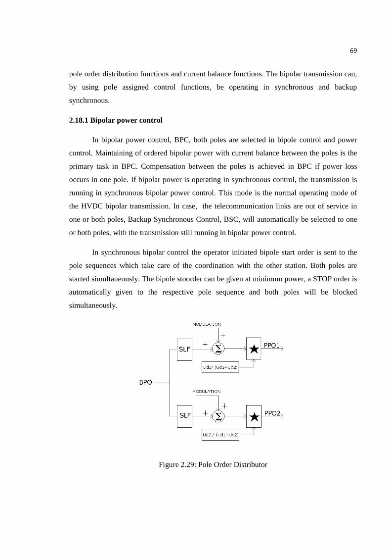
69
pole order distribution functions and current balance functions. The bipolar transmission can,
by using pole assigned control functions, be operating in synchronous and backup
synchronous.
2.18.1 Bipolar power control
In bipolar power control, BPC, both poles are selected in bipole control and power
control. Maintaining of ordered bipolar power with current balance between the poles is the
primary task in BPC. Compensation between the poles is achieved in BPC if power loss
occurs in one pole. If bipolar power is operating in synchronous control, the transmission is
running in synchronous bipolar power control. This mode is the normal operating mode of
the HVDC bipolar transmission. In case, the telecommunication links are out of service in
one or both poles, Backup Synchronous Control, BSC, will automatically be selected to one
or both poles, with the transmission still running in bipolar power control.
In synchronous bipolar control the operator initiated bipole start order is sent to the
pole sequences which take care of the coordination with the other station. Both poles are
started simultaneously. The bipole stoorder can be given at minimum power, a STOP order is
automatically given to the respective pole sequence and both poles will be blocked
simultaneously.
Figure 2.29: Pole Order Distributor

70
Pole Order Distributor
In BPC the Bipole Power Order, BPO, is scaled in each pole by its own DC pole
voltage divided by the bipole voltage, to obtain pole orders, which ensures a current balance
between the poles, independent of DC voltage fluctuations, and thereby a low earth current
shown in figure 2.29.
Pole Power Transfer Scheme
When one pole is in bipole control, it has the possibility to compensate for power
fluctuations, due to limitation, start/stop or fault in the other pole that may occur.
Figure 2.30: Pole Power Transfer Scheme
The compensation is carried out as fast as possible up to pole limit with maintained
bipole power. The compensation is performed by adding an order contribution from the other
pole, to the pole order. The order contribution is the difference between the pole order and
limited pole order. To ensure fast compensation, the measured power of the faulty pole used
in the pole power transfer scheme, is set to zero at fault show in figure 2.30.
71
Fine Current Balancer
To minimize the earth current of the bipole in BPC further, a PI-regulator, fed by the
earth current, is giving a current balance contribution to the pole current order, in each pole.
The earth current is measured on the electrode line with high accuracy.
2.19 Views of Other Researchers
Many researchers have contributed in the field of HVDC transmission systems. The
contribution which seems to be the mile stones is described in preceding paragraphs.
Narain G. Hingorani in his paper, ‘HIGH-VOLTAGE DC TRANSMISSION: A
power electronics workhorse’ has discussed about the roll and scope of HVDC technology in
the context of power electronics in transmission systems and the state of the art and new
developments within the technology are reviewed. He mentions the applications,
configurations etc. Further he has discussed international business and reliability of the
systems and reasons for failures. He states, ‘Work is under way to raise the voltage capability
of the 100-mm wafer from the 8-kV thyristor to 1@-12-kV. Then, too, thyristors based on
120- to 150-mm silicon wafers are in development’. He further narrates the achievements of
ABB, Siemens and others suppliers in continuous development of the HVDC technology [2].
Dr. B.K.Anderson has published many papers related to various aspects of HVDC
technology. In one of his paper he states, ‘During the B4 session at the 2004 CIGRE meeting
a new method for the conversion of AC lines to HVDC operation was outlined. The idea is to
use all three conductors of the AC line, with three converters. This has the advantage of
utilisation of the full current capacity of the three existing conductors, and does not require a
metallic earth return [4].
Hirofumi Akagi narrates the major developments in large static converters and its
utility/industry applications in the past years upto 2000 [7].
Madhu Chinthavali et.al has published their article regarding 4H-SiC GTO Thyristor
models for HVDC converters [9-10].
R.A.Valiquette has written a paper about Life Extension of the New Zealand HVDC
Link .The New Zealand HVDC link is one of the two oldest HVDC links that is still running
with original installed equipment from 1965. The New Zealand HVDC link was upgraded

72
and modernized in 1992 when a new thyristor pole was added, the line voltage was raised,
new cables added and the original mercury arc poles were equipped with new control
equipment and rearranged to operate in parallel on one pole. Their report describes briefly
the original link, the upgrade in1992, the life-extension initiatives that have been completed
to date, and some future options etc.[39].
Douglas A. Halamay et al. have highlighted the technical aspects and feasibility study
etc. of HVDC transmission links [40-43].
R. Billinton, S. Aboreshaid, M. Fotuhi-Firuzabad presented a probability analysis
technique to evaluate the degree of reliability well-being of bulk generation and HVDC
transmission systems. The system well-being is categorized in terms of system health and
margin in addition to the conventional risk index. Such a technique enables power system
designers, planners and engineers to analyze the generating system and the HVDC
transmission system independently by obtaining the wellbeing area diagrams for each
system. The technique is illustrated by application to a simple hypothetical configuration and
a practical HVDC system [44-53].
C.T. Wu et.al. and Masahiro Hirose et. al. have given their operational experiences
of respective HVDC projects [54-57].
C. B. Modolo et.al. have contributed regarding telecommunication in HVDC systems
[58-60] . Farouk A.M. Rizk et.al. are discussed about their research regarding components in
HVDC like bushings , transformer etc.[61-63]
M. R. Aghaebrahimi et.al. have contributed to power tapping from HVDC systems [64-67]
Gerhard Schmidt, Bernd Fiegand and Stephan Callbeck have discussed about
Environmental aspects of HVDC transmission System. They have discussed, ‘”Electrical and
magnetic fields are linked inseparably to their sources and are not carried into residential
areas by wind are other meteorological factors. Above certain frequencies, the energy present
in electromagnetic fields can lead to electrons being ejected from atoms, which could be the
cause of hereditary damage or even cancer in animals and human beings. This invasive
interference cannot be produced by electrical or magnetic fields up to 30 kHz because the
energy content is too low”. They also have discussed about corona effects and materials and
concluded that “Corona effects on the surface of high voltage overhead power transmission
lines are the principal source of radiated noise. Appropriate design measures can minimise

73
these effects. When choosing the materials for the thyristor valve towers, it is important to
ensure that only self-extinguishing or noncombustible, non-flammable and non-drip
substances defined by the most stringent fire behaviour classification UL 94 V-0 are used.
This practice can almost eliminates the risk of fire”[ 68].
Figure 2.31: Electric Field of Monopolar and Bipolar 450 kV HVDC
Overhead line
Stephen A. Sebo and others have worked for the environmental aspects. Field
measurements, corona discharge are the issues of interest [69-77].
Denis Lee et. al. have mentioned the probabilities of exploring added advantages
with the use of Multi-Terminal HVDC [78].
K. R. Padiyar, Nagesh Prabhu have provided a model for analysis and control of
VSC based HVDC system which uses twelve pulse three level converter topology. The
modelling of the VSC system including network transients is discussed in details and is
expressed in D-Q variables. A systematic approach for parameter optimization in selecting
the controller gains is discussed in detail [79].
F. Schettler et. al. has contributed for modeling, control design and analysis of VSC
based HVDC transmission systems as well as CSC technology [80-86].
A. M. Gole et. al. has published their article regarding hybrid HVDC converters and
their impact on dynamic performance [87].

74
Guo-Jie Li et.al. has discussed means for Nonlinear Control for Stability
Improvement [88-90].
J. Arrillaga et.al. has discussed modeling in harmonic domain and small signal
modeling and EMTP and other simulation software etc.[91-93].
A.K. David et. al. have developed the ‘Robust Co-ordinated Control Scheme for
HVDC Transmission with Parallel AC Systems’ and various such alternatives are suggested
by many researchers to enhance the control of HVDC systems [94].
Zhu Yi-ying et.al. have conducted research related to ‘Measures of Restraining DC
Current through Transformer Neutrals’. It is mentioned that, monopole ground return mode
may cause DC current through the transformer neutrals which are connected to the ground
and make the transformers DC biases. With the increase of HVDC transmission power, some
transformers through which there will be more DC current going may be saturated, which
brings some problems such as acutely shaking, increased noises and overheating when power
system is in the normal operation. Not only the safety of transformer but also the normal
operation of power system may be impacted in this case. There are various measures to
restrain DC current through transformer neutrals and one of them is putting a capacitor in
series between transformer neutral and ground.
Figure 2.32: The Sketch Map of the Capacitor and Corresponding Protection Equipment
It has been proved to be the optimal measure. A capacitor with very big capability
will be needed to endure big fault current. It is also stressed that bypass equipment is
needed to connect in parallel with the capacitor [95].
Haifeng Liu, Zheng Xu have put forward a new method to tune the parameters of an
HVDC small signal modulation controller. Small signal stability of an AC/DC power
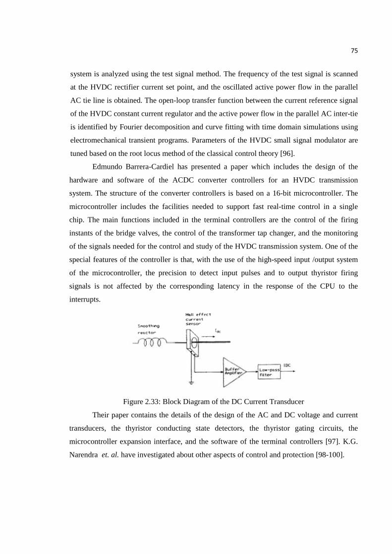
75
system is analyzed using the test signal method. The frequency of the test signal is scanned
at the HVDC rectifier current set point, and the oscillated active power flow in the parallel
AC tie line is obtained. The open-loop transfer function between the current reference signal
of the HVDC constant current regulator and the active power flow in the parallel AC inter-tie
is identified by Fourier decomposition and curve fitting with time domain simulations using
electromechanical transient programs. Parameters of the HVDC small signal modulator are
tuned based on the root locus method of the classical control theory [96].
Edmundo Barrera-Cardiel has presented a paper which includes the design of the
hardware and software of the ACDC converter controllers for an HVDC transmission
system. The structure of the converter controllers is based on a 16-bit microcontroller. The
microcontroller includes the facilities needed to support fast real-time control in a single
chip. The main functions included in the terminal controllers are the control of the firing
instants of the bridge valves, the control of the transformer tap changer, and the monitoring
of the signals needed for the control and study of the HVDC transmission system. One of the
special features of the controller is that, with the use of the high-speed input /output system
of the microcontroller, the precision to detect input pulses and to output thyristor firing
signals is not affected by the corresponding latency in the response of the CPU to the
interrupts.
Figure 2.33: Block Diagram of the DC Current Transducer
Their paper contains the details of the design of the AC and DC voltage and current
transducers, the thyristor conducting state detectors, the thyristor gating circuits, the
microcontroller expansion interface, and the software of the terminal controllers [97]. K.G.
Narendra et. al. have investigated about other aspects of control and protection [98-100].