Convergence of a large time-step scheme for Mean Curvature ... · max a∈B(0,1) {c(y)a · ∇T(x)}...

Outline

Convergence of a large time-step scheme

for Mean Curvature Motion

M. Falcone

Dipartimento di MatematicaSAPIENZA, Universita di Roma

in collaboration with E. Carlini (SAPIENZA) and R. Ferretti (Roma Tre)

College de France, June 12, 2009

M. Falcone Convergence of a large time-step scheme for MCM

Outline

Outline

1 Introduction

2 Construction of the scheme

3 Consistency and monotonicity

4 Barles-Souganidis theorem revisited

5 Numerical experiments and comparisons

6 MCM in codimension 2


IntroductionConstruction of the scheme

Consistency and monotonicityBarles-Souganidis theorem revisited

Numerical experiments and comparisonsMCM in codimension 2

Outline

1 Introduction










Level Set Method

The Level Set method has had a great success for the analysis offront propagation problems for its capability to handle manydifferent physical phenomena within the same theoreticalframework.One can use it for isotropic and anisotropic front propagation, formerging different fronts, for Mean Curvature Motion (MCM) andother situations when the velocity depends on some geometricalproperties of the front.It allows to develop the analysis also after the on set ofsingularities.





Level Set Method

Our unknown is the ”representation” function u : Rn × [0,T ] → R

and looking at the 0-level set of u we can back to the front, i.e.

Γt ≡ x : u(x , t) = 0The model equation corresponding to the LS method is

ut + c(x)|∇u(x)| = 0 x ∈ R

n × [0,T ]u(x) = u0(x) x ∈ R

n

where u0 must be a representation function for the front (i.e.

u0 > 0, x ∈ Rn \ Ω0

u(x) = 0 x ∈ Rn

u(x) < 0 x ∈ Ω0

(1)

The front Γ0 = ∂Ω0.M. Falcone Convergence of a large time-step scheme for MCM




Front propagation and minimum time problem

Let the velocity of the front in the normal direction is a givenc : R

n → R

Minimum time problemTarget set =Ω0

Dynamics

y(t) = −c(y)a, a ∈ B(0, 1)y(0) = x

(2)

Minimum time function

T (x) ≡ inft ∈ R+ : yx(t; a(t)) ∈ Ω0





Monotone evolution

T (·) is the unique viscosity solution of

maxa∈B(0,1)

c(y)a · ∇T (x) = 1 ∈ Rn \ Ω0

with the Dirichlet condition

T (x) = 0 on ∂Ω0

If c does not change sign the evolution is monotone (increasing ordecreasing) and we have the following link

u(x , t) = T (x) − t

So we can solve the stationary problem and get any front Γt , fort > 0.





More General Models

In the standard model the normal velocity c : Rn → R is given, but

the same approach applies to other scalar velocities

c(x , t) isotropic growth with time varying velocityc(x , η) anisotropic growth, cristal growthc(x , k(x)) Mean Curvature Motionc(x) obtained by convolution (dislocation dynamics)





Outline

1 Introduction










Construction of the scheme

Soner–Touzi formula between t and t + ∆t :

u(x , t + ∆t) = Eu(y(x , t + ∆t,∆t), t)

Brownian dimension reduction

√2PdW =

√2

|Du|

(ux2

−ux1

)(ux2dW1

|Du| − ux1dW2

|Du|

)= σdW

where

σ(x , t) =

√2

|Du|

(ux2

−ux1

)





we can replace the stochastic Cauchy problem by

dy(x , t, s) = σ(y , t, s)dW (s)

y(x , t, 0) = x .

i.e. with a 1-dimensional brownian motion in the direction tangentto the curve.





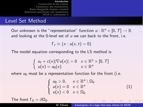
Euler scheme for SDE

yk+1 = yk +

√2σ(y , tk , 0)∆Wk

y0 = x .

with

P(∆Wk = ±√

∆t) =1

2.

Time-discretization

u∆t(x , tn+1) = 12u∆t(x +

√2σ(x , tn, 0)

√∆t, tn) +

+12u∆t(x −

√2σ(x , tn, 0)

√∆t, tn).

Fully discrete scheme Du 6= 0

un+1j =

1

2

(I [un](xj + σn

j

√∆t) + I [un](xj − σn

j

√∆t)

)





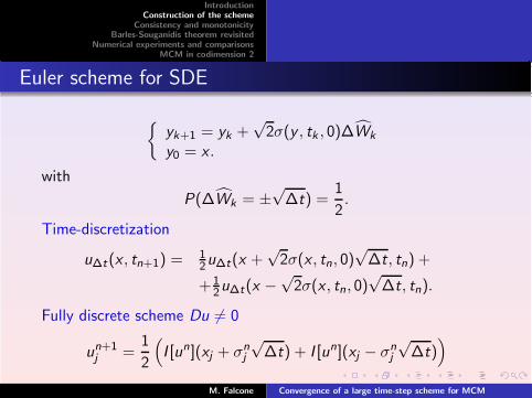
Some references

MCM via viscosity solution techniquesEvans-Spruck, J. Diff. Geom., 1991Evans - Soner-Souganidis, Comm. Pure Appl. Math, 1992, .....Kohn-Serfaty, Comm. Pure Appl. Math., 2006Soner-Touzi, J. Eur. Math. Soc, 2002 and Ann. Prob. 2003Numerical methodsOsher-Sethian, JCP, 1988Merriman-Bence-Osher, AMS LN, 1993Crandall-Lions, Numer. Math., 1996Barles-Georgelin, SIAM J. Num. Anal., 1995Catte-Dibos-Koepfler, SIAM J. Num. Anal., 1995F. Ferretti, ENUMATH 2001Carlini- F. -Ferretti, JCP 2005 and Interfaces and Free Boundaries,2009 (submitted)





Outline

1 Introduction










Modified scheme with threshold C∆x s

un+1j = 1

2

[I [un](xj + σn

j

√∆t) + I [un](xj − σn

j

√∆t)

]if |Dn

j | > C∆xs

un+1j = 1

4

∑i∈D(j)

uni if |Dn

j | ≤ C∆xs

Consistency error (case |Dnj | > C∆xs)

τ∆x ,∆t = O

(∆x r

∆t

)+ O

(∆xq−s

∆t12

)+ O(∆t

12 ) + O(∆t)





Consistency for small gradients

Let us consider the case |Dnj | ≤ C∆xs .

Case a: (xj , tn) is such that Du(xj , tn) = 0.This is a stardad computation based on the consistency with theheat equation.Case b : (xj , tn) is such that |Du(xj , tn)| 6= 0 and |Dj [w ]| ≤ C∆x s .By the lower semicontinuity of F we have that for any ε1 > 0 thereexists a δ1(ε1) such that

F (Du,D2u)(y , s) ≥ F (Du,D2u)(x , t)−ε1 for any (y , s) ∈ Bδ1(x , t).

(3)






The upper semicontinuity of F implies that for any ε2 > 0 thereexists a δ2(ε2) such that

F (Du,D2u)(y , s) ≤ F (Du,D2u)(x , t)+ε2 for any (y , s) ∈ Bδ2(x , t).

(4)The interesting case is when for ε ≡ max(ε1, ε2) there exists

(y , s) ∈ Bδ1(x , t) ∩ Bδ2

(x , t)

such that Du(y , s) = 0. For (x , t) = (xj , tn), we can apply both (3)and (4) getting

F (Du,D2u)(xj , tn) ≤ F (Du,D2u)(xj , tn) + 2ε (5)






In fact, we have

F (Du,D2u)(xj , tn) ≤ −2|D2u(y , s)| + ε ≤ ε =

= lim inf∆t→0

u(xj ,tn)−H(w ;j)∆t

+ ε = lim sup∆t→0

u(xj ,tn)−H(w ;j)∆t

+ ε ≤

≤ 2|D2u(y , s)| + ε ≤ F (Du,D2u)(xj , tn) + 2ε

and, since ε1 and ε2 are arbitrary, we obtain the result.





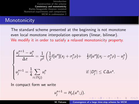
Monotonicity

The standard scheme presented at the beginning is not monotoneeven local monotone interpolation operators (linear, bilinear).We modify it in order to satisfy a relaxed monotonicity property.

un+1j − un

j

∆t=

1

ρ2

(1

2I [un](xj + σn

j ρ)+12 I [un](xj − σn

j ρ) − unj

)

un+1j =

1

4

∑

i∈D(j)

uni if |Dn

j | ≤ C∆xs .

In compact form we write

un+1j = Hρ(u

n; j).





Monotonicity

Since for this scheme Hρ we have

∂Hρ(un; j)

∂uni

≥ −4∆tLI [un],G

Cρ∆xs+1

we need to compensate the negative bound and we add a smallviscosity

Hρ(un; j) = Hρ(u

n; j) + ∆t W∆xρ∆x s

Pi∈D(j) un

i−4un

j

∆x2 , if |Dnj | > C∆xs

un+1j =

1

4

∑

i∈D(j)

uni if |Dn

j | ≤ C∆xs .

where W is a positive constant.





Monotonicity

Differentiating Hρ we get:

∂Hρ(un; j)

∂unj

≥ 1 − ∆t

ρ2− 4W ∆t

ρ∆x1+s

∂Hρ(un; j)

∂uni

= ψi (xj + σnj ρ) ≥ 0 for i ∈ S(j) \ (D(j) ∪ j)

∂Hρ(un; j)

∂uni

≥ −4∆tLI [un],G

Cρ∆xs+1+

W ∆t

ρ∆x1+sfor i ∈ D(j).

(6)Then Hρ(u

n; j) is monotone if

1 − ∆t

ρ2− 4W ∆t

ρ∆x1+s≥ 0

4LI [un],G

C< W .

(7)





Weak monotonicity property

Theorem Under the above assumption, the scheme Hρ satisfies

Hρ ≤ Hρ(η; j) + o(∆t).





Outline

1 Introduction










Let us consider now a general scheme that is supposed toapproximate our HJ equation. Its abstract form on a lattice will begiven by

un+1j = SDt(un; j) for j ∈ Z2 n = 0, ...,N − 1

u0j = u0(xj ) for j ∈ Z2

(HJDt)

where SDt : B(G∆x) → R and B(D) is the space of the boundedfunctions defined on D.





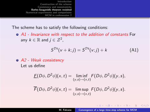
The scheme has to satisfy the following conditions:

A1 - Invariance with respect to the addition of constants Forany k ∈ R and j ∈ Z2,

SDt(v + k; j) = SDt(v ; j) + k (A1)

A2 - Weak consistencyLet us define

F (Dφ,D2φ)(x , t) = lim inf(y ,s)→(x ,t)

F (Dφ,D2φ)(y , s),

F (Dφ,D2φ)(x , t) = lim sup(y ,s)→(x ,t)

F (Dφ,D2φ)(y , s).





Consistency

The consistency assumption (A2) requires

φt(x , t) + F (Dφ,D2φ)(x , t) ≤ lim inf(xj ,tn)→(x ,t)

∆t→0

φ(xj , tn) − SDt(φn−1; j)

∆t

≤ lim sup(xj ,tn)→(x ,t)

∆t→0

φ(xj , tn) − SDt(φn−1; j)

∆t

≤ φt(x , t) + F (Dφ,D2φ)(x , t)

where φ ∈ C∞(R2 × (0,T ]) and φn−1 = (φ(xj , tn−1))xj∈G∆x.

Note that F (Dφ,D2φ), F (Dφ,D2φ)(x , t) are respectively lowerand upper semicontinuous extension of F .





Note that if F is continuous, then the lim inf and the lim sup mustcoincide, and the definition reduces to the usual definition ofconsistency.

A3 - Generalized monotonicity

vj ≤ φn−1j for j ∈ Z2 implies SDt(v ; j) ≤ SDt(φn−1; j)+o(Dt)

where v ∈ B(G∆x) and SDt is a (possibly different) schemeweakly consistent.





Then, consider un = (unj )j∈Z2 with un

j solution of (HJDt) and its

piecewise constant (in time) interpolation uDt defined as:

uDt(x , t) =

I [un](x) if t ∈ [tn, tn+1) ,

u0(x) if t ∈ [0,∆t),

where I [·] : B(G∆x) → R is a general interpolation operator

I [un](x) ≡∑

l∈I(x)

ψl(x)unl (8)

where ψl(x) are basis functions in R2 and I(x) is the set of indices

corresponding to the vertices of the cell containing x .





Let us note that we can always couple the choice of Dt and Dxaccording to Dt = CDxγ , with C a positive constant, in order todeal with a unique discretization parameter. We assume γ ≥ 1(this parameter has to be tuned to guarantee monotonicity).The interpolation operator I [·] has to verify a relaxed monotonicityproperty:

if vj ≤ ηj for any j ∈ I(x) then I [v ](x) ≤ I [η](x)+o(Dt) (A4)

with v ∈ B(G∆x) and η = (f (xj ))xj∈G∆x,where f (x) is a smooth

function.





Moreover I [·] satisfies

|I [η](x) − f (x)| = o(Dt) for any x ∈ R2. (A5)

Theorem

Assume (A1)–(A5) and let u(x , t) be the unique viscosity solutionof (HJ). Then uDt(x , t) → u(x , t) locally uniformly on R

2 × [0,T ]as Dt → 0.





Outline

1 Introduction










TEST: a shrinking circle

∆t = O(∆x34 ), s =

1

4.

∆x ∆t ‖ · ‖∞ ‖ · ‖1 L∞ − order L1 − order

0.04 0.08 3.04 · 10−4 6.50 · 10−6

0.02 0.053 1.25 · 10−4 3.42 · 10−6 1.2 0.9

0.01 0.032 5.22 · 10−5 1.82 · 10−6 1.2 1.6

0.005 0.02 2.09 · 10−5 7.75 · 10−7 1.3 1.2Errors for the SL scheme





TEST: Development of non empty interior

-2

-1.5

-1

-0.5

0

0.5

1

1.5

2-2 -1.5 -1 -0.5 0 0.5 1 1.5 2

-2

-1.5

-1

-0.5

0

0.5

1

1.5

2-2 -1.5 -1 -0.5 0 0.5 1 1.5 2

-2

-1.5

-1

-0.5

0

0.5

1

1.5

2-2 -1.5 -1 -0.5 0 0.5 1 1.5 2

-2

-1.5

-1

-0.5

0

0.5

1

1.5

2-2 -1.5 -1 -0.5 0 0.5 1 1.5 2

Fattening: evolution of the level curves u = 0.095, 1, 1.05





The torus evolving into a sphere, R < rM. Falcone Convergence of a large time-step scheme for MCM




The torus collapsing in a circle, R > rM. Falcone Convergence of a large time-step scheme for MCM




Dumb-bell: topology change in R3





Crandall-Lions scheme

In the scheme proposed by such problems are avoided by replacingthe matrix Θ in the equation of MCM by the following one:

Θǫ(Du) = I − Du⊗

Du

|Du|2 + ǫ,

with ǫ > 0.





Crandall-Lions scheme cntd

Denoting by ej (j = 1, 2) the canonical base of R2, we can write

the CL scheme as:un+1j = HCL(u

n; j)

where

HCL(un; j) = un

j +∆t

ρ2(I [un](xj + ρΘǫ(Dj [u

n])e1)+

+I [un](xj + ρΘǫ(Dj [un])e2) +

+I [un](xj − ρΘǫ(Dj [un])e1) +

+ I [un](xj − ρΘǫ(Dj [un])e2) − un

j

)





The scheme for which convergence is proved is

un+1j = HCL(u

n; j) +∆tK

ρ∆x

∑

i∈D(j)

uni − 4un

j

.





Kohn-Serfaty scheme

It has been proved that we can write

div

(Du(x , t)

|Du(x , t)|

)|Du(x , t)| = min

a∈S1,a·Du=0

aTD2u(x , t)a

, (9)

By penalization we can write

mina∈S1

max

aTD2u(x , t)a − 1

εa · Du, aTD2u(x , t)a +

1

εa · Du





Kohn-Serfaty scheme

We write the scheme as un+1j = HKS (un; j),

where

HKS (w ; j) = mina∈S1

max

I [w ](xj +

√2∆t a

), I [w ]

(xj −

√2∆t a

)

The average of the (SL) scheme is replaced by a min-max operator.This scheme is more expensive and difficult to extend to higherdimension.





Test : Evolution of a circle (shrinking)

Errors for the SL scheme

∆x ∆t ‖ · ‖∞ ‖ · ‖1 order∞ order1 CPU

0.08 0.16 2.96 · 10−3 4.76 · 10−5 0.15s

0.04 0.08 8.45 · 10−4 1.88 · 10−5 1.80 1.34 0.61

0.02 0.04 3.13 · 10−4 8.19 · 10−6 1.43 1.21 2.5s

0.01 0.02 1.14 · 10−4 3.84 · 10−6 1.45 1.09 12.38s





Test : Evolution of a circle (shrinking)

Errors for the min−max scheme

∆x ∆t ‖ · ‖∞ ‖ · ‖1 order∞ order1 CPU

0.08 0.16 2.95 · 10−3 4.51 · 10−5 0.8s

0.04 0.08 1.81 · 10−3 1.88 · 10−5 0.7 1.21 6s

0.02 0.04 9.04 · 10−4 7.76 · 10−6 1.0 1.27 1m29s

0.01 0.02 2.54 · 10−4 3.45 · 10−6 1.83 1.16 26m11s





Outline

1 Introduction










Cuves evolving in the space

Let us consider the evolution of a curve C in R3.

There are two ways to handle the problem:

The curve is described as the intersection of two surfaces Thisleads to a system of HJ equation (Osher at alia)

The curve is replaced by an ε-tube centered at the curve C.We study the evolution of the surface and get back to thecurve in the limit for ε→ 0.

Following the second characterization, the (SL) scheme has beenextended to codimension-2 problems.





Cuves evolving in the space

ut = F (D2u,Du) R

3 × [0,∞)

u(x , 0) = 12d(x , C)2

whereF (A, p) = inf

ν∈N (p)trace[APν ]

and N (p) = ν ∈ S2 : Pνp = 0, and Pν = ννT

Soner–Touzi formula

u(x , t) = infν∈U

Eu(yν(x , t, t), 0)

with U = ν : [0,T ] → S2 ⊂ R3 : ν · Du(x , t) = 0





MCM in codimension 2

The generalized characteristics curves solve

dyν(x , t, s) =

√2ν(s)dW (s)

yν(x , t, 0) = x

L.Ambrosio, M.Soner, Level Set Approach to Mean Curvature Flowin Arbitrary Codimension, J.Differential Geometry, 43 (1996),693-737.





MCM cod 2: Numerical approximation

Time-discrete scheme

u∆t(x , tn+1) =1

2inf

νn∈ bU

u∆t(x +

√2∆tνn, tn) + u∆t(x −

√2∆tνn, tn)

Fully-discrete scheme

unj = min

νn∈R31

2 I [un](x +√

2∆tνn) + 12 I [un](x −

√2∆tνn) +

+(|Dn

jνn|)2

ǫ1+ (|νn|−1)2

ǫ2.





Evolution of ǫ helical surface,ǫ = 0.008.M. Falcone Convergence of a large time-step scheme for MCM




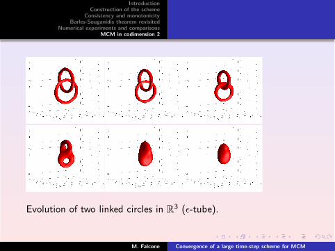
Evolution of two linked circles in R3 (ǫ-tube).





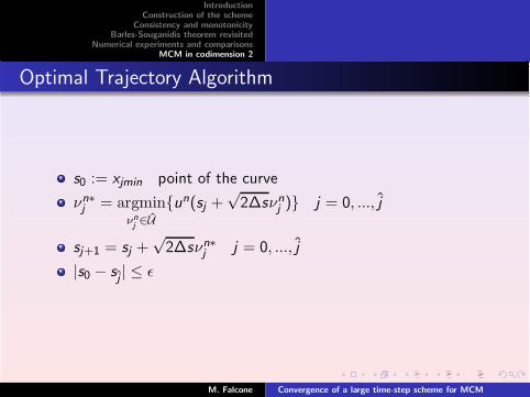
Optimal Trajectory Algorithm

s0 := xjmin point of the curve

νn∗j = argmin

νnj∈U

un(sj +√

2∆sνnj ) j = 0, ..., j

sj+1 = sj +√

2∆sνn∗j j = 0, ..., j

|s0 − sj| ≤ ǫ





0

0.5

1

00.20.40.60.810

0.1

0.2

0.3

0.4

0.5

0.6

0.7

0.8

0.9

1

0

0.5

1

00.20.40.60.810

0.1

0.2

0.3

0.4

0.5

0.6

0.7

0.8

0.9

1

0

0.5

1

00.20.40.60.810

0.1

0.2

0.3

0.4

0.5

0.6

0.7

0.8

0.9

1

0

0.5

1

00.20.40.60.810

0.1

0.2

0.3

0.4

0.5

0.6

0.7

0.8

0.9

1

0

0.5

1

00.20.40.60.810

0.1

0.2

0.3

0.4

0.5

0.6

0.7

0.8

0.9

1

0

0.5

1

00.20.40.60.810

0.1

0.2

0.3

0.4

0.5

0.6

0.7

0.8

0.9

1

Evolution of a helix in R3.





−1

0

1

−1 0 1

−1.5

−1

−0.5

0

0.5

1

1.5

2

2.5

−1

0

1

−1 0 1

−1.5

−1

−0.5

0

0.5

1

1.5

2

2.5

−1

0

1

−1 0 1

−1.5

−1

−0.5

0

0.5

1

1.5

2

2.5

−1

0

1

−1 0 1

−1.5

−1

−0.5

0

0.5

1

1.5

2

2.5

−1

0

1

−1 0 1

−1.5

−1

−0.5

0

0.5

1

1.5

2

2.5

−1

0

1

−1 0 1

−1.5

−1

−0.5

0

0.5

1

1.5

2

2.5

Evolution of two linked circles in R3.


Convergence of a large time-step scheme for Mean Curvature ... · max a∈B(0,1) {c(y)a · ∇T(x)}...

Documents

Transcript of Convergence of a large time-step scheme for Mean Curvature ... · max a∈B(0,1) {c(y)a · ∇T(x)}...