CONVERGENCE OF A FINITE ELEMENT METHOD …

mathematics of computationvolume 59, number 200october 1992, pages 383-401

CONVERGENCE OF A FINITE ELEMENT METHODFOR THE DRIFT-DIFFUSION

SEMICONDUCTOR DEVICE EQUATIONS:THE ZERO DIFFUSION CASE

BERNARDO COCKBURN AND IOANA TRIANDAF

Abstract. In this paper a new explicit finite element method for numerically

solving the drift-diffusion semiconductor device equations is introduced and an-

alyzed. The method uses a mixed finite element method for the approximation

of the electric field. A finite element method using discontinuous finite elements

is used to approximate the concentrations, which may display strong gradients.

The use of discontinuous finite elements renders the scheme for the concentra-

tions trivially conservative and fully parallelizable. In this paper we carry out

the analysis of the model method (which employs a continuous piecewise-linear

approximation to the electric field and a piecewise-constant approximation to

the electron concentration) in a model problem, namely, the so-called unipolar

case with the diffusion terms neglected. The resulting system of equations is

equivalent to a conservation law whose flux, the electric field, depends globally

on the solution, the concentration of electrons. By exploiting the similarities of

this system with classical scalar conservation laws, the techniques to analyze the

monotone schemes for conservation laws are adapted to the analysis of the new

scheme. The scheme, considered as a scheme for the electron concentration,

is shown to satisfy a maximum principle and to be total variation bounded.

Its convergence to the unique weak solution is proven. Numerical experiments

displaying the performance of the scheme are shown.

1. Introduction

This is the first paper of a series in which we introduce and analyze a new fi-

nite element method for numerically solving the equations of the drift-diffusion

model for semiconductor devices, [39]:

(1.1a) -eAtp = q(C - n+p),

(1.1b) qnt - div Jn --qR,

(1.1c) qp, + div Jp = -qR,

where ip is the electric potential, n is the electron concentration, p is the

hole concentration, e is the dielectric constant, q is the electronic elementary

Received by the editor October 29, 1990 and, in revised form, December 9, 1991.

1991 Mathematics Subject Classification. Primary 65N30, 65N12, 35L60, 35L65.Key words and phrases. Semiconductor devices, conservation laws, finite elements, convergence.

The first author was partly supported by the National Science Foundation (GrantDSM-91003997)

and by the University of Minnesota Army High Performance Computing Research Center.

The second author was supported by a Fellowship of the University of Minnesota Army High

Performance Computing Research Center.

©1992 American Mathematical Society

0025-5718/92 $1.00+ $.25 per page

383

License or copyright restrictions may apply to redistribution; see https://www.ams.org/journal-terms-of-use

384 BERNARDO COCKBURN AND IOANA TRIANDAF

charge, C is the doping profile, R = R(n, p) is the carrier recombination-

generation rate, and Jn and Jp are the current densities. They are given by

(l.ld) Jn = qpn(UTgradn-n%rad\i/),

(l.le) Jp = -qpp(UTèradp+pgradt//),

where pn and pp are the electron and hole mobilities, and Ut is the thermal

voltage; see [29, pp. 7-13].The main ideas of our method are as follows. Following [16], we discretize

Poisson's equation (1.1a) by using a mixed finite element method, [33], [5].

This method has the advantage of directly giving a numerical approximation of

the electric field, - grad y/, which is the only quantity depending on y/ that

appears in the convection-diffusion equations (1.1b) and (1.1c). To discretize

the latter equations, we use an extension of the Runge-Kutta Discontinuous

Galerkin (RKDG) method, which is a fully parallelizable method initially de-vised for numerically solving nonlinear conservation laws. In the scalar case,

the RKDG method can be proven to satisfy maximum principles, even when

the approximate solution is locally a polynomial of total degree k > 0. More-

over, extensive numerical simulations show that the RKDG method can capture

discontinuities within a couple of elements without producing spurious oscilla-

tions; see [9, 10, 11, 12]. Thus, the RKDG method is a natural choice in this

framework, since the concentrations may present strong gradients.

The main computational advantages of our method are the following. Since

the use of Lagrange multipliers, see [5] and the bibliography therein, renders

the matrix of the mixed element method symmetric and positive definite, the

computation of the approximation to grad y/ is very much facilitated. Also,

since the RKDG method uses discontinuous approximations, the 'mass' matrix

turns out to be a blockdiagonal matrix whose entries can be inverted by hand(in fact, the order of the blockdiagonal matrices is exactly equal to the number

of degrees of freedom of the approximate solution wA on the corresponding ele-

ment). Moreover, since the Runge-Kutta method used is explicit, the scheme for

the convection-diffusion equations is fully parallelizable. Finally, no nonlinear

equation is required to be solved at each timestep.

For the sake of clarity, the analysis of our finite element method will be done

on a one-dimensional model problem. We set R = 0, and scale the equations

(see [29, pp. 26-28], [38] and [3] for details) to obtain

(1.2a) -cj)xx = c-u + v, x>0, x£(-X,X),

(1.2b) uT + (u(px)x-À2uxx = 0, t>0, x£ (-1, 1),

(1.2c) vx-(vd>x)x-X2vxx = 0, x>0, x£(-X, X),

0||C|U~/2'

and / is the typical diameter of the semiconductor device. Since typical values

of A range from 10~3 to 10-5, [29, p. 28; 37], it seems reasonable to neglect

the second-order terms in (1.2b) and (1.2c). The resulting equations give a good

approximation of the initial system in the so-called 'fast' time scale, see [37, 30,

34]. See also the singular perturbation analyses carried out in [4, 6]. By using

where

(1.2d)


A NUMERICAL SCHEME FOR THE SEMICONDUCTOR DEVICE EQUATIONS 385

a symmetry assumption, [37, 34], we can decouple equations (1.2b) and (1.2c)

and obtain the following equations for the scaled electron concentration u and

the scaled electric potential </> :

-<t>xx = X-U, X£(0, X), T>0,

uT + (u<t>x)x = 0, x£(0, X), x>0,

where we have assumed, for simplicity, that the scaled doping profile c is iden-

tically equal to 1 on (0, 1). All our results also hold for c inBV(0, 1). These

are the equations of our model problem. To complete it, we have to impose the

boundary conditions

(f>(x,0) = 0, forr>0,

<¡>(x, X) = cj>x(x), forr>0,

and

W(T,0) = Ko(T), if(/.x(T,0)>0, T>0,

u(x, X) = ux(x), if^(T, 1)<0, T>0,

and the initial condition

w(0, X) = Uj(x), X £ (0, 1).

The solution of this problem has been proven to be the limit as X goes to zero

of the corresponding 'viscous' solutions, see (2.15), in [8]. The problem of how

close these solutions are will be addressed in this paper numerically only. It will

be considered analytically in a forthcoming paper.

To study the above problem, we prefer to rewrite it as the following conser-

vation law:

(1.3a) uT + (uß)x = 0, t>0, x£(0, X),

(1.3b) u(x, 0) = u0(x), if ß(x, 0) >0, t>0,

(1.3c) u(x, X) = ux(x), if ß(x, X) <0, t>0,

(1.3d) u(0,x) = u¡(x), x£ (0, 1),

where

(1.4a) -ßx = X-u, x£(0, 1), t>0,

(1.4b) ß = 4>x, x£(0, X), t>0,

(1.4c) <f>(x,0) = 0, forr>0,

(1.4d) <f>(x, X) = <j>x(r), forr>0,

since written in this form, it is easier to compare it with a classical conservation

law:(i) Notice that the equation ( 1.3a) would be a classical nonlinear conservation

law if the operator ß were an evaluation operator, i.e., if ß = ß(u). However,

in our case the value of ß at a single point (t, x) £ (0, T) x (0, 1) contains

the information of all the values of the function u(x, •) on (0,1). Hence a

perturbation of the function u at any given point of the domain does have a



global effect immediately. This is in sharp contrast with the classical conser-

vation laws, for which local perturbations of the solution have a local effect in

finite time.(ii) The smoothness of ß(x, •) guarantees the uniqueness of the weak solu-

tion, [31], and so the worry about convergence to the so-called entropy solution

that pervades the numerical analysis of schemes for classical conservation laws

is not present here. Nevertheless, the continuity of ß also guarantees that the

characteristics of our system never intersect each other. Numerically, this means

that there is no natural mechanism that would help the scheme to 'sharpen' the

discontinuities, as happens in classical conservation laws when the nonlinearity

is convex (for example).

(iii) Note that u = 0 and u = X are equilibrium points of the equation of

u along the characteristics. In fact, if x - x(x) denotes a given characteristic,

and if we set u = u(x, x(x)), then

(1.5) -j- u = (X - u)u.ax

From this equation it is clear that u = 0 is an unstable equilibrium point

whereas u = X is an asymptotically stable point. (This situation never occurs

for classical conservation laws.) The instability of u = 0 indicates that the

numerical approximation, uh , has to be prevented from taking negative values,

however small. It also indicates that the numerical approximation of the points

u = 0 might be a delicate matter. The asymptotic stability of u = X suggests the

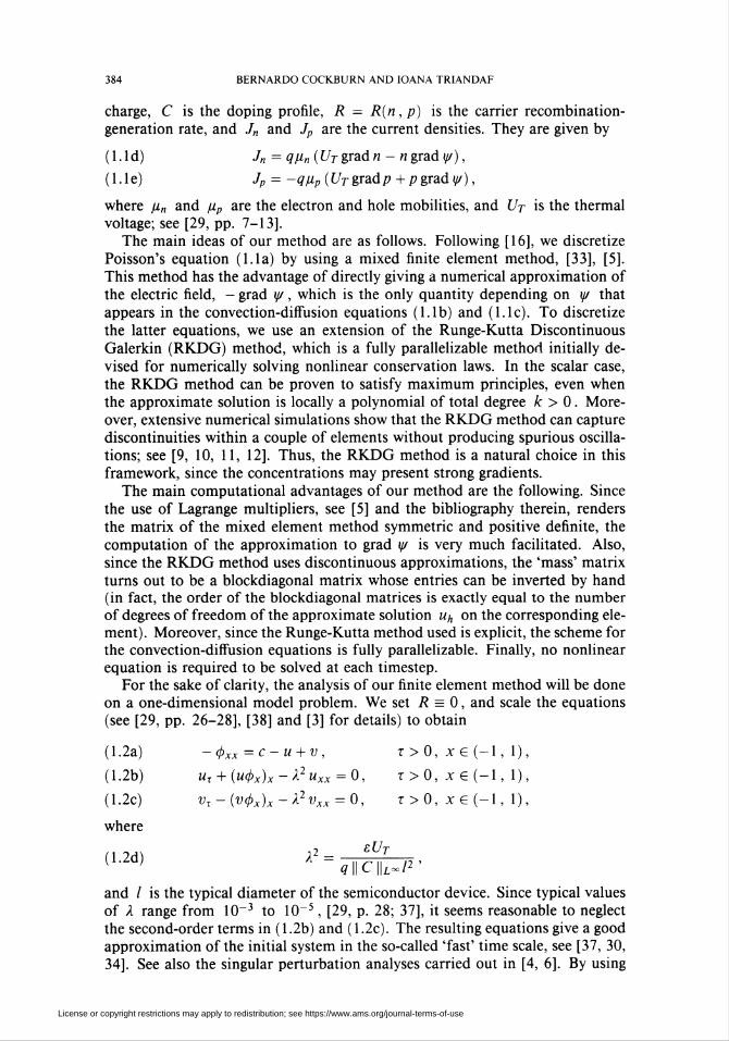
existence of a maximum principle for the solution u. Notice that for the very

simple case in which ß = ß(x) = X ¡2 - x , u0 = 0, ux = X , and u¡(x) = x, the

solution of the conservation law (1.3) does not remain bounded. In this case,

II w(r) lk~(o, i) goes to infinity as x goes to infinity; see Figure 1.

6

4

2

0

0.0 0.2 0.4 0.6 0.8 1.0

Figure 1. Blowing up of the solution u of (1.3) when

ß(x) = 1/2 - x , wo = 0, u\ = 1 , and u¡(x) = x

i-'-1-'-1-'-r

J_,_I_,_I_,_L



(iv) Finally, since the solution of equation (1.5) is

u¡(x(0))u(x, x(x)) = eT

[X + (e*-X)Ui(x(0))_

» u,(x(0))ez, forO<T«l,

we expect the total variation of the concentration to grow in time as fast as ex,

without the boundary data being responsible for such a growth. This is also in

strong contrast to what happens in classical conservation laws, where the total

variation does not increase in such a situation.

The finite element method we consider in this paper takes the approximation

to grad (f> to be a continuous piecewise linear function and the approximation to

u to be a piecewise constant function. The resulting scheme can be considered

to be a counterpart of the monotone schemes for conservation laws. With this

fact in mind, the techniques for analyzing monotones schemes, [15, 18], will

be suitably extended to our present setting. The main objective of this paper is

to establish the stability of the new method and to prove its convergence in the

case of the model problem (1.3), (1.4). Particular care has to be taken to relate

the behavior of the piecewise linear continuous approximate electric field given

by the mixed finite element method, with the behavior of the piecewise constant

convected approximate electron concentration. Our analysis of the boundary

conditions is inspired by the ideas introduced in [25]. A forthcoming paper will

be devoted to obtaining error estimates.

No finite element method seems to have been proposed and analyzed for the

hyperbolic problem (1.3), (1.4). Most methods are defined on the full equations

(1.1), and take advantage of the parabolicity of equations for the concentrations.

In order to do that, a widespread practice consists in using the so-called Boltz-

mann statistics as variables. This change of variables allows the currents to be

expressed in the form {c gradz} in an effort to render the equations (1.1b)

and (1.1c) 'naturally' parabolic; see, e.g., [40, 2]. However, this practice 'hides'

the convective character of the equations. This is why we do not use Boltzmann

statistics as variables. The same point of view is taken in [16, 32], where adirect hold of the convection phenomenon is attempted through the modified

method of characteristics. We want to emphasize that, unlike the methods in

[16, 32], our scheme is conservative.

Our proposed method can also be used to compute the stationary solution of

( 1.1 ) by simply letting the final time T be large enough. Of course, other more

efficient ways to do so can be devised, but we shall not pursue this matter in

this paper. Methods for computing stationary solutions of ( 1.1 ) can be found

in, e.g., [1, 17, 22, 35]. The stationary solutions of (1.1) may be considered to

be the fixed points of the so-called Gummel map; see, e.g., [19]. The iterative

procedures of the above-mentioned papers try to construct numerical approx-

imations to the Gummel map (and to its fixed points). A rigorous analysis of

the convergence of such numerical approximations can be found in [20]. These

iterative procedures can also be applied to solve the transient problem; see [21]

and [14]. We finally point out that a new discretization technique that gen-

eralizes to the two-dimensional case the (one-dimensional) Sharfetter-Gummel

method has recently been introduced in [7].

The paper is organized as follows. In §2a, we define the set of data with

which we deal in this paper and define the weak solution of problem (1.3),



(1.4). In §2b, we present our numerical method. In §2c, we state and briefly

discuss our results on stability (Theorem 2.1), continuity with respect to the

data (Theorem 2.2), and convergence to the weak solution (Theorem 2.3). We

also include therein an additional convergence result (Theorem 2.4) that will be

used in a forthcoming paper to obtain error estimates. In §2d, we state a result

(Theorem 2.5) concerning the smoothness with which the boundary conditions

are satisfied by the approximate solution. This result requires reasonable ad-

ditional restrictions on the data. Finally, in §2e, we show several numerical

results illustrating the performance of the scheme. The proofs of our theorems

are contained in the Supplement section at the end of this issue.

2. The numerical method and the main results

2a. The weak solution. We shall assume that the initial data u¡ and the

boundary data uo,ux and 4>x satisfy the following regularity conditions:

(2.1a) Ho(T),Ki(T),K,(jc)€[0,tt*], T £ [0, T], X £ [0, 1],

(2.1b) Uo,ux£BY(0,T), and u¡(x) £ BV(0, 1),

(2.1c) ¿i(T)e[0,tf], x£[0,T],

(2. Id) 0,eBV(O,r),

where, see remark (iii) in § 1, we assume that

(2.1e) «*>1.

The weak solution of (1.3) and (1.4) is defined to be a function (u, ß, 0) e

L°°(0, T; BV(0, l))xL°°(0, T; Wx^(0, l))xL°°(0, T; BV(0, X)) satisfyingthe following weak formulation:

-/ / {u(x, x)tpr(x,x) + u(x, x)ß(x, x)tpx(x,x)}dxdxJo Jo

— j Ui(x) <p(Q, x)dxJo

(2.2a) + / f(u(x, X-),ux(x); ß(x, X))<p(x, X)dxJo

- [ f(uo(x),u(x,0+); ß(x,0))tp(x,0)dx = 0,Jo

V(p£%x([0,T)x[0, 1]),

where the flux / is defined by

(2.2b) /(«left , «right ; ß) = "left ß+ + »right ß~ ,

with ß~ = min{)?, 0}, and ß+ = max{ß, 0}, and

(2.3a) Jo/ ßx(x, x)w(x)dx

Jo

= [ (X -u(x,x))w(x)dx, Vu;eL2(0,l),



/ ß(x, x)v(x)dx(2.3b) Jo ,

= -( cp(x,x)vx(x)dx + <px(x)v(X), Mv£Hx(Q,X).Jo

Notice that any function in Wl'x(0, X) is continuous, and that any function

in BV (0,1) has well-defined limits from the left and from the right. Thus, thelast two integrals of (2.2a) have a meaning.

Notice also that the role of the flux / is to select the correct boundary

value for u according to (1.3b) and (1.3c). To see this, assume that « is a

very smooth solution of (2.2). Take functions tp £ W0X((0, T) x [0, X)), and

integrate by parts in (2.2a). Since u satisfies equation (1.3a) pointwise, we get

• T

(u(x, 0+) - Uo(x))ß+(x, Q)<p(x, 0)dx = 0,/o

and since we are assuming u to be smooth, this implies

u(x, 0+) ß+(x, 0) = uo(x) ß+(x, 0), t £ (0, T),

/'Jo

or

u(x, 0+) = uo(x) lf/?(T,0)>0, X£(0,T),

which is nothing but condition (1.3b). Condition (1.3a) can be obtained in a

similar way.

2b. The numerical scheme. We first introduce some notation. Let

{xi+1/2},=o.nx be a partition of [0, 1] with xx¡2 = 0 and xnx+X/2 = X . Simi-

larly, let {T"}„=o,...,nr be a Partition of [0, T], with t° = 0 and x"T = T. We

set /, = (-X/-1/2, xM/2). àxi = xi+x/2 - X/-1/2, and /" = [xn , t"+1), At" =

Tn+i _ T« Define Ax = max,=i ... >Bjt{ Ax¡} and At = max„=0,... ,«r-i{ At" }.

We associate with these partitions the following spaces:

(2.4a) V^ = {VAx £ &°(0, 1) : V&x\i, 6 Pl(I¡), i=X,...,nx},

(2Ab) WAx = {wAx£L°°(0, X):wAx\Ii£P°(Ii),i= X,...,nx},

(2.4c) H/Ar = {ioAt right-continuous: wàT\j» £ P°(J"), n — 0, ... , «r - 1}.

If Vax £ V^y-, then vi+x/2 denotes vAx(x,+x/2) for / = 0, •■• ,nx. If w^ £

W^ , then Wi denotes the constant value w^x), x £ I¡, for i = X, ... , nx;

the values wo and wnx+x denote the exterior trace at x = 0, ^ax(O-) , and

at x = X, wAx(X+), respectively. Finally, if wàT £ WAr, then w" denotes the

constant value wAr(x), x £ J" .

To discretize (1.3), (1.4), we first discretize the data by setting

(2.5a) 0i,at = P^Ai(</>i),

(2.5b) Mn,At = JrViT("o),

(2.5c) "i,at = PK("i),

(2.5d) ultAx = rw^(u,),

where P> denotes the L2-projection into the space 'V. The approximate

solution Uh is taken to be in the space W&ï ® W^ and is required to satisfy

the equation

(2.6a) «+1 - u1)IAx" + (f» - f,1x/2)/Ax, = 0,



where the numerical flux f"+l/2 = f(u] , uni+{ ; ß"+l/2) is given by (2.2b), i.e., by

(2.6b) y;"+,/2 = "r^+i/2 + <+i^"i/2-

The function (ßh, </>/,) £ **at ® Vax x ^at ® W^ is defined by the followingmixed finite element method:

(2.7a)/W(t\Jo

x)wAx(x)dx

= / (1 -uh(x", x))wAx(x)dx, VwAx£WAx,Jo

(2.7b)/ ßh(x",x)vAx(x)dx

Jo

= -/ Mrn,x)(vAx)x(x)dx + (f)XtAT(xn)vAx(X), VvAx£VAx.Jo

Note that, for a given function ßh, the scheme (2.6) is nothing but the well-

known upwinding scheme (which coincides with the Godunov scheme in this

case). Since this is a monotone scheme under a suitable CFL condition, it is

reasonable to expect to have for this scheme convergence properties similar to

the convergence properties of monotone schemes for scalar conservation laws,

[15]. We shall see below that this is indeed the case.

Notice that for the upwinding numerical flux fi"+l /2, (2.6b), to be well de-

fined, the function ßh(x, •) has to be continuous. This requirement is naturally

taken into account by the mixed finite element method used to compute it. Thisis an important advantage of using the mixed method (2.7).

Thus the algorithm of our numerical method is:

(2.8a) Compute the functions u0 at> «i at> ui a* , and 4>x At by (2.5);

(2.8b) Set wA(0, •) = "/,Ax(-);

(2.8c) For n = 0, ... , nT - X compute W/,(t"+1 , •) as follows:

(i) Compute (ßh(r" , •), 0/,(t" , •)) by using the mixed finite element

method (2.7);(ii) Set uh(xn,Q-) = UQ^T(xn) and uh(xn , 1+) = «i,at(tb);

(iii) Compute uh(xn+x, x) for x £ (0, 1) by using the scheme (2.6).

2c. Stability and convergence results. In this section we state and briefly dis-cuss the stability properties of the scheme (2.8), Theorem 2.1, its property of

continuity with respect to the data, Theorem 2.2, and its convergence property

to the weak solution of the original problem, Theorem 2.3. We also obtain an

estimate which will be used elsewhere to obtain error estimates for the scheme

under consideration, Theorem 2.4.

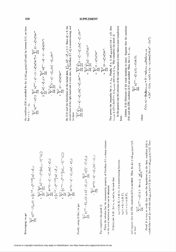
Theorem 2.1 (Stability). Suppose that for n = 0, ... , nF - X the following CFLcondition is satisfied:

(2.9) At" < min J ^u* ' (2 u* - X) Ax, + (j)*,+ j max{ X, u* - X)



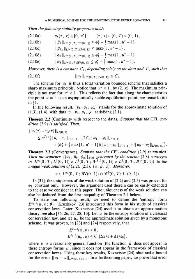
Then the following stability properties hold:

(2.10a) uh(x,x)£[0,u*], (x,x)£(0,T)x(0,X),

(2.10b) ||A,||z~(o,r;z,»(o,i)) < 4>*x + ^ max{X, u* - 1},

(2.10c) \\ßhx\\L°°(0,T;mo,i)) < max{ 1, u* - X),

(2.10d) ||0a||l«»(o,7';z.«(o,i)) < <t>\ + \max{X, u* - 1},

(2.10e) ||0aIIl~(o,7';bv(o,i)) < 4>\ + 2 max{ 1, u* - 1}.

Moreover, there is a constant Cx, depending solely on the data and T, such that

(2.1 Of) || Uh ||l°°(0)7';BV(0,1)) < Cx-

The scheme for «/, is thus a total variation bounded scheme that satisfies a

sharp maximum principle. Notice that u* > X, by (2.le). The maximum prin-

ciple is not true for u* < X. This reflects the fact that along the characteristics

the point u = X is an asymptotically stable equilibrium point; see remark (iii)

in §1.In the following result, (vh , yn, \ph) stands for the approximate solution of

(1.3), (1.4), with data v¡, v0,Vx, y/x satisfying (2.1).

Theorem 2.2 (Continuity with respect to the data). Suppose that the CFL con-

dition (2.9) is satisfied. Then,

\\Uh(r)-Vh(r)\\v(o,x)

< ec^{\\ m - Vi ||Li(0,i) + 2 Cill <f>i - \px \\Li{QjT)

+ (4>\ + ±max{l, u* - X})(\\ux - vx lb(o,r) + II «o - «ökuo.t))}-

Theorem 2.3 (Convergence). Suppose that the CFL condition (2.9) is satisfied.

Then the sequence {(uh , ßh , <t>h)}h>o generated by the scheme (2.8) convergesin L°°(0, T; Lx(0, X)) x L'(0, T; Wx<x(0, X)) x Lx(0, T; BV(0, X)) to the

unique weak solution of (2.2), (2.3), (u, ß ,<¡>). Moreover,

u £ L°°(0, T; BV(0, 1)) n f °(0, T; Ll(0, X)).

In [31], the uniqueness of the weak solution of (2.2) and (2.3) was proven for

0i constant only. However, the argument used therein can be easily extended

to the case we consider in this paper. The uniqueness of the weak solution can

also be deduced from the first inequality of Theorem 2.4 below.

To state our following result, we need to define the 'entropy' form

EE°'e(u, v ; ß). Kruzhkov [23] introduced this form in his study of classical

conservation laws. Later, Kuznetsov [24] used it to obtain an approximation

theory; see also [36, 26, 27, 28, 13]. Let u be the entropy solution of a classical

conservation law, and let «/, be the approximate solution given by a monotone

scheme. It was proven, in [23] and [24] respectively, that

E£0'E(u,v)<0,

EE<"£(uh, u)<C (Ax/e + Ax/eq),

where v is a reasonably general function (the function ß does not appear in

these entropy forms E, since it does not appear in the framework of classical

conservation laws). Using these key results, Kuznetsov [24] obtained a bound

for the error \\uh~ u ||l°°{0, t-,V) ■ 1° a forthcoming paper, we prove that error



estimates can be obtained for the scheme under consideration provided that

similar results are obtained. Our next result contains those results.

Let eo and e be arbitrary positive real numbers, and let w : R —> M be an

even nonnegative function in ^°°(R) with support included in [-1,1], and

such that /_! w = X. We set

tp(x,x;x', x') = weo(x - x') we(x - x'),

where wv(s) = w(s/u)/u, Vs 6 1. Let us denote by U an arbitrary even

convex function with Lipschitz second derivative, such that U(0) = 0.

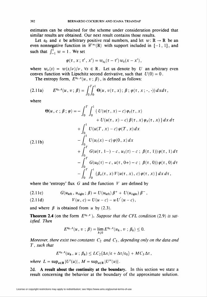
The entropy form, E£°'£(u, v ; ß), is defined as follows:

(2.11a) E£o'£(u,v; ß) = if 0(u, v(x, x) ; ß ; <p(x, x; -, -))dxdx,Jo Jo

where

e(u,c; ß; <p) =- / / {U(u(x,x)-c)<pT(x,x)Jo Jo

+ U(u(x, x) - c) ß(x, x) q>x(x, x) }dxdx

+ U(u(T, x) - c)tp(T, x)dxJo

(2.iib) -/ U(Ui(x)-c)tp(0,x)dx

+ [ G(u(x, X-) - c, ux(x) - c ; ß(x, X))<p(x, X)dxJo

- f G(uq(x) - c, u(x, 0+) - c ; ß(x, 0)) <p(x, 0)dxJo

-ff {ßx(x,x)V(u(x,x),c)tp(x,x)}dxdx,Jo Jo

where the 'entropy' flux G and the function V are defined by

(2.11c) C7(wleft, Hright; ß) = U(uXeü)ß++ U(uúghl) ß~ ,

(2.1 Id) V(u,c) = U(u-c)-uU'(u-c),

and where ß is obtained from u by (2.3).

Theorem 2.4 (on the form E£°'£ ). Suppose that the CFL condition (2.9) is sat-

isfied. Then

E£°<£(u,v ;ß) = XimEE0'E(Uh,v ; ßh) < 0.h[0

Moreover, there exist two constants C2 and C3, depending only on the data and

T, such that

E£o>E(uh, u ; ßh) < LC2{Ax/e + Ax/eq) + MC3Ax,

where L = supueR \U'(u)\, M = supueR \U"(u)\.

2d. A result about the continuity at the boundary. In this section we state a

result concerning the behavior at the boundary of the approximate solution.



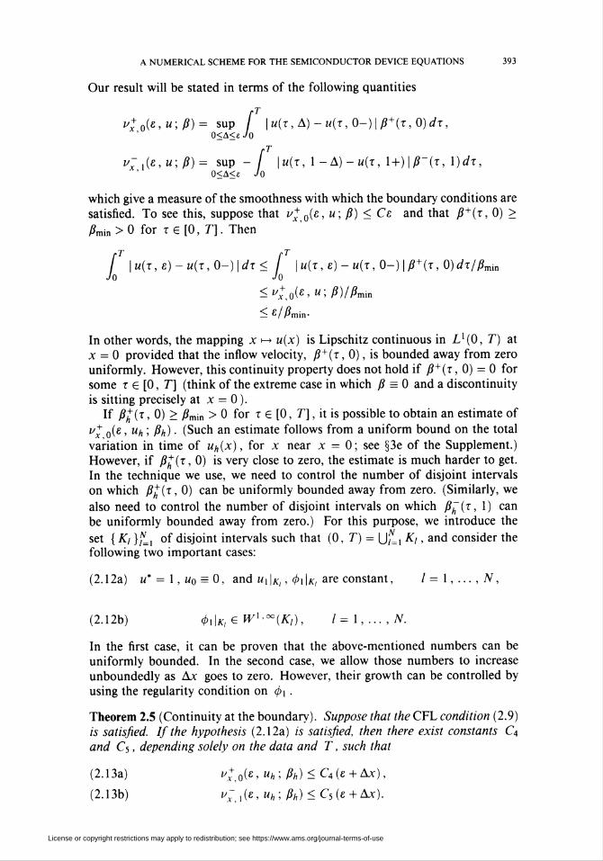
Our result will be stated in terms of the following quantities

u+ 0(e,u; ß)= sup / \u(x,A)-u(x,0-)\ß+(x,0)dx,0<A<« Jo

v~ ,(e, u; ß) = sup - / \u(x, X -A) - u(x, X+)\ß~(x, X)dx,0<A<£ Jo

which give a measure of the smoothness with which the boundary conditions are

satisfied. To see this, suppose that i/+ 0(e, u; ß) < Ce and that ß+(x, 0) >

ßmin>0 for Te[0J], Then

/ \u(x,e)- u(x, 0-) I dx < [ | u(x, e) - u(x, 0-) \ß+(x, 0) dx/ßminJo Jo

<i/+0(e, u; ß)/ßmin

< e/^min-

In other words, the mapping x i-> u(x) is Lipschitz continuous in Lx(0, T) at

x = 0 provided that the inflow velocity, ß+(x, 0), is bounded away from zero

uniformly. However, this continuity property does not hold if ß+(x, 0) = 0 for

some t £ [0, T] (think of the extreme case in which ß = 0 and a discontinuity

is sitting precisely at x = 0 ).If ß£(x, 0) > /?min > 0 for t £ [0, T], it is possible to obtain an estimate of

ux q(e , Uh ; ßh) ■ (Such an estimate follows from a uniform bound on the total

variation in time of uh(x), for x near x = 0; see §3e of the Supplement.)

However, if ß^(x, 0) is very close to zero, the estimate is much harder to get.

In the technique we use, we need to control the number of disjoint intervals

on which ß£(x, 0) can be uniformly bounded away from zero. (Similarly, we

also need to control the number of disjoint intervals on which ßh~(x, X) can

be uniformly bounded away from zero.) For this purpose, we introduce the

set {AT/ }^, of disjoint intervals such that (0, T) = \J¡=1 K¡, and consider the

following two important cases:

(2.12a) m* = 1,«o = 0, and «iIa:, , 0i|jt; are constant, l=X,...,N,

(2.12b) 4>x\Kl£Wx^(K,), l=X,...,N.

In the first case, it can be proven that the above-mentioned numbers can be

uniformly bounded. In the second case, we allow those numbers to increase

unboundedly as Ax goes to zero. However, their growth can be controlled by

using the regularity condition on 0i .

Theorem 2.5 (Continuity at the boundary). Suppose that the CFL condition (2.9)

is satisfied. If the hypothesis (2.12a) is satisfied, then there exist constants C4

and Ci, depending solely on the data and T, such that

(2.13a) v+0(E,uh;ßh)<CA(E + Ax),

(2.13b) v;l(£,uh;ßh)<C5(E + Ax).


394 BERNARDO COCRBURN AND IOANA TRIANDAF

1.0

0.8

0.6

0.4

0.2

0.0

0.0 0.2 0.4 0.6 0.8 1.0

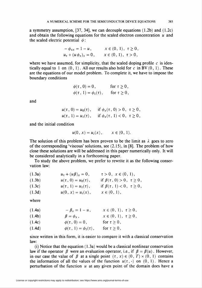
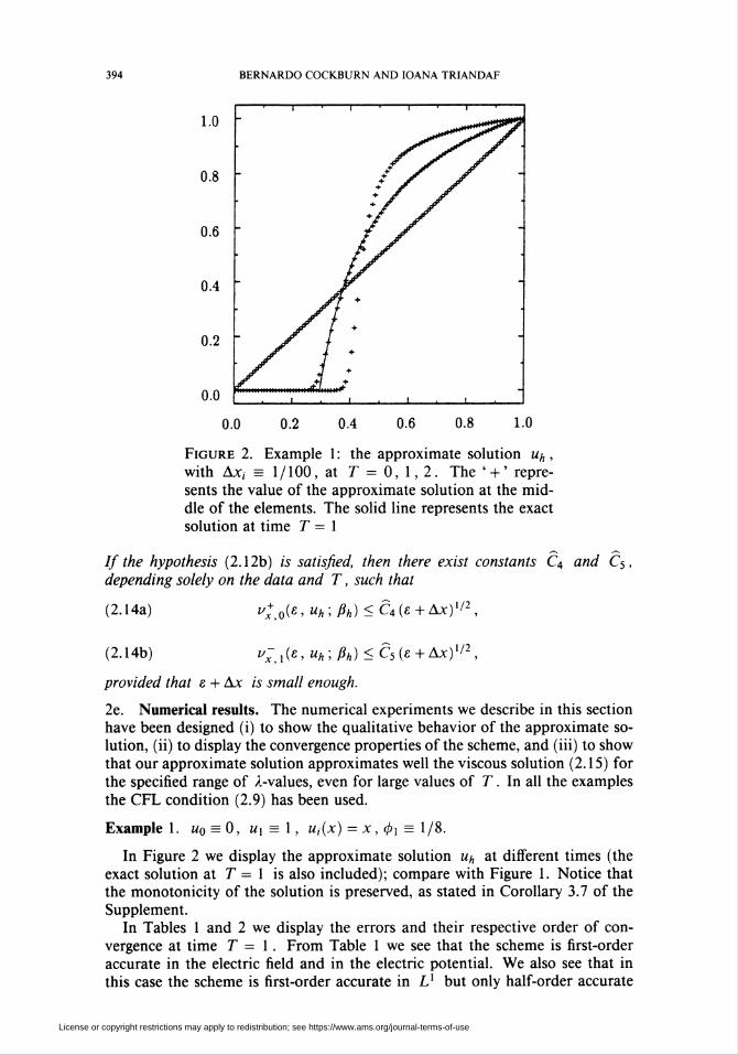
Figure 2. Example 1: the approximate solution «/,,

with Ax, = 1/100, at T = 0, 1, 2. The ' + ' repre-sents the value of the approximate solution at the mid-

dle of the elements. The solid line represents the exact

solution at time T = X

If the hypothesis (2.12b) is satisfied, then there exist constants C4 and C5,

depending solely on the data and T, such that

(2.14a) u^0(e,uh;ßh)<C4(E + Ax)1'2,

(2.14b) !/",(«, uh;ßh) < C5(£ + Ax)'/2,

provided that e + Ax is small enough.

2e. Numerical results. The numerical experiments we describe in this section

have been designed (i) to show the qualitative behavior of the approximate so-

lution, (ii) to display the convergence properties of the scheme, and (iii) to show

that our approximate solution approximates well the viscous solution (2.15) for

the specified range of A-values, even for large values of T. In all the examples

the CFL condition (2.9) has been used.

Example 1. wn = 0, ux = X, u¡(x) = x, </>i = 1/8.

In Figure 2 we display the approximate solution ma at different times (the

exact solution at T = X is also included); compare with Figure 1. Notice that

the monotonicity of the solution is preserved, as stated in Corollary 3.7 of the

Supplement.In Tables 1 and 2 we display the errors and their respective order of con-

vergence at time T = X . From Table 1 we see that the scheme is first-order

accurate in the electric field and in the electric potential. We also see that in

this case the scheme is first-order accurate in L1 but only half-order accurate

i-'-1-'-r



Table 1. Example 1: Convergence in (0,1]

and Ax = 1/100

at T = X

102-error order 102-error order

u

ß4>

5.77130.11760.1820

0.5450.9240.986

0.40450.02790.0286

0.9370.9971.003

Table 2. Example 1: Convergence in (0, 1) \ [.25, .35]

at T = X and Ax = 1/100

102-error order 102- error order

u

ß

2.20750.10050.1819

0.8901.0550.986

0.21420.02110.0244

1.1211.1121.051

in L°° in the concentration. This discrepancy is caused by the discontinuity of

the derivative of the exact electron concentration in the interval (.25, .35). To

see this, it is enough to study the errors outside this interval. Indeed, in Table 2

we see that the scheme is first-order accurate (in the electron concentration) in

both L1 and L°° on [0, .25] U [.35, 1]. These observations indicate that the

scheme is first-order accurate when the solution is smooth enough. They also

indicate that the influence of the discontinuity in the derivative of the electron

concentration on the quality of the approximation has only a local effect.

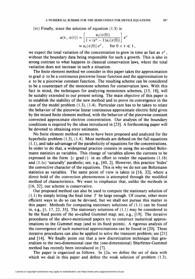
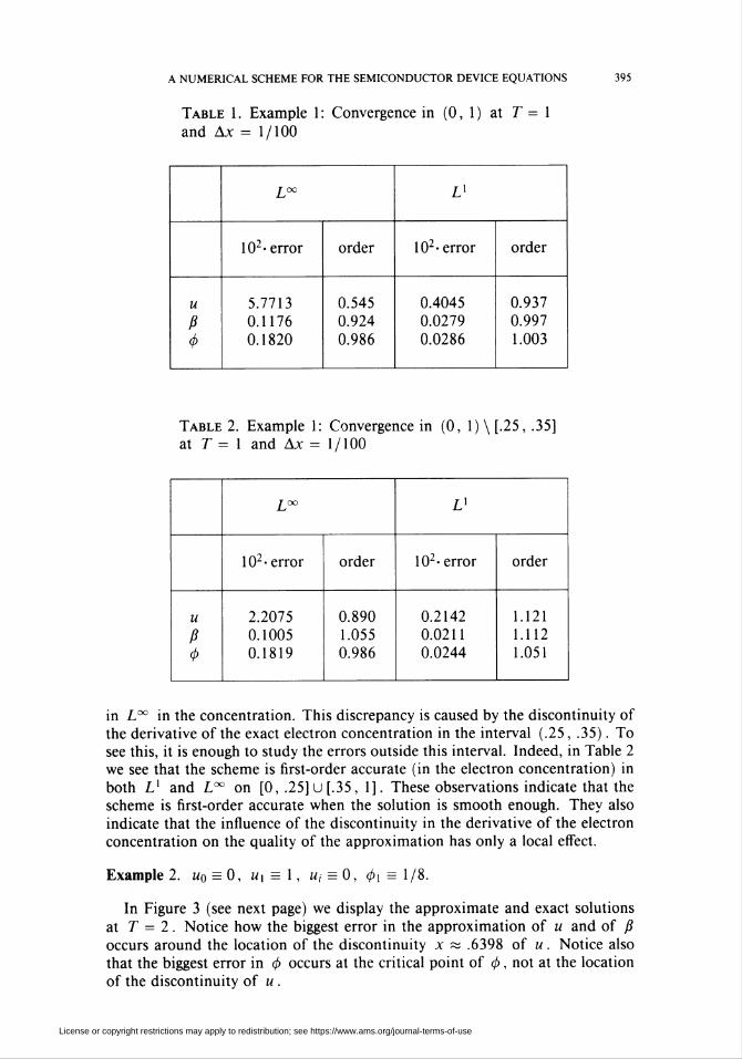
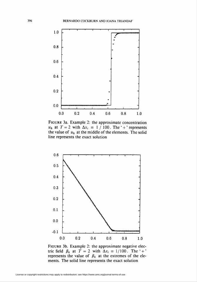
Example 2. Uq = 0, U\ = X, u¡ = 0, 4>x = 1/8.

In Figure 3 (see next page) we display the approximate and exact solutions

at T = 2. Notice how the biggest error in the approximation of u and of ß

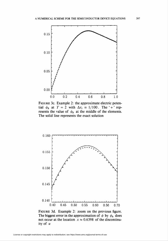
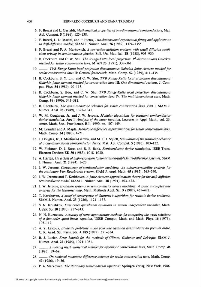
occurs around the location of the discontinuity x « .6398 of u. Notice also

that the biggest error in 0 occurs at the critical point of 0, not at the location

of the discontinuity of u .



1.0

0.8

0.6

0.4

0.2

0.0 r MMinin»MMHH»MHHHMMII»HMHHIHHHIHlH»

JIIIIHIIIIHIIMMIHMWI

0.0 0.2 0.4 0.6 0.8 1.0

Figure 3a. Example 2: the approximate concentration

uh at T = 2 with Ax, = 1 / 100. The ' + ' representsthe value of Uh at the middle of the elements. The solidline represents the exact solution

0.6

0.5

0.4

0.3

0.2

0.1

0.0 L

-0.1

0.0 0.2 0.4 0.6 0.8 1.0

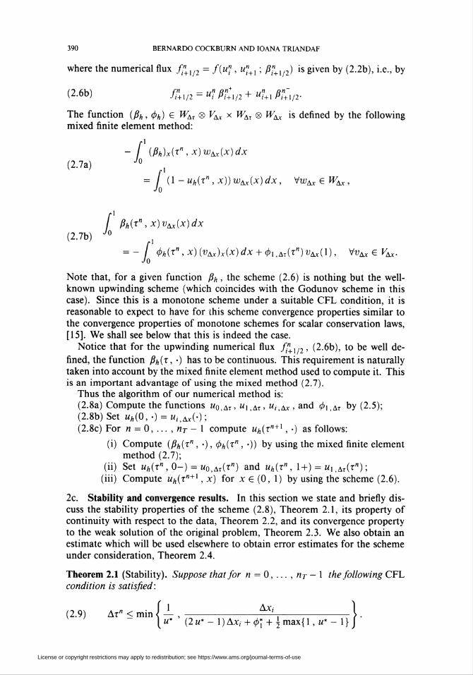
Figure 3b. Example 2: the approximate negative elec-

tric field ßh at T = 2 with Ax, = 1/100. The ' + 'represents the value of ßh at the extremes of the ele-

ments. The solid line represents the exact solution



0.15

0.10

0.05

0.00 P-

Figure 3c. Example 2: the approximate electric poten-

tial <ph at T = 2 with Ax, = 1/100. The ' + ' rep-resents the value of 0Ä at the middle of the elements.

The solid line represents the exact solution

0.160

0.155 h

0.150

0.145

0.140

0.40 0.45 0.50 0.55 0.60 0.56 0.70

Figure 3d. Example 2: zoom on the previous figure.The biggest error in the approximation of 0 by <ph does

not occur at the location x « 0.6398 of the discontinu-

ity of u



Table 3. Example 2: Convergence in (0,1) at T = 2

and Ax = 1/800

V

102-error order 102-error order

u

ß

00.38770.0271

0.4890.998

0.78860.01460.0068

0.4870.9640.996

In Table 3 we show the errors and their orders of convergence. Notice that

the orders of convergence, in Lx, to u and ß are ~ 1/2 and ~ 1, respectively.

This indicates that the presence of the discontinuity in u has only a local effect

in the approximation of ß .

Example 3. «o = 0, ux = X, u, = 0, <f>x = 1/8. In this experiment we want to

compare the approximate solution given by the method (2.8) with the 'viscous'

solution (ux, ßx, 0A) defined by the following equations:

u\ + (ulßx)x=X2uxx, t>0, xe(0, 1),

T>0,

T>0,

xe(0, 1),

(2.15a)

(2.15b)

(2.15c)

(2.15d)

where

ux(x,0) = u0(x),

ux(x, X) = ux(x),

ul(0, x) = Uj(x),

(2.15e)

(2.15Í)

(2.15g)

(2.15h)

ßx = l u

£.ßX

0A(T,O) = O,

0A(T,1) = 0,(T),

X€(0, 1),

xe(0, 1):

for t > 0,

for t > 0.

T>0,

T>0,

We take the same discretization parameters as in the previous example. In

Figure 4 the approximate concentration, the 'nonviscous' and the 'viscous' con-

centrations are compared at time T = 10 around the boundary layer. (If those

concentrations would have been compared on the full interval [0, 1], no dif-

ference between them would have been detected.) At that time all the solutions

are very close to the stationary solutions. We see that the size of the boundary

layer created by the diffusion is approximately equal to Ax = 1/100 for the

biggest value of X2, i.e., for X2 = 10"6. We see that the approximate solution

provides an excellent approximation to the 'viscous' concentration.

Our numerical results thus indicate that the method (2.8) is a very robust

method, which is uniformly first-order accurate in L°° for the electron concen-

tration, the electric field, and the electric potential when the exact solution is



1.0 L

0.8

0.6

0.4

0.2

0.0

0.46 0.48 0.50 0.52 0.54

Figure 4. Example 3: detail of the concentrations un ,

u and ux at 7=10. In this case Ax, = 1 /100 and

X = 10-3. The ' + ' represent the values of Uf, at the

midpoints of the elements, the dashed line represents

u, and the solid line ux

smooth. If the electron concentration is discontinuous, the scheme is half-order

accurate in L1 for the electron concentration and half-order accurate in L°°

for the electric field. We have also verified that in this case, the presence of

the discontinuity has only a local effect on the quality of the approximation.

Finally, we have verified that the scheme provides a good approximation to the

'viscous' solution, see (2.15), even near the stationary state.

Acknowledgments

The authors want to thank Franco Brezzi, Donatella Marini and Huanan

Yang for fruitful discussions. The authors also want to thank the reviewer, the

Managing Editor, and Zhangxin Chen for their remarks leading to an improved

presentation of this paper.

Bibliography

1. R. E. Bank, D. J. Rose and W. Fichtner, Numerical methods for the semiconductor device

simulation, IEEE Trans. Electron Devices ED-30 (1983), 1031-1041.

2. R. E. Bank, W. M. Coughran, Jr., W. Fichtner, E. H. Grosse, D. J. Rose, and R. K. Smith,

Transient simulation of silicon devices and circuits, IEEE Trans. Computer-Aided Design

CAD-4 (1985), 436-451.

3. F. Brezzi, Theoretical and numerical problems in reverse biased semiconductor devices, Com-

puting methods in Applied Sciences and Engineering, VII (R. Glowinski and J. L. Lions,

eds.), Elsevier, Amsterdam, 1986, pp. 45-58.

4. F. Brezzi, A. Capelo, and L. D. Marini, A singular perturbation analysis for semiconductor

devices, SIAM J. Math. Anal. 20 (1989), 372-387.

5. F. Brezzi, J. Douglas, Jr., and L. D. Marini, Two families of mixed finite elements for second

order elliptic problems, Numer. Math. 47 (1985), 217-235.



6. F. Brezzi and L. Gastaldi, Mathematical properties of one-dimensional semiconductors, Mat.

Apl. Comput. 5 (1986), 123-138.

7. F. Brezzi, L. D. Marini, and P. Pietra, Two-dimensional exponential fitting and applications

to drift-diffusion models, SIAM J. Numer. Anal. 26 (1989), 1324-1355.

8. F. Brezzi and P. A. Markowich, A convection-diffusion problem with small diffusion coeffi-

cient arising in semiconductor physics, Boll. Un. Mat. Ital. 2B (1988), 903-930.

9. B. Cockburn and C. W. Shu, The Runge-Kutta local projection P[ -discontinuous Galerkin

method for scalar conservation laws, M2AN 25 (1991), 337-361.

10._, TVB Runge-Kutta local projection discontinuous Galerkin finite element method for

scalar conservation laws II: General framework, Math. Comp. 52 (1989), 411-435.

11. B. Cockburn, S. Y. Lin, and C. W. Shu, TVB Runge-Kutta local projection discontinuous

Galerkin finite element method for conservation laws III: One dimensional systems, J. Com-

put. Phys. 84 (1989), 90-113.

12. B. Cockburn, S. Hou, and C. W. Shu, TVB Runge-Kutta local projection discontinuous

Galerkin finite element method for conservation laws IV: The multidimensional case, Math.

Comp. 54(1990), 545-581.

13. B. Cockburn, The quasi-monotone schemes for scalar conservation laws. Part I, SIAM J.

Numer. Anal. 26 (1989), 1325-1341.

14. W. M. Coughran, Jr. and J. W. Jerome, Modular algorithms for transient semiconductor

device simulation, Part I: Analysis of the outer iteration, Lectures in Appl. Math., vol. 25,

Amer. Math. Soc, Providence, R.I., 1990, pp. 107-149.

15. M. Crandall and A. Majda, Monotone difference approximations for scalar conservation laws,

Math. Comp. 34(1980), 1-21.

16. J. Douglas, Jr., I. Martinez-Gamba, and M. C. J. Squeff, Simulation of the transient behavior

of a one-dimensional semiconductor device, Mat. Apl. Comput. 5 (1986), 103-122.

17. W. Fichtner, D. J. Rose, and R. E. Bank, Semiconductor device simulation, IEEE Trans.

Electron Devices ED-30 (1983), 1018-1030.

18. A. Harten, On a class of high-resolution total-variation-stable finite-difference schemes, SIAM

J. Numer. Anal. 21 (1984), 1-23.

19. J. W. Jerome, Consistency of semiconductor modeling. An existence/stability analysis for

the stationary Van Roosbroeck system, SIAM J. Appl. Math. 45 (1985), 565-590.

20. J. W. Jerome and T. Kerkhoven, A finite element approximation theory for the drift diffusion

semiconductor model, SIAM J. Numer. Anal. 28 (1991), 403-422.

21. J. W. Jerome, Evolution systems in semiconductor device modeling. A cyclic uncoupled line

analysis for the Gummel map, Math. Methods Appl. Sei. 9 (1987), 455-492.

22. T. Kerkhoven, A proof of convergence of Gummel's algorithm for realistic device problems,

SIAM J. Numer. Anal. 23 (1986), 1121-1137.

23. S. N. Kruzhkov, First order quasilinear equations in several independent variables, Math.

USSRSb. 10(1970), 217-243.

24. N. N. Kuznetsov, Accuracy of some approximate methods for computing the weak solutions

of a first-order quasi-linear equation, USSR Comput. Math, and Math. Phys. 16 (1976),

105-119.

25. A. Y. LeRoux, Elude du problème mixte pour une équation quasilinéaire du premier ordre,

C. R. Acad. Sei. Paris, Sér. A 285 (1977), 351-354.

26. B. J. Lucier, Error bounds for the methods of Glimm, Godunov and LeVeque, SIAM J.

Numer. Anal. 22 (1985), 1074-1081.

27. _, A moving mesh numerical method for hyperbolic conservation laws, Math. Comp. 46

(1986), 59-69.

28. _, On nonlocal monotone difference schemes for scalar conservation laws, Math. Comp.

47(1986), 19-36.

29. P. A. Markovich, The stationary semiconductor equations, Springer-Verlag, New York, 1986.



30. _, Spatial-temporal structure of solutions of the semiconductor problem, computational

aspects of VLSI Design with an emphasis on semiconductor device simulation, Lectures in

Appl. Math., vol. 25, Amer. Math. Soc, Providence, R.I., 1990, pp. 1-26.

31. P. A. Markowich and P. Szmolyan, A system of convection-diffusion equations with small

diffusion coefficient arising in semiconductor physics, preprint.

32. I. Martinez-Gamba and M. C. J. SquefF, Simulation of the transient behavior of a one-dimen-

sional semiconductor device, II, SIAM J. Numer. Anal. 26 (1989), 539-552.

33. P. A. Raviart and J. M. Thomas, A mixed finite element method for second order elliptic

problems, Lecture Notes in Math., Springer-Verlag, 1977.

34. C. Ringhofer, An asymptotic analysis of a transient pn-junction model, SIAM J. Appl. Math.

47(1987), 624-642.

35. C. Ringhofer and C. Schmeiser, An approximate Newton method for the solution of the basic

semiconductor device equations, SIAM J. Numer. Anal. 26 (1989), 507-516.

36. R. Sanders, On convergence of monotone finite difference schemes with variable spatial dif-

ferencing, Math. Comp. 40 (1983), 91-106.

37. P. Szmolyan, Initial transients of solutions of the semiconductor equations, preprint.

38. _, Asymptotic methods for transient semiconductor device equations, COMPEL 8(1989),

113-122.

39. V. W. Van Roosbroeck, Theory of flow of electrons and holes in germanium and other

semiconductors, Bell Syst. Tech. J. 29 (1950), 560-607.

40. M. Zlámal, Finite element solution of the fundamental equations of semiconductor devices,

Math. Comp. 46 (1986), 27-43.

School of Mathematics, University of Minnesota, Minneapolis, Minnesota 55455

Current address, I. Triandaf: U.S. Naval Research Laboratory, Code 4700.3, Washington, D.C.

20375-5000


MATHEMATICS OF COMPUTATIONVOLUME 59, NUMBER 200OCTOBER 1992, PAGES S29-S46

Supplement to

CONVERGENCE OF A FINITE ELEMENT METHODFOR THE DRIFT-DIFFUSION

SEMICONDUCTOR DEVICE EQUATIONS:THE ZERO DIFFUSION CASE

BERNARDO COCKBURN AND IOANA TRIANDAF

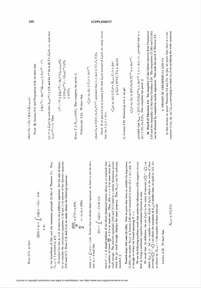
3. PROOFS OF THEOREMS 2.1, 2.2 AND 2.5

In this section we prove Theorems 2.1, 2.2 and 2.5. In §3a we obtain a maximum

principle for u¿, and in §3b a bound on the total variation in space. In §3c the important

continuity result (with respect to the data) is obtained. In §3d we end the proof of Theo-

rems 2.1 and 2.2. In §3e we prove several results that will allow us to prove Theorem 2.5

in §3f.

3a. A maximum principle fcr ua. We begin by showing that under a suitable

condition the approximate concentration u^ satisfies a maximum principle. We show in

particular that uj, > 0 provided u», uq, «i > 0, as we expect from the physical point of view.

In this section we prove a maximum principle for the approximate solution u/,. We stress

the fact that in the framework of conservation laws it is very well known that any maximum

principle for explicit schemes is valid only under a certain Courant-Friedrichs-Levy (CFL)

condition. Roughly speaking, this condition asks for the speed of the propagation of the

information allowed by the numerical scheme to be bigger than the maximum speed of

propagation of the information inherent in the conservation law. Since in our case the

latter speed is approximated by the quantity [| /?/, ||l<»(o,i) ft ls clear that in order to get

a maximum principle for u/,, we must obtain an upper bound for that quantity. The next

three lemmas are devoted to obtain the CFL condition. The bound on ||/?/, ||¿«(o,i) 's

obtained in Proposition 3.4. The maximum principle is given in Proposition 3.5.

The following simple but important result is the essential link between the mixed finite

element method (2.7) and the monotone scheme (2.6). It is a restatement of equation

1, x G /,,

0, otherwise.

Lemma 3.1. For n = 0,• ■ • , nr — 1 we have

The next result displays the CFL condition under which a maximum principle is sat-

isfied.

Lemma 3.2 (The CFL condition). Let u£ be such that

u^(0-)(<(x),u^(l+)€[0,u*]) *€(0,1).

Suppose that

(3.1 ) i - |^(í*;v+x - Ci ) s Ar"- ' = !■•■•.»*■

Then

uj+1(i)6[0,u*], ie(0,l).

© 1992 American Mathematical Society

0025-5718/92 $ 1.00 + $.25 per page

S29

(2.7a) with w&z(x) -


S30 SUPPLEMENT

VI Al VIVI AI VI

ail

v

-1

AI

vi S

E-1 <_cci ^ ^

<¡l<¡

A

kl+

<l<ih

« <a tu

i

v *"

S 5.

° .2 c

II

r. s3 e

s!"

S "3

ci "^ 'S

^ 7

B--

«i +

+ %■

,-r. +

t. H -

I 2.

e I - < < 01 r1t- « e I -

< < I t. H

I e <l<II I! Il

et cq" ci

I

<A!

I

Al

Cl"

Al

L"e _

"! ■*!

° I

O

I

^ egl I

S- s.Il II

< a+ §

+

Cl

+

II

Al —«- S■3 -s

m S


SUPPLEMENT S31


S32 SUPPLEMENT

»W3-iVI

<1+

?ñ.i

+

œ -s

bC g

C J0 .-

M H Ce

-1

+

I +

VI

+

lv

I i

•<3|<

+

1+

<l<

VI

2L <

o .S

II

E(6il 3

«i

'-La+

: Et

'-lu++*Et

< E

a < m -

I £

.3 Ci :3

a s s

-1

+Al H >

-T° I5 t Al S

OO

'O E =


SUPPLEMENT S33

o --o :=.cu =

il

+

-I*.

üVI

ËV

2. H

= +

I «

n

+ ¿o S~ 8

a -^

i. "i° i< _,

f += P

CQ> o ;_m *~ — <]

=; « + + ¿

i + +

ÇG G t-

Z »,ia

<- + V

< + +vi

í o —

.1

H

< - î »

VI

-\A\

o cm

u a a« s i

U to-

2 "a

«2 .-

■a ~t » <¡ -s

le" I

0 _¿¡ -^

<ll<t- 13 o-

.■W.1II

< <

Ï-W

-1

4-

-1

+

+

1+

+

5 jSS -5- er


S34 SUPPLEMENT

et

+

I

VI

. |(M -< IN —i<|N .

VI +

ça.

+

i

■ t'S

?WI

< ¡r:3 I

I•- TZ «±

ñ i ^~

+ ¿ b"

1« in

<1 IC-l

+

-•IN

I

VI +

++e -,"

V<

?W! 1<

"IN

I

+-IC-l

VI

< <■H |N ~H |N

+ +

S Ï

-s-I

~ CD

II

i S

<l<

HS ^ cT- sT- sT-<| <J ->|M ,_ H I. H i. H-IN I < < < < < <

<1

"i

I

— » i

-i

Os

_-£-^21

=

<1-l IN

VI

<-C N

+

<

+

1 a

•« Je


SUPPLEMENT S35


S36 SUPPLEMENT

S- <t +

ilsWS

i-Wl i-W!

ÎW1

-i+ +

- -,w VI

<

+

¿ c. _ s

S *

nj 0

LW1+

LW1i +r e

<l< v

+

. — T +

<l<

Il VI

o S O «

a « i*-

LWI

+

w. ir> cl

I

■Wi

•Wï+

I

Al

Wï

+ I

-n

+

oi

LWÏ tWï tW! -

à'


SUPPLEMENT S37

i S

"Ó x.

+

I <l<

ii ii

[Wl+

<+

I

< V+ X

«T «Toa. <t>.

°t- H V I H

2 i

1+

:¿ -S 3

< «

-1

-1

+

1+

ÏWI+

1}

■Wí

Iwi+<

iwiI

Iwi

+Í-H

I

+

=+

■WÎ+

■Wl

ÍW^+

I

a--u

II

Wl ¡Wl i

I

» í !¿" =Wl a ¿Wi

ï, i


S38 SUPPLEMENT

e -,

I

VIH

<

[Wl+ -- <

»W!+

VI «

3 C5

i £>

w"„ Xi

3 s■o 13

[WiVI

LW!

J, -Wï 5 ;_2_ o

•Wï ^= irW! 1

c. .S1

J3 ï

< n

■Wl -WïtWï jLW>

à "S

1 Iu

VI «. 13

H H

:Wï•rWï

fWÎII

¡rL-Nï =3 vi13S H. 13

5 IIO* N

<

+

S vi

en °. Il

+

üvi

1 î ¿ iwi«3 U3

1 O

S q

_£. 3

N lu

[Wl ï +

[Wi

[Wï

^- u

[Wl [Wï+

<[Wl

[Wl .2 '3

w u; -43

I

Wlri [W¡

oo — —r —

r

5O

IW! c 5

^ %


SUPPLEMENT S39

<+

<1

i

n

<

CD

1

II

3CD

VI

§

CD

1+

AI

A

<

JiWï

++

¿Wï

<CD

<+

<+

+

VI

CD o ~

| !'S w

I 'S

o

i +. -q iZ,

;tS vi

s r

g -g jD

J 13

•3

—- V *3

+

>.tch

ai- , *—o ,0 K, —

ilO ü

-a <aî ^ r^

-o £ -o

co ^->+ -^ •-1

IW+

++

G S

§ -S

£ -2

^ M

Oí A

¿ Ô¿H

o oi•o -cG ucd -G

-1

+■

+

V

+

h

CD

§

CD

[Wl

iso

w ¿ -a

h -2-S

«3 Cw 0

<1+

+

h

II


S40 SUPPLEMENT

N C*i

0,

B

c -1

+1+

a

4

CII

cV

01

I

<ï A

w ¡p

A

H

c

1+

VI

C 14

O Ü

C

c

1+

Silh Irj ¡

<J .2N 4G

Il ¿

.= Ü

M -- O

13 «"S vi> ^.S H

h 3H

N TJH^ N

>. CÔ

S al

0 _s «

b. SO JH

H J2 ï

S Ä

"3 B

2 S

-1

+

s -.S A I £

en ^

•a § iG 4= I

4= B

a 43

t; g

M

M "S

c"V

::0

4.

™ 1kN "*

N "S

S a* —

° ïï G

Il §1

*l3

Í? .2 C4

tr-

i «

II II

tu -

-G «

G ^taskq; "il .12 a*

■5 S

g g 22 9!

- S G

&11

Il N

1-1es >•

fi CM

O --h -=î

«S _• J3 ^o ~

J3 M» S VI J*

? g"o -— <y


S42 SUPPLEMENT

13

S. ¡- -o

,_, o

4*

»a

^ "a ^

o ~~-

2 «¡"■5 bO

O ^

•■s s_d J=

CiI

+

I

oi

+■

oi

II

Ü ¡=.

3u

•g

I

s

< <<l<

CG —-

I

fi, biO .S

. 6

i

on+

^^ 4J

VI

+ So -c

«H

1 œ

£» Il

-— ,o

■c ** ■* 2 K 5


SUPPLEMENT S43

3-

»3

> w

0+

01

9.

oí

CDII

oî

¡3I

+c -

s

I

^ .4»Wï sW?i C|-1 Sl <\<' Il +

I

tai

H

<

H

>.

»"Wl g c"Wïi

IW1 + ¿wï

3-

■a

Eo

CD

=Wï[Wï+

-G

-

3 «I

© >

g 1.2 '-3

C

Si+

+

oî

il

,0 3. 3. G G

© -n .S

as+

Si S m X

3 £ "H

¿ - H

- 3 Û

~ ^-, 4J

^ ^s

Il ï "S

G »-" I

to

+

**

3 C 5

i i -S »I 7" 7m ¡p

4i o ■"o. a E

1 s K aa; CL. O

^ H *o a' . ¿» wï h- •- uL ̂ -a s

S a- aÊ ^ a* g -5 g

T3 a

13 -G

O <d¿3 J3G **4> ho

S ifi -c

.2 a

-3 T3

3- " r.. bO ^

G 01- o>

G

<

3 u

" ~£ = E Ë

E 'S S g■■ S 5 © <i. © 'S ^ J


S44 SUPPLEMENT

ta+

i 2

3 N

ü 3

©

II

01

a

toI

Wï[W¡

to+

-1

+= ~9.

I

-1

H1

«wjiw;

01

■Wïiwi+

3-

03.

9-

o?

I

toI

© =II

to,

¡Wl

4-1

LWi■Wliwi+

5

s+

toi

3. i—. <s>

to

I ©- +

to_+

it 3-3- ~i

toI

=Wï¡Wl

+

u

Wï[Wl

<

■w«

to*WSiwi

+9."

3-

~ +Oí"

3-

[WlI

to

Wï

fWï[Wl

I

-1

1

4

St

1

iwi+

'WS[Wl

II

«3

toI

Wï[Wl

II'S

oî

-1

4

9.-H«

ü

I

«4o

W[W

I

« =Wï1 iwi

+

9-

01

9.

oí

oa

I

to

Í

<

1

+St-I

Wl[Wl

«Wïiwi

«Wïiwi


SUPPLEMENT S45

-H IN

+

1

t4 +

-1

+

n

'O

cII

c

1

-1

c1

? e

n^4

3. 3-I

3_ J).

- <

VI

3

25_tg

h|« <;

+ +

K| 3 ¿. •«

.8 ü S. 5-0 i-g K 0)

§ VI „» ■!

O. G

3 £

0O

>-4 0

©

S

P '53

— a

X+

Wï[Wl+

3-

u

WïWl

© i+ 6»"

3-

=5

© ̂

3

oí•- Go a;

- '-„ te

© -ïï

o 9

00 <-

5 CJ

<

+

«

■G'k4

VI

3-

+

cj

C

■Ü 'Ü

0 >o -1

Go.—

W»Wl

VI

3

Wl[W!

ÏW1

kg

+

¡J 2 -S © ©


S46 SUPPLEMENT

G Ei

§>cf

V

©

<: h

Í4- -«-

•ö oí

I* í

Sh

et » a, | ,:

i fgai9- 3 B g 8

u ** ^^ S3 Gw .-, 43 G

A "* Jf h S

£ a .2 § s - 3 ä£ a li riS^o a •- w ¡s ̂ g" .£•

Sg'ö^ ! s î s^ o -a a g" « g. ri ~ _h g S » '"

* G y 43 43 HJ¿2 HS S


CONVERGENCE OF A FINITE ELEMENT METHOD …

Documents

Transcript of CONVERGENCE OF A FINITE ELEMENT METHOD …